Non-overlapping domain decomposition methods for structural mechanics

C A C H A N

Rapport interne LMT-Cachan n2652006

Non-overlapping domain decompositionmethods in structural mechanics

Méthodes de décomposition de domaine sans recouvrementen mécanique des structures

PIERRE GOSSELET ETCHRISTIAN REY

Laboratoire de Mécanique et TechnologieENS Cachan/CNRS/Université Paris 6

61, avenue du Président Wilson, F-94235 CACHAN CEDEX

mailto:protect T1extbraceleft gosselet,reyprotect T1extbraceright @lmt.ens-cachan.fr

Non-overlapping domain decomposition methods instructural mechanics

The modern design of industrial structures leads to very complex simulations charac-terized by nonlinearities, high heterogeneities, tortuous geometries... Whatever the mod-elization may be, such an analysis leads to the solution to a family of large ill-conditionedlinear systems. In this paper we study strategies to efficiently solve to linear system basedon non-overlapping domain decomposition methods. We present a review of most em-ployed approaches and their strong connections. We outlinetheir mechanical interpreta-tions as well as the practical issues when willing to implement and use them. Numericalproperties are illustrated by various assessments from academic to industrial problems.An hybrid approach, mainly designed for multifield problems, is also introduced as itprovides a general framework of such approaches.

Méthodes de décomposition de domainesans recouvrement

en mécanique des structures

La conception moderne des structures industrielles conduit à des simulations d’unegrande complexité caractérisées par des non-linéarités, de fortes hétérogénéités, des géométriestorturées... Quelle que que soit la modélisation retenue, une telle analyse nécessite larésolution d’une famille de problèmes de grande taille mal conditionnés. Dans ce rap-port, nous étudions des stratégies efficaces, basées sur lesdécompositions de domainesans recouvrement, pour résoudre des systèmes linéaires. Nous présentons une revue desméthodes les plus employées, en mettant en évidence leurs fortes connexions, leurs inter-prétations mécaniques, et les problèmes pratiques rencontrés lors de leur mise en oeuvre.Les propriétés numériques sont illustrées par de nombreux exemples académiques et in-dustriels. Une approche hybride, principalement destinéeaux problèmes multiphysiques,est également introduite, elle fournit un cadre générique pour les approches étudiées.

Contents

Contents i

Introduction 1

1 Formulation of an interface problem 51.1 Reference problem. . . . . . . . . . . . . . . . . . . . . . . . . . . . . 61.2 Two-subdomain decomposition. . . . . . . . . . . . . . . . . . . . . . . 61.3 N-subdomain decomposition. . . . . . . . . . . . . . . . . . . . . . . . 71.4 Discretization. . . . . . . . . . . . . . . . . . . . . . . . . . . . . . . . 8

1.4.1 Boolean operators. . . . . . . . . . . . . . . . . . . . . . . . . 81.4.2 Basic equations. . . . . . . . . . . . . . . . . . . . . . . . . . . 111.4.3 Local condensed operators. . . . . . . . . . . . . . . . . . . . . 121.4.4 Block notations. . . . . . . . . . . . . . . . . . . . . . . . . . . 141.4.5 Brief review of classical strategies. . . . . . . . . . . . . . . . . 15

2 Classical solution strategies to the interface problem 172.1 Primal domain decomposition method. . . . . . . . . . . . . . . . . . . 18

2.1.1 Preconditioner to the primal interface problem. . . . . . . . . . 182.1.2 Coarse problem. . . . . . . . . . . . . . . . . . . . . . . . . . . 192.1.3 Error estimate. . . . . . . . . . . . . . . . . . . . . . . . . . . . 202.1.4 P-FETI method. . . . . . . . . . . . . . . . . . . . . . . . . . . 20

2.2 Dual domain decomposition method. . . . . . . . . . . . . . . . . . . . 212.2.1 Preconditioner to the dual interface problem. . . . . . . . . . . . 212.2.2 Coarse problem. . . . . . . . . . . . . . . . . . . . . . . . . . . 222.2.3 Error estimate. . . . . . . . . . . . . . . . . . . . . . . . . . . . 232.2.4 Interpretation and improvement on the initialization . . . . . . . . 23

2.3 Three fields method / A-FETI method. . . . . . . . . . . . . . . . . . . 262.4 Mixed domain decomposition method. . . . . . . . . . . . . . . . . . . 27

2.4.1 Coarse problem. . . . . . . . . . . . . . . . . . . . . . . . . . . 292.5 Hybrid approach . . . . . . . . . . . . . . . . . . . . . . . . . . . . . . 29

2.5.1 Hybrid preconditioner. . . . . . . . . . . . . . . . . . . . . . . 302.5.2 Coarse problems. . . . . . . . . . . . . . . . . . . . . . . . . . 302.5.3 Error estimate. . . . . . . . . . . . . . . . . . . . . . . . . . . . 31

3 Adding optional constraints 333.1 Augmentation strategy. . . . . . . . . . . . . . . . . . . . . . . . . . . 343.2 Recondensation strategy. . . . . . . . . . . . . . . . . . . . . . . . . . 34

3.2.1 Basic method. . . . . . . . . . . . . . . . . . . . . . . . . . . . 343.2.2 More complex constraints. . . . . . . . . . . . . . . . . . . . . 35

3.3 Adding "constraints" to the preconditioner. . . . . . . . . . . . . . . . . 36

Non-overlapping domain decomposition methods i

4 Classical issues 394.1 Rigid body motion detection. . . . . . . . . . . . . . . . . . . . . . . . 40

4.1.1 Simple algebraic approach. . . . . . . . . . . . . . . . . . . . . 404.1.2 Geometric approach. . . . . . . . . . . . . . . . . . . . . . . . 414.1.3 Generalized inverse. . . . . . . . . . . . . . . . . . . . . . . . . 41

4.2 Choice of optional constraints. . . . . . . . . . . . . . . . . . . . . . . 414.2.1 Forth order elasticity. . . . . . . . . . . . . . . . . . . . . . . . 414.2.2 Second order elasticity. . . . . . . . . . . . . . . . . . . . . . . 424.2.3 Link with homogenization theory. . . . . . . . . . . . . . . . . 43

4.3 Linear Multiple Points Constrains. . . . . . . . . . . . . . . . . . . . . 434.4 Choice of decomposition. . . . . . . . . . . . . . . . . . . . . . . . . . 454.5 Extensions. . . . . . . . . . . . . . . . . . . . . . . . . . . . . . . . . . 46

4.5.1 Nonsymmetric problems. . . . . . . . . . . . . . . . . . . . . . 464.5.2 Nonlinear problems. . . . . . . . . . . . . . . . . . . . . . . . . 46

4.6 Implementation issues. . . . . . . . . . . . . . . . . . . . . . . . . . . 464.6.1 Organization of the topological information. . . . . . . . . . . . 474.6.2 Defining algebraic interface objects (fig. 4.3). . . . . . . . . . . 474.6.3 Articulation between formulation and solver (fig. 4.4) . . . . . . 48

5 Assemssments 495.1 Two dimensional plane stress problem. . . . . . . . . . . . . . . . . . . 505.2 Bending plate. . . . . . . . . . . . . . . . . . . . . . . . . . . . . . . . 515.3 Heterogeneous 3D problem. . . . . . . . . . . . . . . . . . . . . . . . . 525.4 Homogeneous non-structured 3D problem. . . . . . . . . . . . . . . . . 525.5 Bitraction test specimen. . . . . . . . . . . . . . . . . . . . . . . . . . . 53

Conclusion 55

Bibliography 57

A Krylov iterative solvers 65A.1 Principle of Krylov solvers. . . . . . . . . . . . . . . . . . . . . . . . . 66A.2 Most used solvers. . . . . . . . . . . . . . . . . . . . . . . . . . . . . . 66A.3 GMRes . . . . . . . . . . . . . . . . . . . . . . . . . . . . . . . . . . . 66A.4 Conjugate gradient. . . . . . . . . . . . . . . . . . . . . . . . . . . . . 67A.5 Study of the convergence, preconditioning. . . . . . . . . . . . . . . . . 68A.6 Constrained Krylov methods, projector implementation. . . . . . . . . . 68A.7 Augmented-Krylov methods, projector implementation. . . . . . . . . . 69A.8 Constrained augmented Krylov methods. . . . . . . . . . . . . . . . . . 70

ii Non-overlapping domain decomposition methods

Introduction

Hermann Schwarz (1843-1921) is often referred to as the father of domain decompositionmethods. In a 1869-paper he proposed an alternating method to solve a PDE equationset on a complex domain composed the overlapping union of a disk and a square (fig.1),giving the mathematical basis of what is nowadays one of the most natural ways to benefitthe modern hardware architecture of scientific computers.

Figure 1: Schwarz’ original prob-lem

Figure 2: 16 subdomains bitraction test specimen(courtesy of ONERA – Pascale Kanouté)

In fact the growing importance of domain decomposition methods in scientific com-putation is deeply linked to the growth of parallel processing capabilities (in terms ofnumber of processors, data exchange bandwidth between processors, parallel library ef-ficiency, and of course performance of each processor). Because of the exponential in-crease of computational resource requirement for numerical simulation of more and morecomplex physical phenomena (non-linearities, couplings between physical mechanismsor between physical scales, random variables...) and more and more complex problems(optimization, inverse problems...), parallel processing appears to be an essential tool tohandle the resulting numerical models.

Parallel processing is supposed to take care of two key-points of modern computa-tions, the amount of operations and the required memory. Letus consider the simulationof a physical phenomenon, classically modeled by a PDEL (x) = f , x∈ H(Ω). To takeadvantage of the parallel architecture of a calculator, a reflexion has to be carried outon how the original problem could be decomposed into collaborating subprocesses. Thecriteria for this decomposition will be: first, the ability to solve independent problems(on independent processors); second, how often processes have to be synchronized; andlast what quantity of data has to be exchanged when synchronizing. When tracing backthe idle time of resolution processes and analyzing hardware and software solutions, it is

Non-overlapping domain decomposition methods 1

often observed that inter-processor communications are the most penalizing steps.If we now consider the three great classes of mathematical decomposition of our refer-

ence problem which are operator splitting (e.g.L = ∑i L i Fortin and Glowinski[1982]),function-space decomposition (for instanceH(Ω) = span(vi), an example of which ismodal decomposition) and domain decomposition (Ω =

S

Ωi), though the first two canlead to very elegant formulations, only domain decompositions ensure (once one subdo-main or more have been associated to one processor) that independent computations arelimited to small quantities and that the data to exchange is limited to the interface (or smalloverlap) between subdomains which is always one-to-one exchange of small amount ofdata.

So domain decomposition methods perfectly fit the criteria for building efficient algo-rithms running on parallel computers. Their use is very natural in engineering (and moreprecisely design) context : domain decomposition methods offer a framework where dif-ferent design services can provide the virtual models of their own parts of a structure,each assessed independently, domain decomposition can then evaluate the behavior of thecomplete structure just setting specific behavior on the interface (perfect joint, unilateralcontact, friction). Of course domain decomposition methods also work with one-piecestructure (for instance fig.2), then decomposition can be automated according to criteriawhich will be discussed later.

From an implementation point of view, programming domain decomposition methodsis not an overwhelming task. Most often it can be added to existing solvers as a upperlevel of current code using the existing code as a black-box.The only requirement to im-plement domain decomposition is to be able to detect the interface between subdomainsand use a protocol to share data on this common part. In this paper we will mostly fo-cus on domain decomposition methods applied to finite element methodCiarlet [1979],Zienkiewicz and Taylor[1989], anyhow they can be applied to any discretization method(among others meshless methodsBelytschko et al.[1996], Breitkopt and Huerta[2002],Liu and Gu[2005] and discrete element methodsD’Addetta et al.[2004], Bolander and Sukumar[2005], Delaplace[2005]).

Though domain decomposition methods were more than one century old, they had notbeen extensively studied. Recent interest arose as they were understood to be well-suitedto modern engineering and modern computational hardware. An important date in reinter-est in domain decomposition methods is 1987 as first international congress dedicated tothese methods occurred and DDM association was created (seehttp://www.ddm.org).

Yet the studies were first mathematical analysis oriented and emphasized on Schwarzoverlapping family of algorithms. As interest in engineering problems grew, non-overlappingSchwarz and Schur methods, and coupling with discretization methods (mainly finite el-ement) were more and more studied. Indeed, these methods arevery natural to interpretmechanically, and moreover mechanical considerations often resulted in improvementto the methods. Basically the notion of interface between neighboring subdomains isa strong physical concept, to which is linked a set of conservation principles and phe-nomenological laws: for instance the conservation of fluxes(action-reaction principle)imposes the pointwise mechanical equilibrium of the interface and the equality of incom-ing mass (heat...) from one subdomain to the outgoing mass (heat...) of its neighbors; the"perfect interface" law consists in supposing that displacement field (pressure, temper-ature) is continuous at the interface, contact laws enable disjunction of subdomains butprohibit interpenetration.

In this context two methods arose in the beginning of the 90’s: so-called Finite Ele-ment Tearing and Interconnecting (FETI) methodFarhat and Roux[1991] and BalancedDomain Decomposition (BDD)Le Tallec et al.[1991]. From a mechanical point of viewBDD consists in choosing the interface displacement field asmain unknown while FETIconsists in privileging the interface effort field. BDD is usually referred to as a primalapproach while FETI is a dual approach. One of the interests of these methods, beyond

2 Non-overlapping domain decomposition methods

http://www.ddm.org

their simple mechanical interpretation, is that they can easily be explained from a purelyalgebraic point of view (ie directly from the matrix form of the problem). In order to fitparallelization criteria, it clearly appeared that the interface problem should be solved us-ing an iterative solver, each iteration requiring local (ie independent on each subdomain)resolution of finite element problem, which could be done with a direct solver. Thenthese methods combined direct and iterative solver trying to mix robustness of the firstand cheapness of the second. Moreover the use of an iterativesolver was made moreefficient by the existence of relevant preconditioners (based on the resolution of a localdual problem for the primal approach and a primal local problem for the dual approach).

When first released, FETI could not handle floating substructures (ie substructureswithout enough Dirichlet conditions), thus limiting the choice of decomposition, whilethe primal approach could handle such substructures but with loss of scalability (conver-gence decayed as the number of floating substructures increased). A key point then wasthe introduction of rigid body motions as constraints and the use of generalized inverses.Because of its strong connections with multigrid methodsWesseling[2004], the rigidbody motions constraint took the name of "coarse problem", it made the primal and dualmethods able to handle most decompositions without loss of scalability Farhat and Roux[1994a], Mandel[1993], Le Tallec[1994]. From a mechanical point of view, the coarseproblem enables non-neighboring subdomains to interact without requiring the transmis-sion of data through intermediate subdomains, it then enables to spread global informationon the whole structure scale.

Once equipped with their best preconditioners and coarse problems, mathematicalresultsFarhat et al.[1994], Klawonn and Widlund[2001], Brenner[2005] provide the-oretical scalability of the methods. For instance for 3D elasticity problems, ifh is thediameter of finite elements andH the diameter of subdomains, condition numberκ of theinterface problem reads (C is a real constant):

κ ≃C

(1+ log

(Hh

))2

(1)

which proves that the condition number only depends logarithmatically on the numberof elements per subdomain. Many numerical assessment campaigns confirmed the goodproperties of the methods, their robustness compared to iterative solvers applied to thecomplete structure and their low cost (in terms of memory andCPU requirements) com-pared to direct solvers. Thus because they are well-suited to modern hardware (like PCclusters) they enable to achieve computations which could not be realized on classicalcomputers because of too high memory requirement or too longcomputational time: thesemethods can handle problems with several millions of degrees of freedom.

Primal and dual methods were extended to heterogeneous problems by a cheap inter-vention on the preconditionersRixen and Farhat[1999] and on the initializationGosselet et al.[2003b], and to forth order elasticity (plates and shells) problems by the adjunction of so-called "second level problem" in order to regularize the displacement field around thecorners of subdomainsFarhat and Mandel[1998], Le Tallec et al.[1998], Farhat et al.[2000c]. As it became clear that the regularization of the displacement field was suffi-cient to suppress rigid body motions, specific algorithms which regularizeda priori thesubdomain problems were proposed: FETIDPFarhat et al.[2001] and its primal counter-part BDDCCros[2002], first in the plates and shells context, then in the second orderelasticity contextKlawonn et al.[2005]. Now FETIDP and BDDC are considered as effi-cient as original FETI and BDD.

Methods were employed in many other contexts such as transient dynamicsFragakis and Papadrakakis[2004], multifield problems (multiphysic problems such as porousmediaGosselet et al.[2003a] and constrained problems such as incompressible flowsLi [2002], Goldfeld[2002]),Helmotz equationsFarhat et al.[1999, 2000b], de La Bourdonnaye et al.[1998] and con-tact Dureisseix and Farhat[2001], Dostal et al.[2005]. The use of domain decomposi-


tion methods in structural dynamic analysis is a rather old idea though it can now beconfronted to well established methods in static analysis;the Craig-Bampton algorithmCraig and Bampton[1968] is somehow the application of the primal strategy to such prob-lems, the dual version of which was proposed inRixen [2004], moreover ideas like theadjunction of coarse problems enabled to improve these methods.

Because of the strong connection between primal and dual approaches, some meth-ods try to propose frameworks which generalize the two methods. The hybrid approachGosselet[2003], Gosselet et al.[2004] enables to select specific treatment (primal or dual)for each interface degree of freedom, if all degrees of freedom have the same treatment,the hybrid approach is exactly a classical approach, for certain multifield problems thehybrid approach enables to define physic-friendly solvers.Mixed approachesLadevèze[1999], Nouy [2003], Series et al.[2003b] consist in searching a linear combination ofinterface displacement and effort field, depending on the artificial stiffness introduced onthe interface one can recover the classical approaches (null stiffness for the dual approach,infinite stiffness for the primal approach). Moreover, the mixed approaches enable to pro-vide the interface mechanical behavior and provide a more natural framework to handlecomplex interfaces (contact, friction...) than classicalapproaches.

In this paper we aim at reviewing most of non-overlapping domain decompositionmethods. To adopt a rather general point of view we introducea set of notations stronglylinked to mechanical considerations as it gives the interface the main role of the methods.We try to include all methods inside the same pattern so that we can easily highlightthe connections and differences between them. We adopt a practical point of view aswe describe the mechanical concepts, the algebraic formulations, the algorithms and thepractical implementation of the methods. At each step we tryto emphasize keypoints andnot to avoid theoretical and practical difficulties.

This paper is organized as follows. In section1 we introduce the mechanical frame-work of our study, the common notations and the notion of interface assembly operatorsand mechanical operators which will play a central role in the methods. Section2 pro-vides a rather extensive review of the nonoverlapping domain decomposition methods inthe framework of discretized problems: basic primal and dual approaches (with their vari-ations), three-field method for conforming grids, mixed andhybrid approaches. A key-point of the previous methods is the adjunction of optional constraints to form a "coarseproblem" which transmits global data through the whole structure, the strategies to intro-duce these optional constraints are studied in section3, which leads to the definition of"recondensed" strategies FETIDP and BDDC. Section4 deals with practical issues whichare very often common to most of the methods. Assessments aregiven in section5 toillustrate the methods and outline their main properties. Section5.5concludes the paper.As Krylov iterative solvers are often coupled to domain decomposition methods, mainconcepts and algorithms to use them are given in appendixA.


Chapter 1

Formulation of an interface problem

To present as smoothly as possible non-overlapping domaindecomposition methods we first consider a reference

continuous mechanics problem, decompose the domain in twosubdomains in order to introduce interface fields, then in

order to describe correctly the interface we study aN-subdomain decomposition. Since our aim is not to prove

theoretical performance results but make the reader feel somekey-points of substructuring, we do not go too far in

continuous formulation and quickly introduce discretizedsystems.

Contents1.1 Reference problem. . . . . . . . . . . . . . . . . . . . . . . . . . . . . . 6

1.2 Two-subdomain decomposition. . . . . . . . . . . . . . . . . . . . . . . 6

1.3 N-subdomain decomposition . . . . . . . . . . . . . . . . . . . . . . . . 7

1.4 Discretization . . . . . . . . . . . . . . . . . . . . . . . . . . . . . . . . . 8

1.4.1 Boolean operators. . . . . . . . . . . . . . . . . . . . . . . . . . 8

1.4.2 Basic equations. . . . . . . . . . . . . . . . . . . . . . . . . . . . 11

1.4.3 Local condensed operators. . . . . . . . . . . . . . . . . . . . . . 12

1.4.4 Block notations. . . . . . . . . . . . . . . . . . . . . . . . . . . . 14

1.4.5 Brief review of classical strategies. . . . . . . . . . . . . . . . . . 15


1.1 Reference problem

Ωg

f

u0

∂gΩ

∂uΩ

Figure 1.1: Reference problem

Let us consider domainΩ in Rn (n=1, 2 or 3) submitted to a classical linear elasticity

problem (see figure1.1) : displacementu0 is imposed on part∂uΩ of the boundary ofthe domain, effortg is imposed on complementary part∂gΩ, volumic effort f is imposedon Ω, elasticity tensor isa Germain[1986], con [1988]. The system is governed by thefollowing equations :

div(σ)+ f = 0 in Ωσ = a : ε(u) in Ωε(u) = 1

2

(grad(u)+grad(u)T

)in Ω

σ.n = g on∂gΩu = u0 on∂uΩ

(1.1)

In order to have the problem well posed, we suppose mes(∂uΩ) > 0. We also supposethat tensora defines a symmetric definite positive bilinear form on 2nd-order symmetrictensors. Under these assumptions, problem (1.1) has a unique solutionDuvaut[1990].

1.2 Two-subdomain decomposition

Ω(1)Ω(2)

ϒ

Figure 1.2: Two-subdomain decomposition

Let us consider a partition of domainΩ into 2 substructuresΩ(1) andΩ(2). We defineinterfaceϒ between substructures (figure1.2) :

ϒ = ∂Ω(1)\

∂Ω(2) (1.2)

System (1.1) is posed on domainΩ, we write its restrictions toΩ(1) andΩ(2) :

s= 1 or 2,

div(σ(s))+ f

(s)= 0 in Ω(s)

σ(s)= a

(s) : ε(u(s)) in Ω(s)

ε(u(s)) = 12

(grad(u(s))+grad(u(s))T

)in Ω(s)

σ(s).n(s) = g(s) on ∂gΩ

T

∂Ω(s)

u(s) = u(s)0 on ∂uΩ

T

∂Ω(s)

(1.3)


and the interface connection conditions, continuity of displacement

u(1) = u(2) on ϒ (1.4)

and equilibrium of efforts (action-reaction principle)

σ(1)n(1) +σ(2)

n(2) = 0 onϒ (1.5)

Of course system (1.3, 1.4, 1.5) is strictly equivalent to global problem (1.1).

1.3 N-subdomain decomposition

Ω(1)

Ω(2)

Ω(3)ϒ

(a) Primal (geometric) interface

Ω(1)

Ω(2)

Ω(3)ϒ(1,2)

ϒ(1,3)

ϒ(2,3)

(b) Dual interface (connectiv-ity)

Figure 1.3: Definition of the interface for aN-subdomain decomposition

Let us consider a partition of domainΩ into N subdomains denotedΩ(s). We candefine the interface between two subdomains, the complete interface of one subdomainand the geometric interface at the complete structure scale:

ϒ(i, j) = ϒ( j ,i) = ∂Ω(i) T

∂Ω( j)

ϒ(s) =S

j ϒ(s, j)

ϒ =S

sϒ(s)(1.6)

When implementing the method, one (possibly virtual) processor is commonly as-signed to each subdomain, hence because we can tell "local" computations (realized in-dependently on each processor) from "global" computations(realized by exchanging databetween processors), we often refer to values as being global or local. Thenϒ(s) is thelocal interface andϒ the global interface. Because exchanges are most often one-to-one,ϒ(i, j) is the(i − j)-communication interface.

Using more than two subdomains (except when using "band"-decomposition) leads tothe appearance of "multiple-points" also called "crosspoints" (which are nodes shared bymore than two subdomains). These crosspoints lead to the existence of two descriptionsof the interface (figure1.3): so-called geometric interfaceϒ and so-called connectivity in-terface made out of the set of one-to-one interfaces(ϒ(i, j))16i< j6N. Each of the two mostclassical methods exclusively uses one of these descriptions so the geometric interfaceϒis often referred to as the primal interface while the connectivity interfaceϒ is referred toas the dual interface.

How crosspoints are handled is a fundamental key in the differentiation of domain de-composition methods. In the remainder of the paper we will always refer to data attachedto the dual interface using underlined notation.


Remark 1.3.1 Reader may have observed that the above presented connectivity descrip-tion is redundant for crosspoints: let x be a crosspoint if x belongs toϒ(1,2) andϒ(2,3), itof course belongs toϒ(1,3). In the general case of a m-multiple crosspoint, there are

(m2

)

connectivity relationships while only(m−1) would be sufficient and necessary. We willpresent strategies to remove these redundancies in the algebraic analysis of the methods.

Remark 1.3.2 Cross-points may also introduce, at the continuous level, punctual-interfacesin 2d or edge-interfaces in 3d, which are interface with zeromeasure. Most often from aphysical point of view these are not considered as interfaces. Anyhow after discretizationall relationships are written node-to-node and the problemno longer exists.

1.4 Discretization

We suppose that the reference problem has been discretized,leading to the resolution ofn×n linear system:

Ku = f (1.7)

Because of its key role in structural mechanics we will oftenrefer to finite element dis-cretization though any other technique would suit. The key points are the link betweenmatrix K and the domain geometry and the sparse filling of matrixK (related to the factthat only narrow nodes have non-zero interaction).

We restrict to the case of element-oriented decomposition (each element belongs toone and only one substructure) which are conforming to the mesh which implies threeconditionsRixen[1997]:

• there is a one-to-one correspondence between degrees of freedom by the interface ;

• approximation spaces are the same by the interface ;

• models (beam, shell, 3d...) are the same by the interface.

Under these assumptions connection conditions simply write as node equalities. For non-conforming meshes, a classical solution is to use mortar-elements for which continuityand equilibrium are verified in a weak senseAchdou and Kuznetsov[1995], Achdou et al.[1996], Stefanica and Klawonn[1999].

1.4.1 Boolean operators

In order to write communication relation between subdomains we have to introduce sev-eral operators.

The first one is the "local trace" operatort(s) which is the discrete imbedding fromΩ(s) to ϒ(s). It enables to cast data from a complete subdomain to its interface, and oncetransposed to extend data set on the interface to the whole subdomain (setting internaldegrees of freedom to zero). In the remainder of the paper we will use subscriptb forinterface data and subscripti for internal data.

Then data lying on one subdomain interface has to be exchanged with its neighboringsubdomains. It can be either realized on the primal interface or the dual interface, leadingto two (global) "assembly" operators: the primal oneA(s), and the dual oneA(s). Theprimal assembly operator is a strictly boolean operator while the dual assembly operatoris a signed boolean operator (see figure1.4): if a degree of freedom is set to 1 on one sideof the interface, its corresponding degree of freedom on theother side of the interface isset to−1. Non-boolean assembly operators can be used in order to average connectionconditions when using non-conforming domain decomposition methodsBernardi et al.[1989].


Remark 1.4.1 Our (t(s),A(s),A(s)) set of operators is not the most commonly used inpapers related to domain decomposition. The interest of this choice is to be sufficientto explain most of the available strategies with only three operators. Other notations

use "composed operators" like (B(s) = A(s)t(s) or L(s)T= A(s)t(s)) which are not sufficient

to describe all methods and which, in a way, omit the fundamental role played by theinterface.

Boolean operators have important classical properties. Please note the first one whichexpresses the orthogonality of the two assembly operators.

∑s

A(s)A(s)T= 0 (1.8a)

A(s)TA(s) = Iϒ(s) (1.8b)

A(s)TA(s) = diag(multiplicity−1)ϒ(s) (1.8c)

A(s)A(s)T=

∣∣∣∣I onϒ(s)

0 elsewhere(1.8d)

Remark 1.4.2 An interesting choice of description would have been to use redundantlocal interface (defining some kind of t(s)). This choice would stick to most classicalimplementations where the local interface of one subdomainis defined neighborwise.Dual assembly operator would write easily as a simple signing operator, but handlingmultiple points would be slightly more difficult for the primal assembly operator (seesection4.6).

Remark 1.4.3 Redundancies can easily be removed from the dual description of the in-terface. One has just to modify the connectivity table, so that one multiple point is con-nected only once to each subdomain. This can be carried out introducing two differ-ent assembly operators the "non-redundant" one and the "orthonormal" one (see fig-ure 1.5) Fragakis and Papadrakakis[2002]. Only relationship1.8c is modified (then

A(s)TA(s) = Iϒ(s)). The interest of the use of these assembly operators will bediscussed in

section2.3.


1(1) 2(1)3(1)

4(1)

5(1)

1(2) 2(2)3(2)

4(2)5(2)

1(3)

2(3)

3(3)

4(3)

(a) Subdomains

1(1)b

2(1)b

3(1)b

1(2)b

2(2)b3(2)

b

1(3)b

2(3)b

3(3)b

(b) Local interface

2(3)b

1ϒ

2ϒ

3ϒ

4ϒ

(c) Primal interface

1ϒ

2ϒ

3ϒ

4ϒ

5ϒ

6ϒ

(d) Dual interface

t(1) =

0 0 1 0 00 0 0 1 00 0 0 0 1

t(2) =

0 0 1 0 00 0 0 1 00 0 0 0 1

t(3) =

1 0 0 00 1 0 00 0 1 0

A(1) =

0 0 00 1 01 0 00 0 1

A(2) =

1 0 00 0 10 0 00 1 0

A(3) =

0 0 10 0 01 0 00 1 0

A(1) =

0 0 00 1 01 0 00 0 00 0 10 0 1

A(2) =

1 0 00 0 −10 0 00 1 00 −1 00 0 0

A(3) =

0 0 −10 0 0−1 0 00 −1 00 0 00 −1 0

Figure 1.4: Local numberings, interface numberings, traceand assembly operators


1(1)b

2(1)b

3(1)b

1(2)b

2(2)b3(2)

b

1(3)b

2(3)b

3(3)b

(a) Local interface

1ϒ

2ϒ

3ϒ

4ϒ

5ϒ

6ϒ

(b) Redundant connectivity

1ϒ

2ϒ

3ϒ

4ϒ

5ϒ

(c) Non-redundant connectivity

1ϒ

2ϒ

3ϒ

4ϒ

5ϒ

(d) Orthonormal connectivity

A(1) =

0 0 00 1 01 0 00 0 00 0 10 0 1

A(2) =

1 0 00 0 −10 0 00 1 00 −1 00 0 0

A(3) =

0 0 −10 0 0−1 0 00 −1 00 0 00 −1 0

A(1)N =

0 0 00 1 01 0 00 0 00 0 1

A(2)

N =

1 0 00 0 −10 0 00 1 00 −1 0

A(3)

N =

0 0 −10 0 0−1 0 00 −1 00 0 0

A(1)O =

0 0 00 1√

20

1√2

0 0

0 0 00 0 2√

6

A(2)O =

1√2

0 0

0 0 − 1√2

0 0 00 1√

20

0 − 1√6

0

A(3)O =

0 0 − 1√2

0 0 0− 1√

20 0

0 − 1√2

0

0 − 1√6

0

Figure 1.5: Suppressing redundancies of dual interface

1.4.2 Basic equations

In order to rewrite equation (1.7) in a domain-decomposed context, we have to introduce

the reaction unknown which is the discretization ofσ(1)n(1) =−σ(2)

n(2) in equation (1.5).λ(s) is the reaction imposed by neighboring subdomains on subdomain (s). Commonlyλ(s) is defined on the whole subdomain(s) while it is non-zero only on its interface, so

λ(s) = t(s)Tλ(s)

b .

∀s, K(s)u(s) = f (s) +λ(s) (1.9a)

∑s

A(s)t(s)u(s) = 0 (1.9b)


∑s

A(s)t(s)λ(s) = 0 (1.9c)

Equation (1.9a) corresponds to the (local) equilibrium of eachsubdomain submitted toexternal conditionsf (s) and reactions from neighborsλ(s). Equation (1.9b) correspondsto the (global) continuity of the displacement field throughthe interface. Equation (1.9c)corresponds to the (global) equilibrium of the interface (action-reaction principle).

This three-equation system (1.9) is the starting point from a rich zoology of methods,most of which possess strong connections we will try to emphasis on. Before going furtherin the exploration of these methods, we propose to introducelocal condensed operatorsthat represent a subdomain on its interface, then a set of synthetic notations.

1.4.3 Local condensed operators

Philosophically, local condensed operators are operatorsthat represent how neighboringsubdomains "see" one subdomain: a subdomain can be viewed asa black-box, the onlyinformation necessary for neighbors is how it behaves on itsinterface. Associated to thisidea is the classical assumption that local operations are "exactly" performed. From animplementation point of view, when solving problems involving local matrices, a directsolver is employed. As we will see, the use of exact local solvers will be coupled with theuse of iterative global solvers leading to a powerful combination of speed and precisionof computations.

In this section we will always refer to the local equilibriumof subdomain(s) underinterface loading:

K(s)u(s) = λ(s) = t(s)T

λ(s)b (1.10)

Primal Schur complementS(s)p : If we renumber the local degrees of freedom of sub-

domain(s) in order to separate internal and boundary degrees of freedom, system(1.10) writes (

K(s)ii K(s)

ib

K(s)bi K(s)

bb

)(u(s)

i

u(s)b

)=

(0

λ(s)b

)(1.11)

From the first line we draw

u(s)i = −K(s)

ii

−1K(s)

ib u(s)b (1.12)

then the Gauss elimination ofu(s)i leads to

(K(s)

bb −K(s)bi K(s)

ii

−1K(s)

ib

)u(s)

b = S(s)p u(s)

b = λ(s)b (1.13)

which is the condensed form of the local equilibrium of subdomains expressed in

terms of interface fields. OperatorS(s)p is called local primal Schur complement.

Its computation is realized by the inversion of matrixK(s)ii which corresponds to

Dirichlet conditions imposed on the interface of subdomain(s), so the primal Schurcomplement is always well defined, and commonly called the "local Dirichlet oper-ator". Note that the symmetry, positivity, and definition properties are inherited by

matrixS(s)p from matrixK(s).

An important result is that the kernel of matricesK(s) andS(s)p can be deduced one

from the other (I (s)b is the identity matrix on the interface):

K(s)R(s) = 0 =⇒ S(s)p t(s)R(s) = S(s)

p R(s)b = 0 (1.14)

S(s)p R(s)

b = 0 =⇒ K(s)

(−K(s)

ii

−1K(s)

ib

I (s)b

)R(s)

b = K(s)R(s) = 0 (1.15)


Primal Schur complement can also be interpreted as the discretization of the Stecklov-Poincaré operator. From a mechanical point of view, it is thelinear operator thatprovides the reaction associated to given interface displacement field.

If we consider that the subdomain is also loaded on internal degrees of freedom,then the condensation of the equilibrium on the interface reads:

K(s)u(s) = f (s) ⇒ S(s)p u(s)

b = b(s)p (1.16)

b(s)p = f (s)

b −K(s)bi K(s)

ii

−1f (s)i (1.17)

b(s)p is the condensed effort imposed on the substructure.

Dual Schur complementS(s)d : the dual Schur complement is a linear operator that com-

putes interface displacement field from given interface effort. From equation (1.10)and (1.13) we have:

(t(s)K(s)+t(s)

T)

λ(s)b = S(s)

p+

λ(s)b = S(s)

d λ(s)b = u(s)

b (1.18)

whereK(s)+ is the generalized inverse of matrixK(s), and where it is assumed thatno rigid body motion is excited. If we denote byR(s) the kernel of matrixK(s) thislast condition reads:

R(s)Tλ(s) = 0 or equivalently R(s)

b

Tλ(s)

b = 0 (1.19)

Remark 1.4.4 A generalized inverse (or pseudo-inverse) of matrix M is a matrix, de-noted M+, which verifies the following property:∀y∈ range(M), MM+y = y. Note thatthis definition leads to non-unique generalized inverse, however all results presented areindependent of the choice of generalized inverse.

Of course in order to take into account, inside (1.18), the possibility of the substructure tohave zero energy modes, an arbitrary rigid displacement canbe added leading to the nextexpression where vectorα(s) denotes the magnitude of rigid body motions:

u(s)b = S(s)

d λ(s)b +R(s)

b α(s) (1.20)

Hybrid Schur complement: S(s)pd this operator corresponds to an interface where degrees

of freedom are partitioned into two subsets. Suppose that the first subset is submit-

ted to given Dirichlet conditions and the second to Neumann condition,S(s)pd is the

linear operator that associates resulting reaction on the first subset and resulting dis-placement on the second subset to those given conditions. Wedenote by subscriptpdata defined on the first subset and by subscriptd data defined on the second subset(schematicallyb = p∪d andp∩d = /0).

S(s)pd

(u(s)

p

λ(s)d

)=

(λ(s)

p

u(s)d

)(1.21)

The computation of operatorS(s)pd though no more complex than the computation of

S(s)p or S(s)

d , requires more notations. A synthetic option is to denote bysubscript ¯pthe sets of internal (subscripti) data and second-interface-subset (subscriptd) data,schematically ¯p = i ∪d. We introduce a modified trace operator:

t(s)d vp = t(s)d

(vi

vd

)= vd (1.22)


Then internal equilibrium (1.10) reads:

(K(s)

pp K(s)pp

K(s)pp K(s)

pp

)(u(s)

p

u(s)p

)=

(t(s)d

Tλ(s)

d

λ(s)p

)(1.23)

Then hybrid Schur complement is:

S(s)pd =

K(s)

pp −K(s)ppK(s)

pp

+K(s)

pp K(s)ppK(s)

pp

+t(s)d

T

−t(s)d K(s)pp

+Kpp t(s)d K(s)

pp

+t(s)d

T

(1.24)

As can be noticed the diagonal blocks ofS(s)pd look like fully primal and fully dual

Schur complements, while extradiagonal blocks are antisymmetric (assumingK(s)

is symmetric). Of course if all interface degrees of freedombelong to the samesubset, the hybrid Schur complement equals "classical" fully primal or fully dualSchur complement. Moreover it stands out clearly that:

S(s)pd

+= S(s)

dp =

t(s)p K(s)dd

+t(s)p

T−t(s)p K(s)

dd

+Kdd

K(s)dd

K(s)dd

+t(s)p

TK(s)

dd −K(s)dd

K(s)dd

+K(s)

dd

(1.25)

S(s)dp is the operator which associates displacement on the first subset and reaction

on the second subset to given effort on the first subset and given displacement onthe second subset.

As both matricesK(s)pp andK(s)

ddmay not be invertible, only their pseudo-inverse has

been introduced. The invertibility is strongly dependent on the choice of interfacesubsets.

1.4.4 Block notations

While condensed operators simplify the writing of local operations, the block notationsmake it easer to understand the global operations of domain decomposition. We proposeto denote by superscript⋄ the row-block repetition of local vectors and the diagonal-block repetition of matrices, block assembly operators arewritten in one row (column-block) and denoted by special font, for instance:

u⋄ =

u(1)

...u(N)

f ⋄ =

f (1)

...f (N)

λ⋄ =

λ(1)

...λ(N)

K⋄ =

K(1) 0 . . . 0

0... ...

......

. . . . . . 00 . . . 0 K(N)

t⋄ =

t(1) 0 . . . 0

0... ...

......

.. . . . . 00 . . . 0 t(N)

A =(A(1) . . . A(N)

)A =

(A(1) . . . A(N)

)

Remark 1.4.5 The specific notation for assembly operators aims at emphasizing at theirspecific role in terms of parallelism for the methods. Moreover, the only operation thatrequires exchange of data between subdomains is the use of non-transposed assemblyoperators.


Fundamental system (1.9) then reads:

K⋄u⋄ = f ⋄ +λ⋄ (1.26a)

At⋄λ⋄ = 0 (1.26b)

At⋄u⋄ = 0 (1.26c)

or in condensed form:S⋄pu⋄b = b⋄p+λ⋄

b (1.27a)

Aλ⋄b = 0 (1.27b)

Au⋄b = 0 (1.27c)

The orthogonal property of assembly operators (1.8a) simply reads:

AAT = 0 (1.28)

Relation (1.8d) reads:AA

T = diag(multiplicity) (1.29)

Remark 1.4.6 For improved readability, we will denote by bold font objects defined ina unique way on the interface (ie "assembled" quantities). Schematically, assembly op-erators enable to go from block notations to bold notations and transposed assemblyoperators realize the reciprocal operations.

1.4.5 Brief review of classical strategies

We can define general strategies to solve system (1.26) or (1.27):

Primal approaches Le Tallec et al.[1991], Le Tallec and Vidrascu[1993], Mandel[1993],Le Tallec[1994], Mandel and Brezina[1996], Le Tallec and Vidrascu[Bergen 1996],Le Tallec et al.[1998] a unique interface displacement unknownub satisfying equa-tion (1.27c) is introduced, then an iterative process enables to satisfy (1.27b) whilealways verifying (1.27a).

Dual approaches Farhat and Roux[1991, 1994a,b], Farhat[1992], Farhat et al.[1994],Mandel and Tezaur[1996], Bhardwaj et al.[2000] a unique interface effort unknownλb satisfying equation (1.27b) is introduced, then an iterative process enables to sat-isfy (1.27c) while always verifying (1.27a).

Three fields approachesBrezzi and Marini[1993], Rixen et al.[1999], Park et al.[1997a,b]a unique interface displacementub is introduced, then relation (1.27c) is dual-ized so that interface effortsλ⋄

b are introduced as Lagrange multipliers which yethave to verify relation (1.27b). Then the iterative process looks simultaneously for(λ⋄

b,ub,u⋄b)

verifying exactly equation (1.27a). As this method is mostly designedfor non-matching discretizations it will not be exposed in the remaining of thispaper, anyhow a variant of the dual method which is equivalent to the three-fieldmethod with conforming grids will be described.


Mixed approaches Glowinski and Le Tallec[1990], Ladevèze[1999], Series et al.[2003a,b]new interface unknown is introduced which is a linear combination of interface dis-placement and effort,µ⋄b = λ⋄

b+T⋄b u⋄b, then the interface system is rewritten in terms

of unknownµ⋄b, this new system is solved iteratively and thenλ⋄b andu⋄b are post-

processed. Of course matrixT⋄b is an important parameter of these methods.

Hybrid approaches Klawonn and Widlund[1999], Mandel and Tezaur[2000],Farhat et al.[2000a, 2001], Gosselet et al.[2004] interface is split into parts whereprimal, dual or mixed approaches are applied, specific recondensation methods maythen be applied.

Many different methods can be deduced from these large strategies, the most commonwill be presented and discussed in section2. Anyhow since iterative solvers are used tosolve interface problems, we recommend the reader to refer to appendixA where mostused solvers are presented, including important details about constrained resolutions.


Chapter 2

Classical solution strategies to theinterface problem

The aim of this section is to give extended review of classicaldomain decomposition methods, the principle of which has

just been exposed. The association with Krylov iterativesolvers is an important point of these methods, appendixA

provides a summary of important results and algorithms thatare used in this section.

Contents2.1 Primal domain decomposition method. . . . . . . . . . . . . . . . . . . 18

2.1.1 Preconditioner to the primal interface problem. . . . . . . . . . . 18

2.1.2 Coarse problem. . . . . . . . . . . . . . . . . . . . . . . . . . . . 19

2.1.3 Error estimate. . . . . . . . . . . . . . . . . . . . . . . . . . . . . 20

2.1.4 P-FETI method. . . . . . . . . . . . . . . . . . . . . . . . . . . . 20

2.2 Dual domain decomposition method. . . . . . . . . . . . . . . . . . . . 21

2.2.1 Preconditioner to the dual interface problem. . . . . . . . . . . . . 21

2.2.2 Coarse problem. . . . . . . . . . . . . . . . . . . . . . . . . . . . 22

2.2.3 Error estimate. . . . . . . . . . . . . . . . . . . . . . . . . . . . . 23

2.2.4 Interpretation and improvement on the initialization . . . . . . . . . 23

2.3 Three fields method / A-FETI method . . . . . . . . . . . . . . . . . . . 26

2.4 Mixed domain decomposition method. . . . . . . . . . . . . . . . . . . 27

2.4.1 Coarse problem. . . . . . . . . . . . . . . . . . . . . . . . . . . . 29

2.5 Hybrid approach . . . . . . . . . . . . . . . . . . . . . . . . . . . . . . . 29

2.5.1 Hybrid preconditioner. . . . . . . . . . . . . . . . . . . . . . . . 30

2.5.2 Coarse problems. . . . . . . . . . . . . . . . . . . . . . . . . . . 30

2.5.3 Error estimate. . . . . . . . . . . . . . . . . . . . . . . . . . . . . 31


2.1 Primal domain decomposition method

The principle of primal domain decomposition method is to write the interface problemin terms of one unique unknown interface displacement fieldub. The trace of local dis-placement fields then writesu⋄b = ATub. Because of the orthogonality between assemblyoperators (1.28), equation (1.27c) is automatically verified. Using equation (1.27b) toeliminate unknown reactionλ⋄

b inside (1.27a), we get the primal formulation of the inter-face problem:

Spub =(AS⋄pA

T)ub = Ab⋄p = bp (2.1)

OperatorSp is the global primal Schur complement of the decomposed structure, it

results as the sum of local contributions (with non-block notationsSp = ∑sA(s)S(s)p A(s)T

).Using a direct solver to solve system (2.1) implies the exact computation of local contribu-tion, the sum of these contributions (in a parallel computing context, this step correspondto large data exchange between processors) and the inversion of the global primal Schurcomplement which size is the global geometric interface (the size of which is far frombeing neglectable) and which sparsity is very poor (each interface degree of freedom isconnected to degrees of freedom belonging to the same subdomains). Using an iterativesolver is much less expensive since the only required operations are matrix-vector prod-ucts which can be realized in parallel because of the assembled structure of global primalSchur complement; moreover excellent and rather cheap preconditioner exists. Note thatif global matrixK is symmetric positive definite then so is operatorSp and then popularconjugate gradient algorithm can be used to solve the primalinterface problem, in othercases solvers like GMRes or orthodir have to be employed.

2.1.1 Preconditioner to the primal interface problem

An efficient preconditionerS−1p is an interface operator giving a good approximation of

the inverse ofSp. Various strategies are possible. For instance, a direct precondition-ing method is based on the construction of an approximate Schur complement from asimplified structure defined by degrees of freedom "near" theinterface. Anyhow such amethod does not respect the repartition of the data through processors. A good parallelpreconditioner has to minimize data exchange.

Since operatorSp is the sum of local contributions, the most classical strategy is thento defineS−1

p as a scaled sum of the inverse of local contributions:

S−1p = AS⋄p

+A

T = AS⋄dAT (2.2)

SinceS⋄p+ = S⋄d requires the computation of local problems with given effort on the inter-

face, this preconditioner is called the Neumann preconditioner. Scaled assembly operatorA can be defined the following wayKlawonn and Widlund[2001]:

A =(AM⋄

AT)−1

AM⋄ (2.3)

whereM⋄ is a parameter which enables to take into account the heterogeneity of thesubdomains connected by the interface. It should make matrix

(AM⋄AT

)easily invertible

and give a representation of the stiffness of the interface,most commonly:

• M⋄ = I ⋄ for homogeneous structures,

• M⋄ = diag(K⋄bb) for compressible heterogeneous structures,

• M⋄ = µ⋄ for incompressible heterogeneous structures (µ⋄ is the diagonal matrix thecoefficients of which are the shearing modulus of interface degrees of freedom).


The (s) notation makes it easier to understand implementation of scaled assemblyoperators:

S−1p = ∑

sM(s)A(s)S(s)

d A(s)TM(s) (2.4)

• M(s) = diag( 1multiplicity ) for homogeneous structures,

• M(s) = diag(diag(K(s)

bb )i

∑ j diag(K( j)bb )i

) for compressible heterogeneous structures (assumingi

represents the same degree of freedom shared by thej subdomains)

• M(s) = diag( µ(s)i

∑ j µ( j)i

) for incompressible heterogeneous structures (assumingi repre-

sents the same degree of freedom shared by thej subdomains)

The following partition of unity result clearly holds:

AAT = Iϒ (2.5)

∑s

M(s) = Iϒ (2.6)

2.1.2 Coarse problem

The use of dual Schur complement is associated to an optimality condition, as said earliervector being multiplied by the pseudo inverse should lie inside the image ofS⋄p. Sincepreconditioning is applied to residualr, the optimality condition reads:

R⋄bTA

Tr = 0 (2.7)

and introducing classical notationG = AR⋄b, GTr = 0. Such a condition can then be in-

terpreted as an augmented-Krylov algorithm (see sectionA.7). Once equipped with thataugmentation problem, the primal Schur complement method is referred to as the "bal-anced domain decomposition" (BDDMandel[1993], Le Tallec[1994]). Algorithm 2.1.1summarizes the classical BDD approach, and figure2.1provides a schematic representa-tion of the first iteration of the preconditioned primal approach.

Algorithm 2.1.1 Primal Schur complement with conjugate gradient

1: SetP = I −G(GTSpG)−1GTSp

2: Computeu0 = G(GTSpG)−1GTbp

3: Computer0 = bp−Spu0 = PTbp

4: z0 = S−1p r0 setw0 = z0

5: for j = 0, . . . ,m do6: p j = SpPwj (noticeSpP = PTSp = PTSpP )7: α j = (zj , r j)/(p j ,w j)8: u j+1 = u j +α jw j

9: r j+1 = r j −α j p j

10: zj+1 = S−1p r j+1

11: For 06 i 6 j, βij = −(zj+1, pi)/(wi , pi)

12: w j+1 = zj+1+∑ ji=1βi

jwi

13: end for


Figure 2.1: Representation of first iteration of preconditioned primal approach

2.1.3 Error estimate

The reference error estimate is the one linked to the convergence over the complete struc-ture: ‖Ku− f ‖

‖ f ‖ . Assuming local inversions are exact, we reach the following result:

‖Ku− f‖‖ f‖ =

‖Spub−bp‖‖ f‖ (2.8)

During the iterative process‖Spub−bp‖ is the norm of residualr as computed line 9 ofalgorithm2.1.1, so the global convergence can be controlled by the convergence of theinterface iterative process.

2.1.4 P-FETI method

The P-FETI method is a variation of BDD proposed byFragakis and Papadrakakis[2003,2004] inspired by the dual approach (the reader should refer to the dual method beforegoing further inside P-FETI). Its principle is to provide another assembly operator whichincorporate rigid body elimination by a dual-like projector.

S−1p = HS⋄dH

T (2.9)

HT = A

T −ATQG

(GTQG

)−1GT (2.10)

The choice of matrixQ is guided by the same considerations as in the dual method. Itis worth noting that whenQ is chosen equal to the Dirichlet preconditioner of the dual

method (Q = ATS⋄pA) then the P-FETI method is equivalent to the classical balanced

domain decomposition.


2.2 Dual domain decomposition method

The principle of dual domain decomposition method is to write the interface problem interms of one unique unknown interface effort fieldλb. The trace of local effort fieldsthen writesλ⋄

b = ATλb. Because of the orthogonality between assembly operators (1.28),

equation (1.27b) is automatically verified. In order to eliminate unknown interface dis-placement field using (1.27c), we first obtain it from equation (1.27a) (or equivalently(1.26a)): as seen in (1.20) the inversion of local systems may require the use of general-ized inverse and the introduction of rigid body motions the magnitude of which is denotedby vectorα(s), the use of generalized inverse is then submitted to compatibility condition.

u⋄b = S⋄d(b⋄p+A

Tλb)+R⋄bα⋄ (2.11)

R⋄bT(b⋄p+A

Tλb) = 0 (2.12)

The first line is then premultiplied byA. If we introduce classical notations (expressionscan be obtained either from condensed or non-condensed expressions, leading to equiva-lent expressions)

Sd = AS⋄dAT

b⋄d = S⋄db⋄p = t⋄K⋄+ f ⋄

G = AR⋄b

e⋄ = R⋄bTb⋄p = R⋄T f ⋄

we get the dual formulation of the interface problem:(

Sd G

GT 0

)(λbα⋄

)=

(−bd

−e⋄

)(2.13)

This is the basic dual Schur complement method, also called Finite Element Tearing andInterconnecting method (FETIFarhat and Roux[1991, 1994a]). For similar reasons tothe primal Schur complement method, this system is most often solved using an iterativesolver, then we will soon discuss the preconditioning issueand how theGTλb + e⋄ = 0constraint is handled. Let us first remark that global dual Schur complementSd is non-definite as soon as redundancies appear in the connectivity description of the interface,anyhow it is easy to proveFarhat and Roux[1991] that local contributionsλ⋄

b = ATλb are

unique (non-definition only affect the "artificial" splitting of forces on multiple points),and that because the right hand side lies in range(A) iterative process converges; otherconsiderations on the splitting of physical efforts between subdomains will lead to im-proved initialization (see section2.2.4andGosselet et al.[2003b]).

2.2.1 Preconditioner to the dual interface problem

Like it is done in the primal approach, the most interesting preconditioners are researchedas assembly of local contributions, and the global dual Schur complement being a sum ofcontributions, optimal preconditioner is a scaled sum of local inverses.

S−1d = AS⋄d

+A

T= AS⋄pA

T(2.14)

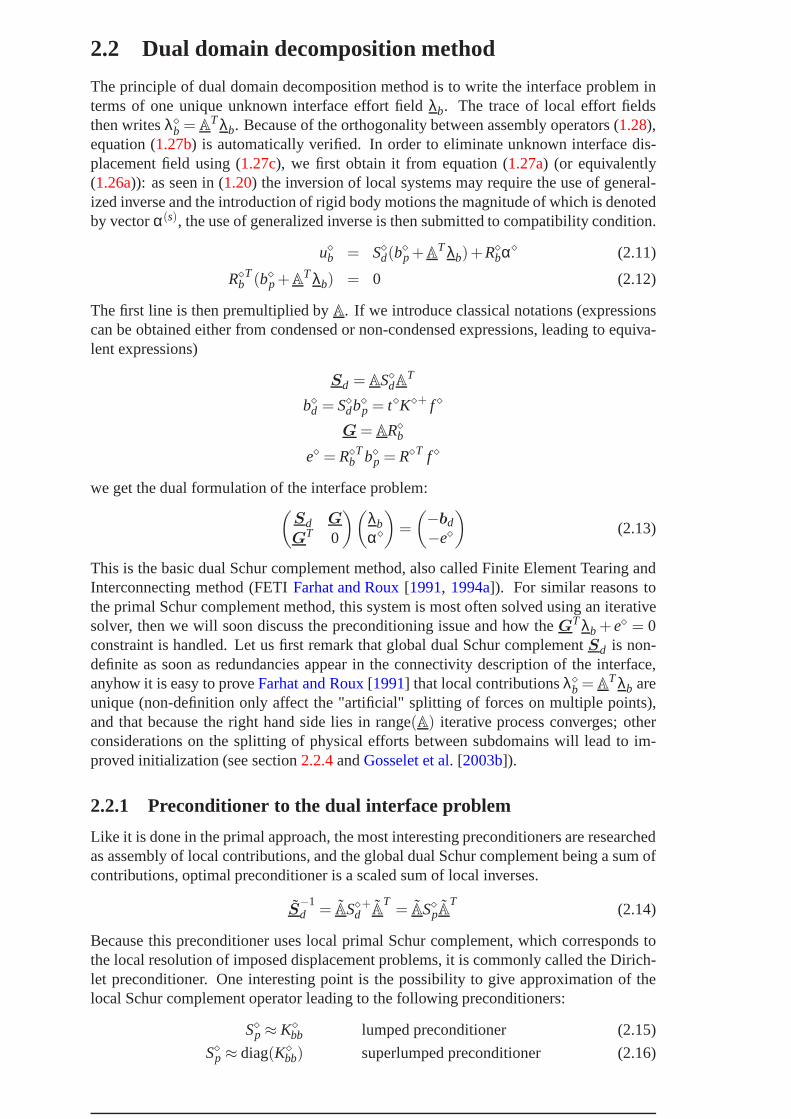
Because this preconditioner uses local primal Schur complement, which corresponds tothe local resolution of imposed displacement problems, it is commonly called the Dirich-let preconditioner. One interesting point is the possibility to give approximation of thelocal Schur complement operator leading to the following preconditioners:

S⋄p ≈ K⋄bb lumped preconditioner (2.15)

S⋄p ≈ diag(K⋄bb) superlumped preconditioner (2.16)


These preconditioners have very low computational cost (they do not require the compu-tation and storage of the inverse of local internal matricesK⋄

ii−1), even if their numerical

efficiency is not as strong as the Dirichlet preconditioner,they can lead to very reducedcomputational time.

Scaled assembly operatorA can be defined the following wayKlawonn and Widlund[2001]:

A =(

AM⋄−1A

T)+

AM⋄−1 (2.17)

whereM⋄ is the same parameter as for the primal approach. Such a definition is not thateasy to implement, an almost equivalent strategy is then used, easily described using the(s) notation:

S−1d = ∑

sM(s)A(s)S(s)

p A(s)TM(s) (2.18)

• M(s) = diag( 1multiplicity ) for homogeneous structures,

• M(s) = diag(diag(K(r)

bb )i

∑ j diag(K( j)bb )i

) for compressible heterogeneous structures (assumingi

represents the same degree of freedom shared by thej subdomains and(r) is thesubdomain connected to(s) on degree of freedomi),

• M(s) = diag( µ(r)i

∑ j µ( j)i

) for incompressible heterogeneous structures (assumingi repre-

sents the same degree of freedom shared by thej subdomains and(r) is the subdo-main connected to(s) on degree of freedomi).

We have the following partition of unity result:

AAT = Iϒ (2.19)

and the following complementarity between primal and dual scalingsGosselet et al.[2003b]:

ATA+A

TA = I ⋄ (2.20)

A(s)TM(s)A(s) +A(s)T

M(s)A(s) = Iϒ(s) (2.21)


Admissibility conditionGTλb +e⋄ = 0, can also be handled with an initialization / pro-jection algorithm (see sectionA.6): λb = λ0 +P λ∗ with GTλ0 = −e⋄ andGTP = 0.

λ0 = −QG(GTQG

)−1e⋄ (2.22)

P = I −QG(GTQG

)−1GT (2.23)

The easiest choice for operatorQ is the identity matrix, projectorP is then orthogonal,this choice is well suited to homogeneous structures. For heterogeneous structures, matrixQ has to provide information on the stiffness of subdomains, thenQ is chosen to be a

version of the preconditioner leading to "superlumped projector" (Q = Adiag(K⋄bb)A

T),

"lumped projector" (Q = AK⋄bbA

T) and "Dirichlet projector" (Q= AS⋄pA

T). Superlumped

projector is often a good compromise between numerical efficiency and computationalcost.

Algorithm 2.2.1presents a classical implementation of FETI method, and figure 2.2provides a schematic representation of the first iteration of the preconditioned dual ap-proach.


Algorithm 2.2.1 Dual Schur complement with conjugate gradient

1: SetP = I −QG(GTQG)−1GT

2: Computeλ0 = −QG(GTQG)−1e3: Computer0 = PTbd−Sdλ0)4: z0 = PS−1

d r0 setw0 = z0

5: for j = 0, . . . ,m do6: p j = PTSdw j

7: α j = (zj , r j)/(p j ,w j)8: λ j+1 = λ j +α jw j

9: r j+1 = r j −α j p j

10: zj+1 = PS−1d r j+1

11: For 06 i 6 j, βij = −(zj+1, pi)/(wi , pi)

12: w j+1 = zj+1+∑ ji=1βi

jwi

13: end for14: α⋄ = (GTQG)−1Gtrm

15: u⋄ = K⋄+λm+R⋄α⋄


The convergence of the dual domain decomposition method is strongly linked to physicalconsiderations. After projection, the residual can be interpreted as the jump of displace-ment between substructures:

r = P T(−bd−Sdλ) = Au⋄ = ∆(u) (2.24)

∆(u)|ϒ(i, j) = u(i)|ϒ(i, j) −u( j)

|ϒ(i, j) (2.25)

Anyhow, such an interpretation cannot be connected to the global convergence of thesystem. In order to evaluate the global convergence, a unique interface displacement fieldhas to be defined (most often using a scaled average of local displacement fields) and usedto evaluate the global residual. When using the Dirichlet preconditioner, it is possible tocheaply evaluate that convergence criterion. Average interface displacementub can bedefined as follow:

ub = AAT∆ (2.26)

then, from equation (2.8), convergence criterion reads:‖Ku− f‖ = ‖AS⋄pATr‖. So when

using the Dirichlet preconditioner, the evaluation of the global residual only requires theuse of a geometric assembly after the local Dirichlet resolution.

2.2.4 Interpretation and improvement on the initialization

Let us come back to the original dual system (1.26).

K⋄u⋄ = f ⋄ + t⋄TA

TλbAt⋄u⋄ = 0

(2.27)

And suppose this system is being initialized with non zero effort λb0:

K⋄u⋄ = f ⋄ + t⋄TA

Tλb (2.28)

let λb = λb +λb0

K⋄u⋄ = f ⋄ + t⋄TA

T λb+ t⋄TA

Tλb0

= f ⋄ + t⋄TA

T λb (2.29)

with f ⋄ = f ⋄ + t⋄TA

Tλb0 (2.30)


Figure 2.2: Representation of first iteration of preconditioned dual approach

So initializationλb0 can be interpreted as modificationt⋄TA

Tλb0 of the intereffort be-tween substructures: local problems are defined except for an equilibrated interface effortfield; the only field that makes mechanical sense (and that is uniquely defined) is theassembly of interface efforts.

At⋄ f ⋄ = At⋄ f ⋄ = fb global interface effort (2.31)

becauseAt⋄t⋄TA

Tλb0 = AATλb0 = 0 (2.32)

Non-zero initialization then can be interpreted as a repartition of global interface effortfb. Two strategies can be defined in order to realize that splitting.

Classical effort splitting Though splitting is hardly ever interpreted as a specific initial-ization, it is commonly realized that, based on the difference of stiffness betweenneighboring substructures (that idea is strongly connected to the definition of scaledassembly operators) the aim is to guide the stress flow insidethe stiffer substructure,sticking to what mechanically occurs.

Global interface effortfb is then split according to the stiffness scaling (M⋄ =diag(K⋄

bb)), which leads to modified local effortf ⋄b .

f ⋄b = M⋄A(AM⋄

AT)−1

fb (2.33)

Complete effortf ⋄ is constituted byf ⋄ inside the substructure ((I − t⋄T t⋄) f ⋄) andsplit effort on its interface (t⋄T f ⋄b ).

f ⋄ = (I − t⋄Tt⋄) f ⋄ + t⋄T f ⋄b (2.34)

Because of the complementarity between scaled assembly operators (2.20), finaleffort reads

f ⋄ = f ⋄− t⋄TA

T(AM⋄−1

AT)+

AM⋄−1t⋄ f ⋄ (2.35)


Interface effort splitting Gosselet et al.[2003b] If we start from condensed dual system(1.27)

S⋄pu⋄b = b⋄p+ATλb

Au⋄b = 0(2.36)

condensed efforts can be split along the interface as long asglobal condensed effortremains unique. Assembled condensed interface effort readsbp = Ab⋄p, if it is splitaccording to the stiffness of the substructures:

b⋄p = M⋄A(AM⋄

AT)−1

bp (2.37)

We have using the complementarity between scalings:

b⋄p = b⋄p−AT(AM⋄−1

AT)+

AM⋄−1b⋄p (2.38)

Or in a non-condensed form:

f ⋄ = f ⋄− t⋄TA

T(AM⋄−1

AT)+

AM⋄−1b⋄p (2.39)

As will be shown in assessments, the classical splitting leads to almost no improvementof the method while the condensed splitting can be very efficient for heterogeneous struc-tures. In fact the initialization associated to this splitting can be proved to be optimalin a mechanical sense; it can also be obtained from the assumptions used for the primalapproach.

Primal approach initialization is realized supposing thatinterface displacement fieldis zero on the condensed problem; from (2.36) we get:

ATλb0+b⋄p ≃ 0 (2.40)

which could only be the solution if null interface displacement was the solution. Thenlocal interface efforts are split into an equilibrated partand its remainingρ⋄:

b⋄p = A

Tγ+ρ⋄

γ =(AD⋄AT)+

AD⋄b⋄p(2.41)

D⋄ is a symmetric definite matrix, remainingρ⋄ is orthogonal to range(D⋄A). If thesystem is initialized by:

λb00 = −γ (2.42)

then initial residualATλb00+ b⋄p = −ρ⋄ is minimal in the sense of the norm associatedto D⋄. If D⋄ = diag(Kbb

⋄)−1 then initialization is equivalent to the splitting of condensedefforts according to the stiffness of substructures ; diag(Kbb

⋄) being an approximation ofSp

⋄ that norm can be interpreted as an energy.The initialization by the splitting of condensed efforts has to be made compatible with

solid body motions by the computation of:

λb0 = P λb00−QG(GTQG

)−1e⋄ (2.43)

Remark 2.2.1 If D⋄ = S⋄d was not computationally too expensive then improved initial-ization with Dirichlet preconditioner would lead to immediate convergence.

Remark 2.2.2 The recommended choice D⋄ = diag(Kbb⋄)−1, is computationally very

cheap, the heaviest operation is the computation of condensed efforts (one applicationof Dirichlet operator). Then if the Dirichlet preconditioner is used, new initialization isjust as expensive as one preconditioning step but it can leadto significant reduction of it-erations, so it should be employed. Of course if light preconditioner is preferred classicalsplitting should be used.


2.3 Three fields method / A-FETI method

The A-FETI methodPark et al.[1997b,a] can be explained as the application of the three-field strategyBrezzi and Marini[1993] to conforming grids, this method is widely studiedin Rixen et al.[1999]. Back to (1.27), we have

S⋄pu⋄b = b⋄p+λ⋄b (2.44)

Aλ⋄b = 0 (2.45)

Au⋄b = 0 (2.46)

A-FETI method is based, like in the primal approach, on the introduction of unknowninterface displacement fieldub, the continuity of displacement then reads:

u⋄b = ATub (2.47)

but local displacements are not eliminated like in the primal approach, complete systemreads:

S⋄p −I 0−I 0 AT

0 A 0

u⋄bλ⋄

bub

=

b⋄p00

(2.48)

In order to eliminate interface displacementub a specific symmetric projector is intro-duced:

B = I −AT (

AAT)−1

A (2.49)

B realizes the orthogonal projection on ker(A) (AB = 0). SinceAλ⋄b = 0 thenλ⋄

b can bewritten as

λ⋄b = Bµ⋄b (2.50)

µ⋄b is a new interface effort, corresponding (recallAAT = diag(multiplicity)) to an av-erage of originalλ⋄

b. Introducing last result and usingBTAT = 0 to eliminate interfacedisplacement we have (

S⋄p −B−BT 0

)(u⋄bµ⋄b

)=

(b⋄p0

)(2.51)

Then using classical elimination of local displacement by the inversion of the first line ofthe previous system, we get

u⋄b = S⋄p+ (b⋄p+Bµ⋄b

)+R⋄

bα⋄ (2.52)

R⋄bT (b⋄p+Bµ⋄b

)= 0 (2.53)

which leads to (BTS⋄dB BTR⋄

bR⋄

bTB 0

)(µ⋄bα⋄

)=

(−BTS⋄+p b⋄p

−R⋄b

Tb⋄p

)(2.54)

This system is very similar to the classical dual approach system, and in consequenceis solved in the same way (using projected algorithm). Anyhow the main difference isthat Lagrange multiplierµ⋄b is defined locally on each subdomain and not globally on theinterface.

Though it was proved inRixen et al.[1999] that A-FETI is mathematically equivalentto classical FETI with special choice of theQ matrix parameter of the rigid body motionprojector. In fact ifQ = diag( 1

multiplicity ) then FETI leads to the same iterates as A-FETI.Moreover operatorB is an orthonormal projector which realizes the interface equilibriumof local reactionsµ⋄b, it can be analyzed as an orthonormal assembly operator as describedin figure1.5.

To sum up, A-FETI can be viewed as the conforming grid versionof the three-fieldapproach, a specific case of classical FETI, and a dual approach with non-redundant de-scription of the connectivity interface with orthonormal assembly operator.


2.4 Mixed domain decomposition method

Mixed approaches offer a rich framework for domain decomposition methods. It en-ables to give a strong mechanical sense to the method, mostlyby providing a behaviorto the interface. The mixed approach is one of the bases of theLaTIn methodLadevèze[1999], Ladevèze et al.[2001], Nouy [2003], which in fact possesses much specifity, themajor of which being that it is designed for non-linear analysis; as we have restrained ourpaper to linearized problems, we do not go further inside this method which deserves ex-tended survey. Several studies were realized on mixed approaches, these methods possessstrong similarities, we here mostly refer to works on so-called "FETI-2-fields" methodSeries et al.[2003a,b].

The principle of the method is to rewrite the interface conditions:

Aλ⋄b = 0

Au⋄b = 0(2.55)

in terms of a new local interface unknown, which is a linear combination of interfaceeffort and displacement.

µ⋄b = λ⋄b+T⋄

b u⋄b (2.56)

µ⋄b is homogeneous to an effort andT⋄b can be interpreted as an interface stiffness. Mixed

methods thus enable to give a mechanical behavior to the interface, in our case (perfectinterfaces) it can be mechanically interpreted as the insertion of springs to connect sub-structures. New interface condition reads:

ATAλ⋄

b+T⋄b A

TAu⋄b = 0⋄ (2.57)

or ATAµ⋄b−

(A

TAT⋄

b −T⋄b A

TA)

u⋄b = 0⋄ (2.58)

It is of course necessary to study the condition for this system being equivalent to system(2.55). It is important to note that two conditions lying on the global interfaces (geometricand connectivity) were traced back to the local interfaces,so up to a zero-measure set(multiple points) the conditions have the same dimension. The new condition is equivalentto the former if facing local interfaces do not hold the same information which is the caseif matrix

(ATAT⋄

b −T⋄b A

TA)

is invertible. An easy method to construct such matriceswill be soon discussed

If unknownµ⋄b is introduced inside local equilibrium equation, the localsystem reads:(S⋄p+T⋄

b

)u⋄b = b⋄p+µ⋄b (2.59)

If we assume thatT⋄b is chosen so that

(S⋄p+T⋄

b

)is invertible then we have:

u⋄b =(S⋄p+T⋄

b

)−1(µ⋄b+b⋄p

)(2.60)

Then substituting this expression inside interface condition (2.58), interface system reads:

(A

TA−

(A

TAT⋄

b −T⋄b A

TA)(

S⋄p+T⋄b

)−1)

µ⋄b

=(A

TAT⋄

b −T⋄b A

TA)(

S⋄p+T⋄b

)−1b⋄p (2.61)

so mixed approaches have the originality to rewrite global interface conditions on thelocal interfaces and to look for purely local unknown (whichmeans that the size of theunknown is about twice the size of the unknown in classical primal or dual methods).

This general scheme for mixed methods has, as far as we know, never been employed.A first reason is that it leads to certain programming complexity, second the manipulationof zero-measure interfaces is not easy for methods aiming atintroducing strong mechani-cal sense and hard to justify from a mathematical point of view. So most often a simplified


method is preferred, which takes only into account non-zero-measure interfaces. Such anapproach simplifies the connectivity description of the interface, every relationship on theinterface only deals with couples of subdomains. In order tohave the clearer expressionpossible, we present the algorithm in the two subdomains case. Interface equilibriumreads:

u(1)b −u(2)

b = 0

λ(1)b +λ(2)

b = 0(2.62)

which is equivalent to

λ(1)

b +λ(2)b +T(1)

(u(1)

b −u(2)b

)= 0

λ(1)b +λ(2)

b +T(2)(

u(2)b −u(1)

b

)= 0

(2.63)

under the condition of invertibility of(

T(1) +T(2))

. Introducing unknownµ(s)b = λ(s)

b +

T(s)u(s) interface system reads:

µ(1)

b +µ(2)b −

(T(1) +T(2)

)u(2) = 0

µ(1)b +µ(2)

b −(

T(1) +T(2))

u(1) = 0(2.64)

Local equilibrium reads:

(S(1)

p +T(1))

u(1)b = µ(1)

b +b(1)p(

S(2)p +T(2)

)u(2)

b = µ(2)b +b(2)

p

(2.65)

AssumingT(s) is chosen so that matrix(

S(s)p +T(s)

)is invertible, we can express dis-

placementu(s)b from local equilibrium equation, and suppress it from global interface

conditions, which leads to:

I I −(

T(1) +T(2))(

S(2)p +T(2)

)−1

(T(1) +T(2)

)(S(1)

p +T(1))−1

I

(

µ(1)

µ(2)

)=

(T(1) +T(2)

)(S(2)

p +T(2))−1

b(2)p

(T(1) +T(2)

)(S(1)

p +T(1))−1

b(1)p

(2.66)

This expression enables to give better interpretation of the stiffness parametersT(s). Sup-

poseT(1) = S(2)p andT(2) = S(1)

p then matrix (2.66) is equal to identity and solution isdirectly achieved. So the aim of matrixT(s) is to provide one substructure with the inter-face stiffness information of the other substructures.

If we generalize toN-subdomain system (2.61), we can deduce that the optimal choicefor T(s) is the Schur complement of the remaining substructures on the interface of domain

(s) (some kind ofS(s)p where s denotes all the substructures buts). Of course such a

choice is not computationally feasible (mostly because it does not respect the localizationof data), and approximations have to be considered. In decreasing numerical efficiencyand computational cost order, we have:

• Approximate the Schur complement of the remaining of the substructure by theSchur complement of the neighbor;


• approximate the Schur complement of the neighbor by the Schur complement ofthe nearer nodes of the neighbor ("strip"-preconditionerswhich idea is developedin Paz and Storti[2005] in another context);

• approximate the Schur complement of the neighbor by the stiffness matrix of theinterface of the neighbor (strategy of dual approach lumpedpreconditioner).

The second strategy is quite a good compromise: it respects data localization, it is notcomputationally too expensive and yet it enables the propagation of the information be-yond the interface. Of course an important parameter is the definition of elements "nearthe interface", which can be realized giving an integern representing the number of layersof elements over the interface.


Because the interface stiffness parameterT⋄ regularizes local operatorsS⋄p, local operator(S⋄p+T⋄) is always invertible. Such a property can be viewed as an advantage because

it simplifies the implementation of the method introducing no kernel and generalized in-verse; but it also can be considered as a disadvantage because no more coarse problem en-ables global transmission of data among the structure. Thenthe communications inductedby this method are always neighbor-to-neighbor which meansthat the transmission of alocalized perturbation to far substructures is always a slow process. It is then necessary toadd an optional coarse problem (see sectionA.7). Most often the optional coarse problemis constituted of would-be rigid body motions (if subdomains had not been regularized).Another possibility, which is proposed inside the LaTIn method is to use rigid body mo-tions and extension modes of each interface as coarse problems, this leads to much largercoarse space. The coarse matrix corresponds to the virtual works of first order of defor-mation of substructures; so mechanically it realizes and propagates a numerical first orderhomogenization of the substructures.

2.5 Hybrid approach

The hybrid approach (seeGosselet et al.[2004] for a specific application) is a propositionto provide a unifying scheme for primal and dual approaches though it could easily beextended to other strategies. It relies on the choice for each interface degree of freedomof its own treatment (for now primal or dual). So let us define two subsets of interfacedegrees of freedom: the first is submitted to primal conditions (subscriptp) and the secondto Neumann conditions (subscriptd). Local equilibrium then reads ( ¯p = i ∪d, b = d∪ p,p∩d = /0): (

K⋄pp K⋄

ppK⋄

pp K⋄pp

)(u⋄pu⋄p

)=

(f ⋄pf ⋄p

)+

(t⋄d

Tλ⋄d

λ⋄p

)(2.67)

Preferred interface unknowns are unique displacement on the first subsetup and uniqueeffort on the second subsetλd. Local contributions then reads:

u⋄p = ATpup (2.68)

λ⋄d = A

Td λd (2.69)

which ensure the continuity of displacement on thep degrees of freedom and the action-reaction principle on thed degrees of freedom, of course operatorAp andAd have beenrestricted respectfully to thep andd subsets. Remaining interface conditions read:

Adu⋄d = Adt⋄du⋄p = 0 (2.70)

Apλ⋄p = 0 (2.71)


To obtain the global interface system, first local unknownu⋄p has to be eliminated:

u⋄p = K⋄pp

+(

f ⋄p + t⋄dTλ⋄

d−K⋄ppu

⋄p

)+R⋄

pα⋄ (2.72)

Applying continuity condition to previous result and equilibrium condition to the secondrow of (2.67), interface system reads:

Spd

(Gp

Gd

)

(−GT

p GTd

)0

up

λdα⋄

=

bp

−bd−e⋄

(2.73)

with the following notations:

Spd =

(Ap 00 Ad

)S⋄pd

(Ap 00 Ad

)T

Gp = ApKpp⋄R⋄

p, Gd = Adt⋄dR⋄p

e⋄ = R⋄pT f ⋄p

bp = Ap(

f ⋄p −K⋄ppK⋄

pp+ f ⋄p

), bd = Adt⋄dK⋄

pp+ f ⋄p

This interface problem corresponds to the constrained resolution of one linear system. Theconstraint is linked to the possible non-invertibility of matrix K⋄

pp and thus to the choiceof primal subset. Notice thatGp represents the reaction of primal degrees of freedomto zero energy modes ofK⋄

pp and then should be zero in most cases (it may be non zeroin buckling cases). Moreover this system may represent classical primal approach (if allinterface degrees of freedom are in subsetp) or classical dual approach (if all interfacedegrees of freedom are in subsetd). OperatorSpd is a primal/dual Schur complement, itis the sum of local contributionsS⋄pd (1.24).

The above system is nonsymmetric semi-definite (because of redundancies on the dualsubset) positive, it has to be solved by GMRes-like algorithm.

2.5.1 Hybrid preconditioner

Inspired by primal and dual preconditioners, we propose to approximate the inverse of thesum of local contributions by a scaled sum of local inverses.

S−1pd =

(Ap 00 Ad

)S⋄dp

(Ap 00 Ad

)T

(2.74)

Scaled assembly operator are defined in the same way as in primal and dual approaches.

2.5.2 Coarse problems

As said earlier, depending on the choice of subsetp, local operatorK⋄pp (involved in the

computation ofS⋄pd) may not be invertible and, like in dual approach, a first coarse cor-rection has been incorporated inside the hybrid formulation. Anyhow local operatorK⋄

ddinvolved in preconditioning step may also not be invertibleand, like in primal approach, asecond coarse problem has to be added to make the preconditioner optimal. Then, the op-timal version of the hybrid system incorporates two coarse problems handled by specificinitialization/projection algorithm. The admissibilitycondition reads:

GTx = e (2.75)


with G =

(Gp

Gd

), x =

(up

λd

)andb =

(bp

−bd

). If r = b−Spdx stands for the residual

before preconditioning, the optimality condition reads:

HTr =

(Hp

Hd

)T(rp

rd

)= 0 (2.76)

with Hp = Apt⋄pR⋄d

andHd = AdK⋄dd

R⋄d

(as said before most oftenHd = 0). To sum upconstraints:

GTx = −e⋄

HTSpdx = HTb(2.77)

Handling such constraints is described in sectionA.8.Figure2.3 provides a schematic representation of the first iteration of the precondi-

tioned hybrid approach, in the specific case of a nodal partition of the interface. Assess-ments will deal with partition at the degree of freedom level.

Figure 2.3: Representation of first iteration of preconditioned hybrid approach


Because GMRes-like solver is used, the euclidian norm of theresidual is directly avail-able, such a norm is the sum of displacement gap on thed part of the interface and aneffort gap on thep part of the interface. For now, no other estimator with better physicalsense is available.


Chapter 3

Adding optional constraints

The aim of this section is to describe the technical point ofview of the adjunction of optional constraints to the resolutionof the interface system: providing meaningful constraintsmaylead to very significant decrease of the number of iterationsand thus important speedup. This section focusses on thedifferent strategies to ensure the constraints; the classical

choices of constraints will be presented in next section. Forsimplicity reason, we restrain to primal and dual domain

decomposition methods.

Contents3.1 Augmentation strategy . . . . . . . . . . . . . . . . . . . . . . . . . . . 34

3.2 Recondensation strategy . . . . . . . . . . . . . . . . . . . . . . . . . . 34

3.2.1 Basic method. . . . . . . . . . . . . . . . . . . . . . . . . . . . . 34

3.2.2 More complex constraints. . . . . . . . . . . . . . . . . . . . . . 35

3.3 Adding "constraints" to the preconditioner . . . . . . . . . . . . . . . . 36


The aim of optional constraints is to ensure that the research space for the iterativesolver possesses a certain regularity. The choice of constraints will be discussed in a latersection. Going back to the interface system:

S⋄p −I ⋄

A 00 A

(

u⋄bλ⋄

b

)=

b⋄p00

(3.1)

any constraint of the formCTAu⋄b = 0 or CTAλ⋄

b = 0 is trivially verified by the solu-tion fields, it is just a restriction of continuity/equilibrium conditions. From an iterativeprocess point of view, these conditions will be reached onceconverged ; the principle ofoptional constraints is to have every iteration verify thatcondition.

There are two classical solutions to ensure these optional constraints: either to re-alize a splitting of research space and ensure, using a projector, that the resolution islimited to convenient subspace, or to realize a condensation of constraints and make it-erations on a smaller space. In other words suppose there arenc independent constraintsin a n-dimension space the first strategy researchesn-sized solution in a(n−nc)-rankedspace, while the second solution researches(n−nc)-sized solution in a(n−nc)-dimensionspace then deduce then-sized solution. From a numerical point of view both solutionsare equivalent, they are just two ways of handling the same constraints, anyhow fromimplementation and computational points of view they have strong differences.

3.1 Augmentation strategy

For this strategy the constraint is reinterpreted in terms of constraint on the residual. Typ-ically, the primal approach can be augmented by constraintson the effort field while thedual approach can have constraints on the displacement field:

CTAλ⋄

b = −CT (Ab⋄p−AS⋄pA

Tub)

(3.2)

CTAu⋄b = CT (

AS⋄dATλb+b⋄d

)(3.3)

The constraint is then handled as an augmentation inside theiterative solver, its is classi-cally realized using a projector (see sectionsA.7 andA.8).

3.2 Recondensation strategy

This strategy was recently introduced in the framework of the dual approach, leading tothe FETIDP algorithmFarhat et al.[2001, 2000a], Lesoinne and Pierson[1999], Klawonn et al.[2005]. Because for now only constraints on theu⋄b field have been considered we willrestrain to this kind of constraints, the application of constraints onλ⋄

b is straightforward.

3.2.1 Basic method

We first consider constraints read as continuity of specific degrees of freedom, in otherterms we suppose matrixC is identity on certain degrees of freedom and zero elsewhere;we will show how any constraint can be rewritten in such a form. Because these degreesof freedom will be submitted to a primal treatment we will denote then with subscriptpwhile the remaining of the interface will be denoted with subscriptd. Constraint reads:

0 = CTAu⋄b =

(0Ip

)T(Adu⋄dApu⋄p

)= Apu⋄p (3.4)


Like in the hybrid approach this constraint is verified usinga unique displacementfield on the primal part of the interface:u⋄p = AT

pup. Interface system then reads like inthe hybrid approach, with the additional assumption that the constraints are so that thelocal problem possesses enough Dirichlet conditions to make it invertible.

Spd

(up

λd

)=

(bp

−bd

)(3.5)

Introducing following notations for blocks composingS⋄pd:

S⋄pd =

(s⋄pp s⋄pd−s⋄dp s⋄dd

)(3.6)

then

Spd =

(spp spd

−sdp sdd

)=

(Ap 00 Ad

)(s⋄pp s⋄pd−s⋄dp s⋄dd

)(Ap 00 Ad

)T

(3.7)

Unknownup is condensed on the remaining of the interface:

up = s−1pp

(bp−spdλd

)(3.8)

sdλd =(sdd +sdps

−1ppspd

)λd = −bd +sdps

−1ppbp (3.9)

The latest equation is solved using an iterative solver, operatorsd has the same proper-ties as the restriction of the dual operator to thed-part of the interface (semi-definition,symmetry and positivity). Operatorsd is the assembly of local contributions

sd = Ads⋄dATd = Ad

(s⋄dd+s⋄dpA

Tps−1

ppAps⋄pd

)A

Td (3.10)

Using operatorsd requires the computation of the inverse of matrixspp = Aps⋄ppATp,

which is an assembled matrix. Then this formulation includes a global coarse problem seton primal variables.

The recommended preconditioner for such an approach is directly inspired by the dualapproach: it consists in solving local Dirichlet problems with scaled imposed displace-ment on thed-part of the interface and null displacement on thep part of the interfaceand extracting the average reaction of thed-part of the interface. Then the preconditionerreads:

s−1d =

(0p A

)S⋄p(0p A

)T(3.11)

Figure3.1 provides schematic representation of the first iteration ofpreconditionedFETID method.

3.2.2 More complex constraints

We now consider constraints which are not limited to one degree of freedom, for instanceone can consider that we want to ensure that the average jump of displacement on oneedge is equal to zero, which involves all the degrees of freedom of the edge.

The classical solutionKlawonn et al.[2005] is to realize a change of basis of degreesof freedom (denoted by matrixT⋄) so that each constraint is represented by one "modi-fied" degree of freedom. The change of basis is the same local operation realized on everysubdomain, then we can define a global changeT so thatAT⋄ = TA

CTAu⋄b = CT

AT⋄u⋄b = CTTAu⋄b = CTAu⋄b (3.12)

with C =

(0I p

)(3.13)

After the change of basis is realized the same algorithm can be employed. Because con-straints most often respect a certain locality of data (for instance independent constraintson each edge), change of basis is not a too expensive operation, and does not make tooworse the sparsity of local matrices.


Figure 3.1: Representation of the first iteration of preconditioned FETIDP

3.3 Adding "constraints" to the preconditioner

This section deals with the dualization of the recondensation strategiesCros [2002],Dohrmann[2003]. For instance the balanced domain decomposition with constraints(BDDC) is a primal version of FETIDP: during the preconditioning step, the continuityof displacement is ensured at specific degrees of freedom (which can be the result of alocal change of basis), so that the local Neumann operator remains fully invertible. Sosolving classical primal approach problem

Spub = AS⋄pATub = bp (3.14)

the preconditioner reads

S−1p =

(Ip 00 Ad

)(s−1

pp −s−1ppAps⋄pd

−s⋄dpATps−1

pp s⋄d

)(Ip 00 Ad

)T

(3.15)

Figure3.1provides a schematic representation of the first iteration of preconditionedBDDC method.


Figure 3.2: Representation of the first iteration of preconditioned BDDC


Chapter 4

Classical issues

In this section we try to provide some answers to questionsthat commonly arise when using domain decomposition

methods.

Contents4.1 Rigid body motion detection . . . . . . . . . . . . . . . . . . . . . . . . 40

4.1.1 Simple algebraic approach. . . . . . . . . . . . . . . . . . . . . . 40

4.1.2 Geometric approach. . . . . . . . . . . . . . . . . . . . . . . . . 41

4.1.3 Generalized inverse. . . . . . . . . . . . . . . . . . . . . . . . . . 41

4.2 Choice of optional constraints . . . . . . . . . . . . . . . . . . . . . . . 41

4.2.1 Forth order elasticity. . . . . . . . . . . . . . . . . . . . . . . . . 41

4.2.2 Second order elasticity. . . . . . . . . . . . . . . . . . . . . . . . 42

4.2.3 Link with homogenization theory. . . . . . . . . . . . . . . . . . 43

4.3 Linear Multiple Points Constrains . . . . . . . . . . . . . . . . . . . . . 43

4.4 Choice of decomposition. . . . . . . . . . . . . . . . . . . . . . . . . . . 45

4.5 Extensions . . . . . . . . . . . . . . . . . . . . . . . . . . . . . . . . . . 46

4.5.1 Nonsymmetric problems. . . . . . . . . . . . . . . . . . . . . . . 46

4.5.2 Nonlinear problems. . . . . . . . . . . . . . . . . . . . . . . . . . 46

4.6 Implementation issues. . . . . . . . . . . . . . . . . . . . . . . . . . . . 46

4.6.1 Organization of the topological information. . . . . . . . . . . . . 47

4.6.2 Defining algebraic interface objects (fig. 4.3). . . . . . . . . . . . 47

4.6.3 Articulation between formulation and solver (fig. 4.4) . . . . . . . 48


4.1 Rigid body motion detection

Handling floating substructures is definitely a very accurate issue. This difficulty is oneof the reason of the success of methods which regularize the stiffness of subdomains likeFETIDP or mixed approaches, leading to fully invertible matrices. Anyhow basic primaland dual methods remain competitive (mostly because zero-energy modes provide a verynatural coarse problem), hence providing an efficient algorithm for the computation ofrigid body motion is essential. Many strategies can be usedFarhat and Géradin[1996],Farhat et al.[2000c], and this review does not claim to be exhaustive.

First we have to discuss the exact composition of the possible kernel of substructures.What can be found is:

• rigid body motions of floating substructures,

• internal mechanisms of substructures,

• weird things due to nonlinearities (buckling, exotic behaviors, ...)

• numerical zero-energy modes.

An internal mechanism can for instance occur when a substructure is made out of twoparts connected by one linear edge (pivot) or one singular point (kneecap). Methodsexist to avoid such substructures either inside the decomposition algorithm or as externalprograms regularizing a given decompositionFragakis and Papadrakakis[2002], and thenshould be employed.

The last two kinds of kernel are non-standard and can only be detected using fullyalgebraic methods (like Gauss pivoting). The problem with algebraic methods is theirhigh sensitivity to the condition number of the stiffness matrix of substructures. Thecondition number can be influenced by the aspect ratio and thematerial composition ofthe substructures, even after adimensionalization the quality of the methods is hard towarranty.

Finally we only develop here two strategies to handle zero-energy modes. The firstone belongs to the purely algebraic methods, it is very simple to implement and can leadto satisfying results for not-too-complex problems, it canhandle more than solid bodymotions but it is strongly dependent ona priori selected degrees of freedom. The secondmethod is purely geometric, it is very robust but only suitedto detect solid body motions.

In order to simplify notations, we consider the research of the zero-energy modes ofmatrixK (which should be a local stiffness matrix).

4.1.1 Simple algebraic approach

This method is based on fundamental relationship between the kernel of a matrix and thekernel of Schur complement (1.14). The principle is to preselect a small set of degrees offreedom which we will denote by subscriptN (the other degrees of freedom are denotedwith subscriptO). Then compute explicitly primal Schur complement associated to thesedegrees of freedom:S= KNN−KNOK−1

OOKON). If N-degrees of freedom are selected sothatK00 is invertible (if only solid body motions have to be detectedthen it is sufficient totake the degrees of freedom associated to three non-alignednodes) thenS is well definedand its kernel is linked to the kernel of matrixK.

SinceN is a "small" set (12 degrees of freedom is often sufficient), computing thekernel of matrixS using "exact" algorithm like singular value decompositionis rathercheap and then kernel of matrixK can be computed using equation (1.14).


4.1.2 Geometric approach

The basic idea of this method is that kinematically admissible solid body motions canbe deduced from boundary conditions imposed on one subdomain. Let Rc be a basis ofcandidate rigid body motions (would be solid body motions ifno Dirichlet conditionswere applied on the subdomain,Rc is a 6-column matrix in 3D and 3-column matrixin 2D), and letE be the matrix of Dirichlet boundary conditions: each columnof Erepresents one (combination of) blocked degree of freedom.Kinematically admissiblerigid body motionsRare linear combinations of candidate rigid body motions (henceR=RcQ) which do not make Dirichlet boundary conditions work (ie ETR= 0). In order tofind such linear combination, we compute singular value decomposition of matrixETRc =UDVT and setQ = V0 whereV0 is the submatrix ofV associated to negligible singularvalues. BecauseETRc is a matrix only made out of geometric considerations, it is wellconditioned and the criterion to detect "zero" singular values is well defined (there is alarge gap between zero and non-zero singular values).

4.1.3 Generalized inverse

The two methods presented above led tor-ranked basisR of the kernel of matrixK. Tocompute generalized inverseK+, the most classical way is to selectr degrees of freedom,so that if they were added Dirichlet conditions, rigidity matrix would be well defined. For

instance after pivoting and renumber one could getR=

(R∗

Ir

)and then ther last degrees

of freedom would suit. Then we have:

K =

(Kr r Krr

Kr r Krr

)and K+ =

(K−1

r r 00 0

)(4.1)

This is just one instance of generalized inverse, other can be built using penalization orother modification to matrixK. Though not theoretically prohibited, choosing "blocked"degrees of freedom on the interface is often a bad idea from a practical point of view.

4.2 Choice of optional constraints

As seen in section3, constraints can be imposed either using augmentation (using oneor two projectors, sectionsA.7 andA.8) or using recondensation algorithms. In the caseof recondensation algorithms, constraints have to be sufficient in order to suppress rigidbody motions and then regularize the local stiffness matrix. In the case of augmentationalgorithm, constraints have to be independent from rigid body motions which are alreadyhandled by the formulation.

Because constraints are expensive to handle, they have to bechosen with care; any-how, except in a few cases, there are no general results on howto choose them. Mechan-ical comprehension of studied phenomena and anticipation of convergence difficultiesmay lead to efficient strategies. In the case of solving several linear systems (even withdifferent left hand sides) interesting strategies existSaad[1987], Erhel and Guyomarc’h[2000], Gosselet and Rey[2002], Rey and Gosselet[2003], Risler and Rey[1998].

The next two sections deal with very common strategies, while the last section de-scribes another framework for constraints inspired by the LaTIn methodLadevèze[1999],Nouy [2003].

4.2.1 Forth order elasticity

As plate and shell models are often used in structural mechanics, forth order problemshave been carefully studiedFarhat and Mandel[1998], Farhat et al.[1998], Roux[1997],


Le Tallec et al.[1998], Farhat et al.[2000c]. Such problems are characterized by the ap-pearance of singularities at the corner of substructures (so-called "corner modes") whichare destroying the scalability of usual methods. The classical solution consists in enforc-ing the continuity of the (most often only normal) displacement field at the corners inorder to regularize the problem. From a practical point of view, corners are most oftendefined as multiple points (nodes shared by more than two substructures), that set can beenriched by extremities of edges.

Because highlighting the singularity have to be adapted to each method, the imple-mentation is strongly dependent on the formulation.

Dual approach: since the projected residual corresponds to the displacement jump be-tween substructures (2.24), one just has to use augmentation algorithm with oneconstraint for each pair of neighbor at each corner. MatrixC is then made out ofcolumns with one coefficient 1 on one corner degree of freedomand 0 elsewhere.Because the dual description of am-multiple point leads to(m−1) relationships,such a coarse space is rather large.

Primal approach: In order to regularize the displacement field, the constraints have tobe imposed on the preconditioned residual (assuming Neumann-Neumann precon-ditioner is employed). The aim is then to have the local contributions of precondi-tioned residual equal to zero on corner points. So ifC⋄ denotes the local interfacematrix made out of columns with one coefficient 1 on one cornerdegree of freedomand 0 elsewhere, andC⋄ the same matrix scaled according to the scaling used insidethe preconditioner, the constraints readC = AS⋄dC⋄. Then am-multiple degree offreedom leads tom constraints.

Recondensed approaches:FETIDP or BDDC were first designed in this context, fromthe consideration that (extended) corners constraints were sufficient to suppressrigid body motions, then the first level constraints could beavoided. So the meth-ods directly apply since they consist in constraining the displacement field. Herewhatever the multiplicity of a corner may be, it always leadsto just 1 constraint.

4.2.2 Second order elasticity

Because classical methods are already scalable in the frameof second order elasticity,optional constraints are not often used in such a context. Furthermore, it is hard to predictwhat constraint should be imposed. In some cases, efficient strategies have been proposed,such as inGosselet and Rey[2002] for nonlinear problems using Newton-Raphson solverwhere approximations of eigen vectors are used.

The question of optional constraints arose when willing to extend recondensed algo-rithms (FETIDP and BDDC) to such problems, mostly because the previous definition ofcorners lead to significant problems in 3D (too many constraints, poor convergence...).The first solution was proposed inLesoinne and Pierson[1999], the idea was to select3 non-aligned nodes on each face (interface between 2 subdomains) which maximizedthe surface of the triangle they defined. The current solution, the scalability of whichis mathematically and numerically proved, is to enforce average convergence on edgesKlawonn et al.[2005], which is realized by a change of basis described in (3.12). In orderto take into account heterogeneity on the interface, the average may be scaled by a coeffi-cient representing the stiffness of the subdomains. For more difficult problems, first ordermoments of edges can also be added.


4.2.3 Link with homogenization theory

This paragraph intends to present a mechanical vision of optional constraint which, thoughhard to implement in the framework of the presented method, may lead to better un-derstanding of what optional constraints and associated coarse problems can provide tothe methods. This analysis is inspired by the multiscale version of the LaTIn methodLadevèze[1999].

The underlying question when choosing optional constraints (except from specificnumerical questions like in the forth order elasticity) is "what global information shouldbe transmitted to the whole structure ?" or more precisely "what should far substruc-tures know from one substructure". A meaningful answer is provided by Saint-Venantprinciple and homogenization theory: at a first order development, a substructure can berepresented by its rigid body motions and its constant strain states (simple traction andshearing states). Such an idea adds six (3 in 2D) more constraints per subdomains; asthese constraints are somehow complex to build, they can be simplified by interfacewisemodes (but of course the number of constraints then grows quickly).

4.3 Linear Multiple Points Constrains

Multiple points constraints are relationships defined between some degrees of freedom,they are often used in order to connect nonconforming meshes, to represent boundaryconditions (for instance periodicity), to model contact orapply control laws. In the caseof linear(ized) constraints we can write, on the whole structure scale:

Ku = f (4.2)

Cu = a (4.3)

What seems most suited to the domain decomposition context is to dualize the constraintand introduce Lagrange multiplierµ in order to enforce the condition. System then reads:

(K CT

C 0

)(uµ

)=

(fa

)(4.4)

After decomposition we have

K⋄ −I ⋄ CT

At⋄ 0 00 At⋄ 0C 0 0

u⋄

λ⋄

µ

=

f ⋄

00a

(4.5)

with C so thatCu⋄ = Cu= a which implies (sinceu⋄b = ATub):

Cu=(Ci Cb

)(u⋄iub

)= Cu⋄ =

(Ci Cb

)(u⋄iu⋄b

)(4.6)

then CbAT = Cb (4.7)

Or in other words, if matrixC deals with interface degrees of freedom, the associatedconstraints have to be correctly distributed between sharing subdomains. The constraintcan be interpreted as specific (non-boolean) assembly operator which explains the chosennotation. Using MPCs with domain decomposition methods wasstudied inRixen[2002]in the dual method context.

In order to provide general methodology to apply MPCs, we then incorporate insidehybrid domain decomposition method (equations (2.67) to (2.70)):

K⋄

pp K⋄ppA

Tp C

Tp

ApK⋄pp ApK⋄

ppATp CT

pCp Cp 0

u⋄pup

µ

=

f ⋄p + t⋄d

TA

Td λd

Ap f ⋄pa

(4.8)

Adt⋄du⋄p = 0 (4.9)


The elimination ofu⋄p leads to, with classical hybrid notations:

SpdC T

pC T

d

Gp

Gd−C p Cd Cµ Gα−GT

p GTd GT

α 0

up

λdµ

α⋄

=

bp

−bdh

−e⋄

(4.10)

with

C p = Cp−CpK⋄pp

+K⋄ppA

Tp (4.11)

Cd = CpK⋄pp

+t⋄Td A

Td (4.12)

Cµ = CpK⋄pp

+C

Tp (4.13)

Gα = CpRp (4.14)

h = a−CpK⋄pp

+ f ⋄p (4.15)

Various strategies can be used in order to solve system (4.10), which combine elim-ination of constraints (rigid body motions and/or MPCs) by projection methods (FETI-like approaches) and/or by recondensation methods (FETIDPlike approaches). All thesemethods correspond to solving rather complex coarse problems but they are suited totraditional preconditioners. We propose, afterRixen [2002], to use classical projectionmethod to handle rigid body motions then use iterative solver to find simultaneously(up,λd,µ) and provide efficient preconditioner to this problem.

System reads with trivial notations (for simplicity reasons we suppose that the rigidbody motion constraints have been symmetrized, which is always possible and which isnaturally the case ifGp = 0 like in many applications):

(Spdµ G

G T 0

)(x

α⋄

)=

(b

−e⋄

)(4.16)

with

Spdµ =

Ap 00 Adt⋄d0 Cp

S⋄pd

Ap 00 Adt⋄d0 Cp

T

+

0 0 Cp

0 0 0−CT

p 0 0

(4.17)

As can be seen, MPCs have very different actions wether they are set on primal interfacedegrees of freedom or not: matrixCp modifies the structure of the hybrid system whiledual and internal constraints lead to classical hybrid approach with modified dual trace

and assembly operatorA =

(Adt⋄dCp

). The definition of efficient preconditioner inspired

by classical methods is then much simplified if no constraints are set on primal degrees offreedom (Cp = 0), which is what we suppose now:

Spdµ =

(Ap 00 A

)S ⋄pd

(Ap 00 A

)T

(4.18)

TheS ⋄pd notation is due to the association of the trace operator withthe assembly operator,which in fact is equivalent to defining "extended interface dual degrees of freedom" madeout of dual degrees of freedom and degrees of freedom involved in MPCs. Since, in thishypothesis, system reads like classical hybrid approachie (modified) assembly of localcontributions, the proposed preconditioner is a scaled assembly of local inverses.

S−1pdµ =

(Ap 00 A

)S ⋄dp

(Ap 00 A

)T

(4.19)


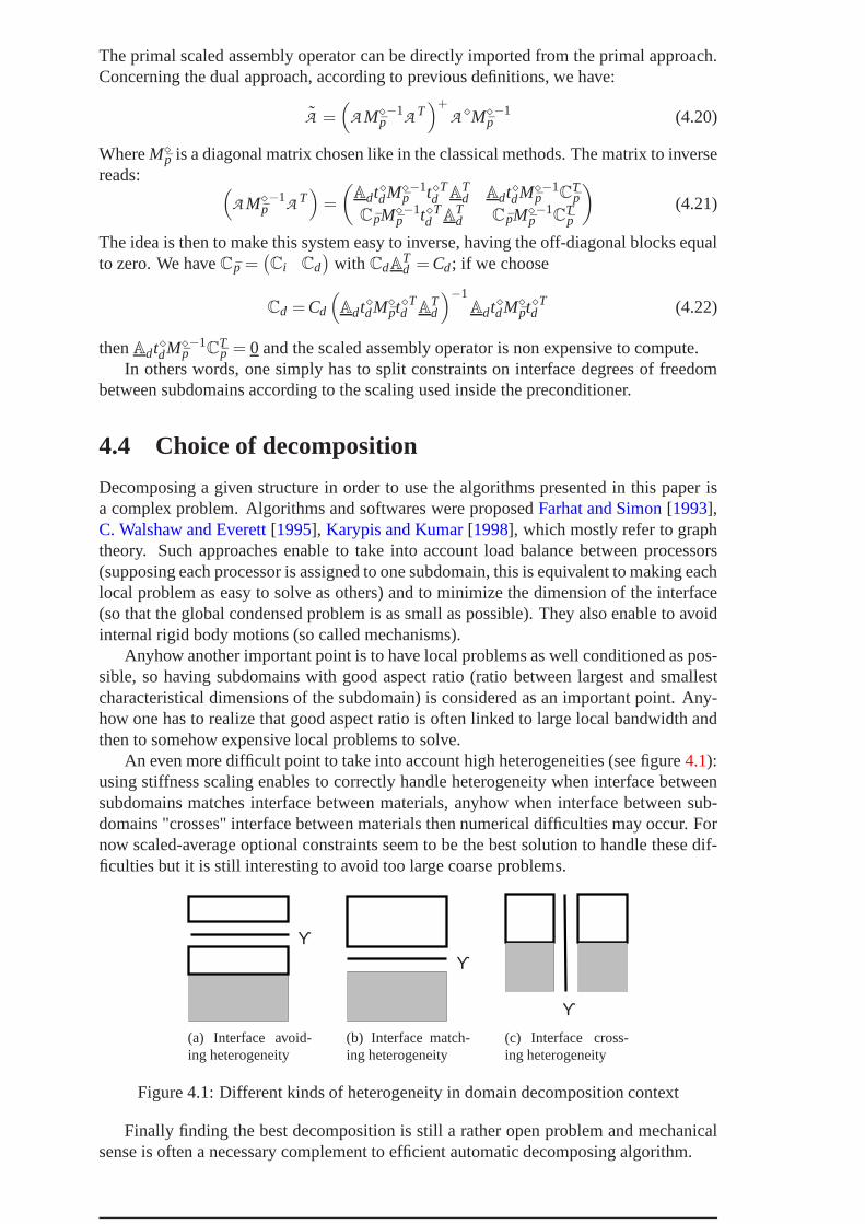
The primal scaled assembly operator can be directly imported from the primal approach.Concerning the dual approach, according to previous definitions, we have:

A =(AM⋄

p−1A T

)+A ⋄M⋄

p−1 (4.20)

WhereM⋄p is a diagonal matrix chosen like in the classical methods. The matrix to inverse

reads: (AM⋄

p−1A T

)=

(Adt⋄dM⋄

p−1t⋄d

TA

Td Adt⋄dM⋄

p−1

CTp

CpM⋄p−1t⋄d

TA

Td CpM⋄

p−1

CTp

)(4.21)

The idea is then to make this system easy to inverse, having the off-diagonal blocks equalto zero. We haveCp =

(Ci Cd

)with CdA

Td = Cd; if we choose

Cd = Cd

(Adt⋄dM⋄

pt⋄d

TA

Td

)−1Adt⋄dM⋄

pt⋄d

T (4.22)

thenAdt⋄dM⋄p−1

CTp = 0 and the scaled assembly operator is non expensive to compute.

In others words, one simply has to split constraints on interface degrees of freedombetween subdomains according to the scaling used inside thepreconditioner.

4.4 Choice of decomposition

Decomposing a given structure in order to use the algorithmspresented in this paper isa complex problem. Algorithms and softwares were proposedFarhat and Simon[1993],C. Walshaw and Everett[1995], Karypis and Kumar[1998], which mostly refer to graphtheory. Such approaches enable to take into account load balance between processors(supposing each processor is assigned to one subdomain, this is equivalent to making eachlocal problem as easy to solve as others) and to minimize the dimension of the interface(so that the global condensed problem is as small as possible). They also enable to avoidinternal rigid body motions (so called mechanisms).

Anyhow another important point is to have local problems as well conditioned as pos-sible, so having subdomains with good aspect ratio (ratio between largest and smallestcharacteristical dimensions of the subdomain) is considered as an important point. Any-how one has to realize that good aspect ratio is often linked to large local bandwidth andthen to somehow expensive local problems to solve.

An even more difficult point to take into account high heterogeneities (see figure4.1):using stiffness scaling enables to correctly handle heterogeneity when interface betweensubdomains matches interface between materials, anyhow when interface between sub-domains "crosses" interface between materials then numerical difficulties may occur. Fornow scaled-average optional constraints seem to be the bestsolution to handle these dif-ficulties but it is still interesting to avoid too large coarse problems.

ϒ

(a) Interface avoid-ing heterogeneity

ϒ

(b) Interface match-ing heterogeneity

ϒ(c) Interface cross-ing heterogeneity

Figure 4.1: Different kinds of heterogeneity in domain decomposition context

Finally finding the best decomposition is still a rather openproblem and mechanicalsense is often a necessary complement to efficient automaticdecomposing algorithm.


4.5 Extensions

4.5.1 Nonsymmetric problems

Nonsymmetry occurs in many physical modeling: plasticity,nonlocal models for fractureGermain et al.[2005], frictional contactBarboteu et al.[2001]. The use of the domaindecomposition methods presented in this paper just requires more care in the implemen-tation because some simplification is not available (for instance coarse problem matricesare nonsymmetric), and of course the use of well suited iterative solver like GMRes, Or-thoDir or BiCG because Schur complements are no longer symmetric.

Globally methods show good numerical performance results.Anyhow a real problemis the absence of theoretical results to ensure good convergence properties (this is mainlydue to the fact that proofs for classical methods rely on the construction of an interfaceinner-product related to Schur complements which is no longer possible).

4.5.2 Nonlinear problems

We considered here the solution to linear systems. To adapt the method to nonlinear prob-lems, a classical solution is to use Newton-Raphson linearization scheme: linearized stiff-ness matrices are computed independently on each subdomainthen the linearized systemis solved using domain decompositionRey and Léné[1998], Gosselet and Rey[2002],Risler and Rey[1998], Farhat et al.[2000c], Gosselet et al.[2002]. For such approaches,domain decomposition methods can be seen as efficient black-boxed linear solvers.

One critical point in such a method is that, depending on the formulation (for instancefully Lagragian formulation of a large deformation elasticity problem) rigid body motionsmay vary from one system to the other. In the proposed context, what has been provedis that translations always belong to zero energy modes, what has been observed is thatrotations only appeared as zero-energy-modes in the first system (which corresponds tolinear elasticity problem). This might be penalizing because the size of the informationtransmitted inside the coarse problem is decreased after the first system; moreover, rota-tions are often converted to "negative-energy modes" which, if they are in small number,can be handled by fully-reorthogonalized conjugate gradient (though convergence will beslower). One classical solution is to reinject disappearedrotations as optional constraints(via augmentation algorithms).

In the case where nonlinearity is localized in few substructures, an interesting strategycan be to carry out subiterations of the nonlinear solver independently in those substruc-turesCai and Keyes[2002], Cresta et al.[2005].

4.6 Implementation issues

Implementing domain decomposition methods from existing code is not a too complextask. We here down give a few details on our software architecture though practical solu-tions are far from being unique. Our code is a plug-in to ZeBuLoN object-oriented finiteelement computational softwareNor [2001b,a], it takes advantage of Frederic Feyel’s pre-vious workFeyel[1998, 2005]. Our implementation aims at being as generic as possible,so for now hybrid domain decomposition method has been developed (and mixed ap-proaches are under construction), and separation between formulation and solver (so thatany iterative solver can be used to solve the interface problem). All classical projectorsand preconditioners are implemented.

The most basic pieces of the code are:

• topological description of the interface,ie ability to realize trace operations;


Figure 4.2: Topological interface information

• exchange library (PVM, MPI),ie ability to realize assembly operations;

• classical FE code,ie ability on any given subdomain to get any local field givensufficient boundary conditions.

4.6.1 Organization of the topological information

In order to implement hybrid approach, we propose to define a specific class for "interfacedegrees of freedom" which wraps classical degrees of freedom and provide informationon:

• the number of subdomains which share this degree of freedom

• the kind of treatment (primal, dual...) which is applied

Then degrees of freedom are set together neighborwise, defining "interface" classmade out of a list of pointer to "interface degrees of freedom", and the global numberof the neighbor (that number enables to identify the subdomain and to realize exchanges).

A "subdomain" is defined as a collection of "interfaces" and aclassical domain inthe sense of usual FE software (mainly mesh), it possesses its own global identificationnumber.

Note that with such a description of the decomposition, the local interface are redun-dant, multiple degrees of freedom appear in several interfaces. It is then necessary to takecertain care to define some operations (transposed trace fordual degrees of freedom). Aspecific class can then be used to ease the management of multiple degrees of freedom.

4.6.2 Defining algebraic interface objects (fig.4.3)

In order to easily connect the domain decomposition formulation to an iterative solver,we propose to define "interface vectors" (displacement, intereffort...), "interface matri-ces" (trace of rigid body motions..., can be seen as a collection of interface vectors) and"interface operators" (square interface matrices), with all classical operations (basicallysum, difference, product and transposed product).

The particularity of these objects is to be defined on the interface and then data isshared between subdomains, so all the previous operations sometimes require to assem-ble data (an interesting idea is to have a boolean member indicating the assembled stateof data). Because of the choice of description of the interface, the assembly operation re-quires certain care for primal multiple degrees of freedom (these degrees of freedom shallhave the same value at their different occurrences). Note that an object like "interfacematrix" can highly be optimized (mainly in terms of memory storage).


Figure 4.3: Algebraic interface objects

Figure 4.4: Articulation between formulation and solver

Interface operators mainly know how to multiple vectors andmatrices, they are usedto defining Schur complements, scaling operators, projectors. Composite design patterncan be used to simplify the succession of operations.

In order to let the user choose the various configurations of the domain decompositionmethod, we use inheritance and object factory design pattern.

4.6.3 Articulation between formulation and solver (fig.4.4)

What we propose is to have client/server relationship between solver and formulation:basically an iterative solver needs to know how to initialize, how to multiply, how to pre-condition, how to do inner products, how to evaluate convergence. All these operationsare implemented inside the "interface formulation" objectwhich is linked to one subdo-main (topology and stiffness) and creates "interface algebraic objects" in order to definerequired operations.


Chapter 5

Assemssments

Contents5.1 Two dimensional plane stress problem. . . . . . . . . . . . . . . . . . . 50

5.2 Bending plate. . . . . . . . . . . . . . . . . . . . . . . . . . . . . . . . . 51

5.3 Heterogeneous 3D problem. . . . . . . . . . . . . . . . . . . . . . . . . 52

5.4 Homogeneous non-structured 3D problem . . . . . . . . . . . . . . . . 52

5.5 Bitraction test specimen. . . . . . . . . . . . . . . . . . . . . . . . . . . 53


Figure 5.1: 16 subdomains decomposed square

The assessments we propose here are based on the code described in the previous sec-tion. Basically, we have implemented the hybrid approach which lets us assess the classi-cal primal and dual approaches with most classical preconditioners and projectors. Theseassessments should be available online on Codiciel website(http://www.codiciel.org),and should be augmented as new methods will be implemented (mixed and recondensedapproaches, mpcs).

We first present a sequence of academical tests in order to recover classical numericalperformance results (scalability and relative efficiency of the different approaches): twodimensional plane stress problem, plate problem, three dimensional problem with hetero-geneity and unstructured decomposition. In these problems, H denotes the characteristicsize of the subdomains andh the characteristic size of the elements. We also presentresults on non-academic problem (bitraction test specimen).

For all those tests, in order to compare all the approaches (including the hybrid ap-proach), GMRes solver is used and convergence is monitored by the norm of the residualas given by the solver (withε set to 10−6). In other cases (when hybrid approach is notassessed), the convergence is monitored through the evaluation of global primal resid-ual |Ku− f |/| f | < ε with ε set to 10−6. Depending on the method, a different coarseproblem may be introduced, we denote by CS:a+b the size of thecoarse problems (a forthe admissibility coarse problem and b for the optimal preconditioning coarse problem)or number_of_iterationstotal_number_of_constraints. Note that the hybrid approach deals withtwo independent coarse problems, so their solutions is muchcheaper than the solution toa unique large coarse problem.

We test the primal approach with or without optimality coarse problem, the dual ap-proach with lumped or Dirichlet preconditioner and identity or superlumped or Dirichletprojector (denoted by P(I), P(W) and P(D) respectively). Asfor such tests no physicalconsideration can guide the choice of hybrid treatment to the interface, in order to showthe potential of the hybrid approach, we present results where all degrees of freedom ofone direction (U1, U2 or U3) are treated in the same way. For instance "D-P" stands for adual treatment for degrees of freedom associated to directionU1, and a primal treatmentfor degrees of freedom associated to directionU2.

5.1 Two dimensional plane stress problem

We consider a simple second order two-dimensional problem,the structure is an homo-geneous square decomposed in squared substructures meshedwith linear square finiteelement (Q1 Lagrange). The behavior is linear elastic (Young modulusE = 200000 MPaand Poisson coefficientν = 0.3), the loading consists in clamping on the left side andpunctual effort on the top right corner (figure5.1).

Table5.1shows the number of iterations of available strategies for different number of


http://www.codiciel.org

``

``

``

``

``

``

``

MethodH/h

8 16 32 64

PrimalSC:0+0 44 45 45 45SC:0+36 11 12 14 15

DualSC:36+0

Lumped - P(I) 14 25 32 42Dirichlet - P(I) 13 15 17 20Dirichlet - P(D) 12 14 15 17

Hybrid D-PSC:12+0 - P(D) 29 30 33 35SC:12+12 - P(D) 12 14 16 18

Hybrid P-DSC:12+0 - P(I) 29 32 36 38SC:12+12 - P(I) 14 17 20 22SC:12+0 - P(D) 26 29 31 33SC:12+12 - P(D) 12 14 16 18

Table 5.1: Scalability results in 2D / 16 subdomains

``

``

``

``

``

``

``

Methodnb. subdomains

4 9 16 25 36 49 64

Primal(Neumann2)

No opt. coarse 130 290 450 630 830 1020 1260

With opt. coarse 86 1018 1236 1360 1490 14126 15168

DualLumped - P(I) 186 2418 2636 2760 2990 29126 31168Dirichlet - P(I) 96 1318 1536 1660 1790 18126 19168

Dirichlet - P(D) 96 1218 1436 1560 1690 17126 18168

Hybrid D-PP(D)

No opt. coarse 92 216 3012 4020 5030 6042 6756With opt. coarse 74 1212 1424 1640 1760 1884 18112

Hybrid P-DP(D)

No opt. coarse 92 206 2912 3820 4830 5742 5756With opt. coarse 74 1212 1424 1640 1760 1884 17112

Table 5.2: Performance results in 2D for givenHh = 16

elements per subdomain (for a 16 subdomains decomposition), and table5.2for differentnumber of subdomains (for given ratioH/h = 16). Globally all approaches (primal, dualand hybrid) equipped with their best preconditioner and projector behave similarly and arescalable. Note that even in its optimal configuration the hybrid approach requires a smallercoarse space (for instance, table5.1, two 12×12 coarse problems against one 36× 36coarse problem for primal or dual approaches) for equivalent efficiency. As expected ifthe optimality coarse problem is suppressed, performance results decay and scalability islost. Finally for such simple problems, the simplified versions of the dual approach givesexcellent results.

5.2 Bending plate

We consider a forth order plate problem, the structure is an homogeneous square decom-posed in squared substructures meshed with square Mindlin plate element. The behavioris linear elastic (Young modulusE = 200000 MPa and Poisson coefficientν = 0.3), theloading consists in clamping on the left side and punctual normal effort on the top rightcorner.

Table5.3presents the number of iterations for the dual and primal approaches, with orwithout optional corner constraints (the subscript indicates the total size of coarse prob-lems, ie rigid body motions and corner modes). As predicted, corner constraints areessential in order to make the algorithms scalable. Anyhow the dimension of the coarsespace associated to corners quickly explodes which makes the methods less interesting


``

``

``

``

``

``

``

Methodnb. subdomains

4 9 16 25 36 49

Primal(Neumann2)

No corner 1512 2436 3272 40120 47180 55252With corners 1316 1764 20108 23184 24280 26396

Dual(Dirichlet)

P(I) - No corner 1712 3136 4372 59120 75180 91252P(I) - With corners 1615 2448 2799 29168 31255 33360

P(D) - No corner 1512 2536 3472 43120 51180 59252P(D) - With corners 1415 2148 2899 31168 31255 36360

Table 5.3: Bending plate: performance results for givenHh = 8

from a CPU time point of view, which justifies the FETIDP philosophy which leads tomuch smaller coarse spaces.

5.3 Heterogeneous 3D problem

We consider a 3D problem, the structure is an heterogeneous cube decomposed in 3×3×3 cubic substructures meshed with 3×3×3 Q2-Lagrange cubic elements (27 nodesper element). The heterogeneity pattern is described in figure 5.2a, behaviors are linearelastic (Young modulusE1 = 200000 MPa,E2 = 2 MPa and Poisson coefficientν = 0.3),the loading consists in clamping on the bottom side and constant pressure on top side.

Method Number of iterationsPrimal 19

Dual P(D)No splitting 28Classical splitting 28Condensed splitting 18

Dual P(W)No splitting 21Classical splitting 21Condensed splitting 20

Dual P(I)No splitting 74Classical splitting 74Condensed splitting 73

Table 5.4: Heterogeneous cube

Table5.4presents the number of iterations for the conjugate gradient to converge. As-sessed methods are classical primal approach and dual approach with different projectorsfor all splittings (or equivalent initializations) presented in section2.2.4, of course stiff-ness scaling is employed. What appears clearly is the good behavior of the approachesface to heterogeneity except the identity projector of the dual approach (which is definitelynot suited to heterogeneous problems), and the efficiency ofthe condensed initialization.For such a problem the superlumped projector leads to very good results, anyhow formore complex cases Dirichlet projector is necessary and shall be improved at no extracomputational cost by the condensed initialization.

5.4 Homogeneous non-structured 3D problem

We consider a 3D problem, the structure is an homogeneous cube meshed with Q1-Lagrange cubic elements (8 nodes per element). The behavioris linear elastic (Young


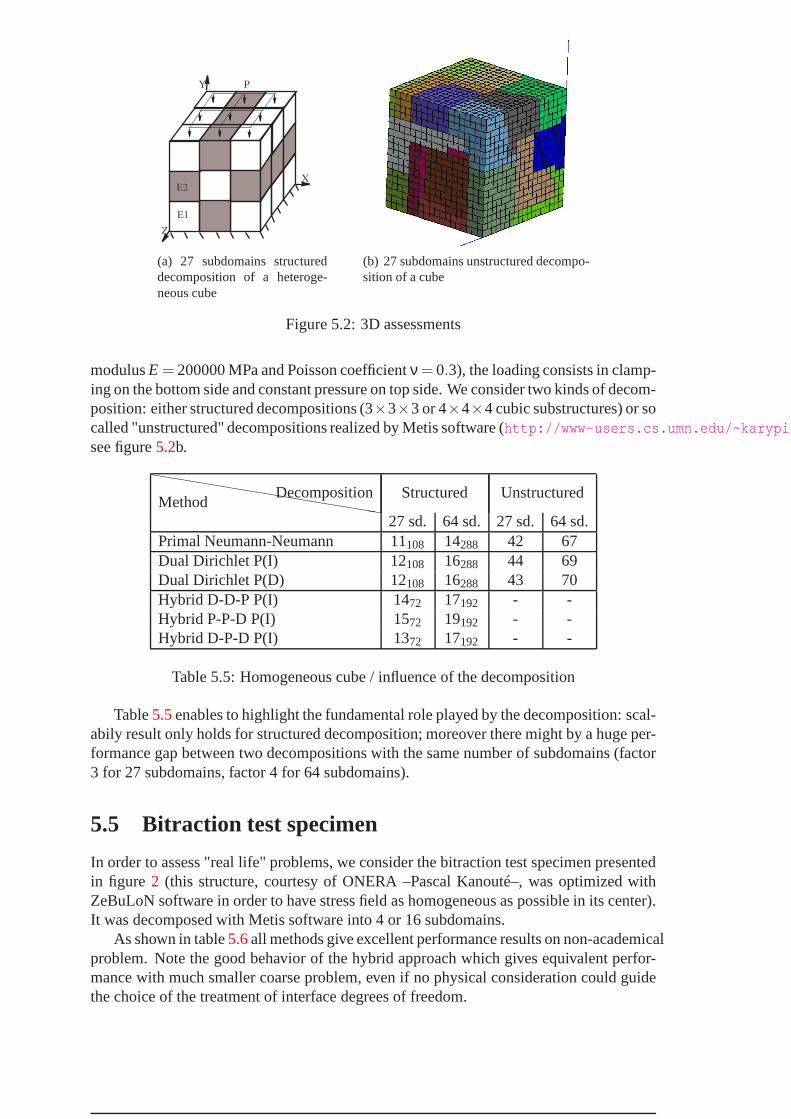
E1

E2

X

Y

Z

P

(a) 27 subdomains structureddecomposition of a heteroge-neous cube

(b) 27 subdomains unstructured decompo-sition of a cube

Figure 5.2: 3D assessments

modulusE = 200000 MPa and Poisson coefficientν = 0.3), the loading consists in clamp-ing on the bottom side and constant pressure on top side. We consider two kinds of decom-position: either structured decompositions (3×3×3 or 4×4×4 cubic substructures) or socalled "unstructured" decompositions realized by Metis software (http://www-users.cs.umn.edu/~karypissee figure5.2b.

hh

hh

hh

hh

hh

hh

hh

hh

hh

MethodDecomposition Structured Unstructured

27 sd. 64 sd. 27 sd. 64 sd.Primal Neumann-Neumann 11108 14288 42 67Dual Dirichlet P(I) 12108 16288 44 69Dual Dirichlet P(D) 12108 16288 43 70Hybrid D-D-P P(I) 1472 17192 - -Hybrid P-P-D P(I) 1572 19192 - -Hybrid D-P-D P(I) 1372 17192 - -

Table 5.5: Homogeneous cube / influence of the decomposition

Table5.5enables to highlight the fundamental role played by the decomposition: scal-abily result only holds for structured decomposition; moreover there might by a huge per-formance gap between two decompositions with the same number of subdomains (factor3 for 27 subdomains, factor 4 for 64 subdomains).

5.5 Bitraction test specimen

In order to assess "real life" problems, we consider the bitraction test specimen presentedin figure 2 (this structure, courtesy of ONERA –Pascal Kanouté–, was optimized withZeBuLoN software in order to have stress field as homogeneousas possible in its center).It was decomposed with Metis software into 4 or 16 subdomains.

As shown in table5.6all methods give excellent performance results on non-academicalproblem. Note the good behavior of the hybrid approach whichgives equivalent perfor-mance with much smaller coarse problem, even if no physical consideration could guidethe choice of the treatment of interface degrees of freedom.


http://www-users.cs.umn.edu/~karypis/metis/

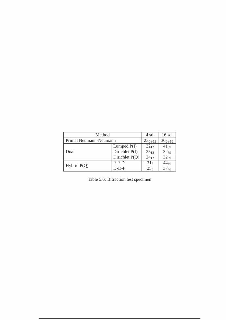
Method 4 sd. 16 sd.Primal Neumann-Neumann 230+12 300+69

DualLumped P(I) 3212 4169Dirichlet P(I) 2512 3269

Dirichlet P(Q) 2412 3269

Hybrid P(Q)P-P-D 318 4446D-D-P 258 3746

Table 5.6: Bitraction test specimen


Conclusion

In this paper, we have reviewed most used non-overlapping domain decomposition meth-ods. These methods are perfectly suited to modern computational hardware, they arebased on very close concepts which we tried to outline. We introduced the hybrid frame-work to include as many methods as possible: the principle isto assign to each interfacedegree of freedom its own treatment, for now primal and dual treatments have been im-plemented, and mixed and recondensed should follow. Hybriding methods also enable todefine physic-friendly approaches for multifield problems.

Because of the conceptual proximity of all methods, assessments showed very closenumerical performance results. Once equipped with convenient preconditioner and coarseproblem, all the methods tested proved their ability to handle second and forth order elas-ticity in presence of strong heterogeneities. Though from acomputational point of viewsome combination may be more interesting: dual approach with lumped preconditioneror simplified projector (if these are sufficient to ensure finerate of convergence), hybridapproach (which generates smaller coarse space). We also outlined the importance of thedecomposition even for very simple problems. The methods have also proved their effi-ciency on industrial cases, some of them were implemented incomputational softwares.

In this paper we limited to the solution to linearized systems, which anyhow enablesto solve nonlinear problems. Another strategy is to commutethe nonlinear solver and thedomain decomposition method so that nonlinear problems canbe solved independentlyon each subdomain. Another evolution of domain decomposition philosophy is the de-composition of the time intervalLions et al.[2001] for evolution problems.


Bibliography

Y. Achdou and Y. A. Kuznetsov. Substructuring preconditioners for finite element meth-ods on nonmatching grids.East-West J. Numer. Math., 3(1):1–28, 1995.

Y. Achdou, Y. Maday, and O. B. Widlund. Méthode itérative de sous-structuration pourles éléments avec joints.C.R. Acad. Sci. Paris, I(322):185–190, 1996.

M. Barboteu, P. Alart, and M. Vidrascu. A domain decomposition strategy for nonclas-sical frictional multicontact problems.Comp. Meth. App. Mech. Eng., 190:4785–4803,2001.

R. Barrett, M. Berry, T. F. Chan, J. Demmel, J. Donato, J. Dongarra, V. Eijkhout, R. Pozo,C. Romine, and H. V. der Vorst.Templates for the Solution of Linear Systems: BuildingBlocks for Iterative Methods. SIAM, 1994.

T. Belytschko, Y. Krongauz, D. Organ, M. Fleming, , and P. Krysl. Meshless methods:An overview and recent developments.Computer Methods in Applied Mechanics andEngineering, 139:3–47, 1996.

C. Bernardi, Y. Maday, and T. Patera. A new non conforming approach to domain de-composition: the Mortar Element Method. In H. Brezis and J. Lions, editors,NonlinearPartial Differential Equations and their Applications. Pitman, London, 1989.

M. Bhardwaj, D. Day, C. Farhat, M. Lesoinne, K. Pierson, and D. Rixen. Applicationof the FETI method to ASCI problems: Scalability results on athousand-processor anddiscussion of highly heterogeneous problems.Int. J. Num. Meth . Eng., 47(1-3):513–536, 2000.

J. E. Bolander and N. Sukumar. Irregular lattice model for quasistatic crack propagation.Phys. Rev. B, 71, 2005.

P. Breitkopt and A. Huerta, editors.Meshfree and particle based approaches in compu-tational Mechanics, volume 11 ofREEF special release. Hermes, 2002.

S. Brenner. Lower bounds in domain decomposition. InProceedings of the 16th inter-national conference on domain decomposition methods, 2005.

F. Brezzi and L. Marini. A three-field domain decomposition method. InProceedingsof the sixth international conference on domain decomposition methods, pages 27–34,1993.

M. C. C. Walshaw and M. G. Everett. A parallelisable algorithm for optimising unstruc-tured mesh partitions. Technical report, School of Mathematics, Statistics & ScientificComputing, University of Greenwich, London, 1995.

X.-C. Cai and D. Keyes. Nonlinearly preconditioned inexactnewton algorithms.SIAMJ. Sci. Comp., 2002.


A. Chapman and Y. Saad. Deflated and augmented Krylov subspace techniques.Numer.Linear Algebra Appl., 1997.

P. Ciarlet.The finite element method for elliptic problems. North Holland, 1979.

J. S. con.Mécanique des milieux continus. Ecole polytechnique. Ellipses, 1988.

R. Craig and M. Bampton. Coupling of substructures for dynamic analysis.AIAA Jour-nal, 6:1313–1319, 1968.

P. Cresta, O. Allix, C. Rey, and S. Guinard. Comparison of multiscale and parallelnonlinear strategies based on domain decomposition for post buckling analysis.Comp.Meth. App. Mech. Eng., 2005. submitted.

J.-M. Cros. A preconditioner for the schur complement domain decomposition method.In Herrera, Keyes, and Widlund, editors,Proceedings of the14th international confer-ence on domain decomposition methods, pages 373–380, 2002.

G. D’Addetta, E. Ramm, S. Diebels, and W. Ehlers. A particle center based homog-enization strategy for granular assemblies.Int J for Computer-Aided Engineering, 21(2-4):360–383, 2004.

A. de La Bourdonnaye, C. Farhat, A. Macedo, F. Magoules, and F.-X. Roux.Advances inComputational Mechanics with High Performance Computing, chapter A method of fi-nite element tearing and interconnecting for the Helmholtzproblem, pages 41–54. Civil-Comp Press, Edinburgh, United Kingdom, 1998.

A. Delaplace. Fine description of fracture by using discrete particle model. InProceed-ings of ICF 11 - 11th International Conference on Fracture, 2005.

C. Dohrmann. A preconditioner for substructuring based on constrained energy mini-mization.SIAM J. Sci. Comp., 25(1):246–258, 2003.

Z. Dostal. Conjugate gradient method with preconditioningby projector.Int. J. Comput.Math., 23:315–323, 1988.

Z. Dostal, D. Horak, and D. Stefanica. An overview of scalable feti-dp algorithms forvariational inequalities. InProceedings of the 16th conference on domain decompositionmethods, 2005.

D. Dureisseix and C. Farhat. A numerically scalable domain decomposition method forthe solution of frictionless contact problems.Internat. J. Num. Meth. Engin., 50(12):2643–2666, 2001.

G. Duvaut.Mécanique des milieux continus. Masson, 1990.

J. Erhel and F. Guyomarc’h. An augmented conjugate gradientmethod for solving con-secutive symmetric positive definite linear systems.SIAM J. Matrix Anal. Appl., 21(4):1279–1299, 2000.

J. Erhel, K. Burrage, and B. Pohl. Restarted GMRes preconditioned by deflation.J.Comput. Appl. Math., 69:303–318, 1996.

C. Farhat. A saddle-point principle domain decomposition method for the solution ofsolid mechanics problems. In D. Keyes, T. Chan, G. Meurant, J. Scroggs, and R. Voigt,editors,Domain Decomposition Methods for Partial Differential Equations, pages 271–292, 1992.


C. Farhat and M. Géradin. On the computation of the null spaceand generalized inversof large matrix, and the zero energy modes of a structure. Technical Report CU-CAS-96-15, Center for aerospace structures, may 1996.

C. Farhat and J. Mandel. The two-level FETI method for staticand dynamic plate prob-lems - part I: An optimal iterative solver for biharmonic systems.J. Comp Meth. Appl.Mech. Eng., 155:129–152, 1998.

C. Farhat and F.-X. Roux. A method of finite tearing and interconnecting and its parallelsolution algorithm.Int. J. Num. Meth . Eng., 32:1205–1227, 1991.

C. Farhat and F. X. Roux. Implicit parallel processing in structural mechanics.Compu-tational Mechanics Advances, 2(1):1–124, 1994a. North-Holland.

C. Farhat and F.-X. Roux. The dual Schur complement method with well-posed localNeumann problems.Contemporary Mathematics, 157:193–201, 1994b.

C. Farhat and H. D. Simon. Top/domdec - a software tool for mesh partitioning andparallel processing. Technical report, NASA Ames, 1993.

C. Farhat, J. Mandel, and F. Roux. Optimal convergence properties of the FETI domaindecomposition method.Comp. Meth. Appl. Mech. Eng., 115:365–385, 1994.

C. Farhat, P.-S. Chen, and F.-X. Roux. The two-level FETI method - part II: Extension toshell problems. parallel implementation and performance results.J. Comp Meth. Appl.Mech. Eng., 155:153–180, 1998.

C. Farhat, A. Macedo, and R. Tezaur. FETI-H: a scalable domaine decompositionmethod for high frequency exterior Helmholtz problems. InDomain decompositionmethods in science and engineering. Domain decomposition press, 1999.

C. Farhat, M. Lesoinne, and K. Pierson. A scalable dual-primal domain decompositionmethod.Numer. Linear Algebra Appl., 7(7-8):687–714, 2000a.

C. Farhat, A. Macedo, and M. Lesoinne. A two-level domain decomposition methodfor the iterative solution of high frequency exterior Helmholtz problems.NumerischeMathematik, 85:283–308, 2000b.

C. Farhat, K. Pierson, and M. Lesoinne. The second generation FETI methods andtheir application to the parallel solution of large-scale linear and geometrically non-linear structural analysis problems.J. Comp Meth. Appl. Mech. Eng., 184(2-4):333–374,2000c.

C. Farhat, M. Lesoinne, P. Le Tallec, K. Pierson, and D. Rixen. FETI-DP: a dual-primalunified FETI method - part i: a faster alternative to the two-level FETI method.Int. J.Num. Meth . Eng., 50(7):1523–1544, 2001.

F. Feyel. Application du calcul parallèle aux modèles à grand nombre de variablesinternes. Thèse de doctorat, Ecole Nationale Supérieure des Mines deParis, 1998.

F. Feyel.Quelques multi-problèmes en mécanique des matériaux et structures. Habili-tation à diriger des recherches, Université Pierre et MarieCurie, 2005.

M. Fortin and R. Glowinski. Méthodes de lagrangien augmenté - applications à larésolution numérique de problèmes aux limites. Dunod, 1982.

Y. Fragakis and M. Papadrakakis. A unified framework for formulating domain de-composition methods in structural mechanics. Technical report, Institute of StructuralAnalysis and Seismic Research, National Technical University of Athens, 2002.


Y. Fragakis and M. Papadrakakis. The mosaic of high-performance domain decomposi-tion methods for structural mechanics – part i: Formulation, interrelation and numericalefficiency of primal and dual methods.Comp. Meth. Appl. Mec. Eng., 192(35-36):3799–3830, 2003.

Y. Fragakis and M. Papadrakakis. The mosaic of high-performance domain decompo-sition methods for structural mechanics – part ii: Formulation enhancements, multipleright-hand sides and implicit dynamics.Comp. Meth. Appl. Mec. Eng., 193(42-44):4611–4662, 2004.

V. Frayssé, L. Giraud, and H. Kharraz-Aroussi. On the influence of the orthogonalizationscheme on the parallel performance of GMRes. Technical report, CERFACS, 1998.

N. Germain, J. Besson, and F. Feyel. Méthodes de calcul non local : Application auxstructures composites. InActes du 7ème colloque national en calcul des structures,Giens, 2005.

P. Germain.Mécanique. Ecole polytechnique. Ellipses, 1986.

R. Glowinski and P. Le Tallec. Augmented lagrangian interpretation of the nonover-lapping Schwartz alternating method. InThird International Symposium on DomainDecomposition Methods for Partial Differential Equations, pages 224–231, 1990.

P. Goldfeld. Balancing Neumann-Neumann for (in)compressible linear elasticity and(generalized) Stokes – parallel implementation. InProceedings of the14th internationalconference on domain decomposition method, pages 209–216, 2002.

P. Gosselet.Méthodes de décomposition de domaine et méthodes d’accélération pourles problèmes multichamp en mécanique non-linéaire. PhD thesis, Université P. et M.Curie, 2003.

P. Gosselet and C. Rey. On a selective reuse of krylov subspaces in newton-krylovapproaches for nonlinear elasticity. InProceedings of the14th conference on domaindecomposition methods, pages 419–426, 2002.

P. Gosselet, C. Rey, P. Dasset, and F. Léné. A domain decomposition method for quasiincompressible formulations with discontinuous pressurefield. Revue européenne desélements finis, 11:363–377, 2002.

P. Gosselet, V. Chiaruttini, C. Rey, and F. Feyel. Une approche hybride de décompositionde domaine pour les problèmes multiphysiques : applicationà la poroélasticité. InActesdu sixième colloque national en calcul de structures, volume 2, pages 297–304, 2003a.

P. Gosselet, C. Rey, and D. Rixen. On the initial estimate of interface forces in FETImethods.Comp. meth. appl. mech. engrg., 192:2749–2764, 2003b.

P. Gosselet, V. Chiaruttini, C. Rey, and F. Feyel. A monolithic strategy based on anhybrid domain decomposition method for multiphysic problems. application to poroe-lasticity. Revue européenne des élements finis, 13:523–534, 2004.

G. Karypis and V. Kumar. Multilevel algorithms for multi-constraint graph partitioning.Technical report, University of Minnesota, Department of Computer Science, 1998.

A. Klawonn and O. Widlund. Dual and dual-primal FETI methodsfor elliptic problemswith discontinuous coefficients. InProceedings of the 12th International Conference onDomain Decomposition Methods, Chiba, Japan, October 1999. submitted.


A. Klawonn and O. Widlund. FETI and Neumann-Neumann iterative substructuringmethods: connections and new results.Comm. pure and appl. math., LIV:0057–0090,2001.

A. Klawonn, O. Rheinbach, and O. Widlund. Some computational results for dual-primal feti methods for three dimensional elliptic problems. Lect. Notes Comput. Sci.Eng., 40:361 – 368, 2005.

P. Ladevèze.Nonlinear Computational Structural Mechanics - New Approaches andNon-Incremental Methods of Calculation. Springer Verlag, 1999.

P. Ladevèze, O. Loiseau, and D. Dureisseix. A micro-macro and parallel computationalstrategy for highly heterogeneous structures.Int. J. Num. Meth. Engnrg., 52:121–138,2001.

P. Le Tallec. Domain-decomposition methods in computational mechanics.Computa-tional Mechanics Advances, 1(2):121–220, 1994. North-Holland.

P. Le Tallec and M. Vidrascu. Méthodes de décomposition de domaines en calcul destructures. InActes du premier colloque national en calcul des structures, volume I,pages 33–49, 1993.

P. Le Tallec and M. Vidrascu. Generalized Neumann-Neumann preconditioners for iter-ative substructuring. InProceedings of the ninth conference on Domain Decomposition,June Bergen 1996. to appear.

P. Le Tallec, Y.-H. D. Roeck, and M. Vidrascu. Domain-decomposition methods forlarge linearly elliptic three dimensional problems.J. Comp. Appl. Math., 34:93–117,1991. Elsevier Science Publishers, Amsterdam.

P. Le Tallec, J. Mandel, and M. Vidrascu. A Neumann-Neumann domain decompositionalgorithm for solving plate and shell problems.SIAM J. Num. Ana., 35(2):836–867,April 1998.

M. Lesoinne and K. Pierson. FETI-DP: An efficient, scalable,and unified Dual-PrimalFETI method. InDomain Decomposition Methods in Sciences and Engineering, pages421–428, 1999.

J. Li. A dual-primal feti method for solving stokes/navier-stokes equations. InPro-ceedings of the14th international conference on domain decomposition method, pages225–233, 2002.

F. Lingen. Efficient Gram-Scmidt orthonormalisation on parallel computers.Com. Nu-mer. Meth. Engng., 16:57–66, 2000.

J. Lions, Y. Maday, and G. Turinici. Résolution d’edp par un schéma en temps pararéel.C. R. Acad. Sci. Paris, 333(1):1–6, 2001.

G.-R. Liu and Y.-T. Gu.An Introduction to Meshfree Methods and Their Programming.Springer, 2005.

J. Mandel. Balancing domain decomposition.Comm. Appl. Num. Meth. Engrg., 9:233–241, 1993.

J. Mandel and M. Brezina. Balancing domain decomposition for problems with largejumps in coefficients.Math. Comp., 65(216):1387–1401, 1996.


J. Mandel and R. Tezaur. Convergence of a substructuring method with Lagrange mul-tipliers. Numerische Mathematik, 73:473–487, 1996.

J. Mandel and R. Tezaur. On the convergence of a dual-primal substructuring method.UCD/CCM Report 150, Center for Computational Mathematics,University of Coloradoat Denver, April 2000. to appear in Numer. Math.

Z-set developper manual. Northwest Numerics, 2001a.

Z-set user manual. Northwest Numerics, 2001b.

A. Nouy. Une stratégie de calcul multiéchelle avec homogénéisationen temps et enespace pour le calcul de structures fortement hétérogènes. PhD thesis, ENS de Cachan,2003.

K. Park, M. Justino, and C. Felippa. An algebraically partitioned FETI method forparallel structural analysis: algorithm description.Int. J. Num. Meth. Eng., 40(15):2717–2737, 1997a.

K. Park, M. Justino, and C. Felippa. An algebraically partitioned FETI method forparallel structural analysis: performance evaluation.Int. J. Num. Meth . Eng., 40(15):2739–2758, 1997b.

R. Paz and M. Storti. An interface strip preconditioner for domain decomposition meth-ods: application to hydrology.Int. J. Numer. Meth. Engng., 62:1873–1894, 2005.

C. Rey and P. Gosselet. Solution to large nonlinear systems:acceleration strategiesbased on domain decomposition and reuse of krylov subspaces. In Proceedings of the6th ESAFORM conference on material forming, 2003.

C. Rey and F. Léné. Reuse of krylov spaces in the solution of large-scale non linearelasticity problems. InDomain Decomposition Methods in Sciences and Engineering,pages 465–471, 1998.

C. Rey and F. Risler. A Rayleigh-Ritz preconditioner for theiterative solution to largescale nonlinear problems.Numerical Algorithms, 17:279–311, 1998.

F. Risler and C. Rey. On the reuse of Ritz vectors for the solution to nonlinear elasticityproblems by domain decomposition methods. InDD10 Proceedings, ContemporaryMathematics, volume 218, pages 334–340, 1998.

F. Risler and C. Rey. Iterative accelerating algorithms with Krylov subspaces for thesolution to large-scale nonlinear problems.Numerical Algorithms, 23:1–30, 2000.

D. Rixen.Substructuring and dual methods in structural analysis. PhD thesis, Universityof Liège, Belgique, 1997.

D. Rixen. Extended preconditioners for the feti method applied to constrained problems.Int. Journal for Numerical methods in engineering, 54(1):1–26, 2002.

D. Rixen. A dual craig-bampton method for dynamic substructuring. J. Comput. Appl.Math., 168:383–391, 2004.

D. Rixen and C. Farhat. A simple and efficient extension of a class of substructure basedpreconditioners to heterogeneous structural mechanics problems. Int. J. Num. Meth.Eng., 44(4):489–516, 1999.


D. Rixen, C. Farhat, R. Tezaur, and J. Mandel. Theoretical comparison of the FETIand algebraically partitioned FETI methods, and performance comparisons with a directsparse solver.Int. J. Num. Meth. Eng., 46(4):501–534, 1999.

F.-X. Roux. Parallel implementation of direct solution strategies for the coarse grigsolvers in 2-level FETI method. Technical report, ONERA, Paris, France, 1997.

Y. Saad. On the Lanczos method for solving symmetric linear systems with several righthand sides.Math. Comp., 48:651–662, 1987.

Y. Saad. Analysis of augmented Krylov subspace methods.SIAM J. Matrix Anal. Appl.,18(2):435–449, April 1997.

Y. Saad. Iterative methods for sparse linear systems. PWS Publishing Company, 3rdedition, 2000.

Y. Saad and M. H. Schultz. GMRes: a generalized minimal residual algorithm for solv-ing nonsymmetric linear systems.SIAM J. Sci. Comput., 7:856–869, 1986.

L. Series, F. Feyel, and F.-X. Roux. Une méthode de décomposition de domaine avecdeux multiplicateurs de Lagrange, application au calcul des structures, cas du contact. InActes du sixième colloque national en calcul des structures, volume III, pages 373–380,2003a.

L. Series, F. Feyel, and F.-X. Roux. Une méthode de décomposition de domaine avecdeux multiplicateurs de Lagrange. InActes du16eme congrès français de mécanique,2003b.

D. Stefanica and A. Klawonn. The FETI method for mortar finiteelements. InPro-ceedings of 11th International Conference on Domain Decomposition Methods, pages121–129, 1999.

A. van der Sluis and H. can der Vorst. The rate of convergence of conjugate gradients.Numer. Math., 48:543–560, 1986.

P. Wesseling.An Introduction to Multigrid Methods. R.T. Edwards, Inc, 2004.

O. Zienkiewicz and R. Taylor.The finite element method. Mc Graw-Hill Book COm-pagny, 1989.


Appendix A

Krylov iterative solvers

Krylov iterative solvers for the resolution of linear systemshave been widely studied. The aim of this section is just tobriefly present important results and algorithms, reader

interested in wider documentation can refer toSaad[2000],and toBarrett et al.[1994] for shorter explanation.

ContentsA.1 Principle of Krylov solvers . . . . . . . . . . . . . . . . . . . . . . . . . 66

A.2 Most used solvers . . . . . . . . . . . . . . . . . . . . . . . . . . . . . . 66

A.3 GMRes . . . . . . . . . . . . . . . . . . . . . . . . . . . . . . . . . . . . 66

A.4 Conjugate gradient . . . . . . . . . . . . . . . . . . . . . . . . . . . . . 67

A.5 Study of the convergence, preconditioning. . . . . . . . . . . . . . . . . 68

A.6 Constrained Krylov methods, projector implementation . . . . . . . . . 68

A.7 Augmented-Krylov methods, projector implementation . . . . . . . . . 69

A.8 Constrained augmented Krylov methods . . . . . . . . . . . . . . . . . 70


Krylov methods belong to the projection class of iterative algorithms, which consistin approximating solutionS−1b of systemSx= b by vectorp(S)b wherep is a smartlybuilt polynomial.

In this section we consider the iterative solution to systemSx= b. S is an×n matrixandb a vector in range(S). The ith iteration leads to approximationxi of the solution,associated residual isr i = b−Sxi = S(x− xi). Initialization is x0 (most oftenx0 = 0).Canonical (orthonormal) basis ofRn reads(e1, . . . ,en).

A.1 Principle of Krylov solvers

Krylov solvers are based on the iterative construction of so-called "Krylov subspace"Km(S, r0) defined by:

Km(S, r0) = span(r0, . . . ,S

m−1r0)

(A.1)

The solution to linear system consists in searchingxm under the following constraints:

xm ∈ x0 +Km(S, r0)rm ⊥?Km(S, r0)

(A.2)

where the choice of the orthogonality relationship enablesto define various approaches.

A.2 Most used solvers

We herein present two of the principal Krylov solvers. FirstGMResSaad and Schultz[1986] which is suited to any type of matrix, then conjugate gradient which is adapted tosymmetric definite positive matrices.

Of course, the iterative solution to a linear system assumesthat a convergence criterionis employed, and that a limit of precision is set so that the system is supposed to haveconverged once the criterion is below this precision. We note ε this limit value of thecriterion.

A.3 GMRes

Algorithm GMRes (alg.A.3.1) consists in an oblique projection based on the constructionof Krylov subspaceKm(S,v0) with v0 = r0/‖r0‖2. The research principle is:

xm ∈ x0 +Km(S, r0)rm ⊥ SKm(S, r0)

(A.3)

which is equivalent to findingxm ∈ x0+Km(S, r0) minimizing‖rm‖2.A particulary striking property of GMRes is not to compute the approximation at each

iteration, a smart implementation of GMRes enables to directly access the norm of theresidual‖r j‖2. Only the final approximationxm is computed (by the inversion of am×mupper triangular matrix). From the computation complexitypoint of view, each iterationconsists in a full orthonormalization of vectorw j with respect toK j .

Algorithm GMRes(m) (or restarted GMRes) consists in stopping computation beforeconvergence ata priori fixed stepm and restart computation using previousxm as initial-ization. This strategy aims at minimizing orthogonalization computations by limiting thesize of Krylov subspacesErhel et al.[1996]. This method may lead to stagnation for nonpositive definite matrices.


Algorithm A.3.1 GMRes1: Computer0 = b−Sx0, v0 = r0/‖r0‖2

2: for j = 0, . . . ,m−1 do3: Computew j = Svj

4: for i = 0, . . . , j do5: hi j = (vi ,w j)6: w j = w j −hi j vi

7: end for8: h( j+1) j = ‖w j‖2

9: if ‖r j‖2 6 ε then10: stop11: else12: v j+1 = w j/h( j+1) j13: end if14: end for15: Computeym minimizing‖‖r0‖2e1− Hmy‖2 and setxm = x0+Vmym

A.4 Conjugate gradient

Let Sbe a symmetric positive definite matrix, a conjugate gradient algorithm consists inan orthogonal projection. The research principle is:

xm ∈ x0+Km(S, r0)rm ⊥ Km(S, r0)

(A.4)

which is equivalent to findingxm ∈ x0 +Km(S, r0) minimizing‖xm−x‖S.Because of the properties ofS, conjugation (orthogonality) properties appear, lead-

ing to algorithmA.4.1. The algorithm is based on the construction of various basis

Algorithm A.4.1 Conjugate gradient1: Computer0 = b−Sx0, setw0 = r0

2: for j = 0, . . . ,m do3: α j = (r j , r j)/(Swj ,w j)4: x j+1 = x j +α jw j

5: r j+1 = r j −α jSwj

6: β j = (r j+1, r j+1)/(r j , r j)7: w j+1 = r j+1+β jw j

8: end for

of Km(S, r0) : (rm) (residual basis) is orthogonal,(wm) (research direction basis) isS-orthogonal. Step 6−7 of algorithmA.4.1 is theS-orthogonalization ofw j+1 with respectto w j which theoretically implies the orthogonality ofw j+1 with respect to all previousresearch directions. However this orthogonality propertyis numerically lost as the num-ber of iterations increases, it is then more suited to use a full orthogonalization of researchdirections leading to algorithmA.4.2.

Full reorthogonalization is often compulsory for complex simulations. Various im-plementations are available (among others Gram-Schmidt, modified Gram-Schmidt, iter-ative Gram-SchmidtLingen[2000], Frayssé et al.[1998]) depending on the chosen ratiobetween precision and computational cost. Our experience leads us to prefer modifiedGram-Schmidt algorithm (the one used in algorithmA.3.1) to classical Gram-Schmidt(the one used in algorithmA.4.2). Note that once fully reorthogonalized, conjugate gra-dient is almost as expensive as GMRes. Anyhow conjugate gradient provides the approx-imation at each iteration, which can be very useful (see for instance section2.2.3, wheresuch an information enables the computation of relevant convergence criterion).


Algorithm A.4.2 Reorthogonalized conjugate gradient1: Computer0 = b−Sx0, setw0 = r0

2: for j = 0, . . . ,mdo3: α j = (r j , r j)/(Swj ,w j)4: x j+1 = x j +α jw j

5: r j+1 = r j −α jSwj

6: For 06 i 6 j, βij = −(r j+1,Swi)/(wi ,Swi)

7: w j+1 = r j+1+∑ ji=1 βi

jwi

8: end for

A.5 Study of the convergence, preconditioning

Because of their error-minimization property, conjugate gradient and GMRes have con-vergence theorems with known minimal convergence rate, forinstance for conjugate gra-dient:

‖x−xm‖S 6 2

[√κ−1√κ+1

]m

‖x−x0‖S (A.5)

whereκ is the condition number of matrixS. Condition number is the ratio between thebiggest and the smallest eigenvalues.

κ =

∣∣∣∣λn

λ1

∣∣∣∣ with |λ1| 6 |λ2| 6 . . . 6 |λn| eigenvalues ofS (A.6)

Moreover performance results of Krylov iterative solvers are strongly linked to thespectrum of matrixS. More precisely only the active spectrum (set of eigenvalues whichthe right hand side is not orthogonal to the associated eigenvectors) influences the conver-gence; condition numberκ can be replaced with active condition numberκact inside rela-tion (A.5) leading to better convergence range. More precise study would lead to the intro-duction of Ritz spectrum and effective condition numbervan der Sluis and can der Vorst[1986].

These simple considerations are sufficient to explain the interest of preconditioningthe system: the idea is to solve equivalent systemS−1Sx= S−1b whereS−1 is a well-chosen matrix providing the system with better spectral properties (if S−1 ≈ S−1 thencondition number is optimal, which justifies the notation).

For conjugate gradient, the use of preconditioner may seem problematic since thesymmetry isa priori lost. However if preconditionerS−1 is symmetric definite positive,applying conjugate gradient to nonsymmetric system is equivalent to a symmetric reso-lution ((L−TSL−1)(Lx) = L−Tb with Cholesky factorizationS= LTL) and the method isstill relevant.

So preconditioning the above two algorithms is simply realized replacingSby S−1Sand b by S−1b in lines 1 and 3 of algorithmA.3.1, and in lines 1 and 5 of algorithmA.4.2(anyhow the research directions are stillS-orthogonal). Of course the main problemremains the definition of an efficient preconditioner.

A.6 Constrained Krylov methods, projector implemen-tation

We may deal (for instance in the dual approach) with constrained systems such as:

(S G

GT 0

)(xα

)=

(be

)(A.7)


Because constraintGTx0 = e is compulsory, it is often referred to as "admissibility con-straint". A classical solution is to find an initializationx0 which satisfies constraint andthen ensure that the remainder of the solution is researchedinside a supplemental space:GT(xi −x0) = 0. A projected algorithm naturally arises:

x = x0+Px∗ (A.8)

GTx0 = e (A.9)

GTP = 0 (A.10)

which leads to:

x0 = QG(GTQG

)−1e (A.11)

P = I −QG(GTQG

)−1GT (A.12)

whereQ is a matrix so that matrixGTQG is invertible. Iterative system then reads:

PTSPx∗ = PT (b−Sx0) (A.13)

α can be post-computedα =(GTQG

)−1GTQ(b−Sx).

A.7 Augmented-Krylov methods, projector implementa-tion

Augmented-Krylov methodsChapman and Saad[1997], Saad[1997] are employed toadd optional constraints to the resolution of a system. The principle is to set subspaceC in Rn of dimensionnc represented byn×nc rectangular matrixC (range(C) = C , formore simplicity we suppose thatC is full-ranked-column), then to define augmented-Krylov subspaceKm(S, r0,C) = Km(S, r0)+ range(C), and to use the following researchprinciple:

xm ∈ x0 + Km(S, r0,C)

rm ⊥? Km(S, r0,C)(A.14)

Augmented-Krylov methods can be implemented either by reorthogonalization schemesor by projection methods which are the one we propose to present here. The researchspace is separated into two subspaces: range(C) and a supplemental subspace. The partof the solution in range(C) is detected during initialization, while the remainder is itera-tively looked for, projectorP ensures the research is realized inside the correct subspace.

x = x0 +Px∗ (A.15)

CTr0 = CT(b−Sx0) = 0 (A.16)

CTSP = 0 (A.17)

Which leads to:

x0 = C(CTSC

)−1CTb (A.18)

P = I −C(CTSC

)−1CTS (A.19)

system then reads:

SPx∗ = b−Sx0 (A.20)

or PTSPx∗ = PT (b−Sx0) = PTb (A.21)


Though it can be proved that projected system is better conditioned than original prob-lem Dostal[1988], the efficiency of the method essentially depends on the choice of ma-trix C, which is most often an opened problem. Within the frameworkof domain decom-position methods, this choice can be guided by several considerations. In the frameworkof multiresolution, reuse of previous numerical information can lead to very interest-ing performance resultsRey and Léné[1998], Gosselet and Rey[2002], Gosselet et al.[2002], Rey and Gosselet[2003], Rey and Risler[1998], Risler and Rey[2000]

A.8 Constrained augmented Krylov methods

We here consider solving constrained system (A.7) with C-augmented algorithm. Theadmissibility constraint is often referred to as first levelconstraint and augmentation assecond level constraint. Two strategies are possible, the first consists in mixing levelstogether while the second respects the hierarchy between constraints.

One projector strategy: setJ =(G STH

)ande=

(−e

HTb

), then system reads:

(S JJT 0

)(xα

)=

(be

)(A.22)

the following initialization/projection are employed (Q is a parameter to tune)

x0 = J(JTQJ

)−1e (A.23)

P = I −QJ(JTQJ

)−1JT (A.24)

BecauseQ is not easy to interpret and choose, this method is hardly ever used.

Two-projector strategy: the two conditions are imbricated. First ensure admissibilityconstraint

x = x0 +Px∗ (A.25)

x0 = G(GTQG

)−1e (A.26)

P = I −QG(GTQG

)−1GT (A.27)

then set

x∗ = x∗0 +P∗x∗∗ (A.28)

x∗0 = C(CTPTSPC

)−1CTPT (b−Sx0) (A.29)

P∗ = I −PC(CTPTSPC

)−1CTPTS (A.30)

so that optimality constraint is verified. As can be seen suchan approach is equiva-lent to classical augmentation with making second level constraints consistent withthe first (settingC∗ = PC).


Non-overlapping domain decomposition methods for structural mechanics

Documents

Transcript of Non-overlapping domain decomposition methods for structural mechanics