Non-linear Real Arithmetic Benchmarks derived from ...

Non-linear Real Arithmetic Benchmarks derivedfrom Automated Reasoning in Economics

Casey B. Mulligan1, Russell Bradford2, James H. Davenport2,Matthew England3, and Zak Tonks2

1 University of Chicago, [email protected] University of Bath, UK

{R.J.Bradford, J.H.Davenport, Z.P.Tonks}@bath.ac.uk3 Coventry University, UK

[email protected]

Abstract. We consider problems originating in economics that maybe solved automatically using mathematical software. We present andmake freely available a new benchmark set of such problems. The prob-lems have been shown to fall within the framework of non-linear realarithmetic, and so are in theory soluble via Quantifier Elimination (QE)technology as usually implemented in computer algebra systems. Fur-ther, they all can be phrased in prenex normal form with only existentialquantifiers and so are also admissible to those Satisfiability Module The-ory (SMT) solvers that support the QF_NRA logic. There is a great bodyof work considering QE and SMT application in science and engineering,but we demonstrate here that there is potential for this technology alsoin the social sciences.

1 Introduction

1.1 Economic reasoning

A general task in economic reasoning is to determine whether, with variablesv = (v1, . . . , vn), the hypotheses H(v) follow from the assumptions A(v), i.e. isit the case that

∀v . A(v)⇒ H(v)?

Ideally the answer would be True or False, and of course logically it is. But theapplication being modelled, like real life, can require a more nuanced analysis. Itmay be that for most v the theorem holds but there are some special cases thatshould be ruled out (additions to the assumptions). Such knowledge is valuableto the economist. Another possibility is that the particular set of assumptionschosen are contradictory4, i.e. A(v) itself is False. As all students of an intro-ductory logic class know, this would technically make the implication True, butfor the purposes of economics research it is important to identify this separately!

4 A lengthy set of assumptions is many times required to conclude the hypothesis ofinterest so the possibility of contradictory assumptions is real.

NRA Benchmarks derived from Automated Reasoning in Economics 49

Table 1. Table of possible outcomes from a potential theorem ∀ .vA ⇒ H

¬∃v[A ∧ ¬H] ∃v[A ∧ ¬H]

∃v[A ∧H] True Mixed

¬∃v[A ∧H] Contradictory Assumptions False

We categorise the situation into four possibilities that are of interest to aneconomist (Table 1) via the outcome of a pair of fully existentially quantifiedstatements which check the existence of both an example (∃v[A∧H]) and coun-terexample (∃v[A∧¬H]) of the theorem. So we see that every economics theoremgenerates a pair of SAT problems, in practice actually a trio since we would firstperform the cheaper check of the compatibility of the assumptions (∃v[A]).

Such a categorisation is valuable to an economist. They may gain a proof oftheir theorem, but if not they still have important information to guide theirresearch: knowledge that their assumptions contradict; or information about{v : A(v)⇒ H(v)}.

Also of great value to an economist are the options for exploration that suchtechnology would provide. An economist could vary the question by strength-ening the assumptions that led to a Mixed result in search of a True theorem.However, of equal interest would be to weaken the assumption that generated aTrue result for the purpose of identifying a theorem that can be applied morewidely. Such weakening or strengthening is implemented by quantifying moreor less of the variables in v. For example, we might partition v as v1,v2 andask for {v1 : ∀v2 . A(v1,v2) ⇒ H(v1,v2)}. The result in these cases would bea formula in the free variables that weakens or strengthens the assumptions asappropriate.

1.2 Technology to solve such problems automatically

Such problems all fall within the framework of Quantifier Elimination (QE). QErefers to the generation of an equivalent quantifier free formula from one thatcontains quantifiers. SAT problems are thus a sub-case of QE when all variablesare existentially quantified.

QE is known to be possible over real closed fields (real QE) thanks to theseminal work of Tarski [34] and practical implementations followed the workof Collins on the Cylindrical Algebraic Decomposition (CAD) method [11] andWeispfenning on Virtual Substitution [36]. There are modern implementationsof real QE in Mathematica [32], Redlog [14], Maple (SyNRAC [21] and theRegularChains Library [10]) and Qepcad-B [6].

The economics problems identified all fall within the framework of QE overthe reals. Further, the core economics problem of checking a theorem can beanswered via fully existentially quantified QE problems, and so also soluble usingthe technology of Satisfiability Modulo Theory (SMT) Solvers; at least those thatsupport the QF_NRA (Quantifier Free Non-Linear Real Arithmetic) logic such asSMT-RAT [12], veriT [18], Yices2 [24], and Z3 [23].

50 Mulligan-Bradford-Davenport-England-Tonks

1.3 Case for novelty of the new benchmarks

QE has found many applications within engineering and the life sciences. Recentexamples include the derivation of optimal numerical schemes [17], artificial in-telligence to pass university entrance exams [35], weight minimisation for trussdesign [9], and biological network analysis [3]. However, applications in the socialsciences are lacking (the nearest we can find is [25]).

Similarly, for SMT with non-linear reals, applications seem focussed on otherareas of computer science. The original nlsat benchmark set [23] was madeup mostly of verification conditions from the Keymaera [30], and theorems onpolynomial bounds of special functions generated by the MetiTarski automatictheorem prover [29]. This category of the SMT-LIB [1] has since been broadenedwith problems from physics, chemistry and the life sciences [33]. However, weare not aware of any benchmarks from economics or the social sciences.

The reader may wonder why QE has not been used in economics previously.On a few occasions when QE algorithms have been mentioned in economics theyhave been characterized as “something that is do-able in principle, but not by anycomputer that you and I are ever likely to see” [31]. Such assertions were basedon interpretations of theoretical computer science results rather than experiencewith actual software applied to an actual economic reasoning problem. Simplyput, the recent progress on QE/SMT technology is not (yet) well known in thesocial sciences.

1.4 Availability and further details

The benchmark set consists of 45 potential economic theorems. Each theoremrequires the three QE/SMT calls to check the compatibility of assumptions,the existence of an example, and the existence of a counterexample, so 135problems in total. In all cases the assumption and example checks are SAT,in fact often fully satisfied (any point can witness it) as they relate to a truetheorem. Correspondingly, the counterexample is usually UNSAT (for 42/45theorems) and thus the more difficult problem from the SMT point of view.

The benchmark problems are hosted on the Zenodo data repository at URLhttps://doi.org/10.5281/zenodo.1226892 in both the SMT2 format and asinput files suitable for Redlog and Maple. The SMT2 files have been acceptedinto the SMT-LIB [1] and will appear in the next release.

Available from http://examples.economicreasoning.com/ are Mathe-matica notebooks5 which contain commands to solve the examples in Mathe-matica and also further information on the economic background: meaning ofvariable names and economic implications of results etc.

5 A Mathematica licence is needed to run them, but static pdf print outs are alsoavailable to download.


1.5 Plan

The paper proceeds as follows. In Section 2 we describe in detail some examplesfrom economics, ranging from textbook examples common in education to ques-tions arising from current research discussions. Then in Section 3 we offer somestatistics on the logical and algebraic structure of these examples. We then givesome final thoughts on future and ongoing work in Section 4.

2 Examples of Economic Reasoning in Tarski’s Algebra

The fields of economics ranging from macroeconomics to industrial organizationto labour economics to econometrics involve deducing conclusions from assump-tions or observations. Will a corporate tax cut cause workers to get paid more?Will a wage regulation reduce income inequality? Under what conditions will po-litical candidates cater to the median voter? We detail in this section a varietyof such examples.

2.1 Comparative static analysis

We start with Alfred Marshall’s [26] classic, and admittedly simple, analysis ofthe consequences of cost-reducing progress for activity in an industry. Marshallconcluded that, for any supply-demand equilibrium in which the two curves havetheir usual slopes, a downward supply shift increases the equilibrium quantity qand decreases the equilibrium price p.

One way to express his reasoning in Tarski’s framework is to look at the indus-try’s local comparative statics: meaning a comparison of two different equilibriumstates between supply and demand. With a downward supply shift representedas da > 0 (where a is a reduction in costs) we have here:

A ≡ D′(q) < 0 ∧ S′(q) > 0

∧ d

da

(S(q)− a

)=

dp

da∧ dp

da=

d

daD(q)

H ≡ dq

da> 0 ∧ dp

da< 0

where:

– D′(q) is the slope of the inverse demand curve in the neighborhood of theindustry equilibrium;

– S′(q) is the slope of the inverse supply curve;

–dq

dais the quantity impact of the cost reduction; and

–dp

dais the price impact of the cost reduction.

Economically, the first atoms of A are the usual slope conditions: that demandslopes down and supply slopes up. The last two atoms of A say that the cost


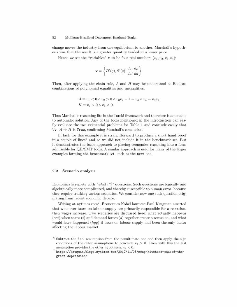
change moves the industry from one equilibrium to another. Marshall’s hypoth-esis was that the result is a greater quantity traded at a lesser price.

Hence we set the “variables” v to be four real numbers (v1, v2, v3, v4):

v =

{D′(q), S′(q),

dq

da,dp

da

}.

Then, after applying the chain rule, A and H may be understood as Booleancombinations of polynomial equalities and inequalities:

A ≡ v1 < 0 ∧ v2 > 0 ∧ v3v2 − 1 = v4 ∧ v4 = v3v1,

H ≡ v3 > 0 ∧ v4 < 0.

Thus Marshall’s reasoning fits in the Tarski framework and therefore is amenableto automatic solution. Any of the tools mentioned in the introduction can eas-ily evaluate the two existential problems for Table 1 and conclude easily that∀v . A⇒ H is True, confirming Marshall’s conclusion.

In fact, for this example it is straightforward to produce a short hand proofin a couple of lines6 and so we did not include it in the benchmark set. Butit demonstrates the basic approach to placing economics reasoning into a formadmissible for QE/SMT tools. A similar approach is used for many of the largerexamples forming the benchmark set, such as the next one.

2.2 Scenario analysis

Economics is replete with “what if?” questions. Such questions are logically andalgebraically more complicated, and thereby susceptible to human error, becausethey require tracking various scenarios. We consider now one such question orig-inating from recent economic debate.

Writing at nytimes.com7, Economics Nobel laureate Paul Krugman assertedthat whenever taxes on labour supply are primarily responsible for a recession,then wages increase. Two scenarios are discussed here: what actually happens(act) when taxes (t) and demand forces (a) together create a recession, and whatwould have happened (hyp) if taxes on labour supply had been the only factoraffecting the labour market.

6 Subtract the final assumption from the penultimate one and then apply the signconditions of the other assumptions to conclude v3 > 0. Then with this the lastassumption provides the other hypothesis, v4 < 0.

7 https://krugman.blogs.nytimes.com/2012/11/03/soup-kitchens-caused-the-

great-depression/


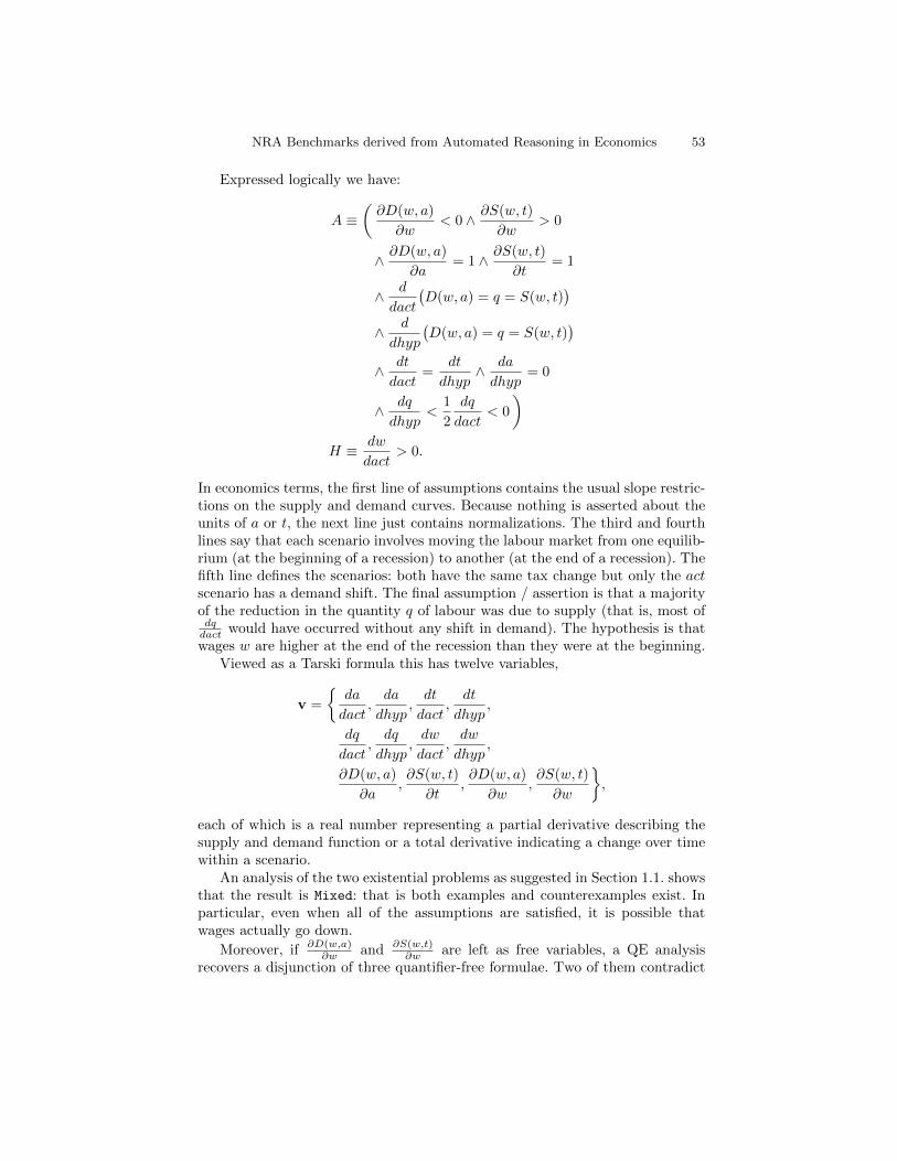
Expressed logically we have:

A ≡(

∂D(w, a)

∂w< 0 ∧ ∂S(w, t)

∂w> 0

∧ ∂D(w, a)

∂a= 1 ∧ ∂S(w, t)

∂t= 1

∧ d

dact

(D(w, a) = q = S(w, t)

)∧ d

dhyp

(D(w, a) = q = S(w, t)

)∧ dt

dact=

dt

dhyp∧ da

dhyp= 0

∧ dq

dhyp<

1

2

dq

dact< 0

)H ≡ dw

dact> 0.

In economics terms, the first line of assumptions contains the usual slope restric-tions on the supply and demand curves. Because nothing is asserted about theunits of a or t, the next line just contains normalizations. The third and fourthlines say that each scenario involves moving the labour market from one equilib-rium (at the beginning of a recession) to another (at the end of a recession). Thefifth line defines the scenarios: both have the same tax change but only the actscenario has a demand shift. The final assumption / assertion is that a majorityof the reduction in the quantity q of labour was due to supply (that is, most ofdq

dact would have occurred without any shift in demand). The hypothesis is thatwages w are higher at the end of the recession than they were at the beginning.

Viewed as a Tarski formula this has twelve variables,

v =

{da

dact,

da

dhyp,

dt

dact,

dt

dhyp,

dq

dact,

dq

dhyp,dw

dact,dw

dhyp,

∂D(w, a)

∂a,∂S(w, t)

∂t,∂D(w, a)

∂w,∂S(w, t)

∂w

},

each of which is a real number representing a partial derivative describing thesupply and demand function or a total derivative indicating a change over timewithin a scenario.

An analysis of the two existential problems as suggested in Section 1.1. showsthat the result is Mixed: that is both examples and counterexamples exist. Inparticular, even when all of the assumptions are satisfied, it is possible thatwages actually go down.

Moreover, if ∂D(w,a)∂w and ∂S(w,t)

∂w are left as free variables, a QE analysisrecovers a disjunction of three quantifier-free formulae. Two of them contradict


the assumptions, but the third does not and can therefore be added to A inorder to guarantee the truth of H:

∂S(w, t)

∂w≥ −∂D(w, a)

∂w> 0.

I.e. assuming that labour supply is at least as sensitive to wages as labour demandis (recall that the demand slope is a negative number) guarantees that wages ware higher at the end of the recession that is primarily due to taxes on laboursupply. See also [27] for further details on the economics.

This example can be found in the benchmark set as Model #0013.

2.3 Vector summaries

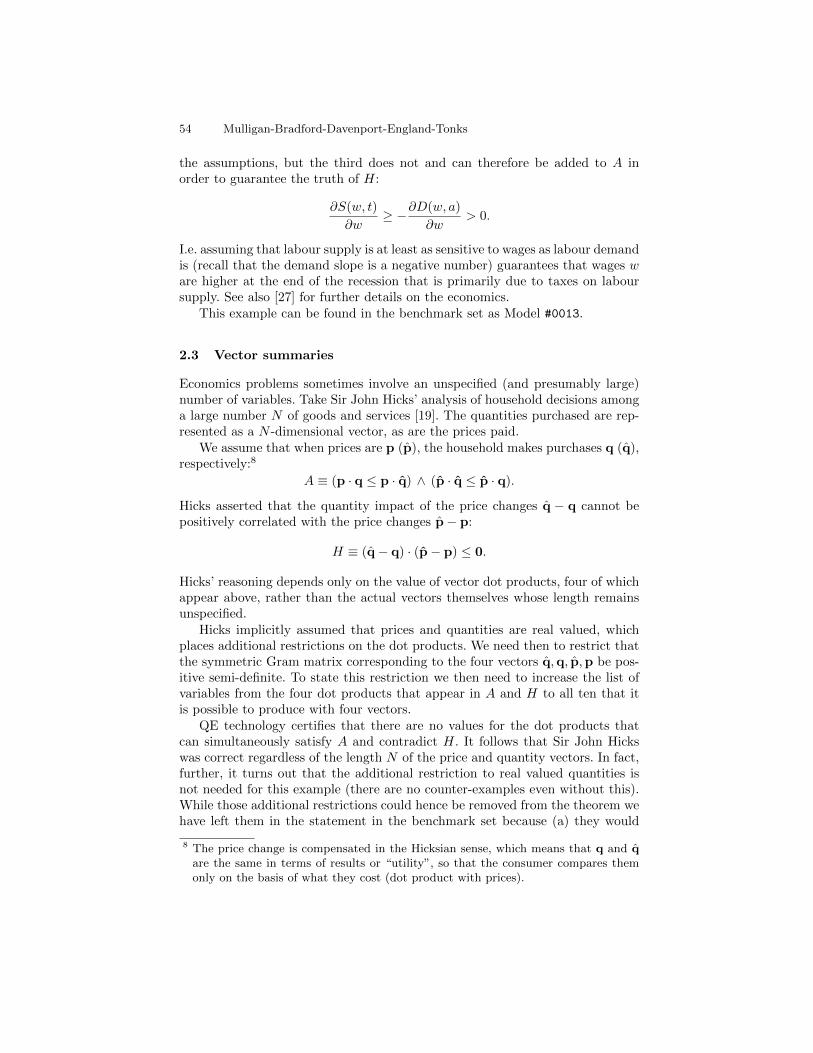
Economics problems sometimes involve an unspecified (and presumably large)number of variables. Take Sir John Hicks’ analysis of household decisions amonga large number N of goods and services [19]. The quantities purchased are rep-resented as a N -dimensional vector, as are the prices paid.

We assume that when prices are p (p), the household makes purchases q (q),respectively:8

A ≡ (p · q ≤ p · q) ∧ (p · q ≤ p · q).

Hicks asserted that the quantity impact of the price changes q − q cannot bepositively correlated with the price changes p− p:

H ≡ (q− q) · (p− p) ≤ 0.

Hicks’ reasoning depends only on the value of vector dot products, four of whichappear above, rather than the actual vectors themselves whose length remainsunspecified.

Hicks implicitly assumed that prices and quantities are real valued, whichplaces additional restrictions on the dot products. We need then to restrict thatthe symmetric Gram matrix corresponding to the four vectors q,q, p,p be pos-itive semi-definite. To state this restriction we then need to increase the list ofvariables from the four dot products that appear in A and H to all ten that itis possible to produce with four vectors.

QE technology certifies that there are no values for the dot products thatcan simultaneously satisfy A and contradict H. It follows that Sir John Hickswas correct regardless of the length N of the price and quantity vectors. In fact,further, it turns out that the additional restriction to real valued quantities isnot needed for this example (there are no counter-examples even without this).While those additional restrictions could hence be removed from the theorem wehave left them in the statement in the benchmark set because (a) they would

8 The price change is compensated in the Hicksian sense, which means that q and qare the same in terms of results or “utility”, so that the consumer compares themonly on the basis of what they cost (dot product with prices).


be standard restrictions an economist would work with and (b) it is not obviousthat they are unnecessary before the analysis.

The above analysis could be performed easily with both Mathematica andZ3 but proved difficult for Redlog. We have yet to find a variable orderingthat leads to a result in reasonable time9. It is perhaps not surprising that a toollike Z3 excels in comparison to computer algebra here, since the problem has alarge part of the logical statement irrelevant to its truth: the search based SATalgorithms are explicitly designed to avoid considering this.


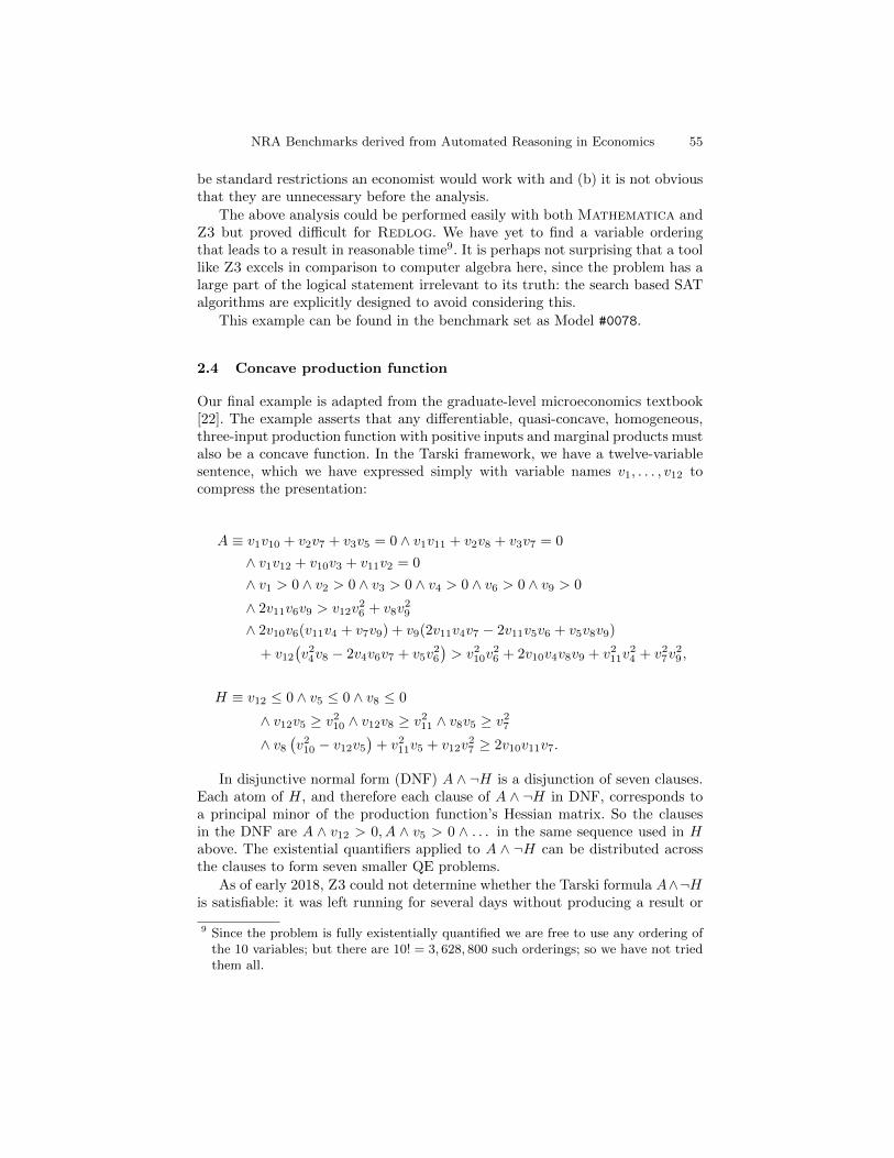
2.4 Concave production function

Our final example is adapted from the graduate-level microeconomics textbook[22]. The example asserts that any differentiable, quasi-concave, homogeneous,three-input production function with positive inputs and marginal products mustalso be a concave function. In the Tarski framework, we have a twelve-variablesentence, which we have expressed simply with variable names v1, . . . , v12 tocompress the presentation:

A ≡ v1v10 + v2v7 + v3v5 = 0 ∧ v1v11 + v2v8 + v3v7 = 0

∧ v1v12 + v10v3 + v11v2 = 0

∧ v1 > 0 ∧ v2 > 0 ∧ v3 > 0 ∧ v4 > 0 ∧ v6 > 0 ∧ v9 > 0

∧ 2v11v6v9 > v12v26 + v8v

29

∧ 2v10v6(v11v4 + v7v9) + v9(2v11v4v7 − 2v11v5v6 + v5v8v9)

+ v12(v24v8 − 2v4v6v7 + v5v

26

)> v210v

26 + 2v10v4v8v9 + v211v

24 + v27v

29 ,

H ≡ v12 ≤ 0 ∧ v5 ≤ 0 ∧ v8 ≤ 0

∧ v12v5 ≥ v210 ∧ v12v8 ≥ v211 ∧ v8v5 ≥ v27

∧ v8(v210 − v12v5

)+ v211v5 + v12v

27 ≥ 2v10v11v7.

In disjunctive normal form (DNF) A ∧ ¬H is a disjunction of seven clauses.Each atom of H, and therefore each clause of A ∧ ¬H in DNF, corresponds toa principal minor of the production function’s Hessian matrix. So the clausesin the DNF are A ∧ v12 > 0, A ∧ v5 > 0 ∧ . . . in the same sequence used in Habove. The existential quantifiers applied to A ∧ ¬H can be distributed acrossthe clauses to form seven smaller QE problems.

As of early 2018, Z3 could not determine whether the Tarski formula A∧¬His satisfiable: it was left running for several days without producing a result or

9 Since the problem is fully existentially quantified we are free to use any ordering ofthe 10 variables; but there are 10! = 3, 628, 800 such orderings; so we have not triedthem all.


error message. For this problem virtual substitution techniques may be advan-tageous (note the degree in any one variable is at most two). Indeed, Redlogand Mathematica can resolve it quickly. The problem would certainly be dif-ficult for CAD based tools (which underline the theory solver used by Z3 forsuch problems). For example, if we take only the first clause of the disjunction(the one containing v12 > 0), then the Tarski formula has twelve polynomialsin twelve variables, and just three CAD projections (using Brown’s projectionoperator) to eliminate {v12, v11, v10} results in 200 unique polynomials with ninevariables still remaining to eliminate!

We note that the problem has a lot of structure to exploit in regards tothe sparse distribution of variables in atoms. One approach currently underinvestigation is to eliminate quantifiers incrementally, taking advantage of therepetitive structure of the sub-problems one uncovers this way (an approach thatworks on several other problems in the benchmark set). This will be the topicof a future paper.


3 Analysis of the Structure of Economics Benchmarks

The examples collected for the benchmark set come from a variety of areas ofeconomics. They were chosen for their importance in economic reasoning andtheir ability to be expressed in the Tarski framework, not on the basis of theircomputational complexity. The sentences tend to be significantly larger formulaethan the initial examples described above. We summarise some statistics on thebenchmarks. These statistics are generated for the 45 counterexample checks(∃v[A ∧ ¬H]) which are representative of the full 135 problems.

3.1 Logical size

Presented in DNF the benchmarks have number of clauses ranging from 7 to 43with a mean average of 18.5 and median of 18. Of course each clause can be aconjunction but this is fairly rare: the average number of literals in a clause isat most 1.5 in the dataset, with the average number of atoms in a formula onlyslightly more than the number of clauses at 19.3.

3.2 Algebraic size

The number of polynomials involved in the benchmarks varies from 7 to 43 withboth mean average of 19.2 and median average of 19. The number of variablesranges from 8 to 101 with an mean average of 17.2 and median of 14. It is worthnoting that examples with this number of variables would rarely appear in theQE literature, since many QE algorithms have complexity doubly exponentialin the number of variables [15], [16], with QE itself doubly exponential in thenumber of quantifier changes [2]. The number of polynomials per variable rangesfrom 0.4 to 2.0 with an average of 1.2.


3.3 Low degrees

While the algebraic dimensions of these examples are large in comparison tothe QE literature, their algebraic structure is usually less complex. In particularthe degrees are strictly limited. The maximum total degree of a polynomial in abenchmark ranges from 2 to 7 with an average of 4.2. So although linear methodscannot help with any of these benchmarks the degrees do not rise far. The meantotal degree of a polynomial in a benchmark is only 1.8 so the non-linearity whilealways present can be quite sparse.

However, of greater relevance to QE techniques is not total degree of a poly-nomial but the maximum degree in any one variable: e.g. this controls the num-ber of potential roots of a polynomial and thus cell decompositions in a CAD(with this degree becoming the base for the double exponent in the complexitybound); see for example the complexity analysis in [4]. The maximum degree inany one variable is never more than 4 in any polynomial in the benchmarks. Ifwe take the maximum degree in any one variable in a formula and average forthe dataset we get 2.1; if we take the maximum degree in any one variable in apolynomial and average for the dataset we get 1.3.

3.4 Plentiful useful side conditions

With variables frequently multiplying each other in a sentence’s polynomials, apotentially large number of polynomial singularities might be relevant to a QEprocedure. However, we note that the benchmarks here will typically include signconditions that in principle rule out the need to consider many such singularities.That is, these side conditions will often coincide with unrealistic economic inter-pretations that are excluded in the assumptions. Of course, the computationalpath of many algorithms may not necessarily exploit these currently withouthuman guidance.

3.5 Sparse occurrence of variables

For each sentence ∃v[A ∧ ¬H] (these are the computationally more challengingof the 135) we have formed a matrix of occurrences, with rows representingvariables and columns representing polynomials. A matrix entry is one if andonly if the variable appears in the polynomial, and zero otherwise. The averageentry of all 45 occurrence matrices is 0.15. This sparsity indicates that the useof specialised methods or optimisations for sparse systems could be beneficial.

3.6 Variable orderings

Since the problems are fully existentially quantified we have a free choice ofvariable ordering for the theory tools. It is well known that the ordering cangreatly affect the performance of tools. A classic result in CAD presents a classof problems in which one variable ordering gave output of double exponentialcomplexity in the number of variables and another output of a constant size


[7]. Heuristics have been developed to help with this choice (e.g. [13] [5]) with amachine learned choice performing the best in [20]. The benchmarks come witha suggested variable ordering but not a guarantee that this is optimal: toolsshould investigate further (see also [28]).

4 Final Thoughts

4.1 Summary

We have presented a dataset of examples from economic reasoning suitable forautomatic solution by QE or SMT technology. These clearly broaden the ap-plication domains present in the relevant category of the SMT-LIB, and theliterature of QE. Further, their logical and algebraic structure are sources ofadditional diversity.

While some examples can be solved easily there are others that prove chal-lenging to the various tools on offer. The example in Section 2.3 could not betackled by Redlog while the one in Section 2.4 caused problems for Z3. Of thetools we tried, only Mathematica was able to decide all problems in the bench-mark set. However, in terms of median average timing over the benchmark setMathematica takes longer with 825ms than Redlog (50ms) or Z3 (< 15ms).

4.2 Ongoing and future work

As noted at the end of Section 2, some of these problems have a lot of structure toexploit and so the optimisation of existing QE tools for problems from economicsis an ongoing area of work.

More broadly, we hope these benchmarks and examples will promote interestfrom the Computer Science community in problems from the social sciences, andcorrespondingly, that successful automated solution of these problems will pro-mote greater interest in the social sciences for such technology. A key barrier tothe latter is the learning curve that technology like Computer Algebra Systemsand SMT solvers has, particularly to users from outside Mathematics and Com-puter Science. In [28] we describe one solution for this: a new Mathematicapackage called TheoryGuru which acts as a wrapper for the QE functionality inthe Resolve command designed to ease its use for an economist.

References

1. C. Barrett, P. Fontaine, and C. Tinelli. The Satisfiability Modulo Theories Library(SMT-LIB). www.SMT-LIB.org, 2016.

2. S. Basu, R. Pollack, and M.F. Roy. Algorithms in Real Algebraic Geometry. 10 ofAlgorithms and Computations in Mathematics. Springer-Verlag, 2006.

3. R. Bradford, J.H. Davenport, M. England, H. Errami, V. Gerdt, D. Grigoriev,C. Hoyt, M. Kosta, O. Radulescu, T. Sturm, and A. Weber. A case study onthe parametric occurrence of multiple steady states. In Proc. 2017 ACM Inter-national Symposium on Symbolic and Algebraic Computation, ISSAC ’17, pages45–52. ACM, 2017.


4. R. Bradford, J.H. Davenport, M. England, S. McCallum, and D. Wilson. Truthtable invariant cylindrical algebraic decomposition. Journal of Symbolic Compu-tation, 76:1–35, 2016.

5. R. Bradford, J.H. Davenport, M. England, and D. Wilson. Optimising problemformulations for cylindrical algebraic decomposition. In J. Carette, D. Aspinall,C. Lange, P. Sojka, and W. Windsteiger, editors, Intelligent Computer Mathemat-ics, vol. 7961 of Lecture Notes in Computer Science, pages 19–34. Springer BerlinHeidelberg, 2013.

6. C.W. Brown. QEPCAD B: A program for computing with semi-algebraic setsusing CADs. ACM SIGSAM Bulletin, 37(4):97–108, 2003.

7. C.W. Brown and J.H. Davenport. The complexity of quantifier elimination andcylindrical algebraic decomposition. In Proc. 2007 International Symposium onSymbolic and Algebraic Computation, ISSAC ’07, pages 54–60. ACM, 2007.

8. B. Caviness and J. Johnson. Quantifier Elimination and Cylindrical AlgebraicDecomposition. Texts & Monographs in Symbolic Computation. Springer-Verlag,1998.

9. A.E. Charalampakis and I. Chatzigiannelis. Analytical solutions for the minimumweight design of trusses by cylindrical algebraic decomposition. Archive of AppliedMechanics, 88(1):39–49, 2018.

10. C. Chen and M. Moreno Maza. Quantifier elimination by cylindrical algebraicdecomposition based on regular chains. In Proc. 39th International Symposium onSymbolic and Algebraic Computation, ISSAC ’14, pages 91–98. ACM, 2014.

11. G.E. Collins. Quantifier elimination for real closed fields by cylindrical algebraicdecomposition. In Proc. 2nd GI Conference on Automata Theory and FormalLanguages, pages 134–183. Springer-Verlag (reprinted in the collection [8]), 1975.

12. F. Corzilius, U. Loup, S. Junges, and E. Abraham. SMT-RAT: An SMT-compliantnonlinear real arithmetic toolbox. In A. Cimatti and R. Sebastiani, editors, Theoryand Applications of Satisfiability Testing - SAT 2012, vol. 7317 of Lecture Notesin Computer Science, pages 442–448. Springer Berlin Heidelberg, 2012.

13. A. Dolzmann, A. Seidl, and T. Sturm. Efficient projection orders for CAD. In Proc.2004 International Symposium on Symbolic and Algebraic Computation, ISSAC’04, pages 111–118. ACM, 2004.

14. A. Dolzmann and T. Sturm. REDLOG: Computer algebra meets computer logic.SIGSAM Bull., 31(2):2–9, 1997.

15. M. England, R. Bradford, and J.H. Davenport. Improving the use of equationalconstraints in cylindrical algebraic decomposition. In Proc. 2015 InternationalSymposium on Symbolic and Algebraic Computation, ISSAC ’15, pages 165–172.ACM, 2015.

16. M. England and J.H. Davenport. The complexity of cylindrical algebraic decompo-sition with respect to polynomial degree. In V.P. Gerdt, W. Koepf, W.M. Werner,and E.V. Vorozhtsov, editors, Computer Algebra in Scientific Computing: 18thInternational Workshop, CASC 2016, vol. 9890 of Lecture Notes in Computer Sci-ence, pages 172–192. Springer International Publishing, 2016.

17. M. Erascu and H. Hong. Real quantifier elimination for the synthesis of optimalnumerical algorithms (Case study: Square root computation). Journal of SymbolicComputation, 75:110–126, 2016.

18. P. Fontaine, M. Ogawa, T. Sturm, and X.T. Vu. Subtropical satisfiability. InC. Dixon and M. Finger, editors, Frontiers of Combining Systems (FroCoS 2017),vol. 10483 of Lecture Notes in Computer Science, pages 189–206. Springer Inter-national Publishing, 2017.


19. J.R. Hicks. Value and Capital. Clarendon Press, 2nd edition, 1946.20. Z. Huang, M. England, D. Wilson, J.H. Davenport, L. Paulson, and J. Bridge. Ap-

plying machine learning to the problem of choosing a heuristic to select the variableordering for cylindrical algebraic decomposition. In S.M. Watt, J.H. Davenport,A.P. Sexton, P. Sojka, and J. Urban, editors, Intelligent Computer Mathematics,vol. 8543 of Lecture Notes in Artificial Intelligence, pages 92–107. Springer, 2014.

21. H. Iwane, H. Yanami, and H. Anai. SyNRAC: A toolbox for solving real algebraicconstraints. In H. Hong and C. Yap, editors, Mathematical Software – Proc. ICMS2014, vol. 8592 of Lecture Notes in Computer Science, pages 518–522. SpringerHeidelberg, 2014.

22. G.A. Jehle and P.J. Reny. Advanced Microeconomic Theory. Pearson, 2011.23. D. Jovanovic and L. de Moura. Solving non-linear arithmetic. In B. Gramlich,

D. Miller, and U. Sattler, editors, Automated Reasoning: 6th International JointConference (IJCAR), vol. 7364 of Lecture Notes in Computer Science, pages 339–354. Springer, 2012.

24. D. Jovanovic and B. Dutertre. LibPoly: A library for reasoning about polynomi-als. In M. Brain and L. Hadarean, editors, Proc. 15th International Workshop onSatisfiability Modulo Theories (SMT 2017), number 1889 in CEUR-WS, 2017.

25. X. Li and D. Wang. Computing equilibria of semi-algebraic economies using tri-angular decomposition and real solution classification. Journal of MathematicalEconomics, 54:48–58, 2014.

26. A. Marshall. Principles of Economics. MacMillan and Co., 1895.27. C.B. Mulligan. The Redistribution Recession: How Labor Market Distortions Con-

tracted the Economy. Oxford University Press, 2012.28. C.B. Mulligan, J.H. Davenport, and M. England. TheoryGuru: A Mathematica

package to apply quantifier elimination technology to economics. In: J.H. Dav-enport, M. Kauers, G. Labahn and J. Urban editors, Mathematical Software –Proc. ICMS 2018, vol. 10931 of Lecture Notes in Computer Science, pages 369-378. Springer, 2018.

29. L.C. Paulson. Metitarski: Past and future. In L. Beringer and A. Felty, editors,Interactive Theorem Proving, vol. 7406 of Lecture Notes in Computer Science,pages 1–10. Springer, 2012.

30. A. Platzer, J.D. Quesel, and P. Rummer. Real world verification. In R.A. Schmidt,editor, Automated Deduction (CADE-22), vol. 5663 of Lecture Notes in ComputerScience, pages 485–501. Springer Berlin Heidelberg, 2009.

31. C. Steinhorn. Tame Topology and O-Minimal Structures, pages 165–191. SpringerBerlin Heidelberg, 2008.

32. A. Strzebonski. Cylindrical algebraic decomposition using validated numerics.Journal of Symbolic Computation, 41(9):1021–1038, 2006.

33. T. Sturm and A. Weber. Investigating generic methods to solve Hopf bifurcationproblems in algebraic biology. In K. Horimoto, G. Regensburger, M. Rosenkranz,and H. Yoshida, editors, Algebraic Biology, pages 200–215. Springer, 2008.

34. A. Tarski. A Decision Method For Elementary Algebra And Geometry. RANDCorporation, Santa Monica, CA (reprinted in the collection [8]), 1948.

35. Y. Wada, T. Matsuzaki, A. Terui, and N.H. Arai. An automated deduction and itsimplementation for solving problem of sequence at university entrance examina-tion. In G.-M. Greuel, T. Koch, P. Paule, and A. Sommese, editors, MathematicalSoftware – Proc. ICMS 2016, vol. 9725 of Lecture Notes in Computer Science,pages 82–89. Springer International Publishing, 2016.

36. V. Weispfenning. The complexity of linear problems in fields. Journal of SymbolicComputation, 5(1/2):3–27, 1988.

Non-linear Real Arithmetic Benchmarks derived from ...

Documents

Transcript of Non-linear Real Arithmetic Benchmarks derived from ...