Non-linear Dynamics - uni- · PDF fileNon-linear Dynamics Prof. Dr. Ulrich Schwarz Heidelberg...

Non-linear Dynamics

Prof. Dr. Ulrich SchwarzHeidelberg University, Institute for Theoretical Physics

Email: [email protected]: http://www.thphys.uni-heidelberg.de/˜biophys/

Winter term 2016/17Last update: January 25, 2017

http://www.thphys.uni-heidelberg.de/~biophys/

Contents

1 The central equation 5

2 Flow on a line 9

3 Bifurcations in 1d 15

3.1 Saddle-node bifurcation . . . . . . . . . . . . . . . . . . . . . 15

3.2 Transcritical bifurcation . . . . . . . . . . . . . . . . . . . . . 19

3.3 Pitchfork bifurcation . . . . . . . . . . . . . . . . . . . . . . . 21

3.3.1 Supercritical pitchfork bifurcation . . . . . . . . . . . 21

3.3.2 Subcritical pitchfork bifurcation . . . . . . . . . . . . 22

3.4 Influence of high order terms . . . . . . . . . . . . . . . . . . 22

3.5 Summary of 1d bifurcations . . . . . . . . . . . . . . . . . . . 24

4 Flow on a circle 27

5 Flow in linear 2d systems 33

5.1 General remarks . . . . . . . . . . . . . . . . . . . . . . . . . 33

5.2 Phase plane flow for linear systems . . . . . . . . . . . . . . . 35

6 Flow in non-linear 2d systems 39

3

4 CONTENTS

7 Oscillations in 2d 47

8 Bifurcations in 2d 59

9 Excitable systems 67

10 Reaction-diffusion systems 77

Chapter 1

The central equation

We consider dynamical systems of dimension d which are described by ODEs.This implies that we use continuous time. (One alternative would be differ-ent equations with discrete time.) Calling ~x the state vector of the systemwe consider the equation

d~xdt = ~f(~x)

with a vector-valued function ~f which can be non-linear. In case of a linearfunction ~f the equation simplifies to

~x = A · ~x

with a matrix A and the system shows exponential behavior.

Examples

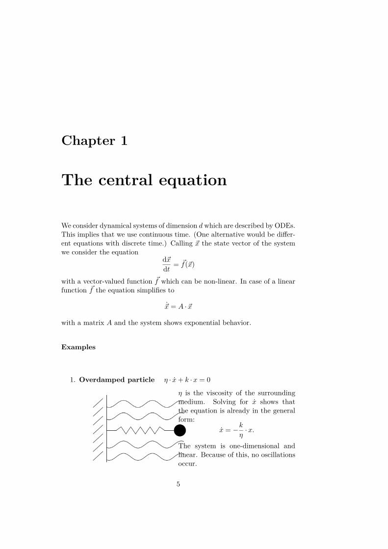
1. Overdamped particle η · x+ k ·x = 0

η is the viscosity of the surroundingmedium. Solving for x shows thatthe equation is already in the generalform:

x = −kη·x.

The system is one-dimensional andlinear. Because of this, no oscillationsoccur.

5

6 CHAPTER 1. THE CENTRAL EQUATION

2. Harmonic oscillator ~x+ ω20~x = 0

This looks superficially like an one-dimensional system. But the fol-lowing trick eliminates the second derivative and shows the linear buttwo-dimensional character of the harmonic oscillator:Choose x1 = x and x2 = v = x with the velocity v. Then, the equationwritten in the general form is

~x =(x1x2

)=(

0 1−ω2

0 0

)· ~x.

3. Pendulum x+ gl sin(x) = 0

Using the same trick as for the har-monic oscillator, we get x1 = x2and x2 = −g

l sin(x1), hence a non-linear, two-dimensional system. Onlyfor small angles x (⇒ sin(x) ≈ x) weend up with a harmonic oscillator.

4. Driven harmonic oscillator mx+ k ·x = F · cos(ωt)The equation of the driven harmonic oscillator explicitly depends ontime t. But rewriting the equation using x1 = x, x2 = x and intro-ducing a third variable x3 = t leads to the relations x1 = x2, x2 =1m (−kx1 + F · cos(ωx3)) , x3 = 1. The system is non-linear withd = 3.

5. Electric curcuit R · I + QC = V0

7

Using Kirchhoff’s law and the relation I = Q we get the ODE of anoverdamped particle:

Q = V0R− 1RC·Q.

Remember this is a linear, one-dimensional system. If we put in asolenoid the dependence of Q will lead to d = 2 and oscillations canoccur.

8 CHAPTER 1. THE CENTRAL EQUATION

Chapter 2

Flow on a line

In this chapter, we are looking at one-dimensional systems. Therefore, thecentral equation becomes x = f(x) with an arbitrary function f .

The first example we want to discuss is non-linear: x = sin(x). The separa-tion of variables leads to

dxsin(x) = csc(x)dx = dt

which can be integrated with the result

t = ln(csc(x0) + cot(x0)

csc(x) + cot(x)

).

Even in this simple non-linear example, the behavior of the system is noteasy to understand from this solution. But graphical analysis shows themost important properties.

Plotting a phase portrait (left figure), stable and unstable fixed points canbe determined. In 1d, the systems dynamics corresponds to flow on the line.The corresponding trajectories are shown in the right figure.

9

10 CHAPTER 2. FLOW ON A LINE

For a stable fixed point a little change in x drives the system back, whereasfor an unstable fixed point it causes a flow away from the fixed point.

Choosing different starting points x∗ the time-dependence of the accelerationcomputes as follows: for starting points |x∗−π| ≤ π

2 the acceleration directlydecreases. But if x∗ = π ± ∆x with π

2 < ∆x <= π the acceleration firstincreases and decreases after the deflection point.

The graphical analysis can be performed for the earlier examples as well:

• Overdamped particle

x = −xx∗ = 0 , stable fixed point

• Electrical curcuit

x∗ 6= 0

11

The applied method works for any graph.

In an one-dimensional system, there are three possibilities in total the systemcan behave:

1. staying at a fixed point

2. flowing to a stable fixed point

3. flowing to infinity

There is also a mathematical method to analyze fixed points. It is calledlinear stability analysis. Firstly, one determines the fixed points by solvingx = f(x) = 0 for x. Take x∗ to be a fixed point. Then, the deviation η fromthis fixed point is given by η = x− x∗.

The derivative η can be written in dependence of the sum x∗ + η.

η = x = f(x) = f(x∗ + η)

The first order Taylor expansion η = f(x∗)=0

+ f ′(x∗) · η + O(η2) leads to a

first order ODEη = f ′(x∗) · η

which can be integrated to a time-dependent deviation

η(t) = η0 · exp(f ′(x∗) · t)

with the starting deviation η0 at t = 0. Introducing the relaxation timet0 = | 1

f ′(x∗) | this yields

η(t) = η0 · exp(sign(f ′(x∗)) · t/t0

).


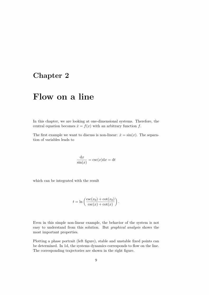
Thus, f ′(x∗) hints towards the characteristics of a fixed point x∗.

Conclusion

If f ′(x∗) < 0: stable fixed point, exponential decayf ′(x∗) > 0: unstable fixed point, blow-upf ′(x∗) = 0: further investigations are needed

Examples

In both cases x = ±x3 the character of the fixed point is not clear from f ′.

For x = x2 the system has a half-stable point at x = 0. If x is constant, theresult is a line of fixed points.

Uniqueness theorem

If f(x) and f ′(x) are continuous on an open interval around x0, then asolution exists and is unique.

13

This leads to the impossibility of oscillations in an one-dimensional system.Instead, everything is overdamped. Consider a potential V . In 1d, we canwrite

x = f(x) = −dV (x)dx .

Hence, the time derivative of V yieldsdVdt = dV

dxdxdt = −

(dVdx

)2≤ 0.

So, the energy of the system can never increase. It always decreases duringflow.

Examples

1. Overdamped particle

2. Mexican hat

The Mexican hat is an example of a bistable system.

The figures show the following relation for d = 1:

minimum in V : stable fixed pointmaximum in V : unstable fixed point

Chapter 3

Bifurcations in 1d

As we have seen in chapter 2, flow can easily be understood in d = 1. How-ever, up to now we did not consider any parameter which in principal couldchange the flow structure. A sudden change in the character of the solu-tion is called bifurcation. Physical examples for this are phase transitions,mechanical instabilities, laser thresholds, population thresholds etc.

There are exactly three types of bifurcations in d = 1. Mathematically itcan be shown that each type can be described by one general form usingthe bifurcation parameter r. The general properties are summarized in thefollowing table.

Saddle-node bifurcation x = r + x2 fixed points can appear or disappeardepending on r

Transcritical bifurcation x = rx− x2 fixed points always exist for all rbut they can exchange stability

Pitchfork bifurcation x = rx± x3 fixed points appear or disappearas a symmetrical pair

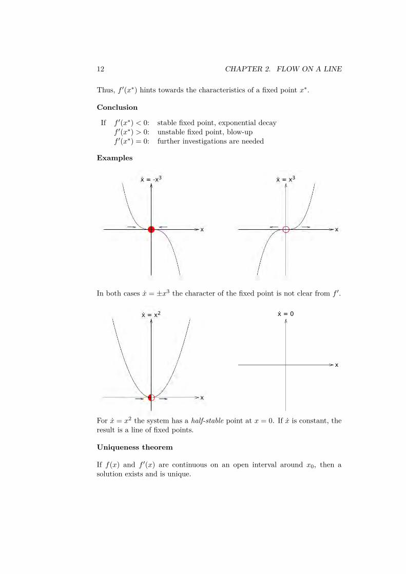
3.1 Saddle-node bifurcation

Consider x = r + x2 with the bifurcation parameter r. The roots are givenby x∗ = ±

√r. For various r the system behaves differently.

15

16 CHAPTER 3. BIFURCATIONS IN 1D

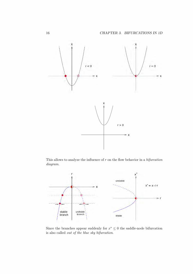
This allows to analyze the influence of r on the flow behavior in a bifurcationdiagram.

Since the branches appear suddenly for x∗ ≤ 0 the saddle-node bifurcationis also called out of the blue sky bifurcation.

3.1. SADDLE-NODE BIFURCATION 17

This corresponds to a phase transition of second order like the magnetizationof an Ising magnet.

But why does x = r + x2 describe all saddle-node bifurcations? We assumex to be a function of x and the parameter r.

Expanding x = f(x, r) around x = x∗ and r = rc leads to

x ≈ f(x∗, rc)+∂f

∂x|(x∗,rc) · (x−x∗)+

∂f

∂r|(x∗,rc) · (r−rc)+

12∂2f

∂x2 |(x∗,rc) · (x−x∗)2.

Considering f(x∗, rc) = 0 and ∂f∂x |(x∗,r∗) = 0 the general form computes as

x = a(r − rc) + b(x− x∗)2 .

Example: Stability of adhesion cluster under constant force


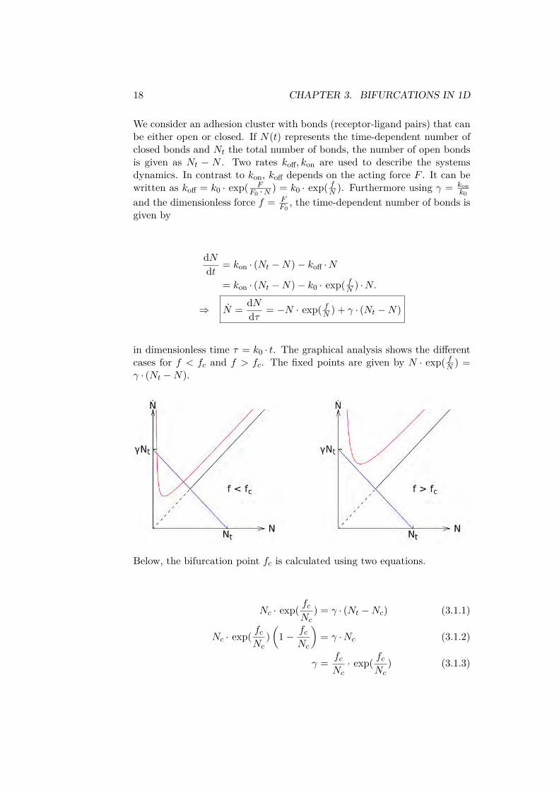
We consider an adhesion cluster with bonds (receptor-ligand pairs) that canbe either open or closed. If N(t) represents the time-dependent number ofclosed bonds and Nt the total number of bonds, the number of open bondsis given as Nt − N . Two rates koff, kon are used to describe the systemsdynamics. In contrast to kon, koff depends on the acting force F . It can bewritten as koff = k0 · exp( F

F0 ·N ) = k0 · exp( fN ). Furthermore using γ = konk0

and the dimensionless force f = FF0

, the time-dependent number of bonds isgiven by

dNdt = kon · (Nt −N)− koff ·N

= kon · (Nt −N)− k0 · exp( fN ) ·N.

⇒ N = dNdτ = −N · exp( fN ) + γ · (Nt −N)

in dimensionless time τ = k0 · t. The graphical analysis shows the differentcases for f < fc and f > fc. The fixed points are given by N · exp( fN ) =γ · (Nt −N).

Below, the bifurcation point fc is calculated using two equations.

Nc · exp( fcNc

) = γ · (Nt −Nc) (3.1.1)

Nc · exp( fcNc

)(

1− fcNc

)= γ ·Nc (3.1.2)

γ = fcNc· exp( fc

Nc) (3.1.3)

3.2. TRANSCRITICAL BIFURCATION 19

Equation (1) represents the fixed points. Dividing (2) by (1) results in(1− fc

Nc

)= − Nc

Nt −Nc⇒ fc = NtNc

Nt −Nc⇒ fc

Nc= fcNt

+ 1

Using this, γ can be written as

γ = fcNt· exp( fc

Nt+1) ⇒ fc

Nt· exp( fc

Nt) = γ

e ⇒ fc = Nt · plog(γ

e

)

. In the last step, the function plog is used, defined by x · exp(x) = Q ⇒x = plog(Q).

3.2 Transcritical bifurcation

The general form of a transcritical bifurcation x = r ·x − x2 leads to thefixed point x∗ = 0 which exists for an arbitrary bifurcation parameter r andalso represents the bifurcation point rc = 0. The second fixed point x∗ = ris stable for r > 0 and unstable for r < 0. Depending on the application,not every fixed point is reasonable, e.g. when the population size is alwayspositive.

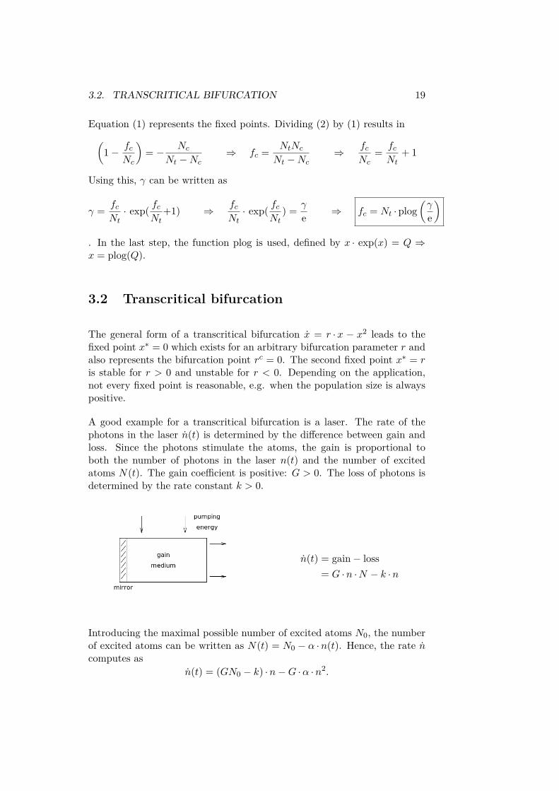
A good example for a transcritical bifurcation is a laser. The rate of thephotons in the laser n(t) is determined by the difference between gain andloss. Since the photons stimulate the atoms, the gain is proportional toboth the number of photons in the laser n(t) and the number of excitedatoms N(t). The gain coefficient is positive: G > 0. The loss of photons isdetermined by the rate constant k > 0.

n(t) = gain− loss= G ·n ·N − k ·n

Introducing the maximal possible number of excited atoms N0, the numberof excited atoms can be written as N(t) = N0 − α ·n(t). Hence, the rate ncomputes as

n(t) = (GN0 − k) ·n−G ·α ·n2.


Thus, the fixed points are n∗1 = 0 and n∗2 = GN0−kαG . Since n describes a

particle number, demanding n∗2 > 0 is reasonable and leads to N0 >kG .

The fixed points stability analysis is done by evaluating

g′N (n∗) = dndn(n∗) = (GN0 − k)− 2Gαn∗.

g′n(n∗1) = GN0 − k =< 0, for N0 <

kG , stable fixed point

> 0, for N0 >kG , unstable fixed point

g′n(n∗2) = k −GN0 < 0, since N0 >kG , stable fixed point

Obviously, N0 = kG is a bifurcation point.

3.3. PITCHFORK BIFURCATION 21

3.3 Pitchfork bifurcation

As the general form reads x = rx± x3 two different types exist: the super-critical and the subcritical pitchfork bifurcation.

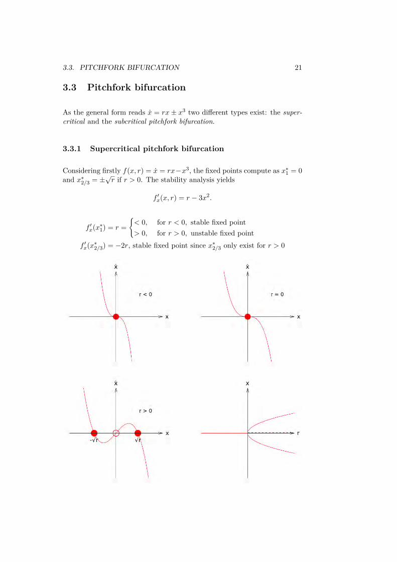
3.3.1 Supercritical pitchfork bifurcation

Considering firstly f(x, r) = x = rx−x3, the fixed points compute as x∗1 = 0and x∗2/3 = ±

√r if r > 0. The stability analysis yields

f ′x(x, r) = r − 3x2.

f ′x(x∗1) = r =< 0, for r < 0, stable fixed point> 0, for r > 0, unstable fixed point

f ′x(x∗2/3) = −2r, stable fixed point since x∗2/3 only exist for r > 0


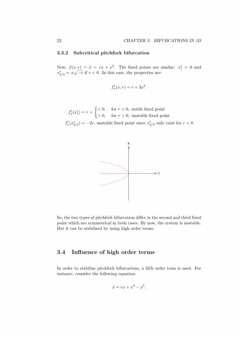
3.3.2 Subcritical pitchfork bifurcation

Now, f(x, r) = x = rx + x3. The fixed points are similar: x∗1 = 0 andx∗2/3 = ±

√−r if r < 0. In this case, the properties are:

f ′x(x, r) = r + 3x2.

f ′x(x∗1) = r =< 0, for r < 0, stable fixed point> 0, for r > 0, unstable fixed point

f ′x(x∗2/3) = −2r, unstable fixed point since x∗2/3 only exist for r < 0

So, the two types of pitchfork bifurcation differ in the second and third fixedpoint which are symmetrical in both cases. By now, the system is unstable.But it can be stabilized by using high order terms.

3.4 Influence of high order terms

In order to stabilize pitchfork bifurcations, a fifth order term is used. Forinstance, consider the following equation:

x = rx+ x3 − x5.

3.4. INFLUENCE OF HIGH ORDER TERMS 23

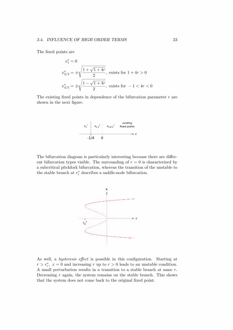
The fixed points are

x∗1 = 0

x∗2/3 = ±

√1 +√

1 + 4r2 , exists for 1 + 4r > 0

x∗4/5 = ±

√1−√

1 + 4r2 , exists for − 1 < 4r < 0

The existing fixed points in dependence of the bifurcation parameter r areshown in the next figure.

The bifurcation diagram is particularly interesting because there are differ-ent bifurcation types visible. The surrounding of r = 0 is characterized bya subcritical pitchfork bifurcation, whereas the transition of the unstable tothe stable branch at r∗c describes a saddle-node bifurcation.

As well, a hysteresis effect is possible in this configuration. Starting atr > r∗c , x = 0 and increasing r up to r > 0 leads to an unstable condition.A small perturbation results in a transition to a stable branch at same r.Decreasing r again, the system remains on the stable branch. This showsthat the system does not come back to the original fixed point.


3.5 Summary of 1d bifurcations

The general form is f(x, r) = x and behaves as shown in the following table:

normal form f(x∗) f ′x(x∗, rc) f ′r(x∗, rc) f ′′xx(x∗, rc) f ′′xr(x∗, rc) f ′′′xxx(x∗, rc)

saddle-node x = r + x2 0 0 6= 0 6= 0bifurcation

transcritical x = rx− x2 0 0 0 6= 0 6= 0bifurcation

pitchfork x = rx± x3 0 0 0 0 0 6= 0bifurcation

Example: Overdamped bead on a rotating hoop

The hoop is rotating around the axis with an angular velocity ω. The actingforces are the gravitational force FG, the centrifugal force FC and a frictionforce FR which describes the system in a fluid. They are projected on theφ-plane.

3.5. SUMMARY OF 1D BIFURCATIONS 25

FG = m · g → mg · sin(φ)FC = m · ρ ·ω2 → mρω2 · cos(φ)FR = −bφ

Using ρ = r · sin(φ), the total acting force yields

F = m · rφ = −b · φ−mg · sin(φ) +mrω2 · sin(φ) cos(φ).

In order to receive a first order equation, the term m · rφ shall be neglected.The time τ = t

T with the timescale T is introduced. In a second step, theequation is reformulated dimensionless by dividing by the gravitational forceFG.

(mτ

T 2

)2 d2φ

dτ2 = − bT

dφdτ −mg · sin(φ) +mrω2 · sin(φ) cos(φ)(

τ

gT 2

)2 d2φ

dτ2 = − b

Tmg

dφdτ − sin(φ) + rω2

g· sin(φ) cos(φ)

How to define T so that ε2 :=(

τgT 2

)2is negligible?

Choosing the prefactor of the friction force − bTmg to be of order 1, T is

defined to be T = bmg . With this, ε is negligible if ε = τ

gT 2 = m2gτg2 1, so

if the inertia is much smaller than the friction.

Set ε = 0 from now on and introduce γ := τω2

g . The equation computes as

dφdτ = sin(φ) (γ · cos(φ)− 1) .

The applied procedure has reduced the number of parameters from five totwo: ε and γ. But setting ε = 0 transforms the equation to dimension one.So, only one initial condition can be considered. Thus, the behavior of thesystem ”at the very beginning” is neglected. After that, the system behavesas if it was of the order of 1.

The fixed points result from sin(φ) = 0 and cos(φ)− 1γ = 0. Therefore, the

number of fixed points depends on γ:For |γ| > 1 there are only the fixed points due to sin(φ) = 0. For thebifurcation point |γ| = 1, one additional fixed point exists for each periodof φ and for |γ| < 1, there are actually two.

Chapter 4

Flow on a circle

So far, we considered linear systems x = f(x) and visualized their dynamicsas flow on a line. Now, we are taking into account periodic behavior usingthe differential equation θ = f(θ). Then, f(θ+2π) = f(θ). This correspondsto a vector field on the circle.

The simplest case is a constant velocity θ = f(θ) = const = ω leading to anoscillation with period T = 2π

ω but without amplitude, θ(t) = ω · t+ ω0.

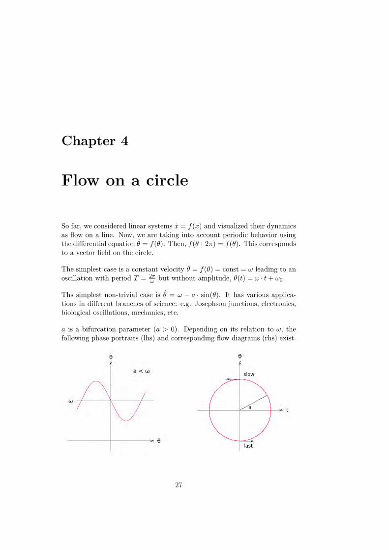
Ths simplest non-trivial case is θ = ω − a · sin(θ). It has various applica-tions in different branches of science: e.g. Josephson junctions, electronics,biological oscillations, mechanics, etc.

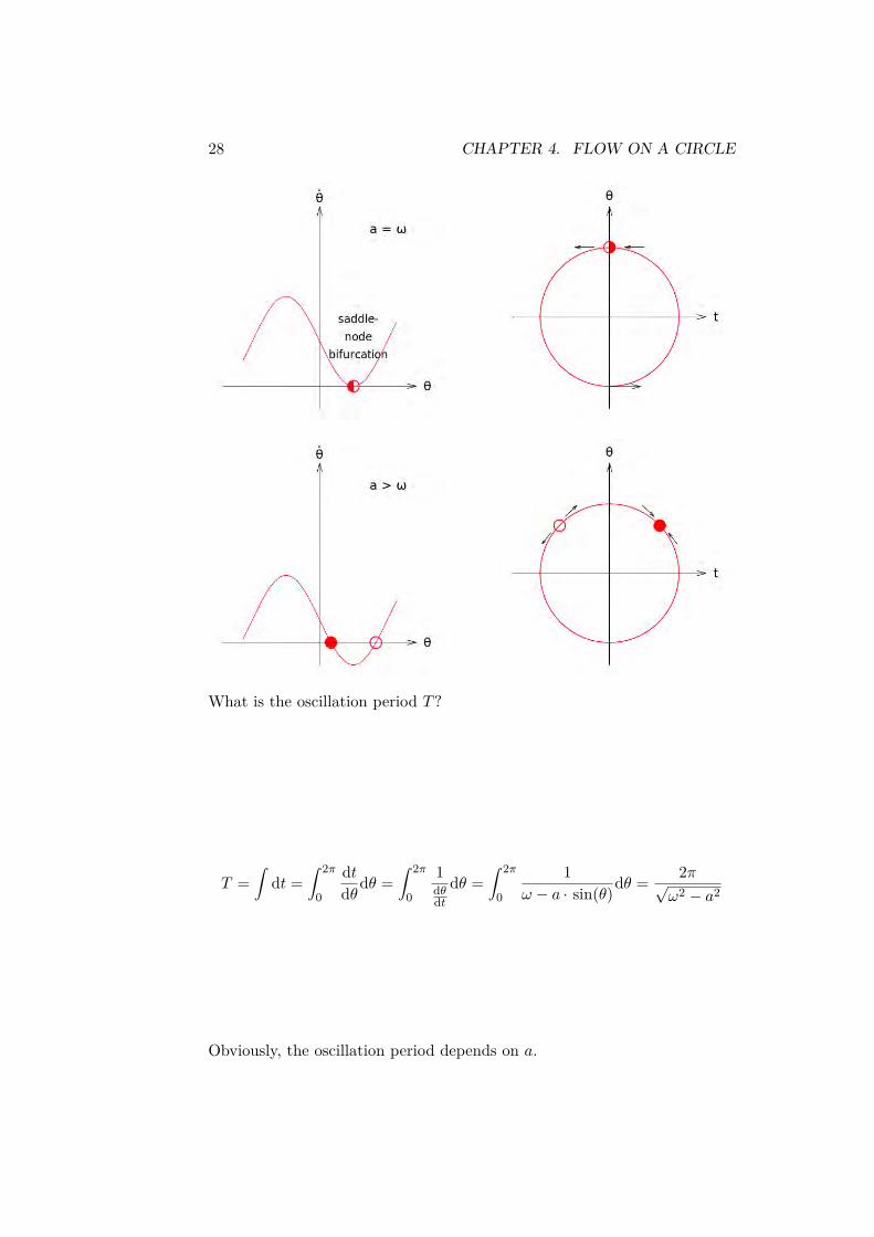
a is a bifurcation parameter (a > 0). Depending on its relation to ω, thefollowing phase portraits (lhs) and corresponding flow diagrams (rhs) exist.

27

28 CHAPTER 4. FLOW ON A CIRCLE

What is the oscillation period T?

T =∫

dt =∫ 2π

0

dtdθdθ =

∫ 2π

0

1dθdt

dθ =∫ 2π

0

1ω − a · sin(θ)dθ = 2π√

ω2 − a2

Obviously, the oscillation period depends on a.

29

a = 0 ⇒ T = 2πω

a→ ω ⇒ T = 2π√(ω − a)(ω + a)

= 2π√2ω√ω − a

The scaling is generic for a saddle-node bifurcation.

A Taylor expansion around the critical value θ∗ = π2 by introducing Φ =

θ − θ∗

Φ = ω − a · sin(

Φ + π

2

)= ω − a · cos(Φ)

≈ ω − a+ 12a ·Φ

2

results in the normal form of saddle-node bifurcations:

x :=(a

2

)1/2Φ

r := ω − a

⇒(2a

)1/2x = r + x2.


Most of the time will be spent close to θ∗.

T =∫

dt =∫ ∞−∞

dtdxdx =

(2a

)1/2 ∫dr 1r + x2 =

(2a

)1/2 π√r

=( 2ω

)1/2 π√ω − a

This is the same result as above. Therefore, extending the integrationboundaries to infinity is indeed not a problem.

Examples

1. Driven overdamped pendulum bθ +mgL sin(θ) = Γ

Dividing by mgL leads to the dimen-sionless equation

b

mgL︸︷︷︸=τ0

θ + sin(θ) = ΓmgL

=: γ.

The bifurcation parameter γ is the quotient of the applied torque Γto the maximum gravitational torque. Having also introduced thedimensionless time τ0 = t

τ the system is described by the equation

θ = dθdτ = γ − sin(θ).

At γ = 1 the pendulum stops its motion. For γ < 1 the externaltorque is too weak to drive the pendulum around.

2. Firefly synchronization

Identify θ = 0 with the emission of the flash.

31

Without external stimulus, each fire-fly has θ = ω. Now, consider a peri-odic stimulus with phase Ξ which sat-isfies

Ξ = Ω. (4.0.1)

The basic model to simulate the fire-fly’s reaction to the stimulus is givenby

θ = ω +A · sin(Ξ− θ) (4.0.2)

with the resetting or coupling strengthA.

The last equation can be expressed using the phase difference Φ =Ξ−θ. Substracting (4.0.2) from (4.0.1) leads to Φ = Ω−ω−A · sin(Φ).Defining furthermore µ := Ω−ω

A and τ = A · t the final equation reads

Φ = dΦdτ = µ− sin(Φ)

.

This leads to the following phase space diagrams:

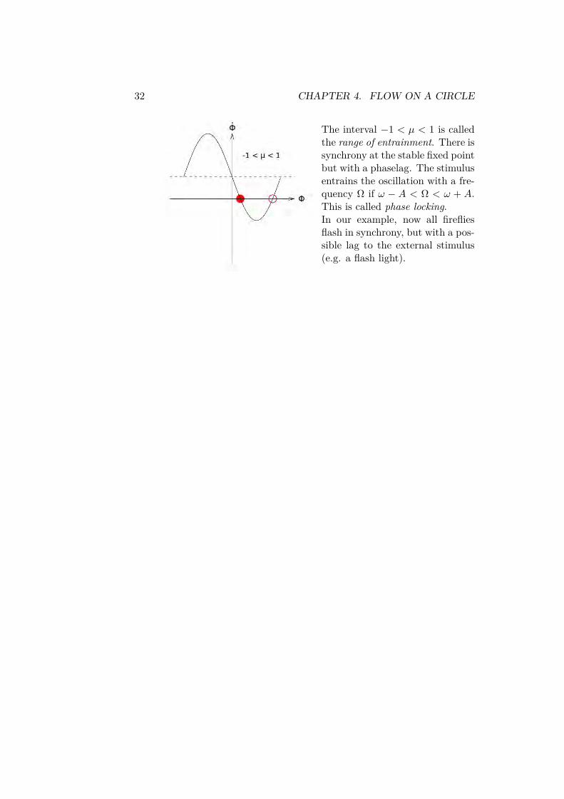
For µ = 0, there is a perfect synchrony at Φ = 0. If µ > 1 (or µ < −1)there aren’t any stable fixed points. So, there is no synchrony but aphase drift. The oscillation occurs with T = 2π√

(Ω−ω)2−A2 .


The interval −1 < µ < 1 is calledthe range of entrainment. There issynchrony at the stable fixed pointbut with a phaselag. The stimulusentrains the oscillation with a fre-quency Ω if ω − A < Ω < ω + A.This is called phase locking.In our example, now all firefliesflash in synchrony, but with a pos-sible lag to the external stimulus(e.g. a flash light).

Chapter 5

Flow in linear 2d systems

5.1 General remarks

In 2d, the varity of dynamical behavior is much larger than in 1d.

As a first step, we look at linear systems in two dimensions. Then, a completeclassification is possible and starts from

x = A · ~x =(a bc d

)(x1x2

).

In general, if ~x1(t) and ~x2(t) are solutions of the equation, so is c1 · ~x1+c2 · ~x2.In addition, ~x = 0 is always a solution.

Graphical analysis can be done by drawing and analyzing the ”phase plane”(x1, x2).

Examples

1. Harmonic oscillator: mx+ kx = 0

Defining the frequency ω0 =√

km and choosing x1 = x, x2 = x = v as

done in section 1 the matrix is A =(

0 1−ω2

0 0

).

33

34 CHAPTER 5. FLOW IN LINEAR 2D SYSTEMS

Why are the trajectories ellipses?

x

v= v

−ω20 ·x

⇒ −ω20 ·x dx = v dv

⇒ −ω20 ·x2 − v2 = const

This corresponds to energy conserva-tion:

12kx

2 + 12mv

2 = const.

2. A linear 2d system without oscillation:(xy

)=(a 00 −1

)(xy

)

For the given matrix A =(a 00 −1

), the two equations are uncoupled.

They can be separately solved using an exponential ansatz.

x = a ·x x(t) = x0 · exp(a · t)y = −y y(t) = y0 · exp(−t)

The phase portraits differ depending on a.

5.2. PHASE PLANE FLOW FOR LINEAR SYSTEMS 35

5.2 Phase plane flow for linear systems

Consider the linear case

~x = A · ~x =(a bc d

)~x.

Our analysis is based on the two eigenvalues λ1, λ2 of A =(a bc d

). They

are calculated using the characteristic equation A ·~v = λ ·~v.

0 != det(a− λ bc d− λ

)= λ2 − τλ−∆

= (λ− λ1)(λ− λ2)

⇒ λ1/2 = τ ±√τ2 − 4∆2

with τ = a+ d = tr A = λ1 + λ2 and ∆ = ad− cb = det A = λ1λ2.

In general, the eigenvalues are complex numbers depending on the traceτ and the determinant ∆ of A. If the eigenvalues are different λ1 6= λ2,the eigenvectors ~v1/2 are linearly independent. Hence, the characteristics ofA determines the phase plane flow as shown below. The time-dependenteigenvectors can be calculated using ~x1/2(t) = exp(λ1/2 · t) ·~v1/2.

We now completely enumerate all possible cases.

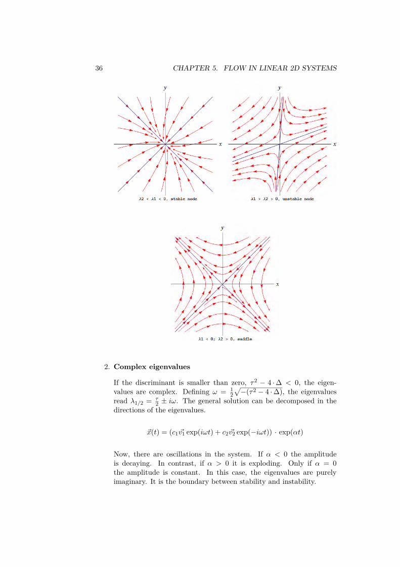
1. Real eigenvalues


2. Complex eigenvalues

If the discriminant is smaller than zero, τ2 − 4 ·∆ < 0, the eigen-values are complex. Defining ω = 1

2√−(τ2 − 4 ·∆), the eigenvalues

read λ1/2 = τ2 ± iω. The general solution can be decomposed in the

directions of the eigenvalues.

~x(t) = (c1 ~v1 exp(iωt) + c2 ~v2 exp(−iωt)) · exp(αt)

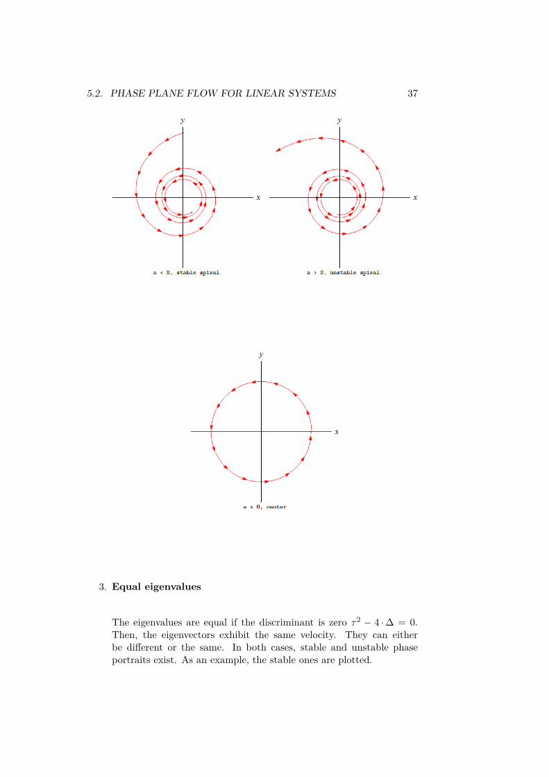
Now, there are oscillations in the system. If α < 0 the amplitudeis decaying. In contrast, if α > 0 it is exploding. Only if α = 0the amplitude is constant. In this case, the eigenvalues are purelyimaginary. It is the boundary between stability and instability.

5.2. PHASE PLANE FLOW FOR LINEAR SYSTEMS 37

3. Equal eigenvalues

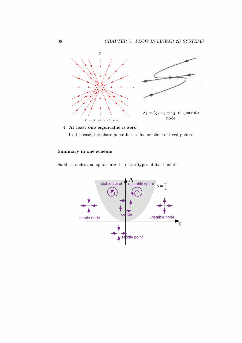
The eigenvalues are equal if the discriminant is zero τ2 − 4 ·∆ = 0.Then, the eigenvectors exhibit the same velocity. They can eitherbe different or the same. In both cases, stable and unstable phaseportraits exist. As an example, the stable ones are plotted.


λ1 = λ2, v1 = v2, degeneratenode

4. At least one eigenvalue is zeroIn this case, the phase portrait is a line or plane of fixed points.

Summary in one scheme

Saddles, nodes and spirals are the major types of fixed points.

Chapter 6

Flow in non-linear 2dsystems

Non-linear systems show a much larger variety of flow behavior.

~x =(f1(x)f2(x)

)

Example

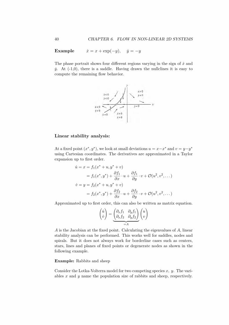
Recipe for phase space analysis:

1. Identify nullclines: lines with x = 0 or y = 0

2. Identify fixed points: intersections of nullclines

3. Linear stability analysis around fixed points

39

40 CHAPTER 6. FLOW IN NON-LINEAR 2D SYSTEMS

Example x = x + exp(−y), y = −y

The phase portrait shows four different regions varying in the sign of x andy. At (-1,0), there is a saddle. Having drawn the nullclines it is easy tocompute the remaining flow behavior.

Linear stability analysis:

At a fixed point (x∗, y∗), we look at small deviations u = x−x∗ and v = y−y∗using Cartesian coordinates. The derivatives are approximated in a Taylorexpansion up to first order.

u = x = f1(x∗ + u, y∗ + v)

= f1(x∗, y∗) + ∂f1∂x·u+ ∂f1

∂y· v +O(u2, v2, . . . )

v = y = f2(x∗ + u, y∗ + v)

= f2(x∗, y∗) + ∂f2∂x·u+ ∂f2

∂y· v +O(u2, v2, . . . )

Approximated up to first order, this can also be written as matrix equation.(uv

)=(∂xf1 ∂yf1∂xf2 ∂yf2

)︸︷︷︸

=A

(uv

)

A is the Jacobian at the fixed point. Calculating the eigenvalues of A, linearstability analysis can be performed. This works well for saddles, nodes andspirals. But it does not always work for borderline cases such as centers,stars, lines and planes of fixed points or degenerate nodes as shown in thefollowing example.

Example: Rabbits and sheep

Consider the Lotka-Volterra model for two competing species x, y. The vari-ables x and y name the population size of rabbits and sheep, respectively.

41

The rabbit population exhibits a faster logistic growth than the sheep pop-ulation. As the sheep compete for grass with the rabbits, the growth rate ofthe rabbits x decreases if more sheep exist while the sheep suffer only littleunder more rabbits.

x = x(3− x− 2y)y = y(2− y − x)

The Jacobian computes as A =(

3− 2x− 2y −2x−y 2− 2y − x

). The character

of the four fixed points is different.

fixed point (0, 0) (0, 2) (3, 0) (1, 1)

A

(3 00 2

) (−1 0−2 −2

) (−3 −60 −1

) (−1 −2−1 −1

)

τ 5 -3 -4 -2

∆ 6 2 4 -1

λ1 3 -1 -2√

2− 1

λ2 2 -2 -2 −(√

2− 1)

classification unstable node stable node stable node saddle


Example: Pathological example

x = −y + ax(x2 + y2)y = x+ ay(x2 + y2)

Obviously, (x∗, y∗) = (0, 0) is a fixed point. In order to calculate the Jaco-bian, only the linear terms have to be considered.

A =(

0 −11 0

)⇒ τ = 0; ∆ = 1; λ1/2 = ±i

In linear approximation, the fixed point is a center.

But this is not true for the non-linear case. To analyze this in more detail,we switch to polar coordinates x = r · cos θ, y = r · sin θ and derive theequation of motion for r

r2 = x2 + y2

r · r = x · x+ y · y = x(−y + axr2) + y(x+ ayr2) = a · r4

⇒ r = a · r3

and θ:

θ = arctan(y

x

)⇒ θ = 1

1 +( yx

)2 · xy − xyx2 = · · · = 1.

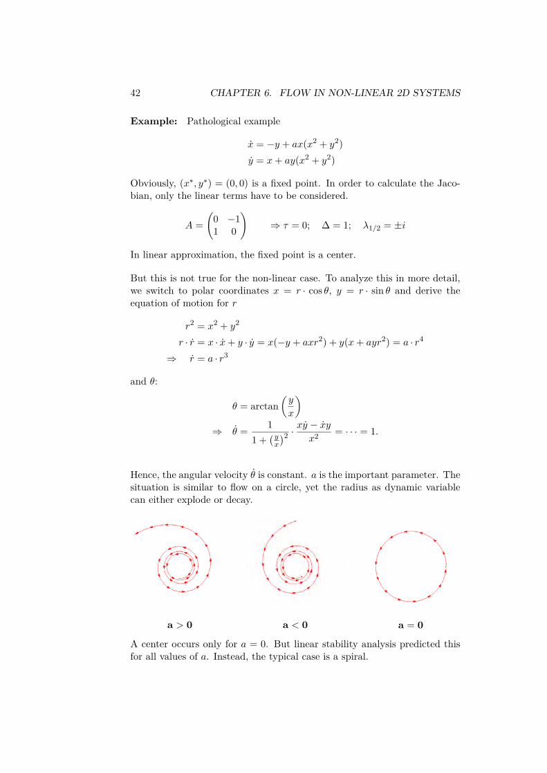
Hence, the angular velocity θ is constant. a is the important parameter. Thesituation is similar to flow on a circle, yet the radius as dynamic variablecan either explode or decay.

a > 0 a < 0 a = 0

A center occurs only for a = 0. But linear stability analysis predicted thisfor all values of a. Instead, the typical case is a spiral.

43

We next have a brief look at two different types of special situations: conser-vative (e.g. earth orbiting around the sun) and reversible systems (systemswith time-reversal). These cases are sufficiently restrictive such that generalrules follow that make calculations easier.

1. Conservative systemsIn a conservative system, the acting force F can be derived for a po-tential V . For example, in 1d we have:

m · x = F (x) = −dVdx .

Multiplying with the velocity x leads to

m

2ddt(x

2) = −dVdt

⇒ ddt(

12mx

2 + V︸︷︷︸=E

) = 0.

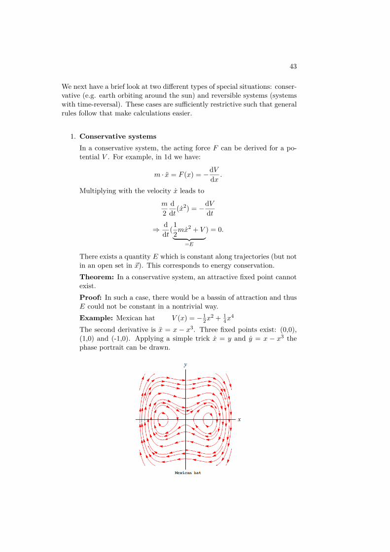
There exists a quantity E which is constant along trajectories (but notin an open set in ~x). This corresponds to energy conservation.Theorem: In a conservative system, an attractive fixed point cannotexist.Proof: In such a case, there would be a bassin of attraction and thusE could not be constant in a nontrivial way.Example: Mexican hat V (x) = −1

2x2 + 1

4x4

The second derivative is x = x − x3. Three fixed points exist: (0,0),(1,0) and (-1,0). Applying a simple trick x = y and y = x − x3 thephase portrait can be drawn.


Example: Hamiltonian system H(q, p)

It is q = ∂H∂p and p = −∂H

∂q . From this, energy conservation simplyfollows:

H = ∂pH · p+ ∂qH · q = 0.

We know from the theorem that there are no attractive fixed pointsin the system. Instead, a typical fixed point is a center and thus oftenoscillations occur in the system.

2. Reversible systems

Time reversal symmetry is more general than energy conservation.Reversible, non-conservative systems occur e.g. fluid flow, laser, su-perconductors, etc.

Mechanical systems without damping are invariant under t → −t.Consider in 1d, m · x = F (x), thus the force is time-independent. Thisis time-independent because of the second derivative. We introducethe velocity

v = x ⇒ v = 1mF (x).

Both (x(t), v(t)) and(x(−t),−v(−t)) are solutionsof the system in this framework.In general, there is a twin for eachtrajectory Note the similarity tocenters, which have trajectoriesthat have merged at the ends.

Examples:

(a) x = y − y3 y = −x− y2

The system is invariant under t→−t and y → −y. There are threefixed points: two saddles and acenter.There is mirror symmetry aroundthe x-axis in regard to the flowlines (but not the flow vectors).

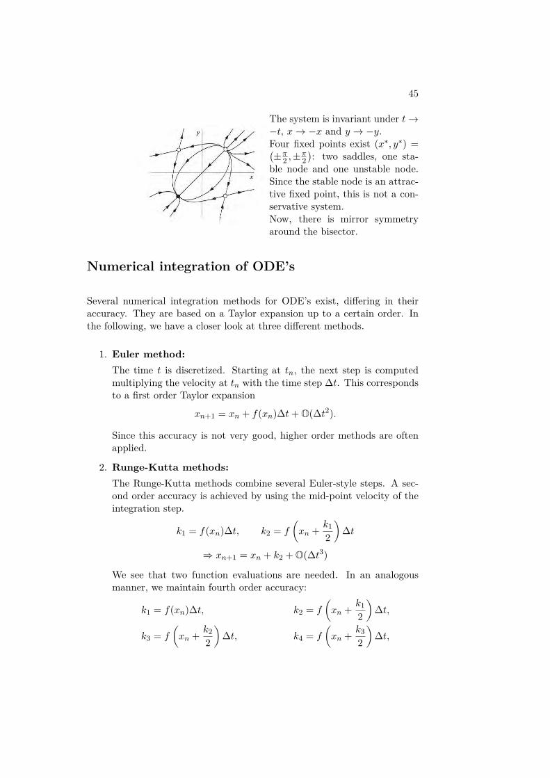
(b) x = −2 cos(x)− cos(y) y = −2 cos(y)− cos(x)

45

The system is invariant under t→−t, x→ −x and y → −y.Four fixed points exist (x∗, y∗) =(±π

2 ,±π2): two saddles, one sta-

ble node and one unstable node.Since the stable node is an attrac-tive fixed point, this is not a con-servative system.Now, there is mirror symmetryaround the bisector.

Numerical integration of ODE’s

Several numerical integration methods for ODE’s exist, differing in theiraccuracy. They are based on a Taylor expansion up to a certain order. Inthe following, we have a closer look at three different methods.

1. Euler method:The time t is discretized. Starting at tn, the next step is computedmultiplying the velocity at tn with the time step ∆t. This correspondsto a first order Taylor expansion

xn+1 = xn + f(xn)∆t+ O(∆t2).

Since this accuracy is not very good, higher order methods are oftenapplied.

2. Runge-Kutta methods:The Runge-Kutta methods combine several Euler-style steps. A sec-ond order accuracy is achieved by using the mid-point velocity of theintegration step.

k1 = f(xn)∆t, k2 = f

(xn + k1

2

)∆t

⇒ xn+1 = xn + k2 + O(∆t3)

We see that two function evaluations are needed. In an analogousmanner, we maintain fourth order accuracy:

k1 = f(xn)∆t, k2 = f

(xn + k1

2

)∆t,

k3 = f

(xn + k2

2

)∆t, k4 = f

(xn + k3

2

)∆t,


⇒ xn+1 = xn + 16 (k1 + 2k2 + 2k3 + k4) + O(∆t5)

Obviously, this requires four function evaluations. It is the a very goodchoice if the number of evaluations is not essential. To realize this, onestandard choice is Matlab ODE 45 (see also on the web page).

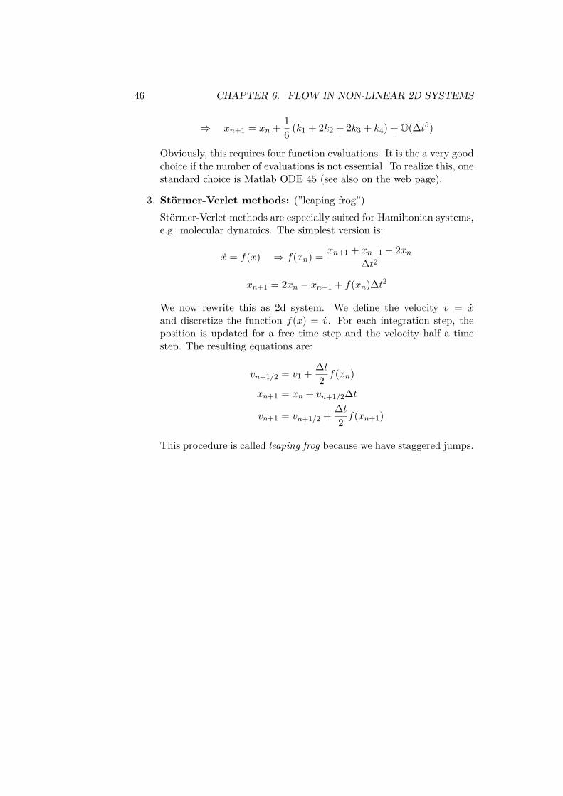
3. Stormer-Verlet methods: (”leaping frog”)Stormer-Verlet methods are especially suited for Hamiltonian systems,e.g. molecular dynamics. The simplest version is:

x = f(x) ⇒ f(xn) = xn+1 + xn−1 − 2xn∆t2

xn+1 = 2xn − xn−1 + f(xn)∆t2

We now rewrite this as 2d system. We define the velocity v = xand discretize the function f(x) = v. For each integration step, theposition is updated for a free time step and the velocity half a timestep. The resulting equations are:

vn+1/2 = v1 + ∆t2 f(xn)

xn+1 = xn + vn+1/2∆t

vn+1 = vn+1/2 + ∆t2 f(xn+1)

This procedure is called leaping frog because we have staggered jumps.

Chapter 7

Oscillations in 2d

In contrast to linear systems, non-linear ones allow for limit cycles. Theseare isolated closed trajectories in the phase plane. They cannot exist inlinear systems because with x(t) also cx(t) is a trajectory, thus closed orbitscannot exist in isolation.

Poincare-Bendixson theorem:If R is a closed, bounded subset of the plane without any fixed point, andif there is a trajectory that is confined in R, then R contains a closed orbit.

The second condition is satisfied if a trapping region R exists. To prove thata stable limit cycle exists, we have to show that a trapping region existswithout a fixed point inside. The Poincare-Bendixson theorem also impliesthat there is no chaos in two dimensions; in three dimensions and higher,the Poincare-Bendixson theorem does not apply and the trajectory couldwander around in a constrained space without settling into a closed orbit.

Examples:

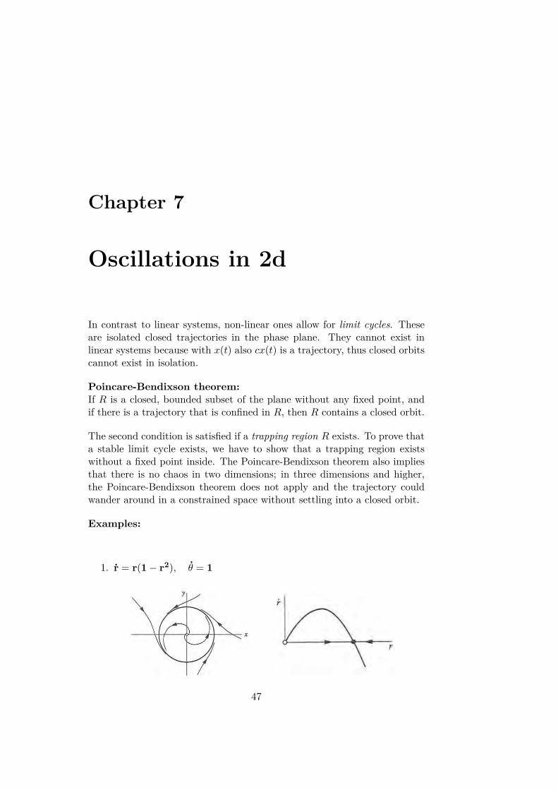
1. r = r(1− r2), θ = 1

47

48 CHAPTER 7. OSCILLATIONS IN 2D

In Cartesian coordinates:

x = (1− x2 − y2)x− yy = (1− x2 − y2)y − x.

2. r = r(1− r2) + µr cos(θ), θ = 1In this more complicated example, for which values of µ ≥ 0 does astable limit cycle exist?The trapping region can be determined for the given example by con-structing minimum and maximum radius rmin, rmax and demandingan increasing and decreasing flow, respectively.

rmin : r ≥ r(1− r2)− µr > 0 ⇒ rmin <√

1− µrmax : r ≤ r(1− r2) + µr < 0 ⇒ rmax >

√1 + µ

Since√

1 + µ is always real for µ ≥ 0, the only restriction for thetrapping region comes from rmin: 0 ≤ µ < 1. Due to the Poincare-Bendixson theorem, we have a stable limit cycle for these values ofµ.

3. Biological example:Biochemical oscillations are very common in biology, but the first oneswere directly observed rather late, namely the periodic conversion ofsugar to alcohol in yeast in 1964. This is a specific example for a classof oscillators called the substrate-depletion oscillator. In 1968, Selkovsuggested a simple 2d mathematical model for it.Because it is so central to evolution, sugar metabolism is extremlyefficient:

C6H12O6︸︷︷︸glycose

+ 6 O2 −→ 6 CO2 + 6 H2O + ∆E

The produced energy is stored in up to 36 ATP molecules. The abilityto oscillate comes from the fact that ADP/ATP enters the details ofthis pathway in several ways:

glycose ATP→ADP−→ glycose 6-P −→ fructose 6-P︸︷︷︸=F6P

ATP→ADP−→PFK

fructose 1,6-P︸︷︷︸=FBP

Therefore the first steps of the glycolysis pathway use up ATP ratherthan producing it. On the other hand, the enzyme PFK is activatedby ADP, thus switching on the ATP-generating pathway on demand.We call this autocatalysis or a positive feedback loop. Overall, moreATP is produced than used up by this pathway.

49

In order to model these conflicting trends that eventually lead to os-cillations, we introduce the following grouping:

y =

ATPF6P

and x =

ADPFBP

Introducing the reaction rates a, b, we get:

glucose b−−→ y

⊕xa−−→ x−→ products.

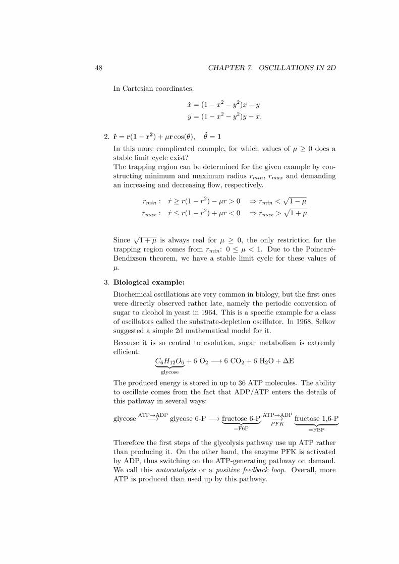
x is produced with a constant rate a from y and it reacts to prod-ucts with a normalized rate. The production rate of x increases inproporation to its amount. We analyze the following equations:

x = −x+ ay + x2y

y = b− ay − x2y.

The nullclines are y = xa+x2 and

y = ba+x2 . So, there is a fixed

point (x∗, y∗) = (b, ba+b2 ).

In order to show that a trapping region exists, we consider the regionbounded by the green lines. We know for the left part x = 0 and0 ≤ y ≤ b

a . So we get 0 ≤ x ≤ b and 0 ≤ y ≤ b. The flow goes inside.For the right part we calculate x − (−y) = x + y = b − x < 0 sincex > b. This yields −y > x. Therefore, the flow is more negative than−1 and goes inside.We have thus found a trapping region. The Poincare-Bendixson theo-rem demands that no fixed points exist. Hence, we make a hole aroundthe fixed point and show that no trajectory goes into the hole. This isequivialent to a repulsive (unstable) fixed point. The Jacobian is

A =(−1 + 2xy a+ x2

−2xy −(a+ x2)

).


We need a positive trace τ and determinant ∆ of the matrix A.

∆ = a+ b2 > 0

τ = b4 + (2a− 1)b2 + (a+ a2)a+ b2

!= 0

Thus, the boundary between stable and unstable fixed points τ = 0is given by b2 = 1

2(1 − 2a) ±√

1− 8a. This can be represented via astate-diagram.

The arrow indicates an increasingb. If a is small enough, the systemperforms oscillations in a certaininterval of b. We call this a re-entrance process.

Lienard systems / van der Pol oscillator

The following structure often occurs in mechanics and electronics:

x︸︷︷︸inertia

+ f(x) · x︸︷︷︸damping

+ g(x)︸︷︷︸restoring force

= 0.

It is called Lienard-system. Note, that this is the equation of the harmonicoscillator for f = 0 and g = x.

We consider the most famous example of Lienard systems, the van der Poloscillator :

f = µ(x2 − 1)g = x.

For x 1 we have negative damping. The system can be driven by puttingenergy into the system. For large x, the damping is positive. Energy isdissipated.

Example: Tetrode circuit (electronics)

51

The system is described as follows:

LI + V + F (I) = 0⇒ LI + V + F ′(I)I = 0⇒ LC · I + I + CF ′(I) · I = 0.

This is a van der Pol oscillator with f(I) = CF ′(I) and g = 1.

Lienard systems are very widespread: e.g.

1. neural activity, action potential

2. biological oscillators (ear, circadian rhythms)

3. stick-slip oscillations in sliding friction

Lienard theorem:A Lienard system has a stable limit cycle around the origin at the phaseplane if

1. g(−x) = −g(x), g(x) > 0 for x > 0

2. f(−x) = f(x), F (x) =∫ x

0f(x′)dx′ has to have a zero at a > 0

and F (x) < 0 for 0 < x < a, F (x) > 0 for x > a, F (∞) =∞.

Obviously, the first condition is fullfilled for the van der Pol oscillator. Con-sider the second condition:

F (x) = µ

(x3

3 − x)

= µx

3(x2 − 3

)⇒ a =

√3.

As for the harmonic oscillator the deflection behaves sine-shaped, the de-flection of the van der Pol oscillator follows a sawtooth. The phase portraitshows a deformed circle.

Now, we analyze the van der Pol oscillator in two limits: µ 1 and µ 1.

1. µ 1: Lienard phase plane analysis


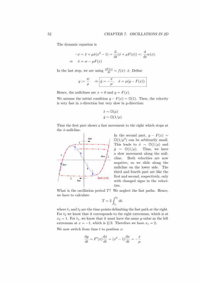
The dynamic equation is

−x = x+ µx(x2 − 1) = ddt(x+ µF (x)) =: d

dtw(x).

⇒ x = w − µF (x)

In the last step, we are using dF (x)dt = f(x) · x. Define

y := w

µ⇒ y = −x

µ, x = µ(y − F (x)).

Hence, the nullclines are x = 0 and y = F (x).We assume the initial condition y − F (x) ∼ O(1). Then, the velocityis very fast in x-direction but very slow in y-direction:

x ∼ O(µ)y ∼ O(1/µ)

Thus the first part shows a fast movement to the right which stops atthe x-nullcline.

In the second part, y − F (x) ∼O(1/µ2) can be arbitrarily small.This leads to x ∼ O(1/µ) andy ∼ O(1/µ). Thus, we havea slow movement along the null-cline. Both velocities are nownegative, so we slide along thenullcline on the lower side. Thethird and fourth part are like thefirst and second, respectively, onlywith changed signs in the veloci-ties.

What is the oscillation period T? We neglect the fast paths. Hence,we have to calculate

T = 2∫ t2

t1dt.

where t1 and t2 are the time points delimiting the fast path at the right.For t2 we know that it corresponds to the right extremum, which is atx2 = 1. For t1, we know that it must have the same y-value as the leftextremum at x = −1, which is 2/3. Therefore we have x1 = 2.We now switch from time t to position x:

dydt = F ′(x)dx

dt = (x2 − 1)dxdt = −x

µ

53

and from this

dt = dx−µ(x2 − 1)x

.

Therefore, the oscillation period is T ∼ O(µ):

⇒ T = 2∫ x2=1

x1=2dx−µ(x2 − 1)

x= 2µ

[x2

2 − ln(x)]2

1= µ(3− 2 ln(2))

⇒ T ∼ O(µ).

2. µ 1:

This case is a small perturbation to the harmonic oscillator

x+ x+ ε ·h(x, x) = 0.

The systems dynamics depend on h(x, x).

(a) For h = (x2 − 1)x, the system is a van der Pol oscillator.

(b) For h = 2x, we have a weakly damped harmonic oscillator. Thesystem is linear.

(c) For h = x3, the system corresponds to an unharmonic spring witha spring constant k = 1 + εx2 that increases by extending thespring. This is called strain stiffening. The system is a Duffingoscillator.

We first consider the second case h = 2x, because this linear casecan be solved exactly. This can be done by rewriting the equation ofmotion in two dimensions with x and v. The corresponding matrix

A =(

0 1−1 −2ε

)has the following eigenvalues and eigenvectors:

λ1,2 = −ε± ic, ~v1,2 = (−ε∓ ic, 1) (7.0.1)

where c = (1− ε2)1/2. Thus the general solution is

~x(t) = (a1 ~v1 exp(λ1t) + a2 ~v2 exp(λ2t))

For the initial condition ~x(0) = (0, 1) we find a1,2 = 1/2 ± (εi)/(2c).Putting all this together, we get the analytical solution

x(t) = 1c

exp(−εt) sin(ct).


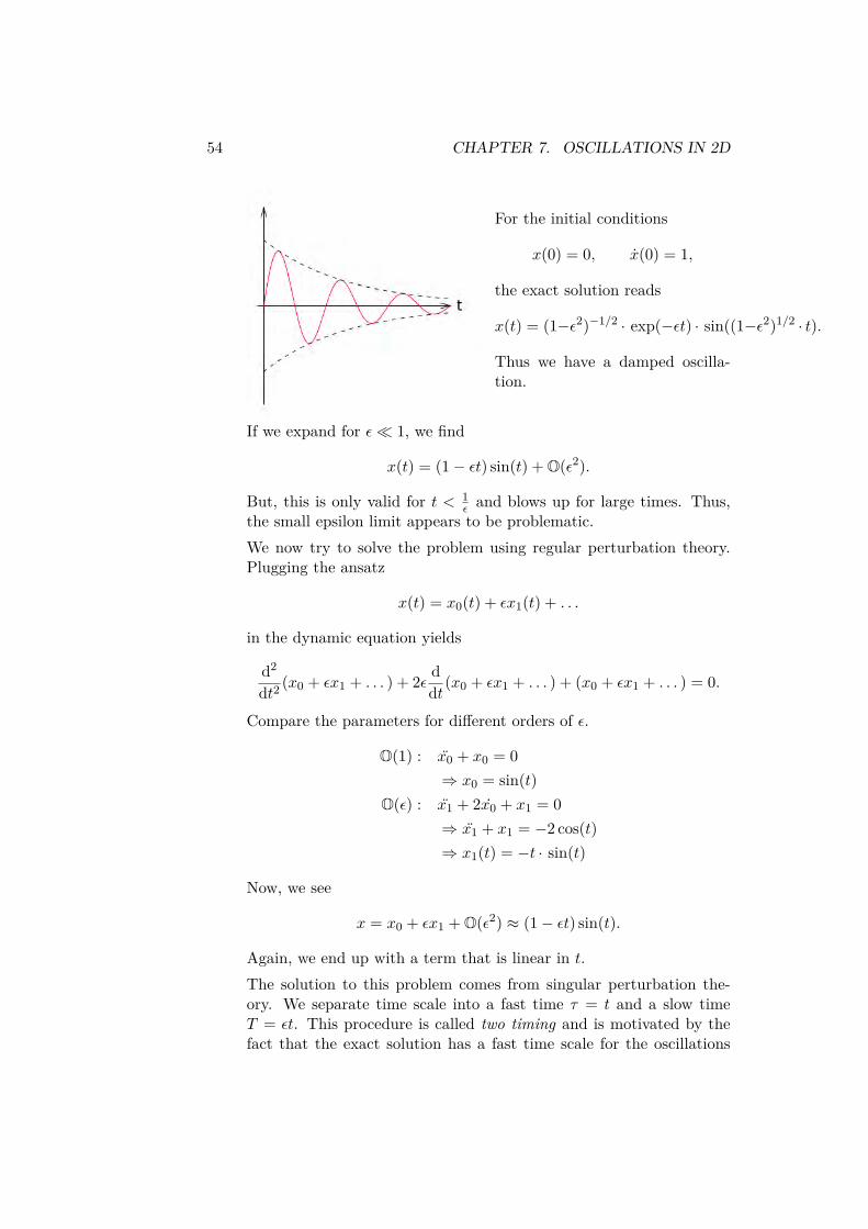
For the initial conditions

x(0) = 0, x(0) = 1,

the exact solution reads

x(t) = (1−ε2)−1/2 · exp(−εt) · sin((1−ε2)1/2 · t).

Thus we have a damped oscilla-tion.

If we expand for ε 1, we find

x(t) = (1− εt) sin(t) + O(ε2).

But, this is only valid for t < 1ε and blows up for large times. Thus,

the small epsilon limit appears to be problematic.We now try to solve the problem using regular perturbation theory.Plugging the ansatz

x(t) = x0(t) + εx1(t) + . . .

in the dynamic equation yields

d2

dt2 (x0 + εx1 + . . . ) + 2ε ddt(x0 + εx1 + . . . ) + (x0 + εx1 + . . . ) = 0.

Compare the parameters for different orders of ε.

O(1) : x0 + x0 = 0⇒ x0 = sin(t)

O(ε) : x1 + 2x0 + x1 = 0⇒ x1 + x1 = −2 cos(t)⇒ x1(t) = −t · sin(t)

Now, we see

x = x0 + εx1 + O(ε2) ≈ (1− εt) sin(t).

Again, we end up with a term that is linear in t.The solution to this problem comes from singular perturbation the-ory. We separate time scale into a fast time τ = t and a slow timeT = εt. This procedure is called two timing and is motivated by thefact that the exact solution has a fast time scale for the oscillations

55

and a slow one for the damping. Similar approaches are in generalhelpful for multiscale problems, such as e.g. the boundary layer inhydrodynamics.We use the new ansatz:

x(t) = x0(τ, T ) + εx1(τ, T ) + O(ε2)

and therefore calculate the derivatives

x = ∂τ x∂t τ + ∂Tx∂t T

= ∂τ x+ ∂T x · ε= ∂τ x0 + ε(∂τ x1 + ∂T x0) + O(ε2)

x = ∂ττ x0 + ε(∂ττ x1 + 2∂Tτ x0) + O(ε2)

and plug them into the dynamic equation

⇒ 0 = ∂ττ x0 + ε(∂ττ x1 + 2∂Tτ x0) + 2ε∂τ x0 + (x0 + εx1) + O(ε2).

O(1) : ∂ττ x0 + x0 = 0O(ε) : ∂ττ x1 + x1 = −2(∂Tτ x0 + ∂τ x0)O(1) : ⇒ x0 = A(T ) sin(τ) +B(T ) cos(τ)O(ε) : ⇒ ∂ττ x1 + x1 = −2 · (A′(T ) +A(T )) cos(τ) + 2 · (B′(T ) +B(T )) sin(τ)

In order to end up with a well-behaved solution, demand the prefactors(A′ +A) and (B′ +B) to be zero.

⇒ A = A0 · exp(−T ), B = B0 · exp(−T )

For the initial conditions x(0) = 0, x(0) = 1 ⇒ B0 = 0, A0 = 1,the general solution is sine-shaped with an envelope decaying in time

⇒ x0 = exp(−T ) · sin(τ) = exp(−εt) · sin(t).

This is identical to the exact solution in order O(ε2). To do better, wehad to introduce a super-slow time scale of order O(ε2), but at leastthe blow-up is avoided and we get the correct damping.

Application to van der Pol oscillator

The dynamic equation

x+ ε(x2 − 1)x+ x = 0


holds

[∂ττ x0 + ε(∂ττ x1 + 2∂Tτ x0)] + ε(x20 − 1)∂τ x0 + (x0 + εx1) = 0.

O(1) : ∂ττ x0 + x0 = 0O(ε) : ∂ττ x1 + x1 = −2∂Tτ x0 − (x2

0 − 1)∂τ x0

In polar coordinates:

x0 = r(T ) · cos(τ + Φ(T ))⇒ ∂ττ x1 + x1 = 2[r′ sin(τ + Φ) + rΦ′ cos(τ + Φ)] + r sin(τ + Φ)[r2 cos2(τ + Φ)− 1]

− [2r′ − r + 14r

3] sin(τ + Φ) + 2rΦ′ cos(τ + Φ) + 14r

3 sin(3(τ + Φ)).

In the last step, we used the relation sin(θ) · cos2(θ) = 14 [sin(θ)+sin(3θ)]. In

order to avoid a resonance catastrophe, demand the prefactors [2r′−r+ 14r

3]and 2rΦ′ to be zero.

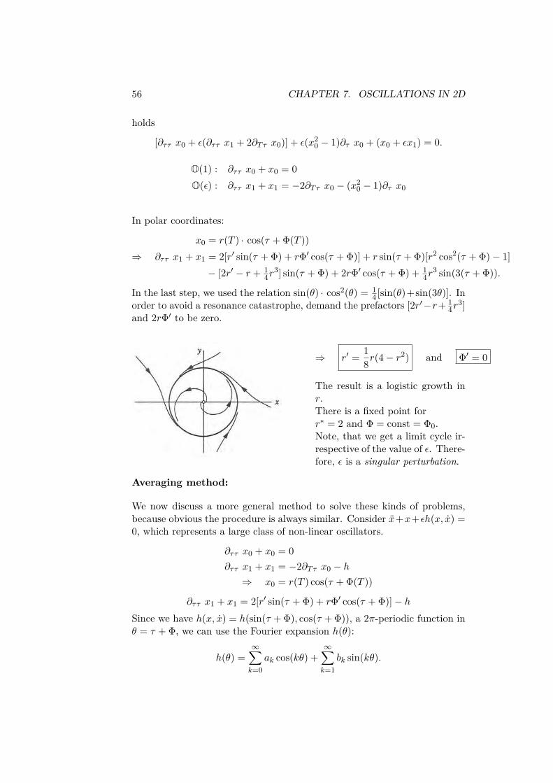
⇒ r′ = 18r(4− r

2) and Φ′ = 0

The result is a logistic growth inr.There is a fixed point forr∗ = 2 and Φ = const = Φ0.Note, that we get a limit cycle ir-respective of the value of ε. There-fore, ε is a singular perturbation.

Averaging method:

We now discuss a more general method to solve these kinds of problems,because obvious the procedure is always similar. Consider x+x+εh(x, x) =0, which represents a large class of non-linear oscillators.

∂ττ x0 + x0 = 0∂ττ x1 + x1 = −2∂Tτ x0 − h⇒ x0 = r(T ) cos(τ + Φ(T ))

∂ττ x1 + x1 = 2[r′ sin(τ + Φ) + rΦ′ cos(τ + Φ)]− hSince we have h(x, x) = h(sin(τ + Φ), cos(τ + Φ)), a 2π-periodic function inθ = τ + Φ, we can use the Fourier expansion h(θ):

h(θ) =∞∑k=0

ak cos(kθ) +∞∑k=1

bk sin(kθ).

57

Up to O(ε), the only resonant terms for x1 are (2r′ − b1) sin(θ) and (2rΦ′ −a1) cos(θ). From this, we get the conditions

⇒ r′ = b12 , rΦ′ = a1

2

to avoid the resonance catastrophe. We write the Fourier coefficients interms of averages of θ:

a1 = 1π

∫ 2π

0dθ h(θ) cos(θ)

= 2 〈h cos(θ)〉θb1 = 2 〈h sin(θ)〉θ

⇒ r′ = 〈h sin(θ)〉θrΦ′ = 〈h cos(θ)〉θ .

dynamical equations for (r,Φ)

Example: van der Pol oscillator

Consider h = (x2 − 1)x = (r2 cos2(θ)− 1)(−r sin(θ)).

r′ = 〈h sin(θ)〉θ= −r3

⟨cos2(θ) sin2(θ)

⟩θ

+ r⟨

sin2(θ)⟩

= 12r −

18r

3

= 18r(4− r

2) ⇒ r∗ = 2

rΦ′ = 〈h cos(θ)〉θ= −r〈sin(θ) cos(θ)〉θ︸︷︷︸

=0

− r3⟨

cos3(θ) sin(θ)⟩θ︸︷︷︸

=0

= 0 ⇒ Φ = const

This is the same result as before, as it should be.

Chapter 8

Bifurcations in 2d

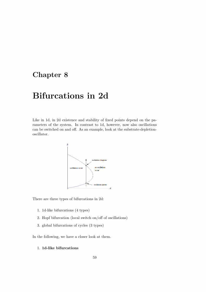
Like in 1d, in 2d existence and stability of fixed points depend on the pa-rameters of the system. In contrast to 1d, however, now also oscillationscan be switched on and off. As an example, look at the substrate-depletion-oscillator.

There are three types of bifurcations in 2d:

1. 1d-like bifurcations (4 types)

2. Hopf bifurcation (local switch on/off of oscillations)

3. global bifurcations of cycles (3 types)

In the following, we have a closer look at them.

1. 1d-like bifurcations

59


All four types of 1d bifurcations exist in 2d (cf. center manifold theo-rem).Example: Griffith model for genetic switchConsider a gene that codes for a certain protein. The activity of thegene shall be induced by the protein and its copies which are translatedfrom the messenger RNA. The system is described as

x = y − ax

y = x2

1 + x2 − by,

where, x and y are the concentrations of the protein and the mRNA,respectively.The following figure shows a protein acting as transcription factor.

The nullclines are y = a ·x and y = x2

b(1+x2) . We see that the systemdepends on the parameters a, b. For increasing a, the two upper fixedpoints approach each other until they fall together when the nullclinesintersect tangentially. For even larger a, only the fixed point in theorigin remains.

The two upper fixed points are given by

x∗ = ab(1 + x∗2)

⇒ x∗ = 1±√

1− 4a2b2

2ab .

For 2ab = 1, the fixed points collide. The critical values are

ac = 12b x∗c = 1.

61

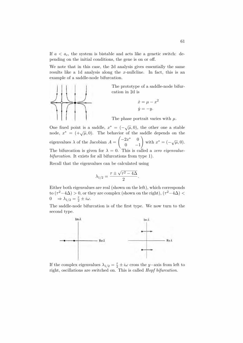
If a < ac, the system is bistable and acts like a genetic switch: de-pending on the initial conditions, the gene is on or off.We note that in this case, the 2d analysis gives essentially the sameresults like a 1d analysis along the x-nullcline. In fact, this is anexample of a saddle-node bifurcation.

The prototype of a saddle-node bifur-cation in 2d is

x = µ− x2

y = −y.

The phase portrait varies with µ.

One fixed point is a saddle, x∗ = (−√µ, 0), the other one a stablenode, x∗ = (+√µ, 0). The behavior of the saddle depends on the

eigenvalues λ of the Jacobian A =(−2x∗ 0

0 −1

)with x∗ = (−√µ, 0).

The bifurcation is given for λ = 0. This is called a zero eigenvalue-bifurcation. It exists for all bifurcations from type 1).Recall that the eigenvalues can be calculated using

λ1/2 = τ ±√τ2 − 4∆2 .

Either both eigenvalues are real (shown on the left), which correspondsto (τ2−4∆) > 0, or they are complex (shown on the right), (τ2−4∆) <0 ⇒ λ1/2 = τ

2 ± iω.The saddle-node bifurcation is of the first type. We now turn to thesecond type.

If the complex eigenvalues λ1/2 = τ2 ± iω cross the y−axis from left to

right, oscillations are switched on. This is called Hopf bifurcation.


2. Hopf bifurcation

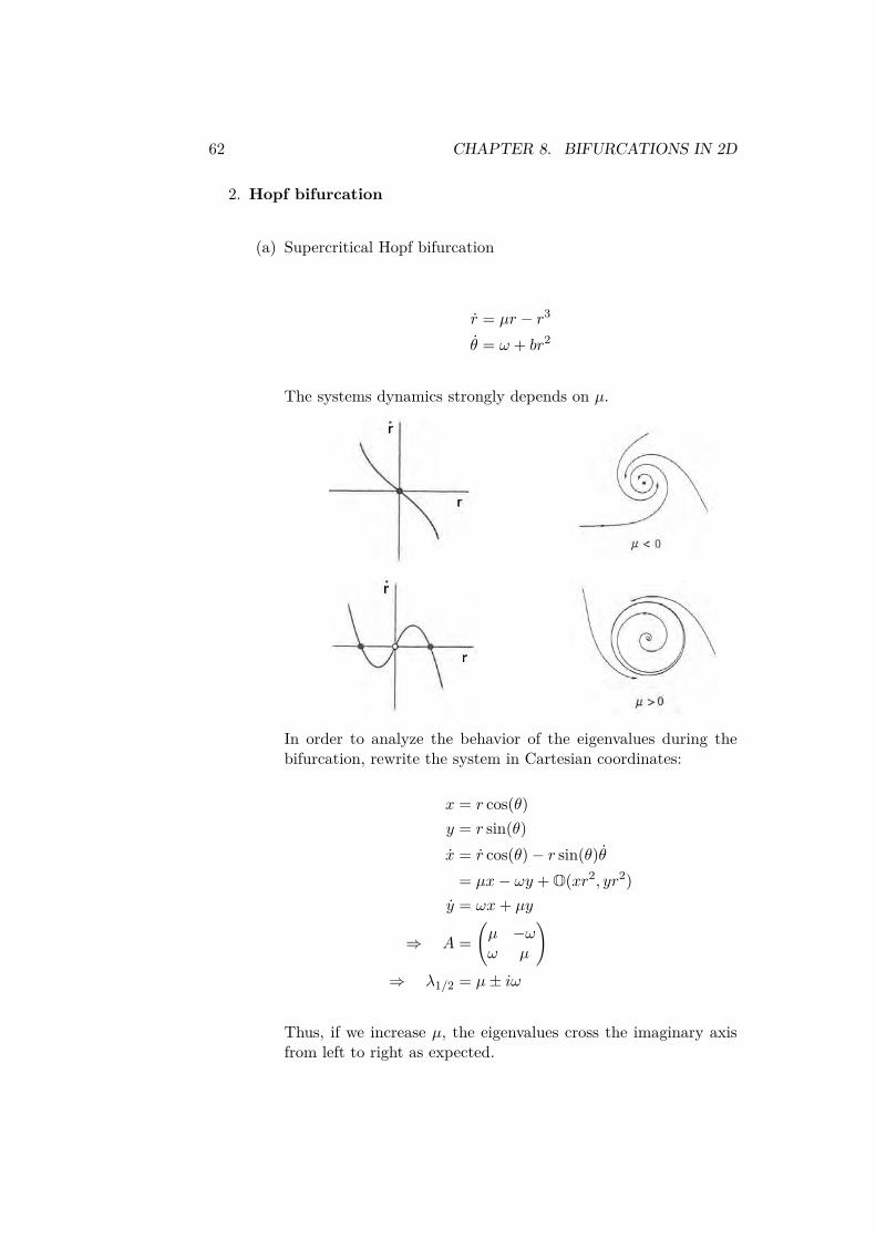
(a) Supercritical Hopf bifurcation

r = µr − r3

θ = ω + br2

The systems dynamics strongly depends on µ.

In order to analyze the behavior of the eigenvalues during thebifurcation, rewrite the system in Cartesian coordinates:

x = r cos(θ)y = r sin(θ)x = r cos(θ)− r sin(θ)θ

= µx− ωy + O(xr2, yr2)y = ωx+ µy

⇒ A =(µ −ωω µ

)⇒ λ1/2 = µ± iω

Thus, if we increase µ, the eigenvalues cross the imaginary axisfrom left to right as expected.

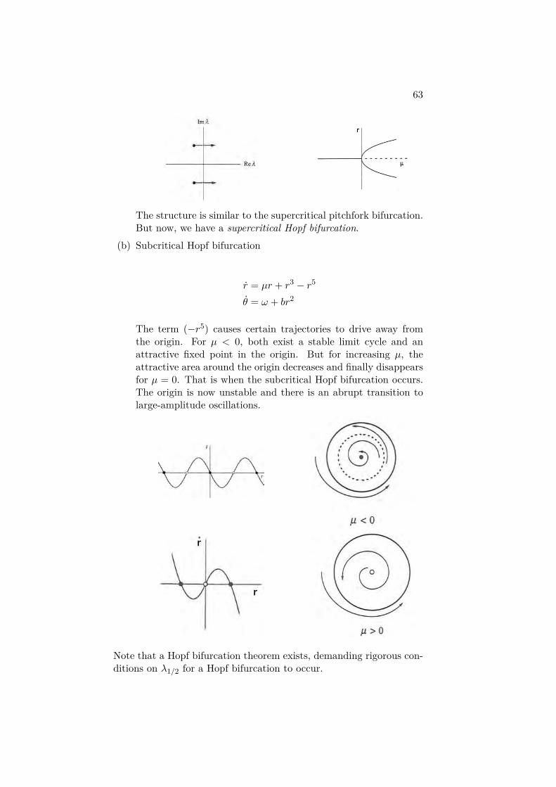
63

The structure is similar to the supercritical pitchfork bifurcation.But now, we have a supercritical Hopf bifurcation.

(b) Subcritical Hopf bifurcation

r = µr + r3 − r5

θ = ω + br2

The term (−r5) causes certain trajectories to drive away fromthe origin. For µ < 0, both exist a stable limit cycle and anattractive fixed point in the origin. But for increasing µ, theattractive area around the origin decreases and finally disappearsfor µ = 0. That is when the subcritical Hopf bifurcation occurs.The origin is now unstable and there is an abrupt transition tolarge-amplitude oscillations.

Note that a Hopf bifurcation theorem exists, demanding rigorous con-ditions on λ1/2 for a Hopf bifurcation to occur.


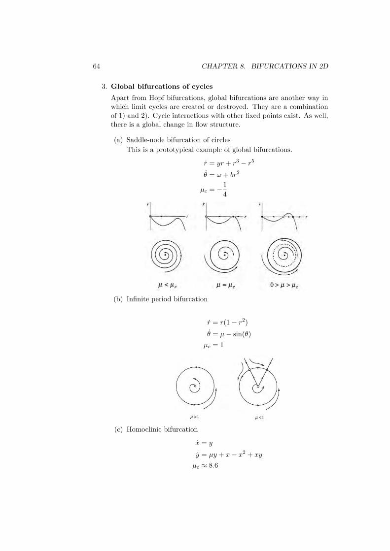
3. Global bifurcations of cyclesApart from Hopf bifurcations, global bifurcations are another way inwhich limit cycles are created or destroyed. They are a combinationof 1) and 2). Cycle interactions with other fixed points exist. As well,there is a global change in flow structure.

(a) Saddle-node bifurcation of circlesThis is a prototypical example of global bifurcations.

r = yr + r3 − r5

θ = ω + br2

µc = −14

(b) Infinite period bifurcation

r = r(1− r2)θ = µ− sin(θ)µc = 1

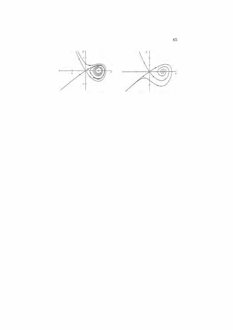
(c) Homoclinic bifurcation

x = y

y = µy + x− x2 + xy

µc ≈ 8.6

Chapter 9

Excitable systems

In this chapter, we discuss so-called ”excitable systems”. One example isgrass, that is burned down and then regrows. Obviously, this process canbe repeated over and over again. We also see that such a process can occurin the spatial domain as a wave. Our biological example is neuronal activityin the brain. Here, the wave is called an ”action potential” and it travelsalong the axon of a neuron.

A human neuron has a diameter ofr ≈ 50 µm for the cell body andan axon that is up to 1 m long.The axon transports the signalscalled action potentials or spikes.We think about them as travelingwaves V (x, t).

It is approximately cylindricallyshaped containing mainly potas-sium (K+) and organic anions(A−) and being surrounded pre-dominantly by sodium (Na+), cal-cium (Ca2+) and chlorine (Cl−).

Typical values of the concentrations of the two dominant ions potassiumand sodium are given in the following table:

67

68 CHAPTER 9. EXCITABLE SYSTEMS

inside outside ∆V[mM] [mM] [mV]

K+ 155 4 -98

Na+ 12 154 67

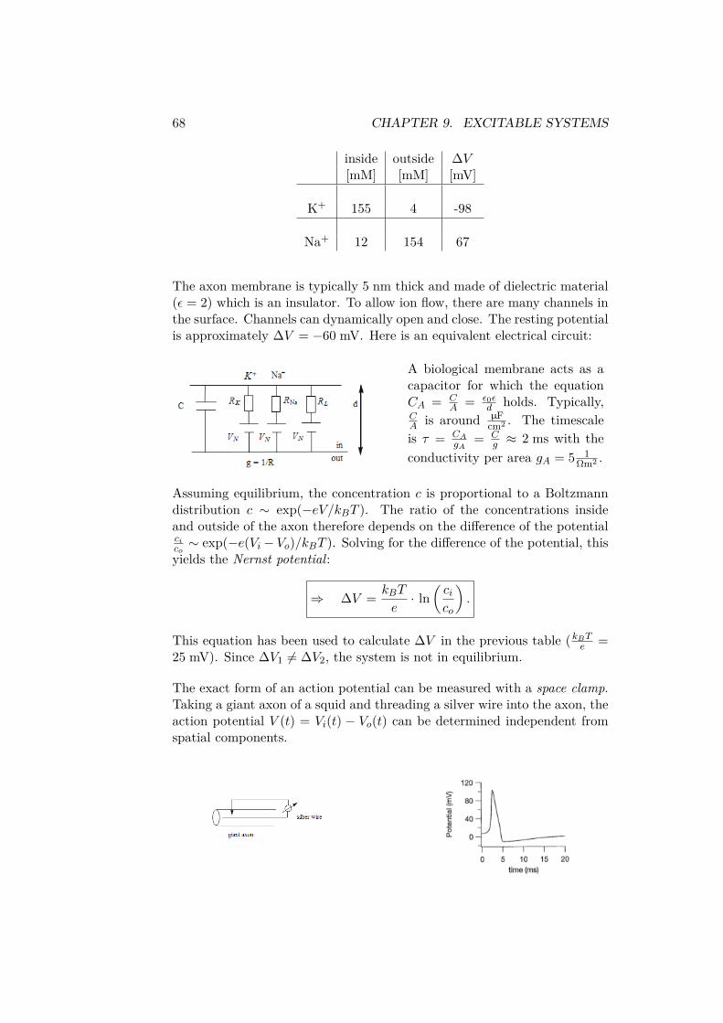
The axon membrane is typically 5 nm thick and made of dielectric material(ε = 2) which is an insulator. To allow ion flow, there are many channels inthe surface. Channels can dynamically open and close. The resting potentialis approximately ∆V = −60 mV. Here is an equivalent electrical circuit:

A biological membrane acts as acapacitor for which the equationCA = C

A = ε0εd holds. Typically,

CA is around µF

cm2 . The timescaleis τ = CA

gA= C

g ≈ 2 ms with theconductivity per area gA = 5 1

Ωm2 .

Assuming equilibrium, the concentration c is proportional to a Boltzmanndistribution c ∼ exp(−eV/kBT ). The ratio of the concentrations insideand outside of the axon therefore depends on the difference of the potentialcico∼ exp(−e(Vi− Vo)/kBT ). Solving for the difference of the potential, this

yields the Nernst potential:

⇒ ∆V = kBT

e· ln

(cico

).

This equation has been used to calculate ∆V in the previous table (kBTe =

25 mV). Since ∆V1 6= ∆V2, the system is not in equilibrium.

The exact form of an action potential can be measured with a space clamp.Taking a giant axon of a squid and threading a silver wire into the axon, theaction potential V (t) = Vi(t) − Vo(t) can be determined independent fromspatial components.

69

1938 Hodgkin worked at Woods Hole (with Cole). Cole later invented thespace clamp.

1949 Hodgkin performed experiments with the space clamp at Plymouthtogether with his student Huxley.

1952 Famous Hodgkin and Huxley papers (some together with Katz): thedynamics of so-called gates produce temporal changes in conductivity

1960 Richard FitzHugh and later Nagumo et al. independently analyzed areduced HH-model with phase plane analysis, leading to the standardNLD-model for action potentials

1963 Nobel prize for Hodgkin and Huxley (together with John Eccles, whoworked on motorneuron synapses)

1991 Nobel prize for Erwin Neher and Bert Sakmann for the patch clamptechnique: the molecular basis of an action potential could bedemonstrated directly for the first time

2003 Nobel prize for Roderick MacKinnon for his work (Science 1998) onthe structure of the K+ channel, which in particular explained whyNa+ ions cannot pass

May2012 Andrew Huxley dies at the age of 94; after his work on the action

potential, he revolutionized muscle research (the sliding filamenthypothesis from 1954 and the Huxley model for contraction from 1957could have earned him a second Nobel prize)

Table 9.1: Overview historical development.


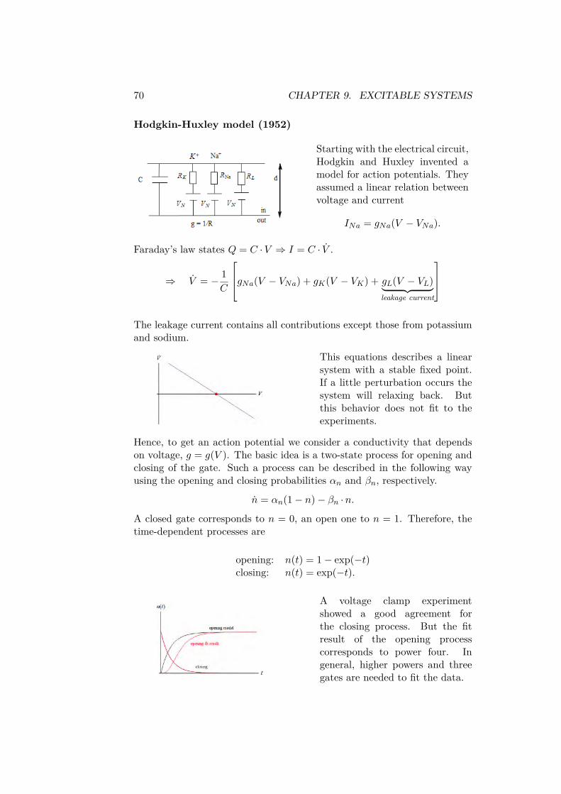
Hodgkin-Huxley model (1952)

Starting with the electrical circuit,Hodgkin and Huxley invented amodel for action potentials. Theyassumed a linear relation betweenvoltage and current

INa = gNa(V − VNa).

Faraday’s law states Q = C ·V ⇒ I = C · V .

⇒ V = − 1C

gNa(V − VNa) + gK(V − VK) + gL(V − VL)︸︷︷︸leakage current

The leakage current contains all contributions except those from potassiumand sodium.

This equations describes a linearsystem with a stable fixed point.If a little perturbation occurs thesystem will relaxing back. Butthis behavior does not fit to theexperiments.

Hence, to get an action potential we consider a conductivity that dependson voltage, g = g(V ). The basic idea is a two-state process for opening andclosing of the gate. Such a process can be described in the following wayusing the opening and closing probabilities αn and βn, respectively.

n = αn(1− n)− βn ·n.

A closed gate corresponds to n = 0, an open one to n = 1. Therefore, thetime-dependent processes are

opening: n(t) = 1− exp(−t)closing: n(t) = exp(−t).

A voltage clamp experimentshowed a good agreement forthe closing process. But the fitresult of the opening processcorresponds to power four. Ingeneral, higher powers and threegates are needed to fit the data.

71

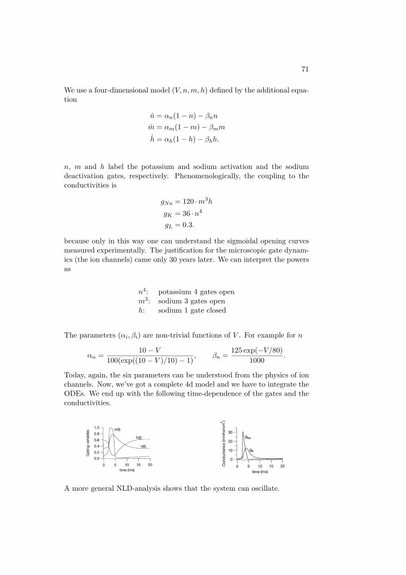
We use a four-dimensional model (V, n,m, h) defined by the additional equa-tion

n = αn(1− n)− βnnm = αm(1−m)− βmmh = αh(1− h)− βhh.

n, m and h label the potassium and sodium activation and the sodiumdeactivation gates, respectively. Phenomenologically, the coupling to theconductivities is

gNa = 120 ·m3h

gK = 36 ·n4

gL = 0.3.

because only in this way one can understand the sigmoidal opening curvesmeasured experimentally. The justification for the microscopic gate dynam-ics (the ion channels) came only 30 years later. We can interpret the powersas

n4: potassium 4 gates openm3: sodium 3 gates openh: sodium 1 gate closed

The parameters (αi, βi) are non-trivial functions of V . For example for n

αn = 10− V100(exp((10− V )/10)− 1) , βn = 125 exp(−V/80)

1000 .

Today, again, the six parameters can be understood from the physics of ionchannels. Now, we’ve got a complete 4d model and we have to integrate theODEs. We end up with the following time-dependence of the gates and theconductivities.

A more general NLD-analysis shows that the system can oscillate.


Fitzhugh-Nagumo model

For an in-depth analysis of the Hodgkin-Huxley model, Fitzhugh in the1960s used 2D phase plane obtained as cuts through 4D phase space. Hefirst used the two fast variables V and m and kept n and h constant. Thetwo equations then read

eV = −gKn40(V − VK)− ¯gNam3h0(V − VNa)− gL(V − VL)

m = α(V )m (1−m)− β(V )

m ·m

with the parameters g denoting constants. The phase plane dependency ofm and V is shown in the figure below.

This analysis explains the threshold between a resting and an excited state,but not the relaxation, because this comes later. Then the V -nullcline movesup and the excited state vanishes in a saddle-node bifurcation.

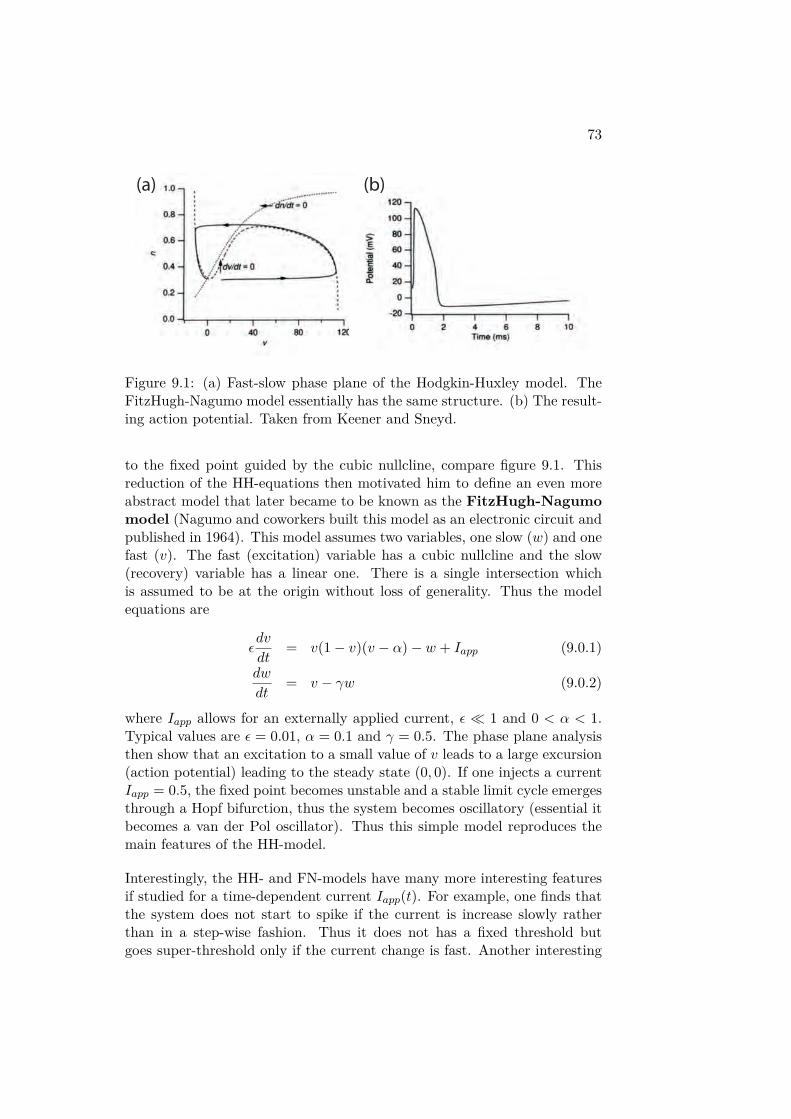
As a next step, Fitzhugh considered one fast variable v responsible for theexcitation and a slow variable n responsible for the relaxation. He foundthat the v-nullcline has a cubic shape, that there is one fixed point andthat the action potential is emerging as a long excursion away and back

73

(a) (b)

Figure 9.1: (a) Fast-slow phase plane of the Hodgkin-Huxley model. TheFitzHugh-Nagumo model essentially has the same structure. (b) The result-ing action potential. Taken from Keener and Sneyd.

to the fixed point guided by the cubic nullcline, compare figure 9.1. Thisreduction of the HH-equations then motivated him to define an even moreabstract model that later became to be known as the FitzHugh-Nagumomodel (Nagumo and coworkers built this model as an electronic circuit andpublished in 1964). This model assumes two variables, one slow (w) and onefast (v). The fast (excitation) variable has a cubic nullcline and the slow(recovery) variable has a linear one. There is a single intersection whichis assumed to be at the origin without loss of generality. Thus the modelequations are

εdv

dt= v(1− v)(v − α)− w + Iapp (9.0.1)

dw

dt= v − γw (9.0.2)

where Iapp allows for an externally applied current, ε 1 and 0 < α < 1.Typical values are ε = 0.01, α = 0.1 and γ = 0.5. The phase plane analysisthen show that an excitation to a small value of v leads to a large excursion(action potential) leading to the steady state (0, 0). If one injects a currentIapp = 0.5, the fixed point becomes unstable and a stable limit cycle emergesthrough a Hopf bifurction, thus the system becomes oscillatory (essential itbecomes a van der Pol oscillator). Thus this simple model reproduces themain features of the HH-model.

Interestingly, the HH- and FN-models have many more interesting featuresif studied for a time-dependent current Iapp(t). For example, one finds thatthe system does not start to spike if the current is increase slowly ratherthan in a step-wise fashion. Thus it does not has a fixed threshold butgoes super-threshold only if the current change is fast. Another interesting


observation is that an inhibitory step (negative step function) triggers aspike at the end rather than at the start of the stimulation period. Thusthe direction in which the current is changed matters.

Cable equation

Up to now, we did not consider the effects of space. We now couple manyHH-elements in series to describe wave propagation along the axon.

Describing the signal as traveling wave, Ohm’s law holds in lateral direction

V (x+ ∆x)− V (x) = −I(x) ρ

πr2dx

where ρ = 0.3 Ωm is the resistivity of the medium and r = 250µm is theradius of the squid giant axon. Looking at a node of the circuit, currentconservation demands

I(x+ ∆x)− I(x) = −gA(2πr)V (x)dx

Taking ∆x→ 0, this yields

V ′(x) = − ρ

πr2 I(x)

I ′(x) = −gA · 2πr ·V (x)

⇒ V ′′(x) = 1λ2V

In the last step, the decay length λ =√

r2ρgA

= 9 mm has been introduced.

Injecting a voltage V0 at left and asking for a decaying voltage at the right,the space dependence is

V (x) = V0 · exp(−xλ

).

75

Because of this, the signal would just decay if the conductivities were inde-pendent from the voltage. This has been found earlier by Lord Kelvin wheninvestigating the decay of a signal along a passive cable like the transatlanticcable.

We next combine the longitudinal equation with the full transverse Hodkin-Huxley current for the current conservation

I ′ = −[gNa(V − V NaN ) + gK(V − V K

N ) + gL(V − V LN )]− C∂U

∂t.

⇒ λ2V ′′ − τ V = gNa(V − V NaN ) + gK(V − V K

N ) + gL(V − V LN )

g.

The result is a non-linear PDE, the ”cable equation” with time-dependentconductivity.

Considering one type of channel (e.g. Na) and injecting a voltage V0 at theleft, a front propagates to the right. To get a wave propagation, one hasto add a counteracting process (e.g. opening of K channels). Hodgkin andHuxley showed the waves in 1952. To understand this better, we considerthe bistable cable equation

V = V ′′ + f(V )

with f(V ) = −V (V −α)(V −1). We look for solutions of the form V (x, t) =U(x+c · t) which describe waves propagating from right to left with velocityc. Defining y := x+ ct, we can convert the system into an ODE.

∂yU · c = ∂2yU + f(U)

Now, we do a phase plane analysis and therefore define

W = ∂yU ⇒ ∂yW = c ·W − f(U), f(U) = −U(U − α)(U − 1).

A traveling front solution must connect the fixed points (U = 0,W = 0) and(U = 1,W = 0) in the (U,W )-plane as we vary y from −∞ to +∞. Thereis a unique c∗ which results in such a trajectory (finding this unique valueis called shooting). It can be calculated analytically. For this, we guess thatthe connection between the two resting states is given by

W (U) = dUdy = −BU(U − 1).


So, we calculate

0 = −∂yU · c+ ∂2yU + f(U)

= −W · c+ ∂yW + f(U)= −W · c+ ∂UW∂yU + f(U)= −cBU(U − 1) +B2(2U − 1) ·U(U − 1)− U(U − α)(U − 1)= cB +B2(2U − 1)− (U − α)

Because this has to vanish for any U , we find

B = 1√2, c = 1√

2(1− 2α).

The speed is a decreasing function of α and the direction of propagationchanges at α = 1

2 . In this case, there is no propagation. The profile of thetraveling front is found by integrating the assumption

W (U) = dUdy = −BU(U − 1).

⇒ U(y) = 12

[1 + tanh

( 12√

2y

)].

A propagating wave is a trajectory which comes back to the original state.This occurs in the Hodgkin-Huxley model as well as in the Fitzhugh-Nagumomodel with diffusive coupling

V = V ′′ + f(V,W )W = g(V,W ).

Until now, we studied 1d wave propagation. The cable equation can also beextended to 2d or 3d. We then obtain propagation fronts (planar or circular),but also spirals. In the context of heart and muscle biology, spirals are asign of a pathophysiological situation.

Chapter 10

Reaction-diffusion systems

We started this lecture with the central equationd~xdt = ~f(~x)

which mathematically is an ODE. We now add space in the form of diffusiond~xdt = ~f(~x) +D∆~x

where D is the diagonal matrix of the diffusion constants (a non-diagonalcoupling could exist in hydrodynamic theories). Mathematically we now dealwith a PDE, similar to the Schrodinger equation, the Maxwell equations orthe Fokker-Planck equation. Naively, one might think that diffusion stabi-lizes the system, but Alan Turing showed in 1952 that there exist diffusion-driven instabilities (in a similar vein, stochastic noise can either stabilizeor destabilize a system). Turing suggested that diffusion-driven instabilitiesmight account for the spontaneous emergence of patterns in morphogenesisof animals (like the stripes of zebra or the spots of the leopard). Althoughit is hard to identify Turing instabilities in development, it is clear that theyare very important in (bio)chemical networks. Here we introduce the mainideas and results of Turing1.

Turing investigated under which condition a reaction-diffusion system pro-duces a heterogeneous spatial pattern. To answer this question, he consid-ered a two-dimensional system of the type:

A = F (A,B) +DA∆AB = G(A,B) +DB∆B.

1For a detailed discussion, consult the book on Mathematical Biology by JD Murray,Springer, 3rd edition 2003.

77

78 CHAPTER 10. REACTION-DIFFUSION SYSTEMS

A simple choice for the reaction part would be the activator-inhibitor modelfrom Gierer and Meinhardt, where species A is autocatalytic and activates B,while B inhibits A. An even simplier choice is the activator-inhibitor modelfrom Schnackenberg, where the autocatalytic species A is the inhibitor of Band B activates A. Both models form stripes in the Turing version and herewe choose the second one because it is mathematically easier to analyse:

F = k1 − k2A+ k3A2B

G = k4 − k3A2B.

We first non-dimensionalize the system:

u = A

(k3k2

)1/2, v = B

(k3k2

)1/2,

t = DAt

L2 , x = x

L, d = DB

DA,

a = k1k2

(k3k2

)1/2, b = k4

k2

(k3k2

)1/2,

γ = L2k2DA

Note that the variables u and v are positive since they are concentrationsof reactants. By introducing the variables above, the system is described asfollows

u = γ(a− u+ u2v)︸︷︷︸=:f(u,v)

+ ∆u

v = γ(b− u2v)︸︷︷︸=:f(u,v)

+ d∆v

with the ratio of the diffusion d and the relative strength of the reactionversus the diffusion terms γ which scales as γ ∼ L2.

We first consider the case without diffusionD = 0 and ask for a homogeneousstate which is stable; we then ask under which conditions diffusion leads toan instability, the Turing instability.

Stabilizing diffusion. 1D reaction-diffusion system

For single reactant u(x, t) there is no Turing instability:

ut = Duxx + f(u), x ∈ [0, l] + BC

79

An ”uniform” (x - independent) ODE

u = f(u)

has either: stable m = f ′(u∗) < 0, or unstable m > 0 equilibrium atstationary point u∗ : f(u∗) = 0.

The diffusion will maintain a stable one, and it can stabilize the unstableone.To check it we take the linearized problem about u∗, for v(x, t) = u(x, t)−u∗ : vt = Dvxx +mv, x ∈ [0, l]

m = f ′(u∗)

We use the Neumann BC (no flux):

∂xv

∣∣∣∣0,l

= 0

and eigenfunction expansion.Separation of variables: look for the solution in the form:

v(x, t) = ϕ(t) ·ψ(x)

Leading to:ϕ′ ·ψ = ϕ · (D ·ψ′′ +m ·ψ)

⇒ ϕ′

ϕ= Dψ′′ +mψ

ψ=: µ

Hence, the solution stability depends on the sign of µ :

ϕ(t) ≈ exp(µt)

The second equation:

Dψ′′ + (m− µ)ψ = 0, ψ(0, l) = 0

orψ′′ + λ2ψ = 0, λ2 = m− µ

D

The eigenfunctions are:

ψk(x) = cosλkx = cos πkxl, k = 0, 1, ...


Using the expression for λ we get:

µ = m−D(πkx

l

)2

So:

• stable case (m < 0) remains stable,

• For unstable case the system get bifurcation values at D(πkxl

)2= m.

The diffusion stabilize the unstable ”uniform” equillibrium.

2d reaction-diffusion system

We now turn to two dimensions, where the Turing instability occurs. Solet’s start with a linear stability analysis of the reaction part using ~W =(u− u∗v − v∗

). We denote the steady state with ~W ∗ =

(u∗

v∗

)and a partial

derivative with fu = ∂f∂u etc. This yields

~W = γA ~W

with the matrixA =

(fu fvgu gv

)| ~W ∗ .

Linear stability is guaranteed if the real part of the eigenvalues λ is smallerthan zero, Re λ < 0. Thus, the trace of A is smaller than zero

tr A = fu + gv < 0 (10.0.1)

and the determinant larger than zero

det A = fugv − fvgu > 0. (10.0.2)

The u- and v- nullcline is given by setting f = 0 and g = 0, respectively.

u-nullcline: v = u− au2

v-nullcline: v = b

u2

For the steady state ~W ∗ =(u∗

v∗

), we demand u∗ and v∗ to be positive for

physical reasons.

⇒ (u∗, v∗) =(a+ b,

b

(a+ b)2

)

81

Thus, it is a+ b > 0 and b > 0.

⇒ A =(−1 + 2uv u2

−2uv −u2

)| ~W ∗ =

(b−ab+a (a+ b)2

−2aba+b −(a+ b)2

)⇒ det A = (a+b)2 > 0

We get a stable spiral for b = 2and a = 0.2.

We now turn to the full reaction-diffusion system and linearize it about thesteady state

~W = γA ~W +D∆ ~W

with D =(

1 00 d

).

In order to obtain an ODE from this PDE, we use the solutions of theHelmholtz wave equation

∆ ~W + k2 ~W = 0

with no-flux boundary of size p in 1d, we have

~Wk(x) ∼ cos(k ·x)

with wavenumber k = nπp and wavelength λ = 2π

k = 2pn (n integer).

⇒ ~W (~r, t) =∑k

ck exp(λt) ~Wk(~r)

⇒ λ ~Wk = γA ~Wk −Dk2 ~Wk

We now have to solve this eigenvalue problem. A Turing instability occursif Re λ(k) > 0. Our side constraint is that the eigenvalue problem for D = 0(only reactions) is assumed to be stable, that is Re λ(k = 0) < 0.

⇒ 0 = λ2 + λ[k2(1 + d)− γtr A] + [dk4 − γ(dfu + gv)k2 + γ2det A].

We first note that the coefficient of λ is always positive because k2(1+d) > 0and tr A < 0 (for reasons of the stability of the reaction system). In order


to get an instability, Re λ > 0, the constant part has to be negative. Sincethe first and last terms are positive, this implies

dfu + gv > 0 ⇒ d 6= 1. (10.0.3)

This is the main result by Turing: An instability can occur if one componentdiffuses faster than the other. (10.0.3) is only a necessary, but not a sufficientcondition. We require that the constant term as a function of k2 has anegative minimum.

(dfu + gv)2

4d > det A = fugv − fvgu (10.0.4)

The critical wavenumber can be calculated to be

kc = γ

(det Adc

)1/2

with the critical diffusion constant from

d2cf

2u + 2(2fvgu − fugv)dc + g2

v = 0.

For d > dc, we have a band of instable wavenumbers. The relation λ =λ(k2) is called the dispersion relation. The maximum singles out the fastestgrowing mode. This one dominates the solution

~W (~r, t) =∑k

ck exp(λ(k2)t)

for large t. Note however, that in this case also non-linear effects will becomeimportant and thus will determine the final pattern.

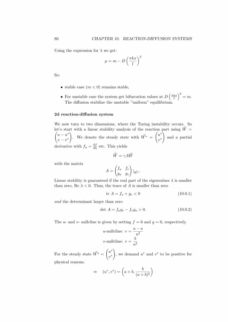
In summary, we have found four conditions (10.0.1) - (10.0.4) for the Turinginstability to occur. We now analyze the Schnackenberg-model in one spatialdimension. We already noted that a+ b > 0 and b > 0 for the steady stateto make sense. From the phase plane we see that f > 0 for large u andf < 0 for small u. Hence, fu > 0 around the steady state. Thus, b > a.

All in all, there are four relations:fu, fv > 0 and gu, gv < 0.

⇒ A ∼(

+ +− −

)

From condition (10.0.1) and (10.0.3), we now calculate that d > 1 in this case(the activation B diffuses faster in this model). In general, the conditions(10.0.1)-(10.0.4) define a domain in (a, b, d)−space, the Turing space, in

83

which the instabilities occurs. The structure of the matrix A tells us howthis will happen: as u or v increases, u increases and v decreases. So, thetwo species will grow out of phase. If there is a fluctuation to a larger A-concentration, it would grow due to the autocatalytic feature. Locally thiswould inhibit B and it decreases strongly. However, because B is diffusingfast, it now is depleted from the environment and there A is not activatedanymore. Therefore A goes down in the environment, whereas B is high.This is the basic mechanism for stripe formation.

In the Gierer-Meinhardt model, the two species grow in phase. When theautocatalytic species A grows, so does B, because A is the activator in thismodel. Now B diffuses out and suppressed A in the environment. This isan alternative mechanism for stripe formation.

The domain size p has to be large enough for a wavenumber k = nπp to be

within the range of the unstable wavenumbers (γ ∼ L2):

γL(a, b, d) <(nπ

p

)2< γM(a, b, d)

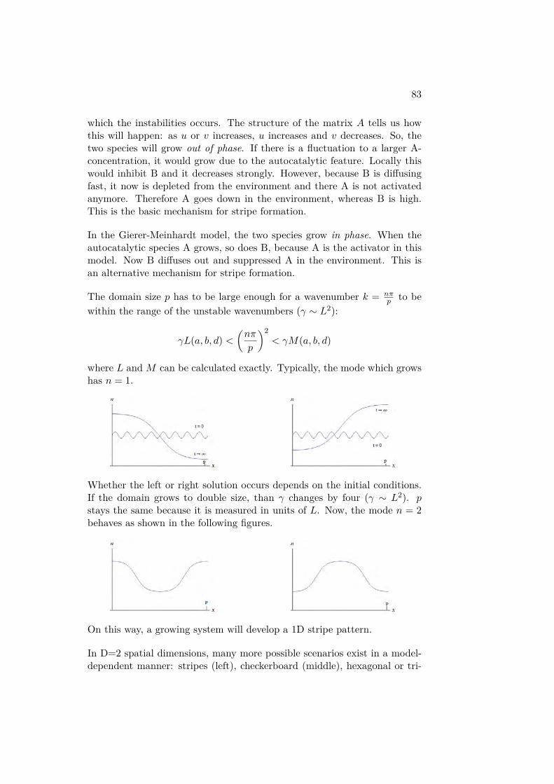
where L and M can be calculated exactly. Typically, the mode which growshas n = 1.

Whether the left or right solution occurs depends on the initial conditions.If the domain grows to double size, than γ changes by four (γ ∼ L2). pstays the same because it is measured in units of L. Now, the mode n = 2behaves as shown in the following figures.

On this way, a growing system will develop a 1D stripe pattern.

In D=2 spatial dimensions, many more possible scenarios exist in a model-dependent manner: stripes (left), checkerboard (middle), hexagonal or tri-


angular (right) patterns, etc.

Today, the corresponding models are usually explored numerically, thusmaking it easy to also analyse the effects of the non-linear parts.

Non-linear Dynamics - uni- · PDF fileNon-linear Dynamics Prof. Dr. Ulrich Schwarz Heidelberg...

Documents

Transcript of Non-linear Dynamics - uni- · PDF fileNon-linear Dynamics Prof. Dr. Ulrich Schwarz Heidelberg...