Non-linear Analysis of Cello Pitch and Timbre

by

Andrew Choon-ki Hong

S.B. Computer Science and Engineering

Massachusetts Institute of Technology

1989

Submitted to the

Media Arts and Sciences Section,

School of Architecture and Planning

in partial fulfillment of the requirements of the Degree of

Master of Science

at the

Massachusetts Institute of Technology

September 1992

@ Massachusetts Institute of Technology, 1992

All rights reserved

Signature of Author Media Arts and Sciences Ctio25 Augus 2

Certified by ( Tod Machover, M.M.A ociate Prof sor of Music and Media

Accepted byMASSACHUSETS INSTITUTE

OF TECHNOLOGY

NOV 23 1992UBRARIES

Stephen A. Benton, Ph.D.Chairperson

Departmental Committee on Graduate Students

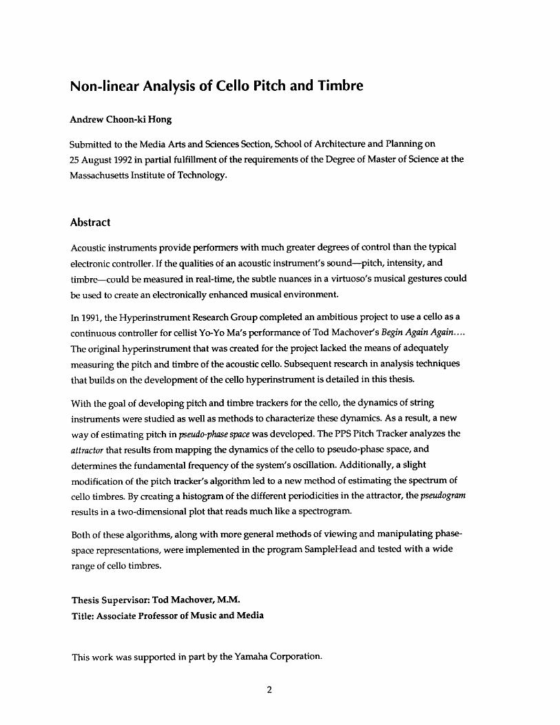
Non-linear Analysis of Cello Pitch and Timbre

Andrew Choon-ki Hong

Submitted to the Media Arts and Sciences Section, School of Architecture and Planning on

25 August 1992 in partial fulfillment of the requirements of the Degree of Master of Science at the

Massachusetts Institute of Technology.

Abstract

Acoustic instruments provide performers with much greater degrees of control than the typical

electronic controller. If the qualities of an acoustic instrument's sound-pitch, intensity, and

timbre-could be measured in real-time, the subtle nuances in a virtuoso's musical gestures could

be used to create an electronically enhanced musical environment.

In 1991, the Hyperinstrument Research Group completed an ambitious project to use a cello as a

continuous controller for cellist Yo-Yo Ma's performance of Tod Machover's Begin Again Again....

The original hyperinstrument that was created for the project lacked the means of adequately

measuring the pitch and timbre of the acoustic cello. Subsequent research in analysis techniques

that builds on the development of the cello hyperinstrument is detailed in this thesis.

With the goal of developing pitch and timbre trackers for the cello, the dynamics of string

instruments were studied as well as methods to characterize these dynamics. As a result, a new

way of estimating pitch in pseudo-phase space was developed. The PPS Pitch Tracker analyzes the

attractor that results from mapping the dynamics of the cello to pseudo-phase space, and

determines the fundamental frequency of the system's oscillation. Additionally, a slight

modification of the pitch tracker's algorithm led to a new method of estimating the spectrum of

cello timbres. By creating a histogram of the different periodicities in the attractor, the pseudogram

results in a two-dimensional plot that reads much like a spectrogram.

Both of these algorithms, along with more general methods of viewing and manipulating phase-

space representations, were implemented in the program SampleHead and tested with a wide

range of cello timbres.

Thesis Supervisor: Tod Machover, M.M.

Title: Associate Professor of Music and Media

This work was supported in part by the Yamaha Corporation.

Readers

- i

Certified by Neil A. Gershenfeld, Ph.D.Assistant Professor of Media Arts and Sciences

Program in Physics and Media, MIT Media Laboratory

Certified by Joseph A. Paradiso, Ph.D.Research Scientist

Charles Stark Draper Laboratory, Cambridge, MA

Acknowledgments

to...

My Family-Mom, Dad, Unnee, Trez, Gregor, John-for always being there.

Gary Leskowitz, for giving me the original ideas. Good luck at CalTech Gare!

Joe Steel Talons Chung, for flying wingman.

Fumi-Man Matsumoto, for imbibin' more Cambridge Amber with me than all my other friends

combined.

Alex Rigopulos, for offering to kick a certain someone's ass.

Casimir CasHead Wierznski, for doing a certain someone-else's accent so well.

Lester Longley @ Zola Technologies, for putting together the coolest set of DSP tools for the

Macintosh-DSP Designer-and for providing the fastest technical support and bug fixes in the

business.

to my pal...

Molly Bancroft, who's the best you-know-what'er in the world.

to my way cool readers...

Neil Gershenfeld, for not only flowing me lots-o'-cool ideas about non-linear dynamics, but also

for buying me an Ultraman doll in Tokyo.

Joe Paradiso, for keeping me psyched, for being so laid back, and for taking me down to the

bat cave.

and most of all, to my advisor (spiritual and otherwise)...

Tod Machover, for having infinite patience, for trusting in me even when I didn't, for not being

stingy with his political capital, and for showing us the world.

Thank you.

Contents

1 Introduction.................................................................................................... 7

1.1 H yperinstrum ents ............................................................................................................... 7

1.2 Loudness and Pitch ............................................................................................................. 8

1.3 T im bre ................................................................................................................................... 10

1.4 Towards a Non-linear Approach..................................................................................... 11

2 Existing Methods ........................................................................................... 142.1 Pitch Estim ation ................................................................................................................... 14

2.2 Timbre Estimation ............................................................................................................. 15

3 Dynamics of Bowed String Instruments ......................................................... 203.1 The String Bow Interface ................................................................................................... 20

3.2 T he B rid ge ............................................................................................................................. 23

3.3 Effects of the Instrument Body ......................................................................................... 24

4 Specifying Pitch and Timbre Space ................................................................ 26

5 BAA's Hypercello DSP Subsystem................................................................. 285.1 First Attempts at Pitch Tracking..................................................................................... 28

5.2 The DSP Subsystem........................................................................................................... 30

5.3 The Time Domain Pitch Tracker..................................................................................... 30

5.4 The Energy Tracker .......................................................................................................... 34

5.5 The Bow Direction Tracker............................................................................................... 35

5.6 Concurrent Processing ...................................................................................................... 36

6 Representing Dynamics in Phase-Space ......................................................... 386.1 Configuration, Phase, and Pseudo-Phase Space ........................................................... 38

6.2 Limit Sets, Attractors, and Poincar6 Sections ................................................................ 40

6.3 Experiments with Pseudo-Phase Space.......................................................................... 40

7 Pseudo-Phase Space Analysis of the Cello..................................................... 42

7.1 Pseudo-Phase Space and Cello Dynamics ..................................................................... 42

7.2 Estimating Pitch in Pseudo-Phase Space........................................................................ 43

7.3 Estimating Spectral Content with Pseudograms ........................................................... 49

7.4 Symmetrized Dot Patterns for Fun and Profit.............................................................. 52

8 Conclusions and Further Research ................................................................ 548.1 Goals and Accomplishments ........................................................................................... 54

8.2 PPS Pitch Tracker ................................................................................................................ 55

8.3 Pseudogram Representation .............................................................................................. 56

8.4 Making it Real-time ........................................................................................................... 57

8.5 Further Research ................................................................................................................ 58

9 Appendix...................................................................................................... 60

9.1 SampleHead Implementation Details............................................................................. 60

10 References .................................................................................................... 62

1 Introduction

1.1 Hyperinstruments

Since its onset in 1986, the Hyperinstrument Research Group (part of the Music & Cognition

Group at the MIT Media Laboratory) has been developing real-time music systems that give

performers the ability to control many levels of expressivity. These systems communicate with

each other and with synthesizers which use MIDI [34], the music-industry standard interface.

Most of these systems have thus used traditional MIDI controllers (like keyboards, guitars, and

percussion pads) or non-musical controllers (like the Exos DHM glove) to effect the progression

of musical sound and structure [27]. A major goal of current hyperinstrument research focuses on

the integration of traditional acoustic instruments into such a real-time electronically enhanced

musical environment [29]. Besides the practical advantages of providing a platform for existing

instruments to act as controllers, this approach is important because it offers the advantage of

exploiting the sonic richness and gestural complexity that these instruments afford.

The typical MIDI controller provides the performer with control over the abstract notions of pitch

(note number), loudness (velocity), and pressure (aftertouch), with a global method of varying

pitch (pitch wheel) in smaller than semitone steps. Control is limited to the amount and quality of

a keyboard-based instrument. On the other hand, an acoustic instrument can respond to the

subtlest expressive variations in performance-these variations are reflected in the vast array of

sounds that acoustic instruments can make.

In order to use acoustic instruments as controllers, there must be a means of extracting the

musical information in an instrument's sound and communicating that information to devices

that can manipulate this sound or add their own sounds to the performance. This extraction

requires a system to track the characteristics that we hear in a sound-intensity and loudness;

frequency and pitch; and in a less quantitative measure, timbre-dynamically updating the

measurements of these characteristics as the sound evolves over time. The tracking of these

qualities could allow synthesis or manipulation of sounds with the fine gestural variation that an

acoustic instrument offers-in synch with the acoustic instrument controller-and could provide

the fine gestural cues to effect higher level changes and progressions in the performance.

However, it is just these qualities of a sound-especially that of pitch and timbre-which have

proven to be extremely difficult to analyze in a meaningful way. Most real-time digital signal

processing techniques are currently too imprecise or result in unmanageably large parameter sets;

hence, they fail to meet the demands of MIDI-based real-time systems. The underlying problem

of any analysis system is reducing the input stream to a small set of orthogonal parameters that

can be readily manipulated and communicated. Furthermore, these parameters must be

perceptually salient, corresponding not only to a low-dimensional set of parameters, but also to

what we hear. This problem of data reduction to a perceptual map must therefore be solved in

order to analyze timbre, one of the most important components of acoustic instruments, and to

dynamically derive and parametrize musical gesture from the audio data stream.

1.2 Loudness and Pitch

Measuring the intensity of a sound is relatively easy. The Sound Pressure Level (SPL), in units of

dB, is an accepted method of describing loudness. There are a number of devices, including the

common VU meter, that can provide an SPL measurement; and there are a number of algorithms

to measure the energy of an electrical signal representing a recorded sound. One implementation

is presented in Section 5.4.

Measuring pitch, on the other hand, is a harder problem. The pitch (sometimes referred to in

classical literature as the low note) is most often defined in terms of the fundamental frequency

(i.e., the first partial) of a composite sound. This definition relates to Helmholtz's idea that the low

pitch of a complex tone is based on the strength of the fundamental component, and that the

higher harmonics are related to timbre [44].

Pitch refers to the psychological while frequency refers to the physical-and the two are not

necessarily interchangeable. Experiments by Scharf (1975) proved that for simple tones, the

relationship between pitch and frequency is not direct. A graph of mels (the unit of pitch) on one

axis and the corresponding frequencies in Hz (logarithmically spaced) is not a straight line but is

curved so that the doubling of frequency does not necessitate an octave change in pitch, as might

be expected [16]. Instead, at ranges below about 1000 Hz, the psychological change is less than

the physical change.

This ratio of pitch and frequency is also affected by loudness. A pitch shift of a pure tone occurs

when its intensity is increased. At alternating levels of 40 dB and 80 dB SPL, a 200 Hz tone

exhibits a one percent drop in its perceived pitch at the higher volume. On the other hand, a

6 kHz tone exhibits a three percent increase of pitch at the higher volume [52]. Complex tones

also exhibit pitch shift.

Furthermore, studies by Terhardt, Schouten, and others have shown that for complex tones, the

harmonic structure can affect the perceived pitch of a fundamental [4]. Terhardt (1971) showed

that the pitch of a complex tone at a given frequency was lower than the pitch of a sinusoidal tone

at the same frequency. Schouten (1938) came up with the periodicity pitch theory to explain the case

of the missing fundamental, in which a complex tone is perceived to have a certain pitch although

the lowest partial is missing in the frequency spectrum.

Pitch strength is an independent measure from the common definition of pitch/frequency. Pure

tones produce the highest pitch strength, while high-pass noise produces the lowest, with

complex tones and band-pass noise in the middle [521. (Broadband noise produces zero pitch

strength.) The existence of this measure tends to suggest that pitch is not just a one-dimensional

scale related to frequency.

1.3 Timbre

Timbre is a characteristic quality of sound that distinguishes tones that are played at the same

pitch and intensity. Everything that is not related to pitch or loudness is part of a sound's timbre.

It is therefore an important quality of sound that can determine the content of musical gesture in

a performance.

Unlike pitch and intensity, timbre is a perceptual attribute that is not well-defined. In the broad

sense of the word, timbre relates to the notion that one can differentiate between different

orchestral instruments. For example, an oboe sounds like an oboe due to its characteristic timbre,

regardless of what notes are being played. Whether it's heard in the context of an orchestra in a

hall or whether its heard playing solo on the radio, the oboe is recognizable by its timbre-

unmistakably different from the timbre of a cello or any other instrument.

In a smaller scope, timbre can refer to perceptual differences of sounds played on the same

instrument. For example, an oboe player can vary his armature and air pressure in order to affect

the "color" of his instrument's sound, even while holding the same note. Similarly, a cellist can

vary speed, location, and pressure of his bowing in order to change the timbre of notes played on

his instrument.

The classical view of timbre is that tonal quality is associated solely with the Fourier spectrum,

the relative magnitudes of the frequency components that make up a sound [451. Until recently,

most studies dealt with the average spectrum, discounting phase relationships between

harmonics and amplitude dynamics of the component frequencies. More current views of timbre

define it as a function of attack and decay transients as well as of the frequency spectrum [45].

Aperiodic complexity and noise are also qualities of timbre [46]. For example, a clarinet note that

is tongued has a noticeably different sound than a clarinet note that is slurred-the first has a

short spurt of reed noise in its attack.

When speaking of timbre as a trait of an instrument that identifies it from others, a quantitative

definition must be approached from a number of views. Handel [16] outlines three different

conceptualizations of timbre:

" Harmonic spectra. Steady tones can be analyzed for frequency content by measuring the

amplitudes of the harmonics. This approach is not feasible when comparing the timbre

of two differently pitched notes of the same instrument. One can say that the two

notes share the same timbre, but their harmonic structure may not be consistent.

" Formant structure. Formants refer to selectively amplified ranges of frequencies due to

one or more similar resonance modes of a sound body (e.g., cello body, vocal tract,

etc.). Formant structure, therefore, can be independent of pitch. But for some

instruments, such as the trumpet and clarinet, the relative strengths of formant regions

can change due to intensity.

" Attack/decay transients. Transitions of harmonics are descriptive of sound. Different

vibration modes of a violin, for example, will result in large differences of

attack/decay times of different harmonics, which also may vary according to pitch

and intensity.

Even when speaking of the range of sounds that a single instrument can make, however, there is

no single approach to defining and quantifying timbre. Later in this thesis, a timbre space will be

defined for cello sounds, providing a means of discussing timbre in the context of different

sounds (at fixed pitches and amplitudes) that can be produced by bowing the strings of a cello.

1.4 Towards a Non-linear Approach

In 1990, the Hyperinstrument Research Group began an ambitious project to use a modified cello

as a continuous controller for a hyperinstrument system developed for cellist Yo-Yo Ma's

performance of Tod Machover's composition Begin Again Again... [261. The goal was to provide

Mr. Ma with real-time gestural control of the hyperinstrument performance [31], and one path to

reaching this goal was to develop a system to analyze the sounds of the specially modified RAAD

electric cello. A reliable and efficient signal-processing subsystem was needed to dynamically

measure intensity, pitch, and timbre of the electrical signal from the cello.

The hypercello DSP subsystem was limited by a number of constraints:

e The subsystem had to work together with the Hyperlisp [81 environment running on a

Macintosh II computer.

" The bandwidth of the MIDI based Hyperlisp system was low enough that real-time

communication was limited to small sets of parameters, especially considering the

number of physical sensing devices also communicating with the central computer.

" The complete cello hyperinstrument needed to be sufficiently self-contained to ship

around the world and be rapidly configured for performance.

Existing methods of pitch and timbre estimation were researched. But none of the popular

methods of pitch estimation involving autocorrelation or Discrete Fourier spectrum analysis met

the above criteria; thus, they were considered infeasible standard methods of timbre estimation

based on Discrete Fourier analysis were likewise deemed unusable.

Instead, the dynamics of the cello were studied to gain a further understanding of how the cello

sound is created. A time-domain based pitch tracker that took advantage of the characteristics of

the cello waveform was implemented as part of the cello hyperinstrument DSP subsystem.

Experimentation with and implementation of a non-real-time pitch and timbre estimation system

based on phase-space mapping of the cello's dynamics followed. This thesis presents the research

that led to the development of the phase-space analysis techniques-and the findings and

implementation details of these techniques.

An algorithm to do pitch tracking using pseudo-phase space to represent the dynamics of the cello

was designed along with a related method of viewing the periodicity spectrum of the cello's

dynamics. The algorithms are discussed in detail, and their advantages over existing methods of

pitch and timbre estimation are outlined. Both these algorithms were implemented as part of

SampleHead, a non-real-time application, but the high feasibility of real-time implementation is

also presented in detail.

2 Existing Methods

2.1 Pitch Estimation

Pitch tracking is typically done in one of three ways: time-domain, autocorrelation, and

frequency-domain.

Time-domain pitch tracking involves detection of similar waveform features and measurement of

the time between matching features. For very simple waveforms, for example, a zero-crossing

detector can count the number of times a signal crosses the zero voltage point over a period of

time, and peak detectors can be used to measure the time between waveform crests.

Any time-domain pitch tracker must have an input signal that is close to strictly periodic. The

waveform shape must repeat regularly with the period. Such a time-domain based pitch tracker

was used in the implementation of the hypercello subsystem. Its major disadvantage was that it

needed a period guess (provided by sensing hardware) in order to limit its search for peaks-

otherwise, the lag time (as it searched for matching peaks) between sampling of the input signal

and measurement of the peak period would have been too high for real-time operation. (See

section 5.3 for more details.)

Autocorrelation involves copying a sample train, successively delaying the copy, and

accumulating the sample-to-sample product of the two sample trains for each delay. In effect, a

section of the input signal is compared with time-delayed versions of itself. In theory, the result

of the autocorrelation is a third sample train with large peaks located at multiples of the original

sample train's period.

Autocorrelation is not suited for real-time pitch tracking because it requires that the original

sample train contain at least several cycles of the lowest expected period, and the resulting

operation requires n x L multiply-accumulates, where n is the number of delay times to try and L

is the length of the sample train.

As the name implies, frequency-domain pitch tracking involves transformation of the input

signal into frequency-domain, usually with a Discrete Fourier Transform. The resulting frequency

components are analyzed. Typically, for a system with discrete harmonics, the lowest common

divisor of the frequencies of all the components (that have a minimum threshold amplitude) is

the candidate for the perceived low-note pitch.

In order to get usable pitch resolution at low frequencies, where semitone differences are only a

few Hz apart, a large transform must be computed. A frequency-domain system was actually

tested for the cello hyperinstrument, but it required more computational power than was

available with the system.

Pitch estimation has become a relatively well-defined problem, but a search for a reliable and

efficient real-time solution continues. Commercial pitch tracking systems exist, including at least

one specifically tuned for the cello. Section 5.1 details the failed attempts to use this system, along

with other available pitch tracking systems, with the cello hyperinstrument.

2.2 Timbre Estimation

Unlike pitch estimation, timbral analysis is not a well-defined problem. Timbre is an elusive

measure that has yet to be quantified in detail, and researchers have been struggling for years to

analyze timbre with computers.

A number of methods for representing timbre have been developed, the most common of which

is based on a technique introduced by Moorer [36] which he calls additive synthesis analysis. Using

a Fast Fourier Transform (FFT), a signal is dynamically represented as the amplitude and

frequency-variance envelopes of the dominant component sinusoids. If this model is given to a

bank of oscillators that follow the amplitude and frequency envelopes, the summed sound would

be a synthesized approximation of the original analyzed sound.

For a musical instrument with a rich timbre, the additive synthesis analysis would result in a data

set of about 25 amplitude and 25 frequency envelopes [48]. Not only would storage and

manipulation of this data require more resources than are available on the typical synthesizer, but

transfer of the envelope values over MIDI would add a significant delay between processing and

resynthesis during a real-time performance. A number of techniques have been used to reduce

the data set of the additive synthesis model to a manageable size.

Charbonneau [71 experimented with three methods of data reduction: the set of amplitude

envelopes was reduced to a single reference envelope of the fundamental frequency along with

parameters that specified the envelopes of the harmonics as scaled versions of the reference

envelope; the same was done for the frequency-variance envelopes; and the start and stop times

of all envelopes were fitted to polynomial curves. Results showed that some data-reduced

synthesized tones had similar timbres to the original tones. On the other hand, experiments have

pointed out that when subjects were asked to identify instruments resynthesized from additive

synthesis models, changes in amplitude envelopes and elimination of amplitude and frequency

variations affected the perceived timbre. The most pronounced timbral changes were evident

when the attack transients were modified [16].

The Fast Fourier Transform of an aperiodic waveform necessarily results in frequency/amplitude

smearing. To perform an FF7, a signal must be split into windows of data. After each window of

data is collected, its Discrete Fourier Transform is computed. A tradeoff between time accuracy

and frequency resolution occurs when choosing the window size. The number of sampled points

that result from the transform is equal to the number of sampled points that are used for the

input. In order to achieve high resolution in the frequency domain, the window size, which

determines the number of samples used in the transform, must be large. As a result, aperiodic

attack transients can be lost if they occur at time scales smaller than the window size [24].

A system developed by Serra and Smith [461 called Spectral Modeling Synthesis (SMS) tries to

address this issue. The analysis of a sound is split into two regimes: a deterministic part and a

stochastic part. The deterministic decomposition is based on the Short Time Fourier Transform of

the additive synthesis model. Frequency guides are computed from the time-varying spectrum,

and amplitude envelopes of the partials are determined for these guides. The resulting

frequency /amplitude signals are added together, and the summed spectrum is subtracted from

the original spectrum of each transform frame. This difference is the stochastic part, which can be

modeled as noise passed through a time-varying filter (an amplitude modulated bandpass filter

or a frequency shaping filter). This stochastic part models aperiodic attack transients, which have

been shown to be an important timbral quality of sound.

Using the SMS method, Feiten and Ungvary [10] developed a sound analysis system for editing

and creating sounds with an additive synthesis model. A sound is recorded and then reduced

using SMS. The envelopes of the reduced sound can be edited graphically.

Laughlin, Truax, and Funt [21] claimed that this analysis process would be difficult to implement

as a system for real-time control with low-bandwidth communication links such as MIDI. Not

only is it often a tedious and trial-by-error technique to approximate harmonic amplitude

envelopes by straight lines, no standardized line-segment envelope representation exists; a full-

resolution envelope could be represented by any number of line-segment envelopes. Thus, two

very different envelope sets could represent the same timbre, making it difficult to compare and

categorize timbres reduced to this model. Instead, Laughlin, Truax, and Funt proposed a solution

in which the envelopes are further decomposed into linear combinations of basis envelopes. As

long as the basis envelopes are chosen as orthogonal vectors, only one combination can be used to

represent a given result.

The wavelet transform takes this concept further by providing a powerful framework in which to

analyze combined timbral and temporal structure and dynamics. Wavelets have begun to be

applied to music analysis/synthesis [20], and are proving to be especially useful for recognizing

transient acoustic events [23].

A different kind of orthogonality is addressed by Wessel [48] in his experiments with timbre

space. Studies at IRCAM, Michigan State University, and CCRMA attempted to characterize

perceptual similarities and differences in sound by placing timbral descriptions in a Euclidean

space. Specifying a timbre would be specifying a point in this space. Wessel created a system that

mapped timbres to a two-dimensional area in which one axis represented "brightness" and the

other "bite." The test to see if the space was useful in categorizing timbres was to choose a point

between two timbres-to make sure the corresponding timbre would sound as if it were

"between" the two known timbres. Indeed, the timbre space seemed valid when one dimension

was chosen to adjust the spectral energy distribution and the other was chosen to change the

attack rate or extent of synchronicity between the spectral components.

Lo and Hitt [241 took this abstraction further by breaking the timbre space into sets of "local

timbre spaces." They argued that because the perception of attack, decay, vibrato, tremolo, etc.,

are all within the characterization of timbre, timbre is related to the dynamic structural change of

a sound. Therefore, timbre can not be characterized by the periodic or quasi-periodic state of

sound; the transitions that make up the variations must be studied as well. The states that result

from these transitions make up the local timbre spaces; the sound is decomposed into a set of

frames.

All of this research in analyzing timbre has dealt with the problem of determining how to

represent timbre as a set of parameters. In order to compare and categorize timbres, these sets of

parameters-or feature vectors-must occupy a well connected vector space whose individual

points specify particular timbres. Furthermore, the dimension of the timbre space must be low

enough to enable real-time transmission of the updated feature vectors without perceivable

delay. (In some cases, compression schemes may lower the needed transmission bandwidth, at

the expense of added computation.) This problem of reducing sounds to positions in a timbre

space is a crucial step in quantifying timbre. Once this space is defined, a timbre tracker can

parametrize timbres and their dynamics as points and trajectories in this space.

3 Dynamics of Bowed String Instruments

Through the years, many experiments have been made to analyze the physics of string

instruments. Some of these have been driven by the desire to recreate the sound of exceptional

violins-for example, the Stradivarius-in newly constructed instruments. A thorough

explanation of the workings of bowed string instruments is covered by Cremer [9].

3.1 The String Bow Interface

A study of the sound of a string instrument must begin with an understanding of the dynamics of

the string. When the string is not in contact with the bow, it oscillates freely after it is excited with

a force perpendicular to the longitudinal x-direction. Discrete disturbances travel down the string

as waves. The local dynamics of the transverse wave propagating along the string are given by a

function of both time t and space x,

d2 (p =c2 , (3.1)0t dx2

the scalar wave equation, where Tp is the displacement of the excitation point from the axis of the

string.

D'Alembert's solution of the wave equation described the propagation of triangular waves down

a plucked string and effect of the reflected waves that occur at the endpoints of the string. Given

the mass, length, and tensile force of the string, the resulting fundamental frequency can be

calculated [9]. Furthermore, the natural modes of vibration support periodic waves that include

harmonics with frequencies that are whole number multiples of the fundamental. The Helmholtz

approximation results in a frequency spectrum with amplitudes of nth harmonics at 1/n of the

height of the fundamental, giving a purely periodic waveform [47]. The fact that the string has

some tensile strength prevents the waves from being perfect triangles produces damping.

Experiments have shown that damping is related to frequency-some partials decay more

quickly than others [9].

The simplest model of a bowed string involves substituting a mass m concentrated at the bow-

string contact point for the mass of the string. The string's tensile force is replaced by a reacting

spring with a spring constant of k. As the bow is moved, it tries to take the mass with it. As long as

the sticking friction is greater than the restoring force of the spring, the mass moves at the same

velocity as the bow. But once the spring's tensile force exceeds the sticking friction, the mass tries

to slide back according to the spring tension. This motion is governed by

mI p +kp=Rg, (3.2)

the inhomogenous equation of oscillation. Rg, a function of the relative velocity between the bow and

the string, is the force of sliding friction.

The oscillation (as the system alternates between the regimes of sticking friction and sliding

friction) occurs at the frequency determined by the effective mass and spring:

co = -. (3.3)

The amplitude of the vibration increases with bow speed and pressure, and the durations of the

sticking and sliding states are also determined by bow speed and pressure.

The physics behind the bowed string instrument can be modeled by combining the examination

of a string in free oscillation with the simple theory of the bowed mass/spring. As the bow is

drawn across the string, it pulls the string with it until the force of tension exceeds the force of

sticking friction. When the string snaps back, the sudden displacement launches a wave down the

string. The wave travels to the end and reflects back with its polarity reversed.

Bridge .

Bow

------ ------

........ ........

......... ... ... ........................... ...................

............................. ........................ .............................

...... .. ................... . ........ ........ ...........................

** .. .............. ........

.... ..... ........................................ ............... ............. ...... ... ........... ... ...... ............. ....

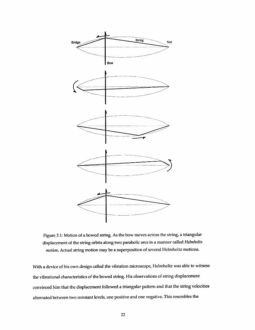
Figure 3.1: Motion of a bowed string. As the bow moves across the string, a triangular

displacement of the string orbits along two parabolic arcs in a manner called Helmholtz

motion. Actual string motion may be a superposition of several Helmholtz motions.

With a device of his own design called the vibration midcroscope, Helmholtz was able to witness

the vibrational characteristics of the bowed string. His observations of string displacement

convinced him that the displacement followed a triangular pattern and that the string velocities

alternated between two constant levels, one positive and one negative. This resembles the

behavior of the mass/spring model and its sticking/sliding stages. The change from sticking to

sliding friction is sudden and discontinuous. Once the sideways force of the string reaches the

threshold of the static frictional force, the string jumps back quickly [471.

In his theoretical solution, Helmholtz assumed that the motion of the bowed string was a free

oscillation. By analyzing the wave equation after making his observations, he characterized the

displacement along the string as a triangle with its base as the line between the fixed endpoints of

the string and with the other two sides as straight segments of the displaced string. The apex of

the triangle would move back and forth along the string-the polarity of the triangle would

change when the apex reflected off the string's endpoints-inscribing two parabolas in what is

now termed Helmholtz motion. Various Helmholtz motions can occur singularly or together, and

Helmholtz and his pupils observed that bowing speed, pressure, and location (along with

irregular alteration of sticking and sliding) could lead to superpositions of Helmholtz motions.

Other theories have been fashioned since Helmholtz, including Raman's model (1918) of the

bowed string as a forced oscillation, but the Helmholtz model still holds as an accepted method

of describing the bowed string dynamics. Current theories, such as those that describe the effect

of corrective waves and account for the torsion and bending stiffness of the string, are based on

Helmholtz motion [9].

3.2 The Bridge

The bridge acts as one of the endpoints of the vibrating string, and transfers the energy of the

string into the body. The velocity of the vibrating string, and the resulting force that is transferred

into the bridge, are perpendicular to the axis of the string but parallel to the top plate of the

instrument body. In order for this force to be efficiently transferred into the body, it must be

"rotated" so that it is perpendicular to the top plate. The bridge accomplishes just that with its

shape, touching the body with two feet.

The bridge dynamics can affect the cello timbre. For example, studies by Reinicke (1973) using

holographic photographs revealed that the cutouts in violin and cello bridges allows for

oscillatory modes [9]. Resonances at 985 Hz and 2,100 Hz, for example, were discovered in a cello

bridge-the first one corresponding to a purely translational motion of the upper part of the

bridge made possible by the two feet, the second one to a rotating motion around the heart of the

bridge, made possible by the side indentations in the bridge.

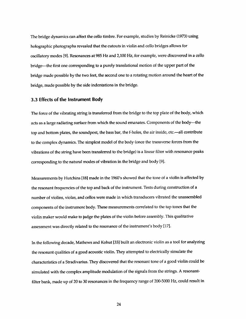
3.3 Effects of the Instrument Body

The force of the vibrating string is transferred from the bridge to the top plate of the body, which

acts as a large radiating surface from which the sound emanates. Components of the body-the

top and bottom plates, the soundpost, the bass bar, the f-holes, the air inside, etc.-all contribute

to the complex dynamics. The simplest model of the body (once the transverse forces from the

vibrations of the string have been transferred to the bridge) is a linear filter with resonance peaks

corresponding to the natural modes of vibration in the bridge and body [9].

Measurements by Hutchins [18] made in the 1960's showed that the tone of a violin is affected by

the resonant frequencies of the top and back of the instrument. Tests during construction of a

number of violins, violas, and cellos were made in which transducers vibrated the unassembled

components of the instrument body. These measurements correlated to the tap tones that the

violin maker would make to judge the plates of the violin before assembly. This qualitative

assessment was directly related to the resonance of the instrument's body [17].

In the following decade, Mathews and Kohut [33] built an electronic violin as a tool for analyzing

the resonant qualities of a good acoustic violin. They attempted to electrically simulate the

characteristics of a Stradivarius. They discovered that the resonant tone of a good violin could be

simulated with the complex amplitude modulation of the signals from the strings. A resonant-

filter bank, made up of 20 to 30 resonances in the frequency range of 200-5000 Hz, could result in

good tonal quality as long as the following conditions were met: the peak frequencies were

irregularly spaced relative to the string harmonics, so that the amplitude of the harmonics would

be differently modulated during vibrato; the resonance curves were steep, so that significant

changes in modulation were produced; and the peaks were sufficiently close together, so that

valley depths in the spectrum would not cause a hollow sound. All of these conditions were

necessary for modeling the resonant effect of the body on the acoustics of the violin.

4 Specifying Pitch and Timbre Space

To measure pitch and timbre, both a pitch space and timbre space must be defined. (See

sections 1.2 and 1.3 for a short review of the attributes of pitch and timbre.) In order to contain the

scope of the research presented in this thesis, the following limits were observed:

" Pitch is considered a one-dimensional measure that specifies the position of a sound

on the frequency scale. The word pitch is used interchangeably with the word

frequency, and it refers to the period of the fundamental of the cello signal. More

specifically, it refers to the time between the largest periodic features in the cello

waveform. Perceptual anomalies are ignored.

" Timbre is considered a one-dimensional measure that specifies the position of a sound

(at any point) on a complexity scale. On one end of the scale, the cello sound is clean.

Close to the other end, it is complex. The far end is noise. Because timbre is measured at

an instant in time-as opposed to relating the whole sound in time to a single position

in the timbre space-a sound can dynamically move along the axis as it progresses in

time.

The pitch range for the cello was limited naturally by the frequency of the lowest note that could

be played (C2=65.41 Hz) and by an arbitrary cutoff point at the upper end (A5=880 Hz).

Therefore, the pitch space is a one-dimensional line that spans the frequency range from 65 Hz to

880 Hz.

The one-dimensional timbre space was defined by recording examples of points in the space. For

five different pitches (C2, G2, D3, A3, E4), cellist Tod Machover was asked to play the note five

times col arco (bowed) with as little timbral variation in each playing as possible: four in the range

from clean to complex; the fifth as noisy as possible. Each of the recorded sounds was about two

seconds long. The sustain portions of these were then positioned as timbre-0 (clean) to timbre-4

(noise) along the axis.

The cellist was also asked to play a note for each of the five pitches that varied from clean to noisy

(not necessarily smoothly). These were recorded and saved for later analysis. They were not

positioned on the timbre axis since their locations on the axis would vary during playback.

(An acoustic cello was used for timbre measurements. The cello were recorded direct to hard disk

using a Neumann KM84 microphone, a Sony MXP-2000 recording console, a Digidesign Sound

Accelerator DSP board [61, and Sound Designer II software on a Macintosh II computer.)

5 BAA's Hypercello DSP Subsystem

The cello hyperinstrument for Begin Again Again... [26] required a system for analyzing basic

parameters of the sound from the specially modified RAAD electric cello. Although physical

sensors on the cello provided some parameters for gestural control, the tracking of pitch, energy,

and bow direction was implemented as a DSP subsystem of the hyperinstrument. The signal

processing algorithms were designed to take advantage of the characteristic waveform shape of

the cello's sound.

Figure 5.1: A typical cello waveform recorded with a piezoelectric pickup between the

string and the bridge. As seen in this time-domain plot, large excursions tend to occur

at the fundamental frequency of the cello note.

5.1 First Attempts at Pitch Tracking

Before finalizing on the hybrid DSP/physical-sensor scheme, a number of pitch-tracking systems

were experimented with. Originally, a Zeta cello was tested, in hopes that it would automatically

provide pitch information. The Zeta was equipped with an external controller (built by Ivl

Technologies) that mapped the electro-acoustic signal from the cello bridge to MIDI note

messages. Within a few months of use, it was determined that its ability to supply MIDI pitch

values was worse than expected and its electro-acoustic sound was unacceptable.

Giving up on the Zeta cello, efforts were concentrated on using the RAAD cello with external

pitch-trackers. The Roland CP-40 Pitch-to-MIDI Converter was the first attempt at pitch tracking

on the RAAD. The device worked well with singing voice, but its performance degraded rapidly

when given any sort of harmonically complex cello timbre; the CP-40 was deemed unstable for

use with generic cello sounds.

Attempts were then made to develop a general software-based pitch tracker that could analyze

the electric signal from the RAAD cello. S.D. Yadegari developed a pitch detection program based

on a linear FFT [49]. This algorithm first detected a certain number of peaks in the FFT bin and

then used perception-based theory to determine pitch by examining peak values.

After executing an FFT on the incoming signal, an average and standard deviation of the values

of the magnitude information in the FFT frame is taken. Then, a threshold value (a program

parameter, set according to the timbre of the signal and the noise of the environment) is

calculated according to a quality factor. Magnitudes lower than the threshold are considered to

be noise and are filtered out. All significant peaks are detected, and an adjustment is made to the

location and magnitude of the peaks according to an algorithm proposed in [46]. The program

then uses the peaks and their values to detect the position of the pitch according to the

interdifference spaces between them, as explained below.

An assumption is made that human pitch detection may be performed by perceiving the pitch of

a "missing fundamental" by using the beating between partials as a strong cue. If so, using the

interdifference method for pitch detection has the advantage of quickly finding the beating value

as well as the highest common divisor. Every peak as well as every interdifference between two

adjacent peaks suggest a new pitch. If a suggestion has already been made within a quantization

factor (0.2 was used), then the new suggestion is averaged with the old suggestion weighted by

their energies; and a counter is incremented. The suggestion with the highest number of counts

wins as the pitch. Ties are broken according to the previous values.

Several factors made the hyperinstrument group abandon this method of pitch tracking as a

viable real-time approach to acoustic cello analysis. First, although quite fast, the algorithm was

not implemented on a platform compatible with the general hyperinstrument environment.

Second, this pitch tracker keeps very little context from one FF17 frame to another. Consequently,

the pitch printing procedure keeps a single pitch context and deletes any single stray pitch, such

as those produced at very fast pitch changes.

With no success in building a robust signal-based pitch detector, a system to measure fingerboard

positions was designed [301. Tests with the fingerboard sensors, however, proved that the design

constraints reduced the accuracy of this system. Limited types of materials could be used for the

fingerboard sensors; materials stiff enough to provide good string-to-fingerboard contact did not

provide for reliable electrical measurements. Finger position estimations were only stable to

within two or three semitones. At this point, efforts were focused at building a software-based

pitch tracker that would take advantage of both the approximate fingerboard position data and

the characteristic shape of a bowed-string waveform to fine tune its pitch measurements.

5.2 The DSP Subsystem

Two Audiomedia cards (Digidesign, Inc., Menlo Park, CA), each equipped with a 22.578 MHz

Motorola DSP56001 processor and two channels of CD-quality input and output (16-bit,

44.1 kHz), were used to implement the signal processing subsystem inside a Macintosh IIfx. A

single program was developed to analyze energy and pitch, operating on both cards and tracking

two channels of audio input for each card. A total of four input channels provided individual

processing for each of the four strings on the cello.

5.3 The Time Domain Pitch Tracker

The pitch tracker works in the time domain, taking advantage of the unique shape of the bowed-

string waveform. The signal from each audio channel is first decimated to reduce the sampling

rate to 22.05 kHz and then pre-filtered to enhance the fundamental frequency and reduce the

strength of harmonics.

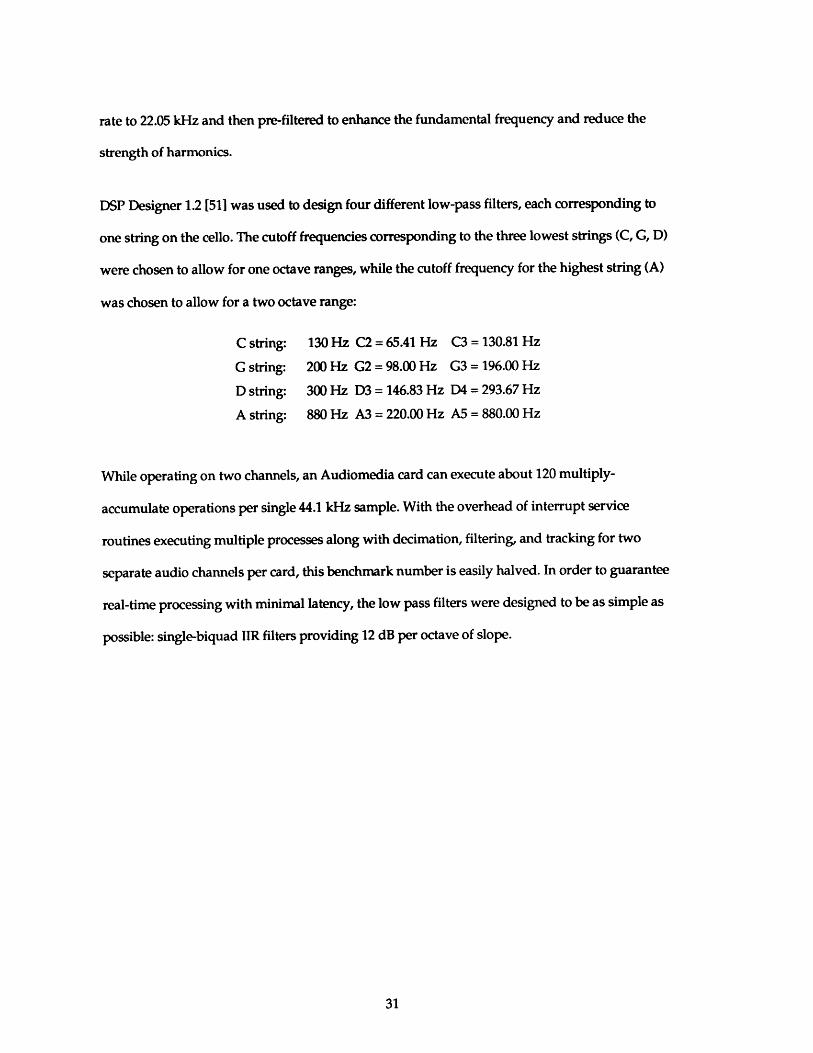
DSP Designer 1.2 [51] was used to design four different low-pass filters, each corresponding to

one string on the cello. The cutoff frequencies corresponding to the three lowest strings (C, G, D)

were chosen to allow for one octave ranges, while the cutoff frequency for the highest string (A)

was chosen to allow for a two octave range:

C string: 130 Hz C2 = 65.41 Hz C3 = 130.81 Hz

G string: 200 Hz G2= 98.00 Hz G3 = 196.00 Hz

D string: 300 Hz D3 = 146.83 Hz D4 = 293.67 Hz

A string: 880 Hz A3= 220.00 Hz A5 = 880.00 Hz

While operating on two channels, an Audiomedia card can execute about 120 multiply-

accumulate operations per single 44.1 kHz sample. With the overhead of interrupt service

routines executing multiple processes along with decimation, filtering, and tracking for two

separate audio channels per card, this benchmark number is easily halved. In order to guarantee

real-time processing with minimal latency, the low pass filters were designed to be as simple as

possible: single-biquad IIR filters providing 12 dB per octave of slope.

Single BiqUed Filters fir Pitch TrackerSingle Biqued Filters for Pitch Tracker n lnfitw

t~gff - -- -- -- -fld.fllt~r-- ---

110251000Fre-nme

Figure 5.2: Frequency magnitude plots of the four filters, one for each string.

Figure 5.3: The effect of the G string filter on an open G note is quite visible.

The pitch tracker uses a period-length estimate Pf calculated from the fingerboard position as a

starting point to compare sections of the time-domain, filtered waveform. Given the period

estimate, the pitch tracker finds the largest peak in the waveform, looking back at the most recent

filtered samples collected in the time period

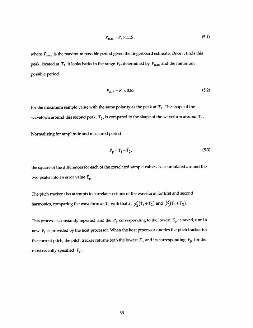
Pmax = Pf x1.1, (5

where Pmax is the maximum possible period given the fingerboard estimate. Once it finds this

peak, located at T1, it looks backs in the range Pr, determined by Pm. and the minimum

possible period

Pmm = Pf x 0.8 5 (5.2)

for the maximum sample value with the same polarity as the peak at T1.The shape of the

waveform around this second peak, T2, is compared to the shape of the waveform around T1.

Normalizing for amplitude and measured period

P, = T, - T2, (5.3)

the square of the differences for each of the correlated sample values is accumulated around the

two peaks into an error value EP.

The pitch tracker also attempts to correlate sections of the waveform for first and second

harmonics, comparing the waveform at T1 with that at Y (T1 + T2 ) and (Tj+ T2).

This process is constantly repeated, and the P, corresponding to the lowest E, is saved, until a

new Pf is provided by the host processor. When the host processor queries the pitch tracker for

the current pitch, the pitch tracker returns both the lowest E, and its corresponding P, for the

most recently specified Pf .

(5.1)

--- PIPmax

I PminIPma

-I pP

Filtered Cello Waveform (Attack)

Ep= sum of the differences squared

T1

Figure 5.4: Time domain pitch tracker parameters.

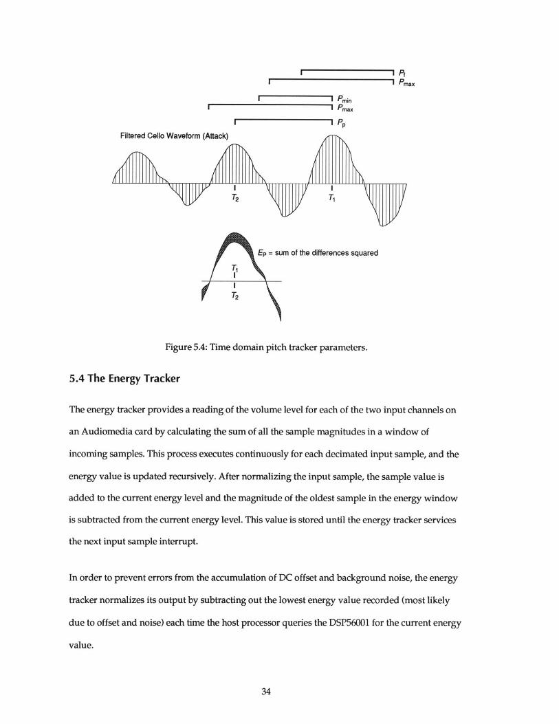
5.4 The Energy Tracker

The energy tracker provides a reading of the volume level for each of the two input channels on

an Audiomedia card by calculating the sum of all the sample magnitudes in a window of

incoming samples. This process executes continuously for each decimated input sample, and the

energy value is updated recursively. After normalizing the input sample, the sample value is

added to the current energy level and the magnitude of the oldest sample in the energy window

is subtracted from the current energy level. This value is stored until the energy tracker services

the next input sample interrupt.

In order to prevent errors from the accumulation of DC offset and background noise, the energy

tracker normalizes its output by subtracting out the lowest energy value recorded (most likely

due to offset and noise) each time the host processor queries the DSP56001 for the current energy

value.

5.5 The Bow Direction Tracker

A bow direction tracker was implemented to work as an integral part of the energy tracker. Using

the same data windows as the energy tracker, the direction tracker measured and stored the

peaks in the incoming sample, while also keeping the average signed value (as opposed to the

energy tracker's magnitude measurements) of the samples in the input buffer. Taking advantage

of the characteristic shape of a bowed string, the tracker could determine the direction of the bow

stroke by comparing the direction of the maximum peaks relative to the window average.

I Bow DirectionWindow Average

Window Average

Bow Direction

Figure 5.5: The bow direction tracker takes advantage of asymmetries.

Use of the window average as the zero value (as opposed to assuming a hard zero) for

determining the direction of the waveform peaks greatly reduced the detrimental effect of

subharmonics and DC-offsets. This simple algorithm proved to be efficient and robust when used

with piezo-electric pickups that were placed appropriately underneath the string such that signed

voltage changes reflected similarly directional movement of the bowed string.

5.6 Concurrent Processing

From the beginning, the DSP subsystem was designed to provide a framework for implementing

different trackers that execute concurrently. In the current configuration, the pitch tracker runs as

the main process on the DSP56001, while the energy tracker and other processes (i.e., decimation

and filtering) run at the interrupt level. A sample that is received in either channel interrupts the

main process. Bookkeeping and final calculations for the energy tracker, as well as prefiltering for

the pitch tracker, are executed at a sample-to-sample level.

Host communication (with Hyperlisp running on the Motorola 68030 processor onboard the

Macintosh) works at a second interrupt level. The host processor interrupts the DSP56001

whenever it needs to exchange data. While pitch and energy are being calculated constantly, the

trackers only return data when queried by the host.

Furthermore, the host can signal the DSP subsystem to suspend execution of certain tasks in

order to give other tasks more computing cycles or to facilitate debugging (e.g., the state of the

pre-filtered and post-filtered buffers can be frozen for analysis).

Main Program

Main Loop {

Find peaks

For measured periodand harmonics {

Calculate Error

Save minimum error

Receive Interrupt

Host Interrupts

With host command {

Calculate return value

Communicate to host

Programs Data Paths

Decimated Sample Input Buffer

Filtered Sample Buffer

Variable Tables

Data

Figure 5.6: Concurrent processes within the DSP subsystem.

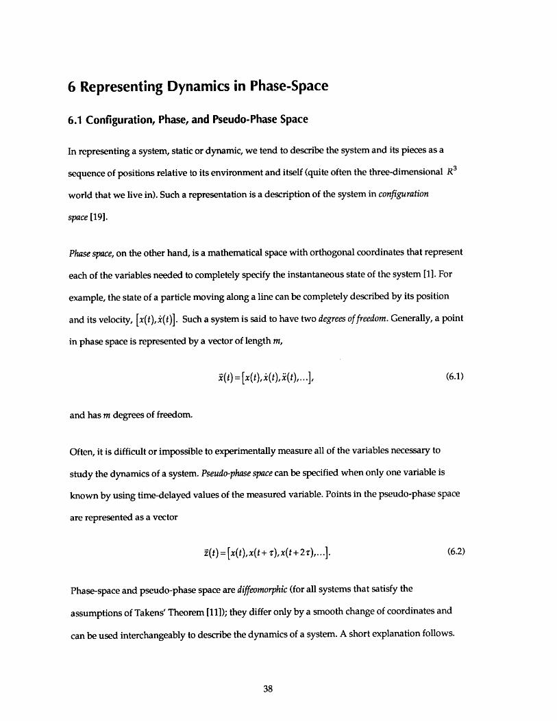
6 Representing Dynamics in Phase-Space

6.1 Configuration, Phase, and Pseudo-Phase Space

In representing a system, static or dynamic, we tend to describe the system and its pieces as a

sequence of positions relative to its environment and itself (quite often the three-dimensional R3

world that we live in). Such a representation is a description of the system in configuration

space [19].

Phase space, on the other hand, is a mathematical space with orthogonal coordinates that represent

each of the variables needed to completely specify the instantaneous state of the system [1]. For

example, the state of a particle moving along a line can be completely described by its position

and its velocity, [x(t),i(t)]. Such a system is said to have two degrees of freedom. Generally, a point

in phase space is represented by a vector of length m,

i(t) = [x(t), (t),i(t),...|, (6.1)

and has m degrees of freedom.

Often, it is difficult or impossible to experimentally measure all of the variables necessary to

study the dynamics of a system. Pseudo-phase space can be specified when only one variable is

known by using time-delayed values of the measured variable. Points in the pseudo-phase space

are represented as a vector

i(t) = [x(t),x(t +,r),x(t +2),...|. (6.2)

Phase-space and pseudo-phase space are diffeomorphic (for all systems that satisfy the

assumptions of Takens' Theorem [11]); they differ only by a smooth change of coordinates and

can be used interchangeably to describe the dynamics of a system. A short explanation follows.

The one-to-one mapping of points P E R" in P to points P' E R' in P' such that

f: P -> P' means p'= f(P) (p e R" ,p'eR" ), (6.3)

where both f(P) and f-1(P') are single valued and continuous, is said to be homeomorphic. A

homeomorphism is a continuous bijection-it is one-to-one and onto (i.e., every single point in the

domain space ( P) has a mapping to exactly one point in the range space ( P'), and vice-versa).

Additionally, if f(p) and f 1(p') are differentiable at all points, then the homeomorphism is

called a diffeomorphism.

An embedding is an injective immersion-it is one-to-one, but not necessarily onto (i.e., every single

point in the domain space has a mapping to exactly one point in the range space, but all points in

the range space may not have equivalents in the domain), and the map is of full rank everywhere.

By the theorems of Takens, the function that maps each point i(t) = [x(t), i(t),t),...] of an m-

dimensional phase-space to a point i(t) = [x(t),x(t+r),x(t +2r),...] in a pseudo-phase space of

2m + 1 dimensions (as long as the time increment r is uniform), is an embedding. 2m + 1 is an

upper limit on the pseudo-phase space dimension; it is often possible to have a dimension of only

m [11].

The choice of the time delay r for the pseudo-phase space diagram affects the quality of the plot

due to loss of precision in finite-resolution computers and displays. For small r's, the trajectories

will lie together near the diagonal of the embedding space, possibly resulting in lack of distinct

paths. For large t's, the trajectories will expand away from the diagonal and fold over. An

algorithm based on information theory that calculates the mutual information evident in the data

to be plotted is presented by Gershenfeld [11] as an automated way of choosing r, but the easiest

way is to simply plot the diagram for different values of r to get a feeling of how the attractor is

affected.

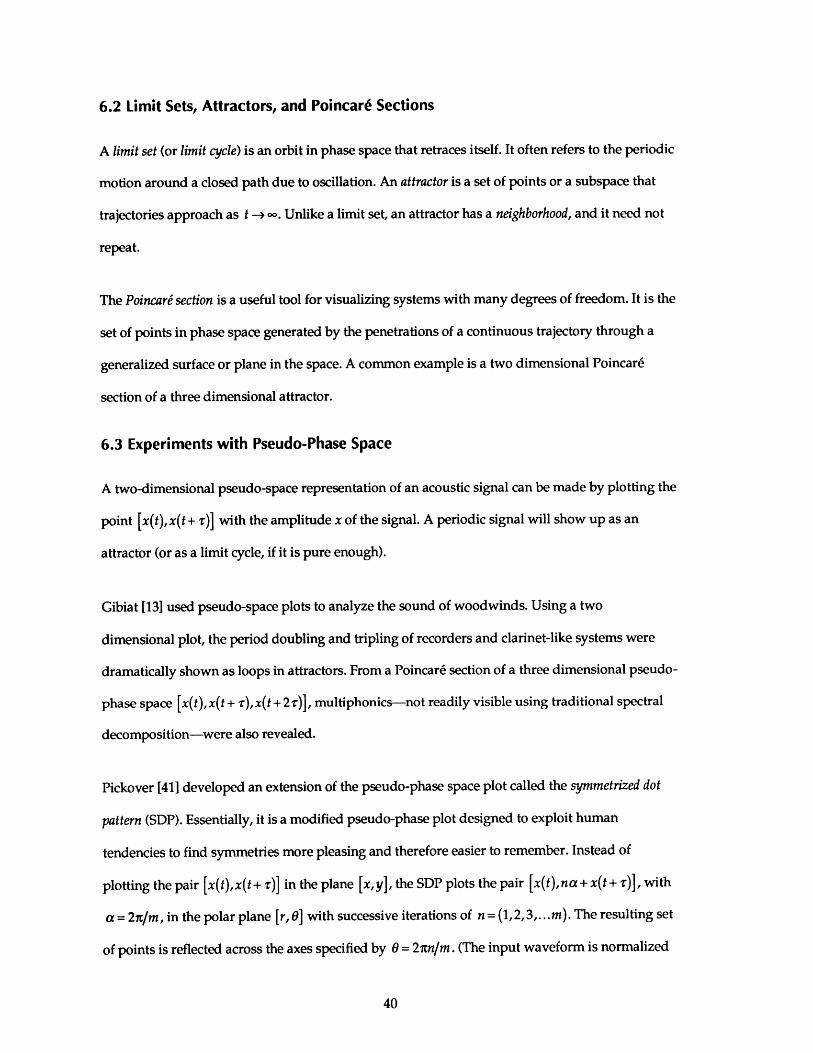
6.2 Limit Sets, Attractors, and Poincard Sections

A limit set (or limit cycle) is an orbit in phase space that retraces itself. It often refers to the periodic

motion around a closed path due to oscillation. An attractor is a set of points or a subspace that

trajectories approach as t -+ oo. Unlike a limit set, an attractor has a neighborhood, and it need not

repeat.

The Poincari section is a useful tool for visualizing systems with many degrees of freedom. It is the

set of points in phase space generated by the penetrations of a continuous trajectory through a

generalized surface or plane in the space. A common example is a two dimensional Poincare

section of a three dimensional attractor.

6.3 Experiments with Pseudo-Phase Space

A two-dimensional pseudo-space representation of an acoustic signal can be made by plotting the

point [x(t),x(t+ r)] with the amplitude x of the signal. A periodic signal will show up as an

attractor (or as a limit cycle, if it is pure enough).

Gibiat [13] used pseudo-space plots to analyze the sound of woodwinds. Using a two

dimensional plot, the period doubling and tripling of recorders and clarinet-like systems were

dramatically shown as loops in attractors. From a Poincare section of a three dimensional pseudo-

phase space [x(t), x(t + r),x(t + 2-)], multiphonics-not readily visible using traditional spectral

decomposition-were also revealed.

Pickover [41] developed an extension of the pseudo-phase space plot called the symmetrized dot

pattern (SDP). Essentially, it is a modified pseudo-phase plot designed to exploit human

tendencies to find symmetries more pleasing and therefore easier to remember. Instead of

plotting the pair [x(t),x(t+,r)] in the plane [x,y], the SDP plots the pair [x(t),na+ x(t + r)], with

a = 2ir/m, in the polar plane [r, 6] with successive iterations of n = (1,2,3,.. .m). The resulting set

of points is reflected across the axes specified by 0= 27cn/m. (The input waveform is normalized

to the peak of the sampled audio so that overall amplitude does not affect the characterization,

and the SDP states are plotted for all pairs in the audio sample.)

Pickover [41] used SDP's to characterize animal vocalizations, human speech, and heart sounds.

He discovered that symmetrized dot patterns were especially useful as a visualization tool for

characterizing the spectral content of a sound without having to make direct measurements,

because humans tend to spot symmetries quickly, with good recall. Even people with no training

in phonetics or acoustics were able to use SDP's to identify phoneme groups and individual

speakers.

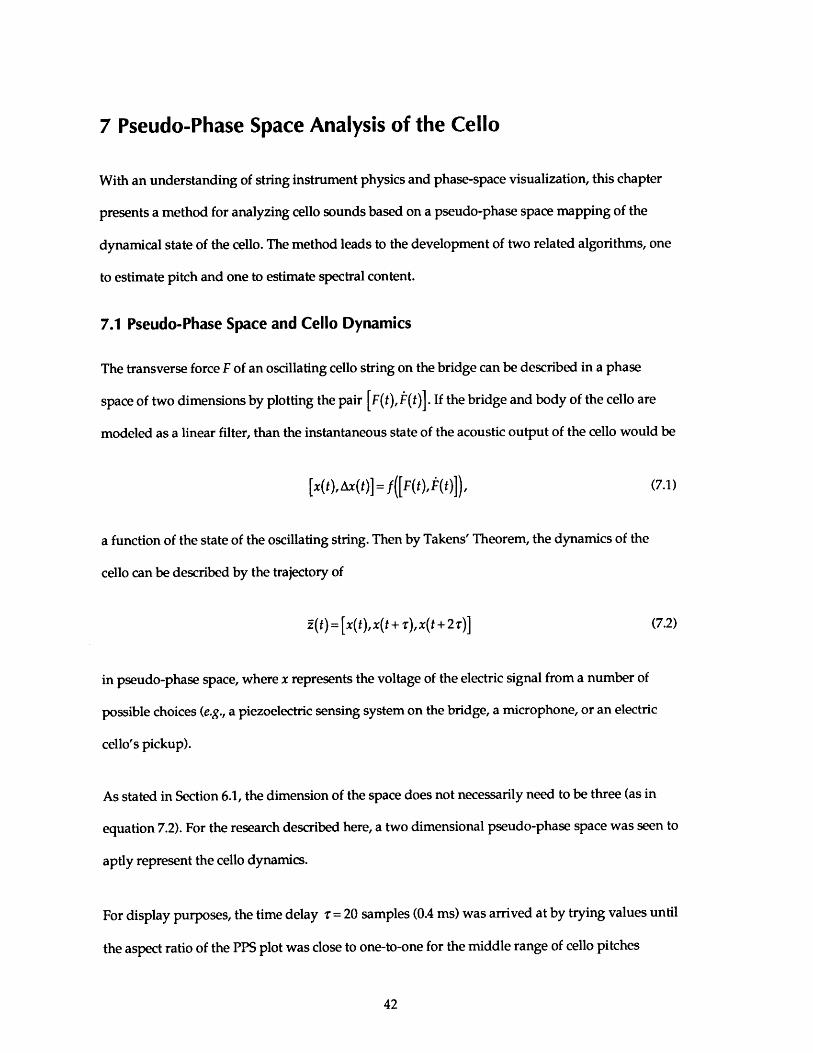
7 Pseudo-Phase Space Analysis of the Cello

With an understanding of string instrument physics and phase-space visualization, this chapter

presents a method for analyzing cello sounds based on a pseudo-phase space mapping of the

dynamical state of the cello. The method leads to the development of two related algorithms, one

to estimate pitch and one to estimate spectral content.

7.1 Pseudo-Phase Space and Cello Dynamics

The transverse force F of an oscillating cello string on the bridge can be described in a phase

space of two dimensions by plotting the pair [F(t),t(t)]. If the bridge and body of the cello are

modeled as a linear filter, than the instantaneous state of the acoustic output of the cello would be

[ x(t ), Ax(t) )= f([F(t ),#t(t )], (7.1)

a function of the state of the oscillating string. Then by Takens' Theorem, the dynamics of the

cello can be described by the trajectory of

i(t )= [ x(t),x(t+,r),x(t+2r)] (7.2)

in pseudo-phase space, where x represents the voltage of the electric signal from a number of

possible choices (e.g., a piezoelectric sensing system on the bridge, a microphone, or an electric

cello's pickup).

As stated in Section 6.1, the dimension of the space does not necessarily need to be three (as in

equation 7.2). For the research described here, a two dimensional pseudo-phase space was seen to

aptly represent the cello dynamics.

For display purposes, the time delay r= 20 samples (0.4 ms) was arrived at by trying values until

the aspect ratio of the PPS plot was close to one-to-one for the middle range of cello pitches

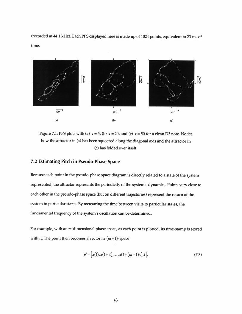
(recorded at 44.1 kHz). Each PPS displayed here is made up of 1024 points, equivalent to 23 ms of

time.

X(t) t)x)

(a) (b) (c)

Figure 7.1: PPS plots with (a) r =5, (b) r = 20, and (c) T =50 for a clean D3 note. Notice

how the attractor in (a) has been squeezed along the diagonal axis and the attractor in

(c) has folded over itself.

7.2 Estimating Pitch in Pseudo-Phase Space

Because each point in the pseudo-phase space diagram is directly related to a state of the system

represented, the attractor represents the periodicity of the system's dynamics. Points very close to

each other in the pseudo-phase space (but on different trajectories) represent the return of the

system to particular states. By measuring the time between visits to particular states, the

fundamental frequency of the system's oscillation can be determined.

For example, with an m-dimensional phase space, as each point is plotted, its time-stamp is stored

with it. The point then becomes a vector in (m + 1)-space

p'=[x(t),x(t+ ),...,x(t+(m-1)r),t]. ((7.3)

The projection of this point into the pseudo-phase space is the familiar vector

p = [x(t),x(t +,r),...,x(t +(m-1)T )] . (7.4)

As samples of the system's state variable are collected and plotted on the attractor, the time-

stamps of the other points in the region of the new points (but on different trajectories) are

compared to the running time. The fundamental frequency of the system's oscillation can then be

derived by determining the periodicity of neighboring points.

Figure 7.2: Determining the periodicity of a system's state dynamics within a pseudo-

phase space: For each new point plotted on the attractor, its time-stamp is compared to

the time-stamps of neighboring points on other trajectories.

This algorithm could only be useful as a real-time operation if it can perform the search for

neighboring points efficiently. Although it may seem simple, the problem of finding points that

could be arbitrarily located in a given domain is not trivial. In general, the process of searching

for neighboring points to a given point in space is a range-searching problem. For repetitive-mode

applications, an initial investment in preprocessing and storage leads to a long term gain in

searching speed. (Preparata and Shamos [421 discuss range-searching theory.)

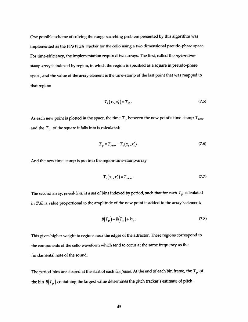
One possible scheme of solving the range-searching problem presented by this algorithm was

implemented as the PPS Pitch Tracker for the cello using a two dimensional pseudo-phase space.

For time-efficiency, the implementation required two arrays. The first, called the region-time-

stamp-array is indexed by region, in which the region is specified as a square in pseudo-phase

space, and the value of the array element is the time-stamp of the last point that was mapped to

that region:

Tr (r {x,x r)= TIP. (7.5)

As each new point is plotted in the space, the time T, between the new point's time-stamp Tne,

and the Ti, of the square it falls into is calculated:

T = Tne -Tr (Xr,Xr'). (7.6)

And the new time-stamp is put into the region-time-stamp-array

Tr (xr,xr X)= Tne.. (7.7)

The second array, period-bins, is a set of bins indexed by period, such that for each T, calculated

in (7.6), a value proportional to the amplitude of the new point is added to the array's element:

B(TP)= B(Tp)+ krr . (7.8)

This gives higher weight to regions near the edges of the attractor. These regions correspond to

the components of the cello waveform which tend to occur at the same frequency as the

fundamental note of the sound.

The period-bins are cleared at the start of each bin frame. At the end of each bin frame, the T, of

the bin B(T,) containing the largest value determines the pitch tracker's estimate of pitch.

The bin frame lasts for only 2.9 ms, which is the time for 128 samples to be collected at a rate of

44.1 kHz. For most of the notes in the usable range of the cello, this is less than the period. The

pitch tracker, if implemented as a real-time process, could thus provide a new pitch estimate 345

times a second. (See section 8.4 for arguments for its feasibility as a real-time program on a

Motorola DSP56001.)

The bin frame size should not be confused with window size, as related to block-processed

operations like Discrete Fourier Transforms. It is independent of the region-time-stamp-array.

Instead, it determines the number of time-stamp comparisons to make between new samples and

possible neighboring samples before hazarding an estimate of pitch.

Also, the region-time-stamp-array is never explicitly cleared. Each element holds the time-stamp

of the last point that occupied that region, whether it was many eons ago or whether it was

plotted recently (beyond a certain minimum threshold time to prevent matching of points on the

same trajectory). When an element in the region-time-stamp-array has become stale (i.e., it

corresponds to a period that is longer than the period of the lowest cello note), it is ignored and

overwritten next time its region is visited. The amount of previously sampled data used for

period estimation is therefore different for each frequency. Each element in the period-bins

accumulates weights for data collected only in the period of time that the period-bin element

represents.

This particular implementation used 128 period-bins (an arbitrary number) indexed such that

they were evenly spaced by period (in time). Any number of period-bins and spacing could be

implemented in the software.

525 Hz330 Hz

220 Hz

150 Hz

120 Hz

-100 Hz

Figure 7.3: Four clean cello note attacks (G2, D3, A3, E4) spliced together shown in time

domain, with the pitch tracker's estimates below. The total time shown is 675 ms.

Of course, this scheme would not work unless the input signal approached a limit cycle quickly.

For notes of timbre-0 and timbre-1 complexity, the pitch tracker was still accurate. In the case of

the cello generating more complex sounds, a limit cycle is never quite reached because of a lack of

periodicity. As the complexity of the cello's dynamics increases, the plot becomes too noisy, and

the attractor loses its features at timbre-3 and disappears into noise at timbre4.

1 +-oI +

x

x- x(t)

Figure 7.4: PPS plots of a timbre-2 and timbre-3 D3 note.

The limit cycle can be induced by using a low-pass filter that attenuates the added harmonics of

complex oscillations before mapping the signal to pseudo-phase space. Because a pitch tracker

needs to work reliably for a relatively large frequency range, a filter with a response that provides

attenuation of harmonics in the whole range of the pitch tracker would be ideal. By using a low-

pass filter with a response that tapers as the frequency increases, this effect can be achieved.

-60 1-0.02 0.1 0.3 1 3

Frequenog (kHz)10 22.05

Figure 7.5: The response of the PPS pitch tracker's 9-biquad IR input filter for cello.

-525 Hz-330 Hz-220 Hz

-150 Hz

-120 Hz

-100 Hz

Figure 7.6: Four harmonically rich cello notes filtered and spliced together; and the

pitch tracker's estimates.

DSP Designer 1.2 [51] was used to design a 9-biquad IIR filter with 20 dB of attenuation at 440 Hz

and a downward slope starting at 100 Hz. This design was chosen for the fact that it could be

implemented as a real-time operation on one of the two Audiomedia boards for the hypercello

DSP subsystem.

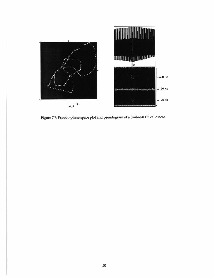
7.3 Estimating Spectral Content with Pseudograms

By using the same algorithm as the PPS Pitch Tracker, but directly displaying the values stored in

the period-bins as intensities, a display that reads similarly to a spectrogram can be shown. The

pseudogram, as the author has coined it, can be useful in judging the dynamics of a system. The

pseudogram can be thought of as a time progression of pseudo-phase-space plots that have been

squeezed into a vertical line such that each point in that line represents a frequency and the

intensity of each point specifies the number of local PPS features that recur at that frequency.

With a simple waveform like a sinusoid, the pseudogram simply shows the pitch of the signal.

For a less simple input, like a timbre-0 cello sound, the pitch of the input remains prominent, but

the system's dynamical characteristics, which result in the sound's harmonic and noise content,

are also represented as additional horizontal bands and scattering.

As input to the pseudogram becomes more complex, the spread across the vertical axis does too.

The attractor in the pseudo-phase space plot becomes less apparent, and the pseudogram

intensities move away from the fundamental period. In the case of a very complex sound, such as

timbre-4 cello note, the lack of an attractor is perceived as a noisy pseudogram.

300 Hz

150 Hz

75 Hz

x(t)

Figure 7.7: Pseudo-phase space plot and pseudogram of a timbre-0 D3 cello note.

--300 Hz

.. -150 Hz

75 Hz

Figure 7.8: Top: pseudogram of a D3 cello note progressing from timbre-0 to timbre-4

(total time = 2.6 s). Bottom: five PPS plots of the same note showing the same

progression.

0.14 - 0.12

0.12 0.1

0.10.00-

6 0.06

0.06

0.040.04-

0.02-

OMI fA . . . .0 low8 21000 536= s 0 low 2W &M 40 000

Frequen Frequ .eg

Figure 7.9: Frequency magnitude plots of timbre-0 and timbre-2 D3 cello notes.

7.4 Symmetrized Dot Patterns for Fun and Profit

Symmetrizing the pseudo-phase plot highlights can make it easier to visually categorize the

differences between timbres. The SDP provides a dramatic visual image that is easy to recognize

and remember. Because it is difficult to use the ear alone to accurately compare and characterize

timbres, especially if listening experiments are done over time, SDP's could be useful for visually

specifying points in a timbre space. Compare the PPS plots in figure 7.8 to the SDP's in

figure 7.10.

In terms of analysis by computer, the SDP, which is displayed in polar coordinates, holds no

more information than the normal PPS in Cartesian coordinates.

d-mire2fftSigal

r-

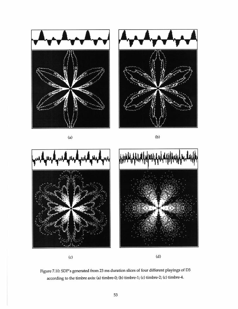
Ablj 4 9AA IYA IIbk

(c) (d)

Figure 7.10: SDP's generated from 23 ms duration slices of four different playings of D3

according to the timbre axis: (a) timbre-0; (b) timbre-1; (c) timbre-2; (c) timbre-4.

Aevke y

611IM10M1 T4 1I if I ? III

8 Conclusions and Further Research

8.1 Goals and Accomplishments

The original goal of this project was twofold: to explore the use of phase-space representations for

specifying timbre; and to develop a real-time timbre tracker as part of the cello hyperinstrument.

Although the second half was not entirely realized, research into the non-linear dynamics of

string instruments and subsequent experimentation with phase-space representations of cello

dynamics resulted in potentially powerful new methods of analyzing both pitch and timbre.

To experiment with the different phase-space representations described in this thesis, a modular

window-based program, SampleHead, was written in a high-level language. (See appendix for

implementation details.) SampleHead is a Macintosh application program that supports multiple

windows and views, and allows the user to use the familiar point-and-click interface of the

Macintosh to open sample files and display them in various formats. The PPS Pitch Tracker and

the pseudogram display, as well as the pseudo-phase space and symmetrized dot pattern

displays, were implemented in SampleHead.

As a visual tool, symmetrized dot patterns (SDP) proved useful in specifying timbre; but as an

automated analysis tool, these plots had no advantages over the pseudo-phase space (PPS)

representation, from which the SDP was formed. The PPS Pitch Tracker, and the pseudogram

display, both based on an easily computable map from time domain to periodicity domain, were

shown to be useful tools for estimating qualities of cello sounds.

8.2 PPS Pitch Tracker

The PPS Pitch Tracker follows the state of the system it is tracking, and measures the period of

the system's oscillation. It has a number of advantages over other estimation schemes:

" A method that can synchronously analyze the input signal as it is collected will be

faster than a design that requires the collection of windows of data before any analysis

can be performed. The PPS Pitch Tracker, because it maps the time-domain

representation of the input signal to the periodicity domain, can correlate incoming

waveform features to previous ones immediately, instead of as a nonsynchronous

process.

" Many methods of estimating pitch rely on performing a DFT on the input signal in

order to directly analyze the frequency content. As described above, the PPS map does

not require windows of data, as the DFT does. In addition, the PPS technique does not

require as much computation as the DFT. The DFT is an 0(nlog(n)) process, while the

PPS is O(n). In order to get acceptable frequency accuracy, a DFT must be performed

with many thousands of points. Furthermore, the PPS requires only simple integer

operations.

" Because of the dynamic windowing built-in to the pseudogram, it converges

optimally for each frequency band, as opposed to converging at the rate of a fixed

window size.

" On highly periodic signals, the PPS Pitch Tracker needs to collect and analyze only

one period of the input signal to converge-especially with higher sampling rates.

With less periodic signals, two or more periods are adequate. Higher pitched signals-

which tend to have less harmonics and variation in waveform features-result in

especially quick estimation.

The PPS Pitch Tracker does have one major disadvantage over other systems. Because it measures

periodicity of time-domain waveform features, it can not be used as a general pitch estimator. It

requires input signals, like cello notes, that have prominent and periodic waveform features.

With a square-wave input, for example, because the input's time domain representation has

broad "flat" sections, the PPS-based algorithm would not converge to the fundamental pitch

without an input filter specifically tuned for a range of possible pitches or without a region

lookup scheme that would have previous knowledge of the input's waveform shape. In the case

of the square-wave, the PPS Pitch Tracker would need to concentrate on correlating regions

corresponding to the "vertical" sections and the corners of the square-wave signal.

For cello sounds, the PPS Pitch Tracker, implemented with a specific input filter for the range of

pitches available from a cello, worked well, especially for pitches that were above the lowest

octave. The lowest notes, because of their greater periods and because of the relatively lesser

effect of the input filter on attenuating their harmonics, required more samples (and therefore,

more time) for convergence of the pitch estimate.

8.3 Pseudogram Representation

Like the PPS Pitch Tracker, the Pseudogram representation of timbre shared similar advantages

over systems based on the DFT.

" Unlike the DFT based spectrogram, which requires fixed window sizes, the

pseudogram window sizes are dynamic for each frequency that it displays. Therefore,

the time/frequency smearing of the DFT is not evident in the pseudogram .Instead,

within each vertical frame of the pseudogram, the amount of periodicity is displayed

for the period of each frequency band.

" The DFT is an 0(nlog(n)) process, while the pseudogram is O(n) with simple integer

math. Furthermore, no special windowing operations are necessary for an

pseudogram, while the DFT requires further computations for overlapping windows.

" Because of the dynamic windowing built-in to the pseudogram, it converges

optimally for each frequency band, as opposed to converging at the rate of a fixed

window size.

The pseudogram does have potential disadvantages that may prevent it from being used as a

general tool:

" Because it is not an exact one-to-one representation, it can not be inverted for

synthesis.

" Not all harmonics are displayed in the pseudogram display. Instead, it highlights

periodicities in time-domain waveform features.

When used for the purposes of this study-as a tool for specifically analyzing cello timbre-it

works well. Because the harmonics of the cello sounds are phase-locked and occur at integer

multiples, the transform from time-domain to phase-space domain yields enough useful

information to estimate harmonic content. Also, inharmonic components of the cello sound show

up as a scattering of intensities, highlighting the aperiodicities of the sound.

8.4 Making it Real-time

From the code in SampleHead, it can be shown that both the PPS and FPPS algorithms can be

implemented as real-time systems. The PPS Pitch Tracker, for example, could be based on a

Macintosh computer with two Digidesign Audiomedia DSP boards. The first Audiomedia would

be dedicated to the PPS Pitch Tracker's input filter. The second board, deriving its input from the

analog output of the first card, would compute the PPS representation and estimate the pitch.

On the second Audiomedia, for each sample that is received, the necessary operations would be

to:

" Calculate the region in pseudo-phase space that the new sample occupies. (Two

normalizing multiplies and a move.)

- Calculate the period between the current time-stamp and the time-stamp stored in the

region. (Index array lookup, subtraction, assignment of new time-stamp to region

array.)

" Range check the calculated period. (Two comparisons.)

a Add weighted value to period-indexed bin. (Array lookup, multiply-accumulate,

assignment.)

e Keep track of maximum bin. (Comparison, assignment.)

For a single-channel operation, the Motorola 56001 based Audiomedia board can perform about

250 multiply-accumulate operations during the time between two samples (received at a rate of

44.1 kHz). This is adequate computing power to implement the PPS Pitch Tracker for real-time

operation. Similarly, the pseudogram algorithm can be coded for real-time operation on a single

Audiomedia board (without the first board for input filtering).

8.5 Further Research

A more detailed timbre space, with more dimensions, could be specified. The one-dimensional

space applied in this document was adequate for testing SDP's; as static displays, they map well

to the complexity axis. The pseudogram was also quite useful in specifying this dimension. A

larger catalogue of cello sounds, along with varying playing techniques (instead of just sustained

notes), would be a greater test of both the PPS Pitch Tracker and of the pseudogram

representation.

More degrees of freedom could be added to the pseudo-phase space representation. Only two

degrees are used in accordance with the simple cello model assumed here, a one-dimensional

oscillation of a bowed string. In truth, the cello model should have more degrees of freedom to

take into account the nonlinearities in the bridge, the body, and in the instrument/air interface.

A timbral analysis scheme based on geometric measurement of attractors could be studied. By

observing the path of the trajectories through phase space, one could come up with a map

between timbral perception and the shape of the attractor. This leads quickly to a study in

perceptual theory and psychoacoustics.

All of this research could extend beyond the domain of the cello and string instruments; the

techniques of using pseudo-phase space to analyze the dynamics of a system is extendable to any

system. As long as the waveform of an instrument's sound has prominent features that are

periodic, as in the cello's case, the PPS Pitch Tracker could be tuned to work with the instrument.

Furthermore, pseudograms could be made of a wide variety of acoustic instruments to determine

if different timbres among many instruments could be represented this way.

9 Appendix

9.1 SampleHead Implementation Details

SampleHead is a Macintosh application program that supports multiple windows and views, and

allows the user to use the familiar point-and-click interface of the Macintosh to open sample files

and display them in time-domain and in the various phase-space representations described in

this thesis. Because it is written mainly in Object Pascal, it is easily expandable, and can be

modified to display other transforms. The program is about 2000 lines of code.

SampleHead opens and edits files created by Sound Designer II or Audiomedia software. Files

can be of any length, limited only by disk space. Samplehead does not support real-time capture

of sounds, nor does it do real-time analysis.

All of the figures in this document featuring time-domain, phase space, pseudo-phase space,

SDP, and pseudogram representations were screen captures of SampleHead.

The Object Pascal routine for calculating and displaying PPS plots is:

for point := 0 to fXform.fDataTrack.Length - 1 - fLag do beginwith fXform do begin

x1 fDataBuffer[point];x2 fDataBuffer[point + fLag];

end;if theta > signedRadius then begin

color.red :- kMaxSampleVal + x1;color.green 0;color.blue kMaxSampleVal + abs (x2);

endelse begin

color.blue 0;color.green kMaxSampleVal + x1;color.blue kMaxSampleVal + abs (x2);

end;PlotColorPt(x1,x2,color);end;

end;

where the variable fLag represents the pseudo-phase space delay r, and the variables x and x2

specify the PPS point. On a color screen, the PPS is displayed so that points representing positive

slope in time domain are a blend of red and blue, and points representing negative slope are a

blend of green and blue.

The implementation for displaying the pseudogram is:

for line := area.left to area.right do begin

for count := 0 to binSize - 1 dofTsBin[count] := 0;

for count 1 to fZoomFactor do beginsampT1 SamplePtr(sampAddr)^;sampT2 SamplePtr(sampAddr - fLag)^;

regionTI RegionLocate(sampTl);regionT2 RegionLocate(sampT2);

matchPeriod :-Min (sampAddr - fTsBox [regionT1, regionT2] ,kMaxMatchPeriod);

if matchPeriod > kMinMatchPeriod then beginfTsBin[matchPeriod div binDiv] :=

Min (Weight (sampT1) + fTsBin[matchPeriod div binDiv] ,32767);fTsBox[regionT1,regionT2] := sampAddr;

end;

sampAddr := sampAddr + frameSize;end;for count := 0 to binSize - 1 do

PlotColorPt(line,count + viewCenter,Color(fTsBin[count]));end;

This algorithm is also the heart of the PPS Pitch Tracker. By keeping track of the greatest bin

value and its index in the fTsBin array, the period of the filtered input signal can be reported.

10 References

[1] G.L. Baker and J.P. Gollub. Chaotic Dynamics. Cambridge: Cambridge University Press,

1990.

[2] K. Blair Benson. Audio Engineering Handbook. New York: McGraw-Hill, 1988.

[3] P. Berg6, Y. Pomeau, and Christian Vidal. Order within Chaos. New York: John Wiley &

Sons, 1984.

[4] E. de. Boer. Pitch theories unified. Psychophysics and Physiology of Hearing, E.F. Evans and

J.P. Wilson, eds. New York: Academic Press, 1977.

[5] Hal Chamberlin. Musical Applications of Microprocessors. Rochelle Park, NJ: Hayden Book

Company, Inc., 1980.

[61 Evan Brooks and Robert Currie. Digidesign developer documentation, version 4.0. April

1990.

[7] G. R. Charbonneau. Timbre and the perceptual effects of three types of data reduction.

Computer Music Journal, 5(2):10-19, 1981.

[8] Joseph Chung. Hyperlisp reference manual. Music & Cognition Group, MIT Media Lab,

1990.

[91 Lothar Cremer. The Physics of the Violin. Cambridge, MA: MIT Press, 1983.

[10] Bernhard Feiten and Tamas Ungvary. Sound data base using spectral analysis reduction

and an additive synthesis model. ICMC Glasgow 1990 Proceedings, 72-74, 1990.

[11] Neil Gershenfeld. An experimentalist's introduction to the observation of dynamical

systtems. Directions in Chaos, vol 2, Hao Bai-lin ed. World Scientific, 1988.

[12] Neil Gershenfeld. Dimension measurement on high-dimensional systems. Department

of Physics, Harvard University, 1992.

[13] V. Gibiat. Phase space representations of acoustical musical signals. Journal of Sound and

Vibration, 123(3):529-36, 1988.

[14] Herbert Goldstein. Classical Mechanics. Reading, MA: Addison-Wesley, 1981.

[15] John Guckenheimer and Philip Holmes. Nonlinear Oscillations, Dynamical Systems, and

Bifurcations of Vector Fields. New York: Springer-Verlag, 1983.

[16] Stephen Handel. Listening. Cambridge, MA: MIT Press, 1989.

[17] C. M. Hutchins and F. L. Fielding. Acoustical measurement of violins. Physics Today, 35-

40, July 1968.

[18] C. M. Hutchins, A. S. Hopping, and F. A. Saunders. Subharmonics and plate tap tones in

violin acoustics. 1. Acoust. Soc. Am., 32(11):1443-49, 1960.

[19] E. Atlee Jackson. Perspectives of Nonlinear Dynamics, vol. 1. Cambridge: Cambridge

University Press, 1989.

[20] Richard Kronland-Martinet. The wavelet transform for analysis, synthesis, and

processing of speech and music sounds. Computer Music Journal, 12(4):11-20, 1988.

[21] R. G. Laughlin, B. D. Truax, and B. V. Funt. Synthesis of acoustic timbres using principal

component analysis. ICMC Glasgow 1990 Proceedings, 95-99, 1990.

[22] W. Lauterborn and U. Parlitz. Methods of chaos physics & their applications to acoustics.

J. Acoust. Soc. Am., 84(6):1975-93, 1988.

[23] Rachel E. Learned, William C. Karl, Alan S. Willsky. Wavelet packet based transient

signal classification. IEEE-SP Conference on Time-Frequency Analysis, Victoria, Canada,

4-6 Oct, 1992.

[24] Yeen On Lo and Dan Hitt. A language for exploring timbre composition. CCRMA,

Stanford University, 1990.

[25] Tod Machover. Begin Again Again..., musical score. Milan/Paris: Ricordi, 1991.

[26] Tod Machover. Begin Again Again..., live concert recording of world premiere

performance. Recorded at Tanglewood Festival, 14 August 1991.

[27] Tod Machover. Flora, compact disc liner notes accompanying four hyperinstrument

recordings. New York: Bridge Records, Inc., 1990.

[28] Tod Machover. Hyperinstruments: musically intelligent/interactive performance and

creativity systems. Music & Cognition Group, MIT Media Lab, 1988.

[29] Tod Machover. Hyperinstruments: yearly progress report to the Yamaha Corporation.

Music & Cognition Group, MIT Media Lab, 1990.

[30] Tod Machover. Hyperinstruments: yearly progress report to the Yamaha Corporation.

Music & Cognition Group, MIT Media Lab, 1991.

[31] Tod Machover. Hyperinstruments: a progress report, 1987-1991. Music & Cognition

Group, MIT Media Lab, 1992.

[32] Benoit B. Mandelbrot. The Fractal Geometry of Nature. New York: W.H. Freeman and

Company, 1983.

[33] M.V. Mathews and J. Kohut. Electronic simulation of violin resonances. J. Acoust. Soc.

Am., 53(6):1620-26, 1973.

[34] MIDI Manufacturers Association. MIDI 1.0 detailed specification. Los Angeles: The

International MIDI Association, 1989.

[35] Moon, F. Chaotic Vibrations. New York: John Wiley and Sons, 1987.

[36] James A. Moorer. Signal processing aspects of computer music-a survey. Computer

Music Journal, 1(1):4-37, 1977.

[37] Alan V. Oppenheim and Ronald W. Shafer. Discrete-Time Signal Processing. Englewood

Cliffs, NJ: Prentice-Hall, Inc., 1989.

[38] Alan V. Oppenheim, Alan S. Willsky, and Ian T. Young. Signals and Systems. Englewood

Cliffs, NJ: Prentice-Hall, Inc., 1983.

[39] Clifford A. Pickover. Computers, Pattern, Chaos, and Beauty. New York: St. Martin's Press,

1990.

[40] Clifford A. Pickover. Fractal characterization of speech waveform graphs. Computers and

Graphics, 10(1):51-61, 1986.

[41] Clifford A. Pickover. On the use of computer generated symmetrized dot-patterns for

the visual characterization of speech waveforms and other sampled data. J. Acoust. Soc.

Am., 80(3):955-60, 1986.

[42] Franco P. Preparata and Michael Ian Shamos. Computational Geometry. New York:

Springer-Verlag, 1985.

[43] L.R. Rabiner and Ronald W. Shafer. Digital Processing of Speech Signals. Englewood Cliffs,

NJ: Prentice-Hall, 1978.

[44] R.A. Rasch and R. Plomp. The perception of musical tones. The Psychology of Music,

Diana Deutsch, ed. Orlando: Academic Press, Inc., 1982.

[45] Jean-Claude Risset and David L. Wessel. Exploration of timbre by analysis and synthesis.

The Psychology of Music, Diana Deutsch, ed. Orlando: Academic Press, Inc., 1982.

[46] Xavier Serra and Julius Smith. Spectral modeling synthesis: a sound analysis/synthesis

system based on a deterministic plus stochastic decomposition. Computer Music Journal,

14(4):12-24, 1990.

[47] John C. Shelleng. The physics of the bowed string. Sci. Am., 230(1):87-95,1974.

[48] David L. Wessel. Timbre space as a musical control structure. Computer Music Journal,

3(2):45-52, 1979.

[49] Yadegari, S. D. Using self-similarity for sound/music synthesis. M.S. thesis proposal,

MIT Media Laboratory, 1991.

[50] Yadegari, S. D. Using self-similarity for sound/music synthesis. Proceedings of ICMC,

Montr6al, 1991.

[51] Zola Technologies, Inc. DSP Designer Version 1.2, user manual. Zola Technologies, Inc.,

Atlanta, GA, 1991.

[52] E. Zwicker and H. Fastl. Psychoacoustics. New York: Springer-Verlag, 1990.