Non-Equilibrium Phase Behavior of Hydrocarbons in ...

Article

Non-Equilibrium Phase Behavior of Hydrocarbons in Compositional Simulations and Upscaling Ilya M. Indrupskiy 1,*, Olga A. Lobanova 2 and Vadim R. Zubov 3

1 Oil and Gas Research Institute, Russian Academy of Sciences (OGRI RAS), 3, Gubkina str., Moscow 119333, Russian

2 OGRI RAS, 3, Gubkina str., Moscow 119333, Russian; [email protected] 3 Rock Flow Dynamics 25A, Profsoyuznaya str., Moscow 117418, Russian; [email protected] * Correspondence: [email protected]; Tel: +7-499-135-54-67.

Abstract: Numerical models widely used for hydrocarbon phase behavior and compositional flow simulations are based on assumption of thermodynamic equilibrium. However, it is not uncommon for oil and gas-condensate reservoirs to exhibit essentially non-equilibrium phase behavior, e.g., in the processes of secondary recovery after pressure depletion below saturation pressure, or during gas injection, or for condensate evaporation at low pressures. In many cases the ability to match field data with equilibrium model depends on simulation scale. The only method to account for non-equilibrium phase behavior adopted by the majority of flow simulators is the option of limited rate of gas dissolution (condensate evaporation) in black oil models. For compositional simulations no practical yet thermodynamically consistent method has been presented so far except for some upscaling techniques in gas injection problems. Previously reported academic non-equilibrium formulations have a common drawback of doubling the number of flow equations and unknowns compared to the equilibrium formulation. In the paper a unified thermodynamically-consistent formulation for compositional flow simulations with non-equilibrium phase behavior model is presented. Same formulation and a special scale-up technique can be used for upscaling of an equilibrium or non-equilibrium model to a coarse-scale non-equilibrium model. A number of test cases for real oil and gas-condensate mixtures are given. Model implementation specifics in a flow simulator are discussed and illustrated with test simulations. A non-equilibrium constant volume depletion algorithm is presented to simulate condensate recovery at low pressures in gas-condensate reservoirs. Results of satisfactory model matching to field data are reported and discussed.

Keywords: non-equilibrium phase behavior; compositional flow simulations; phase transitions; upscaling; hydrocarbon mixtures; non-equilibrium constant volume depletion

1. Introduction

Compositional equation-of-state (EOS) flow simulations are essential for oil and gas-condensate reservoirs with intensive interphase mass transfer. In practical implementations of the compositional model, equilibrium phase behavior of the hydrocarbon system is assumed [3, 10]. Thermodynamic equilibrium is also the fundamental concept of phase behavior studies [7, 12, 14, 30, 35].

However, significant deviation from equilibrium phase behavior is observed during secondary/tertiary oil or gas-condensate recovery for reservoirs primarily developed under depletion with the release of the second hydrocarbon phase [1, 6]. The well-known problem of non-equilibrium gas dissolution is one of the main reasons for hysteresis of inflow performance relationships (IPRs) for oil wells [34]. Non-equilibrium effects are also evident in gas injection projects [5], as well as in experimental studies both in bulk and porous media [8, 21]. Data of late-stage gas-condensate field depletion clearly indicate non-equilibrium condensate re-vaporization at low pressures [13, 22].

Preprints (www.preprints.org) | NOT PEER-REVIEWED | Posted: 18 April 2017 doi:10.20944/preprints201704.0108.v1

© 2017 by the author(s). Distributed under a Creative Commons CC BY license.

Peer-reviewed version available at Computational Geosciences 2017; doi:10.1007/s10596-017-9648-x

http://dx.doi.org/10.20944/preprints201704.0108.v1

http://creativecommons.org/licenses/by/4.0/

https://doi.org/10.1007/s10596-017-9648-x

2 of 22

Only limited number of studies introduce non-equilibrium phase transitions in compositional flow simulation models [26, 32]. Those models are not straightforward to implement as an extension over existing numerical codes for the equilibrium case. They also significantly increase computational costs and require input data which are too difficult to be identified practically, such as each component's diffusion coefficient, porous medium influence factors and distance to local vapor-liquid contact.

Several industry-adopted approaches were proposed to simulate the effects of incomplete mixing and oil bypassing in gas-injection projects, with most focus on miscible and near-miscible displacements [4, 5, 9, 11, 25, 27, 29]. All of them are based on some tuning parameters used to correct input mixture composition or output equilibrium constants for flash calculations in a grid cell, or component flows in mass conservation equations, with no control over thermodynamic consistency of the model formulation. Tuning parameters are adjusted during history matching or obtained by upscaling of an equilibrium small-scale model.

Non-equilibrium phase behavior may result from interaction of fluids with porous media. The possible causes are adsorption, capillary condensation, wettability-controlled phase transitions, layered crystallization, critical adsorption, etc. [8]. The most significant factor not necessarily associated with the influence of porous media is the limited area of interphase contact which hinders components' mass transfer between phases. In this case, scale factor is of great importance in phase behavior and compositional flow simulations. The processes which can be successfully simulated with an equilibrium model on small scale require the use of a non-equilibrium model on larger scale. In numerical simulations, this effect is associated with model grid cell sizes. In addition to upscaling methods based on tuning parameters, such as the well-known method of alpha-factors [4, 5, 29], two thermodynamically-consistent procedures were independently presented in [19, 33]. Further progress was reported in [16, 17]. Both procedures are thermodynamically-consistent and based on similar modifications to the flash problem formulation as far as upscaling is considered. Here we demonstrate that the method of [16, 19] provides clear physical interpretation of both sides of the flash equations and can be readily incorporated in a unified thermodynamically-consistent framework for non-equilibrium simulations at different scales.

In the paper, we present formulation for the non-equilibrium phase behavior model suitable both for compositional flow simulations, upscaling and stand-alone phase behavior simulations. Some aspects of the model for specific applications were reported in our previous, mostly local, papers [16, 19, 20, 22, 37]. Here we introduce for the first time a unified approach and provide physical interpretation of the method in terms of normalized interphase mass transfer rates, Gibbs energy plot and relaxation. The unified formulation is first derived in terms of the non-equilibrium phase behavior model for compositional simulations suitable to be incorporated in existing general-purpose EOS-based implementations without principal modifications to flow simulation algorithms. Then we focus on relaxation of chemical potentials to introduce a model for components' mass transfer rates between hydrocarbon phases which govern the intensity of non-equilibrium behavior. We illustrate the method with stand-alone phase behavior simulation cases for non-equilibrium transitions in real oil and gas-condensate mixtures. Specifics of implementation of the method in a compositional flow simulator are also discussed in a unified framework including stability-based criterion for non-equilibrium phase transitions and illustrated with test simulations. What follows is an analysis of the impact of scale factor on the significance of non-equilibrium effects, and we discuss the upscaling method of [16, 19] within the unified framework to non-equilibrium simulations. Finally, we show how the unified non-equilibrium formulation can be used for simulation of condensate revaporization at low pressures using a non-equilibrium constant volume depletion (NCVD) algorithm verified with a real gas-condensate field case.

2. The non-equilibrium phase behavior model

Standard formulation for equilibrium isothermal compositional model is based on mass balance equations and Darcy's law [2, 3, 10]. For a hydrocarbon mixture containing N components, the resulting set of flow equations may be given in the following form




https://doi.org/10.1007/s10596-017-9648-x

3 of 22

( ) ( ) ( ) , 1V V L Li V V i L L V V i L L i i

V L

k k k kdiv y p g h x p g h mS y mS x q i ,N

t

ρ ρρ ρ ρ ρμ μ

∂∇ − ∇ + ∇ − ∇ = + + = ∂ , (1)

A table of symbols is given at the end of the text. To close the system, mass balance equation for water, which is usually considered an inert

phase, is required, as well as normalizing conditions for saturations and compositions, and introduction of capillary pressures between phases.

To calculate equilibrium phase state, phase fractions and compositions for given pressure, temperature and total mixture composition, stability test is performed [23] and, in case of mixture instability, an additional 'flash' system of 2N+2 equations is solved [7, 24, 35]:

, ,

1

ln ln 0, 1,

0, 1,

1 0

1

i L i V

i i i

N

ii

f f i N

x L y V z i N

y

L V=

= = +

− =+ − =− ==

(2)

where 11

==

N

iiz .

The system (2), based on a cubic equation of state, e.g., Peng-Robinson equation of state [18, 31], corresponds to the condition of minimum Gibbs energy of an equilibrium hydrocarbon mixture, which is equivalent to the equality of component fugacities (chemical potentials) in coexisting phases.

A thermodynamically-consistent non-equilibrium formulation of compositional flow equations is common for a majority of previous studies. It is based on separate mass balance equations for each component in each hydrocarbon phase, with additional terms corresponding to interphase mass transfer [26, 32]:

( ) ( ) , , , 1,V Vi V V V V i i V i L V

V

kkdiv x p g h mS x q i N

tρ ρ ρ ω

μ − ∂− ∇ − ∇ + + = = ∂

(3)

( ) ( ) , , , 1,L Li L L L L i i L i L V

L

kkdiv x p g h mS x q i N

tρ ρ ρ ω

μ − ∂− ∇ − ∇ + + = − = ∂

(4)

In the non-equilibrium system (3)-(4), the number of equations is doubled compared to system (1), thus increasing simulation time and memory requirements. Also significant changes to the typical numerical code of compositional simulators are required.

A more practical model formulation for non-equilibrium compositional simulations was presented in [16, 19]. Here we show it to produce a unified framework to treat non-equilibrium phase transitions, both for compositional flow simulations and stand-alone phase behavior simulations. To justify the model formulation, we present here a complete derivation starting from Onsager's hypothesis with illustration of physical backgrounds in terms of Gibbs energy surface and 'embedded processes' concept.

Experimental studies indicate that in the majority of practical situations non-equilibrium phase behavior may be considered as a locally-equilibrium process [21]. Hence, Onsager’s hypothesis holds assuming linear relation between generalized flows W and forces F [28]:

1

, 1, ,k

i ij jj

W L F i N=

= = (5)

where Lij are the elements of a phenomenological coefficient matrix. Thus, as a particular case of (5) with small cross-terms omitted, one can introduce component mass transfer rates ,i L Vω − proportional to the difference of component chemical potentials in the phases:

, , ,( )i L V i L i VCω μ μ− = − , 1,i N= , (6)




https://doi.org/10.1007/s10596-017-9648-x

4 of 22

where 0, ,lni V i V iRT fμ μ= + , 0

, ,lni L i L iRT fμ μ= + are the chemical potentials of the component i in the vapor and liquid phases respectively, and the factor C is a function of reservoir properties (e.g., porosity and permeability) and dynamic flow parameters (e.g., water saturation).

Now let mass balance equations in the non-equilibrium compositional flow model remain in the form of equations (1). Introducing the normalized component mass transfer rate

,, i L Vi L V CRTω ω −− = , one obtains the following set of non-equilibrium flash equations to replace the equilibrium flash system (2) for calculation of phase fractions and compositions:

, , ,

1

ln ln , 1,

0, 1,

1 0

1,

i L i V i L V

i i i

N

ii

f f i N

x L y V z i N

y

L V

ω −

=

− = = + − = =

− = + =

(7)

Note that the first equation of (7) just reflects the fact that normalized component mass transfer rate equals to the difference in chemical potentials between phases. However, if current value of

,i L Vω − is known (together with pressure and total composition), one can solve (7) for phase fractions and compositions. Let's first discuss the numerical and physical aspects of (7) and then turn back to

,i L Vω − . For the equilibrium case, several well-developed algorithms for solution of flash (phase-split)

equations (2) are widely used in compositional flow simulations and stand-alone phase behavior simulations [7, 24, 35]. Among most popular are the Successive Substitution method and the Newton-Raphson method or their combinations. As the non-equilibrium flash system (7) differs from (2) only by ,i L Vω − in the right-hand side, and since the values of ,i L Vω − are given and fixed within the flash problem, both the algorithms are modified straightforward in the non-equilibrium case.

In the Successive Substitution method, equilibrium update of K-values is given by

ViLim

im

i ffKK ,,)1()( /−= , 1,i N= , (8)

and stopping criterion is ε>−1)/( ,, ViLi ff , 1,i N= . (9)

For the non-equilibrium flash system (7) the update is

VLief

fKK

Vi

Limi

mi

−−⋅= − ,

,

,)1()( ω, 1,i N= , (10)

and the stopping criterion is

εω >− −VLieff ViLi,)/( ,, , 1,i N= . (11)

In the Newton-Raphson method, ,i L Vω − are included in the right hand side of linear equations at each iteration, while calculation of the Jacobian matrix is the same as in the equilibrium case.

Our testing of both the methods for quite a number of test examples with different mixtures and p–T conditions indicated comparable performance to the equilibrium calculations. However, especially when ,i L Vω − is large enough, to ensure comparable convergence rate it is not advised to use equilibrium first guesses for K-values such as those from Wilson correlation or stability test [35]. Instead, it is better to use non-equilibrium K-values obtained from calculations at previous time (or pressure) step for the initial guess at current step. With the latter approach we didn't notice any problems with convergence, uniqueness or physical nature of solution specific for non-equilibrium calculations. This seems reasonable if we note that mathematically equations (7) are equivalent to equations (2) except for a constant shift by ,i L Vω − .

Physical backgrounds of the method can be described as follows. Classical thermodynamic concepts assume equal logarithms of component's fugacities in coexisting phases (2) at equilibrium,




https://doi.org/10.1007/s10596-017-9648-x

5 of 22

which corresponds to the minimum of Gibbs energy at fixed pressure, temperature and mixture composition. For illustration, let us plot reduced (dimensionless) Gibbs energy [35] vs. one of the free parameters, e.g., mole fraction of one of the components in a certain phase (Figure 1). Equilibrium assumption postulates that as soon as the system somehow gets into a certain state with reduced Gibbs energy g* at a pressure value p1, it immediately jumps to the state with the minimum Gibbs energy g*min. Thus g*min is the only state to be considered for p1 at given temperature and total composition.

Now if the pressure changes from p1 to p2, the mixture is characterized by another Gibbs energy surface having the minimum g~*min instead of g*min. In this case the concept of equilibrium assumes that the system would jump from the g*min state to the g~*min state instantaneously (compared to characteristic time of pressure transition). Mixture phase behavior can then be described in terms of the two embedded processes: inner (thermodynamic) and outer (hydrodynamic). Equilibrium flash calculations are naturally based on fixation of the outer process parameters (pressure, total composition, temperature) while solving the flash problem (2) for the 'inner' system.

For non-equilibrium case, let us adopt the same embedded processes concept. Within the inner (thermodynamic) process, at certain pressure, temperature and total composition the mixture behaves as a closed locally-equilibrium system and tends to minimize its Gibbs energy. Therefore the dynamics of mixture parameters are subject to relaxation equations. For Figure 1 this means that at fixed pressure value p1 transition of the system from the state with reduced Gibbs energy g* to the state with the minimum one g*min is not instantaneous, and the inner relaxation process is to be considered.

The outer process consists in pressure and total composition changes (and temperature, for non-isothermal case). In the context of the inner process, the outer one may be considered as the change of Gibbs energy surface over time in the space of thermodynamic parameters.

Let's get back to the Figure 1. As the pressure has changed from p1 to p2, the mixture first gets into a corresponding point on the Gibbs energy surface for p2, not the minimum g~*min, and starts relaxing to g~*min. Time for relaxation to the new equilibrium state depends on how far the new energy value is from the minimum g~*min. And it does not depend on whether the mixture has been in equilibrium (g*min) or non-equilibrium (g*) state at pressure p1 before it has changed to p2.

Normalized components' interphase flows ,i L Vω − at the right hand side of (7) are equal to the normalized difference in chemical potentials and express the intensity of interphase diffusion mass transfer during relaxation which tends to zero as the system approaches equilibrium. Thus the value of ,i L Vω − for a certain moment in time determines the deviation of the current point on the Gibbs energy plot at given pressure, temperature and total composition from the point with minimum Gibbs energy. If the outer system parameters are fixed, ,i L Vω − goes to zero as the system relax to equilibrium.




https://doi.org/10.1007/s10596-017-9648-x

6 of 22

Figure 1. Reduced Gibbs energy surfaces at pressures p1 (solid line) and p2 (dashed line)

Note that ,i L Vω − in the system (6) can also be interpreted as the virtual external potential which

forces the inner system to be currently in the state not corresponding to the equilibrium state with minimum Gibbs energy.

Now we recall the problem of ,i L Vω − calculation. The fully-coupled implementation of the presented non-equilibrium formulation assumes strong interaction between flow (1) and flash (7) equations. This means that ,i L Vω − are to be calculated from the solution of flow equations (1) at current Newtonian iteration (using (3) and (4)) and then substituted in (7). In this case, a proper model for C is to be introduced to control the non-equilibrium dynamics of the system. However, for practical reasons an alternative parametrical model for ,i L Vω − may be presented based on relaxation equations with possibility of matching to dynamic field data.

3. Calculation of the interphase mass transfer rates

Several research groups reported the results of calorimeter cell experiments to study non-equilibrium phase behavior of hydrocarbon mixtures [8, 15]. Though these results were obtained for isochoric processes, physical interpretation of the experiments highlight the following general principles of non-equilibrium phase behavior of multicomponent hydrocarbon mixtures which should hold for processes of different type including isothermal. (To our knowledge, similar experimental data of isothermal relaxation dynamics in multicomponent hydrocarbon mixtures have not been reported.)

1. Processes associated with appearance of the second phase and increase of its fraction in the originally single-phase system exhibit equilibrium behavior. This is attributed to the fact that phase transition develops in the entire volume of the existing phase providing intensive interphase diffusion. In this case, characteristic relaxation times are small enough, so that phase behavior can be considered equilibrium.

2. The reverse process is running under different conditions due to phase separation and segregation while the system is in the dual-phase state. This results in limited interphase contact area, which slows down diffusion of components during the reverse transition of the system to the single-phase state. In that case, non-equilibrium model is required.

3. Phase compositions and fractions at given pressure, temperature and overall mixture composition relax to their equilibrium values. Typical relaxation dynamics is exponential. Characteristic relaxation time depends on external conditions, e.g., porous medium properties, and

g~*min

g*

g*min

р2 р1

Free parameter

Red

uced

Gib

bs e

nerg

y, g

*




https://doi.org/10.1007/s10596-017-9648-x

7 of 22

simulation scale. Also, the more significant is the system deviation from equilibrium state, the higher are the interphase mass transfer rates during relaxation.

4. Under dynamic conditions, the process of composition relaxation is overlapped by pressure and total composition (as well as temperature in the general case) variation in time with appropriate change of equilibrium system parameters (see Figure 1). In the limiting case of infinitely fast pressure change, phase compositions and fractions aren't able to relax and remain constant.

Principles 1 and 2 are essential for choosing between equilibrium (equations (2)) and non-equilibrium (equations (7)) calculations each time phase transition dynamics are simulated. Principles 3 and 4 provide a basis for relaxation model to compute ,i L Vω − .

As dictated by the 'embedded processes' concept, let's consider a pressure change from ( )p t to ( )p t t+ Δ followed by relaxation of phase fractions and compositions during tΔ . That is, we would

split the processes of pressure change and relaxation. As the result of pressure change at fixed phase compositions and fractions, the normalized

difference of chemical potentials (of normalized interphase mass transfer rate) for a certain component i changes from

( ) ( ), ,ln ( ), ( ) ln ( ), ( )i L i Vf x t p t f y t p t− , (12)

to ( ) ( ), ,ln ( ), ( ) ln ( ), ( )i L i Vf x t p t t f y t p t t+ Δ − + Δ

, (13) which corresponds to the 'outer' process illustrated in Figure 1 by vertical arrows starting from g* or g*min (for g*min (12) equals to zero).

Now we consider relaxation of the 'inner' system at fixed pressure ( )p t t+ Δ . Solving a classical relaxation equation for the normalized difference in chemical potentials from t to t t+ Δ , we arrive at the following final expression for ,i L Vω − :

( ) ( )( ) ( )

, , ,

, ,

( ) ln ( ), ( ) ln ( ), ( )

[ln ( ), ( ) ln ( ), ( ) ]exp( )

i L V i L i V

i L i V

t t f x t t p t t f y t t p t t

f x t p t t f y t p t t t

ωλ

− + Δ = + Δ + Δ − + Δ + Δ =

+ Δ − + Δ − Δ

, (14)

where λ is the inverse of characteristic relaxation time which is adjustable to the experimental data or field production data through the history matching process.

Thus, the first factor in the right hand side of (14) is the value of normalized difference of component i chemical potentials in the two phases resulting from the change in pressure (principle 4). The second factor stands for exponential relaxation during tΔ (principle 3).

Substitution of (14) to the non-equilibrium flash equations (7) makes it possible to compute phase fractions and compositions at t t+ Δ . Note that physically non-equilibrium solution at t t+ Δ is not determined by current state only. It depends on system state at time t , rate of pressure change, and relaxation rate (diffusion intensity). These factors are correspondingly incorporated in (14) via ( )x t

and ( )y t

, tΔ and ( )p t t+ Δ , and λ . Hence the resulting non-equilibrium solution of

(7) at t t+ Δ depends just on physical attributes of the system. Initial guess for phase fractions and compositions at t t+ Δ may only affect convergence of the flash iterations, which has yet been discussed.

The two limiting cases for the system behavior are as follows. If λ is very small, that is, relaxation is very slow compared to the rate of pressure change, expression (14) corresponds to constant phase fractions and compositions in time. On the contrary, if λ is large, so that relaxation is very fast, the resulting normalized difference of component i chemical potentials in the two phases at t t+ Δ tends to zero, that is, the mixture gets to equilibrium.

It is of practical importance that the model (14) provides control over system relaxation rate by the only parameter λ which ensures more controllable and robust history matching. However, different absolute relaxation rates for individual components are dictated by the first factor in the right hand side of (14). The value of λ in a particular implementation can be defined as a constant, or a function of coordinates, or current reservoir characteristics, e.g. porosity or water saturation, or




https://doi.org/10.1007/s10596-017-9648-x

8 of 22

local grid cell sizes. Note also that different values of λ for individual components can be incorporated in (14) if required.

4. Phase behavior simulations

The non-equilibrium flash problem (7) and the model for components interphase mass transfer rates (14) were applied to a number of phase behavior simulation cases with oil and gas-condensate mixtures [20]. Here we present a few examples for illustration purposes.

Total mole composition of an oil mixture is (%): N2 – 0.77; CO2 – 2.60; H2S – 16.20; CH4 – 42.23; C2H6 – 8.47; C3H8 – 5.21; i-C4H10 – 1.00; n-C4H10 – 2.34; C5+ – 21.18. C5+ group density is 0.80 g/cm3, molar mass – 158 g/mol. Reservoir temperature is 380.15 K. Simulated saturation pressure is 19.9 MPa. Dependence of vapor phase mole fraction V on pressure for various values of λ is shown in Figure 2.

The simulated process is as follows. We start at pressure above the saturation pressure, and the mixture is initially in the single-phase liquid state. First we simulate the depletion process, i.e. the pressure is decreased. Below the saturation pressure, the second (vapor) phase develops, and its fraction V increases with the decrease in pressure. This process is equilibrium and is simulated with the standard flash system (2). Curve 1 shows the results.

Then we assume that at a certain value (10.3 MPa or 16.3 MPa) pressure starts to increase, which is the non-equilibrium process. In oilfield development that corresponds to, e.g., intensive water injection after primary pressure depletion with gas liberation. The rate of pressure increase is 1/30 MPa/hr. Curves 2-7 show the results of non-equilibrium simulations with the model (7), (14) for different values of λ . At each of the curves, the apparent non-equilibrium saturation pressure (at which the mixture gets back to the single-phase state) corresponds to the zero value of V. The value of λ affects the deviation of the curve from the equilibrium one and, respectively, the value of non-equilibrium saturation pressure for the given pressure changing rate. In the limiting case of zero λ value the phase state observed at the beginning of the non-equilibrium process remains unchanged (not shown here). For high enough λ values, the dynamics of the vapor phase fraction closely reproduces the equilibrium one.

The two minimum pressure depletion levels (10.3 MPa or 16.3 MPa) of the oil mixture correspond to different values of maximum second (vapor) phase fraction. The more pronounced dual-phase state is at the start of pressure increase (i.e., the larger is the second phase fraction), the more significant is the deviation from equilibrium phase behavior and the larger is the non-equilibrium saturation pressure at the same value of λ .

0

0.1

0.2

0.3

0.4

0.5

0.6

0.7

0.8

0 5 10 15 20 25 30 35 40

Pressure, MPa

Mol

e fr

actio

n of

vap

or p

hase 1 2 3 4

5 6 7

Figure 2. Fraction of vapor phase V vs pressure for oil mixture for various values of λ (1/hr) and minimum level of pressure depletion pmin (MPa) (rate of pressure change 1/30 MPa/hr): 1 – λ = ∞ (equilibrium); 2 - pmin = 10,3, λ = 0,0005; 3 - pmin = 10,3, λ = 0,002; 4 - pmin = 10,3, λ = 0,005; 5 - pmin = 16,3, λ = 0,0005; 6 - pmin = 16,3, λ = 0,002; 7 - pmin = 16,3, λ = 0,005.




https://doi.org/10.1007/s10596-017-9648-x

9 of 22

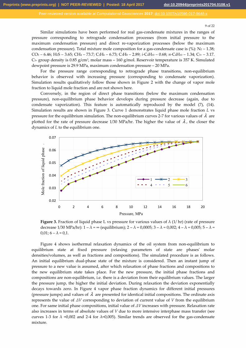
Similar simulations have been performed for real gas-condensate mixtures in the ranges of pressure corresponding to retrograde condensation processes (from initial pressure to the maximum condensation pressure) and direct re-vaporization processes (below the maximum condensation pressure). Total mixture mole composition for a gas-condensate case is (%): N2 – 1.38; CO2 – 6.46; H2S – 3.65; CH4 – 73.7; C2H6 – 6.73; C3H8 – 2.89; i-C4H10 – 0.68; n-C4H10 – 1.34; C5+ – 3.17. C5+ group density is 0.85 g/cm3, molar mass – 160 g/mol. Reservoir temperature is 357 K. Simulated dewpoint pressure is 29.9 MPa, maximum condensation pressure – 20 MPa.

For the pressure range corresponding to retrograde phase transitions, non-equilibrium behavior is observed with increasing pressure (corresponding to condensate vaporization). Simulation results qualitatively follow those shown in Figure 2 with the change of vapor mole fraction to liquid mole fraction and are not shown here.

Conversely, in the region of direct phase transitions (below the maximum condensation pressure), non-equilibrium phase behavior develops during pressure decrease (again, due to condensate vaporization). This feature is automatically reproduced by the model (7), (14). Simulation results are shown in Figure 3. Curve 1 demonstrates liquid phase mole fraction L vs pressure for the equilibrium simulation. The non-equilibrium curves 2-7 for various values of λ are plotted for the rate of pressure decrease 1/30 MPa/hr. The higher the value of λ , the closer the dynamics of L to the equilibrium one.

0.02

0.03

0.04

0.05

0.06

0.07

0 2 4 6 8 10 12 14 16 18 20

Pressure, MPa

Mol

e fr

actio

n of

liqu

id p

hase

/

1 2 3

4 5 6

Figure 3. Fraction of liquid phase L vs pressure for various values of λ (1/ hr) (rate of pressure decrease 1/30 MPa/hr): 1 – λ = ∞ (equilibrium); 2 – λ = 0,0005; 3 – λ = 0,002; 4 – λ = 0,005; 5 – λ = 0,01; 6 – λ = 0,1.

Figure 4 shows isothermal relaxation dynamics of the oil system from non-equilibrium to

equilibrium state at fixed pressure (relaxing parameters of state are phases' molar densities/volumes, as well as fractions and compositions). The simulated procedure is as follows. An initial equilibrium dual-phase state of the mixture is considered. Then an instant jump of pressure to a new value is assumed, after which relaxation of phase fractions and compositions to the new equilibrium state takes place. For the new pressure, the initial phase fractions and compositions are non-equilibrium, i.e. there is a deviation from their equilibrium values. The larger the pressure jump, the higher the initial deviation. During relaxation the deviation exponentially decays towards zero. In Figure 4 vapor phase fraction dynamics for different initial pressures (pressure jumps) and values of λ are presented for identical initial compositions. The ordinate axis represents the value of ΔV corresponding to deviation of current value of V from the equilibrium one. For same initial phase compositions, initial value of ΔV increases with pressure. Relaxation rate also increases in terms of absolute values of V due to more intensive interphase mass transfer (see curves 1-3 for λ =0,002 and 2-4 for λ=0,005). Similar trends are observed for the gas-condensate mixture.




https://doi.org/10.1007/s10596-017-9648-x

10 of 22

The examples presented indicate that phase behavior dynamics for oil and gas-condensate mixtures simulated with the proposed model (7), (14) qualitatively reproduce all the key features of non-equilibrium processes reported in experimental studies [20, 21], though direct quantitative comparison is not possible due to different types of the processes considered (isothermal / isochoric).

0

0.01

0.02

0.03

0.04

0.05

0.06

0 100 200 300 400 500 600 700 800 900 1000

Time, h

ΔV

1 2

3 4

Figure 4. Relaxation dynamics of vapor phase fraction V for various values of initial pressure (MPa) and λ (1/ hr): 1 –р = 10,3, λ = 0,002; 2 – р = 10,3, λ = 0,005; 3 –р = 17,3, λ = 0,002; 4 – р = 17,3, λ = 0,005.

5. Implementation in a compositional flow simulator

The proposed phase behavior model (7), (14) can be incorporated in existing compositional simulators without principal modifications to flow simulation algorithms. Commercially available compositional simulators (as well as general purpose academic simulators) are based on simultaneous (iterative) solution of the flow simulation equations and flash equations at each time step. With the proposed model, no changes to flow simulation algorithms are required. Calculation of interphase mass transfer terms ,i L Vω − and non-equilibrium phase compositions requires only corrections to the flash algorithm according to equations (7) and (14). Little extra memory is required to store component K-values from previous time step to calculate 1 ( )jx x t−

=

and 1 ( )jy y t− =

to be used in (14). But in the majority of current implementations of the equilibrium flash algorithm these values are also stored as initial estimates to solution at the new time step. Thus, the non-equilibrium algorithm does not require significant extra memory or execution time.

However, to implement the presented model (7), (14) in a compositional flow simulator one has to account for changing total mixture composition in a grid block during the flow process. To do that, we recall the 'embedded processes' concept. As the change in total composition is a part of the outer process, the Rachford-Rice equation [35] is solved with the 'old' K-values 1j

iK − and 'new'

total composition jz to obtain initial vapor phase fraction j

inV at the new time step satisfying mass

balance for jz . Thus, relaxation at the new time step with pressure jp and total composition jz

is

assumed to take place from the old phase compositions 1jx − and 1jy − and modified phase fractions j

inV and 1j jin inL V= − . Then equations (7), (14) are used to compute components interphase mass

transfer rates ,i L Vω − and the new phase compositions ( )jx x t t= + Δ and ( )jy y t t= + Δ

, as well as

the new phase fractions jV and jL . Note that jp (and jz for fully implicit scheme) are updated at

each Newtonian iteration within the solution of flow equations, which means that jinV , j

inL and

,i L Vω − are also updated and used in (7) to update jx

, jy

, jV and jL .




https://doi.org/10.1007/s10596-017-9648-x

11 of 22

Another specific problem of the model implementation is the choice between equilibrium and non-equilibrium phase behavior calculations at current time step in a grid block. As yet discussed, transition of a multicomponent system from single-phase to dual-phase state is a volumetric process and can be described by an equilibrium model due to short characteristic relaxation times. On the contrary, the reverse process is controlled by diffusion of components through limited interface area with much larger relaxation times and should be modelled as non-equilibrium.

For an isothermal system with fixed phase behavior type (oil or gas-condensate), parameters (e.g., maximum condensation pressure) and total composition, direction of phase transition can be predicted by the direction of pressure change. Thus decision is straightforward whether the non-equilibrium model should be used – as in the earlier presented stand-alone phase behavior cases.

In compositional flow simulations total mixture composition in a grid block changes in time which results in changing mixture parameters and even phase behavior type. We propose a universal criterion to control phase transition type based on stability analysis of individual phases. To identify whether phase transition develops volumetrically or through gas-liquid interface, we propose to examine stability of individual phases. Phase transition is equilibrium if for current direction of pressure change individual phases are unstable, i.e. components get evaporized or condensated in the volume of the phases. If the phase is stable, component transfer between phases happens only through the gas-liquid interface, i.e. in a non-equilibrium manner. Stability of phases is checked by the standard stability test [23].

More accurate treatment of the criterion is performed at individual components' level. The component transition between phases is equilibrium if the phase which the component tends to leave is unstable for given direction of pressure change. That is, one should check stability of phases and signs of ,i L Vω − for individual components.

Also we should note the problem of non-equilibrium stability analysis. Stability analysis is used for two purposes: to omit unnecessary phase split calculations and to obtain good initial guesses for K-values to ensure flash convergence to physical solution.

Discussing the first purpose we should note that although a non-equilibrium equivalent of the stability test can, in principle, be developed, it is not crucial for compositional simulations for the following reason. If currently hydrocarbon mixture in a grid block is in the single-phase state, then its phase behavior for the next time step would be equilibrium even if transition to the dual-phase state happens. Thus standard equilibrium stability test [23] is suitable to control the necessity of phase split calculations. And if the hydrocarbon mixture is yet in the dual-phase state, then it is likely that phase split calculations would be necessary for the next time step also. In this case the criterion of non-equilibrium phase transition is checked and equilibrium or non-equilibrium phase split flash system is solved to obtain the new phase state and compositions for the grid block.

As for the second purpose of stability analysis, the physical nature of relaxation process expressed in (14) prescribes that in most cases K-values taken from previous time step should serve as reasonable initial guesses for phase split calculations, especially in cases with large deviation from equilibrium (low λ values or high characteristic relaxation times). However, additional study is required for situations with large total composition changes within timestep, which are also untrivial to handle in equilibrium compositional simulations.

The non-equilibrium model (7), (14) with the criterion for non-equilibrium phase transition has been incorporated in an existing commercial EOS-based flow simulator. For illustration, some results of flow simulations with non-equilibrium phase transitions are presented here for the following test case.

The synthetic case model (Figure 5) represents a quarter of a five-spot pattern. The model is assumed homogeneous. The model parameters are: distance between wells (injector WU1_2 and producer WU1_1) – 550 m, reservoir thickness – 1 m, cell sizes along X and Y axes – from 5 to 15 m, grid dimensions – 35×35×1, effective permeability – 100 mD, effective porosity – 0.3, initial oil saturation (in fractions of effective pore volume) – 100%. Reservoir fluid properties and compositions, as well as relative permeability curves, are similar to those of the Sherkalinskaya formation Tala zone of the Krasnoleninskoye oil field. Initial reservoir pressure is 250 bar, saturation pressure – 220 bar.




https://doi.org/10.1007/s10596-017-9648-x

12 of 22

For the first 150 days, oil is produced under depletion, i.e. only the producer operates at bottom-hole pressure of 50 bar. Thus pressure in grid cells falls below the saturation pressure, and free gas appears in the model. At the day 151 water injection starts via the injector with constant bottom-hole pressure of 400 bar, while the producer continues to operate at the previously set conditions. Injection continues for as long as necessary for free gas to be dissolved in oil.

Figure 5. General 3D view of the test model grid

For the test model described, simulations were performed for a number of λ values: λ = ∞

(equilibrium), 0, 0.001, 0.005, 0.01, 0.05λ = 1/day. The simulation results for production gas-oil ratio are shown in Figure 6. Strong effect on dynamics of non-equilibrium transition of the hydrocarbon mixture from two-phase to single-phase state is clearly seen. Thus, the test case demonstrates potential application of the non-equilibrium model to history matching and forecast simulations of oil production processes influenced by non-equilibrium gas dissolution.

More details on model implementation and test simulations are presented in [37].

0

2000

4000

6000

8000

10000

12000

14000

16000

18000

1 51 101 151 201 251 301 351

Gas-

Oil R

atio

, m^3

/m^3

Days

1

2

3

4

5

6

Figure 6. Dynamics of production gas-oil ratio for different values of λ : λ = ∞ (equilibrium),

0, 0.001, 0.005, 0.01, 0.05λ = 1/day




https://doi.org/10.1007/s10596-017-9648-x

13 of 22

6. Upscaling of phase behavior model

As yet noted, one of the main causes for non-equilibrium reverse transition of hydrocarbon mixture to single-phase state (both in bulk and in porous media) is the limited liquid-vapor interface area. Though local phase behavior at each point of the whole volume may be considered equilibrium, compositions in elementary volumes are different and diffusive mass transfer between them is hindered. Therefore when considering the total volume of the mixture non-equilibrium phase behavior is observed.

We would illustrate the influence of scale effect on appearance of non-equilibrium effects by isothermal phase behavior simulations performed with oil mixture on coarse and fine scales [19]. The coarse scale model consists of a single grid block. The fine scale model has the same geometry but consists of a stack of 10 equal grid blocks. If the total system is in the dual-phase state, gravity segregation of components is taken into account on the fine grid via well-known algorithm for compositional gradient simulation [7, 35]. Pressure, phase state and composition are calculated for each fine grid block within the volume. For the grid block involving gas-oil contact (GOC), position of the interphase surface is determined from the calculated phase fractions.

The same mixture phase state may be considered on the coarse scale – for the whole volume at once. In this case, calculation is performed for integrated mixture composition obtained by weighting of the compositions in the fine grid blocks. Obviously in this case one fails to introduce compositional changes with depth, as well as the presence of GOC. However, for equilibrium processes (transition from single-phase to dual-phase state), results of the phase behavior simulations for the whole volume are equivalent on the fine (after averaging) and coarse scales.

Phase transition for the reverse process of pressure increase above the saturation pressure depends on the intensity of diffusive mass transfer across the GOC. In this case equilibrium simulation for the whole volume at once corresponds to the assumption of intensive mixing of phases, and mixture gets back to the single-phase liquid state (Figure 7b).

For the actual lab or field conditions the assumption of intensive mixing is not natural. In the locally equilibrium fine scale model mixture composition varies with depth. If mass transfer between grid blocks is limited it takes long for the system to get back to the single-phase state even for pressures well above the saturation pressure.

a) V = 0,28 b) V = 0 c) V = 0,28 (two-phase (single-phase liquid (two-phase state) state) state)

ГЖКGOC

Figure 7. Phase state simulations for isothermal pressure increase: (a) equilibrium simulation on the fine grid with no interblock mass transfer, (b) equilibrium simulation for the coarse gridblock and (c) non-equilibrium simulation for the coarse gridblock

Figure 7a shows the results of the locally equilibrium phase behavior simulation in the limiting case of no diffusive mass transfer between grid blocks. The fluid model corresponds to the oil mixture of the previous section. Here, as observed in the experiments without mixing, the two phases are still present in the volume although the pressure is greater than the equilibrium saturation pressure. Thus the process of pressure increase in the experiments without mixing may be considered as locally equilibrium with limited mass transfer between individual elementary




https://doi.org/10.1007/s10596-017-9648-x

14 of 22

volumes (Figure 7a). However, equilibrium simulation on the coarse scale is only able to reproduce the process with intensive interphase mass transfer (Figure 7b).

As shown in Figure 7c simulations on the coarse-scale with the non-equilibrium flash algorithm (7) can be used to accurately reproduce the integrated phase behavior of the system obtained in the locally equilibrium simulation (Figure 7a) using thermodynamically-consistent method that has been developed for upscaling of the flash problem [19].

The method is based on the following principle. To reproduce the system phase behavior obtained in fine scale simulations the difference between logarithms of each component's fugacities in vapour and liquid phases on the coarse scale has to be equal to the same value taken from the fine scale simulation with logarithms of fugacities averaged over the fine grid blocks.

Considering the unified formulation of the non-equilibrium phase behavior model, normalized components' interphase mass transfer rates ,i L Vω − in (7) are defined by

( ) ( ), , ,ln , ln ,i L V i L i Vf x p f y pω − = − , (15)

where angle brackets stand for mole-weighted averaging of logarithms of components' fugacities in the phases over the fine scale grid blocks.

Physical interpretation of the method is as follows. On the coarse scale it is impossible to introduce the effects of limited mass transfer within a grid block explicitly. Thus equivalent counterbalancing components' flows (or – counterbalancing potentials) ,i L Vω − are introduced to force the system get in the same integral phase state.

In practical implementation of the method the values of ,i L Vω − obtained by averaging the fine-scale simulation results may be parameterized as functions of pressure, certain phase fraction or total mixture composition.

The proposed approach provides an alternative to standard techniques for upscaling of compositional models like the well-known method of alpha factors and its variations [4, 5, 11]. The new method is characterized by more accurate representation of the physics, simplicity of implementation without intervention to flow simulation algorithms and applicability not only to oil recovery processes by gas injection but to a wide variety of oil and gas flow problems with intensive phase transitions.

It should be pointed out that almost identical method for upscaling was presented in [33]. However, in that study both the formulation of the left hand side of equations (7) and the calculations of the right hand side in the upscaling process are based on differences between components' fugacities, not their logarithms. This doesn't make difference for the resulting coarse-scale solution in terms phase fractions and compositions. However, in the formulation of [33] one is unable to give physical interpretation of both sides of the flash equations in terms of acting potentials or interphase mass transfer intensity. Thus application of the method is limited only to upscaling in case of equilibrium fine-scale simulations.

The upscaling method described herein is based on unified physical formulation (7) for non-equilibrium flash equations on either scale. Physically the 'driving force' responsible for system deviation from equilibrium and components' interphase mass transfer is the difference of chemical potentials. By definition, normalized difference of chemical potentials is the difference of logarithms of fugacities. Thus both sides of (7) have clear physical interpretation, and the upscaling method follows the unified formulation of the non-equilibrium phase behavior model. Therefore it can be used for upscaling both equilibrium and non-equilibrium fine-scale models, considering non-equilibrium effects not necessarily associated with scale.

As experimentally shown in [8, 15], characteristic relaxation times for non-equilibrium phase transitions due to segregation in hydrocarbon mixtures are estimated by tens of hours for experimental cells few centimeters in height. Characteristic time for these processes is governed by diffusion across the vapor-liquid interface and scales proportionally to characteristic vertical length of the cell. Hence even fine-scale (geologic-scale) simulation models may require non-equilibrium treatment of phase behavior. Other mechanisms, such as porous medium influence or incomplete mixing of phases, may also require non-equilibrium fine-scale simulations. In either case, the




https://doi.org/10.1007/s10596-017-9648-x

15 of 22

unified flash formulation (7) with the relaxation model (18) may be used with fine-scale λ values matched to scaled experimental data or available field data.

Due to unified formulation of the non-equilibrium flash equations, two options are then available for transition to coarse scale. The first one is to apply the upscaling method and compute parametrized ,i L Vω − values for coarse-scale simulations with non-equilibrium flash formulation (7). The second option is to re-match λ values in the relaxation model (18) for coarse-scale simulations. Note that in the latter case we should expect coarse-scale λ to be a function of reservoir properties and local grid-block sizes, while upscaled ,i L Vω − should also depend on dynamic variables like pressure and liquid/vapor phase fractions.

Thus, dealing with non-equilibrium compositional simulation, upscaling and history matching on the same basis of the modified flash system (7) provides principal basis for unified simulation workflow with non-equilibrium phase behavior occurring on different scales. Careful implementation of the multiscale workflow for different practical scenarios is the subject for future studies.

7. Non-equilibrium condensate revaporization and the non-equilibrium constant volume depletion (NCVD) algorithm

Non-equilibrium phase behavior simulations are required when actual dynamics of hydrocarbon recovery cannot be reproduced by equilibrium models. One example of this kind is the dynamics of condensate recovery at the late stage of gas-condensate field development.

The majority of gas condensate fields are developed by pressure depletion. At the late stage of development reservoir pressure falls below the maximum condensation pressure, and the process of retrograde condensation is replaced by direct revaporization. Thus the direction of phase transitions changes from increasing to decreasing of the hydrocarbon liquid phase fraction resulting in the non-equilibrium phase behavior.

Experimental data of constant volume depletion (CVD) [35] are used for matching pVT-model of the reservoir hydrocarbon mixture. At each stage of the CVD experiment mixing of phases in the bulk is carried out to assure equilibrium conditions. Same equilibrium concept holds in the mathematical simulations of the CVD process. Matched pVT-model is involved in phase behavior and compositional flow simulations, including forecast of condensate recovery dynamics. Experimental and simulated CVD data are also directly used for reservoir engineering calculations, as well as to control consistency between the pVT model and the integral field data on condensate recovery dynamics during depletion [7, 35].

Figure 8, according to [13], shows the actual (by averaged well production data) and predicted (by equilibrium experiments) curves of the condensate (group С5+) content in reservoir gas of Vuktylskoye field. The experimental Curve 1 corresponds to the average composition of the initial gas-condensate system. The actual Curve 2 is shown in [13] to be influenced by the change in time of the gas production interval depths. That explains the difference between the curves for pressures above 5 MPa, and the difference almost vanishes at that value of pressure. Curve 2 is based on production data of 'dry field' wells only, i.e. it is not influenced by inflow of condensate in liquid phase and it reflects composition of the gas phase only.

Although condensate production dynamics of individual wells is thought to be influenced by fluid redistribution and reservoir heterogeneity, we note that integral field data of Curve 2 in Figure 8 reasonably reproduces the behavior of experimental Curve 1 in the region of retrograde processes (above 5 MPa). This fact is in accordance with long-term experience of data analysis for gas-condensate fields during depletion [7, 35]. Thus we conclude that phase behavior controls the integral dynamics of С5+ recovery by 'dry field' wells and follow a common reservoir engineering concept which treats CVD data as a basis for field-scale forecast of condensate production in the gas phase.

However, if we look at the region of pressures less than 5 MPa, an increasing deviation of the actual Curve 2 from the predicted Curve 1 is clearly seen. Note that this deviation starts exactly at the pressure of minimal С5+ content which corresponds to the change from С5+ condensation to С5+




https://doi.org/10.1007/s10596-017-9648-x

16 of 22

evaporation. Recalling the fact that condensation is an equilibrium process while evaporation is non-equilibrium, we conclude that non-equilibrium phase behavior model is required for proper description of actual condensate recovery dynamics in the gas phase below the maximum condensation pressure.

To simulate the actual dynamics of condensate revaporization at low pressures an algorithm was developed for non-equilibrium constant volume depletion simulations (NCVD). The difference between the equilibrium and the non-equilibrium CVD algorithms lies in the calculation of phases’ fractions and compositions at each pressure step. In the NCVD algorithm the non-equilibrium model (7), (14) is used instead of the equilibrium equations (2).

Figure 8. Dynamics of the C5+ content in reservoir gas for Vuktylskoye field: 1 - predicted, 2 - actual The NCVD algorithm may be described as follows. First, we use actual data on reservoir

pressure dynamics to form a sequence of time steps jtΔ and pressure values jp . Following the

'embedded processes' concept, at each step we assume pressure change from 1jp − to jp followed

by system relaxation during the period jtΔ . This means that we use 'old' phase compositions, 'new' pressure jp and jtΔ to compute normalized difference of chemical potentials ,i L Vω − at the end of the period using (14). Then non-equilibrium flash system (7) is used to compute 'new' phase fractions and compositions. (Note that depending on jtΔ and the rate of pressure change, calculated phase fractions and compositions may significantly differ from the equilibrium ones.) Then the 'extra' volume of gas phase ('produced' gas) at this stage is calculated, just as in the equilibrium CVD algorithm [35], and molar fractions of the phases are adjusted accordingly. The algorithm proceeds to the next pressure (and time) step.

The NCVD algorithm has been applied to the case of Vuktylskoe field. A pVT-model of the gas-condensate system is based on the Peng-Robinson three-parameter equation of state [18, 31] and well-known methods of phase behavior simulations for multicomponent hydrocarbon systems [23, 24]. The pVT-model has been matched to results of lab experiments using the method described in [36]. The results of the matching are shown in Figure 9. Initial composition of the reservoir fluid is, % mol: N2 – 5,01; CO2 – 0,04; C1 – 74,85; C2 – 8,56; C3 – 3,47; iC4 – 0,45; nC4 – 0,80; iC5 – 0,16; nC5 – 0,14; С6+ – 6,52 (split into 6 pseudocomponents: C6+(1) – 2,08; C6+(2) – 2,67; C6+(3) – 1,38; C6+(4) – 0,35; C6+(5) – 0,04; C6+(6) – 0,003).

Since non-equilibrium phase behavior occurs during condensate revaporization, the NCVD algorithm was used for pressures below 5 MPa. Average reservoir pressure vs. time was taken from

C5+

in g

as, g

/m3

Pressure, MPa




https://doi.org/10.1007/s10596-017-9648-x

17 of 22

the actual field data and is shown in Figure 10. Parameter λ in equation (14) was used as a control parameter to match the NCVD simulation results to the actual data of condensate recovery.

Simulated dynamics of C5+ content in reservoir gas for different values of λ are shown in Figure 11. Curve 1 is the equilibrium experimental curve of Figure 8. Curve 2 corresponds to the actual curve of Figure 8. Curve 3 for λ→∞, which is equivalent to equilibrium simulation, provides a close approximation to Curve 1. Reasonable approximation to actual data of Curve 2 is achieved with λ=0,032 1/year (Curve 5).

0

50

100

150

200

250

300

350

400

0 5 10 15 20 25 30 35

Pressure, MPa

C5+

in g

as, g

/m3

pVT-model

Experiment

Figure 9. Results of the pVT model matching to the lab CVD data for the reservoir mixture of Vuktylsloye field

0

1

2

3

4

5

6

1985 1990 1995 2000 2005 2010 2015

Year

Pres

sure

, MPa

Figure 10. Average reservoir pressure vs. time for Vuktylskoye field




https://doi.org/10.1007/s10596-017-9648-x

18 of 22

40

50

60

70

80

90

100

110

120

130

1 1.5 2 2.5 3 3.5 4 4.5 5 5.5 6

Pressure, MPa

C5+

in g

as, g

/m3

1 2 34 5 67

Figure 11 C5+ content in reservoir gas vs pressure: 1 - experimental [13]; 2 - actual [13]; 3-7 - simulated: 3 - λ→∞ (equilibrium); 4 - λ=0,1 1/year; 5 - λ=0,032 1/ year; 6 - λ=0,01 1/ year; 7 - λ=0 For illustrative purposes another two simulated non-equilibrium dynamics are also shown in

Figure 11 by Curves 4 and 6. Curve 7 corresponds to the limiting case of infinitely slow condensate revaporization (λ=0). For clarity of comparison with the simulated data, Curves 1 and 2 in Figure 11 are normalized by the value of minimal С5+ content in reservoir gas at 5 MPa.

Thus the actual dynamics of condensate recovery for Vuktylskoye field at low reservoir pressures have been satisfactory matched by the proposed NCVD simulation algorithm and the non-equilibrium model (7), (14).

The physical meaning of parameter λ is the inverse of the characteristic relaxation time. Hence, the characteristic relaxation time for condensate revaporization in the Vuktylskoye reservoir system at low pressures is about 30 years. Considering scale effect this value is in good agreement with the results of calorimeter-cell experimental studies of non-equilibrium phase behavior of hydrocarbon mixtures both in bulk and porous media [8, 15] – see Figure 12. However this value is valid only for the integral phase behavior of Vuktylskoe gas-condensate field. One should take into account that relaxation times for the same processes on smaller scales (e.g., on the scale of grid blocks of a flow model) would also be proportionally smaller.

Figure 12. Characteristic relaxation times according to calorimeter cell experiments [15, 8] and model matching of Vuktylskoe field data




https://doi.org/10.1007/s10596-017-9648-x

19 of 22

8. Conclusions

In the paper we have presented and discussed unified non-equilibrium phase behavior model for stand-alone and compositional flow simulations.

Introduction of non-equilibrium phase transitions in compositional flow simulations is essential for consistent history matching and increased accuracy of production forecast. The presented model of non-equilibrium phase behavior requires no modifications to the form of compositional flow equations but only corrections to the flash problem formulation. Hence it is ready to be implemented in existing compositional simulators without principal modifications to flow simulation algorithms.

A physical method for calculation of components' interphase mass transfer rates has been developed which enables robust history matching of the non-equilibrium model to actual system relaxation dynamics with account for variations of pressure and total composition. Simulation results for test cases with real oil and gas-condensate mixtures demonstrate principal correspondence with experimental data on the physics of non-equilibrium processes.

Specifics of the model implementation in a commercial compositional simulator have been studied. A special criteria has been developed based on individual phases' stability for choosing between equilibrium and non-equilibrium flash calculations at current time step in a grid block.

The influence of scale on the significance of non-equilibrium effects has been demonstrated and an upscaling technique suitable for both equilibrium and non-equilibrium fine-scale compositional models has been presented.

Simulation algorithm for non-equilibrium constant volume depletion (NCVD) has been developed and successfully applied to history matching of the actual condensate recovery data at low pressures for Vuktylskoye field. Considering the similarity principle, the estimated value of characteristic relaxation time of the reservoir fluid system is in accordance with reported experimental data.

Acknowledgements: Authors are thankful to A.I. Brusilovsky, E.S. Zakirov, K.Yu. Bogachev, E.E. Gorodetskii and T.S. Yushchenko for fruitful discussions during the study, and gratefully acknowledge the permission from Rock Flow Dynamics to incorporate and test the developed algorithms in the numerical code of the RFD tNavigator® flow simulator.

Nomenclature

V, L – molar fractions of vapor and liquid phases; N – number of components in a hydrocarbon mixture;

Vk , Lk – relative permeabilities of vapor and liquid phases; μ – viscosity; ρ – molar density; ρ – mass density; p – pressure; m – effective porosity; k – effective permeability (permeability to oil at irreducible water saturation); S – saturation normalized by the effective pore volume;

iy , ix – molar fractions (concentrations) of component i in vapor and liquid phases;

ii

i

yK

x= – K-value for component i;

iq – molar intensity of a source/sink for component i; h – depth; g – gravity acceleration; fi,V, fi,L – fugacities of component i in vapor and liquid phases; zi – total mole fraction of component i in hydrocarbon mixture;




https://doi.org/10.1007/s10596-017-9648-x

20 of 22

,i L Vω − – normalized rate of component i interphase mass transfer; x

, y

– compositions of vapor and liquid phases; t – time;

tΔ – time step size; R – universal gas constant; T – absolute temperature; M – molar weight; z – vertical coordinate; ε – flash convergence tolerance;

0iμ – chemical potential of component i in ideal gas condition at temperature T and unit pressure.

Subscripts

V – vapor phase; L – liquid phase; in – initial value for relaxation at current timestep; i – index of a mixture component.

Superscripts

j, 1j − – timestep number, (m) – flash iteration.

References

1. Al-Wahaibi Y.M., Muggeridge A.H., Grattoni A.C. [2006] Gas/oil nonequilibrium in multicontact miscible displacement within homogeneous porous media. Paper SPE 99727 presented at SPE/DOE Symposium on Improved Oil Recovery, Tulsa, Oklahoma, 2006.

2. Aziz K., Settari A. [1979] Petroleum reservoir simulation. New York: Elsevier. 3. Aziz K., Wong T. [1989] Considerations in the development of multipurpose reservoir

simulation models. First and Second Forum on Reservoir Simulation, Alpbach, Austria, pp. 77-208. 4. Barker J.W., Fayers F.J. [1994] Transport coefficients for compositional simulation with coarse

grids in heterogeneous media. SPE Advanced Technology Series, Vol. 2, No. 2, pp. 103-112. SPE Paper 22591.

5. Bourgeois M.J., Gommard D.R., Gouas H. [2012] Simulating early gas breakthrough in undersaturated oil using alpha-factors. Paper SPE 161460 presented at Abu Dhabi International Petroleum Exhibition & Conference, Abu Dhabi, UAE, 11-14 November 2012.

6. Brilliant L.S., Evdoshchuk P.A., Plitkina Yu.A. et al. [2014] Study of effective brownfield development by the means of oil resaturation with evolved gas in situ. Neftyanoye Khoziaystvo (Oil Industry). 2014. No. 4. P. 54-59. (In Russian)

7. Brusilovsky A.I. [2002] Fazovye prevrashcheniya pri razrabotke mestorozhdeniy nefti i gaza (Phase Transitions in the Development of Oil and Gas Fields). Moscow: Graal Publ., 575 p. (In Russian)

8. Buleyko V.M. [2007] Zakonomernosti fazovykh prevrasheniy uglevodorodnykh smesey v neftegazonosnykh plastakh razrabatyvaemykh mestorozhdeniy (The principles of phase behavior of hydrocarbon mixtures in oil- and gas-bearing formations of developed reservoirs) Dr.Tech.Sci Thesis, Moscow, VNIIGAS-OGRI RAS, 2007, 277 p.(In Russian)

9. Coats K., Smith B. [1964] Dead-end pore volume and dispersion in porous media. SPE Journal, Vol. 41, 1964, P. 73–84.

10. Coats K.H. [1989] Implicit Compositional Simulation of Single-Porosity and Dual-Porosity Reservoirs, SPE 18427 presented at the SPE Symposium on Reservoir Simulation, Houston, Texas, February 6-8, 1989.

11. Coats K.H., Thomas L.K., Pierson R.G. [2007] Simulation of Miscible Flow Including Bypassed Oil and Dispersion Control. SPE Reservoir Evaluation and Engineering, Vol. 10, No. 5, October 2007




https://doi.org/10.1007/s10596-017-9648-x

21 of 22

12. Danesh A. [1998] PVT and Phase Behavior of Petroleum Reservoir Fluids. Elsevier Science B.V.. 13. Dolgushin N.V. [2007] Metodologia izucheniya gazokondensatnoy kharakteristiki

neftegazokondensatnikh mestorojdeniy s vysokim soderjaniem kondensata i bolshim etajom gazonosnosti (Methodology of gas condensate characteristics study of oil-gas-condensate fields with high condensate content and large gas column). DrSci Thesis, Ukhta, Russia.

14. Firoozabadi A. [1999] Thermodynamics of Hydrocarbon Reservoirs. New York: McGraw-Hill. 15. Gorodetskii E.E., Voronov V.P., Muratov A.R. et al. [2005] Study of non-equilibrium phase

transitions in binary and ternary hydrocarbon mixtures. OGRI RAS Research Report, Moscow, 2005.

16. Indrupskiy I.M., Lobanova O.A. [2015] Simulation of nonequilibrium phase behavior of hydrocarbon mixtures. Doklady Earth Sciences, 2015, Vol. 463, Part 1, P. 695-698.

17. Iranshahr A., Chen Yu., Voskov D. [2014] A coarse-scale compositional model. Computational Geosciences, Vol. 18 (2014), P. 797-815.

18. Jhavery B.S., Youngren G.K. [1988] Three-parameter modification of the Peng-Robinson equation of state to improve volumetric predictions SPE Reservoir Engineering 1988. V. 3. P. 1033.

19. Lobanova O.A., Indrupskiy I.M. [2012] Non-equilibrium and scale effects in modeling phase behavior of hydrocarbon mixtures (Neravnovesnye i masshtabniye effekty v modelirovanii fazovogo povedeniya uglevodorodnykh smesey). Neftyanoye Khoziaystvo (Oil Industry). 2012. No. 6. P. 18-23

20. Lobanova O.A., Indrupskiy I.M. [2015] Modelling Non-Equilibrium Phase Behavior of Hydrocarbon Mixtures. Paper SPE 176632-MS presented at SPE Russian Petroleum Technology Conference, 26-28 October 2015, Moscow, Russia

21. Lobanova O.A., Zubov V.R., Indrupskiy I.M [2014] Neravnovesnoye fazovoye povedeniye uglevodorodnykh smesey. Chast 1: eksperimenty (Non-equilibrium phase behavior of hydrocarbon mixtures. Part 1: experiments). Avtomatizatsiya, telemekhanizatsiya i svyaz v neftyanoy promyshlennosti. 2014. No. 11. P. 18-23.

22. Lobanova O.A., Indrupskiy I.M., Yushchenko T.S. [2016] Modeling non-equilibrium dynamics of condensate recovery for mature gas-condensate fields. // SPE Russian Petroleum Technology Conference and Exhibition, Moscow, Russia, 24–26 October 2016. SPE 181977.

23. Michelsen M.L. [1982a] The Isothermal Flash Problem. Part I. Stability. Fluid Phase Equilibria, 9, P. 1-19.

24. Michelsen M.L. [1982b] The Isothermal Flash Problem. Part II. Phase-Split Calculation. Fluid Phase Equilibria, 9, P. 21-40.

25. Nigmatulin R.I., L. M. S., Fedorov K. M. [1980] Mathematical modelling of micellar-polymer-gas flooding. Dokl. Of USSR Academy of Sciences. Vol. 255, No. 1. P. 52-56.

26. Nghiem L.X., Sammon P.H. [1997] A non-equilibrium equation-of-state compositional simulator. Paper SPE 37980 presented at SPE Reservoir Simulation Symposium, Dallas, USA, 8-11 June 1997.

27. Nghiem L.X., Li Y.K., Agarwal R.K. [1989] A method for modelling incomplete mixing in compositional simulation of unstable displacements. Reservoir Simulation Symposium, Houston, USA, Feb. 6-8, 1989. SPE 18439.

28. Onsager L. [1931] Reciprocal Relations in Irreversible Processes. I., Phys. Rev. 37, P. 405–426. 29. Patacchini L., Duchenne S., Bourgeois M., Moncorge A., Pallotta Q. [2014] Simulation of

residual oil saturation in near-miscible gas flooding through saturation-dependent tuning of equilibration constants. Abu Dhabi International Petroleum Exhibition & Conference, Abu Dhabi, UAE, 10-13 November 2014. SPE 1714806.

30. Pedersen K.S., Christensen P.L. [2006] Phase Behavior of Petroleum Reservoir Fluids. Taylor & Francis, Bota Raton, USA.

31. Peng D.Y., Robinson D.B. [1976] A new two-constant equation of state. Ind. Eng. Chem. Fundam. Vol. 15, P. 59.




https://doi.org/10.1007/s10596-017-9648-x

22 of 22

32. Rozenberg M.D., Kundin S.A. [1976] Mnogofaznaya mnogokomponentnaya fil'tratsiya pri dobyche nefti I gaza (Multiphase multicomponent flow at oil and gas development). Moscow: Nedra Publ., 335 p.

33. Salehi A., Voskov D.V., Tchelepi H.A. [2013] Thermodynamically Consistent Transport Coefficients for Upscaling of Compositional Processes. Paper SPE 163576 presented at SPE Reservoir Simulation Symposium, Woodlands, Texas USA, 18-20 February 2013.

34. Usenko V.F. [1967] Issledovaniye neftyanykh mestorojdeniy pri davleniyah nije davleniya nasystcheniya (Oil reservoir testing at pressures below saturation pressure), Moscow: Nedra Publ., 1967, 214 p.

35. Whitson C.H., Brule M.R. [2000] Phase Behavior. SPE Monograph (Henry L. Doherty) Series, Vol. 20, SPE, Richardson, Texas USA, 233 p.

36. Yushchenko T.S., Brusilovsky A.I. [2016] Mathematical modeling of gas-condensate mixture PVT-properties including presence of brine in reservoir. Fluid Phase Equilibria, 409 (2016), pp. 37-48.

37. Zubov V.R., Indrupskiy I.M., Bogachev K.Yu. [2016] Compositional simulator with non-equilibrium phase transitions. SPE Russian Petroleum Technology Conference and Exhibition, 24-26 October 2016, Moscow, Russia. SPE 182001-MS




https://doi.org/10.1007/s10596-017-9648-x

Non-Equilibrium Phase Behavior of Hydrocarbons in ...

Documents

Transcript of Non-Equilibrium Phase Behavior of Hydrocarbons in ...