
Non-Commutative Topology and Topological...
26
Non-Commutative Topology and Topological Quantisation Johannes Kellendonk Institut Camille Jordan, Universit ´ e Lyon 1 Quy Nho’n, July 2017
Transcript of Non-Commutative Topology and Topological...

Non-Commutative Topology andTopological Quantisation
Johannes Kellendonk
Institut Camille Jordan, Universite Lyon 1
Quy Nho’n, July 2017
KeywordsI Bulk Boundary CorrespondanceI Topological QuantisationI Topological InsulatorsI K -theoryI Cyclic cohomologyI K -homology

OverviewInsulators and their boundary
Consider a high pressure and a low pressure system in theatmosphere. How does the wind blow in high altitude?
I Coriolis force is perpendicular to the wind directionI Gradient force balances Coriolis force (are parallel)I Hence wind blows parallel to lines of equal pressure!
No air flows from the high to the low: system is an insulator.
So does the pressure difference remain?I On the ground there is friction (opposite to wind direction)I Gradient force balances Coriolis force and frictionI Hence there is a wind component parallel to pressure gradient!
Along the boundary is air flow from high to low: transport at boundary.Similar phenomenon occurs in the classical Hall effect.The systems we are interested in are
bulk insulating & boundary conductingThis is a bulk boundary effect.

OverviewInsulators and their boundary
Consider a high pressure and a low pressure system in theatmosphere. How does the wind blow in high altitude?
I Coriolis force is perpendicular to the wind directionI Gradient force balances Coriolis force (are parallel)I Hence wind blows parallel to lines of equal pressure!
No air flows from the high to the low: system is an insulator.
So does the pressure difference remain?
I On the ground there is friction (opposite to wind direction)I Gradient force balances Coriolis force and frictionI Hence there is a wind component parallel to pressure gradient!
Along the boundary is air flow from high to low: transport at boundary.Similar phenomenon occurs in the classical Hall effect.The systems we are interested in are
bulk insulating & boundary conductingThis is a bulk boundary effect.

OverviewInsulators and their boundary
Consider a high pressure and a low pressure system in theatmosphere. How does the wind blow in high altitude?
I Coriolis force is perpendicular to the wind directionI Gradient force balances Coriolis force (are parallel)I Hence wind blows parallel to lines of equal pressure!
No air flows from the high to the low: system is an insulator.
So does the pressure difference remain?I On the ground there is friction (opposite to wind direction)I Gradient force balances Coriolis force and frictionI Hence there is a wind component parallel to pressure gradient!
Along the boundary is air flow from high to low: transport at boundary.
Similar phenomenon occurs in the classical Hall effect.The systems we are interested in are
bulk insulating & boundary conductingThis is a bulk boundary effect.

OverviewInsulators and their boundary
Consider a high pressure and a low pressure system in theatmosphere. How does the wind blow in high altitude?
I Coriolis force is perpendicular to the wind directionI Gradient force balances Coriolis force (are parallel)I Hence wind blows parallel to lines of equal pressure!
No air flows from the high to the low: system is an insulator.
So does the pressure difference remain?I On the ground there is friction (opposite to wind direction)I Gradient force balances Coriolis force and frictionI Hence there is a wind component parallel to pressure gradient!
Along the boundary is air flow from high to low: transport at boundary.Similar phenomenon occurs in the classical Hall effect.The systems we are interested in are
bulk insulating & boundary conductingThis is a bulk boundary effect.

OverviewTopological quantisation
I Roughly, a quantity is topologically quantised if it is invariantunder continuous deformation (homotopy)
I Topological quantisation should rather be called homotopic quantisation.It has nothing to do with the usual quantisation of quantum mechanics
I In early examples these quantities were integer valued
I What means continuous deformation?Need topological background space with non-trivial homotopy classes
I Examples:1. Rank of a projection in space of projections of MN(C)2. Index of a Fredholm operator in the space of Fredholm operators3. Chern number of a vector bundle
I Physical examples are wave mechanical (operator algebras)I Topologically quantised numbers serve two purposes
I mathematically as invariants of homotopy classesI physically as quantised transport coefficients (Nobel prize 2016)

OverviewQuantum mechanical insulators
I An insulator is described by a Schrodinger equation with aHamiltonian which has a gap � in its spectrum
I All states below the gap are occupied whereas those above thegap are empty.
I Excitation of an occupied state needs an amount of energywhich is at least as large as the size |�| of the gap
I Their probability decays as e�|�|T if the temperature T �! 0.
Excitations are therefore suppressed and so is the transport.I We may shift the gap to energy 0
insulator = self-adjoint invertible operatorand occupied states are precisely the states of negative energy
I Insulators belong to the same topological phase if they can bedeformed into each other preserving self-adjointness andinvertibility

OverviewSymmetry protection
I Notion of topological phase may be refined by ”symmetry”I A symmetry is usually represented by a C-linear map which
preserves the Hamiltonian HI Here we allow for ”extra ordinary symmetries” which may be
anti-linear or anti-preserve the HamiltonianI time reversal (TRS) is anti-linear and preserves HI particle hole exchange (PHS) is anti-linear and maps H to �HI chiral symmetry (CS) is C-linear and maps H to �H
I Insulators belong to the same symmetry protected topologicalphase if they can be deformed into each other preservingself-adjointness, invertibility and the symmetry
I the ”extra ordinary symmetries” need extra ordinary treatment

OverviewPlan of the cours
I Tasks1. Develop a computable theory of symmetry protected topological
phases and classify them2. Define numerical topological invariants and relate them to physics3. Explain the bulk-boundary correspondance
I Tools:1. Physical models for insulators2. How they relate to C⇤-algebras3. K -theory of real and complex C⇤-algebras4. Cyclic cohomology and its pairing with K -theory5. Exact sequences of C⇤-algebras and boundary maps

I Models for insulatorsThe local structure 1
We will describe the atomic configuration of the material bycolored Delone sets of finite local complexity (FLC).
I Delone set L is a relatively dense, uniformly discrete subset ofRd
I relat. dense: 9rmax everywhere is a point within distance rmaxI unif. discrete: 9rmin everywhere within dist. rmin is at most 1 point
I A decoration of L by colors of a finite set C is a map L• : L! C.We view L• also as the colored set.
I L• has finite local complexity if, for any R, there are only finitelymany R-patches up to translation
I the R-patch at x 2 L is restriction of L• to BR(x) \ L(set of colored points in BR(x))
I Denote BR[L• � x ] the R-patch of L• � x = {y � x |y 2 L•} at 0,then {BR[L• � x ] : x 2 L} is finite.
I L is the set of atomic positions of the materialI the coloring allows to distinguish the atomic type

I Models for insulatorsThe local structure 2
RecallI the R-patch at x 2 L is restriction of L• to BR(x) \ LI BR[L• � x ] = R-patch of L• � x at 0
= R-patch of L• at x shifted to the originThe local structure of material is encoded in the R-patches of L•.
I A function f : L! Y (a set) is called strongly pattern equivariantfor L• if, for some R > 0, its value at x 2 L depends only onBR[L• � x ].We also say that the values of f are locally derivable from L•.
I such a function takes only finitely many valuesI A subset X ⇢ Rd is locally derivable from L• if the indicator
function 1X is strongly pattern equivariant for L•.I CL•(L) ⇢ C(L) is the sup-norm closure of strongly pattern
equivariant (for L•) functions f : L! C.I 8✏ > 09R > 0 s.th. |f (x)� f (x 0)| < ✏ if BR[L• � x ] = BR[L• � x 0].
Call such functions pattern equivariant (they are determined by thelocal structure)

Example: Penrose tiling, model for quasicrystalTilings and colored Delone sets are mutually locally derivable
I Coloring is strongly pattern equivariantI Set of centers of 5-stars is locally derivable from tiling

I Models for insulatorsBulk models 1
Bulk models are quantum mechanical models for physical processesinside material: no boundary. Atomic positions and type are encodedby L•, L relatively dense in Rd .
I Tight binding approximation: (quasi) particles are tight to theatoms, occupy a finite number of states
I Hilbert space is `2(L)⌦CN , for some finite N. The internal spaceCN accounts for different atomic species and their internaldegrees of freedom (spin).
I The Hamiltonian H for the Schrodinger equation i~ @@t = H
describing a particle moving in the insulator has the form
H (x) =X
y2LHxy (y) (1)
where (x) 2 CN , so each Hxy is an element of MN(C).I Complex matrix coefficients may be interpreted as internal
magnetic fields, (spin-orbit coupling or the like)

I Models for insulatorsBulk models 2
Recall the form of the Hamiltonian
H (x) =X
y2LHxy (y) (2)
(x) 2 CN . RequirementsI Short range: kHxyk decays sufficiently fast when kx � yk ! 1.I Locality: In the absence of external fields, Hxy depends only on
the local environment around x and y in L•.I Self-adjointness: H is self-adjoint (observable of energy).I Insulating: H has a gap � in its spectrum at the Fermi-energy.
I 8E 2 � = (E0, E1): H � E1 is invertible.I All states of energy E0 are occupied and � E1 unoccupied.
Replacing H by H � E1 we have 0 2 �, i.e. H is invertible andnegative energy states occupied.

I Models for insulatorsBulk models 3
The only external fields we look at are magnetic fields. They areincorporated via a vector potential by Peierl’s substitution
I An external magnetic field B(x), x 2 Rd , is a 2-form.I B has a vector potential A, i.e. a 1-form such that B = dA.I A is not unique and the choice of A is referred to as the choice of
gauge.I Peierl’s substitution (minimal coupling): Multiply the translation
operator from x to y with the phase exp(i�xy )
�xy =q~
Z
[x,y ]A
Thus Hxy has to be substituted by Hxy exp(i�xy ).

I Models for insulatorsPeriodic bulk models
A model is periodic if its Hamiltonian H is invariant under translationby vectors from a regular (rank d) lattice ⇤ ⇢ Rd .
I L• is ⇤-invariant and hence also L is ⇤-invariant.|L/⇤| = K is finite (no accidental invariance).
I choose representatives {r1, · · · , rK} for L/⇤ so x = � + ri
I unitary transformation `2(L) ! `2(⇤)⌦ CK : �x 7! �� ⌦ �i
Hxx0 = H(�,i)(�0,i0)
I Invariance of H means H(�,i)(�0,i0) = H(�+µ,i)(�0+µ,i0) 8µ 2 ⇤ and so thereare matrix valued functions Hi,i0 : ⇤ ! MN(C) such that
H(�,i)(�0,i0) = Hi,i0(�� �0)
I H is thus given by a function H : ⇤ ! MNK (C).I The Fourier transformation of H yields a continuous function
H : Rd/⇤rec ! MNK (C)
I H is self-adjoint iff H(k) is a self-adjoint matrix for each k .I Position ri in elementary cell is encoded by color, L (and L•) are
decorations of ⇤.

Example: Haldane model 1
Haldane [Nobel prize 2016] model.I Let ⇤ is lattice generated by b1, b2 and b3 = �b1 � b2.I L = LA [ LB, two orbits, LA = ⇤, LB = ⇤+ a1 (hexagonal ”lattice”),
So L = ⇤• with two colors (A- and B-sublattice).I Real parameters, M, t , t2, '.
Hxx =
⇢M if x 2 LA�M if x 2 LB
onsite, distinguishes sublattices
Hxy = t if y � x = ±ai nearest neighbour
Hxy =
⇢t2ei' if y � x = +bit2e�i' if y � x = �bi
next nearest neighbour
c1 =1
4�
�
BZ
�h
�h�3·���h� kx� �
�h� ky
�dkx � dky (24)
One recognises in the expression (21) the index of the map �h (see Appendix C). Hence, the first Chernnumber c1 = deg(�h, 0). This identification provides a geometrical interpretation of the Chern number in the caseof two-band insulators. When k spreads over Brillouin torus, �h describes a closed surface �. The Chern numbercan then be viewed as
– the (normalized) flux of a magnetic monopole located at the origin through the surface �– the number of times the surface � wraps around the origin (in particular, it is zero if the origin is « outside »� ; more precisely it is the homotopy class of � in the punctured space �3 � 0)
– the number of (algebraically counted) intersections of a ray coming from the origin with �, which is themethod used in [29].
3.5. Haldane’s model3.5.1. General considerations
In this section, we consider an explicit example of such a two band model displaying a topological insulatingphase, namely the model proposed by Haldane [5]. Besides its description using the semi-metallic graphene,Haldane’s model describes a whole class of simple two bands insulating phases with possibly a nontrivialtopological structure, and proposes a description of one of the simplest examples of a topological insulator,namely a Chern insulator. In this model, both inversion symmetry and time-reversal symmetry are simultaneouslybroken in a sheet of graphene. Inversion symmetry is broken by assigning different on-site energies to the twoinequivalent sublattices of the honeycomb lattice, while time-reversal invariance is lifted by local magnetic fluxesorganized so that the net flux per unit cell vanishes. Therefore, the first neighbors hopping amplitudes are notaffected by the magnetic fluxes, whereas the second neighbors hopping amplitudes acquire an Aharonov–Bohmphase.
3.5.2. NotationsWe consider a tight-binding model of spinless electrons on a two-dimensional hexagonal (honeycomb) lattice.
Crucially, this lattice is not a Bravais lattice, and the cristal is described as a triangular Bravais lattice with twonon-equivalent atoms in a unit cell, hence its description requires a two-level Hamiltonian. Let us denote by A andB the two inequivalent sublattices corresponding to those atoms (See Fig. 5). The lattice parameter a, defined asthe shortest distance between nearest neighbors, sets the unit of length: a = 1.
A
B a1a2
a3
b1
b2
b3
Figure 5: Honeycomb lattice used in Haldane’s model
The vectors between nearest neighbors, i.e. between sites of different sublattices A and B, are:
a1 =��
3/21/2
�a2 =���
3/21/2
�a3 =�
0�1
�= �(a1 + a2), (25)
whereas the vectors between second-nearest neighbors belonging to the same sublattice are:
10
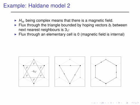
Example: Haldane model 2
I Hxy being complex means that there is a magnetic field.I Flux through the triangle bounded by hoping vectors bi between
next nearest neighbours is 3'I Flux through an elementary cell is 0 (magnetic field is internal)
−6��
�
�
�
�
�
Figure 6: Example of a choice for magnetic flux in an Haldane cell (left). We have used � = �/2 to simplify. Second-neighbors hoppingcorresponds to a nonzero flux (middle), whereas first-neighbors hopping gives a zero flux (right), so the total flux through a unit cell is zero.
with
h0 = 2t2 cos�3�
i=1
cos(k · bi) ; hz = M � 2t2 sin�3�
i=1
sin(k · bi) ; (34a)
hx = t�
1+ cos(k · b1) + cos(k · b2)�
; hy = t�
sin(k · b1)� sin(k · b2)�
; (34b)
with a convention where �h is periodic: �h(k+ Gmn) =�h(k).
3.5.4. Phase diagram of Haldane’s modelTo determine the phase diagram, let us find the points in the parameter space where the local gap closes
(i.e. h= �h� = 0) at some points of the Brillouin torus. In graphene, which corresponds to (M ,�) = (0, 0) in thediagram, the two energy bands are degenerate (h= 0) at the Dirac points K et K � (see eq. (29)). At a generic pointof the diagram, this degeneracy is lifted, and the system is an insulator (h �= 0), except when |M |= 3
�3t2 sin�.
The corresponding line separates four a priori different insulating states, see Fig. 7. Haldane has shown that for|M |> 3
�3t2 sin�, the Chern number of the filled band vanishes, which means that the corresponding insulator
is topologically trivial. On the contrary, when |M | < 3�
3t2 sin�, the Chern number is ±1 [5]. This definesHaldane’s phase diagram (Fig. 7); we will recover these results in section 3.5.6.
Figure 7: Phase diagram of the Haldane model, giving the first Chern number c1 on the plane (�, M/t2) (the manifold of parameters isS1 ��, variable � being a phase).
Let us note that on the critical lines which separate insulating phases with different topologies, there isa phase transition and the system is not insulating anymore: it is a semi-metal with low energy Dirac states.
12

Example: Haldane model 3
I Recall L = ⇤•. Rewrite H as a function H : ⇤! M2(C).I Apply Fourier transformation to H(�). Using Pauli matrices
�1 =
✓0 11 0
◆, �2 =
✓0 �ii 0
◆, �3 =
✓1 00 �1
◆and
�0 = 1 =
✓1 00 1
◆as base of M2(C) one obtains
H(k) =P3
i=0 di(k)�i , k 2 R2/⇤rec .
d0(k) = 2t2 cos '3X
i=1
cos(k · bi)
d1(k) = t�
cos(k · b1) + cos(k · b2) + 1�
d2(k) = t�
sin(k · b1)� sin(k · b2)�
d3(k) = M � 2t2 sin '3X
i=1
sin(k · bi)

Example: Haldane model 4
I The spectrum spec(H) of H is a band spectrum:I H(k) has two eigenvalues E±(k). spec(H) = B+ [ B� where
B± =S
k2R2/⇤rec E±(k).I k 7! E±(k) are continuous functions called band functions. If
E�(k) = E+(k) then the bands touch at k .I If B+ \ B� = ; then the spectrum of H has a gap.
Exercise:1. Verify the above form of H(k).2. Find out, for given parameters M, t , t2, ', whether and where the
bands touch.3. If they do not touch, find out whether H has a gap.
Indication: (H(k)� d0(k)1)2 =P3
i=1 di(k)21.

I Models for insulatorsModels for decorations of lattices 1
We consider the case in which L = ⇤ is a regular lattice, butL• : L! C is not necessarily periodic. Chosing generators{�1, · · · , �d} for ⇤ we have an action of Zd : ↵ei (�) = � + ei .
I Hilbert space is `2(L)⌦ CN .I Hxy is a N ⇥ N matrix. Setting Hn(x) := Hx,↵n(x) for n 2 Zd , the
Schrodinger equation reads
H (x) =X
n2Zd
Hn(x) (↵n(x)) =X
n2Zd
Hn(x)(T n )(x)
T n the translation operator on `2(L). Thus H =P
n2Zd HnT n
I We required Hxy to depend only on the local environment aroundx and y . This can be formalised by requiring that, for fixed n,x 7! Hn(x) is pattern equivariant for L•.
I We required Hxy to have short range. This means thatZd 3 n 7! supx kHn(x)k decays with n (the sum converges).

I Models for insulatorsModels for decorations of lattices 2
RecallH =
X
n2Zd
HnT n
with pattern equivariant Hn and translation operators T n.I We may add an external magnetic field by means of the Peierl’s
substitution. This means to replace T ei by T ei� where
(T ei� )(x) = ei�x x�ei (↵ei (x))
the phases being determined by a choice of vector potential forthe magnetic field.
I T ei� and T ej
� no longer commute! We have to fix an order whendefining T n
� .
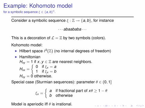
Example: Kohomoto modelfor a symbolic sequence ⇠ 2 {a, b}Z.
Consider a symbolic sequence ⇠ : Z ! {a, b}, for instance
· · ·abaababa · · ·
This is a decoration of L = Z by two symbols (colors).
Kohomoto model:I Hilbert space `2(Z) (no internal degrees of freedom)I Hamiltonian
Hxy = 1 if x , y 2 Z are nearest neighbors.
Hxx =
⇢0 if ⇠x = a1 if ⇠x = b
Hxy = 0 otherwise.Special case (Sturmian sequences): parameter ✓ 2 (0, 1]
⇠x =
⇢a if fractional part of x✓ � 1� ✓b otherwise
Model is aperiodic iff ✓ is irrational.

Plot of spec(H✓) versus ✓ 2 (0, 12 ]


![Neutrino pathways to cosmology - ffp14.cpt.univ-mrs.frffp14.cpt.univ-mrs.fr/DOCUMENTS/SLIDES/VALLE_Jose_W.F.pdf · RENO: 800 days [talk by Seon-Hee Seo@ICHEP2014] Daya Bay: 621 days](https://static.fdocuments.us/doc/165x107/6009857d021d252e1a074234/neutrino-pathways-to-cosmology-ffp14cptuniv-mrs-reno-800-days-talk-by-seon-hee.jpg)
