NOMINAL RIGIDITIES IN A DSGE M BASIC CALVO-YUN MODEL · tit t tttt t t tst ss ttsst pPP x py E y E...

1

NOMINAL RIGIDITIES IN A DSGEMODEL: BASIC CALVO-YUN MODEL

OCTOBER 9, 2008

October 9, 2008 2

DIFFERENTIATED-GOODS FIRMS

DSGE Calvo-Yun Model

Optimal-pricing condition

With sticky prices, optimal Pi balances current and future marginal revenues against current and future marginal costs until the next (expected) price re-optimization

Differentiated firm i’s (and hence the aggregate) markup will be time-varying

As “initial marginal revenues” > “initial marginal costs” to balance against “later marginal revenues” < “later marginal costs”See King and Wolman (1999)

Conduct full non-linear analysis (around distorted steady state)Later: typical New Keynesian analysis (around efficient steady state)

|1 0s t i i

ts

t s t s s ss s

t t

t

P PE P y mcP P

ε

εα ε

−∞

−+

=

⎧ ⎫⎛ ⎞ ⎡ ⎤−⎪ ⎪− =⎨ ⎬⎜ ⎟ ⎢ ⎥⎝ ⎠ ⎣ ⎦⎪

Ξ⎪⎩ ⎭

∑

Real marginal revenue

As inflation erodes the relative price of firm i

2

October 9, 2008 3

OPTIMAL-PRICING CONDITION


Optimal-pricing condition

Define

Optimal-pricing condition:Emphasizes that optimal Pi balances current and future mr against current and future mc

Write recursively (following SGU (2005 NBER Macro Annual))

|1 0s t it it

t t s t s s ss t s s

P PE P y mcP P

εεαε

−∞

−+

=

⎧ ⎫⎛ ⎞ ⎡ ⎤−⎪ ⎪Ξ − =⎨ ⎬⎜ ⎟ ⎢ ⎥⎝ ⎠ ⎣ ⎦⎪ ⎪⎩ ⎭

∑

1|

1s t it itt t t t s t s s

s t s s

P PPx E P yP P

εεαε

−∞

−+

=

⎧ ⎫⎛ ⎞ −⎪ ⎪= Ξ⎨ ⎬⎜ ⎟⎝ ⎠⎪ ⎪⎩ ⎭

∑

1 2t tx x=

2|

s t itt t t t s t s s s

s t s

PPx E P y mcP

ε

α−

∞−

+=

⎧ ⎫⎛ ⎞⎪ ⎪= Ξ⎨ ⎬⎜ ⎟⎝ ⎠⎪ ⎪⎩ ⎭

∑

PDV of nominal marginal revenues until next price change

PDV of nominal marginal costs until next price change

1 2,t tx x

October 9, 2008 4



Some notation and definitions

itit

t

PpP

≡

itP

1it itP P+ =

Relative price of good i in period t

Evolution of nominal price if no price change

Nominal price of good i in period t

3

October 9, 2008 5



Some notation and definitions

1

1

1

1

1

1

it iit

it

t

t t

it t

t

t

t

P PP PPP

p

P

pP

π

+

+ +

+

+

+

=

= =

=

Relative price of good i in period t

Evolution of nominal price if no price change

As long as no nominal price change, a firm’s relative price erodes at the rate of inflation

(πt+1 = Pt+1/Pt)

Nominal price of good i in period t

itit

t

PpP

≡

itP

1it itP P+ =

October 9, 2008 6



Write recursively

1|


s t s s

P PPx E P yP P

εεαε

−∞

−+

=

⎧ ⎫⎛ ⎞ −⎪ ⎪= Ξ⎨ ⎬⎜ ⎟⎝ ⎠⎪ ⎪⎩ ⎭

∑

1tx

1 11 1

1| 1 |21

1 1 s tt it t it s itt t t t t t t t s t s s

s tt t t t t s

P P P P P Px y E y E y mcP P P P P P

ε ε εε εα αε ε

− − −∞

−++ + +

= ++

⎧ ⎫ ⎧ ⎫⎛ ⎞ ⎛ ⎞ ⎛ ⎞− −⎪ ⎪ ⎪ ⎪= + Ξ + Ξ⎨ ⎬ ⎨ ⎬⎜ ⎟ ⎜ ⎟ ⎜ ⎟⎝ ⎠ ⎝ ⎠ ⎝ ⎠⎪ ⎪ ⎪ ⎪⎩ ⎭ ⎩ ⎭

∑

Divide by Pt; write out first two terms

4

October 9, 2008 7



Write recursively

1|


s t s s

P PPx E P yP P

εεαε

−∞

−+

=

⎧ ⎫⎛ ⎞ −⎪ ⎪= Ξ⎨ ⎬⎜ ⎟⎝ ⎠⎪ ⎪⎩ ⎭

∑

1tx

1 11 1

1| 1 |21


s tt t t t t s



− − −∞

−++ + +

= ++

⎧ ⎫ ⎧ ⎫⎛ ⎞ ⎛ ⎞ ⎛ ⎞− −⎪ ⎪ ⎪ ⎪= + Ξ + Ξ⎨ ⎬ ⎨ ⎬⎜ ⎟ ⎜ ⎟ ⎜ ⎟⎝ ⎠ ⎝ ⎠ ⎝ ⎠⎪ ⎪ ⎪ ⎪⎩ ⎭ ⎩ ⎭

∑


Pit+1 = Pit while no price change opportunity

1 11 1 1

1| 1 |21

1 1 s tit t it s itt t t t t t t t s t s s

s tt t t t s

P P P P Px y E y E y mcP P P P P


− − −∞

−+ ++ + +

= ++

⎧ ⎫ ⎧ ⎫⎛ ⎞ ⎛ ⎞ ⎛ ⎞− −⎪ ⎪ ⎪ ⎪= + Ξ + Ξ⎨ ⎬ ⎨ ⎬⎜ ⎟ ⎜ ⎟ ⎜ ⎟⎝ ⎠ ⎝ ⎠ ⎝ ⎠⎪ ⎪ ⎪ ⎪⎩ ⎭ ⎩ ⎭

∑

October 9, 2008 8



Write recursively

1|


s t s s

P PPx E P yP P

εεαε

−∞

−+

=

⎧ ⎫⎛ ⎞ −⎪ ⎪= Ξ⎨ ⎬⎜ ⎟⎝ ⎠⎪ ⎪⎩ ⎭

∑

1tx

1 11 1

1| 1 |21


s tt t t t t s



− − −∞

−++ + +

= ++

⎧ ⎫ ⎧ ⎫⎛ ⎞ ⎛ ⎞ ⎛ ⎞− −⎪ ⎪ ⎪ ⎪= + Ξ + Ξ⎨ ⎬ ⎨ ⎬⎜ ⎟ ⎜ ⎟ ⎜ ⎟⎝ ⎠ ⎝ ⎠ ⎝ ⎠⎪ ⎪ ⎪ ⎪⎩ ⎭ ⎩ ⎭

∑



1 11 1 1

1| 1 |21


s tt t t t s



− − −∞

−+ ++ + +

= ++

⎧ ⎫ ⎧ ⎫⎛ ⎞ ⎛ ⎞ ⎛ ⎞− −⎪ ⎪ ⎪ ⎪= + Ξ + Ξ⎨ ⎬ ⎨ ⎬⎜ ⎟ ⎜ ⎟ ⎜ ⎟⎝ ⎠ ⎝ ⎠ ⎝ ⎠⎪ ⎪ ⎪ ⎪⎩ ⎭ ⎩ ⎭

∑Use definitions

11 11| 1 1 1 |

2

1 1 s t s itt it t t t t t it t t t s t s s

s t t s

P Px p y E p y E y mcP P

εε εε εα π α

ε ε

−∞

− − −+ + + + +

= +

⎧ ⎫⎛ ⎞− − ⎪ ⎪⎧ ⎫= + Ξ + Ξ⎨ ⎬ ⎨ ⎬⎜ ⎟⎩ ⎭ ⎝ ⎠⎪ ⎪⎩ ⎭

∑

5

October 9, 2008 9



Write recursively

1|


s t s s

P PPx E P yP P

εεαε

−∞

−+

=

⎧ ⎫⎛ ⎞ −⎪ ⎪= Ξ⎨ ⎬⎜ ⎟⎝ ⎠⎪ ⎪⎩ ⎭

∑

1tx

1 11 1

1| 1 |21


s tt t t t t s



− − −∞

−++ + +

= ++

⎧ ⎫ ⎧ ⎫⎛ ⎞ ⎛ ⎞ ⎛ ⎞− −⎪ ⎪ ⎪ ⎪= + Ξ + Ξ⎨ ⎬ ⎨ ⎬⎜ ⎟ ⎜ ⎟ ⎜ ⎟⎝ ⎠ ⎝ ⎠ ⎝ ⎠⎪ ⎪ ⎪ ⎪⎩ ⎭ ⎩ ⎭

∑



1 11 1 1

1| 1 |21


s tt t t t s



− − −∞

−+ ++ + +

= ++

⎧ ⎫ ⎧ ⎫⎛ ⎞ ⎛ ⎞ ⎛ ⎞− −⎪ ⎪ ⎪ ⎪= + Ξ + Ξ⎨ ⎬ ⎨ ⎬⎜ ⎟ ⎜ ⎟ ⎜ ⎟⎝ ⎠ ⎝ ⎠ ⎝ ⎠⎪ ⎪ ⎪ ⎪⎩ ⎭ ⎩ ⎭

∑Use definitions

11 11| 1 1 1 |

2


s t t s


εε εε εα π α

ε ε

−∞

− − −+ + + + +

= +

⎧ ⎫⎛ ⎞− − ⎪ ⎪⎧ ⎫= + Ξ + Ξ⎨ ⎬ ⎨ ⎬⎜ ⎟⎩ ⎭ ⎝ ⎠⎪ ⎪⎩ ⎭

∑1 1/it it tp p π+ +=Use

October 9, 2008 10



Write recursively 1tx

111

1| 1 1 |21

1 1 s tit s itt it t t t t t t t t s t s s

s tt t s

p P Px p y E y E y mcP P

ε εε ε εα π α

ε π ε

− −∞

− −+ + + +

= ++

⎧ ⎫ ⎧ ⎫⎛ ⎞ ⎛ ⎞− −⎪ ⎪ ⎪ ⎪= + Ξ + Ξ⎨ ⎬ ⎨ ⎬⎜ ⎟ ⎜ ⎟⎝ ⎠ ⎝ ⎠⎪ ⎪ ⎪ ⎪⎩ ⎭ ⎩ ⎭

∑

6

October 9, 2008 11




Rearrange

111

1| 1 1 |21


s tt t s



ε π ε

− −∞

− −+ + + +

= ++

⎧ ⎫ ⎧ ⎫⎛ ⎞ ⎛ ⎞− −⎪ ⎪ ⎪ ⎪= + Ξ + Ξ⎨ ⎬ ⎨ ⎬⎜ ⎟ ⎜ ⎟⎝ ⎠ ⎝ ⎠⎪ ⎪ ⎪ ⎪⎩ ⎭ ⎩ ⎭

∑

1 111| 1 1 |

2


s t t s


εε εεε εα π α

ε ε

−∞

− − −+ + + +

= +

⎧ ⎫⎛ ⎞− − ⎪ ⎪⎧ ⎫= + Ξ + Ξ⎨ ⎬ ⎨ ⎬⎜ ⎟⎩ ⎭ ⎝ ⎠⎪ ⎪⎩ ⎭

∑

October 9, 2008 12




Rearrange

111

1| 1 1 |21


s tt t s



ε π ε

− −∞

− −+ + + +

= ++

⎧ ⎫ ⎧ ⎫⎛ ⎞ ⎛ ⎞− −⎪ ⎪ ⎪ ⎪= + Ξ + Ξ⎨ ⎬ ⎨ ⎬⎜ ⎟ ⎜ ⎟⎝ ⎠ ⎝ ⎠⎪ ⎪ ⎪ ⎪⎩ ⎭ ⎩ ⎭

∑

1 111| 1 1 |

2


s t t s



ε ε

−∞

− − −+ + + +

= +

⎧ ⎫⎛ ⎞− − ⎪ ⎪⎧ ⎫= + Ξ + Ξ⎨ ⎬ ⎨ ⎬⎜ ⎟⎩ ⎭ ⎝ ⎠⎪ ⎪⎩ ⎭

∑1

1itp ε−+Multiply and divide by

111 1

1| 1 1 1 |21

1 1 s tit s itt it t t t t t it t t t s t s s

s tit t s

p P Px p y E p y E y mcp P P

ε εε ε εε εα π α

ε ε

− −∞

− − −+ + + + +

= ++

⎧ ⎫ ⎧ ⎫⎛ ⎞ ⎛ ⎞− −⎪ ⎪ ⎪ ⎪= + Ξ + Ξ⎨ ⎬ ⎨ ⎬⎜ ⎟ ⎜ ⎟⎝ ⎠ ⎝ ⎠⎪ ⎪ ⎪ ⎪⎩ ⎭ ⎩ ⎭

∑

7

October 9, 2008 13




Rearrange

111

1| 1 1 |21


s tt t s



ε π ε

− −∞

− −+ + + +

= ++

⎧ ⎫ ⎧ ⎫⎛ ⎞ ⎛ ⎞− −⎪ ⎪ ⎪ ⎪= + Ξ + Ξ⎨ ⎬ ⎨ ⎬⎜ ⎟ ⎜ ⎟⎝ ⎠ ⎝ ⎠⎪ ⎪ ⎪ ⎪⎩ ⎭ ⎩ ⎭

∑

1 111| 1 1 |

2


s t t s



ε ε

−∞

− − −+ + + +

= +

⎧ ⎫⎛ ⎞− − ⎪ ⎪⎧ ⎫= + Ξ + Ξ⎨ ⎬ ⎨ ⎬⎜ ⎟⎩ ⎭ ⎝ ⎠⎪ ⎪⎩ ⎭

∑1


111 1

1| 1 1 1 |21


s tit t s



ε ε

− −∞

− − −+ + + + +

= ++

⎧ ⎫ ⎧ ⎫⎛ ⎞ ⎛ ⎞− −⎪ ⎪ ⎪ ⎪= + Ξ + Ξ⎨ ⎬ ⎨ ⎬⎜ ⎟ ⎜ ⎟⎝ ⎠ ⎝ ⎠⎪ ⎪ ⎪ ⎪⎩ ⎭ ⎩ ⎭

∑

Have generated a recursive term

October 9, 2008 14




Rearrange

111

1| 1 1 |21


s tt t s



ε π ε

− −∞

− −+ + + +

= ++

⎧ ⎫ ⎧ ⎫⎛ ⎞ ⎛ ⎞− −⎪ ⎪ ⎪ ⎪= + Ξ + Ξ⎨ ⎬ ⎨ ⎬⎜ ⎟ ⎜ ⎟⎝ ⎠ ⎝ ⎠⎪ ⎪ ⎪ ⎪⎩ ⎭ ⎩ ⎭

∑

1 111| 1 1 |

2


s t t s



ε ε

−∞

− − −+ + + +

= +

⎧ ⎫⎛ ⎞− − ⎪ ⎪⎧ ⎫= + Ξ + Ξ⎨ ⎬ ⎨ ⎬⎜ ⎟⎩ ⎭ ⎝ ⎠⎪ ⎪⎩ ⎭

∑1


111 1

1| 1 1 1 |21


s tit t s



ε ε

− −∞

− − −+ + + + +

= ++

⎧ ⎫ ⎧ ⎫⎛ ⎞ ⎛ ⎞− −⎪ ⎪ ⎪ ⎪= + Ξ + Ξ⎨ ⎬ ⎨ ⎬⎜ ⎟ ⎜ ⎟⎝ ⎠ ⎝ ⎠⎪ ⎪ ⎪ ⎪⎩ ⎭ ⎩ ⎭

∑

Express recursively

111 1

1| 1 11

1 itt it t t t t t t

it

px p y E xp

εε εε α π

ε

−−

+ + ++

⎧ ⎫⎛ ⎞− ⎪ ⎪= + Ξ⎨ ⎬⎜ ⎟⎝ ⎠⎪ ⎪⎩ ⎭

x1 expressed recursively

Have generated a recursive term

8

October 9, 2008 15



Both recursively 1 2,t tx x1

11 11| 1 1

1


it

px p y E xp

εε εε α π

ε

−−

+ + ++

⎧ ⎫⎛ ⎞− ⎪ ⎪= + Ξ⎨ ⎬⎜ ⎟⎝ ⎠⎪ ⎪⎩ ⎭


2 1 21| 1 1

1

itt it t t t t t t t

it

px p y mc E xp

εε εα π

−− +

+ + ++

⎧ ⎫⎛ ⎞⎪ ⎪= + Ξ⎨ ⎬⎜ ⎟⎝ ⎠⎪ ⎪⎩ ⎭


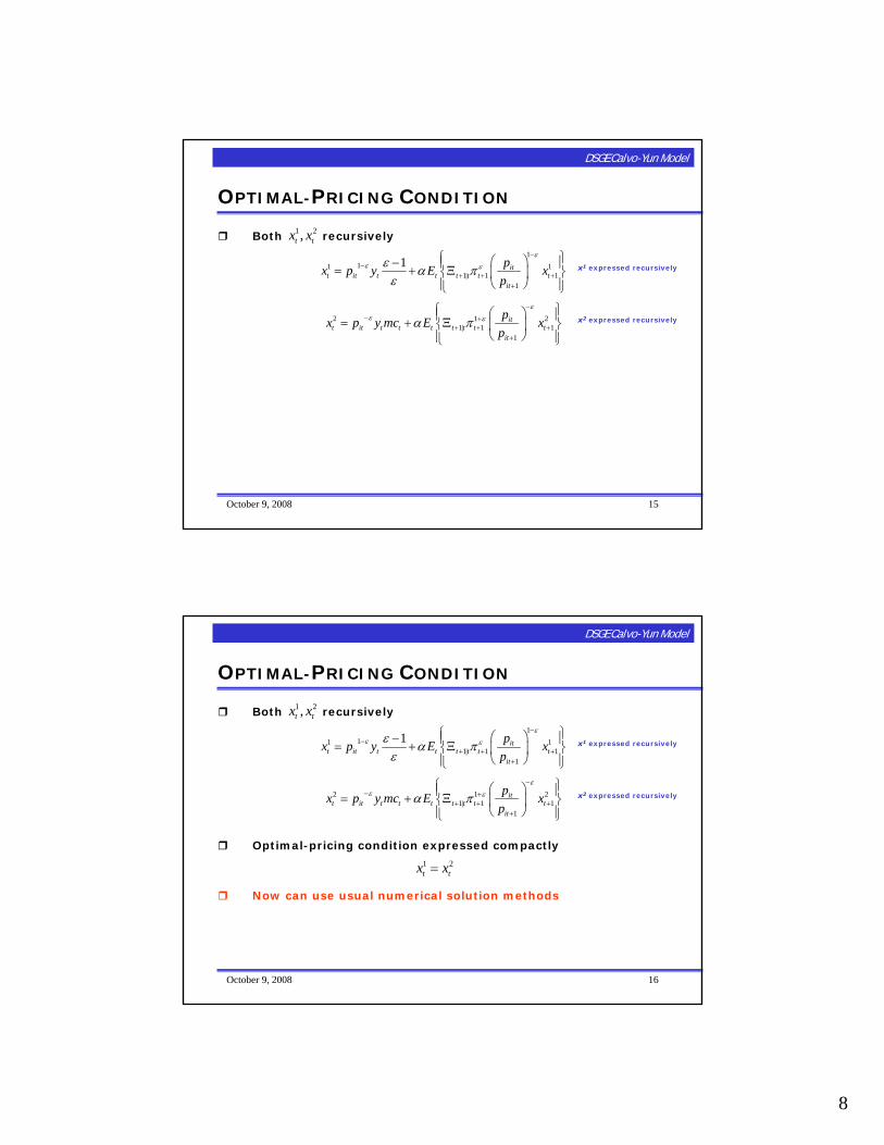
October 9, 2008 16



Both recursively

Optimal-pricing condition expressed compactly

Now can use usual numerical solution methods

1 2,t tx x1

11 11| 1 1

1


it

px p y E xp

εε εε α π

ε

−−

+ + ++

⎧ ⎫⎛ ⎞− ⎪ ⎪= + Ξ⎨ ⎬⎜ ⎟⎝ ⎠⎪ ⎪⎩ ⎭


2 1 21| 1 1

1

itt it t t t t t t t

it

px p y mc E xp

εε εα π

−− +

+ + ++

⎧ ⎫⎛ ⎞⎪ ⎪= + Ξ⎨ ⎬⎜ ⎟⎝ ⎠⎪ ⎪⎩ ⎭


1 2t tx x=

9

October 9, 2008 17

AGGREGATE PRICE LEVEL


Aggregate price index follows from Dixit-Stiglitz aggregation

1 11 1 1 *1

10 0

t it it itP P di P di P diα

ε ε ε ε

α

− − − −−= = +∫ ∫ ∫

adjustersnon-adjusters

Obtained by substituting demand functions into D-S aggregator

October 9, 2008 18




1 11 1 1 *1

10 0


ε ε ε ε

α

− − − −−= = +∫ ∫ ∫

adjustersnon-adjustersEmphasize optimal new price


10

October 9, 2008 19




1 11 1 1 *1

10 0


ε ε ε ε

α

− − − −−= = +∫ ∫ ∫


1 *11 (1 )t tP Pε εα α− −−= + −

KEY: Because adjusters were randomly selected, average (aggregate) price of non-adjusters is same as previous period’s average (aggregate) price

Fraction 1 - α re-set price optimally (and symmetrically)


October 9, 2008 20




1 11 1 1 *1

10 0


ε ε ε ε

α

− − − −−= = +∫ ∫ ∫


1 *11 (1 )t tP Pε εα α− −−= + −


Obtained by substituting demand functions into D-S aggregatorTRACTABILITY DUE TO THE

CALVO RANDOM-ADJUSTMENT ASSUMPTION


11

October 9, 2008 21




1 11 1 1 *1

10 0


ε ε ε ε

α

− − − −−= = +∫ ∫ ∫


1 *11 (1 )t tP Pε εα α− −−= + −

1 *11 (1 )t tpε εαπ α− −= + − EQUILIBRIUM EVOLUTION OF AGGREGATE INFLATION –depends on relative price set by firms currently adjusting nominal price



TRACTABILITY DUE TO THE CALVO RANDOM-ADJUSTMENT ASSUMPTION


October 9, 2008 22




1 11 1 1 *1

10 0


ε ε ε ε

α

− − − −−= = +∫ ∫ ∫


1 *11 (1 )t tP Pε εα α− −−= + −

1 *11 (1 )t tpε εαπ α− −= + − EQUILIBRIUM EVOLUTION OF AGGREGATE INFLATION –depends on relative price set by firms currently adjusting nominal price


Optimal-pricing condition1 2t tx x=

Together form the “aggregate supply” block of New Keynesian sticky-price model


TRACTABILITY DUE TO THE CALVO RANDOM-ADJUSTMENT ASSUMPTION


12

October 9, 2008 23

PRICE DISPERSION


Calvo model implies dispersion of relative pricesAs does Taylor model (see Chari, Kehoe, McGrattan (2000 Econometrica for an example))……but not Rotemberg model (quadratic cost of nominal price adjustment)

October 9, 2008 24

PRICE DISPERSION



Dispersion often ignored until recently...…due to linearization around a zero-inflation steady state (typical simple New Keynesian model soon…)With better numerical tools, easier to take account of dispersion

13

October 9, 2008 25

PRICE DISPERSION




Price dispersion the basic source of welfare losses of non-zero inflation

Because it implies quantity dispersion across intermediate producers……which is inefficient because Dixit-Stiglitz aggregator is symmetric and concave in every good i

October 9, 2008 26

PRICE DISPERSION




Price dispersion the basic source of welfare losses of non-zero inflation

Because it implies quantity dispersion across intermediate producers……which is inefficient because Dixit-Stiglitz aggregator is symmetric and concave in every good i

The basic driving force of optimal policy in any NK model

14

October 9, 2008 27

PRICE DISPERSION


For firm i, ( , )itit t t it it

t

Py y z f k nP

ε−⎛ ⎞

= =⎜ ⎟⎝ ⎠

October 9, 2008 28

PRICE DISPERSION


For firm i,

Integrating over i

( , )itit t t it it

t

Py y z f k nP

ε−⎛ ⎞

= =⎜ ⎟⎝ ⎠

1 1

0 0

( , )itt t it it

t

Py di z f k n diP

ε−⎛ ⎞

=⎜ ⎟⎝ ⎠∫ ∫

15

October 9, 2008 29

PRICE DISPERSION


For firm i,

Integrating over i

( , )itit t t it it

t

Py y z f k nP

ε−⎛ ⎞

= =⎜ ⎟⎝ ⎠

1 1

0 0

( , )itt t it it

t

Py di z f k n diP

ε−⎛ ⎞

=⎜ ⎟⎝ ⎠∫ ∫

Symmetric choices of k/n ratio across all firms i…

1 1

0 0

,1it tt t it

t t

P ky di z f n diP n

ε−⎛ ⎞ ⎛ ⎞

=⎜ ⎟ ⎜ ⎟⎝ ⎠ ⎝ ⎠∫ ∫

October 9, 2008 30

PRICE DISPERSION


For firm i,

Integrating over i

( , )itit t t it it

t

Py y z f k nP

ε−⎛ ⎞

= =⎜ ⎟⎝ ⎠

1 1

0 0

( , )itt t it it

t

Py di z f k n diP

ε−⎛ ⎞

=⎜ ⎟⎝ ⎠∫ ∫

ts≡

1 1

0 0

,1it tt t it

t t

P ky di z f n diP n

ε−⎛ ⎞ ⎛ ⎞

=⎜ ⎟ ⎜ ⎟⎝ ⎠ ⎝ ⎠∫ ∫

A measure of dispersion: relative price dispersion leads to dispersion of factor usage across differentiated firms, hence dispersion of quantity across differentiated firms

Express st recursively

Symmetric choices of k/n ratio across all firms i…

16

October 9, 2008 31

PRICE DISPERSION


1 1 *

0 0

it it itt

t t t

P P Ps di di diP P P

ε ε εα

α

− − −⎛ ⎞ ⎛ ⎞ ⎛ ⎞

= = +⎜ ⎟ ⎜ ⎟ ⎜ ⎟⎝ ⎠ ⎝ ⎠ ⎝ ⎠∫ ∫ ∫

Re-setters all choose same price

*

0

(1 ) t it

t t

P P diP P

ε εα

α− −

⎛ ⎞ ⎛ ⎞= − +⎜ ⎟ ⎜ ⎟

⎝ ⎠ ⎝ ⎠∫

October 9, 2008 32

PRICE DISPERSION


1 1 *

0 0

it it itt

t t t


ε ε εα

α

− − −⎛ ⎞ ⎛ ⎞ ⎛ ⎞

= = +⎜ ⎟ ⎜ ⎟ ⎜ ⎟⎝ ⎠ ⎝ ⎠ ⎝ ⎠∫ ∫ ∫


*

0

(1 ) t it

t t

P P diP P

ε εα

α− −

⎛ ⎞ ⎛ ⎞= − +⎜ ⎟ ⎜ ⎟

⎝ ⎠ ⎝ ⎠∫

Pit = Pit-1 for firms that cannot re-set price

*1

0

(1 ) t it

t t

P P diP P

ε εα

α− −

−⎛ ⎞ ⎛ ⎞= − +⎜ ⎟ ⎜ ⎟

⎝ ⎠ ⎝ ⎠∫

17

October 9, 2008 33

PRICE DISPERSION


1 1 *

0 0

it it itt

t t t


ε ε εα

α

− − −⎛ ⎞ ⎛ ⎞ ⎛ ⎞

= = +⎜ ⎟ ⎜ ⎟ ⎜ ⎟⎝ ⎠ ⎝ ⎠ ⎝ ⎠∫ ∫ ∫


*

0

(1 ) t it

t t

P P diP P

ε εα

α− −

⎛ ⎞ ⎛ ⎞= − +⎜ ⎟ ⎜ ⎟

⎝ ⎠ ⎝ ⎠∫

*1

0

(1 ) t it

t t

P P diP P

ε εα

α− −

−⎛ ⎞ ⎛ ⎞= − +⎜ ⎟ ⎜ ⎟

⎝ ⎠ ⎝ ⎠∫

Multiply by (Pt-1/Pt-1)-ε

*1 1

10

(1 ) t t it

t t t

P P P diP P P

ε ε εα

α− − −

− −

−

⎛ ⎞ ⎛ ⎞ ⎛ ⎞= − +⎜ ⎟ ⎜ ⎟ ⎜ ⎟

⎝ ⎠ ⎝ ⎠ ⎝ ⎠∫


October 9, 2008 34

PRICE DISPERSION


1 1 *

0 0

it it itt

t t t


ε ε εα

α

− − −⎛ ⎞ ⎛ ⎞ ⎛ ⎞

= = +⎜ ⎟ ⎜ ⎟ ⎜ ⎟⎝ ⎠ ⎝ ⎠ ⎝ ⎠∫ ∫ ∫


*

0

(1 ) t it

t t

P P diP P

ε εα

α− −

⎛ ⎞ ⎛ ⎞= − +⎜ ⎟ ⎜ ⎟

⎝ ⎠ ⎝ ⎠∫

*1

0

(1 ) t it

t t

P P diP P

ε εα

α− −

−⎛ ⎞ ⎛ ⎞= − +⎜ ⎟ ⎜ ⎟

⎝ ⎠ ⎝ ⎠∫


*1 1

10

(1 ) t t it

t t t

P P P diP P P

ε ε εα

α− − −

− −

−

⎛ ⎞ ⎛ ⎞ ⎛ ⎞= − +⎜ ⎟ ⎜ ⎟ ⎜ ⎟

⎝ ⎠ ⎝ ⎠ ⎝ ⎠∫

1tsα −≡tεπ≡


18

October 9, 2008 35

PRICE DISPERSION


1 1 *

0 0

it it itt

t t t


ε ε εα

α

− − −⎛ ⎞ ⎛ ⎞ ⎛ ⎞

= = +⎜ ⎟ ⎜ ⎟ ⎜ ⎟⎝ ⎠ ⎝ ⎠ ⎝ ⎠∫ ∫ ∫


*

0

(1 ) t it

t t

P P diP P

ε εα

α− −

⎛ ⎞ ⎛ ⎞= − +⎜ ⎟ ⎜ ⎟

⎝ ⎠ ⎝ ⎠∫

*1

0

(1 ) t it

t t

P P diP P

ε εα

α− −

−⎛ ⎞ ⎛ ⎞= − +⎜ ⎟ ⎜ ⎟

⎝ ⎠ ⎝ ⎠∫


*1 1

10

(1 ) t t it

t t t

P P P diP P P

ε ε εα

α− − −

− −

−

⎛ ⎞ ⎛ ⎞ ⎛ ⎞= − +⎜ ⎟ ⎜ ⎟ ⎜ ⎟

⎝ ⎠ ⎝ ⎠ ⎝ ⎠∫

1tsα −≡tεπ≡


1

0 0

1it itt

t t

P Ps di diP P

ε εα

α

− −⎛ ⎞ ⎛ ⎞

= =⎜ ⎟ ⎜ ⎟⎝ ⎠ ⎝ ⎠∫ ∫

Because of Calvorandom adjustment and all adjusters choose same price

October 9, 2008 36

PRICE DISPERSION


1 1 *

0 0

it it itt

t t t


ε ε εα

α

− − −⎛ ⎞ ⎛ ⎞ ⎛ ⎞

= = +⎜ ⎟ ⎜ ⎟ ⎜ ⎟⎝ ⎠ ⎝ ⎠ ⎝ ⎠∫ ∫ ∫


*

0

(1 ) t it

t t

P P diP P

ε εα

α− −

⎛ ⎞ ⎛ ⎞= − +⎜ ⎟ ⎜ ⎟

⎝ ⎠ ⎝ ⎠∫

*1

0

(1 ) t it

t t

P P diP P

ε εα

α− −

−⎛ ⎞ ⎛ ⎞= − +⎜ ⎟ ⎜ ⎟

⎝ ⎠ ⎝ ⎠∫


*1 1

10

(1 ) t t it

t t t

P P P diP P P

ε ε εα

α− − −

− −

−

⎛ ⎞ ⎛ ⎞ ⎛ ⎞= − +⎜ ⎟ ⎜ ⎟ ⎜ ⎟

⎝ ⎠ ⎝ ⎠ ⎝ ⎠∫

tεπ≡

NOTE:

α= 0: st = 1 (no dispersion)

α > 0: st > 1 (dispersion)


Because of Calvorandom adjustment and all adjusters choose same price

1tsα −≡

1

0 0

1it itt

t t

P Ps di diP P

ε εα

α

− −⎛ ⎞ ⎛ ⎞

= =⎜ ⎟ ⎜ ⎟⎝ ⎠ ⎝ ⎠∫ ∫

19

October 9, 2008 37

RESOURCE CONSTRAINT


Summarized by three conditions

( , )t t tt

t

z f k nys

=

1 (1 )t t t t ty c k k gδ+= + − − +

*1(1 )t t t ts p sε εα απ−−= − +

“Usual” resource constraint

Some output is a pure deadweight loss

(note st < 1 cannot occur)

Law of motion for deadweight loss

1 1

0 0

,t it t itk k di n n di= =∫ ∫

And using factor market clearing conditions here

October 9, 2008 38

RESOURCE CONSTRAINT

Yun 1996 Model

Summarized by three conditions

Law of motion for st represented using laws of motion for both Pt-1and P*t-1

See equations (25) and (26)

( , )t t tt

t

z f k nys

=

1 (1 )t t t t ty c k k gδ+= + − − +

*1(1 )t t t ts p sε εα απ−−= − +

“Usual” resource constraint

Some output is a pure deadweight loss

(note st < 1 cannot occur)

Law of motion for deadweight loss

= 0 in Yun model

20

October 9, 2008 39

OTHER MODEL DETAILS

Yun 1996 Model

Cash/credit to motivate money demandi.e., Lucas and Stokey (1983), Chari, Christiano, and Kehoe (1991)

(Habit persistence (i.e., time-non-separability) in leisure)As in Kydland and Prescott (1982); unimportant for main results…

Could have been cashless…

October 9, 2008 40

OTHER MODEL DETAILS

Yun 1996 Model



Exogenous AR(1) money growth processAlso “endogenous” money supply process, but not as interesting

Exogenous AR(1) TFP process


21

October 9, 2008 41

OTHER MODEL DETAILS

Yun 1996 Model



Exogenous AR(1) money growth processAlso “endogenous” money supply process, but not as interesting

Exogenous AR(1) TFP process

Indexation of prices to average (i.e., steady-state) inflationFor firms not re-setting price, (will see again in Christiano, Eichenbaum, and Evans (2005 JPE))

Approximated and simulated using “usual” methodsUsing King, Plosser, Rebelo (1988) linear approximation method

(One…) predecessor to SGU algorithm

1it itP Pπ −=


October 9, 2008 42

NOMINAL EFFECTS OF STICKY PRICES

Yun 1996 Model

Effects on inflation not very different compared to flex-price case

Flexible Prices

Sticky Prices

22

October 9, 2008 43

NOMINAL EFFECTS OF STICKY PRICES

Yun 1996 Model

Effects on inflation not very different compared to flex-price case

Flexible Prices

Sticky Prices

Lack of inflation persistence in basic Calvo-Yun model (now) well-known –see Steinsson (2001 JME)

October 9, 2008 44

REAL EFFECTS OF STICKY PRICES

Yun 1996 Model

Effects on GDP much bigger the stickier are prices

Flexible Prices

Sticky Prices

23

October 9, 2008 45

MARKUP DYNAMICS

Sticky-Price Mechanism

Money (i.e., nontechnology) shock output expands

With zt, kt fixed, output expansion due to increased (equilibrium) hours

October 9, 2008 46

MARKUP DYNAMICS




Downward-sloping product demand curves individual (differentiated) firms must expand their output (partial equilibrium)

Recall aggregate output a shifter of firm i demand function

Can only be achieved in the short-run if a given firm i hires more labor at any real wage

24

October 9, 2008 47

MARKUP DYNAMICS




Downward-sloping product demand curves individual (differentiated) firms must expand their output (partial equilibrium)

Recall aggregate output a shifter of firm i demand function

Can only be achieved in the short-run if a given firm i hires more labor at any real wage

S

Labor

Real wage D

1( , )

t

t n t t t

wz f k n μ

= Sticky-price (or sticky-wage) model delivers endogenously-countercyclical markup

tmc=

October 9, 2008 48

DSGE STICKY-PRICE MODELS

Summary and Roadmap

Nominal rigidities embedded in DSGE modelMonetary shifts quantitatively “big” effects on output(Re-)articulates “old” Keynesian ideasGoodfriend and King (1997 NBER Macroeconomics Annual): the New-Neoclassical Synthesis

25

October 9, 2008 49


Summary and Roadmap


Output effect not very long-lasting (peak response occurs in period of monetary shock, inconsistent with data)

The “Persistence Puzzle”Examined in Chari, Kehoe, and McGrattan (2000 Econometrica) (next) and Christiano, Eichenbaum, and Evans (2005 JPE)

October 9, 2008 50


Summary and Roadmap




Inflation not very persistentSteinsson (2001 JME): “backward-looking price-setting”

26

October 9, 2008 51


Summary and Roadmap




Inflation not very persistentSteinsson (2001 JME): “backward-looking price-setting”

A Phillips Curve?

Optimal policy?

NOMINAL RIGIDITIES IN A DSGE M BASIC CALVO-YUN MODEL · tit t tttt t t tst ss ttsst pPP x py E y E...

Documents

Transcript of NOMINAL RIGIDITIES IN A DSGE M BASIC CALVO-YUN MODEL · tit t tttt t t tst ss ttsst pPP x py E y E...