
Noise - arxiv-export-lb.library.cornell.edu
31
arXiv:2109.11850v1 [math.DS] 24 Sep 2021 An Optimized Dynamic Mode Decomposition Model Robust to Multiplicative Noise ∗ Minwoo Lee † , Jongho Park ‡ , and Chae Hoon Sohn † Abstract. Dynamic mode decomposition (DMD) is an efficient tool for decomposing spatio-temporal data into a set of low-dimensional modes, yielding the oscillation frequencies and the growth rates of physically significant modes. In this paper, we propose a novel DMD model that can be used for dynamical systems affected by multiplicative noise. We first derive a maximum a posteriori (MAP) estimator for the data-based model decomposition of a linear dynamical system corrupted by certain multiplicative noise. Applying a penalty relaxation to the MAP estimator, we obtain the proposed DMD model whose epigraphical limits are the MAP estimator and the Askham–Kutz optimized DMD model. We also propose an efficient alternating gradient descent method for solving the proposed DMD model, and analyze its convergence behavior. The proposed model is demonstrated on both the synthetic data and the numerically generated one-dimensional combustor data, and is shown to have superior reconstruction properties compared to state-of-the-art DMD models. Considering that multiplicative noise is ubiquitous in numerous dynamical systems, the proposed DMD model opens up new possibilities for accurate data-based modal decomposition. Key words. dynamic mode decomposition, multiplicative noise, variational model, alternating descent AMS subject classifications. 37M10, 49M37, 49R05, 65P99 1. Introduction. Various natural and engineered systems exhibit complex spatio-temporal dynamics, involving nonlinearities and high-dimensionalities. In many cases, however, the system’s dynamics are governed by a few significant modes that represent the coherent features of the system. From a practical point of view, it is essential to extract these modes from the experimental data, so as to identify the fundamental dynamics, analyze the underlying physics, and build the low-dimensional model of the system [13, 24]. Over the past few decades, various data-based modal decomposition techniques have been proposed and applied to analyze complex dynamical systems, including fluid flow [50], combustion system [39], neural activity recording [10], and spread of infectious disease [45], among many others. Two classes of data-based modal decomposition techniques are commonly used: proper orthogonal decomposition (POD) and dynamic mode decomposition (DMD). POD, which is also known as the principal component analysis in the statistics community, is a method of obtaining a low-dimensional approximation by projecting the full dynamical system onto a ∗ Submitted to arXiv. Funding: ML was supported by the National Research Foundation of Korea (NRF) grant funded by the Korean government (MSIT) (No. 2021R1G1A1091278). JP was supported by NRF grant funded by MSIT (No. 2021R1C1C2095193). CHS was partly supported by the Korea Institute of Energy Technology Eval- uation and Planning (KETEP) grant funded by the Korean government (MOTIE, 20206710100030, Development of Ecofriendly GT Combustor for 300 MWe-Class High-Efficiency Power Generation with 50% Hydrogen Co-firing). † Department of Mechanical Engineering, Sejong University, Seoul, 05006, Korea ([email protected], [email protected]). ‡ Natural Science Research Institute, KAIST, Daejeon, 34141, Korea ([email protected], https://sites. google.com/view/jonghopark). 1
Transcript of Noise - arxiv-export-lb.library.cornell.edu
arX
iv:2
109.
1185
0v1
[m
ath.
DS]
24
Sep
2021
An Optimized Dynamic Mode Decomposition Model Robust to MultiplicativeNoise∗
Minwoo Lee† , Jongho Park‡ , and Chae Hoon Sohn†
Abstract. Dynamic mode decomposition (DMD) is an efficient tool for decomposing spatio-temporal data intoa set of low-dimensional modes, yielding the oscillation frequencies and the growth rates of physicallysignificant modes. In this paper, we propose a novel DMD model that can be used for dynamicalsystems affected by multiplicative noise. We first derive a maximum a posteriori (MAP) estimator forthe data-based model decomposition of a linear dynamical system corrupted by certain multiplicativenoise. Applying a penalty relaxation to the MAP estimator, we obtain the proposed DMD modelwhose epigraphical limits are the MAP estimator and the Askham–Kutz optimized DMD model.We also propose an efficient alternating gradient descent method for solving the proposed DMDmodel, and analyze its convergence behavior. The proposed model is demonstrated on both thesynthetic data and the numerically generated one-dimensional combustor data, and is shown to havesuperior reconstruction properties compared to state-of-the-art DMD models. Considering thatmultiplicative noise is ubiquitous in numerous dynamical systems, the proposed DMD model opensup new possibilities for accurate data-based modal decomposition.
Key words. dynamic mode decomposition, multiplicative noise, variational model, alternating descent
AMS subject classifications. 37M10, 49M37, 49R05, 65P99
1. Introduction. Various natural and engineered systems exhibit complex spatio-temporaldynamics, involving nonlinearities and high-dimensionalities. In many cases, however, thesystem’s dynamics are governed by a few significant modes that represent the coherent featuresof the system. From a practical point of view, it is essential to extract these modes fromthe experimental data, so as to identify the fundamental dynamics, analyze the underlyingphysics, and build the low-dimensional model of the system [13, 24]. Over the past fewdecades, various data-based modal decomposition techniques have been proposed and appliedto analyze complex dynamical systems, including fluid flow [50], combustion system [39],neural activity recording [10], and spread of infectious disease [45], among many others.
Two classes of data-based modal decomposition techniques are commonly used: properorthogonal decomposition (POD) and dynamic mode decomposition (DMD). POD, which isalso known as the principal component analysis in the statistics community, is a method ofobtaining a low-dimensional approximation by projecting the full dynamical system onto a
∗Submitted to arXiv.Funding: ML was supported by the National Research Foundation of Korea (NRF) grant funded by
the Korean government (MSIT) (No. 2021R1G1A1091278). JP was supported by NRF grant funded byMSIT (No. 2021R1C1C2095193). CHS was partly supported by the Korea Institute of Energy Technology Eval-uation and Planning (KETEP) grant funded by the Korean government (MOTIE, 20206710100030, Developmentof Ecofriendly GT Combustor for 300 MWe-Class High-Efficiency Power Generation with 50% Hydrogen Co-firing).
†Department of Mechanical Engineering, Sejong University, Seoul, 05006, Korea ([email protected],[email protected]).
‡Natural Science Research Institute, KAIST, Daejeon, 34141, Korea ([email protected], https://sites.google.com/view/jonghopark).
1

2 M. LEE, J. PARK, AND C. H. SOHN
set of spatially orthogonal basis functions [48, 52]. Although POD can efficiently decomposea physical field to a lower order system, it suffers from several limitations. For instance, thebasis functions drawn from POD do not necessarily represent the physically significant modes.Thus, a reduced-order model constructed from POD can be inaccurate due to the user’s wrongchoice of modes [26]. Furthermore, POD is sensitive to the data used and is therefore difficultto be used when the experimental data is contaminated [46].
On the contrary, the second approach, DMD, computes eigenvalues and eigenvectors of alinear-approximated model that represent the full dynamics of the system [50, 54]. Specifically,a dynamical system z = f(z(t)) at equally spaced time space tn1≤n≤N is approximated asξn+1 = Aξn, where ξn ∈ C
N , 1 ≤ n ≤ N , is a snapshot at time tn and A is a linear operator.Then, a set of eigenvalues and eigenvectors of A is found from the snapshots ξnn. Whenapplied to nonlinear systems, DMD can be viewed as a method for finding the approximatemodes of the Koopman operator [41]. Unlike POD, growth rates and frequencies associatedwith each mode can be drawn from DMD, enabling the construction of a physically meaningfullow-order model [13]. However, owing to the fact that DMD uses pairs of data (one snapshotand the next), rather than the whole set of data at once, DMD is prone to the bias caused bysensor noise [15, 23].
Addressing this issue, the optimized DMD was proposed in [13]; it processes the wholesnapshot data at once. Specifically, this algorithm finds a set of eigenvalues that minimizes theresidual between the original spatio-temporal data and the reduced-order model. Although theoptimized DMD uses a computationally expensive optimization method, namely the Nelder–Mead simplex method, it is shown that the optimized DMD can reduce the bias of the originalDMD. Later, Askham and Kutz [2] improved the optimized DMD by reshaping the above-mentioned minimization problem and adopting the Levenberg–Marquardt algorithm [1, 40].They showed that their proposed algorithm is robust to noise and does not require the originaldata to be evenly spaced in time.
In this study, we build on the work [2] by tailoring the Askham–Kutz optimized DMDalgorithm. Specifically, we focus on the fact that the Askham–Kutz algorithm is designedparticularly to handle additive Gaussian noise (this claim will be discussed in subsection 2.2with details). In many physical systems, however, the noise is multiplicatively coupled to thesystem, i.e., it amplifies with the signal itself. For example, turbulence in the combustors [14],instrumental instabilities in nuclear magnetic resonance devices [20], pump fluctuation of dyelasers [16, 51], and electrohydrodynamic instability in liquid crystals [8] act as the source ofthe multiplicative noise, to name just a few. The effect of multiplicative noise on a system hasbeen studied extensively over the past few decades, because such noise not only contaminatesthe signal but also affects the dynamical stability of the system [36, 55]. Therefore, whenanalyzing the system influenced by the multiplicative noise, it is crucial to remove or suppressthe effect of noise to unveil the original dynamics of the system.
In this paper, we propose a data-based modal decomposition algorithm that can accuratelydecompose a system affected by multiplicative noise. We combine the ideas of the Askham–Kutz model and an image denoising model specific to multiplicative noise proposed in [3],aiming to develop an optimized DMD model that is robust to multiplicative noise. Specifically,by closely following [3], we construct a maximum a posteriori (MAP) estimator for data-basedmodal decomposition of a linear dynamical system corrupted by gamma multiplicative noise.
DMD FOR MULTIPLICATIVE NOISE 3
Because the constructed MAP estimator is complicated to solve numerically, an appropriatepenalty relaxation should be applied to the MAP estimator to obtain the proposed DMDmodel. We also present an efficient numerical algorithm to solve the proposed DMD model;we propose an alternating gradient descent method and suggest how to obtain a good initialguess for the algorithm. The convergence properties of the proposed alternating descentmethod will also be mathematically analyzed. Finally, we demonstrate the proposed DMDmodel on three numerical systems and show the reconstruction properties.
This paper is organized as follows. In section 2, we provide preliminaries required forthis paper, focusing on the Askham–Kutz optimized DMD model [2] and the Aubert–Aujoldenoising model [3]. In section 3, we propose a novel optimized DMD model that is robustto multiplicative noise and investigate some mathematical properties of the proposed model.Next, an efficient numerical solver for the proposed model is considered in section 4. Numericalresults of the proposed model for various dynamic systems, including an engineering problem,are presented in section 5. Lastly, we conclude our paper with remarks in section 6.
2. Preliminaries. In this section, we introduce notations that are used throughout thispaper. We also summarize key features of the optimized DMD model proposed in [2] and someimportant variational models for noise removal [3, 49]. Motivated by the existing works [2, 3],we design a novel optimized DMD model that is robust to multiplicative noise in section 3.
2.1. Notation. As in [19], we mostly use the standard notation accompanied with someMATLAB column notation. Let A ∈ C
M×N be a complex matrix of size M × N , and letξ ∈ C
N be a complex vector of length N , respectively. We have the following list of notationassociated with A and ξ:
• Aij denotes the entry of A in the ith row and jth column.• A(i, :) denotes the ith row vector of A.• A(:, j) denotes the jth column vector of A.• AT denotes the transpose of A.• AH denotes the Hermitian transpose of A.• A+ denotes the Moore–Penrose pseudoinverse of A.• ‖A‖F denotes the Frobenius norm of A.• ‖ξ‖2 denotes the ℓ2 norm of ξ.
As many matrices and vectors related to various physical dimensions will appear in thispaper, it is convenient to use a unified notation for indices with respect to physical dimensions.In what follows, we use the indices m, n, and r for the space, time, and rank dimensions,respectively.
2.2. Askham–Kutz optimized dynamic mode decomposition. For the sake of complete-ness, we present a brief summary of the optimized DMD model proposed by Askham andKutz [2]. Let X = [ξ1, . . . , ξN ] ∈ R
M×N be a matrix of snapshots, where each ξn = X(:, n) ∈RM , 1 ≤ n ≤ N , represents the snapshot at time tn ∈ R (t1 < · · · < tN ). We write H = XT.
Then the Askham–Kutz optimized DMD model is written as
(2.1) minα∈A, B∈CR×M
1
2‖H − Φ(α)B‖2F ,
4 M. LEE, J. PARK, AND C. H. SOHN
where R ∈ Z>0 is a target rank, A ⊂ CR is a solution space for the DMD eigenvalues, and
Φ(α) ∈ CN×R is defined by
(2.2) Φ(α)nr = eαrtn , 1 ≤ n ≤ N, 1 ≤ r ≤ R.
In order to investigate the meaning of (2.1) in more details, we first write BT = [β1, . . . , βR],where βr ∈ C
M , 1 ≤ r ≤ R. It follows that
1
2‖H − Φ(α)B‖2F =
1
2
N∑
n=1
‖H(n, :) − Φ(α)(n, :)B‖22 =1
2
N∑
n=1
∥∥∥∥∥ξn −
R∑
r=1
eαrtnβr
∥∥∥∥∥
2
2
.
That is, the model (2.1) finds a least squares approximation for ξn of the form∑R
r=1 eαrtnβr.
Recall that, for a linear dynamic system
(2.3) z(t) = Az(t), z(0) = z0
with a diagonalizable matrix A ∈ RM×M and z0 ∈ R
M , the solution is given by
z(t) =
M∑
m=1
eαmtβm,
where αm ∈ C is an eigenvalue of A and βm ∈ CM is an eigenvector associated with αm,
1 ≤ m ≤ M . In this sense, the Askham–Kutz model (2.1) can be interpreted as follows: theentries of α approximate the R dominant eigenvalues of a linear operator underlying the timeseries X, and the rows of B approximate eigenvectors associated with the entries of α. Onemay eliminate the variable B from (2.1) by variable projection [18]. For a fixed α ∈ A, thevariable B minimizing (2.1) has a closed-form formula
(2.4) B = Φ(α)+H.
If we substitute (2.4) into (2.1), then we obtain the following minimization problem whosevariable is α only:
(2.5) minα∈A
1
2
∥∥H − Φ(α)Φ(α)+H∥∥2F.
For the equivalence relation between (2.1) and (2.5), see [18, Theorem 2.1]. Since (2.5) is anonlinear least-squares problem and the dimension R of A is not very big in general, a goodstrategy to solve (2.5) is to use the Levenberg–Marquardt algorithm [1, 40]. One may referto [2] for implementation details of the Levenberg–Marquardt algorithm for the Askham–Kutzmodel (2.5).
It was shown by numerical experiments in [2] that a strong point of the Askham–Kutzmodel is that it is robust to additive noise than other existing DMD models such as [15, 54].That is, the Askham–Kutz model results in more accurate eigenvalues and eigenvectors thanthe other models, even in the presence of additive noise of high variance. As another advantageof the model, because it can be regarded as a particular case of nonlinear fitting problem, itallows data collected at unevenly spaced sample times.

DMD FOR MULTIPLICATIVE NOISE 5
2.3. Variational noise removal. After a pioneering work of Rudin et al. [49], variationalmodels have been broadly used in the field of signal and image processing for the purpose ofdenoising data. Here, we review several variational denoising models for image processing [3,49]. Let Ω ⊂ R
2 be an image domain, and let V be a suitable Banach space for digital images,e.g., V = L2(Ω). Suppose that we have a noisy image f ∈ V and want to find a denoisedcounterpart u ∈ V. If we model the noise in f as additive Gaussian noise, then we get thefollowing linear inverse problem:
(2.6) f = u+ ǫ,
where the pointwise value of the noise ǫ is normally distributed with mean 0 and variance σ2
for some σ > 0. A popular approach to solve (2.6) is to find a MAP estimator for u [17].Noting that the conditional probability density p(f |u) is given by
p(f |u) = 1√2πσ
exp
(− 1
2σ2
∫
Ω(f − u)2 dx
),
we can compute the MAP estimator for u as follows:
argmaxu∈V
p(u|f) = argmaxu∈V
p(u)p(f |u)p(f)
= argminu∈V
− log p(u)− log p(f |u)
= argminu∈V
1
2σ2
∫
Ω(f − u)2 dx+ φ(u)
,
(2.7)
where we used the Bayes’ theorem in the first equality, and φ(u) = − log p(u) is the prioron u. If we set φ(u) by the total variation of u (see, e.g., [30] for the definition of the totalvariation), then the last line of (2.7) becomes the celebrated Rudin–Osher–Fatemi model [49].
Meanwhile, one may consider a situation that the noise in f is multiplicative. We assumethat
(2.8) f = uǫ,
where u > 0 and the pointwise value of the noise ǫ follows the gamma distribution of mean 1and variance σ2. Proceeding similarly to (2.7), a MAP estimator for u satisfying (2.8) can becharacterized as a solution of the following Aubert–Aujol model [3]:
(2.9) minu∈V
1
σ2
∫
Ω
(log u+
f
u
)dx+ φ(u)
.
In the field of image processing, a typical choice for the prior φ(u) in (2.9) is the total variationof u. Practical performance of the model (2.9) for multiplicative noise removal can be foundin [3, 34].
As we have observed in (2.7) and (2.9), it is effective to use different data fidelity termsin denoising models for different kinds of noise. Several notable works [12, 28, 42] have beenon tailored data fidelity terms for various types of noise. Dependency of the quality of noiseremoval on data fidelity terms can be found in, e.g., [30].

6 M. LEE, J. PARK, AND C. H. SOHN
3. Proposed model. The purpose of this section is to propose a novel optimized DMDmodel that is robust to multiplicative noise. The essential idea of the construction of ourproposed model is to combine the Askham–Kutz optimized DMD model (2.1) and the Aubert–Aujol denoising model (2.9). In what follows, the indices n and m run from 1 to N and M ,respectively.
First, we observe that a solution of (2.1) can be regarded as a MAP estimator using acertain prior. Suppose that the matrix of observed snapshots H in (2.1) is expressed as thesum of a matrix H ∈ R
N×M representing clean snapshots and a noise matrix E ∈ RN×M
whose all entries follow the normal distribution of mean 0 and variance σ2, i.e.,
(3.1) Hnm = Hnm + Enm, Enm ∼ N(0, σ2).
For a fixed R ∈ Z>0, we define the set DR ⊂ RN×M by
(3.2) DR =K ∈ R
N×M : K = Φ(α)B for some α ∈ A, B ∈ CR×M
,
where Φ(α) ∈ CN×R was defined in (2.2). Let χDR: RN×M → R denote the characteristic
function of DR, i.e.,
χDR(K) =
0 if K ∈ DR,
∞ otherwise.
In DMD, we assume that dynamic features of the snapshots are determined by a few governingeigenvalues and eigenvectors of the dynamical system. In this perspective, a natural a prioriassumption on H is that H belongs to the set χDR
; we set
(3.3) − log p(H) = χDR(H),
with the convention − log 0 = ∞. In the same manner as (2.7), one can obtain the MAPestimator for H as follows:
(3.4) argmaxH∈RN×M
p(H |H) = argminH∈RN×M
1
2σ2‖H − H‖2F + χDR
(H)
.
In the minimization problem on the right-hand side of (3.4), one may drop the constant σ2
since χDRtakes a value either 0 or∞. Invoking the definition (3.2) of the set DR, we introduce
two auxiliary variables α ∈ A and B ∈ CR×M and set H = Φ(α)B. Then, the right-hand side
of (3.4) reduces to
minα∈A, B∈CR×M
1
2‖H − Φ(α)B‖2F ,
which is identical to the Askham–Kutz model (2.1). In conclusion, we have derived theAskham–Kutz model as the MAP estimator with the DMD prior (3.3) for the denoisingproblem (3.1).

DMD FOR MULTIPLICATIVE NOISE 7
Remark 3.1. In the prior assumption (3.3) on H, it is not ensured that p(H) is a proba-bility density. However, thanks to the notion of improper prior, Bayesian analysis can be donesuccessfully without assuming the prior knowledge is given by a probability density. One mayrefer to [37, 53] for mathematically rigorous treatments on the notion of improper prior.
Now, motivated by the observation that the Askham–Kutz model is a MAP estimator andthe relation between the Rudin–Osher–Fatemi [49] and Aubert–Aujol [3] models, we designan optimized DMD model that is suitable for data corrupted by multiplicative noise. Similarto (2.8), we consider the setting
(3.5) Hnm = HnmEnm,
where each Enm follows the gamma distribution of mean 1 and variance σ2. Since Enm isalways positive, Hnm must have the same sign as Hnm. Hence, we may restrict the solutionspace for H as the closed convex subset SH of RN×M defined by
SH =K ∈ R
N×M : Knm 0 if Hnm 0, ∈ ≥,≤.
Note that the value of Hnm is determined by 0 if Hnm = 0. Invoking [3, Proposition 3.1], forHnm 6= 0, we have
(3.6) p(Hnm|Hnm) = p
(Hnm
Hnm
)1
|Hnm|=
ββ
|Hnm|βΓ(β)|Hnm|β−1 exp
(−βHnm
Hnm
),
where β = 1/σ2. Assuming all the entries of H and H are mutually independent, it followsby a similar argument to (2.7) that
argmaxH∈SH
p(H|H) = argmaxH∈SH
∏
Hnm 6=0
p(Hnm|Hnm)
= argminH∈SH
− log p(H)−
∑
Hnm 6=0
log p(Hnm|Hnm)
= argminH∈SH
β
∑
Hnm 6=0
(log |Hnm|+
Hnm
Hnm
)+ χDR
(H)
= argminH∈SH
∑
Hnm 6=0
(log |Hnm|+
Hnm
Hnm
)+ χDR
(H)
,
(3.7)
where we used (3.3) and (3.6) in the penultimate equality and dropped β in the last equality.That is, the last line of (3.7), or equivalently,
(3.8) minα∈A, B∈CR×M
∑
Hnm 6=0
(log |(Φ(α)B)nm|+
Hnm
(Φ(α)B)nm
),
is the MAP estimator with the DMD prior (3.3) for the multiplicative denoising problem (3.5).
8 M. LEE, J. PARK, AND C. H. SOHN
Unfortunately, the structure of either the last line of (3.7) or (3.8) is so complicated thatit is difficult to design a suitable numerical solver for that. To simplify the model, we relaxthe χDR
(H)-term by introducing a quadratic penalty term [47, section 1.A]:
(3.9) minH∈SH , α∈A, B∈CR×M
∑
Hnm 6=0
(log |Hnm|+
Hnm
Hnm
)+
η
2‖H − Φ(α)B‖2F
,
where η > 0 is a tunable parameter. In (3.9), a minimizer with respect to B for fixed H ∈ SHand α ∈ A is given by B = Φ(α)+H. Hence, similar to (2.5), the variable B in (3.9) can beeliminated by variable projection [18] as follows:
(3.10) minH∈SH , α∈A
E(H, α) :=
∑
Hnm 6=0
(log |Hnm|+
Hnm
Hnm
)+
η
2‖H − Φ(α)Φ(α)+H‖2F
.
The problem (3.10) is our proposed optimized DMD model. In the remainder of this paper,we study mathematical and numerical aspects of the proposed model (3.10).
Remark 3.2. One may notice that E(H, α) is not defined by the formula (3.10) if Hnm = 0for any n and m such that Hnm 6= 0. In this case, we simply set E(H, α) = ∞ in view ofthe following fact: for a nonzero real constant a, it satisfies that log |x| + a/x → ∞ if x→ 0keeping the same sign as a.
3.1. Mathematical study. First of all, it is necessary to investigate the existence anduniqueness of a solution of the proposed model. Unfortunately, due to the nature of DMD,optimized DMD models such as (2.5) and (3.10) may admit nonunique global minimizers.The following example describes a situation when optimized DMD models have infinitelymany global minimizers.
Example 3.3. We take any N ≥ 2, and set M = R = 2. For 1 ≤ n ≤ N , let ξn = [0, 1]T
be a snapshot at time tn = 2nπ, i.e.,
X =[ξ1, . . . , ξN
]=
[0 . . . 01 . . . 1
]∈ R
M×N .
We consider the linear dynamic system
(3.11) zk(t) =
[0 k−k 0
]zk(t), zk(0) =
[01
],
for k ∈ Z>0. It is easy to verify that the eigenvalues of the system matrix of (3.11) are ±kiand that the solution zk(t) is given by
zk(t) =
[sin ktcos kt
].
Hence, we have
ξn = zk(tn), 1 ≤ n ≤ N, k ∈ Z>0.
DMD FOR MULTIPLICATIVE NOISE 9
This implies that the Askham–Kutz model (2.5) possesses infinitely many solutions α =[ki,−ki]T , k ∈ Z>0. Moreover, one can check that the proposed model (3.10) also admitsinfinitely many global minimizers (H, α) = (XT , [ki,−ki]T ), k ∈ Z>0.
Example 3.3 implies that we may require additional information in order to find a phys-ically meaningful solution among all the global minimizers of the proposed optimized DMDmodel. For instance, suppose that we have an additional piece of information on the boundsof desired DMD eigenvalues; we assume that the solution space A for the DMD eigenvaluesis a compact subset of CR throughout this section.
Before presenting an existence result for the proposed model, we need the following trivialfact.
Lemma 3.4. For a ∈ R \ 0, we define the function g : R \ 0 → R by
g(x) = log |x|+ a
x, x ∈ R \ 0.
Then we have the following:1. If a > 0, then the function g(x) (x > 0) has the minimum log a+ 1 at x = a.2. If a < 0, then the function g(x) (x < 0) has the minimum log(−a) + 1 at x = a.
Now, we have the following existence theorem.
Proposition 3.5. The proposed optimized DMD model (3.10) admits a solution, i.e., it hasa global minimizer in SH ×A.
Proof. We define a modified energy functional
(3.12) E(H, α) =∑
Hnm 6=0
(log |Hnm|+
Hnm
Hnm
− log |Hnm| − 1
)+
η
2‖H − Φ(α)Φ(α)+H‖2F .
As E(H, α) and the proposed energy functional E(H, α) differ by a constant, minimizingE(H, α) is equivalent to (3.10); we consider the minimization problem for E(H, α) insteadof (3.10).
Because E(H, α) is nonnegative due to Lemma 3.4, we have
E := infH∈SH , α∈A
E(H, α) ≥ 0.
We choose a sequence (H(k), α(k))k in SH × A such that limk→∞ E(H(k), α(k)) = E andE(H(k), α(k)) ≤ E + 1 for all k. It follows that
log |H(k)nm|+
Hnm
H(k)nm
− log |Hnm| − 1 ≤ E(H(k), α(k)) ≤ E + 1
for all n and m such that Hnm 6= 0. Hence, the sequence H(k)k lies on the subset SH of SHgiven by
SH =
K ∈ SH : log |Knm|+
Hnm
Knm≤ log |Hnm|+ E + 2 if Hnm 6= 0
.
10 M. LEE, J. PARK, AND C. H. SOHN
As both SH and A are compact, we can ensure that a limit point (H(∞), α(∞)) of the sequence(H(k), α(k))k belongs to SH ×A. By the continuity of E(H, α), we get E(H(∞), α(∞)) = E .That is, (H(∞), α(∞)) is a global minimizer of E(H, α) in SH ×A.
Next, we observe how two minimization problems (3.9) and (3.10) are related. Proposi-tion 3.6 summarizes the equivalence relation between (3.9) and (3.10). As it can be shown byalmost the same argument as [29, Proposition 3.1], we omit its proof.
Proposition 3.6. If (H, α,B) ∈ SH × A × CR×M is a solution of (3.9), then (H, α) is a
solution of (3.10). Conversely, if (H, α) ∈ SH×A is a solution of (3.10), then (H, α,Φ(α)+H)is a solution of (3.9).
Recall that the proposed model (3.9) is not a MAP estimator for the denoising prob-lem (3.5) but a penalty relaxation of that. Therefore, it is necessary to analyze that how wella solution of (3.9) approximates a solution of the exact MAP estimator (3.8). The followingproposition says that the proposed model (3.9) acts like (3.8) if the penalty parameter η issufficiently large, while its behavior becomes similar to the Askham–Kutz model (2.1) if ηapproaches to 0.
Proposition 3.7. For η > 0, let (Hη, αη) denote a solution of (3.10) such that all the entriesof αη are distinct. Then we have the following:
1. Let (H∞, α∞) be a limit point of (Hη , αη)η as η →∞, where all the entries of α∞
are distinct. Then (α∞,Φ(α∞)+H∞) solves (3.8).2. Let (H0, α0) be a limit point of (Hη , αη)η as η → 0, where all the entries of α0 are
distinct. Then (α0,Φ(α0)+H0) solves (2.1).
Proof. Throughout this proof, the energy functional of (3.9) is denoted by Eη∗ (H, α,B). ByProposition 3.6, for each η > 0, (Hη , αη,Φ(αη)+Hη) solves (3.9), i.e., it is a global minimizerof Eη∗ (H, α,B).
1. Since the entries of αη (η > 0) and α∞ are distinct, the matrices Φ(αη) and Φ(α∞) havefull column rank. Invoking [56, Theorem 2.1], we deduce that (H∞, α∞,Φ(α∞)+H∞)is a limit point of (Hη , αη ,Φ(αη)+Hη)η as η tends to infinity. Meanwhile, we observe
that Eη∗ (H, α,B) increases pointwise to
E∞∗ (H, α,B) =∑
Hnm 6=0
(log |Hnm|+
Hnm
Hnm
)+ χH=Φ(α)B(H, α,B)
as η →∞, where
χH=Φ(α)B(H, α,B) =
0 if H = Φ(α)B,
∞ otherwise.
By [47, Proposition 7.4(d)], Eη∗ (H, α,B) epi-converges to E∞∗ (H, α,B) when η → ∞.Hence, we conclude by [47, Theorem 7.33] that the limit point (H∞, α∞,Φ(α∞)+H∞)minimizes E∞∗ (H, α,B). Equivalently, it solves (3.8).
DMD FOR MULTIPLICATIVE NOISE 11
2. Similar to (3.12), we define
Eη∗ (H, α,B) =1
η
∑
Hnm6=0
(log |Hnm|+
Hnm
Hnm
− log |Hnm| − 1
)+
1
2‖H −Φ(α)B‖2F .
Here, the∑
Hnm 6=0-term vanishes if and only if H = H. Invoking Proposition 3.6
and [56, Theorem 2.1], we deduce that (Hη , αη,Φ(αη)+Hη) minimizes Eη∗ (H, α,B)and it accumulates at (H0, α0,Φ(α0)+H0) when η tends to 0. Observe that as η → 0,Eη∗ (H, α,B) increases pointwise to
E0∗ (H, α,B) =1
2‖H − Φ(α)B‖2F + χ
H=H(H),
where
χH=H(H) =
0 if H = H,
∞ otherwise.
Again by [47, Proposition 7.4(d) and Theorem 7.33], Eη∗ (H, α,B) epi-converges toE0∗ (H, α,B) when α→ 0, which implies that (H0, α0,Φ(α0)+H0) is a global minimizerof E0∗ (H, α,B). Therefore, (H0, α0,Φ(α0)+H0) is a solution of (2.1).
Remark 3.8. In Proposition 3.7, we assumed that any α obtained as a solution of theproposed DMD model (3.10) has no repeated entries. Such an assumption is natural sinceany algorithms for the optimized DMD models such as (2.5) and (3.10) suffer from numericalinstability near a solution if the matrix Φ(α) is rank-deficient. In addition, it was mentionedin [2, Remark 2] it is difficult to approximate dynamics using exponentials alone when a systemmatrix is not diagonalizable.
Proposition 3.7 displays a favorable aspect of the proposed model. By tuning the penaltyparameter η in (3.10) appropriately, not only the proposed model can approximate the MAPestimator (3.8) well, but also it can lie between two limiting models (2.1) and (3.8) andinherit some advantages of them. For instance, the proposed DMD model is expected to berobust on not only the multiplicative noise but also the mixture of additive and multiplicativenoise. Numerical results that verify the effectiveness of the proposed model on a realisticphysical system corrupted by mixed additive and multiplicative noise will be presented insubsection 5.3.
4. Algorithm. This section is devoted to an efficient numerical algorithm to solve theproposed optimized DMD model (3.10). Since (3.10) has two sets of unknowns H and α, anatural idea to solve (3.10) is to adopt an alternating descent method [4, 6, 7]. In addition, dueto the nonconvexity of the energy functional E(H, α), a good initialization strategy should beconsidered in order to expect good performance [2, 57]. Throughout this section, we assumethat A = C
R for simplicity.
4.1. Alternating descent method. To implement an alternating descent method for theproposed model (3.10), we should be able to compute the H-gradient ∇
HE and α-gradient
12 M. LEE, J. PARK, AND C. H. SOHN
∇αE of the energy functional E(H, α). Note that H is a real matrix while α is a complexvector. Since both real and complex variables appear in (3.10), some careful considerationsare required in the computation of gradients. We first state an elementary lemma on thedifferentiation of a norm of a complex matrix with respect to a real matrix.
Lemma 4.1. For A ∈ CL×N , we define the functional J : RN×M → R by
J (K) =1
2‖AK‖2F .
Then we have
∇KJ (K) = Re(AHAK).
Proof. Let ReA = U ∈ RL×N and ImA = V ∈ R
L×N , i.e., A = U + iV . Then we have
AHAK = (UT − iV T )(U + iV )K = (UTU + V TV )K + i(UTV − V TU)K,
so that Re(AHAK) = (UTU + V TV )K. Meanwhile, since
‖AK‖2F = ‖UK + iV K‖2F = ‖UK‖2F + ‖V K‖2F ,it follows that
∇KJ (K) =1
2∇K
(‖UK‖2F + ‖V K‖2F
)= (UTU + V TV )K.
Therefore, we conclude that ∇KJ (K) = Re(AHAK).
When we differentiate the energy functional E(H, α) with respect to H, the∑
Hnm6=0-term
can be handled entrywise by the single variable calculus; we have
∇H
∑
Hnm 6=0
(log |Hnm|+
Hnm
Hnm
) = D(H),
where the matrix D(H) ∈ RN×M is given by
D(H)nm =
1
Hnm
− Hnm
H2nm
if Hnm 6= 0,
0 otherwise.
On the other hand, invoking Lemma 4.1, the differentiation of ‖H−Φ(α)Φ(α)+H‖2F is straight-forward:
1
2∇
H
(‖H − Φ(α)Φ(α)+H‖2F
)= (I−Φ(α)Φ(α)+)H(I−Φ(α)Φ(α)+)H = (I−Φ(α)Φ(α)+)H,
where the last equality is due to the fact that I −Φ(α)Φ(α)+ is an orthogonal projection [2].In summary, we get the following formula for ∇
HE :
(4.1) ∇HE(H, α) = D(H) + ηRe(H − Φ(α)Φ(α)+H).
DMD FOR MULTIPLICATIVE NOISE 13
Note that E(H, α) is not differentiable if Hnm = 0 for some n and m such that Hnm = 0. Wedefine the subset SH of SH as
SH =K ∈ R
N×M : Knm 0 if Hnm 0, ∈ >,=, <,
so that E(H, α) is differentiable at every element in SH . Remark 3.2 implies that E(H, α) =∞in SH \ SH .
Next, we focus on the differentiation of E(H, α) with respect to α. Because E(H, α) isnonconstant real-valued, it is not complex differentiable in the standard sense. That is, it isimpossible to design gradient-based optimization algorithms for this kind of problems withthe standard complex calculus. We notice that, in several existing works [1, 35], the CR-calculus [27] has been successfully adopted to design gradient-based algorithms instead of thestandard complex calculus. Similar to [27], we define the complex gradient ∇αE(H, α) by
(4.2) ∇αE(H, α) = 2
(∂E∂α
(H, α)
)H
,
where ∂E/∂α denotes the Wirtinger derivative of E with respect to α, i.e., the derivative withrespect to α with α held constant. It was shown in [35, Proposition 2] that the definition (4.2)of the complex gradient agrees with that of the real gradient. By the chain rule for theWirtinger derivatives [27], we have
∂E∂α
(H, α) =η
2(H − Φ(α)Φ(α)+H)HJ(H, α),
where J(H, α) is the Jacobian matrix of H − Φ(α)Φ(α)+H with respect to α. Hence, we geta formula for ∇αE(H, α) as follows:
(4.3) ∇αE(H, α) = ηJ(H, α)H(H − Φ(α)Φ(α)+H).
One may refer to [2, section 2.2] for a detailed explanation on how to compute J(H, α).Now, we are ready to propose an alternating descent method for the proposed DMD
model (3.10); see Algorithm 4.1.Algorithm 4.1 is composed of gradient descent steps with respect to H and α described
in (4.1) and (4.3), respectively. To ensure that H(k), k ≥ 0, always belongs to SH , we employthe projected gradient descent for H. Moreover, an intial guess H(0) for H is chosen such thatH(0) ∈ SH since the energy functional is not differentiable with respect to H on SH \SH . It is
easy to verify that H(k) remains in SH for all k ≥ 0 if H(0) ∈ SH . Meanwhile, Algorithm 4.1has backtracking steps to determine suitable step sizes τ
Hand τα in each iteration. We note
that there have been a number of existing works on applications of backtracking strategiesfor mathematical optimization; see, e.g., [6, 11, 44]. In particular, the backtracking strategyused in Algorithm 4.1 is motivated by the block coordinate descent method with backtrackingproposed in [6].
We make a brief discussion on the computational cost of each iteration of Algorithm 4.1.

14 M. LEE, J. PARK, AND C. H. SOHN
Algorithm 4.1 Alternating descent method for the proposed model (3.10)
Choose H(0) ∈ SH , α(0) ∈ A, τH
> 0, and τα > 0.for k = 0, 1, 2, . . . do(Projected gradient descent with respect to H)
τH← 2τ
H
repeat
H(k+1) = projSH
(H(k) − τ
H∇
HE(H(k), α(k))
)(see (4.1))
if E(H(k+1), α(k)) > E(H(k), α(k))− 1
2τH
‖H(k+1) − H(k)‖2F then
τH← τ
H/2
end if
until E(H(k+1), α(k)) ≤ E(H(k), α(k))− 1
2τH
‖H(k+1) − H(k)‖2F(Gradient descent with respect to α)
τα ← 2τα
repeat
α(k+1) = α(k) − τα∇αE(H(k+1), α(k)) (see (4.3))
if E(H(k+1), α(k+1)) > E(H(k+1), α(k))− 1
2τα‖α(k+1) − α(k)‖22 then
τα ← τα/2
end if
until E(H(k+1), α(k+1)) ≤ E(H(k+1), α(k))− 1
2τα‖α(k+1) − α(k)‖22
end for
The projection projSHonto the set SH can be done cheaply by using the following formula:
(projSH
(K))nm
=
maxKnm, 0 if Hnm > 0,
0 if Hnm = 0,
minKnm, 0 if Hnm < 0.
Computation of the gradients ∇HE(H(k), α(k)) and ∇αE(H(k+1), α(k)) is required only once
DMD FOR MULTIPLICATIVE NOISE 15
at the kth iteration of Algorithm 4.1. Once the gradients are evaluated, the gradients can bestored and used in the backtracking steps without additional computation. Similarly, in thegradient descent steps for H and α, it is enough to evaluate the energy values E(H(k), α(k))and E(H(k+1), α(k)) only once, respectively. The computational cost of backtracking steps ismarginal. At each inner iteration in the backtracking step for searching the step size τ
H, the
required computations are a single evaluation of the energy value E(H(k+1), α(k)) and someminor scalar operations; the values of E(H(k), α(k)) and ‖∇
HE(H(k), α(k))‖F are computed
before the backtracking step and stored as explained above. A similar explanation can bemade for each iteration in the backtracking step for τα.
4.2. Convergence analysis. In order to ensure the robustness of the proposed algorithm,it is crucial to observe the asymptotic behavior of Algorithm 4.1 as the iteration count k tendsto infinity. First, we present an elementary fact on functions with locally Lipschitz gradients;although Lemma 4.2 shows the result for functions with complex domains, the same resultholds for functions with real domains [5, Lemma 2.3].
Lemma 4.2. Let S be a closed convex subset of CN . Assume that a function g : CN → R
has the locally Lipschitz complex gradient. That is, for any x ∈ CN , there exists a neighborhood
Nx ⊂ CN of x and a constant Lx > 0 such that
(4.4) ‖∇g(y) −∇g(x)‖2 ≤ Lx‖y − x‖2, y ∈ Nx,
where ∇g is the complex gradient of g defined as (4.2). Then, for any x ∈ S and τ ∈ (0, 1/Lx]satisfying z = projS (x− τ∇g(x)) ∈ Nx, we have
g(z) ≤ g(x) − 1
2τ‖z − x‖22.
Proof. For a fixed x ∈ CN , we take Nx ⊂ C
N and Lx > 0 as given in (4.4). Take anyy ∈ Nx. If we define a function G : [0, 1] ⊂ R→ R by
G(t) = g((1 − t)x+ ty), t ∈ [0, 1],
then we get
G′(t) =∂g
∂zz′(t) +
∂g
∂zz′(t)
= 2Re
(∂g
∂z(y − x)
)= Re
(∇g(z(t))H(y − x)
),
16 M. LEE, J. PARK, AND C. H. SOHN
where z(t) = (1− t)x+ ty. It follows that
g(y) − g(x) =
∫ 1
0G′(t) dt
= Re
(∫ 1
0(∇g((1 − t)x+ ty)−∇g(x))H (y − x) dt
)+Re
(∇g(x)H(y − x)
)
≤∫ 1
0Lxt‖y − x‖22 dt+Re
(∇g(x)H(y − x)
)
=Lx
2‖y − x‖22 +Re
(∇g(x)H(y − x)
).
That is, we obtain
(4.5) g(y) ≤ g(x) + Re(∇g(x)H(y − x)
)+
Lx
2‖y − x‖22.
Now, we assume that x ∈ S and that z = projS (x− τ∇g(x)) ∈ Nx. The elementaryproperty of the projection presented in [9, Theorem 5.2] implies that
Re((z − (x− τ∇g(x)))H (z − x)
)≤ 0.
We substitute y in (4.5) by z. Then we get
g(z) ≤ g(x) + Re(∇g(x)H(z − x)
)+
Lx
2‖z − x‖22
≤ g(x) + Re(∇g(x)H(z − x)
)+
Lx
2‖z − x‖22 −
1
τRe((z − (x− τ∇g(x)))H (z − x)
)
= g(x) +
(Lx
2− 1
τ
)‖z − x‖22
≤ g(x) − 1
2τ‖z − x‖22,
which completes the proof.
Using Lemma 4.2, we can prove that the backtracking processes for the step sizes τH
andτα in Algorithm 4.1 are always finite.
Proposition 4.3. In Algorithm 4.1, let us assume that the entries of each α(k), k ≥ 0, aredistinct. Then the backtracking processes for the step sizes τ
Hand τα terminate in finite steps.
Proof. Observing that Φ(α) is infinitely many differentiable with respect to α and thateach Φ(α(k)) has full column rank, one can verify that ∇
HE(H, α) and ∇αE(H, α) given
in (4.1) and (4.3) are continuously differentiable with respect to H and α in SH ×A, respec-tively (see [18] for the differentiability of Φ(α)+). Hence, they are locally Lipschitz. InvokingLemma 4.2, we conclude that at the kth iteration of Algorithm 4.1, the backtracking processfor τ
Hterminates when τ
Hbecomes sufficiently small so that
τH≤ 1/L
H(k) and projSH
(H(k) − τ
H∇
HE(H(k), α(k))
)∈ N
H(k),

DMD FOR MULTIPLICATIVE NOISE 17
where LH(k) is a local Lipschitz constant of ∇
HE(·, α(k)) in a neighborhood N
H(k) of H(k)
defined in (4.4). Similarly, the backtracking process for τα terminates when
τα ≤ 1/Lα(k) and α(k) − τα∇αE(H(k+1), α(k)) ∈ Nα(k) ,
where Lα(k) is a local Lipschitz constant of ∇αE(H(k+1), ·) in a neighborhood Nα(k) of α(k).
Finally, we present a monotone convergence property of Algorithm 4.1 in Proposition 4.4;it is guaranteed that the energy values corresponding to the sequence (H(k), α(k))k generatedby Algorithm 4.1 always decreases when t grows up to infinity.
Proposition 4.4. In Algorithm 4.1, the sequence E(H(k), α(k))k of the energy values isdecreasing. Consequently, it is convergent when k tends to infinity.
Proof. Take any k ≥ 0. Thanks to Proposition 4.3, the values of τH
and τα at the
kth iteration of Algorithm 4.1 are successfully determined in finite steps, say τ(k)
Hand τ
(k)α ,
respectively. It follows that
E(H(k), α(k)) ≥ E(H(k+1), α(k)) +1
2τ(k)
H
‖H(k+1) − H(k)‖2F ,(4.6a)
E(H(k+1), α(k)) ≥ E(H(k+1), α(k+1)) +1
2τ(k)α
‖α(k+1) − α(k)‖22.(4.6b)
Summing (4.6a) and (4.6b) yields
E(H(k), α(k)) ≥ E(H(k+1), α(k+1)) +1
2τ(k)
H
‖H(k+1) − H(k)‖2F +1
2τ(k)α
‖α(k+1) − α(k)‖22,
which implies that the sequence E(H(k), α(k))k is decreasing. Moreover, since E(H, α) isbounded below (see Lemma 3.4), we deduce that E(H(k), α(k))k is convergent when t→∞.
4.3. Initialization. Since the proposed model (3.10) is nonconvex, an output of Algo-rithm 4.1 is an approximation for one of the local minima of the energy functional E(H, α).The corresponding local minimum is sensitive to the choice of an initial guess (H(0), α(0)) ofAlgorithm 4.1 [57]. Here, we deal with some ways to choose initial guesses of Algorithm 4.1that yield satisfactory results. We note that the same issue was considered for the Askham–Kutz model in [2, section 3.2]. Choosing H(0) is straightforward; we simply set H(0) = H.Then we clearly have H(0) ∈ SH . Meanwhile, choosing α(0) is relatively complicated.
The first simple strategy for choosing α(0) is to adopt the initialization scheme [2, Algo-rithm 4] designed for the Askham–Kutz model. The initialization routine [2, Algorithm 4]solves a finite difference approximation of the target linear dynamical system (2.3) using thegiven time series X. Since the Askham–Kutz model and the proposed model shares the sametarget linear dynamical system (2.3), we may adopt the initialization routine proposed byAskham and Kutz without modification.
The second strategy is to regard Algorithm 4.1 as a postprocessing step for the Askham–Kutz model. That is, we set α(0) as the output of the Askham–Kutz model equipped with
18 M. LEE, J. PARK, AND C. H. SOHN
the same data X. Then, starting from the output of the Askham–Kutz model, Algorithm 4.1will find an output that is more suitable for multiplicative noise according to the proposedmodel (3.10).
It is not clear that which of the two initialization strategies for α(0) explained above resultsin better output than the other. To obtain a better result, we can do the following procedure:we run Algorithm 4.1 twice with the above-mentioned initialization schemes, then pick theone with smaller energy value E(H, α) among the outputs. This procedure is summarized inAlgorithm 4.2.
Algorithm 4.2 Full procedure to solve the proposed model (3.10) incorporating two initial-ization strategies
• Run Algorithm 4.1 with (H(0), α(0)) = (H,α0,1), where α0,1 is obtained by [2, Algo-rithm 4]. Let (H⋆,1, α⋆,1) denote the result.• Run Algorithm 4.1 with (H(0), α(0)) = (H,α0,2), where α0,2 is obtained by the Askham–Kutz model (2.5). Let (H⋆,2, α⋆,2) denote the result.if E(H⋆,1, α⋆,1) ≤ E(H⋆,2, α⋆,2) thenReturn (H⋆,1, α⋆,1).
elseReturn (H⋆,2, α⋆,2).
end if
5. Numerical experiments. In this section, we demonstrate the proposed DMD model tothree numerical examples. Two of these examples are simple synthetic data presented in [2, 15],which represent a periodic linear system and a system containing the hidden dynamics. Thethird example is the pressure fluctuation in a one-dimensional combustor [55].
In the numerical experiments presented in this section, we used the stop criterion
‖α(k) − α(k−1)‖2‖α(k)‖2
< TOL,
for the Levenberg–Marquardt algorithm to solving Askham–Kutz model (2.5), while we used
max
‖H(k) − H(k−1)‖F
‖H(k)‖F,‖α(k) − α(k−1)‖2‖α(k)‖2
< TOL,
for Algorithm 4.1 solving the proposed model (3.10), where TOL = 10−5. We often use thefollowing distance function allowing permutations over entries to measure how far two vectorsare apart from each other:(5.1)
d(α1, α2) = min ‖α1 − α2‖2 : α1 and α2 are permutations of α1 and α2, respectively.
For the step sizes of Algorithm 4.1, we simply set τH
= 0.1 and τα = 0.1/η; thanks tothe backtracking processes in Algorithm 4.1, initial choices on τ
Hand τα do not critically
affect on the performance of the proposed model. All algorithms presented in this section

DMD FOR MULTIPLICATIVE NOISE 19
are implemented in MATLAB R2020b and are performed on a computer equipped with twoIntel Xeon SP-6148 CPUs (2.4GHz, 20C), 384GB RAM, and the operating system CentOS7.8 64-bit.
5.1. Periodic system. As the first example, we consider the two-dimensional linear system
z =
[1 −21 −1
]z
with the initial condition z(0) = (1, 0.1). It is straightforward to check that the solution ofthe above system is given by
(5.2a) z(t) =
[z1(t)z2(t)
]= c1
[sin t+ cos t
sin t
]+ c2
[−2 sin t
cos t− sin t
],
where c1 = 1 and c2 = 0.1. The continuous-time eigenvalues of (5.2a) are ±i. Snapshotsξnn are taken as
(5.2b) ξn =
[z1((n − 1)∆t)ǫ1nz2((n − 1)∆t)ǫ2n
], 1 ≤ n ≤ N,
where ∆t = 0.1 and ǫmn (m = 1, 2) represents multiplicative noise following the gammadistribution of mean 1 and variance σ2.
To validate that the proposed model is well-designed for multiplicative noise, we verifywhether there exists a local minimum of (3.10) very close to the exact eigenvalues αexact =[i,−i]T when X = HT is given by (5.2b). Table 1 presents the average and sample standarddeviation of d(α⋆, αexact) over 1,000 independent trials for various settings on the noise varianceσ2, the number of snapshots N , and the penalty parameter η, where α⋆ is a solution obtainedby either the Askham–Kutz model (2.5) or the proposed model (3.10) with the initial guessα(0) = αexact. In all cases, the proposed model results in smaller d(α⋆, αexact) than that ofthe Askham–Kutz model. This means that (3.10) possesses a local minimum close to αexact,and the distance between the local minimum and αexact is smaller than that of (2.5). Wecan also observe that the proposed model performs especially well when the value of η isaround 103 and 104, i.e., when η is sufficiently large. This verifies Proposition 3.7; when ηis large enough, the proposed model (3.10) behaves like (3.8), which is an optimal model formultiplicative noise in the sense of MAP estimator, so that it gives more accurate results thanother models when the data is corrupted by multiplicative noise.
Next, we observe the practical performance of the proposed model. We set η = 103
in (3.10). The following algorithms are used in the numerical experiments for Figure 1:• AK: Levenberg–Marquardt algorithm to solve the Askham–Kutz model (2.5) with the
initial guess determined by [2, Algorithm 4].• AK-i: Levenberg–Marquardt algorithm to solve the Askham–Kutz model (2.5) with
an ideal initial guess α(0) = αexact.• Prop: Algorithm 4.2 to solve the proposed model (3.10).• Prop-i: Algorithm 4.1 to solve the proposed model (3.10) with an ideal initial guess
α(0) = αexact.

20 M. LEE, J. PARK, AND C. H. SOHN
N Askham–KutzProposed model
η = 101 η = 102 η = 103 η = 104
249.14 × 10⁻¹
(7.02 × 10⁻¹)7.33 × 10⁻¹
(6.40 × 10⁻¹)6.68 × 10⁻¹
(4.81 × 10⁻¹)6.03 × 10⁻¹
(4.15 × 10⁻¹)4.43 × 10⁻¹
(3.86 × 10⁻¹)
251.07 × 10⁻¹
(6.37 × 10⁻²)7.23 × 10⁻²
(4.79 × 10⁻²)6.15 × 10⁻²
(4.32 × 10⁻²)5.46 × 10⁻²
(4.10 × 10⁻²)3.75 × 10⁻²
(2.92 × 10⁻²)
263.00 × 10⁻²
(1.65 × 10⁻²)1.85 × 10⁻²
(1.18 × 10⁻²)1.44 × 10⁻²
(1.10 × 10⁻²)1.20 × 10⁻²
(1.02 × 10⁻²)1.28 × 10⁻²
(9.66 × 10⁻³)
271.00 × 10⁻²
(5.36 × 10⁻³)5.71 × 10⁻³
(3.48 × 10⁻³)4.21 × 10⁻³
(3.21 × 10⁻³)3.34 × 10⁻³
(3.16 × 10⁻³)4.61 × 10⁻³
(3.32 × 10⁻³)
(a) σ2 = 10−1
N Askham–KutzProposed model
η = 101 η = 102 η = 103 η = 104
242.41 × 10⁻¹
(1.52 × 10⁻¹)1.94 × 10⁻¹
(1.19 × 10⁻¹)1.88 × 10⁻¹
(1.15 × 10⁻¹)1.73 × 10⁻¹
(1.17 × 10⁻¹)8.31 × 10⁻²
(5.83 × 10⁻²)
253.34 × 10⁻²
(1.90 × 10⁻²)1.94 × 10⁻²
(1.32 × 10⁻²)1.57 × 10⁻²
(1.13 × 10⁻²)1.29 × 10⁻²
(1.06 × 10⁻²)9.28 × 10⁻³
(5.66 × 10⁻³)
269.45 × 10⁻³
(5.34 × 10⁻³)4.61 × 10⁻³
(2.64 × 10⁻³)2.87 × 10⁻³
(1.93 × 10⁻³)1.61 × 10⁻³
(1.41 × 10⁻²)3.44 × 10⁻³
(2.25 × 10⁻³)
273.25 × 10⁻³
(1.82 × 10⁻³)1.52 × 10⁻³
(8.68 × 10⁻⁴)8.24 × 10⁻⁴
(4.79 × 10⁻³)3.61 × 10⁻⁴
(3.17 × 10⁻⁴)1.18 × 10⁻³
(7.54 × 10⁻⁴)
(b) σ2 = 10−2
N Askham–KutzProposed model
η = 101 η = 102 η = 103 η = 104
247.45 × 10⁻²
(4.35 × 10⁻²)6.08 × 10⁻²
(3.72 × 10⁻²)5.73 × 10⁻²
(3.52 × 10⁻²)4.21 × 10⁻²
(3.15 × 10⁻²)2.15 × 10⁻²
(1.19 × 10⁻²)
251.03 × 10⁻²
(6.20 × 10⁻³)5.35 × 10⁻³
(3.28 × 10⁻³)3.69 × 10⁻³
(2.76 × 10⁻³)2.19 × 10⁻³
(1.65 × 10⁻³)2.95 × 10⁻³
(1.83 × 10⁻³)
263.05 × 10⁻³
(1.68 × 10⁻³)1.32 × 10⁻³
(7.43 × 10⁻⁴)7.56 × 10⁻⁴
(4.34 × 10⁻⁴)3.44 × 10⁻⁴
(2.17 × 10⁻⁴)1.15 × 10⁻³
(6.45 × 10⁻⁴)
271.04 × 10⁻³
(5.90 × 10⁻⁴)4.15 × 10⁻⁴
(2.33 × 10⁻⁴)2.29 × 10⁻⁴
(1.35 × 10⁻⁴)6.23 × 10⁻⁵
(4.41 × 10⁻⁵)7.87 × 10⁻⁵
(8.93 × 10⁻⁵)
(c) σ2 = 10−3
Table 1: The average and sample standard deviation (given in parentheses) of the eigenvalueerror d(α⋆, αexact) over 1,000 independent trials for the problem (5.2) when the noise varianceσ2, the number of snapshots N , and the penalty parameter η vary, where d(·, ·) is givenin (5.1), αexact = [i,−i]T denotes the exact eigenvalue of the clean dynamics (5.2a), and α⋆
is a solution obtained by either the Askham–Kutz model (2.5) or the proposed model (3.10)with the initial guess α(0) = αexact.
DMD FOR MULTIPLICATIVE NOISE 21
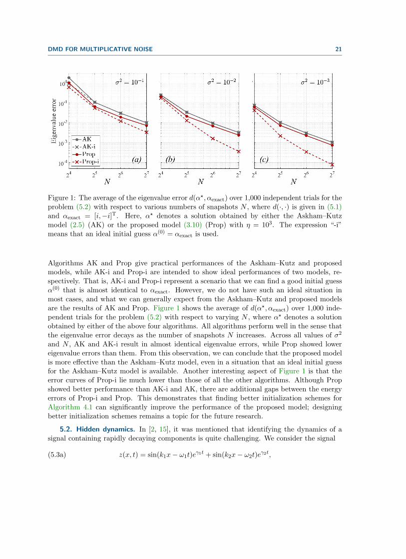
Figure 1: The average of the eigenvalue error d(α⋆, αexact) over 1,000 independent trials for theproblem (5.2) with respect to various numbers of snapshots N , where d(·, ·) is given in (5.1)and αexact = [i,−i]T. Here, α⋆ denotes a solution obtained by either the Askham–Kutzmodel (2.5) (AK) or the proposed model (3.10) (Prop) with η = 103. The expression “-i”means that an ideal initial guess α(0) = αexact is used.
Algorithms AK and Prop give practical performances of the Askham–Kutz and proposedmodels, while AK-i and Prop-i are intended to show ideal performances of two models, re-spectively. That is, AK-i and Prop-i represent a scenario that we can find a good initial guessα(0) that is almost identical to αexact. However, we do not have such an ideal situation inmost cases, and what we can generally expect from the Askham–Kutz and proposed modelsare the results of AK and Prop. Figure 1 shows the average of d(α⋆, αexact) over 1,000 inde-pendent trials for the problem (5.2) with respect to varying N , where α⋆ denotes a solutionobtained by either of the above four algorithms. All algorithms perform well in the sense thatthe eigenvalue error decays as the number of snapshots N increases. Across all values of σ2
and N , AK and AK-i result in almost identical eigenvalue errors, while Prop showed lowereigenvalue errors than them. From this observation, we can conclude that the proposed modelis more effective than the Askham–Kutz model, even in a situation that an ideal initial guessfor the Askham–Kutz model is available. Another interesting aspect of Figure 1 is that theerror curves of Prop-i lie much lower than those of all the other algorithms. Although Propshowed better performance than AK-i and AK, there are additional gaps between the energyerrors of Prop-i and Prop. This demonstrates that finding better initialization schemes forAlgorithm 4.1 can significantly improve the performance of the proposed model; designingbetter initialization schemes remains a topic for the future research.
5.2. Hidden dynamics. In [2, 15], it was mentioned that identifying the dynamics of asignal containing rapidly decaying components is quite challenging. We consider the signal
(5.3a) z(x, t) = sin(k1x− ω1t)eγ1t + sin(k2x− ω2t)e
γ2t,

22 M. LEE, J. PARK, AND C. H. SOHN
Figure 2: The average of the eigenvalue error d(α⋆, αexact) over 1,000 independent trials for theproblem (5.3) with respect to various numbers of snapshots N , where d(·, ·) is given in (5.1)and αexact = [1 + i, 1 − i,−0.2 + 3.7i,−0.2 − 3.7i]T. Here, α⋆ denotes a solution obtainedby either the Askham–Kutz model (2.5) (AK) or the proposed model (3.10) (Prop). Theexpression “-i” means that an ideal initial guess α(0) = αexact is used.
which is a superposition of two travelling sinusoidal signals, with one growing and the otherdecaying. It has four continuous-time eigenvalues γ1 ± iω1 and γ2 ± iω2. As in [2, 15], weuse the settings k1 = 1, ω1 = 1, γ1 = 1, k2 = 0.4, ω2 = 3.7, and γ2 = −0.2, i.e., we haveαexact = [1+ i, 1− i,−0.2+3.7i,−0.2−3.7i]T . We set the spatial domain as [0, 15] and use 300equispaced points to discretize, i.e., M = 300 and ∆x = 15/(M−1). We also set the temporaldomain as [0, 1], with N equispaced discretization points, i.e., ∆t = 1/(N −1). In this setting,the corresponding matrix of snapshots X corrupted by gamma multiplicative noise is givenby
(5.3b) Xmn = z((m− 1)∆x, (n − 1)∆t)ǫmn, 1 ≤ m ≤M, 1 ≤ n ≤ N,
where ǫmn follows the gamma distribution of mean 1 and variance σ2.As for the case of the periodic problem, we conduct numerical experiments that can
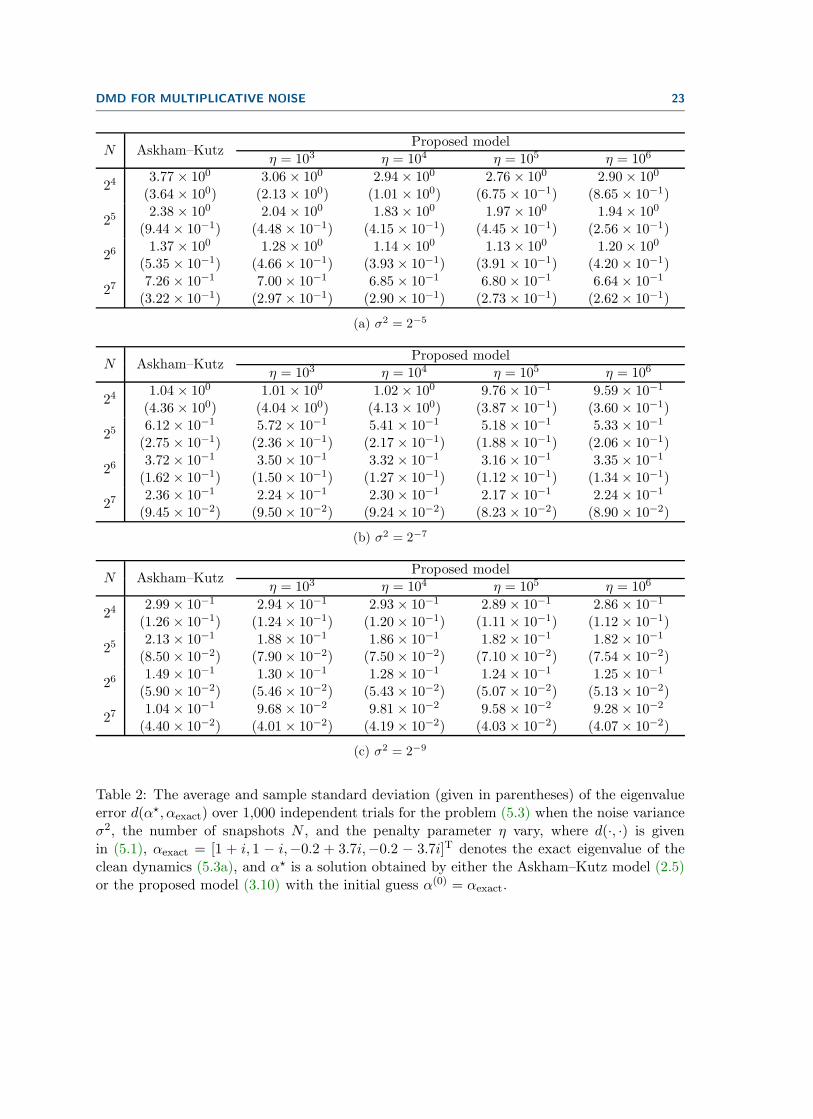
validate the suitability of the proposed model to the multiplicative noise. The average andsample standard deviation of the eigenvalue errors d(α⋆, αexact) over 1,000 independent trialsfor various σ2, N , and η are presented in Table 2, where α⋆ denotes a solution obtained byeither (2.5) or (3.10) with the ideal initial guess α(0) = αexact. We can again assure that theeigenvalue errors resulted from the proposed model are smaller than that of the Askham–Kutzmodel for all cases. Hence, the same discussion as in Table 1 can be made for the hiddendynamics problem. In Table 2, an optimal range for the penalty parameter η that results inthe best performance of the proposed model is observed to be between 105 and 106.
To evaluate the practical performance of the proposed model for the hidden dynamicsproblem, we compare four algorithms AK, AK-i, Prop, and Prop-i for solving (5.3). In all
DMD FOR MULTIPLICATIVE NOISE 23
N Askham–KutzProposed model
η = 103 η = 104 η = 105 η = 106
243.77 × 100
(3.64 × 100)3.06 × 100
(2.13 × 100)2.94 × 100
(1.01 × 100)2.76 × 100
(6.75 × 10⁻¹)2.90× 100
(8.65 × 10⁻¹)
252.38 × 100
(9.44 × 10⁻¹)2.04 × 100
(4.48 × 10⁻¹)1.83 × 100
(4.15 × 10⁻¹)1.97 × 100
(4.45 × 10⁻¹)1.94× 100
(2.56 × 10⁻¹)
261.37 × 100
(5.35 × 10⁻¹)1.28 × 100
(4.66 × 10⁻¹)1.14 × 100
(3.93 × 10⁻¹)1.13 × 100
(3.91 × 10⁻¹)1.20× 100
(4.20 × 10⁻¹)
277.26 × 10⁻¹
(3.22 × 10⁻¹)7.00 × 10⁻¹
(2.97 × 10⁻¹)6.85 × 10⁻¹
(2.90 × 10⁻¹)6.80 × 10⁻¹
(2.73 × 10⁻¹)6.64 × 10⁻¹
(2.62 × 10⁻¹)
(a) σ2 = 2−5
N Askham–KutzProposed model
η = 103 η = 104 η = 105 η = 106
241.04 × 100
(4.36 × 100)1.01 × 100
(4.04 × 100)1.02 × 100
(4.13 × 100)9.76 × 10⁻¹
(3.87 × 10⁻¹)9.59 × 10⁻¹
(3.60 × 10⁻¹)
256.12 × 10⁻¹
(2.75 × 10⁻¹)5.72 × 10⁻¹
(2.36 × 10⁻¹)5.41 × 10⁻¹
(2.17 × 10⁻¹)5.18 × 10⁻¹
(1.88 × 10⁻¹)5.33 × 10⁻¹
(2.06 × 10⁻¹)
263.72 × 10⁻¹
(1.62 × 10⁻¹)3.50 × 10⁻¹
(1.50 × 10⁻¹)3.32 × 10⁻¹
(1.27 × 10⁻¹)3.16 × 10⁻¹
(1.12 × 10⁻¹)3.35 × 10⁻¹
(1.34 × 10⁻¹)
272.36 × 10⁻¹
(9.45 × 10⁻²)2.24 × 10⁻¹
(9.50 × 10⁻²)2.30 × 10⁻¹
(9.24 × 10⁻²)2.17 × 10⁻¹
(8.23 × 10⁻²)2.24 × 10⁻¹
(8.90 × 10⁻²)
(b) σ2 = 2−7
N Askham–KutzProposed model
η = 103 η = 104 η = 105 η = 106
242.99 × 10⁻¹
(1.26 × 10⁻¹)2.94 × 10⁻¹
(1.24 × 10⁻¹)2.93 × 10⁻¹
(1.20 × 10⁻¹)2.89 × 10⁻¹
(1.11 × 10⁻¹)2.86 × 10⁻¹
(1.12 × 10⁻¹)
252.13 × 10⁻¹
(8.50 × 10⁻²)1.88 × 10⁻¹
(7.90 × 10⁻²)1.86 × 10⁻¹
(7.50 × 10⁻²)1.82 × 10⁻¹
(7.10 × 10⁻²)1.82 × 10⁻¹
(7.54 × 10⁻²)
261.49 × 10⁻¹
(5.90 × 10⁻²)1.30 × 10⁻¹
(5.46 × 10⁻²)1.28 × 10⁻¹
(5.43 × 10⁻²)1.24 × 10⁻¹
(5.07 × 10⁻²)1.25 × 10⁻¹
(5.13 × 10⁻²)
271.04 × 10⁻¹
(4.40 × 10⁻²)9.68 × 10⁻²
(4.01 × 10⁻²)9.81 × 10⁻²
(4.19 × 10⁻²)9.58 × 10⁻²
(4.03 × 10⁻²)9.28 × 10⁻²
(4.07 × 10⁻²)
(c) σ2 = 2−9
Table 2: The average and sample standard deviation (given in parentheses) of the eigenvalueerror d(α⋆, αexact) over 1,000 independent trials for the problem (5.3) when the noise varianceσ2, the number of snapshots N , and the penalty parameter η vary, where d(·, ·) is givenin (5.1), αexact = [1 + i, 1 − i,−0.2 + 3.7i,−0.2 − 3.7i]T denotes the exact eigenvalue of theclean dynamics (5.3a), and α⋆ is a solution obtained by either the Askham–Kutz model (2.5)or the proposed model (3.10) with the initial guess α(0) = αexact.
24 M. LEE, J. PARK, AND C. H. SOHN
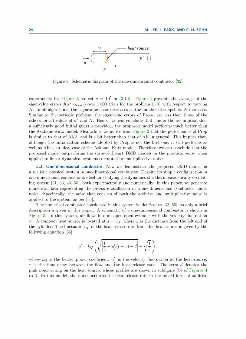
Figure 3: Schematic diagram of the one-dimensional combustor [32].
experiments for Figure 2, we set η = 105 in (3.10). Figure 2 presents the average of theeigenvalue errors d(α⋆, αexact) over 1,000 trials for the problem (5.3) with respect to varyingN . In all algorithms, the eigenvalue error decreases as the number of snapshots N increases.Similar to the periodic problem, the eigenvalue errors of Prop-i are less than those of theothers for all values of σ2 and N . Hence, we can conclude that, under the assumption thata sufficiently good initial guess is provided, the proposed model performs much better thanthe Askham–Kutz model. Meanwhile, we notice from Figure 2 that the performance of Propis similar to that of AK-i, and is a bit better than that of AK in general. This implies that,although the initialization scheme adopted by Prop is not the best one, it still performs aswell as AK-i, an ideal case of the Askham–Kutz model. Therefore, we can conclude that theproposed model outperforms the state-of-the-art DMD models in the practical sense whenapplied to linear dynamical systems corrupted by multiplicative noise.
5.3. One-dimensional combustor. Now we demonstrate the proposed DMD model ona realistic physical system, a one-dimensional combustor. Despite its simple configuration, aone-dimensional combustor is ideal for studying the dynamics of a thermoacoustically oscillat-ing system [21, 33, 43, 55], both experimentally and numerically. In this paper, we generatenumerical data representing the pressure oscillation in a one-dimensional combustor undernoise. Specifically, the noise that consists of both the additive and multiplicative noise isapplied to the system, as per [55].
The numerical combustor considered in this system is identical to [32, 55], so only a briefdescription is given in this paper. A schematic of a one-dimensional combustor is shown inFigure 3. In this system, air flows into an open-open cylinder with the velocity fluctuationu′. A compact heat source is located at x = xf , where x is the distance from the left end ofthe cylinder. The fluctuation q′ of the heat release rate from this heat source is given by thefollowing equation [55]:
q′ = kQ
(√∣∣∣∣1
3+ u′f (t− τ) + d
∣∣∣∣−√
1
3
),
where kQ is the heater power coefficient, u′f is the velocity fluctuation at the heat source,τ is the time delay between the flow and the heat release rate. The term d denotes thepink noise acting on the heat source, whose profiles are shown in subfigure (b) of Figures 4to 6. In this model, the noise perturbs the heat release rate in the mixed form of additive

DMD FOR MULTIPLICATIVE NOISE 25
and multiplicative noise. It is worth mentioning that this simple noise model can effectivelyreproduce the qualitative features of the Ornstein–Uhlenbeck process [25, 55].
The momentum and energy equations governing the one-dimensional combustor are asfollows:
γMa∂u′
∂t+
∂p′
∂x= 0,
∂p′
∂t+ γMa
∂u′
∂x+ ǫp′ = q′δ(x − xf ),
where p′ is the pressure fluctuation inside the combustor, t is time, γ is the specific heatratio, Ma is the Mach number of the mean flow, and ǫ is the acoustic damping coefficient. Inthe right-hand side of the second equation, δ denotes a Dirac delta expressing the local heatrelease at the heat source.
By using the Galerkin expansion [38, 58], a set of ordinary differential equations can bederived from the momentum and energy equations. Specifically, we set ∂u
∂x=0 and p′ = 0 at
both ends of the cylinder, and choose appropriate Galerkin basis functions so that
u′ =
jmax∑
j=1
ζj cos (jπx),(5.4a)
p′ = −jmax∑
j=1
γMa
jπζj sin (jπx),(5.4b)
where jmax is the number of superpositioned Galerkin modes and ζj denotes the state variableof the jth mode. It should be noted that all Galerkin modes are orthogonal, but are notnecessarily the eigenmodes of the system. By replacing u′ and p′ of the governing equationswith equations (5.4a) and (5.4b), respectively, we obtain
(5.5) ζj + (jπ)2ζj + ǫj ζj = −kQ2jπ
γMasin (jπxf )
(√∣∣∣∣1
3+ u′f (t− τ) + d
∣∣∣∣−√
1
3
),
where ǫj = 0.1 + 0.06√j represents the acoustic damping coefficient of the jth Galerkin
mode [22, 32]. Equation (5.5) is solved numerically using the fourth-order Runge–Kuttamethod with a time step ∆t = 0.01 for t ∈ [0, 200]. The combustor is spatially divided into500 equal-length segments. We set the parameters of (5.5) as follows: Ma = 0.005, xf = 0.25,τ = 0.16, kQ = 0.0035, and γ = 1.4, following previous practices [31, 32]. By numericallysolving this time-marching problem, we obtain a data matrix X whose rows represent thespatial distribution of p′ and columns represent the time.
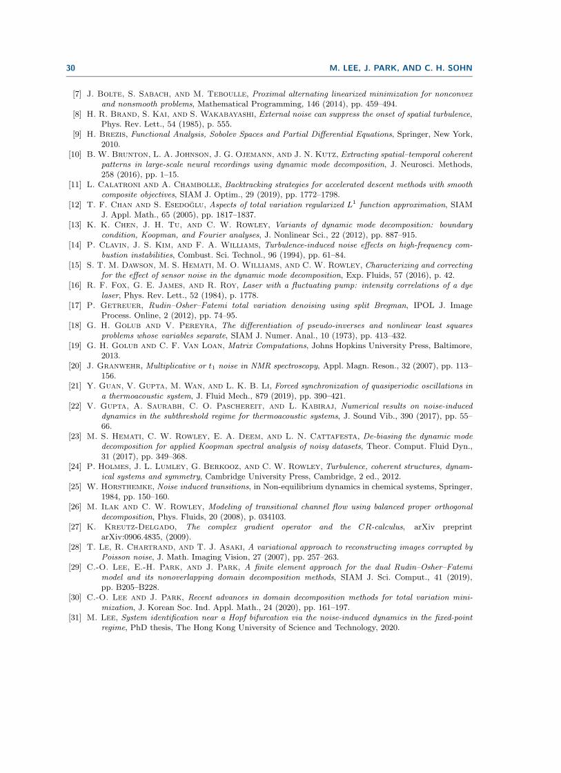
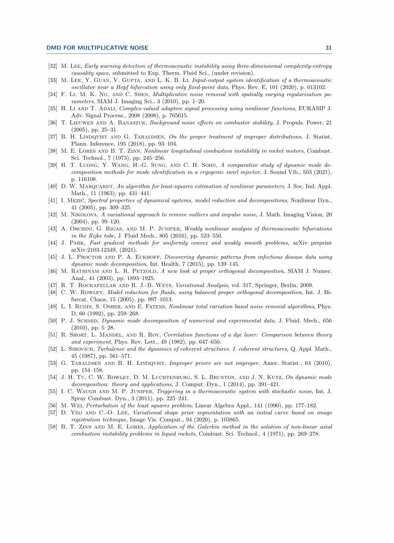
We normalize the noise intensity with the average flow fluctuation amplitude (d/u0)and consider three distinctive cases: weak (d/u0=0.0016), intermediate (d/u0=0.0031) andstrong (d/u0=0.0079) noise. The profiles of weak, intermediate and strong noise are shown insubfigures (a, b) of Figures 4 to 6, respectively.
The pressure fluctuation signals at the pressure antinode (x = 0.5) are shown in subfigure(c) of Figures 4 to 6. Regardless of the noise intensity, the pressure fluctuation develops

26 M. LEE, J. PARK, AND C. H. SOHN
Figure 4: (a, b) Noise profile, (c) pressure signal and (d) reconstruction error for the one-dimensional combustor problem under weak noise.
gradually until t ≈ 110 when the nonlinearity starts to dominate the dynamics of the system.In order to capture the local linearity of the system, we divide the pressure signal into ten timesections [0, 20], [20, 40], . . . , [180, 200], and apply the proposed DMD model at each section.Specifically, we use R = 10 (i.e., five pairs of eigenvectors) to decompose the noisy signalsegments. We then reconstruct the pressure signal using the obtained modes and compare itwith the clean (zero-noise) data. The reconstruction error Erecon at each segment is calculated
DMD FOR MULTIPLICATIVE NOISE 27
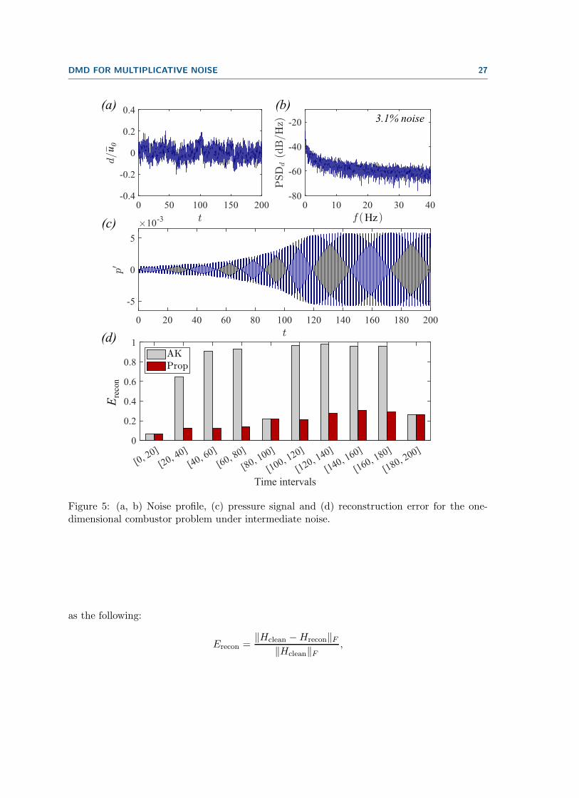
Figure 5: (a, b) Noise profile, (c) pressure signal and (d) reconstruction error for the one-dimensional combustor problem under intermediate noise.
as the following:
Erecon =‖Hclean −Hrecon‖F‖Hclean‖F
,

28 M. LEE, J. PARK, AND C. H. SOHN
Figure 6: (a, b) Noise profile, (c) pressure signal and (d) reconstruction error for the one-dimensional combustor problem under strong noise.
where Hclean is the snapshots of the zero-noise data and Hrecon is given by
Hrecon =
Φ(α)Φ(α)+H for the Askham–Kutz model (2.5),
Φ(α)Φ(α)+H for the proposed model (3.10).
It can be found from Figure 4(c) that the proposed DMD model can accurately decomposethe signal with minimal reconstruction error. Specifically, Erecon is 6.5% in the first segmentand is less than 4% in all other segments. A significant decrease in the reconstruction error is
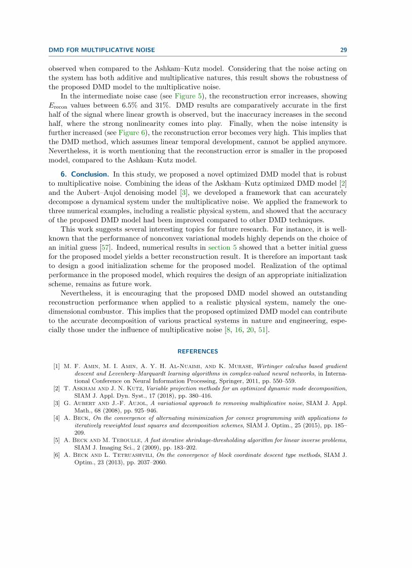
DMD FOR MULTIPLICATIVE NOISE 29
observed when compared to the Ashkam–Kutz model. Considering that the noise acting onthe system has both additive and multiplicative natures, this result shows the robustness ofthe proposed DMD model to the multiplicative noise.
In the intermediate noise case (see Figure 5), the reconstruction error increases, showingErecon values between 6.5% and 31%. DMD results are comparatively accurate in the firsthalf of the signal where linear growth is observed, but the inaccuracy increases in the secondhalf, where the strong nonlinearity comes into play. Finally, when the noise intensity isfurther increased (see Figure 6), the reconstruction error becomes very high. This implies thatthe DMD method, which assumes linear temporal development, cannot be applied anymore.Nevertheless, it is worth mentioning that the reconstruction error is smaller in the proposedmodel, compared to the Ashkam–Kutz model.
6. Conclusion. In this study, we proposed a novel optimized DMD model that is robustto multiplicative noise. Combining the ideas of the Askham–Kutz optimized DMD model [2]and the Aubert–Aujol denoising model [3], we developed a framework that can accuratelydecompose a dynamical system under the multiplicative noise. We applied the framework tothree numerical examples, including a realistic physical system, and showed that the accuracyof the proposed DMD model had been improved compared to other DMD techniques.
This work suggests several interesting topics for future research. For instance, it is well-known that the performance of nonconvex variational models highly depends on the choice ofan initial guess [57]. Indeed, numerical results in section 5 showed that a better initial guessfor the proposed model yields a better reconstruction result. It is therefore an important taskto design a good initialization scheme for the proposed model. Realization of the optimalperformance in the proposed model, which requires the design of an appropriate initializationscheme, remains as future work.
Nevertheless, it is encouraging that the proposed DMD model showed an outstandingreconstruction performance when applied to a realistic physical system, namely the one-dimensional combustor. This implies that the proposed optimized DMD model can contributeto the accurate decomposition of various practical systems in nature and engineering, espe-cially those under the influence of multiplicative noise [8, 16, 20, 51].
REFERENCES
[1] M. F. Amin, M. I. Amin, A. Y. H. Al-Nuaimi, and K. Murase, Wirtinger calculus based gradient
descent and Levenberg–Marquardt learning algorithms in complex-valued neural networks, in Interna-tional Conference on Neural Information Processing, Springer, 2011, pp. 550–559.
[2] T. Askham and J. N. Kutz, Variable projection methods for an optimized dynamic mode decomposition,SIAM J. Appl. Dyn. Syst., 17 (2018), pp. 380–416.
[3] G. Aubert and J.-F. Aujol, A variational approach to removing multiplicative noise, SIAM J. Appl.Math., 68 (2008), pp. 925–946.
[4] A. Beck, On the convergence of alternating minimization for convex programming with applications to
iteratively reweighted least squares and decomposition schemes, SIAM J. Optim., 25 (2015), pp. 185–209.
[5] A. Beck and M. Teboulle, A fast iterative shrinkage-thresholding algorithm for linear inverse problems,SIAM J. Imaging Sci., 2 (2009), pp. 183–202.
[6] A. Beck and L. Tetruashvili, On the convergence of block coordinate descent type methods, SIAM J.Optim., 23 (2013), pp. 2037–2060.
30 M. LEE, J. PARK, AND C. H. SOHN
[7] J. Bolte, S. Sabach, and M. Teboulle, Proximal alternating linearized minimization for nonconvex
and nonsmooth problems, Mathematical Programming, 146 (2014), pp. 459–494.[8] H. R. Brand, S. Kai, and S. Wakabayashi, External noise can suppress the onset of spatial turbulence,
Phys. Rev. Lett., 54 (1985), p. 555.[9] H. Brezis, Functional Analysis, Sobolev Spaces and Partial Differential Equations, Springer, New York,
2010.[10] B. W. Brunton, L. A. Johnson, J. G. Ojemann, and J. N. Kutz, Extracting spatial–temporal coherent
patterns in large-scale neural recordings using dynamic mode decomposition, J. Neurosci. Methods,258 (2016), pp. 1–15.
[11] L. Calatroni and A. Chambolle, Backtracking strategies for accelerated descent methods with smooth
composite objectives, SIAM J. Optim., 29 (2019), pp. 1772–1798.[12] T. F. Chan and S. Esedoglu, Aspects of total variation regularized L
1 function approximation, SIAMJ. Appl. Math., 65 (2005), pp. 1817–1837.
[13] K. K. Chen, J. H. Tu, and C. W. Rowley, Variants of dynamic mode decomposition: boundary
condition, Koopman, and Fourier analyses, J. Nonlinear Sci., 22 (2012), pp. 887–915.[14] P. Clavin, J. S. Kim, and F. A. Williams, Turbulence-induced noise effects on high-frequency com-
bustion instabilities, Combust. Sci. Technol., 96 (1994), pp. 61–84.[15] S. T. M. Dawson, M. S. Hemati, M. O. Williams, and C. W. Rowley, Characterizing and correcting
for the effect of sensor noise in the dynamic mode decomposition, Exp. Fluids, 57 (2016), p. 42.[16] R. F. Fox, G. E. James, and R. Roy, Laser with a fluctuating pump: intensity correlations of a dye
laser, Phys. Rev. Lett., 52 (1984), p. 1778.[17] P. Getreuer, Rudin–Osher–Fatemi total variation denoising using split Bregman, IPOL J. Image
Process. Online, 2 (2012), pp. 74–95.[18] G. H. Golub and V. Pereyra, The differentiation of pseudo-inverses and nonlinear least squares
problems whose variables separate, SIAM J. Numer. Anal., 10 (1973), pp. 413–432.[19] G. H. Golub and C. F. Van Loan, Matrix Computations, Johns Hopkins University Press, Baltimore,
2013.[20] J. Granwehr, Multiplicative or t1 noise in NMR spectroscopy, Appl. Magn. Reson., 32 (2007), pp. 113–
156.[21] Y. Guan, V. Gupta, M. Wan, and L. K. B. Li, Forced synchronization of quasiperiodic oscillations in
a thermoacoustic system, J. Fluid Mech., 879 (2019), pp. 390–421.[22] V. Gupta, A. Saurabh, C. O. Paschereit, and L. Kabiraj, Numerical results on noise-induced
dynamics in the subthreshold regime for thermoacoustic systems, J. Sound Vib., 390 (2017), pp. 55–66.
[23] M. S. Hemati, C. W. Rowley, E. A. Deem, and L. N. Cattafesta, De-biasing the dynamic mode
decomposition for applied Koopman spectral analysis of noisy datasets, Theor. Comput. Fluid Dyn.,31 (2017), pp. 349–368.
[24] P. Holmes, J. L. Lumley, G. Berkooz, and C. W. Rowley, Turbulence, coherent structures, dynam-
ical systems and symmetry, Cambridge University Press, Cambridge, 2 ed., 2012.[25] W. Horsthemke, Noise induced transitions, in Non-equilibrium dynamics in chemical systems, Springer,
1984, pp. 150–160.[26] M. Ilak and C. W. Rowley, Modeling of transitional channel flow using balanced proper orthogonal
decomposition, Phys. Fluids, 20 (2008), p. 034103.[27] K. Kreutz-Delgado, The complex gradient operator and the CR-calculus, arXiv preprint
arXiv:0906.4835, (2009).[28] T. Le, R. Chartrand, and T. J. Asaki, A variational approach to reconstructing images corrupted by
Poisson noise, J. Math. Imaging Vision, 27 (2007), pp. 257–263.[29] C.-O. Lee, E.-H. Park, and J. Park, A finite element approach for the dual Rudin–Osher–Fatemi
model and its nonoverlapping domain decomposition methods, SIAM J. Sci. Comput., 41 (2019),pp. B205–B228.
[30] C.-O. Lee and J. Park, Recent advances in domain decomposition methods for total variation mini-
mization, J. Korean Soc. Ind. Appl. Math., 24 (2020), pp. 161–197.[31] M. Lee, System identification near a Hopf bifurcation via the noise-induced dynamics in the fixed-point
regime, PhD thesis, The Hong Kong University of Science and Technology, 2020.
DMD FOR MULTIPLICATIVE NOISE 31
[32] M. Lee, Early warning detection of thermoacoustic instability using three-dimensional complexity-entropy
causality space, submitted to Exp. Therm. Fluid Sci., (under revision).[33] M. Lee, Y. Guan, V. Gupta, and L. K. B. Li, Input-output system identification of a thermoacoustic
oscillator near a Hopf bifurcation using only fixed-point data, Phys. Rev. E, 101 (2020), p. 013102.[34] F. Li, M. K. Ng, and C. Shen, Multiplicative noise removal with spatially varying regularization pa-
rameters, SIAM J. Imaging Sci., 3 (2010), pp. 1–20.[35] H. Li and T. Adalı, Complex-valued adaptive signal processing using nonlinear functions, EURASIP J.
Adv. Signal Process., 2008 (2008), p. 765615.[36] T. Lieuwen and A. Banaszuk, Background noise effects on combustor stability, J. Propuls. Power, 21
(2005), pp. 25–31.[37] B. H. Lindqvist and G. Taraldsen, On the proper treatment of improper distributions, J. Statist.
Plann. Inference, 195 (2018), pp. 93–104.[38] M. E. Lores and B. T. Zinn, Nonlinear longitudinal combustion instability in rocket motors, Combust.
Sci. Technol., 7 (1973), pp. 245–256.[39] H. T. Luong, Y. Wang, H.-G. Sung, and C. H. Sohn, A comparative study of dynamic mode de-
composition methods for mode identification in a cryogenic swirl injector, J. Sound Vib., 503 (2021),p. 116108.
[40] D. W. Marquardt, An algorithm for least-squares estimation of nonlinear parameters, J. Soc. Ind. Appl.Math., 11 (1963), pp. 431–441.
[41] I. Mezic, Spectral properties of dynamical systems, model reduction and decompositions, Nonlinear Dyn.,41 (2005), pp. 309–325.
[42] M. Nikolova, A variational approach to remove outliers and impulse noise, J. Math. Imaging Vision, 20(2004), pp. 99–120.
[43] A. Orchini, G. Rigas, and M. P. Juniper, Weakly nonlinear analysis of thermoacoustic bifurcations
in the Rijke tube, J. Fluid Mech., 805 (2016), pp. 523–550.[44] J. Park, Fast gradient methods for uniformly convex and weakly smooth problems, arXiv preprint
arXiv:2103.12349, (2021).[45] J. L. Proctor and P. A. Eckhoff, Discovering dynamic patterns from infectious disease data using
dynamic mode decomposition, Int. Health, 7 (2015), pp. 139–145.[46] M. Rathinam and L. R. Petzold, A new look at proper orthogonal decomposition, SIAM J. Numer.
Anal., 41 (2003), pp. 1893–1925.[47] R. T. Rockafellar and R. J.-B. Wets, Variational Analysis, vol. 317, Springer, Berlin, 2009.[48] C. W. Rowley, Model reduction for fluids, using balanced proper orthogonal decomposition, Int. J. Bi-
furcat. Chaos, 15 (2005), pp. 997–1013.[49] L. I. Rudin, S. Osher, and E. Fatemi, Nonlinear total variation based noise removal algorithms, Phys.
D, 60 (1992), pp. 259–268.[50] P. J. Schmid, Dynamic mode decomposition of numerical and experimental data, J. Fluid. Mech., 656
(2010), pp. 5–28.[51] R. Short, L. Mandel, and R. Roy, Correlation functions of a dye laser: Comparison between theory
and experiment, Phys. Rev. Lett., 49 (1982), pp. 647–650.[52] L. Sirovich, Turbulence and the dynamics of coherent structures. I. coherent structures, Q. Appl. Math.,
45 (1987), pp. 561–571.[53] G. Taraldsen and B. H. Lindqvist, Improper priors are not improper, Amer. Statist., 64 (2010),
pp. 154–158.[54] J. H. Tu, C. W. Rowley, D. M. Luchtenburg, S. L. Brunton, and J. N. Kutz, On dynamic mode
decomposition: theory and applications, J. Comput. Dyn., 1 (2014), pp. 391–421.[55] I. C. Waugh and M. P. Juniper, Triggering in a thermoacoustic system with stochastic noise, Int. J.
Spray Combust. Dyn., 3 (2011), pp. 225–241.[56] M. Wei, Perturbation of the least squares problem, Linear Algebra Appl., 141 (1990), pp. 177–182.[57] D. Yeo and C.-O. Lee, Variational shape prior segmentation with an initial curve based on image
registration technique, Image Vis. Comput., 94 (2020), p. 103865.[58] B. T. Zinn and M. E. Lores, Application of the Galerkin method in the solution of non-linear axial
combustion instability problems in liquid rockets, Combust. Sci. Technol., 4 (1971), pp. 269–278.

![Toward Forecasting Volcanic Eruptions using Seismic Noise ... · arXiv:0706.1935v1 [physics.geo-ph] 13 Jun 2007 Toward Forecasting Volcanic Eruptions using Seismic Noise Florent Brenguier,1,2∗](https://static.fdocuments.us/doc/165x107/5f65df0007692a29db660dda/toward-forecasting-volcanic-eruptions-using-seismic-noise-arxiv07061935v1.jpg)


![a arXiv:1609.09554v1 [nlin.AO] 30 Sep 2016 · · 2016-10-03against increasing noise strength when noise is applied to nodes in di erent ... Red a random graph used in [18]. ...](https://static.fdocuments.us/doc/165x107/5ae6543c7f8b9a8b2b8d2133/a-arxiv160909554v1-nlinao-30-sep-2016-increasing-noise-strength-when-noise.jpg)


![Stochastic continuity equations with conservative …arXiv:1710.04906v1 [math.AP] 13 Oct 2017 Stochastic continuity equations with conservative noise Benjamin Gess and Scott Smith](https://static.fdocuments.us/doc/165x107/5f866d8333a8b54c8864eab5/stochastic-continuity-equations-with-conservative-arxiv171004906v1-mathap-13.jpg)
![arXiv:1904.08598v3 [stat.ML] 25 Jun 2020Reducing Noise in GAN Training with Variance Reduced Extragradient Tatjana Chavdarova Mila, Université de Montréal Idiap, École Polytechnique](https://static.fdocuments.us/doc/165x107/6024fda30076bc77d721f6e5/arxiv190408598v3-statml-25-jun-2020-reducing-noise-in-gan-training-with-variance.jpg)