JULY 2009

NOAA-TM-NMFS-SWFSC-447

U.S. DEPARTMENT OF COMMERCENational Oceanic and Atmospheric AdministrationNational Marine Fisheries ServiceSouthwest Fisheries Science Center

NOAA Technical Memorandum NMFS

U

AN

CI IT

RE

EDMS ATA FT OE S

OFT CN OE MM MT

R E

A R

P C

E E

D

S.T. Lindley, C.B. Grimes, M.S. Mohr, W. Peterson, J. Stein,

J.T. Anderson, L.W. Botsford, D.L. Bottom, C.A. Busack, T.K. Collier,

J. Ferguson, J.C. Garza, A.M. Grover, D.G. Hankin, R.G. Kope

P.W. Lawson, A. Low, R.B. MacFarlane, K. Moore, M. Palmer-Zwahlen,

F.B. Schwing, J. Smith, C. Tracy, R. Webb, B.K. Wells, and T.H. Williams

WHAT CAUSED THE SACRAMENTO RIVER

FALL CHINOOK STOCK COLLAPSE?

The National Oceanic and Atmospheric Administration (NOAA), organized in 1970, has evolved into an agency that establishes national policies and manages and conserves our oceanic, coastal, and atmospheric resources. An organizational element within NOAA, the Office of Fisheries is responsible for fisheries policy and the direction of the National Marine Fisheries Service (NMFS).

In addition to its formal publications, the NMFS uses the NOAA Technical Memorandum series to issue informal scientific and technical publications when complete formal review and editorial processing are not appropriate or feasible. Documents within this series, however, reflect sound professional work and may be referenced in the formal scientific and technical literature.

MOSTA PHD EN RA ICCI AN DA ME IC N

O IS

L T

A R

N ATOI IOT

A N

N

U

E.S C. RD EE MPA MR OT CM FENT O

NOAA Technical Memorandum NMFSThis TM series is used for documentation and timely communication of preliminary results, interim reports, or specialpurpose information. The TMs have not received complete formal review, editorial control, or detailed editing.

NOAA-TM-NMFS-SWFSC-447

JULY 2009

U.S. DEPARTMENT OF COMMERCEGary F. Locke, SecretaryNational Oceanic and Atmospheric AdministrationJane Lubchenco, Undersecretary for Oceans and AtmosphereNational Marine Fisheries ServiceJames W. Balsiger, Acting Assistant Administrator for Fisheries

S.T. Lindley, C.B. Grimes, M.S. Mohr, W. Peterson, J. Stein,

J.T. Anderson, L.W. Botsford, D.L. Bottom, C.A. Busack, T.K. Collier,

J. Ferguson, J.C. Garza, A.M. Grover, D.G. Hankin, R.G. Kope

P.W. Lawson, A. Low, R.B. MacFarlane, K. Moore, M. Palmer-Zwahlen,

F.B. Schwing, J. Smith, C. Tracy, R. Webb, B.K. Wells, and T.H. Williams

National Oceanic & Atmospheric AdministrationNational Marine Fisheries Service

Southwest Fisheries Science CenterFisheries Ecology Division

110 Shaffer RoadSanta Cruz, California, USA 95060

WHAT CAUSED THE SACRAMENTO RIVER

FALL CHINOOK STOCK COLLAPSE?

Contents1 Summary 4

2 Introduction 7

3 Analysis of recent broods 103.1 Review of the life history of SRFC . . . . . . . . . . . . . . . . . . 103.2 Available data . . . . . . . . . . . . . . . . . . . . . . . . . . . . . 113.3 Conceptual approach . . . . . . . . . . . . . . . . . . . . . . . . . 113.4 Brood year 2004 . . . . . . . . . . . . . . . . . . . . . . . . . . . 15

3.4.1 Parents . . . . . . . . . . . . . . . . . . . . . . . . . . . . 153.4.2 Eggs . . . . . . . . . . . . . . . . . . . . . . . . . . . . . 163.4.3 Fry, parr and smolts . . . . . . . . . . . . . . . . . . . . . . 173.4.4 Early ocean . . . . . . . . . . . . . . . . . . . . . . . . . . 213.4.5 Later ocean . . . . . . . . . . . . . . . . . . . . . . . . . . 303.4.6 Spawners . . . . . . . . . . . . . . . . . . . . . . . . . . . 323.4.7 Conclusions for the 2004 brood . . . . . . . . . . . . . . . 32

3.5 Brood year 2005 . . . . . . . . . . . . . . . . . . . . . . . . . . . 333.5.1 Parents . . . . . . . . . . . . . . . . . . . . . . . . . . . . 333.5.2 Eggs . . . . . . . . . . . . . . . . . . . . . . . . . . . . . 333.5.3 Fry, parr and smolts . . . . . . . . . . . . . . . . . . . . . . 333.5.4 Early ocean . . . . . . . . . . . . . . . . . . . . . . . . . . 343.5.5 Later ocean . . . . . . . . . . . . . . . . . . . . . . . . . . 353.5.6 Spawners . . . . . . . . . . . . . . . . . . . . . . . . . . . 353.5.7 Conclusions for the 2005 brood . . . . . . . . . . . . . . . 35

3.6 Prospects for brood year 2006 . . . . . . . . . . . . . . . . . . . . 363.7 Is climate change a factor? . . . . . . . . . . . . . . . . . . . . . . 363.8 Summary . . . . . . . . . . . . . . . . . . . . . . . . . . . . . . . 38

4 The role of anthropogenic impacts 384.1 Sacramento River fall Chinook . . . . . . . . . . . . . . . . . . . . 384.2 Other Chinook stocks in the Central Valley . . . . . . . . . . . . . 43

5 Recommendations 475.1 Knowledge Gaps . . . . . . . . . . . . . . . . . . . . . . . . . . . 495.2 Improving resilience . . . . . . . . . . . . . . . . . . . . . . . . . 505.3 Synthesis . . . . . . . . . . . . . . . . . . . . . . . . . . . . . . . 51

2

List of Figures1 Sacramento River index. . . . . . . . . . . . . . . . . . . . . . . . 82 Map of the Sacramento River basin and adjacent coastal ocean. . . . 133 Conceptual model of a cohort of fall-run Chinook. . . . . . . . . . . 144 Discharge in regulated reaches of the Sacramento River, Feather

River, American River and Stanislaus River in 2004-2007. . . . . . 165 Daily export of freshwater from the Delta and the ratio of exports

to inflows. . . . . . . . . . . . . . . . . . . . . . . . . . . . . . . . 186 Releases of hatchery fish. . . . . . . . . . . . . . . . . . . . . . . . 197 Mean annual catch-per-unit effort of fall Chinook juveniles at Chipps

Island by USFWS trawl sampling. . . . . . . . . . . . . . . . . . . 208 Cumulative daily catch per unit effort of fall Chinook juveniles at

Chipps Island by USFWS trawl sampling in 2005. . . . . . . . . . . 209 Relative survival from release into the estuary to age two in the

ocean for Feather River Hatchery fall Chinook. . . . . . . . . . . . 2210 Escapement of SRFC jacks. . . . . . . . . . . . . . . . . . . . . . . 2211 Conceptual diagram displaying the hypothesized relationship be-

tween wind-forced upwelling and the pelagic ecosystem. . . . . . . 2412 Sea surface temperature (colors) and wind (vectors) anomalies for

the north Pacific for Apr-Jun in 2005-2008. . . . . . . . . . . . . . 2513 Cumulative upwelling index (CUI) and anomalies of the CUI. . . . 2714 Sea surface temperature anomalies off central California in May-

July of 2003-2006. . . . . . . . . . . . . . . . . . . . . . . . . . . 2815 Surface particle trajectories predicted from the OSCURS current

model . . . . . . . . . . . . . . . . . . . . . . . . . . . . . . . . . 2916 Length, weight and condition factor of juvenile Chinook over the

1998-2005 period. . . . . . . . . . . . . . . . . . . . . . . . . . . . 3119 The fraction of total escapement of SRFC that returns to spawn in

hatcheries. . . . . . . . . . . . . . . . . . . . . . . . . . . . . . . . 4220 Escapement trends in various populations of Central Valley Chinook. 4521 Escapement trends in the 1990s and 2000s of various populations

of Chinook. . . . . . . . . . . . . . . . . . . . . . . . . . . . . . . 4622 Maximum autocorrelation factor analysis (MAFA) of Central Val-

ley Chinook escapement timeseries. . . . . . . . . . . . . . . . . . 48

List of Tables1 Summary of data sources used in this report. . . . . . . . . . . . . . 12

3

1 SummaryIn April 2008, in response to the sudden collapse of Sacramento River fall Chi-nook salmon (SRFC) and the poor status of many west coast coho salmon popula-tions, the Pacific Fishery Management Council (PFMC) adopted the most restric-tive salmon fisheries in the history of the west coast of the U.S. The regulationsincluded a complete closure of commercial and recreational Chinook salmon fish-eries south of Cape Falcon, Oregon. Spawning escapement of SRFC in 2007 is es-timated to have been 88,000, well below the PFMC’s escapement conservation goalof 122,000-180,000 for the first time since the early 1990s. The situation was evenmore dire in 2008, when 66,000 spawners are estimated to have returned to naturalareas and hatcheries. For the SRFC stock, which is an aggregate of hatchery andnatural production, many factors have been suggested as potential causes of the poorescapements, including freshwater withdrawals (including pumping of water fromthe Sacramento-San Joaquin delta), unusual hatchery events, pollution, eliminationof net-pen acclimatization facilities coincident with one of the two failed broodyears, and large-scale bridge construction during the smolt outmigration (CDFG,2008). In this report we review possible causes for the decline in SRFC for whichreliable data were available.

Our investigation was guided by a conceptual model of the life history of fallChinook salmon in the wild and in the hatchery. Our approach was to identify whereand when in the life cycle abundance became anomalously low, and where and whenpoor environmental conditions occurred due to natural or human-induced causes.The likely cause of the SRFC collapse lies at the intersection of an unusually largedrop in abundance and poor environmental conditions. Using this framework, all ofthe evidence that we could find points to ocean conditions as being the proximatecause of the poor performance of the 2004 and 2005 broods of SRFC. We recognize,however, that the rapid and likely temporary deterioration in ocean conditions isacting on top of a long-term, steady degradation of the freshwater and estuarineenvironment.

The evidence pointed to ocean conditions as the proximate cause because con-ditions in freshwater were not unusual, and a measure of abundance at the entranceto the estuary showed that, up until that point, these broods were at or near normallevels of abundance. At some time and place between this point and recruitment tothe fishery at age two, unusually large fractions of these broods perished. A broadbody of evidence suggests that anomalous conditions in the coastal ocean in 2005and 2006 resulted in unusually poor survival of the 2004 and 2005 broods of SRFC.Both broods entered the ocean during periods of weak upwelling, warm sea surfacetemperatures, and low densities of prey items. Individuals from the 2004 broodsampled in the Gulf of the Farallones were in poor physical condition, indicatingthat feeding conditions were poor in the spring of 2005 (unfortunately, comparabledata do not exist for the 2005 brood). Pelagic seabirds in this region with diets sim-ilar to juvenile Chinook salmon also experienced very poor reproduction in theseyears. In addition, the cessation of net-pen acclimatization in the estuary in 2006may have contributed to the especially poor estuarine and marine survival of the

4

2005 brood.Fishery management also played a role in the low escapement of 2007. The

PFMC (2007) forecast an escapement of 265,000 SRFC adults in 2007 based onthe escapement of 14,500 Central Valley Chinook salmon jacks in 2006. The real-ized escapement of SRFC adults was 87,900. The large discrepancy between theforecast and realized abundance was due to a bias in the forecast model that hassince been corrected. Had the pre-season ocean abundance forecast been more ac-curate and fishing opportunity further constrained by management regulation, theSRFC escapement goal could have been met in 2007. Thus, fishery management,while not the cause of the 2004 brood weak year-class strength, contributed to thefailure to achieve the SRFC escapement goal in 2007.

The long-standing and ongoing degradation of freshwater and estuarine habitatsand the subsequent heavy reliance on hatchery production were also likely contrib-utors to the collapse of the stock. Degradation and simplification of freshwaterand estuary habitats over a century and a half of development have changed theCentral Valley Chinook salmon complex from a highly diverse collection of nu-merous wild populations to one dominated by fall Chinook salmon from four largehatcheries. Naturally-spawning populations of fall Chinook salmon are now ge-netically homogeneous in the Central Valley, and their population dynamics havebeen synchronous over the past few decades. In contrast, some remnant populationsof late-fall, winter and spring Chinook salmon have not been as strongly affectedby recent changes in ocean conditions, illustrating that life-history diversity canbuffer environmental variation. The situation is analogous to managing a financialportfolio: a well-diversified portfolio will be buffeted less by fluctuating marketconditions than one concentrated on just a few stocks; the SRFC seems to be quiteconcentrated indeed.

Climate variability plays an important role in the inter-annual variation in abun-dance of Pacific salmon, including SRFC. We have observed a trend of increasingvariability over the past several decades in climate indices related to salmon sur-vival. This is a coast-wide pattern, but may be particularly important in California,where salmon are near the southern end of their range. These more extreme climatefluctuations put additional strain on salmon populations that are at low abundanceand have little life-history or habitat diversity. If the trend of increasing climatevariability continues, then we can expect to see more extreme variation in the abun-dance of SRFC and salmon stocks coast wide.

In conclusion, the development of the Sacramento-San Joaquin watershed hasgreatly simplified and truncated the once-diverse habitats that historically supporteda highly diverse assemblage of populations. The life history diversity of this histor-ical assemblage would have buffered the overall abundance of Chinook salmon inthe Central Valley under varying climate conditions. We are now left with a fish-ery that is supported largely by four hatcheries that produce mostly fall Chinooksalmon. Because the survival of fall Chinook salmon hatchery release groups ishighly correlated among nearby hatcheries, and highly variable among years, wecan expect to see more booms and busts in this fishery in the future in responseto variation in the ocean environment. Simply increasing the production of fall

5

Chinook salmon from hatcheries as they are currently operated may aggravate thissituation by further concentrating production in time and space. Rather, the key toreducing variation in production is increasing the diversity of SRFC.

There are few direct actions available to the PFMC to improve this situation,but there are actions the PFMC can support that would lead to increased diversityof SRFC and increased stability. Mid-term solutions include continued advocacyfor more fish-friendly water management and the examination of hatchery prac-tices to improve the survival of hatchery releases while reducing adverse interac-tions with natural fish. In the longer-term, increased habitat quantity, quality, anddiversity, and modified hatchery practices could allow life history diversity to in-crease in SRFC. Increased diversity in SRFC life histories should lead to increasedstability and resilience in a dynamic, changing environment. Using an ecosystem-based management and ecological risk assessment framework to engage the manyagencies and stakeholder groups with interests in the ecosystems supporting SRFCwould aid implementation of these solutions.

6

2 IntroductionIn April 2008 the Pacific Fishery Management Council (PFMC) adopted the mostrestrictive salmon fisheries in the history of the west coast of the U.S., in response tothe sudden collapse of Sacramento River fall Chinook (SRFC) salmon and the poorstatus of many west coast coho salmon populations. The PFMC adopted a com-plete closure of commercial and recreational Chinook fisheries south of Cape Fal-con, Oregon, allowing only for a mark-selective hatchery coho recreational fisheryof 9,000 fish from Cape Falcon, Oregon, to the Oregon/California border. Salmonfisheries off California and Oregon have historically been robust, with seasons span-ning May through October and catches averaging over 800,000 Chinook per yearfrom 2000 to 2005. The negative economic impact of the closure was so drasticthat west coast governors asked for $290 million in disaster relief, and the U.S.Congress appropriated $170 million.

Escapement of several west coast Chinook and coho salmon stocks was lowerthan expected in 2007 (PFMC, 2009), and low jack escapement in 2007 for somestocks suggested that 2008 would be at least as bad (PFMC, 2008). The mostprominent example is SRFC salmon, for which spawning escapement in 2007 isestimated to have been 88,000, well below the escapement conservation goal ofthe PFMC (122,000–180,000 fish) for the first time since the early 1990s (Fig. 1).While the 2007 escapement represents a continuing decline since the recent peakescapement of 725,000 spawners in 2002, average escapement since 1983 has beenabout 248,000. The previous record low escapement, observed in 1992, is believedto have been due to a combination of drought conditions, overfishing, and poorocean conditions (SRFCRT, 1994). Although conditions have been wetter than av-erage over the 2000-2005 period, the spawning escapement of jacks in 2007 wasthe lowest on record, significantly lower than the 2006 jack escapement (the secondlowest on record), and the preseason projection of 2008 adult spawner escapementwas only 59,0001 despite the complete closure of coastal and freshwater Chinookfisheries.

Coastal coho salmon have also experience low escapement during this sametime frame. For California, coho salmon escapement in 2007 averaged 27% ofparent stock abundance in 2004, with a range from 0% (Redwood Creek) to 68%(Shasta River). In Oregon, spawner estimates for the Oregon Coast natural (OCN)coho salmon were 30% of parental spawner abundance. These returns are the lowestsince 1999, and are near the low abundances of the 1990s. Columbia River cohoand Chinook stocks experienced mixed escapement in 2007 and 2008.

For coho salmon in 2007 there was a clear north-south gradient, with escape-ment improving to the north. California and Oregon coastal escapement was downsharply, while Columbia River hatchery coho were down only slightly (PFMC,2009). Washington coastal coho escapement was similar to 2006. Even withinthe OCN region, there was a clear north-south pattern, with the north coast region(predominantly Nehalem River and Tillamook Bay populations) returning at 46%

1Preliminary postseason estimate for 2008 SRFC adult escapement is 66,000.

7

1983 1986 1989 1992 1995 1998 2001 2004 2007

Year

SI (t

hous

ands

)

050

010

0015

00 river harvestocean harvestescapement

Figure 1: Sacramento River fall Chinook escapement, ocean harvest, and river harvest,1983–2007. The sum of these components is the Sacramento Index (SI). From O’Farrellet al. (2009).

8

of parental abundance while the mid-south coast region (predominantly Coos andCoquille populations) returned at only 14% of parental abundance. The RogueRiver population was only 21% of parental abundance. Low 2007 jack escapementfor these three stocks in particular suggests a continued low abundance in 2008.In addition, Columbia River coho salmon jack escapement in 2007 was also nearrecord lows.

There have been exceptions to these patterns of decline. Klamath River fallChinook experienced a very strong 2004 brood, despite parent spawners being wellbelow the estimated level necessary for maximum production. Columbia Riverspring Chinook production from the 2004 and 2005 broods will be at historicallyhigh levels, according to age-class escapement to date. The 2008 forecasts forColumbia River fall Chinook “tule” stocks are significantly more optimistic thanfor 2007. Curiously, Sacramento River late-fall Chinook escapement has declinedonly modestly since 2002, while the SRFC in the same river basin fell to record lowlevels.

What caused the observed general pattern of low salmon escapement? For theSRFC stock, which is an aggregate of hatchery and natural production (but prob-ably dominated by hatchery production (Barnett-Johnson et al., 2007)), freshwaterwithdrawals (including pumping of water from the Sacramento-San Joaquin Delta),unusual hatchery events, pollution, elimination of net-pen acclimatization facilitiescoincident with one of the two failed brood years, and large-scale bridge construc-tion during the smolt outmigration along with many other possibilities have beensuggested as prime candidates causing the poor escapement (CDFG, 2008).

When investigating the possible causes for the decline of SRFC, we need to rec-ognize that salmon exhibit complex life histories, with potential influences on theirsurvival at a variety of life stages in freshwater, estuarine and marine habitats. Thus,salmon typically have high variation in adult escapement, which may be explainedby a variety of anthropogenic and natural environmental factors. Also, environ-mental change affects salmon in different ways at different time scales. In the shortterm, the dynamics of salmon populations reflect the effects of environmental vari-ation, e.g., high freshwater flows during the outmigration period might increasejuvenile survival and enhance recruitment to the fishery. On longer time scales,the cumulative effects of habitat degradation constrain the diversity and capacity ofhabitats, extirpating some populations and reducing the diversity and productivityof surviving populations (Bottom et al., 2005b). This problem is especially acute inthe Sacramento-San Joaquin basin, where the effects of land and water developmenthave extirpated many populations of spring-, winter- and late-fall-run Chinook andreduced the diversity and productivity of fall Chinook populations (Myers et al.,1998; Good et al., 2005; Lindley et al., 2007).

Focusing on the recent variation in salmon escapement, the coherence of varia-tions in salmon productivity over broad geographic areas suggests that the patternsare caused by regional environmental variation. This could include such eventsas widespread drought or floods affecting hydrologic conditions (e.g., river flowand temperature), or regional variation in ocean conditions (e.g., temperature, up-welling, prey and predator abundance). Variations in ocean climate have been in-

9

creasingly recognized as an important cause of variability in the landings, abun-dance, and productivity of salmon (e.g, Hare and Francis (1995); Mantua et al.(1997); Beamish et al. (1999); Hobday and Boehlert (2001); Botsford and Lawrence(2002); Mueter et al. (2002); Pyper et al. (2002)). The Pacific Ocean has manymodes of variation in sea surface temperature, mixed layer depth, and the strengthand position of winds and currents, including the El Nino-Southern Oscillation, thePacific Decadal Oscillation and the Northern Oscillation. The broad variation inphysical conditions creates corresponding variation in the pelagic food webs uponwhich juvenile salmon depend, which in turn creates similar variation in the popula-tion dynamics of salmon across the north Pacific. Because ocean climate is stronglycoupled to the atmosphere, ocean climate variation is also related to terrestrial cli-mate variation (especially precipitation). It can therefore be quite difficult to teaseapart the roles of terrestrial and ocean climate in driving variation in the survivaland productivity of salmon (Lawson et al., 2004).

In this report we review possible causes for the decline in SRFC, limiting ouranalysis to those potential causes for which there are reliable data to evaluate. First,we analyze the performance of the 2004, 2005 and 2006 broods of SRFC and lookfor corresponding conditions and events in their freshwater, estuarine and marineenvironments. Then we discuss the impact of long-term degradation in freshwaterand estuarine habitats and the effects of hatchery practices on the biodiversity ofChinook in the Central Valley, and how reduced biodiversity may be making Chi-nook fisheries more susceptible to variations in ocean and terrestrial climate. Weend the report with recommendations for future monitoring, research, and conser-vation actions. The appendix answers each of the more than 40 questions posed tothe workgroup and provides summaries of most of the data used in the main report(CDFG, 2008).

3 Analysis of recent broods

3.1 Review of the life history of SRFCNaturally spawning SRFC return to the spawning grounds in the fall and lay theireggs in the low elevation areas of the Sacramento River and its tributaries (Fig. 2).Eggs incubate for a month or more in the fall or winter, and fry emerge and rearthroughout the rivers, tributaries and the Delta in the late winter and spring. In Mayor June, the juveniles are ready for life in the ocean, and migrate into the estuary(Suisun Bay to San Francisco Bay) and on to the Gulf of the Farallones. Emigra-tion from freshwater is complete by the end of June, and juveniles migrate rapidlythrough the estuary (MacFarlane and Norton, 2002). While information specific tothe distribution of SRFC during early ocean residence is mostly lacking, fall Chi-nook in Oregon and Washington reside very near shore (even within the surf zone)and near their natal river for some time after ocean entry, before moving awayfrom the natal river mouth and further from shore (Brodeur et al., 2004). SRFCare encountered in ocean salmon fisheries in coastal waters mainly between cen-

10

tral California and northern Oregon (O’Farrell et al., 2009; Weitkamp, In review),with highest abundances around San Francisco. Most SRFC return to freshwater tospawn after two or three years of feeding in the ocean.

Hatcheries raise a large portion of the SRFC that contributed to ocean fisheries(Barnett-Johnson et al., 2007). These hatcheries are Coleman National Fish Hatch-ery (CNFH) on Battle Creek, Feather River Hatchery (FRH), Nimbus Hatchery onthe American River, and the Mokelumne River Hatchery. Hatcheries collect fishthat ascend hatchery weirs, breed them, and raise progeny to the smolt stage. Thestate hatcheries transport >90% of their production to the estuary in trucks, wheresome smolts usually are acclimatized briefly in net pens and others released di-rectly into the estuary; Coleman National Fish Hatchery (CNFH) usually releasesits production directly into Battle Creek.

3.2 Available dataA large number of datasets are potentially relevant to the investigation at hand.These are summarized in Table 1.

3.3 Conceptual approachThe poor landings and escapement of Chinook in 2007 and the record low escape-ment in 2008 suggests that something unusual happened to the SRFC 2004 and2005 broods, and more than forty possible causes for the decline were evaluatedby the committee. Poor survival of a cohort can result from poor survival at one ormore stages in the life cycle. Life cycle stages occur at certain times and places, andan examination of possible causes of poor survival should account for the temporaland spatial distribution of these life stages. It is helpful to consider a conceptualmodel of a cohort of fall-run Chinook that illustrates how various anthropogenicand natural factors affect the cohort (Fig. 3). The field of candidate causes can benarrowed by looking at where in the life cycle the abundance of the cohort becameunusually low, and by looking at which of the causal factors were at unusual levelsfor these broods. The most likely causes of the decline will be those at unusuallevels at a time and place consistent with the unusual change in abundance.

In this report, we trace through the life cycle of each cohort, starting with theparents of the cohort and ending with the return of the adults. Coverage of life stagesand possible causes for the decline varies in depth, partly due to differences in theinformation available and partly to the committee’s belief in the likelihood thatparticular life stages and causal mechanisms are implicated in the collapse. Eachpotential factors identified by CDFG (2008) is, however, addressed individually inthe Appendix. Before we delve into the details of each cohort, it is worthwhile tolist some especially pertinent observations relative to the 2004 and 2005 broods:

• Near-average numbers of fall Chinook juveniles were captured at Chipps Is-land

11

Table 1: Summary of data sources used in this report.Data type Period Source

Time series of ocean harvest, river harvest and es-capement

1983-2007 PFMC

Coded wire tag recoveries in fisheries andhatcheries

1983-2007 PSMFC

Fishing effort 1983-2007 PSMFC

Bycatch of Chinook in trawl fisheries 1994-2007 NMFS

Hatchery releases and operations varies CDFG, USFWS

Catches of juvenile salmon in survey trawls nearChipps Island

1977-2008 USFWS

Recovery of juvenile salmon in fish salvage oper-ations at water export facilities

1997-2007 DWR

Time series of river conditions (discharge, tem-perature, turbidity) at various points in the basin

1990-2007 USGS, DWR

Time series of hydrosystem operations (diver-sions and exports)

1955-2007 DWR, USBR

Abundance of striped bass 1990-2007 CDFG

Abundance of pelagic fish in Delta 1993-2007 CDFG

Satellite-based observations of ocean conditions(sea surface temperature, winds, phytoplanktonbiomass)

various NOAA, NASA

Observations of estuary conditions (salinity, tem-perature, Chl, dissolved O2)

1990-2007 USGS

Zoolankton abundance in the estuary 1990-2007 W. Kimmerer,SFSU

Ship-based observations of physical and biologi-cal conditions in the ocean (abundance of salmonprey items, mixed layer depth)

1983-2007 NOAA

Ocean winds and upwelling 1967-2008 NMFS

Abundance of marine mammals varies NMFS

Abundance of groundfish 1970-2005 NMFS

Abundance of salmon prey items 1983-2005 NMFS

Condition factor of juvenile Chinook in estuaryand coastal ocean

1998-2005 NOAA

Seabird nesting success 1971-2005 PRBO

12

Nimbus Fish Hatchery

Coleman Fish Hatchery

Mokelumne River Hatchery

Merced River Fish Hatchery

Feather River Fish Hatchery

Gulf of the Farallones

Red Bluff Diversion Dam

!

!

!

!

!

!

!

!

!

!

!!

!

!!

!(

!(

!(

!(

!(

!

115°0'0"W

120°0'0"W

120°0'0"W125°0'0"W45

°0'0

"N 45°0

'0"N

40°0

'0"N 40

°0'0

"N

#

#

#

TracyPumping Facility

Barker SloughPumping Plant

Harvey O. Banks Pumping Plant

San Pablo Bay

Carquinez Strait

San Francisco Bay

Grizzley BayChipps Island

0 100 20050km

Figure 2: Map of the Sacramento River basin and adjacent coastal ocean. Inset showsthe Delta and bays. Black dots denote the location of impassable dams; black triangledenote the location of major water export facilities in the Delta. The contour line indicatesapproximately the edge of the continental shelf.

13

parents

eggs

fry

smolts

age 2

age 3

eggs

fry

smolts

diseasewater quality

diseasewater quality

diseasewater qualityfeed

diseasenet penstrucks

high templow flowsdisease

scourstrandinghigh tempdisease

entrainment

lethal noise

release timingsize at release

poor feedingpredation

predation

fishing

terrestrial/fw climate

bridge construction

hydro ops

hydro ops

marine climate

birds, fish, mammals

fish, birds

pollutiondisease

diseasepestisidespredation

parents

agriculture

oil spills

BY

+3B

Y+2

sprin

g, B

Y +1

win

ter,

BY

+1fa

ll, B

Y

timeline

predation

fishing

recruitment

In Captivity In Nature

Figure 3: Conceptual model of a cohort of fall-run Chinook and the factors affecting itssurvival. Orange boxes represent life stages in the hatchery, and black boxes represent lifestages in the wild.

14

• Near-average numbers of SRFC smolts were released from state and federalhatcheries

• Hydrologic conditions in the river and estuary were not unusual during thejuvenile rearing and outmigration periods (in particular, drought conditionswere not in effect)

• Although water exports reaches record levels in 2005 and 2006, these lev-els were not reached until June and July, a period of time which followedoutmigration of the vast majority of fall Chinook salmon smolts from theSacramento system

• Survival of Feather River fall Chinook from release into the estuary to re-cruitment to fisheries at age two was extremely poor

• Physical and biological conditions in the ocean appeared to be unusually poorfor juvenile Chinook in the spring of 2005 and 2006

• Returns of Chinook and coho salmon to many other basins in California,Oregon and Washington were also low in 2007 and 2008.

From these facts, we infer that unfavorable conditions during the early marinelife of the 2004 and 2005 broods is likely the cause of the stock collapse. Fresh-water factors do not appear to be implicated directly because of the near averageabundance of smolts at Chipps Island and because tagged fish released into the es-tuary had low survival to age two. Marine factors are further implicated by poorreturns of coho and Chinook in other west coast river basins and numerous obser-vations of anomalous conditions in the California Current ecosystem, especiallynesting failure of seabirds that have a diet and distribution similar to that of juvenilesalmon.

In the remainder of this section, we follow each brood through its lifecycle,bringing relatively more detail to the assessment of ocean conditions during theearly marine phase of the broods. While we are confident that ocean conditions arethe proximate cause of the poor performance of the 2004 and 2005 broods, humanactivities in the freshwater environment have played an important role in creating astock that is vulnerable to episodic crashes; we develop this argument in section 4.

3.4 Brood year 20043.4.1 Parents

The possible influences on the 2004 brood of fall-run Chinook began in 2004, withthe maturation, upstream migration and spawning of the brood’s parents. Most sig-nificantly, 203,000 adult fall Chinook returned to spawn in the Sacramento Riverand its tributaries in 2004, slightly more than the 1970-2007 mean of 195,000; es-capement to the Sacramento basin hatcheries totaled 80,000 adults (PFMC, 2009).In September and October of 2004, water temperatures were elevated by about

15

J F M A M J J A S O N D J F0

500

1000

1500

2000

2500

3000Sacramento R. (BND)

Date

Dis

char

ge (

m3 s−

1 )

J F M A M J J A S O N D J F0

1000

2000

3000

4000Feather R (GRL)

Date

Dis

char

ge (

m3 s−

1 )

2004200520062007

J F M A M J J A S O N D J F0

50

100

150

200

250

300American R (NAT)

Date

Dis

char

ge (

m3 s−

1 )

J F M A M J J A S O N D J F0

50

100

150

200Stanislaus R (RIP)

Date

Dis

char

ge (

m3 s−

1 )

Figure 4: Discharge in regulated reaches of the Sacramento River, Feather River, Amer-ican River and Stanislaus River in 2004-2007. Heavy black line is the weekly averagedischarge over the period of record for the stream gage (indicated in parentheses in theplot titles); dashed black lines indicate weekly maximum and minimum discharges. Datafrom the California Data Exchange Center, http://cdec.water.ca.gov.

1◦C above average at Red Bluff, but remained below 15.5◦C. Temperatures inhibit-ing the migration of adult Chinook are significantly higher than this (McCullough,1999). Flows were near normal through the fall and early winter (Fig. 4). Es-capement to the hatcheries was near record highs, and no significant changes tobroodstock selection or spawning protocols occurred. Carcass surveys on the Sacra-mento River showed very low levels of pre-spawning mortality in 2004 (D. Killam,CDFG, unpublished data). It therefore appears that factors influencing the parentsof the 2004 brood were not the cause of the poor performance of that brood.

3.4.2 Eggs

The naturally-spawned portion of the 2004 brood spent the egg phase in the gravelfrom October 2004 through March 2005 (Vogel and Marine, 1991). Water tempera-tures at Red Bluff were within the optimal range for egg incubation for most of thisperiod, with the exception of early October. Flows were below average throughoutthe incubation period, but mostly above the minimum flow levels observed for thelast 20 years or so. It is therefore unlikely that the eggs suffered scouring flows; wehave no information about redd dewatering, although flows below the major dams

16

are regulated to reduce significant redd dewatering.In the hatcheries, no unusual events were noted during the incubation of the

eggs of the 2004 brood. Chemical treatments of the eggs were not changed for the2004 brood.

3.4.3 Fry, parr and smolts

As noted above, flows in early 2005 were relatively low until May, when conditionsturned wet and flows rose to above-normal levels (Fig. 4). Higher spring flowsare associated with higher survival of juvenile salmon (Newman and Rice, 2002).Water temperature at Red Bluff was above the 1990-2007 average for much of thewinter and spring, but below temperatures associated with lower survival of juvenilelife stages (McCullough, 1999). In 2005, the volume of water pumped from theDelta reached record levels in January before falling to near-average levels in thespring, then rising again to near-record levels in the summer and fall (Fig. 5,top), butonly after the migration of fall Chinook smolts was nearly complete (Fig. 8). Waterdiversions, in terms of the export:inflow ratio (E/I), fluctuated around the averagethroughout the winter and spring (Fig. 5,bottom). Statistical analysis of coded-wire-tagged releases of Chinook to the Delta have shown that survival declineswith increasing exports and increasing E/I at time of release (Kjelson and Brandes,1989; Newman and Rice, 2002).

Releases of Chinook smolts were at typical levels for the 2004 brood, with ahigh proportion released into the bay, and of these, a not-unusual portion acclima-tized in net pens prior to release (Fig. 6). No significant disease outbreaks or otherproblems with the releases were noted.

Systematic trawl sampling near Chipps Island provides an especially usefuldataset for assessing the strength of a brood as it enters the estuary2. The US-FWS typically conducts twenty-minute mid-water trawls, 10 times per day, 5 daysa week. An index of abundance can be formed by dividing the total catch per day bythe total volume swept by the trawl gear. Fig. 7 shows the mean annual CPUE from1976 to 2007; CPUE in 2005 was slightly above average. The timing of catchesof juvenile fall Chinook at Chipps Island was not unusual in 2005 (Fig. 8). Hadthe survival of the 2004 brood been unusually poor in freshwater, catches at ChippsIsland should have been much lower than average, since by reaching that location,fish have survived almost all of the freshwater phase of their juvenile life.

There are two reasons, however, that apparently normal catches at Chipps Islandcould mask negative impacts that occurred in freshwater. One possibility is thatcatches were normal because the capture efficiency of the trawl was much higherthan usual. The capture efficiency of the trawl, as estimated by the recovery rateof coded-wire-tagged Chinook, is variable among years, but the recovery rate ofChinook released at Ryde in 2005 was about average (P. Brandes, USFWS, un-published data). This suggests that the actual abundance of fall Chinook passing

2Catches at Chipps Island include naturally-produced fish and CNFH hatchery fish released atBattle Creek; almost all fish from the state hatcheries are released downstream of Chipps Island.

17

J F M A M J J A S O N D J0

50

100

150

200

250

300

350

400

Date

Expo

rts fr

om th

e D

elta

(m3 s−

1 )

2004200520062007

J F M A M J J A S O N D J0

0.1

0.2

0.3

0.4

0.5

0.6

0.7

0.8

0.9

1

Date

Wat

er e

xpor

ts /

inflo

w to

Del

ta

2004200520062007

Figure 5: Weekly average export of freshwater from the Delta (upper panel) and the ratioof exports to inflows (bottom panel). Heavy black line is the weekly average discharge overthe 1955-2007 period; dashed black lines indicate maximum and minimum weekly averagedischarges. Exports, as both rate and proportion, were higher than average in all years inthe summer and fall, but near average during the spring, when fall Chinook are migratingthrough the Delta. Flow estimates from the DAYFLOW model (http://www.iep.ca.gov/dayflow/).

18

1990 1995 2000 2005

0

10

20

30

40

50

Brood Year

Tot

al R

elea

sed

(mill

ions

)

0.0

0.2

0.4

0.6

0.8

1.0

Pro

port

ion

Total released

P(Bay|Total)

P(Pens|Bay)

Figure 6: Total releases of hatchery fall Chinook, proportion of releases made to the bay,and the proportion of bay releases acclimatized in net pens. Unpublished data of CDFGand USFWS.

19

1975 1980 1985 1990 1995 2000 2005 20100

0.2

0.4

0.6

0.8

1

1.2

1.4x 10−3

Year

Mea

n C

PUE

Figure 7: Mean annual catch-per-unit effort of fall Chinook juveniles at Chipps Island byUSFWS trawl sampling conducted between January 1 and July 18. Error bars indicate thestandard error of the mean. USFWS, unpublished data.

03/01 04/01 05/01 06/01 07/010.0

10.0

20.0

30.0

40.0

50.0

60.0

Date

Cum

ulat

ive

Cat

ch p

er T

hous

and

m3

2004200520062007

Figure 8: Cumulative daily catch per unit effort (CPUE) of fall Chinook juveniles at ChippsIsland by USFWS trawl sampling. Black line shows the mean cumulative CPUE for 1976-2007.

20

Chipps Island was not low. The other explanation is that the effects of freshwa-ter stressors result in delayed mortality that manifests itself after fish pass ChippsIsland. Delayed mortality from cumulative stress events has been hypothesized toexplain the relatively poor survival to adulthood of fish that successfully pass morehydropower dams on the Columbia River (Budy et al., 2002). However, there is nodirect evidence, to date, for delayed mortality in Chinook from the Columbia River(ISAB, 2007), and its causes remain a mystery. In any case, we do not have the datato test this hypothesis for SRFC.

3.4.4 Early ocean

Taken together, two lines of evidence suggest that something unusual befell the2004 brood of fall Chinook in either the bay or the coastal ocean. First, near-average numbers of juveniles were observed at Chipps Island (Fig. 8), and the statehatcheries released normal numbers of smolts into the bay. Second, survival of FRHsmolts to age two was very low for the 2004 brood, only 8% that of the 2000 brood(Fig. 9; see the appendix for the rationale and details behind the survival rate indexcalculations), and the escapement of jacks from the 2004 brood was also very low in2006 (Fig. 10). The Sacramento Index of for 2007 was quite close to that expectedby the escapement of jacks in 2006 (see appendix), indicating that the unusual mor-tality occurred after passing Chipps Island and prior to recruitment to the fishery atage two. Environmental conditions in the bay were not unusual in 2005 (see ap-pendix), suggesting that the cause of the collapse was likely in the ocean. Beforereviewing conditions in the ocean, it is helpful to consider a conceptual model ofphysical and biological processes that characterize upwelling ecosystems, of whichthe California Current is an example.

Rykaczewski and Checkley (2008) provides such a model (Fig. 11). Severalfactors, operating at different scales, influence the magnitude and distribution ofprimary and secondary productivity3 occurring in the box. At the largest scale, thewinds that drive upwelling ecosystems are generated by high-pressure systems cen-tered far offshore that generate equator-ward winds along the eastern edge of theocean basin (Barber and Smith, 1981). The strength and position of pressure sys-tems over the globe change over time, which is reflected in various climate indicessuch as the Southern Oscillation Index and the Northern Oscillation index (Schwinget al., 2002), and these large-scale phenomena have local effects on the CaliforniaCurrent. One effect is determining the source of the water entering the northernside of the box in Fig. 11. This source water can come from subtropical waters(warmer and saltier, with subtropical zooplankton species that are not particularlyrich in lipids) or from subarctic waters (colder and fresher, with subarctic zooplank-ton species that are rich in lipids) (Hooff and Peterson, 2006). Where the sourcewater comes from is determined by physical processes acting at the Pacific Oceanbasin scale. The productivity of the source water entering the box is also influencedby coastal upwelling occurring in areas to the north.

3Primary production is the creation of organic material by phytoplankton; secondary productionis the creation of animal biomass by zooplankton.

21

2000 2001 2002 2003 2004 2005

0.0

0.2

0.4

0.6

0.8

1.0

Brood Year

Sur

viva

l Rat

e In

dex

Figure 9: Index of FRH fall Chinook survival rate between release in San Francisco Bayand age two based on coded-wire tag recoveries in the San Francisco major port arearecreational fishery; brood years 2000-2005. The survival rate index is recoveries of coded-wire tags expanded for sampling divided by the product of fishing effort and the number ofcoded-wire tags released, relative to the maximum value observed (brood year 2000).

1990 1995 2000 2005

010

2030

4050

6070

Brood Year

SR

FC

Jac

k E

scap

emen

t (th

ousa

nds)

Figure 10: Escapement of SRFC jacks. Escapements in 2006 (brood year 2004) and 2007(brood year 2005) were record lows at the time. Escapement estimate for 2008 (brood year2006) is preliminary.

22

Within the box, productivity also depends on the magnitude, direction, spatialand temporal distribution of the winds (e.g., Wilkerson et al., 2006). Northwestwinds drive surface waters away from the shore by a process called Ekman flow,and are replaced from below by colder, nutrient-rich waters near shore through theprocess of coastal upwelling. Northwest winds typically become stronger as onemoves away from shore, a pattern called positive windstress curl, which causesoffshore upwelling through a processes called Ekman pumping. The vertical ve-locities of curl-driven upwelling are generally much smaller than those of coastalupwelling, so nutrients are supplied to the surface waters at a lower rate by Ekmanpumping (although potentially over a much larger area). Calculations by Dever et al.(2006) indicate that along central California, coastal upwelling supplies about twicethe nutrients to surface waters as curl-driven upwelling. The absolute magnitude ofthe wind stress also affects mixing of the surface ocean; wind-driven mixing bringsnutrients into the surface mixed layer but deepens the mixed layer, potentially lim-iting primary production by decreasing the average amount of light experienced byphytoplankton.

Yet another factor influencing productivity is the degree of stratification4 in theupper ocean. This is partly determined by the source waters– warmer waters in-crease the stratification, which impedes the effectiveness of wind-driven upwellingand mixing. The balance of all of these processes determines the character of thepelagic food web, and when everything is “just right”, highly productive and shortfood chains can form and support productive fish populations that are characteristicof coastal upwelling ecosystems (Ryther, 1969; Wilkerson et al., 2006).

It is also helpful to consider how Chinook use the ocean. Juvenile SRFC typ-ically enter the ocean in the springtime, and are thought to reside in near shorewaters, in the vicinity of their natal river, for the first few months of their lives inthe sea (Fisher et al., 2007). As they grow, they migrate along the coast, remainingover the continental shelf mainly between central California and southern Wash-ington (Weitkamp, In review). Fisheries biologists believe that the time of oceanentry is especially critical to the survival of juvenile salmon, as they are small andthus vulnerable to many predators (Pearcy, 1992). If feeding conditions are good,growth will be high and starvation or the effects of size-dependent predation maybe lower. Thus, we expect conditions at the time of ocean entry and near the pointof ocean entry to be especially important in determining the survival of juvenile fallChinook.

The timing of the onset of upwelling is critical for juvenile salmon that migrateto sea in the spring. If upwelling and the pelagic food web it supports is well-developed when young salmon enter the sea, they can grow rapidly and tend tosurvive well. If upwelling is not well-developed or if its springtime onset is delayed,growth and survival may be poor. As shown next, most physical and biologicalmeasures were quite unusual in the northeast Pacific, and especially in the Gulf ofthe Farallones, in the spring of 2005, when the 2004 brood of fall Chinook enteredthe ocean.

4Stratification is the layering of water of different density.

23

Figure 11: Conceptual diagram displaying the hypothesized relationship between wind-forced upwelling and the pelagic ecosystem. Alongshore, equatorward wind stress resultsin coastal upwelling (red arrow), supporting production of large phytoplankters and zoo-plankters. Between the coast and the wind-stress maximums, cyclonic wind-stress curlresults in curl-driven upwelling (yellow arrows) and production of smaller plankters. Blackarrows represent winds at the ocean surface, and their widths are representative of windmagnitude. Young juvenile salmon, like anchovy (red fish symbols), depend on the foodchain supported by large phytoplankters, whereas sardine (blue fish symbols) specializeon small plankters. Growth and survival of juvenile salmon will be highest when coastalupwelling is strong. Redrawn from Rykaczewski and Checkley (2008).

Figure 12 shows temperature and wind anomalies for the north Pacific in theApril-June period of 2005-2008. There were southwesterly anomalies in windspeed throughout the California Current in May of 2005, and sea surface tempera-ture (SST) in the California Current was warmer than normal. This indicates thatupwelling-inducing winds were abnormally weak in May 2005. By June of 2005,conditions off of California were more normal, with stronger than usual northwest-erly winds along the coast.

Because Fig. 12 indicates that conditions were unusual in the spring of 2005throughout the California Current and also the Gulf of Alaska, we should expectto see wide-spread responses by salmon populations inhabiting these waters at thistime. This was indeed the case. Fall Chinook in the Columbia River from broodyear 2004 had their lowest escapement since 1990, and coastal fall Chinook fromOregon from brood year 2004 had their lowest escapement since either 1990 or the1960s, depending on the stock. Coho salmon that entered the ocean in the spring of2005 also had poor escapement.

Conditions off north-central California further support the hypothesis that oceanconditions were a significant reason for the poor survival of the 2004 brood of fallChinook salmon. The upper two panels of Fig. 13 show a cumulative upwellingindex (CUI;Schwing et al. (2006)), an estimate of the integrated amount of up-welling for the growing season, for the nearshore ocean area where fall Chinookjuveniles initially reside (39◦N) and the coastal region to the north, or “upstream”

24

Apr May Jun

20

05

20

06

20

07

20

08

Figure 12: Sea surface temperature (colors) and wind (vectors) anomalies for the north Pa-cific for April-June in 2005-2008. Red indicates warmer than average SST; blue is coolerthan average. Note the southwesterly wind anomalies (upwelling-suppressing) in May 2005and 2006 off of California, and the large area of warmer-than-normal water off of Califor-nia in May 2005. Winds and surface temperatures returned to near-normal in 2007, andbecome cooler than normal in spring 2008 along the west coast of North America.

25

(42◦N). Typically, upwelling-favorable winds are in place by mid-March, as shownby the start dates of the CUI. In 2005, upwelling-favorable winds were unseason-ably weak in early spring, and did not become firmly established until late May andJune further delayed to the north. The resulting deficit in the CUI (Fig. 13, lowertwo panels) is thought to have resulted in a delayed spring bloom, reduced biologi-cal productivity, and a much smaller forage base for Chinook smolts. The low anddelayed upwelling was also expressed as unusually warm sea-surface temperaturesin the spring of 2005 (Fig. 14).

The anomalous spring conditions in 2005 and 2006 were also evident in surfacetrajectories predicted from the OSCURS current simulations model5. The modelcomputes the daily movement of water particles in the North Pacific Ocean surfacelayer from daily sea level pressures (Ingraham and Miyahara, 1988). Lengths anddirections of trajectories of particles released near the coast are an indication ofthe strength of offshore surface movement and upwelling. Fig. 15 shows particletrajectories released from three locations March 1 and tracked to May 1 for 2004,2005, 2006 and 2007. In 2005 and 2006 trajectories released south of 42◦N stayednear coast; a situation suggesting little upwelling over the spring.

The delay in 2005 upwelling to the north of the coastal ocean habitat for thesesmolts is particularly important, because water initially upwelled off northern Cali-fornia and Oregon advected south, providing the source of primary production thatsupports the smolts prey base. Transport in spring 2005 (Fig. 15b) supports the con-tention that the water encountered by smolts emigrating out of SF Bay originatedfrom off northern California, where weak early spring upwelling was particularlynotable.

Some of the strongest evidence for the collapse of the pelagic food chain comesfrom observations of seabird nesting success on the Farallon Islands. Nearly allCassin’s auklets, which have a diet very similar to that of juvenile Chinook, aban-doned their nests in 2005 because of poor feeding conditions (Sydeman et al., 2006;Wolf et al., 2009). Other notable observations of the pelagic foodweb in 2005 in-clude: emaciated gray whales (Newell and Cowles, 2006); sea lions foraging farfrom shore rather than their usual pattern of foraging near shore (Weise et al., 2006);various fishes at record low abundance, including common salmon prey items suchas juvenile rockfish and anchovy (Brodeur et al., 2006); and dinoflagellates be-coming the dominant phytoplankton group in Monterey Bay, rather than diatoms(MBARI, 2006). While the overall abundance of anchovies was low, they werecaptured in an unusually large fraction of trawls, indicating that they were moreevenly distributed than normal (NMFS unpublished data). The overall abundanceof krill observed in trawls in the Gulf of the Farallones was not especially low, butkrill were concentrated along the shelf break and sparse inshore.

Observations of size, condition factor (K, a measure of weight per length) andtotal energy content (kilojoules (kJ) per fish, from protein and lipid contents) ofjuvenile salmon offer direct support for the hypothesis that feeding conditions in

5Live access to OSCURS model, Pacific Fisheries Environmental Laboratory. Available at www.pfeg.noaa.gov/products/las.html. Accessed 26 December 2007.

26

0

8000

16000

24000

32000

40000

CU

I (m

3 /s/1

00m

)

125 W, 42 N° °

↑

0

10000

20000

30000

40000

50000125 W, 39 N° °

↑

MeanSt.Dev1967-200420052006 2007

2008

-8000

-4000

0

4000

8000

CU

I Ano

mal

y (m

3 /s/1

00m

)

125 W, 42 N° °

-6000

0

6000

12000

18000

0 60 120 180 240 300 360Yearday

125 W, 39 N° °

Figure 13: Cumulative upwelling index (CUI) and anomalies of the CUI at 42◦N (nearBrookings, Oregon) and 39◦N (near Pt. Arena, California). Gray lines in the upper twopanels are the individual years from 1967-2004. Black line is the average, dashed linesshow the standard deviation. Arrow indicates the average time of maximum upwelling rate.The onset of upwelling was delayed in 2005 and remained weak through the summer; in2006, the onset of upwelling was again delayed but became quite strong in the summer.Upwelling in 2007 and 2008 was stronger than average.

27

Figure 14: Sea surface temperature anomalies off central California in May-July of 2003-2006.

28

-130 -128 -126 -124 -122 -120

3540

4550

2005

1-M

ar.1

-May

.

-130 -128 -126 -124 -122 -120

3540

4550

2004

1-M

ar.1

-May

.

2004March April

2005March April

-130 -128 -126 -124 -122 -120

3540

4550

2006

1-M

ar.1

-May

.

-130 -128 -126 -124 -122 -120

3540

4550

2007

1-M

ar.1

-May

.

2007March April

2006March April

A B

C D

Figure 15: Surface particle trajectories predicted from the OSCURS current model. Par-ticles released at 38◦N, 43◦N and 46◦N (dots) were tracked from March 1 through May 1(lines) for 2004-2007.

29

the Gulf of the Farallones were poor for juvenile salmon in the summer of 2005.Variation in feeding conditions for early life stages of marine fishes has been linkedto subsequent recruitment variation in previous studies, and it is hypothesized thatpoor growth leads to low survival (Houde, 1975). In 2005, length, weight, K, andtotal energy content of juvenile Chinook exiting the estuary during May and June,when the vast majority of fall-run smolts enter the ocean, was similar to other ob-servations made over the 1998-2005 period (Fig. 16). However, size, K, and totalenergy content in the summer of 2005, after fish had spent approximately one monthin the ocean, were all significantly lower than the mean of the 8-year period. Thesedata show that growth and energy accumulation, processes critical to survival dur-ing the early ocean phase of juvenile salmon, were impaired in the summer, butrecovered to typical values in the fall. A plausible explanation is that poor feedingconditions and depletion of energy reserves in the summer produced low growthand energy content, resulting in higher mortality of juveniles at the lower end of thedistribution. By the fall, however, ocean conditions and forage improved and size,K, and total energy content had recovered to typical levels in survivors.

Taken together, these observations of the physical and biological state of thecoastal ocean offer a plausible explanation for the poor survival of the 2004 brood.Due to unusual atmospheric and oceanic conditions, especially delayed coastal up-welling, the surface waters off of the central California coast were relatively warmand stratified in the spring, with a shallow mixed layer. Such conditions do notfavor the large, colonial diatoms that are normally the base of short, highly produc-tive food chains, but instead support greatly increased abundance of dinoflagellates(MBARI, 2006; Rykaczewski and Checkley, 2008). The dinoflagellate-based foodchain was likely longer and therefore less efficient in transferring energy to juve-nile salmon, juvenile rockfish and seabirds, which all experienced poor feedingconditions in the spring of 2005. This may have resulted in outright starvation ofyoung salmon, or may have made them unusually vulnerable to predators. What-ever the mechanism, it appears that relatively few of the 2004 brood survived toage two. These patterns and conditions are consistent with Gargett’s (1997) “opti-mal stability window” hypothesis, which posits that salmon stocks do poorly whenwater column stability is too high (as was the case for the 2004 and 2005 broods)or too low, and with Rykaczewski and Checkley’s (2008) explanation of the roleof offshore, curl-driven upwelling in structuring the pelagic ecosystem of the Cal-ifornia Current. Strong stratification in the Bering Sea was implicated in the poorescapement of sockeye, chum and Chinook populations in southwestern Alaska in1996-97 (Kruse, 1998).

3.4.5 Later ocean

In the previous section we presented information correlating unusual conditionsin the Gulf of the Farallones, driven by unusual conditions throughout the northPacific in the spring of 2005, that caused poor feeding conditions for juvenile fallChinook. It is possible that conditions in the ocean at a later time, such as the springof 2006, may have also contributed to or even caused the poor performance of the

30

Figure 16: Changes in (a) fork length, (b) weight, and (c) condition (K) of juvenile Chinooksalmon during estuarine and early ocean phases of their life cycle. Boxes and whiskersrepresent the mean, standard deviation and 90% central interval for fish collected in SanFrancisco Estuary (entry = Suisun Bay, exit = Golden Gate) during May and June andcoastal ocean between 1998-2004; points connected by the solid line represent the means(± 1 SE) of fish collected in the same areas in 2005. Unpublished data of B. MacFarlane.

31

2004 brood. This is because fall Chinook spend at least years at sea before returningto freshwater, and thus low jack escapement could arise due to mortality or delayedmaturation caused by conditions during the second year of ocean life. While itis generally believed that conditions during early ocean residency are especiallyimportant (Pearcy, 1992), work by Kope and Botsford (1990) and Wells et al. (2008)suggests that ocean conditions can affect all ages of Chinook. As discussed belowin section 3.5.4, ocean conditions in 2006 were also unusually poor. It is thereforeplausible that mortality of sub-adults in their second year in the ocean may havecontributed to the poor escapement of SRFC in 2007.

Fishing is another source of mortality to Chinook that could cause unusuallylow escapement (discussed in more detail in the appendix). The PFMC (2007)forecasted an escapement of 265,000 SRFC adults in 2007 based on the escape-ment of 14,500 Central Valley Chinook jacks in 2006. The realized escapement ofSRFC adults was 87,900. The error was due mainly to the over-optimistic forecastof the pre-season ocean abundance of SRFC. Had the pre-season ocean abundanceforecast been accurate and fishing opportunity further constrained by managementregulation in response, so that the resulting ocean harvest rate was reduced by half,the SRFC escapement goal would have been met in 2007. Thus, fishery manage-ment, while not the cause of the 2004 brood weak year-class strength, contributedto the failure to achieved the SRFC escapement goal in 2007.

3.4.6 Spawners

Jack returns and survival of FRH fall Chinook to age two indicates that the 2004brood was already at very low abundance before they began to migrate back tofreshwater in the fall 2007. Water temperature at Red Bluff was within roughly1◦C of normal in the fall, and flows were substantially below normal in the last 5weeks of the year. We do not believe that these conditions would have preventedfall Chinook from migrating to the spawning grounds, and there is no evidenceof significant moralities of fall Chinook in the river downstream of the spawninggrounds.

3.4.7 Conclusions for the 2004 brood

All of the evidence that we could find points to ocean conditions as being the proxi-mate cause of the poor performance of the 2004 brood of fall Chinook. In particular,delayed coastal upwelling in the spring of 2005 meant that animals that time theirreproduction so that their offspring can take advantage of normally bountiful foodresources in the spring, found famine rather than feast. Similarly, marine mammalsand birds (and juvenile salmon) which migrate to the coastal waters of northernCalifornia in spring and summer, expecting to find high numbers of energetically-rich zooplankton and small pelagic fish upon which to feed, were also impacted.Another factor in the reproductive failure and poor survival of fishes and seabirdsmay have been that 2005 marked the third year of chronic warm conditions in thenorthern California Current, a situation which could have led to a general reduction

32

in health of fish and birds, rendering them less tolerant of adverse ocean conditions.

3.5 Brood year 20053.5.1 Parents

In 2005, 211,000 adult fall Chinook returned to spawn in the Sacramento Riverand its tributaries to give rise to the 2005 brood, almost exactly equal to the 1970-2007 mean (Fig. 1). Pre-spawning mortality in the Sacramento River was about1% of the run (D. Killam, CDFG, unpublished data). River flows were near normalthrough the fall, but rose significantly in the last weeks of the year. Escapement toSacramento basin hatcheries was near record highs, but this did not result in anysignificant problems in handling the broodstock.

3.5.2 Eggs

Flows in the winter of 2005-2006 were higher than usual, with peak flows aroundthe new year and into the early spring on regulated reaches throughout the basin.Flows generally did not reach levels unprecedented in the last two decades (Fig. 4;see appendix for more details), but may have resulted in stream bed movementand subsequent mortality of a portion of the fall Chinook eggs and pre-emergentfry. Water temperature at Red Bluff in the spring was substantially lower thannormal, probably prolonging the egg incubation phase, but not so low as to causeegg mortality (McCullough, 1999).

3.5.3 Fry, parr and smolts

The spring of 2006 was unusually wet, due to late-season rains associated with acut-off low off the coast of California and a ridge of high pressure running overnorth America from the southwest to the northeast. This weather pattern gener-ated high flows in March and April 2006 (Fig. 4) and a very low ratio of waterexports to inflows to the Delta (Fig. 5). Water temperatures in San Francisco Baywere unusually low, and freshwater outflow to the bay was unusually high (seeappendix). These conditions, while anomalous, are not expected to cause low sur-vival of smolts migrating through the bay to the ocean. It is conceivable that thewet spring conditions had a delayed and indirect negative effect on the 2005 brood.For example, surface runoff could have carried high amounts of contaminants (e.g.pesticide residues, metals, hydrocarbons) into the rivers or bay, and these contam-inants could have caused health problems for the brood that resulted in increasedmortality after they passed Chipps Island. We found no evidence for or against thishypothesis.

Total water exports at the state and federal pumping facilities in the south Deltawere near average in the winter and spring, but the ratio of water exports to inflow tothe Delta (E/I) was lower than average for most of the winter and spring, only risingto above-average levels in June. Total exports were near record levels throughoutthe summer and fall of 2006, after the fall Chinook emigration period.

33

Catch-per-unit-effort of juvenile fall Chinook in the Chipps Island trawl sam-pling was slightly higher than average in 2006, and the timing of catches was verysimilar to the average pattern, with perhaps a slight delay (roughly one week) inmigration timing.

Releases from the state hatcheries were at typical levels, although in a poten-tially significant change in procedure, fish were released directly into CarquinezStrait and San Pablo Bay without the usual brief period of acclimatization in netpens at the release site. This change in procedure was made due to budget con-straints at CDFG. Acclimatization in net pens has been found to increase survivalof release groups by a factor of 2.6, (CDFG, unpublished data) so this change mayhave had a significant impact on the survival of the state hatchery releases. CNFHreleased near-average numbers of smolts into the upper river, with no unusual prob-lems noted.

Conditions in the estuary and bays were cooler and wetter in the spring of 2006than is typical. Such conditions are unlikely to be detrimental to the survival ofjuvenile fall Chinook.

3.5.4 Early ocean

Overall, conditions in the ocean in 2006 were similar to those in 2005. At thenorth Pacific scale, northwesterly winds were stronger than usual far offshore in thenortheast Pacific during the spring, but weaker than normal near shore (Fig. 12).The seasonal onset of upwelling was again delayed in 2006, but this anomaly wasmore distinct off central California (Fig. 13). Unlike 2005, however, nearshoretransport in 2006 was especially weak (Fig. 15b). In contrast to 2005, conditionsunfavorable for juvenile salmon were restricted to central California, rather than be-ing a coast-wide phenomenon (illustrated in Fig. 13, where upwelling was delayedlater at 39◦N than 42◦N). Consequently, we should expect to see correspondinglatitudinal variation in biological responses in 2006.

These relatively poor conditions, following on the extremely poor conditionsin 2005, had a dramatic effect on the food base for juvenile salmon off centralCA. Once again, Cassin’s auklets on the Farallon Islands experienced near-totalreproductive failure. Krill, which were fairly abundant but distributed offshore nearthe continental shelf break in 2005, were quite sparse off central California in 2006(see appendix). Juvenile rockfish were at very low abundance off central California,according to the NMFS trawl surveys (see appendix). These observations indicatefeeding conditions for juvenile salmon in the spring of 2006 off central Californiawere as bad as or worse than in 2005.

Consistent with the alongshore differences in upwelling and SST anomalies, andwith better conditions off of Oregon and Washington, abundance of juvenile springChinook, fall Chinook and coho were four to five times higher in 2006 than in 2005off of Oregon and Washington (W. Peterson, NMFS, unpublished data from trawlsurveys). Catches of juvenile spring Chinook and coho salmon in June 2005 werethe lowest of the 11 year time series; catches of fall Chinook were the third lowest.Similarly, escapement of adult fall Chinook to the Columbia River in 2007 for the

34

fish that entered the sea in 2005 was the lowest since 1993 but escapement in 2008was twice as high as in 2007. A similar pattern was seen for Columbia River springChinook. Cassin’s auklets on Triangle Island, British Columbia, which sufferedreproductive failure in 2005, fared well in 2006 (Wolf et al., 2009).

Estimated survival from release to age two for the 2005 brood of FRH fall Chi-nook was 60% lower than the 2004 brood, only 3% of that observed for the 2000brood (Fig. 9). We note that the failure to acclimatize the bay releases in net pensmay explain the difference in survival of the 2004 and 2005 Feather River releases,but would not have affected survival of naturally produced or CNFH smolts. Jackescapement from the 2005 brood in 2007 was extremely low. Unfortunately, lipidand condition factor sampling of juvenile Chinook in the estuary, bays and Gulfof the Farallones was not conducted in 2006 due to budgetary and ship-time con-straints.

3.5.5 Later ocean

Ocean conditions improved in 2007 and 2008, with some cooling in the spring inthe California Current in 2007, and substantial cooling in 2008. Data are not yetavailable on the distribution and abundance of salmon prey items, but it is likelythat feeding conditions improved for salmon maturing in 2008. However, improvedfeeding conditions appear to have had minimal benefit to survival after recruitmentto the fishery, because the escapement of 66,000 adults in 2008 was very close tothe predicted escapement (59,000) based on jack returns in 2007. Fisheries werenot a factor in 2008 (they were closed).

3.5.6 Spawners

As mentioned above, about 66,000 SRFC adults returned to natural areas and hatcheriesin 2008. Although detailed data have not yet been assembled on freshwater andestuarine conditions for the fall of 2008, the Sacramento Valley has been experi-encing severe drought conditions, and river temperatures were higher than normaland flows have been lower than normal. Neither of these conditions are beneficialto fall Chinook and may have impacted the reproductive success of the survivors ofthe 2005 brood.

3.5.7 Conclusions for the 2005 brood

For the 2005 brood, the evidence suggests again that ocean conditions were theproximate cause of the poor performance of that brood. In particular, the cessationof coastal upwelling in May of 2006 was likely a serious problem for juvenile fallChinook entering the ocean in the spring. In contrast to 2005, anomalously poorocean conditions were restricted to central California. The poorer performance ofthe 2005 brood relative to the 2004 brood may be partly due to the cessation ofnet-pen acclimatization of fish from the state hatcheries.

35

3.6 Prospects for brood year 2006In this section, we briefly comment on some early indicators of the possible per-formance of the 2006 brood. The abundance of adult fall Chinook escaping to theSacramento River, its tributaries and hatcheries in 2006 had dropped to 168,000, alevel still above the minimum escapement goal of 122,000. Water year 2007 (whichstarted in October 2006) was categorized as “critical”6, meaning that drought con-ditions were in effect during the freshwater phase of the 2006 brood. While thelevels of water exports from the Delta were near normal, inflows were below nor-mal, and for much of the winter, early spring, summer and fall of 2007, the E/I ratiowas above average. During the late spring, when fall Chinook are expected to bemigrating through the Delta, the E/I ratio was near average. Ominously, catches offall Chinook juveniles in the Chipps Island trawl survey in 2007 were about halfthat observed in 2005 and 2006. A tagging study conducted by NMFS and UCDavis found that survival of late-fall Chinook from release in Battle Creek (upperSacramento River near CNFH) to the Golden Gate was roughly 3% in 2007; suchsurvival rates are much lower than have been observed in similar studies in theColumbia River (Williams et al., 2001; Welch et al., 2008).

Ocean conditions began to improve somewhat in 2007, with some cooling evi-dent in the Gulf of Alaska and the eastern equatorial Pacific. The California Currentwas roughly 1◦C cooler than normal in April and May, but then warmed to above-normal levels in June-August 2007. The preliminary estimate of SRFC jack escape-ment was 4,060 (Fig. 10, PFMC (2009)), double that of the 2005 brood, but still thesecond lowest on record and a level that predicts an adult escapement in 2009 at thelow end of the escapement goal absent any fishing in 2009. A survival rate estimatefrom release to age two is not possible for this brood due to the absence of a fisheryin 2008, but jack returns will provide some indication of the survival of this brood7.

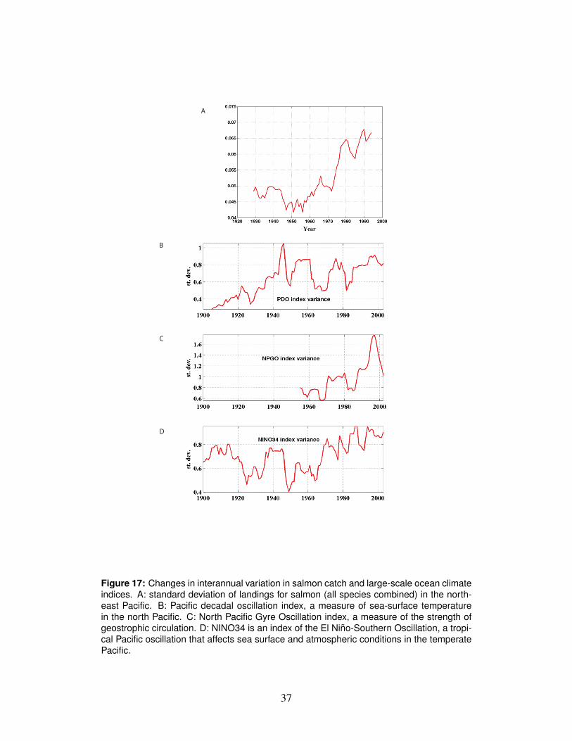
3.7 Is climate change a factor?An open question is whether the recent unusual conditions in the coastal ocean arethe result of normal variation or caused in some part by climate change. We tendto think of the effects of climate change as a trajectory of slow, steady warming.Another potential effect is an increased intensity and frequency of many types ofrare events (Christensen et al., 2007). In fact, along with a general upward trendin sea surface temperatures, the variability of ocean conditions as indexed by thePacific Decadal Oscillation, the North Pacific Gyre Oscillation, and the NINO34index appears to be increasing in concert with increasing variation in salmon catchescoast-wide (Fig. 17).

In the Sacramento River system there are additional factors leading to increasedvariability in salmon escapements, including variation in harvest rates, freshwater

6California Department of Water Resources water year hydrological classification indices,http://cdec.water.ca.gov/cgi-progs/iodir2/WSIHIST

7Proper cohort reconstructions are hindered because of inadequate sampling of tagged fish in thehatchery and on the spawning grounds, and high rates of straying.

36

A

B

C

D

Figure 17: Changes in interannual variation in salmon catch and large-scale ocean climateindices. A: standard deviation of landings for salmon (all species combined) in the north-east Pacific. B: Pacific decadal oscillation index, a measure of sea-surface temperaturein the north Pacific. C: North Pacific Gyre Oscillation index, a measure of the strength ofgeostrophic circulation. D: NINO34 is an index of the El Nino-Southern Oscillation, a tropi-cal Pacific oscillation that affects sea surface and atmospheric conditions in the temperatePacific.

37

habitat simplification, and reduced life history diversity in salmon stocks (discussedin detail in the section 4). In addition, freshwater temperature and flow patterns aresubject to the same forces that drive variability in the ocean environment (Lawsonet al., 2004), although they are modified significantly in the Central Valley by thewater projects. These factors, in combination with increasingly large swings inocean survival, would tend to increase the likelihood of extreme events such as theunusually high escapements of the early 2000s and the recent low escapements thatare the subject of this report.

3.8 SummaryA broad body of evidence suggests that anomalous conditions in the coastal oceanin 2005 and 2006 resulted in unusually poor survival of the 2004 and 2005 broodsof SRFC. Both broods entered the ocean during periods of weak upwelling, warmsea surface temperatures, and low densities of prey items. Pelagic seabirds withdiets similar to juvenile Chinook also experienced very poor reproduction in theseyears. A dominant role for freshwater factors as proximate causes of poor survivalfor the 2004 and 2005 broods were ruled out by observations of near-normal fresh-water conditions during the period of freshwater residency, near-normal numbers ofjuvenile fall-run Chinook entering the estuary, and typical numbers of juvenile fallChinook released from hatcheries. However, as Lawson (1993) reasoned, long-termdeclines in the condition of freshwater habitats are expected to result in increasinglysevere downturns in abundance during episodes of poor ocean survival (Fig. 18). Inthe following section, we explain how human activities may be making the CentralValley Chinook salmon stock complex more susceptible to natural stressors.

4 The role of anthropogenic impactsSo far, we have restricted our analysis to the question of whether there were un-usual conditions affecting Sacramento River fall-run Chinook from the 2004 and2005 broods that could explain their poor performance, reaching the conclusionthat unfavorable ocean conditions were the proximate cause. But what about theultimate causes?

4.1 Sacramento River fall ChinookWith regard to SRFC, anthropogenic effects are likely to have played a signifi-cant role in making this stock susceptible to collapse during periods of unfavorableocean conditions. Historical modifications have eliminated salmon spawning andrearing habitat, decreased total salmon abundance, and simplified salmon biodi-versity (McEvoy, 1986; Yoshiyama et al., 1998, 2001; Williams, 2006a). To theextent that these changes have concentrated fish production and reduced the ca-pacity of populations to spread mortality risks in time and space, we hypothesize

38

Figure 18: Conceptual model of effects of declining habitat quality and cyclic changes inocean productivity on the abundance of salmon. a: trajectory over time of habitat quality.Dotted line represents possible effects of habitat restoration projects. b: generalized timeseries of ocean productivity. c: sum of top two panels where letters represent the following:A = current situation, B = situation in the future, C = change in escapement from increasingor decreasing harvest, and D = change in time of extinction from increasing or decreasingharvest. Copied from Lawson (1993).

39

that the Central Valley salmon ecosystem has become more vulnerable to recurringstresses, including but not limited to periodic shifts in the ocean environment.

Modifications in the Sacramento River basin since early in the nineteenth cen-tury have reduced the quantity, quality, and spatial distribution of freshwater habitatfor Chinook. Large dams have blocked access to spawning habitat upriver anddisrupted geomorphic processes that maintain spawning and rearing habitats down-stream. Levees have disconnected flood plains, and bank armoring and dewateringof some river reaches have eliminated salmon access to shallow, peripheral habitats.By one estimate at least 1700 km or 48% of the stream lengths available to salmonfor spawning, holding, and migration (not including the Delta) have been lost fromthe 3500 km formerly available in the Central Valley (Yoshiyama et al., 2001).

One of the most obvious alterations to fall Chinook habitat has been the lossof shallow-water rearing habitat in the Delta. Mid-nineteenth century land surveyssuggest that levee construction and agricultural conversion have removed all butabout 5% of the 1,300 km2 of Delta tidal wetlands (Williams, 2006a). Becausegrowth rates in shallow-water habitats can be very high in the Central Valley (Som-mer et al., 2001; Jeffres et al., 2008), access to shallow wetlands, floodplains andstream channel habitats could increase the productive capacity of the system. Fromthis perspective, the biggest problem with the state and federal water projects is notthat they kill fish at the pumping facilities, but that by engineering the whole systemto deliver water from the north of the state to the south while preventing flooding,salmon habitat has been greatly simplified.

Although historical habitat losses undoubtedly have reduced salmon productionin the Central Valley ecosystem, other than commercial harvest records, quantita-tive abundance estimates did not become available until the 1940s, nearly a centuryafter hydraulic gold mining, dam construction, and other changes had drasticallymodified the habitat landscape. Harvest records indicate that high volumes of fishwere harvested by nineteenth-century commercial river fisheries. From the 1870sthrough early 1900s, annual in-river harvest in the Central Valley often totaled fourto ten million pounds of Chinook, approaching or exceeding the total annual harvestby statewide ocean fisheries in recent decades (Yoshiyama et al., 1998). Maximumannual stock size (including harvest) of Central Valley Chinook salmon before thetwentieth century has been estimated conservatively at 1-2 million spawners withfall-run salmon totals perhaps reaching 900,000 fish (Yoshiyama et al., 1998). In re-cent decades, annual escapement of SRFC, which typically accounts for more than90% of all fall Chinook production in the Central Valley, has remained relativelystable, totaling between 100,000 and 350,000 adults in most years from the 1960sthrough the 1990s. However, escapement began to fluctuate more erratically in thepresent decade, climbing to a peak of 775,000 in 2002 but then falling rapidly tonear-record lows thereafter (Fig. 1).

Beyond the effects of human activities on production of SRFC are the less obvi-ous influences on biodiversity. The diversity of life histories in Chinook (variationsin size and age at migration, duration of freshwater and estuarine residency, timeof ocean entry, etc.) has been described as a strategy for spreading mortality risksin uncertain environments (Healey, 1991). Diverse habitat types allow the expres-

40

sion of diverse salmon rearing and migration behaviors (Bottom et al., 2005b), andlife history diversity within salmon stocks allows the stock aggregate to be moreresilient to environmental changes (Hilborn et al., 2003).

Juvenile SRFC have adopted a variety of rearing strategies that maximize useof the diverse habitat types throughout the basin, including: (1) fry (< 50 mm forklength) migrants that leave soon after emergence to rear in the Delta or in the es-tuarine bays; (2) fingerling migrants that remain near freshwater spawning areasfor several months, leaving at larger sizes (> 60 mm fork length) in the spring butpassing quickly through the Delta; and (3) later migrants, including some juvenilesthat reside in natal streams through the summer or even stay through the winterto migrate as yearlings (Williams, 2006a). Today most SRFC exhibit fry-migrantstrategies, while the few yearling migrants occur in areas where reservoir releasesmaintain unusually low water temperatures. Historical changes reduced or elim-inated habitats that supported diverse salmon life histories throughout the basin.Passage barriers blocked access to cool upper basin tributaries, and irrigation di-versions reduced flows and increased water temperatures, eliminating cool-waterrefugia necessary to support juveniles with stream-rearing life histories (Williams,2006a). The loss of floodplain and tidal wetlands in the Delta eliminated a con-siderable amount of habitat for fry migrants, a life history strategy that is not veryeffective in the absence of shallow-water habitats downstream of spawning areas.Similar fresh water and estuarine habitat losses have been implicated in the simplifi-cation of Chinook life histories in the Salmon (Bottom et al., 2005a) and ColumbiaRiver basins (Bottom et al., 2005b; Williams, 2006b). In Oregon’s Salmon River,an extensive estuarine wetland restoration program has increased rearing opportu-nities for fry migrants, expanding life history diversity in the Chinook population,including the range of times and sizes that juveniles now enter the ocean (Bottomet al., 2005a). Re-establishing access to shallow wetland and floodplain habitats inthe Sacramento River and Delta similarly could extend the time period over whichSRFC reach sufficient sizes to enter the ocean, strengthening population resilienceto a variable ocean environment.

Hatchery fish are a large and increasing proportion of SRFC (Barnett-Johnsonet al., 2007), and a rising fraction of the population is spawning in hatcheries(Fig. 19). The Central Valley salmon hatcheries were built and operated to miti-gate the loss of habitat blocked by dams, but may have inadvertently contributed tothe erosion of biodiversity within fall Chinook. In particular, the release of hatcheryfish into the estuary greatly increases the straying of hatchery fish to natural spawn-ing areas (CDFG and NMFS, 2001). Central Valley fall Chinook are almost unique8

among Chinook ESUs in having little or no detectable geographically-structured ge-netic variation (Williamson and May, 2005). There are two plausible explanationsfor this. One is that Central Valley fall Chinook never had significant geographicalstructuring because of frequent migration among populations in response to highlyvariable hydrologic conditions (on a microevolutionary time scale). The other ex-

8The exception to this rule is Sacramento River winter-run Chinook, which now spawn only inthe mainstem Sacramento River below Keswick Reservoir.

41

1965 1970 1975 1980 1985 1990 1995 2000 2005 20100

0.05

0.1

0.15

0.2

0.25

0.3

0.35

0.4

0.45

Year

Hat

cher

y/(H

atch

ery+

Nat

ural

)

Figure 19: The fraction of total escapement of SRFC that returns to spawn in hatcheries.

planation is that straying from hatcheries to natural spawning areas has geneticallyhomogenized the ESU. One implication of the latter explanation is that populationsof SRFC may have lost adaptations to their local environments. It is also likely thathatchery practices cause unintentional evolutionary change in populations (Reisen-bichler and Rubin, 1999; Bisson et al., 2002), and high levels of gene flow fromhatchery to wild populations can overcome natural selection, reducing the geneticdiversity and fitness of wild populations.

Another consequence of the hatchery mitigation program was the subsequentharvest strategy, which until the 1990s was focused on exploiting the aggregatestock, with little regard for the effects on naturally produced stocks. For manyyears, Central Valley Chinook stocks were exploited at rates averaging more than60 percent in ocean and freshwater fisheries (Myers et al., 1998). Such levels maynot be sustainable for natural stocks, and could result in loss of genetic diversity,contributing to the homogeneity of Central Valley fall Chinook stocks. Harvestdrives rapid changes in the life history and morphological phenotypes of many or-ganisms, with Pacific salmon showing some of the largest changes (Darimont et al.,2009). An evolutionary response to the directional selection of high ocean harvestis expected, including reproduction at an earlier age and smaller size and spawn-ing earlier in the season (reviewed by Hard et al. (2008)). A truncated age structuremay also increase variation in population abundance (Huusko and Hyvarinen, 2005;Anderson et al., 2008).

Hatchery practices also may cause the aggregate abundance of hatchery and nat-ural fish to fluctuate more widely. Increased variability arises in two ways. First,high levels of straying from hatcheries to natural spawning areas can synchronizethe dynamics of the hatchery and natural populations. Second, hatcheries typically

42

strive to standardize all aspects of their operations, releasing fish of a similar sizeat a particular time and place, which hatchery managers believe will yield highreturns to the fishery on average. Such strategies can have strong effects on ageat maturation through effects on early growth (Hankin, 1990), reducing variationin age at maturity. A likely product of this approach is that the high variation insurvival among years and high covariation in survival and maturation among hatch-ery releases within years may create boom and bust fluctuations in salmon returns,as hatchery operations align, or fail to align, with favorable conditions in stream,estuarine or ocean environments.

Hankin and Logan’s (2008) analysis of survival rates from release to oceanage 2 of fall-run Chinook released from Iron Gate, Trinity River and Cole Rivershatcheries provides an example. Survival of 20+ brood years of fingerling releasesranged from 0.0002 to 0.046, and yearling releases ranged from 0.0032 to 0.26, a230-fold and 80-fold variation in survival, respectively. Hankin and Logan (2008)found that survival covaried among release groups, with the highest covariationbetween groups released from the same hatchery at nearly the same time, althoughcovariation among releases from different hatcheries made at similar times was sub-stantial. Because Central Valley fall Chinook are dominated by hatchery produc-tion, and Central Valley hatcheries release most of their production at similar times,this finding is significant: very high variation in ocean abundance and escapementshould be expected from the system as currently operated.

A similar mechanism has been proposed to explain the collapse of coho salmonfisheries along the Oregon coast following the 1976 ocean regime shift. Cumulativehabitat loss, overharvest, and the gradual replacement of diverse wild populationsand life histories with a few hatchery stocks left coho salmon vulnerable to col-lapse when ocean conditions suddenly changed (Lawson, 1993; Lichatowich, 1999;Williams, 2006b)). The situation is analogous to managing a financial portfolio: awell-diversified portfolio will be buffeted less by fluctuating market conditions thanone concentrated on just a few stocks; the SRFC seems to be quite concentrated in-deed.

4.2 Other Chinook stocks in the Central ValleySacramento River fall Chinook have been the most abundant stock of Chinooksalmon off of central California in recent decades, but this has not always beenthe case. Sacramento River winter Chinook, late-fall Chinook and especially springChinook once dominated the production of Chinook from the Central Valley (Fisher,1994), but over the decades have dwindled to a few remnant populations mostlynow under the protection of the Endangered Species Act (Lindley et al., 2004). Thecauses for these declines are the same as those that have affected fall Chinook, butbecause these other stocks spend some portion of their life in freshwater duringthe summer, they have been more strongly impacted by impassable dams that limitaccess to cold-water habitats.

Spring-run Chinook were once the most abundant of the Central Valley runs,with large populations in snow-melt and spring-fed streams in the Sierra Nevada

43

and southern Cascades, respectively (Fisher, 1994). Spring-run Chinook have beenreduced from perhaps 18 major populations spawning in four distinct ecoregionswithin the Central Valley to three remnant populations inhabiting a single ecoregion(Lindley et al., 2007). Winter-run Chinook were less abundant than spring Chinook,spawning in summer months in a few spring-fed tributaries to the upper SacramentoRiver. Perhaps four distinct populations of winter Chinook have been extirpatedfrom their historical spawning grounds, with survivors founding a population in thetailwaters of Shasta Dam (Lindley et al., 2004). The historical distribution of late-fall-run Chinook is less clear, but their life history requires cool water in summer,and thus their distribution has probably also been seriously truncated by impassabledams at low elevations in the larger tributaries.

An examination of the population dynamics of extant Central Valley Chinookpopulations illustrates that if spring, winter and late-fall Chinook contributed sig-nificantly to the fishery, the aggregate abundance of Chinook in central Californiawaters would be less variable. Populations of Central Valley fall-run Chinook ex-hibited remarkably similar dynamics over the past two decades, while other runsof Central Valley Chinook did not (Fig. 20 , 21 and 22). Almost all fall Chinookpopulations reached peak abundances around 2002, and have all been decliningrapidly since then. In contrast, late-fall, winter and naturally-spawning spring Chi-nook populations have been increasing in abundance over the past decade, althoughescapement in 2007 and 2008 was down in some of them and the growth of thesepopulations through the 1990s and 2000s has to some extent been driven by habitatrestoration efforts. This begs the question of why have these other stocks respondeddifferently to recent environmental variation.

44

1970 1980 1990 20000

50

100

150

200American R Fall Natural

1970 1980 1990 20000

100

200

300

400Battle Cr Fall Natural

1970 1980 1990 20000

5

10

15

20Clear Cr Fall Natural

1970 1980 1990 20000

50

100

150CNFH Fall Hatchery

1970 1980 1990 20000

50

100

150

200Feather R Fall Natural

1970 1980 1990 20000

5

10

15

20

25FRH Fall Hatchery

1970 1980 1990 20000

10

20

30Merced R Fall Natural

1970 1980 1990 20000

20

40

60

80Middle Sac Fall Natural

1970 1980 1990 20000

5

10

15Mokelumne Fall Natural

1970 1980 1990 20000

1

2

3

4MRFF Fall Hatchery

1970 1980 1990 20000

5

10

15MRH Fall Hatchery

1970 1980 1990 20000

10

20

30Nimbus H Fall Hatchery

1970 1980 1990 20000

5

10

15Stanislaus Fall Natural

1970 1980 1990 20000

10

20

30

40

50Tuolumne R Fall Natural

1970 1980 1990 20000

50

100

150Upper Sac Fall Natural

1970 1980 1990 20000

10

20

30

40Yuba R Fall Natural

1970 1980 1990 20000

2

4

6

8CNFH Late Fall Hatchery

1970 1980 1990 20000

10

20

30

40Sacramento Late Fall Natural

1970 1980 1990 20000

5

10

15

20

25Butte Cr Spring Natural

1970 1980 1990 20000

2

4

6

8

10Deer Cr Spring Natural

1970 1980 1990 20000

2

4

6

8

10FRH Spring Hatchery

1970 1980 1990 20000

1

2

3

4Mill Cr Spring Natural

1970 1980 1990 20000

20

40

60Sacramento Winter Natural

Figure 20: Escapement trends in selected populations of Chinook since 1970. Plots arecolor-coded according to run timing. Y - axis is thousands of fish; X-axis is year. CNFH =Coleman National Fish Hatchery; FRH = Feather River Hatchery; MRFF = Merced RiverFish Facility; MRH = Mokelumne River Hatchery.

45

−0.3 −0.2 −0.1 0 0.1 0.2 0.3 0.4 0.5 0.6−0.8

−0.6

−0.4

−0.2

0

0.2

0.4

0.6

Change in log(abundance) per year, 1990−2000

Cha

nge

in lo

g(ab

unda

nce)

per

yea

r, 2

000−

2007

F

S

F

S

F

SF

S

F

S

F

S

F

F

FF

S

F

LF

S

W

F

F

F

F

Figure 21: Escapement trends in the 1990s and 2000s of various populations of Chinook.F = fall Chinook, S = spring Chinook, LF= late fall Chinook, W= winter Chinook. If popu-lations maintained constant growth rates over the 1990-2007 period, they would fall alongthe dashed diagonal line. All populations fall below the diagonal line, showing that growthrates are lower in the 2000s than in the 1990s, and fall Chinook populations have tendedto decline the fastest in the 2000s.

46

The answer may have two parts. One part has to do with hatcheries. As dis-cussed above, hatcheries may be increasing the covariation of fall Chinook popu-lations by erasing genetic differences among populations that might have causedthe populations to respond differently to environmental variation. They may be fur-ther synchronizing the demographics of the naturally-spawning populations throughstraying of hatchery fish into natural spawning areas, a problem exacerbated by out-planting fish to the Delta and bays. Finally, hatchery practices minimize variationin size, condition and migration timing, which should tend to increase variation insurvival rates because “bet hedging” is minimized.

The other part of the answer may lie in the observation that the other runs ofChinook have life history tactics that differ in important ways from fall Chinook.While named according to the time of year that adults enter freshwater, each runtype of Central Valley Chinook has a characteristic pattern of habitat use acrossspace and time that leads to differences in the time and size of ocean entry. Forexample, spring-run Chinook juveniles enter the ocean at a broader range of ages(with a portion of some populations migrating as yearlings) than fall Chinook, dueto their use of higher elevations and colder waters. Winter run Chinook spawn insummer, and the juveniles enter the ocean at a larger size than fall Chinook, dueto their earlier emergence and longer period of freshwater residency. Late-fall-runChinook enter freshwater in the early winter, and spawn immediately, but juvenilesmigrate as yearlings the following winter. Thus, if ocean conditions at the timeof ocean entry are critical to the survival of juvenile salmon, we should expectthat populations from different runs should respond differently to changing oceanconditions because they enter the ocean at different times and at different sizes.

In conclusion, the development of the Sacramento-San Joaquin watershed hasgreatly simplified and truncated the once-diverse habitats that historically supporteda highly diverse assemblage of populations. The life history diversity of this histor-ical assemblage would have buffered the overall abundance of Chinook salmon inthe Central Valley under varying climate conditions. We are now left with a fish-ery that is supported largely by four hatcheries that produce mostly fall Chinooksalmon. Because the survival of fall Chinook salmon hatchery release groups ishighly correlated among nearby hatcheries, and highly variable among years, wecan expect to see more booms and busts in this fishery in the future in responseto variation in the ocean environment. Simply increasing the production of fallChinook salmon from hatcheries as they are currently operated may aggravate thissituation by further concentrating production in time and space. Rather, the key toreducing variation in production is increasing the diversity of SRFC. In the follow-ing section, we make some recommendations towards this goal.

5 RecommendationsIn this section, we offer recommendations in three areas. First, we identify majorinformation gaps that hindered our analysis of the 2004 and 2005 broods. Fillingthese gaps should lead to a better understanding of the linkages between survival

47

1970 1975 1980 1985 1990 1995 2000 2005 2010

0

5

MAF1

1970 1975 1980 1985 1990 1995 2000 2005 2010

0

2

MAF2

Max

imum

aut

ocor

rela

tion

fact

or

1970 1975 1980 1985 1990 1995 2000 2005 2010

0

2

MAF3

1970 1975 1980 1985 1990 1995 2000 2005 2010

0

2

MAF4

Year

−0.8 −0.6 −0.4 −0.2 0 0.2 0.4 0.6 0.8 1

CNFH F HatcheryCNFH Late Fall Hatch

FRH Fall HatchMRH Fall Hatch

MRFF Fall HatchNimbus Fall HatchFRH Spring HatchAmerican Fall NatBattle Cr Fall Nat

Butte Cr Spring NatFeather R Fall Nat

Middle Sac Fall NatMill Cr Fall Nat

Upper Sacramento Fall NatYuba Fall Nat

Mokelumne Fall NatMerced Fall Nat

Stanislaus Fall NatTuolumne Fall Nat

Deer Cr Spring NatMill Cr Spring Nat

Sacramento Spring NatSacramento Late Fall Nat

Sacramento Winter Nat

Factor Loading

MAF1MAF2MAF3MAF4

Figure 22: Maximum autocorrelation factor analysis (MAFA) of Central Valley Chinook es-capement timeseries. MAFA identifies smooth trends in multivariate time series(Fujiwara,2008). Top panel: Maximum autocorrelation factors with the four largest lag-one correla-tions (black circles). Smooth lines are a twice-applied three-point moving average. Bottompanel: loadings on factors with highest lag-one autocorrelation identified by maximum au-tocorrelation factor analysis. Populations are grouped by spawning habitat (hatchery ornatural area) and adult run timing. Hatchery fall Chinook salmon populations in the Sacra-mento basin and populations spawning naturally in streams adjacent to hatcheries havelarge positive loadings on MAF1; Late-fall, spring- and winter-run Chinook have large pos-itive loadings on MAF2 and weak loadings on MAF1. Fall Chinook salmon populations inSan Joaquin tributaries (Stanislaus, Tuolumne and Merced rivers) have largest loadings onMAF4.

48

and environmental conditions. Second, we offer some suggestions on how to im-prove the resilience of SRFC and the Central Valley Chinook stock complex. Whilechanges in harvest opportunities are unavoidable given the expected fluctuations inenvironmental conditions, it is the panel’s opinion that reducing the volatility ofabundance, even at the expense of somewhat lower average catches, would benefitthe fishing industry and make fishery disasters less likely. Finally, we point out thatan ecosystem-based management and ecological risk assessment framework couldimprove management of Central Valley Chinook stocks by placing harvest man-agement in the broader context of the Central Valley salmon ecosystem, which isstrongly influenced by hatchery operations and management of different ecosystemcomponents, including water, habitat and other species.

5.1 Knowledge GapsWe are confident in our conclusion that unusual conditions in the coastal ocean in2005 and 2006 caused the poor performance of the 2004 and 2005 broods. Ourcase could have been strengthened further, however, with certain kinds of informa-tion that are not currently available. Chief among these is the need for constantfractional marking and tagging of hatchery production, and adequate sampling offish on the natural spawning grounds. Such information would better identify thecontribution of hatcheries to the ocean fishery and natural spawning escapement,survival rates of different hatchery release groups, and the likely degree to whichhatchery populations are impacting naturally-spawning populations. Central Valleyhatcheries have recently started a constant-fractional marking program for fall Chi-nook, and CDFG is currently planning how to improve in-river sampling for markand tag recovery. These efforts are critical to improved assessment of SRFC in thefuture.

CDFG has also recently begun to determine the age of returns to the river, whichwill allow stock assessment scientists to produce cohort reconstructions of the nat-ural stocks in addition to hatchery stocks. Cohort reconstructions provide bettersurvival estimates than the method used in this report (releases of tagged juvenileand recovery of tagged fish at age-two in recreational fisheries) because they arebased on many more tag recoveries and provide estimates of fishery mortality andmaturation rates.

In the case of the 2004 and 2005 broods, freshwater factors did not appear to bethe direct cause of the collapse, but future collapses may have multiple contribut-ing causes of similar importance. In such cases, it would be extremely valuable tohave reach-specific survival rates like those routinely available for several salmonidspecies in the Columbia River and recently available for late-fall Chinook and steel-head in the Sacramento River. This would provide powerful and direct informationabout when and where exceptional mortality occurs.

Observations of growth and energetic condition of Chinook in the estuary andocean provided valuable evidence for the 2004 brood, but were unavailable for the2005 and later broods, due to funding limitations.

It is important to continue to monitor and analyze the apparent decadal scale

49

shift in the Gulf of the Farallones ecosystem. The shift is evidenced in the breedingfailure of the rhinoceros auklet in 2005, and some subsequent years, reduced repro-duction in other bird species nesting on these islands, a possible recent downturnin anchovy abundance, and recent increases in marine mammal and seabird mor-tality. The mechanisms underlying these shifts in the Gulf of the Farallones andCalifornia Current are poorly understood. Enhanced monitoring and more in-depthanalysis could provide valuable insights, especially if resource managers move to-wards ecosystem-based management (discussed in Section 5.3).

5.2 Improving resilienceIt appears that the abundance of SRFC is becoming increasingly variable. Excep-tionally high abundance of SRFC may not seem like a serious problem (although itdoes create some problems), but exceptionally low abundances are treated as a dis-aster. We are concerned that such disasters are to be expected at a frequency muchhigher than is acceptable, and that this frequency may be increasing with time dueto changes in the freshwater environment, the ocean environment, and the SRFCstock itself. The main hope of reducing this volatility is increasing the diversitywithin and among the populations of fall Chinook in the Central Valley. There area number of ways to increase diversity.

Perhaps the most tractable area for increasing diversity is in changing hatcheryoperations. We recommend that a hatchery science review panel, be formed toreview hatchery practices in the Central Valley. The panel should address a numberof questions, including the following:

1. assess impacts of outplanting and broodstock transfers among hatcheries onstraying and population structure and evaluate alternative release strategies

2. evaluate alternative rearing strategies to increase variation in timing of out-migration and age at maturity

3. assess whether production levels are appropriate and if they could be adjustedaccording to expected ocean conditions

Ongoing efforts to recover listed Chinook ESUs and increase natural productionof anadromous fish in the Central Valley (e.g., the fisheries programs of the CentralValley Project Improvement Act) are also relevant to the problem and should besupported. In particular, efforts to increase the quantity and diversity of spawningand rearing habitats for fall Chinook are likely to be effective in increasing thediversity of life history tactics in that stock.

The PFMC should consider creating specific conservation objectives for naturalpopulations of SRFC. Especially in coordination with revised hatchery operationsand habitat restoration, managing for natural production could increase diversitywithin Central Valley fall Chinook. Because conditions for reproduction and juve-nile growth are more variable within and among streams than hatcheries, natural

50

production can be expected to generate a broader range of outmigration and age-at-maturity timings. If straying from hatcheries to natural areas is greatly reduced, thepopulation dynamics of natural populations would be less similar to the dynamics ofthe hatchery populations, which would smooth the variation of the stock aggregate.

5.3 SynthesisAddressing hatcheries, habitat and harvest independently would provide benefitsto Central Valley Chinook, but addressing them together within a holistic frame-work is likely to be much more successful. The fisheries management communityis increasingly recognizing the need to move towards an ecosystem based manage-ment approach. While there is still much uncertainty about what this should en-tail, the ecosystem-based management and ecological risk assessment (EBM/ERA)approach used by the south Florida restoration program (e.g., Harwell et al., 1996;Gentile et al., 2001) is readily applicable to management of Central Valley Chinook.That approach could lead stakeholders to a common view of the different problemsafflicting Central Valley Chinook, identify and organize the information neededto effectively manage the ecosystem, better connect this information to decision-making, and reduce the uncertainty surrounding our decisions.

At the core of the EBM/ERA approach are conceptual models of how the sys-tem works. The current fishery management regime for SRFC has some featuresof adaptive management, in that there are clearly stated goals and objectives forthe fisheries, monitoring and evaluation programs, and an analytic framework forconnecting the data to decisions about operation of the fishery. If one were to makeexplicit the conceptual model underlying SRFC harvest management, it would in-clude hatcheries that maintain a roughly constant output of fish coupled with oceanand in-river fisheries operating on aggregate stock abundance. The goal is to max-imize harvest opportunities in the current year within constraints posed by vari-ous weak stocks, which do not include naturally-spawning populations of SRFC.The panel feels that it would be useful to expand this conceptual model to includenaturally-spawning populations, revised hatchery operations, habitat effects, oceaneffects, and climate change. Also, resource managers might consider changing thegoal of management from maximizing harvest opportunity for the current year toreducing fluctuations in opportunity from year to year and maintaining the stabilityof the system for the long term. Both of these goals require viable and productivepopulations of wild salmon. Not all of the factors in the revised system would besubject to control by fisheries managers, but including them in the model wouldat least make clear the contribution of these factors to the problem of effectivelymanaging Chinook salmon fisheries.

We are well aware that the resource management institutions are not currentlywell-equipped to pursue this approach, and that many of the actions that couldimprove the status and resilience of Central Valley Chinook are beyond the authorityof the any other single agency or entity. Nonetheless, significantly improving theresilience of Central Valley Chinook and the sustainability of California’s Chinooksalmon fishery will require resource managers and stakeholders to work together,

51

and EBM/ERA offers a framework for facilitating such cooperation.

52

ReferencesAnderson, C. N. K., C. H. Hsieh, S. A. Sandin, R. Hewitt, A. Hollowed, J. Bed-

dington, R. M. May, and G. Sugihara. 2008. Why fishing magnifies fluctuationsin fish abundance. Nature 452:835–839.

Barber, R. T. and R. L. Smith. 1981. Coastal upwelling ecosystems. In Analysisof marine ecosystems, A. R. Longhurst, editor, pages 31–68. Academic Press,London.

Barnett-Johnson, R., C. B. Grimes, C. F. Royer, and C. J. Donohoe. 2007b. Iden-tifying the contribution of wild and hatchery Chinook salmon (Oncorhynchustshawytscha) to the ocean fishery using otolith microstructure as natural tags.Canadian Journal of Fisheries and Aquatic Sciences 64:1683–1692.

Beamish, R. J., D. J. Noakes, G. A. McFarlane, L. Klyashtorin, V. V. Ivanov, andV. Kurashov. 1999. The regime concept and natural trends in the production ofPacific salmon. Can. J. Fish. Aquat. Sci. 56:516–526.

Bisson, P. A., C. C. Coutant, D. Goodman, R. Gramling, D. Lettenmaier, J. Licha-towich, W. Liss, E. Loudenslager, L. McDonald, D. Philipp, and B. Riddell. 2002.Hatchery surpluses in the Pacific Northwest. Fisheries 27:16–27.

Botsford, L. W. and C. A. Lawrence. 2002. Patterns of co-variability among Califor-nia Current chinook salmon, coho salmon, Dungeness crab, and physical oceano-graphic conditions. Progress In Oceanography 53:283–305.

Bottom, D. L., K. K. Jones, T. J. Cornwell, A. Gray, and C. A. Simenstad. 2005a.Patterns of Chinook salmon emigration and residency in the Salmon River estu-ary (Oregon). Estuarine Coastal and Shelf Science 64:79–93.

Bottom, D. L., C. A. Simenstad, J. Burke, A. M. Baptista, D. A. Jay, K. K.Jones, E. Casillas, and M. H. Schiewe. 2005b. Salmon at river’s end: the roleof the estuary in the decline and recovery of Columbia River salmon. NOAATech. Memo. NMFS-NWFSC-68, U.S. Dept. Commer.

Brodeur, R. D., J. P. Fisher, D. J. Teel, R. L. Emmett, E. Casillas, and T. W. Miller.2004. Juvenile salmonid distribution, growth, condition, origin, and environmen-tal and species associations in the Northern California Current. Fishery Bulletin102:25–46.

Brodeur, R. D., S. Ralston, R. L. Emmett, M. Trudel, T. D. Auth, and A. J. Phillips.2006. Anomalous pelagic nekton abundance, distribution, and apparent recruit-ment in the northern California Current in 2004 and 2005. Geophysical ResearchLetters 33:L22S08.

Budy, P., G. P. Thiede, N. Bouwes, C. E. Petrosky, and H. Schaller. 2002. Evidencelinking delayed mortality of Snake River salmon to their earlier hydrosystemexperience. North American Journal of Fisheries Management 22:35–51.

53

CDFG (California Department of Fish and Game). 2008. Focus areas of researchrelative to the status of the 2004 and 2005 broods of the Central Valley fall Chi-nook salmon stock. Pacific Fishery Management Council.

CDFG and NMFS(California Department of Fish and Game and National MarineFisheries Service). 2001. Final report on anadromous salmonid fish hatcheriesin California. Technical report, California Department of Fish and Game andNational Marine Fisheries Service Southwest Region.

Christensen, J., B. Hewitson, A. Busuioc, A. Chen, X. Gao, I. Held, R. Jones,R. K. Kolli, W. T. Kwon, R. Laprise, V. Magana Rueda, L. Mearns, C. Men-ndez, J. Raisanen, A. Rinke, S. A., and P. Whetton. 2007. Regional climateprojections. In Climate Change 2007: The Physical Science Basis. Contributionof Working Group I to the Fourth Assessment Report of the IntergovernmentalPanel on Climate Change, S. Solomon, D. Qin, M. Manning, Z. Chen, M. Mar-quis, K. Averyt, M. Tignor, and H. Miller, editors. Cambridge University Press,Cambridge, United Kingdom and New York, NY, USA.

Darimont, C. T., S. M. Carlson, M. T. Kinnison, P. C. Paquet, T. E. Reimchen, andC. C. Wilmers. 2009. Human predators outpace other agents of trait change inthe wild. Proceedings of the National Academy of Sciences of the United Statesof America 106:952–954.

Dever, E. P., C. E. Dorman, and J. L. Largier. 2006. Surface boundary-layer vari-ability off Northern California, USA, during upwelling. Deep Sea Research PartII: Topical Studies in Oceanography 53:2887–2905.

Fisher, F. W. 1994. Past and present status of Central Valley chinook salmon. Con-servation Biology 8:870–873.

Fisher, J. P., M. Trudel, A. Ammann, J. A. Orsi, J. Piccolo, C. Bucher, E. Casillas,J. A. Harding, R. B. MacFarlane, R. D. Brodeur, J. F. T. Morris, and D. W. Welch.2007. Comparisons of the coastal distributions and abundances of juvenile Pacificsalmon from central California to the northern Gulf of Alaska. In The ecologyof juvenile salmon in the northeast Pacific Ocean: regional comparisons, C. B.Grimes, R. D. Brodeur, L. J. Haldorson, and S. M. McKinnell, editors, pages31–80. American Fisheries Society, Bethesda, MD.

Fujiwara, M. 2008. Identifying interactions among salmon populations from ob-served dynamics. Ecology 89:4–11.

Gargett, A. E. 1997. The optimal stability ‘window’: a mechanism underlyingdecadal fluctuations in North Pacific salmon stocks? Fisheries Oceanography6:109–117.

Gentile, J. H., M. A. Harwell, W. Cropper, C. C. Harwell, D. DeAngelis, S. Davis,J. C. Ogden, and D. Lirman. 2001. Ecological conceptual models: a framework

54

and case study on ecosystem management for South Florida sustainability. Sci-ence of the Total Environment 274:231–253.

Good, T. P., R. S. Waples, and P. Adams. 2005. Updated status of federally listedESUs of west coast salmon and steelhead. NOAA Tech. Memo. NMFS-NWFSC-66, U.S. Dept. Commer.

Hankin, D. G. 1990. Effects of month of release of hatchery-reared chinook salmonon size at age, maturation schedule, and fishery contribution. Information ReportsNumber 90-4, Fish Division, Oregon Department of Fish and Wildlife.

Hankin, D. G. and E. Logan. 2008. A preliminary analysis of chinook salmoncoded-wire tag recovery data from Iron Gate, Trinity River and Cole Rivershatcheries, brood years 1978-2001. Review draft.

Hard, J. J., M. R. Gross, M. Heino, R. Hilborn, R. G. Kope, R. Law, and J. D.Reynolds. 2008. Evolutionary consequences of fishing and their implications forsalmon. Evolutionary Applications 1:388–408.

Hare, S. R. and R. C. Francis. 1995. Climate change and salmon production inthe Northeast Pacific Ocean. In Climate Change and Northern Fish Popula-tions. Canadian Special Publications in Fisheries and Aquatic Sciences 121, R. J.Beamish, editor, pages 357–372.

Harwell, M. A., J. F. Long, A. M. Bartuska, J. H. Gentile, C. C. Harwell, V. Myers,and J. C. Ogden. 1996. Ecosystem management to achieve ecological sustain-ability: The case of south Florida. Environmental Management 20:497–521.

Healey, M. C. 1991. Life history of chinook salmon (Oncorhynchus tswawytscha).In Pacific salmon life histories, C. Margolis and L. Groot, editors, pages 311–394. University of British Columbia Press, Vancouver.

Hilborn, R., T. P. Quinn, D. E. Schindler, and D. E. Rogers. 2003. Biocomplexityand fisheries sustainability. Proceedings of the National Academy of Sciences,USA 100:6564–6568.

Hobday, A. J. and G. W. Boehlert. 2001. The role of coastal ocean variation inspatial and temporal patterns in survival and size of coho salmon (Oncorhynchuskisutch). Canadian Journal of Fisheries and Aquatic Sciences 58:2021–2036.

Hooff, R. C. and W. T. Peterson. 2006. Copepod biodiversity as an indicatorof changes in ocean and climate conditions of the northern California currentecosystem. Limnology and Oceanography 51:2607–2620.

Houde, E. D. 1975. Effects of stocking density and food density on survival, growthand yield of laboratory-reared larvae of sea bream Archosargus rhomboidalis (L.)(Sparidae). Journal of Fish Biology 7:115–127.

55

Huusko, A. and P. Hyvarinen. 2005. A high harvest rate induces a tendency togeneration cycling in a freshwater fish population. Journal of Animal Ecology74:525–531.

ISAB (Independent Scientific Advisory Board). 2007. Latent mortality report: re-view of hypotheses and causative factors contributing to latent mortality and theirlikely relevenace to he ”below Bonneville” component of the COMPASS model.ISAB 2007-1. ISAB, Portland, OR.

Ingraham, J. W. J. and R. K. Miyahara. 1988. Ocean surface current simulations inthe North Pacific Ocean and Bering Sea (OSCURS – Numerical Models). NOAATech. Memo. NMFS F/NWC-130, U.S. Dept. Commer.

Jeffres, C. A., J. J. Opperman, and P. B. Moyle. 2008. Ephemeral floodplain habitatsprovide best growth conditions for juvenile Chinook salmon in a California river.Environmental Biology of Fishes 83:449–458.

Kjelson, M. A. and P. L. Brandes. 1989. The use of smolt survival estimates toquantify the effects of habitat changes on salmonid stocks in the Sacramento-San Joaquin rivers, California. In Proceedings of the National Workshop on theeffects of habitat alteration on salmonid stocks, C. D. Levings, L. B. Holtby,and M. A. Henderson, editors, Canadian Special Publications in Fisheries andAquatic Sciences, volume 105, pages 100–115.

Kope, R. G. and L. W. Botsford. 1990. Determination of factors affecting recruit-ment of chinook salmon Oncorhynchus tshawytscha in central California. Fish-ery Bulletin 88:257–269.

Kruse, G. H. 1998. Salmon run failures in 1997–1998: a link to anomalous oceanconditions? Alaska Fishery Research Bulletin 5:55–63.

Lawson, P. W. 1993. Cycles in ocean productivity, trends in habitat quality, and therestoration of salmon runs in Oregon. Fisheries 18:6–10.

Lawson, P. W., E. A. Logerwell, N. J. Mantua, R. C. Francis, and V. N. Agostini.2004. Environmental factors influencing freshwater survival and smolt produc-tion in Pacific Northwest coho salmon (Oncorhynchus kisutch). Canadian Journalof Fisheries and Aquatic Sciences 61:360–373.

Lichatowich, J. 1999. Salmon without rivers: a history of the Pacific salmon crisis.Island Press, Washington, DC.

Lindley, S. T., R. S. Schick, B. May, J. J. Anderson, S. Greene, C. Hanson,A. Low, D. McEwan, R. B. MacFarlane, C. Swanson, and J. G. Williams.2004. Population structure of threatened and endangered chinook salmon ESUsin California’s Central Valley basin. NOAA Tech. Memo. NMFS-SWFSC-360,U.S. Dept. Commer.

56

Lindley, S. T., R. S. Schick, E. Mora, P. B. Adams, J. J. Anderson, S. Greene,C. Hanson, B. P. May, D. McEwan, R. B. MacFarlane, C. Swanson, and J. G.Williams. 2007. Framework for assessing viability of threatened and endangeredChinook salmon and steelhead in the Sacramento-San Joaquin basin. San Fran-cisco Estuary and Watershed Science 5(1):Article 4.

MacFarlane, R. B. and E. C. Norton. 2002. Physiological ecology of juvenile chi-nook salmon (Oncorhynchus tshawytscha) at the southern end of their distribu-tion, the San Francisco Estuary and Gulf of the Farallones, California. FisheryBulletin 100:244–257.

Mantua, N., S. Hare, Y. Zhang, J. Wallace, and R. Francis. 1997. A Pacific inter-decadal climate oscillation with impacts on salmon production. Bulletin of theAmerican Meteorological Society 78:1069–1079.

MBARI (Monterey Bay Aquarium Research Institute). 2006. Annual report.MBARI, Moss Landing, CA.

McCullough, D. A. 1999. A review and synthesis of effects of alteration to thewater temperature regime on freshwater life stages of salmonids, with specialreference to chinook salmon. Document 910-R-99010, United States Environ-mental Protection Agency. Seattle, WA.

McEvoy, A. F. 1986. The fisherman’s problem: ecology and law in the Californiafisheries. Cambridge University Press, New York, New York.

McIsaac, D. O. 2008. Pacific Fishery Management Council request for scientificreview of factors affecting certain west coast salmon stocks. Supplemental Infor-mational Report 5, Pacific Fishery Management Council. Portland, OR.

Mueter, F. J., R. M. Peterman, and B. J. Pyper. 2002. Opposite effects of oceantemperature on survival rates of 120 stocks of Pacific salmon (Oncorhynchusspp.) in northern and southern areas. Canadian Journal of Fisheries and AquaticSciences 59:456–463.

Myers, J. M., R. G. Kope, G. J. Bryant, D. Teel, L. J. Lierheimer, T. C. Wainwright,W. S. Grant, F. W. Waknitz, K. Neely, S. T. Lindley, and R. S. Waples. 1998. Sta-tus review of chinook salmon from Washington, Idaho, Oregon, and California.NOAA Tech. Memo. NMFS-NWFSC-35, U.S. Dept. Commer.

Newell, C. L. and T. J. Cowles. 2006. Unusual gray whale Eschrichtius robus-tus feeding in the summer of 2005 off the central Oregon Coast. GeophysicalResearch Letters 33:L22S11.

Newman, K. B. and J. Rice. 2002. Modeling the survival of chinook salmon smoltsoutmigrating through the lower Sacramento River system. Journal of the Ameri-can Statistical Association 97:983–993.

57

O’Farrell, M. R., M. S. Mohr, M. L. Palmer-Zwahlen, and A. M. Grover. 2009. TheSacramento Index. Report in preparation.

Pearcy, W. G. 1992. Ocean ecology of North Pacific salmonids. University ofWashinton, Seattle, WA.

PFMC (Pacific Fishery Management Council). 2007. Preseason report III: Anal-ysis of council adopted management measures for 2007 ocean salmon fisheries.Pacific Fishery Management Council, 7700 NE Ambassador Place, Suite 101,Portland, Oregon 97220-1384.

PFMC (Pacific Fishery Management Council). 2008. Preseason report I: Stockabundance analysis for 2008 ocean salmon fisheries. Pacific Fishery ManagementCouncil, 7700 NE Ambassador Place, Suite 101, Portland, Oregon 97220-1384.

PFMC (Pacific Fishery Management Council). 2009. Review of 2008 ocean salmonfisheries. Pacific Fishery Management Council, 7700 NE Ambassador Place,Suite 101, Portland, Oregon 97220-1384.

Pyper, B. J., F. J. Mueter, R. M. Peterman, D. J. Blackbourn, and C. C. Wood.2002. Spatial covariation in survival rates of Northeast Pacific chum salmon.Transactions of the American Fisheries Society 131:343–363.

Reisenbichler, R. R. and S. P. Rubin. 1999. Genetic changes from artificial prop-agation of Pacific salmon affect the productivity and viability of supplementedpopulations. ICES Journal of Marine Science 56:459–466.

Rykaczewski, R. R. and D. J. Checkley. 2008. Influence of ocean winds on thepelagic ecosystem in upwelling regimes. Proceedings of the National Academyof Sciences 105:1967–1970.

Ryther, J. H. 1969. Photosynthesis and fish production in the sea. Science 166:72–76.

Schwing, F. B., N. A. Bond, S. J. Bograd, T. Mitchell, M. A. Alexander, andN. Mantua. 2006. Delayed coastal upwelling along the US West Coast in 2005:A historical perspective. Geophysical Research Letters 33:L22S01.

Schwing, F. B., T. Murphree, and P. M. Green. 2002. The Northern OscillationIndex (NOI): a new climate index for the northeast Pacific. Progress In Oceanog-raphy 53:115–139.

Sommer, T. R., M. L. Nobriga, W. C. Harrel, W. Batham, and W. J. Kimmerer. 2001.Floodplain rearing of juvenile chinook salmon: evidence of enhanced growth andsurvival. Can. J. Fish. Aquat. Sci. 58:325–333.

SRFCRT (Sacramento River Fall Chinook Review Team). 1994. Sacramento RiverFall Chinook Review Team: An assessment of the status of the Sacramento Riverfall chinook stiock as required under the salmon fishery management plan. PacificFishery Management Council.

58

Sydeman, W. J., R. W. Bradley, P. Warzybok, C. L. Abraham, J. Jahncke, K. D.Hyrenbach, V. Kousky, J. M. Hipfner, and M. D. Ohman. 2006. Planktivorousauklet Ptychoramphus aleuticus responses to ocean climate, 2005: Unusual at-mospheric blocking? Geophysical Research Letters 33:L22S09.

Vogel, D. A. and K. R. Marine. 1991. Guide to upper Sacramento chinook salmonlife history. CH2M Hill.

Weise, M. J., D. P. Costa, and R. M. Kudela. 2006. Movement and diving behaviorof male California sea lion (Zalophus californianus) during anomalous oceano-graphic conditions of 2005 compared to those of 2004. Geophysical ResearchLetters 33:L22S10.

Weitkamp, L. A. In review. Marine distributions of Chinook salmon (Oncorhynchustshawytscha) from the west coast of North America determined by coded wire tagrecoveries.

Welch, D. W., E. L. Rechisky, M. C. Melnychuk, A. D. Porter, C. J. Walters,S. Clements, B. J. Clemens, R. S. McKinley, and C. Schreck. 2008. Survivalof migrating salmon smolts in large rivers with and without dams. PLoS Biology6:2101–2108.

Wells, B. K., J. C. Field, J. A. Thayer, C. B. Grimes, S. J. Bograd, W. J. Sydeman,F. B. Schwing, and R. Hewitt. 2008. Untangling the relationships among climate,prey and top predators in an ocean ecosystem. Marine Ecology Progress Series364:15–29.

Wilkerson, F. P., A. M. Lassiter, R. C. Dugdale, A. Marchi, and V. E. Hogue. 2006.The phytoplankton bloom response to wind events and upwelled nutrients duringthe CoOP WEST study. Deep Sea Research Part II: Topical Studies in Oceanog-raphy 53:3023–3048.

Williams, J. G. 2006a. Central Valley salmon: a perspective on Chinook and steel-head in the Central Valley of California. San Francisco Estuary and WatershedScience 4(3):Article 2.

Williams, J. G., S. G. Smith, and W. D. Muir. 2001. Survival estimates for down-stream migrant yearling juvenile salmonids through the Snake and Columbiarivers hydropower system, 1966–1980 and 1993–1999. North American Jour-nal of Fisheries Management 21:310–317.

Williams, R. N., editor. 2006b. Return to the river: restoring salmon to theColumbia River. Elsevier Academic Press, San Diego, CA.

Williamson, K. S. and B. May. 2005. Homogenization of fall-run Chinook salmongene pools in the Central Valley of California, USA. North American Journal ofFisheries Management 25:993–1009.

59

Wolf, S. G., W. J. Sydeman, J. M. Hipfner, C. L. Abraham, B. R. Tershy, and D. A.Croll. 2009. Range-wide reproductive consequences of ocean climate variabilityfor the seabird Cassins Auklet. Ecology 90:742–753.

Yoshiyama, R. M., F. W. Fisher, and P. B. Moyle. 1998. Historical abundanceand decline of chinook salmon in the Central Valley region of California. NorthAmerican Journal of Fisheries Management 18:487–521.

Yoshiyama, R. M., E. R. Gerstung, F. W. Fisher, and P. B. Moyle. 2001. Historicand present distribution of chinook salmon in the Central Valley drainage of Cal-ifornia. In Fish Bulletin 179: Contributions to the biology of Central Valleysalmonids., R. L. Brown, editor, volume 1, pages 71–176. California Departmentof Fish and Game, Sacramento, CA.

60

Appendix A: Assessment of factors relative to the sta-tus of the 2004 and 2005 broods of Sacramento Riverfall Chinook

S. T. Lindley, C. B. Grimes, M. S. Mohr, W. Peterson, J. Stein, J. T. Anderson,L. W. Botsford, , D. L. Bottom, C. A. Busack, T. K. Collier, J. Ferguson, J. Field,J. C. Garza, A. M. Grover, D. G. Hankin, R. G. Kope, P. W. Lawson, A. Low,R. B. MacFarlane, K. Moore, M. Palmer-Zwahlen, F. B. Schwing, J. Smith, C. Tracy,R. Webb, B. K. Wells, and T. H. Williams

1

Contents

1 Purpose of the appendix 8

2 Freshwater Biological Focus 82.1 Was the level of parent spawners too low, for natural or hatchery

populations? . . . . . . . . . . . . . . . . . . . . . . . . . . . . . . 82.2 Was the level of parent spawners too high, for natural or hatchery

populations? . . . . . . . . . . . . . . . . . . . . . . . . . . . . . . 82.3 Was there a disease event in the hatchery or natural spawning areas?

Was there a disease event in the egg incubation, fry emergence,rearing, or downstream migration phases? Was there any diseaseevent during the return phase of the 2 year old jacks? . . . . . . . . 8

2.4 Were there mortalities at the time of trucking and release of hatch-ery fish? . . . . . . . . . . . . . . . . . . . . . . . . . . . . . . . . 9

2.5 Was there a change in the pattern of on-site release of hatcheryfingerlings compared to trucked downstream release? Was therea change in recovery, spawning and/or release strategies duringhatchery operations? . . . . . . . . . . . . . . . . . . . . . . . . . 9

2.6 Did thermal marking occur for any hatchery releases? What werethe effects of this or other studies (e.g. genetic stock identificationof parental broodstock)? . . . . . . . . . . . . . . . . . . . . . . . 11

2.7 Was there a change in the methodology or operations of the SanFrancisco Bay net pen acclimation program for trucked hatchery fish? 13

2.8 Were there any problems with fish food or chemicals used at hatcheries? 13

3 Freshwater Habitat Areas Focus 143.1 Were there drought or flood conditions during the spawning, incu-

bation, or rearing phases? . . . . . . . . . . . . . . . . . . . . . . . 143.2 Was there any pollution event where juveniles were present? . . . . 143.3 Was there anything unusual about the flow conditions below dams

during the spawning, incubation, or rearing phases? . . . . . . . . . 163.4 Were there any in-water construction events (bridge building, etc.)

when this brood was present in freshwater or estuarine areas? . . . . 163.5 Was there anything unusual about the water withdrawals in the rivers

or estuary areas when this brood was present? . . . . . . . . . . . . 163.6 Was there an oil spill in the estuary when the 2005 brood was

present, as juveniles or jacks? . . . . . . . . . . . . . . . . . . . . 203.7 Were there any unusual temperature or other limnological condi-

tions when this brood was in freshwater or estuarine areas? . . . . . 203.8 Were there any unusual population dynamics of typical food or prey

species used by juvenile Chinook in the relevant freshwater andestuarine areas? . . . . . . . . . . . . . . . . . . . . . . . . . . . . 23

2

3.9 Was there anything unusual, in the same context as above for juve-nile rearing and outmigration phases, about habitat factors duringthe return of the 2 year olds from this brood? . . . . . . . . . . . . 24

3.10 Were there any deleterious effects caused by miscellaneous hu-man activities (e.g., construction, waterfront industries, pollution)within the delta and San Francisco bay areas? . . . . . . . . . . . . 24

3.11 Was there a change in the recovery of juvenile outmigrants observedin the USFWS mid-water trawl surveys and other monitoring pro-grams in the Delta. . . . . . . . . . . . . . . . . . . . . . . . . . . 25

4 Freshwater Species Interactions Focus 254.1 Was there any unusual predation by bird species when this brood

was in freshwater or estuarine areas? . . . . . . . . . . . . . . . . . 254.2 Was there any unusual sea lion abundance or behavior when this

brood was in freshwater or estuarine areas? . . . . . . . . . . . . . 254.3 Was there any unusual striped bass population dynamics or behav-

ior when this brood was in freshwater or estuarine areas? . . . . . . 254.4 Were northern pike present in any freshwater or estuarine areas

where this brood was present? . . . . . . . . . . . . . . . . . . . . 264.5 Is there a relationship between declining Delta smelt, longfin smelt,

and threadfin shad populations in the Delta and Central Valley Chi-nook survival? . . . . . . . . . . . . . . . . . . . . . . . . . . . . . 27

4.6 Was there additional inriver competition or predation with increasedhatchery steelhead production? . . . . . . . . . . . . . . . . . . . . 27

5 Marine Biological Focus 275.1 Was there anything unusual about the ocean migration pattern of

the 2004 and 2005 broods? Was there anything unusual about therecovery of tagged fish groups from the 2004 and 2005 broods theocean salmon fisheries? . . . . . . . . . . . . . . . . . . . . . . . . 27

5.2 Has the bycatch in non-salmonid fisheries (e.g., whiting, ground-fish) increased? . . . . . . . . . . . . . . . . . . . . . . . . . . . . 30

6 Marine Habitat Areas Focus 306.1 Were there periods of reduced upwelling or other oceanographic

physical conditions during the period of smolt entry into the marineenvironment, or during the period of marine residence up to thereturn to freshwater of the jacks? . . . . . . . . . . . . . . . . . . 30

6.2 Were there any effects to these fish from the “dead zones” reportedoff Oregon and Washington in recent years? . . . . . . . . . . . . . 38

6.3 Were plankton levels depressed off California, especially during thesmolt entry periods? . . . . . . . . . . . . . . . . . . . . . . . . . . 39

6.4 Was there a relationship to an increase in krill fishing worldwide? . 396.5 Oceanography: temperature, salinity, upwelling, currents, red tide,

etc. . . . . . . . . . . . . . . . . . . . . . . . . . . . . . . . . . . . 39

3

6.6 Were there any oil spills or other pollution events during the periodof ocean residence? . . . . . . . . . . . . . . . . . . . . . . . . . . 39

6.7 Was there any aquaculture occurring in the ocean residence area? . . 396.8 Was there any offshore construction in the area of ocean residence,

for wave energy or other purposes? . . . . . . . . . . . . . . . . . . 42

7 Marine Species Interactions Focus 427.1 Were there any unusual population dynamics of typical food or prey

species used by juvenile Chinook in marine areas? (plankton, krill,juvenile anchovy or sardines, etc.) . . . . . . . . . . . . . . . . . . 42

7.2 Was there an increase in bird predation on juvenile salmonids causedby a reduction in the availability of other forage food? . . . . . . . . 42

7.3 Was there an increase of marine mammal predation on these broods? 447.4 Was there predation on salmonids by Humboldt squid? . . . . . . . 477.5 Was there increased predation on salmonids by other finfish species

(e.g., lingcod)? . . . . . . . . . . . . . . . . . . . . . . . . . . . . 50

8 Cumulative Ecosystem Effects Focus 528.1 Were there other ecosystem effects? Were there synergistic effects

of significant factors? . . . . . . . . . . . . . . . . . . . . . . . . . 52

9 Salmon Fisheries Focus 539.1 To what extent did fisheries management contribute to the unusually

low SRFC spawning escapements in 2007 and 2008? . . . . . . . . 53

4

List of Tables

1 Releases of Chinook from state hatcheries. . . . . . . . . . . . . . . 122 Releases of Chinook after acclimation in net pens. . . . . . . . . . 143 Monthly river runoff. . . . . . . . . . . . . . . . . . . . . . . . . . 154 Estimated loss of fall- and spring-run Chinook fry and smolts at

Delta water export facilities. Water year corresponds to outmigra-tion year. Unpublished data of California Department of Water Re-sources. . . . . . . . . . . . . . . . . . . . . . . . . . . . . . . . . 18

5 Striped bass adult abundance. . . . . . . . . . . . . . . . . . . . . . 266 Recreational fishery coded-wire tag recoveries of age-2 FRH fall

Chinook in the San Francisco major port area. . . . . . . . . . . . . 317 PFMC 2007 SRFC spawning escapement prediction model compo-

nents: forecast and realized values. . . . . . . . . . . . . . . . . . . 558 PFMC 2008 SRFC spawning escapement prediction model compo-

nents: forecast and realized values. . . . . . . . . . . . . . . . . . . 57

5

List of Figures

1 Summary of CNFH releases of fall Chinook . . . . . . . . . . . . . 102 Size of fall Chinook released from Coleman National Fish Hatch-

ery. Horizontal lines indicate mean size, boxes delineate the inner-quartile range, and whiskers delineate the 95% central interval. . . 11

3 Releases of fall-run Chinook from state hatcheries. . . . . . . . . . 124 Weekly mean discharge at selected stations on the Sacramento, Feather,

American and Stanislaus rivers. . . . . . . . . . . . . . . . . . . . . 175 Daily export of freshwater from the delta and the ratio of exports to

inflows. . . . . . . . . . . . . . . . . . . . . . . . . . . . . . . . . 196 Observed Chinook salvage at the State Water Project and Central

Valley Project pumping facilities in the Delta. . . . . . . . . . . . . 207 Temperature and turbidity in 2005 and 2006 at Red Bluff. . . . . . . 218 Oceanographic conditions in the San Francisco estuary. . . . . . . . 229 Mean annual freshwater outflow through San Francisco Estuary be-

tween January and June. . . . . . . . . . . . . . . . . . . . . . . . 2310 Mean annual abundance of calanoid copepods in the Delta, Suisun

Bay and San Pablo Bay from 1990 and 2007. . . . . . . . . . . . . 2411 Daily catches of juvenile fall-run Chinook at Chipps Island. . . . . . 2512 Abundance indices for Delta smelt, longfin smelt, and threadfin shad. 2813 Recreational fishery CPUE of age-2 FRH fall Chinook by major

port area. . . . . . . . . . . . . . . . . . . . . . . . . . . . . . . . 3014 Index of FRH fall Chinook survival rate between release in San

Francisco Bay and ocean age-2. . . . . . . . . . . . . . . . . . . . 3215 SRFC jack spawning escapement versus FRH fall Chinook survival

rate index. . . . . . . . . . . . . . . . . . . . . . . . . . . . . . . . 3316 Composition of the Monterey Bay sport fishery landings as deter-

mined by genetic stock identification. . . . . . . . . . . . . . . . . 3417 Landings of Chinook taken in trawl fisheries and landed at Califor-

nia ports.. . . . . . . . . . . . . . . . . . . . . . . . . . . . . . . . 3418 Cumulative upwelling at four locations along the California and

Oregon coast. . . . . . . . . . . . . . . . . . . . . . . . . . . . . . 3519 Strength of meridional winds along the central California coast in

2003-2006. . . . . . . . . . . . . . . . . . . . . . . . . . . . . . . 3620 Sea surface temperature anomalies off central California. . . . . . . 3721 Average depth of the thermocline during May and June in the Gulf

of the Farallones. . . . . . . . . . . . . . . . . . . . . . . . . . . . 3822 Chl-a anomalies. . . . . . . . . . . . . . . . . . . . . . . . . . . . 4023 Time series of temperature, water column stratification, nitrate, chloro-

phyll and and dinoflagellates observed in Monterey Bay. . . . . . . 4124 Time series of catches from pelagic trawl surveys along the central

California coast. . . . . . . . . . . . . . . . . . . . . . . . . . . . . 4326 Abundance of krill measured during May-June survey cruises off

central California. . . . . . . . . . . . . . . . . . . . . . . . . . . . 45

6

27 Diet of three species of seabirds in the Gulf of the Farallones be-tween 1972 and 2007. . . . . . . . . . . . . . . . . . . . . . . . . . 46

28 Population estimates of killer whales off the California coast. . . . . 4729 Count of California sea lion pups. . . . . . . . . . . . . . . . . . . 4830 Harbor seal haulout counts in California during May and June. . . . 4831 Spawning biomass and recruitment of selected groundfish species

off of central California. . . . . . . . . . . . . . . . . . . . . . . . 5232 PFMC 2007 CVI forecast regression model. . . . . . . . . . . . . . 5433 PFMC 2008 SI forecast regression model. . . . . . . . . . . . . . . 56

7

1 Purpose of the appendix

In this appendix, we attempt to answer the specific questions posed by the Pa-cific Fishery Management Council regarding potential causes for the SRFC decline(McIsaac, 2008). Some closely-related questions have been combined. In additionand for completeness, we also address the question of whether ocean salmon fish-eries and fishery management contributed to the low escapement of SRFC in 2007and 2008.

2 Freshwater Biological Focus

2.1 Was the level of parent spawners too low, for natural or hatchery populations?

The abundance of naturally-spawning SRFC adults in 2004 and 2005 was 203,000and 211,000, respectively (PFMC, 2009). This level of escapement is near the1970-2007 mean of 195,000 spawners. It therefore does not appear that the levelof parent spawners was too low. SRFC adult returns to the hatcheries in 2004 and2005 were some of the highest on record, well in excess of that needed for egg take,so the level of parent spawners in the hatchery could not have been responsible forthe poor adult returns observed in 2007 and 2008.

2.2 Was the level of parent spawners too high, for natural or hatchery popula-tions?

While the level of parent spawners for the 2004 and 2005 broods was higher thanaverage, these levels of abundance are not unusual over the 1970-2007 period, andother broods from similar-sized returns are not associated with particularly low sur-vival. It therefore does not appear that the level of parent spawners was too highon the spawning grounds. Returns to the hatcheries were near record highs, buthatchery managers control the matings of hatchery fish, so it is unlikely that thehigh level of hatchery returns had a negative impact on hatchery operations.

2.3 Was there a disease event in the hatchery or natural spawning areas? Wasthere a disease event in the egg incubation, fry emergence, rearing, or down-stream migration phases? Was there any disease event during the return phaseof the 2 year old jacks?

There were no known disease events affecting naturally-produced brood-year 2004and 2005 fall-run Chinook in the Sacramento River or tributaries, although thereis no routine fish health sampling program for naturally produced fish the Sacra-mento River system. In the Feather River Hatchery, brood-year 2004 and 2005Chinook were treated an average of five to six times a year, primarily for bacte-rial infection. The typical treatment was copper sulfate flushes. This incidence ofdisease was not unusually high compared to other recent years. In the MokelumneRiver Hatchery, brood-year 2004 and 2005 Chinook experienced minimal losses

8

from coagulated yolks. At the Nimbus Hatchery, there were no significant diseaseevents affecting brood-year 2004 Chinook. Brood-year 2005 fall-run Chinook ex-perienced an outbreak of infectious hematopoietic necrosis (IHN). Losses began tospike in mid-April and continued through May before declining. Losses incurredrepresented 44% of the fish on hand at the time of the outbreak. However, the hatch-ery planted 3,002,600 brood-year 2005 fish, approximately 75% of the mitigationgoal of 4 million fish. There were no significant disease outbreaks at the ColemanNational Fish hatchery for the 2004 and 2005 broods. We therefore conclude thatdisease events during the freshwater lifestages are an unlikely explanation for thepoor performance of the 2004 and 2005 broods.

2.4 Were there mortalities at the time of trucking and release of hatchery fish?

No unusual mortality events were noted for these broods.

2.5 Was there a change in the pattern of on-site release of hatchery fingerlingscompared to trucked downstream release? Was there a change in recovery,spawning and/or release strategies during hatchery operations?

Hatchery practices, particularly the numbers and life stages of fish released, havebeen stable over the last decade. Coleman National Fish Hatchery has been releas-ing only smolts or pre-smolts since 2000, and releases from brood-year 2004 and2005 were at typical levels (Fig. 1). The vast majority of fall-run smolts and pre-smolts have been released at or very near the hatchery, within two weeks of April15 of each release year. Individual fish size also has remained very steady with theaverage size at release varying only 2 mm around an average of 75 mm (Fig. 2).

There were no significant changes in broodstock collection or spawning proto-cols for brood-year 2004 and 2005 fall-run Chinook at state-operated hatcheriesin the Sacramento River Basin. Feather River, Mokelumne River, and NimbusHatcheries are operated by California Department of Fish and Game (CDFG) ac-cording to Operational Plans (Production Goals and Constraints). These plans havenot been significantly modified in recent years. Fish ladders at each of the facilitiesare operated seasonally to allow fall-run to volitionally enter the hatchery. Eggsare taken from fall-run fish to represent the entire spectrum of the run. Some orall of each pooled lot of eggs are retained for rearing according to a predeterminedschedule of weekly egg take needs. Sacramento River fall-run Chinook reared formitigation purposes are released at smolt size (7.5 g or greater), and those reared forenhancement purposes are released at post-smolt size (10 g). Most are transportedby truck to the Carquinez Straits-San Pablo Bay area for release from April throughJuly while a small portion may be released in-stream.

The production levels of fall-run Chinook released from each of the SacramentoRiver Basin state hatchery facilities into anadromous waters from 1990 through2006 is shown in Fig. 3. From 1990 to 1998, and in 2001, the total productionshown includes some releases of fry-sized fish. Production levels for brood-year

9

Figure 1: Top: Releases of fall-run Chinook from Coleman National Fish Hatchery. Bottom:number of smolts and pre-smolts released to the bay, upper river and on site (Battle Creek).

10

Figure 2: Size of fall Chinook released from Coleman National Fish Hatchery. Horizontallines indicate mean size, boxes delineate the inner-quartile range, and whiskers delineatethe 95% central interval.

2004 and 2005 fall-run Chinook (21.4 million and 19.3 million fish, respectively)were not significantly different from other recent years.

Most of the state hatchery production of Sacramento River fall-run Chinook hasbeen transported to the San Pablo Bay and Carquinez Straits area for release sincethe 1980s (average of 93% over last decade). Coded-wire tagging studies indicatethat transporting salmon smolts or yearlings to San Pablo Bay and Carquinez Straitsplanting sites significantly increases their survival to adults (unpublished data ofCDFG).

Table1 shows the release locations of fall-run Chinook from each of the Sacra-mento River Basin state hatchery facilities, 1990 to 2006. Instream releases includereleases into the stream of origin, the mainstem Sacramento River, or within theDelta. Bay releases include fish transported for release in the San Pablo Bay/CarquinezStraits/San Francisco Bay area or to ocean net pens.

For brood-years 2004 and 2005 (release-years 2005 and 2006), release locationswere not changed significantly from other recent years. As in other recent years,more than 95% were transported for release in the San Pablo Bay/Carquinez Straitsarea.

2.6 Did thermal marking occur for any hatchery releases? What were the effectsof this or other studies (e.g. genetic stock identification of parental brood-stock)?

At Feather River Hatchery, a pilot program of otolith thermal marking was con-ducted on the 2004 brood of fall-run Chinook. The entire 2005 brood was thermallymarked. Fish were marked after hatching. There has been an increase in the inci-dence of cold water disease at the hatchery in recent years, but there is no evidencethat the otolith thermal marking study contributed to this increase. The literature onotolith thermal marking reports no adverse effects on survival (Volk et al., 1994).

11

Figure 3: Releases of fall-run Chinook from state hatcheries.

Table 1: Releases of Chinook from state hatcheries.Feather River Nimbus Mokelumne

Release Year Brood Year Instream Bay Instream Bay Instream Bay1990 1991 3,368,726 7,815,311 6,995,625 438,140 295,150 1,983,4001991 1992 0 6,078,920 9,963,840 939,652 858,836 3,476,3101992 1993 3,439,465 9,691,616 9,540,285 602,705 563,414 3,011,6001993 1994 8,676,431 5,624,222 8,795,300 638,000 1,396,390 2,384,1801994 1995 0 7,659,432 8,578,437 3,915,870 1,886,084 1,772,8001995 1996 7,381,185 6,417,755 5,733,951 3,009,840 0 3,740,9981996 1997 825,785 7,395,468 0 9,520,696 0 2,873,7501997 1998 854,593 4,978,070 1,253,570 4,348,210 0 3,023,7821998 1999 1,755,126 6,170,994 0 5,270,678 0 3,422,1801999 2000 1,834,947 5,769,640 0 3,851,700 0 4,629,5592000 2001 848,622 4,188,000 101,856 4,273,950 0 9,697,3582001 2002 997,723 5,746,188 0 2,314,800 0 5,846,7432002 2003 1,321,727 6,815,718 0 4,361,300 106,506 7,991,9612003 2004 699,688 7,850,188 115,066 4,578,400 102,121 6,273,8392004 2005 673,401 8,323,279 0 4,570,000 0 6,485,9142005 2006 786,557 9,560,592 0 3,002,600 0 6,539,1122006 2007 1,616,657 10,252,718 0 5,045,900 3,712,240 2,480,3912007 2008 2,273,413 10,550,968 0 4,899,350 468,736 4,660,707

12

2.7 Was there a change in the methodology or operations of the San FranciscoBay net pen acclimation program for trucked hatchery fish?

Coleman National Fish Hatchery production is not acclimated in net pens.CDFG initiated a net pen acclimation program for hatchery-reared fall-run Chi-

nook in 1993. When fish are transported for release into the Carquinez Straits-SanPablo Bay area, they may experience immediate and delayed mortality associatedwith the transfer to seawater. Instantaneous temperature and salinity changes arepotential sources of direct mortality as well as indirect mortality due to predationon disoriented fish and stress-induced susceptibility to disease. Temporary transferof salmon yearlings to net pens has been shown to reduce loss of fish due to preda-tion at the time of their planting and greatly increase survival. A three-year studyby the California Department of Fish and Game (unpublished) found that holdingsmolts in net pens for two hours increased the recovery rate by a factor of 2.2 to 3.0compared to smolts released directly into the bay.

The Fishery Foundation of California has been contracted to operate the projectsince 1993. Fish are offloaded from CDFG hatchery trucks into the mobile pens inSan Pablo Bay at the Wickland Oil Company pier facility in Selby (between Rodeoand Crockett) in Contra Costa County from May through July. Upon receiving thefish, the net pens are towed into San Pablo Bay. The pens are allowed to float withthe current and the fish are held for up to two hours until they become acclimatedto their surroundings. The net pens are then dropped and the fish released in SanPablo Bay.

Methods used for net pen acclimation were not significantly changed from 1993through 2007, although the number of hatchery fish acclimated in the pens hasvaried over the years. Significantly, no hatchery releases from the 2005 brood wereacclimated in net pens before release. The following table shows the total numberof Chinook acclimated in the Carquinez Straits net pens and released from 1993through 2006.

Similar numbers of brood-year 2004 fish were acclimated in the net pens com-pared to other recent years. For this brood year, there is no evidence that lack ofacclimation contributed to poor escapement in 2007. However, the net pen projectwas not operated in the spring of 2006 due to insufficient funds, a change in oper-ations that may have had a significant impact on the survival of the portion of the2005 brood produced by state hatcheries.

2.8 Were there any problems with fish food or chemicals used at hatcheries?

Coleman National Fish Hatchery had no issues or problems with fish food or chem-icals used at the hatchery for the release years 2004-06 that would have caused anysignificant post-release mortality (pers. comm., Scott Hamelberg, USFWS).

All chemical treatments at the state hatcheries were used under the guidelinesset by the CDFG Fish Health Lab. There were no significant changes in chemicaluse or feeds over the 1990-2007 period. Some Bio-Oregon/Skretting salmon feedswere recalled in 2007 due to contamination with melamine, but this is not believed

13

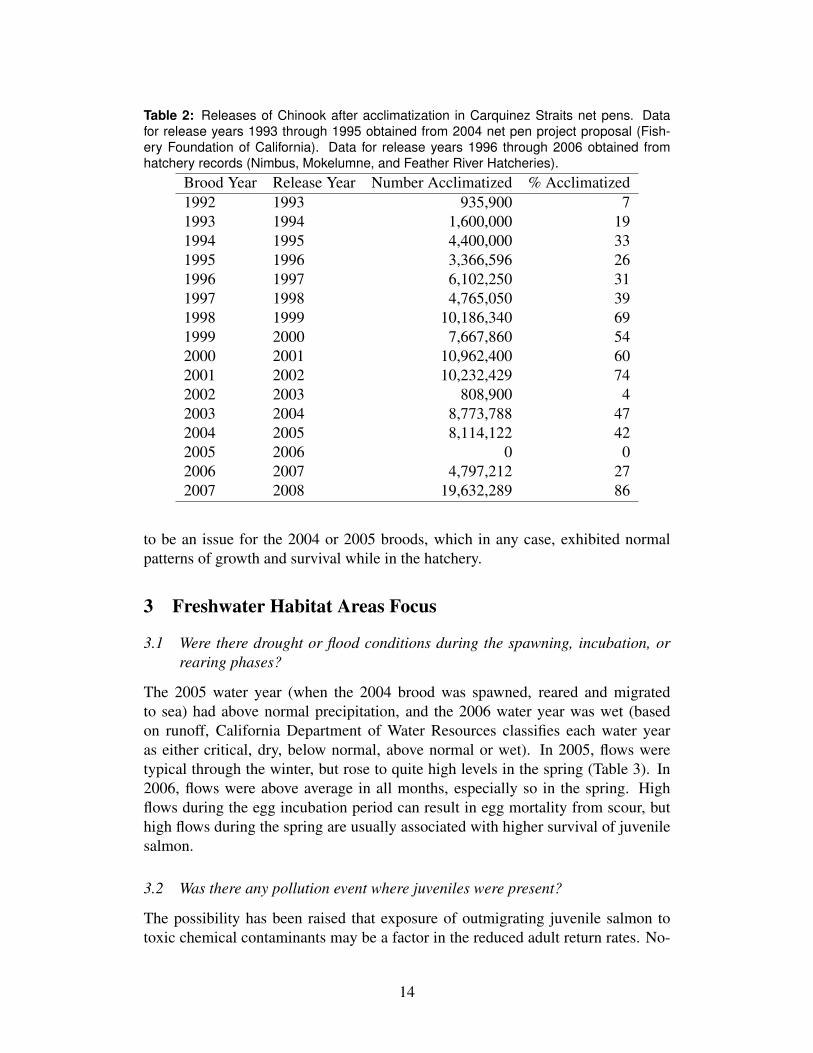
Table 2: Releases of Chinook after acclimatization in Carquinez Straits net pens. Datafor release years 1993 through 1995 obtained from 2004 net pen project proposal (Fish-ery Foundation of California). Data for release years 1996 through 2006 obtained fromhatchery records (Nimbus, Mokelumne, and Feather River Hatcheries).

Brood Year Release Year Number Acclimatized % Acclimatized1992 1993 935,900 71993 1994 1,600,000 191994 1995 4,400,000 331995 1996 3,366,596 261996 1997 6,102,250 311997 1998 4,765,050 391998 1999 10,186,340 691999 2000 7,667,860 542000 2001 10,962,400 602001 2002 10,232,429 742002 2003 808,900 42003 2004 8,773,788 472004 2005 8,114,122 422005 2006 0 02006 2007 4,797,212 272007 2008 19,632,289 86

to be an issue for the 2004 or 2005 broods, which in any case, exhibited normalpatterns of growth and survival while in the hatchery.

3 Freshwater Habitat Areas Focus

3.1 Were there drought or flood conditions during the spawning, incubation, orrearing phases?

The 2005 water year (when the 2004 brood was spawned, reared and migratedto sea) had above normal precipitation, and the 2006 water year was wet (basedon runoff, California Department of Water Resources classifies each water yearas either critical, dry, below normal, above normal or wet). In 2005, flows weretypical through the winter, but rose to quite high levels in the spring (Table 3). In2006, flows were above average in all months, especially so in the spring. Highflows during the egg incubation period can result in egg mortality from scour, buthigh flows during the spring are usually associated with higher survival of juvenilesalmon.

3.2 Was there any pollution event where juveniles were present?

The possibility has been raised that exposure of outmigrating juvenile salmon totoxic chemical contaminants may be a factor in the reduced adult return rates. No-

14

Table 3: Combined monthly runoff (in millions of acre-feet) of eight rivers in theSacramento-San Joaquin basin. Data from the California Department of Water Resources(http://cdec.water.ca.gov/cgi-progs/iodir/WSIHIST). The hi-lighted rowscorrespond to the spawning, rearing and outmigration periods of the 2004 and 2005 broods.

tably, NMFS has recently issued a biological opinion in response to the EPA’s pro-posed re-registration and labeling of three pesticides commonly used in the region.These pesticides are chlorpyrifos, diazinon, and malathion. In the opinion, NMFSstates ’After considering the status of the listed resources, the environmental base-line, and the direct, indirect, and cumulative effects of EPA’s proposed action onlisted species, NMFS concludes that the proposed action is likely to jeopardize thecontinued existence of 27 listed Pacific salmonids as described in the attached Opin-ion’. However, because so many of the outmigrating salmon which are the subjectof this current analysis are transported around the river system and released into thebay/delta, it is not likely that chemical contaminants in the river (e.g. urban runoff,current use pesticides, sewage treatment plant effluents) are the primary driver be-hind the reduced adult return rates. It is possible that contaminants in the bay/deltaproper may be contributing to a reduced resilience of SR salmon runs overall, butthere are very little empirical data by which to evaluate this hypothesis. Rather,that possibility is derived from work being done in Puget Sound and the lowerColumbia River, where contaminant exposure in the river and estuary portion ofjuvenile salmon outmigration is shown to reduce fitness, with inferred consequencefor reduced early ocean survival.

15

3.3 Was there anything unusual about the flow conditions below dams during thespawning, incubation, or rearing phases?

Flows below dams in 2004, 2005 and 2006 were consistent with the hydrologicconditions discussed above (Fig. 4). For the 2004 brood on the Sacramento andAmerican rivers, flows were near normal during the spawning period, and lowerthan normal during the juvenile rearing and migration period. Flows on the Featherand Stanislaus rivers were substantially below normal during the juvenile rearingand migration phase for this brood.

A different pattern was observed for the 2005 brood, which experienced highflows late in the year when eggs would be incubating, and generally higher thannormal flows throughout the rearing and migration period in 2006. Flows on theStanislaus River were near or at the highest observed from all of 2006. It is likelythat flows were high enough in early January to cause bed load movement andpossibly redd scour in some river reaches. It is difficult to determine the extent ofthe scour and loss of eggs but it did come at a time after all of the fall run hadcompleted spawning and were beginning to emerge. Only 20-30% of the fall runfry should have emerged by early January in time to avoid the high flows, so losscould have been significant. These types of flows are generally infrequent but dooccur in years when reservoir carry-over storage is relatively high and rainfall ishigh in December and January.

3.4 Were there any in-water construction events (bridge building, etc.) when thisbrood was present in freshwater or estuarine areas?

According to D. Woodbury (Fishery Biologist with the National Marine FisheriesService, Southwest Region, Santa Rosa, California; pers. comm.), the main con-struction events were pile driving for the Benecia-Martinez Bridge, the Richmond-San Rafael Bridge, and the Golden Gate Bridge. Pile driving for the Benecia-Martinez Bridge was completed in 2003. Pile driving for the Richmond-San RafaelBridge was conducted between 2002 and 2004. Pile driving for the Golden GateBridge is ongoing, but the largest diameter piles were installed before 2005. At-tempts are made to limit pile installation to summer months when salmonids areminimally abundant in the estuary. If piles are installed during salmonid migration,attenuation systems are used that substantially reduce the level of underwater sound.Based on the construction schedule for the large bridges (2002-2004), underwatersound from the installation of large diameter steel piles should not have limitedsalmonid returns in 2007. There is no evidence these activities had a significantimpact on production of the 2004 or 2005 broods.

3.5 Was there anything unusual about the water withdrawals in the rivers or es-tuary areas when this brood was present?

Statistical analysis of coded-wire-tagged releases of Chinook have shown that sur-vival declines when the proportion of Sacramento River flow entering the interior

16

J F M A M J J A S O N D J F0

500

1000

1500

2000

2500

3000Sacramento R. (BND)

Date

Dis

char

ge (

m3 s−

1 )

J F M A M J J A S O N D J F0

1000

2000

3000

4000Feather R (GRL)

Date

Dis

char

ge (

m3 s−

1 )

2004200520062007

J F M A M J J A S O N D J F0

50

100

150

200

250

300American R (NAT)

Date

Dis

char

ge (

m3 s−

1 )

J F M A M J J A S O N D J F0

50

100

150

200Stanislaus R (RIP)

Date

Dis

char

ge (

m3 s−

1 )

Figure 4: Weekly mean discharge at selected stations on the Sacramento, Feather, Amer-ican and Stanislaus rivers. Heavy black line is the weekly mean flow over the period ofrecord at each station (BND=1993-2007; GRL=1993-2007, NAT=1990-2007, RIP=1999-2007); dashed black lines are the maximum and minimum flows. Colored lines are averageweekly flows for 2004 (green), 2005 (red) and 2006 (blue). Data from the California DataExchange Center (http://cdec.water.ca.gov/).

17

Table 4: Estimated loss of fall- and spring-run Chinook fry and smolts at Delta water exportfacilities. Water year corresponds to outmigration year. Unpublished data of CaliforniaDepartment of Water Resources.

Water Year Non-clipped Loss Adclipped Loss1997 78,786 4,0171998 124,799 5,2821999 262,758 42,8642000 210,180 17,0302001 114,058 3,6142002 19,166 6,5452003 51,802 2,8542004 38,938 7032005 59,148 9,8602006 56,227 1,9352007 8,045 81

Delta rises (Kjelson and Brandes, 1989) and that there is a weak negative rela-tionship between survival and the ratio of water exported from the Delta to waterentering the Delta (the E/I ratio) (Newman and Rice, 2002). In January 2005, wa-ter diversion rates, in terms of volume of water diverted, reached record levels inJanuary before falling to near-average levels in the spring, then rising again to near-record levels in the summer and fall, presumably after the migration of fall Chinooksmolts. Water diversions, in terms of the E/I ratio, fluctuated around the averagethroughout the winter and spring (Fig. 5). In 2006, total water exports at the stateand federal pumping facilities in the south delta were near average in the winter andspring, but the ratio of water exports to inflow to the Delta (E/I) was lower than av-erage for most of the winter and spring, only rising to above-average levels in June.Total exports were near record levels throughout the summer and fall of 2006, afterthe fall Chinook emigration period (Fig. 6).

At the time the majority of fall-run Chinook are emigrating through the Delta,the Delta Cross Channel (DCC) gates are closed. The 1995 Water Quality ControlPlan requires the gates to be closed from February 1 through May. Therefore, forthe majority of period that fall-run Chinook are emigrating through the lower Sacra-mento River, they are vulnerable to diversion into the interior Delta only throughGeorgianna Slough, not the through the DCC. Loss of Chinook fry and smolts at theDelta export facilities in 2005 and 2006 were lower than the average for the 1997-2007 period (Table 4). Because of the timing of water withdrawls, it seems unlikelythat the high absolute export rates in the summer months had a strong effect on the2004 and 2005 broods of SRFC.

18

J F M A M J J A S O N D0

50

100

150

200

250

300

350

400

Expo

rts fr

om th

e D

elta

(m3 s−

1 )

2004200520062007

J F M A M J J A S O N D J0

0.1

0.2

0.3

0.4

0.5

0.6

0.7

0.8

0.9

1

Date

Wat

er e

xpor

ts /

inflo

w to

Del

ta

2004200520062007

Figure 5: Daily export of freshwater from the delta (upper panel) and the ratio of exportsto inflows (bottom panel). Heavy black line is the daily average discharge over the 1955-2007 period; dashed black lines indicate daily maximum and minimum discharges. Flowestimates from the DAYFLOW model (http://www.iep.ca.gov/dayflow/).

19

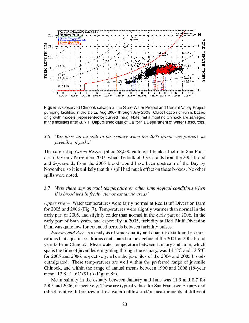
Figure 6: Observed Chinook salvage at the State Water Project and Central Valley Projectpumping facilities in the Delta, Aug 2007 through July 2005. Classification of run is basedon growth models (represented by curved lines). Note that almost no Chinook are salvagedat the facilities after July 1. Unpublished data of California Department of Water Resources.

3.6 Was there an oil spill in the estuary when the 2005 brood was present, asjuveniles or jacks?

The cargo ship Cosco Busan spilled 58,000 gallons of bunker fuel into San Fran-cisco Bay on 7 November 2007, when the bulk of 3-year-olds from the 2004 broodand 2-year-olds from the 2005 brood would have been upstream of the Bay byNovember, so it is unlikely that this spill had much effect on these broods. No otherspills were noted.

3.7 Were there any unusual temperature or other limnological conditions whenthis brood was in freshwater or estuarine areas?

Upper river– Water temperatures were fairly normal at Red Bluff Diversion Damfor 2005 and 2006 (Fig. 7). Temperatures were slightly warmer than normal in theearly part of 2005, and slightly colder than normal in the early part of 2006. In theearly part of both years, and especially in 2005, turbidity at Red Bluff DiversionDam was quite low for extended periods between turbidity pulses.

Estuary and Bay– An analysis of water quality and quantity data found no indi-cations that aquatic conditions contributed to the decline of the 2004 or 2005 broodyear fall-run Chinook. Mean water temperature between January and June, whichspans the time of juveniles emigrating through the estuary, was 14.4◦C and 12.5◦Cfor 2005 and 2006, respectively, when the juveniles of the 2004 and 2005 broodsoutmigrated. These temperatures are well within the preferred range of juvenileChinook, and within the range of annual means between 1990 and 2008 (19-yearmean: 13.8±1.0◦C (SE).) (Figure 8a).

Mean salinity in the estuary between January and June was 11.9 and 8.7 for2005 and 2006, respectively. These are typical values for San Francisco Estuary andreflect relative differences in freshwater outflow and/or measurements at different

20

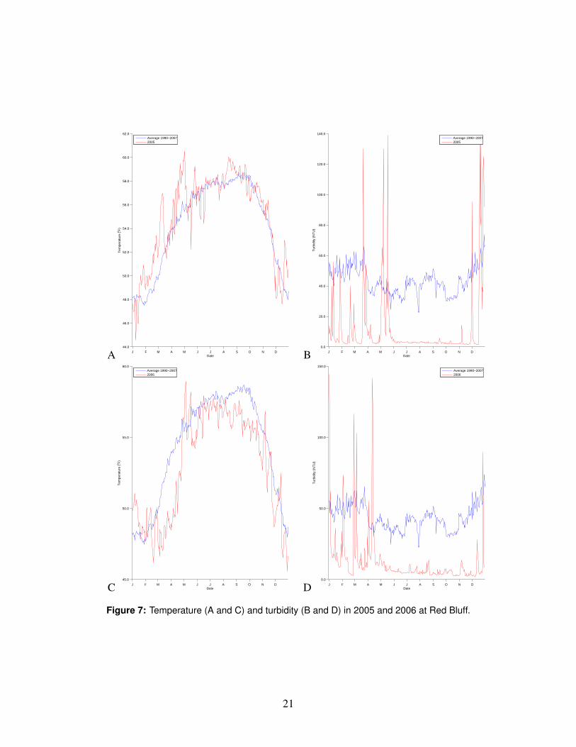
A J F M A M J J A S O N D

44.0

46.0

48.0

50.0

52.0

54.0

56.0

58.0

60.0

62.0

Date

Tem

pera

ture

(o F)

Average 1990−20072005

B J F M A M J J A S O N D

0.0

20.0

40.0

60.0

80.0

100.0

120.0

140.0

Date

Tur

bidi

ty (

NT

U)

Average 1990−20072005

C J F M A M J J A S O N D

45.0

50.0

55.0

60.0

Date

Tem

pera

ture

(o F)

Average 1990−20072006

D J F M A M J J A S O N D

0.0

50.0

100.0

150.0

Date

Tur

bidi

ty (

NT

U)

Average 1990−20072006

Figure 7: Temperature (A and C) and turbidity (B and D) in 2005 and 2006 at Red Bluff.

21

Figure 8: Mean annual values near the surface between January and June for a) watertemperature, b) salinity, c) chlorophyll, and d) dissolved oxygen for San Francisco Estu-ary between Chipps Island and the Golden Gate. (Source: USGS Water Quality of SanFrancisco Bay: http://sfbay.wr.usgs.gov/water.)

times on the tidal cycle. Mean salinity for the 19 years was 12.1±2.9 (Fig. 8b).Mean chlorophyll concentrations, an indicator of primary productivity, were

similar to the long-term mean of 3.3±1.2 mg/l (Fig. 8c). The mean chlorophyllconcentrations for 2005 and 2006 were 3.3 and 3.5 I1

4g/l, respectively, indicating

neither an oligotrophic or eutrophic system. The long-term trend, however, doessuggest an increasing amount of phytoplankton in the estuary.

As with the other hydrologic variables, dissolved oxygen concentrations werewithin the span typical of the estuary and do not reveal hypoxia as a contributor tothe salmon decline (Fig. 8d). Mean O2 levels were 8.4 mg/l for both years, whichis the same as the long-term average of 8.7±0.4 mg/l.

Freshwater outflow has been highly variable in the period 1990 to 2007 (Fig-ure 9). During the outmigrating season, mean flows were 963 and 3,033 m3s-1 for2005 and 2006, respectively. The long-term mean for January to June is 1,190±978m3s−1, thus 2005 was a relatively dry year and 2006 a relatively wet year. In fact,2006 had the greatest mean outflow of any year in the past 18. High flows throughthe estuary are considered beneficial for juvenile salmonids, thus 2006 was favor-able. Although 2005 had lower flows, it was situated in the middle of the range:nine years had lower flows, eight had higher. Since 2001 and 2005 had similar val-ues, and since fall Chinook returns were high and low respectively in those years, itwould seem that flow does not appear to be a factor contributing to the poor survivalof the 2004 and 2005 broods.

22

Figure 9: Mean annual freshwater outflow through San Francisco Estuary between Jan-uary and June. (Source: http://iep.water.ca.gov/dayflow/).

3.8 Were there any unusual population dynamics of typical food or prey speciesused by juvenile Chinook in the relevant freshwater and estuarine areas?

Juvenile Chinook feed on a wide variety of organisms during freshwater and estu-arine phases of their life cycle (MacFarlane and Norton 2002). Stomach contents offish sampled at the west end of the Delta, at Chipps Island, had decapods, mysids,amphipods and insects as the primary prey. In particular, the gammaridean amphi-pod Corophium is a dominant food item. In Suisun Bay, larval aquatic and terres-trial insects form a major part of juvenile Chinook diets, but mysids, amphipods,small fish, and calanoid copepods are also important food items. In San Pablo Bay,cumaceans make up a large fraction of stomach contents, but insects remain im-portant. In the central San Francisco Bay, small fish greatly dominate the stomachcontents, but cumaceans and amphipods are often present. These species are notsampled regularly, or at all, in the salmon outmigrating corridor, except for calanoidcopepods, which are monitored by the Interagency Ecological Program (IEP) at sta-tions in the Delta, Suisun and San Pablo Bays. Although calanoid copepods are nota major food item to juvenile salmon, they represent an important component ofaquatic food webs and offer a view of the zooplankton community and will be usedhere as a surrogate for the juvenile prey community.

The IEP zooplankton survey categorizes copepod samples into salinity zones:less than 0.5, 0.5–6, and greater than 6. Fluctuations in the annual copepod abun-dance can be large, ranging from 2,000 to over 7,000 copepods m−3 (Fig. 10).The annual mean abundance since 1990 is 4,238±322 (SE) copepods/m3 for thecombined total of the samples from the three salinity bands. In 2005 the meanabundance of copepods was 3,300 m−3. This value is 21% below the longer term

23

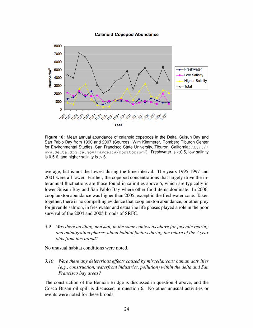
Figure 10: Mean annual abundance of calanoid copepods in the Delta, Suisun Bay andSan Pablo Bay from 1990 and 2007 (Sources: Wim Kimmerer, Romberg Tiburon Centerfor Environmental Studies, San Francisco State University, Tiburon, California; http://www.delta.dfg.ca.gov/baydelta/monitoring/). Freshwater is <0.5, low salinityis 0.5-6, and higher salinity is > 6.

average, but is not the lowest during the time interval. The years 1995-1997 and2001 were all lower. Further, the copepod concentrations that largely drive the in-terannual fluctuations are those found in salinities above 6, which are typically inlower Suisun Bay and San Pablo Bay where other food items dominate. In 2006,zooplankton abundance was higher than 2005, except in the freshwater zone. Takentogether, there is no compelling evidence that zooplankton abundance, or other preyfor juvenile salmon, in freshwater and estuarine life phases played a role in the poorsurvival of the 2004 and 2005 broods of SRFC.

3.9 Was there anything unusual, in the same context as above for juvenile rearingand outmigration phases, about habitat factors during the return of the 2 yearolds from this brood?

No unusual habitat conditions were noted.

3.10 Were there any deleterious effects caused by miscellaneous human activities(e.g., construction, waterfront industries, pollution) within the delta and SanFrancisco bay areas?

The construction of the Benicia Bridge is discussed in question 4 above, and theCosco Busan oil spill is discussed in question 6. No other unusual activities orevents were noted for these broods.

24

J F M A M J J A S0.0

0.2

0.4

0.6

0.8

1.0

1.2

1.4

1.6

1.8

2.0

Date

Cat

ch p

er T

hous

and

m3

Average 1976−20072005

J F M A M J J A S0.0

0.2

0.4

0.6

0.8

1.0

1.2

1.4

Date

Cat

ch p

er T

hous

and

m3

Average 1976−20072006

Figure 11: Daily catches of juvenile fall-run Chinook at Chipps Island in 2005 (left) and2006 (right), in red, compared to average daily catches (in blue) for 1976-2007.

3.11 Was there a change in the recovery of juvenile outmigrants observed inthe USFWS mid-water trawl surveys and other monitoring programs in theDelta.

Patterns of juvenile recoveries by midwater trawling near Chipps Island in 2005and 2006 were were similar in 2005 and 2006 compared to the pattern observed inother recent years (Fig. 11). In 2005, total catch and the timing of catches was quitenear the average for the 1976-2007 period of record. In 2006, total catches were abit higher than average, with typical timing.

4 Freshwater Species Interactions Focus

4.1 Was there any unusual predation by bird species when this brood was in fresh-water or estuarine areas?

None was noted.

4.2 Was there any unusual sea lion abundance or behavior when this brood wasin freshwater or estuarine areas?

None was noted.

4.3 Was there any unusual striped bass population dynamics or behavior whenthis brood was in freshwater or estuarine areas?

Annual abundance estimates for adult striped bass in the Sacramento-San JoaquinEstuary from 1990 through 2005 are shown in Table 5. Estimates represent thenumber of adult fish in the estuary in the spring of the reporting year. The estimatefor 2005 is preliminary and subject to change based on additional data. There is noestimate for 2006 because tagging was not conducted in that year.

25

Table 5: Striped bass abundance. NA indicates estimate unavailable. Unpublished data ofCDFG.

Year Abundance1990 830,7421991 1,045,9751992 1,071,8051993 838,3861994 908,4801995 NA1996 1,391,7451997 NA1998 1,658,3791999 NA2000 2,133,0432001 NA2002 1,296,9302003 1,179,6562004 1,904,6232005 1,373,8862006 NA

Brood-year 2004 and 2005 fall-run Chinook emigrated through the estuary, andwere vulnerable to predation by adult striped bass, in the spring of 2005 and 2006.In 2005, the preliminary estimate of adult striped bass abundance was not signifi-cantly higher than in previous years. In 2000, the striped bass population was thehighest among recent years, when the brood-year 1999 fall-run Chinook were em-igrating through the estuary. This year class returned to spawn in 2002 at recordhigh levels.

There is no apparent correlation between the estimated abundance of the adultstriped bass population in the estuary and the subsequent success of SacramentoRiver Basin fall-run Chinook year classes. Predation in freshwater may be a signif-icant factor affecting survival of fall-run Chinook emigrating through the system,but there is no indication that increased predation in the spring of 2005 or 2006contributed significantly to the decline observed in the subsequent escapement ofSacramento River fall-run Chinook.

4.4 Were northern pike present in any freshwater or estuarine areas where thisbrood was present?

Northern pike have not been noted in these areas to date.

26

4.5 Is there a relationship between declining Delta smelt, longfin smelt, and threadfinshad populations in the Delta and Central Valley Chinook survival?

Indices of abundance for Delta smelt (Hypomesus transpacificus), longfin smelt(Spirinchus thaleichthys), and threadfin shad (Dorosoma petenense) from the Cali-fornia Department of Fish and Game’s Fall Mid-water Trawl Surveys in the Delta,Suisun Bay, and San Pablo between 1993 and 2007 reveal a pattern of substantialvariation in abundance (Fig. 12). From 1993 to 1998, Delta smelt and longfin smeltabundances vary similarly among years; Threadfin Shad dynamics were somewhatout of phase with the smelt species. However, longfin smelt abundances declinedgreatly from 1998 to 2002, about one year prior to Delta smelt declines. By 2002,all three species were in low numbers in the study area and have remained lowsince. Juvenile salmon abundance between April and June at Chipps Island wassomewhat reflective of threadfin shad abundance until 2002, but then departed fromthe shad trend (Fig. 12). Since 2002, juvenile salmon abundance appears to beincreasing, in general, but there are relatively wide variations among years. In par-ticular, juvenile fall-run abundance appeared to be relatively high in 2004. In 2005,the abundance index value was greater than in 2002 and 2003, but below estimatesfor 2006 and 2007. Correlation analysis found no significant relationships (P>0.05)between population fluctuations of the smelt and shad species with juvenile fall-runChinook catch at Chipps Island. Differences in abundance patterns between juve-nile salmon at Chipps Island and the three other species, which are all species ofconcern in the Pelagic Organism Decline (POD) in the Delta, indicate that whateveris affecting the POD species is not a major influence on juvenile salmon productionin the Central Valley.

4.6 Was there additional inriver competition or predation with increased hatcherysteelhead production?

Releases of steelhead from state and federal hatcheries have been fairly constantover the decade, suggesting that predation by steelhead is an unlikely cause of thepoor survival of the 2004 and 2005 broods of fall-run Chinook.

5 Marine Biological Focus

5.1 Was there anything unusual about the ocean migration pattern of the 2004and 2005 broods? Was there anything unusual about the recovery of taggedfish groups from the 2004 and 2005 broods the ocean salmon fisheries?

Unfortunately, in contrast to previous years, little of the 2004 and 2005 broodswere coded-wired tagged at the basin hatcheries. As a consequence the informa-tion available for addressing these questions is limited to Feather River Hatchery(FRH) fall Chinook coded-wire tag recoveries. The analysis was further restrictedto recreational fishery age-2 recoveries for the following reasons. First, it is gen-erally accepted that SRFC brood recruitment strength is established prior to ocean

27

0

200

400

600

800

1000

1200

1400

1600

1800

1993

1995

1997

1999

2001

2003

2005

2007

Year

Central Valley Index

Juvenile salmon ChippsIsland IndexDelta smelt Index

Longfin smelt Index

Threadfin shad Index

Inde

x Va

lue

Figure 12: Abundance indices for Delta smelt, longfin smelt, and threadfin shad fromCalifornia Department of Fish and Game Mid-water Trawl Surveys between 1993 and 2007in the Delta, Suisun Bay, and San Pablo Bay (Source: http://www.delta.dfg.ca.gov)

28

age-2. Thus, age-2 recoveries provide the least disturbed signal of brood strengthand distribution prior to the confounding effects of fishery mortality. Second, manymore age-2 fish are landed by the recreational fishery than by the commercial fish-ery, in part because of differences in the minimum size limits for the two fisheries.Effort in the recreational fishery is also generally more evenly distributed along thecoast and more consistent across years than in the commercial fishery.

Ocean salmon recreational fishery coded-wire tag recoveries of age-2 FRH fallChinook, brood years 2000-2005, were expanded for sampling and summed acrossmonths by major port area for each brood year. Catch per unit of effort (CPUE)was derived by dividing the expanded recoveries by the corresponding fishing ef-fort. For any given recovery year, assuming catchability is the same for each portarea, the pattern of CPUE across the port areas reflects the ocean distribution of thecohort (Fig. 13). The coherent pattern across brood years suggests that the oceandistribution of age-2 fish was similar for all of these broods, and concentrated in theSan Francisco major port area.

Within a port area, assuming catchability is the same each year, differencesin CPUE across brood years reflect differences in the age-2 abundance of thesebroods. Clearly, the 2004 and 2005 (and 2003) brood age-2 cohorts were at very lowabundance relative to the 2000-2002 broods (Fig. 13). Was this because there werefewer numbers of coded-wire tagged FRH fall Chinook released in those years,or was it the result of poor survival following release? The number of releasedfish was very similar in each of these brood years (Table 6), except for brood-year2003 which was about half that of the other years. An index of the survival ratefrom release to ocean age-2 was derived by dividing the San Francisco major portarea CPUE by the respective number of fish released (Table 6, Figure 14). TheSan Francisco CPUE time series is the most robust available for this purpose giventhat the number of recoveries it is based are significantly greater than those for theother ports (stock concentration and fishing effort is highest here). This index isproportional to the actual survival rate to the degree that the fraction of the age-2ocean-wide cohort abundance and catchability in the San Francisco major port arearemains constant across years, both of which are supported by the coherence of theCPUE pattern across all areas and years (Fig. 13). The survival rate index showsa near monotonic decline over the 2000-2005 brood-year period (Table 6, Fig. 14).In particular, the survival rate index for 2004 and 2005 broods was very low: lessthan 10% of that observed for the 2000 brood (Table 6, Fig. 14). The survival rateindex in turn is fairly well-correlated with the SRFC jack escapement for the 2000-2005 broods (correlation = 0.78, Fig. 15 ). Taken together, this indicates that thesurvival rate was unusually low for the 2004 and 2005 broods between release inSan Francisco Bay and ocean age-2, prior to fishery recruitment, and that broodyear strength was established by ocean age-2. Genetic stock identification methodsapplied to catches in the Monterey Bay salmon sport fishery showed relatively lowabundance of Central Valley fall Chinook in the 2007 landings (Fig. 16). We alsonote that the survival rate for the 2003 brood was also considerably lower than forprevious broods in this decade.

29

020

4060

8010

012

0

Major Port Area

CP

UE

NO CO KO KC FB SF MO

200020012002200320042005

Figure 13: Recreational fishery CPUE of age-2 FRH fall Chinook by major port area;brood-years 2000-2005. CPUE was calculated as Recoveries / Effort, where “Recoveries”is coded-wire tag recoveries expanded for sampling; “Effort” is fishing angler days ×10−4.Major port areas shown from north to south: “NO” is northern Oregon; “CO” is centralOregon; “KO” is the Klamath Management Zone, Oregon portion; “KC” is the KlamathManagement Zone, California portion; “FB” is Fort Bragg, California; “SF” is San Francisco,California; “MO” is Monterey, California.

5.2 Has the bycatch in non-salmonid fisheries (e.g., whiting, groundfish) increased?

Bycatch of Chinook in trawl fisheries off of California has been variable over thelast two decades (Fig. 17). The magnitude of bycatch by trawl fisheries is quitesmall compared to combined landings by the commercial and recreational salmonfisheries (1.4 metric tons (t) and 686 t respectively, in 2007), so it is unlikely thatvariations in bycatch in non-salmonid fisheries are an important cause of variationin the abundance of Chinook.

6 Marine Habitat Areas Focus

6.1 Were there periods of reduced upwelling or other oceanographic physicalconditions during the period of smolt entry into the marine environment, orduring the period of marine residence up to the return to freshwater of thejacks?

Conditions in the coastal ocean in the spring of 2005 were unusual. Most notably,the onset of upwelling was delayed significantly compared to the climatologicalaverage (Schwing et al., 2006); Fig. 18) due to weaker than normal northerly winds

30

Table 6: Recreational fishery coded-wire tag recoveries of age-2 FRH fall Chinook in theSan Francisco major port area, brood-years 2000-2005. “Released” is number released×10−5; “Effort” is fishing angler days ×10−4; “Recoveries” is coded-wire tag recoveriesexpanded for sampling; “Survival Rate Index” is Recoveries/(Effort × Released) relative tothe maximum value observed (brood-year 2000).

Brood Year2000 2001 2002 2003 2004 2005

Released 11.23 13.78 13.11 7.41 13.13 13.71Effort 9.88 6.71 10.10 8.00 7.45 4.30Recoveries 1169 429 777 124 78 19Survival Rate Index 1.00 0.44 0.56 0.20 0.08 0.03

(Fig. 19). Off central California (36◦N), there was a only a brief period of upwellingin the early spring before sustained upwelling began around mid May. Movingnorthward along the coast, sustained upwelling began later: late May off Pt. Arena,early June near the California-Oregon border, and not until July in central Oregon(Fig. 18, see also Kosro et al. (2006)). In the north (> 42◦N) a delay in the advent ofupwelling led to a lag in cumulative upwelling, which was made up for in the latterpart of the year, leading to an average annual total. In the south, upwelling waslower than average all year, leading to a low annual total. The delay in upwellingin the north was associated with a southward shift of the jet stream, which led toanomalous winter-storm-like conditions (i.e., downwelling) (Sydeman et al., 2006;Barth et al., 2007). The delay in upwelling was not unprecedented, having occurredalso in ’83, ’86, ’88, ’93 and ’97.

Sea surface temperatures along the coast of central California were anomalouslywarm in May (Fig. 20), before becoming cooler than normal in the summer, coinci-dent with strong, upwelling-inducing northwesterly winds. The mixed layer depthin the Gulf of the Farallones was shallower than normal in May and June in both2005 and 2006 (Fig. 21). Warm sea surface temperatures, strong stratification, andlow upwelling have been associated with poor survival of salmon during their firstyear in the ocean in previous studies (Pearcy, 1992).

A number of researchers observed anomalies in components of the Califor-nia Current food web in 2005 consistent with poor feeding conditions for juvenilesalmon. For example, gray whales appeared emaciated (Newell and Cowles, 2006);sea lions foraged far from shore rather than their usual pattern of foraging nearshore (Weise et al., 2006); various fishes were at low abundance, including commonsalmon prey items such as juvenile rockfish and anchovy (Brodeur et al., 2006);Cassin’s auklets on the Farallon Islands abandoned 100% of their nests (Sydemanet al., 2006); and dinoflagellates became the dominant phytoplankton group, ratherthan diatoms (MBARI, 2006). While the overall abundance of anchovies was low,they were captured in an unusually large fraction of trawls, indicating that theywere more evenly distributed than normal. The anomalous negative effect on thenekton was also compiled from a variety of sampling programs (Brodeur et al.,2006) indicating some geographic displacement and reduced productivity of early

31

2000 2001 2002 2003 2004 2005

0.0

0.2

0.4

0.6

0.8

1.0

Brood Year

Sur

viva

l Rat

e In

dex

Figure 14: Index of FRH fall Chinook survival rate between release in San Francisco Bayand ocean age-2 based on coded-wire tag recoveries in the San Francisco major port arearecreational fishery; brood-years 2000-2005. Survival rate index was derived as describedin Table 6.

life stages. In central California, the abundance of young-of-the-year rockfisheswas the lowest seen in the previous 22 years, even lower than the recent El Nino of1998. Brodeur et al. (2006) noted that (1) “these changes are likely to affect juve-nile stages and recruitment of many species (rockfishes, salmon, sardine) that aredependent on strong upwelling-based production,” and (2) the presence of unusualspecies not quantitatively sampled such as blue sharks, thresher sharks and alba-core which “likely became important predators on juvenile rockfishes, salmon, andother forage fish species.” The latter adds the possibility of a top down influenceof this event on nektonic species. To this list of potential predators might be addedjumbo squid, which since 2003 have become increasingly common in the CaliforniaCurrent (discussed in detail below).

Conditions in the coastal ocean were also unusual in the spring of 2006. Offcentral California (36◦N), upwelling started in the winter, but slowed or stoppedin March and April, before resuming in May. At 39◦N, little upwelling occurreduntil the middle of April, but then it closely followed the average pattern. At 42◦N,the start of sustained upwelling was delayed by about one month, but by the endof the upwelling season, more than the usual amount of water had been upwelled.At 45◦N, the timing of upwelling was normal, but the intensity of both upwellingand downwelling winds was on average greater than normal. In late May and earlyJune, upwelling slowed or ceased at each of the three northern stations.

In the Gulf of the Farallones region, northwest winds were stronger offhsore

32

0.0 0.2 0.4 0.6 0.8 1.0

020

000

4000

060

000

Survival Rate Index

Jack

Esc

apem

ent

00

01

02

03

04

05

Figure 15: SRFC jack spawning escapement versus FRH fall Chinook survival rate in-dex. Line is ratio estimate. Numbers in plot are last two digits of brood year; e.g., “05”denotes brood-year 2005 (jack return-year 2007). Line denotes ratio estimator fit to thedata (through the origin with slope equal to average jack escapement/average survival rateindex).

33

Central Valley Fall-(92.0%)

Central Valley Spring- (2.2%)

Klamath- (0.7%)

Central Valley Winter- (3.3%)

Coastal CA- (0.7%)Oregon Coast- (1.1%)

Columbia- (0.1%)

CentralValleyFall-71.4%CentralValleySpring-8.4%Rogue-4.5%CentralValleyWinter-4.2%CoastalCA-3.9%Klamath-3.3%Ucolumbia-1.2%Mid-Oregon-1.2%NPugetSound-0.6%Chetco-0.6%Thompson-0.3%Snake-0.3%

a)

b)

Figure 16: Composition of the Monterey Bay sport fishery landings as determined bygenetic stock identification. Based on samples of 735 fish in 2006 and 340 fish in 2007.NMFS unpublished data.

Figure 17: Landings of Chinook taken in trawl fisheries and landed at California ports.Data from the CALCOM database (D. Pearson, SWFSC, pers. comm.).

34

A M J J A S−2

0

2

4

6

8

Date

Cum

ulat

ive

upw

ellin

g (m

illio

n m

3 /m−

1 ) 45°N

200520062007

A M J J A S−5

0

5

10

15

Date

Cum

ulat

ive

upw

ellin

g (m

illio

n m

3 /m−

1 ) 42°N

A M J J A S−5

0

5

10

15

20

Date

Cum

ulat

ive

upw

ellin

g (m

illio

n m

3 /m−

1 ) 39°N

A M J J A S−5

0

5

10

15

20

Date

Cum

ulat

ive

upw

ellin

g (m

illio

n m

3 /m−

1 ) 36°N

Figure 18: Cumulative upwelling at four locations along the California and Oregon coast;45◦N is near Lincoln City, Oregon; 42◦N is near Brooking, Oregon, 39◦N is near Pt. Arena,and 36◦N is near Santa Cruz, California. Units are in millions of cubic meters per meter ofshoreline. The black line represents the average cumulative upwelling at each location forthe 1967-2008 period. Upwelling is indicated by increasing values of the upwelling index.

35

Figure 19: Strength of meridional winds (negative from the north) along the central Califor-nia coast in 2003-2006. Note weak winds near the coast and in the Gulf of the Farallonesin 2005 and 2006.

36

Figure 20: Sea surface temperature anomalies off central California in May (left), June(center) and July (right). Note especially warm temperatures in the Gulf of Farallones inMay 2005 and June 2006, and warm temperatures along the coast in 2006. Data obtainedfrom CoastWatch (http://coastwatch.noaa.gov/).

37

Figure 21: Average depth of the thermocline during May and June in the Gulf of the Faral-lones. NMFS unpublished data.

in 2006 than 2005, but were relatively weak near the coast between Pt. Reyesand Monterey Bay. At NMFS trawl survey stations in the Gulf of the Farallones,the mixed layer depth in May was the shallowest on record since 1987. Cassin’sauklets again abandoned all their nests in 2006 (J. Thayer, PRBO, unpublisheddata), juvenile rockfish abundance was very low in the NMFS trawl survey, andanchovies were again encountered in a high fraction of trawls, even though overallabundance was low (NMFS unpublished data). While conditions in the spring of2006 might not have been as unusual as 2005, it is important to realize that thepelagic ecosystem of the California Current is not created from scratch each year,but the animals in the middle and upper trophic levels (where salmon feed) havelife spans longer than one year. This means that the food web will reflect pastconditions for some time. Overall, it appears that the continuation of relativelypoor feeding conditions in the spring of 2006, following on the poor conditions in2005, contributed significantly to the poor survival of Sacramento River fall-runChinook in their first year in the ocean

6.2 Were there any effects to these fish from the “dead zones” reported off Oregonand Washington in recent years?

Hypoxia in inner-shelf waters can extend from the bottom to within 12 m of the sur-face at certain times and places (Chan et al., 2008), but juvenile salmon are usuallyfound in the upper 10 m of the water column and are capable of rapid movement, soare not expected to be directly impacted by hypoxic events. Furthermore, hypoxia

38

has not been observed on the inner shelf in California waters, where juvenile Chi-nook from the Central Valley are thought to rear. It is conceivable that outbreaksof hypoxia alter the distribution of Chinook, their prey, and their predators, but thisseems an unlikely explanation for the poor performance of brood-year 2004 and2005 Sacramento River fall-run Chinook.

6.3 Were plankton levels depressed off California, especially during the smolt en-try periods?

Phytoplankton levels, based in remotely sensed observations of chlorophyll-a con-centrations in the surface waters, were not obviously different in the spring and earlysummer of 2005 and 2006 compared to 2003 and 2004 (Fig. 22). Zooplankton arediscussed in the answer to the first question in section 7.

6.4 Was there a relationship to an increase in krill fishing worldwide?

To date, there have been no commercial fisheries for krill in US waters; kill fishingin other parts of the world is unlikely to impact SRFC.

6.5 Oceanography: temperature, salinity, upwelling, currents, red tide, etc.

These issues are addressed in the response to question 1 in this section above, withthe exception of red tides. Red tides are frequently caused by dinoflagellates (butcan also be formed by certain diatom species). MBARI (2006; Fig. 23) reportedthat dinoflagellates in Monterey Bay have become relatively abundant since 2004,concurrent with increased water column stratification, reduced mixed layer depthand increased nitrate concentrations at 60 m depth. Increased stratification favorsmotile dinoflagellates over large diatoms which lack flagella, and thus diatoms areprone to sinking out of the photic zone when the upper ocean is not well-mixed.

6.6 Were there any oil spills or other pollution events during the period of oceanresidence?

As discussed in the answer to question 6 of the section “Freshwater habitat areafocus”, the cargo ship Cosco Busan spilled 58,000 gallons of bunker fuel into SanFrancisco Bay on 7 November 2007, and some of this fuel dispersed from the bayinto the coastal ocean, eventually fouling beaches in San Francisco and Marin coun-ties. This would have had the most impact on brood-year 2006 Chinook, some ofwhich would have been in nearshore areas of the Gulf of the Farallones at that time.The actual effects of this spill on fish in the coastal ocean are unknown.

6.7 Was there any aquaculture occurring in the ocean residence area?

Aquaculture in California is generally restricted to onshore facilities or estuaries(e.g., Tomales Bay) where it is unlikely to impact salmonids from the Central Val-ley; we are unaware of any offshore aquaculture in California.

39

Figure 22: Chlorophyll-a (Chl-a) anomalies obtained from MODIS (CoastWatch) duringMay, June, and July. Black indicates low values and white high values. Anomalies representmonthly Chl-a concentrations minus mean Chl-a concentration values at the pixel resolutionfor the 1998-2007 period. From Wells et al. (2008).

40

Figure 23: Time series of temperature, water column stratification, nitrate, chlorophyll andand dinoflagellates observed in Monterey Bay. “El Viejo” refers to the warm-water regimelasting from 1976-1998, and “La Veija” refers to the present regime. El Nino and La Ninaevents are indicated by the colored vertical bars spanning the subplots. Figure from MBARI(2006).

41

6.8 Was there any offshore construction in the area of ocean residence, for waveenergy or other purposes?

A review of NMFS Endangered Species Act consultations indicate no significantoffshore construction projects occurred during the time period of interest.

7 Marine Species Interactions Focus

7.1 Were there any unusual population dynamics of typical food or prey speciesused by juvenile Chinook in marine areas? (plankton, krill, juvenile anchovyor sardines, etc.)

Prey items of juvenile salmon, especially juvenile rockfish, were at very low abun-dance in 2005 (Brodeur et al. (2006), Fig. 24) and 2006. Catches of adult anchoviesin midwater trawls conducted by NMFS exhibited an unusual pattern: the averagecatch in the Gulf of the Farallones was moderately low, but the frequency of en-counter (fraction of trawls with at least some anchovy) was higher than normal,indicating that the distribution of anchovy was less clustered than normal (Fig. 25).Sardines have been increasing since 2003, possibly indicating a shift in the Califor-nia Current to a state more favorable to warm-water species and less favorable tocold-water species such as salmon and anchovy.

Data are limited for krill, but it appears that krill abundance was fairly normalin the spring of 2005 (Fig 26a and b), but krill were distributed more evenly than in2002-2004, which may have made it harder for salmon to find high concentrationsof krill upon which to feed. In spring 2006, krill abundance was very low in theGulf of the Farallones (Fig. 26c).

7.2 Was there an increase in bird predation on juvenile salmonids caused by areduction in the availability of other forage food?

Among the more abundant species of seabirds, common murres (Uria aalge) andrhinoceros auklets Cerorhinca monocerata eat juvenile salmon (Fig. 27; Roth et al.(2008); Thayer et al. (2008)) . In 2005 and 2006, chicks of these species in theGulf of the Farallones, the initial ocean locale of juvenile Chinook from the CentralValley, had juvenile salmon in their diet at 1-4% for rhinoceros auklets and 7-10%for murres. This represented a smaller than typical contribution to stomach contentsfor auklets, and a larger than typical proportion for murres during the 1972-2007time period (calculated from data in Fig. 27; Bill Sydeman, Farallon Institute forAdvanced Ecosystem Research, Petaluma, California, unpublished data).

The rhinoceros auklet population in the Gulf of the Farallones has remainedstable at about 1,500 birds for the past 20 years, but murre numbers have doubledbetween the 1990s and 2006 to about 220,000 adults (Bill Sydeman, Farallon Insti-tute for Advanced Ecosystem Research, Petaluma, California, personal communi-cation). A study in 2004 found that murres in the Gulf of the Farallones consumedabout four metric tons of juvenile salmon (Roth et al., 2008). This represents the

42

Figure 24: Time series of catches from pelagic trawl surveys along the central Californiacoast from 1983 to 2005 for (a) the dominant nekton species and (b) juvenile rockfishes.From Brodeur et al. 2006.

43

Figure 25: Standardized abundances (bars) of four Chinook salmon prey items (the tenmost frequently encountered rockfish of the NOAA trawl survey, market squid, sardinesand anchovies) estimated from the mid-water trawl survey conducted by NOAA Fisheries,Santa Cruz. Lines indicate the frequency of occurrences of sardines and northern anchovyin the trawls.

equivalent of about 20,000 to 40,000 juvenile Chinook salmon (100-200 g each).Although a greater proportion of murre stomach contents were salmon in 2005 and2006 than in 2004, considering that >30 million juvenile salmon entered the oceaneach year, this increase could not account for the poor survival of the 2004 and 2005broods.

7.3 Was there an increase of marine mammal predation on these broods?

Among marine mammals, killer whales (Orcinus orca), California sea lions (Za-lophus californianus), and harbor seals (Phoca vitulina) are potential predators onsalmon (Parsons et al., 2005; Weise and Harvey, 2005; Ford and Ellis, 2006; Za-mon et al., 2007). A coast-wide marine mammal survey off Washington, Oregon,and California conducted in 2005 to 550 km offshore reported cetacean abundancessimilar to those found in the 2001 survey (K. Forney, NMFS, unpublished data).In coastal waters of California during July 2005 the population estimate for killerwhales was 203, lower than abundance estimates from surveys in 1993, 1996, and2001 (Barlow and Forney, 2007) (Fig. 28).

Of five recognized killer whale stocks within the Pacific U.S. Exclusive Eco-nomic Zone, the Eastern North Pacific Southern Resident stock has been most im-plicated in preying on salmon. This stock resides primarily in inland waters ofWashington state and southern British Columbia, but has been observed as far south

44

A

B

C

Figure 26: Abundance of krill measured by echosounder during May-June survey cruisesoff central California in 2004-2006. A) Average abundance of krill over the survey period.B) Abundance of krill in 2005 and C) 2006. Unpublished data of J. Santora.

45

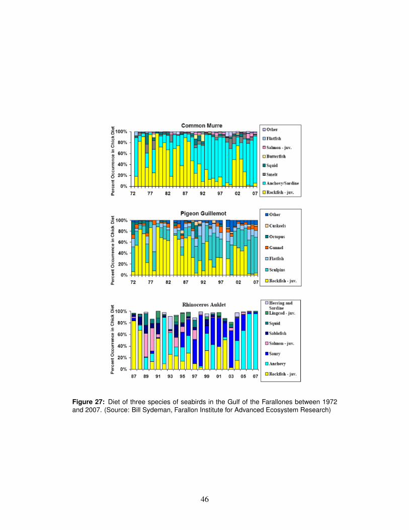
Figure 27: Diet of three species of seabirds in the Gulf of the Farallones between 1972and 2007. (Source: Bill Sydeman, Farallon Institute for Advanced Ecosystem Research)

46

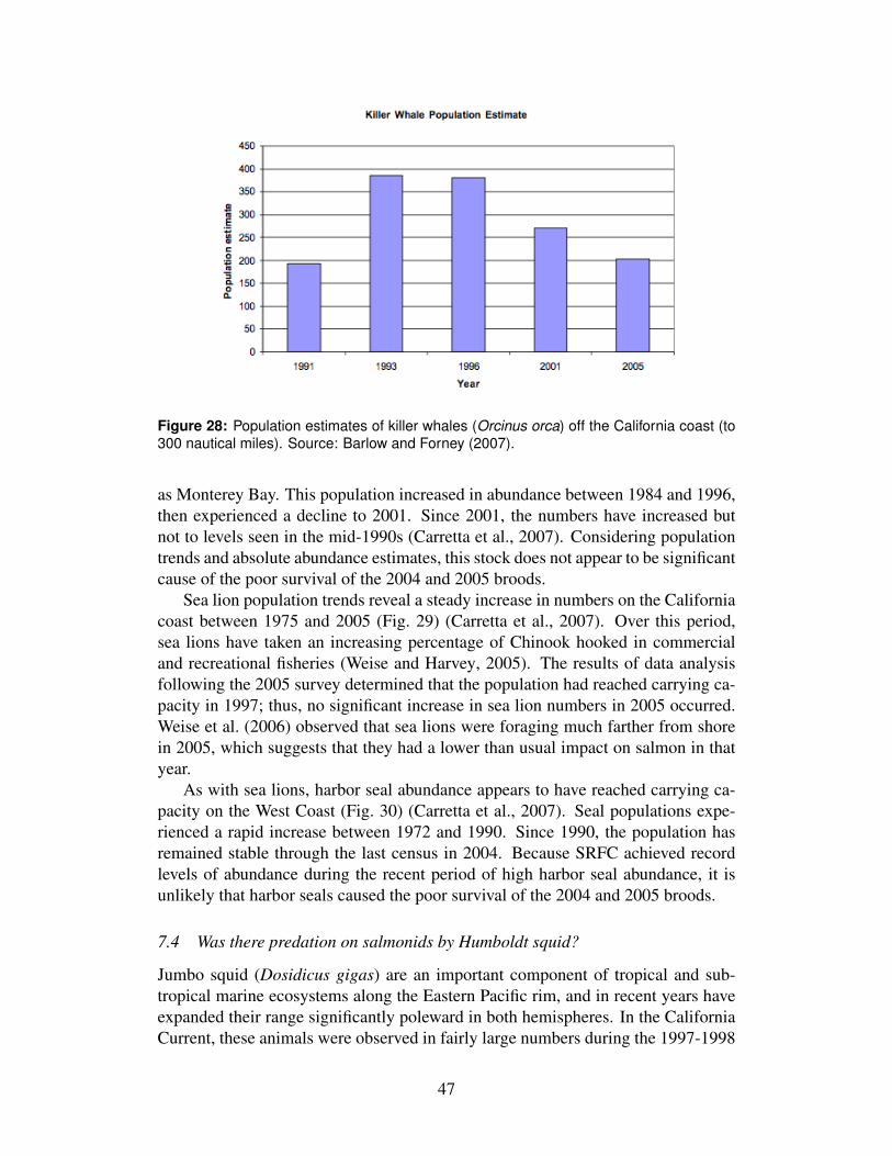
Figure 28: Population estimates of killer whales (Orcinus orca) off the California coast (to300 nautical miles). Source: Barlow and Forney (2007).

as Monterey Bay. This population increased in abundance between 1984 and 1996,then experienced a decline to 2001. Since 2001, the numbers have increased butnot to levels seen in the mid-1990s (Carretta et al., 2007). Considering populationtrends and absolute abundance estimates, this stock does not appear to be significantcause of the poor survival of the 2004 and 2005 broods.

Sea lion population trends reveal a steady increase in numbers on the Californiacoast between 1975 and 2005 (Fig. 29) (Carretta et al., 2007). Over this period,sea lions have taken an increasing percentage of Chinook hooked in commercialand recreational fisheries (Weise and Harvey, 2005). The results of data analysisfollowing the 2005 survey determined that the population had reached carrying ca-pacity in 1997; thus, no significant increase in sea lion numbers in 2005 occurred.Weise et al. (2006) observed that sea lions were foraging much farther from shorein 2005, which suggests that they had a lower than usual impact on salmon in thatyear.

As with sea lions, harbor seal abundance appears to have reached carrying ca-pacity on the West Coast (Fig. 30) (Carretta et al., 2007). Seal populations expe-rienced a rapid increase between 1972 and 1990. Since 1990, the population hasremained stable through the last census in 2004. Because SRFC achieved recordlevels of abundance during the recent period of high harbor seal abundance, it isunlikely that harbor seals caused the poor survival of the 2004 and 2005 broods.

7.4 Was there predation on salmonids by Humboldt squid?

Jumbo squid (Dosidicus gigas) are an important component of tropical and sub-tropical marine ecosystems along the Eastern Pacific rim, and in recent years haveexpanded their range significantly poleward in both hemispheres. In the CaliforniaCurrent, these animals were observed in fairly large numbers during the 1997-1998

47

Figure 29: Count of California sea lion pups (1975-2005). Source: Carretta et al. (2007)

Figure 30: Harbor seal haulout counts in California during May and June (Source: Carrettaet al. 2007)

48

El Nino, and since 2003 they have been regularly encountered by fishermen andresearchers throughout the West Coast of North America as far north as South-east Alaska. While the primary drivers of these range expansions remain uncertain,climate-related mechanisms are generally considered the most likely, and some evi-dence suggests that that an ongoing expansion of the oxygen minimum zone (OMZ)in the California Current could be a contributing factor (Bograd et al., 2008). Al-though accounts of squid off of Southeast Alaska consuming salmon have beenreported, ongoing monitoring of food habits from squid collected off of California(with limited sampling in Oregon) since 2005 have failed to document any predationon salmonids. While salmon smolts are clearly within the size range of commonsquid prey, their distribution (generally inshore of the continental shelf break) likelyoverlaps very little with the distribution of squid (generally offshore of the conti-nental shelf break), and predation on older salmon is probably unlikely given theirswimming capabilities relative to other prey.

In a sample of 700 jumbo squid stomachs collected in California waters, themost frequent prey items have been assorted mesopelagic fishes, Pacific hake, north-ern anchovy, euphausids, Pacific sardine, several species of semi-pelagic rockfish(including shortbelly, chilipepper, widow and splitnose rockfish) and other squids(Field et al., 2007). The size of prey items ranges from krill to fishes of sizes up to45 centimeters, however most of the larger fishes (and squids) consumed by squidcan probably be considered relatively weak swimmers (Pacific hake, rockfish, Pa-cific ratfish). Although squid have also been reported to strike larger salmon, rock-fish, sablefish and other species that have been hooked on fishing lines, predationon larger prey items that may be swimming freely seems unlikely. Similarly, squidcaught in purse seines in the Eastern Tropical Pacific will often attack skipjackand yellowfin tuna schools, while predation by free-swimming squids appears tobe limited almost exclusively to mesopelagic fishes and invertebrates (Olson et al.,2006). However, the impacts of jumbo squid on fisheries could possibly be moresubtle than direct predation alone, as recent research conducted during hydroacous-tic surveys of Pacific hake in the California Current has suggested that the presenceof squid may lead to major changes in hake schooling behavior, confounding theability to monitor, assess, and possibly manage this important commercial resource(Holmes et al., 2008). Although unlikely, it is plausible that the presence of squidcould result in changes in the behavior of other organisms (such as salmon or theirprey or other predators) as well, even in the absence of intense predation.

The absolute abundance of squid in the California Current in recent years is animportant factor in assessing the potential impacts of predation, yet this is entirelyunknown. However, the total biomass could potentially be quite large based on thesignificance of squid in the diets of some predators (such as mako sharks, for whichjumbo squid appear to be the most important prey in recent years), the frequency ofsquid encounters and catches during recreational fishing operations and scientificsurveys, and the magnitude of catches in comparable ecosystems. For example, inrecent years jumbo squid landings in similar latitudes in the Southern Hemispherehave grown from nearly zero to over 200,000 tons per year.

Although it is impossible to conclusively rule out squid predation as a primary

49

cause of the poor survival of the 2004 and 2005 broods of SRFC, it is unlikely thatsquid predation is a major contributing factor. Instead, the large numbers of jumbosquid observed since 2003, and particularly during 2005-2006, may have been areflection of the same unusual ocean conditions (poor upwelling, heavy stratifica-tion, warm offshore water, poor juvenile rockfish and seabird productivity, etc) thatcontributed to the poor feeding conditions for salmon during those years.

7.5 Was there increased predation on salmonids by other finfish species (e.g., ling-cod)?

Predation is typically considered to be a major source of salmon mortality, particu-larly during ocean entry (Pearcy, 1992). Seabirds and marine mammals (addressedin section 7.3) are often considered the greatest sources of salmon smolt and adultpredation mortality, respectively. In general, available food habits data do not in-dicate that groundfish or other fishes are substantial predators of either juvenile oradult salmon, although as Emmett and Krutzikowsky (2008) suggest, this could bein part due to biases in sampling methodologies. As very little data are available forpiscivirous predators in the Central California region, we summarize examples ofthose species of groundfish that could potentially have an impact on Pacific salmonbased on existing food habits data, much of which was collected off of the Pa-cific Northwest, and briefly discuss relevant population trends for key groundfishspecies. However, it is unlikely that any are at sufficiently high population levels,or exhibit sufficiently high predation rates, to have contributed to the magnitude ofthe 2008 salmon declines.

Pacific hake (Merluccius productus) are by far the most abundant groundfishin the California Current, and are widely considered to have the potential to driveeither direct or indirect food web interactions. However, despite numerous foodhabits studies of Pacific hake dating back to the 1960s, evidence of predation onsalmon smolts is very limited, despite strong predation pressure on comparablysized forage fishes such as Pacific sardines, northern anchovies and Pacific herring.Emmet and Krutzikowsky (2008) found a total of five Chinook (four of which wereocean entry year fish, one of which was age one) in six years of monitoring predatorabundance and food habits near the mouth of the Columbia river. As the populationof Pacific hake is substantial, their extrapolation of the potential impact to salmonpopulations suggested consumption of potentially millions of smolts during yearsof high hake abundance, although the relative impact to the total number of smoltsin the region (on the order of 100 million per year) was likely to be modest (al-beit uncertain). Jack mackerel (Trachurus symetricus) were another relative abun-dant predator with limited predation on salmon in their study, and Pacific mackerel(Scomber japonicus) have also been implicated with inflicting significant predationmortality on outmigrating salmon smolts at some times and places (Ashton et al.,1985).

In nearshore waters, examples of piscivores preying upon salmonids are rel-atively rare. Brodeur et al. (1987) found infrequent but fairly high predation onsalmon smolts (both Chinook and coho) from black rockfish (Sebastes melanops)

50

collected from purse-seine studies off of the Oregon coast in the early 1980s, butno other rockfish species have been documented to prey on salmonids. Cass et al.(1990) included salmon in a long list of lingcod prey items in Canadian waters,but studies in California have not encountered salmon in lingcod diets and thereis no evidence that lingcod are a significant salmon predator. In offshore waters,sablefish (Anoplopoma fimbria) are one of the most abundant higher trophic levelgroundfish species, however with the exception of trace amounts of Oncorhynchussp. reported by Buckley et al. (1999), several other sablefish food habits studies inthe California Current have not reported predation on salmonids. Salmon have alsobeen noted as important prey of soupfin sharks (Galeorhinus galeus) in historicalstudies off of Washington and California. Larger salmon have also been noted in thediets of sleeper sharks, and presumably salmon sharks (Lamna ditropis) are likelysalmon predators when they occur in the California Current. However, none ofthese species are likely to be sufficiently abundant, nor were reported to be presentin unusual numbers, throughout the 2005-2006 period.

Population turnover rates for most groundfish species are typically relativelylow, and consequently it is unlikely that short term fluctuations in the relativeabundance of predatory groundfish could make a substantive short-term impact onsalmon productivity. However, many groundfish population in the California Cur-rent have experienced significant to dramatic changes in abundance over the pastdecade, a consequence of both reduced harvest rates and dramatically successfulrecruitment observed immediately following the 1997-98 El Nino. Specifically, formost stocks in which recruitment events are reasonably well specified, the 1999year class was estimated to be as great or greater than any recruitment over thepreceding 15 to 20 years (Fig. 31). For example, the 1999 bocaccio (Sebastes pau-cispinis) year class was the largest since 1989, resulting in a near doubling of stockspawning biomass between 1999 and 2005 (MacCall, 2006). Similarly, the 1999Pacific hake year class was the largest since 1984, which effectively doubled thestock biomass between 2000 and 2004 (Helser et al., 2008). Lingcod, cabezon,sablefish, most rockfish and many flatfish also experienced strong year classes, re-sulting in a doubling or even tripling in total biomass between 1999 and 2005 formany species. There is growing evidence that many of these species also experi-enced a strong 2003 year class, although the relative strength may not have beenas great as the 1999 event. Biomass trends for jack mackerel are unknown butthere is no evidence of recent, dramatic increases; the Pacific mackerel biomass hasbeen increasing modestly in recent years based on the latest assessment, but is stillestimated to be far below historical highs.

These population trends could potentially have increased the abundance, andtherefore predation rates, on salmon by some of these species. However, all ofthese species are considered to still be at levels far below their historical (unfished)abundance levels, and many have again shown signs of population decline (Pacifichake and sablefish) heading into the 2005-2006 period. For Pacific hake, the dis-tributional overlap of larger hake with salmon smolts is likely to be much less thanthat off of the Columbia River, particularly in warm years when adult hake tend tobe distributed further north. In the absence of any evidence for unusual distribution

51

Figure 31: Spawning biomass (black line) and recruitment (light gray line) of selectedgroundfish species off of central California.

or behavior of these stocks, it is difficult to envision a mechanism by which thesespecies could have inflicted any more than modest changes in predation mortalityrates for Pacific salmon in recent years.

8 Cumulative Ecosystem Effects Focus

8.1 Were there other ecosystem effects? Were there synergistic effects of signifi-cant factors?

These questions are addressed in the main text.

52

9 Salmon Fisheries Focus

9.1 To what extent did fisheries management contribute to the unusually low SRFCspawning escapements in 2007 and 2008?

While the evidence clearly indicates that the weak year-class strength of the 2004and 2005 broods was well established by ocean age-2, prior to fishery recruitment,the question nevertheless arises, to what extent did ocean and river fisheries con-tribute to the unusually low SRFC spawning escapements in 2007 and 2008? SRFCcontribute to fishery harvest and spawning escapement primarily as age-3 fish, andthus the 2004 and 2005 broods primarily contributed to the 2007 and 2008 escape-ments, respectively, which in turn were primarily impacted by the 2007 and 2008fisheries, respectively.

Ocean fishery management regulations are developed anew each year by thePFMC with the aim of meeting, in expectation, the annual conservation objec-tives for all stocks under management. For SRFC, the annual conservation ob-jective is a spawning escapement of 122,000–180,000 adults (hatchery plus naturalarea spawners). The PFMC uses mathematical models to forecast SRFC expectedspawning escapement as a function of the stock’s current ocean abundance and aproposed set of fishery management regulations.

For 2007, the PFMC forecast SRFC expected spawning escapement as

ESRFC = CVI × (1− hCV )× pSRFC (1)

based on forecasts of the three right-hand side quantities. The Central Valley In-dex (CVI ) is an annual index of ocean abundance of all Central Valley Chinookstocks combined, and is defined as the calendar year sum of ocean fishery Chinookharvests in the area south of Point Arena, California, plus the Central Valley adultChinook spawning escapement. The CV harvest rate index (hCV ) is an annual in-dex of the ocean harvest rate on all Central Valley Chinook stocks combined, andis defined as the ocean harvest landed south of Point Arena, California, dividedby the CVI . Finally, pSRFC is the annual proportion of the Central Valley adultChinook combined spawning escapement that are Sacramento River fall Chinook.The model above implicitly assumed an average SRFC river fishery harvest rate for2007, which was appropriate given that the fishery was managed under the normalset of regulations.

The model used to forecast the 2007 CVI is displayed in Figure 32. Based onthe previous year’s Central Valley Chinook spawning escapement of 14,500 jacks,the 2007 CVI was forecast to be 499,900 (PFMC, 2007a). The harvest rate index,hCV , was forecast as the sum of the fishery-area-specific average harvest rate in-dices observed over the previous five years, each scaled by the respective numberof days of fishing opportunity in 2007 relative to the average opportunity over theprevious five years. The 2007 hCV was forecast to be 0.39. The 2007 SRFC spawn-ing proportion, pSRFC , was forecast to be 0.87; the average proportion observedover the previous five years. Thus, the 2007 SRFC adult spawning escapement was

53

0 20 40 60 8010 30 50 70

040

080

012

0020

060

010

00

CV Jack Escapement (thousands)

Year t−1

CV

I (th

ousa

nds)

Yea

r t

90

91

92

93

94

95

96

97

98

99

00

01

02

0304 05

06

Figure 32: PFMC 2007 CVI forecast regression model. Numbers in plot are last two digitsof CVI year; e.g., “92” denotes CVI year 1992. Arrow depicts CVI prediction of 499,900based on the 2006 Central Valley Chinook spawning escapement of 14,500 jacks.

forecast to be (PFMC, 2007b)

ESRFC = 499, 900× (1− 0.39)× 0.87 = 265, 500; (2)

exceeding the upper end of the escapement goal range.The 2007 realized values of the CVI , hCV , pSRFC , and ESRFC are displayed

alongside their forecast values in Table 7. The errors of all three model compo-nent forecasts contributed to the over-optimistic ESRFC forecast. Ocean harvest ofChinook salmon generally off California was about one-third of the previous ten-year average in both the commercial and recreational fisheries, and the CPUE inthe recreational fishery was the lowest observed in the previous 25 years (PFMC,2008d). However, the CVI was also the lowest on record so that hCV was higherthan forecast, although within the range of variation to be expected. The realizedriver fishery harvest rate was 0.14 (O’Farrell et al., 2009), which closely matchedthe average rate implicitly assumed by the ESRFC forecast model. The realizedpSRFC was the lowest observed over the previous 20 years, resulting from the lowescapement of SRFC in 2007 combined with the relatively level escapements of theother runs of Central Valley Chinook (late-fall, winter, spring) as discussed earlierin this report. The most significant forecast error, however, was of the CVI itself.Had the CVI forecast been accurate and fishing opportunity further constrainedby management regulation in response, so that the resulting hCV was reduced byhalf, the SRFC escapement goal would have been met in 2007. Thus, fishery man-agement, while not the cause of the weakness of the 2004 brood, contributed tothe SRFC escapement goal not being achieved in 2007, primarily due to an over-

54

Table 7: PFMC 2007 SRFC spawning escapement prediction model components: forecastand realized values. Ratio = Realized ÷ Forecast.

2007 Forecast Realized RatioCVI 499,900 232,700 0.47hCV 0.39 0.48 1.23pSRFC 0.87 0.73 0.84ESRFC 265,500 87,900 0.33

optimistic forecast of the strength of the 2004 brood.The 2007 SRFC escapement of jacks was the lowest on record (1,900 fish),

significantly lower than the 2006 jack escapement (8,000 fish), which itself wasthe record low at that time. These back-to-back SRFC brood failures and the over-optimistic 2007 forecast of ESRFC prompted a thorough review of the data andmethods used to forecast ESRFC prior to the development of fishery managementregulations for 2008 (PFMC, 2008a,b). The review findings included the followingrecommendations: (1) the ESRFC model components should all be made SRFC-specific, if possible; (2) SRFC ocean harvest north of Point Arena, California, toCape Falcon, Oregon, and SRFC river harvest should be explicitly accounted for inthe model; and (3) inclusion of the 2004 record high jack escapement data point inthe ocean abundance forecast model results in overly-optimistic predictions at lowjack escapement levels; it should be omitted from the model when making forecastsat the opposite end of the scale.

Following these recommendations, the methods used to forecast ESRFC in 2008were revised as follows (PFMC, 2008b). First, historical SRFC coded-wire tagrecovery data in ocean salmon fisheries were used to develop estimates of SRFCocean harvest in all month-area-fishery strata south of Cape Falcon, Oregon, foryears 1983–2007. Second, Sacramento River historical angler survey data was usedto develop estimates of SRFC river harvest for years in which these surveys wereconducted (1991–1994, 1998–2000, 2002, 2007). Third, a SRFC-specific annualocean abundance index, the Sacramento Index (SI ) was derived by summing SRFCocean harvest from September 1, year t − 1 through August 31, year t and SRFCadult spawning escapement, year t1. The fall year t − 1 through summer year taccounting of ocean harvest better reflects the period during which ocean fisherymortality directly impacts the year t spawning escapement of SRFC, given the late-summer / early-fall run timing of the stock. Fourth, an SRFC-specific ocean harvestrate index, hSRFC ,o, was defined as the SRFC harvest divided by the SI . Fifth, anSRFC-specific river harvest rate, hSRFC ,r was defined as the SRFC river harvestdivided by the SRFC river run (harvest plus escapement). Sixth, a new ESRFC

forecast model was constructed based on these quantities as (Mohr and O’Farrell,2009)

ESRFC = SI × (1− hSRFC ,o)× (1− hSRFC ,r)/(1− h∗SRFC ,r), (3)

1the SI has since been modified to include SRFC adult river harvest as well for assessmentsbeginning in 2009 (O’Farrell et al., 2009).

55

0 10 20 30 40 50 60 70

040

080

012

0020

060

010

0014

00

SRFC Jack Escapement (thousands)

Year t−1

SI (

thou

sand

s)

Yea

r t

90

91

92

9394

95

96

97

98

99

0001

02

0304

05

06

07

Figure 33: PFMC 2008 SI forecast regression model. Numbers in plot are last two digitsof SI year; e.g., “07” denotes SI year 2007. Circled data point (SI year 2005) omittedfrom model. Arrow depicts SI prediction of 54,600 based on the 2007 SRFC spawningescapement of 1,900 jacks.

where h∗SRFC ,r is the SRFC river harvest rate expected under normal managementregulations. The PFMC used this model in 2008 to predict ESRFC based on fore-casts of the right-hand side quantities.

The 2008 SI forecast model is displayed in Figure 33. The 2004 record highjack escapement data point (SI year 2005) was omitted from the model, and the re-lationship was fitted through the origin. From the 2007 SRFC spawning escapementof 1,900 jacks, the 2008 SI was forecast to be 54,600 (PFMC, 2008b). For hSRFC ,o,a forecast model was developed by relating the SRFC month-area-fishery-specifichistorical harvest rate indices to the observed fishing effort and, subsequently, fish-ing effort to operative management measures. The previous year September 1through December 31 SRFC harvest was estimated directly using observed coded-wire tag recoveries, divided by the forecast SI , and incorporated in the hSRFC ,o

forecast. Methods were also developed to include in hSRFC ,o non-landed fishingmortality in the case of non-retention fisheries. With the PFMC adopted fisheryclosures in 2008, the forecast hSRFC ,o was 0.08. The non-zero forecast was primar-ily due to SRFC ocean harvest the previous fall (2007), with a minor harvest impact(< 100 fish) expected from the 2008 mark-selective coho recreational fishery con-ducted off Oregon. For the river fishery, the average harvest rate under normalmanagement regulations was estimated to be 0.14 based on the historical anglersurvey data (O’Farrell et al., 2009). With the California Fish and Game Commis-sion (CFGC) closure of the 2008 SRFC river fishery, hSRFC ,r was forecast to bezero. Thus, the 2008 SRFC adult spawning escapement was forecast to be (PFMC,

56

Table 8: PFMC 2008 SRFC spawning escapement prediction model components: forecastand realized values. Ratio = Realized ÷ Forecast.

2008 Forecast Realized RatioSI 54,600 70,400 1.29hSRFC ,o 0.08 0.06 0.75hSRFC ,r 0.00 0.01 –ESRFC 59,000 66,300 1.12

2008c)

ESRFC = 54, 600× (1− 0.08)× (1− 0.00)/(1− 0.14) = 59, 000; (4)

less than one-half of the lower end of the escapement goal range.The 2008 realized values of the SI , hSRFC ,o, hSRFC ,r, and ESRFC are displayed

alongside their forecast values in Table 8. The SI and harvest rates were well-forecast in April 2008, leading to a forecast of ESRFC that was very close to therealized escapement. Given this forecast, the PFMC and CFGC took immediateaction to close all Chinook fisheries impacting the stock for the remainder of 2008.The one exception to the complete closure was the Sacramento River late-fall runtarget fishery, which was assumed to have a small number of SRFC impacts whichare reflected in the non-zero realized value of hSRFC ,r. The 2007 ocean fall fisheriesdid contribute to fewer SRFC spawning adults in 2008 than would have otherwisebeen the case, but only minimally so. Clearly, the proximate reason for the recordlow SRFC escapement in 2008 was back-to-back recruitment failures, and this wasnot caused by fisheries management.

57

References

Ashton, H., V. Haiste, and D. Ware. 1985. Observations on abundance and diet ofPacific mackerel (Scomber japonicus) caught off the West Coast of VancouverIsland, September 1984. Canadian Technical Report of Fisheries and AquaticSciences 1394.

Barlow, J. and K. A. Forney. 2007. Abundance and population density of cetaceansin the California Current ecosystem. Fishery Bulletin 105:509–526.

Barth, J. A., B. A. Menge, J. Lubchenco, F. Chan, J. M. Bane, A. R. Kirincich,M. A. McManus, K. J. Nielsen, S. D. Pierce, and L. Washburn. 2007. Delayedupwelling alters nearshore coastal ocean ecosystems in the northern Californiacurrent. Proceedings of the National Academy of Sciences 104:3719–3724.

Bograd, S., C. Castro, E. D. Lorenzo, D. Palacios, H. Bailey, W. Gilly, andF. Chaves. 2008. Oxygen declines and the shoaling of the hypoxic boundaryin the California Current. Geophysical Research Letters 35:L12607.

Brodeur, R., H. V. Lorz, and W. G. Pearcy. 1987. Food habits and dietaryvariability of pelagic nekton off Oregon and Washington, 1979-1984. NOAATech. Rep. NMFS 57, U.S. Dept. Commer.

Brodeur, R. D., S. Ralston, R. L. Emmett, M. Trudel, T. D. Auth, and A. J. Phillips.2006. Anomalous pelagic nekton abundance, distribution, and apparent recruit-ment in the northern California Current in 2004 and 2005. Geophysical ResearchLetters 33:L22S08.

Buckley, T., G. Tyler, D. Smith, and P. Livingston. 1999. Food habits of some com-mercially important groundfish off the coasts of California, Oregon, Washington,and British Columbia. NOAA Tech. Memo. NFMS-AFSC- 102, U.S. Dept. Com-mer.

Carretta, J., K. A. Forney, M. S. Lowry, J. Barlow, J. Baker, B. Hanson, and M. M.Muto. 2007. U.S. Pacific Marine Mammal Stock Assessments: 2007. NOAATech. Memo. NMFS-SWFSC-414, U.S. Dept. Commer.

Cass, A. J., R. J. Beamish, and G. A. McFarlane. 1990. Lingcod (Ophiodon elon-gates). Canadian Special Publication of Fisheries and Aquatic Sciences 109.

Chan, F., J. A. Barth, J. Lubchenco, A. Kirincich, H. Weeks, W. T. Peterson, andB. A. Menge. 2008. Emergence of anoxia in the California Current large marineecosystem. Science 319:920.

Emmett, R. L. and G. K. Krutzikowsky. 2008. Nocturnal feeding of Pacific hakeand jack mackerel off the mouth of the Columbia River, 1998-2004: Implicationsfor juvenile salmon predation. Transactions of the American Fisheries Society137:657–676.

58

Field, J., K. Baltz, A. Phillips, and W. Walker. 2007. Range expansion and trophicinteractions of the jumbo squid, Dosidicus gigas, in the California Current. CaL-COFI Reports 48:131–146.

Ford, J. K. B. and G. M. Ellis. 2006. Selective foraging by fish-eating killer whalesOrcinus orca in British Columbia. Marine Ecology-Progress Series 316:185–199.

Helser, T. E., I. J. Stewart, and O. S. Hamel. 2008. Stock Assessment of PacificHake (Whiting) in U.S. and Canada. In Appendix to the status of the Pacificcoast groundfish fishery through 2008: Stock assessment and fishery evaluation.Pacific Fishery Management Council.

Holmes, J., K. Cooke, and G. Cronkite. 2008. Interactions between jumbo squid(Dosidicus gigas) and Pacific hake (Merluccius productus) in the northern Cali-fornia Current in 2007. CaLCOFI Reports 49 (in press).

Kjelson, M. A. and P. L. Brandes. 1989. The use of smolt survival estimates toquantify the effects of habitat changes on salmonid stocks in the Sacramento-San Joaquin rivers, California. In Proceedings of the National Workshop on theeffects of habitat alteration on salmonid stocks, C. D. Levings, L. B. Holtby,and M. A. Henderson, editors, Canadian Special Publications in Fisheries andAquatic Sciences, volume 105, pages 100–115.

Kosro, P. M., W. T. Peterson, B. M. Hickey, R. K. Shearman, and S. D. Pierce. 2006.Physical versus biological spring transition: 2005. Geophysical Research Letters33:L22S03.

MacCall, A. D. 2006. Status of Bocaccio off California in 2005. In Volume 1:Status of the Pacific Coast Groundfish Fishery Through 2005, Stock Assessmentand Fishery Evaluation: Stock Assessments and Rebuilding Analyses, volume 1.Pacific Fishery Management Council, Portland, OR.

MBARI (Monterey Bay Aquarium Research Institute). 2006. Annual report.MBARI, Moss Landing, CA.

McIsaac, D. O. 2008. Pacific Fishery Management Council request for scientificreview of factors affecting certain west coast salmon stocks. Supplemental Infor-mational Report 5, Pacific Fishery Management Council.

Mohr, M. S. and M. R. O’Farrell. 2009. The Sacramento Harvest Model. Report inpreparation.

Newell, C. L. and T. J. Cowles. 2006. Unusual gray whale Eschrichtius robus-tus feeding in the summer of 2005 off the central Oregon Coast. GeophysicalResearch Letters 33:L22S11.

59

Newman, K. B. and J. Rice. 2002. Modeling the survival of chinook salmon smoltsoutmigrating through the lower Sacramento River system. Journal of the Ameri-can Statistical Association 97:983–993.

O’Farrell, M. R., M. S. Mohr, M. L. Palmer-Zwahlen, and A. M. Grover. 2009. TheSacramento Index. Report in preparation.

Olson, R., M. H. Roman-Verdesoto, and G. L. Macias-Pita. 2006. Bycatch of jumbosquid Dosidicus gigas in the tuna purse-seine fishery of the eastern Pacific Oceanand predatory behavior during capture. Fisheries Research 79:48–55.

Parsons, K. M., S. B. Piertney, S. J. Middlemas, P. S. Hammond, and J. D. Arm-strong. 2005. DNA-based identification of salmonid prey species in seal faeces.Journal of Zoology 266:275–281.

Pearcy, W. G. 1992. Ocean ecology of North Pacific salmonids. University ofWashinton, Seattle, WA.

PFMC (Pacific Fishery Management Council). 2007a. Preseason report I: Stockabundance analysis for 2007 ocean salmon fisheries. Pacific Fishery ManagementCouncil, 7700 NE Ambassador Place, Suite 101, Portland, Oregon 97220-1384.

PFMC (Pacific Fishery Management Council). 2007b. Preseason report III: Anal-ysis of council adopted management measures for 2007 ocean salmon fisheries.Pacific Fishery Management Council, 7700 NE Ambassador Place, Suite 101,Portland, Oregon 97220-1384.

PFMC (Pacific Fishery Management Council). 2008a. Preseason report I: Stockabundance analysis for 2008 ocean salmon fisheries. Pacific Fishery ManagementCouncil, 7700 NE Ambassador Place, Suite 101, Portland, Oregon 97220-1384.

PFMC (Pacific Fishery Management Council). 2008b. Preseason report II: Analysisof proposed regulatory options for 2008 ocean salmon fisheries. Pacific FisheryManagement Council, 7700 NE Ambassador Place, Suite 101, Portland, Oregon97220-1384.

PFMC (Pacific Fishery Management Council). 2008c. Preseason report III: Anal-ysis of council adopted management measures for 2008 ocean salmon fisheries.Pacific Fishery Management Council, 7700 NE Ambassador Place, Suite 101,Portland, Oregon 97220-1384.

PFMC (Pacific Fishery Management Council). 2008d. Review of 2007 oceansalmon fisheries. Pacific Fishery Management Council, 7700 NE AmbassadorPlace, Suite 101, Portland, Oregon 97220-1384.

PFMC (Pacific Fishery Management Council). 2009. Review of 2008 ocean salmonfisheries. Pacific Fishery Management Council, 7700 NE Ambassador Place,Suite 101, Portland, Oregon 97220-1384.

60

Roth, J. E., N. Nur, P. Warzybok, and W. J. Sydeman. 2008. Annual prey consump-tion of a dominant seabird, the common murre, in the California Current system.ICES Journal of Marine Science 65:1046–1056.

Schwing, F. B., N. A. Bond, S. J. Bograd, T. Mitchell, M. A. Alexander, andN. Mantua. 2006. Delayed coastal upwelling along the US West Coast in 2005:A historical perspective. Geophysical Research Letters 33:L22S01.

Sydeman, W. J., R. W. Bradley, P. Warzybok, C. L. Abraham, J. Jahncke, K. D.Hyrenbach, V. Kousky, J. M. Hipfner, and M. D. Ohman. 2006. Planktivorousauklet Ptychoramphus aleuticus responses to ocean climate, 2005: Unusual at-mospheric blocking? Geophysical Research Letters 33:L22S09.

Thayer, J. A., D. F. Bertram, S. A. Hatch, M. J. Hipfner, L. Slater, W. J. Sydeman,and Y. Watanuki. 2008. Forage fish of the Pacific Rim as revealed by diet of apiscivorous seabird: synchrony and relationships with sea surface temperature.Canadian Journal of Fisheries and Aquatic Sciences 65:1610–1622.

Volk, E. C., S. L. Schroder, J. J. Grimm, and H. S. Ackley. 1994. Use of a bar codesymbology to produce multiple thermally induced otolith marks. Transactions ofthe American Fisheries Society 123:811–816.

Weise, M. J., D. P. Costa, and R. M. Kudela. 2006. Movement and diving behaviorof male California sea lion (Zalophus californianus) during anomalous oceano-graphic conditions of 2005 compared to those of 2004. Geophysical ResearchLetters 33:L22S10.

Weise, M. J. and J. T. Harvey. 2005. Impact of the California sea lion (Zalophuscalifornianus) on salmon fisheries in Monterey Bay, California. Fishery Bulletin103:685–696.

Wells, B. K., J. C. Field, J. A. Thayer, C. B. Grimes, S. J. Bograd, W. J. Sydeman,F. B. Schwing, and R. Hewitt. 2008. Untangling the relationships among climate,prey and top predators in an ocean ecosystem. Marine Ecology Progress Series364:15–29.

Zamon, J., T. Guy, K. Balcomb, and D. Ellifrit. 2007. Winter observation of south-ern resident killer whales (Orcinus orca) near the Columbia River plume duringthe 2005 spring Chinook salmon (Oncorhynchus tshawytscha) spawning migra-tion. Northewestern Naturalist 88:193–198.

61

RECENT TECHNICAL MEMORANDUMSSWFSC Technical Memorandums are accessible online at the SWFSC web site (http://swfsc.noaa.gov). Copies are also available form the National Technical Information Service, 5285 Port Royal Road, Springfield, VA 22161 (http://www.ntis.gov). Recent issues of NOAA Technical Memorandums from the NMFS Southwest Fisheries Science Center are listed below:

NOAA-TM-NMFS-SWFSC-437 Developing a structure for quantitative listing criteria for the U.S. endangered species act using performance testing. Phase 1 report. T. REGAN, B. TAYLOR, G. THOMPSON, J. COCHRANE, R. MERRICK, M. NAMMACK, S. RUMSEY, K. RALLS, and M. RUNGE (March 2009)

438 Report on the NMFS California Current Ecosystem Survey (CCES) (April and July-August 2008) Edited by S. McCLATCHIE (March 2009)

439 Vaquita expedition 2008: Preliminary results from a towed hydrophone survey of the Vaquita from the Vaquita Express in the upper Gulf of California. S. RANKIN, R. SWIFT, D. RISCH, B. TAYLOR, L. ROJAS-BRACHO, A. JARAMILLO-LEGORRETA, J. GORDON, T. AKAMATSU, and S. KIMURA (April 2009)

440 Atlas of cetacean sightings for Southwest Fisheries Science Center cetacean and ecosystem surveys: 1986-2005. T.A. HAMILTON, J.V. REDFERN, J. BARLOW, L.T. BALANCE, T. GERRODETTE, R.S. HOLT, K.A. FORNEY and B.L. TAYLOR (April 2009)

441 Fish and invertebrate bycatch estimates for the California set gillnet fishery, 1990-2006. J.P. LARESE (April 2009)

442 Ichthyoplankton and station data for surface (Manta) and oblique (Bongo) plankton tows for California Cooperative Oceanic Fisheries Investigations Survey Cruises and California Current Ecosystem Survey in 2006. N.M. BOWLIN, W. WATSON, R.L. CHARTER, and S.M. MANION (April 2009)

443 Testing and validation of automated whistle and click detectors using PAMGUARD 1.0. T.M. YACK, J.P. BARLOW, S. RANKIN, and D. GILLESPIE (May 2009)

444 Predictive modeling of cetacean densities in the eastern Pacific ocean. J. BARLOW, M.C. FERGUSON, E.A. BECKER, J.V. REDFERN, K.A. FORNEY, I.L. VILCHIS, P.C. FIEDLER, T. GERRODETTE, and L.T. BALLANCE (May 2009)

445 AMLR 2008/09 field season report: Objectives, Accomplishments, and Tentative Conclusions. A.M. VAN CISE, Editor (May 2009)

446 Life history aspects of greenspotted rockfish (Sebastes chlorostictus) from central California. D.L. BENET, E.J. DICK, and D.E. PEARSON (July 2009)