Real Options

Katharina LewellenFinance Theory II

April 28, 2003

Real options

Managers have many options to adapt and revise decisions in response to unexpected developments.

Such flexibility is clearly valuable and should be accounted for in the valuation of a project or firm.

2

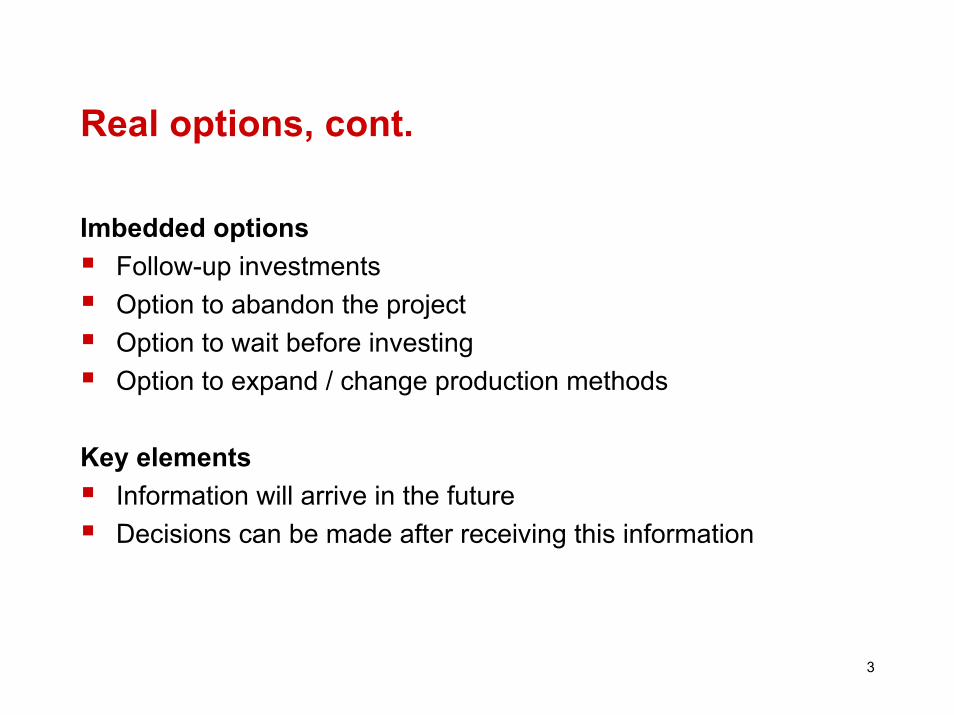
Real options, cont.

Imbedded optionsFollow-up investmentsOption to abandon the projectOption to wait before investingOption to expand / change production methods

Key elementsInformation will arrive in the futureDecisions can be made after receiving this information

3

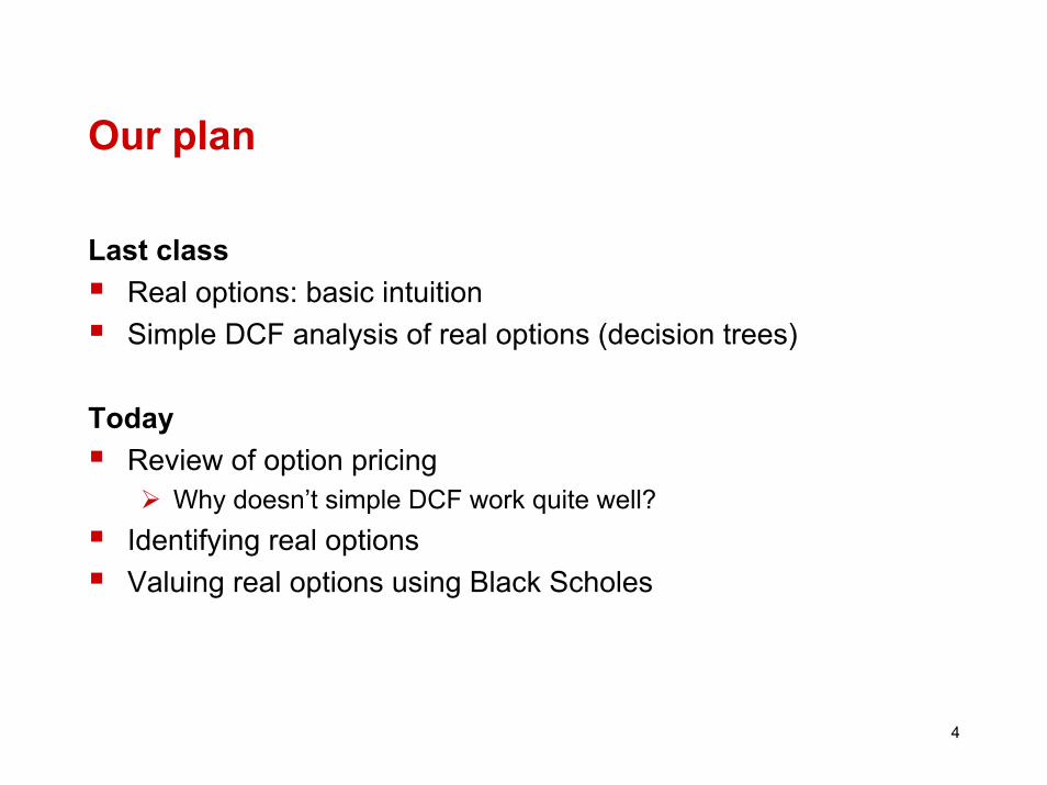
Our plan

Last classReal options: basic intuitionSimple DCF analysis of real options (decision trees)

TodayReview of option pricing

Why doesn’t simple DCF work quite well?Identifying real optionsValuing real options using Black Scholes

4

1. Review of option pricing

Real options and financial options

Option Definition The right (but not the obligation), to buy/sell an underlying asset at a price (the exercise price) that may be different than the market price.

Financial Options Vs. Real Options:

Options on stocks,

stock indices, foreign exchange,gold, silver, wheat, etc.

Not traded on exchange.

Underlying asset is something other than a security

6

Pricing of a call option on stockStock Option (X = 110)

S1 = 12010

S0 = 100?

S1 = 800

The challenge is to find the value of the call option today

7

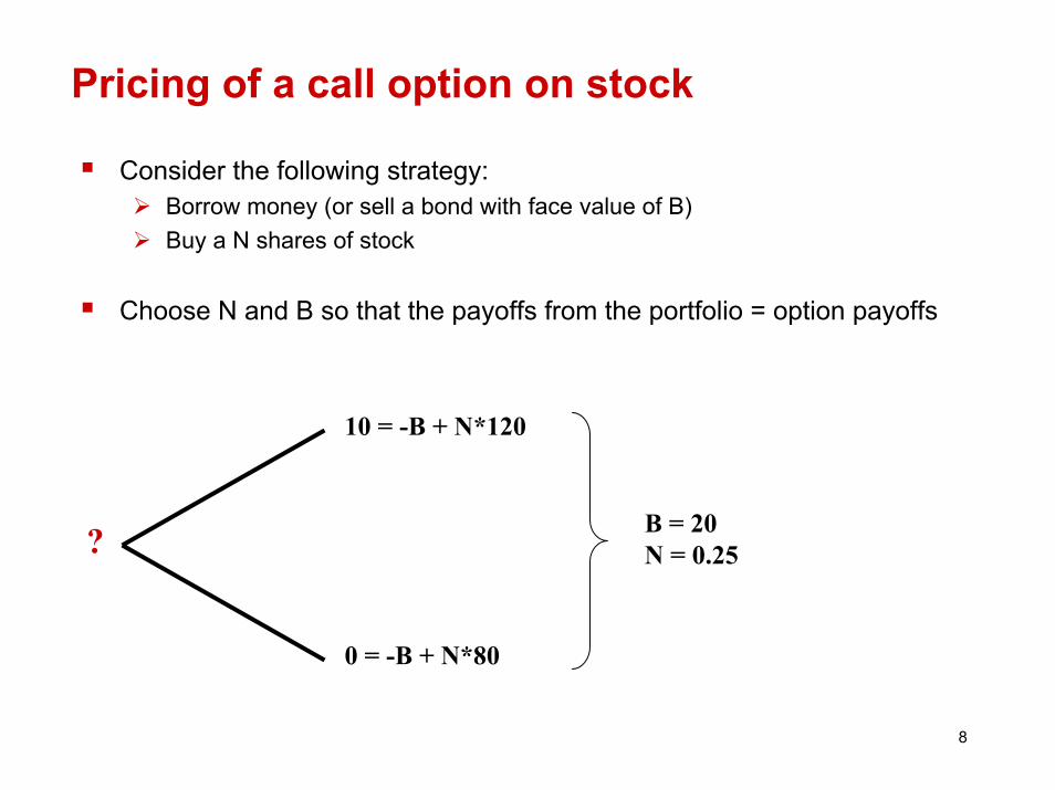
Pricing of a call option on stock

Consider the following strategy:Borrow money (or sell a bond with face value of B)Buy a N shares of stock

Choose N and B so that the payoffs from the portfolio = option payoffs

10 = -B + N*120

B = 20N = 0.25?

0 = -B + N*80

8

Pricing of a call option on stock

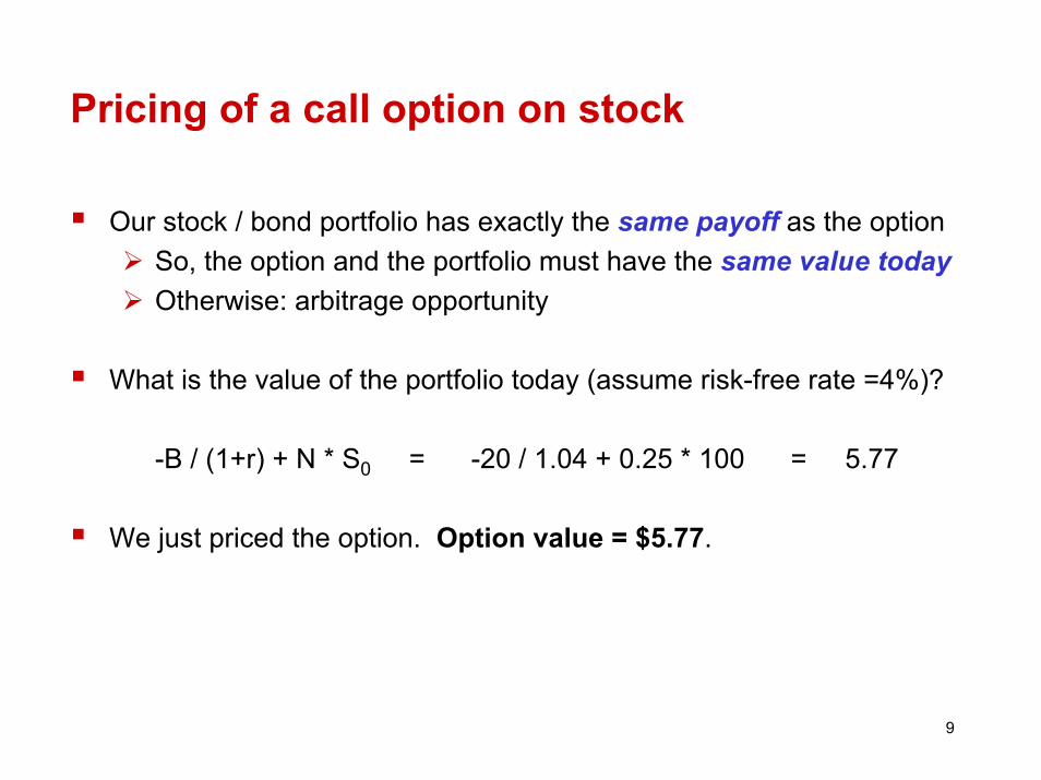
Our stock / bond portfolio has exactly the same payoff as the optionSo, the option and the portfolio must have the same value todayOtherwise: arbitrage opportunity

What is the value of the portfolio today (assume risk-free rate =4%)?

-B / (1+r) + N * S0 = -20 / 1.04 + 0.25 * 100 = 5.77

We just priced the option. Option value = $5.77.

9

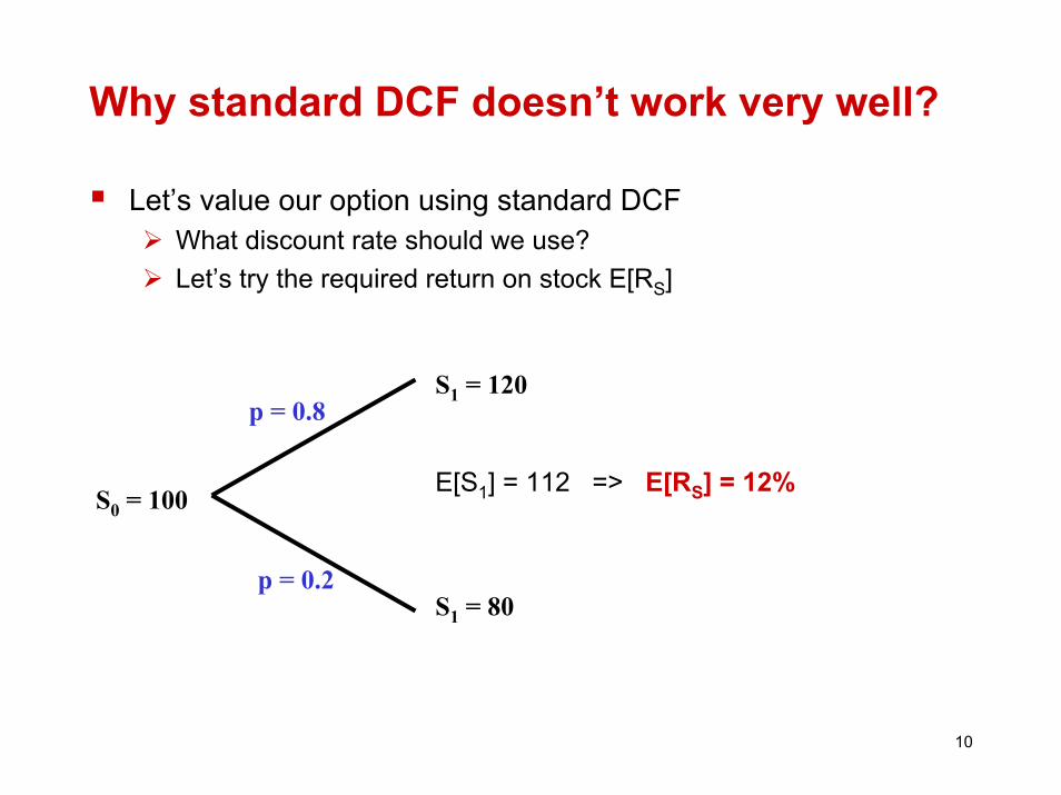
Why standard DCF doesn’t work very well?

Let’s value our option using standard DCFWhat discount rate should we use?Let’s try the required return on stock E[RS]

S1 = 120p = 0.8

E[S1] = 112 => E[RS] = 12%S0 = 100

p = 0.2S1 = 80

10

Why standard DCF doesn’t work very well?

DCF gives us the following option value:

(0.8 * 10 + 0.2 * 0) / 1.12 = $7.14 ≠ $5.77

What’s wrong?

Discount rate of 12% is too low => the option is riskier than the underlying stock

Why?

Option is a levered position in a stock. Recall the analogy with firms’ financial leverage: Higher financial leverage => higher equity betas and equity returns.

11

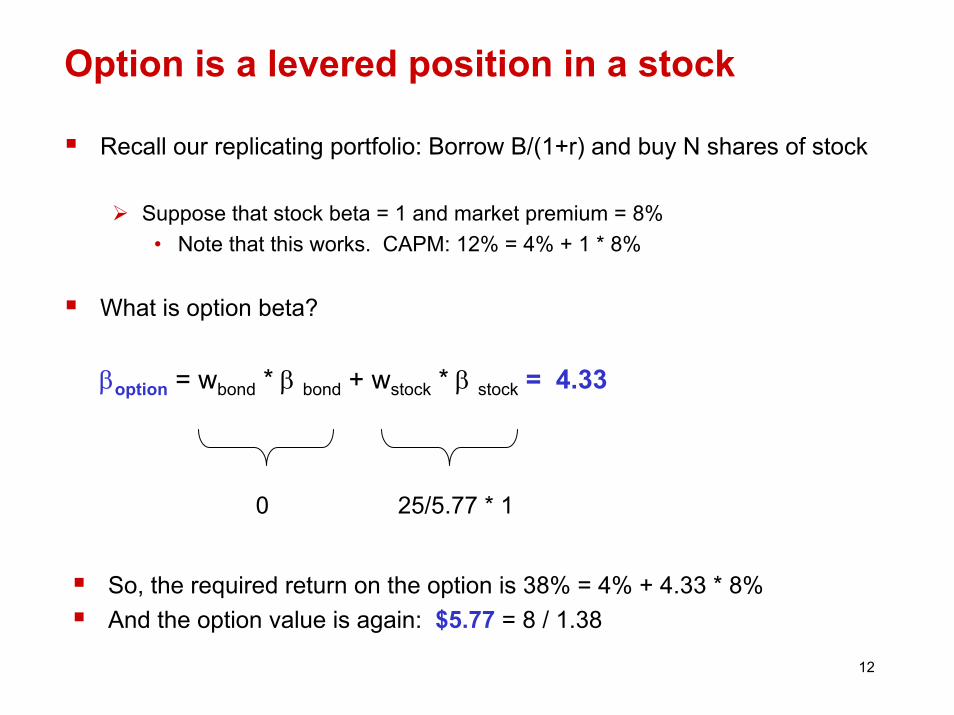
Option is a levered position in a stock

Recall our replicating portfolio: Borrow B/(1+r) and buy N shares of stock

Suppose that stock beta = 1 and market premium = 8%• Note that this works. CAPM: 12% = 4% + 1 * 8%

What is option beta?

βoption = wbond * β bond + wstock * β stock = 4.33

0 25/5.77 * 1

So, the required return on the option is 38% = 4% + 4.33 * 8%And the option value is again: $5.77 = 8 / 1.38

12

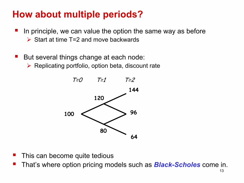
How about multiple periods?In principle, we can value the option the same way as before

Start at time T=2 and move backwards

But several things change at each node:Replicating portfolio, option beta, discount rate

T=0 T=1 T=2

120

80

144

96100

64

13

This can become quite tediousThat’s where option pricing models such as Black-Scholes come in.

Options valuation techniques

“Dynamic” DCF (decision trees)Recall our “Handheld PC” and “Copper Mine” examplesApproximation used for real-options problemsNot an exact answer because of problems with discounting

Binomial modelSimilar to our one-period example from today’s classRequires more computations than Black-ScholesCan be useful when Black-Scholes doesn’t work very well

Black-ScholesWe will focus on this model from now on

14

Black-Scholes formula

Black-Scholes formula relies on the same valuation principles as the binomial model (replicating portfolios, no arbitrage)

Option value = N(d1) * S – N(d2) * PV(X)

Note the similarities to the one-period binomial model

Option value = N * S – PV(B)

N(d): Cumulative normal probability density functiond1 = ln[S/PV(X)] / (σT1/2) + (σT1/2)/2 d2 = d1 - (σT1/2)S = Current stock price X = Exercise pricer = Risk-free interest rate T = Time to maturity in years.σ = Standard deviation of stock return

15

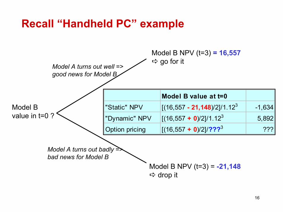
Recall “Handheld PC” example

Model B NPV (t=3) = 16,557go for it

Model A turns out well => good news for Model B

Model A turns out badly => bad news for Model B

Model B value in t=0 ?

Model B value at t=0"Static" NPV [(16,557 - 21,148)/2]/1.123 -1,634"Dynamic" NPV [(16,557 + 0)/2]/1.123 5,892Option pricing [(16,557 + 0)/2]/???3 ???

Model B NPV (t=3) = -21,148drop it

16

2. Identifying Real Options

Two Issues with Real Options

IdentificationAre there real options imbedded in this project?What type of options?

ValuationHow do we value options?How do we value different types of options?Can’t we just use NPV?

18

Identifying Real Options

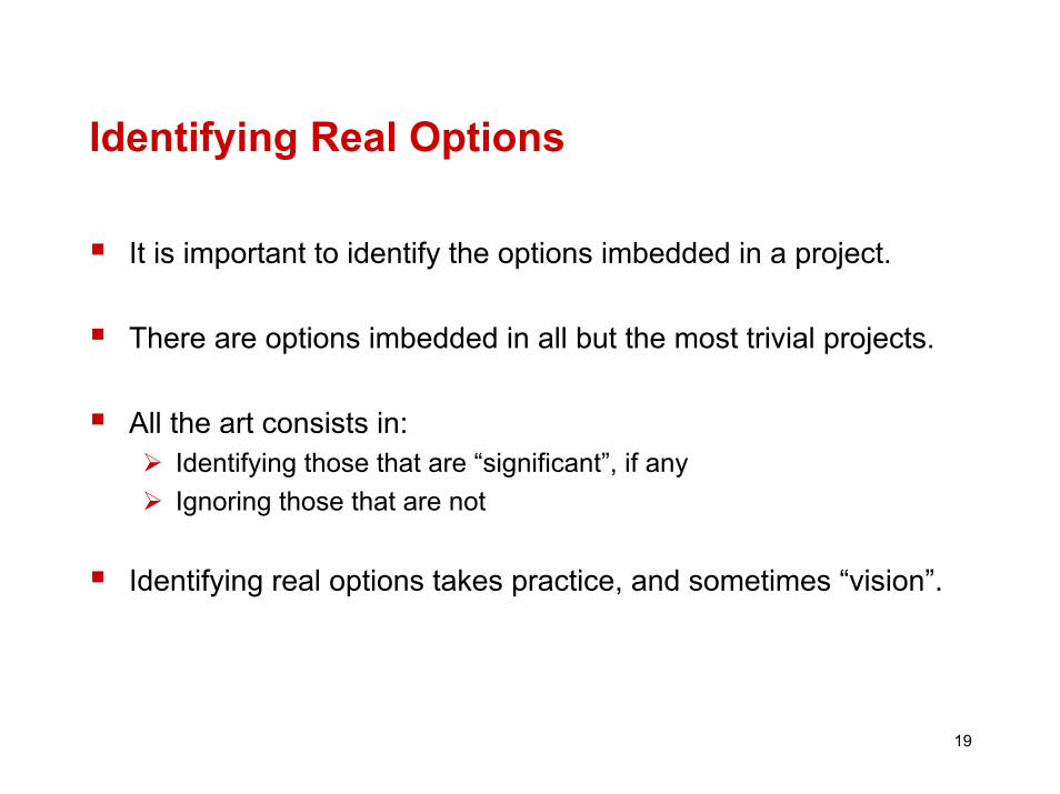
It is important to identify the options imbedded in a project.

There are options imbedded in all but the most trivial projects.

All the art consists in:Identifying those that are “significant”, if anyIgnoring those that are not

Identifying real options takes practice, and sometimes “vision”.

19

Identifying Real Options (cont.)

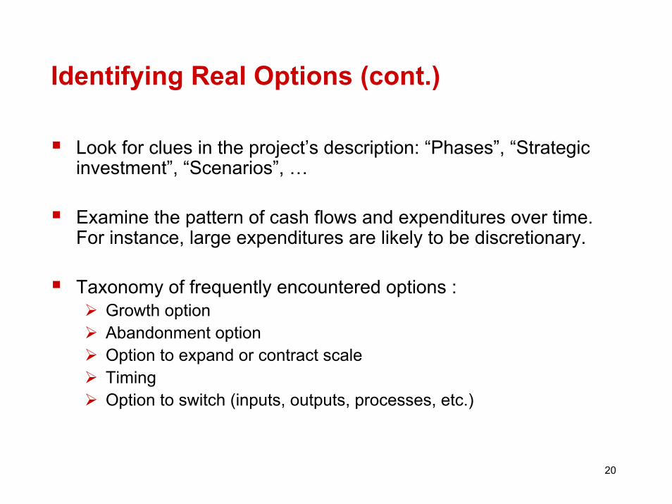
Look for clues in the project’s description: “Phases”, “Strategic investment”, “Scenarios”, …

Examine the pattern of cash flows and expenditures over time. For instance, large expenditures are likely to be discretionary.

Taxonomy of frequently encountered options :Growth optionAbandonment optionOption to expand or contract scaleTimingOption to switch (inputs, outputs, processes, etc.)

20

Is There An Option?

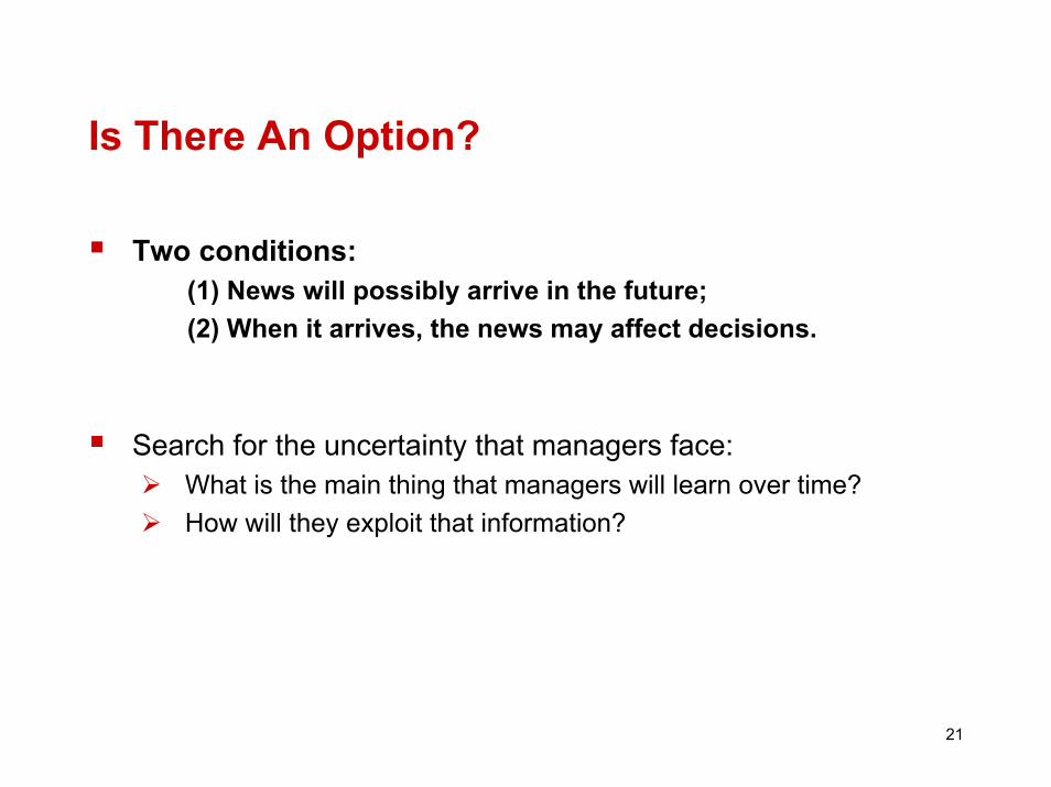
Two conditions:(1) News will possibly arrive in the future;(2) When it arrives, the news may affect decisions.

Search for the uncertainty that managers face:What is the main thing that managers will learn over time?How will they exploit that information?

21

Oz Toys’ Expansion Program

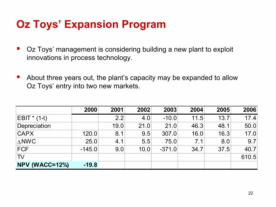
Oz Toys’ management is considering building a new plant to exploit innovations in process technology.

About three years out, the plant’s capacity may be expanded to allow Oz Toys’ entry into two new markets.

2000 2001 2002 2003 2004 2005 2006EBIT * (1-t) 2.2 4.0 -10.0 11.5 13.7 17.4Depreciation 19.0 21.0 21.0 46.3 48.1 50.0CAPX 120.0 8.1 9.5 307.0 16.0 16.3 17.0∆NWC 25.0 4.1 5.5 75.0 7.1 8.0 9.7FCF -145.0 9.0 10.0 -371.0 34.7 37.5 40.7TV 610.5NPV (WACC=12%) -19.8

22

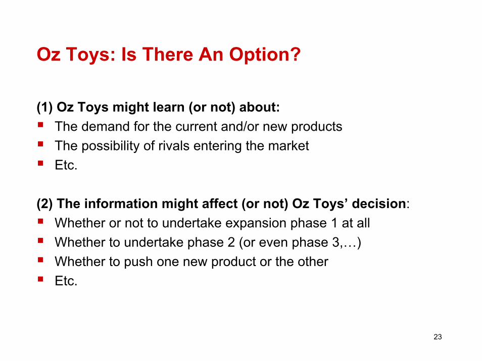
Oz Toys: Is There An Option?

(1) Oz Toys might learn (or not) about:The demand for the current and/or new productsThe possibility of rivals entering the marketEtc.

(2) The information might affect (or not) Oz Toys’ decision:Whether or not to undertake expansion phase 1 at allWhether to undertake phase 2 (or even phase 3,…)Whether to push one new product or the otherEtc.

23

Oz Toys: Identifying the Option

Project’s description refers to two distinct phases

Phase 1: New plantPhase 2: Expansion

Spike in spending: Probably discretionary

Possibly, an imbedded growth option

FCF

-400

-300

-200

-100

0

100

2000 2001 2002 2003 2004 2005 2006

FCF

0

50

100

150

200

250

300

350

2000 2001 2002 2003 2004 2005 2006

CAPX Change in NWC

24

Practical Issue #1: Simplifications

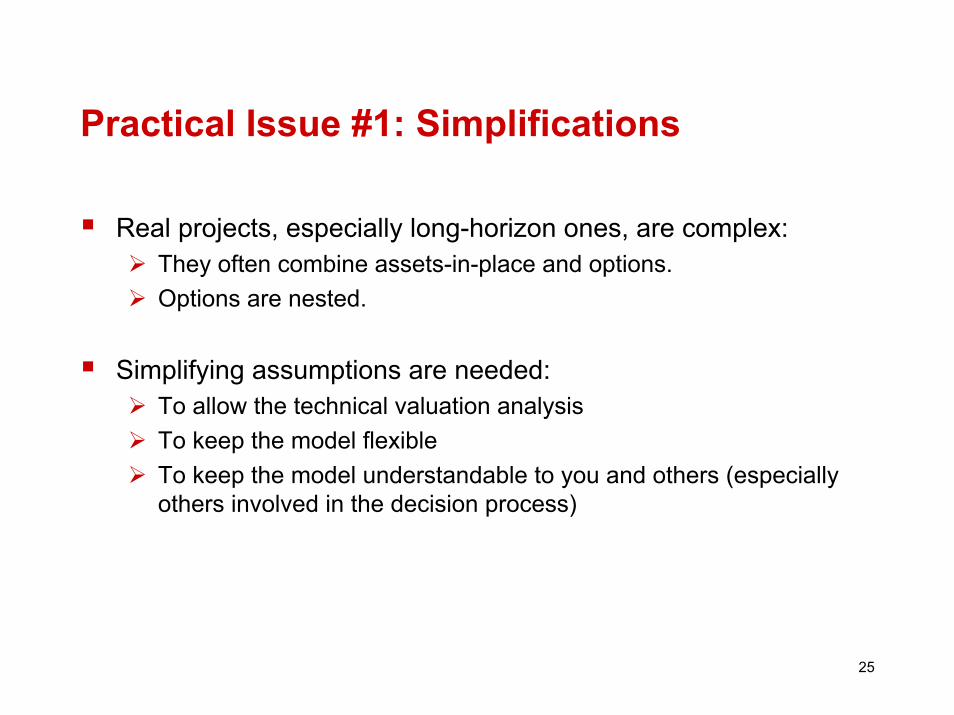
Real projects, especially long-horizon ones, are complex:They often combine assets-in-place and options.Options are nested.

Simplifying assumptions are needed:To allow the technical valuation analysisTo keep the model flexibleTo keep the model understandable to you and others (especially others involved in the decision process)

25

Practical Issue #1: Simplifications (cont.)

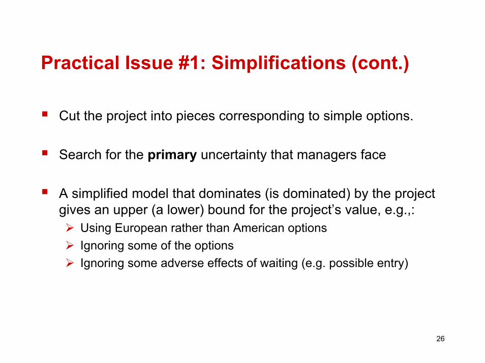
Cut the project into pieces corresponding to simple options.

Search for the primary uncertainty that managers face

A simplified model that dominates (is dominated) by the project gives an upper (a lower) bound for the project’s value, e.g.,:

Using European rather than American optionsIgnoring some of the optionsIgnoring some adverse effects of waiting (e.g. possible entry)

26

Oz Toys: Simplifications

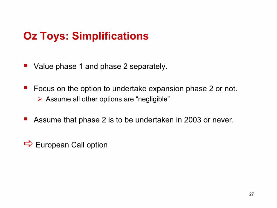
Value phase 1 and phase 2 separately.

Focus on the option to undertake expansion phase 2 or not.Assume all other options are “negligible”

Assume that phase 2 is to be undertaken in 2003 or never.

European Call option

27

3. Valuing Real Options

Valuation of Real Options

Tools developed to value financial options can be useful to estimate the value of real options embedded in some projects.

Real options are much more complex than financial options.

The aim here is to develop numerical techniques to “keep score” and assist in the decision-making process, not provide a recipe to replace sound business sense.

29

Options vs. DCF

The real options approach is often presented as an alternative to DCF.

In fact, the real options’ approach does not contradict DCF: It is a particular form that DCF takes for certain types of investments.

Recall that option valuation techniques were developed because discounting is difficult

I.e., due to the option, one should not use the same discount rate (e.g. WACC) for all cash flows.

30

Options vs. DCF (cont.)

DCF method:“expected scenario” of cash flows,discount the expected cash flows

This is perfectly fine as long as:expected cash flows are estimated properlydiscount rates are estimated properly

Precisely, it is complex to account for options in estimating:expected cash flowdiscount rates

31

Start with the “static” DCF Analysis

Begin by valuing the project as if there was no option involved

Pretend that the investment decision must be taken immediately.

This benchmark constitute a lower bound for the project’s value.

NPV<0 does not mean that you will never want to undertake the investment.

NPV>0 does not mean that you should go ahead immediately with the invest (nor that you will definitely invest in the future).

32

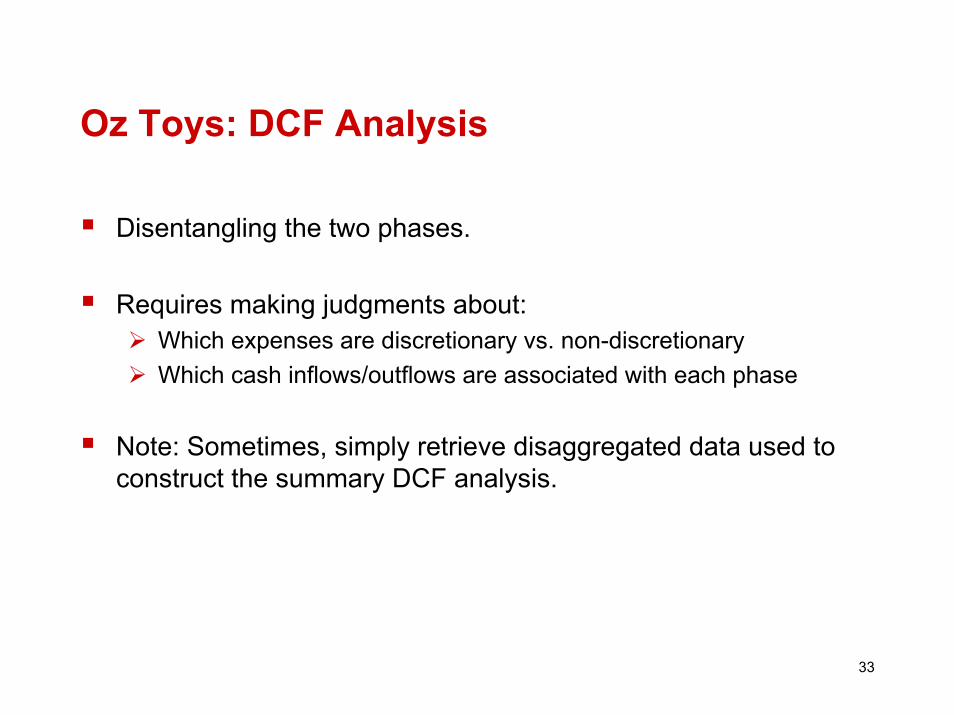
Oz Toys: DCF Analysis

Disentangling the two phases.

Requires making judgments about:Which expenses are discretionary vs. non-discretionaryWhich cash inflows/outflows are associated with each phase

Note: Sometimes, simply retrieve disaggregated data used to construct the summary DCF analysis.

33

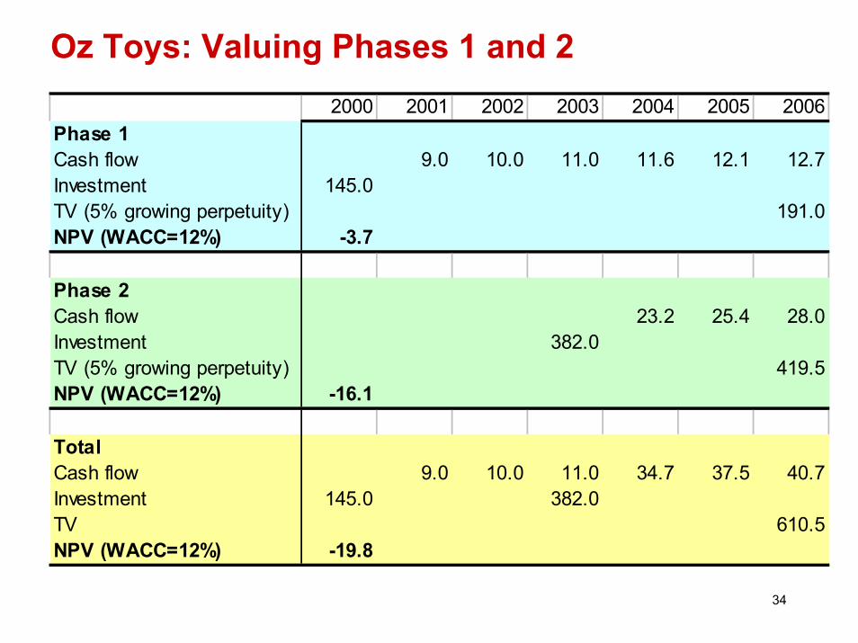
Oz Toys: Valuing Phases 1 and 22000 2001 2002 2003 2004 2005 2006

Phase 1Cash flow 9.0 10.0 11.0 11.6 12.1 12.7Investment 145.0TV (5% growing perpetuity) 191.0NPV (WACC=12%) -3.7

Phase 2Cash flow 23.2 25.4 28.0Investment 382.0TV (5% growing perpetuity) 419.5NPV (WACC=12%) -16.1

TotalCash flow 9.0 10.0 11.0 34.7 37.5 40.7Investment 145.0 382.0TV 610.5NPV (WACC=12%) -19.8

34

Oz Toys: DCF Analysis (cont.)

Both phases have negative NPV

Phase 2’s NPV is probably largely overstated:Investment ($382M) is likely to be less risky than cash flows.Using the three-year risk-free rate of 5.5%

2000 2001 2002 2003 2004 2005 2006Phase 2Cash flow 23.2 25.4 28.0Investment 382.0TV (5% growing perpetuity) 419.5NPV (WACC=12%) -69.5

DCF Analysis of Phase 2 Discounting the Investment at 5.5%

35

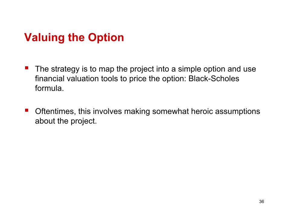
Valuing the Option

The strategy is to map the project into a simple option and use financial valuation tools to price the option: Black-Scholesformula.

Oftentimes, this involves making somewhat heroic assumptions about the project.

36

Mapping: Project Call Option

Project Call Option

Expenditure required to acquire the assets X Exercise price

Value of the operating assets to be acquired S Stock price (price of the

underlying asset)Length of time the decision may be deferred T Time to expiration

Riskiness of the operating assets σ2 Variance of stock return

Time value of money r Risk-free rate of return

37

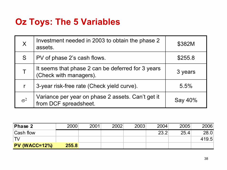
Oz Toys: The 5 Variables

X Investment needed in 2003 to obtain the phase 2 assets. $382M

S PV of phase 2’s cash flows. $255.8

T It seems that phase 2 can be deferred for 3 years (Check with managers). 3 years

r 3-year risk-free rate (Check yield curve). 5.5%

σ2 Variance per year on phase 2 assets. Can’t get it from DCF spreadsheet. Say 40%

Phase 2 2000 2001 2002 2003 2004 2005 2006Cash flow 23.2 25.4 28.0TV 419.5PV (WACC=12%) 255.8

38

Practical Issue #2: What Volatility?

Volatility (σ) cannot be looked up in a table or newspaper.Note: Even a rough estimate of σ can be useful, e.g., to decide whether to even bother considering the option value.

1. Take an informed guess:

Systematic and total risks are correlated: High β projects tend to have a higher σ.

The volatility of a diversified portfolio within that class of assets is a lower bound.

20-30% per year is not remarkably high for a single project.

39

Practical Issue #2: What Volatility? (cont.)

2. Data:

For some industries, historical data on investment returns.

Implied volatilities can be computed from quoted option prices for many traded stocks

Note: These data need adjustment because equity returns being levered, they are more volatile than the underlying assets.

40

Practical Issue #2: What Volatility? (cont.)

3. Simulation:

Step 1: Build a spread-sheet based (simplified) model of the project’s future cash flows

Model how CFs depend on specific items (e.g. commodity prices, interest and exchange rates, etc.)

Step 2: Use Monte Carlo simulation to simulate a probability distribution for the project’s returns and infer σ.

41

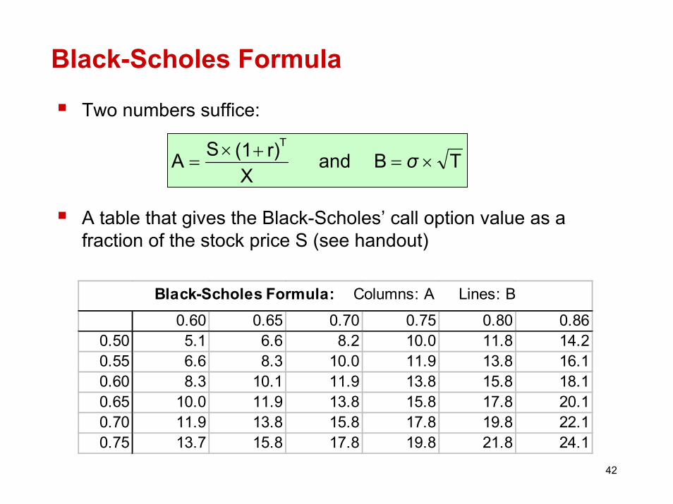
Black-Scholes Formula

Two numbers suffice:

A table that gives the Black-Scholes’ call option value as a fraction of the stock price S (see handout)

TB and X

r)(1SAT

×=+×= σ

0.60 0.65 0.70 0.75 0.80 0.860.50 5.1 6.6 8.2 10.0 11.8 14.20.55 6.6 8.3 10.0 11.9 13.8 16.10.60 8.3 10.1 11.9 13.8 15.8 18.10.65 10.0 11.9 13.8 15.8 17.8 20.10.70 11.9 13.8 15.8 17.8 19.8 22.10.75 13.7 15.8 17.8 19.8 21.8 24.1

Black-Scholes Formula: Columns: A Lines: B

42

Black-Scholes Formula (cont.)

The number A captures phase 2’s value if the decision could not be delayed (but investment and cash flows still began in 2003).

Indeed, in that case, A would be phase 2’s Profitability Index:

The option’s value increases with A (as shown in the table).

0NPV 1 Aand

A

r)(1XS

PV(inv.) PV(cf)PI

T

>⇔>

=

⎟⎟⎠

⎞⎜⎜⎝

⎛

+

==

43

Black-Scholes Formula (cont.)

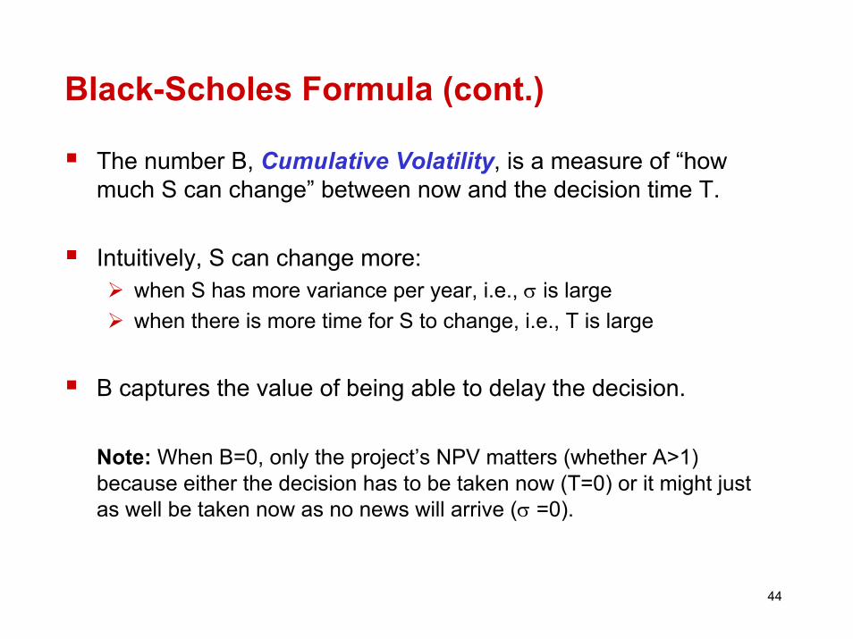
The number B, Cumulative Volatility, is a measure of “how much S can change” between now and the decision time T.

Intuitively, S can change more:when S has more variance per year, i.e., σ is largewhen there is more time for S to change, i.e., T is large

B captures the value of being able to delay the decision.

Note: When B=0, only the project’s NPV matters (whether A>1) because either the decision has to be taken now (T=0) or it might just as well be taken now as no news will arrive (σ =0).

44

Oz Toys: Valuation

693.034.0TB and 786.0382

)055.1(8.255X

)r1(SA3T

=⋅=⋅σ==⋅

=+⋅

=

0.60 0.65 0.70 0.75 0.80 0.860.50 5.1 6.6 8.2 10.0 11.8 14.20.55 6.6 8.3 10.0 11.9 13.8 16.10.60 8.3 10.1 11.9 13.8 15.8 18.10.65 10.0 11.9 13.8 15.8 17.8 20.10.70 11.9 13.8 15.8 17.8 19.8 22.10.75 13.7 15.8 17.8 19.8 21.8 24.1

Black-Scholes Formula: Columns: A Lines: B

The value of phase 2 is (roughly): V2 = 19% * S = .19 * 255.8 = $48.6M

The value of the expansion program is: V1 + V2 = -3.7 + 48.6 = $44.9M

45

Practical Issue #3: Checking the Model

Formal option pricing models make distributional assumptions.

Approach 1: Try and find a model that is close to your idea of the real distribution (More and more are available).

Approach 2: Determine the direction in which the model biases the analysis, and use the result as an upper or lower bound.

Approach 3: Simulate the project as a complex decision tree and solve by brute force with a computer (i.e., not analytically).

46

Practical Issue #4: Interpretation

Since we use simplified models, the results need to be taken with a grain of salt and interpreted.

Put complexity back into the model with:Sensitivity analysisConditioning and qualifying of inferences

Iterative process.

Helps you identify the main levers of the project, and where youneed to gather more data or fine tune the analysis.

47