No Slide Titlel2r.cs.uiuc.edu/Teaching/CS446-17/Lectures/08-LecSVM.pdf · KDD Cup 2013:...

SVMs CS446 Spring ’17

Administration

HW4 is due on Saturday 3/11 No extensions!

We will release solutions on Saturday night, so there is enough time for you to look at it before the exam.

Midterm exam on Thursday 3/16 Closed books; in class; ~4 questions

All the material covered before the midterm

Practice midterms will be released over the weekend

Next Tuesday 3/14: Review

Additional Office hours: 8:30-9:30 Tomorrow (Wednesday)

1

Questions?

http://l2r.cs.illinois.edu/~danr/Teaching/CS446-17/Hw/hw4/hw4.pdf


Projects

Projects proposals are due on March 10 2017Within a week we will give you an approval to continue with your project along with comments and/or a request to modify/augment/do a different project. There will also be a mechanism for peer comments.

We encourage team projects – a team can be up to 3 people.

Please start thinking and working on the project now.Your proposal is limited to 1-2 pages, but needs to include referencesand, ideally, some of the ideas you have developed in the direction of the project (maybe even some preliminary results).Any project that has a significant Machine Learning component is good. You can do experimental work, theoretical work, a combination of both or a critical survey of results in some specialized topic. The work has to include some reading. Even if you do not do a survey, you must read (at least) two related papers or book chapters and relate your work to it. Originality is not mandatory but is encouraged. Try to make it interesting!

2

Scale of Projects: 25% of the grade


Examples

Fake News Challenge :- http://www.fakenewschallenge.org/

KDD Cup 2013: "Author-Paper Identification": given an author and a small set of papers, we are asked to

identify which papers are really written by the author.

https://www.kaggle.com/c/kdd-cup-2013-author-paper-identification-challenge

“Author Profiling”: given a set of document, profile the author: identification, gender, native language, ….

Caption Control: Is it gibberish? Spam? High quality text? Adapt an NLP program to a new domain

Work on making learned hypothesis (e.g., linear threshold functions, NN) more comprehensible Explain the prediction

Develop a (multi-modal) People Identifier Compare Regularization methods: e.g., Winnow vs. L1 RegularizationLarge scale clustering of documents + name the clusterDeep Networks: convert a state of the art NLP program to a deep network, efficient, architecture. Try to prove something

3

https://urldefense.proofpoint.com/v2/url?u=http-3A__www.fakenewschallenge.org_&d=DwMFAg&c=8hUWFZcy2Z-Za5rBPlktOQ&r=4vDcLc57cD397QaRxR0yOZWu-Gg0KM96wcN0Jci1clw&m=9N8h2Wns4dC-DEEP0V-pObXSyU3Zl4uG51ahA1VuScE&s=LWaUdjsTWw0Y1xGXjw1TCh2YdQAXX-PgPe8hD0Yup7A&e=

https://www.kaggle.com/c/kdd-cup-2013-author-paper-identification-challenge


COLT approach to explaining Learning

4

No Distributional Assumption

Training Distribution is the same as the Test Distribution

Generalization bounds depend

on this view and affects

model selection.

ErrD(h) < ErrTR(h) +

P(VC(H), log(1/±),1/m)

This is also called the

“Structural Risk Minimization” principle.


COLT approach to explaining Learning

5

No Distributional Assumption

Training Distribution is the same as the Test Distribution

Generalization bounds depend on this view and affect model selection.

ErrD(h) < ErrTR(h) + P(VC(H), log(1/±),1/m)

As presented, the VC dimension is a combinatorial parameter that is associated with a class of functions.

We know that the class of linear functions has a lower VC dimension than the class of quadratic functions.

But, this notion can be refined to depend on a given data set, and this way directly affect the hypothesis chosen for a given data set.


Data Dependent VC dimension

So far we discussed VC dimension in the context of a fixed class of functions.

We can also parameterize the class of functions in interesting ways.

Consider the class of linear functions, parameterized by their margin. Note that this is a data dependent notion.

6


Linear Classification

Let X = R2, Y = {+1, -1}

Which of these classifiers would be likely to generalize better?

7

h1 h2


VC and Linear Classification

Recall the VC based generalization bound:

Err(h) · errTR(h) + Poly{VC(H), 1/m, log(1/±)}

Here we get the same bound for both classifier:

ErrTR (h1) = ErrTR (h2)= 0

h1, h2 2 Hlin(2), VC(Hlin(2)) = 3

How, then, can we explain our intuition that h2 should give better generalization than h1?

8


Linear Classification

Although both classifiers separate the data, the distance with which the separation is achieved is different:

9

h1 h2


Concept of Margin

The margin °i of a point xi 2 Rn with respect to a linear classifier h(x) = sign(w ¢ x +b) is defined as the distance of xi from the hyperplane w ¢ x + b = 0:

°i = |(w ¢ xi +b)/||w|||

The margin of a set of points {x1,…xm} with respect to a hyperplane w, is defined as the margin of the point closest to the hyperplane:

° = mini°i = mini|(w ¢ xi +b)/||w|||

10


VC and Linear Classification

If H° is the space of all linear classifiers in <n that separate the training data with margin at least °, then:

VC(H°) · min(R2/°2, n) +1,

Where R is the radius of the smallest sphere (in <n) that contains the data.

Thus, for such classifiers, we have a bound of the form:

Err(h) · errTR(h) + { (O(R2/°2 ) + log(4/±))/m }1/2

11


Data Dependent VC dimension

Namely, when we consider the class H° of linear hypotheses that separate a given data set with a margin °,

We see that

Large Margin ° Small VC dimension of H°

Consequently, our goal could be to find a separating hyperplane w that maximizes the margin of the set S of examples.

A second observation that drives an algorithmic approach is that:

Small ||w|| Large Margin

This leads to an algorithm: from among all those w’s that agree with the data, find the one with the minimal size ||w||

12


Maximal Margin

13

This discussion motivates the notion of a maximal margin.The maximal margin of a data set S is define as:

°(S) = max||w||=1 min(x,y) 2 S |y wT x|1. For a given w: Find the

closest point. 2. Then, find the one the gives the maximal margin value across all w’s (of size 1). Note: the selection of the point is in the min and therefore the max does not change if we scale w, so it’s okay to only deal with normalized w’s.

(PS0, PS1): The distance between a point x and the hyperplane defined by (w; b) is: |wT x + b|/||w||

How does it help us to derive these h’s?

argmax||w||=1 min(x,y) 2 S |y wT x|


Margin and VC dimension

14

Theorem (Vapnik): If H° is the space of all linear classifiers in <n that separate the training data with margin at least °, then

VC(H°) · R2/°2

where R is the radius of the smallest sphere (in <n) that contains the data.

This is the first observation that will lead to an algorithmic approach.

The second observation is that:

Small ||w|| Large Margin

Consequently: the algorithm will be: from among all thosew’s that agree with the data, find the one with the minimal size ||w||

Believe

We’ll Prove


Hard SVM

We want to choose the hyperplane that achieves the largest margin. That is, given a data set S, find:

w* = argmax||w||=1 min(x,y) 2 S |y wT x|

How to find this w*?

Claim: Define w0 to be the solution of the optimization problem:

w0 = argmin {||w||2 : 8 (x,y) 2 S, y wT x ¸ 1 }.

Then:

w 0/||w0|| = argmax||w||=1 min(x,y) 2 S y wT x

That is, the normalization of w0 corresponds to the largest margin separating hyperplane.

15

1. For a given w: Find the closest point. 2. Among all w’s (of size 1) find the wthe maximizes this point’s margin. Note: the selection of the point in the minand therefore the largest margin w do not change if we scale w, so it’s okay to only deal with normalized w’s.

1. Consider the set of “good” w’s (those that separate the data).2. Among those, choose the one with minimal size.


Hard SVM (2)

Claim: Define w0 to be the solution of the optimization problem:

w0 = argmin {||w||2 : 8 (x,y) 2 S, y wT x ¸ 1 } (**)

Then:

w 0/||w0|| = argmax||w||=1 min(x,y) 2 S y wT x

That is, the normalization of w0 corresponds to the largest margin separating hyperplane.

Proof: Define w’ = w 0/||w0|| and let w* be the largest-margin separating hyperplane of size 1. We need to show that w’ = w*.

Note first that w*/°(S) satisfies the constraints in (**);

therefore: ||w0|| · ||w*/°(S)|| = 1/°(S) .

Consequently:

8 (x,y) 2 S y w’T x = 1/||w0|| y w0T x ¸ 1/||w0|| ¸ °(S)

But since ||w’|| = 1 this implies that w’ corresponds to the largest margin, that is w’= w*

16

Def. of w’ Def. of w0Prev. ineq.

Def. of w0


Margin of a Separating Hyperplane

17

A separating hyperplane: wT x+b = 0Distance between wT x+b = +1 and -1 is 2 / ||w||

What we did: 1. Consider all possible w

with different angles2. Scale w such that the

constraints are tight3. Pick the one with largest

margin/minimal size

wT x+b = 0

wT x+b = -1

wT xi +b¸ 1 if yi = 1wT xi +b· -1 if yi = -1

=> 𝑦𝑖(𝑤𝑇𝑥𝑖 + 𝑏) ≥ 1

Assumption: data is linearly separableLet (x0 ,y0) be a point on wTx+b = 1

Then its distance to the separating plane wT x+b = 0 is: |wT (x0 ,y0) +b|/||w||= 1/||w||

SVMs CS446 Spring ’17 18


Hard SVM Optimization

We have shown that the sought after weight vector w is the solution of the following optimization problem:

SVM Optimization: (***)

Minimize: ½ ||w||2

Subject to: 8 (x,y) 2 S: y wT x ¸ 1

This is a quadratic optimization problem in (n+1) variables, with |S|=m inequality constraints.

It has a unique solution.

19


Maximal Margin

20

The margin of a linear separatorwT x+b = 0

is 2 / ||w||

max 2 / ||w|| = min ||w||

= min ½ wTw

min𝑤,𝑏

1

2𝑤𝑇𝑤

s.t yi(wTxi + 𝑏) ≥ 1, ∀ 𝑥𝑖 , 𝑦𝑖 ∈ 𝑆


Support Vector Machines

The name “Support Vector Machine” stems from the fact that w* is supported by (i.e. is the linear span of) the examples that are exactly at a distance 1/||w*|| from the separating hyperplane. These vectors are therefore called support vectors.

Theorem: Let w* be the minimizer of

the SVM optimization problem (***)

for S = {(xi, yi)}. Let I= {i: w*Tx = 1}.

Then there exists coefficients ®i >0 such that:

w* = i 2 I ®i yi xi

21

This representation should ring a bell…


)(x yr w w,y)f(x If (k)(k)(k)(k) t

t(x))sgn(w))t(xwsgn( f(x) :function DecisionR w:Hypothesis

Rt(x) t(x),x : mapping Nonlinear ;{0,1} x :Examples

i

n'

1i i

n'

n'n

;

If n’ is large, we cannot represent w explicitly. However, the weight vector wcan be written as a linear combination of examples:

Where 𝛼𝑗 is the number of mistakes made on 𝑥(𝑗)

Then we can compute f(x) based on {𝑥(𝑗)} and 𝜶

(recap) Kernel Perceptron

)),(

m

1j

(j)(j)

j

m

1j

(j)(j)

j xxyrsgn(t(x)))t(xyrsgn( t(x))sgn(w f(x) K

m

1j

(j)(j)

j t(xyr w )


In the training phase, we initialize 𝜶 to be an all-zeros vector.For training sample (𝑥(𝑘), 𝑦(𝑘)), instead of using the original Perceptron update rule in the 𝑅𝑛′ space

we maintain 𝜶 by

based on the relationship between w and 𝜶 :

23

)(x yr w w,y)f(x If (k)(k)(k)(k) t

t(x))sgn(w f(x) :function DecisionR w:Hypothesis

Rt(x) t(x),x : mapping Nonlinear ;{0,1} x :Examples

n'

n'n

;

(recap) Kernel Perceptron

m

1j

(j)(j)

j t(xyr w )

1)),(

kk

(k)m

1j

(k)(j)(j)

j

(k) then yxxyrsgn( )f(x if K


Duality

This, and other properties of Support Vector Machines are shown by moving to the dual problem.

Theorem: Let w* be the minimizer of

the SVM optimization problem (***)

for S = {(xi, yi)}.

Let I= {i: yi (w*Txi +b)= 1}.

Then there exists coefficients ®i >0

such that:

w* = i 2 I ®i yi xi

24

08-LecSvm-dual.pdf


Footnote about the threshold

25

Similar to Perceptron, we can augment vectors to handle the bias term

ҧ𝑥 ⇐ 𝑥 , 1 ; ഥ𝑤 ⇐ 𝑤 , 𝑏 so that ഥ𝑤𝑇 ҧ𝑥 = 𝑤𝑇𝑥 + 𝑏

Then consider the following formulation

minഥ𝑤

1

2ഥ𝑤𝑇ഥ𝑤 s.t yiഥ𝑤

T ҧ𝑥i ≥ 1, ∀ 𝑥𝑖 , 𝑦𝑖 ∈ S

However, this formulation is slightly different from (***), because it is equivalent to

min𝑤,𝑏

1

2𝑤𝑇𝑤 +

1

2𝑏2 s.t yi(𝑤

Txi + 𝑏) ≥ 1, ∀ 𝑥𝑖 , 𝑦𝑖 ∈ S

The bias term is included in the regularization. This usually doesn’t matter

For simplicity, we ignore the bias term


Key Issues

26

Computational Issues Training of an SVM used to be is very time consuming – solving

quadratic program.

Modern methods are based on Stochastic Gradient Descent and Coordinate Descent.

Is it really optimal? Is the objective function we are optimizing the “right” one?


Real Data

27

17,000 dimensional context sensitive spelling

Histogram of distance of points from the hyperplaneIn practice, even in the separable case, we may not want to depend on the points closest to the hyperplane but rather on the distribution of the distance. If only a few are close, maybe we can dismiss them.

This applies both to generalizationbounds and to the algorithm.


Soft SVM

Notice that the relaxation of the constraint: yiw

Txi ≥ 1

Can be done by introducing a slack variable 𝜉𝑖 (per example) and requiring:

yiwTxi ≥ 1 − 𝜉𝑖 ; 𝜉𝑖 ≥ 0

Now, we want to solve:

28

min𝑤,𝜉𝑖

1

2𝑤𝑇𝑤 + 𝐶 σ𝑖 𝜉𝑖

s.t yiwTxi ≥ 1 − 𝜉𝑖 ; 𝜉𝑖 ≥ 0 ∀𝑖

A large value of C means that misclassifications are bad - resulting in

smaller margins and less training error (but more expected true error). A small C results in more training error, hopefully

better true error.


Soft SVM (2)

Now, we want to solve:

Which can be written as:

min𝑤

1

2𝑤𝑇𝑤 + 𝐶

𝑖

max(0, 1 − 𝑦𝑖𝑤𝑇𝑥𝑖) .

What is the interpretation of this?

29

min𝑤,𝜉𝑖

1


s.t yiwTxi ≥ 1 − 𝜉𝑖 ; 𝜉𝑖 ≥ 0 ∀𝑖

In optimum, ξi = max(0, 1 − yiwTxi)

min𝑤,𝜉𝑖

1


s.t 𝜉𝑖 ≥ 1 − yiwTxi; 𝜉𝑖≥ 0 ∀𝑖


Soft SVM (3)

The hard SVM formulation assumes linearly separable data.

A natural relaxation: maximize the margin while minimizing the # of examples that violate the margin (separability) constraints.

However, this leads to non-convex problem that is hard to solve.

Instead, move to a surrogate loss function that is convex.

SVM relies on the hinge loss function (note that the dual formulation can give some intuition for that too).

Minw ½ ||w||2 + C (x,y) 2 S max(0, 1 – y wTx)

where the parameter C controls the tradeoff between large margin (small ||w||) and small hinge-loss.

30


SVM Objective Function

31

The problem we solved is:

Min ½ ||w||2 + c »i

Where »i > 0 is called a slack variable, and is defined by:

» i = max(0, 1 – yi wtxi)

Equivalently, we can say that: yi wtxi ¸ 1 - »; »¸ 0

And this can be written as:

Min ½ ||w||2 + c »i

General Form of a learning algorithm: Minimize empirical loss, and Regularize (to avoid over fitting)

Theoretically motivated improvement over the original algorithm we’ve see at the beginning of the semester.

Can be replaced by other loss functionsCan be replaced by other regularization functions

Empirical lossRegularization term


Balance between regularization and empirical loss


Balance between regularization and empirical loss

33

(DEMO)

http://www.csie.ntu.edu.tw/~cjlin/libsvm/js-toy/example.html


Underfitting Overfitting

Model complexity

ExpectedError

Underfitting and Overfitting

34

Simple models: High bias and low variance

Variance

Bias

Complex models: High variance and low bias

Smaller C Larger C


What Do We Optimize?

35


What Do We Optimize(2)?

36

We get an unconstrained problem. We can use the gradient descent algorithm! However, it is quite slow.

Many other methods Iterative scaling; non-linear conjugate gradient; quasi-Newton

methods; truncated Newton methods; trust-region newton method.

All methods are iterative methods, that generate a sequence wk that converges to the optimal solution of the optimization problem above.

Currently: Limited memory BFGS is very popular


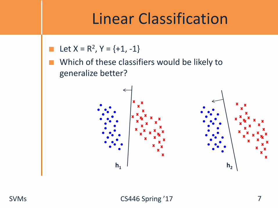
Optimization: How to Solve

37

1. Earlier methods used Quadratic Programming. Very slow.

2. The soft SVM problem is an unconstrained optimization problems. It is possible to use the gradient descent algorithm! Still, it is quite slow.

Many options within this category:

Iterative scaling; non-linear conjugate gradient; quasi-Newton methods; truncated Newton methods; trust-region newton method.

All methods are iterative methods, that generate a sequence wk that converges to the optimal solution of the optimization problem above.

Currently: Limited memory BFGS is very popular

3. 3rd generation algorithms are based on Stochastic Gradient Decent The runtime does not depend on n=#(examples); advantage when n is very large.

Stopping criteria is a problem: method tends to be too aggressive at the beginning and reaches a moderate accuracy quite fast, but it’s convergence becomes slow if we are interested in more accurate solutions.

4. Dual Coordinated Descent (& Stochastic Version)


SGD for SVM

38

Goal: min𝑤

𝑓 𝑤 ≡1

2𝑤𝑇𝑤 +

𝐶

𝑚σ𝑖max 0, 1 − 𝑦𝑖𝑤

𝑇𝑥𝑖 . m: data size

Compute sub-gradient of 𝑓 𝑤 :

𝛻𝑓 𝑤 = 𝑤 − 𝐶𝑦𝑖𝑥𝑖 if 1 − 𝑦𝑖𝑤𝑇𝑥𝑖 ≥ 0 ; otherwise 𝛻𝑓 𝑤 = 𝑤

1. Initialize 𝑤 = 0 ∈ 𝑅𝑛

2. For every example xi, yi ∈ 𝐷

If 𝑦𝑖𝑤𝑇𝑥𝑖 ≤ 1 update the weight vector to

𝑤 ← 1 − 𝛾 𝑤 + 𝛾𝐶𝑦𝑖𝑥𝑖 (𝛾 - learning rate)

Otherwise 𝑤 ← (1 − 𝛾)𝑤

3. Continue until convergence is achieved

This algorithm should ring a bell…

Convergence can be proved for a slightly complicated version of SGD (e.g, Pegasos)

m is here for mathematical correctness, it doesn’t matter in the view of modeling.


Nonlinear SVM

39

We can map data to a high dimensional space: x → 𝜙 𝑥 (DEMO)

Then use Kernel trick: 𝐾 𝑥𝑖 , 𝑥𝑗 = 𝜙 𝑥𝑖𝑇 𝜙 𝑥𝑗 (DEMO2)

Primal:

min𝑤,𝜉𝑖

1


s.t yiwT𝜙 𝑥𝑖 ≥ 1 − 𝜉𝑖

𝜉𝑖 ≥ 0 ∀𝑖

Dual:

min𝛼

1

2𝛼𝑇Q𝛼 − 𝑒𝑇𝛼

s.t 0 ≤ 𝛼 ≤ 𝐶 ∀𝑖

Q𝑖𝑗 = 𝑦𝑖 𝑦𝑗𝐾 𝑥𝑖 , 𝑥𝑗

Theorem: Let w* be the minimizer of the primal problem,

𝛼∗ be the minimizer of the dual problem.Then w∗ = σ𝑖 𝛼

∗ yixi

http://www.csie.ntu.edu.tw/~cjlin/libsvmtools/svmtoy3d/examples/

http://www.csie.ntu.edu.tw/~cjlin/libsvm/js-toy/example.html


Nonlinear SVM

Tradeoff between training time and accuracy

Complex model v.s. simple model

40

From: http://www.csie.ntu.edu.tw/~cjlin/papers/lowpoly_journal.pdf

No Slide Titlel2r.cs.uiuc.edu/Teaching/CS446-17/Lectures/08-LecSVM.pdf · KDD Cup 2013:...

Documents

Transcript of No Slide Titlel2r.cs.uiuc.edu/Teaching/CS446-17/Lectures/08-LecSVM.pdf · KDD Cup 2013:...