No Slide Titlel2r.cs.illinois.edu/~danr/Teaching/CS446-17/Lectures/04-LecOnline... · possible...
94
ONLINE LEARNING CS446 -Spring ‘17 There is a hidden conjunctions the learner is to learn The number of conjunctions: log(|C|) = The elimination algorithm makes mistakes Learn from positive examples; eliminate active literals. k-conjunctions: Assume that only k<<n attributes occur in the disjunction The number of k-conjunctions: log(|C|) = Can we learn efficiently with this number of mistakes ? Learning Conjunctions n k log k k k n k n C 2 ) , ( 2 1 100 5 4 3 2 x x x x x f Can mistakes be bounded in the non- finite case? Can this bound be achieved? Last time: - Learning Protocols - Exact (vs. in exact) Learning - On Line Learning - # of examples needed to learn - # of mistakes needed to learn - Developed ideas on what might be possible (finite hypothesis classes)
Transcript of No Slide Titlel2r.cs.illinois.edu/~danr/Teaching/CS446-17/Lectures/04-LecOnline... · possible...

ONLINE LEARNING CS446 -Spring ‘17
There is a hidden conjunctions the learner is to learn
The number of conjunctions:
log(|C|) = n
The elimination algorithm makes n mistakes Learn from positive examples; eliminate active literals.
k-conjunctions: Assume that only k<<n attributes occur in the disjunction
The number of k-conjunctions: log(|C|) =
Can we learn efficiently with this number of mistakes ?
n3
Learning Conjunctions
nk log
kkk nknC 2),(2
1
1005432 xxxxxf
Can mistakes be bounded in the non-finite case?
Can this bound be achieved?
Last time: - Learning Protocols
- Exact (vs. in exact) Learning- On Line Learning
- # of examples needed to learn- # of mistakes needed to learn- Developed ideas on what might be
possible (finite hypothesis classes)

ONLINE LEARNING CS446 -Spring ‘17
Representation
Assume that you want to learn conjunctions. Should your hypothesis space be the class of conjunctions? Theorem: Given a sample on n attributes that is consistent with a conjunctive
concept, it is NP-hard to find a pure conjunctive hypothesis that is both consistent with the sample and has the minimum number of attributes.
[David Haussler, AIJ’88: “Quantifying Inductive Bias: AI Learning Algorithms and Valiant's Learning Framework”]
Same holds for Disjunctions.
Intuition: Reduction to minimum set cover problem.
Given a collection of sets that cover X, define a set of examples so that learning the best (dis/conj)junction implies a minimal cover.
Consequently, we cannot learn the concept efficiently as a (dis/con)junction.
But, we will see that we can do that, if we are willing to learn the concept as a Linear Threshold function.
In a more expressive class, the search for a good hypothesis sometimes becomes combinatorially easier.
2

ONLINE LEARNING CS446 -Spring ‘17
Linear Functions
Disjunctions
At least m of n:
Exclusive-OR:
Non-trivial DNF
3
f (x) =1 if w1 x1 + w2 x2 +. . . wn xn >=
0 Otherwise {
y = (x1 x2 v ) (x1 x2)
y = (x1 x2) v (x3 x4)
y = x1 x3 x5
y = ( 1• x1 + 1• x3 + 1• x5 >= 1)
y = at least 2 of {x1 , x3 , x5}
y = ( 1• x1 + 1• x3 + 1• x5 >=2)

ONLINE LEARNING CS446 -Spring ‘17 4
w ¢ x = 0
- --- -
-
-- -
- -
- -
-
-
w ¢ x =

ONLINE LEARNING CS446 -Spring ‘17
Footnote About the Threshold
5
On previous slide, Perceptron has no threshold
But we don’t lose generality:
,
1,
ww
xxx
0x
1x
xw
0x
1x
01,, xw
ONLINE LEARNING CS446 -Spring ‘17
Perceptron learning rule
On-line, mistake driven algorithm.
Rosenblatt (1959) suggested that when a target output value is provided for a single neuron with fixed input, it can incrementally change weights and learn to produce the output using the Perceptron learning rule
(Perceptron == Linear Threshold Unit)
6
12
6
345
7
6w
1w
T
y
1x
6x

ONLINE LEARNING CS446 -Spring ‘17
Perceptron learning rule
We learn f:X{-1,+1} represented as f =sgn{wx)
Where X= {0,1}n or X= Rn and w Rn
Given Labeled examples: {(x1, y1), (x2, y2),…(xm, ym)}
7
1. Initialize w=0
2. Cycle through all examples
a. Predict the label of instance x to be y’ = sgn{wx)
b. If y’y, update the weight vector:
w = w + r y x (r - a constant, learning rate)
Otherwise, if y’=y, leave weights unchanged.
nR
Mistake driven algorithms
Analysis via mistake bound
Can mistakes be bounded in the non-finite case?
Can we achieve good bounds?

ONLINE LEARNING CS446 -Spring ‘17
Perceptron in action
9
−1 −0.5 0 0.5 1−1
−0.5
0
0.5
1
−1 −0.5 0 0.5 1−1
−0.5
0
0.5
1
−1 −0.5 0 0.5 1−1
−0.5
0
0.5
1
wx = 0Current decision
boundary
wCurrent weight
vector
x (with y = +1)next item to be
classified
x as a vector
x as a vector added to w
wx = 0New
decision boundary
w New weight
vector
(Figures from Bishop 2006)
PositiveNegative

ONLINE LEARNING CS446 -Spring ‘17
Perceptron in action
10
−1 −0.5 0 0.5 1−1
−0.5
0
0.5
1
−1 −0.5 0 0.5 1−1
−0.5
0
0.5
1
−1 −0.5 0 0.5 1−1
−0.5
0
0.5
1
wx = 0Current decision
boundary
wCurrent weight
vector
x (with y = +1)next item to be
classifiedx as a vector
x as a vector added to w
wx = 0New
decision boundary
w New weight
vector
(Figures from Bishop 2006)
PositiveNegative

ONLINE LEARNING CS446 -Spring ‘17
Perceptron learning rule
If x is Boolean, only weights of active featuresare updatedWhy is this important?
11
1. Initialize w=0
2. Cycle through all examples
a. Predict the label of instance x to be y’ = sgn{wx)
b. If y’y, update the weight vector to
w = w + r y x (r - a constant, learning rate)
Otherwise, if y’=y, leave weights unchanged.
nR
1/2x)}exp{-(w1
1 to equivalent is 0xw
1
0
1
1
1
3
2
1
3
2
1
1
w
w
w
w
w
w
iixww

ONLINE LEARNING CS446 -Spring ‘17
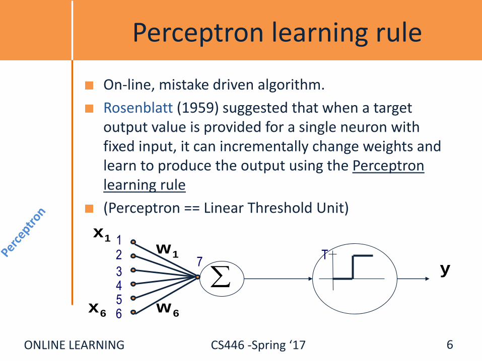
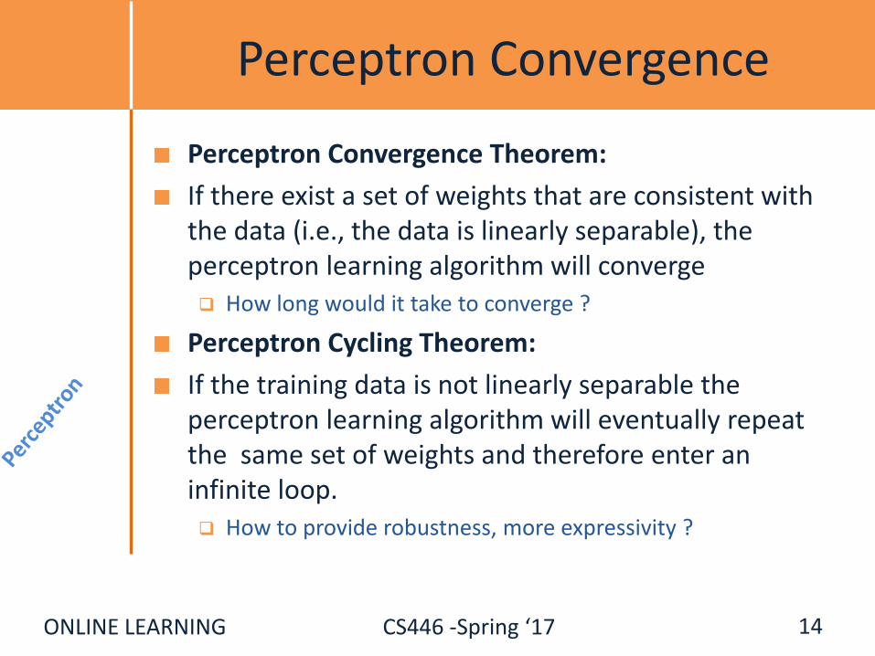
Perceptron Learnability
Obviously can’t learn what it can’t represent (???) Only linearly separable functions
Minsky and Papert (1969) wrote an influential book demonstrating Perceptron’s representational limitations Parity functions can’t be learned (XOR) In vision, if patterns are represented with local features,
can’t represent symmetry, connectivity
Research on Neural Networks stopped for years
Rosenblatt himself (1959) asked,
• “What pattern recognition problems can be transformed so as to become linearly separable?”
12
ONLINE LEARNING CS446 -Spring ‘17 13
(x1 x2) v (x3 x4) y1 y2
ONLINE LEARNING CS446 -Spring ‘17
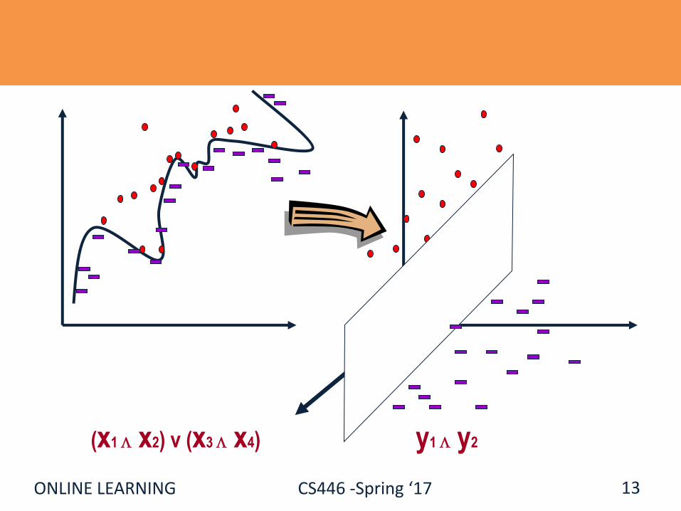
Perceptron Convergence
Perceptron Convergence Theorem:
If there exist a set of weights that are consistent with the data (i.e., the data is linearly separable), the perceptron learning algorithm will converge How long would it take to converge ?
Perceptron Cycling Theorem:
If the training data is not linearly separable the perceptron learning algorithm will eventually repeat the same set of weights and therefore enter an infinite loop. How to provide robustness, more expressivity ?
14
ONLINE LEARNING CS446 -Spring ‘17
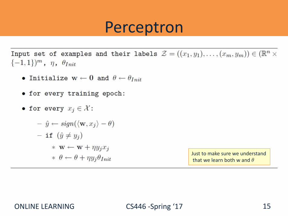
Perceptron
15
Just to make sure we understandthat we learn both w and µ

ONLINE LEARNING CS446 -Spring ‘17
Perceptron: Mistake Bound Theorem
Maintains a weight vector wRN, w0=(0,…,0).
Upon receiving an example x RN
Predicts according to the linear threshold function w•x 0.
Theorem [Novikoff,1963] Let (x1; y1),…,: (xt; yt), be a sequence of labeled examples with xi <
N, xiR and yi {-1,1} for all i. Let u <N, > 0 be such that,
||u|| = 1 and yi u • xi for all i.
Then Perceptron makes at most R2 / 2 mistakes on this example sequence.
(see additional notes)
16
Complexity Parameter

ONLINE LEARNING CS446 -Spring ‘17
Perceptron-Mistake Bound
17
Proof: Let vk be the hypothesis before the k-th mistake. Assume that the k-th mistake occurs on the input example (xi, yi).
Assumptions
v1 = 0
||u|| = 1
yi u • xi
k < R2 / 2
1. Note that the bound does not depend on the dimensionality nor on the number of examples.
2. Note that we place weight vectorsand examples in the same space.
ONLINE LEARNING CS446 -Spring ‘17
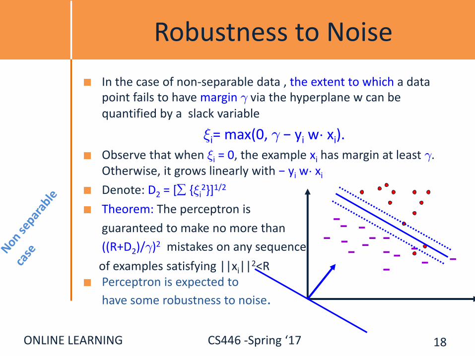
Robustness to Noise
In the case of non-separable data , the extent to which a data point fails to have margin ° via the hyperplane w can be quantified by a slack variable
»i= max(0, ° − yi w¢ xi). Observe that when »i = 0, the example xi has margin at least °. Otherwise, it grows linearly with − yi w¢ xi
Denote: D2 = [ {»i2}]1/2
Theorem: The perceptron is
guaranteed to make no more than
((R+D2)/°)2 mistakes on any sequence
of examples satisfying ||xi||2<RPerceptron is expected to
have some robustness to noise.
18
- --- --
-- -
- -
- -
-
-

ONLINE LEARNING CS446 -Spring ‘17
Perceptron for Boolean Functions
How many mistakes will the Perceptron algorithms make when learning a k-disjunction?
Try to figure out the bound
Find a sequence of examples that will cause Perceptron to make O(n) mistakes on k-disjunction on n attributes.
(Where is n coming from?)
19

ONLINE LEARNING CS446 -Spring ‘17
Winnow Algorithm
The Winnow Algorithm learns Linear Threshold Functions.
For the class of disjunctions: instead of demotion we can use elimination.
20
(demotion) 1)x (if /2w w,xbut w 0f(x) If
)(promotion 1)x (if 2w w,xwbut 1f(x) If
nothing do :mistake no If
xw iff 1 is Prediction
w :Initialize
iii
iii
i
1n;

ONLINE LEARNING CS446 -Spring ‘17
Winnow - Example
21
)hypothesis (final
version)on(eliminati
)1024,1024,...,32,1,0,0,0,1024,1024(
..........................
mistake )256,...,0,..0,1,512( ),0..,111.0,1,0,0(
ok )256,....,256,256,1,512( ),1...,0,1,0,1(
)256,....,256,256,1,512(
variable)goodeach (for log(n/2) .......................
mistake )2...,2,4,1,8( ),1..,0,0,1,0,1(
mistake )1...,2,2,1,4( ),0..,0,1,1,0,1(
mistake )1,....,1,2( ),0,...,0,0,1(
ok )1,....,1,1( ),0,,,,111,0,0(
ok )1,....,1,1( -,0,...,0), 0(
ok )1,...,1,1( ),(1,1,...,1
)1,...,1,1(;1024 :Initialize
1024102321
w
wxw
wxw
w
wxw
wxw
wxw
wxw
wxw
wxw
w
xxxxf
Notice that the same algorithm will learn a conjunction over these variables (w=(256,256,0,…32,…256,256) )

ONLINE LEARNING CS446 -Spring ‘17
Winnow – Mistake Bound
Claim: Winnow makes O(k log n) mistakes on k-disjunctions
u - # of mistakes on positive examples (promotions)
v - # of mistakes on negative examples (demotions)
1. u < k log(2n)A weight that corresponds to a good variable is only promoted.
When these weights get to n there will be no more mistakes on positives.
22
(demotion) 1)x (if /2w w,xbut w 0f(x) If
)(promotion 1)x (if 2w w,xwbut 1f(x) If
nothing do :mistake no If
xw iff 1 is Prediction
w :Initialize
iii
iii
i
1n;

ONLINE LEARNING CS446 -Spring ‘17
Winnow – Mistake Bound
Claim: Winnow makes O(k log n) mistakes on k-disjunctions
u - # of mistakes on positive examples (promotions)
v - # of mistakes on negative examples (demotions)
2. v < 2(u + 1)Total weight TW=n initially
Mistake on positive: TW(t+1) < TW(t) + n
Mistake on negative: TW(t+1) < TW(t) - n/2
0 < TW < n + u n - v n/2 v < 2(u+1)
23
(demotion) 1)x (if /2w w,xbut w 0f(x) If
)(promotion 1)x (if 2w w,xwbut 1f(x) If
nothing do :mistake no If
xw iff 1 is Prediction
w :Initialize
iii
iii
i
1n;

ONLINE LEARNING CS446 -Spring ‘17
Winnow – Mistake Bound
Claim: Winnow makes O(k log n) mistakes on k-disjunctions
u - # of mistakes on positive examples (promotions)
v - # of mistakes on negative examples (demotions)
# of mistakes: u + v < 3u + 2 = O(k log n)
24
(demotion) 1)x (if /2w w,xbut w 0f(x) If
)(promotion 1)x (if 2w w,xwbut 1f(x) If
nothing do :mistake no If
xw iff 1 is Prediction
w :Initialize
iii
iii
i
1n;
ONLINE LEARNING CS446 -Spring ‘17
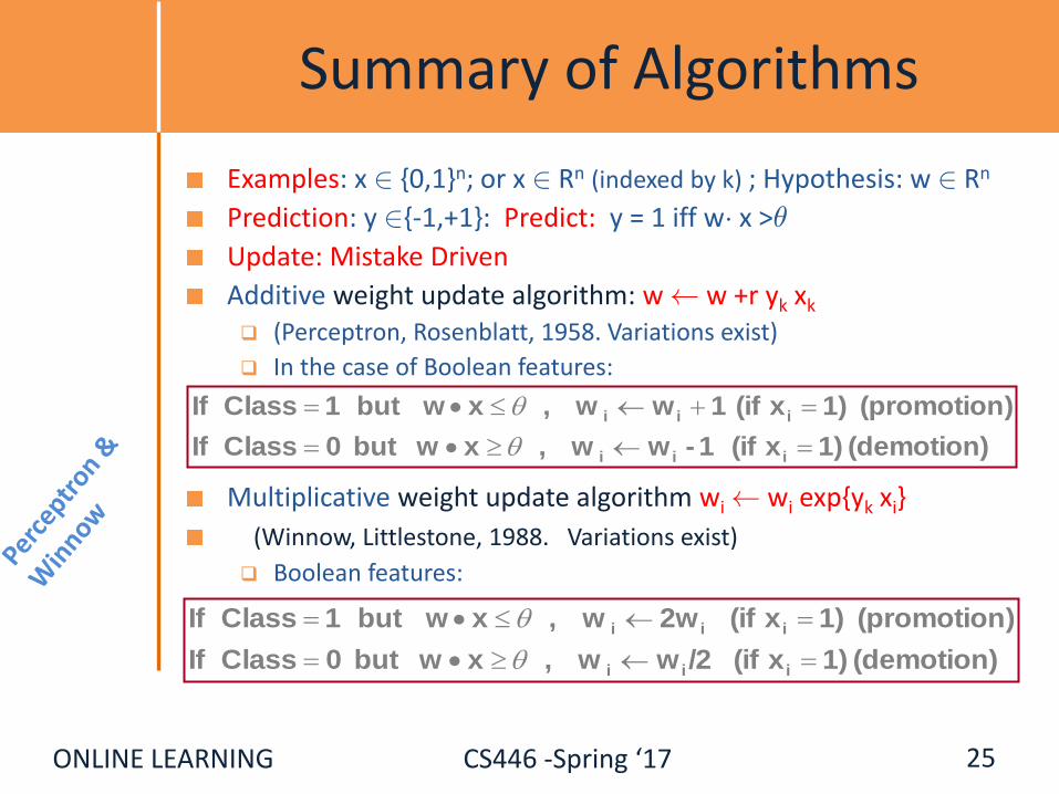
Summary of Algorithms
Examples: x 2 {0,1}n; or x 2 Rn (indexed by k) ; Hypothesis: w 2 Rn
Prediction: y 2{-1,+1}: Predict: y = 1 iff w¢ x >µ
Update: Mistake Driven
Additive weight update algorithm: w à w +r yk xk
(Perceptron, Rosenblatt, 1958. Variations exist)
In the case of Boolean features:
Multiplicative weight update algorithm wi à wi exp{yk xi}
(Winnow, Littlestone, 1988. Variations exist)
Boolean features:
25
(demotion) 1)x (if 1- w w,xbut w 0Class If
)(promotion 1)x (if 1 w w,xwbut 1Class If
iii
iii
(demotion) 1)x (if /2w w,xbut w 0Class If
)(promotion 1)x (if 2w w,xwbut 1Class If
iii
iii

ONLINE LEARNING CS446 -Spring ‘17
Practical Issues and Extensions
There are many extensions that can be made to these basic algorithms.
Some are necessary for them to perform well
Regularization (next; will be motivated in the next section, COLT)
Some are for ease of use and tuning
Converting the output of a Perceptron/Winnow to a conditional probability
P(y = +1 |x) = [1+ exp(-Awx)]-1
Can tune the parameter A
Multiclass classification (later)
Key efficiency issue: Infinite attribute domain
26

ONLINE LEARNING CS446 -Spring ‘17
I Regularization Via Averaged Perceptron
An Averaged Perceptron Algorithm is motivated by the following considerations:
Every Mistake-Bound Algorithm can be converted efficiently to a PAC algorithm – to yield global guarantees on performance.
In the mistake bound model:
We don’t know when we will make the mistakes.
In the PAC model:
Dependence is on number of examples seen and not number of mistakes.
Which hypothesis will you choose…??
Being consistent with more examples is better
To convert a given Mistake Bound algorithm (into a global guarantee algorithm):
Wait for a long stretch w/o mistakes (there must be one)
Use the hypothesis at the end of this stretch.
Its PAC behavior is relative to the length of the stretch.
Averaged Perceptron returns a weighted average of a number of earlier hypotheses; the weights are a function of the length of no-mistakes stretch.
28
ONLINE LEARNING CS446 -Spring ‘17
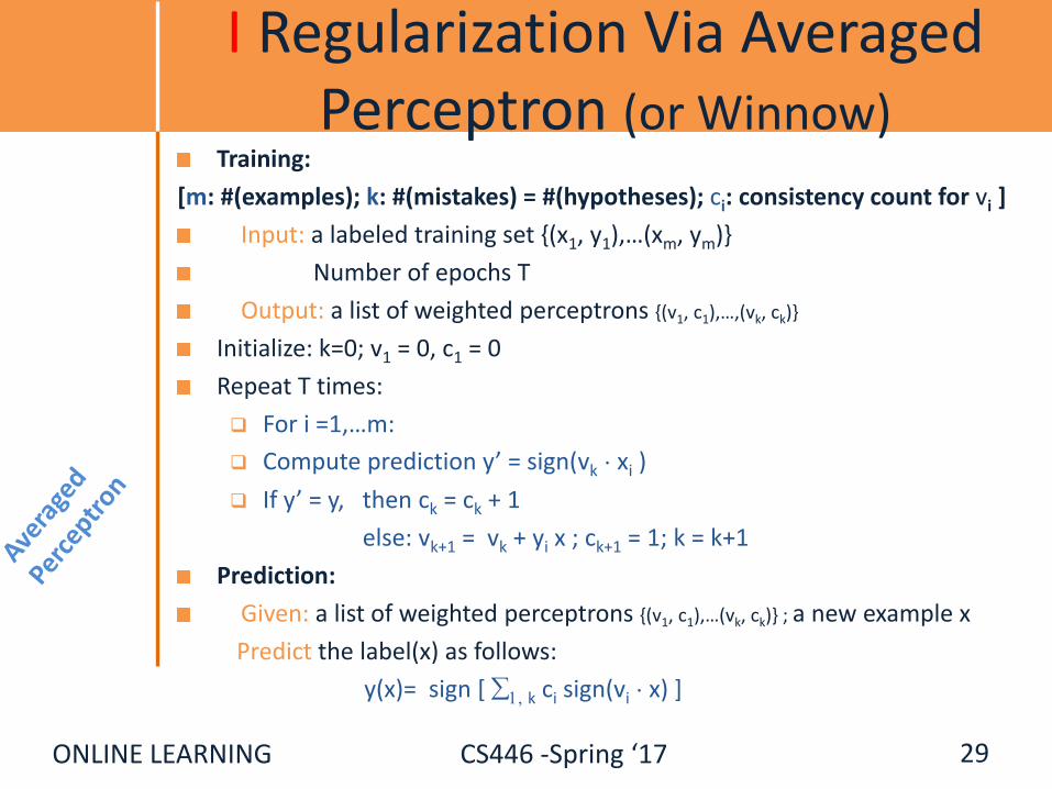
I Regularization Via Averaged Perceptron (or Winnow)
Training:
[m: #(examples); k: #(mistakes) = #(hypotheses); ci: consistency count for vi ]
Input: a labeled training set {(x1, y1),…(xm, ym)}
Number of epochs T
Output: a list of weighted perceptrons {(v1, c1),…,(vk, ck)}
Initialize: k=0; v1 = 0, c1 = 0
Repeat T times:
For i =1,…m:
Compute prediction y’ = sign(vk ¢ xi )
If y’ = y, then ck = ck + 1
else: vk+1 = vk + yi x ; ck+1 = 1; k = k+1
Prediction:
Given: a list of weighted perceptrons {(v1, c1),…(vk, ck)} ; a new example x
Predict the label(x) as follows:
y(x)= sign [ 1,k ci sign(vi ¢ x) ]
29
ONLINE LEARNING CS446 -Spring ‘17
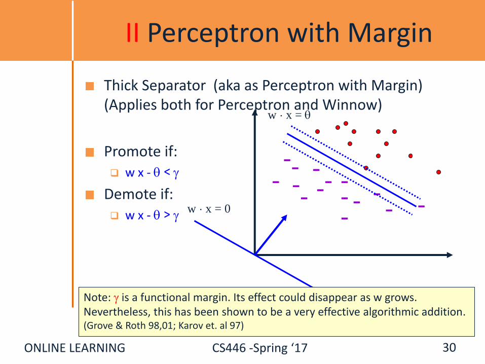
II Perceptron with Margin
Thick Separator (aka as Perceptron with Margin) (Applies both for Perceptron and Winnow)
Promote if:
w x - <
Demote if:
w x - >
30
w ¢ x = 0
- --- -
-
-- -
- -
- -
-
-
w ¢ x =
Note: is a functional margin. Its effect could disappear as w grows.Nevertheless, this has been shown to be a very effective algorithmic addition.(Grove & Roth 98,01; Karov et. al 97)
ONLINE LEARNING CS446 -Spring ‘17
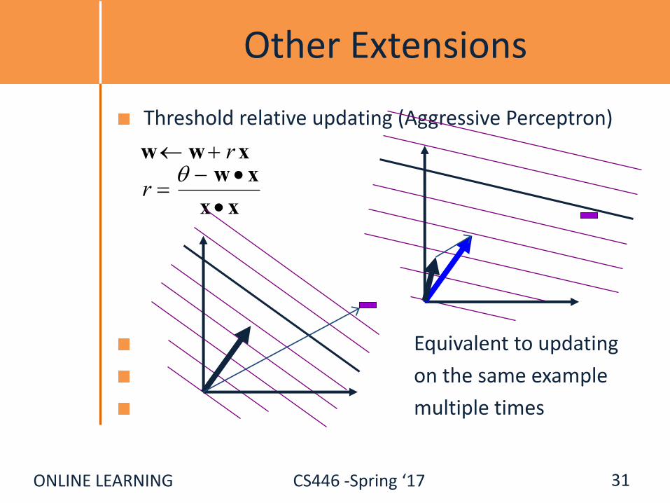
Other Extensions
Threshold relative updating (Aggressive Perceptron)
Equivalent to updating
on the same example
multiple times
31
w w rx
r w x
x x

ONLINE LEARNING CS446 -Spring ‘17
SNoW (also in LBJava)
Several of these extensions (and a couple more) are implemented in the SNoW learning architecture that supports several linear update rules (Winnow, Perceptron, naïve Bayes)
Supports Regularization(averaged Winnow/Perceptron; Thick Separator)
Conversion to probabilities
Automatic parameter tuning
True multi-class classification
Feature Extraction and Pruning
Variable size examples
Good support for large scale domains in terms of number of examples and number of features.
Very efficient
Many other options
[Download from: http://cogcomp.cs.illinois.edu/page/software ]
32

ONLINE LEARNING CS446 -Spring ‘17
Winnow - Extensions
This algorithm learns monotone functions
For the general case: Duplicate variables (down side?)
For the negation of variable x, introduce a new variable y.
Learn monotone functions over 2n variables
Balanced version: Keep two weights for each variable; effective weight is the
difference
We’ll come back to this idea when talking about multiclass.
33
(demotion) 1 where2 2
1 ,)(but 0)( If
)(promotion 1 where2
1 2 ,)(but 1)( If
:Rule Update
iiiii
iiiii
xwwwwxwwxf
xwwwwxwwxf

ONLINE LEARNING CS446 -Spring ‘17
Winnow – A Robust Variation
Winnow is robust in the presence of various kinds of noise. (classification noise, attribute noise)
Moving Target: The target function changes with time.
Importance: sometimes we learn under some distribution but test under
a slightly different one. (e.g., natural language applications)
The algorithm we develop provides a good insight into issues of Adaptation
34

ONLINE LEARNING CS446 -Spring ‘17
Winnow – A Robust Variation
Modeling: Adversary’s turn: may change the target concept by adding
or removing some variable from the target disjunction.
Cost of each addition move is 1.
Learner’s turn: makes prediction on the examples given, and is then told the correct answer (according to current target function)
Winnow-R: Same as Winnow, only doesn’t let weights go below 1/2
Claim: Winnow-R makes O(c log n) mistakes, (c - cost of adversary) (generalization of previous claim)
35

ONLINE LEARNING CS446 -Spring ‘17
Winnow R – Mistake Bound
u - # of mistakes on positive examples (promotions)
v - # of mistakes on negative examples (demotions)
2. v < 2(u + 1)Total weight TW=n initially
Mistake on positive: TW(t+1) < TW(t) + n
Mistake on negative: TW(t+1) < TW(t) - n/4
0 < TW < n + u n - v n/4 v < 4(u+1)
36
Good project:
Push weights to 0 (simple hypothesis, L1 regularization (Lasso)) vs. bounding them away from zero
– impact on adaptation

ONLINE LEARNING CS446 -Spring ‘17
Administration
Registration - Done
Hw2 is due tomorrow
Hw3 will be released tomorrow
37
QuestionsTODAY:
• Administration: HW, Projects
• Flipped Class
• Continuing with On-Line Learning

ONLINE LEARNING CS446 -Spring ‘17
Features; feature types; instances space transformation.
Stopping Criterion left ambiguous deliberately. Multiple options; think and make a decision (e.g., based on loss; based on error).
HW2
38
Decision Trees, Expressivity of Models, Features
Key Reporting Module (RM): Train a model on a given Training Set
Report 5-fold cross validation
Report results on a supplied Test Set.
(a) Convert Data to Feature Representation (given; can be augmented) 2000 * 270 dimensions
(b) Program SGD; run RM
(c) Use Weka to Learn DT using ID2; run RM.
(d) Use Weka to learn DT(depth=4) and DT(depth=8); run RM
(e) Use Weka to generate 100 different DT(d=4)
Generate 100 dimensional data, each dimension is the prediction of a DT
Run (b) on the new data
Compare algorithms from b,c,d,e.

ONLINE LEARNING CS446 -Spring ‘17
Projects
Projects proposals are due on March 10 2017Within a week we will give you an approval to continue with your project along with comments and/or a request to modify/augment/do a different project. There will also be a mechanism for peer comments.
We encourage team projects – a team can be up to 3 people.
Please start thinking and working on the project now.Your proposal is limited to 1-2 pages, but needs to include referencesand, ideally, some of the ideas you have developed in the direction of the project (maybe even some preliminary results).Any project that has a significant Machine Learning component is good. You can do experimental work, theoretical work, a combination of both or a critical survey of results in some specialized topic. The work has to include some reading. Even if you do not do a survey, you must read (at least) two related papers or book chapters and relate your work to it. Originality is not mandatory but is encouraged. Try to make it interesting!
39

ONLINE LEARNING CS446 -Spring ‘17
Examples
Fake News Challenge :- http://www.fakenewschallenge.org/
KDD Cup 2013: "Author-Paper Identification": given an author and a small set of papers, we are asked to
identify which papers are really written by the author.
https://www.kaggle.com/c/kdd-cup-2013-author-paper-identification-challenge
“Author Profiling”: given a set of document, profile the author: identification, gender, native language, ….
Caption Control: Is it gibberish? Spam? High quality text? Adapt an NLP program to a new domain
Work on making learned hypothesis (e.g., linear threshold functions, NN) more comprehensible Explain the prediction
Develop a (multi-modal) People Identifier Compare Regularization methods: e.g., Winnow vs. L1 RegularizationLarge scale clustering of documents + name the clusterDeep Networks: convert a state of the art NLP program to a deep network, efficient, architecture. Try to prove something
40
ONLINE LEARNING CS446 -Spring ‘17
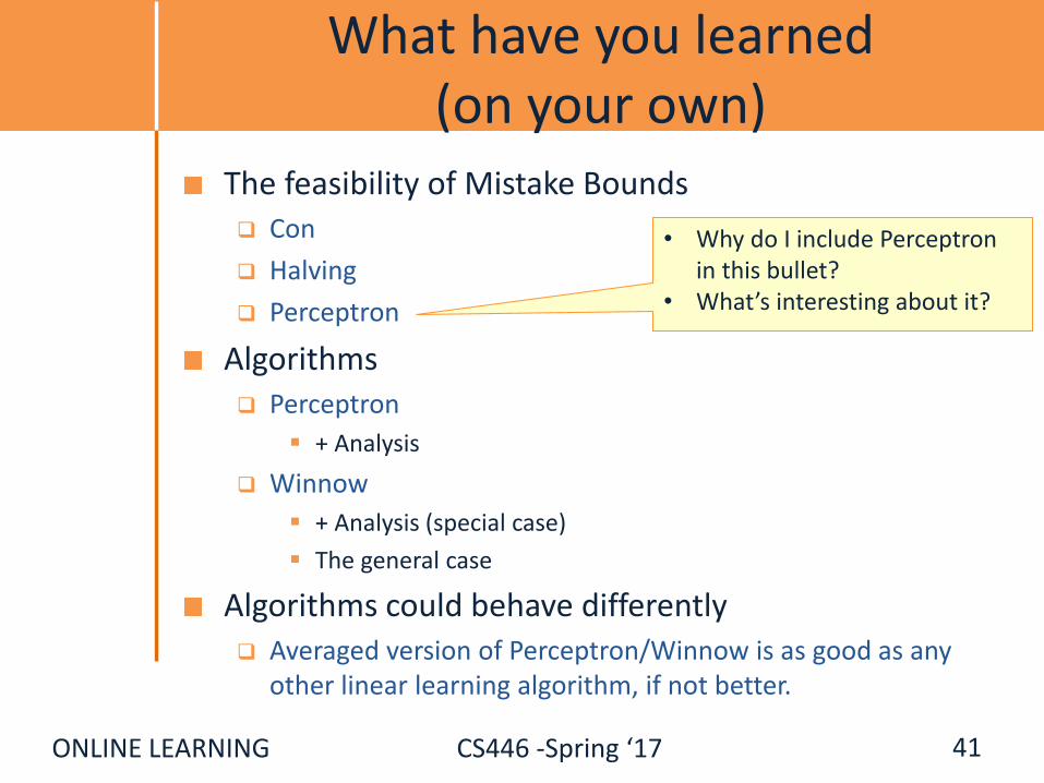
What have you learned(on your own)
The feasibility of Mistake Bounds Con
Halving
Perceptron
Algorithms Perceptron
+ Analysis
Winnow
+ Analysis (special case)
The general case
Algorithms could behave differently Averaged version of Perceptron/Winnow is as good as any
other linear learning algorithm, if not better.
41
• Why do I include Perceptron in this bullet?
• What’s interesting about it?

ONLINE LEARNING CS446 -Spring ‘17
General Stochastic Gradient Algorithms
Given examples {z=(x,y)}1, m from a distribution over XxY, we are trying to learn a linear function, parameterized by a weight vector w, so that we minimize the expected risk function
J(w) = Ez Q(z,w) ~=~ 1/m 1,m Q(zi, wi)In Stochastic Gradient Descent Algorithms we approximate this minimization by incrementally updating the weight vector w as follows:
wt+1 = wt – rt gw Q(zt, wt) = wt – rt gt
Where g_t = gw Q(zt, wt) is the gradient with respect to w at time t.
The difference between algorithms now amounts to choosing a different loss function Q(z, w)
42

ONLINE LEARNING CS446 -Spring ‘17
wt+1 = wt – rt gw Q(zt, wt) = wt – rt gt
LMS: Q((x, y), w) =1/2 (y – w ¢ x)2
leads to the update rule (Also called Widrow’s Adaline):wt+1 = wt + r (yt – wt ¢ xt) xt
Here, even though we make binary predictions based on sign (w ¢ x) we do not take the sign of the dot-product into account in the loss.
Another common loss function is:Hinge loss: Q((x, y), w) = max(0, 1 - y w ¢ x)
This leads to the perceptron update rule:
If yi wi ¢ xi > 1 (No mistake, by a margin): No updateOtherwise (Mistake, relative to margin): wt+1 = wt + r yt xt
Stochastic Gradient Algorithms
43
w ¢ x
Think about the case where x is a Boolean vector.

ONLINE LEARNING CS446 -Spring ‘17
wt+1 = wt – rt gw Q(zt, wt) = wt – rt gt
(notice that this is a vector, each coordinate (feature) has its own wt,j and gt,j)
So far, we used fixed learning rates r = rt, but this can change. AdaGrad alters the update to adapt based on historical information, so that frequently occurring features in the gradients get small learning rates and infrequent features get higher ones. The idea is to “learn slowly” from frequent features but “pay attention” to rare but informative features.Define a “per feature” learning rate for the feature j, as:
rt,j = r/(Gt,j)1/2
where Gt,j = k1,t g2k,j the sum of squares of gradients at feature j
until time t.Overall, the update rule for Adagrad is:
wt+1,j = wt,j - gt,j r/(Gt,j)1/2
This algorithm is supposed to update weights faster than Perceptron or LMS when needed.
New Stochastic Gradient Algorithms
44

ONLINE LEARNING CS446 -Spring ‘17
Regularization
The more general formalism adds a regularization term to the risk function, and attempts to minimize:
J(w) = 1,m Q(zi, wi) + ¸ Ri (wi)Where R is used to enforce “simplicity” of the learned functions.
LMS case: Q((x, y), w) =(y – w ¢ x)2
R(w) = ||w||22 gives the optimization problem called Ridge Regression.
R(w) = ||w||1 gives a problem called the LASSO problem
Hinge Loss case: Q((x, y), w) = max(0, 1 - y w ¢ x) R(w) = ||w||2
2 gives the problem called Support Vector Machines
Logistics Loss case: Q((x,y),w) = log (1+exp{-y w ¢ x}) R(w) = ||w||2
2 gives the problem called Logistics Regression
These are convex optimization problems and, in principle, the same gradient descent mechanism can be used in all cases. We will see later why it makes sense to use the “size” of w as a way to control “simplicity”.
45

ONLINE LEARNING CS446 -Spring ‘17
Algorithmic Approaches
Focus: Two families of algorithms (one of the on-line representative) Additive update algorithms: Perceptron
SVM is a close relative of Perceptron
Multiplicative update algorithms: Winnow
Close relatives: Boosting, Max entropy/Logistic Regression
46

ONLINE LEARNING CS446 -Spring ‘17
How to Compare?
Generalization (since the representation is the same): How many examples
are needed to get to a given level of accuracy?
Efficiency How long does it take to learn a hypothesis and evaluate it
(per-example)?
Robustness; Adaptation to a new domain, ….
47

ONLINE LEARNING CS446 -Spring ‘17
Sentence Representation
S= I don’t know whether to laugh or cry
Define a set of features: features are relations that hold in the sentence
Map a sentence to its feature-based representation The feature-based representation will give some of the
information in the sentence
Use this as an example to your algorithm
48
ONLINE LEARNING CS446 -Spring ‘17
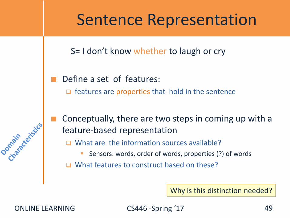
Sentence Representation
S= I don’t know whether to laugh or cry
Define a set of features: features are properties that hold in the sentence
Conceptually, there are two steps in coming up with a feature-based representation What are the information sources available?
Sensors: words, order of words, properties (?) of words
What features to construct based on these?
49
Why is this distinction needed?

ONLINE LEARNING CS446 -Spring ‘17
Embedding
50
Weather
Whether
523341321 xxxxxxxxx 541 yyy
New discriminator in functionally simpler

ONLINE LEARNING CS446 -Spring ‘17
Domain Characteristics
The number of potential features is very large
The instance space is sparse
Decisions depend on a small set of features: the
function space is sparse
Want to learn from a number of examples that is
small relative to the dimensionality
51
ONLINE LEARNING CS446 -Spring ‘17
Generalization
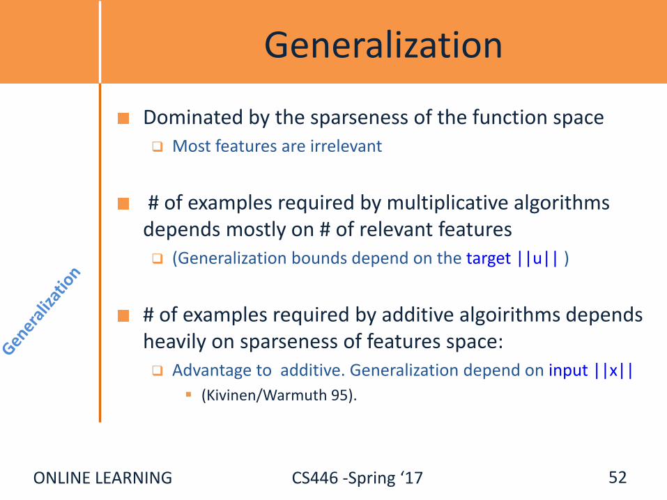
Dominated by the sparseness of the function space Most features are irrelevant
# of examples required by multiplicative algorithms depends mostly on # of relevant features (Generalization bounds depend on the target ||u|| )
# of examples required by additive algoirithms depends heavily on sparseness of features space: Advantage to additive. Generalization depend on input ||x||
(Kivinen/Warmuth 95).
52
ONLINE LEARNING CS446 -Spring ‘17
Which Algorithm to Choose?
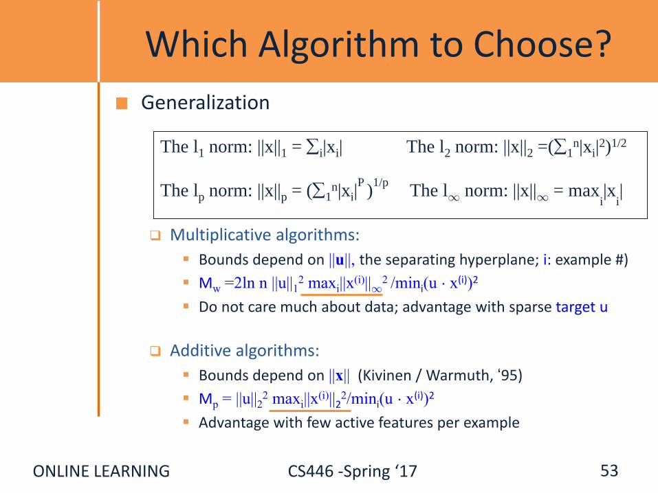
Generalization
Multiplicative algorithms:
Bounds depend on ||u||, the separating hyperplane; i: example #)
Mw =2ln n ||u||12 maxi||x
(i)||12 /mini(u ¢ x(i))2
Do not care much about data; advantage with sparse target u
Additive algorithms:
Bounds depend on ||x|| (Kivinen / Warmuth, ‘95)
Mp = ||u||22 maxi||x
(i)||22/mini(u ¢ x(i))2
Advantage with few active features per example
53
The l1 norm: ||x||1 = i|xi| The l2 norm: ||x||2 =(1n|xi|
2)1/2
The lp norm: ||x||p = (1n|xi|
P)
1/pThe l1 norm: ||x||1 = max
i|x
i|

ONLINE LEARNING CS446 -Spring ‘17
ExamplesExtreme Scenario 1: Assume the u has exactly k active features, and the other n-k are 0. That is, only k input features are relevant to the prediction. Then:
||u||2, = k1/2 ; ||u||1, = k ; max ||x||2, = n1/2 ;; max ||x||1, = 1
We get that: Mp = kn; Mw = 2k2 ln n
Therefore, if k<<n, Winnow behaves much better.
Extreme Scenario 2: Now assume that u=(1, 1,….1) and the instances are very sparse, the rows of an nxn unit matrix. Then:
||u||2, = n1/2 ; ||u||1, = n ; max ||x||2, = 1 ;; max ||x||1, = 1
We get that: Mp = n; Mw = 2n2 ln n
Therefore, Perceptron has a better bound.
54
Mw =2ln n ||u||12 maxi||x
(i)||12 /mini(u ¢ x(i))2
Mp = ||u||22 maxi||x
(i)||22/mini(u ¢ x(i))2
ONLINE LEARNING CS446 -Spring ‘17
`
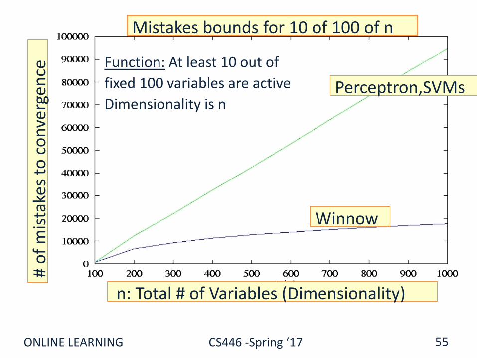
55
Function: At least 10 out of
fixed 100 variables are active
Dimensionality is nPerceptron,SVMs
n: Total # of Variables (Dimensionality)
Winnow
Mistakes bounds for 10 of 100 of n#
of
mis
take
s to
co
nve
rgen
ce

ONLINE LEARNING CS446 -Spring ‘17
Efficiency
Dominated by the size of the feature space
Most features are functions (e.g. conjunctions) of raw attributes
Additive algorithms allow the use of Kernels No need to explicitly generate complex features
Could be more efficient since work is done in the original feature space, but expressivity is a function of the kernel expressivity.
56
kn ) (x)... (x), (x), (x) n321 (),...,,( 321 kxxxxX
i
ii )K(x,xcf(x)
ONLINE LEARNING CS446 -Spring ‘17
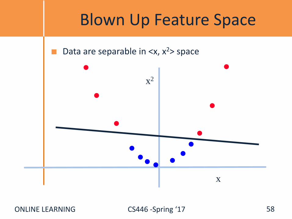
Functions Can be Made Linear
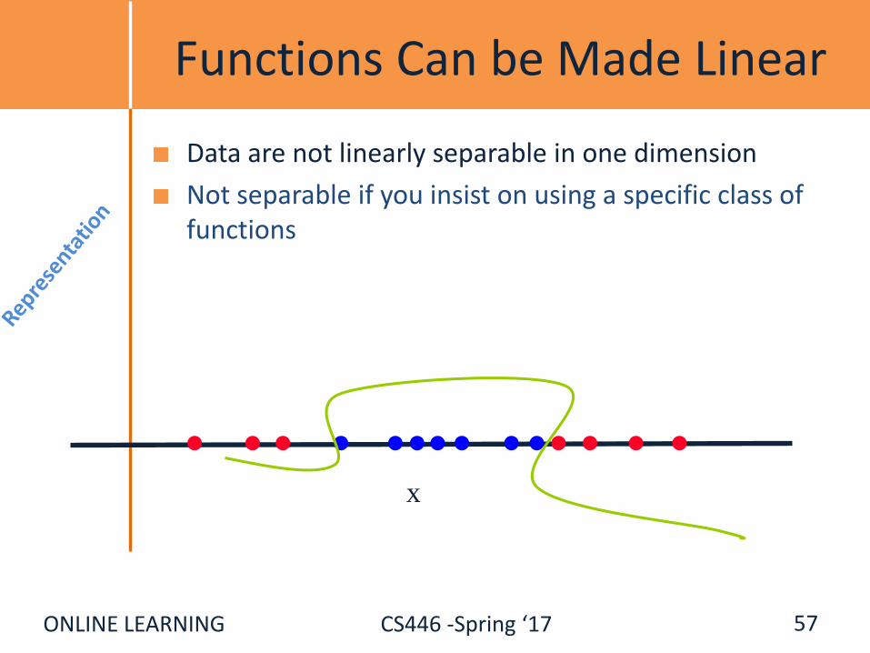
Data are not linearly separable in one dimension
Not separable if you insist on using a specific class of functions
x
57
ONLINE LEARNING CS446 -Spring ‘17
Blown Up Feature Space
Data are separable in <x, x2> space
x
x2
58
ONLINE LEARNING CS446 -Spring ‘17
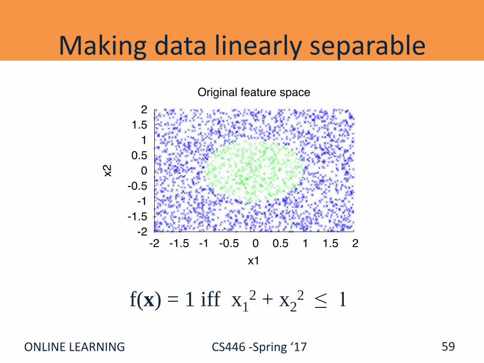
Making data linearly separable
59
f(x) = 1 iff x12 + x2
2 ≤ 1

ONLINE LEARNING CS446 -Spring ‘17
Making data linearly separable
60
Transform data: x = (x1, x2 ) => x’ = (x12, x2
2 ) f(x’) = 1 iff x’1 + x’2 ≤ 1
In order to deal with this, we introduce two new concepts:
Dual Representation
Kernel (& the kernel trick)

ONLINE LEARNING CS446 -Spring ‘17 61
(demotion) 1)x (if 1- w w,xbut w 0Class If
)(promotion 1)x (if 1 w w,xwbut 1Class If
iii
iii
)xxw(Th f(x)
R w:Hypothesis ;{0,1} x :Examples
n
1i ii
nn
)(
Let w be an initial weight vector for perceptron. Let (x1,+), (x2,+), (x3,-), (x4,-) be examples and assume mistakes are made on x1, x2 and x4. What is the resulting weight vector?
w = w + x1 + x2 - x4
In general, the weight vector w can be written as a linear combination of examples:
w = 1,m r ®i yi xi
Where ®i is the number of mistakes made on xi.
Dual Representation
Note: We care about the dot product: f(x) = w ¢ x =
= (1,m r®i yi xi) ¢ x = 1,m r®i yi (xi ¢ x)

ONLINE LEARNING CS446 -Spring ‘17
Kernel Based Methods
A method to run Perceptron on a very large feature set, without incurring the cost of keeping a very large weight vector.
Computing the dot product can be done in the original feature space.
Notice: this pertains only to efficiency: The classifier is identical to the one you get by blowing up the feature space.
Generalization is still relative to the real dimensionality (or, related properties).
Kernels were popularized by SVMs, but many other algorithms can make use of them (== run in the dual). Linear Kernels: no kernels; stay in the original space. A lot of applications
actually use linear kernels.
62
M f(x)
zz))S(z)K(x,(Th

ONLINE LEARNING CS446 -Spring ‘17 63
(demotion) 1)x (if 1- w w,xbut w 0Class If
)(promotion 1)x (if 1 w w,xwbut 1Class If
iii
iii
)xxw(Th f(x)
R w:Hypothesis ;{0,1} x :Examples
n
1i ii
nn
)(
Let I be the set t1,t2,t3 …of monomials (conjunctions) over the feature space x1, x2… xn.
Then we can write a linear function over this new feature space.
)xtw(Th f(x) i ii
I
)(
1 (11011)xxx 0 (11010)xx 1 (11010)xxx :Example 42143421
Kernel Base Methods

ONLINE LEARNING CS446 -Spring ‘17 64
nn R w:Hypothesis ;{0,1} x :Examples
Great Increase in expressivity
Can run Perceptron (and Winnow) but the convergence bound may suffer exponential growth.
Exponential number of monomials are true in each example.
Also, will have to keep many weights.
)xtw(Th f(x) i ii
I
)(
(demotion) 1)x (if 1- w w,xbut w 0Class If
)(promotion 1)x (if 1 w w,xwbut 1Class If
iii
iii
Kernel Based Methods

ONLINE LEARNING CS446 -Spring ‘17 65
Weather
Whether
523341321 xxxxxxxxx 541 yyy
New discriminator in functionally simpler
Embedding

ONLINE LEARNING CS446 -Spring ‘17
The Kernel Trick(1)
Consider the value of w used in the prediction.
Each previous mistake, on example z, makes an additive contribution of +/-1 to w, iff t(z) = 1.
The value of w is determined by the number of mistakes on which t() was satisfied.
66
nn R w:Hypothesis ;{0,1} x :Examples
)xtw(Th f(x) i ii
I
)(
(demotion) 1)x (if 1- w w,xbut w 0Class If
)(promotion 1)x (if 1 w w,xwbut 1Class If
iii
iii

ONLINE LEARNING CS446 -Spring ‘17
I
I
((
)(
i ii
Mz
i i
1(z)tD,z1(z)tP,z
x)z)ttS(z)(Th
)xt11(Th f(x)ii
The Kernel Trick(2)
P – set of examples on which we Promoted
D – set of examples on which we Demoted
M = P [ D
67
nn R w:Hypothesis ;{0,1} x :Examples
)xtw(Th f(x) i ii
I
)(
(demotion) 1)x (if 1- w w,xbut w 0Class If
)(promotion 1)x (if 1 w w,xwbut 1Class If
iii
iii
ONLINE LEARNING CS446 -Spring ‘17
M
I
(( f(x) z
i
ii ))xz)ttS(z)(Th
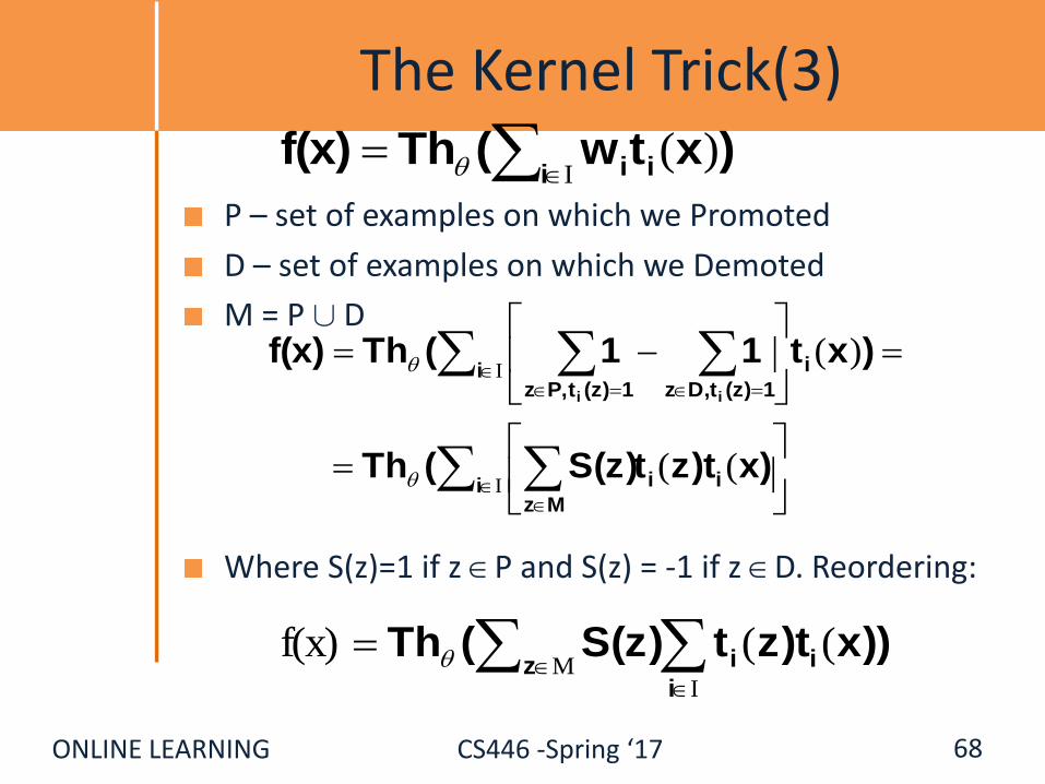
The Kernel Trick(3)
P – set of examples on which we Promoted
D – set of examples on which we Demoted
M = P [ D
Where S(z)=1 if z P and S(z) = -1 if z D. Reordering:
68
)xtw(Th f(x) i ii
I
)(
I
I
((
)(
i ii
Mz
i i
1(z)tD,z1(z)tP,z
x)z)ttS(z)(Th
)xt11(Th f(x)ii
ONLINE LEARNING CS446 -Spring ‘17
M f(x)
zz))S(z)K(x,(Th
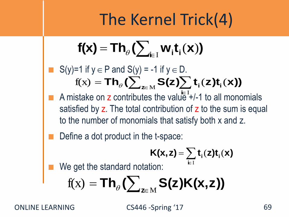
The Kernel Trick(4)
S(y)=1 if y P and S(y) = -1 if y D.
A mistake on z contributes the value +/-1 to all monomials
satisfied by z. The total contribution of z to the sum is equal
to the number of monomials that satisfy both x and z.
Define a dot product in the t-space:
We get the standard notation:
69
M
I
(( f(x) z
i
ii ))xz)ttS(z)(Th
)xz)tt z)K(x,i
ii
I
((
)xtw(Th f(x) i ii
I
)(

ONLINE LEARNING CS446 -Spring ‘17
Kernel Based Methods
What does this representation give us?
We can view this Kernel as the distance between x,z
in the t-space.
But, K(x,z) can be measured in the original space,
without explicitly writing the t-representation of x, z
70
M f(x)
zz))S(z)K(x,(Th
)xz)tt z)K(x,i
ii
I
((
ONLINE LEARNING CS446 -Spring ‘17
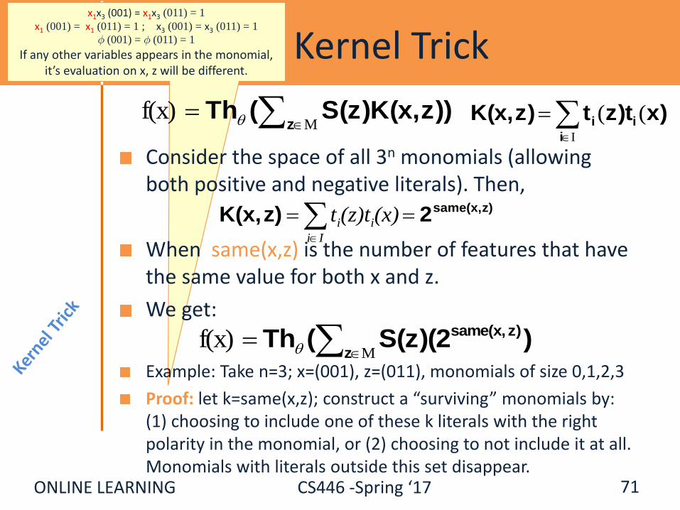
x1x3 (001) = x1x3 (011) = 1
x1 (001) = x1 (011) = 1 ; x3 (001) = x3 (011) = 1
Á (001) = Á (011) = 1
If any other variables appears in the monomial, it’s evaluation on x, z will be different.
Kernel Trick
Consider the space of all 3n monomials (allowing both positive and negative literals). Then,
When same(x,z) is the number of features that have the same value for both x and z.
We get:
Example: Take n=3; x=(001), z=(011), monomials of size 0,1,2,3
Proof: let k=same(x,z); construct a “surviving” monomials by: (1) choosing to include one of these k literals with the right polarity in the monomial, or (2) choosing to not include it at all. Monomials with literals outside this set disappear.
71
M f(x)
zz))S(z)K(x,(Th )xz)tt z)K(x,
i
ii
I
((
z)same(x,2 z)K(x, Ii
ii (x)(z)tt
M f(x)
z
z)same(x, )S(z)(2(Th
ONLINE LEARNING CS446 -Spring ‘17
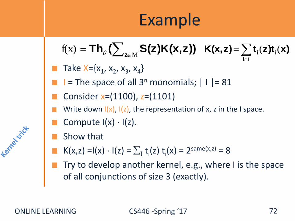
Example
Take X={x1, x2, x3, x4}
I = The space of all 3n monomials; | I |= 81
Consider x=(1100), z=(1101)Write down I(x), I(z), the representation of x, z in the I space.
Compute I(x) ¢ I(z).
Show that
K(x,z) =I(x) ¢ I(z) = I ti(z) ti(x) = 2same(x,z) = 8
Try to develop another kernel, e.g., where I is the space of all conjunctions of size 3 (exactly).
72
M f(x)
zz))S(z)K(x,(Th )xz)tt z)K(x,
i
ii
I
((

ONLINE LEARNING CS446 -Spring ‘17
Implementation: Dual Perceptron
Simply run Perceptron in an on-line mode, but keep track of the set M.
Keeping the set M allows us to keep track of S(z).
Rather than remembering the weight vector w, remember the set M (P and D) – all those examples on which we made mistakes.
Dual Representation
73
M f(x)
zz))S(z)K(x,(Th
)xz)tt z)K(x,i
ii
I
((

ONLINE LEARNING CS446 -Spring ‘17
Administration
Hw3 is out.
Projects: Some of you are thinking about the Fake News Challenge.
Hard, but interesting.
Quizzes: Most of you are doing it.
Scores are ~95%
Questions indicate that you are thinking about it…
74
Questions

ONLINE LEARNING CS446 -Spring ‘17
Example: Polynomial Kernel
Prediction with respect to a separating hyper planes (produced by Perceptron, SVM) can be computed as a function of dot products of feature based representation of examples.
We want to define a dot product in a high dimensional space.
Given two examples x = (x1, x2, …xn) and y = (y1,y2, …yn) we want to map them to a high dimensional space [example- quadratic]:
(x1,x2,…,xn) = (1, x1,…,xn, x12,…,xn
2, x1x2,…,xn-1xn)
(y1,y2,…,yn) = (1, y1,…,yn ,y12,…,yn
2, y1y2,…,yn-1yn)
and compute the dot product A = (x)T(y) [takes time ]
Instead, in the original space, compute
B = k(x , y)= [1+ (x1,x2, …xn )T (y1,y2, …yn)]2
Theorem: A = B (Coefficients do not really matter)
75
Sq(2)

ONLINE LEARNING CS446 -Spring ‘17
We proved that K is a valid kernel by explicitly showing that it corresponds to a dot product.
Kernels – General Conditions
Kernel Trick: You want to work with degree 2 polynomial features, Á(x). Then, your dot product will be in a space of dimensionality n(n+1)/2. The kernel trick allows you to save and compute dot products in an n dimensional space.
Can we use any K(.,.)? A function K(x,z) is a valid kernel if it corresponds to an inner product in some
(perhaps infinite dimensional) feature space.
Take the quadratic kernel: k(x,z) = (xTz)2
Example: Direct construction (2 dimensional, for simplicity):
K(x,z) = (x1 z1 + x2 z2)2 = x12 z1
2 +2x1 z1 x2 z2 + x22 z2
2
= (x12, sqrt{2} x1x2, x2
2) (z12, sqrt{2} z1z2, z2
2)
= ©(x)T ©(z) A dot product in an expanded space.
It is not necessary to explicitly show the feature function Á.
General condition: construct the kernel matrix {k(xi ,zj)}; check that it’s
positive semi definite.
76
M f(x)
zz))S(z)K(x,(Th
)xz)tt z)K(x,i
ii
I
((

ONLINE LEARNING CS446 -Spring ‘17
The Kernel Matrix
The Gram matrix of a set of n vectors S = {x1…xn} is the n×n matrix G with Gij = xixj
The kernel matrix is the Gram matrix of {φ(x1), …,φ(xn)}
(size depends on the # of examples, not dimensionality)
Direct option: If you have the φ(xi), you have the Gram matrix (and it’s
easy to see that it will be positive semi-definite)
Indirect: If you have the Kernel, write down the Kernel matrix Kij, and
show that it is a legitimate kernel, without an explicit construction of φ(xi)
77
ONLINE LEARNING CS446 -Spring ‘17 78
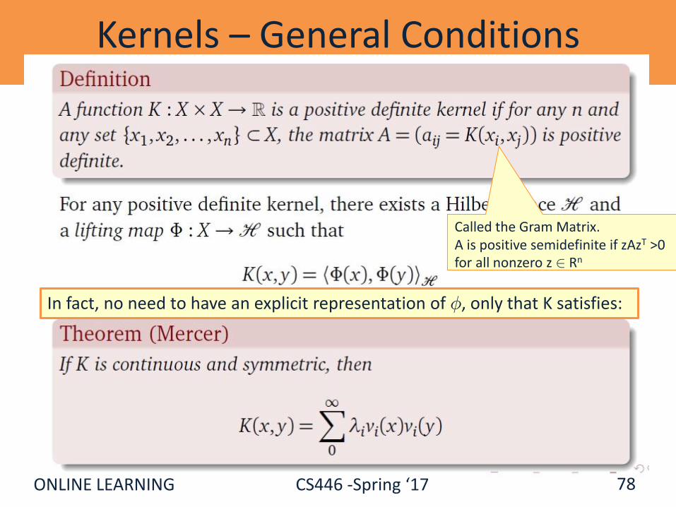
Kernels – General Conditions
Called the Gram Matrix.A is positive semidefinite if zAzT >0 for all nonzero z 2 Rn
In fact, no need to have an explicit representation of Á, only that K satisfies:

ONLINE LEARNING CS446 -Spring ‘17
Polynomial kernels
Linear kernel: k(x, z) = xz
Polynomial kernel of degree d: k(x, z) = (xz)d
(only dth-order interactions)
Polynomial kernel up to degree d: k(x, z) = (xz + c)d (c>0)(all interactions of order d or lower)
81

ONLINE LEARNING CS446 -Spring ‘17
Constructing New Kernels
You can construct new kernels k’(x, x’) from existing ones:
Multiplying k(x, x’) by a constant c:k’(x, x’) = ck(x, x’)
Multiplying k(x, x’) by a function f applied to x and x’: k’(x, x’) = f(x)k(x, x’)f(x’)
Applying a polynomial (with non-negative coefficients) to k(x, x’): k’(x, x’) = P( k(x, x’) ) with P(z) = ∑i aiz
i and ai≥0
Exponentiating k(x, x’):k’(x, x’) = exp(k(x, x’))
82
ONLINE LEARNING CS446 -Spring ‘17
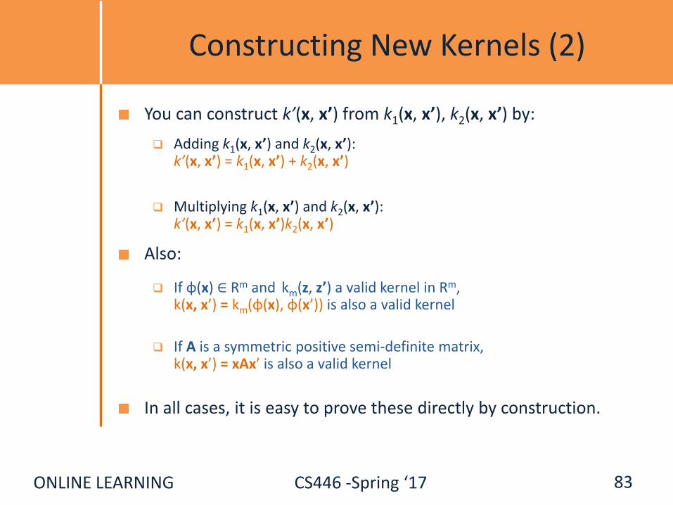
Constructing New Kernels (2)
You can construct k’(x, x’) from k1(x, x’), k2(x, x’) by:
Adding k1(x, x’) and k2(x, x’):k’(x, x’) = k1(x, x’) + k2(x, x’)
Multiplying k1(x, x’) and k2(x, x’):k’(x, x’) = k1(x, x’)k2(x, x’)
Also:
If φ(x) ∈ Rm and km(z, z’) a valid kernel in Rm, k(x, x’) = km(φ(x), φ(x’)) is also a valid kernel
If A is a symmetric positive semi-definite matrix, k(x, x’) = xAx’ is also a valid kernel
In all cases, it is easy to prove these directly by construction.
83

ONLINE LEARNING CS446 -Spring ‘17
Gaussian Kernel (aka radial basis function kernel)
k(x, z) = exp(−(x − z)2/c) (x − z)2: squared Euclidean distance between x and z
c = σ2: a free parameter
very small c: K ≈ identity matrix (every item is different)
very large c: K ≈ unit matrix (all items are the same)
k(x, z) ≈ 1 when x, z close
k(x, z) ≈ 0 when x, z dissimilar
84

ONLINE LEARNING CS446 -Spring ‘17
Gaussian Kernel
k(x, z) = exp(−(x − z)2/c)
Is this a kernel?
k(x, z) = exp(−(x − z)2/2σ2)
= exp(−(xx + zz − 2xz)/2σ2)
= exp(−xx/2σ2)exp(xz/σ2) exp(−zz/2σ2)
= f(x) exp(xz/σ2) f(z)
exp(xz/σ2) is a valid kernel: xz is the linear kernel;
we can multiply kernels by constants (1/σ2)
we can exponentiate kernels
Unlike the discrete kernels discussed earlier, here you cannot easily explicitly blow up the feature space to get an identical representation.
85

ONLINE LEARNING CS446 -Spring ‘17 87
A method to run Perceptron on a very large feature set, without incurring the cost of keeping a very large weight vector.
Computing the weight vector can be done in the original feature space.
Notice: this pertains only to efficiency: the classifier is identical to the one you get by blowing up the feature space.Generalization is still relative to the real dimensionality (or, related properties).Kernels were popularized by SVMs but apply to a range of models, Perceptron, Gaussian Models, PCAs, etc.
Summary – Kernel Based Methods
M f(x)
zz))S(z)K(x,(Th
ONLINE LEARNING CS446 -Spring ‘17
Efficiency-Generalization Tradeoff
There is a tradeoff between the computationalefficiency with which these kernels can be computed and the generalization ability of the classifier.
For example, using such kernels the Perceptronalgorithm can make an exponential number ofmistakes even when learning simple functions.[Khardon,Roth,Servedio,NIPS’01; Ben David et al.]
In addition, computing with kernels depends stronglyon the number of examples. It turns out thatsometimes working in the blown up space is moreefficient than using kernels. [Cumby,Roth,ICML’03]
88

ONLINE LEARNING CS446 -Spring ‘17
Explicit & Implicit Kernels: Complexity
Is it always worthwhile to define kernels and work in the dual space?
Computationally: [Cumby,Roth 2003]
Dual space – t1 m2 vs, Primal Space – t2 m
Where m is # of examples, t1, t2 are the sizes of the (Dual, Primal) feature spaces, respectively.
Typically, t1 << t2, so it boils down to the number of examples one needs to consider relative to the growth in dimensionality.
Rule of thumb: a lot of examples use Primal space
Most applications today: People use explicit kernels. That is, they blow up the feature space explicitly.
89

ONLINE LEARNING CS446 -Spring ‘17
Kernels: Generalization
Do we want to use the most expressive kernels we can? (e.g., when you want to add quadratic terms, do you really
want to add all of them?)
No; this is equivalent to working in a larger feature space, and will lead to overfitting.
Here is a simple argument that shows that simply adding irrelevant features does not help.
90

ONLINE LEARNING CS446 -Spring ‘17 91
Kernels: Generalization(2)
Given: A linearly separable set of points S={x1,…xn} 2 Rn with separator w 2 Rn
Embed S into a higher dimensional space n’>n , by adding zero-mean random noise e to the additional dimensions.
Then w’ ¢ x’= (w,0) ¢ (x,e) = w ¢ x
So w’ 2 Rn’ still separates S.
We will now look at °/||x|| which we have shown to be inversely proportional to generalization (and mistake bound).
(S, w’)/||x’|| = minS w’T x’ / ||w’|| ||x’|| =
minS wT x /||w|| ||x’|| < (S, w’)/||x||
Since ||x’|| = ||(x,e)|| > ||x||
The new ratio is smaller, which implies generalization suffers.
Intuition: adding a lot of noisy/irrelevant features cannot help

ONLINE LEARNING CS446 -Spring ‘17 92
Conclusion- KernelsThe use of Kernels to learn in the dual space is an important idea Different kernels may expand/restrict the hypothesis space in useful ways.
Need to know the benefits and hazards
To justify these methods we must embed in a space much larger than the training set size. Can affect generalization
Expressive structures in the input data could give rise to specific kernels, designed to exploit these structures. E.g., people have developed kernels over parse trees: corresponds to
features that are sub-trees.
It is always possible to trade these with explicitly generated features, but it might help one’s thinking about appropriate features.

ONLINE LEARNING CS446 -Spring ‘17
Functions Can be Made Linear
Data are not linearly separable in one dimension
Not separable if you insist on using a specific class of functions
x
93

ONLINE LEARNING CS446 -Spring ‘17
Blown Up Feature Space
Data are separable in <x, x2> space
x
x2
94

ONLINE LEARNING CS446 -Spring ‘17
Multi-Layer Neural Network
Multi-layer network were designed to overcome the computational (expressivity) limitation of a single threshold element.
The idea is to stack several
layers of threshold elements,
each layer using the output of
the previous layer as input.
Multi-layer networks can represent arbitrary functions, but building effective learning methods for such network was [thought to be] difficult.
95
activation
Input
Hidden
Output

ONLINE LEARNING CS446 -Spring ‘17
Basic Units
Linear Unit: Multiple layers of linear functions oj = w ¢ x produce linear functions. We want to represent nonlinear functions.
Need to do it in a way that
facilitates learning
Threshold units: oj = sgn(w ¢ x)
are not differentiable, hence
unsuitable for gradient descent.
The key idea was to notice that the discontinuity of the threshold element can be represents by a smooth non-linear approximation: oj = [1+ exp{-w ¢ x}]-1
(Rumelhart, Hinton, Williiam, 1986), (Linnainmaa, 1970) , see: http://people.idsia.ch/~juergen/who-invented-backpropagation.html )
96
activation
Input
Hidden
Output
w2ij
w1ij

ONLINE LEARNING CS446 -Spring ‘17
Model Neuron (Logistic)
Us a non-linear, differentiable output function such as the sigmoid or logistic function
Net input to a unit is defined as:
Output of a unit is defined as:
97
iijj xwnet
)T(netjjje1
1O
jT
1
2
6
3
4
5
7
67w
17w
T
jO
1x
7x

ONLINE LEARNING CS446 -Spring ‘17
Learning with a Multi-Layer Perceptron
It’s easy to learn the top layer – it’s just a linear unit.
Given feedback (truth) at the top layer, and the activation at the layer below it, you can use the Perceptron update rule (more generally, gradient descent) to updated these weights.
The problem is what to do with
the other set of weights – we do
not get feedback in the
intermediate layer(s).
98
activation
Input
Hidden
Output
w2ij
w1ij

ONLINE LEARNING CS446 -Spring ‘17
Learning with a Multi-Layer Perceptron
The problem is what to do with
the other set of weights – we do
not get feedback in the
intermediate layer(s).
Solution: If all the activation
functions are differentiable, then
the output of the network is also
a differentiable function of the input and weights in the network.
Define an error function (multiple options) that is a differentiable function of the output, that this error function is also a differentiable function of the weights.
We can then evaluate the derivatives of the error with respect to the weights, and use these derivatives to find weight values that minimize this error function. This can be done, for example, using gradient descent .
This results in an algorithm called back-propagation.
99
activation
Input
Hidden
Output
w2ij
w1ij