No. 6 June 2008 StaffPAPERS - Federal Reserve Bank of ... FEDERAL RESERVE BANK OF DALLAS The...

StaffPAPERSFEDERAL RESERVE BANK OF DALLAS

The Relative Performance of Alternative Taylor Rule Specifications

Adriana Z. FernandezEvan F. Koenig

and Alex Nikolsko-Rzhevskyy

No. 6June 2008

StaffPAPERS is published by the Federal Reserve Bank of Dallas. The views expressed are those of the authors and should not be attributed to the Federal Reserve Bank of Dallas or the Federal Reserve System. Articles may be reprinted if the source is credited and the Federal Reserve Bank of Dallas is provided a copy of the publication or a URL of the website with the material. For permission to reprint or post an article, e-mail the Public Affairs Department at [email protected].

Staff Papers is available free of charge by writing the Public Affairs Department, Federal Reserve Bank of Dallas, P.O. Box 655906, Dallas, TX 75265-5906; by fax at 214-922-5268; or by phone at 214-922-5254. This publication is available on the Dallas Fed website, www.dallasfed.org.

StaffPAPERS Federal Reserve Bank of Dallas

The Relative Performance of Alternative Taylor Rule Specifications

Adriana Z. FernandezResearch Economist

Federal Reserve Bank of Dallas

Evan F. KoenigVice President and Senior Policy Advisor

Federal Reserve Bank of Dallas

and

Alex Nikolsko-RzhevskyyAssistant Professor

University of Memphis

AbstractWe look at how well several alternative Taylor rule specifications de-

scribe Federal Reserve policy decisions in real time, using the newly de-veloped Giacomini and Rossi (2007) test for non-nested model selection in the presence of (possible) parameter instability. Further, we isolate those Taylor rule features that are most important for achieving relatively strong real-time performance. A second-order partial adjustment version of the Koenig (2004a) model performs consistently better than alternative specifications. Key features of this rule are the partial adjustment of the federal funds rate toward an equilibrium rate that depends on the unem-ployment rate and forward-looking inflation measures.

JEL codes: E52, E47, C52 Keywords: Taylor rule, non-nested model selection, real-time data

No. 6, June 2008

StaffP

APER

S Fe

deral

Reser

ve Ba

nk of

Dalla

s

2

Monetary policy prescriptions can be either instrument rules or tar-geting rules. Instrument rules specify the value of the central bank’s

policy instrument (for the United States, either the federal funds rate or nonborrowed bank reserves) as a function of observable economic condi-tions. Targeting rules, in contrast, specify a desired relationship between variables over which the monetary authority has only indirect and im-perfect control. These models call for the monetary authority to adjust its policy instrument as necessary to maintain the desired relationship as closely as possible.1 Instrument rules are more straightforward to imple-ment than targeting rules, but they can also be more fragile because the economic outcomes delivered by a given instrument rule are often sensi-tive to small changes in the links between the instrument and the real economy. This sensitivity raises the possibility that an instrument rule that describes policy choices well over one sample period will perform poorly in other periods.

In this paper, we examine the comparative performance of several monetary policy instrument rules, using a test designed precisely for situ-ations in which there may be parameter instability to which instrument rules are vulnerable (Giacomini and Rossi 2007). The rules we test are all broadly considered Taylor rules (Taylor 1993; Henderson and McKibbin 1993). A Taylor rule is an equation prescribing the federal funds rate as a function of economic slack, inflation, and possibly other variables. A rule of this general form describing Federal Reserve policy is intuitively plau-sible. The Fed has a dual mandate to seek full employment and price sta-bility, and the Federal Open Market Committee (FOMC) has formulated policy in terms of the federal funds rate for almost twenty-five years. We start by presenting the several commonly used versions of the Taylor rule that are examined empirically in this paper. Next, we review the Giaco-mini and Rossi methodology. The core of the paper is Section 3, in which we use the Giacomini–Rossi test to compare the different rules’ ability to explain the behavior of the federal funds rate over the last twenty years and try to identify the specific features that are most important for suc-cessful performance.

Many real-world economic data are subject to ex post revisions. Revi-sions can be substantial and, for some important variables, extend back many years. They are problematic because economic relationships some-times look very different using final data than they do in first-release or once-revised data. For our performance comparison to be meaningful, it is essential that the data used for estimation of each policy rule be limited to what would have been available to a policymaker or economic analyst at the time the policy decisions were made (Orphanides 2001, 2003). We use such real-time data throughout our analysis.

Results suggest that gradualism—a tendency to avoid large, sudden

1 Simple examples of targeting rules include: (1) Milton Friedman’s prescription for constant growth of a broad monetary aggregate (Friedman 1960); (2) rules that call for constant growth in nominal gross domestic product (nominal GDP) or some other measure of nominal spending (Bean 1983; Hall and Mankiw 1994); (3) rules that call for a constant rate of inflation, or for a prespecified inflation path (Berg and Jonung 1999).


3

moves in the funds rate—should be included in the Taylor rule for optimal descriptive performance, while preemption—responding to forecasts of in-flation and slack rather than to past and current measures—is important for inflation measures but not for slack. Also, we find that the unemploy-ment gap seems to be a better measure of current economic slack than the output gap and that the Blue Chip inflation forecast (as used in Koenig 2004a) is a better measure of inflation expectations than the Survey of Professional Forecasters’ inflation forecast.2

1. TAYLOR RULES

The Original Taylor RuleThe original Taylor rule takes the form

(1) it=r*+ πt+δ(πt−πT )+w(yt–y*t)

or, equivalently,

(2) it= µ + (1+δ)πt+w(yt–y*t),

where it , πt, yt , and y* are the overnight lending rate, GDP inflation, (logs of) real GDP, and a measure of trend or potential real GDP, respectively; where r* and πT are the equilibrium real interest rate and the Fed’s im-plicit long-run inflation target (both assumed to be 2 percent); where µ ≡r*−δπT is a constant term that combines parameters that are not separately identifiable from estimation of the Taylor rule alone; and where δ and w are parameters that measure the strength of the Fed’s response to deviations of inflation from target and of output from potential. Given the Fed’s mandate to promote both price stability and full resource uti-lization, one would expect to find δ, w>0 so that the Fed drives the real funds rate (it −πt) above the equilibrium real rate (making policy “tight”) when inflation is unacceptably high and/or output is unsustainably high. Approximate and sometimes exact forms of these rules are the best option under the assumption that a central bank has a quadratic loss function over inflation and output gap and the variability of short-term interest rates. (See Svensson 1999 and Woodford 2001, among others.)

Variants and ExtensionsThe original Taylor rule has several potential weaknesses. First, there

is ambiguity about how best to measure inflation. The original Taylor rule used the GDP deflator for this purpose, but there is no compelling theoretical argument for policymakers to prefer this measure to, for ex-ample, the deflator for personal consumption expenditures (PCE). On grounds of practicality, one can also make a case for the Consumer Price Index (CPI). It is familiar to the public, available with only a small delay, and—unlike the GDP and PCE deflators—is not subject to large ex post

2 Koenig uses the Blue Chip Economic Indicators consensus forecast of CPI inflation before 2000 and of GDP price inflation from 2000 to present.

StaffP

APER

S Fe

deral

Reser

ve Ba

nk of

Dalla

s

4

revisions when expenditure weights are updated. Then there is the ques-tion of whether it is best to use the all-inclusive headline inflation number or a core inflation rate that excludes certain goods and services. It is not always obvious which inflation measure policymakers choose to watch, and there is no guarantee that their choice will not change over time.

The ambiguity about how to measure economic slack for policy pur-poses is at least as great as that for inflation statistics. The potential-output variable that is the key to calculating output gap in the original Taylor rule is notoriously difficult to estimate, particularly in real time (Mishkin 2007; Wynne and Solomon 2007; Solow and Taylor 2001; Or-phanides and van Norden 2005; van Norden 1995; Cayen and van Norden 2005; Watson 2007). Measures of economic slack based on the unemploy-ment rate have been developed, but they remain controversial. Typically, they involve comparing the actual unemployment rate to an estimate of the nonaccelerating inflation rate of unemployment, or NAIRU, which is not directly observed. Solow notes that a 1 percentage point increase in the unemployment rate corresponds to about 1.25 million jobs (equivalent to about a 2 percent increase in GDP), concluding that small errors in policymakers’ estimates of the NAIRU can have huge economic implica-tions (Solow and Taylor 2001). It is sobering, then, that Staiger, Stock, and Watson (1997) estimate that a typical 95 percent confidence interval for the NAIRU is on the order of 2.5 percentage points wide. Here, again, the exact variable that policymakers monitor is ambiguous, their choice may change over time, and the use of real-time data is critical.

Another issue relates to the speed with which the Fed adjusts its policy instrument in response to new information on inflation and slack. Researchers have found that the Federal Reserve tends to move incre-mentally, in a series of small or moderate steps in the same direction—a process called interest rate smoothing, or gradualism. Gradualism is a way to exercise caution in policymaking because it allows policymakers to assess their approach and make adjustments if necessary. It is usually modeled by including one or more lagged values of the federal funds rate as right-hand-side variables in the Taylor rule equation. The greater the combined weight on the lagged funds rates, the more drawn out are policy responses.

Some of what appears to be gradualism may actually be a symptom of misspecification (Rudebusch 2006; Lansing 2002; Nikolsko-Rzhevskyy 2008). That is, policy decisions in part could be based on slowly moving economic variables that the analyst has mistakenly excluded from the right-hand side of the Taylor rule. In some countries, for example, policy appears to depend on exchange rates in addition to inflation and slack (Clarida, Galí, and Gertler 1998; Molodtsova, Nikolsko-Rzhevskyy, and Papell 2007; Gerberding, Seitz, and Worms 2005). In the United States, however, evidence of exchange rate effects is weak. Analysts have had bet-ter luck with measures of output growth and changes in slack (Orphanides 2003; Koenig 2004a). Another potentially excluded variable is a measure of expectations. Given the long lags with which policy actions are thought to be reflected in real activity and inflation, it may make sense for poli-cymakers to be more concerned about near-term outlooks for slack and


5

inflation than current levels (Clarida, Galí, and Gertler 1998; Galí and Gertler 2000; Clarida, Galí, and Gertler 2000; Galí, Gertler, and Lopez-Salido 2001). It certainly is not uncommon to hear policymakers talk of preemptive action to prevent building inflation pressures from manifest-ing themselves as actual increases in inflation. Orphanides (2003) cites the statement from the Federal Reserve Board of Governors’ first annual report, from 1914, which says that a Reserve Bank’s duty “is not to await emergencies but by anticipation, to do what it can to prevent them.” Thus, to control inflation, the policy instrument should respond to deviations of the inflation forecast from the target (Taylor and Davradakis 2006).

The models included in our analysis span the evolution of the Taylor rule, including its most representative variants and extensions. We chose models with different measures of inflation and slack, different speeds of adjustment, and preemptive versus reactive policies. To emulate the policymaker’s situation, we use real-time data in all of the models, imply-ing a one-quarter lag (the time it takes for initial data releases). We use real-time quarterly data from the first quarter of 1988 to the first quarter of 2006.3

We begin by defining a general model that encompasses the tradi-tional backward-looking Taylor rule in Table 1. Since the first three mod-els can be expressed as special cases of Molodtsova, Nikolsko-Rzhevskyy, and Papell (2007), or MNRP, we use MNRP as a baseline to test the validity of its distinctive elements. These include using deviation of GDP from a quadratic trend as the measure of current slack, first-order partial

Table 1: Traditional Backward-Looking Taylor Models

Monetary rule Description

Taylor (1993) it= µ+(1+δ)πt+ wyt

Inflation: Current GDP deflatorCurrent slack: Deviation of GDP from a linear time trendInflation (δ) and GDP gap (w) coefficients fixed at 0.5

Taylor A it= (1−ρ){µ + (1+0.5)πt+0.5yt }+ρit –1

Defined as above with first-order partial adjustment

Taylor B it= µ +(1+δ)πt+ wyt

Defined as Taylor (1993) with estimated inflation (δ) and GDP gap (w) coefficients

MNRP (2007) it= (1−ρ){µ + (1+δ)πt+wyt}+ρit –1

Inflation: Year-over-year percent change in the GDP deflatorCurrent slack: Deviation of real GDP from a quadratic time trendFirst-order partial adjustment

NOTES: Model descriptions are not as authors originally specified. Some were modified to adhere to the strict use of real-time data. The MNRP model is only one backward-looking specification considered in Molodtsova, Nikolsko-Rzhevskyy, and Papell (2007). Refer to the original papers for details.

3 For details on data and sources, see Appendix A.

StaffP

APER

S Fe

deral

Reser

ve Ba

nk of

Dalla

s

6

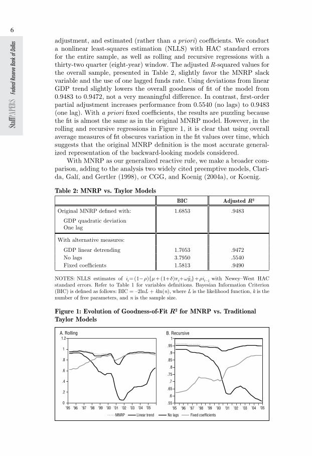
adjustment, and estimated (rather than a priori) coefficients. We conduct a nonlinear least-squares estimation (NLLS) with HAC standard errors for the entire sample, as well as rolling and recursive regressions with a thirty-two quarter (eight-year) window. The adjusted R-squared values for the overall sample, presented in Table 2, slightly favor the MNRP slack variable and the use of one lagged funds rate. Using deviations from linear GDP trend slightly lowers the overall goodness of fit of the model from 0.9483 to 0.9472, not a very meaningful difference. In contrast, first-order partial adjustment increases performance from 0.5540 (no lags) to 0.9483 (one lag). With a priori fixed coefficients, the results are puzzling because the fit is almost the same as in the original MNRP model. However, in the rolling and recursive regressions in Figure 1, it is clear that using overall average measures of fit obscures variation in the fit values over time, which suggests that the original MNRP definition is the most accurate general-ized representation of the backward-looking models considered.

With MNRP as our generalized reactive rule, we make a broader com-parison, adding to the analysis two widely cited preemptive models, Clari-da, Galí, and Gertler (1998), or CGG, and Koenig (2004a), or Koenig.

Table 2: MNRP vs. Taylor ModelsBIC Adjusted R2

Original MNRP defined with:

GDP quadratic deviationOne lag

1.6853 .9483

With alternative measures:

GDP linear detrending 1.7053 .9472No lags 3.7950 .5540Fixed coefficients 1.5813 .9490

NOTES: NLLS estimates of it= (1−ρ){µ + (1+δ)πt+wyt}+ρit –1 with Newey–West HAC standard errors. Refer to Table 1 for variables definitions. Bayesian Information Criterion (BIC) is defined as follows: BIC = –2lnL + kln(n), where L is the likelihood function, k is the number of free parameters, and n is the sample size.

Figure 1: Evolution of Goodness-of-Fit R2 for MNRP vs. Traditional Taylor Models

0

.2

.4

.6

.8

1

1.2

’95 ’96 ’97 ’98 ’99 ’00 ’01 ’02 ’03 ’04 ’05

A. Rolling

.55

.6

.65

.7

.75

.8

.85

.9

.95

1

’95 ’96 ’97 ’98 ’99 ’00 ’01 ’02 ’03 ’04 ’05

B. Recursive

MNRP Linear trend No lags Fixed coefficients


7

The three rules considered all take the general form

(3) it= (1−ρ1−ρ2)[µ + (1+δ) πet+f +wst +β(se

t+f −st)]+ρ1it –1+ρ2it –2 ,

where st is some measure of real slack; πet+f and se

t+f are the inflation rate and slack that policymakers expect f periods hence; where 0≤ρ1+ρ2<1; β, w≥0; and δ>0. However, each model imposes different restrictions on the parameters in equation 3 and uses different measures of inflation and slack.4

In the original version, the restrictions for the MNRP model are ρ2= β = f = 0; for CGG, β = 0 and f = 4; and for Koenig, ρ2= 0 and f = 4. An obvious distinction between the CGG model and MNRP and Koenig is the presence of a second-order partial adjustment in the first model. Given the evidence presented in CGG supporting the use of two lagged values of the federal funds rate, we test whether these models behave better with first- or second-order partial adjustment. We conduct a NLLS estimation for the whole sample, as well as rolling and recursive regressions with a thirty-two quarter (eight-year) window for each model, comparing the re-sults for one and two lags. The NLLS results (Table 3) show that our three real-time models are slightly better specified, on average, with two federal funds lags. These results are supported by the goodness-of-fit estimations for the rolling and recursive regressions, which all favor the use of two lags. So, we include two lags in all our real-time rules.

Table 3: First- vs. Second-Order Partial Adjustment CoefficientsOverall regression One lag (ρ) Two lags (ρ1/ρ2)

MNRP Coefficient .9530 1.5898 / –.6372

Std error .0533 .1139 / .1031

t statistic 17.8527 13.9476 / –6.1803

p value .0000 .0000 / .0000

Adjusted R2 .9483 .9683

CGG Coefficient .7639 1.3511 / –.5127

Std error .0554 .1125 / .1018

t statistic 13.7912 12.0081 / – 5.0350

p value .0000 .0000 / .0000

Adjusted R2 0.9623 .9725

Koenig Coefficient .7237 1.1941 / –.4192

Std error .6999 .1346 / .1024

t statistic 10.3411 8.8691 / –4.0952

p value .0000 .0000 / .0001

Adjusted R2 .9699 .9765

NOTE: NLLS estimates with Newey–West HAC standard errors.

4 For details of the models, see Table 4.

StaffP

APER

S Fe

deral

Reser

ve Ba

nk of

Dalla

s

8

Table 4 shows the second-order partial adjustment definitions for the models, along with their parameter restrictions. Figure 2 shows the good-ness of fit of these partially modified rules. While on the whole, the models poorly in 2001–02, when the funds rate was cut by over 5 percentage points in response to the dot-com bust and 9/11 attacks. We believe this irregularity is due to the fact that the Fed reacts to information not cap-tured by any of these models. Moreover, it does not react in a mechanical way.

Table 4: Taylor Rules Examined

General form it= (1−ρ1−ρ2)[µ + (1+δ) πet+f +wst +β(se

t+f −st)]+ρ1it –1+ρ2it –2

Description

Modified MNRPMolodtsova, Nikolsko-Rzhevskyy,and Papell (2007)

With second-order partial adjustment: β = f = 0Backward lookingInflation: Year-over-year percent change in the GDP deflatorCurrent slack: Deviation of real GDP from a quadratic time trend

CGG Clarida, Galí, andGertler (1998)

With second-order partial adjustment: β = 0, f = 4Forward lookingInflation: Blue Chip four-quarter GDP price inflation forecast*Current slack: Deviation of industrial production from a qua-dratic time trend

Modified Koenig Koenig (2004a)

With second-order partial adjustment: f = 4Forward lookingInflation: Blue Chip inflation forecast (uses CPI until 1998 and GDP deflator from 1999 on)Current slack: Difference between the current and natural rates of unemployment**Anticipated change in slack: Difference between the Blue Chip GDP growth forecast and a five-year average of the GDP growth rate

* Originally, authors used actual future one-year-hence inflation as a measure of expected inflation; we substitute to preserve the real-time nature of the analysis.

** Unemployment gap is defined as the current unemployment rate minus the moving average of the unemployment rate for the previous five years, as in Kim and Ogaki (2008). This specification makes its sign consistent with that of the conventional output gap.

NOTES: Model descriptions are not as authors originally specified. Some were modified to adhere to the strict use of real-time data. Refer to the original papers for details.

The goodness-of-fit test gives us an idea of how the models perform in-dependently, but it does not tell us how they compare with each other, which is a more interesting question and a more relevant one from a policymaking perspective. Models may not be correctly specified, their parameters may not be stable over time, and the measures of inflation, output, and unem-ployment that feed into the rules may not be accurately estimated. These are problems that need to be assessed in an in-depth model comparison.


9

Figure 2: Evolution of Goodness-of-Fit R2 for First- vs. Second-Order Partial Adjustment of Three Models

.7

.75

.8

.85

.9

.95

1

MNRP 1 lag MNRP 2 lags CGG 1 lag CGG 2 lags Koenig 1 lag Koenig 2 lags

’95 ’96 ’97 ’98 ’99 ’00 ’01 ’02 ’03 ’04 ’05

A. Rolling

’95 ’96 ’97 ’98 ’99 ’00 ’01 ’02 ’03 ’04 ’05

B. Recursive

.91

.92

.93

.94

.95

.96

.97

.98

.99

NOTE: For model descriptions, refer to Table 4.

2. METHODOLOGYInstrument rules in general may be fragile in that the economic out-

comes they predict are often sensitive to small changes in links between the instrument and the real economy. This raises the possibility that an instrument rule that well describes policy choices in one sample period will perform poorly in others. This important issue is ignored by traditional non-nested model selection techniques, which evaluate models based on how well they fit the full sample of data or whether they forecast better on average.

The possibility that structural instability and model misspecification may hide time-varying differences has important implications in policy-making, and it had not been formally considered until recently, in the Giacomini–Rossi (2007) fluctuation test for non-nested model selection in unstable environments. We apply this technique to evaluate the per-formance of our three models; it allows us to monitor the relative per-formance of two competing models at every time period, in sequences of test statistics over expanding and rolling samples. The test also provides confidence-interval boundary lines under the null hypothesis that both models perform equally well in every period. Therefore, instability is de-tected when any of the test statistics cross the boundary lines.

Our objective is to select, among the three real-time models in Ta-ble 4, the Taylor rule version that best describes the historical behavior of the federal funds rate, it . The models use a variety of measures of current and expected inflation and output, and all incorporate two lags of the fed-eral funds rate. We denote these variables as zt and define xt= (i′t , z ′t )′ . For details on the variables used in these models, refer to Appendix A.5 For any pair of competing models, we recursively obtain the maximum likeli-hood (ML) estimates at each time t and use them to construct statistics for the Giacomini–Rossi test.

5 Notation and the majority of derivation are taken directly from Giacomini and Rossi (2006), the more extended, older version of Giacomini and Rossi (2007).

StaffP

APER

S Fe

deral

Reser

ve Ba

nk of

Dalla

s

10

The in-sample fluctuation test is performed by examining historical sample data from time t=1(first quarter 1988) to t = T =73 (first quarter 2006). The values of objective functions Qt for models 1 and 2 are calculated recursively beginning with observation R = 32 (for an eight-year window), using both expanding samples of sizes R,R+1, …,T −1, T and rolling samples of size R:

Rolling Recursive

Model 1R j

t=t−R+1∑1Qt(θ�)= ln f(xj,θ�t) t j

t=1∑1Qt(θ�)= ln f(xj,θ�t)

Model 2R j

t=t−R+1∑1Qt(γ�)= ln f(xj,γ�t) Qt(γ�)= ln f(xj,γ�t),t j

t=1∑1

where parameters θ(p×1)∈Θ for model 1 and γ(q×1)∈Γ for model 2, and

(4) θt = arg max Qt(θ) and γt = arg max Qt(γ).

Here, ln f (xj , θt ) and ln f (xj, γt ) are the conditional log likelihoods at time j for models 1 and 2, respectively.6 Denoting θ*

t and γ*t as the

pseudo-true values of the parameter estimates (which may differ in differ-ent samples due to possible data instability), we test the null hypothesis that Q*

t (θ*t )−Q*

t (γ*t )= 0 for all t = 1,…,T by considering a sequence of

recursive estimates of the average relative performance of Qt(θt )−Qt(γt )for t =R,…,T . The starting period is t =R=32 (eight years), and at each time t, we further normalize the average relative performance by its standard deviation, or the square root of the variance σ 2

t of the rescaled relative fit, which is evaluated at the pseudo-true values of the parameter estimates as follows:7

(5) σ θ γt t t t tvar t Q Q2 = −( )( ( ) ( ))* * .

Then the statistics, appropriately normalized, are recursively esti-mated as

(6) FtRolling= σ t

–1 R(Qt(θ�t)–Qt(γ�t)) and FtRecursive= σ t

–1 t(Qt(θ�t)–Qt(γ�)) .

The sample path of the recursively estimated measures tells us about

6 It is assumed that the data-generating process is unknown and allowed to vary over time and that data are weakly dependent.

7 For details on the derivation of the variance estimator σ 2t , see Appendix B.


11

their performance over time.8 The procedure allows us to test whether this observed path departs from the hypothesized path by plotting them together with boundary lines that are crossed with probability α. For the rolling case, the critical value at time t for significance level α is

(7) c ktRolling Rollingα α, = ±

and, for the recursive case, it becomes

(8) c k T Rt

t RT Rt

Recursive Recursiveα α, =±

−+

−−

1 2

,

where k corresponds to the values for a 10 percent confidence interval, 2.600 and 0.850 for the rolling and recursive estimations, respectively.9

3. RESULTS

Model ComparisonWe start by comparing the performance of Koenig to that of the other

two rules. Figure 3 presents the results of the Giacomini–Rossi rolling and recursive tests and shows the 10 percent critical bands (shaded area).

Figure 3: Results of Rolling and Recursive Giacomini–Rossi (2007) Tests

K-CGG K-MNRP

’95 ’96 ’97 ’98 ’99 ’00 ’01 ’02 ’03 ’04 ’05 ’95 ’96 ’97 ’98 ’99 ’00 ’01 ’02 ’03 ’04 ’05–3

–2

–1

0

1

2

3

4A. Rolling B. Recursive

–4

–3

–2

–1

0

1

2

3

4

5

NOTE: Baseline model is modified Koenig, which uses Blue Chip inflation forecast and unemployment for current slack.

Values above the upper band mean that the base model performs better

8 Traditional non-nested model selection techniques determine performance based on overall averages for the entire sample, which would correspond to the last point in the Giacomini–Rossi test. So, if a policymaker were to select a model in this context, he or she would do it by looking at the latest overall average. The Giacomini–Rossi test shows the sample path of relative performance of the models, which contains more information.

9 The approximate critical value for the rolling test is based on R/T 0.44. We decided that a 10 percent confidence interval is more appropriate than the more common 5 percent, given the small sample of seventy-two quarters.

The in-sample fluctuation test is performed by examining historical sample data from time t=1(first quarter 1988) to t = T =73 (first quarter 2006). The values of objective functions Qt for models 1 and 2 are calculated recursively beginning with observation R = 32 (for an eight-year window), using both expanding samples of sizes R,R+1, …,T −1, T and rolling samples of size R:

Rolling Recursive

Model 1

Model 2

where parameters θ(p×1)∈Θ for model 1 and γ(q×1)∈Γ for model 2, and

(4) θt = arg max Qt(θ) and γt = arg max Qt(γ).

Here, ln f (xj , θt ) and ln f (xj, γt ) are the conditional log likelihoods at time j for models 1 and 2, respectively.6 Denoting θ*

t and γ*t as the

pseudo-true values of the parameter estimates (which may differ in differ-ent samples due to possible data instability), we test the null hypothesis that Q*

t (θ*t )−Q*

t (γ*t )= 0 for all t = 1,…,T by considering a sequence of

recursive estimates of the average relative performance of Qt(θt )−Qt(γt )for t =R,…,T . The starting period is t =R=32 (eight years), and at each time t, we further normalize the average relative performance by its standard deviation, or the square root of the variance σ 2

t of the rescaled relative fit, which is evaluated at the pseudo-true values of the parameter estimates as follows:7

(5) .

Then the statistics, appropriately normalized, are recursively esti-mated as

(6) .

The sample path of the recursively estimated measures tells us about

6 It is assumed that the data-generating process is unknown and allowed to vary over time and that data are weakly dependent.

7 For details on the derivation of the variance estimator σ 2t , see Appendix B.

StaffP

APER

S Fe

deral

Reser

ve Ba

nk of

Dalla

s

12

than the competing model, values within the bands mean that the mod-els perform equally well, and values below the lower band mean that the competing model outperforms the base model.

In the recursive test, Koenig is superior to MNRP at every point in time, except for a couple of quarters at the end of 2000, when both models perform equally well. Koenig is also superior to CGG before 2000, al-though CGG seems to be slightly stronger than MNRP. After 2000, CGG and Koenig perform statistically the same. The results of the rolling test lead to a similar conclusion, although the superiority of Koenig is not as overwhelming as in the recursive regression. MNRP performs about the same as Koenig from 1996 to 2004.

Table 5 quantifies the results of both the rolling and recursive tests presented in Figure 3. Overall, we see that our baseline model, Koenig, outperforms the other models.

Table 5: Giacomini–Rossi Test Results: Rolling and Recursive Baseline model: Modified Koenig Inflation: Blue Chip forecast Slack measure: Unemployment gap

Percentage of time the base model outperforms a

competitor model

Percentage of time a competitor model outperforms the

base model

Competitor model

Total percentage

Statistically significant

Total percentage


Rolling eight-year window

Modified MNRP 95.2 28.6 4.8 0

CGG 85.7 9.5 14.3 0

Recursive estimation

Modified Koenig 100.0 90.5 0 0

CGG 100.0 50.0 0 0

NOTE: For model descriptions, refer to Table 4.

Sensitivity AnalysisOur results suggest that Koenig’s model incorporates elements that

better depict the actual behavior of the federal funds rate. To further ana-lyze this model, we tweak it to assess each element’s marginal impact on performance. In an NLLS estimation with the entire sample (Table 6), we see that the unemployment rate and Blue Chip inflation forecast have highmarginal values. The change in slack provides the least benefit, having a very small effect on overall goodness of fit.


13

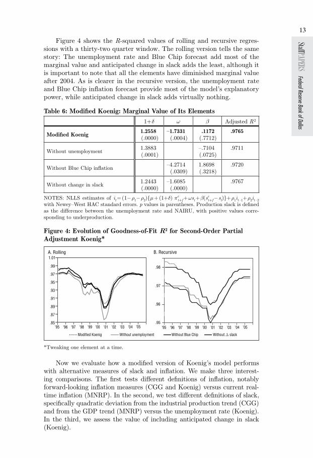
Figure 4 shows the R-squared values of rolling and recursive regres-sions with a thirty-two quarter window. The rolling version tells the same story: The unemployment rate and Blue Chip forecast add most of the marginal value and anticipated change in slack adds the least, although it is important to note that all the elements have diminished marginal value after 2004. As is clearer in the recursive version, the unemployment rate and Blue Chip inflation forecast provide most of the model’s explanatory power, while anticipated change in slack adds virtually nothing.

Table 6: Modified Koenig: Marginal Value of Its Elements1+δ w β Adjusted R2

Modified Koenig 1.2558 (.0000)

–1.7331(.0004)

.1172(.7712)

.9765

Without unemployment 1.3883 (.0001)

–.7104(.0725)

.9711

Without Blue Chip inflation –4.2714(.0309)

1.8698 (.3218)

.9720

Without change in slack 1.2443(.0000)

–1.6085(.0000)

.9767

NOTES: NLLS estimates of it= (1−ρ1−ρ2){µ + (1+δ) πet+f +wst +β(se

t+f −st)}+ρ1it –1+ρ2it –2 with Newey–West HAC standard errors. p values in parentheses. Production slack is defined as the difference between the unemployment rate and NAIRU, with positive values corre-sponding to underproduction.

Figure 4: Evolution of Goodness-of-Fit R2 for Second-Order Partial Adjustment Koenig*

Modified Koenig Without unemployment Without Blue Chip Without ∆ slack

’95 ’96 ’97 ’98 ’99 ’00 ’01 ’02 ’03 ’04 ’05 .85

.87

.89

.91

.93

.95

.97

.99

1.01

’95 ’96 ’97 ’98 ’99 ’00 ’01 ’02 ’03 ’04 ’05 .95

.96

.97

.98

A. Rolling B. Recursive

*Tweaking one element at a time.

Now we evaluate how a modified version of Koenig’s model performs with alternative measures of slack and inflation. We make three interest-ing comparisons. The first tests different definitions of inflation, notably forward-looking inflation measures (CGG and Koenig) versus current real-time inflation (MNRP). In the second, we test different definitions of slack, specifically quadratic deviation from the industrial production trend (CGG) and from the GDP trend (MNRP) versus the unemployment rate (Koenig). In the third, we assess the value of including anticipated change in slack (Koenig).

StaffP

APER

S Fe

deral

Reser

ve Ba

nk of

Dalla

s

14

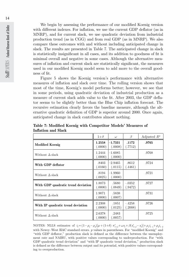
We begin by assessing the performance of our modified Koenig version with different indexes. For inflation, we use the current GDP deflator (as in MNRP), and for current slack, we use quadratic deviation from industrial production trend (as in CGG) and from real GDP (as in MNRP). We also compare these outcomes with and without including anticipated change in slack. The results are presented in Table 7. The anticipated change in slack is statistically insignificant in all cases, and its addition to goodness of fit is minimal overall and negative in some cases. Although the alternative mea-sures of inflation and current slack are statistically significant, the measures used in our modified Koenig model seem to add more to the overall good-ness of fit.

Figure 5 shows the Koenig version’s performance with alternative measures of inflation and slack over time. The rolling version shows that most of the time, Koenig’s model performs better; however, we see that in some periods, using quadratic deviation of industrial production as a measure of current slack adds value to the fit. After 2003, the GDP defla-tor seems to be slightly better than the Blue Chip inflation forecast. The recursive estimation clearly favors the baseline measure, although the alt-ernative quadratic definition of GDP is superior around 2000. Once again, anticipated change in slack contributes almost nothing.

Table 7: Modified Koenig with Competitor Models’ Measures of Inflation and Slack

1+δ w β Adjusted R2

Modified Koenig 1.2558(.0000)

–1.7331(.0008)

.1172(.7712)

.9765

Without ∆ slack 1.2444(.0000)

–1.6085(.0000)

.9768

With GDP deflator .8403 (.0160)

–2.9465(.0115)

.8612(.4461)

.9724

Without ∆ slack .8194(.0025)

–1.9960(.0000)

.9721

With GDP quadratic trend deviation 1.8873(.0000)

.5680(.0849)

–.0352(.9472)

.9727


.5838(.0007)

.9731

With IP quadratic trend deviation 2.2308 (.0000)

.1851(.0125)

–.4258(.2008)

.9726


.2483(.0057)

.9725

NOTES: NLLS estimates of it= (1−ρ1−ρ2)[µ + (1+δ) πet+f +wst +β(se

t+f −st)]+ρ1it –1+ρ2it –2 with Newey–West HAC standard errors. p values in parentheses. For “modified Koenig” and “with GDP deflator,” production slack is defined as the difference between the unemploy-ment rate and NAIRU, with positive values corresponding to underproduction. For “with GDP quadratic trend deviation” and “with IP quadratic trend deviation,” production slack is defined as the difference between output and its potential, with positive values correspond-ing to overproduction.


15

Figure 5: Evolution of Goodness-of-Fit R2 for Modified Koenig with Alternative Measures of Inflation and Slack

’95 ’96 ’97 ’98 ’99 ’00 ’01 ’02 ’03 ’04 ’05’95 ’96 ’97 ’98 ’99 ’00 ’01 ’02 ’03 ’04 ’05 .85

.87

.89

.91

.93

.95

.97

.99

1.01

.95

.96

.97

.98

.99

Modified Koenig GDP quadratic IP quadratic GDP deflator

A. Rolling B. Recursive

Measure ComparisonThe evidence so far suggests that our modified Koenig model in a par-

simonious setup (without expected change in slack) and the measures used to define it are the most accurate way to explain the federal funds rate.

We cannot be certain that his model—or any other, for that matter—is correctly specified or that the variables included are accurately mea-sured. We do know, however, that monetary policy rules’ performance varies as different inflation and output gap statistics are used, so we must extend our analysis to statistics other than those in the MNRP and CGG models to see if we can find superior alternatives.

Using only real-time data, we compare various measures of inflation and the output gap using the Giacomini–Rossi test in the same way we compare monetary policy models. We want to identify the most infor-mative variables to be used in the best Taylor rule possible. With the Giacomini–Rossi technique, we test the in-sample performance of different inflation and output measures, including those from the models.

For inflation, we compare the CPI, GDP deflator, Blue Chip inflation forecast, Survey of Professional Forecasters (SPF) GDP inflation forecast, and M1 and M2 growth.10 For output gap, we compare GDP deviations from linear and quadratic time trends, Hodrick–Prescott 1600 filter devia-tions from real GDP, industrial production deviations from a quadratic time trend, and the difference between current and natural rates of unem-ployment (NAIRU), as used in Koenig.

10 We do not include PCE or core PCE inflation rates because forecasts are essentially unavailable (we are interested in real-time forward-looking measures). Other authors seem to have had similar problems, including Koenig (2004b), who notes in this article that “historical PCE inflation forecasts are not easy to find.” The Survey of Professional Forecasters started to ask about PCE inflation expectations only in 2007. To indirectly include this important measure, we follow Koenig (2004b) and use forecasts of the GDP deflator after 1999, when Fed policymakers presumably shifted their attention from CPI to PCE. Koenig uses the GDP deflator because, as he notes, “the correlation between GDP and PCE price inflation rates since 1998 [the beginning of our sample] is 0.96.”

StaffP

APER

S Fe

deral

Reser

ve Ba

nk of

Dalla

s

16

Figure 6 presents the relative performance (rolling and recursive) of the different inflation measures compared with the Blue Chip inflation forecast, the measure used in our baseline model (including anticipated change in slack), along with the critical 10 percent bands. In the rolling regression, the Blue Chip inflation forecast performs better than the GDP deflator, SPF inflation forecasts, M1, M2 and CPI at the beginning of the sample and equally well after 1997. In the recursive regression, the Blue Chip forecast outperforms the GDP deflator, SPF inflation forecast, M1, M2 and CPI until 2000 and does equally well afterward. CPI performs as well all the time. Thus, the Blue Chip inflation forecast seems to be the best measure. These results are very similar when the base model excludes the anticipated-change-in-slack term.

Figure 7 presents the results for the output gap measures. In the

Figure 6: Results of Rolling and Recursive Giacomini–Rossi (2007) Tests for Inflation Measures

’95 ’96 ’97 ’98 ’99 ’00 ’01 ’02 ’03 ’04 ’05

A. Rolling

–4

–3

–2

–1

0

1

2

3

4

5

GDP deflator M1 growth M2 growth SPF deflator CPI

’95 ’96 ’97 ’98 ’99 ’00 ’01 ’02 ’03 ’04 ’05

B. Recursive

–3

–2

–1

0

1

2

3

4

5

6


Figure 7: Results of Rolling and Recursive Giacomini–Rossi (2007) Tests for Output Measures

’95 ’96 ’97 ’98 ’99 ’00 ’01 ’02 ’03 ’04 ’05

A. Rolling

–5

–4

–3

–2

–1

0

1

2

3

4

5

’95 ’96 ’97 ’98 ’99 ’00 ’01 ’02 ’03 ’04 ’05

B. Recursive

GDP QuadGDP LinearHP FilterIP Quad

–3

–2

–1

0

1

2

3

GDP quad GDP linear HP filter IP quad



17

rolling regression, all the measures perform equally well most of the time, except for brief periods in which Koenig’s measure outperforms the rest. Industrial production is the only statistic that ever outperforms Koenig’s measure, for three quarters in 1998. The recursive regression favors the unemployment rate even more. At the beginning of the sample, Koenig’s model performs better than the rest of the measures; after 2000, all the measures perform equally well, except for deviation of GDP from a linear trend, which falls short of the base measure in nearly the entire sample. We obtain similar results when anticipated change in slack is excluded from our base model.

Tables 8 (rolling regression) and 9 (recursive regression) present the above results for inflation and output measures compared with the base models (Blue Chip inflation forcast for inflation and unemployment gap for output). In terms of inflation, the Blue Chip inflation forecast is the best, followed by SPF (rolling). In both the rolling and recursive regressions, the Blue Chip inflation forecast is better almost all the time, and this difference is often statistically significant. Among output gap variables, the base measure is clearly best, especially in the recursive regression.

Table 8: Giacomini–Rossi Rolling Test: Relative Performance of Various Inflation and Slack MeasuresBase measure: Modified Koenig

Percentage of time base model outperforms competitor model

Percentage of time competitor model

outperforms base model

Competitor model Sample period

Total percentage


Total percentage


Inflation variables

CPIWithout ∆ slack

1988:1– 2006:1

66.061.0

17.0 17.0

34.039.0

00

M1 growthWithout ∆ slack

1988:1– 2006:1

71.454.8

7.19.5

28.645.2

00


1988:1– 2006:1

73.873.8

9.511.9

26.226.2

00

SPF inflationWithout ∆ slack

1988:1– 2006:1

64.378.6

7.111.9

35.721.4

00

GDP deflatorWithout ∆ slack

1988:1– 2006:1

76.266.7

14.314.3

23.833.3

00

Output gap and growth variables

GDP quadraticWithout ∆ slack

1988:1– 2006:1

78.692.9

0 0

21.47.1

00

GDP linearWithout ∆ slack

1988:1– 2006:1

100.097.6

4.80

02.4

00

HP filterWithout ∆ slack

1988:1– 2006:1

54.838.1

4.80

45.261.9

04.8

IP quadraticWithout ∆ slack

1988:1– 2006:1

59.559.5

7.114.3

40.540.5

4.80

StaffP

APER

S Fe

deral

Reser

ve Ba

nk of

Dalla

s

18

Table 9: Giacomini–Rossi Recursive Test: Relative Performance of Various Inflation and Slack MeasuresBase measure: Modified Koenig

Percentage of time base model outperforms competitor model

Percentage of time competitor model

outperforms base model

Competitor model Sample period

Total percentage


Total percentage


Inflation variables

CPIWithout ∆ slack

1988:1– 2006:1

100.0100.0

41.278.8

00

00


1988:1– 2006:1

95.292.9

40.540.5

4.87.1

00


1988:1– 2006:1

100.0100.0

50.083.3

00

00

SPF inflationWithout ∆ slack

1988:1– 2006:1

100.0100.0

40.540.5

00

00

GDP deflatorWithout ∆ slack

1988:1– 2006:1

100.0100.0

40.554.8

00

00

Output gap and growth variables

GDP quadraticWithout ∆ slack

1988:1– 2006:1

92.988.1

19.023.8

7.111.9

00

GDP linearWithout ∆ slack

1988:1– 2006:1

97.6100.0

2.492.9

2.40

0 0

HP filterWithout ∆ slack

1988:1– 2006:1

100.0100.0

33.342.9

00

00

IP quadraticWithout ∆ slack

1988:1– 2006:1

100.0100.0

40.547.6

00

00

4. CONCLUSIONSOur examination of alternative specifications suggests strongly that to

describe Federal Reserve funds-rate decisions consistently well, one needs to adopt a version of the Taylor rule that includes both gradualism and preemption. FOMC members appear to try to avoid sharp changes in the target funds rate and to respond to signs of emerging inflation pressures as reflected in inflation forecasts. In our examination, we use only real-time data—i.e., data that would have been available to the FOMC at the time that policy decisions were made. We rely on statistical methodology that is appropriate for comparing non-nested models over sample periods dur-ing which parameter instability is a concern.

Specifically, we find that in quarterly data, descriptive performance is best with two lagged values of the target funds rate among the right-hand-side variables in the Taylor rule rather than with no lagged values or just one. Also, Blue Chip inflation expectations seems to be a better measure of inflation pressures that concern policymakers than either lagged actual inflation or the SPF inflation forecast. Finally, our evidence suggests that


19

the unemployment rate is a more useful measure of slack in the economy, for purposes of explaining monetary policy decisions, than either detrend-ed real GDP or detrended industrial production. A second-order partial adjustment version of Koenig’s 2004a variant of the Taylor rule satisfies all these criteria.

StaffP

APER

S Fe

deral

Reser

ve Ba

nk of

Dalla

s

20

APPENDIXES

A. Variables, Sources, and Definitions

Blue Chip CPI inflation forecast: Consensus forecast for the upcoming four-quarter period, as published during the third month of the current quarter. (Source: Blue Chip professional forecasters.)

Blue Chip GDP forecast: Consensus four-quarter GDP growth forecast. (Source: Blue Chip professional forecasters.)

Blue Chip GDP inflation forecast: Consensus forecast for the upcoming four-quarter period, as published during the third month of the current quarter. (Source: Blue Chip professional forecasters.)

Effective federal funds rate: Monthly average of daily data, percent per annum.

GDP deflator: Year-over-year difference in log of price index. (Source: Philadelphia Fed.)

Industrial production gap: Industrial production deviation from quadratic time trend. Available following month, seasonally adjusted. (Source: Phil-adelphia Fed.)

M1 growth rate: Log difference. (Source: Philadelphia Fed.)

M2 growth rate: Log difference. (Source: Philadelphia Fed.)

Natural growth of real GDP: Five-year moving average of real GDP. (Source: Authors’ calculations from above.)

Natural unemployment rate: Five-year moving average of unemployment rate. (Source: Authors’ calculations from the last available value of the unemployment rate, below, published by the Philadelphia Fed.)

Real GDP gap (HP 1600): Real GDP gap using a Hodrick–Prescott 1600 filter. (Source: Authors’ calculations from real output, below.)11

Real GDP gap (linear): Real output deviations from a linear time trend. (Source: Authors’ calculations from real output, below.)

Real GDP gap (quadratic): Real output deviations from a quadratic time trend. (Source: Authors’ calculations from real output, below.)

Real output: Last available value in the middle of the current quarter. (Source: Philadelphia Fed.)

11 The HP filter is corrected for its well-known end-of-sample problem by extending the series twelve points in both directions using an AR(4) model in growth rates before applying the filter. This is in line with Clausen and Meier (2005) and Watson (2007).


21

Semi-real-time CPI: Log difference. Data come from fourth quarter 2007, shifted by one quarter to reflect the fact that releases of real-time data lag one quarter. (Source: Philadelphia Fed.)

SPF inflation forecast: Four-quarter forecast for growth in the GDP defla-tor, available from SPF_medianGrowth.xls, PGDP sheet. (Source: Survey of Professional Forecasters.)

Unemployment rate: Last available value in the middle of the current quarter. (Source: Philadelphia Fed.)

B. Additional Details on the Giacomini–Rossi (2007) Test

The variance σ 2t is estimated as follows:

σ 2t =

j t S

t

= − +∑

1

1i j

t

= +∑

1= − +∑

j t S

h

S −1 (ln f(xj,θ�t)−ln f(xj,γ�t)−µt)2+

2[S −1 {ln f(xi,θ�t)−ln f(xi,γ�t)−µt}2×

{ln f(xi −j+t−S,θ�t)−ln f(xi −j+t−S,γ�t)−µt}],

wt,j

where S= t for the recursive case and S =R for the rolling case. {lt} is a sequence of integers such that lt →∞ as T →∞, lt= o(T ), and {wt,j :t = 1, 2,…, T ; k = 1,2,…, lt} is a triangular array such that |wi,j |<∞, t = 1,2,…, j=1,2,…, lt , and wi,j →1 as T→∞ for each j=1,2,…, lt . Then, σ

2t −σ2

t→0.

Following Newey and West (1987), we set l St = 3 and wj

li jt

, = −+

11.

StaffP

APER

S Fe

deral

Reser

ve Ba

nk of

Dalla

s

22

REFERENCES

Bean, Charles R. (1983), “Targeting Nominal Income: An appraisal,” Economic Journal 93 (December): 806–19.

Berg, Claes, and Lars Jonung (1999), “Pioneering Price Level Targeting: The Swedish Experience 1931–1937,” Journal of Monetary Economics 43 (June): 525–51.

Cayen, Jean-Philippe, and Simon van Norden (2005), “The Reliability of Cana-dian Output-Gap Estimates,” North American Journal of Economics and Finance 16 (December): 373–93.

Clarida, Richard, Jordi Galí, and Mark Gertler (1998), “Monetary Policy Rules in Practice: Some International Evidence,” European Economic Review 42 (June): 1033–67.

——— (2000), “Monetary Policy Rules and Macroeconomic Stability: Evidence and Some Theory,” Quarterly Journal of Economics 115 (February): 147–80.

Clausen, Jens, and Carsten-Patrick Meier (2005), “Did the Bundesbank Follow a Taylor Rule? An Analysis Based on Real-Time Data,” Swiss Journal of Eco-nomics and Statistics 127 (June): 213–46.

Friedman, Milton (1960), A Program for Monetary Stability (New York: Fordham University Press).

Galí, Jordi, and Mark Gertler (2000), “Inflation Dynamics: A Structural Econo-metric Analysis,” NBER Working Paper Series, no. 7551 (Cambridge, Mass., National Bureau of Economic Research, February).

Galí, Jordi, Mark Gertler, and J. David Lopez-Salido (2001), “European Inflation Dynamics,” European Economic Review 45: 1237–70.

Gerberding, Christina, Franz Seitz, and Andreas Worms (2005), “How the Bundes-bank Really Conducted Monetary Policy,”North American Journal of Eco-nomics and Finance 16 (December): 277–92.

Giacomini, Raffaella, and Barbara Rossi (2007), “Model Selection and Forecast Comparison in Unstable Environments” (University of California, Los Ange-les, and Duke University, January, unpublished paper). An earlier version of this paper was circulated as Giacomini and Rossi (2006).

Hall, Robert E., and Gregory N. Mankiw (1994), “Nominal Income Targeting,” NBER Working Paper Series, no. 4439 (Cambridge, Mass., National Bureau of Economic Research, October).

Henderson, Dale W., and Warwick J. McKibbin (1993), “An Assessment of Some Basic Monetary-Policy Regime Pairs: Analytical and Simulation Results from Simple Multiregion Macroeconomic Models,” in Evaluating Policy Regimes: New Research in Empirical Macroeconomics, ed. Ralph C. Bryant, Peter Hooper, and Catherine L. Mann (Washington, D.C.: Brookings Institution), 45–218.

Hodrick, Robert J., and Edward C. Prescott (1997), “Postwar U.S. Business Cy-cles: An Empirical Investigation,” Journal of Money, Credit and Banking 29 (February): 1–16.


23

Kim, Hyeongwoo, and Masao Ogaki (2008), “Purchasing Power Parity and the Taylor Rule” (Presented at the 72nd Midwest Economics Association Annual Meeting, Chicago, March 14 –16).

Koenig, Evan. F. (2004a), “Monetary Policy Prospects,” Federal Reserve Bank of Dallas Southwest Economy, May/June, 1, 11–16.

——— (2004b), “Monetary Policy Prospects,” Federal Reserve Bank of Dallas Economic and Financial Policy Review 3 (2).

Lansing, Kevin (2002), “Real-Time Estimation of Trend Output and the Illusion of Interest Rate Smoothing,” Federal Reserve Bank of San Francisco Economic Review, 17–34.

Mishkin, Federic S. (2007), “Estimating Potential Output” (Remarks at the Con-ference on Price Measurement for Monetary Policy, Federal Reserve Bank of Dallas, Dallas, May 24).

Molodtsova, Tanya, Alex Nikolsko-Rzhevskyy, and David Papell (2007), “Taylor Rules and Real-Time Data: A Tale of Two Countries and One Exchange Rate,” University of Houston Working Paper Series, no. 2007–3 (Houston).

Newey, Whitney K., and Kenneth D. West (1987), “A Simple, Positive Semi-Defi-nite, Heteroskedasticity and Autocorrelation Consistent Covariance Matrix,” Econometrica 55 (May): 703–08.

Nikolsko-Rzhevskyy, Alex (2008), “Monetary Policy Evaluation in Real Time: Forward-Looking Taylor Rules Without Forward-Looking Data,” University of Houston Working Paper Series, no. 2008–01 (Houston).

Orphanides, Athanasios (2001), “Monetary Policy Rules Based on Real-Time Data,” American Economic Review 91 (September): 964–85.

——— (2003), “Historical Monetary Policy Analysis and the Taylor Rule,” Fi-nance and Economics Discussion Series, no. 2003–36, Board of Governors of the Federal Reserve System (Washington, D.C., June).

Orphanides, Athanasios, and Simon van Norden (2005), “The Reliability of Infla-tion Forecasts Based on Output Gap Estimates in Real Time,” Journal of Money, Credit, and Banking 37 (June): 583–601.

Rudebusch, Glenn D. (2006), “Monetary Policy Inertia: Fact or Fiction?” Interna-tional Journal of Central Banking 2 (December): 85–135.

Solow, Robert M., and John B. Taylor (2001), Inflation, Unemployment, and Mon-etary Policy (Cambridge, Mass., MIT Press).

Staiger, Douglas, James H. Stock, and Mark W. Watson (1997), “The NAIRU, Unemployment, and Monetary Policy,” Journal of Economic Perspectives 11 (Winter): 33–49.

Svensson, Lars E. O. (1999), “Inflation Targeting: Some Extensions,” Scandina-vian Journal of Economics 101 (September): 337–61.

Taylor, John B. (1993), “Discretion Versus Policy Rules in Practice,” Carnegie–Rochester Conference Series on Public Policy 39 (December): 195–214.

StaffP

APER

S Fe

deral

Reser

ve Ba

nk of

Dalla

s

24

Taylor, Mark P., and Emmanuel Davradakis (2006), “Interest Rate Setting and Inflation Targeting: Evidence of a Nonlinear Taylor Rule for the United King-dom,” Studies in Nonlinear Dynamics and Econometrics 10 (December): 1359.

Van Norden, Simon (1995), “Why It Is So Hard to Measure the Current Output Gap?” Macroeconomics Series, no. 9506001, EconWPA.

Watson, Mark W. (2007), “How Accurate Are Real-Time Estimates of Output Trends and Gaps?” Federal Reserve Bank of Richmond Economic Quarterly, Spring, 143–61.

Woodford, Michael (2001), “The Taylor Rule and Optimal Monetary Policy,” American Economic Review 91 (May): 232–37.

Wynne, Mark A., and Genevieve R. Solomon (2007), “Obstacles to Measuring Global Output Gaps,” Federal Reserve Bank of Dallas Economic Letter 2, March.

No. 6 June 2008 StaffPAPERS - Federal Reserve Bank of ... FEDERAL RESERVE BANK OF DALLAS The...

Documents

Transcript of No. 6 June 2008 StaffPAPERS - Federal Reserve Bank of ... FEDERAL RESERVE BANK OF DALLAS The...