Joint Discussion Paper

Series in Economics

by the Universities of

Aachen ∙ Gießen ∙ Göttingen Kassel ∙ Marburg ∙ Siegen

ISSN 1867-3678

No. 48-2016

Markus Engler and Vahidin Jeleskovic

Intraday volatility, trading volume and trading intensity in

the interbank market e-MID

This paper can be downloaded from http://www.uni-marburg.de/fb02/makro/forschung/magkspapers

Coordination: Bernd Hayo • Philipps-University Marburg

School of Business and Economics • Universitätsstraße 24, D-35032 Marburg Tel: +49-6421-2823091, Fax: +49-6421-2823088, e-mail: hayo@wiwi.uni-marburg.de

Intraday volatility, trading volume and trading intensity in

the interbank market e-MID

Markus Engler and Vahidin Jeleskovic

University of Kassel

December 2016

Abstract

We apply a multivariate multiplicative error model (MMEM) and investigate effects in the

simultaneous processes of high-frequency return volatilities, trading volume, and trading intensities

on the Italien Electronic Interbank Credit Market (e-MID). Analysing five minutes data from the

Italian interbank market (e-MID), we found that volatilities, volumes and trading intensities on

electronic Interbank Credit Market share strong causal relationship resulting in highly significant

estimates of MMEM. In addition, we run several estimations to observe a change in the market

behaviour of the e-MID during the last financial crisis. The main results of our study are the usability

of high-frequency data models for the analysis of interbank credit market data. Moreover, we find

out that changes in the market behaviour occur during the crisis. Before the financial crises, liquidity

variables have a negative influence on the volatility, in contrast to the time period after the outbrake

of the financial turmoil. To our best knowledge, our paper presents the first empirical application of

MMEM to an interbank credit market.

Keywords: Multiplicative error models, interbank markets, e-MID, interstate volatility, trading

intensity, intraday trading process, high-frequency financial data

JEL Classification: C15, C32, C52, C55, C58, E43, G01, G12

1. Introduction

In the light of the increasing availability of high-frequency financial data, the empirical analysis of

trading behaviour and the modelling of trading processes has become a major subject in financial

econometrics. In several empirical studies, a strong contemporaneous relation between daily

aggregated volume and volatility was documented for mostly all financial markets. This observation

is in line with the mixture-of-distribution hypothesis (MDH) pioneered by Clark (1973), which relies

on central limit arguments based on the assumption that daily returns consist of the sum of intra-

daily (logarithmic) price changes associated with intraday equilibria. A numerous further studies also

investigate this relation for smaller intra-daily time intervals. Referred to these studies, the first aim

of this work is to analyse the interbank credit market for the relationships given above. In addition,

Markus Engler, University of Kassel, Email: markusengler@gmx.net

Vahidin Jelekovic, University of Kassel, Email: jeleskovic@uni-kassel.de

further variables of interest are price volatilities, trading volume, trading intensities, bid-ask spreads

and market depth as displayed by an open limit order book.

These variables are positive-valued and persistently clustered over time, which is an important

characteristic for high-frequency financial data models. To capture the stochastic attributes of

positive-valued autoregressive processes, multiplicative error models (MEM) have been introduced.

According to this, the second aim of this work is to verify if these high-frequency models are also

applicable to aggregated and to model the dynamic of intraday interbank market data.

The idea of modelling a positive-valued process based on the product of positive-valued innovation

terms and an observation-driven (or parameter driven) dynamic function is a common application in

financial econometrics. The basic models are the autoregressive conditional heteroscedasticity

(ARCH) model introduced by Engle (1982) or the stochastic volatility (SV) model proposed by Taylor

(1982).

Engle and Russell (1997, 1998) introduced the autoregressive conditional duration (ACD) model to

model autoregressive duration processes in terms of a multiplicative error process and a GARCH-type

parameterization of the dependent duration mean for financial data. The term MEM was firstly

introduced by Engle (2002). In his work, he approached the (“standard”) MEM as a general

framework to model positive-valued dynamic processes. Manganelli (2005) extended this work and

proposed a multivariate MEM to model jointly high-frequency volatilities, trading volume and trading

intensities. Hautsch (2007) generalizes the basic MEM structure by adding a common latent dynamic

factor serving as a subordinated process driving the used components. This model combines features

of a GARCH type model and an SV type model and is called stochastic MEM. Engle and Gallo (2006)

also deploy several MEM specifications to model jointly different volatility indicators like absolute

returns, daily range, and realized volatility. Cipollini et al. (2007) extend the MEM by a copula

specification to capture contemporaneous relationships between the used variables.

Because of the growing importance of MEMs for the modelling of high-frequency trading processes,

liquidity dynamics, volatility and other market processes, we will present an application of the MEM

to model the multivariate dynamics of volatility, trade sizes and trading intensities based on

transaction data from the Italian interbank market (e-MID).

There are already several studies on the interbank market, in particular on the e-MID, with different

research topics. Gabbi et al. (2012) examine the market microstructure, the behaviour of the banks

and the interbank spreads for a period from 1999 to 2009 on daily aggregated data. The same time

period is object of the work of Raddant (2012) who focused on the trade flow, the absolute volume

and the preferred lending relationships in the market. In addition, Politi et al. (2010) give an overview

on the market using simple statistics and introduce some variable computation for the time before

and during the financial crisis.

A second object of the studies on the market is the network analysis executed by Iori et al. (2007,

2008) or Mistrulli (2011). Their findings show that the Italian interbank network is divided in two

groups - one consisting of Italian banks and another one composed of foreign banks, and has two

main junctures represented by huge Italian banks.

The behaviour of the interest rate and the micro- and macroeconomic determinants of the interest

rate is examined by Kapar et al. (2012), Angelini et al. (2009) and Gabrielli (2010). They use

transaction data from overnight loans as well as longer maturities. Baglioni and Montecini (2008b)

construct a hypothetic market for one hour interbank loans to compute “intraday price of money”

for the Italian interbank market.

The volume represents another main topic of the studies on the Italian interbank market. Porzio et

al. (2010) use an autoregressive model with multiple predictors to forecast the traded volume of the

market. The liquidity distribution during the crisis was investigated by Vento (2010). Brunetti et al.

(2009) combine their study on the volume with the investigation of the effect of the Central Banks

decisions on the market. Fricke (2012) also does a combined work on the volume of the market and

the trading strategy of the market participants. All these studies find constant decrease of the market

volume during the crisis, which leads to market break down.

However, to our best knowledge, there is no work on the analysing the microstructure of an

interbank credit market applying multivariate multiplicative error models. Hence, the aim of our

paper is to close this gap and to present first results in the context of the framework of multiplicative

multivariate error models for an interbank credit market.

The paper is organized as follows: Section 2 presents the major principles of the MEM and will also

introduce a multivariate specification of a MEM. The used data and the mechanism of the Italian

interbank market are described in section 3. Section 4 gives an overview on the variable

computation, the used model specifications and the estimation results. Finally, Section 5 concludes.

2. Multiplicative multivariate error models

In this section of the study, we give an overview about the econometric model and we present the

model specification used for our analysis.

The univariate MEM

Let , denote a non-negative random variable. Then, the univariate multiplicative error

model (MEM) for is given by

(1)

(2)

where denotes the information set up to , is a non-negative conditionally deterministic process

given and is a unit mean, i.i.d. variate process defined on non-negative support with variance

.Than the following shall apply:

(3) [ ]

(4) [ ]

The major idea of the MEM is to parameterize the conditional mean in terms of a function of the

information set and parameters . The basic linear MEM (p, q) than can be written as,

(5) ∑ ∑

with , and .

This basic linear MEM was introduced by Manganelli (2005) and Engle (2002). For a closer look at the

specifications and variations of the model of our interest, see Hautsch (2007), Hautsch and

Jeleskovich (2008) and Engle et al. (2012).

The linear MEM specification is extended to an often used logarithmic specification of a MEM. This

specification ensures the positivity of without implying parameter constraints. This is especially

important whenever the model is augmented by explanatory variables or when the model has to

accommodate negative cross correlations or autocorrelations in a multivariate setting. Two versions

of the logarithmic MEM, already introduced by Bauwens and Giot (2000), are given (with p = q = 1)

by

(6)

where is given either by or . The process is covariance

stationary if , E[ ] and E[ ] . For more details, see

Bauwens and Giot (2000).

The multivariate vector MEM

For a -dimensional positive-valued time series, denoted by , t=1…T, with

,

the vector MEM (VMEM) for is defined by

(7)

where denotes the Hadamard product (element-wise multiplication) and is a -dimensiond

vector of reciprocal and serially innovation processes where the -th element is given by

(8) (

)

The extension of the linear MEM proposed by Manganelli (2005) and Engle (2002) is than given by

(9) ∑ ∑

where is a (k 1) vector and , and are (k k) parameter matrices. The matrix captures

the relationships between the elements of and only its upper triangular elements are non-zero.

This structure implies that is predetermined for all variables

with . So

is conditionally

i.i.d. given for . With this specification the relationship between the variables is

taken into account without requiring multivariate distributions for and eases the estimation of the

model. The ordering of the variables in the matrix is typically chosen in accordance with the

research objective or follows economic reasons.

In correspondence to the univariate logarithmic MEM, we obtain a logarithmic VMEM specification

by

(10) ∑ ( ) ∑

where ( ) or ( ) , respectively.

3. Data and e-MID

In this section, we explain the main characteristics of the e-MID interbank market and the dataset we

used in this study. We also describe the computation of the used variables and show some statistical

facts and descriptive statistics.

e-MID

The e-MID interbank market is a full automatic platform for interbank loan, managed by the e-MID

company (Italy) and supervised by the Bank of Italy. Credit institutions and investment companies

can participate in the market system if their total asset size is about 10 Million US-Dollar (or its

equivalent in another currency) or 300 million Euros (or equivalent in another currency).

One main difference to other interbank markets is that it is almost fully transparent to all

participants. Buy and sell proposals appear on the market platform together with the identity (bank-

ID) of the market member. In sell transactions, the money flows from the aggressor bank to the

quoter bank. In this case, the quoter bank is borrowing money and the aggressor is lending money. In

buy transactions, the money flows from the quoter bank to the aggressor bank which indicates that

the aggressor is borrowing and the quoter bank is lending. The aggressor bank is the bank placing the

order in the market or the bank which actively chooses an existing order. The trading takes place

during the time period from 8:00 a.m. to 6:00 p.m. ECT.

The e-MID market does not offset any counter party risk because the participants always know the

opponent by its bank-ID. Also the search costs for all platform participants are identical. In the

market, each bank can actively choose any counter party present in the order book to start a trade.

The two parties than can negotiate about the trade, change the volume or price (credit rate) or deny

the transaction.

This transparency in the market can bring a disadvantage during a financial crisis. If there is a high

uncertainty in financial markets and banks also give importance to reputation game, the banks avoid

trading in such transparent markets. Given this behaviour, the transaction volume and the number of

participants in the market consequently decrease during the financial crisis.1

1 For further details about e-MID, see e.g. Baglioni and Monticini (2008b) or Gabbi et al. (2012).

Dataset

We use a dataset which includes all transactions in the e-MID interbank market from 1.10.2005 to

31.03.2010.2 For each transaction we have information about the date, the time of the trade, the

quantity, the interest rate, the type of the transaction (sell or buy) and the Bank-ID of the quoter and

the aggressor. Table 1 shows an example of the transaction data.

In this study we concentrate on the overnight (ON) and the overnight large (ONL) transactions,

because these transactions cover more than 90% of the total transaction volume in the market. The

overnight large trades have a size over 100 Million euros. We also compute the volume-weighted

mean rate as

(11)

∑

∑

where is the number of transactions in an interval and and represent the volume and the

rate of the transaction in the interval. This computation is necessary, because we only have

information about the executed orders and information about the whole order back of the market.

According to Politi (2010), Gabrieli (2011), Masi et al. (2006), Gaspar et al. (2007), Iori et al. (2007),

Iori and Precup (2007), Iori et al. (2008), Gabbi et al. (2012) and Raddant (2012), who use a similar

dataset for their investigations on the Italian interbank market, these computed rate (and also its

volatility) can be used in statistic models or for statistical analyses. In addition, Brunetti (2009) and

Baglioni and Monticini (2008 a,b) used the data for intra-daily analyses of the interest rate, intraday

volatility and intraday market behaviour.

To investigate a change in the market behaviour before, during and after the crisis we divide the total

data set in four sub periods. For the length of each period we orientate ourselves by the definition of

Gabbi et al. (2012), Gabrieli (2011) and Politi et al. (2010) for their analyses. In addition, we split the

third period into two sub periods, because we recognise that the preferred classification of the

former studies accord to the EZB key rate (RPS3 and DEP4) decisions. So we split the third period by

13. March 2009 (latest change of the RPS) to see if there are any changes in the market behaviour

based on the rate decisions of the EZB. Figure 1 shows the e-MID rate, the RPS and the DEP.

The first analysed period reaches from 1.10.2005 to 8.8.2007 (P1), the second period reaches from

9.8.2007 to 14.9.2008 (P2), the third period reaches from 15.9.2008 to 12.5.2009 (P3) and the fourth

period reaches from 13.5.2009 to 31.3.2010 (P4). According to the mentioned literature, the two

main events of the financial crisis are the first intervention of the ECB on 9.8.2007 and the collapse of

Lehman Brothers in the USA on 15.9.2008. In addition we see the 13.5.2009 as an important event in

2 We use the German date notation (dd.mm.jjjj).

3 Main refinancing facility operations (RPS) are regular liquidity-providing reverse transactions with a frequency

and maturity of one week. They are executed by the NCBs on the basis of standard tenders and according to a

pre-specified calendar. The main refinancing operations play a pivotal role in fulfilling the aims of the Euro

system’s open market operations and normally provide the bulk of refinancing to the financial sector.

4 Deposit facility rate (DEP): counterparties can use the deposit facility to make overnight deposits with the

NCBs. The interest rate on the deposit facility normally provides a floor for the overnight market interest rate.

the European interbank markets, because it is the date of the latest reduction of the key interest

rates by the ECB.

4. Main results

In this section, we will describe the variables and their computations, show some descriptive

statistics of the Italian interbank market and illustrate an application of the VMEM to model jointly

return volatilities, average trade sizes and the number of trades for intra-day trading in the interbank

market.

Variables and descriptive statistics

Based on the early findings of Karpoff (1987) and Harris (1994) and in line with Hautsch (2007) and

Hautsch and Jeleskovic (2008), the main purpose of our study is to analyse the influence of the

volume and the trade intensity on the volatility in the interbank market. We want to examine if there

is a similar link between these variables as the authors above have figured out for other financial

markets. For our analysis we use five minute intervals for aggregate the variables like Hautsch (2007)

uses for his (S)MEM study on US Blue Chips or like Brunetti et al. (2009) for their study on the News

Effect on the e-MID market. This aggregation helps to reduce the complexity of the model and allows

us to compute usable data even in periods with very low trading intensity. For applications of MEMs

to irregularly spaced data, see Manganelli (2005) or Engle (2000). Table 2 shows the descriptive

statistics of the variables for each period (including all zero value intervals).

In order to reduce the impact of opening and closure effects, we decide to use only the observations

from 9:00 a.m. to 5:30 p.m., because in the opening and closing hours the market participants

typically analyse the information of the former day to plan their activities and so the market volume

and market activity is very low and not representative for the relationships between the variables.5

A typical feature of high-frequency intraday data is the strong influence of intraday seasonality,

which is shown by several empirical studies. For closer look see Bauwens and Giot (2001) or Hautsch

(2004). According to empirical findings from other markets (for example, Hautsch and Jeleskovic

(2008)), we observe that the liquidity demand (volume per trade and trade intensity) follows a U-

shape pattern with a period of low trading activity around noon. Like Hautsch and Jeleskovic (2008),

we also observe the highest volatility after the opening of the market and before the closure, which

is an indication of information processing during the first minutes of trading similar to the most other

financial markets.

One possibility to face intraday seasonality is to augment the specification of by appropriate

regressors. An alternative way is to adjust to seasonality in a first step. For this possibility the effect

of a pre-adjustment on the final parameter estimates is controversially discussed in the literature

(see Veredas et al. (2001)). Like most empirical studies prefer the two-stage method since it reduces

the model complexity and the number of parameters to be estimated in the final step, we also follow

this proceed in pre-adjust the variables. For the seasonal adjustment we use a moving average (MA)

5 We based our decision on the work of Brunetti (2009) and Baglioni and Montichini (2008b). Brunetti identifies

a time interval from 8:30 a.m. to 5:00 p.m. as representative in his study of Central Bank intervention effects. Baglioni and Montichini identify the time interval from 9:00 a.m. to 18:00 p.m. as representative in their study of the hypothetical intraday loan market.

with the total length of 97 intervals to compute the seasonal factor of each interval on every day.6 In

the next step we compute the average of the seasonal components for each interval over each sub

period. Then, we divide the variable by the seasonal component of the corresponding interval to get

the adjusted variables. At last, we divide the variable by the seasonal factor to get an estimate for

the seasonal component of each interval.7 The resulting seasonality patterns are shown in Figure 2 to

Figure 5.

In the first two periods the main volatility occurs at the end of the trading time. In the third period

the volatility decreases in the evening hours 4 p.m. to 6 p.m. and increases again in the morning

hours and increases in the morning hours 8 a.m. to 9 a.m. However, as a contrast, in the fourth

period the main volatility occurs in the morning hours, the opening of the market. The volatility in

the evening hours is still present in period four (and higher compared to the previous periods). The

intraday seasonality of the volume variable has the typical U shape with huge orders in the morning

and evening hours. A small spike is also visible around the lunch time (1 p.m. to 3 p.m.), which

represents a period with only a few but huge orders in the market. In period one, two and four the

mean volume drops rapidly for the last hour of trading. The intraday seasonality pattern for the

number of trades per five minute interval also shows that the main trading activity takes place

between 9:30 a.m. to 4:30 p.m., with a dip around noon. The pattern is similar for all periods.

For the estimation purpose we use the autocorrelation and cross correlation of the computed

variables as indication for the ordering of the variables. All variables are significantly auto correlated

at lag one for all four periods, except the volume variable in period four, which is highest auto

correlated at lag four. The cross correlation for all variables is highest (or lowest) at lag zero, expect

for the cross correlation of the squared returns and the number of trades in the third period. The two

variables are significantly cross correlated at lag 13, which is an indication of the change of the

trading behaviour in the crisis period.8 Due to the autocorrelations and cross correlations of the

variables and in respect to the subject of this work, we chose the volatility variable (squared log

returns as the dependent variable9. Furthermore, we assume the volume variable dependents on the

number of trades per five minute interval.

Like Hautsch (2007) and Hautsch and Jeleskovic (2008) for the process of squared returns,

, we assume

,

and for

, , we assume

,

. Though it is well-known that both the normal and the

exponential distribution are not flexible enough to capture the distributional properties of high-

frequency trading processes, they allow for a QML estimation of the model, but the trading size in

the most cases is less than 100 Million (and it is only possible to trade a volume which is multiple of

five million). The number of trades in the most cases is also between zero and 20 with a maximum of

28 per interval.

6 Due to 97 intervals per day.

7 Hautsch (2007) uses cubic spline function for seasonal adjustment. For our case of equal-length time intervals

the both methods lead to the same results. 8 The higher lag in the cross correlation of the volatility variable and the number of trades indicates a low level

of market activity in the third period combined with still remaining high volatility. 9 Depends on volume and number of trades.

Because the VMEM is not tractable with non-positive valued variables, we remove all the intervals

with zero values for at least one of the three variables and normalize the variables dividing them by

their mean value.

Finally we estimate a three-dimensional Log-VMEM for squared log returns, trade sizes and the

number of trades by their corresponding seasonality components. For simplicity and to keep the

model tractable, we restrict our analysis to a specification of the order p = q = 1 and fully

parameterized matrix and diagonal matrix. The innovation term is chosen as .

Estimation results for multivariate VMEM

Table 3 shows the estimation results for the four periods and Table 4 shows the descriptive statistics

of the used variables and the VMEM residuals based on the specification explained above.

We can summarize the following major findings:

First, we achieve significant parameter estimates, and thus, we can state that there is the significant

and relevant interdependency between all variables during all periods. Confirming the descriptive

statistics, volatility is positively correlated with liquidity demand and liquidity supply. Periods of

active trading driven by high volumes and high trading intensities is accompanied by high volatility.

Second, as indicated by the diagonal elements in and the elements in , all trading components

are strongly positively auto correlated but are not persistent in equal measure and in each period.

The persistence for trade sizes and trading intensities is higher than for volatility in the first two

periods. In the last two periods the persistence for trade sizes and trading intensities is lower than

for volatility. This is an impact of the consequently decreasing liquidity supply (volume and market

participants) during the crisis and is in line with the findings of Brunetti (2009), who investigates a

crowding out effect on the interbank market by rising ECB activities.

Third, trade sizes are significantly positively driven by past trading intensities during all periods. This

finding indicates that a higher speed of trading tends to raise trade sizes over time. Hence, market

participants observing a low liquidity supply raise the trade sizes but trade less. A possible

explanation for this finding is that the market participants demand higher loan sizes to have an

amortization reserve to eventually pay back outstanding loans, even if the interbank market is short

on liquidity supply.

Fourth, the influence of the liquidity variables on the volatility changes during the crisis. In the first

period both liquidity variables have a negative influence on the volatility. From the second to the

fourth period the trading size has positive influence on the volatility. The trading intensity is still

negatively correlated with the volatility during the second and third period, but in the fourth period

the correlation also becomes positive. This fact is a clear evidence for a change in the behaviour of

the market participants during the crisis. A low number of trades in an interval and a higher average

volume per trade lead, per definition of the volume weighted mean rate, to a rising volatility in the

market in period two and three.

Fifth, as shown by the summary statistics of the MEM residuals, the model captures a substantial

part of the serial dependence in the data. This is indicated by a significant reduction of the

corresponding Ljung-Box statistics, but for some processes, there is still significant remaining serial

dependence in the residuals. The Ljung-Box statistics also indicate the presence of a strong serial

dependence in volatilities and the two liquidity variables, which is a clear indication for the well-

known clustering structures in the trading processes.

5. Conclusion

In summary, we find strong dynamic interdependencies and causalities between high-frequency

volatility, liquidity supply and liquidity demand on e-MID. Such results might serve as valuable input

for trading strategies and (automated) trading algorithms. The results are also useful for political and

financial decisions as they could help indicating and estimating the possible effects on the interbank

markets and in addition, they could enhance the timing of macroeconomic driven decisions. By using

econometric models for high-frequency data like the MEM on interbank markets (with a

macroeconomic nature), the direction of the required effects can be assumed and the behaviour of

the market members my be more foreseeable in this case.

We also show that models for high-frequency financial data can also be used for the analysis of the

interbank market. In this case it may be recommendable to compute tractable variables which

correspond to the normally used variables like in other financial markets (for example computing the

interest rates without whole order book information).

In addition, we show that the already known influence from the liquidity variables on the volatility in

the market also exists in the interbank market, but the behaviour of the market participants is

different during the financial crises. This change in the trading behaviour may be a signal for some

shortcomings of the e-MID and a market failure or market inefficiency during and after the financial

crisis, which is already observed by other authors (e.g. Porzio et al. (2009)).

References

Angelini P., Nobili A. and Picillo M. C., (2009). "The interbank market after August 2007: what has

changed, and why?," Temi di discussione (Economic working papers) 731, Bank of Italy, Economic

Research and International Relations Area.

Baglioni, A., Monticini, A., 2008a. The intraday interest rate under a liquidity crisis: the case of august

2007. Quaderni dell’Istituto di Economia e Finanza IEF0083, Dipartimenti e Istituti di Scienze

Economiche (DISCE), Universit`a Cattolica del Sacro Cuore, Milano.

Baglioni, A., Monticini, A., 2008b. The intraday price of money: evidence from the e-MID interbank

market. Journal of Money, Credit and Banking 40, 1533–1540.

Bauwens, L. and Giot, P. (2001). Econometric Modelling of Stock Market Intraday Activity, Springer

Verlag.

Bauwens, L., and P. Giot (2000): “The Logarithmic ACD Model: An Application to the Bid/Ask Quote

Process of two NYSE Stocks,” Annales d’Economie et de Statistique, 60, 117–149.

Brunetti, C.; di Filippo, M.; Harris, J. H.; (2011); Effects of Central Bank Intervention on the Interbank

Market During the Subprime Crisis; Review of Financial Studies; Jun 2011; Vol. 24 ; Issue 6; p2053

Cipollini, F., Engle, R. F. and Gallo, G. M. (2007). Vector Multiplicative Error Models: Representation

and Inference. Technical Report, NBER.

Clark, P. (1973): “A Subordinated Stochastic Process Model with Finite Variance for Speculative

Prices,” Econometrica, 41, 135–155.

Engle, R. F. (1982). Autoregressive Conditional Heteroskedasticity with Estimates of the Variance of

United Kingdom Inflation. Econometrica: 50, 987-1008.

Engle, R. F. (2000): “The Econometrics of Ultra-High-Frequency Data,” Econometrica, 68, 1, 1–22.

Engle, R. F. (2002). New frontiers for ARCH models. Journal of Applied Econometrics: 17, 425-446.

Engle, R.F., M.J. Fleming, E. Ghysels and G. Nguyen (2012): “Liquidity, volatility, and flights to safety

in the US Treasury market: Evidence from a new class of dynamic order book models”, FRB of New

York Staff Report, 2013-20.

Engle, R. F. and Russell, J. R. (1997). Forecasting the Frequency of Changes in Quoted Foreign

Exchange Prices with the Autoregressive Conditional Duration Model. Journal of Empirical Finance: 4,

187-212.

Engle, R. F. and Russell, J. R. (1998). Autoregressive Conditional Duration: A New Model for

Irregularly Spaced Transaction Data. Econometrica: 66, 1127-1162.

Engle, R. F., and G. M. Gallo (2006): “A Multiple Indicators Model for Volatility Using Intra-Daily

Data,” Journal of Econometrics, 131, 3–27.

Fricke, D. (2012). Trading Strategies in the Overnight Money Market: Correlations and Clustering on

the e-MID Trading Platform, Physica A.

Gabbi, G. ,Iori, G., Germano, G., Hatzopoulos, V. & Politi, M. (2012); Market microstructure, bank's

behaviour and interbank spreads (Report No. 12/06); London; UK: Department of Economics; City

University London.

Gabrieli, S., 2011. The functioning of the European interbank market during the 2007–08 financial

crisis. CEIS Tor Vergata Working Paper Series, Nr. 158.

Gaspar, V., Perez-Quiros, G., Mendiz´abal, H.R., 2007. Interest rate determination in the interbank

market. European Economic Review 52, 413–440.

Harris, L. E. (1994); Minimum Price Variations, Discrete Bid-Ask Spreads, and Quotation Sizes;The

review of financial studies; Cary; NC : Oxford Univ. Press; ISSN 0893-9454; ZDB-ID 10436662; Vol.

7.1994, 1; p. 149-178

Hautsch, N. (2004). Modelling Irregularly Spaced Financial Data - Theory and Practice of Dynamic

Duration Models, vol. 539 of Lecture Notes in Economics and Mathematical Systems. Springer, Berlin.

Hautsch, N. (2007). Capturing Common Components in High-Frequency Financial Time Series: A

Multivariate Stochastic Multiplicative Error Model. Journal of Economic Dynamics & Control,

forthcoming.

Hautsch, N. and Jeleskovic, V. (2008); Modelling High-Frequency Volatility and Liquidity Using

Multiplicative Error Models; SFB 649DP2008047; Humboldunivärsität, Berlin; Germany

Iori, G., Masi, G.D., Precup, O.V., Gabbi, G., Caldarelli, G., 2008. A network analysis of the Italian

overnight money market. Journal of Economic Dynamics & Control 32, 259–278.

Iori, G., Precup, O.V., 2007. Weighted network analysis of high-frequency cross-correlation measures.

Physical Review E 75, 036110.

Iori, G., Ren`o, R., Masi, G.D., Caldarelli, G., 2007. Trading strategies in the Italian interbank market.

Physica A 376, 467–479.

Kapar, B., Iori, G., Olmo, J. (2012). The cross-section of interbank rates: A nonparametric empirical

investigation, Department of Economics, City University London in its series Working Papers with

number 12/03.

Karpoff, J. M. (1987); "The Relation between Price Changes and Trading Volume: A Survey"; Journal

of Financial and Quantitative Analysis; Cambridge University Press; vol. 22(01); pages 109-126;

March.

Manganelli, S. (2005). Duration, Volume and Volatility Impact of Trades. Journal of Financial Markets:

131, 377-399.

Masi, G.D., Iori, G., Caldarelli, G., (2006). A fitness model for the Italian interbank money market.

Physical Review E 74, 066112.

Mistrulli, P. E., (2011). "Assessing financial contagion in the interbank market: Maximum entropy

versus observed interbank lending patterns," Journal of Banking & Finance, Elsevier, vol. 35(5), pages

1114-1127, May.

Politi, M., Iori, G., Germano, G., Gabbi, G., (2010); The overnight interbank market. Simple statistics

and facts before and during the credit crisis; https://editorialexpress.com/cgi-

bin/conference/download.cgi?db_name=CEF2010&paper_id=509 (28.5.2013).

Porzio, C., Battaglia, F., Meles, A. and Starita, M. G. (2010). Financial turmoil and asymmetric

information theory : evidence from the e-mid platform New issues in financial and credit markets.

Basingstoke, Hampshire [u.a.] : Palgrave Macmillan, 2010, p. 29-40.

Raddant, Matthias (2012). "Structure in the Italian Overnight Loan Market;" Kiel Working Papers

1772; Kiel Institute for the World Economy.

Taylor, S. J. (1982). Financial Returns Modelled by the Product of Two Stochastic Processes - a Study

of Daily Sugar Prices, in O. D. Anderson (eds), Time Series Analysis: Theory and Practice, North-

Holland, Amsterdam.

Vento, G. (2010). “Interbank Market and Liquidity Distribution during the Great Financial Crisis: the e-

MID Case”, in New Issues in Financial Institutions and Markets (edited by F. Fiordelisi, P. Molyneux

and D. Previati), Palgrave Macmillan, July.

Veredas, D., Rodriguez-Poo, J. and Espasa, A. (2001). On the (Intradaily) Seasonality, Dynamics and

Durations Zero of a Financial Point Process. Universidad Carlos III, Departamento de Estad ´istica y

Econometr´ia.

Appendix

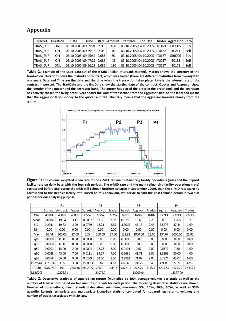
Table 1: Example of the used data set of the e-MID (Italian interbank market). Market shows the currency of the

transaction. Duration shows the maturity of contract, which was traded (there are different maturities from overnight to one year). Date and Time are the date and the time when the transaction takes place. Rate is the interest rate of the contract in percent. The StartDate and the EndDate show the starting date of the contract. Quoter and Aggressor show the identity of the quoter and the aggressor bank. The quoter has placed the order in the order book and the aggressor has actively chosen the living order. Verb shows the kind of transaction from the aggressor side. So the label Sell means that the aggressor lends money to the quoter and the label Buy means that the aggressor borrows money from the quoter.

Figure 1: The volume weighted mean rate of the e-MID, the main refinancing facility operations (rate) and the deposit

facility rate on daily base with the four sub periods. The e-MID rate and the main refinancing facility operations (rate) correspond before and during the crisis (till Lehman brothers collapse in September 2009), than the e-MID rate starts to correspond to the Deposit facility rate. Based on this behaviour, we decide to split the post Lehman period in two sub periods for our analysing purpose.

Table 2: Descriptive statistics of squared log returns (multiplied by 100), average volumes per trade as well as the

number of transactions based on five minutes intervals for each period. The following descriptive statistics are shown: Number of observations, mean, standard deviation, minimum, maximum, 5%-, 10%-, 50%-, 90%-, as well as 95%-quantile, kurtosis, univariate and multivariate Ljung-Box statistic (computed for squared log returns, volumes and number of trades) associated with 20 lags.

Market Duration Date Time Rate Amount StartDate EndDate Quoter Aggressor Verb

TRAS_EUR ONL 03.10.2005 09:39:04 2.08 400 03.10.2005 04.10.2005 DE0021 FR0005 Buy

TRAS_EUR ON 03.10.2005 09:39:18 2.08 10 03.10.2005 04.10.2005 IT0162 IT0211 Sell

TRAS_EUR ON 03.10.2005 09:45:42 2.085 50 03.10.2005 04.10.2005 IT0177 GB0005 Buy

TRAS_EUR ON 03.10.2005 09:47:21 2.085 45 03.10.2005 04.10.2005 IT0257 IT0183 Sell

TRAS_EUR ONL 03.10.2005 09:56:28 2.085 130 03.10.2005 04.10.2005 IT0257 IT0171 Sell

Sq. ret. Avg. vol. Trades Sq. ret. Avg. vol. Trades Sq. ret. Avg. vol. Trades Sq. ret. Avg. vol. Trades

Obs 45881 45881 45881 27257 27257 27257 16102 16102 16102 22213 22213 22213

Mean 0.0086 19.94 3.11 0.0092 17.36 2.98 0.5716 19.69 2.20 0.8513 13.68 1.71

S.D. 0.2041 19.82 2.99 0.0769 18.23 2.85 3.3016 45.16 2.46 3.5775 37.44 1.99

Min 0.00 0.00 0.00 0.00 0.00 0.00 0.00 0.00 0.00 0.00 0.00 0.00

Max 16.44 100.00 27.00 5.27 100.00 27.00 138.92 1000.00 28.00 134.67 2000.00 21.00

q05 0.0000 0.00 0.00 0.0000 0.00 0.00 0.0000 0.00 0.00 0.0000 0.00 0.00

q10 0.0000 0.00 0.00 0.0000 0.00 0.00 0.0000 0.00 0.00 0.0000 0.00 0.00

q50 0.0001 15.00 2.00 0.0004 12.78 2.00 0.0194 9.67 2.00 0.0377 7.50 1.00

q90 0.0023 45.00 7.00 0.0111 39.17 7.00 0.9931 41.71 5.00 1.8166 30.00 4.00

q95 0.0058 56.50 9.00 0.0279 52.00 8.00 2.2962 71.87 7.00 3.7374 45.07 6.00

Kurtosis 3323.14 3.85 3.98 1560.33 5.82 4.61 665.46 110.25 6.43 421.06 955.55 4.93

LB(20) 5287.78 491 2344.84 8802.05 284.01 1145.71 4422.61 277.25 1145.71 4274.57 1121.75 2290.71

MLB(20)

P1 P2 P3 P4

17876.31 21076.7 12209.94 13377.09

Figure 2: Intraday seasonality pattern for squared log returns (left), mean trading volume (middle) and number of

trades (right) for the first period.

Figure 3: Intraday seasonality pattern for squared log returns (left), mean trading volume (middle) and number of

trades (right) for the second period.

Figure 4: Intraday seasonality pattern for squared log returns (left), mean trading volume (middle) and number of

trades (right) for the third period.

Figure 5: Intraday seasonality pattern for squared log returns (left), mean trading volume (middle) and number of

trades (right) for the fourth period.

Figure 6: Autocorrelation function [acf] (left) and cross correlation function [ccf] (right) for the variables of the three

dimensional framework for the first period.

Figure 7: Autocorrelation function [acf] (left) and cross correlation function [ccf] (right) for the variables of the three

dimensional framework for the second period.

Figure 8: Autocorrelation function [acf] (left) and cross correlation function [ccf] (right) for the variables of the three

dimensional framework for the third period.

Figure 9: Autocorrelation function [acf] (left) and cross correlation function [ccf] (right) for the variables of the three

dimensional framework for the fourth period.

Table 3: Quasi-maximum likelihood estimation results of the MMEM for seasonally adjusted squared log returns,

average trade sizes and number of trades per five-minute interval. Standard errors are computed based on the OPG covariance matrix. (Log likelihood function (LL), Bayes Information Criterion (BIC)).

Table 4: Summary statistics of the standardized seasonality adjusted time series and the corresponding MEM residuals

for the four periods. Ljung-Box statistics of the residuals (LB), squared filtered residuals (LB2) as well as multivariate Ljung-Box statistic (MLB). The Ljung-Box statistics are computed based on 20 lags.

Coeff. Std. err. Coeff. Std. err. Coeff. Std. err. Coeff. Std. err.

OM1 -0.7742 0.0105 -0.8279 0.0130 -0.4203 0.0127 -0.4553 0.0159

OM2 -0.1525 0.0186 -0.0690 0.0179 -0.0870 0.0115 -0.0496 0.0106

OM3 -0.2249 0.0132 -0.2697 0.0108 -0.2738 0.0169 -0.2779 0.0195

A0_12 -0.0398 0.0037 0.0449 0.0043 0.0114 0.0038 0.0434 0.0065

A0_13 -0.1527 0.0051 -0.1956 0.0068 -0.0859 0.0059 0.0597 0.0085

A0_23 0.0372 0.0105 0.0875 0.0093 0.2050 0.0070 0.2504 0.0054

A1_11 0.5489 0.0048 0.5315 0.0064 0.3716 0.0077 0.6064 0.0113

A1_12 0.0123 0.0043 -0.0187 0.0049 -0.0081 0.0029 -0.0130 0.0020

A1_13 0.2648 0.0086 0.3967 0.0094 0.1351 0.0089 -0.0051 0.0102

A1_21 0.0290 0.0100 0.0203 0.0088 0.0427 0.0057 0.0370 0.0058

A1_22 0.0871 0.0083 0.0658 0.0068 0.0570 0.0027 0.0322 0.0028

A1_23 0.0498 0.0120 0.0057 0.0112 0.0269 0.0082 0.0284 0.0072

A1_31 0.1051 0.0075 0.1154 0.0069 0.0929 0.0129 0.0689 0.0157

A1_32 0.0252 0.0054 0.0526 0.0042 0.0224 0.0035 0.0071 0.0055

A1_33 0.1252 0.0079 0.1318 0.0060 0.1791 0.0125 0.2071 0.0129

B1_11 0.9682 0.0008 0.9684 0.0009 0.9856 0.0008 0.8552 0.0046

B1_22 0.6030 0.0470 0.5540 0.0479 0.5833 0.0148 0.4722 0.0178

B1_33 0.7930 0.0161 0.7996 0.0114 0.7766 0.0222 0.6026 0.0331

LL

BIC

-41717.36

-41802.81

P1 P2 P3 P4

-48603.24

-48692.37

-57789.30

-57878.43

-32406.08

-32489.91

Sq. ret. Avg. vol. Trades Sq. ret. Avg. vol. Trades Sq. ret. Avg. vol. Trades Sq. ret. Avg. vol. Trades

Mean 1.13 1.00 1.02 1.01 1.01 1.00 1.00 1.00 1.00 1.00 1.00 1.00

S.D. 19.24 0.89 0.77 6.08 0.95 0.74 4.75 2.17 0.93 4.05 2.32 1.02

LB(20) 5287.78 491.00 2344.84 8802.05 284.01 1767.76 4422.61 277.25 1145.71 4274.57 121.75 2290.71

LB2(20) 4122.97 486.70 1944.57 963.93 125.19 831.00 624.25 42.11 41.20 2373.77 21.64 1580.96

MLB(20)

Sq. ret. Avg. vol. Trades Sq. ret. Avg. vol. Trades Sq. ret. Avg. vol. Trades Sq. ret. Avg. vol. Trades

Mean 1.00 1.00 1.00 1.00 1.00 1.00 1.00 1.00 1.00 1.00 1.00 1.00

S.D. 7.34 0.85 0.67 3.84 0.92 0.68 2.38 1.78 0.75 2.46 2.11 0.81

LB(20) 6.15 19.53 59.10 24.21 25.42 45.00 241.95 17.94 23.67 123.43 29.39 24.78

LB2(20) 0.01 21.99 35.57 0.01 15.38 23.35 7.73 5.61 10.39 4.16 0.59 19.17

MLB(20) 196.87 602.18 383.97 84.00

P1 P2 P3 P4

17876.31 21076.71 12209.94 13377.09

P1 P2 P3 P4

Descriptive statistics of raw data

Summary Statistics MEM Residuals