No. 46. 46 The opinions expressed in this discussion paper are those of the author(s) and should not...

October 2016

Discussion Paper

No. 46

The opinions expressed in this discussion paper are those of the author(s) and should not be

attributed to the Puey Ungphakorn Institute for Economic Research.

Value Investing: Circle of Competence in theThai Insurance Industry

Sampan Nettayanun∗

Naresuan University

[Latest update: 4/2016]

Abstract

This study explores the strategy of value investing, specifically for the insuranceindustry in Thailand. It employs multiple measures of “value,” suitable for insurancecompanies, such as the price-to-earning (PE), price-to-book (PB), and cyclically ad-justed price-to-earnings (CAPE). Value premium exists in the Thai insurance industry.Most of the value portfolios constructed from these measures significantly outperformthe market, even when adjusting for price volatility and portfolio’s β. The cumulativereturns are also higher for the value stocks, when compared to the growth stocks, andthe Thai stock market. Constructing a value portfolio, using the PE ratio, results inthe highest returns and are far better than PB and CAPE. The value anomaly cannotbe fully explained by either the capital asset pricing model or the Fama-French 3 factormodels.

Keywords: Value Investing; Portfolio Management; Circle of Competence; RiskManagement; Insurance; Property&Liability Insurance; Life Insurance.

∗Faculty of Business, Economics and Communications, Naresuan University, Thailand,e-mail: [email protected].

1

1 Introduction

Value investing has been popular among institutional and individual investors in Thailand.

The idea is originally from Dodd and Graham (1951) and Graham (2003). Various studies,

such as Basu (1977), Fama and French (1992, 1993, 1996, 1998, 2006, 2012, 2015), Piotroski

(2000), Piotroski and So (2012), Asness, Moskowitz, and Pedersen (2013), Asness, Frazz-

ini, Israel, and Moskowitz (2015), and Novy-Marx (2013, 2015), find that value portfolios

outperform growth portfolios. Value stocks are defined as either having a low price-to-book

ratio, or a low price-to-earning ratio. Growth stocks are defined as either having high a PB

ratio, or a high PE ratio.

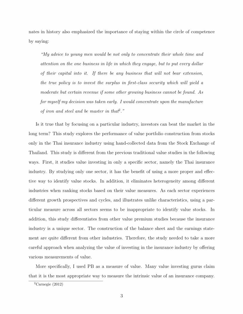
Notable value investors also claim that the value investor does not have to know or

understand every company in the market. Investors might be able to implement value

investing using some companies or some industries that they truly understand. The notion

of a circle of competence has been introduced by Warren Buffett and Charlie Munger, two

of the most successful value investors, which means that investors should focus their efforts

in the circle of knowledge that they have. They do not need to invest in companies or

industries that they do not understand. For example, in a 1996 letter to shareholders of

Berkshire Hathaway, Buffett stated:

“Should you choose, however, to construct your own portfolio, there are a few

thoughts worth remembering. Intelligent investing is not complex, though that is

far from saying that it is easy. What an investor needs is the ability to correctly

evaluate selected businesses. Note that word ‘selected’: You don’t have to be an

expert on every company, or even many. You only have to be able to evaluate

companies within your circle of competence. The size of that circle is not very

important; knowing its boundaries, however, is vital1.”

In the same spirit as Warren Buffett, Andrew Carnegie, one of the world’s wealthiest mag-

1See the 1996 Warren Buffett’s Letter to Berkshire Shareholders of Berkshire Hathaway Inc.

2

nates in history also emphasized the importance of staying within the circle of competence

by saying:

“My advice to young men would be not only to concentrate their whole time and

attention on the one business in life in which they engage, but to put every dollar

of their capital into it. If there be any business that will not bear extension,

the true policy is to invest the surplus in first-class security which will yield a

moderate but certain revenue if some other growing business cannot be found. As

for myself my decision was taken early. I would concentrate upon the manufacture

of iron and steel and be master in that2.”

Is it true that by focusing on a particular industry, investors can beat the market in the

long term? This study explores the performance of value portfolio construction from stocks

only in the Thai insurance industry using hand-collected data from the Stock Exchange of

Thailand. This study is different from the previous traditional value studies in the following

ways. First, it studies value investing in only a specific sector, namely the Thai insurance

industry. By studying only one sector, it has the benefit of using a more proper and effec-

tive way to identify value stocks. In addition, it eliminates heterogeneity among different

industries when ranking stocks based on their value measures. As each sector experiences

different growth prospectives and cycles, and illustrates unlike characteristics, using a par-

ticular measure across all sectors seems to be inappropriate to identify value stocks. In

addition, this study differentiates from other value premium studies because the insurance

industry is a unique sector. The construction of the balance sheet and the earnings state-

ment are quite different from other industries. Therefore, the study needed to take a more

careful approach when analyzing the value of investing in the insurance industry by offering

various measurements of value.

More specifically, I used PB as a measure of value. Many value investing gurus claim

that it is the most appropriate way to measure the intrinsic value of an insurance company.

2Carnegie (2012)

3

As the balance sheet of an insurance company consists of financial assets and liabilities, the

book value is the remainder of assets and liabilities that belong to equity owners. The PB

measure is similar to previous “value” studies. In addition, I also used price-to-earnings

ratio, similar to Basu (1977) to capture the value stocks. I also used the cyclically adjusted

price-to-earnings (CAPE), similar to Campbell and Shiller (1988). This is due to the fact

that the earnings of an insurance company in a single year might affect the way we pick value

stocks. For example, an insurance company might have one particular bad year, due to a

catastrophic event, and the event might create much lower earnings than the true earning

power of the company. The company might also be a good underwriter over a long period of

time. We can call this kind of company, “good but unlucky.” Therefore, this might result in

a negative PE ratio for a catastrophic year. If we use only a PE ratio to capture the value

stock, some insurers might be eliminated from the analysis. Hence, average earnings might

result in a more appropriate measure of a value stock.

The results are in line with other studies. Constructing value portfolios based on PB, PE,

and CAPE33 outperform both the market portfolios and the growth portfolios. However,

using CAPE54 does not result in value premium. Adjusting for volatility yields the same

results. This implies that CAPM does not fully capture the value premium, similar to Fama

and French (2006)’s results. In addition, the Fama-French 3 factor model does not capture

the value anomaly. This might be due to the fact that the number of stocks in each portfolio

is small. Therefore, the dispersion from non-systematic risks (the sample variance of εs

is too high to be explained by the market returns). It dominates systematic risk which

is represented by β. Therefore, there is no apparent relationship between the returns of

the value portfolio and the Fama-French factors. Overall, investors can outperform the

market, even adjusting for the price risks, by applying a value investing strategy in the

Thai insurance industry. However, investors must choose an appropriate value measure to

construct the insurance value portfolio.

3CAPE3 is cyclically adjusted price-to-earnings ratio based on three-year earnings.4CAPE5 is cyclically adjusted price-to-earnings ratio based on five-year earnings.

4

This study proceeds as follows. Section II explores related theories and empirical findings

about value investing. Section III outlines the portfolio construction procedures and how I

collected the data. Section IV reports the performance of various portfolios when compared

to the market. Section V uses CAPM to explain the value anomaly in the Thai insurance

industry. Section VI attempts to explain the anomaly using the Fama-French 3 factor model.

Lastly, I conclude the study by discussing the implications of my findings, and I give some

further recommendations for future researches.

2 Related Theories and Empirical Findings

Benjamin Graham is the father of value investing. In his famous books, including Dodd and

Graham (1951), and Graham (2003), he proposes a value strategy for investing. He states

that investors can outperform the general market by constructing a portfolio consisting of

a low price-to-book ratio or a low price-to-earnings ratio. By using this strategy, investors

have what Benjamin Graham calls margins of safety, which means that the price is below

the intrinsic value of the business. Many prominent investors have sucessfully followed

this unique strategy, such as Warren Buffett, Charlie Munger, Irvin Kahn, Walter Schloss,

Joel Greenblatt, Christopher Browne, Seth Klarman, and Martin Whitman. For instance,

Frazzini, Kabiller, and Pedersen (2013) find that Berkshire Hathaway outperforms any stocks

and mutual funds using Sharpe’s ratio criteria. This is due to the combination of value,

safe, quality investing, plus leverage. In addition to the success of the superinvestors from

Graham-and-Doddsville5, researchers also find evidence that value portfolios outperform the

market portfolios and “growth” portfolios.

Fama and French (1992, 1993, 1998, 2006, 2015) also discover that portfolios of value

stocks with a low PB, tend to outperform the market. There are doubts that the capital

asset pricing model can capture the anomalies in the stock returns. For example, Fama

5Buffett, Warren (2004).“The Superinvestors of Graham-and-Doddsville” Hermes: the Columbia BusinessSchool Magazine: 415.

5

and French (2006) also find that value stocks outperform the market, but CAPM does not

capture the value premium. In addition to stocks, Asness, Moskowitz, and Pedersen (2013)

find that value premium exists through many other asset classes.

Focusing on Thai stock market, Sareewiwatthana (2011, 2012, 2013), in line with Fama

and French (1992, 1993, 1998, 2006, 2015), find that portfolios consisting of value stocks

significantly outperform the market. Sareewiwatthana (2011) uses various measures, such

as PB, PE, and dividend yield to pick value stocks. The study ranks them in order to

form value portfolios and defines the low PB, PE, and dividend yield to be value stocks.

The study finds that value portfolios significantly outperformed the SET index. Sareewi-

watthana (2012) combines growth and the price-to-earnings ratio to form a PEG ratio to

capture the value stocks. The study constructs a portfolio a low PEG ratio and finds that it

outperforms the market and also a high-PEG portfolio. Sareewiwatthana (2013) implements

Sareewiwatthana (2012) by adding the other ratios, such as return of equity (ROE) and

return on asset (ROA). Adding these ratios help value portfolios to outperform the market

even better. Overall, the evidence suggests that value investing outperforms the market in

the Stock Exchange of Thailand.

Value anomaly can be explained by both a rational and behavioral argument. According

to the model in Sharpe (1964), higher (lower) risk stocks should have higher (lower) expected

return. Value stocks occur because investors require higher than expected returns from riskier

stocks. In the other words, investors get higher return due to investing in distressed and

risky companies. Therefore, the investors gets higher than average returns due to the fact

that they have to bear more risk in the portfolio. For example, Fama and French (1995) show

that lower PB stocks tend to be in a distressed situation and tend to provide a low return

on equity. On the other hand, the behavioral finance literatures explains that value stocks

happen as a result of human’s behavior. For example, investors overreacting to news about

a company can result in the stock prices being much lower than their fundamental value,

according to Bondt and Thaler (1985), Lakonishok, Shleifer, and Vishny (1994), and Daniel,

6

Hirshleifer, and Subrahmanyam (1998). Noise traders and arbitrageurs can also create the

situation where the price and the fundamental value are diverged, according to Shleifer and

Vishny (1997). A classic statement that explains the value premium from both schools of

thought is from Dodd and Graham (1951):

“In other words, the market is not a weighing machine, on which the value of

each issue is recorded by an exact and impersonal mechanism, in accordance with

its specific qualities. Rather should we say that the market is a voting machine,

whereon countless individuals register choices which are the product partly of rea-

son and partly of emotion.”

This statement implies that value investing works because in the short term, stock prices

can deviate from their fundamental value. However, over the long term, the price can reflect

the intrinsic value. The price can get to be very close or at the true fundamental value. It

is the job of value investors to find and get the benefit of this anomaly by buying securities

when the price and value are deviated, and then waiting until the prices to go back to the

intrinsic value in the long term.

3 Portfolio Construction and Data Collection

This study uses the Stock Exchange of Thailand dataset from January of 1990 until December

of 2014, that is available from the SETSMART database. To test whether value stocks

outperform the general market, I constructed portfolios of stocks using the following criteria.

First, I constructed portfolios of insurance companies using the price-to-book ratio. Second, I

constructed portfolios using the price-to-earnings ratio. Third, I used the cyclically adjusted

price-to-earnings ratio. I used all property and casualty, and life insurers within the Thai

stock market to test my hypothesis.

7

3.1 Value Portfolio from PB Ratio

For each year, the portfolios rebalance in the beginning of January. For PB, I constructed

two portfolios by ordering the PB ratios of all insurers6. I then constructed the LOW PB

portfolio, consisting of the lowest quartile of stocks with the lowest PB ratios. There were

18 insurers listed in the most recent data. Therefore, one quartile consists of 4.5 companies,

which I rounded down to 4 companies. Returns with the adjusted dividend of the portfolio

for each month will be collected. As the data does not provide the exact date of the dividend,

I used the dividend yield divided by 12 and added it to the price return to adjust for the

total return. The proportion of each position was equally weighted. I also constructed the

HIGH PB portfolio to capture the growth stocks. This is the same as the LOW PB portfolio,

except the portfolio picks the highest quartile of PB. The two portfolios were compared to

the SET-index portfolio with adjusted dividend.

3.2 Value Portfolio from PE Ratio

I constructed the value portfolio using the PE ratio7. For each year, the portfolio was

rebalanced in the beginning of January. I constructed two portfolios by ordering the PE

ratios of each insurer. The negative value stocks are not considered in constructing the value

portfolio. I constructed the LOW PE portfolio, consisting of the lowest quartile of stocks

with the lowest PE ratios. The proportion of each position was equally weighted. Returns,

including the dividend of the portfolio, for each month were collected. The available period

of PE portfolios are different from PB portfolios due to the fact that SETSMART does not

have earnings per share until 1997. Therefore, the analysis of the PE portfolio starts in the

beginning of 1998. I also constructed the HIGH PB portfolio to capture the growth stocks.

6The PB ratio is defined as price per share divided by book value per share.7PE ratio is defined as price per share divided by earning per share. PE is thought to be a better measure

of value as it takes return on equity (ROE) into consideration. Since, PE = priceEPS , hence PE = price

book ∗ bookEPS .

This is the same as writing PE = PBROE . A higher PB increases PE if ROE stays constant. On the other

hand, a higher ROE lowers the PE ratio if PB stays constant. Therefore, PE is superior to PB in the sensethat it captures both ROE and PB at the same time. However, PB is superior to PE because assets aremore stable than earnings.

8

This is the same as the LOW PE portfolio, except the portfolio picks the highest quartile

of PE. The two portfolios were compared to the SET-index portfolio and adjusted with the

dividend.

3.3 Value Portfolio from Cyclically Adjusted Price-to-Earnings

Ratio

Insurer’s earnings are different from other businesses. According to Cummins, Weiss, and Zi

(1999) and Nettayanun (2014), there are three main operations within an insurance company.

First, it pools and bears underwriting risks. Second, it serves its customers through servicing,

related to the incurred loss. Third, it gets some other earnings from the investment of the

insurance float, which is the premium that the insurer collects and waits to be paid in the

future. The first component can be quite volatile due to catastrophe loss. For example, there

was a great flood in Thailand in 2011. Most of the insurers faced underwriting losses. Using

a regular PE ratio might not give a complete view of the value of the insurers. Therefore,

it might be better to capture value stock via the cyclically adjusted price-to-earnings ratio.

The ratio averages the earnings in multiple years, according to Campbell and Shiller (1988).

Basically, it is the price divided by average earnings adjusted by inflation for 10 years.

Particularly,

CAPE =pricecurrent

(eps∗t−1 + eps∗t−2 + · · · + eps∗t−10)/10(1)

where eps∗i is earnings adjusted by the inflation rate to the current period from year i.

The inflation rates for each year are from the Bank of Thailand8. In this study, I used three

and five years, instead of 10 years, of CAPE to construct my portfolio due to the fact that

I could only start my analysis in 2002 as earnings can be found starting in 1997. Using 10

years of CAPE resulted in very short time frame to test the portfolio performance, from

8See www.bot.or.th/Thai/Statistics/Graph/Pages/Main3.aspx

9

2007 to 2014, which might not be sufficient to show value premium. I called it CAPE3,

CAPE5 for CAPE, using an average of three and five years, respectively. I constructed two

portfolios by ordering the CAPE3 of each insurer. The negative value of CAPE3 stocks were

not considered in constructing the value portfolio. I constructed the LOW CAPE3 portfolio

consisting of the lowest quartile of stocks with the lowest CAPE3 ratios. The proportion

of each position were equally weighted. Returns, including the dividend of the portfolio,

were collected for each month. I also constructed the HIGH CAPE3 portfolio to capture

the growth stocks. This is the same as the LOW CAPE3 portfolio except that the portfolio

picks the highest quartile of CAPE3. I repeated the same exercise for CAPE5. All portfolios

were compared to the SET-index portfolio adjusted with dividend.

4 Results

The results of the simulated portfolios from various measures will be discussed in detail.

First, I explain the results from the portfolio ordering of the PB ratios. Second, I show the

results of the portfolio construction using the PE ratio. The performance of the last two

portfolios use CAPE3 and CAPE5, respectively.

4.1 Portfolios Constructed from Price per Book Ratio

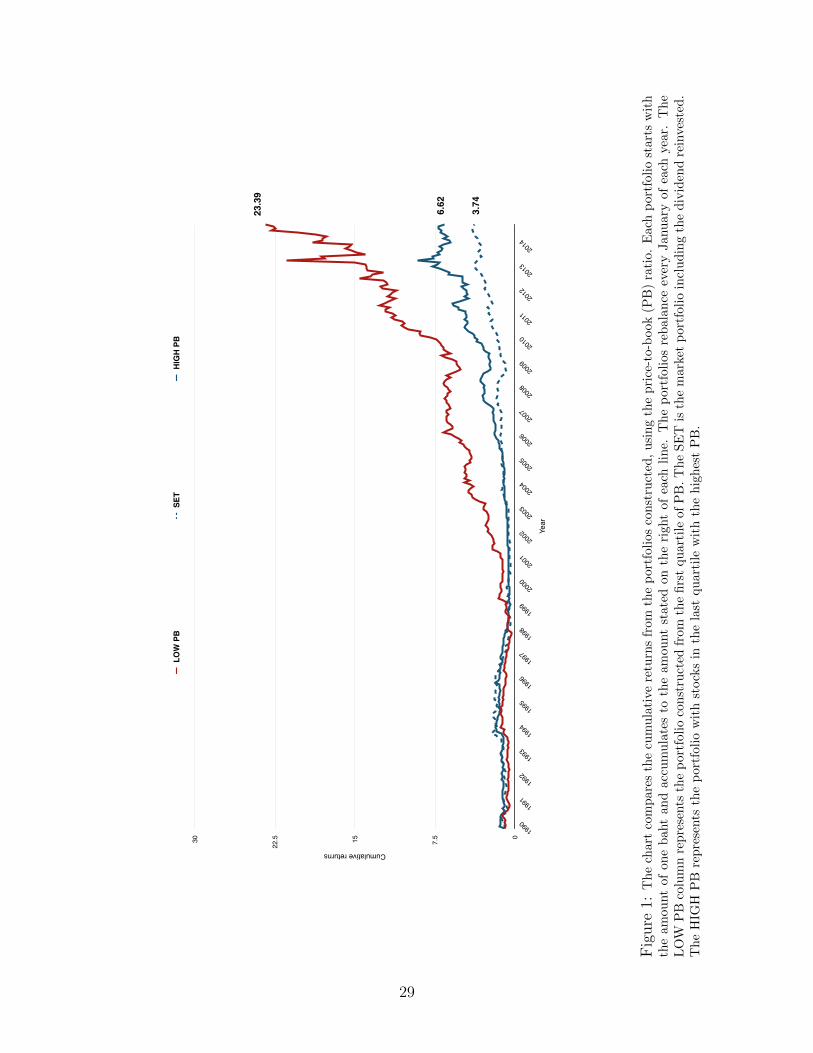
According to the table, 1, the portfolio that consisted of low PB stocks, outperformed the

portfolio consisting of high PB stocks, based on the monthly arithmetic average, the annual

geometric average, and the monthly excess average of returns. The low PB portfolio achieved

1.52% arithmetic average return compared to 0.91% of the high PB portfolio. The low PB

stocks give 14.04% geometric average returns per year compared to 5.65% of the high PB

stocks. However, the low PB stocks have lower minimum monthly returns(-30.62%) than

the high PB stocks(-22.33%). In addition, low PB stocks have a maximum return(74.55%)

higher than the high PB stocks(46.54%). This can be interpreted as follows. On average,

10

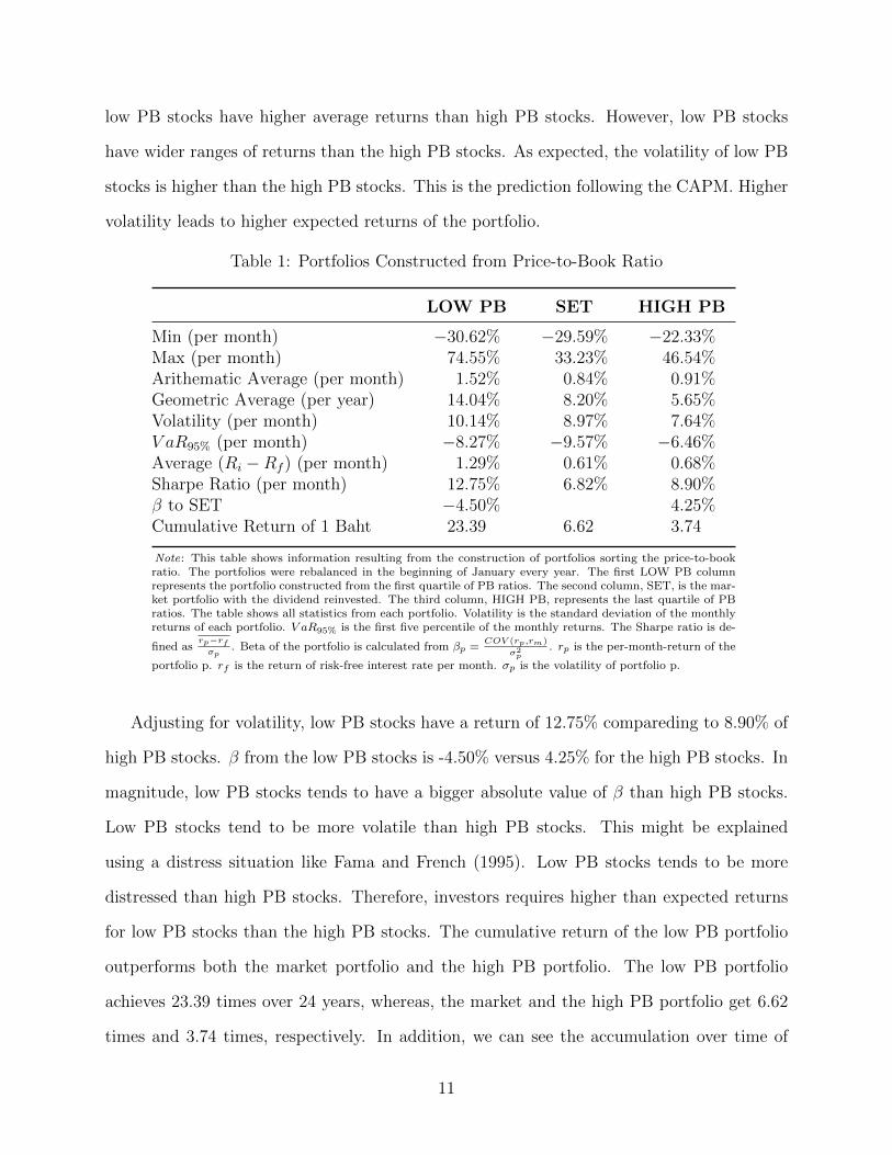
low PB stocks have higher average returns than high PB stocks. However, low PB stocks

have wider ranges of returns than the high PB stocks. As expected, the volatility of low PB

stocks is higher than the high PB stocks. This is the prediction following the CAPM. Higher

volatility leads to higher expected returns of the portfolio.

Table 1: Portfolios Constructed from Price-to-Book Ratio

LOW PB SET HIGH PB

Min (per month) −30.62% −29.59% −22.33%Max (per month) 74.55% 33.23% 46.54%Arithematic Average (per month) 1.52% 0.84% 0.91%Geometric Average (per year) 14.04% 8.20% 5.65%Volatility (per month) 10.14% 8.97% 7.64%V aR95% (per month) −8.27% −9.57% −6.46%Average (Ri −Rf ) (per month) 1.29% 0.61% 0.68%Sharpe Ratio (per month) 12.75% 6.82% 8.90%β to SET −4.50% 4.25%Cumulative Return of 1 Baht 23.39 6.62 3.74

Note: This table shows information resulting from the construction of portfolios sorting the price-to-bookratio. The portfolios were rebalanced in the beginning of January every year. The first LOW PB columnrepresents the portfolio constructed from the first quartile of PB ratios. The second column, SET, is the mar-ket portfolio with the dividend reinvested. The third column, HIGH PB, represents the last quartile of PBratios. The table shows all statistics from each portfolio. Volatility is the standard deviation of the monthlyreturns of each portfolio. V aR95% is the first five percentile of the monthly returns. The Sharpe ratio is de-

fined asrp−rfσp

. Beta of the portfolio is calculated from βp =COV (rp,rm)

σ2p

. rp is the per-month-return of the

portfolio p. rf is the return of risk-free interest rate per month. σp is the volatility of portfolio p.

Adjusting for volatility, low PB stocks have a return of 12.75% compareding to 8.90% of

high PB stocks. β from the low PB stocks is -4.50% versus 4.25% for the high PB stocks. In

magnitude, low PB stocks tends to have a bigger absolute value of β than high PB stocks.

Low PB stocks tend to be more volatile than high PB stocks. This might be explained

using a distress situation like Fama and French (1995). Low PB stocks tends to be more

distressed than high PB stocks. Therefore, investors requires higher than expected returns

for low PB stocks than the high PB stocks. The cumulative return of the low PB portfolio

outperforms both the market portfolio and the high PB portfolio. The low PB portfolio

achieves 23.39 times over 24 years, whereas, the market and the high PB portfolio get 6.62

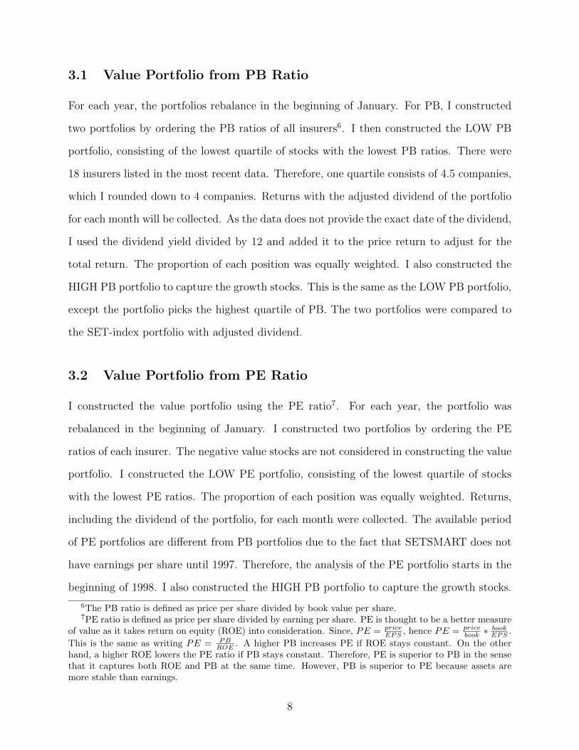
times and 3.74 times, respectively. In addition, we can see the accumulation over time of

11

the low PB portfolio, the high PB portfolio and the market portfolio in figure 1.

Overall, the results are in line with previous studies. There exists a value premium, not

only across all stocks, but also in the insurance industry in particular. CAPM seems to be

able to explain this value premium in the Thai insurance industry. Even though the low

PB ratio has a higher averaged return, but investors face higher volatility of holding these

stocks. The portfolio of low PB stocks have a deeper worst month than the high PB stocks.

On the other hand, the low PB stocks have the best returns in a single month. However, low

PB insurer’s stocks cumulatively outperform the high PB insurers’ stocks by a wide margin.

4.2 Portfolios Constructed from Price-to-Earning Ratio

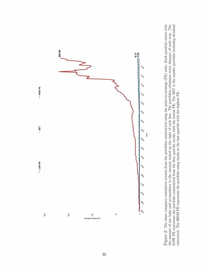
The following is the result of the portfolios’ returns constructed from the price-to-earnings

(PE) ratio. According to the table, 2, the portfolio consists of stocks with low PE outper-

forming the portfolio that consists of high PE, based on the monthly arithematic average, the

annual geometric average, and the monthly excess average. The low PE portfolio achieves

3.15% arithematic average compared to 0.96% of the high PE portfolio. Low PE stocks give

41.21% geometric average per year compared to 10.03% of the high PE stocks. The difference

on the geometric average is very wide. The low PE portfolio has the worst return for each

month(-21.51%) compared to the high PE stocks(-20.77%). In addition, low PE stocks have

a much higher maximum monthly return (68.11%) higher than the high PE stocks(38.18%).

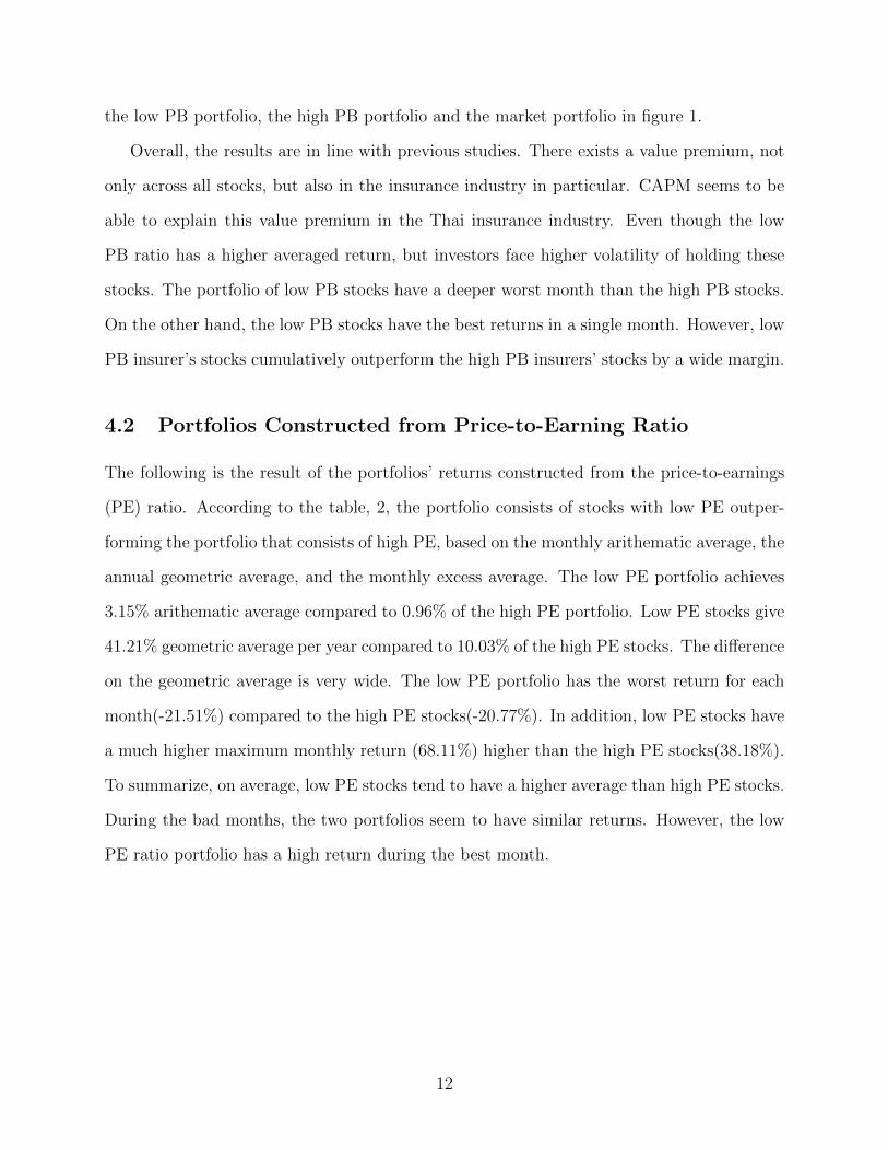
To summarize, on average, low PE stocks tend to have a higher average than high PE stocks.

During the bad months, the two portfolios seem to have similar returns. However, the low

PE ratio portfolio has a high return during the best month.

12

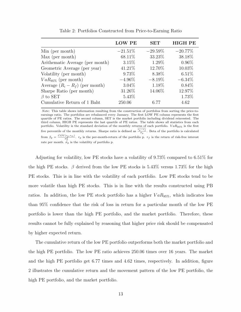
Table 2: Portfolios Constructed from Price-to-Earning Ratio

LOW PE SET HIGH PE

Min (per month) −21.51% −29.59% −20.77%Max (per month) 68.11% 33.23% 38.18%Arithematic Average (per month) 3.15% 1.29% 0.96%Geometric Average (per year) 41.21% 12.70% 10.03%Volatility (per month) 9.73% 8.38% 6.51%V aR95% (per month) −4.96% −8.19% −6.34%Average (Ri −Rf ) (per month) 3.04% 1.18% 0.84%Sharpe Ratio (per month) 31.26% 14.06% 12.97%β to SET 5.43% 1.73%Cumulative Return of 1 Baht 250.06 6.77 4.62

Note: This table shows information resulting from the construction of portfolios from sorting the price-to-earnings ratio. The portfolios are rebalanced every January. The first LOW PE column represents the firstquartile of PE ratios. The second column, SET is the market portfolio including dividend reinvested. Thethird column, HIGH PE represents the last quartile of PE ratios. The table shows all statistics from eachportfolio. Volatility is the standard deviation of the monthly returns of each portfolio. V aR95% is the first

five percentile of the monthly returns. Sharpe ratio is defined asrp−rfσp

. Beta of the portfolio is calculated

from βp =COV (rp,rm)

σ2p

. rp is the per-month-return of the portfolio p. rf is the return of risk-free interest

rate per month. σp is the volatility of portfolio p.

Adjusting for volatility, low PE stocks have a volatility of 9.73% compared to 6.51% for

the high PE stocks. β derived from the low PE stocks is 5.43% versus 1.73% for the high

PE stocks. This is in line with the volatility of each portfolio. Low PE stocks tend to be

more volatile than high PE stocks. This is in line with the results constructed using PB

ratios. In addition, the low PE stock portfolio has a higher V aR95%, which indicates less

than 95% confidence that the risk of loss in return for a particular month of the low PE

portfolio is lower than the high PE portfolio, and the market portfolio. Therefore, these

results cannot be fully explained by reasoning that higher price risk should be compensated

by higher expected return.

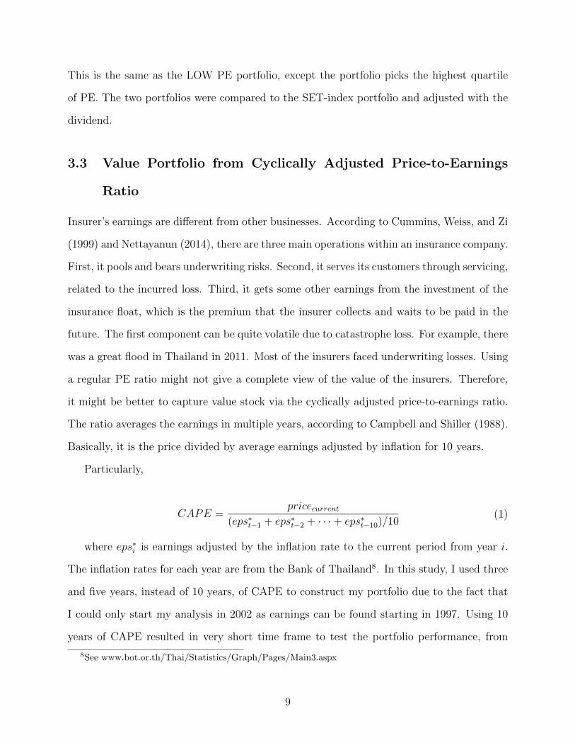
The cumulative return of the low PE portfolio outperforms both the market portfolio and

the high PE portfolio. The low PE ratio achieves 250.06 times over 16 years. The market

and the high PE portfolio get 6.77 times and 4.62 times, respectively. In addition, figure

2 illustrates the cumulative return and the movement pattern of the low PE portfolio, the

high PE portfolio, and the market portfolio.

13

Overall, the results are in line with previous studies that show a value premium in the Thai

insurance industry. Although value premium can be explained by having higher volatility

in stock prices, it cannot be explained from the perspective of the minimum return and the

value at risk. However, low PE stocks in the insurance industry outperform the high PE

stocks by a wide margin in terms of cumulative returns over a period of 16 years9.

4.3 Portfolios Constructed from Three Year Cyclically Adjusted

Price-to-Earnings Ratio

The following are the results from portfolios constructed from the three year cyclically ad-

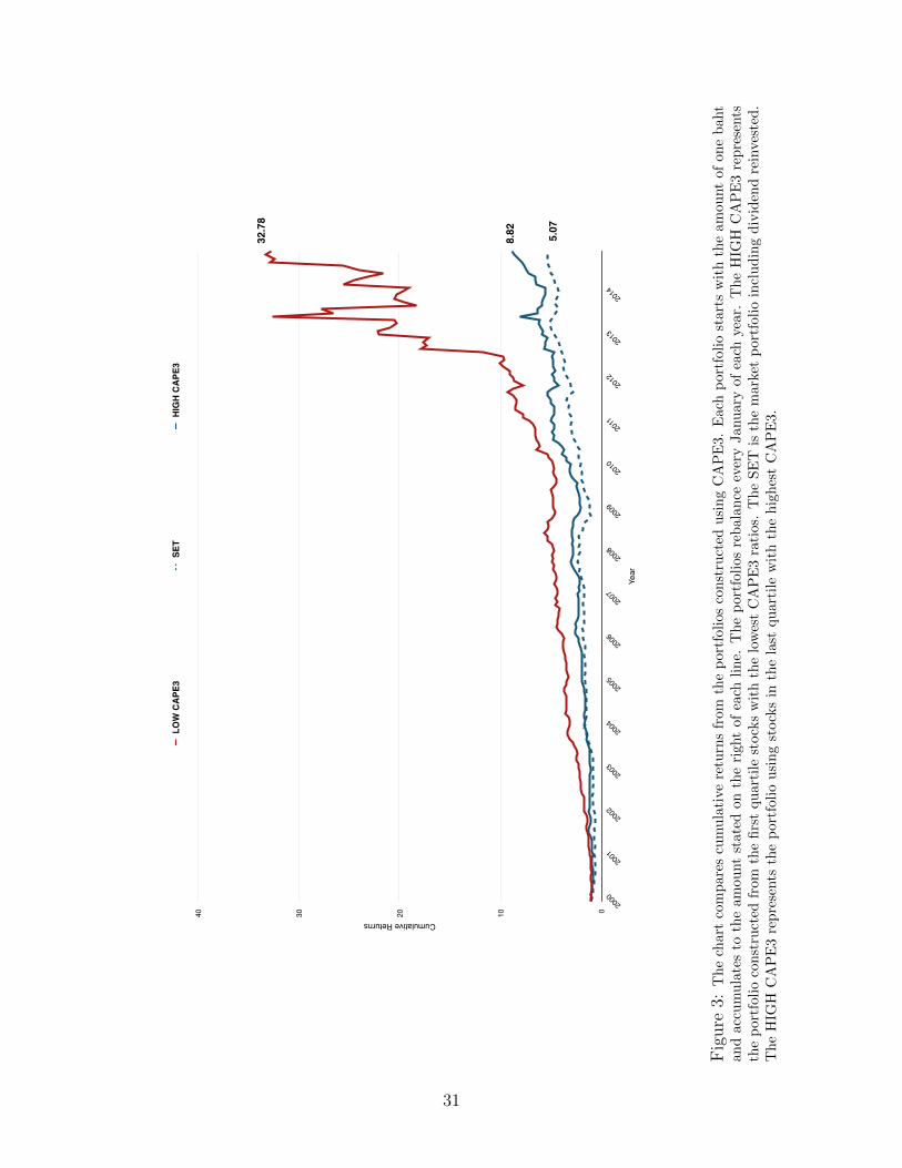
justed price-to-earnings ratio. According to the table, 3, a portfolio consisting of stocks

with a low level of CAPE3 outperforms a portfolio consisting of high CAPE3, based on the

monthly arithmetic average, the annual geometric average, and the excess average. The Low

CAPE3 portfolio achieves a 2.31% arithmetic average compared to 1.42% for the high CAPE3

portfolio. Low CAPE3 stocks give a 28.31% geometric average per year versus 16.83% for

high CAPE3 stocks. The low CAPE3 portfolio has the worst return (-34.14%) for each

month and is lower than the high CAPE3 stocks(-22.96%). In addition, low CAPE3 stocks

have a much higher best monthly return (59.64%) than the high CAPE3 stocks(33.68%).

9The data of earnings for each stock started in 1997, Therefore, there are only about 16 years to accumulatereturns. This is different from the PB case. The PB ratios have been available since 1990. There are 24years for portfolio construction in the PB case.

14

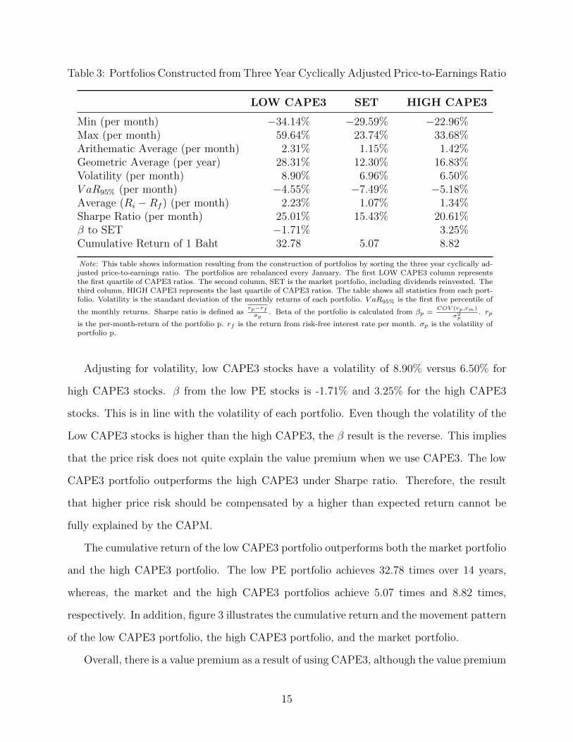
Table 3: Portfolios Constructed from Three Year Cyclically Adjusted Price-to-Earnings Ratio

LOW CAPE3 SET HIGH CAPE3


Note: This table shows information resulting from the construction of portfolios by sorting the three year cyclically ad-justed price-to-earnings ratio. The portfolios are rebalanced every January. The first LOW CAPE3 column representsthe first quartile of CAPE3 ratios. The second column, SET is the market portfolio, including dividends reinvested. Thethird column, HIGH CAPE3 represents the last quartile of CAPE3 ratios. The table shows all statistics from each port-folio. Volatility is the standard deviation of the monthly returns of each portfolio. V aR95% is the first five percentile of

the monthly returns. Sharpe ratio is defined asrp−rfσp


σ2p

. rp

is the per-month-return of the portfolio p. rf is the return from risk-free interest rate per month. σp is the volatility ofportfolio p.

Adjusting for volatility, low CAPE3 stocks have a volatility of 8.90% versus 6.50% for

high CAPE3 stocks. β from the low PE stocks is -1.71% and 3.25% for the high CAPE3

stocks. This is in line with the volatility of each portfolio. Even though the volatility of the

Low CAPE3 stocks is higher than the high CAPE3, the β result is the reverse. This implies

that the price risk does not quite explain the value premium when we use CAPE3. The low

CAPE3 portfolio outperforms the high CAPE3 under Sharpe ratio. Therefore, the result

that higher price risk should be compensated by a higher than expected return cannot be

fully explained by the CAPM.

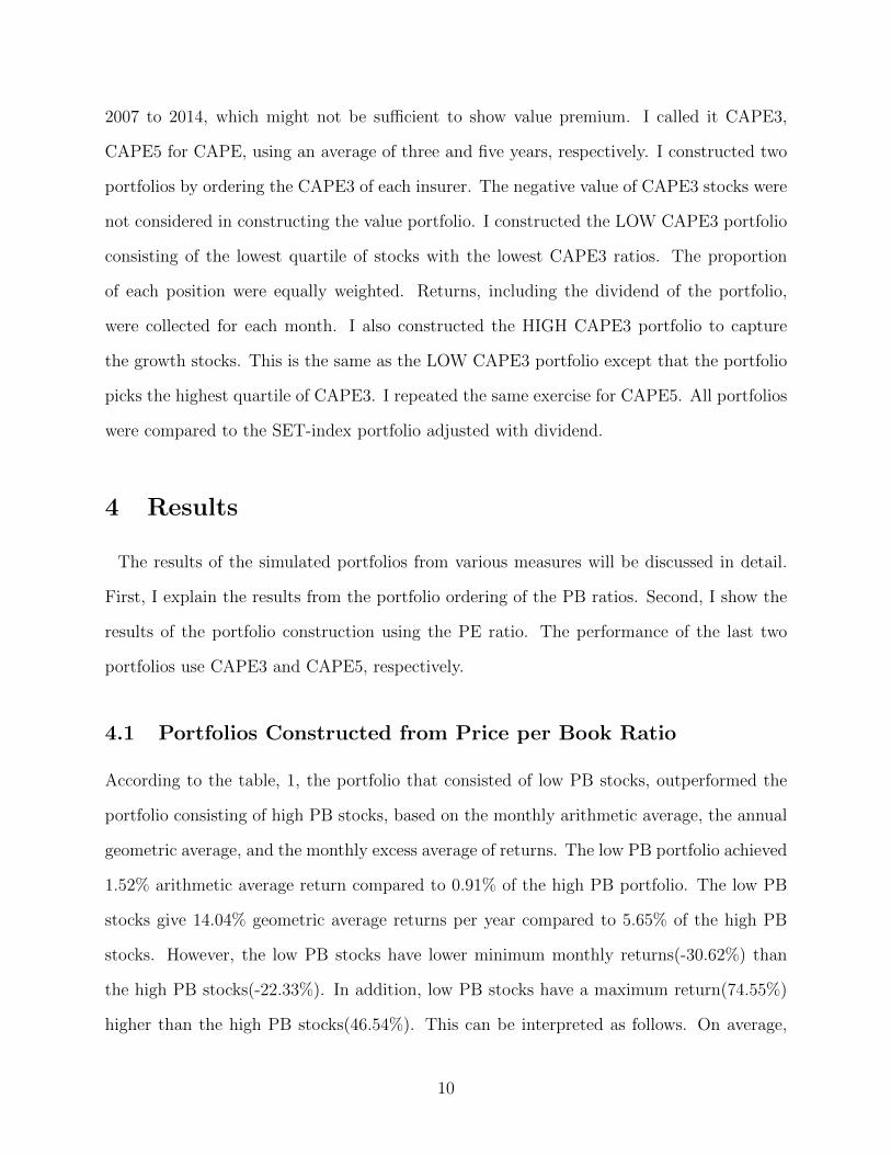
The cumulative return of the low CAPE3 portfolio outperforms both the market portfolio

and the high CAPE3 portfolio. The low PE portfolio achieves 32.78 times over 14 years,

whereas, the market and the high CAPE3 portfolios achieve 5.07 times and 8.82 times,

respectively. In addition, figure 3 illustrates the cumulative return and the movement pattern

of the low CAPE3 portfolio, the high CAPE3 portfolio, and the market portfolio.

Overall, there is a value premium as a result of using CAPE3, although the value premium

15

can be explained by having higher volatility in stock prices. In addition, using the Sharpe

ratio, the low CAPE3 stocks still outperform the high CAPE3. Interestingly, both the low

and high CAPE3 stocks outperform the market as a whole. This is due to the fact that

the insurance industry outperforms the market as a whole during the period used. The

setback of this result is due to the shorter time period as we lose about three years of data

for averaging the lagged earnings. The results would be more reliable if there were a longer

time period.

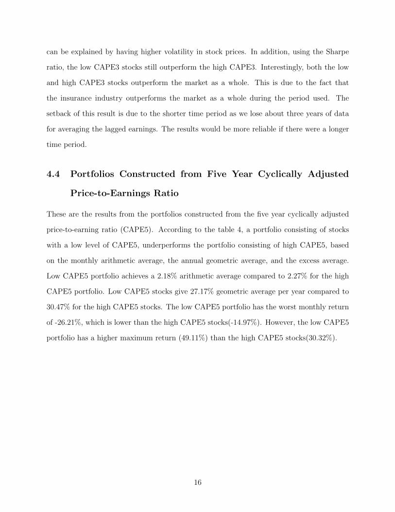
4.4 Portfolios Constructed from Five Year Cyclically Adjusted

Price-to-Earnings Ratio

These are the results from the portfolios constructed from the five year cyclically adjusted

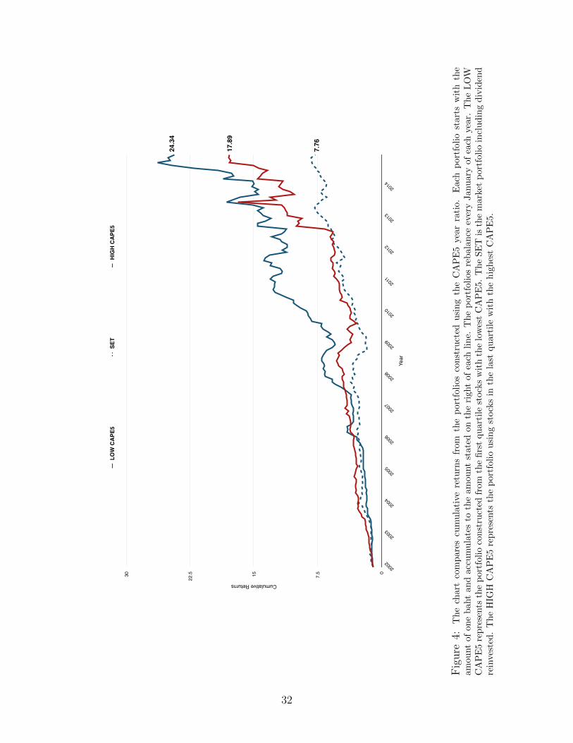
price-to-earning ratio (CAPE5). According to the table 4, a portfolio consisting of stocks

with a low level of CAPE5, underperforms the portfolio consisting of high CAPE5, based

on the monthly arithmetic average, the annual geometric average, and the excess average.

Low CAPE5 portfolio achieves a 2.18% arithmetic average compared to 2.27% for the high

CAPE5 portfolio. Low CAPE5 stocks give 27.17% geometric average per year compared to

30.47% for the high CAPE5 stocks. The low CAPE5 portfolio has the worst monthly return

of -26.21%, which is lower than the high CAPE5 stocks(-14.97%). However, the low CAPE5

portfolio has a higher maximum return (49.11%) than the high CAPE5 stocks(30.32%).

16

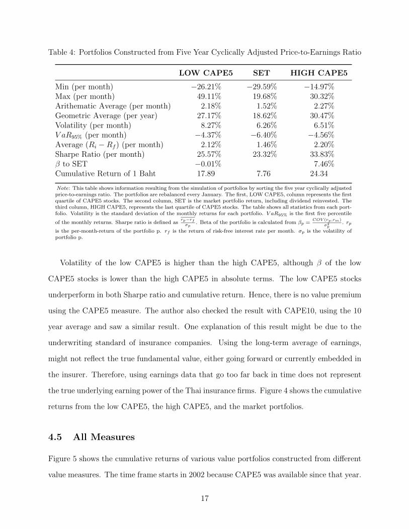
Table 4: Portfolios Constructed from Five Year Cyclically Adjusted Price-to-Earnings Ratio

LOW CAPE5 SET HIGH CAPE5


Note: This table shows information resulting from the simulation of portfolios by sorting the five year cyclically adjustedprice-to-earnings ratio. The portfolios are rebalanced every January. The first, LOW CAPE5, column represents the firstquartile of CAPE5 stocks. The second column, SET is the market portfolio return, including dividend reinvested. Thethird column, HIGH CAPE5, represents the last quartile of CAPE5 stocks. The table shows all statistics from each port-folio. Volatility is the standard deviation of the monthly returns for each portfolio. V aR95% is the first five percentile

of the monthly returns. Sharpe ratio is defined asrp−rfσp


σ2p

. rp

is the per-month-return of the portfolio p. rf is the return of risk-free interest rate per month. σp is the volatility ofportfolio p.

Volatility of the low CAPE5 is higher than the high CAPE5, although β of the low

CAPE5 stocks is lower than the high CAPE5 in absolute terms. The low CAPE5 stocks

underperform in both Sharpe ratio and cumulative return. Hence, there is no value premium

using the CAPE5 measure. The author also checked the result with CAPE10, using the 10

year average and saw a similar result. One explanation of this result might be due to the

underwriting standard of insurance companies. Using the long-term average of earnings,

might not reflect the true fundamental value, either going forward or currently embedded in

the insurer. Therefore, using earnings data that go too far back in time does not represent

the true underlying earning power of the Thai insurance firms. Figure 4 shows the cumulative

returns from the low CAPE5, the high CAPE5, and the market portfolios.

4.5 All Measures

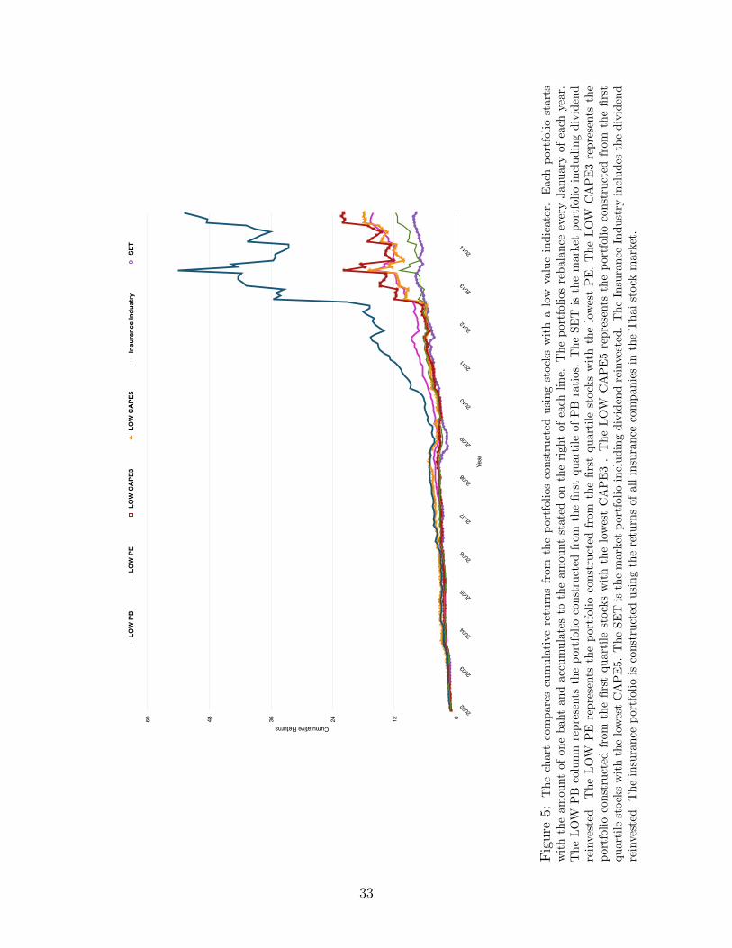
Figure 5 shows the cumulative returns of various value portfolios constructed from different

value measures. The time frame starts in 2002 because CAPE5 was available since that year.

17

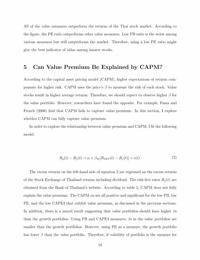
All of the value measures outperform the returns of the Thai stock market. According to

the figure, the PE ratio outperforms other value measures. Low PB ratio is the worst among

various measures but still outperforms the market. Therefore, using a low PE ratio might

give the best indicator of value among insurer stocks.

5 Can Value Premium Be Explained by CAPM?

According to the capital asset pricing model (CAPM), higher expectations of returns com-

pensate for higher risk. CAPM uses the price’s β to measure the risk of each stock. Value

stocks result in higher average returns. Therefore, we should expect to observe higher β for

the value portfolio. However, researchers have found the opposite. For example, Fama and

French (2006) find that CAPM fails to capture value premium. In this section, I explore

whether CAPM can fully capture value premium.

In order to explore the relationship between value premium and CAPM, I fit the following

model.

Rp(t) −Rf (t) = α + βM [RSET (t) −Rf (t)] + ε(t). (2)

The excess returns on the left-hand side of equation 2 are regressed on the excess returns

of the Stock Exchange of Thailand returns including dividend. The risk-free rates Rf (t) are

obtained from the Bank of Thailand’s website. According to table 5, CAPM does not fully

explain the value premium. The CAPM αs are all positive and significant for the low PB, low

PE, and the low CAPE3 that exhibit value premium, as discussed in the previous sections.

In addition, there is a mixed result suggesting that value portfolios should have higher βs

than the growth portfolios. Using PB and CAPE3 measures, βs in the value portfolios are

smaller than the growth portfolios. However, using PE as a measure, the growth portfolio

has lower β than the value portfolio. Therefore, if volatility of portfolio is the measure for

18

risk, we cannot conclude that the value portfolio achieves higher returns than the growth

portfolio due to risk. The R2’s are also low in all the cases. Therefore, market excess returns

do a poor job in explaining the portfolios’ excess returns.

Table 5: CAPM Using SET Index

Portfolio α βSET R2 F-Stat P-Val Obs Year

LOW PB 1.32 ** −0.04 0.0013 0.3904 0.5326 298 1990-2014[2.24] [−0.63]

HIGH PB 0.65 0.05 0.0030 0.8878 0.3468 298 1990-2014[1.47] [0.94]

LOW PE 2.98 *** 0.05 0.0022 0.4388 0.5085 203 1998-2014[4.33] [0.66]

HIGH PE 0.82 * 0.02 0.0006 0.1270 0.7220 203 1998-2014[1.78] [0.36]

LOW CAPE3 2.24 *** −0.02 0.0002 0.0269 0.8700 179 2000-2014[3.33] [−0.16]

HIGH CAPE3 1.30 *** 0.03 0.2459 0.2459 0.6206 179 2000-2014[0.49] [0.07]

Note: This table shows information resulting from OLS regressions of the value portfolio excessreturns, constructed from PB, PE and CAPE3, based on SET market index excess returns, in-cluding dividends. LOW PB is the portfolio containing the lowest quartile of PB. HIGH PB is theportfolio containing stocks with the highest quartile of PB. LOW PE is the portfolio consisting ofstocks with the lowest quartile of PE. HIGH PE is a portfolio consisting of stocks with the high-est quartile of PE. LOW CAPE3 is a portfolio that contains the lowest quartile of CAPE3 stocks.Lastly, HIGH CAPE3 is a portfolio containing high CAPE3 stocks. α column represents the con-stant coefficients from all OLS regressions. βSET is the column that contains the coefficients ofthe SET index excess returns, including dividend. R2 is the column that represents the R2 valueof each regression. F − Stat is the value of the F-statistics to test whether the βSET should bezero. P − V al is the column that represents the p-value from the F-test. Obs is the observationcolumn that represents the number of observations in each particular regression. Year is the col-umn to represent the year for which data was used, due to the availability of PB, PE and CAPE3.The numbers in square brackets are the t-statistics to test whether each coefficient is significantlydifferent from zero. ∗,∗∗, and ∗ ∗ ∗ represent the significant levels of 0.10, 0.05, and 0.01, respec-tively, from the t-tests.

Table 6 is the same as table 5 except I use Asia market returns instead of the SET index’s

returns. Asia market returns and Asia risk-free rates are from Kenneth French’s website.

Again, CAPM does not fully explain the value premium. All the α’s of the value portfolios

are positive and significant. Value portfolios have higher βs than the growth portfolios in

absolute terms and in all cases. Therefore, using the Asia market index to capture the

portfolio returns has the same results as implied by CAPM. However, R2’s are low for all the

cases similar to the previous case when I used SET index returns. Therefore, Asian market

index excess returns doe a poor job in explaining the portfolios’ excess returns.

19

Table 6: CAPM Using Asia Market Index

Portfolio α βAsia R2 F-Stat P-Val Obs Year

LOW PB 1.36 ** −0.06 0.0012 0.3540 0.5523 293 1990-20142.27 −0.60

HIGH PB 0.52 0.04 0.0009 0.2732 0.6016 293 1990-20141.23 0.52

LOW PE 3.06 *** −0.11 0.0049 0.9901 0.3209 203 1998-20144.45 −1.00

HIGH PE 0.81 * −0.05 0.0019 0.3934 0.5312 203 1998-20141.76 −0.63

LOW CAPE3 2.26 *** −0.15 0.0108 1.9360 0.1658 179 2000-20143.39 −1.39

HIGH CAPE3 1.22 *** 0.06 0.0031 0.5458 0.4610 179 2000-20142.50 0.74

Note: This table shows information resulting from OLS regressions of value portfolio excess re-turns, constructed from PB, PE and CAPE3, based on the Asia market index excess returns fromKenneth Frenchs website. LOW PB is the portfolio containing the lowest quartile of PB. HIGH PBis a portfolio containing stocks with the highest quartile of PB. LOW PE is the portfolio consistingof stocks with the lowest quartile of PE. HIGH PE is a portfolio consisting of stocks with the high-est quartile of PE. LOW CAPE3 is a portfolio that contains the lowest quartile of CAPE3 stocks.Lastly, HIGH CAPE3 is a portfolio containing high CAPE3 stocks. The α column represents theconstant coefficients from all OLS regressions. βAsia is a column that contains the coefficients ofthe Asia market excess returns. R2 is the column that represents the R2 value of each regression.F − Stat is the value of the F-statistics to test whether the βAsia should be zero. P − V al is thecolumn that represents the p-value from the F-test. Obs is the observation column that representsthe number of observations in each particular regression. Year is the column to represent the yearfor which data was used due to the availability of PB, PE and CAPE3. The numbers in squarebrackets are the t-statistics to test whether each coefficient is significantly different from zero. ∗,∗∗,and ∗ ∗ ∗ represent the significant levels of 0.10, 0.05, and 0.01, respectively, from the t-tests.

Next, I test whether value premium can be explained by the global market index in table

7. I use the global portfolio returns and global risk-free rates from Kenneth Frenchs website.

According to the table 7, αs are all positive and significant for the value portfolio. Therefore,

CAPM, using global market returns, does not fully explain the value anomaly. In addition,

βs in the value portfolios is not shown to be more than the growth portfolio in all cases. In

the PE case, β of the portfolio is lower than the growth portfolio. Therefore, if we use price

volatility as a proxy for risks, we cannot conclude that the value portfolio is riskier than the

growth portfolio.

20

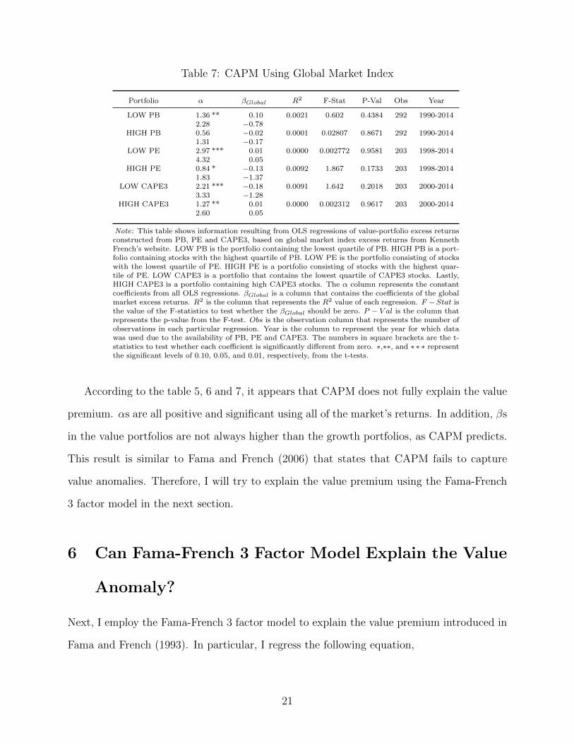
Table 7: CAPM Using Global Market Index

Portfolio α βGlobal R2 F-Stat P-Val Obs Year

LOW PB 1.36 ** 0.10 0.0021 0.602 0.4384 292 1990-20142.28 −0.78

HIGH PB 0.56 −0.02 0.0001 0.02807 0.8671 292 1990-20141.31 −0.17

LOW PE 2.97 *** 0.01 0.0000 0.002772 0.9581 203 1998-20144.32 0.05

HIGH PE 0.84 * −0.13 0.0092 1.867 0.1733 203 1998-20141.83 −1.37

LOW CAPE3 2.21 *** −0.18 0.0091 1.642 0.2018 203 2000-20143.33 −1.28

HIGH CAPE3 1.27 ** 0.01 0.0000 0.002312 0.9617 203 2000-20142.60 0.05

Note: This table shows information resulting from OLS regressions of value-portfolio excess returnsconstructed from PB, PE and CAPE3, based on global market index excess returns from KennethFrench’s website. LOW PB is the portfolio containing the lowest quartile of PB. HIGH PB is a port-folio containing stocks with the highest quartile of PB. LOW PE is the portfolio consisting of stockswith the lowest quartile of PE. HIGH PE is a portfolio consisting of stocks with the highest quar-tile of PE. LOW CAPE3 is a portfolio that contains the lowest quartile of CAPE3 stocks. Lastly,HIGH CAPE3 is a portfolio containing high CAPE3 stocks. The α column represents the constantcoefficients from all OLS regressions. βGlobal is a column that contains the coefficients of the globalmarket excess returns. R2 is the column that represents the R2 value of each regression. F −Stat isthe value of the F-statistics to test whether the βGlobal should be zero. P − V al is the column thatrepresents the p-value from the F-test. Obs is the observation column that represents the number ofobservations in each particular regression. Year is the column to represent the year for which datawas used due to the availability of PB, PE and CAPE3. The numbers in square brackets are the t-statistics to test whether each coefficient is significantly different from zero. ∗,∗∗, and ∗ ∗ ∗ representthe significant levels of 0.10, 0.05, and 0.01, respectively, from the t-tests.

According to the table 5, 6 and 7, it appears that CAPM does not fully explain the value

premium. αs are all positive and significant using all of the market’s returns. In addition, βs

in the value portfolios are not always higher than the growth portfolios, as CAPM predicts.

This result is similar to Fama and French (2006) that states that CAPM fails to capture

value anomalies. Therefore, I will try to explain the value premium using the Fama-French

3 factor model in the next section.

6 Can Fama-French 3 Factor Model Explain the Value

Anomaly?

Next, I employ the Fama-French 3 factor model to explain the value premium introduced in

Fama and French (1993). In particular, I regress the following equation,

21

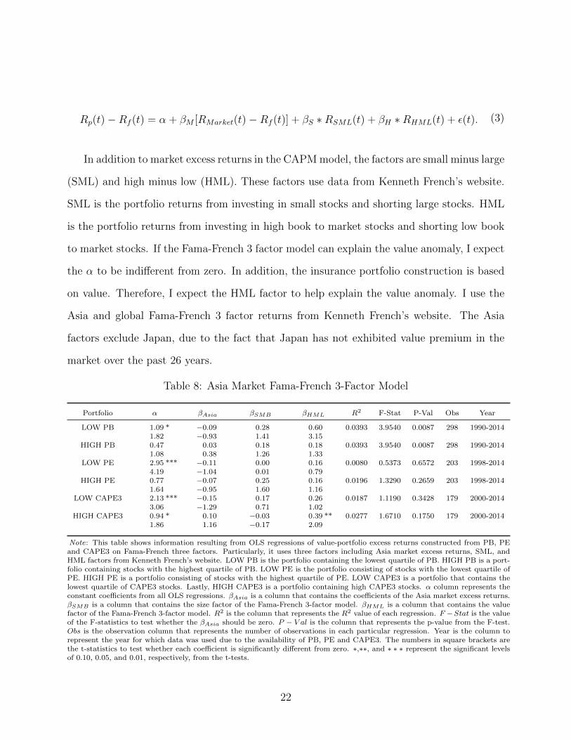
Rp(t) −Rf (t) = α + βM [RMarket(t) −Rf (t)] + βS ∗RSML(t) + βH ∗RHML(t) + ε(t). (3)

In addition to market excess returns in the CAPM model, the factors are small minus large

(SML) and high minus low (HML). These factors use data from Kenneth French’s website.

SML is the portfolio returns from investing in small stocks and shorting large stocks. HML

is the portfolio returns from investing in high book to market stocks and shorting low book

to market stocks. If the Fama-French 3 factor model can explain the value anomaly, I expect

the α to be indifferent from zero. In addition, the insurance portfolio construction is based

on value. Therefore, I expect the HML factor to help explain the value anomaly. I use the

Asia and global Fama-French 3 factor returns from Kenneth French’s website. The Asia

factors exclude Japan, due to the fact that Japan has not exhibited value premium in the

market over the past 26 years.

Table 8: Asia Market Fama-French 3-Factor Model

Portfolio α βAsia βSMB βHML R2 F-Stat P-Val Obs Year

LOW PB 1.09 * −0.09 0.28 0.60 0.0393 3.9540 0.0087 298 1990-20141.82 −0.93 1.41 3.15

HIGH PB 0.47 0.03 0.18 0.18 0.0393 3.9540 0.0087 298 1990-20141.08 0.38 1.26 1.33

LOW PE 2.95 *** −0.11 0.00 0.16 0.0080 0.5373 0.6572 203 1998-20144.19 −1.04 0.01 0.79

HIGH PE 0.77 −0.07 0.25 0.16 0.0196 1.3290 0.2659 203 1998-20141.64 −0.95 1.60 1.16

LOW CAPE3 2.13 *** −0.15 0.17 0.26 0.0187 1.1190 0.3428 179 2000-20143.06 −1.29 0.71 1.02

HIGH CAPE3 0.94 * 0.10 −0.03 0.39 ** 0.0277 1.6710 0.1750 179 2000-20141.86 1.16 −0.17 2.09

Note: This table shows information resulting from OLS regressions of value-portfolio excess returns constructed from PB, PEand CAPE3 on Fama-French three factors. Particularly, it uses three factors including Asia market excess returns, SML, andHML factors from Kenneth French’s website. LOW PB is the portfolio containing the lowest quartile of PB. HIGH PB is a port-folio containing stocks with the highest quartile of PB. LOW PE is the portfolio consisting of stocks with the lowest quartile ofPE. HIGH PE is a portfolio consisting of stocks with the highest quartile of PE. LOW CAPE3 is a portfolio that contains thelowest quartile of CAPE3 stocks. Lastly, HIGH CAPE3 is a portfolio containing high CAPE3 stocks. α column represents theconstant coefficients from all OLS regressions. βAsia is a column that contains the coefficients of the Asia market excess returns.βSMB is a column that contains the size factor of the Fama-French 3-factor model. βHML is a column that contains the valuefactor of the Fama-French 3-factor model. R2 is the column that represents the R2 value of each regression. F −Stat is the valueof the F-statistics to test whether the βAsia should be zero. P − V al is the column that represents the p-value from the F-test.Obs is the observation column that represents the number of observations in each particular regression. Year is the column torepresent the year for which data was used due to the availability of PB, PE and CAPE3. The numbers in square brackets arethe t-statistics to test whether each coefficient is significantly different from zero. ∗,∗∗, and ∗ ∗ ∗ represent the significant levelsof 0.10, 0.05, and 0.01, respectively, from the t-tests.

22

According to the table 8, the Fama-French 3 factor model, using the Asia data excluding

Japan, still does not capture the value anomaly. The intercept or α is still significantly

positive. The R2 is higher than previous sections from CAPM, although this is what is

expected as more variables are added to the regression. Observations are different in each

measure (PB, PE, CAPE3) due to the availability of each measure. The only factor that

is significant is from the use of CAPE3. The βHML is positive and significant, which is

counterintuitive. βHML should be positive for the low CAPE3 case, as expected.

Table 9: Global Fama-French 3-Factor Model

Portfolio α βGlobal βSMB βHML R2 F-Stat P-Val Obs Year

LOW PB 1.20 ** −0.07 0.67 ** 0.36 0.0244 2.4140 0.0668 298 1990-20142.00 −0.48 2.37 1.37

HIGH PB 0.54 −0.01 0.38 * 0.01 0.0120 1.1750 0.3196 298 1990-20141.25 −0.08 1.86 0.07

LOW PE 2.93 *** 0.01 0.12 0.07 0.0008 0.0527 0.9840 203 1998-20144.18 0.07 0.35 0.25

HIGH PE 0.73 −0.13 0.41 * 0.16 0.0274 1.8760 0.1349 203 1998-20141.57 −1.32 1.86 0.92

LOW CAPE3 2.18 *** −0.18 0.08 0.03 0.0095 0.5630 0.6401 179 2000-20143.14 −1.27 0.25 0.11

HIGH CAPE3 1.13 ** 0.01 0.22 0.17 0.0068 0.4027 0.7512 179 2000-20142.23 0.08 0.91 0.84

Note: This table shows information resulting from OLS regressions of value-portfolio excess returns constructed from PB, PEand CAPE3 on Fama-French three factors. Particularly, it uses three factors, including global market excess returns, SML, andHML factors from Kenneth Frenchs website. LOW PB is the portfolio containing the lowest quartile of PB. HIGH PB is a port-folio containing stocks with the highest quartile of PB. LOW PE is a portfolio consisting of stocks with the lowest quartile ofPE. HIGH PE is a portfolio consisting of stocks with the highest quartile of PE. LOW CAPE3 is a portfolio that contains thelowest quartile of CAPE3 stocks. Lastly, HIGH CAPE3 is a portfolio containing high CAPE3 stocks. α column represents theconstant coefficients from all OLS regressions. βGlobal is a column that contains the coefficients of the global market excess re-turns. βSMB is a column that contains the size factor of the Fama-French 3-factor model. βHML is a column that contains thevalue factor of the Fama-French 3-factor model. R2 is the column that represents the R2 value of each regression. F − Stat isthe value of the F-statistics to test whether the βGlobal should be zero. P − V al is the column that represents the p-value fromthe F-test. Obs is the observation column that represents the number of observations in each particular regression. Year is a col-umn to represent the year that data is used due to the availability of PB, PE and CAPE3. The numbers in square brackets arethe t-statistics to test whether each coefficient is significantly different from zero. ∗,∗∗, and ∗ ∗ ∗ represent the significant levelsof 0.10, 0.05, and 0.01, respectively, from the t-tests.

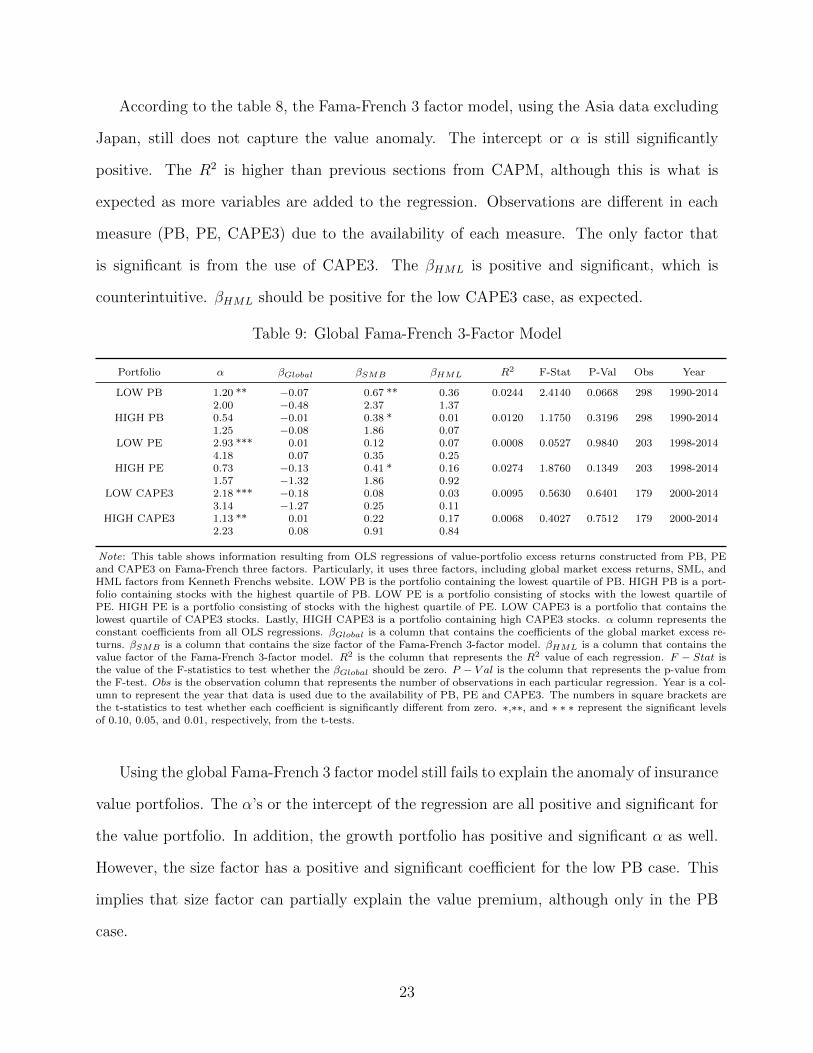
Using the global Fama-French 3 factor model still fails to explain the anomaly of insurance

value portfolios. The α’s or the intercept of the regression are all positive and significant for

the value portfolio. In addition, the growth portfolio has positive and significant α as well.

However, the size factor has a positive and significant coefficient for the low PB case. This

implies that size factor can partially explain the value premium, although only in the PB

case.

23

Overall, the global and Asia Fama-French 3 factor models do not fully explain the value

premiums of insurance value portfolios. The explanation of this finding could involve several

issues, including the number of stocks in the value portfolio and the factors themselves. On

average, each value portfolio consists of about four stocks. These stocks can be volatile in

comparison to the studies of Fama and French (1993) that contain hundreds of stocks. The

noise in the regression is so high that the Fama-French 3 factor fails to find the relationship

between portfolio returns and the factors. The implication of this is that if investors con-

centrate on a few stocks instead of many, they can outperform the market with low portfolio

volatility. In addition, as I used the available Fama-French 3 Factor models, globally and

for Asia, an these factors might not be able to provide the explanation within the local

market of Thailand. Therefore, it leaves some room for future research to construct a local

Fama-French 3 factor model to explain this anomaly.

7 Conclusion

The study explores value stocks, specifically for insurance industry in Thailand. According

to the results, we can argue that by focusing on a particular industry, investors can still

outperform the market using a value investing strategy. Similar to previous value studies,

this study finds value premiums within the Thai insurance industry. Investing in low value

measures, such as PE, PB, CAPE3, and CAPE5, outperforms the market, although value

premium does not always occur when we look too far back over many years, for example in

the CAPE5 case. Using the traditional PE ratio can be very profitable to beat the market.

This result is similar to Basu (1977). Using the value measure by PB ratio does not perform

quite as well for insurance stocks, compared to the PE measure. However, the study does

not consider size, so we cannot draw a conclusion that is similar to Fama and French (1992)

that combines size and value factors, and absorbs the price-to-earnings factor to predict the

returns from the stocks.

24

According to the results, price volatility from CAPM does not fully explain the value

premium. Value stocks widely outperform the high PE, PB and CAPE3, even when adjusted

for volatility and beta. Jensen’s alpha is also higher for the value portfolio. In addition, the

Fama-French 3 factor model using global and Asia factors do not capture the value anomaly.

The author suspects that this is due to the small number of stocks in the portfolio, and also

because the factors are not local enough for the Thai market. On the other hand, it shows

that investors can achieve superior results by investing in low PB, PE and CAPE3 insurance

stocks. It also achieves superior absolute returns with lower portfolio volatility.

Still, this study has some limitations. First, it focuses particularly on the insurance

industry. It assumes that investors have a circle of competence that is based on the insurance

industry. The study can expand to other industries within the stock market. Second, the

number of stocks in the portfolio is arguably small (four, on average). Therefore, this result

might be biased toward this limited dataset. One might argue that this is a result from a

data snooping problem. However, one might also argue that in order to beat the market,

there does not need to be a huge amount of stocks in the portfolio, which is the main point of

this study. In addition, the study also uses a long period of time to construct and rebalance

the portfolio. The results that show the value portfolio outperforming the growth portfolio

seems to be in line with previous studies of the Thai stock market, such as Sareewiwatthana

(2011, 2012, 2013).

In addition, there might be other factors in the behavior of investors to explain the value

anomaly. The author leaves it to future research to explore these issues. In addition, the

paper does not incorporate any quality measures into constructing the portfolios, as in Novy-

Marx (2013) or Novy-Marx (2015), although the pure value portfolio can still outperform

the market. The notion of investing in the things that an investor understands, or within a

circle of competence has begun.

25

References

Asness, C., A. Frazzini, R. Israel, and T. Moskowitz (2015): “Fact, Fiction, and

Value Investing,” Available at SSRN 2595747.

Asness, C. S., J. Moskowitz, and L. H. Pedersen (2013): “Value and Momentum

Everywhere,” Journal of Finance, 68(3), 929–985.

Basu, S. (1977): “Investment Performance of Common Stocks in Relation to Their Price-

Earnings Ratios: A Test of the Efficient Market Hypothesis,” Journal of Finance, 32(3),

663–682.

Bondt, W. F., and R. Thaler (1985): “Does the Stock Market Overreact?,” Journal of

Finance, 40(3), 793–805.

Campbell, J. Y., and R. J. Shiller (1988): “Stock Prices, Earnings, and Expected

Dividends,” The Journal of Finance, 43(3), 661–676.

Carnegie, A. (2012): The Autobiography of Andrew Carnegie. CreateSpace Independent

Publishing Platform.

Cummins, J. D., M. A. Weiss, and H. Zi (1999): “Organizational Form and Efficiency:

The Coexistence of Stock and Mutual Property-Liability Insurers,” Management Science,

45(9), 1254–1269.

Daniel, K., D. Hirshleifer, and A. Subrahmanyam (1998): “Investor Psychology

and Security Market Under and Overreactions,” Journal of Finance, 53(6), 1839–1885.

Dodd, D., and B. Graham (1951): Security Analysis: The Classic 1951 Edition. New

York: McGraw Hill.

Fama, E. F., and K. R. French (1992): “The Crosssection of Expected Stock Returns,”

Journal of Finance, 47(2), 427–465.

26

(1993): “Common Risk Factors in the Returns on Stocks and Bonds,” Journal of

Financial Economics, 33, 3–56.

(1995): “Size and Book-to-Market Factors in Earnings and Returns,” Journal of

Finance, 50(1), 131–155.

(1996): “Multifactor Explanations of Asset Pricing Anomalies,” Journal of Finance,

51(1), 55–84.

(1998): “Value versus Growth: The International Evidence,” Journal of Finance,

53(6), 1975–1999.

(2006): “The value premium and the CAPM,” Journal of Finance, 61(5), 2163–

2185.

(2012): “Size, value, and momentum in international stock returns,” Journal of

Financial Economics, 105(3), 457–472.

(2015): “A Five-Factor Asset Pricing Model,” Journal of Financial Economics,

116(1), 1–22.

Frazzini, A., D. Kabiller, and L. H. Pedersen (2013): “Buffett’s Alpha,” Working

Paper.

Graham, B. (2003): The Intelligent Investor: The Definitive Book on Value Investing. A

Book of Practical Counsel (Revised 7th Edition). New York:Harper & Collins.

Lakonishok, J., A. Shleifer, and R. W. Vishny (1994): “Contrarian Investment,

Extrapolation, and Risk,” Journal of Finance, 49(5), 1541–1578.

Nettayanun, S. (2014): “Essays on Strategic Risk Management,” Georgia State University.

Novy-Marx, R. (2013): “The Other Side of Value: The Gross Profitability Premium,”

Journal of Financial Economics, 108(1), 1–28.

27

(2015): “Quality Investing,” Working Paper.

Piotroski, J. D. (2000): “Value Investing: The Use of Historical Financial Statement

Information to Separate Winners from Losers,” Journal of Accounting Research, pp. 1–41.

Piotroski, J. D., and E. C. So (2012): “Identifying Expectation Errors in

Value/Glamour Strategies: A Fundamental Analysis Approach,” Review of Financial

Studies, hhs061.

Sareewiwatthana, P. (2011): “Value Investing in Thailand: The Test of Basic Screening

Rules,” International Review of Business Research Papers, 7(4), 1–13.

(2012): “Value Investing in Thailand: Evidence from the Use of PEG,” Technology

and Investment, 3(2), 113–120.

(2013): “Common Financial Ratios and Value Investing in Thailand,” Journal of

Finance and Investment Analysis, 2(3), 69–85.

Sharpe, W. F. (1964): “Capital Asset Prices: A Theory of Market Equilibrium under

Conditions of Risk*,” Journal of Finance, 19(3), 425–442.

Shleifer, A., and R. W. Vishny (1997): “The Limits of Arbitrage,” Journal of Finance,

52(1), 35–55.

28

6.62

3.74

Cumulative returns

0

7.515

22.530

Year

1990

1991

1992

1993

1994

1995

1996

1997

1998

1999

2000

2001

2002

2003

2004

2005

2006

2007

2008

2009

2010

2011

2012

2013

2014

LOW

PB

SET

HIG

H P

B

23.3

9

Fig

ure

1:T

he

char

tco

mp

ares

the

cum

ula

tive

retu

rns

from

the

port

folios

con

stru

cted

,u

sin

gth

ep

rice

-to-b

ook

(PB

)ra

tio.

Each

port

foli

ost

art

sw

ith

the

amou

nt

ofon

eb

aht

and

accu

mu

late

sto

the

am

ou

nt

state

don

the

right

of

each

lin

e.T

he

port

foli

os

reb

ala

nce

ever

yJanu

ary

of

each

yea

r.T

he

LO

WP

Bco

lum

nre

pre

sents

the

por

tfol

ioco

nst

ruct

edfr

om

the

firs

tqu

art

ile

of

PB

.T

he

SE

Tis

the

mark

etp

ort

folio

incl

ud

ing

the

div

iden

dre

inves

ted

.T

he

HIG

HP

Bre

pre

sents

the

por

tfol

iow

ith

stock

sin

the

last

qu

art

ile

wit

hth

eh

igh

est

PB

.

29

6.77

250.

06

4.62

Cumulative Returns

075150

225

300

Year

1998

1999

2000

2001

2002

2003

2004

2005

2006

2007

2008

2009

2010

2011

2012

2013

2014

LOW

PE

SET

HIG

H P

E

Fig

ure

2:T

he

char

tco

mp

ares

cum

ula

tive

retu

rns

from

the

port

foli

os

con

stru

cted

usi

ng

the

pri

ce-t

o-e

arn

ings

(PE

)ra

tio.

Each

port

foli

ost

art

sw

ith

the

amou

nt

ofon

eb

aht

and

accu

mu

late

sto

the

am

ou

nt

state

don

the

right

of

each

lin

e.T

he

port

foli

os

reb

ala

nce

ever

yJanu

ary

of

each

yea

r.T

he

LO

WP

Ere

pre

sents

the

por

tfol

ioco

nst

ruct

edfr

om

the

firs

tqu

art

ile

stock

sw

ith

the

low

est

PE

.T

he

SE

Tis

the

mark

etp

ort

foli

oin

clu

din

gd

ivid

end

rein

vest

ed.

Th

eH

IGH

PE

rep

rese

nts

the

por

tfol

iou

sin

gst

ock

sin

the

last

qu

art

ile

wit

hth

eh

igh

est

PE

.

30

8.82

32.7

8

5.07

Cumulative Returns

010203040

Year

2000

2001

2002

2003

2004

2005

2006

2007

2008

2009

2010

2011

2012

2013

2014

LOW

CA

PE3

SET

HIG

H C

APE

3

Fig

ure

3:T

he

char

tco

mp

ares

cum

ula

tive

retu

rns

from

the

port

foli

os

con

stru

cted

usi

ng

CA

PE

3.

Each

port

foli

ost

art

sw

ith

the

am

ou

nt

of

on

eb

aht

and

accu

mu

late

sto

the

amou

nt

stat

edon

the

right

of

each

lin

e.T

he

port

foli

os

reb

ala

nce

ever

yJanu

ary

of

each

year.

Th

eH

IGH

CA

PE

3re

pre

sents

the

por

tfol

ioco

nst

ruct

edfr

omth

efirs

tqu

arti

lest

ock

sw

ith

the

low

est

CA

PE

3ra

tios.

Th

eSE

Tis

the

mark

etp

ort

foli

oin

clu

din

gd

ivid

end

rein

vest

ed.

Th

eH

IGH

CA

PE

3re

pre

sents

the

por

tfol

iou

sin

gst

ock

sin

the

last

qu

art

ile

wit

hth

eh

igh

est

CA

PE

3.

31

24.3

4

7.76

17.8

9

Cumulative Returns

0

7.515

22.530

Year

2002

2003

2004

2005

2006

2007

2008

2009

2010

2011

2012

2013

2014

LOW

CA

PE5

SET

HIG

H C

APE

5

Fig

ure

4:T

he

char

tco

mp

ares

cum

ula

tive

retu

rns

from

the

port

foli

os

con

stru

cted

usi

ng

the

CA

PE

5ye

ar

rati

o.

Each

port

foli

ost

art

sw

ith

the

amou

nt

ofon

eb

aht

and

accu

mu

late

sto

the

amou

nt

state

don

the

right

of

each

lin

e.T

he

port

foli

os

reb

ala

nce

ever

yJanu

ary

of

each

year.

The

LO

WC

AP

E5

rep

rese

nts

the

por

tfol

ioco

nst

ruct

edfr

omth

efi

rst

qu

art

ile

stock

sw

ith

the

low

est

CA

PE

5.

Th

eS

ET

isth

em

ark

etp

ort

foli

oin

clu

din

gd

ivid

end

rein

vest

ed.

Th

eH

IGH

CA

PE

5re

pre

sents

the

por

tfoli

ou

sin

gst

ock

sin

the

last

quart

ile

wit

hth

eh

igh

est

CA

PE

5.

32

Cumulative Returns

01224364860

Year

2002

2003

2004

2005

2006

2007

2008

2009

2010

2011

2012

2013

2014

LOW

PB

LOW

PE

LOW

CA

PE3

LOW

CA

PE5

Insu

ranc

e In

dust

rySE

T

Fig

ure

5:T

he

char

tco

mp

ares

cum

ula

tive

retu

rns

from

the

port

foli

os

con

stru

cted

usi

ng

stock

sw

ith

alo

wva

lue

ind

icato

r.E

ach

port

foli

ost

art

sw

ith

the

amou

nt

ofon

eb

aht

and

accu

mula

tes

toth

eam

ou

nt

state

don

the

right

of

each

lin

e.T

he

port

foli

os

reb

ala

nce

ever

yJanu

ary

of

each

year.

Th

eL

OW

PB

colu

mn

rep

rese

nts

the

por

tfol

ioco

nst

ruct

edfr

om

the

firs

tqu

art

ile

of

PB

rati

os.

Th

eS

ET

isth

em

ark

etp

ort

foli

oin

clu

din

gdiv

iden

dre

inve

sted

.T

he

LO

WP

Ere

pre

sents

the

por

tfoli

oco

nst

ruct

edfr

om

the

firs

tqu

art

ile

stock

sw

ith

the

low

est

PE

.T

he

LO

WC

AP

E3

rep

rese

nts

the

por

tfol

ioco

nst

ruct

edfr

omth

efi

rst

qu

arti

lest

ock

sw

ith

the

low

est

CA

PE

3.

Th

eL

OW

CA

PE

5re

pre

sents

the

port

foli

oco

nst

ruct

edfr

om

the

firs

tqu

arti

lest

ock

sw

ith

the

low

est

CA

PE

5.T

he

SE

Tis

the

mark

etp

ort

foli

oin

clu

din

gd

ivid

end

rein

vest

ed.

Th

eIn

sura

nce

Ind

ust

ryin

clu

des

the

div

iden

dre

inve

sted

.T

he

insu

ran

cep

ortf

olio

isco

nst

ruct

edu

sin

gth

ere

turn

sof

all

insu

ran

ceco

mp

an

ies

inth

eT

hai

stock

mark

et.

33

No. 46. 46 The opinions expressed in this discussion paper are those of the author(s) and should not...

Documents

Transcript of No. 46. 46 The opinions expressed in this discussion paper are those of the author(s) and should not...