Univerza v Ljubljani 

Fakulteta za matematiko in fiziko 

 

 

 

 

Oddelek za fiziko 

 

 

 

Seminar Ia – 2.letnik, II.stopnja 

NMRinalowfieldofapermanentmagnet 

Author: Janez Lužnik 

Advisor: prof. dr. Janez Dolinšek 

Ljubljana, March 2014 

 

 

 

 

 

 

 

 

Abstract 

In this seminar we first  look at the experimental setup of nuclear magnetic resonance spectroscopy 

in  a magnetic  field   of  a permanent magnet  at  room  temperature.  Then we  look  at  two possible 

practical  applications of  such  a  system.  In  conclusion we  also discus  some of  the  advantages  and 

disadvantages of both applications.   

2  

Tableofcontents 

1  Introduction ..................................................................................................................................... 2 

2  Nuclear magnetic resonance ........................................................................................................... 3 

2.1. Spin‐lattice relaxation .................................................................................................................. 4 

2.2. Spin‐spin relaxation ...................................................................................................................... 5 

3  Experimental setup ......................................................................................................................... 5 

4  Measuring the pore size distribution of cement pastes and mortar .............................................. 6 

4.1  Theoretical background ........................................................................................................... 6 

4.2  Results ..................................................................................................................................... 7 

5  NMR based liquid explosive detector ........................................................................................... 10 

5.1  Measurements of a series of samples ................................................................................... 10 

5.2  Simulation of different alcoholic beverages and shielding effect ......................................... 11 

6  Conclusions .................................................................................................................................... 12 

7  References ..................................................................................................................................... 13 

1 Introduction 

Nuclear magnetic  resonance  (NMR)  is a powerful non‐invasive  technique used  to measure various 

physical and chemical properties of molecules or materials. It usually requires strong magnetic fields 

generated by large superconducting magnets, which have to be cooled by liquid nitrogen and helium. 

The use of this technique is therefore limited to laboratories with suitable equipment.  

 

However systems that enable NMR in permanent fields at room temperature do exist. Some like the 

one that will be discussed in this paper are also small and portable. They broaden the use of NMR as 

an  investigative  technique  as  they  allow  on‐site  testing  and  give  fast  results.  Two  practical 

applications of such system will also be presented. 

   

3  

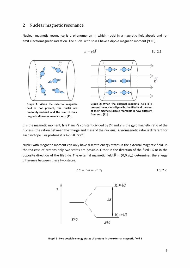
2 Nuclearmagneticresonance 

Nuclear magnetic  resonance  is  a  phenomenon  in which  nuclei in  a magnetic  field absorb  and  re‐

emit electromagnetic radiation. The nuclei with spin   have a dipole magnetic moment [9,10]: 

 

ħ                                                                       Eq. 2.1. 

 

 

 

 

 

 

 

 

 

 

 

 

 

 

 is the magnetic moment, ħ is Planck’s constant divided by 2π and   is the gyromagnetic ratio of the 

nucleus (the ration between the charge and mass of the nucleus). Gyromagnetic ratio is different for 

each isotope. For protons it is 42,6 / . 

 

Nuclei with magnetic moment can only have discrete energy states in the external magnetic field. In 

the tha case of protons only two states are possible. Either in the direction of the filed +½ or in the 

opposite direction of the filed  ‐½. The external magnetic field  0,0,  determines the energy 

difference between these two states. 

 

∆ ħ ħ                                                                      Eq. 2.2. 

 

 Graph 3: Two possible energy states of protons in the external magnetic field B 

Graph  1:  When  the  external  magnetic

field  is  not  present,  the  nuclei  are

randomly  ordered  and  the  sum  of  their

magnetic dipole moments is zero [11]. 

Graph  2:  When  the  external  magnetic  field  B  ispresent the nuclei allign wiht the filed and the sumof their magnetic dipole moments  is now differentfrom zero [11]. 

4  

 

 

The occupation of both energy states is defined by Boltzmann’s distribution: 

 

∝ħ

.                                                                   Eq. 2.3. 

At our conditions (frequency of 2MHz and temperature of 300K) the ratio ħ

 is about 10‐7. Therefore 

we can only  take  into account  the  linear part of  the extrapolation of the exponential  function. We 

can then define the difference between the occupations of both energy states as: 

∆ħ

.                                                   Eq. 2.4. 

There  is an  initial magnetization  in the sample  in the thermal equilibrium, which  is aligned with the 

direction of the field: 

∆ħ

.                                                     Eq. 2.5. 

The net magnetization   behaves in the external filed just as a single magnetic moment would. We 

can  flip  the  magnetization  out  of  its  initial  direction  for  an  angle  ,  using  a  short 

radiofrequency pulse (perpendicular to the initial magnetization) with the frequency  . The flipped 

magnetization  starts  to precess around  the external magnetic  field   with  the  frequency   and 

induces a signal in our detection coil. 

 

 

 

 

 

 

2.1.Spin‐latticerelaxationAfter  the  RF  pulse  is  turned  off,  the magnetization  slowly  returns  towards  the  equilibrium  state. 

During this process the spin system exchanges the energy with  its surrounding and the  longitudinal 

component  of  the  magnetization  changes.  The  process  is  called  spin‐lattice  relaxation  and  is 

characterized  by  the  spin‐lattice  relaxation  time  T1.  The  relaxation  is  described  by  the  following 

equations [11]: 

 

                                                                  Eq. 2.6. 

0                                             Eq. 2.7. 

Typical relaxation times for protons are around 2 to 3 seconds.  

Graph 4: The induction of NMR signal in the detection coil

5  

 

2.2.Spin‐spinrelaxationWe can flip the initial magnetization (oriented along the z axis) around the x axis using the π/2 pulse. 

The  magnetization  is  now  perpendicular  to  the  external  magnetic  filed  nad  we  refer  to  it  as 

transversal magnetization. After the pulse that was used to flip the magnetization  is turned of, the 

spins preces around the external magnetic filed B0 with the Larmor frequency    in the shape of a 

cone spiral. Initiall all spins precess in phase. However as time passes the spins begin to dephase and 

the transverzal magnetization decays towards  its equlibrium value of zero. The process  is described 

by the following equations: 

 

                                                             Eq. 2.8. 

                                                             Eq. 2.9. 

The spin‐spin relaxation  is characterized by the spin‐spin relaxation time T2.  It  is usually faster than 

spin‐lattice relaxation.  

 

3 Experimentalsetup 

In the two experiments we used a commercial system Magritek 2 MHz Rock CoreAnalyzer [1]. It is a 

cylindrical shaped magnet with the proton Larmor frequency of 2MHz. The system uses a heater to 

keep  the magnet temperature at 30 °C needed for field stability. The samples of maximal dimensions 

l = 62 mm and φ = 39 mm sit in a sample chamber, which is isolated form the magnet. All mea 

surements were done at room temperature. 

 

 

Grpah 5:  The complete Magritek 2 MHz Rock CoreAnalyzer system is shown on the left. On the right is a picture of the probe and sample chamber [2].  

6  

4 Measuringtheporesizedistributionofcementpastesandmortar 

Made  by mixing  water,  cement  and  sand  (mortar)  or  only  water  and  cement  (cement  pastes), 

mortars  and  cement pastes  are widely used  construction materials. As  they harden  they become 

porous,  which  affects  different  properties  of  these  materials  such  as  strength  and  durability. 

Measuring the pore size distribution gives us information about the types of porosity present in the 

material and helps us determine the quality of the material [3,4]. 

 

During  our  experiment we  analysed  four  different  groups  of  samples,  each  group  containing  six 

samples. Types of samples are shown in the table below. 

 

Type of sample  Number of sample (x)  Composition 

cp5 (cement pastes)  1 to 6  1 kg cement paste +500 ml water 

cp6 (cement pastes)  1 to 6  1 kg cement paste +650 ml water 

mr5 (mortars)  1 to 6  1 kg cement paste +3 kg sand+500 ml water 

mr6 (mortars)  1 to 6  1 kg cement paste +3 kg sand+650 ml water 

 

4.1 Theoreticalbackground 

In porous cement materials, the relaxation can be attributed to three main processes [5]:   

1

2

1

2

1

2

1

2           Eq. 4.1. 

 

Our  experiment  was  done  in  a  homogeneous  magnetic  field  so  that  the  diffusion  contribution 

( ) is negligible. Bulk relaxation ( ) is a slow process compared to the relaxation at the pore 

surface  ( ), which happens much  faster due  to paramagnetic  ions  in  the concrete, such as 

iron. Therefore we only measured the surface relaxation that is directly proportional to the pore size 

ratio [6,7]: 

                      Eq. 4.2. 

V  is  pore  volume,  S  is  the  pore  surface  and  ρ2  is  the  relaxivity  (μm/s),  defined  as  the  ability  of 

magnetic  compounds  to  increase  the  relaxation  rates of  the  surrounding water proton  spins. The 

spin‐lattice  relaxation  is  also proportional  to pore  size distribution.   Relaxivity  is different but  the 

relation is the same as for spin‐spin relaxation: 

                   Eq. 4.3. 

We fitted the T2 and T1 data to a broad distribution of relaxation times, using a NNLS (non‐negative 

least squares) algorithm. The stability and accuracy of results are better for T2 data due to the fact 

that 100 points per T2 experiment were used. For T1 measurements only 20 points per experiment 

were used. 

Table 1: Sample types 

7  

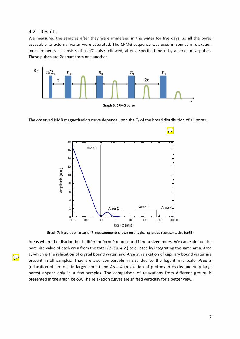
4.2 ResultsWe measured  the  samples  after  they were  immersed  in  the water  for  five days,  so  all  the pores 

accessible  to external water were saturated. The CPMG sequence was used  in spin‐spin  relaxation 

measurements.  It  consists of a π/2 pulse  followed, after a  specific  time  τ, by a  series of π pulses. 

These pulses are 2τ apart from one another. 

 

The observed NMR magnetization curve depends upon the T2 of the broad distribution of all pores. 

 

 

 

 

 

 

 

 

 

 

Areas where the distribution is different form 0 represent different sized pores. We can estimate the 

pore size value of each area from the total T2 (Eq. 4.2.) calculated by integrating the same area. Area 

1, which is the relaxation of crystal bound water, and Area 2, relaxation of capillary bound water are 

present  in  all  samples.  They  are  also  comparable  in  size  due  to  the  logarithmic  scale.  Area  3 

(relaxation  of  protons  in  larger  pores)  and Area  4  (relaxation  of  protons  in  cracks  and  very  large 

pores)  appear  only  in  a  few  samples.  The  comparison  of  relaxations  from  different  groups  is 

presented in the graph below. The relaxation curves are shifted vertically for a better view. 

   

Graph 6: CPMG pulse

1E-3 0,01 0,1 1 10 100 1000 100000

2

4

6

8

10

12

14

16

18

Area 3 Area 4

Am

plitu

de (

a.u

.)

log T2 (ms)

Area 1

Area 2

Graph 7: Integration areas of T2 measurements shown on a typical cp group representative (cp53) 

8  

 

 

 

 

 

 

 

 

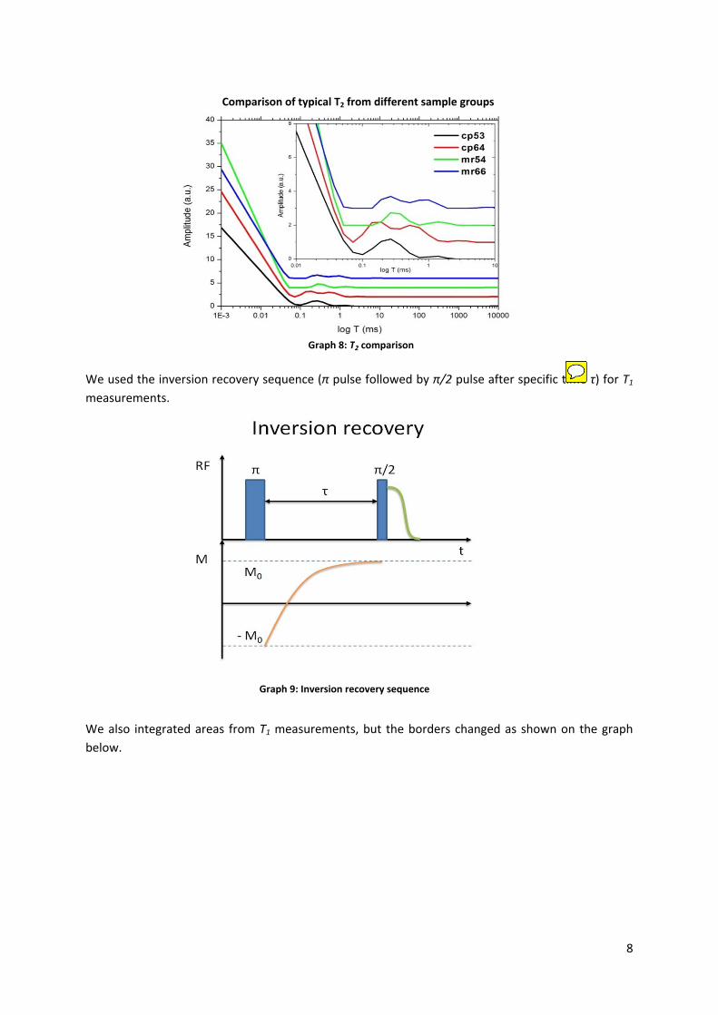
We used the inversion recovery sequence (π pulse followed by π/2 pulse after specific time τ) for T1 

measurements. 

 

 

 

 

 

 

 

 

 

We also  integrated areas  from T1 measurements, but  the borders changed as shown on  the graph 

below.  

 

   

Graph 8: T2 comparison

Graph 9: Inversion recovery sequence

Comparison of typical T2 from different sample groups

9  

1E-3 0,01 0,1 1 10 100 10000,0

0,1

0,2

0,3

0,4

Area 4

Area 3

Area 2

Am

plitu

de

(a.u

.)

log T (ms)

Area 1

 

 

 

 

 

 

 

 

The comparison of the relaxation curves  from different groups are shown on »Graph 6». Again we 

shifted them vertically for a better view. 

 

 

 

 

 

 

 

 

 

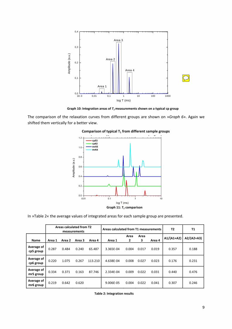
In »Table 2« the average values of integrated areas for each sample group are presented. 

  

Areas calculated from T2 measurements 

Areas calculated from T1 measurements T2  T1 

Name  Area 1  Area 2  Area 3  Area 4  Area 1 Area 2 

Area 3  Area 4 

A1/(A1+A2)  A2/(A2+A3) 

Average of cp5 group 

0.287  0.484  0.240  65.487  3.365E‐04  0.004  0.017  0.019  0.357  0.188 

Average of cp6 group 

0.220  1.075  0.267  113.210 4.638E‐04  0.008  0.027  0.023  0.176  0.231 

Average of mr5 group 

0.334  0.371  0.163  87.746  2.334E‐04  0.009  0.022  0.031  0.440  0.476 

Average of mr6 group 

0.219  0.642  0.620     9.006E‐05  0.004  0.022  0.041  0.307  0.246 

Graph 10: Integration areas of T1 measurements shown on a typical cp group 

Graph 11: T1 comparison

Table 2: Integration results 

Comparison of typical T1 from different sample groups 

10  

As  expected  because  of  the  different  relaxivities,  areas  calculated  from  T1  and  T2  do  not match. 

Instead we compared the area ratios (last two columns in »Table 2«), which matched quite well. They 

are important, because they offer us direct comparison between the water located in the pores (Area 

2) and crystal bound water (Area 1). 

5 NMRbasedliquidexplosivedetector 

In  the  past  there were  some  attempts  by  terrorists  to  detonate  liquid  explosives  on  commercial 

planes. As a result of that the amount of liquid that a person can bring on‐board in hand luggage has 

been  limited  to  several  containers with  a  volume  of  100ml  each.  A  detector  that  could  identify 

potential  threats could  increase security checks and possibly allow some  lighter restrictions.  In this 

experiment we  tested  the Magritek 2 MHz Rock CoreAnalyzer as a possible detector, which  could 

discriminate between various liquids on the basis of spin‐lattice and spin‐spin relaxation times.   

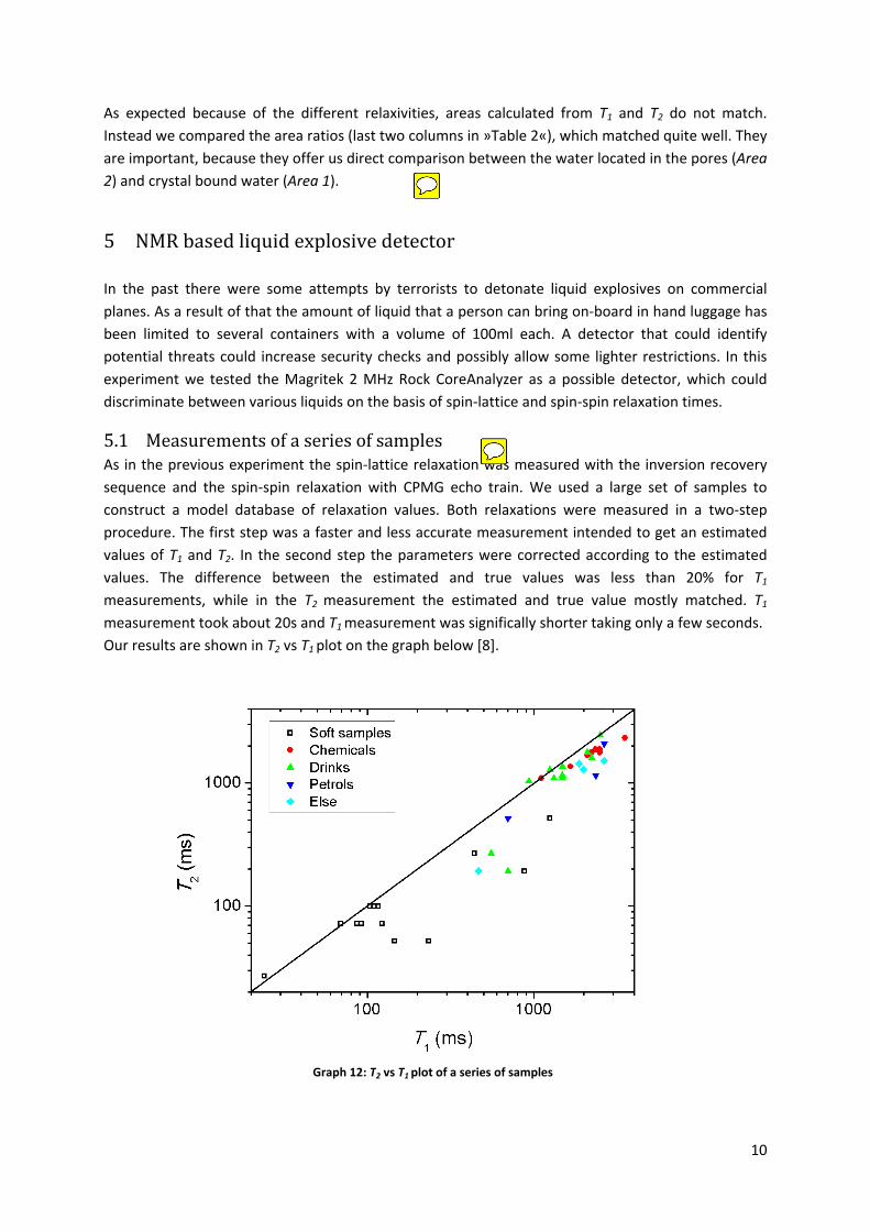
5.1 MeasurementsofaseriesofsamplesAs  in the previous experiment the spin‐lattice relaxation was measured with the  inversion recovery 

sequence  and  the  spin‐spin  relaxation with  CPMG  echo  train. We  used  a  large  set  of  samples  to 

construct  a model  database  of  relaxation  values.  Both  relaxations were measured  in  a  two‐step 

procedure. The first step was a faster and less accurate measurement intended to get an estimated 

values of T1 and T2.  In  the second step  the parameters were corrected according  to  the estimated 

values.  The  difference  between  the  estimated  and  true  values  was  less  than  20%  for  T1 

measurements,  while  in  the  T2  measurement  the  estimated  and  true  value mostly matched.  T1 

measurement took about 20s and T1 measurement was significally shorter taking only a few seconds. 

Our results are shown in T2 vs T1 plot on the graph below [8]. 

 

 

 

 

 

 

 

 

 

 

 

 

 

 

 

 

 

   Graph 12: T2 vs T1 plot of a series of samples

11  

We divided  the  samples  in  several  groups.  The  first  group  (laboratory  chemicals  such  as  ethanol, 

methanol,  toluene, etc.) and  the second group  (various non‐alcoholic and alcoholic drinks) overlap 

slightly with only a few samples form the second group such as milk having shorter relaxation times. 

95 and 100 octane petrol and diesel represent the next group. Here the T1 for diesel (0,7s) was much 

shorter than T1 for 95 (2,35s) and 100 (2,64s) octane petrol. Last group were viscous edible samples 

such as jam, honey, fruits, butter and several vegetable oils. These samples mostly had much shorter 

T1 and T2 values than the rest. 

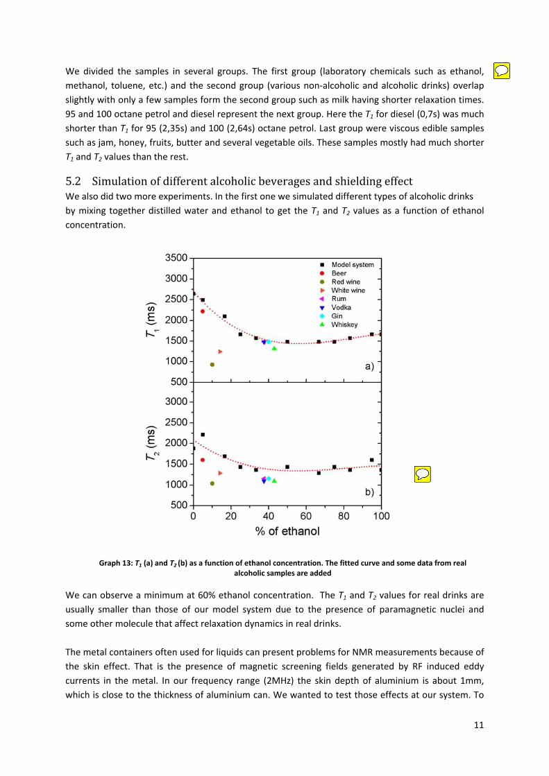
5.2 SimulationofdifferentalcoholicbeveragesandshieldingeffectWe also did two more experiments. In the first one we simulated different types of alcoholic drinks 

by mixing  together distilled water and ethanol  to get  the T1 and T2 values as a  function of ethanol 

concentration.   

 

 

 

 

 

 

 

 

 

 

 

 

 

 

 

 

 

 

 

 

 

 

 

 

 

We can observe a minimum at 60% ethanol concentration.   The T1 and T2 values for real drinks are 

usually  smaller  than  those of our model  system due  to  the  presence of  paramagnetic nuclei  and 

some other molecule that affect relaxation dynamics in real drinks. 

 

The metal containers often used for liquids can present problems for NMR measurements because of 

the  skin  effect.  That  is  the  presence  of magnetic  screening  fields  generated  by  RF  induced  eddy 

currents  in  the metal.  In our  frequency  range  (2MHz)  the  skin depth of aluminium  is about 1mm, 

which is close to the thickness of aluminium can. We wanted to test those effects at our system. To 

Graph 13: T1 (a) and T2 (b) as a function of ethanol concentration. The fitted curve and some data from real alcoholic samples are added 

12  

do that we used a 40ml sample of water with added CuSO4. First we measured the unshielded bottle. 

Then the bottle was wrapped with aluminium foil 30μm thick. It was still possible to measure both T1 

and T2 after wrapping the bottle in though the signal was two times smaller than without the shield. 

The problem was that we could not tune the resonant circle after adding two layers of foil due to the 

limited range of capacitors. 

 

6 Conclusions 

Measuring the pore size distribution of cement pastes and mortar 

It  is  essential  to  know  the  properties  of mortars  and  concretes  to  guarantee  their  stability  and 

durability.  NMR  spectroscopy  is  an  ideal  tool with which we  can  inspect  such materials without 

influencing  their  structure.  The  pore‐size  distribution  ratios  were  not  very  specific.  We  can 

distinguish among different groups but not among individual samples. Another useful measurement 

would  be  effective  porosity,  which  could  be  done  by modifying  our  system  with  gradient  coils 

allowing us to measure diffusion constant of water saturated samples. 

NMR based liquid explosive detector 

As  a  liquid  explosive  detector  our  system  offers  simple  T1  and  T2 measurements  of  large  sample 

volumes. Though  the measurements are quite  fast  for an efficient use  they would  still need  to be 

faster. Other disadvantages are the  lack of spatial resolution and that the proton density cannot be 

determined.  Again  as  was  the  case  in  the  first  experiment  we  could  benefit  from  diffusion 

measurements which are not possible without the gradient coils. 

   

Graph 14: T1 (left) and T2(right) relaxation curves with and without aluminium shielding 

13  

7 References 

[1] http://magritek.com/ 

[2] http://www.act‐aachen.com/halbach_magnets.html 

[3] McCain & Dewoolkar : Porous Concrete Pavements: Mechanical and Hydraulic 

Properties. http://www.uvm.edu/~transctr/publications/TRB_2010/10‐2228.pdf 

[4] Hildegard Westphal, Iris Surholt, Christian Kiesl, Holger F. Thern, Thomas Kruspe; Pure 

appl. geophys. 162 (2005) p.549 

[5] NMR Petrophysics. http://www.slideshare.net/sstromberg/NMRCOURSE 

[6] J.H. Strange, J. Mitchell, J.B.W. Webber; Magnetic Resonance Imaging 21 (2003) p.221 

[7] R M E Valckenborg, L Pel and K Kopinga; J. Phys. D: Appl. Phys. 35 (2002) p.249 

[8] A. Gradišek, J.Luzar, J.Lužnik, T. Apih; Magnetic Resonance Detection of Explosives and Illicit Materials, NATO Science for Peace and Security Series B: Physics and Biophysics 2014, pp. 123 

[9] M. H. Levitt: Spin dynamics: Basics of Nuclear Magnetic Resonance; Wiley, Chichester, 

UK (2008) 

[10] C. P. Slichter: Principles of Magnetic Resonance; Springer Verlag, Berlin (1996) 

[11] J. Dolinšek (2012); Spektroskopija trdne snovi, p.33