NLTK Parsing Demos - UCSC Directory of …abrsvn/NLTK_parsing_demos.pdfNLTK Parsing Demos Adrian...
35
NLTK Parsing Demos Adrian Brasoveanu * March 3, 2014 Contents 1 Recursive descent parsing (top-down, depth-first) 1 2 Shift-reduce (bottom-up) 4 3 Left-corner parser: top-down with bottom-up filtering 5 4 General Background: Memoization 6 5 Chart parsing 11 6 Bottom-Up Chart Parsing 15 7 Top-down Chart Parsing 21 8 The Earley Algorithm 25 9 Back to Left-Corner chart parsing 30 1 Recursive descent parsing (top-down, depth-first) [py1] >>> import nltk, re, pprint >>> from __future__ import division [py2] >>> grammar1 = nltk.parse_cfg(""" ... S -> NP VP ... VP -> V NP | V NP PP ... PP -> P NP ... V -> "saw" | "ate" | "walked" * Based on the NLTK book (Bird et al. 2009) and created with the PythonTeX package (Poore 2013). 1
Transcript of NLTK Parsing Demos - UCSC Directory of …abrsvn/NLTK_parsing_demos.pdfNLTK Parsing Demos Adrian...
NLTK Parsing Demos
Adrian Brasoveanu∗
March 3, 2014
Contents
1 Recursive descent parsing (top-down, depth-first) 1
2 Shift-reduce (bottom-up) 4
3 Left-corner parser: top-down with bottom-up filtering 5
4 General Background: Memoization 6
5 Chart parsing 11
6 Bottom-Up Chart Parsing 15
7 Top-down Chart Parsing 21
8 The Earley Algorithm 25
9 Back to Left-Corner chart parsing 30
1 Recursive descent parsing (top-down, depth-first)
[py1] >>> import nltk, re, pprint>>> from __future__ import division
[py2] >>> grammar1 = nltk.parse_cfg("""... S -> NP VP... VP -> V NP | V NP PP... PP -> P NP... V -> "saw" | "ate" | "walked"
∗Based on the NLTK book (Bird et al. 2009) and created with the PythonTeX package (Poore 2013).
1
... NP -> "John" | "Mary" | "Bob" | Det N | Det N PP
... Det -> "a" | "an" | "the" | "my"
... N -> "man" | "dog" | "cat" | "telescope" | "park"
... P -> "in" | "on" | "by" | "with"
... """)
[py3] >>> rd_parser = nltk.RecursiveDescentParser(grammar1)>>> sent = ’Mary saw a dog’.split()>>> sent[’Mary’, ’saw’, ’a’, ’dog’]>>> trees = rd_parser.nbest_parse(sent)>>> for tree in trees:... print tree, "\n\n"...(S (NP Mary) (VP (V saw) (NP (Det a) (N dog))))
[py4] >>> rd_parser = nltk.RecursiveDescentParser(grammar1, trace=2)>>> rd_parser.nbest_parse(sent)Parsing ’Mary saw a dog’
[ * S ]E [ * NP VP ]E [ * ’John’ VP ]E [ * ’Mary’ VP ]M [ ’Mary’ * VP ]E [ ’Mary’ * V NP ]E [ ’Mary’ * ’saw’ NP ]M [ ’Mary’ ’saw’ * NP ]E [ ’Mary’ ’saw’ * ’John’ ]E [ ’Mary’ ’saw’ * ’Mary’ ]E [ ’Mary’ ’saw’ * ’Bob’ ]E [ ’Mary’ ’saw’ * Det N ]E [ ’Mary’ ’saw’ * ’a’ N ]M [ ’Mary’ ’saw’ ’a’ * N ]E [ ’Mary’ ’saw’ ’a’ * ’man’ ]E [ ’Mary’ ’saw’ ’a’ * ’dog’ ]M [ ’Mary’ ’saw’ ’a’ ’dog’ ]+ [ ’Mary’ ’saw’ ’a’ ’dog’ ]E [ ’Mary’ ’saw’ ’a’ * ’cat’ ]E [ ’Mary’ ’saw’ ’a’ * ’telescope’ ]E [ ’Mary’ ’saw’ ’a’ * ’park’ ]E [ ’Mary’ ’saw’ * ’an’ N ]E [ ’Mary’ ’saw’ * ’the’ N ]E [ ’Mary’ ’saw’ * ’my’ N ]E [ ’Mary’ ’saw’ * Det N PP ]E [ ’Mary’ ’saw’ * ’a’ N PP ]M [ ’Mary’ ’saw’ ’a’ * N PP ]E [ ’Mary’ ’saw’ ’a’ * ’man’ PP ]
2
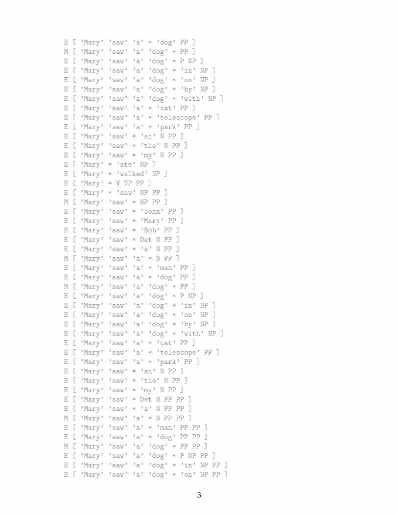
E [ ’Mary’ ’saw’ ’a’ * ’dog’ PP ]M [ ’Mary’ ’saw’ ’a’ ’dog’ * PP ]E [ ’Mary’ ’saw’ ’a’ ’dog’ * P NP ]E [ ’Mary’ ’saw’ ’a’ ’dog’ * ’in’ NP ]E [ ’Mary’ ’saw’ ’a’ ’dog’ * ’on’ NP ]E [ ’Mary’ ’saw’ ’a’ ’dog’ * ’by’ NP ]E [ ’Mary’ ’saw’ ’a’ ’dog’ * ’with’ NP ]E [ ’Mary’ ’saw’ ’a’ * ’cat’ PP ]E [ ’Mary’ ’saw’ ’a’ * ’telescope’ PP ]E [ ’Mary’ ’saw’ ’a’ * ’park’ PP ]E [ ’Mary’ ’saw’ * ’an’ N PP ]E [ ’Mary’ ’saw’ * ’the’ N PP ]E [ ’Mary’ ’saw’ * ’my’ N PP ]E [ ’Mary’ * ’ate’ NP ]E [ ’Mary’ * ’walked’ NP ]E [ ’Mary’ * V NP PP ]E [ ’Mary’ * ’saw’ NP PP ]M [ ’Mary’ ’saw’ * NP PP ]E [ ’Mary’ ’saw’ * ’John’ PP ]E [ ’Mary’ ’saw’ * ’Mary’ PP ]E [ ’Mary’ ’saw’ * ’Bob’ PP ]E [ ’Mary’ ’saw’ * Det N PP ]E [ ’Mary’ ’saw’ * ’a’ N PP ]M [ ’Mary’ ’saw’ ’a’ * N PP ]E [ ’Mary’ ’saw’ ’a’ * ’man’ PP ]E [ ’Mary’ ’saw’ ’a’ * ’dog’ PP ]M [ ’Mary’ ’saw’ ’a’ ’dog’ * PP ]E [ ’Mary’ ’saw’ ’a’ ’dog’ * P NP ]E [ ’Mary’ ’saw’ ’a’ ’dog’ * ’in’ NP ]E [ ’Mary’ ’saw’ ’a’ ’dog’ * ’on’ NP ]E [ ’Mary’ ’saw’ ’a’ ’dog’ * ’by’ NP ]E [ ’Mary’ ’saw’ ’a’ ’dog’ * ’with’ NP ]E [ ’Mary’ ’saw’ ’a’ * ’cat’ PP ]E [ ’Mary’ ’saw’ ’a’ * ’telescope’ PP ]E [ ’Mary’ ’saw’ ’a’ * ’park’ PP ]E [ ’Mary’ ’saw’ * ’an’ N PP ]E [ ’Mary’ ’saw’ * ’the’ N PP ]E [ ’Mary’ ’saw’ * ’my’ N PP ]E [ ’Mary’ ’saw’ * Det N PP PP ]E [ ’Mary’ ’saw’ * ’a’ N PP PP ]M [ ’Mary’ ’saw’ ’a’ * N PP PP ]E [ ’Mary’ ’saw’ ’a’ * ’man’ PP PP ]E [ ’Mary’ ’saw’ ’a’ * ’dog’ PP PP ]M [ ’Mary’ ’saw’ ’a’ ’dog’ * PP PP ]E [ ’Mary’ ’saw’ ’a’ ’dog’ * P NP PP ]E [ ’Mary’ ’saw’ ’a’ ’dog’ * ’in’ NP PP ]E [ ’Mary’ ’saw’ ’a’ ’dog’ * ’on’ NP PP ]
3
E [ ’Mary’ ’saw’ ’a’ ’dog’ * ’by’ NP PP ]E [ ’Mary’ ’saw’ ’a’ ’dog’ * ’with’ NP PP ]E [ ’Mary’ ’saw’ ’a’ * ’cat’ PP PP ]E [ ’Mary’ ’saw’ ’a’ * ’telescope’ PP PP ]E [ ’Mary’ ’saw’ ’a’ * ’park’ PP PP ]E [ ’Mary’ ’saw’ * ’an’ N PP PP ]E [ ’Mary’ ’saw’ * ’the’ N PP PP ]E [ ’Mary’ ’saw’ * ’my’ N PP PP ]E [ ’Mary’ * ’ate’ NP PP ]E [ ’Mary’ * ’walked’ NP PP ]E [ * ’Bob’ VP ]E [ * Det N VP ]E [ * ’a’ N VP ]E [ * ’an’ N VP ]E [ * ’the’ N VP ]E [ * ’my’ N VP ]E [ * Det N PP VP ]E [ * ’a’ N PP VP ]E [ * ’an’ N PP VP ]E [ * ’the’ N PP VP ]E [ * ’my’ N PP VP ]
[Tree(’S’, [Tree(’NP’, [’Mary’]), Tree(’VP’, [Tree(’V’, [’saw’]), Tree(’NP’, [Tree(’Det’, [’a’]), Tree(’N’, [’dog’])])])])]
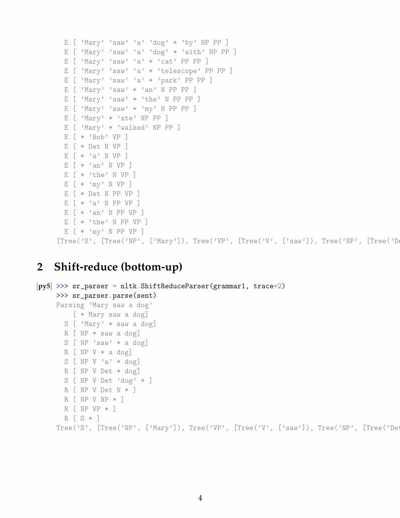
2 Shift-reduce (bottom-up)
[py5] >>> sr_parser = nltk.ShiftReduceParser(grammar1, trace=2)>>> sr_parser.parse(sent)Parsing ’Mary saw a dog’
[ * Mary saw a dog]S [ ’Mary’ * saw a dog]R [ NP * saw a dog]S [ NP ’saw’ * a dog]R [ NP V * a dog]S [ NP V ’a’ * dog]R [ NP V Det * dog]S [ NP V Det ’dog’ * ]R [ NP V Det N * ]R [ NP V NP * ]R [ NP VP * ]R [ S * ]
Tree(’S’, [Tree(’NP’, [’Mary’]), Tree(’VP’, [Tree(’V’, [’saw’]), Tree(’NP’, [Tree(’Det’, [’a’]), Tree(’N’, [’dog’])])])])
4
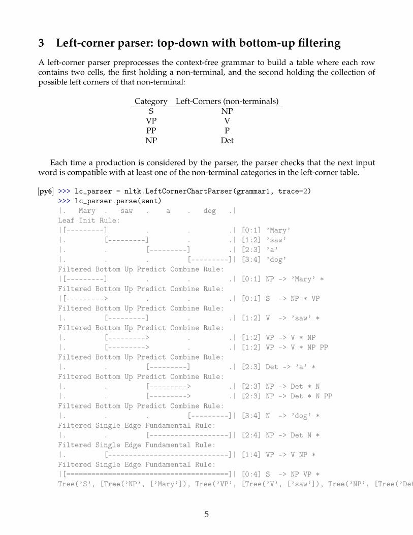
3 Left-corner parser: top-down with bottom-up filtering
A left-corner parser preprocesses the context-free grammar to build a table where each rowcontains two cells, the first holding a non-terminal, and the second holding the collection ofpossible left corners of that non-terminal:
Category Left-Corners (non-terminals)S NP
VP VPP PNP Det
Each time a production is considered by the parser, the parser checks that the next inputword is compatible with at least one of the non-terminal categories in the left-corner table.
[py6] >>> lc_parser = nltk.LeftCornerChartParser(grammar1, trace=2)>>> lc_parser.parse(sent)|. Mary . saw . a . dog .|Leaf Init Rule:|[---------] . . .| [0:1] ’Mary’|. [---------] . .| [1:2] ’saw’|. . [---------] .| [2:3] ’a’|. . . [---------]| [3:4] ’dog’Filtered Bottom Up Predict Combine Rule:|[---------] . . .| [0:1] NP -> ’Mary’ *Filtered Bottom Up Predict Combine Rule:|[---------> . . .| [0:1] S -> NP * VPFiltered Bottom Up Predict Combine Rule:|. [---------] . .| [1:2] V -> ’saw’ *Filtered Bottom Up Predict Combine Rule:|. [---------> . .| [1:2] VP -> V * NP|. [---------> . .| [1:2] VP -> V * NP PPFiltered Bottom Up Predict Combine Rule:|. . [---------] .| [2:3] Det -> ’a’ *Filtered Bottom Up Predict Combine Rule:|. . [---------> .| [2:3] NP -> Det * N|. . [---------> .| [2:3] NP -> Det * N PPFiltered Bottom Up Predict Combine Rule:|. . . [---------]| [3:4] N -> ’dog’ *Filtered Single Edge Fundamental Rule:|. . [-------------------]| [2:4] NP -> Det N *Filtered Single Edge Fundamental Rule:|. [-----------------------------]| [1:4] VP -> V NP *Filtered Single Edge Fundamental Rule:|[=======================================]| [0:4] S -> NP VP *Tree(’S’, [Tree(’NP’, [’Mary’]), Tree(’VP’, [Tree(’V’, [’saw’]), Tree(’NP’, [Tree(’Det’, [’a’]), Tree(’N’, [’dog’])])])])
5
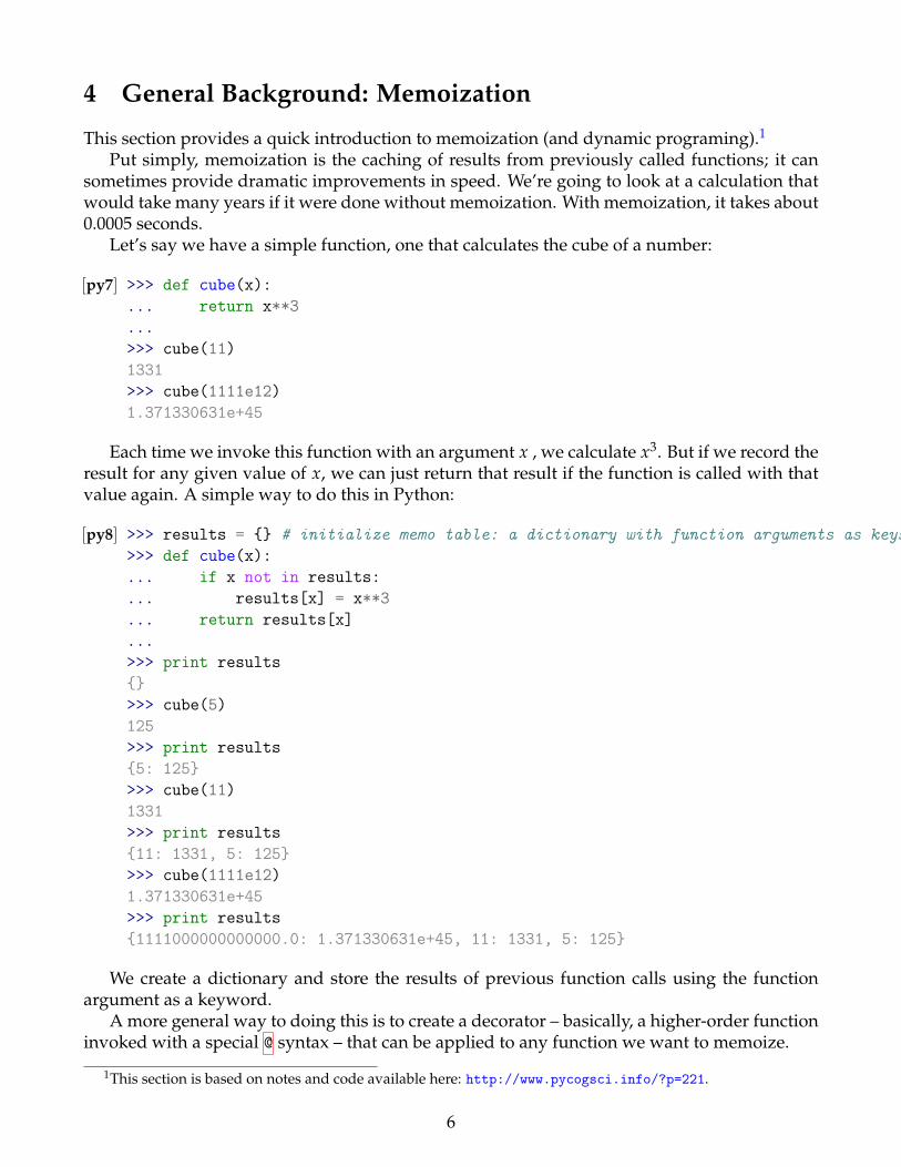
4 General Background: Memoization
This section provides a quick introduction to memoization (and dynamic programing).1
Put simply, memoization is the caching of results from previously called functions; it cansometimes provide dramatic improvements in speed. We’re going to look at a calculation thatwould take many years if it were done without memoization. With memoization, it takes about0.0005 seconds.
Let’s say we have a simple function, one that calculates the cube of a number:
[py7] >>> def cube(x):... return x**3...>>> cube(11)1331>>> cube(1111e12)1.371330631e+45
Each time we invoke this function with an argument x , we calculate x3. But if we record theresult for any given value of x, we can just return that result if the function is called with thatvalue again. A simple way to do this in Python:
[py8] >>> results = {} # initialize memo table: a dictionary with function arguments as keys>>> def cube(x):... if x not in results:... results[x] = x**3... return results[x]...>>> print results{}>>> cube(5)125>>> print results{5: 125}>>> cube(11)1331>>> print results{11: 1331, 5: 125}>>> cube(1111e12)1.371330631e+45>>> print results{1111000000000000.0: 1.371330631e+45, 11: 1331, 5: 125}
We create a dictionary and store the results of previous function calls using the functionargument as a keyword.
A more general way to doing this is to create a decorator – basically, a higher-order functioninvoked with a special @ syntax – that can be applied to any function we want to memoize.
1This section is based on notes and code available here: http://www.pycogsci.info/?p=221.
6
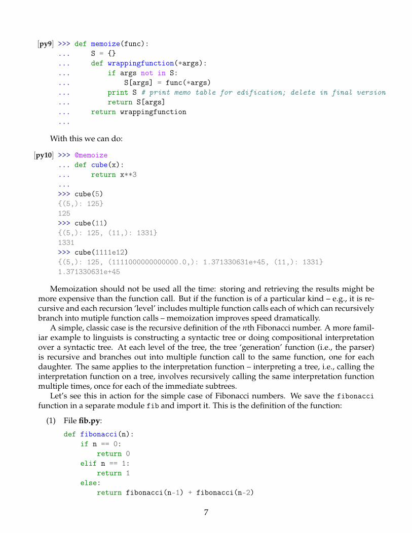
[py9] >>> def memoize(func):... S = {}... def wrappingfunction(*args):... if args not in S:... S[args] = func(*args)... print S # print memo table for edification; delete in final version... return S[args]... return wrappingfunction...
With this we can do:
[py10] >>> @memoize... def cube(x):... return x**3...>>> cube(5){(5,): 125}125>>> cube(11){(5,): 125, (11,): 1331}1331>>> cube(1111e12){(5,): 125, (1111000000000000.0,): 1.371330631e+45, (11,): 1331}1.371330631e+45
Memoization should not be used all the time: storing and retrieving the results might bemore expensive than the function call. But if the function is of a particular kind – e.g., it is re-cursive and each recursion ‘level’ includes multiple function calls each of which can recursivelybranch into mutiple function calls – memoization improves speed dramatically.
A simple, classic case is the recursive definition of the nth Fibonacci number. A more famil-iar example to linguists is constructing a syntactic tree or doing compositional interpretationover a syntactic tree. At each level of the tree, the tree ‘generation’ function (i.e., the parser)is recursive and branches out into multiple function call to the same function, one for eachdaughter. The same applies to the interpretation function – interpreting a tree, i.e., calling theinterpretation function on a tree, involves recursively calling the same interpretation functionmultiple times, once for each of the immediate subtrees.
Let’s see this in action for the simple case of Fibonacci numbers. We save the fibonaccifunction in a separate module fib and import it. This is the definition of the function:
(1) File fib.py:
def fibonacci(n):if n == 0:
return 0elif n == 1:
return 1else:
return fibonacci(n-1) + fibonacci(n-2)
7
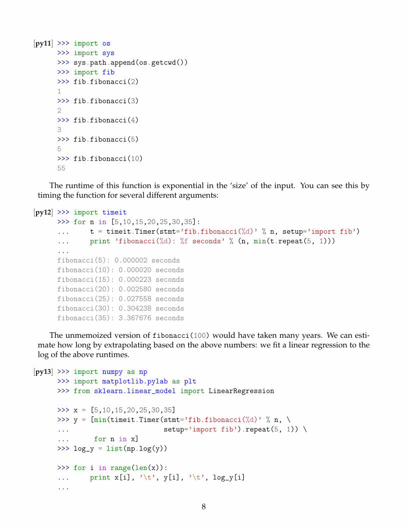
[py11] >>> import os>>> import sys>>> sys.path.append(os.getcwd())>>> import fib>>> fib.fibonacci(2)1>>> fib.fibonacci(3)2>>> fib.fibonacci(4)3>>> fib.fibonacci(5)5>>> fib.fibonacci(10)55
The runtime of this function is exponential in the ‘size’ of the input. You can see this bytiming the function for several different arguments:
[py12] >>> import timeit>>> for n in [5,10,15,20,25,30,35]:... t = timeit.Timer(stmt=’fib.fibonacci(%d)’ % n, setup=’import fib’)... print ’fibonacci(%d): %f seconds’ % (n, min(t.repeat(5, 1)))...fibonacci(5): 0.000002 secondsfibonacci(10): 0.000020 secondsfibonacci(15): 0.000223 secondsfibonacci(20): 0.002580 secondsfibonacci(25): 0.027558 secondsfibonacci(30): 0.304238 secondsfibonacci(35): 3.367676 seconds
The unmemoized version of fibonacci(100) would have taken many years. We can esti-mate how long by extrapolating based on the above numbers: we fit a linear regression to thelog of the above runtimes.
[py13] >>> import numpy as np>>> import matplotlib.pylab as plt>>> from sklearn.linear_model import LinearRegression
>>> x = [5,10,15,20,25,30,35]>>> y = [min(timeit.Timer(stmt=’fib.fibonacci(%d)’ % n, \... setup=’import fib’).repeat(5, 1)) \... for n in x]>>> log_y = list(np.log(y))
>>> for i in range(len(x)):... print x[i], ’\t’, y[i], ’\t’, log_y[i]...
8
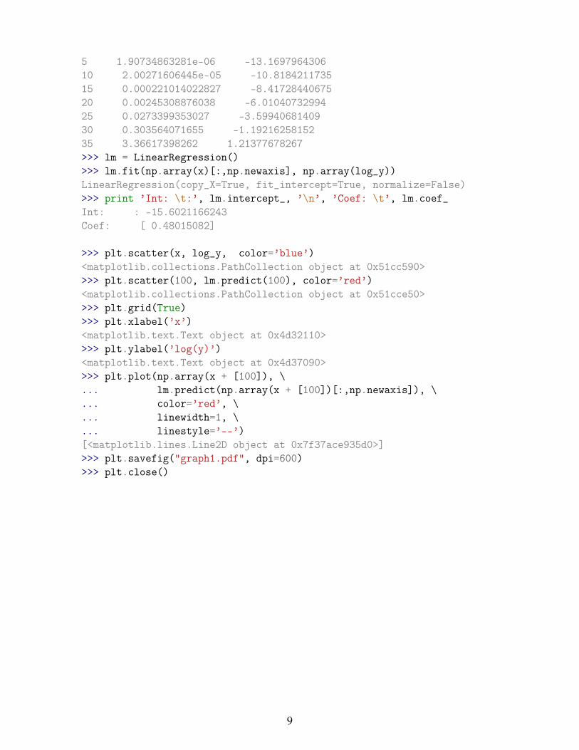
5 1.90734863281e-06 -13.169796430610 2.00271606445e-05 -10.818421173515 0.000221014022827 -8.4172844067520 0.00245308876038 -6.0104073299425 0.0273399353027 -3.5994068140930 0.303564071655 -1.1921625815235 3.36617398262 1.21377678267>>> lm = LinearRegression()>>> lm.fit(np.array(x)[:,np.newaxis], np.array(log_y))LinearRegression(copy_X=True, fit_intercept=True, normalize=False)>>> print ’Int: \t:’, lm.intercept_, ’\n’, ’Coef: \t’, lm.coef_Int: : -15.6021166243Coef: [ 0.48015082]
>>> plt.scatter(x, log_y, color=’blue’)<matplotlib.collections.PathCollection object at 0x51cc590>>>> plt.scatter(100, lm.predict(100), color=’red’)<matplotlib.collections.PathCollection object at 0x51cce50>>>> plt.grid(True)>>> plt.xlabel(’x’)<matplotlib.text.Text object at 0x4d32110>>>> plt.ylabel(’log(y)’)<matplotlib.text.Text object at 0x4d37090>>>> plt.plot(np.array(x + [100]), \... lm.predict(np.array(x + [100])[:,np.newaxis]), \... color=’red’, \... linewidth=1, \... linestyle=’--’)[<matplotlib.lines.Line2D object at 0x7f37ace935d0>]>>> plt.savefig("graph1.pdf", dpi=600)>>> plt.close()
9
0 20 40 60 80 100 120x
20
10
0
10
20
30
40lo
g(y
)
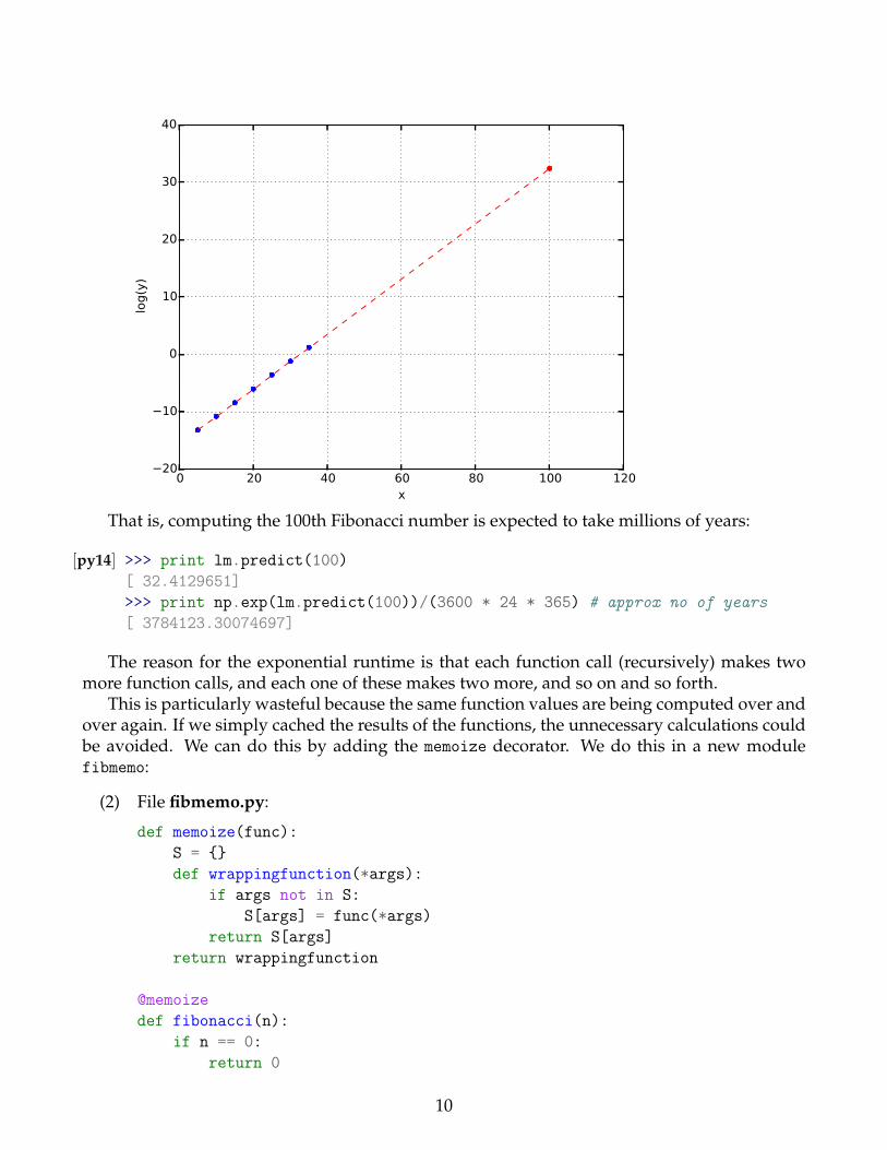
That is, computing the 100th Fibonacci number is expected to take millions of years:
[py14] >>> print lm.predict(100)[ 32.4129651]>>> print np.exp(lm.predict(100))/(3600 * 24 * 365) # approx no of years[ 3784123.30074697]
The reason for the exponential runtime is that each function call (recursively) makes twomore function calls, and each one of these makes two more, and so on and so forth.
This is particularly wasteful because the same function values are being computed over andover again. If we simply cached the results of the functions, the unnecessary calculations couldbe avoided. We can do this by adding the memoize decorator. We do this in a new modulefibmemo:
(2) File fibmemo.py:
def memoize(func):S = {}def wrappingfunction(*args):
if args not in S:S[args] = func(*args)
return S[args]return wrappingfunction
@memoizedef fibonacci(n):
if n == 0:return 0
10
elif n == 1:return 1
else:return fibonacci(n-1) + fibonacci(n-2)
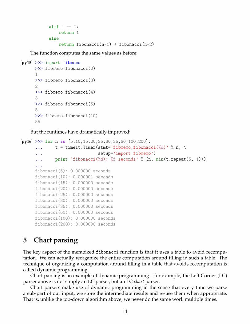
The function computes the same values as before:
[py15] >>> import fibmemo>>> fibmemo.fibonacci(2)1>>> fibmemo.fibonacci(3)2>>> fibmemo.fibonacci(4)3>>> fibmemo.fibonacci(5)5>>> fibmemo.fibonacci(10)55
But the runtimes have dramatically improved:
[py16] >>> for n in [5,10,15,20,25,30,35,60,100,200]:... t = timeit.Timer(stmt=’fibmemo.fibonacci(%d)’ % n, \... setup=’import fibmemo’)... print ’fibonacci(%d): %f seconds’ % (n, min(t.repeat(5, 1)))...fibonacci(5): 0.000000 secondsfibonacci(10): 0.000001 secondsfibonacci(15): 0.000000 secondsfibonacci(20): 0.000000 secondsfibonacci(25): 0.000000 secondsfibonacci(30): 0.000000 secondsfibonacci(35): 0.000000 secondsfibonacci(60): 0.000000 secondsfibonacci(100): 0.000000 secondsfibonacci(200): 0.000000 seconds
5 Chart parsing
The key aspect of the memoized fibonacci function is that it uses a table to avoid recompu-tation. We can actually reorganize the entire computation around filling in such a table. Thetechnique of organizing a computation around filling in a table that avoids recomputation iscalled dynamic programming.
Chart parsing is an example of dynamic programming – for example, the Left Corner (LC)parser above is not simply an LC parser, but an LC chart parser.
Chart parsers make use of dynamic programming in the sense that every time we parsea sub-part of our input, we store the intermediate results and re-use them when appropriate.That is, unlike the top-down algorithm above, we never do the same work multiple times.
11
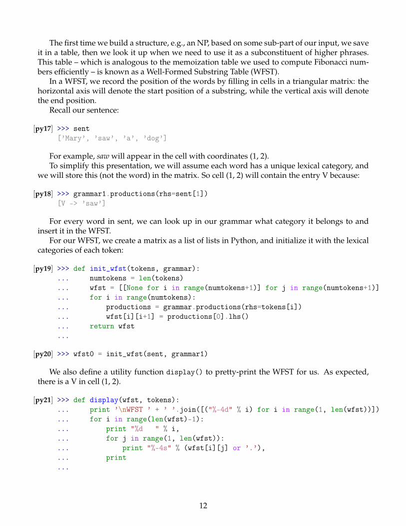
The first time we build a structure, e.g., an NP, based on some sub-part of our input, we saveit in a table, then we look it up when we need to use it as a subconstituent of higher phrases.This table – which is analogous to the memoization table we used to compute Fibonacci num-bers efficiently – is known as a Well-Formed Substring Table (WFST).
In a WFST, we record the position of the words by filling in cells in a triangular matrix: thehorizontal axis will denote the start position of a substring, while the vertical axis will denotethe end position.
Recall our sentence:
[py17] >>> sent[’Mary’, ’saw’, ’a’, ’dog’]
For example, saw will appear in the cell with coordinates (1, 2).To simplify this presentation, we will assume each word has a unique lexical category, and
we will store this (not the word) in the matrix. So cell (1, 2) will contain the entry V because:
[py18] >>> grammar1.productions(rhs=sent[1])[V -> ’saw’]
For every word in sent, we can look up in our grammar what category it belongs to andinsert it in the WFST.
For our WFST, we create a matrix as a list of lists in Python, and initialize it with the lexicalcategories of each token:
[py19] >>> def init_wfst(tokens, grammar):... numtokens = len(tokens)... wfst = [[None for i in range(numtokens+1)] for j in range(numtokens+1)]... for i in range(numtokens):... productions = grammar.productions(rhs=tokens[i])... wfst[i][i+1] = productions[0].lhs()... return wfst...
[py20] >>> wfst0 = init_wfst(sent, grammar1)
We also define a utility function display() to pretty-print the WFST for us. As expected,there is a V in cell (1, 2).
[py21] >>> def display(wfst, tokens):... print ’\nWFST ’ + ’ ’.join([("%-4d" % i) for i in range(1, len(wfst))])... for i in range(len(wfst)-1):... print "%d " % i,... for j in range(1, len(wfst)):... print "%-4s" % (wfst[i][j] or ’.’),... print...
12
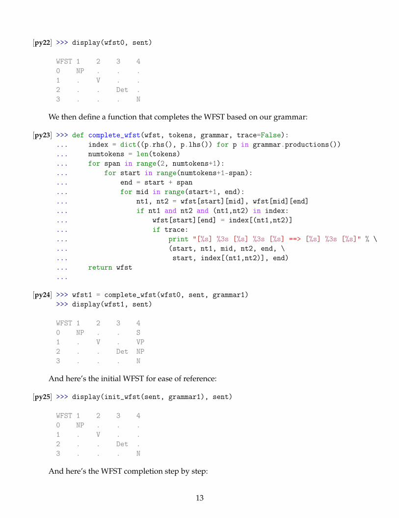
[py22] >>> display(wfst0, sent)
WFST 1 2 3 40 NP . . .1 . V . .2 . . Det .3 . . . N
We then define a function that completes the WFST based on our grammar:
[py23] >>> def complete_wfst(wfst, tokens, grammar, trace=False):... index = dict((p.rhs(), p.lhs()) for p in grammar.productions())... numtokens = len(tokens)... for span in range(2, numtokens+1):... for start in range(numtokens+1-span):... end = start + span... for mid in range(start+1, end):... nt1, nt2 = wfst[start][mid], wfst[mid][end]... if nt1 and nt2 and (nt1,nt2) in index:... wfst[start][end] = index[(nt1,nt2)]... if trace:... print "[%s] %3s [%s] %3s [%s] ==> [%s] %3s [%s]" % \... (start, nt1, mid, nt2, end, \... start, index[(nt1,nt2)], end)... return wfst...
[py24] >>> wfst1 = complete_wfst(wfst0, sent, grammar1)>>> display(wfst1, sent)
WFST 1 2 3 40 NP . . S1 . V . VP2 . . Det NP3 . . . N
And here’s the initial WFST for ease of reference:
[py25] >>> display(init_wfst(sent, grammar1), sent)
WFST 1 2 3 40 NP . . .1 . V . .2 . . Det .3 . . . N
And here’s the WFST completion step by step:
13
[py26] >>> complete_wfst(wfst0, sent, grammar1, trace=True)[2] Det [3] N [4] ==> [2] NP [4][1] V [2] NP [4] ==> [1] VP [4][0] NP [1] VP [4] ==> [0] S [4][[None, NP, None, None, S], [None, None, V, None, VP], [None, None, None, Det, NP], [None, None, None, None, N], [None, None, None, None, None]]
All of the edges that we’ve seen so far represent complete constituents. But it is helpful torecord incomplete constituents to document the work already done by the parser. For example,when a top-down parser processes VP → VNP, it may find V, but not NP. This work can bereused when processing VP→ VNP, so we should record the hypothesis that the V constituentsaw is the beginning of a VP.
We can do this by adding a dot to the edge’s right hand side. Material to the left of the dotrecords what has been found so far; material to the right of the dot specifies what still needs tobe found in order to complete the constituent. This is very similar to LC parsing.
Types of edges:
• self-loop edges, e.g. an edge [VP → �VNPPP, (i, i)] recording the hypothesis that a VPbegins at location i, and that we anticipate finding a sequence V NP PP starting here
• incomplete edges, e.g., an edge [VP → V � NPPP, (i, j)] recording the fact that we havediscovered a V spanning (i, j), and hypothesize a following NP PP sequence to completea VP beginning at i
• complete edges, e.g., an edge [VP → VNPPP�, (i, k)] recording the discovery that a VPconsisting of the sequence VNPPP has been discovered for the span (i, j)
• parse edges: these are complete edges that span the entire sentence and have the gram-mar’s start symbol as their left-hand side; they encode one or more parse trees for thesentence.
To parse a sentence, a chart parser first creates an empty chart spanning the sentence. It thenfinds edges that are licensed by its knowledge about the sentence, and adds them to the chartone at a time until one or more parse edges are found.
The edges that it adds can be licensed in one of three ways:
• the input can license an edge: each word wi in the input licenses the complete edge [wi →�, (i, i + 1)].
• the grammar can license an edge: each grammar production A→ α licenses the self-loopedge [A→ �α, (i, i)] for every i, 0 ≤ i ≤ n.
• the current chart contents can license an edge: a suitable pair of existing edges triggersthe addition of a new edge
Chart parsers use a set of rules to heuristically decide when an edge should be added toa chart. This set of rules together with a specification of when they should be applied form aparsing strategy.
(3) The Fundamental Rule (‘Completion’): if the chart contains the edges [A→ α �Bβ, (i, j)]and [B→ γ�, (j, k)], then add a new edge [A→ αB � β, (i, k)].
14
• this rule is used by every chart parser
• as per the usual conventions in formal language theory, α, β, γ, · · · denote (possiblyempty) sequences of terminals or non-terminals
• in the new edge, the dot has moved one place to the right
• the span of the new edge is the combined span of the original edges
• when we add this new edge, we do not remove the other two because they mightbe used again
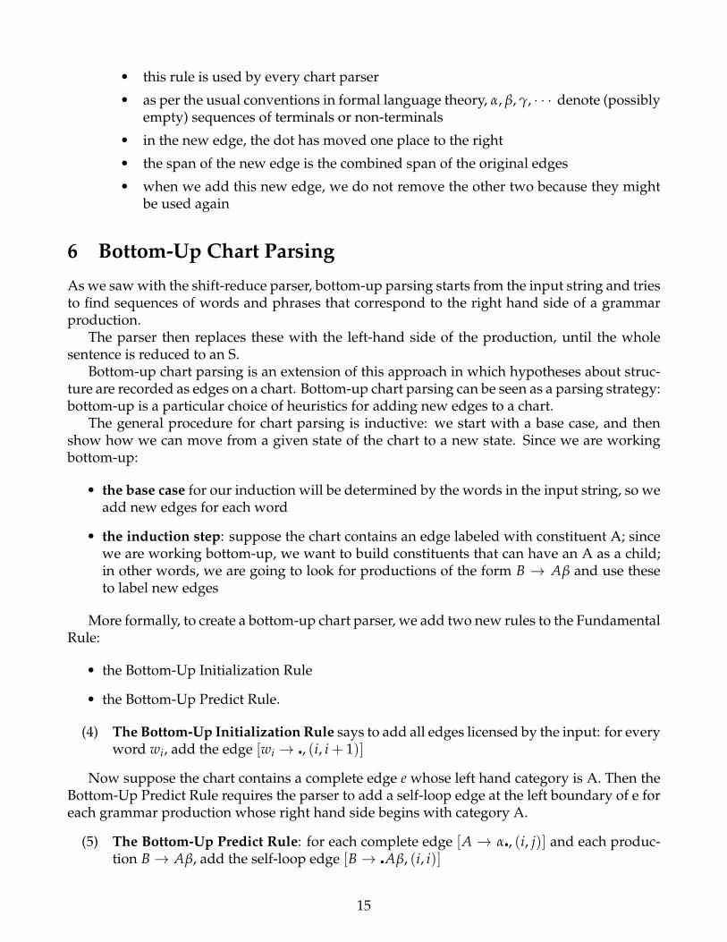
6 Bottom-Up Chart Parsing
As we saw with the shift-reduce parser, bottom-up parsing starts from the input string and triesto find sequences of words and phrases that correspond to the right hand side of a grammarproduction.
The parser then replaces these with the left-hand side of the production, until the wholesentence is reduced to an S.
Bottom-up chart parsing is an extension of this approach in which hypotheses about struc-ture are recorded as edges on a chart. Bottom-up chart parsing can be seen as a parsing strategy:bottom-up is a particular choice of heuristics for adding new edges to a chart.
The general procedure for chart parsing is inductive: we start with a base case, and thenshow how we can move from a given state of the chart to a new state. Since we are workingbottom-up:
• the base case for our induction will be determined by the words in the input string, so weadd new edges for each word
• the induction step: suppose the chart contains an edge labeled with constituent A; sincewe are working bottom-up, we want to build constituents that can have an A as a child;in other words, we are going to look for productions of the form B → Aβ and use theseto label new edges
More formally, to create a bottom-up chart parser, we add two new rules to the FundamentalRule:
• the Bottom-Up Initialization Rule
• the Bottom-Up Predict Rule.
(4) The Bottom-Up Initialization Rule says to add all edges licensed by the input: for everyword wi, add the edge [wi → �, (i, i + 1)]
Now suppose the chart contains a complete edge e whose left hand category is A. Then theBottom-Up Predict Rule requires the parser to add a self-loop edge at the left boundary of e foreach grammar production whose right hand side begins with category A.
(5) The Bottom-Up Predict Rule: for each complete edge [A → α�, (i, j)] and each produc-tion B→ Aβ, add the self-loop edge [B→ �Aβ, (i, i)]
15
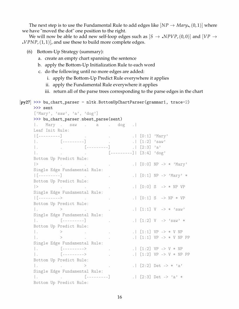
The next step is to use the Fundamental Rule to add edges like [NP → Mary�, (0, 1)] wherewe have "moved the dot" one position to the right.
We will now be able to add new self-loop edges such as [S → �NPVP, (0, 0)] and [VP →�VPNP, (1, 1)], and use these to build more complete edges.
(6) Bottom-Up Strategy (summary):a. create an empty chart spanning the sentenceb. apply the Bottom-Up Initialization Rule to each wordc. do the following until no more edges are added:
i. apply the Bottom-Up Predict Rule everywhere it appliesii. apply the Fundamental Rule everywhere it appliesiii. return all of the parse trees corresponding to the parse edges in the chart
[py27] >>> bu_chart_parser = nltk.BottomUpChartParser(grammar1, trace=2)>>> sent[’Mary’, ’saw’, ’a’, ’dog’]>>> bu_chart_parser.nbest_parse(sent)|. Mary . saw . a . dog .|Leaf Init Rule:|[---------] . . .| [0:1] ’Mary’|. [---------] . .| [1:2] ’saw’|. . [---------] .| [2:3] ’a’|. . . [---------]| [3:4] ’dog’Bottom Up Predict Rule:|> . . . .| [0:0] NP -> * ’Mary’Single Edge Fundamental Rule:|[---------] . . .| [0:1] NP -> ’Mary’ *Bottom Up Predict Rule:|> . . . .| [0:0] S -> * NP VPSingle Edge Fundamental Rule:|[---------> . . .| [0:1] S -> NP * VPBottom Up Predict Rule:|. > . . .| [1:1] V -> * ’saw’Single Edge Fundamental Rule:|. [---------] . .| [1:2] V -> ’saw’ *Bottom Up Predict Rule:|. > . . .| [1:1] VP -> * V NP|. > . . .| [1:1] VP -> * V NP PPSingle Edge Fundamental Rule:|. [---------> . .| [1:2] VP -> V * NP|. [---------> . .| [1:2] VP -> V * NP PPBottom Up Predict Rule:|. . > . .| [2:2] Det -> * ’a’Single Edge Fundamental Rule:|. . [---------] .| [2:3] Det -> ’a’ *Bottom Up Predict Rule:
16
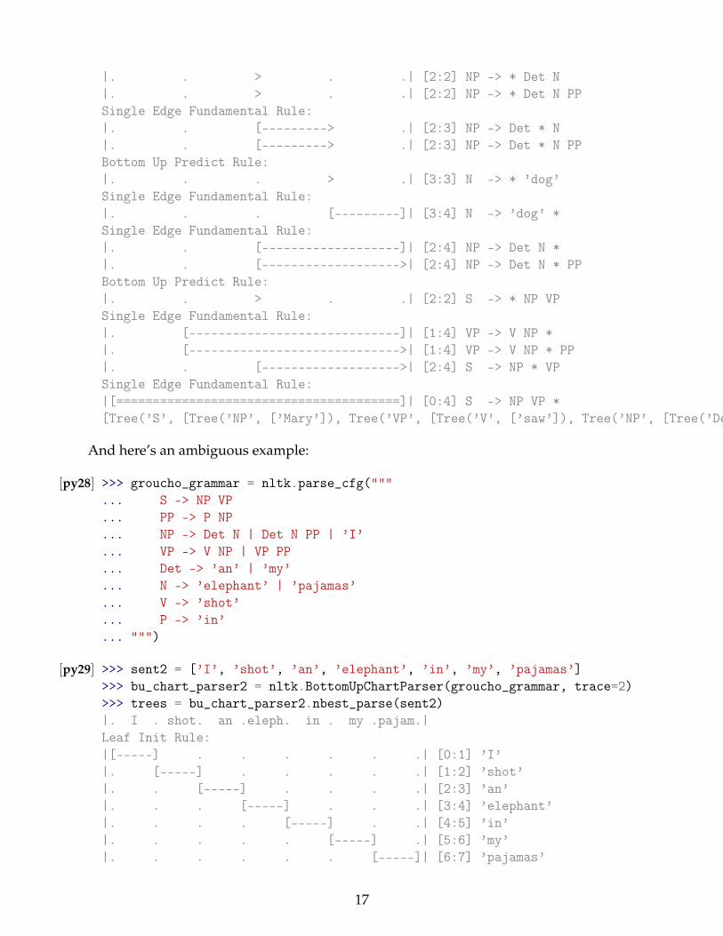
|. . > . .| [2:2] NP -> * Det N|. . > . .| [2:2] NP -> * Det N PPSingle Edge Fundamental Rule:|. . [---------> .| [2:3] NP -> Det * N|. . [---------> .| [2:3] NP -> Det * N PPBottom Up Predict Rule:|. . . > .| [3:3] N -> * ’dog’Single Edge Fundamental Rule:|. . . [---------]| [3:4] N -> ’dog’ *Single Edge Fundamental Rule:|. . [-------------------]| [2:4] NP -> Det N *|. . [------------------->| [2:4] NP -> Det N * PPBottom Up Predict Rule:|. . > . .| [2:2] S -> * NP VPSingle Edge Fundamental Rule:|. [-----------------------------]| [1:4] VP -> V NP *|. [----------------------------->| [1:4] VP -> V NP * PP|. . [------------------->| [2:4] S -> NP * VPSingle Edge Fundamental Rule:|[=======================================]| [0:4] S -> NP VP *[Tree(’S’, [Tree(’NP’, [’Mary’]), Tree(’VP’, [Tree(’V’, [’saw’]), Tree(’NP’, [Tree(’Det’, [’a’]), Tree(’N’, [’dog’])])])])]
And here’s an ambiguous example:
[py28] >>> groucho_grammar = nltk.parse_cfg("""... S -> NP VP... PP -> P NP... NP -> Det N | Det N PP | ’I’... VP -> V NP | VP PP... Det -> ’an’ | ’my’... N -> ’elephant’ | ’pajamas’... V -> ’shot’... P -> ’in’... """)
[py29] >>> sent2 = [’I’, ’shot’, ’an’, ’elephant’, ’in’, ’my’, ’pajamas’]>>> bu_chart_parser2 = nltk.BottomUpChartParser(groucho_grammar, trace=2)>>> trees = bu_chart_parser2.nbest_parse(sent2)|. I . shot. an .eleph. in . my .pajam.|Leaf Init Rule:|[-----] . . . . . .| [0:1] ’I’|. [-----] . . . . .| [1:2] ’shot’|. . [-----] . . . .| [2:3] ’an’|. . . [-----] . . .| [3:4] ’elephant’|. . . . [-----] . .| [4:5] ’in’|. . . . . [-----] .| [5:6] ’my’|. . . . . . [-----]| [6:7] ’pajamas’
17
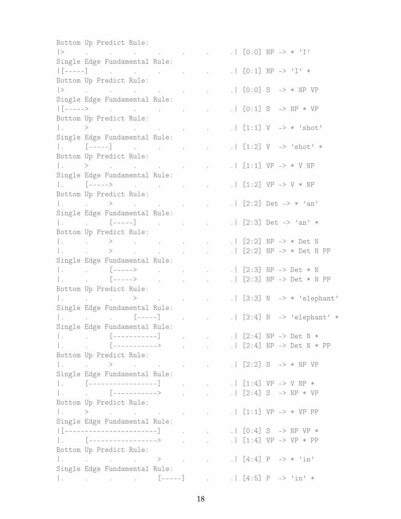
Bottom Up Predict Rule:|> . . . . . . .| [0:0] NP -> * ’I’Single Edge Fundamental Rule:|[-----] . . . . . .| [0:1] NP -> ’I’ *Bottom Up Predict Rule:|> . . . . . . .| [0:0] S -> * NP VPSingle Edge Fundamental Rule:|[-----> . . . . . .| [0:1] S -> NP * VPBottom Up Predict Rule:|. > . . . . . .| [1:1] V -> * ’shot’Single Edge Fundamental Rule:|. [-----] . . . . .| [1:2] V -> ’shot’ *Bottom Up Predict Rule:|. > . . . . . .| [1:1] VP -> * V NPSingle Edge Fundamental Rule:|. [-----> . . . . .| [1:2] VP -> V * NPBottom Up Predict Rule:|. . > . . . . .| [2:2] Det -> * ’an’Single Edge Fundamental Rule:|. . [-----] . . . .| [2:3] Det -> ’an’ *Bottom Up Predict Rule:|. . > . . . . .| [2:2] NP -> * Det N|. . > . . . . .| [2:2] NP -> * Det N PPSingle Edge Fundamental Rule:|. . [-----> . . . .| [2:3] NP -> Det * N|. . [-----> . . . .| [2:3] NP -> Det * N PPBottom Up Predict Rule:|. . . > . . . .| [3:3] N -> * ’elephant’Single Edge Fundamental Rule:|. . . [-----] . . .| [3:4] N -> ’elephant’ *Single Edge Fundamental Rule:|. . [-----------] . . .| [2:4] NP -> Det N *|. . [-----------> . . .| [2:4] NP -> Det N * PPBottom Up Predict Rule:|. . > . . . . .| [2:2] S -> * NP VPSingle Edge Fundamental Rule:|. [-----------------] . . .| [1:4] VP -> V NP *|. . [-----------> . . .| [2:4] S -> NP * VPBottom Up Predict Rule:|. > . . . . . .| [1:1] VP -> * VP PPSingle Edge Fundamental Rule:|[-----------------------] . . .| [0:4] S -> NP VP *|. [-----------------> . . .| [1:4] VP -> VP * PPBottom Up Predict Rule:|. . . . > . . .| [4:4] P -> * ’in’Single Edge Fundamental Rule:|. . . . [-----] . .| [4:5] P -> ’in’ *
18
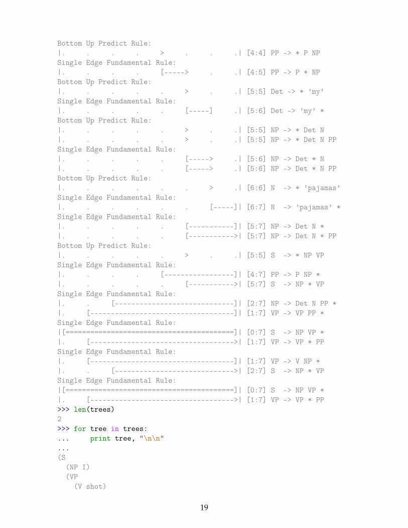
Bottom Up Predict Rule:|. . . . > . . .| [4:4] PP -> * P NPSingle Edge Fundamental Rule:|. . . . [-----> . .| [4:5] PP -> P * NPBottom Up Predict Rule:|. . . . . > . .| [5:5] Det -> * ’my’Single Edge Fundamental Rule:|. . . . . [-----] .| [5:6] Det -> ’my’ *Bottom Up Predict Rule:|. . . . . > . .| [5:5] NP -> * Det N|. . . . . > . .| [5:5] NP -> * Det N PPSingle Edge Fundamental Rule:|. . . . . [-----> .| [5:6] NP -> Det * N|. . . . . [-----> .| [5:6] NP -> Det * N PPBottom Up Predict Rule:|. . . . . . > .| [6:6] N -> * ’pajamas’Single Edge Fundamental Rule:|. . . . . . [-----]| [6:7] N -> ’pajamas’ *Single Edge Fundamental Rule:|. . . . . [-----------]| [5:7] NP -> Det N *|. . . . . [----------->| [5:7] NP -> Det N * PPBottom Up Predict Rule:|. . . . . > . .| [5:5] S -> * NP VPSingle Edge Fundamental Rule:|. . . . [-----------------]| [4:7] PP -> P NP *|. . . . . [----------->| [5:7] S -> NP * VPSingle Edge Fundamental Rule:|. . [-----------------------------]| [2:7] NP -> Det N PP *|. [-----------------------------------]| [1:7] VP -> VP PP *Single Edge Fundamental Rule:|[=========================================]| [0:7] S -> NP VP *|. [----------------------------------->| [1:7] VP -> VP * PPSingle Edge Fundamental Rule:|. [-----------------------------------]| [1:7] VP -> V NP *|. . [----------------------------->| [2:7] S -> NP * VPSingle Edge Fundamental Rule:|[=========================================]| [0:7] S -> NP VP *|. [----------------------------------->| [1:7] VP -> VP * PP>>> len(trees)2>>> for tree in trees:... print tree, "\n\n"...(S
(NP I)(VP
(V shot)
19
(NP (Det an) (N elephant) (PP (P in) (NP (Det my) (N pajamas))))))
(S(NP I)(VP
(VP (V shot) (NP (Det an) (N elephant)))(PP (P in) (NP (Det my) (N pajamas)))))
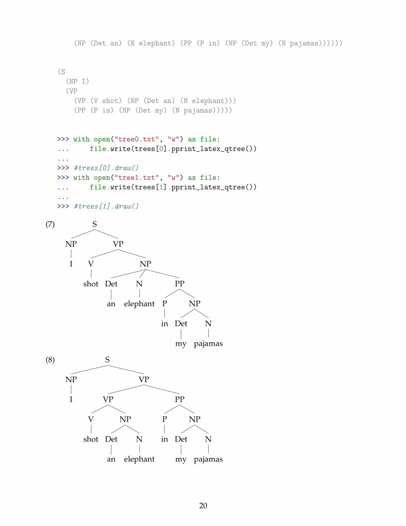
>>> with open("tree0.txt", "w") as file:... file.write(trees[0].pprint_latex_qtree())...>>> #trees[0].draw()>>> with open("tree1.txt", "w") as file:... file.write(trees[1].pprint_latex_qtree())...>>> #trees[1].draw()
(7) S
VP
NP
PP
NP
N
pajamas
Det
my
P
in
N
elephant
Det
an
V
shot
NP
I
(8) S
VP
PP
NP
N
pajamas
Det
my
P
in
VP
NP
N
elephant
Det
an
V
shot
NP
I
20
7 Top-down Chart Parsing
Top-down chart parsing works in a similar way to the recursive descent parser:
• it starts off with the top-level goal of finding an S
• this goal is broken down into the subgoals of trying to find constituents such as NP andVP predicted by the grammar
To create a top-down chart parser, we use the Fundamental Rule as before plus three otherrules:
• the Top-Down Initialization Rule
• the Top-Down Expand Rule
• the Top-Down Match Rule
(9) The Top-Down Initialization Rule captures the fact that the root of any parse must bethe start symbol S: for each production S→ α, add the self-loop edge [S→ �α, (0, 0)]
In our running example, we are predicting that we will be able to find an NP and a VPstarting at 0, but have not yet satisfied these subgoals.
In order to find an NP we need to invoke a production that has NP on its left hand side. Thiswork is done by the Top-Down Expand Rule.
(10) The Top-Down Expand Rule tells us that if our chart contains an incomplete edgewhose dot is followed by a nonterminal B, then the parser should add any self-loopedges licensed by the grammar whose left-hand side is B: for each incomplete edge[A→ α � Bβ, (i, j)] and for each grammar production B→ γ, add the edge [B→ �γ, (j, j)]
Finally:
(11) The Top-Down Match Rule allows the predictions of the grammar to be matched againstthe input string – if the chart contains an incomplete edge whose dot is followed by aterminal w, then the parser should add an edge if the terminal corresponds to the currentinput symbol: for each incomplete edge [A → α � wjβ, (i, j)], where wj is the jth word ofthe input (counting from 0), add a new complete edge [wj → �, (j, j + 1)].
(12) Top-Down Strategy (summary):a. create an empty chart spanning the sentenceb. apply the Top-Down Initialization Rule (at node 0)c. do until no more edges are added:
i. apply the Top-Down Expand Rule everywhere it appliesii. apply the Top-Down Match Rule everywhere it appliesiii. apply the Fundamental Rule everywhere it applies
d. return all of the parse trees corresponding to the parse edges in the chart
21
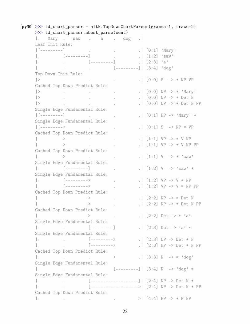
[py30] >>> td_chart_parser = nltk.TopDownChartParser(grammar1, trace=2)>>> td_chart_parser.nbest_parse(sent)|. Mary . saw . a . dog .|Leaf Init Rule:|[---------] . . .| [0:1] ’Mary’|. [---------] . .| [1:2] ’saw’|. . [---------] .| [2:3] ’a’|. . . [---------]| [3:4] ’dog’Top Down Init Rule:|> . . . .| [0:0] S -> * NP VPCached Top Down Predict Rule:|> . . . .| [0:0] NP -> * ’Mary’|> . . . .| [0:0] NP -> * Det N|> . . . .| [0:0] NP -> * Det N PPSingle Edge Fundamental Rule:|[---------] . . .| [0:1] NP -> ’Mary’ *Single Edge Fundamental Rule:|[---------> . . .| [0:1] S -> NP * VPCached Top Down Predict Rule:|. > . . .| [1:1] VP -> * V NP|. > . . .| [1:1] VP -> * V NP PPCached Top Down Predict Rule:|. > . . .| [1:1] V -> * ’saw’Single Edge Fundamental Rule:|. [---------] . .| [1:2] V -> ’saw’ *Single Edge Fundamental Rule:|. [---------> . .| [1:2] VP -> V * NP|. [---------> . .| [1:2] VP -> V * NP PPCached Top Down Predict Rule:|. . > . .| [2:2] NP -> * Det N|. . > . .| [2:2] NP -> * Det N PPCached Top Down Predict Rule:|. . > . .| [2:2] Det -> * ’a’Single Edge Fundamental Rule:|. . [---------] .| [2:3] Det -> ’a’ *Single Edge Fundamental Rule:|. . [---------> .| [2:3] NP -> Det * N|. . [---------> .| [2:3] NP -> Det * N PPCached Top Down Predict Rule:|. . . > .| [3:3] N -> * ’dog’Single Edge Fundamental Rule:|. . . [---------]| [3:4] N -> ’dog’ *Single Edge Fundamental Rule:|. . [-------------------]| [2:4] NP -> Det N *|. . [------------------->| [2:4] NP -> Det N * PPCached Top Down Predict Rule:|. . . . >| [4:4] PP -> * P NP
22
Single Edge Fundamental Rule:|. [-----------------------------]| [1:4] VP -> V NP *|. [----------------------------->| [1:4] VP -> V NP * PPSingle Edge Fundamental Rule:|[=======================================]| [0:4] S -> NP VP *[Tree(’S’, [Tree(’NP’, [’Mary’]), Tree(’VP’, [Tree(’V’, [’saw’]), Tree(’NP’, [Tree(’Det’, [’a’]), Tree(’N’, [’dog’])])])])]
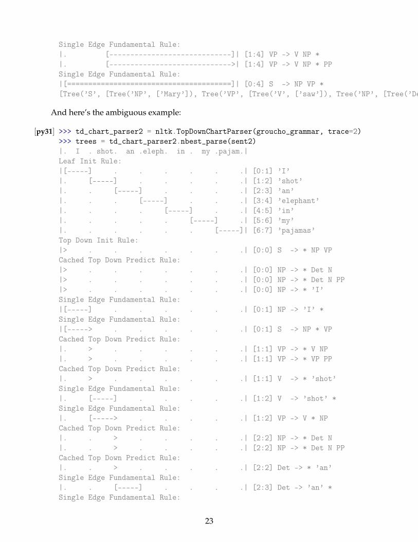
And here’s the ambiguous example:
[py31] >>> td_chart_parser2 = nltk.TopDownChartParser(groucho_grammar, trace=2)>>> trees = td_chart_parser2.nbest_parse(sent2)|. I . shot. an .eleph. in . my .pajam.|Leaf Init Rule:|[-----] . . . . . .| [0:1] ’I’|. [-----] . . . . .| [1:2] ’shot’|. . [-----] . . . .| [2:3] ’an’|. . . [-----] . . .| [3:4] ’elephant’|. . . . [-----] . .| [4:5] ’in’|. . . . . [-----] .| [5:6] ’my’|. . . . . . [-----]| [6:7] ’pajamas’Top Down Init Rule:|> . . . . . . .| [0:0] S -> * NP VPCached Top Down Predict Rule:|> . . . . . . .| [0:0] NP -> * Det N|> . . . . . . .| [0:0] NP -> * Det N PP|> . . . . . . .| [0:0] NP -> * ’I’Single Edge Fundamental Rule:|[-----] . . . . . .| [0:1] NP -> ’I’ *Single Edge Fundamental Rule:|[-----> . . . . . .| [0:1] S -> NP * VPCached Top Down Predict Rule:|. > . . . . . .| [1:1] VP -> * V NP|. > . . . . . .| [1:1] VP -> * VP PPCached Top Down Predict Rule:|. > . . . . . .| [1:1] V -> * ’shot’Single Edge Fundamental Rule:|. [-----] . . . . .| [1:2] V -> ’shot’ *Single Edge Fundamental Rule:|. [-----> . . . . .| [1:2] VP -> V * NPCached Top Down Predict Rule:|. . > . . . . .| [2:2] NP -> * Det N|. . > . . . . .| [2:2] NP -> * Det N PPCached Top Down Predict Rule:|. . > . . . . .| [2:2] Det -> * ’an’Single Edge Fundamental Rule:|. . [-----] . . . .| [2:3] Det -> ’an’ *Single Edge Fundamental Rule:
23
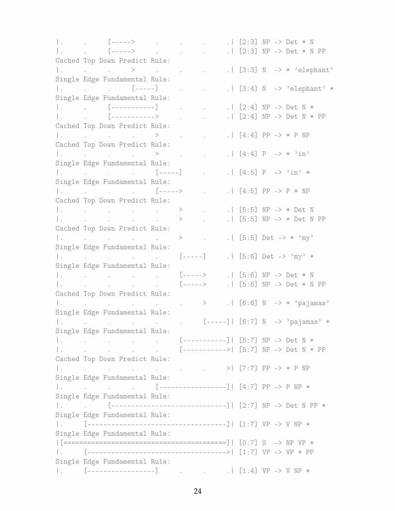
|. . [-----> . . . .| [2:3] NP -> Det * N|. . [-----> . . . .| [2:3] NP -> Det * N PPCached Top Down Predict Rule:|. . . > . . . .| [3:3] N -> * ’elephant’Single Edge Fundamental Rule:|. . . [-----] . . .| [3:4] N -> ’elephant’ *Single Edge Fundamental Rule:|. . [-----------] . . .| [2:4] NP -> Det N *|. . [-----------> . . .| [2:4] NP -> Det N * PPCached Top Down Predict Rule:|. . . . > . . .| [4:4] PP -> * P NPCached Top Down Predict Rule:|. . . . > . . .| [4:4] P -> * ’in’Single Edge Fundamental Rule:|. . . . [-----] . .| [4:5] P -> ’in’ *Single Edge Fundamental Rule:|. . . . [-----> . .| [4:5] PP -> P * NPCached Top Down Predict Rule:|. . . . . > . .| [5:5] NP -> * Det N|. . . . . > . .| [5:5] NP -> * Det N PPCached Top Down Predict Rule:|. . . . . > . .| [5:5] Det -> * ’my’Single Edge Fundamental Rule:|. . . . . [-----] .| [5:6] Det -> ’my’ *Single Edge Fundamental Rule:|. . . . . [-----> .| [5:6] NP -> Det * N|. . . . . [-----> .| [5:6] NP -> Det * N PPCached Top Down Predict Rule:|. . . . . . > .| [6:6] N -> * ’pajamas’Single Edge Fundamental Rule:|. . . . . . [-----]| [6:7] N -> ’pajamas’ *Single Edge Fundamental Rule:|. . . . . [-----------]| [5:7] NP -> Det N *|. . . . . [----------->| [5:7] NP -> Det N * PPCached Top Down Predict Rule:|. . . . . . . >| [7:7] PP -> * P NPSingle Edge Fundamental Rule:|. . . . [-----------------]| [4:7] PP -> P NP *Single Edge Fundamental Rule:|. . [-----------------------------]| [2:7] NP -> Det N PP *Single Edge Fundamental Rule:|. [-----------------------------------]| [1:7] VP -> V NP *Single Edge Fundamental Rule:|[=========================================]| [0:7] S -> NP VP *|. [----------------------------------->| [1:7] VP -> VP * PPSingle Edge Fundamental Rule:|. [-----------------] . . .| [1:4] VP -> V NP *
24
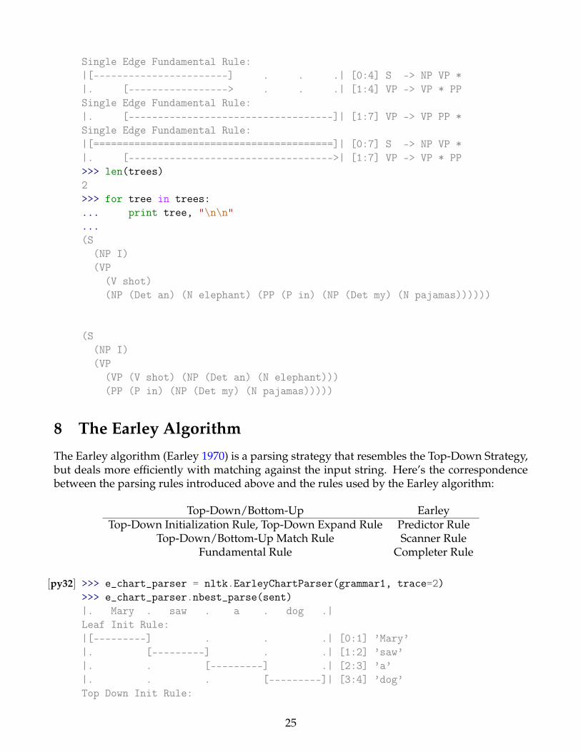
Single Edge Fundamental Rule:|[-----------------------] . . .| [0:4] S -> NP VP *|. [-----------------> . . .| [1:4] VP -> VP * PPSingle Edge Fundamental Rule:|. [-----------------------------------]| [1:7] VP -> VP PP *Single Edge Fundamental Rule:|[=========================================]| [0:7] S -> NP VP *|. [----------------------------------->| [1:7] VP -> VP * PP>>> len(trees)2>>> for tree in trees:... print tree, "\n\n"...(S
(NP I)(VP
(V shot)(NP (Det an) (N elephant) (PP (P in) (NP (Det my) (N pajamas))))))
(S(NP I)(VP
(VP (V shot) (NP (Det an) (N elephant)))(PP (P in) (NP (Det my) (N pajamas)))))
8 The Earley Algorithm
The Earley algorithm (Earley 1970) is a parsing strategy that resembles the Top-Down Strategy,but deals more efficiently with matching against the input string. Here’s the correspondencebetween the parsing rules introduced above and the rules used by the Earley algorithm:
Top-Down/Bottom-Up EarleyTop-Down Initialization Rule, Top-Down Expand Rule Predictor Rule
Top-Down/Bottom-Up Match Rule Scanner RuleFundamental Rule Completer Rule
[py32] >>> e_chart_parser = nltk.EarleyChartParser(grammar1, trace=2)>>> e_chart_parser.nbest_parse(sent)|. Mary . saw . a . dog .|Leaf Init Rule:|[---------] . . .| [0:1] ’Mary’|. [---------] . .| [1:2] ’saw’|. . [---------] .| [2:3] ’a’|. . . [---------]| [3:4] ’dog’Top Down Init Rule:
25
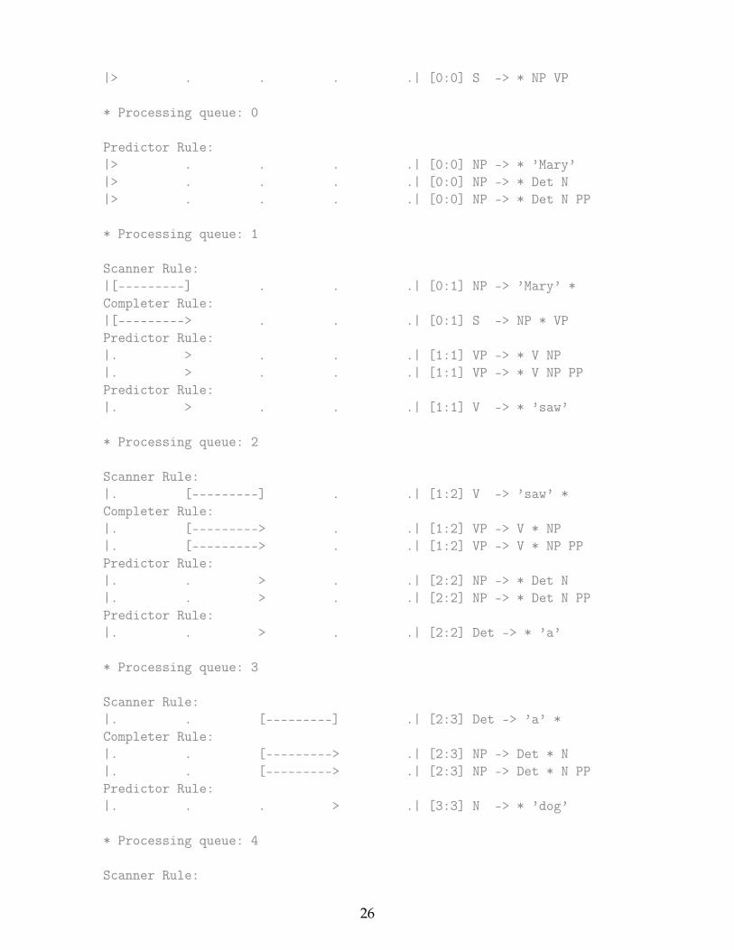
|> . . . .| [0:0] S -> * NP VP
* Processing queue: 0
Predictor Rule:|> . . . .| [0:0] NP -> * ’Mary’|> . . . .| [0:0] NP -> * Det N|> . . . .| [0:0] NP -> * Det N PP
* Processing queue: 1
Scanner Rule:|[---------] . . .| [0:1] NP -> ’Mary’ *Completer Rule:|[---------> . . .| [0:1] S -> NP * VPPredictor Rule:|. > . . .| [1:1] VP -> * V NP|. > . . .| [1:1] VP -> * V NP PPPredictor Rule:|. > . . .| [1:1] V -> * ’saw’
* Processing queue: 2
Scanner Rule:|. [---------] . .| [1:2] V -> ’saw’ *Completer Rule:|. [---------> . .| [1:2] VP -> V * NP|. [---------> . .| [1:2] VP -> V * NP PPPredictor Rule:|. . > . .| [2:2] NP -> * Det N|. . > . .| [2:2] NP -> * Det N PPPredictor Rule:|. . > . .| [2:2] Det -> * ’a’
* Processing queue: 3
Scanner Rule:|. . [---------] .| [2:3] Det -> ’a’ *Completer Rule:|. . [---------> .| [2:3] NP -> Det * N|. . [---------> .| [2:3] NP -> Det * N PPPredictor Rule:|. . . > .| [3:3] N -> * ’dog’
* Processing queue: 4
Scanner Rule:
26
|. . . [---------]| [3:4] N -> ’dog’ *Completer Rule:|. . [-------------------]| [2:4] NP -> Det N *|. . [------------------->| [2:4] NP -> Det N * PPPredictor Rule:|. . . . >| [4:4] PP -> * P NPCompleter Rule:|. [-----------------------------]| [1:4] VP -> V NP *|. [----------------------------->| [1:4] VP -> V NP * PPCompleter Rule:|[=======================================]| [0:4] S -> NP VP *[Tree(’S’, [Tree(’NP’, [’Mary’]), Tree(’VP’, [Tree(’V’, [’saw’]), Tree(’NP’, [Tree(’Det’, [’a’]), Tree(’N’, [’dog’])])])])]
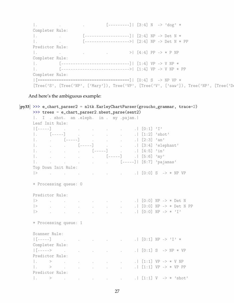
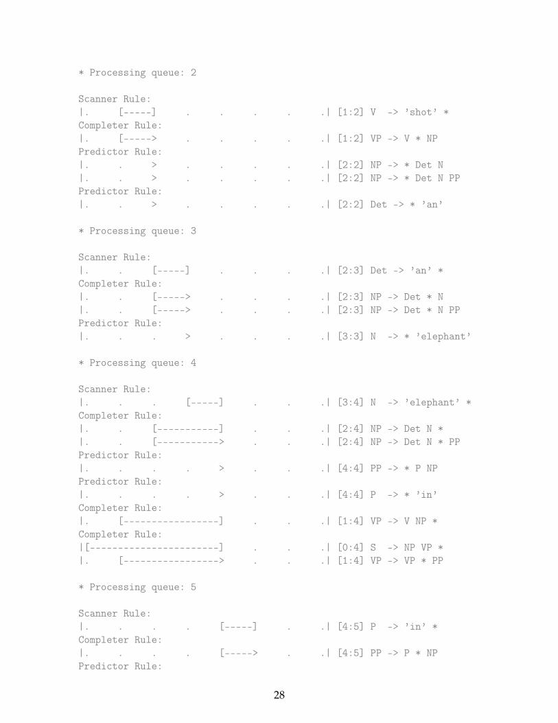
And here’s the ambiguous example:
[py33] >>> e_chart_parser2 = nltk.EarleyChartParser(groucho_grammar, trace=2)>>> trees = e_chart_parser2.nbest_parse(sent2)|. I . shot. an .eleph. in . my .pajam.|Leaf Init Rule:|[-----] . . . . . .| [0:1] ’I’|. [-----] . . . . .| [1:2] ’shot’|. . [-----] . . . .| [2:3] ’an’|. . . [-----] . . .| [3:4] ’elephant’|. . . . [-----] . .| [4:5] ’in’|. . . . . [-----] .| [5:6] ’my’|. . . . . . [-----]| [6:7] ’pajamas’Top Down Init Rule:|> . . . . . . .| [0:0] S -> * NP VP
* Processing queue: 0
Predictor Rule:|> . . . . . . .| [0:0] NP -> * Det N|> . . . . . . .| [0:0] NP -> * Det N PP|> . . . . . . .| [0:0] NP -> * ’I’
* Processing queue: 1
Scanner Rule:|[-----] . . . . . .| [0:1] NP -> ’I’ *Completer Rule:|[-----> . . . . . .| [0:1] S -> NP * VPPredictor Rule:|. > . . . . . .| [1:1] VP -> * V NP|. > . . . . . .| [1:1] VP -> * VP PPPredictor Rule:|. > . . . . . .| [1:1] V -> * ’shot’
27
* Processing queue: 2
Scanner Rule:|. [-----] . . . . .| [1:2] V -> ’shot’ *Completer Rule:|. [-----> . . . . .| [1:2] VP -> V * NPPredictor Rule:|. . > . . . . .| [2:2] NP -> * Det N|. . > . . . . .| [2:2] NP -> * Det N PPPredictor Rule:|. . > . . . . .| [2:2] Det -> * ’an’
* Processing queue: 3
Scanner Rule:|. . [-----] . . . .| [2:3] Det -> ’an’ *Completer Rule:|. . [-----> . . . .| [2:3] NP -> Det * N|. . [-----> . . . .| [2:3] NP -> Det * N PPPredictor Rule:|. . . > . . . .| [3:3] N -> * ’elephant’
* Processing queue: 4
Scanner Rule:|. . . [-----] . . .| [3:4] N -> ’elephant’ *Completer Rule:|. . [-----------] . . .| [2:4] NP -> Det N *|. . [-----------> . . .| [2:4] NP -> Det N * PPPredictor Rule:|. . . . > . . .| [4:4] PP -> * P NPPredictor Rule:|. . . . > . . .| [4:4] P -> * ’in’Completer Rule:|. [-----------------] . . .| [1:4] VP -> V NP *Completer Rule:|[-----------------------] . . .| [0:4] S -> NP VP *|. [-----------------> . . .| [1:4] VP -> VP * PP
* Processing queue: 5
Scanner Rule:|. . . . [-----] . .| [4:5] P -> ’in’ *Completer Rule:|. . . . [-----> . .| [4:5] PP -> P * NPPredictor Rule:
28
|. . . . . > . .| [5:5] NP -> * Det N|. . . . . > . .| [5:5] NP -> * Det N PPPredictor Rule:|. . . . . > . .| [5:5] Det -> * ’my’
* Processing queue: 6
Scanner Rule:|. . . . . [-----] .| [5:6] Det -> ’my’ *Completer Rule:|. . . . . [-----> .| [5:6] NP -> Det * N|. . . . . [-----> .| [5:6] NP -> Det * N PPPredictor Rule:|. . . . . . > .| [6:6] N -> * ’pajamas’
* Processing queue: 7
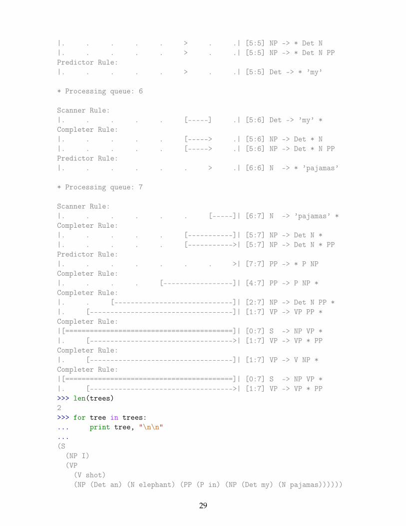
Scanner Rule:|. . . . . . [-----]| [6:7] N -> ’pajamas’ *Completer Rule:|. . . . . [-----------]| [5:7] NP -> Det N *|. . . . . [----------->| [5:7] NP -> Det N * PPPredictor Rule:|. . . . . . . >| [7:7] PP -> * P NPCompleter Rule:|. . . . [-----------------]| [4:7] PP -> P NP *Completer Rule:|. . [-----------------------------]| [2:7] NP -> Det N PP *|. [-----------------------------------]| [1:7] VP -> VP PP *Completer Rule:|[=========================================]| [0:7] S -> NP VP *|. [----------------------------------->| [1:7] VP -> VP * PPCompleter Rule:|. [-----------------------------------]| [1:7] VP -> V NP *Completer Rule:|[=========================================]| [0:7] S -> NP VP *|. [----------------------------------->| [1:7] VP -> VP * PP>>> len(trees)2>>> for tree in trees:... print tree, "\n\n"...(S
(NP I)(VP
(V shot)(NP (Det an) (N elephant) (PP (P in) (NP (Det my) (N pajamas))))))
29
(S(NP I)(VP
(VP (V shot) (NP (Det an) (N elephant)))(PP (P in) (NP (Det my) (N pajamas)))))
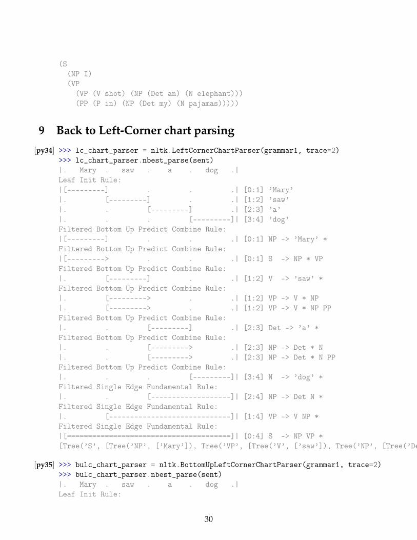
9 Back to Left-Corner chart parsing
[py34] >>> lc_chart_parser = nltk.LeftCornerChartParser(grammar1, trace=2)>>> lc_chart_parser.nbest_parse(sent)|. Mary . saw . a . dog .|Leaf Init Rule:|[---------] . . .| [0:1] ’Mary’|. [---------] . .| [1:2] ’saw’|. . [---------] .| [2:3] ’a’|. . . [---------]| [3:4] ’dog’Filtered Bottom Up Predict Combine Rule:|[---------] . . .| [0:1] NP -> ’Mary’ *Filtered Bottom Up Predict Combine Rule:|[---------> . . .| [0:1] S -> NP * VPFiltered Bottom Up Predict Combine Rule:|. [---------] . .| [1:2] V -> ’saw’ *Filtered Bottom Up Predict Combine Rule:|. [---------> . .| [1:2] VP -> V * NP|. [---------> . .| [1:2] VP -> V * NP PPFiltered Bottom Up Predict Combine Rule:|. . [---------] .| [2:3] Det -> ’a’ *Filtered Bottom Up Predict Combine Rule:|. . [---------> .| [2:3] NP -> Det * N|. . [---------> .| [2:3] NP -> Det * N PPFiltered Bottom Up Predict Combine Rule:|. . . [---------]| [3:4] N -> ’dog’ *Filtered Single Edge Fundamental Rule:|. . [-------------------]| [2:4] NP -> Det N *Filtered Single Edge Fundamental Rule:|. [-----------------------------]| [1:4] VP -> V NP *Filtered Single Edge Fundamental Rule:|[=======================================]| [0:4] S -> NP VP *[Tree(’S’, [Tree(’NP’, [’Mary’]), Tree(’VP’, [Tree(’V’, [’saw’]), Tree(’NP’, [Tree(’Det’, [’a’]), Tree(’N’, [’dog’])])])])]
[py35] >>> bulc_chart_parser = nltk.BottomUpLeftCornerChartParser(grammar1, trace=2)>>> bulc_chart_parser.nbest_parse(sent)|. Mary . saw . a . dog .|Leaf Init Rule:
30
|[---------] . . .| [0:1] ’Mary’|. [---------] . .| [1:2] ’saw’|. . [---------] .| [2:3] ’a’|. . . [---------]| [3:4] ’dog’Bottom Up Predict Combine Rule:|[---------] . . .| [0:1] NP -> ’Mary’ *Bottom Up Predict Combine Rule:|[---------> . . .| [0:1] S -> NP * VPBottom Up Predict Combine Rule:|. [---------] . .| [1:2] V -> ’saw’ *Bottom Up Predict Combine Rule:|. [---------> . .| [1:2] VP -> V * NP|. [---------> . .| [1:2] VP -> V * NP PPBottom Up Predict Combine Rule:|. . [---------] .| [2:3] Det -> ’a’ *Bottom Up Predict Combine Rule:|. . [---------> .| [2:3] NP -> Det * N|. . [---------> .| [2:3] NP -> Det * N PPBottom Up Predict Combine Rule:|. . . [---------]| [3:4] N -> ’dog’ *Single Edge Fundamental Rule:|. . [-------------------]| [2:4] NP -> Det N *|. . [------------------->| [2:4] NP -> Det N * PPBottom Up Predict Combine Rule:|. . [------------------->| [2:4] S -> NP * VPSingle Edge Fundamental Rule:|. [-----------------------------]| [1:4] VP -> V NP *|. [----------------------------->| [1:4] VP -> V NP * PPSingle Edge Fundamental Rule:|[=======================================]| [0:4] S -> NP VP *[Tree(’S’, [Tree(’NP’, [’Mary’]), Tree(’VP’, [Tree(’V’, [’saw’]), Tree(’NP’, [Tree(’Det’, [’a’]), Tree(’N’, [’dog’])])])])]
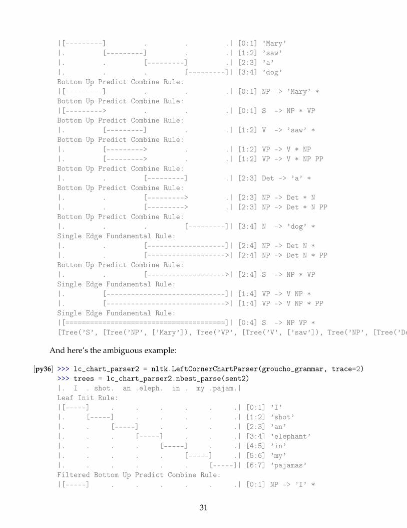
And here’s the ambiguous example:
[py36] >>> lc_chart_parser2 = nltk.LeftCornerChartParser(groucho_grammar, trace=2)>>> trees = lc_chart_parser2.nbest_parse(sent2)|. I . shot. an .eleph. in . my .pajam.|Leaf Init Rule:|[-----] . . . . . .| [0:1] ’I’|. [-----] . . . . .| [1:2] ’shot’|. . [-----] . . . .| [2:3] ’an’|. . . [-----] . . .| [3:4] ’elephant’|. . . . [-----] . .| [4:5] ’in’|. . . . . [-----] .| [5:6] ’my’|. . . . . . [-----]| [6:7] ’pajamas’Filtered Bottom Up Predict Combine Rule:|[-----] . . . . . .| [0:1] NP -> ’I’ *
31
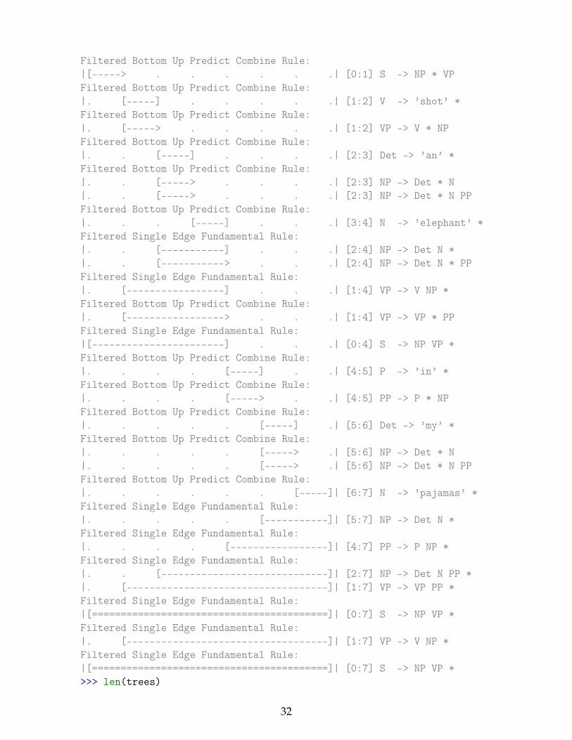
Filtered Bottom Up Predict Combine Rule:|[-----> . . . . . .| [0:1] S -> NP * VPFiltered Bottom Up Predict Combine Rule:|. [-----] . . . . .| [1:2] V -> ’shot’ *Filtered Bottom Up Predict Combine Rule:|. [-----> . . . . .| [1:2] VP -> V * NPFiltered Bottom Up Predict Combine Rule:|. . [-----] . . . .| [2:3] Det -> ’an’ *Filtered Bottom Up Predict Combine Rule:|. . [-----> . . . .| [2:3] NP -> Det * N|. . [-----> . . . .| [2:3] NP -> Det * N PPFiltered Bottom Up Predict Combine Rule:|. . . [-----] . . .| [3:4] N -> ’elephant’ *Filtered Single Edge Fundamental Rule:|. . [-----------] . . .| [2:4] NP -> Det N *|. . [-----------> . . .| [2:4] NP -> Det N * PPFiltered Single Edge Fundamental Rule:|. [-----------------] . . .| [1:4] VP -> V NP *Filtered Bottom Up Predict Combine Rule:|. [-----------------> . . .| [1:4] VP -> VP * PPFiltered Single Edge Fundamental Rule:|[-----------------------] . . .| [0:4] S -> NP VP *Filtered Bottom Up Predict Combine Rule:|. . . . [-----] . .| [4:5] P -> ’in’ *Filtered Bottom Up Predict Combine Rule:|. . . . [-----> . .| [4:5] PP -> P * NPFiltered Bottom Up Predict Combine Rule:|. . . . . [-----] .| [5:6] Det -> ’my’ *Filtered Bottom Up Predict Combine Rule:|. . . . . [-----> .| [5:6] NP -> Det * N|. . . . . [-----> .| [5:6] NP -> Det * N PPFiltered Bottom Up Predict Combine Rule:|. . . . . . [-----]| [6:7] N -> ’pajamas’ *Filtered Single Edge Fundamental Rule:|. . . . . [-----------]| [5:7] NP -> Det N *Filtered Single Edge Fundamental Rule:|. . . . [-----------------]| [4:7] PP -> P NP *Filtered Single Edge Fundamental Rule:|. . [-----------------------------]| [2:7] NP -> Det N PP *|. [-----------------------------------]| [1:7] VP -> VP PP *Filtered Single Edge Fundamental Rule:|[=========================================]| [0:7] S -> NP VP *Filtered Single Edge Fundamental Rule:|. [-----------------------------------]| [1:7] VP -> V NP *Filtered Single Edge Fundamental Rule:|[=========================================]| [0:7] S -> NP VP *>>> len(trees)
32
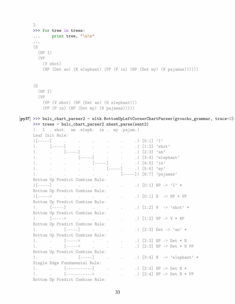
2>>> for tree in trees:... print tree, "\n\n"...(S
(NP I)(VP
(V shot)(NP (Det an) (N elephant) (PP (P in) (NP (Det my) (N pajamas))))))
(S(NP I)(VP
(VP (V shot) (NP (Det an) (N elephant)))(PP (P in) (NP (Det my) (N pajamas)))))
[py37] >>> bulc_chart_parser2 = nltk.BottomUpLeftCornerChartParser(groucho_grammar, trace=2)>>> trees = bulc_chart_parser2.nbest_parse(sent2)|. I . shot. an .eleph. in . my .pajam.|Leaf Init Rule:|[-----] . . . . . .| [0:1] ’I’|. [-----] . . . . .| [1:2] ’shot’|. . [-----] . . . .| [2:3] ’an’|. . . [-----] . . .| [3:4] ’elephant’|. . . . [-----] . .| [4:5] ’in’|. . . . . [-----] .| [5:6] ’my’|. . . . . . [-----]| [6:7] ’pajamas’Bottom Up Predict Combine Rule:|[-----] . . . . . .| [0:1] NP -> ’I’ *Bottom Up Predict Combine Rule:|[-----> . . . . . .| [0:1] S -> NP * VPBottom Up Predict Combine Rule:|. [-----] . . . . .| [1:2] V -> ’shot’ *Bottom Up Predict Combine Rule:|. [-----> . . . . .| [1:2] VP -> V * NPBottom Up Predict Combine Rule:|. . [-----] . . . .| [2:3] Det -> ’an’ *Bottom Up Predict Combine Rule:|. . [-----> . . . .| [2:3] NP -> Det * N|. . [-----> . . . .| [2:3] NP -> Det * N PPBottom Up Predict Combine Rule:|. . . [-----] . . .| [3:4] N -> ’elephant’ *Single Edge Fundamental Rule:|. . [-----------] . . .| [2:4] NP -> Det N *|. . [-----------> . . .| [2:4] NP -> Det N * PPBottom Up Predict Combine Rule:
33
|. . [-----------> . . .| [2:4] S -> NP * VPSingle Edge Fundamental Rule:|. [-----------------] . . .| [1:4] VP -> V NP *Bottom Up Predict Combine Rule:|. [-----------------> . . .| [1:4] VP -> VP * PPSingle Edge Fundamental Rule:|[-----------------------] . . .| [0:4] S -> NP VP *Bottom Up Predict Combine Rule:|. . . . [-----] . .| [4:5] P -> ’in’ *Bottom Up Predict Combine Rule:|. . . . [-----> . .| [4:5] PP -> P * NPBottom Up Predict Combine Rule:|. . . . . [-----] .| [5:6] Det -> ’my’ *Bottom Up Predict Combine Rule:|. . . . . [-----> .| [5:6] NP -> Det * N|. . . . . [-----> .| [5:6] NP -> Det * N PPBottom Up Predict Combine Rule:|. . . . . . [-----]| [6:7] N -> ’pajamas’ *Single Edge Fundamental Rule:|. . . . . [-----------]| [5:7] NP -> Det N *|. . . . . [----------->| [5:7] NP -> Det N * PPBottom Up Predict Combine Rule:|. . . . . [----------->| [5:7] S -> NP * VPSingle Edge Fundamental Rule:|. . . . [-----------------]| [4:7] PP -> P NP *Single Edge Fundamental Rule:|. . [-----------------------------]| [2:7] NP -> Det N PP *|. [-----------------------------------]| [1:7] VP -> VP PP *Bottom Up Predict Combine Rule:|. [----------------------------------->| [1:7] VP -> VP * PPSingle Edge Fundamental Rule:|[=========================================]| [0:7] S -> NP VP *Bottom Up Predict Combine Rule:|. . [----------------------------->| [2:7] S -> NP * VPSingle Edge Fundamental Rule:|. [-----------------------------------]| [1:7] VP -> V NP *Bottom Up Predict Combine Rule:|. [----------------------------------->| [1:7] VP -> VP * PPSingle Edge Fundamental Rule:|[=========================================]| [0:7] S -> NP VP *>>> len(trees)2>>> for tree in trees:... print tree, "\n\n"...(S
(NP I)
34
(VP(V shot)(NP (Det an) (N elephant) (PP (P in) (NP (Det my) (N pajamas))))))
(S(NP I)(VP
(VP (V shot) (NP (Det an) (N elephant)))(PP (P in) (NP (Det my) (N pajamas)))))
References
Bird, Steven et al. (2009). Natural Language Processing with Python. O’Reilly Media.Earley, Jay (1970). “An Efficient Context-free Parsing Algorithm”. In: Commun. ACM 13.2, pp. 94–
102.Poore, Geoffrey M. (2013). “Reproducible Documents with PythonTeX”. In: Proceedings of the
12th Python in Science Conference. Ed. by Stéfan van der Walt et al., pp. 78–84.
35


![Bare-Bones Dependency Parsing - Uppsala Universitystp.lingfil.uu.se/~nivre/docs/BareBones.pdf · I Parsing methods for bare-bones dependency parsing I Chart parsing ... Eisner 2000]:](https://static.fdocuments.us/doc/165x107/5b1dbccd7f8b9a397f8b5558/bare-bones-dependency-parsing-uppsala-nivredocsbarebonespdf-i-parsing-methods.jpg)