NLSSI High Frequency Response Study - Department … High Frequency Response Study U.S. Department...

ww

w.in

l.gov

Bob Spears Contact: 208-526-4109, [email protected] Structural Analysis Idaho National Laboratory October 18-19th, 2016 INL/MIS-16-39106

NLSSI High Frequency Response Study

U.S. Department of Energy Natural Phenomena Hazards Meeting

2

Purpose

The purpose of this study is to better understand how nonlinear soil-structure interaction (NLSSI) analysis and linear soil-structure interaction (SHAKE and SASSI) differ in high frequency response

3

Scope

• Compare nonlinear and linear results for a deep soil column

• Show nonlinear, single element results to better understand the high frequency response

• Conclusions

4

Comparison of Nonlinear and Linear Deep Soil Column Results

• Is performed on a deep soil column to show high frequency response differences between nonlinear and linear techniques

• Considers the Vogtle soil column which is 1058•ft deep

• Uses the Lake Hughes #9, metamorphic rock (gneiss) seismic time histories from the Northridge earthquake of January 17, 1994

• Is run in Abaqus/Explicit with nonlinear soil shear stress versus shear strain curves having 100 points

5

Vogtle Soil Column

Elastic element with the load time history applied on its top surface and a non-reflective boundary condition applied to the bottom surface

• Is defined with 41 nonlinear soil material properties

• Is free at the top

• Has non-reflecting boundary conditions at the bottom

• Has seismic motion input as a load time history at a depth of 1058•ft

• Has each set for four nodes at an elevation constrained to move together

• Has element heights set to pass up to 67•Hz waves with at least 10 elements per wave length

Rock Outcrop Time Histories

6

Acceleration versus Time

Acce

lera

tion

[ft/s

ec2 ]

Time [sec] Velocity versus Time

Velo

city

[ft/s

ec]

Time [sec] Displacement versus Time

Dis

plac

emen

t

[ft

]

Time [sec]

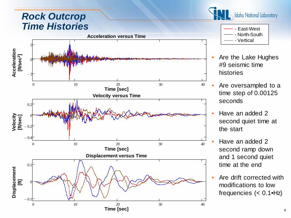
• Are the Lake Hughes #9 seismic time histories

• Are oversampled to a time step of 0.00125 seconds

• Have an added 2 second quiet time at the start

• Have an added 2 second ramp down and 1 second quiet time at the end

• Are drift corrected with modifications to low frequencies (< 0.1•Hz)

0 10 20 30 40

5−

0

5

0 10 20 30 400.4−

0.2−

0

0.2

0 10 20 30 400.1−

0

0.1

- East-West ____- North-South ____- Vertical ____

Acce

lera

tion

[g]

Frequency [Hz]

0.1 1 10 1000

0.2

0.4

0.6

0.8

1 - East-West ____- North-South ____- Vertical ____

7

Rock Outcrop Acceleration Response Spectra

Vogtle Soil Column Animation (100 Point Soil Constitutive Model)

8

Maximum strain = 5•10-4 ft/ft

Acce

lera

tion

[g]

Frequency [Hz]

0.1 1 10 1000

0.5

1

1.5

2

9

Results based on 100 point soil constitutive models

Top-of-Soil Acceleration Response Spectra

- East-West (Top-of-Soil) ____- North-South (Top-of-Soil) ____- Vertical (Top-of-Soil) ____- East-West (Rock Outcrop) ____- North-South (Rock Outcrop) ____- Vertical (Rock Outcrop) ____

Acce

lera

tion

[g]

Frequency [Hz]

10

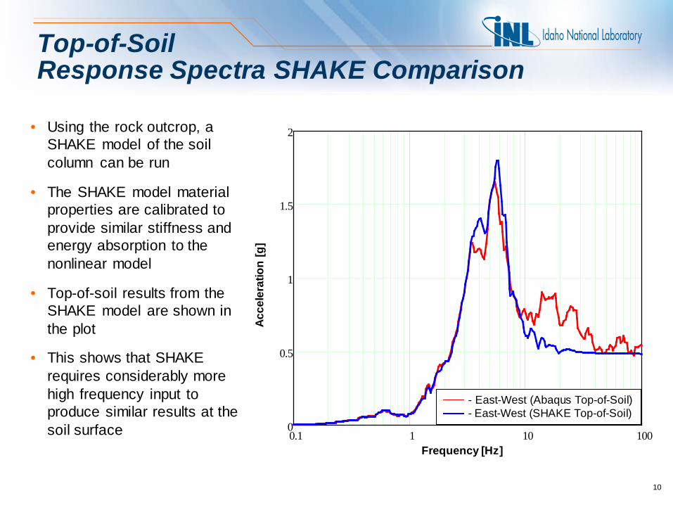
Top-of-Soil Response Spectra SHAKE Comparison

• Using the rock outcrop, a SHAKE model of the soil column can be run

• The SHAKE model material properties are calibrated to provide similar stiffness and energy absorption to the nonlinear model

• Top-of-soil results from the SHAKE model are shown in the plot

• This shows that SHAKE requires considerably more high frequency input to produce similar results at the soil surface 0.1 1 10 100

0

0.5

1

1.5

2

- East-West (Abaqus Top-of-Soil) ____- East-West (SHAKE Top-of-Soil) ____

11

Results Summary for Nonlinear and Linear Deep Soil Column Comparison

• Show that the nonlinear soil model can produce a reasonably shaped top-of-soil response spectra when an actual rock outcrop time history is applied

• Show that to produce similar top-of-soil results, a SHAKE model must have significantly more high frequency rock outcrop input

• Begs the question “is the difference in the nonlinear model high frequency content realistic?”

12

High Frequency Response in Nonlinear, Single Element Models

• Is performed on a single element with a single frequency input

• Studies the existence (or nonexistence) of frequency output other than that of the input frequency

• Considers different nonlinear stress versus strain curves

13

First Soil Column Model • Is a single element model

evaluated with a 4th order Runge-Kutta solver (defined in Mathcad)

• Has a 1.22 Hz frequency displacement time history applied at its base


• Has a time step of 6.25•10-4 sec (Nyquist frequency = 800 Hz)

• Has a height of 125•ft

0 2 4 6 80.2−

0.1−

0

0.1

0.2

Time [sec]

Dis

plac

emen

t [ft]

Free

Applied horizontal time history

Soil element

*Note: The displacement time history is linearly ramped for 2 cycles and then has a constant amplitude that continues to 51 seconds

14

First Model Soil Constitutive Model • Is based on a ten point shear

stress versus shear strain curve for soil at the INL

• Is interpolated with a cubic fit in log-log space to smoothly produce 500 data points

• Is evaluated with a nested surface constitutive model (like the LS-DYNA MAT_79)

Shea

r Stre

ss [k

sf]

Shear Strain [ft/ft] 0 5 10 4−

× 1 10 3−×

0

1

2

3

15

First Animation

- Top ____- Base ____

16

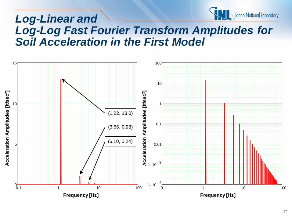
First Soil Column Model Output

• The output includes free surface acceleration and shear stress time histories

• A fast Fourier transform is performed on the steady-state portion of the free surface acceleration (for times from 10 – 51 seconds)

• The fast Fourier transform shows how a single frequency input produces a multi-frequency output

• A similar process is performed for the shear stress time history to show that it produces similar results

Acce

lera

tion

Ampl

itude

s [ft

/sec

2 ]

Frequency [Hz]

17

Acce

lera

tion

Ampl

itude

s [ft

/sec

2 ]

Frequency [Hz] 0.1 1 10 100

0

5

10

15

0.1 1 10 1001 10 4−×

1 10 3−×

0.01

0.1

1

10

100

Log-Linear and Log-Log Fast Fourier Transform Amplitudes for Soil Acceleration in the First Model

(1.22, 13.0)

(3.66, 0.98)

(6.10, 0.24)

Shea

r Stre

ss A

mpl

itude

s [k

sf]

Frequency [Hz]

18

Shea

r Stre

ss A

mpl

itude

s [k

sf]

Frequency [Hz] 0.1 1 10 100

0

1

2

3

0.1 1 10 1001 10 5−×

1 10 4−×

1 10 3−×

0.01

0.1

1

10

Log-Linear and Log-Log Fast Fourier Transform Amplitudes for Soil Shear Stress in the First Model

(1.22, 2.98)

(3.66, 0.22)

(6.10, 0.06)

The acceleration plot shows the information being studied but the same basic information can be gathered from the shear stress plot.

19

Second Soil Column Model • Is similar to the first model except

the boundary conditions are different

• Has a 1.22 Hz frequency displacement time history applied at its top

• Is fixed at the base

• Is performed because it provides very exact control for testing different shear stress versus shear strain curves

• Is also more representative of actual soil tests

Fixed Base

Soil element

0 2 4 6 81− 10 3−×

5− 10 4−×

0

5 10 4−×

1 10 3−×

Time [sec]

Dis

plac

emen

t [ft]


20

Second Model Soil Constitutive Model • Is the same as the first model soil

constitutive model

Shea

r Stre

ss [k

sf]


× 1 10 3−×

0

1

2

3

21

Second Animation

- Stress ____- Strain ____

22

Second Soil Column Model Output

• The output includes the shear stress time history

• A fast Fourier transform is performed on the steady-state portion of the shear stress time history (for times from 2 – 41 seconds)

• The fast Fourier transform shows how similar conclusions can be drawn from this model as were drawn from the first model

This model is run with a strain amplitude of 0.0009 ft/ft where the first model was run with a strain amplitude of a little more than 0.00097 ft/ft.

Note:

Shea

r Stre

ss A

mpl

itude

s [k

sf]

Frequency [Hz]

23

Shea

r Stre

ss A

mpl

itude

s [k

sf]

Frequency [Hz]

Log-Linear and Log-Log Fast Fourier Transform Amplitudes for Soil Shear Stress in the Second Model

0.1 1 10 1000

1

2

3

0.1 1 10 1001 10 5−×

1 10 4−×

1 10 3−×

0.01

0.1

1

10

(1.22, 2.88)

(3.66, 0.17)

(6.10, 0.04)

The maximum hysteresis loop shear stress is 2.91 ksf Note:

24

Third Soil Column Model and Soil Constitutive Model • Is similar to the second model

except for the soil constitutive model shear stress versus shear strain curve

• Has shear stress versus shear strain curve shape that produces a hysteresis loop similar to that of a linear, viscous damped model (if it is cycled at a strain amplitude of 0.0009 ft/ft)

Shea

r Stre

ss [k

sf]


× 1 10 3−×

0

1

2

3

25

Third Animation

- Stress ____- Strain ____

26

Third Soil Column Model Output



• The fast Fourier transform shows how a soil constitutive model with a hysteresis loop shaped like that of a linear viscous damped model passes only the input frequency content

Shea

r Stre

ss A

mpl

itude

s [k

sf]

Frequency [Hz] 0.1 1 10 1000

1

2

3

27

Shea

r Stre

ss A

mpl

itude

s [k

sf]

Frequency [Hz]

Log-Linear and Log-Log Fast Fourier Transform Amplitudes for Soil Shear Stress in the Third Model

(1.22, 2.88)

0.1 1 10 1001 10 5−×

1 10 4−×

1 10 3−×

0.01

0.1

1

10


Shea

r Stre

ss

[ksf

]

Shear Strain [ft/ft]

Shea

r Stre

ss [k

sf]

Shear Strain [ft/ft]

0 5 10 4−× 1 10 3−

×0

1

2

3

28

Fourth Soil Column Model and Soil Constitutive Model • Is similar to the third model except

for the soil constitutive model shear stress versus shear strain curve

• Has a smooth sine wave addition (shown in the lower plot) to the middle of the curve

• Is unchanged within 2% of the curve ends

- Fourth soil column model ____- Third soil column model

0 2 10 4−× 4 10 4−

× 6 10 4−× 8 10 4−

×0

0.10.20.3

29

Fourth Animation - Stress

____- Strain ____

30

Fourth Soil Column Model Output



• The fast Fourier transform shows how a soil constitutive model with a smooth hysteresis loop shaped slightly different than a linear viscous damped model generates additional frequency content

Shea

r Stre

ss A

mpl

itude

s [k

sf]

Frequency [Hz] 0.1 1 10 1000

1

2

3

31

Shea

r Stre

ss A

mpl

itude

s [k

sf]

Frequency [Hz]

Log-Linear and Log-Log Fast Fourier Transform Amplitudes for Soil Shear Stress in the Fourth Model

(1.22, 2.97)

(3.66, 0.12)

(6.10, 0.02)


0.1 1 10 1001 10 5−×

1 10 4−×

1 10 3−×

0.01

0.1

1

10

32

Results Summary for the High Frequency Response in Nonlinear, Single Element Models

• Added high frequency can be expected in actual soil response

• Or, if a sine wave shear strain is applied to a soil sample and the resulting shear stress is anything other than a sine wave of the same frequency, added high frequency motion should be expected

Conclusions

• Two studies were performed

• The first study showed • That a deep nonlinear soil column could produce a reasonably

shaped response spectra using an actual rock outcrop time history • The difference in high frequency content when compared to

SHAKE • The second study showed that added high frequency content can be

expected in actual soil response

33

The National Nuclear Laboratory

34

35

High Frequency Response Due to the Input Stress versus Strain

• If test data shows a smooth shear stress versus shear strain curve and a few points with straight lines between them are used for the nonlinear model, erroneous high frequency content can be expected

• Example results are shown for the Vogtle soil column and the single element models

• Additionally, strategies to reduce erroneous high frequency content are explored

Acce

lera

tion

[g]

Frequency [Hz]

0.1 1 10 1000

0.5

1

1.5

36

Top-of-Soil Response Spectra 100 and 10 Point Comparison

• Running the Vogtle soil column again with 10 point soil constitutive models produces the plotted results

• The primary difference occurs at high frequencies (> 12 Hz) in the horizontal directions

• This model shows significant sensitivity at high frequencies to the number of points in the shear stress versus shear strain curve

- East-West (10 Point) ____- North-South (10 Point) ____- Vertical (10 Point) ____- East-West (100 Point) ____- North-South (100 Point) ____- Vertical (100 Point) ____

Acce

lera

tion

[g]

Frequency [Hz] 0.1 1 10 1000

0.2

0.4

0.6

37

Top-of-Soil Response Spectra Added Mass Comparison

• Running the same Vogtle soil column with a mass of 5.7 kip/ft2 added to the surface (representing a nuclear structure) produces the plotted results

• This model is not very sensitive to the number of points in the shear stress versus shear strain curve

• Less soil constitutive model points is desirable because it significantly reduces the amount of computation required to perform a model run

- East-West (10 Point) ____- North-South (10 Point) ____- Vertical (10 Point) ____- East-West (100 Point) ____- North-South (100 Point) ____- Vertical (100 Point) ____

38

Soil Column Model (10 Point) • Is a single element model

evaluated with a 4th order Runge-Kutta solver (defined in Mathcad)

• Has a 1.22 Hz frequency displacement time history applied at its base


• Has a time step of 6.25•10-4 sec (Nyquist frequency = 800 Hz)

• Has a height of 125•ft

0 2 4 6 80.2−

0.1−

0

0.1

0.2

Time [sec]

Dis

plac

emen

t [ft]

Free


Soil element

*Note: The displacement time history is linearly ramped for 2 cycles and then has a constant amplitude that continues to 51 seconds

Shea

r Stre

ss [k

sf]


× 1 10 3−×

0

1

2

3

39

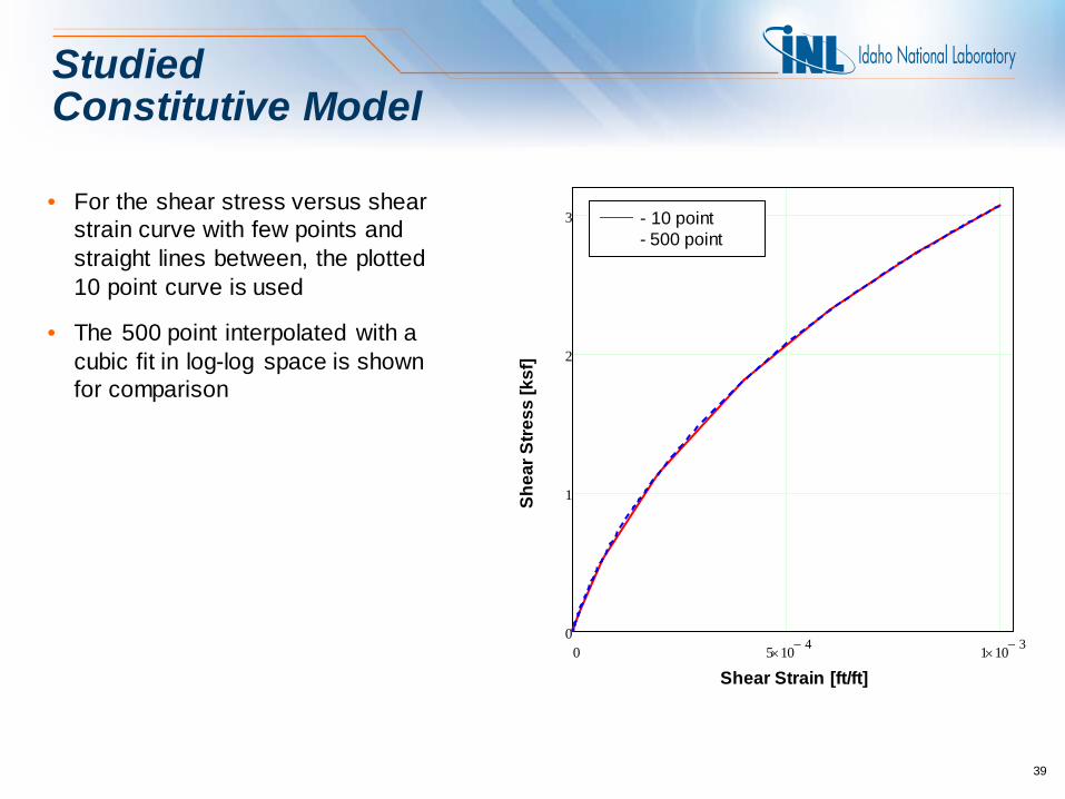
Studied Constitutive Model • For the shear stress versus shear

strain curve with few points and straight lines between, the plotted 10 point curve is used

• The 500 point interpolated with a cubic fit in log-log space is shown for comparison

- 10 point ____- 500 point ____

40

Animation (10 Point) - Top

____- Base ____

Acce

lera

tion

[g]

Frequency [Hz]

0.1 1 10 1001 10 4−×

1 10 3−×

0.01

0.1

1

10

100

41

Single Element Log-Log Fast Fourier Transform (10 and 500 Point)

- 10 Point ____- 500 Point

• The output is the free surface acceleration

• A fast Fourier transform is performed on the steady-state portion of the free surface acceleration (for times from 10 – 51 seconds)

• This shows the increased high frequency content for the model run with 10 points

Shea

r Stre

ss [k

sf]


× 4 10 7−× 6 10 7−

× 8 10 7−× 1 10 6−

×0

2 10 4−×

4 10 4−×

6 10 4−×

42

Smoothing for a 10 Point Curve

• To reduce unwanted high frequency content for a 10 point shear stress versus shear strain curve, one option is to remove the discontinuity in the “layers”

• Rather than elastic-perfectly plastic, a smooth continuous curve could be added

• The modified “layer” curve is an exponential curve applied continuously to the end of the linear elastic region

42

- Modified “layer” ____- Original “layer”

For the nonlinear soil model being used, there is a “layer” for each data point on the shear stress versus shear strain curve. The total response of a given element is the summation of its defined “layers”.

Note:

Smoothing Test Soil Column Model

43

• Includes upper alluvial soil (UAS) (28 ft. deep) and lower alluvial soil (LAS) (48 ft. deep)

• Has an element height of two foot throughout which passes up to 45 Hz waves with at least 10 elements per wavelength

• Has a base excitation that is applied as a displacement time history


• Is run for three versions • Original “layers” and 100 point curve • Original “layers” and 10 point curve • Modified “layers” and 10 point curve

UAS

LAS

Acceleration Time History

44

Acceleration versus Time

Acce

lera

tion

[ft/s

ec2 ]

Time [sec] Velocity versus Time

Velo

city

[ft/s

ec]

Time [sec] Displacement versus Time

Dis

plac

emen

t

[ft

]

Time [sec]

• INL East-West seismic time history

• The displacement time history is sampled as a smooth function defined with the Fast Fourier Transform values

0 10 20 30 405−

0

5

0 10 20 30 40

0.5−

0

0.5

0 10 20 30 400.2−

0

0.2

12

INL Soil Column Animation (10 Point Modified Soil Model)

45

• Is evaluated with a 4th order Runge-Kutta solver (defined in Mathcad) with a time step of 7.81•10-5 seconds

• The results are sampled at a time step of 0.00125 seconds

Acce

lera

tion

[g]

Frequency [Hz]

1 10 100

1

2

3

4

46

Top-of-Soil Response Spectra Added Mass Comparison

• The plot shows that the modified 10 point shear stress versus shear strain curve provides significantly better results than the original 10 point shear stress versus shear strain curve

• If the added computation is not problematic, the 100 point shear stress versus shear strain curve provides the best result

- 100 Point ____- 10 Point ____- 10 Point Modified

47

Results Summary for the High Frequency Response Due to the Input Stress versus Strain

• Show that significant erroneous high frequency content is

possible in nonlinear analysis if care is not taken with the definition of the shear stress versus shear strain curve

• Show that the sensitivity for having erroneous high frequency is model dependent

• Show that constitutive model modifications could be performed to reduce the sensitivity for having erroneous high frequency

Conclusions

• Three studies were performed

• The first study showed • That a deep nonlinear soil column could produce a reasonably

shaped response spectra using an actual rock outcrop time history • The difference in high frequency content when compared to

SHAKE • The second study showed that added high frequency content can be

expected in actual soil response • The third study showed that significant erroneous high frequency

content is possible in nonlinear analysis but it can be managed and minimized

48

The National Nuclear Laboratory

49

50

Seismic Motion Near Corbin VA for Mineral VA Earthquake 8-23-2011

Sensor

Epicenter

Acce

lera

tion

[g]

Frequency [Hz]

0.1 1 10 1000

0.1

0.2

0.3

51

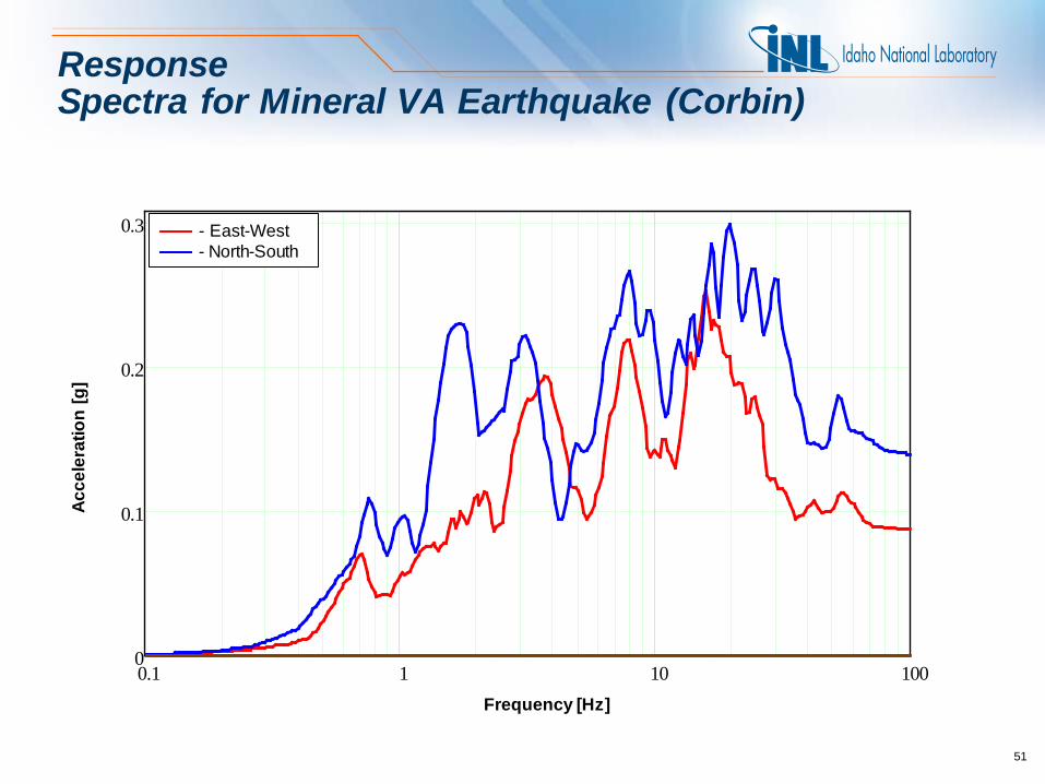
Response Spectra for Mineral VA Earthquake (Corbin)

- East-West ____- North-South

52

Seismic Motion at Charlottesville VA for Mineral VA Earthquake 8-23-2011

Sensor

Epicenter

Acce

lera

tion

[g]

Frequency [Hz]

0.1 1 10 1000

0.2

0.4

53

Response Spectra for Mineral VA Earthquake (Charlottesville)

- East-West ____- North-South ____- Vertical ____

Nonlinear Soil Constitutive Model (LS-DYNA)

54

• LS-DYNA has a constitutive model developed to address hysteretic behavior in soil (*MAT_HYSTERETIC_SOIL or *MAT_079)

• The hysteretic behavior is dictated by post yielding stress versus strain (at a given hydrostatic pressure)

• The yielding and the stress versus strain data can vary with changes in hydrostatic pressure (but this is not used in this study as this is not included in the material property data used in this study)

• Other available soil parameters include yield function constants, dilation parameters, cut-off pressure, and an exponent for bulk modulus pressure sensitivity (the z-direction must be vertical for these to work correctly)

• This constitutive model is of a form that includes the Drucker-Prager model and is reasonable for nonlinear soil behavior

σ = E ε⋅ ==> P t( )A

= E v t( )c

⋅ = E v t( )Eρ

⋅ = E ρ⋅ v t( )⋅ ==> P t( ) = A E ρ⋅⋅ v t( )⋅

Where:

σ - Stress of concern (shear stress in this case)

E - Stiffness relative to the stress of concern (shear modulus in this case)

ε - Strain of concern (shear strain in this case)

P t( ) - Force time history v t( ) - Velocity time history where

A - Cross-sectional area c - Speed of sound ρ - Density

Seismic Model Load Time History Application

55

• The velocity time history for this portion of the study is rock outcrop • Applying this load time history to the basalt without soil on top of it produces

a rock outcrop motion • Applying this load time history to the basalt with soil on top of it produces top

of rock motion • This fact can be validated by observing the similarities of the transfer

functions used for comparison between the linear SHAKE model and the nonlinear LS-DYNA model

Acce

lera

tion

[g]

Frequency [Hz]

0.1 1 10 1000

0.5

1

1.5

- East-West (Original Rock Outcrop) ____- East-West (SHAKE Rock Outcrop) ____

56

Rock Outcrop Response Spectra SHAKE Comparison

• Using the top-of-soil East-West results, a SHAKE model of the soil column can be run

• The SHAKE model material properties are calibrated to provide similar stiffness and energy absorption to the nonlinear model

• Rock outcrop results from the bottom of the SHAKE model are shown in the plot

• This shows that SHAKE requires considerably more high frequency input to produce similar results at the soil surface

NLSSI High Frequency Response Study - Department … High Frequency Response Study U.S. Department...

Documents

Transcript of NLSSI High Frequency Response Study - Department … High Frequency Response Study U.S. Department...