
NLOGIT Student User Manual - New York University
141
User’s Guide by William H. Greene Econometric Software, Inc.
Transcript of NLOGIT Student User Manual - New York University

User’s Guide
by
William H. Greene Econometric Software, Inc.

© 1986 - 2007 Econometric Software, Inc. All rights reserved. ⎯⎯⎯⎯⎯⎯⎯⎯⎯⎯⎯⎯⎯⎯⎯⎯⎯⎯⎯⎯⎯⎯⎯⎯⎯⎯⎯⎯⎯⎯⎯ This software product, including both the program code and the accompanying documentation, is copyrighted by, and all rights are reserved by Econometric Software, Inc. No part of this product, either the software or the documentation, may be reproduced, stored in a retrieval system, or transmitted in any form or by any means without prior written permission of Econometric Software, Inc. LIMDEPTM and NLOGITTM are trademarks of Econometric Software, Inc. All other brand and product names are trademarks or registered trademarks of their respective companies. Econometric Software, Inc. 15 Gloria Place Plainview, NY 11803, USA Tel: +1 516-938-5254 Fax: +1 516-938-2441 Email: [email protected] Websites: www.limdep.com and www.nlogit.com Econometric Software, Australia 215 Excelsior Avenue Castle Hill NSW 2154 Australia Tel: +61 (0)418-433-057 Fax: +61 (0)2-9899-6674 Email: [email protected]

End-User License Agreement ⎯⎯⎯⎯⎯⎯⎯⎯⎯⎯⎯⎯⎯⎯⎯⎯⎯⎯⎯⎯⎯⎯⎯⎯⎯⎯⎯⎯⎯⎯⎯
This is a contract between you and Econometric Software, Inc. The software product refers to the computer software and documentation as well as any upgrades, modified versions, copies or supplements supplied by Econometric Software. By installing, downloading, accessing or otherwise using the software product, you agree to be bound by the terms and conditions of this agreement. Copyright, Trademark, and Intellectual Property
This software product is copyrighted by, and all rights are reserved by Econometric Software, Inc. No part of this software product, either the software or the documentation, may be reproduced, distributed, downloaded, stored in a retrieval system, transmitted in any form or by any means, sold or transferred without prior written permission of Econometric Software. You may not modify, adapt, translate, or change the software product. You may not reverse engineer, decompile, dissemble, or otherwise attempt to discover the source code of the software product. LIMDEPTM and NLOGITTM are trademarks of Econometric Software, Inc. The software product is licensed, not sold. Your possession, installation and use of the software product does not transfer to you any title and intellectual property rights, nor does this license grant you any rights in connection with software product trademarks. Use of the Software Product You have only the non-exclusive right to use this software product. A single user license is registered to one specific individual, and is not intended for access by multiple users on one machine, or for installation on a network or in a computer laboratory. For a single user license only, the registered single user may install the software on a primary stand alone computer and one home or portable secondary computer for his or her exclusive use. However, the software may not be used on the primary computer by another person while the secondary computer is in use. For a multi-user site license, the specific terms of the site license agreement apply for scope of use and installation. Limited Warranty Econometric Software warrants that the software product will perform substantially in accordance with the documentation for a period of ninety (90) days from the date of the original purchase. To make a warranty claim, you must notify Econometric Software in writing within ninety (90) days from the date of the original purchase and return the defective software to Econometric Software. If the software does not perform substantially in accordance with the documentation, the entire liability and your exclusive remedy shall be limited to, at Econometric Software’s option, the replacement of the software product or refund of the license fee paid to Econometric Software for the software product. Proof of purchase from an authorized source is required. This limited warranty is void if failure of the software product has resulted from accident, abuse, or misapplication. Some states and jurisdictions do not allow limitations on the duration of an implied warranty, so the above limitation may not apply to you. To the extent permissible, any implied warranties on the software product are limited to ninety (90) days.

Econometric Software does not warrant the performance or results you may obtain by using the software product. To the maximum extent permitted by applicable law, Econometric Software disclaims all other warranties and conditions, either express or implied, including, but not limited to, implied warranties of merchantability, fitness for a particular purpose, title, and non-infringement with respect to the software product. This limited warranty gives you specific legal rights. You may have others, which vary from state to state and jurisdiction to jurisdiction. Limitation of Liability
Under no circumstances will Econometric Software be liable to you or any other person for any indirect, special, incidental, or consequential damages whatsoever (including, without limitation, damages for loss of business profits, business interruption, computer failure or malfunction, loss of business information, or any other pecuniary loss) arising out of the use or inability to use the software product, even if Econometric Software has been advised of the possibility of such damages. In any case, Econometric Software’s entire liability under any provision of this agreement shall not exceed the amount paid to Econometric Software for the software product. Some states or jurisdictions do not allow the exclusion or limitation of liability for incidental or consequential damages, so the above limitation may not apply to you.

Preface to the Student Version of NLOGIT 4 ⎯⎯⎯⎯⎯⎯⎯⎯⎯⎯⎯⎯⎯⎯⎯⎯⎯⎯⎯⎯⎯⎯⎯⎯ NLOGIT is a major suite of programs for the estimation of discrete choice models. It is built on the original DISCRETE CHOICE command in LIMDEP Version 6.0 which provided some of the features that are described with the estimator presented in Chapter 9 of this reference guide. NLOGIT, itself, began with the development, in 1996, of the nested logit command, originally an extension of the multinomial logit model. With the additions of the multinomial probit model and the mixed logit model among several others, NLOGIT has now grown to a self standing superset of LIMDEP. The focus of most of the recent development is the random parameters logit model, or ‘mixed logit’ model as it is frequently called in the literature. NLOGIT is now the only generally available package that contains panel data (repeated measures) versions of this model, in random effects and autoregressive forms. We note, the technology used in the random parameters model, originally proposed by Dan McFadden and Kenneth Train, has proved so versatile and robust, that we have been able to extend it into most of the other modeling platforms that are contained in LIMDEP. They, like NLOGIT, now contain random parameters versions. Finally, a major feature of NLOGIT is the simulation package. With this program, you can use any model that you have estimated to do ‘what if’ sorts of simulations to examine the effects on predicted behavior of changes in the attributes of choices in your model. NLOGIT Version 4.0 is the result of an ongoing (since 1985) collaboration of William Greene (Econometric Software, Inc.) and David Hensher (Econometric Software, Inc., Australia.) Recent developments, especially the random parameters logit in its cross section and panel data variants have also benefited from the suggestions of Kenneth Train of UC Berkeley. Version 4.0 has also been greatly improved by the enthusiastic collaboration of John Rose (Econometric Software, Inc., Australia). The student version of NLOGIT 4.0 is the entire program. The limitations of the program relate only to the data set size: 1000 observations, 99 variables, and 25 parameters in a model We note, the recently published work Applied Choice Analysis: A Primer (Hensher, D., Rose, J. and Greene, W., Cambridge University Press, 2005) is a wide ranging introduction to discrete choice modeling that contains numerous applications developed with Versions 3.0 and 4.0 of NLOGIT. This book should provide a useful companion to the documentation for NLOGIT. Econometric Software, Inc. January, 2008

Preface to the User’s Guide for the Student Version of NLOGIT 4
⎯⎯⎯⎯⎯⎯⎯⎯⎯⎯⎯⎯⎯⎯⎯⎯⎯⎯⎯⎯⎯⎯⎯⎯ This user’s guide is constructed specifically for the student who is using NLOGIT for the first time and is, most likely, taking their first course in econometrics. Since NLOGIT is an extension of LIMDEP, we assume that you have at hand the manual for the student version of LIMDEP. This guide is a distillation of the full manual for NLOGIT that will show you how to use the program extensions that comprise NLOGIT. Note, however, that NLOGIT contains all of LIMDEP plus the modeling extensions for analysis of discrete choices. Having introduced the manual as above, we do emphasize, this user’s guide is not an econometrics or statistics text, and does not strive to be one. The material below will present only the essential background needed to illustrate the use of the program. In order to accommodate as many readers as possible, we have attempted to develop the material so that it is accessible to both undergraduates and graduate students. (For the latter, a text that would be useful to accompany this guide is Econometric Analysis, 6th Edition (William Greene, Prentice Hall, 2008), which was written by the author of both NLOGIT and this manual.)
Student NLOGIT 4.0 TOC
Student NLOGIT 4.0 Table of Contents ⎯⎯⎯⎯⎯⎯⎯⎯⎯⎯⎯⎯⎯⎯⎯⎯⎯⎯⎯⎯⎯⎯⎯⎯ Chapter 1 Introduction to LIMDEP and NLOGIT 1.1 The LIMDEP Program 1-1 1.2 References for Econometric Methods 1-2 Chapter 2 Installation and Setup 2.1 Introduction 2-1 2.2 Equipment 2-1 2.3 Installation Procedure 2-1 2.4 Registration 2-7 Chapter 3 Discrete Choice Models 3.1 Introduction 3-1 3.2 Random Utility Models 3-1 3.3 Binary Choice Models 3-2 3.4 Bivariate and Multivariate Binary Choices 3-4 3.5 Ordered Choice Models 3-5 3.6 Multinomial Logit Model 3-7 3.6.1 Random Effects and Common (True) Random Effects 3-8 3.6.2 A Dynamic Multinomial Logit Model 3-9 3.7 Conditional Logit Models 3-10 3.8 Error Components Logit Model 3-10 3.9 Heteroscedastic Extreme Value 3-11 3.10 Nested and Generalized Nested Logit 3-12 3.11 Random Parameters Logit 3-14 3.12 Multinomial Probit 3-15 Chapter 4 Model and Command Summary for Discrete Choice Models 4.1 Introduction 4-1 4.2 Model Summary 4-1 4.3 Basic Discrete Choice Models 4-1 4.3.1 Binary Choice Models 4-1 4.3.2 Bivariate Binary Choices 4-2 4.3.3 Multivariate Binary Choice Models 4-2 4.3.4 Ordered Choice Models 4-2 4.4 Multinomial Logit Models 4-3 4.4.1 Multinomial Logit 4-3 4.4.2 Conditional Logit 4-3 4.4.3 Random Parameters Logit 4-4 4.4.4 Latent Class Logit 4-5 4.4.5 Multinomial Probit 4-5 4.6 Command Summary 4-6
Student NLOGIT 4.0 TOC
Chapter 5 Basic Models for Discrete Choice 5.1 Introduction 5-1 5.2 Modeling Binary Choice 5-1 5.2.1 Model Commands 5-2 5.2.2 Output 5-2 5.2.3 Analysis of Marginal Effects 5-6 5.2.4 Robust Covariance Matrix Estimation 5-7 5.3 Ordered Choice Models 5-9 5.3.1 Estimating Ordered Probability Models 5-10 5.3.2 Model Structure and Data 5-10 5.3.3 Output from the Ordered Probability Estimators 5-11 5.3.4 Marginal Effects 5-13 Chapter 6 The Multinomial Logit Model 6.1 Introduction 6-1 6.2 The Multinomial Logit Model 6-2 6.3 Model Command for the Multinomial Logit Model 6-3 6.4 Robust Covariance Matrix 6-3 6.5 Output for the Multinomial Logit Model 6-4 6.6 Marginal Effects 6-8 6.7 Computing Predicted Probabilities 6-12 Chapter 7 Data Setup for NLOGIT 7.1 Introduction 7-1 7.2 Basic Data Setup for NLOGIT 7-1 7.3 Fixed and Variable Numbers of Choices 7-3 7.4 Data for the Applications 7-4 Chapter 8 NLOGIT Commands and Results 8.1 Introduction 8-1 8.2 NLOGIT Commands 8-1 8.2.1 Specifying the Choice Variable and the Choice Set 8-4 8.2.2 Specifying the Utility Functions with Rhs and Rh2 8-5 8.2.3 Building the Utility Functions 8-9 8.3 Estimation Results 8=14 8.3.1 Descriptive Headers for NLOGIT Models 8-14 8.3.2 Standard Model Results 8-15 8.3.3 Retained Results 8-18 8.3.4 Robust Standard Errors 8-18 8.4 Marginal Effects and Elasticities 8-19 8.5 Testing the Assumption of Independence from Irrelevant Alternatives (IIA) 8-21 Chapter 9 The Conditional Logit Model 9.1 Introduction 9-1 9.2 Command for the Multinomial Logit Model 9-2 9.3 Results for the Multinomial Logit Model 9=4 9.4 Application 9-4 9.5 Marginal Effects 9-9

Student NLOGIT 4.0 TOC
Chapter 10 The Nested Logit Model 10.1. Introduction 10-1 10.2 Mathematical Specification of the Model 10-2 10.3 Commands for FIML Estimation 10-3 10.3.1 Data Setup 10-3 10.3.2 Tree Definition 10-4 10.3.3 Utility Functions 10-5 10.3.4 Command Builder 10-6 10.4 Marginal Effects and Elasticities 10-8 Chapter 11 The Random Parameters Logit Model 11.1 Introduction 11-1 11.2 Random Parameters (Mixed) Logit Models 11-2 11.3 Command for the Random Parameters Logit Models 11-6 11.3.1 Distributions of Random Parameters in the Model 11-7 11.3.2 Alternative Specific Constants 11-9 11.3.3 Heterogeneity in the Means of the Random Parameters 11-9 11.3.4 Correlated Parameters 11-10 Chapter 12 The Multinomial Probit Model 12.1 Introduction 12-1 12.2 Model Command 12-2 12.3 An Application 12-4

Student NLOGIT 4.0 TOC
This page intentionally left blank.

Introduction to LIMDEP and NLOGIT 1-1
Chapter 1
Introduction to LIMDEP and NLOGIT ⎯⎯⎯⎯⎯⎯⎯⎯⎯⎯⎯⎯⎯⎯⎯⎯⎯⎯⎯⎯⎯⎯⎯⎯
1.1 The LIMDEP Program LIMDEP is an integrated package for estimating and analyzing econometric models. It is primarily oriented toward cross section and panel data. But, many standard problems in time series analysis can be handled as well. LIMDEP’s basic procedures for data analysis include:
• descriptive statistics (means, standard deviations, minima, etc.), with stratification, • multiple linear regression and stepwise regression, • time series identification, autocorrelations and partial autocorrelations, • cross tabulations, histograms, and scatter plots of several types.
You can also model many extensions of the linear regression model such as:
• heteroscedasticity with robust standard errors, • autocorrelation with robust standard errors, • multiplicative heteroscedasticity, • groupwise heteroscedasticity and cross sectional correlation, • the Box-Cox regression model, • one and two way random and fixed effects models for balanced or unbalanced panel data • distributed lag models, ARIMA, and ARMAX models, • time series models with GARCH effects, • dynamic linear models for panel data, • nonlinear single and multiple equation regression models, • seemingly unrelated linear and nonlinear regression models, • simultaneous equations models.
LIMDEP is best known for its extensive menu of programs for estimating the parameters of nonlinear models for qualitative and limited dependent variables. (We take our name from LIMited DEPendent variables.) No other package supports a greater variety of nonlinear econometric models. Among LIMDEP’s more advanced features, each of which is invoked with a single command, are:
• univariate, bivariate and multivariate probit models, probit models with partial observability, selection, heteroscedasticity and random effects,
• Poisson and negative binomial models for count data, with fixed or random effects, sample selection, underreporting, and numerous other models of over and underdispersion,
• tobit and truncation models for censored and truncated data, • models of sample selection with one or two selection criteria, • parametric and semiparametric duration models with time varying covariates, • stochastic frontier regression models, • ordered probit and logit models, with censoring and sample selection, • switching regression models,

Introduction to LIMDEP and NLOGIT
1-2
• nonparametric and kernel density regression, • fixed effects models, random parameters models and latent class models for over 25
different linear and nonlinear model classes,
and over fifty other model classes. Each of these allows a variety of different specifications. Most of the techniques in wide use are included. Among the aspects of this program which you will notice early on is that regardless of how advanced a technique is, the commands you use to request it are the same as those for the simplest regression. LIMDEP also provides numerous programming tools, including an extensive matrix algebra package and a function optimization routine, so that you can specify your own likelihood functions and add new specifications to the list of models. All results are kept for later use. You can use the matrix program to compute test statistics for specification tests or to write your own estimation programs. The structure of LIMDEP’s matrix program is also especially well suited to the sorts of moment based specification tests suggested, for example, in Pagan and Vella (1989) – all the computations in this paper were done with LIMDEP. The programming tools, such as the editor, looping commands, data transformations, and facilities for creating ‘procedures’ consisting of groups of commands will also allow you to build your own applications for new models or for calculations such as complicated test statistics or covariance matrices. Most of your work will involve analyzing data sets consisting of externally generated samples of observations on a number of variables. You can read the data, transform them in any way you like, for example, compute logarithms, lagged values, or many other functions, edit the data, and, of course, apply the estimation programs. You may also be interested in generating random (Monte Carlo) samples rather than analyzing ‘live’ data. LIMDEP contains random number generators for 15 discrete and continuous distributions including normal, truncated normal, Poisson, discrete or continuous uniform, binomial, logistic, Weibull, and others. A facility is also provided for random sampling or bootstrap sampling from any data set, whether internal or external, and for any estimation technique you have used, whether one of LIMDEP’s routines or your own estimator created with the programming tools. LIMDEP also provides a facility for bootstrapping panel data estimators, a feature not available in any other package.
1.2 References for Econometric Methods This manual will document how to use LIMDEP for econometric analysis. There will be a number of examples and applications provided as part of the documentation. However, we will not be able to provide extensive background for the models and methods. A few of the main general textbooks currently in use are:
• Baltagi, B., Econometric Analysis of Panel Data, 3rd ed., Wiley, 2005 • Cameron, C. and Trivedi, P., Microeconometrics: Methods and Applications, Cambridge
University Press, 2005. • Greene, W., Econometric Analysis, 6th Edition, Prentice Hall, 2008. • Gujarati, D., Basic Econometrics, McGraw Hill, 2003. • Johnston, J. and DiNardo, J., Econometric Methods, 4th Edition, McGraw-Hill, 1997. • Stock, J. and Watson, M., Introduction to Econometrics, 2nd. Ed., Addison Wesley, 2007. • Wooldridge, J., Econometric Analysis of Cross Section and Panel Data, MIT Press, 2002. • Wooldridge, J., Modern Econometrics, 2nd ed., Southwestern, 2007.

Installation and Setup 2-1
Chapter 2
Installation and Setup ⎯⎯⎯⎯⎯⎯⎯⎯⎯⎯⎯⎯⎯⎯⎯⎯⎯⎯⎯⎯⎯⎯⎯⎯
2.1 Introduction This chapter will show you how to install NLOGIT on your computer. The installation process will take only a few seconds, and does not require you to change any settings or make any decisions about parameters, switches, destination folders, etc.
2.2 Equipment LIMDEP/NLOGIT is written for use on Windows based microcomputers using Windows 95 or a later version. As of this writing, we do not support operation on any Apple computers or mainframe systems. Emulation software for Apple machines that allows users to run Windows based software may work, but we are unable to offer any assurance, nor any specific advice. We assume that Apple’s (spring, 2006) decision to create dual operating system computers with both Windows and OS capabilities will close this gap. Operation of peripheral devices, such as printers, external disk drives, etc. is under the control of the operating system, and does not require any settings within LIMDEP/NLOGIT. Use these devices as you do in other programs.
2.3 Installation Procedure To install LIMDEP/NLOGIT, close all applications. Download the software, setup.exe, to your hard drive. Open My Computer or Windows Explorer and make your way to the setup.exe file. Launch the Setup program, by double clicking the file Setup.exe.
The installation will take about 30 seconds.

Installation and Setup
2-2
Figure 2.1 Setup Program Initial Screen
Figure 2.2 Installation Program

Installation and Setup 2-3
If you have a previous version of NLOGIT or LIMDEP already installed on your computer Setup will request that you uninstall the old version of the program. The Program Maintenance dialog shown in Figure N2.3 is used so that you do not have to use Control Panel/ Add Remove Programs. The first two options in this dialog, Modify and Repair, are not used. Use only the third one if necessary. No changes will be made to your working files; this only removes the old version of the program. After this operation is completed, Setup will close down automatically. You must then restart Setup. This step will now be bypassed, and the installation will be completed. Standard operation of Setup takes only a few seconds. Then, the license agreement and some information about the program are displayed.
Figure 2.3 Uninstalling a Previous Version of NLOGIT or LIMDEP The default destination folder for installation of the LIMDEP/NLOGIT program is C:\Program Files\Econometric Software. (See Figure 2.4) During the installation, the only information that you need to provide the Setup procedure is the name of the folder where you wish to install the program if you choose not to use the default. Unless you have a particular arrangement of your computer’s hard drive in mind, we recommend that you use the default choice for where to install the program.

Installation and Setup
2-4
Figure 2.4 Changing the Installation Folder

Installation and Setup 2-5
Figure 2.5 Installation Procedure
Figure 2.6 Installation Folder

Installation and Setup
2-6
Figure 2.7 Setup Completion Setup will attempt to place LIMDEP/NLOGIT in Programs in your Start menu and will put icons for the software in the Programs menu and on your desktop. If this not possible, you can
Figure 2.8 NLOGIT Installed in Start Menu modify the Start menu and create a shortcut on your desktop at the same time using Windows Explorer.

Installation and Setup 2-7
1. Right click Start, then click Explore All Users. 2. Locate the NLOGIT.EXE file (in the Program Files\Econometric Software
\NLOGIT4\Program folder). 3. To create a shortcut on your desktop, right click the NLOGIT.EXE file, click Send
To, then click Desktop (create shortcut). 4. To put LIMDEP/NLOGIT in your Start Menu\Programs folder, scroll to the Start
Menu\Programs folder, drag the LIMDEP.EXE file and drop it into the Programs folder of the Start Menu.
2.4 Registration The first time you use LIMDEP/NLOGIT you will be presented with the Welcome and Registration dialog box. There are two steps to register LIMDEP/NLOGIT. First, please provide the registration information requested in the dialog box. Carefully input the serial number included with your program. This will place the registration information, including your serial number, in the About box. You must complete this dialog box in order to begin using LIMDEP/NLOGIT. See Figure 2.9. Second, please send your registration information to Econometric Software. You can register with Econometric Software by completing the registration card included with your order and faxing or mailing it to us. You can also send your registration information to Econometric Software online via our website. To submit your registration information on our website, click the Help button, then select NLOGIT Web Site and proceed to the Registration page on our website.
Figure 2.9 Welcome and Registration Dialog Box

Installation and Setup
2-8
This page intentionally left blank.

Discrete Choice Models 3-1
Chapter 3
Discrete Choice Models ⎯⎯⎯⎯⎯⎯⎯⎯⎯⎯⎯⎯⎯⎯⎯⎯⎯⎯⎯⎯⎯⎯⎯⎯ 3.1 Introduction This chapter will provide a short, thumbnail sketch of the discrete choice models discussed in this manual. NLOGIT supports a large array of models for both discrete and continuous variables, including regression models, survival models, models for counts and, of relevance to this setting, models for discrete outcomes. The group of models described in this manual are those that arise naturally from a random utility framework, that is, those that arise from a consumer choice setting in which the model is of an individual’s selection among two or more alternatives. This includes several of the models described in the LIMDEP manual, such as the binary logit and probit models, but also excludes some others, including the models for count data and some of the loglinear models such as the geometric regression model. Two groups of models are considered. The first set are the binary, ordered and multivariate choice models. These form the basic building blocks for the NLOGIT extensions that are the main focus of this part of the program. Since they are developed in detail elsewhere, we will only provide the basic forms and only the essential documentation here. The second group of estimators are the multinomial logit models and extensions of them that form the group of tools specific to NLOGIT.
3.2 Random Utility Models The random utility framework starts with a structural model, U(choice 1) = f1 (attributes of choice 1, characteristics of the consumer, ε1,v,w), ... U(choice J) = fJ (attributes of choice J, characteristics of the consumer, εJ,v,w), where ε1,...,εJ denote the random elements of the random utility functions and in our later treatments, v and w will represent the unobserved individual heterogeneity built into models such as the error components and random parameters (mixed logit) models. The assumption that the choice made is alternative j such that U(choice j) > U(choice q) ∀ q ≠ j. The observed outcome variable is then y = the index of the observed choice. The econometric model that describes the determination of y is then built around the assumptions about the random elements in the utility functions that endow the model with its stochastic characteristics. Thus, where Y is the random variable that will be the observed discrete outcome, Prob(Y = j) = Prob(U(choice j) > U(choice q) ∀ q ≠ j).
Discrete Choice Models 3-2
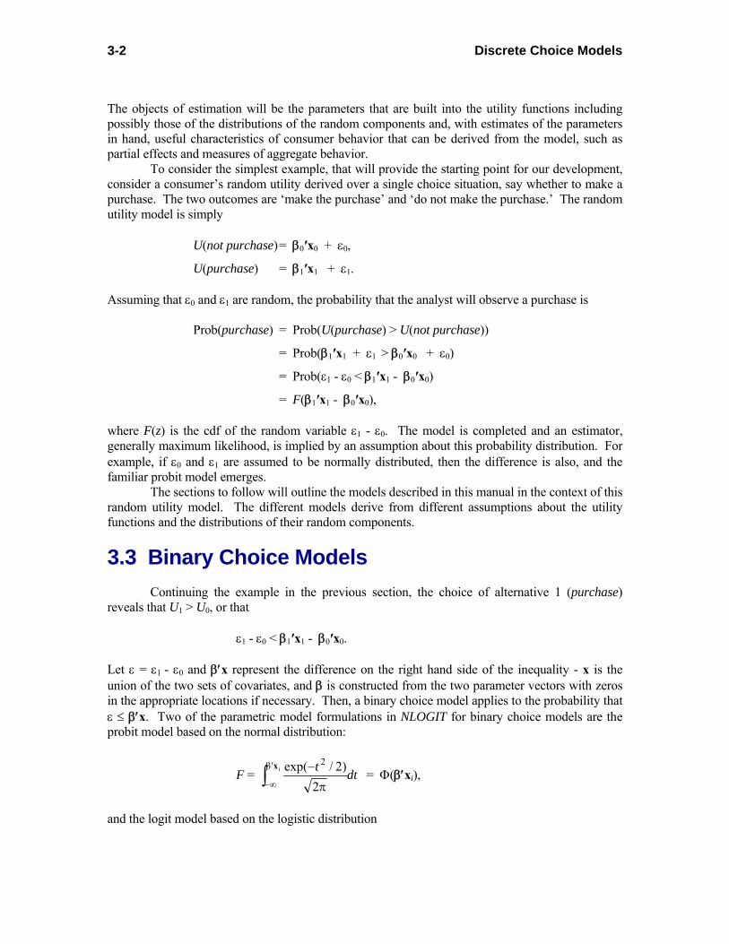
The objects of estimation will be the parameters that are built into the utility functions including possibly those of the distributions of the random components and, with estimates of the parameters in hand, useful characteristics of consumer behavior that can be derived from the model, such as partial effects and measures of aggregate behavior. To consider the simplest example, that will provide the starting point for our development, consider a consumer’s random utility derived over a single choice situation, say whether to make a purchase. The two outcomes are ‘make the purchase’ and ‘do not make the purchase.’ The random utility model is simply U(not purchase) = β0′x0 + ε0,
U(purchase) = β1′x1 + ε1. Assuming that ε0 and ε1 are random, the probability that the analyst will observe a purchase is Prob(purchase) = Prob(U(purchase) > U(not purchase))
= Prob(β1′x1 + ε1 > β0′x0 + ε0)
= Prob(ε1 - ε0 < β1′x1 - β0′x0)
= F(β1′x1 - β0′x0), where F(z) is the cdf of the random variable ε1 - ε0. The model is completed and an estimator, generally maximum likelihood, is implied by an assumption about this probability distribution. For example, if ε0 and ε1 are assumed to be normally distributed, then the difference is also, and the familiar probit model emerges. The sections to follow will outline the models described in this manual in the context of this random utility model. The different models derive from different assumptions about the utility functions and the distributions of their random components.
3.3 Binary Choice Models Continuing the example in the previous section, the choice of alternative 1 (purchase) reveals that U1 > U0, or that ε1 - ε0 < β1′x1 - β0′x0. Let ε = ε1 - ε0 and β′x represent the difference on the right hand side of the inequality - x is the union of the two sets of covariates, and β is constructed from the two parameter vectors with zeros in the appropriate locations if necessary. Then, a binary choice model applies to the probability that ε ≤ β′x. Two of the parametric model formulations in NLOGIT for binary choice models are the probit model based on the normal distribution:
F = dtti
∫β
∞− π
−x' 2
2)2/exp( = Φ(β′xi),
and the logit model based on the logistic distribution

Discrete Choice Models 3-3
F = exp( )1 exp( )
i
i
′′+
xx
ββ
= Λ(β′xi).
Numerous variations on the model can be obtained. A model with multiplicative heteroscedasticity is obtained with the additional assumption εi ~ normal or logistic with variance ∝ [exp(γ′zi)]2, where zi is a set of observed characteristics of the individual. A model of sample selection can be extended to the probit and logit binary choice models. In both cases, we depart from Prob(yi = 1 |xi) = F(β′xi), where F(t) = Φ(t) for the probit model and Λ(t) for the logit model, di* = α′zi + ui, ui ~ N[0,1], di = 1(di* > 0), yi, xi observed only when di = 1. where zi is a set of observed charactristics of the individual. In both cases, as stated, there is no obvious way that the selection mechanism impacts the binary choice model of interest. We modify the models as follows: For the probit model, yi* = β′xi + εi, εi ~ N[0,1], yi = 1(yi* > 0), which is the structure underlying the probit model in any event, and ui, εi ~ N2[(0,0),(1,ρ,1)]. (We use NP to denote the P-variate normal distribution, with the mean vector followed by the definition of the covariance matrix in the succeeding brackets.) For the logit model, a similar approach does not produce a convenient bivariate model. The probability is changed to
Prob(yi = 1 | xi,εi) = exp( )1 exp( )
i i
i i
′ + σε′+ + σε
xx
ββ
.
With the selection model for zi as stated above, the bivariate probability for yi and zi is a mixture of a logit and a probit model. The log likelihood can be obtained, but it is not in closed form, and must be computed by approximation. We do so with simulation. There are several formulations for extensions of the binary choice models to panel data setting. These include • Fixed effects: Prob(yit = 1) = F(β′xit + αi), αi correlated with xit. • Random effects: Prob(yit = 1) = Prob(β′xit + εit + ui > 0), ui uncorrelated with xit. • Random parameters: Prob(yit = 1) = F(βi′xit), βi | i ~ h(β|i) with mean vector β and covariance matrix Σ. • Latent class: Prob(yit = 1|class j) = F(βj′xit),
Prob(class = j) = Gj(θ,zi), where zi is a set of observed charactristics of the individual. Other variations include simultaneous equations models and semiparametric formulations.

Discrete Choice Models 3-4
3.4 Bivariate and Multivariate Binary Choices The bivariate probit model is a natural extension of the model above in which two decisions are made jointly; yi1* = β1′xi1 + εi1, yi1 = 1 if yi1* > 0, yi1 = 0 otherwise,
yi2* = β2′xi2 + εi2, yi2 = 1 if yi2* > 0, yi2 = 0 otherwise,
[εi1,εi2] ~ N2[0,0,1,1,ρ], -1 < ρ < 1,
individual observations on y1 and y2 are available for all i.
This model extends the binary choice model to two different, but related outcomes. One might, for example, model Y1 = home ownership (vs. renting) and Y2 = automobile purchase (vs. leasing). The two decisions are obviously correlated (and possibly even jointly determined). A special case of the bivariate probit model is useful for formulating the correlation between two binary variables. The tetrachoric correlation coefficient is equivalent to the correlation coefficient in the following bivariate probit model:
yi1* = μ + εi1, yi1 = 1(yi1* > 0),
yi2* = μ + εi2, yi2 = 1(yi2* > 0),
(εi1,εi2) ~ N2[(0,0),(1,1,ρ)]. The bivariate probit model has been extended to the random parameters form of the panel data models. For example, a true random effects model for a bivariate probit outcome can be formulated as follows: Each equation has its own random effect, and the two are correlated. The model structure is yit1* = β1′xit1 + εit1 + ui1, yit1 = 1 if yit1* > 0, yit1 = 0 otherwise,
yit2* = β2′xit2 + εit2 + ui2, yit2 = 1 if yit2* > 0, yit2 = 0 otherwise,
[εit1,εit2] ~ N2[0,0,1,1,ρ], -1 < ρ < 1,
[ui1 , ui2] ~ N2[0,0,1,1,θ], -1 < θ < 1. Individual observations on yi1 and yi2 are available for all i. Note, in the structure, the idiosyncratic εitj creates the bivariate probit model, whereas the time invariant common effects, uij create the random effects (random constants) model. Thus, there are two sources of correlation across the equations, the correlation between the unique disturbances, ρ, and the correlation between the time invariant disturbances, θ.
The multivariate probit model is the extension to M equations of the bivariate probit model
yim* = βm′xim+ εim, m = 1,…,M
yim = 1 if yim* > 0, and 0 otherwise,
εim, m =1,...,M ~ NM[0,R],
where R is the correlation matrix. Each individual equation is a standard probit model. This generalizes the bivariate probit model for up to M = 20 equations.

Discrete Choice Models 3-5
3.5 Ordered Choice Models The basic ordered choice model can be cast in an analog to our random utility specification. We suppose that preferences over a given outcome are reflected as earlier, in the random utility function: yi* = β′xi + εi,
εi ~ F(εi |θ), θ = a vector of parameters,
E[εi|xi] = 0,
Var[εi|xi] = 1. The consumer is asked to reveal the strength of their preferences over the outcome, but is given only a discrete, ordinal scale, 0,1,...,J. The observed response represents a complete censoring of the latent utility as follows: yi = 0 if yi* ≤ μ0,
= 1 if μ0 < yi* ≤ μ1,
= 2 if μ1 < yi* ≤ μ2,
... = J if yi* > μJ-1. The latent ‘preference’ variable, yi* is not observed. The observed counterpart to yi* is yi. (The model as stated does embody the strong assumption that the threshold values are the same for all individuals. We will relax that assumption below.) The ordered probit model based on the normal distribution was developed by Zavoina and McElvey (1975). It applies in applications such as surveys, in which the respondent expresses a preference with the above sort of ordinal ranking. The ordered logit model arises if εi is assumed to have a logistic distribution rather than a normal. The variance of εi is assumed to be the standard, one for the probit model and π2/6 for the logit model, since as long as yi*, β, and εi are all unobserved, no scaling of the underlying model can be deduced from the observed data. (The assumption of homoscedasticity is arguably a strong one. We will also relax that assumption.) Since the μs are free parameters, there is no significance to the unit distance between the set of observed values of yi. They merely provide the coding. Estimates are obtained by maximum likelihood. The probabilities which enter the log likelihood function are Prob(yi = j) = Prob(yi* is in the jth range). The model may be estimated either with individual data, with yi = 0, 1, 2, ... or with grouped data, in which case each observation consists of a full set of J+1 proportions, pi0,...,piJ. There are many variants of the ordered probit model. A model with multiplicative heteroscedasticity of the same form as in the binary choice models is Var[εi] = [exp(γ′zi)]2. The following describes an ordered probit counterpart to the standard sample selection model. (This is only available for the ordered probit specification.) The structural equations are, first, the main equation, the ordered choice model that was given above and, second, a selection equation, a univariate probit model, di* = α′zi + ui,
Discrete Choice Models 3-6
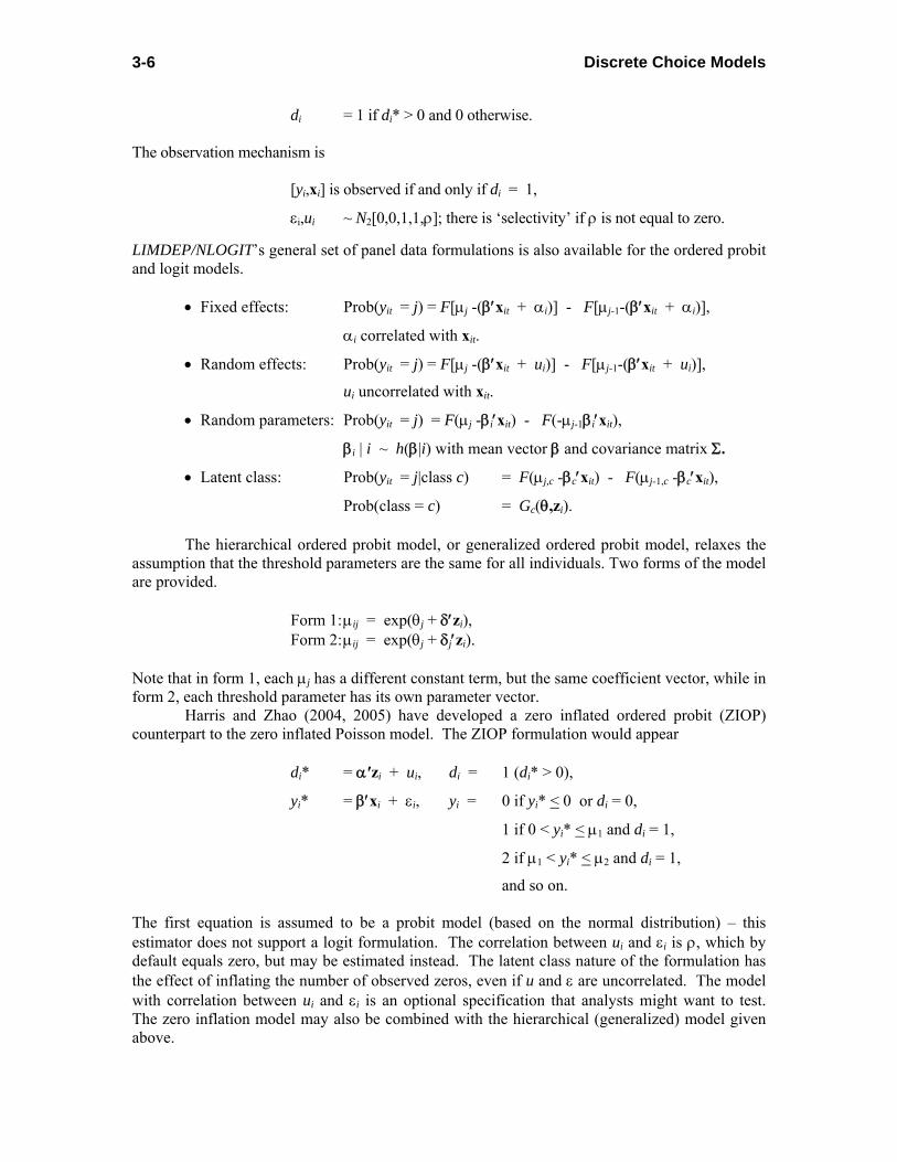
di = 1 if di* > 0 and 0 otherwise. The observation mechanism is [yi,xi] is observed if and only if di = 1,
εi,ui ~ N2[0,0,1,1,ρ]; there is ‘selectivity’ if ρ is not equal to zero. LIMDEP/NLOGIT’s general set of panel data formulations is also available for the ordered probit and logit models. • Fixed effects: Prob(yit = j) = F[μj -(β′xit + αi)] - F[μj-1-(β′xit + αi)],
αi correlated with xit.
• Random effects: Prob(yit = j) = F[μj -(β′xit + ui)] - F[μj-1-(β′xit + ui)],
ui uncorrelated with xit.
• Random parameters: Prob(yit = j) = F(μj -βi′xit) - F(-μj-1βi′xit),
βi | i ~ h(β|i) with mean vector β and covariance matrix Σ.
• Latent class: Prob(yit = j|class c) = F(μj,c -βc′xit) - F(μj-1,c -βc′xit),
Prob(class = c) = Gc(θ,zi). The hierarchical ordered probit model, or generalized ordered probit model, relaxes the assumption that the threshold parameters are the same for all individuals. Two forms of the model are provided. Form 1: μij = exp(θj + δ′zi), Form 2: μij = exp(θj + δj′zi). Note that in form 1, each μj has a different constant term, but the same coefficient vector, while in form 2, each threshold parameter has its own parameter vector. Harris and Zhao (2004, 2005) have developed a zero inflated ordered probit (ZIOP) counterpart to the zero inflated Poisson model. The ZIOP formulation would appear di* = α′zi + ui, di = 1 (di* > 0),
yi* = β′xi + εi, yi = 0 if yi* < 0 or di = 0,
1 if 0 < yi* < μ1 and di = 1,
2 if μ1 < yi* < μ2 and di = 1,
and so on. The first equation is assumed to be a probit model (based on the normal distribution) – this estimator does not support a logit formulation. The correlation between ui and εi is ρ, which by default equals zero, but may be estimated instead. The latent class nature of the formulation has the effect of inflating the number of observed zeros, even if u and ε are uncorrelated. The model with correlation between ui and εi is an optional specification that analysts might want to test. The zero inflation model may also be combined with the hierarchical (generalized) model given above.

Discrete Choice Models 3-7
The bivariate ordered probit model is analogous to the seemingly unrelated regressions model for the ordered probit case: yij* = βj′xji + εij,
yij = 0 if yij* < 0,
1 if 0 < yij* < μ1,
2, ... and so on, j = 1,2, for a pair of ordered probit models that are linked by Cor(εi1,εi2) = ρ. The model can be estimated one equation at a time using the results described earlier. Full efficiency in estimation and an estimate of ρ are achieved by full information maximum likelihood estimation. Either variable (but not both) may be binary. (If both are binary, the bivariate probit model should be used.) The polychoric correlation coefficient is used to quantify the correlation between discrete variables that are qualitative measures. The standard interpretation is that the discrete variables are discretized counterparts to underlying quantitative measures. We typically use ordered probit models to analyze such data. The polychoric correlation measures the correlation between y1 = 0,1,...,J1 and y2 = 0,1,...,J2. (Note, J1 need not equal J2.) One of the two variables may be binary as well. (If both variables are binary, we use the tetrachoric correlation coefficient described in Section E21.3.) For the case noted, the polychoric correlation is the correlation in the bivariate ordered probit model, so it can be estimated just by specifying a bivariate ordered choice model in which both right hand sides contain only a constant term.
3.6 Multinomial Logit Model The canonical random utility model is as follows: U( alternative 0 ) = β0′xi0 + ε i0,
U( alternative 1 ) = β1′xi1 + ε i1, ... U( alternative J ) = βJ ′xiJ + εiJ,
Observed yi = choice j if Ui( alternative j ) > Ui( alternative q ) ∀ q ≠ j.
The ‘disturbances’ in this framework (individual heterogeneity terms) are assumed to be independently and identically distributed with identical type 1extreme value distribution; the CDF is F(εj) = exp(-exp(-εj)). Based on this specification, the choice probabilities are Prob(choice j) = Prob(Uj > Uq), ∀ q ≠ j
= 0
exp( )
exp( )j ij
Jq iqq=
′
′∑x
x
β
β, j = 0,...,J.

Discrete Choice Models 3-8
At this point we make a purely semantic distinction between two cases of the model. When the observed data consist of individual choices and (only) data on the characteristics of the individual, identification of the model parameters will require that the parameter vectors differ across the utility functions, as they do above. The study on labor market decisions by Schmidt and Strauss (1975) is a classic example. For the moment, we will call this the multinomial logit model. When the data also include attributes of the choices that differ across the alternatives, then the forms of the utility functions can change slightly – and the coefficients can be generic, that is the same across alternatives. Again, only for the present, we will call this the conditional logit model. (It will emerge that the multinomial logit is a special case of the conditional logit model, though the reverse is not true.)
The general form of the multinomial logit model is
Prob(choice j) = 0
exp( )
exp( )j i
Jq iq=
′
′∑x
x
β
β, j = 0,...,J.
A possible J+1 unordered outcomes can occur. In order to identify the parameters of the model, we impose the normalization β0 = 0. This model is typically employed for individual or grouped data in which the ‘x’ variables are characteristics of the observed individual(s), not the choices. The data will appear as follows: • Individual data: yi coded 0, 1, ..., J, • Grouped data: yi0, yi1,...,yiJ give proportions or shares. 3.6.1 Random Effects and Common (True) Random Effects The structural equations of the multinomial logit model are Uijt = βj′xit + εijt, t = 1,...,Ti, j = 0,1,...,J,i=1,...,N, where Uijt gives the utility of choice j by person i in period t – we assume a panel data application with t = 1,...,Ti. The model about to be described can be applied to cross sections, where Ti = 1. Note also that as usual, we assume that panels may be unbalanced. We also assume that εijt has a type 1 extreme value distribution and that the J random terms are independent. Finally, we assume that the individual makes the choice with maximum utility. Under these (IIA inducing) assumptions, the probability that individual i makes choice j in period t is
Pijt = 0
exp( )
exp( )j it
Jq itq=
′
′∑x
x
β
β.
We now suppose that individual i has latent, unobserved, time invariant heterogeneity that enters the utility functions in the form of a random effect, so that ` Uijt = βj′xit + αij + εijt, t = 1,...,Ti, j = 0,1,...,J,i=1,...,N.

Discrete Choice Models 3-9
The resulting choice probabilities, conditioned on the random effects, are
Pijt | αi1,...,αiJ = 0
exp( )
exp( )j it ij
Jq it iqq=
′ + α
′ + α∑x
x
β
β.
To complete the model, we assume that the heterogeneity is normally distributed with zero means and (J+1)×(J+1) covariance matrix, Σ. For identification purposes, one of the coefficient vectors, βq, must be normalized to zero and one of the αiqs is set to zero. We normalize the first element – subscript 0 – to zero. For convenience, this normalization is left implicit in what follows. It is automatically imposed by the software. To allow the remaining random effects to be freely correlated, we write the J×1 vector of nonzero αs as αi = Γ vi where Γ is a lower triangular matrix to be estimated and vi is a standard normally distributed (mean vector 0, covariance matrix, I) vector. 3.6.2 A Dynamic Multinomial Logit Model The preceding random effects model can be modified to produce the dynamic multinomial logit model proposed in Gong, van Soest and Villagomez (2000). The choice probabilities are
Pijt | αi1,...,αiJ = 1
exp( )
exp( )j it j it ij
Jq it q it iqq=
′ ′+ + α
′ ′+ + α∑x z
x z
β γ
β γ t = 1,...,Ti, j = 0,1,...,J,i=1,...,N,
where zit contains lagged values of the dependent variables (these are binary choice indicators for the choice made in period t) and possibly interactions with other variables. The zit variables are now endogenous, and conventional maximum likelihood estimation is inconsistent. The authors argue that Heckman’s treatment of initial conditions is sufficient to produce a consistent estimator. The core of the treatment is to treat the first period as an equilibrium, with no lagged effects,
Pij0 | θi1,...,θiJ = 0
01
exp( )
exp( )j i ij
Jq i iqq=
′ + θ
′ + θ∑x
x
δ
δ, t = 0, j = 0,1,...,J,i=1,...,N,
where the vector of effects, θ, is built from the same primitives as α in the later choice probabilities. Thus, αi = Γvi and θi = Φ vi, for the same vi, but different lower triangular scaling matrices. (This treatment slightly less than doubles the size of the model – it amounts to a separate treatment for the first period.) Full information maximum likelihood estimates of the model parameters, (β1,...,βJ,γ1,...,γJ,δ1,...,δJ,Γ,Φ) are obtained by maximum simulated likelihood, by modifying the random effects model. The likelihood function for individual i consists of the period 0 probability as shown above times the product of the period 1,2,...,Ti probabilities defined earlier.

Discrete Choice Models 3-10
3.7 Conditional Logit Models If the utility functions are conditioned on observed individual, choice invariant characteristics, zi, as well as the attributes of the choices, xij, then we write U( choice j for individual i ) = Uij = β′xij + γj′zi + εij, j = 1,...,Ji. (For this model, which uses a different part of NLOGIT, we number the alternatives 1,...,Ji rather than 0,...,Ji. There is no substantive significance to this – it is purely for convenience in the context of the model development for the program commands.) The random, individual specific terms, (εi1,εi2,...,εiJ) are once again assumed to be independently distributed across the utilities, each with the same type 1 extreme value distribution F(εij) = exp(-exp(-εij)). Under these assumptions, the probability that individual t chooses alternative j is Prob(Uij > Uiq) for all q ≠ j. It has been shown that for independent type 1 extreme value distributions, as above, this probability is
Prob(yi = j) = ( )( )1
exp
expi
ij j iJ
iq q iq=
′ ′+
′ ′+∑x z
x z
β γ
β γ
where yi is the index of the choice made. We note at the outset that the IID assumptions made about εj are quite stringent, and induce the ‘Independence from Irrelevant Alternatives’ or IIA features that characterize the model. This is functionally identical to the multinomial logit model. Indeed, the earlier model emerges by the simple restriction γj = 0. We have distinguished it in this fashion because the nature of the data suggests a different arrangement than for the multinomial logit model and, second, the models in the section to follow are formulated as extensions of this one.
3.8 Error Components Logit Model When the sample consists of a ‘panel’ of data, that is, when individuals are observed in more than one choice situation, the conditional logit model can be augmented with individual effects, similar to the use of common effects models in regression and other single equation cases. A ‘panel data’ form of this model that is a counterpart to the random effects model is what we label the ‘error components model.’ (This has been called the ‘kernel logit model’ in some treatments in the literature.) The model arises by introducing M up to maxi Ji alternative and individual specific random terms in the utility functions as in U( choice j for individual i in choice setting t )
= Uijt
= β′xij + γj′zi + εij + 1Mm jm m imd u=Σ σ , j = 1,...,Ji, t = 1,...,Ti.
where djm = 1 if effect m appears in utility function j, 0 if not,
σm = the standard deviation of effect m (to be estimated)

Discrete Choice Models 3-11
vim = effect m for individual i. The M random individual specifics are (σmuim). The are distributed as normal with zero means and variances σm
2. The constants djm equal one if random effect m appears in the utility function for alternative j, and zero otherwise. The error components account for unobserved, alternative specific variation. With this device, the sets of random effects in different utility functions can overlap, so as to accommodate correlation in the unobservables across choices. The random effects may also be heteroscedastic, with σm,i
2 = σm2 exp(θm′zi).
The probabilities attached to the choices are now
Prob(yi = j) = ( )
( )1
11
exp
expi
Mij j i m jm m im
J Miq q i m qm m imq
d u
d u=
==
′ ′+ + Σ σ
′ ′+ Σ σ∑x z
x z
β γ
β γ.
This is precisely an analog to the random effects model for single equation models. Given the patterns of djm, this can provide a nesting structure as well.
3.9 Heteroscedastic Extreme Value In the conditional logit model, U( choice j for individual i ) = Uij = β′xij + γj′zi + εij, j = 1,...,Ji,
Prob(yi = j) = ( )( )1
exp
expi
ij j iJ
im m im=
′ ′+
′ ′+∑x z
x z
β γ
β γ,
an implicit assumption is that the variances of εji are the same. With the type 1extreme value distribution assumption, this common value is π2/6. This assumption is a strong one, and it is not necessary for identification or estimation. The heteroscedastic extreme value model relaxes this assumption. We assume, instead, that F(εij) = exp(-exp(-θjεij)], Var[εij] = σj
2 (π2/6) where σj2 = 1/θj
2, with one of the variance parameters normalized to one for identification. A further extension of this model allows the variance parameters to be heterogeneous, in the standard fashion σij
2 = σj2 exp(γ′zi).

Discrete Choice Models 3-12
3.10 Nested and Generalized Nested Logit The nested logit model is an extension of the conditional logit model. The models supported by NLOGIT are based on variations of a four level tree structure such as the following: ROOT root │ ┌───────────────┴────────────────┐ │ │ TRUNKS trunk1 trunk2 │ │ ┌───────┴───────┐ ┌────────┴──────┐ │ │ │ │ LIMBS limb1 limb2 limb3 limb4 │ │ │ │ ┌───┴───┐ ┌───┴───┐ ┌───┴───┐ ┌───┴───┐ │ │ │ │ │ │ │ │ BRANCHES branch1 branch2 branch3 branch4 branch5 branch6 branch7 branch8 │ │ │ │ │ │ │ │ ┌─┴─┐ ┌─┴─┐ ┌─┴─┐ ┌─┴─┐ ┌─┴─┐ ┌─┴─┐ ┌─┴─┐ ┌─┴─┐ │ │ │ │ │ │ │ │ │ │ │ │ │ │ │ │ ALTS a1 a2 a3 a4 a5 a6 a7 a8 a9 a10 a11 a12 a13 a14 a15 a16 The choice probability under the assumption of the nested logit model is defined to be the conditional probability of alternative j in branch b, limb l, and trunk r, j|b,l,r:
P(j|b,l,r) = | , ,| , ,
| , , | ,| , ,
exp( )exp( )exp( ) exp( )
j b l rj b l r
q b l r b l rq b l rJ
′′
′∑xx
= x
ββ
β,
where Jb|l,r is the inclusive value for branch b in limb l, trunk r, Jb|l,r = log Σq|b,l,rexp(β′xq|b,l,r). At the next level up the tree, we define the conditional probability of choosing a particular branch in limb l, trunk r,
P(b|l,r) = | , | , | , | , | , | ,
| , | , | , || ,
exp( ) exp( )exp( ) exp( )
b l r b l r b l r b l r b l r b l r
s l r s l r s l r l rs l r
J JJ I
′ ′+ τ + τ′ + τ∑
y y =
yα α
α,
where Il|r is the inclusive value for limb l in trunk r, Il|r = log Σs|l,rexp(α′ys|l,r + τs|l,rJs|l,r). The probability of choosing limb l in trunk r is
P(l|r) = | | | | | |
| | ||
exp( ) exp( )exp( ) exp( )
l r l r l r l r l r l r
q r s r s r rs r
I II H
′ ′+ σ + σ′ + σ∑
z z =
zδ δ
δ,
where Hr is the inclusive value for trunk r, Hr = log Σs|lexp(δ′zs|r + σs|rIs|r). Finally, the probability of choosing a particular limb is
P(r) = exp( )exp( )
r r r
s s ss
HH
′ + φ′ + φ∑
h . h
θθ

Discrete Choice Models 3-13
By the laws of probability, the unconditional probability of the observed choice made by an individual is
P(j,b,l,r) = P(j|b,l,r) × P(b|l,r) × P(l|r) × P(r). This is the contribution of an individual observation to the likelihood function for the sample. The ‘nested logit’ aspect of the model arises when any of the τb|l,r or σl|r or φr differ from 1.0. If all of these deep parameters are set equal to 1.0, the unconditional probability reduces to
P(j,b,l,r) = | , , | , |
, , , , , ,
exp( )exp( )
j b l r b l r l r r
j b l r b l r l r rr l b j
′ ′ ′ ′+ + +′ ′ ′ ′+ + +∑ ∑ ∑ ∑
x y z hx y z h
β α δ θ
β α δ θ,
which is the probability for a one level conditional (multinomial) logit model. The generalized nested logit model is an extension of the nested logit model in which alternatives may appear in more than one branch. Alternatives that appear in more than one branch are allocated across branches probabilistically. The model estimated includes the usual nested logit framework (only two levels are supported in this framework), as well as the matrix of allocation parameters. The only difference between this and the more basic nested logit model is the specification of the tree. For the allocations of choices to branches, a multinomial logit form is used, πj,b = Prob(alternative j is in branch b) = exp(θj,b) / Σs exp(θj,s), where the parameters θ are estimated by the program. Note the denominator summation is over branches that the alternative appears in. The probabilities sum to one. The identification rule that one of the θs for each alternative modeled equals one is imposed. These allocations may depend on an individual characteristic (not a choice attribute), such as income. In this instance, the multinomial logit probabilities become functions of this variable, πj,b = Prob(alternative j is in branch b) = exp(θj,b + γj,bzi ) / Σs exp(θj,s+ γj,szi). Now, to achieve identification, one of the θs and one of the γs is set equal to zero. It is convenient to form the matrix Π = [πj,b]. This is a J×B matrix of allocation parameters. The rows sum to one, and note that some values in the matrix are zero. But, no rows have all zeros – every alternative appears in at least one branch, and no columns have all zeros – every branch contains at least one alternative. The probabilities for the observed choices are formed as Prob(alternative, branch) = P(j,b) = P(j|b) × P(b) where
,
,1
[ ]( | )
[ ]
b
s
j b jB
j s ss
UP j b
U
σ
σ=
π=
π∑
(the denominator summation is over the alternatives in that branch) and

Discrete Choice Models 3-14
1/
,|1/
,1 |
[ ]( )
[ ]
bb
bb
j b jj b
Bj b jb j b
UP b
U
σσ
σσ
=
⎡ ⎤π⎣ ⎦=⎡ ⎤π⎣ ⎦
∑∑ ∑
3.11 Random Parameters Logit In its most general form, we write the multinomial logit probability as
1
exp( )( | )
exp( )ji j i j ji ji ji
i Jqi q i q qi qi qiq
P j=
′ ′ ′α + +=
′ ′ ′α + +∑θ z + f x
vθ z + f x
φ β
φ β,
where U(j,i) = ji j i j ji ji ji′ ′ ′α + +z + f xθ φ β , j = 1,...,Ji alternatives in individual i’s choice set,
αji is an alternative specific constant which may be fixed or random, αJi = 0,
θj is a vector of nonrandom (fixed) coefficients, θJi = 0,
φj is a vector of nonrandom (fixed) coefficients,
βji is a coefficient vector that is randomly distributed across individuals; vi enters βji,
zi is a set of choice invariant individual characteristics such as age or income,
fji is a vector of M individual and choice varying attributes of choices, multiplied by φj,
xji is a vector of L individual and choice varying attributes of choices, multiplied by βji.
The term ‘mixed logit’ is often used in the literature (e.g., Revelt and Train (1998)) for this model. The choice specific constants, αji and the elements of βji are distributed randomly across individuals such that for each random coefficient, ρki = any (not necessarily all of) αji or βjki, the coefficient on attribute xjik, k=1,...,K, ρjki = αji or βjki = ρjk + δk′wi + σkvki,
or ρjki = αji or βjki = exp(ρjk + δjk′wi + σjkvjki). The vector wi (which does not include one) is a set of choice invariant characteristics that produce individual heterogeneity in the means of the randomly distributed coefficients; ρjk is the constant term and δjk is a vector of ‘deep’ coefficients which produce an individual specific mean. The random term, vjki is normally distributed (or distributed with some other distribution) with mean 0 and standard deviation 1, so σjk is the standard deviation of the marginal distribution of ρjki. The vjkis are individual and choice specific, unobserved random disturbances - the source of the heterogeneity. Thus, as stated above, in the population αji or βjki ~ Normal or Lognormal [ρjk + δjk′wi, σjk
2]. (Other distributions may be specified.) For the full vector of K random coefficients in the model, we may write ρi = ρ + Δwi + Γvi.
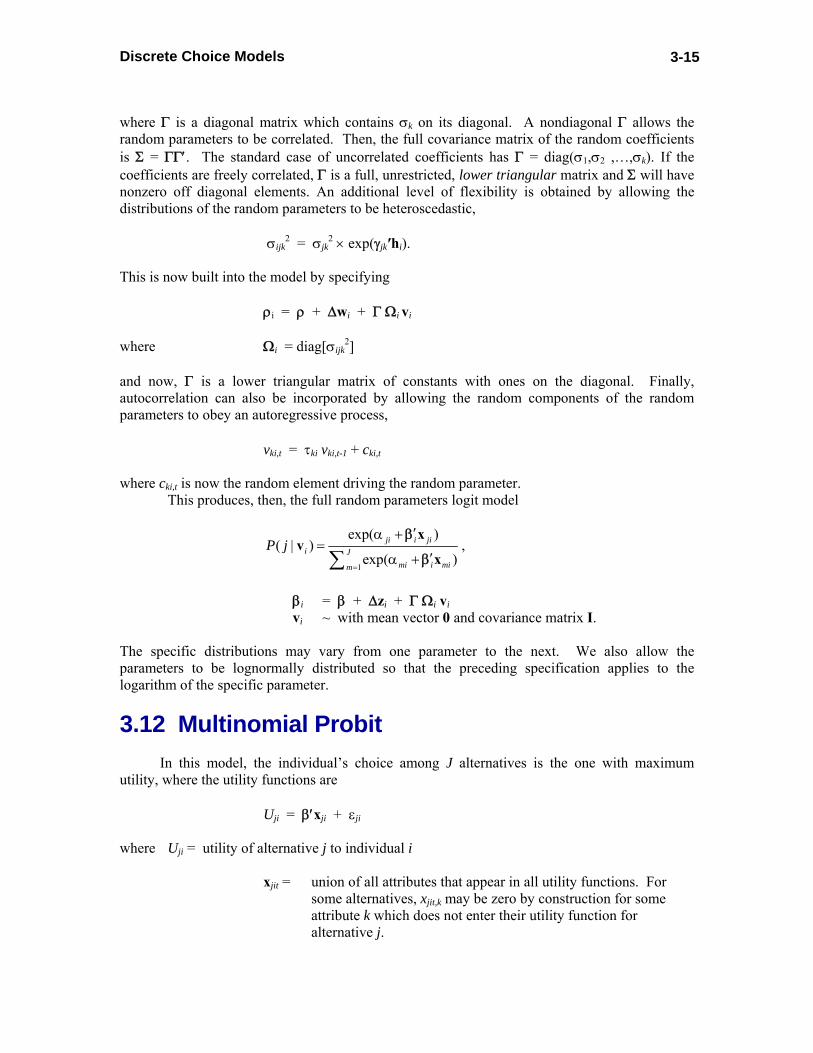
Discrete Choice Models 3-15
where Γ is a diagonal matrix which contains σk on its diagonal. A nondiagonal Γ allows the random parameters to be correlated. Then, the full covariance matrix of the random coefficients is Σ = ΓΓ′. The standard case of uncorrelated coefficients has Γ = diag(σ1,σ2 ,…,σk). If the coefficients are freely correlated, Γ is a full, unrestricted, lower triangular matrix and Σ will have nonzero off diagonal elements. An additional level of flexibility is obtained by allowing the distributions of the random parameters to be heteroscedastic, σijk
2 = σjk2 × exp(γjk′hi).
This is now built into the model by specifying ρi = ρ + Δwi + Γ Ωi vi where Ωi = diag[σijk
2] and now, Γ is a lower triangular matrix of constants with ones on the diagonal. Finally, autocorrelation can also be incorporated by allowing the random components of the random parameters to obey an autoregressive process, vki,t = τki vki,t-1 + cki,t where cki,t is now the random element driving the random parameter. This produces, then, the full random parameters logit model
1
exp( )( | )
exp( )ji i ji
i Jmi i mim
P j=
′α +=
′α +∑x
vx
β
β,
βi = β + Δzi + Γ Ωi vi vi ~ with mean vector 0 and covariance matrix I. The specific distributions may vary from one parameter to the next. We also allow the parameters to be lognormally distributed so that the preceding specification applies to the logarithm of the specific parameter.
3.12 Multinomial Probit
In this model, the individual’s choice among J alternatives is the one with maximum utility, where the utility functions are
Uji = β′xji + εji where Uji = utility of alternative j to individual i
xjit = union of all attributes that appear in all utility functions. For some alternatives, xjit,k may be zero by construction for some attribute k which does not enter their utility function for alternative j.

Discrete Choice Models 3-16
The multinomial logit model specifies that εji are draws from independent extreme value distributions (which induces the IIA condition). In the multinomial probit model, we assume that εji are normally distributed with standard deviations Sdv[εji] = σj and correlations Cor[εji, εqi] = ρjq (the same for all individuals). Observations are independent, so Cor[εji,εqs ] = 0 if i is not equal to s, for all j and q. A variation of the model allows the standard deviations and covariances to be scaled by a function of the data, which allows some heteroscedasticity across individuals.
The correlations ρjq are restricted to -1 < ρjq < 1, but they are otherwise unrestricted save for a necessarily normalization. The correlations in the last row of the correlation matrix must be fixed at zero. The standard deviations are unrestricted with the exception of a normalization - two standard deviations are fixed at 1.0 - NLOGIT fixes the last two. This model may also be fit with panel data. In this case, the utility function is modified as follows:
Uji,t = β′xji,t + εji,t + vji,t where ‘t’ indexes the periods or replications. There are two formulations for vji,t, Random effects vji,t = vji,t (the same in all periods)
First order autoregressive vji,t = αj vji,t-1 + aji,t. It is assumed that you have a total of Ti observations (choice situations) for person i. Two situations might lend themselves to this treatment. If the individual is faced with a set of choice situations that are similar and occur close together in time, then the random effects formulation is likely to be appropriate. However, if the choice situations are fairly far apart in time, or if habits or knowledge accumulation are likely to influence the latter choices, then the autoregressive model might be the better one. You can also add a form of individual heterogeneity to the disturbance covariance matrix. The model extension is
Var[εi] = exp[γ′hi] × Σ
where Σ is the matrix defined earlier (the same for all individuals), and hi is an individual (not alternative) specific set of variables not including a constant.
Model and Command Summary for Discrete Choice Models 4-1
Chapter 4
Model and Command Summary for Discrete Choice Models
⎯⎯⎯⎯⎯⎯⎯⎯⎯⎯⎯⎯⎯⎯⎯⎯⎯⎯⎯⎯⎯⎯⎯⎯ 4.1 Introduction The chapters to follow will provide details on the various discrete choice models you can estimate with NLOGIT and on the model commands you will use to request the estimates. This chapter will provide a brief summary listing of the models and model commands. The variety of logit models now use a set of specific names, rather than qualifiers to more general model classes as in earlier versions of NLOGIT and LIMDEP. For example, the model name OLOGIT can be used instead of ORDERD;Logit. The earlier formats remain available, but the newer ones may prove more convenient. The full listing of these commands is also given below. The commands below specify the essential parts needed to fit the model. The numerous options and different forms are discussed in the chapters to follow (and, were noted, in the LIMDEP Econometric Modeling Guide as well).
4.2 Model Summary The descriptions below present the different discrete choice models that are the main feature of NLOGIT. Note, once again, NLOGIT contains all of LIMDEP, so all of the models documented in the Econometric Modeling Guide, including the regression models, limited dependent vriable models, generalized linear models, sample selection models, and so on are supported in NLOGIT., as well as the ancillary tools including MATRIX, etc. The models described below include several listed in Section N4.3 that are part of the general LIMDEP/NLOGIT econometric modeling package, two listed in Section N4.4 that provide a bridge between the discrete choice models in LIMDEP and NLOGIT, then the set listed in Section N4.5 that are supported only by NLOGIT.
4.3 Basic Discrete Choice Models The binomial probit and logit and the ordered probit and logit models are LIMDEP’s primary model frameworks for single equation, single decision, discrete choice models. The ordered choice and the bivariate and multivariate probit models are multivariate extensions of the simple probit model. 4.3.1 Binary Choice Models There are numerous binary choice models. The ones that interest us here are the binary probit and logit models. The probit model is requested with PROBIT ; Lhs = dependent variable ; Rhs = independent variables $

Model and Command Summary for Discrete Choice Models
4-2
The binary logit model may be invoked with BLOGIT ; Lhs = dependent variable ; Rhs = independent variables $ In earlier versions, you would use the LOGIT comand, which is still useable. LOGIT is the same as BLOGIT when the data on the dependent variable are either binary (zeros and ones) or proportions (strictly between zero and one). 4.3.2 Bivariate Binary Choices The command for the bivariate probit model is BVPROBIT ; Lhs = variable 1, variable 2 ; Rh1 = independent variables for equation 1 ; Rh2 = independent variables for equation 2 $ In this form, the Lhs specifies two binary dependent variables. You may use proportions data instead, in which case, you will provide four proportions variables, in order, p00, p01, p10, p11. This command is the same as BIVARIATE PROBIT in earlier versions. (You may also use BIVARIATE PROBIT.) 4.3.3 Multivariate Binary Choice Models The multivariate probit model is specified with MVPROBIT ; Lhs = y1, y2, ..., yM ; Eq1 = Rhs variables for equation 1 ; Eq2 = Rhs variables for equation 2 ... ; EqM = Rhs variables for equation M $ Data for this model must be individual. The Lhs specifies a set of binary dependent variables. This command is the same as MPROBIT (which may still be used) in earlier versions of NLOGIT. 4.3.4 Ordered Choice Models Chapter E22 of the LIMDEP Econometric Modeling Guide describes four forms for the ordered choice model, probit, logit, complementary log log and Gompertz. The first two interest us here. The ordered probit model is requested with OPROBIT ; Lhs = dependent variable ; Rhs = independent variables $ This is the same as the ORDERED PROBIT command, which may still be used. In this model, the dependent variable is integer valued, taking the values 0, 1, ..., J. All J+1 values must appear in the data set, including zero. You may supply a set of J+1 proportions variables instead. Proportions will sum to 1.0 for every observation.
Model and Command Summary for Discrete Choice Models 4-3
The ordered logit model is requested with OLOGIT ; Lhs = dependent variable ; Rhs = independent variables $ The same arrangement for the dependent variables as for the ordered probit model is assumed. This command is the same as ODRERED ; Logit in earlier versions of NLOGIT and LIMDEP.
4.4 Multinomial Logit Models The ‘multinomial logit model’ is an early, restrictive version of the conditional logit model, which, itself, is the gateway model to the main model extensions described in Section N4.5. 4.4.1 Multinomial Logit The multinomial logit model is invoked with MLOGIT ; Lhs = dependent variable ; Rhs = independent variables $ Data for the MLOGIT command/model consist of an integer valued variable taking the values 0, 1, ..., J. This model may also be fit with proportions data. In that case, you will provide the names of J+1 Lhs variables that will be strictly between zero and one, and will sum to one at every observation. The MLOGIT command is the same as LOGIT. The program inspects the command (Lhs) and the data, and determines internally whether BLOGIT or MLOGIT is appropriate. Note, on proportions data, if you want to fit a binary logit model with proportions data, you will supply a single proportions variable, not two. (What would be the second one is just one minus the first.) If you want to fit a multinomial logit model with proportions data with three or more outcomes, you must provide the full set of proportions. Thus, you would never supply two Lhs variables in a LOGIT, BLOGIT or MLOGIT command. 4.4.2 Conditional Logit The command for the conditional model, and the commands in the sections to follow, are variants of the NLOGIT command. This is a full class of estimators based on the conditional logit form. The commands that follow this one are also specific to NLOGIT, and are not available in LIMDEP.) There are several forms of the essential command for fitting the conditional logit model with NLOGIT. The simpler one is CLOGIT ; Lhs = dependent variable ; Choices = the names of the J alternatives ; Rhs = list of choice specific attributes ; Rh2 = list of choice invariant individual characteristics $ The data for this estimator consist of a set of J observations, one for each alternative. (The observation resembles a group in a panel data set.) The command just given assumes that every individual in the sample chooses from the same size choice set, J. The choice sets may have different numbers of choices, in which case, the command is changed to

Model and Command Summary for Discrete Choice Models
4-4
; Lhs = dependent variable, choice set size variable The second Lhs variable is structured exactly the same as a ;Pds variable for a panel data estimator. In the second form of the model command, the utility functions are specified directly, symbolically. The ;Rhs and ;Rh2 specifications can be replaced with ; Model: ... specification of the utility functions. The CLOGIT command is the same as DISCRETE CHOICE in LIMDEP. It is also the same as NLOGIT when the only information given in the command is that specified above, that is when none of the specifications that invoke the model extensions that are described in the sections to follow are provided. 4.4.3 Random Parameters Logit The random parameters logit model (mixed logit model) is requested by specifying a conditional logit model, and adding the specification of the random parameters. The model command is RPLOGIT ; Lhs = dependent variable ; Choices = the names of the J alternatives ; Rhs = list of choice specific attributes ; Rh2 = list of choice invariant individual characteristics ; Fcn = the specifications of the random parameters ; ... other specifications for the random parameters model $ Once again, variable choice set sizes and utility function specifications are specified as in the CLOGIT command. This command is the same as NLOGIT ; RPL ; ... the rest of the command $ There is one modification that might be necessary. If you are providing variables that affect the means of the random parameters, you would generally use NLOGIT ; RPL = the list of variables ; ... the rest of the command $ The RPL specification may still be used this way. The command can be NLOGIT as above, or RPLOGIT ; RPL = the list of variables ; ... the rest of the command $ These are identical.

Model and Command Summary for Discrete Choice Models 4-5
The random parameters model may also include an error components specification defined in the next section. The command will be RPLOGIT ; Lhs = dependent variable ; Choices = the names of the J alternatives ; Rhs = list of choice specific attributes ; Rh2 = list of choice invariant individual characteristics ; Fcn = the specifications of the random parameters ; ... other specifications for the random parameters model ; ECM = specification $ 4.4.4 Latent Class Logit The essential form of the command for the latent class model is LCLOGIT ; Lhs = dependent variable ; Choices = the names of the J alternatives ; Rhs = list of choice specific attributes ; Rh2 = list of choice invariant individual characteristics ; Pts = the number of classes $ Like the RPLOGIT command, you need to modify this command if you are providing variables that affect the class probabilities. You would generally use NLOGIT ; LCM = the list of variables ; ... the rest of the command $ The LCM specification may still be used this way. The command can be NLOGIT as above, or identically, LCLOGIT ; LCM = the list of variables ; ... the rest of the command $ 4.4.5 Multinomial Probit The essential command for the multinomial probit model is MNPROBIT ; Lhs = dependent variable ; Choices = the names of the J alternatives ; Rhs = list of choice specific attributes ; Rh2 = list of choice invariant individual characteristics $ Variable choice set sizes and utility function specifications are specified as in the CLOGIT command. This command is the same as NLOGIT ; MNP ; ... the rest of the command $

Model and Command Summary for Discrete Choice Models
4-6
4.6 Command Summary The following lists the current and where applicable, alternative forms of the discrete choice model commands. The two sets of commands are identical, and for each model, in NLOGIT 4.0, either command may be used for that model. Models Command Alternative Command Form Binary Choice Models in NLOGIT and LIMDEP Binary Probit PROBIT PROBIT Binary Logit BLOGIT LOGIT Bivariate Probit BVPROBIT BIVARIATE PROBIT Multivariate Probit MVPROBIT MPROBIT
Ordered Choice Models in NLOGIT and LIMDEP Ordered Probit OPROBIT ORDERED PROBIT Ordered Logit OLOGIT ORDERED;Logit
Multinomial Logit Mode in NLOGIT and LIMDEP Multinomial Logit MLOGIT LOGIT Conditional Logit CLOGIT DISCRETE CHOICE
Conditional Logit Extensions in NLOGIT Conditional Logit CLOGIT CLOGIT Multinomial Logit NLOGIT NLOGIT (Same as CLOGIT) Error Components Logit ECLOGIT NLOGIT;ECM=... Heteroscedastic Extreme Value HLOGIT NLOGIT;HET Nested Logit NLOGIT;Tree=... NLOGIT;Tree=... Generalized Nested Logit GNLOGIT;Tree=... NLOGIT;GNL;Tree=... Random Parameters Logit RPLOGIT NLOGIT;RPL Latent Class Logit LCLOGIT NLOGIT;LCM Multinomial Probit MNPROBIT NLOGIT;MNP

Basic Models for Discrete Choice 5-1
Chapter 5
Basic Models for Discrete Choice ⎯⎯⎯⎯⎯⎯⎯⎯⎯⎯⎯⎯⎯⎯⎯⎯⎯⎯⎯⎯⎯⎯⎯⎯⎯⎯⎯⎯⎯⎯⎯ 5.1 Introduction We define models in which the response variable being described is inherently discrete as qualitative response (QR) models. This chapter will describe two of LIMDEP’s many estimators for qualitative dependent variable model estimators. The simplest of these is the binomial choice models. The ordered choice model is an extension of the binary choice model in which there are more than two ordered, nonquantitative outcomes, such as scores on a preference scale.
5.2 Modeling Binary Choice A binomial response may be the outcome of a decision or the response to a question in a survey. Consider, for example, survey data which indicate political party choice, mode of transportation, occupation, or choice of location. We model these in terms of probability distributions defined over the set of outcomes. There are a number of interpretations of an underlying data generating process that produce the binary choice models we consider here. All of them are consistent with the models that LIMDEP estimates, but the exact interpretation is a function of the modeling framework.
The essential model command for the parametric binary choice models is
⎫⎪⎬⎪⎭
PROBIT; Lhs = dependent variable ; Rhs = regressors $or
LOGIT
A latent regression is specified as y* = β′x + ε. The observed counterpart to y* is y = 1 if and only if y* > 0. This is the basis for most of the binary choice models in econometrics, and is described in further detail below. It is the same model as the reduced form in the previous paragraph. Threshold models, such as labor supply and reservation wages lend themselves to this approach.

Basic Models for Discrete Choice 5-2
The probabilities and density functions for the most common binary choice specifications are as follows: Probit
F = dtti
∫β
∞− π
−x' 2
2)2/exp( = Φ(β′xi), f = φ(β′xi)
Logit
F = exp( )1 exp( )
i
i
′′+
xx
ββ
= Λ(β′xi), f = Λ(β′xi)[1 - Λ(β′xi)]
5.2.1 Model Commands The model commands for the five binary choice models listed above are largely the same:
⎫⎪⎬⎪⎭
PROBIT; Lhs = dependent variable ; Rhs = regressors $or
LOGIT
Data on the dependent variable may be either individual or proportions. You need not make any special note of which. LIMDEP will inspect the data to determine which type of data you are using. In either case, you provide only a single dependent variable. As usual, you should include a constant term in the model unless your application specifically dictates otherwise. 5.2.2 Output The binary choice models generate a very large amount of output. Computation begins with least squares estimation in order to obtain starting values. NOTE: The OLS results will not normally be displayed in the output. To request the display, use ; OLS in any of the model commands. Reported Estimates Final estimates include:
• logL = the log likelihood function at the maximum, • logL0 = the log likelihood function assuming all slopes are zero. If your Rhs variables do
not include one, this statistic will be meaningless. It is computed as logL0 = n[PlogP + (1-P)log(1-P)]
where P is the sample proportion of ones.

Basic Models for Discrete Choice 5-3
• The chi squared statistic for testing H0: β = 0 (not including the constant) and the significance level = probability that χ2 exceeds test value. The statistic is
χ2 = 2(logL - logL0). Numerous other results, listed in detail, will appear with these in the output. The standard statistical results, including coefficient estimates, standard errors, t ratios, and descriptive statistics for the Rhs variables appear next. A complete listing is given below with an example. After the coefficient estimates are given, two additional sets of results appear, an analysis of the model fit and an analysis of the model predictions. We will illustrate with binary logit and probit estimates of a model for visits to the doctor using the German health care data described in Chapter E2. The first model command is LOGIT ; Lhs = doctor ; Rhs = one,age,hhninc,hhkids,educ,married ; OLS $ Note that the command requests the optional listing of the OLS starting values. The results for this command are as follows. With the exception of the table noted below, the same results (with different values, of course) will appear for all five parametric models. Some additional optional computations and results will be discussed later. The initial OLS estimates are generally not reported unless requested with ; OLS. +------------------------------------------------+ | Binomial logit model for binary choice | | These are the OLS values based on the | | binary variables for each outcome Y(i) = j. | +------------------------------------------------+ +--------+--------------+----------------+--------+--------+----------+ |Variable| Coefficient | Standard Error |b/St.Er.|P[|Z|>z]| Mean of X| +--------+--------------+----------------+--------+--------+----------+ ---------+Characteristics in numerator of Prob[Y = 1] Constant| .56661068 .02118790 26.742 .0000 AGE | .00468710 .00029114 16.099 .0000 43.5256898 HHNINC | -.03976003 .01726656 -2.303 .0213 .35208362 HHKIDS | -.05217181 .00680260 -7.669 .0000 .40273000 EDUC | -.01071245 .00131378 -8.154 .0000 11.3206310 MARRIED | .01946888 .00757540 2.570 .0102 .75861817 Standard results for maximum likelihood estimation appear next (or first if OLS is not presented). These are the results generated for all models fit by maximum likelihood. The Hosmer-Lemeshow chi squared statistic is specific to the binary choice models. The information criteria are computed from the log likelihood, logL, and the number of parameters estimated, K, as follows: AIC = Akaike Information Criterion = -2(logL – K)/n
BIC = Bayesian Information Criterion = -2(logL – KlogK)/n
Finite Sample AIC = -2(logL – K –K(K+1)/(n-K-1))/n
HQIC = -2(logL – Klog(logn))/n

Basic Models for Discrete Choice 5-4
Normal exit from iterations. Exit status=0. +---------------------------------------------+ | Binomial Logit Model for Binary Choice | | Maximum Likelihood Estimates | | Dependent variable DOCTOR | | Weighting variable None | | Number of observations 27326 | | Iterations completed 4 | | Log likelihood function -17673.10 | | Number of parameters 6 | | Info. Criterion: AIC = 1.29394 | | Finite Sample: AIC = 1.29394 | | Info. Criterion: BIC = 1.29574 | | Info. Criterion:HQIC = 1.29452 | | Restricted log likelihood -18019.55 | | McFadden Pseudo R-squared .0192266 | | Chi squared 692.9077 | | Degrees of freedom 5 | | Prob[ChiSqd > value] = .0000000 | | Hosmer-Lemeshow chi-squared = 110.37153 | | P-value= .00000 with deg.fr. = 8 | +---------------------------------------------+ +--------+--------------+----------------+--------+--------+----------+ |Variable| Coefficient | Standard Error |b/St.Er.|P[|Z|>z]| Mean of X| +--------+--------------+----------------+--------+--------+----------+ ---------+Characteristics in numerator of Prob[Y = 1] Constant| .25111543 .09113537 2.755 .0059 AGE | .02070863 .00128517 16.114 .0000 43.5256898 HHNINC | -.18592232 .07506403 -2.477 .0133 .35208362 HHKIDS | -.22947000 .02953694 -7.769 .0000 .40273000 EDUC | -.04558783 .00564646 -8.074 .0000 11.3206310 MARRIED | .08529305 .03328573 2.562 .0104 .75861817 The next set of results computes various fit measures for the model. This table of information statistics is produced only for the logit model. It is generally used for analysis of the generalized maximum entropy (GME) estimator of the multinomial logit model, but it also provides some useful information for the binomial model even when fit by ML instead of GME. The entropy statistics are computed as follows: Entropy = - Σi Pi log Pi where Pi is the probability predicted by the model. The three ‘models’ are ‘M,’ the model fit by maximum likelihood, ‘MC,’ the model in which all predicted probabilities are the sample proportion of ones (here 0.6291), and ‘M0,’ (no model) in which all predicted probabilities are 0.5. The normalized entropy is the entropy divided by nlog2. Finally, the entropy ratio statistic equals 2(nlog2)(1 - normalized entropy). The percent correct predicted values are discussed below. The next set of results examines the success of the prediction rule Predict yi = 1 if Pi > P* and 0 otherwise where P* is a defined threshold probability. The default value of P* is 0.5, which makes the prediction rule equivalent to ‘Predict yi = 1 if the model says the predicted event yi = 1 | xi is more likely than the complement, yi = 0 | xi.’ You can change the threshold from 0.5 to some other value with ; Limit = your P*

Basic Models for Discrete Choice 5-5
+--------------------------------------------------------------------+ | Information Statistics for Discrete Choice Model. | | M=Model MC=Constants Only M0=No Model | | Criterion F (log L) -17673.09788 -18019.55173 -18940.93986 | | LR Statistic vs. MC 692.90772 .00000 .00000 | | Degrees of Freedom 5.00000 .00000 .00000 | | Prob. Value for LR .00000 .00000 .00000 | | Entropy for probs. 17673.09788 18019.55173 18940.93986 | | Normalized Entropy .93306 .95135 1.00000 | | Entropy Ratio Stat. 2535.68395 1842.77624 .00000 | | Bayes Info Criterion 1.29537 1.32072 1.38816 | | BIC(no model) - BIC .09270 .06744 .00000 | | Pseudo R-squared .01923 .00000 .00000 | | Pct. Correct Pred. 62.85223 .00000 50.00000 | | Means: y=0 y=1 y=2 y=3 y=4 y=5 y=6 y>=7 | | Outcome .3709 .6291 .0000 .0000 .0000 .0000 .0000 .0000 | | Pred.Pr .3709 .6291 .0000 .0000 .0000 .0000 .0000 .0000 | | Notes: Entropy computed as Sum(i)Sum(j)Pfit(i,j)*logPfit(i,j). | | Normalized entropy is computed against M0. | | Entropy ratio statistic is computed against M0. | | BIC = 2*criterion - log(N)*degrees of freedom. | | If the model has only constants or if it has no constants, | | the statistics reported here are not useable. | +--------------------------------------------------------------------+
A variety of fit measures for the model are listed. +----------------------------------------+ | Fit Measures for Binomial Choice Model | | Logit model for variable DOCTOR | +----------------------------------------+ | Proportions P0= .370892 P1= .629108 | | N = 27326 N0= 10135 N1= 17191 | | LogL= -17673.098 LogL0= -18019.552 | | Estrella = 1-(L/L0)^(-2L0/n) = .02528 | +----------------------------------------+ | Efron | McFadden | Ben./Lerman | | .02435 | .01923 | .54487 | | Cramer | Veall/Zim. | Rsqrd_ML | | .02470 | .04348 | .02504 | +----------------------------------------+ | Information Akaike I.C. Schwarz I.C. | | Criteria 1.29394 1.29574 | +----------------------------------------+ +---------------------------------------------------------+ |Predictions for Binary Choice Model. Predicted value is | |1 when probability is greater than .500000, 0 otherwise.| |Note, column or row total percentages may not sum to | |100% because of rounding. Percentages are of full sample.| +------+---------------------------------+----------------+ |Actual| Predicted Value | | |Value | 0 1 | Total Actual | +------+----------------+----------------+----------------+ | 0 | 378 ( 1.4%)| 9757 ( 35.7%)| 10135 ( 37.1%)| | 1 | 394 ( 1.4%)| 16797 ( 61.5%)| 17191 ( 62.9%)| +------+----------------+----------------+----------------+ |Total | 772 ( 2.8%)| 26554 ( 97.2%)| 27326 (100.0%)| +------+----------------+----------------+----------------+

Basic Models for Discrete Choice 5-6
This table computes a variety of conditional and marginal proportions based on the results using the defined prediction rule. For examples, the 97.708% equals (16797/17191)100% while the 63.256% is (16797/26554)100%. ======================================================================= Analysis of Binary Choice Model Predictions Based on Threshold = .5000 ----------------------------------------------------------------------- Prediction Success ----------------------------------------------------------------------- Sensitivity = actual 1s correctly predicted 97.708% Specificity = actual 0s correctly predicted 3.730% Positive predictive value = predicted 1s that were actual 1s 63.256% Negative predictive value = predicted 0s that were actual 0s 48.964% Correct prediction = actual 1s and 0s correctly predicted 62.852% ----------------------------------------------------------------------- Prediction Failure ----------------------------------------------------------------------- False pos. for true neg. = actual 0s predicted as 1s 96.270% False neg. for true pos. = actual 1s predicted as 0s 2.292% False pos. for predicted pos. = predicted 1s actual 0s 36.744% False neg. for predicted neg. = predicted 0s actual 1s 51.036% False predictions = actual 1s and 0s incorrectly predicted 37.148% =======================================================================
Retained Results The results saved by the binary choice models are: Matrices: b = estimate of β (also contains γ for the Burr model) varb = asymptotic covariance matrix
Scalars: kreg = number of variables in Rhs nreg = number of observations logl = log likelihood function 5.2.3 Analysis of Marginal Effects Marginal effects in a binary choice model may be obtained as
[ | ] ( ) ( )( )
E y F dFd
′ ′∂ ∂= =
′∂ ∂x x x
x x xβ β
ββ
= F′(β′x)β = f(β′x)β
That is, the vector of marginal effects is a scalar multiple of the coefficient vector. The scale factor, f(β′x), is the density function, which is a function of x. This function can be computed at any data vector desired. You can request the computation to be done automatically at the vector of means of the current sample by adding ; Marginal Effects to your command.

Basic Models for Discrete Choice 5-7
Marginal Effects for Dummy Variables When one of the variables in x is a dummy variable, the derivative approach to estimating the marginal effect is not appropriate. An alternative which is closer to the desired computation for a dummy variable which we denote z, is ΔFz = Prob[y = 1 | z = 1] - Prob[y = 1 | z = 0]
= F(β′x + αz | z = 1) - F(β′x + αz | z = 0). For this type of variable, the asymptotic standard error must be changed as well. This is accomplished simply by changing the appropriate row of G to
Gz = [f(β′x+ αz)] ⎟⎟⎠
⎞⎜⎜⎝
⎛1x
′ - [f(β′x + αz)] '0⎟⎟⎠
⎞⎜⎜⎝
⎛x
NLOGIT examines the variables in the model and makes this adjustment automatically. 5.2.4 Robust Covariance Matrix Estimation The preceding describes a covariance estimator that accounts for a specific, observed aspect of the data. The concept of the ‘robust’ covariance matrix is that it is meant to account for hypothetical, unobserved failures of the model assumptions. The intent is to produce an asymptotic covariance matrix that is appropriate even if some of the assumptions of the model are not met. (It is an important, but infrequently discussed issue whether the estimator, itself, remains consistent in the presence of these model failures – that is, whether the so called robust covariance matrix estimator is being computed for an inconsistent estimator.) The Sandwich Estimator It is becoming common in the literature to adjust the estimated asymptotic covariance matrix for possible misspecification in the model which leaves the MLE consistent but the estimated asymptotic covariance matrix incorrectly computed. One example would be a binary choice model with unspecified latent heterogeneity. A frequent adjustment for this case is the ‘sandwich estimator,’ which is the choice based sampling estimator suggested above with weights equal to one. (This suggests how it could be computed.) The desired matrix is
Est.Asy.Var ˆ⎡ ⎤⎣ ⎦β =
1 12 2
1 1 1
log log log log'ˆ ˆ ˆ ˆ ˆ ˆn n ni i i ii i i
F F F F− −
= = =
⎡ ⎤ ⎡ ⎤ ⎡ ⎤⎛ ⎞ ⎛ ⎞⎛ ⎞ ⎛ ⎞∂ ∂ ∂ ∂⎢ ⎥ ⎢ ⎥ ⎢ ⎥⎜ ⎟ ⎜ ⎟⎜ ⎟ ⎜ ⎟
′ ′ ′∂ ∂ ∂ ∂ ∂ ∂⎢ ⎥ ⎢ ⎥ ⎢ ⎥⎝ ⎠ ⎝ ⎠⎝ ⎠ ⎝ ⎠⎣ ⎦ ⎣ ⎦ ⎣ ⎦∑ ∑ ∑
β β β β β β
Three ways to obtain this matrix are ; Wts = one ; Choice Based sampling or ; Robust or ; Cluster = 1 The computation is identical in all cases. (As noted below, the last of them will be slightly larger, as it will be multiplied by n/(n-1).)

Basic Models for Discrete Choice 5-8
Clustering A related calculation is used when observations occur in groups which may be correlated. This is rather like a panel; one might use this approach in a random effects kind of setting in which observations have a common latent heterogeneity. The parameter estimator is unchanged in this case, but an adjustment is made to the estimated asymptotic covariance matrix. The calculation is done as follows: Suppose the n observations are assembled in G clusters of observations, in which the number of observations in the ith cluster is ni. Thus,
1
Gii
n=∑ = n. Let the observation specific
gradients and Hessians be
gij = log ijL∂
∂β Hij =
2 log'ijL∂
∂ ∂β β.
The uncorrected estimator of the asymptotic covariance matrix based on the Hessian is
VH = -H-1 = ( ) 1
1 1iG n
iji j
−
= =−∑ ∑ H
Estimators for some models will use the BHHH estimator, instead;
VB = ( ) 1
1 1iG n
ij iji j
−
= =′∑ ∑ g g
Let V be the estimator chosen. Then, the corrected asymptotic covariance matrix is
Est.Asy.Var ˆ⎡ ⎤⎣ ⎦β = ( )( )1 1 11
i iG n nij iji j j
GG = = =
⎡ ⎤′⎢ ⎥− ⎣ ⎦∑ ∑ ∑V g g V
Note that if there is exactly one observation per cluster, then this is G/(G-1) times the sandwich estimator discussed above. Also, if you have fewer clusters than parameters, then this matrix is singular – it has rank equal to the minimum of G and K, the number of parameters. To request the estimator, your command must include ; Cluster = specification where the specification is either the fixed value if all the clusters are the same size, or the name of an identifying variable if the clusters vary in size. Note, this is not the same as the variable in the Pds function that is used to specify a panel. The cluster specification must be an identifying code that is specific to the cluster. For example, our health care data used in our examples is an unbalanced panel. The first variable is a family id, which we will use as follows ; Cluster = id

Basic Models for Discrete Choice 5-9
5.3 Ordered Choice Models The basic ordered choice model is based on the following specification: There is a latent regression, yi* = β′xi + εi, εi ~ F(εi |θ), E[εi|xi] = 0, Var[εi|xi] = 1, The observation mechanism results from a complete censoring of the latent dependent variable as follows: yi = 0 if yi ≤ μ0,
= 1 if μ0 < yi ≤ μ1,
= 2 if μ1 < yi ≤ μ2, ...
= J if yi > μJ-1. The latent ‘preference’ variable, yi* is not observed. The observed counterpart to yi* is yi. Four stochastic specifications are provided for the basic model shown above. The ordered probit model applies in applications such as surveys, in which the respondent expresses a preference with the above sort of ordinal ranking. The variance of εi is assumed to be one, since as long as yi*, β, and εi are unobserved, no scaling of the underlying model can be deduced from the observed data. Since the μs are free parameters, there is no significance to the unit distance between the set of observed values of y. They merely provide the coding. Estimates are obtained by maximum likelihood. The probabilities which enter the log likelihood function are Prob[yi = j] = Prob[yi* is in the jth range]. The model may be estimated either with individual data, with yi = 0, 1, 2, ... or with grouped data, in which case each observation consists of a full set of J+1 proportions, p0i,...,pJi. NOTE: If your data are not coded correctly, this estimator will abort with one of several possible diagnostics – see below for discussion. Your dependent variable must be coded 0,1,...,J. We note that this differs from some other econometric packages which use a different coding convention. There are numerous variants and extensions of this model which can be estimated: The underlying mathematical forms are shown below, where the CDF is denoted F(z) and the density is f(z). (Familiar synonyms are given as well.)
Probit: F(z) = 2exp( / 2)
2z t dt−∞
−π∫ = Φ(z), f(z) = φ(z)
Logit: F(z) = exp( )1 exp( )
zz+
= Λ(z), f(z) = Λ(z)[1 - Λ(z)]
The ordered probit model is an extension of the probit model for a binary outcome with normally distributed disturbances. The ordered logit model results from the assumption that ε has a standard logistic distribution instead of a standard normal.

Basic Models for Discrete Choice 5-10
5.3.1 Estimating Ordered Probability Models The essential command for estimating ordered probability models is ORDERED ; Lhs = y ; Rhs = regressors $ If you are using individual data, the Lhs variable must be coded 0,1,...,J. All the values must be present in the data. LIMDEP will look for empty cells. If there are any, estimation is halted. (If value ‘j’ is not represented in the data, then the threshold parameter, μj is not estimable.) In this circumstance, you will receive a diagnostic such as
ORDE,Panel,BIVA PROBIT:A cell has (almost) no observations. Empty cell: Y never takes value 2
This diagnostic means exactly what it says. The ordered probability model cannot be estimated unless all cells are represented in the data. Users frequently overlook the coding requirement, y = 0,1,... If you have a dependent variable that is coded 1,2,..., you will see the following diagnostic:
Models - Insufficient variation in dependent variable. The reason this particular diagnostic shows up is that LIMDEP creates a new variable from your dependent variable, say y, which equals zero when y equals zero, and one when y is greater than zero. It then tries to obtain starting values for the model by fitting a regression model to this new variable. If you have miscoded the Lhs variable, the transformed variable always equals one, which explains the diagnostic. In fact, there is no variation in the transformed dependent variable. If this is the case, you can simply use CREATE to subtract 1.0 from your dependent variable to use this estimator. The probit model is the default specification. To estimate an ordered logit, add ; Model = Logit to the command. The standardized logistic distribution (mean zero, standard deviation approximately 1.81) is used as the basis of the model instead of the standard normal. 5.3.2 Model Structure and Data This model must include a constant term, one, as the first Rhs variable. Since the equation does include a constant term, one of the μs is not identified. We normalize μ0 to zero. (Consider the special case of the binary probit model with something other than zero as its threshold value. If it contains a constant, this cannot be estimated.) Data may be grouped or individual. (Survey data might logically come in grouped form.) If you provide individual data, the dependent variable is coded 0, 1, 2, ..., J. There must be at least three values. Otherwise, the binary probit model applies. If the data are grouped, a full set of proportions, p0, p1, ..., pJ, which sum to one at every observation must be provided. In the individual data case, the data are examined to determine the value of J, which will be the largest observed value of y which appears in the sample. In the grouped data case, J is one less than the number of Lhs variables you provide. Once again, we note that other programs sometimes use different normalizations of the model. For example, if the constant term is

Basic Models for Discrete Choice 5-11
forced to equal zero, then one will instead, add a nonzero threshold parameter, μ0, which equals zero in the presence of a nonzero constant term. 5.3.3 Output from the Ordered Probability Estimators All of the ordered probit/logit models begin with an initial set of least squares results of some sort. These are suppressed unless your command contains ; OLS. The iterations are then followed by the maximum likelihood estimates in the usual tabular format. The final output includes a listing of the cell frequencies for the outcomes. When the data are stratified, this output will also include a table of the frequencies in the strata. The log likelihood function, and a log likelihood computed assuming all slopes are zero are computed. For the latter, the threshold parameters are still allowed to vary freely, so the model is simply one which assigns each cell a predicted probability equal to the sample proportion. This appropriately measures the contribution of the nonconstant regressors to the log likelihood function. As such, the chi squared statistic given is a valid test statistic for the hypothesis that all slopes on the nonconstant regressors are zero. The sample below shows the standard output for a model with six outcomes. These are the German health care data described earlier. The dependent variable is the self reported health satisfaction rating. For the purpose of a convenient sample application, we have truncated the health satisfaction variable at five by discarding observations – in the original data set, it is coded 0,1,...,10. +---------------------------------------------+ | Ordered Probability Model | | Maximum Likelihood Estimates | | Dependent variable NEWHSAT | | Weighting variable None | | Number of observations 8140 | | Log likelihood function -11284.69 | | Number of parameters 9 | | Info. Criterion: AIC = 2.77486 | | Info. Criterion: BIC = 2.78261 | | Restricted log likelihood -11308.02 | | McFadden Pseudo R-squared .0020635 | | Chi squared 46.66728 | | Degrees of freedom 4 | | Prob[ChiSqd > value] = .0000000 | | Underlying probabilities based on Normal | | Cell frequencies for outcomes | | Y Count Freq Y Count Freq Y Count Freq | | 0 447 .054 1 255 .031 2 642 .078 | | 3 1173 .144 4 1390 .170 5 4233 .520 | +---------------------------------------------+ +--------+--------------+----------------+--------+--------+----------+ |Variable| Coefficient | Standard Error |b/St.Er.|P[|Z|>z]| Mean of X| +--------+--------------+----------------+--------+--------+----------+ ---------+Index function for probability Constant| 1.32892012 .07275667 18.265 .0000 FEMALE | .04525825 .02546350 1.777 .0755 .52936118 HHNINC | .35589979 .07831928 4.544 .0000 .32998942 HHKIDS | .10603682 .02664775 3.979 .0001 .33169533 EDUC | .00927669 .00629721 1.473 .1407 10.8759203 ---------+Threshold parameters for index Mu(1) | .23634786 .01236704 19.111 .0000 Mu(2) | .62954428 .01439990 43.719 .0000 Mu(3) | 1.10763798 .01405938 78.783 .0000 Mu(4) | 1.55676227 .01527126 101.941 .0000
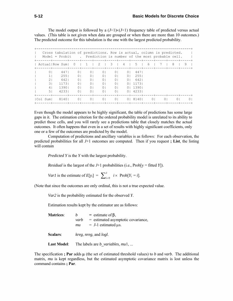
Basic Models for Discrete Choice 5-12
The model output is followed by a (J+1)×(J+1) frequency table of predicted versus actual values. (This table is not given when data are grouped or when there are more than 10 outcomes.) The predicted outcome for this tabulation is the one with the largest predicted probability. +---------------------------------------------------------------------------+ | Cross tabulation of predictions. Row is actual, column is predicted. | | Model = Probit . Prediction is number of the most probable cell. | +-------+-------+-----+-----+-----+-----+-----+-----+-----+-----+-----+-----+ | Actual|Row Sum| 0 | 1 | 2 | 3 | 4 | 5 | 6 | 7 | 8 | 9 | +-------+-------+-----+-----+-----+-----+-----+-----+-----+-----+-----+-----+ | 0| 447| 0| 0| 0| 0| 0| 447| | 1| 255| 0| 0| 0| 0| 0| 255| | 2| 642| 0| 0| 0| 0| 0| 642| | 3| 1173| 0| 0| 0| 0| 0| 1173| | 4| 1390| 0| 0| 0| 0| 0| 1390| | 5| 4233| 0| 0| 0| 0| 0| 4233| +-------+-------+-----+-----+-----+-----+-----+-----+-----+-----+-----+-----+ |Col Sum| 8140| 0| 0| 0| 0| 0| 8140| 0| 0| 0| 0| +-------+-------+-----+-----+-----+-----+-----+-----+-----+-----+-----+-----+ Even though the model appears to be highly significant, the table of predictions has some large gaps in it. The estimation criterion for the ordered probability model is unrelated to its ability to predict those cells, and you will rarely see a predictions table that closely matches the actual outcomes. It often happens that even in a set of results with highly significant coefficients, only one or a few of the outcomes are predicted by the model. Computation of predictions and ancillary variables is as follows: For each observation, the predicted probabilities for all J+1 outcomes are computed. Then if you request ; List, the listing will contain Predicted Y is the Y with the largest probability. Residual is the largest of the J+1 probabilities (i.e., Prob[y = fitted Y]).
Var1 is the estimate of E[yi] = i
J
=∑ 0i × Prob[Yi = i].
(Note that since the outcomes are only ordinal, this is not a true expected value. Var2 is the probability estimated for the observed Y. Estimation results kept by the estimator are as follows: Matrices: b = estimate of β, varb = estimated asymptotic covariance, mu = J-1 estimated μs. Scalars: kreg, nreg, and logl. Last Model: The labels are b_variables, mu1, ... The specification ; Par adds μ (the set of estimated threshold values) to b and varb. The additional matrix, mu is kept regardless, but the estimated asymptotic covariance matrix is lost unless the command contains ; Par.

Basic Models for Discrete Choice 5-13
5.3.4 Marginal Effects Marginal effects in the ordered probability models are quite involved. Since there is no meaningful conditional mean function to manipulate, we consider, instead, the effects of changes in the covariates on the cell probabilities. These are:
∂Prob[cell j]/∂xi = [f(μj-1 - β′xi) - f(μj - β′xi)] × β, where f(.) is the appropriate density for the standard normal, φ(•), logistic density, Λ(•)(1-Λ(•)), Weibull or Gompertz. Each vector is a multiple of the coefficient vector. But it is worth noting that the magnitudes are likely to be very different. In at least one case, Prob[cell 0], and probably more if there are more than three outcomes, the partial effects have exactly the opposite signs from the estimated coefficients. Thus, in this model, it is important to consider carefully the interpretation of the coefficient estimates. Marginal effects for all cells can be requested by including ; Marginal Effects in the command. An example appears below. NOTE: This estimator segregates dummy variables for separate computation in the marginal effects. The marginal effect for a dummy variable is the simple difference of the two probabilities, with and without the variable. See the application below for an illustration. +----------------------------------------------------+ | Marginal effects for ordered probability model | | M.E.s for dummy variables are Pr[y|x=1]-Pr[y|x=0] | | Names for dummy variables are marked by *. | +----------------------------------------------------+ +--------+--------------+----------------+--------+--------+----------+ |Variable| Coefficient | Standard Error |b/St.Er.|P[|Z|>z]| Mean of X| +--------+--------------+----------------+--------+--------+----------+ ---------+These are the effects on Prob[Y=00] at means. Constant| .000000 ......(Fixed Parameter)....... *FEMALE | -.00498024 .00280960 -1.773 .0763 .52936118 HHNINC | -.03907462 .00862973 -4.528 .0000 .32998942 *HHKIDS | -.01131976 .00277405 -4.081 .0000 .33169533 EDUC | -.00101850 .00069179 -1.472 .1409 10.8759203 ---------+These are the effects on Prob[Y=01] at means. Constant| .000000 ......(Fixed Parameter)....... *FEMALE | -.00209668 .00118069 -1.776 .0758 .52936118 HHNINC | -.01647123 .00362630 -4.542 .0000 .32998942 *HHKIDS | -.00483428 .00119623 -4.041 .0001 .33169533 EDUC | -.00042933 .00029148 -1.473 .1408 10.8759203 Effects for Y=02, Y=03 and Y=04 are omitted. ---------+These are the effects on Prob[Y=05] at means. Constant| .000000 ......(Fixed Parameter)....... *FEMALE | .01803285 .01014562 1.777 .0755 .52936118 HHNINC | .14180876 .00073836 192.060 .0000 .32998942 *HHKIDS | .04218672 .00029837 141.390 .0000 .33169533 EDUC | .00369631 .00250467 1.476 .1400 10.8759203 +-------------------------------------------------------------------------+ | Summary of Marginal Effects for Ordered Probability Model (probit) | +-------------------------------------------------------------------------+ Variable| Y=00 Y=01 Y=02 Y=03 Y=04 Y=05 Y=06 Y=07 | --------------------------------------------------------------------------+ ONE .0000 .0000 .0000 .0000 .0000 .0000 *FEMALE -.0050 -.0021 -.0041 -.0047 -.0021 .0180 HHNINC -.0391 -.0165 -.0326 -.0373 -.0164 .1418 *HHKIDS -.0113 -.0048 -.0096 -.0112 -.0052 .0422 EDUC -.0010 -.0004 -.0008 -.0010 -.0004 .0037

Basic Models for Discrete Choice 5-14
This page intentionally left blank

The Multinomial Logit Model
6-1
Chapter 6
The Multinomial Logit Model ⎯⎯⎯⎯⎯⎯⎯⎯⎯⎯⎯⎯⎯⎯⎯⎯⎯⎯⎯⎯⎯⎯⎯⎯⎯⎯⎯⎯⎯⎯⎯ 6.1 Introduction This chapter will describe a basic form of the ‘multinomial logit’ model. These models are also known variously as ‘conditional logit,’ ‘discrete choice,’ and ‘universal logit’ models, among other names. All of them can be viewed as special cases of a general model of utility maximization: An individual is assumed to have preferences defined over a set of alternatives (travel modes, occupations, food groups, etc.) Ui(alternative 0) = β0′xi0 + ε i0,
Uj(alternative 1) = β1′xi1 + ε i1, ... Ui(alternative J) = βJ ′xiJ + εiJ,
Observed Yi = j if Ui( alternative j ) > Ui( alternative q ) ∀ q ≠ j.
The ‘disturbances’ in this framework (individual heterogeneity terms) are assumed to be independently and identically distributed with identical type 1 extreme value distribution; the CDF is F(εj) = exp(-exp(-εj)). Based on this specification, the choice probabilities, Prob(choice j ) = Prob(Uj > Uq), ∀ q ≠ j
= 0
exp( )
exp( )j ji
Jm mim=
′
′∑x
x
β
β, j = 0,...,J,
where ‘i’ indexes the observation, or individual, and ‘j’ and ‘m’ index the choices. The IID assumptions made about εj are quite stringent, and lead to the ‘Independence from Irrelevant Alternatives’ or IIA implications that characterize the model. Much (perhaps all) of the research on forms of this model consists of development of alternative functional forms and stochastic specifications that avoid this feature. The observed data consist of the Rhs vectors, xjt, and the outcome, or choice, yt. (We also consider a number of variants.) This chapter will examine what we call, for the present, the multinomial logit model. In this model, it is assumed that the Rhs variables consist of a set of individual specific characteristics, such as age, education, marital status, etc. These are the same for all choices, so the choice subscript on x in the formula above is dropped. The observation setting is the individual’s choice among a set of alternatives, where it is assumed that the determinant of the choice is the characteristics of the individual. An example might be a model of choice of occupation. (This is the model originally devised by Nerlove and Press (1973).) The remaining chapters of this manual

The Multinomial Logit Model
6-2
after this one will examine what we call (again only for convenience) the discrete choice model and, also, to differentiate the command, the conditional logit model. In this framework, we observe the attributes of the choices, rather than the characteristics of the individual. A well known example is travel mode choice. Samples of observations often consist of the attributes of the different modes and the choice actually made. Usually, no characteristics of the individuals are observed beyond their actual choice. Models may also contain mixtures of the two types of choice determinants. These are considered in the later chapters as well. (We emphasize, these naming distinctions are meaningless in the modeling framework – we just use them here only to organize the applicable parts of NLOGIT.
6.2 The Multinomial Logit Model The general form of the multinomial logit model is
Prob(choice j) = 1
exp( )
exp( )j t
Jm tm=
′
′∑x
x
β
β, j = 0,...,J.
A possible J+1 unordered outcomes can occur. In order to identify the parameters of the model, we impose the normalization β0 = 0. This model is typically employed for individual or grouped data in which the ‘x’ variables are characteristics of the observed individual(s), not the choices. The characteristics are the same across all outcomes. The study of occupational choice, by Schmidt and Strauss (1975) provides a well known application. The data will appear as follows: • Individual data: yi coded 0, 1, ..., J, • Grouped data: y0i, y1i,...,yJi give proportions or shares. In the grouped data case, a weighting variable, nt, may also be provided if the observations happen to be frequencies. The proportions variables must range from zero to one and sum to one at each observation. The full set must be provided, even though one is redundant. The data are inspected to determine which specification is appropriate. The number of Lhs variables given and the coding of the data provide the full set of information necessary to estimate the model, so no additional information about the dependent variable is needed. This model proliferates parameters. There are J×K nonzero parameters in all, since there is a vector βj for each probability except the first. Consequently, even moderately sized models quickly become very large ones if your outcome variable, y, takes many values. The maximum number of parameters which can be estimated in a model is 150 as usual with the standard configuration. However, if you are able to forego certain other optional features, the number of parameters can increase to 300. (This is the only model in NLOGIT that extends the 150 parameter limit.) The model size is detected internally. If your configuration contains more than 150 parameters, the following options and features become unavailable: • marginal effects • choice based sampling • ; Rst = list for imposing restrictions • ; CML = specification for imposing linear constraints • ; Hold for using the multinomial logit model as a sample selection equation

The Multinomial Logit Model
6-3
In addition, if your model size exceeds 150 parameters, the matrices b and varb cannot be retained. (But, see below for another way to retrieve large parameter matrices). The choice set should be restricted to no more than 25 choices. If you have more than 25 choices, the number of characteristics that may be used becomes very small. Nonetheless, it is possible to fit models with up to 100 choices by using CLOGIT.
6.3 Model Command for the Multinomial Logit Model The command for fitting this form of multinomial logit model is MLOGIT ; Lhs = y or y0,y1,...yJ ; Rhs =regressors $ (The verb may also be LOGIT, which is what has always been used in previous versions of LIMDEP and NLOGIT.) All general options for controlling output and iterations are available except ;Keep=name. (A program which can be used to obtain the fitted probabilities is listed below.) There are internally computed predictions for the multinomial logit model. The ;Rst = list form of restrictions is supported for imposing constraints on model parameters, either fixed value or equality. One possible application of the constrained model involves making the entire vector of coefficients in one probability equal that in another. You can do this as follows: NAMELIST ; x = the entire set of Rhs variables $ CALC ; k = Col(x) $ LOGIT ; Lhs = y ; Rhs = x ; Rst = k_b, k_b, ... , k_b $ This would force the corresponding coefficients in all probabilities to be equal. You could also apply this to some, but not all of the outcomes, as in ; Rst = k_b, k_b, k_b2, k_b3
HINT: The coefficients in this model are not the marginal effects. But, forcing the coefficient on a characteristic in probability j to equal its counterpart in probability m also forces the two marginal effects to be equal. 6.4 Robust Covariance Matrix It has become common in the literature to compute a ‘robust covariance matrix’ for the MLE. (The misspecification to which the matrix is robust is left unspecified in most cases.) The desired robust covariance matrix would result in the preceding computation if wi equals one for all observations. This suggests a simple way to obtain it, just by specifying ;Choice Based;Wts=one. Alternatively, just use ; Robust which is equivalent.

The Multinomial Logit Model
6-4
A related calculation is used when observations occur in groups which may be correlated. This is rather like a panel; one might use this approach in a random effects kind of setting in which observations have a common latent heterogeneity. The parameter estimator is unchanged in this case, but an adjustment is made to the estimated asymptotic covariance matrix. The calculation is done as follows: Suppose the n observations are assembled in C clusters of observations, in which the number of observations in the cth cluster is nc. Thus,
1
Ccc
n=∑ = n.
Denote by β the full set of model parameters, [β1′, ..., βJ′]′. Let the observation specific gradients and Hessians for individual i in cluster c be
gic = log icL∂∂β
,
Hic = 2 log
'icL∂
∂ ∂β β.
The uncorrected estimator of the asymptotic covariance matrix based on the Hessian is
VH = -H-1 = ( ) 1
1 1cC n
icc i
−
= =−∑ ∑ H .
The corrected asymptotic covariance matrix is
Est.Asy.Var ˆ⎡ ⎤⎣ ⎦β = ( )( )1 1 1
'1
c cC n nH ic ic Hc i i
CC = = =
⎡ ⎤⎢ ⎥⎣ ⎦− ∑ ∑ ∑V g g V .
Note that if there is exactly one observation per cluster, then this is C/(C-1) times the sandwich (robust) estimator discussed above. Also, if you have fewer clusters than parameters, then this matrix is singular - it has rank equal to the minimum of C and JK, the number of parameters. This estimator is requested with ; Cluster = specification where the specification is either a fixed number of observations per cluster, or an identifier that distinguishes clusters, such as an identification number. This estimator can also be extended to stratified as well as clustered data, using ; Stratum = specification
6.5 Output for the Multinomial Logit Model Initial ordinary least squares results are used for the starting values for this model. For individual data, J binary variables are implied by the model. These are used in a least squares regression. For the grouped data case, a minimum chi squared, generalized least squares estimate is obtained by the weighted regression of oij = log(Pij / Pi0)

The Multinomial Logit Model
6-5
on the regressors, with weights hij = (niPijPi0)1/2 (ni may be 1.0). (Note that the dependent variables in these regressions are the ‘odds ratios.’) The OLS estimates based on the individual data are inconsistent, but the grouped data estimates are consistent (and, in the binomial case, efficient). The least squares estimates are included in the displayed results by including ; OLS in the model command. The iterations are followed by the maximum likelihood estimates with the usual diagnostic statistics. An example is shown below. NOTE: Minimum chi squared (MCS) is an estimator, not a model. Moreover, the MCS estimator has the same properties as, but is different from the maximum likelihood estimator. Since the MCS estimator in NLOGIT is not iterated, it should not be used as the final result of estimation. Without iteration, the MCS estimator is not a fixed point - the weights are functions only of the sample proportions, not the parameters. For current purposes, these are only useful as starting values. Standard output for the logit model will begin with a table such as the following which results from estimation of a model in which the dependent variable takes values 0,1,2,3,5: LOGIT ; Lhs = newhsat ; Rhs = one,educ,hhninc,age,hhkids $ +---------------------------------------------+ | Multinomial Logit Model | | Maximum Likelihood Estimates | | Model estimated: Mar 25, 2006 at 07:40:03PM.| | Dependent variable NEWHSAT | | Weighting variable None | | Number of observations 8140 | | Iterations completed 5 | | Log likelihood function -11246.97 | | Number of parameters 25 | | Info. Criterion: AIC = 2.76953 | | Finite Sample: AIC = 2.76955 | | Info. Criterion: BIC = 2.79104 | | Info. Criterion:HQIC = 2.77688 | | Restricted log likelihood -11308.02 | | McFadden Pseudo R-squared .0053989 | | Chi squared 122.1013 | | Degrees of freedom 20 | | Prob[ChiSqd > value] = .0000000 | +---------------------------------------------+ (This is based on the health satisfaction variable analyzed in the preceding chapter. We reduced the sample to those with newhsat reported zero to five. We would note, though these make for a fine numerical example, the multinomial logit model would be inappropriate for these ordered data.) The restricted log likelihood is computed for a model in which one is the only Rhs variable. In this case, log L0 = Σj nj logPj, where nj is the number of individuals who choose outcome j and Pj = nj/n = the jth sample proportion. The chi squared statistic is 2(log L - log L0). If your model does not contain a constant

The Multinomial Logit Model
6-6
term, this statistic need not be positive, in which case it is not reported. But, even if it is, the statistic is meaningless if your model does not contain a constant. The diagnostic statistics are followed by the coefficient estimates: These are β1,...,βJ. Recall β0 is normalized to zero, and not reported. +--------+--------------+----------------+--------+--------+----------+ |Variable| Coefficient | Standard Error |b/St.Er.|P[|Z|>z]| Mean of X| +--------+--------------+----------------+--------+--------+----------+ ---------+Characteristics in numerator of Prob[Y = 1] Constant| -1.77566023 .69486152 -2.555 .0106 EDUC | .07325707 .04476186 1.637 .1017 10.8759203 HHNINC | .28572052 .58129003 .492 .6231 .32998942 AGE | .00565832 .00838172 .675 .4996 46.9925061 HHKIDS | .27187563 .19642471 1.384 .1663 .33169533 ---------+Characteristics in numerator of Prob[Y = 2] Constant| -.54216913 .54865993 -.988 .3231 EDUC | .06151644 .03616780 1.701 .0890 10.8759203 HHNINC | .85929376 .44943471 1.912 .0559 .32998942 AGE | -.00089766 .00650574 -.138 .8903 46.9925061 HHKIDS | .13920984 .15529658 .896 .3700 .33169533 ---------+Characteristics in numerator of Prob[Y = 3] Constant| -.25432932 .49206457 -.517 .6053 EDUC | .10995580 .03246796 3.387 .0007 10.8759203 HHNINC | 1.54516927 .40166793 3.847 .0001 .32998942 AGE | -.00955207 .00583708 -1.636 .1017 46.9925061 HHKIDS | .08177804 .14014086 .584 .5595 .33169533 ---------+Characteristics in numerator of Prob[Y = 4] Constant| .09378185 .48301274 .194 .8461 EDUC | .10453491 .03201865 3.265 .0011 10.8759203 HHNINC | 1.74362305 .39382043 4.427 .0000 .32998942 AGE | -.01430375 .00571476 -2.503 .0123 46.9925061 HHKIDS | .19548647 .13659829 1.431 .1524 .33169533 ---------+Characteristics in numerator of Prob[Y = 5] Constant| 1.58458651 .45170179 3.508 .0005 EDUC | .07526768 .03034831 2.480 .0131 10.8759203 HHNINC | 1.64030015 .37209397 4.408 .0000 .32998942 AGE | -.01481141 .00525964 -2.816 .0049 46.9925061 HHKIDS | .19988328 .12654882 1.579 .1142 .33169533 The coefficient estimates are followed by an analysis of the multinomial logit criterion function, shown in the table below. Some of this table repeats part of the previous diagnostic information. Three log likelihoods are shown; M applies to the estimated model, MC is for the constants only model – these two values appear above – and M0 is the log likelihood for a model in which every predicted probability is 1/(J+1), that is, no model. Most of the remaining entries in this table relate to the information criteria and the and pseudo R2 = 1 – MC/M. To underscore a point, we note that even though the model predicts more than half the observations correctly, the pseudo R2 is only 0.0054. This is not a measure of fit. The sample means and average predicted probabilities match exactly because the model contains a constant term. This will always be the case. Finally, the table contains information about the entropy of the predicted probabilities.

The Multinomial Logit Model
6-7
+--------------------------------------------------------------------+ | Information Statistics for Discrete Choice Model. | | M=Model MC=Constants Only M0=No Model | | Criterion F (log L) -11246.96937 -11308.02002 -14584.92208 | | LR Statistic vs. MC 122.10132 .00000 .00000 | | Degrees of Freedom 20.00000 .00000 .00000 | | Prob. Value for LR .00000 .00000 .00000 | | Entropy for probs. 11246.96937 11308.02002 14584.92208 | | Normalized Entropy .77114 .77532 1.00000 | | Entropy Ratio Stat. 6675.90543 6553.80411 .00000 | | Bayes Info Criterion 2.78551 2.80051 3.60564 | | BIC(no model) - BIC .82014 .80514 .00000 | | Pseudo R-squared .00540 .00000 .00000 | | Pct. Correct Pred. 52.00246 .00000 16.66667 | | Means: y=0 y=1 y=2 y=3 y=4 y=5 y=6 y>=7 | | Outcome .0549 .0313 .0789 .1441 .1708 .5200 .0000 .0000 | | Pred.Pr .0549 .0313 .0789 .1441 .1708 .5200 .0000 .0000 | | Notes: Entropy computed as Sum(i)Sum(j)Pfit(i,j)*logPfit(i,j). | | Normalized entropy is computed against M0. | | Entropy ratio statistic is computed against M0. | | BIC = 2*criterion - log(N)*degrees of freedom. | | If the model has only constants or if it has no constants, | | the statistics reported here are not useable. | +--------------------------------------------------------------------+ The statistical output for the coefficient estimates is followed by a table of predicted and actual frequencies, such as the following: Frequencies of actual & predicted outcomes Predicted outcome has maximum probability. Predicted ------ ------------------------------ + ----- Actual 0 1 2 3 4 5 | Total ------ ------------------------------ + ----- 0 0 0 0 0 0 447 | 447 1 0 0 0 0 0 255 | 255 2 0 0 0 0 0 642 | 642 3 0 0 0 0 0 1173 | 1173 4 0 0 0 0 0 1390 | 1390 5 0 0 0 0 0 4233 | 4233 ------ ------------------------------ + ----- Total 0 0 0 0 0 8140 | 8140 The prediction for any observation is the cell with the largest predicted probability for that observation. NOTE: If you have more than three outcomes, it is very common, as occurred above, for the model to predict zero outcomes in one or more of the cells. Even in a model with very high t-ratios and great statistical significance, it takes a very well developed model to make predictions in all cells.

The Multinomial Logit Model
6-8
The ;List specification produces a listing such as the following: Observation Observed Y Predicted Y Residual MaxPr(i) Prob[Y*=y] 1 2.0000 .00000 .0000 .2905 .1443 2 .00000 .00000 .0000 .2538 .2538 3 .00000 .00000 .0000 .2866 .2866 4 5.0000 3.0000 .0000 .2532 .1088 5 4.0000 3.0000 .0000 .2535 .2452 6 4.0000 3.0000 .0000 .2584 .2503 7 4.0000 4.0000 .0000 .2568 .2568 8 5.0000 .00000 .0000 .2354 .1440 9 .00000 4.0000 .0000 .2596 .2045 10 1.0000 .00000 .0000 .2554 .1027 In the listing, the MaxPR(i) is the probability attached to the outcome with the largest predicted probability; the outcome is shown as the Predicted Y. The last column shows the predicted probability for the observed outcome. Residuals are not computed - there is no significance to the reported zero. The results kept for further use are: Matrices: b and varb. An additional matrix named b_logit is created which is (J+1)×K. This matrix contains the parameters arranged so that βj′ is the jth row. The first row is zero. This matrix can be used to obtain fitted probabilities, as discussed below. Scalars: kreg, nreg, logl, and exitcode. Labels for WALD are constructed from the outcome and variable numbers. For example, if there are three outcomes and Rhs=one,x1,x2, the labels will be Last Model: [b1_1,b1_2,b1_3,b2_1,b2_2,b2_3]. 6.6 Marginal Effects The marginal effects in this model are δj = ∂Pj/∂x, j = 0,1,...,J. For the present, ignore the normalization β0 = 0. The notation Pj is used for Prob[y = j]. After some tedious algebra, we find δj = Pj(βj - β ),
where β = ∑ =
Jj 0
Pj βj. It follows that neither the sign nor the magnitude of δj need bear any relationship to those of βj. (This is worth bearing in mind when reporting results.) The asymptotic covariance matrix for the

The Multinomial Logit Model
6-9
estimator of δj would be computed using Asy.Var. ˆ
j⎡ ⎤⎣ ⎦δ = Gj Asy.Var ˆ
j⎡ ⎤⎣ ⎦β Gj′,
where β is the full parameter vector. It can be shown that
Asy.Var. ˆj
⎡ ⎤⎣ ⎦δ = Σl Σm Vjl Asy.Cov.[ β̂ l, ˆ
m′β ]Vjm′, j=0,...,J, where Vjl = [1(j = l) - Pl ]{PjI + δjx′} - Pjδlx′, and 1(j = l) = 1 if j = l, and 0 otherwise. This full set of results is produced automatically when your LOGIT command includes ; Marginal Effects NOTE: Marginal effects are computed at the sample averages of the Rhs variables in the model. There is no conditional mean function in this model, so marginal effects are interpreted a bit differently from the usual case. What is reported is the derivatives of the probabilities. (Note this is the same as the ordered probability models.) These derivatives are saved in a matrix named partials which has J+1 rows and K columns. Each row is the vector of partial effects of the corresponding probability. Since the probabilities will always sum to one, the column sums in this matrix will always be zero. That is,
MATRIX ; list ; 1 ’ partials $
will display a row matrix of zeros. The elasticities of the probabilities, (∂Pj/∂xk)×(xk/Pj) are placed in a (J+1)×K matrix named elast_ml. The format of the results is illustrated in the example below.

The Multinomial Logit Model
6-10
+-------------------------------------------+ | Partial derivatives of probabilities with | | respect to the vector of characteristics. | | They are computed at the means of the Xs. | | Observations used for means are All Obs. | | A full set is given for the entire set of | | outcomes, NEWHSAT = 0 to NEWHSAT = 5. | | Probabilities at the mean vector are | | 0= .052 1= .030 2= .078 3= .145 4= .171 | | 5= .523 | +-------------------------------------------+ +--------+--------------+----------------+--------+--------+----------+ |Variable| Coefficient | Standard Error |b/St.Er.|P[|Z|>z]|Elasticity| +--------+--------------+----------------+--------+--------+----------+ ---------+Marginal effects on Prob[Y = 0] Constant| -.03681271 .02185753 -1.684 .0921 EDUC | -.00415059 .00144841 -2.866 .0042 -.87310224 HHNINC | -.07533229 .01759541 -4.281 .0000 -.48080659 AGE | .00059378 .00025180 2.358 .0184 .53968780 HHKIDS | -.00874507 .00608176 -1.438 .1505 -.05610378 ---------+Marginal effects on Prob[Y = 1] Constant| -.07581474 .01624087 -4.668 .0000 EDUC | -.00021399 .00101558 -.211 .8331 -.07636415 HHNINC | -.03569724 .01353007 -2.638 .0083 -.38652184 AGE | .00052245 .00019922 2.622 .0087 .80558651 HHKIDS | .00313091 .00463577 .675 .4994 .03407609 ---------+Marginal effects on Prob[Y = 2] Constant| -.09814200 .02502533 -3.922 .0001 EDUC | -.00146816 .00158947 -.924 .3557 -.20405436 HHNINC | -.04677448 .02027747 -2.307 .0211 -.19724874 AGE | .00082844 .00031003 2.672 .0075 .49750446 HHKIDS | -.00234229 .00728521 -.322 .7478 -.00992853 ---------+Marginal effects on Prob[Y = 3] Constant| -.13990259 .03064835 -4.565 .0000 EDUC | .00429655 .00187257 2.294 .0218 .32276832 HHNINC | .01275949 .02392200 .533 .5938 .02908292 AGE | .00027978 .00039814 .703 .4822 .09081229 HHKIDS | -.01264824 .00934649 -1.353 .1760 -.02897839 ---------+Marginal effects on Prob[Y = 4] Constant| -.10599103 .03277396 -3.234 .0012 EDUC | .00415859 .00200931 2.070 .0385 .26381106 HHNINC | .04913321 .02486677 1.976 .0482 .09457056 AGE | -.00048333 .00042477 -1.138 .2552 -.13248126 HHKIDS | .00451648 .00978660 .461 .6444 .00873817 ---------+Marginal effects on Prob[Y = 5] Constant| .45666308 .04483400 10.186 .0000 EDUC | -.00262240 .00279117 -.940 .3475 -.05449699 HHNINC | .09591130 .03450901 2.779 .0054 .06047510 AGE | -.00174112 .00056626 -3.075 .0021 -.15633760 HHKIDS | .01608821 .01313247 1.225 .2205 .01019657 Marginal Effects Averaged Over Individuals --------+---------+---------+---------+---------+---------+---------+ Variable| Y=00 | Y=01 | Y=02 | Y=03 | Y=04 | Y=05 | --------+---------+---------+---------+---------+---------+---------+ ONE | -.0377 | -.0772 | -.0975 | -.1380 | -.1051 | .4556 | EDUC | -.0044 | -.0002 | -.0014 | .0043 | .0042 | -.0025 | HHNINC | -.0786 | -.0361 | -.0459 | .0136 | .0494 | .0977 | AGE | .0006 | .0005 | .0008 | .0003 | -.0005 | -.0018 | HHKIDS | -.0092 | .0033 | -.0023 | -.0125 | .0045 | .0162 | --------+---------+---------+---------+---------+---------+---------+ Averages of Individual Elasticities of Probabilities

The Multinomial Logit Model
6-11
--------+---------+---------+---------+---------+---------+---------+ Variable| Y=00 | Y=01 | Y=02 | Y=03 | Y=04 | Y=05 | --------+---------+---------+---------+---------+---------+---------+ ONE | -.7050 | -2.4807 | -1.2472 | -.9593 | -.6112 | .8796 | EDUC | -.8732 | -.0764 | -.2041 | .3227 | .2638 | -.0545 | HHNINC | -.4847 | -.3904 | -.2011 | .0252 | .0907 | .0566 | AGE | .5315 | .7974 | .4894 | .0827 | -.1406 | -.1645 | HHKIDS | -.0571 | .0330 | -.0110 | -.0300 | .0077 | .0092 | --------+---------+---------+---------+---------+---------+---------+
Figure N9.1 Matrices Computed by MLOGIT Marginal effects are computed by averaging the effects over individuals rather than computing them at the means. The difference between the two is likely to be quite small. Current practice favors the averaged individual effects, rather than the effects computed at the means. MLOGIT also reports elasticities with the marginal effects. An example appears below.

The Multinomial Logit Model
6-12
6.7 Computing Predicted Probabilities Predicted probabilities can be computed automatically for the multinomial logit model. Since there are multiple outcomes, this must be handled a bit differently from other models. The procedure is as follows: Request the computation with ; Prob = name as you would normally for a discrete choice model. However, for this model, NLOGIT does the following: 1. A namelist is created with name consisting of up to the first four letters of ‘name’ and prob is appended to it. Thus, if you use ;Prob=Pfit, the namelist will be named pfitprob. 2. The set of variables, one for each outcome, are named with the same convention, with prjj instead of prob. For example, in a five outcome model, the specification ; Prob = Job produces a namelist jpbprob = jobpr00, jobpr01, jobpr02, jobpr03, jobpr04. The variables will then contain the respective probabilities. You may also use ; Fill with this procedure to compute probabilities for observations that were not in the sample. Observations which contain missing data are bypassed as usual. You can also compute a vector of probabilities for a specific observation, for example the sample means, by using the matrix b_logit. The following suggests how this might be done using the group means NAMELIST ; x = the Rhs variables $
MATRIX ; xb = Mean(x)$ MATRIX ; pvec = b_logit*xb
; pvec = Expn(pvec) ; pvec = <1’pvec> * pvec $

Data Setup for NLOGIT
7-1
Chapter 7
Data Setup for NLOGIT ⎯⎯⎯⎯⎯⎯⎯⎯⎯⎯⎯⎯⎯⎯⎯⎯⎯⎯⎯⎯⎯⎯⎯⎯⎯⎯⎯⎯⎯⎯⎯ 7.1 Introduction The preceding chapters of this manual described estimators for discrete choice models that are common to NLOGIT and LIMDEP, and use the data conventions and arrangements for the full set of models in LIMDEP. In this chapter and those to follow, we describe estimators that are specific to NLOGIT. In general, your data for these models will be arranged in a format that is set up to work well with this style of modeling. In almost all cases, the data used for all models that you fit with NLOGIT will be set up as if they were a panel. That is, each individual ‘observation’ will have a set of observations, with one ‘line’ of data for each choice in the choice set. Thus, in the analogy to a panel, the ‘group’ is a person and the group size would be the number of choices. You will use this arrangement in nearly all cases. This chapter will explain the various aspects of setting up the data for the NLOGIT models.
7.2 Basic Data Setup for NLOGIT In the base case, the data are arranged as follows, where we use a specific set of values for the problem to illustrate. Suppose you observe 25 individuals. Each individual in the sample faces three choices and there are two attributes, q and w. For each observation, we also observe which choice was made. Suppose further that in the first three observations, the choices made were two, three, and one, respectively. The data matrix would consist of 75 rows, with 25 blocks of three rows. Within each block, there would be the set of attributes and a variable y, which, at each row, takes the value one if the alternative is chosen and zero if not. Thus, within each block of J rows, y will be one once and only once. For the hypothetical case, then, we have: and so on, continuing to i = 25, where marks the row of the respondent’s actual choice. When you read these data, the data set is not treated any differently from any other panel. Nobs would be the total number of rows in the data set, in the hypothetical case, 75, not 25. The
Y Q W i=1 0 q1,1 w1,1 1 q2,1 w2,1 0 q3,1 w3,1 ⎯⎯⎯⎯⎯⎯⎯⎯⎯⎯⎯⎯ i=2 0 q1,2 w1,2 0 q2,2 w2,2 1 q3,2 w3,2 ⎯⎯⎯⎯⎯⎯⎯⎯⎯⎯⎯⎯ i=3 1 q1,3 w1,3 0 q2,3 w2,3 0 q3,3 w3,3

Data Setup for NLOGIT
7-2
separation of the data set into the above groupings would be done at the time your particular model is estimated. NOTE: Missing values are handled automatically by estimation programs in NLOGIT. You should not reset the sample or use SKIP with the NLOGIT models. Observations that have missing values are bypassed as a group. Thus far, it is assumed that the observed outcome is an indicator of which choice was made among a fixed set of up to 100 choices. Numerous variations on this are possible:
• Data on the observed outcome may be in the form of frequencies, market shares, or ranks.
• The number of choices may differ across observations.
• The choice set may be extremely large.
The preceding described the base case model for a fixed number of choices using individual level data. There are several alternative formulations that might apply to the data set you are using.
7.3 Fixed and Variable Numbers of Choices When every individual in the sample chooses from the same choice set, and all alternatives are available to all individuals, then the data set will appear as in the first example above, and will consist of n sets of J ‘observations.’ You indicate this case with a command such as: NLOGIT ; Lhs = y or CLOGIT ; Choices = ... a list of J names for the choices or ... ; ... the rest of the command $ (Section N4.11 lists the eight different model commands that are used for estimation with NLOGIT. For convenience in what follows, where the same model format is used for all of them, we will use the generic model name NLOGIT in the command. The specific verbs, CLOGIT, ECLOGIT, RLPOGIT, etc. will be used in the specific chapters where the model itself is developed.) For example, NLOGIT ; Lhs = mode ; Choices = air,train,bus,car ; ... the rest of the command $ The list of choices is crucial, as it tells the program how many choices constitute an observation. (Otherwise, for example, there is no way to tell if 12 rows of data are three observations on a four choice setting or four observations on a three choice setting.) We now consider the random utility model first in which the number of choices is not constant from one observation to the next. Two possible arrangements that might occur are as follows:
• There is a ‘universal choice set,’ from which individuals make their choices. But, not all choices are available to all individuals. Consider, for example, the choice of

Data Setup for NLOGIT
7-3
travel mode among (air, train, bus, car). If respondents are observed at many different locations, one or more of the choices, for example, train, might be unavailable to some of them, and those might vary from person to person.
• Individuals each choose among a set of Ji alternatives. However, there is no
universal choice set defined as such. Consider, for example, the choice of which shopping center to shop at. If observations are taken in many different cities, we will observe numerous different choice sets, but there is no well defined universal choice set.
Either case can be accommodated. For both cases, you will provide a second ;Lhs variable which gives the number of choices for each observation. The command is NLOGIT ; Lhs = y,nij ; ... specification of the utility functions ; ... the rest of the command $ Note that the ;Choices=list is not defined in this command, since in this case (the second one above), there is no clearly defined choice set. Nothing else need be changed. NLOGIT does all of the accounting internally. In this case, it is simply assumed that each individual has his or her own choice set. For example, one such data set might appear as follows. The model command might be NLOGIT ; Lhs = y,nij ; Rhs = q,w $ Notice, once again, that the command does not contain a definition of the choice set, such as ;Choices=list specification.
Y Q W Nij i=1 0 q1,1 w1,1 3 1 q2,1 w2,1 3 0 q3,1 w3,1 3 ⎯⎯⎯⎯⎯⎯⎯⎯⎯⎯⎯⎯⎯⎯⎯⎯⎯ i=2 0 q1,2 w1,2 4 0 q2,2 w2,2 4 1 q3,2 w3,2 4 0 q4,2 w4,2 4 ⎯⎯⎯⎯⎯⎯⎯⎯⎯⎯⎯⎯ ⎯⎯⎯⎯⎯ i=3 1 q1,3 w1,3 2 0 q2,3 w2,3 2

Data Setup for NLOGIT
7-4
For the case of a universal choice set, suppose that the data set were, instead: The specific choice identifier, when it is needed, is provided as a third Lhs variable. For this case, the choice set would have to be defined. For example, NLOGIT ; Lhs = y, nij, altij ; Choices = air,train,bus,car $ ; Rhs = q,w $ Once again, in this setting, every individual is assumed to choose from a set of four alternatives, though the altij variable indicates that some of these choices are unavailable to some individuals.
7.4 Data for the Applications The documentation of the NLOGIT program in the chapters to follow includes numerous applications based on the data set CLOGIT.DAT, that is distributed with NLOGIT. These data are a survey of the transport mode chosen by a sample of 210 travelers between Sydney and Melbourne (about 500 miles) and other points in nonmetropolitan New South Wales. As discussed in Section N10.7, data for NLOGIT will generally consist of a record (row of data) for each alternative in the choice set, for each individual. Thus, the data file contains 210 observations, or 840 records. The variables in the data set are as follows: Original Data mode = 0/1 for four alternatives: air, train, bus, car (this variable equals one for the choice made, labeled choice below), ttme = terminal waiting time, invc = invehicle cost for all stages, invt = invehicle time for all stages, gc = generalized cost measure = Invc + Invt × value of time, chair = dummy variable for chosen mode is air, hinc = household income in thousands, psize = traveling party size.
Y Q W Nij Altij i=1 0 q1,1 w1,1 3 1 (Air) 1 q2,1 w2,1 3 2 (Train) 0 q3,1 w3,1 3 4 (Car) ⎯⎯⎯⎯⎯⎯⎯⎯⎯⎯⎯⎯⎯⎯⎯⎯⎯⎯⎯⎯⎯⎯⎯⎯⎯⎯ i=2 0 q1,2 w1,2 4 1 (Air) 0 q2,2 w2,2 4 2 (Train) 1 q3,2 w3,2 4 3 (Bus) 0 q4,2 w4,2 4 4 (Car) ⎯⎯⎯⎯⎯⎯⎯⎯⎯⎯⎯⎯ ⎯⎯⎯⎯⎯⎯⎯⎯⎯⎯⎯⎯⎯⎯ i=3 1 q1,3 w1,3 2 3 (Bus) 0 q2,3 w2,3 2 4 (Car)

Data Setup for NLOGIT
7-5
Transformed variables aasc = choice specific dummy for air (generated internally), tasc = choice specific dummy for train, basc = choice specific dummy for bus, casc = choice specific dummy for car, hinca = hinc × aasc psizea = psize × aasc, The table below lists the first five observations in the data set. In the terms used here, each ‘observation’ is a block of four rows. The mode chosen in each block is boldfaced. mode choice ttme invc invt gc chair hinc psize aasc tasc basc casc hinca psizea obs. Air 0 69 59 100 70 0 35 1 1 0 0 0 35 1 i=1 Train 0 34 31 372 71 0 35 1 0 1 0 0 0 0 Bus 0 35 25 417 70 0 35 1 0 0 1 0 0 0 Car 1 0 10 180 30 0 35 1 0 0 0 1 0 0
Air 0 64 58 68 68 0 30 2 1 0 0 0 30 2 i=2 Train 0 44 31 354 84 0 30 2 0 1 0 0 0 0 Bus 0 53 25 399 85 0 30 2 0 0 1 0 0 0 Car 1 0 11 255 50 0 30 2 0 0 0 1 0 0
Air 0 69 115 125 129 0 40 1 1 0 0 0 40 1 i=3 Train 0 34 98 892 195 0 40 1 0 1 0 0 0 0 Bus 0 35 53 882 149 0 40 1 0 0 1 0 0 0 Car 1 0 23 720 101 0 40 1 0 0 0 1 0 0
Air 0 64 49 68 59 0 70 3 1 0 0 0 70 3 i=4 Train 0 44 26 354 79 0 70 3 0 1 0 0 0 0 Bus 0 53 21 399 81 0 70 3 0 0 1 0 0 0 Car 1 0 5 180 32 0 0 3 0 0 0 1 0 0
Air 0 64 60 144 82 0 45 2 1 0 0 0 45 2 i=5 Train 0 44 32 404 93 0 45 2 0 1 0 0 0 0 Bus 0 53 26 449 94 0 45 2 0 0 1 0 0 0 Car 1 0 8 600 99 0 45 2 0 0 0 1 0 0

Data Setup for NLOGIT
7-6
This page intentionally left blank

NLOGIT Commands and Results
8-1
Chapter 8
NLOGIT Commands and Results ⎯⎯⎯⎯⎯⎯⎯⎯⎯⎯⎯⎯⎯⎯⎯⎯⎯⎯⎯⎯⎯⎯⎯⎯⎯⎯⎯⎯⎯⎯⎯ 8.1 Introduction NLOGIT is built around estimation of the parameters of the random utility model for discrete choice,
U( choice j for individual i ) = Uij = βij′xij + εij, j = 1,...,Ji, in which individual i makes choice j if Uij is the largest among the Ji utilities in the choice set. The parameters in the model are the weights in the utility functions and the deeper parameters of the distribution of the random terms. In some cases, the ‘taste’ parameters in the utility functions might vary across individuals and in most cases, they will vary across choices. The latter is simple to accommodate just by merging all parameters into one grand β and redefining x with some zeros in the appropriate places. But, for the former case, we will be interested in a lower level parameterization that involves what are sometimes labeled the ‘hyperparameters.’ Thus, it might be the extreme case (as in the random parameters logit model) that βij = f(zi, Δ, Γ, β, vi) where Δ, Γ, β are lower level parameters, zi is observed data, and vi is a set of latent unobserved variables. The parameters of the random terms will generally be few in number, usually consisting of a small number of scaling parameters as in the heteroscedastic logit model, but they might be quite numerous, again in the random parameters model. In all cases, the main function of the routines is estimation of the structural parameters, then use of the estimated model for analysis of individual and aggregate behavior.
8.2 NLOGIT Commands The essential command for the set of discrete choice models in NLOGIT is the same for all, with the exception of the model name: Model ; Lhs = variable which indicates the choice made ; Choices = a set of J names for the set of choices ; Rhs = choice varying attributes in the utility functions ; Rh2 = choice invariant variables, including one for ASCs $ The various models are as follows, where either of the two forms given may be used: Model Model Name Alternative Command Form Conditional Logit CLOGIT NLOGIT Error Components Logit ECLOGIT NLOGIT;ECM=... Heteroscedastic Extreme Value HLOGIT NLOGIT;HET Nested Logit NLOGIT NLOGIT;Tree=...

NLOGIT Commands and Results
8-2
Generalized Nested Logit GNLOGIT NLOGIT;GNL Random Parameters Logit RPLOGIT NLOGIT;RPL Latent Class Logit LCLOGIT NLOGIT;LCM Multinomial Probit MNPROBIT NLOGIT;MNP The description to follow in the rest of this chapter applies equally to all models. For convenience, we will use the generic NLOGIT command in most of the discussion, while you can use the specific model names in your estimation commands. The command builder for this model is found in Model:Discrete Choice/Discrete Choice. (Some features of the models, and the ECM model, are not provided by the command builders. Most of the features of these models are much easier to specify in the editor/command mode of entry.) The model and the choice set are set up on the Main page. The Rhs variables (attributes) and Rh2 variables (characteristics) are defined on the Options page. Note in the two windows on the options page, the Rhs of the model is defined in the left window and the Rh2 variables are specified in the right window. A set of exactly J choice labels must be provided in the command. These are used to label the choices in the output. The number you provide is used to determine the number of choices there are in the model. Therefore, the set of the right number of labels is essential. Use any descriptor of eight or fewer characters desired - these do not have to be valid names, just a set of labels, separated in the list by commas. The internal limit on J, the number of choices, is 100. There are K attributes (Rhs variables) measured for the choices. The sections below will describe variations of this for different formulations and options. The total number of parameters in the utility functions will include K1 for the Rhs variables and (J-1)K2 for the Rh2 variables. The total number of utility function parameters is thus K = K1 + (J-1)K2. The internal limit on K, the number of utility function parameters, is 100. The random utility model specified by this setup is precisely of the form Ui,j = β1xi,1 + β2xi,2 + ... + βK1xi,K1 + γ1,jzi,1 + ... + γK2,jzi,K2 + εi,j, where the x variables are given by the Rhs list and the z variables are in the Rh2 list. By this specification, the same attributes and the same characteristics appear in all equations, at the same position. The parameters, βk appear in all equations, and so on. There are various ways to change this specification of the utility functions - i.e., the Rhs of the equations that underlie the model, and several different ways to specify the choice set. These will be discussed at several points below.

NLOGIT Commands and Results
8-3
Figure 8.1 Command Builder for the Conditional Logit Model

NLOGIT Commands and Results
8-4
8.2.1 Specifying the Choice Variable and the Choice Set Every model fit by NLOGIT must include a specification for the choice variable and a definition of the choice set. The basic formulation would appear as ; Lhs = the dependent, or choice variable ; Choices = the names of the choices in the model In general, your dependent variable is the name of a variable which indicates by a one or zero whether a particular alternative is selected, or it gives the proportion or frequency of individuals sampled that selected a particular alternative. When they are enumerated, the ;Choices list gives names and possibly sampling weights for the set of alternatives. All command builders begin with these two specifications. The discrete choice and nested logit models allow the full set of variants, while the other command builders expect the simple form with a fixed choice set. The Main page of the conditional logit command builder shown in Figure 8.2 illustrates. (A similar Main page is used for the nested logit command builder.) The command builder allows you to specify the choice variable and type of choice set in the three sections of this dialog box.
Figure 8.2. Main Page of Command Builder for Conditional Logit Model

NLOGIT Commands and Results
8-5
NOTE: The command builder for the multinomial probit, HEV and RPL models requires you to provide a fixed sized choice set. This is a limitation of the command builder window, not the estimator. With the exception of the multinomial probit model, this is not a requirement of the models themselves. Only the multinomial probit model requires the number of choices to be fixed. For the HEV and RPL models, if you build your command in the text editor, rather than with the command builder, you may specify a variable choice set. 8.2.2 Specifying the Utility Functions with Rhs and Rh2 There are several ways to specify the utility functions in your NLOGIT command, in the text editor and in the command builder. In order to provide a simple explanation that covers the cases, we will develop the application that will be used in the chapters to follow to illustrate the models. The application is based on the data summarized in Section 7.4. We will model travel mode choice for trips between Sydney and Melbourne with utility functions for the four choices as follows: gc ttme one hinc one hinc one hinc one hinc
U(air) = GC TTME A_AIR AIR_HIN1 0 0 0 0 0 0
U(train) = GC TTME 0 0 A_TRAIN TRA_HIN2 0 0 0 0
U(bus) = GC TTME 0 0 0 0 A_BUS BUS_HIN3 0 0
U(car) = GC TTME 0 0 0 0 0 0 0 0 The columns are headed by the names of variables, generalized cost (gc), terminal time (ttme) and household income (hinc). The entries in the body of the table are the names given to coefficients that will multiply the variables. Note that the generic coefficients in the first two columns are given the names of the variables they multiply while the interactions with the constants are given compound names. It is important to note the last two columns. The last one in a set of choice specific constants or variables that are interacted with them must be dropped to avoid a problem of collinearity in the model. In what follows, for brevity, we will omit these two columns. Before proceeding, we note the format of a set of parameter estimates for a model set up in exactly this fashion: +--------+--------------+----------------+--------+--------+ |Variable| Coefficient | Standard Error |b/St.Er.|P[|Z|>z]| +--------+--------------+----------------+--------+--------+ GC | -.01092735 .00458775 -2.382 .0172 TTME | -.09546055 .01047320 -9.115 .0000 A_AIR | 5.87481336 .80209034 7.324 .0000 AIR_HIN1| -.00537349 .01152940 -.466 .6412 A_TRAIN | 5.54985728 .64042443 8.666 .0000 TRA_HIN2| -.05656186 .01397335 -4.048 .0001 A_BUS | 4.13028388 .67636278 6.107 .0000 BUS_HIN3| -.02858418 .01544418 -1.851 .0642 Note the construction of the compound names includes what might seem to be a redundant number at the end. This is necessary to avoid constructing identical names for different variables.

NLOGIT Commands and Results
8-6
Utility Functions A basic four choice model which contains cost, time, one and income will have utility functions Ui,air = βcost costi,air + βtimetimei,air + αair + γairIncomei + εi,air, Ui,train = βcost costi,train + βtimetimei,train + αtrain + γtrain Incomei + εi,train, Ui,bus = βcost costi,bus + βtimetimei,bus + αbus + γbus Incomei + εi,bus, Ui,car = βcost costi,car + βtimetimei,car + εi,bus. The simple device you will use to construct utility functions in this fashion is ; Rhs = list of attributes that vary across choices and ; Rh2 = list of variables that do not vary across choices. The Rh2 variables are automatically expanded into a set of J-1 interactions with the choice specific constants, as they are in the matrix shown above. The implication is that, generally, you do not need to have these variables in your data set. They are automatically created by your command. (Note that our CLOGIT.DAT data set in Section 7.4 actually does contain the superfluous set of four choice specific constants, aasc, tasc, basc and casc. NOTE: If you include one in your Rhs, it is automatically expanded to become a set of alternative specific constants. That is, one is automatically move to Rh2 if it is placed in the Rhs list. The model specification for the four utility functions shown above would be ; Rhs = cost,time ; Rh2 = one,income Note that the distinction between Rh2 and Rhs variables is that all variables in the first category are expanded by interacting with the choice specific binary variables. (The last term is dropped.) Generic Coefficients The simpler, but less flexible way to specify generic coefficients in a model is to use NLOGIT’s standard construction, by specifying a set of Rhs variables. The specification ; Rhs = gc,ttme produces the utility functions in the first two columns in the table. Rhs variables are assumed to vary across the choices and will receive generic coefficients. Alternative Specific Constants and Interactions with Constants The logit model is homogeneous of degree zero in the attributes. Any attribute which does not vary across the choices, such as age, marital status, income etc., will simply fall out of the probability. Consider an example with a constant, one attribute and one characteristic,

NLOGIT Commands and Results
8-7
1 2
1 1 2
2 1
1 2 1
2
exp( )Prob( )
exp( )
exp( )exp( )
exp( )exp( )
exp( )e
ij iJj ij i
i ijJj i ij
i
cost incomechoice j
cost income
income costincome cost
income
=
=
α + β +β=Σ α +β +β
α +β β=Σ α +β β
α +β= 1
2 1 1
1
1 1
xp( )exp( ) exp( )
exp( ) .
exp( )
ijJ
i j ij
ijJj ij
costincome cost
costcost
=
=
β
α +β Σ β
β=Σ β
With a generic coefficient, the choice invariant characteristic falls out of the model. This includes the constant term, one. A model which contains such a characteristic with a generic coefficient is not estimable. This carries over to all of the more elaborate models such as the HEV, nested logit and MNP models as well. The solution to this complication is to create choice specific constant terms and, if need be, interact the invariant characteristic with the constant term. This is what appears in the last eight columns in the example above. (This is how the MLOGIT model in Chapter N9 arises – in that model, all variables are choice invariant.) Here, it produces a hybrid model, which can have both types of variables in the utility functions.
1 ,
1 ,1
exp( )Prob( ) .
exp( )i j j j i
Ji j j j ij
cost Incomechoice j
cost Income=
β + α + γ= =
β + α + γ∑
There remains an indeterminacy in the model after it is expanded in this fashion. Suppose the same constant, say θ, is added to each γj. The resulting model is
1 ,
1 ,1
1 ,
1 ,1
exp( ( ) )Prob( )
exp( ( ) )
exp( )
exp( )
i j j j iJ
i j j j ij
i j j j i iJ
i j j j i ij
cost Incomechoice j
cost Income
cost Income Income
cost Income Income
=
=
β + α + γ + θ= =
β + α + γ + θ
β + α + γ + θ=
β + α + γ + θ
∑
∑1 ,
1 ,1
1 ,
1 ,1
exp( )exp( )
exp( ) exp( )
exp( ) .
exp( )
i i j j j iJ
i i j j j ij
i j j j iJ
i j j j ij
Income cost Income
Income cost Income
cost Income
cost Income
=
=
θ β + α + γ=
θ β + α + γ
β + α + γ=
β + α + γ
∑
∑
So, the identical model arises for any θ. This means that the model still cannot be estimated in this form. The solution to this remaining issue is to normalize the coefficients so that one of the choice varying parameters is equal to zero. NLOGIT sets the last one to zero. The same result applies to the choice specific constant terms that you create with one. This produces the data matrix shown earlier, with the last two columns (in the dashed box) normalized to zeros. Finally, while it is necessary for choice invariant variables to appear in Rh2, it is not necessary that all variables in the Rh2 list actually be choice invariant. Indeed, one could specify the preceding model with choice specific coefficients on the cost variable; it would appear

NLOGIT Commands and Results
8-8
Ui,air = γcost,air costi,air + βtime timei,air + αair + γairIncomei + εi,air, Ui,train = γcost,train costi,train + βtime timei,train + αtrain + γtrain Incomei + εi,train, Ui,bus = γcost,bus costi,bus + βtime timei,bus + αbus + γbus Incomei + εi,bus, Ui,car = γcost,car costi,car + βtime timei,car + εi,bus. Note also, that there is no need to drop one of the cost coefficients because the variable cost varies by choices. You can estimate a model with four separate coefficients for cost, one in each utility function. However, it is not possible to do it by including cost in the Rh2 list as described above, because this form will automatically drop the last term (the one in the car utility function). You could obtain this form, albeit a bit clumsily, by creating the four interaction terms yourself and including them on the Rhs. We already have the alternative specific constants, so the following would work CREATE ; cost_a = gc * aasc ; cost_t = gc * tasc ; cost_b = gc * basc ; cost_c = gc * casc $ NLOGIT ; ... ; Rhs = time,cost_a,cost_t,cost_b,cost_c ; Rh2 = one,income $ Having to create the interaction variables is going to be inconvenient. The alternative method of specifying the model described in the next section will be much more convenient. This method also allows you much greater flexibility in specifying utility functions. HINT: There are many different possible configurations of alternative specific constants (ASCs) and alternative specific variables. In estimating a model, it is not possible to determine a priori if a singularity will arise as a consequence of the specification. You will have to discern this from the estimation results for the particular model. The constant term, one fits the hint above. Recognizing this, NLOGIT assumes that if your Rhs list includes one, you are requesting a set of alternative specific constants. As such, when the Rhs list includes one, NLOGIT will create a full set of J-1 choice specific constants. (One of them must be dropped to avoid what amounts to the dummy variable trap.)
HINT: You need not have choice specific dummy variables in your data set. The Rh2 setup described here allows you to produce these variables as part of the model specification. The remaining columns of the utility functions in the example above are produced with ; Rh2 = one,hinc You should note, in addition, how the variables are expanded, as a set, in constructing the utility functions. Command Builders You can specify utility functions in this format in any of the command builders, as shown in Figure 8.3. The two windows allow you to select variables from the list at the right and assemble the Rhs list at the left or the Rh2 list in the center.

NLOGIT Commands and Results
8-9
8.2.3 Building the Utility Functions The model specification thus far builds the utility functions from the common Rhs and Rh2 specification. For example, in a four outcome model which contains cost, time, one and income, the data for the choice variable and the utility functions are contained in
choice cost time constants income1 0 0 0 00 1 0 0 00 0 1 0 00 0 0 0 0 0
air a a
train t ti
bus b b
car c c
y c t incomey c t incomey c t incomey c t
⎡ ⎤⎢ ⎥⎢ ⎥=⎢ ⎥⎢ ⎥⎣ ⎦
Z.
Figure 8.3. Specifying Utility Functions in the Command Builder The utility functions are all the same; Ui,j = β1costi,j + β2timei,j + αj + γjincomei + εi,j. One might want to have different attributes appear in the different utility functions, or impose other kinds of constraints on the parameters. This section will describe how to structure the utility functions individually, rather than generically with Rhs and Rh2. The utility functions need not be the same for all choices. Different attributes may enter and the coefficients may be constrained in different ways. The following more flexible format can

NLOGIT Commands and Results
8-10
be used instead of the ;Rhs=list and Rh2=list parts of the command described above. This format also provides way to provide starting values for parameters, so this can also replaces the ;Start=list specification. Finally, you will also be able to use this format to fix coefficients, so it will be an easy way to replace the ;Rst = list specification. We begin with the case of a fixed (and named) set of choices, then turn to the cases of variable numbers of choices. We replace the Rhs/Rh2 setup with explicit definitions of the utility functions for the alternatives. Utility functions are built up from the format ; Model : U ( choice 1 ) = linear equation / U ( choice 2 ) = linear equation / ... U ( choice J ) = linear equation $ Though we have shown all J utility functions, for a given model specification, you could, in principle, not specify a utility function in the list. The implied specification would be Uij = εij.) The :U( list ) is mandatory. NLOGIT scans for the ‘U’ and the parentheses. For example: ; Model: U ( air ) = ba + bcost * gc Note that the specification begins with ‘;Model:’ - the colon (‘:’) is also mandatory. Parameters always come first, then variables. Constant terms need not multiply variables. Thus, ba in this model could be an ‘Air specific constant.’ (It depends on whether ba appears elsewhere in the model.) Notice that the utility function defines both the variables and the parameters. Usually, you would give an equation for each choice in the model. For example: NLOGIT ; Lhs = mode ; Choices = air,train,bus,car ; Model: U( air ) = ba + bcost * gc + btime * ttme / U( car ) = bc + bcost * gc / U( bus ) = bb + bcost * gc / U(train) = bcost * gc +btime * ttme $ Utility functions are separated by slashes. Note also that the alternative specific constants stand alone without multiplying a variable. Your utility definitions now provide the names for the parameters. The estimates produced by this model command are as follows: +--------+--------------+----------------+--------+--------+ |Variable| Coefficient | Standard Error |b/St.Er.|P[|Z|>z]| +--------+--------------+----------------+--------+--------+ BA | 1.55491032 .37580063 4.138 .0000 BCOST | -.02020918 .00434927 -4.647 .0000 BTIME | -.08680295 .01122237 -7.735 .0000 BC | -3.65316491 .46378035 -7.877 .0000 BB | -3.91982604 .45611114 -8.594 .0000 One point that you might find useful to note. The order of the parameters in this list is determined by moving through the model definition from beginning to end. Each time a new parameter name is encountered, it is added to the list. Looking at the model command above, you can now see how the order in the displayed output arose. The last example in the preceding subsection, which has four separate coefficients on a cost variable, gc, could be specified using

NLOGIT Commands and Results
8-11
NLOGIT ; Lhs = mode; Choices = air,train,bus,car
; Model : U(air) = bc*invc+bt*invt+aa+cha*hinc + cga*gc / U(train) = bc*invc+bt*invt+at+cht*hinc + cgt*gc / U(bus) = bc*invc+bt*invt+ab+chb*hinc + cgb*gc / U(car) = bc*invc+bt*invt + cgc*gc $
The estimates are +--------+--------------+----------------+--------+--------+ |Variable| Coefficient | Standard Error |b/St.Er.|P[|Z|>z]| +--------+--------------+----------------+--------+--------+ BC | -.04386562 .01712959 -2.561 .0104 BT | -.00815115 .00241976 -3.369 .0008 AA | -1.37473591 .83837138 -1.640 .1011 CHA | .00703267 .01078793 .652 .5145 CGA | .03762100 .01676624 2.244 .0248 AT | 2.53156832 .60800716 4.164 .0000 CHT | -.05096641 .01214303 -4.197 .0000 CGT | .03348741 .01506250 2.223 .0262 AB | 1.17857565 .73948909 1.594 .1110 CHB | -.03339204 .01299642 -2.569 .0102 CGB | .03455919 .01516387 2.279 .0227 CGC | .03808057 .01523791 2.499 .0125 Alternative Specific Constants and Interactions You can also specify alternative specific constants in this format, by using a special notation. When you have a U(a1, a2, ..., aJ) for J alternatives, then you may specify, instead of a single parameter, a list of parameters enclosed in pointed brackets, to signify interaction with choice specific constants. Thus, <b1,b2,...,bL> indicates L interactions with choice specific dummy variables. L may be any number up to the number of alternatives. Use a zero in any location in which the variable does not appear in the corresponding equation. For example, ; Model: U( air ) = ba + bcost * gc / U( car ) = bc + bcost * gc / U( bus ) = bcost * gc / U(train) = bt + bcost * gc $ could be specified as ; Model: U(air,car,bus,train) = <ba,bc,0,bt> + bcost * gc $ NOTE: Within a < ... > construction, the correspondence between positions in the list is with the U( ... list ...) list, not with the original ;Choices list. Note the considerable savings in notation. The same device may also be used in interactions with attributes. For example: ; Model: U( air ) = ba + bcprv * gc / U( car ) = bc + bcprv * gc / U( bus ) = bcpub * gc / U(train) = bt + bcpub * gc $ There are two cost coefficients, but the variable gc is common. This entire model can be collapsed into the single specification

NLOGIT Commands and Results
8-12
; Model: U(air,car,bus,train) = <ba,bc,0,bt> + <bcprv,bcprv,bcpub,bcpub> * gc $ Parameters inside the brackets need not all be different if you wish to impose equality constraints. Command Builders The command builders provide space for you to build the utility functions in this fashion. See Figure 8.4. Since this is done by typing out the functions in the windows - there is no menu construction that would allow this - these will not save much effort. Note that in the window, you must provide the entire specification for the utility functions, including the listing of which alternatives the definitions are to apply to. The model shown in the window in Figure 8.4 produces these results. +---------------------------------------------+ | Discrete choice (multinomial logit) model | | Maximum Likelihood Estimates | | Dependent variable Choice | | Weighting variable None | | Iterations completed 6 | | Log likelihood function -199.6825 | | Number of parameters 6 | | Info. Criterion: AIC = 1.95888 | | Finite Sample: AIC = 1.96085 | | Info. Criterion: BIC = 2.05451 | | Info. Criterion:HQIC = 1.99754 | | R2=1-LogL/LogL* Log-L fncn R-sqrd RsqAdj | | Constants only -283.7588 .29630 .28953 | | Chi-squared[ 3] = 168.15262 | | Prob [ chi squared > value ] = .00000 | | Response data are given as ind. choice. | | Number of obs.= 210, skipped 0 bad obs. | +---------------------------------------------+ +---------------------------------------------+ | Notes No coefficients=> P(i,j)=1/J(i). | | Constants only => P(i,j) uses ASCs | | only. N(j)/N if fixed choice set. | | N(j) = total sample frequency for j | | N = total sample frequency. | | These 2 models are simple MNL models. | | R-sqrd = 1 - LogL(model)/logL(other) | | RsqAdj=1-[nJ/(nJ-nparm)]*(1-R-sqrd) | | nJ = sum over i, choice set sizes | +---------------------------------------------+ +--------+--------------+----------------+--------+--------+ |Variable| Coefficient | Standard Error |b/St.Er.|P[|Z|>z]| +--------+--------------+----------------+--------+--------+ AA | 6.41353627 1.10452186 5.807 .0000 AT | 3.69564345 .52116476 7.091 .0000 AB | 2.96221779 .54485066 5.437 .0000 BC | -.01702110 .00471351 -3.611 .0003 BTA | -.10758045 .01791733 -6.004 .0000 BTG | -.08939996 .01419339 -6.299 .0000

NLOGIT Commands and Results
8-13
Figure 8.4 Utility Functions Assembled in Command Builder Window

NLOGIT Commands and Results
8-14
8.3 Estimation Results This section will detail the common results produced by the different models in NLOGIT.
8.3.1 Descriptive Headers for NLOGIT Models The output for the NLOGIT estimators may contain a description of the model before the statistical results. The description consists of a table that shows the sample proportions and the tree structure if your fit a nested logit model, and a table that lists the components of the utility functions. You can request these listings by adding ; Show Model to your NLOGIT command. (We used this device in several earlier examples.) Starting values for the iterations are either zeros or the values you provide with ;Start = list. As such, there is no initial listing of OLS results. Output begins with the final results for the model. Here is a sample: The command is
NLOGIT ; Lhs = mode; Choices = air,train,bus,car ; Rhs = invc,invt,gc
; Rh2 = one,hinc ; Show model $ Sample proportions are marginal, not conditional. Choices marked with * are excluded for the IIA test. +----------------+------+---+ |Choice (prop.)|Weight|IIA| +----------------+------+---+ |AIR .27619| 1.000| | |TRAIN .30000| 1.000| | |BUS .14286| 1.000| | |CAR .28095| 1.000| | +----------------+------+---+ +---------------------------------------------------------------+ | Model Specification: Table entry is the attribute that | | multiplies the indicated parameter. | +--------+------+-----------------------------------------------+ | Choice |******| Parameter | | |Row 1| INVC INVT GC A_AIR AIR_HIN1 | | |Row 2| A_TRAIN TRA_HIN2 A_BUS BUS_HIN3 | +--------+------+-----------------------------------------------+ |AIR | 1| INVC INVT GC Constant HINC | | | 2| none none none none | |TRAIN | 1| INVC INVT GC none none | | | 2| Constant HINC none none | |BUS | 1| INVC INVT GC none none | | | 2| none none Constant HINC | |CAR | 1| INVC INVT GC none none | | | 2| none none none none | +---------------------------------------------------------------+ The initial header includes a display of the tree structure when you fit a nested logit model. For example, the command

NLOGIT Commands and Results
8-15
NLOGIT ; Lhs = mode; Choices = air,train,bus,car ; Rhs = invc,invt,gc
; Rh2 = one,hinc ; Tree = Public[(air),(train,bus)],Private[(car)] ; Show model $ produces the header Tree Structure Specified for the Nested Logit Model Sample proportions are marginal, not conditional. Choices marked with * are excluded for the IIA test. ----------------+----------------+----------------+----------------+------+--- Trunk (prop.)|Limb (prop.)|Branch (prop.)|Choice (prop.)|Weight|IIA ----------------+----------------+----------------+----------------+------+--- Trunk{1} 1.00000|PUBLIC .71905|B(1|1,1) .27619|AIR .27619| 1.000| | |B(2|1,1) .44286|TRAIN .30000| 1.000| | | |BUS .14286| 1.000| |PRIVATE .28095|B(1|2,1) .28095|CAR .28095| 1.000| ----------------+----------------+----------------+----------------+------+--- (Note, this particular model is not identified – we specified it only for purpose of illustrating the display of its tree structure.) 8.3.2 Standard Model Results Estimation results for the model commands consist of the initial display of diagnostic followed by notes about the model, then the estimated coefficients. The preceding command, without the tree structure or the initial echo of the model specification,
NLOGIT ; Lhs = mode; Choices = air,train,bus,car ; Rhs = invc,invt,gc
; Rh2 = one,hinc $ produces the following results: Normal exit from iterations. Exit status=0. +---------------------------------------------+ | Discrete choice (multinomial logit) model | | Maximum Likelihood Estimates | | Dependent variable Choice | | Weighting variable None | | Number of observations 210 | | Iterations completed 5 | | Log likelihood function -246.1098 | | Number of parameters 9 | | Info. Criterion: AIC = 2.42962 | | Finite Sample: AIC = 2.43390 | | Info. Criterion: BIC = 2.57306 | | Info. Criterion:HQIC = 2.48761 | | R2=1-LogL/LogL* Log-L fncn R-sqrd RsqAdj | | Constants only -283.7588 .13268 .12011 | | Chi-squared[ 6] = 75.29796 | | Prob [ chi squared > value ] = .00000 | | Response data are given as ind. choice. | | Number of obs.= 210, skipped 0 bad obs. | +---------------------------------------------+

NLOGIT Commands and Results
8-16
+---------------------------------------------+ | Notes No coefficients=> P(i,j)=1/J(i). | | Constants only => P(i,j) uses ASCs | | only. N(j)/N if fixed choice set. | | N(j) = total sample frequency for j | | N = total sample frequency. | | These 2 models are simple MNL models. | | R-sqrd = 1 - LogL(model)/logL(other) | | RsqAdj=1-[nJ/(nJ-nparm)]*(1-R-sqrd) | | nJ = sum over i, choice set sizes | +---------------------------------------------+ +--------+--------------+----------------+--------+--------+ |Variable| Coefficient | Standard Error |b/St.Er.|P[|Z|>z]| +--------+--------------+----------------+--------+--------+ INVC | -.04612501 .01664864 -2.770 .0056 INVT | -.00838543 .00214019 -3.918 .0001 GC | .03633292 .01477727 2.459 .0139 A_AIR | -1.31602481 .72323155 -1.820 .0688 AIR_HIN1| .00648950 .01079433 .601 .5477 A_TRAIN | 2.10710471 .43179879 4.880 .0000 TRA_HIN2| -.05058498 .01206873 -4.191 .0000 A_BUS | .86502331 .50318615 1.719 .0856 BUS_HIN3| -.03316081 .01299094 -2.553 .0107 NOTE: (This is one of our frequently asked questions.) The ‘R-squareds’ shown in the output are R2s in name only. They do not measure the fit of the model to the data. It has become common for researchers to report these with results as a measure of the improvement that the model gives over one that contains only a constant. But, users are cautioned not to interpret these measures as suggesting how well the model predicts the outcome variable. It is essentially unrelated to this. To underscore the point, we will examine in detail the computations in the diagnostic measures shown in the box that precedes the coefficient estimates. Consider the example below, which was produced by fitting a model with five coefficients subject to two restrictions, or three free coefficients - npfree = 3. (The effect is achieved by specifying ;Choices=air,(train),(bus),car. +------------------------------------------------------+ |WARNING: Bad observations were found in the sample. | |Found 93 bad observations among 210 individuals. | |You can use ;CheckData to get a list of these points. | +------------------------------------------------------+ Sample proportions are marginal, not conditional. Choices marked with * are excluded for the IIA test. +----------------+------+--- |Choice (prop.)|Weight|IIA +----------------+------+--- |AIR .49573| 1.000| |TRAIN .00000| 1.000|* |BUS .00000| 1.000|* |CAR .50427| 1.000| +----------------+------+---

NLOGIT Commands and Results
8-17
+---------------------------------------------------------------+ | Model Specification: Table entry is the attribute that | | multiplies the indicated parameter. | +--------+------+-----------------------------------------------+ | Choice |******| Parameter | | |Row 1| GC TTME A_AIR A_TRAIN A_BUS | +--------+------+-----------------------------------------------+ |AIR | 1| GC TTME Constant none none | |TRAIN | 1| GC TTME none Constant none | |BUS | 1| GC TTME none none Constant | |CAR | 1| GC TTME none none none | +---------------------------------------------------------------+ Normal exit from iterations. Exit status=0. +---------------------------------------------+ | Discrete choice (multinomial logit) model | | Maximum Likelihood Estimates | | Dependent variable Choice | | Weighting variable None | | Number of observations 117 | | Iterations completed 6 | | Log likelihood function -62.58418 | | Number of parameters 3 | | Info. Criterion: AIC = 1.12110 | | Finite Sample: AIC = 1.12291 | | Info. Criterion: BIC = 1.19192 | | Info. Criterion:HQIC = 1.14985 | | R2=1-LogL/LogL* Log-L fncn R-sqrd RsqAdj | | Constants only -81.0939 .22825 .20794 | | Chi-squared[ 2] = 37.01953 | | Prob [ chi squared > value ] = .00000 | | Response data are given as ind. choice. | | Number of obs.= 210, skipped 93 bad obs. | +---------------------------------------------+ | Restricted choice set. Excluded choices are | | TRAIN BUS | +---------------------------------------------+ +--------+--------------+----------------+--------+--------+ |Variable| Coefficient | Standard Error |b/St.Er.|P[|Z|>z]| +--------+--------------+----------------+--------+--------+ GC | .01320101 .00694790 1.900 .0574 TTME | -.07141256 .01604643 -4.450 .0000 A_AIR | 3.96116758 .98004184 4.042 .0001 A_TRAIN | .000000 ......(Fixed Parameter)....... A_BUS | .000000 ......(Fixed Parameter)....... There are 210 individuals in the data set, but this model was fit to a restricted choice set which reduced the data set to n = 210 - 93 = 117 useable observations. The original choice set had Ji = 4 choices, but two were excluded, leaving Ji = 2 in the sample. The log likelihood is -62.58418. The ‘constants only’ log likelihood is obtained by setting each choice probability to the sample share for each outcome in the choice set. For this application, those are 0.49573 for air and 0.50427 for car. (This computation cannot be done if the choice set varies by person or if weights or frequencies are used.) Thus, the log likelihood for the restricted model is Log L0 = 117 ( 0.49573 × log 0.49573 + 0.50427 × log 0.50427 ) = -81.09395.

NLOGIT Commands and Results
8-18
The ‘R2’ is 1 - (-62.54818/-81.0939) = 0.22869 (including some rounding error). The adjustment factor is K = (Σi Ji - n) / [(Σi Ji - n) - npfree] = (234 - 117)/(234 - 117 - 3) = 1.02632. and the ‘Adjusted R2’ is 1 - K(log L /LogL0); Adjusted R2 = 1 - 1.02632 (-62.54818/-81.0939) = 0.20794. 8.3.3 Retained Results Results kept by this estimator are: Matrices: b and varb = coefficient vector and asymptotic covariance matrix, Scalars: logl = log likelihood function, nreg = N, the number of observational units, kreg = the number of Rhs variables. Last Model: b_variable = the labels kept for the WALD command. NOTE: In the Last Model, groups of coefficients for variables that that are interacted with constants get labels choice_variable, as in trai_gco. (Note that the names are truncated - up to four characters for the choice and three for the attribute.) The alternative specific constants are a_choice, with names truncated to no more than 6 characters. For example, the sum of the three estimated choice specific constants could be analyzed as follows: WALD ; Fn1 = a_air + a_train + a_bus $ +-----------------------------------------------+ | WALD procedure. Estimates and standard errors | | for nonlinear functions and joint test of | | nonlinear restrictions. | | Wald Statistic = 57.91928 | | Prob. from Chi-squared[ 1] = .00000 | +-----------------------------------------------+ +---------+--------------+----------------+--------+---------+ |Variable | Coefficient | Standard Error |b/St.Er.|P[|Z|>z] | +---------+--------------+----------------+--------+---------+ Fncn(1) 13.32858178 1.7513477 7.610 .0000 8.3.4 Robust Standard Errors. The ‘cluster’ estimator described elsewhere in this document is available in NLOGIT. However, this routine does not support hierarchical samples. There may be only one level of clustering. Also, the cluster specification is defined with respect to the NLOGIT groups of data, not the data set. NLOGIT sorts out how many clusters there are and how they are delineated. But, since the row count of the data set is used in constructing the estimator, you must treat a group of NALT observations as one. For example, our sample data used in this section contain 210 groups of 4 rows of data. Each group of 4 is an observation. Suppose that these data were grouped in clusters of 3 choice situations. The estimation command with the cluster estimator would appear

NLOGIT Commands and Results
8-19
NLOGIT ; ... (the model) ; Cluster = 12 $ The relevant part of the output would appear as follows: +---------------------------------------------------------------------+ | Covariance matrix for the model is adjusted for data clustering. | | Sample of 210 observations contained 70 clusters defined by | | 3 observations (fixed number) in each cluster. | +---------------------------------------------------------------------+ +--------+--------------+----------------+--------+--------+ |Variable| Coefficient | Standard Error |b/St.Er.|P[|Z|>z]| +--------+--------------+----------------+--------+--------+ GC | -.01578375 .00543575 -2.904 .0037 TTME | -.09709052 .01366784 -7.104 .0000 A_AIR | 5.77635888 .74564933 7.747 .0000 A_TRAIN | 3.92300124 .47890812 8.192 .0000 A_BUS | 3.21073471 .48991386 6.554 .0000 You may also request a cross tabulation of the model predictions against the actual choices. (The predictions are obtained as the integer part of Σt P̂ jt yjt.) Add ; Crosstab to your model command. For the same model, this would produce +------------------------------------------------------+ | Cross tabulation of actual vs. predicted choices. | | Row indicator is actual, column is predicted. | | Predicted total is F(k,j,i)=Sum(i=1,...,N) P(k,j,i). | | Column totals may be subject to rounding error. | +------------------------------------------------------+ AIR TRAIN BUS CAR Total +---------------------------------------------------------------------- AIR | 19.00000 13.00000 8.00000 18.00000 58.00000 TRAIN | 12.00000 30.00000 9.00000 12.00000 63.00000 BUS | 10.00000 8.00000 6.00000 6.00000 30.00000 CAR | 17.00000 12.00000 7.00000 23.00000 59.00000 Total | 58.00000 63.00000 30.00000 59.00000 210.00000
8.4 Marginal Effects and Elasticities In the discrete choice model, the effect of a change in attribute ‘k’ of alternative ‘j’ on the probability that individual i would choose alternative ‘m’ (where m may or may not equal j) is δim(k|j) = ∂Prob[yi = m]/∂xi(k|j) = [1(j = m) – Pij]Pimβk.. You can request a listing of the effects of a specific attribute on a specified set of outcomes with ; Effects : attribute [ list of outcomes ] The outcomes listing defines the variables ‘j’ in the definition above. The attribute is the ‘kth.’ A calculated marginal effect is then listed for all alternatives (i.e., all ‘m’) in the model. You can request additional tables by separating additional specifications with slashes. For example:

NLOGIT Commands and Results
8-20
; Effects : gc [ car, train ] / ttme [bus,train] HINT: It may generate quite a lot of output if your model is large, but you can request an analysis of ‘all’ alternatives by using the wildcard, attribute [ * ]. The tables below are produced by
NLOGIT ; Lhs = mode; Choices = air,train,bus,car ; Rhs = invc,invt,gc
; Rh2 = one,hinc ; Effects:gc[*] $ +---------------------------------------------------+ | Derivative (times 100) averaged over observations.| | Attribute is GC in choice AIR | | Effects on probabilities of all choices in model: | | * = Direct Derivative effect of the attribute. | | Mean St.Dev | | * Choice=AIR .6042 .2397 | | Choice=TRAIN -.2007 .1132 | | Choice=BUS -.1237 .0798 | | Choice=CAR -.2798 .2044 | +---------------------------------------------------+ | Derivative (times 100) averaged over observations.| | Attribute is GC in choice TRAIN | | Effects on probabilities of all choices in model: | | * = Direct Derivative effect of the attribute. | | Mean St.Dev | | Choice=AIR -.2007 .1132 | | * Choice=TRAIN .6180 .2612 | | Choice=BUS -.1754 .1377 | | Choice=CAR -.2420 .1305 | +---------------------------------------------------+ | Derivative (times 100) averaged over observations.| | Attribute is GC in choice BUS | | Effects on probabilities of all choices in model: | | * = Direct Derivative effect of the attribute. | | Mean St.Dev | | Choice=AIR -.1237 .0798 | | Choice=TRAIN -.1754 .1377 | | * Choice=BUS .4332 .1431 | | Choice=CAR -.1342 .0648 | +---------------------------------------------------+ | Derivative (times 100) averaged over observations.| | Attribute is GC in choice CAR | | Effects on probabilities of all choices in model: | | * = Direct Derivative effect of the attribute. | | Mean St.Dev | | Choice=AIR -.2798 .2044 | | Choice=TRAIN -.2420 .1305 | | Choice=BUS -.1342 .0648 | | * Choice=CAR .6559 .2159 | +---------------------------------------------------+ These effects are always extremely small. They are multiplied by 100 in the output to make sure that some significant digits are shown in the tables. The effects are computed by averaging the

NLOGIT Commands and Results
8-21
individual specific results, so the report contains the average partial effects. Since the mean is computed over a sample of observations, we also report the standard deviation of the estimates. NOTE: The standard deviations are not the asymptotic standard errors for the estimators of the marginal effects. In principle, that could be computed using the delta method. However, the estimates computed by NLOGIT are average partial effects. They are computed for each individual in the sample, then averaged. Computing an appropriate standard error for that statistic is difficult to impossible owing to its extreme nonlinearity and due to the fact that all observations in the average are correlated – they use the same estimated parameter vector. Nonetheless, it may be tempting to use the standard deviations for tests of hypotheses that the marginal effects are zero. We advise against this. There is no meaning that could be attached to an elasticity or marginal effect being zero – these are complicated of all parameters in the model. The hypothesis that a variable is not influential in the determination of the choices should be tested at the coefficient level. 8.5 Testing the Assumption of Independence from Irrelevant Alternatives (IIA) Hausman and McFadden (1984) have proposed a specification test for this model to test the inherent assumption of the independence from irrelevant alternatives (IIA). (IIA is a consequence of the initial assumption that the stochastic terms in the utility functions are independent and extreme value distributed. Discussion may be found in standard texts on qualitative choice modeling, such as Hensher, Rose and Greene (2005) and Greene (2008).) The procedure is, first, to estimate the model with all choices. The alternative specification is the model with a smaller set of choices. Thus, the model is estimated with this restricted set of alternatives and the same model specification. The set of observations is reduced to those in which one of the smaller set of choices is made. The test statistic is q = [br - bu]′[Vr - Vu]-1[br - bu], where ‘u’ and ‘r’ indicate unrestricted and restricted (smaller choice set) models and V is an estimated variance matrix for the estimates. To use NLOGIT to carry out this test, it is necessary to estimate both models. In the second, it is necessary to drop the outcomes indicated. This is done with the ; Ias=list specification. The list gives the names of the outcomes to be dropped. This procedure is automated as shown in the following example: CLOGIT ; Lhs = mode ; Choices = air,train,bus,car ; Rhs = invc, invt, gc, ttme $ CLOGIT ; Lhs = mode ; Choices = air,train,bus,car ; Ias = car ; Rhs = invc, invt, gc, ttme $

NLOGIT Commands and Results
8-22
+---------------------------------------------+ | Discrete choice (multinomial logit) model | | Dependent variable Choice | | Number of observations 210 | | Log likelihood function -244.1342 | | Number of parameters 4 | | R2=1-LogL/LogL* Log-L fncn R-sqrd RsqAdj | | Constants only -283.7588 .13964 .13414 | | Response data are given as ind. choice. | | Number of obs.= 210, skipped 0 bad obs. | +---------------------------------------------+ +--------+--------------+----------------+--------+--------+ |Variable| Coefficient | Standard Error |b/St.Er.|P[|Z|>z]| +--------+--------------+----------------+--------+--------+ INVC | -.02242963 .01435409 -1.563 .1181 INVT | -.00634473 .00184168 -3.445 .0006 GC | .03182946 .01372856 2.318 .0204 TTME | -.03480667 .00469397 -7.415 .0000 +------------------------------------------------------+ |WARNING: Bad observations were found in the sample. | |Found 59 bad observations among 210 individuals. | |You can use ;CheckData to get a list of these points. | +------------------------------------------------------+ Normal exit from iterations. Exit status=0. +---------------------------------------------+ | Discrete choice (multinomial logit) model | | Dependent variable Choice | | Number of observations 151 | | Log likelihood function -103.2012 | | Number of parameters 4 | | R2=1-LogL/LogL* Log-L fncn R-sqrd RsqAdj | | Constants only -159.0502 .35114 .34243 | | Response data are given as ind. choice. | | Number of obs.= 210, skipped 59 bad obs. | +---------------------------------------------+ | Hausman test for IIA. Excluded choices are | | CAR | | ChiSqrd[ 4] = 51.9631, Pr(C>c) = .000000 | +---------------------------------------------+ +--------+--------------+----------------+--------+--------+ |Variable| Coefficient | Standard Error |b/St.Er.|P[|Z|>z]| +--------+--------------+----------------+--------+--------+ INVC | -.04641792 .02108920 -2.201 .0277 INVT | -.00963276 .00271137 -3.553 .0004 GC | .04116251 .01984102 2.075 .0380 TTME | -.07938809 .00991501 -8.007 .0000 In order to compute the coefficients in the restricted model, it is necessary to drop those observations that choose the omitted choice(s). In the example above, 59 observations were skipped. They are marked as bad data because with car excluded, no choice is made for those observations. As a consequence, the log likelihood functions are not comparable. The Hausman statistic is used to carry out the test. In the preceding example, the large value suggests that the IIA restriction should be rejected. Note that you can carry out several tests with different subsets of the choices without refitting the benchmark model. Thus, in the example above, you could follow with a third model in which ;Ias=bus instead of car. There is a possibility that restricting the choice set can lead to a singularity. It is possible that when you drop one or more alternatives, some attribute will be constant among the remaining choices. Thus, you might induce the case in which there is a ‘regressor’ which is constant across

NLOGIT Commands and Results
8-23
the choices. In this case, NLOGIT will issue a diagnostic about a singular Hessian (it is). Hausman and McFadden (1984) suggest estimating the model with the smaller number of choice sets and a smaller number of regressors. There is no question of consistency, or omission of a relevant attribute, since if the attribute is always constant among the choices, variation in it is obviously not affecting the choice. After estimation, the subvector of the larger parameter vector in the first model can be measured against the parameter vector from the second model using the Hausman statistic given earlier. This possibility arises in the model with alternative specific constants, so it is going to be a common case. The examples below suggest one way you might proceed in such as case. The first step is to fit the original model using the entire sample and retrieve the results. NLOGIT ; Lhs = mode ; Choices = air,train,bus,car ; Rhs = invc, invt, gc, ttme, one $ MATRIX ; bu = b(1:4) ; vu = varb(1:4,1:4) $ The variable choice takes values 1,2,3,4,1,2,3,4... indicating the indexing scheme for the choices CREATE ; choice = Trn(-4,0)$ Chair is a dummy variable that equals one for all four rows when choice made is air. Now restrict the sample to the observations for choices train, bus, car. REJECT ; chair = 1 | choice = 1 $ Fit the model with the restricted sample (choice set) and one less constant term. NLOGIT ; Lhs = mode ; Choices = train,bus,car ; Rhs = invc, invt, gc, ttme,one $ Retrieve the restricted results and compute the Hausman statistic. MATRIX ; br = b(1:4) ; vr = varb(1:4,1:4) ; db = br - bu ; vdb = Nvsm(vr,-vu) $ CALC ; List ; q = Qfr(db,vdb) ; 1 - chi(q,4) $ The results are: Q = .33784450384775710D+02
Result = .82501941289780950D-06 NOTE: (We’ve been asked this one several times.) The difference matrix in this calculation, vdb, might be nonsingular (have an inverse), but not be positive definite. In such a case, the chi squared can be negative. If this happens, the right conclusion is probably that it should be zero.

NLOGIT Commands and Results
8-24
This page intentionally left blank.

The Conditional Logit Model
9-1
Chapter 9
The Conditional Logit Model ⎯⎯⎯⎯⎯⎯⎯⎯⎯⎯⎯⎯⎯⎯⎯⎯⎯⎯⎯⎯⎯⎯⎯⎯⎯⎯⎯⎯⎯⎯⎯ 9.1 Introduction In the multinomial logit model described in Chapter 6, there is a single vector of characteristics, which describes the individual, and a set of J parameter vectors. In the ‘discrete choice’ setting of this section, these are essentially reversed. The J alternatives are each characterized by a set of K ‘attributes,’ xij. Respondent ‘i’ chooses among the J alternatives. There is a single parameter vector, β. The model underlying the observed data is assumed to be the following random utility specification: U( choice j for individual i ) = Uij = β′xij + εij, j = 1,...,Ji. The random, individual specific terms, (εi1,εi2,...,εiJ) are assumed to be independently distributed, each with an extreme value distribution. Under these assumptions, the probability that individual i chooses alternative j is Prob(Uij > Uiq) for all q ≠ j. It has been shown that for independent extreme value distributions, as above, this probability is
Prob(yi = j) = ( )( )1
exp
expi
ijJ
imm=
′
′∑x
x
β
β
where yi is the index of the choice made. Regardless of the number of choices, there is a single vector of K parameters to be estimated. This model does not suffer from the proliferation of parameters that appears in the logit model described in Section 6. It does, however, make the very strong ‘Independence From Irrelevant Alternatives’ assumption which will be discussed below. NOTE: The distinction made here between ‘discrete choice’ and ‘multinomial logit’ is not hard and fast. It is made purely for convenience in the discussion. As noted in Chapters 6 and 8, by interacting the characteristics with the alternative specific constants, the discrete choice model of this chapter becomes the multinomial logit model of Chapter 6. From this point, in the remainder of this reference guide for NLOGIT, we will refer to the model described in this chapter, with mathematical formulation as given above, as the ‘multinomial logit model,’ or MNL model as is common in the literature. The basic setup for this model consists of observations on n individuals, each of whom makes a single choice among Ji choices, or alternatives. There is a subscript on Ji because we do not restrict the choice sets to have the same number of choices for every individual. The data will typically consist of the choices and observations on K ‘attributes’ for each choice. The attributes that describe each choice, i.e., the arguments that enter the utility functions, may be the same for all
The Conditional Logit Model
9-2
choices, or may be defined differently for each utility function. The estimator described in this section allows a large number of variations of this basic model. In the discrete choice framework, the observed ‘dependent variable’ usually consists of an indicator of which among Ji alternatives was most preferred by the respondent. All that is known about the others is that they were judged inferior to the one chosen. But, there are cases in which information is more complete and consists of a subjective ranking of all Ji alternatives by the individual. NLOGIT allows specification of the model for estimation with ‘ranks data.’ In addition, in some settings, the sample data might consist of aggregates for the choices, such as proportions (market shares) or frequency counts.
9.2 Command for the Multinomial Logit Model The simplest form of the command for the discrete choice models is CLOGIT ; Lhs = variable which indicates the choice made ; Choices = a set of J names for the set of choices ; Rhs = choice varying attributes in the utility functions ; Rh2 = choice invariant characteristics $ (With no qualifiers to indicate a different model, such as RPL or MNP, CLOGIT and NLOGIT are the same.) There are various ways to specify the utility functions - i.e., the Rhs of the equations that underlie the model, and several different ways to specify the choice set.. These are discussed in Sections N11.2.4 and N11.2.5. The ;Rhs specification may be replaced with an explicit definition of the utility functions, using ;Model... This is described in Section N11.2.5. A set of exactly J choice labels must be provided in the command. These are used to label the choices in the output. The number you provide is used to determine the number of choices there are in the model. Therefore, the set of the right number of labels is essential. Use any descriptor of eight or fewer characters desired - these do not have to be valid names, just a set of labels, separated in the list by commas. The command builder for this model is found in Model:Discrete Choice/Discrete Choice. The Main and Options pages are both used to set up the model. The model and the choice set are defined in the Main page; the attributes are defined in the Options page.

The Conditional Logit Model
9-3
Figure 9.1 Main Page of Command Builder for Multinomial Logit Model
Figure 9.2 Options Page of Command Builder for Conditional Logit Model

The Conditional Logit Model
9-4
9.3 Results for the Multinomial Logit Model Results for the multinomial logit model will consist of the standard model results and any additional descriptive output you have requested. The application below will display the full set of available results. Results kept by this estimator are: Matrices: b and varb = coefficient vector and asymptotic covariance matrix, Scalars: logl = log likelihood function, nreg = N, the number of observational units, kreg = the number of Rhs variables, Last Model: b_variable = the labels kept for the WALD command. In the Last Model, groups of coefficients for variables that are integrated with constants get labels choice_variable, as in trai_gco. (Note that the names are truncated - up to four characters for the choice and three for the attribute.) The alternative specific constants are a_choice, with names truncated to no more than six characters. For example, the sum of the three estimated choice specific constants could be analyzed as follows: WALD ; Fn1=a_air+a_train+a_bus$ +-----------------------------------------------+ | WALD procedure. Estimates and standard errors | | for nonlinear functions and joint test of | | nonlinear restrictions. | | Wald Statistic = 57.91928 | | Prob. from Chi-squared[ 1] = .00000 | +-----------------------------------------------+ +---------+--------------+----------------+--------+---------+ |Variable | Coefficient | Standard Error |b/St.Er.|P[|Z|>z] | +---------+--------------+----------------+--------+---------+ Fncn(1) 13.32858178 1.7513477 7.610 .0000
9.4 Application The MNL model based on the CLOGIT data is estimated with the command CLOGIT ; Lhs = mode ; Choices = air,train,bus,car ; Rhs = gc,ttme ; Rh2 = one,hinc ; Show model ; Describe ; Crosstab ; Effects: gc(*) ; Ivb = incvlu ; Prob = pmnl
; List $

The Conditional Logit Model
9-5
This requests all the optional output from the model. The ;Describe specification requests a set of descriptive statistics for the variables in the model, by choice. The leftmost set of results gives the coefficient estimates. Note that in this model, they are the same for the two generic coefficients, on gc and ttme, but they vary by choice for the alternative specific constant and its interaction with income. Also, since there is no ASC for car (it was dropped to avoid the dummy variable trap), there are no coefficients for the car grouping. The second set of values in the center section gives the mean and standard deviation for that attribute in that outcome for all observations in the sample. The third set of results gives the mean and variance for the particular attribute for the individuals that made that choice. The full set of results from the model is as follows. +---------------------------------------------+ | Discrete choice (multinomial logit) model | +---------------------------------------------+ Sample proportions are marginal, not conditional. Choices marked with * are excluded for the IIA test. +----------------+------+--- |Choice (prop.)|Weight|IIA +----------------+------+--- |AIR .27619| 1.000| |TRAIN .30000| 1.000| |BUS .14286| 1.000| |CAR .28095| 1.000| +----------------+------+--- +---------------------------------------------------------------+ | Model Specification: Table entry is the attribute that | | multiplies the indicated parameter. | +--------+------+-----------------------------------------------+ | Choice |******| Parameter | | |Row 1| GC TTME A_AIR AIR_HIN1 A_TRAIN | | |Row 2| TRA_HIN2 A_BUS BUS_HIN3 | +--------+------+-----------------------------------------------+ |AIR | 1| GC TTME Constant HINC none | | | 2| none none none | |TRAIN | 1| GC TTME none none Constant | | | 2| HINC none none | |BUS | 1| GC TTME none none none | | | 2| none Constant HINC | |CAR | 1| GC TTME none none none | | | 2| none none none | +---------------------------------------------------------------+ Normal exit from iterations. Exit status=0. +---------------------------------------------+ | Discrete choice (multinomial logit) model | | Dependent variable Choice | | Number of observations 210 | | Log likelihood function -189.5252 | | Number of parameters 8 | | Info. Criterion: AIC = 1.88119 | | R2=1-LogL/LogL* Log-L fncn R-sqrd RsqAdj | | Constants only -283.7588 .33209 .32350 | | Chi-squared[ 5] = 188.46723 | | Prob [ chi squared > value ] = .00000 | | Response data are given as ind. choice. | | Number of obs.= 210, skipped 0 bad obs. | +---------------------------------------------+

The Conditional Logit Model
9-6
+---------------------------------------------+ | Notes No coefficients=> P(i,j)=1/J(i). | | Constants only => P(i,j) uses ASCs | | only. N(j)/N if fixed choice set. | | N(j) = total sample frequency for j | | N = total sample frequency. | | These 2 models are simple MNL models. | | R-sqrd = 1 - LogL(model)/logL(other) | | RsqAdj=1-[nJ/(nJ-nparm)]*(1-R-sqrd) | | nJ = sum over i, choice set sizes | +---------------------------------------------+ +--------+--------------+----------------+--------+--------+ |Variable| Coefficient | Standard Error |b/St.Er.|P[|Z|>z]| +--------+--------------+----------------+--------+--------+ GC | -.01092735 .00458775 -2.382 .0172 TTME | -.09546055 .01047320 -9.115 .0000 A_AIR | 5.87481336 .80209034 7.324 .0000 AIR_HIN1| -.00537349 .01152940 -.466 .6412 A_TRAIN | 5.54985728 .64042443 8.666 .0000 TRA_HIN2| -.05656186 .01397335 -4.048 .0001 A_BUS | 4.13028388 .67636278 6.107 .0000 BUS_HIN3| -.02858418 .01544418 -1.851 .0642 PREDICTED PROBABILITIES (* marks actual, + marks prediction.) Indiv AIR TRAIN BUS CAR 1 .0984 .3311 .1959 .3746*+ 2 .2566 .2262 .0530 .4641*+ 3 .1401 .1795 .1997 .4808*+ 4 .2732 .0297 .0211 .6759*+ 5 .3421 .1478 .0527 .4575*+ 6 .0831 .3962*+ .2673 .2534 7 .6066*+ .0701 .0898 .2335 8 .0626 .6059 + .1925 .1390* 9 .1125 .2932 .1995 .3947*+ 10 .1482 .0804 .1267 .6447*+ (Rows 11 – 210 are omitted.) +------------------------------------------------------+ | Cross tabulation of actual vs. predicted choices. | | Row indicator is actual, column is predicted. | | Predicted total is F(k,j,i)=Sum(i=1,...,N) P(k,j,i). | | Column totals may be subject to rounding error. | +------------------------------------------------------+ Matrix Crosstab has 5 rows and 5 columns. AIR TRAIN BUS CAR Total +---------------------------------------------------------------------- AIR | 33.00000 7.00000 4.00000 14.00000 58.00000 TRAIN | 7.00000 39.00000 5.00000 12.00000 63.00000 BUS | 3.00000 6.00000 15.00000 6.00000 30.00000 CAR | 15.00000 11.00000 6.00000 27.00000 59.00000 Total | 58.00000 63.00000 30.00000 59.00000 210.00000

The Conditional Logit Model
9-7
+---------------------------------------------------+ | Elasticity averaged over observations.| | Attribute is GC in choice AIR | | Effects on probabilities of all choices in model: | | * = Direct Elasticity effect of the attribute. | | Mean St.Dev | | * Choice=AIR -.8019 .3834 | | Choice=TRAIN .3198 .3370 | | Choice=BUS .3198 .3370 | | Choice=CAR .3198 .3370 | +---------------------------------------------------+ +---------------------------------------------------+ | Elasticity averaged over observations.| | Attribute is GC in choice TRAIN | | Effects on probabilities of all choices in model: | | * = Direct Elasticity effect of the attribute. | | Mean St.Dev | | Choice=AIR .3534 .3511 | | * Choice=TRAIN -1.0693 .7134 | | Choice=BUS .3534 .3511 | | Choice=CAR .3534 .3511 | +---------------------------------------------------+ +---------------------------------------------------+ | Elasticity averaged over observations.| | Attribute is GC in choice BUS | | Effects on probabilities of all choices in model: | | * = Direct Elasticity effect of the attribute. | | Mean St.Dev | | Choice=AIR .1679 .2308 | | Choice=TRAIN .1679 .2308 | | * Choice=BUS -1.0916 .5183 | | Choice=CAR .1679 .2308 | +---------------------------------------------------+ +---------------------------------------------------+ | Elasticity averaged over observations.| | Attribute is GC in choice CAR | | Effects on probabilities of all choices in model: | | * = Direct Elasticity effect of the attribute. | | Mean St.Dev | | Choice=AIR .2934 .2674 | | Choice=TRAIN .2934 .2674 | | Choice=BUS .2934 .2674 | | * Choice=CAR -.7492 .4430 | +---------------------------------------------------+

The Conditional Logit Model
9-8
+-------------------------------------------------------------------------+ | Descriptive Statistics for Alternative AIR : | Utility Function | | 58.0 observs. | | Coefficient | All 210.0 obs.|that chose AIR | | Name Value Variable | Mean Std. Dev.|Mean Std. Dev. | | ------------------- -------- | -------------------+------------------- | | GC -.0109 GC | 102.648 30.575| 113.552 33.198 | | TTME -.0955 TTME | 61.010 15.719| 46.534 24.389 | | A_AIR 5.8748 ONE | 1.000 .000| 1.000 .000 | | AIRxHIN1 -.0054 HINC | 34.548 19.711| 41.724 19.115 | +-------------------------------------------------------------------------+ +-------------------------------------------------------------------------+ | Descriptive Statistics for Alternative TRAIN : | Utility Function | | 63.0 observs. | | Coefficient | All 210.0 obs.|that chose TRAIN | | Name Value Variable | Mean Std. Dev.|Mean Std. Dev. | | ------------------- -------- | -------------------+------------------- | | GC -.0109 GC | 130.200 58.235| 106.619 49.601 | | TTME -.0955 TTME | 35.690 12.279| 28.524 19.354 | | A_TRAIN 5.5499 ONE | 1.000 .000| 1.000 .000 | | TRAxHIN2 -.0566 HINC | 34.548 19.711| 23.063 17.287 | +-------------------------------------------------------------------------+ +-------------------------------------------------------------------------+ | Descriptive Statistics for Alternative BUS : | Utility Function | | 30.0 observs. | | Coefficient | All 210.0 obs.|that chose BUS | | Name Value Variable | Mean Std. Dev.|Mean Std. Dev. | | ------------------- -------- | -------------------+------------------- | | GC -.0109 GC | 115.257 44.934| 108.133 43.244 | | TTME -.0955 TTME | 41.657 12.077| 25.200 14.919 | | A_BUS 4.1303 ONE | 1.000 .000| 1.000 .000 | | BUSxHIN3 -.0286 HINC | 34.548 19.711| 29.700 16.851 | +-------------------------------------------------------------------------+ +-------------------------------------------------------------------------+ | Descriptive Statistics for Alternative CAR : | Utility Function | | 59.0 observs. | | Coefficient | All 210.0 obs.|that chose CAR | | Name Value Variable | Mean Std. Dev.|Mean Std. Dev. | | ------------------- -------- | -------------------+------------------- | | GC -.0109 GC | 95.414 46.827| 89.085 49.833 | | TTME -.0955 TTME | .000 .000| .000 .000 | +-------------------------------------------------------------------------+
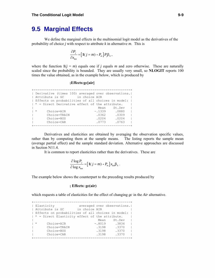
The Conditional Logit Model
9-9
9.5 Marginal Effects We define the marginal effects in the multinomial logit model as the derivatives of the probability of choice j with respect to attribute k in alternative m. This is
[ ]( )jm j k
km
Pj m P P
x∂
= = β∂
1 - ,
where the function 1(j = m) equals one if j equals m and zero otherwise. These are naturally scaled since the probability is bounded. They are usually very small, so NLOGIT reports 100 times the value obtained, as in the example below, which is produced by ;Effects:gc[air] +---------------------------------------------------+ | Derivative (times 100) averaged over observations.| | Attribute is GC in choice AIR | | Effects on probabilities of all choices in model: | | * = Direct Derivative effect of the attribute. | | Mean St.Dev | | * Choice=AIR -.1339 .0880 | | Choice=TRAIN .0362 .0309 | | Choice=BUS .0204 .0204 | | Choice=CAR .0773 .0763 | +---------------------------------------------------+
Derivatives and elasticities are obtained by averaging the observation specific values, rather than by computing them at the sample means. The listing reports the sample mean (average partial effect) and the sample standard deviation. Alternative approaches are discussed in Section N11.4.
It is common to report elasticities rather than the derivatives. These are
[ ]log
( )log
jm km k
km
Pj m P x
x∂
= = β∂
1 - .
The example below shows the counterpart to the preceding results produced by ; Effects: gc(air) which requests a table of elasticities for the effect of changing gc in the Air alternative. +---------------------------------------------------+ | Elasticity averaged over observations.| | Attribute is GC in choice AIR | | Effects on probabilities of all choices in model: | | * = Direct Elasticity effect of the attribute. | | Mean St.Dev | | * Choice=AIR -.8019 .3834 | | Choice=TRAIN .3198 .3370 | | Choice=BUS .3198 .3370 | | Choice=CAR .3198 .3370 | +---------------------------------------------------+

The Conditional Logit Model
9-10
The difference between the two commands is the use of ‘[air]’ for derivatives and ‘(air)’ for elasticities. The full set of tables, one for each alternative, is requested with alternative[*] or alternative(*). Note that for this model, the elasticities take only two values, the ‘own’ value when j equals m and the ‘cross’ elasticity when j is not equal to m. The fact that the cross elasticities are all the same is one of the undesirable consequences of the IIA property of this model.

The Nested Logit Model
10-1
Chapter 10
The Nested Logit Model ⎯⎯⎯⎯⎯⎯⎯⎯⎯⎯⎯⎯⎯⎯⎯⎯⎯⎯⎯⎯⎯⎯⎯⎯⎯⎯⎯⎯⎯⎯⎯ 10.1. Introduction The nested logit model is an extension of the multinomial model presented in Chapter 9 The models described here are based on variations of a four level tree structure such as the following: ROOT root │ ┌───────────────┴────────────────┐ │ │ TRUNKS trunk1 trunk2 │ │ ┌───────┴───────┐ ┌────────┴──────┐ │ │ │ │ LIMBS limb1 limb2 limb3 limb4 │ │ │ │ ┌───┴───┐ ┌───┴───┐ ┌───┴───┐ ┌───┴───┐ │ │ │ │ │ │ │ │ BRANCHES branch1 branch2 branch3 branch4 branch5 branch6 branch7 branch8 │ │ │ │ │ │ │ │ ┌─┴─┐ ┌─┴─┐ ┌─┴─┐ ┌─┴─┐ ┌─┴─┐ ┌─┴─┐ ┌─┴─┐ ┌─┴─┐ │ │ │ │ │ │ │ │ │ │ │ │ │ │ │ │ ALTS a1 a2 a3 a4 a5 a6 a7 a8 a9 a10 a11 a12 a13 a14 a15 a16 Individuals are assumed to make a choice among NALT = J alternatives (alts) in a choice set. The ‘twigs’ in the tree are the elemental alternatives in the choice set. There may be up to 100 alternatives in the model, a total of 25 branches throughout the tree, 10 limbs, and 5 trunks. The model may contain one or more limbs. Each limb may contain one or more branches, and each branch may contain one or more twigs (choices). If there is only one trunk and one limb, the model is, by implication, a two level model. As for single level models, choice sets may vary by individual. However, in order to construct a tree for such a setting, a universal choice set, as described in Section N10.3, is necessary. The variable sized choice set is then indicated by setting up the full tree structure, and indicating that certain choices are unavailable for the particular individual. The command for fitting nested logit models is the same as described in Chapter 9 for one level models, save for the addition of the tree definition in the command and, optionally, the specification of additional utility functions for choices made at higher levels in the tree. The nested logit model is limited to four level models for full information maximum likelihood (FIML) estimation. It also allows estimation of two and higher level models by sequential, or two step estimation. Utility functions can be specified for trunks the same as for limbs and branches (though it is unlikely that there will be very many attributes at this level in a tree). All options are available, including logs, Box-Cox transformation, fixed values, starting values, trunk specific constants, interaction terms, and so on. Utility functions for the trunks may include up to 10 variables

The Nested Logit Model
10-2
including the set of constant terms if used. Since the command structure and options for the nested logit model are the same as those for the one level model, we will present in this chapter only the parts of the command setup that are specific to nested models.
10.2 Mathematical Specification of the Model Individuals are assumed to choose one of the alternatives at the lowest level of the tree. Thus, they also choose a branch, a limb and a trunk. We denote by ‘j|b,l,r’ the choice of alternative j in branch b in limb l in trunk r. The number of alternatives in the branch/limb/trunk, Nb|l,r, can vary in every branch, limb, and trunk, and the number of branches in the l,rth limb/trunk, Nl|r is likely to vary across limbs and trunks as well. No assumption of equal choice set sizes is made at any point in the following. (Note that for ease of presentation, we have dropped the observation subscript.) The choice probability defined in the Chapter 9 is now redefined to be the conditional probability of alternative j in branch b, limb l, and trunk r, j|b,l,r:
P(j|b,l,r) = | , , | , ,
| , , | ,| , ,
exp( ) exp( )exp( ) exp( )
x x =
xj b l r j b l r
q b l r b l rq b l rJ
′ ′
′∑β β
β,
where Jb|l,r is the inclusive value for branch b in limb l, trunk r, Jb|l,r = log Σq|b,l,r exp(β′xq|b,l,r). At the next level up the tree, we define the conditional probability of choosing a particular branch in limb l, trunk r,
P(b|l,r) = | , | , | , | , | , | ,
| , | , | , || ,
exp( ) exp( )exp( ) exp( )
y y =
yb l r b l r b l r b l r b l r b l r
s l r s l r s l r l rs l r
J JJ I
′ ′+ τ + τ′ + τ∑
α α
α,
where Il|r is the inclusive value for limb l in trunk r, Il|r = log Σs|l,r exp(α′ys|l,r + τs|l,rJs|l,r). The probability of choosing limb l in trunk r is
P(l|r) = | | | | | |
| | ||
exp( ) exp( )exp( ) exp( )
z z =
zl r l r l r l r l r l r
s r s r s r rs r
I II H
′ ′+ σ + σ′ + σ∑
δ δ
δ,
where Hr is the inclusive value for trunk r, Hr = log Σs|r exp(δ′zs|r + σs|r Is|r). Finally, the probability of choosing a particular limb, r, is
P(r) = exp( ) .exp( )
hh
r r r
s s ss
HH
′ + φ′ + φ∑
θθ
By the laws of probability, the unconditional probability of the observed choice made by an individual is
P(j,b,l,r) = P(j|b,l,r) × P(b|l,r) × P(l|r) × P(r). This is the contribution of an individual observation to the likelihood function for the sample.

The Nested Logit Model
10-3
The ‘nested logit’ aspect of the model arises when any of the τj|i,l or σi|l or φl differ from 1.0. If all of these deep parameters are set equal to 1.0, the unconditional probability specializes to
P(j,bj,l,r) = | , , | , |
, , , ,
exp( )exp( )
x y z hx y z h
j b l r b l r l r r
jmbml r b l r l r rr l b j
′ ′ ′ ′+ + +′ ′ ′ ′+ + +∑ ∑ ∑ ∑
β α δ θ
β α δ θ,
which is the probability for a one level model. The model is written in a very general form. The parameters of the model are, in exactly this order: β1,β2,...,βnx,α1,α2,...,αny,δ1,δ2,...δnz,θ1,θ2,...,θnh,τ1...τB,σ1...,σL,φ1,...,φR where B is the total number of branches in the model, L is the number of limbs, and R is the number of trunks in the model. The x, y, z, and h vectors in the formulation above include all basic variables as well as all variables that interact with choice, branch, or limb specific dummy variables, etc. Once again, in this form, there may be different utility functions for each choice and, as described below, different utility functions defined for branches and limbs. There is a vector of ‘shallow’ parameters, [β,α,δ,θ] at each level, which multiplies the attributes (at the lowest level), or, e.g., demographics, at a higher level. There are also three vectors of ‘deep’ parameters, which multiply the inclusive values at the middle and high levels. In principle, there is one free inclusive value parameter for each branch in the model (Jb|l,r), one for each limb (σl|r), and one for each trunk (φr). But, some may have to be restricted to equal 1.0 for identification purposes. There are some degenerate cases: • If the model has one trunk, then the one φ equals 1.0. • If the model has one limb in a trunk, the one σ also equals 1.0. • If a limb contains a single branch, the τ for that branch equals 1.0 The preceding describes a ‘nonnormalized’ model. The nested logit model also accommodates an explicit scaling factor at each level.
10.3 Commands for FIML Estimation This section will describe how to set up a nested logit model. The default estimation technique is full information maximum likelihood (FIML). That is, the entire model is estimated in a single pass. In Section N16.9, we will describe how to obtain two step, limited information maximum likelihood (LIML) estimators for a two level model. In general, LIML has no advantage when FIML is available, and is generally inferior. Moreover, as will emerge below, the LIML estimator is not able to impose many of the parametric restrictions inherent in the model. 10.3.1 Data Setup The arrangement of the data set for estimation of the nested logit model is exactly the same as shown in Chapter 7. There is no requirement that the choice sets be the same across individuals, but the nested logit model will require a definition of a universal choice set, so the command must contain the

The Nested Logit Model
10-4
; Choices = list of labels ... specification. The nested model structure does mandate one special consideration if you are going to define utility functions for branches (ys), or limbs (zs). Since you have one line of data for each alternative, you will have more than one line of data for the variables in any branch or limb. In these cases, the values of ‘y’ and ‘z’ must be repeated for each alternative in the branch or limb. The following model and setup illustrate this for a three level model: (all in trunk 1) x1 x2 y1 y2 z1 z2 limb 1 branch 1|1 twig 1|1,1 .6 1 3 .02 104 .9 twig 2|1,1 .1 2 3 .02 104 .9 branch 2|1 twig 1|2,1 .8 2 7 .15 104 .9 twig 2|2,1 .2 3 7 .15 104 .9 limb 2 branch 1|2 twig 1|1,2 .9 6 11 .08 96 .4 twig 2|1,2 .3 1 11 .08 96 .4 twig 3|1,2 .4 0 11 .08 96 .4 10.3.2 Tree Definition The model command for estimating nested logit models is exactly as described in Chapter 8 for single level models, where the model name is now the generic NLOGIT; NLOGIT ; Lhs = ... ; Choices = ... definition of choice set ; ... definition of utility functions for alternatives All of the options described earlier are available. The nested logit model is requested by adding ; Tree = ... definition of the tree structure to the command. In order to specify the tree, use these conventions: { } specifies a trunk, [ ] specifies a limb within a trunk, ( ) specifies a branch within a limb in a trunk. Entries in a list are separated by commas. Names for trunks, limbs and branches are optional before the opening ‘{‘ or ‘[‘ or ‘(‘. If you elect not to provide names, the defaults chosen will be ‘Trunk{l}’ ‘Lmb[i|l]’ and ‘Br(j|i,l)’ respectively, where the numbering is developed reading from left to right in your tree definition. Alternative names appear inside the parentheses. Some examples are as follows: One limb:
; Tree = travel [ fly (air), ground (train,bus,car) ] One limb: (With one limb, the [ ] is optional.)
; Tree = fly (air) , ground (train,bus,car) One limb: (Branch names are optional. These would be Limb[1], Br(1|1) and Br(2|1).)
; Tree = (air) , (train,bus,car)

The Nested Logit Model
10-5
One limb, one branch, no nesting: (This would be unnecessary and could be omitted.)
; Tree = (air,train,bus,car) Nested logit model - two limbs, one with one branch:
; Tree = private[ fly(air), ground(car_pas, car_drv) ], public [ (train, bus) ] The fully nested 2×2×2×2 model shown in Section N16.1 could be specified with
; Choices = a1,a2,a3,a4,a5,a6,a7,a8,a9,a10,a11,a12,a13,a14,a15,a16 ;Tree = Trunk1 { limb1 [ branch1 ( a1 , a2 ) , branch2 ( a3 , a4 ) ],
limb2 [ branch3 ( a5 , a6 ) , branch4 ( a7 , a8 ) ] } , Trunk2 { limb3 [ branch5 ( a9 , a10 ) , branch6 ( a11 , a12 ) ] ,
limb4 [ branch7 ( a13 , a14 ) , branch8 ( a15 , a16 ) ] } 10.3.3 Utility Functions You may define the utility functions exactly as described in Chapter 8 for one level models. You may also define utility functions for branches and limbs and trunks, but note that in order to do so, you must use the explicit form described in Section 8.2.3. These are specified exactly the same as those for elemental alternatives. For example, in a two level model, you might put demographic characteristics, such as income or family size, at the top level. A complete model might appear as follows: NLOGIT ; Lhs = mode ; Choices = air, train, bus, car ; Tree = travel[public(bus,train), private(air, car)] ; Model: U( air ) = ba + bcost * gc + btime * ttme / U(train) = bt + bcost * gc + btime * ttme / U( car ) = bc + bcost * gc + btime * ttme / U( bus ) = bcost * gc + btime * ttme / U(public) = ap + apub * hinc / U(private) = aprv * hinc $ This model can be considerably collapsed; ; Model: U(air, train, bus,car) = <ba,bc,0,bt> + bcost * gc + btime * ttme / U(public,private) = <ap,0> + <apub, aprv> * Income $ Note that the same function specification U(...) is used for all three kinds of equations, for alternatives, branches, and limbs. Finally, as noted earlier, you may impose equality constraints at any points in the model, just by using the same parameter name where you want the equality imposed. For example, if, for some reason, you desired to force the parameters apub and bcost to be equal, you could just change apub to bcost in the utility equation for public. That is, you can, if you wish, force equality of parameters at different levels of a model, once again, just by using the same

The Nested Logit Model
10-6
parameter name in the model specification. (Given the impact of the scale parameters, this is probably inadvisable, but the program will allow you to do it nonetheless.) The interaction of alternative specific constants, and branch and limb specific constants is complex, and it is difficult to draw generalities. As a general rule, models will usually become overdetermined, resulting in a singular Hessian, when there are more than NALT-1 constants, of all three types, in the entire model. Likewise, interactions of attributes and choice specific dummy variables can produce this effect as well. Users who encounter problems in which NLOGIT claims either that it is impossible to maximize the log likelihood function, or there is a singular Hessian, should examine the model for this pitfall. 10.3.4 Command Builder The command builders can be used to specify the nested logit models. Select Model:Discrete Choice/Nested Logit to access the command builder. The choice variable is defined on the Main page, shown in Figure 10.1. The Options page, shown in Figure 19.2, may be used to specify the rest of the model.
Figure 10. 1 Main Page of Command Builder for Nested Logit Models

The Nested Logit Model
10-7
Figure 10.2 Options Page of Command Builder for Nested Logit Models The tree is specified in a subsidiary dialog box by selecting Tree Specification at the bottom of the Options page. The dialog box, shown in Figure 10.3, allows you to define the tree graphically. Note in the dialog shown, public and private are siblings while bus is a child node of public.
Figure 10.3Tree Specification Dialog Box for Defining the Tree Structure The remaining options for output and results to be saved are defined in the Output page as shown in Figure 10.4.

The Nested Logit Model
10-8
Figure 10.4 Output Page of Command Builder for Nested Logit Models
10.4 Marginal Effects and Elasticities In the nested logit model with P(j,b,l,r) = P(j|b,l,r) × P(b|l,r) × P(l|r) × P(r), the marginal effect of a change in attribute ‘k’ in the utility function for alternative ‘J’ in branch ‘B’ of limb ‘L’ of trunk ‘R’ on the probability of choice ‘j’ in branch ‘b’ of limb ‘l’ of trunk ‘r’ is computed using the following result: Lower case letters indicate the twig, branch, limb and trunk of the outcome upon which the effect is being exerted. Upper case letters indicate the twig, branch, limb and trunk which contain the outcome whose attribute is being changed:
log ( , , , ) ( | , , , ) ( )( ) | , , , )
P alt j limb l branch b trunk r D k J B L R k Fx k alt J limb L branch B trunk r∂ = = = =
= = Δ ×∂ = = = =
,
where Δ(k) = coefficient on x(k) in U(J|B,L,R) and F = 1(r=R) × 1(l=L) × 1(b=B) × [1(j=J) - P(J|BLR)] (trunk effect), 1(r=R) × 1(l=L) × [1(b=B) - P(B|LR)] × P(J|BLR)] × τB|LR (limb effect), 1(r=R) × [1(l=L) - P(L|R)] × P(B|LR) × P(J|BLR) × τB|LR × σL|R (branch effect), [1(r=R) - P(R)] × P(L|R) × P(B|LR) × P(J|BLR) × τB|LR × σL|R × φR (twig effect). (Note, in this expression, J, B, L and R are being used generically to indicate a particular choice, branch, limb and trunk, not the total numbers of twigs, branches, limbs and trunks.) The marginal effect is
∂ P(j,b,l,r)/∂x(k)|J,B,L,R = P(j,b,l,r) Δ(k) F. A marginal effect has four components, an effect on the probability of the particular trunk, one on the probability for the limb, one for the branch, and one for the probability for the twig.

The Nested Logit Model
10-9
(Note that with one trunk, P(l) = P(1) = 1, and likewise for limbs and branches.) For continuous variables, such as cost, you might be interested, instead, in the Elasticity = x(k)|J,B,L,R × Δ(k|J,B,L,R) × F. NLOGIT will provide either. As in the case of nonnested models, marginal effects are requested with ;Effects: attribute [list of outcomes] / ... or attributes ( list ) / ... for elasticities This generates a table of results for each of the outcomes listed. For example, NLOGIT ; Lhs = mode ; Choices = air,train,bus,car ; Tree = travel[public(bus,train), private(air,car)] ; Model: U( air ) = ba + bcost * gc + btime * ttme / U(train) = bc + bcost * gc + btime * ttme / U(bus) = bcost * gc + btime * ttme / U(car) = bc + bcost * gc ; Effects: gc ( car ) $ This lists the effects on all four probabilities of changes in attribute generalized cost (gc) of choice car.

The Nested Logit Model
10-10
+------------------------------------------------------------+ | Partial effects = average over observations | | | | dlnP[alt=j,br=b,lmb=l,tr=r] | | ---------------------------- = D(k:J,B,L,R) = delta(k)*F | | dx(k):alt=J,br=B,lmb=L,tr=R] | | delta(k) = coefficient on x(k) in U(J|B,L,R) | | F = (r=R) (l=L) (b=B) [(j=J)-P(J|BLR)] | | + (r=R) (l=L) [(b=B) -P(B|LR)]P(J|BLR)t(B|LR) | | + (r=R) [(l=L)-P(L|R)] P(B|LR) P(J|BLR)t(B|LR)s(L|R) | | + [(r=R) -P(R)] P(L|R) P(B|IR) P(J|BIR)t(B|LR)s(L|R)f(R) | | | | P(J|BLR)=Prob[choice=J |branch=B,limb=L,trunk=R] | | P(B|LR), P(L|R), P(R) defined likewise. | | (n=N) = 1 if n=N, 0 else, for n=j,b,l,r and N=J,B,L,R. | | Elasticity = x(k) * D(j|B,L,R) | | Marginal effect = P(JBLR)*D = P(J|BLR)P(B|LR)P(L|R)P(R)D | | F is decomposed into the 4 parts in the tables. | +------------------------------------------------------------+ +-----------------------------------------------------------------------+ | Elasticity averaged over observations. | | Attribute is GC in choice CAR | | Effects on probabilities of all choices in the model: | | * indicates direct Elasticity effect of the attribute. | | Decomposition of Effect if Nest Total Effect| | Trunk Limb Branch Choice Mean St.Dev| | Trunk=Trunk{1} | | Limb=TRAVEL | | Branch=PUBLIC | | Choice=BUS .000 .000 .857 .000 .857 .532 | | Choice=TRAIN .000 .000 .857 .000 .857 .532 | | Branch=PRIVATE | | Choice=AIR .000 .000 -1.015 .571 -.444 .746 | | * Choice=CAR .000 .000 -1.015 -.338 -1.353 1.059 | +-----------------------------------------------------------------------+ Note that across a row, the effects sum to the total effect given. The default method of computing the elasticities is to average the observation specific results. The results show the mean and the sample standard deviations. If you use the ;Means specification, then the elasticities are computed once, and the results reflect the change, as shown below. (The differences are noticeably large.) +-----------------------------------------------------------------------+ | Elasticity computed at sample means. | | Attribute is GC in choice CAR | | Effects on probabilities of all choices in the model: | | * indicates direct Elasticity effect of the attribute. | | Decomposition of Effect if Nest Total Effect| | Trunk Limb Branch Choice Mean St.Dev| | Trunk=Trunk{1} | | Limb=TRAVEL | | Branch=PUBLIC | | Choice=BUS .000 .000 .584 .000 .584 .000 | | Choice=TRAIN .000 .000 .584 .000 .584 .000 | | Branch=PRIVATE | | Choice=AIR .000 .000 -.411 .303 -.107 .000 | | * Choice=CAR .000 .000 -.411 -.605 -1.016 .000 | +-----------------------------------------------------------------------+
The Random Parameters Logit Model
11-1
Chapter 11
The Random Parameters Logit Model ⎯⎯⎯⎯⎯⎯⎯⎯⎯⎯⎯⎯⎯⎯⎯⎯⎯⎯⎯⎯⎯⎯⎯⎯⎯⎯⎯⎯⎯⎯⎯ 11.1 Introduction The random parameters (RP) logit model, also referred to as the mixed logit model is the most general model form in NLOGIT in terms of the variety of model specifications it can accommodate and in terms of the range of behavior that it can model. (On this latter point, see McFadden and Train (2000).) This chapter will develop the numerous different specifications of the model that can be accommodated. NLOGIT offers an extensive set of specifications within the mixed logit structure. This model is gaining great popularity in applications. Capabilities provided by the estimator include (i) choosing from among a large number of analytical distributions for each random parameter, (ii) accounting for the non-independence between observations associated with the same respondent (a theme of importance in stated choice studies), (iii) decomposing the mean and standard deviation of one or more random parameters to reveal sources of systematic taste heterogeneity, (iv) accounting for correlation of random parameters, (v) imposing priors based on known choices in model estimation, (vi) imposing constraints on distributions (e.g. constraining the triangular or normal to ensure that it does not change sign over its range), (vii) selecting subsets of pre-specified variables to interact with the mean and standard deviation of random parameterized attributes, and (viii) deriving willingness to pay estimates when both the numerator and denominator are random parameter estimates.

The Random Parameters Logit Model
11-2
11.2 Random Parameters (Mixed) Logit Models This model is somewhat similar to the random coefficients model for linear regressions. (See Bhat (1996), Jain, Vilcassim, and Chintagunta (1994), Revelt and Train (1998), Train, Revelt, and Ruud (1996), and Berry, Levinsohn, and Pakes (1995).) The model formulation is a one level multinomial logit model, for individuals i = 1,...,N in choice setting t. Neglecting for the moment the error components aspect of the model, we begin with the basic form of the multinomial logit model, with (optional) alternative specific constants αji and attributes xji,
Prob(yit = j) = ( )( )1
exp
exp
x
xi
ji i jiJ
qi i qiq=
′α
′α∑+ β
+ β.
The RP model emerges as the form of the individual specific parameter vector, βi is developed. The most familiar, simplest version of the model specifies βki = βk + σkvik, and αji = αj + σjvji, where βk is the population mean, vik is the individual specific heterogeneity, with mean zero and standard deviation one, and σk is the standard deviation of the distribution of βiks around βk. The term ‘mixed logit’ is often used in the literature (e.g., Revelt and Train (1998)) for this model. The choice specific constants, αji and the elements of βi are distributed randomly across individuals with fixed means. A refinement of the model is to allow the means of the parameter distributions to be heterogeneous with observed data, zi, (which does not include one). This would be a set of choice invariant characteristics that produce individual heterogeneity in the means of the randomly distributed coefficients so that βki = βk + δk′zi + σkvki, and likewise for the constants. The model is not limited to the normal distribution. We consider several alternatives below. One important variation is the lognormal model, βki = exp(ρk + δk′zi + σkvki). The vjkis are individual and choice specific, unobserved random disturbances - the source of the heterogeneity. Thus, as stated above, in the population, if the random terms are normally distributed, αji or βki ~ Normal or Lognormal [ρj or k + δj or k′zi, σj or k
2]. (Other distributions may be specified.) For the full vector of K random coefficients in the model, we may write the full set of random parameters as ρi = ρ + Δzi + Γvi.

The Random Parameters Logit Model
11-3
where Γ is a diagonal matrix which contains σk on its diagonal. For convenience at this point, we will simply gather the parameters, choice specific or not, under the subscript ‘k.’ (The notation is a bit more cumbersome for the lognormally distributed parameters. We will return to that in the technical details.) We can go a step further and allow the random parameters to be correlated. All that is needed to obtain this additional generality is to allow Γ to be a triangular matrix with nonzero elements below the main diagonal. Then, the full covariance matrix of the random coefficients is Σ = ΓΓ′. The standard case of uncorrelated coefficients has Γ = diag(σ1,σ2 ,…,σk). If the coefficients are freely correlated, Γ is a full, unrestricted, lower triangular matrix and Σ will have nonzero off diagonal elements. (It will be convenient to aggregate this one step further. We may gather the entire parameter vector for the model in this formulation simply by specifying that for the nonrandom parameters in the model, the corresponding rows in Δ and Γ are zero.) We will also define the data and parameter vector so that any choice specific aspects are handled by appropriate placements of zeros in the applicable parameter vector. An additional extension of the model allows the distribution of the random parameters to be heteroscedastic. As stated above, the variance of vik is taken to be a constant. The model is made heteroscedastic by assuming, instead, that Var[vik] = σjk
2 [exp(ωk′hri)]2
A convenient way to parameterize this is to write the full model as ρi = ρ + Δzi + ΓΩivi where Ωi is the diagonal matrix of individual specific variance terms; ωik = exp(ωk′hri). The list of variations above produces an extremely flexible, general model. Typically, you would use only some of them, though in principle, all could appear in the model at once. We will develop them in parts in the sections to follow. A convenient form of the full random parameters logit model to begin with is
Prob(yit = j) = 1
exp( )
exp( )
x
xit
ji i jitJ
qi i qitq=
′α +
′α +∑β
β,
Finally, an additional layer of individual heterogeneity may be added to the model in the form of the error components detailed in Chapter N14. The full model with all components is
Prob(yit = j) = 1
11
exp exp( )
exp exp( )
x he
x hei
Mji i jit m jm m m i im
J Mqi i qit m qm m m i imq
d E
d E=
==
′ ′⎡ ⎤α + + θ⎣ ⎦′ ′⎡ ⎤α + + θ⎣ ⎦∑
β Σ γ
β Σ γ,
where the components of the model are as follows:

The Random Parameters Logit Model
11-4
Random Alternative Specific Constants and Taste Parameters: ( , ) ( , ) z vji i j i i iα = α + +β β Δ ΓΩ , Ωi = diag(ωi1, ωi2, ...) or Ωi = diag(σ1,...,σk), β,αji = constant terms in the distributions of the random taste parameters,
Uncorrelated Parameters with Homogeneous Means and Variances βik = βk + σkvik when Δ = 0, Γ = I, Ωi = diag(σ1,...,σk),
xjit = all observed choice attributes and individual characteristics,
vi = random unobserved taste variation, with mean vector 0 and covariance matrix I
Uncorrelated Parameters with Heterogeneous Means and Variances βik = βk + δk′zi + σk exp(ωk′hri)vik when Γ = I, Ωi = diag(ωi1, ωi2, ...)
Δ = parameters that enter the heterogeneous means of the distributions of the random parameters; β + Δzi = the heterogeneous means,
ωik = exp(ωk′hri) = heterogeneity in the variances of the distributions of the random parameters,
ωk = parameters in the variance heterogeneity of the random parameters,
σik = σkωik = heterogeneous standard deviations in the distributions of the random parameters; σik = σk in a homoscedastic model,
zi = observed variables that measure the heterogeneity in the means of the random parameters,
hri = observed variables that measure the heterogeneity in the variances of the random parameters,
Correlated Parameters with Heterogeneous Means βik = βk + δk′zi + 1
ks=Σ Γks vis when Γ ≠ I, and Ωi = diag(σ1,...,σk),
Γ = lower triangular matrix with ones on the diagonal that allows correlation across random parameters when Γ ≠ I,
Individual Error Components Eim = the individual specific underlying random error components, m = 1,...,M, Eim ~ N[0,1].
djm = 1 if Eim appears in utility for alternative j and 0 otherwise.
θm = scale factor for error component m,
γim = exp(γm′hei) = heterogeneity in the variances of the error components
λim = θmγim = standard deviations of random error components,

The Random Parameters Logit Model
11-5
γm = parameters in the heteroscedastic variances of the error components,
hei = individual choice invariant characteristics that produce heterogeneity in the variances of the error components, The model specification will dictate which parameters are random and which are not, how the heteroscedasticity if any is parameterized, the distributions of the random terms, and how the error components enter the model. The probabilities defined above are conditioned on the random terms, vi and the error components, Ei. The unconditional probabilities are obtained by integrating vik and Eim out of the conditional probabilities: Pj = Ev,E[P(j|vi,Ei)]. This is a multiple integral which does not exist in closed form. The integral is approximated by sampling nrep draws from the assumed populations and averaging. (See Bhat (1996) and Revelt and Train (1998) and Greene (2003) for discussion.) Parameters are estimated by maximizing the simulated log likelihood,
log Ls = 1 ,
1 1 11 ,1
exp exp( )1logexp exp( )
x he
x hei
i
MTN R ji ir jit m jm m m i im r
Ji r t Mqi ir qit m qm m m i im rq
d ER d E
=
= = ===
′ ′⎡ ⎤α + + θ⎣ ⎦′ ′⎡ ⎤α + + θ⎣ ⎦
∑ ∑ ∏∑
β Σ γ
β Σ γ,
with respect to (β, Δ, Γ, Ω, θ, γ), where R = the number of replications,
βir = β + Δzi + ΓΩivir = the rth draw on βi,
vir = the rth multivariate draw for individual i,
Eim,r = the rth univariate normal draw on the underlying effect for individual i. (Note that the multivariate draw, vir is actually K independent draws. The heteroscedasticity is induced first by multiplying by Ωi, then the correlation is induced by multiplying Ωivir by Γ.) The model components may be restricted and varied in several ways.
• A variety of distributions may be chosen for the random parameters, and they need need not be the same for all parameters. • The observed heterogeneity, Δzi, is optional. You may specify that a coefficient is randomly distributed around a fixed mean. Thus, δk may be set to a zero vector for some or all random coefficients. • σk may be set equal to zero for some coefficients. This may change the way a coefficient enters the model. If σk = 0 and δk = 0, then the coefficient is a nonrandom fixed parameter. But, including it in β allows you to force a coefficient to be positive. This device also allows you to form a hierarchical model with nonrandom coefficients. • Any coefficient in the model may be fixed at a specific value. • The heteroscedasticity may apply to some or all (or none) of the random parameters. • Different variables may be placed in the heterogeneous means (Δzi) or the heteroscedastic variances (Ωi) of any of the random parameters. • The variables that enter the heteroscedasticity of the error components may be different.

The Random Parameters Logit Model
11-6
11.3 Command for the Random Parameters Logit Models
The command for the mixed logit model is as follows: RPLOGIT ; Lhs = ... as usual
; Choices = ... ; ... Utility function specification using ; Rhs = ... ;Rh2=... or ; Model: U(...) = ... to specify utilities ; Fcn = specification of random parameters $
(The model command NLOGIT;RPL is equivalent.) The last specification is used to define the random parameters. There are many variants. We begin with the simplest, and add features as we proceed. The ;Fcn specification takes the basic form ; Fcn = parameter label (type) where parameter label is defined either by a variable name that you use in your ;Rhs specification or by the name you give in your ;Model:... definitions and the type is one of the distributions defined in the next section. Alternative specific constants are a special case. You will generally not want to specify the parameters that multiply Rh2 variables as random. These two cases are considered specifically below. For example, the following specifies two normally distributed random parameters: RPLOGIT ; Lhs = mode ; Choices = air,train,bus,car ; Rhs = gc,ttme,invc ; Rh2 = hinc ; Fcn = gc(n), ttme(n) $ (The ‘type’ in the example is n, indicating normally distributed parameters. Several other specifications would probably be added.) Alternatively, you might use the following to specify a model with two random parameters: RPLOGIT ; Lhs = mode ; Choices = air,train,bus,car ; Model: U(air) =a_air+bgc*gc + btt*ttme + binvc*invc + ghinc*hinc / U(train,bus,car) = a_ground + bgc*gc ; Fcn = a_ground(n), btt(n) $ Note that the specifications of the random parameters are separated by commas, not semicolons. The next several subsections will describe the various parts of the specifications of the random parameters. The last part of this section describes the command builder for this model. Because so much of this model is custom made for the particular application, the command builder is somewhat limited compared to the command form indicated above.

The Random Parameters Logit Model
11-7
11.3.1 Distributions of Random Parameters in the Model There are many distributions that can be used for the random parameters. The most common will be the normal, which is used in the example above. Many alternatives are supported, however. A few of these are listed below. The basic distributions are specified with the following: ; Fcn = parameter name ( type ), ... The types are
n normal βi = β + σvi, vi ~ N[0,1],
l lognormal βi = exp(β + σvi), vi ~ N[0.1],
u uniform βi = β + σvi, vi ~ U[-1.1,]
t triangular βi = β + σvi, vi ~ Triangle[-1.1],
d dome βi = β + σvi, vi ~ 2×Beta(2,2) - 1
e Erlang βi = β + σvi, vi ~ Gamma(1,4) - 4,
w Weibull βi = β + σ vi, vi = 2(-logui)√.5, ui ~ U[0,1],
p exponential βi = β + σvi, vi ~ exponential - 1
c nonstochastic βi = β.
In the list above, we have denoted the constant in the distribution as ‘β.’ However, the parameter definition may involve heterogeneity in the mean so, what appears there may be of the form θi = β + δ′zi. We have also written the scaling parameter in each form as ‘σ,’ however, you may also specify heterogeneity in the variances so what appears there may be of the form σi = σ exp(ω′hi). The list above suggests the variety of different distributions that may be used. Any distribution may be used for any parameter. The normal distribution will the the usual choice. However, you may wish to restrict a particular coefficient in the model to be positive. The lognormal distribution is the obvious choice, though there are several other possibilities. The normal, lognormal, exponential, Erlang and Weibull distributions all have infinite ranges. If you wish to restrict the range of variation of a parameter, then the triangular, dome or uniform can be used. The lognormal distribution has an infinite tail in the positive direction and is anchored at zero while the Erlang and Weibull models as specified have infinite range from [ ]iE vβ −σ to +∞. It is important to note that the means and variances of the distributions are not always simple functions when the parameters are not linear functions of the underlying random variables. For all but the Weibull distributions shown above, the mean of vi is zero, which centers the distributions at β. For the lognormal and Weibull models, the mean depends on the parameters. This is also true of the modified distributions shown below. This means that one must be careful in interpretating the estimated coefficients, even in simple cases in which there is no heterogeneity in the means or variances. It is possible to learn about these empirically, as described in Section N17.8, however, it is often not possible to state a priori what the population means are for most of the distributions. The problem becomes yet more complicated as additional features such as heterogeneity in the means and heteroscedasticity are added to the model.

The Random Parameters Logit Model
11-8
Some practical aspects of the specifications are as follows: • If you will be mixing distributions, the specification of correlated parameters, while
allowable, produces ambiguous results. The nature of the correlation is difficult to define. However, the program will have no unusual difficulty estimating a model in which correlated parameters have different distributions. One particular case worth noting is a mixture of normal and lognormal parameters. In such a model, the reported correlation will be between the normally distributed parameter and the log of the lognormally distributed parameter. This is probably not a useful result.
• Researchers often find that the long, thick tail of the lognormal distribution produces an implausible distribution of parameters. The restricted triangular distribution as well as several alternatives may be preferable.
• Type ‘c’ is the same as not including the parameter in the Fcn list, which is how this usually should be done. But sometimes, for convenience, this might be preferred. Variablename(c) specifies a free mean and zero variance of the parameter.
Model results for these distributions will display the structural parameters, not necessarily the means and variances of the parameter distributions. Note, for example, that the means of the lognormal and the Weibull distributions are not equal to β; for the lognormal it is exp(β+σ2/2) while for the Weibull it is β+2σΓ(1+1/√2). Consider an example. The following estimates a model with two random parameters. We will use the normal, Weibull and exponentiated Weibull (our ‘Rayleigh’) distributions. Since the exponentiated Weibull estimator forces the coefficient to be positive, and the coefficients on the two variables would naturally be negative, we reverse the signs on the data before estimation. CREATE ; mgc=-gc ; mttme=-ttme$
RPLOGIT ; lhs=mode ; choices=air,train,bus,car
; rhs=mgc,mttme ; rh2=one ; fcn=mgc(n),mttme(n) ? Normally distributed parameters ; maxit=50;pts=25;halton; pds=3 $
RPLOGIT ; lhs=mode ; choices=air,train,bus,car
; rhs=mgc,mttme ; rh2=one ; fcn=mgc(w),mttme(w) ? Weibull distributed parameters ; maxit=50;pts=25;halton; pds=3 $
RPLOGIT ; lhs=mode ; choices=air,train,bus,car
; rhs=mgc,mttme ; rh2=one ; fcn=mgc(r),mttme(r) ? Modified Weibull distributed parameters ; maxit=50;pts=25;halton; pds=3 $
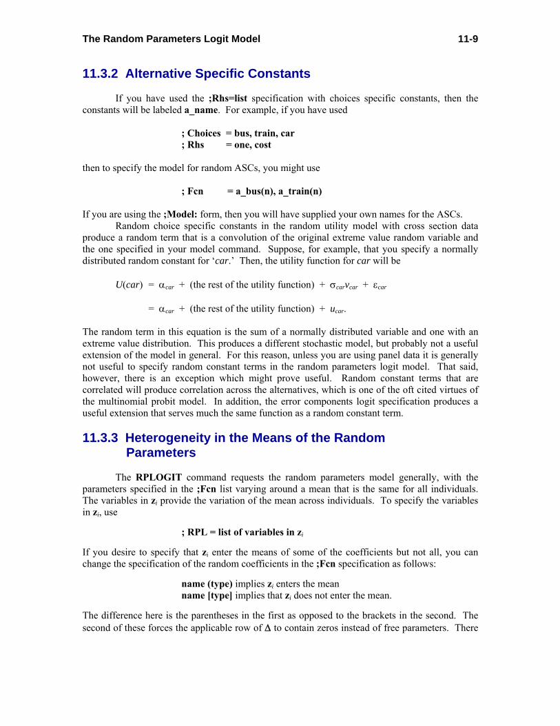
The Random Parameters Logit Model
11-9
11.3.2 Alternative Specific Constants
If you have used the ;Rhs=list specification with choices specific constants, then the constants will be labeled a_name. For example, if you have used
; Choices = bus, train, car ; Rhs = one, cost
then to specify the model for random ASCs, you might use
; Fcn = a_bus(n), a_train(n) If you are using the ;Model: form, then you will have supplied your own names for the ASCs. Random choice specific constants in the random utility model with cross section data produce a random term that is a convolution of the original extreme value random variable and the one specified in your model command. Suppose, for example, that you specify a normally distributed random constant for ‘car.’ Then, the utility function for car will be U(car) = αcar + (the rest of the utility function) + σcarvcar + εcar = αcar + (the rest of the utility function) + ucar. The random term in this equation is the sum of a normally distributed variable and one with an extreme value distribution. This produces a different stochastic model, but probably not a useful extension of the model in general. For this reason, unless you are using panel data it is generally not useful to specify random constant terms in the random parameters logit model. That said, however, there is an exception which might prove useful. Random constant terms that are correlated will produce correlation across the alternatives, which is one of the oft cited virtues of the multinomial probit model. In addition, the error components logit specification produces a useful extension that serves much the same function as a random constant term. 11.3.3 Heterogeneity in the Means of the Random Parameters
The RPLOGIT command requests the random parameters model generally, with the parameters specified in the ;Fcn list varying around a mean that is the same for all individuals. The variables in zi provide the variation of the mean across individuals. To specify the variables in zi, use
; RPL = list of variables in zi If you desire to specify that zi enter the means of some of the coefficients but not all, you can change the specification of the random coefficients in the ;Fcn specification as follows: name (type) implies zi enters the mean name [type] implies that zi does not enter the mean. The difference here is the parentheses in the first as opposed to the brackets in the second. The second of these forces the applicable row of Δ to contain zeros instead of free parameters. There

The Random Parameters Logit Model
11-10
are also some variations on this that allow some flexibility in the construction of Δ. First, an alternative, equivalent form of name[type] is
name (type | # ) This requests that if there are RPL variables (;RPL = list) that these not appear in the mean for this parameter. This puts a row of zeros in the Δ matrix. For example, ; RPL = Income
; Fcn = gc(n), ttme (n|#) specifies that income does not appear in the mean of the ttme parameter. This form may be extended to exclude and include specific variables from the RPL list in the mean of a particular parameter. The specification is
name(type | # pattern) where the pattern consists of 1s and 0s which indicate which variables in the list are included (1s) and excluded (zeros). There must be the same number of items in the pattern as there in the list. For example, the specification
; RPL = age,sex,income ; Fcn = gc(n), ttme(n|#101) invt (n|# 011) invc (n|#000)
includes all three variables in the mean of gc, excludes sex from the mean of ttme, excludes age from the men of invt, and excludes all three variables from the mean of invc. All parameters may be specified independently, and there is no restriction on how this feature is used. Do note, however, if you exclude an RPL variable from all parameters, the model becomes inestimable. 11.3.4 Correlated Parameters
The model specified thus far assumes that the random parameters are uncorrelated. Use
; Correlation to allow free correlation among the parameters. In this case, estimates of the below diagonal elements of Γ will be obtained with the other parameters of the model. No restrictions may be imposed on these new parameters. After these are presented, the elements of Σ = ΓΓ′ are given. An example appears below. The second note in Section N17.3.1 gives some cautions about this specification. In particular, some ambiguity in the results will be unavoidable when this feature is used with other modifications of the model, such as mixed distributions and heteroscedasticity. The most favorable case for use of this feature would be a sparse model, βi = β + Γvi.

The Random Parameters Logit Model
11-11
We would note, many, perhaps most of the received applications of the mixed logit model are of this form – it is much less restrictive than its bare appearance would suggest. In the model developed thus far, the covariance matrix for the random components for the simple distributions (normal, uniform, triangle) is Var[βi|xi,zi] = Σ = ΓΓ′. In the uncorrelated case, Γ is a diagonal matrix, and the variance of βik is simply σk
2. When the parameters are correlated, then the diagonal element of Σ is γk′γk where γk is the kth row of Γ. The model results will show the elements of Γ and the implied standard deviations. The following demonstrates the computations. The command below specifies two correlated random parameters.
RPLOGIT ; lhs=mode ; choices=air,train,bus,car ; rhs=gc,ttme ; rh2=one ; fcn=gc(n),ttme(n) ; Correlated ; maxit=50;pts=25;halton;output=3; pds=3 $
The relevant results from estimation are as follows. The coefficients reported are, first, β from the random parameter distributions, then the nonstochastic β from the distributions of the nonrandom alternative specific constants. The next results display the elements of the 2×2 lower triangular matrix, Γ. The diagonal elements appear first, then the below diagonal element(s). The matrix Γ is shown again, in natural form at the end of the results, labeled ‘Cholesky matrix.’ The ‘Standard deviations of parameter distributions’ are derived from Γ. The first is (.011001342)1/2 = .001100134. The second is ((-.07458)2 + .036782)1/2 = .08315251. The standard errors for these estimators are computed using the delta method. Hensher, Rose and Greene (2005) discuss the Cholesky decomposition in detail with numerous examples.

The Random Parameters Logit Model
11-12
+--------+--------------+----------------+--------+--------+ |Variable| Coefficient | Standard Error |b/St.Er.|P[|Z|>z]| +--------+--------------+----------------+--------+--------+ ---------+Random parameters in utility functions GC | -.02260684 .00724332 -3.121 .0018 TTME | -.14522848 .02205029 -6.586 .0000 ---------+Nonrandom parameters in utility functions A_AIR | 8.70238058 1.22465947 7.106 .0000 A_TRAIN | 6.95973395 1.03548341 6.721 .0000 A_BUS | 6.12199207 1.13357506 5.401 .0000 ---------+Diagonal values in Cholesky matrix, L. NsGC | .01100134 .01124017 .979 .3277 NsTTME | .03678160 .03024421 1.216 .2239 ---------+Below diagonal values in L matrix. V = L*Lt TTME:GC | -.07457516 .02353048 -3.169 .0015 ---------+Standard deviations of parameter distributions sdGC | .01100134 .01124017 .979 .3277 sdTTME | .08315251 .01967123 4.227 .0000 Correlation Matrix for Random Parameters Matrix COR.MAT. has 2 rows and 2 columns. GC TTME +---------------------------- GC | 1.00000 -.89685 TTME | -.89685 1.00000 Covariance Matrix for Random Parameters Matrix COV.MAT. has 2 rows and 2 columns. GC TTME +---------------------------- GC | .00012 -.00082 TTME | -.00082 .00691 Cholesky Matrix for Random Parameters Matrix Cholesky has 2 rows and 2 columns. GC TTME +---------------------------- GC | .01100 .0000000D+00 TTME | -.07458 .03678
We emphasize, these results apply to the linear functions of the underlying random variables, not necessarily to the implied distributions of the random parameters themselves. In most of the specifications, the parameters involve nonlinear transformations of these variables.

The Multinomial Probit Model
12-1
Chapter 12
The Multinomial Probit Model ⎯⎯⎯⎯⎯⎯⎯⎯⎯⎯⎯⎯⎯⎯⎯⎯⎯⎯⎯⎯⎯⎯⎯⎯⎯⎯⎯⎯⎯⎯⎯ 12.1 Introduction
In this model, the individual’s choice among J alternatives is the one with maximum
utility, where the utility functions are
Uji = β′xji + εji, where Uji = utility of alternative j to individual i,
xji = union of all attributes that appear in all utility functions. For some alternatives, xi,tk may be zero by construction for some attribute k which does not enter their utility function for alternative j,
εji = unobserved heterogeneity for individual i and alternative j. The multinomial logit model specifies that εji are draws from independent extreme value distributions (which induces the IIA condition). In the multinomial probit model, we assume that εji are normally distributed with standard deviations Sdv[εji] = σj and correlations Cor[εji, εmi] = ρjm (the same for all individuals). Observations are independent, so Cor[εji,εms ] = 0 if i is not equal to s, for all j and m. A variation of the model allows the standard deviations and covariances to be scaled by a function of the data, which allows some heteroscedasticity across individuals.
The correlations ρjm are restricted to -1 < ρjm < 1, but they are otherwise unrestricted save for a necessarily normalization. The correlations in the last row of the correlation matrix must be fixed at zero. The standard deviations are unrestricted with the exception of a normalization - two standard deviations are fixed at 1.0 - NLOGIT fixes the last two. In principle, up to 20 alternatives may be in the model, but our experience thus far is that this model is extremely difficult to estimate, and will usually not be estimable with a completely free correlation matrix even with only five alternatives. The difficulty increases greatly with the number of alternatives. (Imposition of constraints which may improve this situation is discussed below.) This model may also be fit with panel data. In this case, the utility function is modified as follows: Uji,t = β′xjt,t + εji,t + vji,t, where ‘t’ indexes the periods or replications. There are two formulations for vji,t, Random effects vji,t = vji,s (the same in all periods),
First order autoregressive vji,t = αj vji,t-1 + aji,t.

The Multinomial Probit Model
12-2
12.2 Model Command This is a one level (nonnested) model. To request it, use
MNPROBIT ; Lhs = ... ; Choices = ...
; Rhs = ... or ; Model: U(...)=... / U(...) = ... all as usual ; ... any other options $
(The alternative model command used in earlier versions of NLOGIT, NLOGIT;MNP is equivalent and may be used instead.) Other options include ; Prob = name to use for estimated probabilities ; Utility = name for estimated utilities and the usual other options for output, technical output, elasticities, descriptive statistics, etc. There are some special cases for this estimator:
• The number of alternatives must be fixed - it may not vary across observations. • The choice set must be fixed. • Choice based sampling is not supported, though you can use ordinary weights. • Data may be individual, proportions, or frequencies.
(The second derivatives matrix is not computed for this model, so it is not possible to compute a robust covariance matrix estimator.) An additional option is
; Pts = number of replications to compute multivariate normal probabilities
The command builder may also be used for this model by selecting Model/Discrete Choice/Multinomial Probit, HEV, RPL. The choice set and utility functions for the model are defined on the Main page and the MNP format of the model is selected on the Options page.
The following features of NLOGIT are not available for this model:
; Tree ... This is not a nested logit model ; Ivb = name, ; Ivl=name, ; Ivt=name. No inclusive values are computed. ; IIA = list. IIA is not testable here, since it is not imposed. ; Cprob = name. Conditional and unconditional probabilities are the same. ; Ranks This estimator may not be based on ranks data. ; Scale ... Data scaling is only for the nested logit model.
The remainder of the command setup is identical to the multinomial logit model with one level. All other options are available, including
; Probs = name to retain the predicted probabilities ; Utility = name to retain the predicted systematic utilities
and so on.

The Multinomial Probit Model
12-3
Figure 12.1 Main Page of Command Builder for the MNP model
Figure 12.2 Options Page of Command Builder for the MNP model

The Multinomial Probit Model
12-4
12.3 An Application The multinomial probit (MNP) model based on the CLOGIT data is estimated with the command MNPROBIT ; Lhs = mode ; Choices = air,train,bus,car ; Rhs = gc,ttme ; Rh2 = one,hinc ; Effects: gc( air ) ; Pts = 20 $ This is the model that was fit as an MNL model in Chapter 9. We have now relaxed the equal variances assumption and replaced the extreme value distribution with a multivariate normal distribution. The probabilities are computed with 20 replications, which is fairly small; we do this for purposes of a simple illustration. Results are shown below. The MNL model is fit first to obtain the starting values for the iterations. The results for the MNP model are given next. The two sets of results are merged in the display below. +---------------------------------------------+ | Discrete choice (multinomial logit) model | | Dependent variable MODE | | Log likelihood function -189.5252 | | Info. Criterion: AIC = 1.88119 | | Finite Sample: AIC = 1.88460 | | Info. Criterion: BIC = 2.00870 | | Info. Criterion:HQIC = 1.93274 | | R2=1-LogL/LogL* Log-L fncn R-sqrd RsqAdj | | Constants only -283.7588 .33209 .31802 | | Chi-squared[ 5] = 188.46723 | | Prob [ chi squared > value ] = .00000 | | Response data are given as ind. choice. | | Number of obs.= 210, skipped 0 bad obs. | +---------------------------------------------+ +---------------------------------------------+ | Multinomial Probit Model | | Log likelihood function -189.8452 | | Info. Criterion: AIC = 1.93186 | | Finite Sample: AIC = 1.94070 | | Info. Criterion: BIC = 2.13906 | | Info. Criterion:HQIC = 2.01562 | | Restricted log likelihood -291.1218 | | McFadden Pseudo R-squared .3478840 | | Chi squared 202.5532 | | Degrees of freedom 13 | | Prob[ChiSqd > value] = .0000000 | | R2=1-LogL/LogL* Log-L fncn R-sqrd RsqAdj | | No coefficients -291.1218 .34788 .33414 | | Constants only -283.7588 .33096 .31687 | | At start values -216.5343 .12326 .10478 | +---------------------------------------------+

The Multinomial Probit Model
12-5
These are the estimates for the multinomial logit model +--------+--------------+----------------+--------+--------+ |Variable| Coefficient | Standard Error |b/St.Er.|P[|Z|>z]| +--------+--------------+----------------+--------+--------+ GC | -.01092735 .00458775 -2.382 .0172 TTME | -.09546055 .01047320 -9.115 .0000 A_AIR | 5.87481336 .80209034 7.324 .0000 AIR_HIN1| -.00537349 .01152940 -.466 .6412 A_TRAIN | 5.54985728 .64042443 8.666 .0000 TRA_HIN2| -.05656186 .01397335 -4.048 .0001 A_BUS | 4.13028388 .67636278 6.107 .0000 BUS_HIN3| -.02858418 .01544418 -1.851 .0642 These are the estimates for the multinomial probit model +--------+--------------+----------------+--------+--------+ |Variable| Coefficient | Standard Error |b/St.Er.|P[|Z|>z]| +--------+--------------+----------------+--------+--------+ ---------+Attributes in the Utility Functions (beta) GC | -.02333086 .00896463 -2.603 .0093 TTME | -.09131236 .03629673 -2.516 .0119 A_AIR | 4.68057508 1.91530359 2.444 .0145 AIR_HIN1| .00832932 .02520384 .330 .7410 A_TRAIN | 5.90782858 1.92699048 3.066 .0022 TRA_HIN2| -.06016958 .02223662 -2.706 .0068 A_BUS | 4.40097868 1.27339698 3.456 .0005 BUS_HIN3| -.01884772 .01615587 -1.167 .2434 ---------+Std. Devs. of the Normal Distribution. s[AIR] | 2.85536857 1.29978748 2.197 .0280 s[TRAIN]| 1.96198515 .91344112 2.148 .0317 s[BUS] | 1.00000000 ......(Fixed Parameter)....... s[CAR] | 1.00000000 ......(Fixed Parameter)....... ---------+Correlations in the Normal Distribution rAIR,TRA| .12923578 .74351679 .174 .8620 rAIR,BUS| .11759913 .92452141 .127 .8988 rTRA,BUS| .61859572 .38300577 1.615 .1063 rAIR,CAR| .000000 ......(Fixed Parameter)....... rTRA,CAR| .000000 ......(Fixed Parameter)....... rBUS,CAR| .000000 ......(Fixed Parameter)....... The table below compares the elasticities from the MNP model to the MNL model. The MNL results appear first. The are clearly similar, but the specification does make a difference. +---------------------------------------------------+ | Elasticity averaged over observations.| | Attribute is GC in choice AIR | | * = Direct Elasticity effect of the attribute. | | Mean St.Dev | | * Choice=AIR -.8019 .3834 | | Choice=TRAIN .3198 .3370 | | Choice=BUS .3198 .3370 | | Choice=CAR .3198 .3370 | +---------------------------------------------------+ | Effects on probabilities of all choices in model: | | * Choice=AIR -1.0453 .4797 | | Choice=TRAIN .3796 .3184 | | Choice=BUS .5557 .3826 | | Choice=CAR .4221 .2957 | +---------------------------------------------------+

The Multinomial Probit Model
12-6
This page intentionally left blank.

References
R-1
References ⎯⎯⎯⎯⎯⎯⎯⎯⎯⎯⎯⎯⎯⎯⎯⎯⎯⎯⎯⎯⎯⎯⎯⎯⎯⎯⎯⎯⎯⎯⎯ Berry, S., Levinsohn, J. and Pakes, A. [1995] ‘Automobile Prices in Market Equilibrium,’ Econometrica, 63, pp. 841-890. Bhat, C. [1999] ‘Quasi-Random Maximum Simulated Likelihood Estimation of the Mixed
Multinomial Logit Model,’ Manuscript, Department of Civil Engineering, University of Texas, Austin, 1999.
Gong, van Soest and Villagomez [2000] ‘Mobility in the Urban Labor Market: A Panel Data Analysis for Mexico,’ IZA, Working paper 213, November. Greene, W. [2008] Econometric Analysis, 6th Edition, Prentice Hall, Englewood Cliffs, New Jersey. Hausman, J. and McFadden, D. [1984] ‘Specification Tests for the Multinomial Logit Model,’ Econometrica, 52, pp. 1219-1240. Hensher, D., Rose, J. and Greene, W. [2005], Applied Choice Analysis, Cambridge University Press. Jain, D., N. Vilcassim, and P. Chintagunta. “A Random-Coefficients Logit Brand Choice Model
Applied to Panel Data.” Journal of Business and Economic Statistics, 12, 3, 1994, pp. 317–328.
Nerlove, M. and Press, J. [1973] ‘Univariate and Multivariate Log-Linear and Logistic Models,’ RAND Corporation Report R-1306-EDA/NIH. Revelt, D. and Train, K. [1998] ‘Mixed Logit with Repeated Choices: Households’ Choices of
Appliance Efficiency Level,’ Review of Economics and Statistics, 80, pp. 1-11. Zavoina, R. and McElvey, W. [1975] ‘A Statistical Model for the Analysis of Ordinal Level Dependent Variables,’ Journal of Mathematical Sociology, Summer, pp. 103-120.

References
R-2
This page intentionally left blank.
Index
I-1
Index ⎯⎯⎯⎯⎯⎯⎯⎯⎯⎯⎯⎯⎯⎯⎯⎯⎯⎯⎯⎯⎯⎯⎯⎯⎯⎯⎯⎯⎯⎯⎯ AIC 5-3 Alternative specific constants 8-6, 8-8, 8-10, 11-9 Autoregression 3-15 Autoregressive, MNP 12-1 BHHH 5-8 Binary choice 3-2, 5-1 Binary choice model 4-1 Bivariate normal 3-3 Bivariate ordered choice 3-7 Bivariate probit 3-4, 4-2 Branches 3-13 Characteristics 3-2, 3-3 Choice set, 7-1 Maximum 8-2 Universal 7-2 Variable 7-2, 8-4 Cholesky 3-15 Cluster 8-18 Clustering 5-8, 6-4 Command BLOGIT 4-2 BIVARIATE PROBIT 4-2 BVPROBIT 4-2 CLOGIT 4-3, 9-2 DISCRETE CHOICE 4-4 ECLOGIT 4-6 LCLOGIT 4-5 LOGIT 5-1, 5-2 ORDERED 4-1 MATRIX 4-1 MLOGIT 4-3, 6-3 MNPROBIT 4-5, 12-2 MVPROBIT 4-2 NLOGIT 4-3, 4-4, 8-1 OLOGIT 4-3 OPROBIT 4-2 ORDERED 5-9 PROBIT 4-1, 5-1, 5-2 RPLOGIT 4-4, 4-5, 11-6 Command builder 8-2, 8-3, 8-4, 8-8, 8-9, 8-12, 8-13 Commands 4-1
Commands, discrete choice 8-1 Conditional logit 3-10, 4-3, 8-1, 9-1 Cluster 8-18 Coefficients 8-7 Descriptive statistics 8-14 Elasticities 9-9 IIA, test 8-21, 8-22, 8-23 Log likelihood 8-17 Marginal effects 8-19, 9-9 Output 8-14, 8-15, 9-4 Retained results 8-18, 9-4 Robust covariance matrix 8-18 Correlation 3-4, 3-7 Covariance matrix 5-7 Data, NLOGIT 7-1 CLOGIT 7-4, 7-5 Descriptive statistics 8-14 Discrete choice 3-1 Discrete choice model 4-1, 9-1 Dynamic model 3-9 Elasticities 9-9 Entropy 5-4 Error components 3-10, 3-11 Logit 4-6 Extreme value 3-10 Fit measures, binary choice 5-5 Fixed effects 3-6 Grouped data 6-2 Hausman test 8-21, 8-23 Heterogeneity 3-3, 3-9, 3-14, 3-15, 11-2, 11-10 Heteroscedastic extreme value 3-11 Heteroscedasticity 3-3, 3-5, 11-3 Hierarchical model 3-6 Inclusive value 3-12 IIA 3-8 Test 8-21 IID 3-10 Inclusive value 10-2

Index
I-2
Individual data 3-8, 6-2 Information criteria 5-3 Installation 2-1 Kernel logit 3-10 Latent class 3-3, 4-5 Latent regression 5-1, 5-9 LIMDEP 1-1 Likelihood ratio test 5-3 Log likelihood 5-2, 8-17 Constrained 5-2 Logit 3-3, 5-1, 5-2, 6-1 Lagged variable 3-9 Lognormal 3-14 Marginal effects 5-6, 5-13, 6-2, 6-8, 8-19, 9-9, 10-8, 10-9 Dummy variable 5-7, 5-13 Matrices, MLOGIT 6-11 Matrix 3-15 Matrix algebra 1-2 Maximum likelihood 3-2, 3-5 Missing data 7-2 Mixed logit 3-14, 11-2 Model, utility functions 8-5, 8-6, 8-9, 8-10 Monte Carlo 1-2 Multinomial logit 3-7, 3-8, 3-10, 4-3, 6-1, 6-2, 6-3 Dynamic 3-9 Multinomial logit model 6-3 Log likelihood 6-5 Marginal effects 6-8 Matrices 6-8 Output 6-4, 6-6 OLS 6-4 Predictions 6-7 Probabilities 6-12 Robust covariance matrix 6-3 Saved results 6-8 Multinomial probit 3-4, 3-15, 4-2, 4-5, 12-1 Multivariate probit 4-2, 3-4, 4-5 Nested logit 3-12, 3-13, 10-1 Branch 10-3 Command builder 10-6 Data 10-3 FIML 10-3 Limbs 10-4
Log likelihood 10-3 Marginal effects 10-8, 10-9 Tree 10-1, 10-4 Utility functions 10-5 Inclusive value 10-2 NLOGIT 8-1 Choice set 7-1 Data 7-1 Utility functions 8-5, 8-6, 8-9, 8-10 Nonlinear models 1-1 Normalization 3-15 OLS results 5-2, 5-3, 6-4 Ordered choice 3-5, 4-2 Data 5-9 Ordered choice model 5-9 Command 5-9 Empty cells 5-10 Marginal effects 5-13 Model 5-10 Output 5-11 Predictions 5-12 Saved results 5-12 Ordered logit 4-2, 5-9 Ordered probit 3-5, 3-6, 3-9 Panel data 3-3, 3-6, 3-10 Polychoric correlation 3-7 Precictions, binary choice 5-4 Probabilities, MNL 6-12 Probit 3-2, 5-2 R squared, choice model 8-16 Random effects 3-3, 3-6, 3-8, 12-1 Random effects, true 3-8 Random parameters 3-3, 3-4, 3-14, 11-1, 11-4, 11-5 Correlated 11-10 Distribution 11-7 Lognormal 11-7 Heterogeneity 11-9 Means 11-9 Normal 11-7 Random parameters logit 4-4, 11-1 Command 11-6 Random utility 3-1, 3-7, 6-1 Registration 2-7 Residuals 5-12 Robust covariance matrix 5-7, 6-3, 8-18

Index
I-3
Sandwich 5-7 Clustering 5-8, 6-4 Sample selection 3-3, 3-6 Simulation 3-3, 3-15 Start menu 2-6 Time invariant heterogeneity 3-8 Tetrachoric correlation 3-4 Text 1-2 Utility functions 8-4 Variance heterogeneity 3-16 Windows 2-1 Zero inflation 3-6 Zero inflated Poisson 3-6