nline appendix to “Kinship and Conflict: Evidence S L S A

Online Appendix

Online appendix to “Kinship and Conflict: Evidence

from Segmentary Lineage Societies in Sub-Saharan

Africa”

Jacob Moscona

M.I.T.

Nathan Nunn

Harvard University, NBER, BREAD

James A. Robinson

University of Chicago, NBER, BREAD

17 December 2019

Abstract:

This is an online appendix that accompanies the paper “Kinship andConflict: Evidence from Segmentary Lineage in Sub-Saharan Africa”.Section 1 provides an overview of the data used in the paper, includingthe source material and a description of the construction of each vari-able. Section 3 provides additional information that accompanies thetables reported in the paper’s Supplementary Materials. It is reportedhere, rather than with the tables, due to Econometrica’s page restrictionson the Supplementary Materials. Section 4 reports additional tables,not reported in the paper or the Supplementary Materials and alsoprovides a description of them.

1. Data, their Sources, and their Construction

A. Conflict

Our primary source of conflict data is the Armed Conflict Location and Event Data Project (ACLED):

https://www.acleddata.com. The data are coded from a variety of sources, including “reports

from developing countries and local media, humanitarian agencies, and research publications”

(http://www.acleddata.com/about-acled/). The database includes information on the location

(latitude and longitude), date, and other characteristics of all known conflict events in Africa since

1997, including the number of conflict deaths resulting from each conflict event and information

about conflict type. We use the “Interaction" variable to group conflicts by the following three

sub-types:

• Civil Conflict if the Interaction variable takes a value between 10–28. These are all conflict

events that involve the government military or rebels (who are seeking to replace the central

government) as one of the actors.

• Non-Civil Conflict if the Interaction variable takes a value between 30–67. These are all

conflict events that are not civil conflicts.

• Within-Group or Localized Conflict if the Interaction variable takes a value between 40–

47, 50–57, or 60–67. These are all conflict events for which both actors in the conflict are

geographically local and/or ethnically local groups.

For each of the four types (the three listed above plus any conflict) of conflict, we construct

three measures of the frequency or prevalence of each type: the number of deadly conflict

incidents, number of conflict deaths, and number of months from 1997–2014 with a deadly

conflict incident. A deadly conflict is one with at least one battle death. In total, we have

twelve measures of conflict. As reported in Table B1, all measures are positively correlated,

with correlation coefficients that range from 0.49–0.93.

As an alternative source of conflict data, we use the Uppsala Conflict Data Program (UCDP):

http://ucdp.uu.se/#/exploratory. The UCDP data record the location, date, and other char-

acteristics of conflict events beginning in 1989 and only include conflict events with at least one

associated fatality.

1

Table B1: Pairwise correlation between conflict measures.(1) (2) (3) (4)

AllConflict CivilConflictNon-CivilConflict

Within-GroupConflict

ln(1+DeadlyConflictIncidents):AllConflict 1.000CivilConflict 0.831 1.000Non-CivilConflict 0.827 0.781Within-GroupConflict 0.736 0.481 0.772 1.000

ln(1+ConflictDeaths)AllConflict 1.000CivilConflict 0.925 1.000Non-CivilConflict 0.896 0.722 1.000Within-GroupConflict 0.685 0.487 0.845 1.000

ln(1+MonthsofDeadlyConflict)AllConflict 1.000CivilConflict 0.932 1.000Non-CivilConflict 0.947 0.811 1.000Within-GroupConflict 0.769 0.617 0.868 1.000

Notes : The unit of observation is an ethnic group. Each cell reports thepairwise correlationcoefficient between the conflict measure noted in the left column and the conflict measurenotedinthetoprow.Allcoefficientsarestatisticallysignificant(p<0.01).

Conflicts are matched to ethnic groups using the map of African ethnic groups from Murdock

(1959). They were matched to grid cells using the location of the conflict incidents. Summary

statistics of the various conflict measures at the ethnicity-level and grid-cell-level are reported in

Tables B2 and B3 respectively.

B. Segmentary Lineage Organization

We now turn to our coding of segmentary lineage organization and each of its components. We

provide an example of the coding that was used for the Idoma, which is from pages 60–61 of

Dudley (1968). This is reported in Figure B1 with information for each part of the definition

circled in blue. The first line notes that individuals are related in the “male line,” indicating

unilineal lineage. This is confirmed later in the paragraph where it is written that within a

lineage “members are related to each other in the male line and claim descent from a common

male ancestor.” This is part (i) of the definition that we use. The entry also states that there

are “sublineages.” Further in the paragraph it is written that the “units in question are political

groups, normally possessing a more or less unified, fairly identifiable tract of land.” This suggests

that parts (ii) and (iii) of the definition also hold. There are segmented sub-lineages that are

political (part (ii)) and that they live on a more or less unified, fairly identifiable tract of land (part

(iii)).

2

Coding example (from Ethno. Survey of Africa): Idoma

1. Society is patrilineal: “male line”.

2. There are segmented “sub-lineages” that are “political”.

3. Live on “a more or less unified, fairly identifiable track ofland”.

Literature Match: B.J. Dudley, Parties and Politics in NorthernNigeria, pp. 60–61.

Figure B1: An example illustrating the coding of our segmentary lineage variable.

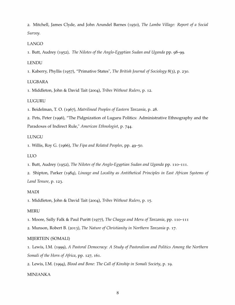
We next document all sources that were used to code the segmentary lineage variable. All

ethnic groups in the sample are listed by classification, along with the source(s) used to determine

whether the ethnic group was a segmentary lineage society or not. If one of the sources is from

the Ethnographic Survey of Africa, it is listed first.

Ethnic groups with segmentary lineages:

ACHOLI

1. Butt, Audrey (1952), The Nilotes of the Anglo-Egyptian Sudan and Uganda, pp. 81–82.

2. Parkin, David (1969) Neighbors and Nationals in an African City Ward, p. 200.

ALUR


2. Southall, Aidan W. (2004), Alur Society: A Study in Processes and Types of Domination, p. 62.

3. Middleton, John & David Tait (2004), Tribes Without Rulers, p. 15.

AMBA

3

1. Taylor, Brian K. (1963), The Western Lacustrine Bantu, pp. 74, 76–77.

2. Runciman, W. G. (1989), A Treatise on Social Theory (Volume II), p. 321.

ANUAK


2. Eisenstadt, S. N. (1959), “Primitive Political Systems: A Preliminary Comparative Analysis,"

American Anthropologist, p. 209.

BALANTE

1. Morier-Genou, Eric (2012), Sure Road? Nationalisms in Angola, Guinea-Bissau & Mozambique, p.

62.

2. Sigrist, Christian (2004), “Segmentary Societies: The Evolution and Actual Relevance of an

Interdisciplinary Conception," Difference and Integration, p. 15.

BAMBARA

1. Paques, Viviana (1954), Les Bambara, pp. 50–51.

BANZA

1. Burssens, Herman (1956), Les peuplades de l’entre Congo-Ubangi (Ngbandi, Ngbaka, Mbanja,

Ngombe et Gens d’Eau), p. 117.

BARI

1. Huntingford, George W. B. (1953), The Northern Nilo-Hamites, pp. 35–36.

2. Barclay, Harold (1982), “Sudan (North): On the Frontier of Islam" in Religion and Societies: Asia

and the Middle East ed. Carlo Caldarola, p. 148.

CHOKWE

1. McCulloch, Merran (1978), The Southern Lunda and Related Peoples, pp. 40–41.

2. Miller, Joseph C. (1977), “Imbangala Lineage Slavery" in Slavery In Africa: Historical and

Anthropological Perspectives eds. Suzanne Miers and Igor Koptoff, p. 207.

DIGO

1. Waaijenberg, Henk (1994) Mijikenda Agriculture in Coast Province of Kenya?: Peasants in between

Tradition, Ecology and Policy, p. 35, 38.

2. UNESCO World Heritage Convention (2008), “The Sacred Mijikenda Kaya Forests," p. 59.

DINKA

4



DOGON

1. Palau Martí, Montserrat (1957), Les Dogon, p. 37.

2. Tait, David (1950), “An Analytical Commentary on the Social Structure of the Dogon," Africa

20(3), p. 197.

DOROBO

1. Huntingford, George W. B. (1969), The Southern Nilo-Hamites, pp. 72–73.

2. Eisenstadt, Shmuel Noah (2009), From Generation to Generation, p. 119.

DUALA

1. Ardener, Edwin (1956), Coastal Bantu of the Cameroons, pp. 51, 57.

2. Teresa, Meredith (2013), Nation of Outlaws, State of Violence, p. 270.

EDO

1. Bradbury, R. E. (1957), The Benin Kingdom and the Edo-Speaking Peoples of the South-Western

Nigeria, pp. 88–89.

EWE

1. Manoukian, Madeline (1952), The Ewe-speaking people of Togoland and the Gold Coast, pp. 22–24.

FALI

1. Palau Martí, Montserrat (1957), Les Dogon, p. 37.

FANG

1. Alexandre, Pierre & Jaques Binet (1960), “Le groupe dit Pahouin (Fang, Boulou, Beti)," Revue

de l’histoire des religions 160(1), pp. 48–49.

2. Terretta, Meredith (2013), Nation of Outlaws, State of Violence: Nationalism, Grassfields Tradition,

and State Building in Cameroon, p. 270.

GA

1. Manoukian, Madeline (1964), Akan and Ga-Adangme Peoples of the Gold Coast, p. 73.


GANDA

1. Fallers, Marcaret Chave (1968), The Eastern Lacustrine Bantu (Ganda, Soga), p. 52.

5

2. F.B. Welbourn, “A Sacral Kingship in Buganda? An Essay in the Meaning of Religion,"

Department of Religious Studies, University of Bristol, p. 2.

GBARI

1. Gunn, Harold D. & F. p. Conant (1960), Peoples of the Middle Niger Region: Northern Nigeria, pp.

94–96.

GISU

1. La Fontaine, J.S. (1959), The Gisu of Uganda, pp. 24–26, 29–31.

2. La Fontaine, J.S., “Witchcraft in Bugisu" in Witchcraft and Sorcery in East Africa eds. John

Middleton and E.H. Winter, p. 188.

GURENSI (TALENSI)

1. Manoukian, Madeline (1951), Tribes of the Northern Territories of the Gold Coast, pp. 26–27.

2. Smith, M.G., “On Segmentary Lineage Systems," in The Journal of the Royal Anthropological

Institute of Great Britain and Ireland 86(2), p. 40.


GUSII

1. Cohen, Yehudi (1971), Man in Adaptation: The Institutional Framework, pp. 294-295.

2. Smith, M.G., “On Segmentary Lineage Systems," in The Journal of the Royal Anthropological


IBO

1. Forde, Darryll & G.I. Jones (1967), The Ibo and Ibibio Speaking Peoples of South Eastern Nigeria,

pp. 15-16.

2. Southall, Aidan (1975), “From Segmentary Lineage to Ethnic Association–Luo, Luhuya, Ibo

and Others" in Colonialism and Change; Ikenna Nzimiro, Studies in Ibo Political Systems ed. Maxwell

Owusu, pp. 100–101.


IDOMA

1. Armstrong, Robert G. (1955), “The Idoma-Speaking Peoples" in Peoples of the Niger-Benue

Confluence ed. Darryll Forde, pp. 94–95.

2. Dudley, B.J. (1968), Parties and Politics in Northern Nigeria, pp. 60–61.

6

ITSEKIRI

1. Lloyd p.C. (1957), “The Itsekiri" in The Benin Kingdom and the Edo-Speaking Peoples of the

South-Western Nigeria ed. R.E. Bradbury, pp. 182, 186.

KAMBA

1. Middleton, John & Greet Kershaw (1972), The Central Tribes of the North-Eastern Bantu, pp.

71–74.

2. Edgerton, Robert B. (1970), “Violence in East African Tribal Societies," in Collective Violence eds.

James F. Short Jr. & Marvin E. Wolfgang, pp. 168–169.

KARANGA

1. Hughes, A.J. B. & J. van Velsen (1954), The Shona and Ndebele of Southern Rhodesia, p. 19.

KIKUYU

1. Middleton, John & Greet Kershaw (1972), The Central Tribes of the North-Eastern Bantu, pp.

23–24, 27–29, 38.

KIPSIGI


KISSI


KONGO

1. Soret, Marcel (1959), Les Kongo, pp. 72–73.

KONJO

1. Taylor Brian K. (1969), The Western Lacustrine Bantu, p. 92.

KONKOMBA

1. Froelich, J. C. et al. (1965), Les population du Nord-Togo, p. 142.


KEWRE

1. Beidelman, T. O. (1967), Matrilineal Peoples of Eastern Tanzania, p. 23.

LAMBA


7

2. Mitchell, James Clyde, and John Arundel Barnes (1950), The Lamba Village: Report of a Social

Survey.

LANGO

1. Butt, Audrey (1952), The Nilotes of the Anglo-Egyptian Sudan and Uganda pp. 98–99.

LENDU

1. Kaberry, Phyllis (1957), “Primative States", The British Journal of Sociology 8(3), p. 230.

LUGBARA


LUGURU


2. Pets, Peter (1996), “The Pidgnization of Luguru Politics: Administrative Ethnography and the

Paradoxes of Indirect Rule," American Ethnologist, p. 744.

LUNGU

1. Willis, Roy G. (1966), The Fipa and Related Peoples, pp. 49–50.

LUO


2. Shipton, Parker (1984), Lineage and Locality as Antithetical Principles in East African Systems of

Land Tenure, p. 123.

MADI


MERU

1. Moore, Sally Falk & Paul Puritt (1977), The Chagga and Meru of Tanzania, pp. 110–111

2. Munson, Robert B. (2013), The Nature of Christianity in Northern Tanzania p. 17.

MIJERTEIN (SOMALI)

1. Lewis, I.M. (1999), A Pastoral Democracy: A Study of Pastoralism and Politics Among the Northern

Somali of the Horn of Africa, pp. 127, 161.

2. Lewis, I.M. (1994), Blood and Bone: The Call of Kinship in Somali Society, p. 19.

MINIANKA

8

1. Holas, Bohumil (2006), Les Sénufo: (y compris les Minianka), pp. 65, 78.

MOBA


MONDARI

1. Huntingford, George W. B. (1953), The Northern Nilo-Hamites, pp. 58, 63–64.

NANDI

1. Huntingford, George W. B. (1953), The Northern Nilo-Hamites, pp. 24–26.

NDEMBU

1. McCulloch, Merran (1978), The Southern Lunda and Related Peoples, pp. 18–21.

2. Gough, Kathleen (1961), “Descent Group Variation Among Mobile Cultivators" in Matrilineal

Kinship eds. David Murray Schneider & Kathleen Gough, p. 537.

NGBANDI

1. Burssens, Herman (1956), Les Peuplades de l’Entre Congo-Ubangi (Ngbandi, Ngbaka, Mbanja,


NGURU


NUER



POKOMO

1. Prins, A. H. J. (1952), The Coastal Tribes of the North-Eastern Bantu, pp. 16–22.

REGA

1. Biebuyck, Daniel p. (1973), Lega Culture: Art, Initiation and Moral Philosophy Among a Central

African People, pp. 44–46.

2. Biebuyck (1973), p. 46.

RUANDA

1. Trouwborst, A. A., Mercel d’Hertefelt & J. H. Scherer (1962), Les Anciens royaumes de la zone

interlacustre méridionale, Rwanda, Burundi, Buha, p. 41.

9

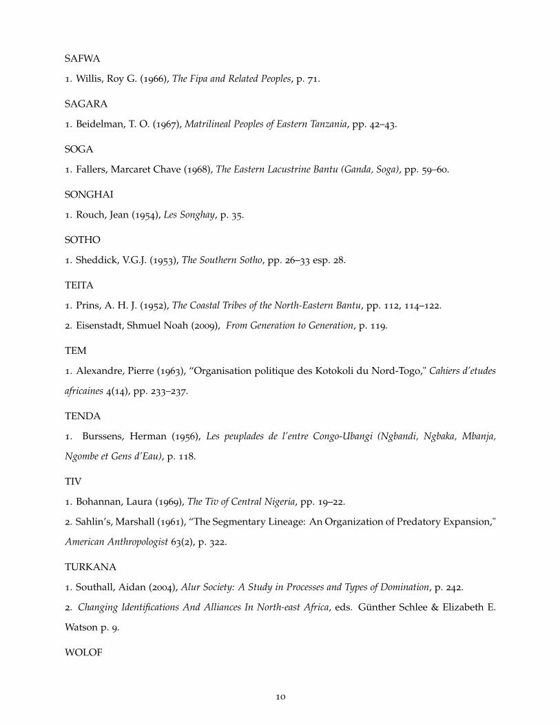
SAFWA

1. Willis, Roy G. (1966), The Fipa and Related Peoples, p. 71.

SAGARA

1. Beidelman, T. O. (1967), Matrilineal Peoples of Eastern Tanzania, pp. 42–43.

SOGA

1. Fallers, Marcaret Chave (1968), The Eastern Lacustrine Bantu (Ganda, Soga), pp. 59–60.

SONGHAI

1. Rouch, Jean (1954), Les Songhay, p. 35.

SOTHO

1. Sheddick, V.G.J. (1953), The Southern Sotho, pp. 26–33 esp. 28.

TEITA

1. Prins, A. H. J. (1952), The Coastal Tribes of the North-Eastern Bantu, pp. 112, 114–122.

2. Eisenstadt, Shmuel Noah (2009), From Generation to Generation, p. 119.

TEM

1. Alexandre, Pierre (1963), “Organisation politique des Kotokoli du Nord-Togo," Cahiers d’etudes

africaines 4(14), pp. 233–237.

TENDA

1. Burssens, Herman (1956), Les peuplades de l’entre Congo-Ubangi (Ngbandi, Ngbaka, Mbanja,


TIV

1. Bohannan, Laura (1969), The Tiv of Central Nigeria, pp. 19–22.

2. Sahlin’s, Marshall (1961), “The Segmentary Lineage: An Organization of Predatory Expansion,"

American Anthropologist 63(2), p. 322.

TURKANA

1. Southall, Aidan (2004), Alur Society: A Study in Processes and Types of Domination, p. 242.

2. Changing Identifications And Alliances In North-east Africa, eds. Günther Schlee & Elizabeth E.

Watson p. 9.

WOLOF

10

1. Gamble, David (1957), The Wolof of Senegambia, pp. 46–52.

YAKO

1. Smith, M. G. (1956), “On Segmentary Lineage Systems" The Journal of the Royal Anthropological


2. Douglass, Mary & Phyllis Kaberry (1969), Man in Africa p. xxii.

YORUBA

1. Forde, C. Daryll (1951), The Yoruba Speaking Peoples of South Western Nigeria, pp. 10–15.

ZANDE

1. Vansina, Jan M. (1990), Paths in the Rainforest, p. 116.

ZIGULA


ZULU

1. Laband, John (2007), Kingdom in Crisis: The Zulu Response to the British Invasion of 1879, p. 23.

2. Radcliffe-Brown, A. R. & Daryll Forde (1950), African Systems of Kinship and Marriage, p. 186.

Ethnic groups without segmentary lineages:

AKYEM

1. Bamfo, Napoleon (2000), “The Hidden Elements of Democracy among Akyem Chieftaincy:

Enstoolment, Destoolment, and Other Limitations of Power," Journal of Black Studies 31(2), pp.

1156–1157.

BAGIRMI

1. Azevedo, M. J. (2005), The Roots of Violence: A History of War in Chad, pp. 28–33.

BAKAKARI


39–40.

BAMILEKE

1. Littewood, Margaret (1954), “Bamum and Bamileke" in Peoples of the Central Cameroons ed.

Merran McCulloch, pp. 102–103.

11

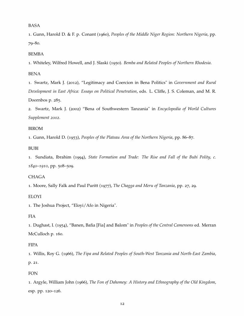
BASA


79–80.

BEMBA

1. Whiteley, Wilfred Howell, and J. Slaski (1950). Bemba and Related Peoples of Northern Rhodesia.

BENA

1. Swartz, Mark J. (2012), “Legitimacy and Coercion in Bena Politics" in Government and Rural

Development in East Africa: Essays on Political Penetration, eds. L. Cliffe, J. S. Coleman, and M. R.

Doornbos p. 285.

2. Swartz, Mark J. (2002) “Bena of Southwestern Tanzania" in Encyclopedia of World Cultures

Supplement 2002.

BIROM

1. Gunn, Harold D. (1953), Peoples of the Plateau Area of the Northern Nigeria, pp. 86–87.

BUBI

1. Sundiata, Ibrahim (1994), State Formation and Trade: The Rise and Fall of the Bubi Polity, c.

1840–1910, pp. 508–509.

CHAGA

1. Moore, Sally Falk and Paul Puritt (1977), The Chagga and Meru of Tanzania, pp. 27, 29.

ELOYI

1. The Joshua Project, “Eloyi/Afo in Nigeria".

FIA

1. Dughast, I. (1954), “Banen, Bafia [Fia] and Balom" in Peoples of the Central Cameroons ed. Merran

McCulloch p. 160.

FIPA

1. Willis, Roy G. (1966), The Fipa and Related Peoples of South-West Tanzania and North-East Zambia,

p. 21.

FON

1. Argyle, William John (1966), The Fon of Dahomey: A History and Ethnography of the Old Kingdom,

esp. pp. 120–126.

12

GURMA

1. Skutsch, Carl (2013), Encyclopedia of the World’s Minorities, p. 534.

HAYA

1. Taylor, Brian K. (1962), The Western Lacustrine Bantu, p. 134.

IBIBIO

1. Forde, Darryll & G.I. Jones (1967), The Ibo and Ibibio Speaking Peoples of South Eastern Nigeria,

pp. 72–73.

IGALA

1. Armstrong, Robert G. (1955), “The Igala" in Peoples of the Niger-Benue Confluence ed. Darryll

Forde, pp. 86–87.

IGBIRA

1. Brown, Paula (1955), “The Igbira" in Peoples of the Niger-Benue Confluence ed. Darryll Forde, pp.

63–64.

IRAQW

1. Huntingford, G.W.B. (1969), The Southern Nilo-Hamites, p. 130.

JERAWA, CHAWAI (SW)

1. Gunn, Harold D. (1953), Peoples of the Plateau Area of the Northern Nigeria, p. 23.

KABRE

1. Piot, Charles D. (1993), “Secrecy, Ambiguity, and the Everyday in Kabre Culture" American

Anthropologist 95(2), pp. 355–356.

KAMUKU


65–66.

KANEMBU

1. Bondarev, Dimitry & Abba Tijani (2014), “Performance of Multilayered Literacy: Tarjumo

of the Kanuri Muslim Scholars" in African Literacies: Ideologies, Scripts, Education eds. Ashraf

Abdelhay, Yonas Mesfun Asfaha & Kasper Juffermans, pp. 119–120.

KATAB

13

1. Gunn, Harold D. (1956), Pagan Peoples of the Central Area of Northern Nigeria, pp. 67, 74, 85.

KORANKO

1. McCulloch, Merran (1950), The Peoples of the Sierra Leone Protectorate, pp. 91–92.

KORO

1. Gunn, Harold D. & F. p. Conant (1960), Peoples of the Middle Niger Region: Northern

Nigeria, p. 120.

KPE

1. Ardener, Edwin (1956), The Coastal Bantu of the Cameroons, pp. 54, 71.

KUBA

1. Vansina, Jan (1978), “The Kuba State," in The Early State eds. H.J.M. Claessen & Peter Skalink,

pp. 359–360.

KUKU

1. Huntingford, G.W.B. (1968), The Northern Nilo-Hamites, pp. 45–46, 48.

KUNG

1. Lee, Richard B. (1972), “The Intensification of Social Life Among the !Kung Bushmen," in

Population Growth: Anthropological Implications ed. B. Spooner, pp. 346–348.

KURAMA, GURE (NE)

1. Gunn, Harold D. (1956), Pagan Peoples of the Central Area of Northern Nigeria, pp. 42–43.

LELE

1. Douglas, Mary (1963), The Lele of Kasai, p. 51.

LOTUKO

1. Somerset, Fitz R.R. (1918), “The Lotuko" in Sudan Notes and Records 1(3), p. 155.

LOZI

1. Turner, V.W. (1954), The Lozi Peoples of North-Western Rhodesia, p. 33.

LUBA

1. Maret, Pierre de (1979), “Luba Roots: The First Complete Iron Age Sequence in Zaire" Current

Anthropology 20(1), p. 234.

LUNDA

14

1. McCulloch, Merran (1978), The Southern Lunda and Related Peoples, pp. 11–12, 19.

LUCHAZI

1. McCulloch, Merran (1978), The Southern Lunda and Related Peoples, p. 67.

MAKONDE

1. Douglas, Mary (1950), The Peoples of the Lake Nyasa Region, p. 28.

MAKUA


MAMVU

1. Geluwe, H. van (1957), Mamvu-Mangutu et Balese-Mvuba, pp. 56, 61.

MASAI


2. Southall, Aidan (2004), Alur Society: A Study in Processes and Types of Domination, p. 243.

MATAKAM

1. Lembezat, B. (1950), Lew Populations Paiennes du Nord-Cameroun, pp. 37–39.

MBUNDU

1. McCulloch, Merran (1952), The Ovimbundu of Angola, pp. 17, 29.

MENDE

1. McCulloch, Merran (1950), The Peoples of the Sierra Leone Protectorate, p. 16.

MUM

1. Littewood, Margaret (1954), “Bamum and Bamileke" in Peoples of the Central Cameroons ed.

Merran McCulloch p. 66.

MUNDANG

1. Schilder, Kees (1993), “Local Rulers in Northern Cameroon: The Interplay of Politics and

Conversion" Afrika Focus 9(1-2), pp. 44–45.

NDEBELE

1. Hughes, A.J.B. & J. van Velsen (1954), The Shona and Ndebele of Southern Rhodesia, pp. 63–64.

NEN

1. Dugast, I. (1954), “Banen, Bafia, and Balom" in Peoples of the Central Cameroons ed. Merran

15

McCulloch, p. 141.

NGWATO (TSWANA)

1. Schapera, Isaac & John L. Comaroff (1953), The Tswana, p. 34.

NKOLE

1. Steinhart, Edward I. (1978), “Ankole: Pastoral Hegemony," in The Early State eds. Claessen,

H.J.M., and Peter Skalník, pp. 132–135 & throughout.

NUPE

1. Forde, Darryll (1955), “The Nupe" in Peoples of the Niger-Benue Confluence ed. Darryll Forde, p.

32.

NYAKYUSA


NYAMWEZI

1. Abrahams, R. G. (1967), The Peoples of Greater Unyamwezi, Tanzania, p. 43.

NYANJA


NYORO

1. Taylor, Brian K. (1963), The Western Lacustrine Bantu, pp. 21–22, 25.

PIMBWE

1. Seel, Sarah-Jane, Peter Mgawe, Monique Mulder, & Mizengo K.P. Pinda, (2014), The History

and Traditions of the Pimbwe, p. 20 & throughout.

SANDAWE

1. Raa, Eric Ten (1970), “The Couth and the Uncouth: Ethnic, Social and Linguistic Deviations

Among the Sandawe of Central Tanzania" Anthropos 65(1-2), pp. 145–146.

SHERBRO


SHILLUK


SINZA

16

1. Taylor, Brian K. (1963), The Western Lacustrine Bantu, p. 146.

SONINKE

1. Juang, Richard M. (2002), Africa and the Americas: Culture, Politics, and History, p. 522.

2. Alexander, Leslie (2010) Encyclopedia of African American History. p. 79.

SUKUMA


SUMBWA


SUSU

1. Thayer, J.S. (1981), Religion and social organization among a West African Muslim people: The Susu

of Sierra Leone, p. 1.

TEMNE


TIKAR

1. Merran McCulloch (1954), “Tikar" in Peoples of the Central Cameroons ed. Merran McCulloch,

pp. 30–31.

2. Ngengong, Tangie Evelyn (2007), From Friends to Enemies: Inter-Ethnic conflict amongst the Tikars

of the Bamenda Grassfields (North West Province of Cameroon) C. 1950–1998, p. 2.

TOPOTHA

1. Müller-Dempf, Harald K. (1991), “Generation-Sets: Stability and Change, with Special

Reference to Toposa and Turkana Societies," Bulletin of the School of Oriental and African Studies

54(3), pp. 561–562.

TORO

1. Taylor, Brian K. (1963), The Western Lacustrine Bantu, pp. 47, 50.

TUMBUKA

1. Douglas, Mary (1950), The Peoples of the Lake Nyasa Region, pp. 58–61.

VAI

1. McCulloch, Merran (1950), The Peoples of the Sierra Leone Protectorate, pp. 91–92.

17

YALUNKA

1. Fyle, C.M. (1979), The Solima Yalunka Kingdom: Pre-Colonial Politics, Economics & Society, pp. 12,

48–49.

YAO


C. Geographic variables (ethnicity level)

• Land Area. The land area occupied by each ethnic group calculated in square kilometers

from the Murdock Map (Murdock, 1959).

• Distance to National Border. Distance calculated in kilometers from the centroid of each

ethnic group in the Murdock Map (Murdock, 1959) to the nearest national border.

• Split Ethnic Group Indicator. An indicator that equals one when at least 10% of an

ethnic group’s land area partitioned into different countries. This variable is motivated

by Michalopoulos and Papaioannou (2016).

• Agricultural Suitability Index and Crop-Specific Maximum Potential Yield. The suit-

ability index is calculated by the Food and Agriculture Organization (FAO) and reported

in their Global Agro-Ecological Zones (GAEZ) database. We compute the average suitability

for each ethnic group using the shapefile associated with Plate 46 that can be accessed at:

http://webarchive.iiasa.ac.at/Research/LUC/GAEZ/index.htm. The index ranges from

0-1. The crop-specific suitability measures are computed from the maximum potential yield

data files for those crops reported by FAO GAEZ and are measured in hectograms per

hectare. For both the suitability index and the measures for individual crops, we assume

rain-fed cultivation with low input use.

• Elevation. Calculated as the mean elevation in kilometers in each ethnic group as defined by

the boundaries on the Murdock Map (Murdock, 1959). Data are from GTOPO30, a “global

digital elevation model (DEM) with a horizontal grid spacing of 30 arc seconds," which can

be accessed at: https://lta.cr.usgs.gov/GTOPO30.

18

• Ecological Diversity. This variable measures of local ecological diversity and is constructed

as a Herfindahl index from the shares of the area in an ethnic group that are located in each

ecological zone. These data are from Fenske (2014).

• Temperature. Calculated as the mean temperature in degrees Celsius within an ethnic

group’s boundaries as defined by Murdock (1959). The data used for this measure are from

Alsan (2015), and originally from the University of East Anglia Climatic Research Unit:

http://www.cru.uea.ac.uk/data.

• Malaria Ecology Index and Tse Tse Suitability Index. The malaria ecology index is

computed from a model incorporating both the “human biting tendency” of the mosquito

and the mortality rate; data used to compute the index are collected from field studies and

incorporate the most prevalent mosquito type in a given area. These data are from Alsan

(2015), and originally from Kiszewski, A.Mellinger, Spielman, Malaney, Sachs and Sachs

(2004). The Tse Tse Suitability Index is a measure of how favorable the environment of each

ethnic group is to the Tse Tse Fly. This measure is from Alsan (2015).

• Sickle Cell Allele Frequency. This variable measures the average frequency of the sickle

cell allele in each ethnic group. The data are from Depetris-Chauvin and Weil (2017) and

were originally constructed by Piel, Patil, Howes, Nyangiri, Gething, Williams, Weatherall

and Hay (2010).

• Latitude & Longitude. Calculated at the centroid of each ethnic group in the Murdock Map

(Murdock, 1959).

• Precipitation. The rainfall data are from the Tropical Rainfall Measuring Mission (TRMM)

satellite. Wherever possible, TRMM data are also validated using data from “ground-based

radar, rain gauges and disdrometers” (https://pmm.nasa.gov/TRMM/ground-validation).

The TRMM precipitation data are available at a 0.25-by-0.25-degree resolution at three-hour

intervals. We first calculate the average daily precipitation (mm) in each month and grid-

cell. We then calculate the average daily precipitation for each month and ethnic group by

taking the average over all grid-cells that fall within the land occupied by each ethnicity,

where ethnic group land area is defined by Murdock (1959). The data can be accessed

at https://pmm.nasa.gov/data-access/downloads/trmm. The relevant download is the

19

“3B42 RT: 3-Hour Realtime TRMM Multi-satellite Precipitation Analysis.”

D. Historical characteristics (ethnicity level)

• Levels of Jurisdictional Hierarchy Beyond the Local Community. Variable v33 from

Murdock’s Ethnographic Atlas. This variable takes integer values from 1–5.

• Levels of Jurisdictional Hierarchy of the Local Community. Variable v32 from Murdock’s

Ethnographic Atlas. This variable takes integer values from 1–3.

• Election of Local Headman. Coded from variable v72 in Murdock’s Ethnographic Atlas.

We construct an indicator variable that equals 1 if v72=6 (that is, if succession to the office

of local headman determined by “election or other formal consensus, nonhereditary”).

• Property Rights in Land. Coded from variable v74 in Murdock’s Ethnographic Atlas as

an indicator variable that equals 1 if v74 is not equal to 1 (‘absence of individual property

rights’).

• Settlement Complexity. Variable v30 from Murdock’s Ethnographic Atlas. This variable

takes integer values from 1–8 increasing in pre-colonial settlement complexity. The cate-

gories range from ‘nomadic or fully migratory’ (1) to ‘complex settlements’ (8).

• Major City in 1800. An indicator that equals 1 if a major city fell within the Murdock

boundary of the ethnic group in 1800. Geospatial data on city location – defined as locations

with over 20,000 inhabitants – are from Chandler (1987). They have been used in Nunn and

Wantchekon (2011), Alsan (2015), Michalopoulos and Papaioannou (2016), among other

studies.

• Population Density. Ethnic group population density, parameterized as log (0.01 + pop-

ulation per square kilometer), is computed for 1960. The data, from the UN Environ-

ment Programme / Global Resource Information Database (UNEP/GRID), can be accessed at:

https://na.unep.net/siouxfalls/datasets/datalist.php.

• Single Inheritor of Land. Coded from variable v75 in Murdock’s Ethnographic Atlas as

an indicator variable that equals 1 if v75 is equal to 2, 3, or 4 (exclusive, ultimogeniture, or

primogeniture).

20

• Patrilineality and Matrilineality. Coded from variable v43 in Murdock’s Ethnographic

Atlas as indicator variables that equals 1 when v43 = 1 (‘patrilineal’) or 3 (‘matrilineal’),

respectively.

• Patrilocality and Matrilocality. Coded from variable v12 in Murdock’s Ethnographic

Atlas as indicator variables that equals one when v12 = 8 (‘patrilocal’) or 5 (‘matrilocal’)

respectively.

• Polygyny. Coded from variable v9 in Murdock’s Ethnographic Atlas as an indicator variable

that equals one if v9>2

• Cousin Marriage. Coded from variable v24 in Murdock’s Ethnographic Atlas as indicator

variables that equals one when v24 is not equal to 8 (‘no first or second cousin marriages’).

• Bride Price. Coded from variable v6 in Murdock’s Ethnographic Atlas as indicator variables

that equals one when v6 = 1 (‘bride price or bride wealth’).

• Presence of Active God. Coded from variable v34 in Murdock’s Ethnographic Atlas. We

construct an indicator that equals 1 if v34=3 or 4 (i.e. if there is a high god that is either

“active in human affairs but not supportive of human morality" or “supportive of human

morality.")

• Herding Society. Constructed as in Becker (2019) as an interaction between the ethnic

group’s dependence on agriculture and an indicator that equals one if the if the group’s

predominant animal is a herding animal. Dependence on agriculture (measured as a share

of total subsistence, between 0 and 1) is computed from v4 in Murdock’s Ethnographic

Atlas using the midpoint of each bin. The herding animal indicator is also constructed from

Murdock’s Ethnographic Atlas. as an indicator that equals one if v40>2. The final variable

ranges from 0–1.

• Female Participation in Agriculture. Coded from variable v54 in Murdock’s Ethnographic

Atlas. We construct from v54 a variable that takes integer values from 1–5 increasing in

female participation in agriculture. The raw v54 variable takes integer values ranging from

1–9. We exclude groups where v45>6. No ethnic groups in the Ethnographic Atlas are

coded as 7 or 8, and groups are coded as 9 if agriculture is an “absent or unimportant

21

activity." We also combine groups coded as 3 or 4 into a single category, since both suggest

equal participation of men and women in agriculture.

• Historical Dependence on Gathering, Hunting, Fishing, Animal Husbandry, and Agri-

culture. Variables v1–v5 respectively in Murdock’s Ethnographic Atlas. The variables take

integer values from 0–9 increasing in percent dependence on the food source. For example,

the integer 0 indicates 0–5% dependence while 9 indicates 86–100% dependence.

• Intensity of Agriculture. Variable v28 from Murdock’s Ethnographic Atlas. The variable

takes integer values from 1–6 increasing in agricultural intensity. The categories range from

‘no agriculture’ (1) to ‘intensive irrigated agriculture’ (6)

• Historical Slave Exports. We use ethnic group-level measures of At-

lantic and Indian Ocean slave exports from Nunn and Wantchekon (2011):

https://scholar.harvard.edu/nunn/pages/data-0. Following Nunn (2008), we

normalize slave exports by land area using ethnic group land area in the map from

(Murdock, 1959).

• Mission Stations. Data on the location of Catholic and Protestant mission states are from

Nunn (2010), originally from Roome (1924). We compute an indicator that equals one if

there was a mission station in an ethnic group using the digitized geo-coded map from

Nunn (2010).

• Railway Lines. Data on the location of colonial railways are from Nunn and Wantchekon

(2011), and originally from Century Company (1911). We compute an indicator that equals

one if an ethnic group is intersected by a colonial railway line.

• Pre-Colonial Conflict. We use historical conflict data from Besley and Reynal-Querol (2014)

and Jaques (2007). Using Besley and Reynal-Querol (2014), we construct an indicator that

equals 1 for ethnic groups that experienced a pre-colonial conflict between 1400AD and

1700AD. Using Jaques (2007), we construct an indicator that equals 1 for ethnic groups that

experienced a pre-colonial conflict between 0 and 1900AD. We also compute each group’s

total number of conflicts and number of years with at least one conflict in the Jaques (2007)

data. Conflicts were linked to ethnic groups using the location of each conflict and the map

from (Murdock, 1959).

22

E. Contemporary characteristics (ethnicity level)

• Muslim Majority. We construct an indicator that equals 1 if the majority of an ethnic

group’s population is Muslim. This was coded individually for each ethnic group using the

World Religion Database: http://www.worldreligiondatabase.org/wrd_default.asp.

• Light Density. Following Michalopoulos and Papaioannou (2013), we compute light density

as the average luminosity across pixels that fall within an ethnic group’s boundaries in

Murdock (1959). For the empirical analysis, we take the log of ethnicity-level light density

normalized by population. We use data from the U.S. National Oceanic and Atmospheric

Administration/National Geophysical Data Center Earth Observation Group, which can be

accessed at: https://ngdc.noaa.gov/eog/.

F. Motivation behind the characteristics examined in Table 1

We now discussion the reasoning and motivation behind the characteristics examined in Table

1. Panel A of Table 1 includes the twelve conflict outcome variables that we use throughout the

analysis. These are discussed in detail in Section A of the paper. Panels B, C, and D report balance

tests for variables that are geographic, historical, and contemporary in nature.

Panel B: Geographic Variables. A first set of geographic variables are included because they are

potentially correlated with conflict. These include each ethnic group’s: land area, distance to the

nearest national border, and an indicator if a group is split by a national border (Michalopoulos

and Papaioannou, 2016).

A next set of geographic characteristics is designed to capture differences across ethnic groups

in productivity and the potential for self-sufficiency and trade. This was motivated in part by

the fact that some anthropological work suggests that geographic characteristics related to self-

sufficiency and trade affected the emergence of segmentary lineage organization (e.g. Forde, 1953,

1970, Verdon, 1982). To capture local agricultural productivity, we include a total agricultural

suitability index, as well as separate measures of each group’s suitability for maize, cassava,

millet, sorghum, potato and yam. To capture factors that might be correlated with access to

or demand for trade, we included measures of elevation, a measure of ecological diversity from

Fenske (2014), the standard deviation of agricultural suitability, an indicator for whether an ethnic

23

group is on the coast, an indicator if it contains a perennial river, terrain ruggedness, and average

temperature.

The next set of geographic characteristics are motivated by the hypothesis, discussed recently

in Enke (2019), that a hostile disease environment makes individuals less likely to venture beyond

the limits of their own ethnic groups, which might make the development of segmentary lineage

organization more likely. Therefore, we include in our set of geographic variables a malaria

suitability index, a tsetse fly suitability index, and a measure of sickle cell allele frequency, which

is a measure of the historical prevalence of malaria.

Finally, we include latitude, longitude, and absolute latitude to assess whether segmentary

lineage groups and non-segmentary lineage groups are systematically located in different parts

of sub-Saharan Africa.

Panel C: Ethnicity-Level and Historical Variables. The ethnicity-level and historical characteristics

reported in Panel C of Table 1 are meant to capture characteristics that could be correlated

with segmentary lineage organization and/or conflict. In segmentary lineage societies, lineage

segments take a corporate form and affect administrative and political organization. Therefore,

it is important to know whether segmentary lineage societies are, on average, different from

non-segmentary lineage societies along observable political dimensions. The political variables

that we include are: levels of jurisdictional hierarchy beyond the local level, levels of jurisdictional

hierarchy of the local community, an indicator that equals one if the headman is elected, and an

indicator for the presence of individual property rights in land.

It also might be the case that, historically, segmentary lineage societies were poorer than non-

segmentary lineage societies. If this were true, then then it would affect our interpretation of

the mechanism underpinning our baseline results. To check for this, we include measures of

settlement pattern complexity, the presence of a city in 1800, and population density in 1960.

Segmentary lineage organization might be correlated with a range of characteristics of an

ethnic group’s social structure. Motivated by this, we examine a range of ethnicity-level charac-

teristics related to other features of an ethnic group’s social structure, including indicators that

equal one if: land is inherited by a single child, descent is patrilineal, descent is matrilineal,

living arrangements are patrilocal, living arrangements are matrilocal, marriage customs are

polygynous, there is cousin marriage, and the marriage custom is bride price. We also examine

24

an indicator that equals one if the ethnic group believes in a moralizing high God.

We also include a measure of traditional reliance on pastoralism, measured using the de-

pendence on pastoralism index from Becker (2019). This is done to examine the potential that

segmentary lineage organization might be correlated with a ‘culture of honor’, which can lead to

an escalation of violence and conflict (Nisbett and Cohen, 1996, Grosjean, 2014). We also include

female participation in agriculture to check whether the role of women (in this activity) is different

in segmentary lineage societies.

It has been hypothesized that segmentary lineage societies are more likely to develop in

particular geographic settings. While we included a range of geographic characteristics to test for

these differences in Panel B, in Panel C we include additional measure that capture geographic

endowments that affect the nature of subsistence activities and production. These are a group’s:

dependence on agriculture, dependence on husbandry, intensity of agricultural production.

The last set of variables we include are measures of historical European contact, before and

during the colonial period. Given the evidence of the effects of the various forms of European

contact on African development, we check whether segmentary lineage organization is associated

with these. The variables we include are: (natural log of) slave exports, an indicator for the

presence of a Christian mission station, and an indicator for the presence of a colonial railroad.

Panel D: Contemporary Variables. The contemporary controls are included to better understand

whether segmentary lineage societies are systematically poorer or more unequal today. If this

is the case, our results might be due, in part, to the effect of poverty or inequality on conflict

rather than solely a direct effect of the social structure. To measure wealth today, we include light

density in 2010 (in levels and logs). To measure inequality, we include the standard deviation

of light density in 2010 (in levels and logs). To capture recent changes in wealth and inequality,

we also include the growth in the mean and standard deviation of light density from 2000–2010.

Last, we include an indicator variable that equals one if an ethnic group is majority Muslim today.

G. Grid-cell level characteristics

• Self-Reported Ethnicity. Self reported ethnicity, used in Figure 5, is from geo-referenced

versions of rounds 3–6 of the Afrobarometer Surveys. Individuals in the survey were matched

to grid cells based on their location (latitude and longitude). To construct Figure 5, for each

25

grid cell in a segmentary lineage society (based on the Murdock Map and our coding) in

our sample, we compute the fraction of individuals from the Afrobarometer Surveys whose

self-reported ethnicity matched the segmentary lineage society. For each grid cell in a non-

segmentary lineage society, we compute the fraction of individuals from the Afrobarometer

survey whose self reported ethnicity matched the adjacent segmentary lineage society. This

variable is on the y-axis in Figure 5.

• Latitude and Longitude. Latitude and longitude are computed at the centroid of each grid

cell.

• Agricultural Suitability Index. This suitability index is from the Food and

Agriculture Organization’s (FAO) GAEZ database and is calculated for rain-fed

crops and low input intensity. We compute the average suitability for each

grid cell using the shapefile associated with Plate 46 that can be accessed at:

http://webarchive.iiasa.ac.at/Research/LUC/GAEZ/index.htm.

• Split Grid Cell. An indicator that equals one if a grid cell is intersected by an international

border. This variable is motivated by Michalopoulos and Papaioannou (2016).

• Elevation and Slope. Data for both elevation (m) and slope (degrees) are from GTOPO30,

a “global digital elevation model (DEM) with a horizontal grid spacing of 30 arc seconds,”

which can be accessed at: https://lta.cr.usgs.gov/GTOPO30. To compute slope, we take

the absolute value of each cell in the GTOPO30 data and compute the average over all cells

within each grid cell. This an uphill slope measure equivalent to, for example, the measure

used in Nunn and Puga (2012).

• Temperature. Average grid-cell level temperature in degrees Celsius was calculated

for the period 2000–2010 from the University of East Anglia Climatic Research Unit,

http://www.cru.uea.ac.uk/data.

• Water Coverage. We constructed an indicator that equals one if a grid cell is intersected

by a body of water. Data on the distribution of land water are from the Inland Water Area

Features dataset published by Global Mapping International (GMI). GMI shut down in June

2017.

26

• Cereal Suitability. Agro-ecological suitability cereal crops is from the FAO GAEZ database.

The cereal composite measure incorporates the suitability of wheat, wetland rice, dryland

rice, maize, barley, rye, pearl millet, foxtail millet, sorghum, oat, and buckwheat. We com-

pute average suitability for each grid cell for both measures, assuming rain-fed cultivation

and low input intensity. The data can be accessed at: http://gaez.fao.org/Main.html#.

• Land Cultivation. Data on the distribution of cultivated land, including both irrigated

and rain-fed crops, are from the FAO GAEZ. For each grid cell, we compute the frac-

tion of land under cultivation based on FAO estimates. The data can be accessed at

http://gaez.fao.org/Main.html#.

• Mission Stations. Data on the location of Catholic and Protestant mission states are from

Nunn (2010), originally from Roome (1924). We compute the number of mission stations in

each grid cell using the digitized geo-coded map from Nunn (2010).

• Railway Lines. Data on the location of colonial railways are from Nunn and Wantchekon

(2011), and originally from Century Company (1911). We compute an indicator that equals

one if a grid cell is intersected by a colonial railway line.

• Petroleum. We compute an indicator that equals one if there is an oil field in

the grid cell. Data on the distribution of oil fields is from the Petroleum Dataset

published by the Peace Research Institute Oslo (PRIO), and can be accessed at:

https://www.prio.org/Data/Geographical-and-Resource-Datasets/Petroleum-

Dataset/.

• Diamond Mines. We compute an indicator that equals one if there is a diamond

mine in the grid cell. Data on the distribution of diamond mines is from the

Diamond Resources dataset published by the Peace Research Institute Oslo (PRIO),

and can be accessed at: https://www.prio.org/Data/Geographical-and-Resource-

Datasets/Diamond-Resources/

27

2. Additional Figures

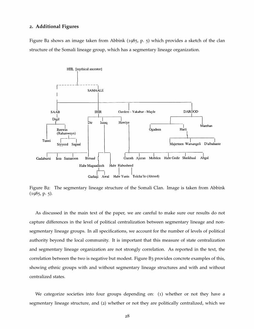
Figure B2 shows an image taken from Abbink (1985, p. 5) which provides a sketch of the clan

structure of the Somali lineage group, which has a segmentary lineage organization.

Figure B2: The segmentary lineage structure of the Somali Clan. Image is taken from Abbink(1985, p. 5).

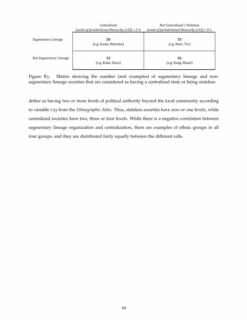
As discussed in the main text of the paper, we are careful to make sure our results do not

capture differences in the level of political centralization between segmentary lineage and non-

segmentary lineage groups. In all specifications, we account for the number of levels of political

authority beyond the local community. It is important that this measure of state centralization

and segmentary lineage organization are not strongly correlation. As reported in the text, the

correlation between the two is negative but modest. Figure B3 provides concrete examples of this,

showing ethnic groups with and without segmentary lineage structures and with and without

centralized states.

We categorize societies into four groups depending on: (1) whether or not they have a

segmentary lineage structure, and (2) whether or not they are politically centralized, which we

28

Centralized NotCentralized/StatelessLevelsofJurisdictionalHierarchy(v33)=2-4 LevelsofJurisdictionalHierarchy(v33)=0-1

SegmentaryLineage 20 53(e.g.Duala,Ndembu) (e.g.Nuer,Tiv)

NotSegmentaryLineage 32 36(e.g.Kuba,Haya) (e.g.Kung,Masai)

Figure B3: Matrix showing the number (and examples) of segmentary lineage and non-segmentary lineage societies that are considered as having a centralized state or being stateless.

define as having two or more levels of political authority beyond the local community according

to variable v33 from the Ethnographic Atlas. Thus, stateless societies have zero or one levels, while

centralized societies have two, three or four levels. While there is a negative correlation between

segmentary lineage organization and centralization, there are examples of ethnic groups in all

four groups, and they are distributed fairly equally between the different cells.

29

3. Text to accompany of Appendix Tables reported in the ‘Supplementary Materials’

In the Supplementary Materials, we present as series of extensions to our baseline OLS estimates.

In this section, we provide further of the details of estimation procedure for those for which this

is necessary.

In Appendix Table A1, we investigate the relationship between characteristics of our baseline

sample and characteristics of ethnic groups in the Ethnographic Atlas outside of our sample. We

report the coefficient on an indicator variable that equals one if a group is in our sample for a

range of outcome variables. The main take away is that groups in the sample are more populous

and have more centralized states, which is intuitive since these are the groups about which there

is most information.

We undertake several tests of the sensitivity of our OLS estimates. We test the robustness of

our results to linking ethnic groups to conflict events using the description of the actors in the

conflict rather than the location of the conflict. These estimates are reported in columns 1–3 of

Appendix Table A5. We also test the robustness of our results by using the UCDP-GED data.

Columns 4–6 of Appendix Table A5 report the results of this exercise for three of our outcome

variables, (log of) total conflict incidents, (log of) total fatalities and (log of) years of conflict. The

results are very similar to our baseline results using the ACLED dataset both in the size of the

coefficients and in their levels of statistical significance, which is reassuring.

An additional check of our cross-ethnic group results is to examine the sensitivity of the

OLS estimates to the inclusion of potentially endogenous variables. Given the evidence from

Besley and Reynal-Querol (2014) that historical conflict is correlated with post-colonial conflict,

we include controls for the intensity of historical conflicts in our baseline regressions. It is

possible that segmentary lineage organization increased conflict in the past, which results in more

present-day conflict. Appendix Table A6 reports estimates where we control for historical conflict

in our baseline regression, using the most conservative specification from Table 2. We measure

conflicts using two sources: Jaques (2007) and Besley and Reynal-Querol (2014). Columns 1–3

report estimates where we control for measures of conflict, from 0–1900AD, taken from Jaques

(2007); either, an indicator for the presence of at least one conflict, the number of conflicts during

the historical period, or years of conflict during the period. Column 4 reports estimates where

we control for the historical incidence of conflict measure taken from Besley and Reynal-Querol

30

(2014). Column 5 simultaneously controls for historical incidence measures from the two sources.

As shown, the estimated coefficients for our variable of interest remain significant and very

similar in magnitude, suggesting that historical conflict and its relationship to current conflict

is not a primary channel.

One potential concern is that our OLS estimates could be driven by outliers or conflicts that

have very large numbers of fatalities and last for longer stretches of time. This could include

conflict events involving the Lord’s Resistance Army in Uganda, in the territory of segmentary

lineage societies such as the Acholi. Although Figure 3 in the paper suggests that this is not an

obvious concern, we also take a more systematic approach to testing for the robustness of our

estimates to the exclusion of outliers. One strategy is to drop observations with high Cook’s

Distance, which is a commonly used measure of the leverage of an observation. Following Bollen

and Jackman (1990), we drop observations with Cook’s Distance greater than 4/n where n = 141

is the number of observations in the regression. These estimates are reported in panel A of

Appendix Table A7. Our results are largely the same, aside from a drop in significance of the

segmentary lineage indicator for outcome variables related to civil conflicts. As an additional

test, we re-estimate the fully-controlled specification for each outcome variable after removing

observations whose value for the dependent variable falls in the top 5 percent. As reported in

Panel B of Appendix Table A7, the estimates remain robust to this procedure.

Another potential concern is that the results are biased by conflict incidents that are incorrectly

or imprecisely geocoded in the ACLED database. To address this, we re-estimate our baseline

regression after excluding conflict incidents coded in the ACLED data as having low geographic

precision. Low precision incidents make up 4.75% of the overall ACLED data. While a minimum

level of geographic information about a conflict incident is required for inclusion in the ACLED

data, an incident is considered to have low geographic precision if the conflict can only be traced

to a “larger region” within a province. These results, which are reported in panel C of Table A7,

are very similar to the baseline estimates.

We also use nearest neighbor matching to compare each segmentary lineage society to the

non-segmentary lineage society that is most similar, based on a range of observable char-

acteristics. We measure distance using Mahalanobis distance, which is defined as Dij =√(Xi −Xj)′S−1(Xi −Xj), where Xi and Xj are vectors of observable covariates and S−1 is

the variance-covariance matrix of Xj .

31

Appendix Table A8 presents the results from this approach using different choices of Xi and

Xj . In column 1, Xi and Xj consist of latitude and longitude. In column 2, they consist of

our baseline set of geographic and historical controls. Finally, in the column 3, we continue

to match ethnic groups based on all geographic and historical controls, and we additionally

impose the requirement that members of a matched pair have the same number of levels of

jurisdictional hierarchy beyond the local community. As discussed in the body of the paper,

levels of jurisdictional hierarchy is of particular interest as a potential confounder. These results

are similarly robust.

Since all of the conflict outcome variables are count variables, we check that our baseline

estimates are robust to the use of count models instead of OLS. In Appendix Table A9, we report

estimates of our most stringent specification but using using either Poisson (columns 1–3) or

negative binomial (columns 4–6) regression models. For all outcome variables, our results remain

robust to these alternative estimation strategies. In all cases, the coefficient of interest is positive

and significant.

The next set of appendix tables in the Supplementary Materials investigate the heterogeneous

effects of segmentary lineage organization. Heterogeneous effects based on country-level charac-

teristics are reported in Table A10 and heterogeneous effects based on ethnicity-level character-

istics are reported in Appendix Table A11. We do not find evidence of heterogeneous effects of

segmentary lineage organization across a range of characteristics. We do find that the relationship

between segmentary lineage organization and conflict is muted in wealthier countries and that

the effect is substantially reduced if there is a capital city in the homeland of the ethnic group.

We also investigate whether the relationship between adverse rainfall shocks and climate is

more pronounced in segmentary lineage societies. Estimates of equation (2) of the paper – the

equation used to estimate the heterogeneous impact of adverse rainfall shocks – are reported in

Appendix Table A12. Results are reported using both the for the log number of deadly conflict

incidents and number of conflict deaths as the outcome variables. Columns 1 and 3 report esti-

mates of a version of equation (2) in the paper that does not have the interaction term. Consistent

with previous estimates, we find that adverse rainfall shocks tend to be associated with greater

conflict (e.g., Miguel, Satyanath and Saiegh, 2004). However, in line with other studies, we also

find that this relationship is not fully robust (e.g., Ciccone, 2013, Buhaug, Nordkvelle, Bernauer,

Bohmelt, Brzoska, Busby, Ciccone, Fjelde, Gartzke, Gleditsch, Goldstone, Hegre, Holtermann,

32

Koubi, Link, Link, Lujala, O’Loughlin, Raleigh, Scheffran, Schilling, Smith, Theisen, Tol, Urdal

and van Uexkull, 2014). In many specifications, the estimated relationship is not statistically

different from zero.

The weak positive relationship between adverse rainfall and conflict masks systematic hetero-

geneity. Allowing for an interaction between adverse rainfall and segmentary lineage organiza-

tion, we find that the effect of adverse rainfall is much stronger for segmentary lineage groups.

For non-segmentary lineage groups, the estimated relationships are not statistically different from

zero.1 The estimated coefficient for the (uninteracted) segmentary lineage indicator variable,

is positive, sizeable, and statistically significant. This is consistent with other factors, besides

adverse rainfall, being a catalyst for conflict – the impact of adverse rainfall is then exacerbated

by segmentary lineage organization.

Next, we turn to a series of tests of the sensitivity and validity of the RD estimates. Appendix

Table A13 presents fuzzy RD estimates using the sample of grid cells matched to at least one

individual in Rounds 3-6 of the Afrobarometer survey. The endogenous variable is the share of

respondents in each grid cell who self identify as a member of the segmentary lineage society in

the cell’s ethnic group pair. Across outcome variables, the fuzzy RD estimates are larger than the

baseline reduced form estimates, suggesting that the difference in magnitude between the OLS

and RD estimates could be driven by the fact that near the border, below 100% of respondents

identify as a member of the group to which their grid cell is assigned.

We also check the robustness of our baseline RD estimates to the use of different estimators

and inclusion of a series of different running variables. These estimates are reported in Appendix

Table A14. For example, in panels B–C, we report Poisson and negative binomial estimates,

and in the remaining panels D–I, we report estimates from regressions that include a wide

variety of running variables, including higher degree polynomials, running variables in latitude

and longitude, and versions of each in which we estimate a separate coefficient for each set of

continuous ethnic groups or ethnic group pair.

Since the RD analysis estimates differences in conflict intensity between regions that are

geographically close, it may be particularly sensitive to imprecision in the geocoding of conflict

1Given the presence of lagged dependent variables in equation (2), there is potential concern about Nickel bias. Ifwe instead use an Arellano-Bond estimator, we obtain very similar results to what we report here. The coefficient onthe interaction term in column 2 of Panel A, for example, is 2.60 and significant at the 5% level. We obtain very similarestimates when we specifications that do not include lags of the dependent variable.

33

events. To address this potential concern, we re-estimate our baseline RD regression after

excluding conflict events coded in the ACLED data as having a low level of geographic precision.

Results from this robustness check are reported in Table A15 and look very similar to the baseline

results. A key assumption of the RD analysis is that observable characteristics vary smoothly at

the ethnic group boundary. To check this, we estimate our baseline RD specification with a series

of geographic and historical grid-cell level variables as the outcome. These results are reported in

Appendix Table A16.

In Appendix Table A18, we examine kinship ties directly. The fact that members of segmentary

lineage societies have closer ties to their kin might help explain the obligation to join in conflict

that involves lineage members. Using individual-level data from rounds 3–6 of the Afrobarometer

Survey, we find that members of segmentary lineage societies have a larger gap in trust between

relatives and non-relatives (other people they know, fellow countrymen, or non-coethnics). This

relationship has been previously documented in by Moscona, Nunn and Robinson (2017).

Next, we investigate a series of other potential mechanisms and differences between segmen-

tary lineage and non-segmentary lineage societies that might drive the baseline result. First, we

examine differences in income and prosperity between segmentary lineage and non-segmentary

lineage societies. Appendix Table A19 reports differences in various proxies for income between

segmentary lineage and non-segmentary lineage societies: (i) wealth, using individual level data

from Demographic and Health Surveys (DHS), (ii) light density at night, and (iii) educational

attainment, also measured using the DHS. We do not find a systematic relationship between seg-

mentary lineage organization and income; if anything, segmentary lineage societies are slightly

richer making it unlikely that variation in income is the causal mechanism. We also examine the

relationship between segmentary lineage organization and access to a series of public goods

using individual-level data from rounds 3–6 of the Afrobarometer Surveys. These results are

presented in Appendix Table A20. Columns 1–6 report the relationship between segmentary

lineage organization and indicator variables for the presence of a series of public goods: electricity,

clean water, sewage, a school, a health clinic, and a police station. In column 7, the outcome

variable is the average of the six indicators and in column 8, it is the first principal component.

We do not uncover any systematic relationship between segmentary lineage organization and

access to public goods.

While we find no relationship between segmentary lineage organization and wealth, it’s still

34

possible that segmentary lineage societies are more unequal. We investigate this possibility in

Appendix Table A21. In columns 1–2, the outcome variable is the (log of the) standard deviation

of light density at night and in columns 3–4 it is the ethnic group level wealth Gini coefficient,

computed from individual-level wealth information in the DHS (see Appendix Table A19). We

find no evidence that segmentary lineage societies are more unequal than non-segmentary lineage

societies.

We also investigate whether segmentary lineage societies are more likely to be excluded from

national politics or discriminated against by the government. The Ethnic Power Relations (EPR)

database determines the extent to which each politically relevant ethnic group has access to state

power at the national level. It identifies groups that are “excluded” from state power and further

categorize those who are excluded into three categories: (i) “Powerless,” which means they hold

no political power and do not influence decision-making in the national executive level, but they

are not actively discriminated against; (ii) “Discrimination”, which means that the ethnic group

is actively and intentionally discriminated against; and (iii) “Self-exclusion,” which means the

ethnic group has intentionally excluded itself from state power by controlling or attempting to

control a territory that they consider independent from the nation state (this is very infrequent).

Using this information, which is provided for each ethnic group and each year since 1960, we

identify the number of years each group was classified as being excluded from power in any way;

as being powerless due to discrimination; and as being powerless but not due to discrimination.

The latter two categories are are mutually exclusive in the EPR data, so the number of years a

group was excluded for any reason is simply the sum of the number of years that the group

was powerless without discrimination and the number of years that the group was discriminated

against. We do not examine the third category (self-exclusion) individually since there is only

one such case in our sample. The estimates are reported in Appendix Table A23.

We also study representation in national politics using data from Francois, Rainer and Trebbi

(2015), which reports the share of all cabinet positions in the national government and the share

of the top cabinet positions in national government that are held by individuals from each ethnic

group. Their data are available for ten African countries since independence. We use these

measures of ethnic representation in the national cabinet, conditioning on the share of each ethnic

group in the total population, as an alternative measure of an ethnic group’s access to state power.

The estimates are reported in Appendix Table A24. We find no evidence using either EPR data or

35

Francois et al. (2015) data that segmentary lineage societies are more likely to be excluded from

politics.

4. Additional Tables

Summary statistics of all variables, calculated at the ethnicity-level are reported in Appendix Table

B2 and summary statistics of variables calculated at the grid-cell-level are reported in Appendix

Table B3.

In Table A4, we report baseline OLS estimates using an interpolated proxy for segmentary

lineage organization for all African ethnic groups in the Ethnographic Atlas using a LASSO

procedure. The estimated coefficients from this procedure are reported in online Appendix Table

B4.

Table B5 reports the results from a set of tests that investigate the potential role of omitted

variables in biasing our baseline results. We employ a strategy adapted by Nunn and Wantchekon

(2011) from Altonji, Elder and Taber (2005) that allows us to determine how much stronger

selection on unobservables would have to be compared to selection on observables in order to

fully explain away our result. To perform this test, we calculate the ratio β̂F /(β̂R − β̂F ), where

β̂F is our coefficient of interest from a regression that includes a full set of controls while β̂R is

our coefficient of interest from a regression that includes a restricted set of covariates.

In the first three columns of Table B5, we report the results for each of the twelve outcome

variables. The country fixed effects, geographic controls, and historical controls are included in

the full set of controls, while the restricted set of controls only includes country fixed effects. Each

panel reports a ratio where the fully-controlled regression includes the geographic and historical

controls, while the restricted regression including country fixed effects only. This yields twelve

ratios that range from −34.64 to 24.05. In some cases, the coefficient in the fully-controlled model

is larger than that on the uncontrolled model giving a negative ratio. The ratios suggest that

the influence of unobservable characteristics would have to be far greater than the influence of

observable characteristics to fully account for our findings.

We also use results from Oster (2017) in order to calculate a lower bound for our coefficient of

interest (columns 4–6). Oster’s result relies on the assumption that observables and unobservables

have the same explanatory power in the outcome variable, then the following estimator is a

36

consistent estimator:β∗ = β̂F − (β̂R − β̂F )× R2max−R2

F

R2F−R2

R, where β̂F and β̂R are as defined above, R2

F

is the R2 from the fully controlled regression, and R2R is the R2 from the regression with restricted

controls. R2max is the R2 from a regression that includes all observable and unobservable controls.

R2max is unobserved; however, we know that the maximum value for R2

max is one and this value

yields the most conservative estimate of β∗. While recent research, such as Gonzalez and Miguel

(2015) has shown that Oster’s R2max should be below one, which thereby raises the lower bound

for β∗, in this analysis we assume R2max = 1 and rely only on the most conservative lower bound

estimate.

We report lower bound estimates corresponding to the fully controlled and restricted regres-

sions in columns 4–6 of Table B5. All lower bound estimates remain positive and economically

significant. These results indicate that it is unlikely that our OLS estimates are biased by the

presence of some unobservable factor, and suggest that the relationship that we have identified

between segmentary lineage organization and conflict is indeed causal.

In the placebo RD analysis discussed in the paper, we construct principal components to

separate ethnic groups into treatment and control categories based on a broad range of historical

characteristics. These principal components are used in panels C and D of Table 4. Table

B6 reports the factor loading of both principal components used to construct the treatment

variables for the placebo RD estimates. The first principal component (columns 7–9 of Table 4)

is constructed from twelve indicator variables for each level of jurisdictional hierarchy and level

of historical settlement complexity. The second principal component (columns 10–12 of Table 4)

adds to these twelve variables additional ethnic group level historical characteristics.

37

Table B2: Summary statistics, ethnicity-level variables.(1) (2) (3) (4) (5)

Obs. Mean. St.Dev Min Max

Ethnicity-LevelVariablesln(1+DeadlyConflictIncidents):AllConflicts 145 2.556 1.798 0 6.685

CivilConflicts 145 1.848 1.848 0 6.846

Non-CivilConflicts 145 2.024 1.577 0 5.852

Within-GroupConflicts 145 1.266 1.299 0 5.094

ln(1+ConflictDeaths):AllConflicts 145 4.006 2.761 0 11.723

CivilConflicts 145 3.109 2.817 0 11.688



ln(1+MonthsofDeadlyConflict):AllConflicts 145 2.158 1.445 0 4.836

CivilConflicts 145 1.631 1.398 0 4.625



GeographicVariables:lnLandArea 145 9.718 1.145 7.424 12.310

MeanAltitude 145 0.365 0.342 0.002 1.676

lnDistancetoNationalBorder 145 4.401 1.099 0.575 6.293

AgriculturalSuitabilityIndex 145 0.564 0.170 0.913 0.857

SplitEthnicGroup(10%) 145 0.317 0.467 0 1

AbsoluteLatitude 145 7.700 5.364 0 29

Longitude 145 19.679 15.994 -17 48

HistoricalVariables:LevelsofJurisdictionalHierarchy 141 1.270 0.992 0 4

SettlementPattern 145 5.821 1.727 0 8

EndogenousVariables:Pre-ColonialConflictIndicator 145 0.083 0.276 0 1

ln(1+LightDensityPerCapita) 145 -6.038 0.909 -6.908 -1.679

ln(Pop.Densityin2000) 145 3.744 1.298 -1.133 7.432

IslamIndicator 145 0.200 0.401 0 1

Notes: Columns 1-5 report summary statistics for the variables listed on the left side of the table. All variableslistedarecalculatedattheleveloftheethnicgroup.

38

Table B3: Summary statistics, grid-cell level.

(1) (2) (3) (4) (5)Obs. Mean. St.Dev Min Max

Grid-CellLevelVariables(BaseSample,<60kmfromBorder)ln(1+DeadlyConflictIncidents):AllConflicts 10739 0.088 0.382 0 5.220CivilConflicts 10739 0.059 0.319 0 5.024Non-CivilConflicts 10739 0.040 0.231 0 4.585Within-GroupConflicts 10739 0.020 0.157 0 3.296

ln(1+ConflictDeaths):AllConflicts 10739 0.158 0.709 0 8.619CivilConflicts 10739 0.103 0.588 0 8.619Non-CivilConflicts 10739 0.077 0.460 0 7.910Within-GroupConflicts 10739 0.042 0.345 0 6.753

ln(1+MonthsofDeadlyConflict):AllConflicts 10739 0.077 0.325 0 4.554CivilConflicts 10739 0.051 0.268 0 4.060Non-CivilConflicts 10739 0.037 0.208 0 4.111Within-GroupConflicts 10739 0.019 0.142 0 2.944

GeographicVariables:lnElevation 10739 6.445 0.991 0 8.375AgriculturalSuitabilityIndex 10739 4.033 1.876 0 9SplitGridCell 10739 0.050 0.217 0 1Slope 10739 3.351 4.600 0 47.684MeanTemperature 10739 24.135 2.748 14.200 30.100WaterIndicator 10739 0.037 0.189 0 1LandCultivated 10739 19.189 18.022 0 84.315PetroleumIndicator 10739 0.030 0.170 0 1DiamondIndicator 10739 0.190 0.392 0 1

HistoricalVariables:MissionStations 10739 0.022 0.157 0 3RailwayIndicator 10739 0.015 0.121 0 1ExplorerRouteIndicator 10739 0.047 0.211 0 1FractionSL,SelfReported 275 0.285 0.381 0 1

Notes: Columns 1-5 report summary statistics for the variables listed on the left side of the table. All variableslisted are calculated at the level of the 10km-by-10km grid-cell, and the summary statisics are reported for thesample used in the baseline regression discontinuity analysis, consisting of all grid-cells within 60km of aborder.

39

Table B4: LASSO coefficients used for the interpolated segmentary lineage measure.

IncludedVariables.EachvariablelistedbelowisaquadrupleinteractionbetweenindicatorsforacategoryofeachofthefollowingfourvariablesfromtheEthnographicAtlas:clanstructure(v15),largestpatrilinealkingroup(v17),largestmatrilinealkinroup(v19),andresidencestructure(v12).

LASSOCoefficient

(missing)x(missing)x(missing)x(patrilocal) -0.445(missing)x(none)x(singlecommunity)x(virilocal) -0.445(missing)x(none)x(sibs)x(matrilocal) 0.475(missing)x(singlecommunity)x(none)x(patrilocal) 0.159(missing)x(sibs)x(none)x(missing) -0.445(missing)x(sibs)x(none)x(patrilocal) -0.224(missing)x(sibs)x(singlecommunity)x(patrilocal) -0.445(seg,nolocalexog.)x(missing)x(missing)x(patrilocal) -0.445(seg,nolocalexog.)x(none)x(none)x(patrilocal) -0.445(seg,nolocalexog.)x(none)x(sibs)x(missing) -0.445(seg,nolocalexog.)x(none)x(sibs)x(avunculocal) -0.215(seg,nolocalexog.)x(none)x(sibs)x(uxorilocaloravunculocal) -0.445(seg,nolocalexog.)x(none)x(sibs)x(matrilocal) 0.245(seg,nolocalexog.)x(singlecommunity)x(none)x(nocommonresidence) 0.475(seg,nolocalexog.)x(singlecommunity)x(none)x(patrilocal) -0.167(seg,nolocalexog.)x(singlecommunity)x(singlecommunity)x(patrilocal) 0.475(seg,nolocalexog.)x(singlecommunity)x(sibs)x(patrilocal) 0.475(seg,nolocalexog.)x(sibs)x(none)x(patrilocal) -0.032(seg,nolocalexog.)x(phratries)x(none)x(patrilocal) -0.445(seg,nolocalexog.)x(moieties)x(none)x(patrilocal) 0.475(agamous)x(none)x(none)x(virilocal) -0.462(agamous)x(none)x(sibs)x(matrilocal) -0.445(agamous)x(none)x(sibs)x(patrilocal) 0.475(agamous)x(singlecommunity)x(none)x(neolocal) -0.445(agamous)x(singlecommunity)x(none)x(patrilocal) -0.129(agamous)x(sibs)x(none)x(neolocal) -0.445(agamous)x(sibs)x(none)x(patrilocal) 0.105(agamous)x(sibs)x(none)x(virilocal) 0.475(exogamous)x(none)x(none)x(ambilocal) -0.445(exogamous)x(none)x(none)x(virilocal) -0.445(exogamous)x(singlecommunity)x(none)x(neolocal) -0.445(exogamous)x(sibs)x(none)x(neolocal) 0.475(exogamous)x(sibs)x(none)x(patrilocal) 0.097(segmented)x(sibs)x(none)x(patrilocal) 0.475(clancommunities)x(none)x(sibs)x(avunculocal) 0.245(clancommunities)x(singlecommunity)x(none)x(patrilocal) -0.267(clancommunities)x(sibs)x(none)x(missing) 0.475(clancommunities)x(sibs)x(none)x(patrilocal) 0.348(clancommunities)x(sibs)x(none)x(virilocal) 0.475(clancommunities)x(sibs)x(matrilinealexog.)x(patrilocal) 0.492(clancommunities)x(phratries)x(none)x(virilocal) 0.475(clancommunities)x(moieties)x(none)x(patrilocal) -0.445Constant 0.485Notes : This table reports LASSO coefficient estimates from the procedure used to produce thesegmentary lineage proxy for all African groups in the Ethnographic Atlas . The first columnreports the variable, which is an interaction between categories from variable v15, v17, v19,and v12 (listed in that order). The second column reports the estimated coefficient. The LASSOcoefficientforinteractionsnotreportediszero.

40

Table B5: Assessing the importance of bias from unobservables by controlling for observablecharacteristics.

(1) (2) (3) (4) (5) (6)

ln(1+DeadlyConflictIncidents)

ln(1+ConflictDeaths)

ln(1+MonthsofConflict)

ln(1+DeadlyConflictIncidents)

ln(1+ConflictDeaths)

ln(1+MonthsofConflict)

PanelA:AllConflicts24.05 7.67 23.83 1.03 1.11 0.82

PanelB:CivilConflicts2.92 4.13 4.55 0.24 0.51 0.35

PanelC:Non-CivilConflicts-11.23 -13.23 -11.37 1.14 1.85 0.95

PanelD:Within-GroupConflicts-29.75 17.92 -34.64 0.87 1.07 0.73

Coeff.RatioTest(Altonji,ElderandTaber,2005) MinimumCoeff.LowerBound(Oster,forthcoming)

Notes : Each cell in columns 1-3 report ratios based on the estimated coefficient for the segmentary lineage indicator fromtwo regressions; one with a more-restricted set of controls, which includes country fixed effects only, and the other with aless-restricted set of controls that includes country fixed effects, our baseline set of geographic controls, and our baselineset of historical controls. If B_R is the coefficient in the restricted set and B_F is the coefficient in the full set, then the ratiois B_F/(B_R-B_F). The controls included in each set are listed on the left side of the table and the dependent variables arelisted at the top. In panels A-D, the dependent variable is constructed using all ACLED conflict, civil conflicts, non-civilconflicts,andwithin-groupconflictsrespectively.Eachcellincolumns4-6reportcoefficientlowerboundsbasedonOster(forthcoming). If we define R2_R as the R2 for the regression with the restricted set of controls and R2_F as the R2 for theregression with the full set of controls, then the minimum coefficient lower bound is: B_F-(B_R-B_F)*((1-R2_F)/(R2_F-R2_R)). Again, the controls in the full and restricted sets are listed on the left side of the table, dependent variables arelistedatthetop,andineachpanelthedependentvariableisconstructedusingadifferentconflicttype.

41

Table B6: Principal component factor loadings for the placebo RD analysis.

FactorLoadings

Columns7-9 Columns10-12LevelsofJurisdictionalHierarchy:Zero 0.0406 0.0235One -0.6203 -0.2411Two 0.4705 0.1979Three 0.2351 0.0649

SettlementComplexity:Nomadicorfullymigratory -0.334 -0.4275Seminomadic -0.2621 -0.2222Semisendentary 0.0197 0.0015Compactbutimpermanentsettlements 0.2207 0.0364Neighborhoodsofdispersedfamilyhomesteads 0.2767 0.0848Separatedhamlets,formingasinglecommunity -0.1095 0.1769Compactandrelativelypermanentsettlements 0.1334 0.0978Complexsettlements -0.0346 0.0651

DependenceonAgriculture - 0.5104DependenceonHusbandry - -0.4875MajorCityin1800 - 0.0433lnSlaveexports(/landarea) - 0.2193lnPop.Density1960 - 0.2071SplitbyNationalBorder - -0.1455

ProportionofVariationExplained: 16.40% 18.90%Notes: Columns 1 and 2 report the factor loadings for the principal component usedto construct the treatment variable in columns of Table 5 respectively. The variablesused to construct the principal component are listed on the left side of the table. Thefirst twelve variables are indicators that equal one if an ethnic group has the listednumber of levels of jurisdictional hierarchy or historical settlement complexity. Theproportion of variation explained by the first principal component used for theanalysisislistedatthebottomofeachcolumn.

Specification

42

References

Abbink, J., The Total Somali Clan Genealogy: A Preliminary Sketch, Leiden: Afrika-Studiecentrum,1985.

Alsan, Marcella, “The Effect of the TseTse Fly on African Development,” American EconomicReview, 2015, 105 (1), 382–410.

Altonji, Joseph G., Todd E. Elder, and Christopher R. Taber, “An Evaluation of InstrumentalVariable Strategies for Estimating the Effects of Catholic Schooling,” Journal of Human Resource,2005, 40 (4), 791–821.

Becker, Anke, “On the Economic Origins of Constraints on Women’s Sexuality,” 2019. Workingpaper, Harvard University.

Besley, Timothy and Marta Reynal-Querol, “The Legacy of Historical Conflict: Evidence fromAfrica,” American Political Science Review, 2014, 108 (2), 319–336.

Bollen, Kenneth A. and Robert W. Jackman, “Regression Diagnostics: An Expository Treatmentof Outliers and Influential Cases,” in J. Fox and J.S. Long, eds., Modern Methods of Data Analysis,Newbury Park, CA: Sage Publications, 1990, pp. 177–215.

Buhaug, H., J. Nordkvelle, T. Bernauer, T. Bohmelt, M. Brzoska, J.W. Busby, A. Ciccone,H. Fjelde, E. Gartzke, N.P. Gleditsch, J.A. Goldstone, H. Hegre, H. Holtermann, V. Koubi,J.S.A. Link, P.M. Link, P. Lujala, J. O’Loughlin, C. Raleigh, J. Scheffran, J. Schilling, T.G.Smith, O.M. Theisen, R.S.J. Tol, H. Urdal, and N. van Uexkull, “One Effect to Rule Them All?A Comment on Climate and Conflict,” Climate Change, 2014, 127, 391–397.

Century Company, The Century Atlas: Africa [map] Matthews-Northrup Company 1911.

Ciccone, Antonio, “Economic Shocks and Civil Conflict: A Comment,” American Economic Journal:Applied Economics, 2013, 3 (4), 215–227.

Depetris-Chauvin, Emilio and David N Weil, “Malaria and Early African Development: Evi-dence from the Sickle Cell Trait,” The Economic Journal, 2017, 128 (610), 1207–1234.

Enke, Benjamin, “Kinship Systems, Cooperation, and the Evolution of Moral Systems,” QuarterlyJournal of Economics, 2019, 134 (2), 953–1019.

Fenske, James, “Ecology, Trade, and States in Pre-Colonial Africa,” Journal of the European Eco-nomic Association, 2014, 12 (3), 75–90.

Forde, Daryll, “The Conditions of Social Development in West Africa: Retrospect and Prospect,”Civilisations, 1953, 3 (4), 471–489.

, “Ecology and Social Structure,” Proceedings of the Royal Anthropological Institute of Great Britainand Ireland, 1970, pp. 15–29.

Francois, Patrick, Ilia Rainer, and Francesco Trebbi, “How is Power Shared in Africa?,” Econo-metrica, 2015, 83 (2), 185–234.

Gonzalez, Felipe and Edward Miguel, “War and Local Collective Action in Sierra Leone: AComment on the Use of Coefficient Stability Approaches,” 2015. Mimeo, University of.

Grosjean, Pauline, “A History of Violence: The Culture of Honor and Homicide in the U.S.South,” Journal of the European Economic Association, 2014, 12 (5), 1285–1316.

43

Jaques, Tony, Battles and Sieges: A Guide to 8,500 Battles from Antiquity through the Twenty-FirstCentury, Westport, CT: Greenwood Press, 2007.

Kiszewski, A., A.Mellinger, A. Spielman, P. Malaney, S.E. Sachs, and J. Sachs, “A. Kiszewskiand A.Mellinger and A. Spielman and P. Malaney and S.E. Sachs and J. Sachs,” American Journalof Tropical Medicine and Hygene, May 2004, 70 (5), 486–498.

Michalopoulos, Stelios and Elias Papaioannou, “Precolonial Ethnic Institutions and Contempo-rary African Development,” Econometrica, 2013, 81 (1), 113–152.

and , “The Long-Run Effects of the Scramble in Africa,” American Economic Review, 2016, 106(7), 1802–1848.

Miguel, Edward, Shanker Satyanath, and Sebastian Saiegh, “Economic Shocks and Civil Con-flict: An Instrumental Variables Approach,” Journal of Political Economy, 2004, 112 (4), 725–753.

Moscona, Jacob, Nathan Nunn, and James A. Robinson, “Keeping It in the Family: LineageOrganization and the Scope of Trust in Sub-Saharan Africa,” American Economic Review Papersand Proceedings, 2017, 107 (5), 565–571.

Murdock, George Peter, Africa: Its Peoples and Their Cultural History, New York: McGraw-HillBook Company, 1959.

, Ethnographic Atlas, Pittsburgh: University of Pittsburgh Press, 1967.

Nisbett, Richard E. and Dov Cohen, Culture of Honor: The Psychology of Violence in the South,Boulder: Westview Press, 1996.

Nunn, Nathan, “The Long-Term Effects of Africa’s Slave Trades,” Quarterly Journal of Economics,2008, 123 (1), 139–176.

, “Religious Conversion in Colonial Africa,” American Economic Review, 2010, 100 (2), 147–152.

and Diego Puga, “Ruggedness: The Blessing of Bad Geography in Africa,” Review of Economicsand Statistics, 2012, 94 (1), 20–36.

and Leonard Wantchekon, “The Slave Trade and Origins of Mistrust in Africa,” AmericanEconomic Review, 2011, 101 (7), 3221–3252.

Oster, Emily, “Unobservable Selection and Coefficient Stability: Theory and Validation,” 2017.Journal of Business Economics and Statistics, forthcoming.

Piel, Frédéric B, Anand P Patil, Rosalind E Howes, Oscar A Nyangiri, Peter W Gething,Thomas N Williams, David J Weatherall, and Simon I Hay, “Global distribution of the sicklecell gene and geographical confirmation of the malaria hypothesis,” Nature communications,2010, 1, 104.

Roome, William R.M., “Ethnographic Survey of Africa: Showing the Tribes and Languages; Alsothe Stations of Missionary Societies [map],” 1924. (1:5,977,382).

Verdon, Michel, “Where Have All Their Lineages Gone?,” American Anthropologist, 1982, 84 (3),566–579.

44

nline appendix to “Kinship and Conflict: Evidence S L S A

Documents

Transcript of nline appendix to “Kinship and Conflict: Evidence S L S A