NIPRL Chapter 10. Discrete Data Analysis 10.1 Inferences on a Population Proportion 10.2 Comparing...
31
NIPRL Chapter 10. Discrete Data Analysis 10.1 Inferences on a Population Proportion 10.2 Comparing Two Population Proportions 10.3 Goodness of Fit Tests for One-Way Contingency Tables 10.4 Testing for Independence in Two-Way Contingency Tables 10.5 Supplementary Problems
-
Upload
brian-coate -
Category
Documents
-
view
221 -
download
1
Transcript of NIPRL Chapter 10. Discrete Data Analysis 10.1 Inferences on a Population Proportion 10.2 Comparing...
NIPRL
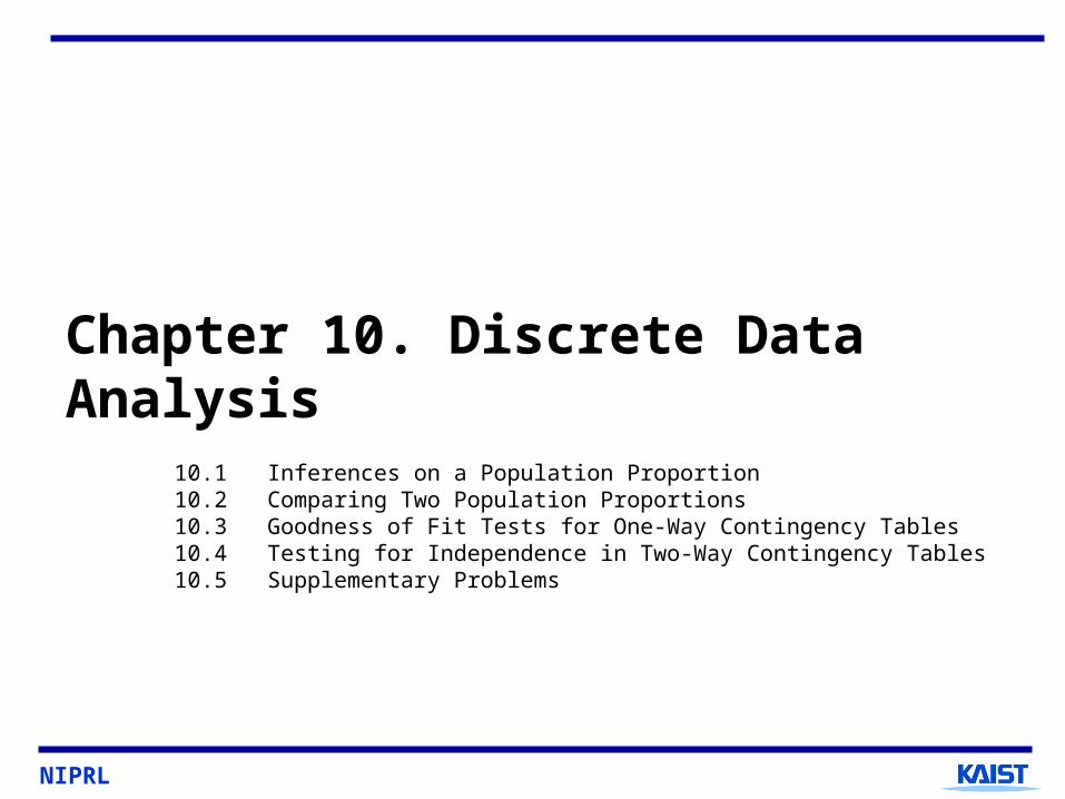
Chapter 10. Discrete Data Analysis
10.1 Inferences on a Population Proportion10.2 Comparing Two Population Proportions10.3 Goodness of Fit Tests for One-Way Contingency Tables10.4 Testing for Independence in Two-Way Contingency Tables10.5 Supplementary Problems
NIPRL 2
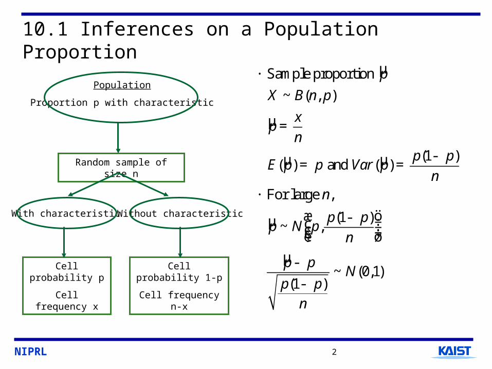
10.1 Inferences on a Population Proportion
µ
µ
µ µ
µ
µ
Sample proportion
~ ( , )
(1 )( ) and ( )
For large ,
(1 )~ ,
~ (0,1)(1 )
p
X B n p
xp
np p
E p p Var pn
n
p pp N p
n
p pN
p pn
·
=
-= =
·
æ ö- ÷ç ÷ç ÷÷çè ø
-
-
Population
Proportion p with characteristic
Random sample of size n
With characteristic Without characteristic
Cell probability p
Cell frequency x
Cell probability 1-p
Cell frequency n-x
NIPRL 3
10.1.1 Confidence Intervals for Population Proportions
µ
µ µ
µ µ
µµ µ
/ 2 / 2
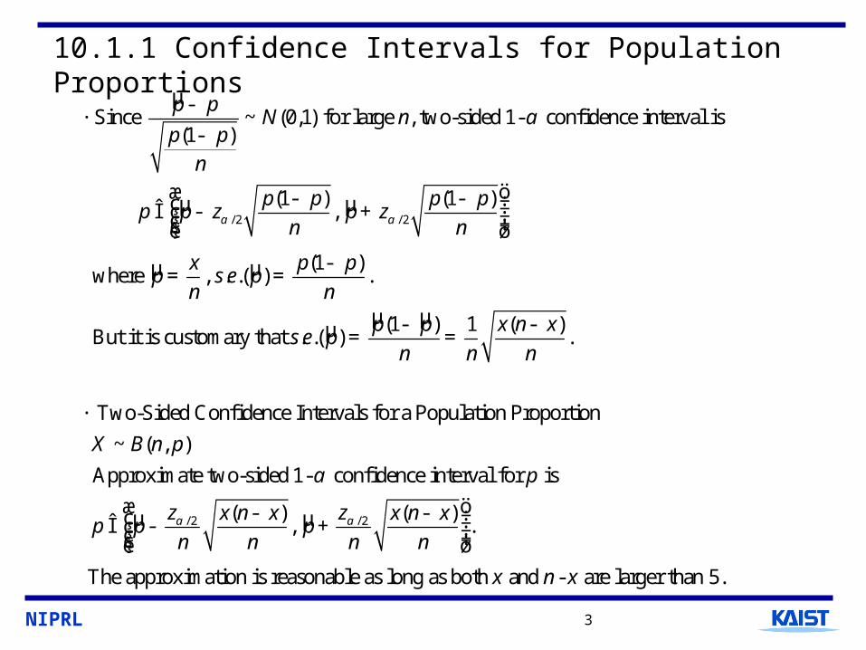
Since ~ (0,1) for large , two-sided 1- confidence interval is(1 )
(1 ) (1 ),
(1 )where , . .( ) .
(1 ) 1But it is customary that . .( )
p pN n
p pn
p p p pp p z p z
n n
x p pp s e p
n n
p ps e p
n n
a a
a-
·-
æ ö- - ÷ç ÷Î - +ç ÷ç ÷÷çè ø
-= =
-= =
µ µ/ 2 / 2
( ).
Two-Sided Confidence Intervals for a Population Proportion
~ ( , )
Approximate two-sided 1- confidence interval for is
( ) ( ) , .
The approximation
x n x
n
X B n p
p
z zx n x x n xp p p
n n n na a
a
-
·
æ ö- - ÷ç ÷Î - +ç ÷ç ÷÷çè ø
is reasonable as long as both and - are larger than 5.x n x
NIPRL 4
10.1.1 Confidence Intervals for Population Proportions
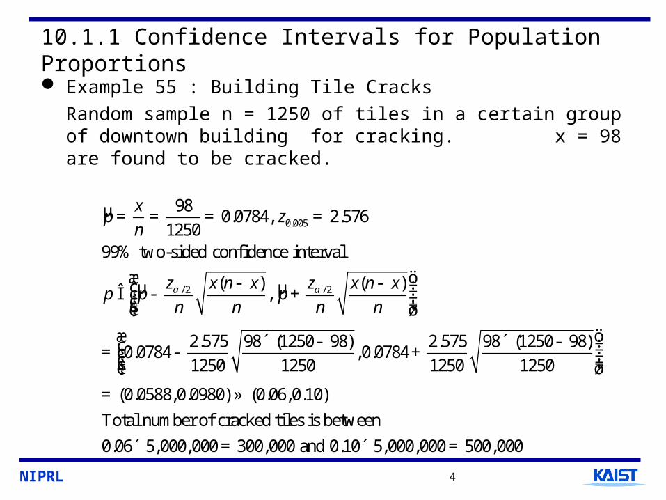
Example 55 : Building Tile Cracks
Random sample n = 1250 of tiles in a certain group of downtown building for cracking. x = 98 are found to be cracked.
µ
µ µ
0.005
/ 2 / 2
980.0784, 2.576
125099% two-sided confidence interval
( ) ( ),
2.575 98 (1250 98) 2.575 98 (1250 98)0.0784 ,0.0784
1250 1250 1250 1250
(0.0588,0.0980)
xp z
n
z zx n x x n xp p p
n n n na a
= = = =
æ ö- - ÷ç ÷Î - +ç ÷ç ÷÷çè ø
æ ö´ - ´ - ÷ç ÷= - +ç ÷ç ÷÷çè ø
= (0.06,0.10)
Total number of cracked tiles is between
0.06 5,000,000 300,000 and 0.10 5,000,000 500,000
»
´ = ´ =
NIPRL 5
10.1.1 Confidence Intervals for Population Proportions
µ
µ
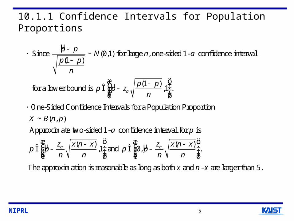
Since ~ (0,1) for large , one-sided 1- confidence interval (1 )
(1 )for a lower bound is ,1 .
One-Sided Confidence Intervals for a Population Proportion
~ ( , )
Ap
p pN n
p pn
p pp p z
n
X B n p
a
a-
·-
æ ö- ÷ç ÷Î -ç ÷ç ÷÷çè ø
·
µ µ
proximate two-sided 1- confidence interval for is
( ) ( ) ,1 and 0, .
The approximation is reasonable as long as both and - are larger than 5.
p
z zx n x x n xp p p p
n n n n
x n x
a a
a
æ ö æ ö- -÷ ÷ç ç÷ ÷Î - Î -ç ç÷ ÷ç ç÷ ÷÷ ÷ç çè ø è ø
NIPRL 6
10.1.2 Hypothesis Tests on a Population Proportion
µ
µ
0 0 0
0
0
0
0 0
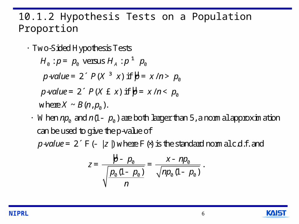
Two-Sided Hypothesis Tests
: versus :
- 2 ( ) if /
- 2 ( ) if /
where ~ ( , ).
When and (1 ) are both larger than 5, a normal a
AH p p H p p
p value P X x p x n p
p value P X x p x n p
X B n p
np n p
·
= ¹
= ´ ³ = >
= ´ £ = <
· -
µ0 0
0 0 0 0
pproximation
can be used to give the p-value of
- 2 ( | |) where ( ) is the standard normal c.d.f. and
.(1 ) (1 )
p value z
p p x npz
p p np p
n
= ´ F - F ×
- -= =
- -
NIPRL 7
10.1.2 Hypothesis Tests on a Population Proportion
0 0
0
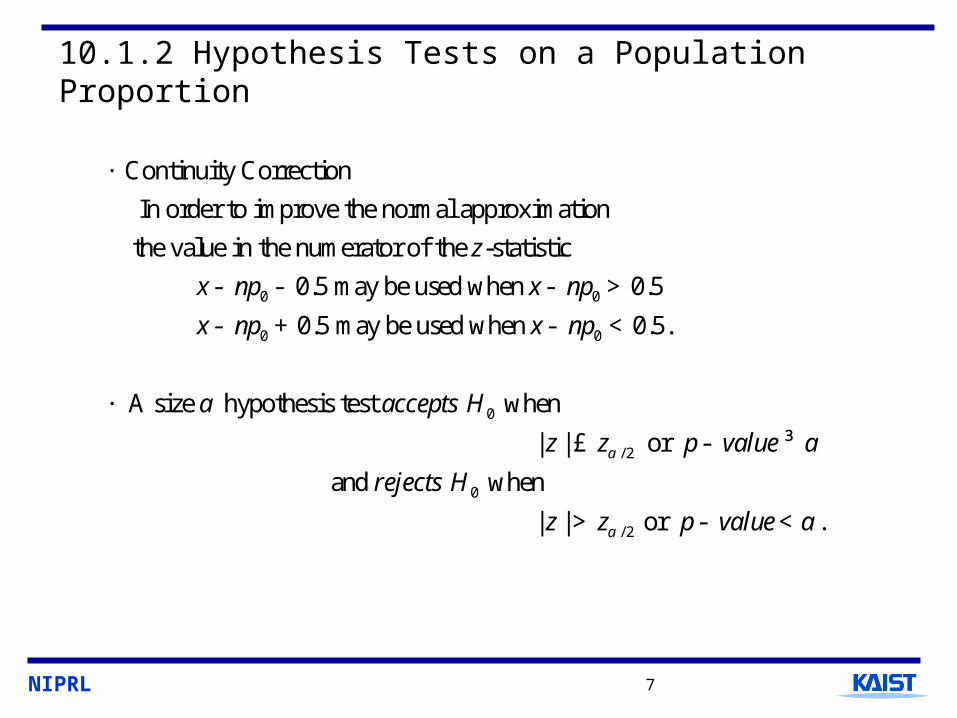
Continuity Correction
In order to improve the normal approximation
the value in the numerator of the -statistic
0.5 may be used when 0.5
0.5 may
z
x np x np
x np
·
- - - >
- +
0
0
/ 2
be used when 0.5.
A size hypothesis test when
| | or
and
x np
accepts H
z z p value
rea
a
a
- <
·
£ - ³
0
/ 2
when
| | or .
jects H
z z p valuea a> - <
NIPRL 8
10.1.2 Hypothesis Tests on a Population Proportion
0 0 0
0
0
0 0
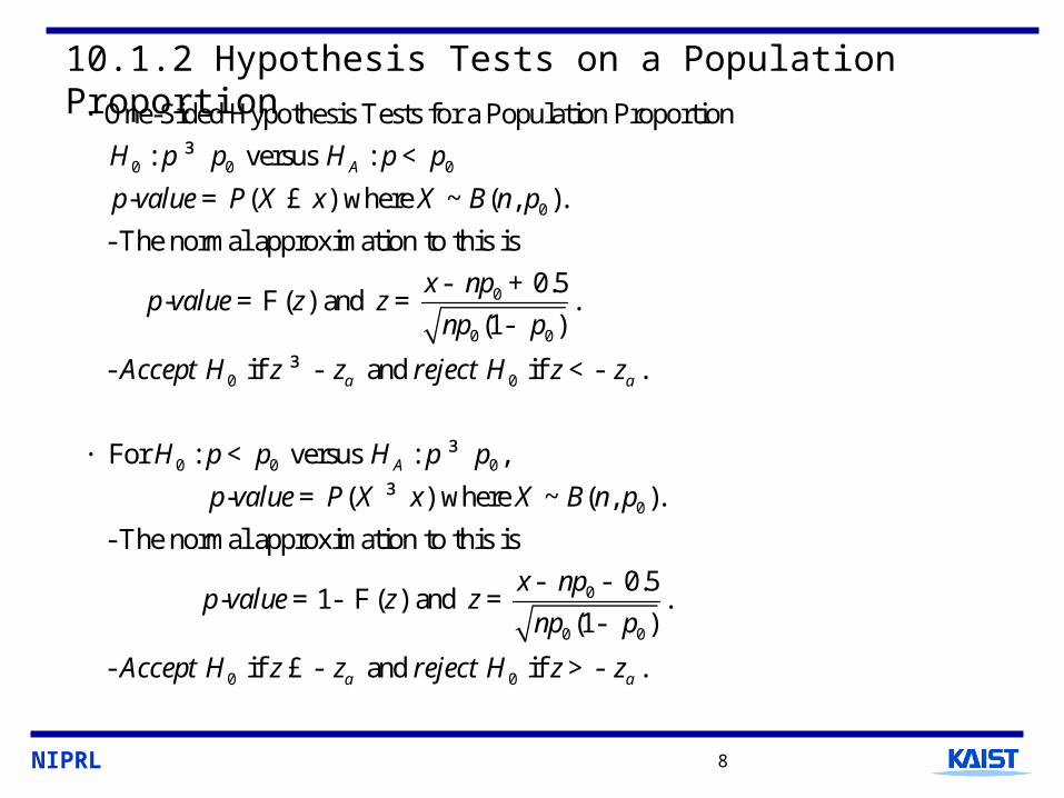
One-Sided Hypothesis Tests for a Population Proportion
: versus :
- ( ) where ~ ( , ).
- The normal approximation to this is
0.5 - ( ) and .
(1 )
AH p p H p p
p value P X x X B n p
x npp value z z
np p
·
³ <
= £
- +=F =
-
0 0
0 0 0
0
- if and if .
For : versus : ,
- ( ) where ~ ( , ).
- The normal approximation to this is
- 1 ( ) and
A
Accept H z z reject H z z
H p p H p p
p value P X x X B n p
p value z
a a³ - <-
· < ³
= ³
= - F
0
0 0
0 0
0.5.
(1 )
- if and if .
x npz
np p
Accept H z z reject H z za a
- -=
-
£ - >-
NIPRL 9
10.1.2 Hypothesis Tests on a Population Proportion
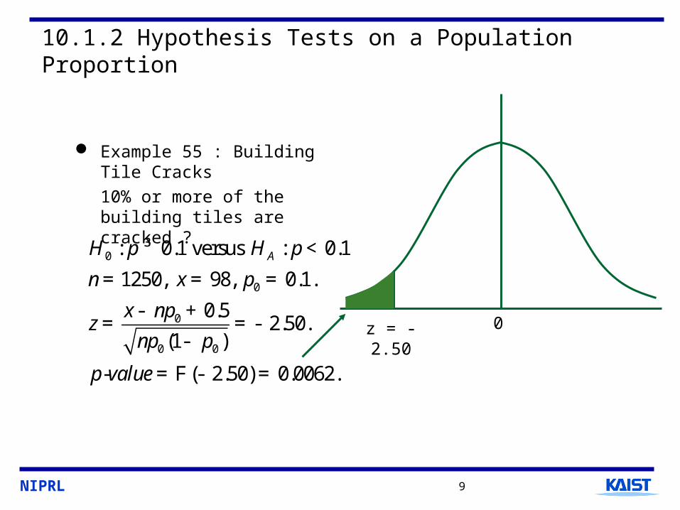
Example 55 : Building Tile Cracks
10% or more of the building tiles are cracked ?
0
0
0
0 0
: 0.1 versus : 0.1
1250, 98, 0.1.
0.52.50.
(1 )
- ( 2.50) 0.0062.
AH p H p
n x p
x npz
np p
p value
³ <
= = =
- += =-
-
=F - =
z = -2.50 0
NIPRL 10
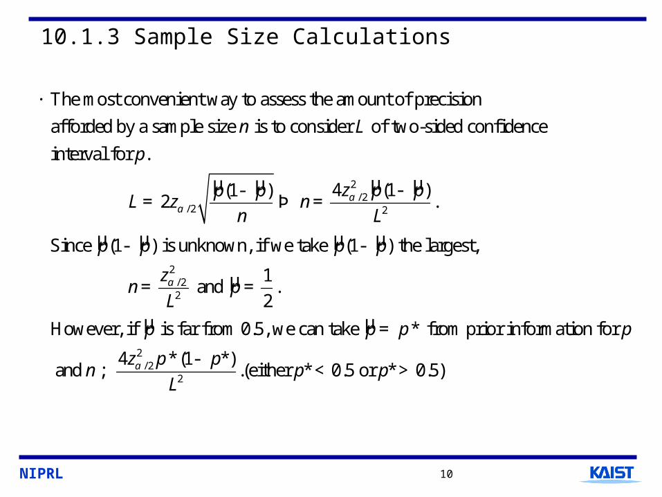
10.1.3 Sample Size Calculations
µ µ µ µ2/ 2
/ 2 2
The most convenient way to assess the amount of precision
afforded by a sample size is to consider of two-sided confidence
interval for .
4 (1 )(1 )2
n L
p
z p pp pL z n
n La
a
·
--= Þ =
µ µ µ µ
µ
µ µ
2/ 22
2/ 2
.
Since (1 ) is unknown, if we take (1 ) the largest,
1 and .
2
However, if is far from 0.5, we can take * from prior information for
4 *(1 *and
p p p p
zn p
L
p p p p
z p pn
a
a
- -
= =
=
-;
2
).(either * 0.5 or * 0.5)p p
L< >
NIPRL 11
10.1.3 Sample Size Calculations
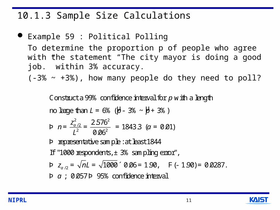
Example 59 : Political Polling
To determine the proportion p of people who agree with the statement “The city mayor is doing a good job.” within 3% accuracy.
(-3% ~ +3%), how many people do they need to poll?
µ µ
2 2/ 22 2
Construct a 99% confidence interval for with a length
no large than 6% ( 3% ~ 3%)
2.576 1843.3 ( 0.01)
0.06representative sample : at least 1844
If "1000 respondents, 3% sampling erro
p
L p p
zn
La a
= - +
Þ = = = =
Þ
±
/ 2
r",
1000 0.06 1.90, ( 1.90) 0.0287.
0.057 95% confidence interval
z nLa
a
Þ = = ´ = F - =
Þ Þ;
NIPRL 12
10.1.3 Sample Size Calculations
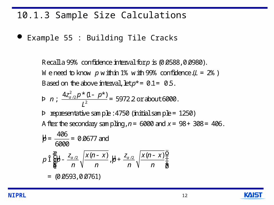
Example 55 : Building Tile Cracks
2/ 2
2
Recall a 99% confidence interval for is (0.0588, 0.0980).
We need to know within 1% with 99% confidence.( 2%)
Based on the above interval, let * 0.1 0.5.
4 *(1 *)5972.2 or about 6000.
r
p
p L
p
z p pn
La
=
=
-Þ =
Þ
=
;
µ
µ µ/ 2 / 2
epresentative sample : 4750 (initial sample 1250)
After the secondary sampling, 6000 and 98 308 406.
4060.0677 and
6000
( ) ( ),
(0.0593, 0.0761)
n x
p
z zx n x x n xp p p
n n n na a
=
= = + =
= =
æ ö- - ÷ç ÷Î - +ç ÷ç ÷÷çè ø
=
NIPRL 13
10.2 Comparing Two Population Proportions
µ µ µ µ
µ µ µ µ
µ µ
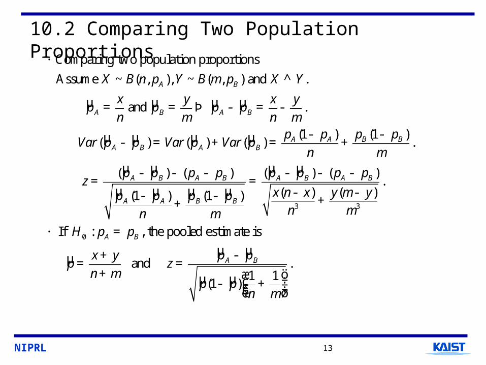
Comparing two population proportions
Assume ~ ( , ), ~ ( , ) and .
and .
(1 ) (1 )( ) ( ) ( ) .
( ) (
A B
A B A B
A A B BA B A B
AA B
X B n p Y B m p X Y
x y x yp p p p
n m n mp p p p
Var p p Var p Var pn m
p p p pz
·
^
= = Þ - = -
- -- = + = +
- - -=
µ µ µ µ
µ µ
µµ µ
µ µ
3 3
0
) ( ) ( ).
( ) ( )(1 ) (1 )
If : , the pooled estimate is
and .1 1
(1 )
B A BA B
A A B B
A B
A B
p p p p
x n x y m yp p p pn mn m
H p p
p px yp z
n mp p
n m
- - -=
- -- - ++
· =
-+= =
+ æ ö÷ç- + ÷ç ÷çè ø
NIPRL 14
10.2.1 Confidence Intervals for the Difference Between Two Population Proportions
µ µµ
/ 2
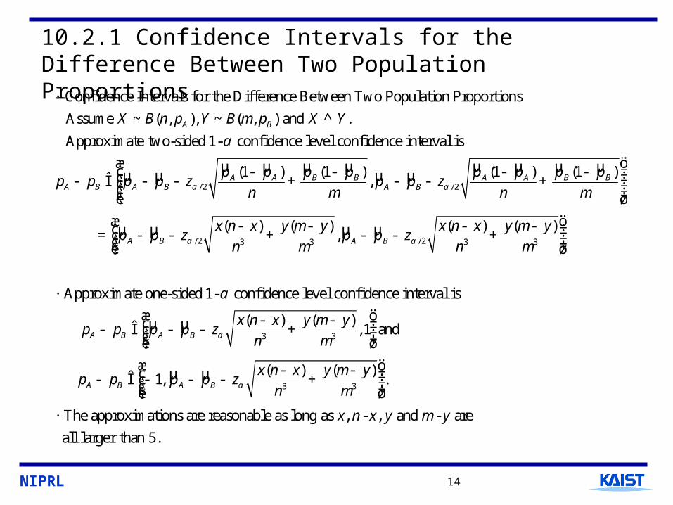
Confidence Intervals for the Difference Between Two Population Proportions
Assume ~ ( , ), ~ ( , ) and .
Approximate two-sided 1- confidence level confidence interval isA B
A B A B
X B n p Y B m p X Y
pp p p p za
a
·
^
- Î - -
µ µ µµ µ
µ µ µ µ
µ µ µ µ
/ 2
/ 2 / 23 3 3 3
(1 ) (1 ) (1 ) (1 ),
( ) ( ) ( ) ( ),
Approximate one-sided 1- confidence level con
A A B B A A B BA B
A B A B
p p p p p p pp p z
n m n m
x n x y m y x n x y m yp p z p p z
n m n m
a
a a
a
æ ö÷ç - - - - ÷ç ÷+ - - +ç ÷ç ÷ç ÷è ø
æ ö- - - - ÷ç ÷= - - + - - +ç ÷ç ÷÷çè ø
·
µ µ
µ µ
3 3
3 3
fidence interval is
( ) ( ), 1 and
( ) ( )1, .
The approximations are reasonable as long as , - , and - ar
A B A B
A B A B
x n x y m yp p p p z
n m
x n x y m yp p p p z
n m
x n x y m y
a
a
æ ö- - ÷ç ÷- Î - - +ç ÷ç ÷÷çè ø
æ ö- - ÷ç ÷- Î - - - +ç ÷ç ÷÷çè ø
·
e
all larger than 5.
NIPRL 15
10.2.1 Confidence Intervals for the Difference Between Two Population Proportions
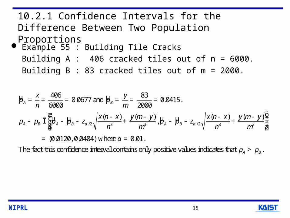
Example 55 : Building Tile Cracks
Building A : 406 cracked tiles out of n = 6000.
Building B : 83 cracked tiles out of m = 2000.
µ µ
µ µ µ µ/ 2 / 23 3 3 3
406 830.0677 and 0.0415.
6000 2000
( ) ( ) ( ) ( ),
(0.0120, 0.0404) where 0.01.
The fact this confidence interval contain
A B
A B A B A B
x yp p
n m
x n x y m y x n x y m yp p p p z p p z
n m n ma a
a
= = = = = =
æ ö- - - - ÷ç ÷- Î - - + - - +ç ÷ç ÷÷çè ø
= =
s only positive values indicates that .A Bp p>
NIPRL 16
10.2.2 Hypothesis Tests on the Difference Between Two Population Proportions
¶ 
µ µ
0
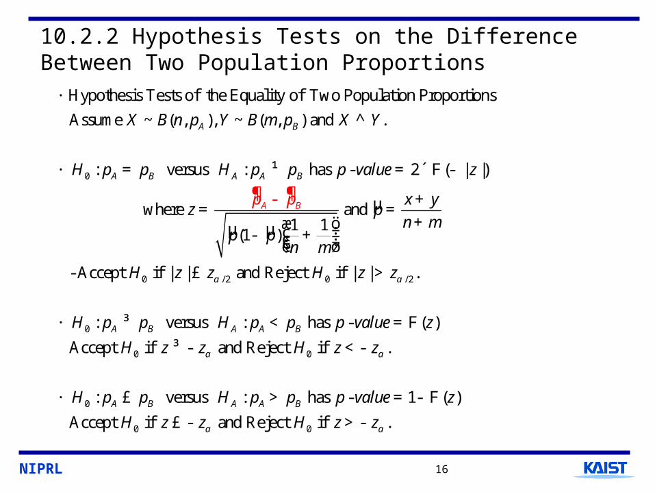
Hypothesis Tests of the Equality of Two Population Proportions
Assume ~ ( , ), ~ ( , ) and .
: versus : has - 2 ( | |)
where1 1
(1 )
A B
A B A A
A
B
B
X B n p Y B m p X Y
H p p H p p p value z
z
p p
p
m
p
n
·
^
· = ¹ = ´ F -
=æ
- +
-
µ
0 / 2 0 / 2
0
0 0
0
and
- Accept if | | and Reject if | | .
: versus : has - ( )
Accept if and Reject if .
: versus : ha
A B A A B
A B A A B
x yp
n m
H z z H z z
H p p H p p p value z
H z z H z z
H p p H p p
a a
a a
+=
+ö÷ç ÷ç ÷çè ø
£ >
· ³ < =F
³ - <-
· £ >
0 0
s - 1 ( )
Accept if and Reject if .
p value z
H z z H z za a
= - F
£ - >-
NIPRL 17
10.2.2 Hypothesis Tests on the Difference Between Two Population Proportions
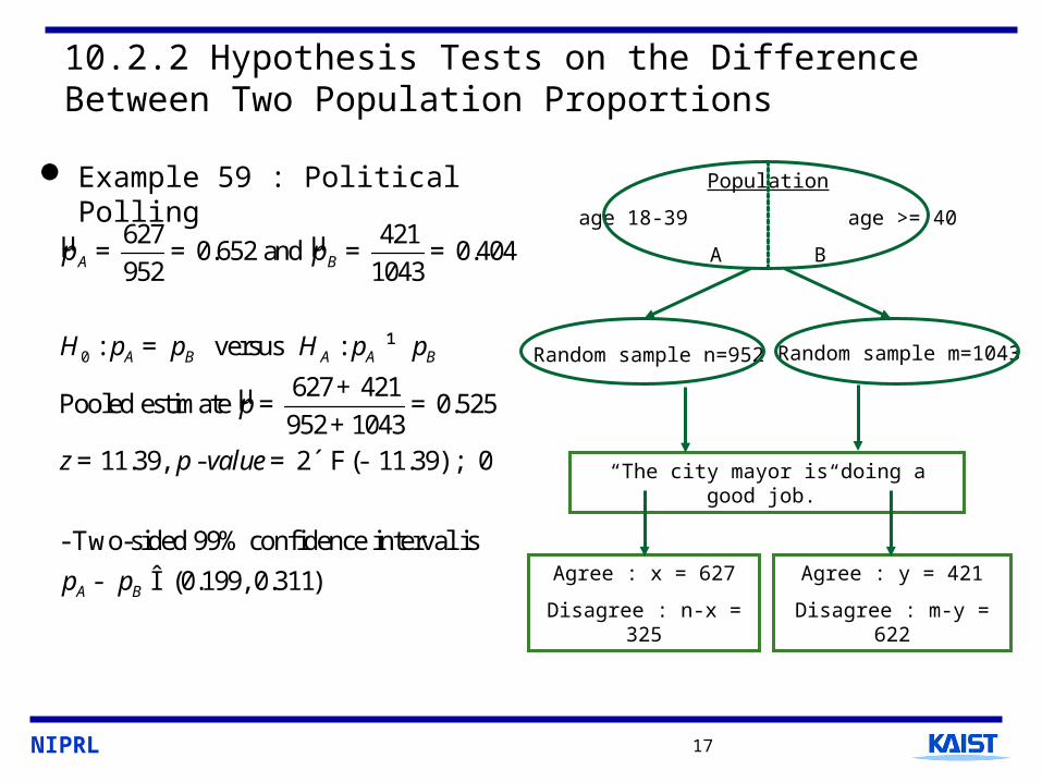
Example 59 : Political Polling Population
age 18-39 age >= 40
A B
“The city mayor is doing a good job.”
Random sample n=952 Random sample m=1043
Agree : x = 627
Disagree : n-x = 325
Agree : y = 421
Disagree : m-y = 622
µ µ
µ
0
627 4210.652 and 0.404
952 1043
: versus :
627 421Pooled estimate 0.525
952 104311.39, - 2 ( 11.39) 0
- Two-sided 99% confidence interval is
(0.199, 0.311)
A B
A B A A B
A B
p p
H p p H p p
p
z p value
p p
= = = =
= ¹
+= =
+= = ´ F -
- Î
;
NIPRL 18
Summary problems
(1) Why do we assume large sample sizes for statistical inferences concerning proportions?
So that the Normal approximation is a reasonable approach.
(2) Can you find an exact size test concerning proportions?
No, in general.
NIPRL 19
10.3 Goodness of Fit Tests for One-Way Contingency Tables10.3.1 One-Way Classifications
µ
1 2 1 2
1 2 1 2
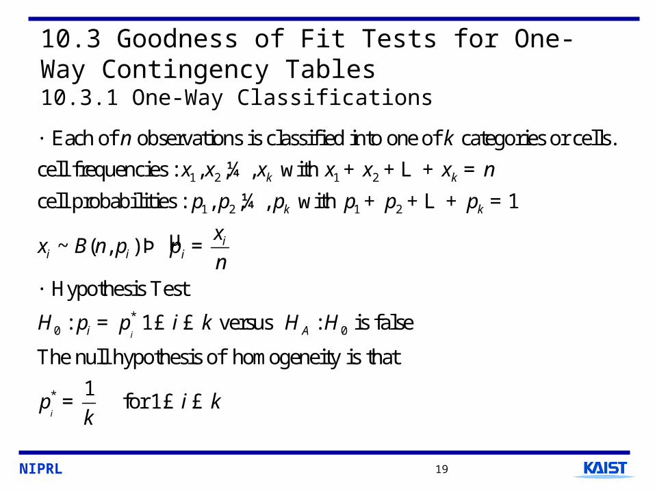
Each of observations is classified into one of categories or cells.
cell frequencies : , , , with
cell probabilities : , , , with 1
~ ( , )
Hypothesis T
k k
k k
ii i i
n k
x x x x x x n
p p p p p p
xx B n p p
n
·
¼ + + + =
¼ + + + =
Þ =
·
L
L
*
0 0
*
est
: 1 versus : is false
The null hypothesis of homogeneity is that
1for 1
i
i
i AH p p i k H H
p i kk
= £ £
= £ £
NIPRL 20
10.3.1 One-Way Classifications
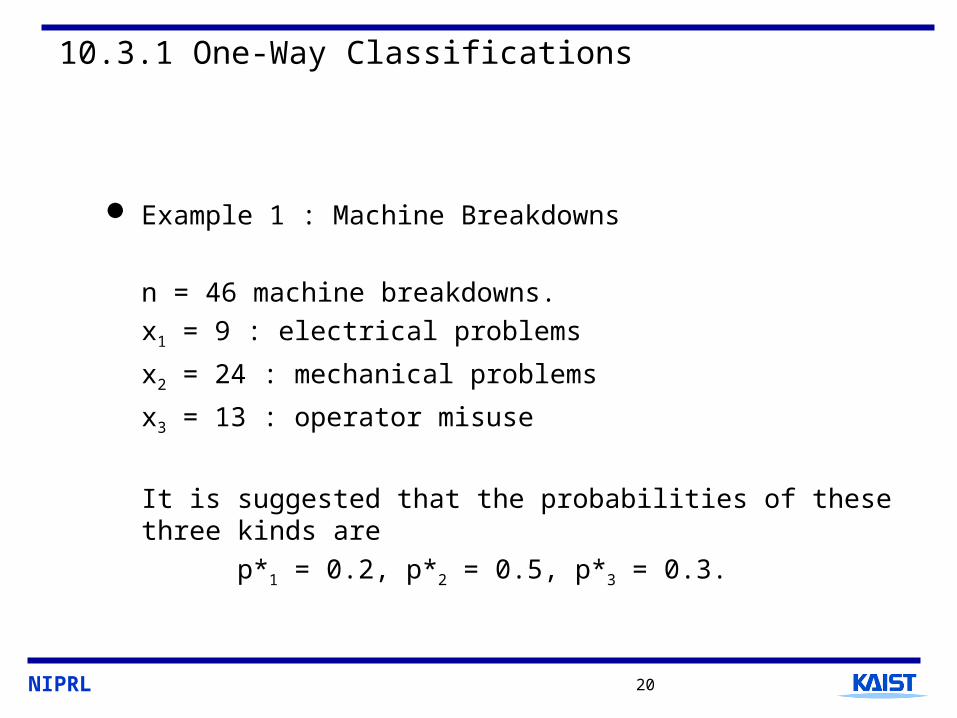
Example 1 : Machine Breakdowns
n = 46 machine breakdowns.
x1 = 9 : electrical problems
x2 = 24 : mechanical problems
x3 = 13 : operator misuse
It is suggested that the probabilities of these three kinds are
p*1 = 0.2, p*2 = 0.5, p*3 = 0.3.
NIPRL 21
10.3.1 One-Way Classifications
1 2
1 2
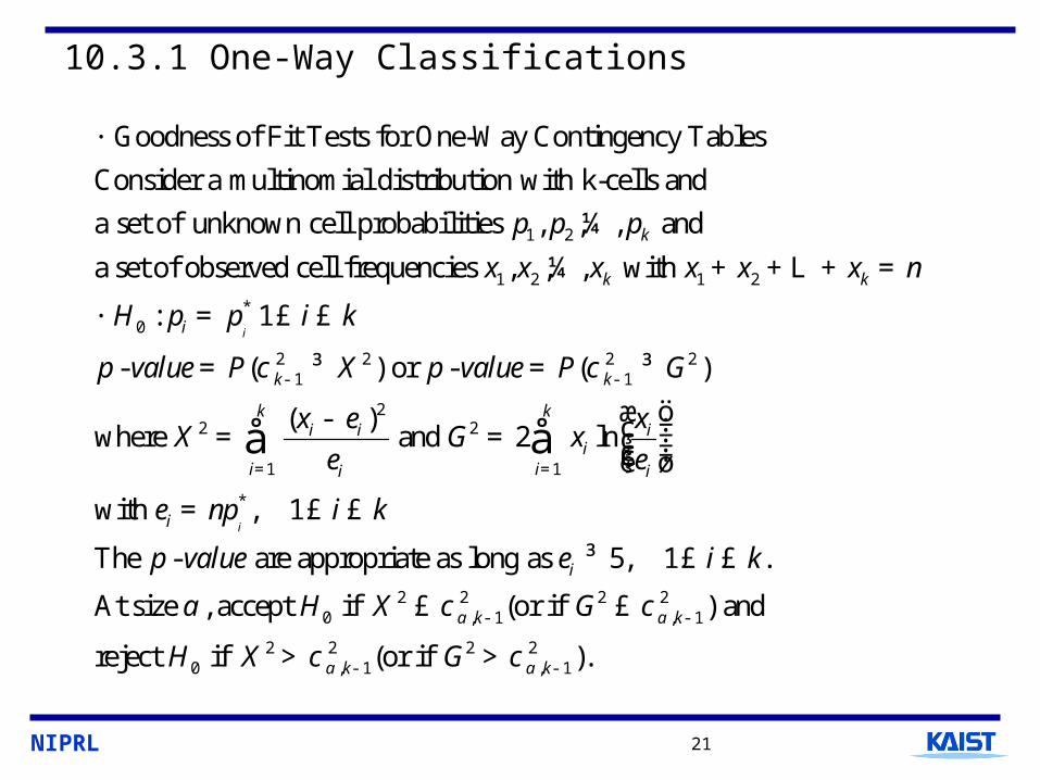
Goodness of Fit Tests for One-Way Contingency Tables
Consider a multinomial distribution with k-cells and
a set of unknown cell probabilities , , , and
a set of observed cell frequencies , ,kp p p
x x
·
¼
¼
1 2
*0
2 2 2 21 1
22 2
1 1
*
, with
: 1
- ( ) or - ( )
( )where and 2 ln
with , 1
The - are appropriate as long as
i
i
k k
i
k k
k ki i i
ii ii i
i
x x x x n
H p p i k
p value P X p value P G
x e xX G x
e e
e np i k
p value e
c c- -
= =
+ + + =
· = £ £
= ³ = ³
æ ö- ÷ç ÷= = ç ÷ç ÷çè ø
= £ £
å å
L
2 2 2 20 , 1 , 1
2 2 2 20 , 1 , 1
5, 1 .
At size , accept if (or if ) and
reject if (or if ).
i
k k
k k
i k
H X G
H X G
a a
a a
a c c
c c
- -
- -
³ £ £
£ £
> >
NIPRL 22
10.3.1 One-Way Classifications
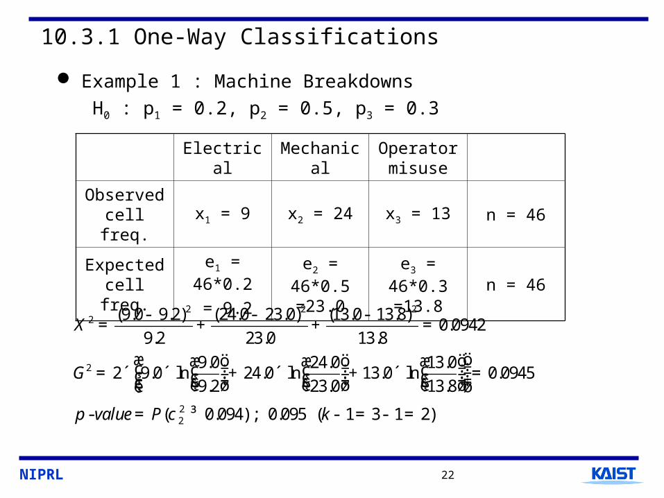
Example 1 : Machine Breakdowns
H0 : p1 = 0.2, p2 = 0.5, p3 = 0.3
Electrical MechanicalOperator misuse
Observed cell freq.
x1 = 9 x2 = 24 x3 = 13 n = 46
Expected cell freq.
e1 = 46*0.2
= 9.2
e2 = 46*0.5 =23.0
e3 = 46*0.3 =13.8
n = 46
2 2 22
2
22
(9.0 9.2) (24.0 23.0) (13.0 13.8)0.0942
9.2 23.0 13.8
9.0 24.0 13.02 9.0 ln 24.0 ln 13.0 ln 0.0945
9.2 23.0 13.8
- ( 0.094) 0.095 ( 1 3 1 2)
X
G
p value P kc
- - -= + + =
æ öæ ö æ ö æ ö÷ç ÷ ÷ ÷ç ç ç= ´ ´ + ´ + ´ =÷÷ ÷ ÷ç ç ç ç ÷÷ ÷ ÷÷ ÷ ÷ç ç çç ÷ç è ø è ø è øè ø
= ³ - = - =;
NIPRL 23
10.3.1 One-Way Classifications
( )
20 2
2
2
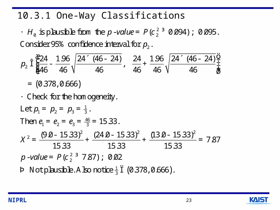
is plausible from the - ( 0.094) 0.095.
Consider 95% confidence interval for .
24 1.96 24 (46 24) 24 1.96 24 (46 24),
46 46 46 46 46 46
0.378, 0.666
Check for the homo
H p value P
p
p
c· = ³
æ ö´ - ´ - ÷ç ÷Î - +ç ÷ç ÷÷çè ø
=
·
;
( )
11 2 3 3
461 2 3 3
2 2 22
22
13
geneity.
Let .
Then 15.33.
(9.0 15.33) (24.0 15.33) (13.0 15.33)7.87
15.33 15.33 15.33
- ( 7.87) 0.02
Not plausible. Also notice 0.378, 0.666 .
p p p
e e e
X
p value P c
= = =
= = = =
- - -= + + =
= ³
Þ Ï
;
NIPRL 24
10.3.2 Testing Distributional Assumptions
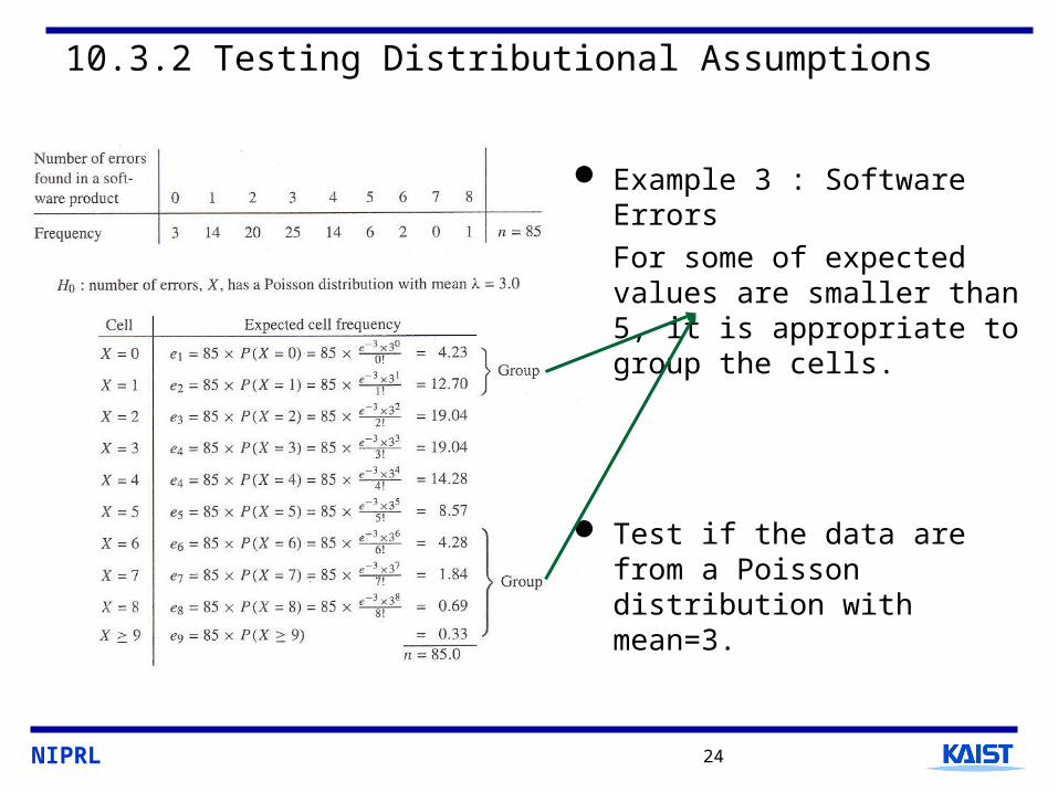
Example 3 : Software Errors
For some of expected values are smaller than 5, it is appropriate to group the cells.
Test if the data are from a Poisson distribution with mean=3.

NIPRL 25
10.3.2 Testing Distributional Assumptions
2 2 22
2 2 2
25
(17.00 16.93) (20.0 19.04) (25.00 19.04)
16.93 19.04 19.04
(14.00 14.28) (6.00 8.57) (3.00 7.14)
14.28 8.57 7.145.12
- ( 5.12) 0.40
Plausible that the software errors have a Po
X
p value P c
- - -= + +
- - -+ + +
=
= ³ =
Þ
0
isson distribution
with mean 3.
If : the software errors have a Poisson distribution,
would be calculated using 2.76 and - would
be calculated from a chi-square distribution withi
H
e x p value
l
l
=
·
= =
1 1 4 degrees of freedom.k - - =
NIPRL 26
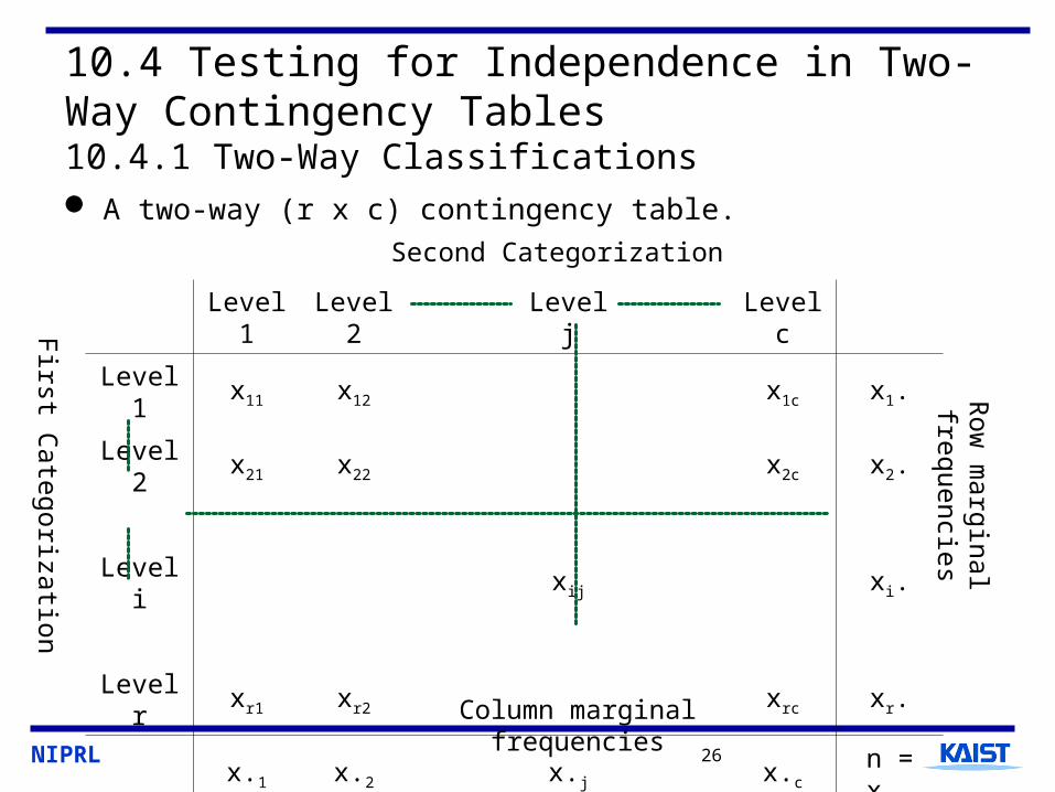
10.4 Testing for Independence in Two-Way Contingency Tables10.4.1 Two-Way Classifications
Level 1 Level 2 Level j Level c
Level 1 x11 x12 x1c x1.
Level 2 x21 x22 x2c x2.
Level i xij xi.
Level r xr1 xr2 xrc xr.
x.1 x.2 x.j x.c n = x..
A two-way (r x c) contingency table.
Second Categorization
First C
ategorization
Row
marginal frequencies
Column marginal frequencies
NIPRL 27
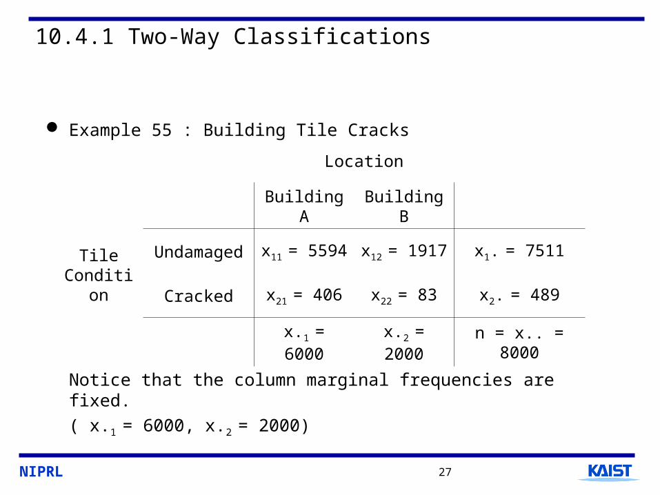
10.4.1 Two-Way Classifications
Example 55 : Building Tile Cracks
Notice that the column marginal frequencies are fixed.
( x.1 = 6000, x.2 = 2000)
Location
Tile Condition
Building A Building B
Undamaged x11 = 5594 x12 = 1917 x1. = 7511
Cracked x21 = 406 x22 = 83 x2. = 489
x.1 = 6000 x.2 = 2000 n = x.. = 8000
NIPRL 28
10.4.2 Testing for Independence
0
22 2
1 1 1 1
. .
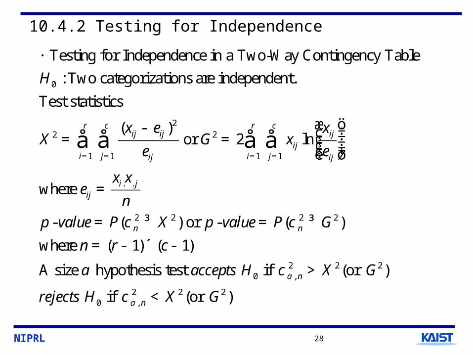
Testing for Independence in a Two-Way Contingency Table
: Two categorizations are independent.
Test statistics
( )or 2 ln
where
-
r c r cij ij ij
iji j i jij ij
i jij
H
x e xX G x
e e
x xe
n
p
= = = =
·
æ ö- ÷ç ÷ç= = ÷ç ÷÷çè ø
=
å å å å
2 2 2 2
2 2 20 ,
2 2 20 ,
( ) or - ( )
where ( 1) ( 1)
A size hypothesis test if (or )
if (or )
value P X p value P G
r c
accepts H X G
rejects H X G
n n
a n
a n
c c
n
a c
c
= ³ = ³
= - ´ -
>
<
NIPRL 29
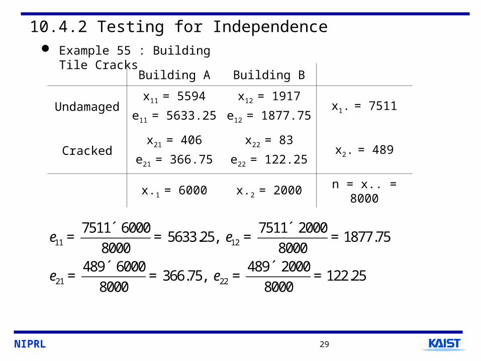
10.4.2 Testing for Independence Example 55 : Building Tile Cracks
Building A Building B
Undamagedx11 = 5594
e11 = 5633.25
x12 = 1917
e12 = 1877.75x1. = 7511
Crackedx21 = 406
e21 = 366.75
x22 = 83
e22 = 122.25x2. = 489
x.1 = 6000 x.2 = 2000 n = x.. = 8000
11 12
21 22
7511 6000 7511 20005633.25, 1877.75
8000 8000489 6000 489 2000
366.75, 122.258000 8000
e e
e e
´ ´= = = =
´ ´= = = =
NIPRL 30
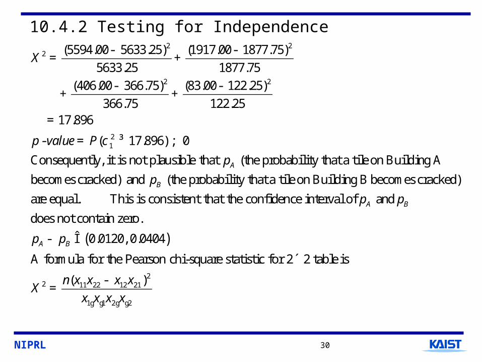
10.4.2 Testing for Independence2 2
2
2 2
21
(5594.00 5633.25) (1917.00 1877.75)
5633.25 1877.75
(406.00 366.75) (83.00 122.25)
366.75 122.2517.896
- ( 17.896) 0
Consequently, it is not plausible that (the probability tA
X
p value P
p
c
- -= +
- -+ +
=
= ³ ;
hat a tile on Building A
becomes cracked) and (the probability that a tile on Building B becomes cracked)
are equal. This is consistent that the confidence interval of and
does not c
B
A B
p
p p
( )
22 11 22 12 21
1 1 2 2
ontain zero.
0.0120, 0.0404
A formula for the Pearson chi-square statistic for 2 2 table is
( )
A Bp p
n x x x xX
x x x x
- Î
´
-=
g g g g
NIPRL 31
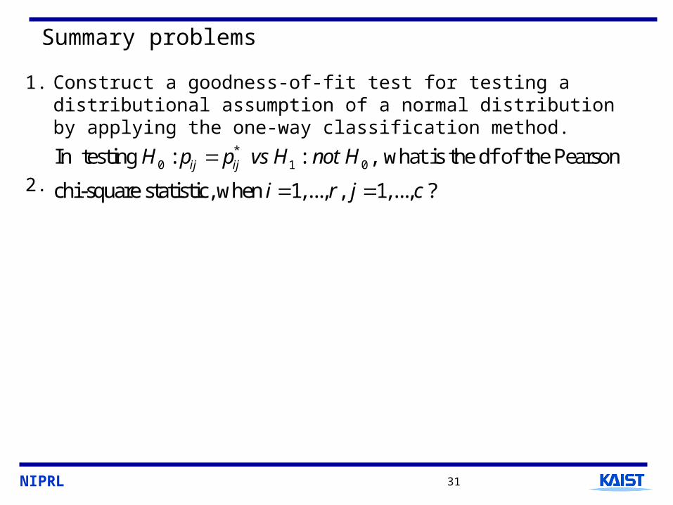
Summary problems
1. Construct a goodness-of-fit test for testing a distributional assumption of a normal distribution by applying the one-way classification method.
2.
*0 1 0In testing : : , what is the df of the Pearson
chi-square statistic, when 1,..., , 1,..., ?
ij ijH p p vs H not H
i r j c