NILE RIVER SEDIMENT TRANSPORT SIMULATION (CASE STUDY ... · Eleventh International Water Technology...

Eleventh International Water Technology Conference, IWTC11 2007 Sharm El-Sheikh, Egypt 423

NILE RIVER SEDIMENT TRANSPORT SIMULATION

(CASE STUDY: DAMIETTA BRANCH)

Ahmed Moustafa A. Moussa 1 and Medhat S. Aziz 2 1 Researcher, Nile Research Institute (NRI). E-mail: [email protected]

2 Deputy Director, Nile Research Institute (NRI), Egypt ABSTRACT Sediment transport is an important element in the quantitative and qualitative management of river engineering. The rate of sediment transport, at any given river cross section, depends mainly on the availability of the transported material and transport ability of the stream. Many different formulas have been used to predict the amount of sediment discharge in the Nile River, but only few equations give reasonable results compared with field measurements. Some examples of these equations are Ackers and White, Engelund and Hansen and Yang equations. Damietta Branch was selected as a case study for this analysis. This study has been performed to simulate the period from 1982 to 2001 for Damietta Branch. Analysis and comparison of the selected formulas for both trend and value are discussed at each cross section. Keyword: Damietta Branch, Nile River Sediment, Sediment Transport Equation, Sediment Transport Simulation. INTRODUCTION Nile River consists of four reaches from Aswan to Cairo and two branches from Cairo to Mediterranean Sea. Damietta Branch is located from Delta Barrage to Mediterranean Sea with length of about 245 km. Damietta Branch is considered the second longest part of the Nile River. This study was performed to study the first part of Damietta Branch from Delta Barrages at km 953.2 on Damietta Branch to Zifta Barrages at km 1046.7 with length about 93.5 km. An important aspect of fluvial process is the movement of sediment in rivers, to which river morphology and river channel changes are closely related. The total load transported by the stream is divided into bed load and suspended load. Some equations are used to compute either bed, suspended, or total load. The main purpose of this study is to select the most suitable transported load formula to be used for the Nile River.


SEDIMENT TRANSPORT MATHEMATICAL MODELS There are many available commercial sediment transport models. The selection bases for simulation models are different from case to case and some broad outlines for model selection can be given as follows: (1) Model applicability to the Nile River. (2) The availability of the model and its user's manual (theoretical and physical

basics). (3) The documentation pertaining to the application of the model to other streams. (4) Model cost, and (5) Model ease of adaptation. Some of the commercial models such as HEC-6 model, MOBED, RIVDEG, Modified HEC-6 and MARS are used by Nile Research Institute (NRI) for the Nile River during the period from 1989 to 1992 to select the suitable model to applicant it [6]. The comparison study shows that only two models behaved as expected on the idealized reach. These are the Modified HEC-6 and MARS. Both of these models also proved to correctly represent the degradation and aggradation processes on the simplified perturbed reach. By the end of the last century there is a new model called GSTARS 2 .0 which was developed by the U.S. Bureau of Reclamation in 1998. This model was used by the authors for Reach Four of the Nile River, and it is used by NRI to study both Reach Two and Reach Three of the Nile River. All of these studies have shown that GSTARS 2.0 model gives good and close results. Based on these studies, GSTARS 2.0 model will used in this study. USED MATHEMATICAL MODEL The used mathematical model for this analysis is GSTARS 2.0 Model which was developed by the U.S. Bureau of Reclamation in 1998 [9]. This model is developed to simulate generalized water and sediment routing. GSTARS 2.0 uses the standard step method for backwater computations. The algorithm uses the energy equation when there are no changes in flow regime, and uses the momentum equation when there is a change from sub-critical to supercritical flow or vice-versa. MODEL SEDIMENT ROUTING The basics for sediment routing computations is the sediment continuity equation. GSTARS 2.0 uses ten different equations that used to calculate bed-material sediment load (lump both bed and suspended load) and an additional equation for cohesive sediment transport. These equations are as follows:

1- Meyer-Peter and Muller’s 1948 method [5]. 2- Laursen’s 1958 method [4]. 3- Toffaleti’s 1969 method [8]. 4- Engelund and Hansen’s 1972 method [2].


5- Ackers and White’s 1973 method [1]. 6- Revised Ackers and White’s 1990 method. 7- Yang’s 1973 sand and 1984 gravel transport method [10]. 8- Yang’s 1979 sand and 1984 gravel transport method [11]. 9- Parker’s 1990 method [7]. 10- Yang’s 1996 modified method [12]. 11- Krone’s 1962 and Ariathurai and Krone’s 1976 methods for cohesive sediment

transport [3].

EQUATIONS OF BED-MATERIAL SEDIMENT LOAD The model has been used to calibrate the sediment transport of the study reach of the Nile River between the years 1982 and 2001 using ten different bed-material sediment load equations. The more reasonable equations are the equations of the bed-material sediment load transport (Qs) that were suggested by Ackers-White in 1973, Yang 1973 and Engluned and Hansen. The equation and its variables and parameters are shown as follows: Ackers-White in 1973

Qs = K * U * D35 *(*U

U )N * (cr

cr

YYY −

)M (1)

In which: Qs = total bed-material sediment load transport (m2/sec) U = depth-averaged velocity = Q/A (m/sec) Q = water discharge released through the reach of the river under study (m3/sec) A = area of cross section (m2) U* = bed shear velocity = gDS (m/sec) (2) Where: g = Acceleration of gravity (m/sec2)

D = Hydraulic Depth = widthTop

Areationalcross sec (m) (3)

S = frictional slope (-) Y = Particle mobility parameter (-) Ycr = Critical Particle mobility parameter (-) D35 = the sieve diameter where 35 % of sediments by weight pass through (m)

D* = D35 3

1

2

)1(��

��

� −υ

gs (4)

s = Specific density = 2.65 ��= Kinematic Viscosity coefficient = 1.519 * 10-6 (m2/sec) K = exp[2.86 ln(D*) – 0.434 (ln D*)

2 –8.13] for D* <60 (5) N = 1- 0.56 * log (D*) for D* < 60 (6)

M = *

66.9D

+ 1.34 for D* < 60 (7)


Ycr = *

23.0

D + 0.14 for D* < 60 (8)

In case D* > 60 & D* = 60 then, N = 0, M = 1.50, Ycr = 0.17

Y =

)1(

35

35

*

)*10

log(66.5*

)1(

N

N

DD

U

gDs

U

−

��

�

�

��

�

�

��

�

��

�

− (9)

The form of Y-parameter ensures that the fine sediment transport depends upon the total bed shear stress and coarse transport rate upon the effective shear stress. Yang 1973 Yang 1973 assumed that the sediment transport is related to the unit stream power, defined as u I. the total sediment concentration (ct), defined as the ratio of the sediment and fluid discharge per unit width (ct = qs/ q) , was expressed as :

Log (ct) = 1α + 2α log ��

�

�

��

�

� −

sW

IcrUIU (10)

Analysis of flume and field data resulted in:

1α = 5.435 – 0.286 log (Ws d50 /υ ) – 0.457 log (U* / Ws) (11)

2α = 1.799 – 0.409 log (Ws d50 /υ ) – 0.314 log (U* / Ws) (12) In which: ct = total load concentration in parts per million by weight (ppm) U = depth -averaged velocity (m/s) Ucr = depth -averaged velocity at initiation of motion I = energy gradient d 50 = median particle diameter of bed material Ws = fall velocity (based on d 50 of bed material) U* = bed –shear velocity (m/s)

Ucr = ( ) sWdU �

��

�

��

�+

−66.0

06.0/log5.2

50* υ for 1.2 <

υ50* dU

< 70 (13)

Ucr = 2.05 Ws for υ

50* dU ≥ 70 (14)

The total load transport rate (in kg/sm) is given by


q t,c = 10-3 ct U h (15) in which: q t,c = total load transport rate (kg/sm) h = water depth Engluned and Hansen The method of Engluned and Hansen is based on a energy-balance concept. The work (per unit time and width) required to elevate the sediment load over a height equal to the bed form height is :

( ) ∆−= tsr qgW ρρ

The work (per unit time and width) done by fluid on moving the particles over a length equal to the bed form length is:

The energy balance Wr = Wa yields:

( ) ff

dUdg

qs

crbbt

1*

,/

1 ∆��

�

�

�

−−

=λ

ρρττ

α

In which: qt = volumetric total load transport (m2/s)

d = particle diameter (m) U* = overall bed-shear velocity (m/s) f = friction coefficient = 2g / C2 C = Chezy-Coefficient

Based on data analysis, it was found that ∆

fλ is approximately constant, giving:

( ) dUf

q crt *'2 θθα

−= (16)

The dimensionless transport rate ( ) 5.15.05.01 dgs

q tt −

=ϕ is introduced, yielding:

( ) 5.0'2 θθθαϕ crt f−= (17)

( ) λττα *,/

1 UW crbba −=

( )2/ / mNstressshearbedeffectiveb =τ

( )2, / mNShildstoacordingstressshearbedcriticalcrb =τ

lengthformbed=λ


Using Equation lower regime: 'θ = 0.06 + 0.4 2θ forθ and assuming crθ = 0.06, it

follows that crθθ −' = 0.4 2θ for the lower regime. Thus:

ft

5.23 θα

ϕ = (18)

The 3α - coefficient was determined by data fitting (approx. 100 flume data), giving

3α = 0.1 thus

ft

5.21.0 θϕ = (19)

In which:

( ) 5.15.05.01 dgs

q tt −

=ϕ (20)

( ) ( ) ( ) 5050502

2*

11 dsIh

dgdgsU

s

b

−=

−=

−=

ρρτθ (21)

2

2C

gf = (22)

Equation (18) does not account for the critical bed-shear stress and is, therefore, not accurate close to initiation of motion. Equation (18) can be rearranged to:

( ) 350

5.02

5

,1

05.0

Cdgs

Uq ct −

= (23)

In which: ctq , = Volumetric current-related total load transport (m2/s)

U = Depth averaged velocity (m/s) C = Chezy coefficient (m.5/s)

s = specific density ��

��= ρ

ρ s

d50 = Median particle size of bed material DATA COLLECTION

1- Geometric Data

The cross sections surveyed in 1982 used as an input file and compare the results of the model by the cross sections surveyed in 2001 to make sure that the model gives acceptable results. GSTARS 2.0 model is used to select the suitable equation for the bed-material load formula. As we mentioned before the length of the study reach is about 93.5 km; this length was presented by 93 cross sections. There is a cross section representing each kilometer. The 93 cross sections were surveyed by NRI in 1982 and 2001 by Hydraulic Research Institute (HRI). To be sure that the cross sections location and direction are at the same places; the coordinates (Easting & Northing) of the two


ends of each cross section are used to define the cross sections with the same values. The cross sections surveyed in 1982 entered to the model as points. Each point has two coordinates; the distance (X) and the elevation (Z). 2- Bed Materials The samples of the bed material along the study reach were collected by NRI and analyzed by the sediment lab. General description for the collected bed material samples along the study reach as follows: Km 1: 3 from Delta Barrage: Fine Sand. Km 4: 45 from Delta Barrage: Medium to Fine Sand, Fine to Medium Sand, then

Medium to Fine Sand. Km 46: 65 from Delta Barrage: Gravely Medium Sand, Medium Sand, then Medium

Sand. Km 65: 74 from Delta Barrage: Coarse to Medium Sand, Medium Sand, then Medium

Sand. Km 74: 93from Delta Barrage: Fine to Medium Sand, then Medium to Fine Sand. RESULTS AND ANALYSIS Tables (1 & 2) show that the equations of Ackers-White (A&W) and Yang (1973) give similar results and slightly different from the results given by Engluned and Hansen (E&H). 1- The right prediction is about 76.34% for A& W and Yang and 74.19% for

E&H. 2- Also the range of error for the cross sections have a close prediction is generally

smaller for A& W equation than the other two equations.

Table (1) The results of 93 cross sections that cover the study reach

Equations A&W E&H Yang Total number of cross sections 93 93 93

right predict 71 69 71

wrong predict 22 24 22

range of error A&W E&H Yang

Range 0% to 10% 22 22 25

Range 10% to 20% 24 15 26

Range 20% to 30% 10 18 11

Range 30% to 40% 9 8 4

Range 40% to 50% 4 3 2

Range 50% to 60% 1 2 2

Range 60% to 70% 1 1 1


Table (2) The results of 93 cross sections that cover the study reach as a percentage

Equations A&W E&H Yang Right predict 76.34% 74.19% 76.34%

Wrong predict 23.66% 25.81% 23.66%

Range of error A&W E&H Yang

Range 0% to 10% 30.99% 31.88% 35.21%

Range 10% to 20% 33.80% 21.74% 36.62%

Range 20% to 30% 14.08% 26.09% 15.49%

Range 30% to 40% 12.68% 11.59% 5.63%

Range 40% to 50% 5.63% 4.35% 2.82%

Range 50% to 60% 1.41% 2.90% 2.82%

Range 60% to 70% 1.41% 1.45% 1.41% Figures (1 & 2) show some examples of the cross sections that distributed along the study reach. Only three of these equations were found to give reasonable results during this study. These equations are A&W, Yang and E&H.

Figure (1) cross section calibration for GSTARS 2 model at km 8 downstream Delta Barrage

4

6

8

10

12

14

16

18

0 100 200 300 400 500 600 700 800

Distance (m)

Leve

l (m

)

1982Eq.5Eq.4Eq.1Eq.7Eq.2Eq.6Eq.92001


Figure (2) cross section calibration for GSTARS 2 model at km 16 downstream Delta Barrage

0

2

4

6

8

10

12

14

16

18

0 50 100 150 200 250 300

Distance (m)

Leve

l (m

)

1982Eq.5Eq.4Eq.1Eq.7Eq.2Eq.6Eq.92001

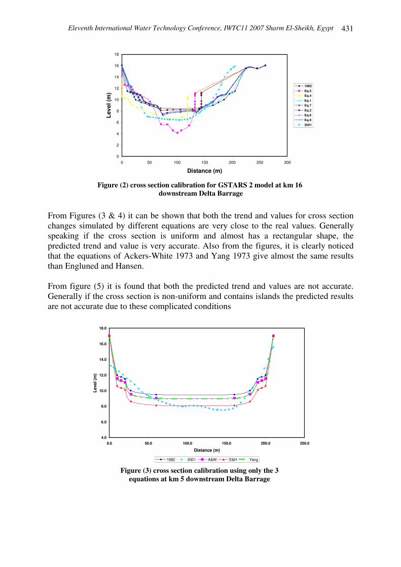
From Figures (3 & 4) it can be shown that both the trend and values for cross section changes simulated by different equations are very close to the real values. Generally speaking if the cross section is uniform and almost has a rectangular shape, the predicted trend and value is very accurate. Also from the figures, it is clearly noticed that the equations of Ackers-White 1973 and Yang 1973 give almost the same results than Engluned and Hansen. From figure (5) it is found that both the predicted trend and values are not accurate. Generally if the cross section is non-uniform and contains islands the predicted results are not accurate due to these complicated conditions

4.0

6.0

8.0

10.0

12.0

14.0

16.0

18.0

0.0 50.0 100.0 150.0 200.0 250.0

Distance (m)

Leve

l (m

)

1982 2001 A&W E&H Yang

Figure (3) cross section calibration using only the 3 equations at km 5 downstream Delta Barrage


6.0

7.0

8.0

9.0

10.0

11.0

12.0

13.0

14.0

15.0

16.0

0.0 50.0 100.0 150.0 200.0 250.0 300.0

Distance (m)

Leve

l (m

)

2001 2001 A&W E&H Yang


0.0

2.0

4.0

6.0

8.0

10.0

12.0

14.0

16.0

0.0 50.0 100.0 150.0 200.0 250.0 300.0 350.0

Distance (m)

Leve

l (m

)

1982 2001 A&W E&H Yang


The future plan of the Ministry of Water Resources and Irrigation (MWRI) are to pass flow through this branch can reach up to 80 mm3/day. During this study, this flow is simulated for a period of one year for comparison purposes and the three equations were studied. From Figures (6 & 7) it is found that both the trend and values are very close especially if the equation of A&W 1973 is used. A relatively small flow of 20 mm3/day is also simulated during this study for a period of one year and from Figure (8), it is found that almost no change in the cross section geometry because the flow is small. That is clear if we compare this figure with Figure (3) for the period of 1982 and 2001.


0.0

2.0

4.0

6.0

8.0

10.0

12.0

14.0

16.0

0.0 50.0 100.0 150.0 200.0 250.0 300.0 350.0 400.0 450.0

Distance (m)

Leve

l (m

)

1982 2001 A&W-80 E&H-80 Yang-80

Figure (6) cross section calibration using only the 3 equations for Q = 80 mm3/day at km 45 downstream Delta Barrage

0.0

2.0

4.0

6.0

8.0

10.0

12.0

14.0

16.0

0.0 50.0 100.0 150.0 200.0 250.0 300.0

Distance (m)

Lev

el (

m)

1982 2001 A&W -80 E&H-80 Yang-80



4.0

6.0

8.0

10.0

12.0

14.0

16.0

18.0

0.0 50.0 100.0 150.0 200.0 250.0

Distance (m)

Lev

el (

m)

1982 2001 A&W-20 E&H-20 Yang-20


CONCLUSIONS

• Three methods for predicting bed-material load discharge were selected. These methods are Ackers-White (1973), Yang (1973) and Engluned and Hansen. These methods were selected because they are widely accepted and used for sand bed rivers such as Nile River.

• Equations of Ackers-White 1973 and Yang 1973 gave very close and similar results and differ from Engluned and Hansen equation results.

• Ackers-White Yang gave very close prediction compared with actual cross section changes with a percentage of 76.34% while E&H gave a percentage of 74.19%.

• The range of error for the cross sections have close predictions is generally small in the A&W equation than the other two equations.

• It can be concluded that uniform and rectangular shape cross sections are simulated more accurately in both trend and value of changes rather than non-uniform and containing islands cross sections.

• The best close simulated results is obtained for cross sections at Km 23 to Km 28, Km 31 to Km 36, Km 40 to Km 44 and Km 87 to Km 92 downstream Delta Barrage. These cross sections have some common characteristics:

- The cross sections are almost having a rectangular shape. - The cross sections is located in a straight part of the reach with

sinuosity S = 1.2 to 1.3 - The bed sample material is ranged from fine sand to medium sand.


- The cross section hydraulics characteristics: average velocity V = 0.2 to 0.5 m/s, average depth D = 2 to 4.5 m and top width T = 200 to 250 m.

• The less accurate results are observed for cross section at Km 57 to Km 60 and Km 60 to Km 65 downstream Delta Barrage these cross sections have some common characteristics:

- The cross sections is located in a sinuous part of the reach with sinuosity S = 2.4 to 2.9.

- The bed sample material is ranged from gravelly to medium sand.

• Finally Ackers-White 1973 equation gave the best results for both the trends and values as a general.

REFERENCES

1. Ackers and White, W. R., Sediment Transport: A New Approach and Analysis, Journal of the Hydraulics Division, ASCE, 99(HY11), pp. 2041-2060.

2. Engelund, F. and Hansen, E., A monograph on Sediment Transport in alluvial streams, Teknish farlg, Copenhagen, Denmark, 1967.

3. Krorne, R.B. Flume Studies of the Transport of Sediment in Estuarial Processes, Hydraulic Engineering Laboratory and Sanitary Engineering Research Laboratory, University of California Berkeley, California, USA,1962.

4. Laursen. E.M., The Total Sediment Load of Streams, Journal of Hydraulics Division, ASCE, Vol. 84, No. 1.

5. Meyer-Peter, E. and R. Fuller. Formula for Bed Load Transport, Proceedings of International Association for Hydraulic Research, 2nd Meeting, Stockholm, 1948.

6. NRI. An Appraisal of Mathematical Models of Degradation, working paper 200-9, Nile Research Institute, National Water Research Center, El-Qanater, Egypt,1990.

7. Parker, G. Surface Based Bedload Transport Relationship for Gravel Rivers, Journal of Hydraulic Research, Vo1. 28, No. 4.

8. Toffaleti, F. B. Definitive Computations of Sand Discharge in Rivers, Journal of the Hydraulic Division, ASCE, Vol. 95, No.HY1, pp. 225-246.

9. U.S. Bureau of Reclamation, GSTARS 2.0 Model Manual, U.S. Bureau of Reclamation Denver, Colorado, 1990.

10. Yang, C.T. Incipient Motion and Sediment Transport, Journal of the Hydraulics Division, ASCE, 99(HY10), 1679-1704.

11. Yang, C.T. Unit Stream Power Equations for Total Load, Journal of Hydrology, Vol. 40, pp. 123-138.

12. Yang, C.T., A. Molinas, and B. Wu. Sediment Transport in the Yellow River, Journal of Hydraulic Engineering, ASCE, in Press.

NILE RIVER SEDIMENT TRANSPORT SIMULATION (CASE STUDY ... · Eleventh International Water Technology...

Documents

Transcript of NILE RIVER SEDIMENT TRANSPORT SIMULATION (CASE STUDY ... · Eleventh International Water Technology...