Nikzad Falahati - University of Cambridge

STRENGTH OF DRILLING FLUID FILTER CAKES

Nikzad Falahati

Fitzwilliam College

Department of Chemical Engineering and

Biotechnology

University of Cambridge

This thesis is submitted for the degree of Doctor of Philosophy

August 2020

https://www.google.co.uk/url?sa=i&rct=j&q=&esrc=s&source=images&cd=&cad=rja&uact=8&docid=k_pt9rrcOmZ_tM&tbnid=bYymm3LPH6CneM:&ved=0CAUQjRw&url=https://www.irononsticker.com/cambridge-university-logo-p-4092.html&ei=xnB6U5vTAsGPO-PegfAD&bvm=bv.66917471,d.ZWU&psig=AFQjCNGb4LWSlLJZRK8N_Ab-xK47qxM1iw&ust=1400619588131648

3

Declaration of originality

This thesis is the result of my own work and includes nothing which is the outcome of work

done in collaboration except as declared in the Preface and specified in the text. It is not

substantially the same as any that I have submitted, or, is being concurrently submitted for a

degree or diploma or other qualification at the University of Cambridge or any other

University or similar institution except as declared in the Preface and specified in the text. I

further state that no substantial part of my thesis has already been submitted, or, is being

concurrently submitted for any such degree, diploma or other qualification at the University

of Cambridge or any other University or similar institution except as declared in the Preface

and specified in the text. The work was carried out in the Department of Chemical Engineering

and Biotechnology, University of Cambridge, and the BP Institute for Multiphase Flow

between October 2016 and August 2020.

It does not exceed the prescribed word limit for the Engineering Degree Committee. This

dissertation contains a total of 39752 words, 86 figures and 12 tables.

5

Abstract

Wellbore strengthening techniques are commonly used to prevent drilling fluid losses.

Current methods generally require that particles are added to the drilling fluid to hinder

fracture propagation, which creates practical difficulties as the particles are often relatively

large. An alternative approach is the idea of using the filter cake that forms against the

wellbore rock to create a robust seal, the efficacy of which will depend on cake strength.

However, little is currently understood about filter cake strength and how it is impacted by

typical particulates in the drilling fluid.

In this work, the strength of drilling fluid filter cakes is assessed. Furthermore, filter cake

properties such as porosity and thickness that are altered by constituent particles and that

affect cake strength are explored. The cake strength was measured using the hole punch test

and particle properties such as particle concentration, size distribution and shape were

evaluated.

Representative water-based and oil-based drilling fluids were analysed to establish

benchmark results, which were based on the rheological and filtration behaviours as well as

filter cake properties. These results produced similar trends to those of model water-based

drilling fluids composed of typical drilling fluid components, such as an increase in cake

strength and a decrease in cake porosity as the barite volume fraction in the fluid increased.

For these model fluids, the cake strength also increased as the particle size and cake porosity

decreased whilst calcium carbonate cakes were stronger than the barite equivalents. Cake

strength may have been influenced by interparticle contact surface area, which was affected

by cake porosity and thickness.

The relationships between particle size, pore distributions and thickness were better

understood by visualising the internal structure of filter cakes, using images captured via X-

ray computed tomography. The images showed that the size of the pores decreased as the

particle size decreased, the cakes had a more porous bottom layer than top and the porosity

decreased with filtration time. Discrete element method simulations were compared with

experimental results, and relationships between cake strength and the interparticle contact

surface area, determined using cake porosity and particle size, were found.

Strength of drilling fluid filter cakes Nikzad Falahati

6

“Even after all this time

The sun never says to the earth,

“You owe me.”

Look what happens

With a love like that.

It lights up the whole sky.”

- Hafiz

7

Acknowledgements

Firstly, I would like to express my immense gratitude to my supervisor, Alex Routh, who has

helped me throughout the entire journey and provided me with his invaluable guidance.

Without his unwavering support, this thesis would not have been possible.

Secondly, I would like to express my great appreciation for the support and technical advice

from my BP mentor, Kuhan Chellappah, who has also helped me throughout my entire PhD

project.

I would like to acknowledge the funding and technical support from BP through the BP

International Centre for Advanced Materials (BP-ICAM) which made this research possible. I

would also like to thank the rest of my BP-ICAM group: Mark Aston and Ian Collins from BP

for their advice; Giovanna Biscontin, Ramesh Kandasami and Gianmario Sorrentino from

Geotechnical Engineering at the University of Cambridge for their discussions and assistance;

Parmesh Gajjar, Tristan Lowe and Jose Godinho from X-Ray Imaging Facility at the University

of Manchester for their technical advice and expertise; and Tara Love from Chemical

Engineering at the University of Cambridge for her advice and discussions.

Then, I would like to thank Louise Bailey from Schlumberger for her help with the hole punch

test, and Nathalie Vriend, Jonathan Tsang and Patrick Welche from the BP Institute at the

University of Cambridge for their advice and support with the discrete element method

simulations.

I would like to thank all of my group members and the people that I’ve met at the BP Institute,

the Department of Chemical Engineering and Biotechnology as well as at Fitzwilliam College

for their continuous assistance, encouragement and for the many fruitful discussions

throughout my time in Cambridge.

And, of course, I am eternally grateful to my family and friends for their continuous care,

patience and inspiration.

8

Publications

The work from this thesis has been published as follows:

Journal papers

[1] Nikzad Falahati, Alexander F. Routh, Kuhan Chellappah. The effect of particle properties

and solids concentration on the yield stress behaviour of drilling fluid filter cakes. Chemical

Engineering Science: X, 2020, 7: 100062. DOI: 10.1016/j.cesx.2020.100062.

Conference presentations

[1] Poster presentation at 16th European Student Colloid Conference. Florence, Italy (June

2017).

[2] Oral presentation at BP Institute Seminar Series. Cambridge, UK (November 2017)

[3] Oral presentation at BP-ICAM Annual Conference. Manchester, UK (November 2017 and

2018)

[4] Poster presentation at BP-ICAM Annual Conference. Manchester, UK (November 2017,

2018 and 2019)

[5] Oral presentation at 17th European Student Colloid Conference. Varna, Bulgaria (June 2019).

9

Contents

Declaration of originality ........................................................................................................... 3

Abstract ...................................................................................................................................... 5

Acknowledgements .................................................................................................................... 7

Publications ................................................................................................................................ 8

Contents ..................................................................................................................................... 9

List of Figures ........................................................................................................................... 12

List of Tables ............................................................................................................................ 19

Chapter 1. Introduction ....................................................................................................... 21

1.1. Context of the study ..................................................................................................... 21

1.1.1. Research aims............................................................................................................ 22

1.1.2. Filter cake strength ................................................................................................... 22

1.1.3. Thesis outline ............................................................................................................ 23

1.2. Literature review ........................................................................................................... 24

1.2.1. Drilling fluids .............................................................................................................. 24

1.2.1.1. Functions ............................................................................................................... 24

1.2.1.2. Components .......................................................................................................... 26

1.2.1.3. Filtration characteristics ........................................................................................ 27

1.2.2. Filter cakes ................................................................................................................. 28

1.2.2.1. Filter cake formation theory .................................................................................. 28

1.2.2.2. Filter cake strength ................................................................................................ 31

1.2.2.3. Filter cake strength measurement techniques ..................................................... 33

1.2.2.4. Filter cake thickness measurement techniques .................................................... 37

1.2.2.5. Filter cake porosity measurement techniques ...................................................... 38

1.2.2.6. Filter cake imaging ................................................................................................. 38

1.2.2.7. Discrete element modelling .................................................................................. 42

Chapter 2. Experimental methods and materials ................................................................ 45

2.1. Introduction .................................................................................................................. 45

2.2. Methods ........................................................................................................................ 46

2.2.1. Analysis of drilling fluids ............................................................................................ 46

2.2.1.1. Rheology ................................................................................................................ 46

2.2.1.2. Static light scattering ............................................................................................. 46

10

2.2.1.3. Static image analysis .............................................................................................. 46

2.2.2. Analysis of filter cakes ............................................................................................... 47

2.2.2.1. Filtration ................................................................................................................ 47

2.2.2.2. Hole punch tester .................................................................................................. 49

2.2.2.3. Filter cake thickness .............................................................................................. 49

2.2.2.4. Filter cake porosity ................................................................................................ 50

2.2.2.5. X-ray computed tomography ................................................................................ 51

2.3. Materials ....................................................................................................................... 53

2.3.1. Representative and initial model drilling fluids ........................................................ 53

2.3.2. Model water-based drilling fluids ............................................................................. 55

2.3.3. XRCT imaging samples ............................................................................................... 57

Chapter 3. Representative and model drilling fluids ........................................................... 59

3.1. Introduction .................................................................................................................. 59

3.2. Drilling fluid properties ................................................................................................. 60

3.2.1. Rheological measurements ....................................................................................... 60

3.2.2. Filtration measurements ........................................................................................... 61

3.3. Filter cake properties .................................................................................................... 64

3.3.1. Filter cake thickness .................................................................................................. 64

3.3.2. Stress-strain measurements ..................................................................................... 65

3.4. Comparison with model filter cakes ............................................................................. 66


3.4.2. Filter cake yield stress ............................................................................................... 67

3.5. Conclusions ................................................................................................................... 68

Chapter 4. Filter cake yield stress behaviour ...................................................................... 71

4.1. Introduction .................................................................................................................. 71

4.2. Results ........................................................................................................................... 72


4.2.2. Varying solids volume fraction .................................................................................. 74

4.2.3. Varying particle shape ............................................................................................... 75

4.2.4. Varying particle size distribution ............................................................................... 76

4.3. Discussions .................................................................................................................... 77

4.3.1. Yield stress and thickness .......................................................................................... 77

4.3.2. Yield stress and porosity ........................................................................................... 79

11

4.4. Conclusions ................................................................................................................... 82

Chapter 5. Filter cake internal structure ............................................................................. 83

5.1. Introduction .................................................................................................................. 83

5.2. Filtration behaviour ...................................................................................................... 84

5.2.1. Filtration measurements ........................................................................................... 84

5.2.2. Cake permeability ..................................................................................................... 86

5.3. XRCT imaging ................................................................................................................ 88

5.3.1. Varying particle size distribution ............................................................................... 88

5.3.1.1. Ortho slices ............................................................................................................ 89

5.3.1.2. 3D representation of pore networks ..................................................................... 93

5.3.1.3. Pore network analysis............................................................................................ 97

5.3.2. Varying barite volume fraction ............................................................................... 101

5.3.3. Varying filtration time ............................................................................................. 104

5.4. Conclusions ................................................................................................................. 109

Chapter 6. Simulation of particle systems ......................................................................... 111

6.1. Introduction ................................................................................................................ 111

6.2. Discrete element method ........................................................................................... 112

6.2.1. Simulation timestep ................................................................................................ 113

6.2.2. Contact models ....................................................................................................... 115

6.2.3. Numerical setup ...................................................................................................... 119

6.3. Simulations .................................................................................................................. 122

6.3.1. Hertz-Mindlin contact model .................................................................................. 122

6.3.2. Linear viscoelastic friction contact model ............................................................... 127

6.3.3. Comparison with experimental results ................................................................... 128

6.3.3.1. Surface plots ........................................................................................................ 136

6.4. Conclusions ................................................................................................................. 139

Chapter 7. Conclusions and future work ........................................................................... 141

7.1. Conclusions ................................................................................................................. 141

7.2. Limitations and future work ....................................................................................... 144

References ............................................................................................................................. 148

Appendix A: code for DEM simulations ................................................................................. 159

12

List of Figures

Figure 1.1: Diagram showing the circulation of drilling fluid (image reproduced from Encyclopaedia Britannica (2012))

Figure 1.2: Schematic showing the mud density window as determined by the pore pressure and fracture gradients. ECD window is equivalent to the fluid density window (image reproduced from Cook, Growcock and Hodder (2011))

Figure 1.3: Schematic of filter cake formation on wellbore rock surface (image reproduced from Hashemzadeh and Hajidavalloo (2016))

Figure 1.4: A plot of t/V versus V for constant pressure filtration showing examples of non-linearities (image reproduced from Wakeman and Tarleton (2005))

Figure 1.5: Conceptual rupture mechanisms of filter cake: (a) stretching failure and (b) bending or squeezing failure

Figure 1.6: ‘Lift-off’ of filter cake from wellbore wall during flow-back (top); lift up and ‘pinholing’ of filter cake during flow-back (bottom) (image reproduced from Suri (2005))

Figure 1.7: Sample driving force vs. embedded area curve obtained from a bentonite filter cake test (image reproduced from Amanullah and Tan (2001))

Figure 1.8: Diagrammatic set-up of the split plate apparatus (image reproduced from Schubert (1975))

Figure 1.9: A schematic of the hole punch test as developed by Bailey et al. (1998) (from which the image was adapted)

Figure 1.10: SEM micrographs of filter cakes made from fluids of density 2.1 g cm-3 (left) and 2.3 g cm-3 (right) (image reproduced from Yao et al. (2014))

Figure 1.11: ESEM micrographs of filter cakes made from fluids without (left) and with (right) blast furnace slag (image reproduced from Nandurdikar, Takach and Miska (2002))

Figure 1.12: The porosity (top) and thickness (bottom) profiles throughout a cake made after different filtration times (image reproduced from Elkatatny, Mahmoud and Nasr-El-Din (2013))

Figure 1.13: Particles settling in a filling cylinder placed above a shear cell. Single spheres (left) and paired spheres used as non-spherical particles (right) were generated using DEM (image reproduced from Härtl and Ooi (2011))

Figure 2.1: The Kinexus rheometer used for viscometry tests (left) and representative shear

viscosity vs shear stress curves (right)

Figure 2.2: Summary of experimental procedure showing the tests performed on filter cakes

made in the API filter press (top left)

Figure 2.3: Schematic of hole punch test and conversion of force-displacement data

13

Figure 2.4: A cake sample placed on the sample holder used for imaging (left) and the High

Flux Nikon XTEK bay at the University of Manchester used for XRCT imaging (right)

Figure 2.5: An ortho slice (left) and its corresponding binary image (right) where blue

represents pores and black represents solid material. Scale bar represents 5 mm

Figure 2.6: Samples placed inside storage boxes for XRCT imaging

Figure 2.7: Particle size distributions of calcium carbonate and barite particles

Figure 3.1: Shear viscosity against shear stress curves of water-based drilling fluids, obtained

using the Kinexus rheometer (see Section 2.2.1.1.)

Figure 3.2: Filtrate volume against filtration time curves of representative water-based drilling

fluids for a static filtration at 690 kPa for 30 mins

Figure 3.3: Filtration time/filtrate volume against filtrate volume curves of representative

water-based drilling fluids for a static filtration at 690 kPa for 30 mins

Figure 3.4: Stress-strain curves for representative water-based drilling fluids

Figure 3.5: Stress-strain curves for filter cakes composed of calcium carbonate (SCal samples)

or barite particles (SC samples); the numbers inside the square brackets in the legend are the

particles’ d50 value (as measured by the Malvern Mastersizer 2000) and the particle volume

fraction in each sample

Figure 3.6: Yield stresses of filter cakes composed of calcium carbonate (SCal samples) or

barite particles (SC samples); the number inside the square brackets in the legend is the

particle volume fraction in each sample. Repeats were run for the sample with a barite loading

of 6.2 vol% (SC2) and the standard error was 8%; error bars are not shown for clarity

Figure 4.1: Stress-strain curves for samples with varying barite compositions

Figure 4.2: Stress-strain curves for samples that have varying particle shape; the number

inside square brackets in the legend is the circularity of each particle

Figure 4.3: Yield stress for cakes made from fluids with varying volume percentage of barite

or calcium carbonate. Repeats were run for the sample with a barite loading of 6.2 vol% (SC2)

and the standard error was 8%; error bars are not shown for clarity

Figure 4.4: Cake yield stress for cakes of different porosities, made from samples with varying

particle shape; the number inside square brackets in the legend is the circularity of each

particle

Figure 4.5: Cake yield stress for cakes of different spans; the span of the calcium carbonate

particles in the sample was used to create the graph

Figure 4.6: Cake yield stress and peak force results for barite samples filtered for 5, 10, 15, 20

and 30 minutes which gives differing cake thicknesses. Repeats were run for SC2 filtered for

30 minutes and the standard error of the yield stress was 8%; error bars are not shown for

clarity

14

Figure 4.7: Cake yield stress for cakes of different thicknesses (made via static filtration at

690 kPa for 30 mins). The insert shows the effect on yield stress as the blended ratio (the

number after the ‘X’ in the sample name), and so the proportion of coarser particles,

increases

Figure 4.8: Calcium carbonate particles supplementing the core barite network

Figure 4.9: Cake yield stress for cakes of different porosities (made via static filtration at 690

kPa for 30 mins)

Figure 5.1: Filtration time/filtrate volume vs filtrate volume plots of some samples, displaying

the general filtration behaviour. The numbers inside square brackets in the legend are the

barite and calcium carbonate volume fractions in that order

Figure 5.2: Filtration time/filtrate volume vs filtrate volume plots of samples with varying

particle shape. The number inside square brackets in the legend is the circularity of each

particle


particle size distributions. The number inside square brackets in the legend is the d50 size of

each sample

Figure 5.4: Cake permeability of samples made from solids such as barite and/or calcium

carbonate, glass spheres, talc and cellulose microcrystalline

Figure 5.5: Ortho slices of DB1 (d50 of 65.0 µm) near top of cake (top image), centre of cake

(centre) and near bottom of cake (bottom). Scale bar represents 5 mm











Figure 5.11: 3D slices of DB1 (d50 of 65.0 µm) near top of cake (top image), centre of cake

(centre) and near bottom of cake (bottom). Each colour represents an unconnected pore or

a connected pore network. Scale bar represents 5 mm




15










Figure 5.16: VLP (volume fraction of large pores) in cake layers through cake samples with

varying particle size distribution. A distance into cake of 0.0 is at the filter medium and 1.0 is

at the top of cake. Note that DB6 has an average VLP of 0.0014

Figure 5.17: Cumulative volume distributions of pore sizes (larger than the resolution) in the

bottom, middle and top layers of cake sample DB3 (d50 of 21.8 µm)

Figure 5.18: Schematic showing bridging filtration as large particles (blue) form a large pore

which is bridged over by smaller particles (green), blocking other particles (white) from

entering. Arrows indicate the flow direction

Figure 5.19: Cumulative volume distribution of pore sizes (larger than the resolution) for

samples with varying particle size distribution. Both plots show the same distribution except

in the plot to the right, the largest pore has been removed from the distribution

Figure 5.20: A 3D representation of the pore network (left) and the connected pore network

only (right) of the whole of DB1 (d50 of 65.0 µm). Note that these pores are larger than the

resolution

Figure 5.21: Ortho slices of SC2 (6.2 vol% barite) near top of cake (top image), centre of cake


Figure 5.22: Ortho slices of SC5 (24.8 vol% barite) near top of cake (top image), centre of cake


Figure 5.23: 3D representations of the whole of SC2 (top) and SC5 (bottom), where SC5 is 3.8

mm thicker than SC2. Each colour represents an unconnected pore or a connected pore

network. Scale bar represents 5 mm


samples containing 6.2 vol% (SC2) and 24.8 vol% (SC5) barite

Figure 5.25: VLP (volume fraction of large pores) in cakes over cake thickness starting at the

filter medium at 0.0 mm. Cakes were produced via filtration of the 6.2 vol% barite fluid after

different filtration times

16

Figure 5.26: Ortho slices of SC25 (5 mins filtration of 6.2 vol% barite fluid) near top of cake

(top image), centre of cake (centre) and near bottom of cake (bottom). Scale bar represents

5 mm

Figure 5.27: Ortho slices of SC220 (20 mins filtration of 6.2 vol% barite fluid) near top of cake

(top image), centre of cake (centre) and near bottom of cake (bottom). Scale bar represents

5 mm

Figure 5.28: 3D slices of SC25 (5 mins filtration of 6.2 vol% barite fluid) near top of cake (top

image), centre of cake (centre) and near bottom of cake (bottom). Each colour represents an

unconnected pore or a connected pore network. Scale bar represents 5 mm

Figure 5.29: 3D slices of SC220 (20 mins filtration of 6.2 vol% barite fluid) near top of cake

(top image), centre of cake (centre) and near bottom of cake (bottom). Each colour represents

an unconnected pore or a connected pore network. Scale bar represents 5 mm

Figure 5.30: 3D slices of SC2 (30 mins filtration of 6.2 vol% barite fluid) near top of cake (top

image), centre of cake (centre) and near bottom of cake (bottom). Each colour represents an

unconnected pore or a connected pore network. Scale bar represents 5 mm

Figure 6.1: A schematic of forces included in DEM simulations

Figure 6.2: DEM simulation steps (image reproduced from O’Sullivan (2008))

Figure 6.3: A schematic showing particle overlap at contact due to normal forces

Figure 6.4: A schematic of a liquid bridge between two spheres of radii R1 and R2 with a

separation distance of 2S. The liquid bridge has a volume V, surface tension γ, neck radius rN,

a liquid-solid contact angle φ and half-filling angles β1 and β2 (reprinted with permission from

Willett et al. (2000). Copyright 2000 American Chemical Society)

Figure 6.5: A 2D schematic of the simulation setup. Each colour represents a different type of

wall or boundary

Figure 6.6: 3D representations of the simulations using DEM data on ParaView. Images show

an array of particles (or cake) at the start of the simulation (top), once the plunger has

punched through a couple of particle layers (middle), and once the plunger has punched

through the whole cake thickness (bottom). Note, the plunger is travelling in the negative z-

direction and the colours indicate particle velocity (red particles are moving and blue particles

are still)

Figure 6.7: Using the Hertz-Mindlin contact model, force required by the plunger over time

to descend through cake at a constant velocity of 8 mm s-1. The bottom graph shows the same

results as the top graph zoomed in. The yellow box represents the forces that were summed

to find the total energy. The legend shows the different particle radii

Figure 6.8: Using the Hertz-Mindlin contact model, total energy required to punch through

simulated cakes of different thicknesses

17


simulated 3 mm thick cakes (Narea only slightly varied due to a constant Nz) of different

porosities and with particles of different radii. The legend shows the different particle radii


simulated 8 mm thick cakes (Narea varied significantly due to a varying Nz) of different

porosities and with particles of different radii. The legend shows the different particle radii

Figure 6.11: Using the linear viscoelastic friction contact model with the liquid bridge Willet

species, force required by the plunger over time to descend through simulated 8 mm thick

cakes at a constant velocity of 8 mm s-1. For each curve in the legend, the cake porosity then

the particle radius (in mm) are shown

Figure 6.12: Yield strain of simulated and experimental cakes of different porosities and with

particles of different radii. All simulated cakes were 8 mm thick. The simulation results were

found using the linear viscoelastic friction contact model with the liquid bridge Willet species

(LVFLB DEM). The legend shows the different particle radii (in mm)

Figure 6.13: Yield stress of simulated and experimental cakes of different porosities and with



(LVFLB DEM). The legend shows the different particle radii (in mm)

Figure 6.14: Total energy required to punch through simulated and experimental cakes of

different porosities and with particles of different radii. All simulated cakes were 8 mm thick.

The simulation results were found using the linear viscoelastic friction contact model, with

(LVFLB DEM) and without (LVF DEM) the liquid bridge Willet species, and the Hertz-Mindlin

contact model (HM DEM). The legend shows the different particle radii (in mm)

Figure 6.15: Yield strain of simulated and experimental cakes of different porosities and with



(LVFLB DEM). The legend shows the different approximate porosities

Figure 6.16: Yield stress of simulated and experimental cakes of different porosities and with



(LVFLB DEM). The legend shows the different porosities to the nearest decimal point. The blue

dotted line goes through the simulations and SC samples with the same porosity and has a

slope of -2/3. The red dotted line goes through the SCal samples with the same porosity and

has a slope of -2


different porosities and with particles of different radii. All simulated cakes were 8 mm thick.

The simulation results were found using the linear viscoelastic friction contact model, with

(LVFLB DEM) and without (LVF DEM) the liquid bridge Willet species, and the Hertz-Mindlin

contact model (HM DEM). The legend shows the different porosities to the nearest decimal

point. The blue dotted line goes through the simulations and SC samples with the same

18

porosity and has a slope of approximately 0. The red dotted line goes through the SCal

samples with the same porosity and has a slope of -2

Figure 6.18: Surface plot using the relationship in Equation 6.30 between total energy,

porosity and particle radius, for when Nz is used as the number of contacting particles. The

red points represent the experimental data whilst the green points represent the simulation

data


porosity and particle radius, for when Narea is used as the number of contacting particles.

The red points represent the experimental data whilst the green points represent the

simulation data


porosity and particle radius, for when N is used as the number of contacting particles. The red

points represent the experimental data whilst the green points represent the simulation data

Figure 7.1: Images of the rupture resistant device (left and middle) developed by Giovanna

Biscontin, Ramesh Kandasami and Gianmario Sorrentino from the Geotechnical Engineering

department at the University of Cambridge, and the plug cut from the porous substrate (right)

which is the filter medium

19

List of Tables

Table 2.1: Representative water-based drilling fluid compositions

Table 2.2: Representative oil-based drilling fluid compositions

Table 2.3: Model water-based drilling fluid compositions

Table 2.4: Model water-based drilling fluid compositions for varying barite and calcium

carbonate concentration, and, varying particle size distribution samples. Each sample was

prepared using the same mixing procedure and conditions

Table 2.5: Properties of the substances used for particle shape analysis

Table 3.1: Filter cake properties of representative and model water-based samples.

Compositions are shown in Tables 2.1 and 2.3. Total filtrate volumes were for a static filtration

at 690 kPa for 30 mins

Table 3.2: Measured filter cake thickness and yield stress values for representative water-

based and oil-based drilling fluids. Cakes were made via static filtration at 690 kPa for 30 mins.

Some yield stresses could not be obtained because the cakes were either too thin or had too

strong an adhesion to the nylon filter membrane to be separated for testing. Repeat yield

stress measurements were run for some samples and their standard errors are shown

Table 5.1: Properties of samples with varying particle size distribution. VLP is the volume fraction of large pores in the cake

Table 6.1: Summary of the setup dimensions used for DEM simulations of the hole punch test with cake

Table 6.2: Summary of the particle properties and contact model parameters in DEM simulations using the Hertz-Mindlin contact model (HM DEM), where cakes were 3 or 8 mm thick

Table 6.3: Summary of the particle properties and contact model parameters in DEM simulations using the linear viscoelastic friction contact model (LVF DEM), where all cakes were 8 mm thick

Table 6.4: Summary of the particle properties and contact model parameters in DEM simulations using the linear viscoelastic friction contact model with the liquid bridge Willet species (LVFLB DEM), where all cakes were 8 mm thick

21

Chapter 1. Introduction

1.1. Context of the study

When hydrocarbons are produced from a reservoir, the fluid pressure in the rocks decreases

over time (known as depletion). This has a weakening effect such that the rocks become

difficult to subsequently drill. If during drilling the rock fractures, drilling fluid may be lost

leading to difficulty in being able to maintain the wellbore full of fluid and to continue drilling.

Techniques known as ‘wellbore strengthening’ are commonly used to address this issue

(Chellappah, Kumar and Aston, 2015). Current methods generally require that particles are

added to the drilling fluid to hinder fracture propagation; this creates practical difficulties as

the particles are often relatively large (up to 2 mm in diameter). Soft particles, such as calcium

carbonate, will quickly grind down during drilling, whereas hard materials can cause the

erosion of tools and equipment. The large particles currently used are difficult to keep in

suspension and often settle, plugging flow lines and accumulating at the bottom of tanks

and/or wellbores. Another challenge of using larger particles is that in order to retain them in

the circulating system it is necessary to use larger mesh sizes in or to bypass the sieve shakers,

which are used at surface to remove the drilled cuttings from the system. This leads to a build-

up of very high solids loadings in the drilling fluid, requiring that the fluid is regularly diluted

to retain the desired rheological characteristics and density.

An alternative approach to conventional wellbore strengthening is the idea of using the filter

cake that naturally forms against the rock to create a robust seal, arresting fracture

propagation (Cook et al., 2016). Such cakes typically contain particles no larger than a few

hundred microns and would avoid the practical issues associated with the larger particles. The

efficacy of the filter cake will depend to a large extent on cake strength. However, little is

currently understood about the mechanical properties of filter cakes and how they are

impacted by typical particulates in the drilling fluid.

The industrial interest in developing more effective or practical methods of wellbore

strengthening comes from three main areas:

• Reducing the risk of having to curtail production to limit depletion effects

• Enabling access to deeper reserves that otherwise might be difficult to reach

22

• Reducing operational complexity and cost in current wellbore strengthening designs

Production curtailment can involve shutting production from highly productive wells within a

field. The threat of having to do this has been very real based on rapidly increasing depletion

levels, leading to lower rock fracture pressures for wells that need to be subsequently drilled

through the same formations. Drilling further wells through depleted zones is important to

access untapped parts of an existing reservoir and to access deeper reserves.

1.1.1. Research aims

The aim of this project is to assess the ‘strength’ of typical drilling fluid filter cakes and how

they are affected by the constituent particles. The primary reason for this assessment is to

evaluate how the filter cakes may contribute to wellbore strengthening. There are other

reasons for undertaking this study; for example, a filter cake’s failure mode (during clean-up

prior to production) depends to a large extent on the cake strength.

Furthermore, the constituent particles influence filter cake strength by altering cake

properties such as porosity and thickness. These cake properties are very important to

understand from a drilling and production perspective. For instance, thick filter cakes can

result in excessive torque when rotating the drill-string, excessive drag when pulling it, and

issues such as differential sticking (Fisher et al., 2000). Therefore, in this thesis, the

relationships between cake porosity, thickness and strength are explored.

1.1.2. Filter cake strength

During drilling, a weak filter cake can lose its integrity and, subsequently, allow drilling fluid

invasion into the rock, as well as increasing the tendency of wellbore stability issues. A

competent filter cake can contribute to so-called wellbore strengthening phenomena

whereby the maximum pressure the wellbore can withstand is effectively increased (Guo et

al., 2014). Wellbore strengthening is frequently employed when drilling through weak

formations which are susceptible to fracturing during drilling. Cook et al. (2016) claim that the

strength of a filter cake is particularly important in determining how effectively it can

contribute to wellbore strengthening. This claim is backed up by experimental data from Guo

et al. (2014).

23

Once a reservoir section is drilled and preparations are being made to produce hydrocarbons,

the integrity of a filter cake across a reservoir is critical for different reasons. The function of

a filter cake as a barrier to flow is no longer desirable. This is particularly significant for open-

hole completions where the operator does not have the option of, for instance, perforating

past the near-wellbore region. In this case, filter cake failure is generally induced chemically

(e.g. the use of breaker fluids), mechanically (e.g. using scrapers), or hydrodynamically (e.g.

by back flow). The back-flow procedure is perhaps the most convenient. Two failure modes

during backflow include the formation of pinholes in the filter cake (erosion channels through

which flow can be achieved) or detachment of large slabs of cake from the rock surface. The

latter mode can result in undesirable plugging of the completion (e.g. slotted liner or gravel

pack) (Cerasi et al., 2001). Which failure mode is likely to dominate is therefore a significant

consideration during the design of drilling fluids and completion strategies, and will depend

to a large extent on the strength of the filter cake.

Although some researchers have developed techniques to characterise filter cake strength

(Zamora, Lai and Dzialowski, 1990; Bailey et al., 1998; Cerasi et al., 2001; Tan and Amanullah,

2001; Cook et al., 2016), research involving direct measurements of cake strength has been

relatively scarce considering its significance. For practical purposes, the strength of a filter

cake is often characterised by its shear yield stress. This quantity is conceptually identical to

the shear yield stress commonly used to describe drilling fluids (Bailey et al., 1998), although

the fluids tend to give lower yield stress values than their resulting filter cakes; this is not

surprising considering a filter cake is essentially a concentrated drilling fluid. From cake

strength tests, either an elastic or viscous response is expected from the stress-strain

relationship, with a critical stress at the yield point. Filter cakes predominantly behave as

elastic solids (Cerasi et al., 2001), and the yield stress marks the transition from elastic

behaviour, where the cake is considered competent to a plastic flow regime (Cook et al., 2016).

Above this stress threshold, the filter cake can be considered to have ‘failed’.

1.1.3. Thesis outline

This thesis has been divided into the following chapters:

Chapter 2 outlines the experimental methods used to analyse drilling fluid and filter cake

samples as well as the materials used for each sample.

24

Chapter 3 analyses representative water-based and oil-based drilling fluids to establish

benchmark results, which are compared with those of model water-based drilling fluids. The

cake strength, which is measured using the hole punch test, as well as other filter cake

properties are compared.

Chapter 4 examines the effects of model water-based drilling fluid particle concentration, size

distribution and shape on the properties of the resulting filter cakes. Relationships between

cake properties such as porosity, thickness and the yield shear stress are explored.

Chapter 5 presents the filtration behaviour of different cake samples made from model water-

based drilling fluids. The internal structure of typical samples is investigated using images

from X-ray computed tomography scans.

Chapter 6 investigates the strength of filter cakes by means of the discrete element method

which simulates the hole punch test. The effects of particle size and cake porosity on the

strength of filter cakes are studied, and these results are compared with experimental results.

Chapter 7 summarises conclusions from the work and offers directions for future study.

1.2. Literature review

1.2.1. Drilling fluids

1.2.1.1. Functions

During the drilling process, a drill bit, which is attached to the end of a drill string, drives down

into the rock formation creating the wellbore (Figure 1.1). Drilling fluid is pumped down the

drill string from surface and exits through nozzles in the drill bit. While the chemistry of drilling

fluids has become much more complex, the concept has remained the same as drilling fluids

continue to both maximise recovery and minimise the amount of time it takes to achieve first

oil.

Drilling fluids perform several important tasks such as: maintaining a favourable pressure

difference between the wellbore and the rock formation, maintaining wellbore stability,

transporting drilled cuttings to surface, lubrication of the drill bit, and, cooling down the

cutters. Therefore, preventing drilling fluid losses which occur through fractures that are

25

induced during drilling is of great importance. Magzoub et al. (2020) define lost circulation as

uncontrolled flow of drilling fluids from the wellbore into the surrounding rock formation.

Maintaining the desired pressure in the wellbore and preventing hydrocarbons within the

rock formation from entering the borehole during drilling becomes more difficult when losing

drilling fluid. Consequently, loss of drilling fluid plays a significant part in non-productive time

in the drilling industry (Cook, Growcock and Hodder, 2011). In addition to the loss of

expensive drilling fluids, lost circulation can lead to difficulties such as differential sticking of

the drill string, which can further add to the non-productive time and drilling costs (Shahri et

al., 2014). Lost circulation costs an estimated 2 to 4 billion dollars annually during well

construction due to lost time and the loss of drilling fluid and lost circulation materials (Cook,

Growcock and Hodder, 2011).

In a wellbore, drilling fluid density is the primary source of hydrostatic pressure. Figure 1.2

shows a fluid density window that is determined by the pore pressure or wellbore collapse

pressure (whichever is higher) and the fracture gradient. The density must be high enough to

create a pressure that exceeds the pore pressure or wellbore collapse pressure, so that the

inflow of formation fluids can be prevented, but not so high as to induce fractures in the

surrounding rock formation (Cook, Growcock and Hodder, 2011). Maintaining wellbore

pressure within the window, therefore, is critical during the drilling process. Depletion (prior

Figure 1.1: Diagram showing the circulation of drilling fluid (image reproduced from Encyclopaedia Britannica (2012))

26

extraction of hydrocarbons) narrows this window and, in severe cases, can make it disappear

altogether. The term wellbore strengthening is used to define the techniques applied to

increase the pressure a wellbore can withstand prior to inducing fractures, which result in lost

circulation (Guo et al., 2014). This is achieved by plugging and sealing fractures whilst drilling

to prevent fracture propagation and increase the

fracture gradient (Salehi, 2012).

Preventive methods are less expensive and less

complicated than using corrective ones after lost

circulation has occurred (Magzoub et al., 2020). A

commonly used preventive method is to include

engineered particulates in the drilling fluid (Aston et al.,

2004; Fuh, Beardmore and Morita, 2007; Van Oort et

al., 2011; Guo et al., 2014). For depleted wells, where

the pore pressure has declined which in turn reduces

the fracture gradient, increasing the proportion of large

particles in the fluid has led to an increase in wellbore

strengthening. Although using higher concentrations of

large particles has been observed to prevent induced

fractures from propagating, the mechanisms are not

well understood. These large particles create practical

issues during drilling such as particle attrition, settling

and erosion of expensive equipment (Chellappah,

Kumar and Aston, 2015).

1.2.1.2. Components

Drilling fluids are composed of a base fluid (water, nonaqueous or pneumatic), solids and

additives (to control the properties of the fluid). Water-based and oil-based drilling fluids are

more commonly used, and oil-based fluids tend to be emulsions. The properties that are

controlled using additives are, for example, the drilling fluid density, viscosity, lubricity, fluid

loss and chemical reactivity (such as pH, flocculation and emulsification). The most common

material used to control fluid density in the field is barite. The amount of barite in the fluid

Figure 1.2: Schematic showing the mud density window as determined by the pore pressure and fracture gradients. ECD window is equivalent to the fluid density window (image reproduced from Cook, Growcock and Hodder (2011))

27

depends on the fluid density required to remain within the fluid density window. Calcium

carbonate particles, used primarily as bridging agents, also contribute to fluid density. Since

they come in a wide range of sizes and are acid-soluble making the cleanup process before

production easier, calcium carbonate particles are used to control fluid loss by acting as

bridging agents: blocking pore throats or fractures thereby developing a filter cake that

prevents fluid losses.

The rheological properties of drilling fluids are also vitally important in the success of the

drilling operation. These properties strongly influence the ability to suspend and transport

drilled cuttings, and unsatisfactory performance can lead to major problems such as stuck

pipe, loss of circulation, and even a blowout. Xanthan gum is used to control the rheology of

water-based drilling fluids, enhancing the low-shear rate viscosity (Caenn, Darley and Gray,

2011). Xanthan gum improves the shear-thinning capabilities of water-based drilling fluids,

which was shown to increase the drill rate (Deily et al., 1967) due to the ease of pumping at

high shear rates, and, can adequately suspend drilled cuttings at low shear rates (Caenn,

Darley and Gray, 2011). Blkoor and Fattah (2013) investigated the effect of XC-Polymer

(xanthan gum) on drilling fluid filter cake properties by varying the concentration of the

polymer in water-based drilling fluid samples. They found that as the XC-Polymer

concentration increased, filter cake thickness decreased and there was a slight decrease in

porosity and permeability. Fattah and Lashin (2016) compared water-based fluids at different

densities using barite as the weighting material to find the optimum fluid weight and

compared barite with calcite as weighting material. They observed an increase in filter cake

porosity with a decrease in fluid density, whilst filter cakes containing calcite instead of barite

were less porous.

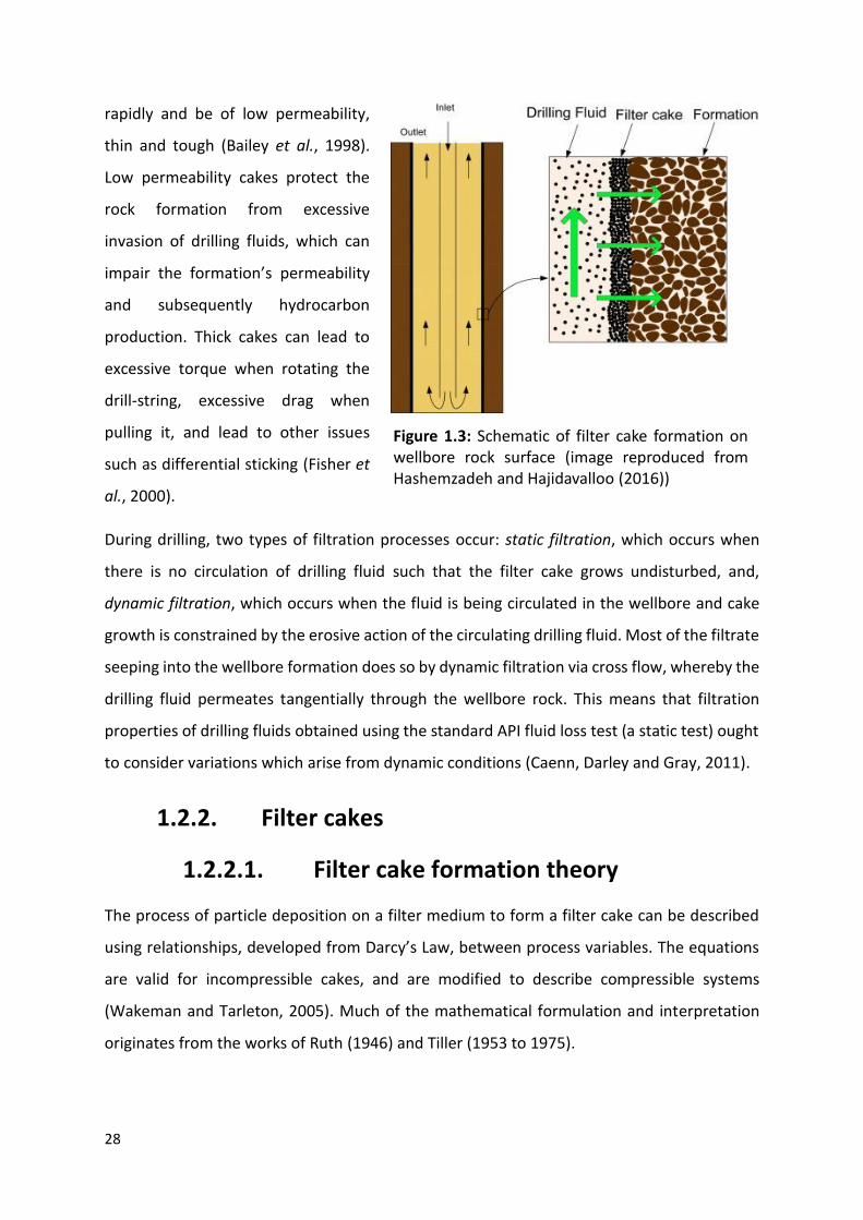
1.2.1.3. Filtration characteristics

Cake filtration occurs inherently in many in situ hydrocarbon reservoir exploitation processes

(Civan, 2015). For instance, as fresh rock surface is exposed during overbalanced drilling (the

wellbore pressure less the fluid pressure in the rock pores), the drilling fluid is forced into the

rock pores whilst particulates build up on the rock surfaces to form a filter cake (see Figure

1.3). Properties of this cake largely depend on the pressure gradient driving its growth, drilling

fluid properties and the rock’s porous structure. Ideally, drilling fluid filter cakes should form

28

rapidly and be of low permeability,

thin and tough (Bailey et al., 1998).

Low permeability cakes protect the

rock formation from excessive

invasion of drilling fluids, which can

impair the formation’s permeability

and subsequently hydrocarbon

production. Thick cakes can lead to

excessive torque when rotating the

drill-string, excessive drag when

pulling it, and lead to other issues

such as differential sticking (Fisher et

al., 2000).

During drilling, two types of filtration processes occur: static filtration, which occurs when

there is no circulation of drilling fluid such that the filter cake grows undisturbed, and,

dynamic filtration, which occurs when the fluid is being circulated in the wellbore and cake

growth is constrained by the erosive action of the circulating drilling fluid. Most of the filtrate

seeping into the wellbore formation does so by dynamic filtration via cross flow, whereby the

drilling fluid permeates tangentially through the wellbore rock. This means that filtration

properties of drilling fluids obtained using the standard API fluid loss test (a static test) ought

to consider variations which arise from dynamic conditions (Caenn, Darley and Gray, 2011).

1.2.2. Filter cakes

1.2.2.1. Filter cake formation theory

The process of particle deposition on a filter medium to form a filter cake can be described

using relationships, developed from Darcy’s Law, between process variables. The equations

are valid for incompressible cakes, and are modified to describe compressible systems

(Wakeman and Tarleton, 2005). Much of the mathematical formulation and interpretation

originates from the works of Ruth (1946) and Tiller (1953 to 1975).

Figure 1.3: Schematic of filter cake formation on wellbore rock surface (image reproduced from Hashemzadeh and Hajidavalloo (2016))

29

The filtrate flux, u, of fluid passing through a filter medium is related to the pressure

difference (p – p0) driving the flow by an appropriate form of Darcy’s Law, where Rm is the

filter medium resistance and µ is the filtrate viscosity (Equation 1.1).

𝑢 =𝑝 − 𝑝0

𝜇𝑅𝑚 (1.1)

The cumulative volume of filtrate, V, is often measured during filtration experiments and

converted to a volume flow rate dV/dt. Equation 1.2 shows the relationship between filtrate

flux and volume flow rate, where A is the area of the filter medium.

𝑢 =1

𝐴

𝑑𝑉

𝑑𝑡

(1.2)

Hence, Equation 1.3 shows the instantaneous filtrate flux through a cake-medium interface,

where Rc is the cake resistance and Δp is the total pressure drop over the cake and filter

medium.

1

𝐴

𝑑𝑉

𝑑𝑡=

∆𝑝

𝜇(𝑅𝑐 + 𝑅𝑚)

(1.3)

The deposited mass of dry solids per unit area of filter medium, w, is directly proportional to

the cake resistance, which is inversely proportional to cake permeability, k, as shown by

Equation 1.4, where ρs is the density of the solids and ε is the cake porosity. Using the specific

cake resistance, α, as a proportionality constant and Equation 1.4, the relationship between

w and cake resistance can be written as Equation 1.5.

𝛼 =1

𝜌𝑠(1 − 휀)𝑘 (1.4)

𝑅𝑐 = 𝛼𝑤 =𝑤

𝜌𝑠(1 − 휀)𝑘 (1.5)

A material balance of the filtration system provides a relationship between the mass of dry

cake, Ms, and the filtrate volume. During the formation of a cake which comprises Ms of dry

solids and with moisture content (mass of wet cake divided by mass of dry cake), m, the total

filtrate volume, V, is collected. The liquid material balance can be rearranged to give Equation

1.6, where s is the mass fraction of solids in the slurry to be filtered and ρl is the liquid density.

30

The material balance follows the assumption that all the feed slurry is filtered to form a cake.

The term ρls/(1-ms) in Equation 1.6 may be considered as a concentration, c, adjusted for the

liquid retained in the cake.

M𝑠 = 𝑤𝐴 =𝜌𝑙𝑠𝑉

1 − 𝑚𝑠

(1.6)

The basic filtration equation (Equation 1.7) is given by substituting for the cake resistance, Rc,

in Equation 1.3 using Equations 1.5 and 1.6. For compressible cakes, an average cake

permeability, kav, can be used instead of the cake permeability, which includes the

compressibility index, n.

1

𝐴

𝑑𝑉

𝑑𝑡=

𝐴∆𝑝

𝜇(𝑐𝑉

𝜌𝑠(1 − 휀)𝑘+ 𝐴𝑅𝑚)

(1.7)

For filtration experiments at constant pressure, Equation 1.7 may be integrated to provide a

relationship between filtrate volume and time (as shown in Equations 1.8 and 1.9).

∫ 𝑑𝑡 = ∫ (𝐾1𝑉 + 𝐾2)𝑑𝑉𝑉

𝑉𝑖

𝑡

𝑡𝑖

(1.8)

𝑡 − 𝑡𝑖

𝑉 − 𝑉𝑖=

𝐾1

2(𝑉 + 𝑉𝑖) + 𝐾2

𝑤ℎ𝑒𝑟𝑒 𝐾1 =𝑐𝜇

𝜌𝑠(1 − 휀𝑎𝑣)𝑘𝑎𝑣𝐴2∆𝑝𝑎𝑛𝑑 𝐾2 =

𝜇𝑅𝑚

𝐴∆𝑝

(1.9)

Matching the start of filtration with the start of the integration so that ti = Vi = 0, a plot of t/V

against V may give a straight line from which cake properties, such as permeability, can be

determined. Figure 1.4 shows an example of a t/V vs V plot for a constant pressure filtration

setup. From Equation 1.9, the gradient of the plot gives K1/2 from which the cake resistance

can be evaluated, and the intercept on the t/V axis gives K2 from which the filter medium

resistance can be evaluated. Near the start of filtration, non-linearities can be observed

because K1 and K2 are not necessarily constant in these early stages. Initially, most of the total

pressure decline is over the filter medium since the cake is very thin, but, as the cake grows,

more of the total pressure decline is lost over the cake. At this point, cake resistance

dominates the medium resistance.

31

1.2.2.2. Filter cake strength

The ability of the filter cake to seal the mouth of a crack, withstand the wellbore pressure and

prevent lost circulation depends on several factors (Cook et al., 2016):

i. the ratio between thickness of the cake and crack opening width;

ii. the shear and tensile strength of filter cakes;

iii. the adhesion of the cake to the wellbore rock;

iv. the particle size distribution of the drilling fluid.

A thicker cake is more resistant to both shear and tensile failures, and a narrower crack also

makes it harder for these types of failures to occur. If there are sufficient barite particles in

the cake that are larger than the fracture opening, the particles are likely to screen over the

opening and form a seal. If these particles are no longer able to screen over the opening, the

integrity of the cake and seal across the opening depends on its continuum strength.

During the drilling process, when overbalanced pressures (wellbore pressure is higher than

pore pressure) are used, two main mechanisms of cake rupture over fracture openings have

been identified, as shown in Figure 1.5: stretching the cake apart (tensile failure) or forcing a

Figure 1.4: A plot of t/V versus V for constant pressure filtration showing examples of non-linearities (image reproduced from Wakeman and Tarleton (2005))

32

section of cake into the opening by wellbore pressure (shear failure). The filter cake which

forms within the wellbore rock will not affect fracture behaviour, as it fails as soon as the rock

fails and is considerably weaker than the rock itself (Cook et al., 2016).

Once drilling has been completed and back-production is initiated, the filter cake can fail

affecting well cleanup. These failure mechanisms (Figure 1.6) depend on the extent of cake-

rock adhesion in relation to the filter cake strength: ‘pinholing’ may occur, allowing flow, if

the adhesion is strong in relation to the internal strength of the cake, or, the cake may detach

(‘lift-off’) from the wellbore wall if the adhesive forces are overcome. During ‘lift-off’ some of

the internal cake remains and the filter cake is not cleanly detached from the wellbore surface.

This means that, with stress

being normal to the wellbore

surface, the filter cake

undergoes a tensile failure. This

is also the case for pinholing

except that the stress is parallel

to the surface (Bailey et al.,

1998). The tensile failure stress

of filter cakes depends on the

material properties and the

stresses applied to them

(Atkinson and Bransby, 1978).

Figure 1.5: Conceptual rupture mechanisms of filter cake: (a) stretching failure and (b) bending or squeezing failure

Figure 1.6: ‘Lift-off’ of filter cake from wellbore wall during flow-back (top); lift up and ‘pinholing’ of filter cake during flow-back (bottom) (image reproduced from Suri (2005))

33

The strength of a material is described as the maximum shear stress it can sustain before

failure. The stress at the yield point (the point on a stress-strain curve that signifies the

transition from elastic to plastic behaviour) is called the yield stress, and is usually a more

important property than strength, because once the yield stress is surpassed, deformation

occurs beyond acceptable limits. For filter cakes, the shear strength is often characterised by

the shear yield stress, τy, which is the maximum applied stress it can sustain before cake

failure (Cook et al., 2016). Therefore, studies focus on finding the shear yield stress of filter

cakes, as discussed in Section 1.2.2.3.

A filter cake will grow, as more filtrate permeates into the rock formation, until the differential

pressure is exactly counteracted by the stress in the cake, which is derived from the sum of

the interparticle forces within the cake’s structure. This stress within the filter cake is

therefore a compressive yield stress (uniaxial in API fluid loss cells), Py, and for further strain

to happen a stress greater than Py must be applied. Using the approximation that suspensions

exhibit linear elasticity up until the yield point, Meeten (1994) suggested a relation (Equation

1.10) between τy and Py as observed in a study on bentonite suspensions, where ν is Poisson’s

ratio of the drained filter cake structure (network of particles or flocs).

Although a convenient order-of-magnitude estimate can be obtained, Channell and Zukoski

(1997) realised that slight variations in ν cause large variations in τy, making it unreliable to

find τy from a simple measurement of Py. Hence, methods of measuring yield stress directly

must be used instead.

1.2.2.3. Filter cake strength measurement

techniques

There are several techniques in the literature for assessing filter cake strength. One of the

earliest was a cake penetrometer, which records the force as a probe drives into the cake and

the depth is increased. It was highlighted that the point at which the force readings begin may

not necessarily be the top of the cake, but, instead, may be the top of a highly gelled fluid

region (Zamora, Lai and Dzialowski, 1990). An embedment device (Tan and Amanullah, 2001)

𝑃𝑦

𝜏𝑦=

2(1 − 𝜈)

(1 − 2𝜈)

(1.10)

34

was made to force a

cylindrical foot into the filter

cake at a controlled rate to

find the embedment modulus,

which is defined as the secant

slope of the line intersecting

the origin and the point on the

driving force vs. embedded

area curve with an embedded

area of 1000 mm2 (Figure 1.7).

The curves are composed of an initial linear section followed by a non-linear section of

upward concavity. According to Amanullah and Tan, the linear section indicates the top

viscoplastic material of the filter cake. Here the driving force is proportional to the embedded

area due to the shear stress between probe and cake. As the indenter drives further into the

cake, the inner layer is penetrated, and the non-linear section begins. The embedment device

was used to test filter cakes made from water, bentonite and a range of additives. Barite-

bentonite filter cakes displayed the highest embedment resistance as the barite particles

filled in the bentonite structure, reducing cake porosity and increasing the structural rigidity.

NaCl-bentonite-polyanionic polymer cakes had comparable embedment resistances, possibly

due to the PAC polymer chains entangling with other particles to produce a cake with a higher

structural rigidity (Tan and Amanullah, 2001).

Rheometers in a parallel plate configuration have been used to assess filter cake yield stresses

and dynamic shear moduli via continuous stress ramping and small strain oscillation modes.

The main concern arises when a particle-depleted zone forms next to the plate, because if

slip occurs, the measured yield stress does not relate to the shearing in the bulk of the cake,

but rather the stress required to overcome the static friction with the plates. An alternative

is the scraping method which entails running a razor blade across the surface of the external

filter cake at a constant speed. The shear stress is related to the cake yield stress and a shear

strength profile of the whole filter cake is obtained. However, since the theory behind this

calculation is oversimplified, only an order of magnitude estimate of the yield stress can be

obtained (Cerasi et al., 2001).

Figure 1.7: Sample driving force vs. embedded area curve obtained from a bentonite filter cake test (image reproduced from Amanullah and Tan (2001))

35

Methods used for tensile strength testing of agglomerates can be replicated for cakes, since

they are both bulk materials with low tensile strength (Dawes, 1952). Schubert (1975)

proposed a split plate method (Figure 1.8) as a way of testing slightly compacted bulk

materials. Factors such as the adhesion between the material and plates can significantly

influence the measured tensile strength values. A way around this is to assume the filter cake

strength to be predominantly a result of the cohesive forces between particles, instead of the

external stresses applied to the cake. This assumption allows the tensile strength to be

estimated as proportional to the shear strength or shear yield stress (Cook et al., 2016).

Bailey et al. (1998) developed a hole punch test (Figure 1.9) to directly measure the shear

failure of filter cakes. Nandurdikar et al. (2002) and Hao et al. (2016) used a similar hole punch

method to perform cake strength tests. The technique directly measures the force required

for cake failure so that the yield stress can be determined. Bailey et al. compared the hole

punch method with the vane method, which uses a bladed vane sensor to find the maximum

torque through a cake sample, and the squeeze-film method, which uses parallel plates to

squeeze a cake sample whilst recording the force. These methods produced consistent results

suggesting each to be reliable, but the hole punch method was favoured because it required

neither the thick filter cakes used in the vane method nor the complex equipment used in the

squeeze-film method.

Figure 1.8: Diagrammatic set-up of the split plate apparatus (image reproduced from Schubert (1975))

36

Bailey et al. (1998) pressed barite weighted bentonite-based drilling fluids at 2000 kPa, whilst

varying the barite concentration to manipulate fluid density. Their hole punch test results

exhibited a peak yield strength at a critical barite concentration. Bailey et al. explain this trend

by suggesting that below a critical concentration, barite particles behaved as a filler to bolster

the bentonite network, increasing its yield stress. However, beyond this critical concentration,

there is sufficient barite to form the core load-bearing matrix, and the bentonite-water gel

fills the available space. The roles that the barite and bentonite-water fluid serve essentially

switch past this critical concentration. Since the cohesive strength of the barite matrix is much

lower than that of the bentonite gel it replaces, the yield stress declines.

Bailey et al. (1998) also used their technique to study the effects of particle size on cake yield

stress by adding barite and constant volume fractions of different grades of calcium carbonate

to fluids composed of polymer dissolved in water. Their results showed that higher solids

loadings led to an increase in yield stress, and that barite weighted filter cakes gave lower

yield stress values than correspondingly sized calcium carbonate weighted filter cakes.

Furthermore, they found finer particles to form stronger cakes. The coarser particles formed

cakes with low cohesive strength and poor fluid loss control. It was suggested that the surface

chemistry of the weighting agents and particularly the surface area of the particles affect the

particle interactions, and hence, the measured yield stress.

Figure 1.9: A schematic of the hole punch test as developed by Bailey et al. (1998) (from which this image was adapted)

37

Similar observations on the effects of solids content and fine particles on cake strength were

made by Cerasi et al. (2001), who performed strength tests using a rheometer with a parallel-

plate geometry. In addition to finding out that oil-based fluid cakes had orders of magnitude

lower yield stresses than water-based ones, they investigated the effects of increasing the

drill solids content whilst keeping the overall fluid density constant (presumably by decreasing

the calcium carbonate particle concentration). Cerasi et al. found the increasing

concentration of drill solids, which were finer than the calcium carbonate particles, to

increase yield stress. In a second series of experiments, Cerasi et al. increased the drill solids

loading keeping the calcium carbonate particle concentration fixed. In this case, the extent of

yield stress variation was less than with the first series of experiments. Based on these

findings, Cerasi et al. proposed that the increase of fines in the filter cake had a more

significant influence on yield stress than the increased solids loading in the fluid.

1.2.2.4. Filter cake thickness measurement

techniques

Filter cake thickness is an important property required to convert force-displacement data to

stress-strain values. With regards to the drilling process, a maximum limit of cake thickness is

recommended to avoid problems such as differential sticking of the drill bit. Typical methods

of experimentally finding cake thickness can be split into destructive and non-destructive

techniques. Destructive techniques lead to changes in cake structure that make any further

testing unreliable, and, the methods of thickness measurement tend to cause uncertainties.

For example, tracking cake growth using pressure probes (Murase et al., 1987) or controlling

the filtration rate and, hence, cake growth via disks with a sharp central hole (Fathi-Najafi and

Theliander, 1995) may affect cake build-up. To overcome this, Tarleton (1999) used electrode

type sensing probes, which were small relative to the filter cell, to measure filter cake

properties with minimal impact on the cake structure. Non-destructive methods of

determining cake thickness generally pass a signal (acoustical or optical) through the cake and

monitor the changes in intensity (Takahashi et al., 1991; Amanullah and Tan, 2001; Hamachi

and Mietton-Peuchot, 2001). The methods depend on more complex equipment and require

calibration relationships between the measured parameters and cake thickness.

38

1.2.2.5. Filter cake porosity measurement

techniques

Non-destructive methods for finding filter cake porosity include electrical conductivity

(Shirato et al., 1971), NMR imaging (La Heij et al., 1996; Hall et al., 2001), and gamma and x-

ray attenuation measurements (Shen, Russel and Auzerais, 1994; Tiller, Hsyung and Cong,

1995; Sedin, Johansson and Theliander, 2003). Although the non-destructive nature enables

the measurement of cake porosity profiles over time in a single filtration experiment, these

methods require calibration and/or development of algorithms for signal processing (Tien,

2006). The most common method to determine filter cake porosity, without requiring

complicated and expensive equipment, is to measure the wet cake mass, then completely dry

the cake and measure the dry cake mass (Dewan and Chenevert, 2001; Tien, 2006). By

dissecting the cake and weighing each segment, a porosity profile per 0.5 mm of cake

thickness can be obtained (Meeten, 1993). Using the drying method to determine the void

ratio (defined as the volume of liquid in the cake over the volume of solid), Sherwood and

Meeten (1997) found heterogenous void ratio profiles for filter cakes made from barite-

weighted drilling fluids, whereby the bottom of the cake near the filter paper had the lowest

void ratios and the top of the cake had the highest. In addition, they found that the cake void

ratio decreased with increasing filtration pressure.

1.2.2.6. Filter cake imaging

Although the formation of cake layers is important in affecting the filtration performance of

drilling fluids, there is a lack of literature information about cake structures. Understanding

the structure of filter cakes should enable a better control of filtration processes and lessen

wellbore stability issues (Yao et al., 2014). More specifically, an understanding of the cake

structure may elucidate how constituent particles contribute to cake strength. Hence,

visualisation techniques to investigate the internal structure of filter cakes have been

explored.

From captured scanning electron microscopy (SEM) micrographs, Yao et al. (2014) found that

filter cake porosity increased as the drilling fluid density, which was controlled by the barite

and hematite volume fractions, increased, as shown in Figure 1.10. They also found the

39

bottom layer of the cake to comprise larger particles and a lower polymer content compared

to the top layer. Similarly, Elkatatny et al. (2012) found, from SEM scans, that the cake layer

closer to the filter medium contained large grains whilst both small and large grains were

found in the cake surface layer. A shock-freezing/freeze-drying method has been used to keep

the filter cake’s basic structure intact for SEM imaging. Plank and Gossen (1991) validated this

method by comparing freeze-dried and frozen-hydrated samples. They found the typical

arrangement of bentonite platelets in a honeycomb structure using both methods. Chenevert

and Huycke (1991) concluded from over a hundred viewings that the freeze-drying method

produced samples that are a near representation of the real pore structure with minimal

alterations. They highlighted that due to liquid nitrogen being a poor thermal conductor and

the resulting Leidenfrost1 effect, large ice crystals may form if liquid nitrogen was used to

shock-freeze samples. More recent papers have used nitrogen slush for freezing with cryo-

SEM (Argillier, Audibert and Longeron, 1997).

Environmental scanning electron microscopy (ESEM) has been used as an alternative to SEM

(Tare et al., 1999; Nandurdikar, Takach and Miska, 2002), because the filter cake can be

imaged in its wet state and the cake surface does not need to be treated as the ESEM

functions under a weak vacuum. Nandurdikar et al. (2002) used ESEM to relate the structure

of filter cakes with the measured strengths. In particular, they wanted to find the variation of

the pore size distribution throughout the cake thickness as well as at the cake surface and

1 The Leidenfrost effect is a phenomenon where a liquid, which is close to a surface with a temperature much higher than the liquid’s boiling point, generates an insulating vapour layer that prevents the liquid from boiling.

Figure 1.10: SEM micrographs of filter cakes made from fluids of density 2.1 g cm-3 (left) and 2.3 g cm-3 (right) (image reproduced from Yao et al. (2014))

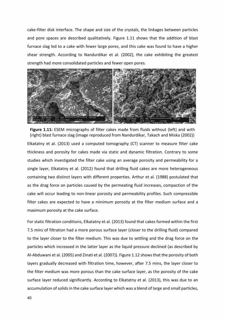
40

cake-filter disk interface. The shape and size of the crystals, the linkages between particles

and pore spaces are described qualitatively. Figure 1.11 shows that the addition of blast

furnace slag led to a cake with fewer large pores, and this cake was found to have a higher

shear strength. According to Nandurdikar et al. (2002), the cake exhibiting the greatest

strength had more consolidated particles and fewer open pores.

Elkatatny et al. (2013) used a computed tomography (CT) scanner to measure filter cake

thickness and porosity for cakes made via static and dynamic filtration. Contrary to some

studies which investigated the filter cake using an average porosity and permeability for a

single layer, Elkatatny et al. (2012) found that drilling fluid cakes are more heterogeneous

containing two distinct layers with different properties. Arthur et al. (1988) postulated that

as the drag force on particles caused by the permeating fluid increases, compaction of the

cake will occur leading to non-linear porosity and permeability profiles. Such compressible

filter cakes are expected to have a minimum porosity at the filter medium surface and a

maximum porosity at the cake surface.

For static filtration conditions, Elkatatny et al. (2013) found that cakes formed within the first

7.5 mins of filtration had a more porous surface layer (closer to the drilling fluid) compared

to the layer closer to the filter medium. This was due to settling and the drag force on the

particles which increased in the latter layer as the liquid pressure declined (as described by

Al-Abduwani et al. (2005) and Zinati et al. (2007)). Figure 1.12 shows that the porosity of both

layers gradually decreased with filtration time, however, after 7.5 mins, the layer closer to

the filter medium was more porous than the cake surface layer, as the porosity of the cake

surface layer reduced significantly. According to Elkatatny et al. (2013), this was due to an

accumulation of solids in the cake surface layer which was a blend of large and small particles,

Figure 1.11: ESEM micrographs of filter cakes made from fluids without (left) and with (right) blast furnace slag (image reproduced from Nandurdikar, Takach and Miska (2002))

41

resulting in poor sorting and a very low porosity by 30 mins of filtration. As discussed in

Section 1.2.2.5., Sherwood and Meeten (1997) also found heterogeneous filter cakes forming

for static filtration conditions, but found the opposite behaviour whereby the layer closer to

the filter medium had the lowest porosities. However, their cakes were filtered until

completion (until no further fluid was pressed from the cake), so filtration times were

significantly longer than 30 mins.

Figure 1.12: The porosity (top) and thickness (bottom) profiles throughout a cake made after different filtration times (image reproduced from Elkatatny, Mahmoud and Nasr-El-Din (2013))

42

Figure 1.12 shows the cake compression and buildup stages during the static filtration process

as the cake layers decrease then increase in thickness. The figure also shows that the layer

closer to the filter medium is initially thicker than the cake surface layer due to the settling of

large particles in the former layer. During the buildup stage, this relationship reverses as the

cake surface layer becomes thicker. According to Elkatatny et al. (2013), this was due to the

decreasing porosity in this layer which prevented particles from reaching the filter medium.

During static filtration, the cake mainly developed via compression then switched to buildup,

whilst cake formation was dominated by buildup throughout dynamic filtration.

1.2.2.7. Discrete element modelling

The discrete element method (DEM) was first introduced by Cundall and Strack (1979) as a

numerical model to simulate the mechanical behaviour of a collection of discs and spheres.

Explicit numerical methods were used to monitor the contacts in every particle interaction

and to model the motion of particles. A DEM simulation calculates the movement of a defined

set of particles based on their body forces, which is assumed to act from each particle’s centre

of mass, and contact forces, acting at the contact point between particles. Once the particles’

preliminary properties are specified, the movement of each particle is simulated based on

Newton’s laws of motion.

DEM has been used to understand the effects of particle and fluid properties on filter cake

formation. Dong et al. (2009) developed a DEM model to simulate cake formation and growth

via constant flow rate and constant pressure filtration. For constant pressure filtrations,

increasing the pressure drop across the cake increased the filtrate flow rate and, hence, the

cake growth rate. They found that decreasing the fluid viscosity and density increased cake

porosity, whilst, for a given filtrate flow rate, increasing particle size in the cake decreased

cake porosity. Deshpande et al. (2020) coupled DEM with computational fluid dynamics to

simulate the filtration of suspensions with particles of varying sphericities. Using a multi-

sphere model to control particle sphericity, they found that the porosity of filter cakes

increased as particle sphericity decreased and as the coefficient of sliding friction increased.

When fluid was passed through dry filter cakes with a constant inlet velocity, the pressure

drop per unit length of cake increased as particle sphericity decreased from 1.00 to 0.93, then

decreased as particle sphericity decreased from 0.93 to 0.82. According to Deshpande et al.

43

(2020), the increase in pressure drop was due to the reduced sphericity as the cake porosity

was unchanged.

DEM has been used to study particle systems under bulk compression. Wiacek et al. (2012)

performed DEM simulations of uniaxial compression to investigate the effects of particle

shape and interparticle coefficient of friction on the mechanical behaviour of granular

systems. They found that as the aspect ratio of the particles increased from 1.0 to 1.6, the

granular systems became less porous and had a higher modulus. From an aspect ratio of 1.6

to 2.8, the modulus did not vary much but the porosity increased. However, increasing the

particle aspect ratio increased the number of particles in the container: 1000 for spherical

particles and 1650 for particles with an aspect ratio of 2.8. In similar compression tests, Feng

et al. (2009) found that, for particles of the same shape, decreasing the particle size, and so

increasing the number of particles, led to an increase in modulus due to the increase in

interparticle contacts. Thus, it is not clear whether the effects of aspect ratio on modulus in

Wiacek’s work were caused by the changes in particle shape and/or the number of

interparticle contacts. Hartl and Ooi

(2011) performed DEM simulations of a

direct shear test on spherical and non-

spherical particles, as shown in Figure

1.13, to investigate the relationship

between particle shape and the bulk

internal friction. They found that as the

particle aspect ratio increased the bulk

friction increased, which was due to an

increase in particle interlocking as well as

in the mobilised particle contact friction

and coordination number. Comparing

the DEM with experimental data, they

concluded that there was quantitative

agreement with regards to the bulk

friction results if the initial packing

densities were similar.

Figure 1.13: Particles settling in a filling cylinder placed above a shear cell. Single spheres (left) and paired spheres used as non-spherical particles (right) were generated using DEM (image reproduced from Härtl and Ooi (2011))

45

Chapter 2. Experimental methods and

materials

2.1. Introduction

To assess the strength of drilling fluid filter cakes and how they are affected by constituent

particles, drilling fluids composed of particles with a range of properties were made. Although

most of the filtrate seeping into wellbore formations does so via dynamic cross flow filtration,

static filtration was used in this work to produce filter cakes from drilling fluids. This meant

that a range of samples could be tested as the equipment and analysis required are simpler.

The hole punch tester (Bailey et al., 1998) was used to determine filter cake strength, since

the test has been shown to produce consistent results when compared to other methods (as

discussed in Section 1.2.2.3.) and it simulates the shear rupture of a filter cake without the

need for complex equipment.

Filter cake thickness was found by tracking the force on a probe descending through the cake,

and, since the suspension/cake is poorly defined, a drying rate method was developed to

determine cake porosity. X-ray computed tomography was used to visualise the internal pore

structures in a non-destructive manner, with minimal sample preparation required. The

distribution of pores and their sizes were obtained from images, and these data were used to

compare cake structures so that the influence of constituent particles on cake properties

could be understood. The hole punch tester was simulated using the discrete element method

(DEM), which, as discussed in Section 1.2.2.7., has been used in the literature (Feng, Owen

and Loughran, 2009; Härtl and Ooi, 2011; Wiacek et al., 2012) to evaluate the granular

response of particulate systems. Discussions on the development of the DEM code are in

Chapter 6.

46

2.2. Methods

2.2.1. Analysis of drilling fluids

2.2.1.1. Rheology Parallel-plate rheometer tests were performed on drilling fluids. For the initial samples, small

globules of xanthan gum were often visible in the sample which indicated improper mixing.

To check the mixing, viscometry tests using the Kinexus rheometer (Figure 2.1) were run to

compare viscosity and yield stress values for different samples. A low viscosity at low shear

stresses (Figure 2.1) could also indicate that the xanthan gum had not been mixed properly.

2.2.1.2. Static light scattering

Static light scattering is a technique that uses the angle and intensity of light scattered from

particles to calculate their size. In this work, a Malvern Mastersizer 2000 was used to measure

the size distributions in samples as outlined in Section 2.3.1.

2.2.1.3. Static image analysis

Static image analysis is a technique which uses microscopy imaging for the dry analysis of

particles. The particles are dispersed on a glass slide which is placed beneath a digital camera

with a magnifying lens. Images are captured of each particle in a selected area of the sample

and algorithms are used to calculate size and shape parameters from the particle perimeters

Figure 2.1: The Kinexus rheometer used for viscometry tests (left) and

representative shear viscosity vs shear stress curves (right)

47

(Entegris, 2019). In this work, a Morphologi G3 Microscope was used to measure the particle

size and shape in samples as outlined in Section 2.3.2.

2.2.2. Analysis of filter cakes

2.2.2.1. Filtration

Filter cakes were made using an API filter press (Figure 2.2) at a constant pressure of 690 kPa

for 30 minutes using a 0.45 µm rated nylon membrane. After an experiment, the filter press

was dismantled, and, the cake was removed with the membrane and sealed in a petri dish to

avoid drying. The sample removal was performed carefully to avoid excess fluid on the top of

the cake surface and to ensure the cake structure was not disrupted. Three separate filter

cake samples were made for each fluid composition: one was weighed and left to dry to

obtain the porosity, another was placed on the texture analyser to measure thickness and the

last was placed on the hole punch platform, which was attached to the texture analyser, to

measure mechanical properties.

48

Figure 2.2: Summary of experimental procedure showing the tests performed on filter

cakes made in the API filter press (top left)

49

2.2.2.2. Hole punch tester

The cake yield stress was found by punching a plunger attached to a Texture Analyser through

the cake sample, having carefully peeled off the attached nylon membrane, which sits on top

of an opening; see Figure 2.2 for images of the test and Figure 2.3 for a schematic description.

The opening in the platform, as shown in Figure 2.3, was made with a slightly larger diameter

than the plunger to prevent friction between the plunger and the inner walls of the opening.

This device, called the hole punch tester, is expected to simulate shear rupture in a simple

and inexpensive manner. Bailey et al. (1998), Nandurdikar et al. (2002) and Hao et al. (2016)

all used a similar hole punch method to carry out cake strength tests. Bailey et al. (1998)

compared the yield stress results using this hole punch method to two other techniques: the

vane method and the squeeze film method. The hole punch data seemed to correspond well

with data from these two other approaches, as discussed in Section 1.2.2.3., suggesting it to

be a reliable technique. Using the Texture Analyser, force-displacement data were obtained

with this technique. The shear stress was determined by dividing the force by the cake surface

area that is being sheared (πDT, where D is the opening diameter and T is the cake thickness),

and the strain was calculated by normalising the displacement with the cake thickness. When

the peak force is used, the resulting shear stress corresponds to the filter cake’s yield stress.

Repeat hole punch tests were run on cakes made from the SC2 sample (see Section 2.3.2.)

with measured yield stresses of 35.7, 43.9 and 46.8 kPa, giving a mean value of 42.1 kPa and

a standard error of 8%.

2.2.2.3. Filter cake thickness

The cake thickness was determined by using the Texture Analyser’s force measurements

through the cake sample (Figure 2.2). A similar method was used by Chen and Hsiau (2009)

Figure 2.3: Schematic of hole punch test and conversion of force-displacement

data

50

who used an on-line powder pressure-displacement system to measure the thickness of dust

filter cakes. The cake sample is placed on a flat surface below the Texture Analyser probe

which is set at a fixed height and approaches the cake at a constant speed, measuring the

force as it descends. A force is recorded as soon as the probe contacts the filter cake’s top

surface and increases further as the probe traverses the cake to approach the bottom surface.

Near the bottom surface, the force increases exponentially until it reaches a maximum force

of 40 N at which point the test is stopped. The height difference between the top and bottom

surfaces is then recorded as the filter cake thickness. Repeat thickness measurements were

run on a cake made from each of the SC samples (see Section 2.3.2.), giving an average

intrasample standard error of less than 1%.

2.2.2.4. Filter cake porosity

A challenge often faced with drilling fluid filter cakes is that the suspension/filter cake

interface is poorly defined, which makes it difficult to accurately determine the cake’s

moisture content. Hence, for this work, a method was developed to track the drying rate of

the cake over time, and it was detected when the rate declined significantly (Figure 2.2). The

shift in the mass transfer rate as water is evaporated from the cake, as opposed to the fluid

on top of the cake, becomes evident in the drying rate curve: the point at which the curve

experiences a sharp transition can be approximated as the point at which the cake itself

begins to dry. With this approach the liquid content of the cake can be determined, and

assuming the void spaces in the filter cake to be saturated with liquid, the average porosity,

εav, is calculated using Equations 2.1 and 2.2, where ρl is the liquid density and ρs is the density

of the solids. In preliminary tests, repeat porosity measurements were run on cakes made

from different samples giving standard errors that ranged from 2 to 6%.

휀𝑎𝑣 =∝

∝ +𝜌𝑙

𝜌𝑠

(2.1)

∝=

𝑛𝑒𝑡 𝑤𝑒𝑡 𝑤𝑒𝑖𝑔ℎ𝑡

𝑛𝑒𝑡 𝑑𝑟𝑦 𝑤𝑒𝑖𝑔ℎ𝑡− 1

(2.2)

51

2.2.2.5. X-ray computed tomography

X-ray computed tomography (XRCT) is a technique used to capture 2D slices of a sample that

can be digitally assembled to produce a 3D image. The use of x-rays enables a non-destructive

visualisation of internal structures. XRCT imaging devices are composed of an x-ray source

and detector with the sample placed in between. X-rays pass through the rotating sample and

are collected by the detector to produce a 2D projection, typically referred to as a ‘slice’, of

the 3D object. The density of the material and the energy of the x-rays dictate the amount of

x-ray attenuation. This means that each material of a different density will attenuate x-rays

differently. For the devices used in this work, the energy of the x-rays could be controlled and

was varied according to the composition of the sample being studied to allow enough x-rays

to penetrate the sample. The number of x-rays that reach the detector is represented by the

greyscale value of each pixel in the slice (University of Manchester, 2013).

In this work, samples of interest were selected for XRCT imaging, as discussed in Section 2.3.3.,

to visualise the internal structure of the cake. For each sample, once the filtration test was

completed, the cake was placed into a petri dish and sealed to prevent the cake from drying.

For imaging, the cakes were put onto a sample holder (Figure 2.4) which held the cake at 45°

to the horizontal. The sample holder was then placed in the XRCT device ready for imaging

(Figure 2.4). Scans were kept under 90 mins to prevent the cake from drying excessively and

their structure was kept unaltered.

Amira-Avizo (ThermoFisher Scientific, 2020), which is a 3D visualisation and analysis software,

was used to obtain 3D representations and quantitative data of the pores. Orthogonal slices,

Figure 2.4: A cake sample placed on the sample holder used for imaging (left) and the

High Flux Nikon XTEK bay at the University of Manchester used for XRCT imaging (right)

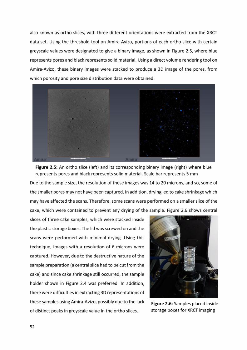
52

also known as ortho slices, with three different orientations were extracted from the XRCT

data set. Using the threshold tool on Amira-Avizo, portions of each ortho slice with certain

greyscale values were designated to give a binary image, as shown in Figure 2.5, where blue

represents pores and black represents solid material. Using a direct volume rendering tool on

Amira-Avizo, these binary images were stacked to produce a 3D image of the pores, from

which porosity and pore size distribution data were obtained.

Due to the sample size, the resolution of these images was 14 to 20 microns, and so, some of

the smaller pores may not have been captured. In addition, drying led to cake shrinkage which

may have affected the scans. Therefore, some scans were performed on a smaller slice of the

cake, which were contained to prevent any drying of the sample. Figure 2.6 shows central

slices of three cake samples, which were stacked inside

the plastic storage boxes. The lid was screwed on and the

scans were performed with minimal drying. Using this

technique, images with a resolution of 6 microns were

captured. However, due to the destructive nature of the

sample preparation (a central slice had to be cut from the

cake) and since cake shrinkage still occurred, the sample

holder shown in Figure 2.4 was preferred. In addition,

there were difficulties in extracting 3D representations of

these samples using Amira-Avizo, possibly due to the lack

of distinct peaks in greyscale value in the ortho slices.

Figure 2.6: Samples placed inside

storage boxes for XRCT imaging

Figure 2.5: An ortho slice (left) and its corresponding binary image (right) where blue

represents pores and black represents solid material. Scale bar represents 5 mm

53

2.3. Materials

2.3.1. Representative and initial model drilling

fluids

Samples were made using representative water-based and oil-based compositions. For the

water-based drilling fluids, the volume fraction of barite was varied to control fluid density

and the volume fractions of starch and Drispac were varied to control cake permeability (see

Table 2.1 for the compositions). The samples were made up to 400 ml using deionised water.

For the oil-based drilling fluids, the samples were made up to 400 ml using a base fluid

composed of oil (Versaclean CBE and Saraline 185V) and deionised water. The oil/water ratios

were 80/20 vol% for OBM128 and OBM188 and 60/40 vol% for OBM126. Table 2.2 shows the

components that were added to make up each sample. The model water-based drilling fluids

were made with typical drilling fluid components and the solid particulate additives were

varied, as shown in Table 2.3. All fluid samples were made up to 400 ml using deionised water,

1.37 g of xanthan gum and 0.4 g of magnesium oxide (to maintain pH 10). Ultra-fine, fine,

medium and coarse calcium carbonate refer to Fordacal 8, 22, 50 and 150, where the number

represents the batch’s d50 value (LKAB Minerals, 2016). Size distributions of the particulate

additives were determined using a Malvern Mastersizer 2000, with the data shown in Figure

2.7.

The components were sequentially added to the base fluids and stirred at 6000 RPM using a

Silverson Laboratory Mixer. For the water-based fluids, a general-purpose mixing head was

used, and the total mixing time was 1 hour for WBM1 and WBM HD and 50 mins for WBM HF

and WBM HF(HD). Viscometry tests were performed on these fluids to check for good mixing

and consistency between samples. For the oil-based fluids, the total mixing time was 1 hour

(excluding the addition of Safe-Carb 20) and a small square hole shear head was used on the

mixer. The Safe-Carb 20 was added after the initial 1-hour mix and, with the shear head

removed, the fluid was then mixed for another 10 minutes. For the model water-based fluids,

the total mixing time was 35 minutes and a general-purpose mixing head was used on the

Silverson to avoid particle size reduction.

54

Table 2.1: Representative water-based drilling fluid compositions

Sample Barite

(vol%)

Starch

(vol%)

Drispac

(vol%)

Potassium

chloride

(vol%)

HMP

clay

(vol%)

Xanthan

gum

(vol%)

Magnesium

oxide

(vol%)

WBM1 6.2 0.6 0.2 3.6 1.2 0.2 0.1

WBM HD 24.8 0.6 0.2 3.6 1.2 0.2 0.1

WBM HF 6.2 - - 3.6 1.2 0.2 0.1

WBM HF(HD) 24.8 - - 3.6 1.2 0.2 0.1

Table 2.2: Representative oil-based drilling fluid compositions

Sample Truvis

(vol%)

Versaclean

CBE (vol%)

Ecotrol

RD

(vol%)

Saraline

185V

(vol%)

Calcium

chloride

(vol%)

Water

(vol%)

Barite

(vol%)

Versatrol

M (vol%)

Safe-

Carb

20

(vol%)

Lime

(vol%)

OBM188 0.5 3.9 0.7 49.5 0.3 13.1 26.5 2.0 2.1 1.0

OBM126 0.6 3.9 - 48.1 1.0 34.0 7.0 2.0 2.1 1.0

OBM128 1.8 3.0 - 64.4 0.4 16.6 8.5 2.0 2.1 1.0

Table 2.3: Model water-based drilling fluid compositions

Sample Barite (vol %)

Calcium carbonate (vol %)

Ultra-fine Fine Medium Coarse

SCal8 - 6.2 - - -

SCal22 - - 6.2 - -

SCal50 - - - 6.2 -

SCal150 - - - - 6.2

SC1 3.1 -

SC2 6.2 -

SC5 24.8 -

55

2.3.2. Model water-based drilling fluids

Samples were made with typical water-based drilling fluid components and the solid

particulate additives were varied. All fluid samples were made up to 400 ml using deionised

water, 1.37 g of xanthan gum and 0.4 g of magnesium oxide (to maintain pH 10). Samples

containing graded calcium carbonate and/or barite are given in Table 2.4. Ultra-fine, fine,

medium and coarse calcium carbonate refer to Fordacal 8, 22, 50 and 150, where the number

represents the batch’s d50 value (LKAB Minerals, 2016). The volume of calcium carbonate

particles in SCal samples are equal to the volume of barite particles in the SC equivalents.

Medium-sized calcium carbonate particles were further graded into size ranges using a

column of sieves on a mechanical shaker. These sieved size ranges were then used to control

the proportion of fine and coarse particles in the blended ratio samples (B1X and B2X): as the

number after the ‘X’ in the sample name increases (see Table 2.4), the proportion of coarser

particles in the sample increases. The total volume fraction of calcium carbonate in each

blended ratio sample was kept constant.

Samples with particles of varying shape were made up of solid particles with a volume fraction

of 6.2 vol% as in SC2 (Table 2.4); these particles were calcium carbonate (SCal2), talc (Stal),

cellulose microcrystalline (Scell) and glass spheres (Sglass). The circularity, given as the

circumference of the equivalent area circle divided by the actual perimeter of the particle, of

these particles is given in Table 2.5. Particle sizes and circularities of the particles used to test

the effect of particle shape were measured in the dry state using a Morphologi G3 Microscope.

Figure 2.7: Particle size distributions of calcium carbonate and barite particles

0.1 1 10 100 1000

0

2

4

6

8

10

Vol

ume

(%)

Particle size (µm)

Ultra fine calcium carbonate

Fine calcium carbonate

Medium calcium carbonate

Coarse calcium carbonate

Barite

56

Table 2.4: Model water-based drilling fluid compositions for varying barite and calcium carbonate concentration, and, varying particle size distribution samples. Each sample was prepared using the same mixing procedure and conditions

Sample Barite

(vol %)

Calcium carbonate (vol %) Sieved calcium carbonate (vol %)

Ultra-

fine Fine Medium Coarse

20-

38µm

38-

53µm

53-

63µm

63-

75µm

75-

108µm

108-

150µm

SC1 3.1 - -

SC2 6.2 - -

SC3 12.4 - -

SC4 18.6 - -

SC5 24.8 - -

DB1 6.2 - - 1.5 1.5 -

DB2 6.2 - 1.5 - 1.5 -

DB3 6.2 1.5 - - 1.5 -

DB4 6.2 - 1.5 1.5 - -

DB5 6.2 1.5 - 1.5 - -

DB6 6.2 1.5 1.5 - - -

DB7 6.2 0.7 0.7 0.7 0.7 -

DB8 6.2 - 1.0 1.0 1.0 -

DB9 6.2 1.0 1.0 1.0 - -

B1X2.0 3.1 - 0.2 0.1 0.1 0.3 0.5 1.7

B1X1.5 3.1 - 0.4 0.2 0.1 0.4 0.5 1.4

B1X1.0 3.1 - 0.7 0.2 0.1 0.4 0.5 1.0

B1X0.5 3.1 - 1.5 0.2 0.1 0.3 0.3 0.5

B2X2.0 6.2 - 0.2 0.1 0.1 0.3 0.5 1.7

B2X1.5 6.2 - 0.4 0.2 0.1 0.4 0.5 1.4

B2X1.0 6.2 - 0.7 0.2 0.1 0.4 0.5 1.0

B2X0.5 6.2 - 1.5 0.2 0.1 0.3 0.3 0.5

SCal1 - 3.1 - - - -

SCal2 - 6.2 - - - -

SCal5 - 24.8 - - - -

57

The components were sequentially added to the water-based fluid and stirred at 6000 RPM

using a Silverson Laboratory Mixer with a total mixing time of 35 minutes. The mixing time

was long enough to ensure that the components were homogeneously dispersed in the fluid,

but short enough to avoid excess heating. A general-purpose mixing head was used on the

Silverson to avoid particle size reduction. Particle size distributions were determined using a

Malvern Mastersizer 2000, with the data shown in Figure 2.7.

2.3.3. XRCT imaging samples

From the samples outlined in Section 2.3.2., those which exhibited an extreme range of cake

thickness, porosity and yield stress values were selected for XRCT imaging. These samples

were DB1, DB2, DB3, DB4, DB5, DB6, SC2 and SC5 (compositions are in Table 2.4). Samples

SC25 and SC220, which had the same composition as SC2 but were filtered for 5 and 20 mins

respectively, were also imaged. The samples were made using the same preparation

procedure as outlined in Section 2.3.2. and were sealed in a petri dish for transportation to

the XRCT device. The mass of each sample was checked before and after transportation, and

minimal changes in mass were recorded.

Table 2.5: Properties of the substances used for particle shape analysis

Substance Circularity D50 (μm)

Glass 0.88 12.9

Calcium carbonate 0.82 19.2

Barite 0.81 9.7

Talc 0.71 15.6

Cellulose microcrystalline 0.77 66.5

59

Chapter 3. Representative and model drilling

fluids

3.1. Introduction

This chapter explores the properties of drilling fluids, which are representative of those used

in the field, and the properties of the filter cakes produced from such fluids. Water-based and

oil-based drilling fluids, the composition and mixing procedure of which are discussed in

Section 2.3.1., were prepared, and, after mixing, a sample was taken for rheology testing as

discussed in Section 2.2.1.1. Then, these fluids were filtered via static filtration using an API

filter press and the filtrate collected over time. Three batches of each fluid were made to

produce three filter cake samples for thickness, porosity and strength testing, as outlined in

Section 2.2.2. The purpose of testing these representative fluids was to establish benchmark

results, which could then be used to compare with model water-based drilling fluids made

using typical drilling fluid components. The model fluids were used to obtain the experimental

results presented in Section 3.4 as well as in Chapters 4 and 5.

Typical drilling fluids are composed of a base fluid (water and oil-based drilling fluids are both

commonly used), solids and additives (to control the fluid properties). Barite is commonly

used to control fluid density and varying volume fractions of it was used in the representative

fluids, as shown in Tables 2.1 and 2.2. Calcium carbonate particles, used primarily as bridging

agents since they come in a wide range of sizes, also contribute to fluid density. A constant

volume fraction of calcium carbonate was added to the representative oil-based drilling fluids

in the form of Safe-Carb 20. The rheological properties of drilling fluids influence the removal

of drilled cuttings, and unsatisfactory performance can lead to major problems such as stuck

pipe, loss of circulation, and even a blowout. Xanthan gum is used to control the rheology of

water-based drilling fluids, enhancing the low-shear rate viscosity (Caenn, Darley and Gray,

2011). Xanthan gum improves the shear-thinning capabilities of water-based drilling fluids,

which was shown to increase the drill rate (Deily et al., 1967) due to the ease of pumping at

high shear rates, and, which means it can adequately suspend drilled cuttings at low shear

rates (Caenn, Darley and Gray, 2011).

60

In this chapter, representative water and oil-based drilling fluids and their filter cakes are

analysed. Shear viscosity against shear stress curves of the water-based fluids are used to

check their rheological behaviour and to ensure uniform mixing. Filtrate volume curves are

used to assess the filtration and to evaluate filter cake permeability. The thickness of these

filter cakes is measured, and, for the water-based fluids, the cake porosity and strength are

determined. The yield stresses of cakes made from representative water-based fluids are

compared with those of model water-based fluids. For the model fluids, the yield stress

variation with particle size and particle volume fraction in the fluid are also discussed.

3.2. Drilling fluid properties

The compositions of the representative water and oil-based drilling fluids are shown in Tables

2.1 and 2.2. These compositions were selected to capture the range of typical drilling fluid

performance and to establish holistic benchmark results, which were then used to compare

with the model fluids. For the representative fluids, compositions commonly used in the field

were explored, which included typical drilling fluids (WBM1, OBM126 and OBM128), high

density fluids (WBM HD and OBM188), high fluid loss fluids (WBM HF), and, high fluid loss

and high density fluids (WBM HF(HD)). The rheological and filtration results obtained were

generally in agreement with those found at the BP Wells laboratories in Sunbury, validating

the drilling fluid preparation procedure.

3.2.1. Rheological measurements

Rheology curves of the representative water-based drilling fluids are shown in Figure 3.1. As

discussed in Section 2.2.1.1., the Kinexus rheometer was used to perform viscometry tests on

fluid samples, from which shear viscosities at fixed shear stresses were obtained. In Figure

3.1, the water-based fluids exhibit high viscosities at low shear stresses, and, as the shear

stress increases, the fluids yield and the viscosities decrease until a constant low value at high

shear stresses. This shear-thinning behaviour is consistent with water-based drilling fluids

that contain xanthan gum, and, as discussed in Section 2.2.1.1., the high viscosity at low shear

stresses indicates that the xanthan gum has been well mixed. As shown in Table 2.1, WBM1

and WBM HF as well as WBM HD and WBM HF(HD) have the same barite volume fraction, but

WBM HF and WBM HF(HD) are without fluid loss materials (Drispac and starch). Comparing

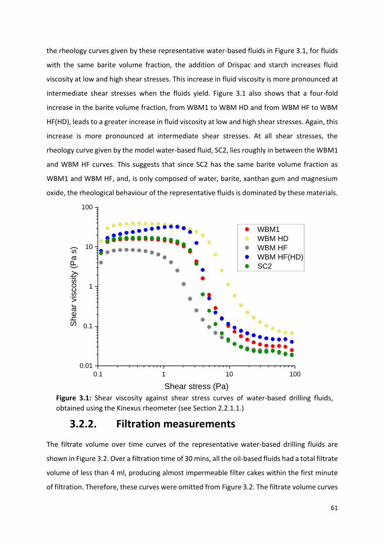
61

the rheology curves given by these representative water-based fluids in Figure 3.1, for fluids

with the same barite volume fraction, the addition of Drispac and starch increases fluid

viscosity at low and high shear stresses. This increase in fluid viscosity is more pronounced at

intermediate shear stresses when the fluids yield. Figure 3.1 also shows that a four-fold

increase in the barite volume fraction, from WBM1 to WBM HD and from WBM HF to WBM

HF(HD), leads to a greater increase in fluid viscosity at low and high shear stresses. Again, this

increase is more pronounced at intermediate shear stresses. At all shear stresses, the

rheology curve given by the model water-based fluid, SC2, lies roughly in between the WBM1

and WBM HF curves. This suggests that since SC2 has the same barite volume fraction as

WBM1 and WBM HF, and, is only composed of water, barite, xanthan gum and magnesium

oxide, the rheological behaviour of the representative fluids is dominated by these materials.

3.2.2. Filtration measurements

The filtrate volume over time curves of the representative water-based drilling fluids are

shown in Figure 3.2. Over a filtration time of 30 mins, all the oil-based fluids had a total filtrate

volume of less than 4 ml, producing almost impermeable filter cakes within the first minute

of filtration. Therefore, these curves were omitted from Figure 3.2. The filtrate volume curves

Figure 3.1: Shear viscosity against shear stress curves of water-based drilling fluids,

obtained using the Kinexus rheometer (see Section 2.2.1.1.)

0.1 1 10 100

0.01

0.1

1

10

100

WBM1

WBM HD

WBM HF

WBM HF(HD)

SC2

Shear

vis

cosity (

Pa s

)

Shear stress (Pa)

62

in Figure 3.2 show that the water-based fluids containing fluid loss materials have significantly

lower filtrate volumes over time than the fluids without fluid loss materials. The filtrate

volume curves of the water-based fluids without fluid loss materials are non-linear near the

start of filtration, which may be due to cake restructuring.

The permeability of each cake made from representative water-based drilling fluids was

obtained using the linear portion of the t/V vs V curves in Figure 3.3 and Equation 1.9. The

cake permeabilities as well as the total filtrate volumes and cake porosities are summarised

in Table 3.1. Although different pressures were used for filtration, drilling fluid filter cakes

have been found with porosities below 0.4 (Elkatatny, Mahmoud and Nasr-El-Din, 2013)

whilst filter cakes made from particulate-based fluids have been found with porosities

exceeding 0.4 (Chellappah, Tarleton and Wakeman, 2010; Lorenzen, Keiding and Christensen,

2017), which agree with the porosities in Table 3.1. The representative water-based fluids

containing fluid loss materials (Drispac and starch) have total filtrate volumes that are at least

16 ml lower than the corresponding fluids without fluid loss materials, as shown in Table 3.1.

The addition of fluid loss materials also leads to a reduction in cake porosity and permeability.

A four-fold increase in the barite volume fraction from sample WBM1 to WBM HD leads to an

increase in total filtrate volume and a decrease in cake porosity. However, the total filtrate

volume is expected to decrease to be consistent with observations from Figure 5.1, where the

Figure 3.2: Filtrate volume against filtration time curves of representative water-based

drilling fluids for a static filtration at 690 kPa for 30 mins

0 200 400 600 800 1000 1200 1400 1600 1800 2000

0

5

10

15

20

25

WBM1

WBM HD

WBM HF

WBM HF(HD)V (

ml)

t (s)

63

total filtrate volume decreases as the barite volume fraction increases. For the fluids without

fluid loss materials, a four-fold increase in the barite volume fraction leads to a 1.5 ml

decrease in total filtrate volume and a decrease of 0.09 in cake porosity (comparing WBM HF

with WBM HF(HD) in Figure 3.3 and Table 3.1).

The total filtrate volumes of the representative drilling fluids are lower than those of all the

model drilling fluids, as shown by comparing Figure 3.3 with Figures 5.1, 5.2 and 5.3. In Table

3.1, for the model drilling fluids, a four-fold increase in the barite volume fraction, from SC2

to SC5, leads to a 17 ml decrease in total filtrate volume and a decrease of 0.08 in cake

porosity. The significant reduction in the filtrate volume of these model fluids, compared to

the representative fluids, is due to the lack of potassium chloride and HMP clay (which are

present in the representative fluids WBM HF and WBM HF(HD)), since these are the only

materials that differ. The addition of potassium chloride and HMP clay also leads to a

significant reduction in cake porosity and permeability as shown in Table 3.1. However, the

trends are similar for the representative and model water-based fluids. The porosity

decreases by roughly 20% whilst the permeability increases for all the sample pairs in Table

3.1 in which the barite volume fraction increases by four-fold and the volume fractions of the

other components stay constant.

Figure 3.3: Filtration time/filtrate volume against filtrate volume curves of

representative water-based drilling fluids for a static filtration at 690 kPa for 30 mins

0 5 10 15 20 25

0

50

100

150

200

250

300

350

400

450

WBM1

WBM HD

WBM HF

WBM HF(HD)

t/V

(s m

l-1)

V (ml)

64

3.3. Filter cake properties

3.3.1. Filter cake thickness

The thickness of filter cakes of the representative drilling fluids was obtained using the

procedure outlined in Section 2.2.2.3. Table 3.2 shows that filter cakes made from water-

based fluids containing fluid loss materials have lower thicknesses than those without such

materials, for an equivalent volume fraction of barite. A four-fold increase in the volume

fraction of barite leads to an increase in thickness (1.0 mm with fluid loss materials and 2.4

mm without). For the oil-based fluids, changing the oil-water ratio does not affect cake

thickness: OBM126 with a ratio of 60/40 has the same thickness as OBM128 with a ratio of

80/20. A three-fold increase in the volume fraction of barite, from OBM128 to OBM188,

increases the cake thickness by 0.3 mm.

Table 3.1: Filter cake properties of representative and model water-based samples. Compositions are shown in Tables 2.1 and 2.3. Total filtrate volumes were for a static filtration at 690 kPa for 30 mins

Sample Total filtrate volume (ml) Permeability (x10-16 m2) Porosity

WBM1 4.2 0.01 0.27

WBM HD 7.7 0.17 0.21

WBM HF 25.0 0.32 0.36

WBM HF(HD) 24.0 1.28 0.27

SC2 44.0 1.74 0.50

SC5 27.0 1.94 0.42

Table 3.2: Measured filter cake thickness and yield stress values for representative water-

based and oil-based drilling fluids. Cakes were made via static filtration at 690 kPa for 30

mins. Some yield stresses could not be obtained because the cakes were either too thin or

had too strong an adhesion to the nylon filter membrane to be separated for testing. Repeat

yield stress measurements were run for some samples and their standard errors are shown

Filter cake sample Thickness (mm) Yield stress (kPa)

WBM1 0.3 -

WBM HD 1.3 9.3 ± 2.2

WBM HF 1.0 18.1 ± 1.2

WBM HF(HD) 3.4 57.4

OBM188 1.5 -

OBM126 1.2 -

OBM128 1.2 -

65

3.3.2. Stress-strain measurements

The strength of filter cakes made from representative drilling fluids was analysed using the

procedure outlined in Section 2.2.2.2. Filter cakes produced from oil-based fluids had a strong

adhesion to the nylon membrane, which meant that these cakes could not be detached for

strength testing. The cake made from WBM1 was extremely thin with a thickness of 0.3 mm

(Table 3.2), which meant that the cake lacked a rigid enough structure for strength testing.

Figure 3.4 shows the stress-strain curves for the water-based fluids. The stress initially

increases linearly as force is applied onto the cake surface. As the filter cake undergoes

deformation, there is an approximately linear relationship between stress and strain in the

elastic region preceding the critical yield stress, as expected from a predominantly elastic

material such as filter cakes (Cerasi et al., 2001). For some filter cakes, such as WBM HF(HD),

there is a lag before this linear portion where the stress-strain curve is almost flat. This lag

may represent the plunger contacting a thin fluid layer which has remained on the cake

surface and has no structural integrity; hence, low stresses are seen as this layer is strained.

At the yield stress, the integrity of the filter cake is broken and the cake ‘fails’. Beyond this

point, the cake continues to strain but the structure can no longer sustain the applied stress,

and, the shape of the curve is likely to be influenced by friction with the walls, as the plunger

forces cake material into the opening.

Figure 3.4: Stress-strain curves for representative water-based drilling

fluids

0.0 0.2 0.4 0.6 0.8 1.0 1.2 1.4

0

10

20

30

40

50

60

WBM HD

WBM HF

WBM HF(HD)

Str

ess (

kP

a)

Strain

66

Figure 3.4 shows that the samples with a high barite volume fraction (WBM HD and WBM

HF(HD)) have stress-strain curves with steeper gradients, meaning they are more resistant to

being strained. In Table 3.2, for the water-based fluids with a high barite volume fraction, the

addition of fluid loss materials decreases the cake yield stress by 48.1 kPa, whilst, as shown

in Figure 3.4, the strains at which the cakes yield are similar. Conversely, as shown in Figure

3.1, the addition of fluid loss materials to these fluids increases the fluid yield stress, as

measured using the Kinexus rheometer. In Figure 3.4, for the samples that lack fluid loss

materials (WBM HF and WBM HF(HD)), a four-fold increase in the barite volume fraction leads

to a three-fold increase in cake yield stress. As shown in Figure 3.1, the yield stresses of these

fluids follow a similar trend as the fluid yield stress increases with barite volume fraction.

3.4. Comparison with model filter cakes


Strength tests were performed on filter cakes made from model water-based drilling fluids,

the compositions of which are outlined in Table 2.3. The solid particulate additives in these

fluids were either barite or calcium carbonate. Size distributions of the particulate additives

are shown in Figure 2.7. In Figure 3.5, the stress-strain curves of filter cakes composed of

calcium carbonate are shown, except for that of SCal150 since the stresses are negligible. The

stress-strain curves in Figure 3.5 are analogous to the curves in Figure 3.4 for representative

fluids, as there is an approximately linear relationship between stress and strain whilst the

filter cake deforms. For SC2, a lag before this linear portion is observed (similar to that of the

WBM HF(HD) curve in Figure 3.4) which may represent the fluid layer on the cake surface

being strained, as discussed in Section 3.3.2. The cake composed of the smallest calcium

carbonate particles, SCal8, has a linear portion (preceding the yield stress) with the steepest

gradient. All the calcium carbonate samples (with the same volume fraction of particles) yield

at strains within a narrow range of between 0.44 and 0.48. For the barite-based cakes, the

strain at which they yield decreases from 0.96 to 0.42 as the barite volume fraction is

increased four-fold. As shown in Figure 3.4, this is analogous to the stress-strain response of

filter cakes made from representative water-based drilling fluids, highlighting the similarities

between representative and model fluids: a four-fold increase in the barite volume fraction

leads to a decrease in yield strain from 0.92 to 0.58. Also, in Figure 3.4, for representative

67

fluids, cakes with the same barite volume fraction yield at a narrower range of strains of

between 0.49 and 0.58. Therefore, the particle volume fraction strongly influences the strain

at which filter cakes yield. This is shown more clearly for model fluids in Figure 4.1, where the

yield strain decreases as the barite volume fraction increases.

3.4.2. Filter cake yield stress

As shown in Figure 3.6, as the particle size in the model fluids decreases, the filter cake yield

stress increases. The barite samples show that for particles of the same size, varying the

particle volume fraction can lead to a variation in cake strength: cake yield stress increases by

49.1 kPa as the volume fraction of barite in the fluid increases from 3.1 vol% to 24.8 vol%. The

rate of increase of yield stress with volume fraction is greatest at lower volume fractions, as

the yield stress increases by 8.8 kPa per vol% between 3.1 vol% and 6.2 vol%, whilst between

6.2 vol% and 24.8 vol%, the rate decreases to 1.2 kPa per vol%.

In Table 3.2, for the representative water-based fluids, as the barite volume fraction increases

from 6.2 vol% to 24.8 vol%, the yield stress increases by 39.3 kPa. For the barite-based cakes

made from model fluids in Figure 3.6, the increase is 21.7 kPa for the same increase in barite

Figure 3.5: Stress-strain curves for filter cakes composed of calcium carbonate (SCal

samples) or barite particles (SC samples); the numbers inside the square brackets in the

legend are the particles’ d50 value (as measured by the Malvern Mastersizer 2000) and

the particle volume fraction in each sample

0.0 0.2 0.4 0.6 0.8 1.0 1.2 1.4

0

10

20

30

40

50

60

70 SCal8 [11 mm, 6.2 vol%]

SCal22 [22 mm, 6.2 vol%]

SCal50 [33 mm, 6.2 vol%]

SC2 [5 mm, 6.2 vol%]

SC5 [5 mm, 24.8 vol%]

Str

ess (

kP

a)

Strain

68

volume fraction, and these samples have yield stresses that are significantly higher than the

representative samples with an equivalent volume fraction of barite. This suggests that

potassium chloride and HMP clay in the representative fluids (since these are the only

materials that differ) are weakening the filter cakes and increasing the dependence of yield

stress on barite volume fraction. However, the trends are similar for the representative and

model water-based samples, as the cake yield stress increases with barite volume fraction,

which suggests that the model samples capture the particulate phase behaviour of the

representative samples.

3.5. Conclusions

In this chapter, the rheological and filtration behaviour of representative water and oil-based

drilling fluids were studied. The properties of their filter cakes were explored and compared

to those produced from model water-based drilling fluids. The shear-thinning behaviour,

which is consistent with fluids containing xanthan gum, was shown by the shear viscosity

Figure 3.6: Yield stresses of filter cakes composed of calcium carbonate (SCal

samples) or barite particles (SC samples); the number inside the square brackets in

the legend is the particle volume fraction in each sample. Repeats were run for the

sample with a barite loading of 6.2 vol% (SC2) and the standard error was 8%; error

bars are not shown for clarity

1 10 100

0.1

1

10

100

SCal8 [6.2 vol%]

SCal22 [6.2 vol%]

SCal50 [6.2 vol%]

SCal150 [6.2 vol%]

SC1 [3.1 vol%]

SC2 [6.2 vol%]

SC5 [24.8 vol%]

Cake y

ield

str

ess (

kP

a)

D50 of solid particles (mm)

69

against shear stress curves of the water-based fluids. Filtrate volume curves were used to

evaluate the filtration of water-based fluids, and oil-based fluids produced almost

impermeable filter cakes with filtrate volumes of less than 4 ml. The addition of fluid loss

materials, Drispac and starch, to water-based fluids led to a reduction in cake porosity and

permeability, and a reduction of at least 16 ml in total filtrate volume. For both water-based

and oil-based fluids, cake thickness increased significantly as the volume fraction of barite in

the fluid increased. For the oil-based fluids, changing the oil-water ratio did not affect cake

thickness. The stress-strain response and yield stress of filter cakes made from representative

water-based fluids were analysed. Water-based fluids with fluid loss materials produced

cakes with a yield stress 48.1 kPa lower than those without, whilst a four-fold increase in the

barite volume fraction led to a three-fold increase in yield stress.

The benchmark results obtained from representative water-based drilling fluids were used to

compare with model water-based drilling fluids. The rheology curve given by the model fluid,

SC2, was roughly in between those of the representative fluids with the same barite volume

fraction. Therefore, the rheological behaviour of the representative fluids was captured by

having similar volume fractions of barite and xanthan gum in the model fluids. Comparing the

filtration of representative and model fluids with the same barite volume fractions, the

addition of potassium chloride and HMP clay significantly reduced the total filtrate volume,

cake porosity and permeability, and the addition of fluid loss materials, Drispac and starch,

reduced these further. However, when the barite volume fraction was increased by four-fold,

the trends were similar for the representative and model fluids as the porosity decreased by

roughly 20% whilst the permeability increased. By increasing the barite volume fraction by

the same amount in both representative and model fluids, a similar decrease in the cake yield

strain was observed. For an equivalent volume fraction of barite, the cakes made from model

fluids had significantly higher yield stresses than those made from representative fluids. This

implies that potassium chloride and HMP clay in representative fluids weakened the filter

cakes. However, the trends were similar for the representative and model fluids, as the cake

yield stress increased with barite volume fraction. Overall, by capturing the barite-dominated

particulate phase behaviour of the representative fluids, the model fluids were able to

produce similar trends in the rheological, filtration and stress-strain results to the

representative fluids.

71

Chapter 4. Filter cake yield stress behaviour

The results from this chapter have been published in Chemical Engineering Science: X:

Nikzad Falahati, Alexander F. Routh, Kuhan Chellappah. The effect of particle properties and

solids concentration on the yield stress behaviour of drilling fluid filter cakes. Chemical

Engineering Science: X, 2020, 7: 100062. DOI: 10.1016/j.cesx.2020.100062.

4.1. Introduction

The strength of a filter cake is important during drilling. If a cake ruptures, drilling fluid will be

allowed to infiltrate the wellbore rock and the occurrence of wellbore stability issues may

increase. A strong filter cake can contribute to wellbore strengthening, increasing the

maximum pressure a wellbore can withstand (Guo et al., 2014). Filter cakes predominantly

behave as elastic solids (Cerasi et al., 2001), and the yield stress marks the transition from

elastic behaviour, where the cake is considered competent to a plastic flow regime (Cook et

al., 2016), beyond which the cake begins to rupture. In this chapter, filter cakes made from

model water-based drilling fluids were tested to determine cake properties such as porosity,

thickness and yield stress. The effects of drilling fluid particle concentration, size distribution

and shape on the properties of the resulting cakes were investigated. The model fluids, the

composition and mixing procedure of which are discussed in Section 2.3.2., were made using

typical drilling fluid components. As discussed in Chapter 3, some of the model fluids made of

calcium carbonate or barite were used to compare with representative drilling fluids.

As discussed in Section 1.2.2.3., techniques have been developed to characterise filter cake

strength (Zamora, Lai and Dzialowski, 1990; Bailey et al., 1998; Cerasi et al., 2001; Tan and

Amanullah, 2001; Cook et al., 2016), but, in general, research involving direct measurements

of cake strength has been relatively scarce. Bailey et al. (1998) developed a hole punch test

to simulate the shear rupture of a filter cake in a simple and inexpensive manner. The

technique directly measures the force required for cake rupture so that the yield stress can

be determined. Nandurdikar et al. (2002) and Hao et al. (2016) also used a similar hole punch

method to carry out cake strength tests. To check the reliability of the hole punch method,

Bailey et al. (1998) compared it with the vane method, which uses a bladed vane sensor to

72

find the maximum torque through a cake sample, and the squeeze-film method, which uses

parallel plates to squeeze a cake sample whilst recording the force. All three methods

produced consistent results suggesting each to be reliable, but the hole punch method was

favoured because it required neither the thick filter cakes used in the vane method nor the

complex equipment used in the squeeze-film method.

In this work, an experimental setup similar to that of Bailey et al. (1998) was used to find the

shear stress of filter cakes, obtaining a yield stress from the measured peak force. Typical

stress-strain curves obtained using the hole punch test are presented, and the influence of

solids volume fraction, shape and size distribution on the cake yield stress as well as other

cake properties are investigated. The relationships between cake properties, such as porosity,

thickness and yield stress, are explored.

4.2. Results


Typical stress-stain curves for samples with varying solids volume fraction and particle shape

are shown in Figures 4.1 and 4.2. From Figure 4.1, the stress is seen to initially increase linearly

as force is applied onto the cake surface. The filter cake undergoes deformation due to this

applied load, accounted for via monitoring displacement of the plunger and used to calculate

the strain. In the elastic region preceding the critical yield stress, there is an approximately

linear relationship between stress and strain, as expected from a predominantly elastic

material such as filter cakes. At the yield stress, the integrity of the filter cake is broken and

the cake ‘fails’. Applying load past this point continues to strain the cake, but the structure

can no longer sustain the applied stress. The shape of the curve after the yield point may also

be influenced by friction with the walls, as the plunger forces cake material into the opening.

73

Figure 4.2 shows that the particles with the highest circularity, glass spheres and calcium

carbonate, produce cakes with stress-strain curves that have the steepest gradients. This

suggests that these cakes are more resistant to being strained. The cakes made from lower

circularity particles have more gradual stress-strain curves up to the yield stress. For barite

and talc particles, the strain at which these cakes yield is significantly higher at 0.96 and 0.88,

than with the more spherical base particles.

Increasing Barite

0.0 0.2 0.4 0.6 0.8 1.0 1.2 1.4

0

5

10

15

20

25

30

35

40

45

50

55

60

65

70

Str

ess

(kP

a)

Strain

SC1 (3.1 vol%)

SC2 (6.2 vol%)

SC3 (12.4 vol%)

SC4 (18.6 vol%)

SC5 (24.8 vol%)

Figure 4.1: Stress-strain curves for samples with varying barite compositions

0.0 0.2 0.4 0.6 0.8 1.0 1.2 1.4

0

5

10

15

20

25

30

35

40

45

50

55

60

65

70

Str

ess

(kP

a)

Strain

Glass spheres [0.88]

Calcium carbonate (SCal2) [0.82]

Barite (SC2) [0.81]

Talc [0.71]

Cellulose microcrystalline [0.77]

Figure 4.2: Stress-strain curves for samples that have varying particle shape; the number

inside square brackets in the legend is the circularity of each particle

74

4.2.2. Varying solids volume fraction

In Figure 4.1, from a barite solids loading of 6.2 vol% to 24.8 vol%, the strain at which the cake

fails decreases from 0.96 to 0.42. Also noted is that the yield stress increases with increasing

solids content in the fluid; from a yield stress of 16.5 kPa at 3.1 vol% to 65.6 kPa at 24.8 vol%.

The effects of varying the solids volume fraction in the fluid on the cake yield stress is

illustrated in Figure 4.3. The yield stress increases with increasing solids volume fraction for

both ultra-fine calcium carbonate and barite samples. Calcium carbonate samples were

stronger than the barite equivalents with yield stresses showing an increase of between 29%

and 56%. Bailey et al. (1998) who performed filtration to completion with cake compaction

and had yield stresses that were around 10 times higher than those presented here, also

found that correspondingly sized calcium carbonate filter cakes gave higher yield stresses

than barite weighted filter cakes.

0 5 10 15 20 25

10

20

30

40

50

60

70

80

90

Barite

Calcium carbonate

Ca

ke y

ield

str

ess

(kP

a)

Solids vol% in fluid

Figure 4.3: Yield stress for cakes made from fluids with varying volume percentage

of barite or calcium carbonate. Repeats were run for the sample with a barite

loading of 6.2 vol% (SC2) and the standard error was 8%; error bars are not shown

for clarity

75

4.2.3. Varying particle shape

Particles of varying circularities were tested: glass spheres, calcium carbonate, barite, talc and

cellulose microcrystalline. These particles were mixed into fluids at a constant volume fraction

of 6.2 vol%. Apart from cellulose microcrystalline, these particles had similar median particle

sizes (see Table 2.5 for d50 values and circularities).

Figure 4.4 shows a plot of yield stress versus porosity for the filter cakes containing the various

shaped particles. It is seen that cakes containing glass spheres and calcium carbonate (most

circular) were strongest with yield stress values of around 64.0 kPa. These cakes also

contained the highest filter cake solids fractions (lowest porosity); glass spheres produced the

lowest porosity cakes out of all the samples tested at 0.34. Conversely, the less circular talc

and cellulose microcrystalline particles produced filter cakes with high porosities of around

0.65. These filter cakes were also amongst the weakest, with talc and cellulose

microcrystalline cakes giving yield stress values of 22.1 kPa and 2.9 kPa, respectively.

Figure 4.4: Cake yield stress for cakes of different porosities, made from samples with

varying particle shape; the number inside square brackets in the legend is the circularity

of each particle

0.30 0.35 0.40 0.45 0.50 0.55 0.60 0.65 0.70

0

10

20

30

40

50

60

70

Glass spheres [0.88]

Calcium carbonate (SCal2) [0.82]

Barite (SC2) [0.81]

Talc [0.71]

Cellulose microcrystalline [0.77]

Ca

ke

yie

ld s

tress (

kP

a)

Cake porosity

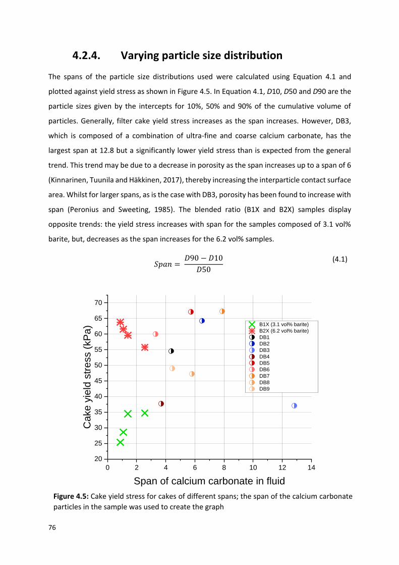
76

4.2.4. Varying particle size distribution

The spans of the particle size distributions used were calculated using Equation 4.1 and

plotted against yield stress as shown in Figure 4.5. In Equation 4.1, D10, D50 and D90 are the

particle sizes given by the intercepts for 10%, 50% and 90% of the cumulative volume of

particles. Generally, filter cake yield stress increases as the span increases. However, DB3,

which is composed of a combination of ultra-fine and coarse calcium carbonate, has the

largest span at 12.8 but a significantly lower yield stress than is expected from the general

trend. This trend may be due to a decrease in porosity as the span increases up to a span of 6

(Kinnarinen, Tuunila and Häkkinen, 2017), thereby increasing the interparticle contact surface

area. Whilst for larger spans, as is the case with DB3, porosity has been found to increase with

span (Peronius and Sweeting, 1985). The blended ratio (B1X and B2X) samples display

opposite trends: the yield stress increases with span for the samples composed of 3.1 vol%

barite, but, decreases as the span increases for the 6.2 vol% samples.

𝑆𝑝𝑎𝑛 = 𝐷90 − 𝐷10

𝐷50

(4.1)

Figure 4.5: Cake yield stress for cakes of different spans; the span of the calcium carbonate

particles in the sample was used to create the graph

0 2 4 6 8 10 12 14

20

25

30

35

40

45

50

55

60

65

70

B1X (3.1 vol% barite)

B2X (6.2 vol% barite)

DB1

DB2

DB3

DB4

DB5

DB6

DB7

DB8

DB9

Ca

ke

yie

ld s

tress (

kP

a)

Span of calcium carbonate in fluid

77

4.3. Discussions

4.3.1. Yield stress and thickness

To understand how cake thickness and yield stress vary with filtration time, tests were

performed on cakes produced over different filtration times of 5, 10, 15, 20 and 30 minutes.

Samples SC2 (6.2 vol%) and SC5 (24.8 vol%) were chosen since, after 30 minutes of filtration,

these samples produced cakes with a wide range of yield stresses, as shown in Figure 4.3. In

Figure 4.6, the thickness of SC2 and SC5 cakes increased with filtration time. For SC2, both the

measured peak force and the yield stress increase exponentially with filtration time and cake

thickness. For SC5, there is an almost linear increase in both the measured peak force and

yield stress with filtration time and cake thickness.

The relationship between cake yield stress and cake thickness for all samples tested (made

via static filtration at 690 kPa for 30 mins) is shown in Figure 4.7, including the SC2 and SC5

cakes in Figure 4.6 that were produced after 30 minutes of filtration. With low solids volume

fraction in the fluid (SC1 and SC2), increasing the volume fraction increases the yield stress

0.0 1.0 2.0 3.0 4.0 5.0 6.0

10

20

30

40

50

60

70

SC2 yield stress

SC5 yield stress

SC2 peak force

SC5 peak force

Cake thickness (mm)

Ca

ke y

ield

str

ess

(kP

a)

0

5

10

15

20

25

30

Pea

k fo

rce

befo

re c

ake

failu

re (

N)

Figure 4.6: Cake yield stress and peak force results for barite samples filtered for 5, 10,

15, 20 and 30 minutes which gives differing cake thicknesses. Repeats were run for SC2

filtered for 30 minutes and the standard error of the yield stress was 8%; error bars are

not shown for clarity

78

significantly. As expected, the cake thickness increases with solids volume fraction. Replacing

the barite with an equivalent volume of calcium carbonate in the fluid produced filter cakes

that are thicker, by between 0.50 and 0.93 mm, and are also stronger.

The addition of calcium carbonate particles of different sizes to the barite samples generally

increased the cake yield stress, as shown by comparing the B1X samples to SC1 and the B2X

and DB samples to SC2. This could mean that the calcium carbonate is supplementing the core

barite structure as shown in Figure 4.8, whilst for two DB samples (DB3 and DB4), the calcium

carbonate is having a detrimental effect. The DB samples are of similar thickness, yet the

strongest cake, DB7, has a yield stress that is approximately double that of DB3, which may

be due to DB7 having a lower porosity than DB3. Again, the blended ratio samples display

opposite trends. As shown in the insert in Figure 4.7, for samples with 3.1 vol% barite, the

yield stress decreases as the blended ratio, and so the proportion of coarser particles,

increases; for samples with 6.2 vol% barite, the yield stress increases as the blended ratio

increases.

1.0 2.0 3.0 4.0 5.0 6.0

10

15

20

25

30

35

40

45

50

55

60

65

70

75

80

85

90

SC1

SC2

SC3

SC4

SC5

SCal1

SCal2

SCal5

DB

B1X2.0

B1X1.5

B1X1.0

B1X0.5

B2X2.0

B2X1.5

B2X1.0

B2X0.5

Ca

ke

yie

ld s

tre

ss (

kP

a)

Cake Thickness (mm)

Figure 4.7: Cake yield stress for cakes of different thicknesses (made via static filtration

at 690 kPa for 30 mins). The insert shows the effect on yield stress as the blended ratio

(the number after the ‘X’ in the sample name), and so the proportion of coarser

particles, increases

0.5 1.0 1.5 2.0

25

30

35

40

45

50

55

60

65

B1X

B2X

Ca

ke y

ield

str

ess

(kP

a)

Blended ratio

79

As was shown in Figure 4.7, the calcium carbonate particles generally seem to be

supplementing the core barite network, leading to higher yield stresses for the samples that

include both particles as opposed to barite only. The strength enhancement observed could

be a result of either an increase in the interparticle contact surface area and/or a material

property of calcium carbonate. It has been found for barite and calcium carbonate samples

with a similar particle size distribution, the latter were observed to form filter cakes with

significantly higher yield stresses (Bailey et al., 1998). From Figure 4.3, a similar observation

can be made as the calcium carbonate samples have yield stresses that are between 9.2 kPa

(3.1 vol%) and 19.8 kPa (6.2 vol%) higher than the barite equivalents. It seems consistent that

the increase in yield stress is more pronounced at the higher solids loading as more particle

contacts will amplify any effects of increased cohesion between calcium carbonate particles.

Also, the calcium carbonate only cakes are thicker (Figure 4.7) and less porous (Figure 4.9)

than their barite only equivalents, hence will have a higher interparticle contact surface area.

The yield stress is likely to be proportional to this surface area and so these cakes have a

higher yield stress.

4.3.2. Yield stress and porosity

The relationship between cake yield stress and cake porosity for all samples tested (made via

static filtration at 690 kPa for 30 mins) is shown in Figure 4.9, including the cakes made from

samples with varying particle shape as shown in Figure 4.4. As porosity decreases, yield stress

increases, with the cakes containing the various shaped particles giving the most extreme

values. From Figure 4.9, it can be seen that glass spheres give around the highest yield stress

Figure 4.8: Calcium carbonate particles supplementing the core barite network

Addition of calcium

carbonate particles

Barite network Barite network + calcium carbonate

80

for the least porous cake; conversely, talc and cellulose microcrystalline give the lowest yield

stresses with the highest porosities. The talc particles for instance have a plate-like shape

(Bumiller, Carson and Prescott, 2002) and low circularity, and hence, may pack in sheet-like

layers that are individually quite porous. Note that an arrangement of overlapping sheets may

yet form a barrier of low permeability despite the filter cake’s high porosity (due to the porous

sheets). This sheet-like structure may be the reason for the low measured yield stress,

because the resistance is derived from breaking these sheets as opposed to overcoming

numerous particle contacts. Conversely, the high solids content glass sphere filter cakes gave

a higher yield stress, presumably due to the high resistance required to restructure the tighter

and more rigid packing structure.

As the barite volume fraction increases, the porosity decreases and the yield stress increases

almost linearly. All the DB and B2X cakes have porosities that are between 0.08 and 0.14 lower

than that of SC2, and, the B1X cakes have porosities that are between 0.10 and 0.14 lower

than that of SC1. This reduction in cake porosity could be a consequence of the introduction

of different particle sizes as calcium carbonate is added to the barite: the barite only samples

Figure 4.9: Cake yield stress for cakes of different porosities (made via static

filtration at 690 kPa for 30 mins)

0.30 0.35 0.40 0.45 0.50 0.55 0.60 0.65 0.70

0

5

10

15

20

25

30

35

40

45

50

55

60

65

70 DB

B1X

B2X

SC1

SC2

SC3

SC4

SC5

SCal2

Scell

Stal

Sglass

Ca

ke

yie

ld s

tre

ss (

kP

a)

Cake porosity

81

(SC1 and SC2) have a span of 2.0, which is relatively low compared to the DB samples (Figure

4.5). As a filter cake grows, fresh particles approaching the cake could either deposit on the

cake’s surface or within interstitial voids. When the homogeneous suspension being filtered

consists of particles of a broad size distribution, this promotes the occurrence of the latter

scenario whereby the finer particles in the distribution can migrate into pre-existing void

spaces within the filter cake structure. This interstitial filling decreases porosity as the cake

grows. Conversely, with a narrow size distribution, fewer particles are available which are fine

enough to penetrate the filter cake’s structure. Hence, filter cake growth will tend to involve

a greater proportion of particles depositing on the cake’s surface. This layered deposition will

increase filter cake thickness more rapidly but has less of an impact on porosity. Both

scenarios lead to an increase in total interparticle contact as the cake grows, and hence the

cake’s yield stress increases with filtration time (see Figure 4.6 for example).

Furthermore, the data gathered suggests that a broad size distribution tends to give cakes

with a higher yield stress (Figure 4.5). Hence it may be postulated that the invasion of new

particles into the filter cake structure followed by deposition within pre-existing voids is more

beneficial to cake strength than a layered deposition mechanism. Intuitively, this could be due

to two reasons: (a) particles depositing within pre-existing voids tend to form more contact

points (per particle) compared to particles depositing on the cake’s surface, and (b) the

decreased void space surrounding particles make it more difficult for the structural

rearrangements required during shearing. The preceding arguments are also consistent with

Figures 4.7 and 4.9 which show the DB filter cake samples to give similar thicknesses but a

range of porosity and yield stress values. However, the DB3 sample, which is composed of

ultra-fine and coarse calcium carbonate (in addition to barite), gave the largest span of the

samples tested but also an unexpectedly low yield stress. This apparent anomaly may be

explained by the formation of segregated packing zones (non-homogeneous) within the filter

cake when the size distribution is broad and concentrated at both ends of the distribution. In

this case, the voids left behind by the coarse particles may be too large to effectively trap

individual (or small clusters of) fine particles. This is analogous to the Brazil nut effect caused

by vibrations in granular systems (Rosato et al., 1987), but in the case of filter cakes, it is

caused by pressure-induced flow. It has been found that the Brazil nut segregation effect is

strongest for mixtures with the largest particle size ratio (Liao, 2016) and the introduction of

82

intermediate particle sizes have been found to reduce segregation of the particle mixture

(Metzger, Remy and Glasser, 2011).

4.4. Conclusions

Filter cakes made from different formulations were tested to assess the cake strength in

relation to other cake properties and properties of the drilling fluid. Cake strength, measured

as the yield stress, was improved by several factors. By increasing the barite solid loading in

the drilling fluid from 3.1 vol% to 24.8 vol%, the cake yield stress increased from 16.5 kPa to

65.6 kPa. A similar trend was observed for cakes made from ultra-fine calcium carbonate.

Furthermore, these cakes were stronger with yield stresses increasing by between 29% and

56% as compared to the barite equivalents. The increase in strength may be due to a higher

interparticle contact surface area, which is a result of the calcium carbonate cakes being

thicker and less porous than their barite equivalents. Fresh particles approaching the cake can

either deposit on the cake’s surface, increasing the cake’s thickness, or within interstitial voids,

decreasing the cake’s porosity. A broad particle size distribution in the fluid encourages

interstitial filling as finer particles migrate into pre-existing voids. Both scenarios lead to an

increase in the total interparticle contact as the cake grows. However, broadening the particle

size distribution in the cake tended to give stronger cakes of a similar thickness, as was

illustrated by adding calcium carbonate of different sizes to barite-loaded fluids. Hence it was

postulated that the deposition of new particles within pre-existing voids is more beneficial to

cake strength than a layered deposition mechanism.

83

Chapter 5. Filter cake internal structure

5.1. Introduction

This chapter explores the filtration behaviour and internal pore structure of cake samples

made via static filtration tests. For the filtration behaviour analysis, the theory describing the

relationship between filtrate volume and time, as discussed in Section 1.2.2.1., was used to

produce filtration plots and to calculate cake permeability. To gain a better understanding of

the filtration, images of the internal pore structure of filter cake samples were captured using

X-ray Computed Tomography (XRCT) imaging. Furthermore, this analysis supports the work

in Chapter 4 on filter cake strength.

As discussed in Section 1.2.2.6., techniques such as SEM, ESEM and CT have been used to

analyse filter cake structures. SEM with shock-freezing/freeze-drying to prepare the cake

sample for imaging has been used (Chenevert and Huycke, 1991; Plank and Gossen, 1991;

Argillier, Audibert and Longeron, 1997; Yao et al., 2014). However, the process of shock-

freezing and obtaining a sample of an appropriate size is destructive and may leave an altered

cake structure. In addition, the small samples required for SEM imaging may not be

representative of the cake structure. ESEM has been used as an alternative to SEM (Tare et

al., 1999; Nandurdikar, Takach and Miska, 2002) since the cake can be imaged in its wet state

and does not need to be treated. However, small sections of the cake still need to be prepared

to use ESEM (Nandurdikar, Takach and Miska, 2002). CT scans of filter cakes, on ceramic disks

as filter medium, have been performed in their wet and dry states to determine filter cake

thickness and porosity (Elkatatny, Mahmoud and Nasr-El-Din, 2012, 2013). Filter cake samples

made via static filtration were scanned in their original state, and porosity and thickness

profiles were obtained. CT scanning is a non-destructive imaging approach, with minimal

sample preparation required, and allows for the entire filter cake to be scanned, which means

that more representative data of the cake structure can be obtained.

For this work, XRCT imaging was used on cake samples (as discussed in Section 2.2.2.5.) to

visualise pore structures in the filter cakes. Quantitative data were acquired by producing 3D

representations of the pore network. The pore distribution within each cake layer as well as

the pore size distribution over all cake layers were analysed. In addition, pore volume fraction

84

profiles through the cake were evaluated. An investigation of the filtration behaviour was

complemented by this knowledge of the pore structure.

5.2. Filtration behaviour

5.2.1. Filtration measurements

The filtration behaviour of samples with varying particle volume fractions are shown in Figure

5.1. The filtration plots are generally linear in most parts, but in some cases the permeability

gradually declines towards the latter stages of filtration, as indicated by an upward curvature

of the plots (increasing gradient). The non-linearity observed in the latter stages of some

filtration plots (such as those for SCal1, SCal2 and SC1) may be due to cake restructuring

during filtration in the form of dynamic cake compression (Christensen et al., 2011). Since the

filtration plots become more linear as the volume fraction of barite increases, less

restructuring may be occurring in the filter cake. Arthur et al. (1988) also found that above a

certain volume fraction of barite, filter cakes become less compressible as the barite volume

fraction increases, which they put down to barite being an incompressible material. As the

barite volume fraction increases from 3.1 vol% to 24.8 vol%, the total filtrate volume over 30

mins decreases and the rate of filtrate volume decrease with volume fraction decreases: the

filtrate volumes of samples with 18.6 vol% and 24.8 vol% barite are almost identical.

The addition of calcium carbonate leads to a significant decrease in the total filtrate volume,

as seen by comparing the plots of SC1 with B1X1.0 and SC2 with B2X1.0. The addition of

calcium carbonate (an amount that is equivalent to 3.0 vol%) seems to have the same effect

on the filtration plots as doubling the barite volume fraction. This is shown in Figure 5.1 by

comparing the plots of B1X1.0 and SC2 with that of SC1, and, the plots of B2X1.0 and SC3 with

that of SC2. The samples which only contain calcium carbonate show a larger range in total

filtrate volumes, when compared to the barite only samples, but the trend with volume

fraction is consistent: increasing the calcium carbonate volume fraction leads to a decrease

in the filtrate volume. However, whilst the samples with 3.1 vol% and 6.2 vol% calcium

carbonate have much greater filtrate volumes than the barite equivalents, the sample with

24.8 vol% calcium carbonate has a similar filtration plot to the barite equivalent.

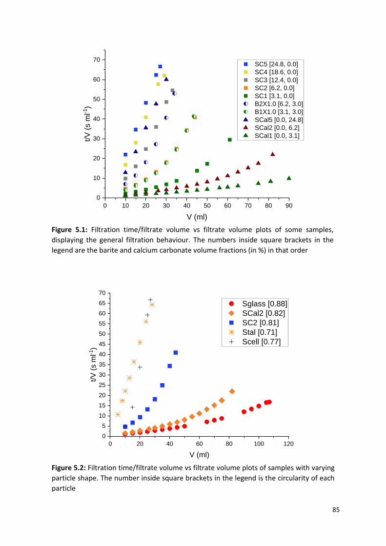
85

Figure 5.1: Filtration time/filtrate volume vs filtrate volume plots of some samples,

displaying the general filtration behaviour. The numbers inside square brackets in the

legend are the barite and calcium carbonate volume fractions (in %) in that order

0 10 20 30 40 50 60 70 80 90

0

10

20

30

40

50

60

70 SC5 [24.8, 0.0]

SC4 [18.6, 0.0]

SC3 [12.4, 0.0]

SC2 [6.2, 0.0]

SC1 [3.1, 0.0]

B2X1.0 [6.2, 3.0]

B1X1.0 [3.1, 3.0]

SCal5 [0.0, 24.8]

SCal2 [0.0, 6.2]

SCal1 [0.0, 3.1]

t/V

(s m

l-1)

V (ml)


particle shape. The number inside square brackets in the legend is the circularity of each

particle

0 20 40 60 80 100 120

0

5

10

15

20

25

30

35

40

45

50

55

60

65

70

Sglass [0.88]

SCal2 [0.82]

SC2 [0.81]

Stal [0.71]

Scell [0.77]

t/V

(s m

l-1)

V (ml)

86

The filtration plots for samples with varying particle shapes are presented in Figure 5.2. As

the particle circularity decreases, the total filtrate volume decreases; the total filtrate volume

of the sample composed of glass spheres is almost four times greater at 107 ml than that of

the cellulose microcrystalline sample at 27 ml. The filtrate volumes of the samples containing

talc and cellulose microcrystalline are equivalent to that of the 24.8 vol% barite sample. The

filtration plots for samples with varying particle size distributions are shown in Figure 5.3. All

the samples have a similar filtration behaviour with roughly the same total filtrate volumes.

However, samples with size distributions of the highest d50 (DB1 and DB2) have slightly lower

filtrate volumes than those with the lowest d50 (DB5 and DB6).

5.2.2. Cake permeability

Figure 5.4 shows the variation of cake permeability, which was calculated using Equation 1.9,

with solids vol% in the fluid sample. For the barite only samples (SC), there is a minimum cake

permeability for the sample with 12.4 vol% barite, and a linear increase in cake permeability

beyond this minimum. The calcium carbonate only sample has a permeability that is 3.76 x

10-16 m2 higher than the barite only equivalent, which may be due to the difference in particle

size. For porous media, the Carman-Kozeny model (Equation 5.1) provides an estimate for

Figure 5.3: Filtration time/filtrate volume vs filtrate volume plots of samples with

varying particle size distributions. The number inside square brackets in the legend is

the d50 size of each sample

0 5 10 15 20 25 30 35 40

0

10

20

30

40

50

60 DB1 [65.0 mm]

DB2 [42.9 mm]

DB3 [21.8 mm]

DB4 [26.7 mm]

DB5 [16.0 mm]

DB6 [14.5 mm]

DB7 [24.3 mm]

DB8 [39.7 mm]

DB9 [17.7 mm]

t/V

(s m

l-1)

V (ml)

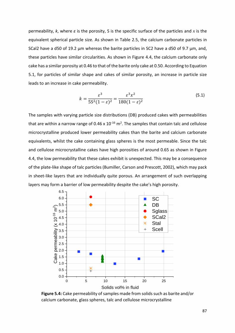
87

permeability, k, where ε is the porosity, S is the specific surface of the particles and x is the

equivalent spherical particle size. As shown in Table 2.5, the calcium carbonate particles in

SCal2 have a d50 of 19.2 µm whereas the barite particles in SC2 have a d50 of 9.7 µm, and,

these particles have similar circularities. As shown in Figure 4.4, the calcium carbonate only

cake has a similar porosity at 0.46 to that of the barite only cake at 0.50. According to Equation

5.1, for particles of similar shape and cakes of similar porosity, an increase in particle size

leads to an increase in cake permeability.

𝑘 =휀3

5S2(1 − 휀)2=

휀3𝑥2

180(1 − 휀)2

(5.1)

The samples with varying particle size distributions (DB) produced cakes with permeabilities

that are within a narrow range of 0.46 x 10-16 m2. The samples that contain talc and cellulose

microcrystalline produced lower permeability cakes than the barite and calcium carbonate

equivalents, whilst the cake containing glass spheres is the most permeable. Since the talc

and cellulose microcrystalline cakes have high porosities of around 0.65 as shown in Figure

4.4, the low permeability that these cakes exhibit is unexpected. This may be a consequence

of the plate-like shape of talc particles (Bumiller, Carson and Prescott, 2002), which may pack

in sheet-like layers that are individually quite porous. An arrangement of such overlapping

layers may form a barrier of low permeability despite the cake’s high porosity.

Figure 5.4: Cake permeability of samples made from solids such as barite and/or

calcium carbonate, glass spheres, talc and cellulose microcrystalline

0 5 10 15 20 25

0.0

0.5

1.0

1.5

2.0

2.5

3.0

3.5

4.0

4.5

5.0

5.5

6.0

6.5

SC

DB

Sglass

SCal2

Stal

Scell

Ca

ke p

erm

eab

ility

(x 1

0-1

6 m

2)

Solids vol% in fluid

88

5.3. XRCT imaging

5.3.1. Varying particle size distribution

The samples with varying particle size distributions (DB1 to DB6) were composed of water,

barite, xanthan gum, magnesium oxide and calcium carbonate particles, as outlined in Section

2.3.2. The d50 of the calcium carbonate particles in each sample are shown in Table 5.1. The

ortho slices for each sample are in Figures 5.5 to 5.10, with each figure displaying an ortho

slice from the top, middle and bottom layers of each sample. The cakes shown in each ortho

slice appear to be of different shapes, which is due to the image reconstruction process, but

they are all circular with a diameter of between 23 and 30 mm. Images for all the samples

were captured with a resolution of between 14 and 20 µm, except for samples DB1, DB3 and

DB5 which had a resolution of 6 µm. The resolution of 6 µm was achieved using the stacked

method, but, due to the destructive nature of the sample preparation in this method (as

discussed in Section 2.2.2.5.), only DB1, DB3 and DB5 were scanned in this way. In addition,

there were difficulties in extracting 3D representations of these samples using Amira-Avizo,

possibly due to the lack of distinct peaks in greyscale value in the ortho slices (see Section

2.2.2.5.). Therefore, with the cake sample kept intact for scanning, 3D representations and

quantitative data of the pore network were obtained from images with a resolution of

between 14 and 20 µm. Scans of DB1 and DB3 were repeated at these resolutions to obtain

quantitative data. At these resolutions, the smallest pores cannot be captured clearly, but,

data on the pores larger than the resolution can be found, including the volume fraction of

large pores (VLP) in the cake.

As shown in Table 5.1, the volume fraction of large pores in the entire cake (XRCT VLP)

decreases from samples DB1 to DB6 whilst the average porosity of the cakes (measured using

the drying rate method as discussed in Section 2.2.2.4.) stays roughly the same. This result is

expected for cakes with similar packing structures: cakes consisting of coarse particles such

as DB1 tend to give larger pores than cakes consisting of fine particles such as DB6. The total

pore volume (and so the average porosity) stays roughly constant because there tends to be

a larger number of smaller pores in the fine particle cake.

89

5.3.1.1. Ortho slices

The visible pores in Figures 5.5 to 5.10 show that the VLP and pore sizes in the cake generally

decrease with decreasing d50 of calcium carbonate particles in the sample. The XRCT VLPs in

Table 5.1 reflect this observation. This trend is expected since DB1 is composed of calcium

carbonate particles with a d50 of 65.0 µm, which are likely to disrupt the network of the finer

(d50 of 5.1 µm) barite particles and produce larger pores, whilst DB6 has the finest particles

with a d50 of 14.5 µm, which produce a more tightly packed network with the barite. An

anomaly to this trend is DB3 because, as shown by Figures 5.5 and 5.7, it has a VLP and pore

sizes that are similar to those of DB1, whilst having particles with a d50 that is significantly

lower. For most cakes, the VLP increases slightly traversing from the top layer to the bottom

layer closest to the filter medium. DB1 and DB6 are mostly homogeneous throughout the

layers.

Table 5.1: Properties of samples with varying particle size distribution. VLP is the volume fraction of large pores in the cake

Sample D50 (µm) XRCT VLP Average porosity

DB1 65.0 0.18 0.40

DB2 42.9 0.14 0.40

DB3 21.8 0.14 0.45

DB4 26.7 0.042 0.43

DB5 16.0 - 0.43

DB6 14.5 0.0014 0.43

90

Figure 5.5: Ortho slices of DB1 (d50 of 65.0

µm) near top of cake (top image), centre of

cake (centre) and near bottom of cake

(bottom). Scale bar represents 5 mm


µm) near top of cake (top image), centre

of cake (centre) and near bottom of cake


91









92





Figure 5.10: Ortho slices of DB6 (d50 of

14.5 µm) near top of cake (top image),

centre of cake (centre) and near bottom of

cake (bottom). Scale bar represents 5 mm

93

5.3.1.2. 3D representation of pore networks

3D representations of the pores (larger than the resolution) in each sample were constructed

using Amira-Avizo. The 3D pores are coloured using a default cyclic colourmap so that pores

in close proximity are shown in a different colour. Each colour may represent an unconnected

pore or a network of connected pores (as deemed by Amira-Avizo). A black background was

used in some images (Figures 5.12, 5.14 and 5.15) to make the pore network clearer. Each

image is composed of a stack of ten ortho slices, and the thickness of each stack is 0.23 mm

for DB1, 0.21 mm for DB3, and 0.13 mm for DB2, DB4 and DB6. In Figures 5.11, 5.12 and 5.13,

the VLP is lower in the top layer than in the middle and bottom layers, whilst in Figure 5.14,

the middle layer has the highest VLP and the top layer the lowest. For DB2 (Figure 5.12) and

DB4 (Figure 5.14), the pores in the top layer seem to be more concentrated in one area, which

could be due to the top layer being more of a gel (composed of drilling fluid and filter cake)

which has been newly formed. Therefore, the top layer is not as developed as other parts of

the cake leading to the heterogenous structure observed. Comparing Figures 5.11 to 5.15, the

VLP and pore sizes in each cake sample generally decrease as the d50 of the calcium carbonate

in the fluid decreases.

94

Figure 5.11: 3D slices of DB1 (d50 of 65.0



(bottom). Each colour represents an

unconnected pore or a connected pore








95













96







97

5.3.1.3. Pore network analysis

VLP profiles for the DB samples are shown in Figure 5.16. The cake VLP decreases as the d50

of the calcium carbonate particles in the sample decreases, as was also shown in Table 5.1.

An anomaly to this trend is DB3 because it has a VLP similar to DB2, although, still following

the trend, with a d50 of 21.8 µm, DB3’s profile should be below that of DB4. Therefore, DB3

has a cake VLP that is higher than expected for the size of the particles in the fluid sample.

This may be due to DB3 having the largest span at 12.8, as discussed in Section 4.2.4., which

can lead to more porous cakes (Peronius and Sweeting, 1985). When the particle size

distribution is concentrated at opposite ends of the distribution, as is the case with DB3,

segregated packing zones may form within the filter cake. The coarse particles may be

creating pores that are too large to effectively trap individual ultra-fine particles. This is similar

to the Brazil nut effect caused by vibrations in granular systems (Rosato et al., 1987). The

Brazil nut segregation effect is found to be strongest for mixtures with larger particle size

ratios (Liao, 2016), and so, for DB3, the voids left behind by the coarse particles are not being

filled, hence, a greater VLP than expected is obtained.

Figure 5.16: VLP (volume fraction of large pores) in cake layers through cake samples with

varying particle size distribution. A distance into cake of 0.0 is at the filter medium and 1.0

is at the top of cake. Note that DB6 has an average VLP of 0.0014

0.0 0.2 0.4 0.6 0.8 1.0

0.00

0.02

0.04

0.06

0.08

0.10

0.12

0.14

0.16

0.18

0.20

0.22

0.24 DB1

DB2

DB3

DB4

DB6

Ca

ke V

LP

Distance into cake

98

Figure 5.16 also shows that cake VLP increases traversing from the top layer to the bottom

layer closest to the filter medium (DB6 appears flat due to its minimal VLP but the VLP

increases from the top to the bottom of the cake also). This supports the idea of having

segregated packing zones, as discussed in Section 4.3.2. Elkatatny et al. (2013) obtained

porosity profiles that followed a similar trend to the VLP profiles in Figure 5.16. As discussed

in Section 1.2.2.6., they found that for cakes made after 7.5 mins of filtration, the layer closer

to the filter medium was more porous than the cake surface layer. However, since the VLP

values in Figure 5.16 represent the volume fraction of pores larger than the resolution, it may

be the case that there are a greater proportion of larger pores as compared to smaller pores

in the bottom layers as opposed to the top layers, and so, the cake porosity may be more

homogeneous than is suggested by Figure 5.16. Alternatively, pores smaller than the

resolution could be more concentrated in the top layer, leading to the top layer being more

porous than the bottom layer.

The higher VLP observed in the bottom layers of each cake, as shown in Figure 5.16,

contradicts the theory that the Brazil nut segregation effect may be occurring in some cakes.

If it were occurring, there would be a greater proportion of larger pores in the top layers,

Figure 5.17: Cumulative volume distributions of pore sizes (larger than the resolution) in

the bottom, middle and top layers of cake sample DB3 (d50 of 21.8 µm)

0.1 1

0

20

40

60

80

100

Cu

mula

tive v

olu

me (

%)

Equivalent diameter (mm)

Bottom

Middle

Top

99

which would not be able capture the finer particles

allowing them to pass through to the bottom layers.

In Figure 5.17, the pore size distributions throughout

sample DB3 show that there are larger pores in the

bottom and middle layers compared to the top. Large

pores at the bottom of the cake could be a result of

the simultaneous settling of large particles during

filtration, which leads to preferential packing of the

large particles in the bottom layer. In addition,

bridging filtration (Wakeman and Tarleton, 2005) may

be occurring in the cake layers whereby, since the fluid

sample contains a high concentration of particles,

particles smaller than the size of the pores (created by

the large particles) form a stable and permeable

bridge over the pore entrance, as shown in Figure 5.18. Such particle bridges can destabilise

if the flow direction is varied considerably, but this is less likely to occur during static filtration.

Figure 5.19 shows the size distribution of pores larger than the resolution in each DB sample.

Both plots in Figure 5.19 show the same pore size distribution, except the plot on the right

has had the largest pore removed from the distributions of DB1, 2 and 3. The reason for this

exclusion is that Amira-Avizo treated a cluster of pores to be one very large pore (significantly

larger than any other pore in the samples, at around 4.5 mm for samples DB1 and DB2, and,

2.8 mm for sample DB3). For example, the large cluster in sample DB1 is illustrated in Figure

5.20 as the purple cluster in the left image and the blue cluster in the right image.

Consequently, for samples DB1, 2 and 3, the plots on the left of Figure 5.19 exhibit pore size

distributions skewed to the larger pore size range, which is not an accurate representation,

and the corrected plots are shown on the right of Figure 5.19. Samples with calcium carbonate

particles of a lower d50 have a greater proportion of smaller pores. Calcium carbonate

particles that are closer in size to the fine barite particles with a d50 of 5.1 µm, which form

the core structure of the cake, are likely to be less disruptive to the structure. Hence, having

a greater proportion of smaller particles is likely to produce a more densely packed cake

(Andreasen, 1930; Dick et al., 2000; Chellappah and Aston, 2012), resulting in a greater

Figure 5.18: Schematic showing

bridging filtration as large

particles (blue) form a large pore

which is bridged over by smaller

particles (green), blocking other

particles (white) from entering.

Arrows indicate the flow direction

100

proportion of smaller pores. Again, an anomaly to this trend is DB3 because it has the lowest

proportion of smaller pores, although, still following the trend, with a d50 of 21.8 µm, DB3’s

distribution should be in between that of DB4 and DB6. Having the largest span of 12.8, the

coarse particles in DB3 may be creating pores that are too large to effectively trap individual

ultra-fine particles, leading to a greater proportion of larger pores in DB3.


samples with varying particle size distribution. Both plots show the same distribution

except in the plot to the right, the largest pore has been removed from the distribution

0.01 0.1 1 100

20

40

60

80

100


DB1

DB2

DB3

DB4

DB6

0.01 0.1 1 100

20

40

60

80

100

Cu

mu

lative

vo

lum

e (

%)


Figure 5.20: A 3D representation of the pore network (left) and the connected pore

network only (right) of the whole of DB1 (d50 of 65.0 µm). Note that these pores are

larger than the resolution

101

5.3.2. Varying barite volume fraction

The samples with varying barite volume fractions (SC2 and SC5) were composed of water,

xanthan gum, magnesium oxide and barite particles, as outlined in Section 2.3.2. The ortho

slices for each sample are in Figures 5.21 and 5.22, with each figure displaying an ortho slice

from the top, middle and bottom layers of each sample. Images for these samples were

captured with a resolution of between 14 and 20 µm. As shown in Figures 5.21 and 5.22, the

samples containing 6.2 vol% and 24.8 vol% barite produce cakes with a homogeneous pore

structure within the cake. However, since these samples are composed of one species of fine

particles (barite with a d50 of 5.1 µm), the pores are likely to be smaller and more

homogeneous than in the DB samples, which contain coarse calcium carbonate particles in

addition to the barite. Hence, a greater proportion of the pores may have been below the

resolution limit, and so, only the largest pores are visible. As shown in Figures 5.21 and 5.22

as well as in Figure 5.23, which shows the visible pore networks of the 6.2 vol% and 24.8 vol%

cakes, the 24.8 vol% cake has a couple of large pores whilst the 6.2 vol% cake contains more

medium and small-sized pores. The pore size distributions in Figure 5.24 show that the 24.8

vol% cake contains pores concentrated at both ends of the size distribution, where the finer

end starts at 0.0175 mm due to the resolution limit, with few pores in between 0.03 mm and

0.3 mm. For the 6.2 vol% cake, the pore size distribution is much more linear, which means

there is a similar volume of pores of each size.

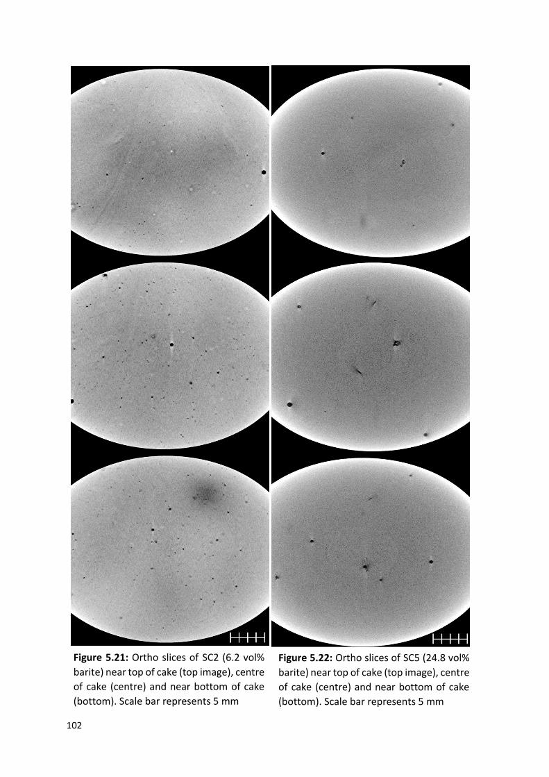
102

Figure 5.21: Ortho slices of SC2 (6.2 vol%

barite) near top of cake (top image), centre



Figure 5.22: Ortho slices of SC5 (24.8 vol%

barite) near top of cake (top image), centre



103

Figure 5.23: 3D representations of the whole of SC2 (top)

and SC5 (bottom), where SC5 is 3.8 mm thicker than SC2.

Each colour represents an unconnected pore or a

connected pore network. Scale bar represents 5 mm

104

5.3.3. Varying filtration time

Figure 5.25 shows the VLP in each 6.2 vol% barite cake produced after different filtration

times and shows that cake VLP decreases with filtration time. Figures 5.26, 5.27 and 5.21

reflect this observation as they show that the 6.2 vol% barite cake produced after 30 mins of

filtration has a noticeably lower VLP than those produced after 5 and 20 mins. This reduction

in VLP may be the reason why the strength of the cake increases significantly from 20 to 30

mins as shown in Figure 4.6. The decrease in VLP may be due to the compression of the cake

layers and/or the infiltration of smaller particles into the pre-existing voids. However, the

samples are composed of barite particles only, which has a narrow size distribution (Figure

2.7), so the likelihood of smaller particles infiltrating pre-existing voids is low. The non-

linearity of the filtration plot of the 6.2 vol% cake, as shown in Figure 5.1, also indicates cake

restructuring during filtration in the form of dynamic cake compression (Christensen et al.,

2011).

Figures 5.28, 5.29 and 5.30 show 3D representations of the pores for the 6.2 vol% cake after

5, 20 and 30 mins of filtration. Each image is composed of a stack of ten ortho slices with a

thickness of 0.13 mm. Figures 5.28 and 5.29 show that for the cakes produced after 5 and 20

mins, the VLP of each layer decreases traversing from top to bottom as the number of smaller


samples containing 6.2 vol% (SC2) and 24.8 vol% (SC5) barite

0.01 0.1 1

0

20

40

60

80

100

Cum

ula

tive v

olu

me (

%)


SC2

SC5

105

pores decreases. However, for the cake produced after 30 mins (Figure 5.30), the top layer

has almost no pores whilst there are several scattered pores in the middle and bottom layers.

This observation is supported by Figure 5.25 which shows the VLP in each cake layer: the 30

mins cake increases in VLP traversing from top to bottom, whilst the 20 mins and 5 mins cake

display the opposite behaviour. Elkatatny et al. (2013) found analogous results for their filter

cakes made from water-based polymer drilling fluids. As discussed in Section 1.2.2.6., cakes

formed within the first 7.5 mins of filtration had a more porous top layer compared to the

bottom layer whilst, after 7.5 mins, the bottom layer became the more porous layer. This

reversal in porosity is also observed in Figure 5.25, except the reversal happens after 20 mins.

The longer filtration time required for reversal may be due to the lower pressure used for

filtration, 690 kPa, as compared to the pressure used by Elkatatny el al. of 2070 kPa. They also

observed that the porosity of both layers decreased with filtration time. However, since the

VLP values in Figure 5.25 represent the volume fraction of pores larger than the resolution,

they are significantly lower than the average porosity (as measured using the drying rate

method discussed in Section 2.2.2.4.) of the 6.2 vol% barite cake at 0.50, as shown in Figure

4.9. This means that the cakes may be more homogeneous or the porosity may vary

differently than depicted in Figure 5.25.

Figure 5.25: VLP (volume fraction of large pores) in cakes over cake thickness starting at

the filter medium at 0.0 mm. Cakes were produced via filtration of the 6.2 vol% barite fluid

after different filtration times

0.0 0.1 0.2 0.3 0.4 0.5 0.6 0.7 0.8 0.9 1.0

0.000

0.002

0.004

0.006

0.008

0.010

0.012

0.014

0.016

0.018

5 mins

20 mins

30 mins

Ca

ke V

LP

Cake thickness (mm)

106

Figure 5.26: Ortho slices of SC25 (5 mins

filtration of 6.2 vol% barite fluid) near top

of cake (top image), centre of cake (centre)

and near bottom of cake (bottom). Scale

bar represents 5 mm

Figure 5.27: Ortho slices of SC220 (20 mins



and near bottom of cake (bottom). Scale

bar represents 5 mm

107

Figure 5.28: 3D slices of SC25 (5 mins



and near bottom of cake (bottom). Each

colour represents an unconnected pore or

a connected pore network. Scale bar

represents 5 mm







represents 5 mm

108







represents 5 mm

109

5.4. Conclusions

The filtration behaviour and pore structure of filter cakes made from different formulations

were studied. The analysis supports the understanding of the cake strength studies in Chapter

4. The filtration behaviour was analysed using filtration plots based on the volume of filtrate

collected over time. The plots showed that as the solids (barite or calcium carbonate) volume

fraction increased from 3.1 vol% to 24.8 vol%, the total filtrate volume decreased. The

addition of calcium carbonate to the barite only samples led to a significant decrease in the

total filtrate volume. For the barite only samples, the filtration plots became more linear as

the volume fraction increased, which may have been due to a decrease in cake restructuring

during filtration. For the barite only samples, there was a minimum cake permeability at a

volume fraction of 12.4 vol%, whilst the calcium carbonate only sample had a permeability

that was 3.76 x 10-16 m2 higher than the barite only equivalent. As shown by the Carman-

Kozeny model, for particles of the same shape and cakes of the same porosity, this increase

in permeability may have been due to the calcium carbonate particles being larger than the

barite particles. Filter cakes made from talc and cellulose microcrystalline had the lowest

permeability despite their high porosities. For talc, this may have been due to the plate-like

shape of the particles, leading to overlapping layers that are individually porous but form a

barrier to fluid flow.

XRCT images of the filter cake samples were analysed and Amira-Avizo was used to produce

3D representations of the pore network. Amira-Avizo was also used to obtain quantitative

data such as pore size distributions and VLP within the cake layers. The images and data

showed that as the d50 of calcium carbonate particles increased, the VLP and pore sizes

increased. For the samples with varying particle size distributions, there was a higher VLP in

the bottom layers of the cake. This is evidence of segregated packing zones being formed.

However, the top layer was expected to have a higher VLP than the bottom layer, so, the

segregated packing zones may have been formed via bridging filtration in the cake layers. For

the 6.2 vol% barite cakes produced after different filtration times, the cake produced after 30

mins had a noticeably lower VLP than those produced after 5 and 20 mins. This reduction in

VLP may be the reason why, as shown in Section 4.3.1., the strength of the cake increased

significantly from 20 to 30 mins. The 30 mins cake increased in VLP traversing from top to

110

bottom, whilst the 20 mins and 5 mins cake displayed the opposite behaviour. This suggests

that segregation may be strongest during the initial 20 mins of filtration, after which bridging

filtration may be more dominant.

111

Chapter 6. Simulation of particle systems

6.1. Introduction

The study of particle systems, which represent the filter cake, was performed using the

discrete element method (DEM) (Cundall and Strack, 1979). Code was developed to simulate

the hole punch test on a predefined system of spherical particles. Particle interactions were

controlled by using different force contact models such as the Hertz-Mindlin contact model

(Hertz, 1882; Mindlin, 1949; Mindlin and Deresiewicz, 1953). As the simulated plunger

descended, force-time data were produced at regular timesteps and converted to stress-

strain data. From this data, the total energy required to punch through the cake as well as the

yield stress and strain for each sample were obtained.

Previous studies have used DEM to investigate the effects of particle and fluid properties on

filter cake formation. For filtration at constant pressure, the effects of fluid viscosity and

density as well as particle size on cake porosity were investigated by Dong et al. (2009). The

filtration of suspensions with particles of varying sphericities were simulated by Deshpande

et al. (2020) using DEM coupled with computational fluid dynamics. Particle sphericity was

controlled using conjoined sub-spheres. They investigated the influence of particle sphericity

and the coefficient of sliding friction on cake porosity and pressure drop per unit length of

cake. Furthermore, various studies have explored particle systems under bulk compression.

Uniaxial compression simulations were performed by Wiacek et al. (2012) to understand the

mechanical behaviour of granular systems. The effects of particle aspect ratio and

interparticle coefficient of friction on the porosity and modulus of the granular system were

studied. Direct shear simulations were performed by Hartl and Ooi (2011) on spherical and

non-spherical particles to investigate the relationship between particle shape and the bulk

internal friction.

In this chapter, the development of a DEM code is outlined and the simulation results are

explored. The simulated hole punch test was used to investigate the effects of particle size

and cake porosity on the strength of filter cakes. The findings from DEM simulations were

compared with the experimental results discussed in Chapters 3 and 4.

112

6.2. Discrete element method

Cundall and Strack (1979) first introduced DEM to simulate granular material as an

arrangement of rigid particles, where such particles overlap upon contact instead of

deforming. For this work, MercuryDPM, which is an open-source software package using

object-orientated C++ code, was used to simulate particle systems with DEM (Weinhart et al.,

2020). A DEM simulation calculates the movement of a defined set of particles based on their

body forces, which are assumed to act from each particle’s centre of mass, and contact forces,

acting at the contact point between particles. Once the particles’ preliminary properties are

specified, the movement of each particle is simulated based on Newton’s laws of motion.

Spherical particles are the simplest to simulate, although it is recognised that granular

material is typically non-spherical. Simulating non-spherical particles is computationally more

expensive because, at every contact point, non-linear equations must be used to calculate the

particle overlaps. A set of walls and boundaries can be implemented to restrict motion. A

simple schematic of the setup including the forces involved in the simulations is shown in

Figure 6.1.

With the system geometry, including the particle positions and boundary conditions, and the

contact model parameters specified, DEM simulations comprise a recurring loop of steps for

a set number of time increments known as timesteps, as shown in Figure 6.2. Contacting

particles are identified at the start of each timestep and contact models are used to evaluate

the magnitude of interparticle forces, which is a function of the distance between contacting

Figure 6.1: A schematic of forces included in DEM simulations

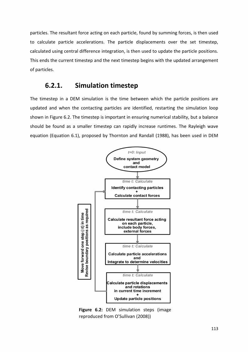
113

particles. The resultant force acting on each particle, found by summing forces, is then used

to calculate particle accelerations. The particle displacements over the set timestep,

calculated using central difference integration, is then used to update the particle positions.

This ends the current timestep and the next timestep begins with the updated arrangement

of particles.

6.2.1. Simulation timestep

The timestep in a DEM simulation is the time between which the particle positions are

updated and when the contacting particles are identified, restarting the simulation loop

shown in Figure 6.2. The timestep is important in ensuring numerical stability, but a balance

should be found as a smaller timestep can rapidly increase runtimes. The Rayleigh wave

equation (Equation 6.1), proposed by Thornton and Randall (1988), has been used in DEM

Figure 6.2: DEM simulation steps (image

reproduced from O’Sullivan (2008))

114

studies (Li, Xu and Thornton, 2005; Washino et al., 2016; Wilkinson et al., 2017; Ghasemi, Razi

and Banisi, 2020) to find an appropriate timestep, known as the critical timestep. In Equation

6.1, the Rayleigh time, TR, is calculated using the particle radius, R, the Poisson’s ratio, ν, the

particle density, ρ, and the shear modulus, G (calculated using the Young’s modulus, E).

Methods have been used to artificially increase the timestep, such as density and stiffness

scaling, to reduce simulation runtimes (C. and Anthony, 1998; O’Sullivan and Bray, 2004;

O’Sullivan, Cui and O’Neill, 2008; Yousefi and Ng, 2017). The critical timestep is set as a

fraction, known as the safety factor, of the Rayleigh time. According to O’Sullivan and Bray

(2004), the critical timestep, and so the safety factor, is a function of the particle packing

configuration and coordination number. However, particle coordination numbers vary

throughout the simulation, and so, a safety factor is often set which keeps the assembly of

particles stable whilst allowing the simulations to be completed within reasonable runtimes.

Some authors (Itasca Consulting Group, 1998; O’Sullivan and Bray, 2004; Li, Xu and Thornton,

2005; Wilkinson et al., 2017; Ghasemi, Razi and Banisi, 2020) have found safety factors that

work for specific conditions. An example is Washino et al. (2016) who found that using 24%

of the Rayleigh time produced stable simulations for dry particles whilst below 1% was best

for wet particles. Suitable safety factors will vary depending on the particle properties and

setup.

𝑇𝑅 =𝜋𝑅

0.01631𝜈 + 0.8766√𝜌/𝐺

(6.1)

𝑤ℎ𝑒𝑟𝑒 𝐺 =𝐸

2(1 + 𝜈)

For this work, a timestep of 2.5 x 10-6 s was used for particles with a density of 1100 kg m-3, a

Poisson’s ratio of 0.24 and a scaled Young’s Modulus of 70 MPa, which represents a safety

factor of between 33% and 45% (depending on the particle radius) of the Rayleigh time. For

the particle setup used, this timestep enabled stable simulations to be run within reasonable

runtimes.

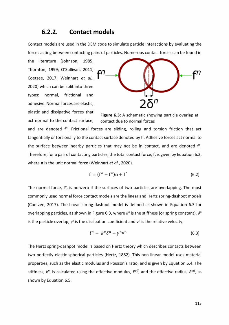
115

6.2.2. Contact models

Contact models are used in the DEM code to simulate particle interactions by evaluating the

forces acting between contacting pairs of particles. Numerous contact forces can be found in

the literature (Johnson, 1985;

Thornton, 1999; O’Sullivan, 2011;

Coetzee, 2017; Weinhart et al.,

2020) which can be split into three

types: normal, frictional and

adhesive. Normal forces are elastic,

plastic and dissipative forces that

act normal to the contact surface,

and are denoted fn. Frictional forces are sliding, rolling and torsion friction that act

tangentially or torsionally to the contact surface denoted by ft. Adhesive forces act normal to

the surface between nearby particles that may not be in contact, and are denoted fa.

Therefore, for a pair of contacting particles, the total contact force, f, is given by Equation 6.2,

where n is the unit normal force (Weinhart et al., 2020).

𝐟 = (f 𝑎 + f 𝑛)𝐧 + 𝐟𝑡 (6.2)

The normal force, fn, is nonzero if the surfaces of two particles are overlapping. The most

commonly used normal force contact models are the linear and Hertz spring-dashpot models

(Coetzee, 2017). The linear spring-dashpot model is defined as shown in Equation 6.3 for

overlapping particles, as shown in Figure 6.3, where kn is the stiffness (or spring constant), δn

is the particle overlap, γn is the dissipation coefficient and vn is the relative velocity.

f 𝑛 = 𝑘𝑛𝛿𝑛 + 𝛾𝑛v𝑛 (6.3)

The Hertz spring-dashpot model is based on Hertz theory which describes contacts between

two perfectly elastic spherical particles (Hertz, 1882). This non-linear model uses material

properties, such as the elastic modulus and Poisson’s ratio, and is given by Equation 6.4. The

stiffness, kn, is calculated using the effective modulus, Eeff, and the effective radius, Reff, as

shown by Equation 6.5.

Figure 6.3: A schematic showing particle overlap at

contact due to normal forces

116

f 𝑛 = 𝑘𝑛(𝛿𝑛)3/2 + 𝛾𝑛v𝑛(𝛿𝑛)1/4 (6.4)

𝑘𝑛 =4

3𝐸𝑒𝑓𝑓√𝑅𝑒𝑓𝑓

(6.5)

The effective modulus is calculated using the elastic moduli, E, and Poisson’s ratios, ν, of both

particles. For particles with the same properties, the effective modulus can be calculated

using Equation 6.6. The effective radius is calculated using Equation 6.7 for particles with radii

R1 and R2.

𝐸𝑒𝑓𝑓 =𝐸

2(1 − 𝜈2)

(6.6)

𝑅𝑒𝑓𝑓 =𝑅1𝑅2

𝑅1 + 𝑅2

(6.7)

The dissipation coefficient, γn, is dependent on the coefficient of restitution, e, as shown in

Equation 6.8, where meff is the effective mass, which can be calculated using Equation 6.9 for

particles with masses m1 and m2.

𝛾𝑛 =ln 𝑒

√ln2 𝑒 + 𝜋2√𝑚𝑒𝑓𝑓𝑘𝑛

(6.8)

𝑚𝑒𝑓𝑓 =𝑚1𝑚2

𝑚1 + 𝑚2 (6.9)

The forces acting in the tangential direction can be described by Equation 6.10, which is

analogous to Equation 6.3 for the normal forces.

f 𝑡 = 𝑘𝑡𝛿𝑡 + 𝛾𝑡v𝑡 (6.10)

The particle begins to slide once the tangential force exceeds a specified fraction, known as

the coefficient of sliding friction, µt, of the normal force. Once the Coulomb yield criterion

(Equation 6.11) is surpassed, the tangential force is evaluated as the product of the coefficient

of sliding friction and the normal force. Rolling and torsion torques, opposing the angular

motion of particles in contact, are modelled in a similar manner, whereby the relative velocity,

vt, in Equation 6.10 is replaced by the product of an effective length and angular velocity, and

the coefficient of sliding friction, µt, in Equation 6.11 is replaced by a coefficient of rolling or

torsion friction.

117

f 𝑡 ≤ µ𝑡f 𝑛 (6.11)

If the normal force is described by the Hertz spring-dashpot model, then the tangential force

is more appropriately described using models derived from the works of Mindlin (1949) and

Mindlin and Deresiewicz (1953). The Mindlin model, as shown by Equation 6.12, calculates

the tangential force using a tangential stiffness, kt, that depends on the effective shear

modulus, Geff, as shown by Equation 6.13.

f 𝑡 = 𝑘𝑡𝛿𝑡 + 𝛾𝑡v𝑡(𝛿𝑡)1/4 (6.12)

𝑘𝑡 = 8𝐺𝑒𝑓𝑓√𝑅𝑒𝑓𝑓𝛿𝑛 (6.13)

For identical particles, the effective shear modulus is calculated using Equation 6.14, where G

is the particle shear modulus. Equation 6.15 is used to calculate the tangential dissipation

coefficient, γt.

𝐺𝑒𝑓𝑓 =𝐺

2(2 − 𝑣)

(6.14)

𝛾𝑡 =ln 𝑒

√ln2 𝑒 + 𝜋2√𝑚𝑒𝑓𝑓𝑘𝑡

(6.15)

Adhesive force models are used to evaluate the forces between particles arising from dry or

wet cohesion. In MercuryDPM (Weinhart et al., 2020), linear elastic-dissipative short-range

forces are modelled using the reversible adhesive contact model. For this adhesive force

model, reversible means that the adhesive force is the same during loading and unloading

(before and after particle contact). The model is used to simulate dry cohesion due to

attractive forces, such as van der Waals forces. A linear irreversible adhesive contact model,

where the adhesive force only acts during unloading, is used to simulate wet cohesion. Liquid

bridges that form between particles cause wet cohesion and are effective throughout

unloading until they collapse. In addition, a non-linear model has been developed in

MercuryDPM to simulate liquid bridges between particles, as shown in Figure 6.4. The liquid

bridge Willet contact model is based on work by Willet et al. (2000), who derived a force-

displacement relation using the Young-Laplace equation and Equation 6.16. In Equation 6.16,

the total downward force on the upper sphere (Figure 6.4), F, is calculated using the neck

radius, rN, the liquid surface tension, γ, the liquid density, ρl, the hydrostatic pressure

118

difference across the air-liquid interface, ΔP, the volume of the upper sphere, Vs, and the

acceleration due to gravity, g. In this model, the adhesive force only acts during unloading

and follows a non-linear path.

𝐹 = 2𝜋𝑟𝑁𝛾 − 𝜋𝑟𝑁2∆𝑃 − 𝑉𝑠𝜌𝑙𝑔 (6.16)

The level of water saturation in a filter cake and the associated capillary forces (derived from

liquid bridges) will depend on environmental conditions. At equilibrium, the chemical

potential of water in the liquid bridge will balance the chemical potential of water in the

atmosphere. Any humidity will ensure a level of saturation within the filter cake, and it will

take time for evaporation to reduce the water saturation level to the equilibrium value. This

means that a filter cake in the hole punch test will be partially saturated, hence, liquid bridges

will exist between particles.

Figure 6.4: A schematic of a liquid

bridge between two spheres of radii

R1 and R2 with a separation distance

of 2S. The liquid bridge has a volume

V, surface tension γ, neck radius rN,

a liquid-solid contact angle φ and

half-filling angles β1 and β2

(reprinted with permission from

Willett et al. (2000). Copyright 2000

American Chemical Society)

119

6.2.3. Numerical setup

A 2D schematic of the simulation setup, including the hole punch test and cake, is shown in

Figure 6.5. The setup dimensions are summarised in Table 6.1 and the code used to perform

simulations is shown in Appendix A. The platform surface of the test is constructed using walls,

the plunger and test opening using axisymmetric walls, the bottom of the opening has a

deletion boundary, and the edges of the cake are defined by periodic boundaries. Periodic

boundaries are used to simulate a periodic section between two parallel planes, which is

achieved by using ghost particles (copies of the existing particles) at the periodic boundary to

transfer forces across the boundary. Periodic boundaries, by limiting the number of particles

required, ensure that simulations are completed within reasonable runtimes. In Figure 6.6,

which shows a 3D representation of the array of spherical particles representing the cake,

periodic boundaries are set at the edges of the cake in the x and y directions. Initially, the

spherical particles are evenly spaced and their centres are aligned in all three dimensions.

Then, still before the start of a simulation, the amount of space allocated between the

particles, which is dependent on the cake porosity, is randomised as shown in Figure 6.5.

Figure 6.6 shows the simulation setup in operation as the cylindrical plunger (not shown)

punches the cake into the opening. Tables 6.2, 6.3 and 6.4 summarise the particle properties

and contact model parameters in simulations using different contact models.

Figure 6.5: A 2D schematic of the simulation setup. Each colour

represents a different type of wall or boundary

120

Figure 6.6: 3D representations of the simulations using DEM data on

ParaView. Images show an array of particles (or cake) at the start of

the simulation (top), once the plunger has punched through a couple

of particle layers (middle), and once the plunger has punched through

the whole cake thickness (bottom). Note, the plunger is travelling in

the negative z-direction and the colours indicate particle velocity (red

particles are moving and blue particles are still)

121

Table 6.1: Summary of the setup dimensions used for DEM simulations of the hole punch test with cake

Cake thickness 3 or 8 mm

Cake width (x axis) 14 mm

Cake width (y axis) 14 mm

Plunger diameter 8 mm

Plunger speed 8 mm s-1

Table 6.2: Summary of the particle properties and contact model parameters in DEM simulations using the Hertz-Mindlin contact model (HM DEM), where cakes were 3 or 8 mm thick

Density 1100 kg m-3

Young’s Modulus 70 MPa

Poisson Ratio 0.24

Coefficient of restitution 0.8

Sliding friction coefficient 0.6

Rolling friction coefficient 0.1

Particle radius 0.25 to 0.34 mm

Number of particles 588 to 8750

Table 6.3: Summary of the particle properties and contact model parameters in DEM simulations using the linear viscoelastic friction contact model (LVF DEM), where all cakes were 8 mm thick

Density 1100 kg m-3

Collision time 5 x 10-5 s




Particle radius 0.34 mm


Table 6.4: Summary of the particle properties and contact model parameters in DEM simulations using the linear viscoelastic friction contact model with the liquid bridge Willet species (LVFLB DEM), where all cakes were 8 mm thick

Density 1100 kg m-3

Collision time 5 x 10-5 s




Liquid bridge volume 6 x 10-11 m3

Liquid surface tension 0.073 N m-1

Contact angle 29°

Particle radius 0.30 to 0.34 mm


122

6.3. Simulations

6.3.1. Hertz-Mindlin contact model

The force curves obtained from simulations using the Hertz-Mindlin contact model are shown

in Figure 6.7. The plunger contacts the top of the cake within 0.025 s, and all the cake has

been punched through the opening by 1.025 s. The top graph in Figure 6.7 shows the entire

force curves for cakes made of particles with different radii. The two sharp peaks observed

for each curve at around 0.9 s are likely due to a few individual particles that have become

stuck between the platform and plunger, because, beyond around 0.9 s, most of the cake has

been punched through the opening. This leads to a contained explosion of particles within a

section of the cake. Hence, the force curve beyond 0.9 s is taken to be noise that does not

represent the shearing of the cake. The bottom graph in Figure 6.7 shows the same force

curves zoomed in so that the cake shearing in the first 0.9 s can be observed. These force

peaks (shown in the yellow box) are summed to find the total energy required to punch

through each cake sample.

The hole punch test simulations were performed on cakes of different thicknesses, but with

the same porosity of 0.5 using particles with a radius of 0.34 mm. These simulations were

used to validate the method of summing up the forces to find a total energy. Figure 6.8 shows

that the total energy increases as the cake thickness increases, which is expected as more

particle layers would lead to more interparticle contacts as the cake is sheared.

123

Figure 6.7: Using the Hertz-Mindlin contact model, force required by the plunger over time

to descend through cake at a constant velocity of 8 mm s-1. The bottom graph shows the

same results as the top graph zoomed in. The yellow box represents the forces that were

summed to find the total energy. The legend shows the different particle radii

0.0 0.2 0.4 0.6 0.80.0000

0.0001

0.0002

0.0003

0.0004

0.0005

Fo

rce

(N

)

Time (s)

0.34 mm

0.32 mm

0.30 mm

0.28 mm

0.0 0.2 0.4 0.6 0.8 1.00.0

0.2

0.4

0.6

0.8

1.0

1.2F

orc

e (

N)

Time (s)

0.34 mm

0.32 mm

0.30 mm

0.28 mm

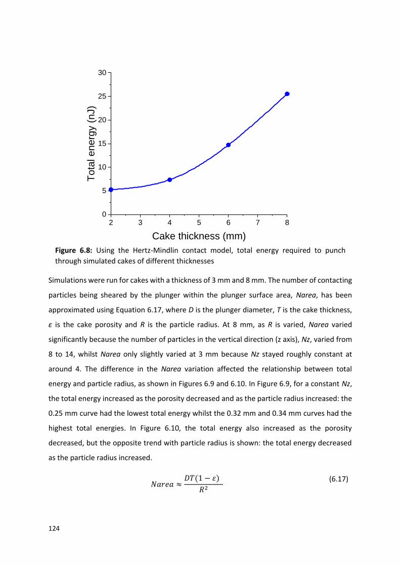
124

Simulations were run for cakes with a thickness of 3 mm and 8 mm. The number of contacting

particles being sheared by the plunger within the plunger surface area, Narea, has been

approximated using Equation 6.17, where D is the plunger diameter, T is the cake thickness,

ε is the cake porosity and R is the particle radius. At 8 mm, as R is varied, Narea varied

significantly because the number of particles in the vertical direction (z axis), Nz, varied from

8 to 14, whilst Narea only slightly varied at 3 mm because Nz stayed roughly constant at

around 4. The difference in the Narea variation affected the relationship between total

energy and particle radius, as shown in Figures 6.9 and 6.10. In Figure 6.9, for a constant Nz,

the total energy increased as the porosity decreased and as the particle radius increased: the

0.25 mm curve had the lowest total energy whilst the 0.32 mm and 0.34 mm curves had the

highest total energies. In Figure 6.10, the total energy also increased as the porosity

decreased, but the opposite trend with particle radius is shown: the total energy decreased

as the particle radius increased.

𝑁𝑎𝑟𝑒𝑎 ≈𝐷𝑇(1 − 휀)

𝑅2

(6.17)

Figure 6.8: Using the Hertz-Mindlin contact model, total energy required to punch

through simulated cakes of different thicknesses

2 3 4 5 6 7 80

5

10

15

20

25

30

Tota

l energ

y (

nJ)

Cake thickness (mm)

125


through simulated 3 mm thick cakes (Narea only slightly varied due to a constant Nz) of

different porosities and with particles of different radii. The legend shows the different

particle radii

0.55 0.60 0.65 0.70 0.75 0.80 0.850.0

0.5

1.0

1.5

2.0

2.5

3.0

3.5

4.0

4.5

5.0

5.5

6.0

6.5

7.0

7.5

8.0

0.34 mm

0.32 mm

0.30 mm

0.28 mm

0.25 mm

To

tal e

ne

rgy (

nJ)

Cake porosity


through simulated 8 mm thick cakes (Narea varied significantly due to a varying Nz) of

different porosities and with particles of different radii. The legend shows the different

particle radii

0.50 0.55 0.60 0.65 0.70 0.75 0.80 0.850

5

10

15

20

25 0.34 mm

0.32 mm

0.30 mm

0.27 mm

To

tal e

ne

rgy (

nJ)

Cake porosity

126

The opposite trends may be due to the variation in the total interparticle contact surface area,

TSA, as the particle radius is varied. The total energy required to punch through the cake, Et,

is a function of the TSA, which is the product of the particle-particle contact surface area, PSA,

the total number of contacting particles in the cake, N, and a fraction of the particle

coordination number, CN, as shown in Equation 6.18. In the Hertz theory (Hertz, 1882), the

radius of the circle of contact, a, is a function of the particle radius, R, the load, F, and the

equivalent elastic modulus, E, as shown in Equation 6.19 for particles of the same size. This

gives an approximate PSA as shown in Equation 6.20. N is found using the total volume of the

cake, V, and the cake porosity, ε, as shown in Equation 6.21. This leads to Equation 6.22 which

shows that the total energy is proportional to R -7/3, therefore, the total energy should always

increase as the particle radius decreases.

However, the opposite occurs when the number of particles in the vertical direction, Nz, is

constant (whilst Narea increases slightly and N increases significantly) as R decreases, which

suggests that the total energy is dictated by Nz and Narea as opposed to N. A small variation

in Narea (due to a constant Nz) means that the number of particles sheared whilst punching

through the cake varies insignificantly as the particle radius is varied. Therefore, if N in

Equation 6.18 is replaced by Narea, as shown in Equation 6.23, the total energy would

increase as the particle radius increases for a roughly constant Narea. This is observed in

Figure 6.9. When a thicker cake is used, Narea varies more as Narea is high for small particle

radii and vice versa, leading to the opposite trend with particle radius as shown in Figure 6.10.

𝐸𝑡 ∝ 𝑇𝑆𝐴 = 𝑃𝑆𝐴 × 𝑁 × 𝐶𝑁

(6.18)

𝐻𝑒𝑟𝑡𝑧 𝑡ℎ𝑒𝑜𝑟𝑦: 𝑎3 =𝑅𝐹

2𝐸

(6.19)

∴ 𝑃𝑆𝐴 = 𝜋 𝑎2 = 𝜋(𝑅𝐹

2𝐸)2/3

(6.20)

𝑁 = 𝑉(1 − 휀)

43 𝜋𝑅3

(6.21)

∴ 𝐸𝑡 ∝ 𝑇𝑆𝐴 =𝑉(1 − 휀)

43

× (𝐹

2𝐸)2/3 × 𝐶𝑁 × 𝑅−7/3

(6.22)

127

In Figure 6.10, for an 8 mm thick cake of varying Narea, the total energy decreased as the

particle radius increased for a cake porosity greater than 0.55, but this trend is reversed for a

cake porosity of 0.55. According to Equation 6.23, for a thick enough cake where Narea varies

significantly with particle radius and is proportional to the reciprocal of R2, as shown in

Equation 6.17, the total energy should decrease as the particle radius increases. This is

assuming the particle coordination number, CN, remains constant. However, for spherical

particles, the particle coordination number has been shown to vary with porosity (Suzuki and

Oshima, 1988) and particle size (Ouchiyama and Tanaka, 1981). Hence, the total energy trend

with particle radius may reverse for a cake porosity of 0.55, as shown in Figure 6.10, due to

the variance in particle coordination number.

6.3.2. Linear viscoelastic friction contact model

When the liquid bridge Willet species is implemented in the linear viscoelastic friction contact

model, the force curves show significant force values as the plunger punches through the

cake, as shown in Figure 6.11. Beyond around 0.9 s, most of the cake has been punched

through the opening, and the sharp peaks observed after 0.9 s are again likely to be a few

particles stuck between the platform and plunger. This leads to a contained explosion of

particles within a section of the cake. Hence, the force curve beyond 0.9 s is again discarded.

Therefore, yield stress values were obtained from peak force values preceding 0.9 s. The

distance travelled by the plunger at each peak was used to calculate the yield strain, and the

total energy required to punch through the cake was found by summing of the forces up to

the peak force value.

Figure 6.11 shows the force curves over time for particles of different radii (0.30 and 0.34

mm) and for cakes of different porosities (0.5 to 0.8). The force curves show that a lower cake

porosity leads to greater forces required to punch through the cake. For a set porosity, a

smaller particle radius leads to greater forces, except for a porosity of 0.5. This exception may

be due to the variance in particle coordination number at a porosity of 0.5, as explained in

Section 6.3.1.

𝐸𝑡 ∝ 𝑇𝑆𝐴 = 𝜋(𝐹

2𝐸)2/3 × 𝐶𝑁 × 𝑅2/3 × 𝑁𝑎𝑟𝑒𝑎

(6.23)

128

6.3.3. Comparison with experimental results

Figures 6.12, 6.13, 6.15 and 6.16 show a comparison of the yield stress and strain for cakes in

experiments and in DEM simulations. The force data using the Hertz-Mindlin contact model

could not be used to obtain yield stress and strain values due to the lack of a curve, as shown

in Figure 6.7. Figures 6.14 and 6.17 show a comparison of the total energy required to punch

through the cake in experiments and in DEM simulations, for the Hertz-Mindlin and linear

viscoelastic friction (with and without the liquid bridge Willet species) contact models. The

particles are monosized in simulations whilst, in experiments, half the d50 of the particle size

distribution in the fluid (see Figure 2.7) is used as the particle radius. The experimental

samples selected for comparison in Figures 6.12 to 6.17 were composed of one species of

particles with a circularity of above 0.80 (see Table 2.5). In Figures 6.15 to 6.17, the porosity

value quoted in the legend is the cake porosity to the nearest decimal point.

Figure 6.11: Using the linear viscoelastic friction contact model with the liquid bridge

Willet species, force required by the plunger over time to descend through simulated 8

mm thick cakes at a constant velocity of 8 mm s-1. For each curve in the legend, the cake

porosity then the particle radius (in mm) are shown

0.0 0.2 0.4 0.6 0.8 1.00.00

0.05

0.10

0.15

0.20

0.25

0.30

0.35

0.40

Fo

rce

(N

)

Time (s)

Porosity, radius (mm)

0.5, 0.30

0.5, 0.34

0.6, 0.30

0.6, 0.34

0.7, 0.30

0.7, 0.34

0.8, 0.30

0.8, 0.34

129

The yield strain results for simulated and experimental cakes with different porosities are

shown in Figure 6.12. For the SC samples, the yield strain decreases as the porosity decreases,

and, the SCal samples have similar yield strains of around 0.45, which may be due to the

samples having the same volume fraction of particles in the model fluid, as discussed in

Section 3.4.1. Except for the simulation with a cake porosity of 0.54 and particle radii of 0.30

mm, the simulations follow a similar trend whereby the yield strain decreases as the porosity

decreases. The yield strains of simulations using a particle radius of 0.34 mm curve towards

most of the experimental results as porosity is decreased, even though the samples used in

experiments have much lower particle radii.

The yield stress results for simulated and experimental cakes with different porosities are

shown in Figure 6.13. For the experiments, the yield stress increases with decreasing porosity

for the SC samples, and, the yield stress increases with decreasing particle radii for the SCal

samples. For the simulations, the yield stress increases with decreasing cake porosity and

Figure 6.12: Yield strain of simulated and experimental cakes of different porosities and

with particles of different radii. All simulated cakes were 8 mm thick. The simulation

results were found using the linear viscoelastic friction contact model with the liquid

bridge Willet species (LVFLB DEM). The legend shows the different particle radii (in mm)

0.3 0.4 0.5 0.6 0.7 0.80.0

0.1

0.2

0.3

0.4

0.5

0.6

0.7

0.8

0.9

1.0

0.30 (LVFLB DEM)

0.34 (LVFLB DEM)

0.0026 (SC experiments)

0.0065 (Sglass experiment)

0.0055 (SCal8 experiment)



Yie

ld s

train

Cake porosity

130

particle radii, except for the porosity of 0.5. This exception may be due to the variance in

particle coordination number, as discussed in Section 6.3.1. At a similar porosity of around

0.53, there is an order of magnitude difference between the simulation yield stresses and the

yield stress of the SC sample.

Figure 6.14 shows that as the cake porosity decreases, the total energy required to punch

through the cake increases in both experiments and simulations, resembling the trend with

yield stress in Figure 6.13. The experimental results show similar trends to those for yield

stress in Figure 6.13, as the total energy increases with decreasing porosity for the SC samples,

and, the total energy increases with decreasing particle radii for the SCal samples. For the

SCal samples, the relationship of total energy with porosity is not as clear, possibly showing

the opposite behaviour. The simulation results follow a similar trend with particle radii, which

is shown most clearly by the LVFLB curves in Figure 6.14.

Figure 6.13: Yield stress of simulated and experimental cakes of different porosities and



bridge Willet species (LVFLB DEM). The legend shows the different particle radii (in mm)

0.3 0.4 0.5 0.6 0.7 0.80.01

0.1

1

10

100

0.30 (LVFLB DEM)

0.34 (LVFLB DEM)






Yie

ld s

tress (

kP

a)

Cake porosity

131

Comparing HM with LVF simulation results in Figure 6.14, the switch from a non-linear to

linear contact model increases the total energy by slightly more than two orders of

magnitude. This may be due to the difference in stiffness and dissipation coefficient used in

each model. Comparing LVFLB with LVF simulation results, the inclusion of the liquid bridge

Willet species increases the total energy required by between one and two orders of

magnitude. This suggests that the adhesion due to liquid bridges in between particles

contributes significantly to cake strength. Although there is a significant difference in radii

between the particles in experiments and simulations, the total energies of the simulations

with liquid bridges almost align with those from experiments, with the SC sample at a porosity

of 0.53 almost overlapping the LVFLB curves at a similar porosity.

The yield strain results for simulated and experimental cakes with particles of different radii

are shown in Figure 6.15. The simulated cakes with a porosity of 0.5 as well as the cakes made


different porosities and with particles of different radii. All simulated cakes were 8 mm

thick. The simulation results were found using the linear viscoelastic friction contact model,

with (LVFLB DEM) and without (LVF DEM) the liquid bridge Willet species, and the Hertz-

Mindlin contact model (HM DEM). The legend shows the different particle radii (in mm)

0.3 0.4 0.5 0.6 0.7 0.810-6

10-5

10-4

10-3

10-2

10-1

100

101

102

Tota

l en

erg

y (

mJ)

Cake porosity

0.30 (LVFLB DEM)

0.34 (LVFLB DEM)

0.34 (LVF DEM)

0.27 (HM DEM)

0.30 (HM DEM)

0.32 (HM DEM)

0.34 (HM DEM)






132

from SC samples seem to have yielded at a broad range of strains. Particle radius does not

affect the yield strain as the range of strains in the simulations is similar to that of some of

the SC samples, despite a difference in particle radius of two orders of magnitude. In addition,

the SCal samples, in which the particle radii are varied, show a narrow range of yield strains.

The yield stress results for simulated and experimental cakes with particles of different radii

are shown in Figure 6.16. For the simulation results, the yield stress increases as the particle

radius decreases, except for the porosity of 0.5. The yield stress values of the cakes in

simulations are more than one order of magnitude lower than those of the SC samples with

a similar porosity of around 0.5, as shown by the blue dotted line. Since the particles used in

the simulations have radii that are two orders of magnitude larger than those in the SC

samples, this suggests that particle radius may influence cake yield stress, more than it

influences the total energy required to punch through the cake as shown in Figure 6.17.

Figure 6.15: Yield strain of simulated and experimental cakes of different porosities and



bridge Willet species (LVFLB DEM). The legend shows the different porosities to the

nearest decimal point

0.001 0.01 0.1 10.0

0.1

0.2

0.3

0.4

0.5

0.6

0.7

0.8

0.9

1.0

Yie

ld s

tra

in

Particle radius (mm)

0.5 (LVFLB DEM)

0.6 (LVFLB DEM)

0.7 (LVFLB DEM)

0.8 (LVFLB DEM)


0.4 (SCal experiments)



133

Particle radius is expected to affect yield stress, YS, according to Equations 6.24, 6.25 and 6.26

for monosized particles, where Δp is the capillary pressure across the air-liquid interface of a

liquid bridge (Willett et al., 2000), and Nz, Narea and N (as defined in Section 6.3.1.) are the

number of contacting particles. If Δp is written in terms of the particle radius, R, as shown in

these equations, then the yield stress is proportional to the reciprocal of R2, R3 or R4,

depending on which parameter is used for the number of contacting particles.

𝑌𝑆 = ∆𝑝 × 𝑁𝑎𝑟𝑒𝑎 ∝1

𝑅×

1

𝑅2=

1

𝑅3

(6.25)

𝑌𝑆 = ∆𝑝 × 𝑁𝑧 ∝1

𝑅×

1

𝑅=

1

𝑅2

(6.24)

Figure 6.16: Yield stress of simulated and experimental cakes of different porosities and



bridge Willet species (LVFLB DEM). The legend shows the different porosities to the

nearest decimal point. The blue dotted line goes through the simulations and SC samples

with the same porosity and has a slope of -2/3. The red dotted line goes through the SCal

samples with the same porosity and has a slope of -2

0.001 0.01 0.1 10.01

0.1

1

10

100Y

ield

str

ess (

kP

a)


0.5 (LVFLB DEM)

0.6 (LVFLB DEM)

0.7 (LVFLB DEM)

0.8 (LVFLB DEM)





134

The yield stress seems to be proportional to the reciprocal of R2 according to the red dotted

line in Figure 6.16, which goes through the SCal samples with the same porosity (to the

nearest decimal point) and has a slope of -2. This relationship can be written as shown in

Equation 6.24. The blue dotted line goes through the simulations and SC samples with the

same porosity (to the nearest decimal point) and has a slope of -2/3. The relationships in

Equations 6.25 and 6.26 are not observed in Figure 6.16. The variation of yield stress with

porosity, which has not been accounted for, may influence the relationships in Equations

6.24, 6.25 and 6.26.

In Figure 6.17, for the simulations and the SCal samples, the total energy increases slightly

with decreasing particle radius, except for the simulations with a cake porosity of 0.5. This

exception may be due to the variance in particle coordination number at a porosity of 0.5, as

explained in Section 6.3.1. Figure 6.17 shows that the experimental cakes required higher

total energies than those in DEM simulations. However, in the LVFLB simulations, the total

energies at a porosity of 0.5 have a similar order of magnitude than the lowest total energies

in the experiments, despite a difference of two orders of magnitude in radii between the

particles used in simulations and experiments. This suggests that particle radius may not

influence the total energy significantly, as shown by the blue dotted line which goes through

the simulations and SC samples with similar porosities.

Particle radius is expected to affect the total energy according to Equations 6.27, 6.28 and

6.29 for monosized particles, where Δp is the capillary pressure across the air-liquid interface

of a liquid bridge (Willett et al., 2000), A is the contact area between two particles, d is the

distance over which the force is applied and Nz, Narea and N (as defined in Section 6.3.1.) are

the number of contacting particles. If each parameter is written in terms of the particle radius,

R, as shown in these equations, then the total energy is proportional to the reciprocal of R0,

R1 or R2, depending on which parameter is used for the number of contacting particles. The

distance over which the force is applied, d, is related to the cake strain, and, as shown in

Figure 6.15, yield strain is not a function of R. Hence, d is proportional to R0 in Equations 6.27,

6.28 and 6.29.

𝑌𝑆 = ∆𝑝 × 𝑁 ∝1

𝑅×

1

𝑅3=

1

𝑅4

(6.26)

135

𝐸𝑡 = ∆𝑝 × 𝐴 × 𝑑 × 𝑁 ∝1

𝑅× 𝑅2 × 𝑅0 ×

1

𝑅3=

1

𝑅2

(6.29)

In Figure 6.17, the blue dotted line goes through the simulations and SC samples with the

same porosity (to the nearest decimal point) and has a slope of approximately 0, whilst the

red dotted line goes through the SCal samples with the same porosity (to the nearest decimal

point) and has a slope of -2. Therefore, the total energy seems to be proportional to the

reciprocal of any value in between R0 and R2, following each of the relationships in Equations

6.27, 6.28 and 6.29. The variation of total energy with porosity, which has not been accounted

for, may influence the relationships in these equations.

𝐸𝑡 = ∆𝑝 × 𝐴 × 𝑑 × 𝑁𝑧 ∝1

𝑅× 𝑅2 × 𝑅0 ×

1

𝑅= 1

(6.27)

𝐸𝑡 = ∆𝑝 × 𝐴 × 𝑑 × 𝑁𝑎𝑟𝑒𝑎 ∝1

𝑅× 𝑅2 × 𝑅0 ×

1

𝑅2=

1

𝑅

(6.28)


different porosities and with particles of different radii. All simulated cakes were 8 mm

thick. The simulation results were found using the linear viscoelastic friction contact

model, with (LVFLB DEM) and without (LVF DEM) the liquid bridge Willet species, and the

Hertz-Mindlin contact model (HM DEM). The legend shows the different porosities to the

nearest decimal point. The blue dotted line goes through the simulations and SC samples

with the same porosity and has a slope of approximately 0. The red dotted line goes

through the SCal samples with the same porosity and has a slope of -2

0.001 0.01 0.1 110-6

10-5

10-4

10-3

10-2

10-1

100

101

102

Tota

l energ

y (

mJ)


0.5 (LVFLB DEM)

0.6 (LVFLB DEM)

0.7 (LVFLB DEM)

0.8 (LVFLB DEM)

0.5 (HM DEM)

0.6 (HM DEM)

0.7 (HM DEM)

0.8 (HM DEM)





136

6.3.3.1. Surface plots

Surface plots were produced using the experimental and LVFLB DEM data shown in Figures

6.12 to 6.17. In Figures 6.18 to 6.20, the experimental data are represented by the red points

whilst the simulation data are represented by the green points. The surfaces are plotted using

Equations 6.30 to 6.32, for which relationships between total energy, Et, particle radius, R,

and cake porosity, ε, have been established. In these equations, the relationship with R

depends on how the number of contacting particles is defined: Nz, Narea or N (as defined in

Section 6.3.1.). The filter cake solids fraction (1 – ε) has been included in Equation 6.31 to

calculate Narea and in Equation 6.32 to calculate N. The particle coordination number, CN,

has been determined using Equation 6.33, which is from Rumpf (1958). For each surface plot,

the least squares regression method was used on the data points to determine the value of

proportionality between Et, R and ε.

The total energy peaks at a porosity of 0.4 and below a particle radius of 0.01 mm, where the

experimental data are situated. The total energy has a minimum at a porosity of 0.8 and above

a particle radius of 0.30 mm, where the simulation data are situated. The surface plots

produced using Equations 6.31 and 6.32 reflect these observations in the data points, as

shown in Figures 6.19 and 6.20. The surface plot produced using Equation 6.30 does not vary

with particle radius, hence, it has a minimum at a porosity of around 0.8 irrespective of the

particle radius, as shown in Figure 6.18. In Figure 6.19, when Narea is used as the number of

contacting particles, and so, the total energy is proportional to the reciprocal of R (Equation

6.31), the surface plot seems to fit the data points better, as it intersects some of the

experimental and simulation data points, than when using Nz or N. This result is expected

since Narea more accurately represents the number of contacting particles being sheared in

the filter cake (as the plunger descends in the hole punch test). However, the data points

show a greater dependence of total energy on porosity as compared to the surface plots. This

means that a relationship between CN and ε that has a greater dependence on ε than in

Equation 6.33 may be required or that ε should appear in Equations 6.30 to 6.32 aside from

via Narea, N and CN.

137

𝐸𝑡 = ∆𝑝 × 𝐴 × 𝑑 × 𝑁𝑧 × 𝐶𝑁 ∝1

𝑅× 𝑅2 × 𝑅0 ×

1

𝑅×

1

휀=

1

휀

(6.30)

𝐸𝑡 = ∆𝑝 × 𝐴 × 𝑑 × 𝑁𝑎𝑟𝑒𝑎 × 𝐶𝑁 ∝1

𝑅× 𝑅2 × 𝑅0 ×

1 − 휀

𝑅2×

1

휀=

1 − 휀

𝑅휀

(6.31)

𝐸𝑡 = ∆𝑝 × 𝐴 × 𝑑 × 𝑁 × 𝐶𝑁 ∝1

𝑅× 𝑅2 × 𝑅0 ×

1 − 휀

𝑅3×

1

휀=

1 − 휀

𝑅2휀

(6.32)

𝐶𝑁 =3.1

휀

(6.33)


porosity and particle radius, for when Nz is the number of contacting particles. The red points

represent the experimental data whilst the green points represent the simulation data

138


porosity and particle radius, for when Narea is the number of contacting particles. The red

points represent the experimental data whilst the green points represent the simulation data


porosity and particle radius, for when N is the number of contacting particles. The red points

represent the experimental data whilst the green points represent the simulation data

139

6.4. Conclusions

The hole punch test was simulated using the discrete element method (DEM) on a predefined

system of spherical particles. Particle interactions were controlled by using different force

contact models and force-time data were produced at regular timesteps, from which the total

energy required to punch through the cake as well as the cake yield stress and strain were

obtained. Since DEM was used to evaluate the granular response of particulate systems, the

disparity between the simulation and experimental force curves may have been due to the

difference in the particle radii and the number of particles used. Filter cakes would have been

better represented by using a greater number of smaller particles in simulations, but this

would have increased the computational effort required, leading to increased simulation

runtimes. The force curves obtained from simulations using the Hertz-Mindlin contact model

showed that the total energy increases as the cake thickness increases, which was expected

as more particle layers would lead to more interparticle contacts as the cake is sheared. The

relationship between total energy and particle radius, R, may have been affected by the total

interparticle contact surface area in the cake, TSA, which was shown to be a function of R2/3

and the number of contacting particles being sheared by the plunger, Narea. The total energy

increased as R decreased since the resulting increase in Narea led to an increase in TSA. For

cakes with a roughly constant Narea, the total energy increased as R increased since TSA

increased. In both cases, the total energy increased as the cake porosity decreased.

Comparisons were made between simulation and experimental data using the total energy

as well as cake yield stress and strain results. For the simulations, the Hertz-Mindlin and linear

viscoelastic friction (with and without the liquid bridge Willet species) contact models were

used. For both simulations and experiments, a decrease in cake porosity led to an increase in

yield stress and total energy as well as a decrease in yield strain. The total energy was

increased by between one and two orders of magnitude due to the inclusion of the liquid

bridge Willet species, which suggests that the adhesion due to liquid bridges contributed

significantly to cake strength. For cakes of the same porosity, the total energies of the

simulations with liquid bridges almost aligned with those from experiments, despite a

difference of two orders of magnitude in the particle radii used. For both simulations and

experiments, a decrease in particle radius led to an increase in yield stress and total energy

140

but did not affect yield strain. The cake yield stress was found to be proportional to the

reciprocal of R2 whilst the total energy was proportional to the reciprocal of any value in

between R0 and R2. Surface plots were produced to investigate the combined effect of cake

porosity and particle radius on the total energy. Despite the data points showing a greater

dependence of total energy on porosity as compared to the surface plots, the surface plot for

which the total energy was proportional to the reciprocal of R fitted the data points well. A

relationship between particle coordination number and porosity with a greater dependence

on porosity may be required, possibly in addition to porosity being included elsewhere in the

total energy equation.

141

Chapter 7. Conclusions and future work

7.1. Conclusions

In this work, the strength of drilling fluid filter cakes was evaluated. To understand how such

cakes are affected by constituent particles in the drilling fluids, the influence of particle

properties on cake properties was explored. Particles properties such as size, shape and

concentration in the fluids were measured, and their relationships with cake porosity,

thickness and strength as well as the relationships between these properties were assessed.

Filter cakes made via static filtration (for 30 mins at 690 kPa) of typical drilling fluids were

tested to determine cake properties such as porosity, thickness and yield stress, and were

imaged to visualise the cake’s internal structure. The hole punch tester, which was used to

obtain cake yield stress by punching a plunger through the sample, was used to simulate the

shear rupture of a filter cake. The filter cake thickness was recorded as the height difference

between the top and bottom surfaces, found by analysing the force on the Texture Analyser’s

probe as it descended through a cake sample. The suspension/filter cake interface is often

poorly defined, which made it difficult to accurately determine the cake’s moisture content.

The shift in the mass transfer rate as water evaporated from the cake, as opposed to the fluid

on top of the cake, became evident when tracking the drying rate of the cake over time. With

this approach the liquid content of the cake, and so the cake porosity, was determined. XRCT

imaging was used to visualise internal pore structures of cake samples, and, from these

images, the pore size distributions and pore volume fractions were obtained by producing 3D

representations of the pore network on Amira-Avizo.

The rheological and filtration behaviour of representative drilling fluids as well as the

properties of their filter cakes were studied. The water and oil-based compositions captured

the range of typical drilling fluid performance, and holistic benchmark results were

established. The water-based fluids had high viscosities at low shear stresses which indicate

that the xanthan gum had been well mixed. The rheological and filtration results obtained

were generally in agreement with those found at the BP Wells laboratories in Sunbury,

validating the drilling fluid preparation procedure. The benchmark results obtained from

representative water-based drilling fluids were used to compare with model water-based

142

drilling fluids. The rheological behaviour of the representative fluids was captured by having

similar volume fractions of barite and xanthan gum in the model fluids. The trends in filter

cake properties were similar for the representative and model fluids. When the barite volume

fraction was increased by four-fold in representative and model fluids, the cake porosity

decreased by roughly 20% whilst the permeability increased. The strain at which a filter cake

yielded was also influenced by particle volume fraction in a similar manner. For an equivalent

volume fraction of barite, the cakes made from model fluids had significantly higher yield

stresses than those made from representative fluids. However, for both representative and

model fluids, the cake yield stress increased with barite volume fraction. Overall, by capturing

the barite-dominated particulate phase behaviour of the representative fluids, the model

fluids produced similar trends in filtration and stress-strain results to the representative fluids.

Filter cakes made from a range of model fluids were tested to assess the cake strength in

relation to properties of the drilling fluid and to other cake properties. Cake strength,

measured as the yield stress, was improved by several factors. The cake yield stress increased

as the volume fraction of barite in the drilling fluid was increased. A similar trend was

observed for cakes made from ultra-fine calcium carbonate. Furthermore, these cakes were

stronger with significantly higher yield stresses as compared to the barite equivalents. The

increase in strength may have been due to a higher interparticle contact surface area, which

was a result of the calcium carbonate cakes being thicker and less porous than their barite

equivalents. Fresh particles approaching the cake can either deposit on the cake’s surface,

increasing the cake’s thickness, or within interstitial voids, decreasing the cake’s porosity. A

broad particle size distribution in the fluid encourages interstitial filling as finer particles

migrate into pre-existing voids. Both scenarios lead to an increase in the total interparticle

contact as the cake grows. However, broadening the particle size distribution in the cake

tended to give stronger cakes of a similar thickness, as was illustrated by adding calcium

carbonate of different sizes to barite-loaded fluids. Hence it was postulated that the

deposition of new particles within pre-existing voids was more beneficial to cake strength

than a layered deposition mechanism.

The filtration behaviour and pore structure of filter cakes made from model fluids were

studied. The filtration plots showed that the total filtrate volume, after 30 mins of filtration

at 690 kPa, decreased as the solids (barite or calcium carbonate) volume fraction was

143

increased. For the barite only samples, the filtration plots became more linear as the volume

fraction increased, which may have been due to a decrease in cake restructuring during

filtration. The calcium carbonate only sample had a permeability that was significantly higher

than the barite only equivalent which, as shown by the Carman-Kozeny model, may have been

due to the calcium carbonate particles being larger than the barite particles. Filter cakes made

from talc and cellulose microcrystalline had the lowest permeability despite their high

porosities. For talc, this may have been due to the plate-like shape of the particles, leading to

overlapping layers that are individually porous but form a barrier to fluid flow.

The XRCT images and Amira-Avizo data showed that as the d50 of calcium carbonate particles

increased, the volume fraction of large pores (VLP) and pore sizes increased. For the samples

with varying particle size distributions, there was a higher VLP in the bottom layers of the cake,

which is evidence of segregated packing zones being formed. However, the top layer was

expected to have a higher VLP than the bottom layer, so, the segregated packing zones may

have been formed via bridging filtration in the cake layers. The barite cake produced after 30

mins of filtration had a noticeably lower VLP than those produced after 5 and 20 mins. This

reduction in VLP may be the reason why the strength of the cake increased significantly from

20 to 30 mins. The 30 mins cake increased in VLP traversing from top to bottom, whilst the

20 mins and 5 mins cake displayed the opposite behaviour. This suggests that segregation

may be strongest during the initial 20 mins of filtration, after which bridging filtration may be

more dominant.

The hole punch test was simulated using the discrete element method on a predefined system

of spherical particles, from which the total energy required to punch through the cake as well

as the cake yield stress and strain were obtained. The relationship between total energy and

particle radius, R, may have been affected by the total interparticle contact surface area in

the cake, which was shown to be a function of R2/3 and the number of contacting particles

being sheared by the plunger. For both simulations and experiments, a decrease in cake

porosity led to an increase in yield stress and total energy as well as a decrease in yield strain.

Including liquid bridges in the simulations led to a significant increase in total energy, which

suggests that the adhesion due to liquid bridges in between particles contributed significantly

to cake strength. For cakes of the same porosity, the total energies of the simulations with

liquid bridges almost aligned with those from experiments, despite a significant difference in

144

the particle radii used. For both simulations and experiments, a decrease in particle radius led

to an increase in yield stress and total energy but did not affect yield strain. The cake yield

stress was found to be proportional to the reciprocal of R2 whilst the total energy was

proportional to the reciprocal of any value in between R0 and R2. Surface plots were produced

to investigate the combined effect of cake porosity and particle radius on the total energy.

Despite the data points showing a greater dependence of total energy on porosity as

compared to the surface plots, the surface plot for which the total energy was proportional

to the reciprocal of R fitted the data points well.

Overall, the strength of drilling fluid filter cakes, which was measured using the hole punch

test and DEM simulations, was compared for cakes made from different constituent particles.

The model water-based fluids, made from typical drilling fluid components, were found to

produce similar trends to the representative drilling fluids. For model fluids, the effects of

particle concentration, size distribution and shape on the properties of the resulting filter

cakes were explored. Cake strength may have been influenced by interparticle contact surface

area, which was affected by cake porosity and thickness. Using XRCT to visualise the internal

structure of filter cakes, the relationships between particle size distribution, pore

distributions and thickness were better understood. DEM simulations were compared with

experimental results, and relationships between cake strength and the interparticle contact

surface area, determined using cake porosity and particle size, were found. Samples with

extreme values for cake strength, porosity and thickness could be advanced for further

studies to learn more about the parameter space. Such samples would include those with the

lowest and highest volume fractions of barite (SC1 and SC5), and, those with the least and

most circular particles (Stal and Sglass), as well as the samples with varying particle size

distributions that made the strongest cakes whilst being under 2 mm thick (DB5 and DB7). In

addition, further studies could include testing more of the representative drilling fluids,

particularly oil-based drilling fluids.

7.2. Limitations and future work

The hole punch tester was used in this work to obtain the cake yield stress by punching a

plunger through a filter cake. The hole punch tester was developed to simulate a shear

rupture of a filter cake. Although yield stress values for a range of cake samples were obtained

145

using this device, the rupture mechanism is not exactly what is occurring in a well, with the

actual mechanism being difficult to assess. In a well, the main difference is that the filter cake

would be under high wellbore pressures whilst shear rupturing occurs. Also, tensile rupturing

may occur due to the opening of a crack. A rupture resistant device (Figure 7.1) has been

developed by Giovanna Biscontin, Ramesh Kandasami and Gianmario Sorrentino from the

Geotechnical Engineering department at the University of Cambridge, which can produce and

shear a filter cake under differential pressures with different fracture geometries. Before a

test, the centre of the porous substrate, which is the filter medium, is cut at an angle to

produce a plug, as shown in Figure 7.1. During a test, a differential pressure is applied across

the substrate and the plug can be displaced upward or downward depending on the

orientation of the angled cut. The displacement of the plug in the substrate simulates a

fracture opening, which can be carefully controlled. Therefore, the differential pressure at

which a filter cake ruptures for a certain displacement (fracture width) or vice versa can be

recorded. Throughout a test, abrupt declines in the pressure indicate the differential pressure

at which a filter cake ruptures. The rupture resistant device is also being designed to produce

filter cakes via cross flow or dead-end filtration.

The XRCT images were captured with a resolution of between 14 and 20 µm and, using Amira-

Avizo, quantitative data on the pores were obtained from these images. At this resolution,

data on the large pores could be analysed. A resolution of 6 µm was achieved using a method

Figure 7.1: Images of the rupture resistant device (left and middle) developed by Giovanna

Biscontin, Ramesh Kandasami and Gianmario Sorrentino from the Geotechnical

Engineering department at the University of Cambridge, and the plug cut from the porous

substrate (right) which is the filter medium

146

that required sample preparation which was quite destructive, and the images could not be

analysed using Amira-Avizo, hence, this method was not pursued. To capture images with a

better resolution, samples could be imaged using a synchrotron, which has a brilliance (in

terms of the brightness and the angular divergence of the beam) that is over a billion times

higher than that of the XRCT device used in this work (Diamond, 2020; ESRF - The European

Synchrotron, 2020). Due to the higher brilliance as well as the fact that the synchrotron-based

X-rays are almost monochromatic, image artefacts are reduced and the beam hardening

effect is avoided, improving the image quality (Thompson et al., 1984; Li and Tang, 2019). In

addition, the in-situ analysis capabilities of a synchrotron could enable temperature and

pressure control of the imaging environment, which could be used to prevent drying of the

cake sample during imaging.

DEM simulations were used to understand the strength response of different particle systems

and to compare the trends in simulation and experimental results. The trends were compared

in relation to particle radii and cake porosity, but it was difficult to make a direct comparison

because the values of these properties in the simulations were not within the range of those

in experiments. In simulations, cake porosities below around 0.5 could be achieved by

arranging the particles to fill in any voids whilst ensuring that particles are not in contact at

the start, otherwise an explosion of particles may occur. Simulating with smaller particle radii

would lead to a greater number of particles (for a cake of fixed volume), which would increase

the simulation runtime.

The simulation runtime, related to the computational effort required, was the dominant

limitation. The computational effort required was a function of the number of particles in the

simulation, as this would determine the number of contacts, and so, the number of force

calculations required at each timestep. In addition, the computational effort was influenced

by the contact models used. For example, for the normal force contact models, the non-linear

Hertz contact model was computationally more expensive than the linear one, and including

an adhesive contact model, such as the liquid bridge Willet contact model, was also

computationally more expensive. The runtime can be reduced by increasing the simulation

timestep, however, this may lead to numerical instabilities. Increasing the computational

power can also reduce the runtime and allow more computationally expensive simulations to

be completed within reasonable runtimes. This can be achieved by using high performance

147

computing with parallelisation. Parallelisation can be done with MercuryDPM, which uses a

parallel computing algorithm that is domain-decomposition based and utilises MPI. Tests

have been performed to assess the efficiency of the parallel algorithm, varying the number of

cores and nodes for each simulation. These tests were performed using a rotating drum of

varying width (Weinhart et al., 2020). Initially, tests would have to be performed using the

hole punch tester DEM code, to find the number of cores and nodes which give efficient

parallelised simulations. With an efficient parallelised method established, the number of

particles can be increased and/or different force contact models used until reasonable

runtimes of these more computationally expensive simulations are achieved.

148

References

Al-Abduwani, F. A. H. et al. (2005) ‘External filter cake erosion: Mathematical model and

experimental study’, SPE - European Formation Damage Conference, Proceedings, EFDC, pp.

257–270. doi: 10.2523/94635-ms.

Amanullah, M. and Tan, C. P. (2001) ‘A Field Applicable Laser-Based Apparatus for Mudcake

Thickness Measurement’, Society of Petroleum Engineers, (SPE 68673), pp. 1–11.

Andreasen, A. H. M. (1930) ‘Über die Beziehung zwischen Kornabstufung und Zwischenraum

in Produkten aus losen Körnern (mit einigen Experimenten).’, Kolloid-Zeitschrift, 50(3), pp.

217–228.

Argillier, J.-F., Audibert, A. and Longeron, D. (1997) ‘Performance Evaluation and Formation

Damage Potential of New Water Based Drilling Formulations’, Society of Petroleum

Engineers, (SPE 38152). doi: 10.2523/38152-ms.

Arthur, K. G. and Peden, J. M. (1988) ‘Evaluation of drilling fluid filter cake properties and

their influence on fluid loss’, Society of Petroleum Engineers, (SPE 17617), pp. 705–717. doi:

10.2523/17617-ms.

Aston, M. S. et al. (2004) ‘Drilling fluids for wellbore strengthening’, Proceedings of the

Drilling Conference, pp. 321–328. doi: 10.2523/87130-ms.

Atkinson, J. H. and Bransby, P. L. (1978) The mechanics of soils. London: McGraw-Hill.

Bailey, L. et al. (1998) ‘Filtercake Integrity and Reservoir Damage’, in SPE Formation Damage

Control Conference. Society of Petroleum Engineers. doi: 10.2523/39429-MS.

Blkoor, S. O. and Fattah, K. A. (2013) ‘The Influence of XC-Polymer on Drilling Fluid Filter

Cake Properties and Formation Damage’, Journal of Petroleum & Environmental

Biotechnology, 4(5), pp. 1–10. doi: 10.4172/2157-7463.1000157.

Bumiller, M., Carson, J. and Prescott, J. (2002) ‘A preliminary investigation concerning the

effect of particle shape on a powder’s flow properties’, in World congress on particle

technology, pp. 21–25.

C., T. and Anthony, S. J. (1998) ‘Quasi-static deformation of particulate media’, Phil. Trans. R.

149

Soc. Lond. A, 356, pp. 2763–2782.

Caenn, R., Darley, H. C. H. and Gray, G. R. (2011) Composition and Properties of Drilling and

Completion Fluids, Composition and Properties of Drilling and Completion Fluids. doi:

10.1016/C2009-0-64504-9.

Cerasi, P. et al. (2001) ‘Measurement of the Mechanical Properties of Filtercakes’, in SPE

European formation damage conference. Society of Petroleum Engineers. doi:

10.2118/68948-ms.

Channell, G. M. and Zukoski, C. F. (1997) ‘Shear and Compressive Rheology of Aggregated

Alumina Suspensions’, AIChE Journal, 43(7), pp. 1700–1708. doi: 10.1002/aic.690430707.

Chellappah, K. and Aston, M. S. (2012) ‘A New Outlook on the Ideal Packing Theory for

Bridging Solids’, Society of Petroleum Engineers, (SPE 151636), pp. 1–11. doi:

10.2118/151636-ms.

Chellappah, K., Kumar, A. and Aston, M. (2015) ‘Drilling depleted sands: Challenges

associated with wellbore strengthening fluids’, SPE/IADC Drilling Conference, Proceedings,

pp. 1013–1025. doi: 10.2118/173073-ms.

Chellappah, K., Tarleton, S. and Wakeman, R. (2010) ‘The porosity, permeability and

restructuring of heterogeneous filter cakes’, Chemical Engineering and Technology, 33(8),

pp. 1283–1289. doi: 10.1002/ceat.201000093.

Chen, Y. S. and Hsiau, S. S. (2009) ‘Cake formation and growth in cake filtration’, Powder

Technology. Elsevier B.V., 192(2), pp. 217–224. doi: 10.1016/j.powtec.2008.12.014.

Chenevert, M. E. and Huycke, J. (1991) ‘Filter cake structure analysis using the scanning

electron microscope’, Society of Petroleum Engineers, (SPE-22208-MS).

Christensen, M. L. et al. (2011) ‘Nonlinear filtration behavior of soft particles: Effect of

dynamic cake compression’, Powder Technology, 207(1–3), pp. 428–436. doi:

10.1016/j.powtec.2010.11.031.

Civan, F. (2015) Reservoir Formation Damage. Gulf Professional Publishing.

Coetzee, C. J. (2017) ‘Review : Calibration of the discrete element method’. Elsevier B.V.,

310, pp. 104–142. doi: 10.1016/j.powtec.2017.01.015.

150

Cook, J. et al. (2016) ‘The Role of Filtercake in Wellbore Strengthening’, IADC/SPE Drilling

Conference and Exhibition. doi: 10.2118/178799-MS.

Cook, J., Growcock, F. and Hodder, M. (2011) ‘Stabilizing the Wellbore to Prevent Lost

Circulation’, Oilfield Review, 23(4), pp. 26–35. Available at:

http://www.slb.com/resources/publications/industry_articles/oilfield_review/2011/or2011

win03_stabilizing.aspx.

Cundall, P. A. and Strack, O. D. L. (1979) ‘A discrete numerical model for granular

assemblies’, Géotechnique. ICE Publishing, 29(1), pp. 47–65. doi:

10.1680/geot.1979.29.1.47.

Dawes, J. G. (1952) Research Report No. 36, 46, 49. Sheffield: Safety in Mines Research

Establishment.

Deily, F. H. et al. (1967) ‘New biopolymer low-solids mud speeds drilling operation’, Oil Gas

J., pp. 62–70.

Deshpande, R., Antonyuk, S. and Iliev, O. (2020) ‘DEM-CFD study of the filter cake formation

process due to non-spherical particles’, Particuology. Chinese Society of Particuology, pp. 1–

10. doi: 10.1016/j.partic.2020.01.003.

Dewan, J. T. and Chenevert, M. E. (2001) ‘A model for filtration of water-base mud drilling:

determination of mud cake parameters’, Petrophysics, 42(3), pp. 237–250.

Diamond (2020) Tomography for Industry. Available at:

https://www.diamond.ac.uk/industry/Industry-News/Latest-News/Synchrotron-Industry-

News--Focus-Tomography.html (Accessed: 26 June 2020).

Dick, M. A. et al. (2000) ‘Optimizing the Selection of Bridging Particles for Reservoir Drilling

Fluids’, Society of Petroleum Engineers, (SPE 58793), pp. 1–8. doi: 10.2523/58793-ms.

Dong, K. J. et al. (2009) ‘DEM simulation of cake formation in sedimentation and filtration’,

Minerals Engineering. Elsevier Ltd, 22(11), pp. 921–930. doi: 10.1016/j.mineng.2009.03.018.

Elkatatny, S. M., Mahmoud, M. A. and Nasr-El-Din, H. A. (2012) ‘Characterization of filter

cake generated by water-based drilling fluids using CT scan’, SPE Drilling and Completion,

27(2), pp. 282–293. doi: 10.2118/144098-PA.

151

Elkatatny, S., Mahmoud, M. and Nasr-El-Din, H. A. (2013) ‘Filter Cake Properties of Water-

Based Drilling Fluids Under Static and Dynamic Conditions Using Computed Tomography

Scan’, Journal of Energy Resources Technology, 135(4), pp. 1–9. doi: 10.1115/1.4023483.

Encyclopædia Britannica (2012) Encyclopædia Britannica. Available at:

https://www.britannica.com/technology/drilling-mud#/media/1/171655/170695 (Accessed:

17 April 2020).

Entegris (2019) Automated Static Image Analysis. Available at:

https://www.entegris.com/content/en/home/resources/technical-

information/glossary/automoted-static-imagine-analysis.html (Accessed: 9 January 2020).

ESRF - The European Synchrotron (2020) Why use the ESRF? Available at:

https://www.esrf.eu/home/Industry/why-use-the-esrf.html (Accessed: 26 June 2020).

Fathi-Najafi, M. and Theliander, H. (1995) ‘Determination of local filtration properties at

constant pressure’, Separations Technology, 5(3), pp. 165–178. doi: 10.1016/0956-

9618(94)00115-9.

Fattah, K. A. and Lashin, A. (2016) ‘Investigation of mud density and weighting materials

effect on drilling fluid filter cake properties and formation damage’, Journal of African Earth

Sciences, 117, pp. 345–357. doi: 10.1016/j.jafrearsci.2016.02.003.

Feng, Y. T., Owen, K. H. and Loughran, D. R. J. J. (2009) ‘On upscaling of discrete element

models: similarity principles’, Engineering Computations. Edited by A. Munjiza. Emerald

Group Publishing Limited, 26(6), pp. 599–609. doi: 10.1108/02644400910975405.

Fisher, K. A. et al. (2000) ‘Numerical modelling of cake formation and fluid loss from non-

Newtonian muds during drilling using eccentric/concentric drill strings with/without

rotation’, Chemical Engineering Research and Design, 78(A), pp. 707–714.

Fuh, G. F., Beardmore, D. and Morita, N. (2007) ‘Further development, field testing, and

application of the Wellbore Strengthening technique for drilling operations’, SPE/IADC

Drilling Conference, Proceedings, (SPE/IADC 105809), pp. 1–12. doi: 10.2523/105809-ms.

Ghasemi, A. R., Razi, E. and Banisi, S. (2020) ‘Determining a lower boundary of elasticity

modulus used in the discrete element method ( DEM ) in simulation of tumbling mills’,

152

Advanced Powder Technology. Society of Powder Technology Japan, pp. 1–7. doi:

10.1016/j.apt.2020.01.014.

Guo, Q. et al. (2014) ‘A Comprehensive Experimental Study on Wellbore Strengthening’, in

IADC/SPE Drilling Conference and Exhibition. Society of Petroleum Engineers. doi:

10.2118/167957-MS.

Hall, L. D. et al. (2001) ‘Magnetic resonance imaging for industrial process tomography’,

Journal of Electronic Imaging, 10(3), pp. 601–607. doi: 10.1117/1.1377307.

Hamachi, M. and Mietton-Peuchot, M. (2001) ‘Cake thickness measurement with an optical

laser sensor’, Chemical Engineering Research and Design, 79(2), pp. 151–155. doi:

10.1205/02638760151095962.

Hao, H. et al. (2016) ‘Comparative study on cementation of cement-mudcake interface with

and without mud-cake-solidification-agents application in oil & gas wells’, Journal of

Petroleum Science and Engineering. Elsevier, 147, pp. 143–153. doi:

10.1016/j.petrol.2016.05.014.

Härtl, J. and Ooi, J. Y. (2011) ‘Numerical investigation of particle shape and particle friction

on limiting bulk friction in direct shear tests and comparison with experiments’, Powder

Technology. Elsevier B.V., 212(1), pp. 231–239. doi: 10.1016/j.powtec.2011.05.022.

Hashemzadeh, S. M. and Hajidavalloo, E. (2016) ‘Numerical investigation of filter cake

formation during concentric/eccentric drilling’, Journal of Petroleum Science and

Engineering. Elsevier, 145, pp. 161–167. doi: 10.1016/j.petrol.2016.03.024.

La Heij, E. J. et al. (1996) ‘Determining Porosity Profiles during Filtration and Expression of

Sewage Sludge by NMR Imaging’, AIChE Journal, 42(4), pp. 953–959. doi:

10.1002/aic.690420408.

Hertz, H. (1882) ‘Ueber die Berührung fester elastischer Körper’, Journal für die reine und

angewandte Mathematik, 92, pp. 156–171.

Itasca Consulting Group (1998) PFC2D 2.00 Particle Flow Code in Two Dimensions.

Minneapolis, Minnesota, MN.

Johnson, K. (1985) Contact Mechanics. Cambridge University Press.

153

Kinnarinen, T., Tuunila, R. and Häkkinen, A. (2017) ‘Reduction of the width of particle size

distribution to improve pressure filtration properties of slurries’, Minerals Engineering.

Elsevier Ltd, 102, pp. 68–74. doi: 10.1016/j.mineng.2016.12.009.

Li, Y., Xu, Y. and Thornton, C. (2005) ‘A comparison of discrete element simulations and

experiments for “sandpiles” composed of spherical particles’, Powder Technology, 160(3),

pp. 219–228. doi: 10.1016/j.powtec.2005.09.002.

Li, Z. Sen and Tang, L. S. (2019) ‘Using Synchrotron-Based X-Ray Microcomputed

Tomography to Characterize Water Distribution in Compacted Soils’, Advances in Materials

Science and Engineering, 2019, pp. 1–12. doi: 10.1155/2019/7147283.

Liao, C. C. (2016) ‘Multisized immersed granular materials and bumpy base on the Brazil nut

effect in a three-dimensional vertically vibrating granular bed’, Powder Technology. Elsevier

B.V., 288, pp. 151–156. doi: 10.1016/j.powtec.2015.10.054.

LKAB Minerals (2016) Fordacal Marble. Available at:

https://www.lkabminerals.com/en/products/fordacal-marble/ (Accessed: 3 February 2020).

Lorenzen, S., Keiding, K. and Christensen, M. L. (2017) ‘The effect of particle surface charge

density on filter cake properties during dead-end filtration’, Chemical Engineering Science,

163, pp. 155–166. doi: 10.1016/j.ces.2017.01.044.

Magzoub, M. I. et al. (2020) ‘Loss circulation in drilling and well construction: The

significance of applications of crosslinked polymers in wellbore strengthening: A review’,

Journal of Petroleum Science and Engineering. Elsevier B.V., 185(106653). doi:

10.1016/j.petrol.2019.106653.

Meeten, G. H. (1993) ‘A dissection method for analysing filter cakes’, Chemical Engineering

Science, 48(13), pp. 2391–2398. doi: 10.1016/0009-2509(93)81060-9.

Meeten, G. H. (1994) ‘Shear and compressive yield in the filtration of a bentonite

suspension’, Colloids and Surfaces A: Physicochemical and Engineering Aspects, 82(1), pp.

77–83. doi: 10.1016/0927-7757(93)02613-J.

Metzger, M. J., Remy, B. and Glasser, B. J. (2011) ‘All the Brazil nuts are not on top: Vibration

induced granular size segregation of binary, ternary and multi-sized mixtures’, Powder

154

Technology. Elsevier B.V., 205(1–3), pp. 42–51. doi: 10.1016/j.powtec.2010.08.062.

Mindlin, R. D. (1949) ‘Compliance of elastic bodies in contact’, J. Appl. Mech., Trans. ASME,

16, pp. 259–267.

Mindlin, R. D. and Deresiewicz, H. (1953) ‘Elastic spheres in contact under varying oblique

forces’, J. Appl. Mech., Trans. ASME, 20, pp. 327–344.

Murase, T. et al. (1987) ‘DETERMINATION OF FILTRATION CHARACTERISTICS DUE TO

SUDDEN REDUCTION IN FILTRATION AREA OF FILTER CAKE SURFACE’, JOURNAL of

CHEMICAL ENGINEERING of JAPAN, 20(3), pp. 246–251.

Nandurdikar, N. S., Takach, N. E. and Miska, S. Z. (2002) ‘Chemically Improved Filter Cakes

for Drilling Wells’, Journal of Energy Resources Technology, 124(4), pp. 223–230. doi:

10.1115/1.1492841.

O’Sullivan, C. (2008) ‘Particle-based discrete element modelling: A geomechanics overview’,

12th International Conference on Computer Methods and Advances in Geomechanics 2008,

pp. 498–505.

O’Sullivan, C. (2011) Particulate Discrete Element Modelling: A Geomechanics Perspective.

CRC Press. Available at: https://books.google.co.uk/books?id=-UJZDwAAQBAJ.

O’Sullivan, C. and Bray, J. D. (2004) ‘Selecting a suitable time step for discrete element

simulations that use the central difference time integration scheme’, Engineering

Computations (Swansea, Wales), 21(2–4), pp. 278–303. doi: 10.1108/02644400410519794.

O’Sullivan, C., Cui, L. and O’Neill, S. C. (2008) ‘Discrete element analysis of the response of

granular materials during cyclic loading’, Soils and Foundations, 48(4), pp. 511–530. doi:

10.3208/sandf.48.511.

Van Oort, E. et al. (2011) ‘Avoiding losses in depleted and weak zones by constantly

strengthening wellbores’, SPE Drilling and Completion, 26(4), pp. 519–530. doi:

10.2118/125093-PA.

Ouchiyama, N. and Tanaka, T. (1981) ‘Porosity of a Mass of Solid Particles Having a Range of

Sizes’, Industrial and Engineering Chemistry Fundamentals, 20(1), pp. 66–71. doi:

10.1021/i100001a013.

155

Peronius, N. and Sweeting, T. J. (1985) ‘On the correlation of minimum porosity with particle

size distribution’, Powder Technology, 42(2), pp. 113–121. doi: 10.1016/0032-

5910(85)80043-7.

Plank, J. P. and Gossen, F. A. (1991) ‘Visualization of fluid-loss polymers in drilling-mud filter

cakes’, SPE drilling engineering, 6(3), pp. 203–208. doi: 10.2118/19534-PA.

Rosato, A. et al. (1987) ‘Why the Brazil nuts are on top: Size segregation of particulate

matter by shaking’, Physical Review Letters, 58(10), pp. 1038–1040. doi:

10.1103/PhysRevLett.58.1038.

Rumpf, H. (1958) ‘No Title’, Chernie Ing. Techn., 30, p. 144.

Ruth, B. F. (1946) ‘Correlating filtration theory with industrial practice’, Ind. Eng. Chem., 38,

pp. 564–571.

Salehi, S. (2012) ‘Numerical simulations of fracture propagation and sealing: implications for

wellbore strengthening’, p. 222. Available at:

http://laurel.lso.missouri.edu/record=b10719057~S5.

Schubert, H. (1975) ‘Tensile Strength of Agglomerates’, Powder Technology, 11, pp. 107–

119.

Sedin, P., Johansson, C. and Theliander, H. (2003) ‘On the measurement and evaluation of

pressure and solidosity in filtration’, Chemical Engineering Research and Design, 81(10), pp.

1393–1405. doi: 10.1205/026387603771339618.

Shahri, M. P. et al. (2014) ‘Advanced Geomechanical Analysis of Wellbore Strengthening for

Depleted Reservoir Drilling Applications’, SPE/IADC Drilling Conference, Proceedings, 1, pp.

526–537. doi: 10.2118/167976-MS.

Shen, C., Russel, W. B. and Auzerais, F. M. (1994) ‘Colloidal gel filtration: Experiment and

theory’, AIChE Journal, 40(11), pp. 1876–1891. doi: 10.1002/aic.690401111.

Sherwood, J. D. and Meeten, G. H. (1997) ‘The filtration properties of compressible mud

filtercakes’, Journal of Petroleum Science and Engineering, 18(1–2), pp. 73–81. doi:

10.1016/S0920-4105(97)00005-3.

Shirato, M. et al. (1971) ‘Porosity variation in filter cake under constant-pressure filtration’,

156

Journal of Chemical Engineering of Japan, 4(2), pp. 172–177. doi: 10.1252/jcej.4.172.

Suri, A. (2005) Cleanup of Internal Filter Cake during Flowback. The University of Texas at

Austin.

Suzuki, M. and Oshima, T. (1988) ‘The relationship between the average coordination

number and void fraction in randomly packed systems of uniform-sized spheres developed

by four kinds of computer simulation.’, Journal of the Society of Powder Technology, Japan,

25(4), pp. 204–208. doi: 10.4164/sptj.25.204.

Takahashi, K. et al. (1991) ‘Measurement of cake thickness on membrane for microfiltration

of yeast using ultrasonic polymer concave transducer’, JOURNAL of CHEMICAL ENGINEERING

of JAPAN, 24(5), pp. 599–603.

Tan, C. P. and Amanullah, M. (2001) ‘Embedment Modulus of Mudcakes - Its Drilling

Engineering Significance’, AADE National Technology Conference & Exhibition, pp. 1–15.

Tare, U. A. et al. (1999) ‘Investigation of Drilling Fluids Containing Blast Furnace Slag for

Their Potential Impact on Formation Damage—A Laboratory Study’, Journal of Energy

Resources Technology, 121(3), pp. 149–153. doi: 10.1115/1.2795974.

Tarleton, S. (1999) ‘The use of electrode probes in determinations of filter cake formation

and batch filter scale-up’, Minerals Engineering, 12(10), pp. 1263–1274. Available at:

https://doi.org/10.1016/S0892-6875(99)00111-9.

ThermoFisher Scientific (2020) 3D Visualization & Analysis Software. Available at:

https://www.thermofisher.com/uk/en/home/industrial/electron-microscopy/electron-

microscopy-instruments-workflow-solutions/3d-visualization-analysis-software.html

(Accessed: 19 June 2020).

Thompson, A. C. et al. (1984) ‘Computed tomography using synchrotron radiation’, Nuclear

Instruments and Methods In Physics Research, 222(1–2), pp. 319–323. doi: 10.1016/0167-

5087(84)90550-7.

Thornton, C. (1999) ‘Interparticle relationships between forces and displacements’, in Oda,

M. and Iwashita, K. (eds) Mechanics of Granular Materials. A.A. Balkema, pp. 207–217.

Thornton, C. and Randall, C. W. (1988) ‘Applications of theoretical contact mechanics to

157

solid particle system simulation’, Studies in Applied Mechanics, 20, pp. 133–142. doi:

https://doi.org/10.1016/B978-0-444-70523-5.50023-0.

Tien, C. (2006) Introduction to Cake Filtration: Analyses, Experiments and Applications.

Elsevier. doi: https://doi.org/10.1016/B978-044452156-9/50001-1.

Tiller, F. M. (1953) ‘The role of porosity in filtration’, Chem. Eng. Prog., 49, pp. 467–479.

Tiller, F. M. (1955) ‘The role of porosity in filtration 2: Analytical formulas for constant rate

filtration’, Chem. Eng. Prog., 51, pp. 282–290.

Tiller, F. M. (1958) ‘The role of porosity in filtration 3: Variable pressure-variable rate

filtration’, AIChE Journal, 2, pp. 171–174.

Tiller, F. M. (1974) ‘Bench scale design of SLS systems’, Chem. Engng., 81, pp. 117–119.

Tiller, F. M. (1975a) ‘Compressible cake filtration’, in Ives, K. J. (ed.) The Scientific Basis of

Filtration. Leyden: Noordhoff.

Tiller, F. M. (1975b) Solid-Liquid Separation. 2nd edn. University of Houston.

Tiller, F. M., Hsyung, N. B. and Cong, D. Z. (1995) ‘Role of porosity in filtration: XII. Filtration

with sedimentation’, AIChE Journal, 41(5), pp. 1153–1164. doi: 10.1002/aic.690410511.

University of Manchester (2013) Manchester X-Ray Imaging Facility - The Fundamentals.

Available at: http://www.mxif.manchester.ac.uk/resources/introduction/fundamentals

(Accessed: 10 January 2020).

Wakeman, R. and Tarleton, S. (2005) Solid Liquid Separation: Principles of Industrial

Filtration. Elsevier Advanced Technology.

Washino, K. et al. (2016) ‘Time step criteria in DEM simulation of wet particles in viscosity

dominant systems’, Powder Technology. Elsevier B.V., 302, pp. 100–107. doi:

10.1016/j.powtec.2016.08.018.

Weinhart, T. et al. (2020) ‘Fast, flexible particle simulations — An introduction to

MercuryDPM’, Computer Physics Communications. Elsevier B.V., 249, p. 107129. doi:

10.1016/j.cpc.2019.107129.

Wiacek, J. et al. (2012) ‘Influence of grain shape and intergranular friction on material

158

behavior in uniaxial compression: Experimental and DEM modeling’, Powder Technology,

217, pp. 435–442. doi: 10.1016/j.powtec.2011.10.060.

Wilkinson, S. K. et al. (2017) ‘A parametric evaluation of powder flowability using a Freeman

rheometer through statistical and sensitivity analysis : A discrete element method ( DEM )

study’, Computers and Chemical Engineering. Elsevier Ltd, 97, pp. 161–174. doi:

10.1016/j.compchemeng.2016.11.034.

Willett, C. D. et al. (2000) ‘Capillary bridges between two spherical bodies’, Langmuir,

16(24), pp. 9396–9405. doi: 10.1021/la000657y.

Yao, R. et al. (2014) ‘Effect of water-based drilling fluid components on filter cake structure’,

Powder Technology. Elsevier B.V., 262, pp. 51–61. doi: 10.1016/j.powtec.2014.04.060.

Yousefi, A. and Ng, T. T. (2017) ‘Dimensionless input parameters in discrete element

modeling and assessment of scaling techniques’, Computers and Geotechnics. Elsevier Ltd,

88, pp. 164–173. doi: 10.1016/j.compgeo.2017.03.017.

Zamora, M., Lai, D. T. and Dzialowski, A. K. (1990) ‘Innovative devices for testing drilling

muds’, SPE drilling engineering, 5(1), pp. 11–16. doi: 10.2118/17240-pa.

Zinati, F. F. et al. (2007) ‘Modeling of External Filter - Cake Build up in Radial Geometry’, SPE

- European Formation Damage Conference, Proceedings, EFDC, (SPE 107638).

159

Appendix A: code for DEM simulations

Nikzad Falahati - University of Cambridge

Documents

Transcript of Nikzad Falahati - University of Cambridge