NII Technical ReportISSN 1346-5597 NII Technical Report GMRES Methods for Least Squares Problems Ken...

ISSN 1346-5597

NII Technical Report

GMRES Methods for Least Squares Problems Ken HAYAMI, Jun-Feng YIN, and Tokushi ITO

NII-2007-009E July 2007

GMRES METHODS FOR LEAST SQUARES PROBLEMS

KEN HAYAMI∗, JUN-FENG YIN†, AND TOKUSHI ITO‡

Abstract.The standard iterative method for solving large sparse least squares problems min

�∈Rn‖�− A�‖2,

A ∈ Rm×n is the CGLS method, or its stabilized version LSQR, which applies the (preconditioned)conjugate gradient method to the normal equation ATA� = AT

�.In this paper, we will consider alternative methods using a matrix B ∈ Rn×m and applying the

Generalized Minimal Residual (GMRES) method to min�∈Rm

‖�− AB�‖2 or min�∈Rn

‖B�− BA�‖2.

Next, we give a sufficient condition concerning B for the GMRES methods to give a least squaressolution without breakdown for arbitrary �, for over-determined, under-determined and possiblyrank-deficient problems. We then give a convergence analysis of the GMRES methods as well as theCGLS method.

Then, we propose using the robust incomplete factorization (RIF) for B.Finally, we show by numerical experiments on over-determined and under-determined problems

that, for ill-conditioned problems, the GMRES methods with RIF give least squares solutions fasterthan the CGLS and LSQR methods with RIF.

Key words. least squares problems, iterative method, Krylov subspace method, GMRES,CGLS, LSQR, robust incomplete factorization.

AMS subject classifications. Primary: 65F10, 65F20, 65F50; Secondary: 15A06, 15A09

1. Introduction. Consider the least squares problem

minx∈Rn

‖b − Ax‖2(1.1)

where A ∈ Rm×n, and m ≥ n or m < n. We also allow the rank-deficient case whenthe equality in rank A ≤ min(m,n) does not hold.

The least squares problem (1.1) is equivalent to the normal equation

ATAx = ATb.(1.2)

For m < n,

AATy = b, x = ATy(1.3)

gives the minimum norm solution of (1.1).The standard direct method for solving the least squares problem (1.1) (where

m ≥ n and A is full rank) is to use the QR decomposition: A = QR where Q ∈ Rm×n

is an orthogonal matrix and R ∈ Rn×n is an upper triangular matrix, which canbe obtained using the Householder or Givens transformations, or by the modifiedGram-Schmidt method. Then, equation (1.2) is transformed as RTRx = RTQTb. Ifrank A = n, R is nonsingular, so that Rx = QTb, and back substitution gives theleast squares solution x of (1.1). When A is large and sparse, techniques are used tosave memory and computation time[4].

∗National Institute of Informatics, 2-1-2, Hitotsubashi, Chiyoda-ku, Tokyo 101-8430, Japan,and Department of Informatics, The Graduate University for Advanced Studies (Sokendai), E-mail:[email protected]

†National Institute of Informatics, 2-1-2, Hitotsubashi, Chiyoda-ku, Tokyo 101-8430, Japan, E-mail: [email protected]

‡Business Design Laboratory Co. Ltd., Design Center Bldg. 7th floor, NADYA Park, 18-1 Sakae3-chome, Naka-ku, Nagoya-shi, Aichi 460-0008, Japan, E-mail: [email protected]

1

2 K. HAYAMI, J.-F. YIN, AND T. ITO

However, for very large and sparse problems, iterative methods become neces-sary, among which the (preconditioned) Conjugate Gradient Least Squares (CGLS)method[4] or its stabilized version LSQR[14] are most commonly used. This is basedon the observation that, in the normal equation (1.2), the coefficient matrix ATAis symmetric, and also positive definite if rank A = n, so that it is natural to ap-ply the conjugate gradient method to (1.2). The preferred implementation is thefollowing[10, 4].

Method 1.1. The CGLS(CGNR) method

Choose x0.r0 = b − Ax0, p0 = s0 = ATr0, γ0 = ‖s0‖2

2

for i = 0, 1, 2, . . . until γi < ε

qi = Api

αi = γi/‖qi‖22

xi+1 = xi + αipi

ri+1 = ri − αiqi

si+1 = ATri+1

γi+1 = ‖si+1‖22

βi = γi+1/γi

pi+1 = si+1 + βipi

endfor

In [5], different versions of the CGLS and the LSQR method are compared.Here, let A† be the generalized inverse of A ∈ Rm×n, rank A = r, and let σ1 and

σr be the largest and smallest (nonzero) singular value of A, respectively. Then, thecondition number of A is

κ(A) := ‖A‖2 ‖A†‖2 =σ1

σr,

and that of ATA is

κ(ATA) =(

σ1

σr

)2

= κ(A)2.

The convergence speed of the CGLS method is known to depend on κ(ATA) =κ(A)2, including the case when A is rank deficient[4]. Hence, the convergence ofthe CGLS method may be slow for ill-conditioned problems, so that preconditioningbecomes necessary.

A simple preconditioning is diagonal scaling using the diagonal elements of ATA.More sophisticated preconditionings are, for example, the incomplete Cholesky de-composition [13], incomplete QR decompositions using incomplete modified Gram-Schmidt methods e.g. [12, 17, 22] or incomplete Givens orthogonalizations[1, 15], andthe robust incomplete factorization (RIF)[3].

For instance, the incomplete QR decomposition A ∼ QR can be used to precon-dition the normal equation (1.2) as

Ax = b,(1.4)

where A = R−TATAR−1, x = Rx, b = R−TATb, after which the CGLS method isapplied to equation (1.4).

GMRES METHODS FOR LEAST SQUARES PROBLEMS 3

Even with preconditioning, the convergence behaviour may deteriorate for highlyill-conditioned problems due to rounding errors, as will be observed in our numericalexperiments.

On the other hand, Zhang and Oyanagi[23] proposed applying the Orthomin(k)method directly to the least squares problem (1.1), instead of treating the normalequation (1.2). This was done by introducing a mapping matrix B ∈ Rn×m totransform the problem to a system with a square coefficient matrix AB ∈ Rm×m,and then applying the Krylov subspace method Orthomin(k) to this nonsymmetricsystem.

In [11, 8, 9], we further extended their method by applying the GMRES methodinstead of the Orthomin(k) method, and also introduced an alternative method oftreating the system with a coefficient matrix BA ∈ Rn×n, and gave a sufficientcondition concerning B for the methods to give the least squares solution withoutbreakdown for over-determined full rank systems.

Similar methods were also proposed by Vuik et al. in [21]. A related idea canalso be found in Tanabe[20] for linear stationary iterations.

In this paper, we will further extend the analysis to rank-deficient as well asunder-determined systems, and derive a sufficient condition concerning B for the gen-eral case. We will also give some convergence analysis for the GMRES methods aswell as the CGLS method. Then, we propose using the robust incomplete factor-ization of Benzi and Tuma[3] for B. Finally, we give numerical experiment resultsfor over-determined and under-determined systems, showing that the GMRES basedmethods using RIF for B are faster than the CGLS or LSQR methods with RIF forill-conditioned problems.

The rest of the paper is organized as follows. In section 2, we briefly review theGMRES method. In section 3, we present the AB- and BA-GMRES methods forover- and under-determined least squares problems, and give a sufficient conditionfor B. In section 4, we discuss the properties of the eigenvalues of AB and BA, andgive some convergence analysis of the GMRES methods as well as the preconditionedCGLS method. In section 5, we propose using RIF for B. In section 6, numericalexperiment results are presented. Section 7 concludes the paper.

2. The GMRES method. The Generalized Minimal Residual (GMRES)method[19] is an efficient and robust Krylov subspace iterative method for solvingsystems of linear equations Ax = b, where A ∈ Rn×n is nonsingular and nonsymmet-ric. Usually, the method is implemented with restarts in order to reduce storage andcomputation time, as in the GMRES(k) method below. (k = ∞ corresponds to theoriginal full GMRES method.)

Method 2.1. The GMRES(k) method

Choose x0.∗ r0 = b − Ax0

v1 = r0/‖r0‖2

for i = 1, 2, . . . , kwi = Avi

for j = 1, 2, . . . , ihj,i = (wi, vj)wi = wi − hj,ivj

end for


hi+1,i = ‖wi‖2

vi+1 = wi/hi+1,i

Find yi ∈ Ri which minimizes ‖ri‖2 =∥∥ ‖r0‖2 ei − Hi y

∥∥2.

if ‖ri‖2 < ε thenxi = x0 + [v1, . . . , vi]yi

stopendif

endforx0 = xk

Go to ∗.Here, Hi = (hpq) ∈ R(i+1)×i and ei = (1, 0, . . . , 0)T ∈ Ri+1. The method is

designed to minimizes the L2 norm of the residual ‖rk‖2 for all xk = x0 +〈v1, · · · , vk〉where 〈v1, · · · , vk〉 = 〈r0, Ar0, · · · , Ak−1r0〉, and (vi, vj) = δij . Here, 〈v1, · · · , vk〉denotes the vector space spanned by the vectors v1, · · · , vk. The method is said tobreak down when hi+1,i = 0.

In the following, we assume exact arithmetic.When A is nonsingular, the GMRES method gives the exact solution for all

b ∈ Rn and x0 ∈ Rn within n steps[19].When A is singular, the following holds[6], where R(A) denotes the range space

of A.Theorem 2.1. Let A ∈ Rn×n. The GMRES method gives a solution to

minx∈Rn

‖b − Ax‖2 without breakdown for arbitrary b ∈ Rn and x0 ∈ Rn if and only if

R(A) = R(AT).

3. Solution of least squares problems using the GMRES method. Con-sider applying the GMRES method directly to the least squares problem (1.1). Thiswould require multiplying A ∈ Rm×n and the residual vector r0 ∈ Rm, which is notfeasible. In the following, we give two methods for overcoming this difficulty using amatrix B ∈ Rn×m.

3.1. The AB-GMRES method. The first method is to use the Krylov sub-space Ki(AB, r0) = 〈 r0, ABr0, . . . , (AB)i−1r0 〉 in Rm generated by AB ∈ Rm×m,as in [23], and to solve the least squares problem min

z∈Rm‖b − ABz‖2 using the GMRES

method.First, we will give a theoretical justification for doing so. In the following, let

N (A) denote the null space of A, and V ⊥ the orthogonal complement of subspace V ,respectively.

Theorem 3.1. minx∈Rn

‖b − Ax‖2 = minz∈Rm

‖b − ABz‖2 holds for all b ∈ Rm if

and only if R(A) = R(AB).Proof. The sufficiency is obvious. The necessity is shown as follows.

R(A) �= R(AB) =⇒ R(A) ⊃ R(AB) =⇒ ∃b ∈ R(A)\R(AB)⇐⇒ ∃x ∈ Rn; b = Ax, b �= ABz ∀z ∈ Rm

⇐⇒ 0 = minx∈Rn

‖b − Ax‖2 < minz∈Rm

‖b − ABz‖2.

Lemma 3.2. R(AAT) = R(A).Proof. R(AAT) = {Ax |x ∈ R(AT)} =

{Ax |x ∈ N (A)⊥

}=

{Ax |x ∈ N (A)⊥ ∪ N (A)

}= R(A).

This gives the following.Lemma 3.3. R(AT) = R(B) =⇒ R(A) = R(AB).


For instance, if rankA = rank B = n, then, R(AT) = R(B) = Rn holds, andhence R(A) = R(AB) holds.

Thus, assume R(A) = R(AB) holds. Then, for arbitrary x0 ∈ Rn, there exists az0 ∈ Rm such that Ax0 = ABz0, and r0 = b − Ax0 = r0 − ABz0. Hence, considersolving the least squares problem

minz∈Rm

‖b − ABz‖2 = minx∈Rn

‖b − Ax‖2

using the GMRES(k) method, letting the initial approximate solution z = z0 suchthat ABz0 = Ax0. Then, we have the following algorithm.

Method 3.1. The AB-GMRES(k) method

Choose x0 (Ax0 = ABz0).∗ r0 = b − Ax0 (= b − ABz0 )

v1 = r0/‖r0‖2

for i = 1, 2, . . . , kwi = ABvi


end forhi+1,i = ‖wi‖2

vi+1 = wi/hi+1,i


∥∥2

xi = x0 + B[v1, . . . , vi]yi (⇐⇒ zi = z0 + [v1, . . . , vi]yi )ri = b − Axi

if ‖ATri‖2 < ε stopendforx0 = xk (⇐⇒ z0 = zk )Go to ∗.Note here that the convergence is assessed by explicitly computing ‖ATri‖2 since

‖ri‖2 does not necessary converge to 0 for the general inconsistent case (b /∈ R(A)).The following hold.Theorem 3.4. If R(AT) = R(B), then

R(AB) = R(BTAT) ⇐⇒ R(A) = R(BT) holds.Proof. If R(AT) = R(B), Lemma 3.2 gives R(AB) = R(AAT) = R(A) and

R(BTAT) = R(BTB) = R(BT).Let AB-GMRES method be the AB-GMRES(k) method with k = ∞ (no restarts).

Then, Theorems 2.1 and 3.4 give the following.Theorem 3.5. If R(AT) = R(B) holds, then the AB-GMRES method determines

a least squares solution of minx∈Rn

‖b − Ax‖2 for all b ∈ Rm and for all x0 ∈ Rn without

breakdown if and only if R(A) = R(BT).As a corollary, we have the following sufficient condition.Corollary 3.6. If R(AT) = R(B) and R(A) = R(BT), the AB-GMRES method

determines a least squares solution of minx∈Rn

‖b − Ax‖2 for all b ∈ Rm and for all

x0 ∈ Rn without breakdown.Note that the condition R(A) = R(BT) is satisfied if B can be expressed as

B = CAT(3.1)


where C is a nonsingular matrix.We note here that Calvetti, Lewis and Reichel[7] proposed a related method for

solving over-determined (m ≥ n) least squares problems using the GMRES method.Their method is to append (m−n) zero column vectors to the right side of the matrixA, to obtain a square singular matrix A = [A, 0] ∈ Rm×m, and applying the GMRESmethod to

minz∈Rm

‖b − Az‖2

(= min

x∈Rn‖b − Ax‖2

).

This corresponds to a special case of our AB-GMRES method with B = [ In, 0 ] ∈Rn×m where In ∈ Rn×n is an identity matrix, i.e. A = AB.

In this case, if rank A = n, then R(AT) = R(B) = Rn holds, but R(A) = R(BT)does not necessarily hold. Hence, from Theorem 3.5, their method may break downbefore giving a least squares solution. In fact, in [16], Reichel and Ye propose abreakdown-free GMRES method to circumvent this difficulty.

3.2. The BA-GMRES method. The other alternative is to use the samematrix B ∈ Rn×m to map the initial residual vector r0 ∈ Rm to r0 = Br0 ∈ Rn,and then to construct the Krylov subspace Ki(BA, r0) = 〈r0, BAr0, . . . , (BA)i−1r0〉in Rn and to solve the least squares problem min

x∈Rn‖Bb − BAx‖2 using the GMRES

method.First, we will give a theoretical justification for doing so.Theorem 3.7.

‖b − Ax∗‖2 = minx∈Rn

‖b − Ax‖2

and

‖Bb − BAx∗‖2 = minx∈Rn

‖Bb − BAx‖2

are equivalent for all b ∈ Rm, if and only if R(A) = R(BTBA).Proof. Note the following.

‖b − Ax∗‖2 = minx∈Rn

‖b − Ax‖2 ⇐⇒ AT(b − Ax∗) = 0.

‖Bb − BAx∗‖2 = minx∈Rn

‖Bb − BAx‖2 ⇐⇒ (BA)TB(b − Ax∗) = 0

⇐⇒ ATBTB(b − Ax∗) = 0 .

Then, note that AT(b−Ax∗) = 0 is equivalent to ATBTB(b−Ax∗) = 0 for all b ∈ Rm,if and only if N (AT) = N (ATBTB), which is equivalent to R(A) = R(BTBA).

Lemma 3.8. R(A) = R(BT) =⇒ R(BA) = R(B).Proof. R(A) = R(BT) =⇒ R(BA) = R(BBT) = R(B) from Lemma 3.2.Lemma 3.9. R(BA) = R(B) =⇒ R(BTBA) = R(BT).Proof. R(BTB) = R(BT).Lemma 3.10. R(A) = R(BT) =⇒ R(A) = R(BTBA).Proof. From Lemmas 3.8 and 3.9, R(A) = R(BT) =⇒ R(BA) = R(B)

=⇒ R(BTBA) = R(BT) = R(A).The following theorem also holds1[9].

1This theorem is due to Professor Masaaki Sugihara.


Theorem 3.11. For all b ∈ Rm, the equation BAx = Bb has a solution, andthe solution attains min

x∈Rn‖b − Ax‖2, if and only if R(A) = R(BT).

Proof. (=⇒) First, for all b ∈ Rm, BAx = Bb has a solution if and only if

R(BA) = R(B).(3.2)

Next, let the equation BAx = Bb have a solution, and the solution attainmin

x∈Rn‖b − Ax‖2. That is, for all b ∈ Rm, if B(b−Ax) = 0, then AT(b−Ax) = 0, if

and only if

N (B) ⊆ N (AT).

This is equivalent to

R(A) ⊆ R(BT).(3.3)

Noting that

rank BA ≤ min{rankA, rank B},

that is

dimR(BA) ≤ min{dimR(B),dimR(A)},

(3.2) gives dimR(B) ≤ dimR(A). This is equivalent to dimR(BT) ≤ dimR(A), andtogether with (3.3) gives R(A) = R(BT).

(⇐=)

R(A) = R(BT) =⇒ R(BA) = R(BBT) = R(B),

and

R(A) = R(BT) =⇒ R(A) ⊆ R(BT).

For instance, if rank A = rank B = m, then R(A) = R(BT) = Rm holds, andhence R(A) = R(BTBA) holds.

Thus, assume R(A) = R(BTBA) holds, and apply the GMRES(k) method to theleast squares problem min

x∈Rn‖Bb − BAx‖2, which gives the following algorithm.

Method 3.2. The BA-GMRES(k) method

Choose x0.∗ r0 = B(b − Ax0)

v1 = r0/‖r0‖2

for i = 1, 2, . . . , kwi = BAvi


end for


hi+1,i = ‖wi‖2

vi+1 = wi/hi+1,i


∥∥2

xi = x0 + [v1, . . . , vi]yi

ri = b − Axi

if ‖ATri‖2 < ε stopendforx0 = xk

Go to ∗.Here, ri = Bri.Similarly to Theorem 3.4, the following holds.Theorem 3.12. If R(A) = R(BT), then

R(BA) = R(ATBT) ⇐⇒ R(AT) = R(B) holds.Proof. If R(A) = R(BT) holds, Lemma 3.2 gives

R(BA) = R(BBT) = R(B) and R(ATBT) = R(ATA) = R(AT).Let BA-GMRES method be the BA-GMRES(k) method with k = ∞ (no restarts).

Then, Theorems 2.1 and 3.12 give the following.Theorem 3.13. If R(A) = R(BT) holds, then the BA-GMRES method deter-

mines a least squares solution of minx∈Rn

‖b − Ax‖2 for all b ∈ Rm and for all x0 ∈ Rn

without breakdown if and only if R(AT) = R(B).As a corollary, we have the following sufficient condition.Corollary 3.14. If R(A) = R(BT) and R(AT) = R(B), the BA-GMRES

method determines a least squares solution of minx∈Rn

‖b − Ax‖2 for all b ∈ Rm and for

all x0 ∈ Rn without breakdown.We note here that Reichel and Ye[16] proposed a related method for solving

under-determined (m ≤ n) least squares problems using the GMRES method. Theirmethod is to append (n − m) zero row vectors to the bottom of the matrix A, toobtain a square singular matrix

A =[

A0

]∈ Rn×n

and let

b =[

b0

]∈ Rn

and apply the GMRES method to minx∈Rn

‖b − Ax‖2.

This corresponds to a special case of our BA-GMRES method with

B =[

Im0

]∈ Rn×m

where Im ∈ Rm×m is an identity matrix, i.e. A = BA and b = Bb.Thus, in this case, if rank A = m, then R(A) = R(BT) = Rm holds, but R(AT) =

R(B) does not necessarily hold. Hence, from Theorem 3.13, their method may breakdown before giving a least squares solution. In fact, in [16], Reichel and Ye proposea breakdown-free GMRES to circumvent this difficulty.


3.3. Summary on condition for B. Summing up the above, for the generalcase rank A ≤ min(m,n), including the rank deficient case, the following holds. If thecondition:

R(A) = R(BT), R(AT) = R(B)(3.4)

is satisfied, then from Corollaries 3.6 and 3.14, the AB-GMRES method and the BA-GMRES method determine a least squares solution of min

x∈Rn‖b − Ax‖2 for all b ∈ Rm

and for all x0 ∈ Rn without breakdown.The condition (3.4) is satisfied if B = αAT, where 0 �= α ∈ R.

Next, consider the full rank case: rank A = min(m,n).First, consider the over-determined case: m ≥ n = rank A. Let

B = CAT,(3.5)

where C ∈ Rn×n is an arbitrary nonsingular matrix. Then, the following holds.B = CAT, C ∈ Rn×n : nonsingular

�BT = ACT, CT : nonsingular

⇓R(A) = R(BT).

Hence,

n = rank AT = rank A = rank BT = rank B

gives

R(AT) = R(B) = Rn.

Since AB ∈ Rm×m, BA ∈ Rn×n, with m ≥ n, the amount of computation periteration is less for the BA-GMRES method compared to the AB-GMRES methodThis is because the BA-GMRES works in a space with smaller dimension, so thatthe amount of computation for the modified Gram-Schmidt procedure is less. Ifrank A = n, ATA and diag(ATA) are nonsingular. Hence, a simple example for C is

C := {diag(ATA)}−1,(3.6)

i.e. B = {diag(ATA)}−1AT, as in [23].

Next, for the full rank under-determined case; rankA = m ≤ n, let

B = ATC,(3.7)

where C ∈ Rm×m is an arbitrary nonsingular matrix. Then, the following holds forB, AT ∈ Rn×m.

B = ATC, C ∈ Rm×m : nonsingular⇓

R(AT) = R(B).Hence, from

m = rank A = rankAT = rank B = rank BT,


R(A) = R(BT) = Rm

also holds.Note here that, since AB ∈ Rm×m, BA ∈ Rn×n, m ≤ n, the amount of compu-

tation per iteration is less for the AB-GMRES method compared to the BA-GMRESmethod. If rank A = m, AAT and diag(AAT) are nonsingular. Hence, a simpleexample for C is

C := {diag(AAT)}−1,(3.8)

i.e. B = AT{diag(AAT)}−1.Note also that when rank A = m,R(A) = Rm � b, so that

minx∈Rn

‖b − Ax‖2 = minz∈Rm

‖b − ABz‖2 = minz∈Rm

‖b − AATCz‖2 = 0.

Hence, the AB-GMRES method with B = ATC gives the minimum norm least squaressolution x∗ = Bz∗ = AT(Cz∗) of (1.1), since AAT(Cz∗) = b.

4. Convergence analysis. Next, we will analyze the convergence of the AB-GMRES method and the BA-GMRES method2.

4.1. Over-determined case. First, we will consider the over-determined casem ≥ n with B := CAT as in (3.5), where C ∈ Rn×n is restricted to be symmetricand positive-definite.

Theorem 4.1. Let A ∈ Rm×n, m ≥ n and B := CAT where C ∈ Rn×n issymmetric and positive-definite. Let the singular values of A := AC

12 be σi(1 ≤ i ≤ n).

Then, σi2 (1 ≤ i ≤ n) are eigenvalues of AB and BA. If m > n, all the other

eigenvalues of AB are 0.Proof. Let A := AC

12 = UΣV T be the singular decomposition of A. Here,

U ∈ Rm×m, V ∈ Rn×n are orthogonal matrices, and

Σ =

⎡⎢⎢⎢⎢⎢⎣σ1 0...

σn

0

⎤⎥⎥⎥⎥⎥⎦ ∈ Rm×n,

where σ1 ≥ . . . ≥ σn ≥ 0 are the singular values of A. Then,

AB = ACAT = A AT = UΣΣTUT,(4.1)

BA = CATA = C12 ATAC− 1

2 = C12 V ΣTΣ(C

12 V )−1.(4.2)

Note that AB is symmetric. It is also positive definite if rank A = n.If rank A = n, then C := {diag(ATA)}−1 in the example in (3.6) is symmetric

positive-definite. Also the C := (LDLT)−1 for the RIF preconditioner introduced inSection 5 is also symmetric positive-definite.

2We would like to thank Professor Michael Eiermann for discussions which lead to the followinganalysis.


Now note the following theorem. (See, for instance, [18].)Theorem 4.2. Assume A′ ∈ Rn×n is diagonalizable and let A′ = XΛX−1 where

Λ = diag{λ1, λ2, . . . , λn} and λ1 ≥ λ2 ≥ · · · ≥ λn > 0.Then, the residual norm achieved by the k-th step of the GMRES applied to A′x′ =

b′ satisfies

‖r′m‖2 ≤ κ2(X)ε(k)‖r′

0‖2

where κ2(X) = ‖X‖2‖X−1‖2 and

ε(k) = minpk∈Qk

maxi=1,...,n

|pk(λi)| ≤ 2

[√κ(A′) − 1√κ(A′) + 1

]k

where Qk := {pk | pk(x) : polynomial of x with degree ≤ k, pk(0) = 1} and

κ(A′) =λ1

λn.

First, consider the AB-GMRES method. Let U = [u1, . . . , um]. Note thatABui = σi

2ui (i = 1, . . . , n), ABui = 0 (i = n + 1, . . . , m), so that R(AB) =R(A) = span{u1, . . . , un} and N (AB) = R(AB)⊥ = R(A)⊥ = span{un+1, . . . , um}.Let

r0 = b − Ax0 =m∑

i=1

ρiui .(4.3)

The k-th residual vector rk = b − Axk satisfies

‖rk‖2 = minζ∈Kk(AB,r0)

‖b − AB(z0 + ζ)‖2 = minpk∈Qk

‖pk(AB)r0‖2 .

Note from (4.1) that

pk(AB) = Upk(ΣΣT)UT =n∑

i=1

pk(σi2)uiui

T + pk(0)m∑

i=n+1

uiuiT.

Hence, (4.3) gives

pk(AB)r0 =n∑

i=1

ρi pk(σi2)ui + pk(0)

m∑i=n+1

ρiui.

Hence, the norm of the R(A)-component of the residual is given by

‖rk|R(A)‖22 = min

pk∈Qk

n∑i=1

ρi2{pk(σi

2)}2

where

‖r0|R(A)‖22 =

n∑i=1

ρi2 .


Thus,

‖rk|R(A)‖2

‖r0|R(A)‖2≤ min

pk∈Qk

max1≤i≤n

|pk(σi2)|

≤ 2[√

κ − 1√κ + 1

]k

= 2(

σ1 − σn

σ1 + σn

)k

where κ =(

σ1

σn

)2

. Here we have assumed σn > 0, i.e. rank A = n.

Thus, we have the following under the same assumptions and notations as inTheorem 4.1.

Theorem 4.3. The residual r = b−Ax achieved by the k-th step of AB-GMRESsatisfies

‖rk|R(A)‖2 ≤ 2(

σ1 − σn

σ1 + σn

)k

‖r0|R(A)‖2.

Next, consider the BA-GMRES method. In Theorem 4.2, let A′ = BA, b′ = Bb,and x′ = x. Then, we have r′ = Br = CATr, λi = σi

2 (i = 1, . . . , n), X =

C12 V, κ2(X) =

√κ(C) where κ(C) =

λmax(C)λmin(C)

, κ(A′) = κ(BA) =(

σ1

σn

)2

,√κ(A′) − 1√κ(A′) + 1

=σ1 − σn

σ1 + σn.

Thus, we have the following under the same assumptions and notations as inTheorem 4.1.

Theorem 4.4. The residual r = b − Ax achieved by the k-th step of the BA-GMRES method satisfies

‖Brk‖2 = ‖CATrk‖ ≤ 2√

κ(C)(

σ1 − σn

σ1 + σn

)k

‖Br0‖2.

Next, we turn to the CGLS method. Consider a symmetric positive-definitepreconditioner matrix C = (LLT)−1 ∈ Rn×n. Here, C may be based on an incompletefactorization LDLT ∼ ATA, L = LD

12 as in the robust incomplete factorization

(RIF). For the diagonal scaling, we have diag(ATA) ∼ ATA, L = (diag(ATA))12 .

Then, the natural way to precondition the CGLS(CGNR) method of (1.1) or themathematically equivalent LSQR method, is to apply the CG method to

A′x′ = b′(4.4)

where A′ = L−1ATAL−T is symmetric positive definite, x′ = LTx and b = L−1ATb.Note the following theorem. (See e.g. [18].)Theorem 4.5. Let xk be the k-th iterate of the CG method applied to A′x′ = b′.

Then,

‖e′k‖A′ ≤ 2

{√κ(A′) − 1√κ(A′) + 1

}k

‖e′0‖A′


where e′k = x′

∗ − x′k, x′

∗ = A′−1b′ and κ(A′) =

λmax(A′)λmin(A′)

.

Since (LT)−1A′(LT) = CATA = BA, λi(A′) = λi(BA) = σi2 (i = 1, . . . , n).

Hence, κ(A′) =(

σ1

σn

)2

, and

√κ(A′) − 1√κ(A′) + 1

=σ1 − σn

σ1 + σn.

Note also that

‖e′k‖A′ = ‖ek‖ATA = ‖ATrk‖(ATA)−1 ,

where ek = L−Te′k, ek = (ATA)−1ATrk, rk = b − Axk.

Hence, we have the following under the same assumptions and notations as inTheorem 4.1.

Theorem 4.6. The residual r = b − Ax of the k-th step of the preconditionedCGLS (CG applied to (4.4) ) satisfies

‖ATrk‖(ATA)−1 = ‖ek‖ATA ≤ 2(

σ1 − σn

σ1 + σn

)k

‖ATr0‖(ATA)−1 .

From the above analysis, we may expect that the AB-GMRES, BA-GMRES andthe preconditioned CGLS methods exhibit similar convergence behaviours for theover-determined case.

4.2. Under-determined case. Similarly, consider the under-determined caserank A = m ≤ n with B = ATC as in (3.7), where C ∈ Rm×m is restricted to besymmetric and positive-definite. The following holds.

Theorem 4.7.

Let A ∈ Rm×n, m ≤ n, where B := ATC and C ∈ Rm×m is symmetric and positive-definite. Let the singular values of A := C

12 A be σi(1 ≤ i ≤ m). Then, σi

2(1 ≤ i ≤ m)are the eigenvalues of AB and BA. If m < n, all the other eigenvalues of BA are 0.

Proof. Let A := C12 A = UΣV T be the singular value decomposition of A. Here,

U ∈ Rm×m, V ∈ Rn×n are orthogonal matrices, and

Σ =

⎡⎢⎣ σ1 0...σm

⎤⎥⎦ ∈ Rm×n,

where σ1 ≥ . . . ≥ σm ≥ 0 are the singular values of A.Then,

AB = AATC = C− 12 A ATC

12 = C− 1

2 UΣΣT(C− 12 U)−1,

BA = ATCA = ATA = V ΣTΣV T.

First, consider the AB-GMRES method. In Theorem 4.2, let A′ = AB, b′ =b, x′ = z. Then we have r′ = b′−A′x′ = b−ABz = r, λi = σi

2 (i = 1, . . . , m), X =

C− 12 U, κ2(X) =

√κ(C) where κ(C) =

λmax(C)λmin(C)

, κ(A′) = κ(AB) =(

σ1

σm

)2

.

Thus, we have the following theorem under the same assumptions and notationsas in Theorem 4.7.


Theorem 4.8. The residual r = b − Ax achieved by the k-th step of the AB-GMRES method satisfies

‖rk‖2 ≤ 2√

κ(C)(

σ1 − σm

σ1 + σm

)k

‖r0‖2.

Next, consider the BA-GMRES method. Note that BA = ATCA is symmetric.Note BAvi = σi

2vi (i = 1, . . . , m) and BAvi = 0 (i = m + 1, . . . , n), so thatR(BA) = R(B) = R(AT) = span{v1, . . . , vm} and N (BA) = R(BA)⊥ = R(B)⊥ =span{vm+1, . . . , vn}.

Let Br0 =n∑

i=1

ρivi ∈ Rm. Then,

pk(BA)Br0 =m∑

i=1

ρipk(σi2)vi + pk(0)

n∑i=m+1

ρivi.

The k-th iterate of the BA-GMRES method satisfies

‖Brk‖2 = minξ∈Kk(BA,Br0)

‖Bv − BA(x0 + ξ)‖2 = minpk∈Qk

‖pk(BA)Br0‖2.

Hence,

‖Brk|R(B)‖22 = min

pk∈Qk

m∑i=1

ρi2pk(σi

2)2,

‖Br0|R(B)‖22 =

n∑i=1

ρi2,

so that

‖Brk|R(B)‖2

‖Br0|R(B)‖2≤ min

pk∈Qk

max1≤i≤m

|pk(σi2)|

≤ 2[√

κ − 1√κ + 1

]k

= 2(

σ1 − σm

σ1 + σm

)k

(4.5)

where κ =(

σ1

σm

)2

, where we assume σm > 0 (rankA = m).

Thus, we have the following theorem under the same assumptions and notationsas in Theorem 4.7.

Theorem 4.9. The residual r = b−Ax achieved by the k-th step of BA-GMRESsatisfies

‖Brk|R(B)‖2 ≤ 2(

σ1 − σm

σ1 + σm

)k

‖Br0|R(B)‖2.


Next, we turn to the CGLS(CGNE) method.Consider a symmetric positive definite preconditioning matrix C = (LLT)−1 ∈

Rm×m, where L = LD12 , LLT = LDLT ∼ AAT as in the RIF method, or L =

(diag(AAT))12 in the diagonal scaling.

Then, one can precondition AATy = b as

A′y′ = b′(4.6)

where A′ = L−1AATL−T, y′ = LTy, b′ = L−1b, r′ = L−1r.Since LA′L−1 = AATC = AB, λi(A′) = λi(AB) = σi

2 (i = 1, . . . , m).From Theorem 4.5, we have the following theorem under the same assumptions

and notations as in Theorem 4.7.Theorem 4.10. The residual r = b−AATy of the k-th step of the preconditioned

CGLS(CGNE) method (CG applied to (4.6) ) satisfies

‖rk‖(AAT)−1 = ‖ek‖AAT ≤ 2(

σ1 − σm

σ1 + σm

)k

‖r0‖(AAT)−1 .

From the above analyses, we may expect that the AB-GMRES, BA-GMRES andthe preconditioned CGLS(CGNE) methods exhibit similar convergence behaviours forthe under-determined case also.

5. The choice of B. Besides satisfying the conditions R(A) = R(BT) andR(AT) = R(B), it is desirable that B satisfies AB ≈ Im or BA ≈ In, in order tospeed up the convergence.

Simple candidates, as mentioned before, are to take C := {diag(ATA)}−1 andB = CAT when m ≥ n = rankA, and to take C := {diag(AAT)}−1 and B = ATCwhen rank A = m ≤ n.

More sophisticated preconditioners based on the incomplete QR decompositionsof A may be considered. That is, A = QR+E, where Q ∈ Rm×n is an (approximately)orthogonal matrix, R ∈ Rn×n is an upper triangular matrix, and E is the error matrix.

Usually, the matrix R is used as a preconditioner for the CGLS method, as men-tioned in (1.4). Similarly, we may let B = R−1QT for the AB-GMRES(k) and BA-GMRES(k) methods, for instance when m ≥ n, and in the case of the BA-GMRES(k)method, we may apply the GMRES(k) method to R−1QTAx = R−1QTb.

There are many approaches to construct the incomplete QR decomposition ofthe matrix A, e.g., the incomplete modified Gram-Schmidt method [12, 17, 22], theincomplete Householder reflection, and the incomplete Givens rotation [1, 15]. In[11, 8, 9], the IMGS(l) method, an approximation of the modified Gram-Schmidtmethod, was applied to the CGLS, AB-GMRES(k) and BA-GMRES(k) methods.

The robust incomplete factorization (RIF) is an attractive method with low mem-ory requirements[2], and was also applied to the CGLS method for large sparse leastsquares problems[3]). The method gives an upper triangular matrix Z, a lower trian-gular matrix L, and a diagonal matrix D = diag(d) such that

ATA ≈ LDLT,

and

ATA ≈ Z−TDZ−1,

where A ∈ Rm×n with m ≥ n = rank A.


The method is based on a ATA-orthogonalization procedure, and will never break-down. Moreover, by using a drop tolerance τ , the number of fill-ins of the matricesZ and L can be controlled. For 1 ≤ j ≤ n, let zj , ej and dj denote the jth columnvector of the matrix Z, the jth unit basis vector and the jth entry of the vector d,respectively. The method is as follows.

Method 5.1. The Robust Incomplete Factorization (RIF) MethodLet Z = L = [e1, e2, . . . , en]For j = 1, . . . , n Do

Compute uj = Azj

Compute dj = (uj ,uj)For i = j + 1, . . . , n Do:

Compute vi = Aei

Compute θij = (vi,uj)dj

IF θij > τStore L(i, j) = θij

EndIFCompute zi = zi − θijzj

Drop the elements in zi which are smaller than τEndDo

EndDo

If τ = 0 in the above method, the complete factorization of the matrix ATA isobtained, so that ATA = LDLT = Z−TDZ−1 where Z−1 = LT. If we let L = LD1/2,we have ATA = LLT, which means that the RIF method is equivalent to the Choleskyfactorization for the coefficient matrix of the normal equation.

The drop tolerance parameter τ plays an important role in the RIF method, sinceit determines not only how the sparse matrices L and Z approximate the correspond-ing complete factorization matrices, but also the amount of computation and storagerequired. The relative drop tolerance can also be used by replacing τ with τ‖ai‖2,where ai is the i-th column of A [3]. In the numerical experiments in Section 6, wewill use the relative drop tolerance.

The matrix LDLT is guaranteed to be positive definite when A is full columnrank, since dj > 0 for all 1 ≤ j ≤ n, and the matrix L is a sparse lower triangularmatrix with all the diagonal elements being one.

Therefore, let C := {LDLT}−1 and B = CAT when m ≥ n = rank A. Since thematrix C is nonsingular, B satisfies the conditions R(A) = R(BT) and R(AT) = R(B)(cf. Section 3.3 and Theorem 3.13). The approximation BA ≈ In improves as τapproaches 0.

Alternatively, let C := ZD−1ZT and B = CAT. Then, C and B satisfy the aboveconditions, respectively.

In the following numerical experiments, we used the latter: C := ZD−1ZT.For the under-determined case where rank A = m ≤ n, we can also construct

the matrices Z, L and D using the RIF method, where AAT ≈ LDLT and AAT ≈Z−TDZ−1. Then, let B = ATC where C := {LDLT}−1 or C := ZD−1ZT. B satisfiesthe conditions in Theorem 3.5 and AB ≈ Im.

6. Numerical Experiments. Finally, we present numerical experiment resultsto show the performance of the AB-GMRES and BA-GMRES methods. We comparethem to the preconditioned CGLS [4] (also called CGNR in [18]) and LSQR [14]


method for over-determined problems, and also compare them to the preconditionedCGNE [18] and LSQR method for under-determined problems.

In the experiments, we first generated the test matrices by the MATLAB rou-tine “sprandn”, so that we could specify the density (the ratio of non-zero elements)and the condition number of the matrices. The value of the non-zero elements aregenerated by a random number generator following the normal distribution and thepattern of the non-zero elements are also determined by a random number generator.

All the computations were run on the Dell Precision 690 where the CPU is 3.00GHz and the memory is 16 GB, and the programming language and compiling envi-ronment was GNU C/C++ 3.4.3.

6.1. Over-determined case. First, consider the over-determined least squaresproblem

minx∈Rn

‖b − Ax‖2, A ∈ Rm×n (m ≥ n).

We test the following matrices with m = 30, 000, n = 3, 000 and density 0.1%.The condition number (denoted by κ(A)) of these matrices are given in Table 6.1.

Table 6.1

The condition number of the test matrices.

Name κ(A)RANDL1 1.9 × 10RANDL2 1.6 × 102

RANDL3 1.3 × 103

RANDL4 2.0 × 104

RANDL5 1.3 × 105

RANDL6 1.3 × 106

RANDL7 1.3 × 107

We set the initial approximate solution to x0 = 0, and the convergence crite-rion was ‖ATr‖2/‖ATb‖2 < 10−6, where r = b − Ax is the residual. For the righthand vector b, each of its components were generated by a random number generatorfollowing the normal distribution, such that b ∈ Rm but b /∈ R(A).

In the experiments, we compare the CGLS (based on Method 1.1), LSQR, re-orthogonalized CGLS, and the BA-GMRES methods with the diagonal scaling pre-conditioner and the RIF preconditioner. The methods are denoted by CGLS-diag.,LSQR-diag., RCGLS-diag., BA-GMRES-diag. and CGLS-RIF, LSQR-RIF, RCGLS-RIF, BA-GMRES-RIF, respectively. We let B = CAT for the BA-GMRES methodswhere C = {diag(ATA)}−1 for the diagonal scaling and C = ZD−1ZT for the RIF.In the reorthogonalized CGLS, the (preconditioned) residual vectors were reorthogo-nalized with respect to all the previous (preconditioned) residual vectors.

We compared with the reorthogonalized CGLS, since it was observed that theconvergence of the CGLS and LSQR methods deteriorate as the problem becomesill-conditioned.

For the BA-GMRES method, ‖Br‖2 = ‖CATr‖2 is readily available in the GM-RES process, so it is practical to use it to judge convergence. However, in the ex-periments below, we have compared all the methods by ‖ATr‖2/‖ATb‖2, and theextra time to compute ‖ATr‖2 was neglected in the CPU times for the BA-GMRESmethod.


First, Figure 6.1 shows ‖ATr‖2/‖ATb‖2 vs. the number of iterations for the fullAB-GMRES and BA-GMRES methods with diagonal scaling and the RIF precondi-tioning for the problem RANDL3. Here the relative drop tolerance for the RIF wasset to the optimal value τ = 0.8.

0 100 200 300 400 500 600 700 800 900 100010

−14

10−12

10−10

10−8

10−6

10−4

10−2

100

Iterations

Rel

ativ

e R

esid

ual

AB−GMRES−Diag.BA−GMRES−Diag.AB−GMRES−RIFBA−GMRES−RIF

Fig. 6.1. Comparison of AB-GMRES method and BA-GMRES method (RANDL3, τ = 0.8 forRIF).

The full AB-GMRES and BA-GMRES methods show similar convergence be-haviours with both the diagonal scaling and the RIF preconditioner. This is in accor-dance with the convergence analysis in Section 4.1.

However, as mentioned in Section 3.3, the amount of computation per iterationfor the BA-GMRES is less than the AB-GMRES method when m ≥ n. Therefore,we compare the BA-GMRES method with the preconditioned CGLS, LSQR and re-orthogonalized CGLS methods in the following experiments.

Next, we show the effect of changing the restart period k for the BA-GMRES(k)method with the RIF preconditioner for the problems RANDL5, RANDL6 andRANDL7 with optimal τ for each in Table 6.2.

In Table 6.2 and the tables below, ∗ indicates the fastest for each problem. In theseexamples, both the number of iterations and the computation time were minimumfor the full GMRES method without restarts, though they require more storage tostore the orthogonal vectors. Hence, in the experiments below, we adopt the fullBA-GMRES method.

Next, we focus on the choice of the optimal relative drop tolerance parameter τin the RIF preconditioner. Table 6.3 and Table 6.4 give the number of iterations andtotal CPU time (the sum of the preconditioning time and iteration time) for eachmethod with different τ , for the problems RANDL3 and RANDL6, respectively. †indicates the fastest for each method. For RANDL3, τ = 0.8 was optimal, whereasfor RANDL6, τ = 0.07 was optimal. The optimal τ was the same for the fourmethods. The optimal parameter τ for the other problems are given in Table 6.5. In


Table 6.2

The effect of the restart period k in the BA-GMRES(k)-RIF method (over-determined problem).

RANDL5 k 100 140 180 220 260 ≥ 295(τ = 0.8) iter 755 668 587 498 453 295

time 25.05 24.81 24.14 22.62 22.15 ∗14.27RANDL6 k 160 200 240 280 300 ≥ 318(τ = 0.07) iter 2,470 2,085 1,856 1,311 599 318

time 144.68 130.08 121.72 92.88 48.92 ∗26.73RANDL7 k 200 280 320 340 360 ≥ 362(τ = 0.02) iter 2,594 2,168 1,567 900 506 362

time 179.83 165.79 129.07 80.13 50.99 ∗37.26k: restart period, iter: number of iterations, time: computation time (sec.).

Convergence criterion: ‖ATr‖2/‖ATb‖2 < 10−6.

the experiments below, we will use these optimal values for τ for each problem.

Table 6.3

The effect of the RIF parameter τ for problem RANDL3.

τ 0.9 0.8 0.7 0.6 0.5 0iter 83 72 77 65 67 1CGLS-RIFtime 5.39 ∗5.38 5.42 5.43 5.59 68.00iter 83 73 78 66 68 1LSQR-RIFtime 5.39 ∗5.38 5.42 5.43 5.60 68.00iter 79 70 73 64 66 1RCGLS-RIFtime 5.68 †5.62 5.69 5.63 5.76 67.99iter 70 60 73 64 66 1BA-GMRES-RIFtime 5.54 †5.47 5.64 5.59 5.63 67.99

iter: number of iterations, time: computation time (sec.).Convergence criterion: ‖ATr‖2/‖ATb‖2 < 10−6.

Table 6.4

The effect of the RIF parameter τ for problem RANDL6.

τ 0.09 0.08 0.07 0.06 0.05 0iter 670 674 615 706 658 1CGLS-RIFtime 34.38 35.39 †33.67 38.17 37.31 60.00iter 680 685 645 736 701 1LSQR-RIFtime 34.87 35.50 †34.15 37.21 37.41 60.00iter 333 324 317 313 307 1RCGLS-RIFtime 27.19 27.00 †26.93 27.26 27.59 60.01iter 335 325 318 315 309 1BA-GMRES-RIFtime 27.03 26.77 ∗26.73 27.16 27.45 60.01

iter: number of iterations, time: computation time (sec.).Convergence criterion: ‖ATr‖2/‖ATb‖2 < 10−6.

When τ = 0, the ATA orthogonal factorization is complete and the iterativemethods act as direct methods and converges in only one iteration. Table 6.3 andTable 6.4 show that the preconditioned Krylov subspace iterative methods are faster


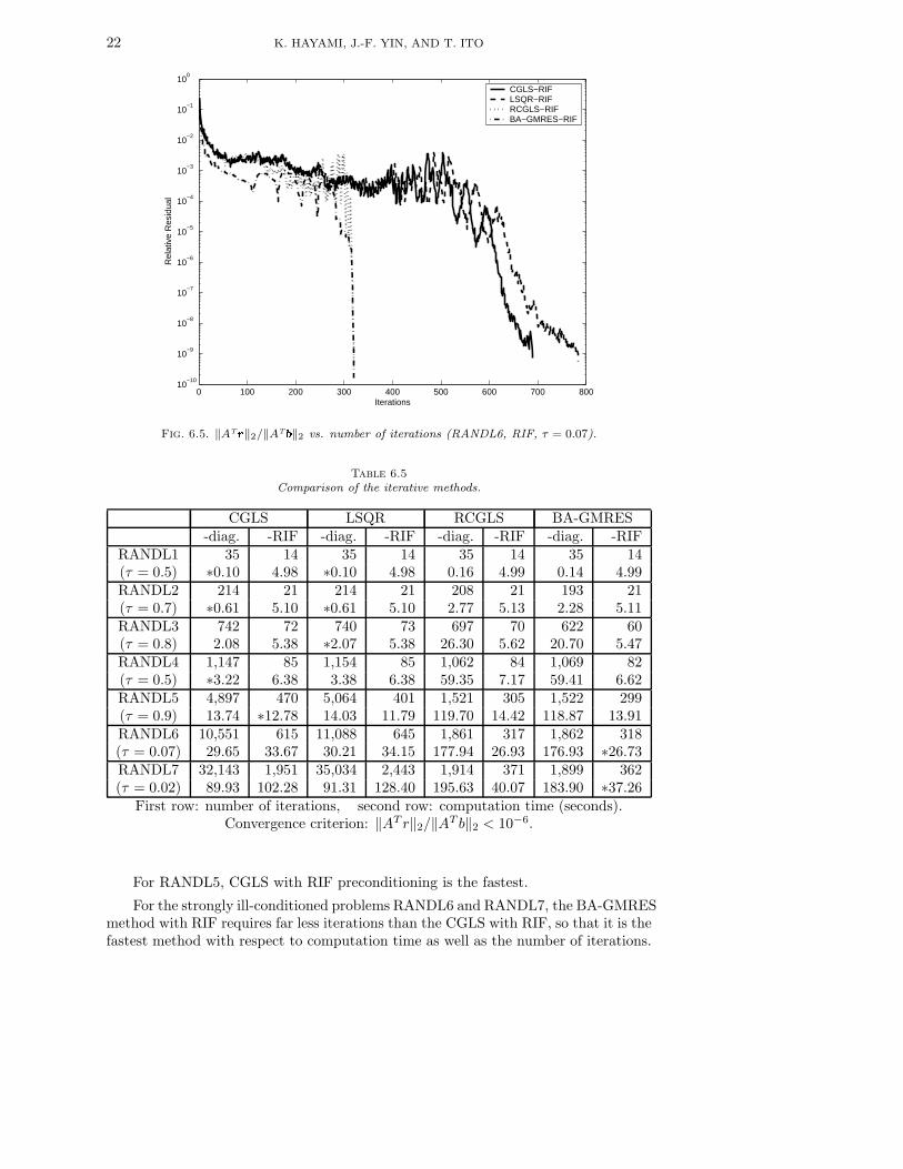
than this “direct method”.Figures 6.2, 6.3, 6.4 and 6.5 show ‖ATr‖2/‖ATb‖2 vs. the number of iterations for

the CGLS, LSQR, reorthogonalized CGLS and BA-GMRES methods, with diagonalscaling and RIF preconditioners, for the problems RANDL5 and RANDL6. τ for RIFwas set to the optimal value 0.8 and 0.07, respectively.

0 1000 2000 3000 4000 5000 600010

−10

10−9

10−8

10−7

10−6

10−5

10−4

10−3

10−2

10−1

100

Iterations

Rel

ativ

e R

esid

ual

CGLS−Diag.LSQR−Diag.RCGLS−Diag.BA−GMRES−Diag.

Fig. 6.2. ‖AT�‖2/‖AT

�‖2 vs. number of iterations (RANDL5, diagonal scaling).

The figures show that the CGLS and LSQR methods are slow to converge com-pared to the BA-GMRES and reorthogonalized CGLS methods for these ill-conditionedproblems. This can be explained by the fact that the CGLS and LSQR methods relyon three-term recurrence and suffer from loss of orthogonality due to rounding errorsespecially for ill-conditioned problems, whereas the BA-GMRES and reorthogonalizedCGLS methods are more robust against loss of orthogonality because they performexplicit orthogonalization by the modified Gram-Schmidt procedure and reorthogo-nalization, respectively.

The BA-GMRES and the reorthogonalized CGLS show similar convergence be-haviours. This is in accordance with the convergence analysis in Section 4.1, where weobtained similar upper bounds for the BA-GMRES and the similarly preconditionedCGLS in the absence of rounding errors.

The RIF preconditioning significantly improves convergence over the diagonalscaling.

The BA-GMRES converges more smoothly compared to the reorthogonalizedCGLS.

In Table 6.5, we compare the methods for the problems in Table 6.1. The first rowin each cell gives the number of iterations required for convergence, and the secondrow gives the total computation time in seconds. The value of the optimal relativedrop tolerance parameter τ for the RIF preconditioning is also indicated for eachproblem.


0 100 200 300 400 500 60010

−10

10−9

10−8

10−7

10−6

10−5

10−4

10−3

10−2

10−1

100

Iterations

Rel

ativ

e R

esid

ual

CGLS−RIFLSQR−RIFRCGLS−RIFBA−GMRES−RIF

Fig. 6.3. ‖AT�‖2/‖AT�‖2 vs. number of iterations (RANDL5, RIF, τ = 0.8).

0 1000 2000 3000 4000 5000 6000 7000 8000 9000 1000010

−10

10−9

10−8

10−7

10−6

10−5

10−4

10−3

10−2

10−1

100

Iterations

Rel

ativ

e R

esid

ual

CGLS−Diag.LSQR−Diag.RCGLS−Diag.BA−GMRES−Diag.

Fig. 6.4. ‖AT�‖2/‖AT

�‖2 vs. number of iterations (RANDL6, diagonal scaling).

For the problems RANDL1 to RANDL4, the CGLS or LSQR method with diag-onal scaling were the fastest.

As the condition number increases, the number of iterations for CGLS (and itsstabilized version, LSQR) increases much more rapidly than the correspondingly pre-conditioned BA-GMRES method.


0 100 200 300 400 500 600 700 80010

−10

10−9

10−8

10−7

10−6

10−5

10−4

10−3

10−2

10−1

100

Iterations

Rel

ativ

e R

esid

ual

CGLS−RIFLSQR−RIFRCGLS−RIFBA−GMRES−RIF

Fig. 6.5. ‖AT�‖2/‖AT�‖2 vs. number of iterations (RANDL6, RIF, τ = 0.07).

Table 6.5

Comparison of the iterative methods.

CGLS LSQR RCGLS BA-GMRES-diag. -RIF -diag. -RIF -diag. -RIF -diag. -RIF

RANDL1 35 14 35 14 35 14 35 14(τ = 0.5) ∗0.10 4.98 ∗0.10 4.98 0.16 4.99 0.14 4.99RANDL2 214 21 214 21 208 21 193 21(τ = 0.7) ∗0.61 5.10 ∗0.61 5.10 2.77 5.13 2.28 5.11RANDL3 742 72 740 73 697 70 622 60(τ = 0.8) 2.08 5.38 ∗2.07 5.38 26.30 5.62 20.70 5.47RANDL4 1,147 85 1,154 85 1,062 84 1,069 82(τ = 0.5) ∗3.22 6.38 3.38 6.38 59.35 7.17 59.41 6.62RANDL5 4,897 470 5,064 401 1,521 305 1,522 299(τ = 0.9) 13.74 ∗12.78 14.03 11.79 119.70 14.42 118.87 13.91RANDL6 10,551 615 11,088 645 1,861 317 1,862 318(τ = 0.07) 29.65 33.67 30.21 34.15 177.94 26.93 176.93 ∗26.73RANDL7 32,143 1,951 35,034 2,443 1,914 371 1,899 362(τ = 0.02) 89.93 102.28 91.31 128.40 195.63 40.07 183.90 ∗37.26

First row: number of iterations, second row: computation time (seconds).Convergence criterion: ‖AT r‖2/‖AT b‖2 < 10−6.

For RANDL5, CGLS with RIF preconditioning is the fastest.

For the strongly ill-conditioned problems RANDL6 and RANDL7, the BA-GMRESmethod with RIF requires far less iterations than the CGLS with RIF, so that it is thefastest method with respect to computation time as well as the number of iterations.


6.2. Under-determined problems. Next, we show numerical experiment re-sults for the under-determined least squares problem

minx∈Rn

‖b − Ax‖2, A ∈ Rm×n (m < n).

Here, we compare the AB-GMRES (BA-GMRES) methods with B = ATC whereC is obtained by diagonal scaling or RIF, with the corresponding preconditionedCGNE, LSQR and reorthogonalized CGNE (RCGNE) methods.

The coefficient matrices A were obtained by transposing the matrices RANDLnin Table 6.1 for the over-determined problems, and are denoted by RANDLnT. Thedensity and condition number of RANDLnT is the same as that of the correspondingmatrix RANDLn.

Since rankA = m < n, the systems are consistent. Hence, the right-hand sidevector b was given by b = Ax∗ where x∗ = (1, . . . , 1)T, and the initial approximatesolution was set to x0 = 0. Hence, the convergence of the methods were judged by‖r‖2/‖b‖2 where r = b − Ax.

Note that for the AB-GMRES method, ‖r‖2 is available at each iteration withoutextra computational cost.

Figure 6.6 shows ‖r‖2/‖b‖2 vs. the number of iterations for the full AB-GMRESand BA-GMRES methods with diagonal scaling and RIF preconditioning, for theproblem RANDL3T. τ for RIF was set to the optimal value 0.8. In the figure, the AB-GMRES and BA-GMRES methods show similar convergence behaviours, as predictedin Section 4.2.

0 100 200 300 400 500 600 700 800 900 100010

−14

10−12

10−10

10−8

10−6

10−4

10−2

100

102

Iterations

Rel

ativ

e R

esid

ual

AB−GMRES−Diag.BA−GMRES−Diag.AB−GMRES−RIFBA−GMRES−RIF

Fig. 6.6. Comparison of GMRES-AB method and GMRES-BA method (RANDL3T, τ = 0.8for RIF).

In the experiments below, we compare the AB-GMRES method with the CGNE,LSQR and reorthogonalized CGNE methods. The reason why the AB-GMRES methodis used instead of the BA-GMRES method is because the former gives the minimum


norm solution, and requires less computation per iteration when m < n. (See section3.3.) The full AB-GMRES method without restart was used. Similar to the over-determined systems, we chose the optimal τ for the RIF preconditioner for all theproblems.

Note that, although the CGNE guarantees to give the minimum norm leastsquares solution, the LSQR does not. However, it was observed that the approximatesolutions converge to the same solution for both methods in the following numericalexperiments.

Figures 6.7, 6.8, 6.9 and 6.10 show the relative residual ‖r‖2/‖b‖2 vs. the numberof iterations for the different methods for the problems RANDL5T and RANDL6T. τfor RIF was set to the optimal value 0.9 and 0.01, respectively. The figures show thatthe AB-GMRES method converges faster than the corresponding CGNE and LSQRmethods, for diagonal scaling and RIF.

0 1000 2000 3000 4000 5000 6000 700010

−12

10−10

10−8

10−6

10−4

10−2

100

102

104

Iterations

Rel

ativ

e R

esid

ual

CGNE−Diag.LSQR−Diag.RCGNE−Diag.AB−GMRES−Diag.

Fig. 6.7. ‖�‖2/‖�‖2 vs. number of iterations (RANDL5T, diagonal scaling).

Table 6.6 compares the methods for under-determined systems RANDLnT. Thefirst row in each box gives the number of iterations required for convergence, andthe second row gives the total computation time in seconds. It is observed thatthe AB-GMRES-RIF method is the fastest method for the ill-conditioned problemsRANDL6T and RANDL7T.

6.3. Required memory. One drawback of the GMRES based methods is thatthey require increasingly more memory with the number of iterations or the restart-ing cycle k, whereas the CG based methods (without reorthogonalization) requireconstant memory. This is because the GMRES based methods require storing theorthonormal vectors v1, . . . , vk in the modified Gram-Schmidt process, as well as theHessenberg matrix.

Table 6.7 shows the memory required other than the coefficient matrix A and thepreconditioner for each method. r, p, x, u, v, w, e and y are the intermediate vectors,


0 100 200 300 400 500 600 70010

−12

10−10

10−8

10−6

10−4

10−2

100

102

104

Iterations

Rel

ativ

e R

esid

ual

CGNE−RIFLSQR−RIFRCGNE−RIFAB−GMRES−RIF

Fig. 6.8. ‖�‖2/‖�‖2 vs. number of iterations (RANDL5T, RIF, τ = 0.9).

0 2000 4000 6000 8000 10000 12000 14000 1600010

−12

10−10

10−8

10−6

10−4

10−2

100

102

104

Iterations

Rel

ativ

e R

esid

ual

CGNE−Diag.LSQR−Diag.RCGNE−Diag.AB−GMRES−Diag.

Fig. 6.9. ‖�‖2/‖�‖2 vs. number of iterations (RANDL6T, diagonal scaling).

and V denotes the k orthonormal vectors in the modified Gram-Schmidt process. Forthe LSQR method, we used the notation of variables according to [14].

If one can keep the number of iterations k of the GMRES type methods sufficientlysmall compared to m or n with the use of an efficient preconditioner like RIF, theymay be faster compared to the CG type methods, and the memory required may not


0 100 200 300 400 500 600 70010

−12

10−10

10−8

10−6

10−4

10−2

100

102

104

Iterations

Rel

ativ

e R

esid

ual

CGNE−RIFLSQR−RIFRCGNE−RIFAB−GMRES−RIF

Fig. 6.10. ‖�‖2/‖�‖2 vs. number of iterations (RANDL6T, RIF, τ = 0.01).

Table 6.6

Comparison of the iterative methods.

CGNE LSQR RCGNE AB-GMRES-diag. -RIF -diag. -RIF -diag. -RIF -diag. -RIF

RANDL1T 37 12 37 12 37 12 37 12(τ = 0.4) ∗0.15 5.01 ∗0.15 5.02 0.23 5.02 0.17 5.01

RANDL2T 259 25 256 25 252 25 247 25(τ = 0.7) ∗1.06 5.16 ∗1.06 5.16 4.22 5.17 3.75 5.17

RANDL3T 838 81 823 80 783 77 754 75(τ = 0.8) ∗3.43 5.53 ∗3.43 5.53 33.87 5.81 30.56 5.67

RANDL4T 1,464 116 1,407 114 1,223 106 1,187 106(τ = 0.5) 5.97 6.94 ∗5.96 6.94 79.67 7.45 73.67 7.21

RANDL5T 5,548 544 5,414 539 1,535 322 1,533 322(τ = 0.9) 22.61 13.88 22.71 ∗13.86 123.80 15.58 121.58 15.11

RANDL6T 12,837 514 12,486 502 1,873 219 1,871 218(τ = 0.01) 52.38 39.04 50.10 38.99 182.51 27.43 179.85 ∗26.99RANDL7T 38,397 3,078 37,792 2,979 2,240 451 2,238 450(τ = 0.04) 156.01 94.19 152.07 91.69 366.88 44.49 353.92 ∗43.76

First row: number of iterations, second row: computation time (seconds).Convergence criterion: ‖r‖2/‖b‖2 < 10−6.

be prohibitive.

7. Conclusions. We proposed two methods for applying the GMRES methodto linear least squares problems with m × n coefficient matrix A, using an n × mmatrix B. The first method is to apply GMRES to min

z∈Rm‖b − ABz‖2 (AB-GMRES


Table 6.7

Intermediate memory required for each method for k iterations.

dim(m) dim(n) dim(k) totalCGLS r, Ap x, p, ATr 2m + 3nCGNE r, Ap x, p, ATr 2m + 3nLSQR u v, w, x m + 3n

AB-GMRES(k) V, w x y, e (k + 1)m + n + 2k + k2/2BA-GMRES(k) V, w, x y, e (k + 2)n + 2k + k2/2

method), and the second method is to apply GMRES to minx∈Rn

‖Bb − BAx‖2 (BA-

GMRES method).Then, we derived a sufficient condition for B, such that the methods give a least

squares solution for arbitrary b and x0 without breakdown.Next, we showed that, theoretically, one may expect similar convergence be-

haviours for the AB- and BA- GMRES methods as well as the corresponding CGLStype methods.

Further, we proposed using the robust incomplete factorization (RIF) method forB in the GMRES methods.

Numerical experiments on over-determined problems with full column rank showedthat the BA-GMRES method with the RIF preconditioner was faster than the RIFpreconditioned CGLS, LSQR and reorthogonalized CGLS methods, for ill-conditionedproblems.

For under-determined problems with full row rank, the AB-GMRES method withRIF preconditioning was faster than the RIF preconditioned CGNE, LSQR and re-orthogonalized CGNE methods, for ill-conditioned problems.

Acknowledgments. We would like to thank Professors Shao-Liang Zhang, Ko-kichi Sugihara, Yimin Wei, Yohsuke Hosoda, Kunio Tanabe, Takashi Tsuchiya, MichaelEiermann, Masaaki Sugihara, Zhong-Zhi Bai, Michele Benzi, Lothar Reichel, GeneGolub, Michael Saunders and Yang-Feng Su for valuable remarks and discussions.

This research was supported by the Grants-in-Aid for Scientific Research (C)No. 17560056 of the Ministry of Education, Culture, Sports, Science and Technology,Japan.

REFERENCES

[1] Z. -Z. Bai, I. S. Duff, and A. J. Wathen, A class of incomplete orthogonal factorizationmethods. I: Methods and theories, BIT, 41 (2001), pp. 53–70.

[2] M. Benzi and M. Tuma, A robust incomplete factorization preconditioner for positive definitematrices, Numer. Linear Algebra Appl., 10 (2003), pp. 385–400.

[3] M. Benzi and M. Tuma, A robust preconditioner with low memory requirements for largesparse least squares problems, SIAM J. Sci. Comput., 25 (2003), pp. 499–512.

[4] A. Bjorck, Numerical Methods for Least Squares Problems, SIAM, Philadelphia, 1996.[5] A. Bjorck, T. Elfving, and Z. Strakos, Stability of conjugate gradient and Lanczos methods

for linear least squares problems, SIAM J. Matrix Anal. Appl., 19 (1998), pp. 720–736.[6] P. N. Brown and H. F. Walker, GMRES on (nearly) singular systems, SIAM J. Matrix

Anal. Appl., 18 (1997), pp. 37–51.[7] D. Calvetti, B. Lewis, and L. Reichel, GMRES-type methods for inconsistent systems,

Linear Algebra Appl., 316 (2000), pp. 157–169.[8] K. Hayami and T. Ito, Application of the GMRES method to singular systems and least

squares problems, in Proceedings of the Seventh China-Japan Seminar on Numerical Math-


ematics and Scientific Computing, Z. -C. Shi and H. Okamoto, eds., Zhangjiajie, 2004,Science Press, Beijing, 2006, pp. 31–44.

[9] K. Hayami and T. Ito, Solution of least squares problems using GMRES methods, Proc. Inst.Statist. Math., 53 (2005), pp. 331–348 (in Japanese).

[10] M. R. Hestenes and E. Stiefel, Methods of conjugate gradients for solving linear systems,J. Res. Nat. Bur. Standards, B49 (1952), pp. 409–436.

[11] T. Ito and K. Hayami, Preconditioned GMRES methods for least squares problems, NII Tech-nical Report, NII-2004-006E, National Institute of Informatics, Tokyo, Japan, May, 2004,pp. 1–29.

[12] A. Jennings and M. A. Ajiz, Incomplete methods for solving ATAx = b, SIAM J. Sci. Statist.Comput., 5 (1984), pp. 978–987.

[13] J. A. Meijerink and H. van der Vorst, An iterative method for linear systems of which thecoefficient matrix is a symmetric M-matrix, Math. Comp., 31 (1977), pp. 148–162.

[14] C. C. Paige and M. A. Saunders, A robust incomplete factorization preconditioner for positivedefinite matrices, ACM Trans. Math. Software, 8 (1982), pp. 43–71.

[15] A. Papadopoulos, I. S. Duff, and A. J. Wathen, A class of incomplete orthogonal factor-ization methods II: implementation and results, BIT, 45 (2005), pp. 159–179.

[16] L. Reichel and Q. Ye, Breakdown-free GMRES for singular systems, SIAM J. Matrix Anal.Appl., 26 (2005), pp. 1001–1021.

[17] Y. Saad, Preconditioning techniques for nonsymmetric and indefinite linear systems, J. Com-put. Appl. Math., 24 (1988), pp. 89–105.

[18] Y. Saad, Iterative Methods for Sparse Linear Systems, Second ed., SIAM, Philadelphia, 2003.[19] Y. Saad and M. H. Schultz, GMRES: A generalized minimal residual method for solving

nonsymmetric linear systems, SIAM J. Sci. Statist. Comput., 7 (1986), pp. 856–869.[20] K. Tanabe, Characterization of linear stationary iterative processes for solving a singular

system of linear equations, Numer. Math., 22 (1974), pp. 349–359.[21] K. Vuik, A. G. J. Sevink, and G. C. Herman, A preconditioned Krylov subspace method for

the solution of least squares problems in inverse scattering, J. Comput. Phys., 123 (1996),pp. 330–340.

[22] X. Wang, K. A. Gallivan, and R. Bramley, CIMGS: An incomplete orthogonal factorizationpreconditioner, SIAM J. Sci. Comput., 18 (1997), pp. 516–536.

[23] S. -L. Zhang and Y. Oyanagi, Orthomin(k) method for linear least squares problem, J. Inf.Process., 14 (1991), pp. 121–125.

NII Technical ReportISSN 1346-5597 NII Technical Report GMRES Methods for Least Squares Problems Ken...

Documents

Transcript of NII Technical ReportISSN 1346-5597 NII Technical Report GMRES Methods for Least Squares Problems Ken...