SWAP RATE VARIANCE SWAPS

NICOLAS MERENER

Business School, Universidad Torcuato Di Tella1010 Saenz Valiente, Buenos Aires, (1428), Argentina.

nmerener@utdt.edu

August 11, 2008

Abstract (first posting at SSRN, June 30th, 2008)

We study the hedging and valuation of variance swaps defined on a swap interest rate. Our mo-tivation is the recognition of the fundamental role of variance swaps in the transfer of variancerisk, and the extensive empirical evidence documenting that the variance realized by interestrates is stochastic. Working in a diffusion setting, we identify a replication rule as the differ-ence between a static European contract and the gains of a dynamic position on interest rateswaps. Two distinguishing features arise in the context of interest rates: the nonlinear andmultidimensional relationship between the values of the dynamically traded contracts and theunderlying rate, and the possible stochasticity of the interest rate used for reinvesting dynamicgains. The combination of these two features leads to additional terms in the cumulative dy-namic trading gains, terms which depend on realized variance and are taken into considerationin the determination of the appropriate static hedge. We characterize the static payoff functionas the solution of an ordinary differential equation, and derive explicitly the associated dynamicstrategy. We use daily interest rate data between 1997 and 2007 to test the effectiveness ofour hedging methodology and verify that the replication error is small compared to the bid-askspread in swaption prices.

1 Introduction

An extensive empirical literature has documented that the variance realized by interest rates

is stochastic. Stochastic volatility as in Andersen and Lund (1997) and Ball and Tourous

(2000), random jumps as in Johannes (2004), switching regimes as in Gray (1996), are just a

few examples of the statistical regularities observed in the behavior of interest rates that lead

to stochastic realized variance. An investor that recognizes uncertainty about future realized

variance as a risk factor distinct from the risk associated to the level of rates might want to

modify his exposure with respect to variance risk. This is possible by trading in a simple

contract that depends exclusively on variance risk: the variance swap. In this contract, two

parties agree at t = 0 to exchange a dollar amount proportional to the variance realized by a

reference interest rate between 0 and T , against a fixed sum set at inception. The valuation

problem associated to a variance swap is the computation of the fixed payment that makes the

contract worthless at inception.

In the absence of other liquidly traded instruments that could be used as hedges, the valua-

tion of a variance swap must take into account subjective probabilities for outcomes in realized

variance as well as preferences toward variance risk. However, it was shown independently by

Neuberger (1992) and Dupire (1993) that the variance realized by a traded asset following a

diffusion can be replicated as the difference between a static European contract on the asset

and the cumulative gains that arise from a dynamic position in the same asset. Moreover, by

Breeden and Litzenberger (1978) and Carr and Madan (1998) (see also Demeterfi et al., 1999),

the payoff of the static contract can be replicated by a sufficiently rich portfolio of call and put

European options. Strikingly, the replicating portfolio is derived under very mild assumptions

about the volatility process of the traded asset. Therefore, the arbitrage-free price of realized

variance is determined by the price of market observable European call and put options.

In reality, the existence of a rich set of liquidly traded options creates an alternative motiva-

tion for trading variance swaps. Future variance can be understood as a fundamental quantity

simultaneously driving the prices of options and variance swaps, therefore a variance swap can

1

be used to set a speculative position by an investor who believes that option prices are far from

his own subjective valuation. A variance swap provides the investor with a tool to speculate

on future variance, relative to the variance implied in observable option prices, without taking

any risk related to the direction of changes in the underlying.

Following the successful development of variance swaps defined on individual stocks and on

equity indices, the literature has moved toward increasingly sophisticated computational ap-

proaches and more complex payoff structures. Little and Pant (2001) studied finite difference

methods for variance swaps with discrete sampling in a local volatility model. Carr and Lewis

(2004) explored the valuation and hedging of corridor variance swaps. The universe of con-

tract payoffs has been expanded to include volatility swaps and volatility derivatives. Howison,

Rafailidis and Rasmussen (2004) priced volatility derivatives in a partial differential equation

framework with emphasis on an asymptotic analysis for fast mean reverting volatility. Java-

heri, Wilmott and Haug (2004) studied volatility swaps in a GARCH setting and derived an

approximate solution for the convexity correction between variance and volatility. Carr et al.

(2005) priced options on realized variance under a pure jump process. Windcliff et al. (2006)

focused on the hedging of discretely sampled volatility derivatives and the effects of jumps and

hedging frequency. Carr and Lee (2008a) developed a robust and nonparametric replication

methodology for volatility derivatives under an independence assumption between the under-

lying and its volatility. Broadie and Jain (2008) studied the pricing and risk management of

volatility derivatives under Heston stochastic volatility model. The variance swap has also been

used by Carr and Wu (2008) as a tool to extract market information about variance risk premia

from observed option prices. Finally, in work done mutually independently from this paper,

Carr and Lee (2008b) studied the hedging of variance options and obtained a replication result

for the weighted variance of a general function of a positive, continuous semimartingale price

process. As in our paper, they characterize the static hedging payoff as a solution of an ordinary

differential equation.

In this paper we investigate variance swaps in the context of interest rates, previously

unexplored in the literature. We focus on the explicit valuation and hedging of variance swaps

2

defined on the volatility of interest rates derived from the Libor curve. This is the yield curve

used in the dominant over-the-counter interest rate derivatives market. Brigo and Mercurio

(2006) thoroughly cover commonly traded interest rate derivatives and related pricing models.

As in earlier work in variance swaps, we identify a replication strategy formulated in terms

of a static European contract and a dynamic trading rule. We design a dynamic strategy

that is consistent with current market practice by using the most flexible and liquidly traded

at-the-money forward interest rate swaps and Libor deposits.

Two issues distinguish the hedging and valuation problem in the context of interest rates:

First, the relationship between the underlying over which variance is computed (forward swap

rate), and the values of available traded instruments (swaps, bonds, Libor deposits) is nonlinear

and multidimensional. A forward swap rate is not a traded security. Second, the contract

depends on the variance of interest rates. Therefore, assuming deterministic interest rates for

reinvesting dynamically accrued gains, as is standard in the literature on variance swaps, is

suspect. Instead, we choose to reinvest gains using Libor deposits at the prevailing (possibly

stochastic) interest rate. We combine these two features under the assumption of a sufficiently

flat forward curve, which allows us to transform the high dimensional hedging problem into

a one dimensional computation, depending only on the dynamics of the swap rate over which

variance is recorded. We obtain a closed form representation for the cumulative gains of a

dynamic trading strategy including novel terms that depend on realized variance. This requires

the identification of an appropriate static payoff function and associated dynamic strategy for

the difference between them to be precisely the variance we intend to replicate. We characterize

the static payoff function as the solution of an ordinary differential equation, compute its

solution numerically, and derive from it a dynamic trading strategy. We perform this exercise

for the replication of the variance of increments in the underlying swap rate as well as for the

variance of returns. In absence of arbitrage, the initial value of the fixed leg of the variance swap

must coincide with the initial value of the replicating portfolio that delivers realized variance.

This includes an initially costless dynamic position, therefore the valuation of the variance

swap is strictly equivalent to the valuation of the European static payoff. The effectiveness of

3

the hedging strategy is tested empirically by comparing historically realized variance with the

performance of the hedging portfolio, using historical interest rate data with daily frequency

between 1997 and 2007. This, implicitly, is also a test of appropriateness of the diffusive

dynamics adopted in this paper. We find that the hedging methodology has small errors

relative to the bid-ask spread of traded swaptions.

The paper is structured as follows. Section 2 describes the features of the variance swap

contract. Section 3 reviews the valuation of a variance swap contract defined over a traded asset

under reinvestment with zero rates. Section 4 presents the forward rate model, its connection

with swap rates, and an approximation that allows us to reduce the high dimensionality of the

yield curve to a single underlying. In Section 5 we present the main theoretical result of the

paper: an explicit hedging strategy based on a characterization of the static European contract

and a dynamic position in swaps. Section 6 contains empirical tests of the hedging methodology.

Our conclusions are in Section 7.

2 The variance swap contract

A variance swap is a derivative security defined on an underlying financial variable S. We model

the underlying dynamics with a continuous time stochastic process St, with time measured in

years. The variance swap is a contract between two parties who agree to exchange, at time T ,

the difference between the empirical variance realized by St on [0, T ], and a fixed amount Tβ2

agreed upon at t = 0. We assume that there are 252 trading days per year. For an integer

N > 0 we consider two types of contracts: an arithmetic variance swap contract, with payoff

at T = N/252

VT =N∑

i=1

(S i252− S i−1

252)2 − T (βn)2, (1)

and a geometric variance contract, with payoff at T

VT =N∑

i=1

(S i

252− S i−1

252

S i−1252

)2 − T (βl)2. (2)

4

For example, S could be a traded asset, as in Section 3 in this paper, or an interest rate, as

in Section 5.

In our analytical work we rely on continuous time processes to derive hedging formulas for

continuously sampled variance. This implies an approximation, which is standard in much of

the variance swap literature, as the variance delivered by real contracts is recorded by squaring

increments over discrete time ((1) and (2)). However, in the empirical tests in Section 6 we

take the dynamic rule derived for continuous execution and implement it in discrete time, with

the same sampling frequency at which increments for variance are recorded.

3 Valuation in the case of a traded underlying

In order to illustrate the essence of the valuation methodology we review first the case in

which the variance swap is defined over a traded asset and gains accumulated dynamically

are reinvested at zero interest rate (the case of nonzero, deterministic interest rates can be

solved essentially along the same lines). We consider the arithmetic variance case, because of

its importance in the interest rate market, and the geometric variance case, previously covered

by Dupire (1993), Carr and Madan (1998), and Demeterfi et al.(1999). We assume a filtered

probability space (Ω, F, Ft, P ) under the usual hypotheses. The traded asset, under the physical

measure P , follows

dSt = µtdt + γnt dWt,

for µt, γt adapted to the filtration Ft and Wt a P -Brownian motion. We assume that µt, γnt are

such that 0 < St. Applying Ito’s lemma on (St − S0)2 leads to

d(St − S0)2 = 2(St − S0)dSt + (γnt )2dt.

Integrating we get

(ST − S0)2 − 2∫ T

0(St − S0)dSt =

∫ T

0(γn

t )2dt. (3)

5

The continuous time arithmetic variance of S realized between 0 and T ,∫ T0 (γn

t )2dt, is

represented in (3) as the terminal gain of a portfolio composed by two pieces: a static position

on a quadratic contract with final payoff (ST − S0)2, and the gains of a dynamic position in

S, with notional −2(St − S0). Remarkably, (3) has been derived under very mild assumptions

about the volatility process γnt which, in particular, could be stochastic.

The initial value of future realized variance must be equal to the initial value of the repli-

cating portfolio. In order to preclude arbitrage, we assume the existence of a risk neutral

probability measure Q that makes discounted assets martingales. Because St is an asset price

and we have assumed zero interest rates, it follows that St itself must be a martingale. There-

fore, by Girsanov’s theorem we have

dSt = γnt dWQ

t , (4)

with WQt a Brownian motion under the risk neutral measure Q. The initial value of the dynamic

component of the replication strategy is

−2EQ[∫ T

0StdSt|F0] = 0, (5)

by virtue of the martingale condition in (4). The static term in the hedging portfolio is a

quadratic European payoff and can be priced explicitly by a replicating portfolio composed of

European call and put options, as shown in Carr and Madan (1998). Therefore, the arbitrage-

free value of future realized variance is determined by the price of liquidly traded European

options. For simplicity, in this paper we will focus on the decomposition of realized swap rate

variance up to a European payoff and a dynamic traded position, and will not be concerned

with the decomposition of the European payoff into calls and puts.

A similar argument to that outlined above can be followed to identify a hedging portfolio

that replicates realized geometric variance. In this case we postulate that the asset dynamics

under the physical measure is

6

dSt = Stµtdt + StγltdWt,

with µt and γt adapted to the filtration Ft, apply Ito’s lemma on ln(St/S0) and integrate

between 0 and T to get

ln(ST /S0) =∫ T

0

1St

dSt − 12

∫ T

0

1S2

t

S2t (γl

t)2dt.

Therefore

−2 ln(ST /S0) + 2∫ T

0

1St

dSt =∫ T

0(γl

t)2dt. (6)

The realized geometric variance to be delivered at T is replicated in (6) in terms of a static

logarithmic contract and a dynamic position on the asset to be rebalanced between 0 and T .

A common feature of the two examples shown in this section is that the variance of interest

is replicated through the gains of a suitable static payoff minus the gains accrued by a dynamic

position in the underlying. We will see that this structure is preserved in the replication of swap

rate variance, although for a more complicated static payoff function and dynamic trading rule.

4 Forward curve model

Swap rates are the most widely quoted interest rates for derivative transactions between high

credit quality banks. Swap rate levels and their implied volatilities are readily extracted from

very liquidly traded instruments. This is the motivation for defining contracts on the variance

of a forward swap rate, as investigated in this paper. However, unlike in the examples explored

in the previous section, swap rates are not traded assets. The most liquidly traded contracts

defined on long dated Libor curve rates are swaps. And the value of a swap depends not only

on the underlying swap rate, but on the yield curve up to the maturity of the swap.

As we intend to hedge variance contracts by trading in interest rate swaps, we must begin by

specifying a general model of forward rates for a consistent description of swap rate dynamics

and swap valuation.

7

Following Heath, Jarrow, and Morton (1994) we consider a family of instantaneous, con-

tinuously compounded forward rates ft(u) for 0 ≤ t ≤ u, u ≤ T ∗. The value of a zero coupon

bond expiring at T ≤ T ∗, for t ≤ T , is denoted by Bt(T ). Bond prices and forward rates are

related through:

Bt(T ) ≡ e−∫ T

t ft(u)du. (7)

Investing 1 dollar at t in a Libor deposit that expires at T is equivalent to buying 1/Bt(T )

units of the zero coupon bond expiring at T and holding it until expiration.

Swap rates and related derivatives are associated to a discrete tenor structure—a finite set

of dates with arbitrary start T0, 0 ≤ T0 < T1 < · · · < TM < T ∗, with Ti+1 − Ti ≡ δ. The fixed

accrual period δ is expressed as a fraction of a year; for instance, δ = 1/2 represents six months.

Discrete forward Libor rates L(T0), . . . , L(TM−1) associated to the tenor structure are de-

fined from bond prices (7) as in Musiela and Rutkowski (1997) by setting

Lt(Tk) =1δ

(Bt(Tk)

Bt(Tk+1)− 1

)=

1δ

(e∫ Tk+1

Tkft(u)du − 1

), t ∈ [0, Tk], k = 0, . . . ,M − 1. (8)

Forward swaps are widely traded derivatives. A payer’s swap holder makes fixed payments

δK and receives floating payments δLTi(Ti) at Ti+1, i = 0, . . . , M − 1. The swap value at the

beginning of the setting of the first floating payment is

VT0(T0, TM ) = δM−1∑

j=0

BT0(Tj+1)(ST0(T0, TM )−K),

where the swap rate S(T0, TM ) at t is

St(T0, TM ) ≡M−1∑

j=0

bt(j)Lt(Tj) with bt(j) ≡ Bt(Tj+1)∑M−1i=0 Bt(Ti+1)

. (9)

The forward swap price at t < T0 is computed under the pricing measure P 0,M that uses

Dt(T0, TM ) = δM−1∑

j=0

Bt(Tj+1), (10)

8

as numeraire, see Brigo and Mercurio (2006) for a detailed treatment. In this case we get

Vt(T0, TM ) = δM−1∑

j=0

Bt(Tj+1) EP 0,M[(ST0(T0, TM )−K)|Ft]. (11)

Furthermore, from the representation

St(T0, TM ) =Bt(T0)−Bt(TM )

δ∑M−1

j=0 Bt(Tj+1), (12)

and the form of the numeraire in (10), it is evident that St(T0, TM ) is a discounted asset price,

therefore a martingale under P 0,M . Therefore (11) becomes

Vt(T0, TM ) = δ

M−1∑

j=0

Bt(Tj+1) (St(T0, TM )−K) = Dt(T0, TM )(St(T0, TM )− k). (13)

4.1 Flat forward curve approximation

As presented so far, the shape and level of the forward curve is unconstrained. In this section

we introduce a set of assumptions about the forward curve that facilitate the development of

an analytical treatment of the variance swap.

Assumption 4.1 For t ≤ T0 ≤ u ≤ TM , there exists ε << 1 such that

(i) 0 < ft(u) < ε,

(ii) maxu∈[T0,TM ] ft(u)−minu∈[T0,TM ] ft(u) < ε2.

Assumption 4.1 imposes interest rates much lower than 100 % per annum and a relatively

flat forward curve. It is important to notice that Assumption (4.1) is static, and is postulated

to hold at all times. We are not concerned here with the identification of the class of dynamic

models for which the evolution of the yield curve satisfies Assumption (4.1).

From Assumption 4.1 and (8) it follows that for fixed t and j = 0, ..., M − 1,

9

1δ(eδ minu∈[T0,TM ] ft(u) − 1) ≤ Lt(j) ≤ 1

δ(eδ maxu∈[T0,TM ] ft(u) − 1). (14)

Since δ < 1, and 0 < minu∈[T0,TM ] ft(u) ≤ maxu∈[T0,TM ] ft(u) < ε, it follows from an exact

truncated Taylor expansion that

eδ minu∈[T0,TM ] ft(u) = 1 + δ minu∈[T0,TM ]

ft(u) + 1/2K1(δ minu∈[T0,TM ]

ft(u))2,

and

eδ maxu∈[T0,TM ] ft(u) = 1 + δ maxu∈[T0,TM ]

ft(u) + 1/2K2(δ maxu∈[T0,TM ]

ft(u))2,

with unknown constants K1,K2 ∈ [0, 1]. Therefore

minu∈[T0,TM ]

ft(u) ≤ Lt(j) ≤ maxu∈[T0,TM ]

ft(u) + 1/2δ( maxu∈[T0,TM ]

ft(u))2. (15)

The forward swap rate St(T0, TM ) can be interpreted through (9) as a weighted average of

forward Libor rates, Lt(T0), ..., Lt(TM−1). Moreover, because bond prices are positive, weights

defined as

Bt(Tj+1)∑M−1i=0 Bt(Ti+1)

, j = 0, ...,M − 1,

are also positive and add up to one. It then follows immediately from (15) that

minu∈[T0,TM ]

ft(u) ≤ St(T0, TM ) ≤ maxu∈[T0,TM ]

ft(u) + 1/2δ( maxu∈[T0,TM ]

ft(u))2. (16)

4.2 Bond ratio approximation

Fixing δ = 0.5 at its standard value in the interest rate derivatives market, we use bound (16)

to state an approximate relationship between the forward swap rate St(T0, TM ) and the ratio

of bond prices Bt(TM )Bt(T0) .

10

PROPOSITION 4.1 If Assumption 4.1 holds, then the yield implied by a ratio of bonds,

yt(T0, TM ) ≡ − 1(TM − T0)

ln(Bt(TM )Bt(T0)

)

satisfies

|yt(T0, TM )− St(T0, TM )| ≤ 5/4ε2.

Proof:

| −1(TM − T0)

ln(Bt(TM )Bt(T0)

)− St(T0, TM )| = | 1(TM − T0)

∫ TM

T0

ft(u)du− St(T0, TM )|.

Invoking (16) we write

| 1(TM−T0)

∫ TM

T0ft(u)du− St(T0, TM )| ≤

max|maxu∈[T0,TM ] ft(u)−minu∈[T0,TM ] ft(u)|,

|minu∈[T0,TM ] ft(u)− (maxu∈[T0,TM ] ft(u) + 1/2δ(maxu∈[T0,TM ] ft(u))2)| ≤ 5/4ε2,

where the last inequality follows from Assumption 4.1.

It is in the sense of Proposition (4.1) that we write

Bt(TM )Bt(T0)

≈ e−(TM−T0)St(T0,TM ). (17)

5 Hedging and valuation

5.1 Preliminaries

In this section we derive a replicating portfolio that delivers swap rate realized variance at

terminal time T0. As in Section 3, the essence of the method consists on replicating realized

variance as the difference between a suitable static payoff and the gains that arise from a

dynamic position. We depart from Section 3 in the fact that the underlying swap rate is not

11

directly tradeable, and by reinvesting dynamic gains at the, possibly stochastic, rate implied

by Bt(T0).

We consider a variance swap defined on the variance realized between 0 and T0 by the swap

rate corresponding to an interest rate swap defined on a discrete tenor structure as in Section 4,

beginning at T0 and ending at TM < T ∗. The starting and ending dates T0 and TM , associated

with the swap rate, are fixed for all t ≤ T0. We write St for St(T0, TM ). Market participants

are typically interested in realized variance for relatively short term horizons, defined on swap

rates of commonly quoted length. For example, to fix ideas, we might take T0 = 0.5 (6 months)

and L = 10 (10 years).

We assume a filtered probability space (Ω, F, Ft, P ) under the usual hypotheses, and postu-

late that the forward swap rate St, under the physical measure P , follows

dSt = µtdt + γnt dWt, (18)

where Wt is a P−Brownian motion. The processes µt and γnt are progressively measurable with

respect to Ft. We assume square integrability of the volatility process:

E[∫ T ∗

0(γn

t )2dt] < ∞. (19)

We also assume that µt and γnt are such that St > 0 for t ≤ T ∗. We define the geometric

instantaneous volatility as

γlt ≡

γnt

St. (20)

By Proposition B.1.2 in Musiela and Rutkowski (1997), St is a square integrable semimartingale.

5.2 Dynamic swap gains

Since our hedging strategy involves trading in forward interest rate swaps, we begin by relating

the gains of a dynamic strategy in swaps to the evolution of the underlying swap rate. Denote

V τt for the value at t ≤ T0 of a forward interest rate swap starting at T0 and ending at TM with

12

strike Sτ set at τ ≤ t. In the expression for the swap value (13) the annuity factor (10) can be

written as a ratio of bond prices and the swap rate using (12)

V τt =

Bt(T0)−Bt(TM )St

(St − Sτ ). (21)

By definition, V ττ = 0.

Our valuation algorithm relies on a replication argument at expiration T0 involving a dy-

namic strategy executed between 0 and T0, in which local swap gains are reinvested through

Libor deposits up to T0. The dynamic strategy is the limit, as the time between portfolio

rebalancings tends to zero, of the discrete trading rule described next.

Let h : < → < be deterministic and smooth. We write ht for h(St). For i = 0, ..., n − 1

consider a portfolio holding, between t = iT0/n and t = (i+1)T0/n, hiT0/n units of the forward

swap defined on the swap rate St with strike SiT0/n. Gains are collected at (i + 1)T0/n and

reinvested in a Libor deposit of maturity T0. Let G(h, n) be the value at T0 of gains accumulated

by following this trading strategy for i = 0, ..., n− 1. We have

G(h, n) ≡n−1∑

i=0

hi

T0n

(Vi

T0n

(i+1)T0n

− Vi

T0n

iT0n

)/B(i+1)

T0n

(T0), (22)

therefore recalling that Vi

T0n

iT0n

= 0, and using (21), we get

G(h, n) ≡n−1∑

i=0

hi

T0n

1−B(i+1)

T0n

(TM )/B(i+1)

T0n

(T0)

S(i+1)

T0n

(S(i+1)

T0n

− Si

T0n

) (23)

Under Assumption 4.1, the ratios of bond prices in (23) can be replaced by (17) to define

the approximate dynamic gain G(h, n)

G(h, n) ≡n−1∑

i=0

hi

T0n

1− e−S

(i+1)T0n

(TM−T0)

S(i+1)

T0n

(S(i+1)

T0n

− Si

T0n

). (24)

The following proposition provides a representation of the value of G(h, n) as the interval

between consecutive portfolio updates tends to zero (n →∞).

13

PROPOSITION 5.1 As n →∞, G(h, n) converges in probability to

∫ T0

0ht

1− e−St(TM−T0)

StdS +

∫ T0

0ht−1 + (1 + St(TM − T0))e−St(TM−T0)

S2t

γ2ndt

We write G(h) ≡ limn→∞ G(h, n).

Proof:

Lighten the notation by introducing εi ≡ (S(i+1)

T0n

−Si

T0n

) for the increment in the underlying

process. We write (24) as

G(h, n) =n−1∑

i=0

hi

T0n

1− e(−(S

iT0n

+εi))(TM−T0)

Si

T0n

+ εiεi.

Because h has been assumed smooth, the coefficient multiplying εi is also smooth in Si

T0n

and εi. A Taylor expansion for small ε leads to

G(h, n) =n−1∑

i=0

hi

T0n

1− e−S

iT0n

(TM−T0)

Si

T0n

εi

+n−1∑

i=0

hi

T0n

−1 + (1 + Si

T0n

(TM − T0))e−S

iT0n

(TM−T0)

S2

iT0n

ε2i

+n−1∑

i=0

hi

T0n

R(εi)

where R(εi) is the exact remainder of the Taylor expansion containing terms of order 3 and

higher in εi. Next, take the limit n → ∞. By Theorem 2.21 in Medvegyev (2007), the sum of

terms linear in εi is convergent in probability to

∫ T0

0ht

1− e−St(TM−T0)

StdS,

because the integrand is adapted and regular. The sum of terms of order 2 in εi converges in

probability to

∫ T0

0ht−1 + (1 + St(TM − T0))e−St(TM−T0)

S2t

γ2ndt

14

by finite quadratic variation of St. And the sum for higher order terms tends to zero in

probability as higher order variations vanish. (Problem 5.11 in chapter 1 of Karatzas and

Shreve (1991)).

We have characterized the gains that arise from dynamically trading in swaps with notional

h(St), for deterministic h, and continuous reinvestment through Libor deposits. Our next step

is to use Proposition 5.1 to identify an appropriate static payoff hedge to isolate realized swap

rate variance.

5.3 The static hedge and its differential equation

Let f : < → < be a twice differentiable function, to be interpreted as the payoff of a European

contract when acting on ST0 . We write ft for f(St), t ≤ T0. Applying Ito’s rule on ft and

integrating on [0, T0] we have

fT0 − f0 −∫ T0

0f ′tdSt =

∫ T0

0

12f ′′t (γn

t )2dt. (25)

In order to express the integral with respect to St in (25) as the accumulated gain of a

dynamically traded strategy in swaps and Libor deposits plus some additional variance related

terms, we take

f ′t = ht1− e−St(TM−T0)

St,

which implies

ht =f ′tSt

1− e−St(TM−T0),

and invoke Proposition 5.1 to obtain

fT0 − f0 − G(f ′tSt

1− e−St(TM−T0)) =

∫ T0

0(12f ′′t −

f ′tSt

1− e−St(TM−T0)

−1 + (1 + St(TM − T0))e−St(TM−T0)

S2t

)(γnt )2dt, (26)

which simplifies to

15

fT0 − f0 − G(f ′tSt

1− e−St(TM−T0)) =

∫ T0

0(12f ′′t + f ′t(

1St− (TM − T0)e−(TM−T0)St

1− e−(TM−T0)St))(γn

t )2dt. (27)

Notional ht = f ′tSt

1−e−St(TM−T0) is more easily interpreted recalling (17) and (21) to recognize that

ht ≈ f ′tBt(T0)Dt

. The bond price in the numerator of the notional function arises from the fact

that gains are reinvested as a Libor deposit, and the denominator is a consequence of the fact

that the position involves swaps.

The integral on the right side of (27) is a (path dependent) weighted sum of realized variance.

Therefore, for a trading strategy that replicates arithmetic variance we must identify f such

that the weighting function is constant over time. Let L = TM −T0. We look for f = f(x) that

satisfies

12f ′′ + f ′(

1x− Le−xL

1− e−xL) = 1. (28)

And (20) implies that to replicate geometric variance we need to find f = f(x) that solves

12f ′′ + f ′(

1x− Le−xL

1− e−xL) =

1x2

. (29)

Notice that terms proportional to f are absent in (28) and (29). Therefore, each of these

equations can be transformed into a system of first order differential equations. For (28) we

define g ≡ f ′ and write

12g′ + g(

1x− Le−xL

1− e−xL) = 1,

f ′ = g. (30)

We solve the system (30) sequentially, computing first g and then using it as input in the

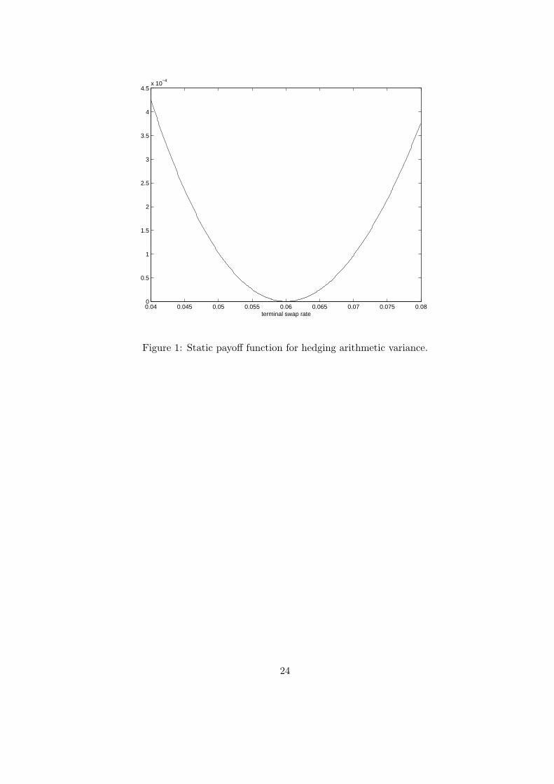
computation of f . Boundary conditions for (28) are chosen to be

f(S0) = f ′(S0) = 0.

16

With these boundary conditions, the solution to (28) agrees at x = S0, in level and slope,

with the payoff function used in Section 3 for the variance in the traded underlying case f(x) =

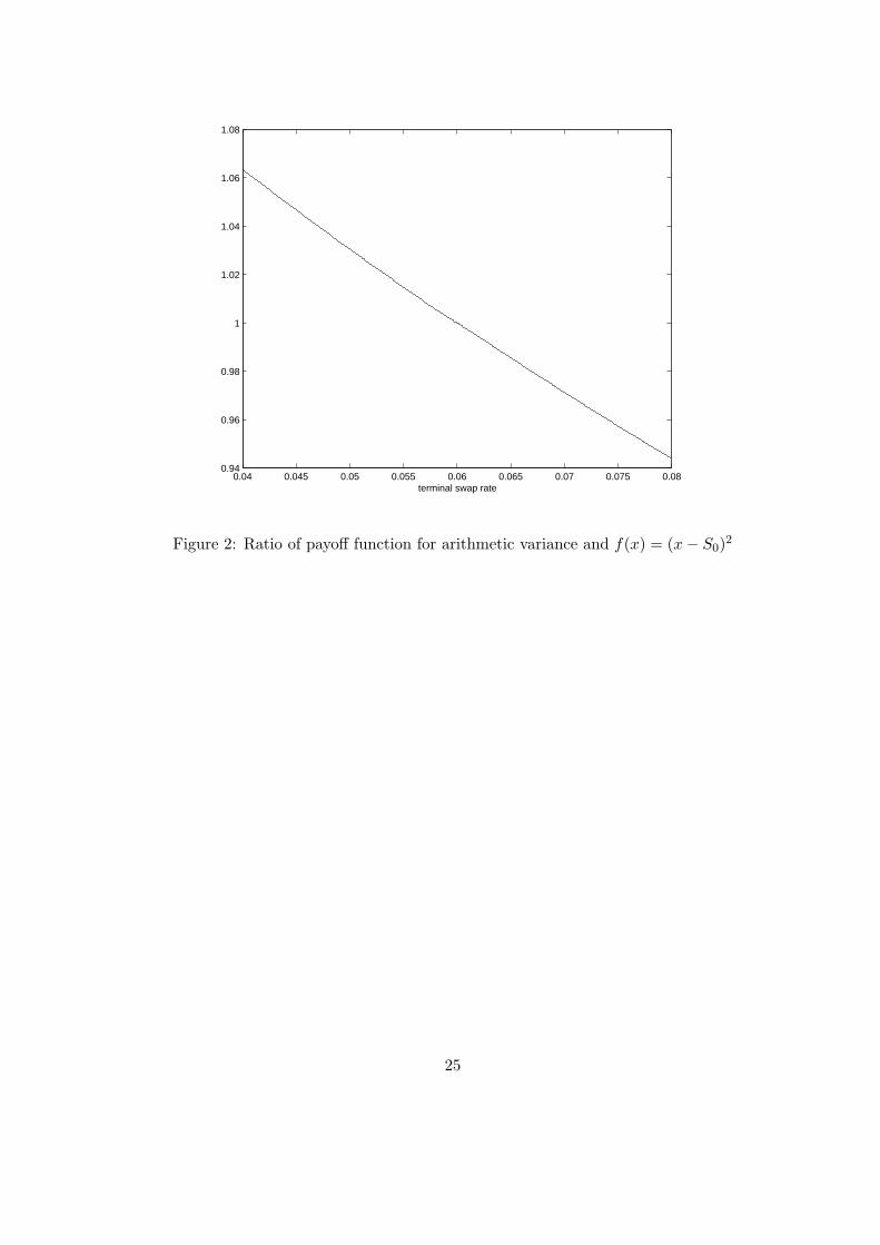
(x − S0)2. The solution to (28) is computed virtually instantly with a standard numerical

integrator and shown in Figure 1 for S0 = 0.06 and L = 10 (10 years). Figure 2 shows how this

solution differs from the traded asset case payoff function f(x) = (x− S0)2.

Figure 1, now at the end of the document, should be inserted here.

Figure 2, now at the end of the document, should be inserted here.

For (29) we define g ≡ f ′ and write

12g′ + g(

1x− Le−xL

1− e−xL) =

1x2

,

f ′ = g, (31)

that we solve numerically as in the arithmetic variance case, with the boundary conditions:

f(S0) = 0 and f ′(S0) = −2/S0.

In this case, the boundary conditions are chosen for our solution to match the level and

slope of the static payoff function of the replication of geometric variance in the traded asset

case, f(x) = −2ln(x/S0), at x = S0

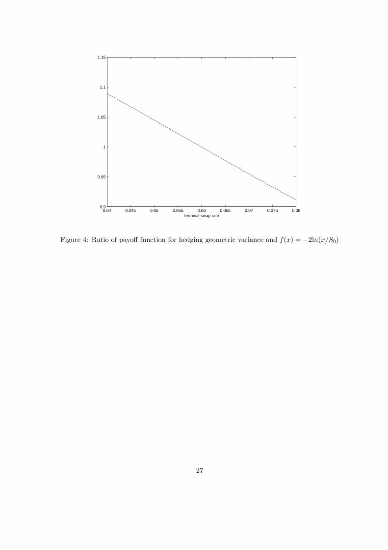
Figure 3 shows the numerical solution to (29) for L=10, and Figure 4 shows how this solution

differs from f(x) = −2ln(x/S0) for S0 = 0.06.

Figure 3, now at the end of the document, should be inserted here.

Figure 4, now at the end of the document, should be inserted here.

It is interesting to note that taking the limit L → 0 in (28) and (29) leads to

12f ′′ = 1, (32)

and

17

12f ′′ =

1x2

, (33)

respectively, which are the ordinary differential equations that are solved by the quadratic

and logarithmic functions that correspond to the traded asset cases of Section 3. This is a

consequence of the fact that the gain accumulated at T0 (24), for a traded swap of vanishing

length, TM −T0, is linear in the increments in the underlying swap rate, leading to a replication

problem mathematically equivalent to that in Section 3.

5.4 Implementation and valuation

In summary, the strategy that replicates arithmetic variance consists on holding a European

contract with static payoff fT that solves (30) and to execute, for the corresponding f ′, a

dynamic trading strategy holding ht = f ′tSt

1−e−St(TM−T0) at-the-money swaps and reinvesting in-

stantaneous dynamic gains via Libor deposits. The payoff function f and its derivative are

computed only at the beginning of the variance swap and stored as a table for later use.

The identity (27) is a valid hedging strategy under Assumption 4.1. The execution of the

strategy in reality involves investing in interest rate swaps and Libor deposits that are priced

in the market without any approximation. Therefore we also test using

f ′tBt(T0)Dt

instead off ′tSt

1− e−(TM−T0)St

as the notional of the position in swaps. Notice that both quantities can be computed directly

from the observable yield curve at t.

The initial value of the fixed leg of the variance swap is equal to the sum of the initial

values of European payoff and dynamic hedging rule. Because it only requires taking positions

in at-the-money swaps that are worthless at inception, the dynamic rule has zero initial value.

The initial value of the static payoff can be obtained by replication with call and put European

options of the same maturity as in Carr and Madan (1998).

Finally, the replication and valuation of geometric variance follows the same steps described

for arithmetic variance, but using the solution to (31) instead of (30).

18

6 Empirical testing

In this section we test the accuracy of the hedging strategy outlined in Section 5 using USD

interest rate data. We are also testing, implicitly, the appropriateness of the diffusive dynamics

adopted in (18) and the flat curve approximation (17) used in (24).

6.1 The data

We use daily interest rate data from December 1, 1997 to December 1, 2007, provided by

Lehman Brothers. For each day in the sample, the set of rates is composed of: 3 month Libor,

the first eight EuroDollar futures, and liquidly traded swap rates with tenors 2y, 3y, 5y, 10y,

15y, 20y and 30y. Rate levels are interpolated to construct a continuous instantaneous forward

rate curve. Zero coupon bond prices, annuity factors, and forward swap rates are priced exactly

from the continuous interest rate curve.

6.2 Testing strategy

We test the accuracy of the hedging strategy implied by (27) when f is the solution of (30) or

(31). We proceed in discrete time, using daily frequency for recording variance increments and

rebalancing the dynamic portfolio. For convenience, we adopt a change of notation to measure

time in days. In this case, for consecutive days i = 0, ...N, (27) motivates a definition of dollar

hedging error as the difference of hedge gains and realized variance

dollar error ≡ fN − f0 −N−1∑

i=0

f ′iBi(T0)Di

(V ii+1 − V i

i )−N−1∑

i=0

(Si+1 − Si)2. (34)

The payoff function f and its derivative are computed only once per variance swap and

stored as a table. Then, having observed the full historical realization of forward curves for days

i = 0, ..., N we compute, for each day, the bond price Bi(T0), annuity factor Di, the exact gain

of the swap initiated the previous day, and the change in the swap rate over consecutive days.

Then, the dollar hedging error in (34) can be computed exactly. Because market participants

are used to quote prices in terms of implied volatilities, we take (34) as motivation, but actually

compute and display errors in volatility terms.

19

We test the hedging of variance swaps of various lengths and underlying rates. The variance

swaps we consider cover non overlapping intervals for the recording of variance. Therefore, in 10

years of data we have 40 observations for variance swaps of length 3 months, and 10 observations

for length 1 year.

6.3 Results

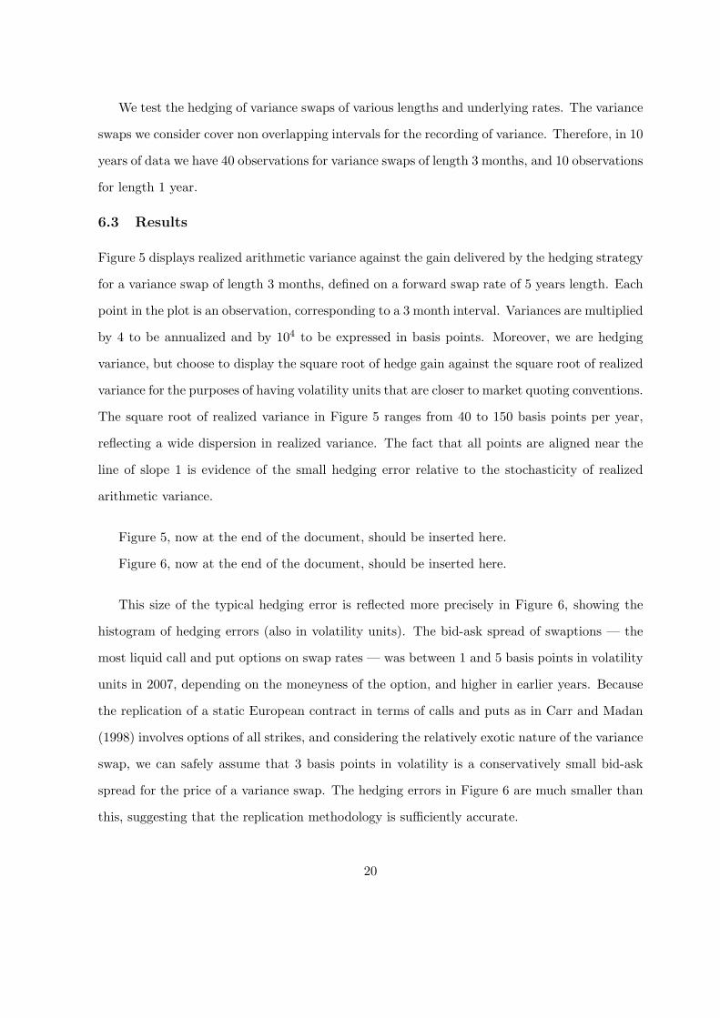
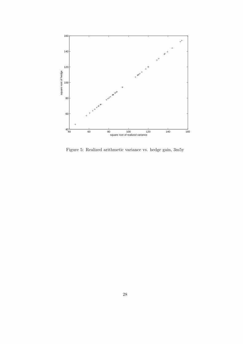
Figure 5 displays realized arithmetic variance against the gain delivered by the hedging strategy

for a variance swap of length 3 months, defined on a forward swap rate of 5 years length. Each

point in the plot is an observation, corresponding to a 3 month interval. Variances are multiplied

by 4 to be annualized and by 104 to be expressed in basis points. Moreover, we are hedging

variance, but choose to display the square root of hedge gain against the square root of realized

variance for the purposes of having volatility units that are closer to market quoting conventions.

The square root of realized variance in Figure 5 ranges from 40 to 150 basis points per year,

reflecting a wide dispersion in realized variance. The fact that all points are aligned near the

line of slope 1 is evidence of the small hedging error relative to the stochasticity of realized

arithmetic variance.

Figure 5, now at the end of the document, should be inserted here.

Figure 6, now at the end of the document, should be inserted here.

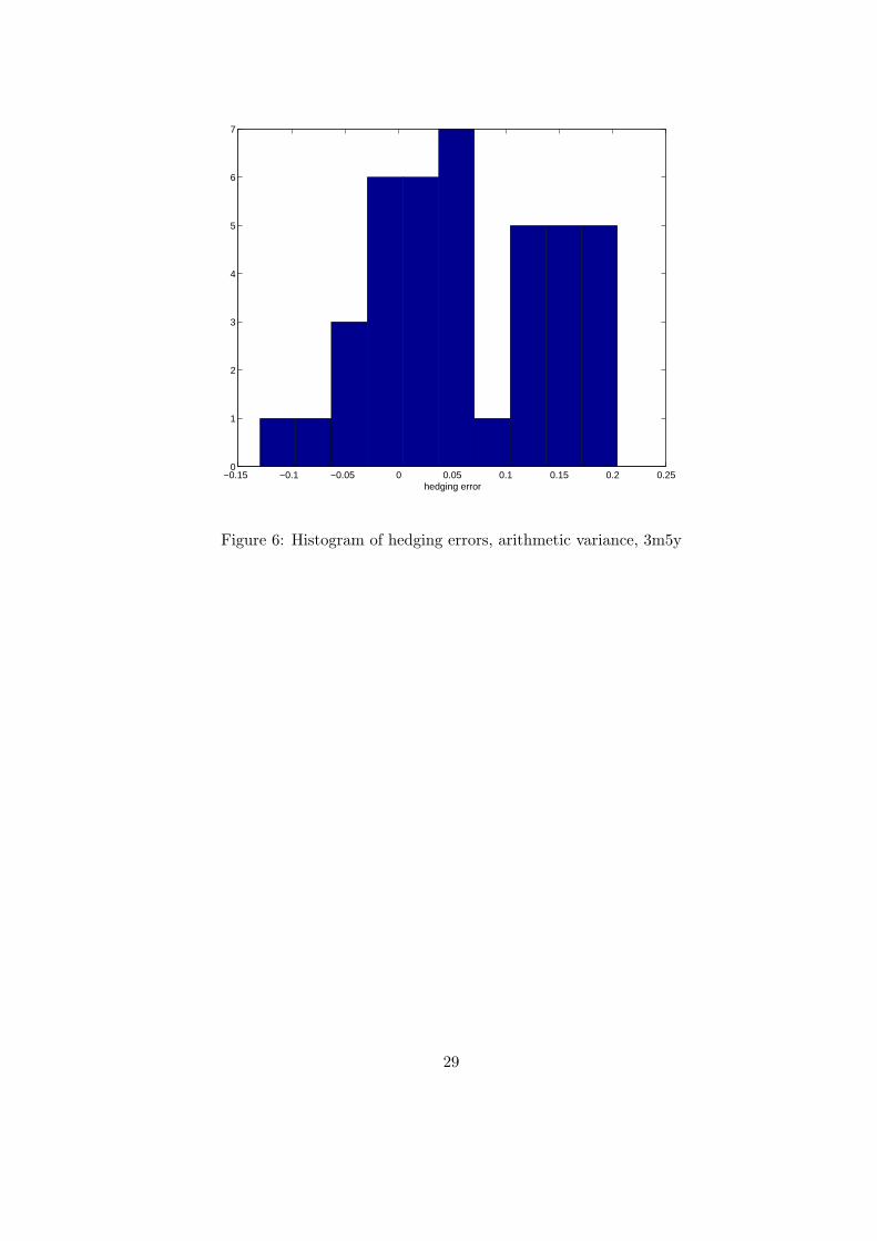
This size of the typical hedging error is reflected more precisely in Figure 6, showing the

histogram of hedging errors (also in volatility units). The bid-ask spread of swaptions — the

most liquid call and put options on swap rates — was between 1 and 5 basis points in volatility

units in 2007, depending on the moneyness of the option, and higher in earlier years. Because

the replication of a static European contract in terms of calls and puts as in Carr and Madan

(1998) involves options of all strikes, and considering the relatively exotic nature of the variance

swap, we can safely assume that 3 basis points in volatility is a conservatively small bid-ask

spread for the price of a variance swap. The hedging errors in Figure 6 are much smaller than

this, suggesting that the replication methodology is sufficiently accurate.

20

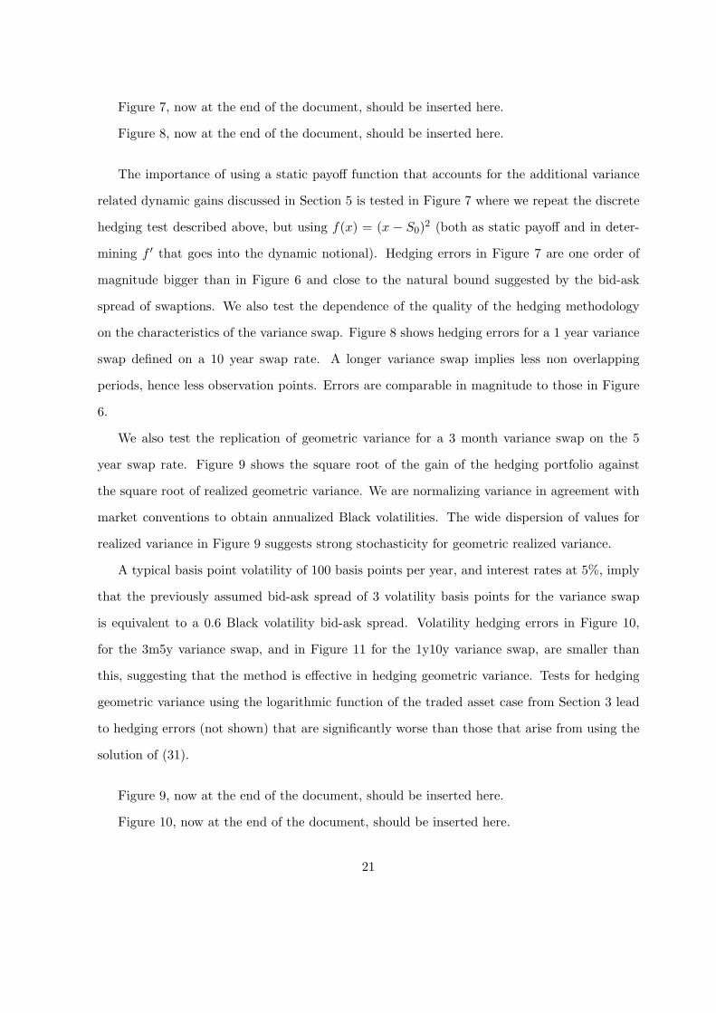
Figure 7, now at the end of the document, should be inserted here.

Figure 8, now at the end of the document, should be inserted here.

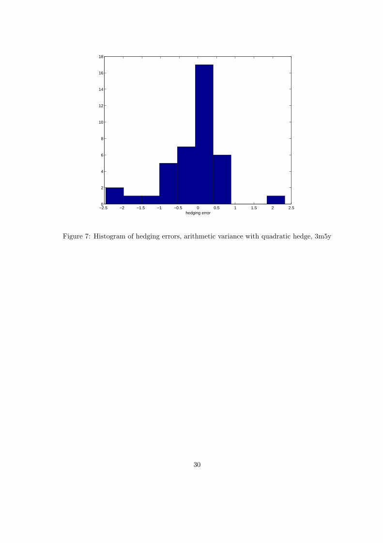
The importance of using a static payoff function that accounts for the additional variance

related dynamic gains discussed in Section 5 is tested in Figure 7 where we repeat the discrete

hedging test described above, but using f(x) = (x − S0)2 (both as static payoff and in deter-

mining f ′ that goes into the dynamic notional). Hedging errors in Figure 7 are one order of

magnitude bigger than in Figure 6 and close to the natural bound suggested by the bid-ask

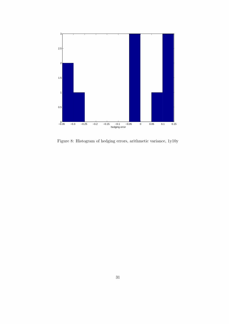
spread of swaptions. We also test the dependence of the quality of the hedging methodology

on the characteristics of the variance swap. Figure 8 shows hedging errors for a 1 year variance

swap defined on a 10 year swap rate. A longer variance swap implies less non overlapping

periods, hence less observation points. Errors are comparable in magnitude to those in Figure

6.

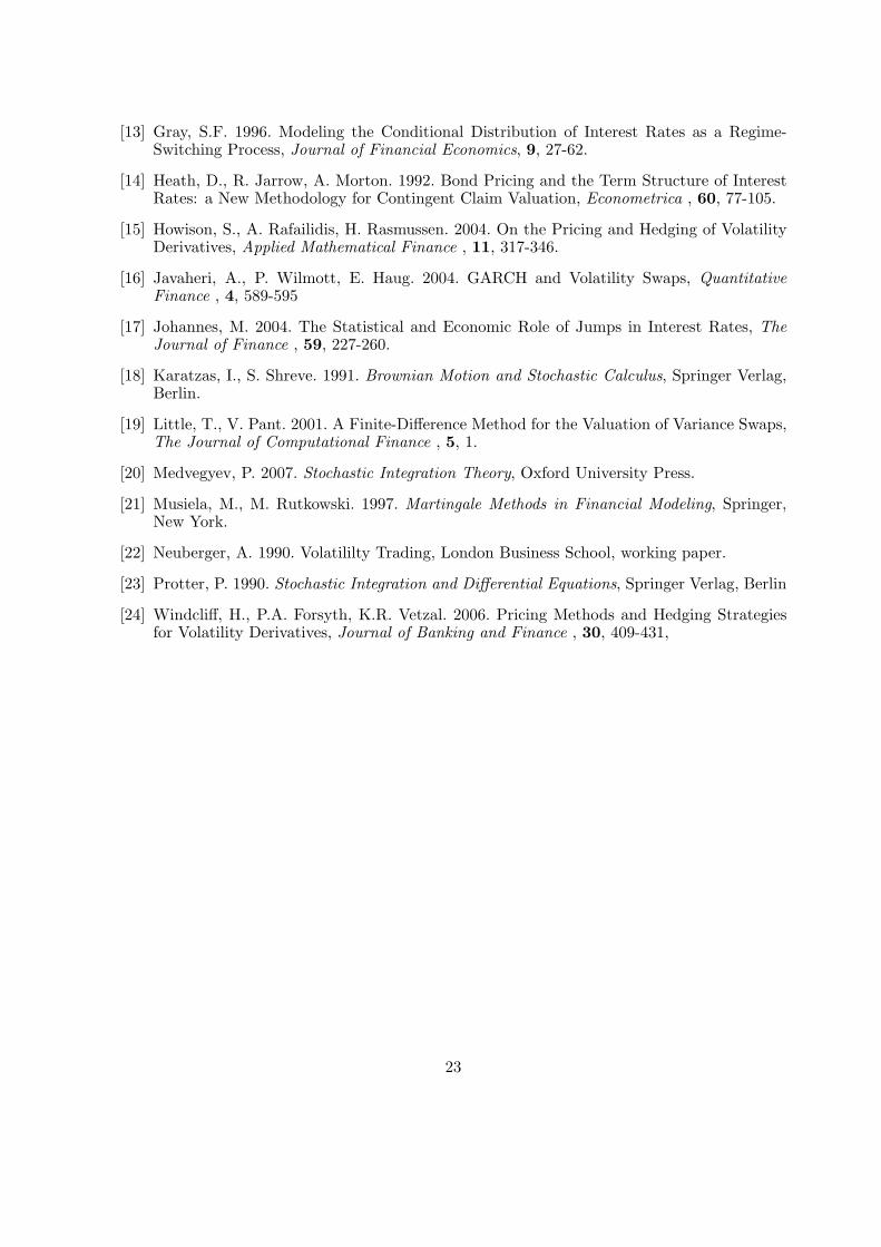
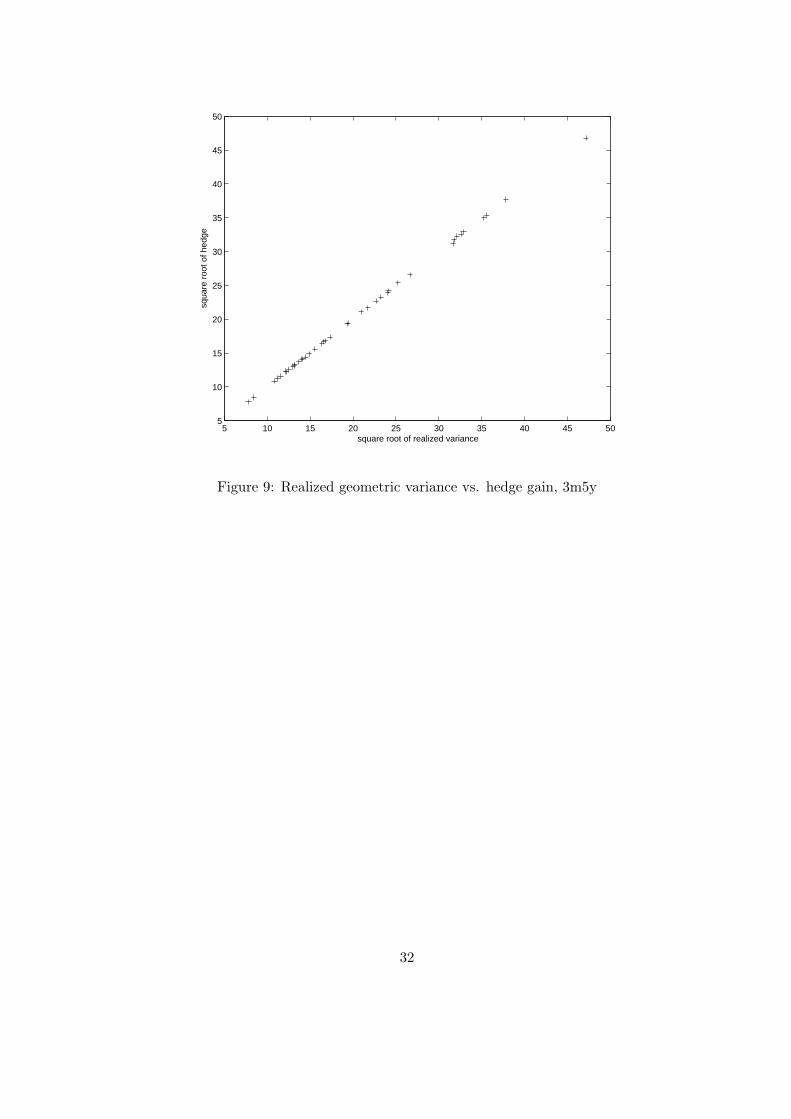
We also test the replication of geometric variance for a 3 month variance swap on the 5

year swap rate. Figure 9 shows the square root of the gain of the hedging portfolio against

the square root of realized geometric variance. We are normalizing variance in agreement with

market conventions to obtain annualized Black volatilities. The wide dispersion of values for

realized variance in Figure 9 suggests strong stochasticity for geometric realized variance.

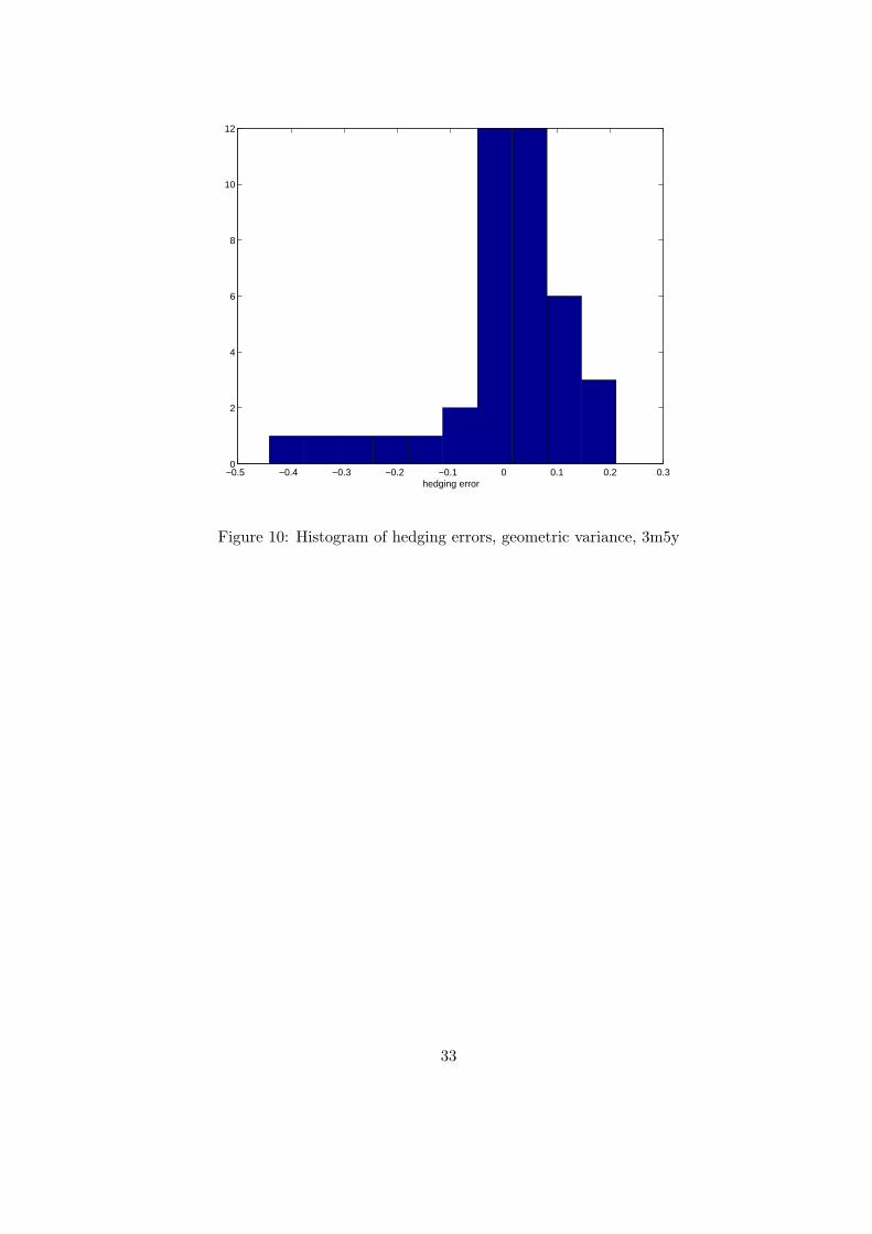
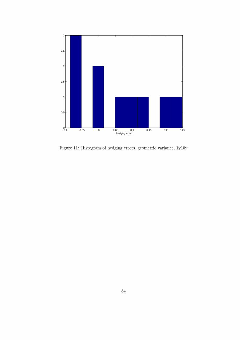
A typical basis point volatility of 100 basis points per year, and interest rates at 5%, imply

that the previously assumed bid-ask spread of 3 volatility basis points for the variance swap

is equivalent to a 0.6 Black volatility bid-ask spread. Volatility hedging errors in Figure 10,

for the 3m5y variance swap, and in Figure 11 for the 1y10y variance swap, are smaller than

this, suggesting that the method is effective in hedging geometric variance. Tests for hedging

geometric variance using the logarithmic function of the traded asset case from Section 3 lead

to hedging errors (not shown) that are significantly worse than those that arise from using the

solution of (31).

Figure 9, now at the end of the document, should be inserted here.

Figure 10, now at the end of the document, should be inserted here.

21

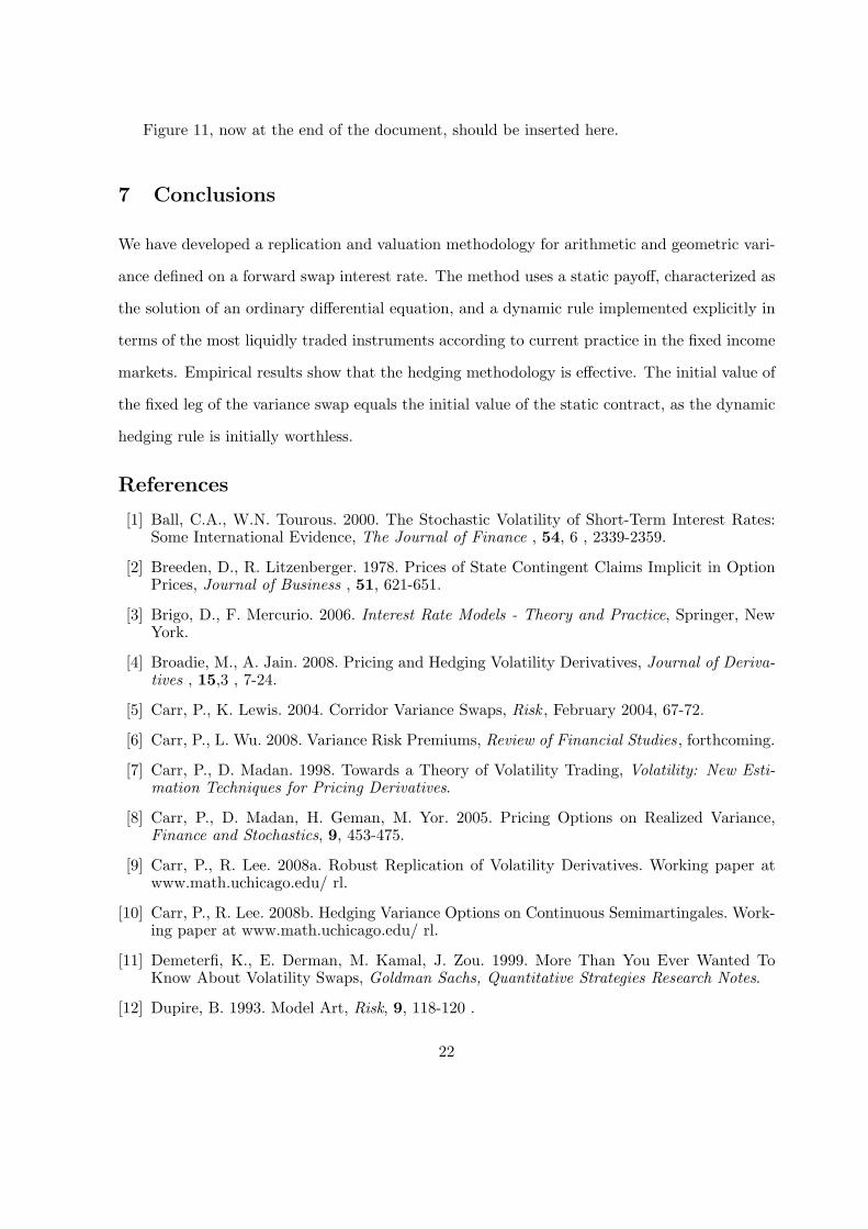
Figure 11, now at the end of the document, should be inserted here.

7 Conclusions

We have developed a replication and valuation methodology for arithmetic and geometric vari-

ance defined on a forward swap interest rate. The method uses a static payoff, characterized as

the solution of an ordinary differential equation, and a dynamic rule implemented explicitly in

terms of the most liquidly traded instruments according to current practice in the fixed income

markets. Empirical results show that the hedging methodology is effective. The initial value of

the fixed leg of the variance swap equals the initial value of the static contract, as the dynamic

hedging rule is initially worthless.

References

[1] Ball, C.A., W.N. Tourous. 2000. The Stochastic Volatility of Short-Term Interest Rates:Some International Evidence, The Journal of Finance , 54, 6 , 2339-2359.

[2] Breeden, D., R. Litzenberger. 1978. Prices of State Contingent Claims Implicit in OptionPrices, Journal of Business , 51, 621-651.

[3] Brigo, D., F. Mercurio. 2006. Interest Rate Models - Theory and Practice, Springer, NewYork.

[4] Broadie, M., A. Jain. 2008. Pricing and Hedging Volatility Derivatives, Journal of Deriva-tives , 15,3 , 7-24.

[5] Carr, P., K. Lewis. 2004. Corridor Variance Swaps, Risk , February 2004, 67-72.

[6] Carr, P., L. Wu. 2008. Variance Risk Premiums, Review of Financial Studies, forthcoming.

[7] Carr, P., D. Madan. 1998. Towards a Theory of Volatility Trading, Volatility: New Esti-mation Techniques for Pricing Derivatives.

[8] Carr, P., D. Madan, H. Geman, M. Yor. 2005. Pricing Options on Realized Variance,Finance and Stochastics, 9, 453-475.

[9] Carr, P., R. Lee. 2008a. Robust Replication of Volatility Derivatives. Working paper atwww.math.uchicago.edu/ rl.

[10] Carr, P., R. Lee. 2008b. Hedging Variance Options on Continuous Semimartingales. Work-ing paper at www.math.uchicago.edu/ rl.

[11] Demeterfi, K., E. Derman, M. Kamal, J. Zou. 1999. More Than You Ever Wanted ToKnow About Volatility Swaps, Goldman Sachs, Quantitative Strategies Research Notes.

[12] Dupire, B. 1993. Model Art, Risk, 9, 118-120 .

22

[13] Gray, S.F. 1996. Modeling the Conditional Distribution of Interest Rates as a Regime-Switching Process, Journal of Financial Economics, 9, 27-62.

[14] Heath, D., R. Jarrow, A. Morton. 1992. Bond Pricing and the Term Structure of InterestRates: a New Methodology for Contingent Claim Valuation, Econometrica , 60, 77-105.

[15] Howison, S., A. Rafailidis, H. Rasmussen. 2004. On the Pricing and Hedging of VolatilityDerivatives, Applied Mathematical Finance , 11, 317-346.

[16] Javaheri, A., P. Wilmott, E. Haug. 2004. GARCH and Volatility Swaps, QuantitativeFinance , 4, 589-595

[17] Johannes, M. 2004. The Statistical and Economic Role of Jumps in Interest Rates, TheJournal of Finance , 59, 227-260.

[18] Karatzas, I., S. Shreve. 1991. Brownian Motion and Stochastic Calculus, Springer Verlag,Berlin.

[19] Little, T., V. Pant. 2001. A Finite-Difference Method for the Valuation of Variance Swaps,The Journal of Computational Finance , 5, 1.

[20] Medvegyev, P. 2007. Stochastic Integration Theory, Oxford University Press.

[21] Musiela, M., M. Rutkowski. 1997. Martingale Methods in Financial Modeling, Springer,New York.

[22] Neuberger, A. 1990. Volatililty Trading, London Business School, working paper.

[23] Protter, P. 1990. Stochastic Integration and Differential Equations, Springer Verlag, Berlin

[24] Windcliff, H., P.A. Forsyth, K.R. Vetzal. 2006. Pricing Methods and Hedging Strategiesfor Volatility Derivatives, Journal of Banking and Finance , 30, 409-431,

23

0.04 0.045 0.05 0.055 0.06 0.065 0.07 0.075 0.080

0.5

1

1.5

2

2.5

3

3.5

4

4.5x 10

−4

terminal swap rate

Figure 1: Static payoff function for hedging arithmetic variance.

24

0.04 0.045 0.05 0.055 0.06 0.065 0.07 0.075 0.080.94

0.96

0.98

1

1.02

1.04

1.06

1.08

terminal swap rate

Figure 2: Ratio of payoff function for arithmetic variance and f(x) = (x− S0)2

25

0.04 0.045 0.05 0.055 0.06 0.065 0.07 0.075 0.08−0.6

−0.4

−0.2

0

0.2

0.4

0.6

0.8

1

terminal swap rate

Figure 3: Static payoff function for hedging geometric variance.

26

0.04 0.045 0.05 0.055 0.06 0.065 0.07 0.075 0.080.9

0.95

1

1.05

1.1

1.15

terminal swap rate

Figure 4: Ratio of payoff function for hedging geometric variance and f(x) = −2ln(x/S0)

27

40 60 80 100 120 140 16040

60

80

100

120

140

160

square root of realized variance

squa

re r

oot o

f hed

ge

Figure 5: Realized arithmetic variance vs. hedge gain, 3m5y

28

−0.15 −0.1 −0.05 0 0.05 0.1 0.15 0.2 0.250

1

2

3

4

5

6

7

hedging error

Figure 6: Histogram of hedging errors, arithmetic variance, 3m5y

29

−2.5 −2 −1.5 −1 −0.5 0 0.5 1 1.5 2 2.50

2

4

6

8

10

12

14

16

18

hedging error

Figure 7: Histogram of hedging errors, arithmetic variance with quadratic hedge, 3m5y

30

−0.35 −0.3 −0.25 −0.2 −0.15 −0.1 −0.05 0 0.05 0.1 0.150

0.5

1

1.5

2

2.5

3

hedging error

Figure 8: Histogram of hedging errors, arithmetic variance, 1y10y

31

5 10 15 20 25 30 35 40 45 505

10

15

20

25

30

35

40

45

50

square root of realized variance

squa

re r

oot o

f hed

ge

Figure 9: Realized geometric variance vs. hedge gain, 3m5y

32

−0.5 −0.4 −0.3 −0.2 −0.1 0 0.1 0.2 0.30

2

4

6

8

10

12

hedging error

Figure 10: Histogram of hedging errors, geometric variance, 3m5y

33

−0.1 −0.05 0 0.05 0.1 0.15 0.2 0.250

0.5

1

1.5

2

2.5

3

hedging error

Figure 11: Histogram of hedging errors, geometric variance, 1y10y

34