Nicola -Thesis -Latest2 - Texas A&M University · iv! iv!...
96
CORROSION DETECTION AND PREDICTION STUDIES A Thesis by SALLY SAMIR FARID NICOLA Submitted to the Office of Graduate Studies of Texas A&M University in partial fulfillment of the requirements for the degree of MASTER OF SCIENCE August 2012 Major Subject: Safety Engineering
Transcript of Nicola -Thesis -Latest2 - Texas A&M University · iv! iv!...

i
CORROSION DETECTION AND PREDICTION STUDIES
A Thesis
by
SALLY SAMIR FARID NICOLA
Submitted to the Office of Graduate Studies of Texas A&M University
in partial fulfillment of the requirements for the degree of
MASTER OF SCIENCE
August 2012
Major Subject: Safety Engineering

ii
Corrosion Detection and Prediction Studies
Copyright 2012 Sally Samir Farid Nicola

iii
CORROSION DETECTION AND PREDICTION STUDIES
A Thesis
by
SALLY SAMIR FARID NICOLA
Submitted to the Office of Graduate Studies of Texas A&M University
in partial fulfillment of the requirements for the degree of
MASTER OF SCIENCE
Approved by:
Chair of Committee, M. Sam Mannan Committee Members, James C. Holste Eric L. Petersen Head of Department, Charles Glover
August 2012
Major Subject: Safety Engineering

iii
iii
ABSTRACT
Corrosion Detection and Prediction Studies. (August 2012)
Sally Samir Farid Nicola, B.S., Texas A&M University at Qatar
Chair of Advisory Committee: Dr. M. Sam Mannan
Corrosion is the most important mechanical integrity issues the petrochemical
industry has to deal with. While significant research has been dedicated to studying
corrosion, it is still the leading cause of pipeline failure in the oil and gas industry.
Not only is it the main contributor to maintenance costs, but also it accounts for
about 15-‐20% of releases from the petrochemical industry and 80% of pipeline
leaks. Enormous costs are directed towards fixing corrosion in facilities across the
globe every year. Corrosion has caused some of the worst incidents in the history of
the industry and is still causing more incidents every year. This shows that the
problem is still not clearly understood, and that the methods that are being used to
control it are not sufficient.
A number of methods to detect corrosion exist; however, each one of them
has shortcomings that make them inapplicable in some conditions, or generally, not
accurate enough. This work focuses on studying a new method to detect corrosion
under insulation. This method needs to overcome at least some of the shortcomings
shown by the commercial methods currently used. The main method considered in
this project is X-‐ray computed tomography. The results from this work show that X-‐
ray computed tomography is a promising technique for corrosion under insulation
iv
iv
detection. Not only does it detect corrosion with high resolution, but it also does
not require the insulation to be removed. It also detects both internal and external
corrosion simultaneously.
The second part of this research is focused on studying the behavior of
erosion/corrosion through CFD. This would allow for determining the
erosion/corrosion rate and when it would take place before it starts happening.
Here, the operating conditions that led to erosion/corrosion (from the literature)
are used on FLUENT® to predict the flow hydrodynamic factors. The relationship
between these factors and the rate of erosion/corrosion is studied. The results from
this work show that along with the turbulence and wall shear stress, the dynamic
pressure imposed by the flow on the walls also has a great effect on the
erosion/corrosion rate.

v
v
DEDICATION
To my father, my mother, my brother, and my sisters

vi
vi
ACKNOWLEDGEMENTS
I would like to thank my committee chair, Dr. Mannan for the guidance,
encouragement, advice and inspiration, and my committee members, Dr. Holste,
and Dr. Petersen, as well as my mentor, Dr. Carreto, for their guidance and support
throughout the course of this research.
I would also like to thank my friends and colleagues and the department faculty and
staff for all their support and for making my experience truly memorable.
Last but certainly not least, I would like to thank my father, Samir Nicola, and my
mother, Magda Nicola for their unconditional love, encouragement, patience, and
advice, and for always believing in me and inspiring me. I would also like to thank
my siblings Dina, Rana and Mina for their continuous love, support and
companionship.
vii
vii
NOMENCLATURE
! Coefficient of thermal expansion
Cµ, C1, C1ε, C2, C2ε Constants for the k-‐epsilon model
ε Turbulence dissipation rate
gi Gravity
k Turbulent kinetic energy
µ Dynamic viscosity
p Node
ρ Density
!!" Prandtl number for energy
yp Distance from point p to the wall
u Axial velocity

viii
viii
TABLE OF CONTENTS
Page
ABSTRACT ......................................................................................................................................... iii
DEDICATION .................................................................................................................................... v
ACKNOWLEDGEMENTS .............................................................................................................. vi
NOMENCLATURE ........................................................................................................................... vii
TABLE OF CONTENTS .................................................................................................................. viii
LIST OF FIGURES ............................................................................................................................ xi
LIST OF TABLES .............................................................................................................................. xiii
1. INTRODUCTION ...................................................................................................................... 1
1.1 Introduction ............................................................................................................ 1 1.2 Corrosion Incidents ............................................................................................. 2 1.3 Objective ................................................................................................................... 5
2. TYPES OF CORROSION ......................................................................................................... 6
2.1 Introduction ............................................................................................................ 6 2.2 Generalized Corrosion ........................................................................................ 6 2.3 Pitting Corrosion ................................................................................................... 7
2.4 Galvanic Corrosion ............................................................................................... 7 2.5 Crevice Corrosion ................................................................................................. 9 2.6 Concentration Cell Corrosion .......................................................................... 9 2.7 Corrosion Under Insulation ............................................................................. 10 2.8 Erosion/Corrosion ............................................................................................... 11 2.9 Microbially-‐Induced Corrosion ...................................................................... 11
3. AVAILABLE METHODS OF INSPECTION ...................................................................... 13
3.1 Introduction ............................................................................................................ 13 3.2 Visual Inspection .................................................................................................. 14 3.3 Ultrasonic and Acoustic Inspection .............................................................. 16 3.4 Radiographic Inspection ................................................................................... 18 3.5 Electromagnetic Inspection ............................................................................. 19

ix
ix
4. CORROSION UNDER INSULATION AND METHODS OF DETECTING IT .......... 21
4.1 History ....................................................................................................................... 21 4.2 Problems with Methods of Inspection ........................................................ 23 4.3 Objective ................................................................................................................... 25
4.4 X-‐Ray Computed Tomography ........................................................................ 25 4.4.1 X-‐Ray Computed Tomography vs. Real Time Radiography ... 26 4.5 Experimental Approach ..................................................................................... 27
4.5.1 Experiment 1: The Accuracy of the X-‐Ray Tomography System ......................................................................................................... 27
4.5.2 Experiment 2: The Effect of the Insulation Material on the Output .......................................................................................................... 29
4.5.3 Experiment 3: Is Internal Corrosion Detected? .......................... 30 4.6 Results and Discussion ....................................................................................... 30 4.6.1 Experiment 1: The Accuracy of the X-‐Ray Tomography
System ......................................................................................................... 30 4.6.2 Experiment 2: The Effect of the Insulation Material on the
Output .......................................................................................................... 32 4.6.3 Experiment 3: Is Internal Corrosion Detected? .......................... 33 4.7 Conclusion ............................................................................................................... 34 5. USING CFD TO STUDY EROSION/CORROSION .......................................................... 36
5.1 History ....................................................................................................................... 36 5.2 Factors Affecting Erosion/Corrosion ........................................................... 38 5.2.1 Effect of Flow Velocity on Erosion/Corrosion Rate .................. 40 5.2.2 Effect of Flow pH on Erosion/Corrosion Rate ............................. 41 5.2.3 Effect of Flow Oxygen Content on Erosion/Corrosion Rate .. 41 5.2.4 Effect of Temperature on Erosion/Corrosion Rate .................. 42 5.2.5 Effect of Pipe Geometry on Erosion/Corrosion Rate ............... 44 5.2.6 Effect of Pipe Material on Erosion/Corrosion Rate .................. 44 5.3 Objective .................................................................................................................. 45 5.4 Computational Fluid Dynamics and Erosion/Corrosion Modeling 45 5.5 Approach .................................................................................................................. 48 5.6 Results and Discussion ...................................................................................... 53
5.7 Conclusion ............................................................................................................... 67 6. CONCLUSIONS .......................................................................................................................... 69
6.1 Summary ................................................................................................................. 69 6.2 Conclusions ............................................................................................................ 70 6.3 Future Work ........................................................................................................... 71

x
x
REFERENCES .................................................................................................................................. 72
APPENDIX A –CORROSION UNDER INSULATION DETECTION ................................ 76
APPENDIX B –EROSION/CORROSION PREDICTION ...................................................... 78
VITA .................................................................................................................................................... 82

xi
xi
LIST OF FIGURES
Figure 1: Corrosion Cases by Year (Wood 2010) ....................................................................... 3
Figure 2: Galvanized Corrosion Process (Corrosion between anodized aluminum and steel) ............................................................................................................................... 8
Figure 3: Concentration Cell Corrosion in a Pipeline Underground (US Department of Defense 2003) .................................................................................... 10
Figure 4: Anaerobic Bacteria Coexisting with Aerobic Bacteria (Beavers and Thompson 2006) .............................................................................................................. 12
Figure 5: Borescope (Chawla and Gupta 1993) ........................................................................ 15
Figure 6: Example of Ultrasonic Testing Acquisition (Ultrasonic Nondestructive Testing -‐Advanced Concepts and Applications n.d.) ......................................... 17
Figure 7: Radiography Results (Wanga and Wong 2004) .................................................... 18
Figure 8: Holes Drilled on the Same Cross-‐Section of a Pipe .............................................. 28
Figure 9: Locations Where X-‐Ray Scans Were Taken ............................................................. 28
Figure 10: Three Insulation Materials Used ............................................................................... 29
Figure 11: 2-‐D Scans of the Pipe Cross Section As Displayed on Computer Screen .. 31
Figure 12: 3-‐D Image of the Pipe Reconstructed on the Computer .................................. 31
Figure 13: Cross-‐Section of Pipe as viewed with Different Insulation Materials Jacketed around it (a) High-‐Density Foam (b) Low-‐Density Foam (c) Fiberglass ............................................................................................................................. 32
Figure 14: Images of Three Internally-‐Corroded Cross-‐Sections of a Pipe ................... 33
Figure 15: TomoCAR Principal (Redmer, Ewert and Neundorf 2007) ........................... 35
Figure 16: Locations of Corrosion Based on Type of Flow (ClassNK 2008) ................. 39
Figure 17: The Relationship between Erosion/Corrosion Rate and Dissolved Oxygen Concentration for Different Pipe Materials (ClassNK 2008) ........ 42
xii
xii
Figure 18: Relationship between Erosion/Corrosion Rate and Temperature (ClassNK 2008) ................................................................................................................. 43
Figure 19: Relationship Between Wall-‐Thinning Rate and Turbulent Kinetic Energy (Ferng and Lin 2010) (a) .............................................................................. 47
Figure 20: (a) Merging T-‐Junction (b) T-‐Branch ...................................................................... 50
Figure 21: Grids of a Bend and a T-‐Junction ............................................................................... 54
Figure 22: Contour Plots of (a) Turbulent Kinetic Energy (b) Wall Shear Stress at Flow Speed 2.5 m/s .................................................................................................... 56
Figure 23: Erosion/Corrosion Plant Measurements as a Function of Turbulent Kinetic Energy ................................................................................................................... 57
Figure 24: Erosion/Corrosion Plant Measurements as a Function of Turbulent Kinetic Energy for Each Shape ................................................................................... 58
Figure 25: Erosion/Corrosion Plant Measurements as a Function of Wall Shear Stress for Each Shape ..................................................................................................... 59
Figure 26: Dynamic Pressure Contour Plot of T-‐Branch ....................................................... 61
Figure 27: Dynamic Pressure Contour Plot of Merging T-‐Junction .................................. 62
Figure 28: Near-‐Wall Dynamic Pressure at Different Velocities for Each Shape ....... 63
Figure 29: Maximum Dynamic Pressure for Each Shape at Four Different Speeds .. 65
Figure 30: Erosion/Corrosion as a Function of Normalized Dynamic Pressure ........ 66

xiii
xiii
LIST OF TABLES
Table 1 Comparison of the Most Commonly Used Methods of Detection of CUI ........ 24

1
1
1. INTRODUCTION
1.1 Introduction
Corrosion has become one of the most important mechanical integrity issues the
petrochemical industry has to deal with. While significant research has been
dedicated to studying the mechanisms of the different kinds of corrosion, methods
to avoid it, and methods to monitor, it is still the leading cause of pipeline failure in
the oil and gas industry. It comes in different forms and each form can happen due
to different reasons, which make it much more complicated than simply a chemical
reaction. A study that was carried out in 2002 revealed that direct costs of
corrosion make up to 3.1% of the Gross Domestic Product (GDP) of the US (Koch
and Thompson, 2002). Not only is it the main contributor to maintenance costs, but
also it accounts for about 15-‐20% of releases from the petrochemical industry and
80% of pipeline leaks. Moreover, enormous costs are directed towards fixing
corrosion in facilities across the globe every year. An average of about 8000
corrosion leaks are repaired every year on natural gas pipelines, and about 1600
spills per year are repaired and cleaned up for liquid products (Beavers and
Thompson, 2006). Another study that was carried out by PHMSA, reported that in
2004, 258 natural gas incidents took place due to corrosion in pipelines (Keeping
Pipelines Safe from Internal Corrosion, 2011).
This thesis follows the style of Journal of Loss Prevention in the Process Industries.
2
2
Some of the recent incidents that were caused by corrosion are discussed in the
next section.
1.2 Corrosion Incidents
Corrosion has caused some of the worst incidents in the history of the industry,
such as the Carlsbad pipeline explosion of 2000, and it is still causing more
incidents every year. These incidents lead to significant economic losses and also
jeopardize the safety of the personnel and the process equipment. In this section,
some of the incidents that were caused by corrosion will be discussed.
According to the European Major Accident Reporting System (MARS), corrosion
was responsible for 21.5% of all the incidents that were reported to the database.
Studies showed that corrosion incidents in refineries the EU caused more than $2.2
billion in property damage. The following figure shows the corrosion case
distribution until 2009 (Wood, 2010).

3
3
Figure 1: Corrosion Cases by Year (Wood, 2010)
Figure 1 shows a general increasing trend for the number of corrosion-‐related
incidents happening with time. Some of the major incidents that have occurred
after 2005 are summarized in the following few paragraphs.
On July 22, 2006, a rupture in a 24-‐inch gas line led to the release of about 43,000
MSCF of natural gas, near Clay City in Clark County, Kentucky. The release led to a
fire that lasted about an hour. While no fatalities or injuries occurred, three homes
had to be evacuated and some nearby properties experienced some minor damages
as a result of the release and the fire. Investigations then showed that external
pitting corrosion was covering 2-‐3 ft near the rupture (Department of
Transportation Pipeline and Hazardous Materials Safety Administration Office of
Pipeline Safety, 2006).
During 2008 several other incidents related to corrosion took place. One of them is
the Cooper County, Missouri natural gas pipeline rupture. This incident took place
on August 29, 2008, a day after the Shairtown, Texas incident. Here a 24-‐inch gas

4
4
transmission pipeline failed releasing about 13.5 million CF of natural gas. While
this incident led to no injuries or fatalities, it led to property damage that cost about
$ 25,000 with much higher associated damages cost. Investigations later on showed
that external corrosion was taking place at the pipe at the rupture area and had
worn out about 75% of the walls. The figure opposite shows external corrosion at
the possible origin of the rupture (CC Technologies, 2008). Also in 2008 another
incident related to corrosion took place in Appomattox, Virginia. On September 14,
a 30-‐inch natural gas pipeline ruptured causing a large fireball that led to a burn
zone of about 1125 ft in diameter. 23 families had to evacuate and two roads had to
be closed. The fire injured 5 individuals, destroyed 2 houses and damaged
hundreds (Department of Transportation Pipeline and Hazardous Materials Safety
Administration, 2008).
PHMSA fined the company operating the line with $952,500 for failing to address
the regulatory requirements for monitoring and preventing external corrosion
(Sidener, 2009). In 2010, another incident caused by corrosion took place on April
5 in Green River, Wyoming. Pressure in a corroded pipeline caused the pipe to
rupture and spill about 84,000 gallons of crude oil. The oil leaked into an irrigation
ditch and contaminated the soil (Federation, 2010).

5
5
1.3 Objective
The industry has been struggling with corrosion since as early as the 1800’s. Even
though numerous studies have been conducted to understand and quantify the
corrosion problem, incidents are still happening that indicate that the problem has
not yet been resolved. The main objective of this work is to study methods of
detection for some of the common types of corrosion, as well as to implement CFD
modeling in order to be able to estimate the amount of corrosion happening, in
order to help schedule maintenance. These methods must overcome the
shortcomings of the commercial methods currently used by the industry, which will
be discussed in a later chapter.

6
6
2. TYPES OF CORROSION
2.1 Introduction
Corrosion is the chemical degradation of a material by the environment
surrounding it. It can come in different forms and grow at different rates. To begin
understanding the extent of the corrosion problem, it is important to first know the
mechanisms by which the damage starts taking place. The problem is that many
forms of corrosion exist and each is caused by different reasons and undergoes
different mechanisms. Moreover, each form of corrosion has its own special
mechanism, which can be quite complex in some cases. This is especially
problematic when two or more types of corrosion take place simultaneously. Some
of the common types of corrosion and their mechanisms will be discussed in the
following few sections.
2.2 Generalized Corrosion
Generalized corrosion (also known as “uniform corrosion”) is a form of corrosion
that affects the entire surface of the metal, whereas other forms affect a specific
spot or portion. It is a very slow reaction that is fairly evenly distributed over the
entire metal surface exposed to any circulating water. The fact that it affects a fairly
large area of the metal makes it much easier to detect, and hence much less severe
than localized corrosion. The problem with generalized corrosion is that it results

7
7
in a large volume of oxides that tend to attach themselves to the heat transfer
surfaces and affect the efficiency of the system (Hansen, et al., 2009) (Piper, 1999).
2.3 Pitting Corrosion
Pitting corrosion is the form of corrosion that occurs in isolated parts of the metal.
It is concentrated to very small areas and affects the useful life of the equipment
itself. The fact that it is localized makes it harder to detect and therefore can be
undetected for long periods, making the equipment more prone to severe damage.
This makes pitting corrosion the most severe form of corrosion (Piper, 1999).
2.4 Galvanic Corrosion
Galvanic corrosion (also known as dissimilar metal corrosion) is another form of
corrosion that takes place when two different metals are in contact. The presence of
water with the two different metals allows corrosion to take place due to the
galvanic cell action, as displayed in Figure 2. The rate of this kind of corrosion is
determined by the amount of contaminants in the circulating water (Piper, 1999).
Galvanic corrosion occurs only if the following conditions are met:
a) Two different metals must be present
b) The two metals must be in contact, or an electrically conductive path
between the two must be present

8
8
c) There must be an electrically conductive path for the ions to move from the
“anode” to the “cathode”
If any of these conditions is not satisfied, galvanic corrosion is not likely to take
place (Galvanic Compatability Corrosion Dissimilar Metal Corrosion). The different
metals react differently and have a different corrosion potential under different
environments. The metal with the most positive corrosion potential then acts as the
cathode, and the one with the more negative corrosion potential becomes the
anode. The coupling of the metals causes the cathode to reduce its corrosion rate,
and the anode to increase its corrosion rate. Therefore, this technique is used as
means of cathodic protection from corrosion. An example could include the
corrosion of iron coupled with copper steel or stainless steel fittings (Beavers and
Thompson, 2006).
Figure 2: Galvanized Corrosion Process (Corrosion Between Anodized Aluminum and Steel, 2009)

9
9
2.5 Crevice Corrosion
Crevice corrosion refers to the localized corrosion that occurs at the crevice or gap
between two or more joining metals (or non-‐metals in some cases), such as in
flanges, and a stagnant solution exists. The damage takes place due to the difference
in constituents’ concentration, mainly oxygen, in the surfaces involved (Rashidi,
Alavi-‐Soltani and Asmatulu, 2007).
2.6 Concentration Cell Corrosion
Concentration cell corrosion is a type of galvanic corrosion that occurs when the
same metal is exposed to different corrosive environments. The difference in the
environment causes the metal to develop an anodic region and a cathodic region.
The electrolyte and the metallic path complete the circuit and cause the
electrochemical reaction to start taking place. This type of corrosion is illustrated in
the Figure 3 (US Department of Defense, 2003).

10
10
Figure 3: Concentration Cell Corrosion in a Pipeline Underground (US Department of Defense, 2003)
2.7 Corrosion Under Insulation
Corrosion Under Insulation (CUI) is a main concern for modern plants. CUI refers to
the external corrosion that takes place underneath the jacketed thermal insulation
on pipes and vessels. The problem with this kind of corrosion is that it is often of
the pitting kind and is localized in areas that are not detected directly by inspection
programs. This is especially hazardous when the insulation covers it until it reaches
severe levels that truly threaten the life of the pipe/vessel. This form of corrosion
will be discussed more thoroughly in a later chapter (Twomey, 1997).
11
11
2.8 Erosion/Corrosion
Erosion/corrosion is a very complex type of material loss that involves both
electrochemical and mechanical processes. This type of corrosion can affect the
lifetime of the component dramatically, because not only does it damage the thin
passive film on the surface of the material, but also the base metal (Barker, et al.,
2011). Erosion/corrosion will also be discussed in more details in a later chapter.
2.9 Microbially-‐Induced Corrosion
Microbially-‐induced corrosion, from the name, is the type of corrosion induced by
the existence of microorganisms, including bacteria and fungi. While the
microorganisms do not cause the corrosion damage per se, their by-‐products
promote different types of corrosion by interacting with the corrosion products and
accelerating the corrosion process. The attack can be caused by aerobic or
anaerobic bacteria, but is most serious when different kinds of bacteria exist. Under
these conditions, the bacteria act cooperatively to coexist and produce an
environment favorable to the growth of all existing species. For example, anaerobic
bacteria, which are the type of bacteria that survives only in the absence of oxygen,
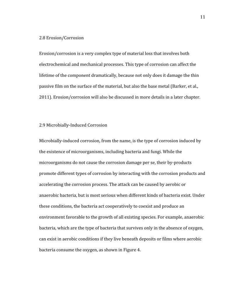
can exist in aerobic conditions if they live beneath deposits or films where aerobic
bacteria consume the oxygen, as shown in Figure 4.

12
12
Figure 4: Anaerobic Bacteria Coexisting with Aerobic Bacteria (Beavers and Thompson, 2006)
Studying this type of corrosion requires understanding the microbiology that is
taking place in relation to corrosion. However, its presence has been problematic in
many industries including the petrochemical, marine, power, aircraft, water supply
and distribution, and process industries. A study found that about 20-‐30% of
external corrosion in underground pipelines is related to microbially-‐induced
corrosion (Al-‐Darbi, et al., 2002) (Beavers and Thompson, 2006).

13
13
3. AVAILABLE METHODS OF INSPECTION
3.1 Introduction
Over the past decades, many methods of inspection have been developed for
detecting and monitoring the various forms of corrosion. Some inspection methods
are more effective than others, but are not as time or cost effective. An effective
corrosion detection technique should be capable of detecting corrosion in any
location and under different conditions, and it should be capable of providing
reliable, accurate data. It should also have rapid response in order to allow for
solutions for severe problems to be studied and implemented immediately.
Moreover, it should be sensitive enough to detect actual minor flaws in order to
make sure corrosion damage as early as possible and ensure that the necessary
measures are taken before it is too late. Finally, corrosion detection techniques
should be cost-‐effective. Several inspection methods need to be implemented in
order to detect the various forms of corrosion. The most common methods of
inspection include: visual inspection, ultrasonic and acoustic methods, radiographic
methods, thermal inspection, electromagnetic inspection, electrical resistance
methods, electrochemical methods, electrochemical noise, electrochemical
impedance spectroscopy, chemical sensors, and others. Some of these methods will
be discussed in this chapter (Agarwala, Reed and Ahmad, 2000).

14
14
3.2 Visual Inspection
Visual inspection is and has always been the primary and most effective corrosion
inspection method, but it is also the most costly in terms of money and time. It
involves periodic visual testing of the exterior of the equipment and pipes for leaks,
distortion, or any evidence of internal damage or physical change. Visual inspection
requires good vision, adequate lighting, and familiarity and understanding of what
is being investigated. Magnifying glasses may be used in order to enhance the
inspection effectiveness. Visual inspection may be conducted through sentry holes,
borescopes, or charged couple devices. Sentry holes are holes that are drilled on the
external surface of the equipment at locations where corrosion is most likely to
occur. The holes are drilled to a depth corresponding to the design wall thickness of
the vessel of pipe minus the permissible corrosion allowance that is usually
included in the design. When corrosion starts consuming the allowance thickness, a
small leak starts developing on the surface of the equipment, which provides a
timely warning of the need for maintenance. The holes are threaded in order to
provide temporary plugging until a shutdown is possible (Howard, Gibbs and Elder,
2003) (Agarwala, Reed and Ahmad, 2000).
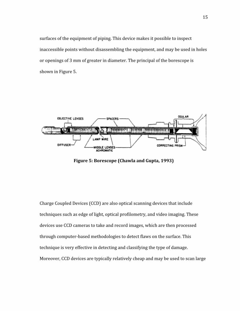
Borescope is an optical device that consists of a tube with an eyepiece at one end
equipped with a light source. The tube may be flexible of rigid depending on the
application and the eyepiece allows for visual on-‐stream inspection of the internal
15
15
surfaces of the equipment of piping. This device makes it possible to inspect
inaccessible points without disassembling the equipment, and may be used in holes
or openings of 3 mm of greater in diameter. The principal of the borescope is
shown in Figure 5.
Figure 5: Borescope (Chawla and Gupta, 1993)
Charge Coupled Devices (CCD) are also optical scanning devices that include
techniques such as edge of light, optical profilometry, and video imaging. These
devices use CCD cameras to take and record images, which are then processed
through computer-‐based methodologies to detect flaws on the surface. This
technique is very effective in detecting and classifying the type of damage.
Moreover, CCD devices are typically relatively cheap and may be used to scan large

16
16
areas. On the other hand, they lack precision and are labor intensive and may be
applied only on open surfaces (Agarwala, Reed and Ahmad, 2000).
3.3 Ultrasonic and Acoustic Inspection
Ultrasonic and Acoustic testing is an inspection technique that has been and still is
widely used across the industry. It provides excellent resolution and can detect
minute material and thickness losses with a relatively short response time. The
main principle here involves utilizing high frequency sound waves above 0.2 MHz
to make measurements. Typical ultrasonic and acoustic systems consist of a
transducer, a receiver (or a pulser) and a display device. The reflection or pulse
echoing shown on the display device allows for flaw detection. The sound energy
that is produced by the transducer propagates through the cross section of the
vessel or pipe in the form of waves and when a flaw is detected, part of the energy
is reflected back. The transducer then transforms the reflected signal into an
electrical signal, which is then displayed on a screen. Figure 6 shows an example of
ultrasonic testing acquisition.

17
17
Figure 6: Example of Ultrasonic Testing Acquisition (Ultrasonic Nondestructive Testing -‐Advanced Concepts and Applications, 2012)
As shown in Figure 6, the reflected signal from the flaw can then be plotted as a
function of the time traveled when the echo was received and this travel time can
then be related to the distance traveled and the flaw may be located. The echo also
gives information about the size of the flaw so the severity of the situation can be
estimated (Agarwala, Reed and Ahmad, 2000).

18
18
3.4 Radiographic Inspection
Radiographic inspection is another non-‐destructive testing technique that has been
commonly used to monitor corrosion, especially in the petrochemical industry. The
radiation type may be neutrons, x-‐rays, or gamma rays. Radiographic methods have
an advantage over other common methods in that they can detect corrosion
without the costly removal of the insulation material. However, these methods
require radiation safety measures to be taken and they have low sensitivity.
Corrosion is detected by measuring the thickness of the cross section of the pipe or
vessel. The radiation rays are sent through the cross section of the pipe or vessel
and penetrating rays are projected as images on a thin film. The extent of the
damage is estimated by comparing the images to those of the undamaged part. An
example of radiography inspection results is shown in Figure 7.
Figure 7: Radiography Results (Wanga and Wong, 2004)
19
19
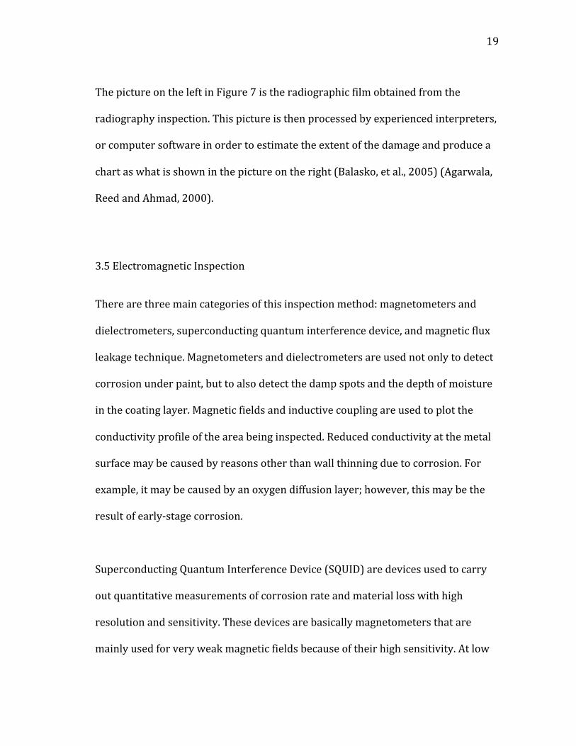
The picture on the left in Figure 7 is the radiographic film obtained from the
radiography inspection. This picture is then processed by experienced interpreters,
or computer software in order to estimate the extent of the damage and produce a
chart as what is shown in the picture on the right (Balasko, et al., 2005) (Agarwala,
Reed and Ahmad, 2000).
3.5 Electromagnetic Inspection
There are three main categories of this inspection method: magnetometers and
dielectrometers, superconducting quantum interference device, and magnetic flux
leakage technique. Magnetometers and dielectrometers are used not only to detect
corrosion under paint, but to also detect the damp spots and the depth of moisture
in the coating layer. Magnetic fields and inductive coupling are used to plot the
conductivity profile of the area being inspected. Reduced conductivity at the metal
surface may be caused by reasons other than wall thinning due to corrosion. For
example, it may be caused by an oxygen diffusion layer; however, this may be the
result of early-‐stage corrosion.
Superconducting Quantum Interference Device (SQUID) are devices used to carry
out quantitative measurements of corrosion rate and material loss with high
resolution and sensitivity. These devices are basically magnetometers that are
mainly used for very weak magnetic fields because of their high sensitivity. At low

20
20
frequency, SQUID eddy current measurements offers phase-‐sensitive detection that
allows a depth selective technique to image material loss within aluminum
structures. In many cases, the sensitivity of SQUIDs makes them useful when other
methods fail to make sensible measurements (Fagaly, 2006) (Agarwala, Reed and
Ahmad, 2000).
Magnetic Flux Leakage Technique is another approach to monitoring corrosion in
pipelines while in-‐service. Smart pigs that employ this technique are the most cost-‐
effective approach out of all in-‐service corrosion inspection methods. However, this
technique is not useful for pipes with smaller diameters, and therefore its usability
is limited to larger pipes and transmission lines (Agarwala, Reed and Ahmad,
2000).
Generally speaking, numerous methods of inspection for corrosion exist. Some are
more effective than others, some are more costly than others, and some are only
useful to some extent or under particular conditions. Therefore, depending on the
application, the most appropriate method of inspection is chosen.

21
21
4. CORROSION UNDER INSULATION AND METHODS OF DETECTING IT
4.1 History
Corrosion under insulation (CUI) has become a serious threat to many of modern
plants. It started receiving a great amount of attention in petroleum refineries,
chemical plants, power generating plants and other facilities in the 1980s. The
reason being that the insulation which had previously been used at locations of 300
oF and above started being used at much lower temperatures ~200 oF after the first
oil crisis in 1973 (Tada, Suetsugu and Mori, 2010). Being localized and hidden by
the insulation, it typically causes failures in areas that are not of primary concern to
the maintenance program. Not only does it often result in catastrophes, but it
always has a strong economic effect in terms of time and money. CUI is especially
problematic in carbon steels and 300 series stainless steels. On carbon steels, it is
usually either of the generalized or the localized nature. However, in stainless
steels, it is more often than not pitting corrosion induced stress corrosion cracking.
The main factor to corrosion under insulation, like most other corrosion forms, is
oxygen combined with moisture. However, in this case, the insulation material,
which acts as a sponge that entraps the moisture, might increase the severity of the
resulting damage, by not allowing the moisture to evaporate and also buy acting as
a carrier that helps the moisture spread from one spot to others. Moreover,
traditional thermal insulation materials may contain chlorides, which upon

22
22
exposure to moisture may be released into the moisture layer on the surface of the
metal and cause pitting corrosion or stress corrosion cracking. The source of the
water can be rain, leakage, deluge system, wash water, or sweating from the
process temperature. CUI can occur at a wide range of temperatures; however, it is
more significant at temperatures between 32 and 300 oF, especially at about 200 oF.
The following five areas are specified by API 570 as susceptible to CUI:
1. Areas exposed to mist from cooling water towers
2. Areas exposed to steam
3. Areas exposed to deluge systems
4. Areas subject spills, moisture, or acid vapors
5. Carbon steel piping insulated for personnel protection operating
between 25 and 250 oF.
Many other areas of the process are also susceptible to CUI, including deadlegs that
operate at a different temperature from the active line. All of these areas are prone
to water ingress and therefore must receive special attention.
It is difficult to calculate the direct costs of corrosion under insulation. However, a
study that was conducted by ExxonMobil and presented in 2003 showed that the
corrosion under insulation, rather than process corrosion, is responsible for the
highest incidence of leaks in the refining and chemical industries. The study also

23
23
showed that corrosion under insulation is responsible for about 40-‐60% of piping
maintenance costs (Industrial Nanotech, Inc., 2006).
4.2 Problems with Methods of Inspection
Some of the most commonly used methods of detection of CUI include visual
inspection (insulation removal), profile radiography, ultrasonic thickness
measurement, real time radiography, and pulsed eddy current testing. Each one of
these methods has some shortcomings that make it either inapplicable under some
conditions, or not accurate enough in detecting corrosion under insulation. Visual
inspection is still the preferred method in many facilities today, because it is very
effective. This method, however, is very costly in terms of money and time lost. It
requires the insulation to be peeled off the entire surface of the metal, the surface
condition to be checked, and finally the insulation to be replaced. If the insulation is
removed while the piping is in service, many process related problems may occur.
The following table summarizes some of the specifications as well as the
advantages and disadvantages that the other four methods have (Callister, 1972)
(Tada, Suetsugu and Mori, 2010).

24
24
Table 1: Comparison of the Most Commonly Used Methods of Detection of CUI
Method Profile Radiography
Ultrasonic Measurement
Real-‐Time Radiography
Pulsed Eddy Current
Influence of internal fluid Yes Yes Yes No
Inspection of Long Distance
Not applicable Applicable Not
applicable Not applicable
Removal of Insulations No need Need No need
No need (less than 80 mm in thickness)
Corrosion can be detected
Corrosion, erosion and the accumulation of deposits
Localized corrosion (10% depth level of sectional area)
Localized corrosion
General corrosion like concave
Inspection accuracy
Reasonably good Not good Good Not good
Safety Concerns Radiation Radiation
As shown in Table 1, each of the main NDT methods used for the detection of CUI
has its own drawbacks. Ultrasonic may have a very high inspection speed, however,
it may not be used for all pipe configurations and it requires some of the insulation
to be removed, and it does not have very high accuracy. Radiography methods
provide accurate results, but there are some safety implications with the radiation
that they require. Pulsed eddy current testing only gives relative results and works
better with flatter objects (Wassink, 2008).
25
25
4.3 Objective
A different non-‐destructive technique of detection of corrosion under insulation
that does not require the insulation to be removed needs to be investigated. This
method is needed to overcome at least some of the shortcomings shown by the
commercial NDT methods currently used. Also this method needs to be safe,
accurate, fast, reliable, and adaptable.
4.4 X-‐Ray Computed Tomography
To meet the objective of this research, many approaches were considered and a
number of methods were studied, particularly electrical computed tomography and
X-‐ray computed tomography. However, based on the results of some preliminary
experiments, it was found that electrical computed tomography would not serve
the purpose of this project. It was found that the metal surface of the pipe would
block the signals from the tomography system, and interference with internal
conductive fluids is possible. Moreover, the insulation material, especially dry
insulation, would not allow the AC current to pass through. Therefore, electrical
tomography was left out of the possible methods to be investigated and X-‐ray
computed tomography was selected for further studies.

26
26
X-‐ray tomography is a non-‐destructive technique that is used to visualize the inside
of opaque objects. This method has been commonly used in the medical profession
in CT and CAT scanners. It has also been used recently in civil engineering to
monitor corrosion in steel reinforcement in concrete (Beck, et al., 2010).
In X-‐ray tomography, the specimen is placed between the X-‐ray source and a
detector. The detector determines the intensity of the X-‐rays after leaving the
specimen, which is then compared to the initial intensity of the X-‐rays leaving the
source, and based on that, the density of the material is determined. The density
distribution of the specimen is then calculated and an image is created with each
density level assigned a color (Advanced Characterization of Infrastructure
Materials Laboratory, 2009). This is done while the object is being rotated 360o in
order to capture the density of the cross section of the object from all angles.
4.4.1 X-‐Ray Computed Tomography vs. Real Time Radiography
While similar to real-‐time radiography, X-‐ray tomography seems to be a better fit
for the purpose of this work. It is different from real-‐time radiography, in that it is
mainly used to perform tomographic reconstructions of static material distribution
and has the ability to determine the material distribution on the outside and inside
of the material. This can be used to investigate both internal and external corrosion
simultaneously. On the other hand, real-‐time radiography provides an X-‐ray
“shadow” of flaws in the specimen, which is not as clear as the image provided by X-‐

27
27
ray computed tomography (Torczynski, et al., 1997). Moreover, X-‐ray tomography
provides a 3-‐D image of the specimen while real time radiography provides a 2D
image, which allows for more accurate inspection of the object. Finally, X-‐ray
tomography has shown more accurate results than real time radiography in
medical applications (Carreon, et al., 2008).
4.5 Experimental Approach
In order to understand whether X-‐ray tomography would be a good option for
corrosion detection, it was necessary to know first to what extent the system can
detect small flaws in an object. This is important in order to make sure the system
is capable of detecting any minor corrosion taking place, even if it is of low severity.
After that, it was necessary to determine whether the results of the system are
affected by the insulation jacketed around the exterior of the pipe. This is important
in order to know whether the insulation would need to be removed for the system
to be used for corrosion inspection. Finally, it was of interest to test whether the
system was useful for detecting internal corrosion as well.
4.5.1 Experiment 1: The Accuracy of the X-‐Ray Tomography System
To test the system for detecting small flaws, three small holes of different sizes
(0.442”, 0.315”, and 0.126”) were drilled along the same cross section of a 4”
carbon steel pipe, as shown in Figure 8. The system was used to take multiple scans
28
28
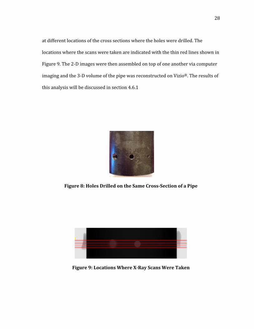
at different locations of the cross sections where the holes were drilled. The
locations where the scans were taken are indicated with the thin red lines shown in
Figure 9. The 2-‐D images were then assembled on top of one another via computer
imaging and the 3-‐D volume of the pipe was reconstructed on Vizio®. The results of
this analysis will be discussed in section 4.6.1
Figure 8: Holes Drilled on the Same Cross-‐Section of a Pipe
Figure 9: Locations Where X-‐Ray Scans Were Taken

29
29
4.5.2 Experiment 2: The Effect of the Insulation Material on the Output
Three main types of insulation of different densities were tested in this experiment:
high-‐density foam, low-‐density foam, and fiberglass. The three insulation materials
were jacketed around the same pipe, each at a time, and scans of the same cross-‐
sections were taken each time. The insulation was wrapped around the pipe with
aluminum casing to test whether that could affect the X-‐rays penetration through
the pipe. Figure 10 shows the three insulation materials that were used for this
experiment. The results of this experiment are analyzed in section 4.6.2.
Figure 10: Three Insulation Materials Used

30
30
4.5.3 Experiment 3: Is Internal Corrosion Detected?
X-‐ray computed tomography outdid real time radiography because of its ability to
inspect the interior and exterior of an object simultaneously. The 3-‐dimensional
output of the system allows for locating exactly where a flaw might be located.
Therefore, it was of interest to see whether this capability could be used for
detecting minor internal corrosion in a pipe. A 0.5” pipe with a layer of galvanized
corrosion was inspected using the system. Scans at different locations were taken
to capture internal corrosion of different severity levels. The results of this section
are shown in section 4.6.3.
4.6 Results and Discussion
4.6.1 Experiment 1: The Accuracy of the X-‐Ray Tomography System
First, 2-‐D scans were taken of the cross-‐section where the three holes were drilled
on the surface of the pipe. The following figure shows ten of the 2-‐D scans that were
taken, in the order from top to bottom.

31
31
Figure 11: 2-‐D Scans of the Pipe Cross Section As Displayed on Computer Screen
As clear from Figure 11, the holes in the cross section of the pipe are very clearly
shown on the images taken by the system. These images were then assembled on
top of one another using Vizio and the 3-‐D volume, shown in Figure 12, was
reconstructed.
Figure 12: 3-‐D Image of the Pipe Reconstructed on the Computer

32
32
As shown in Figure 12, the three holes were detected very accurately by the system.
However, while the holes are perfectly circular in the real pipe, they are not as
perfect in the X-‐ray output. More 2D slices would have to be taken in order to
obtain a more accurate result. Moreover, depending on the application, 2D imaging
might be sufficient for corrosion (both internal and external) detection, and
constructing the 3D volume would be needed only after corrosion damage has been
detected and better visualization would be required in order to see how severe the
damage is. However, many scans would have to be taken in order to ensure that
minor flaws are detected.
4.6.2 Experiment 2: The Effect of the Insulation Material on the Output
As mentioned before, the three types of insulation that were studied here were:
high-‐density foam, low-‐density foam, and fiberglass. The pipe around which the
insulation materials were jacketed was 0.5” in diameter, and the scans were taken
at the same of location each time. Figure 13 shows the scans of the same cross
section with the different insulation materials.
(a) (b) (c)
Figure 13: Cross-‐Section of Pipe as viewed with Different Insulation Materials Jacketed around it (a) High-‐Density Foam (b) Low-‐Density Foam (c)
Fiberglass

33
33
As shown in Figure 13, the insulation material does not affect the accuracy of the
results at all, as the three figures are identical. Also, since the density of the
insulation materials is negligible compared to that of the metal surface, the
insulation was not visible by any means in the images taken by the system.
4.6.3 Experiment 3: Is Internal Corrosion Detected?
Finally, the system was tested for its ability in detecting internal corrosion. A small
pipe with some galvanized internal corrosion that had formed on its surface was
used. The following figure shows three images of the corroded pipe. Image 1 was
taken at the end of the pipe, Image 2 was taken 2 mm away, and Image 3 was taken
2 mm away from Image 2.
Figure 14: Images of Three Internally-‐Corroded Cross-‐Sections of a Pipe
34
34
As clear from Figure 14, since the corrosion is of much lower density than the pipe
surface itself, the shade of grey that the X-‐ray tomography system has assigned it is
much darker than that of the pipe. However, the system was still successful in
detecting the minor corrosion that had formed.
4.7 Conclusion
All in all, X-‐ray tomography gave accurate results and could be used for corrosion
detection. Nevertheless, more research is required to achieve faster scan time to
make the method more feasible for large-‐scale plants. Moreover, it is important to
study the mobility of the system and its applicability with respect to investigating
multiple pipes at the same time, in order to make sure it would be useful in
congested plant areas.
The X-‐ray computed tomography system used in this study was not portable and
cannot be used for on-‐site inspections. It was only used here because it met the
purpose of this study which was to investigate if this method detects corrosion, and
to what extent. However, for real life applications, it is recommended that the
portable version of this system be used instead. The portable X-‐ray computed
tomography that has been developed recently is known as the TomoCAR, which
stands for “Tomographical Computer-‐Aided Radiography”. The operating principal
of TomoCAR, shown in Figure 15, is very similar to that of the classic system.

35
35
Figure 15: TomoCAR Principal (Redmer, Ewert and Neundorf, 2007)
As shown in Figure 15, here the X-‐ray source and the screen are mounted on a pipe
in parallel facing each other, in order to allow for movement of the x-‐ray system for
scanning of different spots, without affecting the accuracy of the results. In
addition, the line camera (screen) that is mounted in front of the X-‐ray source acts
as a radiation collector that reduces any scattered radiation to a very negligible
intensity. This system should be investigated in order to ensure that the radiation
would not have any negative effects on the users of the system in the long run
(Redmer, Ewert and Neundorf, 2007).
36
36
5. USING CFD TO STUDY EROSION/CORROSION
5.1 History
Erosion/corrosion, as described earlier, is the acceleration in the rate of corrosion
that occurs after the protective film (usually oxide layer) on the surface has been
removed via chemical or mechanical processes. The protective film slows down the
corrosion process by forming a barrier between the surface of the metal and the
corrosive environment. The removal of the surface protective film via chemical
processes is usually referred to as flow accelerated corrosion, a term that is more
often than not used to refer to erosion/corrosion. Flow accelerated corrosion is a
single-‐phase process that takes place when the protective film is simply dissolved
into the solution by the corrosive species. Erosion/corrosion, however, is a
mechanical process that involves removing the protective film off the surface by a
physical force. In a single-‐phase flow, this physical force may be caused by the
shear stress imposed on the wall by the flow, in other words, the wall shear stress.
In a two-‐phase flow (e.g. fluid containing solid particles, such as sand), the
dispersed phase can remove the protective film by an erosive process, affecting not
just the protective film, but also the metal underneath.
Erosion/corrosion is a commonly encountered problem and a major concern in
many industries, including transportation, power generation, and the
petrochemical industry. In the oil and gas industry, it is especially a problem at the

37
37
stages involved before the oil or gas is processed at refineries, when it still contains
many impurities of different natures, including sand and water, the combination of
which provides a very encouraging environment for erosion/corrosion to take
place.
Erosion/corrosion has been the root cause of many severe incidents and great
losses in terms of lives and money. One of the rather recent large-‐scale incidents
caused by erosion/corrosion is the Mihama power plant explosion that took place
in Japan in 2004. The incident occurred when the piping system in a pressurized
water reactor led to a steam eruption. First, a fire alarm sounded, alerting the
operators at the control room that there was a leak. The operators suspected that
steam or hot water started leaking from the piping, and therefore began an
emergency load reduction process. Shortly as they were carrying out this process,
the reactor tripped automatically and a rupture occurred in a 22” pipe in the
condensate system. The incident caused five worker fatalities and six injuries. Later
on, investigations determined that the cause of the pipe rupture was in fact
erosion/corrosion that had reduced the thickness of the wall of the pipe from 0.39”
to about 0.02” (United States Nuclear Regulatory Commission Office of Nuclear
Reactor Regulation, 2006).
Another major incident that was caused by erosion/corrosion is the Humber
Refinery incident of 2001 that occurred in South Killingholme, United Kingdom. A

38
38
drastic failure in the piping in the saturate gas plant released about 397,000 pounds
of flammable liquids and gases that ignited causing an explosion and a fire about 20
seconds later. The explosion that threw three people about 570 feet away off their
feet caused severe damage to buildings up to 1,300 feet away from the explosion
source. The catastrophic incident had the potential to cause fatalities, but
fortunately it did not because it occurred when very few people were on site
because of shift changeover and surrounding businesses had taken the day off since
it was Easter Sunday. Investigations found that the primary cause of the explosion
was severe erosion/corrosion of a 6” pipe that had reduced the wall thickness of
the pipe from 0.3” to about 0.01”, that it could not withstand the internal pressure
of the flow (Health and Safety Executive, 2001).
5.2 Factors Affecting Erosion/Corrosion
Many methods have been developed and used for detecting and monitoring
erosion/corrosion. However, once the damage starts taking place, it can go at
extreme rates and threaten the integrity of the pipes and vessels before the
inspection detects it. The main problem with erosion/corrosion is the complexity of
the process that is not clearly understood. It is not described by a simple chemical
reaction or physical wear. It can be a combination of both, and is affected by many
factors related to the flow inside of the pipe; not only the flow material and

39
39
operating conditions, but also a single-‐phase flow would have different
erosion/corrosion locations from a two-‐phase flow, as shown in Figure 16.
Figure 16: Locations of Corrosion Based on Type of Flow (ClassNK, 2008)
In addition, erosion/corrosion is not only affected by the type of flow inside the
pipe, but also the material and geometry of the pipe itself. Some materials are more
prone to erosion/corrosion than others, and therefore, may allow the reaction to
take place at different rates. Also some pipe geometries might encourage
erosion/corrosion more than others, because the geometry of the pipe affects the

40
40
flow turbulence, which then imposes different values of stress on different parts of
the walls, and hence lead to different erosion/corrosion rates.
The following list includes some of the main factors that affect the rate of
erosion/corrosion:
• Flow velocity
• Flow pH
• Flow oxygen content
• Flow temperature
• Pipe shape and geometry
• Pipe material composition
5.2.1 Effect of Flow Velocity on Erosion/Corrosion Rate
Flow velocity is a very important factor in determining the rate of
erosion/corrosion. Typically, the higher the velocity, the higher the
erosion/corrosion likelihood and that is because as the velocity of the flow
increases, the turbulence does as well. At low flow velocities, the corrosion process
is more dominant than erosion, but as the velocity increases, erosion starts
accompanying corrosion, increasing the rate and extent of the damage. However,
after a certain point, any further increase in the flow velocity leads to a lower rate
of erosion/corrosion, as shown in the following figure (Ferng and Lin, 2010) (Bush,
1990). Ferng and Lin (2010) explained that the reason for this decreasing trend is

41
41
that at high velocities and turbulence, the total metal loss rate can be determined
by the chemical reaction rate constant and the metal concentration difference. The
reaction rate constant is not really related to the hydrodynamic factors, but the
concentration of the metal (or the Fe2+) is strongly associated with the turbulence
of fluid inside the piping, and as the mixing increases it also increases, leading to a
lower erosion-‐corrosion rate.
5.2.2 Effect of Flow pH on Erosion/Corrosion Rate
The chemical reaction portion of the erosion/corrosion process is highly affected
by the chemical condition of the flow, particularly its pH. It was found that as the
pH of the solution goes above 8-‐9, the rate of erosion/corrosion starts decreasing
gradually. The rate of erosion-‐corrosion tends to drop dramatically when the pH is
above 9.2-‐9.3. It is recommended that the process pH be maintained between 9.3-‐
9.6 (Chawla and Gupta, 1993) (ClassNK, 2008).
5.2.3 Effect of Flow Oxygen Content on Erosion/Corrosion Rate
The amount of oxygen dissolved in the flow inside the pipe is another important
factor for determining the rate of erosion/corrosion. Generally, as the amount of
dissolved oxygen in the flow decreases, the erosion/corrosion rate increases. If the
oxygen concentration drops below 200 ppb, the rate of erosion/corrosion increases
significantly. This trend is represented in Figure 17.

42
42
Figure 17: The Relationship between Erosion/Corrosion Rate and Dissolved Oxygen Concentration for Different Pipe Materials (ClassNK, 2008)
5.2.4 Effect of Temperature on Erosion/Corrosion Rate
The rate of erosion/corrosion is also affected by the temperature of the process.
Temperatures within the range ~250 oF (121 oC) to ~400 oF (204 oC) tend to
increase the rate of the wall thinning due to erosion/corrosion. For a single-‐phase
flow, the rate reaches maximum at around 275 oF (135 oC) for a single-‐phase flow
and about 356 oF (180 oC) for a two-‐phase flow. However, these values are different
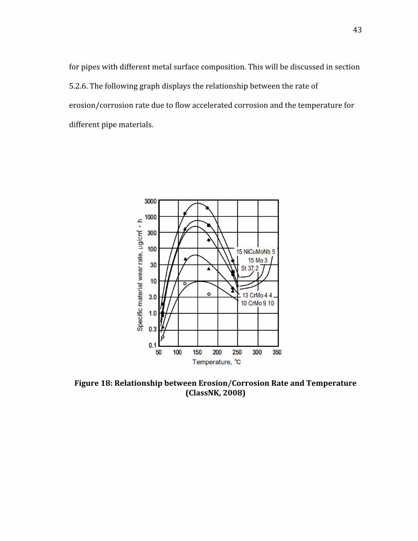
43
43
for pipes with different metal surface composition. This will be discussed in section
5.2.6. The following graph displays the relationship between the rate of
erosion/corrosion rate due to flow accelerated corrosion and the temperature for
different pipe materials.
Figure 18: Relationship between Erosion/Corrosion Rate and Temperature (ClassNK, 2008)
44
44
As shown in Figure 18, the relationship between the erosion/corrosion rate and the
temperature has a convex shape with a maximum point and decreases on both
sides farther from the maximum (ClassNK, 2008).
5.2.5 Effect of Pipe Geometry on Erosion/Corrosion Rate
The geometry of the pipe is essential in determining the corrosion rate. A small
change in a pipe geometry or orientation can drastically change the flow complexity
inside causing different values of turbulence, which in turn affects the rate of
erosion/corrosion. Generally, turbulence is generated in pipefittings, behind
orifices or valves, at T-‐sections, at bends and elbows, as well as at diffusers and
reducers. For this reason, those are the areas that are usually most susceptible to
erosion/corrosion in pipes. Another reason is that the erosion/corrosion process is
further encouraged by water, which different geometries might cause it to
accumulate in certain spots, such as at bend areas and T-‐junctions (ClassNK, 2008).
5.2.6 Effect of Pipe Material on Erosion/Corrosion Rate
Finally, the pipe material plays an important role in determining the
erosion/corrosion rate. The composition of the pipe material determines the nature
of the protective film that forms on the surface and slows down the damage
process. When a continuous, dense, solid film forms over the metal surface, better
protection against erosion/corrosion is provided and the rate of attack decreases.
Stainless steel is considered one of the most corrosion-‐resistant materials because
it has the ability to form a very strong passive film that can withstand any oxidizing

45
45
conditions (Chawla and Gupta, 1993). Some of the main components that may be
added to the metal composition to increase its corrosion-‐resistance include
chromium, copper and molybdenum (Bush, 1990).
5.3 Objective
In this work, computational fluid dynamics tools were implemented in order to
study the effect of some of the flow hydrodynamic factors on the erosion/corrosion
rate. The main purpose of this technique was to understand how the different
hydrodynamic parameters affect the erosion/corrosion rate. This, in turn, would
allow for determining where erosion/corrosion would take place before it occurs
by simply entering the properties of the flow on the computer. Not only would this
technique allow for determining erosion/corrosion sites before it starts taking
place, but it would also give an indication of how much erosion/corrosion would
take place, before it is too late and an incident occurs. In other words, it would help
mechanical integrity staff make predictions while scheduling maintenance services.
5.4 Computational Fluid Dynamics and Erosion/Corrosion Modeling
Computational Fluid Dynamics (CFD) is a fluid mechanics technique that has
become widely used in recent years. It is used to predict flow behaviors by applying
numerical analysis methods to solve partial differential equations. CFD tools were
46
46
first used in the 1940s to predict the behavior of supersonic flows over sharp cones.
The applications of CFD have broadened as the technology advanced and more
numerical models were available, and CFD has become an essential part of fluid
dynamics that builds on with experiments and theory (Wendt, 2009).
Recently, significant amounts of research have been dedicated to study various
types of corrosion through CFD modeling. Many studies were investigated but the
one that was most relevant was a study that investigated the use of CFD to predict
erosion/corrosion in piping systems in pressurized water reactors in power plants.
The main hydrodynamic parameter that is investigated in this study was the near-‐
wall turbulent kinetic energy. Here, a conservative model to define the relationship
between the wall-‐thinning rate due to erosion/corrosion to the turbulent kinetic
energy was proposed. This relation was found by plotting plant measurements of
erosion/corrosion, for different geometries and flow conditions, as a function of the
turbulent kinetic energy as predicted by CFD. By plotting the curve of best fit
through the data points, as well as the more conservative curve that envelops all
the plant measurement point, this relationship was defined. Both of these curves
are shown in Figures 19(a) and 19(b).

47
47
(a)
(b)
Figure 19: Relationship Between Wall-‐Thinning Rate and Turbulent Kinetic Energy (Ferng and Lin, 2010) (a)

48
48
As shown in Figure 19, the wall thinning values were decreasing as the turbulent
kinetic energy increased. The plant measurements were all taken for the same
piping system but at different locations with different turbulent kinetic energy
values (Ferng and Lin, 2010). The same approach was used in this research and is
explained in the next few paragraphs.
5.5 Approach
ClassNK provided some erosion/corrosion data for a period of 20 years in their
report: “Guidelines on Pipe Wall Thinning”. The data was for a nuclear power
station, where erosion/corrosion has been commonly encountered and has caused
several incidents in the past, including the Mihama Nuclear Power Station
explosion of 2004. It included data for different geometries, including bends, T-‐
junctions, and valves. It also included different flow conditions for each geometry.
The maximum wall thickness loss due to erosion/corrosion was provided for each
shape, and the location where it takes place was also specified (ClassNK, 2008).
This data was then used to study the relationship between the flow hydrodynamic
factors and the rate of erosion/corrosion. The following are the general steps that
were carried out to meet the objective of this work:
1. The geometries (discussed later) were built on SolidWorks
2. The meshing of the geometries was formed on Gambit

49
49
3. The operating conditions that led to erosion/corrosion were used on
FLUENT® to carry out the flow hydrodynamic factors predictions
4. The erosion/corrosion values from the literature were then related to the
hydrodynamic flow factors that were predicted by FLUENT®
The main hydrodynamic factors that were considered initially were the surface
shear stress and the flow turbulence, both of which are known to affect the rate of
erosion/corrosion. However, the results showed that the dynamic pressure plays
an important role in the picture, and therefore, it was studied as well.
The simulations were carried out for four of the shapes mentioned in the report,
namely: two bends of different elbow radii (R=1.5D and R=3D, where R is the
radius of the elbow, and D is the diameter of the pipe), a T-‐branch, and a merging T-‐
junction. The T-‐branch and the T-‐junction had the same geometry, but the direction
of the flow inside was different, as shown in Figure 20.

50
50
(a) (b)
Figure 20: (a) Merging T-‐Junction (b) T-‐Branch
The grids that were used for the four shapes were all hexahedral, which provide
more accurate results. Also, the meshes were refined near the walls using Gambit to
better capture the behavior of the flow near the walls.
After the meshing of the geometries was completed, the flow conditions from the
literature were all input on FLUENT®, and the standard k-‐ε model was used to
predict the flow behavior. This model was chosen because it is the most commonly
used model for turbulence calculations. The boundary conditions used in all
simulations were mass flow rate at the inlet(s), and pressure at the outlet(s) and
only steady state solver was used. The y+ value, which is a dimensionless number
calculated by FLUENT® to indicate how well the behavior of the flow near the wall
is captured, was also calculated. Its main purpose is to make sure that the meshes
developed by Gambit were fine enough to make accurate predictions by ensuring

51
51
that its value is within the range 50<y+<300, for standard wall function. The y+
value is given by the following formula:
!! = !!!
!/!!!!/!!!
! (1)
where: p is a node
kp is the turbulent kinetic energy at the near-‐wall node p
yp is the distance from point p to the wall
Cµ is a constant for K-‐epsilon model
ρ is the density
µ is the dynamic viscosity
The standard K-‐epsilon model is given by the following formulas:
1. Transport equation for turbulent kinetic energy “k”:
!!"
!" + !!!!
!"!! = !!!!
! + !!!!
!"!!!
+ !! + !! –!" − !! + !! (2)
2. Transport equation for turbulent dissipation rate “!”:
!!"
!" + !!!!
!"!! = !!!!
! + !!!!
!"!!!
+ !!!!!!! + !!!!! − !!!!
!!
! + !! (3)
3. Turbulent viscosity is modeled as:
!! = !!!!!
! (4)
!! = !! !! (5)
S is the modulus of the mean rate of strain tensor and given by:
! = 2 !!"!!" (6)
52
52
!! = !!!!!!!" !"!!! (7)
where: !!" is the Prandtl number for energy
!! is the gravity
! is the coefficient of thermal expansion
For standard models, the default value of !!" = 0.85, and ! is given by:
! = − !! !"!" !
(8)
The model constants are given as follows:
!!! = 1.44 (9)
!!! = 1.92 (10)
!! = 0.09 (11)
!! = 1.0 (12)
!! = 1.3 (13)
A single-‐phase flow of water was modeled for the four shapes listed previously. The
flow was also modeled at 6 speeds: 0.26, 1.2, 2.4, 2.5, 3.6, and 7.5 m/s. As
mentioned previously, both of the flow velocities and the shape of the pipe affect
the turbulence of the flow inside the pipe and the shear stress imposed by the flow
on the pipe walls. Therefore, studying the same flow in different shapes and at
different speeds provides different turbulence and wall shear stress values.

53
53
Finally, the results from FLUENT® gave the turbulent kinetic energy and surface
shear stress values, as well as other factors, throughout each shape, and this was
used to investigate the relationship between the erosion/corrosion and the
turbulence and wall shear stress. This was accomplished by plotting the maximum
erosion/corrosion value for each shape (obtained from the literature) against the
turbulence and wall shear stress at that point of maximum damage (as predicted by
FLUENT®).
5.6 Results and Discussion
Figure 21 shows the hexahedral grids that were developed on Gambit for one of the
bends as well as the T-‐junction.

54
54
Figure 21: Grids of a Bend and a T-‐Junction
The cross-‐section of the pipe bend was blown up in Figure 21 to show how the
meshes were refined near the edges in order to visualize more clearly the boundary
layer of the flow near the wall. This was necessary in order to obtain more accurate
prediction of the hydrodynamic parameters of the flow near the walls of the pipes.

55
55
After the grids were completed, the conditions of the flows that led to
erosion/corrosion that were collected from the literature were input into
FLUENT®, and the model was set up for each of the four geometries considered.
The simulations were then left to run under steady state conditions until the
solution was complete. After that, the solutions of the simulations were
investigated. The results from FLUENT® were obtained in contour plots for a
variety of different hydrodynamic factors, with a scale to show the value each color
corresponds to, as shown in Figure 22. The main factors that were studied initially
were the turbulent kinetic energy and the wall shear stress, both of which were
produced by FLUENT®. From contour plots similar to the following (Figure 22), the
relationship between erosion/corrosion and factors such as the turbulent kinetic
energy and the wall shear stress was studied.

56
56
Figure 22: Contour Plots of (A) Turbulent Kinetic Energy (B) Wall Shear Stress at Flow Speed 2.5 m/s

57
57
From plots similar to what is shown in Figure 22, the value of the turbulent kinetic
energy and wall shear stress at the point where the erosion/corrosion damage was
most severe (according to the plant measurements), was recorded and used in the
x-‐axes of the following plots, and the erosion/corrosion values were used on the y-‐
axes. First, the erosion/corrosion values were plotted as a function of the turbulent
kinetic energy for all of the 24 simulations that were run, as shown in Figure 23.
Figure 23: Erosion/Corrosion Plant Measurements as a Function of Turbulent Kinetic Energy
0
0.1
0.2
0.3
0.4
0.5
0.6
0.7
0.8
0.9
0 0.5 1 1.5 2 2.5 3
Erosion Corrosion Rate (m
m/yr)
Tubulent Kinetic Energy (m2/s2)
Series1 Cuve of Best Fit

58
58
As shown in Figure 23, the relationship between erosion/corrosion and the
turbulent kinetic energy has a decreasing trend, which agrees with what has been
published in the literature. However, it was interesting to see whether the graph
looks different if the data for each shape is plotted separately. Therefore, the graph
of erosion/corrosion was plotted as a function of the turbulent kinetic energy
(shown in Figure 24) for each shape separately, and again as a function of the wall
shear stress (shown in Figure 25). The curve of best fit was also plotted for the set
of data for each shape on the two graphs.
Figure 24: Erosion/Corrosion Plant Measurements as a Function of Turbulent Kinetic Energy for Each Shape

59
59
Figure 25: Erosion/Corrosion Plant Measurements as a Function of Wall Shear Stress for Each Shape
In both Figure 24 and Figure 25, the curve represents a best fit of the data points,
using the noted function. The curve that seemed to fit the points best was a power
function. As shown in both plots, looking at each shape separately, it is obvious that
the decreasing trend that has been discussed before is still observed, which means
that the same trend as what is published in the literature is obtained for each shape
(Ferng and Lin, 2010).
60
60
By looking at the data of each shape separately, it was evident that the
erosion/corrosion data had much higher values in the case of the T-‐branch than the
rest of the geometries, even though the turbulent kinetic energy values, as
predicted by FLUENT®, were generally within the same range for all pipes. In
addition, the merging T-‐junction had the lowest erosion/corrosion values at similar
turbulent kinetic energy values as the rest of the shapes. Moreover, the pipe bend
with the sharper angle (R=1.5D) had higher erosion/corrosion values than the
smoother pipe bend. The same trend was obtained when the erosion/corrosion
values were plotted against the wall shear stress values. This shows that there must
be another factor that causes the erosion/corrosion to be much more severe in the
case of the T-‐branch. This factor must be significantly higher in the T-‐branch as
compared to the merging T-‐junction, and must be higher in the sharper bend
(R=1.5D) than in the smoother one (R=3D).
Therefore, several other factors that were predicted by FLUENT® were studied.
Particularly, the dynamic pressure showed very interesting results. It was found
that, in the case of the T-‐branch, as the flow enters the branch, it imposes high
dynamic pressure at the point where the flow hits the wall. This is shown in Figure
26, which shows the dynamic pressure contour plot of an internal plane of the pipe.
61
61
Figure 26: Dynamic Pressure Contour Plot of T-‐Branch
The arrow on Figure 26 represents the direction of the flow inside of the pipe, and
the white circle points out the area where the dynamic pressure is highest. On the
other hand, by looking at the same plot for the merging T-‐section, it is clear that the
point of highest impact is actually where the flow from both inlets meets. In other
words, the highest dynamic pressure is not imposed on the walls; it rather occurs
before the flows hit the walls of the branch, as shown in Figure 27.

62
62
Figure 27: Dynamic Pressure Contour Plot of Merging T-‐Junction
Similarly, the maximum dynamic pressure was evidently higher in the case of the
sharper pipe bend than in the bend with the larger radius. To quantify these results,
the highest dynamic pressure for each shape at four speeds (1.2, 2.4, 2.5, and 3.6
m/s) was plotted, and is shown in Figure 28.

63
63
Figure 28: Near-‐Wall Dynamic Pressure at Different Velocities for Each Shape
In Figure 28, the dynamic pressure was plotted for 4 of the speeds. The other two
speeds that the simulations were run at (0.26 and 7.5 m/s) had very extreme
values, causing the trends shown by the other data points seem negligible, and
therefore were not used in this study. The points shown in Figure 26 show that the
dynamic pressure had a general increasing trend with velocity, and that the T-‐
branch had significantly higher values than the rest of the shapes. The bend with
the elbow radius to diameter ratio of 1.5 then had the second highest dynamic
0
1000
2000
3000
4000
5000
6000
7000
8000
9000
10000
Near-‐Wall Dynam
ic Pressure (Pascal)
T-‐Merging
Bend
(R=3D)
Bend
(R=1.5D)
T-‐Branch
1.2 m/s
2.4 m/s
2.5 m/s
3.6 m/s

64
64
pressure values, agreeing with the trend shown by the erosion/corrosion data. The
other bend and the merging T-‐junction had very close dynamic pressure values.
It is important to note that the dynamic pressure is a function of the flow velocity
squared and is given by the following function:
! = 12 !!
!
where: q is the dynamic pressure
ρ is the density of the flow
v is the velocity of the flow
Since the main purpose of this study was to investigate the effect of the change in
geometry on the erosion/corrosion values, and not the change in velocity, it was
necessary to normalize the dynamic pressure values. Therefore, the dynamic
pressure values were normalized with respect to the merging T-‐junction values, in
order to account for the velocities that are squared in the dynamic pressure
equation. After that, the normalized dynamic pressure values were plotted for each
shape at each of the four velocities. This plot is shown in Figure 29.

65
65
Figure 29: Maximum Dynamic Pressure for Each Shape at Four Different Speeds
As clear from Figure 29, the dynamic pressure is much higher in the T-‐branch than
the rest of the other geometries, the sharper elbow has higher dynamic pressure
than the smoother one, and finally, the merging T-‐junction has the same or lower
dynamic pressure values than the smoother bend. This trend is consistent with the
trend that the erosion/corrosion data showed. Therefore, the erosion/corrosion
0.8
0.9
1
1.1
1.2
1.3 Non-‐Dimensional Normalized Dynam
ic
Pressure
T-‐Merging
Bend
(R=3D)
Bend
(R=1.5D)
T-‐
Branch
1.2 m/s
2.4 m/s
2.5 m/s
3.6 m/s
66
66
values were plotted against the dynamic pressure values. This plot is shown in
Figure 30.
Figure 30: Erosion/Corrosion as a Function of Normalized Dynamic Pressure
While the data points on Figure 30 are somewhat scattered, there is a general
increasing trend that shows that as the dynamic pressure increases, the
erosion/corrosion increases as well. This shows that while the turbulence and wall
shear stress do have an effect on the erosion/corrosion values, the dynamic
pressure on the walls of the pipes also has a great effect on the erosion/corrosion
rates.
0
0.1
0.2
0.3
0.4
0.5
0.6
0.7
0.8
0.9
0.8 1 1.2 1.4
Erosion/Corrosion (mm/yr)
Normalized Dynamic Pressure
T-‐Branch
Pipe Bend (R=1.5D)
Pipe Bend (R=3D)
T-‐Merging

67
67
5.7 Conclusion
The main conclusions that can be drawn from this analysis are the following:
• The flow turbulence and the shear stress imposed by the flow on the surface
of the pipe from CFD predictions have highest values where
erosion/corrosion had occurred.
• The erosion/corrosion values from the literature were highest for the T-‐
branch and lowest for the merging T-‐junction, with the two bends with
values in between. However, the turbulence and wall shear stress values,
predicted by CFD were within the same range.
• The dynamic pressure follows the same trend as the erosion/corrosion: it is
highest for the T-‐branch, lowest for the merging T-‐junction, and higher in
the R=1.5D bend than the R=3D bend, both of which have values between
the T-‐branch and merging T-‐junction.
• The dynamic pressure has a significant effect on the erosion/corrosion rate.
• Flow turbulence and wall shear stress may be used to indicate where
erosion/corrosion will take place in the future.
• Dynamic pressure may be used to indicate how much erosion/corrosion
would take place.
In order to understand this relationship better, more data is required to better
quantify this trend and possibly develop empirical formulae for each shape to

68
68
relate the wall thinning rate due to erosion/corrosion to flow hydrodynamic factors
such as the flow turbulence, wall shear stress and dynamic pressure.

69
69
6. CONCLUSIONS
6.1 Summary
In this work, a thorough study of corrosion, a problem most industries have been
struggling with for decades, was carried out. An overview of the most common
types of corrosion was given, which included: generalized corrosion, pitting,
galvanic cell, crevice, concentration-‐cell, microbially induced corrosion, as well as
corrosion under insulation and erosion/corrosion, both of which this thesis focused
on. Moreover, the inspection methods that are most commonly used nowadays
have been outlined. The methods that were discussed include: visual inspection,
ultrasonic and acoustic testing, radiographic methods and electromagnetic
methods.
After that, corrosion under insulation was studied more extensively and a different
potential method of inspection of it was investigated, namely, X-‐ray computed
tomography. The reason a new method of inspection for corrosion under insulation
was studied, is that even though the CUI problem has been discovered for years, it
is still causing many severe incidents and costing the industry plenty in terms of
money and downtime. Finally, an intensive analysis on erosion/corrosion was
conducted through CFD modeling. Erosion/corrosion is also a major problem in the
industry, although it tends to be prevalent in some processes more than others.
70
70
Here the relationship between the behavior of the flow inside pipes of different
shapes was studied and correlated to the erosion/corrosion rates.
6.2 Conclusions
From the X-‐ray tomography analysis, it was concluded that this method has a lot of
potential in detecting both external and internal corrosion simultaneously,
accurately, without requiring the insulation layer to be removed. The output of this
method is a 3D image of the pipe being tested that can be visualized from all
directions on the computer screen. Moreover, it was found that the type of
insulation jacketed around the pipe does not affect the accuracy of the results, since
the density of the insulation is insignificant compared to that of the metal.
As for the erosion/corrosion CFD studies, it was found that as the turbulence of the
flow and the shear stress that is imposed by the flow on the surface of the pipe
increase, the erosion/corrosion rate decreases. Although at low values, they both
increase the rate of erosion/corrosion. This trend is consistent with what has been
published in the literature about the relationship between erosion/corrosion and
the flow turbulence. However, it was found that one of the reasons why different
pipe shapes have different erosion/corrosion rates is the dynamic pressure that is
imposed by the flow on the surface.

71
71
6.3 Future Work
The X-‐ray tomography system that was used for the experiments described earlier
is a large system that would not be very practical to use on sites to carry out
corrosion inspections regularly. Therefore, suggested future work would be to
investigate in a portable X-‐ray tomography system and study the safety
implications of it, which might include radiation.
Moreover, more plant data should be gathered and used to carry out more CFD
simulations in the erosion/corrosion section, and generalize the trends observed in
the preliminary runs that were done in this work. This data should be used to:
• Predict turbulence, wall shear stress, and dynamic pressure inside more
different geometries
• Develop empirical formulae to help predict EC in different pipes based on
the hydrodynamic factors of different flows
72
72
REFERENCES
Agarwala, V., Reed, P., & Ahmad, S. (2000). Corrosion Detection and Monitoring -‐ A Review. Orlando, Fl: NACE International.
Al-‐Darbi, M., Muntasser, Z., Tango, M., & Islam, M. (2002). Control of Microbial Corrosion Using Coatings and Natural Additives. Energy Sources, 24(11), 1009-‐1018.
Balasko, M., Svab, E., Kuba, A., Kiss, Z., Rodek, L., & Nagy, A. (2005). Nuclear Instruments and Methods in Physics Research Section A: Accelerators Spectrometers, Detectors and Associated Equipment. Fifth International Topical Meeting on Neutron Radiography, 302-‐308. Budapest, Hungary: Fifth International Topical Meeting on Neutron Radiography.
Barker, R., Hu, X., Neville, A., & Cushnaghan, S. (2011). Flow-‐Induced Corrosion and Erosion-‐Corrosion Assessment of Carbon Steel Pipework in Oil and Gas Production. NACE International. Houston, Tx: NACE International.
Beavers, J., & Thompson, N. (2006). External Corrosion of Oil and Natural Gas Pipelines. ASM Handbook, 13C, 1015-‐1025. Materials Park, Oh: ASM International.
Beck, M., Goebbels, J., Burkert, A., Isecke, B., & Babler, R. (2010). Monitoring of Corrosion Processes in Chloride Contaminated Mortar by Electrochemical Measurements and X-‐Ray Tomography. Materials and Corrosion, 61(6), 475-‐479.
Bush, S. (1990). The Effects of Erosion-‐Corrosion on Power Plant Piping. 59th General Meeting of the National Board of Boiler and Pressure Vessel Inspector. National Board BULLETIN. Available online 10 January 2012. http://www.nationalboard.org/index.aspx?pageID=164&ID=213
Callister, W. (1972). Profile Radiography by Gamma Rays. Non-‐Destructive Testing, 5(4), 214-‐219.
Carreon, L., Glassman, S., Schwender, J., Subach, B., & Gornet, M. (2008). Reliability and Accuracy of Fine-‐Cut Computed Tomography Scans to Determine the Status of Anterior Interbody Fusions with Metallic Cages. The Spine Journal, 8(6), 998-‐1002.
CC Technologies. (2008). Metallurgical Analysis of 24-‐Inch Houstonia 200 Service Failure at MP 21.6 (8/25/08). Dublin, Ireland: CC Technologies, Inc.

73
73
Chawla, S., & Gupta, R. (1993). Materials Selection for Corrosion Control. Materials Park, Oh: ASM International.
ClassNK. (2008). Guidelines on Pipeline Wall Thinning -‐Taking into Account Flow Accelerated Corrosion of Water and Wet Steam Pipelines in Ships. Chiyoda-‐ku, Japan: ClassNK.
Corrosion Between Anodized Aluminum and Steel. (2009). Available online 23rd February 2012. http://aluminumsurface.blogspot.com/2009/04/corrosion-‐between-‐anodized-‐aluminum-‐and.html
Department of Transportation Pipeline and Hazardous Materials Safety Administration . (2008). Williams Transcontinental Gas Pipe Line Corp. -‐CPF No. 1-‐2008-‐1004H. Washington, D.C.: Department of Transportation Pipeline and Hazardous Materials Safety Administration .
Department of Transportation Pipeline and Hazardous Materials Safety Administration Office of Pipeline Safety. (2006). Tennessee Gas Pipeline, An Affiliate of El Paso Corporation -‐CPF No.2-‐2006-‐1007H. Washington, D.C.: Department of Transportation Pipeline and Hazardous Materials Safety Administration Office of Pipeline Safety.
Fagaly, R. (2006). Superconducting Quantum Interference Device Instruments and Applications. Rev Sci Instrum, 77(10), 101-‐146.
Ferng, Y., & Lin, B. (2010). Predicting the wall thinning engendered by erosion–corrosion using CFD methodology. Nuclear Engineering and Design, 240(10), 2863-‐2841. Washington, D.C.: Elsevier.
Galvanic Compatability Corrosion Dissimilar Metal Corrosion. Available online 19th January 2012. http://www.engineersedge.com/galvanic_capatability.htm
Hansen, D., Davenport, A., Lillard, R., Fujimoto, S., & Buchheit, R. (2009). Corrosion (General) -‐215th ECS Meeting. ECS Meeting, 19(29), 167-‐168. Pennington, NJ: The Electrochemical Society.
Health and Safety Executive. (2001). Public Report of the Fire and Explosion at the ConocoPhillips Humber Refinery. Sudbury, UK: HSE.
Howard, B., Gibbs, K., & Elder, J. (2003). Corrosion Detection Devices. Aiken, South Carolina: U.S. Department of Energy.
Industrial Nanotech, Inc. (2006). Corrosion Under Insulation (CUI) A Nanotechnology Solution. Naples, Fl: Industrial Nanotech, Inc.

74
74
Keeping Pipelines Safe from Internal Corrosion. (2011). Available online 25th February 2012. http://www.ien.com/article/keeping-‐pipelines-‐safe/4252
Koch, G., & Thompson, N. (2002). Corrosion Costs and Preventive Strategies in the United States. McLean: U.S. Federal Highway Administration.
Little, D., Massad, E., & Kassem, E. (2009). Advanced Characterization of Infrastructure Materials Laboratory. College Station: Zachry Department of Civil Engineering.
National Wildlife Federation. (2010). Full Oil Incident List by State. Available online 12th December 2011. http://www.nwf.org/News-‐and-‐Magazines/Media-‐Center/News-‐by-‐Topic/Global-‐Warming/2010/~/media/PDFs/Global%20Warming/Reports/Full-‐Oil-‐Incident-‐List.ashx
Piper, J. (1999). Operations and Maintenance Manual for Energy Management. Armonk, NY: M. E. Sharpe, Inc.
Rashidi, N., Alavi-‐Soltani, S., & Asmatulu, R. (2007). Crevice Corrosion Theory, Mechanisms and Prevention Methods. 3rd Annual GRASP Symposium, 215-‐216. Wichita, Ks: Annual GRASP Symposium.
Redmer, B., Ewert, U., & Neundorf, B. (2007). Developments in Radiographic Inspection Methods: TomoCAR -‐Tomographical Computer-‐Aided Radiography -‐ a New Testing Method for the Visualisation and Sizing of Defects in Circumferential Seams. 6th International Conference on NDE in Relation to Structural Integrity for Nuclear and Pressurized Components. Budapest, Hungary: International Conference on NDE.
Sidener, C. (2009). Company Fined in Appomattox Pipeline Explosion. Available online 21st February 2012. http://www2.newsadvance.com/news/2009/aug/10/company_fined_in_appomattox_pipeline_explosion-‐ar-‐214395/
Tada, T., Suetsugu, H., & Mori, H. (2010). Inspection Technique for CUI (Corrosion under Insulation) by Using Fiber Optical AE Sensor. Chuo-‐ku: Sumitomo Chemical Co, Ltd.
Torczynski, J., O’Hern, T., Adkins, D., Jackson, N., & Shollenberger, K. (1997). Advanced Tomographic Flow Diagnostics for Opaque Multiphase Fluids. Springfield, VA: National Technical Information Service.

75
75
Twomey, M. (1997). Back to Basics -‐Inspection Techniques for Detecting Corrosion Under Insulation. Available online 28th September 2011. http://www.asnt.org/publications/materialseval/basics/feb97basics/feb97basics.htm
Ultrasonic Nondestructive Testing -‐Advanced Concepts and Applications. (2012). Available online 27th March 2012. http://zone.ni.com/devzone/cda/tut/p/id/5369
United States Nuclear Regulatory Commission Office of Nuclear Reactor Regulation. (2006). NRC Information Notice 2006-‐08: Secondary Rupture at the Mihama Power Station in Japan. Washington, D.C.: NRC.
US Department of Defense. (2003). Unified Facilities Criteria (UFC) -‐Operation and Maintenanace: Cathodic Protection Systems. Department of Defense.
Wanga, X., & Wong, B. (2005). Image Enhancement for Radiography Inspection. 3rd International Conference on Experimental Mechanics, 10(4), 462-‐468. Singapore: SPIE.
Wassink, C. (2008). Comparison of Guided Waves Inspection and Alternative Strategies for Inspection of Insulated Pipelines. Saarbrucken, Germany. Available online 15 March 2012. http://www.ndt.net/article/dgzfp-‐utgw-‐2008/Paper04.pdf
Wendt, J. (2009). Computational Fluid Dynamics An Introduction. Berlin: Spinger-‐Verlag Berlin Heidelberg.
Wood, M. (2010). Corrosion Accidents in Refineries -‐Preliminary findings from a study of recent accidents in OECD/EU countries. Brussels, Belgium: JRC.

76
76
APPENDIX A
CORROSION UNDER INSULATION DETECTION
X-‐Ray Computed Tomography Apparatus
Figure A-‐1: X-‐Ray Computed Tomography System
A-‐ Computer screen where results are displayed B-‐ Computer screen where specimen inside the X-‐ray chamber is monitored C-‐ System controllers D-‐ X-‐ray chamber (refer to Figure A-‐2 for more details) E-‐ X-‐ray chamber slide door
A B
C D E

77
77
Figure A-‐2: Details of the interior of the X-‐ray Chamber
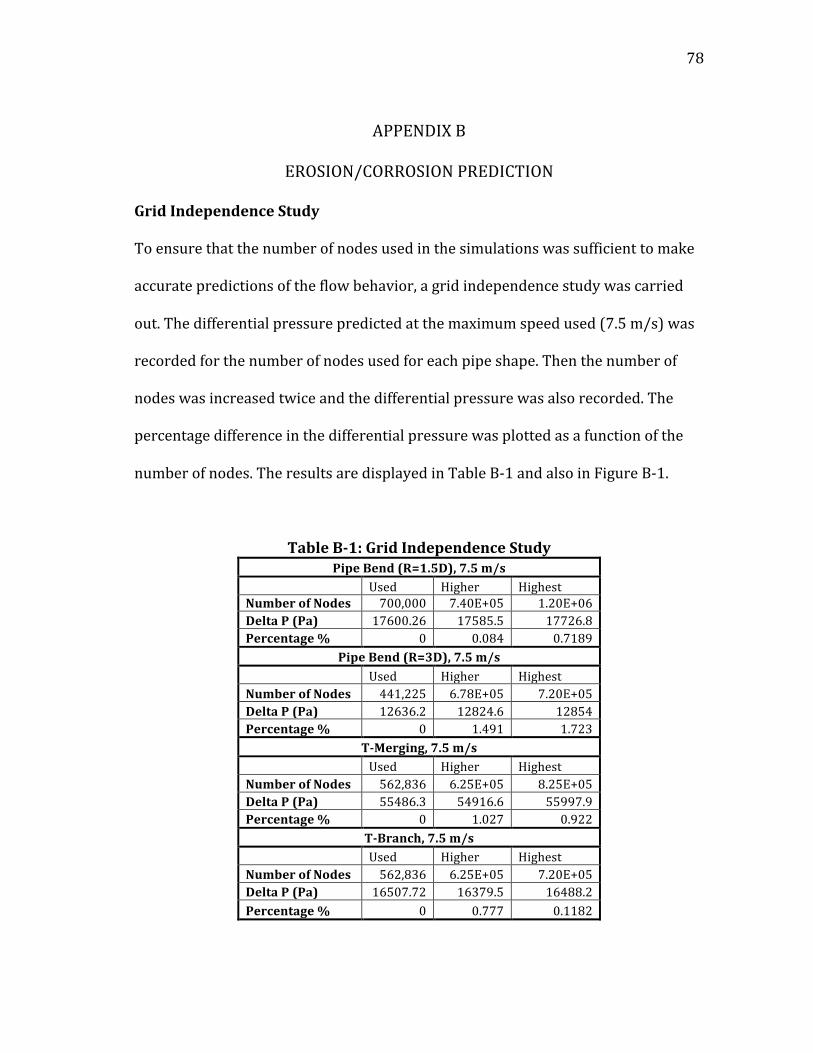
78
78
APPENDIX B
EROSION/CORROSION PREDICTION
Grid Independence Study
To ensure that the number of nodes used in the simulations was sufficient to make
accurate predictions of the flow behavior, a grid independence study was carried
out. The differential pressure predicted at the maximum speed used (7.5 m/s) was
recorded for the number of nodes used for each pipe shape. Then the number of
nodes was increased twice and the differential pressure was also recorded. The
percentage difference in the differential pressure was plotted as a function of the
number of nodes. The results are displayed in Table B-‐1 and also in Figure B-‐1.
Table B-‐1: Grid Independence Study Pipe Bend (R=1.5D), 7.5 m/s
Used Higher Highest Number of Nodes 700,000 7.40E+05 1.20E+06 Delta P (Pa) 17600.26 17585.5 17726.8 Percentage % 0 0.084 0.7189
Pipe Bend (R=3D), 7.5 m/s Used Higher Highest Number of Nodes 441,225 6.78E+05 7.20E+05 Delta P (Pa) 12636.2 12824.6 12854 Percentage % 0 1.491 1.723
T-‐Merging, 7.5 m/s Used Higher Highest Number of Nodes 562,836 6.25E+05 8.25E+05 Delta P (Pa) 55486.3 54916.6 55997.9 Percentage % 0 1.027 0.922
T-‐Branch, 7.5 m/s Used Higher Highest Number of Nodes 562,836 6.25E+05 7.20E+05 Delta P (Pa) 16507.72 16379.5 16488.2 Percentage % 0 0.777 0.1182

79
79
Figure B-‐1: Differential Pressure Percentage Difference as a Function of Number of Nodes
The results of this study show that any increase in the number of nodes has a very
negligible effect on the results (less than 2%) in the worst case. Therefore, the
number of nodes that was used in the simulations was sufficient to make accurate
predictions of the flow.
0 0.5 1
1.5 2
2.5 3
400,000 900,000 1,400,000
Differential Pressure
Percentage difference
(%)
Number of Nodes
Pipe Bend (R=1.5D)
Pipe Bend (R=3D)
T-‐Merging
T-‐Branch

80
80
Tables Used in Figures
Shape Speed (m/s)
Maximum Turbulent Kinetic Energy (near-‐wall) (m2/s2)
Maximum Wall Shear Stress (Pascal)
Maximum EC Rate (mm/yr)
Pipe bend (R=3D) 1.2 0.032 6.67 0.22 2.5 0.08 21 0.225 3.6 0.267 52.5 0.225 2.4 0.121 24.6 0.26 0.26 0.003 1.34 0.195 7.5 0.9 165 0.1 Pipe bend (R=1.5D) 1.2 0.018 6.03 0.29 2.5 0.071 21.5 0.29 3.6 0.146 48.7 0.32 2.4 0.066 22.3 0.34 0.26 0.00335 1.4 0.255 7.5 0.6 162 0.13 T-‐section (merging) 1.2 0.04 10.011 0.155 2.5 0.772 142.5 0.155 3.6 0.89 78.8 0.17 2.4 0.4 36.64 0.18 0.26 0.005 2.26 0.135 7.5 3 331 0.07 T-‐section (branch) 1.2 0.11 7.84 0.72 2.5 0.42 31 0.73 3.6 0.5 62.7 0.795 2.4 0.18 29 0.855 0.26 0.0041 1.68 0.64 7.5 1.95 238.5 0.325
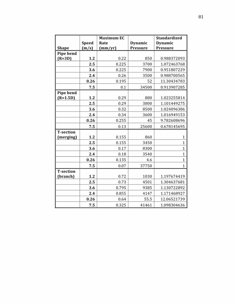
81
81
Shape Speed (m/s)
Maximum EC Rate (mm/yr)
Dynamic Pressure
Standardized Dynamic Pressure
Pipe bend (R=3D) 1.2 0.22 850 0.988372093 2.5 0.225 3700 1.072463768 3.6 0.225 7900 0.951807229 2.4 0.26 3500 0.988700565 0.26 0.195 52 11.30434783 7.5 0.1 34500 0.913907285 Pipe bend (R=1.5D) 1.2 0.29 880 1.023255814 2.5 0.29 3800 1.101449275 3.6 0.32 8500 1.024096386 2.4 0.34 3600 1.016949153 0.26 0.255 45 9.782608696 7.5 0.13 25600 0.678145695 T-‐section (merging) 1.2 0.155 860 1 2.5 0.155 3450 1 3.6 0.17 8300 1 2.4 0.18 3540 1 0.26 0.135 4.6 1 7.5 0.07 37750 1 T-‐section (branch) 1.2 0.72 1030 1.197674419 2.5 0.73 4501 1.304637681 3.6 0.795 9385 1.130722892 2.4 0.855 4147 1.171468927 0.26 0.64 55.5 12.06521739 7.5 0.325 41461 1.098304636
82
82
VITA
Sally Samir Farid Nicola received her Bachelor of Science degree in chemical
engineering from Texas A&M University at Qatar in May 2010. She enrolled in the
Master of Science in safety engineering program at Texas A&M University, College
Station, Texas in September 2010 and joined the Mary Kay O’Connor Process Safety
Center at the same time. She received her M.S. in safety engineering in August 2012.
Ms. Nicola may be reached at Jack E. Brown Engineering Building, 3122 TAMU
Room 200, College Station, Texas-‐77843, or via email at [email protected].