NEW YORK ECONOMIC REVIEW - NY State Economics Association
77
NEW YORK ECONOMIC REVIEW SpECIal ISSuE: SpORtS ECONOMICS GuESt EdItOR: E. FRaNK StEphESON, BERRY COllEGE JOuRNal OF thE NEW YORK StatE ECONOMICS aSSOCIatION VOluME lI NYSEa
Transcript of NEW YORK ECONOMIC REVIEW - NY State Economics Association

NEW YORK ECONOMIC REVIEW
SpECIal ISSuE: SpORtS ECONOMICS GuESt EdItOR: E. FRaNK StEphESON, BERRY COllEGE
JOuRNal OF thE NEW YORK StatE
ECONOMICS aSSOCIatION
VOluME lI
NYSEa
NEW YORK ECONOMIC REVIEW Volume 51, Fall 2020
1
NEW YORK STATE ECONOMICS ASSOCIATION
FOUNDED 1948
2018-2019 OFFICERS President:
SEAN MacDONALD • NEW YORK CITY COLLEGE OF TECHNOLOGY, CUNY Vice-President: Secretary: MICHAEL McAVOY • SUNY ONEONTA Treasurer:
PHILIP SIRIANNI • SUNY ONEONTA Editorial Board: DAVID VITT • EDITOR • FARMINGDALE STATE COLLEGE BRID G. HANNA • ASSOCIATE EDITOR • ROCHESTER INSTITUTE OF TEHCHNOLGOY CRISTIAN SEPULVEDA • ASSOCIATE EDITOR • FARMINGDALE STATE COLLEGE
RICK WEBER • ASSOCIATE EDITOR • FARMINGDALE STATE COLLEGE Web Coordinator: KPOTI KITISSOU • SUNY ONEONTA Board of Directors: LAUREN CALIMERIS • ST. JOHN FISHER COLLEGE
CHUKWUDI IKWUEZE • QUEENSBOROUGH COMMUNITY COLLEGE, CUNY KENNETH LIAO • FARMINGDALE STATE COLLEGE ARIDAM MANDAL • SIENA COLLEGE MICHAEL O’HARA • ST. LAWRENCE UNIVERSITY MANIMOY PAUL • SIENA COLLEGE
KASIA PLATT • SUNY OLD WESTBURY DELLA SUE • MARIST COLLEGE
WADE THOMAS • SUNY ONEONTA RICK WEBER • FARMINGDALE STATE COLLEGE
Conference Proceedings Editor MANIMOY PAUL • SIENA COLLEGE
The views and opinions expressed in the Journal are those of the individual authors and do not necessarily represent those of individual staff members or the New York State Economics
Association.

NEW YORK ECONOMIC REVIEW Volume 51, Fall 2020
2
Vol. 51, Summer 2020
CONTENTS
ARTICLES The Impact of WVU Football and Basketball on Hotel Demand Daniel D. Bonneau, Joshua C. Hall …………..…………………………..…………………………..5 Would Columbus Miss the Crew? Major League Soccer and Hotel Occupancy Kathleen M. Sheehan, E. Frank Stephenson ………..……………………..…….…………...………16 Fan Reaction to Pace-of-Play Rule Changes: Game Duration and Attendance in Major League Baseball Rodney J. Paul, Andrew Weinbach …………………..…………………………..………………..……23 Waving the White Flag: The Attendance Effects of Trading Away Talent by Contending Teams Sammi Schussele, Michael Davis …………………………………………..……………………..……35 Collector Preferences for Hall-of_fame Baseball Player Picture Cards 1981-2010 Michael R. McAvoy………………………………………………………………………………………..44 Determinants of Division 1 NCAA Soccer Participation
Andrew Weinbach, Robert F. Salvino..…………………………………………..…………..…………63 Referees……..………………………………………………….……………………………………………..……77
NEW YORK ECONOMIC REVIEW Volume 51, Fall 2020
3
EDITORIAL
The New York Economic Review (NYER) is an annual publication of the New York State Economics Association (NYSEA). The NYER publishes theoretical and empirical articles, and also interpretive reviews of the literature in the fields of economics and finance. All well-written, original manuscripts are welcome for consideration at the NYER. We also encourage the submission of short articles and replication studies. Special Issue proposals are welcome and require a minimum of 4 papers to be included in the proposal, as well as a list of suggested referees.
MANUSCRIPT GUIDELINES
1. All manuscripts are to be submitted via e-mail to the editor in a Microsoft Word file format, with content
formatted according to the guidelines at: https://www.nyseconomicsassociation.org/NYER/Guidelines
Manuscript submissions should be emailed to editor David Vitt at [email protected] The NYER is cited in:
• EconLit by the American Economic Association • Ulrich’s International Periodicals Directory • Cabell’s Directory of Publishing Opportunities
in Business and Economics
ISSN NO: 1090-5693

NEW YORK ECONOMIC REVIEW Volume 51, Fall 2020
4
Copyright Notice
As a condition of publication in the New York Economic Review, all authors agree to the following terms of
licensing/copyright ownership:
First publication rights to original work accepted for publication is granted to the New York Economic
Review but copyright for all work published in the journal is retained by the author(s).
Works published in the New York Economic Review will be distributed under a Creative Commons
Attribution License (CC-BY-NC-ND). By granting a CC-BY-NC-ND license in their work, authors retain
copyright ownership of the work, but they give explicit permission for others to download, reuse, reprint,
distribute, and/or copy the work, as long as the original source and author(s) are properly cited (i.e. a complete
bibliographic citation and link to the New York State Economics Association website). No permission is
required from the author(s) or the publishers for such use. According to the terms of the CC-BY-NC-ND
license, any reuse or redistribution must indicate the original CC-BY-NC-ND license terms of the work. The
No-Derivatives attribute of the license allows changing the format, but not modifying the text or tables as to
content. The Non-Commercial attribute of the license disallows users to reproduce the work or create
derivatives for the purpose of commercial gain.
Exceptions to the application of the CC-BY-NC-ND license may be granted at the editors’ discretion if
reasonable extenuating circumstances exist. Such exceptions must be granted in writing by the editors of
the Journal; in the absence of a written exception, the CC-BY-NC-ND license will be applied to all published
works. We provisionally exclude indexing services like EconLit or Ebsco from the Non-Commercial attribute,
contact the editor for a letter reflecting this.
Authors may enter into separate, additional contractual agreements for the non-exclusive distribution of the
published version of the work, with an acknowledgement of its initial publication in the New York Economic
Review
Authors are permitted to post their work online in institutional/disciplinary repositories or on their own
websites. Pre-print versions posted online should include a citation and link to the final published version
in the New York Economic Review as soon as the issue is available; post-print versions (including the final
publisher's PDF) should include a citation and link to the website of the New York State Economics
Association.

NEW YORK ECONOMIC REVIEW Volume 51, Fall 2020
5
The Impact of WVU Football and Basketball on Hotel Demand
Daniel D. Bonneau* & Joshua C. Hall* *Department of Economics, John Chambers College of Business and Economics, West Virginia University, Morgantown WV 26506. ABSTRACT
This paper uses daily hotel occupancy data for the Greater Morgantown area to estimate the effect of West Virginia
University football and basketball games on hotel demand. Hotel demand is an important part of the economic activity
generated by sporting events because hotel rooms are largely occupied by out-of-town guests. Their expenditures,
therefore, are likely to represent new local economic activity. We look at the effect of Mountaineer football and basketball
games on average daily room rates, revenue per room, demand, occupancy, and total revenue. We find large and
statistically significant effects of Mountaineer football on hotel demand with very little evidence of crowding out. Our
estimates for basketball, while statistically significant in a positive direction, are considerably smaller. WVU football
games bring in approximately $360,000 in additional hotel revenue from each football home game, while WVU basketball
games generate about $20,000 in additional hotel revenue.
INTRODUCTION
For some communities, tourism is the fuel the drives the local economy. For others, tourism plays a
small, but economically meaningful role in their economy through increased employment and tax revenue
due to the spending of out-of-town visitors. With the largest university in the state of West Virginia located in
the greater Morgantown area (population approximately 140,000), it plays host to regular events such as
motorcycle rallies, challenging marathons, visits from prospective parents and students, and of course the
West Virginia University Mountaineers. The college town is visibly packed with economic activity on days
where the 60,000 capacity Milan Puskar Stadium hosts a WVU football game.
While it may appear obvious that these mega sporting events (for a college town) bring many visitors
from outside the greater Morgantown area; measuring the net impact of WVU football and basketball games
can prove to be difficult due to offsetting behavior on behalf of local residents or tourists uninterested in
major college athletics. For example, while spending on sports might increase due to a major athletic event
that might largely reflect substitution from consumer spending elsewhere in economy (Coates and
Humphreys, 2002). Similarly, convention organizers know that average daily room rates at hotels will be
higher during major sporting events. Therefore, they may move conventions that attract out-of-town guests
to weekends with away games, or to the spring. This redistribution of economic activity to other dates makes
it difficult to estimate the economic impact of athletic events and is one reason why many ex ante analyses
tend to overestimate the magnitude of the positive impacts compared to ex post analyses of the same event
(Matheson, 2002).

NEW YORK ECONOMIC REVIEW Volume 51, Fall 2020
6
This paper tests for economic impacts associated with WVU football and basketball games by examining
daily hotel occupancy data on the Morgantown metropolitan area, provided by STR, a firm that specializes
in metropolitan lodging data worldwide. In doing so, we build off a growing literature that uses changes in
hotel demand to estimate part of the economic impact of sports (Depken and Stephenson, 2018), same- sex
marriage legalization (Earhart and Stephenson, 2018), and political conventions (Heller et al., 2018). The
current paper contributes to the existing literature on the economic impact of college sports on local
economies. Baade et al. (2008) look at 63 metropolitan areas that host major college football from 1970 to
2004 and find no positive impact on employment or income levels. Most relevant to the current paper, they
examine 42 small college towns and find football success reduces the growth rate of per capita personal
income. Baade et al. (2011) investigate the effect of home football and basketball games at the University
of Florida and Florida State University, finding that basketball has zero impact on taxable sales, while football
increases taxable sales by $2 million per home game. Using monthly sales revenue, Coates and Depken
(2009) find that, on average, increases in sales tax revenue due to the game is exactly offset by a reduction
in local spending in other areas. Coates and Depken (2011) find, however, that a full season of major college
football has the same impact on local sales tax revenue as a hosting the Super Bowl. Lentz and Laband
(2009) conduct an MSA level analysis of college athletics and find that there exists a positive relationship
between athletics revenues and employment in accommodations and food services industries.
Our analysis provides an estimate of the economic impact of WVU football and basketball on the
Morgantown economy, which may be of interest to policymakers. A 2012 study conducted by WVU’s Bureau
of Business and Economics Research (BBER) found that each home football game generated approximately
$1.6 million in revenue, creating an impact of over $11 million over the course of a season (Christiadi, 2012).
The study employs a survey method in which local lodging, drinking, and eating establishment self-report
their data for game days and non-game days to gauge the net impact. While our methodology cannot
estimate the local impacts from dining and drinking, we hope to more precisely estimate the net effects of
WVU football and basketball from out-of-town visitors using hotel demand. Given that very few Morgantown
residents use hotels for home games, increases in room rates and occupancy rates related to these events
provide a good estimate of out-of-area visitors. To preview our results, we find statistically significant
evidence that WVU football and basketball home games increase hotel occupancy and revenue. Only
football games, however, have an economically meaningful impact.
We proceed as follows. Section 2 discusses our daily hotel data and our empirical approach. In Section
3 we present our primary results, while Section 4 focuses on robustness checks. Section 5 concludes. DATA AND EMPIRICAL APPROACH
This study uses nightly hotel data from Greater Morgantown for the period January 1, 2005 to December
31, 2017. The data were obtained from STR, a firm that compiles hotel occupancy data from the U.S. and
other countries. This detailed data is then matched with WVU’s football and basketball schedule. Our
variables of interest are occupancy, average daily room rate (ADR), demand, revenue per available room
NEW YORK ECONOMIC REVIEW Volume 51, Fall 2020
7
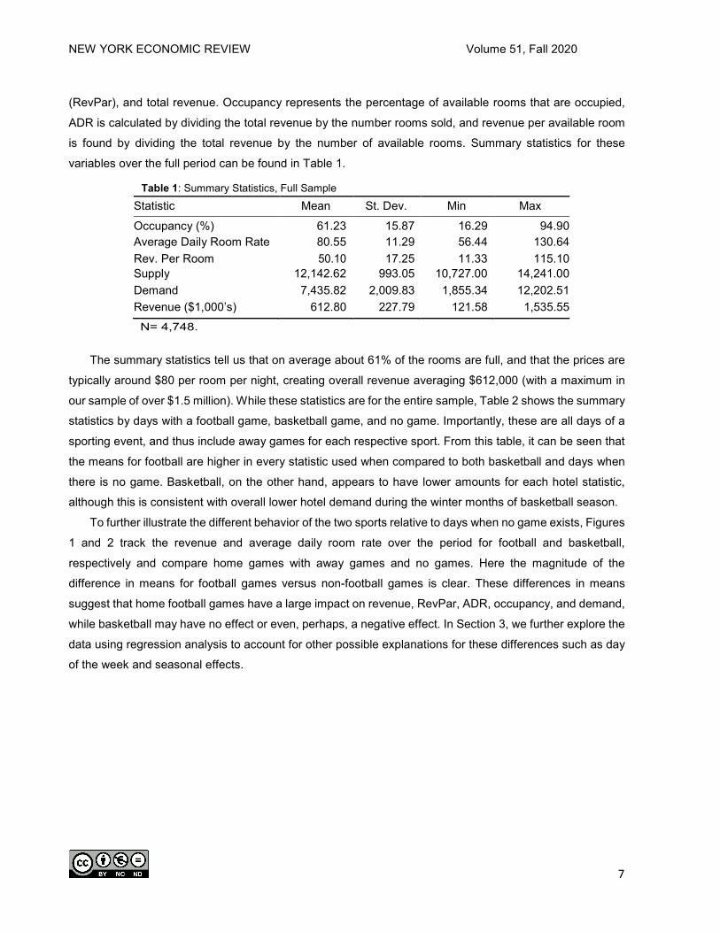
(RevPar), and total revenue. Occupancy represents the percentage of available rooms that are occupied,
ADR is calculated by dividing the total revenue by the number rooms sold, and revenue per available room
is found by dividing the total revenue by the number of available rooms. Summary statistics for these
variables over the full period can be found in Table 1.
Table 1: Summary Statistics, Full Sample
Statistic Mean St. Dev. Min Max
Occupancy (%) 61.23 15.87 16.29 94.90 Average Daily Room Rate 80.55 11.29 56.44 130.64 Rev. Per Room 50.10 17.25 11.33 115.10 Supply 12,142.62 993.05 10,727.00 14,241.00 Demand 7,435.82 2,009.83 1,855.34 12,202.51 Revenue ($1,000’s) 612.80 227.79 121.58 1,535.55 N= 4,748.
The summary statistics tell us that on average about 61% of the rooms are full, and that the prices are
typically around $80 per room per night, creating overall revenue averaging $612,000 (with a maximum in
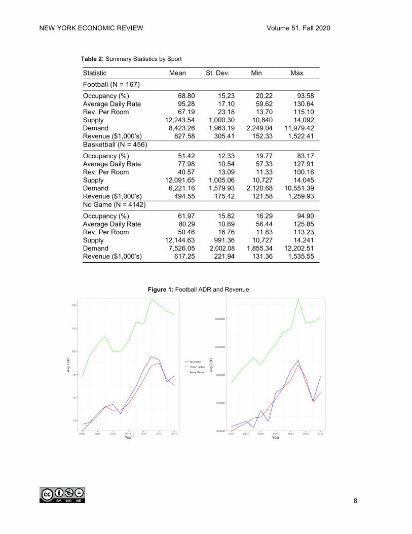
our sample of over $1.5 million). While these statistics are for the entire sample, Table 2 shows the summary
statistics by days with a football game, basketball game, and no game. Importantly, these are all days of a
sporting event, and thus include away games for each respective sport. From this table, it can be seen that
the means for football are higher in every statistic used when compared to both basketball and days when
there is no game. Basketball, on the other hand, appears to have lower amounts for each hotel statistic,
although this is consistent with overall lower hotel demand during the winter months of basketball season.
To further illustrate the different behavior of the two sports relative to days when no game exists, Figures
1 and 2 track the revenue and average daily room rate over the period for football and basketball,
respectively and compare home games with away games and no games. Here the magnitude of the
difference in means for football games versus non-football games is clear. These differences in means
suggest that home football games have a large impact on revenue, RevPar, ADR, occupancy, and demand,
while basketball may have no effect or even, perhaps, a negative effect. In Section 3, we further explore the
data using regression analysis to account for other possible explanations for these differences such as day
of the week and seasonal effects.
NEW YORK ECONOMIC REVIEW Volume 51, Fall 2020
8
Table 2: Summary Statistics by Sport
Statistic Mean St. Dev. Min Max Football (N = 167)
Occupancy (%) 68.80 15.23 20.22 93.58 Average Daily Rate 95.28 17.10 59.62 130.64 Rev. Per Room 67.19 23.18 13.70 115.10 Supply 12,243.54 1,000.30 10,840 14,092 Demand 8,423.26 1,963.19 2,249.04 11,979.42 Revenue ($1,000’s) 827.58 305.41 152.33 1,522.41 Basketball (N = 456) Occupancy (%) 51.42 12.33 19.77 83.17 Average Daily Rate 77.98 10.54 57.33 127.91 Rev. Per Room 40.57 13.09 11.33 100.16 Supply 12,091.65 1,005.06 10,727 14,045 Demand 6,221.16 1,579.93 2,120.68 10,551.39 Revenue ($1,000’s) 494.55 175.42 121.58 1,259.93 No Game (N = 4142) Occupancy (%) 61.97 15.82 16.29 94.90 Average Daily Rate 80.29 10.69 56.44 125.85 Rev. Per Room 50.46 16.76 11.83 113.23 Supply 12,144.63 991.36 10,727 14,241 Demand 7,526.05 2,002.08 1,855.34 12,202.51 Revenue ($1,000’s) 617.25 221.94 131.36 1,535.55
Figure 1: Football ADR and Revenue

NEW YORK ECONOMIC REVIEW Volume 51, Fall 2020
9
Figure 2: Basketball ADR and Revenue
EMPIRICAL RESULTS
Table 3: Football Regressions
Dep. Variable ADR RevPar Demand Occupancy Revenue Mean 80.54 50.09 7,435.81 61.22 612.8 Football - 4 -0.117 0.577 75.831 0.381 9.779 (0.408) (0.811) (96.171) (0.804) (10.055) Football - 3 0.59 1.103 88.234 0.484 16.451 (0.411) (0.818) (96.975) (0.811) (10.139) Football - 2 1.439 *** 1.326 52.648 0.288 18.15 * (0.415) (0.824) (97.729) (0.817) (10.218) Football -1 21.159 *** 22.575 *** 1023.701 *** 8.165 *** 280.781 *** (0.416) (0.827) (98.095) (0.820) (10.256) Home Football 24.816 *** 29.220 *** 1499.803 *** 12.121 *** 360.789 *** (0.423) (0.841) (99.734) (0.834) (10.427) Football +1 1.617 *** 0.567 -43.529 -0.128 5.235 (0.389) (0.773) (91.714) (0.767) (9.589) Football +2 0.453 -0.342 -119.983 -0.981 -3.737 (0.389) (0.773) (91.648) (0.766) (9.582) Football +3 0.370 1.160 111.516 0.841 15.363 (0.382) (0.760) (90.096) (0.753) (9.420) Football +4 -0.036 1.03 135.189 1.092 13.19 (0.381) (0.756) (89.716) (0.750) (9.380) Day of Week FE Week FE Month FE Year FE R-Squared 0.943 0.904 0.901 0.888 0.915
Note: ∗∗∗ p < 0.01, ∗∗p < 0.05, ∗p < 0.1. Intercept included but not reported. N = 4,748 for all models. The dependent variable is noted across the top of each model. The full sample mean of each dependent variable is provided above the regression results for reference.
NEW YORK ECONOMIC REVIEW Volume 51, Fall 2020
10
The effect of a home football game is significant across all dependent variables, as is the day before a
home football game. This makes sense as many football games have a start time of noon on Saturday,
suggesting we should expect an increase on the day before as visitors come in. The results are quite stark,
with over a 50% increase in the revenue and revenue per available room. Average daily room rates increase
as well by almost 30% while occupancy increases to about 75%.
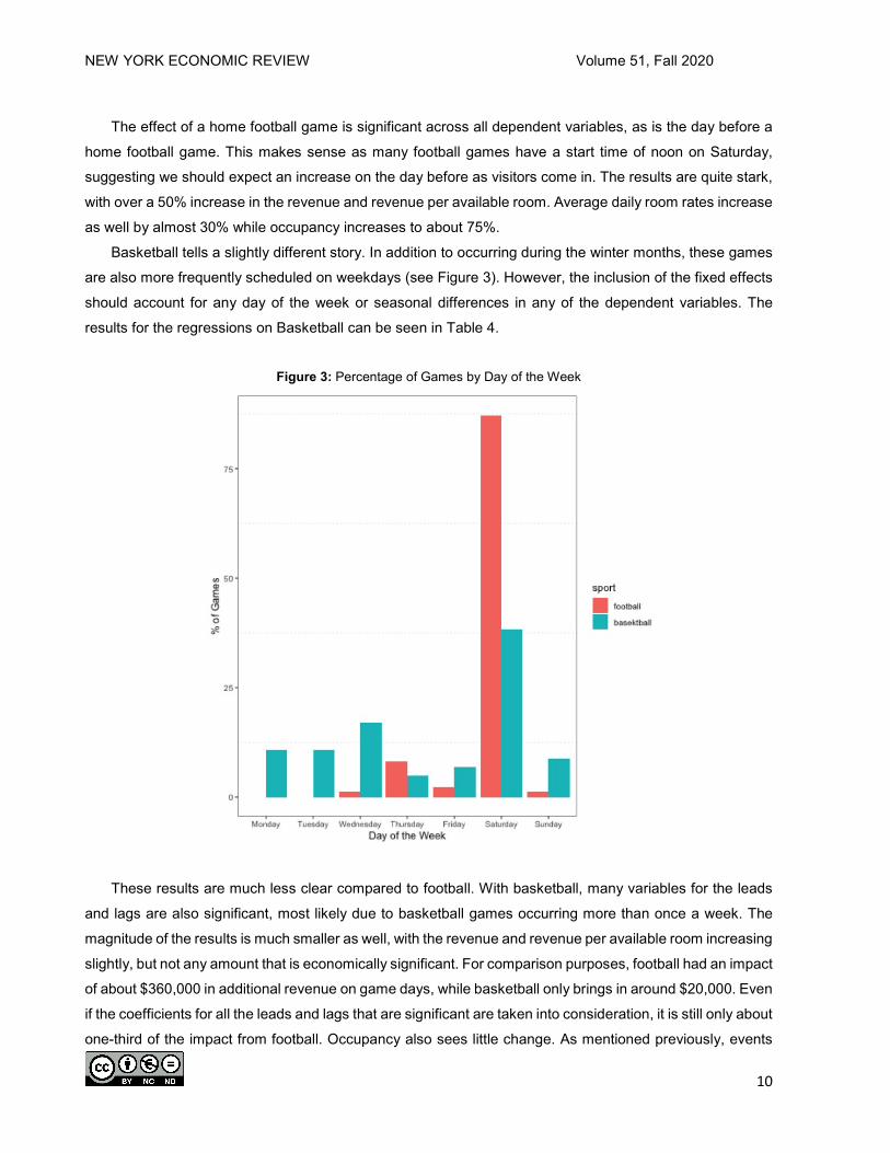
Basketball tells a slightly different story. In addition to occurring during the winter months, these games
are also more frequently scheduled on weekdays (see Figure 3). However, the inclusion of the fixed effects
should account for any day of the week or seasonal differences in any of the dependent variables. The
results for the regressions on Basketball can be seen in Table 4.
Figure 3: Percentage of Games by Day of the Week
These results are much less clear compared to football. With basketball, many variables for the leads
and lags are also significant, most likely due to basketball games occurring more than once a week. The
magnitude of the results is much smaller as well, with the revenue and revenue per available room increasing
slightly, but not any amount that is economically significant. For comparison purposes, football had an impact
of about $360,000 in additional revenue on game days, while basketball only brings in around $20,000. Even
if the coefficients for all the leads and lags that are significant are taken into consideration, it is still only about
one-third of the impact from football. Occupancy also sees little change. As mentioned previously, events

NEW YORK ECONOMIC REVIEW Volume 51, Fall 2020
11
may have the adverse effect of crowding out other visitors who would be coming to the area for other events.
This most likely occurs because Morgantown is a destination city for little else than events hosted by the
University, with only a few other events occurring throughout any given year. While it is clear that basketball
would not have a crowding out effect due to the small impact of games on occupancy, football’s impact is
much greater. Even with this larger effect, occupancy remains around 75% on average, though there may
be certain games, namely games against rivals or highly ranked opponents, where this crowding out effect
may occur.
Table 4: Basketball Regressions
Dep. Variable ADR RevPar Demand Occupancy Revenue Mean 80.54 50.09 7,435.81 61.22 612.8 Basketball - 4 0.136 0.099 -7.079 -0.049 -1.622 (0.413) (0.628) (63.277) (0.527) (7.769) Basketball - 3 0.518 1.790 *** 223.898 *** 1.792 *** 22.276 *** (0.444) (0.675) (67.962) (0.567) (8.350) Basketball - 2 0.433 1.613 ** 208.324 *** 1.705 *** 20.09 ** (0.447) (0.679) (68.411) (0.571) (8.406) Basketball -1 -0.338 0.583 162.659 ** 1.363 ** 7.062 (0.434) (0.660) (66.436) (0.554) (8.163) Home Basketball 0.588 1.614 ** 228.084 *** 1.844 *** 19.846 ** (0.433) (0.658) (66.231) (0.553) (8.138) Basketball +1 1.466 *** 2.610 *** 207.997 *** 1.706 *** 31.823 *** (0.438) (0.666) (67.106) (0.560) (8.245) Basketball +2 1.138 ** 1.298 * 62.782 0.634 14.509 * (0.446) (0.678) (68.312) (0.570) (8.393) Basketball +3 0.902 ** 0.863 31.873 0.360 9.453 (0.439) (0.667) (67.202) (0.561) (8.257) Basketball +4 1.135 *** 1.672 *** 108.446 * 0.877 * 20.839 *** (0.417) (0.634) (63.842) (0.533) (7.844) Day of Week FE Week FE Month FE Year FE R-Squared 0.855 0.856 0.892 0.88 0.874
Note: ∗∗∗ p < 0.01, ∗∗p < 0.05, ∗p < 0.1. Intercept included but not reported. N = 4,748 for all models. The dependent variable is noted across the top of each model. The full sample mean of each dependent variable is provided above the regression results for reference.
The results presented in this section suggest that while including a number of fixed effects, sports games
in the Morgantown area have a positive impact on hotel revenues and occupancy, suggesting that there is
an increase in visitors from outside of the area. These results lend credence to the idea that these events
are having the expected positive effect. However, to test if this is due to any sort of random chance, placebo
regressions are run and included in the following section. Additionally, the impact of changing conferences
is evaluated.
NEW YORK ECONOMIC REVIEW Volume 51, Fall 2020
12
ROBUSTNESS CHECKS
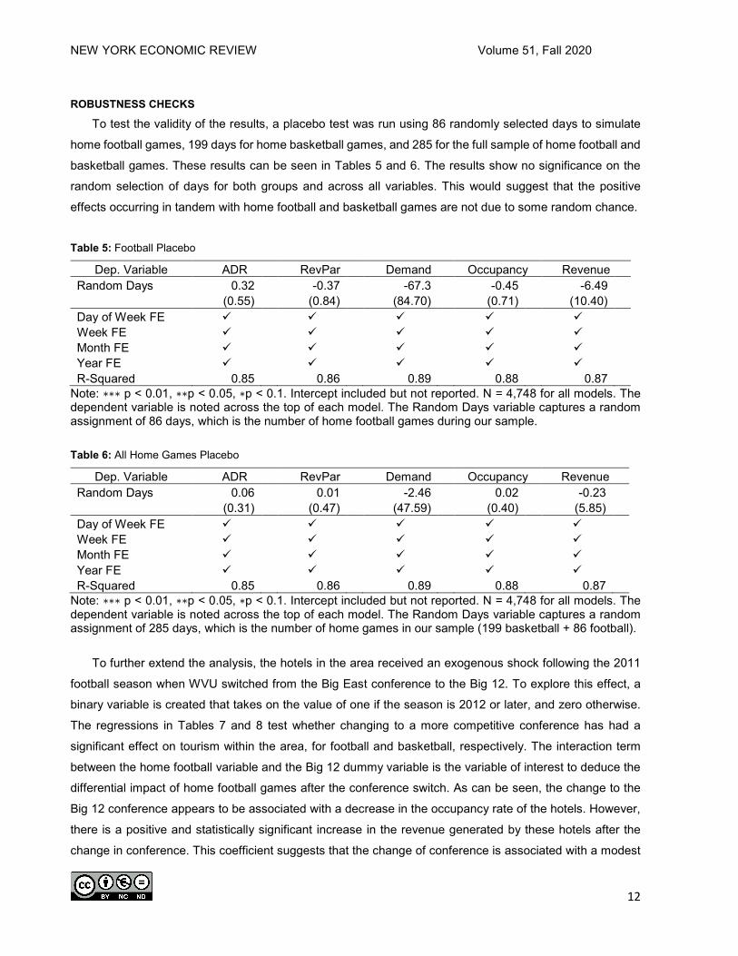
To test the validity of the results, a placebo test was run using 86 randomly selected days to simulate
home football games, 199 days for home basketball games, and 285 for the full sample of home football and
basketball games. These results can be seen in Tables 5 and 6. The results show no significance on the
random selection of days for both groups and across all variables. This would suggest that the positive
effects occurring in tandem with home football and basketball games are not due to some random chance.
Table 5: Football Placebo
Dep. Variable ADR RevPar Demand Occupancy Revenue Random Days 0.32 -0.37 -67.3 -0.45 -6.49 (0.55) (0.84) (84.70) (0.71) (10.40) Day of Week FE Week FE Month FE Year FE R-Squared 0.85 0.86 0.89 0.88 0.87
Note: ∗∗∗ p < 0.01, ∗∗p < 0.05, ∗p < 0.1. Intercept included but not reported. N = 4,748 for all models. The dependent variable is noted across the top of each model. The Random Days variable captures a random assignment of 86 days, which is the number of home football games during our sample. Table 6: All Home Games Placebo
Dep. Variable ADR RevPar Demand Occupancy Revenue Random Days 0.06 0.01 -2.46 0.02 -0.23 (0.31) (0.47) (47.59) (0.40) (5.85) Day of Week FE Week FE Month FE Year FE R-Squared 0.85 0.86 0.89 0.88 0.87
Note: ∗∗∗ p < 0.01, ∗∗p < 0.05, ∗p < 0.1. Intercept included but not reported. N = 4,748 for all models. The dependent variable is noted across the top of each model. The Random Days variable captures a random assignment of 285 days, which is the number of home games in our sample (199 basketball + 86 football).
To further extend the analysis, the hotels in the area received an exogenous shock following the 2011
football season when WVU switched from the Big East conference to the Big 12. To explore this effect, a
binary variable is created that takes on the value of one if the season is 2012 or later, and zero otherwise.
The regressions in Tables 7 and 8 test whether changing to a more competitive conference has had a
significant effect on tourism within the area, for football and basketball, respectively. The interaction term
between the home football variable and the Big 12 dummy variable is the variable of interest to deduce the
differential impact of home football games after the conference switch. As can be seen, the change to the
Big 12 conference appears to be associated with a decrease in the occupancy rate of the hotels. However,
there is a positive and statistically significant increase in the revenue generated by these hotels after the
change in conference. This coefficient suggests that the change of conference is associated with a modest

NEW YORK ECONOMIC REVIEW Volume 51, Fall 2020
13
increase of about $38,000 per game. Basketball, however, does not appear to be affected in any way by the
move to the Big 12 conference. Table 7: Big 12 Football
Dep. Variable ADR RevPar Demand Occupancy Revenue Home Football 20.72 *** 24.89 *** 1365.36 *** 12.11 *** 282.58 *** (0.64) (1.05) (114.40) (0.95) (13.02) Big 12 21.32 *** 19.11 * 2732.80 ** 13.93 317.12 *** (6.61) (10.85) (1181.02) (9.85) (134.46) Home Football * Big 12 -0.70 -1.09 -207.36 -3.81 *** 38.03 ** (0.92) (1.51) (164.26) (1.37) (18.70) Day of Week FE Week FE Month FE Year FE R-Squared 0.85 0.86 0.89 0.88 0.87
Note: ∗∗∗ p < 0.01, ∗∗p < 0.05, ∗p < 0.1. Intercept included but not reported. N = 4,748 for all models. The dependent variable is noted across the top of each model. The Big 12 dummy variable is equal to one if the year of the game is 2012 or later (the year WVU joined the conference). Table 8: Big 12 Basketball
Dep. Variable ADR RevPar Demand Occupancy Revenue Home Basketball 0.53 0.90 134.34 * 1.25 * 8.69 (0.51) (0.78) (78.37) (0.65) (9.63) Big 12 12.54 8.54 2167.36 * 9.31 187.68 (7.90) (12.02) (1210.71) (10.10) (148.78) Home Basketball * Big 12 -0.84 -0.77 -50.28 -0.82 -4.06 (0.74) (1.12) (1113.00) (0.94) (13.89) Day of Week FE Week FE Month FE Year FE R-Squared 0.85 0.86 0.89 0.88 0.87
Note: ∗∗∗ p < 0.01, ∗∗p < 0.05, ∗p < 0.1. Intercept included but not reported. N = 4,748 for all models. The dependent variable is noted across the top of each model. The Big 12 dummy variable is equal to one if the year of the game is 2012 or later (the year WVU joined the conference). CONCLUSION
This paper has investigated the impact of WVU home football and basketball games on hotel demand
and revenue. These measurements are used to uncover the extent to which major collegiate sports
contribute to the economy of a college town by bringing in external tourism dollars. The statistical significance
for both football and basketball games in the demand, occupancy, revenue, and average daily room rates
suggest that there is a positive impact of these games on tourism. The effects are economically meaningful
for football games.

NEW YORK ECONOMIC REVIEW Volume 51, Fall 2020
14
One concern of any small city holding large-scale events is that they may crowd out other visitors. We
find that the percentage of rooms that are occupied increases during WVU football and basketball games.
On average, however, this increase in the number of occupied rooms brings Morgantown hotels to about
75% of capacity. This suggests that while there may be individual games that induce crowding out, it is not
seen on average. Our results are robust to the inclusion of numerous fixed effects as well a placebo test.
Lastly, we find that the switch from the Big East to the Big 12 for WVU in 2012 appears to only have a modest
impact on revenue received from football games, with no impact from home basketball games. This finding
is perhaps unsurprising given the geographic distance from WVU to the rest of the Big 12 (Chatmon, 2016).
Our results suggest that there is an increase in hotel revenue of over $640,000 for each home football
game. (This is including the increased revenue of $360,789 for the day of a home football game and
$280,781 for the day before the game.) To put these results into context, we will use the local 6% lodging
tax rate to estimate the impact these games have on tax revenue using back of the envelope calculations.
Doing this suggests that there is an increase of over $38,000 in additional tax revenue for each home football
game. Extending these numbers throughout an entire season of 7 home games, the impact is quite large.
Hotels earn an additional $4.35 million in revenue, with over $261,000 in additional tax revenue collected
annually. This result of $4.35 million is about one-third of the estimates of Christiadi (2012), who evaluated
the impact of WVU home football games using a survey sent to local establishments. Basketball has a much
smaller impact, with only $1,100 per game in additional tax revenue, which over the course of a season,
does not reach the magnitude of a single home football game.
REFERENCES
Baade, Robert A., Robert W. Baumann and Victor. A. Matheson. 2008. “Assessing the Economic Impact of
College Football Games on Local Economies.” Journal of Sports Economics, 9(6): 628–643.
Baade, Robert A., Robert W. Baumann and Victor. A. Matheson. 2011. “Big Men on Campus: Estimating
the Economic Impact of College Sports on Local Economies.” Regional Studies, 45(3): 371–380.
Chatmon, Brandon. (2016). “Big 12 Move Bumps up Travel Time, Costs for West Virginia.” ESPN.com, 1
June.
Christiadi. 2012. The Economic Impact of One WVU Home Football Game on the Monongalia County
Economy. Morgantown WV: Bureau of Business and Economic Research.
Coates, Dennis and Craig A. Depken. 2009. “The Impact of College Football Games on Local Sales Tax
Revenue: Evidence from Four Cities in Texas.” Eastern Economic Journal, 35(4): 531–547.
Coates, Dennis and Craig A. Depken. 2011. “Mega-events: Is Baylor Football to Waco What the Super Bowl
is to Houston?” Journal of Sports Economics, 12(6): 599–620.
Coates, Dennis and Brad R. Humphreys. 2002. “The Economic Impact of Postseason Play in Professional
Sports.” Journal of Sports Economics, 3(3): 291–299.
Depken, Craig A. and E. Frank Stephenson. 2018. “Hotel Demand Before, During, and After Sports Events:
Evidence from Charlotte, North Carolina.” Economic Inquiry, 56(3): 1764–1776.

NEW YORK ECONOMIC REVIEW Volume 51, Fall 2020
15
Earhart, Michael and E. Frank Stephenson. 2018. “Same-sex Marriage Legalization and Wedding Tourism:
Evidence from Charleston and Savannah.” Journal of Economics and Finance, 42(3): 566–574.
Heller, Lauren R., Victor A. Matheson and E. Frank Stephenson. 2018. “Unconventional Wisdom: Estimating
the Economic Impact of the Democratic and Republican National Political Conventions.” Papers in
Regional Science, 97(4): 1267-1278.
Lentz, Bernard F. and David N. Laband. 2009. “The Impact of Intercollegiate Athletics on Employment in the
Restaurant and Accommodations Industries.” Journal of Sports Economics, 10(4): 351–368.
Matheson, Victor A. 2002. “Upon Further Review: An Examination of Sporting Event Economic Impact
Studies.” The Sport Journal, 5(1): 1–4.

NEW YORK ECONOMIC REVIEW Volume 51, Fall 2020
16
Would Columbus Miss the Crew? Major League Soccer and Hotel Occupancy
Kathleen M. Sheehan* & E. Frank Stephenson**
*Department of Economics and Finance, Creighton University, 2500 California Plaza, Omaha, NE 68178 **Department of Accounting, Economics, and Finance, Berry College, Box 5024, Mount Berry, GA 30149
ABSTRACT In late 2017, reports indicated that the Columbus Crew soccer team would relocate to Austin, Texas. This paper uses three years of daily data to examine the effect of the Crew, as well as other sports teams and events, on hotel room rentals, hotel room rates, and hotel revenues in Columbus. The results indicate that Ohio State University football games and a three-day rock music festival generate large increases in hotel room rentals, rates, and revenues, while the Crew, an NHL hockey franchise, and a minor league baseball team have small effects. The Crew ultimately stayed in Columbus under new ownership and with a large subsidy for a new stadium; nonetheless this paper yields insights on the overnight drawing power of various sporting and other events. INTRODUCTION
On October 16, 2017, news broke that the operator of Major League Soccer’s (MLS) Columbus
Crew was planning to move the club to Austin, Texas in 2019 (Arace 2017, Moore-Bloom 2019). The Crew’s
average home match attendance of 15,439 ranked 20th among the MLS’s 22 teams, and the team’s
management blamed its poor attendance in part to playing in an outdated stadium. With Columbus
apparently unwilling to publicly fund construction of a more modern playing facility, the team thought Austin
would provide greener pastures.
Crew fans were outraged at the possibility of losing their team, especially since the Crew were
among the league’s ten inaugural teams in 1996 and Columbus does not have NFL, NBA, or MLB franchises.
Crew fans formed an organization called Save the Crew and undertook highly publicized activities pressuring
Columbus and Ohio politicians to prevent the move. On October 22, 2017 Save the Crew held a large rally
at city hall, and the October 31, 2017 home game featured fans chanting “Save the Crew” (Moore-Bloom
2019). Ultimately, Ohio Attorney General Mike DeWine sued MLS and the Crew’s operator/investor Precourt
Ventures under the provisions of Ohio’s “Art Modell law” to prevent the Crew from moving (McCann 2018).
The Art Modell law, named for the team owner who moved the Cleveland Browns to Baltimore in 1996,
prohibits Ohio sports franchises that have played in taxpayer subsidized facilities from relocating unless they
have government permission or provide an opportunity for the team to be sold to new owners who would
keep the team in Ohio. Eventually, when this paper was at an advanced stage, MLS announced the Crew
would be transferred to an investor/operator group including Cleveland Browns owners Dee and Jimmy
Haslam and Crew team doctor Pete Edwards and would remain in Columbus on the condition of playing in
a new, publicly subsidized stadium (Ferenchik and Rouan 2018).
NEW YORK ECONOMIC REVIEW Volume 51, Fall 2020
17
Of course, a common concern in franchise relocations or the hosting of prominent sport events is
the economic impact associated with the event or franchise. Like many team or events, the Crew’s economic
impact had been analyzed. An economic impact study released by the team in 2012 reported that the Crew
had generated $384 million in additional spending between 1996 and 2011, with $160 million coming from
outside Franklin County (home of Columbus).1 The study also claimed that 69% of attendees came from
outside Columbus with 20% coming from outside Ohio.
Economic impact studies of this sort are controversial in the sports economics literature. Research
going back at least as far as Baade and Dye (1988, 1990) casts doubt on claims of large economic gains
associated with sports events and franchises. In a now somewhat dated literature review, Coates and
Humphreys (2008) found little evidence of large gains relative to the frequently sizable public subsidies
associated with sports teams and events. Among the limitations noted about traditional economic impact
studies such as the one performed for the Crew, one of the most important is the failure to differentiate
between gross and net visitors (Porter 1999, Baumann et al. 2009). Studies that fail to account for any
displacement of would be visitors overstate the gains associated with the event. In an effort to get a better
grasp on marginal visitors associated with sports events, recent papers such as Collins and Stephenson
(2016), Depken and Stephenson (2018), and Heller et al. (2018) use granular hotel occupancy data to
estimate the net effect of sports and other events on hotel occupancy, a key component of visitors’ economic
impact.
This paper uses a similar approach to examine the effect of Columbus Crew matches on local hotel
occupancy. While it appears the Columbus will retain the Crew, this paper remains valuable because, to
our knowledge, it is first paper to analyze the relationship between MLS matches and hotel occupancy.
Since the MLS continues to seek public subsidies as it expands to new cities, understanding the economic
impact of MLS franchises has important public policy implications. In addition, the paper controls for other
events in order to avoid omitted variable bias; it also estimates the effect of Columbus Blue Jackets National
Hockey League (NHL) games, Ohio State University (OSU) football and basketball games, Columbus
Clippers minor league baseball games, OSU graduation ceremonies, and a large rock music festival on hotel
occupancy.
EMPIRICAL FRAMEWORK
We use three years of daily hotel occupancy data from the Columbus metropolitan area spanning
December 1, 2014 to November 30, 2017 (1,066 observations) in the analysis. The data are obtained from
STR, a firm that compiles data from hotels in the U.S. and many other countries.
Our regression model is as follows:
1 https://www.columbuscrewsc.com/post/2012/02/08/columbus-crew-nets-regional-economic-benefits
NEW YORK ECONOMIC REVIEW Volume 51, Fall 2020
18
DEPt = β0 + β1EVENTS + β2UNEMPRATE + β3DAY + β4WEEK + εt. where DEPt is the number of hotel rooms rented on night t, the average daily rate (ADR) or price of the
rooms rented on night t, or the aggregate amount of hotel revenue on night t. Descriptive statistics for the
dependent variables are reported in Table 1.
Table 1: Descriptive Statistics Mean Std. Dev. Min. Max. Rooms 17,651 4,371 5,945 26,599 ADR 99.18 10.57 65.82 131.87 Revenue 1,792,012 585,573 401,093 3,507,765 Unemp Rate 4.86 0.42 4.1 5.7
The vector EVENTS contains dummy variables for Columbus Crew home matches, Columbus Blue
Jackets home games, Columbus Clippers home games, home games for OSU football and basketball,
OSU’s spring, summer, and autumn commencement ceremonies, and the Rock on the Range music festival.
OSU football games (21) are the least common event in our study while Columbus Clippers baseball games
(220) are the most common. The Crew had 56 home matches during our study period, or roughly 18-19 per
season. Counts for all of the included events are reported in Table 2. For Crew matches and OSU football
games, we also include dummies for the night before scheduled games in order to capture visitors who arrive
early. We also experimented with a dummy for two days before Crew matches and OSU football games, a
dummy for the day after Crew matches and OSU football games, and dummies for the day before Blue
Jackets games and OSU basketball games, but they are omitted because their inclusion has no effect on
the estimation results reported below. Our not needing to include day after effects for any events and day
before effects for only Crew matches and OSU football games indicates that there is little evidence that
Columbus’s sports events attract fans who come in advance of the events or stay beyond the events.
Table 2: Event Counts
Event Number of Occurrences Columbus Crew Home Matches 56 Ohio State Football Home Games 21 Ohio State Basketball Home Games 58 Columbus Blue Jackets Home Games 134 Columbus Clippers Home Games 220
Since the number of graduates likely differs for the commencement ceremonies, separate dummy
variables are created for the spring, summer, and autumn commencements. A dummy for the night before
each of the graduation exercises is also included since guests might arrive the day before the event. Rock
on the Range is a Friday to Sunday music festival held in May of each year. To allow for possible spillover
effects of the festival on hotel occupancy, we also include the Thursday before the festival and the Monday
after the festival in the regression models.

NEW YORK ECONOMIC REVIEW Volume 51, Fall 2020
19
To control for other factors affecting hotel occupancy, the unemployment rate (UNEMPRATE) is
included to control for changes in macroeconomic conditions. The model also includes fixed effects for days
of the week (DAY) since hotel occupancy can vary systematically across days of the week. Similarly, fixed
effects for week in the year (WEEK) are included to control for systematic variation in hotel occupancy across
seasons or because of holidays. (We also experimented with a trend variable but it had no qualitative effect
on the results.)
ESTIMATION RESULTS
The hotel occupancy data are stationary so the model is estimated via OLS with Newey-West
corrected standard errors to control for serial correlation. The estimation results are reported in Table 3.
Crew matches have no statistically significant effect on the number of hotel rooms let. The
magnitude is small—an additional 273 rooms rented on match days and 499 rooms rented on the night
before matches. These effects are smaller than would be expected based on the Crew’s economic impact
report. During the 2015-2017 seasons, the Crew averaged about 16,000 fans per home game so the
economic impact report implies more than 3,000 would come from outside Ohio and would presumably need
more than a few hundred rooms of lodging per night to accommodate them. Hotel data would fail to detect
out of state visitors who stay with local friends or family members or in AirBnBs, though short term rentals
account for a relatively small share of lodging relative to hotels. Another possible explanation for the
discrepancy between our findings and the claims of the economic impact report would be if that report
classified out of state OSU students who attended games as being out of state residents even though they
are at least temporarily residing in Columbus. Likewise, the estimated coefficients on the Crew variables in
the ADR regression are small (less than $1.15) and not statistically significant. The ADR results indicate
that Crew games are not associated with increases in daily room rates, a result which buttresses the
conclusion that Crew matches do not appreciably increase the demand for hotel rooms. With both the
number of rooms let and the ADR effects associated with Crew matches being small and statistically
insignificant, it is unsurprising that Crew matches also have no effect on hotel revenue.
Looking at the other events, OSU football has a significantly positive effect on room rentals, ADR,
and hotel revenue. The number of rooms rented increases by about 3,650 over the two nights, a figure
roughly one-third larger than Bonneau and Hall (this issue) find for West Virginia University home football
games. OSU football games also see prices increase $7-10 per room and hotel revenue increase by more
than $730,000. OSU basketball games are associated with increases of 357 rooms let and $55,000 in hotel
revenue, though neither effect is statistically different from zero. Neither Blue Jackets hockey games nor
Clippers baseball games has an economically or statistically significant increase in hotel rooms rented, ADR,
or hotel revenue.
OSU’s graduation ceremonies also have large effects on the number of hotel rooms let. The largest
effect is associated with the autumn graduation which increases room rentals by about 7,360 room nights,
ADR by $8-11 per night, and hotel revenue by $953,000. The spring commencement increases room rentals

NEW YORK ECONOMIC REVIEW Volume 51, Fall 2020
20
by about 4,000, ADR by roughly $5-9 per night, and hotel revenue by nearly $680,000. The summer
graduation has the smallest effects but it still generates nearly 1,900 additional room nights and
approximately $240,000 in additional hotel revenue.
Table 3: Estimation Results for Columbus Hotel Occupancy
Dependent Variable
Rooms ADR Revenue Day Before Crew 370.46 0.69 39,989 (1.03) (0.63) (0.70) Crew 151.44 -0.02 4,593 (0.42) (0.02) (0.08) Day Before OSU Football 1,319.84* 7.13** 259,091** (2.36) (3.47) (2.83) OSU Football 2,152.60** 10.13** 434,279** (3.48) (4.19) (3.91) OSU Basketball 374.74 0.89 57,975 (1.19) (0.88) (1.25) Blue Jackets -91.11 -0.60 -23,959 (0.49) (1.02) (0.87) Clippers -282.17 -1.74** -62,353 (1.23) (2.67) (1.84) Day Before Spring Grad. 3,247.86** 9.14** 545,808** (4.81) (4.59) (4.67) Spring Graduation 926.74 4.88* 150,058 (1.89) (2.23) (1.87) Day Before Summer Grad. 1,412.69** 2.92 195,034* (3.29) (1.55) (2.33) Summer Graduation 532.94 1.55 57,650 (0.87) (0.96) (0.70) Day Before Autumn Grad. 2,548.42* 10.12** 301,311* (2.50) (2.72) (2.29) Autumn Graduation 4,658.08** 8.56** 624,944** (5.49) (2.77) (5.99) Rock on the Range
Thursday 2,919.69** 1.98 327,076.75** (6.88) (1.67) (5.00)
Friday 6,150.75** 20.85** 1,110,373.55** (10.32) (15.04) (15.46)
Saturday 5,587.96** 22.01** 1,101,812.71** (7.56) (13.14) (11.22)
Sunday 5,923.12** 9.72** 695,358.61** (7.17) (4.50) (6.10)
Monday 1,850.73** 4.69** 250,883.10** (3.10) (3.75) (3.53) Unemp. Rate -982.31** -4.34** -180,673.49** (5.23) (7.61) (6.52) Constant 16,513.03** 103.36** 1,887,098.46** (15.06) (29.53) (11.98)
Parentheses contain t-statistics derived from Newey-West standard errors. * and ** indicate statistical significance at
the 5% and 1% level, respectively. The models also include fixed effects for days of the week and weeks of the year.
NEW YORK ECONOMIC REVIEW Volume 51, Fall 2020
21
The Rock on the Range music festival has large effects on hotel room nights, ADR, and hotel
revenue, and its effects begin the Thursday before the festival and continue through the Monday following
the festival. Over the five days, the festival generates more than 22,000 room nights and nearly $3.5 million
in additional hotel revenue. ADR increases by $21-22 for the Friday and Saturday nights of the festival and
by smaller amounts on the other three nights.
Macroeconomic conditions also have a large effect on the Columbus hotel market; a one percentage
point increase in the unemployment rate is associated with almost 1,000 fewer rooms rented per night, a $4
per night decrease in ADR, and a reduction of $179,000 per night in hotel revenue.
CONCLUSION
Contrary to claims by the Crew’s economic impact report, this paper’s results indicate that the Crew
have little effect in attracting overnight visitors to Columbus. Hence, it seems that most Crew fans reside in
Columbus or are close enough for day trips. While day trippers might increase economic activity in bars,
restaurants, or souvenir shops, much spending associated with the Crew is likely redirected from other local
activities. While some passionate fans would have missed the Crew, losing the team would have had little
effect on overnight visitors to Columbus. Yet taxpayers in Ohio, Franklin County, and Columbus are now
expected to pay at least $140 million for the new publically subsidized stadium (Bush 2019). The lack of
overnight visitors to Columbus should also be of concern to cities such as nearby Cincinnati which is currently
partially funding a stadium for an MLS expansion franchise through hotel taxes (Seitz 2018).
As previously noted, the overall economic impact of stadiums has long been questioned by
economists (Coates and Humphreys 2008). However, the Crew’s ability to obtain taxpayer subsidies by
threatening to move to Austin highlights how MLS and other closed sports leagues exploit their monopoly
power to restrict the supply of teams and foster competition among cities. Perhaps a new stadium will
generate more overnight visitors and economic gain than the existing stadium, but if it doesn’t much of the
economic benefit of the new stadium will be internalized by the Crew’s owners (Humphreys and Zhou 2015).
REFERENCES Arace, Michael, 2017, “Crew SC owner considering moving team to Austin, Texas,” Columbus Dispatch, October 16. https://www.dispatch.com/sports/20171016/crew-sc-owner-considering-moving-team-to-austin-texas Baumann, Robert, Victor Matheson, and Chihiro Muroi (2009), “Bowling in Hawaii: Examining the Effectiveness of Sports-Based Tourism Strategies,” Journal of Sports Economics, 10(1), pp. 107-123. Bonneau, Daniel D. and Joshua C. Hall, 2020, “The Impact of WVU Football and Basketball on Hotel Demand,” New York Economic Review, 51, pp. 5-15. Bush, Bill, 2019, “Public funding for new Crew stadium now up to $140 million, and land not yet acquired,” Columbus Dispatch, June 18. https://www.dispatch.com/news/20190618/public-funding-for-new-crew-stadium-now-up-to-140-million-and-land-not-yet-acquired.

NEW YORK ECONOMIC REVIEW Volume 51, Fall 2020
22
Coates, Dennis, and Brad R. Humphreys (2008), “Do Economists Reach a Conclusion on Subsidies for Sports Franchises, Stadiums, and Mega-events?” Econ Journal Watch, 5(3), pp. 294-315. Collins, Clay and E. Frank Stephenson (2016), “Using Hotel Occupancy Data to Evaluate the Efficacy of Sports Tourism: The Case of Rome, Georgia,” mimeo, Berry College. Depken, Craig A. II, and E. Frank Stephenson (2018), “Hotel Demand Before, During, and after Sports Events: Evidence from Charlotte, North Carolina,” Economic Inquiry, 56(3), pp. 1764-1776. Ferenchik, Mark, and Rick Rouan, 2018, “Columbus Crew is saved: MLS, ownership group reach agreement,” Columbus Dispatch, December 28. https://www.dispatch.com/news/20181228/columbus-crew-is-saved-mls-ownership-group-reach-agreement Heller, Lauren R., Victor A. Matheson, and E. Frank Stephenson (2018), “Unconventional wisdom: Estimating the economic impact of the Democratic and Republican national political conventions,” Papers in Regional Science, 97(4), pp. 1267-1278. Humphreys, Brad R. and Li Zhou (2015), “Sports Facilities, Agglomeration, and Public Subsidies,” Regional Science and Urban Economics, 54, pp. 60-73. McCann, Michael, 2018, “Can a Lawsuit vs. Anthony Precourt and MLS Save the Crew for Columbus?” si.com, March 18. https://www.si.com/soccer/2018/03/06/columbus-crew-lawsuit-austin-texas-relocation-precourt-mls-ohio-modell-law Moore-Bloom, Arlo, 2019, “How Columbus #SavedTheCrew,” wbur.org, November 8, https://www.wbur.org/onlyagame/2019/11/08/columbus-crew-mls-save-the-crew. Porter, Philip (1999), “Mega-Sports Events as Municipal Investments: A Critique of Impact Analysis,” in Fizel, J., Gustafson, E. and Hadley, L. (eds), Sports Economics: Current Research. Westport, CT: Praeger Press, pp. 61-74. Seitz, Amanda (2018), “City council approved FC Cincinnati stadium infrastructure funding,” wcpo.com, April 16, https://www.wcpo.com/sports/fc-cincinnati/fc-cincinnati-plans-to-sign-contract-with-west-end-stakeholders.

NEW YORK ECONOMIC REVIEW Volume 51, Fall 2020
23
Fan Reaction to Pace-of-Play Rule Changes: Game Duration
and Attendance in Major League Baseball
Rodney J. Paul* & Andrew Weinbach**
*Department of Sport Management, Syracuse University, Syracuse, NY 13244 **Department of Finance and Economics, Coastal Carolina University, 100 Chanticleer Dr. E., Conway, SC 29528 ABSTRACT
Major League Baseball introduced pace of play initiatives to speed up the game. Using an attendance model
with individual per-game attendance as the dependent variable and game duration, measured by minutes per out, and
control variables such as team quality, outcome uncertainty, weather, etc. as independent variables, we test whether
the length of a game influences attendance. We find that, after the rule changes were announced, teams that played
shorter games were rewarded by fans through higher attendance. INTRODUCTION In 2014, Major League Baseball (MLB) expanded its replay and challenge system during a game
and announced proposed rule changes related to games’ pace of play. The proposed rule changes were
designed to add more excitement to the game by lessening time where no action is occurring on the field
and to decrease the overall length of games. At the time, game length had increased by fifteen minutes since
2005 and nearly an hour since 1981. Some of the increased game length had to do with in-game advertising,
but the main changes occurred due to increased substitutions in terms of pitchers and hitters throughout the
game.
The proposed rule changes in 2014 consisted of a twenty-second pitch clock, enforcement of the
batters’ box rule, no-pitch intentional walks, a maximum of two minutes and five seconds in the break
between innings, a two-and-a-half-minute maximum on length of pitching change delays, and a limitation on
mound meetings. The proposed rule changes were hotly debated between MLB and the Players Association,
and only some of the proposed changes have been implemented.
A timeline of actual pace-of-play rule changes in MLB is outlined below. In 2015, MLB stated that
the batters’ box rule in the rulebook would be more strictly enforced. Specifically, batters must keep one foot
in the batters’ box, with various exceptions that can occur. Penalties for non-adherence to this rule involved
individual player “progressive discipline” from the league. Also, the league added timers to measure non-
game action, specifically the break time between innings and duration of pitching changes. For 2015, the
rules were a maximum of two minutes and twenty-five seconds for locally broadcast games and two minutes
and forty-five seconds for a nationally televised game. Also, beginning that year, managers were able to
NEW YORK ECONOMIC REVIEW Volume 51, Fall 2020
24
initiate instant replay challenges directly from the dugout, instead of adding the time it would take for them
to walk on the field to challenge the play.
The following season, 2016, pace of play rules were amended to add a thirty-second time limit for
visits to the mound by pitching coaches or managers. In addition, the timers for break time in the game for
between innings and pitching changes were reduced by twenty seconds to two minutes and five seconds
for local broadcasts and two minutes and twenty-five seconds for national broadcasts.
In 2017, no pitch intentional walks, which allowed managers to simply call for an intentional walk
from the dugout, were added. In addition, a thirty-second-time limit was placed on managers to challenge a
play on the field. Also, although it contains many exceptions and has not been enforced regularly, the league
stipulated a two minute limit for umpires to decide replays. For the 2018 season, pace of play rules were
also adjusted. Mound visits by pitching coaches and managers are limited to six per game, with one
additional mound visit per inning if the game goes to extra innings. In 2019, the number of mound visits were
reduced to five per nine innings.
Although initial tests of the pace of play rules were positive, including a test in the Arizona Fall
League in 2014 where game duration fell by ten minutes, the rules have not appeared to be overly successful
at reducing the length of games in MLB. In 2014, the average length of a game was just over three hours
(3:02). In 2015, the average length of games fell below three hours (2:56), perhaps showing some positive
results of the rule changes. However, in 2016 the average length of a game rose back to three hours and in
2017 the average game length hit a record of three hours and five minutes. There are also substantial
differences across teams within seasons.
Since the purpose of the pace of play rule changes was increasing the appeal of games to
consumers, this study tests if the pace of play for different teams in MLB significantly influences attendance
at games. Using four years of data, 2014-2017 on all MLB games played, an attendance model is specified
to test if game duration, all else equal, tends to have any significant impact on attendance and, if so, by how
much. Controlling for a variety of factors including team success, uncertainty of outcome, weather effects,
days of the week, months of the season, opening day, etc., we test whether a variable called minutes per
out is related to attendance. We calculate minutes per out from the game length information and game
details on www.retrosheet.com (not all baseball games contain the same number of outs based upon if the
home team wins the game without having to bat in the bottom of the ninth inning, games with extra innings,
weather-shortened games, etc.). Through several specifications, we hope to determine MLB gate
attendance is related to game duration or if pace of play is an issue with which the league should not be
overly concerned.
The paper proceeds as follows. Section II contains a brief overview of the literature on baseball
attendance. Section III describes the variables used in the regression model and shows the empirical results.
The last section discusses the implications of the results and concludes the paper.

NEW YORK ECONOMIC REVIEW Volume 51, Fall 2020
25
LITERATURE REVIEW
Prior to the implementation of the pace of play rules, Paul et. al. (2016) examined game duration as
it related to attendance and found a statistically insignificant relationship between the two variables. Beyond
that study, we did not find other research related to game duration and attendance. However, there are
studies that have contributed to the regression model used in this paper. There is a wide range of published
papers on attendance in baseball at both the game-by-game and season-by-season levels. Some key
studies in the history of research on baseball attendance, with the key independent variables they
introduced, are noted below.
To describe all the papers on baseball attendance would be beyond the scope of the literature for
this study, but some important papers that influenced our choice of regression models in this study are noted
below. Demmert (1973) studied the roles of televised games, team quality, and availability of substitute
sports in baseball attendance. Noll (1974) introduced the role of population, income per capita, recent team
success, and star players. The impact of a new stadium on attendance has been studied (Coates and
Humphreys, 2005; Depken, 2006) to ascertain the magnitude and sustaining impact of the investment into
a new stadium for the local team. Other key independent variables introduced by different studies in the
literature include the expected probability of winning a championship (Whitney, 1988), the role of salary
structure of a team on attendance (Richards and Guell, 1998), turnover in team rosters (Kahane and
Shmanske, 1997), and interleague play (Butler, 2002; Paul et al., 2004).
Many of the key research papers related to baseball attendance in general are discussed in formal
literature reviews on the topic that have appeared in a variety of journals. Studies by Schofield (1983),
MacDonald and Rascher (2000), and Villar and Guerrero (2009) have highlighted the literature surrounding
the topic and each gives a perspective for the differences in these studies by era.
REGRESSION MODEL OF GAME DURATION AND MLB ATTENDANCE
To examine the role of game duration on attendance, we used an ordinary least squares (OLS)
regression model. For each MLB team, all home games are included in the sample for the four seasons
following the introduction of the new pace of play rules in 2014. Attendance for each game was gathered
from the compiled box scores as reported on www.retrosheet.com.
The key variable of interest for this study is the game duration, measured as minutes per out. This
variable was constructed by taking the number of minutes in each game played (taken from
www.retrosheet.com) and dividing it by the number of outs in each game. In baseball, the assigned duration
of the game is 9 innings, with 3 outs per half-inning for a total of 54 outs. Not all games consist of 54 outs,
however, as when the home team is leading after the visitor bats in the 9th inning, the home team has won
the game and does not bat, resulting in a game with 51 outs. If the home team takes the lead in the bottom
of the 9th inning the game ends immediately so the game may have between 51-53 outs. When the road
team wins in a 9-inning game, there will be 54 outs. When games are tied after 9 innings, the game goes
NEW YORK ECONOMIC REVIEW Volume 51, Fall 2020
26
into extra-innings, resulting in more than 54 outs. Also, there are sometimes weather-shortened games,
which have fewer than 54 outs. Minutes per out therefore allows the pace of the game to be compared more
evenly across all games. Minutes per out is calculated for each home game, but the variable used in the
regression model is a running average throughout the season for each team. Specifically, the minutes per
out was represented as the home team’s average for their home games entering that day’s game. If fans do
not enjoy longer baseball games, minutes per out should have a negative and statistically significant impact
on game attendance.
Team performance is likely to influence attendance for MLB teams. To control for past performance,
the win percentage from the previous season for the home team is included in the regression model.
Additionally, current season home and visiting win percentages entering the game were also included as
independent variables in the regression model to account for within-season team performance. It is assumed
that fans prefer successful teams to unsuccessful teams; therefore, home win percentage should have a
positive and significant effect on attendance. The impact of the visiting team win percentage is ambiguous,
as less successful visiting teams should make it more likely for the home team to win, which home fans are
likely to find favorable, but successful visiting teams likely have better players and more superstars, which
fans of the home team likely would enjoy viewing in person as well. If fans want to see successful visiting
teams, either because there are some fans of the road team in attendance, home team fans hope to see
their team beat other quality teams in the league in person, or baseball fans in general enjoy seeing talented
players and teams, this variable should have a positive effect on attendance.
A dummy variable for the home opener was included as an independent variable in the regression
model to account for the popularity of the festivities surrounding opening day in baseball. Historically, fans
have flocked to opening day, even in cold-weather cities, as the start of the baseball season is met with
much fanfare. If fans enjoy attending the first game of the season, this variable should have a positive and
significant effect on attendance. There are other holidays where baseball has also become a tradition and
likely see significant increases in attendance. These days are Memorial Day, July 4th, and Labor Day.
Dummy variables for these holidays are also included in the regression model.
Days of the week and months of the season dummy variables were included in the regression model
to control for any systematic patterns in attendance. In terms of weekdays, we expected weekends to be
more popular than weekdays for attendance due to the opportunity cost of fans’ time. The reference category
for the days of the week is Wednesday. In terms of months of the season, outside of opening day, early
season games are often less popular than games in the summer. Therefore, we would expect lower early
season attendance. Summer months are likely to be most popular and late-season games could be popular
in places where playoff races are still active, and less popular in cities where teams are not in playoff
contention.
Betting market data from www.covers.com was included in the regression model to account for
uncertainty of outcome and expected scoring. The odds on the games were converted into win probabilities
and the win probability (and in some specifications, its square) are included to account for expectations of

NEW YORK ECONOMIC REVIEW Volume 51, Fall 2020
27
game outcome. The betting market total, in terms of the numerical value stipulated in the wagering market,
was included in the regression model to account for expected scoring to control for the possibility that fans
like higher scoring games. The total has multicollinearity issues with game duration as games that are
expected to be higher-scoring typically take longer to play. Therefore, model specifications with and without
the total included in the model are presented.
Weather variables likely affect fans’ decisions to attend games, but also could influence how long a
game takes to play as adverse conditions could lead to longer games. A wide variety of variables are
available and archived on www.weatherunderground.com. We used this resource to capture daily
information on temperature, humidity, wind speed, and precipitation (in inches). We would generally expect
temperature to have a non-linear relationship with attendance as warmer weather is preferred to cold, but
temperatures that are too high are also uncomfortable when choosing to attend an outdoor sporting event.
We also allow for a non-linear relationship with humidity and attendance, although we expected that higher
humidity would decrease attendance. There are some multicollinearity issues between temperature and
humidity, so regression model results with both variables included and with only temperature are presented.
Wind could also make the game less enjoyable to attend, so we also expected a negative relationship with
this variable. Precipitation should also detract from attendance, therefore the greater the amount of
precipitation, the fewer fans we expected to see in attendance for baseball games.
Fans’ desire to attend baseball games can change over time for reasons other than pace of play
(e.g., the presence of new stars or a changes in the availability and attractiveness of substitute activities).
Including year dummies can, therefore, be an important control for unobservable changes over time, but
could also pick up the rule changes administered in each season. With this in mind, a separate set of
regression models were run, and the results are shown in the paper as a form of robustness check. In the
models where yearly effects are included, dummy variables for the individual seasons were incorporated
into the regression (all results compared to the reference category of 2014). In all models shown, home and
road team dummies are included. The summary statistics for the non-binary variables are included in Table
I.
Table I: Summary Statistics Variable Mean Median Standard Deviation
Attendance 30,264.93 30,434.00 9,758.60 Minutes 185.53 182.00 27.93
Outs 53.59 54.00 5.05 Minutes Per Out 3.46 3.44 0.39
Home Win Probability 0.54 0.55 0.08 Total 8.20 8.00 1.06
Temperature 70.51 72.00 10.92 Humidity 64.62 66.00 14.19
Wind Speed 6.83 7.00 3.74 Precipitation (in) 0.09 0.00 0.28
NEW YORK ECONOMIC REVIEW Volume 51, Fall 2020
28
OLS regression results are shown in Table II and Table III below. The sample includes 9684 MLB
games over four seasons (2014-2017), including all games played except where data on attendance or
game duration were missing from the records. Each result is presented using Newey-West HAC-consistent
standard errors and covariances due to initial results indicating heteroskedasticity and autocorrelation
issues. In both tables, *-notation denotes statistical significance at the 10% (*), 5% (**), and 1% (***) levels.
There are eight model specifications shown for validation and to allow for some exploration of the
interaction of some variables that may be multicollinear. The major difference between the results presented
in Tables II and III relate to the inclusion of weather-related variables and season dummies. In Table II
neither of these categories of independent variables are included in the model, while in Table III both weather
variables and year dummies are included. Across the different specifications shown in each table, the key
differences revolve around the way the home team win probability and the total were treated within the
respective models. For Table II, the first specification includes only the home team win probability and not
the total. The second specification includes the home team win probability and its square, but not the total.
The third specification includes the home team win probability and the total, while the fourth specification
includes the home team win probability, its square, and the total.
In Table III, in the first specification (model V), the home team win probability and both temperature
and humidity and their squares are included in the model. Specification II in Table III (model VI) includes
everything in model V, but also includes the square of the home team win probability variable. Model VII in
Table III includes everything in model V except for the betting market total, while the last specification (model
VIII) includes everything in specification I except humidity and humidity squared.

NEW YORK ECONOMIC REVIEW Volume 51, Fall 2020
29
Table II: Game Duration and MLB Attendance – 2014-2017 Seasons Variable I II III IV Intercept 20,763.28***
(11.7420) 24,9441.20***
(9.1288) 21,626.68***
(12.1538) 25,841.15***
(9.4105) Minutes Per Out -1,297.88***
(-2.9792) -1,359.14***
(-3.1121) -930.25** (-2.0736)
-990.20** (-2.2026)
Lagged Win % 20,376.85*** (18.8828)
20,290.04*** (18.7874)
20,136.64*** (18.6528)
20,047.80*** (18.5574)
Home Win % 6,523.81*** (10.5647)
6,506.20*** (10.5383)
6,449.40*** (10.4506)
6,431.04*** (10.4227)
Visitor Win % 4,680.64*** (7.5495)
4,682.54*** (7.5446)
4,525.57*** (7.3148)
4,527.13*** (7.3093)
Home Opener 16,026.61*** (21.9442)
16,026.33*** (21.9857)
16,100.00*** (22.1210)
16,099.36*** (22.1623)
Memorial Day 5,657.94*** (6.5907)
5,652.83*** (6.5867)
5,724.36*** (6.6911)
5,719.56*** (6.6875)
July 4th 3,427.28*** (4.0856)
3,415.26*** (4.0805)
3,426.07*** (4.0688)
3,413.95*** (4.0634)
Labor Day 3,261.66*** (4.6013)
3,291.94*** (4.6524)
3,293.84*** (4.6634)
3,324.55*** (4.7153)
Sunday 5,335.56*** (28.4922)
5,341.29*** (28.5243)
5,356.16*** (28.5655)
5,362.03*** (28.5994)
Monday -1.141.66*** (-5.2295)
-1,141.02*** (-5.2269)
-1,129.27*** (-5.1696)
-1,128.61*** (-5.1670)
Tuesday -414.19** (-2.2296)
-415.87** (-2.2388)
-407.72** (-2.1971)
-409.39** (-2.2063)
Thursday 566.57*** (2.6696)
566.01*** (2.6678)
570.75*** (2.6905)
570.21*** (2.6887)
Friday 4,545.50*** (24.9319)
4,546.87*** (24.9324)
4,541.34*** (24.9154)
4,452.71*** (24.9163)
Saturday 7,714.21*** (41.1666)
7,715.70*** (41.1778)
7,729.19*** (41.2720)
7,730.76*** (41.2852)
March 1,395.95 (0.6359)
1,422.22 (0.6470)
1,067.57 (0.4842)
1,093.13 (0.6205)
April -2,929.99*** (-15.6212)
-2,912.53*** (-15.5154)
-3,022.04*** (-15.9912)
-3,004.88*** (-15.8884)
May -2,002.49*** (-11.3777)
-1,985.54*** (-11.2788)
-2,057.44*** (-11.6762)
-2,040.61*** (-11.5783)
July 1,084.16*** (6.0213)
1,076.57*** (5.9798)
1,087.76*** (6.0376)
1,080.13*** (5.9961)
August -302.69* (-1.7483)
-319.10* (-1.8415)
-310.34* (-1.7939)
-326.92* (-1.8880)
September -2.044.07*** (-11.5226)
-2,087.12*** (-11.7049)
-2,063.68*** (-11.6482)
-2,107.16*** (-11.8308)
October -2.198.79*** (-3.5601)
-2,249.97*** (-3.6469)
-2,255.47*** (-3.6471)
-2,307.31*** (-3.7348)
Home Win Probability 6,457.02*** (7.4445)
-8,254.18 (-1.1141)
6,459.29*** (7.4515)
-8,366.80 (-1.1260)
Home Win Probability2 13,664.38** (1.9906)
13,771.31** (2.0000)
Total -219.78*** (-3.3155)
-220.82*** (-3.3343)
Home Team Dummies Yes Yes Yes Yes Road Team Dummies Yes Yes Yes Yes
R-squared 0.7220 0.7222 0.7225 0.7227
Adjusted R-squared 0.7197 0.7199 0.7202 0.7203

NEW YORK ECONOMIC REVIEW Volume 51, Fall 2020
30
Table III: Alternate Specifications of Game Duration and MLB Attendance – 2014-2017 Seasons Variable V VI VII VIII
Intercept 10,527.88*** (3.0161)
14,485.87*** (3.5961)
9,033.83*** (2.6114)
10,554.87*** (3.2993)
Minutes Per Out -972.02* (-1.7753)
-1,013.12* (-1.8504)
-1,141.68** (-2.0902)
-951.65* (-1.7372)
Lagged Win % 20,222.73*** (18.7665)
20.154.40*** (10.6844)
20,508.23*** (19.0538)
20.357.33*** (18.7932)
Home Win % 6,546.21*** (10.6964)
6,535.91*** (10.6844)
6,632.30*** (10.8317)
6,542.36*** (22.8987)
Visitor Win % 4,603.63*** (7.5034)
4,612.71 (7.5115)
4,761.73*** (7.7541)
4,617.95*** (7.5403)
Home Opener 16,475.99*** (22.8477)
16.478.79*** (22.8826)
16,404.11*** (22.6004)
16,452.32*** (22.8987)
Memorial Day 5,467.28*** (6.2680)
5,460.05*** (6.2622)
5,420.60*** (6.1905)
5,378.58*** (6.2496)
July 4th 3,398.65*** (4.0202)
3,386.68*** (4.0138)
3,388.84*** (4.0157)
3,424.94*** (4.0290)
Labor Day 3,263.74*** (4.6089)
3,292.44*** (4.6583)
3,249.33*** (4.5812)
3,228.26*** (4.5532)
Sunday 5,283.23*** (28.3420)
5,288.09*** (28.3727)
5,260.68*** (28.2624)
5,306.29*** (28.4474)
Monday -1,162.81*** (-5.3526)
-1,161.96*** (-5.3489)
-1,173.87*** (-5.4047)
-1,150.59*** (-5.2905)
Tuesday -406.05** (-2.2050)
-407.95** (-2.2156)
-410.27*** (-2.2259)
-407.45** (-2.2113)
Thursday 594.61*** (2.8265)
593.26*** (2.8211)
588.08*** (2.7940)
590.81*** (2.8090)
Friday 4,562.34*** (25.2072)
4,563.42*** (25.2061)
4,565.08*** (25.2181)
4,557.31*** (25.1481)
Saturday 7,714.17*** (41.4684)
7,714.73*** (41.4767)
7,696.15*** (41.3600)
7,722.54*** (41.4918)
March 1,108.60 (0.5026)
1,114.43 (0.5050)
1,259.41 (0.5752)
1,431.94 (0.6531)
April -2,445.41*** (-10.3350)
-2,427.26*** (-10.2438)
-2.408.54*** (-10.1946)
-2,265.51*** (-9.8720)
May -1,816.08*** (-9.4577)
-1,798.03*** (-9.3592)
-1,790.31*** (-9.3122)
-1,729.92*** (-9.0650)
July 996.05*** (5.4154)
989.42*** (5.3806)
1,007.35*** (5.4835)
966.35*** (5.2725)
August -402.02 (-2.2843)
-417.32** (-2.3691)
-383.46*** (-2.1778)
-458.05*** (-2.6140)
September -2,062.83 (-11.5770)
-2,104.13*** (-11.7478)
-2,051.55*** (-11.5068)
-2,098.99*** (-11.7749)
October -1,684.83*** (-2.7620)
-1,733.63*** (-2.8456)
-1,673.55*** (-2.7496)
-1,776.34*** (-2.8827)
Home Win Probability 6,382.37*** (7.4585)
-7,869.45 (-1.0780)
6,390.90*** (7.4599)
6,406.09*** (7.4746)
Home Win Probability2 13,237.01** (1.9622)
Total -250.78*** (-3.2551)
-240.08*** (-3.1137)
-249.51*** (-3.2350)
Temperature 306.62*** (4.6494)
305.93*** (4.6351)
305.78*** (4.7092)
300.93*** (4.3477)
Temperature2 -2.03*** (-4.2700)
-2.03*** (-4.2597)
-2.06*** (-4.3810)
-1.93 (-3.8736)
Humidity 32.48 (1.0400)
31.51 (1.0083)
31.58 (1.0179)
Humidity2 -0.45* (-1.8472)
-0.44* (-1.8075)
-0.44* (-1.8217)
Wind Speed -69.05*** (-3.7693)
-69.03*** (-3.7647)
-68.08*** (-3.7192)
-65.78*** (-3.5871)
Precipitation -464.17** (-2.5210)
-456.33** (-2.4711)
-472.56** (-2.5635)
-854.73*** (-5.0211)
2015 -130.24 (-0.7401)
-139.83 (-0.7946)
-158.71 (-0.9020)
148.32 (-0.8441)
2016 -206.53 (-1.2967)
-252.15 (-1.5705)
-361.21** (-2.3769)
-233.32 (-1.4644)
2017 -29.38 (-0.1739)
-74.87 (-0.4394)
-286.24* (-1.8843)
-104.28 (-0.6171)
Home Team Dummies Yes Yes Yes Yes Road Team Dummies Yes Yes Yes Yes
R-squared 0.7266 0.7267 0.7261 0.7259
Adjusted R-squared 0.7240 0.7241 0.7236 0.7233

NEW YORK ECONOMIC REVIEW Volume 51, Fall 2020
31
Results are analyzed for the models included in Table II first, where weather-related variables and
season dummies were not included in the models. The key variable of interest in this study, the minutes per
out per game, has a negative and statistically significant effect on attendance at the 1% level in specifications
I and II and at the 5% level in specifications III and IV. Teams which played longer games, all else equal,
were found to attract fewer fans to the ballpark since the new rules on pace of play were initiated. For each
additional second added per out in a game, the number of fans decreased by around 16-22 fans, across the
four specifications (the coefficient on minutes per out divided by 60).
Team performance also affects attendance for MLB games. Home team performance from the
previous season is positive and statistically significant at the 1% level in all four specifications. Both home
team and road team performance, measured by the win percentage of the team, have positive and significant
effects at the 1% level on attendance. The coefficient on home team performance is larger than road team
performance, as would be expected, but the relatively large coefficient on road team win percentage implies
that fans also pay attention to the quality of the road team when choosing games to attend.
In terms of the scheduling of games during the season, special events and holidays including the
home opener, Memorial Day, July 4th, and Labor Day have positive and significant effects on attendance.
For the days of the week, weekend days have a statistically significant effect on attendance. Saturday is the
most popular day for attending games, followed by Sunday, and then Friday. Thursday also has a positive
and significant effect on attendance compared to the reference day category of Wednesday. Monday and
Tuesday have negative and statistically significant results compared to the reference category of
Wednesday. The monthly dummies revealed that July is the best month for MLB attendance, followed by
the reference category of June. Both early season and late season games have fewer fans at games with
these monthly dummies having negative signs and being statistically significant.
The uncertainty of outcome involving the individual game, measured by the home team win
probability calculated from the betting market odds on the game, was shown to have a positive and
significant effect on attendance. Fans of MLB appear to prefer less outcome uncertainty as they attend more
games where the home team is expected to win. The second specification shows the result of an alternative
model which included both the home team win probability and the home team win probability squared, and
the squared term was shown to dominate with a positive and significant effect on attendance. Given the
coefficients on the variables and the range of home team win probabilities in the sample, this again illustrated
the fans’ desire for less uncertainty of outcome in games.
The betting market total, where included in the model, has a negative and statistically significant
effect on attendance. This reinforces the results for minutes per out, as higher scoring games generally take
longer to complete. Specifications I and II, which do not include the total in the model, reveal the minutes
per out variables are still negative and significant even without controlling for total. Although scoring has
been shown to be popular for viewing games on television in different sports, fans do not appear to enjoy
attending higher-scoring baseball games.
NEW YORK ECONOMIC REVIEW Volume 51, Fall 2020
32
Table III presents alternative models including weather-related variables and season dummy
variables. As noted previously, these variables are related to game duration as poor weather conditions
could lead to longer games and seasonal dummies could be capturing the rule changes made in relation to
pace of play for that individual season. Even with the possibility of multicollinearity issues, however, the
variable of interest, minutes per out, continues to have a negative and statistically significant effect on
attendance.
Turning to the control variables added in Table III, weather-related variables have statistically
significant effects on attendance. Temperature has a non-linear relationship with attendance, as temperature
has found to have a positive coefficient but temperature squared has a negative coefficient. Humidity
squared has a negative effect on attendance, indicating high humidity discourages fans from attending
games. Wind speed and precipitation also have negative and significant effects on attendance as fans stay
away from games on days with precipitation and/or high winds. Dummy variables for seasons are statistically
significant only in the model that did not include the betting market total; in this model the 2016 and 2017
have a negative effect.
CONCLUSIONS
Starting in the 2014 season, MLB instituted new rules to increase the pace of the game and shorten
the overall length of games. Given the opportunity cost of time to fans, which has risen over time due to
technology and additional entertainment options available on-demand, league officials hoped to offer an
improved product, prevent the loss of fans who may abandon the game due to its increasing time
commitment, and attract new fans to the game.
This study investigates whether the length of a MLB game affects game attendance. To properly
account for the varying length of baseball games, we calculate minutes per out for each game and create a
running average for each home game for the first four seasons following the rule changes. This variable is
included in linear regression models with per game attendance as the dependent variable and independent
variables including measures of home and visiting team quality, uncertainty of outcome, expectations of
scoring, timing of the game in terms of weekday, month, and holidays/opening day, and detailed weather
effects across different specifications
The regression model results indicate that MLB fans prefer to watch better teams play (both home
and road team quality had positive coefficients and were statistically significant), prefer less uncertainty of
outcome (would prefer to see the home team win), attend more games on weekends, and are impacted by
inclement weather (precipitation, cold temperatures, etc.). In terms of the key variable of interest of the study,
the minutes-per-out proxy for the pace of play, the variable had a negative effect on attendance, thereby
indicating that fans appear to reward teams that play faster-paced games.
A particularly surprising aspect of this result is not that fans may prefer shorter games, as the pace
of play rule changes were instituted for this reason, but how fans reacted after the focus on pace of play in
the media compared to before. Paul et al. (2015) examined the role of pace of play on attendance in the
NEW YORK ECONOMIC REVIEW Volume 51, Fall 2020
33
seasons before the announced and initiated rule changes (2011-2013) and found statistically insignificant
results for the minutes per out variable, suggesting fans did not seem to attend fewer games due to
increasing duration of the contests. The strong negative reaction to the minutes per out variable post-rule
changes, however, suggests a form of behavioral bias on the part of MLB fans. It appears that MLB fans
may behave according to an observational selection bias, where after the media attention and league focus
on pace of play, fans paid more attention to the length of games, choosing to attend fewer in situations where
the minutes-per-out increased and more when minutes-per-out decreased. An observational selection bias
is the effect of noticing things now that were not noticed before and assuming their frequency has increased.
It appears the focus on pace of play may have become a self-fulfilling prophecy, as fans reacted to a
condition which has always been there (baseball being a game that takes longer to play than other substitute
sports) after league and media attention brought it to the forefront of their thoughts.
Given this result post-rule change compared to pre-rule change, it is difficult to speculate if the
positive fan reaction to teams who play shorter games is merely transitory, due to the behavioral bias, or
has brought out a lasting, more permanent effect on MLB attendance. Much may depend on how many new
fans the sport attracted due to the focus on pace of play, who may be much more sensitive to this variable,
compared to fans with a much longer attachment to baseball. Those long-term fans, due to the behavioral
bias that appears to be occurring, may only care about pace of play if it is a hot topic, and perhaps be less
sensitive to this variable in the long-run.
References: Butler, M. 2002. Interleague Play and Baseball Attendance. Journal of Sports Economics, 3(4), 320-334.
Coates, D. and Humphreys, B. 2005. Novelty Effects of New Facilities on Attendance at Professional Sports
Events. Contemporary Economic Policy, 23(3), 436-455.
Demmert, H. G. 1973. The Economics of Professional Team Sports. Lexington Books, Lexington, MA.
Depken, C. A. II 2006. The Impact of New Stadiums on Professional Baseball Team Finances. Public
Finance and Management, 6(3), 436-474.
Kahane, L. and Shmanske, S. 1997. Team Roster Turnover and Attendance in Major League Baseball.
Applied Economics, 29(4), 425-431.
McDonald M. and Rascher D. 2000. Does Bat Day Make Cents? The Effect of Promotions on Demand for
Major League Baseball. Journal of Sport Management, 14, 8-27.
Noll, R. 1974. Attendance and price setting. In R. Noll (Ed.), Government and the sports business (115-158).
Washington DC: The Brookings Institute.
Paul, R. J., Losak, J., and Mattingly, J. 2016 "The Impact of Game Duration on Major League Baseball
Attendance." Academy of Economics and Finance Journal, 6: 16-29.
Paul, R. J., Weinbach, A. P., and Melvin, P. 2004. The Yankee Effect: The Impact of Interleague Play and
the Unbalanced Schedule on Major League Baseball Attendance. New York Economic Review, 35,
3-15.
NEW YORK ECONOMIC REVIEW Volume 51, Fall 2020
34
Richards, D. G. and Guell, R. C. 1998. Baseball Success and the Structure of Salaries. Applied Economics
Letters, 5(5), 291-296.
Schofield, J. A. 1983. Performance and Attendance at Professional Team Sports. Journal of Sport
Behaviour, 6(4), 196-206.
Villar, J. G. and Guerrero, P. R. 2009. Sports Attendance: A Survey of the Literature 1973-2007. Rivista di
Diritto ed Economia dello Sport, 5(2), 111-151.
Whitney, J.D. 1988. Winning Games Versus Winning Championships: The Economics of Fan interest and
Team Performance. Economic Inquiry, 26(4), 703-724.

NEW YORK ECONOMIC REVIEW Volume 51, Fall 2020
35
Waving the White Flag: The Attendance Effects of Trading Away Talent by Contending Teams
Sammi Schussele* & Michael Davis*
*Department of Economics, Missouri University of Science and Technology, 301 W. 14th St., 101 Harris Hall,
Rolla, MO 65409-1250.
ABSTRACT This paper analyzes the attendance effect of a White Flag trade, one in which a team seems to give up when it still has
a chance to make the playoffs. We hypothesize that the attendance should drop following a White Flag trade; however,
neither of the two examples of White Flag trades analyzed in the paper has a significant decrease in attendance. These
results suggest White Flag trades do not harm attendance, but properly accounting for confounding variables such as
properly accounting for team success or for the effects of the baseball strike of 1994 remains a concern.
INTRODUCTION There are occasions when baseball teams make trades seemingly at odds with their immediate on-field
success. One particular case is the White Flag Trade, which occurs when a team in playoff contention trades
away star players mid-season, seemingly surrendering (or waving the white flag, hence the name). In
general, trades such as these receive negative press and would be expected to have a negative effect on
the team’s standing with its fans, leading to fewer ticket sales. In this paper, the effect of these White Flag
trades is tested to determine whether they affect individual-game attendance.
We have two examples of this type of trade to analyze. In 1997, the Chicago White Sox traded three
major players (Wilson Alvarez, Danny Darwin and Roberto Hernandez) to the San Francisco Giants for six
minor leaguers in a trade that coined the term White Flag trade. More recently, in 2008, the Oakland A’s
traded Rich Harden and Chad Gaudin to the Cubs for four young players. In both of these cases the teams
were in contention for the playoffs at the time of the trade. The White Sox record at the time of their trade
was only 53-53, but they were only three games back in the AL Central. Similarly, the Oakland A’s in 2008
were 49-41, five games back and in second place. Furthermore, they were even closer in the wild card race,
trailing the Boston Red Sox by only 3.5 games.
Silver (2008) examined the White Sox trade in 1997, but also examined a trade by the 2002 Cleveland
Indians who he describes as one game back. However, on the date of their trade they were actually 36-41,
seven games back and in third place. He does not explain why he chooses to include this trade, and since
this team had a losing record and was many games back, we exclude this Indians trade.
We estimate the impact of the White Sox and A’s White Flag trades on the teams’ individual game
attendance. Silver (2008) used regression analysis to model projected annual per-game attendance in the
years following the trades by the White Sox and by the Indians, which he then compared to the actual per-

NEW YORK ECONOMIC REVIEW Volume 51, Fall 2020
36
game attendance for the teams. His analysis of the White Sox does show a decline from expected
attendance following the trade, but does not indicate the significance of the results or provide evidence that
the decrease is due to the trade. Furthermore, there could also be an impact on attendance in the season
in which the trade is made which an annual attendance model would miss, but that individual-game
attendance analysis would account for.
MODEL
Presumably, a team will make a mid-season trade of a veteran for prospects if the benefits outweigh the
costs. There seem to be two primary costs associated with making this type of trade: a lower probability of
making the playoffs and lower attendance. This paper examines the attendance effects. As to the playoff
impact, Krautmann and Ciecka (2009) estimate that making the playoffs has an expected value of $11
million.
Of course, the team also receives benefits from the trade. It gets to lower its costs by removing the
salary of the traded players. It also will potentially improve its team in the future by receiving prospects who
will help the team in subsequent seasons. Increasing the probability of making the playoffs in future years
by a substantial amount could outweigh the cost of lowering the probability of making the playoffs this year
even after discounting the future value.
Regardless of the reason for the trade, our purpose is to examine the impact on attendance. We
therefore model the attendance of a team:
Attendance = Constant + β1*Measure of Team Quality+ β2*White Flag Trade+β3*X+ε (1)
An important determinant of attendance is team quality; we account for this factor by including a measure
of how the team is doing during the year. However, even after controlling for team quality, a White Flag trade
could cause attendance to drop because fans expect the team to do worse. We therefore include a White
Flag trade dummy variable for all of the games following the trade for the remainder of the season.
X includes other standard factors that affect a team’s attendance. Dummy variables are included for the
year, the month, the day of the week, and the time of day (night or day). A variable for opening day has also
been included due to the atypically large showing seen by most teams. To account for potentially larger than
normal crowds we include indicator variables for Memorial Day, Labor Day and Independence Day. For
both White Sox and A’s attendance, the Augmented Dickey Fuller test rejects the presence of a unit root so
we estimate the model as an ARMA (1,1).
One additional concern might be that the player who is traded away may be a superstar. Even if the
returning players were providing equal value, the attendance may drop because the traded player is likely
to be better known and thus more marketable. Previous studies have shown some effect from star players
on attendance at sporting events (Berri, Schmidt and Brook, 2004; Brandes, Franck and Nuesch, 2008;

NEW YORK ECONOMIC REVIEW Volume 51, Fall 2020
37
Mullin and Dunn, 2002; Treme and Allen, 2011). However, this concern should not apply to the two white
flag trades we consider; while all of the veteran players traded away were key contributors, none of them
were considered superstars.
DATA
The data come from Retrosheet.org. For each team we examine attendance for five years of home
games: the year of the trade, the preceding two years and the following two years.
The choice of team success variable warrants some discussion. Win percentage is often used when
looking at yearly attendance, but varies drastically early in the season. As an alternative we use Davis’s
(2009) approach of games above or below .500 which provides a steady movement up and down. As a
robustness check we re-estimate the model with winning percentage. As can be seen in the A’s results
below, winning percentage does not account for team success very well. We therefore include a third model
with a modified winning percentage. Meehan et al. (2007) dropped the first ten observations, but we do not
have enough data to drop observations, so our similar solution is to set the winning percentage equal to .500
for the first twenty games and then set it at the actual value afterward. This adjustment should help to
alleviate the early season fluctuations.
Summary statistics for the key variables for the White Sox are presented in Table 1. The White Flag
Trade variable is for the games after the trade for the remainder of the 1997 season. However, since year-
indicator variables are included, the variable is functionally the same as an indicator variable for all games
after the trade. Attendance and Games Above .500 are shown for the full sample, as well as for samples
representing before and after the trade (within the year and the following years). Table 2 presents similar
data for the A’s sample. Both teams have lower average attendance after the trades than before them.
Table 1: Summary Statistics for White Sox
Variable Sample Obs Mean Std. Dev. Min Max White Flag Trade Full 383 .0679 NA 0 1
Attendance Full 383 20551 6840 746 44249
Games Above .500 Full 383 -3.731 8.408 -18 19
Attendance Pre-Trade 202 22407 6260 746 44249
Games Above .500 Pre-Trade 202 -1.119 9.312 -17 19
Attendance Post-Trade 181 18479 6880 8980 44153
Games Above .500 Post-Trade 193 -6.646 6.083 -18 4

NEW YORK ECONOMIC REVIEW Volume 51, Fall 2020
38
Table 2: Summary Statistics for A’s
Variable Sample Obs Mean Std. Dev. Min Max White Flag Full 403 .0769 NA 0 1
Attendance Full 403 20599 7300 8874 36067
Games Above .500 Full 403 -.6129 7.798 -17 27
Attendance Pre-Trade 210 23124 7072 10128 36067
Games Above .500 Pre-Trade 210 3.286 7.495 -11 27
Attendance Post-Trade 193 17852 6524 8874 36067
Games Above .500 Post-Trade 193 -4.855 6.113 -17 9
RESULTS
The results for the White Sox are presented in Table 3. The three columns are the same except for the
method for controlling for team success. The estimated effect on the White Flag trade dummy variable is
negative as hypothesized in all three specifications. However, even though the estimated effect is large—a
decrease of more than 5% relative to mean attendance—it is not statistically different from zero in any of the
three specifications.
There are a number of factors that might be influencing the results and causing the data to give
insignificant results. First of all, the Games Above .500 variable for the White Sox is low relative to what was
found by Davis (2009) in which the coefficient averaged about 228. The regression equations used here are
not the same and the time period shorter than what was used by Davis, but failing to account for team
success could bias the White Flag Trade variable, although it is unclear in which direction. The White Sox
performed about as well after the trade (.491 winning percentage) as they did beforehand (.500 winning
percentage). The alternative specifications for team success, winning percentage and winning percentage
after 20 games, are not any more successful accounting for winning. They also did not have a substantial
impact on any of the other coefficients.
Aside from the uncharacteristic Games Above .500 results, another factor that could be influencing the
results is the baseball strike of 1994. With the cancellation of many major league games, including the World
Series, many baseball fans were angry and likely not to attend as many games following the strike (see
Schmidt and Berri, 2002, 2004). Since the data used in the White Sox analysis is immediately following this
strike, it is possible that there is still an effect on attendance from the strike that is not accounted for by the
year indicator variables. To attempt to reduce the impact of the strike, Table 4 presents the results of a re-
estimation of the model with 1995 and 1999 dropped from the analysis. The results are essentially the same
as the results from the full sample—the estimated coefficient on the White Flag trade variable is negative
and large but not statistically significant.

NEW YORK ECONOMIC REVIEW Volume 51, Fall 2020
39
Table 3: White Sox Results
(1) (2) (3)
Variable Coefficient P-Value Coefficient P-Value Coefficient P-Value
White Flag -1671.45 0.370 -1374.65 0.456 -1273.51
0.492
Games Above .500 124.99 0.178
Winning % 5214.87 0.487
Win % After 20 3896.61 0.747
Sunday 8220.71 <0.001 8252.81 <0.001 8179.38 <0.001
Monday 3413.01 <0.001 3450.32 <0.001 3422.07 <0.001
Wednesday 1259.56 0.137 1272.34 0.138 1274.33 0.134
Thursday 1117.28 0.282 1167.45 0.260 1154.79 0.267
Friday 3320.42 <0.001 3308.02 <0.001 3315.72 <0.001
Saturday 9748.37 <0.001 9767.91 <0.001 9726.73 <0.001
April -9693.68 <0.001 -9227.10 <0.001 -9608.90 <0.001
May -5968.69 <0.001 -5655.38 <0.001 -5831.19 <0.001
June -2086.79 0.028 -1967.99 0.039 -1990.42 0.041
August -2521.42 0.071 -2869.88 0.030 -2882.27 0.031
September -4521.66 0.002 -4814.57 0.001 -4839.50 0.001
October -7416.80 0.147 -7878.18 0.147 -7823.25 0.139
Night 2466.86 <0.001 2480.29 <0.001 2422.10 <0.001
1995 5151.42 <0.001 4924.08 0.001 4575.21 0.003
1996 2378.86 0.173 3645.94 0.005 3637.21 0.019
1997 7604.77 <0.001 7751.84 <0.001 7550.43 <0.001
1998 1220.36 0.431 665.42 0.636 512.67 0.724
Opening Day 19066.97 <0.001 19178.59 <0.001 19112.58 <0.001
Memorial Day 3761.34 0.757 3725.16 0.774 3767.48 0.762
Labor Day -1163.00 0.717 -1005.16 0.748 -994.08 0.752
4th of July -1770.76 0.379 -1674.39 0.416 -1676.56 0.414
Constant 15537.1 <0.001 12462.32 <0.001 13291.01 0.027
MA (1) 0.045 0.670 0.042 0.695 0.040 0.706
AR (1) 0.372 <0.001 0.375 <0.001 0.377 <0.001

NEW YORK ECONOMIC REVIEW Volume 51, Fall 2020
40
Table 4: White Sox Results (1996-1998)
Variable Coefficient P-Value
White Flag -1618.87 0.397
Games Above .500 135.14 0.241
Sunday 6727.81 <0.001
Monday 3556.16 0.001
Wednesday 1541.09 0.123
Thursday 1521.15 0.210
Friday 3389.69 0.001
Saturday 8899.45 <0.001
April -8018.10 <0.001
May -4177.93 0.026
June 784.81 0.553
August -770.59 0.637
September -2616.44 0.115
Night 1290.26 0.130
1996 972.62 0.724
1997 6221.06 <0.001
Opening Day 19468.33 <0.001
Memorial Day 2917.74 0.764
Labor Day -1744.63 0.569
4th of July 6725.56 0.312
Constant 16218.0 <0.001
MA (1) 0.048 0.772
AR (1) 0.377 0.005
Table 5 has estimation results for the Oakland A’s. As with the White Sox, there is no statistically
significant evidence that White Flag trades harm attendance; the estimated coefficients are actually positive
in two of the three specifications. The results suggest that the A’s simply did not experience a negative
direct effect on attendance from their trade, though it is possible that they did have a negative impact from
the trade, but that the impact is all accounted for through the team’s performance. The A’s saw their winning
percentage drop from .544 before the trade to .366 after. Given the coefficient in Column 3, such a drop in
winning percentage cost them about 6600 fans a game, and a similar impact from the Games Above .500,
depending on the win total, can be deduced from Column (1).

NEW YORK ECONOMIC REVIEW Volume 51, Fall 2020
41
Table 5: A’s Results
(1) (2) (3)
Variable Coefficient P-Value Coefficient P-Value Coefficient P-Value
White Flag 1494.66 0.534 -444.23 0.855 1660.64
0.500
Games Above .500 215.88 0.007
Winning % 718.97 0.894
Win % After 20 37118.63 0.016
Sunday 7040.89 <0.001 6968.22 <0.001 6908.46 <0.001
Monday -767.44 0.409 -756.05 0.421 -808.44 0.385
Wednesday 5955.74 <0.001 5981.08 <0.001 5873.51 <0.001
Thursday 58.58 0.965 -54.33 0.967 -114.65 0.932
Friday 3216.58 0.001 3181.11 0.001 3080.53 0.001
Saturday 7179.20 <0.001 7111.62 <0.001 7055.26 <0.001
April -2176.68 0.121 -2120.44 0.159 -2182.64 0.115
May -906.44 0.473 -857.54 0.517 -659.50 0.601
June -489.23 0.699 -384.52 0.767 -398.50 0.754
August 310.55 0.826 131.78 0.927 131.04 0.925
September -2210.39 0.157 -1810.37 0.259 -2230.63 0.150
October -3963.25 0.903 -4050.89 0.873 -4948.19 0.845
Night 940.96 0.285 887.62 0.309 906.83 0.294
2006 5193.10 <0.001 6839.42 <0.001 5581.28 <0.001
2007 6179.81 <0.001 5915.74 <0.001 5816.16 <0.001
2008 1306.53 0.406 2227.89 0.169 644.85 0.707
2009 1816.20 0.241 -81.98 0.958 1932.36 0.717
Opening Day 17592.79 0.001 17562.96 <0.001 17641.71 <0.001
Memorial Day 4036.40 0.207 3482.20 0.289 4427.96 0.168
Labor Day 2318.97 0.851 2695.86 0.708 2465.00 0.793
4th of July -2346.16 0.728 -2312.68 0.721 -2466.28 0.719
Constant 14161.68 <0.001 13740.95 <0.001 -4208.89 0.591
MA (1) -0.023 0.879 -0.044 0.753 -0.018 0.904
AR (1) 0.360 0.008 0.403 0.001 0.353 0.009
NEW YORK ECONOMIC REVIEW Volume 51, Fall 2020
42
Most of the other parameters have expected coefficients. A standing promotion to have $2 tickets on
Wednesdays likely explains the A’s unusually large Wednesday coefficient (Saldivar, 2009). As with the
White Sox, the holidays do not have a significant impact, which may be due to the rareness of these events
in our samples. Since we have only five years included in the analysis and half the games are on the road,
each holiday will only occur around two or three times during the sample.
CONCLUSION
The findings of this study suggest that the white flag trades had no significant impact on attendance for
either the White Sox or the A’s. The White Sox results are the closest to the expected result of lost
attendance following the trade but are still not significant. There may be an indirect impact through reduced
team success, at least for the A’s. The A’s saw a drop in team success following the trade, and lower
attendance. However, it is not clear if the trade had an impact on the team or if it would have performed
worse even without the trade. It may be that fans will not lessen their attendance just from the team signaling
that they are not trying to win, but will stop attending if the team actually stops winning.
Possible explanations for the lack of an impact on attendance include the possibility that the negative
impact on team quality is cancelled out by increased media attention from the trade. The fans may also be
acting rationally and not expecting the teams to compete with or without the trades.
Lastly, a selection bias may exist in that teams who expected a large loss in attendance from these types
of trades simply do not make them. This limitation should also make us reluctant to generalize too strongly
to other teams considering trades. However, the addition of a second wild card in 2012 financially devalues
some post-season appearances, since some playoff teams are no longer guaranteed even one home playoff
game. A reduction of the financial incentive of contending could make more of these trades rational.
ENDNOTES
1. The authors would like to thank Michael Leeds, Eva Marikova Leeds, an anonymous referee and
participants at the 2013 Eastern Economic Association and Missouri Valley Economics meetings for their
helpful suggestions. This research was partially funded by a grant from the Missouri University of Science
and Technology Office of Undergraduate Research Experience program.
REFERENCES
Berri, David; Schmidt, Martin and Brook, Stacey. “Stars at the Gate: The Impact of Star Power on NBA Gate
Revenues.” Journal of Sports Economics, 2004, 5, 33-50.
Brandes, Leif; Franck, Egon and Nuesch, Stephan. “Local Heroes and Superstars: An Empirical Analysis of
NEW YORK ECONOMIC REVIEW Volume 51, Fall 2020
43
Star Attraction in German Soccer.” Journal of Sports Economics, 2008, 9(3), 266-286.
Davis, Michael C. "Analyzing the Relationship Between Team Success and MLB Attendance With GARCH
Effects." Journal of Sports Economics, 2009, 10(1), 44-58.
Krautmann, Anthony C.; and Ciecka, James. “The Postseason Value of an Elite Player to a Contending
Team.’ Journal of Sports Economics, 2009, 10(2), pp. 168-179.
Meehan, James, W.; Nelson, Randy A. and Richardson, Thomas V. “Competitive Balance and Game
Attendance in Major League Baseball.” Journal of Sports Economics, 2007, 8(6), 563-580.
Mullin, Charles and Dunn, Lucia. “Using Baseball Prices to Measure Star Quality and Monopsony.”
Economic Inquiry, 2002, 40, 620-632.
Saldivar, Steve “Take Me Out to the $2 Ball Game.” Oakland North. May 14, 2009.
Schmidt, Martin, and Berri, David. “The Impact of the 1981 and 1994-1995 Strikes and Major League
Baseball Attendance: A Time-Series Analysis,” Applied Economics, 2002, 34(4), 471-478.
Schmidt, Martin, and Berri, David. “The Impact of Labor Strikes on Consumer Demand: An Application to
Professional Sports,” American Economic Review, 2004, 94(1), 344-357.
Silver, Nate. “Lies, Damned Lies: Running Up the White Flag.” Baseball Prospectus, 2008,
http://www.baseballprospectus.com/article.php?articleid=7788.
Treme, Julianne and Allen, Samuel K. “Press Pass: Payoffs to Media Exposure Among National Football
League (NFL) Wide Receivers.” Journal of Sports Economics, 2011, 12(3), 370-390.

NEW YORK ECONOMIC REVIEW Volume 51, Fall 2020
44
Collector Preferences for Hall-of-Fame Baseball Player Picture Cards 1981-2010
Michael R. McAvoy∗ ◊i
*School of Economics and Business, SUNY Oneonta, 108 Ravine Parkway, Oneonta, New York, 13820,
ABSTRACT
Better understanding consumer behavior in collector markets may provide evidence of the broader pervasiveness
of attitudes towards race and ethnicity. This paper examines the effects of race and ethnicity on prices in guides
published between 1982 and 2010 for cards picturing Hall of Fame baseball players between 1956 and 1980. Using a
hedonic pricing model, we estimate 750 models, account for card scarcity, and control for performance with the career
Wins Above Replacement statistic. We find evidence that race negatively affects the listed prices, and this effect persists
after 1992, a period for which prior studies have not identified consumer discrimination.
INTRODUCTION In this paper, we examine consumer preferences for players inducted into the National Baseball Hall of
Fame and Museum (Hall of Fame) who appear on picture cards issued by the Topps Company for the
baseball seasons between 1956 and 1980. A voluminous amount of prior research has reviewed racial and
ethnic preferences of collectors of sports memorabilia. As a hobby, identification of collector preferences
may inform how a society values some traits and allocates its resources. Almost all published empirical
research concludes that there is little evidence of collector discrimination for players pictured on baseball
cards by the early-1990s. Using a simple hedonic pricing model, we estimate 750 models to find evidence
of collector discrimination, including since the 1990s.
The effects of discrimination are difficult to empirically detect. Becker (1971) identifies employer
discrimination, employee discrimination, and customer discrimination as sources of prejudice which may
result in differential treatment. Two individuals with identical characteristics (gender, age, experience, skills,
etc.) may be negatively affected in their relative labor productivity by racial or ethnic characteristics.
Employers may give in to their customers’ preferences and pass on the higher costs of discrimination in the
price that the customer pays. Whether these forms of discrimination are systemic or cultural, individuals
negatively affected by discrimination may suffer from fewer opportunities and lower expected lifetime
compensation.
Performance statistics for players in Major League Baseball (MLB) are widely available. Researchers
have extensively studied racial and ethnic salary differentials in MLB player compensation controlling for

NEW YORK ECONOMIC REVIEW Volume 51, Fall 2020
45
performance. By the 1980s, their empirical models show statistically inconclusive or insignificant results for
racial or ethnic discrimination.ii
Scholars have turned their attention to whether collectors exhibit a preference for racial or ethnic
characteristics when making choices to purchase in the secondary market for sports player memorabilia. As
the market for memorabilia is independent of the player and cannot affect the player’s performance, the
observed prices reflect collectors’ preferences when controlling for players’ performances. When consumers’
attitudes towards race and ethnicity are reflected in their preferences when purchasing baseball
memorabilia, they may affect mediums in which players appear and/or perform, including advertisements,
magazine covers, ballots, and votes for the MLB All-Star Game and Hall of Fame inductions.iii
The retail baseball card market today is like that which existed between 1956 and 1980, when Topps
was the sole nationwide distributor of baseball cards sold with a confectionary product.iv In the retail market,
player cards are offered to collectors in a package including a known number of cards of unknown content,
with an average per card retail price that ranges from about 15 cents to more than $1. The variability in retail
prices should reflect the various costs incurred to produce, including licensing, design, marketing,
manufacturing, etc. Once a card is produced and sold at retail its production cost is sunk and no longer
relevant to its secondary market price. The forces of supply and demand from consumers determine a card’s
secondary market price.
The benefits of an active secondary market enable a consumer to assemble a collection through
purchases which reflect the collector’s preferences. This secondary market is attractive for study due to its
numerous transactions and relative pricing transparency. Secondary market exchanges can occur via face-
to-face, online, phone, text, or mail contact. Transactions may be observed and recorded at shows and
auctions. COMC.com, eBay.com, and other websites and forums offer the means for anyone to offer his
cards to everyone in an auction or sale format. Pricing information is readily available online, in at least one
monthly magazine, and in at least one annual guide.v
This study focuses on prices between 1982 and 2010, a period during which baseball card collecting
rose into a national fascination.vi During the 1980s, the hobby exploded into the mainstream with millions of
collectors, thousands of dealers, perhaps a store in every large town, and multitudes of weekend
conventions. The price appreciation of old baseball cards was widely observed in the newspapers and
magazines.vii Eventually, the hobby exhibited characteristics of a mania, with books and magazines which
offered advice to collectors for how to invest or speculate in baseball cards.viii These publications
emphasized that long-term values could rise or fall, but their relative values were assured only for the cards
picturing players who became enshrined in the Hall of Fame.ix Many of these views continue today, although
the size of the retail and secondary markets has decreased since the 1980s. More recently, the spread of
third-party grading and the introduction of registries which rank the average condition of a card collection
have altered the way collectors assemble their collections.x
During the 1980s and 1990s, newspapers and magazines reported perceptions of collector biases for
race and ethnicity when purchasing baseball memorabilia. Writers observed that serious baseball card

NEW YORK ECONOMIC REVIEW Volume 51, Fall 2020
46
collectors were generally white, male, middle age, and middle class.xi They prominently noted the price
differentials observed between cards which pictured white and black players.xii As an explanation for
collectors’ racism, Bloom (1997) suggests that collectors of baseball memorabilia revealed their childhood
experiences with race and gender. Therefore, secondary market card prices reflected the narrower culture
and racial preferences of white, middle class males.
EVIDENCE FOR COLLECTOR DISCRIMINATION
Significant evidence of collector discrimination has been identified in price guides up to 1992, and very
little after 1992. Nardinelli and Simon (1990) find evidence in prices from 1989 that consumers discriminate
against Latin hitters and black pitchers in the 1970 Topps series. Anderson and La Croix (1991) use samples
of the 1960-1961 and 1977 Topps series, and several years of price guides (1982, 1983, and 1985), to find
consumer discrimination against black players but not against Hispanic players. Using a continuous measure
for consumer perception of race or ethnicity, Fort and Gill (2000) evaluate the impact of race and ethnicity
on prices from a 1987 guide for the 1987 Topps series, and conclude that consumers discriminate against
African American hitters and pitchers, as well as Hispanic pitchers. Reviewing pricing for the 1960-1969
Topps series, Burnett and Van Scyoc (2004, 2013) and Van Scyoc and Burnett (2013) find evidence for
collector discrimination against African American and Hispanic hitters in the 1992 guide, none in the 2008
guide, and evidence against African American hitters in the 1981 guide. They also find no evidence for
collector discrimination in the 1986 series using the 2008 guide.xiii Scahill (2005) repeats the Nardinelli and
Simon (1990) study for the 1970 Topps series using almost 20 years of price guides. Scahill observes that
the race variable is negative and significant for some years, primarily between 1984 and 1991, but between
1992 and 2001 Scahill identifies no evidence that race significantly affects prices.
Other studies review the impact of race and ethnicity for memorabilia and rookie cards. Reviewing
memorabilia prices in a guide from 1995-1996, Sharpe and La Croix (2001) conclude there is not sufficient
evidence that collectors discriminate.xiv Reviewing April 1992 prices and race/ethnicity for players with Topps
rookie cards issued between 1984 and 1990, Gabriel, Johnson and Stanton (1995) observe no significant
evidence of customer discrimination. Burge and Zillante (2014) find that for cards issued between 1986 and
1993, African American players have an estimated 15 to 19 percent premium above that of comparable
white ones.xv
Several studies examine Hall of Fame player rookie card prices. A sample with 1990 prices shows a
very weak impact of race and ethnicity (Regoli, 1991). Another sample across a longer time period does not
identify racial or ethnic discrimination (Regoli, 2000). Regoli (2000) concludes that collectors evaluate white
Hall of Fame players by their career statistics but evaluate African American players for their more subjective
Hall of Fame career achievement. However, Hewitt, Munoz, Oliver, and Regoli (2005) find a Hall of Fame
player’s rookie card price is not affected by his race, when controlling for career performance and card
scarcity. Replicating the Hewitt, Munoz, Oliver, and Regoli (2005) study with corrected data, Findlay and
Santos (2012) confirm the conclusion by Hewitt, Munoz, Oliver, and Regoli (2005), then include ethnicity

NEW YORK ECONOMIC REVIEW Volume 51, Fall 2020
47
and find it does not affect prices. Primm, Piquero, Regoli, and Piquero (2010) collect a sample of rookie
cards for 66 players who were elected into the Hall of Fame via a vote conducted by the Baseball Writers’
Association of America (BBWAA). They find that the April 2003 price is affected by performance and card
availability but neither race nor ethnicity. Primm, Piquero, Piquero, and Regoli (2011) review rookie card
prices for those players who received at least one vote in the balloting for induction into the Hall of Fame.
They find that race rather than skin tone affects price.
THE SAMPLES AND VARIABLES
Prior studies generally use all cards issued in a single year or examine star cards from several years or
for several manufacturers.xvi We record a sample of players inducted into the Hall of Fame for 25 Topps
series and review almost 30 years of price data from a single annual source, rather than a sample from a
single series, rookie cards from multiple series, or prices from a single period. Instead of several different
performance measures, our specification includes a single career performance variable, Wins Above
Replacement (WAR), which allows us to combine the player sample within each series. We explain further
below.
This study focuses on Hall of Fame baseball players because enshrinement is an independent stamp of
approval.xviii
xvii Compared to almost all other baseball cards, Hall of Fame player cards are the most collectible
and relatively liquid. Markets for cards of active players are volatile. Collectors evaluate recent events and
project current and future performance to forecast career statistics sufficient for consideration to be honored
within the Hall of Fame. Collector perceptions and expectations about career performance can drastically
change as the player ages, changes teams, suffers an injury, etc. Because retired players’ career statistics
are well-known and final, the impact on prices due to speculative demand is reduced. As of 2019, 232 former
MLB players are enshrined.
Topps has produced baseball cards series continuously since 1951. Following its purchase of its
competitor Bowman, it had a monopoly on the distribution of licensed cards distributed with gum between
1956 and 1980.xix In this study, we focus on the years of issue between 1956 and 1980, when no nationally
distributed substitutes were available.
The Official Price Guide to Baseball Cards was a comprehensive list published annually beginning in
1981 and ceasing after 2010.xx These guides state their prices reflect actual market pricing from observed
transactions. Guides are popular because they reduce collector uncertainty regarding prices.xxi We record
Hall of Fame baseball player card prices for the highest grade cards, beginning with the 1982 guide and
concluding with the 2010 guide. Rather than select a specific Topps series year, we use an extensive range,
1956 through 1980.xxii Pricing information is recorded for those Hall of Fame baseball players on single
image, regular Topps manufactured gum cards, and appear on a Topps card prior to the 1981 season and
for the years after the players are inducted.
The sample consists of regular series cards picturing Hall of Fame players on their non-rookie cards
issued by Topps between 1956 and 1980, using the guides between the years 1982 and 2010 for the years

NEW YORK ECONOMIC REVIEW Volume 51, Fall 2020
48
following when the player was enshrined. The initial issued Topps card – the so-called “rookie card” – is not
included, as some collectors specialize in collecting Hall of Fame player rookie cards.xxiii Players who do not
appear as an active player on a Topps card after 1955 are not included within the sample. Cards picturing
managers, executives, umpires, coaches, and other non-players are not in the sample. Cards picturing All-
Stars, statistical leaders, groups, milestone events, or a team are not included in the sample.
For example, Mike Schmidt is a member of the 1995 Hall of Fame class and first appeared on a Topps
card in 1973. For our study, we include the Topps issues picturing Schmidt between 1974 and 1980, exclude
card prices from the 1995 and previous years’ samples, and include the prices for these cards in the 1996
and following years’ samples. Alternatively, Ralph Kiner is last pictured in a 1955 Topps card (before 1956)
and was inducted with the 1975 class. No cards picturing Kiner are in the samples. Ron Santo and Ted
Simmons are examples of players active sometime between 1956 and 1980 but are not in our samples.
Santo is first pictured on a Topps card in 1961 but is a member of the 2012 class (after 2010), while Simmons
is first pictured on a Topps card in 1971 and a member of the 2020 class. Similarly, Harold Baines and Lee
Smith are not in our samples as members of the class of 2019 (after 2010), and they is first pictured on a
baseball card in 1981 and 1982 (after 1980).
Given these restrictions, Table A in the Appendix shows the 74 players – 49 hitters and 25 pitchers –
who are possible within the yearly samples. These are players who were active at some point between 1956
and 1980. We record approximately 15,000 prices between 1982 and 2010 for the Topps cards issued
between 1956 and 1980.
The observed card price is transformed into a premium, the ratio of the player’s card price to the common
card series price. Consider two greats, Willie Mays and Mickey Mantle, who played center field for New York
City teams during baseball’s golden age. In the 1991 price guide, the classic 1957 card for Mr. Mays was
priced at $180 while Mr. Mantle’s card was $750. Topps printed the 1957 picture cards in separate series
and sold each series separately. Series printed early in 1957 were distributed early in 1957 while series
printed later in 1957 were distributed later in 1957. Often, series were printed in different quantities. The
1957 series is listed as printed in five series. Mays is pictured on card number 10, and a common card in
the series which includes Mays is listed at $5. Mantle is pictured on card number 95, a different series, and
a common card in that series is listed at $4. For Mays, the premium is $180 divided by $5 or 36.00. The
Mantle card’s premium is 187.50. Since Hall of Fame players are the all-time greats, their picture cards are
priced higher than common cards and their premiums exceed 1. If the listed common price reflects relative
series scarcity, this ratio controls for scarcity differences within and between issues.
The different premiums for different Hall of Fame players reveal collectors have different demands for
these players. These differences in premiums can be explained by measures of productivity or quality of
players’ careers. The measures include WAR and the number of Most Valuable Player (MVP) and Cy Young
awards.xxiv Rather than batting average, slugging percentage, on base percentage, runs batted in, wins,
strikeouts, earned runs average, etc., we use the single performance variable career WAR. The
interpretation for WAR is the number of wins that the player contributes to his club above that of a

NEW YORK ECONOMIC REVIEW Volume 51, Fall 2020
49
replacement player, generally viewed to be like the team’s AAA player at the appropriate position. The
meaning of WAR is similar to the economic concept opportunity cost. The replacement player is the relevant
comparison because the average player is already under contract to an MLB club. To give up the MLB player
for a replacement player means that the club would lose the MLB player’s contribution to its wins. The
statistic is computed differently for pitchers and position players, but the interpretation is the same.
To identify differences in collector preferences between position players and pitchers, as well as to
account for some differences in measurement, we use a dummy variable taking the value of 1 if the player
is a pitcher and 0 otherwise.
We measure collector preferences for player picture cards by including a dummy variable to identify the
race and ethnicity of the player. For the race variable, we use Ashe (1993) to identify African-American
players. The assignment of race and ethnicity is provided in Table A in the Appendix. If the player is African-
American, the variable takes the value of 1. For the ethnic variable, the variable takes the value of 1 if the
player is a native of a Latin-American country or has a Latin surname.
Table 1 lists the summary measures of the entire sample. Of the 74 players in the sample, 21 are African
American, 6 are ethnically Hispanic, and 47 are White. A total of 72 MVP or Cy Young awards were received
by the players in the sample. The WAR statistic has a maximum value of 156.2 (Willie Mays) and a minimum
of 21.3 (Monte Irvin), a sample mean of 71.39, and a sample median of 66.50.
Table 1: Summary Statistics
African-
American Hispanic White Pitcher Awards Career WAR
Observations 21 6 47 25 72 74
Maximum 1 1 1 1 4 156.20
Minimum 0 0 0 0 0 21.30
Mean 0.28 0.08 0.64 0.34 0.96 71.52
Median 0.00 0.00 1.00 0.00 1.00 67.20
Standard Deviation 0.45 0.27 0.48 0.48 1.05 26.86 Note: The 74 players in the sample are listed in Table A in the Appendix. See the text for explanation of the variables.
NEW YORK ECONOMIC REVIEW Volume 51, Fall 2020
50
Table 2: Summary Statistics by Race and Ethnicity, All Players and All Position Players
Measure Maximum Minimum Mean Median Standard Deviation WAR
All Players (74) 156.20 21.30 71.52 67.20 26.86
White (47) 128.10 24.50 70.31 67.20 24.83
African American (21) 156.20 21.30 75.67 67.40 33.30
Hispanic (6) 94.50 50.30 66.43 59.40 17.59
Position players (49) 156.20 21.30 73.70 67.80 28.66
White (25) 128.10 36.20 73.24 69.05 24.60
African American (19) 156.20 21.30 74.44 64.40 34.85
Hispanic (5) 94.50 50.30 67.10 55.70 19.58
Awards
All Players (74) 4 0 0.96 1 1.05
White (47) 4 0 1.02 1 1.15
African American (21) 3 0 0.95 1 0.92
Hispanic (6) 1 0 0.50 0.5 0.55
Position players (49) 3 0 0.90 1 0.98
White (25) 3 0 0.93 1 1.05
African American (19) 3 0 0.84 1 0.90
Hispanic (5) 1 0 0.60 1 0.55
Table 2 provides a refined review of the summary measures for WAR and Awards, by race and ethnicity,
for all 74 Hall of Fame players, and for the 49 position players (non-pitchers). For all 74 players, African
American players on average have WARs above the mean while Hispanic and White players on average
have WARs below the mean. The same pattern holds when looking only at the 49 position players (non-
pitchers) or when looking at the median WAR rather than mean WAR.
METHODOLOGY
Nardinelli and Simon (1990) author the initial published empirical research for the impact of race or
ethnicity on baseball card prices. In contrast to measuring baseball player behaviors, they noted measuring
consumer behavior for cards is relatively easy because prices are recorded in guides. Their model connects
consumers’ entertainment preferences for a card with the secondary market for cards and links consumer
racial attitudes to prices. They assume player productivity and consumer discrimination are independent. A
player’s productivity should be unaffected by the secondary market for cards, and therefore any collector
discrimination for cards should not affect their prices.
When consumers receive satisfaction from players’ baseball cards, their preferences affect secondary
market pricing. The level of satisfaction is a linear function of players’ career performances. As a player’s
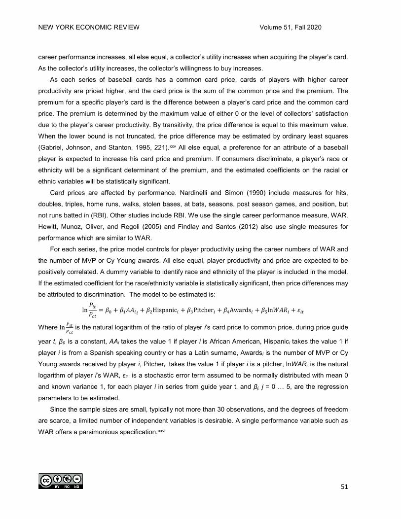
NEW YORK ECONOMIC REVIEW Volume 51, Fall 2020
51
career performance increases, all else equal, a collector’s utility increases when acquiring the player’s card.
As the collector’s utility increases, the collector’s willingness to buy increases.
As each series of baseball cards has a common card price, cards of players with higher career
productivity are priced higher, and the card price is the sum of the common price and the premium. The
premium for a specific player’s card is the difference between a player’s card price and the common card
price. The premium is determined by the maximum value of either 0 or the level of collectors’ satisfaction
due to the player’s career productivity. By transitivity, the price difference is equal to this maximum value.
When the lower bound is not truncated, the price difference may be estimated by ordinary least squares
(Gabriel, Johnson, and Stanton, 1995, 221).xxv All else equal, a preference for an attribute of a baseball
player is expected to increase his card price and premium. If consumers discriminate, a player’s race or
ethnicity will be a significant determinant of the premium, and the estimated coefficients on the racial or
ethnic variables will be statistically significant.
Card prices are affected by performance. Nardinelli and Simon (1990) include measures for hits,
doubles, triples, home runs, walks, stolen bases, at bats, seasons, post season games, and position, but
not runs batted in (RBI). Other studies include RBI. We use the single career performance measure, WAR.
Hewitt, Munoz, Oliver, and Regoli (2005) and Findlay and Santos (2012) also use single measures for
performance which are similar to WAR.
For each series, the price model controls for player productivity using the career numbers of WAR and
the number of MVP or Cy Young awards. All else equal, player productivity and price are expected to be
positively correlated. A dummy variable to identify race and ethnicity of the player is included in the model.
If the estimated coefficient for the race/ethnicity variable is statistically significant, then price differences may
be attributed to discrimination. The model to be estimated is:
ln𝑃𝑃𝑖𝑖𝑖𝑖𝑃𝑃𝑐𝑐𝑖𝑖
= 𝛽𝛽0 + 𝛽𝛽1𝐴𝐴𝐴𝐴𝑖𝑖𝑖𝑖 + 𝛽𝛽2Hispanic𝑖𝑖 + 𝛽𝛽3Pitcher𝑖𝑖 + 𝛽𝛽4Awards𝑖𝑖 + 𝛽𝛽5ln𝑊𝑊𝐴𝐴𝑊𝑊𝑖𝑖 + 𝜀𝜀𝑖𝑖𝑖𝑖
Where ln 𝑃𝑃𝑖𝑖𝑖𝑖𝑃𝑃𝑐𝑐𝑖𝑖
is the natural logarithm of the ratio of player i’s card price to common price, during price guide
year t, β0 is a constant, AAi takes the value 1 if player i is African American, Hispanici takes the value 1 if
player i is from a Spanish speaking country or has a Latin surname, Awardsi is the number of MVP or Cy
Young awards received by player i, Pitcheri takes the value 1 if player i is a pitcher, lnWARi is the natural
logarithm of player i’s WAR, εit is a stochastic error term assumed to be normally distributed with mean 0
and known variance 1, for each player i in series from guide year t, and βj, j = 0 … 5, are the regression
parameters to be estimated.
Since the sample sizes are small, typically not more than 30 observations, and the degrees of freedom
are scarce, a limited number of independent variables is desirable. A single performance variable such as
WAR offers a parsimonious specification.xxvi

NEW YORK ECONOMIC REVIEW Volume 51, Fall 2020
52
ESTIMATED COEFFICIENTS Table 3 summarizes the numbers of regressions providing estimates of the model equation. A sample
includes the cards of Hall of Fame players in a Topps series for a single price guide year. We estimated 656
samples which had enough degrees of freedom using ordinary least squares estimation. Of those 656 542
estimated models, almost 82 percent, are statistically significant using an F-test at the 10 percent level of
significance. In 429 models, the estimated coefficients of WAR for the WAR variable are statistically
significant, as well as for the estimated coefficients for the Awards variable in 419 models. Few Hispanic
variables, 5, have a statistically significant estimate for the coefficient.
In 104 estimated models, the estimated coefficient for the African-American variable – 19.19 percent of
statistically significant models – is statistically significant and negative. While these results are meaningful,
the effect is not large. The estimated impact for price due to an African American player picture on the card
is expected to be about two cents. Across a sample of 100,000 cards, all else equal, all collectors impute a
total reduction of $2,000 in the value of this card compared to a card picturing a White player. If there are
ten African American players pictured in a year’s series for Topps and in the Hall of Fame, then the
cumulative impact is an estimated reduction of $20,000.
Overall, as seen in Table 3, roughly four of five estimated models are at least statistically significant at
the 10 percent level of significance; of these, almost one in five of these have a statistically significant and
negative sign on the coefficient for the African-American variable.

NEW YORK ECONOMIC REVIEW Volume 51, Fall 2020
53
Table 3: All Topps Series, Numbers of Estimated Regressions, Statistically Significant Regressions, and
Statistically Significant Regression Coefficients, 1982-2010 Price Guides
Topps Series Year
Regressions Negative Coefficients Positive Coefficients Total
Estimated Statistically Significant
African-American
Hispanic WAR Awards
1956 28 28 0 0 28 28
1957 29 29 2 0 29 29
1958 29 29 21 0 29 29
1959 29 29 0 0 27 29
1960 29 27 0 0 27 27
1961 29 23 3 0 23 14
1962 29 29 0 0 29 28
1963 29 28 0 0 28 27
1964 29 27 0 0 14 27
1965 29 28 0 0 20 27
1966 29 29 25 0 4 29
1967 29 27 13 0 26 23
1968 29 28 11 0 28 27
1969 28 26 19 0 18 23
1970 28 12 1 0 12 6
1971 28 27 1 1 24 7
1972 27 26 0 0 20 17
1973 27 22 1 0 13 4
1974 26 15 0 0 12 3
1975 19 8 0 0 3 4
1976 19 14 0 0 11 1
1977 19 10 1 0 2 5
1978 19 8 2 0 2 1
1979 19 6 3 0 0 3
1980 19 7 1 4 0 1
Total 656 542 104 5 429 419
Percent
Regressions 100.00 82.62 15.85 0.76 65.40 63.87
Percent Significant
Regressions 100.00 19.19 0.92 79.15 77.31
Note: Level of significance at 10 percent
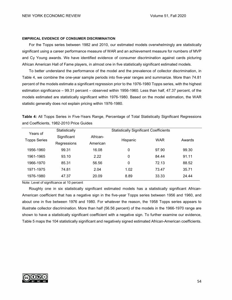
NEW YORK ECONOMIC REVIEW Volume 51, Fall 2020
54
EMPIRICAL EVIDENCE OF CONSUMER DISCRIMINATION
For the Topps series between 1982 and 2010, our estimated models overwhelmingly are statistically
significant using a career performance measure of WAR and an achievement measure for numbers of MVP
and Cy Young awards. We have identified evidence of consumer discrimination against cards picturing
African American Hall of Fame players, in almost one in five statistically significant estimated models.
To better understand the performance of the model and the prevalence of collector discrimination, in
Table 4, we combine the one-year sample periods into five-year ranges and summarize. More than 74.81
percent of the models estimate a significant regression prior to the 1976-1980 Topps series, with the highest
estimation significance – 99.31 percent – observed within 1956-1960. Less than half, 47.37 percent, of the
models estimated are statistically significant within 1976-1980. Based on the model estimation, the WAR
statistic generally does not explain pricing within 1976-1980.
Table 4: All Topps Series in Five-Years Range, Percentage of Total Statistically Significant Regressions
and Coefficients, 1982-2010 Price Guides
Years of
Topps Series
Statistically
Significant
Regressions
Statistically Significant Coefficients
African-
American Hispanic WAR Awards
1956-1960 99.31 16.08 0 97.90 99.30
1961-1965 93.10 2.22 0 84.44 91.11
1966-1970 85.31 56.56 0 72.13 88.52
1971-1975 74.81 2.04 1.02 73.47 35.71
1976-1980 47.37 20.09 8.89 33.33 24.44 Note: Level of significance at 10 percent
Roughly one in six statistically significant estimated models has a statistically significant African-
American coefficient that has a negative sign in the five-year Topps series between 1956 and 1960, and
about one in five between 1976 and 1980. For whatever the reason, the 1958 Topps series appears to
illustrate collector discrimination. More than half (56.56 percent) of the models in the 1966-1970 range are
shown to have a statistically significant coefficient with a negative sign. To further examine our evidence,
Table 5 maps the 104 statistically significant and negatively signed estimated African-American coefficients.

NEW YORK ECONOMIC REVIEW Volume 51, Fall 2020
55
Table 5: Statistically Significant African American Regression Coefficient, 1982-2010 Price Guides, 1956-
1980 Topps Series
Year 57T 58T 61T 66T 67T 68T 69T 70T 71T 73T 77T 78T 79T 80T Total 1982
1983
1984
1985 X X 2
1986 X 1
1987 X X 2
1988 X X 2
1989 X X 2
1990 X X X X 4
1991 X X X X X 5
1992 X X X X X X 6
1993 X X X X X 5
1994 X X 2
1995 X X X 3
1996 X X 2
1997 X X 2
1998 X X X X 4
1999 X X X X X X X 7
2000 X X X X X 5
2001 X X X X X 5
2002 X X X X 4
2003 X X X X 4
2004 X X X X 4
2005 X X X X X 5
2006 X X X X X 5
2007 X X X X X 5
2008 X X X X X 5
2009 X X X X X X 6
2010 X X X X X X X 7
Total 2 21 3 25 13 11 19 1 1 1 1 2 3 1 104 Note: Level of significance at 10 percent
Table 5 shows collector discrimination appears particularly in the Topps series for 1966 and 1969 and
prior to the price guide years of 1999. For the Topps series of 1966, 1967, 1968, and 1969, collector

NEW YORK ECONOMIC REVIEW Volume 51, Fall 2020
56
discrimination is especially seen following the price guide years following 1999. We have identified evidence
of collector discrimination. Between 1956 and 1980, 14 of 25 Topps series (as shown) have at least one
statistically significant negative coefficient for the African-American variable. By 1990, the coefficient is
significant and negative for more than two Topps series.
Scahill (2005) identified 1992 as the beginning of the period when race or ethnicity have no significant
effect on prices. We have seen differently. For the price guides published between 1992 and 2010, Tables
6 and 7 repeat the summarizations shown in Tables 3 and 4, beginning with the 1992 price guides. We limit
the information shown in Table 6 for the years with statistically significant coefficients for race or ethnicity.xxvii
Table 6 shows that the model estimates with statistical significance with a slightly higher proportion
(83.79 percent to 82.27), with a higher proportion of WAR coefficients with statistical significance (82.91
percent to 79.01). Similarly, a higher proportion of estimated coefficients with a negative sign is observed
for the African-American variable (21.36 percent to 19.15).
Table 6: All Topps Series, Numbers of Estimated Regressions, Statistically Significant Regressions, and
Statistically Significant Regression Coefficients, 1992-2010 Price Guides
Topps Series Year
Regressions Negative Coefficients Positive Coefficients Total
Estimated Statistically Significant
African-American
Hispanic WAR Awards
1957 19 19 2 0 19 19
1958 19 19 16 0 18 19
1961 19 19 3 0 19 14
1966 19 19 19 0 19 19
1967 19 19 12 0 19 19
1968 19 19 11 0 19 19
1969 19 19 16 0 16 19
1977 19 10 1 0 2 5
1978 19 8 1 0 2 1
1979 19 6 3 0 0 3
1980 19 7 1 4 0 1
Total 475 399 85 4 330 282
Percent
Regressions 100.00 84.00 17.89 0.84 69.47 59.37
Percent Significant
Regressions 100.00 21.30 1.00 82.71 70.68
Note: Level of significance at 10 percent

NEW YORK ECONOMIC REVIEW Volume 51, Fall 2020
57
That the model estimates statistical significance of collector discrimination with greater frequency
beginning with the 1992 guide is confirmed in Table 7. Notably, compared to Table 4, proportionally more
estimated African American coefficients are statistically significant for the five-year periods 1956-1960, 1966-
1970, and 1976-1980 Topps series, but fewer (or the same) are statistically significant for 1961-1965 and
1971-1975. Contrary to conclusion in Scahill (2005), we find evidence of collector discrimination after 1992,
particularly in the Topps series for 1958, 1966, 1967, 1968, and 1969. Table B, in the Appendix, lists the
Hall of Fame players pictured on card appearing in a Topps series between 1966 and 1970.xxviii
Table 7: All Topps Series in Five-Years Range, Regressions Percentage Statistically Significant, and
Statistically Significant Coefficients, 1992-2010 Price Guides
Years of
Topps Series Regressions
Coefficients
African-
American Hispanic WAR Awards
1956-1960 100 18.95 0 98.95 100
1961-1965 100 3.16 0 94.74 94.74
1966-1970 94.74 64.44 0 91.11 91.11
1971-1975 75.79 0 0 72.22 47.22
1976-1980 47.37 13.33 8.89 26.67 24.44 Note: Level of significance at 10 percent
CONCLUDING OBSERVATIONS
The simple hedonic pricing model statistically explains the variation in Hall of Fame player card prices
in Topps series between 1956 and 1980. By limiting the performance variable to WAR, we increase sample
sizes and the degrees of freedom available in estimation. There is buyer discrimination for some card series
but not others.
This study provides evidence that since 1992, until at least 2010, collectors sometimes discriminate
against African American players who have been inducted in the Baseball Hall of Fame and appear on
Topps picture cards issued in series between 1956 and 1980. The comprehensive identification of this
persistence since the early 1990s differs from most published scholarship which study prices and collector
perceptions of race and ethnicity. For many Topps card series, particularly 1958, 1966, 1967, 1968, and
1969, this discrimination means collectors have less apparent interest in Topps cards picturing an African
American Hall of Fame player which results in a lower price, compared to collectors who have more interest
in purchasing a Topps card picturing a Hall of Fame White or Hispanic player at a higher price. While the
effect on an individual card price is very small, the cumulative impact for the total surviving examples of the
card may be thousands of dollars; when multiplied by the number of affected players in a series, and then
by the number of series, the total effect may be considerably large. Such an estimated cumulative reduction

NEW YORK ECONOMIC REVIEW Volume 51, Fall 2020
58
in expected value by collectors could reflect a broader monetary devaluation for identical social contributions
made by affected groups.
One could also speculate why this discrimination persists from the 1990s into the new millennium.
Collecting picture cards may be a hobby no longer enjoyed by large numbers of young persons.xxix The
current collector base may be aging and thus card prices most likely reflect the preferences of this specific
demographic rather than those of the broader population. As the relative size of those born prior to 1945
shrinks, the relatively few collectors from the Millennial Generation could result in a concentration of
collectors from the Baby Boom Generation. Collectors from this generation may be less aware of their biases
and unconsciously prefer players who look more like themselves.
Other possibilities may relate to our specification or changes in how the game is played. Our model may
be too simple. It may, for instance, omit key explanatory variables or important control variables, such as a
likeability Q-Score. The style and strategy of play has changed during the periods during the baseball card
series which affect career, and play has also changed during the price guide years. These changes could
affect consumer perceptions of prior performance when compared with recent performance. The end of the
recent steroid era coincident with “money ball,” the development and adoption of new performance
measures, and broader acceptance of sabermetrics may reflect a transition which reflects changes in
consumer preference for the game’s style and strategy. As a result, collector preferences may be in transition
and the market be in adjustment during our sample periods.
Nonetheless, our results reflect that of another study for the BBWAA ballots and racism. Jewell, Brown
and Miles (2002) find discrimination against retired African American and Hispanic players. For whatever
reason, our evidence shows this discrimination does not end for those players who are able to achieve
election. We identify more recent evidence of collector discrimination against African American players who
are enshrined at the Hall of Fame and appear on cards issued by Topps between 1956 and 1980.
∗ Assistant Professor of Economics, SUNY Oneonta, School of Economics and Business, 108 Ravine Parkway,
Oneonta, New York, 13820, [email protected].
◊ I thank Andrew Turner (SUNY Oneonta alumnus, 2010 B.S. Economics) for assisting me with the collection of the
price data between 1994-2008. Any errors in the data recorded and used remain my own.
END NOTES
1. This paper is based upon McAvoy (2019). “WAR, Race, and Ethnicity: Collector Discrimination for Hall-
of-Fame Player Baseball Cards.” This paper was first presented at the Twenty-Ninth Cooperstown
Symposium on Baseball and American Culture, 2017. It was selected for publication in The
Cooperstown Symposium on Baseball and American Culture, 2017-2018 anthology by McFarland &
Company, Publishers, Inc. This paper further extends and revises McAvoy (2013).
2. For an extensive literature review up to the time of its publication, see Kahn (1992).

NEW YORK ECONOMIC REVIEW Volume 51, Fall 2020
59
3. Minority representation on the covers of Sports Illustrated has increased, but less than the increase in
minority participation rates (Primm, DuBois, and Regoli, 2007). When assigning numbers, Topps did not
consider race (Regoli, Primm, and Hewitt, 2007).
4. MLB granted Topps the exclusive rights to manufacture and distribute series of cards through 2025
(Mueller, 2018). Topps has had this exclusive right since 2011.
5. Professional Sports Authenticator, a prominent third party grading company, maintains an online price
guide and records of prior auction sales. See “SMR Online” and “Auction Prices Realized,” psacard.com
(site accessed August 1, 2018).
6. Jamieson (2010) provides a comprehensive history of the hobby from its rise to national prominence to
its decline and fall.
7. This continues to be true (Seideman, 2018).
8. Examples include Chadwick and Ray (1989), Green and Pearlman (1989), Rosen (1991), and Stewart
(1993).
9. See Green and Pearlman (1989), Kirk (1990), and Stewart (1993). Election by the Baseball Writers’
Association of America is considered most prestigious.
10. Interestingly, these trends have been observed in other hobbies such as coins and stamps. It is easy to
use a smart phone and apps to quickly compare what is offered online and view the prices recorded in
recent transactions. Third party grading and registries have resulted in very high prices for top condition
scarcities.
11. Chadwick and Ray (1989) claim 99.5 percent of collectors were white in the late 1980s.
12. Rosenblatt (1990) provides a very good example of the public perception. Green and Pearlman (1989)
and Chadwick and Ray (1989) provide hobby writers’ perceptions. Rosen (1991) provides a dealer’s
view. Kiefer gives the hobby editor’s view (1988). Regoli (1991, 2000) provides academic views.
13. They do not adjust for series scarcity.
14. Sharpe and La Croix (2001) find evidence collectors prefer memorabilia of African American baseball
players.
15. The premium is the difference between the prices at initial release and 17 years later (Burge and Zillante,
2014).
16. Scahill (2005) is an exception and uses guides from 1979-1984, 1986-1997, and 1999-2001.
17. At present, no player active from 1956-1980 appears on the BBWAA ballot. The Veterans Committee
now selects players from our sample period. Jack Morris and Alan Trammell, in 2018, were the most
recent players inducted from this era. For information for how players are selected by the Veterans
Committee, see the Baseball Hall of Fame and Museum, “Eras Committees,” baseballhall.org (site
accessed August 1, 2018).
18. Liquidity refers to the time and cost to convert a baseball card into money. As collectibles, baseball cards
are not as liquid as financial instruments (checking account balances, stocks, bonds, etc.).

NEW YORK ECONOMIC REVIEW Volume 51, Fall 2020
60
19. Topps defended its licenses, using courts against companies which infringed its rights. In 1981 the courts
held for the Fleer Corporation which had contested Topps’ claims to its rights. Besides Fleer, other
issues or manufacturers produced baseball memorabilia between 1956 and 1980, including pictures on
cereal boxes, bread labels, bottle caps, plastic cups, statues, cans, and others. The Topps series differed
in terms of the size of each series, showing nearly every player who appeared on a team roster. Topps
purchased licenses from the MLB and MLBPA, and it contracted individually with players for the rights
to distribute their pictures. Only Topps offered a near complete series of picture cards during the season
which showed the player in his team uniform and with his club name.
20. Hudgeons authors the 1981-1985 guides, and Beckett authors them after 1985. These pocket guides
began their publication in 1981 and ceased in 2010. eBay, google.com searches, and online subscription
databases have largely replaced the printed price guide.
21. Beckett attributes the success of his guide because it, “… is complete, current, and valid. … the most
accurate, with integrity.” See, “How to Use This Book” (Beckett, 1993). Stewart (1993) describes how
the price guide developed into an authoritative resource.
22. Beckett (1985-2010). The price recorded is based upon the title cover year. The 2002-2003 22nd edition
is excluded since it has a 2003 copyright. Prior to the 22nd, the copyright year preceded the title year by
one year. After the 22nd, the copyright year matched the title year.
23. Excluding these rookie cards removes the difficulty of determining the rookie premiums identified by
Burge and Zillante (2014).
24. WAR and numbers of awards are recorded from <baseball-reference.com>. We use the WAR 2.2
measure. Alternative measures of WAR are available, but all are understood to have similar relative
player career rankings.
25. The price difference may be estimated by a Tobit technique, if the lower bound is truncated (Nardinelli
and Simon, 1990). Hall of Fame player cards are priced above the common price. All sample prices
have a multiple greater than 1 and estimated coefficients of the performance variables are positive. We
proceed with the ordinary least squares estimation method.
26. Because of small sample sizes Anderson and La Croix (1991) delete insignificant variables when neither
fit nor estimated ethnic coefficients are significantly affected. We remove neither explanatory nor control
variables.
27. Available from the author upon request.
28. I thank an anonymous referee for observing that 1966-1970 may be perceived to be an era of heightened
racial sensitivity and suggesting that some of these players may be perceived by collectors as
controversial.
29. The Millennial Generation has a reputation for enjoying consumption of experiences rather than things.
NEW YORK ECONOMIC REVIEW Volume 51, Fall 2020
61
REFERENCES
Anderson, Torben and Sumner J. La Croix. 1991. “Customer Racial Discrimination in Major League
Baseball.” Economic Inquiry, 29(4): 665-677.
Ashe, Jr., Arthur R. 1993. A Hard Road to Glory – Baseball: The African-American Athlete in Baseball. New
York: Amistad.
Becker, Gary. 1971. The Economics of Discrimination, 2nd ed. Chicago: University of Chicago Press.
Beckett, Dr. James. (1985-2010). The [Year] Official Price Guide to Baseball Cards, 5th – 28th eds.
Orlando/New York: House of Collectibles.
Bloom, John. 1997. A House of Cards Baseball Card Collecting and Popular Culture, American Culture, Vol.
12. Minneapolis: University of Minnesota Press.
Burge, Gregory S. and Arthur Zillante. 2014. “Racial Discrimination or Statistical Discrimination? MLB Rookie
Card Values and Performance Uncertainty.” UNC Charlotte Economics Working Paper Series, Working
Paper No. 2014-002.
Burnett, Nancy J. and Lee VanScyoc. 2004. “Discriminating Buyers of Baseball Cards: Does Race Affect
Value.” Journal of Economics and Economic Education, 5(3).
Burnett, Nancy J. and Lee Van Scyoc. 2013. “Changing Levels of Discrimination in the Market for Baseball
Cards.” Journal of Economics and Economic Education, 13(2): 1-20.
Chadwick, Bruce and Danny Ray. 1989. How to Buy, Trade & Invest in Baseball Cards & Collectibles: Smart
Strategies for Starting, Building & Enjoying Your Collection. New York: Simon & Shuster.
Findlay, David W. and John M. Santos. 2012. “Race, Ethnicity, and Baseball Card Prices: A Replication,
Correction, and Extension of Hewitt, Munoz, Oliver, and Regoli.” Econ Journal Watch, 9(2): 122-140.
Fort, Rodney and Andrew Gill. 2000. “Race and Ethnicity Assessment in Baseball Card Markets.” Journal of
Sports Economics, 1(1): 21-38.
Gabriel, Paul E., Curtis Johnson, and Timothy Stanton. 1995. “An Examination of Customer Racial
Discrimination in the Market for Baseball Memorabilia.” Journal of Business, 60(2): 215-230.
Green, Paul M. and Donn Pearlman. 1989. Making Money with Baseball Cards: A Handbook of Insider
Secrets and Strategies. Chicago: Bonus Books.
Hewitt, John D., Robert Munoz, Jr., William L. Oliver, and Robert M. Regoli. 2005. “Race, Performance, and
Baseball Card Values.” Journal of Sport and Social Issues, 29(4): 411-425.
Hudgeons, Thomas E. 1981-1985. The [Year] Official Price Guide to Baseball Cards, 1st – 4th eds. Orlando:
House of Collectibles.
Kahn, Lawrence M. 1992. “Discrimination in Baseball.” In Paul M. Somers (ed.), Diamonds Are Forever: The
Business of Baseball. Washington, D. C.: The Brookings Institution: 163-188.
Jamieson, Dave. 2010. Mint Condition. New York: Atlantic Monthly Press.
Jewell, Todd R. Robert W. Brown and Scott E. Miles. 2002. “Measuring Discrimination in Major League
Baseball: Evidence from the Baseball Hall of Fame.” Applied Economics, 34(2): 167-177.

NEW YORK ECONOMIC REVIEW Volume 51, Fall 2020
62
Kiefer, Kit. 1988. “So Where Are the Black Collectors?” Baseball Cards Magazine, (September): 75-76.
Kirk, Troy. 1990. Collector’s Guide to Baseball Cards. Radnor, Pennsylvania: Wallace-Homestead.
Mueller, Rich. 2018. “Topps, MLB Extend Exclusive License Through 2025.” sportscollectorsdaily.com (July
12, 2018, site accessed August 1, 2018).
Nardinelli, Clark and Curtis Simon. 1990. “Customer Discrimination in the Market for Memorabilia: The Case
of Baseball.” The Quarterly Journal of Economics, 105(3), 577-584.
Primm, Eric, Summer DuBois, and Robert M. Regoli. 2007. “An Exercise and Transmission of Racism: An
Analysis of Sports Illustrated Covers.” Journal of African American Studies, 11(3/4): 239-250.
Primm, Eric, Nicole L. Piquero, Robert M. Regoli, and Alex R. Piquero. 2010. “Racial Bias in Baseball Card
Collecting Revisited.” The Social Science Journal, 47(4): 865-874.
Primm, Eric, Nicole Leeper Piquero, Alex R. Piquero, and Robert M. Regoli. 2011. “Investigating Customer
Racial Discrimination in the Secondary Baseball Card Market.” Sociological Inquiry, 81(1): 110-132.
Regoli, Bob. 1991. “Racism in Baseball Card Collecting: Fact or Fiction?” Human Relations, 44(3): 255-264.
Regoli, Robert. 2000. “Racism, Racism Everywhere: Looking Inside the Hobby of Baseball Card Collecting.”
Race and Society, 3(2): 183-192.
Regoli, Robert M., Eric Primm, and John D. Hewitt. 2007. “Where O’ Where Did My Baseball Cards Go?
Race, Performance, and Placement in the Topps Era, 1956-1980.” The Social Science Journal, 44(4):
742-750.
Rosenblatt, Carl. 1990. “Baseball Card Sales Reflect Race.” Daily Press. Newport News, Virginia: 17 June
1990: C1.
Rosen, Alan (with Doug Garr). 1991. Mr. Mint’s Insider’s Guide to Investing in Baseball Cards and
Collectibles. New York: Warner Books.
Scahill, Edward M. 2005. “A Reinvestigation of Racial Discrimination and Baseball Cards.” Eastern
Economic Journal, 31(4): 537-550.
Seideman, David. 2018. “New Index Shows Vintage Trading Cards Have Beat The S&P 500.”
www.forbes.com, (February 23, 2018, site accessed August 1, 2018).
Sharpe, Rhonda and Sumner La Croix. 2001. “Customer Discrimination in Memorabilia: New Evidence for
Major League Baseball.” In William M. Simons, ed., The Cooperstown Symposium on Baseball and
American Culture 2000. Jefferson, North Carolina: McFarland: 184-202.
Stewart, Mark. 1993. The Ultimate Insider’s Guide to Baseball Cards. New York: Crown.
Van Scyoc, L. J. and N. J. Burnett. 2013. “How Times Have Changed: Racial Discrimination in the Market
for Sports Memorabilia (Baseball Cards).” Applied Economic Letters, 20(7-9): 875-878.
NEW YORK ECONOMIC REVIEW Volume 51, Fall 2020
63
Determinants of Division I NCAA Soccer Participation
Andrew Weinbach* and Robert F. Salvino*
*Department of Finance and Economics, Coastal Carolina University, 100 Chanticleer Dr. E., Conway, SC 29528.
ABSTRACT Previous research has shown the importance of industrialization and immigration in the sport of men’s soccer
in the early 20th century. We test economic determinants for soccer and offer new evidence on the relationship between socioeconomic factors and labor supply for NCAA soccer participation. Exploiting a sample of 30,935 Division 1 college athletes, and the counties where these athletes attended high school, we observe income incentives and agglomeration economies at work. NCAA soccer players tend to come from higher income counties, but we also find that regions tend to develop sport-specific specializations over time, specifically, the Northeastern states.
INTRODUCTION Soccer is a seemingly inexpensive sport. All you need is a ball, a field, and a few players to make a
go of it. Yet most Americans regard it as a mere caricature of suburban prosperity in the United States. More
perplexing, the U.S. Men’s National Team has never been a serious contender on the world stage, and all
of the income and marketing power in the country has achieved only a fraction of the revenues of the major
U.S. sports. Since the NCAA is the ultimate proving ground for aspiring athletes in the U.S., we turn there
for a logical explanation.
Sports teams and organizations share their knowledge directly and indirectly through the competitive
landscape. Youth travel soccer is decidedly market-oriented. Indeed critics repeatedly level the “pay-to-play”
argument against the U.S. Soccer Federation for the perennially weak showings of the U.S. Men’s Soccer
Team on the world stage. The argument assumes community-funded soccer would attract better athletes
away from the more popular sports. An alternative view recognizes soccer’s growth in the U.S., driven by
market forces, as entrepreneurs have worked to provide a good that is under-supplied in many communities
across the country. Forced to compete for resources and players in towns where traditional American sports
are deeply embedded in the community culture, soccer has gained through entrepreneurial pursuits
(Cuadros 2006). Add to this the influence of Title IX, through restrictions and incentives on college athletic
programs, and the economic analysis of the collegiate sports is compelling.
Urban and regional economic theory provides a convenient lens for analyzing spatial phenomena.
Youth sports apparently gain from regional concentration, similar to firms clustering in cities to benefit from
labor pooling, knowledge spillovers, and the sharing of intermediate inputs, collectively referred to as
agglomeration economies. Initial clusters of specific sport hotbeds may happen by accident, as Bigalke
(2018) demonstrates for men’s soccer and the Northeast with the 1930 U.S. World Cup team. The urban
and regional literature has repeatedly documented agglomeration for places including Dalton, Georgia and
carpet making, banking in Charlotte, technology in Silicon Valley and many more. Over time, the benefits of

NEW YORK ECONOMIC REVIEW Volume 51, Fall 2020
64
agglomeration tend to increase the concentration and economic value-added (Henderson 2003, Rosenthal
and Strange 2001).
We examine Division 1 soccer participation through a sample of over 22,000 male athletes and over
8,000 female athletes on rosters at FBS schools in 2018. We limit the empirical analysis to major team sports
based on data availability (football, baseball, basketball, soccer, and hockey for men, and soccer, softball,
volleyball, and basketball for women) and find regional clustering consistent with economic theory. Our
findings reinforce much of the work expounded in Kuper and Szymanski’s (2014) Soccernomics, but we
provide evidence suggesting a much weaker climb toward prominence in men’s soccer than they suggest
for the U.S. among the world’s elite soccer nations. Examining the collegiate soccer player pool reveals
important spatial and economic attributes of areas producing relatively higher numbers of soccer athletes at
major universities and emphasizes a pecuniary tradeoff in favor of other major U.S. sports. The remainder
of the paper proceeds as follows. We discuss the background for the research and economic intuition in
Section 2 and present the empirical analysis in Section 3. We conclude with the results discussion in Section
4.
BACKGROUND Sports participation studies typically focus on sport as a leisure or fitness activity. Consumers maximize
utility across a set of leisure and labor alternatives and allocate time and income to the consumption of sport
according to relative prices of available goods (Kokolakakis et al. 2012, 2014; Humphreys and Ruseski 2006,
2007). Other studies have examined the benefits of sports participation in high school in terms of college
completion and income generation in the future (Barron, Ewing, and Waddell 2000). Sports economists have
examined other more traditional microeconomic problems through the lens of sport, including anti-trust and
industrial organization as well as labor markets more generally (Leeds and von Allmen, 2016; Downward,
Dawson, and Dejonghe 2009). Our study focuses exclusively on NCAA sanctioned competitive sport
participation. It does not apply to the European markets in general but makes a unique contribution to the
sports economics literature. We believe this is the first study to examine the determinants of American
collegiate soccer participation from a microeconomic framework and a local market geographical
perspective.
Given the relatively low popularity of collegiate and professional soccer in the United States, the
decision for an athlete of high ability to choose to play soccer, over football or baseball, for example, would
seem an inferior one. However, at the margin we assume the representative player-household chooses the
best option relative to a host of limiting economic and spatial factors, including the local resources available
and the competitive environment inclusive of other sports. We expect to find that certain areas are good
places for soccer players to develop, and these places likely see more public and private resources go to
soccer and have more people experienced with the sport. See Figures 1 and 2 for evidence of the variation
in the number of soccer players per capita from each state playing D1 soccer (as measured by number of
players in our dataset appearing on rosters at FBS hosting universities per 100,000 citizens).

NEW YORK ECONOMIC REVIEW Volume 51, Fall 2020
65
Figure 1: Sending NCAA Men’s Soccer per 100,000 Population
Source: 2018 NCAA Division 1 FBS School Rosters
Figure 2: Sending NCAA Women’s Soccer per 100,000 Population
Source: 2018 NCAA Division 1 FBS School Rosters
NEW YORK ECONOMIC REVIEW Volume 51, Fall 2020
66
Earning a college degree is challenging without the additional demands of playing an NCAA
sanctioned competitive sport, yet for athletes the economic and psychic rewards are alluring. Young athletes
and their families invest significant resources to increase the probability of receiving a Division 1 athletic
scholarship. Assuming a constant supply of athletes, this probability increases with the number of
scholarships available for each sport. Beyond college, some sports offer potentially lucrative professional
opportunities, increasing the implicit value of the scholarship. This potential for earnings as a professional
athlete varies across sports and is relatively low for men’s soccer in the United States, in comparison to
other sports. For women however, professional soccer may be relatively more attractive, given the smaller
number of alternative opportunities for women in professional sport in the United States.
Sanderson and Siegfried (2015) provides an insightful discussion of the monetary incentives for
colleges and universities with Division I sports programs and the vast financial differences across sports.
For the male soccer athlete, the financial rewards in the form of scholarships available and potential for
earnings as a professional athlete after college are much smaller when compared with the other major men’s
professional sports. Additionally, resources for youth soccer may reflect or partially contribute to the incentive
differences. Regional disparities in median household income and educational attainment may skew the
participation levels across men’s team sports. These factors increase the relative value of an athletic
scholarship for male athletes in the Southeast.
Other regional disparities may affect the environment for youth sport and individual development as
well. The data show the South and West produce the most soccer athletes. Climate is an obvious factor in
favor of these two regions, enabling more practice time for the outdoor sports. The availability of abundant,
inexpensive land may also promote the development of large-scale recreational and athletic facilities,
whereas higher-valued commercial and residential uses compete for land in more densely populated metros,
such as those of the Northeast. Culture is another external factor that is difficult to measure. Soccer has
greater economic and cultural significance in other countries. In the United States, soccer may have greater
popularity where global influences due to immigration have been greater over time. This popularity should
translate indirectly to ability, increasing the competitive environment where one’s skills are refined.
Ultimately, how these and other factors collectively affect an area’s sports performance environment is an
empirical question. In Table 1.A. we show states that send the greatest number of soccer athletes to FBS
programs. Table 1.B., shows soccer athletes as a share of major FBS team sport athletes in our sample.
The greater proportion of soccer athletes in the Northeast suggests culture, partly due to immigration and
partly due to income and education, affects outcomes. However, fundamental economic factors may best
predict NCAA soccer participation. In Section 3 we present our data, empirical models, and results.

NEW YORK ECONOMIC REVIEW Volume 51, Fall 2020
67
Table 1.A: Soccer Players by State
Men's Soccer Women's Soccer Top 5 States Soccer Players Top 5 States Soccer Players California 130 California 431 Florida 101 Texas 367 Texas 78 Florida 201 North Carolina 69 Ohio 148 Georgia 60 Illinois 140
Source: 2018 NCAA Division 1 FBS School Rosters
Table 1.B: Soccer as a Share of Total Athletes by State*
Men's Soccer Women's Soccer
Top 5 States Soccer Concentration
Soccer Players Top 5 States
Soccer Concentration
Soccer Players
Connecticut 13% 24 Colorado 65% 131 Washington 11% 35 New Jersey 60% 91 Massachusetts 11% 32 Utah 57% 52 New Jersey 10% 50 New Mexico 53% 36 Colorado 10% 29 Massachusetts 53% 30
*States with at least 1 million population producing at least 15 soccer players. Source: 2018 NCAA Division 1 FBS School Rosters Men’s sports included in this dataset are Football, Baseball, Basketball, Soccer, and Hockey Women’s sports included in this dataset are Soccer, Softball, Volleyball, and Basketball
EMPIRICAL ANALYSIS Data We obtained individual soccer player data from 2018 team roster web pages available on the websites of
the 130 universities hosting FBS football programs. Rosters for each sport provide position-specific
information for each player as well as their hometown and high school of record, including zip code. With
this geographical information, we add county level economic and demographic data. Where reporting was
incomplete, such as no zip code reported, we attempted to match the player’s hometown with their
corresponding high school to determine precise zip code. The National Center for Education Statistics
(NCES.ed.gov https://nces.ed.gov/ccd/pubschuniv.asp ) provides a database of all U.S. public and private
high schools with addresses. For approximately 10% of the athletes on rosters, we could not reliably match
reported information to the high schools in our database. Reasons for a failed match include the following:
student attended high school in another country, student was home schooled, no high school was reported,
or the name of the high school provided on the website was either not present in the database or no
unambiguous match was present.

NEW YORK ECONOMIC REVIEW Volume 51, Fall 2020
68
Our economic and demographic indicators come from the 2016 American Community Survey 5-
year estimates for counties. Excluding U.S. territories, as well as Kalawao County, Hawaii (which is an
isolated peninsula that has served as a leper colony since 1870, and is now solely populated by the surviving
colony members, along with caregivers and support personnel), and Loving County, Texas, with a population
of 74. Both of these counties had incomplete data on housing values, and perhaps not surprisingly, had no
representation of athletes on rosters of any sport in our dataset. This leaves 3,140 counties remaining in
the dataset. We include measures for income, population, population density, education, race, and age. A
binary variable for each county captures roster information from Bigalke (2018) that indicates whether a
county is in one of the five states that produced U.S. Team soccer players for the 1930 FIFA World Cup in
Uruguay. These states were New York, New Jersey, Pennsylvania, Massachusetts, and Missouri. Ten of
the sixteen players on the 1930 team came from these states, with the remaining six players coming from
Great Britain. The 1930 team was the most successful U.S. Men’s World Cup soccer team in history. This
indicator attempts to capture a cultural or local scale effect that income or education may not explain. Finally,
a count variable for the number of FBS schools in each state captures an element of demand for athletes
and visibility of the sport and opportunities at the Division 1 level. For complete data source information,
definitions, and summary statistics, see Tables 2 and 3.
Modeling and Results We model NCAA soccer participation at the county level to understand where soccer athletes come from
and what factors tend to support greater numbers of soccer athletes from a given region playing NCAA
Division 1 soccer at FBS schools. Our modeling approach needs to incorporate individual motivation as well
as the regional economic and demographic environment. Ideally, we could observe household level
characteristics over time, following the approach of Farrell and Shields (2002). Their study of leisure sport
participation exploits data on individuals in households in England and models the unobserved propensity
to participate in leisure sports. They estimate a random effects probit model of the following form:
S*ih = x’ihβ+vih for i = 1,2,…,n and h = 1,2,…,H, (1)
Vih = αh + µih (2)
and
Sih = �1 if 𝑆𝑆𝑖𝑖ℎ∗ > 0, 0 otherwise
where S is observed sports participation for the ith individual from household h. Exogenous, observable
factors include demographic characteristics, region aspects, and individual health. The composite error term,
vih, captures unobservable household preferences toward leisure sports.
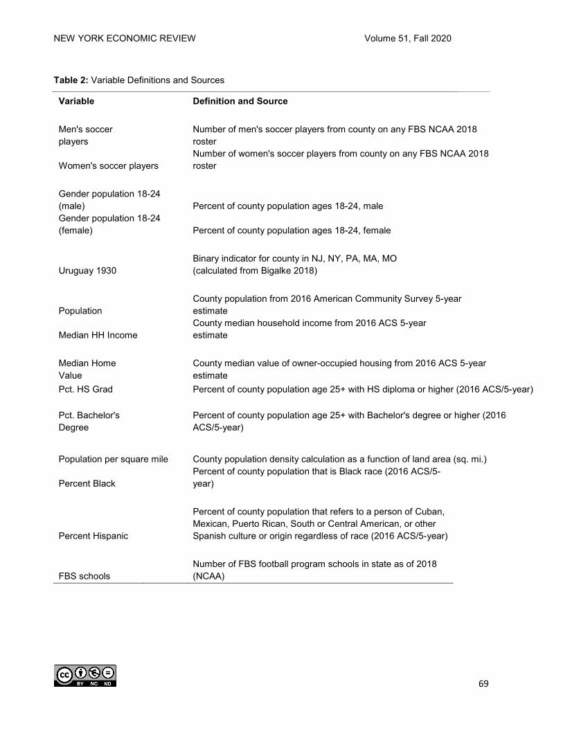
NEW YORK ECONOMIC REVIEW Volume 51, Fall 2020
69
Table 2: Variable Definitions and Sources
Variable Definition and Source
Men's soccer players
Number of men's soccer players from county on any FBS NCAA 2018 roster
Women's soccer players Number of women's soccer players from county on any FBS NCAA 2018 roster
Gender population 18-24 (male) Percent of county population ages 18-24, male
Gender population 18-24 (female) Percent of county population ages 18-24, female
Uruguay 1930 Binary indicator for county in NJ, NY, PA, MA, MO (calculated from Bigalke 2018)
Population County population from 2016 American Community Survey 5-year estimate
Median HH Income County median household income from 2016 ACS 5-year estimate
Median Home Value
County median value of owner-occupied housing from 2016 ACS 5-year estimate
Pct. HS Grad Percent of county population age 25+ with HS diploma or higher (2016 ACS/5-year) Pct. Bachelor's Degree
Percent of county population age 25+ with Bachelor's degree or higher (2016 ACS/5-year)
Population per square mile County population density calculation as a function of land area (sq. mi.)
Percent Black Percent of county population that is Black race (2016 ACS/5-year)
Percent Hispanic
Percent of county population that refers to a person of Cuban, Mexican, Puerto Rican, South or Central American, or other Spanish culture or origin regardless of race (2016 ACS/5-year)
FBS schools Number of FBS football program schools in state as of 2018 (NCAA)
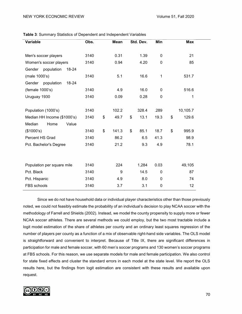
NEW YORK ECONOMIC REVIEW Volume 51, Fall 2020
70
Table 3: Summary Statistics of Dependent and Independent Variables
Variable Obs. Mean Std. Dev. Min Max
Men's soccer players 3140 0.31 1.39 0 21
Women's soccer players 3140 0.94 4.20 0 85
Gender population 18-24
(male 1000’s) 3140 5.1 16.6 1 531.7
Gender population 18-24
(female 1000’s) 3140 4.9 16.0 0 516.6
Uruguay 1930 3140 0.09 0.28 0 1
Population (1000’s) 3140 102.2 328.4 .289 10,105.7
Median HH Income ($1000’s) 3140 $ 49.7 $ 13.1 19.3 $ 129.6
Median Home Value
($1000’s) 3140 $ 141.3 $ 85.1 18.7 $ 995.9
Percent HS Grad 3140 86.2 6.5 41.3 98.9
Pct. Bachelor's Degree 3140 21.2 9.3 4.9 78.1
Population per square mile 3140 224
1,284 0.03
49,105
Pct. Black 3140 9 14.5 0 87
Pct. Hispanic 3140 4.9 8.0 0 74
FBS schools 3140 3.7 3.1 0 12
Since we do not have household data or individual player characteristics other than those previously
noted, we could not feasibly estimate the probability of an individual’s decision to play NCAA soccer with the
methodology of Farrell and Shields (2002). Instead, we model the county propensity to supply more or fewer
NCAA soccer athletes. There are several methods we could employ, but the two most tractable include a
logit model estimation of the share of athletes per county and an ordinary least squares regression of the
number of players per county as a function of a mix of observable right-hand side variables. The OLS model
is straightforward and convenient to interpret. Because of Title IX, there are significant differences in
participation for male and female soccer, with 60 men’s soccer programs and 130 women’s soccer programs
at FBS schools. For this reason, we use separate models for male and female participation. We also control
for state fixed effects and cluster the standard errors in each model at the state level. We report the OLS
results here, but the findings from logit estimation are consistent with these results and available upon
request.

NEW YORK ECONOMIC REVIEW Volume 51, Fall 2020
71
The general model predicting the number of county male soccer players takes the following form
and is otherwise identical for female soccer players:
SCis = x’iβj + fiγ + wid + ui for i = 1,2,…,n and s = 1,2,…,S (3)
where SCis is the total number of male soccer players coming from county i of state s and ranges from 0 to
21. For females the count ranges from 0 to 85. We also tried models in which we scaled the dependent
variable by county population, creating a players per capita model. The applicability and interpretation is not
as intuitive. Ultimately, soccer clubs and college recruiters are interested in the richness of a soccer-
producing area, in terms of the number of players. The per capita measure does not translate readily into
recruiting demand. For example, the highest per capita county for male soccer players is in Nebraska, with
only one soccer player but less than 5,000 people in the county. This is not a meaningful statistic. We have
estimated these models and can provide the results upon request. The coefficient estimates are not
fundamentally different from our absolute number model results.
In the following models, we have 3,140 county level observations. State level fixed effects control
for unobservable differences across counties within a state. Analogous to Farrell and Shields (2002), each
county is technically a member of a state, and a state may induce better or worse conditions for the
development of NCAA soccer athletes. Our estimation clusters the standard errors by state to ensure
accurate variance calculations for inference testing. The vector x includes economic and demographic
variables. The variable f represents the number of FBS programs in a state and ranges from 0 to 12. Finally,
w is the binary indicator for whether the county is in one of the five states that provided players for the 1930
FIFA Men’s World Cup team.
The first set of results examines the supply of NCAA soccer players controlling for the general
population of their home county. In Table 4, we find that a doubling of population produces a near doubling
of soccer players per county. The coefficient on population, converted to population in hundreds of
thousands, is 0.29. The mean population for a county in our sample is 102,231, while the mean number of
NCAA-bound soccer players per county is 0.31. Thus, an increase of 100,000 people produces an additional
0.29 players, almost double the mean of 0.31. We find a similar effect for females. The coefficient on
population is much stronger, 0.97, per 100,000 population, but the mean number of female players is greater
at 0.94. Population density has a negative effect, but it is minor in magnitude. This is an interesting result
compared with population’s positive effect. It is consistent with scarcity of land supply that forces youth
development organizations further from the central city, out to the suburbs. Higher income in the suburbs
may also contribute to the negative density effect.
Income has a positive effect on NCAA soccer player production. For males, increasing county
median household income $10,000 yields 48 percent more soccer players, an elasticity value of 2.4. The
effect is even greater for females. The coefficient of 0.64 yields an elasticity of 3.4. Similarly, we find a more
college-educated population is consistent with greater soccer player production. For males, the coefficient
on Pct. Bach is 0.023. A one unit increase in the percentage of the population with at least a bachelor’s

NEW YORK ECONOMIC REVIEW Volume 51, Fall 2020
72
degree, an increase of 5 percent at the mean, yields 7 percent more soccer players. For females, the
elasticity effect is similar. We control for adult population with at least a high school diploma or equivalent in
the same models. Holding constant the population with a bachelor’s degree or more, the Pct. HS Grad
variable captures the difference in counties with less college attainment, since each of these variables has
no limit in the upper bound of education, only a bottom. An increase in a county’s population with no more
than a high school diploma has a negative effect, but it is only significant in the women’s soccer model.
Women’s soccer players at the D1 level from a county fall 8 percent for a 1-unit increase in the share of the
adult population with only a high school diploma or equivalent.
We also control separately for the Hispanic and Black percentages of county population. Similar
with the results for high school education, the percent of population of Hispanic origin has no significant
effect in the men’s model but a negative and significant effect in the women’s model. We suspect some
multicollinearity between the measures for high school education and Hispanic origin.2 One plausible reason
for the difference between the coefficients on percentage of Hispanic population in the men’s and women’s
models could relate to the difference in culture across the populations. Hispanic countries have a culture
that is less interested in female athletics in general, perhaps indicative of overall having less equality for
females. Thus, we may reasonably expect that this cultural element would lead to lower female participation
in soccer among those populations. There is likely less cultural distance between the American Hispanic
population and Hispanic countries. We also expect that this coefficient difference is not obtained with the
black percentage as there may be a much more significant cultural distance between African Americans and
African cultures as compared to Hispanics and Central- and South-American countries.1
We also controlled for the states that produced male players for the 1930 FIFA World Cup
competition in Uruguay, the Uruguay 1930 variable to see if a possible outsized regional interest in soccer
persisted nearly a century later. The coefficient was significant at the 5 percent level for males but
insignificant for females. The coefficient in the model for male soccer players is 1.34. Recall, this is a binary
indicator. A county in one of these five states has 1.34 more male soccer players on a Division 1 roster. At
the mean of 0.31 male players per county, these states, all other things equal, have 4.3 times the number
of college-bound soccer players. We find this apparent persistence of the cultural tradition of playing soccer
interesting, and potentially important for future analysis of patterns of sports adoption in a particular area.
We also tested the model for the 18-24 year-old population in a county to see if the relevant
population pool increased the precision of the estimation. The R-squared is slightly lower for these models,
0.5538 for men compared with 0.5872 in the previous model, and 0.6098 for women compared with 0.6436
in the previous model. The coefficient estimates are similar. The effect of more population in the 18-24 year-
old range is near unitary elastic for males. An increase of 1,000 18-24 year-olds, about 20 percent, produces
17.4 percent more players. For females, a 20.6% increase in 18-24 year-old population yields 20% more
players.

NEW YORK ECONOMIC REVIEW Volume 51, Fall 2020
73
Table 4: Soccer players by county
Men's Soccer
Women's Soccer
Variable Coefficient t-Stat Coefficient t-Stat
Population 0.0029 6.53 0.0097 14.01
Median HHI 0.0145 3.30 0.0640 4.86
Median Home
Value -0.0006 -0.54 -0.0054 -1.80
Pct. HS Grad -0.0131 -1.22 -0.0794 -4.43
Pct. Bach 0.0270 3.64 0.0871 4.51
Pop. Per Sq. Mile -0.0001 -2.83 -0.0004 -5.59
Pct. Black 0.0060 2.70 0.0061 1.34
Pct. Hispanic 0.0006 0.54 -0.0531 -4.01
FBS Schools 0.0053 0.30 0.0183 0.41
Uruguay 1930 1.3428 2.11 1.4686 0.96
Constant -0.2202 -0.25 4.0226 3.03 (OLS using county level data, 3140 observations. R-squared = 0.5872 for Men’s, 0.6436 for Women’s. State dummy
variables omitted from table.)
Table 5: Soccer players and 18 – 24 population per county
Variable Men's
Soccer Coefficient
t-Stat Women's
Soccer Coefficient
t-Stat
Pop. 18-24 (1,000s) 0.05384 6.02 0.1906 12.43
Median HHI 0.01820 4.05 0.0781 5.90
Median Home
Value -0.00310 -0.25 -0.0039 -1.32
Pct. HS Grad -0.14298 -1.19 -0.0812 -4.37
Pct. Bach 0.02306 2.88 0.0681 3.49
Pop. Per Sq. Mile -0.00006 -1.81 -0.0004 -4.23
Pct. Black 0.00649 2.73 0.0076 1.47
Pct. Hispanic 0.00573 0.46 -0.0526 -4.36
FBS Schools 0.00688 0.39 0.0250 0.58
Uruguay 1930 1.39759 2.16 1.6574 1.04
Constant -0.26257 -0.26 3.6918 2.66 (OLS using county level data, 3140 observations. R-squared = 0.5538 for Men’s, 0.6098 for Women’s. State dummy
variables omitted from table.)

NEW YORK ECONOMIC REVIEW Volume 51, Fall 2020
74
CONCLUSION We offer empirical evidence that income, population, education, and to some extent, culture and
tradition have measurable impacts on an athlete’s propensity to play college soccer in the United States.
Despite the fact that soccer is arguably the easiest logistically (you can practice with varying numbers of
players) and least expensive sport to play in theory (all you really need is a ball and a field to play), the
results suggest soccer athletes come from higher income areas. A lack of community support may partially
drive this, but that may be the result of a lack of enthusiasm among student-athletes. They do not see soccer
as a path to high status or prosperity in the United States. Baseball, basketball, and football players are
highly paid, with the top players potentially earning tens or even hundreds of millions of dollars over the
course of their careers, and enjoying celebrity status, while the top U.S. male soccer players are relatively
unknown.
Therefore, while the sport of soccer has some scholarship opportunities, student-athletes likely do
not perceive it as a lucrative career path in the United States. The economic logic suggests it is more of a
leisure sport than an investment in future earnings, aside from potential college scholarships. Intuitively,
NCAA soccer players are more likely to come from higher income, more highly educated areas, and the data
is consistent with this.
We have also demonstrated the relevance of the market environment for soccer. It is a global sport,
yet the competition for athletes necessary to deliver the product is a local phenomenon. While Kuper and
Szymanski (2014) suggest that the United States should over time produce an elite-level men’s soccer team,
we suggest it may take longer than Kuper and Szymanski predict it will take to do so. Even a large, rich
market must confront the competitive landscape and economic reality that other major sports offer the
potential for greater returns for the typical student-athlete, which dampens its appeal in the U.S., relative to
most other countries. Incentives matter. This is just a state of the world.
ENDNOTES 1 The latest Current Population Survey release (2018 – Tables 1-2, 1-4, and 1-6) shows only 73 percent of
the Hispanic origin population age 18 and over with at least a high school diploma, while the percentage is
87% and 90% for Black and White populations respectively. 2 We would like to thank the editor for the suggestion about the Hispanic variable interaction and high
school education attainment. We also thank our colleague, Dr. Phillip Njoroge, for the suggestion of
cultural difference. Separate effects for women’s soccer have also been found in published research. See
Congdon-Homan and Matheson (2013).
REFERENCES
Barron, J., Ewing, B. and Waddell, G. 2000. The effects of high school athletic participation on education and labor
market outcomes. The Review of Economics and Statistics, 82(3): 409-421.

NEW YORK ECONOMIC REVIEW Volume 51, Fall 2020
75
Bigalke, Z. 2018. Anything but ringers: early American soccer hotbeds and the 1930 US World Cup team. Soccer
and Society, 19(7): 986-1006.
Congdon-Hohman, J. and Matheson, V. 2013. International women’s soccer and gender inequality: Revisited.
Chapter 16 in Handbook on the economics of women’s sports. Marikova, E. and Leeds, M. (Eds.). Edward
Elgar Publishing.
Cuadros, P. 2006. A Home on the Field: How one championship soccer team inspires hope for the revival of small
town America. New York: Harper Collins.
Downward, P., Dawson, A. and Dejonghe, T. 2009. Sports economics: Theory, evidence, and policy. Oxford:
Butterworth-Heinemann.
Farrell, L. and Shields, M. 2002. Investigating the economic and demographic determinants of sports participation in
England. Journal of the Royal Statistical Society, 165(2): 335-348.
Henderson, J.V. 2003. Marshall’s scale economies. Journal of Urban Economics, 53: 1-28.
Humphreys, B. and Ruseski, J. 2006. Economic determinants of participation in physical activity and sport.
Unpublished Working Paper Series. No. 06-13. International Association of Sports Economists.
Humphreys, B. and Ruseski, J. 2007. Participation in physical activity and government spending on parks and
recreation. Contemporary Economic Policy, 25(4): 538-552.
Kokolakakis, T., Lera-Lopez, F. and Castellanos, P. 2014. Regional differences in sports participation: The case of
local authorities in England. International Journal of Sport Finance, 9(2): 149-171.
Kokolakakis, T., Lera-Lopez, F. and Panagouleas, T. 2012. Analysis of the determinants of sports participation in
Spain and England. Applied Economics, 44: 2785-2798.
Kuper, S., & Szymanski, S. 2014. Soccernomics: Why England loses, why Spain, Germany, and Brazil win, and
why the U.S., Japan, Australia - and even Iraq - are destined to become the kings of the world's most popular
sport. New York: Nation Books.
Leeds, M. and von Allmen, P. 2016. The economics of sports, 5th Edition. New York: Routledge.
Rosenthal, S. and Strange, W. 2001. The determinants of agglomeration. Journal of Urban Economics, 50: 191-229.
Sanderson, A. and Siegfried, J. 2015. The case for paying college athletes. Journal of Economic Perspectives, 29(1):
115-138.

NEW YORK ECONOMIC REVIEW Volume 51, Fall 2020
76
REFEREE ACKNOWLEDGMENT
The New York State Economics Association is grateful for the time spent by the following referees in recent years. Without your efforts, we would not be able to produce this journal.
1. Alexander F. McQuoid
2. Pinar Uysal
3. Kasia Plat
4. Richard Deitz
5. Julie Anna Golebiewski
6. Renzo Alvarez
7. Sean MacDonald
8. Michael Toma
9. Brent Evans
10. Shahdad Nagshpour
11. Eddery Lam
12. Garrison Song
13. Paul Bauer
14. James Booker
15. Fan Chen
16. Kai Chen
17. Robert Jones
18. James Murtagh
19. Philip Sirianni
20. Jeffrey Wagner
21. Mark Zaparowski
22. Xu Zhang