New Techniques for Regular Expression Searching ∗

Gonzalo Navarro†

Mathieu Raffinot‡

Abstract

We present two new techniques for regular expression searching and use them to derive fasterpractical algorithms.

Based on the specific properties of Glushkov’s nondeterministic finite automaton constructionalgorithm, we show how to encode a deterministic finite automaton (DFA) using O(m2m) bits,where m is the number of characters, excluding operator symbols, in the regular expression.This compares favorably against the worst case of O(m2m|Σ|) bits needed by a classical DFArepresentation (where Σ is the alphabet) and O(m22m) bits needed by the Wu and Manberapproach implemented in Agrep.

We also present a new way to search for regular expressions, which is able to skip textcharacters. The idea is to determine the minimum length ℓ of a string matching the regularexpression, manipulate the original automaton so that it recognizes all the reverse prefixes oflength up to ℓ of the strings originally accepted, and use it to skip text characters as done forexact string matching in previous work.

We combine these techniques into two algorithms, one able and one unable to skip textcharacters. The algorithms are simple to implement, and our experiments show that theypermit fast searching for regular expressions, normally faster than any existing algorithm.

1 Introduction

The need to search for regular expressions arises in many text-based applications, such as text re-trieval, text editing and computational biology, to name a few. A regular expression is a generalizedpattern composed of (i) basic strings, (ii) union, concatenation and Kleene closure of other regularexpressions. Readers unfamiliar with the concept and terminology related to regular expressionsare referred to a classical book such as [1]. We call m the length of our regular expression, notcounting operator symbols. The alphabet is denoted Σ, and n is the length of the text.

The traditional techniques to search for a regular expression achieve O(n) search time. Theirmain problem has been always their space requirement, which can be as high as O(m22m|Σ|) bitsto code the deterministic automaton (DFA) [26, 1]. An alternative is O(mn) search time and O(m)space [26], which is slow in practice.

∗Supported in part by ECOS-Sud project C99E04 and, for the first author, Fondecyt grant 1-020831.†Dept. of Computer Science, University of Chile. Blanco Encalada 2120, Santiago, Chile.

gnavarro@dcc.uchile.cl.‡Equipe Genome et Informatique, Tour Evry 2, 523, place des terrasses de l’Agora, 91034 Evry, France.

raffinot@genopole.cnrs.fr.

1

Newer techniques based on the Four Russians approach have obtained O(mn/ log s) searchtime using O(s) space [19]. The same result with a simpler implementation was obtained usingbit-parallelism [29]: they use a table of O(m22m) bits that can be split in k tables of O(m22m/k)bits each, at a search cost of O(kn) table inspections.

These approaches are based on Thompson’s nondeterministic finite automaton (NFA) construc-tion [26], which produces an NFA of m + 1 to 2m states. Several regularities of Thompson’s NFAhave been essential in the design of the newer algorithms [19, 29]. Another NFA construction isGlushkov’s [12, 4]. Although it does not provide the same regularities of Thompson’s, this con-struction always produces an NFA of minimal number of states, m + 1. Hence its correspondingDFA needs only O(m2m|Σ|) bits, which is significantly less than the worst case using Thompson’sNFA.

Another more recent trend in regular expression searching is to avoid inspecting every textcharacter. Adapting well known techniques in simple string matching, these techniques find a setof strings such that some string in the set appears inside every occurrence of the regular expression.Hence the problem is reduced to multi string searching plus verification of candidate positions ([27,Chapter 5] and Gnu Grep v2.0). The verification has to be done with a classical algorithm.

This paper presents new contributions to the problem of regular expression searching. A firstone is a bit-parallel representation of the DFA based on Glushkov’s NFA and its specific properties,which needs O(m2m) bits and can be split in k tables as the existing one [29]. This is the mostcompact representation we are aware of. A second contribution is an algorithm able to skip textcharacters based on a completely new concept that borrows from the BDM and BNDM stringmatching algorithms [11, 22].

The net result is a couple of algorithms, one unable and one able of skipping text characters. Theformer is experimentally shown to be at least 10% faster than any previous nonskipping algorithmto search for regular expressions of moderate size, which include most cases of interest. The latteris interesting when the regular expression does not match too short or too frequent strings, inwhich case it is faster than the former algorithm and generally faster than every character skippingalgorithm.

We organize the paper as follows. In the rest of this section we introduce the notation used.Section 2 reviews related work and puts our contribution in context in more detail. Section 3presents basic concepts on Glushkov’s construction and Section 4 uses them to present our compactDFA and our first search algorithm. Section 5 presents the general character skipping approach,and Section 6 our extension to regular expressions. Section 7 gives an empirical evaluation of ournew algorithms compared to the best we are aware of. Finally, Section 8 gives our conclusions.

Earlier versions of this work appeared in [21, 23]. The techniques presented here have beenused in the recent pattern matching software Nrgrep [20].

1.1 Notation

Some definitions that are used in this paper follow. A word is a string or sequence of characters overa finite alphabet Σ. The empty word is denoted ε and the set of all words built on Σ (ε included)is Σ∗. A word x ∈ Σ∗ is a factor (or substring) of p if p can be written p = uxv, u, v ∈ Σ∗. A factorx of p is called a suffix (resp. prefix) of p is p = ux (resp. p = xv), u ∈ Σ∗.

We define also the language to denote regular expressions. Union is denoted with the infix

2

sign “|”, Kleene closure with the postfix sign “∗”, and concatenation simply by putting the sub-expressions one after the other. Parentheses are used to change the precedence, which is normally“∗”, “.”, “|”. We adopt some widely used extensions: [c1...ck] (where ci are characters) is ashorthand for (c1|...|ck). Instead of a character c, a range c1-c2 can be specified to avoid enumeratingall the characters between (and including) c1 and c2. Finally, the period (.) represents any character.We call RE our regular expression pattern, which is of length m. We note L(RE) the set of wordsgenerated by RE.

We also define some terminology for bit-parallel algorithms. A bit mask is a sequence of bits.Typical bit operations are infix “|” (bitwise or), infix “&” (bitwise and), prefix “∼” (bit comple-mentation), and infix “<<” (“>>”), which moves the bits of the first argument (a bit mask) tohigher (lower) positions in an amount given by the argument on the right. Additionally, one cantreat the bit masks as numbers and obtain specific effects using the arithmetic operations +, −,etc. Exponentiation is used to denote bit repetition, e.g. 031 = 0001.

2 Our Work in Context

The traditional technique [26] to search for a regular expression of length m in a text of length n isto convert the expression into a nondeterministic finite automaton (NFA) with m + 1 to 2m nodes.Then, it is possible to search the text using the automaton at O(mn) worst case time. The costcomes from the fact that more than one state of the NFA may be active at each step, and thereforeall may need to be updated. A more efficient choice [1] is to convert the NFA into a deterministicfinite automaton (DFA), which has only one active state at a time and therefore allows searchingthe text at O(n) cost, which is worst-case optimal. The problem with this approach is that theDFA may have O(22m) states, which implies a preprocessing cost and extra space exponential inm. Several heuristics have been proposed to alleviate this problem, from the well-known lazy DFAthat builds only the states reached while scanning the text (implemented for example in Gnu Grep)to attempts to represent the DFA more compactly [18]. Yet, the space usage of the DFA is still themain drawback of this approach.

Some techniques have been proposed to obtain a good tradeoff between both extremes. In 1992,Myers [19] presented a Four-Russians approach which obtains O(mn/ log s) worst-case time andO(s) extra space. The idea is to divide the syntax tree of the regular expression into “modules”,which are subtrees of a reasonable size. These subtrees are implemented as DFAs and are thereafterconsidered as leaf nodes in the syntax tree. The process continues with this reduced tree until asingle final module is obtained.

The DFA simulation of modules is done using bit-parallelism, which is a technique to code manyelements in the bits of a single computer word (which is called a “bit mask”) and manage to updateall them in a single operation. In our case, the vector of active and inactive states is stored as bits ofa computer word. Instead of (ala Thompson [26]) examining the active states one by one, the wholecomputer word is used to index a table which, together with the current text character, providesthe new bit mask of active states. This can be considered either as a bit-parallel simulation of anNFA, or as an implementation of a DFA (where the identifier of each deterministic state is the bitmask as a whole).

Pushing even more in this direction, we may resort to pure bit-parallelism and forget about the

3

modules. This was done in [29] by Wu and Manber, and included in their software Agrep [28]. Acomputer word is used to represent the active (1) and inactive (0) states of the NFA. If the statesare properly arranged and the Thompson construction [26] is used, all the arrows carry 1’s from bitpositions i to i+1, except for the ε-transitions. Then, a generalization of Shift-Or [3] (the canonicalbit-parallel algorithm for exact string matching) is presented, where for each text character twosteps are performed. First, a forward step moves all the 1’s that can move from a state to the nextone. This is achieved by precomputing a table B of bit masks, such that the i-th bit of B[c] is setif and only if the character c matches at the i-th position of the regular expression. Second, theε-transitions are carried out. As ε-transitions follow arbitrary paths, a table E : 2O(m) → 2O(m) isprecomputed, where E[D] is the ε-closure of D. To move from the state set D to the new D′ afterreading text character c, the action is

D′ ← E[(D << 1) & B[c]]

Possible space problems are solved by splitting this table “horizontally” (i.e. less bits per entry)in as many subtables as needed, using the fact that E[D1D2] = E[D10

|D2|] | E[0|D1|D2]. This canbe thought of as an alternative decomposition scheme, instead of Myers’ modules.

All the approaches mentioned are based on the Thompson construction of the NFA, whoseproperties have been exploited in different ways. An alternative and much less known NFA con-struction algorithm is Glushkov’s [12, 4]. A good point of this construction is that, for a regularexpression of m characters, the NFA obtained has exactly m + 1 states and is free of ε-transitions.Thompson’s construction, instead, produces between m+1 and 2m states. This means that Wu andManber’s table may need a table of size 22m entries of 2m bits each, for a total space requirementof 2m(22m+1 + |Σ|) bits (E plus B tables).

Unfortunately, the structural property that arrows are either forward or ε-transitions does nothold on Glushkov’s NFA. As a result, we need a table M : 2m+1×Σ→ 2m+1 indexed by the currentstate and text character, for a total space requirement of (m+1)2m+1|Σ| bits. The transition actionis simply D′ ← M [D, c], just as for a classical DFA implementation.

In this paper, we use specific properties of the Glushkov construction (namely, that all thearrows arriving to a state are labeled by the same letter) to eliminate the need of a separate tableper text character. As a result, we obtain the best of both worlds: we can have tables whosearguments have just m + 1 bits and we can have just one table instead of one per character. Thuswe can represent the DFA using (m + 1)(2m+1 + |Σ|) bits, which is not only better than bothprevious bit parallel implementations but also better than the classical DFA representation, whichneeds in the worst case (m + 1)2m+1|Σ| bits using Glushkov’s construction.

The net result is a simple algorithm for regular expression searching which uses normally lessspace and has faster preprocessing and search time. Although all are O(n) search time, a smallerDFA representation implies more locality of reference.

The ideas presented up to now aim at a good implementation of the automaton, but they mustinspect all the text characters. In many cases, however, the regular expression involves sets ofrelatively long substrings that must appear inside any occurrence of the regular expression. In[27, chapter 5], a multipattern search algorithm is generalized to regular expression searching, inorder to take advantage of this fact. The resulting algorithm finds all suffixes (of a predeterminedlength) of words of the language denoted by the regular expression and uses the Commentz-Walter

4

algorithm [9] to search for them. Another technique of this kind is used in Gnu Grep v2.0, whichextracts a single string (the longest) that must appear in any match. This string is searched for andthe neighborhoods of its occurrences are checked for complete matches using a lazy deterministicautomaton. Note that it is possible that there is no such single string, in which case the schemecannot be applied.

In this paper, we present a new regular expression search algorithm able to skip text characters.It is based on extending BDM and BNDM [11, 22]. These are simple string search algorithmswhose main idea is to build an automaton able to recognize the reverse prefixes of the pattern, andto examine backwards a window of length m on the text. This automaton helps us to determine(i) when it is possible to shift the window because no pattern substring has been seen, and (ii)the next position where the window can be placed, i.e. the last time that a pattern prefix wasseen. BNDM is a bit-parallel implementation of this automaton, faster and much simpler than thetraditional version, BDM, which makes the automaton deterministic.

Our algorithm for regular expression searching is an extension where, by manipulating the orig-inal automaton, we search for any reverse prefix of a possible occurrence of the regular expression.Hence, this transformed automaton is a compact device to achieve the same multipattern searching,at much less space.

3 Glushkov Automaton

There exist currently many different techniques to build an NFA from a regular expression REof m characters (without counting the special symbols). The most classical one is the Thompsonconstruction [26], which builds an NFA with at most 2m states (and at least m + 1). This NFAhas some particular properties (e.g. O(1) transitions leaving each node) that have been extensivelyexploited in several regular expression search algorithm such as that of Thompson [26], Myers [19]and Wu and Manber [29, 28].

Another particularly interesting NFA construction algorithm is by Glushkov [12], popularizedby Berry and Sethi in [4]. The NFA resulting from this construction has the advantage of havingjust m + 1 states (one per position in the regular expression). Its number of transitions is worstcase quadratic, but this is unimportant under bit-parallel representations (it just means denser bitmasks). We present this construction in depth.

3.1 Glushkov Construction

The construction begins by marking the positions of the characters of Σ in RE, counting only char-acters. For instance, (AT|GA)((AG|AAA)*) is marked (A1T2|G3A4)((A5G6|A7A8A9)∗). A markedexpression from a regular expression RE is denoted RE and its language (including the indiceson each character) L(RE). On our example, L((A1T2|G3A4)((A5G6|A7A8A9)

∗)) = {A1T2, G3A4,

A1T2A5G6, G3A4A5G6, A1T2A7A8A9, G3A4A7A8A9, A1T2A5G6A5G6, . . .}. Let Pos(RE) bethe set of positions in RE (i.e., Pos = {1 . . . m}) and Σ the marked character alphabet.

The Glushkov automaton is built first on the marked expression RE and it recognizes L(RE).We then derive from it the Glushkov automaton that recognizes L(RE) by erasing the positionindices of all the characters (see below).

5

The idea of Glushkov is the following. The set of positions is taken as a reference, becoming theset of states of the resulting automaton (adding an initial state 0). So we build m+1 states labeledfrom 0 to m. Each state j represents the fact that we have read in the text a string that ends atNFA position j. Now if we read a new character σ, we need to know which positions {j1 . . . jk}we can reach from j by σ. Glushkov computes from a position (state) j all the other accessiblepositions {j1 . . . jk}.

We need four new definitions to explain in depth the algorithm. We denote below by σy theindexed character of RE that is at position y.

Definition First(RE) = {x ∈ Pos(RE), ∃u ∈ Σ∗, σxu ∈ L(RE)}, i.e. the set of initial

positions of L(RE), that is, the set of positions at which the reading can start. In our example,First((A1T2|G3A4)((A5G6|A7A8A9)∗)) = {1, 3}).

Definition Last(RE) = {x ∈ Pos(RE), ∃u ∈ Σ∗, uσx ∈ L(RE)}, i.e. the set of final positions

of L(RE), that is, the set of positions at which a string read can be recognized. In our example,Last((A1T2|G3A4)((A5G6|A7A8A9)∗)) = {2, 4, 6, 9}).

Definition Follow(RE,x) = {y ∈ Pos(RE), ∃u, v ∈ Σ∗, uσxσyv ∈ L(RE)}, i.e. all the positions

in Pos(RE) accessible from x. For instance, in our example, if we consider position 6, the set ofaccessible positions Follow((A1T2|G3A4) ((A5G6| A7A8A9)∗), 6) = {7, 5}.

Definition EmptyRE is true if ε belongs to L(RE) and false otherwise.

The Glushkov automaton GL = (S,Σ, I, F, δ) that recognizes the language L(RE) is built fromthese three sets in the following way (Figure 1 shows our example NFA).

9AA8A7G6A5A4A1

G3

2T

A5 A5

A7

A7

A7

A5

0 1 2 3 4 5 6 7 98

Figure 1: Marked Glushkov automaton built on the marked regular expression (A1T2|G3A4)((A5G6|A7A8A9)∗). The state 0 is initial. Double-circled states are final.

1. S is the set of states, S = {0, 1, . . . ,m}, i.e., the set of positions Pos(RE) and the initialstate is I = 0.

2. F is the set of final states, F = Last(RE) if EmptyRE = false and F = Last(RE) ∪ {0}otherwise. Informally, a state (position) i is final if it is in Last(RE) (in which case whenreaching such a position we know that we recognized a string in L(RE)). The initial state 0is also final if the empty word ε belongs to L(RE).

6

3. δ is the transition function of the automaton, defined by

∀x ∈ Pos(RE), ∀y ∈ Follow(RE,x), δ(x, σy) = y. (1)

Informally, there is a transition from state x to y by σy if y follows x.

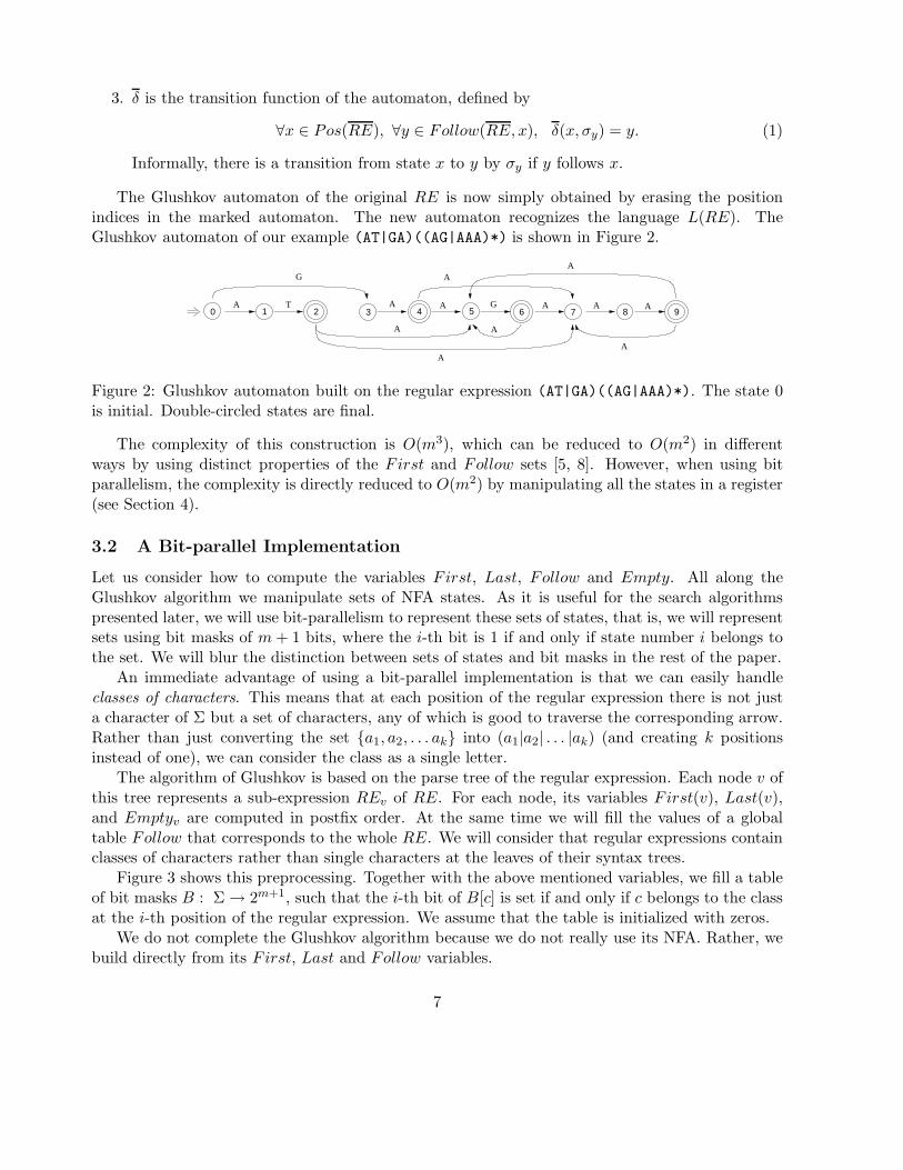
The Glushkov automaton of the original RE is now simply obtained by erasing the positionindices in the marked automaton. The new automaton recognizes the language L(RE). TheGlushkov automaton of our example (AT|GA)((AG|AAA)*) is shown in Figure 2.

0 1 2 3 4 5 6 7 98

G

A T A

A

A

A

A

A

G A A

A

A

A

Figure 2: Glushkov automaton built on the regular expression (AT|GA)((AG|AAA)*). The state 0is initial. Double-circled states are final.

The complexity of this construction is O(m3), which can be reduced to O(m2) in differentways by using distinct properties of the First and Follow sets [5, 8]. However, when using bitparallelism, the complexity is directly reduced to O(m2) by manipulating all the states in a register(see Section 4).

3.2 A Bit-parallel Implementation

Let us consider how to compute the variables First, Last, Follow and Empty. All along theGlushkov algorithm we manipulate sets of NFA states. As it is useful for the search algorithmspresented later, we will use bit-parallelism to represent these sets of states, that is, we will representsets using bit masks of m + 1 bits, where the i-th bit is 1 if and only if state number i belongs tothe set. We will blur the distinction between sets of states and bit masks in the rest of the paper.

An immediate advantage of using a bit-parallel implementation is that we can easily handleclasses of characters. This means that at each position of the regular expression there is not justa character of Σ but a set of characters, any of which is good to traverse the corresponding arrow.Rather than just converting the set {a1, a2, . . . ak} into (a1|a2| . . . |ak) (and creating k positionsinstead of one), we can consider the class as a single letter.

The algorithm of Glushkov is based on the parse tree of the regular expression. Each node v ofthis tree represents a sub-expression REv of RE. For each node, its variables First(v), Last(v),and Emptyv are computed in postfix order. At the same time we will fill the values of a globaltable Follow that corresponds to the whole RE. We will consider that regular expressions containclasses of characters rather than single characters at the leaves of their syntax trees.

Figure 3 shows this preprocessing. Together with the above mentioned variables, we fill a tableof bit masks B : Σ→ 2m+1, such that the i-th bit of B[c] is set if and only if c belongs to the classat the i-th position of the regular expression. We assume that the table is initialized with zeros.

We do not complete the Glushkov algorithm because we do not really use its NFA. Rather, webuild directly from its First, Last and Follow variables.

7

Glushkov variables(vRE , lpos)1. If v = [ | ] (vl, vr) or v = · (vl, vr) Then2. lpos← Glushkov variables(vl, lpos)3. lpos← Glushkov variables(vr, lpos)4. Else If v = ∗ (v∗) Then lpos← Glushkov variables(v∗, lpos)5. End of if6. If v = (ε) Then7. First(v)← 0m+1, Last(v)← 0m+1, Emptyv ← true

8. Else If v = (C) , C ⊆ Σ Then9. lpos← lpos + 110. For σ ∈ C Do B[σ]← B[σ] | 0m−lpos10lpos

11. First(v)← 0m−lpos10lpos, Last(v)← 0m−lpos10lpos

12. Emptyv ← false , Follow(lpos)← 0m+1

13. Else If v = [ | ] (vl, vr) Then14. First(v)← First(vl) | First(vr), Last(v)← Last(vl) | Last(vr)15. Emptyv ← Emptyvl

or Emptyvr

16. Else If v = · (vl, vr) Then17. First(v)← First(vl), Last(v)← Last(vr)18. If Emptyvl

= true Then First(v)← First(v) | First(vr)19. If Emptyvr

= true Then Last(v)← Last(vl) | Last(v)20. Emptyv ← Emptyvl

and Emptyvr

21. For x ∈ Last(vl) Do Follow(x)← Follow(x) | First(vr)22. Else If v = ∗ (v∗) Then23. First(v)← First(v∗), Last(v)← Last(v∗), Emptyv ← true

24. For x ∈ Last(v∗) Do Follow(x)← Follow(x) | First(v∗)25. End of if26. Return lpos

Figure 3: Computing the variables for the Glushkov algorithm. The syntax tree can be a union node([ | ] (vl, vr)) or a concatenation node ( · (vl, vr)) of subtrees vl and vr; a Kleen star node ( ∗ (v∗))with subtree v∗, or a leaf node corresponding to the empty string (ε) or a class of characters (C).

8

4 A Compact DFA Representation

The classical algorithm to produce a DFA from an NFA consists in making each DFA state representa set of NFA states which may be active at that point. A possible way to represent the states ofa DFA (i.e. the sets of states of an NFA) is to use a bit mask of O(m) bits, as already explained.Previous bit-parallel implementations [19, 29] are built on this idea. We present in this section anew bit-parallel DFA representation based on Glushkov’s construction (recall Section 3.2).

4.1 Properties of Glushkov’s Construction

We study now some properties of the Glushkov construction which are necessary for our compactDFA representation. All them are very easy to prove [6]. The proofs are include here for self-containment.

First, since we do not build any ε-transitions (see Formula (1)), we have that Glushkov’s NFA isε-free. That is, in the approach of Wu and Manber [29], the ε-transitions are the complicated part,because all the others move forward. We do not have these transitions in the Glushkov automaton,but on the other hand the normal transitions do not follow such a simple pattern. However, thereare still important structural properties in the arrows. One of these is captured in the followingLemma.

Lemma 1 All the arrows leading to a given state in Glushkov’s NFA are labeled by the samecharacter. Moreover, if classes of characters are permitted at the positions of the regular expression,then all the arrows leading to a given state in Glushkov’s NFA are labeled by the same class.

Proof. This is easily seen in Formula (1). The character labeling every arrow that arrives at statey is precisely σy. This also holds if we consider that σy is in fact a subset of Σ. 2

These properties can be combined with the B table to yield our most important property.

Lemma 2 Let B(σ) be the set of positions of the regular expression that contain character σ. LetFollow(x) be the set of states that can follow state x in one transition, by Glushkov’s construction.Let δ : S × Σ→ P(S) be the transition function of Glushkov’s NFA, i.e. y ∈ δ(x, σ) if and only iffrom state x we can move to state y by character σ. Then, it holds

δ(x, σ) = Follow(x) ∩ B(σ)

Proof. The lemma follows from Lemma 1. Let state y ∈ δ(x, σ). This means that y can be reachedfrom x by σ and therefore y ∈ Follow(x) ∩ B(σ). Conversely, let y ∈ Follow(x) ∩ B(σ). Then ycan be reached by letter σ and it can be reached from x. But Lemma 1 implies that every arrowleading to y is labeled by σ, including the one departing from x, and hence y ∈ δ(x, σ). 2

Finally, a last property is necessary for technical reasons made clear shortly.

Lemma 3 The initial state 0 in Glushkov’s NFA does not receive any arrow.

Proof. This is clear since all the arrows are built in Formula (1), and the initial state is not in theFollow set of any other state (see the definition of Follow). 2

9

4.2 A Compact Representation

We now use Lemma 2 to obtain a compact representation of the DFA. The idea is to computethe transitions by using two tables: the first one is simply B[σ], which is built in algorithmGlushkov variables and gives a bit mask of the states reachable by each letter (no matter fromwhere). The second is a deterministic version of Follow, i.e. a table T from sets of states to setsof states (in bit mask form) which tells which states can be reached from an active state in D, nomatter by which character:

T [D] =⋃

i∈D

Follow(i) (2)

By Lemma 2, it holds that

δ(D,σ) =⋃

i∈D

Follow(i) ∩ B(σ) = T [D] & B[σ]

(we are now using the bit mask representation for sets). Hence instead of the complete transitiontable δ : 2m+1 × Σ → 2m+1 we build and store only T : 2m+1 → 2m+1 and B : Σ → 2m+1. Thenumber of bits required by this representation is (m+1)(2m+1 + |Σ|). Figure 4 shows the algorithmto build T from Follow at optimal cost O(2m).

BuildT (Follow, m)1. T [0] ← 02. For i ∈ 0 . . .m Do3. For j ∈ 0 . . . 2i − 1 Do4. T [2i + j] ← Follow(i) | T [j]5. End of for6. End of for7. Return T

Figure 4: Construction of table T from Glushkov’s variables. We use a numeric notation for theargument of T and use Follow in bit mask form.

4.3 A Search Algorithm

We present now the search algorithm based on the previous construction. Let us call First andLast the variables corresponding to the whole regular expression.

Our first step will be to set Follow(0) = First for technical convenience. Second, we will add aself loop at state 0 which can be traversed by any σ ∈ Σ. This is because, for searching purposes,the NFA that recognizes a regular expression must be converted into one that searches for theregular expression. This is achieved by appending Σ∗ at its beginning, or which is the same, addinga self-loop as described. As, by Lemma 3, no arrow goes to state 0, it still holds that all the arrowsleading to a state are labeled the same way (Lemma 1). Figure 5 shows the search algorithm.

10

Search(RE, T = t1t2 . . . tn)1. Preprocessing

2. (vRE , m)← Parse(RE) /* parse the regular expression */3. Glushkov variables(vRE ,0) /* build the variables on the tree */4. Follow(0) ← 0m1 | First /* add initial self-loop */5. For σ ∈ Σ Do B[σ] ← B[σ] | 0m16. T ← BuildT(Follow, m) /* build T table */7. Searching

8. D ← 0m1 /* the initial state */9. For j ∈ 1 . . . n Do10. If D & Last 6= 0m+1 Then report an occurrence ending at j − 111. D ← T [D] & B[tj ] /* simulate transition */12. End of for

Figure 5: Glushkov-based bit-parallel search algorithm. We assume that Parse gives the syntaxtree vRE and the number of positions m in RE, and that Glushkov variables builds B, First,Last and Follow.

4.4 Horizontal Table Splitting

As mentioned, we can split the T table if it turns out to be too large. The splitting is based onthe following property. Let T : 2m+1 → 2m+1 be the table obtained applying Eq. (2). LetD = D1 : D2 be a splitting of mask D into two submasks, a left and a right submask. In ourset representation of bit masks, D1 = D ∩ {0 . . . ℓ − 1} and D2 = D ∩ {ℓ . . . m}. If we defineT1 : 2ℓ → 2m+1 and T2 : 2m−ℓ+1 → 2m+1 using for T1[D1] and T2[D2] the same formula ofEq. (2), then it is clear that T [D] = T [D1] ∪ T [D2]. In the bit mask view, we have a table T1 thatreceives the first ℓ bits of D and a table T2 that receives the last m− ℓ + 1 bits of D. Each tablegives the bit mask of the states reachable from states in their submask. The total set of states is nomore than the union of both sets: those reachable from states in {0 . . . ℓ− 1} and those reachablefrom states in {ℓ . . . m}. Note that the results of each subtable still has m + 1 bits.

In general we can split T in k tables T1 . . . Tk, such that Ti addresses the bits roughly from(i− 1)(m + 1)/k to i(m + 1)/k− 1, that is, (m + 1)/k bits. Each such table needs 2(m+1)/k(m + 1)bits to be represented, for a total space requirement of O(2m/kmk) bits. The cost is that, in orderto perform each transition, we need to pay for k table accesses so as to compute

T [D1D2 . . . Dk] = T1[D1] | T2[D2] | . . . | Tk[Dk]

which makes the search time O(kn) in terms of table accesses. If we have O(s) bits of space, thenwe solve for s = 2m/kmk, to obtain a search time of O(kn) = O(mn/ log s).

4.5 Comparison

Compared to Wu and Manber’s algorithm [29], ours has the advantage of needing (m+1)(2m+1+|Σ|)bits of space instead of their m(22m+1 + |Σ|) bits in the worst case (their best case is equal to our

11

complexity). Just as they propose, we can split T horizontally to reduce space, so as to obtainO(mn/ log s) time with O(s) space. Compared to our previous algorithm [21], the new one comparesfavorably against its (m + 1)2m+1|Σ| bits of space. Therefore, our new algorithm should be alwayspreferred over previous bit parallel algorithms.

With respect to a classical DFA implementation, its worst case is 2m+1 states, and it stores atable which for each state and each character stores the new state. This requires (m + 1)2m+1|Σ|bits in the worst case. However, in the classical algorithm it is customary to build only the statesthat can actually be reached, which can be much less than all the 2m+1 possibilities.

We can do something similar, in the sense of filling only the reachable cells of T (yet, we cannotpack them consecutively in memory as a classical DFA). Figure 6 shows the recursive constructionof this table, which is invoked with D = 0m1, the initial state, and assumes that T is initializedwith zeros and that B, Follow and m are already computed.

BuildTrec (D)1. For i ∈ 0 . . .m Do /* first build T [D] */2. If D & 0m−i10i 6= 0m+1 Then T [D] ← T [D] | Follow(i)3. End of for4. N ← T [D]5. For σ ∈ Σ Do6. If T [N & B[σ]] = 0m+1 Then /* not built yet */7. BuildTrec (N & B[σ])8. End of for

Figure 6: Recursive construction of table T . We fill only the reachable cells.

Finally, we notice that we do not need to represent state 0, as it is always active. This reducesour space requirement to m(2m + |Σ|) bits of space. This improvement, however, cannot be usedin the techniques presented later in this paper.

5 The Reverse Factor Search Approach

In this section we describe the general reverse factor search approach currently used to search forsingle patterns [17, 11, 22] or multiple patterns [10, 25].

The search is done using a window which has the length of the minimum word that we searchfor (if we search for a single word, we just take its length). We note this minimum length ℓ.

We shift the window along the text, and for each position of the window, we search backwards(i.e from right to left, see Figure 7) for any factor of any length-ℓ prefix of our set of patterns (if wesearch for a single word, this means any factor of the word). Also, each time we recognize a factorwhich is indeed a prefix of some of the patterns, we store our position in the window in a variablelast (which is overwritten, so we know the last time that this happened). Now, two possibilitiesappear:

(i) We do not reach the beginning of the window. This case is shown in Figure 7. The search

12

for a factor fails on a letter σ, i.e σu is not a factor of a length-ℓ prefix of any pattern. Wecan directly shift the window to start at position last, since no pattern can start before, andbegin the search again.

(ii) We reach the beginning of the window. If we search for just one pattern, we have recognizedit and we report the occurrence. Otherwise, we just recognized a length-ℓ prefix of one ormore patterns. We verify directly in the text if there is a match of a pattern that starts atthe initial window position, with a forward (i.e left to right) scan. This can be done with atrie of the patterns. Next, in both cases, we shift the window to position last.

σlast

Window

Record in last the window position when a prefix of any pattern is recognizedSearch for a factor

last

The longest prefix starts at lastFail of the search for a factor in σ.

σ

safe shift New window

Figure 7: The reverse factor search approach.

This simple approach leads to very fast algorithms in practice, such as BDM [11] and BNDM [22].For a single pattern, this is optimal on average, matching Yao’s bound [30] of O(n log(ℓ)/ℓ), whereℓ the pattern length. In the worst case, this scheme is quadratic (O(nℓ) complexity). There existshowever a general technique to keep the algorithms sub-linear on average and linear in the worstcase.

5.1 A Linear Worst Case Algorithm

The main idea used in [11, 22, 10, 25] is to avoid retraversing the same characters in the backwardwindow verification. We divide the work done on the text in two parts: forward and backwardscanning. To be linear in the worst case, none of these two parts must retraverse characters. In theforward scan, it is enough to keep track of the longest pattern prefix v that matches the current textsuffix. This is easily achieved with a KMP automaton [16] (for one pattern) or an Aho-Corasickautomaton [2] (for multiple patterns). All the matches are found using the forward scan.

However, we need to use also backward searching in order to skip characters. The idea is thatthe window is placed so that the current longest prefix matched v is aligned with the beginning ofthe window. The position of the current text character inside the window (i.e. |v|) is called thecritical position. At any point in the forward scan we can place the window (shifted |v| charactersfrom the current text position) and try a backward search. Clearly, this is only promising when v

13

is not very long compared to ℓ. Usually, a backward scan is attempted when the prefix is less than⌊ℓ/α⌋, where 0 < α < ℓ is fixed arbitrary (usually α = 2).

The backward search proceeds almost as before, but it finishes as soon as the critical positionis reached. The two possibilities are:

(i) We reach the critical position. This case is shown in Figure 8. In this case we are not able toskip characters. The forward search is resumed in the place where it was left (i.e. from thecritical position), totally retraverses the window, and continues until the condition to try anew backward scan holds again.

We reached the critical position

u

Window

v

v′

Window

Critpos

Critpos′End of the forward searchback to a normal state

Window

Re-read with a forward search

Figure 8: The critical position is reached, in the linear-time algorithm.

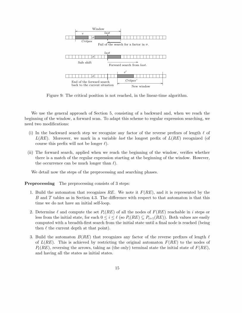
(ii) We do not reach the critical position. This case is shown in Figure 9. This means that therecannot be a match in the current window. We start a forward scan from scratch at positionlast, totally retraverse the window, and continue until a new backward scan seems promising.

6 A Character Skipping Algorithm

In this section we explain how to adapt the general approach of Section 5 to regular expressionsearching. We first explain a simple extension of the basic approach and later show how to keepthe worst case linear. Recall that we search for a regular expression called RE of size m, whichgenerates the language L(RE).

6.1 Basic Approach

The search in the general approach needs a window of length ℓ (shortest pattern we search for).In regular expression searching this corresponds to the length of the shortest word of L(RE). Ofcourse, if this word is ε, the problem of searching is trivial since every text position matches. Weconsider in the following that ℓ > 0.

14

Windowlast

σ

Fail of the search for a factor in σ.

σlast

σCritpos

v

Forward search from last.Safe shift

New window

Critpos’

v′

End of the forward searchback to the current situation

Figure 9: The critical position is not reached, in the linear-time algorithm.

We use the general approach of Section 5, consisting of a backward and, when we reach thebeginning of the window, a forward scan. To adapt this scheme to regular expression searching, weneed two modifications:

(i) In the backward search step we recognize any factor of the reverse prefixes of length ℓ ofL(RE). Moreover, we mark in a variable last the longest prefix of L(RE) recognized (ofcourse this prefix will not be longer ℓ).

(ii) The forward search, applied when we reach the beginning of the window, verifies whetherthere is a match of the regular expression starting at the beginning of the window. However,the occurrence can be much longer than ℓ).

We detail now the steps of the preprocessing and searching phases.

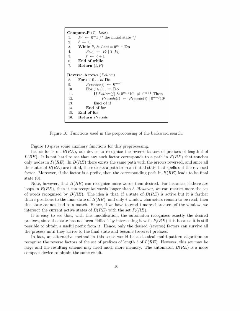
Preprocessing The preprocessing consists of 3 steps:

1. Build the automaton that recognizes RE. We note it F (RE), and it is represented by theB and T tables as in Section 4.3. The difference with respect to that automaton is that thistime we do not have an initial self-loop.

2. Determine ℓ and compute the set Pi(RE) of all the nodes of F (RE) reachable in i steps orless from the initial state, for each 0 ≤ i ≤ ℓ (so Pi(RE) ⊆ Pi+1(RE)). Both values are easilycomputed with a breadth-first search from the initial state until a final node is reached (beingthen ℓ the current depth at that point).

3. Build the automaton B(RE) that recognizes any factor of the reverse prefixes of length ℓof L(RE). This is achieved by restricting the original automaton F (RE) to the nodes ofPℓ(RE), reversing the arrows, taking as (the only) terminal state the initial state of F (RE),and having all the states as initial states.

15

Compute P (T, Last)1. P0 ← 0m1 /* the initial state */2. ℓ ← 03. While Pℓ & Last = 0m+1 Do4. Pℓ+1 ← Pℓ | T [Pℓ]5. ℓ ← ℓ + 16. End of while7. Return (ℓ, P )

Reverse Arrows (Follow)8. For i ∈ 0 . . .m Do9. Precede(i) ← 0m+1

10. For j ∈ 0 . . .m Do11. If Follow(j) & 0m−i10i 6= 0m+1 Then12. Precede(i) ← Precede(i) | 0m−j10j

13. End of if14. End of for15. End of for16. Return Precede

Figure 10: Functions used in the preprocessing of the backward search.

Figure 10 gives some auxiliary functions for this preprocessing.Let us focus on B(RE), our device to recognize the reverse factors of prefixes of length ℓ of

L(RE). It is not hard to see that any such factor corresponds to a path in F (RE) that touchesonly nodes in Pℓ(RE). In B(RE) there exists the same path with the arrows reversed, and since allthe states of B(RE) are initial, there exists a path from an initial state that spells out the reversedfactor. Moreover, if the factor is a prefix, then the corresponding path in B(RE) leads to its finalstate (0).

Note, however, that B(RE) can recognize more words than desired. For instance, if there areloops in B(RE), then it can recognize words longer than ℓ. However, we can restrict more the setof words recognized by B(RE). The idea is that, if a state of B(RE) is active but it is fartherthan i positions to the final state of B(RE), and only i window characters remain to be read, thenthis state cannot lead to a match. Hence, if we have to read i more characters of the window, weintersect the current active states of B(RE) with the set Pi(RE).

It is easy to see that, with this modification, the automaton recognizes exactly the desiredprefixes, since if a state has not been “killed” by intersecting it with Pi(RE) it is because it is stillpossible to obtain a useful prefix from it. Hence, only the desired (reverse) factors can survive allthe process until they arrive to the final state and become (reverse) prefixes.

In fact, an alternative method in this sense would be a classical multi-pattern algorithm torecognize the reverse factors of the set of prefixes of length ℓ of L(RE). However, this set may belarge and the resulting scheme may need much more memory. The automaton B(RE) is a morecompact device to obtain the same result.

16

How to represent B(RE) deserves further consideration. After reversing the arrows of ourautomaton, it is not anymore the result of Glushkov’s construction over a regular expression, andin particular the property that all the arrows arriving at a state being labeled by the same characterdoes not hold anymore. Hence, our bit-parallel simulation of Section 4 cannot be applied.

Fortunately, a dual property holds: all the arrows leaving a state are labeled by the samecharacter or class. Hence, if we read a text character σ, we can first kill the automaton stateswhose leaving transitions are not labeled by σ, and then take all the transitions from them. LetTb be the T mask corresponding to B(RE), and B the mask of F (RE). Then, a transition can becarried out by

δb(D,σ) = Tb[D & B[σ]]

Searching The search follows the general approach of Section 5. For each window position, weactivate all the states of B(RE) and traverse the window backwards updating last each time thefinal state of B(RE) is reached (recall that after each step, we “kill” some states of B(RE) usingPi(RE)). If B(RE) runs out of active states we shift the window to position last. Otherwise, ifwe reach the beginning of the window, we start a forward scan using F (RE) from the beginning ofthe window until either a match is found1, we reached the end of the text, or F (RE) runs out ofactive states. After the forward scan, we shift the window to position last.

Figure 11 shows the search algorithm. As before, large T tables can be split.

6.2 Linear Worst Case Extension

We also extended the general linear worst case approach (Section 5.1) to the case of regular ex-pression searching.

We transform the forward scan automaton F (RE) of the previous algorithm by adding a self-loop at its initial state, for each letter of Σ (so now it recognizes Σ∗L(RE)). This is our forwardscanning automaton of Section 4.3.

The main difficulty to extend the general linear approach is determining where to place thewindow in order to not lose a match. The general approach considers the longest prefix of thepattern already recognized. However, this information cannot be inferred only from the activestates of the automaton (for instance, it is not known how many times we have traversed a loop).We use an alternative concept: instead of considering the longest prefix already matched, weconsider the shortest path to reach a final state. This value can be determined from the currentset of states. We devise two different alternatives that differ on the use of this information.

Prior to explaining both alternatives, we introduce some notation. In general, the window isplaced so that it finishes ℓ′ characters ahead of the current text position (for 0 ≤ ℓ′ ≤ ℓ). Tosimplify the exposition, we call this ℓ′ the “forward-length” of the window.

In the first alternative the forward-length of the window is the shortest path from an activestate of F (RE) to a final state (this same idea has been used for multipattern matching in [10]).In this case, we need to recognize any reverse factor of L(RE) in the backward scan (not only

1Since we report the beginning of matches, we stop the forward search as soon as we find a match.

17

Backward-Search(RE, T = t1t2 . . . tn)1. Preprocessing

2. (vRE , m)← Parse(RE) /* parse the regular expression */3. Glushkov variables(vRE ,0) /* build the variables on the tree */4. Follow(0) ← First5. T ← BuildT(Follow, m) /* build T table */6. (ℓ, P ) ← Compute P(T, Last)7. Precede ← Reverse Arrows(Follow)8. Tb ← BuildT(Precede, m)9. Searching

10. pos ← 011. While pos ≤ n− ℓ Do12. j ← ℓ, last ← ℓ13. D ← Pℓ

14. While D 6= 0m+1and j > 0 Do

15. D ← Tb[D & B[tpos+j ]] & Pj−1

16. j ← j − 117. If D & 0m1 6= 0m+1 Then /* prefix recognized */18. If j > 0 Then last← j19. Else /* check a possible occurrence starting at pos + 1 */20. D ← 0m1, i ← pos + 121. While i ≤ n and D & Last = 0m+1

and D 6= 0m+1 Do22. D ← T [D] & B[ti]23. End of while24. If D & Last 6= 0m+1 Then25. Report an occurrence beginning at pos + 126. End of if27. End of if28. End of if29. End of while30. pos ← pos + last31. End of while

Figure 11: Backward search algorithm for regular expressions. Do not confuse the bit-mask Lastof final states with the window position last of the last prefix recognized.

18

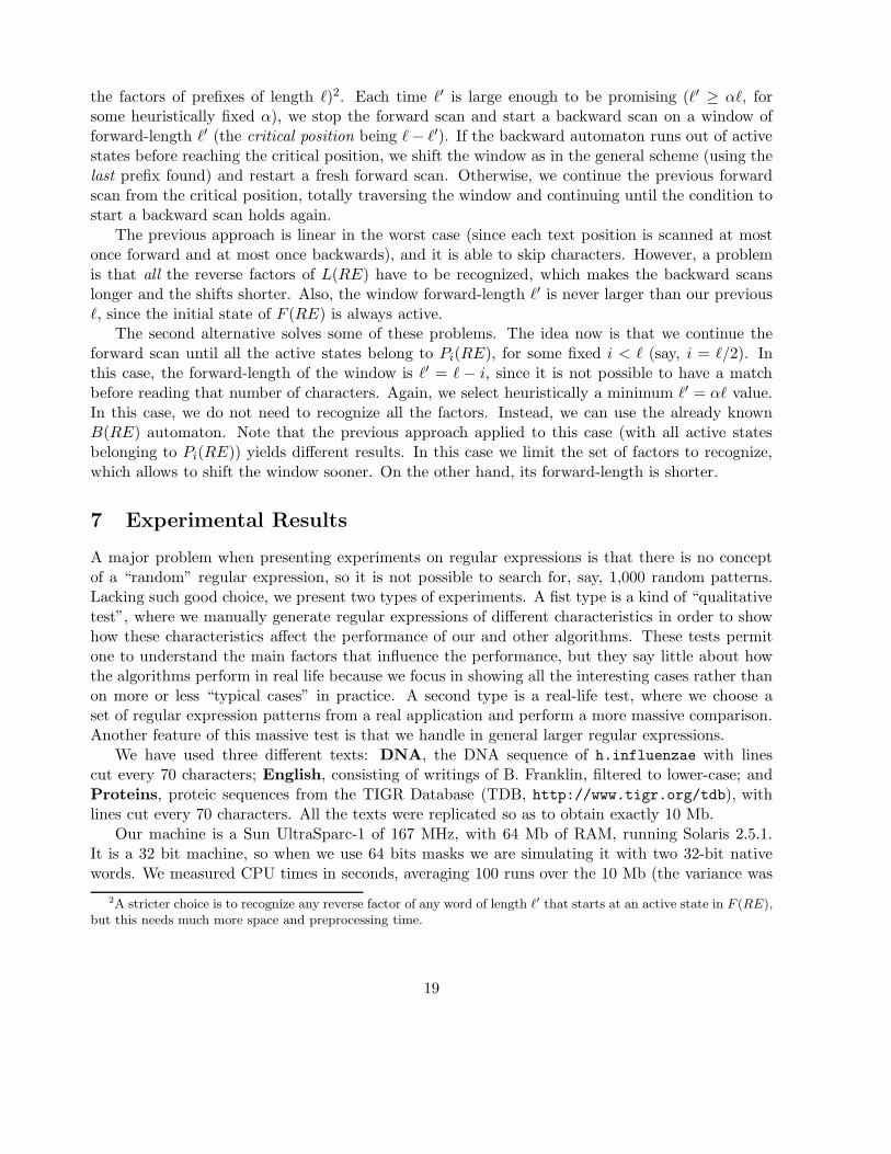
the factors of prefixes of length ℓ)2. Each time ℓ′ is large enough to be promising (ℓ′ ≥ αℓ, forsome heuristically fixed α), we stop the forward scan and start a backward scan on a window offorward-length ℓ′ (the critical position being ℓ− ℓ′). If the backward automaton runs out of activestates before reaching the critical position, we shift the window as in the general scheme (using thelast prefix found) and restart a fresh forward scan. Otherwise, we continue the previous forwardscan from the critical position, totally traversing the window and continuing until the condition tostart a backward scan holds again.

The previous approach is linear in the worst case (since each text position is scanned at mostonce forward and at most once backwards), and it is able to skip characters. However, a problemis that all the reverse factors of L(RE) have to be recognized, which makes the backward scanslonger and the shifts shorter. Also, the window forward-length ℓ′ is never larger than our previousℓ, since the initial state of F (RE) is always active.

The second alternative solves some of these problems. The idea now is that we continue theforward scan until all the active states belong to Pi(RE), for some fixed i < ℓ (say, i = ℓ/2). Inthis case, the forward-length of the window is ℓ′ = ℓ − i, since it is not possible to have a matchbefore reading that number of characters. Again, we select heuristically a minimum ℓ′ = αℓ value.In this case, we do not need to recognize all the factors. Instead, we can use the already knownB(RE) automaton. Note that the previous approach applied to this case (with all active statesbelonging to Pi(RE)) yields different results. In this case we limit the set of factors to recognize,which allows to shift the window sooner. On the other hand, its forward-length is shorter.

7 Experimental Results

A major problem when presenting experiments on regular expressions is that there is no conceptof a “random” regular expression, so it is not possible to search for, say, 1,000 random patterns.Lacking such good choice, we present two types of experiments. A fist type is a kind of “qualitativetest”, where we manually generate regular expressions of different characteristics in order to showhow these characteristics affect the performance of our and other algorithms. These tests permitone to understand the main factors that influence the performance, but they say little about howthe algorithms perform in real life because we focus in showing all the interesting cases rather thanon more or less “typical cases” in practice. A second type is a real-life test, where we choose aset of regular expression patterns from a real application and perform a more massive comparison.Another feature of this massive test is that we handle in general larger regular expressions.

We have used three different texts: DNA, the DNA sequence of h.influenzae with linescut every 70 characters; English, consisting of writings of B. Franklin, filtered to lower-case; andProteins, proteic sequences from the TIGR Database (TDB, http://www.tigr.org/tdb), withlines cut every 70 characters. All the texts were replicated so as to obtain exactly 10 Mb.

Our machine is a Sun UltraSparc-1 of 167 MHz, with 64 Mb of RAM, running Solaris 2.5.1.It is a 32 bit machine, so when we use 64 bits masks we are simulating it with two 32-bit nativewords. We measured CPU times in seconds, averaging 100 runs over the 10 Mb (the variance was

2A stricter choice is to recognize any reverse factor of any word of length ℓ′ that starts at an active state in F (RE),

but this needs much more space and preprocessing time.

19

very low). We include the time for preprocessing in the search figures, except where we show themseparately. We show the results in tenths of second per megabyte.

The conclusion of the experiments is that our forward scanning algorithm is better than anycompeting technique on patterns that do not permit enough character skipping. On the patternsthat do, our backward scanning algorithm is in most cases the best choice, although depending onthe particularities of the pattern other character skipping techniques may work better. We alsoshow that our algorithms adapt better than the others to long patterns.

A good rule of thumb to determine whether a regular expression RE permits character skippingis to consider the length ℓ of the shortest string in L(RE), and then count how many differentprefixes of length ≤ ℓ exist in L(RE). As this number approaches σℓ, character skipping becomesmore difficult and a forward scanning becomes a better choice.

7.1 Qualitative Tests

We divide this comparison in three parts. First, we compare different existing algorithms to im-plement an automaton. These algorithms process all the text characters, one by one, and theyonly differ in the way they keep track of the state of the search. Second, we compare, using ourautomaton simulation, a simple forward-scan algorithm against the different variants of backwardsearch proposed, to show that backward searching can be faster depending on the pattern. Finally,we compare our backward search algorithm against other algorithms that are also able to skipcharacters.

For this comparison we have fixed a set of 10 patterns for English and 10 for DNA, which wereselected to illustrate different interesting cases, as explained. The patterns are given in Tables 1 and2. We show their number of letters, which is closely related to the size of the automata recognizingthem, the minimum length ℓ of a match for each pattern, and a their empirical matching probability(number of matches divided by n). The period (.) in the patterns matches any character exceptthe end of line (lines have approximately 70 characters).

No. Pattern Size Minimum Prob. match(# letters) length ℓ (empirical)

1 AC((A|G)T)*A 6 3 .0157100002 AGT(TGACAG)*A 10 4 .0029040003 (A(T|C)G)|((CG)*A) 7 1 .3316000004 GTT|T|AG* 6 1 .6651000005 A(G|CT)* 4 1 .3825000006 ((A|CG)*|(AC(T|G))*)AG 9 2 .0467000007 AG(TC|G)*TA 7 4 .0038860008 [ACG][ACG][ACG][ACG][ACG][ACG]T 7 7 .0331500009 TTTTTTTTTT[AG] 11 11 .00000104910 AGT.*AGT 7 6 .003109000

Table 1: The patterns used on DNA.

20

No. Pattern Size Minimum Prob. match(# letters) length ℓ (empirical)

1 benjamin|franklin 16 8 .0000358602 benjamin|franklin|writing 23 7 .0001014003 [a-z][a-z0-9]*[a-z] 3 2 .6092000004 benj.*min 8 7 .0000079155 [a-z][a-z][a-z][a-z][a-z] 5 5 .2024000006 (benj.*min)|(fra.*lin) 15 6 .0000358607 ben(a|(j|a)*)min 9 6 .0094910008 be.*ja.*in 8 6 .0000121109 ben[jl]amin 8 8 .00000791510 (be|fr)(nj|an)(am|kl)in 14 8 .000035860

Table 2: The patterns used on English text.

7.1.1 Forward Scan Algorithms

In principle, any forward scan algorithm can be enriched with backward searching to skip characters.Some are easier to adapt than others, however. In this experiment we only consider the performanceof the forward scan methods. The purpose of this test is to evaluate our new forward searchalgorithm of Section 4.3. We have tested the following algorithms for the forward scanning (seeSection 2 for detailed descriptions of previous work). We left aside some algorithms which provednot competitive, at least for the sizes of the regular expressions we are considering: Thompson’s [26]and Myers’ [19]. This last one is more competitive for larger patterns, as we show in Section 7.2.We have also left aside lazy deterministic automata implementations. However, as we show inSection 7.1.3, these also tend to be slower than ours.

DFA: builds the classical deterministic automaton and runs it over the text. We have implementedthe scheme using Glushkov’s construction, not minimizing the final automaton.

Agrep: builds over Thompson’s NFA and uses a bit mask to handle the active states [29]. Thesoftware [28] is from S. Wu and U. Manber. We forced the best choice of number of subtables.

Ours-naive: our new algorithm of Section 4.3, building the whole table T with BuildT. We alwaysuse one table.

Ours-optim: our new algorithm where we build only the T mask for the reachable states, usingBuildTrec. We always use one table.

The goal of showing two versions of our algorithm is as follows. Ours-naive builds the com-plete Td table for all the 2m+1 possible combinations (reachable or not) of active and inactivestates. It permits comparing directly against Agrep and showing that our technique is superior.Ours-optim builds only the reachable states and it permits comparing against DFA, the classicalalgorithm. The disadvantage of Ours-optim is that it does not permit splitting the tables (neitherdoes DFA), while Ours-naive and Agrep do.

21

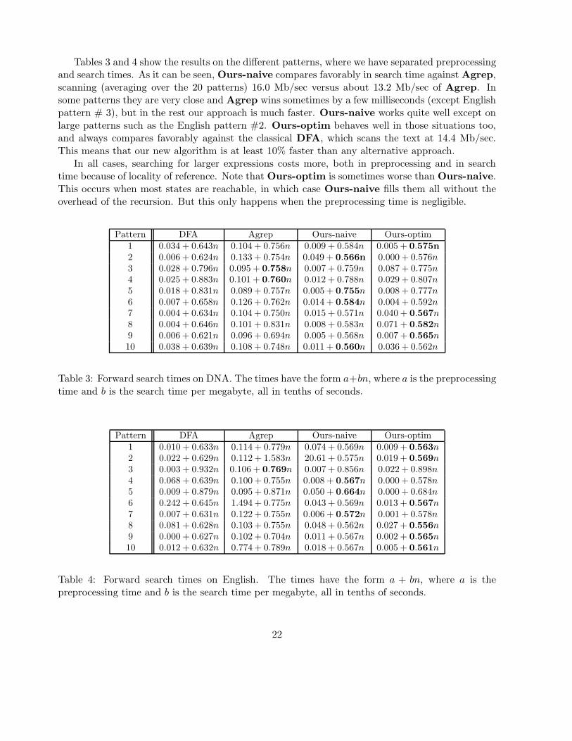
Tables 3 and 4 show the results on the different patterns, where we have separated preprocessingand search times. As it can be seen, Ours-naive compares favorably in search time against Agrep,scanning (averaging over the 20 patterns) 16.0 Mb/sec versus about 13.2 Mb/sec of Agrep. Insome patterns they are very close and Agrep wins sometimes by a few milliseconds (except Englishpattern # 3), but in the rest our approach is much faster. Ours-naive works quite well except onlarge patterns such as the English pattern #2. Ours-optim behaves well in those situations too,and always compares favorably against the classical DFA, which scans the text at 14.4 Mb/sec.This means that our new algorithm is at least 10% faster than any alternative approach.

In all cases, searching for larger expressions costs more, both in preprocessing and in searchtime because of locality of reference. Note that Ours-optim is sometimes worse than Ours-naive.This occurs when most states are reachable, in which case Ours-naive fills them all without theoverhead of the recursion. But this only happens when the preprocessing time is negligible.

Pattern DFA Agrep Ours-naive Ours-optim1 0.034 + 0.643n 0.104 + 0.756n 0.009 + 0.584n 0.005 + 0.575n2 0.006 + 0.624n 0.133 + 0.754n 0.049 + 0.566n 0.000 + 0.576n3 0.028 + 0.796n 0.095 + 0.758n 0.007 + 0.759n 0.087 + 0.775n4 0.025 + 0.883n 0.101 + 0.760n 0.012 + 0.788n 0.029 + 0.807n5 0.018 + 0.831n 0.089 + 0.757n 0.005 + 0.755n 0.008 + 0.777n6 0.007 + 0.658n 0.126 + 0.762n 0.014 + 0.584n 0.004 + 0.592n7 0.004 + 0.634n 0.104 + 0.750n 0.015 + 0.571n 0.040 + 0.567n8 0.004 + 0.646n 0.101 + 0.831n 0.008 + 0.583n 0.071 + 0.582n9 0.006 + 0.621n 0.096 + 0.694n 0.005 + 0.568n 0.007 + 0.565n10 0.038 + 0.639n 0.108 + 0.748n 0.011 + 0.560n 0.036 + 0.562n

Table 3: Forward search times on DNA. The times have the form a+bn, where a is the preprocessingtime and b is the search time per megabyte, all in tenths of seconds.

Pattern DFA Agrep Ours-naive Ours-optim1 0.010 + 0.633n 0.114 + 0.779n 0.074 + 0.569n 0.009 + 0.563n2 0.022 + 0.629n 0.112 + 1.583n 20.61 + 0.575n 0.019 + 0.569n3 0.003 + 0.932n 0.106 + 0.769n 0.007 + 0.856n 0.022 + 0.898n4 0.068 + 0.639n 0.100 + 0.755n 0.008 + 0.567n 0.000 + 0.578n5 0.009 + 0.879n 0.095 + 0.871n 0.050 + 0.664n 0.000 + 0.684n6 0.242 + 0.645n 1.494 + 0.775n 0.043 + 0.569n 0.013 + 0.567n7 0.007 + 0.631n 0.122 + 0.755n 0.006 + 0.572n 0.001 + 0.578n8 0.081 + 0.628n 0.103 + 0.755n 0.048 + 0.562n 0.027 + 0.556n9 0.000 + 0.627n 0.102 + 0.704n 0.011 + 0.567n 0.002 + 0.565n10 0.012 + 0.632n 0.774 + 0.789n 0.018 + 0.567n 0.005 + 0.561n

Table 4: Forward search times on English. The times have the form a + bn, where a is thepreprocessing time and b is the search time per megabyte, all in tenths of seconds.

22

7.1.2 Forward Versus Backward Scanning

We compare now our new forward scan algorithm (called Fwd in this section and Ours-optimin Section 7.1.1) against backward scanning. There are three backward scanning algorithms. Thesimplest one, presented in Section 6.1, is called Bwd. The two linear variations presented inSection 6.2 are called LBwd-All (that recognizes all the reverse factors) and LBwd-Pref (thatrecognizes reverse factors of length-ℓ prefixes). The linear variations depend on an α parameter,which is between 0 and 1. We have tested the values 0.25, 0.50 and 0.75 for α. We have built onlythe reachable entries of their Tb tables.

Tables 5 and 6 show the results. The improvements are modest on the DNA patterns weselected. This is a consequence of their shortness and high probability of occurrence (in particular,the method makes little sense if the minimum length is 1, and therefore patterns 3 to 5 wereremoved). However, from minimum length 4 or more the backward search becomes competitive(with the exception of pattern 8, because it matches with very high probability).

Pattern Fwd Bwd LBwd-All LBwd-Prefα = 0.25 α = 0.50 α = 0.75 α = 0.25 α = 0.50 α = 0.75

1 0.576 0.823 1.931 2.058 2.112 1.764 1.854 1.9112 0.576 0.658 1.653 1.648 1.640 1.478 1.491 1.5346 0.592 2.066 2.572 3.164 3.147 2.512 3.043 3.0137 0.571 0.710 1.534 1.530 1.568 1.564 1.572 1.6018 0.589 1.416 1.669 1.702 1.707 1.804 1.818 1.8709 0.566 0.265 0.591 0.573 0.559 0.671 0.669 0.66810 0.566 1.086 1.927 1.949 2.240 1.593 1.591 1.909

Table 5: Backward search times on DNA, in seconds for 10 Mb. Preprocessing times are included.

The results are much better on our English patterns, where we obtained improvements in halfof the patterns. In general, the linear versions are quite bad in comparison with the simple one,although in some cases they are faster than a forward search. It is difficult to determine which ofthe two versions is better in which cases, and which is the best value for α.

7.1.3 Character Skipping Algorithms

Finally, we consider other algorithms able to skip characters. Basically, the other algorithms arebased in extracting one or more strings from the regular expression, so that some of those stringsmust appear in any match. A single- or multi-pattern exact search algorithm is then used as afilter, and only where some string in the set is found, its neighborhood is checked for an occurrenceof the whole regular expression. Two approaches exist:

Single pattern: one string is extracted from the regular expression, so that the string must appearinside every match. If this is not possible the scheme cannot be applied. We use Gnu Grepv2.4, which implements this idea. Where the filter cannot be applied, Grep uses a forwardscanning algorithm based on a lazy deterministic automaton (i.e., built on the fly as the text

23

Pattern Fwd Bwd LBwd-All LBwd-Prefα = 0.25 α = 0.50 α = 0.75 α = 0.25 α = 0.50 α = 0.75

1 0.564 0.210 0.442 0.432 0.463 0.468 0.489 0.4992 0.571 0.294 1.173 1.001 1.092 0.932 0.981 0.9523 0.900 2.501 3.303 2.591 3.012 2.559 2.562 2.5614 0.578 0.589 1.702 1.684 1.712 0.941 0.928 0.9175 0.684 1.951 2.051 2.404 2.094 2.128 2.147 2.1776 0.568 0.725 1.821 1.846 1.842 1.009 1.122 1.0927 0.578 0.250 0.459 0.447 0.471 0.511 0.519 0.5108 0.559 0.934 1.748 1.855 1.871 1.333 1.447 1.4709 0.565 0.184 0.373 0.368 0.391 0.413 0.393 0.41110 0.562 0.216 0.421 0.454 0.438 0.468 0.461 0.483

Table 6: Backward search times on English, in seconds for 10 Mb.

is read). Hence, we plot this value only where the idea can be applied. We point out thatGrep also abandons a line when it finds the first match in it.

Multiple patterns: this idea was presented in [27]. A length ℓ′ < ℓ is selected, and all the possiblesuffixes of length ℓ′ of L(R) are generated and searched for. The choice of ℓ′ is not obvious,since longer strings make the search faster, but there are more of them. Unfortunately, thecode of [27] is not public, so we have used the following procedure: first, we extract by handthe suffixes of length ℓ′ for each regular expression; then we use the multipattern search ofAgrep [28], which is very fast, to search for those suffixes; and finally the matching lines aresent to Grep, which checks the occurrence of the regular expression in the matching lines. Wefind by hand the best ℓ′ value for each regular expression. The resulting algorithm is quitesimilar to the idea of [27].

Tables 7 and 8 show the results. The single pattern filter is a very effective trick, but it can beapplied only in a restricted set of cases. It improves over Bwd in a couple of cases, only one reallysignificant. The multipattern filter, on the other hand, is more general, but its times are higherthan ours in general, especially where backward searching is better than forward searching. Notethat, in general, Bwd is the best whenever it is better than Fwd.

7.2 A Real-Life Test

It is not hard to find dozens of examples of regular expression patterns used in real life. A quickoverview on the Web shows patterns to recognize URLs, email addresses, email fields, IP addresses,phone numbers, zip codes, HTML tags, dates, hours, floating point numbers, programming languagevariables, comments, and so on. In general, these patterns are rather small and we have obtainedthe same performance as for our short frequently-matching patterns of the previous sections. Thisshows that many real-life patterns would behave as our examples on DNA.

We would like to consider other applications where the above conditions do not hold. We havefocused on a computational biology application related to peptidic site searching, which permits us

24

Pattern Fwd Bwd Single pattern Multipatternfilter filter

1 0.576 0.823 1.231 2.2822 0.576 0.658 0.919 1.2036 0.592 2.066 1.060 2.2487 0.571 0.710 1.331 1.6508 0.589 1.416 1.162 2.1049 0.566 0.265 0.202 0.31010 0.566 1.022 0.932 1.833

Table 7: Algorithm comparison on DNA, in seconds for 10 Mb.

Pattern Fwd Bwd Single pattern Multipatternfilter filter

1 0.564 0.210 — 0.3092 0.571 0.294 — 0.3713 0.900 2.501 — 1.6484 0.578 0.589 0.171 0.8735 0.684 1.951 — 2.0246 0.568 0.725 — 1.0037 0.578 0.250 0.260 0.4428 0.559 0.934 0.632 0.6619 0.565 0.184 0.193 0.30710 0.562 0.216 0.983 0.348

Table 8: Algorithm comparison on English, in seconds for 10 Mb.

experimenting with larger patterns.PROSITE is a well known set of patterns used for protein searching [13]. Proteins are regarded

as texts over a 20-letter upper case alphabet. PROSITE patterns are formed by the followingitems: (i) classes of characters, denoted by the set of characters they match, for example [AKDE]is equivalent to (A|K|D|E); (ii) bounded length gaps, denoted by x(a, b), which matches anystring of length a to b, for example x(1, 3) is equivalent to Σ(Σ|ε)(Σ|ε). Except for very recentdevelopments [24], PROSITE patterns are searched for as regular expressions, so this is quite a realapplication in computational biology.

Not every PROSITE pattern is interesting for our purposes. In particular, many of them haveno gaps and hence are in fact linear patterns, very easy to search with much simpler algorithms[3, 22]. We also removed 8 patterns having more than 64 states because they were too few to berepresentative of these large NFAs. The result is 329 PROSITE patterns. Those patterns occurtoo frequently (classes are large and gaps are long) to permit any backward search approach, so weconsider only forward searching in this experiment.

Our forward scanning algorithm is that of Section 4.3. To accommodate up to 64 states, wehave used a couple of integers (or a long integer) to hold the bit mask of 64 bits. This time we

25

have horizontally split the tables into subtables, so the preprocessing is done using BuildT. Thewidth of the subtables is limited to 16 bits, so the number of subtables is ⌈m/16⌉, ranging from 1to 4. For 1 and 2 subtables we use specialized code, while the cases of 3 and 4 tables are handledwith a loop sentence. On the other hand, using bit masks of 32 bits makes all the operations muchfaster for the shorter patterns that can be accommodated in 32 bits. So, when comparing againstalgorithms that cannot handle more than 32 NFA states, we use our 32-bit-masks version; andwhen comparing against other algorithms we use our slower 64-bit-masks version.

Figure 12 shows the search time of our algorithm as a function of Glushkov’s NFA size (that is,m+1), both for 32-bit and 64-bit masks. Clear jumps can be seen when moving to more subtables.The difference between specialized code for up to 2 tables is also clear. Inside homogeneous areas,the increase in time corresponding to having larger subtables is also clear.

0.4

0.5

0.6

0.7

0.8

0.9

1

1.1

1.2

5 10 15 20 25 30 35

Our

s (3

2 bi

ts)

Glushkov NFA size

0

2

4

6

8

10

12

14

16

0 10 20 30 40 50 60 70

Our

s (6

4 bi

ts)

Glushkov NFA size

Figure 12: Our search times as a function of the NFA size (m + 1), using 32-bit masks (left) and64-bit masks (right).

Let us compare those times against other approaches. We start with the full DFA implemen-tation, that is, the DFA is completely built and later used for searching. The code was written byourselves and built over Glushkov’s NFA. We removed all the patterns that requested more than64 Mb of memory for the automaton because they needed more than 10 minutes to be searchedfor. This left us with only 215 patterns. Figure 13 shows the relative performance as a functionof the number of states in the NFA. We are considering only NFAs of up to 32 states in this case,so we compare against our 32-bit version. As it can be seen, our technique is always faster than afull DFA implementation, which takes an unreasonable amount of time for a significant number ofpatterns as their length grow. At the best moment of the full DFA implementation, it takes about1.5 times the time we need for the search.

Only 7 patterns of more than 32 states can be handled by the full DFA implementation usingless than 64 Mb. From these 7 patterns, 6 were 4 to 12 times slower than our 64-bit version, so wecan say that this method cannot handle in general patterns of more than 32 states. That is, thefull DFA method does not generalize to long regular expressions, and for short ones, we are clearlyfaster.

In order to test an external DFA implementation, we considered Grep. Since Grep took more

26

0

20

40

60

80

100

120

5 10 15 20 25 30 35

DF

A/O

urs(

32)

Glushkov NFA size

1

1.5

2

2.5

3

3.5

4

4.5

5

5 10 15 20 25 30 35

DF

A/O

urs(

32)

Glushkov NFA size

Figure 13: Comparison on PROSITE patterns between our algorithm and the full DFA implemen-tation for NFAs of up to 32 states. On the right we show in detail the patterns where the full DFAimplementation is up to 5 times slower than our algorithm.

than 10 minutes on NFAs of more than 20 states, we considered only those of up to 20 states. Thisleft us with 98 patterns. We compared against our 32-bit version, as it was more than enough forthe patterns that Grep could handle.

Figure 14 shows the results. As it can be seen, there were still 5 patterns, some with as fewas 17 states, which were more than 40 times slower than our algorithm. For the majority, we areabout 1.3 times faster for short patterns and about 1.1 times faster for patterns needing two tableaccesses. In 3 cases Grep was up to 5% faster than us. Observe, however, that Grep cannot handlelonger patterns and that, even in the area shown, it can give rise to surprises with exceedingly longexecution times.

0.1

1

10

100

1000

10000

8 10 12 14 16 18 20 22

Gre

p/O

urs(

32)

Glushkov NFA size

0.9

1

1.1

1.2

1.3

1.4

1.5

1.6

1.7

8 10 12 14 16 18 20 22

Gre

p/O

urs(

32)

Glushkov NFA size

Figure 14: Comparison on PROSITE patterns between our algorithm and Gnu Grep for NFAs ofup to 20 states. On the right we show in detail the patterns where Gnu Grep implementation is upto 2 times slower than our algorithm.

27

Let us now compare our algorithm against Myers’ [19]. The code, from G. Myers, builds an NFAof DFAs based on Thompson’s construction. The main purpose of this comparison is to comparetwo different mechanisms to handle large patterns, so we have used only the 64-bit version of ourcode. As it can be seen in Figure 15 (left), our table splitting technique is not only a simpler, butalso a more efficient, mechanism to handle longer patterns than Myers’. Our technique is 2 to 5times faster for NFAs of up to 32 states (where we handcode the use of 1 or 2 tables), and about1.5 times faster for up to 64 states, where we use a normal loop to update the bit mask.

1

1.5

2

2.5

3

3.5

4

4.5

5

5.5

0 10 20 30 40 50 60 70

Mye

rs/O

urs(

64)

Glushkov NFA size

1.8

2

2.2

2.4

2.6

2.8

3

3.2

3.4

3.6

3.8

8 10 12 14 16 18 20 22 24 26 28A

grep

/Our

s(32

)Glushkov NFA size

Figure 15: Comparison between ours and Myers’ algorithm (left) and Agrep (right) for PROSITEpatterns. Our algorithm uses masks of 64 bits against Myers and 32 bits against Agrep.

Finally, we show a comparison against Agrep software [29, 28] by S. Wu and U. Manber, wherewe have respected its original decisions about splitting tables. Agrep is limited to Thompson NFAsof less than 32 states, so only some patterns could be tested and we only show our 32-bit code.Figure 15 (right) shows the comparison, where it can be seen that we are twice as fast on shortpatterns and around 3 times faster for longer patterns. This shows the superiority of Glushkov’sover Thompson’s based constructions.

It is important to notice that the results on bit-parallel algorithms improve with technologicalprogress, whereas those on classical algorithms do not. For example, if we ran our experimentson a 64-bit machine, our search times on 64-bit masks would be as good as those on 32-bit masks(apart from the effects on the number of tables used).

8 Conclusions

We have presented new techniques and algorithms for faster regular expression searching. Wehave shown how to represent a deterministic finite automaton (DFA) in a compact form and howto manipulate an automaton in order to permit skipping text characters at search time. Thesetechniques yield fast and simple search algorithms, which we have shown experimentally to befaster than previous approaches in most cases.

Bit-parallelism has been an essential tool in recent research on regular expression searching, andour work is not an exception. The flexibility of bit-parallelism permits extending the search problem,

28

for example to permit a limited number of errors in the occurrences of the regular expression, and ithas been demonstrated in pattern matching software such as Agrep [28] and Nrgrep [20]. The latteris built on the ideas presented in this paper. Also, it extends Grep’s idea of selecting a necessarystring, so it chooses the most promising subgraph of the NFA for the scanning.

The preprocessing time is a subject of future work. In our experiments the patterns were rea-sonably short and the simple technique of using one transition table was the best choice. However,longer patterns would need the use of the table splitting technique, which worsens the search times.Also, it seems difficult to split the table when we are trying to build only the reachable states.

Finally, we point out that there is some recent work on reducing the number of states of NFAs[7, 15], and on restricting these types of reductions in order to retain the useful properties ofGlushkov construction (especially that of Lemma 2), which permits applying the compact DFArepresentation we propose in this paper [14].

References

[1] A. Aho, R. Sethi, and J. Ullman. Compilers: Principles, Techniques and Tools. Addison-Wesley, 1985.

[2] A. V. Aho and M. J. Corasick. Efficient string matching: an aid to bibliographic search.Communications of the ACM, 18(6):333–340, 1975.

[3] R. Baeza-Yates and G. Gonnet. A new approach to text searching. Communications of theACM, 35(10):74–82, October 1992.

[4] G. Berry and R. Sethi. From regular expression to deterministic automata. Theoretical Com-puter Science, 48(1):117–126, 1986.

[5] A. Bruggemann-Klein. Regular expressions into finite automata. Theoretical Computer Sci-ence, 120(2):197–213, November 1993.

[6] J.-M. Champarnaud. Subset construction complexity for homogeneous automata, positionautomata and ZPC-structures. Theoretical Computer Science, 267:17–34, 2001.

[7] J.-M. Champarnaud and F. Coulon. NFA reduction algorithms by means of regular inequalities.In Proc. DLT 2003, LNCS 2710, pages 194–205, 2003.

[8] C.-H. Chang and R. Paige. From regular expression to DFA’s using NFA’s. In Proc. of the 3rdAnnual Symposium on Combinatorial Pattern Matching (CPM), LNCS v. 664, pages 90–110,1992.

[9] B. Commentz-Walter. A string matching algorithm fast on the average. In Proc. of the 6thInternational Colloquium on Automata, Languages and Programming (ICALP), number 6 inLNCS, pages 118–132. Springer-Verlag, 1979.

[10] M. Crochemore, A. Czumaj, L. Gasieniec, S. Jarominek, T. Lecroq, W. Plandowski, andW. Rytter. Fast practical multi-pattern matching. Rapport 93–3, Institut Gaspard Monge,Universite de Marne la Vallee, 1993.

29

[11] A. Czumaj, Maxime Crochemore, L. Gasieniec, S. Jarominek, Thierry Lecroq, W. Plandowski,and W. Rytter. Speeding up two string-matching algorithms. Algorithmica, 12:247–267, 1994.

[12] V-M. Glushkov. The abstract theory of automata. Russian Mathematical Surveys, 16:1–53,1961.

[13] K. Hofmann, P. Bucher, L. Falquet, and A. Bairoch. The PROSITE database, its status in1999. Nucleic Acids Res., 27:215–219, 1999.

[14] L. Ilie, G. Navarro, and S. Yu. On NFA reductions. In Theory is Forever (Salomaa Festschrift),LNCS 3113, pages 112–124. Springer-Verlag, Heidelberg, 2004.

[15] L. Ilie and S. Yu. Reducing NFAs by invariant equivalences. Theoretical Computer Science,306:373–390, 2003.

[16] D. E. Knuth, J. H. Morris, and V. R. Pratt. Fast pattern matching in strings. SIAM Journalon Computing, 6(1):323–350, 1977.

[17] T. Lecroq. Experimental results on string matching algorithms. Software Practice and Expe-rience, 25(7):727–765, 1995.

[18] M. Mohri. String matching with automata. Nordic Journal of Computing, 4(2):217–231, 1997.

[19] E. Myers. A four-russian algorithm for regular expression pattern matching. Journal of theACM, 39(2):430–448, 1992.

[20] G. Navarro. NR-grep: a fast and flexible pattern matching tool. Software Practice and Expe-rience (SPE), 31:1265–1312, 2001.

[21] G. Navarro and M. Raffinot. Fast regular expression search. In Proceedings of the 3rd Workshopon Algorithm Engineering (WAE’99), LNCS v. 1668, pages 199–213, 1999.

[22] G. Navarro and M. Raffinot. Fast and flexible string matching by combining bit-parallelismand suffix automata. ACM Journal of Experimental Algorithmics (JEA), 5(4), 2000.http://www.jea.acm.org/2000/NavarroString.

[23] G. Navarro and M. Raffinot. Compact DFA representation for fast regular expression search.In Proceedings of the 5th Workshop on Algorithm Engineering (WAE’01), LNCS 2141, pages1–12, 2001.

[24] G. Navarro and M. Raffinot. Fast and simple character classes and bounded gaps patternmatching, with applications to protein searching. Journal of Computational Biology, 10(6):903–923, 2003. Earlier version in Proc. RECOMB 2001.

[25] Mathieu Raffinot. On the multi backward dawg matching algorithm (MultiBDM). In Proc.of the 4th South American Workshop on String Processing (WSP), pages 149–165. CarletonUniversity Press, 1997.

30

[26] K. Thompson. Regular expression search algorithm. Communications of the ACM, 11(6):419–422, 1968.

[27] B. Watson. Taxonomies and Toolkits of Regular Language Algorithms. Phd. dissertation,Eindhoven University of Technology, The Netherlands, 1995.

[28] S. Wu and U. Manber. Agrep – a fast approximate pattern-matching tool. In Proc. of theUSENIX Technical Conference, pages 153–162, 1992.

[29] S. Wu and U. Manber. Fast text searching allowing errors. Communications of the ACM,35(10):83–91, October 1992.

[30] A. Yao. The complexity of pattern matching for a random string. SIAM Journal on Computing,8:368–387, 1979.

31