New Streaming Algorithms for Fast Detection of

Superspreaders

Shobha Venkataraman1 Dawn Song1

Phillip B. Gibbons2 Avrim Blum1

May 2004

CMU-CS-04-142

School of Computer ScienceCarnegie Mellon University

Pittsburgh, PA 15213

1Computer Science Dept, Carnegie Mellon University. Email: shobha@cs., dawnsong@, avrim@cs.cmu.edu2Intel Research Pittsburgh. Email: phillip.b.gibbons@intel.com

This research was supported in part by NSF-ITR CCR-0122581 and the Center for Computer and Communica-

tions Security at Carnegie Mellon under grant DAAD19-02-1-0389 from the Army Research Office. The views and

conclusions contained here are those of the authors and should not be interpreted as necessarily representing the

official policies or endorsements, either express or implied, of NSF, ARO, Carnegie Mellon University, or the U.S.

Government or any of its agencies.

Keywords: network monitoring, streaming algorithms, anomaly detection, heavy distinct-hitters, superspreaders

Abstract

High-speed monitoring of Internet traffic is an important and challenging problem, with applica-tions to real-time attack detection and mitigation, traffic engineering, etc. However, packet-levelmonitoring requires fast streaming algorithms that use very little memory space and little commu-nication among collaborating network monitoring points.In this paper, we consider the problem of detecting superspreaders, which are sources that connect toa large number of distinct destinations. We propose several new streaming algorithms for detectingsuperspreaders, and prove guarantees on their accuracy and memory requirements. We also showexperimental results on real network traces. Our algorithms are substantially more efficient (boththeoretically and experimentally) than previous approaches. We also provide several extensionsto our algorithms – we show how to identify superspreaders in a distributed setting, with slidingwindows, and when deletions are allowed in the stream.More generally, our algorithms are applicable to any problem that can be formulated as follows:given a stream of (x, y) pairs, find all the x’s that are paired with a large number of distinct y’s. Wecall this the heavy distinct-hitters problem. There are many network security applications of thisgeneral problem. This paper discusses these and other applications, and for concreteness, focuseson the superspreader problem.

1 Introduction

Internet attacks such as distributed denial-of-service (DDoS) attacks and worm attacks are increas-ing in severity. Network security monitoring can play an important role in defending and mitigatingsuch large-scale Internet attacks – it can be used to detect drastic traffic pattern changes that mayindicate attacks, or more actively, to identify misbehaving hosts or victims being attacked, and todevelop appropriate filters to throttle attack traffic automatically.

For example, a compromised host doing fast scanning for worm propagation often makes anunusually high number of connections to distinct destinations within a short time. The Slammerworm, for instance, caused some infected hosts to send up to 26, 000 scans a second [26]. We callsuch a host a superspreader. (Note that a superspreader may also be known as a port scanner incertain cases.) By identifying in real-time any source IP address that makes an unusually highnumber of distinct connections within a short time, a network monitoring point can identify hoststhat may be superspreaders, and take appropriate action. For example, the identified potentialattackers (and victims) can be used to trigger the network logging system to log attacker traffic fordetailed real-time and post-mortem analysis of attacks (including payload analysis), and can alsobe used to help develop filters that throttle subsequent (similar) attack traffic in real-time.

In addition to network monitoring at a single point, distributed network security monitoring,where network monitoring points distributed throughout the network collaborate and share in-formation, can contribute additional benefits and enhance the monitoring capability. Distributednetwork monitoring collectively covers more traffic, and can often identify distributed attacks fasterthan any single monitoring point can.

Network security monitoring, however, has many challenges and requires efficient algorithms.More and more high speed links are being deployed. The traffic volume on high speed links canbe tens of gigabits per second, and can contain millions of flows per minute. In addition, withinsuch a great number of flows and high volume of traffic, most of the flows may be normal flows.How does one find the needle in the haystack efficiently? That is, how does one find attack trafficin the huge volume of normal traffic efficiently? Many traditional approaches require the networkmonitoring points to maintain per-flow state. Keeping per-flow state, however, often requires highmemory storage, and hence is not practical for high speed links. Because DRAM is too slow for linespeed access on high speed links, network monitoring points would need to use SRAM to keep statefor monitoring; however, SRAM is very expensive, and hence any monitoring algorithm should usememory sparingly.

Moreover, distributed network monitoring poses additional challenges – because distributednetwork monitoring relies on the communication among network monitoring points, the distributedmonitoring algorithm needs to have low communication overhead among cooperating peers to avoidoverburdening monitoring points with update traffic.

In this paper, we propose several new efficient algorithms for fast network security monitoringand distributed network security monitoring. In particular, we present new efficient algorithms foridentifying superspreaders. We provide both theoretical analysis and experimental results of our newalgorithms, and demonstrate that these algorithms have important applications. Our algorithmsare substantially more efficient (both theoretically and experimentally) than previous approaches,and have additional benefits. Our analysis yields tight accuracy and performance bounds on ouralgorithms.

Note that a superspreader is different from the usual definition of a heavy-hitter ([18, 6, 15,25, 11, 22]). A heavy-hitter might be a source that sends a lot of packets, and thus exceeds acertain threshold of the total traffic. A superspreader, on the other hand, is a source that contactsmany distinct destinations. So, for instance, a source that is involved in a few extremely large file

1

(s1, d1), (s2, d2), (s1, d1), (s3, d3), (s1, d1), (s2, d3), (s4, d1), (s2, d4), (s1, d1), (s5, d4), (s6, d6)

Figure 1: Example stream of (source, destination) pairs, starting with (s1, d1) and ending with(s6, d6).

transfers may be a heavy-hitter, but is not a superspreader. On the other hand, a source that sendsa single packet to many destinations might not create enough traffic to be a heavy-hitter, even ifit is a superspreader – some of the sources in our traces that are superspreaders create less than0.004% of the total traffic analyzed; heavy-hitters typically involve a significantly higher fractionof the traffic.

The superspreader problem is an instance of a more general problem that we term heavy distinct-hitters, which may be formulated as follows: given a stream of (x, y) pairs, find all the x’s that arepaired with a large number of distinct y’s. Figure 1, for example, depicts a stream where source s2is paired with three distinct destinations, whereas all other sources in the stream are paired withonly one distinct destination; thus s2 is a heavy distinct-hitter for this (short) stream. We discussother applications of heavy distinct-hitters in Section 2.

To summarize, this paper makes the following contributions:

• We propose new streaming algorithms for identifying superspreaders. Our algorithms are thefirst to address this problem efficiently and provide proven accuracy and performance bounds.The best previous approach [16] requires a certain amount of memory to be allocated for eachsource within the time window. Our algorithms are the first ones where the amount of memoryallocated is independent of the number of sources in the time window, resulting in significantmemory savings. In addition, one of our algorithms is based on a novel two-level samplingscheme, which may be of independent interest.

• We also propose several extensions to enhance our algorithms – we propose efficient distributedversions of our algorithms (Section 4.1), we extend our algorithms to scenarios when deletionis allowed in the stream (Section 4.2), and we extend our algorithms to the sliding windowscenario (Section 4.3).

• Our experimental results on traces with up to 4.5 million packets confirm our theoreticalresults. Further, they show that the memory usage of our algorithms is substantially smallerthan alternative approaches. Finally, they study the effect of different superspreader thresh-olds on the performance of the algorithms, again confirming the theoretical analysis.

Note that the contribution of this paper is in the proposal of new streaming algorithms to enableefficient network monitoring for attacks detection and defense, when given certain parameters.Selecting and testing the correct parameters, however, is application-dependent and out of thescope of this paper.

The rest of the paper is organized as follows. Section 2 motivates and defines the superspreaderproblem. Section 3 presents and compares two novel algorithms for the superspreader problem.Section 4 presents our extensions to handle distributed monitoring, deletions, and sliding windows.Section 5 presents our experimental results. Section 6 describes related work, and Section 7 presentsconclusions.

2 Finding Superspreaders

In this section, we motivate the superspreaders problem, present a formal definition of the problem,and then discuss the deficiencies of previous techniques in addressing the problem.

2

2.1 Motivation and Applications

During fast scanning worm propagation, a compromised host may try to connect to a high numberof distinct hosts in order to spread the worm; we call such a host a superspreader. Superspreaderscould be responsible for contacting a lot of destinations early during worm propagation; so, detectingthem early is of paramount importance. Thus, given a sequence of packets, we would like to designan efficient monitoring algorithm to identify in real-time which source IP addresses have contacteda high number of distinct hosts within a time window. We call this problem the superspreaderproblem. Note that if a source makes multiple connections or sends multiple packets to the samedestination within the time window, the source-destination connection will be counted only once.This is necessary in order to avoid flagging the common legitimate communication patterns wherea source either makes several connections to the same destination within a time window (such aswith webpage downloads) or sends many packets to the same destination (such as when sending alarge file).

It is important to develop efficient mechanisms to identify superspreaders on high-speed net-works. For example, for a large enterprise network or an ISP network for a large number of homeusers, identifying such superspreaders in real-time would aid in throttling attack traffic, and helpsystem administrators to find the computers that are compromised and need to be isolated andcleaned-up. This is a difficult problem on a high-speed monitoring point, as there may be millionsof legitimate flows passing by per minute and the attack traffic may be an extremely small portionof the total traffic.

Extensions We also consider several extensions to the superspreader problem. First, we con-sider the distributed version of the superspreader problem. In the distributed setting, distributednetwork monitoring points collectively identify superspreaders in the overall traffic.

In the second extension, we consider the superspreader problem with deletion. For example,instead of identifying a source IP address that contacts a high number of distinct destinationswithin a time window, we may wish to identify a source IP address that contacts a number ofdistinct destinations and did not get a legitimate response from a high number of those contacteddestinations (this may indicate a scanning behavior). Thus, once the network monitoring point seesa response from a destination for a connection from a source, the source-destination connection willbe deleted from the count of the number of distinct connections a source makes.

In the third extension, we consider the superspreader problem over a sliding window of the mostrecent packets, e.g., the million most recent packets or the packets arriving in the last 60 minutes.The goal is to use far less space than would be needed to store all the packets in the window.

Other Applications Beyond identifying superspreaders, the techniques we propose solve amore general problem, which we call the heavy-distinct-hitters problem. In its abstract formulation,we have a stream of (x, y) pairs, and we want to identify the values of x occur in pairs with a largenumber of distinct y values. (For example, in the superspreader problem, x is the source IP andy is the destination IP.) The heavy-distinct-hitters problem has a wide range of applications. Itcan be used to identify which port has a high number of distinct destinations or distinct source-destination pairs without keeping per-port information and thus aid in detection of attacks such asworm propagation. Such a port is a heavy-distinct-hitter in our setting (x is the port and y is thedestination or source-destination pair). Our technique can also be used to identify which port hashigh ICMP traffic which often indicates high scanning activity and scanning worm propagation,without keeping per-port information. The heavy distinct-hitters problem also has many networkingapplications. For example, spammers often send the same emails to many distinct destinationswithin a short period, and we could identify potential spammers without keeping information forevery sender. For another example, in peer-to-peer networks, it could be used to find nodes that

3

N Total no. of packets in a given time intervalt A superspreader sends to more than tN distinct

destinationsb A false positive is a source that contacts fewer

than tN/b distinct destinations but is reported asa superspreader

δ Probability that a given source becomes a falsenegative or a false positive

k = t · NW Sliding window sizes Source IP addressd Destination IP address

Table 1: Summary of notation

talk to a lot of other nodes, without keeping per-node information.For simplicity, in the rest of this section, we describe our algorithms for identifying superspread-

ers. The algorithms can be easily applied to the other security applications mentioned above.

2.2 Problem Definition

We define a t-superspreader as a host which contacts more than t · N unique destinations withina given window of N source-destination pairs. In Figure 1, for example, with t = 1

4 , source s2 isthe only t-superspreader.1 It follows from a lower bound in [1] that any deterministic algorithmthat accurately estimates (e.g., within 10%) the number of unique destinations for a source needsΩ(t · N) space. Because we are interested in small space algorithms, we must consider insteadrandomized algorithms.

More formally, given a user-specified b > 1 and confidence level 0 < δ < 1, we seek to reportsource IPs such that a source IP which contacts more than tN unique destination IPs is reportedwith probability at least 1− δ while a source IP with at most tN/b distinct destinations is (falsely)reported with probability at most δ.

Table 1 summarizes the notation used in this paper.

2.3 Challenges and Previous Approaches

Identifying superspreaders efficiently on a high-speed network monitoring point is a challenging task.We now discuss existing approaches that may be applied to this problem, and their deficiencies.

• Approach 1: As a first approach, Snort [29] simply keeps track of each source and the set ofdistinct destinations it contacts within a specified time window. Thus, the memory requiredby Snort will be at least the total number of distinct source-destination pairs within the timewindow, which is impractical for high-speed networks.

• Approach 2: Instead of keeping a list of distinct destinations that a source contacts for eachsource, an improved approach may be to use a (randomized) distinct counting algorithm to

1Alternatively, a superspreader could be defined based on exceeding a given threshold k independent of N . The

algorithms we present can readily be adapted to this case.

4

keep an approximate count of distinct destinations a source contacts to for each source [16].(A distinct counting algorithm estimates the number of distinct elements in a data stream [1,3, 4, 8, 10, 17, 19, 20, 16]). Along these lines, Estan et al. [16] propose using bitmapsto identify port-scans. The triggered bitmap construction that they propose keeps a smallbitmap for each distinct source, and once the source contacts more than 4 distinct destinations,expands the size of the bitmap. Such an approach requires n · S space where n is the totalnumber of distinct sources (which can be Ω(N)) and S is the amount of space required for thedistinct counting algorithm to estimate its count. These approaches are particularly inefficientwhen the number of t-superspreaders is small and many sources contact much fewer than tdestinations.

• Approach 3: Another approach that has not been previously considered is using a heavy-hitter algorithm in conjunction with a distinct-counting algorithm. We use a modified versionof a heavy-hitter algorithm to identify sources that send to many destinations. Specifically,whereas heavy-hitters count the number of destinations, we count (approximately) the numberof distinct destinations. This is done using a distinct counting algorithm. In our experimentswe compare with this approach, with LossyCounting [25] as the heavy-hitter algorithm, andthe first algorithm from [3] as the distinct-counting algorithm. The results show that ouralgorithms use much less memory than this approach; the details are in Section 5. Forcompleteness, we summarize LossyCounting and the distinct counting algorithm we use inAppendix IV.

3 Algorithms for Finding Superspreaders

We propose new efficient algorithms where the memory storage space is independent of the size ofthe stream. In the remainder of this section, we describe two efficient algorithms for identifyingsuperspreaders and evaluate their efficiency and accuracy. Algorithm I is simpler than AlgorithmII; however, Algorithm II is more space-efficient for most cases. Further, Algorithm II presents anovel two-level sampling scheme, which may be of independent interest.

3.1 Algorithm I

The intuition for our first algorithm for identifying t-superspreaders over a given interval of Nsource-destination pairs is as follows.

We observe that if we sample the distinct source-destination pairs in the packets such thateach distinct pair is included in the sample with probability p, then any source with k distinctdestinations is expected to occur kp times in the sample. If p were 1

tN , then any t-superspreader(with its k ≥ tN distinct destinations) would be expected to occur at least once in the sample,whereas sources that are not t-superspreaders would be expected not to occur in the sample. Inthis way, we may hope to use the sample to identify t-superspreaders.

There are several difficulties with this approach. First, the resulting sample would be a mixtureof t-superspreaders and other sources that got “lucky” to be included in the sample. In fact, theexpected size of the sample is independent of the number of t-superspreaders: If there are no t-superspreaders, for example, the sample will consist only of lucky sources. To overcome this, weset p to be a constant factor c1 larger than 1

tN . Then, any t-superspreader is expected to occurat least c1 times in the sample, whereas lucky sources may occur a few times in the sample butnowhere near c1 times. To minimize the space used by the algorithm, we seek to make c1 as smallas possible while being sufficiently large to distinguish t-superspreaders from lucky sources.

5

A second, related difficulty is that there may be “unlucky” t-superspreaders that fail to appearin the sample as many times as expected. To overcome this, we have a second parameter r < c1

and report a source as a t-superspreader as long as it occurs at least r times in the sample. Acareful choice of c1 and r are required.

Finally, we need an approach for uniform sampling from the distinct source-destination pairs.To accomplish this, we use a random hash function that maps source-destination pairs to [0, 1) andinclude in the sample all distinct pairs that hash to [0, p). Thus each distinct pair has probabilityp of being included in the sample. Using a hash function ensures that the probability of beingincluded in the sample is not influenced by how many times a particular pair occurs. On the otherhand, if a pair is selected for the sample, then all its duplicate occurrences will also be selected. Tofix this, our algorithm checks for these subsequent duplicates and discards them.

3.1.1 Algorithm Description

Let srcIP and dstIP be the source and destination IP addresses, respectively, in a packet. Let h1

be a uniform random hash function that maps (srcIP, dstIP) pairs to [0, 1), (that is, each inputis equally likely to map to any value in [0, 1) independently of other inputs). At a high level, thealgorithm is as follows:

• Retain all distinct (srcIP, dstIP) pairs such that h1(srcIP, dstIP) < c1tN , where

c1 =

ln(1/δ)(

3b+2b√

6b+2b2

(b−1)2

)

if b ≤ 3

ln(1/δ)·max(b, 2/(1 − e

b )2) if 3 < b < 2e2

8 ln(1/δ) if b ≥ 2e2

(1)

is determined by the analysis.

• Report all srcIPs with more than r retained, where

r =

c1b +

√

3c1b ln(1/δ) if b ≤ 3

ec1b if 3 < b < 2e2

c12 if b ≥ 2e2

(2)

Note that c1 is a modest constant when b and δ are Θ(1). Consider for example δ = .05. Whenb = 2, c1 ≈ 21. When 3 < b < 2e2, c1 < 45, and in particular, c1 ≈ 29 when b = 5 and c1 ≈ 30when b = 10. When b ≥ 2e2, c1 ≈ 24.

In more detail, the above steps can be implemented as follows. Our implementation has thedesirable property that each t-superspreader is reported as soon as it is detected. We use twohash tables: one to detect and discard duplicate pairs from the sample, and the other to count thenumber of distinct destinations for each source in the sample. This latter hash table uses a seconduniform random hash function h2 that maps srcIPs to [0, 1).

• Initially: Let T1 be a hash table with c1/t entries, where each entry contains an initiallyempty linked list of (srcIP, dstIP) pairs. Let T2 be a hash table with c1/t entries, where eachentry contains an initially empty linked list of (srcIP, count) pairs.

• On arrival of a packet with srcIP s and dstIP d: If h1(s, d) ≥ c1/(tN) then ignore the packet.Otherwise:

6

1. Check entry c1t · h1(s, d) of T1, and insert (s, d) into the list for this entry if it is not

present. Otherwise, it is a duplicate pair and we ignore the packet.

2. At this point we know that d is a new destination for s, i.e., this is the first time (s, d)has appeared in the interval. We use c1

t ·h2(s) to look-up s in T2. If s is not found, insert(s, 1) into the list for this entry, as this is the first destination for s in the sample. Onthe other hand, if s is found, then we increment its count, i.e., we replace the pair (s, k)with (s, k + 1). If the new count equals r + 1, we report s. In this way, each declaredt-superspreader is reported exactly once.

Note that at the end of the interval, the counts in T2 can be used to provide a good estimateon the number of distinct dstIPs for each reported srcIP (by scaling them up by the inverse of thesampling rate, i.e., by a factor of tN/c1).

3.1.2 Analysis

Accuracy Analysis Our analysis yields the following theorem for precision:

Theorem 3.1. For any given b > 1, positive δ < 1, and t such that b/N < t < 1, the abovealgorithm reports srcIPs such that any t-superspreader is reported with probability at least 1 − δ,while a srcIP with at most tN/b distinct destinations is (falsely) reported with probability at mostδ.

Please see Appendix II for a detailed proof.Overhead Analysis The total space is an expected O(c1/t) memory words. The choice of c1

depends on b. By equation 1, we have that c1 = O(ln(1/δ)( bb−1 )2) = O((1 + 1

(b−1)2) ln(1/δ)) for

b ≤ 3. For 3 < b < 2e2, b is a constant, so c1 = O(ln(1/δ)). For larger b, c1 = O(ln(1/δ)). Thusacross the entire range for b, we have c1 = O((1+ 1

(b−1)2 ) ln(1/δ)). This implies that the total space

is an expected O(

ln(1/δ)t (1 + 1

(b−1)2))

bits. For the typical case where δ is a constant and b ≥ 2,

the algorithm requires space for only O(1/t) memory words.As for the per-packet processing time, note that each hash table is expected to hold O(c1/t)

entries throughout the course of the algorithm. Thus each hash table look-up takes constantexpected time, and hence each packet is processed in O(1) expected time.

3.2 Algorithm II

We have just presented an algorithm that uses a single sampling rate to detect superspreaders. Wenow present another algorithm that uses two sampling rates, and is more memory-efficient in mostcases.

At a high level, the algorithm uses two levels of sampling in the following manner: the first-levelsampling effectively decides whether we should keep more information about a particular source,while the second-level sampling effectively keeps a small digest that can then be used to identifysuperspreaders. The first level has a lower sampling rate than the second level. Thus intuitively,the first level is a coarse filter that filters out sources that contact to a small number of distinctdestinations, so that we do not need to allocate any memory space for them. The second level isa more precise filter which uses more memory space, and we only use it for sources that pass thefirst filter.

Intuitively, the reason why Algorithm II is more space-efficient than Algorithm I is becausethe first sampling rate of Algorithm II is lower than the sampling rate of Algorithm I. If a source

7

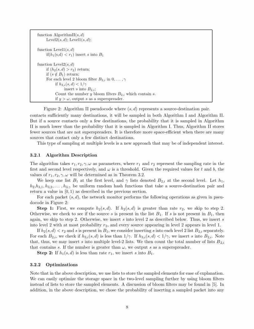
function AlgorithmII(s, d)Level2(s, d); Level1(s, d);

function Level1(s, d)if(h1(s,d) < r1) insert s into B1

function Level2(s, d)if (h2(s, d) > r2) return;if (s /∈ B1) return;For each level 2 bloom filter B2,i in 0, . . . , γ

if h3,i(s, d) < 1/γinsert s into B2,i;

Count the number y bloom filters B2,i which contain s.if y > ω, output s as a superspreader.

Figure 2: Algorithm II pseudocode where (s, d) represents a source-destination pair.

contacts sufficiently many destinations, it will be sampled in both Algorithm I and Algorithm II.But if a source contacts only a few destinations, the probability that it is sampled in AlgorithmII is much lower than the probability that it is sampled in Algorithm I. Thus, Algorithm II storesfewer sources that are not superspreaders. It is therefore more space-efficient when there are manysources that contact only a few distinct destinations.

This type of sampling at multiple levels is a new approach that may be of independent interest.

3.2.1 Algorithm Description

The algorithm takes r1, r2, γ, ω as parameters, where r1 and r2 represent the sampling rate in thefirst and second level respectively, and ω is a threshold. Given the required values for t and b, thevalues of r1, r2, γ, ω will be determined as in Theorem 3.2.

We keep one list B1 at the first level, and γ lists denoted B2,i at the second level. Let h1,h2,h3,1, h3,2, . . . , h3,γ be uniform random hash functions that take a source-destination pair andreturn a value in [0, 1) as described in the previous section.

For each packet (s, d), the network monitor performs the following operations as given in pseu-docode in Figure 2:

Step 1: First, we compute h2(s, d). If h2(s, d) is greater than rate r2, we skip to step 2.Otherwise, we check to see if the source s is present in the list B1. If s is not present in B1, thenagain, we skip to step 2. Otherwise, we insert s into level 2 as described below. Thus, we insert sinto level 2 with at most probability r2, and every source appearing in level 2 appears in level 1.

If h2(s, d) < r2 and s is present in B1, we consider inserting s into each level 2 list B2,i separately.For each B2,i, we check if h3,i(s, d) is less than 1/γ. If h3,i(s, d) < 1/γ, we insert s into B2,i. Notethat, thus, we may insert s into multiple level-2 lists. We then count the total number of lists B2,i

that contains s. If the number is greater than ω, we output s as a superspreader.Step 2: If h1(s, d) is less than rate r1, we insert s into B1.

3.2.2 Optimizations

Note that in the above description, we use lists to store the sampled elements for ease of explanation.We can easily optimize the storage space in the two-level sampling further by using bloom filtersinstead of lists to store the sampled elements. A discussion of bloom filters may be found in [5]. Inaddition, in the above description, we chose the probability of inserting a sampled packet into any

8

level-2 list B2,i to be equal to 1/γ, for simpler description and analysis. We can easily generalizethis to alter the probability of inserting a sampled packet into any level-2 list to be non-uniform,e.g., an exponential distribution.

Another optimization is to reduce the number of times Algorithm II must hash the (s, d) pair,and thus increase its computational efficiency. Instead of hashing once for each list (or bloom filter)at the second level, we could just directly use the hash value h2(s, d) to choose a single list (or bloomfilter) for insertion. The parameters for this optimized algorithm may be chosen in a manner similarto Algorithm II, with similar theoretical bounds. The memory usage of this optimized algorithmis similar to Algorithm II as well.

3.2.3 Analysis

Our analysis yields the following theorem for precision:

Theorem 3.2. Given t such that 0 < t < 1, N, b > 1, and positive δ < 1. Let z = max( 2bb−1 , 5).

Let r1 = ztN log 2

δ , and r2 be minimal value that satisfies the following constraints:

r2 ≥ 2 ln 2/δ

tN(1 − e−(z−1)/z)ε21

,

r2 ≥ ln 1/δ

tN(1 − e−3/2b)((1 + ε2) ln(1 + ε2) − ε2),

where ε1 = 1 − 1 − e−3/2b

1 − 1/e(1 + ε2),

ε2 > 0, and 0 < ε1 < 1.

Let ε′1 be the value of ε1 when r2 is minimized in the above constraints. Let γ = r2tN , andω = (1 − ε′1)γ(1 − 1

e ).Thus, for any given b > 1, positive δ < 1, and t such that b/N < t < 1, Algorithm II reports

srcIPs such that any t-superspreader is reported with probability at least 1 − δ, while a srcIP withat most tN/b distinct destinations is (falsely) reported with probability at most δ.

Please see Appendix III for a detailed proof.

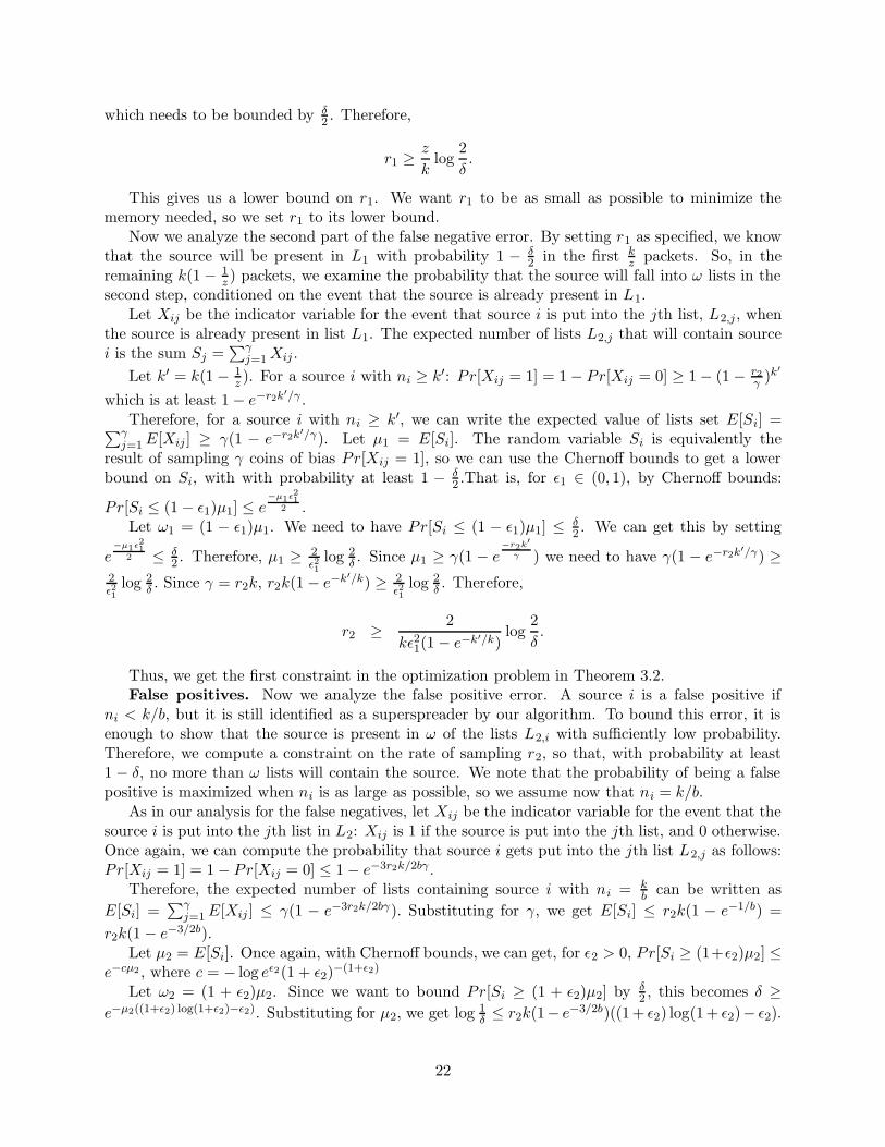
0 5 10 15 20 25 300

0.1

0.2

0.3

0.4

0.5

Rat

e r 2

Parameter b

Graph showing how rate r

2 varies with b

Figure 3: The rate r2 required for tN = 1000, δ = 0.01, with varying b,

Figure 3 shows how the required rate r2 varies with b. The threshold ω and the number of listsγ vary similarly.

Overhead Analysis The expected space required is O(r1N + r2N). Note that, for a fixed b,both r1 and r2 are O( 1

tN ln 1δ ), and thus the space required is O( 1

t ln 1δ ).

9

Stream 1: (s1, d1), (s2, d2), (s3, d3), (s4, d4)Stream 2: (s2, d3), (s1, d1), (s1, d1), (s3, d2)Stream 3: (s4, d2), (s4, d4), (s2, d4), (s4, d3)

Figure 4: Example streams at 3 monitoring points

We may make a similar statement when we use bloom filters rather than exact lists to storesampled elements as described in the optimization above. Using bloom filters does not affect thefalse negative rate, but only the false positive rate. We can easily reduce the additional false positiverate caused by the bloom filter collision by setting the correct parameters of the bloom filters usingthe theorems in [5].

We observe also that the performance guarantees of both algorithms is independent of theinput distribution of source-destinations pairs, as long as the assumption of uniform random hashfunction is obeyed. In addition, note that it is important to pick secret hash functions at run-timeeach time so that the attacker cannot generate an input sequence that avoid certain hash values.

4 Extensions

In this section we show how to extend our algorithms to handle distributed monitoring, deletions,and sliding windows.

4.1 Distributed Superspreaders

In the distributed setting, we would like to identify source IP addresses that contact a large numberof unique hosts in the union of the streams monitored by a set of distributed monitoring points.Consider for example, the three streams in Figure 4 and t = 1

5 . Sources s1, s2, s3, and s4 contact1, 3, 2, and 3 distinct destinations, respectively. Thus for the total of N = 12 source-destinationpairs, only s2 and s4 are t-superspreaders.

Note that a source IP address may contact a large number of hosts overall, but only a smallnumber of hosts in any one stream. Source s2 in Figure 4 is an example of this. A key challengeis to enable this distributed identification while having only limited communication between themonitoring points.

The following algorithm identifies t-superspreaders in the union of j streams using Algorithm I:

1. Each network monitor runs Algorithm I as described in Section 3.1 on an interval of N/jpackets, all using the same hash function h1. A packet is ignored if h1(s, d) ≥ c1

tN , as in thesingle stream case. However, because each monitor only sees N/j packets, it expects to storeat most c1

tj entries, so it suffices to have hash tables T1 and T2 have only c1tj entries. Any

locally detected superspreader can be reported (e.g., source s4 in stream 3 in Figure 4).

2. At the end of the interval, each monitor sends its hash table T1 to the centralized point. For1 ≤ i ≤ j, let T1,i be the hash table for stream i.

3. The centralized point merges the information sent by all the monitors and reports t-superspreaders,as follows. It scans through T1,1, . . . , T1,j and treats the collection of (s, d) pairs as a streamof packets. It performs Algorithm I on this stream (using hash tables of size c1

t ), except thatit can skip the test of whether h1(s, d) ≥ c1

tN because the T1,i’s only contain pairs that failthis test.

10

Note that an alternative approach of simply summing the source counts in the hash tables T2 ateach monitor would not be correct, because duplicates would be multiply counted (e.g., in Figure 4,although source s1 has one distinct destination in stream 1 and one in stream 2, it has only onedistinct destination overall, not two).

The overall space and time overhead of step 1 above summed over all the monitors is the same asif one monitor monitors the union of the streams. Step 2 requires a total amount of communicationequal to the sum of the space for the T1,i’s, i.e., an expected O(c1/t) memory words. Accountingfor Step 3 increases the total space and time by at most a factor of 2. Note that the algorithm doesnot require that all streams use an interval of N/j packets. As long as there are exactly N packetsin all, the algorithm achieves the precision bounds given in Theorem 3.1. Thus our distributedalgorithm uses little memory and little communication.

Algorithm II can be extended similarly.

4.2 Superspreaders with Deletion

We can also extend our algorithms to support streams that include both newly arriving (srcIP,dstIP) pairs and the deletion of earlier (srcIP, dstIP) pairs. Recall from Section 2.1 that a motivatingscenario for supporting such deletions is finding source IP addresses that contact a high numberof distinct destinations and do not get legitimate replies from a high number of these destinations.Each in-bound legitimate reply packet with source IP x and destination IP y is viewed as a deletionof an earlier request packet with source IP y and destination IP x from the corresponding flow, sothat the source y is charged for only distinct destinations without legitimate replies.

For Algorithm I of Section 3.1, a deletion of (s, d) is handled by first checking to see if (s, d)is in the list for entry c1

t · h1(s, d) of T1. If it is not, then d is already not being accounted for ins’s distinct destination count, so we can ignore the deletion. Otherwise, we delete (s, d) from T1.We use c1

t · h2(s) to look-up s in T2, and decrement its count. If its count drops to 0, we remove(s, 0) from T2. The precision bounds, space bounds, and time bounds are the same as in the casewithout deletions.

Similarly, we can handle deletions in Algorithm II of Section 3.2 by deleting from the sample,for the variant where we use lists to store sampled elements.

Note that the definition of a t-superspreader under deletions is not a stable one. At any pointin time, the monitor may have just processed a packet, and have no idea whether this pair will besubsequently deleted. There may be a source right at the t-superspreader threshold that exceedsthe threshold unless the pair is subsequently deleted. Our algorithms can be readily adapted tohandle a variety of ways of treating this issue. For example, Algorithm I can report a source asa tentative t-superspreader when its count in T2 reaches r + 1, and then report at the end of theinterval which sources (still) have counts greater than r.

4.3 Superspreaders over Sliding Windows

In this section, we show how to extend our algorithms to handle sliding windows. Our goal is toidentify t-superspreaders with respect to the most recent W packets, i.e., hosts which contact morethan t · W unique destinations in the last W packets. Our goal is to use far less space than thespace needed to hold all the pairs in the current window.

What makes the sliding window setting more difficult than the standard setting is that a packetis dropped from the window at each step, but we do not have the space to hold on to the packetuntil it is time to drop it. This is in contrast to the deletions setting described in Section 4.2where we are given at time of deletion the source-destination pair to delete. In the sliding window

11

(s1, d1), (s1, d2), (s2, d2), (s1, d3)(s1, d2), (s2, d2), (s1, d3), (s2, d3)

(s2, d2), (s1, d3), (s2, d3), (s2, d1)

Figure 5: Example stream, showing three steps of a sliding window of size W = 4. The top rowshows the packets in the sliding window after the arrival of (s1, d3). The middle row shows thaton the arrival of (s2, d3), the window includes this pair but drops (s1, d1). The bottom row showsthat on the arrival of (s2, d1), the window adds this pair but drops (s1, d2).

setting, a source may transition between being a t-superspreader and not, as the window slides. InFigure 5, for example, suppose that the threshold for being a t-superspreader is having at least 3distinct destinations (e.g., t = .7). Then source s1 is a superspreader in the first window, but notthe second or third windows.

We show how to adapt Algorithm I to handle sliding windows. We keep a running counter ofpackets that is used to associate each packet with its stream sequence number (seqNum). Thus if thecounter is currently x, the sliding window contains packets with sequence numbers x−W +1, . . . , x.At a high-level, the algorithm works by (1) maintaining the pairs in our sample sorted by sequencenumber, in order to find in O(1) time sample points that drop out of the sliding window, and (2)keeping track of the largest sequence number for each pair in our sample, in order to determine inO(1) time whether there is at least one occurrence of the pair still in the window. In further detail,the steps of the algorithm are as follows.

• Initially: Let L be an initially empty linked list of (srcIP, dstIP, seqNum) triples, sorted byincreasing seqNum. Let T1 and T2 be as in the original Algorithm I, except that T1 nowcontains (srcIP, dstIP, seqNum) triples.

• On arrival of a packet with srcIP s and dstIP d: Let x be its assigned sequence number.

1. Account for a pair dropping out of the window, if any: If the tail of L is a triple (s, d, n)such that n = x−W , then remove the triple from L and check to see if the triple existsin entry c1

t · h1(s, d) of T1. If the triple exists, then because T1 holds the latest sequencenumbers for each source-destination pair in the sample, we know that (s, d) will not existin the window after dropping (s, d, n). Accordingly, we perform the following steps:

(a) Remove the triple from T1.

(b) Use c1t · h2(s) to look-up s in T2, and decrement the count of this entry in T2, i.e.,

replace the pair (s, k) with (s, k − 1).

(c) If the new count equals 0, we know that the source no longer appears in the sampleand we remove the pair from T2.

On the other hand, if the triple does not exist, then there is some other triple (s, d, n ′)corresponding to a more recent occurrence of (s, d) in the stream (n < n′). Thus dropping(s, d, n) changes neither the sampled pairs nor the source counts, so we simply proceedto the next step.

2. Account for the new pair being included in the window: If h1(s, d) ≥ c1/(tW ) ignore thepacket. Else:

(a) Check entry c1t · h1(s, d) of T1 for a triple with s and d. If such an entry exists,

replace it with (s, d, x), maintaining the invariant that the entry has the latestsequence number, and return to process the next packet. Otherwise, insert (s, d, x)into the list for this entry.

12

(b) At this point we know that d is a new destination for s, i.e., this is the first time(s, d) has appeared in the window. We use c1

t · h2(s) to look-up s in T2. If s is notfound, insert (s, 1) into the list for this entry, as this is the first destination for s inthe sample. On the other hand, if s is found, then we increment its count, i.e., wereplace the pair (s, k) with (s, k + 1). If the new count equals r + 1, we report s.

The precision, time and space bounds are the same as in Algorithm I of Section 3.1 with Wsubstituted for N .

Note that the algorithm is readily modified to handle sliding windows based on time, e.g., overthe last 60 minutes, by using timestamps instead of sequence numbers. The precision, time andspace bounds are unchanged, except that the time is now an amortized time bound instead of anexpected one. This is because multiple pairs can drop out of the window during the time betweenconsecutive arrivals of new pairs. If more than a constant number of pairs drop out, then thealgorithm requires more than a constant amount of time to process them. However, each arrivingpair can drop out only once, so the amortized per-arrival cost is constant.

5 Experimental Results

We implemented our algorithms for finding superspreaders, and we evaluated them on networktraces taken from the NLANR archive [28], after they were injected with appropriate superspreadersas needed. All of our experiments were run on an Intel Pentium IV, 1.8Ghz. We use the OPENSSLimplementation of the SHA1 hash function, picking a random key during each run, so that theattacker cannot predict the hashing values. For a real implementation, one can use a more efficienthash function. We ran our experiments on several traces and obtain similar results. Our resultsshow that our algorithms are fast, have high precision, and use a small amount of memory. Onaverage, the algorithms take on the order of a few seconds for a hundred thousand to a millionpackets (with a non-optimized implementation).

In this section, we first examine the precision of the algorithms experimentally, then examinethe memory used as k, b and N change, and finally compare with the alternate approach proposedin Section 2.3.

5.1 Experimental evaluation of precision

To illustrate the precision of the algorithms, we show a set of experimental results below. To thebase trace 1 (see Table 3), we inserted various attack packets where some sources contacted a highnumber of distinct destinations. That is, for given parameters k = t ·N and b, we added 100 sourcesthat sends to k destinations each, and 100 sources that send to about k/b destinations each. Thiswas done in order to test if our algorithms do indeed distinguish between sources that send to morethan k destinations and fewer than k/b destinations.

We set δ = 0.05. In the Table 2, we show the results of our experiments, with regards toprecision of the algorithms. We examine the correctness of our algorithm by comparing it againstan exact calculation. The other parameters are set as given by Theorems 3.1 and 3.2.

We observe that the accuracy of both algorithms is comparable and bounded by δ, whichconfirms our theoretical results. We note that the false positive rate is much lower than the falsenegative rate. Our sampling rates are chosen to distinguish sources that send to k destinationsfrom sources that send to k/b destinations with error rate δ. When a source sends to a verysmall number of destinations (much smaller than k/b), the probability that it becomes a falsepositive is significantly lower than δ. Likewise, when a source sends to a very large number of

13

k = t · N b False Positives False Negatives

Alg I Alg II Alg I Alg II

500 2 8.1e-4 6.3e-5 0 0

500 5 2.75e-4 2.43e-4 0 0

500 10 1.35e-4 1.94e-4 0.01 0

1000 2 4.95e-5 1.13e-4 0.02 0

1000 5 1.62e-4 0 0.02 0.02

1000 10 4.95e-4 9.45e-5 0 0.03

5000 2 6.75e-4 0 0 0

5000 5 4.95e-5 1.62e-5 0 0

5000 10 3.19e-5 1.62e-5 0 0.01

10000 2 1.62e-4 0 0.02 0

10000 5 3.2e-5 0 0.01 0

10000 10 1.62e-5 3.2e-5 0.04 0

Table 2: Evaluation of the Precision of Algorithms I and II over various settings for t and b, withδ = 0.05.

No. distinct No. distinct N (no. ofsources src-dst pairs packets)

Trace 1 59,862 194,060 2.88 × 106

Trace 2 282,484 416,730 3.09 × 106

Trace 3 1.21 × 106 1.35 × 106 4.02 × 106

Trace 4 2.12 × 106 2.29 × 106 4.49 × 106

Table 3: Base traces used for experimentsdestinations ( k), the probability that it becomes a false negative is much less than δ. Throughthe construction of our traces, there are only a 100 possible sources that may be false negatives,and all of them send to just over k destinations. There are many more sources that could be falsepositives, and only a 100 of these sources send to nearly k/b destinations. Thus, the false positiverate that is seen is much less than the set δ.

5.2 Memory usage on long traces

We now examine memory used on very long traces by Algorithm I (Section 3.1) and the list andbloom-filter implementations of Algorithm II (Section 3.2). To distinguish the two implementationsof Algorithm II, we will refer to the list implementation as Algorithm II-L, and the bloom-filterimplementation as Algorithm II-B. We examine the memory used as the parameters k, b and Nare allowed to vary.

The traces used for this section are constructed by taking four base traces of varying lengths,and adding to each of them a hundred sources that send to k destinations, and a hundred sourcesthat send to k/b destinations. The details of the base traces are shown in Table 3. We observethat, with the largest of these traces, a source that sends to 200 distinct destinations contributesjust about 0.004% to the total traffic analyzed. The memory used is the number of words (or IPaddresses) that need to be stored.

The graphs in Figure 6 show the total memory used by each algorithm plotted against thenumber of distinct sources in the trace, at different values of b. Notice that through our traceconstruction procedure, the traces in Figure 6(a), 6(b), and 6(c) contain the same number of

14

0 0.5 1 1.5 2 2.5

x 106

0

2

4

6

8

10

12x 10

5

number of sources (in millions)

tota

l mem

ory

used

(in

wor

ds)

Algorithm IAlgorithm II−LAlgorithm II−B

0 0.5 1 1.5 2 2.5

x 106

0

0.5

1

1.5

2

2.5

3

3.5x 10

5

number of sources (in millions)

tota

l mem

ory

used

(in

wor

ds)

Algorithm IAlgorithm II−LAlgorithm II−B

0 0.5 1 1.5 2 2.5

x 106

0

0.5

1

1.5

2

2.5x 10

5

number of sources (in millions)

tota

l mem

ory

used

(in

wor

ds)

Algorithm IAlgorithm II−LAlgorithm II−B

(a) b = 2 (b) b = 5 (c) b = 10

Figure 6: Total memory used by the algorithms in words (i.e., IP addresses) vs number of distinctsources, for b = 2, 5 and 10, at k = 200.

0 0.5 1 1.5 2 2.5

x 106

0

1

2

3

4

5x 10

5

number of sources (in millions)

tota

l mem

ory

used

(in

wor

ds)

Algorithm IAlgorithm II−LAlgorithm II−B

0 0.5 1 1.5 2 2.5

x 106

0

0.5

1

1.5

2

2.5x 10

5

number of sources (in millions)

tota

l mem

ory

used

(in

wor

ds)

Algorithm IAlgorithm II−LAlgorithm II−B

0 0.5 1 1.5 2 2.5

x 106

0

1

2

3

4

5

6x 10

4

number of sources (in millions)

tota

l mem

ory

used

(in

wor

ds)

Algorithm IAlgorithm II−LAlgorithm II−B

(a) k = 500 (b) k = 1000 (c) k = 5000

Figure 7: Total memory used by the algorithms in words (i.e., IP addresses) vs number of distinctsources, for k = 500, 1000 and 5000, at b = 2.

distinct sources, even though the value of b differs.We observe that the memory used by the two algorithms is strongly correlated with b, as pointed

out by our theoretical analysis. For both algorithms, the memory required decreases sharply as bincreases from 2 to 5, and then decreases more slowly. This can also be seen (for Algorithm II)from Figure 3, in section 3.2.

Another observation is that, as expected, the memory used by Algorithm I eventually exceedsthe memory used by Algorithms II-L & II-B, for every value of b. The number of sources at whichthe memory used by Algorithm I exceeds the memory used by Algorithms II-L & II-B also dependson b. We also note that, as expected, the memory used by Algorithm II-B is much less than thememory used by Algorithm II-L and Algorithm I.

We next examine the memory usage as k changes, which is shown in Figures 7 and 8. Weobserve that the total memory used drops sharply as k increases, as expected: in 7(a), at k = 500,the memory used ranges from 20, 000 to 200, 000 IP addresses; in 7(c), at k = 5000, it ranges from10, 000 to 55, 000 IP addresses. Even though the number of source-destination pairs increases whenk increases, we can afford to sample much less frequently. This in turn decreases the number ofsources stored that have very few destinations, and thus the total memory used decreases.

Also, for every k, as the number of packets N increases, the memory used by Algorithm Ieventually exceeds the memory used by Algorithm II-L & II-B. This is because of the two-levelsampling scheme. Since the first sampling rate r1 is much smaller than c1/k in Algorithm I, thenumber of non-superspreader sources stored in the Algorithm II (r1N in expectation) is muchless than in Algorithm I. The actual number of sources at which this occurs depends on k. As k

15

0 0.5 1 1.5 2 2.5

x 106

0

0.2

0.4

0.6

0.8

1

1.2

1.4

number of sources (in millions)

mem

ory

per

so

urc

e (i

n w

ord

s) k=200k=500k=1000k=5000k=10000

0 0.5 1 1.5 2 2.5

x 106

0

0.1

0.2

0.3

0.4

0.5

0.6

0.7

number of sources (in millions)

mem

ory

per

so

urc

e (i

n w

ord

s) k=200k=500k=1000k=5000k=10000

0 0.5 1 1.5 2 2.5

x 106

0

0.05

0.1

0.15

0.2

0.25

0.3

0.35

number of sources (in millions)

mem

ory

per

so

urc

e (i

n w

ord

s) k=200k=500k=1000k=5000k=10000

(a) Alg I (b) Alg II-L (c) Alg II-B

Figure 8: Memory used per source vs number of distinct sources, for all k, by Algorithms I, II-L,& II-B at b = 2.

b Alg I Alg II-L Alg II-B Alt I Alt II

Trace 1

2 37610 16234 7223 49063 1055895 9563 3241 1377 20746 4842410 5685 2698 1136 16839 36823

Trace 2

2 71852 17536 7711 133988 2731015 19298 4543 1865 76543 16825610 12030 4000 1624 67007 135540

Table 4: Comparisons of total memory used with traces 1 & 2 for k = 1000 and varying b.

increases, the number of sources at which the memory used by Algorithm I exceeds the memoryused by Algorithm II also increases, since the sampling rates for both algorithms decrease in thesame way. We also observe that, once again, the memory used by Algorithms II-B is significantlylower than Algorithm I and Algorithm II-L.

The graphs in Figure 8 show the memory used per source plotted against the number of distinctsources, for various k – as k increases, the total memory used drops. We observe that each algorithmhas a similar dependence on k, though the absolute memory usage is different, as discussed.

5.3 Comparison with an Alternate Approach

We now show some results comparing our approach to the approach described in Section 2.3: wecount the number of distinct destinations that a source sends to using LossyCounting [25], replacingthe regular counter with a distinct-element counter. The details are in Appendix IV.

We chose the parameters for LossyCounting and the distinct counting algorithm so that (a)the memory usage was minimized for each b and (b) they produced the false positive rates similarto Algorithms I & II over 10 iterations. We show experimental results with two variants of theapproach: (1) use one distinct counter per source (this is Alt I), and (2) use log 1

δ distinct countersper source, and use their median for the estimate of the number of distinct elements is used (thisis Alt II). The memory used is reported as the maximum of the total number of hash values storedfor all the sources at any particular time.

Table 4 shows the result of the comparison of memory usage at k = 1000, for b = 2, 5 and 10,on Trace 1 & Trace 2. Note that all our algorithms show better performance than Alt I and Alt IIon Traces 1 & 2. The results for Trace 3 & Trace 4 are similar, except that Alt I uses less memory

16

than Algorithm I when b = 2. We explain why Alt I is better than Alt II in Appendix IV.

6 Related Work

We review related work in this section. There has been a volume of work done in the area ofstreaming algorithms. However, to the best of our knowledge, no previous work directly addressesthe problems we address in this paper.

Distinct values counting has been studied by a number of papers (e.g., [1, 3, 4, 8, 10, 17, 19,20, 16]). The seminal algorithm by Flajolet and Martin [17] and its variant due to Alon, Matiasand Szegedy [1] estimate the number of distinct values in a stream (and also the number of 1’s ina bit stream) up to a relative error of ε > 1. Cohen [7], Gibbons and Tirthapura [19], and Bar-Yossef et al. [4] give distinct counting algorithms that work for arbitrary relative error. Of these,the algorithm in [19] has the best space and time bounds: their (ε, δ)-approximation scheme usesO( 1

ε2log(1/δ) log R) memory bits, where the values are in [0..R], and an expected O(1) time per

stream element. More recently, Bar-Yossef et al. [3] improve the space complexity of distinct valuescounting on a single stream, and Cormode et al. [8] show how to compute the number of distinctvalues in a single stream in the presence of additions and deletions of items in the stream. Gibbonsand Tirthapura [20] give an (ε, δ)-approximation scheme for distinct values counting over a slidingwindow of the last N items, using B = O( 1

ε2log(1/δ) log N log R) memory bits. The per-element

processing time is dominated by the time for O(log(1/δ)) finite field operations. The algorithmextends to handle distributed streams, where B bits are used for each stream.

There are a number of papers that have proposed algorithms for other problems in networktraffic analysis as well. Estan et al. [16] present a series of bitmap algorithms for counting thenumber of distinct flows for different applications. Estan and Varghese [15] propose two algorithmsto identify the large flows in network traffic, and give an accurate estimate of their sizes. Estan etal. [14] present an offline algorithm that computes the multidimensional traffic clusters reflectingnetwork usage patterns. Duffield et al. [12] show that the number and average length of flows maybe inferred even when some flows are not sampled, and in [13] they compute the entire distributionof flow lengths. Golab et al. [21] present a deterministic single-pass algorithm to identify frequentitems over sliding windows. Cormode and Muthukrishnan [9] present sketch-based techniques toidentify significant changes in network traffic.

There have been many papers for other problems involving data streaming algorithms (see thesurveys in [2, 27]). None of this work has addressed the problems considered in this paper.

7 Conclusion

In this paper, we have described two new streaming algorithms for identifying superspreaders onhigh-speed networks. Our algorithms give proven guarantees on the accuracy and the memoryrequirement. Compared to previous approaches, our algorithms are substantially more efficient,both theoretically and experimentally. The best previous approach [16] requires a certain amountof memory to be allocated for each source within the time window. Our algorithms are the firstones where the amount of memory allocated is independent on the number of sources in the timewindow. We also provide several extensions to our algorithms – we provide solutions to identifysuperspreaders in the distributed setting, as well as solutions to allow deletions in the stream andsolutions for the sliding window case. We are the first ones to give solutions for these extensions.Our algorithms have many important networking and security applications. We also hope that

17

our algorithms will shed new light on developing new fast streaming algorithms for high-speednetworking and security monitoring.

References

[1] N. Alon, Y. Matias, and M. Szegedy. The space complexity of approximating the frequencymoments. J. of Computer and System Sciences, 58:137–147, 1999.

[2] B. Babcock, S. Babu, M. Datar, R. Motwani, and J. Widom. Models and issue in data streamsystems. In Proc. 21st ACM SIGMOD-SIGACT-SIGART Symp. on Principles of DatabaseSystems (PODS), pages 1–16, June 2002.

[3] Z. Bar-Yossef, T. Jayram, R. Kumar, D. Sivakumar, and L. Trevisan. Counting distinctelements in a data stream. In Proc. 6th International Workshop on Randomization and Ap-proximation Techniques (RANDOM), pages 1–10, September 2002. Lecture Notes in ComputerScience, vol. 2483, Springer.

[4] Z. Bar-Yossef, R. Kumar, and D. Sivakumar. Reductions in streaming algorithms, with anapplication to counting triangles in graphs. In Proc. 13th ACM-SIAM Symposium on DiscreteAlgorithms (SODA), January 2002.

[5] A. Broder and M. Mitzenmacher. Network applications of bloom filters: A survey. In Allerton,2002.

[6] M. Charikar, K. Chen, and M. Farach-Colton. Finding frequent items in data streams. InProc. 29th Intl. Colloq. on Automata, Languages, and Programming, 2002.

[7] E. Cohen. Size-estimation framework with applications to transitive closure and reachability.J. of Computer and System Sciences, 55(3):441–453, 1997.

[8] G. Cormode, M. Datar, P. Indyk, and S. Muthukrishnan. Comparing data streams usinghamming norms (how to zero in). In Proc. 28th International Conf. on Very Large Data Bases(VLDB), pages 335–345, August 2002.

[9] G. Cormode and S. Muthukrishnan. What’s new: Finding significant differences in networkdata streams. In Proceedings of IEEE Infocom’04, 2004.

[10] M. Datar, A. Gionis, P. Indyk, and R. Motwani. Maintaining stream statistics over slidingwindows. SIAM Journal on Computing, 31(6):1794–1813, 2002.

[11] E. Demaine, A. Lopez-Ortiz, and J. Ian-Munro. Frequency estimation of internet packetstreams with limited space. In Proceedings of the 10th Annual European Symposium on Algo-rithms, pages 348–360, September 2002.

[12] N. Duffield, C. Lund, and M. Thorup. Properties and prediction of flow statistics from sampledpacket streams. In ACM SIGCOMM Internet Measurement Workshop, 2002.

[13] N. Duffield, C. Lund, and M. Thorup. Estimating flow distributions from sampled flow statis-tics. In Proceedings of ACM SIGCOMM, 2003.

[14] C. Estan, S. Savage, and G. Varghese. Automatically inferring patterns of resource consump-tion in network traffic. In Proceedings of SIGCOMM’03, 2003.

18

[15] C. Estan and G. Varghese. New directions in traffic measurement and accounting. In Proceed-ings of SIGCOMM’02, 2002.

[16] C. Estan, G. Varghese, and M. Fisk. Bitmap algorithms for counting active flows on highspeed links. In ACM SIGCOMM Internet Measurement Workshop, 2003.

[17] P. Flajolet and G. N. Martin. Probabilistic counting algorithms for data base applications.J. Computer and System Sciences, 31:182–209, 1985.

[18] P. B. Gibbons and Y. Matias. New sampling-based summary statistics for improving approx-imate query answers. In Proc. ACM SIGMOD International Conf. on Management of Data,pages 331–342, June 1998.

[19] P. B. Gibbons and Srikanta Tirthapura. Estimating simple functions on the union of datastreams. In Proc. ACM Symp. on Parallel Algorithms and Architectures (SPAA), pages 281–291, June 2001.

[20] P. B. Gibbons and Srikanta Tirthapura. Distributed streams algorithms for sliding windows.In Proc. ACM Symp. on Parallel Algorithms and Architectures (SPAA), pages 63–72, August2002.

[21] L. Golab, D. DeHaan, E. Demaine, A. Lopez-Ortiz, and J. Ian-Munro. Identifying frequentitems in sliding windows over online packet streams. In Proceedings of 2003 ACM SIGCOMMconference on Internet measurement, pages 173–178. ACM Press, 2003.

[22] R. Karp, S. Shenker, and C. Papadimitriou. A simple algorithm for finding frequent elementsin streams and bags. ACM Trans. Database Syst., 28(1):51–55, 2003.

[23] B. Krishnamurthy, S. Sen, Y. Zhang, and Y. Chen. Sketch-based change detection: methods,evaluation, and applications. In Proceedings of the 2003 ACM SIGCOMM conference onInternet measurement, pages 234–247. ACM Press, 2003.

[24] A. Kumar, L. Li, and J. Wang. Space-code bloom filter for efficient traffic flow measurement.In Proceedings of IEEE Infocom’04, 2004.

[25] G. Manku and R. Motwani. Approximate frequency counts over data streams. In Proceedingsof VLDB 2002, 2002.

[26] D. Moore, V. Paxson, S. Savage, C. Shannon, S. Staniford, and N. Weaver. Inside the slammerworm. Security and Privacy Magazine, July/August 2003.

[27] S. Muthukrishnan. Data streams: Algorithms and applications. Technical report, RutgersUniversity, Piscataway, NJ, 2003.

[28] NLANR. National laboratory for applied network research. http://pma.nlanr.net/Traces/,2003.

[29] M. Roesch. Snort - lightweight intrusion detection for networks. In Proceedings of the 13thSystems Administration Conference. USENIX, 1999.

19

A Analysis background

In the analysis of our algorithms, we will use the following Chernoff bounds.

Fact A.1. Let X be the sum of n independent Bernoulli random variables with success probabilityp. Then for all β > 1,

Pr[X ≥ βnp] ≤ e(1−1/β−ln β)βnp (3)

Moreover, for any ε, 0 < ε < 1,

Pr[X ≥ (1 + ε)pn] ≤ e−ε2np/3 (4)

and

Pr[X ≤ (1 − ε)pn] ≤ e−ε2np/2 (5)

B Proof for Theorem 3.1

Proof. Each distinct (srcIP, dstIP) pair occuring during the interval is retained according to aBernoulli trial with success probability c1

tN . The probability of a srcIP being reported increasesmonotonically with its number of distinct destinations. Thus it suffices to show that

P1. False negatives: the probability that a srcIP s1 with tN distinct destinations has at most rsuccesses is at most δ, and

P2. False positives: the probability that a srcIP s2 with tN/b distinct destinations has at least rsuccesses is at most δ.

We seek to achieve P1 and P2 while keeping c1 small. Let X1 be the number of successes for s1

and let X2 be the number of successes for s2. Let k = tN . We consider each of the three rangesfor b in turn.

Consider the case when b ≤ 3. By equation 5, we have Pr[X1 ≤ (1− ε1)(c1/k)k] ≤ e−ε21k(c1/k)/2

for any ε1 between 0 and 1. Setting e−ε21c1/2 = δ and solving for ε1, we get ε1 =

√

2c1

ln(1/δ).

Because δ < 1, we have that ln(1/δ) > 0. Thus as long as c1 > 2 ln(1/δ), we have 0 < ε1 < 1. Byequation 4, we have Pr[X2 ≥ (1 + ε2)(c1/k)(k/b)] ≤ e−ε2

2(k/b)(c1/k)/3 for any ε2 between 0 and 1.

Setting e−ε22c1/(3b) = δ and solving for ε2, we get ε2 =

√

3bc1

ln(1/δ). As long as c1 > 3b ln(1/δ), we

have 0 < ε2 < 1.Because the same cut-off r is used for s1 and s2, we require that r = (1− ε1)c1 = (1+ ε2)(c1/b),

i.e., that b(

1 −√

2c1

ln(1/δ))

= 1 +√

3bc1

ln(1/δ). Thus, b√

c1 − b√

2 ln(1/δ) =√

c1 +√

3b ln(1/δ).

Solving for c1, we get√

c1 =√

ln(1/δ)(√

3b + b√

2)/(b − 1), and hence

c1 = ln(1/δ)

(

3b + 2b√

6b + 2b2

(b − 1)2

)

when b ≤ 3 (6)

This is the smallest c1 that works for both s1 and s2, when applying the above Chernoff bounds(equations 4 and 5). Because b > 1 and 2b2/(b − 1)2 > 2, we have that c1 > 2 ln(1/δ). Toshow that c1 > 3b ln(1/δ) when b ≤ 3, we must show that 3b + 2b

√6b + 2b2 > 3b(b − 1)2, i.e.,

3 + 2√

6b + 2b > 3b2 − 6b + 3, i.e., 2√

6 > (3b− 8)√

b. Now when b ≤ 3, we have 3b− 8 ≤ 1 < 2 and

20

√b <

√6, and hence c1 > 3b ln(1/δ). It follows that for the c1 in equation 6, P1 and P2 hold when

r = (1 + ε2)(c1/b) = c1b +

√

3c1b ln(1/δ).

Next consider the case when 3 < b < 2e2. As argued above, P1 holds with ε1 =√

2c1

ln(1/δ),

as long as c1 > 2 ln(1/δ). (This analysis did not depend on b.) On the other hand, note thatwe cannot use the same analysis as in the previous case to show P2 holds because for example,when b = 4, the c1 in equation 6 is less than 3b ln(1/δ). Instead, we apply equation 3 withβ = e: Pr[X2 ≥ ec1/b] ≤ e(1−1/e−1)ec1/b = e−c1/b. We require that r = ec1/b = (1 − ε1)c1, i.e.,

ε1 = 1 − e/b =√

2c1

ln(1/δ). Solving for c1, we get c1 = 2 ln(1/δ)/(1 − eb )

2. Moreover, P1 holds for

all c1 ≥ 2 ln(1/δ)/(1 − eb )

2.

Similarly, setting e−c1/b = δ and solving for c1, we get that c1 = b ln(1/δ) and moreover, P2holds for all c1 ≥ b ln(1/δ). Thus selecting c1 such that

c1 = ln(1/δ) · max(b, 2/(1 − e/b)2)

when 3 < b < 2e2 (7)

implies both P1 and P2 hold when r = ec1/b. (Note that 0 < (1−e/b)2 < 1 and hence c1 > 2 ln(1/δ),as required for P1.)

Finally, consider the case when b ≥ 2e2. Note that the c1 from equation 7 grows linearly inb. Thus for large b, we seek a modified analysis in which c1 does not grow asymptotically withb. First we apply equation 3 with β = b/2: Pr[X2 ≥ (b/2)(c1/b)] ≤ e(1−2/b−ln(b/2))c1/2 < e−c1/2

because b ≥ 2e2 implies ln(b/2) ≥ 2 implies 1 − 2/b − ln(b/2) < −1. Thus r = c1/2 = (1 − ε1)c1,i.e. ε1 = 1/2. By equation 5, we have Pr[X1 ≤ r] ≤ e−(1/2)2c1/2 = e−c1/8. It follows that selectingc1 = 8 ln(1/δ) when b ≥ 2e2 implies that both P1 and P2 hold when r = c1/2.

C Proof for Theorem 3.2

We begin our analysis by making an observation. Our sampling is done by hashing source-destination pairs; therefore, if the same source-destination pair appears multiple times, its chancesof being sampled do not change. Thus, hashing effectively reduces all the packets in the stream toa set of distinct source-destination pairs, and in this transformed set, a superspreader appears atleast k = tN times. Effectively, we sample only from this transformed set. Therefore, we analyzethe algorithm in this transformed set, in which all source-destination pairs are distinct.

Proof. We consider Algorithm II in Section 3.2, under the parameters given by the theorem. Wewill first analyze the false negatives, and then the false positives.

False negatives. We analyze the false negative error in two parts. For a source i with ni > k,we first show that the source is inserted into L1, with probability 1− δ

2 , in the first 1/z fraction ofits total pairs. Then, we show that it is inserted into at least ω of the lists L2,i over the rest of itspairs, with probability 1 − δ

2 , conditioned on its presence in L1. Together, these two parts ensurethat, with probability at least 1− δ, the source is present in ω of the lists L2,i, after all the distinctdestinations for that source are seen.

For the first part of the false negative analysis, we need to set the rate of sampling r1 so that anysource that appears more than k times in the sampled set will be sampled with a probability of 1− δ

2 ,

within its first 1z fraction of packets. This is equivalent to saying that any source s with k

z packets

is present in L1 with probability at least 1 − δ2 . Equivalently, 1 − Pr[s ∈ L1|ns ≥ k/z] = (1 − r1)

kz

21

which needs to be bounded by δ2 . Therefore,

r1 ≥ z

klog

2

δ.

This gives us a lower bound on r1. We want r1 to be as small as possible to minimize thememory needed, so we set r1 to its lower bound.

Now we analyze the second part of the false negative error. By setting r1 as specified, we knowthat the source will be present in L1 with probability 1 − δ

2 in the first kz packets. So, in the

remaining k(1 − 1z ) packets, we examine the probability that the source will fall into ω lists in the

second step, conditioned on the event that the source is already present in L1.Let Xij be the indicator variable for the event that source i is put into the jth list, L2,j, when

the source is already present in list L1. The expected number of lists L2,j that will contain sourcei is the sum Sj =

∑γj=1 Xij .

Let k′ = k(1 − 1z ). For a source i with ni ≥ k′: Pr[Xij = 1] = 1 − Pr[Xij = 0] ≥ 1 − (1 − r2

γ )k′

which is at least 1 − e−r2k′/γ .Therefore, for a source i with ni ≥ k′, we can write the expected value of lists set E[Si] =

∑γj=1 E[Xij ] ≥ γ(1 − e−r2k′/γ). Let µ1 = E[Si]. The random variable Si is equivalently the

result of sampling γ coins of bias Pr[Xij = 1], so we can use the Chernoff bounds to get a lowerbound on Si, with with probability at least 1 − δ

2 .That is, for ε1 ∈ (0, 1), by Chernoff bounds:

Pr[Si ≤ (1 − ε1)µ1] ≤ e−µ1ε2

1

2 .Let ω1 = (1 − ε1)µ1. We need to have Pr[Si ≤ (1 − ε1)µ1] ≤ δ

2 . We can get this by setting

e−µ1ε2

1

2 ≤ δ2 . Therefore, µ1 ≥ 2

ε21

log 2δ . Since µ1 ≥ γ(1 − e

−r2k′

γ ) we need to have γ(1 − e−r2k′/γ) ≥2ε21

log 2δ . Since γ = r2k, r2k(1 − e−k′/k) ≥ 2

ε21

log 2δ . Therefore,

r2 ≥ 2

kε21(1 − e−k′/k)

log2

δ.

Thus, we get the first constraint in the optimization problem in Theorem 3.2.False positives. Now we analyze the false positive error. A source i is a false positive if

ni < k/b, but it is still identified as a superspreader by our algorithm. To bound this error, it isenough to show that the source is present in ω of the lists L2,i with sufficiently low probability.Therefore, we compute a constraint on the rate of sampling r2, so that, with probability at least1 − δ, no more than ω lists will contain the source. We note that the probability of being a falsepositive is maximized when ni is as large as possible, so we assume now that ni = k/b.

As in our analysis for the false negatives, let Xij be the indicator variable for the event that thesource i is put into the jth list in L2: Xij is 1 if the source is put into the jth list, and 0 otherwise.Once again, we can compute the probability that source i gets put into the jth list L2,j as follows:Pr[Xij = 1] = 1 − Pr[Xij = 0] ≤ 1 − e−3r2k/2bγ .

Therefore, the expected number of lists containing source i with ni = kb can be written as

E[Si] =∑γ

j=1 E[Xij ] ≤ γ(1 − e−3r2k/2bγ). Substituting for γ, we get E[Si] ≤ r2k(1 − e−1/b) =

r2k(1 − e−3/2b).Let µ2 = E[Si]. Once again, with Chernoff bounds, we can get, for ε2 > 0, Pr[Si ≥ (1+ε2)µ2] ≤

e−cµ2 , where c = − log eε2(1 + ε2)−(1+ε2)

Let ω2 = (1 + ε2)µ2. Since we want to bound Pr[Si ≥ (1 + ε2)µ2] by δ2 , this becomes δ ≥

e−µ2((1+ε2) log(1+ε2)−ε2). Substituting for µ2, we get log 1δ ≤ r2k(1− e−3/2b)((1+ ε2) log(1+ ε2)− ε2).

22

Thus,

r2 ≥ 1

k(1 − e−3/2b)

1

((1 + ε2) log(1 + ε2) − ε2)log

1

δ.

Thus, we have the second constraint for r2.We finally have to establish the relationship between ε1 and ε2. This we get by equating the

definitions of ω1 and ω2, since the algorithm uses only one threshold ω:

µ1(1 − ε1) = µ2(1 + ε2)

(1 − e−1)(1 − ε1) = (1 − e−3

2b )(1 + ε2)

ε1 = 1 − 1 − e−3/2b

1 − e−1(1 + ε2).

Thus, we get the last relation in the problem.We wish to minimize r2, subject to these constraints, because the expected memory is O(r2N).

Therefore, the solution to the problem in Theorem 3.2, gives us a sampling rate r2 such that asource with k distinct destinations will be in at least ω lists, and a source sending to less than kdistinct destinations will not be in ω lists, with probability at least 1 − δ.

D LossyCounting and Distinct Counting Algorithm

The following is a summary of LossyCounting and the distinct counting algorithms that we use inour experimental comparisons in Section 5.3.

• LossyCounting: The stream of elements is divided into epochs, where each epoch contains 1ε

elements; thus, for an input stream of N elements, we will have εN epochs. Each epoch hastwo phases: in the first phase, the incoming elements are simply stored, and if already present,their frequency is updated; in the second phase, the algorithm looks over all elements, anddiscards those with a low frequency count. It can be shown that the final frequency count ofthe elements is at most ε lower than the true frequency count, and clearly, it cannot be largerthan the true frequency count.

• Distinct Counting: Every element in the input stream is hashed (uniformly) between (0, 1),and the t lowest hash values are stored. At the end, the algorithm reports t/mint as thenumber of distinct elements in the stream, where mint is the value of the tth smallest hashvalue. In order to get an (ε, δ)-approximate answer, the authors show that t needs to be nolarger than 96/ε2, when O(log 1

δ ) copies of the algorithm are run in parallel.

• Putting them together: In order to find superspreaders using LossyCounting, we need toreplace the regular frequency counter in LossyCounting with a distinct counter. Therefore,when a source-destination pair is examined, the source and destination is hashed, and the tsmallest hash values (of any particular source) are stored. At the end of each epoch, all thesources whose counts of distinct destinations are below the threshold set by LossyCountingare discarded. We need to run O(log 1

δ ) copies of the distinct counter per source, and usethe median value of the multiple copies. At the end, all sources whose threshold exceedsk/b + ε are returned, where ε comes from the error in distinct-counting. The tolerable errorin LossyCounting determines the number of epochs (and therefore, space required), and weset these error parameters so that the expected memory usage is minimized.

23

We show experimental results with two algorithms based on this approach: (1) use one distinctcounter per source (Alt I), and (2) use log 1

δ distinct counters per source, and use their median forcounting approximately the number of distinct elements (Alt II). The distinct counting algorithmrequires O(log 1

δ ) parallel runs for its guarantees. However, Alt I is always better than Alt II inour experiments. This is because many sources send packets to only a few destinations, and forthose sources, there is log 1

δ factor increase in the memory usage, even though the actual constantt decreases.

24