1

New Market Power Models and Sex Differences in Pay

by

Michael R Ransom* Brigham Young University and IZA

130 FOB Provo, Utah 84602

USA ransom@byu.edu

and

IZA Bonn, Germany

Ronald L. Oaxaca* University of Arizona and IZA

McClelland Hall Tucson, Arizona

USA rlo@u.arizona.edu

and IZA

Bonn, Germany

Revised November 2007

*We acknowledge helpful comments by Dan Hammermesh and Alois Stutzer and participants at the IZA workshop, “The Nature of Discrimination,” in June, 2004, and helpful research assistance of Eric Lewis. We also acknowledge the generous hospitality of IZA which permitted us to revise this paper during June, 2005.

2

Abstract. We use a simple framework, adopted from general equilibrium search models, to estimate the extent to which monopsony power (or labor market frictions) can account for gender differences in pay at a chain of regional grocery stores. In this framework, the elasticity of labor supply to the firm can be inferred from estimates of the elasticity of the separation rate with respect to the wage. We identify elasticities of separation from differences in wages and separation rates across job titles and across different years. We estimate elasticities of labor supply to the firm of about 2.5 for men and about 1.6 for women, suggesting significant wage-setting power for the firm. The differences in elasticities predict gender wage differentials that are close to the estimated gender wage differentials at the firm.

3

I. Introduction

In one of the earliest explanations of the “gender gap” in wages, Joan Robinson (1969,

pp. 224-27) showed that if an employer is a monopsonist and the elasticities of labor supply of

men and women differ, it is profitable for employers to engage in wage discrimination, paying

higher wages to the group with the higher elasticity of supply. Although Robinson’s model

appears in many economics textbooks, the discussion of it is usually skeptical, as it is based on

the assumption of a pure monopsony--a single employer of labor in a market--and this seems at

odds with the marketplace that we observe almost everywhere. Perhaps for this reason, models

of monopsony have not been very influential in the economics literature on labor market

discrimination in the past forty years, which has focused primarily on explaining how

discriminatory wage differences could occur in competitive markets, with much of this literature

following Becker (1971).

However, some recent models of labor markets suggest that employers may have market

power, even when there are numerous employers. One of the most influential of these, and the

foundation for the analysis in this paper, is the general equilibrium search model of Burdett and

Mortensen (1998). Individual firms, although “small” with respect to the labor market, face

labor supply curves that slope upward. The monopsony implications of this model have been

explored in some detail in a recent book by Manning (2003). Boal and Ransom (1997) refer to

these and related models as “dynamic monopsony,” because they stress the dynamic nature of

the labor market. Essentially, these models formalize the idea that labor market “frictions” can

have an important impact on the operation of the market.

In an application of the equilibrium search model to labor market discrimination, Black

(1995) examines how some employers’ tastes for discrimination may result in equilibrium wage

differences between groups. Basically, Black’s model permits Beckerian type tastes of some

4

employers to influence the wage outcomes in the general labor market. In contrast, our approach

is essentially Robinsonian--employers have no prejudice, but pursue wage discrimination simply

because it is profitable.

An implication of the Burdett/Mortensen/Manning models is that the labor supply curve

to the firm is related to its wage elasticity of separations. In this paper, we use this relationship

as a framework within which to estimate the labor supply curve to an individual firm (a retail

grocer), taking advantage of the differences in wages and separation rates across different job

titles. We find that the elasticity of labor supply to the firm does differ between men and women

employees, and that this is difference is consistent with profit-maximizing discrimination by the

firm.

II. A Model of Labor Market Monopsony

Here we present a simple version of the general equilibrium search model of Burdett and

Mortensen (1998), following closely the notation and presentation of Manning (2003, Sections

2.2 and 4.4). Firms have identical constant returns to scale production functions, with average

and marginal product of workers equal to p. Workers are also identical, and each has the same

value of leisure, b. Some workers are employed and others are unemployed. Workers and

potential workers receive job offers from a distribution F(w) at rate λ. An employed worker

accepts the offered wage if it is greater than his or her current wage. An unemployed worker

accepts any offer greater than b. (In equilibrium, no firm will offer a wage less than b, so this

means that an unemployed worker will accept any job offer.) Jobs are also exogenously

randomly destroyed at rate δ.

In equilibrium, all firms earn the same profit,

Β = (p-w)N(w;F),

5

but there is wage dispersion in equilibrium, described by the distribution F(w). Firms that offer

higher wages employ more workers, so the labor supply function to the firm, N(w) is positively

sloped. The distribution of wages across employees who are employed is G(w). G(w) differs

from F(w) because workers are more likely to work for high wage firms. The relationship

between F(w) and G(w) is described by the following equation:

(1) G(w; F) = δF(w)/{ δ + λ [1-F(w)]}.

This model yields the standard “monopsony” results–that the labor supply curve to the

firm is upward sloping ( because in order to have a larger workforce, a firm must offer a higher

wage), and that all workers, even those at the highest wage firms, are paid less than the marginal

product of labor.

In this paper we exploit the dynamic nature of employment in the context of the

equilibrium search model to identify the firm’s labor supply elasticity. In equilibrium, the flow

of recruits to the firm just balances those who leave the firm:

(2) s(w; F)N(w; F) = R(w; F) or, N(w; F) = R(w; F)/s(w; F)

where s(w) is the separation rate at the specific wage, and R(w) is the number of recruits.

In terms of the parameters of the model, the separation rate is

(3) s(w; F) = δ + λ [1 - F(w)]:

employees leave the firm either because they lose their job or leave the labor market (the first

term), or move to a different employer in response to a better job offer (the second term). The

elasticity of the separation rate with respect to the wage is

(3a) εsw = -λw f(w)/s(w). The recruitment function can be written as:

(4) R(w; F) = RU + λ ∫w f(x)N(x)dx ,

where RU is the recruitment from the unemployed (which does not depend on the wage offered),

6

and the second term of the expression reflects the number of recruits hired from employers with

lower wages. The elasticity of the recruitment function with respect to the wage can thus be

written as:

(4a) εRw = λw f(w)N(w)/R(w).

Since the flow of recruits must equal the flow of separations in steady state, as stated in

equation (2), s(w) = R(w)/N(w), so (3a) is simply the negative of (4a):

(5) εRw = -εsw.

This is intuitive, since one firm’s recruitment is another firm’s separation. Rewriting the

equilibrium condition from (2) in terms of the elasticities, and (5), we have

(6) εNw = εRw - εsw = -2 εsw.

Thus, the elasticity of labor supply to the firm is just twice (the negative of) the separation

elasticity. We exploit this because it is conceptually and practically much easier to estimate the

elasticity of separation than it is to estimate the elasticity of recruitment. It is this relationship

that makes it possible for us to estimate the elasticity of labor supply to the firm.

III. The Firm

The data we analyze comes from a regional grocery retailer in the western United States.

We have year-end employment and wage data for the retail employees of the firm between 1976

and 1986. (By retail employees, we mean those who worked in the retail operations of the

grocery stores themselves. Accountants, truck drivers, and the like, are not included in our

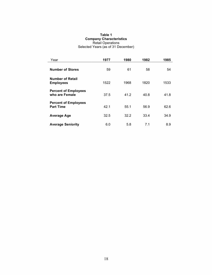
analysis.) Table 1 summarizes a few of the characteristics of the firm during the time period that

we analyze. The firm operated between 54 and 61 stores, and had between about 1500 and 2000

employees. The number of stores and employees fluctuated, increasing early, then declining.

During this period the firm opened several new stores and closed several old ones. Many of the

7

company’s retail employees worked part time, with the prevalence of part-time work increasing

noticeably over the period of our analysis. About 40 percent of employees were female, and this

fraction remained fairly constant.

Figure 1 presents a simple organizational chart for employees of the company’s retail

operations. Each store had three “management” positions: the store manager, the assistant

manager, and the relief manager. The rest of the workers were paid on an hourly basis. The

largest group of these workers held the title of “food clerk.” Food clerk assignments included

stocking shelves and operating cash registers. “Produce clerks” had the same pay scale as food

clerks but worked in the produce department. “Variety clerks” stocked shelves in the non-foods

department, but earned less than food clerks. Some stores had other departments, such as delis

or bakeries--workers from those departments are included in the “Other” category. Courtesy

clerks bagged and carried groceries. The produce and meat departments had “managers” who

received a pay premium but were part of their bargaining units. The night crew chief supervised

stocking operations during the hours the stores were closed, and also received a premium.

In Figure 1, the vertical position of the job title roughly shows the relative pay of each

position. Courtesy clerks earned slightly more than the legal minimum wage. Variety clerks and

“other” employees were paid substantially less than food clerks. The jobs on the bottoms of the

ladders were entry level positions. Courtesy clerks were sometimes promoted into one of the

other clerk positions, but most were short term employees. There was some mobility between

the different departments of the store, but meat department employees almost never changed

departments. Most of the management positions were filled from within the store ranks by

promotion, and this was true, to some extent, even of the store manager job.

In another paper, we examine job mobility within the store and its implications for pay

differentials between men and women (Ransom and Oaxaca, 2005). That paper also provides

8

more details about the organization of employment within the store. It is clear that the meat

department employees had special skills. However, the other employees were, apparently,

mostly trained on the job. According to a supplementary survey of a small sample of employees,

most were high school graduates with little or no college training. Analysis of that sample

showed that formal educational credentials were unimportant in determining job placement and

promotion.

All non-management retail employees (including the department “managers”) were

covered by collective bargaining agreements. One contract covered the meat department

employees, and another covered the other employees. We have examined the contract of one of

the locals, which was affiliated with the United Food & Commercial Workers Union. This was a

multi-employer agreement that covered several other employers in the region. Basically, the

contract dictated pay, hours scheduling, benefits and working conditions. The contract specified

the wage levels for each of the job titles at the store, including seniority increments. However, it

did not restrict the employer in terms of whom it could hire, nor did it place restrictions on whom

the employer could place in a particular job. For example, if the employer chose to promote a

courtesy clerk to the food clerk position, the contract required only that the most senior courtesy

clerk be considered for the job. Movements between departments were quite rare, but were at

the discretion of the employer.

In the early 1980s, several women initiated a class-action lawsuit, alleging that the

employer had discriminated against women in job assignment (particularly in promotion to

management), and in part-time/full-time work assignments. The court found the defendant guilty

of discrimination in 1984, and the two parties reach a negotiated settlement in mid-1986 on terms

of backpay and affirmative relief. However, the affirmative relief outlined in the settlement did

not take place during the period of our analysis. Nevertheless, we might expect that the lawsuit

9

itself may have had some impact on employment practices at the firm.

IV. Wage Differentials

Table 2 reports several regressions that summarize the differences in hourly wages of

men and women in non-management jobs in 1980. These regressions report robust standard

errors. The regression results in Column I show that there was no gender difference in hourly

wages. However, women at this firm were older and had more seniority than men. Column II

shows that when men and women of the same age and seniority are compared, women were paid

about 11.3 percent less than men. Column III shows that when job title is included in the

analysis, the wage gap falls to only about 1.8 percent, although the difference is still statistically

significant. (We include Column IV simply to show that job title alone explains about 84

percent of the variation in wages.) The preceding analysis understates the size of the pay gap

because it considers only hourly workers. The high-pay management jobs were held almost

exclusively by men in 1980. The results in column IV also provide a good summary of the

average wage of each of the positions, relative to courtesy clerks. For example, food clerks

earned about 15 percent more than variety clerks, and variety clerks earned about 15 percent

more than “other” employees. All of these employees earned substantially more than courtesy

clerks. Table 3 shows the distribution of men and women across the various job titles in the

company for year-end 1980.

The regression results of Table 2 are not the least bit surprising–we know that wages are

set by job title according to the collective bargaining agreement. However, the analysis does

make clear that the wage differential in the workplace is basically an issue of which job

assignment an employee receives. Thus, the question we have to answer is this: “Why are

women assigned to the jobs with lower pay?” We believe that monopsonistic wage

10

discrimination provides an answer.

V. Data

Our strategy here is to estimate the elasticity of labor supply to the firm by estimating the

elasticity of separations, as specified in equations (5) and (6). The data we use come from year-

end payroll files of the firm. These data include the pay rate and job title of the employee’s

current job, earnings for the past year, date of hire and date of birth. Each year-end file contains

a record of all employees who worked for the firm during the year, even though they may have

terminated their employment before the end of the year. By matching consecutive years, we can

identify those who stopped working for the firm during a given year. We have pooled workers

for all years between 1977 and 1985. (We lose the first and last year because we cannot identify

separation dates from the year-end files directly.) According to our definition, a separation

occurred in year t if someone was employed at the end of year t-1, and was no longer employed

at the end of year t. We do not know the reason for the separation. We assume that virtually all

of these are quits, but at least a few would have been dismissals, retirements, or the like.

We analyze two periods. First, we use the entire sample of nine years. Next, we use a

shorter sample of 6 years, from 1977 through 1982, since we have some concerns about how the

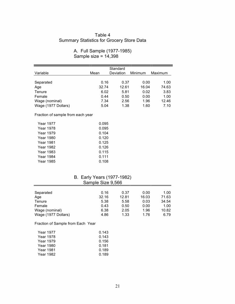
lawsuit influenced employment practices. Table 4 presents summary statistics for the data we

use in our analysis. The turnover rate over this period was fairly high–about 16 percent of the

workforce left the employer each year, on average. Most of the variables appear to be quite

similar across time periods used in the analysis.

VI. Estimation

In order to infer the labor supply elasticities to the firm, we must first estimate the

elasticity of the separation rate with respect to the wage. This can be calculated from a probit

11

regression model of the form:

(7) sit = Φ(α0 + α1 ln(wit) + α2 ln(wit)*FEMALEi + XitB) = Φ(Iit)

where sit is the probability that an individual separates from the firm during the year, Φ(Iit) is the

normal cumulative distribution function evaluated at Iit, Wit is the real wage at the start of the

year, FEMALE is an indicator equal to 1 if the worker is female, and X represents a vector of

other explanatory variables.

We have estimated three versions of this model for each of the sample periods. Model I

includes only the female indicator and powers of age as the “other” explanatory variables. Age

is included to capture differences in labor market experience, which might reflect differences in

the skills of the workers. Model II additionally includes tenure with the firm and its square. It is

not clear that tenure ought to be included in a model of separations, but since some promotion

and job assignment decisions may be based on seniority, we include these here.1

In the last version of the model, we have also included dummy variables for each of the

years. We include these because if the firm opens new stores, or closes stores in a given year,

this may have an impact on separations, independent of the wage structure. Also, the business

cycle may influence the other opportunities of workers within the firm. We do find that

separations varied quite a bit from year to year, and that the rate was especially high during the

last year of our analysis. However, the coefficients that we are most interested in change very

little across the different specifications of the model.

Table 5 reports the results of our estimation. Most of the variables are strongly related to

the separation probabilities. The age variable enters as a cubic, but over the range from about 20

1One alternative model of separations is a matching model in which those who find a good match at the firm stay with the firm, while those who do not match will leave the firm quickly. If there is a seniority component to the wage, then this would appear to make separations sensitive to the wage, when in fact they are not. However, our estimates of the

12

years old to 50 years old, the probability of separation decreases with age, as expected. The

tenure variable enters as a quadratic. The probability of separation decreases with tenure for the

first 15 or 20 years (depending on version and sample period), then it increases with tenure. The

log wage coefficients are somewhat larger for the “Early Years” sample, and the female-wage

interaction term is much larger for the early sample.

The separation elasticities for men can be calculated from the estimates of equation (7) in

the following way:

(8) ))(

)(()())(( 1

1

I

II

ws

w

w

s

s

wm

sw

!==

"

"=

#$#

$% ,

where I is the value of the index function that is estimated in the probit regression. In similar

fashion, the separation elasticity for women can be calculated as:

(9) ))(

)()(( 21

I

Imf

sw!

+="

##$ .

The ratio, φ(I)/Φ(I), that appears in this equation is sometimes called the inverse Mill’s ratio.

In the context of our version of the Burdett/Mortensen/Manning model, the elasticity of

labor supply to the firm is simply twice the negative of the separation elasticity, as derived in

equation (6). However, because of the nonlinearity of the probit regression model, there is some

ambiguity as to how to calculate “the” elasticity of labor supply to the firm. We adopt two

approaches that are often used to evaluate the results of probit regressions. In the first, Method

A, we evaluate the elasticity at the sample mean of the explanatory variables. That is, we

evaluate the index function, I, using for the explanatory variables the sample means of each

variable. The top panel of Table 6 reports the results of method A. The second method (Method

B) evaluates the elasticity for each individual in the sample, then averages those individual

estimates for men and women. The lower panel of Table 6 reports results using this method.

separation elasticities are not very sensitive to whether tenure is included in the model.

13

The monopsony model of wage discrimination provides predictions of male/female wage

differences. If we express the wage bill for the jth group of workers as NjW(Nj), the marginal

cost of hiring a worker of type j is

)1

1(j

Nw

jj wMLC!

+=

The employer maximizes profits by setting MLCf equal to MLCm, so

(10) )/11()/11( m

Nwm

f

Nwf ww !! +=+ ,

and therefore the ratio of female to male wages is

(11) )/11/()/11(/ f

Nw

m

Nwmf ww !! ++= .

The logarithm of this ratio corresponds to the estimated log wage gap of ln(wf) - ln(wm). The

wage ratio and the log wage gap are also reported in Table 6.

It is informative to compare the wage gaps in Table 6, which are derived from the

estimated elasticities of labor supply to the firm, with the wage gaps estimated directly in column

II of Table 2, for year-end 1980. (The “early years” sample period ends in 1982, so these results

are relevant.) The monopsony model yields estimates of the log wage gap of 15.1 or 14.4

percent, which are remarkably close to the unexplained wage gap of 11.3 percent reported in

Table 2.

VII. Discussion

Two issues merit discussion here. The first deals with the measurement of monopsony

power. In these models, the source of the firm’s market power arises from search frictions, so it

is interesting to try to quantify the extent to which these frictions bestow labor market power to

individual firms.

The traditional measure of monopsony power is called Pigou’s exploitation index. It is

14

defined as

Nw

L

w

wMRPE

!

1=

"= ,

where MRPL is the marginal revenue product of labor. E measures the percentage deviation of

the market value of the worker’s output from his or her wage. (This corresponds directly to the

Lerner index used to measure monopoly power.) As shown by Boal and Ransom (1997) and

others, this is just the inverse of the labor supply elasticity to the firm. Our estimates indicate

that this firm has substantial market power—values of E are around 0.4 for men and almost 0.6

for women. In other words, wages of these workers would increase by 40 to 60 percent if market

information were suddenly made perfect.

The log wage gap is approximately the difference between the exploitation indexes.

From (11) above,

(12) fm

f

Nw

m

Nw

f

Nw

m

Nwmf EEww !=!"+!+=! #### /1/1)/11ln()/11ln()ln()ln( .

if the exploitation is small (or the elasticity of labor supply to the firm is large). This

approximation is not very accurate for our particular example, however, as our estimated

elasticities are quite small.

The other issue relates to the notion of how the firm exercises monopsony power within

its institutional context. Each job title at the firm is connected to a specific contractual wage,

with associated seniority steps. These differences across job titles allow us to identify the

separation elasticity with respect to the wage under the assumption that working conditions are

not very different across jobs and that we can identify individual differences in ability with the

few variables that we have at our disposal. These assumptions seem reasonable for most

positions, although less so for the meat department employees. Within the limits of these data,

we have estimated the elasticities of labor supply to the firm for men and women. We have no

15

reason to believe that the elasticity of labor supply that this firm faces would be much different

than that faced by other similar firms in the labor markets in which it operates. Therefore, our

results suggest monopsony power due to labor market frictions could be an explanation for

difference in pay between men and women.

Unfortunately, the same institutional framework makes it a bit of a stretch to compare our

“monopsonistic” wage gaps to those that we have estimated directly in our wage regressions.

Since wages are fixed by contract, it is possible to think of the firm as having no wage setting

power at all! The regression models of Table 2 stress the importance of worker heterogeneity in

the wage determination process. The empirical wage gap arises because women tend to be more

highly qualified within job titles. In terms of the monopsony model, our argument must be that

the lower labor supply elasticity of women permits the firm to staff lower paying jobs with more

qualified women. This benefits the firm by having more productive workers than if these jobs

were staffed by men. However, the simple search model on which we base our empirical

estimates of the labor supply elasticity to the firm does not address worker heterogeneity.

Although our estimates of the wage gap from the wage regressions match closely the wage gaps

that are predicted from our estimated labor supply elasticities, the theoretical connection between

the two empirical models is not transparent.

VIII. Summary and Conclusions

In this paper we have estimated the sensitivity of separations to the wage rates offered to

different employees within a regional grocery chain. Within the context of an equilibrium search

model, these results inform us about the elasticity of labor supply that the firm faces. Our results

suggest an elasticity of about about 2.5 for men and about 1.6 for women. This indicates that

firms have significant monopsony power—competitive firms in the same situation would pay

16

wages that were 40 to 60 percent higher. Although the estimated labor supply elasticities suggest

implausibly high monopsony power, the difference in the labor supply elasticities of men and

women suggests a role for monopsony power in explaining male/female difference in pay. In

fact, the differences in elasticities predict wage differences that are very close to the actual

unexplained gender wage gap.

Of course, since the employees that we examine in this paper are all covered by collective

bargaining agreements, we must interpret these results with some caution, as the firm is not free

to set wages without bargaining. We may think of the firm’s wage policy as the following:

When bargaining with the union, the firm does its best to create lower paying jobs. Thus,

although the type of work is very similar between some who have the “variety clerk” title and

others who have the “food clerk” title, the variety clerk is paid much less. Once the wage

structure of jobs is set, the firm chooses a level of quality for employees, and then fills the jobs.

Our answer to the question of “Why do women have the bad jobs?” is that women are less

sensitive to the pay of the jobs, so it makes sense for the company to fill those jobs with women.

In the context of the model we have developed here, that means the firm takes advantage of its

market power to discriminate against women employees.

17

References

Barth, E. & Dale-Olsen, H. (1999), Monopsonistic Discrimination and the Gender Wage Gap, National Bureau of Economic Research (NBER) Working Paper No. 7197, Cambridge, MA.

Becker, Gary S. (1971) The Economics of Discrimination, 2nd Edition, Chicago: University of

Chicago Press. Bhaskar, V. and Ted To. (1999) "Minimum Wages for Ronald McDonald Monopsonies: A

Theory of Monopsonistic Competition," The Economic Journal, 109, 190-203.

Blau, Francine D., and Lawrence M. Kahn. 1981. "Race and Sex Differences in Quits by Young Workers." Industrial and Labor Relations Review, 34(4), pp. 563-77.

Boal, William M. and Michael R Ransom. (1997) “Monopsony in the Labor Market,” Journal of

Economic Literature, 35, 86-112. Black, Dan. (1995) “Discrimination in an Equilibrium Search Model,” Journal of Labor

Economics, 13(2), 309-33. Burdett, Kenneth and Dale T. Mortensen. (1998) “Wage Differentials, Employer Size, and

Unemployment,” International Economic Review, 39(2), 257-73. Hirsch, Boris, Thorsten Schank and Claus Schnabel, (2006) “Gender Differences in Labor

Supply to Monopsonistic Firms: An Empirical Analysis Using Linked Employer-Employee Data from Germany,” Institute for the Study of Labor (IZA), Discussion Paper No. 2443, IZA, Bonn, Germany.

Manning, Alan. (2003) Monopsony in Motion. Princeton: Princeton University Press. Meitzen, M. E. (1986) "Differences in Male and Female Job-Quitting Behavior," Journal of

Labor Economics, Vol. 4, IV (1986), 151-67. Powell, Irene, Mark Montgomery and James Cosgrove (1994) “Compensation Structure and

Establishment Quit and Fire Rates,” Industrial Relations, 33(3), 229-248. Ransom, Michael and Ronald L. Oaxaca. (2005) “Intrafirm Mobility and Sex Differences in

Pay,” Industrial and Labor Relations Review, 58(2), 219-237. Robinson, Joan. (1969) The Economics of Imperfect Competition, 2nd Edition, London:

Macmillan. Viscusi, W. Kip. (1980) "Sex Differences in Worker Quitting." Review of Economics and

Statistics, Vol. 62, No. 3 (August), pp. 388-98. .

18

Table 1 Company Characteristics

Retail Operations Selected Years (as of 31 December)

Year 1977 1980 1982 1985

Number of Stores 59 61 58 54

Number of Retail Employees 1522 1968 1820 1533 Percent of Employees who are Female 37.5 41.2 40.8 41.8 Percent of Employees Part Time 42.1 55.1 56.9 62.6 Average Age 32.5 32.2 33.4 34.9 Average Seniority 6.0 5.8 7.1 8.9

19

Table 2

Regression Results for Hourly Workers, 1980 Dependent Variable is Logarithm of Hourly Wage

(Standard Errors are in Parentheses)

I II III IV Intercept 1.901 0.2600 0.807 1.063

(0.017) (0.058) (.029) (0.007) Female 0.0016 -0.113 -0.0183 0.017

(0.013) (0.012) (0.009) (0.009) Seniority . 0.046 0.0286 .

. (0.003) (0.002) . (Seniority)2 . -0.0016 -0.00094 .

. (0.0001) (7.61E-05) . Age . 0.085 0.0172 .

. (0.003) (0.002) . (Age)2 . -0.0010 -0.0002 .

. (4.37E-05) (2.45E-05) . Food Clerk . . 0.7582 0.902

. . (0.0119) (0.009) Night Crew Chief . . 0.8794 1.040

. . (0.0155) (0.009) Produce Manager . . 0.8231 1.065

. . (0.0170) (0.009) Produce Clerk . . 0.7787 0.927

. . (0.0180) (0.018) Meat Manager . . 0.9506 1.212

. . (0.0158) (0.007) Meat Cutter . . 0.9936 1.180

. . (0.0141) (0.007) Meat Wrapper . . 0.8848 1.054

. . (0.0143) (0.010) Variety Clerk . . 0.6022 0.743

. . (0.0151) (0.018) Other . . 0.4624 0.580

. . (0.0345) (0.045) Courtesy Clerk . . . .

. . . . R2 0.000 0.552 0.883 0.839

20

Table 3

Distribution of Men and Women Across Jobs

Year-end 1980

Women Holding

Title

Fraction of All

Women

Men Holding

Title

Fraction of All Men

Store Manager 0 0.000 55 0.475

Assistant Manager 2 0.003 50 0.043

Relief Manager 2 0.003 52 0.045

Food Clerk 559 0.634 432 0.373

Night Crew Chief 2 0.003 44 0.038

Courtesy Clerk 69 0.085 155 0.134

Produce Manager 0 0.000 57 0.049

Produce Clerk 6 0.007 99 0.086

Meat Manager 0 0.000 57 0.049

Meat Cutter 6 0.007 146 0.126

Meat Wrapper 78 0.096 4 0.004

Variety Clerk 74 0.091 1 0.001

Other 13 0.016 5 0.004

Total 811 1.000 1157 1.000

21

Table 4 Summary Statistics for Grocery Store Data

A. Full Sample (1977-1985) Sample size = 14,398

Variable

Mean

Standard Deviation

Minimum

Maximum

Separated 0.16 0.37 0.00 1.00 Age 32.74 12.61 16.04 74.63 Tenure 6.02 5.81 0.02 3.83 Female 0.44 0.50 0.00 1.00 Wage (nominal) 7.34 2.56 1.96 12.46 Wage (1977 Dollars) 5.04 1.38 1.60 7.10 Fraction of sample from each year

Year 1977 0.095 Year 1978 0.095 Year 1979 0.104 Year 1980 0.120 Year 1981 0.125 Year 1982 0.126 Year 1983 0.115 Year 1984 0.111 Year 1985 0.108

B. Early Years (1977-1982) Sample Size 9,566

Separated 0.16 0.37 0.00 1.00 Age 32.16 12.81 16.03 71.63 Tenure 5.38 5.58 0.03 34.54 Female 0.43 0.50 0.00 1.00 Wage (nominal) 6.38 2.05 1.96 10.82 Wage (1977 Dollars) 4.86 1.33 1.76 6.79 Fraction of Sample from Each Year Year 1977 0.143 Year 1978 0.143 Year 1979 0.156 Year 1980 0.181 Year 1981 0.189 Year 1982 0.189

22

Table 5 Probit Regression Estimates of Separations

All Years

(Sample Size = 14,398) Early Years Only (1977-82)

(Sample Size = 9,566) Model 1 Model 2 Model 3 Model 1 Model 2 Model 3 Intercept -0.5809 -0.6205 -0.2560 -0.9623* -0.9679* -0.9325 (0.4395) (0.4443) (0.4576) (0.4839) (0.4879) (0.3597) Log(W) (real wage) -0.8909 -0.7423 -0.7225 -.9398** -.7931** -0.7971** (0.0616) (0.0640) (0.0648) (0.07366) (0.0772) (0.0782) Female * Log(W) 0.1611 0.1780 0.1724 0.2917** 0.3069** 0.2913* (0.0709) (0.0713) (0.0708) (0.08277) (.0930) (0.0927) Female -0.1905 -0.2326 -0.2263 -0.3617** -0.3996** -0.3757 (0.1087) (0.1091) (0.1087) (0.1383) (0.1388) (0.1384) Age 0.1286 0.1235 0.1105 0.1640** 0.1563** 0.1592** (0.0440) (0.0444) (0.0455) (0.0485) (0.0489) (0.0500) Age2/10 -0.0488 -0.0464 -0.0432 -0.0579** -0.0551** -0.0558** (0.0119) (0.0121) (0.0124) (0.0131) (0.0132) (0.0135) Age3/1000 0.05089 0.0489 0.0465 0.0582** 0.0558** 0.0563** (0.0102) (0.0104) (0.0106) (0.0111) (0.0113) (0.0115) Tenure -0.0554 -0.0616 -0.0578** -0.0592** (0.0077) (0.0078) (0.0078) (0.0100) Tenure2 0.0017 0.0019 0.0021** 0.0021** (0.0003) (0.0003) (0.0003) (0.0004) Year Indicators No No Yes No No Yes Log Likelihood -5,67719 -5,642.33 -5,629.6 -3797..81 -3780.24 -3768.13

Standard Errors are in parentheses. ** indicates the coefficient is statistically significantly different from 0 at the 1 percent level, * at the 5 percent level.

23

Table 6 Estimates of Labor Supply Elasticity to the Firm

Method

Estimates from All-Years

Sample

Estimates from Early-Years

Sample A. At Mean of Sample Characteristics

Men 2.347 2.543 Women 1.765 1.614 Implied female/male wage ratio ln(wf)-ln(wm)

0.910

-0.094

0.860

-0.151

B. Sample Mean of Individualistic Estimates

Men 2.352 2.550 Women 1.792 1.645 Implied female/male wage ratio ln(wf)-ln(wm)

0.915

-0.089

0.866

-0.144

Method A evaluates the elasticity of labor supply to the firm at the mean values of the explanatory variables. Method B evaluates the elasticity of labor supply for each individual in the sample, then averages over individuals.

24

Relief Manager

Courtesy Clerk

Other Jobs

Variety Clerk

Night Crew Chief

Food Clerk

Produce Manager

Produce Clerk

Meat Manager

Meat Cutter

Meat Wrapper

Store Manager

Assistant Manager

Hourly Employees

Figure 1 Organization of Store Level Employees