NEW INTEGRAL TRANSFORM: SHEHU TRANSFORM A …

NEW INTEGRAL TRANSFORM: SHEHU TRANSFORM A

GENERALIZATION OF SUMUDU AND LAPLACE TRANSFORM

FOR SOLVING DIFFERENTIAL EQUATIONS

SHEHU MAITAMA∗, WEIDONG ZHAO

Abstract. In this paper, we introduce a Laplace-type integral transformcalled the Shehu transform which is a generalization of the Laplace and the

Sumudu integral transforms for solving differential equations in the time do-

main. The proposed integral transform is successfully derived from the clas-sical Fourier integral transform and is applied to both ordinary and partial

differential equations to show its simplicity, efficiency, and the high accuracy.

1. Introduction

Historically, the origin of the integral transforms can be traced back to the workof P. S. Laplace in 1780s and Joseph Fourier in 1822. In recent years, differentialand integral equations have been solved using many integral transforms ([1]-[11]).The Laplace transform, and Fourier integral transforms are the most commonlyused in the literature. The Fourier integral transform [12] was named after theFrench mathematician Joseph Fourier. Mathematically, Fourier integral transformis defined as:

z[f(t)] = f(ω) =1√2π

∫ ∞−∞

exp (−iωt) f(t)dt. (1.1)

The Fourier transform have many applications in physics and engineering processes[13]. The Laplace integral transform is similar with the Fourier transform and isdefined as:

£[f(t)] = F (s) =

∫ ∞−∞

exp (−st) f(t)dt. (1.2)

The Laplace transform is highly efficient for solving some class of ordinary andpartial differential equations [14]. By replacing the variable iω with the variables in Equ.(1.1), the well-known Fourier transform will become a Laplace transformand the vice-versa. The only difference between the Laplace transform, and theFourier transform is that the Laplace transform can be defined for both stableand unstable system while the Fourier transform can only be defined on a stablesystem. In mathematical literature, the discrete-time equivalent of the Laplacetransform called z-transform [15] converts a discrete-time signal into a complexfrequency-domain representation. The basic idea of the z-transform was known toLaplace and later it was re-introduced by the Jewish-Polish mathematician WitoldHurewicz to treat a sampled-data control systems used with radar in 1947 ([16]-[17]). In mathematics and signal processing, the bilateral or two-sided z-transform

2010 Mathematics Subject Classification. 44A10, 44A15, 44A20, 44A30, 44A35.Key words and phrases. Shehu transform; Fourier integral transform; Laplace transform; nat-

ural transform; Sumudu transform; ordinary and partial differential equations.

1

arX

iv:1

904.

1137

0v1

[m

ath.

GM

] 1

9 A

pr 2

019

NEW INTEGRAL TRANSFORM FOR SOLVING DIFFERENTIAL EQUATIONS 2

of a discrete-time signal x[n] is the normal power series X(z) which is defined as:

X(z) = Z{x[n]} =

∞∑n=−∞

x[n]z−n, (1.3)

where n is an integer and z is in general a complex number [18].The multiplicative version of the two-sided Laplace transform called the Mellin

integral transform is defined as [19]:

M [f(s); s] = f∗(s) =

∫ ∞0

xs−1f(x)dx. (1.4)

The Mellin integral transform is similar with the Laplace transform and Fouriertransform and is widely applied in computer science and number theory due to itsinvariant property [20, 21]. In railway engineering, the Laplace-Carson transform[22] which is a Laplace-type integral transform named after Pierre Simon Laplaceand John Renshaw Carson is defined as:

fC(p) = p

∫ ∞0

exp (−pt) f(t)dt, t ≥ 0. (1.5)

The Laplace-Carson integral transform have many applications in physics and en-gineering and can easily be converted into a Mellin deconvolution problem, see([23],[24]). In mathematics, the Hankel’s integral transform [25] which is similar tothe Fourier transform was first introduced by the German mathematician HermannHankel and was widely used in physical science and engineering [26]. The Hankel’stransform is defined as:

Fv(s) = Hv[f(r)] =

∫ ∞0

rf(r)Jv(sr)dr, r ≥ 0, (1.6)

where Jv is the Bessel function of the first kind of order v with v ≥ − 12 .

In 1993, Watugala introduced a Laplace-like integral transform called the Sumuduintegral transform [27]. In recent years, Sumudu transform has been applied tomany real-life problems because of its scale and unit preserving properties ([28]-[31]). The mathematical definition of the Sumudu transform is given by:

S[f(t)](u) = G(u) =1

u

∫ ∞0

exp

(−tu

)f(t)dt, (1.7)

provided the integral exists for some u. Based on the basic idea of the Laplace andthe Sumudu integral transform, the Elzaki transform was proposed in 2011. TheElzaki transform is closely related with the Laplace transform, Sumudu transform,and the natural transform. Elzaki transform is defined as [32]:

E[f(t)] = T (u) = u

∫ ∞0

exp

(−tu

)f(t)dt, (1.8)

provided the integral exists for some u.The natural transform [33] which is similar to Laplace and Sumudu integral

transform was introduced in 2008. In recent years, natural transform was success-fully applied to many applications (see [34, 35]). The natural transform is definedby the following integral:

N+[f(t)](s, u) = R(s, u) =1

u

∫ ∞0

exp

(−stu

)f(t)dt, s > 0, u > 0, (1.9)


provided the integral exists for some variables u and s. Recently, a new integraltransform called the M-transform which is also similar to natural transform isintroduced by Srivastava et al. in 2015. Mathematically speaking, M-transform isclosely connected with the well-known Laplace transform and the Sumudu integraltransform. M-transform was successfully applied to first order initial-boundaryvalue problem (see Srivastava et al. [36]). The M-transform is defined as:

Mρ,m[f(t)](u, v) =

∫ ∞0

exp (−ut) f(vt)

(tm + vm)ρ dt, (1.10)

(ρ ∈ C; <(ρ) ≥ 0, m ∈ Z+ = 1, 2, 3, · · ·) , where both u ∈ C and v ∈ R+ are theM-transform variables.

In 2013, Atangana and Kilicman introduced a novel integral transform calledthe Abdon-Kilicman integral transform [37] for solving some differential equationswith some kind of singularities. The novel integral transform is defined as:

Mn(s) = Mn[f(x)](s) =

∫ ∞0

xn exp (−xs) f(x)dx. (1.11)

The Atangana-Kilicman integral becomes Laplace transform when n = 0. Recently,a Laplace-type integral transform called the Yang transform ([38]-[40]) for solvingsteady heat transfer problems was introduced in 2016. The integral transform isdefined as:

Y [φ(τ)] = φ(ω) =

∫ ∞0

exp

(−τω

)φ(τ)dτ, (1.12)

provided the integral exists for some ω.Due to the rapid development in the physical science and engineering models,

there are many other integral transforms in the literature. However, most of theexisting integral transforms have some limitations and cannot be used directly tosolved nonlinear problems or many complex mathematical models. As a result,many authors became highly interested to come up with the alternative approachfor solving many real-life problems. In 2016, Atangana and Alkaltani introduceda new double integral equation and their properties based on the Laplace trans-form and decomposition method. The double integral transform was successfullyapplied to second order partial differential equation with singularity called the two-dimensional Mboctara equation [41]. Recently, Eltayeb applied double Laplacedecomposition method to nonlinear partial differential equations [42]. In 2017, Bel-gacem el at. extended the applications of the natural and the Sumudu transformsto fractional diffusion and Stokes fluid flow realms [43].

Motivated by the above-mentioned researches, in this paper we proposed aLaplace-type integral transform called Shehu transform for solving both ordinaryand partial differential equations. The Laplace-type integral transform convergesto Laplace transform when u = 1, and to Yang integral transform when s = 1.The proposed integral transform is successfully applied to both ordinary and par-tial differential equations. All the results obtained in the applications section caneasily be verified using the Laplace or Fourier integral transforms. Throughout thispaper, the Shehu transform is denoted by an operator S[.].


2. Main result

Definition 1. The Shehu transform of the function v(t) of exponential order isdefined over the set of functions,

A ={v(t) : ∃ N, η1, η2 > 0, |v(t)| < N exp

(|t|ηi

), if t ∈ (−1)i × [0,∞)

},

by the following integral

S [v(t)] = V (s, u) =

∫ ∞0

exp

(−stu

)v(t)dt

= limα→∞

∫ α

0

exp

(−stu

)v(t)dt; s > 0, u > 0. (2.1)

It converges if the limit of the integral exists, and diverges if not.The inverse Shehu transform is given by

S−1 [V (s, u)] = v(t), for t ≥ 0. (2.2)

Equivalently

v(t) = S−1 [V (s, u)] =1

2πi

∫ α+i∞

α−i∞

1

uexp

(st

u

)V (s, u) ds, (2.3)

where s and u are the Shehu transform variables, and α is a real constant and theintegral in Equ.(2.3) is taken along s = α in the complex plane s = x+ iy.

Theorem 1. The sufficient condition for the existence of Shehu trans-form. If the function v(t) is piecewise continues in every finite interval 0 ≤ t ≤ βand of exponential order α for t > β. Then its Shehu transform V (s, u) exists.

Proof. For any positive number β, we algebraically deduce∫ ∞0

exp

(−stu

)v(t)dt =

∫ β

0

exp

(−stu

)v(t)dt+

∫ ∞β

exp

(−stu

)v(t)dt. (2.4)

Since the function v(t) is piecewise continues in every finite interval 0 ≤ t ≤ β, thenthe first integral on the right hand side exists. Besides, the second integral on theright hand side exists, since the function v(t) is of exponential order α for t > β.To verify this claim, we consider the following case∣∣∣∣∫ ∞

β

exp

(−stu

)v(t)dt

∣∣∣∣ ≤ ∫ ∞β

∣∣∣∣exp

(−stu

)v(t)

∣∣∣∣ dt≤

∫ ∞0

exp

(−stu

)|v(t)| dt

≤∫ ∞β

exp

(−stu

)N exp (αt) dt

= N

∫ ∞β

exp

(− (s− αu)t

u

)dt

= − uN

(s− αu)limγ→∞

[exp

(− (s− αu)t

u

)]γ0

=uN

s− αu.

The proof is complete. �


Property 1. Linearity property of Shehu transform. Let the functions αv(t)and βw(t) be in set A, then (αv(t) + βw(t)) ∈A, where α and β are nonzero arbi-trary constants, and

S [αv(t) + βw(t)] = αS [v(t)] + βS [w(t)] . (2.5)

Proof. Using the Definition 1 of Shehu transform, we get

S [αv(t) + βw(t)] =

∫ ∞0

exp

(−stu

)(αv(t) + βw(t))dt

=

∫ ∞0

exp

(−stu

)(αv(t)) dt+

∫ ∞0

exp

(−stu

)(βw(t))dt

= α

∫ ∞0

exp

(−stu

)v(t)dt+ β

∫ ∞0

exp

(−stu

)w(t)dt

= αu

∫ ∞0

exp (−st) v(ut)dt+ βu

∫ ∞0

exp (−st)w(ut)dt

= αS [v(t)] + βS [w(t)] .


In particular, using the Definition 1 and Property 1, we obtain

S [3 cos(t) + 5 sin(2t)] = 3S [cos(t)] + 5S [sin(2t)]

=3us

s2 + u2+

5u2

s2 + (2u)2,

see entries of table 1.

Property 2. Change of scale property of Shehu transform. Let the functionv(βt) be in set A, where β is an arbitrary constant. Then

S [v(βt)] =u

βV

(s

β, u

). (2.6)

Proof. Using the Definition 1 of Shehu transform, we deduce

S [v(βt)] =

∫ ∞0

exp

(−stu

)v(βt)dt (2.7)

Substituting η = βt which implies t = ηβ and dt = dη

β in Equ.(2.7) yields

S [v(βt)] =1

β

∫ ∞0

exp

(−sηuβ

)v(η)dη

=1

β

∫ ∞0

exp

(−stuβ

)v (t) dt

=u

β

∫ ∞0

exp

(−stβ

)v(ut)dt

=u

βV

(s

β, u

).



Theorem 2. Derivative of Shehu transform. If the function v(n)(t) is the nthderivative of the function v(t) ∈ A with respect to ′t′, then its Shehu transform isdefined by

S[v(n)(t)

]=sn

unV (s, u)−

n−1∑k=0

( su

)n−(k+1)

v(k)(0). (2.8)

When n=1, 2, and 3 in Equ. (2.8) above, we obtain the following derivatives withrespect to t.

S [v′(t)] =s

uV (s, u)− v(0). (2.9)

S [v′′(t)] =s2

u2V (s, u)− s

uv(0)− v′(0). (2.10)

S [v′′′(t)] =s3

u3V (s, u)− s2

u2v(0)− s

uv′(0)− v′′(0). (2.11)

Proof. Now suppose Equ. (2.8) is true for n = k. Then using Equ. (2.9) and theinduction hypothesis, we deduce

S[(v(k)(t))′

]=

s

uS[v(k)(t)

]− v(k)(0)

=s

u

[sk

ukS [v(t)]−

k−1∑i=0

( su

)k−(i+1)

v(i)(0)

]− v(k)(0)

=( su

)k+1

S [v(t)]−k∑i=0

( su

)k−iv(i)(0),

which implies that Equ. (2.8) holds for n = k + 1. By induction hypothesis theproof is complete. �The following important properties are obtain using the Leibniz’s rule

S[∂v(x, t)

∂x

]=

∫ ∞0

exp

(−stu

)∂v(x, t)

∂xdt =

∂

∂x

∫ ∞0

exp

(−stu

)v(x, t) dt

=∂

∂x[V (x, s, u)]⇒ S

[∂v(x, t)

∂x

]=

d

dx[V (x, s, u)] ,

S[∂2v(x, t)

∂x2

]=

∫ ∞0

exp

(−stu

)∂2v(x, t)

∂x2dt =

∂2

∂x2

∫ ∞0

exp

(−stu

)v(x, t) dt

=∂2

∂x2[V (x, s, u)]⇒ S

[∂2v(x, t)

∂x2

]=

d2

dx2[V (x, s, u)] ,

and

S[∂nv(x, t)

∂xn

]=

∫ ∞0

exp

(−stu

)∂nv(x, t)

∂xndt =

∂n

∂xn

∫ ∞0

exp

(−stu

)v(x, t)dt

=∂n

∂xn[V (x, s, u)]⇒ S

[∂nv(x, t)

∂xn

]=

dn

dxn[V (x, s, u)] .


3. Some useful results of Shehu transform

Property 3. Let the function v(t) = 1 be in set A. Then its Shehu transform isgiven by

S [1] =u

s. (3.1)

Proof. Using Equ.(2.1), we deduce

S [1] =

∫ ∞0

exp

(−stu

)dt = −u

slimγ→∞

[exp

(−stu

)]γ0

=u

s.

This ends the proof. �

Property 4. Let the function v(t) = t be in set A. Then its Shehu transform isgiven by

S [t] =u2

s2. (3.2)

Proof. Using the Definition 1 of the Shehu transform and integration by parts, weget

S [t] =

∫ ∞0

t exp

(−stu

)dt =

u

slimγ→∞

[t exp

(−stu

)]γ0

+u

s

∫ ∞0

exp

(−stu

)dt

= −u2

s2limγ→∞

[exp

(−stu

)]γ0

=u2

s2.

Thus the proof ends. �

Property 5. Let the function v(t) = tn

n! n = 0, 1, 2.. be in set A. Then its Shehutransform is given by

S[tn

n!

]=(us

)n+1

. (3.3)

Proof. From the Definition 1 of the Shehu transform and integration by parts,we deduce

S [tn] =

∫ ∞0

tn exp

(−stu

)dt =

u

sn

∫ ∞0

tn−1 exp

(−stu

)dt

=u2

s2n(n− 1)

∫ ∞0

tn−2 exp

(−stu

)dt

=u3

s3n(n− 1)(n− 2)

∫ ∞0

tn−3 exp

(−stu

)dt

=u4

s4n(n− 1)(n− 2)(n− 3)

∫ ∞0

tn−4 exp

(−stu

)dt

=u5

s5n(n− 1)(n− 2)(n− 3)(n− 4)

∫ ∞0

tn−5 exp

(−stu

)dt = · · · = n!

(us

)n+1

.

The proof is completed. �


Γ(n+1) n = 0, 1, 2, · · · be in set A. Then its

Shehu transform is given by

S[

tn

Γ(n+ 1)

]=(us

)n+1

. (3.4)


The proof of property 6 follows immediately from the previous property 5.�

Property 7. Let the function v(t) = exp(αt) be in A. Then its Shehu transformis given by

S [exp(αt)] =u

s− αu. (3.5)

Proof. Using Equ.(2.1), we get

S [exp(αt)] =

∫ ∞0

exp

(− (s− αu)t

u

)dt

= − u

s− αulimγ→∞

[exp

(− (s− αu)t

u

)]γ0

=u

s− αu.


Property 8. Let the function v(t) = t exp(αt) be in set A. Then its Shehu trans-form is given by

S [t exp(αt)] =u2

(s− αu)2. (3.6)

Proof. Using the Definition 1 of the Shehu transform and integration by parts,we get

S [t exp(αt)] =

∫ ∞0

t exp

(− (s− αu)t

u

)dt

= − u

s− αulimγ→∞

[t exp

(− (s− αu)t

u

)]γ0

+u

s− αu

∫ ∞0

exp

(− (s− αu)t

u

)dt

= − u2

(s− αu)2limγ→∞

[exp

(− (s− αu)t

u

)]γ0

=u2

(s− αu)2.


Property 9. Let the function v(t) = tn exp(αt)n! n = 0, 1, 2, ... be in set A. Then its

Shehu transform is given by

S[tn exp(αt)

n!

]=

un+1

(s− αu)n+1. (3.7)

Proof. Using the Definition 1 of the Shehu transform and integration by parts,we deduce

S [tn exp(αt)] =

∫ ∞0

tn exp

(− (s− αu)t

u

)dt

=un

(s− αu)

∫ ∞0

tn−1 exp

(− (s− αu)t

u

)dt

=u2n(n− 1)

(s− αu)2

∫ ∞0

tn−2 exp

(− (s− αu)t

u

)dt = · · · = n!

(s− αu)n+1.

Thus the proof is complete. �



Γ(n+1) exp(αt) n = 0, 1, 2, ... be in set A.

Then its Shehu transform is given by

S[tn exp(αt)

Γ(n+ 1)

]=

un+1

(s− αu)n+1. (3.8)

The proof of Property 10 follows as a direct consequence of Property 9. �

Property 11. Let the function v(t) = sin(αt) be in set A. Then its Shehu trans-form is given by

S [sin(αt)] =αu2

s2 + α2u2. (3.9)

Proof. Using the Definition 1 of the Shehu transform and integration by parts, weget

S [sin(αt)] =

∫ ∞0

exp

(−stu

)sin(αt)dt

= −us

limγ→∞

[exp

(−stu

)sin(αt)

]γ0

+uα

s

∫ ∞0

exp

(−stu

)cos(αt)dt

= −αu2

s2limγ→∞

[exp

(−stu

)cos(αt)

]γ0

− α2u2

s2

∫ ∞0

exp

(−stu

)sin(αt)dt

=αu2

s2− α2u2

s2

∫ ∞0

exp

(−stu

)sin(αt)dt.

Simplifying the required integrals complete the proof of Property 11. �

Property 12. Let the function v(t) = cos(αt) be in set A. Then its Shehu transformis given by

S [cos(αt)] =us

s2 + α2u2. (3.10)

Proof. Using the Definition 1 of the Shehu transform and integration by parts, wededuce

S [cos(αt)] =

∫ ∞0

exp

(−stu

)cos(αt)dt

= −us

limγ→∞

[exp

(−stu

)cos(αt)

]γ0

− αu

s

∫ ∞0

exp

(−stu

)sin(αt)dt

=u

s− αu2

s2limγ→∞

[exp

(−stu

)sin(αt)

]γ0

− α2u2

s2

∫ ∞0

exp

(−stu

)cos(αt)dt

=u

s− α2u2

s2

∫ ∞0

exp

(−stu

)cos(αt)dt.


Property 13. Let the function v(t) = sinh(αt)α be in set A. Then its Shehu transform

is given by

S[

sinh(αt)

α

]=

u2

s2 − α2u2. (3.11)


Proof. From the Definition 1 of the Shehu transform and integration by parts, weget

S [sinh(αt)] =

∫ ∞0

exp

(−stu

)sinh(αt)dt

= −us

limγ→∞

[exp

(−stu

)sinh(αt)

]γ0

+uα

s

∫ ∞0

exp

(−stu

)cosh(αt)dt

= −αu2

s2limγ→∞

[exp

(−stu

)cos(αt)

]γ0

+α2u2

s2

∫ ∞0

exp

(−stu

)sinh(αt)dt

=αu2

s2+α2u2

s2

∫ ∞0

exp

(−stu

)sinh(αt)dt.


Property 14. Let the function v(t) = cosh(αt) be in set A. Then its Shehu trans-form is given by

S [cosh(αt)] =us

s2 − α2u2. (3.12)

Proof. Applying the Definition 1 of the Shehu transform and integration by parts,we get

S [cosh(αt)] =

∫ ∞0

exp

(−stu

)cosh(αt)dt

= −us

limγ→∞

[exp

(−stu

)cos(αt)

]γ0

+αu

s

∫ ∞0

exp

(−stu

)sinh(αt)dt

=u

s− αu2

slimγ→∞

[exp

(−stu

)sinh(αt)

]γ0

+α2u2

s2

∫ ∞0

exp

(−stu

)cos(αt)dt

=u

s+α2u2

s2

∫ ∞0

exp

(−stu

)cosh(αt)dt.

Collecting the required integrals complete the proof of Property 14. �

Property 15. Let the function exp(βt) sin(αt)α be in set A. Then its Shehu transform

is given by

S[

exp (βt) sin(αt)

α

]=

u2

(s− βu)2 + α2u2. (3.13)


Proof. Using the Definition 1 of the Shehu transform and integration by parts, wededuce

S [exp (βt) sin(αt)] =

∫ ∞0

exp

(− (s− βu)

ut

)sin(αt)dt

=−u

(s− βu)limγ→∞

[exp

(− (s− βu)

ut

)sin(αt)dt

]γ0

+uα

s− βu

∫ ∞0

exp

(− (s− βu)

ut

)cos(αt)dt

= − u2α

(s− βu)2limγ→∞

[exp

(− (s− βu)

ut

)cos(αt)dt

]γ0

− αu2α2

(s− βu)2

∫ ∞0

exp

(− (s− βu)

ut

)sin(αt)dt

=u2α

(s− βu)2− u2α2

(s− βu)2

∫ ∞0

exp

(− (s− βu)

ut

)sin(αt)dt.

Simplifying the required integrals complete the proof of property 15. This ends theproof. �

Property 16. Let the function exp (βt) cos(αt) be in set A. Then its Shehu trans-form is given by

S [exp (βt) cos(αt)] =u(s− αu)

(s− βu)2 + α2u2. (3.14)

Proof. Applying the Definition 1 of the Shehu transform and integration by parts,we get

S [exp (βt) cos(αt)] =

∫ ∞0

exp

(− (s− βu)

ut

)cos(αt)dt

= − u

s− βulimγ→∞

[exp

(− (s− βu)

ut

)cos(αt)

]γ0

+αu

s− βu

∫ ∞0

exp

(− (s− βu)

ut

)sin(αt)dt

=u

s− βu+

αu

s− βu

∫ ∞0

exp

(− (s− βu)

ut

)sin(αt)dt

=u

s− βu+

αu2

(s− αu)2limγ→∞

[exp

(− (s− βu)

ut

)sin(αt)

]γ0

− α2u2

(s− βu)2

∫ ∞0

exp

(− (s− βu)

ut

)cos(αt)dt

=u

s− βu− α2u2

(s− βu)2

∫ ∞0

exp

(− (s− βu)

ut

)cos(αt)dt.

Simplifying the required integrals complete the proof of property 16. �

Property 17. Let the function exp(βt)−exp(αt)β−α be in set A. Then its Shehu trans-

form is given by

S[

exp (αt)

β − α

]=

u2

(s− αu)(s− βu). (3.15)


Proof. Using the definition of Shehu transform, we get

S[

exp (αt)

β − α

]=

u

β − α

∫ ∞0

exp

(−stu

)(exp(βt)− exp (αt)) dt

=1

β − α

∫ ∞0

e(βu−s)u tdt− 1

β − α

∫ ∞0

exp

((αu− s)t

u

)dt

=u

(β − α)(βu− s)limγ→∞

[exp

(− (s− βu)t

u

)]γ0

− u

(β − α)(αu− s)limγ→∞

[exp

(− (s− βu)t

u

)]γ0

= − u

(β − α)(βu− s)+

u

(β − α)(αu− s)

=−u(αu− s) + u(βu− s)(β − α)(αu− s)(βu− s)

=u2

(s− αu)(s− βu).


Property 18. Let the function β exp(βt)−α exp(αt)β−α be in set A. Then its Shehu trans-

form is given by:

S[β exp (βt)− α exp (αt)

β − α

]=

us

(s− αu)(s− βu). (3.16)

Proof:Using the definition of Shehu transform, we get

S[β exp (βt)− α exp (αt)

β − α

]=

1

β − α

∫ ∞0

exp

(−stu

)(β exp (βt)− α exp (αt)) dt

=β

β − α

∫ ∞0

exp

((βu− s)

ut

)dt− α

β − α

∫ ∞0

exp

((αu− s)t

u

)dt

=uβ

(β − α)(βu− s)limγ→∞

[exp

(− (s− βu)t

u

)]γ0

− uα

(β − α)(αu− s)limγ→∞

[exp

(− (s− αu)t

u

)]γ0

= − uβ

(β − α)(βu− s)+

uα

(β − α)(αu− s)

=−uβ(αu− s) + uα(βu− s)

(β − α)(αu− s)(βu− s)=

us

(s− αu)(s− βu).


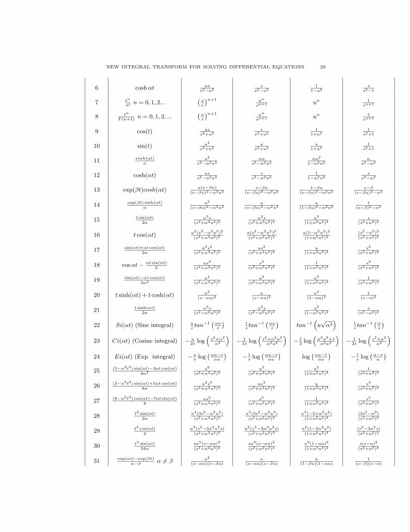
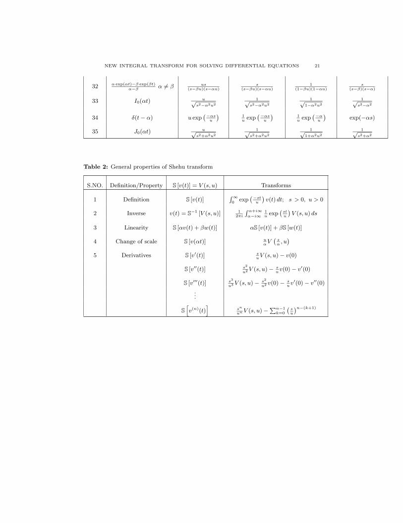
More properties of the Shehu transform and their converges to the natural trans-form, the Sumudu transform, and the Laplace transform are presented in table 1.The comprehensive summary of Shehu transform properties are presented in table2.

4. Applications

In this section, the applications of the proposed transform are presented. Thesimplicity, efficiency and high accuracy of the Shehu transform are clearly illus-trated.


Example 1. Consider the following first order ordinary differential equation

dv(t)

dt+ v(t) = 0, (4.1)

subject to the initial conditionv(0) = 1. (4.2)

Applying the Shehu transform on both sides of Equ. (4.1), we gets

uV (s, u)− v(0) + V (s, u) = 0. (4.3)

Substituting the given initial condition and simplifying, we deduce

V (s, u) =u

s+ u(4.4)

Taking the inverse Shehu transform of Equ. (4.4), yields

v(t) = exp(−t). (4.5)

Example 2. Consider the following second order ordinary differential equation

d2v(t)

dt2+dv(t)

dt= 1 (4.6)

subject to the initial conditions

v(0) = 0,dv(0)

dt= 0. (4.7)

Applying the Shehu transform on both sides of Equ. (4.6), we obtain

s2

u2V (s, u)− s

uv(0)− v′(0) +

s

uV (s, u)− v(0) =

u

s. (4.8)

Substituting the given initial conditions and simplifying, we deduce

V (s, u) = −us

+u2

s2+

u

s+ u. (4.9)

Taking the inverse Shehu transform of Equ. (4.9), we get

v(t) = −1 + t+ exp(−t). (4.10)

Example 3. Consider the following second nonhomogeneous order ordinary differ-ential equation

d2v(t)

dt2− 3

dv(t)

dt+ 2v(t) = exp(3t) (4.11)


v(0) = 1,dv(0)

dt= 0. (4.12)

Applying the Shehu transform on both sides of Equ. (4.11), yields

s2

u2V (s, u)− s

uv(0)− v′(0)− 3

( suV (s, u)− v(0)

)+ 2V (s, u) =

u

s− 3u. (4.13)

Substituting the given initial conditions and simplifying, we obtain

V (s, u) =5

2

u

(s− u)− 2

u

s− 2u+

1

2

u

(s− 3u). (4.14)


v(t) =5

2exp(t)− 2 exp(2t) +

1

2exp(3t). (4.15)


Example 4. Consider the following ordinary differential equation

d2v(t)

dt2+ 2

dv(t)

dt+ 5v(t) = exp(−t) sin(t) (4.16)


v(0) = 0,dv(0)

dt= 1. (4.17)

Applying the Shehu transform on both sides of Equ. (4.16), we get

s2

u2V (s, u)− s

uv(0)− v′(0) + 2

( suV (s, u)− s

uv(0)

)+ 5V (s, u) =

u2

(s+ u)2 + u2

(4.18)

Substituting the given initial conditions and simplifying, we get

V (s, u) =1

3

u2

((s+ u)2 + u2)+

2

3

u2

((s+ u)2 + (2u)2)(4.19)


v(t) =1

3exp(−t) sin(t) +

2

3exp(−t) sin(2t). (4.20)

Example 5. Consider the following homogeneous partial differential equation

∂v(x, t)

∂t=∂2v(x, t)

∂x2(4.21)

subject to the boundary and initial conditions

v(0, t) = 0, v(1, t) = 0, v(x, 0) = 3sin(2πx). (4.22)


s

uV (x, s, u)− v(x, 0) =

d2V (x, s, u)

dx2. (4.23)

Substituting the given initial condition and simplifying, we get

d2V (x, s, u)

dx2− s

uV (x, s, u) = −3sin(2πx). (4.24)

The general solution of Equ. (4.24) can be written as

V (x, s, u) = Vh(x, s, u) + Vp(x, s, u), (4.25)

where Vh(x, s, u) is the solution of the homogeneous part which is given by

Vh(x, s, u) = α1 exp

(√s

ux

)+ α2 exp

(−√s

ux

), (4.26)

and Vp(x, s, u) is the solution of the nonhomogeneous part which is given by

Vp(x, s, u) = β1sin(2πx) + β2cos(2πx). (4.27)

Applying the boundary conditions on Equ. (4.26), we get

α1 + α2 = 0 and α1 exp

(√s

u

)+ α2 exp

(−√s

u

)= 0⇒ Vh(x, s, u) = 0,


since α1 = α2 = 0.Using the method of undetermined coefficients on the nonhomogeneous part, weget

Vp(x, s, u) =3u

s+ 4π2usin(2πx), (4.28)

Since, β1 = 3us+4π2u , and β2 = 0.

Then Equ. (4.25) will become

V (x, s, u) =3u

s+ 4π2usin(2πx), (4.29)


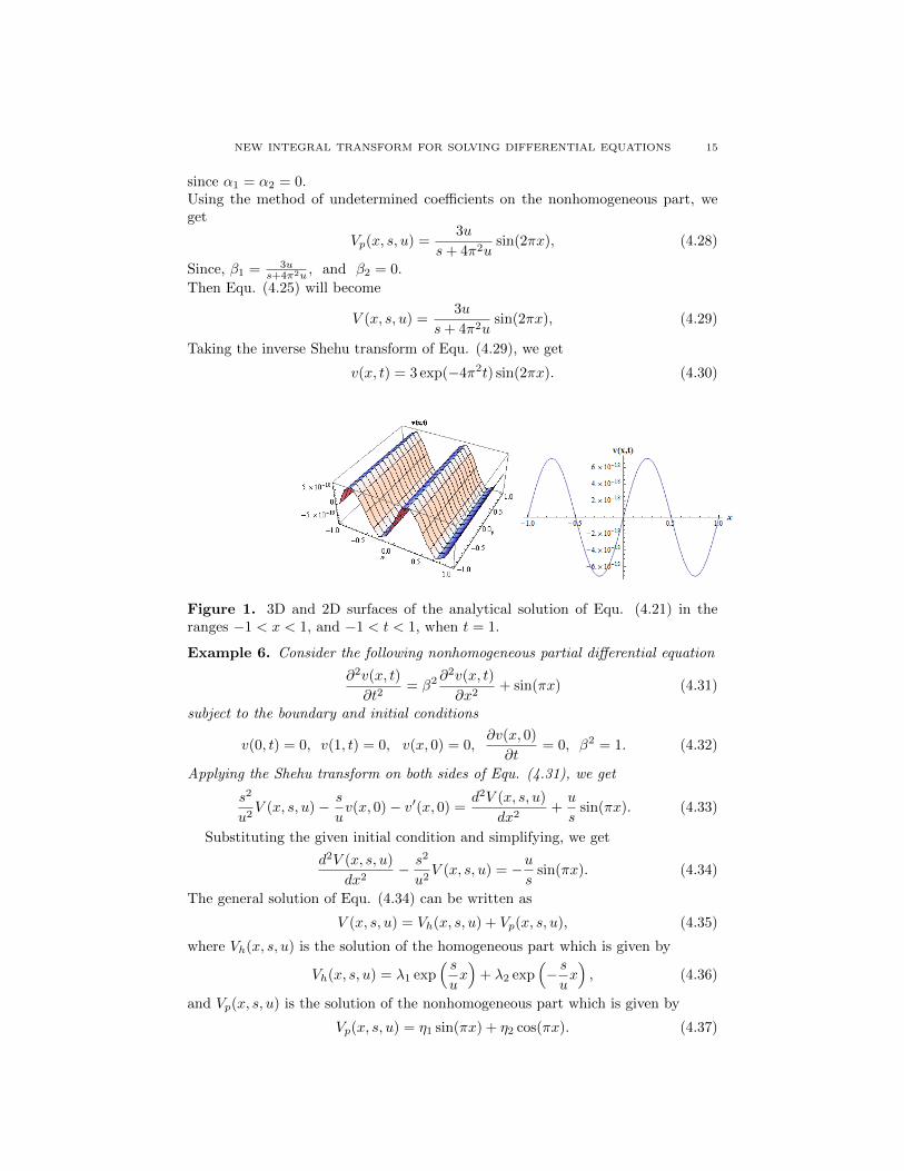
v(x, t) = 3 exp(−4π2t) sin(2πx). (4.30)

Figure 1. 3D and 2D surfaces of the analytical solution of Equ. (4.21) in theranges −1 < x < 1, and −1 < t < 1, when t = 1.

Example 6. Consider the following nonhomogeneous partial differential equation

∂2v(x, t)

∂t2= β2 ∂

2v(x, t)

∂x2+ sin(πx) (4.31)

subject to the boundary and initial conditions

v(0, t) = 0, v(1, t) = 0, v(x, 0) = 0,∂v(x, 0)

∂t= 0, β2 = 1. (4.32)


s2

u2V (x, s, u)− s

uv(x, 0)− v′(x, 0) =

d2V (x, s, u)

dx2+u

ssin(πx). (4.33)

Substituting the given initial condition and simplifying, we get

d2V (x, s, u)

dx2− s2

u2V (x, s, u) = −u

ssin(πx). (4.34)

The general solution of Equ. (4.34) can be written as

V (x, s, u) = Vh(x, s, u) + Vp(x, s, u), (4.35)

where Vh(x, s, u) is the solution of the homogeneous part which is given by

Vh(x, s, u) = λ1 exp( sux)

+ λ2 exp(− sux), (4.36)

and Vp(x, s, u) is the solution of the nonhomogeneous part which is given by

Vp(x, s, u) = η1 sin(πx) + η2 cos(πx). (4.37)


Applying the boundary conditions on Equ. (4.36), we deduce

λ1 + λ2 = 0 and λ1 exp( su

)+ λ2 exp

(− su

)= 0⇒ Vh(x, s, u) = 0,

since λ1 = λ2 = 0.Using the method of undetermined coefficients on the nonhomogeneous part, weget

Vp(x, s, u) =1

π2

(u

s− us

s2 + u2π2

)sin(πx), (4.38)

since,

η1 =u3

s(s2 + u2π2)=

1

π2

(u

s− us

s2 + u2π2

), and η2 = 0.

Then Equ. (4.35) will becomes

V (x, s, u) =1

π2

(u

s− us

s2 + u2π2

)sin(πx). (4.39)


v(x, t) =1

π2(1− cos(πt)) sin(πx). (4.40)

Figure 2. 3D and 2D surfaces of the analytical solution of Equ. (4.31) in theranges −1 < x < 1, and −1 < t < 1.

5. Conclusion

We introduced an efficient Laplace-type integral transform called the Shehu trans-form for solving both ordinary and partial differential equations. We presented itsexistence and inverse transform. We presented some useful properties and theirapplications for solving ordinary and partial differential equations. We provide acomprehensive list of the Laplace transform, Sumudu transform, and the naturaltransform in table 1 to show their mutual relationship with the Shehu transform.Finally, based on the mathematical formulations, simplicity and the findings of theproposed integral transform, we conclude that it is highly efficient because of thefollowing advantages:

• It is a generalization of the Laplace and the Sumudu integral transforms.• Its visualization is easier than the Sumudu transform, the natural trans-

form, and the Elzaki transform.


• The Laplace-type integral transform become Laplace transform when thevariable u = 1 and the Yang integral transform when the variable s = 1.• It can easily be applied directly to some class of ordinary and the partial

differential equations as demonstrated in the application section.• For advanced research in physical science and engineering, the proposed

integral transform can be considered a stepping-stone to the Sumudu trans-form, the natural transform, the Elzaki transform, and the Laplace trans-form.

6. Acknowledgements

The authors are highly grateful to the editor’s and the anonymous referees’ fortheir useful comments and suggestions in this paper. This research is partiallysupported by the National Natural Science Foundations of China under GrantsNo. (11571206). The first author also acknowledges the financial support ofChina Scholarship Council (CSC) in Shandong University with grand (CSC No:2017GXZ025381).

References

[1] H.A. Agwa, F.M. Ali, A. Kilicman, A new integral transform on time scales and its applica-

tions, Advances in Difference Equations, 60(2012), 1–14.

[2] C. Ahrendt, The Laplace transform on time scales, Pan. Am. Math. J., 19(2009), 1–36.

[3] A. Atangana, A note on the triple Laplace transform and its applications to some kind

of third-order differential equation, Abstract and Applied Analysis, 2013(2013), Article ID

769102, 1–10.

[4] H.M. Srivastava, A.K. Golmankhaneh, D. Baleanu, X.Y. Yang, Local fractional Sumudu

transform with applications to IVPs on Cantor sets, Abstr Appl Anal, 2014(2014), Article

ID 620529, 1–7.

[5] G. Dattoli, M. R. Martinelli, P. E. Ricci, On new families of integral transforms for the

solution of partial differential equations, Integral Transforms and Special Functions, 8(2005),

661–667.

[6] H. Bulut, H.M. Baskonus, and F.B.M. Belgacem, The analytical solution of some fractional

ordinary differential equations by the Sumudu transform method, Abstract and Applied Anal-

ysis, 2013(2013), Article ID 203875, 1–6.

[7] S.Weerakoon, The Sumudu transform and the Laplace transform: reply, International Jour-

nal of Mathematical Education in Science and Technology. 28(1997), 159–160.

[8] D. Albayrak, S.D. Purohit, and F. Ucar, Certain inversion and representation formulas for

q-sumudu transforms, Hacettepe Journal of Mathematics and Statistics, 43(2014), 699–713.

[9] S. Weerakoon, Application of Sumudu transform to partial differential equations, Interna-

tional Journal of Mathematical Education in Science and Technology, 25(1994), 277–283.

[10] X.Y. Yang, Y. yang, C. Cattani, and M. Zhu, A new technique for solving 1-D Burgers

equation, Thermal Science, 21(2017), S129–S136.

[11] A. Kilicman, H. Eltayeb, On new integral transform and differential equations, J. Math.

Probl. Eng, 2010(2010), Article ID: 463579, 1–13.


[12] S. Bochner, K. Chandrasekharan, Fourier transforms, Princeton University Press, Princeton,

NJ, USA, (1949).

[13] R. N. Bracewell, The Fourier transform and its applications, McGraw-Hill, Boston, Mass,

USA, 3rd edition, (2000).

[14] R. Murray, Spiegel. Theory and problems of Laplace transform. New York, USA: Schaum’s

Outline Series, McGraw–Hill, (1965).

[15] L. Debnath, D. Bhatta.. Integral transform and their applications. CRC Press, New York,

NY, USA (2010).

[16] B. Davies, Integral transforms and their applications, Texts in Applied Mathematics,

Springer, New York, NY, USA, (2002).

[17] E.I. Jury, Theory and applications of the z-transform Method, John Wiley and Sons, New

York, NY,USA, (1964).

[18] K. Liu, R.J. Hu, C. Cattani, G.N. Xie, X.J. Yang, and Y. Zhao, Local fractional z-transforms

with applications to signals on Cantor sets, Abstract and Applied Analysis, 2014(2014),Ar-

ticle ID: 638648, 1–6.

[19] P.M. Morse, H. Feshbach, Methods of theoretical physics, McGraw-Hill, New York, (1953),

484–485.

[20] P. Flajolet, X. Gourdon, and P. Dumas, Mellin transforms and asymptotics: harmonic sums,

Theoretical Computer Science, 144(1995), 3–58.

[21] C. Donolato, Analytical and numerical inversion of the Laplace-Carson transform by a dif-

ferential method, Computer Physics Communications, 145(2002), 298–309.

[22] A.M. Makarov, Application of the Laplace-Carson method of integral transformation to the

theory of unsteady visco-plastic flows, J. Engrg. Phys. Thermophys 19(1970), 94–99.

[23] E. Sjntoft, A straightforward deconvolution method for use in small computers, Nucl. In-

strum. Methods, 163(1979), 519–522.

[24] A.S. Vasudeva Murthy, A note on the differential inversion method of Hohlfield et al., SIAM

J. Appl. Math., 55(1995), 712–722.

[25] I.N. Sneddon, The Use of integral transform, McGraw-Hill, New York, (1972).

[26] K. Xie, Y. Wanga, K. Wang, and X. Cai, Application of Hankel transforms to boundary

value problems of water flow due to a circular source, Applied Mathematics and Computation,

216(2010), 1469–1477.

[27] Watugala GK. Sumudu transform–a new integral transform to solve differential equations

and control engineering problems. Math. Engg. in Indust., 6(1998), 319–329.

[28] M.A. Asiru, Sumudu transform and solution of integral equations of convolution type, Int. J.

of Math. Edu. Sci. and Tech., 33(2002), 944–949.

[29] F.B.M. Belgacem, S.L. Kalla, A.A. Karaballi, Analytical investigations of the Sumudu trans-

form and applications to integral production equations, Math. Probl. in Engg., 3(2003),

103-118.

[30] F.B.M. Belgacem, A.A. Karaballi, Sumudu transform fundamental properties, investigations

and applications. J. of Appl. Math. and Stoch. Anal., 2006(2006), Article ID 91083, 1–23.

[31] H. ELtayeh and A. kilicman, On Some applications of a new integral transform, Int. Journal

of Math. Analysis, 4(2010), 123–132.


[32] T.M. Elzaki. The new integral transform ”Elzaki transform”. Glob. J. of Pur. and Appl.

Math., 7(2011), 57–64.

[33] Z.H. Khan, W.A. Khan, N-transform-properties and applications. NUST J. of Engg. Sci.,

1(2008), 127–133.

[34] F.B.M. Belgacem, R. Silambarasan, Theory of natural transform. Math. in Engg. Sci., and

Aeros., 3(2012), 99–124.

[35] F.B.M. Belgacem, R. Silambarasan, Advances in the natural transform. AIP Conference

Proceedings; 1493 January 2012; USA: American Institute of Physics. (2012), 106–110.

[36] H.M. Srivastava, Minjie Luo, R.K.Raina, A new integral transform and its applications, Acta

Mathematica Scientia, 35(2015), 1386–1400.

[37] A. Atangana, A. Kilicman, A novel integral operator transform and its application to some

FODE and FPDE with some kind of singularities, Mathematical Problems in Engineering,

2013(2013), Article ID: 531984, 1–7.

[38] X.J. Yang, A new integral transform method for solving steady heat-transfer problem, Ther-

mal Science, 20(2016), S639–S642.

[39] X.J. Yang, A new integral transform operator for solving the heat-diffusion problem, Applied

Mathematics Letters, 64(2017), 193–197.

[40] Y.X. Jun, F. Gao , A new technology for solving diffusion and heat equations, Thermal

Science, 21(2017), 133–140.

[41] A. Atangana, B.S.T. Alkaltani, A novel double integral transform and its applications, Jour-

nal of Nonlinear Science and Applications, 9(2016), 424–434.

[42] H. Eltayeb, A note on double Laplace decomposition method and nonlinear partial differential

equations, New Trends in Mathematical Sciences, 5(2017), 156–164.

[43] F.B.M. Belgacem, R. Silambarasan, H. Zakia, T. Mekkaoui, New and extended applications

of the natural and Sumudu transforms: Fractional diffusion and Stokes fluid flow realms.

Advances Real and Complex Analysis with Applications, Publisher: Birkhuser, Singapore,

(2017). 107–120.

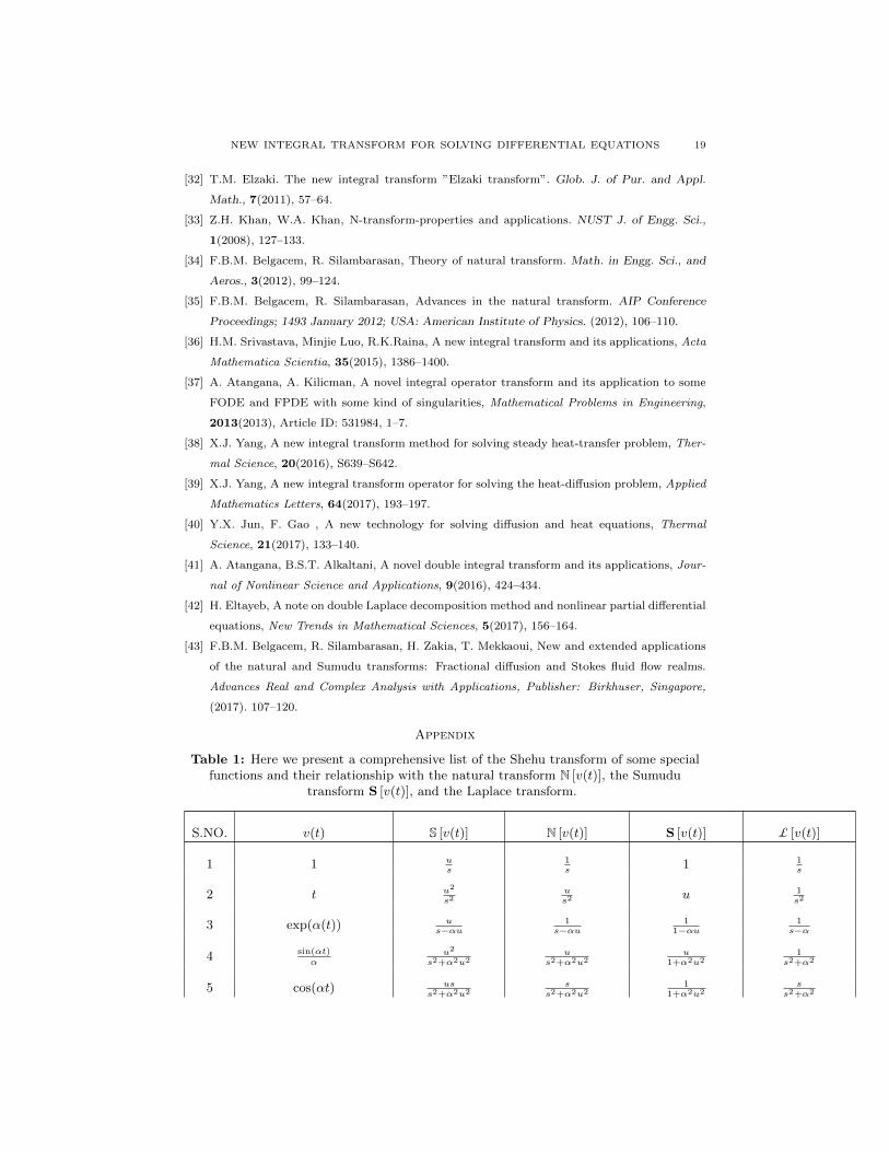
Appendix

Table 1: Here we present a comprehensive list of the Shehu transform of some specialfunctions and their relationship with the natural transform N [v(t)], the Sumudu

transform S [v(t)], and the Laplace transform.

S.NO. v(t) S [v(t)] N [v(t)] S [v(t)] £ [v(t)]

1 1 us

1s

1 1s

2 t u2

s2us2

u 1s2

3 exp(α(t)) us−αu

1s−αu

11−αu

1s−α

4 sin(αt)α

u2

s2+α2u2u

s2+α2u2u

1+α2u21

s2+α2

5 cos(αt) uss2+α2u2

ss2+α2u2

11+α2u2

ss2+α2


6 coshαt uss2−u2

ss2−u2

11−u2

ss2−1

7 tn

n!n = 0, 1, 2...

(us

)n+1 un

sn+1 un 1sn+1

8 tn

Γ(n+1)n = 0, 1, 2, ...

(us

)n+1 un

sn+1 un 1sn+1

9 cos(t) uss2+u2

ss2+u2

11+u2

1s2+1

10 sin(t) u2

s2+u2u

s2+u2u

1+u21

s2+1

11 sinh(αt)α

u2

s2−α2u2αu

s2−α2u2αu2

1−α2u2α

s2−α2

12 cosh(αt) uss2−α2u2

ss2−α2u2

11−α2u2

ss2−α2

13 exp(βt)cosh(αt) u(s−βu)

(s−βu)2−α2u2s−βu

(s−βu)2−α2u21−βu

(s−βu)2−α2u2s−β

(s−βu)2−α2

14 exp(βt) sinh(αt)α

u2

(s−βu)2−α2u2u

(s−βu)2−α2u2u

(1−βu)2−α2u21

(s−β)2−α2

15 t sin(αt)2α

u3s(s2+α2u2)2

u2s(s2+α2u2)2

u3

(1+α2u2)2s

(s2+α2)2

16 t cos(αt) u2(s2−α2u2)2

(s2+α2u2)2u(s2−α2u2)2

(s2+α2u2)2u(1−α2u2)2

(1+α2u2)2(s2−α2)2

(s2+α2)2

17 sin(αt)+αt cos(αt)2α

u2s2

(s2+α2u2)2us2

(s2+α2u2)2u

(1+α2u2)2s2

(s2+α2)2

18 cosαt− αt sin(αt)2

us3

(s2+α2u2)2s3

(s2+α2u2)21

(1+α2u2)2s3

(s2+α2)2

19 sin(αt)−αt cos(αt)

2α3u4

(s2+α2u2)2u3

(s2+α2u2)2u3

(1+α2u2)21

(s2+α2)2

20 t sinh(αt) + t cosh(αt) u2

(s−αu)2u

(s−αu)2u2

(1−αu)21

(s−α)2

21 t sinh(αt)2α

u3s(s2−α2u2)2

u2s(s2−α2u2)2

u2

(1−α2u2)2s

(s2−α2)2

22 Si(αt) (Sine integral) ustan−1

(αus

)1stan−1

(αus

)tan−1

(u√α2)

1stan−1

(αs

)23 Ci(αt) (Cosine integral) − u

2slog(s2+α2

α2

)− 1

2slog(s2+α2u2

α2u2

)− 1

2log(α2u2+1α2u2

)− 1

2slog(s2+α2

α2

)24 Ei(αt) (Exp. integral) −u

slog(αu−sαu

)− 1s

log(αu−sαu

)log(αu−1αu

)− 1s

log(α−sα

)25 (3−α2t2) sin(αt)−3αt cos(αt)

8α5u6

(s2+α2u2)3u5

(s2+α2u2)3u5

(1+α2u2)31

(s2+α2)3

26 (3−α2t2) sin(αt)+5αt cos(αt)8α

u2s4

(s2+α2u2)3us4

(s2+α2u2)3u

(1+α2u2)3s4

(s2+α2)3

27 (8−α2t2) cos(αt)−7αt sin(αt)8

us5

(s2+α2u2)3s5

(s2+α2u2)31

(1+α2u2)3s5

(s2+α2)3

28 t2 sin(αt)2α

u4(3s2−α2u2)

(s2+α2u2)3u3(3s2−α2u3)

(s2+α2u2)3u3(−3+α2u2)

(1+α2u2)3(3s2−α2)

(s2+α2)3

29 t2 cos(αt)2

u3(s3−3α2u2s)

(s2+α2u2)3u2(s3−3α2u2s)

(s2+α2u2)3u2(1−3α2u2)

(1+α2u2)3(s3−3α2s)

(s2+α2)3

30 t3 sin(αt)24α

su5(s−αu)2

(s2+α2u2)4su4(s−αu)2

(s2+α2u2)4u4(1−αu)2

(1+α2u2)4s(s−α)2

(s2+α2)4

31 exp(αt)−exp(βt)α−β α 6= β u2

(s−αu)(s−βu)u

(s−αu)(s−βu)u

(1−βu)(1−αu)1

(s−β)(s−α)


32 α exp(αt)−β exp(βt)α−β α 6= β us

(s−βu)(s−αu)s

(s−βu)(s−αu)1

(1−βu)(1−αu)s

(s−β)(s−α)

33 I0(αt) u√s2−α2u2

1√s2−α2u2

1√1−α2u2

1√s2−α2

34 δ(t− α) u exp(−αs

u

)1u

exp(−αs

u

)1u

exp(−αu

)exp(−αs)

35 J0(αt) u√s2+α2u2

1√s2+α2u2

1√1+α2u2

1√s2+α2

Table 2: General properties of Shehu transform

S.NO. Definition/Property S [v(t)] = V (s, u) Transforms

1 Definition S [v(t)]∫∞

0exp

(−stu

)v(t) dt; s > 0, u > 0

2 Inverse v(t) = S−1 [V (s, u)] 12πi

∫ α+i∞α−i∞

1u

exp(stu

)V (s, u) ds

3 Linearity S [αv(t) + βw(t)] αS [v(t)] + βS [w(t)]

4 Change of scale S [v(αt)] uαV(sα, u)

5 Derivatives S [v′(t)] suV (s, u)− v(0)

S [v′′(t)] s2

u2 V (s, u)− suv(0)− v′(0)

S [v′′′(t)] s3

u3 V (s, u)− s2

u2 v(0)− suv′(0)− v′′(0)

...

S[v(n)(t)

]sn

unV (s, u)−

∑n−1k=0

(su

)n−(k+1)


Table 3: Summary of some integral transform and their definitions

S.No. Integral transform Definition

1 Laplace transform £[f(t)] = F (s) =∫∞

0exp (−st) f(t)dt

2 Fourier transform z[f(t)] = f(ω) = 1√2π

∫∞−∞ exp (−iωt) f(t)dt

3 Melling transform M [f(s); s] = f∗(s) =∫∞

0xs−1f(x)dx

4 Hankel’s transform Fv(s) = Hv[f(r)] =∫∞

0rf(r)Jv(sr)dr, r ≥ 0

5 Sumudu transform S[f(t)] = G(u) = 1u

∫∞0

exp(−tu

)f(t)dt

6 Laplace-Carson transform fC(p) = p∫∞

0exp (−pt) f(t)dt, t ≥ 0

7 Atangana-Kilicman transform Mn(s) = Mn[f(x)](s) =∫∞

0xn exp (−xs) f(x)dx

8 El-zaki transform E[f(t)] = T (u) = u∫∞

0exp

(−tu

)f(t)dt

9 Yang transform Y [φ(τ)] = φ(ω) =∫∞

0exp

(−τω

)φ(τ)dτ

10 natural transform N+[f(t)] = R(s, u) = 1u

∫∞0

exp(−stu

)f(t)dt, s > 0, u > 0

11 z-transform X(z) = Z{x[n]} =∑∞n=−∞ x[n]z−n, n ∈ Z, z ∈ C

12 M-transform Mρ,m[f(t)](u, v) =∫∞

0

exp(−ut)f(vt)(tm+vm)ρ

dt, ρ ∈ C, <(ρ) ≥ 0, m ∈ Z+

School of Mathematics, Shandong University, Jinan, Shandong 250100, P.R. China

∗Corresponding author: [email protected]

NEW INTEGRAL TRANSFORM: SHEHU TRANSFORM A …

Documents

Transcript of NEW INTEGRAL TRANSFORM: SHEHU TRANSFORM A …