New England Case Study

7/22/2019 New England Case Study

http://slidepdf.com/reader/full/new-england-case-study 1/14

DQ U A N T I T A T I V E M O D U L E

Waiting Line Models

DISCUSSION QUESTIONS

1. Three parts of a queuing system: arrivals or inputs to the

system; the queue discipline, or the waiting line itself; and the

service facility.

2. Qualitative concerns include fairness and the aesthetics of the

area in which waiting takes place.

3. Arrivals are governed by: the size of the source population(finite or infinite); the pattern of arrivals at the system (on a

schedule or randomly); and the behavior of the arrivals (joining

the queue, balking, or reneging).

4. Measures of system performance:

the average time each customer or object spends in the

queue;

the average queue length;

the average time each customer or object spends in the

system;

the average number of customers in the system;

the probability that the service facility is idle;

the utilization factor for the system;

and the probability of a specific number of customers or

objects in the system.

5. Assumptions of the “basic” single channel model:

1. Arrivals are served on a first-come, first-served (FIFO)

basis, and every arrival waits to be served, regardless of

the length of the line or queue.

2. Arrivals are independent of preceding arrivals, but the

arrival rate does not change over time.

3. Arrivals are described by a Poisson probability distribution

and come from an infinite population.

4. Service times vary from one customer to the next and are

independent of one another, but their average rate is known.

5. Service times occur according to the negative exponential

distribution.

6. The service rate is faster than the arrival rate.

6. This is, of course, how most supermarket bakeries operate—

FCFS by the use of numbers. This is good, because at the bakery

we cannot distinguish long jobs from short ones. (This can be

compared with the situation at the checkout counter, where we

can estimate job length according to the number of items being

purchased by a customer in a particular line.)

7. “Balk” is to refuse to enter the queue: “renege” is to leave the

queue (without being served) after entering. Examples of balk

come from observing “the line is too long” to “the line isn’t

moving very fast.” Renege examples may come from “the other

line is moving faster” or “I can’t wait any longer.”

8. W s is the time spent waiting plus being serviced, W q is the

time spent waiting for service. W s is therefore larger than W q by

the amount of time spent on the service itself.

9. The first in, first out priority rule is often not valid. Examples

of when other rules are more appropriate include: Hospital emergency room (most severely injured first)

An elevator (last in, first out)

Popcorn stand at a theater (random)

Small store (he who yells loudest)

Mainframe computer system (preassigned priority levels,

highest level gets served first)

Restaurant (service may be based on match between the

number in your party and seats presently available)

Grocery store (“general” checkout counters; counters for

“10” or fewer items)

10. If λ > µ : Intuitively, the queue will grow progressively

longer, because the arrival rate is larger than the service rate.

Analytically, the performance measures take on negative signs,which have no meaning, except as indicators of a queue with a

serious problem.

11. If λ is only slightly smaller than µ : The denominator of the

performance measures all include ( µ − λ). This value is now

very small, making the performance measures large. Average

number of objects in the system grows large, as does the average

time spent waiting.

12. Finite waiting lines exist in:

Barber shops (there are only a limited number of seats)

A company that has five telephone receivers connected

to a single incoming line (multichannel, zero-length waiting

line)

A company that has five lines coming to a single

telephone receiver (single-channel, waiting line of

maximum length five)

Gasoline station where cars lining up for gas are

restricted to a particular, finite parking area (they cannot

continue the line into the street, for example)

Persons leaving an elevator

Finite sources exist when:

A company has only three or four machines that may

need service

A small airport that has only 10 or 15 flights scheduled

each day

68



69 QUANTITATIVE MODULE D WAIT ING L IN E MO D E L S

A maximum of 30 students are due to arrive at a classroom

A hospital ward has only 10 patients who may need a

particular type of care today

13. Barber shop:

Arrivals → customers wanting haircuts

Waiting line → seated customers; limited number of chairs;

priority is informal FIFOService → haircut, shampoo, etc. For simple service, single

phase; for more complex service sequence (shampoo, haircut,

manicure, etc.), probably multiphase

Car wash: usually either a single-channel, single-server system; a

system with each service bay having its own queue; or a self-

service system.

Single channel:

Arrivals → dirty carsWaiting line → cars in single line

Service → single phase (all automatic wash), or multiphase

(vacuum, soap, wash, dry, polish, each performed by a separate

worker or crew) (Note that we term this a single-service facility

even though work may be performed by several individuals or

crews.)

Single phase:

Multiphase:

Multichannel, single phase:

Note: In practice, it is often difficult to differentiate between a

multichannel system, and a system that has multiple, parallel,

service facilities, but that actually operates as several separate

single-channel systems. Usually, if we have a system with m

parallel service facilities, and a single line forms within the

boundary of the system, then we consider the system to be a

multichannel system. If, on the other hand, a line forms within the

system ahead of each

of the m parallel service facilities, we consider the system as if it

were m separate single-channel systems, each with an arrival rate

equal to the original arrival rate divided by m.

Laundromat:

Arrivals→

customers with loads of dirty laundry

Waiting line → customers waiting in a group for the next

available washing machine or drier. Service on an informal FIFO

priority basis.

Service facility → two-phase system (washer, drier); each phase

multichannel.

Small grocery store:

Usually a two-phase system: first phase, self-service (an infinitenumber of channels); second phase, single channel

Arrivals → customers to purchase food items

Waiting line →Phase 1: no line

Phase 2: customers with cart or basket of groceries arrive at cash

register. Usually FIFO, but grocer may check out regular customers

first, or give priority to customer making a small, quick, purchase

Service →Phase 1: gathering groceries; self-servicePhase 2: ring up sale, give change, bag groceries

14. (a) Doctor’s offices generally attempt to schedule “group”

arrivals (10 patients on the hour, every hour), or uniform

arrivals (1 patient every 15 minutes). Arrivals at an



QUANTITATIVE MODULE D WAIT ING L IN E MO D E L S 70

emergency center , on the other hand, are typically Poisson.



7 QUANTITATIVE MODULE D WAIT ING L IN E MO D E L S

(b) Service times often random, and described by either a

negative exponential or normal probability distribution.

(c) Service times would approach a constant only when the

physician provided approximately the same treatment to

each patient. This might occur in the case of physical

exams.

15. Constant service time model will have an average queue

length and an average waiting time that is one-half that of the

same model with exponential service time.

16. This deals with the interesting issue of the value of waiting

time. Some service organizations place a very low value on your

time, leading to a good classroom discussion.

ACTIVE MODEL E!E"CISES

ACTIVE MODEL D.1: Single Server Model

1. For how many minutes do customers wait before their muffler

installation begins?

40

2. How fast would the average installation (service) time have to

be to cut the waiting time in half?

16 minutes

3. Suppose the arrival rate increases by 10 percent to 2.2

customers per hour. By what percentage will the waiting time

rise?

37.5% – From 40 to 55

4. What is the probability that there is no waiting line when a

car arrives for service?

There is no waiting line if no one is in the system or if one

person is in the system. From the graph, the respective

probabilities are .33 and .22 for a total of 55%.

5. What happens to the probabilities as the arrival rate increases?

The probabilities of low numbers of customers in the

system fall while the probabilities of high number of customers

in the system rises.

ACTIVE MODEL D.2: Multiple Server System withCosts

1. What number of mechanics yields the lowest total daily cost?

What is the minimum total daily cost?

2 mechanics; $112 + 6.67 = $118.67

2. Use the scrollbar on the arrival rate. What would the arrival

rate need to be in order that a third mechanic would be required?

3.8 cars per hour

3. Use the scrollbar on the goodwill cost and determine the

range of goodwill costs for which you would have exactly 1mechanic? Two mechanics?

For a goodwill cost of less than $5 per hour use 1

mechanic. Two mechanics would be best for a goodwill cost

anywhere between $5 per hour and $100 per hour.

4. How high would the wage rate need to be in order to make 1

mechanic the least costly option?

From the graph—roughly $12.70

5. If a second mechanic is added, is it less costly to have the two

mechanics working separately or to have the two mechanics work

as a single team with a service rate that is twice as fast.

Separately—$118.67, together, changing the service rate

to 6 and doubling the wages, the single server cost is $112 +

$13.33 or $125.33. Therefore, having them work separately is

less costly.

ACTIVE MODEL D.3: Constant Service Times

1. The arrival rate of truck is, of course, a forecast and therefore

uncertain. What is the breakeven point, in truck arrivals per hour,

between keeping the old compactor and purchasing the new one.

At 10 trucks per hour or higher we should not purchase

the new compactor.

2. The service rate represents, of course, the design capacity.

What minimum rate is needed in order to save money with the

purchase of a new compactor?

10 trucks per hour or more.

END#O$#MODULE %"O&LEMSD.1 This is an M / M /1 queue; λ = 3/hr.; and µ = 5/hr.

2 23 9 (a) 0.9 persons

( ) 5(5 3) 5(2)

3 3(b) 1.5 persons

5 3 2

3 3 (c) hr. 18 min.

( ) 5(5 3) 10

1 1 1 (d) hr. 30 min.

5 3 2

3 ( e) 0.60, or 60%5

q

s

q

s

L

L

W

W

λ

µ µ λ

λ

µ λ

λ

µ µ λ

µ λ

λ ρ µ

= = = =− −

= = = =− −

= = = =− −

= = = =− −

= = =

2

40(a) 0.44 44%

90

(40)(b) 0.356

90(90 40)

40(c) 0.8

90 40

40(d) 0.0089 hours

90(90 40)

0.533 minutes 32 seconds

1 1(e) hour90 40 50

1.2 minutes 72 seconds

40/hour, 90/hour

q

s

q

s

L

L

W

W

ρ

λ µ

= = =

= =−

= =−

= =−

= =

= =−

= == =



QUANTITATIVE MODULE D WAIT ING L IN E MO D E L S 7'

%(o)a)ilit* o+ k o( ,o(e C-sto,e(s

Waiting in Line and.o( &eing

Waited on

k λ

µ

+

>

= ÷

k

n k P

0 0.667 1 0.444 2 0.296 3 0.198

2 2

202 customers in the system on the average

30 20

1 10.1 hour (6 minutes) that the average customer spends in the total system

30 20

20 1.33 customers waiting for serv( ) 30(30 20)

s

s

q

L

W

L

λ

µ λ

µ λ

λ µ µ λ

= = =− −

= = =− −

= = =− −ice in line on the average

201/15 hour = (4 minutes) = average waiting time of a customer in the queue awaiting service

( ) 30(30 20)

20= 0.67 percent of the time that he is busy waiting on cus

30

qW λ

µ µ λ

λ ρ

µ

= = =− −

= = =

0

tomers

1 1 0.33 probability that there are no customers in the system(being waited on or waiting in the queue) at any given time

P λ

ρ µ

= − = − = =

0

2

(a) 1 0.5

(b) = = 0.5

(c) = = 1

(d) = = 0.5( )

(e) = = 0.05 hours( )

(f) = = 0.1 hours

where: 20/ hour, 10 / hour

s

q

q

s

P

L

L

W

W

ρ

λ ρ

µ

λ

µ λ

λ

µ µ λ

λ

µ µ λ

λ

µ λ

µ λ

= − =

−

−

−

−= =

(a) Ls = Average number of prescriptions in the system

λ

µ λ = = = =

− −12 12

415 12 3

(b) W s = Average time a prescription spends in the system

µ λ = = = =

− −1 1 1

.33 hours15 12 3

= 20 minutes.

(c) Lq = Average number of prescriptions in the queue

λ

µ µ λ = = = =

− −

2 212 1443.2

( ) 15(15 12) 45

D.62

(a) 0.6673

λ ρ

µ = = =

λ

µ µ λ

λ

µ µ λ

µ λ

= = =− −

=

= = = =− −

2 2

2 2(b)

( ) 3(3 2) 3

0.667 time units (minutes)

2 4(c) 1.333

( ) 3(3 2) 3

where: = 180/hour, = 120/hour

q

q

W

L

D.7 This is an M/M/ 1 model. λ = 24, µ = 30

0

2 2 2

1 1 1(a) hours

30 24 6

24 24(b) = 4 cars

30 24 6

24 24(c) = 3.2 cars

( ) 30(30 24) 30(6)

24 24 2(d) = hours

( ) 30(30 24) 30(6) 15

1(e) 1 / 1 24 / 30

5

24 4(f)30 5

(g) Probabilit

s

s

q

q

W

L

L

W

P

µ λ

λ

µ λ

λ

µ µ λ

λ

µ µ λ

λ µ

λ ρ µ

= = =− −

= = =− −

= = =− −

= = =− −

= − = − =

= = =

1 2

1 1 2 1

y( 2)

24 24 0.128

30 30

n nn P P> >+ +

= = −

= − = ÷ ÷

D.8 (a) The utilization rate, ρ , is given by:

30.375

8

λ ρ

µ = = =

(b) The average down time, W s, is the time the machine

waits to be serviced plus the time taken to perform the

service.

( ) ( )1 1 0.2 days, or 1.6 hours

8 3sW

µ λ = = =

− −



7/ QUANTITATIVE MODULE D WAIT ING L IN E MODE L S

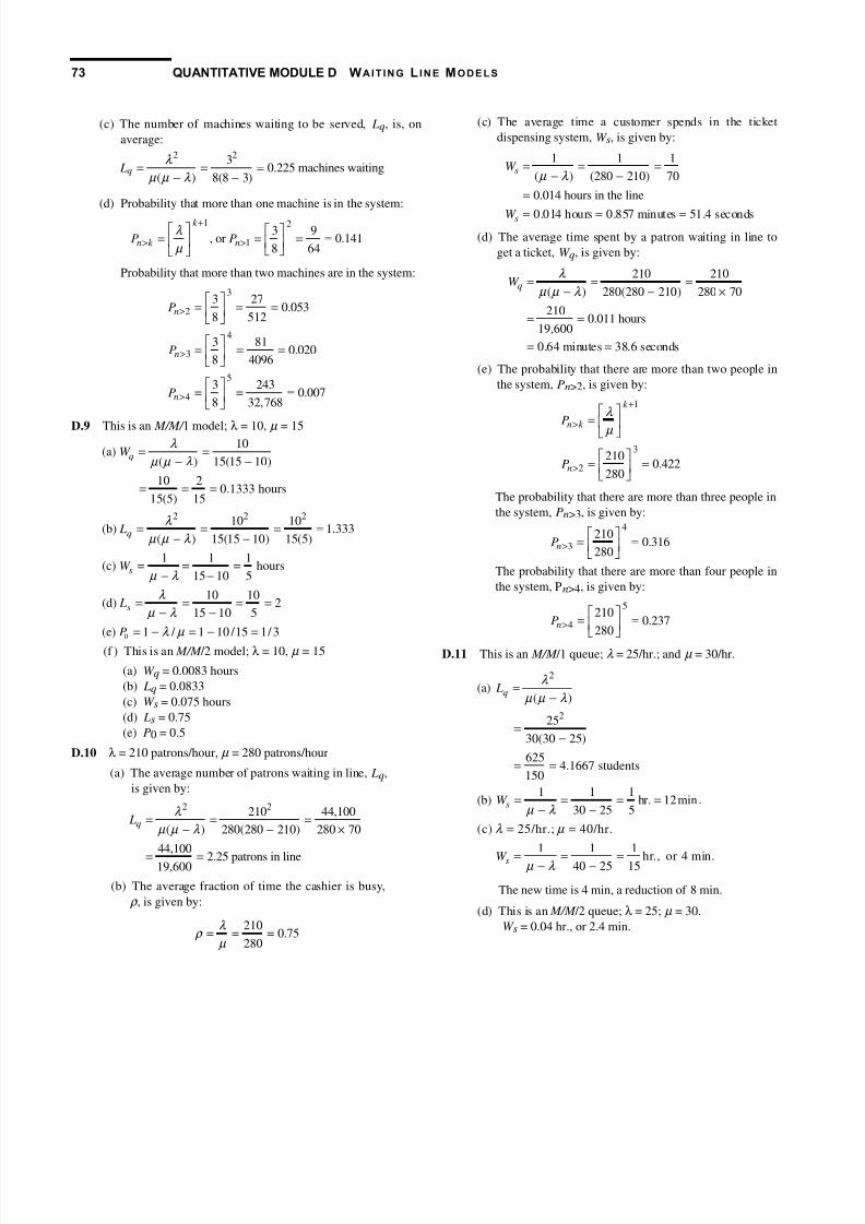
(c) The average time a customer spends in the ticket

dispensing system, W s, is given by:

1 1 1

( ) (280 210) 70

0.014 hours in the line

0.014 hours 0.857 minutes 51.4 seconds

s

s

W

W

µ λ = = =

− −=

= = =(d) The average time spent by a patron waiting in line to

get a ticket, W q, is given by:

210 210

( ) 280(280 210) 280 70

2100.011 hours

19,600

0.64 minutes 38.6 seconds

qW λ

µ µ λ = = =

− − ×

= =

= =

(e) The probability that there are more than two people in

the system, Pn>2, is given by:

1

3

2210

0.422280

k

n k

n

P

P

λ

µ

+

>

>

=

= =

The probability that there are more than three people in

the system, Pn>3, is given by:4

3210

0.316280

nP >

= =

The probability that there are more than four people in

the system, Pn>4, is given by:

5

4210

0.237280

nP > = =

D.11 This is an M/M /1 queue; λ = 25/hr.; and µ = 30/hr.

λ

µ µ λ

µ λ

λ µ

µ λ

=−

=−

= =

= = = =− −

= =

= = =− −

2

2

(a)( )

25

30(30 25)

625 4.1667 students

150

1 1 1(b) hr. 12min.

30 25 5

(c) 25/hr.; 40/hr.

1 1 1

hr., or 4 min.40 25 15

q

s

s

L

W

W

The new time is 4 min, a reduction of 8 min.

(d) This is an M/M /2 queue; λ = 25; µ = 30.

W s = 0.04 hr., or 2.4 min.

(c) The number of machines waiting to be served, Lq, is, on

average:2 23

0.225 machines waiting( ) 8(8 3)

q L λ

µ µ λ = = =

− −

(d) Probability that more than one machine is in the system:

1 2

13 9

, or 0.1418 64

k

n k nP Pλ

µ

+

> >

= = = =

Probability that more than two machines are in the system:

3

2

4

3

5

4

3 270.053

8 512

3 810.020

8 4096

3 2430.007

8 32,768

n

n

n

P

P

P

>

>

>

= = =

= = =

= = =

D.9 This is an M/M/ 1 model; λ = 10, µ = 15λ

µ µ λ

λ

µ µ λ

µ λ

λ

µ λ

λ µ

= =− −

= = =

= = = =− −

= = =− −

= = = =− −

= − = − =0

2 2 2

10(a)

( ) 15(15 10)

10 2 0.1333 hours

15(5) 15

10 10(b) 1.333

( ) 15(15 10) 15(5)

1 1 1(c) hours

15 10 5

10 10(d) 2

15 10 5

(e) 1 / 1 10 /15 1/ 3

q

q

s

s

W

L

W

L

P

(f ) This is an M/M /2 model; λ = 10, µ = 15

(a) W q = 0.0083 hours

(b) Lq = 0.0833

(c) W s = 0.075 hours

(d) Ls = 0.75

(e) P0 = 0.5

D.10 λ = 210 patrons/hour, µ = 280 patrons/hour

(a) The average number of patrons waiting in line, Lq,

is given by:

2 2210 44,100

( ) 280(280 210) 280 70

44,1002.25 patrons in line19,600

q L λ

µ µ λ = = =

− − ×

= =

(b) The average fraction of time the cashier is busy,

ρ , is given by:

2100.75

280

λ ρ

µ = = =



QUANTITATIVE MODULE D WAIT ING L IN E MODE L S 7

D.12 λ = 30 trucks/hour, µ = 35 trucks/hour

(a) The average number of trucks in the system, Ls, is

given by:

30 306 trucks in the system

35 30 5s L

λ

µ λ = = = =

− −

(b) The average time spent by a truck in the system, W s, is

given by:

1 1 10.2hours = 12 minutes

35 30 5sW

µ λ = = = =

− −

(c) The utilization rate for the bin area, ρ , is given by:

30 60.857

35 7

λ ρ

µ = = = =

(d) The probability that there are more than three trucks in

the system, Pn > 3, is given by:

1

4

330

0.54035

k

n k

n

P

P

λ

µ

+

>

>

=

= =

Thus, the probability that there are more than three

trucks in the system is 0.540.

(e) Unloading cost:

hours trucks hours $16 30 0.2 18

day hour truck hour

16 30 0.2 18 $1,728 / day

uC = × × ×

= × × × =

or $12,096 per week

(f ) Enlarging the bin will cut waiting costs by 50% next

year. First, we must compute annual waiting costs:

weeks days $Annual waiting costs 2 7 1,728

year week day

$24,192

= × ×

=

Enlarging the bin will cut waiting costs by 50% next

year, resulting in a savings of $12,096. Because the cost

of enlarging the bin is only $9,000, the cooperative

should proceed to enlarge the bin. The net savings is

$3,096 (= 12,096 – 9,000).

D.13 λ = 12 calls/hour, µ = 60/4 = 15 calls/hour

(a) The average time the catalogue customer must wait,

W q, is given by:

12 12

( ) 15(15 12) 15 3

120.267 hours

45

qW λ

µ µ λ = = =− − ×

= =

(b) The average number of callers waiting to place an

order, Lq, is given by:2 212 144

( ) 15(15 12) 15 3

1443.2 customers

45

q L λ

µ µ λ = = =

− − ×

= =

(c) To decide whether or not to add the second clerk,

we must

Compute present total cost

Compute total cost with the second clerk

Compare the two

Present total cost:

/ hour service cost waiting cost

$10 per hour

(12 calls per hour 0.267 hours

waiting per call $25 per hour)

10 (12 0.267 25)

10 80.1/hour

$90.10/ hour

t C = += +

××

= + × ×= +=

To determine total cost using the second clerk (a second

channel):

( ) ( ) ( )

01

1 1! !

0

0 1 2 2 151 12 1 12 1 120! 15 1 15 1 2 15 2 15 12

2 2 154 1 45 2 5 30 12

16 304 15 2 25 18

48045 900

1

1

1

1

1

1

1

1

n M

n M M n M M

n

P

µ λ λ µ µ µ λ

= −

−=

×× × −

×−

=

+

= + +

= + +

=+ +

=+ +

∑

or:

0

1 10.429

1 0.8 0.53 2.33P = = =

+ +

( )02( 1)!( )

M

qW P M M

λ µ µ

µ λ =

− −

Then:

( )2

1215

2

2

150.429

(2 1)!(2 15 12)

15 0.64 0.4291 (30 12)

4.120.0127 hours

1 324

0.763 minutes

qW ×

= ×− × −

×= ×× −

= =×

=



71 QUANTITATIVE MODULE D WAIT ING L IN E MODE L S

Cost with two clerks:

/ hour service cost waiting cost

calls hours $20 12 0.0127 25

hour call hour

20 12 0.0127 25

20 3.81 $23.81/ hour

t C = +

= + × ×

= + × ×

= + =There is a saving of $90.10 –$23.81 = $66.29/hour

Thus, a second clerk should certainly be added!

(d) With three clerks the cost goes to $30.47. So the costs

are:

1 clerk $90.10

2 clerks $23.81

3 clerks $30.47

For 3 clerks W q = 0.00158 (from Excel OM)

$30 + (12 × 0.0015 × $25) = $30 + 0.47 = $30.47

Therefore, optimum number of clerks is 2.

D.14

λ = 4/minute, µ = 60/10 = 6/minute. For a facility with aPoisson arrival and constant service rate:

(a) The average number of people waiting in line, Lq, is

given by:

2 24 16

2 ( ) 2 6 (6 4) 24

0.67 persons

q L λ

µ µ λ = = =

− × × −=

(b) The average number of people in the system, Ls, is

given by:

40.67 0.67 0.67

6

1.33 persons

s q L L λ

µ = + = + = +

=

(c) The average waiting time, W q, is given by:

4 40.167

2 ( ) 2 6 (6 4) 24qW

λ

µ µ λ = = = =

− × × −

An individual, on average, waits 0.167 minutes or 10seconds, for his/her cup of coffee.

D.15 (a) Entering: λ = 84/minute, µ = 30/minute, ρ = 2.8

Exiting: λ = 48/minute, µ = 30/minute, ρ = 1.6

The manager desires that W q ≤ 0.1 minute = 6 seconds

and that Lq ≤ 8 customers in queue.

Entering:

= =

=

If 3, 12.27 and

= 0.14 minute (too high)

If 4, = 1.00 and= 0.01 minute (this is okay)

If = 5, = 0.24 and

= 0.003 minute (this is also okay)

q

q

q

q

q

q

M L

W

M LW

M L

W

So the manager must open M = 4 or more entrances.

Exiting:

If 2, 2.8, 0.06 minute (this is okay)

If 3, 0.31, 0.006 minute (also okay)

qq

qq

M L W

M L W

= = == = =

So the manager must open M = 2 or more exits. Since

there are only 6 turnstiles, 4 must be used as entrances

and 2 as exits.

(b) The students should recognize and question all the

limiting queuing assumptions that have been applied in

solving the case. For example, it may be reasonable to

assume that arrivals at the entrance turnstiles areindependent and Poisson. But are exiting passengers

independent? More realistically, they arrive in batches

(as a train arrives), and unless trains unload every

minute or two, this assumption may be unreasonable.

Other problems arise as well. If an exiting

passenger’s card does not have the correct fare, the

card is rejected and the passenger must leave the line,

go to an “add fare” machine to correct the deficiency,

and enter the queue again. This resembles the reneging

customer.

Note: In the real-world subway station in Washington,

D.C., common queues are not formed at turnstiles and the

problem becomes a series of single channel queues.

D.16 λ = 10 / hour, µ = 60/4.5 = 13.33/hour 10 10

(a) =2(13.33)(13.33 10) 88.8

0.113 hour 6.8 minutes

100 100(b)

2 2(13.33)(13.33 10) 88.8

1.13 cars waiting

q

q

W

L

λ

µ µ λ

λ

µ µ λ

2

= =2 ( − ) −

= =

= = =( − ) −

=

D.17 N = 5 tools

M = 1 technician

= = = = + ÷

1

4(a) The service factor 0.429+ 1 1

4 3

T

X T U

(which is closer to 0.420 for Table D.7)

(b) Average no. of machines in service (using Table D.7) =

J = NF(1 – X) = 5(0.471) (1 –0.420) = 1.37

(c) With M = 2 technicians, F rises to 0.826. The average

number of machines in service grows to J = 5(0.826)

(1 – 0.420) = 2.39

D.18 N = 5 computers, M = 2 technicians, T = 15 minutes,

U = 85 minutes

15 150.15

15 85 100

T X

T U

= = = =

+ +(a) The average number of computers waiting for service,

Lq, is given by:

= −(1 )q L N F

where F is found from Table D.7. From Table D.7, with

M = 2, X = 0.15: F = 0.990

= × − =5 (1 0.990) 0.05 computersq L




(b) The average number of computers being served, H , is

given by:

H = FNX

where F is found from Table D.7. From Table D.7 with

M = 2, X = 0.145: F = 0.990

H = 0.990 × 5 × 0.15 = 0.743 computers

(c) The average number of computers not working is given

by:

(1 ) [1 (1 )]5 [1 0.990 (1 0.15)]5 [1 0.990 0.85]5 [1 0.8415] 5 0.1585 0.793

N J N N F X N F X − = − × × − = × − × −= × − × −= × − ×= × − = × =

Therefore, on average, 0.793 computers are not

working properly.

D.19 N = 5 drilling machines, M = 1 mechanic, T = 1 day,

U = 6 days

10.143

1 6

T X

T U = = =

+ +The value 0.145 will be used for X when referencing Table

D.7.

(a) The average number of machines waiting for service,

Lq, is given by:

Lq = N (1 – F )

where F is found from Table D.7. From Table D.7,

when M = 1, X = 0.145; F = 0.892

Lq = 5(1 – 0.892) = 0.54 machines waiting

(b) The average number of machines in running order, J , is

given by: J = NF (1 – X) where F is found from Table

D.7. From Table D.7, with M = 1, X = 0.145; F = 0.892

J = 5 × 0.892 × (1 – 0.145) = 3.81 machines

(c) The reduction in waiting time obtained by employing a

second mechanic is found as follows: Waiting time

employing a single mechanic, W 1, is given by:

1(1 )T F

W XF

−=

where F is found from Table D.7. From Table D.7,

when M = 1, X = 0.145; F = 0.892.

11 1(1 0.892)

0.835 days0.145 0.892

W × −

= =×

From Table D.7, with M = 2, X = 0.145: F = 0.991

× −×2

1 1(1 0.991)W = = 0.063 days

0.145 0.991

The time saved is given by: W 1 – W 2

Time saved = 0.835 – 0.063 = 0.772 days

D.20 (a) 9 AM–3 PM: Arrival rate = 6 patients/hour

Service rate = 5 patients/hour

N-,)e( o+ Do2to(s Wait Ti,e 3,in-tes4

1 ∞

2 6.75 3 0.94

4 0.16

Therefore, three doctors are needed between 9 AM and3 PM.

(b) 3 PM–8 PM: Arrival rate = 4 patients/hour

Service rate = 5 patients/hour

N-,)e( o+ Do2to(s Wait Ti,e 3,in-tes4

1 48.0

2 2.29

3 0.28 4 0.04

Therefore, two doctors are sufficient between 3 PM and

8 PM.

(c) 8 PM–Midnight: Arrival rate = 12 patients/hour

Service rate = 5 patients/hour N-,)e( o+ Do2to(s Wait Ti,e 3,in-tes4

1 ∞

2 ∞

3 12.940

4 2.154

Therefore, four doctors are required between 8 PM and

midnight.




Because the minimum total cost per shift relates to two

salespeople, the manager’s optimum strategy is to hire

two salespeople.

D.22 This problem provides an excellent way to involve

students in the learning process, but can involve a lot of work on

the part of the student. This exercise can also provide a lot of

work on the part of the instructor.

Students need to gather the data and may need help on

how to do that.

Students with weak statistical background may need

specific help on plotting their data against Poisson and

negative exponential distributions.

If you can get over those hurdles (and providing the data

fit the models provided in the text), the rest of the problem

is rather standard and can be solved by hand or via the

software.

INTE"NET 5OMEWO" %"O&LEMS

Solutions to problems on our companion web site

(www.prenhall.com/heizer)

D.2340 2

(a)60 3

λ ρ

µ = = =

λ

µ µ λ

λ

µ λ

λ

µ µ λ

µ λ

λ µ

= = =− −

= = =− −

= =− −

=

= = =− −

= =

2 2(40) 4(b)

( ) 60(60 40) 3

40(c) 2

60 40

40(d)

( ) 60(60 40)

0.033 hours = 2 minutes

1 1 1(e) hour = 3 minutes

60 40 20

40/hour, 60/hour

q

s

q

s

L

L

W

W

D.24λ

ρ µ

= =(a) 0.833

λ

µ µ λ = =

−(b) 0.20833 days =1.667 hours

( )qW

λ

µ µ λ

λ µ

µ

λ

+

= =−

> = = = ÷

=

2

1

(c) 4.167( )

(d) ( 5) 0.335 where: 24/day,

20/day

q

k

L

P n

D.25

λ

µ µ λ = =−

2

(a) 3.2( )q L

µ λ

λ ρ µ λ

µ

= =−

= =

1 1(b) hour (10 minutes)

6

(c) 0.8 where = 30 / hour, = 24 / hour

sW

D.26 λ = 20 cars/hour, µ = 30 cars/hour

(a) The average number of cars in line Lq, is given by:

2 2

2

20

( ) 30(30 20)

201.33 cars

30 10

q L λ

µ µ λ = =

− −

= =×

(b) The average time a car waits before it is washed, W q isgiven by:

20

( ) 30(30 20)

200.0667 hours

30 10

qW λ

µ µ λ = =

− −

= =×

(c) The average time a car spends in the service system,

W s is given by:

1 1 10.10 hours

( ) (30 20) 10sW

µ λ = = = =

− −

(d) The utilization rate, ρ , is given by:

200.66730

λ ρ µ = = =

(e) The probability that no cars are in the system, P0, is

given by:

0 1 1 1 0.667 0.33P λ

ρ µ

= − = − = − =

D.21 The manager’s calculations are as follows:

N-,)e( o+ Saleseole

' /

(a) Average !"#er $% &!'$"er' er '*+% 50 50 50 50

(#) Average ,a++g +"e er &!'$"er ("+!e') 7 4 3 2(&) T$a- ,a++g +"e er '*+% (a × b) ("+!e') 350 20

0 150 100

() /$' er "+!e $% ,a++g +"e (e'+"ae) 1.00 1.00 1.00 1.00

(e) Va-!e $% -$' +"e (c × d ) er '*+% 350 200

150 100

(% ) a-ar &$' er '*+% 70 14 210 280




(f) Use of automation (with µ = 60/hour) will produce the

following.

0

2 2200.083

2 ( ) 2 60(60 20)

200.0042 hours

2 ( ) 2 60(60 20)1

0.0042 0.0167 0.0209 hours

200.333

60

1 0.667

q

q

s q

L

W

W W

P

λ

µ µ λ

λ

µ µ λ

µ

λ ρ

µ

ρ

= = =− × −

= = =− × −

= + = + =

= = =

= − =

D.27 λ = 4, students/minute, µ = 60/12 = 5 students/minute

(a) The probability of more than two students in the

system, Pn > 2, is given by:

1

32

4 0.5125

k

n k

n

P

P

λ

µ

+

>

>

=

= =

The probability of more than three students in the


4

34

0.4105

nP >

= =

The probability of more than four students in the


5

44

0.3285

nP > = =

(b) The probability that the system is empty, P0, is given by:

0

41 1 1 0.8 0.2

5P

λ

µ = − = − = − =

(c) The average waiting time, W q, is given by:

40.8 minutes

( ) 5(5 4)qW

λ

µ µ λ = = =

− −

(d) The expected number of students in the queue, Lq, is

given by:

2 243.2 students

( ) 5(5 4)q L

λ

µ µ λ = = =

− −

(e) The average number of students in the system, Ls is

given as:

44 students

5 4s L

λ

µ λ = = =

− −

(f) Adding a second channel, we have:

4 students/minute

605 students/minute

12

2 M

λ

µ

=

= =

=

(b)′ The probability that the two channel system is empty,

P0, is given by:

( ) ( ) ( )

01

1 1! !

0

0 1 22 51 4 1 4 1 4

0! 5 1 5 1 2 5 2 5 4

2 16 104 12 54 1 45 2 25 65 2 5 10 4

16045 360

1

1

1 1

11

1

1

n M n M M

n M M

n

P


= −

−

=

×× × −

×−

=

+

=

+ +

= =+ + + +

=+ +

∑

or:

0

1 10.429

1 0.8 0.53 2.33P = = =

+ +

Thus, the probability of an empty system when usingthe second channel, is 0.429.

(c)′ The average waiting time, W q, for the two channel

system is given by:

1q sW W

µ = −

where:

( )02

1

( 1)!( )

M

sW P M M

λ µ

µ

µ µ λ = +

− −Then:

( )2

4

5 2

2

5

0.429(2 1)!(2 5 4)

5 0.64 1.3730.429

1 361 (10 4)

0.038 minutes 2.3 seconds

qW

×= ×− × −

×= × =

×× −= =

(d)′ The average number of students in the queue for the

two channel system, Lq, is given by:

q s L L λ

µ = −

where:

( )02( 1)!( )

M

s L P M M

λ µ

λµ λ

µ µ λ = +− −




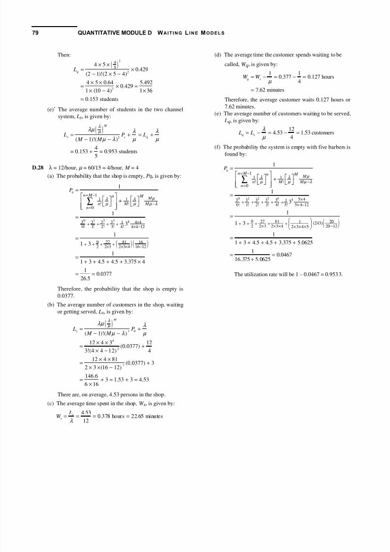
Then:

( )2

2

2

45

4 50.429

(2 1)!(2 5 4)

4 5 0.64 5.4920.429

1 (10 4) 1 36

0.153 students

q L

× ×= ×

− × −× ×

= × =× − ×

=

(e)′ The average number of students in the two channel

system, Ls, is given by:

( )02( 1)!( )

40.153 0.953 students

5

M

s q L P L

M M

λ µ λµ λ λ

µ λ µ µ = + = +

− −

= + =

D.28 λ = 12/hour, µ = 60/15 = 4/hour, M = 4

(a) The probability that the shop is empty, P0, is given by:

( ) ( )


= −

−=

×+ + + + × −

+ + + +× × × −

= +

=

=

=+ + + + ×

= =

∑0

0 1 2 3

!

4

!

11 1!

0

3 3 3 3 1 4 40 1! 2! 3! 4! 4 4 12

9 27 81 162 2 3 2 3 4 16 12

1

1

3

1

1 3

1

1 3 4.5 4.5 3.375 4

10.0377

26.5

n M n M M

n M M n

P

Therefore, the probability that the shop is empty is0.0377.

(b) The average number of customers in the shop, waiting

or getting served, Ls, is given by:

( )02

4

2

2

( 1)!( )

12 4 3 12(0.0377)

3!(4 4 12) 4

12 4 81(0.0377) 3

2 3 (16 12)

146.63 1.53 3 4.53

6 16

M

s L P

M M

λ µ λµ λ

µ λ µ = +

− −

× ×= +

× −× ×

= +× × −

= + = + =

×There are, on average, 4.53 persons in the shop.

(c) The average time spent in the shop, W s, is given by:

4.530.378 hours 22.65 minutes

12s

s

LW

λ = = = =

(d) The average time the customer spends waiting to be

called, W q, is given by:

1 10.377 0.127 hours

4

7.62 minutes

q sW W

µ = − = − =

=

Therefore, the average customer waits 0.127 hours or

7.62 minutes.

(e) The average number of customers waiting to be served,

Lq, is given by:

124.53 1.53 customers

4q s

L L λ

µ = − = − =

(f) The probability the system is empty with five barbers is

found by:

( )


= −

−=

×+ + + + × −

+ + + + +× × × −

+

× × ×

= +

=

=

=+ + + + +

= =+

∑0

0 1 2 3 4

!

5

!

11 1!

0

5 43 3 3 3 3 10 1! 2! 3! 4! 5! 5 4 12

9 27 81 202 2 3 2 3 4 20 12

1 (243)2 3 4 5

1

13

1

1 3

1

1 3 4.5 4.5 3.375 5.0625

10.0467

16.375 5.0625

n M n M M

n M M n

P

The utilization rate will be 1 – 0.0467 = 0.9533.



1


D.30 λ = cars/hour, µ = 12 cars/hour.

(a) The average number of cars in line, Lq, is given by2 2 210 10

( ) 12(12 10) (12)(2)

4.167 cars

q L

λ

µ µ λ = = =

− −=

(b) The average time a car waits before it is washed, W q, is

given by

10 10

( ) 12(12 10) (12)(2)

0.4167 hours

qW

λ

µ µ λ = = =

− −=

(c) The average time a car spends in the service system,

W s, is given by

1 1 10.5 hour

12 10 2s

W µ λ

= = = =− −

(d) The utilization rate, ρ , is given by

100.8333

12

λ ρ

µ = = =

(e) The probability that no cars are in the system, P0, isgiven by:

λ ρ

µ = − = − = − =

01 1 1 0.8333 0.1667P

(a) Average number of prescriptions in the system

(wait time + service time)

12 12 = 4

15 3 3

s L

λ

µ λ

=

= = =− −

D.31

(b) Average time a prescription spends

in the system

1 1 1

= .33 hours= 20 min.15 12 3

sW

µ λ

=

= = =− −

2 2

(c) Average number of prescriptions in the queue

12 144 = 3.2

( ) 15(15 12) 45

q L

λ

µ µ λ

=

= = =

− −

CASE STUDIES

NEW ENGLAND FOUNDRY

1. How much time would the new layout save?

To determine how much time the new layout would save, the

present system must be compared to the new system. The amount

of time that an employee spends traveling to the maintenancedepartment added to the time he spends in the system being

serviced and waiting for service presently, compared to this value

under the proposed system, will give the savings in time.

Under the present system, there are two service channels with

a single line ( M = 2). The number of arrivals per hour is 7(λ = 7).

The number of employees that can be serviced in an hour by each

channel is 5( µ = 5). The average time that a person spends in the

system is:

( )λ µ µ

µ λ µ = +

− − 02

1

( 1)!( )

M

sW P

M M

The average time a person spends in the system under the present

system is 0.392 hours, or 23.5 minutes.Adding the “system time” to the travel times involved

(6 minutes total for casting personnel and 2 minutes for molding

personnel), the total trip takes:

for casting: 29.5 minutes

for molding: 25.5 minutes

Under the new system, waiting lines are converted to single-

channel, single-line operations. Bob will serve the casting

personnel and Pete will serve the molding personnel.

Bob can now service 6 people per hour ( µ = 6). Four people

arrive from the casting department every hour (λ = 4).

The time spent in Bob’s department is:

µ λ

= =

− −

1 1 1= hour = 30 minutes

6 4 2s

W

The reduced travel time is equal to 2 minutes, making the total

trip time equal to 32 minutes. This is an increase in time of 2

minutes and 30 seconds for the maintenance personnel.

Pete can now service 7 people per hour ( µ = 7). Three people

arrive from the molding department every hour (λ = 3).

The time in Pete’s department is:

1 1 hour or 15 minutes

7 3 4s

W = =−

D.29 N-,)e( o+ Ce2:oint Cle(:s

' /

N!"#er $% &!'$"er' 300 300 300 300 Average ,a++g +"e 16 *$!r 110 *$!r 115 *$!r 120 *$!r

(10 "+!e') (6 "+!e') (4 "+!e') (3 "+!e')

T$a- &!'$"er ,a++g +"e 50 *$!r' 30 *$!r' 20 *$!r' 15 *$!r'/$' er ,a++g *$!r 5 5 5 5

T$a- ,a++g &$'' 250 150 100 75

/*e&$! &-er *$!r- 'a-ar 4 4 4 4T$a- a $% &-er' %$r 8*$!r '*+% 32 64 96 128

T$a- ee&e &$'' 282 214 196 203



2


The travel time is equal to 2 minutes, making the total trip timeequal to 17 minutes. This is a decrease in time of 8 minutes and30 seconds per trip for the molding personnel.

2. If casting personnel were paid $9.50 per hour and molding

personnel were paid $11.75 per hour, how much could be saved

per hour with the new factory layout?

To evaluate systemwide savings, the times must be monetized.For the casting personnel who are paid $9.50 per hour, the

2.5 minutes lost per trip costs the company $0.40 per trip (2.5 ÷60 = 0.042 of an hour; 0.042 × 9.50 = 0.40). For the molding

personnel who are paid $11.75 per hour, the 8 minutes and 30

seconds saved per trip saves in monetary terms $1.66 per trip. The

net savings is $1.26 per trip.

Hourly savings:

On average there are 4 arrivals per hour from casting, and 3

arrivals per hour from the molding department. Therefore, the

hourly savings are given by:

= − ×+ ×

= − + =

4 trips $0.40/trip (casting)

3 trips $1.66/trip (molding)

1.60 4.98 $3.38 per hour

S

Because the net savings for the new layout is small, other factors

should be considered before a final decision is made. For

example, the cost of changing from the old layout to the new

layout could completely eliminate the advantages of operating the

new layout. In addition, there may be other factors, some non-

economic, that were not discussed in the case that could cause you

to want to stay with the old layout. In general, when the cost

savings of a new approach, a new layout in this case, is small,

careful analysis should be made of other factors.

THE WINTER PARK HOTEL

1. The current system has five clerks each with his or her own

waiting line. This can be treated as five independent queues, eachwith an arrival time of λ = 90/5 = 18 per hour. The service rate is

one every three minutes or µ = 20 per hour. Assuming Poisson

arrivals and exponential service times, the average amount of time

that a guest spends waiting and checking-in is given by:

1 10.5 hours or 30 minutes

20 18s

W µ λ

= = =− −

If 30 percent of the arrivals (that is, λ = 0.3 × 90 = 27 per hour)

are diverted to a quick-serve clerk who can register them in an

average of two minutes ( µ = 30 per hour), their average time in

the system will be 20 minutes. The remaining 63 arrivals per hour

would distribute themselves equally among the four remaining

clerks (λ = 63/4 = 15.75 per hour), each of whose mean service

time is 3.4 minutes (or 0.5667 hours), so that µ = 1/0.5667 =17.65 per hour. The average time in the system for these guests

will be 0.53 hours or 31.8 minutes. The average time for all

arrivals would be 0.3 × 20 + 0.7 × 31.8 = 28.3 minutes.

A single waiting line for the five clerks yields an M/M/5 queue

with λ = 90 per hour, µ = 20 per hour. The calculation of average

time in system gives W s = 7.6 minutes. This plan is clearly faster.

Use of an ATM with the same service rate as the clerks

(20 per hour) by 20 percent of the arrivals (18 per hour) gives the

same average time for these guests as the current system—

30 minutes. The remaining λ = 72 per hour form an M/M/4 or

M/M/5 queuing system. With four servers, the average time in the

system is 8.9 minutes, resulting in an overall average of:

0.2 × 30 + 0.8 × 8.9 = 13.1 minutes

With five servers, the average time is 3.9 minutes resulting in an

overall average of:

0.2×

30 + 0.8×

3.9 = 9.1 minutes

2. Therefore, the single waiting line with five clerks is the better

option.

INTE"NET CASE STUD;<

PANTRY SHOPPER

Beth wants to get a general idea of the system behavior. She first

will need to decide whether she is interested in time waiting or

time in system. Some students may use system time, but because

most shoppers are relieved when it is their turn, we use waiting

time as our measure. For all of our analyses, we use current

service times, even though a UPC reader is going to be installed.

This means that our waiting times are an upper bound for the new,

better system. We also assume the M/M/s model.We begin with a rough analysis (one that is going to have a

very interesting feature, by the way). We assume that there are no

express lanes. Then, we want to find the average service time and

rate. The time is given by

t = 0.2 (2 minutes) + 0.8 (4 minutes) = 0.4 + 3.2 = 3.6 minutes

This means that the average service rate is 60/3.6 = 16.67

customers per hour. Notice that this is not the same as taking 20

percent of the rate of 30 and 80 percent of the rate of 15, which

would equal 18 and would be wrong.

Using an arrival rate of 100 and a service rate of 16.67, the

minimum number of servers is 6. (This is due to round off.) In

reality, the minimum number is 7, and the average waiting time is

2.2 minutes. Trying one more server leads to a waiting time of0.64 minutes.

Now we separate the express and regular customers. Assume

that all express customers go into the express lane (even though

they can go into any lane) and assume that all nonexpress

customers go into the proper lanes (even though we all have seen

people with 20 packages get into a 10-items-or-less line).

For the express lane, with an arrival rate of 20 and a service

rate of 30, one server yields an average wait of 4 minutes, while

two servers yield an average wait of 0.25 minutes.

For the regular lane, with an arrival rate of 80 and a service

rate of 15, 6 servers yield an average wait of 4.28 minutes, and 7

servers yield an average wait of 0.98 minutes.

If Beth uses 7 servers, they will be split this way: 6 in regular

lanes and 1 in an express lane. If Beth uses 8 servers, a 6–2 splitbetween regular lanes and express lanes yields an average wait of

(0.2)(0.25) + (0.8)(4.28) = 0.05 + 3.424 = 3.47 minutes

A 7–1 split yields an average wait of

(0.2)(4) + (0.8)(0.98) = 0.8 + 0.784 = 1.584 minutes

which is better. However, the express lane would be slower than

the regular lanes!

*Solutions to cases that appear on our companion web site

(www.prenhall.com/heizer).

New England Case Study

Documents

Transcript of New England Case Study