New Decentralized Algorithms for Spacecraft Formation...
258
New Decentralized Algorithms for Spacecraft Formation Control Based on a Cyclic Approach Jaime L Ramirez Riberos, Emilio Frazzoli June 2010 SSL # 9-10
Transcript of New Decentralized Algorithms for Spacecraft Formation...

New Decentralized Algorithms for Spacecraft Formation Control Based on a Cyclic Approach
Jaime L Ramirez Riberos, Emilio Frazzoli
June 2010 SSL # 9-10

New Decentralized Algorithms for Spacecraft Formation Control Based on a Cyclic Approach
Jaime L Ramirez Riberos, Emilio Frazzoli
June 2010 SSL # 9-10 This work is based on the unaltered text of the thesis by Jaime L. Ramirez Riberos submitted to the Department of Aeronautics and Astronautics in partial fulfillment of the requirements for the degree of Doctor in Philosophy at the Massachusetts Institute of Technology.
1

2

New Decentralized Algorithms for Spacecraft Formation Control
Based on a Cyclic Approach
by
Jaime Luıs Ramırez Riberos
Abstract
When considering the formation control problem for large number of spacecraft, the advantages ofimplementing control approaches with a centralized coordination mechanism can be outpaced bythe risks associated with having a primary vital control unit. Additionally, in formations with alarge number of spacecraft, a centralized approach implies an inherent difficulty in gathering andbroadcasting information from/to the overall system. Therefore, there is a need to explore efficientdecentralized control approaches. In this thesis a new approach to spacecraft formation control isformulated by exploring and enhancing the recent results on the theory of convergence to geometricpatterns and exploring the analysis of this approach using the tools of contracting theory.
First, an extensive analysis of the cyclic pursuit dynamics leads to developing control laws usefulfor spacecraft formation flight which, as opposed to the most common approaches in the literature,do not track fixed relative trajectories and therefore, reduce the global coordination requirements.The proposed approach leads to local control laws that verify global emergent behaviors specified asconvergence to a particular manifold. A generalized analysis of such control approach by using toolsof partial contraction theory is performed, producing important convergence results. By applyingand extending results from the theory of partially contracting systems, an approach to derivingsufficient conditions for convergence is formulated. Its use is demonstrated by analyzing severalexamples and obtaining global convergence results for nonlinear, time varying and more complexinterconnected distributed controllers.
Experimental results of the implementation of these algorithms were obtained using the SPHERES
testbed on board the International Space Station, validating many of the important properties of
this decentralized control approach. They are believed to be the first implementation of decen-
tralized formation flight in space. To complement the results we also consider a short analysis of
the advantages of decentralized versus centralized approach by comparing the optimal performance
and the effects of complexity and robustness for different architectures and address the issues of
implementing decentralized algorithms in a inherently coupled system like the Electromagnetic
Formation Flight.
3

4

Acknowledgments
This work was partially performed under contract NX09CA65C, subcontract with Aurora Flight
Sciences, funded through SBIR with Goddard Space Flight Center of the National Aeronautics
and Space Administration with Dr. Ken Carpenter as technical monitor, as part of the Synthetic
Imaging Maneuver Optimization program. The author gratefully thanks the sponsors for their
generous support that enabled this research.
5

6

Contents
1 Introduction 19
1.1 Spacecraft Formation Flight . . . . . . . . . . . . . . . . . . . . . . . . . . . 19
1.2 Problem Statement . . . . . . . . . . . . . . . . . . . . . . . . . . . . . . . . 25
1.3 Thesis Objective . . . . . . . . . . . . . . . . . . . . . . . . . . . . . . . . . 26
1.4 Approach . . . . . . . . . . . . . . . . . . . . . . . . . . . . . . . . . . . . . 27
1.4.1 Approach overview . . . . . . . . . . . . . . . . . . . . . . . . . . . . 27
1.4.2 A new approach to formation flight: generalized pursuit . . . . . . . . 28
2 Literature Review 37
2.1 Background . . . . . . . . . . . . . . . . . . . . . . . . . . . . . . . . . . . . 37
2.1.1 Notation . . . . . . . . . . . . . . . . . . . . . . . . . . . . . . . . . . 38
2.1.2 Kronecker product . . . . . . . . . . . . . . . . . . . . . . . . . . . . 38
2.1.3 Determinant of block matrices . . . . . . . . . . . . . . . . . . . . . . 39
2.1.4 Rotation matrices . . . . . . . . . . . . . . . . . . . . . . . . . . . . . 39
2.1.5 Circulant matrices . . . . . . . . . . . . . . . . . . . . . . . . . . . . 39
2.1.6 Block rotational-circulant matrices . . . . . . . . . . . . . . . . . . . 40
2.1.7 Graph representation of multi-agent systems . . . . . . . . . . . . . . 41
2.1.8 Contraction theory . . . . . . . . . . . . . . . . . . . . . . . . . . . . 42
2.1.9 Decentralized systems theory . . . . . . . . . . . . . . . . . . . . . . 43
2.2 Decentralized Approach to Multivehicle Cooperative Control . . . . . . . . . 45
2.2.1 Potential functions and behavioral approaches . . . . . . . . . . . . . 45
2.2.2 Multiple instantiations of the state . . . . . . . . . . . . . . . . . . . 46
7

2.2.3 Consensus problem and approach to formation control . . . . . . . . 47
2.2.4 Contraction analysis and synchronization . . . . . . . . . . . . . . . . 50
2.2.5 Cyclic pursuit . . . . . . . . . . . . . . . . . . . . . . . . . . . . . . . 50
2.2.6 Spacecraft formation control . . . . . . . . . . . . . . . . . . . . . . . 52
2.2.7 Electromagnetic formation flight . . . . . . . . . . . . . . . . . . . . . 55
2.3 Summary and Gap Analysis . . . . . . . . . . . . . . . . . . . . . . . . . . . 57
3 Cyclic Pursuit Controllers for Spacecraft Formation Applications 59
3.1 Introduction . . . . . . . . . . . . . . . . . . . . . . . . . . . . . . . . . . . . 59
3.2 Cyclic-Pursuit Control Laws for Single-Integrator Models . . . . . . . . . . . 61
3.2.1 Cyclic pursuit in three dimensions with control on the center of the
formation . . . . . . . . . . . . . . . . . . . . . . . . . . . . . . . . . 62
3.2.2 Case kc = 0, i.e., no control on the center of the formation. . . . . . . 64
3.2.3 Case kc > 0, i.e., control on the center of the formation. . . . . . . . . 65
3.2.4 Convergence to circular formations with a prescribed radius . . . . . 66
3.3 Cyclic-Pursuit Control Laws for Double-Integrator Models . . . . . . . . . . 71
3.3.1 Dynamic cyclic pursuit with reference coordinate frame . . . . . . . . 72
3.3.2 Control law with relative information only . . . . . . . . . . . . . . . 75
3.4 General Trajectories: Conformal Mapping . . . . . . . . . . . . . . . . . . . 81
3.5 Applications of Cyclic-Pursuit Algorithms . . . . . . . . . . . . . . . . . . . 84
3.5.1 Interferometric imaging in deep space . . . . . . . . . . . . . . . . . . 85
3.5.2 On reaching natural trajectories . . . . . . . . . . . . . . . . . . . . . 87
3.5.3 Including Earth’s oblateness effect . . . . . . . . . . . . . . . . . . . . 89
3.6 Summary and Conclusions of the Chapter . . . . . . . . . . . . . . . . . . . 92
4 Contraction Theory Approach to Formation Control 95
4.1 Introduction . . . . . . . . . . . . . . . . . . . . . . . . . . . . . . . . . . . . 97
4.1.1 Time varying and nonlinear manifolds . . . . . . . . . . . . . . . . . 102
4.2 Cyclic Controllers for Convergence to Formation . . . . . . . . . . . . . . . . 104
4.2.1 Generalized cyclic approach to formation control . . . . . . . . . . . 105
8

4.2.2 Distributed global convergence to a desired formation size . . . . . . 110
4.2.3 Extension to second order systems . . . . . . . . . . . . . . . . . . . 115
4.3 Convergence Primitives Approach . . . . . . . . . . . . . . . . . . . . . . . . 117
4.4 Applications . . . . . . . . . . . . . . . . . . . . . . . . . . . . . . . . . . . . 121
4.5 Summary and Conclusions of the Chapter . . . . . . . . . . . . . . . . . . . 132
5 Comparison of the Generalized Cyclic Approach to Relevant Architectures133
5.1 Introduction . . . . . . . . . . . . . . . . . . . . . . . . . . . . . . . . . . . . 133
5.2 Benchmark Problem . . . . . . . . . . . . . . . . . . . . . . . . . . . . . . . 134
5.3 Synthesis of Decentralized Controllers . . . . . . . . . . . . . . . . . . . . . . 135
5.4 Cost Metrics . . . . . . . . . . . . . . . . . . . . . . . . . . . . . . . . . . . . 141
5.5 Results . . . . . . . . . . . . . . . . . . . . . . . . . . . . . . . . . . . . . . . 143
6 Experimental Results: Decentralized Formation Flight in Microgravity
Environment 145
6.1 Introduction . . . . . . . . . . . . . . . . . . . . . . . . . . . . . . . . . . . . 145
6.1.1 The SPHERES testbed . . . . . . . . . . . . . . . . . . . . . . . . . . 146
6.2 Algorithm Implementation . . . . . . . . . . . . . . . . . . . . . . . . . . . . 148
6.3 Description and Results of the Tests . . . . . . . . . . . . . . . . . . . . . . 150
6.3.1 Test 1: Joining maneuver 2-sat to 3-sat formation . . . . . . . . . . . 151
6.3.2 Test 2: Convergence to 3-sat formation from arbitrary initial conditions152
6.3.3 Test 3: Pure relative formation maintenance . . . . . . . . . . . . . . 155
6.3.4 Test 4: Implementation with a fault detection and recovery algorithm 159
6.3.5 Test 5: Implementation with a collision avoidance mechanism . . . . 162
6.3.6 Test 6: Implementation as a random initialization algorithm . . . . . 163
6.4 Performance Analysis . . . . . . . . . . . . . . . . . . . . . . . . . . . . . . . 166
6.5 Summary and Conclusions of the Chapter . . . . . . . . . . . . . . . . . . . 171
7 Decentralized Control in Electromagnetic Formation Flight 173
7.1 Introduction . . . . . . . . . . . . . . . . . . . . . . . . . . . . . . . . . . . . 173
7.1.1 Electromagnetic Formation Flight . . . . . . . . . . . . . . . . . . . . 174
9

7.2 Token Based Decoupled Maneuvering . . . . . . . . . . . . . . . . . . . . . . 177
7.2.1 Lower level problem solution . . . . . . . . . . . . . . . . . . . . . . . 179
7.2.2 Higher level problem solution . . . . . . . . . . . . . . . . . . . . . . 181
7.3 Decoupled Regulation by Resource Allocation . . . . . . . . . . . . . . . . . 185
7.3.1 Schedule based regulator . . . . . . . . . . . . . . . . . . . . . . . . . 185
7.3.2 Frequency division . . . . . . . . . . . . . . . . . . . . . . . . . . . . 188
7.3.3 Resource allocation: Simulation results . . . . . . . . . . . . . . . . . 192
7.4 Distributed Computation of the Solution to the Dipole Equation . . . . . . . 197
7.4.1 Theoretical description . . . . . . . . . . . . . . . . . . . . . . . . . . 197
7.4.2 Convergence analysis . . . . . . . . . . . . . . . . . . . . . . . . . . . 199
7.4.3 Closed loop convergence . . . . . . . . . . . . . . . . . . . . . . . . . 202
7.5 Summary and Conclusion of the Chapter . . . . . . . . . . . . . . . . . . . . 204
8 Conclusions and Final Remarks 207
8.1 Thesis Summary and Conclusions . . . . . . . . . . . . . . . . . . . . . . . . 207
8.2 Contributions . . . . . . . . . . . . . . . . . . . . . . . . . . . . . . . . . . . 208
8.2.1 Secondary contributions . . . . . . . . . . . . . . . . . . . . . . . . . 210
8.3 Future Work . . . . . . . . . . . . . . . . . . . . . . . . . . . . . . . . . . . . 210
A Mathematical derivation of proofs 213
A.1 CR Matrices . . . . . . . . . . . . . . . . . . . . . . . . . . . . . . . . . . . . 213
A.2 System (3.10) in Polar Coordinates . . . . . . . . . . . . . . . . . . . . . . . 215
A.3 Proof of Lemma 3.2.8 . . . . . . . . . . . . . . . . . . . . . . . . . . . . . . . 216
A.4 Proof that vi /∈ T(%∗,ϕ∗)M . . . . . . . . . . . . . . . . . . . . . . . . . . . . 221
A.5 Eigenvalues of the projected Laplacian . . . . . . . . . . . . . . . . . . . . . 222
B SIMO: Mission Option Scenarios 225
B.1 Development of the trade study model . . . . . . . . . . . . . . . . . . . . . 225
B.1.1 Trade model methodology . . . . . . . . . . . . . . . . . . . . . . . . 225
B.1.2 Improving the optimality of the trajectories for architectures that use
electromagnetic propulsion . . . . . . . . . . . . . . . . . . . . . . . . 227
10

B.1.3 EMFF-FEPS hybrid propulsion system models . . . . . . . . . . . . . 230
B.1.4 Minimum path coverage to improve mass calculation . . . . . . . . . 230
B.1.5 Trade between uv plane coverage and Fuel/Power usage . . . . . . . . 232
B.1.6 Implementation of models for drift-through architectures . . . . . . . 234
B.1.7 Incremental deployment design . . . . . . . . . . . . . . . . . . . . . 235
B.2 Results . . . . . . . . . . . . . . . . . . . . . . . . . . . . . . . . . . . . . . . 236
B.2.1 Conclusions . . . . . . . . . . . . . . . . . . . . . . . . . . . . . . . . 241
11

12
List of Figures
1-1 As research on multi-vehicle missions evolve, several concepts with increasing
number of vehicles have been proposed, left: TPF-I, center: System F6, right:
SI. (source: NASA, DoD) . . . . . . . . . . . . . . . . . . . . . . . . . . . . 21
1-2 Thesis approach diagram . . . . . . . . . . . . . . . . . . . . . . . . . . . . . 31
3-1 Convergence to circular trajectories centered at the origin. Left Figure: First
coordinate as a function of time for each agent. Right Figure: Trajectories in
3D. . . . . . . . . . . . . . . . . . . . . . . . . . . . . . . . . . . . . . . . . . 66
3-2 A formation achieves a formation with some arbitrary trajectories by selecting
specific linear and nonlinear transformations . . . . . . . . . . . . . . . . . . 85
3-3 u-v plane coverage by a system of multiple spacecraft. (Source [16]) . . . . . 86
3-4 Convergence from random initial conditions to symmetric formations. Left
Figure: Circular trajectories. Right Figure: Archimedes’ spiral trajectories. . 87
3-5 Convergence to elliptical trajectories with dynamics including J2 terms. . . 92
4-1 Constraint description of M5 . . . . . . . . . . . . . . . . . . . . . . . . . . 101
4-2 Different cyclic topologies . . . . . . . . . . . . . . . . . . . . . . . . . . . . 106
4-3 Agents converge to a cube in 3D. (Snapshots every 30 seconds). . . . . . . . 124
4-4 Agents converge to a packed grid by imposing some convergence constrains
shown by the arrows, two different cases can be designed following the same
argument. . . . . . . . . . . . . . . . . . . . . . . . . . . . . . . . . . . . . . 129
5-1 Optimal Cost as the number of vehicle increases . . . . . . . . . . . . . . . . 138
5-2 Optimal Cost as the number of vehicle increases . . . . . . . . . . . . . . . . 141
13

5-3 Trade space Performance vs Complexity of Implementation as a function of
the number of vehicles in the formation . . . . . . . . . . . . . . . . . . . . . 144
5-4 Trade space Performance vs Cost of Robustness as a function of the number
of vehicles in the formation . . . . . . . . . . . . . . . . . . . . . . . . . . . . 144
6-1 Picture of three SPHERES satellites performing a test on board the ISS.
(Fotocredit: NASA - SPHERES) . . . . . . . . . . . . . . . . . . . . . . . . 147
6-2 Experimental results from Test 1: Position and velocity vs. time. From left
to right: satellites 1, 2 and 3. Maneuvers indicated by numbers. . . . . . . . 153
6-3 Experimental results from Test 1: x-z plane. Sequence of maneuvers a) Ma-
neuver 1 , b) Maneuver 2, c) Maneuver 3 and d) Maneuver 4. . . . . . . . . 153
6-4 Experimental results from Test 2: Position and velocity vs. time. From left
to right: satellites 1, 2 and 3. . . . . . . . . . . . . . . . . . . . . . . . . . . 154
6-5 Experimental results from Test 2: x-z plane. Sequence of maneuvers a) and
b). . . . . . . . . . . . . . . . . . . . . . . . . . . . . . . . . . . . . . . . . . 155
6-6 Experimental results from Test 3: Sequence of maneuvers indicated by colors. 157
6-7 Experimental results from Test 3: Position, velocity and control commands
vs. time. . . . . . . . . . . . . . . . . . . . . . . . . . . . . . . . . . . . . . . 158
6-8 Experimental results from Test 4. Top: perception of the formation by each
satellite. . . . . . . . . . . . . . . . . . . . . . . . . . . . . . . . . . . . . . . 161
6-9 Experimental results from Test 5: Trajectories. . . . . . . . . . . . . . . . . . 164
6-10 Experimental results from Test 5: States vs. time. . . . . . . . . . . . . . . . 165
6-11 Experimental results from Test 5: Relative states SPH1 to SPH3 vs. time. . 166
6-12 Experimental results from Test 6: Trajectories. . . . . . . . . . . . . . . . . . 167
6-13 Experimental results from Test 6: SPH1 States vs. time. . . . . . . . . . . . 168
6-14 Experimental results from Test 6: SPH2 States vs. time. . . . . . . . . . . . 168
6-15 Experimental results from Test 6: SPH3 States vs. time. . . . . . . . . . . . 169
6-16 Error in symmetry for three cases in table 6.1. from left to right P162.T2,
P273.T4, P273.T6. Cyclic Pursuit cases are the two on the right. . . . . . . 170
14

7-1 Optimal minimum current two-vehicle maneuvers in Clohessy-Wiltshire dy-
namics . . . . . . . . . . . . . . . . . . . . . . . . . . . . . . . . . . . . . . . 182
7-2 Optimal reconfiguration maneuver - Clohessy-Wiltshire dynamics only two
vehicles actuate at the same time. . . . . . . . . . . . . . . . . . . . . . . . . 184
7-3 Optimal reconfiguration maneuver - Clohessy-Wiltshire dynamics only two
vehicles actuate at the same time. . . . . . . . . . . . . . . . . . . . . . . . . 185
7-4 . Basic results showing the principle of operation of the implementation of
decentralization by resource division . . . . . . . . . . . . . . . . . . . . . . 191
7-5 Time Division allocation - Disturbance rejection transient . . . . . . . . . . 193
7-6 Currents in coils Time Division for different number of vehicles actuating at
a time - Bottom: Steady State Cyclic Pursuit (2 active vehicles) . . . . . . . 194
7-7 Frequency Division allocation - Disturbance rejection transient. The x-input
is zoomed into the first 25 seconds . . . . . . . . . . . . . . . . . . . . . . . . 195
7-8 Frequency Division allocation - Steady State Cyclic Pursuit. The x-input is
zoomed into the first 25 seconds . . . . . . . . . . . . . . . . . . . . . . . . . 196
7-9 Figure showing a group of vehicles following a circular trajectory setting up
the dipoles in a distributed manner. . . . . . . . . . . . . . . . . . . . . . . . 203
B-1 Schematic of the improved trade model architecture . . . . . . . . . . . . . 228
B-2 Improvement in the coverage of the uv plane by using the new approach. In
this case the maneuvers are not constrained to polygons as in the previous
implementation (top) . . . . . . . . . . . . . . . . . . . . . . . . . . . . . . 229
B-3 Fig 3.Comparison of the results of optimizing the combinatorial selection of
coverage points. Both figures cover the same points in the uv plane at each
maneuver but the optimal sequence on the left minimizes the traveled paths. 231
B-4 Comparison of trajectories for different levels of the gain parameter and the
optimal coverage. Top Km/c = 0, Bottom Km/c = 1e−4 . . . . . . . . . . . . 233
B-5 Trade between better uv coverage and mass requirements. . . . . . . . . . . 234
B-6 Trade space: effect of deployment baselines . . . . . . . . . . . . . . . . . . 237
B-7 Trade space: Effect of number of reconfigurations per image . . . . . . . . . 238
15
B-8 Trade space: Different propulsion configurations are shown . . . . . . . . . . 239
B-9 Trade space: Drift-through(green) vs Stop and Stare (red) . . . . . . . . . . 242
B-10 Trade space: Sequential deployment (blue), simultaneous deployment (red) . 243
B-11 Full trade space . . . . . . . . . . . . . . . . . . . . . . . . . . . . . . . . . 244
B-12 High resolution design point . . . . . . . . . . . . . . . . . . . . . . . . . . . 245
B-13 High Productivity design point . . . . . . . . . . . . . . . . . . . . . . . . . 246
B-14 Low mass design point . . . . . . . . . . . . . . . . . . . . . . . . . . . . . . 247
B-15 Example of dominant design . . . . . . . . . . . . . . . . . . . . . . . . . . 248
16

List of Tables
5.1 Different topologies considered for comparison of decentralized controller . . 140
6.1 Comparative fuel use for several control architectures . . . . . . . . . . . . . 170
7.1 Variable descriptions for the higher level DP optimization problem . . . . . . 183
7.2 Increase in RMS current in coils as the number of vehicles that can be moved
at a time changes . . . . . . . . . . . . . . . . . . . . . . . . . . . . . . . . . 183
7.3 Minimum maneuver time as the number of vehicles that can be moved at a
time changes . . . . . . . . . . . . . . . . . . . . . . . . . . . . . . . . . . . . 184
7.4 Sequential Distributed Dipole Solution . . . . . . . . . . . . . . . . . . . . . 200
17

18
Chapter 1
Introduction
1.1 Spacecraft Formation Flight
Conceptual architectures using multiple satellites to achieve a cooperative objective have
been extensively researched in recent years. The main motivation behind these concepts
is the general opinion that a multi-vehicle system could surpass the performance and have
enhanced characteristics compared to those of a single unit.
Among the characteristics of multi-vehicle systems, the intrinsic parallelism of a multi-
agent system provides robustness to failures of single agents, and in many cases can guarantee
better time efficiency. Moreover, it is possible to reduce the total implementation and oper-
ation cost, increase reactivity and system reliability, and add flexibility and modularity as
compared to monolithic approaches.
Numerous applications of multi-agent cooperative systems have been foreseen in surveil-
lance missions, demining, planetary exploration, coordinated attack, and some of them have
been successfully implemented in ground robots [49], unmanned air vehicles [8], autonomous
underwater vehicles [98] and satellites [105]. In particular several applications have been
foreseen for multi-agent technology in space (see Fig. 1-1).
In interferometric missions, the idea that multiple formation flying spacecraft can obtain
19

better performance than a structurally connected spacecraft by achieving larger baselines
and improved flexibility is exploited. Several missions using multi-spacecraft systems with
the science objective of detecting life components in extra-solar planets have been proposed.
Formations of up to 30 spacecraft have been studied for the Stellar Imager concept [9, 27].
Multi-aperture telescopes are another possible application. In this approach, a set of
vehicles achieve improved optical performance and better coverage of multiple targets by
providing a flexible reconfigurable system. Additionally, enhanced upgradeability is con-
sidered as a projected advantage as modules could be changed or added and an assembly
mission could be performed in space achieving total apertures otherwise impossible to launch
as a monolithic unit [81].
Another example is synthetic aperture radar (SAR) missions for earth imaging and remote
sensing. SAR is an implementation of radar technology that uses many small antennas
distributed among two or several spacecraft instead of using a single rotating antenna, are
used to sense the reflection of electromagnetic wavefronts off the earth. An improvement
of the overall performance achieved by implementing large and variable baselines between
antennas [13,89].
Scientific missions for improved measurements of the earth’s magnetosphere have also
been proposed which would take advantage of acquiring simultaneous measurements of the
magnetic field at locations separated by a few kilometers [57].
More recent multi-satellite missions consider clusters of satellites performing as a frac-
tionated spacecraft architecture. In that case, the spacecraft would interchange information
while maintaining neighboring positions in a way such that different components that are
traditionally located in a single satellite could be physically situated on different satellites
distributing functions among the different vehicles. This fractionated architecture has im-
proved reliability and upgradeability, since replacement of individual components would be
reduced to deorbiting the module to be replaced and launching a new component into the
configuration [12,46].
20

Figure 1-1: As research on multi-vehicle missions evolve, several concepts with increasingnumber of vehicles have been proposed, left: TPF-I, center: System F6, right: SI. (source:NASA, DoD)
Scharf and Hadaegh defined spacecraft formation flying in [83] as “a set of more than one
spacecraft whose dynamic states are coupled through a common control law. In particular,
at least one member of the set must 1) track a desired state relative to another member,
and 2) the tracking control law must at the minimum depend upon the state of this other
member.”
This definition could be relaxed in the sense that tracking a desired relative state is a
restrictive condition. For example, in the case where the mission objective can be achieved
by maintaining the vehicles confined to a given region or holding some structural behavior
without tracking specific trajectories.
Multi-agent systems are not linked just through their control. Systems with multiple
actuation that have some level of coordination can be considered multi-agent systems. The
level of interconnection or coupling of the elements in a multi-agent system may vary be-
tween different architectures. One can think for example of the case of multiple actuators
and sensors in an actively controlled structure [50]. The dynamic coupling in this case is
structural, that is, without applying control, the state evolution of one node depends on the
state of some other. A tethered system [18], is a structurally coupled system with a more
relaxed interconnection. In this type of system the formation is linked through tethers which
imply kinematic constraints. This makes the state evolution of one vehicle dependent on the
state of some others. On the other hand, the coupling can be caused by the actuation. Elec-
21

tromagnetic formation flight technology uses electromagnetic forces to control the relative
motion between spacecraft. The spacecraft are not actually structurally connected, and thus,
if no electromagnetic actuation is performed, the evolution of the state of one vehicle does
not depend on any other. However, when the electromagnets are activated in more that one
vehicle the evolution of the state of one of the vehicles depends on the state of some of the
others. Additionally, the system could be coupled through measurements. If the information
that an agent requires to be able to perform its task is obtained through different agents,
any control law based on that information couples the system. Finally, the interconnection
between vehicles can be given by the mission objective pursued by the control system. If
the objective is determined with respect to relative states, like the case of formation flight,
even if the system is decoupled in every other manner, the system is coupled through its
performance.
Control strategies have been classically categorized into centralized approaches, and de-
centralized approaches. A centralized approach is an implementation where a “central”
computation unit (not necessarily on one of the spacecraft) has access to all the states of
the system and has the capability to communicate the optimal control commands to each
actuator in the overall system [10]. This can be considered in terms of design, the simplest
architecture to achieve optimal performance.
In a decentralized scheme, each vehicle has available only partial information of the
formation and decides its own actuation command at each period. The information available
to each vehicle can be implemented in the form of measurements or communication. The
problem of synthesizing decentralized controllers for an arbitrary interconnection topology
is an open problem, and several approaches to deriving control laws have been studied in the
last 30 or 40 years. The sub optimality arises given the knowledge of only partial information.
Different instantiations of a coordination state can coexist in different vehicles and thus, what
is optimal for one instantiation is not necessarily optimal for a different vehicle.
However, decentralization has several important features that could largely impact the
22

realization of a mission. Some of the most important features of decentralized control and
estimation which are especially applicable to space systems are:
• Launch and deployment independence,
• Robustness to failures and delays of a central unit,
• Module repeatability,
• Simplified addition and rejection of modules.
Moreover, for decentralized implementations that only require local information, decentral-
ization has additional advantages in the sense of:
• Linear dependence of the communication complexity with the number of vehicles,
• Simplicity of implementation, especially, a reduced order of the controller states
As examples, consider a centralized mission for which the payload of the central controller
fails, then the whole mission fails, or even before launch, if its development process is delayed,
the whole system is delayed. Additionally, there is an important inverse relationship between
simplicity and reliability. Decentralized systems can be simpler to implement and validate
because in principle, the operation of each satellite does not depend on the others.
Considering the interest in decentralized approaches, the proposed thesis looks also at the
decentralization problem from a control perspective exploring a special type of decentralized
controller.
Scharf et al. [83] identified the three main areas that have not been thoroughly addressed
in the spacecraft formation flight control literature: 1) rigorous stability conditions for cyclic
and behavioral architectures, 2) reduced algorithmic information requirements, and 3) in-
creased robustness/autonomy. A control method that exploits cyclic topologies is studied in
this thesis. The general approach considers a generalization of the cyclic pursuit approaches
and extends its analysis as a manifold convergence problem, which uses local information to
23

converge to global equilibrium states that are in a manifold. This approach can efficiently
address some of these mentioned areas.
This thesis explores the cyclic-pursuit based algorithms recently presented in the lit-
erature because of its fitness for space applications and extend for application in space.
Additionally, the problem is studied under a different theoretical approach which leads to
defining other, more general control algorithms and describe the problem as convergence
to manifolds with desired properties instead of convergence to (time varying) fixed-point
trajectories. Common approaches to formation control have focused on the convergence to
fixed points of the relative states. The research in this thesis presents control algorithms that
achieve convergence to manifolds and have valuable characteristics including not requiring
coordination on specific relative positions, simplicity of implementation, reduced number of
communication links (n links for n agents), reduced number of computations to achieve a
formation, global convergence, synchronization, a better fuel performance than other decen-
tralized algorithms and improved robustness.
Another aspect considered in this thesis, strongly motivated by the decentralization ob-
jective, considers the extension and drawbacks of applying decentralized control techniques
to an inherently coupled system such as Electromagnetic Formation Flight.
Electromagnetic Formation Flight technology (EMFF) is a concept developed by the
Space Systems Lab at MIT, also independently envisioned by Boeing (Formerly Hughes
Aerospace) and a Japanese research group at the university of Tokyo [34]. Its principle
of operation is the force created by the interaction of magnetic fields generated by current
running through High Temperature Superconducting (HTS) coils. These electromagnetic
coils generate fields equivalent at long distance to magnetic dipoles, which can be steered
in any three dimensional direction by the combination of currents running through three
orthogonal coils.
Theoretical studies have demonstrated the superiority of electromagnetic formation flight
versus other propulsion methods for several applications, and a testbed has been built and
24

used to demonstrate the operational principles for control. Open loop control, position hold
and trajectory tracking have been successfully demonstrated in a two-vehicle configuration.
EMFF is a maturing technology and due to the complexity of the challenge, the control
approaches have considered only centralized techniques. An EMFF system will benefit from
decentralization and this work presents techniques to address the issue.
The main portion of this work addresses the development and validation of new control
techniques based on the cyclic pursuit approaches and its extensions based on contraction
theory and concluding sections perform a preliminary study the implications of the proposed
decentralized control approach and the mechanisms to implement it in EMFF systems.
1.2 Problem Statement
Satellite formation flight is an enabling technology in the early stages of its realization and
as new applications are envisioned, some of them consider increasingly larger number of
spacecraft achieving geometric patterns.
As the number of spacecraft increases in a cooperative multiagent system, the implemen-
tation of centralized control approaches becomes less viable, and it is important to identify
effective methods for decentralized spacecraft formation control. Most common decentralized
approaches require global coordination mechanisms, by tracking relative states they constrain
unnecessary degrees of freedom and/or imply information transfer requirements that scale
poorly with the number of agents in the formation.
Mission objectives in several kinds of space applications, may not require tracking specific
fixed point trajectories of the relative states but can be achieved by maintaining the overall
state of the system within a given manifold. Among several approaches to cooperative con-
trol, the cyclic-pursuit algorithm, presents promising features; specifically, it has properties
of reduced information flow and global convergence to manifolds. The analysis of this type
of controller can efficiently address areas in the formation flight control field that have not
25
been thoroughly explored. This approach could bring benefits to spacecraft formation con-
trol missions in terms of reduced information requirements, reduced fuel consumption and
increased robustness and autonomy. However, the theoretical results for this algorithm are
restricted so far to the single integrator case, with convergence only to circles or logarithmic
spirals and precarious robustness properties.
Additionally, promising technologies like EMFF systems are highly coupled through their
actuation. Such coupling does not allow for a direct extrapolation of decentralized techniques
that do not account for this coupling. Specifically, the actuation in one vehicle requires at
least one other vehicle to be actuated, and the fact that the input command of one vehicle
affects all the other active vehicles.
1.3 Thesis Objective
The main objective of this thesis can be summarized as:
To contribute to the field of multi-satellite systems formation control enhancing the cur-
rent state of research in the area of distributed controllers. The work in this thesis will address
the development of formation control algorithms where a global geometric behavior emerges
from local control rules, not based on trajectory tracking, leading to improved properties in
terms of complexity scaling, global convergence and control effort.
Under the overall objective of studying a new approach to decentralized spacecraft for-
mation control, the specific objective is to develop control laws based on the idea of manifold
convergence, especially cyclic algorithms for satellite formation flight.
The following subobjectives are considered:
1. Analysis of the dynamics of cyclic pursuit algorithms for three dimensional cases and
second order dynamics.
2. Development of controllers for the application of the cyclic pursuit approach in space-
craft applications, namely:
26

(a) Approaches considering low earth orbit dynamics that converge to near natural
relative orbital trajectories.
(b) Control approaches for deep space missions that achieve the formation objective
merely based on relative information.
3. Extension to more complex interconnection topologies and nonlinear controllers to
improve the properties of the cyclic pursuit algorithms and achieve more complex
objectives, specifically by developing a theoretical approach to analyze the convergence
properties of more general dynamical systems.
4. Experimental validation of the control approaches in the SPHERES testbed and anal-
ysis of their properties.
Additionally, secondary objectives also addressed in this work include
1. A framework to compare between the interconnection topology of low-level control
architectures, considering the system performance. Specifically, focusing on comparing
the manifold convergence methods to other architectures.
2. Developing techniques to decentralize electromagnetic formation flight considering meth-
ods for implementation of EMFF that do not require the use of centralized computa-
tion,
1.4 Approach
1.4.1 Approach overview
The general approach to address the objectives of this thesis consists of exploring formation
controllers inspired by the cyclic pursuit algorithm, extending and analyzing the applicability
of this approach for spacecraft formation flight problem, and presenting a framework that
achieves a deeper approach to more general dynamic systems.
27

At first, the analysis of the control laws is based on a linear eigendecomposition analysis.
For the basic cases, analytical expressions for the eigenvectors can be derived given the special
structure of the circulant matrices describing the underlying topology. Then, a framework
considering results from contraction theory is presented. By introducing the analysis of this
control algorithms using the framework of partial contraction theory, the control laws can
be extended to more general cases and obtain results for more complex situations.
The basic elements of the control approach developed in the thesis is framed by consider-
ing the performance on a benchmark problem as compared to other architectures. Different
topologies are analyzed by defining a performance quadratic metric and cost metrics that
convey the cost of the complexity of the implementation and the robustness to failures.
Additionally, the analysis of some proposed techniques for the decentralized implemen-
tation of Electromagnetic Formation Flight are studied. The approach to understanding
the performance of the techniques is through simulation, comparing them to a centralized
implementation and preliminary analytical results describing their characteristics.
1.4.2 A new approach to formation flight: generalized pursuit
Following the results in the literature by Pavone and Frazzoli [67] and by Ren [76] this thesis
starts by considering the cyclic pursuit approaches for achieving convergence to formation
while not tracking a specific trajectory.
In the most common approach to formation flight, the distributed control methods are
based on tracking relative states with respect to other vehicles. For a set of n agents with
state described by the variable xi, i ∈ {1, ..., n}. The most basic description of such approach
considers the system [60]:
xi = ui (1.1)
ui =∑j∈Ni
kij(xj − xi − hij(t)) (1.2)
28

The underlying idea in this case is the fact that each vehicle tracks a position with respect
to a set of neighbors. This problem is actually an instantiation of the more general consensus
problem [62], which has been widely studied in many other context, leading to a wide array
of theoretical results extensible to the formation control problem. This approach has been
later generalized to more complex dynamic cases [24], double integrators [72].
On a different approach to formation control, Pavone and Frazzoli [67] studied the cyclic
pursuit control algorithm, by analyzing the dynamic behavior of the system:
xi = kR(α)(xi+1 − xi), R(α) =
cosα sinα
− sinα cosα
. (1.3)
where α ∈ [−π, π) is constant and the overall dynamics of the n agents are described as:
x = kAx, (1.4)
A being a block circulant matrix.
The eigenvalues and eigenvectors of the dynamic matrix A can be analytically determined
based on the special characteristic of the circulant matrix which defines the underlying
topology.
The specific case when α = π/n, leads to two eigenvalues on the imaginary axis, which
determine the circular steady state behavior. If α < π/n, all the eigenvalues are in the
left hand plane which determines the global convergence to a point. On the other hand, if
the angle α > π/n, two eigenvalues will be in the right hand plane determining a unstable
expanding spiral behavior.
In a more recent work, Ren [74] extended these results for more general topologies, by
considering the case:
x =∑j∈N (i)
aijC(xj − xi) (1.5)
29

under the same general idea, selecting C to be a rotation matrix of angle θ, the author
determines that for a critical angle θc, two eigenvalues can be located on the imaginary axis,
leading to rotating circular formations and correspondingly if the angle θ > θc, the right
hand eigenvalues will imply an spiraling behavior and presents a first approach to double
integrators.
Building upon such ideas, the work on this thesis explores theoretical approaches that
verify convergence characteristics of the more general case:
xi = f(x) + ui (1.6)
ui =∑j∈N (i)
k(x, t)Aij(x, t)(xj − xi) (1.7)
by defining invariant manifolds to which convergence is shown using the results from partial
contraction theory.
The approach using contraction theory is used for several reasons: First, an analytic
derivation of eigenvalues and eigenvectors for more complex topologies might not be straight-
forward, second, it allows extensions to the case of time varying and nonlinear controllers.
This way, the analysis of the controllers for more useful applications using more complex for-
mations, and showing global convergence properties for nonlinear controllers can be achieved.
The general focus of the theoretical part of this thesis is the derivation of sufficient
conditions for global convergence using the control approaches to achieve different type of
geometric patterns and behaviors without tracking relative trajectories. Global convergence
properties are an important feature since they guarantee that a stable formation is achieved
from any initial state. The possibly large dimensionality of the state, in the case of multi-
agent systems, makes global convergence an important feature of the control approach. The
main focus of the thesis is to consider cyclic topology and controllers derived from it, having
in mind that this topology minimizes the number of links. However, the idea of convergence
to manifolds is general enough and could be extended to more general interconnections.
30

Ch.4 Formation control via contraction theory
Ch.4 Formation control via contraction theory
Avenue for further analytical results in distributed control.
Decen
tralized
Spacecraft F
ormation
control problem
Ch 5. Comparison of architectures
Ch 5. Comparison of architectures Validation of applicability
and properties of the algorithms.
Ch.3 Cyclic pursuit via spectral analysis
Ch.3 Cyclic pursuit via spectral analysis
Ch.6 ExperimentaldemonstrationIn SPHERES
Ch.6 ExperimentaldemonstrationIn SPHERES
New decentralized control approach for spacecraft formation flight.
Decentralization of particularly coupled propulsion system.
Ch 7. EMFF decentralization
Ch 7. EMFF decentralization
Figure 1-2: Thesis approach diagram
Figure 1-2 illustrate the general flow of the thesis. The theoretical analysis of the pro-
posed control approach is achieved by considering two directions. In a first approach, an
eigendecomposition of the cyclic pursuit dynamics is developed and the required extensions
and results for application in the spacecraft formation flight problem are derived. In a second
part the analysis to more complex dynamical systems is extended by considering the results
of contraction theory. These results define a new path to the analysis of the formation control
problem and open new avenues of research which is not specific to the spacecraft formation
flight problem. The validation of the approach in a testbed on the ISS and an analysis of the
advantages of such approach in a specific benchmark problem validate the applicability and
the characteristics of the results of the theoretical work. Finally, further extensions consider
31

the implementation of decentralized techniques in EMFF systems.
1.4.2.1 Cyclic pursuit for spacecraft formation applications
In the first part of the thesis, the cyclic pursuit algorithm is analyzed and exploited for appli-
cations in spacecraft formation flight. The same general idea of identifying the eigenvectors
and eigenvalues by considering the properties of circulant matrices is used to determine the
convergence properties of controllers for double integrators. Second order dynamics are more
relevant to the spacecraft formation flight problem.
For the most basic case, the eigendecomposition of the dynamics for a second order system
with a control law is presented, which similarly to the approach presented by Ren [74], require
an agreement on an inertial frame. In this thesis, the generalization to achieve control of the
center of the formation is also addressed. Additionally, this controller includes a feedforward
term that makes the dynamics a straightforward extrapolation of the first order system and
allows for a simpler description of the overall time evolution.
Another control algorithm for the case of double integrator dynamics which uses only
relative measurements to its neighbors is proposed and analyzed under the same idea of
dynamic eigendecomposition. In this case it is also shown that by varying a set of parameters
the system can be setup to converge to Archimedean spirals, logarithmic spirals and circles.
The idea is extended to achieve more interesting configurations by considering a similarity
transformation. The control law on each vehicle uses a transformation of the cyclic pursuit
that in the transformed space achieves circular formations, but in the actual physical space
the trajectories are not necessarily so. A simple application of this approach is shown to be
a similarity transformation of the trajectories which converges to elliptical trajectories. The
importance of converging to elliptical trajectories is the fact that for near circular low earth
orbits, ellipses are near-natural relative trajectories. This situation is exploited to consider
controllers that can be used to achieve global formation acquisition and maintenance in
the same lines of the cyclic pursuit algorithm which do not track relative trajectories but
32

converge to the manifold of trajectories that are near-natural and require a reduced control
effort to be maintained.
A last improvement in exploring the cyclic pursuit algorithm via a linear analysis, aimed
to enhance the implementation of cyclic pursuit approaches for spacecraft formation flight is
related to its robustness. In the cyclic-pursuit approach, cyclic trajectories occur only when
two non-zero eigenvalues are on the imaginary axis and all other non-zero eigenvalues have
negative real parts. This makes the behavior not robust from a practical point of view. An
approach to address the problem is using a nonlinear version of the controller.
Intuitively, for a controller in which if the agents are “close to each other” they will spiral
out by setting αi > π/n; and conversely, if they are “far from each other”, the spacecraft will
spiral in by setting αi < π/n. The approach to the proof of the local stability of the systems
uses a sequence of coordinate transformations such that a formation is an equilibrium point
of the coordinate system.
1.4.2.2 Contraction theory approach to generalized pursuit
The eigendecomposition approach to analyze the properties of a system is limited in its
nature to linear or linearized systems with a very specific structure. With the purpose of
expanding the results to nonlinear, more complex interconnections and time varying cases
the tools of contraction theory are explored. In doing this, the underlying idea of the cyclic
pursuit algorithm is generalized as a method to achieve convergence of the formation to a
specified manifold and not necessarily to tracking a trajectory.
Contraction theory is presented as a powerful method to approach the convergence anal-
ysis of distributed control problems for which methods like Lyapunov functions might not
be suitable. In the contraction theory approach, the general idea consists of showing the
negative definiteness of a projected Jacobian matrix which encompasses the dynamics of
an agreement subspace. Showing the negative definiteness of a matrix in the case of a dis-
tributed system can turn more attainable than demonstrating the negativeness of a lyapunov
33
rate, function of multiple states that depend on each other.
The results from partial contraction theory developed by Pham and Slotine [68] describe
the problem of convergence to an invariant manifold of the dynamics system as the problem
of showing convergence of an auxiliary system that describes the dynamics of a component
perpendicular to the desired manifold.
In a first result, applying the contraction approach to a generalized version of the cyclic
pursuit approach leads to a generalization to time varying and state dependent cyclic con-
trollers, namely with the structure:
xi =∑j∈N
k(x, t)R(x, t)(xi − xj)
Convergence results extend straightforward to achieving polygons, circular and spiral
rotating formations, address time varying and state dependent gains and coupling matrices.
Then, a series of results and corollaries of extending the contraction theory approach to
time varying subspaces and linear combinations of basic primitives are derived. Specifically,
a result on the linear combination of basic control functions shown to converge to basic
manifolds Mi, which are dubbed ’primitives’, of the form:
x =∑i
fi(x)
such that:
Vi : Rn → Rpi , Vifi(x) = 0, Vix = 0, ∀ x ∈Mi
showing conditions for the overall system to achieve convergence to the intersection of
the individual manifolds, namely x → x ∈ M =⋂Mi. Several applications of using these
results are shown to illustrate the proposed idea.
34

1.4.2.3 Applications and experiments
Another important component of developing the algorithms presented in this thesis considers
the implementation of the controllers in actual hardware. The SPHERES testbed is used as a
platform to obtain experimental results for different control laws derived from the algorithms
presented in this part of the thesis.
First, the basic algorithms were tested to verify their performance and a comparison
to simulations is presented. In this part the implementation of decentralized methods for
spacecraft formation flight subject to the constraints of real flight hardware in microgravity
environment was validated.
Additionally, several hardware tests demonstrated the use of these decentralized control
algorithms for diverse space scenarios foreseeable in an actual spacecraft formation flight
mission.
1.4.2.4 A benchmark problem framing the results
As a concluding remark of the approach, in a small section a comparison of different control
architectures for formation flight is performed, highlighting the improved performance of
control algorithms derived from the generalized pursuit approach in a trade analysis based
on a benchmark control problem. Some metrics were defined that can be applied for ana-
lyzing the different cases of interest. The metrics considers the performance and competing
dimensions that take s into account the complexity of implementation and the cost of making
it robust to failures. Architectures that can address the problem and for which an optimal
performance can be calculated are studied and a trade analysis based on the defined metrics
is done.
1.4.2.5 Decentralization of EMFF
As a complement to the decentralization results in this thesis, the idea of decentralization
applied to a unique actuation system intended for formation flight applications is considered.
35

Most of the decentralization techniques fail in their implementation for electromagnetic for-
mation flight due to the fact that a different type of coupling is present in this type of
system. With the purpose of achieving the benefit of decentralization in these systems, an
analysis of some ideas for decentralization of electromagnetic formation is proposed. The
general approach in this section is rather heuristic given the difficulty of the problem, and
some different proposed ideas are presented.
A natural approach for the application of forces in a decentralized way in a EMFF
system consists of decoupling the dynamics of the system. Some possibilities are inspired on
the resource allocation schemes used in communication systems. In a time divided resource
allocation, the system is decoupled by allocating time slots of operation for subsets of vehicles.
During a time slot the active subset of vehicles can actuate, and the rest of vehicles remain
’inactive’. By alternating the set of vehicles that are active, the desired forces can be achieved
under the advantage that applying the closed loop control to achieve desired trajectories,
the vehicles would need to solve a set of dipole equations of reduced dimensionality.
In a frequency divided resource allocation strategy, subsets of vehicles can act simultane-
ously applying orthogonal currents for each different subset decoupling the actuation. The
time average interaction with vehicles with an orthogonal frequency will be nulled, allowing
for decoupling the interaction with vehicles other than the ones in its own subset. Different
type of orthogonal functions can be more effective in different situations. Sine functions and
square sine functions are studied.
Another approach to addressing the problem investigates options of a protocol for setting
up the dipoles in a distributed manner and eliminating the dependence in a central unit.
An approach using a distributed protocol for the solution to the dipole equation is proposed
which consists of defining a synchronized protocol that by calculating the local solution to a
local optimization problem and sharing this solution value through a communication network
achieve convergence to the global solution.
36

Chapter 2
Literature Review
In this section, a short review of some mathematical background and an assessment of the
literature covering the topics concerning this thesis is presented. First, we present some
specific mathematical concepts that are of major importance in this thesis and the notation
that we use throughout the document.
The literature review starts with a section that presents the results regarding the theory
and developments of decentralized control. In a second section, a short description of different
approaches that have been presented in the context of cooperative control and especially
those approaches that have been specifically presented for the case of satellite cooperative
flight will be shortly described. A third section highlights papers that have considered in
some extent the selection of different interconnection architectures. A fourth section presents
the literature describing the special case of decentralized controllers describing coordination
by cyclic pursuit algorithms and as a last section the developments and state of the art of
research on electromagnetic formation flight technology will be discussed.
2.1 Background
In this section, we provide some definitions and results from matrix and graph theory.
37

2.1.1 Notation
This is the notation that will be used throughout the document. Let R>0 and R≥0 denote
the positive and nonnegative real numbers, respectively, and denote as R(x) the real part(s)
of the complex element x. Let In denote the identity matrix of size n; we let A> and A∗
denote, respectively, the transpose and the conjugate transpose of a matrix A. A block
diagonal matrix with block diagonal entries Ai is denoted diag[Ai]. For an n× n matrix A,
we let eig(A) denote the set of eigenvalues of A, and we refer to its kth eigenvalue as λA,k,
k ∈ {1, . . . , n} (or simply as λk when there is no possibility of confusion). Also denote as
λmax the largest eigenvalue such that R(λmax) ≥ R(λk) for all k.
The state of a single agent i is denoted by xi which in general xi ∈ R2 and the overall
state of the system will be denoted as x = [xT1 , xT2 , . . . , x
Tn ]T . Additionally, let j
.=√−1.
In general we consider a matrix A to be positive definite if λ(A+A>),k > 0 for all k and
denote it as A > 0. Similarly, a matrix A is said to be positive semi-definite if λ(A+A>),k ≥
and is denoted as A ≥ 0
Definition 2.1.1 Flow-invariant manifolds
A flow invariant manifoldM of a system x = f(x) is a manifold such that if x(to) ∈M then
x(t > to) ∈ M. In this work flow invariant manifolds that can described as the nullspace of
a smooth operator x ∈M⇒ V (x, t) = 0, ddt
(V (x, t)) = 0 are considered.
2.1.2 Kronecker product
Let A and B be m×n and p× q matrices, respectively. Then, the Kronecker product A⊗B
of A and B is the mp× nq matrix
A⊗B =
a11B . . . a1nB
......
am1B . . . amnB
.
38

If λA is an eigenvalue of A with associated eigenvector νA and λB is an eigenvector of B with
associated eigenvector νB, then λAλB is an eigenvalue of A⊗B with associated eigenvector
νA ⊗ νB. Moreover: (A⊗B)(C ⊗D) = AC ⊗BD, where A, B, C and D are matrices with
appropriate dimensions.
2.1.3 Determinant of block matrices
If A, B, C and D are matrices of size n× n and AC = CA, then:
det
A B
C D
= det(AD − CB). (2.1)
2.1.4 Rotation matrices
A rotation matrix is a real square matrix whose transpose is equal to its inverse and whose
determinant is +1. The eigenvalues of a rotation matrix in two dimensions are e±jα, where α
is the magnitude of the rotation. The eigenvalues of a rotation matrix in three dimensions are
1 and e±jα, where α is the magnitude of the rotation about the rotation axis; for a rotation
about the axis (0, 0, 1)T , the corresponding eigenvectors are (0, 0, 1)T , (1,+j, 0)T (1,−j, 0)T .
Denote R(α) or Rα a rotation matrix of angle α.
2.1.5 Circulant matrices
A circulant matrix C is an n× n matrix having the form
C =
c0 c1 c2 . . . cn−1
cn−1 c0 c1 . . ....
... c1
c1 c2 . . . . . . c0
(2.2)
39

The elements of each row of C are identical to those of the previous row, but are shifted one
position to the right and wrapped around. The following theorem summarizes some of the
properties of circulant matrices.
Theorem 2.1.2 (Adapted from Theorem 7 in [28]) Every n × n circulant matrix C
has eigenvectors
ψk =1√n
(1, e2πjk/n, . . . , e2πjk(n−1)/n
)T, k ∈ {0, 1, . . . , n− 1}, (2.3)
and corresponding eigenvalues
λk =n−1∑p=0
cpe2πjkp/n, (2.4)
and can be expressed in the form C = UΛU∗, where U is a unitary matrix whose k-th
column is the eigenvector ψk, and Λ is the diagonal matrix whose diagonal elements are
the corresponding eigenvalues. Moreover, let C and B be n × n circulant matrices with
eigenvalues {λB,k}nk=1 and {λC,k}nk=1, respectively; then,
1. C and B commute, that is, CB = BC, and CB is also a circulant matrix with eigen-
values eig(CB) = {λC,k λB,k}nk=1;
2. C +B is a circulant matrix with eigenvalues eig(C +B) = {λC,k + λB,k}nk=1.
From Theorem 2.1.2 all circulant matrices share the same eigenvectors, and the same matrix
U diagonalizes all circulant matrices.
2.1.6 Block rotational-circulant matrices
The set of matrices that can be written as L ⊗ R where L ∈ RN is a circulant matrix and
R ∈ R3 is a rotation matrix about a fixed axis all belong to a group of matrices denoted in
this thesis as CR.
40

Lemma 2.1.3 The set CR forms a commutative matrix algebra. That is, for any two ma-
trices A,B ∈ CR
1. A and B commute, that is, AB = BA, and AB ∈ CR with eigenvalues eig(AB) =
{λA,k λB,k}nk=1;
2. (A+B) ∈ CR with eigenvalues eig(A+B) = {λA,k + λB,k}nk=1.
The proof is based on the fact that all CR matrices are diagonizable by the same matrix T
of linearly independent eigenvectors and is shown in appendix A.1.
2.1.7 Graph representation of multi-agent systems
This section presents a short review of the approach to the description of the interaction
topology using graphs commonly used in the literature of cooperative control (adapted from
[77]).
A weighted graph can be mathematically described of a node set V = {1, 2, . . . , n}, an
edge set E ⊆ V × V and an adjacency matrix A = [aij] ∈ Rn×n.
The interaction topology of a network of agents is commonly considered to be represented
by a graph G = (V , E), where the set of nodes are the vehicles and the edges denote the
interconnection between vehicles. An edge (i, j) denotes the fact that vehicle j can obtain
information regarding the state of vehicle i. For the case of an undirected graph (i, j) ∈ E
implies (j, i) ∈ E . The weighted adjacency matrix A is defined such that aij is a positive
quantity if (j, i) ∈ E and 0 otherwise.
A tree is a graph such that every node has exactly one incoming edge except for one
node. A spanning tree is a tree that reaches every node of the graph. The neighbors of agent
i are denoted by Ni = {j ∈ V : (i, j) ∈ E}. Several similar definitions are presented in the
literature for the Laplacian matrix. Commonly the Laplacian is defined as the normalized
41

matrix L = [lij] such that:
L =
lii = 1
lij =−aij∑j 6=i aij
i 6= j(2.5)
L has always a 0 eigenvalue with eigenvector 1n, where 1n = {1, 1, .., 1} ∈ Rn and it has
multiplicity 1 if and only if the graph contains a spanning tree.
2.1.8 Contraction theory
The work of Lohmiller & Slotine [47], Pham & Slotine [68] and Chung & Slotine [19] have
laid the groundwork for the development of control approaches based on contraction theory.
The main result of contraction theory can be summarized in the following theorem:
Theorem 2.1.4 Contraction [68] Consider in Rn, the deterministic system
x = f(x, t) (2.6)
where f is a smooth nonlinear function. Denote the Jacobian matrix of f with respect to x as
∂f∂x
. If there exists a square invertible matrix Θ(x, t) such that Θ(x, t)TΘ(x, t) is uniformly
positive definite and the matrix:
F =(
Θ + Θ∂f
∂x
)Θ(x, t)−1 (2.7)
is uniformly negative definite, then all the system trajectories converge exponentially to a
single trajectory. The system is said to be contracting.
Based on the contraction results, Pham and Slotine extended the theory to convergence
to flow invariant subspaces. A main result that defines the partial contraction theory is
presented [68] in the following:
42

Theorem 2.1.5 Partial contraction [68] Consider a flow-invariant subspace M and associ-
ated orthonormal projection matrix V . A particular solution xp(t) of the system 2.6 converges
exponentially to M if the system
y = V f(V >y, t) (2.8)
is contracting with respect to y. If the above condition is fulfilled for all xp then starting from
initial conditions, all trajectories of the system will exponentially converge to M.
This last theorem is shown to have important implications in defining a framework for con-
vergence to manifolds, where the positive definiteness of a projected Laplacian is a sufficient
condition to show convergence to specific manifold, with results that can be extended to
nonlinear systems.
2.1.9 Decentralized systems theory
Fueled by research in economics, the decentralized control problem was initially formulated
by the end of the 1950’s and later reexamined in the 1970’s in the context of linear systems.
The work by Aoki [5] is one of the first references to discuss the stabilization of decentralized
linear time invariant dynamical systems. He defines decentralized systems as “dynamical
systems with several controllers, each operating on the system with partial information on
the states of the system”.
Additionally its work mentions a key characteristic of this type of systems: “In decentral-
ized systems, a realistic assumption must therefore be made that no control agent possesses
the complete descriptions of the systems to be controlled and of the environments in which
the systems are to operate. Since each agent possesses a different set of information on
the true system state, it is possible for the system to become unstable in the absence of
communication among control agents”.
The decentralized control theory deals essentially with the problem of defining controllers
43

Ki that stabilize the system
x = Ax+∑
Biui (2.9)
yi = Cix (2.10)
where the information available to ui is assumed to be:
Ii(t) = {yi(η), ui(ζ) : η ∈ [0, t], ζ ∈ [0, t)} (2.11)
Given the classic motivation of the problem as the interaction of a coupled system through
individual control stations, the general problem considers coupling through the A,B or C
matrices and is generally described as the problem of multiple control stations.
In general the theory of decentralized control has focused on the problem where the system
is interconnected through their non-actuated dynamics instead of through the control.
It has been long known that the synthesis of controller for a linear system under a
decentralized scheme is in general a non-convex problem. Constraining the structure of
the controller results in nonlinear constraints that make the problem non-convex. Recent
development studying the optimality of decentralized controllers have derived conditions on
the structure of the problem that hold optimality. Work by Rotkowitz and Lall [80] has
proposed a property dubbed “Quadratic Invariance”, namely that KGK ∈ S for all K ∈ S,
where K and G are the controller and plant transfer functions respectively. This property
is shown to be a sufficient condition for convexity of the problem. A more recent work by
Motee et al. [56] describes structures for which the problem holds convexity properties.
44

2.2 Decentralized Approach to Multivehicle Coopera-
tive Control
Several approaches have been described in the literature to design control laws for achieving
decentralized cooperative control of multivehicle systems, among them navigation or po-
tential functions, leader follower strategies, behavior based, flocking, graph description and
consensus mechanisms.
2.2.1 Potential functions and behavioral approaches
The research on potential functions approach is based on the basic idea of setting up a control
law that is the gradient of some potential (or navigation) function that has minimum(a) at
the desired target(s), then, the equilibrium is found when a specific configuration is achieved
and the gradients of the navigation functions are zero.
One of the seminal papers on navigation functions was presented by Koditschek in the
early 1990’s [37] and one of the first publications considering this methods in the case of
a formation of satellites was presented by McInnes [53]. He presents a cooperative control
strategy for stationkeeping a constellation of satellites in a circular orbit around earth. By
using a scalar artificial potential function he shows the convergence to the desired configu-
ration.
In the context of cooperative control, Ogren et al. [59] presented artificial potential func-
tions as a method for coordination of multiple vehicles. Olfati-Saber and Murray [64] intro-
duced a more complete mechanism to define a potential function approach that guarantees
collision-free stabilization of a system of multiple vehicles to an unambiguous formation based
on only distance measurements. More recent research by Dimarogonas et al. [21–23] presents
a similar approach by defining navigation functions with sufficient properties to guarantee
convergence of multiple agents while capturing multi-agent proximity situations. Other re-
cent work [111], approaches the problem of maintaining formation while avoiding obstacles,
45

including cases when the environment is time varying [48], by using potential functions. Izzo
and Petazzi [30] also presented a related work to achieve several types of formations based
on a behavioral approach.
An approach similar in objective to the initial part of this thesis has been recently pre-
sented by Sepulchre et al. and Paley et al. [66,88] using a potential function methodology to
stabilize parallel formations or circular formations. Their work considers general intercon-
nection topologies, however, the analysis is restricted to dynamics of unicycle agents with
constant speed and the convergence results for their work are only local.
2.2.2 Multiple instantiations of the state
Another relevant topic presented in the literature refers to addressing the cooperative control
problem by implementing individual controllers on each vehicle based on estimation of the
full state of the formation, thus the control is reduced to defining a MIMO controller for the
full state knowledge on each agent. In this case the decentralization effects are not present
in the controller but in the state estimation.
Several authors have addressed this problem under different assumptions. Carpenter
[14] implements Speyer’s work for the case of formation flight. In Speyer’s work [97] the
problem of defining optimal LQG decentralized controllers is presented where the agents
share measurement and control information with each other and each one produces its own
control based on its local Kalman best estimate. An elaborate communication network where
a link is drawn to every other node forming a total of n(n − 1)/2 links is considered with
the objective that the controllers can be computed using the best estimate of the state of
the system given the information from all the sensors.
The work by Smith and Hadaegh [93, 95], addresses the issue of having on each vehicle,
parallel estimators that calculate a best estimate of the full state of the system, but also the
option of implementing equivalent copies of a centralized controller on each spacecraft which
has enough measurements to reconstruct the state of the formation [94].
46

2.2.3 Consensus problem and approach to formation control
A more recent approach to the cooperative control problem has arisen from the perspective of
consensus. The consensus problem in networks of agents describes the problem of achieving
agreement with respect to a quantity of interest by exchanging information within other
agents.
Olfati-Saber et al. [62, 63] present a very comprehensive review of the literature in the
topic. Here, we briefly discuss contributions that build up the consensus approach and the
connection to the cooperative control problem.
In the most common approach to formation flight, the distributed control methods are
based on tracking relative states with respect to other vehicles. For a set of n agents with
state described by the variable xi, i ∈ {1, ..., n}. The most basic description of such approach
considers the system [60]:
xi = ui (2.12)
ui =∑j∈Ni
kij(xj − xi − hij(t)) (2.13)
The underlying idea in this case is the fact that each vehicle tracks a position with respect
to a set of neighbors. This is actually an instantiation of the consensus problem [62].
The consensus problem appears initially in the context of distributed computing but has
become increasingly popular and has been translated to many other areas of research. This
framework is used to address multiple related problems like collective behavior of flocks and
swarms, sensor fusion, random networks, synchronization of coupled oscillators, algebraic
connectivity of complex networks, asynchronous distributed algorithms, formation control
for multi-robot systems, optimization-based cooperative control, dynamic graphs, complex-
ity of coordinated tasks, and consensus-based belief propagation in Bayesian networks (for
references of publications on those topics refer to [62]).
Among the most commonly studied consensus protocols is the linear protocol for the
47

network of n first order systems xi = ui:
ui =∑j∈Ni
kij (xj(t)− xi(t)) (2.14)
then, the dynamics of the overall system can be written as:
x = −kLx (2.15)
where L is the graph Laplacian in eq. 2.5. Since, 1n is an eigenvector of the system, if all
eigenvalues except the zero eigenvalue are in the Right Hand Plane (RHP) and the graph is
connected, it is straightforward to show that x = (α, α, . . . , α) is a solution to the system,
moreover it can be shown that for balanced graphs α = 1/N∑
i xi(0). An offset bi can
be added to the coordinates such that the equilibrium reaches some desired relative states
xi − xj = bi − bj = hij.
This control approach generalizes to any type of interconnection topologies and has been
widely studied. However, the coordination to formation is done through the vector differences
hij = bj − bi which need to be coordinated via some mechanism throughout the whole
formation, and constrains the formation to an specific instantiation of its structure.
Consensus protocols for double integrators have also been presented in the literature,
(modified from [77]):
xi = ui (2.16)
ui = −∑j∈Ni
kij [(xj(t)− xi(t)) + γ (xj(t)− xi(t))] (2.17)
The work of Fax and Murray [24] was one of the first introductions of the problem of consen-
sus in the context of cooperative control. The problem of consensus as an alignment problem
was studied by Jadbabaie [31] in a paper presenting a formal analysis to the flocking model
used by Vicsek et al. [106] where simulations of a simplified model were used to study the
48

self-ordered motion in systems of particles with biologically motivated interaction. Extend-
ing Jadbabaie’s work, Olfati-Saber [60] presented results that connect results of flocking
behavior to the consensus problem.
Moreau [55] presented an analysis for the specific case of consensus for convex mappings.
His idea generalizes consensus results to the most general types of protocols that satisfy con-
vexity assumptions. These protocols are shown to embrace a great variety of cases including
consensus over stochastic matrix protocols, nonlinear synchronization protocols, time vary-
ing graphs, swarming and flocking models. An extension to Moreau’s work was recently
presented by Angeli and Blimman [4] which includes the possibility of arbitrary bounded
time-delays and relaxes the convexity assumption to simply mappings that strictly decrease
the diameter of a set-valued Lyapunov function.
Ren and Beard [71, 78] considered the problem of information consensus in the presence
of limited and unreliable information exchange with dynamically changing topologies with
an important result, showing that, consensus can be asymptotically achieved under time
switching graphs if the union of the directed interaction graphs have a spanning tree fre-
quently enough as the time topology changes in time. This result defines in a more direct
way similar ones presented in the results by Moreau [55] and Olfati-Saber [61].
In the extension of consensus to the case of second order systems is presented by Ren and
Atkins [74, 77], the authors introduced consensus protocols when knowledge of derivatives
of the disagreement are available and assume double integrator dynamics. They show that
in that case, unlike the first-order dynamics case, having a spanning tree is a necessary
rather than a sufficient condition for consensus and the cases of bounded control input, lack
of knowledge of relative velocities and partial knowledge of the reference state is known
are considered. An important result concerning this last case is that consensus is reached
asymptotically if and only if the reference state flows to all of the vehicles in the team.
Lafarriere’s [40] approach to stabilization of vehicle formations using the consensus ap-
proach for second order systems presents some parallel results considering a more general
49

structure, showing a direct relationship between the rate of convergence to the desired for-
mation and the eigenvalues of the Laplacian matrix.
2.2.4 Contraction analysis and synchronization
In an interesting more recent approach Chung and Slotine [17, 19] present tools of contrac-
tion analysis to synthesize control laws that achieve synchronized motion by introducing a
unified synchronization framework for cooperative control problems. This work considers an
approach similar to consensus while following a desired trajectory but generalizes the results
from [74] to a much more extensive type of dynamical systems. In their approach, a matrix
dubbed the influence matrix is related to a laplacian, but it does not have zero eigenvalues.
The convergence properties are presented in terms of necessary conditions for contracting
mappings. These results are shown to be useful for satellite attitude coordination as well.
2.2.5 Cyclic pursuit
An approach that has received recent attention in the context geometric pattern formation
is the cyclic pursuit algorithm. Such an approach is attractive since it is distributed and
requires the minimum number of communication links (n links for n agents) to achieve a
formation.
Justh et al. [33] presented two strategies to achieve, respectively, rectilinear and circle
formation; their approach, however, requires all-to-all communication among agents.
Lin et al. [45] exploited cyclic pursuit (where each agent i pursues the next i+1, modulo n)
to achieve alignment among agents, while Marshall et al. in [51,52] extended the classic cyclic
pursuit to a system of wheeled vehicles, each subject to a single non-holonomic constraint,
and studied the possible equilibrium formations and their stability.
Pavone and Frazzoli [67] developed distributed control policies for convergence to sym-
metric formations for ground non-holonomic robots. The key characteristics of that approach
50

are the proof of global stability and exponential convergence formations, namely rendez-vous
to a single point, circles, and logarithmic spirals.
Their work consider n ordered mobile agents in the plane, with positions at time t ≥ 0
denoted xi(t) = [xi,1(t), xi,2(t)]T ∈ R2, i ∈ {1, 2, . . . , n}, where agent i pursues the next i+ 1
modulo n.
The dynamics of each agent are considered a simple integrator:
xi = ui,
ui = R(α)(xi+1 − xi),
(2.18)
where R(α), α ∈ [−π, π), is a rotation matrix. They describe as x = [xT1 ,xT2 , . . . ,x
Tn ]T ; the
dynamics of the overall system which can be written in compact form as x = Ax, and prove
that:
Theorem 2.2.1 A(α) has exactly two zero eigenvalues, and
1. if 0 ≤ |α| < π/n, all non-zero eigenvalues lie in the open left-half complex plane;
2. if |α| = π/n, two non-zero eigenvalues lie on the imaginary axis, while all other non-
zero eigenvalues lie in the open left-half complex plane;
3. if π/n < |α| < 2π/n, two non-zero eigenvalues lie in the open right-half complex plane,
while all other non-zero eigenvalues lie in the open left-half complex plane;
After proving that the matrix A is diagonalizable it is straightforward to show that agents
starting at any initial condition (except for a set of measure zero) in R2n and evolving under
(2.18) exponentially converge:
1. if 0 ≤ |α| < π/n, to a single limit point, namely their initial center of mass;
2. if |α| = π/n, to an evenly spaced circle formation;
51
3. if π/n < |α| < 2π/n, to an evenly spaced logarithmic spiral formation.
These results are derived for agents operating in R2 and with a single-integrator dynamics,
(ii) the center of mass is determined by the initial positions of the agents, and (iii) the radius
of a circular formation is also determined by the initial positions of the agents.
Ren [73,75] has recently presented and approach that generalizes this work by consider-
ing the problem as coordinate coupling, and representing the dynamics by using kronecker
product properties. In particular, the fact mentioned in 2.1.2 is used and the case of general
type of interconnections is studied by analyzing the location of the eigenvalues of the system
L⊗R, where L is the interconnection Laplacian and R is the rotation matrix.
2.2.6 Spacecraft formation control
A review of the literature for the different proposed implementations of cooperative control
presented in the context of spacecraft cooperative flight includes the work detailed in this
section.
Wang and Hadaegh’s [108] work present one of the first approaches to the application
of cooperative control in the context of the satellite formations. In this seminal work they
studied different schemes to generate a desired formation and derived control laws based on
nearest neighbor tracking, borrowing concepts of cooperative control that had been matu-
rating on other fields, especially from ground robotics.
The work of Kapila et al. [36] studies leader-follower configurations in the context of
Clohessy-Wiltshire dynamics. The authors define control strategies based on linear pulsed
control where LQ or pole placement strategies are setup based on the discrete state trans-
formation matrix of the dynamics. Their results are mainly illustrative simulations showing
the control performance.
Kang et al. [35], proposed a different approach to formation control derived from previous
approaches in the context of ground robots. In their work, an error function is defined as a
52

function of a parameter s. This parameter itself depends on some function of the state, for
example the state of a leader or more general cases where the dependence is on relationships
of the state of the formation. The stability analysis is based on Lyapunov methods.
The work by Folta and Quinn [26] addresses the formation problem in a more straight-
forward implementation for a leader/follower architecture defining intermediate transition
states and using state transition matrices to solve for open loop δV impulses to reach the
next step until eventually reduce the error to the desired state. In [104], Ulybishev consid-
ers an LQR design based on the description of a formation of satellites using two planar
parameters ∆V and ∆T that describe the state on a circular orbit.
In the work by Carpenter [14,15], one of the first approaches to decentralized formation
control is presented. In his paper, Speyer’s framework [97] is applied to the specific case of
formation of satellites. It is however a very complete study and presents a framework for
decentralized spacecraft formation control to be further studied.
The work by Beard et al. [6, 7] presents an important framework that generalizes other
architectures by considering 3 levels of control in formation flight coordination. Their con-
sideration is that at the highest level of abstraction, the agents must coordinate the subtask.
At the next level there should be a mechanism to coordinate the motion of the vehicles to
achieve the desired objective of the task, and at the lower level, a controller that makes each
spacecraft be consistent with the desired coordination mechanism is to be implemented. In
particular, Lyapunov analysis is performed to define a controller that would converge to
achieve the objective.
An interesting point is presented in the work of Beard et al. [7] on differences between
three approaches in the literature: “In leader-following, coordination is achieved through
shared knowledge of the leaders states. In the behavioral approach, coordination is achieved
through shared knowledge of the relative configuration states. In the virtual structure ap-
proach, coordination is achieved through shared knowledge of the states of the virtual struc-
ture”
53

In the work by Lawton, [42,43], proportional derivative controller approaches are derived
to achieve convergence are based on Lyapunov analysis. The target locations are specified by
linear transformations which allow for a clear presentation of their convergence properties.
In the work by Queiroz [69], an adaptive control scheme is proposed for coordination of
multiple satellites in a Leader/Follower(s) architecture.
The work by Fax [24,25] presents a valuable analysis of necessary conditions for stability.
This work is one of the first publications where a direct connection between the information
topology and the stability conditions of the system are presented. It presents results which
define stability conditions in terms of the eigenvalues of the Laplacian matrix when assuming
an identical copy of the control used on each vehicle. At the same time, Fax’s work discusses
the importance of coordination as flow of information in the improvement of performance.
The work by Mebashi and Hadaegh [54] established important guidelines for Leader/Follower
assignments by expressing the information structure as a directed graph. Their work re-
stricts to a type of “proper leader/follower configurations” where each follower has at most
one leader. The design of a decentralized controller design is expressed as a LMI where the
particular structure of the matrix K is considered and the gains are obtained by solving a
Lyapunov inequality.
The work by Schaub and Alfriend [84] considered impulsive maneuvers to control orbital
parameters in order to maintain the formation. Related to this approach, the work by
Tillerson [102, 103] considers the control of a formation by solving a linear programming
problem to calculate the set of impulses that minimizes a linear cost function while achieving
the final boundary conditions.
In the work by Smith and Hadaegh [91], control using relative positions as states was
studied and a family of equivalent controllers is defined such that a topology switch strategy
can be presented. This approach assumes that each vehicle can have enough knowledge of
the other vehicles to reconstruct the full state of the formation.
Tanner at al. [99,100] studied the problem from the perspective of input-output stability
54

from a leader input to internal state of the formation and characterizes the way this input
affects stability performance. In a more generalized version based on this approach Acikmese
et al. [1] formulate the problem of I/O stability via control interactions between the space-
craft. This formulation is shown to be useful in characterizing disturbance propagation as a
function of the partition interconnection topology. In their work, the authors present a very
inclusive analysis of stability of formation with important conclusions regarding the perfor-
mance of different architectures. Necessary conditions for stability are presented, extending
some of the concepts of Input-Output stability initially studied by Sontag and Wang [96]
and applying stability analysis by defining conditions for bounded performance in terms of
bounded strictly increasing gain functions of the state and the disturbances. Additionally,
they present a frequency domain criteria for stability in terms of Linear Matrix Inequali-
ties that is proven helpful to identify stability and disturbance attenuation in terms of the
interconnection.
Ren [71, 78] presented the idea of using a decentralized version of the virtual structure
originally presented by [6] but proposed an implementation that would not require a cen-
tralized unit, instead, the reference frame of the formation would be defined by agreement
through consensus protocols using inter-vehicle communication.
In the work of Chung [17] contraction theory and synchronization approach is proposed for
achieving regularly spaced spacecraft formations in the context of a multi-satellite formation
with arbitrary number of spacecraft converging into a common time-varying trajectory.
2.2.7 Electromagnetic formation flight
The research on electromagnetic formation flight is relatively new and is in an early stage
of its development. It has been proposed as a propellantless technology able to control the
relative motion in a formation of spacecraft [38]. Kaneda et al. [34] also proposed and tested
the use of electromagnets to generate forces between vehicles.
The main equations that describe Electromagnetic Formation Flight (EMFF)’s principle
55

of operation is:
FEMi =
n∑j 6=i
fEMi,j (2.19)
where:
fEMi,j (µµµi,µµµj) =3µo4π
(−µµµi · µµµj|dij|5
dij −µµµi · dij|dij|5
µµµj −µµµj · dij|dij|5
µµµi + 5(µµµi · dij)(µµµj · dij)
|dij|7dij
)(2.20)
represents the electromagnetic force caused by dipole j to dipole i, where µµµi is the dipole
vector generated by currents running in the coils of vehicle i, µo is the permeability constant,
dij is the relative position vector between vehicles and FEMi is the electromagnetic force
acting vehicle i. The force on each vehicle is coupled to the force on each one of the others
by its dependence on the dipoles of the other vehicles in the formation.
Kwon presented an analysis of its feasibility [39], which demonstrated favorable capabili-
ties in several mission scenarios as compared to propulsion systems that require expendables
for their operation.
The Space Systems Laboratory at MIT has built a 2D testbed for this technology and
tested control algorithms that have demonstrated controllability to achieve different maneu-
vers [44].
An analysis of the dynamics of EMFF and the initial approaches to control strategies were
presented by Schweighart and Ahsun & Miller [2,87]. Ahsun and Miller [3] presented an adap-
tive control method to deal with uncertainties in the model and proposed a dipole switching
strategy to deal with the effects of Earth magnetic field causing angular momentum-build
up in low Earth orbiting systems.
The control strategies so far proposed require a centralized unit to solve for the dipole
setup that achieves the desired forces by simultaneously solving the set of n nonlinear equa-
56

tions. [3]. In such a control scheme, these equations are to be solved at every control period
and the results are to be communicated to each other vehicle in real time.
2.3 Summary and Gap Analysis
The decentralized control problem has been widely studied for several decades. There is not
however, a straightforward answer to the synthesis of decentralized controllers. Research in
the last decade has considered the correlation between the decentralized control problem and
the consensus problem, a widely studied problem in the literature in different fields. One
of the most commonly accepted approaches to decentralized formation flight control is the
control of relative state with respect to some neighbors. The basics of such approach can be
analyzed with tools of consensus theory.
However, a control approach where there is not a need in coordination of the relative
offsets for each neighbor can be desired and useful in many situations. Control approaches
that are not based on tracking relative trajectories while still achieving the desired geometry
have been studied. Some authors have considered potential functions, and more recently a
cyclic pursuit approach in the context of ground robots. Such approaches can be useful for
the specific case of formation flying space missions.
The most essential gap identified in the literature, for which this thesis presents a contri-
bution, is the approach to design spacecraft formation flight controllers not based on relative
trajectory tracking but on convergence to a manifold.
It is also identified that as a first step in such direction, an extension of the cyclic pursuit
to the dynamics of spacecraft formation flight can be used. All previous work on cyclic
pursuit consider planar and the analysis has been restricted to single integrator dynamics.
As part of extending the approach to more useful applications, the extension to generalized
trajectories and types of formations are also identified as missing elements.
Another identified gap is the lack of results for global convergence approached to ’splay-
57

state’ formations, e.g. regular formations with equally spaced separations of a given size and
the development of a theoretical approach that can use those results as building block to
generalize the cyclic pursuit approaches.
And finally, the lack of approaches that can be used to decentralize Electromagnetic
Formation Flight or reduce its dependence on a central computing unit.
58

Chapter 3
Cyclic Pursuit Controllers for
Spacecraft Formation Applications
3.1 Introduction
In the context of formation flight, the problem of formation of geometric patterns is of par-
ticular interest. Engineering applications of this problem include distributed sensing using
mobile sensor networks, and space missions with multiple spacecraft flying in formation, the
major focus of this thesis. Within the robotics community, many distributed control strate-
gies have been recently proposed for convergence to geometric patterns as was mentioned
in the literature review in chapter 2. Several authors have addressed the idea of using dis-
tributed controllers to converge to patterns, exploiting cyclic pursuit approaches (where each
agent i pursues the next i+ 1, modulo n) with extension to non-holonomic planar vehicles,
and studied the possible equilibrium formations and convergence to patterns as equilibrium
of artificial potential functions.
The problem of formation of geometric patterns has been the subject of intensive re-
search efforts also within the aerospace community. In an authoritative survey paper on
formation flying [83], Scharf et al. propose a division of formation flying architectures into
59

three main classes, namely: (i) Multiple-Input Multiple-Output (MIMO), in which the for-
mation is treated as a single multiple-input, multiple-output plant, (ii) Leader/Follower, in
which individual spacecraft controllers are connected hierarchically, and (iii) cyclic, in which
individual spacecraft controllers are connected non-hierarchically. According to Scharf et al.,
by allowing non-hierarchical connections between individual spacecraft controllers, cyclic al-
gorithms can perform better than Leader/Follower algorithms, and can distribute control
effort more evenly. Moreover, cyclic algorithms are generally more robust than MIMO al-
gorithms, for which a local failure can have a global effect [83]. Finally, cyclic algorithms
can also be completely decentralized in the sense that there is neither a coordinating agent
nor instability resulting from single point failures [83]. The two primary drawbacks of cyclic
algorithms are that the stability of these algorithms and their information requirements are
poorly understood [83]; in particular, the stability analysis of cyclic algorithms is difficult
since the cyclic structure introduces feedback paths.
Motivated by the previous discussion, the objective of the work presented on this chapter
is to consider a class of cyclic algorithms for formation flight, for which a rigorous stability
analysis is possible and for which the information requirements are minimal. The starting
point is the previous work by Pavone and Frazzoli [67], where distributed control policies
for ground mobile agents that draw inspiration from the simple idea of cyclic pursuit were
developed which guarantee convergence to symmetric formations. The key features of such
control laws [67] include global stability and the capability to achieve a variety of formations,
namely rendez-vous to a single point, circles, and logarithmic spirals; moreover, those control
laws are distributed and require the minimum number of communication links (n links for
n agents) that a cyclic structure can have.
The organization of this chapter is as follows. In Section 3.2.1 we introduce basic concepts
of the cyclic-pursuit control laws for single-integrator models in two dimensions. In Section
3.2 we extend our previous results along two directions: (i) in Section 3.2.1 we address the
case in which agents move in R3 and it is desired to control the center of the formation, and
60

(ii) in Section 3.2.4 we study “robust” convergence to evenly-spaced circular formations with
a prescribed radius. Then, in Section 3.3, we extend our control laws to double-integrator
models in three dimensions. In particular, we develop control laws that only require relative
measurements of position and velocity with respect to the two leading neighbors in the ring
topology of cyclic pursuit, and allow the agents to converge from any initial condition (except
for a set of measure zero) to a single point, an evenly-spaced circular formation, an evenly-
spaced logarithmic spiral formation, or an evenly-spaced Archimedes’ spiral formation (an
Archimedes’ spiral is a spiral with the property that successive turnings have a constant
separation distance), depending on some tunable control parameters. Control laws that only
rely on relative measurements are indeed of critical importance in deep-space missions, where
global measurements may not be available. In Section 3.5 we discuss potential applications,
including spacecraft formation for interferometric imaging and convergence to zero-effort
orbits, and we argue that Archimedes’ spiral formations are very useful symmetric formations
for applications. Finally, in Section 3.6 a summary of the chapter and conclusions are drawn.
3.2 Cyclic-Pursuit Control Laws for Single-Integrator
Models
In this section, we extend the results in [67] in three directions: (i) we address the case in
which agents move in R3, (ii) we consider control of the center of the formation, and (iii)
we study convergence to evenly-spaced circular formations with a prescribed radius. First
issues (i) and (ii) are addressed.
61

3.2.1 Cyclic pursuit in three dimensions with control on the center
of the formation
Let there be n ordered mobile agents in the space, their positions at time t ≥ 0 denoted by
xi(t) = [xi,1(t), xi,2(t), xi,3(t)]T ∈ R3, i ∈ {1, 2, . . . , n},
and let x = [xT1 ,xT2 , . . . ,x
Tn ]T . The dynamics of each agent are described by a simple vector
integrator
xi = kg ui, kg ∈ R>0; (3.1)
henceforth, without loss of generality, kg can be assumed to be 1, since it is just a time
scaling factor. Consider the following three-dimensional generalization of the cyclic-pursuit
control law in equation (2.18):
ui = R(α)(xi+1 − xi)− kc xi, kc ∈ R≥0, (3.2)
where R(α), α ∈ [−π, π), is the rotation matrix (with rotation axis (0, 0, 1)T without loss of
generality):
R(α) =
cosα sinα 0
− sinα cosα 0
0 0 1
. (3.3)
The overall system can be written in compact form as
x = −(L+ kc I3n) x, (3.4)
62

where L = L1 ⊗R(α) and L1 is a laplacian for 1-circulant topology:
L1 =
1 −1 0 . . . . . .
0 1 −1 0 . . .
......
......
...
−1 0 . . . 0 1
(3.5)
The analysis starts with the following theorem, that characterizes the spectrum of −L.
Theorem 3.2.1 −L has exactly three zero eigenvalues, and
1. if 0 ≤ |α| < π/n, all non-zero eigenvalues lie in the open left-half complex plane;
2. if |α| = π/n, two non-zero eigenvalues lie on the imaginary axis, while all other non-
zero eigenvalues lie in the open left-half complex plane;
3. if π/n < |α| < 2π/n, two non-zero eigenvalues lie in the open right-half complex plane,
while all other non-zero eigenvalues lie in the open left-half complex plane.
Moreover, L⊗R(α) is diagonalizable for all α ∈ [−π, π) as described in appendix A.1.
Proof: By the properties of the Kronecker product, the 3n eigenvalues of −L are:
λk = e2πjk/n − 1,
λ+k = (e2πjk/n − 1) ejα,
λ−k = (e2πjk/n − 1) e−jα,
(3.6)
where k ∈ {1, . . . , n}. Note that for k ∈ {1, . . . , n−1} the eigenvalues λk lie in the open left-
half complex plane, while for k = n we have λn = 0; moreover, the 2n eigenvalues {λ±k }nk=1
are the same as those in Theorem 2.2.1. Then, the claim follows from Theorem 2.2.1.
Corollary 3.2.2 When α = π/n, the two eigenvalues that lie on the imaginary axis are
λ+n−1 = −j 2 sin(π/n) and λ−1 = j 2 sin(π/n), with corresponding eigenvectors µ+
n−1 and µ−1 .
63

When π/n < α < 2π/n, the two eigenvalues with positive real part are λ+n−1 and λ−1 , with
corresponding eigenvectors µ+n−1 and µ−1 ; moreover, the real parts of λ+
n−1 and λ−1 are both
equal to 2 sin(π/n) sin(α− π/n).
Proof: The proof reduces to a straightforward verification in equation (3.6).
Now the formations that can be achieved with control law (3.2) can be studied. The case
with kc = 0 and the case with kc > 0 are separately studied.
3.2.2 Case kc = 0, i.e., no control on the center of the formation.
Combining Theorem 3.2.1 and Corollary 3.2.2 (where, in particular, the eigenvectors corre-
sponding to the dominant eigenvalues are explicitly given), it is easy to show (the arguments
are virtually identical to those in Section 3.5 of [67] and are omitted in the interest of brevity)
that agents starting at any initial condition (except for a set of measure zero) in R3n and
evolving under (3.4) exponentially converge:
1. if 0 ≤ |α| < π/n, to a single limit point, namely their initial center of mass;
2. if |α| = π/n, to an evenly spaced circle formation, whose radius is determined by the
initial positions of the agents;
3. if π/n < |α| < 2π/n, to an evenly spaced logarithmic spiral formation.
The center of the formation is determined by the initial positions of the agents. Similar
results have recently appeared in [76].
Remark 3.2.3 When kc = 0, the control law in equation (3.2) only requires the measure-
ment of the relative position (xi+1−xi); however, it uses a rotation matrix that is common to
all agents. Hence, control law (3.2) requires that all agents agree upon a common orientation,
but it does not require a consensus on a common origin.
64

3.2.3 Case kc > 0, i.e., control on the center of the formation.
The case kc > 0 is studied now; in this case the center of the formation is no longer determined
by the initial positions of the spacecraft, instead it always converges, exponentially fast, to
the origin. In fact, when kc > 0 the eigenvalues of −L⊗R(α) are shifted toward the left-hand
complex plane by an amount precisely equal to kc, while the eigenvectors are left unchanged.
Then, the following corollary is a simple consequence of Corollary 3.2.2.
Corollary 3.2.4 Assume kc > 0; then, if 0 ≤ |α| ≤ π/n, all of the eigenvalues are in the
left-hand complex plane. If, instead, π/n < |α| < 2π/n we have
1. if kc > 2 sin(π/n) sin(α−π/n), all of the eigenvalues are in the open left-hand complex
plane;
2. if kc = 2 sin(π/n) sin(α − π/n), two non-zero eigenvalues lie on the imaginary axis,
while all other eigenvalues lie in the open left-hand complex plane;
3. if kc < 2 sin(π/n) sin(α − π/n), two non-zero eigenvalues lie in the open right-hand
complex plane, while all other eigenvalues lie in the open left-hand complex plane;
Accordingly, by appropriately selecting α and kc, the agents, starting at any initial condition
(except for a set of measure zero) in R3n and evolving under (3.4), exponentially converge
to the origin, or to an evenly spaced circle formation centered at the origin, or to an evenly
spaced logarithmic spiral formation centered at the origin. Simulation results are presented
in Figure 3-1, where 7 agents reach a circular formation centered at the origin.
Remark 3.2.5 When kc > 0, the control law in equation (3.2) requires that the agents agree
on a common reference frame (i.e., both a common origin and a common orientation); in
particular, each agent needs to measure its relative position (xi+1−xi) and know its absolute
position xi.
65

0 2 4 6 8 10−20
−10
0
10
20
30
40
t
x
−10
0
10
20
30
−10
0
10
−5
0
5
Vehicle trajectories
Figure 3-1: Convergence to circular trajectories centered at the origin. Left Figure: Firstcoordinate as a function of time for each agent. Right Figure: Trajectories in 3D.
Remark 3.2.6 Note that the center of the formation can be chosen to be any point in R3.
Assume, in fact, that we desire a formation centered at c ∈ R3. Then, if we modify the
control law (3.2) according to
ui = R(α)(xi+1 − xi)− kc (xi − xc), kc ∈ R>0, (3.7)
it is immediate to see that the center of the formation will converge exponentially to xc.
3.2.4 Convergence to circular formations with a prescribed radius
Circular trajectories occur only when two non-zero eigenvalues are on the imaginary axis and
all other non-zero eigenvalues have negative real part, which makes this behavior not robust
from a practical point of view. In this section we address the problem of robust convergence
to a circular motion on a circle of prescribed radius around the (fixed) center of mass of the
group, with all agents being evenly spaced on the circle. Here, by robust we mean that the
circular formation is now a locally stable equilibrium of a non-linear system. The key idea
is to make the rotation angle a function of the state of the system.
Specifically, let there be n ordered mobile agents in the plane, their positions at time
t ≥ 0 denoted by xi(t) = [xi,1(t), xi,2(t)]T ∈ R2, i ∈ {1, 2, . . . , n}, where agent i pursues the
66

next i+ 1 modulo n. The kinematics of each agent is described by
xi = kg ui,
ui = R(αi)(xi+1 − xi),
(3.8)
where the rotation angle αi is now a function of the state of the system:
αi =π
n+ kα (r − ‖xi+1 − xi‖), kα, r ∈ R>0. (3.9)
Without loss of generality, we assume kg = 1. In equation (3.9) the constant kα is a gain,
while r is the desired inter-agent distance. Intuitively, if the agents are “close to each other”
with respect to r, they will spiral out since αi > π/n; conversely, if they are “far from each
other” with respect to r, they will spiral in since αi < π/n. It is easy to see that a splay state
formation whereby all agents move on a circle of radius r/(2 sin(π/n)) around the (fixed)
center of mass of the group, with all agents being evenly spaced on the circle, is a relative
equilibrium for the system. The next theorem shows that such equilibrium is locally stable.
Theorem 3.2.7 A splay-state formation is a locally stable relative equilibrium for system
(3.8) - (3.9).
Proof: A sequence of coordinate transformations is first considered such that a splay-
state formation is indeed an equilibrium point (and not a relative equilibrium). Consider the
change of coordinates pi.= xi+1 − xi, i ∈ {1, 2, . . . , n}. In the new coordinates, the system
becomes (the index i is, as usual, modulo n)
pi = R(αi+1) pi+1 −R(αi) pi, where αi =π
n+ kα (r − ‖pi‖). (3.10)
By introducing polar coordinates, i.e., by letting the first coordinate pi,1 = %i cosϑi and the
second coordinate pi,2 = %i sinϑi, with %i ∈ R≥0 and αi ∈ R, the system becomes, after some
67

algebraic manipulations (see Appendix A.2 for the details),
%i = %i+1 cos((ϑi+1 − ϑi)− αi+1(%i+1))− %i cos(αi(%i)), (3.11)
ϑi =%i+1
%isin((ϑi+1 − ϑi)− αi+1(%i+1)) + sin(αi(%i)), (3.12)
αi(%i) =π
n+ kα (r − %i), (3.13)
where we have made explicit the dependence of αi on %i. Finally, by letting ϕi = ϑi+1 − ϑi,
we obtain
%i = %i+1 cos(ϕi − αi+1(%i+1))− %i cos(αi(%i)), (3.14)
ϕi =%i+2
%i+1
sin(ϕi+1 − αi+2(%i+2)) + sin(αi+1(%i+1))− %i+1
%isin(ϕi − αi+1(%i+1))− sin(αi(%i)),
(3.15)
αi(%i) =π
n+ kα(r − %i). (3.16)
Define %.= (%1, . . . , %n)T and ϕ
.= (ϕ1, . . . , ϕn)T ; in the new system of coordinates %-
ϕ, a splay state formation corresponds to an equilibrium point %∗ = (r, . . . , r)T and ϕ∗ =
(2πn, . . . , 2π
n,−2π(n−1)
n)T . In compact form we write
%
ϕ
= f(%, ϕ). (3.17)
The linearization of system (3.17) around the equilibrium point (%∗, ϕ∗) is
%i = cos(π/n)(%i+1 − %i)− kαr sin(π/n)(%i+1 + %i)− r sin(π/n)ϕi, (3.18)
ϕi = (kα cos(π/n) +1
rsin(π/n))(%i+2 − 2%i+1 + %i) + cos(π/n)(ϕi+1 − ϕi). (3.19)
Without loss of generality we set r = 1; the linearized system can be written in compact
68

form as %
ϕ
=
an L1 − 2kα sn In −sn In
bn L21 cn L1
%
ϕ
.= P
%
ϕ
, (3.20)
where sn.= sin(π/n), cn
.= cos(π/n), an
.= (kαsn−cn), bn
.= kαcn+sn, and L1 is a 1-circulant
laplacian described in eq. 3.5. The spectrum of P is characterized by the following Lemma.
Lemma 3.2.8 The matrix P has 2n−3 eigenvalues with negative real part, and 3 eigenvalues
with zero real part. The eigenvalues with zero real part are λ1 = 0, and λ2,3 = ±2jsn; the
corresponding eigenvectors v1, v2 and v3 are:
v1 = (1n,−2kα 1n)T , (3.21)
v2 =(ψ1, −2bne
πj/nψ1
)T, (3.22)
v3 = v2, (3.23)
where 1n = (1, 1, . . . , 1)T ∈ Rn, ψ1 is the eigenvector for k = 1 in equation (2.3) and v
indicates the complex conjugate of v.
Proof: The proof of this lemma is presented in Appendix A.3.
System (3.17) is constrained to evolve on a subset of R2n. To see why this is the case,
recall that from the definition of pi we have∑n
i=1 pi = 0, or equivalently∑n
i=1R(ϑ1)pi = 0.
In polar coordinates these constraints become∑n
i=1 %i cos(ϑi−ϑ1) = 0 and∑n
i=1 %i sin(ϑi−
ϑ1) = 0. Thus, in the system of coordinates %-ϕ, the following two constraints must hold at
all time
g1(%, ϕ) =n∑i=1
%i cos
(i−1∑k=1
ϕk
)= 0, (3.24)
g2(%, ϕ) =n∑i=1
%i sin
(i−1∑k=1
ϕk
)= 0. (3.25)
69

Moreover, by definition of ϕ, the following constraint must hold at all time
g3(%, ϕ) =n∑i=1
ϕi = 0. (3.26)
Let g(%, ϕ) = (g1(%, ϕ), g2(%, ϕ), g3(%, ϕ))T and define
M .= {(%, ϕ) ∈ R2n : g(%, ϕ) = 0} ⊂ R2n. (3.27)
Note that (%∗, ϕ∗) ∈M. The Jacobian of g(%, ϕ) evaluated at the equilibrium point is
G=
1 cos(2π/n) . . . cos(2π(n− 1)/n) −
∑ni=2 r sin(2π(i− 1)/n) . . . −r sin(2π(n− 1)/n) 0
0 sin(2π/n) . . . sin(2π(n− 1)/n)∑ni=2 r cos(2π(i− 1)/n) . . . r cos(2π(n− 1)/n) 0
0 0 . . . 0 1 . . . 1 1
.(3.28)
Let Bδ(%∗, ϕ∗) be the open ball of radius δ > 0 centered at point (%∗, ϕ∗) in R2n. The
rank of G is clearly 3; then, there exists δ > 0 such that M .= M∩ Bδ(%
∗, ϕ∗) ⊂ R2n is
a submanifold of R2n. The tangent space of M at (%∗, ϕ∗), that we call T(%∗,ϕ∗)M, is an
invariant subspace of P (since M, by construction, is invariant under (3.17), i.e., f(%, ϕ) ∈
T(%,ϕ)M for all (%, ϕ) ∈ M) and has dimension 2n − 3. Pick a basis {w1, . . . , w2n−3} of
T(%∗,ϕ∗)M and complete it to a basis W of R2n. Then, with respect to this basis, P takes the
upper-triangular form
P1,1 P1,2
03×(2n−3) P2,2
, (3.29)
where 03×(2n−3) is the zero matrix with 3 rows and 2n − 3 columns. Since our system is
constrained to evolve, at (%∗, ϕ∗), along the tangent space T(%∗,ϕ∗)M, the local stability of
the equilibrium point is solely determined by the eigenvalues of P1,1.
Now it is shown that the three eigenvalues of P2,2 are exactly the three eigenvalues of P
70

that have real part equal to zero. It is possible to show (see Appendix A.4) that
G · vi 6= 0, for each i ∈ {1, 2, 3},
where vi, i ∈ {1, 2, 3}, are the three eigenvectors associated to the three eigenvalues with
zero real part. Therefore, we have vi /∈ T(%∗,ϕ∗)M, i ∈ {1, 2, 3}. Let yi be the components
of vi with respect to the basis W ; define yi,1 as the vector of components with respect to
{w1, . . . , w2n−3}, and yi,2 as the vector of components with respect to the remaining basis
vectors in W . Since vi /∈ T(%∗,ϕ∗)M, vector yi,2 is non-zero. Since vi is an eigenvector of P
with eigenvalue λi, we can write
P1,1 P1,2
03×(2n−3) P2,2
yi,1
yi,2
= λi
yi,1
yi,2
, (3.30)
and therefore P2,2 yi,2 = λi yi,2, i.e., λi is an eigenvalue of P2,2, i ∈ {1, 2, 3}. Since, we have
eig(P1,1) = eig(P )\ eig(P2,2), we conclude, by using Lemma 3.2.8, that all eigenvalues of P1,1
have negative real part. Therefore, the equilibrium point (%∗, ϕ∗) is locally stable.
3.3 Cyclic-Pursuit Control Laws for Double-Integrator
Models
In this section, we extend the previous cyclic-pursuit control laws to double integrators. A
control law is presented first, which requires each agent to be able to measure its absolute
position and velocity; then, the of design a control law that only requires relative measure-
ments of position and velocity is detailed. The approach to the problem is done through
through spectral analysis to completely characterize the dynamics of the second order sys-
tem. Particularly, this approach shows how the position behavior is characterized by exactly
the same eigenvectors and eigenvalues as in the first order system.
71

As before, let xi(t) = [xi,1(t), xi,2(t), xi,3(t)]T ∈ R3 be the position at time t ≥ 0 of the ith
agent, i ∈ {1, 2, . . . , n}, and let x = [xT1 ,xT2 , . . . ,x
Tn ]T . Moreover, let R(α) be the rotation
matrix in three dimensions with rotation angle α ∈ [−π, π) and rotation axis (0, 0, 1)T (see
equation (3.3)).
Now the case where the the dynamics of each agent are described by a double-integrator
model is analyzed:
xi = ui. (3.31)
3.3.1 Dynamic cyclic pursuit with reference coordinate frame
Consider the following feedback control law
ui = kdR(α)(xi+1 − xi) +R(α)(xi+1 − xi)
− kckd xi − (kc + kd) xi, kd ∈ R>0, kc ∈ R.(3.32)
Note that each agent needs to measure both its absolute position (if kc 6= 0) and its absolute
velocity (if kc 6= −kd). The overall dynamics of the n agents are described by:
x
x
=
0 I3n
kdA(α) A(α)− kdI3n
x.= C(α) x, (3.33)
where A(α).= −L1 ⊗ R(α) − kcI3n and L1 is the matrix defined in equation (3.5). The
following theorem characterizes eigenvalues and eigenvectors of C(α).
Theorem 3.3.1 Assume that -kd is not an eigenvalue of A(α). The eigenvalues of the state
matrix C(α) in equation (3.33) are the union of:
• the 3n eigenvalues of A(α),
• -kd, with multiplicity 3n.
72

In other words, eig(C(α)) = eig(A(α)) ∪ {−kd}. Moreover, the eigenvector of C(α) corre-
sponding to the kth eigenvalue λk ∈ eig(A(α)), k ∈ {1, . . . , 3n}, is:
νk.=
νk,1
νk,2
=
µk
λkµk
, k ∈ {1, . . . , 3n}, (3.34)
where µk is the eigenvector of A(α) corresponding to λk. The 3n (independent) eigenvectors
corresponding to the eigenvalue −kd (that has multiplicity 3n) are
νk.=
νk,1
νk,2
=
−k−1d ek−3n
ek−3n
, k ∈ {3n+ 1, . . . , 6n}, (3.35)
where ej is the jth vector of the canonical basis in R3n.
Proof: First, we compute the eigenvalues of C(α). The eigenvalues of C(α) are, by
definition, solutions to the characteristic equation:
0 = det
λI3n −I3n
−kdA(α) λI3n − (A(α)− kdI3n)
. (3.36)
By using the result in equation (2.1), we obtain
0 = det(λ2I3n − λ (A(α)− kdI3n)− kdA(α)
)= det((λ+ kd)I3n) det(λI3n − A(α)).
Thus, the eigenvalues of C(α) must satisfy 0 = det((λ + kd)I3n) and 0 = det(λI3n − A(α));
hence, the first part of the claim is proved.
73

By definition, the eigenvector [νTk,1 νTk,2]T corresponding to the eigenvalue λk, k = 1, . . . , 6n,
satisfies the eigenvalue equation:
λk
νk,1
νk,2
=
0 I3n
kdA(α) A(α)− kdI3n
νk,1
νk,2
(3.37)
=
νk,2
kdA(α)νk,1+A(α)νk,2−kdνk,2
. (3.38)
Thus, we obtain
λkνk,1 = νk,2, (3.39)
λkνk,2 = kdA(α)νk,1 + A(α)νk,2 − kd νk,2, (3.40)
and therefore
λk(kd + λk)νk,1 = (kd + λk)A(α) νk,1. (3.41)
If λk = −kd, then we have 3n eigenvectors given by [−k−1d ej, ej]
T , j = {1, . . . , 3n}. If,
instead, λk ∈ eig(A(α)) (note that by assumption −kd /∈ eig(A(α))), we obtain from equation
(3.41)
λkνk,1 = A(α)νk,1,
and we obtain the claim.
The study of the formations that can be achieved with control law (3.32) can be addressed
now.
Theorem 3.3.2 Assume that -kd is not an eigenvalue of A(α). Then, agents’ positions
starting at any initial condition (except for a set of measure zero) in R3n and evolving under
(3.33) exponentially converge:
74

1. if kc = 0, to formations centered at the initial center of mass, in particular:
(a) if 0 ≤ |α| < π/n, to a single limit point;
(b) if |α| = π/n, to an evenly spaced circle formation;
(c) if π/n < |α| < 2π/n, to an evenly spaced logarithmic spiral formation;
2. if kc > 0, to formations centered at the origin, in particular:
(a) if 0 ≤ |α| ≤ π/n, to a single limit point;
(b) if π/n < |α| < 2π/n
i. if kc > 2 sin(π/n) sin(α− π/n), to a single limit point;
ii. if kc = 2 sin(π/n) sin(α− π/n), to an evenly spaced circle formation;
iii. if kc < 2 sin(π/n) sin(α− π/n), to an evenly spaced logarithmic spiral forma-
tion.
Proof: As a consequence of Theorem 3.3.1, the eigenvectors of C(α) are linearly inde-
pendent. Indeed, the eigenvectors νk for k ∈ {1, . . . , 3n} are linearly independent since the
vectors µk are (see Theorem 3.2.1); moreover, the eigenvectors νk for k ∈ {3n + 1, . . . , 6n}
are clearly linearly independent. Since, by assumption, −kd /∈ eig(A(α)), the independence
of the eigenvectors of C(α) follows.
Then, the proof is a simple consequence of Theorem 3.2.1, Corollary 3.2.2, Theorem 3.3.1,
and the arguments in Section 3.5 of [67].
3.3.2 Control law with relative information only
Consider the following feedback control law:
ui = k1R2(α)
((xi+2 − xi+1)− (xi+1 − xi)
)+ k2R(α)(xi+1 − xi), (3.42)
75

where k1 and k2 are two real constants (not necessarily positive). In this case, each agent
only needs to measure its relative position with respect to the positions of agents i+ 1 and
i + 2 (note that (xi+2 − xi+1) = ((xi+2 − xi) − (xi+1 − xi))), and its relative velocity with
respect to the velocity of agent i+1. Note that control law (3.42) uses a rotation matrix that
is common to all agents; hence, it requires that all agents agree upon a common orientation,
but it does not require a consensus on a common origin. Indeed, in the case of spacecraft,
agreement on the orientation can be easily achieved by using star trackers.
It is possible to verify that
L21 =
1 -2 1 0 . . . 0
0 1 -2 1 . . . 0
......
-2 1 0 . . . . . . 1
. (3.43)
Then, the overall dynamics of the n agents can be written in compact form as
x
x
=
0 I3n
k1L21 ⊗R2(α) −k2(L1 ⊗R(α))
x.= F (α) x. (3.44)
Let A(α).= −L1 ⊗R(α), and define
β±.=k2
2±√(k2
2
)2
+ k1. (3.45)
The following theorem characterizes eigenvalues and eigenvectors of F (α).
Theorem 3.3.3 Assume that β± 6= 0.The eigenvalues of the state matrix F (α) in equation
(3.44) are the union of:
• the 3n eigenvalues of A(α), each one multiplied by β+,
• the 3n eigenvalues of A(α), each one multiplied by β−.
76

In other words, eig(F (α)) = β+ eig(A(α))∪β− eig(A(α)). Moreover, the eigenvector of F (α)
corresponding to the kth eigenvalue λk ∈ β+eig(A(α)), k ∈ {1, . . . , 3n}, is:
νk.=
νk,1
νk,2
=
µk
λkµk
, k ∈ {1, . . . , 3n}, (3.46)
where µk is the eigenvector of A(α) corresponding to the eigenvalue λk/β+. Similarly, the
eigenvector corresponding to the kth eigenvalue λ3n+k ∈ β−eig(A(α)), k ∈ {1, . . . , 3n}, is:
ν3n+k.=
ν3n+k,1
ν3n+k,2
=
µk
λkµk
, k ∈ {1, . . . , 3n}, (3.47)
where µk is the eigenvector of A(α) corresponding to the eigenvalue λk/β−.
Proof: First, we compute the eigenvalues of F (α). Note that, by the properties of the
Kronecker product, L2 ⊗ R2(α) = (L ⊗ R(α))2 = A2(α). The eigenvalues of F (α) are, by
definition, solutions to the characteristic equation:
0 = det
λI3n −I3n
−k1A2(α) λI3n − k2A(α)
. (3.48)
Using the result in equation (2.1) we have that
0 = det(λ2I3n − k2λA(α)− k1A
2(α))
= det(
(λI3n − β+A(α))(λI3n − β−A(α))).
(3.49)
Then, the first part of the claim is proven.
By definition, the eigenvector [νk,1 νk,2]T corresponding to the eigenvalue λk, k ∈ {1, . . . , 6n},
satisfies the eigenvalue equation:
77

λk
νk,1
νk,2
=
0 I3n
k1A2(α) k2A(α)
νk,1
νk,2
(3.50)
=
νk,2
k1A2(α)νk,1 + k2A(α)νk,2
. (3.51)
Thus, we obtain
λkνk,1 = νk,2,
λkνk,2 = k1A2(α)νk,1 + k2A(α)νk,2,
(3.52)
and therefore,
λ2kνk,1 = k1A
2(α)νk,1 + k2A(α)λkνk,1, (3.53)
which can be rewritten as
(λkI3n − β+A(α))(λkI3n − β−A(α))νk,1 = 0. (3.54)
Therefore, if λk ∈ β+eigA(α) (analogous arguments hold if λk ∈ β−eigA(α)), the above
equation is satisfied by letting νk,1 be equal to µk, in fact in this case (notice that µk is the
eigenvector of A(α) corresponding to the eigenvalue λk/β+ and that β+ 6= 0):
λkνk,1 =λkβ+
β+µk = β+A(α)µk = β+A(α)νk,1, (3.55)
and the claim easily follows.
By appropriately choosing k1, k2 and α, it is possible to obtain a variety of formations.
Here we focus only on circular formations and Archimedes’ spiral formations (an Archimedes’
78

spiral is a spiral with the property that successive turnings have a constant separation dis-
tance), which are arguably among the most important symmetric formations for applications.
In particular, Archimedes’ spiral formations are useful for the solution of the coverage path-
planning problem, where the objective is to ensure that at least one agent eventually moves
to within a given distance from any point in the target environment. More applications will
be discussed in Section 3.5. Circular formations are initially considered.
3.3.2.1 Circular formations with only relative information
To start, consider the following lemma.
Lemma 3.3.4 The vector wk =
03n×1
µk
, where 03n×1 is the zero matrix with 3n rows
and 1 column, is a generalized eigenvector for the zero eigenvalues λk, where k = n, 2n, 3n.
Proof: The claim can be easily obtained by direct verification into the equation (F (α)−
λk I6n)wk = νk.
Theorem 3.3.5 Let k2 = 2 cos(π/2n) and k1 = −(k2/2)2 − sin2(π/2n). Moreover, assume
that α = π/2n; then, the system converges to an evenly spaced circular formation whose
geometric center has constant velocity.
Proof: With the above choices for k1 and k2, it is straightforward to verify that
β± = ejπ/(2n). From Theorem 3.3.3, F (α) has exactly two eigenvalues on the imaginary axis,
a zero eigenvalue with algebraic multiplicity 6 and geometric multiplicity 3, and all other
eigenvalues β±λk in the open left-half complex plane with linearly independent eigenvectors.
Then, by using Theorem 3.3.3 and Lemma 3.3.4, it is possible to show that, as t→ +∞, the
time evolution of the system satisfies
x(t)
x(t)
=
xG
xG
+t
xG
03n×1
+ c1
w1dom
−ωw2dom
+ c2
w2dom
ωw1dom
, (3.56)
79

where xG
and xG
are the initial position and velocity of the center of the formation, c1 and c2
are constants that depend on the initial conditions, ω is a constant equal to 2 sin(πn
), and,
finally, the eigenfunctions wpdom, p ∈ {1, 2}, are given by:
w1dom = [cos(ωt+δ1), sin(ωt+δ1), 0, . . . , cos(ωt+δn), sin(ωt+δn), 0],
w2dom = [sin(ωt+δ1),− cos(ωt+δ1), 0, . . . , sin(ωt+δn),− cos(ωt+δn), 0], (3.57)
where δi = 2π(i− 1)/n, i ∈ {1, . . . , n}. (Note that w1dom= −ωw2
dom, w2dom= ωw1
dom.)
Next we show how to choose k1, k2 and α to achieve Archimedes’ spiral formations; note
that an Archimedes’ spiral is described in polar coordinates by the equation %(ϕ) = aϕ, with
a ∈ R>0.
3.3.2.2 Archimedes’ spiral formations with only relative information
Consider first the following lemma.
Lemma 3.3.6 Let k1 = −(k2/2)2 and assume α = π/n. Then, wk =
03n×1
µk
is a
generalized eigenvector for the eigenvalue λk/β.
Proof: The claim can be easily obtained by direct verification into the equation (F (α)−
λkI6n)wk = νk.
Theorem 3.3.7 Let k1 = −(k2/2)2, and assume k2 > 0 and α = π/n. Then, the system
converges to an Archimedes’ spiral formation whose geometric center has constant velocity.
Proof: In this case we have β+ = β− ∈ R>0, and thus λk = λk+3n for all k ∈ {1, . . . , 3n};
as a consequence, the eigenvalues of F (α) are β eig(A(α)). Hence, F (α) has exactly two
eigenvalues on the imaginary axis, each one with algebraic multiplicity 2 and geometric
multiplicity 1, a zero eigenvalue with algebraic multiplicity 6 and geometric multiplicity 3,
and all other eigenvalues β±λk in the open left-half complex plane. Then, by using Theorem
80

3.3.3 and Lemma 3.3.6, it is possible to show that, as t → +∞, the time evolution of the
system satisfies
x(t)
x(t)
=
xG
xG
+t
xG
03n×1
+d1
03n×1
w1dom
+d2
03n×1
w2dom
+ (c1+d1t)
w1dom
−ωw2dom
+(c2 + d2t)
w2dom
ωw1dom
,(3.58)
where xG
and xG
are the initial position and velocity of the center of the formation, c1,
c2, d1 and d2 are constants that depend on the initial conditions, ω is a constant equal to
2 sin(πn
), and, finally, the eigenfunctions wp
dom, p ∈ {1, 2}, are defined in equation (3.57).
Then, agents will perform spiraling trajectories; the radial growth rate is a constant equal
to√d1 + d2, and the center of the formation moves with constant velocity xG defined by the
initial conditions.
3.4 General Trajectories: Conformal Mapping
In this section, the extension to achieving more general and useful behaviors is presented
based on the idea of similarity transformation of the control space. In this approach, invert-
ible transformations are applied to the controller to achieve more general trajectories while
maintaining the desirable properties of global convergence and synchronization of the cyclic
pursuit algorithms.
The approach is described for the case of the basic cyclic pursuit controllers in single
integrators which can be extended to second order following the results in the previous
sections.
Proposition 3.4.1 Consider the system x = f(x), x ∈ RN that converges to the invariant
81

set Mx ⊂ RN .
And consider an arbitrary differentiable homeomorphic mapping x′ = h(x), h : RN →
RN .
Then, a control strategy for which the dynamics of the system are such that x′ = ∇xhf(h−1(x′))
converges to an invariant set in Mx′, where: x′ ∈Mx′ = h(x), x ∈Mx.
Proof: Consider the variable x = h−1(x′). Its dynamics are given by
x =d(h−1(x′))
dt= ∇x′h
−1x′ = ∇x′h−1∇xhf(h−1(x′)) (3.59)
Since h is homeomorphic then x = h−1(x′), h−1 : RN → RN , x′ = (∇xh)x and locally
∇x′h−1∇xh = I. Then the dynamics of x are:
x = f(x) (3.60)
which converge to Mx = h−1(Mx′), then x′ = h(x)→ h(Mx).
A similarity transformation is a particular case of the above approach. Consider for
example a simple case, a linear invertible transformation x = (In ⊗ T )x′.= Tx, where
T ∈ R3×3 is an invertible matrix. Consider the system in 3.4 with:
x = −Lx− kcx (3.61)
which was shown to converge to a circular formation. By applying the above proposition
∇xh = T the control law becomes:
ui = TRT−1(xi+1 − xi)− kcxi (3.62)
82

the dynamics of the transformed system become:
x = T (−L− kc)T−1x (3.63)
which is of course a similarity transformation of the system in eq. 3.4. For this new system
the eigenvalues are the same as those of the non-transformed system, but the eigenvectors
are µ′ = T µ.
Of course, each vehicle could have different invertible mappings, yi = ∇xhif(h−1k yk), then
x = diag[h−1i (yi)], ∇xh = diag[∇xhi].
Fig. 3-2 illustrate an example where for a set of 4 single-integrator agents the control
function:
ui = ∇xhiR(h−1i+1(xi+1)− h−1
i (xi))− kc∇xhih−1i (xi) (3.64)
where the functions h are:r′
θ′
z′
= h1(r, θ, z) =
(0.1 + cos(θ))
θ
z
(3.65)
r′
θ′
z′
= h2(r, θ, z) =
(0.4 + cos(θ))
θ
z
(3.66)
83

x
y
z
= h3(x, y, z) =
1.5 0.45 0.45
0.45 3 0.45
0 0.45 1.5
x
y
z
(3.67)
and x
y
z
= h3(x, y, z) = I3
x
y
z
(3.68)
where r, θ, z are cylindrical coordinates in the respective coordinate set.
This section presented an approach that substantially extends the results in the literature
by defining transformations of the basic cyclic pursuit control laws such that the formation
converges to more general types of trajectories and can be useful in many contexts. In the
next section we describe a situation where this similarity transformation approach is used
to converge to natural trajectories of a system with more specific dynamics.
3.5 Applications of Cyclic-Pursuit Algorithms
In the past few years, cyclic pursuit has received considerable attention in the control commu-
nity (see Section 3.1); however to date, to the best of the authors’ knowledge, no application
has been proposed for which cyclic pursuit is a particularly effective control strategy. In this
section, we discuss application domains in which cyclic pursuit is indeed an ideal candidate
control law.
84

-1000
100
-100
0
100
-150
-100
-50
0
50
100
150
x', kmy', km
z', k
m
-400-200
0200
400-500
0
500
-1000
100
x, km
Position
y, km
z, k
m
Sat1Sat2Sat3Sat4
Figure 3-2: A formation achieves a formation with some arbitrary trajectories by selectingspecific linear and nonlinear transformations
3.5.1 Interferometric imaging in deep space
Interferometric imaging, i.e., image reconstruction from interferometric patterns, is an ap-
plication of formation flight that has been devised and studied for space missions such as
NASA’s Terrestrial Planet Finder - Interferometer (TPF-I) and Stellar Imager (SI) and
ESA’s Darwin.
The general problem of interferometric imaging consists of performing measurements in
a way that enough information about the frequency content of the image is obtained. Such
coverage problem is independent of the global positions of the spacecraft [16]; additionally,
missions like TPF-i and Darwin consider locations far out of the reach of GPS signals and are
expected to only rely on relative measurements to perform reconfigurations and observation
maneuvers.
The general problem of interferometric imaging consists of performing measurements in
a region of the observation plane in such a way that enough information about the spatial
frequency content of the image is obtained. A heuristic solution to this coverage problem has
been proposed to be the set of Archimedes’ spiral trajectories [16], where the baselines for
85

Figure 3-3: u-v plane coverage by a system of multiple spacecraft. (Source [16])
each pair of sensors describe “coverage discs” as shown in Fig.3-3. The coverage requirement
is a nonlinear function that conveys the fact that the trajectories of the “coverage discs”
should allow for a minimum amount of time to be spent at each region of the u-v plane to
be covered. Such coverage constraint can be written as [16]:
NR∑k
bakvr(ak|xi+1(t)− xi(t)|)
≥ C (3.69)
Where vr(ρ) is the radial component of the velocity as a function of the intersatellite distance,
NR is the number of rings formed by an specific configuration, and C is a parameter of the
image that defines the total amount of light collection time for each spatial frequency. b has
the value 1 for odd total number of vehicles and 2 for even and ai is a geometric parameter
that defines the ratio between the radius of the formation and the distant between neighbors
i and i+ k.
Figure 3-4 shows simulated trajectories resulting from the application of control law
(3.42); the initial positions are random inside a volume of (10km)3. In the first case spacecraft
converge to circular trajectories, while in the second case spacecraft converge to Archimedes’
spirals. The inertial frame for the plots is the geometric center of the configuration.
86

24
68
4
6
8
10
2
4
6
8
x, km
a)
y, km −10
0
10
20
−10
0
10
20
2468
b)
Figure 3-4: Convergence from random initial conditions to symmetric formations. LeftFigure: Circular trajectories. Right Figure: Archimedes’ spiral trajectories.
3.5.2 On reaching natural trajectories
In this section we modify the previous control laws to achieve convergence to elliptical trajec-
tories. Consider the application of a similarity transformation to the rotation matrix R(α),
as shown in Section 3.4
It is straightforward to see that the trajectories arising with the previous control laws
are then transformed according to
xi(t) = Txi(t), i ∈ {1, . . . , n}; (3.70)
in particular, circular trajectories can be transformed into elliptical trajectories.
Indeed, the above approach is useful to allow the system to globally converge to low-effort
trajectories. Consider the dynamic system
xi = f(xi, xi) + ui
= f(xi, xi)− (f(xi, xi)− unomi), (3.71)
which has a zero-effort (ui=0) invariant set x∗i , for which f(x∗i , x∗i ) = unomi . If we use a
87
controller for which the state reaches x∗i (t) as t → ∞, then the control effort will tend to
ui = 0 as t→∞.
In the case of the dynamics of relative orbits slightly perturbed from a circular orbit,
elliptical relative trajectories are closed near-natural trajectories (i.e. theoretically they
require no control effort); in the following section, cyclic-pursuit controllers are proposed as
promising algorithms for formation acquisition, maintenance and reconfiguration.
3.5.2.1 Clohessy-Wiltshire model
The Clohessy-Wiltshire model approximates the motion of a spacecraft with respect to a
frame that follows a circular orbit with angular velocity ωR and radius Rref = (µ⊕/ω2R)1/3,
where µ⊕ is the gravitational constant of Earth. The equations of motion xi = f(xi,ui) are:
xi = 2ωRyi + 3ω2Rxi + uix,
yi = −2ωRxi + uiy, (3.72)
zi = −ω2Rzi + uiz,
where the x, y and z coordinates are expressed in a right-handed orthogonal reference frame
such that the x-axis is aligned with the radial vector of the reference orbit, the z-axis is
aligned with the angular momentum vector of the reference orbit, and the y-axis completes
the right-handed orthogonal frame.
Consider a formation of spacecraft that use the cyclic-pursuit controller
ui = −f(xi) + kg(kdTR(α)T−1(xi+1 − xi) + TR(α)T−1(xi+1 − xi)
− kckdxi − (kc + kd/kg)xi),
(3.73)
88

with kg = ωR/(2 sin(π/n)), and
T =
12
0 0
0 1 0
z0 cos(φz) z0 sin(φz) 1
, (3.74)
where z0 and φz are tunable parameters (their roles will become clear later). Then, from the
results in Section 3.3, we obtain, as t→∞,
xi(t) = x∗i (t) = T
r sin(ωRt+ δi)
r cos(ωRt+ δi)
0
, i ∈ {1, . . . , n}, (3.75)
where δi = 2π(i− 1)/n, and r is a constant that depends on the initial conditions. Thus, we
obtain
x∗i (t) =1
2r sin(ωRt+ δi),
y∗i (t) = r cos(ωRt+ δi), (3.76)
z∗i (t) = zor sin(ωRt+ δi + φz);
hence, the formation will converge to an evenly-spaced elliptical formation with an x : y
ratio equal to 1 : 2, a y : z ratio equal to 1 : z0, and a phasing between the x and z motion
equal to φz. By replacing these equations into equation (3.72), it is easily shown that as
x(t)→ x∗(t), we have u→ 0.
3.5.3 Including Earth’s oblateness effect
A more accurate model for the motion of a spacecraft formation considers the effects of the
oblateness of the Earth, specifically the higher order spherical harmonics of the gravitational
89

force model, denoted as Jk. In [86], Schweighart and Sedwick show that the equations of
motion relative to a circular non-Keplerian reference orbit and including the J2 term are well
approximated by the linear system:
xi = 2ωRcyi + (5c2 − 2)ω2Rxi + uxi +
3
4KJ2 cos(2kt), (3.77)
yi = −2ωRcxi + uyi +1
2KJ2 sin(2kt), (3.78)
zi = −q2zi + 2lq cos(qt+ Φ) + uzi, (3.79)
where, again, the x, y and z coordinates are expressed in a right-handed orthogonal reference
frame such that the x-axis is aligned with the radial vector of the reference orbit, the z-axis
is aligned with the angular momentum vector of the reference orbit, and the y-axis completes
the right-handed orthogonal frame; moreover, c =√
1 + s, s = 3J2R2e
8r2ref(1+3 cos(2iref )), KJ2 =
3ω2RJ2R
2e
rrefsin2(iref ), Re is the nominal radius of the earth, k = c+ 3J2R2
e
2r2refcos2 iref , rref and iref
are parameters of the reference orbit, q is approximately equal to cωR, and Φ, l are time
varying functions of the difference in orbit inclination (see ref. [86] for the details). Zero-
effort trajectories (i.e, trajectories with ui = 0) for the above dynamic model are shown to
be:
x∗(t) = x0 cos(ωRt√
1− s) +
√1− s
2√
1 + sy0 sin(ωRt
√1− s) + xcc(t),
y∗(t) = x0−2√
1 + s√1− s
sin(ωRt√
1− s) + y0 cos(ωRt√
1− s) + ycc(t), (3.80)
z∗(t) = (lt+m) sin(qt+ Φ),
with
xcc(t)=[α(cos(2kt)−cos(ωRt√
1− s)), β sin(2kt)− 2√
1 + s√1− s
α(cos(ωRt√
1− s)), 0]T , (3.81)
90

where α, β, and m are constants that depend on the reference orbit parameters and for
brevity are not discussed here. (For details we refer the reader to the work of Schweighart
and Sedwick [86].) As in the previous section, by defining the control coordinates in a
reference frame centered in xcc(t), and using the decentralized cyclic-pursuit controller in
equation (3.73) with a transformation matrix
T =
√
1−s2√
1+s0 0
0 1 0
z0 cos(φz) z0 sin(φz) 1
, (3.82)
and kg = ωR√
1− s/(2 sin(π/n)), it is straightforward to show that the formation will
converge to elliptical trajectories centered at the point xcc(t). Then, as t → ∞, x(t) →
T
r sin(ωRt+ δi)
r cos(ωRt+ δi)
0
+ xcc, and thus, as t → ∞, the trajectories for x(t), y(t) are those
described in equation (3.80), and we have that:
ux → 0,
uy → 0, (3.83)
uz → (ω2R − q2) + 2lq cos(qt+ Φ) ≈ 2lq cos(qt+ Φ).
The last term corresponds to the cohesive force required to maintain the formation when
the orbits are not coplanar (i.e. the spacecraft have different inclination and thus different
J2 secular drift rates). For zo → 0, then q = ωR, l → 0 and the theoretical required thrust
converges to zero.
Figure 3-5 shows simulation results for the control laws described in this section. The
system is simulated using dynamics including the J2 terms. The results show convergence
from random initial positions to the desired orbits, i.e., an evenly-spaced elliptical formation
91

0 1 2 3−4
−2
0
2
x 10−4
ux,m
/s2
0 1 2 3−4
−2
0
2
x 10−4
uy,m
/s2
0 1 2 3−4
−2
0
2
x 10−4
uz,m
/s2
t
Figure 3-5: Convergence to elliptical trajectories with dynamics including J2 terms.
in the desired plane. It is also shown (Fig. 3-5b) how the control effort reduces as the
spacecraft reach the desired low-effort trajectories. In this case the orbits are coplanar and
the differential J2 effects in the z direction converge to 0. The dots indicate the positions
after 3 orbits. 3-5a) is a 3D view of the trajectories with respect to reference point xcc. Fig.
3-5b) is a 3D view of the trajectories with respect to non-keplerian circular orbit. 3-5c) is a
plot of the control effort versus time, showing that as t→∞, u→ 0.
Although the achieved trajectories are not natural trajectories for a free orbiting body,
the proposed decentralized control law allows convergence to elliptical formations that are
near-natural and would require low fuel consumption for their maintenance.
3.6 Summary and Conclusions of the Chapter
Linear cyclic pursuit dynamics were analyzed using an eigendecomposition approach. The
special structure of the underlying structure, specifically block rotational-circulant matrices
allows for the derivation of analytical expressions of the decomposition. This analytical
description of the dynamics allowed for developing controllers suited for spacecraft control
problems of interest.
92

The main contributions of this chapter are threefold. First, building upon previous
work on cyclic-pursuit algorithms, we rigorously study cyclic, distributed control laws for
formation flying, for both single-integrator and double-integrator models in three dimensions.
Second, we described a method to achieve decentralized controllers based on the cyclic
pursuit structure that achieve convergence to linear and nonlinear transformations of circular
trajectories.
And lastly, we discuss potential applications and describe the application of the control
approach including spacecraft formation for interferometric imaging and LEO formation
acquisition and maintenance. The control laws are based on those theoretical results and
are shown to be fit to deal with the (linearized) relative dynamics of spacecraft, e.g., in
the Earth’s gravitational field. A key feature of the control approach is that, unlike other
approaches, they do not require any agreement on a set of predetermined trajectories.
93

94

Chapter 4
Contraction Theory Approach to
Formation Control
In this chapter, an alternative direction in the analysis of control laws inspired as a gen-
eralization of the cyclic pursuit control laws from Chapter 3 is presented. This alternative
approach is introduced as a tool to embrace more general dynamical systems, placing the
previous results in the more general context of convergence to manifolds. Understanding
the problem as such could be more intuitive, opens an alternative road to verifying global
convergence for more complex distributed controllers and can be applied in the case of non-
autonomous and nonlinear dynamics.
The proposed approach is based in the theory of partial contraction, shortly mentioned in
Section 2.1. It yields global convergence results and direct extensions for nonlinear systems
and more general dynamic cases. It also allows the introduction of convergence primitives,
where control laws consist of combinations of simpler control laws, converge to a subspace
defined where the constraints in the desired configuration are convergence subspaces of the
primitives and the combination of them achieves more complex formations. Particularly, the
contraction theory results lead to identifying sufficient conditions for the convergence to a
given manifold. Then, distributed control laws that satisfy these conditions can be proposed
95

and their convergence properties verified.
Contraction theory proves itself as a valuable method to analyze the convergence of
distributed systems for which methods like Lyapunov functions might not be suitable. In the
contraction theory approach, the general idea consists of showing the negative definiteness
of a projected Jacobian matrix which characterizes the dynamics of an agreement subspace.
Showing the negative definiteness of a matrix in the case of a distributed system can turn
more attainable than demonstrating the negativeness of a Lyapunov rate which is a function
of multiple states that depend on each other.
In a first result, applying the contraction approach to a generalized version of the cyclic
pursuit approach leads to a generalization to time varying and state dependent cyclic con-
trollers. Convergence results extend in a straightforward way to achieving polygons, circular
and spiral rotating formations, addressing time varying and state dependent gains and cou-
pling matrices. Then, a series of results and corollaries of extending the contraction theory
approach to time varying subspaces and linear combinations of basic primitives are derived.
Specifically, a result on the linear combination of basic control functions shown to converge
to basic manifoldsMi, which are dubbed ’primitives’. Several applications of applying these
results are shown to illustrate the proposed idea.
Since our main objective is the introduction of the dynamic analysis approach, we focus
on examples using simple integrator dynamics but illustrate in a later section the proposed
approach to implementing the control algorithms in more general contexts.
The distribution of this chapter is as follows: Section 4.1 introduces the approach to
convergence analysis based on contraction theory, it is extended by studying a comparison
to the approaches in the previous literature and specifically describing the contraction theory
approach to the control laws as related to an example previously presented in the literature.
Then, Section 4.2 derives control laws for global convergence to regular polygonal formations
and presents a result for global convergence to a regular formation of specific size. Section 4.3
describes the convergence results of the approach based on control primitives which are
96

illustrated through applications in a later Section 4.4. Brief concluding remarks are presented
in Section 4.5.
4.1 Introduction
In this section we introduce the basic idea of contraction theory, and describe the relationship
to an example in a recent work by Pham and Slotine [68]. Then, we extend the results by
addressing the case of convergence to time varying manifolds.
Consider the system with closed loop dynamics:
x = f(x, t) (4.1)
where x ∈ Rn, and consider a flow invariant manifold of f(x, t), defined as the subsetM⊂ Rn
such that f(x) ∈M for all x ∈M.
Consider a smooth, continuous transformation V (x) : Rn → Rp, such that the invariant
manifold M can be described as the null space of V (x), i.e. M : {x | V (x) = 0}.
The dynamics of the perpendicular projection y = V x can be written as:
y = ∇xf(x, t)
= ∇xf(y, x, t) (4.2)
The general idea of the partial contraction theory consists of showing the contractive behavior
of the above system. If this perpendicular system is shown to be contracting, all trajectories
of this system will converge to the same one, y = 0 is a specific trajectory of the system,
therefore all trajectories of 4.1 will converge to trajectories in y = V (x) = 0.
As mentioned in the introduction to the contraction theory in Section 2.1, the system 4.1
is said to be contracting if there exists a square invertible transformation Θ(x, t) such that
97

Θ(x, t)TΘ(x, t) is uniformly positive definite and the matrix:
F =(
Θ + Θ∂f
∂x
)Θ−1 (4.3)
is uniformly negative definite, where ∂f∂x
is the Jacobian matrix of f with respect to x.
Θ can be an identity transformation, and in many cases it is a sufficient definition to
show convergence. In other cases, as will be shown in an example, the problem consists of
finding a transformation Θ.
Now, consider a linear case where V (x) is a linear transformation, V ∈ Rp×n.
Consider an orthogonal partition of the state space V V > = Ip and V >V + U>U = In
such that V = T V . Then, the Jacobian of the perpendicular projection, also referred in this
thesis as the projected Jacobian is:
Jy =d(V f(x, t))
dy(4.4)
= V
(df(V >y + U>Ux, t)
dy
)(4.5)
= V
(df(x)
dx
)V > (4.6)
If V is row independent, T is an invertible transformation. It is clear that for an invertible
T , V df(x)dx
V > = TV df(x)dx
V >T> < 0 ⇔ V df(x)dx
V > < 0. Therefore, we can define a sufficient
condition for global convergence to the manifold V (x) = 0 to be:
V
(df(x, t)
dx
)V > < 0 (4.7)
4.1.0.1 Example
As an introductory example of the application of the approach, we present results for a
three-vehicle cyclic pursuit control algorithm as related to an example presented by Pham
and Slotine [68].
98

In their example, Pham and Slotine consider the set of Androno-Hopf oscillators related
to locomotive behavior of salamanders:
xi = f(xi) + ui (4.8)
f
xy
= k1
x− y − x3 − xy2
x+ y − y3 − yx2
(4.9)
while adding a cyclic coupling:
x1 = f(x1) + k(R2π/3x2 − x1) (4.10)
x2 = f(x1) + k(R2π/3x3 − x2) (4.11)
x3 = f(x1) + k(R2π/3x1 − x3) (4.12)
where R(α) is a rotation matrix for an angle α, and the overall system can then defined as:
x = f(x)− k Lx (4.13)
The manifold Ma, which defines circular formations about the origin:
Ma = {R(2π/3)(x), R(π/3)(x), x} (4.14)
can be shown to be an invariant manifold of f(x) and also an invariant manifold of Ls =
L + L>.
For k > 2/3, the eigenvalues of the projected Laplacian V LV > are guaranteed to be
less than the eigenvalues of the projected Jacobian of f , V(
f(x)dx
)V >, and thus the negative
definiteness of the projected Jacobian of f(x) − k L is verified. If f(x) = 0, the convergence
to Ma is also verified.
99

Now if instead a cyclic pursuit approach is applied, such that
x1 = f(x1) + kRπ/3(x2 − x1)
x2 = f(x1) + kRπ/3(x3 − x2) (4.15)
x3 = f(x1) + kRπ/3(x1 − x3)
in this case the overall dynamics can be described as:
x = f(x)− Lx (4.16)
where L = L ⊗ R(π/3), with L being the laplacian of the ring topology described in eq.
3.5. Then, when considering the same invariant manifold, Ma, it is found that V LV > ≤ 0,
V f(x)V > < 0 and the convergence to the manifold is verified for this dynamical system too.
However, in the case when f = 0, the convergence to V is not verified because the projected
Laplacian is only positive semidefinite.
On the other hand, consider looking at the convergence to the larger subset:
Mn = {x : (xi+1 − xi) = R2πn(xi+2 − xi+1)}, ∀i < n− 1 (4.17)
that describes states where the vehicles are in a regular polygon formation as shown in figure
4-1. Notice thatMa ⊂Mn. Mn can be shown to be a flow-invariant manifold for the cyclic
pursuit law:
xi+1 − xi = R(α)(xi+2 − xi+1)−R 2πn
(xi+1 − xi)
= R 2πnR(α)(xi+3 − xi+2)−R 2π
nR(α)(xi+2 − xi+1)
= R 2πn
(xi+2)−R 2πn
(xi+1)
xi+1 − xi = R 2πn
(xi+2 − xi+1) (4.18)
100

Figure 4-1: Constraint description of M5
Then, the matrix Vrn, such that Vrnx = 0⇔ x ∈Mn is:
Vrn =
−I I +R 2π
n−R 2π
n0 . . . 0
0 −I I +R 2πn−R 2π
n0 . . .
......
......
......
(4.19)
In the case of 3 vehicles, with α = π/3, Vr corresponds to:
Vr3 =
−1 0 3/2√
3/2 −1/2 −√
3/2
0 −1 −√
3/2 3/2√
3/2 −1/2
(4.20)
And the transformed Jacobian is:
Vr3LsV >r3 =
−6 −3√
3
3√
3 −6
(4.21)
which is negative definite, with λ(Vr3LsV >r3 ) = {−6,−6}, which verifies the global conver-
gence to manifoldMn if eig(Vr3diag[df(x)+f>(x)dx
]V >r3 ) < 6. In Section 4.2, a generalized result
that addresses analytical results for any number of vehicles and under combinations of dif-
ferent cyclic topologies is shown.
101

4.1.1 Time varying and nonlinear manifolds
After having introduced the general concept, the case of a more complex type of systems,
namely nonlinear systems with possibly time varying convergence manifolds are introduced
in this section. The framework presented by Pham and Slotine in their previous work [68]
discusses the convergence for linear time invariant manifolds. It is possible however, to
extend their results to a more general version considering nonlinear, time varying manifolds
by proceeding in a similar manner. Such results are shown useful in the developments and
applications presented in the later sections.
A very helpful extension of the contraction theory approach consists of showing the
contracting properties of an auxiliary system that has solutions of the actual system as
particular solutions. Consider a nonlinear system that can be written in the form:
x = F (x, t)x (4.22)
with an invariant manifold x ∈M : {x : V x = 0}, such that V F (x)x = 0.
Consider the auxiliary system:
x = F (z, t)x (4.23)
which has specific solutions z(t) = x(t) and z = 0.
The dynamics of the perpendicular projection are given by:
y = V F (z, t)(V >y + U>Ux) (4.24)
then, the projected Jacobian is:
Jy = V F (z, t)V > (4.25)
102

Therefore, the auxiliary system is contracting if:
(Θ + Θ(V F (z, t)V >))Θ−1 < 0 uniformly (4.26)
in which case all trajectories converge to the same one, and x(t) = 0 is one of them. Again,
since V = T V , then:
V F (x, t)V > < 0 uniformly (4.27)
is a sufficient condition for convergence to M.
The following theorem, extends the partial contraction theory for convergence to nonlin-
ear and time varying manifolds:
Theorem 4.1.1 Consider a nonlinear system that can be written in the form:
x = F (x, t)x (4.28)
with a (possibly time varying) invariant manifold x ∈ M(t) : {x : V (t)x = 0}, such that
ddt
(V (t)x) = 0. Then, the system converges to x ∈M(t) if ∃Θ:
(Θ + Θ(V V > + V F (x, t)V >)Θ−1 < 0 uniformly (4.29)
or,
(V V > + V F (x, t)V >) < 0 uniformly (4.30)
Proof:
The dynamics of the perpendicular projection are given by:
y = ˙V (V >y + U>Ux) + V F (z, t)(V >y + U>Ux) (4.31)
103

then, the projected Jacobian is:
Jy = ˙V V > + V F (z, t)V > (4.32)
Therefore, the auxiliary system is contracting if:
(Θ + Θ( ˙V V + V F (z, t)V >))Θ−1 < 0 uniformly (4.33)
in which case all trajectories converge to the same one, and x(t) = 0 is one of them. Again,
since V = T V , V = T ˙V then:
V V > + V F (x, t)V > < 0 uniformly (4.34)
is a sufficient condition for convergence to M.
4.2 Cyclic Controllers for Convergence to Formation
The most common approach to formation control studied in the literature defines laws based
on tracking relative positions to a set of neighbors. This approach is not always the most
desirable, and the control effort can often be significantly reduced by eliminating the ’un-
necessary’ constraints in the formation degrees of freedom. Then the convergence is given
as converging to desired manifolds defined by linear or nonlinear constraints. Additionally,
if the emergent behavior is an overall formation state with some unconstrained degrees of
freedom, a leader or a pair of leaders can control those states for the whole formation without
the need of a global coordination mechanism reassigning relative position targets.
Some authors have studied the convergence to relevant symmetric formations by using
potential functions, e.g. [64, 88]. A main pitfall is convergence to local equilibria, lead-
ing to a lack of global convergence guarantees and unpredictability of the behavior under
104
disturbances. These difficulties exacerbate in the time-varying case. Guaranteed global con-
vergence to formation, in itself a highly desirable property, also has important implications
in the robustness of the formation architecture.
The results of applying the above described contraction theory approach to the problem
are presented by consider the generalization of the cyclic pursuit to time varying, state
varying control functions. This also leads to addressing the proof of global convergence for
a type of distributed controllers based on cyclic topologies.
4.2.1 Generalized cyclic approach to formation control
Based on the presented approach and the time varying extension on the previous section, we
present theoretical results for the convergence to symmetric formations based on control laws
that generalize the cyclic pursuit algorithm to more general interconnections and nonlinear
cases. First we show the global convergence of a basic control law to regular polygons under
a generalized nonlinear cyclic topology with any number of vehicles and then we show how
this result directly verifies the global convergence to rotating circular formations in the case
of the basic cyclic pursuit algorithm.
These control law generalizes the results and allow the design of distributed algorithms
that converge to formations with geometric characteristics that depend on a common coordi-
nation state, and can be time varying. One can think for example a satellite formation that
expands, contracts (by varying α) or speeds up (by varying k) as a function of its location
in orbit.
Consider the first order system x = f(x)+u and the generalized symmetric cyclic control
law:
ui(x, t) =∑m∈Nr
km(x, t)(Rm(x, t)(x[i+m] − xi) +R>m(x, t)(x[i−m] − xi)
)(4.35)
where Nr is a set of relative neighbors in the ordered set {1, .., N}, and [p] ∈ {1, .., N}
105

1
8
9
7
6
2
3
4
5
1
8
9
7
6
2
3
4
5
L1 L2
Figure 4-2: Different cyclic topologies
indicates p modulo N . The expression in eq. (4.35) indicated that for each link {i, [i+m]}
there is a symmetric link {i, [i − m]}. km(x, t) ∈ R≥0 is a gain and R(x, t) is a coupling
matrix that can be selected to achieve different behaviors. A general description of the
overall dynamics of a system can then be written as:
x = f(x)−∑m
km(x, t)((Lm ⊗Rm(x, t) + L>m ⊗R>m(x, t)))x
.= f(x)−
∑m
km(x, t)(Lm(x, t) + L>m(x, t))x (4.36)
and
Lsm(x, t).= (Lm(x, t) + L>m(x, t)) (4.37)
where x is the vector describing the overall state of the system and Lm are m-circulant
Laplacian matrices describing cyclic underlying topologies with interconnections to each m-
other agent as show in fig. 4-2.
106

Now, consider the manifold Mn, presented in section 4.1:
Mn = {x : (xi+1 − xi) = R 2πn
(xi+2 − xi+1)} = {x : Vrnx = 0}, (4.38)
which can be shown (straightforward from eq. (4.18)) to be a flow-invariant manifold of the
dynamic system x = k(x, t)(Lsm(x, t))x.
Note that Vrn can be written for the general case of n vehicles in 3D as:
Vrn = (K ⊗ I3)(In ⊗Rη)((L1 ⊗Rπ/N) + (L>1 ⊗R>π/N)).= KnRηL(N) (4.39)
with K = [In−3|03n−3], L1 is a cyclic Laplacian for a 1-circulant topology and Rη is a rotation
matrix for any value η.
Since Vrn is full row rank, there exists an invertible transformation Vrn = T Vrn such that
if VrnA(Vrn)> > 0 then VrnAV>rn > 0, where the columns of Vrn are a set of orthonormal basis
such that Vrn(Vrn)> = I. Then, following the results of partial contraction theory described
in sec 4.1, we have that if:
KnRηL(N)
(df(x)
dx−∑m
km(x, t)Lsm(x, t)
)(L(N))>R>ηK>n < 0 uniformly (4.40)
then, the system converges to Mn.
Since Rη, L(N), Lsm(x, t) ∈ CR, the calculation of the eigenvalues of their product and
correspondingly verifying thatKnRηL(N)(∑
m km(x, t)Lsm(x))(L(N))>R>ηK>n < 0 uniformly
is straightforward and is shown in appendix A.5. The results are applied in the following
theorem:
Theorem 4.2.1 Distributed nonlinear approach for global convergence to sym-
metric formations
Consider the distributed system with a generalized cyclic topology, using control law in eq.
107

(4.35):
xi = f(x) + ui(x, t) (4.41)
ui(x, t) =∑m∈Nr
km(x, t)(Rm(x, t)(x[i+m] − xi) +R(−αm(x, t))(x[i−m] − xi)) (4.42)
for which a description of the overall dynamics is written as:
x = f(x)−∑m
km(x, t)Lsm(x, t)x (4.43)
x is the vector describing the overall state, x is a particular regular polygonal state, and
Vrnf(x) = 0. Then, if:
supp,t
{λmax
(RηL(N)∂f(p)
∂x(L(N))>R>η
)
− min1<i<N
q∈{−1,0,1}
4
(1−cos
(2iπ
N
))∑m
km(p, t)
(cos (qαm(p, t))−cos
(qαm(p, t)− 2imπ
N
)) < 0
(4.44)
for some η, the system globally converges to a regular polygon.
Specifically, if f(x) = 0 the system globally converges to a regular polygon formation if:
supp,t
∑m
km(p, t)(cos(qαm(p, t))− cos(qαm(p, t)− 2imπ/N)) > 0 (4.45)
∀q ∈ {−1, 0, 1}, i ∈ {2, N − 1}.
Proof: For a regular formation Vrnx = 0, VrnLsm(x, t)x = 0, then Vrn(f(x)−∑kmLsm(x, t)x) =
0, therefore Mn is an invariant manifold of the system.
From the results in Section A.5.1 it is also true that λ{RL
∑m km(x, t)Lsm(x, t)L>R>
}≥
min 1<i<N
q∈{−1,0,1}λik defined in eq. A.5.1, and that if RLXLR < 0, then KnRηLXLRηK
>n < 0
for a particular matrix X.
108

Thus, if condition in eq. (4.44) is satisfied, then Vrn(∂f(x)∂x−∑
m km(x, t)Lsm(x, t)m)V >rn <
0 and therefore x exponentially converges to x ∈Mn.
If f(x) = 0, the above conditions in f(x) are satisfied and the global convergence to
Vrnx = 0 is verified for specific combinations of km(x, t), αm(x, t). For the case of a 1-
circulant topology L1, if k(x, t) > 0 and |α(x, t)| < 2π/N , convergence to a symmetric
formation is guaranteed.
Remark 4.2.2 The Laplacian Lsm(x, t) is the symmetric part of the Laplacian Lm(x, t) =
Lm ⊗R.From the properties of positive negative matrices V AV > < 0 iff V (A+A>)V > < 0.
It was shown that the manifold Mn is an invariant manifold of the cyclic pursuit control
law R(α)(x[i+m]−xi), then, verifying the conditions for convergence for the symmetric control
law u =∑km(x, t)(Lm(x, t)+Lm(x, t)>)x is a direct proof of convergence to circular rotating
formations for the directed topology u =∑km(x, t)Lm(x, t)x, with asymmetric control law
ui = km(x, t)R(α)(x[i+m] − xi) generalizing the results for cyclic pursuit.
This last result verifies the convergence to rotating regular formations resulting for k, α
constants, agreeing with the results obtained through linear analysis presented in [67,70,73].
Proposition 4.2.3 For a ring topology (L1), if |α| = π/N , the formation converges to a
regular polygon with a constant size
Proof: When a symmetric configuration is achieved:
xi+m − xi = R(−2πm/N)(xi − xi−m) (4.46)
Then
ui = R(π/N)(xi+1 − xi) +R(−π/N)(xi−1 − xi)
= R(π/N)(R(−2π/N)(xi − xi−1)) +R(−π/N)(xi−1 − xi)
= R(−π/N)(xi − xi−1) +R(−π/N)(xi−1 − xi) = 0 (4.47)
109

similarly, for a more general cyclic topology, the condition for km(x, t), αm(x, t) to achieve a
regular polygon with fixed size is given by:
ui =∑m
km(x, t)(R(αm(x, t))(R(−2πm/N)(x, ti − x, t[i−m]))
+R(−αm(x, t))(x, t[i−m] − x, ti)) = 0
=∑m
km(x, t)(R(αm(x, t)− 2πm/N)−R(−αm(x, t))) = 0 (4.48)
4.2.2 Distributed global convergence to a desired formation size
The previous section addresses the problem of converging to a formation under a general
cyclic interconnection. However, the subspace to which convergence is defined allows for
the size of the formation to be an uncontrolled state of the system. In general the problem
of global convergence to a splay-state formation using only neighbor information has been
sought after in the literature. As mentioned in the introduction we consider the approach to
a formation without constraining the relative states to be an specified vector.
One approach that converges to formations without specifying fixed relative vectors in a
global frame consists of using structural potential functions of the magnitude of the distance
to the neighbors [64]. When using only relative magnitude information, if the interconnection
is not a rigid graph, the global convergence to the desired formation is impossible due to the
ambiguity of the possible equilibrium configurations. An extra piece of information, allows
our approach to achieve global convergence results, namely, the agreement on an orientation
which in the case of spacecraft flight can be achieved by individual star trackers. In the case
of the cyclic pursuit, an approach similar to the one presented in previous work [70], where
the angle of the formation is defined as a dynamic variable that depends on the relative
distance to the neighbor seems a reasonable approach however, the stability results are only
local.
110

In this section, using an extension to the approach in the previous section we present a
distributed control law for which global convergence to the desired size can be guaranteed.
Specifically, we determine a sufficient condition in the magnitude of an arbitrary function
that guarantees convergence to the desired formation from any initial conditions.
The overall structure of the proof consists of first showing that a sufficient condition
on the bounds of an arbitrary odd function f(x) guarantees convergence to a symmetric
formation, i.e. convergence to the invariant manifold Mn. And then, to show that the
trajectories within that manifold lead to a formation of the desired size.
Theorem 4.2.4 Global convergence to a regular formation of a desired size
Consider a set of agents with first order dynamics xi = ui, interconnected under an undi-
rected cyclic topology with control law:
ui = Rπ/N(xi+1 − xi) +R>π/N(xi−1 − xi) + f(|xi+1 − xi| − ρ)(xi+1 − xi) (4.49)
where f(z) is an arbitrary bounded odd function of z, such that zf(z) > 0 for z 6= 0 and
f(0) = 0. The overall dynamics can be written as:
x = (−Ls +G(x))x (4.50)
Global convergence to Mnρ, the manifold of regular formations with intervehicle distance ρ,
x ∈Mnρ = {x : Vrnx = 0, |xi − xj| = ρ ∀i, j} is guaranteed if:
λmin(VrnLs(Vrn)>) > Nfmaxλmax(VrnA1(Vrn)>) (4.51)
where Vrn is the matrix of orthonormal bases for Vrn, Ls is the symmetric circulant rotational
Laplacian defined in Section 4.1, A1 is the matrix A1 =
−I I 0 . . .
0 0 0 . . .
......
......
and f(x) < fmax.
111

Proof: To start, consider the following two lemmas:
Lemma 4.2.5 The manifoldMn is a flow-invariant manifold of the dynamics in eq. (4.50)
Proof: It has been shown above that Mn is an invariant manifold of Ls, namely
VrnLsx = 0 for x such that Vrnx = 0. For a regular formation |xk+1 − xk| = |xi+1 − xi|
then f(|xk+1− xk| − ρ) = f(|xi+1− xi| − ρ), and thus without any loss of generality F (x) =
(f(|x2 − x1|)L1 ⊗ I3)x.
Then, Vrn(−Ls +G(x))x = f(|x2 − x1|)Vrn(L1 ⊗ I3)x = 0.
Lemma 4.2.6 eig(VrnAisV>rn) = eig(VrnAksV
>rn) for all i, k ∈ {1, . . . , N}, where Ais = (Ai +
A>i ). Ai = a(i)⊗ I3, a(i) = {a(i)i,j} ∈ RN×N is a matrix of zeros except the elements a
(i)i,i = −1,
a(i)i,i+1 = 1. A1 was explicitly described above.
Proof: eig(VrnAisV>rn) = eig(VrnAksV
>rn) if and only if there exists a similarity transfor-
mation such that:
T VrnAisV>rn = VrnAksV
>rnT (4.52)
Notice that TikAi = AkTki where Tik = T>ki = (In − Lk−i) ⊗ I2, for example, in the case of
i = 1, k = 2:
T12A1 = A2T>12 (4.53)
0 I 0 . . .
0 0 I . . .
......
......
I 0 . . . 0
−I I 0 . . .
0 0 0 . . .
0 0 0 . . .
......
......
=
0 0 0 . . .
0− I I . . .
0 0 0 . . .
......
......
0 0 0 . . . I
I 0 0 . . .
0 I 0 . . .
......
......
(4.54)
and correspondingly TikAis = AksTki. Then we have that VrnV>rn = I, therefore by defining
T = VrnT V>rn:
T VrnAisV>rn = VrnT V
>rnVrnAisV
>rn = VrnTAisV
>rn (4.55)
112

and
VrnAksV>rnT = VrnAksV
>rnVrnT V
>rn = VrnAksT V
>rn (4.56)
shows the desired equivalence.
Based on the above lemmas, we can then show that condition (4.51) guarantees convergence
to the invariant manifoldMn. Specifically, invoking the results in [110] and [68] introduced
in Section 4.1 the convergence to the manifoldMn : {x : Vrnx} is guaranteed if the projected
Laplacian of the auxiliary system y = (−Ls +G(x))y is negative definite, i.e.
Vrn(−Ls +G(x))V >rn < 0 (4.57)
This can be guaranteed if
λmin(VrnLsV >rn) > λmax(VrnG(x)V >rn) (4.58)
Since
λmax(VrnG(x)(Vrn)>) = λmax(Vrn
N∑i=1
f(xi+1 − xi)Ai(x)(Vrn)>) (4.59)
< Nfmaxλmax(VrnAi(x)(Vrn)>) (4.60)
eq. (4.51) guarantees eq. (4.57) and thus, convergence to Mn.
Now, it is shown that convergence to Mn implies convergence to Mnρ. Having that
113

Lx = 0 then, the dynamics of the distance between any two vehicles in Mn are given by:
d
dt|xi+1 − xi| =
(xi+1 − xi)>
|xi+1 − xi|(xi+1 − xi)
=(xi+1 − xi)
>
|xi+1 − xi|f(|xi+2 − xi+1| − ρ)(xi+2 − xi+1)− f(|xi+1 − xi| − ρ)(xi+1 − xi)
=(xi+1 − xi)
>
|xi+1 − xi|(f(|xi+1 − xi| − ρ)R2π/N(xi+1 − xi)− f(|xi+1 − xi| − ρ)(xi+1 − xi)
=(xi+1 − xi)
>
|xi+1 − xi|(f(|xi+1 − xi| − ρ)(R2π/N − I3)(xi+1 − xi)
= − cos(π/N)f(|xi+1 − xi| − ρ)|xi+1 − xi| (4.61)
defining z = |xi+1 − xi| − ρ:
z = − cos(π/N)f(z)(z + ρ). (4.62)
A Lyapunov function candidate for this system is V = 12z2, yielding
V = − cos(π/N)zf(z)(z + ρ) (4.63)
Since f(z) is an odd function, zf(z) > 0 for z 6= 0. Furthermore, z + ρ = |xi+1 − xi| > 0, so
that V ≤ 0. Using Lasalle’s Invariant Set Theorem [90], the system (4.50) globally converges
to the largest invariant set where V = 0, namely Mnρ.
Note that the global guarantee in this control approach is defined by an upper bound on the
arbitrary function f(z). This bound is easily implementable by a saturation function or an
arctangent function.
The two results presented in this section generalize results of cyclic control approach
to nonlinear systems. Specifically, we introduce an analysis approach that achieves global
guarantees for a generalized version of cyclic pursuit, which includes time-varying and state-
dependent gains and coupling matrices as well as more general cyclic interconnections. Ad-
ditionally, we introduce a decentralized control approach with global convergence guarantees
114

to a regular formation by defining upper bounds on a function that controls the separation
between vehicles.
4.2.3 Extension to second order systems
In the derivation of the results we define the systems as first order systems. In general,
for space applications we consider control approaches for second order systems. This section
presents an approach based on a sliding mode control that shows a straightforward extension
of the first order integrators to more complex dynamics when there is knowledge of a reference
velocity for the whole formation.
Let again, xi(t) = [xi,1(t), xi,2(t), xi,3(t)]> ∈ R3 be the position at time t ≥ 0 of the ith
agent, i ∈ {1, 2, . . . , n}, and let x = [x>1 ,x>2 , . . . ,x
>n ]>.
Consider a linear first order system:
xi =∑
Aij(xj − xi) (4.64)
shown to converge to manifold M1.
If the dynamics of each agent are now described by a second order model:
xi = vi
vi = f(xi,vi) + ui (4.65)
consider the feedback control law:
ui = −f(xi,vi) + kd∑
Aij(xj − xi) +∑
Aij(vj − vi)− kd vi, kd ∈ R>0. (4.66)
A useful form to describe the second order system is by using the sliding variables defined
115
as:
si = kdxi + vi (4.67)
Then, the dynamics of the overall system (4.65) with control law (4.66) can be written as:
xi =∑
Aij(kd(xj − xi) + (vj − vi))− kdvi (4.68)
=∑
Aij((kdxj + vj)− (kdxi + vi))− kdvi (4.69)
Then, the system dynamics are described by the equations:
si =∑
Aij(sj − si) (4.70)
xi = −kdxi + si (4.71)
The first equation describes a first order system for which global convergence to a manifold
M⊂ R3 can be analyzed following the approach in the previous sections, the second equation
is an stable first order filter with input si and output xi. Then, the trajectories of the agents
under control law (4.66) are the filtered response of trajectories of the first order system.
Under the control law in eq. (4.66), the physical trajectories converge to trajectories which
are just the response of the filter Gkd(jω) = 11+jkdω
to the trajectories of the first order system
with initial conditions s(0) = kdx(0) + x(0). This last subsection provides an approach for
the implementation of the control laws described in this chapter for the case of spacecraft
formations, where f(x,v) can be a local description of the gravitational dynamics with
respect to some reference frame.
116

4.3 Convergence Primitives Approach
In this section we present an approach to formation control based on the combination of
primitives. This approach is an extension of theorem 4.1. Using the idea of primitives,
controllers that converge to more complex subspaces can be designed and their global con-
vergence properties verified.
Theorem 4.3.1 Consider the system:
x =∑i
fi(x) (4.72)
where each dynamic primitive fi(x) has an invariant manifold Mi:
Vi : Rn → Rpi , Vifi(x) = 0, Vix = 0, ∀ x ∈Mi (4.73)
with rank(Vi) = pi.
Then, if either:
i.)∑i
V∂
∂xfi(x)V > < 0 (4.74)
or,
ii.)
V1df1dxV >1 V1
df2dxV >2 . . . V1
dfndxV >n
V2df1dxV >1 V2
df2dxV >2 . . . V2
dfndxV >n
......
......
Vndf1dxV >1 Vn
df2dxV >2 . . . Vn
dfndxV >n
< 0 (4.75)
where span{V >} = span{[V >1 V >2 ...V >n ]}. Then:
x→⋂i
Mi as t→∞ (4.76)
117

Proof: For the first condition consider x, a particular solution such that 0 = Vix =
Vjx = . . . = Vnx. Since V is full row rank, there exists a linear transformation V = T V where
V is an orthonormal partition of Rn and TV AV >T> < 0⇔ V AV > < 0. Then, if condition
(A.29) holds, the system y = V x is contracting with respect to y and any trajectory of the
system y converges to the same solution, namely x→ x ∈⋂iN (Vi) =
⋂iMi.
For the second sufficient condition, consider the auxiliary system:
y =
y1
y2
...
yn
=
V1
V2
...
Vn
x, (4.77)
then:
yi =∑k
Vifk(V>k yk + U>k Ukx) (4.78)
Vi = T Vi, where Vi are orthonormal projections of the state such that ViV>i = Ipi , and
V >i Vi + U>i Ui = In. Since rank(Vi) = pi, T is an invertible matrix. The Jacobian of the
system y with respect to y is:
V1df1dxV >1 V1
df2dxV >2 . . . V1
dfndxV >n
V2df1dxV >1 V2
df2dxV >2 . . . V2
dfndxV >n
......
......
Vndf1dxV >1 Vn
df2dxV >2 . . . Vn
dfndxV >n
(4.79)
118

which can be written as:
diag[Ti]
V1df1dxV >1 V1
df2dxV >2 . . . V1
dfndxV >n
V2df1dxV >1 V2
df2dxV >2 . . . V2
dfndxV >n
......
......
Vndf1dxV >1 Vn
df2dxV >2 . . . Vn
dfndxV >n
diag[T>i ] (4.80)
and diag[Ti] is an invertible transformation, such that TV AV >T> < 0 if and only if
V >AV > < 0. Then, the negative definiteness in eq. (4.75), proves the global convergence to
y = 0, i.e x→ x ∈⋂iN (Vi) =
⋂iMi.
Notice that additionally, if V ∂∂x
fi(x)V > ≤ 0 then V∑
i∂∂x
fi(x)V > is at least semidefinite
negative. If one of the summation terms is positive definite or if the summation is full rank,
it is positive definite.
Corollary 4.3.2 Consider a set of N agents with dynamics xi = ui grouped in sets Ss s ∈
{m,n, nm}, and a set of control laws um = fm(x), un = fn(x), umn = fmn(x) corresponding
to each group where fs(x) depends only on elements of set Ss and has corresponding invariant
manifolds Ms with respective set of transformations Vs, for which Vsfs = 0.
Control law fm interconnects agents in set Sm ⊂ S, control law fn interconnect agents in
the set Sn ⊂ S, Sm ∩ Sn = ∅, and control law fnm interconnect agents in set Sn and Sm.
If fs, individually converge to their invariant subspaces Ms, i.e. VsdfsdxV >s < 0 for all
i, then, a sufficient condition for the global convergence of the system x =∑
s fs(x) to the
subspace M =⋂iMi is:
VkdfkdxV >k Vl
(dfkldx
+ dfldx
>)V >kl
Vkl(dfldx
+ dfkldx
>)V >l Vl
dfldxV >l
< 0 (4.81)
for all k, l ∈ s. This result can be extended to more than two sets of disjoint groups n,m with
interconnecting links nm.
119

Proof: Since gm ∩ gn = ∅, Vnfm = 0, the Jacobian has a block tridiagonal structure:
J =
VmdfmdxV >m Vm
dfmldxV >ml 0 0 . . . 0
VmldfmdxV >m Vml
dfmldxV >ml Vml
dfldxV >l 0 . . . 0
0 VldfmldxV >ml
. . ....
...
0 0 . . . VnpdfnpdxV >n Vn
dfndxV >n
(4.82)
given the block tridiagonal structure the positive definiteness result can be verified by
verifying the positive definiteness of the lower dimensional matrices following the next propo-
sition.
Proposition 4.3.3 A block tridiagonal matrix with positive block entries Aii:
A =
A11 A12 0 0 . . . 0
A21 A22 A23 0 ... 0
0 A32 A33 A34 ... 0
......
......
......
0 . . . 0 0 An,n−1 An,n
(4.83)
and A11 > 0, Ann > 0, is positive definite if the submatrices
A =
Aii 2Ai,i+1
2Ai+1,i Ai+1,i+1
(4.84)
are positive definite.
120

Proof: By partitioning the space as x = [x1 x2 ... xn], the quadratic form is:
x>Ax = xT1 A11x1 + xT1 (A12 +A>21)x2 + xT2 A22x2 + xT1 (A23 +A>
32)x2 + xT3 A33x3 + . . .
=1
2xT1 A11x1 +
1
2xT1 Ax1 + xT1 (A12 +A>
21)x2 +1
2xT2 A22x2 +
1
2xT2 A22x2 + . . .+
1
2xTnAxn
=1
2xT1 Ax1 +
1
2
x1x2
> A11 2A12
2A21 A22
[x1 x2
]+
1
2
x2x3
> A22 2A23
2A32 A33
[x2 x3
]+ ...+
1
2xTnAxn
(4.85)
which is positive if the condition in eq. (4.84) is met.
In the next section, we illustrate the application of the results in this section with a series
of examples where application of the theorem and the discussed corollaries give insight into
the construction of different convergence mechanisms.
4.4 Applications
In a first example we present a useful application of the analysis approach to define a decen-
tralized control algorithm based on a set of primitives whose global convergence properties
can be verified from the results of theorems 4.3.1 and 4.1.1.
Example 4.4.1 Global convergence to time varying formation with only relative
information
Consider a formation flight mission where we are interested in achieving a cubic for-
mation with each one of the vehicles in a vertex of the cube and allow the cube to rotate
perpendicular to one of the faces with time varying angular velocity ω(t). This is the case
for example of a formation continuously tracking a point on the ground while following an
orbit around the planet.
The following control approach is proposed: Consider the group of 8 agents xi, i ∈ {1, ..8},
with agent groups defined as Sl = {s1, s2..., sm}, S1 = {1, 2, 3, 4},S12 = {3, 4, 6, 5},S2 =
{5, 6, 7, 8}, and a control law based on sets of vehicles S1 and S3, following the cyclic pursuit
121

dynamics:
usi = kω(t)Rl(t)(xsi+1− xsi) for si ∈ S1,S2 (4.86)
with kω = ω(t)/(2 sin(π/4)), and for S12 a time varying coupling control law that converges
to a planar square formation:
usi = k1
(Rl(t)(xsi+1
− xsi) +R>l (t)(xsi−1− xsi)
)for si ∈ S12 (4.87)
where Rl(t) ∈ R3x3 is a rotation that can vary its principal axis with time. Namely, the
rotation matrices can be defined as Rl = Tl(t)Rπ/4T>l (t), where T1 is a constant arbitrary
direction matrix (we can assume T1 = I without loss of generality), T2 = T1, and
T12(t) =
0 − sin(φ(t)) cos(φ(t))
0 cos(φ(t)) − sin(φ(t))
1 0 0
T1 (4.88)
where we assume φ(t) = ω(t) ≥ 0.
The dynamics of the overall system are defined as x = A(t)x, and the constraints defining
the convergence subspace M = {x : V (t)x = 0}, V (t)> =
[V >1 V >2 V3(t)>
]where, in as
similar manner to eq. 4.19:
V1 =
[KηL(4) 06×6
](4.89)
V2 =
[06×6 KηL(4)
](4.90)
V12(t) =
[06×3 KηL(4)T12(t) 06×3
](4.91)
where we use the notation T = In× T andM can be shown to be a flow invariant manifold
since (V (t) + V A(t))x = 0.
122
From theorem 4.3.1 and theorem 4.1.1 we have a way to numerically verify sufficient
conditions for the global convergence and stability to the desired subspace, namely it defines
constraints in the minimum value of k1 as a function of the upper bound in the magnitude
of ω(t), namely ωmax ≥ |ω(t)| such that:
supt
(V (t)V (t)> + V (t)A(t)V (t)>
)< 0 (4.92)
To see how this is true, notice that V1 = 0, V2 = 0, and
V12(t) =
[06×3 KηL(4) [ω(t)×] T12(t) 06×3
](4.93)
= ω(t)
[06×3 KηL(4) [z×] T12(φ) 06×3
]:= ω(t)D(φ) (4.94)
where [z×] is the skew-symmetric matrix In ⊗
0 0 −1
0 0 0
1 0 0
.
Since V (t) = V (φ(t)) then V (φ)A(φ)V (φ)> = V AV > is obviously a constant because the
reference frame is arbitrary.
D(φ)V (φ)> can be verified to be positive semidefinite, the above condition can be guar-
anteed if:
ωmax
[max
0<φ<2π
(D(φ)V (φ)>
)]< V AV > (4.95)
The term in brackets can be numerically calculated for a given gain k1, thus defining an
upper bound in ωmax for which global convergence is guaranteed. Figure 4-3 shows the time
history of the control approach converging to formation and achieving the desired rotating
configuration.
As a second example that illustrates the application to derive convergence properties for
general control a formation of vehicles surrounding a target is studied:
123

−0.2
0
0.2
−0.2
−0.1
0
0.1
0.2
−0.2
−0.1
0
0.1
0.2
3
2
x, m
7
6
1
4
y, m
5
8
−0.2
0
0.2
−0.2
−0.1
0
0.1
0.2
−0.2
−0.1
0
0.1
0.2
3
7
x, m
4
2
6
8
1
5
y, m−0.2
0
0.2
−0.2
−0.1
0
0.1
0.2
−0.2
−0.1
0
0.1
0.2
3
x, m
7
4
8
6
2
1
5
y, m
−0.2
0
0.2
−0.2
−0.1
0
0.1
0.2
−0.2
−0.1
0
0.1
0.2
x, m
3
7
4
8
6
2
1
5
y, m−0.2
0
0.2
−0.2
−0.1
0
0.1
0.2
−0.2
−0.1
0
0.1
0.2
x, m
4
3
7
8
1
5
6
2
y, m−0.2
0
0.2
−0.2
−0.1
0
0.1
0.2
−0.2
−0.1
0
0.1
0.2
x, m
4
8
3
7
1
5
6
2
y, m
−0.2
0
0.2
−0.2
−0.1
0
0.1
0.2
−0.2
−0.1
0
0.1
0.2
x, m
4
8
3
7
1
5
6
2
y, m−0.2
0
0.2
−0.2
−0.1
0
0.1
0.2
−0.2
−0.1
0
0.1
0.2
x, m
4
8
3
7
1
5
6
2
y, m
Figure 4-3: Agents converge to a cube in 3D. (Snapshots every 30 seconds).
124

Example 4.4.2 A regular formation surrounding an (un)cooperative target Con-
sider a system of n + 1 agents, n of them with dynamics as in eq. 4.35, and a leader agent
with state x1 that uses information from all others and/or all other agents use information
from it:
x1 = fp(x1,x) (4.96)
xi = R(xi+1 − xi) +R>(xi−1 − xi) + fc(xi − x1) (4.97)
i = {2, .., n}, and some general functions fc, fp with fc(0) = 0. Denote x> = [x>2 ,x>3 , . . . ,x
>n ]>.
The overall dynamics can then be written as:
x1
x
=
fp(x1,x)
Lx + fc(x,x1)
.= F (ξ) (4.98)
The interest here is to determine convergence to the subspace defined by V ξ = 0, where:
V =
0 Vrn
nI −1Tn ⊗ I
(4.99)
where 1n ∈ Rn is a vector of ones, [nI2 − 1Tn ⊗ I] is a projection matrix into a subspace
where the target is in the center of the formation and Vrn is the projection to the subspace of
regular polygons in eq. 4.19. Considering the following results:
L(1n ⊗ I) = 0, (4.100)
Vrndfcdx
[1n ⊗ I] = 0 (4.101)
125

It is then found that:
V dFdξV > =
VrnLV >rn + VrndfcdxV >rn 0
ndfpdxV >rn n
∑i(dfcdxi− dfp
dxi) + n2( dfp
dx1− dfc
dx1)
(4.102)
Then, if dfcdx< 0, a sufficient condition to surround the target is:
∑i
(dfcdxi− dfpdxi
) + n(dfpdx1
− dfcdx1
) < 0 (4.103)
Note that fc, fp are arbitrary functions and the result gives a sufficient condition to achieve
the mission objective in terms only of the gradients of fp and fc.
In the next example we consider a fragmented aperture application, where individual
telescopes are deployed in an arbitrary configuration and the objective consists on achieving
convergence to a formation where in its final configuration the vehicles are as close as possible
to each while maintaining a minimum separation between them to achieve the recreation
of a full aperture composed by many small segments. The problem is related to the two-
dimensional sphere packing problem and a solution can be described by a series of concentric
hexagonal formations. In this example, a distributed control law based on theorem 4.3.1 is
proposed and sufficient conditions for global converge to such configuration with any number
of spacecraft are derived.
Example 4.4.3 Convergence to a packed formation. Consider a set of agents with
first order dynamics xi = ui, grouped in M sets Sl of 6 vehicles, and consider the input:
ui = Rπ/6(xi+1 − xi) +R>π/6(xi−1 − xi)fm for i ∈ Sm (4.104)
Sm being a group of size 6, m ∈ {1, ...,M}. This input was shown to make the system of
agents xi, i ∈ Sl converge to manifold M6 : {V6x = 0} of regular hexagonal formations.
126

Now, consider interconnection control laws between the different sets Sl:
uk = Rπ/3(xk+1 − xk) +R>π/3(xk−1 − xk) = fml for k ∈ Sml; (4.105)
Sml being a group with 3 agents, some agents in Sm and some in Sl, which has been shown
to converge to triangular formations such that M3 : {Vr3x = 0}.
The constraints of the desired convergence subspace are Vm = [Vr6 04×6], Vl = [04×6 Vr6],
and the corresponding link constraints Vml = [v1, . . . , vN ], vn ∈ R3×3, vm1 = −I,, vm2 =
I +R2π/3, vl1 = −R2π/3 for some m1,m2 ∈ Sm, l1 ∈ Sl.
The Jacobians will be denoted as dfθdx
= Aθ.
Then, from theorem 4.3.1 and corollary 4.3.2 showing global convergence to a grid de-
fined by a pair of concentric, aligned hexagonal patterns Sm and Sl with three-agent link
interconnections between them Sml, requires showing that:
VmAmV>m Vm
(Aml + A>m
)V >ml
Vml(Am + A>ml
)V >m VmlAmlV
>ml
=
Vr6L(6)V >r6 Vm(Aml + A>m)V >ml
Vml(Am + A>ml
)V >m V3L(3)V >3
> 0
and, VmlAmlV>ml Vml
(Al + A>ml
)V >l
Vl(Aml + A>l
)V >ml VlAlV
>l
=
Vr3L(3)V >r3 Vml(Al + A>ml)V >l
Vl(Aml + A>l
)V >ml V6L(6)V >6
> 0
(4.106)
where L(n) = L⊗R + L> ⊗R>, with L ∈ Rn×n.
The remarkable value of this result is that it directly verifies global convergence for any
number of rings with corresponding interconnecting links and the overall global convergence
of the system is verified by the result in eq. 4.106.
Figure 4-4 shows an example of the convergence for such a controller in a scheme with
three hexagonal rings. Agents in S1 = {1, . . . , 6}, S2 = {7, . . . , 12} S3 = {13, . . . , 18} con-
verge to hexagonal formations. Formations S12 = {1, 7, 2},S12 = {5, 4, 10},S13 = {6, 17, 12},S13 =
127

{3, 4, 9}, establish links that define a manifold M =⋂Mi corresponding to a regular sphere
packing grid.
To close this section, an example is presented where the result guarantees global conver-
gence to a desired size of formation when the size is commanded by one of the spacecraft
using only relative information to its neighbor(s).
Example 4.4.4 Leader based convergence to desired size. Consider a system of n
agents with a control law 4.35 and a leader that controls its separation to other agents by a
control law f(d) such that:
ui = R(π/N)(xi+1 − xi) +R(π/N)>(xi−1 − xi) i = 2, 3..N (4.107)
u1 = R(α)(x2 − x1) +R(α)>(xN − x1) + fr(||x2 − x1||2 − ρ)(x2 − x1) (4.108)
where fr(p) is a positive function of p with equilibrium point 0 such that fr(0) = 0. Then,
the system exponentially converges to a symmetric formation with interagent separation ρ.
Proof: The principle of the proof is to show that the dynamics of an auxiliary system
y = V (x) are contracting, and y = 0 is a particular solution of the system.
Consider, the overall dynamics of the system of single integrators with control law 4.107:
x = −Lsx + fr(x)A1x (4.109)
where Ls is the Laplacian defined in previous section which converges to regular formations
and A1 =
−I I 0 . . .
0 0 0 . . .
......
......
. Consider the auxiliary variables
y1
y2
=
V x
fr(x)
(4.110)
128

−0.4 −0.2 0 0.2 0.4 0.6
−0.5
−0.4
−0.3
−0.2
−0.1
0
0.1
0.2
0.3
0.4
0.5
1
2
3
45
6
7
89
12
13
14
15 16
17
18
x, m
y, m
−0.4 −0.2 0 0.2 0.4 0.6
−0.5
−0.4
−0.3
−0.2
−0.1
0
0.1
0.2
0.3
0.4
0.5
1
2
345
6
78
9
10
11
12
13
14
15
16
17
18
19
x, m
y,
m
−0.4 −0.2 0 0.2 0.4 0.6
−0.5
−0.4
−0.3
−0.2
−0.1
0
0.1
0.2
0.3
0.4
0.5
1
2
3
45
6
78
9
10
11
12
1314
15
1617
18
19
x, m
y, m
−0.4 −0.2 0 0.2 0.4 0.6
−0.5
−0.4
−0.3
−0.2
−0.1
0
0.1
0.2
0.3
0.4
0.5
1
2
3
4
5
6
78
9
1011
12
13
14
15
16
17
18
19
x, m
y, m
−0.4 −0.2 0 0.2 0.4 0.6
−0.5
−0.4
−0.3
−0.2
−0.1
0
0.1
0.2
0.3
0.4
0.5
1
2
3
4
5
6
78
9
1011
12
13
14
15
16
17
1819
x, m
y, m
−0.4 −0.2 0 0.2 0.4 0.6
−0.5
−0.4
−0.3
−0.2
−0.1
0
0.1
0.2
0.3
0.4
0.5
1
2
3
4
5
6
78
9
1011
12
13
14
15
16
17
18
19
x, m
y, m
−0.4 −0.2 0 0.2 0.4 0.6
−0.5
−0.4
−0.3
−0.2
−0.1
0
0.1
0.2
0.3
0.4
0.5
1
2
3
4
5
6
78
9
1011
12
13
14
15
16
17
18
19
x, m
y, m
−0.4 −0.2 0 0.2 0.4 0.6
−0.5
−0.4
−0.3
−0.2
−0.1
0
0.1
0.2
0.3
0.4
0.5
1
2
3
4
5
6
78
9
1011
12
13
14
15
16
17
18
19
x, m
y, m
−0.4 −0.2 0 0.2 0.4 0.6
−0.5
−0.4
−0.3
−0.2
−0.1
0
0.1
0.2
0.3
0.4
0.5
1
2
3
4
5
6
78
9
1011
12
13
14
15
16
17
18
19
x, m
y, m
Figure 4-4: Agents converge to a packed grid by imposing some convergence constrains shownby the arrows, two different cases can be designed following the same argument.
129

where V >V + U>U = I, LsU>Ux = 0, which define an nonlinear invariant manifold Mnρ :
{x | V x = 0, fr(x) = 0}, since x = 0 for x ∈Mr. Their dynamics are given by:
y1
y2
=
V x
(∇xfr)x
=
V (−Lsx + y2A1x)
(∇xfr)(−Lsx + y2A1x)
y1
y2
=
−V LsV > V A1x
−(∇xfr)LsV > (∇xfr)A1x
y1
y2
= f(x,y) (4.111)
The auxiliary system (4.111) is contracting and all trajectories will converge to the same
trajectory if:
F = Θ∂f
∂yΘ−1 < 0 (4.112)
Specifically y = 0 is a solution, then, any trajectory of system (4.111) converges to y = 0,
which means that any solution of (4.109) converges to x ∈Mnρ.
V and Vrn are related through an invertible transformation V = TVrn, and consider an
invertible transformation that commutes with T, i.e Θ =
I 0
0 θ
, where θ > 0 ∈ R.
Then, TΘ dfdy
Θ−1T> = ΘT dfdyT>Θ−1 < 0⇔ F < 0.
Then, a sufficient condition for convergence of system (4.109) to a regular formation with
characteristic size ρ is:
Jy =
−VrnLsV >rn θ−1VrnA1x
−θ(∇xfr)LsV >rn (∇xfr)A1x
< 0 (4.113)
130

It has been shown that VrnLsV >rn < 0, and we also have that:
VrnA1x =
−I
0
...
0
(x2 − x1) = D1(x2 − x1) (4.114)
∇xfr = 2(x2 − x1)>dfr(ρ)
dρ[I I 0 . . . 0] = 2
dfr(ρ)
dρ(x2 − x1)>D2 (4.115)
Then, the projected Jacobian Jy is negative definite iff:
(∇xfr)A1x = −2(x2 − x1)2dfr(ρ)
dρ< 0
⇒ dfr(ρ)
dρ> 0 (4.116)
and (from a Schur factorization):
(∇xfr)A1x +1
2(θ−1VrnA1x− θ((∇xfr)LsV >rn))(VrnLsV >rn)−1 1
2(θ−1VrnA1x− θ((∇xfr)LsV >rn))> < 0
⇒ 1
4
[(x2 − x1)>
(D1 − 2θ2dfr
dρD
)(VrnLsV >rn)−1
(D1 − 2θ2dfr
dρD
)T(x2 − x1)
]
< −2θ2dfrdρ
(x2 − x1)2
⇒ 1
4
[(D1 − 2θ2dfr
dρD
)(VrnLsV >rn)−1
(D1 − 2θ2dfr
dρD
)T]< −2θ2dfr
dρI
(4.117)
D = D2LsV >rn.
which verifies that the negative definiteness of Jy does not depend on the value of x. If
for a particular value of x, a constant transformation Θ is found which verifies the negative
definiteness it holds uniformly.
Then, the satisfaction of the two above conditions is sufficient to guarantee convergence
131
in terms of dfdρ
. For example, for dfdx
= 1, N = 5, Θ =
I 0
0 0.5
, verifies global convergence
to any desired size of formation.
4.5 Summary and Conclusions of the Chapter
This section presented an approach to the cyclic pursuit laws in the context of contraction
theory. By doing so, a wider perspective to analyzing the convergence properties of decen-
tralized control approaches that lead the formation to subspaces or submanifolds of the state
space instead of converging to fixed points was devised.
Some of the results are in the form of sufficient conditions that are to be verified nu-
merically, but several important results are obtained as a direct derivation of the approach,
namely, nonlinear control laws that verify global convergence to a regular formation of spe-
cific size as a function of upper bounds of a scalar function, convergence results to time
varying formations as a function of the variation rate, laws that can extend the convergence
properties to an infinite number of interconnected basic blocks by showing convergence to a
basis formation block, or by allowing a straightforward derivation of non-intuitive necessary
conditions to achieve a specific mission that can be defined as convergence to a manifold as
in the case of deriving conditions to surround a non-cooperative vehicle as illustrated in an
example.
The approach to analyzing dynamical systems via contraction theory departs from the
most common Lyapunov analysis and appears to be more fit for the case of nonlinear dis-
tributed systems, and more specifically systems with circulant interconnections.
132

Chapter 5
Comparison of the Generalized Cyclic
Approach to Relevant Architectures
5.1 Introduction
As mentioned in the introductory chapter, the synthesis of a controller with arbitrary in-
formation structure has been widely studied and remains still an open problem. Solving
for an optimal controller is a convex problem only for very specific information structures.
An important part of the work on this thesis presented in previous chapters aims to define
controllers that achieve better performance with reduced complexity in some specific mission
scenarios.
The basis of the approach proposed in this thesis considers controllers that maintain
a formation by converging to a manifold instead of tracking relative trajectories to other
vehicles. One expects that by allowing some extra degrees of freedom the control effort will
be reduced as compared to approaches that track relative trajectories and constraint more
degrees of the system. Evidence of this effect has been noticed in the experimental results
in Chapter 6, showing an improvement as compared to other architectures.
The objective of this section, therefore, is to justify and highlight the importance of
133

the control approach based on cyclic approach in a more theoretical manner. This is done
by considering a benchmark formation control problem and comparing the advantages and
disadvantages of different control architectures in a more analytical trade space framework.
As metric of performance, a common quadratic norm that weights the performance error
and the control effort is traded with the cost of implementing the control architecture in
terms of complexity in as well as the cost of being robust enough to a failure.
5.2 Benchmark Problem
A simple benchmark problem is considered. This problem encompasses the concept of for-
mation maintenance focusing on simple integrator dynamics, but the approach could be
extended to more general cases under some specific assumptions. The problem is simpli-
fied for the purpose of the analysis, by considering the agents with individual homogeneous
dynamics:
xi = Axi +Buui +Bwwi (5.1)
and for simplicity for our purpose we assume Bu = I, Bw = I, Cy = I and A = −εI. For
the objective of comparing the performance of controllers maintaining a certain shape of the
formation, we assume a regular polygon. In that case, the performance can be described by:
z =
−I I +R2π/n −R2π/n 0 . . .
0 −I I +R2π/n −R2π/n . . .
. . . . . . . . . . . . . . .
=Cx (5.2)
Depending on the control architecture, the different vehicles in the formation will be
required to perform calculations to issue their control commands. In the first place each
vehicle has to obtain the state information from itself and from other vehicles which it requires
134

to calculate the control commands. The trade analysis model in this chapter considers a unit
operation per state to be received and a single unit operation per state to be transmitted.
Whether the state information from other vehicles is obtained through communications or
through measurements is irrelevant to the model, but further research could analyze different
situations including differences between such scenarios.
Using the input information each vehicle calculates the control commands. Such cal-
culation is assumed in our model as a matrix multiplication operation and is modeled as
the size of the gain matrix for each respective vehicle. Then, if the commands need to be
communicated to others vehicles the same scheme is considered, assuming a unit per each
command to be transmitted.
5.3 Synthesis of Decentralized Controllers
In general, the control synthesis problem can be described as, given a plant G, find a con-
troller K while minimizing a desired metric of the system J = ||f(P,K)||. This metric
defines the control objective. As mentioned in the introduction, for our case we are going
to analyze the performance of the system in terms of a quadratic metric that considers the
control effort and the error in the desired configuration. The results in this section consider
a continuous system with state feedback.
The trade is based on studying the controllers that minimize a quadratic cost function
of the error and the control effort:
J =
∫ ∞0
zTQz + uTRudt (5.3)
for a system with dynamics:
x = Ax +Buu +Bww (5.4)
135

and error defined as z = C1x.
Consider the dynamics of the closed loop system:
x(t) = (A+BuK)x +B1w (5.5)
with output:
z(t) = (C +DK)x
with C = C1Q1/2, R = DTD, then the metric of interest is (H2
2)w→z, the square of the
2-norm from input w to output z.
Given a system G with state space description A,B,C, 0, the 2-norm from input to output
is given by:
||G||2 =1
2π
∫ ∞−∞
Tr {P ∗(jω)P (jω)}dω (5.6)
which by Plancherel’s Theorem is:
||G||2 =
∫ ∞0
Tr{B∗eA
∗tC∗CeAtB}dt (5.7)
= Tr{B∗YoB} (5.8)
where Yo =∫∞
0eA∗tC∗CeAtdt is the observability gramian, which can be shown to be the
solution to the lyapunov equation:
A∗Yo + YoA+ C∗C = 0 (5.9)
hence, the optimal solution to an unstructured controller, can be obtained by solving the
above equation.
For some very specific cases, the structure of the controller can be derived directly from
properties of the system. In a centralized scheme, there are no restrictions on the structure
136

of K, and a solution of the above equation is calculable though a variety of methods. On
other cases, if A, B, C, Q and R belong to a matrix algebra, it is straightforward to show
that Yo and the optimal controller K = −BR−1Yo, belong to the same algebra [56]. Thus,
for example, if A and C are rotational circulant matrices (see sec. 2.1) and Q,R,B are a
constant time the identity, all of them belong to the algebra CR and thus the controller is
rotational circulant.
However, for a general structure of K accounting for the underlying information trans-
fer structure, the problem is not convex, and even solving for a feasible solution can be
a challenging problem. Some structures, like cyclic or leader follower structures can be
implemented as convex constraints, however, for many cases the degree of freedoms in the
structure of the controller, the best we can do is solve for a constant that multiplies a unitary
Laplacian such that K = kL.
Since the purpose of this chapter is to compare optimal performances for different ap-
proaches, we only consider topologies for which we can solve for an optimal solution under
the same Q, R weights. Thus we restrict to solving for the optimal control problem under
a fix structure times a constant K = kL, where L defines the structure of the decentralized
controller.
In that case the ||Gw→z| = Tr{Yo}|, Yo is given by:
(A+ kL)∗Yo + Yo(A+ kL) + (C + kDL)∗(C + kDL) = 0 (5.10)
which is a convex function of k, and a minimum can be found. Figure 5-1 shows the J as a
function of k highlighting the minimum for different architectures.
The structures considered in the analysis are:
1. Centralized control In this case the computation of the control commands is per-
formed in one of the vehicles. It requires knowledge of the states of all the other vehicles
in the formation which can be either measured or communicated. It also needs to com-
137

1 2 3 4 5 6 7
10
20
30
40
50
60
k
Gen. Pursuit ring
Cyclic Directed
Cyclic Undirected
Chain
Individual
Full
L/F
Figure 5-1: Optimal Cost as the number of vehicle increases
municate the commands to each one of them as well. In this case the only essential
vehicle is the central controlling unit.
2. Parallel implementation of the controller This is a common approach presented
in the literature [29, 92], which is decentralized in the sense that it does not require
a unique vehicle to issue the control commands, each vehicle, individually calculates
its own commands based on knowledge of the overall formation state. It requires
measuring the state of all the other vehicles in the formation but no vehicle is essential
to the operation of the control architecture. We assume that the state estimate of the
formation among all the vehicles is equivalent and the performance can be equivalent
to the centralized approach.
3. Synchronized individual regulation with a global reference frame In this
case, the formation requires an external coordination mechanism, e.g. GPS informa-
tion, which allows them to track individual points and have accurate synchronized
timers to achieve the desired formation. In this case the vehicles do not require any
communication between them, but require individual measurement to a global refer-
ence frame and a time coordination mechanism.
138

4. Relative fixed trajectory regulation This is the approach described in the intro-
ductory chapter, related to the consensus problem which has been widely studied and
is very common approach to decentralized formation control. In this case, each vehicle
requires information of only its neighbors as dictated by the specific interconnection
topology in order to calculate its own control commands. Consider the consensus-like
approach where an individual controller is given by:
ui =∑j∈N
kij(xj − xi − hji), (5.11)
and hij are the agreement biases as described in section 2.2.3. Then the overall closed
loop system is:
x = (A− k L)x + w (5.12)
where x describes the overall description of the formation and w is a vector of uncorre-
lated disturbances. The interconnection between vehicles defined by a matrix L, then,
finding an optimal controller with a given topology reduces to an optimization on the
parameter k.
We consider the following interconnection topologies, for which an optimal controller
can be derived via solving an LMI:
5. Generalized pursuit 1-circulant cyclic topology In a parallel approach, consider
the manifold approach described in eq. 4.35. In that case the controller can be written
as:
ui =∑j∈N
R(xj − xi), (5.13)
where R is a rotation matrix such that V (A + kL)x = 0 for V x = 0 and the overall
139

Table 5.1: Different topologies considered for comparison of decentralized controller
140

2 4 6 8 10 12 14 161
1.5
2
2.5
3
3.5
4
4.5
5
5.5
N
J/N
Gen. Pursuit ring
Cyclic Directed
Cyclic Undirected
Chain
Individual
Multiple K
Centralized
Figure 5-2: Optimal Cost as the number of vehicle increases
structure of the closed loop system is:
x = (A− kLs)x + w (5.14)
where x describes the overall state of the formation, and w is a vector of uncorrelated
disturbances. The interconnection between vehicles defined by a matrix Ls = L⊗R+
L> ⊗R>.
Figure 5-2 shows the solution to the optimization problem for different considered archi-
tectures as the number of vehicles increases. It can be noticed that as the number of vehicles
increases the centralized control is always the most favorable in terms of performance opti-
mality.
5.4 Cost Metrics
In the previous section, we consider only a quadratic performance metric, and the obvious
result is that a centralized controller is the best approach if we are only concerned about the
performance in terms of error and fuel. However, one of the major drivers of the research in
141
decentralized control is that the effective realization of centralized approaches becomes more
difficult or impossible as the number of vehicles increases.
The incurred cost in the realization of a centralized architecture, is mainly due to the cost
of communicating all the team information to and from one single unit and processing all
that information in the same unit for every control period. This justifies a first cost metric
in the trade analysis. This Cost of implementation (CostI) metric considers the maximum
number of operations in any single unit at every control period. The metric is defined as:
CostI = maxiCI(i)
CI(i) = Nopsi +Ncomi +Nsensi
where Nopsi , Ncomi , Nsensi are the estimated number of algebraic operations, number of
communication operations and number of estimation operations on the ith vehicle.
Another disadvantage of the centralized approach, mentioned in the introductory chapter,
is the risk of failure of the overall formation if any one of the vehicles fails, specifically, if
the central control unit or the communication to or from it fail, the whole control scheme is
doomed. A way to circumvent such situation is by allowing more than one of the spacecraft
the same capabilities. This is the justification of a second metric considered in this study
which accounts for the the expected cost of an extra unit to achieve robustness to a failure.
This Cost of robustness metric is defined as:
Cr =∑
ripfail(i)CI(i)
Where pfail is the failure probability of a specific unit i and ri is a parameters that define
how ’critical’ role in achieving control i is and for our analysis we set it to be ri ∈ {0, 1}
142

5.5 Results
Figure 5-4 presents a trade space of the performance of different architecture versus the cost
of complexity as the number of vehicles in the formation is increased.
The following conclusions can be drawn:
• A centralized approach is optimal and the optimal performance per vehicle does not
depends on the number of vehicles
• For every case, the cyclic controller is a non-dominated solution
• Among all non centralized solutions, the cyclic approach has the best performance,
however if the only metric of concern is the cost of implementation, there are topologies
cheaper to implement, for example a chain topology, or each vehicle tracking individual
coordinated trajectories. This last one however, assumes that the cost of having a
common global reference frame is negligible (as might be the case of GPS for LEO
formations)
• Under the defined metric, the centralized solution is dominated, particularly, having
multiple instantiations of the controller has better robustness (in the sense of surviving
a failure).
• If the performance and robustness to failures are metrics of importance, the cyclic
approach that converges to a manifold of regular formations is the predominant archi-
tecture
• For formations with large number of vehicles, the performance difference between a
generalized cyclic controller with convergence to regular formations and a cyclic topol-
ogy tracking relative trajectories tends to vanish
143

0 5 10 15 200
2
4
6
8
N=3
CostI
J
0 5 10 15 200
2
4
6
8
N=5
CostI
J
0 5 10 15 200
2
4
6
8
N=7
CostI
J
0 5 10 15 200
2
4
6
8
N=9
CostI
J
0 5 10 15 200
2
4
6
8
N=12
CostI
J
0 5 10 15 200
2
4
6
8
N=15
CostI
J
Gen. Pursuit ring
Cyclic Directed
Cyclic Undirected
Chain
Individual
Multiple K
Centralized
Figure 5-3: Trade space Performance vs Complexity of Implementation as a function of thenumber of vehicles in the formation
0 50 1000
2
4
6
8
N=3
J
Cr
0 50 1000
2
4
6
8
N=5
J
Cr
0 50 1000
2
4
6
8
N=7
J
Cr
0 50 1000
2
4
6
8
N=9
J
Cr
0 50 1000
2
4
6
8
N=12
J
Cr
0 50 1000
2
4
6
8
N=15
J
Cr
Gen. Pursuit ring
Cyclic Directed
Cyclic Undirected
Chain
Individual
Multiple K
Centralized
Figure 5-4: Trade space Performance vs Cost of Robustness as a function of the number ofvehicles in the formation
144
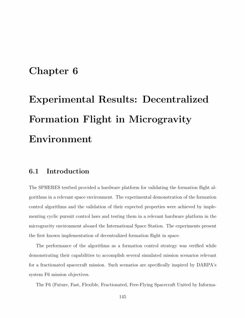
Chapter 6
Experimental Results: Decentralized
Formation Flight in Microgravity
Environment
6.1 Introduction
The SPHERES testbed provided a hardware platform for validating the formation flight al-
gorithms in a relevant space environment. The experimental demonstration of the formation
control algorithms and the validation of their expected properties were achieved by imple-
menting cyclic pursuit control laws and testing them in a relevant hardware platform in the
microgravity environment aboard the International Space Station. The experiments present
the first known implementation of decentralized formation flight in space.
The performance of the algorithms as a formation control strategy was verified while
demonstrating their capabilities to accomplish several simulated mission scenarios relevant
for a fractionated spacecraft mission. Such scenarios are specifically inspired by DARPA’s
system F6 mission objectives.
The F6 (Future, Fast, Flexible, Fractionated, Free-Flying Spacecraft United by Informa-
145

tion Exchange) mission (http://www.darpa.mil/tto/programs/systemf6/index.html) mission
is currently in development. Its objectives include demonstrating the advantages and feasi-
bility of fractionated spacecraft on a near-Earth environment. Among the milestones to be
achieved in order to validate formation flight feasibility are array initialization, satellite ad-
dition maneuvers, collision avoidance and rejection maneuvers. The experiments performed
on SPHERES addressed some of the issues for such mission scenarios using decentralized
cyclic pursuit algorithms, testing the reliability and verifying the important properties of
this approach to formation control.
This chapter is structured as follows: the first section describes the SPHERES testbed
and the implementation of the algorithms, a second section describes the performed tests
and their results, a third section uses experimental data from the different tests to verify
and quantify the performance of the implementations of the algorithm and compare their
performance to other control approaches.
6.1.1 The SPHERES testbed
SPHERES (Synchronized Position Hold Engage Reorient Experimental Satellites) are an
experimental testbed consisting of a set of small vehicles with the basic functions of a satellite.
Three of them are aboard the International Space Station and are operated by the astronauts
in a test volume that allows 6DOF microgravity maneuvering. The operational volume is
approximately a cube of about 1m× 1m× 1m.
There are also three identical vehicles on the ground that can perform 2D maneuvers by
means of frictionless sliding air bearings. This vehicles operate on a flat table and are used
for a first level validation of the algorithms before sending them to the ISS.
The propulsion system of a SPHERES vehicle consists of 12 microthrusters that use
compressed CO2 gas. The microthrusters are controlled by solenoid valves that can achieve
pulses between 10 to 180ms at each control period. Each thrusters delivers 0.11N. The wet
mass of each SPHERE on the ISS is approximately 4.3kg.
146

Figure 6-1: Picture of three SPHERES satellites performing a test on board the ISS. (Foto-credit: NASA - SPHERES)
The metrology system of the SPHERES emulates a global positioning system by calcu-
lating its position and velocity with respect to a fixed frame by measuring the travel time
of synchronized ultrasound signals. Each vehicle has a local estimator that calculates its
global position based on ultrasound and IMU measurements with an accuracy of approxi-
mately 2mm. This metrology system can also be used to calculate the relative range and
bearing, and corresponding rates to a beacon in another vehicle. Such mode of operation
in intended to allow experimentation using pure relative information. In the tests presented
on this thesis however, relative measurements were synthesized from communicated states
as the vector difference of each vehicles global estimate. This simplification is irrelevant to
the verification of the control performance.
A single RF channel is used to communicate the state between/among spacecraft and
the ground. The communication is TDMA based, and allows for a small bandwidth for
transmission within each control period.
Figure 6-1 shows a picture of three SPHERES spacecraft aboard the ISS.
The dynamics of each spacecraft are well approximated by a double integrator. The
147

control commands calculated by the control law are the desired forces which are converted
into open loop pulse times of a set of thrusters to achieve the desired force by a control
allocation (mixing) algorithm.
6.2 Algorithm Implementation
The algorithms were implemented in C, the standard programming language of the testbed
and packed as a library for the SPHERES science utility module.
Three different versions of the control algorithm were implemented and tested on different
experiments performed at different stages of its development.
On a first implementation, a velocity tracking inner loop was used as an approximated
implementation of the single integrator dynamics, in this case the control algorithm was
setup as:
fi = −mγ(kdR(α)(xi+1 − xi)− vi) (6.1)
where m is the mass of the vehicle, xi and vi are position and velocity variables from the local
estimator, xi+1 is a communicated estimated position variable from the estimator in vehicle
i+ 1 and γ and kd are control gains. kd is a time scaling which defines the angular speed of
the formation rotational motion and γ is a regulation gain that dictates the behavior of the
velocity tracking. This controller is basically, the simplistic approach to double integrator
dynamics described by Ren [75].
This implementation requires the agreement on an inertial frame to which v is measured
with respect to, an agreement on a global orientation and does not consider feedforward
terms. It does not require an agreement on an origin of coordinates since it only requires
relative position measurements.
An important consideration for implementation is the discrete nature of the actual system
148

in the selection of the gain γ. In a theoretical sense, for the continuous, unperturbed case,
large values of γ, improve the tracking performance of the velocity regulation, however, in
a discrete, saturation constrained implementation, large gains can easily turn the system
unstable. For the experiments, the gain was selected considering the limitations of the
testbed by selecting it such that the settling time of the velocity tracker is about 1 period.
A second implementation considers a more correct approach to second order systems
by adding a feedforward term which improves the performance. This is specifically, the
approach presented in section 3.32, by setting up the force to:
fi = −m(γkgR(α)(xi+1 − xi) + kgR(vi+1 − vi)− γvi − kcxi) (6.2)
In this case, the gain γ was tuned by considering the rejection of a 2 cm disturbance
over a control period and the value of kg was setup to achieve the desired angular speed for
each specific scenario. Notice that for this implementation too, an agreement on a reference
velocity to which v is measured with respect to and an agreement on a global orientation
are required but not an agreement on the origin of coordinates.
The third version used in the experiments considers the approach in Section 3.42, which
was implemented as:
fi = −m(k1R(α)(dx1 + dx2) + k2R(2α)dv1) (6.3)
where dx1 = xi+2−xi, dx1 = xi+2−xi, dv1 = vi+1−vi are synthesized relative measurements
where xi and vi are from the local estimator, xj, vj are communicated estimated state
variables from the estimator in vehicle j. k1, and k2 were selected to achieve circular or
spiral motion with the desired angular velocity.
As described in the theoretical results, in this implementation, the vehicles do not require
any global positioning information, only an agreement on a global orientation. It is to note
149
that, for real missions, this agreement on the orientation can be achieved through star
trackers, and therefore this approach seems useful for deep space missions.
The tests were designed as a sequence of maneuvers using one of the above described
implementations and will be described in the next section. Every test starts with standard
estimator convergence and initial positioning maneuvers. Each vehicle is programmed with
a role defining a unique identifier and in the description below. The vehicle loaded with role
i will be referred as spacecraft i or SPHi.
Videos of experimental results can be accessed online1.
6.3 Description and Results of the Tests
The experiments present the first known implementation of decentralized formation flight in
space. The main objective of these experiments was to demonstrate the use of the decentral-
ized algorithms as a formation control tool for several mission scenarios. In a first test, the
decentralized properties of the algorithm to achieve a formation and achieve easy addition
of modules were verified. The vehicles performed circular maneuvers, elliptical maneuvers,
and a joining maneuver. In a second set of test we verified the practical implementation of a
controller that uses only relative information to maintain a formation achieving circular and
Archimedean spiral formations. In later tests we use the cyclic pursuit algorithm to achieve
reconfiguration of the maneuver when a failure is detected. In other tests the algorithm was
implemented with a heuristic collision avoidance mechanism that addresses some of the risks
associated with collision while converging to a formation from an arbitrary initial position.
In a last set of experiments presented in this chapter, a simulation of a deployment scenario
is presented where each vehicle joins a circular formation in the order and timing manually
selected by the crew member.
1http://ssl.mit.edu/spheres/video/CyclicPursuit
150

6.3.1 Test 1: Joining maneuver 2-sat to 3-sat formation
The test described in this section was performed during test session 14C, in November 2008.
It was designed as a sequence of maneuvers intended to incrementally build on complexity
following the general guideline protocol for testing on SPHERES. The main idea was to test
the algorithm achieving a circular formation with two vehicles, then add a third one and
then achieve elliptical trajectories. For this test the cyclic pursuit algorithm was implemented
following control law in eq. 6.1.
After initial estimator convergence and positioning the test was designed to achieve the
following maneuver sequence:
1. Two spacecraft perform a rotation maneuver in the x-z plane with a radius r = 0.3m;
2. A change in the desired radius is commanded and the spacecraft spiral out to achieve
a circular formation with r = 0.4m;
3. A third spacecraft joins the formation and the system reconfigures into a three-spacecraft
evenly-spaced circular formation with r = 0.35m;
4. A similarity transformation T is applied to the rotation matrix in a way that the
spacecraft achieve an elliptical formation with eccentricity 0.8.
The initial positioning was x1 = [0,−0.1,−0.2]T , x2 = [0, 0.1, 0.2]T , x3 = [0, 4, 0]T with
zero initial velocity (with respect to the ISS).
6.3.1.1 Test 1 (P237 -T2) results
Data from telemetry shows the formation achieving the defined sequence of maneuvers. In
figure 6-2 the global position and velocity time history is shown. The time history of the
states is depicted for each spacecraft (with respect to the ISS). In fig. 6-3 the trajectories
performed by the spacecraft during the maneuvers 1), 2), 3) and 4) are shown.
151
After a successful initial positioning of the three satellites at 75 seconds, SPH1 and
SPH2 start moving to eventually achieve a circular rotating formation (Fig. 6-3a). In
the next maneuver (Fig. 6-3b), after spiraling out to achieve a larger formation size, the
vehicles asymptotically converge to a constant radius until the next maneuver (Fig. 6-3c) is
initiated. In that next maneuver, satellite 3 joins and a new radius is achieved. A profile
plot is also presented which shows the satellites converge from different x− z planes. In this
maneuver the topology is reconfigured. SPH2 changes its target from SPH1 to SPH3, SPH3
starts following SPH1 and a natural reconfiguration occurs. In a last maneuver (Fig. 6-3d),
a transformation is applied to the control law as described in sec, 3.5.2 and the vehicles
achieve a slightly elliptical formation with eccentricity 0.8.
The experimental results (see in particular Fig. 6-3) present the first demonstration
of the effectiveness of the proposed cyclic-pursuit controllers. It verified the modularity
properties of the algorithm in the sense that each vehicle was running the exact same code,
and the coordination was achieved by defining the interconnection topology. It additionally
experimentally verified the extension to achieving elliptical formations.
6.3.2 Test 2: Convergence to 3-sat formation from arbitrary initial
conditions
This second test, like to the previous one, was performed during test session 14C in November
2008. Again, for this test, the cyclic pursuit algorithm was implemented following control
law in eq. 6.1. The sequence of maneuvers, after initial estimator convergence was defined
as:
1. Three spacecraft achieving a evenly-spaced rotation maneuver in the x-z plane with
radius r = 0.35m;
2. After 75 seconds, a similarity transformation T is applied to the rotation matrix for
the spacecraft to achieve an elliptical formation with eccentricity equal to 0.8.
152

0 50 100 150 200 250 300 350
-1
0
1
Background telemetry states (standard), Sphere logical ID 3
0 50 100 150 200 250 300 350-0.1
-0.05
0
0.05
0.1
VxVyVzMan
0 50 100 150 200 250 300 350-1
-0.5
0
0.5
1
q1q2q3q4Man
0 50 100 150 200 250 300 350
-0.2
-0.1
0
0.1
0.2
Test time, s
wxwywzMan
PxPyPzMan0 50 100 150 200 250 300 350
-1
0
1
Background telemetry states (standard), Sphere logical ID 2
0 50 100 150 200 250 300 350-0.1
-0.05
0
0.05
0.1
0 50 100 150 200 250 300 350-1
-0.5
0
0.5
1
0 50 100 150 200 250 300 350
-0.2
-0.1
0
0.1
0.2
Test time, s
0 50 100 150 200 250 300 350
-1
0
1
Background telemetry states (standard), Sphere logical ID 1
Pos
, m
0 50 100 150 200 250 300 350-0.1
-0.05
0
0.05
0.1
Vel
, m/s
0 50 100 150 200 250 300 350-1
-0.5
0
0.5
1
Atti
tude
0 50 100 150 200 250 300 350
-0.2
-0.1
0
0.1
0.2
Rot
rate
s, ra
d/s
Test time, s
1 2 3 4E P 1 2 3 4E P 1 2 3 4E P
Figure 6-2: Experimental results from Test 1: Position and velocity vs. time. From left toright: satellites 1, 2 and 3. Maneuvers indicated by numbers.
−0.5 0 0.5
−0.4
−0.2
0
0.2
0.4
0.6
x, m
z, m
Sat1
Sat2
Sat3
−0.5 0 0.5
−0.4
−0.2
0
0.2
0.4
0.6
x, m−0.5 0 −0.5
−0.4
−0.2
0
0.2
0.4
0.6
x, m
−0.5 0 0.5
−0.4
−0.2
0
0.2
0.4
0.6
x, m
−0.5
0
0.50 0.2 0.4
−0.4
−0.2
0
0.2
0.4
0.6
y, m
x, m
d)b)a) c)
Figure 6-3: Experimental results from Test 1: x-z plane. Sequence of maneuvers a) Maneuver1 , b) Maneuver 2, c) Maneuver 3 and d) Maneuver 4.
153
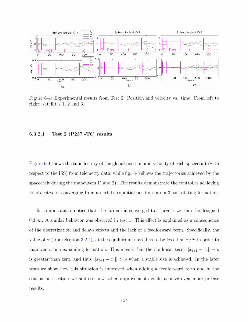
E Pos 1 2 E Pos 1 2 E Pos 1 2
Figure 6-4: Experimental results from Test 2: Position and velocity vs. time. From left toright: satellites 1, 2 and 3.
6.3.2.1 Test 2 (P237 -T6) results
Figure 6-4 shows the time history of the global position and velocity of each spacecraft (with
respect to the ISS) from telemetry data; while fig. 6-5 shows the trajectories achieved by the
spacecraft during the maneuvers 1) and 2). The results demonstrate the controller achieving
its objective of converging from an arbitrary initial position into a 3-sat rotating formation.
It is important to notice that, the formation converged to a larger size than the designed
0.35m. A similar behavior was observed in test 1. This effect is explained as a consequence
of the discretization and delays effects and the lack of a feedforward term. Specifically, the
value of α (from Section 3.2.4), at the equilibrium state has to be less than π/N in order to
maintain a non expanding formation. This means that the nonlinear term ||xi+1 − xi|| − ρ
is greater than zero, and thus ||xi+1 − xi|| > ρ when a stable size is achieved. In the later
tests we show how this situation is improved when adding a feedforward term and in the
conclusions section we address how other improvements could achieve even more precise
results.
154

−0.5 0 0.5
−0.5
0
0.5
x, m
z, m
−0.5
0
0.5
−0.20
0.2
−0.5
0
0.5
y, mx, m
z, m −0.5 0 0.5
−0.5
0
0.5
x, m
z, m
a) b)
Figure 6-5: Experimental results from Test 2: x-z plane. Sequence of maneuvers a) and b).
6.3.3 Test 3: Pure relative formation maintenance
This test validated the decentralized algorithm based on the cyclic pursuit approach that
uses only relative measurements to maintain a formation. This test was performed during
test session 20, in December 2009. In this test, the control approach in eq. 6.3 was used. In
the previous implementations of cyclic pursuit algorithm, the distributed controller relies on
measurements of relative positions but required an agreement on the velocity of the inertial
frame. In this version of the controller, the commands are issued based exclusively on relative
measurements to the neighbors. This characteristic is of important value for deep space
formation flight applications. The algorithm to be used in this test is an implementation of
the cyclic pursuit algorithm for double integrator dynamics with only relative information.
The constants k1, k2 were defined to achieve an angular speed of ω = 2π/120rad/sec. After
the first 45 seconds are for estimator convergence and initial positioning, the sequence of
maneuvers was defined as following:
1. In the first active maneuver the satellites position themselves 60 centimeters from each
other in opposite directions from the center of the test volume and an initial formation
acquisition maneuver using the cyclic pursuit algorithm from previous test sessions
155

achieve a circular formation.
2. After 40 seconds into this maneuver the controller in both satellites switches to the
control law described in eq.6.3 with parameters k1, k2 to achieve an spiraling maneuver
under free drift mode.
3. When reaching a radius of 50cm, the controller switches to maintain a circular forma-
tion including a mode controlling the center of the formation,
4. After 40 seconds the controller mode switches to free drift mode with parameters k1,
k2, α to achieve circular formation (using only relative measurements) and allows the
center of the formation to drift free.
5. Lastly, a stopping maneuver finalizes the test.
6.3.3.1 Test 3 (P282-T3) results
The satellites performed the specified maneuvers, achieving the desired relative motion in
the x-y plane, i.e. relative circular and spiral trajectories. This test successfully validates
a new type of controller inspired by the cyclic pursuit algorithm, which uses only relative
position and velocity information of neighbors to converge to a desired relative motion.
The distributed control laws, shows the desired performance and convergence properties
to achieve an overall desired formation behavior in the x-y plane. A discernible result from
hardware implementation is however, that the relative motion in the z direction showed very
slow convergence to the desired state due to a suspected constant disturbance in the +Z
direction.
The implemented control law shows a slow convergence because of too low gains assigned
for the z-motion control which is the direction perpendicular to the formation maneuvers and
is completely decoupled from the cyclic pursuit control. From eq. 3.42 it can be noticed that
the dynamics in the z-direction are decoupled of the other coordinates. The relative dynamics
156

−1 −0.5 0 0.5 1
−1
−0.8
−0.6
−0.4
−0.2
0
0.2
0.4
0.6
0.8
1
x,m
y,m
E
Pos
1
2
3
4
5
Figure 6-6: Experimental results from Test 3: Sequence of maneuvers indicated by colors.
in such direction reduce to a dynamic consensus which should converge to an agreement in
the z-positions, if the gain is large enough [77]. Therefore, the gains for z-motion, could have
been independently assigned from the gains for x-y motion.
For the purposes of this thesis, the important result is the validation of the performance
in the x-y plane. As mentioned, the x-y motion is decoupled from the z motion, which
is described by consensus dynamics under disturbances, which have been studied in other
contexts and are out of the scope of this thesis.
In Figure 6-6, the relative motion in the x-y directions is shown performing the different
maneuvers. The figure shows the relative state of the satellites as a function of time as well
as the control commands on each vehicle. The underperformance of the controller in the
z-direction is evident when the free drift mode is active. In the maneuvers 1 and 3 in figure
6-7, the center of mass is free and it is noticeable how both vehicles drift in the positive Z
direction.
This experiment was the first experimental validation of the cyclic pursuit approach that
relies only on relative information to control a circular and spiral formation.
157

0 50 100 150 200 250 300
-5
0
5
x 10-3
tes t t im e ,s
Com
man
ded
Forc
e ,N
Sat
1
0 5 0 1 0 0 1 5 0 2 0 0 2 5 0 3 0 0
-5
0
5
x 1 0 - 3
t e s t t im e , s
Com
man
ded
Forc
e ,N
Sat
2
0 50 100 150 200 250 300
-1
0
1
Background telem etry s tates (s tandard), Sphere logical ID 1
Pos
, m
PxPyPzM an
0 50 100 150 200 250 300
-1
0
1
B ac k ground telem etry s tates (s tandard), S phere logic al ID 2
Pos
, m
P xP yP zM an
0 50 100 150 200 250 300-2
-1
0
1
Pos
, m
PxPyPz
2Background telemetry s tate differences (s tandard) for Sphere logical ID 1 and 2
E Pos 1 2 3 4 5
E Pos 1 2 3 4 5
Figure 6-7: Experimental results from Test 3: Position, velocity and control commands vs.time.
158

6.3.4 Test 4: Implementation with a fault detection and recovery
algorithm
The purpose of this test was to verify a cyclic pursuit algorithm as a responsive control
method to achieve reconfiguration maneuvers in a satellite formation in the event of a failure.
This test used a communication failure detection, isolation and recovery (FDIR) algorithm
demonstrated in tests run in previous test sessions developed as part of parallel research on
formation flight at MIT space systems lab.
A feature of the implemented algorithm, is the setup of a logic algorithm that reconfigures
the topology of the formation. Based on this logic, each vehicle decides the vehicle that it
uses as a partner to control its state. In this case it uses knowledge of a global variable which
is updated through communication by the fault detection and identification mechanisms, but
current research aims to identify the formation overall state through local knowledge.
When a vehicle is rejected because a failure was detected, a set of the parameter that
defines the formation and the formation changes automatically reconfigures into a new con-
figuration. In this test, for the purposes of algorithm demonstration, the reconfiguration
consists only on a change to a parallel formation plane. In a more realistic implementation
the idea can be applied to a more general set of parameters that define a reconfiguration to a
formation that optimizes some specific metric, for example, minimizing collision probabilities
with the unresponsive vehicle.
In all the following tests the implemented controller is an improved implementation of
the cyclic pursuit algorithm that includes a feedforward term, specifically 6.2.
The sequence of maneuvers after estimator initialization and initial positioning in this
test was defined as follows:
1. At 55 seconds, a 3-satellite rotating formation in the x-y plane, with center on the
z = 0.2m plane is commanded.
2. At 120 seconds, a failure is simulated in SPH1, by blocking the transmission of data.
159

In response to this, SPH2 and SPH3 should change the formation plane, specifically
to the z = 0m plane.
6.3.4.1 Test 4 (P273-4) results
The results from this test demonstrated a complete fault detection isolation and recovery
mechanism for multi-vehicle formations under a simulated failure and even under an actual
failure. The awareness of the state of the communication link with the other satellites in
each vehicle is monitored by the fault detection module. The plots on the left in Figure 6-8
, show the perception of the transmitters for each one of the satellites. 0 means nominal
operation, 1 means a failure was detected. The black line describes the number of satellites
in the formation for each satellite. The simulated failure in the transmitter of SPH1 (SPH1)
is indicated by the thin line at 120 seconds. 5 seconds later, the detection algorithm on
each vehicle detects that there is a failure seen in the change of the variable defining the
perception of the state of the transmitter (TX1) from 0 to 1.
The detected failure triggers a reconfiguration maneuver in the controller module, which
commands a change in the configuration of the interconnection links and moves the center
of the formation in a way that avoids the failed vehicle. The number of vehicles in the
formation is used by the decentralized algorithm to define the formation parameters. At
about 125 seconds satellite 1 reconfigures.
An actual failure was detected and addressed by the algorithm. At about 160 seconds,
SPH2 reset. SPH1 and SPH3 detected the failure. SPH3 then reconfigures its formation
parameters and changes planes again.
160

0 50 100 150 200
-1
0
1
Background telemetry states (standard), Sphere logical ID 1
Pos
, m
0 50 100 150 2000
0.5
1
1.5
2
2.5
3
Test time, s
Perception of Formation by Sat1
0 50 100 150 2000
0.5
1
1.5
2
2.5
3
Test time, s
Perception of Formation by Sat2
0 50 100 150 2000
0.5
1
1.5
2
2.5
3
Test time, s
Perception of Formation by Sat3
nvTx1Tx2
Tx3
0 50 100 150 200
-0.04
-0.02
0
0.02
0.04
Vel
, m/s
0 50 100 150 200-1
-0.5
0
0.5
1
Atti
tude
0 50 100 150 200
-1
0
1
Background telemetry states (standard), Sphere logical ID 2
0 50 100 150 200-0.1
-0.05
0
0.05
0.1
0 50 100 150 200-1
-0.5
0
0.5
1
0 50 100 150 200
-1
0
1
Background telemetry states (standard), Sphere logical ID 3
PxPyPzMan
0 50 100 150 200-0.1
-0.05
0
0.05
0.1
VxVyVzMan
0 50 100 150 200-1
-0.5
0
0.5
1
q1q2q3q4Man
Figure 6-8: Experimental results from Test 4. Top: perception of the formation by eachsatellite.
161
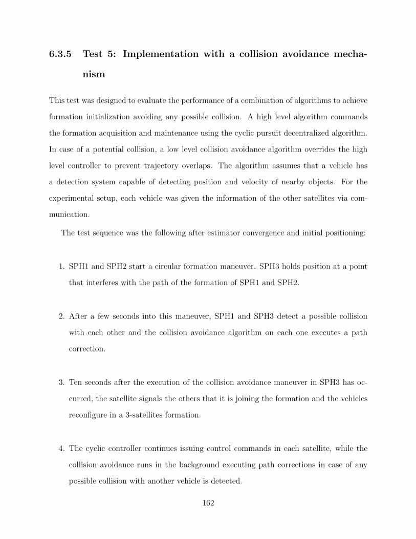
6.3.5 Test 5: Implementation with a collision avoidance mecha-
nism
This test was designed to evaluate the performance of a combination of algorithms to achieve
formation initialization avoiding any possible collision. A high level algorithm commands
the formation acquisition and maintenance using the cyclic pursuit decentralized algorithm.
In case of a potential collision, a low level collision avoidance algorithm overrides the high
level controller to prevent trajectory overlaps. The algorithm assumes that a vehicle has
a detection system capable of detecting position and velocity of nearby objects. For the
experimental setup, each vehicle was given the information of the other satellites via com-
munication.
The test sequence was the following after estimator convergence and initial positioning:
1. SPH1 and SPH2 start a circular formation maneuver. SPH3 holds position at a point
that interferes with the path of the formation of SPH1 and SPH2.
2. After a few seconds into this maneuver, SPH1 and SPH3 detect a possible collision
with each other and the collision avoidance algorithm on each one executes a path
correction.
3. Ten seconds after the execution of the collision avoidance maneuver in SPH3 has oc-
curred, the satellite signals the others that it is joining the formation and the vehicles
reconfigure in a 3-satellites formation.
4. The cyclic controller continues issuing control commands in each satellite, while the
collision avoidance runs in the background executing path corrections in case of any
possible collision with another vehicle is detected.
162

6.3.5.1 Test 5 (P273-3) results
This test was successfully completed and the vehicles performed the expected behavior. An
error in the instructions to the crew in the test procedure files cause an initial misplacement
in the desired position of satellite 1, however, this misplacement did not affect the overall
development of the test.
The plots in Figures 6-9 show the trajectories of the satellites. During the initialization
maneuver, satellite 3 had to move from the negative x position to a positive 0.4m position.
An initial small correction was actually executed by the collision avoidance mechanism during
this positioning stage as noticed in figure. The trajectory initially described by satellite 3 in
the x direction is due to the above mentioned misplacement.
Figure 6-10 show the time history of the states for each vehicle. It can be noticed
how primary (SPH1) and secondary (SPH2) satellites start a circular formation until SPH1
detects the possible collision with the tertiary and activate the collision avoidance path
correction. The trajectory of SPH1 deviates from the circle; SPH3 also tried to move out of
the path. Additionally, the SPH2 was also affected by the path correction since its commands
are coupled to the motion of the other satellites in the formation. Eventually when no more
collision threats are detected the 3-satellite formation continues its path to finally achieve
the formation.
6.3.6 Test 6: Implementation as a random initialization algorithm
This test demonstrates the performance of an algorithm for random formation initialization.
This test builds up on the results of P273 Test 3, by using the same algorithm with an
addition of a module for astronaut input. In this test, the astronaut was able to manually
command, when and which satellite joins the formation.
After the initialization maneuver, the satellites reach initial positions in the boundaries of
the test volume. After the 30 seconds allowed for this positioning, the astronaut was in charge
163

SPH1(0)
SPH2(0)
SPH3(0)
Figure 6-9: Experimental results from Test 5: Trajectories.
of indicating each satellite to join the formation by pressing a key in the laptop. Pressing
the ”A” key commands the SPH1 to join the formation, pressing the ”S” key commands the
SPH2 to join the formation, and pressing the ”D” key commands the third satellite to join
the formation. The astronaut was free to select in which order and when to press the key.
After the three satellites had been commanded to join the formation and the formation is
achieved, the test ends.
6.3.6.1 Test 6 (P273-6) results
This test was partially successful. In general the tests achieved the objective and the perfor-
mance of the control was as expected. However, one of the satellites showed poor performance
on the initial estimator convergence, due to this, its initial positioning was flawed.
The satellites joined the formation as commanded, and achieved the desired configuration
in their estimated states, with the SPH2 having a biased estimation of its state.
Figures 6-12through 6-15 show the corresponding trajectories and the position and atti-
tude states for each satellite. Each one joined the formation from an arbitrary location when
164
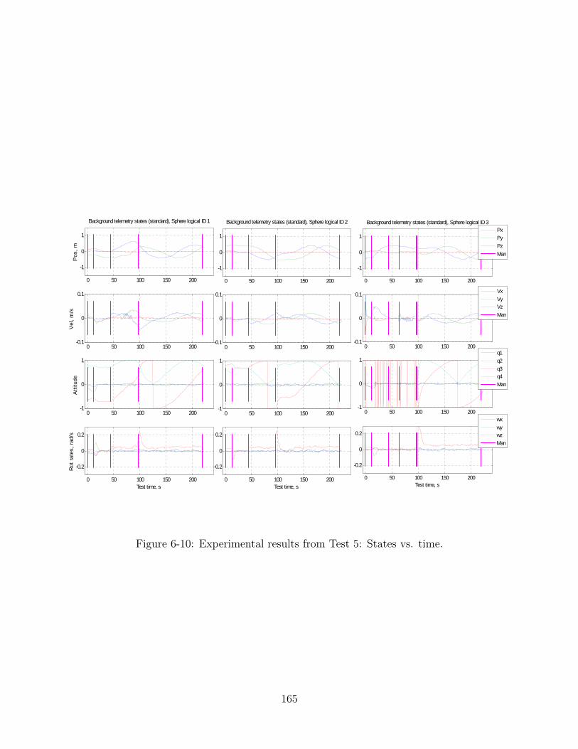
0 50 100 150 200
-1
0
1
Background telemetry states (standard), Sphere logical ID 1
Pos
, m
0 50 100 150 200-0.1
0
0.1
Vel
, m/s
0 50 100 150 200-1
0
1
Atti
tude
0 50 100 150 200
-0.2
0
0.2
Rot
rate
s, ra
d/s
Test time, s
0 50 100 150 200
-1
0
1
Background telemetry states (standard), Sphere logical ID 2
0 50 100 150 200-0.1
0
0.1
0 50 100 150 200-1
0
1
0 50 100 150 200
-0.2
0
0.2
Test time, s
0 50 100 150 200
-1
0
1
Background telemetry states (standard), Sphere logical ID 3
PxPyPzMan
0 50 100 150 200-0.1
0
0.1
VxVyVzMan
0 50 100 150 200-1
0
1
q1q2q3q4Man
0 50 100 150 200
-0.2
0
0.2
Test time, s
wxwywzMan
Figure 6-10: Experimental results from Test 5: States vs. time.
165

50 100 150 200 2500
0.5
1
Background telemetry state differences (standard) for Sphere logical ID 1 and 3
||x
3−
x1||, m
1 → 2 → 3 → 4 → 5 →1 → 2 → 3 → 4 → 5 →
Magnitude
Diameter
50 100 150 200 250−1
0
1
Pos, m
Px
Py
Pz
50 100 150 200 250−0.2
0
0.2
Vel, m
/s
Vx
Vy
Vz
50 100 150 200 250−1
0
1
Attitude
q1
q2
q3
q4
50 100 150 200 250−0.2
0
0.2
Rot ra
tes, ra
d/s
Test time, s
wx
wy
wz
Figure 6-11: Experimental results from Test 5: Relative states SPH1 to SPH3 vs. time.
randomly commanded by the astronaut. The time when each satellite joined is indicated by
the black arrow. Even though the test is not considered completely successful due to the
divergence of the estimator in the SPH2, the actual performance of the algorithm was as
expected.
This test verified the modularity and interchangeability properties of the control ap-
proach, while maintaining reduced complexity as the number of vehicles is increased.
6.4 Performance Analysis
In this section we consider an analysis of the ’steady state’ performance of the formation
control mechanism by considering some metrics that describe the efficiency of the algorithms
in achieving a synchronized rotating formation. The analysis is based on steady state data
extracted from the tests described above and predated tests, performed in early test sessions.
As metrics to analyze the performance of the system we consider the ratio between the
theoretical fuel usage and the actual fuel usage for a given maneuver while also comparing
166
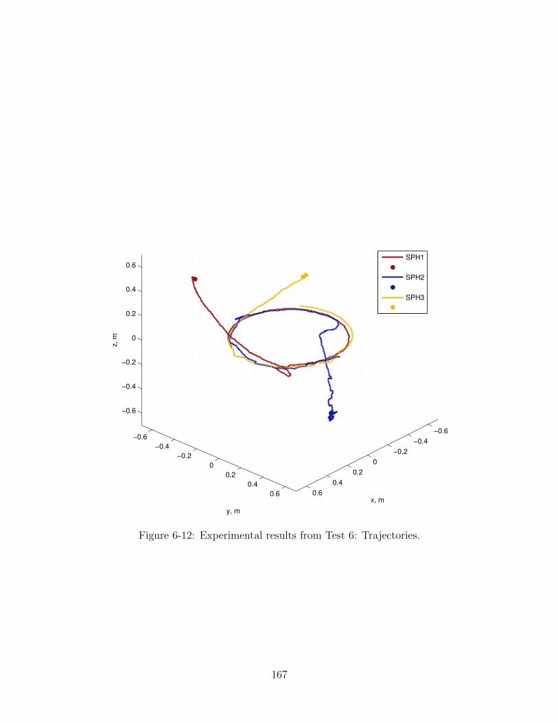
−0.6
−0.4
−0.2
0
0.2
0.4
0.6
−0.6
−0.4
−0.2
0
0.2
0.4
0.6
−0.6
−0.4
−0.2
0
0.2
0.4
0.6
x, m
y, m
z,
m
SPH1
SPH2
SPH3
Figure 6-12: Experimental results from Test 6: Trajectories.
167

0 50 100 150 200
−1
0
1
Background telemetry states (standard), Sphere logical ID 1
Po
s,
m
Px
Py
Pz
Man
0 50 100 150 200−0.1
0
0.1
Ve
l, m
/s
Vx
Vy
Vz
Man
0 50 100 150 200−1
0
1
Att
itu
de
q1
q2
q3
q4
Man
0 50 100 150 200
−0.2
0
0.2
Ro
t ra
tes,
rad
/s
Test time, s
wx
wy
wz
Man
Figure 6-13: Experimental results from Test 6: SPH1 States vs. time.
0 50 100 150 200
−1
0
1
Background telemetry states (standard), Sphere logical ID 2
Pos, m
Px
Py
Pz
Man
0 50 100 150 200−0.1
0
0.1
Vel, m
/s
Vx
Vy
Vz
Man
0 50 100 150 200−1
0
1
Attitude
q1
q2
q3
q4
Man
0 50 100 150 200
−0.2
0
0.2
Rot ra
tes, ra
d/s
Test time, s
wx
wy
wz
Man
Figure 6-14: Experimental results from Test 6: SPH2 States vs. time.
168

0 50 100 150 200
−1
0
1
Background telemetry states (standard), Sphere logical ID 3
Po
s,
m
Px
Py
Pz
Man
0 50 100 150 200−0.1
0
0.1
Ve
l, m
/s
Vx
Vy
Vz
Man
0 50 100 150 200−1
0
1
Att
itu
de
q1
q2
q3
q4
Man
0 50 100 150 200
−0.2
0
0.2
Ro
t ra
tes,
rad
/s
Test time, s
wx
wy
wz
Man
Figure 6-15: Experimental results from Test 6: SPH3 States vs. time.
the error metric to symmetric formation e = Vrnx where, Vrn = L1⊗Rπ/N +L>1 ⊗R>π/N is a
projection into the subspace of regular polygons as presented in Chapter 4. This metric of
error however is only valid for 3 or more satellites. Two satellites will always be in a ’perfect
formation’ under this metric.
The theoretical ∆V is calculated as an integral of the theoretical acceleration magnitude
∆V =∫ tfto||a||2dt.
Table 6.1 compares the fuel performance achieved in different maneuvers in different ISS
test sessions and under different architectures. Figure 6-16 shows the maneuver and the
error performance.
It is important to note that under the error performance as defined by the ’polygon
symmetry’ metric mentioned above is valid only for more than two vehicles. Under this
metric the cyclic pursuit approach shows for all cases error performance better than the
other architectures as shown in fig. 6-16.
169
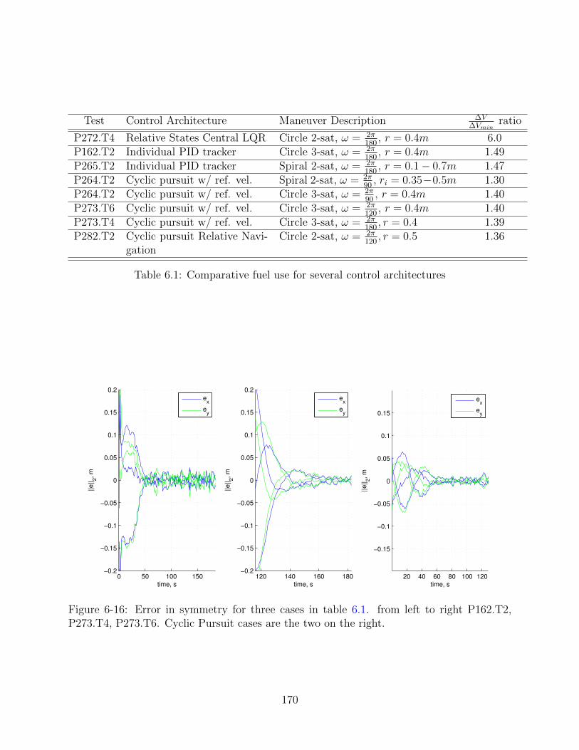
Test Control Architecture Maneuver Description ∆V∆Vmin
ratio
P272.T4 Relative States Central LQR Circle 2-sat, ω = 2π180
, r = 0.4m 6.0P162.T2 Individual PID tracker Circle 3-sat, ω = 2π
180, r = 0.4m 1.49
P265.T2 Individual PID tracker Spiral 2-sat, ω = 2π180
, r = 0.1− 0.7m 1.47P264.T2 Cyclic pursuit w/ ref. vel. Spiral 2-sat, ω = 2π
90, ri = 0.35−0.5m 1.30
P264.T2 Cyclic pursuit w/ ref. vel. Circle 3-sat, ω = 2π90
, r = 0.4m 1.40P273.T6 Cyclic pursuit w/ ref. vel. Circle 3-sat, ω = 2π
120, r = 0.4m 1.40
P273.T4 Cyclic pursuit w/ ref. vel. Circle 3-sat, ω = 2π180, r = 0.4 1.39
P282.T2 Cyclic pursuit Relative Navi-gation
Circle 2-sat, ω = 2π120, r = 0.5 1.36
Table 6.1: Comparative fuel use for several control architectures
0 50 100 150−0.2
−0.15
−0.1
−0.05
0
0.05
0.1
0.15
0.2
time, s
||e||
2, m
ex
ey
120 140 160 180−0.2
−0.15
−0.1
−0.05
0
0.05
0.1
0.15
0.2
time, s
||e||
2, m
ex
ey
20 40 60 80 100 120
−0.15
−0.1
−0.05
0
0.05
0.1
0.15
time, s
||e||
2, m
ex
ey
Figure 6-16: Error in symmetry for three cases in table 6.1. from left to right P162.T2,P273.T4, P273.T6. Cyclic Pursuit cases are the two on the right.
170

The fuel performance presented in table 6.1 shows experimental results agreeing with the
expected improvement on reducing the control effort by using the cyclic pursuit architecture
while maintaining the symmetry of the formation. These results however, should not be
taken as direct verification of this improvement effect since the data used in the comparison
was not specifically designed for achieving the same objective and the variability in the
experiment conditions have not been considered in the analysis. Nevertheless, the results do
show that for the formation flight experiments flown in microgravity environment, the cyclic
pursuit approach has lower fuel use while maintaining similar performance in maintaining a
symmetric formation.
6.5 Summary and Conclusions of the Chapter
This chapter presented experimental results for the first ever implementation of decentralized
formation flight in space. Several experiments were performed on the SPHERES testbed
aboard the International Space Station. Such experiments demonstrate the validity of the
algorithms in achieving geometric pattern formation control in relevant hardware. The
applicability in multiple scenarios demonstrates the versatility and inherent simplicity of
the proposed decentralized approach. Additionally, the analysis of the fuel performance and
error as compared to previously implemented approaches agreed with the expected reduced
control effort in achieving the pattern without specifically tracking trajectory fixed points.
The performance of the algorithms as a formation control strategy was verified while
demonstrating their capabilities to accomplish several simulated mission scenarios relevant
for a fractionated spacecraft mission.
In the joining maneuver test (Test 2), the center of the formation an uncontrolled state.
The invariance of the geometric center of the formation is noticeable in the experimental
results: when the third vehicle joins the two-vehicle formation the center of the formation
moves to include the effect of the initial position of the third vehicle. This effect is of course
171

controllable by using kg > 0 as described in remark at the expense of control effort and
knowledge of the global positioning.
The importance of a nonlinear extension was evident from initial experimental results.
When using only a linear approach, the discretization effects and the time delays caused a
divergent behavior. The effect was compensated by adjusting the pursuit angle applying the
extension as mentioned in Section 3.2.4.
The addition of a feedforward term by upgrading the control approach to eq. 3.32, im-
proved the performance of the controller by achieving a more precise radial control. In the
initial implementation, the equilibrium value of the dynamic angle α was achieved at a radial
distance different from the one specified. In later tests when the feedforward term was imple-
mented, the radius of the formation was much more precise as can be appreciate in figs. 6-3
as compared to 6-8, 6-9. The precision can be further improved by implementing and integral
control approach by including a term: α = π/N−k(||xi+1−xi||−ρ)−k∫
(||xi+1−xi|||−ρ)dt,
dependent on the accumulated error. The theoretical development of this approach is how-
ever, out of the scope of this thesis. Preliminary simulations demonstrate it as a valid
approach but it was not implemented on the tests and is left as a possible venue for future
work.
In the implementation of the only relative measurements controller, based only on theo-
retical results the z-motion gains were setup to 1. Simulations without accounting for noise,
disturbances and constrained actuation showed good convergence performance. However,
under the actual testing conditions on hardware, the underperformance of the control in
the z-direction became evident as seen in the data plots shown below, especially, due to a
constant disturbance in the +Z direction discernible from the debug data.
172

Chapter 7
Decentralized Control in
Electromagnetic Formation Flight
7.1 Introduction
In this chapter, the idea of decentralized control is extended to the case of Electromag-
netic Formation Flight (EMFF) systems. EMFF is a very innovative concept envisioned for
propellantless spacecraft formation. However, these systems have very particular coupled dy-
namics and a straightforward implementation of decentralized control techniques designed
for decoupled systems fails to address their strong actuation coupling.
To achieve the benefits of decentralization in this type of system, an analysis of some
ideas for decentralization of electromagnetic formations is formally presented in this chapter.
A first section introduces the concept of electromagnetic formation flight technology, with
some emphasis on the coupled nature of the actuation commands. Then, the approaches to
decentralization are presented. In summary, several techniques that can achieve control of
a system of EMFF satellites in a decentralized manner are studied by considering two main
different directions. The first one consists on decoupling the dynamics. The second one
addresses the problem by distributing the computation and the need for a central computer.
173
The general approach to the methods presented in this chapter is rather heuristic given
the difficulty of the problem but some specific theoretical results are discussed. The different
proposed ideas are implemented in simulation to compare their performance to a centralized
approach. A more extensive theoretical analysis of each one of them is left out of the scope
of the present work and is suggested as a direction in future work.
7.1.1 Electromagnetic Formation Flight
The Electromagnetic Formation Flight (EMFF) technology has been recently studied and is
currently being developed by the Space Systems Laboratory at MIT in collaboration with
Aurora Flight Science (formerly Payload Systems). Similar approaches have been indepen-
dently proposed by groups at the University of Tokyo and the Boeing company. The principal
advantage of EMFF systems is the independence from expendable propellants. This can be
an extremely important factor for long duration missions, missions that require extensive
reconfiguration maneuvering or missions where the impingement of propellant particles can
affect the system performance.
The principle of operation behind EMFF is the used the coupled electromagnetic forces
and torques to control the relative position of a group of vehicles in space. The mechanism
used to create the electromagnetic forces between vehicles consists of a set of orthogonal
coils that generate magnetic fields when current is run through them.
As opposed to other systems proposed for propellantless formation flight, like flux pinned
[58] or coloumb force formation flight [85], electromagnetic formation flight achieves control of
3N translational degrees of freedom, including shear forces which are not achievable through
other proposed non propellant methods. In EMFF any force and torque command can be
readily achieved by controlling currents running through individual coils on each vehicle.
Different architectures for the coils have been envisioned and studied. In one, the coils
are made out of conventional conductive material. Aluminum has been identified as the most
competitive non-superconductive material for this purpose [82]. In this case pulsed currents
174

used as a mechanism to prevent overheating due to the heating effects of the finite resistance
in this type of materials. Theoretical analysis and experimental results have validated the
principle of operation and the capabilities to achieve net forces which can be large enough
to counteract the effects of J2 differential terms in low Earth multi-satellite systems.
In a second type of architecture, High-Temperature Superconducting (HTS) material can
be used to build the coils. In this case, YBCO or BSSCO composites can be cooled down
below a critical temperature, achieving superconducting behavior. In this case, constant
currents of higher intensity can be run through the coils, generating much larger effective
forces between vehicles.
7.1.1.1 Dynamics of EMFF systems
In this section, we discuss the relevant dynamics of an EMFF system, developed in previous
literature. [3, 87]
In a vehicle i, a current Iix is generated and controlled though an internal computer to
run through the coils. In a circular coil aligned with the body x-axis in vehicle i generates
a magnetic field which can be approximated, as the field generated by a magnetic dipole
µix = nIixA.
When running independent currents through each one of the orthogonal coils in one
satellite, a composed dipole µi = µixx + µiyy + µiz z corresponding to the vectorial sum of
the orthogonal dipoles in satellite i is generated and can be steered in any direction in the i
body-frame. This allows each satellite to independently command its dipole in any direction
and under an agreement on a global coordinate frame, the overall formation can be seen as a
group of interacting dipoles that can be pointed on any direction. Then, the magnetic field
generated by agent i is:
Bi(rij) =−µ0
4π
(3µj · rijr5ij
rij −µjr3ij
)(7.1)
175

The interaction between the fields of the dipoles generate forces between them. The
resultant force of the interaction of two dipoles µi, µj is given by:
Fi =n∑j 6=i
Fij (7.2)
Fij =−3µo
4π
(µi · µj|dij|5
dij +µi · dij|dij|5
µj +µj · dij|dij|5
µi − 5(µi · dij)(µj · dij)
|dij|7
)dij (7.3)
and, the overall force of a formation of vehicles i ∈ {1, ..N}, is given by:
Fi =n∑j 6=i
Fij (7.4)
where Fi is the force on vehicle i, Fij is the force on vehicle i due to vehicle j, µ0 is the
magnetic permeability constant of vacuum and rij is the vector position between vehicle i
and vehicle j.
These set of equation are called the dipole equations. The control commands are the
currents run through each one of the coils on each vehicle which directly translate into
dipole magnetic fields affecting the forces of the overall formation.
The special coupling in a system of EMFF vehicles is evident from this equation: Indi-
vidual control command alters the forces on each other vehicle in the formation, therefore a
straightforward extrapolation of distributed control mechanisms proposed for other type of
propulsion, specifically non-coupled actuation, is not feasible.
Achieving a commanded force requires coordination with at least one other vehicle, since
the force directly depends on the vectorial value of another dipole. Additionally, the dipole
enters into the force equation as a multiplicative parameter, which means that local con-
straints in its magnitude do not guarantee global constraints in its disturbance effect on the
other vehicles in the formation. These coupling effects pose an important challenge to the
decentralization of EMFF.
176
For the closed loop control approaches in the existing literature, the overall formation
state information is gathered in a central computer, the set of dipole equations are solved
every control period and the current commands issued to each one of the vehicles in the
formation.
In this chapter of the thesis we discuss and compare different approaches to achieve the
objective of achieving control of an electromagnetic formation without the need of using a
central computer that solves the set of equations every control period.
7.2 Token Based Decoupled Maneuvering
In this section we study a solution to the EMFF decentralization problem by decoupling the
actuation through time allocation.
A token based mechanisms is used as the time allocation mechanism. The approach
considers the solution to a constrained optimization problem such that only one subset of
the vehicles actuate at a time. It is a token based approach, because only vehicles owning a
’token’ can actuate at a given time. The token sequence is calculated as part of an overall
optimization problem.
In the general trajectory optimization problem, a centralized solution can be obtained,
without restricting the number of vehicles that can actuate at a time. Open loop tracking of
the input time history should achieve the final configuration. It is however known that any
small disturbance, and especially in a nonlinear system like EMFF, will cause divergence from
the desired final state. Therefore, the best approach is a close loop tracking of the optimal
state time history. If however, the solution of the optimization problem is obtained under
the constraint that only a subset of vehicles can actuate at a time, a natural decentralization
of the trajectory tracking problem occurs. Tracking the trajectories would not require an
agreement of the overall set of vehicles but only a subset of them, reducing the complexity
of the tracking problem.
177

Such trajectory optimization problem is special in the sense that it has specific constraints
on the number of vehicles that can be used at a given time and needs to be approached in a
special manner. This problem can be solved considering a two-level structured optimization
problem.
In a lower level problem a set-wise subproblem is to be solved, considering the optimal
dipole selection for achieving an optimal reconfiguration maneuver using only a subset of
vehicles. In the higher level problem, the sequence of vehicles participating at each allocated
time slot is considered.
The approach to solve the lower level trajectory optimization problem was implemented
by using a pseudo-spectral method approach, where the states and controls are mapped
into a parameter discretization based on Legendre polynomials. Optimal reconfiguration
maneuvers using this approach, have been studied in the past for formations with several
vehicles [3] for deep space dynamics. In this thesis, these results are extended by solv-
ing for optimal reconfiguration maneuvers considering more complex dynamic situations, in
particular, Clohessy-Wiltshire dynamics.
A solution algorithm for the higher level problem was implemented using a Dynamic
Programming (DP) approach, solving for the sequence that achieves minimum cost.
The overall reconfiguration problem, considers a set of N vehicles on initial positions x =
x(t0) = [x1(t0),x2(t0), ...,xN(t0)] which we are interested in reconfiguring to final positions
xf = x(tf ) while minimizing some cost (time, angular momentum, current intensity or a
combination of them). A general case with dynamics x = f(x) + ui is assumed.
In a token based time divided decentralized approach like the one proposed in this section,
the vehicles reach the final positions by moving in a sequence Sopt = {S1, S2, . . . , SN−a},
where S1 is the set of active vehicles during time interval [ti, ti+1).
The total time is assumed to be tf − t0 =∑∀i ti, and at each interval only a vehicles can
be active, (card(Si) = a), and at least a− 1 vehicles reach xi(ti+1), such that xi(tf ) = xif .
The description of the two subproblems is specified in the sections below.
178

7.2.1 Lower level problem solution
The lower level problem consist of finding the optimal reconfiguration maneuver for vehicles
i ∈ S[k], where S[k] is the set of vehicles active at interval k.
The approach presented in the solutions in this sections uses the Legendre pseudospectral
decomposition approach developed in [3]. In this method the control and the state variables
are discretized and an optimization problem tries to find the values at the specific dis-
cretization points such that the solution minimizes the desired cost function. Extending this
approach we consider a method to achieve solutions for maneuvers under Clohessy-Wiltshire
dynamics.
The reconfiguration maneuver, bringing a set of vehicles with initial conditions x0, to a
formation with final condition xf can be written as the continuous optimization problem [3]:
g(x) = minµ(t)
J(t,x,µ) (7.5)
subject to :
x = f(x,µ) (Dynamics)
x0 = x(t0) (Initial state)
xf = x(tf ) (Final State)
|µi| < µmax (Actuation saturation)
inf dij(t) > Dmin (Collision avoidance)
|hRWi(t)| < Hmax (angular momentum constraint)
where x = [pv], p being the position and v being the velocity defining the state of
the overall formation, µ(t) is the control variable and J(t,x,µ) is a cost function to be
minimized.
When using the pseudospectral method, the unknown state and control trajectories are
179

parametrized by coefficient of Legendre polynomials:
p =
Nd∑i=0
p(ti)φi(t) (7.6)
u =
Nd∑i=0
u(ti)φi(t) (7.7)
where φi(t) are degree interpolating basis for the Legendre polynomials. The optimization
problem is then, mapped into a Nonlinear Programming Problem as a function of the coef-
ficients P ∈ RN×Nd+1, U ∈ RM×Nd+1 and tf :
g = minP,U,tf
J(t,p,v,µ) (7.8)
subject to :
D2P−(τf − τ0
2
)F = 0 (Dynamics)
ψ0(p0,v0, τ0) = 0 (Initial state)
ψf (pNd ,vNd , τf ) = 0 (Final state)
c0(p0,v0,uk, tk) ≤ 0 ∀k ∈ {0, 1, ..., Nd} (Linear constraints
(e.g. collision avoid., saturation ))(τf − τ0
2
)WQ− Z ≤ 0 (Integral constraints (e.g. angular momentum))
where D ∈ RNd×Nd is a differentiation matrix, P ∈ (Nd + 1)× n is a matrix with columns
pi, that is, each column of P represents the position coefficients at each discretization point.
F ∈ RNd+1×n approximates the dynamic vector field in the space of Ndth order polynomials,
W ∈ RNd×(Nd+1) is an integration matrix, Q ∈ R(Nd+1)×1 approximates the constraint inte-
grands, and Z ∈ RNd×1 is a given matrix of the constraint value at each discretization point.
A more detailed description of this definitions is found in [3].
180

7.2.1.1 Results of the low level optimization problem
The results presented in here use this approach to solve for the optimal reconfiguration
maneuvers for relevant dynamic cases. The solution of the problem was implemented using
a Sequential Quadratic Algorithm (SQP) in MATLAB R© using the SNOPT 6.0 package
routines.
Figure 7-1 shows a surface plot of the the optimal cost for a 2-sat reconfiguration ma-
neuver under Clohessy-Wiltshire dynamics and some examples of the solutions obtained.
In this example the initial relative location of the second satellite is (1, 0)km and the
maneuver time is fixed to half an orbital period. The surface plot is a function of the desired
final position. The boundary conditions are such that the initial and final state of both
vehicles are closed natural orbits (ellipses with the appropriate angular period).
7.2.2 Higher level problem solution
The higher level subproblem consists on defining an ordered sequence {S}k = {S[1], S[2], ..., S[N ]}
of agent subsets such that the overall cost function J is minimized.
The overall cost of achieving the reconfiguration maneuver is the addition of the cost
for each individual reconfiguration maneuver. Then, the overall problem can be written as
finding JS∗ such that:
JS∗ = minS∈S
JS(x[0])
JS(x[0]) = E
{gn(xn) +
n−1∑k=0
gk(x[k], S[k], w[k])
}
where n = N − p is the number of reconfiguration maneuver to achieve the final desired
state, S[k] = {s, s} is the set used at interval [k], s is one of the agents and s is the rest of
the agents in a subset S, and gk is cost of achieving a subset-wise reconfiguration maneuver,
with initial state x such that agent s, achieves its desired final state at the final time.
181

-1 -0.5 0 0.5 1-1
-0.5
0
0.5
1
x
y
Jmin =250.6775, ω=3.1416
sat1sat2
-4 -2 0 2 4-3
-2
-1
0
1
2
3
x
y
Jmin =2854.982, ω=3.1416
sat1sat2
-2 -1 0 1 2-2
-1
0
1
2
x
y
Jmin =74.7167, ω=3.1416
sat1sat2
x(tf)
y(t f)
-2 -1.5 -1 -0.5 0 0.5 1 1.5 2-2
-1.5
-1
-0.5
0
0.5
1
1.5
2
X(0) = (1,0)
Figure 7-1: Optimal minimum current two-vehicle maneuvers in Clohessy-Wiltshire dynam-ics
182

A Dynamic Programming (DP) approach to the problem can be used by defining the
optimization problem with the variables as described in table 7.1:
State variable x[k] = [x1[k],x2[k], ...xN [k]] x[k] is the state of the vehiclesat time interval [k]
Control variable u[k] = Sk ∈ Uk, Uk(xk) = {s, s}, Sk is the ordered pair active, al-lowed to maneuver during inter-val [k], s ∈ {1, 2, .., N}
Dynamics x[k + 1] = f(x[k],u[k],w[k]) x evolves given u[k] and a ran-dom disturbance w[k]
Cost function J [k] = g(Sk,x[k]) , s.t.xs[T ] = xfs
Table 7.1: Variable descriptions for the higher level DP optimization problem
Then, the DP approach consists on solving the problem:
J [k] = minu[k]∈Uk
E {gk(x[k],u[k], w[k]) + Jk+1(f(x[k],u[k], w[k]))} (7.9)
JN(xN) = gN(xN) (7.10)
Fig.7-2 shows the a reconfiguration maneuver where only 2 vehicles are allowed to move
at a given time. The reconfiguration sequence can be compared to a centralized approach
where all vehicles can actuate at the same time in Fig. 7-3. The dashed lines show the
interconnection at a given time.
Nspc card(S) Optimal Sequence CostAmps/γ Cost Increase
5 2{ (
4, 5) (
2, 3) (
3, 5) (
5, 1) }
2.984× 10⁷ 18%5 3
{ (4, 5, 1
) (2, 3, 1
) }2.958× 10⁷ 17%
5 4{ (
2, 4, 5, 1) (
1, 3, 0, 0) }
2.658× 10⁷ 5%5 5
{ (1, 2, 3, 4, 5
) (2, 3, 1
) }2.524× 10⁷ -
Table 7.2: Increase in RMS current in coils as the number of vehicles that can be moved ata time changes
183

−20 −15 −10 −5 0 5 10 15 20−20
−15
−10
−5
0
5
10
15
20
x, km
y, km
−20 −15 −10 −5 0 5 10 15 20−20
−15
−10
−5
0
5
10
15
20
x, km
y, km
−20 −15 −10 −5 0 5 10 15 20−20
−15
−10
−5
0
5
10
15
20
x, km
y, km
−20 −15 −10 −5 0 5 10 15 20−20
−15
−10
−5
0
5
10
15
20
Figure 7-2: Optimal reconfiguration maneuver - Clohessy-Wiltshire dynamics only twovehicles actuate at the same time.
Nspc card(S) Optimal Sequence Maneuver times Total Time
5 3{ (
1, 3, 2) (
4, 5, 2) }
41.8, 61.8 103.65 4
{ (2, 3, 5, 1
) (1, 4, 0, 0
) }34.1, 41.2 75.3
5 5{ (
1, 2, , 3, 4, 5) }
37 37
Table 7.3: Minimum maneuver time as the number of vehicles that can be moved at a timechanges
184

−20 −15 −10 −5 0 5 10 15 20−20
−15
−10
−5
0
5
10
15
20
x, km
y,
km
Figure 7-3: Optimal reconfiguration maneuver - Clohessy-Wiltshire dynamics only twovehicles actuate at the same time.
7.3 Decoupled Regulation by Resource Allocation
In this section we consider a method for decentralizing EMFF, based on the ’allocation’
of the magnetic interaction. This allocation is performed in an analogous manner to a
communication channel allocation. By allocating the interaction, the approach guarantees
that the dynamics are coupled only among the set of vehicles that can coordinate their
dipoles through local information sharing. Two possibilities are considered, a time based
division and a frequency based division.
7.3.1 Schedule based regulator
A method to achieve time division consists in using a synchronization mechanism, based on
synchronized clocks on each vehicle or by an external signal. Additionally, the spacecraft
will require an external agreement or an intervehicle consensus mechanism to define the
time schedule for each set of vehicles. The definition of this higher level time agreement
mechanisms is not in the scope of this work. If the vehicles have access to a global signal
185

like the GPS signal, they will have a synchronization resource available.
The scheduling mechanism has to take into account the interconnection topology. A set of
neighbors that are active have to be able to communicate during the actuation period. Once
each vehicle has knowledge of the time schedule when it can actuate and the neighbors it is
actuating with, the solution of the dipole equation needs to be found for those active vehicles.
A reduced order set of dipole equations is to be solved for the members of the subset, in a
distributed manner as discussed in a later section or by one of them and communicated to
the rest of group.
Several results in the literature have addressed the effects of time varying topologies and
can be used to address the stability of the mechanisms presented in this section [72, 79] for
simple dynamic cases which could be extended to more complex dynamics. Specifically, the
result for theory of consensus regarding convergence under switching information exchange
topologies. Necessary conditions for convergence for consensus based control laws are pre-
sented in [79]. A main result is that the interconnection topology has to be connected over
some time interval. Its extrapolation to more general dynamics is still a topic of research
and some results for connected topologies have been described in more recent work [72].
In general, for fast enough switching rates, the results can be shown to approximate the
constant interconnection case with a disturbance that depends on the length of the time
intervals. It is important however, to consider in the design of the control protocol the
fact that EMFF forces only produce internal forces, and thus, when applying the desired
forces to only a subset of the full formation it is not guaranteed that the sum of the desired
forces of the subset is zero. This situation is addressed in the protocol presented in the next
section and a further theoretical analysis of the effects of the switching period is discussed
in a section below.
186
7.3.1.1 Results
In this section we introduce a switching protocol to decouple the dynamics of the electro-
magnetic formation through time division. Simulations show the protocol implementability
and performance. As mentioned in the introduction to the approach, the idea is based on
periodic switching topologies, in a way that over a full cycle, every vehicle has been ac-
tive at least for one period. Without loss of generality, in examples below, we explore the
performance of an approach based on cyclic sequencing.
The cyclic sequencing can be described as follows: For a formation with vehicles i ∈
N = {1, 2, ..., N}, the active set of vehicles at time interval tk, S(tk) = {s1, s2, ..., sNs},
sn ∈ N, sn = mod(sn, N) is such that S(tk+1) = S(tk) + no, where no < card(S) = Ns is an
offset such that at each switching time S(tk) ∩ S(tk + 1) 6= ∅.
A control period is the time interval tc for which the force command is constant. A
switching period tk = ndtc is the time interval between subset switching. A switching cycle,
is a time interval over which the topology switching repeats itself, specifically, if the switching
cycle is a uniform cyclic protocol Ts = Ntk.
Since at each switching period, the sum of the commanded forces for the subset of vehicles
is not necessarily zero, at least one of the vehicles in the set will not be able to actuate the
commanded force. The key development on the protocol presented in this section consists
of considering one of the vehicles in the subset as a leader. The dipole configuration of the
subset will be setup such that each vehicle in the group other than the leader will set up its
commanded forces as per control law and the leader will have a known residual force which
will be taken into account as the subset changes and the leader changes. If sum of forces over
the whole formation maintains the constraint that the sum of all forces is zero, the residual
force over a cycle through the graph should approximately cancel out.
The following synchronous control protocol with homogeneous switching intervals is pro-
posed and implemented in simulation for different control laws:
187

Sequential Subsetwise Control Algorithm
1. Vehicles in set S(tk) = {s1, s2, ..., sNs} share measurement informa-tion and calculate best estimate of current relative states.
2. Desired force for each vehicle in the set is calculated as per controllaw adding any residual force Fs from previous control periods.
3. The set solves for the dipole configuration, either in a locally central-ized way or in a distributed way as described in Section 7.4. Leaderof the set, vehicle s1, sets its force to:
Fr = −∑
i∈S(tk)/s1
Fi
such that ∑i∈S(tk)
Fi = 0
and stores Fr as its residual force. All other vehicles in the set havezero residual force.
4. If t ≥ tk+1 a new set of vehicles S(tk+1) is activated.5. goto 1.
7.3.2 Frequency division
In a frequency divided resource allocation strategy, subsets of vehicles can act simultaneously
applying currents shaped by orthogonal functions on each different subset. The forces due
to magnetic fields from different subsets average to zero over a control period, thus effec-
tively decoupling the actuation between different subsets. This approach is inspired by the
approach presented by the work of Kaneda et al. [34], where the electromagnetic formation
was decoupled from constant perturbations.
Consider for example the case of sinusoidal functions. The imparted ∆v on each vehicle
over a period of time is:
∆v2π = (1/m)
∫ 2π
0
|µi||µj|~q(t)dt
where ~q(t) is a vector that depends on the position of the vehicles and the direction of the
188
dipoles.
If the dipole magnitudes on the vehicles are setup to be sinusoidal functions µi =
µio sin(ωit), with high enough frequency ωi so that ~q can be considered constant, consider
vehicle i, interacting at the same time with vehicles j and k, ωj = ωi, ωk = nωi, n > 1, n ∈ Z:
∆v2π = (1/m)|µio||µjo| ~qij∫ 2π
0
sin(ωit)sin(ωjt)dt+ |µio||µko| ~qik∫ 2π
0
sin(ωit)sin(ωkt)dt
= |µio||µjo| ~qij/2m+ 0, for n 6= 1
Then, vehicle i and j actuate independently of the actuation of vehicle k with any other
vehicles in the formation.
In general, consider the formation of vehicles i ∈ N = {1, 2, . . . , N}, consisting of subsets
of vehicles Si, shaping their control inputs over a period tk by multiplication by a function
φi(t) such that µi(t) = µioφi(t− tk − T ), for t ∈ [tk, tk + 2T ).
Make each φi, a function of a set of shaping functions {φi(t), φj(t), . . . , φNf (t)} orthogonal
over the interval [−T, T ], such that:
∫ T
−Tφiφjdt = δij (7.11)
Then, the impulse during a control period between a pair of vehicles with dipole µi = µioφi,
and µj = µjoφj, under the assumption that the control period is small enough such that ~q
can be considered constant, will be given by:
∆vtk = (1/m)
∫ tk+2T
tk
|µio||µjo| ~qijφiφjdt
= (1/m)|µio||µjo| ~qijδij
Then, vehicles sharing the same shaping frequency φi will interact between them, but
not vehicles with shaping functions φj. Then, the size of the dipole equation reduces to the
size of the subset Si with dipole shaping φi, and the interactions with other vehicles can be
189

disregarded.
Interconnections between different subsets is achieved by ’shared’ members, which coor-
dinate their dipole configuration with different subsets and apply a superposition of dipoles,
i.e the vectorial sum of its dipole corresponding for each subset. Corresponding orthogonal
sets will cancel out and the ’shared’ vehicle will create forces between different subsets.
As mentioned before, any set of orthogonal functions over a bounded set can be used as
shaping functions. For example, Legendre polynomials are orthogonal over the set [−1, 1]
and any set of polynomials can be used to shape the currents over a period. An advantage
of using a polynomial function is the lower frequency content of the first nth base functions,
however, the lack of periodicity implies that the final value of the current at one period does
not match the initial value of the current (and slope) at the end of that period. There are
however, orthogonal sets of functions that could be more fitted for an specific situation.
If the limitation of the system is given by the maximum current that can be achieved on
a coil (equivalently a maximum dipole magnitude), other type of orthogonal functions can
improve the performance. Consider the Walsh functions:
µi(t) = |µi(t)|nisgn(sin(ωit))
µj(t) = |µj(t)|njsgn(sin(ωjt))
∆v = (1/m)|µio||µjo| ~qij∫ 2π
0
sgn(sin(ωit))sgn(sin(ωjt))dt
=
(1/m)|µio||µjo| ~qij if ωj = ωi
0 if ωj = 2nωi, n ∈ Z
The plots in 7-4 show the basic principle behind the proposed approach.
190

Figure 7-4: . Basic results showing the principle of operation of the implementation ofdecentralization by resource division
191

7.3.3 Resource allocation: Simulation results
Two benchmark case scenarios are considered to illustrate the performance using this ap-
proach. In one, a formation of vehicles achieving a rotating circular formation, where we
study the performance as the a steady state response for a nonzero required output force,
and two, a transient scenario where we study the convergence to formation from the same
arbitrary initial perturbed state.
The simulations in a preliminary way the viability of this methods. In the case in fig.
7-5, the formation achieves a regular polygon from a random disturbed position and the
control currents are shown for each case. The input magnitudes are shown as d2/r2I, which
indicate the required currents to achieve the equivalent (far-field) forces normalized for a 1
meter formation with coils 1 meter in radius. Therefore, the currents in the results scale
with the term r2/d2 where d is the radius of the coil and r is the distance between vehicles.
As it is to expect, as the number of active vehicles decreases the coil currents required to
achieve the forces are larger. The coils are thus, saturated for a longer time. An appropriate
selection of the control gains can assure in any case preventing saturation while making the
most of the maximum currents of the system. The simulations are meant to show how the
approach is valid despite the reduction in control authority.
In a second case we compare the currents, required to maintain a rotating formation
under double integrator dynamics using the cyclic pursuit approach, as a way to integrate
the results in previous chapter to the current approach. The results are shown in fig 7-6
On the other hand we illustrate the approach using the frequency division based approach
in the results presented in figures 7-7, 7-8. The results illustrate how, the control objective
can be achieved, at the expense of larger required currents. Since larger currents are required
to achieve the same forces, the control authority of the actuation system is reduced.
192

0 50 100 1500
0.1
0.2
0.3
0.4
0.5
0.6
0.7
8 vehicle formation − Settling performance
time, s
||e||
22, km
2
Ns = 3
Ns = 2
Ns = 8
0 50 100 150−10
0
10
Input vs t
d2
r2I x,Amp
0 50 100 150−10
0
10
d2
r2I y,Amp
0 50 100 150−10
0
10
d2
r2I z,Amp
t, s
Ns = 2
Ns = 3
Ns = 8
0 50 100 150−10
0
10
Input vs td2
r2I x,Amp
0 50 100 150−10
0
10
d2
r2I y,Amp
0 50 100 150−10
0
10
d2
r2I z,Amp
t, s
Ns = 2
Ns = 3
Ns = 8
0 50 100 150−10
0
10
Input vs t
d2
r2I x,Amp
0 50 100 150−10
0
10
d2
r2I y,Amp
0 50 100 150−10
0
10
d2
r2I z,Amp
t, s
Ns = 2
Ns = 3
Ns = 8
Figure 7-5: Time Division allocation - Disturbance rejection transient
193

0 50 100 150−2
−1
0
1
2
Input vs t
d2
r2I x,Amp
0 50 100 150−2
−1
0
1
2
d2
r2I y,Amp
0 50 100 150−2
−1
0
1
2
d2
r2I z,Amp
t, s
Ns = 2
Ns = 4
Ns = 8
−1
−0.5
0
0.5
−1
−0.5
0
0.5
1
−0.050
0.05
x,km
Position w.r.t center
y,km
z,k
m
Figure 7-6: Currents in coils Time Division for different number of vehicles actuating at atime - Bottom: Steady State Cyclic Pursuit (2 active vehicles)
194
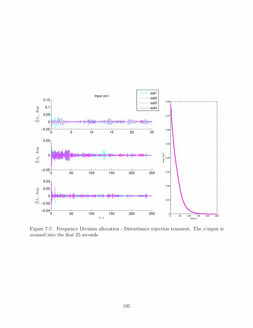
0 5 10 15 20 25−0.05
0
0.05
0.1
0.15
Input vs t
d2
r2I x,Amp
0 50 100 150 200 250−0.05
0
0.05
d2
r2I y,Amp
0 50 100 150 200 250−0.04
−0.02
0
0.02
0.04
d2
r2I z,Amp
t, s
sat1
sat2
sat3
sat4
0 50 100 150 200 2500
0.01
0.02
0.03
0.04
0.05
0.06
0.07
0.08
time, s
err
or,
km
2
Figure 7-7: Frequency Division allocation - Disturbance rejection transient. The x-input iszoomed into the first 25 seconds
195

0 5 10 15 20 25−0.02
−0.01
0
0.01
0.02
Input vs t
d2
r2I x,Amp
0 200 400 600 800 1000−0.04
−0.02
0
0.02
d2
r2I y,Amp
0 200 400 600 800 1000−0.02
−0.01
0
0.01
0.02
d2
r2I z,Amp
t, s
sat1
sat2
sat3
sat4
Figure 7-8: Frequency Division allocation - Steady State Cyclic Pursuit. The x-input iszoomed into the first 25 seconds
196

7.4 Distributed Computation of the Solution to the
Dipole Equation
In this section we explore a different method to achieve decentralization of EMFF systems
which addresses the objective by solving the dipole equation (eq. 7.2) in a distributed
manner. In this sense, the method achieves the objective of defining the control commands
µ, i.e. the dipoles on each vehicle, without recurring to a centralized computing unit and
subsequent communication load to issue the commands to each vehicle in the formation as
proposed in previous approaches [3].
In the proposed technique, the solution is obtained by sharing relative position knowledge
and the solution of a local optimization problem. A first approach to applying this technique
does not necessarily imply the desired characteristics of decentralization at its best, since it
would still require an interconnected network to share states and local optimization solution
results. However, other important characteristics of a decentralized system are achieved like
deployment independence, robustness to individual failures, homogeneity and repeatability,
and more importantly it does not require a powerful central unit solving the nonlinear dipole
equation at each control step.
7.4.1 Theoretical description
The approach to a distributed solution, considers a distributed protocol for solving a global
optimization objective that minimizes the overall formation error while locally solving an
optimization problem. Consider the dipole equation 7.2 that defines the control commands
to achieve the commanded forces:
197

Fi =n∑j 6=i
Fij
Fij =−3µo
4π
(µi · µj|dij|5
dij +µi · dij|dij|5
µj +µj · dij|dij|5
µi − 5(µi · dij)(µj · dij)
|dij|7i
)dij
The electromagnetic force for a pair of vehicles i, j is a bilinear equation on the inputs
µi, µj which can be written as:
Fij = − 1
|dij|5
[dij · µTj + µj · dTij + (I − 5
dij · dTijdTij · dij
)
]µi (7.12)
and then, the overall system of equations can be written as:
F1
F2
...
Fn
=
M1(µi)
M2(µi)
...
Mn(µi)
µi +
V1(µi)
V2(µi)
...
Vn(µi)
where:
Mi =∑j 6=i
1
|dij|5
[dij · µTj + µj · dTij + (I + 5
dij · dTijdTij · dij
)
]
Mi =1
|dij|5
[dij · µTj + µj · dTij + (I + 5
dij · dTijdTij · dij
)
]
Vi =∑k 6=i,j
1
|dij|5
[dij · µTj + dij · µTj + (I + 5
dij · dTijdTij · dij
)
]· µk
Vi = 0
where i = {1, .., N}/i is the set of vehicles in the formation except i, and µi, the set of
corresponding dipoles.
198

For a given set µi, the dipole equation can be written as:
F = M(µi,x)µi + V(µi,x) (7.13)
where the term M(µi,x)µi describe the forces caused on each vehicle by dipole i, and V(µi,x)
the forces caused on each vehicle by vehicles other that i.
The proposed protocol makes use of this structure and considers solving the problem
through a sequence of steps in which each vehicle minimizes a cost function by sharing the
result of solving the local problem:
µ∗i = arg minµi
||Fd(x)− F||22 (7.14)
s.t. M(µi,x)µi = (F−V(µi,x)) (7.15)
h(µi) < 0 (7.16)
where F(x) is the control command known by each vehicle. Notice that to solve this problem,
agent i requires x, the state information of the formation (more specifically, only the relative
states) and µi, the value of the dipole solution for the other vehicles in the formation. By
an iterative process, where µ∗i is shared through a connected network, the convergence to a
stationary solution is guaranteed if h(µi) define a convex subspace. The analysis is presented
in the next section.
7.4.2 Convergence analysis
Consider the following synchronous protocol following a periodic sequence {1, 2, .., N, 1, 2, ..}:
The analysis of the convergence properties of this protocol are based on the fact that the
overall algorithm can be casted as a gradient method with gradient related descent direction.
Notice that the agent do not update their dipole values until the error in the actuated force
199
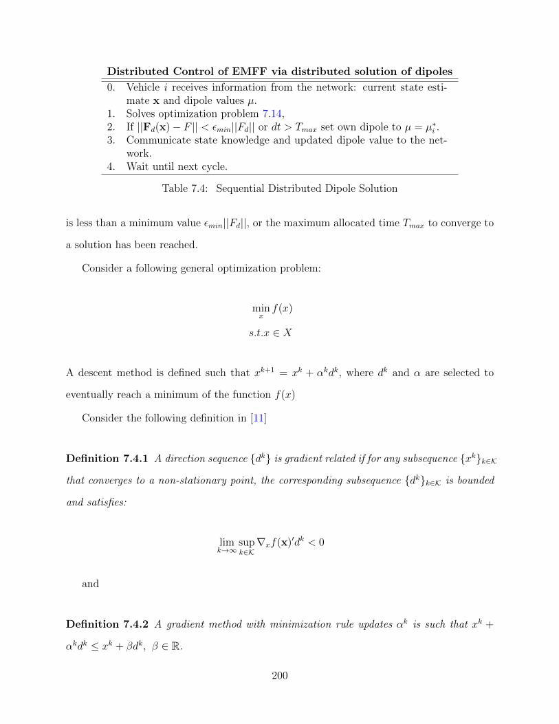
Distributed Control of EMFF via distributed solution of dipoles
0. Vehicle i receives information from the network: current state esti-mate x and dipole values µ.
1. Solves optimization problem 7.14,2. If ||Fd(x)− F || < εmin||Fd|| or dt > Tmax set own dipole to µ = µ∗i .3. Communicate state knowledge and updated dipole value to the net-
work.4. Wait until next cycle.
Table 7.4: Sequential Distributed Dipole Solution
is less than a minimum value εmin||Fd||, or the maximum allocated time Tmax to converge to
a solution has been reached.
Consider a following general optimization problem:
minxf(x)
s.t.x ∈ X
A descent method is defined such that xk+1 = xk + αkdk, where dk and α are selected to
eventually reach a minimum of the function f(x)
Consider the following definition in [11]
Definition 7.4.1 A direction sequence {dk} is gradient related if for any subsequence {xk}k∈K
that converges to a non-stationary point, the corresponding subsequence {dk}k∈K is bounded
and satisfies:
limk→∞
supk∈K∇xf(x)′dk < 0
and
Definition 7.4.2 A gradient method with minimization rule updates αk is such that xk +
αkdk ≤ xk + βdk, β ∈ R.
200

Proposition 7.4.3 Consider the global optimization problem:
minµ||Fd − F (µ)|| (7.17)
For Fd constant, in the overall algorithm in protocol 7.4, µ is updated as a gradient
method with minimization rule updates and with gradient related descent. When including
constraints h(x) < 0, the algorithm is a gradient feasible direction method with minimization
rule and gradient related direction sequence.
Proof: The algorithm in protocol 7.4 can be shown to be an implementation of a
gradient method with gradient related direction and αk selected by minimization rule. The
proof that a gradient descent method with feasible gradient related direction converges to a
stationary point is presented in proposition 2.2.1 in [11].
The gradient of f(x) in given by:
∇xf(x) = 2
((M(µ1)µ1 + V(µ1)− F)′M(µ1) (M(µ2)µ2 + V(µ2)− F)′M(µ2) . . .
)(7.18)
dki ∈ R3N is zero for {i}, then:
∇xf(x)′dki = (M(µ1)µ1 + V(µ1)− F)′M(µ1)µ∗i (7.19)
At every iteration step, if a minimum to the local problem is found, such that µi∗ < µi,
the global variable µ is updated such that µk+1 = µ + αkdk, with dk is a vector with zeros
in the components not corresponding to agent i. Otherwise, if a minimum µ∗i < µi is not
found, µ is not updated and the iteration corresponds to another vehicle in S. Thus, not
necessarily at each iteration of the protocol, there is an update.
If a minimum to the local problem the control variable µ is found, µ is updated as µi = µ∗i
otherwise it is not updated. Then, the update sequence is updated at least once every cycle.
As the protocol progresses over S, µ is updated as µ = µ.
201

Proposition 7.4.4 If a stationary value has not been reached, at least 1update occurs over
a cycle over S.
Proof: Assume that a stationary value has not been reached, and no update occurred
over a cycle, in the next cycle, all the values of µi are the same, which means there will not
be further updates, and a stationary point has been reached.
A straightforward observation from the above proposition is a lower bound in the con-
vergence of the algorithm.
Corollary 7.4.5 The convergence rate over iterations for the distributed protocol 7.4 is
lower bounded by 1Nr, where r is the convergence rate of a gradient based with minimiza-
tion rule and gradient related direction sequence for the global problem.
Consider for example, that the set h(µi) is given by the constraints in the maximum
current that can be run through the coils, then the set C is a convex set.
7.4.3 Closed loop convergence
The relationship between state update, dipole update and distributed optimization step rate
in protocol 7.4, are parameters that affect the behavior of the system.
When the information sharing rate is fast enough compared to the dynamics of the overall
system, the convergence problem can be approximated to the static case where the desired
force Fd(x) is basically constant while the algorithm converges. However, as the data sharing
rate is reduced to the point that it is comparable to the dynamics time constant, a more
complex dynamic situation has to be addressed. In this case the overall objective to be
addressed is the stability of the formation error under the dynamics:
x+ = f(x, Fd + d)
d = minµi
(F (µ,x)− Fd(x))
s.t. h(µ) < 0
202

Initial simulations show that including this algorithm in a control loop can work to
achieve stable control to a fixed point or to follow trajectories, but the theory has to be
further researched to understand under which conditions this approach would work and its
usefulness compared to a centralized approach. Figure 7-9 shows the results of a simulation
where the forces are calculated to follow circular trajectories using a PD controller and the
forces are setup by the distributed calculation of the dipoles as suggested in this section.
The vehicles follow a circular trajectory setting up the dipoles in a distributed manner. The
bottom plot shows the dipole for one of the vehicles
Figure 7-9: Figure showing a group of vehicles following a circular trajectory setting up thedipoles in a distributed manner.
203

7.5 Summary and Conclusion of the Chapter
Control algorithms that require a centralized solution of the dipole equation could be unfeasi-
ble due to limitations in the computation power or communication capabilities. The methods
discussed in this section present an alternative, which can be of major importance in the
implementation of formations with large number of electromagnetic propelled vehicles by
allowing the implementation of control algorithms that do not require a central coordinating
unit calculating, allocating and communicating the formation control commands.
It is important however, to consider the limitations and practical considerations when
implementing the proposed mechanisms. In the case of time divided control, one of the
assumptions is that the control cycles have to be fast enough to reduce the effects of the
time divided actuation. This could imply requirements for the control frequency to be
higher than what it would be for a centralized calculation and thus increasing the number of
computations per second and reducing one of the advantages of decentralization. However, it
is to be noticed that the solution of the dipole equation is a nonlinear optimization problem
with exponentially increasing complexity as the number of dipoles increases. The increase
in the number of cycles per second to achieve the time divided control approach increase
required to achieve similar performance is sublinear. Additionally, there is a limit in the
number of operations per cycle that can be achieved by a computing unit, and the power
requirements and cost of computation translated also escalates exponentially.
The advantage of the token time divided maneuvering as presented in this chapter is
that it derives feasible optimal reconfiguration maneuvers for a problem with a constraint in
the number of active vehicles, however the implementation may require another propulsion
system that maintains control of the unactuated vehicles, a sequential maneuvering that
achieves the final objective in stages and reduce the inactivity period for the vehicles
For the frequency division, the maximum number of different orthogonal sets is driven by
the properties of the mechanism to generate the shaping functions, specifically, the frequency
204

content of the shaping function and the accuracy within which the clocks on each vehicle
can be synchronized.
The frequency division control approach could be combined with the time division ap-
proach in a hybrid mechanism mentioned in the previous section to achieve even better
performance. In such a case, up to Nf sets of vehicles could be active at the same time
without interfering with each other, where Nf is the number of available shaping orthogonal
functions.
The distributed solution to the dipole equation presents also a valid alternative that
can reduce the computational burden and scale down the computational requirements of
EMFF formations with a large number of vehicles. This solution however requires continuous
communication to distribute the information regarding the dipole configuration of all the
vehicles in the formation.
205

206

Chapter 8
Conclusions and Final Remarks
8.1 Thesis Summary and Conclusions
A new approach to formation flight control has been proposed in this thesis. In this approach
the formation globally converges to patterns defined by constraints of the desired state
and not to (time varying) trajectory fixed points. Additionally, the innovative methods
introduced to analyze distributed control laws opened up a new avenue for research to address
more efficient and stable controllers.
In a first part, the cyclic pursuit approach that had previously been studied in the lit-
erature as an algorithm to achieve circles and log-spiral patterns was extended by deriving
a full linear eigendecomposition analysis of the three-dimensional case. The eigendecompo-
sition analysis lead to the derivation of control approaches more relevant to the dynamics
of spacecraft formations. Extensions addressing robustness and convergence to other type
of trajectories were developed to address controllers useful for near-earth and deep space
formation flight missions.
The initially introduced formation acquisition approach was then extended by considering
it as a manifold convergence problem and using the tools of contraction theory to perform
an analysis of its performance. The analysis in the context of the partial contraction the-
207
ory leads to a more general understanding of the problem and allows the generalization
to achieve results for nonlinear and time varying systems otherwise unachievable by the
eigendecomposition method.
The contraction theory approach to the analysis of distributed controllers opened new
avenues for research. First, it demonstrates an approach that determines global stability in
terms of the negative definiteness of a matrix, which for the case of distributed controllers
might seem a more convenient approach than Lyapunov methods where the stability is
defined by demonstrating the negativeness of a function. The general notion of convergence
is reshaped to the more general notion of manifolds (or subspaces) which defines a new
dimension to the widely studied consensus problem.
The experimental results in a relevant testbed under microgravity conditions demon-
strated that the implementation is feasible in the context of spacecraft formation control.
Specifically, the successful results are partially attributed to the decentralized nature of the
approach since the achievement of the desired global behavior emerges from appropriately
verifying the local behavior of the vehicles.
8.2 Contributions
The main contributions of this thesis are:
1. Developed a new approach to decentralized spacecraft formation control inspired by
the cyclic pursuit algorithm. It can be more efficient in terms of control effort by not
tracking trajectories but by converging to a specified manifold. The approach achieves
improved properties with respect to the most common approaches, namely:
• Reduced control effort by not tracking irrelevant degrees of freedom.
• Reduced need for coordination, i.e does not need to agree on relative trajectories.
• Leader(s) can control free degrees freedom of the overall formation.
208

2. Addressed the robustness issues of classic cyclic pursuit by introducing a nonlinear
extension to the control law that achieves equilibrium at a splay-state formation of
determined radius and a corresponding theoretical stability result.
3. Devised a transformation scheme that allows for the design of distributed controllers
that converge to very general types of synchronized trajectories.
4. Developed decentralized control laws based on the cyclic pursuit approach for LEO
formation flight that globally converge to near natural relative trajectories. Theo-
retical results include a full eigendecomposition of the dynamics showing the global
convergence as well as simulation results showing its implementation accounting for J2
effects.
5. Formulated decentralized control laws for second order systems that require only rel-
ative information to converge to different geometric patterns and can be of impor-
tance for formation flight in deep space missions without an accurate global reference
frame. The patterns of convergence include circular formations, ellipse, logarithmic,
archimedean spirals and polygons.
6. Introduced an analytic approach based on contraction theory that allows for a wide
range of global convergence results for nonlinear controllers and complex configura-
tions based on combinations of cyclic algorithms. The wide extent of the approach is
exemplified by obtaining several important results:
(a) Proofs of global convergence to regular formations based general on cyclic inter-
connections.
(b) Global convergence results for distributed controllers that converge to regular
formations of specified size.
(c) Extensions of the contraction theory theorems to allow for proofs of convergence
to time varying manifolds.
209
(d) Corollaries that allow for proofs of global convergence to formations based on any
number of interconnected subformations.
(e) Proof of convergence to formations of specified size through a leader.
(f) Derivation of sufficient conditions for global convergence to surrounding a target
using a cyclic control approach under general tracking functions.
7. Implemented hardware tests and obtained experimental results that validate the char-
acteristics of the approach, namely: no need of central coordination, extensible to any
number of vehicles, reduced control effort and simplicity of implementation for several
formation flight scenarios.
8.2.1 Secondary contributions
Additionally, the thesis added to the field along with other contributions that include:
1. An investigation that compares different formation control architectures to a decentral-
ized control approach where the control is not based on tracking relative trajectories.
2. A preliminary study of the solution to EMFF reconfiguration maneuvers with a reduced
interconnection complexity by solving for the optimal maneuvers that only use a subset
of vehicles at a time.
3. The development and a preliminary comparison of several methods to achieve decen-
tralized control of EMFF by decoupling the dynamics.
4. A protocol to decentralizing EMFF by distributing the solution of the dipole equation.
8.3 Future Work
There are several points that can be addressed as a continuation of this work and new avenues
for future research that were opened by the developments of this thesis.
210

As a first direction, having demonstrated that the convergence to geometric patterns is
achievable under more general cyclic interconnections, a new direction should consider the
design of more robust control approaches that can use informations of neighbors interchange-
ably, reducing the constraint of a cyclic interconnection. At first glance this seems like a
straightforward extension but it may require developing some machinery to achieve formal
proofs that verify the convergence properties.
In this work, the attitude control was left out of the scope other than a basic development
for the experimental setup. It can be convenient however to define controllers that combine
measurements in the local body reference frame of the spacecraft which could achieve a
more precise control performance in cases where measurements are dependent on the relative
orientation of sensor and target.
In Section 3.4, it was shown how a ’similarity’ mapping scheme can be used to achieve
convergence to complex trajectories. Converging to elliptical trajectories was shown to be
useful for a specific application, namely closed natural relative trajectories for near circular
orbits. However, closed natural relative trajectories for orbits with increasing eccentricity
are different from ellipses. A parallel approach, using nonlinear similarity transformations
can be useful for converging to such relative trajectories. Additionally, applications in other
fields can deem useful applications for convergence to formations with very specific geometric
patterns.
A whole new avenue of research has been opened by demonstrating the use of the con-
traction theory approach to the analysis of distributed controllers. Several considerations
that could be addressed are including the effects of saturation, the convergence properties
when collision avoidance mechanisms are added, the effects of delays and random varying
graphs, etc. Further research would consider linear or affine transformation for convergence
to not only regular formations, and the use of the convergence primitive tools to define more
complex convergence states.
Reshaping the general notion of convergence to the more general sense of manifolds (or
211

subspaces) defines a new dimension to the widely studied consensus problem. There might
exist applications in many other fields where the distributed system objective can be achieved
without convergence to the ’common agreement’ subspace ( namelyM is spanned by 1) but
by converging to some more general ’coordination subspace’ defined as h(x) = 0.
A dual of the control problem is of course, the estimation problem. The application
of the cyclic approach for convergence to a subspace, can be defined in the context of dis-
tributed sensors that are required to converge to a coordinated estimate, defined by a linear
transformation of the overall state.
Chapter 7 presented a preliminary study of options that can be applied to decentralize
the control of electromagnetic formation flight systems. Simulations show the feasibility of
the approaches. A deeper and more complete approach to theoretical convergence results
and control design are possibilities for future work.
In the case of time divided resource allocation, the design of the controller is a next
step to be addressed which should take into account the intrinsic disturbance due to the
non-complete nature of the approach ( i.e. the desired force cannot be applied instantly but
only as an ’average’ over a cycle) . The effects in performance defines a clear direction for
future developments.
Experimentation of the time based and frequency based allocation could be feasible on
the HTS EMFF testbed. Resonant frequencies that take advantage of the design of the coils
could also be considered as future developments.
Finally, hybrid methods that use time based, frequency based and distributed solution of
the dipole equation can have important advantages. A higher level analysis that can identify
the most advantageous architectures for decentralized EMFF could also be addressed, as
well as identifying missions that would truly benefit from this developments.
212

Appendix A
Mathematical derivation of proofs
A.1 CR Matrices
All matrices in the CR have the same set of linearly independent eigenvectors, and are
diagonalizable by the matrix T of eigenvectors νL⊗R,ij.
Proof: The eigenvectors of L⊗R are such that
νL⊗R,ij = νLi ⊗ νRj (A.1)
The eigenvectors of L are the same for all circulant matrices L which following Section 2.1.5
are shown to be independent. Equivalently, the eigenvectors of R are the same for all rotation
matrix R that share an axis of rotation and following Section 2.1.4 are shown to be linearly
independent. Then, the set of eigenvectors for all matrices CR which are described as L⊗R
is linearly independent. The Kronecker composition of this two sets of linearly independent
vectors:
µk.= ψk ⊗ (0, 0, 1)T = (0, 0, 1, 0, 0, χk, . . . , 0, 0, χ
n−1k )T ,
µ+k
.= ψk ⊗ (1, j, 0)T = (1, j, 0, χk, j χk, 0, . . . , χ
n−1k , j χn−1
k , 0)T ,
µ−k.= ψk ⊗ (1,−j, 0)T = (1,−j, 0, χk,−j χk, 0, . . . , χn−1
k ,−j χn−1k , 0)T ,
(A.2)
213

where k ∈ {1, . . . , n} and ψk =(
1, χk, χ2k, . . . , χ
n−1k
)T, where χk = e2πjk/n, k ∈ {0, . . . , n− 1}
are the eigenvectors of L (omitting the constant 1/√n). The composed set of eigenvectors,
can then be verified to be a set of linearly independent eigenvectors and since L is diag-
onalizable, R is diagonalizable, then all CR matrices are diagonalizable by a matrix T of
eigenvectors νL⊗R, (See Thm. 13.12 in [41]) namely, the diagonal matrix:
(P−1LP )⊗ (Q−1RQ) = (P−1 ⊗Q−1)(L⊗R)(P ⊗Q) (A.3)
= (P ⊗Q)−1(L⊗R)(P ⊗Q) (A.4)
where P is a matrix of eigenvectors of L and Q is a matrix of eigenvectors of R.
Therefore, if A,B ∈ CR
eig(A+B) = eig(TΛAT−1 + TΛBT
−1)
= eig(T (ΛA + ΛB)T−1) (A.5)
where ΛA is a diagonal matrix the eigenvalues of A λA,i in the diagonal (and correspondingly
the same holds for B). Therefore λA+B,i = λA,i + λB,i.
We also have then that:
AB = eig(TΛAT−1TΛBT
−1)
= eig(T (ΛAΛB)T−1)
= eig(T (ΛBΛA)T−1)
= BA (A.6)
214

A.2 System (3.10) in Polar Coordinates
Assume that ‖pi‖ = %i > 0. Note that pi = %iR(−ϑi) e1, where e1 is the first vector of the
canonical basis, i.e., e1 = (1, 0)T . Then, we can write pi+1 as
pi+1 =%i+1
%i%iR(−ϑi+1) e1 =
%i+1
%i%iR(−ϑi+1)R(ϑi)R(−ϑi) e1 =
%i+1
%iR(ϑi − ϑi+1) pi. (A.7)
Moreover, it also holds
pTi R(γ)pi = ‖pi‖2 cos(γ) = %2i cos(γ), for any γ ∈ R. (A.8)
First, we find the differential evolution for the magnitude of pi, i.e., for %i. We have
%i =d‖pi‖dt
=pTi pi‖pi‖
=1
%ipTi (R(αi+1)pi+1 −R(αi)pi). (A.9)
By using Eqs. (A.7) and (A.8) we then obtain
%i =1
%ipTi
(R(αi+1)
%i+1
%iR(ϑi − ϑi+1) pi −R(αi)pi
)= %i cos((ϑi+1 − ϑi)− αi+1)− %i cos(αi)
(A.10)
We now find the differential evolution for the phase of pi, i.e., for ϑi. Taking time
derivative in both hands of the identity pi,1 sinϑi − pi,2 cosϑi = 0, we easily obtain
ϑi =pi,1 pi,2 − pi,2 pi,1
%2i
=1
%2i
pTi R(π
2
)pi =
1
%2i
pTi R(π
2
)(R(αi+1)pi+1 −R(αi)pi
). (A.11)
Then, by using Eqs. (A.7) and (A.8) we obtain
ϑi =1
%2i
pTi R(π
2
)(R(αi+1)
%i+1
%iR(ϑi−ϑi+1) pi−R(αi)pi
)=%i+1
%isin((ϑi+1−ϑi)−αi+1)+sin(αi).
(A.12)
215

A.3 Proof of Lemma 3.2.8
Proof: The eigenvalues of P are solutions to the characteristic equation
0 = det
( λIn − an L1 + 2kα sn In sn In
−bn L21 λIn − cn L1
). (A.13)
Note that both matrix (λIn − an L+ 2kα sn In) and matrix −bn L2 are circulant; then, since
circulant matrices form a commutative algebra (see Section 2.1), we can apply the result in
equation (2.1) and obtain
0 = det(
(λIn − an L+ 2kα snIn)(λIn − cn L) + snbnL2)
(A.14)
= det
(λ2In + λ
(2kα snIn − (an + cn)L︸ ︷︷ ︸
.=B
)−2kαsncnL+ (ancn + snbn)L2︸ ︷︷ ︸
.=C
)(A.15)
= det(λ2In + λB + C
)(A.16)
= det(λ2In + λB +B2/4− S
), (A.17)
where S.= B2/4−C. Note that B and C are circulant, therefore S is also circulant. Since S
is circulant, it can be diagonalized according to S = U DS U∗, where DS is a diagonal matrix
with the eigenvalues of S on the diagonal; accordingly, we have S1/2 = U D1/2S U∗. Note
that B and S1/2 commute. In fact, since B is circulant, it can be diagonalized via the same
orthogonal matrix U : B = U DBU∗, where DB is a diagonal matrix with the eigenvalues of
B on the diagonal; hence
S1/2B = UD1/2S U∗ UDBU
∗ = UD1/2S DBU
∗ = UDBD1/2S U∗ = UDBU
∗ UD1/2S U∗ = B S1/2.
Therefore, we have
0 = det(λ2In×n+λB+B2/4−S
)= det
(λIn − (−B/2 +
√S))
det(λIn×n − (−B/2−
√S)).
216
Hence, the eigenvalues of P are the union of the eigenvalues of (−B/2 +√S) and (−B/2−
√S). Since B and S1/2 are diagonalized by the same similarity transformation U , we have
− B
2± S1/2 = U
DB
2U∗ ± UD1/2
S U∗ = U
(DB
2±D1/2
S
)U∗. (A.18)
Let λB,k be the kth eigenvalue of B, and λS,k be the kth eigenvalue of S, k ∈ {1, . . . , n}.
Then, from equation (A.18), we have that
eig(P ) ={λB,k/2± λ1/2
S,k
}nk=1
. (A.19)
Hence, we are left with the task of computing the eigenvalues of B and S. Such eigenvalues
can be easily found by using equation (2.4):
eig(B) ={
2kα sn + (an + cn)(1− e2πjk/n)}nk=1
, (A.20)
eig(S) ={
(λ2B,k/4− λC,k
}nk=1
={
(2kα sn + (an + cn)(1− e2πjk/n)2/4
−(
(2kαsncn + ancn + snbn)− (2kαsncn + 2ancn + 2snbn)e2πjk/n
+ (ancn + bnsn)e4πjk/n)}n
k=1. (A.21)
We first consider the eigenvalues of B. By using the following identities
(1− eαkj) = 2 sin(αk/2)ejαk−π
2 , (1− 1
2(1− ejαk)) = cos(αk/2)ejαk/2, (A.22)
and after some algebraic manipulations omitted for brevity, the eigenvalues of B can be
written as
λB,k = (2kαsn) + 2(2cn − kαsn) sin(kπ/n)ej(kπ/n−π2
), k ∈ {1, . . . , n}. (A.23)
217

Hence, we have, for k ∈ {1, . . . , n},
Re(λB,k) = 2kαsn + 2(2cn − kαsn) sin2(kπ/n), (A.24)
Im(λB,k) = −2(2cn − kαsn) sin(kπ/n) cos(kπ/n). (A.25)
Next, we consider the eigenvalues of S. By using, again, the identities in equation (A.22),
and with simple algebraic manipulations, we can write, for k ∈ {1, . . . , n},
λS,k = k2αs
2n(cos(kπ/n)ejkπ/n)2 + (kαsncn + s2
n)(2 sin(kπ/n)ej(kπ/n−π2
))2
= [k2αs
2n + 4 sin2(kπ/n) + (4kαsncn − k2
αs2n − 4c2
n) sin2(kπ/n)]ei2kπ/n.
Notice that kα, cn and sn are positive real numbers; then the term inside the square brackets
is a positive real number. Therefore we have, for k ∈ {1, . . . , n},
Re(√λS,k) = (k2
αs2n + 4 sin2(kπ/n) + (4kαsncn − k2
αs2n − 4c2)(sin2(kπ/n)))1/2 cos(kπ/n),
which can be rearranged as
Re(√λS,k) =
((kαsn + (2cn − kαsn) sin2(kπ/n))2 + 4 sin2(kπ/n)(s2
n − sin2(kπ/n)))1/2
=((λB,1/2)2 + 4 sin2(kπ/n)(s2
n − sin2(kπ/n)))1/2
. (A.26)
From equations (A.24) and (A.26) it is straightforward to show that
• For k = n: we have
λP,n = −λB,n/2 +√λS,n = kαsn − kαsn = 0.
218

• For k = 1, k = n− 1:
Re(√λS,1) = Re(λB,1/2) = (kαsnc
2n + 2s2
ncn), Im(√λS,1) = kαs
2ncn + 2s3
n,
Re(√λS,n−1) = Re(λB,n−1/2) = (kαsnc
2n + 2s2
ncn), Im(√λS,n−1) = −kαs2
ncn − 2s3n.
Therefore, we obtain
Re(λP,1) = −Re(λB,1/2) +Re(λB,1/2)=0,
Im(λP,1) = (2cn−kαsn)sncn + kαs2ncn + 2s3
n=2sn,
Re(λP,n−1) = −Re(λB,n−1/2) +Re(λB,n−1/2)=0,
Im(λP,n−1) = −(2cn−kαsn)sncn − kαs2ncn + 2s3
n=−2sn.
• For 1 < k < n− 1, since sin(kπ/n)2 > sin(π/n)2, we have:
Re(√λS,k) ≤ Re(λB,k/2),
and thus Re(λP,k) < 0 for k /∈ {0, 1, n− 1}.
Now, we proceed to show that v1, v2, v3 in lemma 3.2.8 are the eigenvectors corresponding
to the eigenvalues 0, 2snj and −2snj respectively. First, consider the zero eigenvalue. Since
L · 1n = 0n (where 0n = (0, 0, . . . , 0)T ∈ Rn), it is easy to verify that:
P v1 =
an L− 2kα sn In −sn In
bn L2 cn L
1n
−2kα1n
= 02n. (A.27)
Now, consider the imaginary eigenvalue λ2 = 2snj. By replacing v2 into the eigenvalue
219

equation we obtain
an L− 2kα sn In −sn In
bn L2 cn L
ψ1
fn,2(kα)ψ1
= 2snj
ψ1
fn,2(kα)ψ1
, (A.28)
Note that L and L2 (which are both circulant matrices) satisfy, respectively, Lψ1 = (e2πj/n−
1)ψ1 = (−2snj(cn + jsn))ψ1, and L2ψ1 = (e2πj/n − 1)2ψ1 = −4s2ne
2πj/nψ1; hence, v2 is an
eigenvector for P if and only if:
(an(e2πj/n − 1)− 2kαsn)ψ1 + 2bnejπ/nsnψ1 = 2snjψ1 (A.29)
−4bns2n(cn + jsn)2ψ1 − cn(−2snj(cn + jsn))2bne
jπ/nψ1 = −4bnejπ/nsnjψ1 (A.30)
By using the identities in equation (A.22), the first condition can be verified according to
2sn(−cn + kαsn)jejπ/n − 2snkα + 2snbnejπ/n = 2snj,
2((cn − kαsn)j − (kα + j)(cn − jsn))eπj/n = −2bnejπ/n,
−2(sn + kαcn)eπj/n = −2bnejπ/n.
Similarly, the condition in equation (A.30) can be verified according to
−2bns2n(cn + jsn)2 + 2cn(jsn(cn + jsn))bne
jπ/n = −2bnejπ/nsnj,
−sn(cn + jsn) + cn(j(cn + jsn)) = j,
j(s2n + c2
n) = j.
Similar arguments hold for λ3 and v3 (which are complex conjugates of λ2 and v2). This
concludes the proof.
220
A.4 Proof that vi /∈ T(%∗,ϕ∗)M
Proof: It is enough to prove that at least one of the components of G · vi is nonzero.
The proof that G · v1 6= 0 is trivial. We proceed to show that ∇g1 · v2 6= 0, i.e.:
[1 cos
(2π
n
). . . cos
(2π(n− 1)
n
)−
n∑i=2
r sin
(2π(i− 1)
n
). . . − r sin
(2π(n− 1)
n
)0
] ψ1
−2bnejπ/nψ1
= (∇%g1) · ψ1 + (∇ϕg1) · (−2bne
jπ/nψ1) 6= 0.
Both terms in the above sum can be shown to be real and positive. For the first term we
have that:
(∇%g1) · ψ1 =n−1∑k=0
cos(2πk/n)(cos(2πk/n) + j sin(2πk/n))
=n−1∑k=0
cos2(2kπ/n) + jn−1∑k=0
2 sin(kπ/n) =n−1∑k=0
cos2(2kπ/n) ∈ R>0.
For the second term we have:
(∇ϕg1) · (−2bnejπ/nψ1) =
n−1∑k=0
n∑i=k+1
sin(2πk/n)2bnejπ/ne2πk/n
= 2bn
n−1∑k=0
ake(2k+1)πj/n,
where ak =∑n
i=k+1 sin(2πi/n) = −∑k
i=1 sin(2πi/n). Now we show that∑n
k=0 ake(2k+1)πj/n >
0. First, consider the following facts:
ak ≤ 0 ∀k,
ak+1 = ak − sin(2π(k + 1)/n) < ak for 0 ≤k <n/2− 1,
ab(n−1)/2c < ak ∀k 6= d(n− 1)/2e,
an−k = −n−k∑i=1
sin(2πi/n) =n∑
m=k+1
sin(2πm/n) = ak,
221

n−1∑k=0
ake(2k+1)πj/n =
b(n−1)/2c∑k=0
(akekπj/n + an−ke
−kπj/n) + qa(n−1)/2
=
b(n−1)/2c∑k=0
ak(eπkj/n + e−kπj/n) + qa(n−1)/2
n−1∑k=0
e(2k+1)πj/n =
b(n−1)/2c∑k=0
(eπkj/n + eπ−kj/n) + q = 0
where q = 0 if n is even. Then,
n−1∑k=0
ake(2k−1)πj/n >
n−1∑k=0
ab(n−1)/2ce(2k−1)πj/n = 0.
Since bn = (sn + kαcn) > 0, we have that ∇ϕg1 · (−2bnejπ/n) ∈ R>0.
The proof forG·v3 6= 0 is analogous; in particular, it requires to show that j∇%g2·ψ1 ∈ R>0
and j∇ϕg2 · (−2bnejπ/nψ1) ∈ R>0.
A.5 Eigenvalues of the projected Laplacian
The derivation of the eigenvalues of RL(N)Lm(α)(L(N))>R> uses the properties of block-
circulant matrices, specifically, the fact that they all belong to a commutative algebra. We
have that:
eig[RηL(N)Lsm(α)(L(N))>R>η ] = eig[RR>]eig[L(N)]eig[(L(N))>]eig[L(α) + L>(α)]
= eig[(In ⊗R(π/N))(In ⊗R>(π/N))]
×eig[(L1 ⊗ I3)(L>1 ⊗ I3)]eig[L(α) + L(α)>]
= eig[(L1 ⊗ I3)(L>1 ⊗ I3)]eig[L(α) + L(α)>]
222

Then,
eig[RLLsmL>R>] = λik i ∈ {1, .., N}, k ∈ {−1, 0, 1}
λik = (1− e−j2imπ/N)(1− ej2imπ/N)((ejkα − ejkα−j2imπ/N) + (ejkα − e−jkα+j2iπ/N))
= (2− e−j2iπ/N − ej2iπ/N)2(cos(kα)− cos(kα− 2imπ/N))
= 4(1− cos(2iπ/N))(cos(kα)− cos(kα− 2imπ/N)) (A.31)
Then, for i = 1:
(1− cos(2iπ/N)) = 0
⇒ λ1k = 0
for i = N :
(cos(kα)− cos(kα− 2miπ/N)) = 0⇒ λNk = 0
otherwise for 1 < i < N , |α| ≤ 2π/N :
(cos(kα)− cos(kα− 2imπ/N)) > 0
(1− cos(2iπ/N)) > 0
Proposition A.5.1
VrnLsmV >rn = KnRηL(α)LsmL(α)>R>ηK>n > 0 , (A.32)
Proof: RηL(α)LsmL(α)>R>η is a symmetric matrix, then, its nullity is the algebraic
multiplicity of the 0 eigenvalue. Thus, dim{N (RηL(α)LsmL(α)>R>η )} = 6. On the other
223

hand, the dimension of Kn(RηL(α)LsmL(α)>R>η )K>n = 3N − 6, and thus it is full rank.
Since (RηL(α)LsmL(α)>R>η ) is positive semidefinite, then VrnLsmV >rn is at least positive
semidefinite, but since it is full rank, the proposition is proven.
224

Appendix B
SIMO: Mission Option Scenarios
B.1 Development of the trade study model
The SIMO project considers a trade analysis of a system of spacecraft acting as a team to
obtain images from interferometric measurements. The results suggest that a large number
of vehicles performing precision reconfiguration maneuvers are a dominant design option.
Therefore, this system is an example of the type of applications that would benefit from the
development of decentralized control schemes based on the results in this thesis. The results
of the trade analysis are presented in the next sections.
B.1.1 Trade model methodology
As one of the results from the Phase-I of the SIMO project, a trade analysis methodology
was established by defining design parameters, metrics and basic optimization methodology.
The proposed methodology consisted of a full factorial exploration of the design space, which
considers each and every possible combination of the elements of the design vector. An
optimization module intended to calculate trajectories that optimize the coverage of the uv
plane, a module that calculates the mass of the system based on the science requirements
and the calculated optimized trajectories, and a module computes the performance of the
225

architecture. Specifically, the uv plane coverage is optimized by minimizing h, a metric that
takes into account the relative locations between uv points and penalizes their proximity.
This metric can also be written as:
h =N∑i
1
(yi)2(B.1)
y = TNTnx, where N =
n2
(B.2)
And T, is the n × N matrix that calculates the relative value between every pair of
elements of the vector it multiplies:
Tn =
−1 1 0 . . .
1 −1 0 . . .
1 0 −1 . . .
......
.... . .
0 1 −1 . . .
......
.... . .
∈ Rn×N (B.3)
The trajectories are generated by considering double integrator dynamics and the mass
of the systems takes into account the type of propulsion to be used, either FEPS or EMFF
and includes the propellant mass or the mass required to generate the power to drive the
system. 1.1.1.2 Proposed improvements From the analysis of the results of the Phase-I
study, improvements to the trade model were suggested as constructive objectives for the
Phase-II study. The trade study can be improved and more accurate trades can be obtained
by enhancing the fidelity of the models and considering architectures that might achieve
improved benefits. After an initial analysis of the possible improvements, the following
have been identified as key developments and have been the target of recent developments
226

for this specific subtask of the project: 1. Improving the optimality of the trajectories for
architectures that use electromagnetic propulsion. 2. Developing models that allow the
analysis of architectures with EMFF-FEPS hybrid propulsion systems. 3. Improve the
fidelity of the modules that calculate the required mass by considering optimal trajectory
planners which consider minimum paths. 4. Implementation of models for architecture
with drift-through mode capabilities. 5. Improving the performance metric models. 6.
Implementation of optimization modes that can include a trade between uv plane coverage
and fuel/power usage.
Figure B-1 shows a scheme that better describes the improved trade model to be imple-
mented. The inputs are color coded depending on their nature. Design engineering inputs
are defined in green boxes, the science input are defined in blue boxes.
B.1.2 Improving the optimality of the trajectories for architec-
tures that use electromagnetic propulsion
Electromagnetic formation flight uses inter-vehicle electromagnetic forces to control the rel-
ative positions of the vehicles in the formation. Due to the internal nature of these forces,
the center of mass of the formation is uncontrollable using this type of propulsion. For the
case of coverage of the uv plane, the uncontrollability of the center of mass of the forma-
tion is not a disadvantage since the coverage of the frequency plane is only dependent on
relative trajectories. However, the design of coverage trajectories has to have this fact into
consideration. In a previous approach to formation coverage of the uv plane, electromagnetic
formations that maintain the center of the formation were calculated by considering regu-
lar polygonal formations with expanding and rotating relative separations. By constraining
the trajectories to this specific type of formations the motionlessness of the center of the
formation was guaranteed; however, constraining the formation to specific manifolds. In a
new approach developed for the second phase of the project the center of mass is held static
227

uv coverage optimization X
Minimum path comb.
Nsat
Nrecon
NEMFF/Nsat
Mass
Power
Fuel
treconfig
Optical performance
Productivity
EER
Km/c
b
Eng. input
Science input
Design vector Output
Mass
IRes @50%
Images/10 year
Timage
Min Avg.Pathlengthor dist d-value
Figure B-1: Schematic of the improved trade model architecture
228

-100 -50 0 50 100
-100
-80
-60
-40
-20
0
20
40
60
80
100
u×λ (m)
v ×λ
(m)
u-v coverage
h=0.067
-150 -100 -50 0 50 100 150-150
-100
-50
0
50
100
150
-200 -150 -100 -50 0 50 100 150 200-200
-150
-100
-50
0
50
100
150
200uv Coverage
u×λ (m)
v ×λ
(m)
-150 -100 -50 0 50 100 150-150
-100
-50
0
50
100
150Physical locations
x
y
h=0.0306
h=0.0067
Figure B-2: Improvement in the coverage of the uv plane by using the new approach. Inthis case the maneuvers are not constrained to polygons as in the previous implementation(top)
by first defining each maneuvers optimal coverage points and then defining trajectories that
achieve this coverage without moving the center of mass of the formation. The results of the
approach are shown in Figure B-2. The optimal coverage pattern obtained by the algorithm
in phase-I is compared to the results under the new approach. In both cases the center of
the formation remains static. A significant improvement in the coverage of the uv plane can
be observed.
229

B.1.3 EMFF-FEPS hybrid propulsion system models
In a more advanced analysis, architectures with hybrid propulsion which combine spacecraft
with different propulsion technologies are to be considered. For the second phase of the
project the trade model will consider architectures with spacecraft using FEPS and others
using EMFF propulsion. The approach considered for this model uses a parameter input in
the design vector that defines the number ne out of N spacecraft in the formation that use
EMFF technology. The rest are considered to use FEPS technology. Given the nonlinear
behavior of the electromagnetic force between dipoles which reduces as the fourth power
of the distance, EMFF technology has much better performance at shorter distances. The
model assumes that the ne spacecraft with smaller average inter-spacecraft separation are
those that would use EMFF.
B.1.4 Minimum path coverage to improve mass calculation
In an initial approach to mass calculation defined for the phase I model, the averages of the
distance traveled between maneuvers are considered as a first order approximation of the
metric to define the mass requirements for the architecture. By using a more accurate calcu-
lation that considers the optimal paths that minimize translation of the spacecraft between
maneuvers a model that describes more accurately the values for the optimal performance of
the different architectures. The minimum path calculation is performed by a full exploration
of the combinatorial space of the required coverage positions at each maneuver. Figure B-
3. shows a sequence of coverage points maneuvers obtained as a solution to the uv plane
coverage optimization problem. Both figures cover the same points in the uv plane at each
maneuver but the selection of the optimal sequence minimizes the traveled paths. The left
side plot presents the trajectories found by minimizing the traveled paths.
The separation of the locations of each vehicle between consecutive maneuvers, the min-
imum velocity while obtaining measurements and the time allowed for reconfiguration are
230

-100 -50 0 50 100 150-150
-100
-50
0
50
100
150Optimal paths
-100 -50 0 50 100 150-150
-100
-50
0
50
100
150Not optimal paths
Figure B-3: Fig 3.Comparison of the results of optimizing the combinatorial selection ofcoverage points. Both figures cover the same points in the uv plane at each maneuver butthe optimal sequence on the left minimizes the traveled paths.
231
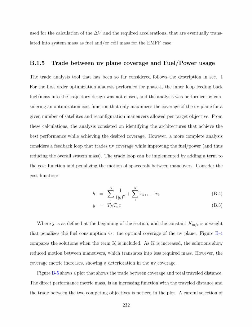
used for the calculation of the ∆V and the required accelerations, that are eventually trans-
lated into system mass as fuel and/or coil mass for the EMFF case.
B.1.5 Trade between uv plane coverage and Fuel/Power usage
The trade analysis tool that has been so far considered follows the description in sec. I
For the first order optimization analysis performed for phase-I, the inner loop feeding back
fuel/mass into the trajectory design was not closed, and the analysis was performed by con-
sidering an optimization cost function that only maximizes the coverage of the uv plane for a
given number of satellites and reconfiguration maneuvers allowed per target objective. From
these calculations, the analysis consisted on identifying the architectures that achieve the
best performance while achieving the desired coverage. However, a more complete analysis
considers a feedback loop that trades uv coverage while improving the fuel/power (and thus
reducing the overall system mass). The trade loop can be implemented by adding a term to
the cost function and penalizing the motion of spacecraft between maneuvers. Consider the
cost function:
h =N∑1
1
(yi)2+
N∑1
xk+1 − xk (B.4)
y = TNTnx (B.5)
Where y is as defined at the beginning of the section, and the constant Km/c is a weight
that penalizes the fuel consumption vs. the optimal coverage of the uv plane. Figure B-4
compares the solutions when the term K is included. As K is increased, the solutions show
reduced motion between maneuvers, which translates into less required mass. However, the
coverage metric increases, showing a deterioration in the uv coverage.
Figure B-5 shows a plot that shows the trade between coverage and total traveled distance.
The direct performance metric mass, is an increasing function with the traveled distance and
the trade between the two competing objectives is noticed in the plot. A careful selection of
232

-100 -50 0 50 100-100
-50
0
50
100uv Coverage
u
v
-100 -50 0 50 100-100
-50
0
50
100Physical locations
x
y
-100 -50 0 50 100-100
-50
0
50
100uv Coverage
u
v
-100 -50 0 50 100-100
-50
0
50
100Physical locations
x
y
h=0.002839
h=0.003035
Figure B-4: Comparison of trajectories for different levels of the gain parameter and theoptimal coverage. Top Km/c = 0, Bottom Km/c = 1e−4
233

1 0 - 9 1 0 - 8 1 0 - 7 1 0 - 6 1 0 - 50
1 0 0
2 0 0
3 0 0
4 0 0
5 0 0
6 0 0
7 0 0
8 0 0
dis
t
K m /c
1 0 - 9 1 0 - 8 1 0 - 7 1 0 - 6 1 0 - 5
0
0 . 0 0 5
0 . 0 1
0 . 0 1 5
0 . 0 2
0 . 0 2 5
0 . 0 3
0 . 0 3 5
h
K m /c
-200 -100 0 100 200-200
-100
0
100
200uv Coverage
u
v
-200 -100 0 100 200-200
-100
0
100
200Physical locations
x
y
-200 -100 0 100 200-200
-100
0
100
200uv Coverage
u
v
-200 -100 0 100 200-200
-100
0
100
200Physical locations
x
y
-200 -100 0 100 200-200
-100
0
100
200uv Coverage
u
v
-200 -100 0 100 200-200
-100
0
100
200Physical locations
x
y
Figure B-5: Trade between better uv coverage and mass requirements.
the value Km/c can be performed by analyzing the pareto frontier for different design vectors
and selecting this gain to obtain solution that maximize the reduction in mass at minimal
cost in the coverage metric.
B.1.6 Implementation of models for drift-through architectures
A new architecture to be considered in the trade analysis is the drift-through mode of
operation. For this mode of operation, the coverage of the uv plane is improved by taking into
account the interferometric information obtained from differential measurements from nearby
uv points, analogous to the information obtained in Differential Interferometry Synthetic
Aperture Radars (D-InSAR) under the additional assumption that the changes in the macro
234

scale of the observed targets are minimal in the amount of time between measurements. As
opposite to the stop and stare approach, in this method the spacecraft perform the coverage
of the uv plane without completely achieving a stop. An exact solution to this problem might
not be achievable due to the complexity of the optimization problem. Heuristic approaches
have considered spiral trajectories, as the one presented in the work of Chakravorty and
Ramirez [1]. For this project a heuristic approach considers the effects of this method to
compare to the stop and stare cases, by using the precomputed solutions for efficient coverage
of the uv plane for the stop and stare case, with the difference that the fuel consumption
calculation considers tracking continuous, non stopping trajectories, which will achieve a
similar coverage of the plane, but with reduced SNR for the same exposure time. In the stop
and stare cases, the fuel consumption is calculated from the delta V required to go from a
stop at each point to a complete stop at the next one. In the drift through mode approach
considered here, the vehicles follow spline trajectories crossing the same points at specified
times. The comparison of trajectories and coverage of the uv plane for the same optimization
solution using the two different approaches shows that the drift through approach has a worst
SNR performance, which needs to be considered in the calculation of the minimum required
time for maneuvers.
B.1.7 Incremental deployment design
Another case that was consider in the trade analysis was the idea of incremental design.
In such case, the design points consider the situation where only a few vehicles at a time
are deployed and the total number of vehicles in the array increases with time. In order
to consider the performance metrics of this situation, the best resolution metric and the uv
coverage ’ h -metric’ was calculated as the time average of the best resolution for each stage
of deployment.
235

B.2 Results
The results of the Mission Scenario Modeling tool are described on this section. The opti-
mization consider an array of model mission architectures composed of:
• Number of spacecraft {4, 7, 10, 13, 16}
• Number of reconfiguration maneuvers per image {1, 5, 9}
• Propulsion type (FEEPs, EMFF, hybrid FEEP-EMFF architectures)
• Aperture diameter {1 and 5m}
• Imaging mode {Stop-and-stare, Drift Through}
• Sequential deployment of apertures.
Notice that the largest number of vehicles is 16, this is due to the numerical complexity of
solving the optimization problem for larger number of vehicles. The implemented algorithm
can allow more than 16 vehicles but running a single optimization case can take over a
couple of days in a desktop computer. We consider that the analysis of this cases is enough
to delineate the general behavior of the trade space. In general, the following findings are
highlighted.
B.2.0.1 Effect of baseline
Designs with the largest baseline are favored. Large separation between vehicles offsets the
poor coverage of the uv plane. In term of the optic performance metric defined as resolution
as encircled energy, a poor uv plane coverage with a large baseline can be comparable to good
coverage of the uv plane at short distances. Figure B-6 show that larger baselines (Orange)
are dominant solutions unless the optical resolution of the system is not an important metric.
236

−15
−10
−5
0
0
0.5
1
1.5
2
2.5
3
0
2
4
6
log
10(P
roductivity),
Im
g/1
0yr
log10
(1/Mass), 1/kglog
10(1/Best Resolution), 1/m
0
25%
50%
100%
Figure B-6: Trade space: effect of deployment baselines
B.2.0.2 Effect of number of reconfigurations
No reconfigurations, or a low number of reconfiguration maneuvers per image are dominant
solutions, especially if the productivity is an important metric. In figure B-7 the color bar
shows the number of reconfigrations per image, showing that the dominant solutions seem
to be designs where a larger number of vehicles that capture an image from a single set of
uv points.
237

−15
−10
−5
0
0
1
2
3
0
1
2
3
4
5
6
log
10(P
roductivity),
Im
g/1
0yr
log10
(1/Mass), 1/kg
log10
(1/Best Resolution), 1/m
1
5
90
25%
50%
100%
Figure B-7: Trade space: Effect of number of reconfigurations per image
B.2.0.3 Propulsion type
Dominat solutions and solutions on the pareto front are EMFF-FEEPS hybrid solutions,
with either 25% or 50% fraction of EMFF vehicles. In the plot in Figure B-8, the full plot
space is plotted, including stop and stare, drift-through mode and sequential deployment,
and optimal designs with low mass, high resolution and high productivity are shown in the
upper right corner of the space, most of these solutions are hybrid designs.
238

−12
−10
−8
−6
−4
−2
0
0
0.5
1
1.5
2
2.5
0
1
2
3
4
5
log
10(P
rod
uctivity),
Im
g/1
0yr
log10
(1/Mass), 1/kg
log10
(1/Best Resolution), 1/m
0
25%
50%
100%
Figure B-8: Trade space: Different propulsion configurations are shown
B.2.0.4 Drift-Through vs Stop and Stare
Although the Drift-through mode of operation has to be further analyzed to more accurately
identify the effect of this interferometric data collection mechanism on the SNR, the esti-
mated effect is a reduction of the SNR and therefore a reduction on productivity. Figure
B-9 shows a plot of the trade space considering the stop and stare mode (red) and the drift-
through mode (green). The dark colors indicate larger number of vehciles in formation. From
the 2D views shown it can be noticed that the drift-through mode under the assumptions of
the model are dominated solution.
239

B.2.0.5 Sequential deployments
Figure B-10 shows a plot of the trade space considering the full deployment vs. the sequential
deployment. Full deployment is shown in red, sequential deployment is shown in blue. The
sequential deployment cases are dominated solutions. It is also important to consider that the
model mass metric does not include the cost of several rocket launches, which will cerrtainly
impact the sequential deployment in a even more negative way.
B.2.0.6 Analysis of specific cases
As a last section we present an exploration of some of the dominant cases to be considered
in further analysis. Figure B-11 shows the full trade space including stop and stare case
(redish), sequential deployment (blueish) and drift-through mode (greenish). The coverage
and values for the specific point designs denoted as A, B C and D are ploted in figures B-12,
B-13, B-14 and B-15.
Point A, describes a solution where the optical resolution is the most important criteria,
in this case, a large number of vehicles, with a large baseline, deployed simultaneously and
performe a few reconfiguration maneuvers per image as seen in figure B-12.
Point B represent an architecture with high productivity, in this case, the design considers
an intermediate number of vehicles with short time between reconfiguration maneuvers.
In Point C, the best design with the lowest mass considers a small number of vehicles in
stop and stare mode, with no reconfiguration maneuvers and 25% EMFF vehicles.
A balanced dominant design, described as point D, is shown in Figure B-15. In this case
a large number of simultaneously deployed spacecraft, 25% of the formation is EMFF, and
the images are static shots, that is there are no reconfiguration maneuver.
240

B.2.1 Conclusions
Figure B-15 presents a design point with some characteristics of architectures that were
found to be dominant in the trade space. Namely:
• Large number of vehicles with simultaneous deployment imaging bright sources.
• No reconfiguration for imaging. The vehicles achieve good enough coverage of the uv
plane without reconfigurations. Reconfigurating architectures have larger mass and
not a good productivity.
• Designs with 25% to 50% EMFF vehicles were favored. EMFF vehicles were considered
to be the vehicles in the center of the formation.
• A sequential deployment does not add advantages unless the specific cost of deployment
are considered, instead of just the mass of the overall system.
241

−15
−10
−5
0
0
1
2
3
0
1
2
3
4
5
6
log
10(P
roductivity),
Im
g/1
0yr
log10
(1/Mass), 1/kglog
10(1/Best Resolution), 1/m
0
25%
50%
100%
−15 −10 −5 00
1
2
3
4
5
6
log
10(P
rod
uctivity),
Im
g/1
0yr
log10
(1/Mass), 1/kg
0
25%
50%
100%
−15 −10 −5 00
0.5
1
1.5
2
2.5
3
log10
(1/Mass), 1/kg
log
10(1
/Best R
esolu
tion),
1/m
0
25%
50%
100%
Figure B-9: Trade space: Drift-through(green) vs Stop and Stare (red)
242

−15
−10
−5
0
0
0.5
1
1.5
2
2.5
3
0
1
2
3
4
5
6
lo
g1
0(P
rod
uctivity),
Im
g/1
0yr
log10
(1/Mass), 1/kglog
10(1/Best Resolution), 1/m
0
25%
50%
100%
−14 −12 −10 −8 −6 −4 −2 00
1
2
3
4
5
6
log
10(P
roductivity),
Im
g/1
0yr
log10
(1/Mass), 1/kg
0
25%
50%
100%
−14 −12 −10 −8 −6 −4 −2 00
0.5
1
1.5
2
2.5
3
log10
(1/Mass), 1/kg
log
10(1
/Best R
esolu
tion),
1/m
0
25%
50%
100%
Figure B-10: Trade space: Sequential deployment (blue), simultaneous deployment (red)
243

−14
−12
−10
−8
−6
−4
−2
0
0
0.5
1
1.5
2
2.5
3
0
2
4
6
log
10(P
rodu
ctivity),
Im
g/1
0yr
log10
(1/Best Resolution), 1/m log10
(1/Mass), 1/kg
0
25%
50%
100%
A
D
B
C
Figure B-11: Full trade space
244

−200 −100 0 100 200−200
−100
0
100
200
uv Coverage
u×λ (m)
v×
λ (
m)
−200 −100 0 100 200−200
−100
0
100
200
Physical locations
x
y
−100 −50 0 50 100−100
−50
0
50
100
MTF
−20 −10 0 10 20
−20
−10
0
10
20
PSF
Stop and Stare Mode
nemff
100%,
R=10m,
Intensity=0.1,
b =10,
Trecf
=6h
Point Data:
Productivity: 1621.7008
Best Resolution: 0.00103
h uv metric: 0.27337
Mass: 13407554978.5543
Figure B-12: High resolution design point
245

−200 0 200−200
−100
0
100
200
uv Coverage
u×λ (m)
v×
λ (
m)
−200 0 200−200
−100
0
100
200
Physical locations
x
y
−100 0 100−100
−50
0
50
100
MTF
−20 0 20
−20
−10
0
10
20
PSF
Stop and Stare Mode
nemff
50%,
R=10m,
Intensity=0.1,
b =10,
Trecf
=0.5h
Point Data:
Productivity: 169223.4573
Best Resolution: 0.0061802
h uv metric: 0.0063054
Mass: 75840.422
Figure B-13: High Productivity design point
246

−200 0 200−200
−100
0
100
200
uv Coverage
u×λ (m)
v×
λ (
m)
−200 0 200−200
−100
0
100
200
Physical locations
x
y
−100 0 100−100
−50
0
50
100
MTF
−20 0 20
−20
−10
0
10
20
PSF
Stop and Stare Mode
nemff
25%,
R=2m,
Intensity=0.1,
b =10,
Trecf
=0.5h
Point Data:
Productivity: 161782.3379
Best Resolution: 0.025751
h uv metric: 0.0043172
Mass: 1152.7091
Figure B-14: Low mass design point
247

−200 −100 0 100 200−200
−100
0
100
200
uv Coverage
u×λ (m)
v×
λ (
m)
−200 −100 0 100 200−200
−100
0
100
200
Physical locations
x
y
−100 −50 0 50 100−100
−50
0
50
100
MTF
−20 −10 0 10 20
−20
−10
0
10
20
PSF
Stop and Stare Mode
nemff
25%,
R=2m,
Intensity=0.1,
b =10,
Trecf
=0.5h
Point Data:
Productivity: 165276.3556
Best Resolution: 0.021631
h uv metric: 0.02899
Mass: 3458.1273
Figure B-15: Example of dominant design
248
Bibliography
[1] Becet Acikmese, Fred Y. Hadaegh, Daniel P Scharf, and Scott R Ploen. Formulationand analysis of stability for spacecraft formations. IET Control Theory & Applications,1(2):461, 2007.
[2] Umair Ahsun and David W. Miller. Dynamics and Control of Electromagnetic SatelliteFormations. In Proc. 2006 American Control Conference, pages 1730–1735, Minneapo-lis, MN, 2006.
[3] Umair Ahsun and David W. Miller. Dynamics and Control of Electromagnetic SatelliteFormations, Massachusetts Institute of Technology, PhD Thesis, 2007.
[4] David Angeli and Pierre-Alexandre Bliman. Stability of leaderless multi-agent systems.Extension of a result by Moreau. ReCALL, pages 1–18, 2008.
[5] M. Aoki. On Feedback Stabilizability of Decentralized Dynamic Systems. Automatica,8:163–173, 1972.
[6] Randal W. Beard and Jonathan Lawton. A Feedback Architecture. In Proc. 2000American Control Conference, number June, pages 4087–4091, Chicago, IL, 2000.
[7] Randal W. Beard, Jonathan Lawton, and Fred Y. Hadaegh. A Coordination Archi-tecture for Spacecraft Formation Control. IEEE Transactions on Control SystemsTechnology, 9(6):777–790, 2001.
[8] Randal W. Beard, T. W. Mclain, D.B. Nelson, Derek B. Kingston, and D. Johan-son. Decentralized Cooperative Aerial Surveillance Using Fixed-Wing Miniature UAVs.Proceedings of the IEEE, 94(7):1306–1324, July 2006.
[9] C. A. Beichman, N. J. Woolf, and C. A. Lindensmith. The Terrestrial Planet Finder(TPF): a NASA Origins Program to search for habitable planets, 1999.
[10] Gene M Belanger, Slava Ananyev, Jason L Speyer, David F. Chichka, and J. RussellCarpenter. Decentralized Control of Satellite Clusters Under Limited Communication.In Proc. AIAA Guidance, Navigation and Control Conference, number August, pages1–22, Providence, RI, 2004.
[11] Dimitri Bertsekas. Nonlinear Programming. Athena Scientific, Belmont, MA, 2 edition,2003.
249

[12] Owen Brown and Paul Eremenko. Fractionated Space Architectures: A Vision forResponsive Space. In Proc. 4th Responsive Space Conference, Los Angeles, CA, 2006.
[13] R. Burns, C.A. McLaughlin, J. Leitner, and M. Martin. TechSat 21: formation design,control, and simulation. Proc. IEEE Aerospace Conference, 7: 19–25, 2000.
[14] J. Russell Carpenter. A Preliminary Investigation of Decentralized Control for SatelliteFormations. In Proc. 2000 IEEE Aerospace Conference, pages 63–74, 2000.
[15] J. Russell Carpenter. Partially decentralized control architectures for satellite forma-tions. In Proc. AIAA Guidance, Navigation and Control Conference, number August,pages 1–11, Monterrey, CA, 2002.
[16] Suman Chakravorty and Jaime Ramirez. Fuel Optimal Maneuvers for Multispace-craft Interferometric Imaging Systems. Journal of Guidance, Control, and Dynamics,30(1):227–236, January 2007.
[17] Soon-Jo Chung, Umair Ahsun, and Jean-Jacques E. Slotine. Application of Synchro-nization to Formation Flying Spacecraft: Lagrangian Approach. Journal of Guidance,Control, and Dynamics, 32(2):512–526, March 2009.
[18] Soon-Jo Chung and David W Miller. Propellant-Free Control of Tethered FormationFlight, Part 1: Linear Control and Experimentation. Journal of Guidance, Control,and Dynamics, 31(3):571–584, May 2008.
[19] Soon-Jo Chung and Jean-Jacques E. Slotine. Cooperative Robot Control and Synchro-nization of Lagrangian Systems. In Proc. 2007 American Control Conference, pages2504–2509, New Orelans, LA, 2007.
[20] J. Corfmat and S. Morse. Stabilization with decentralized Feedback Control. IEEETransactions On Automatic Control, pages 679–682, 1973.
[21] Dimos V. Dimarogonas and Kostas J Kyriakopoulos. Decentralized Navigation Func-tions for Multiple Robotic Agents with Limited Sensing Capabilities. Journal of Intel-ligent and Robotic Systems, 48(3):411–433, 2007.
[22] Dimos V. Dimarogonas, Savvas G. Loizou, Kyriakopoulos Kostas J., and Michael MZavlanos. Decentralized Feedback Stabilization and Collision Avoidance of MultipleAgents, 2004.
[23] Dimos V. Dimarogonas, Savvas G. Loizou, Kostas J Kyriakopoulos, and Michael MZavlanos. A feedback stabilization and collision avoidance scheme for multiple inde-pendent non-point agents. Automatica, 42(2):229–243, February 2006.
[24] J. Alexander Fax. Optimal and Cooperative Control of Vehicle Formations. PhDdissertation, California Institute of Technology, 2002.
[25] J. Alexander Fax and Richard M. Murray. Graph Laplacians and Stabilization ofVehicle Formations, Proc. 15th IFAC Congress, Barcelona, Spain, 2002.
250
[26] David Folta and David Quinn. A universal 3-D method for controlling the relativemotion of multiple spacecraft in any orbit. Proc. AIAA/AAS Astrodynamics SpecialistConference, Paper No. 98-4193, Boston, MA, Aug. 1998.
[27] C Fridlund. The Darwin mission. Advances in Space Research, 34(3):613–617, 2004.
[28] R.M. Gray. Toeplitz and Circulant Matrices: A review. Foundations and Trends inCommunications and Information Theory, 2(3):155–239, 2005.
[29] F. Y. Hadaegh, G Singh, B Acikmese, and D P Scharf. Guidance and Control ofFormation Flying Spacecraft. The Path to Autonomous Robots, Springer, pages 25–43,2009
[30] Dario Izzo and Lorenzo Pettazzi. Autonomous and Distributed Motion Planning forSatellite Swarm. Journal of Guidance, Control, and Dynamics, 30(2):449–459, March2007.
[31] Ali Jadbabaie, Jie Lin, and A Stephen Morse. Coordination of Groups of MobileAutonomous Agents Using Nearest Neighbor Rules. IEEE Transactions On AutomaticControl, 48(6):988–1001, 2003.
[32] Meng Ji, Abubakr Muhammad, and Magnus Egerstedt. Leader-Based Multi-AgentCoordination: Controllability and Optimal Control. In Proc. 2006 American ControlConference, pages 1358–1363, Minneapolis, MN, 2006.
[33] E.W. Justh and P.S. Krishnaprasad. Steering laws and continuum models for planarformations. In Proc. 2003 IEEE Conference on Decision and Control, pages 3609–3614,Maui, HI, 2003. IEEE.
[34] Ryosuke Kaneda, Fumito Yazaki, Shin-ichiro Sakai, Tatsuaki Hashimoto, and Hi-robumi Saito. The relative position control in formation fliying satellites using super-conducting magnets. Papers of Technical Meeting on Industrial Instrumentation andControl, IEE Japan, IIC-04(1):91–96, 2004.
[35] Wei Kang and Ning Xi. Formation Control of Multiple Autonomous Vehicles. In Proc.International Conference on Control Applications, pages 1027–1032, Barcelona, Spain,1999.
[36] Vikram Kapila, Andrew G Sparks, and Qiguo Yan. Spacecraft Formation Flying:Dynamics and Control. Journal of Guidance, 23(3):561–564, 1999.
[37] Daniel Koditschek and Elon Rimon. Robot Navigation Functions on Manifolds withBoundary. Advances in Applied Mathematics, 442(11):412–442, 1990.
[38] Edmund M C Kong, Daniel W Kwon, Samuel A Schweighart, Laila M Elias, Ray-mond J Sedwick, and David W Miller. Electromagnetic Formation Flight for Multi-satellite Arrays. Journal of Guidance, Control, and Dynamics, 41(4):659–666, 2004.
251

[39] Daniel Kwon and David W Miller. Electromagnetic Formation Flight of Satellite ArraysMassachusetts Institute of Technology, M.S. Thesis, 2005.
[40] G. Lafferriere, A. Williams, J Caughman, and J Veerman. Decentralized control ofvehicle formations. Systems & Control Letters, 54(9):899–910, September 2005.
[41] Alan J. Laub Matrix Analysis for Scientists and Engineers SIAM Publications,Philladelphia, PA, 2005, p. 141
[42] Jonathan Lawton. A behavioral approach to multispacecraft formation flying, BrighamYoung University, PhD Thesis, 2000.
[43] Jonathan Lawton, Randal W. Beard, and Fred Y. Hadaegh. Elementary attitudeformation maneuvers via leader-following and behavior-based control. In Proc. AIAAGuidance, Navigation and Control Conference, August, 2000.
[44] Sang-il Lee. Design and Implementation of the State Estimator for Trajectory Followingof an Electromagnetic Formation Flight Testbed,Massachusetts Institute of Technology,M.S. Thesis, 2008.
[45] Z. Lin, M. Broucke, and B. Francis. Local Control Strategies for Groups of MobileAutonomous Agents. IEEE Transactions on Automatic Control, 49(4):622–629, April2004.
[46] David M Lobosco, Glen E Cameron, Richard A Golding, and Theodore M Wong. ThePleiades fractionated space system architecture and the future of national securityspace. In Proceeding Space 2009 Conference, pages 1–10, 2009.
[47] Winfried Lohmiller and Jean-Jacques E. Slotine. On Contraction Analysis for Non-linear Systems. Automatica, 34(6):683–696, June 1998.
[48] Savvas G. Loizou, Herbert G Tanner, Vijay Kumar, and Kostas J Kyriakopoulos.Closed Loop Navigation for Mobile Agents in Dynamic Environments. In MechanicalEngineering, 2007.
[49] Matt Long, Aaron Gage, Robin Murphy, and Kimon Valavanis. Application of theDistributed Field Robot Architecture to a Simulated Demining Task. In Proc. Inter-national Conference on Robotics and Automation,pages 3193–3200, Barcelona, Spain,2005.
[50] Gregory J W Mallory. Development and Experimental Validation of Direct ControllerTuning for Spaceborne Telescopes. PhD Thesis, Massachusetts Institute of Technology,2000.
[51] Joshua A Marshall, Mireille E Broucke, and Bruce A Francis. Formations of Vehiclesin Cyclic Pursuit. IEEE Transactions On Automatic Control, 49(11):1963–1974, 2004.
[52] Joshua A Marshall, Mireille E Broucke, and Bruce A Francis. Pursuit formations ofunicycles. Automatica, 42(1):3–12, January 2006.
252

[53] Colin Mcinnes. Autonomous Ring Formation for a Planar Constellation of Satellites.Jounal of Guidance, 18(5):1215–1217, 1993.
[54] Mehran Mesbahi and Fred Y. Hadaegh. Formation Flying Control of Multiple Space-craft via Graphs, Matrix Inequalities, and Switching. Journal of Guidance, Control,and Dynamics, 24(2), 2001.
[55] Luc Moreau. Stability of Multiagent Systems With Time-Dependent CommunicationLinks. IEEE Transactions On Automatic Control, 50(2):169–182, 2005.
[56] Nader Motee, Ali Jadbabaie, and Bassam Bamieh. On Decentralized Optimal Controland Information Structures . In Proc. 2008 American Control Conference, pages 4985–4990, Seattle, WA, 2008.
[57] S. Sharma, S. Curtis. Magnetospheric Multiscale Mission, Springer, Heidelberg, 2005.
[58] Michael Norman and Mason A. Peck Modeling and Properties of a Flux-Pinned Net-work of Satellites. Advances on Atronautical Siences, In American AstronauticalSociety, Paper AAS 07-270 2007.
[59] P. Ogren, E. Fiorelli, and N.E. Leonard. Cooperative Control of Mobile Sensor Net-works: Adaptive Gradient Climbing in a Distributed Environment. IEEE Transactionson Automatic Control, 49(8):1292–1302, August 2004.
[60] Reza Olfati-Saber. Distributed Kalman Filter with Embedded Consensus Filters. InSimulation, pages 8179–8184, Seville, Spain, 2005.
[61] Reza Olfati-Saber. Flocking for Multi-Agent Dynamic Systems: Algorithms and The-ory. IEEE Transactions On Automatic Control, 51(3):401–420, 2006.
[62] Reza Olfati-Saber, J. Alexander Fax, and Richard M Murray. Consensus and Coop-eration in Networked Multi-Agent Systems. Proceedings of the IEEE, 95(1):215–233,2007.
[63] Reza Olfati-Saber, J. Alexander Fax, and Richard M Murray. Consensus and Coop-eration in Networked Multi-Agent Systems. Proceedings of the IEEE, 95(1):215–233,January 2007.
[64] Reza Olfati-Saber and Richard M Murray. Disribute cooperative control fo multiplevehicle formation using structural potential functions. In IFAC 15th Triennial WorldCongress, Barcelona, Spain, 2002.
[65] Reza Olfati-Saber and Richard M Murray. Consensus Problems in Networks of Agentswith Switching Topology and Time-Delays. IEEE Transactions On Automatic Control,49(9):1520–1533, 2004.
[66] D Paley. Stabilization of collective motion on a sphere. Automatica, 45(1):212–216,January 2009.
253

[67] Marco Pavone and Emilio Frazzoli. Decentralized Policies for Geometric Pattern For-mation and Path Coverage. Journal of Dynamic Systems, Measurement, and Control,129(5):633, 2007.
[68] Quang-Cuong Pham and Jean-Jacques E. Slotine. Stable concurrent synchronizationin dynamic system networks. Neural networks : the official journal of the InternationalNeural Network Society, 20(1):62–77, January 2007.
[69] Marcio S De Queiroz, Vikram Kapila, and Qiguo Yan. Adaptive Nonlinear Control ofMultiple Spacecraft Formation Flying. Journal of Guidance, Control, and Dynamics,23(3):385–390, 2000.
[70] Jaime Ramirez, Marco Pavone, Emilio Frazzoli, and David W Miller. DistributedControl of Spacecraft Formation via Cyclic Pursuit: Theory and Experiments. InProc. 2009 American Control Conference, St. Louis, MO, 2009.
[71] Wei Ren. Consensus Keeping, Formation Keeping and Trajectory Tracking in MultipleVehilce Cooperative Control. PhD thesis, Brigham Young University, 2004.
[72] Wei Ren. Cooperative Control Design Strategies with Local Interactions. In ProceedingIEEE Conference on Decision and Control, 2006.
[73] Wei Ren. Collective Motion from Consensus with Cartesian Coordinate Coupling -Part I: Single-integrator Kinematics. In Proc. 2008 IEEE Conference on Decision andControl, pages 1006–1011, Cancun, Mexico, 2008.
[74] Wei Ren. Collective Motion from Consensus with Cartesian Coordinate Coupling -Part II: Double-integrator Dynamics. In Proc. 2008 IEEE Conference on Decision andControl, pages 1012–1017, Cancun, Mexico, 2008.
[75] Wei Ren. On Consensus Algorithms for Double-integrator Dynamics. In Proc. 2008IEEE Conference on Decision and Control, number 2, pages 2295–2300, New Orelans,LA, 2008.
[76] Wei Ren. Collective Motion From Consensus With Cartesian Coordinate Coupling.IEEE Transactions on Automatic Control, 54(6):1330–1335, June 2009.
[77] Wei Ren and Ella M Atkins. Distributed multi-vehicle coordinated control via lo-cal information exchange. International Journal of Robust and Nonlinear Control,(November 2006):1002–1033, 2007.
[78] Wei Ren and Randal W. Beard. Decentralized Scheme for Spacecraft Formation Flyingvia the Virtual Structure Approach. Journal of Guidance, Control, and Dynamics,27(1):73–82, 2004.
[79] Wei Ren and Randal W. Beard. Consensus Seeking in Multiagent Systems Under Dy-namically Changing Interaction Topologies. IEEE Transactions On Automatic Control,50(5):655–661, 2005.
254
[80] Michael Rotkowitz and Sanjay Lall. A characterization of convex problems in decen-tralized control. IEEE Transactions On Automatic Control, 51(2), 2006.
[81] Gerard Rousset, Laurent Mugner, Cassaing Frederic, and Beatrice Sorrente. Imagingwith multi-aperture optical telescopes and an application. Astronomical techniques,2147(01):17–25, 2001.
[82] Aya Sakaguchi. Micro-Electromagnetic Formation Flight of Satellite Systems. Mas-sachusetts Institute of Technology, M.S. Thesis, 2007.
[83] Daniel P Scharf, Fred Y. Hadaegh, and Scott R Ploen. A Survey of Spacecraft Forma-tion Flying Guidance and Control (Part II): Control. In Proc. 2004 American ControlConference, number Part 11, pages 2976–2985, Boston, MA, 2004.
[84] Hanspeter Schaub and Kyle T Alfriend. Impulsive Feedback Control to EstablishSpecific Mean Orbit Elements of Spacecraft Formations. Journal of Guidance, Control,and Dynamics, 24(4):739–745, 2001.
[85] H. Schaub, G. Parker, G. and L.B. King Challenges and Prospect of Coulomb For-mations. Advances in Astronautical Sciences, American Astronautical Society, PaperAAS-03-278, 2003
[86] Samuel A Schweighart and Raymond J Sedwick. High-Fidelity Linearized J2 Modelfor Satellite Formation Flight. 25(6), 2002.
[87] Samuel A Schweighart and Raymond J Sedwick. Propellantless Formation Flight Op-erations using Electromagnetic Formation Flight. In SpaceOps Conference, 2006.
[88] Rodolphe Sepulchre, Derek a. Paley, and Naomi Ehrich Leonard. Stabilization ofPlanar Collective Motion With Limited Communication. IEEE Transactions on Au-tomatic Control, 53(3):706–719, April 2008.
[89] Xuan-Min Shao, William Junor, Aaron Rogers, Raymond Zenick, and Kalpak Dighe.Passive interferometric millimeter-wave imaging: achieving big results with a constel-lation of small satellites. Proceedings of SPIE, 5410:270–277, 2004.
[90] J-J. E. Slotine and Weiping Li. Applied Nonlinear Control. Number 1. Prentice Hall,Upper Saddle River, NJ, 1991.
[91] Roy S Smith and Fred Y. Hadaegh. Control Topologies for Deep Space Formation Fly-ing Spacecraft. In Proc. American Control Conference, pages 2836–2841, Anchorage,AK, 2002.
[92] Roy S Smith and Fred Y. Hadaegh. Reconfigurable topologies for decentralized con-trol of spacecraft formations in deep space. In Proc. American Astronomical SocietyGuidance and Control Conference, volume 1, Breckenridge, CO, 2004.
255

[93] Roy S Smith and Fred Y. Hadaegh. A Distributed Parallel Estimation Architecture forCooperative Vehicle Formation Control. In Proc. 2006 American Control Conference,pages 4219–4224, Minneapolis, MN, 2006.
[94] Roy S Smith and Fred Y. Hadaegh. Closed-Loop Dynamics of Cooperative VehicleFormations With Parallel Estimators and Communication. IEEE Transactions OnAutomatic Control, 52(8):1404–1414, 2007.
[95] Roy S Smith and Fred Y. Hadaegh. Distributed estimation, communication and controlfor deep space formations. IET Control Theory and Applications, 1(2):445–451, 2007.
[96] Eduardo D. Sontag and Yuan Wang. Notions of Input to Output Stability. In Proc.European Control Conference, pages 1–20, Brussels, 1997.
[97] Jason L Speyer. Computation and Transmission Requirements for a DecentralizedLinear-Quadratic-Gaussian Control Problem. IEEE Transactions On Automatic Con-trol, (2):266–269, 1979.
[98] Daniel J Stilwell and Bradley E Bishop. Communication, Feedback, and DecentralizedControl. IEEE Control Systems Magazine, (December):45–52, 2000.
[99] Herbert G Tanner, Ali Jadbabaie, and George J Pappas. Stability of Flocking Motion,University of Pennsylvania, Technical Report, 2003.
[100] Herbert G Tanner, George J Pappas, and Vijay Kumar. Input-to-state Stability onFormation Graphs. In Proc. 2002 IEEE Conference on Decision and Control, numberDecember, pages 2439–2444, Las Vegas, NV, 2002.
[101] Herbert G Tanner, George J Pappas, and Vijay Kumar. Leader-to-Formation Stability.IEEE Transactions on Robotics and Automation, 20(3):443–455, 2004.
[102] Michael Tillerson Coordination and Control of Multiple Spacecraft using Convex Op-timization Techniques, Massachusetts Institute of Technology, M.S. Thesis. 2002.
[103] Michael Tillerson, Louis Breger, and Jonathan P How. Distributed Coordination andControl of Formation Flying Spacecraft. In Proc. 2003 American Control Conference,Denver, CO, 2003.
[104] Yuri Ulybyshev. Long-Term Formation Keeeping of Stellite Constellation Using Linear-Quadratic Controller. Journal of Guidance, Control, and Dynamics, 21(1):109–115,1998.
[105] Stephen G Ungar, Jay S Pearlman, Jeffrey A Mendenhall, and Dennis Reuter.Overview of the Earth Observing One (EO-1) Mission. IEEE Transactions on Geo-science and Remote Sensing, 41(6):1149–1159, 2003.
[106] Tamas Vicsek, Andras Czirok, Eshel Ben-Jacob, Inon Cohen, and Ofer Shochet. NovelType of phase transition in a system of self-driven particles. Physics Review Letter,75:1226–1229, 1995.
256

[107] P. Wang. Navigation Strategies for Multiple Autonomous Mobile Robots moving inFormation. In Proc. IEEE International Conference on Intelligent Robots and Systems,pages 486–493, Tsukuba, Japan, 1989.
[108] P. Wang and Fred Y. Hadaegh. Optimal Formation-reconfiguration for multiple space-craft. In Proc. AIAA Guidance Navigation and Control Conference, pages 686–696,Reston, VA, 1998.
[109] Shih-ho Wang and Edward Davidson. On the Stabilization of Decentralized ControlSystems. IEEE Transactions On Automatic Control, 18(5):473–478, 1973.
[110] Wei Wang and Jean-Jacques E. Slotine. On partial contraction analysis for couplednonlinear oscillators. Biological cybernetics, 92(1):38–53, January 2005.
[111] Jingyi Yao, Raul Ordonez, and Veysel Gazi. Swarm Tracking Using Artificial Potentialsand Sliding Mode Control. Journal of Dynamic Systems, Measurement, and Control,129(5):749, 2007.
257