New Approaches to Performance Evaluation
79
New Approaches to Performance Evaluation Campbell R. Harvey Duke University, NBER and Man Group plc 1
-
Upload
jaymin-brahmbhatt -
Category
Government & Nonprofit
-
view
203 -
download
1
Transcript of New Approaches to Performance Evaluation

New Approaches to Performance Evaluation
Campbell R. HarveyDuke University, NBER and
Man Group plc
1

Terminology
2Campbell R. Harvey 2016

Terminology
3
I thought this manager was skilled but that was a mistake
Campbell R. Harvey 2016
Terminology
4Campbell R. Harvey 2016

Terminology
5
I didn’t invest inthis manager but that was a mistake
Campbell R. Harvey 2016

Three forces contributing to Type I errors
• Evolutionary propensity to tolerate Type I error• Randomness – with enough tests, something will look
“significant”• Rare effects – we incorrectly ignore prior beliefs leading to a
high error rate
6Campbell R. Harvey 2016

Evolutionary Foundations
• We have a very high tolerance for Type I error• There is a tradeoff of Type I and Type II errors• For example, if we declared all patients pregnant there would
be a 0% Type II error, but a very large Type I error
7Campbell R. Harvey 2016

Randomness: Noise routinely mistaken for signal
8Campbell R. Harvey 2016

Rare Effects: 500 Shades of Gray
Experiment conducted at University of Virginia• Hypothesis: Political extremists see only black and white – literally.• Experiment: Show words in different shades of gray and then ask
participants to try to match color on gradient. • Afterwards, evaluate where their political beliefs place on the spectrum
and test hypothesis that moderates are more accurate.
Nosek, Spies and Motyl (2012)9Campbell R. Harvey 2016

Rare Effects: 500 Shades of Gray
Hello
Drag slider to match the color of the word
10Campbell R. Harvey 2016

Rare Effects: 500 Shades of Gray
Group 1: Moderates
Group 2: Extremists Group 2: Extremists
11Campbell R. Harvey 2016
Presenter
Presentation Notes
Sonata #11 K 331 Sonata in F, H XVI:23

Rare Effects: 500 Shades of Gray
Dramatic results with large sample of 2,000 participants• Moderates were able to see significantly more shades of gray• P-value<0.001 which is highly significant; Implying only a 0.1% chance
that the observed test results were consistent with the null hypothesis of no effect
12Campbell R. Harvey 2016
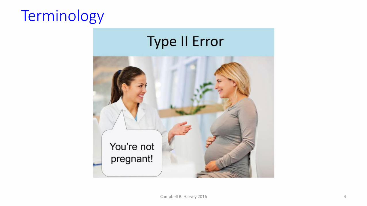
Rare Effects: 500 Shades of Gray
Researchers decided to replicate before submitting results for publication in a top journal• Replication saw no significant difference• P-value was 0.59 (not even close to significant)
13Campbell R. Harvey 2016

Rare Effects: 500 Shades of Gray
Lesson: If the hypothesis is unlikely, then we need to be especially careful. There will be a lot of false positives using standard testing procedures. Ideally, we incorporate information in the testing procedure when we know the effect is rare.
14Campbell R. Harvey 2016

Rare Effects: Medicine
Fact: 1% of women aged 40-50 have breast cancer• 90% of breast cancers correctly identified with mammogram• There is a 10% error rate
Question:Suppose the test comes back positive. What is the probability you have breast cancer?
15Campbell R. Harvey 2016

Rare Effects: Medicine
• Sample size=1,000, 10 true cases• Test 90% accurate, 9/10 of women with cancer will test
significant. What about the remaining 990 tests?
16Campbell R. Harvey 2016

Rare Effects: Medicine
• Sample size=1,000, 10 true cases• Test 90% accurate, 9/10 of women with cancer will test
significant. What about the remaining 990 tests? • 99/990 will be false significant
Given a significant test, what is the probability of cancer? 9/(9+99) = 8%
17Campbell R. Harvey 2016

What about Finance?
Performance of trading strategyis very impressive. • SR=1• Consistent• Drawdowns acceptable
Source: AHL Research
18Campbell R. Harvey 2016

What about Finance?
Source: AHL Research
19Campbell R. Harvey 2016

What about Finance?Sharpe = 1
Sharpe = 2/3
Sharpe = 1/3
Source: AHL Research
200 random time-seriesmean=0; volatility=15%
20Campbell R. Harvey 2016

Other Sciences?
Particle Physics Higg’s boson proposed in 1964 (same year as Sharpe
published the CAPM) First tests of the CAPM in 1972 and
Nobel award in 1990. Longer road for Higgs: $5 billion to construct LHC. “Discovered” in 2012. Nobel 2013.
21Campbell R. Harvey 2016

Other Sciences?
Particle Physics Testing method very important Particle rare and decays quickly and the key is measuring the
decay signature Frequency is 1 in 10 billion collisions and over a quadrillion
collisions were conducted Problem is that the decay signature could also be caused by
normal events from known processes
22Campbell R. Harvey 2016

Other Sciences?
Particle Physics The two groups involved in testing (CMS and ATLAS) decided
on what appears to be a tough standard: t-ratio must exceed 5
23Campbell R. Harvey 2016

Terminology
P-value (probability value, low value is good) In a test, we want a low chance of a Type I error (false positive)
and usually set the significance level at 5%. (Often referred to as 95% confidence.) This is the 2-sigma rule. If the effect is two standard deviations
or more from zero, then there is roughly only a 5% chance of a Type I error. Ideally, we look for more than 2-sigma (smaller p-values)
24Campbell R. Harvey 2016

Examples in Financial Economics
Two sigma rule only appropriate for a single test As we do more tests, there is a chance we find something “significant” (by the two
sigma rule) but it is a fluke. Here is a simple way to see the impact of multiple tests:
# of tests 1 5 10 20 26 50 nProb of fluke 5% 23% 40% 64% 74% 92% 1-0.95^n
Alphabet
25Campbell R. Harvey 2016

Examples in Financial Economics
3.4 sigma strategy• Profitable during fin crisis• Zero beta vs. market, value,size, and momentum• Impressive performance recently
26Campbell R. Harvey 2016
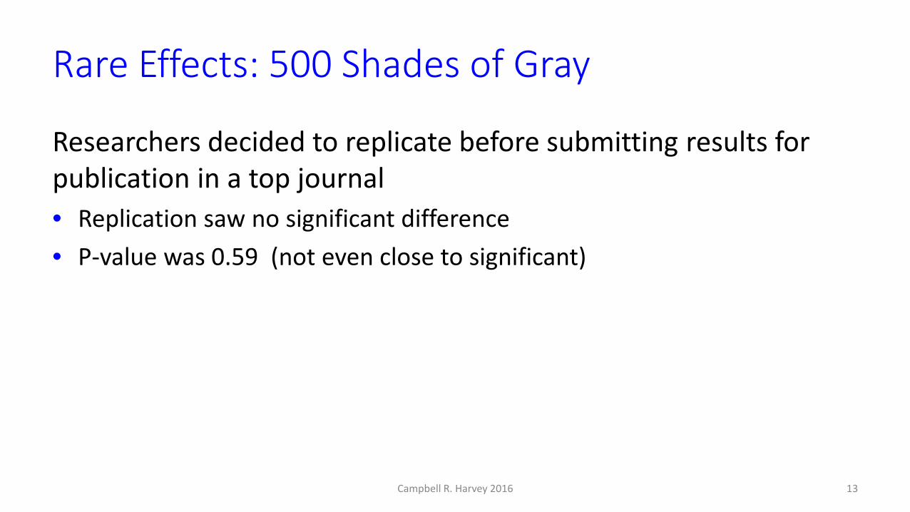
Examples in Financial Economics
Details• Long tickers “S”• Short tickers “U”
27Campbell R. Harvey 2016

Examples in Financial Economics
Research• Companies with meaningful ticker symbols, like Southwest’s LUV, and
show they outperform.1
• There is another study that argues that tickers that are easy to pronounce, like BAL vs. BDL, outperform in IPOs.2
• There is yet another study that suggests that tickers that are congruentwith the company’s name, outperform.3
281 Head, Smith and Watson, 2009; 2 Alter and Oppenheimer, 2006; 3 Srinivasan and Umashankar
Campbell R. Harvey 2016

Examples in Financial Economics
Product?
29
‘
Campbell R. Harvey 2016

Examples in Financial Economics
Product?
30
‘
Fortunately, …just a spoof Campbell R. Harvey 2016

Examples in Financial Economics
5 factors
31Campbell R. Harvey 2016

Examples in Financial Economics
15 factors
32Campbell R. Harvey 2016

Examples in Financial Economics82 factors
Source: The Barra US Equity Model (USE4), MSCI (2014)33Campbell R. Harvey 2016

Examples in Financial Economics
400 factors!
Source: https://www.capitaliq.com/home/who-we-help/investment-management/quantitative-investors.aspx34Campbell R. Harvey 2016

Examples in Financial Economics
18,000 signals examined in Yan and Zheng (2015)
35Campbell R. Harvey 2016

A framework to separate luck from skill
Three research initiatives:1. Explicitly adjust for multiple tests (“Backtesting”)2. Bootstrap (“Lucky Factors”)3. Noise reduction (“Rethinking Performance Evaluation”)
36Campbell R. Harvey 2016

1. Multiple Tests: Number of Factors and Publications
0
40
80
120
160
200
240
280
0
10
20
30
40
50
60
70
Cum
ulat
ive
Per y
ear
Factors and Publications
# of factors # of papers Cumulative # of factors
37Campbell R. Harvey 2016

1. Multiple Tests: How Many Discoveries Are False?
In multiple testing, how many tests are likely to be false? In single testing (significance level = 5%), 5% is the “error rate” (false
discoveries) In multiple testing, the false discovery rate (FDR) is usually much
larger than 5%
38Campbell R. Harvey 2016

1. Multiple Tests: Bonferroni's Method
Here is a simple adjustment called the Bonferroni adjustment For a single test, you are tolerant of 5% false discoveries Hence, a p-value of 5% or less means you declare a finding
“true” Bonferroni simply multiplies the p-value by the number of tests
39Campbell R. Harvey 2016

1. Multiple Tests: Bonferroni's Method
Bonferroni simply multiplies the p-value by the number of tests In a single test, if you get a p-value of 0.05 you declare
“significant” Returning to the ticker example, suppose the S-U portfolio has
a p-value of 0.02 – which appears very “significant” Bonferroni adjustment 26 x 0.02 = 0.52 which is “not
significant” – not even close!
40Campbell R. Harvey 2016

1. Multiple Tests: Rewriting HistoryHML MOM
MRT
EP SMB
LIQ
DEFIVOL
SRV
CVOL
DCG
LRV
316 factors in 2012 if working
papers are included
0
80
160
240
320
400
480
560
640
720
800
0.0
0.5
1.0
1.5
2.0
2.5
3.0
3.5
4.0
4.5
5.0
1965 1975 1985 1995 2005 2015 2025
Cum
ulat
ive
# of
fact
ors
t-ra
tio
BonferroniHolmBHYT-ratio = 1.96 (5%)
41Campbell R. Harvey 2016

1. Multiple Tests: A New Framework
No skill. Expected return = 0%
Skill. Expected return = 6%
42Campbell R. Harvey 2016

1. Multiple Tests: Harvey, Liu and Zhu Approach
Allows for correlation among strategy returns Allows for missing tests Review of Financial Studies, 2016
43Campbell R. Harvey 2016

1. Multiple Tests: Backtesting
Due to data mining, a common practice in evaluating backtests of trading strategies is to discount Sharpe ratios by 50% The 50% haircut is only a rule of thumb; we develop an
analytical way to determine the haircut
44Campbell R. Harvey 2016

1. Multiple Tests: Backtesting
Method Suppose we observe a strategy with an attractive Sharpe Ratio. This Sharpe Ratio directly implies a p-value (which roughly tells
you the probability that your strategy is a fluke) Suppose the p-value is 0.01 which looks pretty good.
45Campbell R. Harvey 2016

1. Multiple Tests: Backtesting
Method However, suppose you tried 10 strategies and picked the best
one The Bonferroni adjusted p-value is 10x0.01 = 0.10 which would
not be deemed “significant” Reverse engineer the 0.10 back to the “haircut” Sharpe Ratio*
*Note Tstat = SR√T 46Campbell R. Harvey 2016

1. Multiple Tests: Backtesting
Results: Percentage Haircut is Non-Linear
Journal of Portfolio Management
47Campbell R. Harvey 2016

2. Bootstrapping
Multiple testing approach has drawbacks Need to know the number of tests Need to know the correlation among the tests With similar sample sizes, this approach does not impact the
ordering of performance
*Note Tstat = SR√T 48Campbell R. Harvey 2016

2. Bootstrapping: Lucky Factors
Suppose we have 100 possible fund returns and 500 observations.Step 1. Strip out the alpha from all fund returns (e.g. regress on benchmark and use residuals). This means alpha and t-stat exactly equal zero – we have enforced “no skill”.Step 2. Bootstrap rows of the data to produce a new sheet 500x100* (note some rows sampled more than once and some not sampled at all)
*500x101 with the benchmark included49Campbell R. Harvey 2016

Insert animation here
50Campbell R. Harvey 2016

2. Bootstrapping: Lucky Factors
Step 3. Recalculate the alphas and t-stats on new data. Save the highest t-statistic from the 100 funds. Note, in the unbootstrapped data, every t-statistic is exactly zero.Step 4. Repeat steps 2 and 3 10,000 times.Step 5. Now that we have the empirical distribution of the max t-statistic under the null of no skill, compare to the max t-statistic in real data.
51Campbell R. Harvey 2016

2. Bootstrapping: Lucky Factors
Step 5a. If the max t-stat in the real data fails to exceed the threshold (95th percentile of the null distribution), stop (no fund has skill). Step 5b. If the max t-stat in the real data exceeds the threshold, declare the fund, say, F7, “true”
-6 -5 -4 -3 -2 -1 0 1 2 3 4 5 6
Bootstrap distributionof the max t-stat
95th percentile t=4.2
52Campbell R. Harvey 2016

2. Bootstrapping: Lucky Factors
Step 6. Replace the F7 (no skill) with the actual F7 (positive alpha). Step 7. Note that 99 funds have zero alpha and one fund has positive alpha.
53Campbell R. Harvey 2016

2. Bootstrapping: Lucky Factors
Step 8. Repeat Steps 3-5 but now we are saving the “second to max” and comparing to the second highest t-ratio in the real data.Step 9. Continue until the max ordered t-statistic in the data fails to exceed the max ordered from the bootstrap.
54Campbell R. Harvey 2016

2. Bootstrapping: Lucky Factors
Baseline model
YesAugmented model
No
Candidate factors
Terminate to arrive at the final model
55Campbell R. Harvey 2016

2. Bootstrapping: Lucky Factors
Addresses data mining directlyAllows for cross-correlation of the fund strategies because we are bootstrapping rows of dataAllows for non-normality in the data (no distributional assumptions imposed – we are resampling the original data)Potentially allows for time-dependence in the data by changing to a block bootstrap.Answers the questions: How many funds out-perform? Which ones were just lucky?
56Campbell R. Harvey 2016

2. Bootstrapping: Lucky Factors
57Campbell R. Harvey 2016

3. Noise reduction: Rethinking
Issue Past alphas do a poor job of predicting future alphas (e.g., top
quartile managers are about as likely to be in top quartile next year as this year’s bottom quartile managers!)
58Campbell R. Harvey 2016

3. Noise reduction: Rethinking
Issue This could be because all managers are unskilled (or all betas
are false betas) – or it could be a result of a lot of noise historical performance
59Campbell R. Harvey 2016

3. Noise reduction: Rethinking
Goal Develop a metric that maximizes cross-sectional predictability
of performance Useful for separating “skill” vs. “luck” and “smart” vs. “not-smart”
60Campbell R. Harvey 2016

3. Noise reduction: Rethinking
Observed performance consists of four components:• Alpha• True factor premia• Unmeasured risk (e.g. low vol strategy having negative convexity)• Noise (good or bad luck)
61Campbell R. Harvey 2016

3. Noise reduction: Rethinking
Intuition Current alpha is overfit. Regression maximizes the time-series
R2 for a particular fund. This time-series regression has nothing to do with cross-
sectional predictability. All of the noise will be put in the alpha. No surprise that past alphas have no ability to forecast future
alphas
62Campbell R. Harvey 2016

3. Noise reduction: Rethinking
Our approach We follow the machine learning literature and “regularize” the
problem by imposing a parametric distribution on the cross-section of alphas. Leads to lower time-series R2 – but higher cross-sectional R2
63Campbell R. Harvey 2016

3. Noise reduction: Rethinking
• t-stat = 3.9%/4.0% = 0.98 < 2.0• alpha = 0 cannot be ruled out
64Campbell R. Harvey 2016

3. Noise reduction: Rethinking
• Both t-stats < 2.0• alpha = 0 cannot be rejected for either
65Campbell R. Harvey 2016

3. Noise reduction: Rethinking
• t-stat < 2.0 for all funds• alpha = 0 cannot be excluded for all• However, population mean seems to
cluster around 4.0%. Should we declare all alphas as zero?
Estimated alphas cluster around 4.0%
66Campbell R. Harvey 2016

3. Noise reduction: Rethinking
• Although no individual fund has a statistically significant alpha, the population mean seems to be well estimated at 4.0%.
67Campbell R. Harvey 2016

3. Noise reduction: Rethinking
68Campbell R. Harvey 2016

3. Noise reduction: Rethinking
• An exemplar outperforming fund
69Campbell R. Harvey 2016

3. Noise reduction: Rethinking
• In-sample: 1984-2001; Out-of-sample: 2002-2011 In-sample,
𝒕𝒕𝑶𝑶𝑶𝑶𝑶𝑶NRA forecast
error (%)OLS forecast
error (%)# of funds
(-∞, -2.0) 3.29 6.61 64
[-2.0, -1.5) 3.09 3.70 75
[-1.5, 0) 2.75 2.92 565
[0, 1.5) 2.61 5.54 610
[1.5, 2.0) 2.38 10.47 87
[2.0, +∞) 2.77 12.02 87
Overall 2.71 5.17 1,488
*Mean absolute forecast errors.70Campbell R. Harvey 2016
Final perspectives
Combination of: propensity for Type I errors, incorrect testing methods, and lack of effort to reduce noise implies Most published empirical research findings are likely false Most managers are just “lucky” Most the smart beta products are not “smart” No predictability in performance
My research makes progress on goal of identifying repeatable performance
There are a host of other issues: Factor loadings also noisy Ex-post factor loading unfairly punish market timers It is essential to look beyond the Sharpe Ratio and incorporate other info
71Campbell R. Harvey 2016
CreditsJoint work with
Yan LiuTexas A&M University
Based on our joint work:
“… and the Cross-section of Expected Returns”http://ssrn.com/abstract=2249314 [Best paper in investment, WFA 2014]
“Backtesting”http://ssrn.com/abstract=2345489 [Bernstein Fabozzi/Jacobs-Levy best paper, JPM 2015]
“Evaluating Trading Strategies” [Bernstein Fabozzi/Jacobs-Levy best paper, JPM 2014]http://ssrn.com/abstract=2474755
“Lucky Factors”http://ssrn.com/abstract=2528780
“Rethinking Performance Evaluation”http://ssrn.com/abstract=2691658
72Campbell R. Harvey 2016

Supplement: Changing your beliefs
Three experiments:1. The musicologist2. The tea drinker3. The bar patron
73Campbell R. Harvey 2016

Supplement: Changing your beliefs
Musicologist claims to be able to identify from unlabeled score whether Haydn or Mozart is the composer
Simple experiment: 10 pairs of scores. Musicologist gets 10/10 correct74Campbell R. Harvey 2016
Presenter
Presentation Notes
Sonata #11 K 331 Sonata in F, H XVI:23

Supplement: Changing your beliefs
Tea drinker claims to be able to identify whether milk was in the tea cup before the tea was poured
Simple experiment: 10 pairs of tea cups. The tea drinker gets 10/10 correct75Campbell R. Harvey 2016

Supplement: Changing your beliefs
Bar patron claims that alcohol enables him to foresee the future
Simple experiment: Flip coin 10 times. Drunk gets 10/10 correct. 76Campbell R. Harvey 2016

Supplement: Changing your beliefs
All three experiments have the identical p-value:0.510=0.000977 (or p-value<0.001)
• This means there is less than 1 out a 1000 chance that what we observed is consistent with the null hypothesis (no ability to choose correct answers)
• Though p-values are identical, the results have different impacts on our beliefs
77Campbell R. Harvey 2016

Supplement: Changing your beliefs
Three experiments:1. The musicologist: We already know she is an expert. Indeed, it
is not even clear that we need to do the experiment. Are beliefs are barely impacted.
2. The tea drinker: We might have been bit skeptical of this long time tea drinker. However, after these results, the plausibility of claim is greatly strengthened and our beliefs shift.
3. The bar patron: The hypothesis is preposterous. P-value of 0.001 or even lower would not change our beliefs.
78Campbell R. Harvey 2016

See
The Scientific Outlook in Financial Economics, Presidential Address to the American Finance Association, forthcoming, Journal of Finance https://ssrn.com/abstract=2893930
The Scientific Outlook in Financial Economics: Transcript and Presentation Slides https://ssrn.com/abstract=2895842
79Campbell R. Harvey 2016