New Approach for Sparse Matrix Classification

Based on Deep Learning Techniques

Juan C. Pichel and Beatriz Pateiro-López

Version: post-print

HOW TO CITE

J. C. Pichel and B. Pateiro-López (2018), A New Approach for Sparse Matrix

Classification Based on Deep Learning Techniques, 2018 IEEE International

Conference on Cluster Computing (CLUSTER), Belfast, pp. 46-54. doi:

10.1109/CLUSTER.2018.00017

FUNDING

Research has been funded by project INNPAR2D (reference code MTM2016-76969-

P), from the Ministry of Economy and Competitiveness and the European Regional

Development Fund (ERDF).

A New Approach for Sparse Matrix Classification Based on Deep

Learning Techniques∗

Juan C. Pichel1 and Beatriz Pateiro-Lopez2

1CiTIUS, Universidade de Santiago de Compostela, Spain2Dpto. de Estadıstica, Analisis Matematico y Optimizacion Universidade de Santiago de

Compostela, Spaine-mail: {juancarlos.pichel,beatriz.pateiro}@usc.es

Abstract

In this paper, a new methodology to select the beststorage format for sparse matrices based on deeplearning techniques is introduced. We focus on theselection of the proper format for the sparse matrix-vector multiplication (SpMV), which is one of themost important computational kernels in many sci-entific and engineering applications. Our approachconsiders the sparsity pattern of the matrices as animage, using the RGB channels to code several ofthe matrix properties. As a consequence, we gener-ate image datasets that include enough informationto successfully train a Convolutional Neural Network(CNN). Considering GPUs as target platforms, thetrained CNN selects the best storage format 90.1%of the time, obtaining 99.4% of the highest SpMVperformance among the tested formats.

Sparse matrix, Classification, Deep Learning,CNN, Performance

1 Introduction

Sparse matrix-vector multiplication (SpMV) is a keykernel at the core of many scientific and engineeringapplications. SpMV is notorious for sustaining low

∗This work has been supported by MINECO (TIN2014-54565-JIN and MTM2016-76969-P), Xunta de Galicia(ED431G/08) and European Regional Development Fund.

fractions of the peak performance on modern parallelarchitectures. As a consequence, it has attracted a lotof attention from the research community to developefficient and optimized implementations. The perfor-mance of the SpMV depends on both the target hard-ware platform and the sparsity structure of the ma-trix. For this reason many storage formats have beenproposed for a particular application domain, matrixstructure and computer architecture [1]. It has beendemonstrated that the selection of the proper stor-age format has a big impact on the SpMV perfor-mance. The compressed sparse row (CSR) format isthe de-facto standard representation for CPUs, whilethere is no a dominant format for GPUs. We findthe cause in several factors that often conflict witheach other [2]: maximizing coalesced memory access,minimizing thread divergence and maximizing warpoccupancy.

In this paper we address the problem of the auto-matic selection of the best storage format for sparsematrices on GPUs. With this goal in mind a newmethodology based on deep learning technologies isintroduced. In particular, we have considered Con-volutional Neural Networks (CNNs), which are themost important deep learning networks for imagerecognition and classification. Our goal is to demon-strate that a simple standard CNN architecture asAlexNet [3] is powerful enough to provide very goodclassification results. Therefore, it is not necessary to

1

build an ad-hoc CNN architecture to deal with theproblem. In this way, our methodology can be easilyadopted by the research community since AlexNet isavailable in the most important and common deeplearning frameworks. To train the network the spar-sity pattern of the matrices is considered as an im-age. Since the input size of CNNs is fixed, originalsparse matrices are scaled down to fit the CNN insuch a way that pixels in the images represent sub-matrices. The RGB color of pixels is used to repre-sent properties of the matrix. In this way, we createimage datasets with enough information to success-fully train a CNN. An exhaustive experimental eval-uation has been carried out using two different GPUsas target platforms. Results show the benefits of ourmethodology in terms of the global accuracy of the re-sulting classifiers, reaching values above 90%. In ad-dition, we are able to obtain within 99.4% on averageof the best SpMV performance available. Finally, wedemonstrate that using a pre-trained model speedsup the training process with respect to training thenetwork for each GPU from scratch.

The paper is structured as follows. Section 2 ex-plains the background of the work. Section 3 intro-duces the deep learning methodology to deal with thesparse matrix classification problem. Experimentalresults are shown and discussed in Section 4. Relatedwork is presented in Section 5. Finally, the main con-clusions derived from the work together with someideas for future work are explained.

2 Background

2.1 Sparse Matrix Formats

For a sparse matrix, substantial memory require-ment reductions can be obtained by storing only thenonzero entries. There exist many different stor-age formats (an exhaustive list can be found in [1]),being ones more appropriate than others for a par-ticular sparse matrix depending on the number anddistribution of its nonzeros. These formats differ interms of the amount of storage required, the accessingmethods, and their adaptability to different applica-tions or parallel architectures such as GPUs. Some of

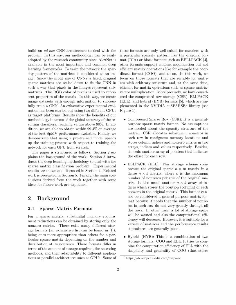
these formats are only well suited for matrices witha particular sparsity pattern like the diagonal for-mat (DIA) or block formats such as BELLPACK [4],other formats support efficient modification but notefficient matrix operations like for example the coor-dinate format (COO), and so on. In this work, wefocus on those formats that are suitable for matri-ces with arbitrary structure and, at the same time,efficient for matrix operations such as sparse matrix-vector multiplication. More precisely, we have consid-ered the compressed row storage (CSR), ELLPACK(ELL), and hybrid (HYB) formats [5], which are im-plemented in the NVIDIA cuSPARSE1 library (seeFigure 1):

• Compressed Sparse Row (CSR): It is a general-purpose sparse matrix format. No assumptionsare needed about the sparsity structure of thematrix. CSR allocates subsequent nonzeros ineach row in contiguous memory locations andstores column indices and nonzero entries in twoarrays, indices and values respectively. Besides,it needs another array of pointers that indicatesthe offset for each row.

• ELLPACK (ELL): This storage scheme com-presses the original sparse n × m matrix in adense n × k matrix, where k is the maximumnumber of nonzeros per row of the original ma-trix. It also needs another n × k array of in-dices which stores the position (column) of eachnonzero in the original matrix. This format can-not be considered a general-purpose matrix for-mat because it needs that the number of nonze-ros in each row do not vary greatly through allthe rows. In other case, a lot of storage spacewill be wasted and also the computational effi-ciency will decrease. However, it is suitable for avariety of matrices and the performance resultsit produces are generally good.

• Hybrid (HYB): This is a combination of twostorage formats: COO and ELL. It tries to com-bine the computation efficiency of ELL with thesimplicity and generality of COO (that stores

1https://developer.nvidia.com/cusparse

2

Column Indices

0 2 3 1 4 0 2 3 0 4

0 3 5 7 8 10 Row Pointers

Data values

0 0 1 2 3 4

1 2 3 4 Compressed Sparse Row (CSR) ELLPACK (ELL)

Column Indices

Data values

0

103

0

4

42*

2

*

***

3

**

***

Figure 1: CSR and ELL sparse matrix storage formats.

row and column indices explicitly). The ma-jority of the matrix entries are stored in ELLformat, and those rows with a substantially dif-ferent number of nonzeros are stored in COOformat.

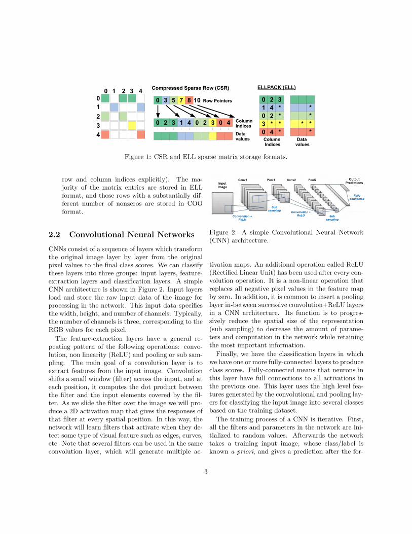
2.2 Convolutional Neural Networks

CNNs consist of a sequence of layers which transformthe original image layer by layer from the originalpixel values to the final class scores. We can classifythese layers into three groups: input layers, feature-extraction layers and classification layers. A simpleCNN architecture is shown in Figure 2. Input layersload and store the raw input data of the image forprocessing in the network. This input data specifiesthe width, height, and number of channels. Typically,the number of channels is three, corresponding to theRGB values for each pixel.

The feature-extraction layers have a general re-peating pattern of the following operations: convo-lution, non linearity (ReLU) and pooling or sub sam-pling. The main goal of a convolution layer is toextract features from the input image. Convolutionshifts a small window (filter) across the input, and ateach position, it computes the dot product betweenthe filter and the input elements covered by the fil-ter. As we slide the filter over the image we will pro-duce a 2D activation map that gives the responses ofthat filter at every spatial position. In this way, thenetwork will learn filters that activate when they de-tect some type of visual feature such as edges, curves,etc. Note that several filters can be used in the sameconvolution layer, which will generate multiple ac-

InputImage

Conv1 Conv2Pool1 Pool2 OutputPredictions

Fullyconnected

Sub sampling

Sub sampling

Convolution + ReLUConvolution +

ReLU

Figure 2: A simple Convolutional Neural Network(CNN) architecture.

tivation maps. An additional operation called ReLU(Rectified Linear Unit) has been used after every con-volution operation. It is a non-linear operation thatreplaces all negative pixel values in the feature mapby zero. In addition, it is common to insert a poolinglayer in-between successive convolution+ReLU layersin a CNN architecture. Its function is to progres-sively reduce the spatial size of the representation(sub sampling) to decrease the amount of parame-ters and computation in the network while retainingthe most important information.

Finally, we have the classification layers in whichwe have one or more fully-connected layers to produceclass scores. Fully-connected means that neurons inthis layer have full connections to all activations inthe previous one. This layer uses the high level fea-tures generated by the convolutional and pooling lay-ers for classifying the input image into several classesbased on the training dataset.

The training process of a CNN is iterative. First,all the filters and parameters in the network are ini-tialized to random values. Afterwards the networktakes a training input image, whose class/label isknown a priori, and gives a prediction after the for-

3

ward propagation step (convolution, ReLU and pool-ing operations along with forward propagation in thefully-connected layers). A prediction error is calcu-lated comparing the output of the network and theexpected result. The training process (by means ofback propagation) revises the network parameters it-eratively to minimize the overall error on each train-ing input. The network will be trained on the inputdataset for a given number of epochs (that is, passesover the entire image dataset). Note that parameterslike number of filters, filter sizes, architecture of thenetwork, etc., do not change during the training pro-cess. There are additional parameters in the trainingprocess known as hyperparameters such as the learn-ing rate or number of epochs that should be tuned tomake networks train better and faster.

Many CNN architectures have been proposed,some of the most popular are LeNet [6], AlexNet [3],GoogLeNet [7], VGGNet [8] and ResNet [9]. In thispaper we have used AlexNet, which has five convo-lution layers of decreasing filter size, three poolinglayers, and three fully-connected layers with approxi-mately 60 million free parameters. Although AlexNetis relatively simple with respect to other standardnetworks, we demonstrate in the following sectionsthat it is powerful enough to deal with the sparsematrix format selection problem.

3 Methodology

In this section a new methodology to select the beststorage format for sparse matrices based on deeplearning techniques is introduced. In particular, wehave focused on the selection of the proper formatfor the sparse matrix-vector multiplication (SpMV),which is one of the most important computationalkernels in scientific and engineering applications.

Figure 3 shows the different phases of our ap-proach. We assume that a large set of sparse matricescoming from different real problems and representinga variety of characteristics and nonzero patterns isavailable. This dataset will be used as input of theSpMV benchmarking and image generation phase.The goal of the first step is to evaluate for all thematrices in the dataset the performance of the SpMV

kernel when different storage formats are considered.As a result we obtain the best format in terms of per-formance for each matrix. That format associates alabel (class) to each matrix in the dataset, which willbe used later as ground truth in the CNN trainingphase. Therefore, there are as many classes as stor-age formats. Note that in this work we have consid-ered GPUs as hardware platforms to build the groundtruth information, but our methodology is completelyagnostic with respect to the underlying parallel sys-tem and can be applied, for example, to multicoreCPUs or accelerators as the Intel Xeon Phi.

The image dataset generation is the core of ourmethodology. To build the dataset we consider thesparsity pattern of the matrices as an image. Asa first approach, a n × m matrix is equivalent toa n × m binary image where a white pixel at loca-tion (i, j) represents a nonzero in row i and columnj. Black pixels correspond to zeros in the sparsitypattern. However, the size of the input to a CNN isfixed, so matrices of different sizes should be scaledto the same size. The following method explains howto scale a matrix. Let’s assume that the size of theinput image should be p × p pixels and, for simplic-ity, the considered sparse matrix is n × n (i.e., it isa square matrix), where n > p. We split the matrixinto p× p submatrices. To build the new p× p scaledmatrix, we insert a nonzero at position (i, j) if thereis, at least, one nonzero value in the correspondingsubmatrix (i, j). If the submatrix only contains ze-ros then the corresponding entry in the scaled matrixwill be zero. In this way, creating a p× p binary im-age from the scaled matrix is straightforward. Figure4(a) illustrates this procedure showing a 63× 63 pix-els image generated from a 71, 505 × 71, 505 sparsematrix.

The above method is a simple and easy way to gen-erate a binary image dataset that fits a CNN. How-ever, scaling down a sparse matrix simplifies the ap-pearance of its sparsity pattern, which could causea loss in the information provided to the CNN inthe training phase. Recall that a single pixel in theimage represents a submatrix in the original matrix.For instance, one pixel in Figure 4(a) corresponds toa 1, 135 × 1, 135 submatrix (that is, 71,505/63). Aswe demonstrate in Section 4, training the network

4

Figure 3: Scheme of the new classification methodology.

using the binary image dataset do not provide com-petitive results. In this way, it is necessary to provideadditional information to the CNN with the aim ofimproving the global accuracy of the classifier. Withthis goal in mind, we propose to use the RGB chan-nels of the image to code information related to somecharacteristics and properties of the original sparsematrix. In particular, we have considered the follow-ing global metrics about the matrices (numbers areused as identifier of the metric):

(0) Matrix size (n): number of rows and columns ofthe matrix.

(1) Average number of nonzeros per row of the ma-trix (nnzrow).

(2) Standard deviation of the number of nonzerosper row of the matrix (σrow).

(3) Matrix density (ρ): calculated as the ratio be-tween the number of nonzeros and the numberof rows multiplied by the number of columns.

(4) Maximum number of nonzeros in a row of thematrix (maxrow).

In our implementation pixels corresponding to emptysubmatrices are always black, that is, their RGB coloris (0, 0, 0). Only those pixels representing non-emptysubmatrices have a different associated RGB color.The color of these pixels is always the same, whosevalue for each RGB channel is within the interval[1, 255]. Metrics should be normalized to fit that in-terval (details about the normalization of our dataset

are provided in Section 4). Note that it is possibleto use one, two or three color channels to include thematrix information. When a channel is not used, itsvalue for all the pixels in the image is 0.

From now on the notation RxGyBz is used to in-dicate that metrics x, y and z were selected to calcu-late the R, G and B values of an image, respectively.There are multiple combinations of number of chan-nels and metrics that can be utilized in the imagedataset generation phase. In this paper we only showresults for the most relevant combinations in termsof performance. In particular, datasets were gen-erated using the following configurations: R1G2B3,R2G3B4, R1G3B4 and R0G1B4. In addition, for il-lustrative purposes, we have also included results fora binary image dataset (black and white pixels, with-out metrics) and R1 (using only the red channel tocode the average number of nonzeros per row of thematrix). Therefore, six different image datasets havebeen generated and analyzed in the paper. An ex-ample is shown in Figure 4 that displays the result-ing images obtained for the same input sparse matrixwhen considering different configurations. We musthighlight that the assignment of metrics to channelsdo not affect the results of the CNN training phase.It means that is irrelevant to consider, for instance,R1G2B3 or R3G1B2.

The next stage in our method involves the train-ing of the CNN. To do so, it is necessary to feed theCNN with a set of images labeled with their class(best storage format). This data was generated inthe previous phases: SpMV benchmarking and im-age generation. Note that the image dataset is di-

5

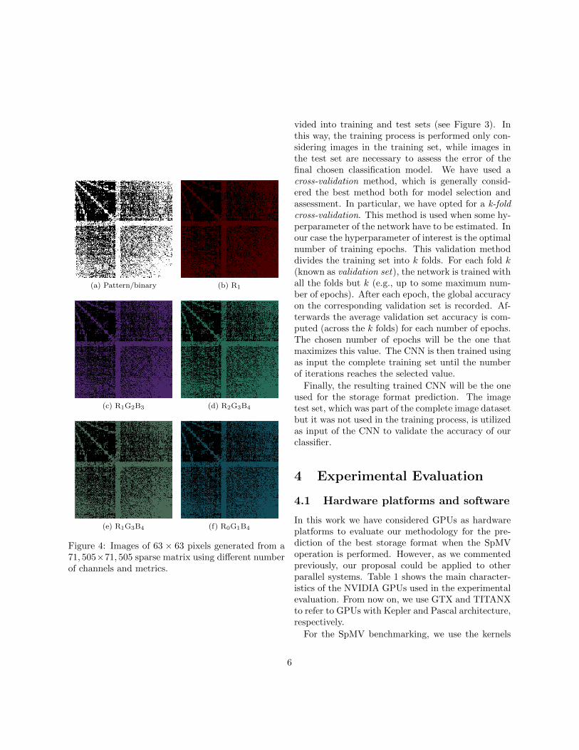
(a) Pattern/binary (b) R1

(c) R1G2B3 (d) R2G3B4

(e) R1G3B4 (f) R0G1B4

Figure 4: Images of 63 × 63 pixels generated from a71, 505×71, 505 sparse matrix using different numberof channels and metrics.

vided into training and test sets (see Figure 3). Inthis way, the training process is performed only con-sidering images in the training set, while images inthe test set are necessary to assess the error of thefinal chosen classification model. We have used across-validation method, which is generally consid-ered the best method both for model selection andassessment. In particular, we have opted for a k-foldcross-validation. This method is used when some hy-perparameter of the network have to be estimated. Inour case the hyperparameter of interest is the optimalnumber of training epochs. This validation methoddivides the training set into k folds. For each fold k(known as validation set), the network is trained withall the folds but k (e.g., up to some maximum num-ber of epochs). After each epoch, the global accuracyon the corresponding validation set is recorded. Af-terwards the average validation set accuracy is com-puted (across the k folds) for each number of epochs.The chosen number of epochs will be the one thatmaximizes this value. The CNN is then trained usingas input the complete training set until the numberof iterations reaches the selected value.

Finally, the resulting trained CNN will be the oneused for the storage format prediction. The imagetest set, which was part of the complete image datasetbut it was not used in the training process, is utilizedas input of the CNN to validate the accuracy of ourclassifier.

4 Experimental Evaluation

4.1 Hardware platforms and software

In this work we have considered GPUs as hardwareplatforms to evaluate our methodology for the pre-diction of the best storage format when the SpMVoperation is performed. However, as we commentedpreviously, our proposal could be applied to otherparallel systems. Table 1 shows the main character-istics of the NVIDIA GPUs used in the experimentalevaluation. From now on, we use GTX and TITANXto refer to GPUs with Kepler and Pascal architecture,respectively.

For the SpMV benchmarking, we use the kernels

6

Table 1: Main characteristics of the NVIDIA GPUs used in the tests.

Model GeForce GTXTITAN

TITAN X

Architecture Kepler PascalCUDA capability 3.5 6.1Multiprocessors (MP) 14 28CUDA Cores/MP 192 128GPU Max Clock rate (GHz) 0.88 1.53Global memory (MBytes) 6,082 12,190L2 Cache Size (MBytes) 1.5 3

implemented by the NVIDIA cuSPARSE library in-cluded in the CUDA toolkit version 8. CSR, HYBand ELL storage formats were studied (see Section 2for details). Training the CNN was also performedusing a GPU. In particular, the most powerful GPU(TITANX) was utilized with the aim of reducing thetraining times. NVIDIA Deep Learning GPU Train-ing System2 (DIGITS) was the selected software plat-form to carry out the training phase. DIGITS allowsto design, train and visualize deep neural networksfor image classification taking advantage of the deeplearning framework Caffe3. Several of the most im-portant CNN architectures such as LeNet, AlexNetand GoogLeNet are predefined and ready to use inthe platform.

4.2 Sparse matrix dataset

As we point out in Section 3, it is necessary to havea large set of sparse matrices in order to train thenetwork. This dataset should contain matrices com-ing from different real problems and applications. Inthis way, we expect that these matrices cover a widerange of characteristics and nonzero patterns. Wehave created a dataset that fulfills those assumptionsconsisting of 8,111 sparse matrices. The dataset wasgenerated using as basis 812 square matrices fromthe SuiteSparse matrix collection [10] and applyingto them some transformations like cropping (similarto [11]). The main characteristics of the dataset in

2https://developer.nvidia.com/digits3http://caffe.berkeleyvision.org

terms of the average, minimum and maximum valuesare displayed in Table 2.

4.3 SpMV benchmarking

To train the CNN, a class (best storage format)should be assigned to matrices in the dataset. This isthe goal of the SpMV benchmarking phase. We con-ducted experiments by measuring the performanceof the single precision SpMV kernel using differentstorage formats (CSR, HYB and ELL) on the con-sidered GPUs (see Table 1). For each matrix andformat, the performance was calculated as the aver-age of 1,000 SpMV operations. Each matrix is thenlabeled according to the highest performing format.The classification results expressed as the numberand percentage of matrices belonging to each classare displayed in Table 3. Note that there are no-ticeable differences in the classification depending onthe considered GPU. For example, we observe thatthe largest class is different on the two GPUs (ELLfor the GTX and CSR for the TITANX). This de-pendence on the hardware platform confirms the im-portance and difficulty of the issue addressed in thiswork.

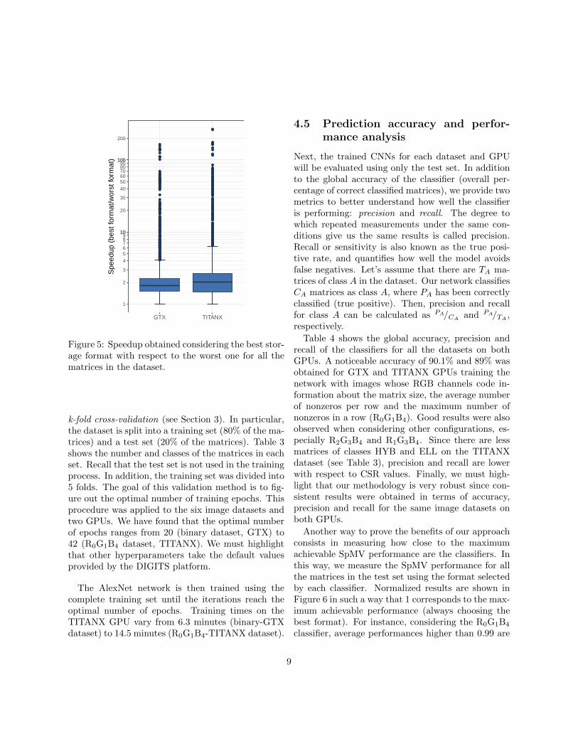
On the other hand, a bad choice of the storage for-mat will have a negative effect on the SpMV perfor-mance. Figure 5 illustrates this behavior measuringthe speedup between the best and the worst perform-ing formats for all the matrices in the dataset. Con-sidering the GTX platform, the boxplot shows thatthe median, first quartile and third quartile speedupsare 1.81×, 1.51× and 2.25×, respectively. It means

7

Table 2: Global metrics of the sparse matrices in the dataset.

Avg. Min. Max.

Number of rows/columns (n) 153.3K 1.9K 21.2MNonzeros (nnz) 1.4M 120K 89.3MNonzeros per row (nnzrow) 29.03 0.08 1.26KStd. Dev. nonzeros per row (σrow) 27.02 0 1.81KDensity (ρ) 4.35×10−3 4.08×10−8 2.82×10−1

Maximum nonzeros in a row (maxrow) 1.84K 1 2.31M

Table 3: Classes of the matrices in the complete dataset (left), and only considering matrices for training(middle) and tests (right).

Dataset Training set Test set

Class GTX TITANX GTX TITANX GTX TITANX

CSR 2,661[32.8%]

4,612[56.9%]

2,128[32.8%]

3,689[56.9%]

533 [32.8%] 923 [56.9%]

HYB 1,882[23.2%]

1,455[17.9%]

1,505[23.2%]

1,164[17.9%]

377 [23.2%] 291 [17.9%]

ELL 3,568[44.0%]

2,044[25.2%]

2,855[44.0%]

1,635[25.2%]

713 [44.0%] 409 [25.2%]

Total 8,111 6,488 1,623

that for 50% of the matrices choosing the best storageformat accelerates the SpMV operation more than1.81×. The median, first quartile and third quar-tile speedups for the TITANX are 1.47×, 2.05× and2.66×. In addition, we have detected some outliers(points in the plots) where the SpMV is performedfrom tenths to hundreds of times faster when choos-ing the proper format. Therefore, a misprediction inthe classification may lead to important performancedegradations.

4.4 Image dataset generation & Net-work training

Several of the characteristics in Table 2 correspondto the global metrics detailed in Section 3. Metricsshould be normalized to fit the interval [1,255] sincetheir values will be assigned to a RGB color channelin the images. The way this normalization is per-formed has an impact on the results of the classifier.As a consequence, many experiments have been car-

ried out in order to find out the best normalizationmethod. Next, we detail how the RGB values werecalculated for the image datasets used in the evalua-tion (numbers identify the corresponding metric):

(0) b n4000c+ 1

(1) nnzrow = nnzn (no normalization is required)

(2) σrow (no normalization is required)

(3) b100000× nnzn×nc+ 1

(4) bmaxrow

4 c+ 1

In case some of the previous values exceeds 255 fora particular matrix, the corresponding color in theimage will be automatically fixed to 255.

We have generated and studied six different im-age datasets: binary image dataset (no metrics),R1,R1G2B3, R2G3B4, R1G3B4 and R0G1B4. Thesize of the images is always 256×256 pixels, whichcorresponds to the input size for the AlexNet net-work. To train the AlexNet network we have used a

8

●●

●

●●

●

●

●●●

●

●

●●

●

●●

●●

●

●

●●

●

●

●

●

●●

●●

●●

●

●

●

●

●

●

●

●

●

●

●●

●

●

●

●

●

●

●

●

●

●

●

●

●

●

●

●

●

●●

●

●

●

●

●

●●

●

●

●

●

●●

●

●

●

●

●

●

●

●

●

●

●

●

●

●●●

●

●

●

●

●

●

●

●

●

●

●

●

●

●

●●

●

●

●

●

●

●

●

●

●

●

●

●●●

●

●

●

●

●

●

●

●

●

●

●

●

●

●

●

●

●

●

●

●

●

●

●

●

●

●

●

●

●

●

●●

●

●

●

●

●

●

●

●

●

●

●

●

●

●

●

●

●

●

●

●

●

●●

●

●●

●

●

●

●

●

●

●●●

●

●●

●

●

●

●

●

●

●

●

●

●

●

●●

●

●

●

●

●

●

●

●

●

●

●

●

●

●

●

●

●

●●

●

●

●

●

●

●

●

●

●

●

●

●

●●

●

●

●

●

●

●

●

●●

●●

●

●

●

●

●

●

●

●●

●

●

●

●

●

●

●

●

●

●

●

●

●

●

●

●

●

●

●

●

●

●

●

●

●

●●

●

●

●

●

●●

●

●

●

●

●

●

●

●

●

●

●

●

●

●

●

●

●

●

●

●

●

●

●

●

●

●

●

●

●

●

●

●

●

●●

●

●

●

●

●

●

●

●

●

●

1

2

3

456789

1010

20

30

405060708090

100100

200

GTX TITANX

Spe

edup

(be

st fo

rmat

/wor

st fo

rmat

)

Figure 5: Speedup obtained considering the best stor-age format with respect to the worst one for all thematrices in the dataset.

k-fold cross-validation (see Section 3). In particular,the dataset is split into a training set (80% of the ma-trices) and a test set (20% of the matrices). Table 3shows the number and classes of the matrices in eachset. Recall that the test set is not used in the trainingprocess. In addition, the training set was divided into5 folds. The goal of this validation method is to fig-ure out the optimal number of training epochs. Thisprocedure was applied to the six image datasets andtwo GPUs. We have found that the optimal numberof epochs ranges from 20 (binary dataset, GTX) to42 (R0G1B4 dataset, TITANX). We must highlightthat other hyperparameters take the default valuesprovided by the DIGITS platform.

The AlexNet network is then trained using thecomplete training set until the iterations reach theoptimal number of epochs. Training times on theTITANX GPU vary from 6.3 minutes (binary-GTXdataset) to 14.5 minutes (R0G1B4-TITANX dataset).

4.5 Prediction accuracy and perfor-mance analysis

Next, the trained CNNs for each dataset and GPUwill be evaluated using only the test set. In additionto the global accuracy of the classifier (overall per-centage of correct classified matrices), we provide twometrics to better understand how well the classifieris performing: precision and recall. The degree towhich repeated measurements under the same con-ditions give us the same results is called precision.Recall or sensitivity is also known as the true posi-tive rate, and quantifies how well the model avoidsfalse negatives. Let’s assume that there are TA ma-trices of class A in the dataset. Our network classifiesCA matrices as class A, where PA has been correctlyclassified (true positive). Then, precision and recallfor class A can be calculated as PA/CA

and PA/TA,

respectively.

Table 4 shows the global accuracy, precision andrecall of the classifiers for all the datasets on bothGPUs. A noticeable accuracy of 90.1% and 89% wasobtained for GTX and TITANX GPUs training thenetwork with images whose RGB channels code in-formation about the matrix size, the average numberof nonzeros per row and the maximum number ofnonzeros in a row (R0G1B4). Good results were alsoobserved when considering other configurations, es-pecially R2G3B4 and R1G3B4. Since there are lessmatrices of classes HYB and ELL on the TITANXdataset (see Table 3), precision and recall are lowerwith respect to CSR values. Finally, we must high-light that our methodology is very robust since con-sistent results were obtained in terms of accuracy,precision and recall for the same image datasets onboth GPUs.

Another way to prove the benefits of our approachconsists in measuring how close to the maximumachievable SpMV performance are the classifiers. Inthis way, we measure the SpMV performance for allthe matrices in the test set using the format selectedby each classifier. Normalized results are shown inFigure 6 in such a way that 1 corresponds to the max-imum achievable performance (always choosing thebest format). For instance, considering the R0G1B4

classifier, average performances higher than 0.99 are

9

Table 4: Prediction accuracy of the trained network considering different image datasets on the GTX (top)and TITANX (down) platforms.

GTX Binary R1 R1G2B3 R2G3B4 R1G3B4 R0G1B4

Rec. Prec. Rec. Prec. Rec. Prec. Rec. Prec. Rec. Prec. Rec. Prec.

CSR 0.62 0.70 0.79 0.73 0.84 0.81 0.87 0.86 0.89 0.86 0.90 0.90HYB 0.63 0.72 0.53 0.80 0.73 0.90 0.82 0.91 0.82 0.92 0.82 0.90ELL 0.80 0.69 0.84 0.75 0.89 0.83 0.91 0.88 0.92 0.90 0.95 0.90

Global Accuracy 0.702 0.750 0.836 0.876 0.888 0.901

TITANX Binary R1 R1G2B3 R2G3B4 R1G3B4 R0G1B4

Rec. Prec. Rec. Prec. Rec. Prec. Rec. Prec. Rec. Prec. Rec. Prec.

CSR 0.85 0.75 0.86 0.62 0.91 0.91 0.94 0.91 0.95 0.91 0.94 0.93HYB 0.43 0.78 0.46 0.69 0.68 0.65 0.72 0.92 0.71 0.93 0.71 0.95ELL 0.61 0.60 0.74 0.66 0.87 0.77 0.86 0.80 0.87 0.80 0.91 0.78

Global Accuracy 0.713 0.758 0.861 0.879 0.885 0.890

achieved for both GPUs. It means that the differencein the SpMV performance between the best possi-ble classification and the one obtained by our clas-sifier is less than 1%. Therefore, considering onlythe global accuracy, precision and recall to evaluatethe quality of classifiers for sparse matrix classifica-tion hide important information regarding the per-formance. Since the final objective of choosing theproper storage format is obtain the maximum SpMVperformance, the above analysis is of great impor-tance.

4.6 Speeding up the training process

As we pointed out previously the classes of the ma-trices depend on the hardware platform consideredin the SpMV benchmarking phase. As a consequencenetworks should be trained for each particular GPU.However, next we will demonstrate that it is not nec-essary to carry out the training process from scratch.

The idea is to consider a pre-trained model as start-ing point of the training process instead of consid-ering the AlexNet network initialized with randomvalues (i.e., training from scratch). This pre-trainedmodel corresponds to a CNN trained for a differentGPU. In this way, the network inherits many param-eters which captured important characteristics and

features from the considered storage formats and ma-trices in the dataset. In addition, we must take intoaccount that classes of the matrices differ betweenGPUs, but not for all the dataset.

As a result of using this methodology very goodaccuracy results are obtained with less training datain comparison to training from scratch. Therefore,since the data required to train the network decrease,training times are also lower. Figure 7 illustrates thisbehavior training a classifier for GTX using a pre-trained TITANX model. In this example we haveconsidered the R0G1B4 image dataset. For instance,we get a 88.1% and 89% accuracies training the net-work using only 30% and 50% of the training data,respectively.

Another important consequence of reducing thetraining data size is the impact on the SpMV bench-marking phase (see Figure 3). This is the most timeconsuming phase, requiring several hours to obtainthe best storage format (class) for all the dataseton each GPU. Note that it requires to perform theSpMV operation 1,000 times for each matrix and for-mat. In this way, it is possible to reduce noticeablythe benchmarking times while achieving very goodperformance in terms of accuracy.

10

0.9

0.92

0.94

0.96

0.98

1

No

rmal

ized

P

erfo

rman

ce

GTX

TITANX

R0G

1B

4

R1G

3B

4

R2G

3B

4

R1G

2B

3

R1

Pattern

Figure 6: Average SpMV performance obtained usingthe storage format selected by the classifiers.

5 Related Work

We can find in the literature many analytical ap-proaches that deal with the identification of the opti-mal sparse matrix format for GPUs based on perfor-mance models [12–14]. They show a good accuracybut models are usually tested considering a small setof matrices. Other authors use traditional machinelearning approaches to select automatically the beststorage format for sparse matrices. Only some ofthem focus on GPUs as target platforms. In [2], theauthors build a decision tree to choose the best repre-sentation for a given sparse matrix based on a severalmatrix structure features. Their classifiers report aglobal accuracy in the range 64.6-83.8%, obtaining a95% of the maximum achievable SpMV performance.A similar approach that takes advantage of supportvector machines to deal with the classification prob-lem was published in [15]. They demonstrated accu-racies in the range 73-88.5%, increasing the obtainedaverage SpMV performance up to 98%. We musthighlight that the best results in both works are be-

5% 10% 20% 30% 40% 50% 75%0.8

0.81

0.82

0.83

0.84

0.85

0.86

0.87

0.88

0.89

0.9

Training dataset size

Glo

bal A

ccur

acy

0

200

400

600

800

Tra

inin

g tim

e (s

econ

ds)

Figure 7: Global accuracy (blue line) and times(green line) required to train a GTX classifier usingas basis a pre-trained TITANX model.

low the numbers obtained using our approach. Inaddition, the maximum accuracy observed in bothworks was always obtained training the classifiers us-ing feature sets with more than three matrix prop-erties. None of the works commented above haveconsidered deep learning technologies. In a recentpaper [11] the authors deal with the sparse matrixformat selection problem using CNNs. They proposeseveral ways to represent the matrices to train thenetwork. Best results are achieved using histogramsthat capture the spatial distribution of nonzero ele-ments in the matrix. Unlike our approach, they donot take advantage of the RGB channels of the imagesto code some features of the matrices. Using theirrepresentation leads the authors to create an ad-hocCNN architecture. Our approach demonstrates thata simple standard CNN architecture as AlexNet isenough to provide good classification results. In thisway, our methodology can be easily adopted by theresearch community since AlexNet is available in themost important and common deep learning frame-works. In addition, AlexNet could be easily replacedin the future by other standard architectures such asVGGNet [8] and ResNet [9] in order to improve theaccuracy results or speed up the learning process.

Other papers focus only on applying machine

11

learning techniques to multicore processors [16]. Fi-nally, in [17] the authors propose a mechanism toselect the best SpMV code implementation for bothCPUs and GPUs using deep learning technologies.It is an interesting work conceptually but their ap-proach obtains low accuracy results (only 54%) with75% of the maximum attainable performance.

6 Conclusions

In this work we demonstrated that deep learningtechnologies can be successfully applied to classifica-tion problems different from the traditional machinelearning tasks. We focused on the selection of thebest storage format for the SpMV kernel on GPUs.A new methodology is introduced based on the ideaof considering the sparsity pattern of the matrices asan image. Coding several matrix characteristics asthe RGB color of the pixels in the images, we areable to generate image datasets with enough infor-mation to successfully train a CNN. We prove that asimple trained CNN architecture as AlexNet, withoutany fine-tuning, achieves very good results in terms ofaccuracy, precision, recall and average SpMV perfor-mance. In particular, we observed a maximum globalaccuracy of 90.1%, obtaining within 99.4% on aver-age of the best performance available. In addition,we demonstrate that it is possible to speed up thetraining process using a pre-trained model as start-ing point instead of training from scratch. Using apre-trained model reduces the requirements of train-ing data to obtain high global accuracies.

As future work we will deal with the classificationproblem on GPUs and other parallel architecturesadding specialized storage formats [18–20]. In ad-dition, we will apply dimensionality reduction tech-niques such as Principal Component Analysis (PCA)to code more than three matrix properties in theRGB channels of the images with the aim of improv-ing the global accuracy of the classifiers.

References

[1] D. Langr and P. Tvrdık, “Evaluation Crite-ria for Sparse Matrix Storage Formats,” IEEETransactions on Parallel and Distributed Sys-tems, vol. 27, no. 2, pp. 428–440, 2016.

[2] N. Sedaghati, T. Mu, L.-N. Pouchet,S. Parthasarathy, and P. Sadayappan, “Auto-matic Selection of Sparse Matrix Representationon GPUs,” in 29th ACM on Int. Conf. on Su-percomputing (ICS), 2015, pp. 99–108.

[3] A. Krizhevsky, I. Sutskever, and G. E. Hin-ton, “ImageNet Classification with Deep Con-volutional Neural Networks,” in 25th Int. Conf.on Neural Information Processing Systems - Vol-ume 1, 2012, pp. 1097–1105.

[4] J. W. Choi, A. Singh, and R. W. Vuduc, “Model-driven Autotuning of Sparse Matrix-vector Mul-tiply on GPUs,” in 15th ACM SIGPLAN Sympo-sium on Principles and Practice of Parallel Pro-gramming (PPoPP), 2010, pp. 115–126.

[5] N. Bell and M. Garland, “Efficient SparseMatrix-Vector Multiplication on CUDA,”NVIDIA Corporation, NVIDIA TechnicalReport NVR-2008-004, Dec. 2008.

[6] Y. Lecun, L. Bottou, Y. Bengio, and P. Haffner,“Gradient-based learning applied to documentrecognition,” Proceedings of the IEEE, vol. 86,no. 11, pp. 2278–2324, 1998.

[7] C. Szegedy, W. Liu, Y. Jia, P. Sermanet,S. Reed, D. Anguelov, D. Erhan, V. Vanhoucke,and A. Rabinovich, “Going Deeper with Con-volutions,” in IEEE Conf. on Computer Visionand Pattern Recognition (CVPR), 2015, pp. 1–9.

[8] K. Simonyan and A. Zisserman, “VeryDeep Convolutional Networks for Large-Scale Image Recognition,” CoRR, vol.abs/1409.1556, 2014. [Online]. Available:http://arxiv.org/abs/1409.1556

[9] K. He, X. Zhang, S. Ren, and J. Sun,“Deep Residual Learning for Image Recogni-tion,” CoRR, vol. abs/1512.03385, 2015.

12

[10] T. A. Davis and Y. Hu, “The University ofFlorida Sparse Matrix Collection,” ACM Trans.Math. Softw., vol. 38, no. 1, pp. 1:1–1:25, 2011.

[11] Y. Zhao, J. Li, C. Liao, and X. Shen, “Bridgingthe gap between deep learning and sparse ma-trix format selection,” in Proc. of the 23rd ACMSIGPLAN Symposium on Principles and Prac-tice of Parallel Programming, 2018, pp. 94–108.

[12] P. Guo, L. Wang, and P. Chen, “A PerformanceModeling and Optimization Analysis Tool forSparse Matrix-Vector Multiplication on GPUs,”IEEE Transactions on Parallel and DistributedSystems, vol. 25, no. 5, pp. 1112–1123, 2014.

[13] B. Neelima, G. R. M. Reddy, and P. S.Raghavendra, “Predicting an Optimal SparseMatrix Format for SpMV Computation onGPU,” in IEEE Int. Parallel Distributed Pro-cessing Symposium Workshops, 2014, pp. 1427–1436.

[14] K. Li, W. Yang, and K. Li, “Performance Anal-ysis and Optimization for SpMV on GPU UsingProbabilistic Modeling,” IEEE Transactions onParallel and Distributed Systems, vol. 26, no. 1,pp. 196–205, 2015.

[15] A. Benatia, W. Ji, Y. Wang, and F. Shi, “SparseMatrix Format Selection with Multiclass SVMfor SpMV on GPU,” in 45th Int. Conf. on Par-allel Processing (ICPP), 2016, pp. 496–505.

[16] J. Li, G. Tan, M. Chen, and N. Sun, “SMAT: AnInput Adaptive Auto-tuner for Sparse Matrix-vector Multiplication,” in 34th ACM SIGPLANConf. on Programming Language Design andImplementation, 2013, pp. 117–126.

[17] H. Cui, S. Hirasawa, H. Takizawa, andH. Kobayashi, “A Code Selection MechanismUsing Deep Learning,” in IEEE MCSOC, 2016,pp. 385–392.

[18] A. Ashari, N. Sedaghati, J. Eisenlohr, andP. Sadayappan, “An Efficient Two-dimensionalBlocking Strategy for Sparse Matrix-vector Mul-tiplication on GPUs,” in Proc. of the 28th ACM

Int. Conf. on Supercomputing, 2014, pp. 273–282.

[19] M. Kreutzer, G. Hager, G. Wellein, H. Fehske,and A. Bishop, “A Unified Sparse Matrix DataFormat for Efficient General Sparse Matrix-Vector Multiplication on Modern Processorswith Wide SIMD Units,” SIAM Journal on Sci-entific Computing, vol. 36, no. 5, pp. C401–C423, 2014.

[20] D. Merrill and M. Garland, “Merge-based Par-allel Sparse Matrix-vector Multiplication,” inProc. of the Int. Conf. for High PerformanceComputing, Networking, Storage and Analysis(SC), 2016, pp. 58:1–58:12.

13