NEW AND ENHANCED CAPABILITIES IN RELEASE 8 OF THE SCA ...
203
NEW AND ENHANCED CAPABILITIES IN RELEASE 8 OF THE SCA STATISTICAL SYSTEM
Transcript of NEW AND ENHANCED CAPABILITIES IN RELEASE 8 OF THE SCA ...

NEW AND ENHANCED CAPABILITIES IN
RELEASE 8
OF THE SCA STATISTICAL SYSTEM


NEW AND ENHANCED CAPABILITIES IN
RELEASE 8
OF THE SCA STATISTICAL SYSTEM
Lon-Mu Liu William J. Lattyak
Scientific Computing Associates Corp. 525 N. Lincoln Avenue
Villa Park, Illinois 60181 U.S.A
Telephone: 630-834-4567 FAX: 630-834-1510 Email: [email protected] Website: www.scausa.com
Copyright © Scientific Computing Associates® Corp., 2007


TABLE OF CONTENTS
CHAPTER 1 ................................................................................................................................................................... 1
INTRODUCTION ............................................................................................................................................................ 1 New Features (Release 8.0) .................................................................................................................................... 2 Educational Edition ................................................................................................................................................ 2 Practitioner Edition ................................................................................................................................................ 3 Professional Edition (A) ......................................................................................................................................... 3 Professional Edition (B) ......................................................................................................................................... 4 Advanced Edition ................................................................................................................................................... 4
CHAPTER 2 ................................................................................................................................................................... 5
DATE HANDLING AND TIME SERIES AGGREGATION .................................................................................................... 5 2.1 Creating a Date Variable Using the DATEBUILD Command .................................................................... 5 2.2 Extracting Day-of-Week Information from a Date Variable Using DOWEEK ............................................ 7 2.3 Building Dummy Variables Using the DVECTOR Command ..................................................................... 9 2.4 Temporal Aggregation of a Time Series Using the DAGGREGATE Command ........................................ 11
CHAPTER 3 ................................................................................................................................................................. 15
UNIT ROOT TESTS ...................................................................................................................................................... 15 3.1 Dickey-Fuller Unit Root Tests ................................................................................................................... 15 3.2 Phillips-Perron Unit Root Tests ................................................................................................................. 17 3.3 Example: Canadian Real Exchange Rate .................................................................................................. 18
CHAPTER 4 ................................................................................................................................................................. 21
NEW IDENTIFICATION METHOD FOR SEASONAL TIME SERIES.................................................................................... 21
CHAPTER 5 ................................................................................................................................................................. 31
ENHANCED EXPERT ARIMA MODELING ................................................................................................................... 31
CHAPTER 6 ................................................................................................................................................................. 35
POWER TRANSFORMATION IN TIME SERIES FORECASTING ................................................................................ 35 6.1 Retransformation of Power Transformed Forecasts .................................................................................. 36 6.2 U.S. GNP Example of Retransformation.................................................................................................... 38
CHAPTER 7 ................................................................................................................................................................. 41
CAUSALITY TESTING ................................................................................................................................................. 41 7.1 Causality Testing Using Vector ARMA Models ......................................................................................... 41 7.2 A Decision Tree Approach for Detecting Dynamic Relationships ............................................................. 42 7.3 Test Statistic for Each Pair-wise Test ........................................................................................................ 47 7.4 Causal Relationships between Price and Interest Rate in the United States ............................................. 48 7.5 Causal Relationships between Housing Starts and Houses Sold in the United States (Based on Non-
Seasonally Adjusted Series) ....................................................................................................................... 51
CHAPTER 8 ................................................................................................................................................................. 55
INTRODUCTION TO NONLINEAR TIME SERIES ANALYSIS IN THE SCA SYSTEM .................................. 55
CHAPTER 9 ................................................................................................................................................................. 57
SEARCH FOR THE BEST POWER TRANSFORMATION FOR TIME SERIES FORECASTING ................................ 57

9.1 Procedures for Searching a Power Transformation .................................................................................. 58 9.2 Peak Electricity Load Forecasting Example of Power Transformation Search ........................................ 59
CHAPTER 10 ............................................................................................................................................................... 67
GARCH MODELING AND ANALYSIS................................................................................................................. 67
CHAPTER 11 ............................................................................................................................................................... 69
TIME SERIES MODELS WITH TIME-VARYING PARAMETERS ................................................................................. 69 11.1 Example of the TVPEXPLORE Command Using a Day-of-Week Effect Model ................................... 69 11.2 Example of TVPEXPLORE in the Context of Simple Moving Averages ............................................... 75
CHAPTER 12 ............................................................................................................................................................... 77
WEIGHTED TIME SERIES MODEL ESTIMATION AND FORECASTING ............................................................... 77 12.1 Model Estimation Using the Weighted Method .................................................................................... 77 12.2 Example of Time-varying Day-of-Week Effects in Daily Sales ............................................................. 79 12.3 Example of Weighted Estimation with Outlier Adjustment Using Stock Market Data ........................ 86 12.4 Example of Value-segmented Analysis Using the HSOLD and BON10Y Series ................................... 91
CHAPTER 13 ............................................................................................................................................................... 97
THRESHOLD TIME SERIES MODELING AND FORECASTING ....................................................................... 97 13.1 Threshold Autoregressive Models ......................................................................................................... 97 13.2 Nonlinearity Test................................................................................................................................... 99 13.3 Arranged Autoregression .....................................................................................................................100 13.4 Example of TAR Modeling Using Chickenpox Cases in New York City ..............................................101 13.5 Modified Methods for the Identification of Threshold Values .............................................................105
(A) Reverse Arranged Autoregression Method ...........................................................................................105 (B) Local Autoregression Method ..............................................................................................................106 (C) Combined Use of the Methods.............................................................................................................109
13.6 Guidelines for the Identification of Threshold Values .........................................................................110 13.7 TAR Model Estimation .........................................................................................................................111 13.8 Forecasting ..........................................................................................................................................114 13.9 Example of TAR Modeling Using the U.S. Real GNP ..........................................................................121
APPENDIX A ..............................................................................................................................................................133
SCA COMMAND LIST GROUPED BY FOCUS AND EDITION .........................................................................133 Univariate Time Series Analysis and Forecasting ..............................................................................................134 Automatic Univariate Time Series Analysis and Forecasting .............................................................................135 Multivariate Time Series Analysis and Forecasting ...........................................................................................135 Seasonal Adjustment ...........................................................................................................................................136 Transformation and Forecasting ........................................................................................................................136 Nonlinear Time Series Modeling and Forecasting .............................................................................................136 General Statistical Analysis ................................................................................................................................137 Date Handling .....................................................................................................................................................137 Data Editing ........................................................................................................................................................138 Descriptive Statistics ...........................................................................................................................................138 Input and Output .................................................................................................................................................139 Macro Procedures ...............................................................................................................................................139 Utilities ................................................................................................................................................................140 Applets.................................................................................................................................................................140

Graphics ............................................................................................................................................................. 140
APPENDIX B ............................................................................................................................................................. 141
SCA COMMAND SYNTAX LISTING .................................................................................................................. 141 CAUSALTEST .................................................................................................................................................... 141 DAGGREGATE .................................................................................................................................................. 143 DATEBUILD ...................................................................................................................................................... 145 DOWEEK ........................................................................................................................................................... 147 DVECTOR .......................................................................................................................................................... 148 IARIMA .............................................................................................................................................................. 150 NLTEST .............................................................................................................................................................. 153 REGIME ............................................................................................................................................................. 154 RETRANSFORM ................................................................................................................................................ 156 RSFILTER .......................................................................................................................................................... 158 TARESTIM ......................................................................................................................................................... 160 TARFORECAST ................................................................................................................................................. 163 TARTEST ............................................................................................................................................................ 166 TARXTEST ......................................................................................................................................................... 169 THMTEST........................................................................................................................................................... 171 THMEXPLORE .................................................................................................................................................. 173 TSEARCH ........................................................................................................................................................... 176 TVPEXPLORE ................................................................................................................................................... 181 UROOT .............................................................................................................................................................. 184 WESTIM ............................................................................................................................................................. 186 WFORECAST ..................................................................................................................................................... 190
INDEX ........................................................................................................................................................................ 193


CHAPTER 1
INTRODUCTION
This document serves as a supplement to the primary SCA user guides which document the well established capabilities in Release 7.0 of the SCA System and earlier. New and enhanced capabilities in Release 8.0 of the SCA System are described in this document along with the newer capabilities introduced in Release 7.3.
Release 8.0 of the SCA System is organized into editions designed to meet the needs of users with varying capability requirements and expertise in time series analysis and forecasting applications. The current SCA editions are
• Educational Edition • Practitioner Edition • Professional Edition (A) • Professional Edition (B) • Advanced Edition For academic users teaching or learning the fundamentals of time series methods, the Educational
Edition encapsulates time-tested capabilities in time series analysis and forecasting. Users who require automatic time series modeling and automatic outlier handling methods in addition to traditional user-directed methods will find the Practitioner Edition suited to their applications. This edition also appeals to users with large-scale forecasting applications or users interested in time series data mining and exploration.
For those users with interest in expanded capabilities, Professional Edition A or B of the SCA System add vector ARIMA and simultaneous transfer function models, causality tests, time-varying parameter models, segmented time series modeling and forecasting, GARCH and other nonlinear modeling, and more.
In an appendix to this document, all SCA System commands are summarized. The appendix indicates which SCA edition(s) the capability can be found, and the SCA user guide that best documents the capability’s usage. A listing of the SCA System user guides is provided below:
(A) SCA Reference Manual for Fundamental Capabilities (B) SCA Reference Manual for General Statistical Analysis (C) Forecasting and Time Series Analysis Using the SCA Statistical System, Volume 1 (D) Forecasting and Time Series Analysis Using the SCA Statistical System, Volume 2 (E) GARCH Modeling using SCAB34S-GARCH and SCA WorkBench (F) New and Enhanced Capabilities in Release 8 of the SCA Statistical System (this document) (G) On-line Syntax Help (Accessible through SCA WorkBench)

2 Introduction
An in-depth discussion of the forecasting and time series analysis capabilities in the SCA System are also provided in the book, Time Series Analysis and Forecasting (Second Edition) by Liu (2006). For those interested in using the SCA System in a classroom environment, we highly recommend this book. The book can be purchased on the SCA website (www.scausa.com).
New Features (Release 8.0)
The SCA System provides many new capabilities and enhancements related to the following topics:
• Time series power transformation analysis and diagnostics • Improved forecasting using power transformations • Time-varying parameter models • Generalized threshold AR and ARIMA modeling • Segmented time series modeling and forecasting • GARCH modeling and application environment • New seasonal ARIMA identification method • Unit root testing • Causality tests using vector ARIMA models • Improved estimation with root checking of ARMA factors • Date building, handling, indexing, and aggregation
These new capabilities of the SCA System are contained within select editions based on topic. We begin by summarizing the focus of the SCA System editions below.
Educational Edition
The SCA Educational Edition includes essential time series analysis and forecasting capabilities for teaching and learning. It is this fundamental module on which other SCA forecasting and time series products are built. The Educational Edition focuses on time-tested modeling capabilities, providing all the necessary tools to identify, estimate, diagnostically check, and forecast using various time series models. The SCA Educational Edition includes
• Box-Jenkins nonseasonal/seasonal ARIMA modeling • New identification method for seasonal ARIMA models • Powerful transfer function modeling and forecasting • Effective LTF model identification for transfer functions • Lagged regression with autocorrelated errors • Intervention (impact) analysis • Exponential smoothing using various methods • Time series simulation • Constrained parameter estimation

Introduction 3
• A wide array of capabilities for general statistical analysis • Large workspace (60,000 words) allocation
Practitioner Edition
The SCA Practitioner Edition builds on the Educational Edition by adding expert-system automatic time series modeling and forecasting features. In addition, it includes power packed capabilities to automatically detect and adjust for outliers during estimation which is a great tool for time series data mining. The Practitioner Edition offers an effective solution to handle repetitive modeling and forecasting tasks on a large number of time series. It is a natural choice in driving large scale forecasting applications that require automation. The SCA Practitioner Edition builds on the Educational Edition by adding
• Automatic identification of seasonal and nonseasonal ARIMA models • Automatic transfer function modeling and intervention analysis • Automatic detection and adjustment for outliers using a joint estimation algorithm by C. Chen
and L.-M. Liu • Automatically handles level shifts, temporary changes, additive, and innovational outliers • Improved estimates of intervention effects through joint estimation of model parameters and
outlier effects • Better forecasting results by special handling of outliers occurring at the end of a time series • Time series data mining and exploration • Improve forecasting using power transformation • Model identification and estimation with missing data • Trading day and moving holiday adjustment • Date functions to facilitate daily, weekly, and monthly modeling and forecasting • Unrestricted workspace allocation
Professional Edition (A)
The SCA Professional Edition (A) builds on the Practitioner Edition by adding multivariate time series analysis and forecasting using vector ARIMA and simultaneous transfer function (STF) models. These advanced modeling approaches are well-suited to business, economic, industrial and social science time series data. The SCA Professional Edition (A) builds on the Practitioner Edition by adding
• Analysis and forecasting of multivariate time series using vector ARIMA models • Causality tests using vector ARIMA models • Analysis and forecasting of multivariate time series using simultaneous transfer function
models that accommodate for intervention, trading day and moving holiday effects • Analysis of spatial time series data • Multivariate time series simulation using vector ARIMA and STF models

4 Introduction
• Study of contemporaneous effects using structural form models employing STF models, or use reduced form vector ARMA models to leverage lagged dependencies
• Extend upon conventional econometric models by addressing serially correlated errors • Model-based seasonal adjustment
Professional Edition (B)
The SCA Professional Edition (B) builds on the Practitioner Edition by adding power transformation, segmented time series modeling, nonlinear time series testing, identification, modeling, forecasting using TAR, threshold ARIMA, and threshold transfer function models. Also included are new analysis capabilities for time-varying parameter models and GARCH models. The SCA Professional Edition (B) adds capabilities for
• New criterion for power transformation to improve forecasting accuracy • Segmented time series modeling and forecasting using weighted estimation methods • Effective handling of clustered outliers, and desensitizing parameter estimates from temporary
structural changes • Threshold autoregressive (TAR) and general threshold ARIMA modeling and forecasting • Piecewise and threshold transfer function modeling and forecasting • Nonlinearity tests on time series • Analysis using time-varying parameter models • GARCH modeling (See SCAB34S GARCH below)
Advanced Edition
The Advanced Edition provides SCA’s full breadth of capabilities to model and forecast time series data combining the features of Professional Editions (A) and (B).

CHAPTER 2
DATE HANDLING AND TIME SERIES AGGREGATION
The SCA Statistical System (Practitioner Edition and above) includes capabilities for date handling and aggregation of time series. In this chapter, the commands DATEBUILD, DOWEEK, DAGGREGATE, and DVECTOR are discussed. These capabilities are particularly helpful for modeling and forecasting daily and weekly time series. Through these commands, time series can also be modeled in a more deterministic manner which often is useful in understanding the characteristics of a time series. Related capabilities including AGGREGATE, DAYS, DMATRIX, and EASTER are documented in the SCA reference manual, Forecasting and Time Series Analysis Using the SCA Statistical System, Volume 1.
A date variable must be stored as a double precision variable in the SCA System. The DATEBUILD command automatically creates a date variable in double precision. If a date variable is read into the SCA System workspace from a file, the user must specify its precision as DOUBLE in the INPUT command. Storing a date variable with single precision will cause the date values to lose accuracy after the seventh digit. Dates are represented as 8-digit numbers of the format YYYYMMDD in the SCA System, where YYYY is the 4-digit year, MM is the 2-digit month, and DD is the 2-digit day. For example, August 1, 2007 is represented as the double precision number 20070801 in the SCA System.
2.1 Creating a Date Variable Using the DATEBUILD Command
The DATEBUILD command is used to generate a sequence of dates within a specified beginning period and ending period. An example of the DATEBUILD command follows. We begin by creating a yearly date variable beginning from 1970 to 2005. The following DATEBUILD command is specified
DATEBUILD VYRS. BEGIN 1970. END 2005.
Alternatively, it is sometimes easier to specify the beginning period and the number of date values needed. This can be achieved using the command (the generated information is printed below)
DATEBUILD VYRS. BEGIN 1970. NOBS 36. PRINT VYRS
VYRS IS A 36 BY 1 VARIABLE; DOUBLE PRECISION 1970.000 1971.000 1972.000 1973.000 1974.000 1975.000 1976.000 1977.000 1978.000 1979.000 1980.000 1981.000 1982.000 1983.000 1984.000 1985.000 1986.000 1987.000 1988.000 1989.000 1990.000 1991.000 1992.000 1993.000 1994.000 1995.000 1996.000 1997.000 1998.000 1999.000 2000.000 2001.000 2002.000 2003.000 2004.000 2005.000

6 Date Handling and Time Series Aggregation
We now illustrate the creation of quarterly, monthly, and daily dates using the DATEBUILD command. The BEGIN subcommand requires two arguments for quarterly and monthly dates. The first argument specifies the 4-digit year. The second argument specifies the beginning quarter or month. In the case of daily dates, a third argument is required to specify the beginning day.
DATEBUILD VQTRS. BEGIN 1970,1. QUARTERLY. NOBS 36. DATEBUILD VMNTHS. BEGIN 1970,1. NOBS 36. DATEBUILD VDATES. BEGIN 1970,1,1. NOBS 36. PRINT VYRS, VQTRS, VMNTHS, VDATES. FORMAT ‘4F12.0’.
VYRS IS A 36 BY 1 VARIABLE; DOUBLE PRECISION VQTRS IS A 36 BY 1 VARIABLE; DOUBLE PRECISION VMNTHS IS A 36 BY 1 VARIABLE; DOUBLE PRECISION VDATES IS A 36 BY 1 VARIABLE; DOUBLE PRECISION VARIABLE VYRS VQTRS VMNTHS VDATES ROW 1 1970 197001 197001 19700101 2 1971 197002 197002 19700102 3 1972 197003 197003 19700103 4 1973 197004 197004 19700104 5 1974 197101 197005 19700105 6 1975 197102 197006 19700106 7 1976 197103 197007 19700107 8 1977 197104 197008 19700108 9 1978 197201 197009 19700109 10 1979 197202 197010 19700110 11 1980 197203 197011 19700111 12 1981 197204 197012 19700112 13 1982 197301 197101 19700113 14 1983 197302 197102 19700114 15 1984 197303 197103 19700115 16 1985 197304 197104 19700116 17 1986 197401 197105 19700117 18 1987 197402 197106 19700118 19 1988 197403 197107 19700119 20 1989 197404 197108 19700120 21 1990 197501 197109 19700121 22 1991 197502 197110 19700122 23 1992 197503 197111 19700123 24 1993 197504 197112 19700124 25 1994 197601 197201 19700125 26 1995 197602 197202 19700126 27 1996 197603 197203 19700127 28 1997 197604 197204 19700128 29 1998 197701 197205 19700129 30 1999 197702 197206 19700130 31 2000 197703 197207 19700131 32 2001 197704 197208 19700201 33 2002 197801 197209 19700202 34 2003 197802 197210 19700203 35 2004 197803 197211 19700204 36 2005 197804 197212 19700205

Date Handling and Time Series Aggregation 7
Weekly dates can be created from the daily dates using a two step procedure. The DATEBUILD command contains a HOLD subcommand that stores the components of the generated date variable. Through the HOLD subcommand, the user can store the year, quarter, month, day-of-month, and day-of-week information. Using the following commands, a weekly date variable (with the dates of Monday in each week) is created
DATEBUILD VDATES. BEGIN 1970,1,1. NOBS 36. HOLD DOWEEK(VDOW). SELECT VDOW, VDATES. VALUES (1,1). NEW DOWT,WKBEGIN.
VARIABLE VDOW IS EDITED, THE RESULT IS STORED IN VARIABLE DOWT VARIABLE DOWT IS A 5 BY 1 MATRIX VARIABLE VDATES IS EDITED, THE RESULT IS STORED IN VARIABLE WKBEGIN VARIABLE WKBEGIN IS A 5 BY 1 MATRIX
PRINT WKBEGIN. FORMAT ‘F12.0’.
WKBEGIN IS A 5 BY 1 VARIABLE; DOUBLE PRECISION 19700105 19700112 19700119 19700126 19700202
2.2 Extracting Day-of-Week Information from a Date Variable Using DOWEEK
In the previous example, we used the HOLD subcommand in DATEBUILD to store the day-of-week information of the generated date variable. Sometimes a double precision date variable (say VDATES) in the form YYYYMMDD already exists in the SCA workspace (e.g., read into the SCA workspace through the INPUT command). In such a case, the following DOWEEK command can be used to generate the day-of-week information
DOWEEK VDATES. DAYOFWEEK VDOW. PRINT VDATES, VDOW. FORMAT ‘F12.0, F4.0’.
VDATES IS A 36 BY 1 VARIABLE; DOUBLE PRECISION VDOW IS A 36 BY 1 VARIABLE VARIABLE VDATES VDOW ROW 1 19700101 4 2 19700102 5 3 19700103 6 4 19700104 7 5 19700105 1 6 19700106 2 7 19700107 3 8 19700108 4 9 19700109 5 10 19700110 6 11 19700111 7 12 19700112 1

8 Date Handling and Time Series Aggregation
13 19700113 2 14 19700114 3 15 19700115 4 16 19700116 5 17 19700117 6 18 19700118 7 19 19700119 1 20 19700120 2 21 19700121 3 22 19700122 4 23 19700123 5 24 19700124 6 25 19700125 7 26 19700126 1 27 19700127 2 28 19700128 3 29 19700129 4 30 19700130 5 31 19700131 6 32 19700201 7 33 19700202 1 34 19700203 2 35 19700204 3 36 19700205 4
The DOWEEK command can also extract the year, month, and day components of a date variable by specifying the optional DATEPARTS subcommand as illustrated below
DOWEEK VDATES. DAYOFWEEK VDOW. @ DATEPARTS YRDATE, MNDATE, DYDATE.
PRINT VDATES, VDOW, YRDATE, MNDATE, DYDATE. FORMAT 'F12.0,4F7.0'
VARIABLE VDATES VDOW YRDATE MNDATE DYDATE ROW 1 19700101 4 1970 1 1 2 19700102 5 1970 1 2 3 19700103 6 1970 1 3 4 19700104 7 1970 1 4 5 19700105 1 1970 1 5 6 19700106 2 1970 1 6 7 19700107 3 1970 1 7 8 19700108 4 1970 1 8 9 19700109 5 1970 1 9 10 19700110 6 1970 1 10 11 19700111 7 1970 1 11 12 19700112 1 1970 1 12 13 19700113 2 1970 1 13 14 19700114 3 1970 1 14 15 19700115 4 1970 1 15 16 19700116 5 1970 1 16 17 19700117 6 1970 1 17 18 19700118 7 1970 1 18 19 19700119 1 1970 1 19 20 19700120 2 1970 1 20 21 19700121 3 1970 1 21 22 19700122 4 1970 1 22 23 19700123 5 1970 1 23

Date Handling and Time Series Aggregation 9
24 19700124 6 1970 1 24 25 19700125 7 1970 1 25 26 19700126 1 1970 1 26 27 19700127 2 1970 1 27 28 19700128 3 1970 1 28 29 19700129 4 1970 1 29 30 19700130 5 1970 1 30 31 19700131 6 1970 1 31 32 19700201 7 1970 2 1 33 19700202 1 1970 2 2 34 19700203 2 1970 2 3 35 19700204 3 1970 2 4 36 19700205 4 1970 2 5
2.3 Building Dummy Variables Using the DVECTOR Command
The DVECTOR command is used to construct a set of dummy variables (design matrix) from the values of factor variables and stores the dummy variables as vector variables. The resultant dummy variables can then be used in subsequent time series modeling and forecasting.
The functionality of DVECTOR is similar to that of the DMATRIX command, but the resultant dummy variables are in vector form (as opposed to matrix form) and are more convenient to use in time series modeling and forecasting. By default, the dummy variables generated from DVECTOR are in a form such that their effect will be estimated as a deviation from the overall mean in a regression-like or time series model. The TYPE subcommand is used to specify whether a dummy variable will be created as a deviation from the model’s mean (TYPE is DEVIATION); the first level contained in the factor variable is to be omitted (TYPE is T01); the last level contained in the factor variable is to be omitted (TYPE is T10); or whether a dummy variable should be generated for all levels in the factor variable (TYPE is T11). The default TYPE is DEVIATION.
To illustrate, the following DVECTOR command creates a set of dummy variables from the day-of-week factor variable VDOW. Using the default type (TYPE is DEVIATION), only six dummy variables are created since the last factor is confounded with the overall mean in a model. The root name for the dummy variables is defined in the MAIN-EFFECTS subcommand. Here, DY is specified as the root name which generates variable names DY1 to DY6 in our example.
DVECTOR VDOW. MAIN-EFFECTS DY. PRINT VDATES, VDOW, DY1 TO DY6. FORMAT 'F12.0,8F4.0'
VARIABLE VDATES VDOW DY1 DY2 DY3 DY4 DY5 DY6 ROW 1 19700101 4 0 0 0 1 0 0 2 19700102 5 0 0 0 0 1 0 3 19700103 6 0 0 0 0 0 1 4 19700104 7 -1 -1 -1 -1 -1 -1 5 19700105 1 1 0 0 0 0 0 6 19700106 2 0 1 0 0 0 0 7 19700107 3 0 0 1 0 0 0

10 Date Handling and Time Series Aggregation
8 19700108 4 0 0 0 1 0 0 9 19700109 5 0 0 0 0 1 0 10 19700110 6 0 0 0 0 0 1 11 19700111 7 -1 -1 -1 -1 -1 -1 12 19700112 1 1 0 0 0 0 0 13 19700113 2 0 1 0 0 0 0 14 19700114 3 0 0 1 0 0 0 15 19700115 4 0 0 0 1 0 0 16 19700116 5 0 0 0 0 1 0 17 19700117 6 0 0 0 0 0 1 18 19700118 7 -1 -1 -1 -1 -1 -1 19 19700119 1 1 0 0 0 0 0 20 19700120 2 0 1 0 0 0 0 21 19700121 3 0 0 1 0 0 0 22 19700122 4 0 0 0 1 0 0 23 19700123 5 0 0 0 0 1 0 24 19700124 6 0 0 0 0 0 1 25 19700125 7 -1 -1 -1 -1 -1 -1 26 19700126 1 1 0 0 0 0 0 27 19700127 2 0 1 0 0 0 0 28 19700128 3 0 0 1 0 0 0 29 19700129 4 0 0 0 1 0 0 30 19700130 5 0 0 0 0 1 0 31 19700131 6 0 0 0 0 0 1 32 19700201 7 -1 -1 -1 -1 -1 -1 33 19700202 1 1 0 0 0 0 0 34 19700203 2 0 1 0 0 0 0 35 19700204 3 0 0 1 0 0 0 36 19700205 4 0 0 0 1 0 0
In a later chapter, the DVECTOR command is used to generate a set of day-of-week dummy variables to explore time-varying parameters in time series models through the TVPEXPLORE command.
In some circumstances, the user may want to create the dummy variables in an alternative form. In such cases, the user can specify the keyword T11, T01, or T10 in the TYPE subcommand. In the next example, the T11 keyword is specified in the TYPE subcommand. This will create a dummy variable for each factor in the VDOW variable (DY1 to DY7).
DVECTOR VDOW. MAIN-EFFECTS DY. TYPE T11.
THE MAIN-EFFECT DESIGN MATRIX FOR THE FACTOR DOW IS GENERATED. THE RESULT IS STORED IN VECTOR VARIABLES DY# . THE LEVELS ARE: 1 2 3 4 5 6 7
PRINT VDATES,VDOW, DY1 TO DY7. FORMAT 'F12.0,8F4.0'.
VARIABLE VDATES VDOW DY1 DY2 DY3 DY4 DY5 DY6 DY7 ROW 1 19700101 4 0 0 0 1 0 0 0 2 19700102 5 0 0 0 0 1 0 0 3 19700103 6 0 0 0 0 0 1 0 4 19700104 7 0 0 0 0 0 0 1 5 19700105 1 1 0 0 0 0 0 0 6 19700106 2 0 1 0 0 0 0 0

Date Handling and Time Series Aggregation 11
7 19700107 3 0 0 1 0 0 0 0 8 19700108 4 0 0 0 1 0 0 0 9 19700109 5 0 0 0 0 1 0 0 10 19700110 6 0 0 0 0 0 1 0 11 19700111 7 0 0 0 0 0 0 1 12 19700112 1 1 0 0 0 0 0 0 13 19700113 2 0 1 0 0 0 0 0 14 19700114 3 0 0 1 0 0 0 0 15 19700115 4 0 0 0 1 0 0 0 16 19700116 5 0 0 0 0 1 0 0 17 19700117 6 0 0 0 0 0 1 0 18 19700118 7 0 0 0 0 0 0 1 19 19700119 1 1 0 0 0 0 0 0 20 19700120 2 0 1 0 0 0 0 0 21 19700121 3 0 0 1 0 0 0 0 22 19700122 4 0 0 0 1 0 0 0 23 19700123 5 0 0 0 0 1 0 0 24 19700124 6 0 0 0 0 0 1 0 25 19700125 7 0 0 0 0 0 0 1 26 19700126 1 1 0 0 0 0 0 0 27 19700127 2 0 1 0 0 0 0 0 28 19700128 3 0 0 1 0 0 0 0 29 19700129 4 0 0 0 1 0 0 0 30 19700130 5 0 0 0 0 1 0 0 31 19700131 6 0 0 0 0 0 1 0 32 19700201 7 0 0 0 0 0 0 1 33 19700202 1 1 0 0 0 0 0 0 34 19700203 2 0 1 0 0 0 0 0 35 19700204 3 0 0 1 0 0 0 0 36 19700205 4 0 0 0 1 0 0 0
2.4 Temporal Aggregation of a Time Series Using the DAGGREGATE Command
The DAGGREGATE command is used to generate a new time series through the temporal aggregation of a specified time series according to a companion date variable. The aggregated series will be organized based on a specified time interval such as year, quarter, month, week, or day. Aggregation method may be specified as the sum, mean, first, last, high or low of the data values in each date period.
In the following illustration of the DAGGREGATE command, we first generate values 1 to 36 and store them in a variable Y. The VDATES variable is used from the earlier example. The generated data is printed below.
GENERATE Y. NROWS 36. PATTERN STEP(1,1). PRINT VDATES,Y. FORMAT ‘F12.0, F7.1’.
VARIABLE VDATES Y ROW 1 19700101 1.0 2 19700102 2.0 3 19700103 3.0 4 19700104 4.0 5 19700105 5.0

12 Date Handling and Time Series Aggregation
6 19700106 6.0 7 19700107 7.0 8 19700108 8.0 9 19700109 9.0 10 19700110 10.0 11 19700111 11.0 12 19700112 12.0 13 19700113 13.0 14 19700114 14.0 15 19700115 15.0 16 19700116 16.0 17 19700117 17.0 18 19700118 18.0 19 19700119 19.0 20 19700120 20.0 21 19700121 21.0 22 19700122 22.0 23 19700123 23.0 24 19700124 24.0 25 19700125 25.0 26 19700126 26.0 27 19700127 27.0 28 19700128 28.0 29 19700129 29.0 30 19700130 30.0 31 19700131 31.0 32 19700201 32.0 33 19700202 33.0 34 19700203 34.0 35 19700204 35.0 36 19700205 36.0
Below, we use the DAGGREGATE command to aggregate the Y variable into a monthly time series YMNTHLY. The new monthly dates are stored in the variable MN and the number of cases aggregated in each period is stored in the variable MNNOBS.
DAGGREGATE Y. NEW YMNTHLY. DATE VDATES. METHOD MONTH(SUM). @ HOLD DATE(MNDATE), NOBS(MNNOBS).
PRINT MNDATE, YMNTHLY,MNNOBS. FORMAT 'F12.0,F7.1,F7.0'
VARIABLE MNDATE YMNTHLY MNNOBS ROW 1 197001 496.0 31 2 197002 170.0 5
The DAGGREGATE command can also aggregate a series by year, quarter, week, and day. Next, we perform a weekly temporal aggregation of the Y series using the subcommand METHOD WEEK(LAST). The keyword LAST in parenthesis selects the last value in each period as the aggregation method.

Date Handling and Time Series Aggregation 13
When aggregating daily data into weekly periods, it is necessary to define the first day of the week. By default, DAGGREGATE uses Monday as the first day of the week. If a different first day of the week is required, the WBEGIN subcommand is employed to specify the first day of the week using 1=Monday, 2=Tuesday, …, or 7=Sunday. In this example, Monday is treated as the first day in the week if we set WBEGIN to 1 (the default value). If WBEGIN is set to 2, then Tuesday will be treated as the first day of the week, and so on.
In the following command, the weekly aggregated series is stored in YWEEK. The dates of the newly aggregated series are stored in WKDATE, and the number of cases aggregated within each period is stored in WKNOBS.
DAGGREGATE Y. NEW YWEEK. DATE VDATES. METHOD WEEK(LAST). @ WBEGIN 1. HOLD DATES(WKDATE), NOBS(WKNOBS).
PRINT WKDATE,YWEEK,WKNOBS. FORMAT 'F12.0,F7.1, F7.0'.
VARIABLE WKDATE YWEEK WKNOBS ROW 1 1970010101 4.0 4 2 1970010501 11.0 7 3 1970011202 18.0 7 4 1970011903 25.0 7 5 1970012604 32.0 7 6 1970020205 36.0 4
Notice that the WKDATE variable is a 10-digit number instead of an 8-digit number. When a series is aggregated into weekly periods, the 2-digit week-in-year value is appended to the usual date value in the format, YYYYMMDDWW. If the user wants to separate the week-in-year component from the regular date value, the following commands may be employed
PROFILE PRECISION DOUBLE. WEEKDT=INT(WKDATE/100) WEEKNUM=MOD(WKDATE,100) PRINT WKDATE,WEEKDT,WEEKNUM. FORMAT ‘2F12.0, F7.0’.
VARIABLE WKDATE WEEKDT WEEKNUM ROW 1 1970010101 19700101 1 2 1970010501 19700105 1 3 1970011202 19700112 2 4 1970011903 19700119 3 5 1970012604 19700126 4 6 1970020205 19700202 5
The DAGGREGATE command also aggregates a series using the method of SUM, MEAN, FIRST, LAST, HIGH or LOW of the data values in each period being aggregated. The FIRST and LAST methods are well suited to aggregate financial time series where FIRST is the price on Monday

14 Date Handling and Time Series Aggregation
and LAST is the price on Friday. The HIGH and LOW methods also have application in finance as well as other areas such as load forecasting where HIGH is considered as peak load.

CHAPTER 3
UNIT ROOT TESTS
The SCA System provides the UROOT command to perform unit root tests on a time series following the works by Dickey and Fuller (1979,1981), Phillips and Perron (1988), and others.
3.1 Dickey-Fuller Unit Root Tests
To begin discussion of unit root testing in the SCA System, first consider the following regression model that represents a first-order autoregressive AR(1) process:
t t 1 tY Y a−= ρ + (3.1)
Subtracting t 1Y − from both sides of equation (3.1), the above regression model can be recast into its equivalent form
t t 1 tY Y a−∇ = γ + (3.2)
where 1γ = ρ − .
The regression model in (3.2) can be estimated using ordinary least squares (OLS) and the one-tailed unit root test is based on the estimated parameter where the null and alternative hypotheses are
0 t
1 t
H : 0 (Y contains a unit root)H : 0 (Y is stationary).
γ =
γ <
In addition to the unit root regression model in (3.2), Dickey and Fuller (1979) consider two alternative regression models for time series that can be represented by an AR(1) process. The regression models are
t t 1 tY Y a−∇ = μ + γ + (3.3)
t t 1 tY t Y a−∇ = μ +β + γ + (3.4)
Whereas the regression model in (3.2) is appropriate to test a time series that follows a pure random walk process, the regression model in (3.3) adds a constant parameter μ to better represent a time series that exhibits drift. Further, if a time series exhibits drift and linear trend, the regression model in (3.4) extends (3.3) by including the time trend parameterβ .

16 Unit Root Tests
In the SCA System, the regression model in (3.2) is referred to as the simple Dickey-Fuller test (DF), the regression model in (3.3) is referred to as the Augmented Dickey-Fuller test with constant (DFC), and the regression model in (3.4) is referred to as the Augmented Dickey-Fuller test with both constant and trend (DFT).
If a time series cannot be adequately represented by an AR(1) process, the regression models in (3.3) and (3.4) can be expanded to include higher-order autoregressive terms, AR(p), as shown below:
t t 1 1 t 1 2 t 2 p t p tY Y Y Y ... Y a− − − −∇ = μ + γ + φ ∇ + φ ∇ + + φ ∇ + (3.5)
t t 1 1 t 1 2 t 2 p t p tY t Y Y Y ... Y a− − − −∇ = μ +β + γ + φ ∇ + φ ∇ + + φ ∇ + (3.6)
The common parameter γ in the above regression models is the key to the Dickey-Fuller unit root tests. After the model is estimated using ordinary least squares (OLS) method, if γ is not statistically different from zero, the time series is determined to contain a unit root. The test statistic for γ is the t-statistic derived from the OLS estimation, where
t-statistic = ˆ sγγ . (3.7)
However, the critical values to test the hypothesis of a unit root do not follow a typical t-distribution. Dickey and Fuller (1981) derive a non-standard set of critical values to account for bias in the OLS estimators. The SCA UROOT command uses the critical values that are interpolated from the Dickey-Fuller tables to test the hypothesis of a unit root.
It is important to note that the asymptotic distribution of the t-statistic on γ is independent of the number of lagged first-order differences ( t iY 's−∇ ) included in the Augmented Dickey-Fuller testing models in (3.5) and (3.6). Therefore, the nonstandard critical value tables derived by Dickey-Fuller are still applicable when lagged first-order difference terms are included in the Augmented Dickey-Fuller models.
The usual i.i.d. assumptions apply on the Dickey-Fuller unit tests. However, these assumptions are relaxed under the Phillips-Perron method of unit root testing.
Mills (1993) indicates that it is desirable to include enough lagged first-order differences in the Dickey-Fuller regression models because as the sample size increases, the effects of the correlation structure of the residuals become more precise on the shape of the distribution of the non-standard critical values. The exact number of lagged first-order differences included in the regression model is arbitrary, and may be influenced by both sample size and seasonality of the time series. For example, Schwert (1987) recommends setting the number of lags (p) to

Unit Root Tests 17
( )( )0.25INT s n 100 ,
where “s” is the seasonal lag (e.g., 12 for monthly seasonality) and “n” is the sample size. On the other hand, Diebold and Nerlove (1990) recommend that in practice the simpler function
( )0.25INT n ,
is adequate and works well in practice.
3.2 Phillips-Perron Unit Root Tests
Phillips and Perron (1988) presented an alternative unit root test method based on nonparametric methods. By doing so, the i.i.d. assumptions on the innovations of the estimated regression models can be relaxed. This is appealing to those working with financial time series, since it is often desirable to allow for heterogeneity of the variance. The Phillips-Perron unit root test is based on the same models employed by Dickey-Fuller, namely the equations in (3.2) - (3.4), to obtain the estimate of γ . Since lagged differencing terms are not included in these regression models, Phillips-Perron provide a correction for general forms of serial correlation and heterogeneity in the computation of the test statistic for γ .
The derivation of the Phillips-Perron unit root test will not be detailed in this document. For those interested in its derivation, the original works of Phillips (1987) and Phillips and Perron (1988) are recommended. Hamilton (1994) also provides a detailed discussion regarding this topic.
To provide a brief overview of the Phillips-Perron unit root test, consider the regression equation in (3.3), which is repeated below for convenience:
t t 1 tY Y a−∇ = μ + γ +
An OLS estimation is performed on this model to obtain an estimate of γ without regard to possible serial correlation in the residuals, ta . Given γ , Phillips proposes that the test statistic be adjusted to correct for serial correlation and/or the lack of constant variance in the residuals as shown below
( ) ( ) ( ) ( )0.5n 22 2 2
j t 1 1j jt 2
ˆ ˆ ˆ ˆ ˆz 0.5 n Y Y−
μ μ τ − −τ τ=
⎧ ⎫⎪ ⎪τ = τ σ σ − σ −σ σ −∑⎨ ⎬⎪ ⎪⎩ ⎭ (3.8)
where 2σ is the sample variance of ta

18 Unit Root Tests
( )n 11
1 tt 1
jn n2 1 2 1t ij t t ij
t 1 i 1 t i 1
Y n 1 Y , and
ˆ n a 2n a a
−−−
=
− −−τ
= = = +
= − ∑
σ = + ω∑ ∑ ∑
3.3 Example: Canadian Real Exchange Rate
In this section we illustrate unit root tests using an example of Canadian real exchange rates (RCANADA). The data consist of monthly series from February 1973 up to and including December 1989 (a total of 203 observations), see Enders (1995, page 261) for more information regarding this time series.
Time Series Plot of Real Exchange Rates in Canada
RCANADA
Obs 0 20 40 60 80 100 120 140 160 180 200
.84
.86
.88
.90
.92
.94
.96
.98
1.00
1.02
1.04
REA L EX CHA N GE RA T ES I N CA N A D A (FEB 1973 - D EC 1989)
The sample autocorrelation functions of the original series and the first-order difference of the RCANADA series are:
Sample ACF of Real Exchange Rates in Canada (Original)

Unit Root Tests 19
Sample ACF of Real Exchange Rates in Canada (1st Order Difference)
We are interested in testing whether a unit root is present using both the Augmented Dickey-Fuller and Phillips-Perron tests. After the data are brought into the SCA System, we begin by performing an Augmented Dickey-Fuller test with a constant term (DFC) on the RCANADA series. The equation used for this test is presented in (3.5). It is shown below for convenience
t t 1 1 t 1 2 t 2 p t p tY Y Y Y ... Y a− − − −∇ = μ + γ + φ ∇ + φ ∇ + + φ ∇ + .
The UROOT command is specified using the DFC method and orders of 0 and 12. The order of 0 denotes that no lagged first-order differences will be employed in the above model which assumes that the time series follows a random walk process. The order of 12 denotes that lagged first-order differences of 1 through 12 will be employed to accommodate for higher-order autoregressive processes in the residual series.
UROOT RCANADA. METHOD IS DFC. ORDERS ARE 0, 12.
AUGMENTED DICKEY-FULLER TEST WITH CONSTANT SERIES TO BE TESTED FOR UNIT ROOT(S) IS: RCANADA TEST BASED ON SAMPLE SIZE: 203 PROBABILITY OF A SMALLER VALUE IS SET TO: 0.050 (<---- INTERPOLATED D-F TABLE ---->) CRITICAL VALUE BASED ON OLS t-STATISTIC TEST 0.010 0.050 0.100 0.050 ORDER STATISTIC LEVEL LEVEL LEVEL LEVEL UROOT 0 -1.81 -3.48 -2.88 -2.57 -2.88 YES 12 -1.51 -3.48 -2.88 -2.57 -2.88 YES (<---- INTERPOLATED D-F TABLE ---->) CRITICAL VALUE BASED ON OLS AR COEFF. TEST 0.010 0.050 0.100 0.050 ORDER STATISTIC LEVEL LEVEL LEVEL LEVEL UROOT 0 -7.15 -20.14 -13.91 -11.14 -13.91 YES 12 -7.23 -20.14 -13.91 -11.14 -13.91 YES
Upon executing the UROOT command, the above results are obtained. The output provides two forms of the DFC test statistic and corresponding critical values across multiple significance levels. If a

20 Unit Root Tests
significance level is not specified by the user, the UROOT command bases the one-tailed hypothesis test on a critical value of 0.05 (i.e., 5% one-tailed test) which are interpolated from the published tables of Dickey and Fuller (1981). The upper portion of the UROOT table, which is based on the OLS t-statistic, indicates that the null hypothesis of a unit root cannot be rejected at the 5% level with lag 0 (t=-1.81) or lags 1 to 12 (t=-1.51). Therefore, we conclude that a unit root is present in the RCANADA time series. The second table provides the unit root test results based on the estimated AR parameters of the Dickey-Fuller regression model.
It may be interesting to compare the results from the Augmented Dickey-Fuller test with constant (DFC) with the results of the corresponding Phillips-Perron test with constant (PPC). The same model used by the DFC method is also used for the PPC method. The difference is that Phillips and Perron (1988) adjust the test statistic using a nonparametric approach.
UROOT RCANADA. METHOD IS PPC. ORDERS ARE 0, 12.
AUGMENTED PHILLIPS-PERONE TEST WITH CONSTANT SERIES TO BE TESTED FOR UNIT ROOT(S) IS: RCANADA TEST BASED ON SAMPLE SIZE: 203 PROBABILITY OF A SMALLER VALUE IS SET TO: 0.050 (<---- INTERPOLATED D-F TABLE ---->) CRITICAL VALUE BASED ON OLS t-STATISTIC TEST 0.010 0.050 0.100 0.050 ORDER STATISTIC LEVEL LEVEL LEVEL LEVEL UROOT 0 -1.81 -3.48 -2.88 -2.57 -2.88 YES 12 -1.59 -3.48 -2.88 -2.57 -2.88 YES (<---- INTERPOLATED D-F TABLE ---->) CRITICAL VALUE BASED ON OLS AR COEFF. TEST 0.010 0.050 0.100 0.050 ORDER STATISTIC LEVEL LEVEL LEVEL LEVEL UROOT 0 -7.15 -20.14 -13.91 -11.14 -13.91 YES 12 -5.62 -20.14 -13.91 -11.14 -13.91 YES
Notice that the same critical values proposed by Dickey-Fuller are used for the Phillips-Perron test. However, the test statistic for lag 12 (t=-1.59) differs slightly from the test statistic obtained by using the DFC method (t=-1.51). Both methods conclude that the real exchange rate of Canada has a unit root at the 5% level.

CHAPTER 4
NEW IDENTIFICATION METHOD FOR SEASONAL TIME SERIES
The SCA Statistical System (Educational Edition and above) includes a new method of model identification for seasonal or periodic time series. In this chapter, the RSFILTER command is presented. A few supporting commands, ACF, PACF, TSMODEL, and ESTIM, are also used to complete the RSFILTER examples. Related capabilities to RSFILTER including IARIMA and IESTIM are documented in the SCA reference manual, Forecasting and Time Series Analysis Using the SCA Statistical System, Volume 2.
The RSFILTER command is intended as an educational tool for seasonal time series model identification. RSFILTER implements the filtering identification method (Liu, 1989) to generate a pure nonseasonal (Rt) series and a pure seasonal (St) series from the original series. The models for the Rt and St series can then be easily identified, leading to simplification of seasonal model identification. The IARIMA command, discussed later in this document, internally uses the filtering identification method to automatically identify time series models. The RSFILTER is intentionally designed not to provide the user with the final model.
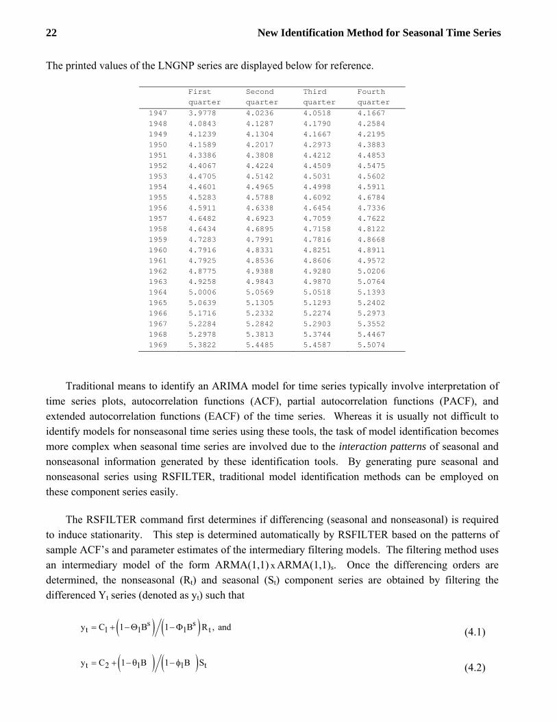
To illustrate the RSFILTER command, we begin by displaying a graph of the log transformed quarterly nominal gross national product (GNP, in billions of current dollars) of the United States between the first quarter of 1947 and the fourth quarter of 1969. This series will be referred to by LNGNP in this example. This series is not seasonally adjusted; therefore we observe distinct recurring patterns from year to year. A time series plot of the LNGNP series is displayed using SCAGRAF by issuing the command
GRAPH LNGNP. TYPE TSPLOT.
22 New Identification Method for Seasonal Time Series
The printed values of the LNGNP series are displayed below for reference.
First quarter
Second quarter
Third quarter
Fourth quarter
1947 3.9778 4.0236 4.0518 4.1667 1948 4.0843 4.1287 4.1790 4.2584 1949 4.1239 4.1304 4.1667 4.2195 1950 4.1589 4.2017 4.2973 4.3883 1951 4.3386 4.3808 4.4212 4.4853 1952 4.4067 4.4224 4.4509 4.5475 1953 4.4705 4.5142 4.5031 4.5602 1954 4.4601 4.4965 4.4998 4.5911 1955 4.5283 4.5788 4.6092 4.6784 1956 4.5911 4.6338 4.6454 4.7336 1957 4.6482 4.6923 4.7059 4.7622 1958 4.6434 4.6895 4.7158 4.8122 1959 4.7283 4.7991 4.7816 4.8668 1960 4.7916 4.8331 4.8251 4.8911 1961 4.7925 4.8536 4.8606 4.9572 1962 4.8775 4.9388 4.9280 5.0206 1963 4.9258 4.9843 4.9870 5.0764 1964 5.0006 5.0569 5.0518 5.1393 1965 5.0639 5.1305 5.1293 5.2402 1966 5.1716 5.2332 5.2274 5.2973 1967 5.2284 5.2842 5.2903 5.3552 1968 5.2978 5.3813 5.3744 5.4467 1969 5.3822 5.4485 5.4587 5.5074
Traditional means to identify an ARIMA model for time series typically involve interpretation of time series plots, autocorrelation functions (ACF), partial autocorrelation functions (PACF), and extended autocorrelation functions (EACF) of the time series. Whereas it is usually not difficult to identify models for nonseasonal time series using these tools, the task of model identification becomes more complex when seasonal time series are involved due to the interaction patterns of seasonal and nonseasonal information generated by these identification tools. By generating pure seasonal and nonseasonal series using RSFILTER, traditional model identification methods can be employed on these component series easily.
The RSFILTER command first determines if differencing (seasonal and nonseasonal) is required to induce stationarity. This step is determined automatically by RSFILTER based on the patterns of sample ACF’s and parameter estimates of the intermediary filtering models. The filtering method uses an intermediary model of the form ARMA(1,1) x ARMA(1,1)s. Once the differencing orders are determined, the nonseasonal (Rt) and seasonal (St) component series are obtained by filtering the differenced Yt series (denoted as yt) such that
( ) ( )s st 1 1 1 ty C 1 B 1 B R , and= + −Θ −Φ (4.1)
( ) ( )t 2 1 1 ty C 1 B 1 B S= + −θ − φ (4.2)

New Identification Method for Seasonal Time Series 23
Note that Rt is like the residual series generated using (4.1) and St is like the residual series generated using (4.2).
Once the Rt and St series are generated as pure nonseasonal and pure seasonal component series using this filtering method, model identification becomes much easier. The RSFILTER command also displays the intermediary models which provide the user with information regarding the differencing orders selected by RSFILTER. The user can also employ alternative differencing in the RSFILTER command by specifying the DFORDER and NODFORDER subcommands.
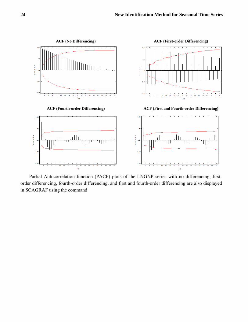
We continue the example by displaying autocorrelation function (ACF) plots of the LNGNP series with no differencing, first-order differencing, fourth-order differencing, and first and fourth-order differencing using the command
GRAPH LNGNP. TYPE ACF. PAUSE
The PAUSE subcommand allows the user to overwrite the options of the ACF plots generated. The following dialog box will be displayed where the differencing orders scenarios are specified for a quarterly time series
Clicking on the OK button then displays the ACF plots below that are typically used for ARIMA model identification.
24 New Identification Method for Seasonal Time Series
ACF (No Differencing)
ACF (First-order Differencing)
ACF (Fourth-order Differencing)
ACF (First and Fourth-order Differencing)
Partial Autocorrelation function (PACF) plots of the LNGNP series with no differencing, first-order differencing, fourth-order differencing, and first and fourth-order differencing are also displayed in SCAGRAF using the command

New Identification Method for Seasonal Time Series 25
GRAPH LNGNP. TYPE PACF. PAUSE
PACF (No Differencing
PACF (1st Order Differencing)
PACF (4th Order Differencing)
PACF (1st and 4th Order Differencing)
Using traditional identification methods, the ACF plots suggest a fourth-order differencing is appropriate for the LNGNP series. A first-order differencing is not needed since the ACF plot does not possess a slow die-out pattern after a fourth-order differencing is employed. We now explore the RSFILTER capability to help in ARIMA model identification.
The RSFILTER command shown below is employed to assist in the identification of an ARIMA model for the LNGNP series. Potential seasonality is specified using the SEASONALITY subcommand. In this example, the LNGNP series is a quarterly time series and therefore a potential seasonality of four is specified. Failure to specify potential seasonality in the RSFLITER command will result in the use of inappropriate intermediate models and produce undesirable results. The nonseasonal and seasonal component series are saved under the NEW-SERIES subcommand.

26 New Identification Method for Seasonal Time Series
RSFILTER LNGNP. NEW-SERIES R,S. SEASONALITY 4.
SUMMARY FOR UNIVARIATE TIME SERIES MODEL -- UTSMODEL ----------------------------------------------------------------------- VARIABLE TYPE OF ORIGINAL DIFFERENCING VARIABLE OR CENTERED LNGNP RANDOM ORIGINAL NONE ----------------------------------------------------------------------- PARAMETER VARIABLE NUM./ FACTOR ORDER CONS- VALUE STD T LABEL NAME DENOM. TRAINT ERROR VALUE 1 CNST 1 0 NONE 14.0528 14.4065 .98 2 LNGNP MA 1 1 NONE -.1715 .1305 -1.31 3 LNGNP MA 2 4 NONE .6008 .1033 5.81 4 LNGNP D-AR 1 1 NONE .8402 .0732 11.47 5 LNGNP D-AR 2 4 NONE .9936 .0115 86.75 TOTAL NUMBER OF OBSERVATIONS . . . . 92 EFFECTIVE NUMBER OF OBSERVATIONS . . 87 RESIDUAL STANDARD ERROR. . . . . . . 0.190659E-01 PARAMETER ESTIMATES DURING DIFFERENCING DETERMINATION SUMMARY FOR UNIVARIATE TIME SERIES MODEL -- UTSMODEL ----------------------------------------------------------------------- VARIABLE TYPE OF ORIGINAL DIFFERENCING VARIABLE OR CENTERED 4 LNGNP RANDOM ORIGINAL (1-B ) ----------------------------------------------------------------------- PARAMETER VARIABLE NUM./ FACTOR ORDER CONS- VALUE STD T LABEL NAME DENOM. TRAINT ERROR VALUE 1 CNST 1 0 NONE .0623 .0085 7.36 2 LNGNP MA 1 1 NONE -.1312 .1433 -.92 3 LNGNP MA 2 4 NONE .2811 .1872 1.50 4 LNGNP D-AR 1 1 NONE .8531 .0843 10.13 5 LNGNP D-AR 2 4 NONE -.3206 .1743 -1.84 TOTAL NUMBER OF OBSERVATIONS . . . . 92 EFFECTIVE NUMBER OF OBSERVATIONS . . 83 RESIDUAL STANDARD ERROR. . . . . . . 0.190460E-01
The output displayed by the RSFILTER command provides two model summaries. The initial model summary shows the filtering model prior to its determination of differencing required to induce stationarity. The second model summary shows the filtering model after differencing has been determined. Based on this second model, the Rt and St series are generated.
We now direct our attention to model identification of the nonseasonal Rt series. The IDEN keyword for the TYPE subcommand in the following GRAPH command will generate both ACF and PACF plots.

New Identification Method for Seasonal Time Series 27
GRAPH R. TYPE IDEN. PAUSE.
ACF (No Differencing)
PACF (No Differencing)
The extended autocorrelation function (EACF) is also a valuable tool in identifying ARIMA models. The EACF table is computed using the EACF command
EACF R.
THE EXTENDED ACF TABLE (Q-->) 0 1 2 3 4 5 6 7 8 9 10 11 12 ------------------------------------------------------------------------ (P= 0) .87 .71 .48 .30 .12 .01 -.05 -.08 -.09 -.11 -.11 -.10 -.06 (P= 1) .24 .38 .18 .22 .13 .02 -.09 -.08 -.02 -.11 -.03 -.10 -.05 (P= 2) -.47 .35 -.20 .20 -.05 -.10 .07 -.08 .02 -.12 .04 -.11 .06 (P= 3) .17 -.15 .00 .19 -.06 -.12 -.04 -.03 .17 .05 .02 .05 .00 (P= 4) .45 -.20 .01 .04 -.07 -.04 .02 -.03 .15 -.03 .01 .04 -.00 (P= 5) .35 .26 -.10 -.06 -.01 -.05 .04 -.03 .14 .01 -.01 .04 -.01 (P= 6) -.30 .38 -.44 .03 -.03 -.00 .00 -.02 .10 -.03 -.08 .06 -.02 SIMPLIFIED EXTENDED ACF TABLE (5% LEVEL) (Q-->) 0 1 2 3 4 5 6 7 8 9 10 11 12 ----------------------------------------------- (P= 0) X X X O O O O O O O O O O (P= 1) X X O O O O O O O O O O O (P= 2) X X O O O O O O O O O O O (P= 3) O O O O O O O O O O O O O (P= 4) X O O O O O O O O O O O O (P= 5) X O O O O O O O O O O O O (P= 6) X X X O O O O O O O O O O
Based on the ACF, PACF, and EACF of the nonseasonal component series, an AR(3) or ARMA(1,2) model may be appropriate for Rt. We now produce the ACF and PACF plots for the seasonal component series, St

28 New Identification Method for Seasonal Time Series
GRAPH S. TYPE IDEN. PAUSE.
ACF (No Differencing)
PACF (No Differencing)
Based on the ACF and PACF of the seasonal component series, a seasonal MA(1)4 model is appropriate for St. Now, the models for the nonseasonal and seasonal component series can be combined. We specify the first candidate model as an ARIMA(3,0,0) x ARIMA(0,1,1)4 using the TSMODEL command,
TSMODEL MODELA. MODEL IS @ LNGNP(4)=C1+(4 ; TH4A)/(1,2,3 ; PH1A,PH2A,PH3A)NOISE.
The model is then estimated using exact maximum likelihood using the ESTIMATE command shown below.
ESTIMATE MODELA. METHOD EXACT. HOLD RESIDUALS(RESA).
SUMMARY FOR UNIVARIATE TIME SERIES MODEL -- MODELA ----------------------------------------------------------------------- VARIABLE TYPE OF ORIGINAL DIFFERENCING VARIABLE OR CENTERED 4 LNGNP RANDOM ORIGINAL (1-B ) ----------------------------------------------------------------------- PARAMETER VARIABLE NUM./ FACTOR ORDER CONS- VALUE STD T LABEL NAME DENOM. TRAINT ERROR VALUE 1 C1 CNST 1 0 NONE .0609 .0041 14.91 2 TH4A LNGNP MA 1 4 NONE .4237 .1123 3.77 3 PH1A LNGNP D-AR 1 1 NONE 1.0437 .1005 10.38 4 PH2A LNGNP D-AR 1 2 NONE .0181 .1516 .12 5 PH3A LNGNP D-AR 1 3 NONE -.3375 .1013 -3.33 EFFECTIVE NUMBER OF OBSERVATIONS . . 85 R-SQUARE . . . . . . . . . . . . . . 0.998 RESIDUAL STANDARD ERROR. . . . . . . 0.173031E-01

New Identification Method for Seasonal Time Series 29
The second candidate model ARIMA(1,0,2) x ARIMA(0,1,1)4 is specified and estimated below using the TSMODEL and ESTIMATE commands
TSMODEL MODELB. MODEL IS @ LNGNP(4)=C2+(1,2 ; TH1B,TH2B)(4 ; TH4B)/(1; PH1B)NOISE.
ESTIMATE MODELB. METHOD EXACT. HOLD RESIDUALS(RESB).
SUMMARY FOR UNIVARIATE TIME SERIES MODEL -- MODELB ----------------------------------------------------------------------- VARIABLE TYPE OF ORIGINAL DIFFERENCING VARIABLE OR CENTERED 4 LNGNP RANDOM ORIGINAL (1-B ) ----------------------------------------------------------------------- PARAMETER VARIABLE NUM./ FACTOR ORDER CONS- VALUE STD T LABEL NAME DENOM. TRAINT ERROR VALUE 1 C2 CNST 1 0 NONE .0611 .0057 10.64 2 TH1B LNGNP MA 1 1 NONE -.3034 .1187 -2.56 3 TH2B LNGNP MA 1 2 NONE -.3434 .1106 -3.10 4 TH4B LNGNP MA 2 4 NONE .5607 .0930 6.03 5 PH1B LNGNP D-AR 1 1 NONE .7460 .0904 8.25 EFFECTIVE NUMBER OF OBSERVATIONS . . 87 R-SQUARE . . . . . . . . . . . . . . 0.998 RESIDUAL STANDARD ERROR. . . . . . . 0.175058E-01
The user can now perform diagnostic tests on the residual series, evaluate the two candidate models, and select the one that best fits the user’s application.
The determination of differencing is handled very well in the RSFILTER command automatically and typically should be accepted by the user. However in some situations, the user may have special reasons to impose alternative differencing other than the differencing automatically determined by the RSFILTER command. This can be accomplished using the DFORDER and NODFORDER subcommands. For example, if we want to generate the Rt and St component series based on first-order and fourth-order differencing, the RSFILTER command is
RSFILTER LNGNP. NEW-SERIES R, S. SEASONALITY 4. DFORDERS 1, 4.
If the user wants to exclude fourth-order differencing and impose first-order differencing, the following RSFILTER command can be specified
RSFILTER LNGNP. NEW-SERIES R, S. SEASONALITY 4. @ DFORDERS 1. NODFORDER 4.
Other examples for the use of the optional DFORDER and NODFORDER subcommands can be found in the next chapter which describes the IARIMA command.

30 New Identification Method for Seasonal Time Series

CHAPTER 5
ENHANCED EXPERT ARIMA MODELING
The SCA expert ARIMA modeling capabilities (IARIMA) are detailed in Chapter 2 of the SCA reference manual, Forecasting and Time Series Analysis Using the SCA Statistical System, Volume 2 along with related commands such as IESTIM. The other related command, RSFILTER, is discussed in the previous chapter of this document. In Release 7.0 (and above) of the SCA System, the capabilities of the IARIMA command have been further enhanced.
The algorithms and the rules for identifying ARIMA models using the IARIMA capability have been modified to perform more robustly. In addition, new options have been added to the IARIMA capability that provides more control to the user in final model determination. Specifically, options are now available to set the critical value for determining the statistical significance of parameter estimates retained in a model (through the CRITERIA subcommand), and for overriding differencing employed in the final model (through the DFORDER and NODFORDER subcommands).
The algorithm for the IARIMA command has been enhanced to better identify an ARIMA model when the selection between a pure AR and mixed ARMA model is marginal. For example, in earlier releases of the SCA System, the IARIMA command sometimes identified an AR(2) model when an ARMA(1,1) model may have been more appropriate. The SCA System now addresses such marginal cases more appropriately. Other improvements are made to the automatic model identification methods used in the IARIMA command on an ongoing basis. Modifications are typically made whenever users report data sets that prove to adversely affect general model identification.
The SEASONALITY (or PERIODICITY) subcommand in the IARIMA capability has been enhanced to search for seasonal patterns at very long lags. The previous release of the SCA System limited the seasonality cycle to 120 periods. Release 7.0 (and above) of the SCA System removes all practical limitations related to the identification of potential seasonality in a time series. For example, when considering hourly data, it is often important to include the 24 hour periodicity. Due to weekly patterns, it then becomes necessary to include a 168 periodicity in the model. The new release of the SCA System now allows for modeling high-order seasonal or periodic behaviors. However, when high-orders are used to handle higher frequency data, the exact maximum likelihood estimation method cannot be used. This is due to the fact that exact maximum likelihood estimation requires matrix inversion of high-order (e.g., 168 x 168). This will cause problems for matrix inversion in both accuracy and storage space. Therefore, conditional likelihood estimation must be used for such high-order models.
In previous releases of the SCA System, the DFORDER subcommand in the IARIMA command allowed the user to include specific differencing orders in an identified ARIMA model. However, if the IARIMA command found that the specified differencing order was not needed, it would exclude it

32 Enhanced Expert ARIMA Modeling
from the final model. This behavior has been modified so that differencing orders specified in the DFORDER subcommand will always be retained in the final model.
Whereas the DFORDER subcommand allows the inclusion of specific differencing orders in the final model, it did not preclude the possibility that additional differencing orders may be found important and therefore added into the final model. For example, if a user specified a first-order difference using the DFORDER subcommand, the IARIMA command may also include a seasonal differencing term if the time series requires a seasonal differencing.
In the event a user wants to exclude specific differencing orders from the final model, Release 7.0 (and above) of the SCA System now includes a new subcommand, NODFORDER, that can be used in conjunction with the DFORDER subcommand to achieve full control of differencing orders in the automatic model identification of a time series.
If the NODFORDER subcommand is not specified, the IARIMA command will automatically determine whether any differencing orders are to be employed in the final model. Typically, if a differencing order is forced out of consideration through the NODFORDER subcommand, the IARIMA algorithm will compensate for the lack of differencing through one or more ARMA parameters.
The previous release of the IARIMA command used a critical value of 1.96 when determining whether a parameter estimate is statistically significant. A subcommand, CRITERIA, has been added to the IARIMA command to allow users more control over parameters included in the final model. This option is particularly useful when the time series to be modeled is either very long or rather short.
The IARIMA command uses the same approach of model identification as described for the RSFILTER command. However, the IARIMA command will provide the final identified model besides generating the nonseasonal and seasonal component series.
To illustrate the use of the IARIMA command, we use the LNGNP series introduced in the previous chapter to explain the RSFILTER command. The LNGNP series is the log transformed quarterly nominal gross national product (GNP, in billions of current dollars) of the United States between the first quarter of 1947 and the fourth quarter of 1969.
The IARIMA command requires the user to specify the potential seasonality of the time series being modeled (e.g., a monthly series would have a potential seasonality of 12, a daily series would have a potential seasonality of 7, and so on). Since the LNGNP series is a quarterly time series, it has a potential seasonality of 4. The following IARIMA command can be easily specified to automatically identify an appropriate model for the LNGNP series.

Enhanced Expert ARIMA Modeling 33
IARIMA LNGNP. SEASONALITY 4.
SUMMARY FOR UNIVARIATE TIME SERIES MODEL -- UTSMODEL ----------------------------------------------------------------------- VARIABLE TYPE OF ORIGINAL DIFFERENCING VARIABLE OR CENTERED 4 LNGNP RANDOM ORIGINAL (1-B ) ----------------------------------------------------------------------- PARAMETER VARIABLE NUM./ FACTOR ORDER CONS- VALUE STD T LABEL NAME DENOM. TRAINT ERROR VALUE 1 CNST 1 0 NONE .0606 .0041 14.96 2 LNGNP MA 1 4 NONE .4306 .1167 3.69 3 LNGNP D-AR 1 1 NONE 1.0401 .1005 10.35 4 LNGNP D-AR 1 2 NONE .0234 .1516 .15 5 LNGNP D-AR 1 3 NONE -.3405 .1011 -3.37 TOTAL NUMBER OF OBSERVATIONS . . . . 92 EFFECTIVE NUMBER OF OBSERVATIONS . . 85 RESIDUAL STANDARD ERROR. . . . . . . 0.174545E
This model is good and can immediately be used for further application such as forecasting. By simply specifying the potential seasonality of the series, the IARIMA command automatically determines whether seasonal differencing and/or regular differencing is required to induce stationarity. In typical circumstances, the user should not override the differencing order(s) automatically determined by the IARIMA command unless there is good reason to do so. If the need to override differencing arises, the DFORDER and NODFORDER subcommands can be specified to force inclusion or exclusion of certain differencing order(s) in the final model similar to the RSFILTER command explained in a previous chapter.
In the above example, fourth-order differencing was automatically determined by the IARIMA command. If first-order differencing is also desired in the model, it can be forced into the final model by the following IARIMA command
IARIMA LNGNP. SEASONALITY 4. DFORDER 1.
SUMMARY FOR UNIVARIATE TIME SERIES MODEL -- UTSMODEL ----------------------------------------------------------------------- VARIABLE TYPE OF ORIGINAL DIFFERENCING VARIABLE OR CENTERED 4 1 LNGNP RANDOM ORIGINAL (1-B ) (1-B ) ----------------------------------------------------------------------- PARAMETER VARIABLE NUM./ FACTOR ORDER CONS- VALUE STD T LABEL NAME DENOM. TRAINT ERROR VALUE 1 LNGNP MA 1 1 NONE -.1982 .1050 -1.89 2 LNGNP MA 1 2 NONE -.2522 .1068 -2.36 3 LNGNP MA 2 4 NONE .5997 .0906 6.62 TOTAL NUMBER OF OBSERVATIONS . . . . 92 RESIDUAL STANDARD ERROR. . . . . . . 0.193055E-01

34 Enhanced Expert ARIMA Modeling
Note that by employing the “DFORDER 1” subcommand in the above IARIMA command, we effectively force first-order differencing in the model. Because IARIMA determined that seasonal differencing is also needed, the fourth-order differencing remains in the final model.
Whereas it is possible to force differencing by specifying the DFORDER subcommand, it is also possible to exclude differencing by specifying the NODFORDER subcommand. For example, if we had reason to force first-order differencing and exclude fourth-order differencing for the LNGNP series, the following command can be specified.
IARIMA LNGNP. SEASONALITY 4. DFORDER 1. NODFORDER 4.
THE CRITICAL VALUE FOR SIGNIFICANCE TESTS OF ACF AND ESTIMATES IS 1.875 SAMPLE ACF OF THE RESIDUALS (** SIGNIFICANT VALUES EXIST **) 1 - 12 -.01 .02 -.12 .00 -.30 -.08 -.08 .07 .00 .11 -.00 -.07 T-VALUE -.14 .15-1.09 .03-2.75 -.67 -.69 .56 .02 .94 -.04 -.60 SUMMARY FOR UNIVARIATE TIME SERIES MODEL -- UTSMODEL ----------------------------------------------------------------------- VARIABLE TYPE OF ORIGINAL DIFFERENCING VARIABLE OR CENTERED 1 LNGNP RANDOM ORIGINAL (1-B ) ----------------------------------------------------------------------- PARAMETER VARIABLE NUM./ FACTOR ORDER CONS- VALUE STD T LABEL NAME DENOM. TRAINT ERROR VALUE 1 LNGNP MA 1 1 NONE -.1703 .1031 -1.65 2 LNGNP MA 1 2 NONE -.3072 .1066 -2.88 3 LNGNP MA 2 4 NONE .6068 .0920 6.60 4 LNGNP D-AR 1 4 NONE .9739 .0129 75.25 TOTAL NUMBER OF OBSERVATIONS . . . . 92 RESIDUAL STANDARD ERROR. . . . . . . 0.188898E-01
The IARIMA command (and RSFILTER command) does a very good job at determining
appropriate differencing for the final model. Overriding the automatically determined differencing by alternative differencing is done at your own risk as it may result in over-differencing (or under-differencing) and produce less than optimal models. In the event the final model does not remove all significant autocorrelation from the residuals, the output from the IARIMA command informs the user that significant values exist in the autocorrelations of the residuals. This indicates that the model may have problems as demonstrated in the case of over differencing in the above example.
In practice, if the user is alerted to potential problems by significant residual autocorrelations, the user should check if potential seasonality is specified appropriately and then allow the IARIMA command to determine differencing automatically. Significant autocorrelations in the residual series may also be caused by other issues such as calendar effects, outliers, or the exclusion of important explanatory variables in the model. Such issues must be handled in an appropriate manner by studying the underlying causes rather than simply adding more ARMA parameters to the model.

CHAPTER 6
POWER TRANSFORMATION IN TIME SERIES FORECASTING
The Practitioner Edition (and above) provides the RETRANSFORM command to retransform forecasts back into original units when the forecasted series was transformed. It is important to note that a straight retransformation of forecasts produces biased forecasts. The RETRANSFORM command, based on the work of Guerrero (1993), adjusts for such bias. In this chapter, the RETRANSFORM command is presented. A few supporting SCA analytic statements are also used to complete the examples. More information on SCA analytic statements is documented in the SCA Reference Manual for Fundamental Capabilities. A related command, TSEARCH, which is used to search for the best power transformation for forecasting is described in Chapter 10.
Pankratz and Dudley (1987) and Guerrero (1993) developed a unified method to adjust for bias in retransforming forecasts. In the SCA System, we have implemented the RETRANSFORM command which is based on the method provided in Guerrero (1993). The capability provided in the RETRANSFORM command is not only appropriate for ARIMA model forecasts, it is also appropriate for forecasts generated by other models such as transfer function models, STF models, and vector ARMA models. Below is a brief summary of the method provided in Guerrero (1993).
In univariate time series analysis, Box and Jenkins (1976) discussed the feasibility of obtaining an ARIMA model with homogenous residual variance based on a time series derived from a power transformed series similar to that proposed in Box and Cox (1964). Using tY to denote the original series with positive value (if tY is non-positive, a positive constant value can be added to tY before the transformation), this class of transformation can be expressed as
ttt
(Y 1) / if 0 Zn(Y ) if 0
λ⎧ − λ λ ≠⎪= ⎨λ =⎪⎩
(6.1)
where tZ is the transformed series, λ (referred to as lambda) is the power value of the transformation, and t=1, 2, …, n. The above formulation of power transformations is continuous in the parameter λ . While the transformation in (6.1) has desirable properties such as continuity of λ at 0, the variances of transformed series are not comparable when 'sλ are different. To address this issue, the following scaled power transformation is recommended by Box and Jenkins (1976), and Ansley, Spivey, and Wrobleski (1977)
1t
tt
(Y 1) / ( Y ) if 0 Z
Y n(Y ) if 0
λ λ−⎧ − λ λ ≠⎪= ⎨λ =⎪⎩
(6.2)
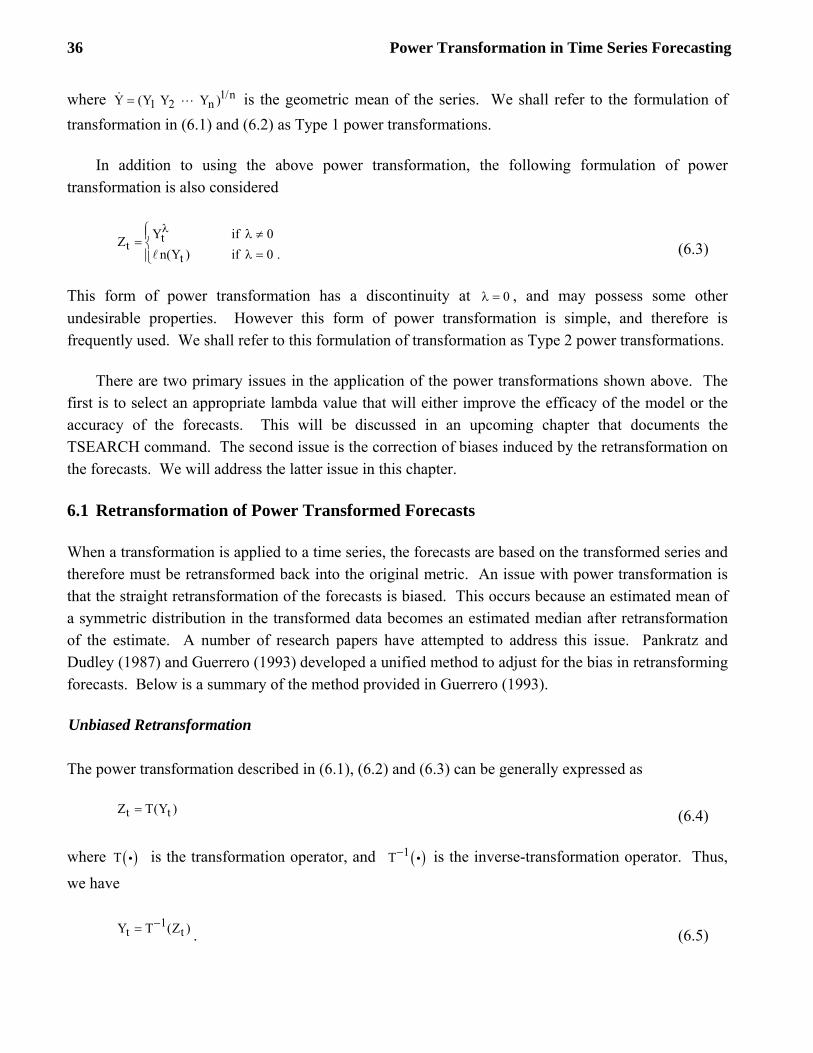
36 Power Transformation in Time Series Forecasting
where 1/n1 2 nY (Y Y Y )= ⋅⋅⋅ is the geometric mean of the series. We shall refer to the formulation of
transformation in (6.1) and (6.2) as Type 1 power transformations.
In addition to using the above power transformation, the following formulation of power transformation is also considered
ttt
Y if 0 Z n(Y ) if 0 .
λ⎧ λ ≠⎪= ⎨λ =⎪⎩
(6.3)
This form of power transformation has a discontinuity at 0λ = , and may possess some other undesirable properties. However this form of power transformation is simple, and therefore is frequently used. We shall refer to this formulation of transformation as Type 2 power transformations.
There are two primary issues in the application of the power transformations shown above. The first is to select an appropriate lambda value that will either improve the efficacy of the model or the accuracy of the forecasts. This will be discussed in an upcoming chapter that documents the TSEARCH command. The second issue is the correction of biases induced by the retransformation on the forecasts. We will address the latter issue in this chapter.
6.1 Retransformation of Power Transformed Forecasts
When a transformation is applied to a time series, the forecasts are based on the transformed series and therefore must be retransformed back into the original metric. An issue with power transformation is that the straight retransformation of the forecasts is biased. This occurs because an estimated mean of a symmetric distribution in the transformed data becomes an estimated median after retransformation of the estimate. A number of research papers have attempted to address this issue. Pankratz and Dudley (1987) and Guerrero (1993) developed a unified method to adjust for the bias in retransforming forecasts. Below is a summary of the method provided in Guerrero (1993).
Unbiased Retransformation The power transformation described in (6.1), (6.2) and (6.3) can be generally expressed as
t tZ T(Y )= (6.4)
where ( )T i is the transformation operator, and ( )1T− i is the inverse-transformation operator. Thus,
we have
1t tY T (Z )−= . (6.5)

Power Transformation in Time Series Forecasting 37
Assuming that nZ ( ) is the -step-ahead MMSE forecast of nZ + at the forecast origin t n= , the
straight retransformation of nZ ( ) under (6.1) is
n
1/n1
n n Z ( )
ˆ( Z ( ) 1) if 0ˆ ˆY ( ) T (Z ( ))e if 0 .
λ−
⎧ λ + λ ≠⎪= = ⎨⎪ λ =⎩
(6.6)
It has been shown that nY ( ) is biased. To correct for the bias, Guerrero (1993) derives the following
unbiased estimate nY ( ) where
1n nˆY ( ) T (Z ( )) C ( )−
λ= ⋅ . (6.7)
The C ( )λ is the debiasing factor which can be expressed as
( ) ( )( )
2
11 21 21
n
2
0.5 0.5 1 2 1 R , R if 0ˆC Z
e if =0
λ−
−λ
σ
⎧⎧ ⎫ σ⎪ ⎪⎡ ⎤⎪ + + λ − = λ ≠⎨ ⎬⎪ ⎢ ⎥⎣ ⎦= λ +⎪ ⎪⎨⎩ ⎭⎪⎪ λ⎩
(6.8)
and σ is the -step-ahead forecast standard error of nZ ( ) . It is readily seen that the debiasing factor is a function of the transformed forecast and its standard error if 0λ ≠ , and is a function of forecast standard error only if 0λ = .
The forecast limits of nZ + can be expressed as
( )n 2Z zα± ⋅σ . (6.9)
The straight retransformation of the above forecast limits ( )( )1n 2ˆT Z z−
α± ⋅σ is also biased. To
correct for the bias, Guerrero (1993) suggests multiplying the forecast limits by their respective debiasing factors.
The unbiased retransformation of the forecasts under (6.2) and (6.3) can be derived similarly. In the case of (6.2), the straight retransformation of ( )nZ is
( ) ( )( ) ( )( )( )( )n
11n1
n nZ
Z Y 1 if 0ˆ ˆY T Z
e if 0 .
λλ−−
⎧λ + λ ≠⎪⎪= = ⎨
⎪λ =⎪⎩
(6.10)
Again the above retransformed forecast nY ( ) is biased. Using equation (6.7), the unbiased forecast
( )nY can be obtained by using the following debiasing factor C ( )λ

38 Power Transformation in Time Series Forecasting
( )( )
( )
( )2
1 11 21 21 1
n
Y 2
Y0.5 0.5 1 2 1 R , R if 0
Z YC
e if =0 .
λ λ−−
− λ−λ
σ
⎧⎧ ⎫ σ⎪ ⎪⎡ ⎤⎪ + + λ − = λ ≠⎨ ⎬⎢ ⎥⎪ ⎣ ⎦ λ +⎪ ⎪= ⎩ ⎭⎨⎪⎪ λ⎩
(6.11)
For the class of power transformation in (6.3) which we refer to as Type 2 power transformations, the straight retransformation of nZ ( ) is
( ) ( )( ) ( )( )n
1n1
n n Z
Z if 0ˆ ˆY T Ze if 0
λ−
⎧ λ ≠⎪= = ⎨⎪ λ =⎩
(6.12)
which is also biased. Using equation (6.7), the unbiased forecast nY ( ) can be obtained by using the following debiasing factor C ( )λ
( ) ( ) ( )2
11 21 2
n
2
0.5 0.5 1 2 1 R , R if 0ZC
e if =0 .
λ−
λ
σ
⎧⎧ ⎫ σ⎪ ⎪⎡ ⎤⎪ + + λ − = λ ≠⎨ ⎬⎪ ⎢ ⎥⎣ ⎦= ⎪ ⎪⎨⎩ ⎭⎪⎪ λ⎩
(6.13)
6.2 U.S. GNP Example of Retransformation
In previous chapters of the document, the log transformed quarterly nominal gross national product of the United States (LNGNP) was used to illustrate the RSFILTER and IARIMA commands. The LNGNP series shall be used to illustrate the retransformation of forecasts back into original units. Using the model identified by the IARIMA command, the model is re-specified below using the TSMODEL command and estimated using the ESTIMATE command. The FORECAST command is then specified to generate eight forecasts from the end of the LNGNP series
TSMODEL UTSMODEL. MODEL LNGNP(4)=C+(4)/(1 TO 3)NOISE. ESTIMATE UTSMODEL. METHOD EXACT. FORECAST UTSMODEL. NOFS 8. HOLD FORECAST(FLN), STDERR(FSELN).
---------------------------------- 8 FORECASTS, BEGINNING AT 92 ---------------------------------- TIME FORECAST STD. ERROR ACTUAL IF KNOWN 93 5.4366 0.0175 94 5.4934 0.0252 95 5.4930 0.0317 96 5.5490 0.0349 97 5.4822 0.0399 98 5.5469 0.0422 99 5.5524 0.0434 100 5.6133 0.0436

Power Transformation in Time Series Forecasting 39
The RETRANSFORM command is used to retransform the forecasts back into original units. The unbiased method is employed. However, it is necessary to specify 0λ = (indicating that a logarithmic transformation was applied to the original series) and TYPE=1 (indicating Type 1 transformation was applied)
VLAMBDA=0.0 VTYPE=1 RETRANSFORM FLN, FSELN. METHOD UNBIASED. @
FORM VLAMBDA, VTYPE.
TIME FORECAST STD. ERROR RETRANSFORMED 1 5.437 0.017 229.751 2 5.494 0.025 243.287 3 5.494 0.032 243.332 4 5.550 0.035 257.363 5 5.483 0.040 240.833 6 5.548 0.042 256.983 7 5.554 0.043 258.452 8 5.614 0.043 274.618
For comparison purposes, the following straight retransformation of the forecasts is presented.
RETRANSFORM FLN, FSELN. METHOD STRAIGHT. @ FORM VLAMBDA, VTYPE.
TIME FORECAST STD. ERROR RETRANSFORMED 1 5.437 0.017 229.716 2 5.494 0.025 243.211 3 5.494 0.032 243.211 4 5.550 0.035 257.209 5 5.483 0.040 240.644 6 5.548 0.042 256.755 7 5.554 0.043 258.210 8 5.614 0.043 274.358
As shown in the above table, the unbiased and straight retransformed forecasts for this series are somewhat different, with the unbiased forecasts slightly larger than the straight retransformed forecasts.
The natural logarithmic transformation is often used in practice because of its desirable properties and the ease of interpretation when used for business and econometric applications. However, in some situations we may wish to investigate alternative power transformations that may be better suited for the time series under study. Such capability is provided by the TSEARCH command.

40 Power Transformation in Time Series Forecasting

CHAPTER 7
CAUSALITY TESTING
The Professional Edition (A) of the SCA Statistical System implements new capabilities for causality testing following the work of Chen and Lee (1990) and others. In this chapter, the CAUSALTEST command is presented. Related commands including MTSMODEL and MESTIM are documented in the SCA reference manual, Forecasting and Time Series Analysis Using the SCA Statistical System, Volume 2.
Chen and Lee (1990) used vector ARMA (VARMA) models for causality testing. The traditional hypothesis testing procedure provides a framework to contrast a null hypothesis versus an alternative hypothesis. Without imposing a priori restrictions, an empirical study of dynamic relationships often involves several non-nested hypotheses. Consequently, a more systematic approach is required to examine the multiple hypotheses so that the test conclusion is not affected by a priori choice of the alternative. The bivariate VARMA test developed by Chen and Lee (1990) addresses these issues more adequately and is the focus of causality testing discussed in this chapter.
7.1 Causality Testing Using Vector ARMA Models
A number of time series models can be employed for causality testing (see e.g., Sims, 1972; and Haugh, 1976). Because vector ARMA (VARMA) models have been shown to be effective in forecasting, this class of models can also be used for causality testing (see e.g., Pierce and Haugh, 1977; Kang, 1981; Koreisha, 1983; and Chen and Lee, 1990). Using conventional notations, a bivariate VARMA(p,q) model can be expressed as
t 1tp q1 p 1 q
t 2t
Y a( B B ) ( B B )
X a⎡ ⎤ ⎡ ⎤
− − ⋅⋅ ⋅ − = + − − ⋅⋅⋅ −⎢ ⎥ ⎢ ⎥⎣ ⎦ ⎣ ⎦
I C Iφ φ θ θ (7.1)
where i 'sφ and j 'sθ are 2 2× matrices, C is a 2 1× constant vector, and t 1t 2t[a , a ]'=a is a sequence of
2 1× random shock vectors identically and independently distributed as a normal distribution with zero
mean and covariance matrix Σ with 11 12
21 22
σ σ⎡ ⎤= ⎢ ⎥σ σ⎣ ⎦
Σ . For convenience, the model in (7.1) can be re-
written as
t 1t11 12 11 12
21 22 t 21 22 2t
Y a(B) (B) (B) (B)
(B) (B) X (B) (B) aφ φ θ θ⎡ ⎤ ⎡ ⎤⎡ ⎤ ⎡ ⎤
= +⎢ ⎥ ⎢ ⎥⎢ ⎥ ⎢ ⎥φ φ θ θ⎣ ⎦ ⎣ ⎦⎣ ⎦ ⎣ ⎦C (7.2)
where 2ij ij0 ij1 ij2(B) B Bφ = φ − φ − φ − ⋅⋅ ⋅ , and 2
ij ij0 ij1 ij2(B) B Bθ = θ − θ − θ − ⋅⋅ ⋅ . It is important to note that
ij0 ij0 1φ = θ = if i j= , and ij0 ij0 0φ = θ = if i j≠ .

42 Causality Testing
Assuming the form of the model in (7.2) is known, sufficient conditions for testing the hypotheses 1H , 2H , 3H , 4H , and 5H using ij(B)φ and ij(B)θ of equation (7.2) are listed below:
Hypothesis Sufficient Conditions (Constraints)
1H : Y X∧ 12 21 12 21 12 21(B) (B) 0, (B) (B) 0, 0φ = φ = θ = θ = σ = σ = .
2H : Y X↔ 12 21 12 21(B) (B) 0, (B) (B) 0φ = φ = θ = θ = .
3H : Y X⇐/ 12 12(B) (B) 0φ = θ = (7.3)
4H : Y X⇒/ 21 21(B) (B) 0φ = θ =
5H : Y X⇔ no constraints
The conditions in (7.3) become necessary and sufficient conditions if the model in (7.2) is a pure vector AR or a pure vector MA model. In the above hypotheses, 3H implies the past X does not help to predict future Y, and 4H implies the past Y does not help to predict X. In both situations, we assume 12σ may be nonzero. However, if 12σ equals to zero, the hypotheses 3H , 4H , and 5H can be tested under a more stringent condition. Therefore the following three additional hypotheses should also be considered:
Hypothesis Sufficient Conditions (Constraints)
*3H : Y X<⇐/ 12 12 12(B) (B) 0, 0φ = θ = σ =
*4H : Y X⇒>/ 21 21 12(B) (B) 0, 0φ = θ = σ = (7.4)
*5H : Y X<⇔> 12 0σ =
In the above hypotheses, *3H implies both past and concurrent X do not help to predict Y, and *
4H
implies both past and concurrent Y do not help to predict X. For *5H , it implies a “true” feedback
relationship since Y and X are not contemporaneously related.
7.2 A Decision Tree Approach for Detecting Dynamic Relationships
It is important to note that the eight hypotheses stated in (7.3) and (7.4) are neither nested nor mutually exclusive to each other. This situation leads to significant complications in conducting appropriate hypothesis testing. In the causality testing literature (see e.g., Sims, 1972; Haugh, 1976; Pierce, 1977; Feige and Pearce, 1979; and Hsiao, 1979), most tests are designed to discriminate between independency and an alternative hypothesis. The primary purpose of these tests is to reject the independency (so called “neutrality”) hypothesis. However, it is more useful to identify the true nature of the relationship between two series. To accomplish this goal, Chen and Lee (1990) proposed a decision tree approach which consists of testing a sequence of pair-wise hypotheses that are defined by each of the above relationships. This inference procedure is based on the principle that a maintained hypothesis should not be rejected unless there is sufficient evidence against it.

Causality Testing 43
Two procedures for identifying dynamic relationships are considered here: (1) the backward procedure and (2) the forward procedure. The backward procedure takes the position that a hypothesis should not be rejected in favor of a more restrictive one unless sufficient evidence indicates otherwise. Consequently, the statistical procedure starts from the most general hypothesis, 5H , and then examines the relative validity of competing hypotheses in an increasing order of parameter restrictions. On the other hand, the forward procedure asserts that a simpler model is preferred unless the evidence strongly suggests otherwise. Hence, the forward procedure starts its test from the most restrictive hypothesis,
1H , and moves toward less restrictive hypotheses. In both procedures, each step of the test examines one or two pairs of nested hypotheses. Typically, both testing procedures result in the same conclusion. In some marginal situations, the backward procedure tends to favor more complicated relationships while the forward procedure tends to favor simpler relationships.
Generally speaking, the forward procedure works better (i.e., the test procedure has higher discriminating power) if the variables considered are likely to be independent or have a more restrictive relationship. On the other hand, the backward procedure works better if the variables considered are likely to have more complex relationships. Since we are more interested in the latter situation, the backward procedure is discussed first. The flow charts for both testing procedures are included in the following discussion.
The Backward Procedure The first step of backward procedure, B1, is to examine two pairs of hypotheses: (a) 3H vs 5H and (b)
4H vs 5H . This step, distinguishing the feedback relationship from unidirectional relationship, gives rise to four possible outcomes, 1E to 4E , as follows:
1E : 3H is not rejected in the pair-wise test (a) and 4H is rejected in the pair-wise test (b),
2E : 3H is rejected in test (a) and 4H is not rejected in test (b),
3E : 3H is not rejected in test (a) and 4H is not rejected in (b),
4E : 3H is rejected in test (a) and 4H is rejected in test (b).
The outcome of 1E implies that the past information of Y may help to predict current X, but the
past X does not help to predict current Y. Hence, this outcome leads to the next pair-wise test (g), *3H
vs 3H , where we try to detect the contemporaneous effect in the unidirectional relationship. If *3H is
rejected in test (g), the conclusion, Y X⇒ , is reached; otherwise the conclusion, Y X⇒> , would be made. Similarly, the occurrence of events 2E and 4E , respectively, suggests a possible unidirectional relationship from X to Y and a possible feedback relationship between Y and X. Therefore, the outcome of 2E leads to the pair-wise test (h), which helps us to choose between *
4H and 4H . Under the outcome of 4E , it requires the test (i) which discriminates between the strong feedback hypothesis

44 Causality Testing
( *5H ) and the weak feedback hypothesis ( 5H ). The rejection of *
4H in test (h) implies Y X⇐ .
Otherwise, the conclusion, Y X<⇐ , would be reached. In test (i), the rejection of *5H implies Y X⇔ .
If *5H is not rejected, we can conclude Y X<⇔> .
When one of the events, 1E , 2E , and 4E , occurs in sequence B1, the backward procedure stops at the end of test (g), test (h), and test (i) respectively. If neither 3H nor 4H is rejected, (i.e., 3E is realized), the backward procedure will move to sequence B2 where two pairs of hypotheses will be examined: (c) 2H vs 3H and (d) 2H vs 4H . Again, four possible results may come out of this sequence. They are summarized as follows:
5E : 2H is rejected in pair-wise test (c) but is not rejected in test (d),
6E : 2H is not rejected in test (c) but is rejected in test (d),
7E : 2H is rejected in either test (c) or test (d),
8E : 2H is rejected in both test (c) and test (d).
Since test (c) examines the possibility of Y X⇒ and test (d) examines that of Y X⇐ , outcome 5E implies that the relationship Y X⇒ is more probable than Y X⇐ . Therefore, the result of event 5E leads to test (g). A similar argument suggests that the occurrence of 6E leads to test (h). A definitive conclusion will be reached at the end of tests (g) and (h). The rejection of 2H in both test (c) and test (d) indicate the equal possibility of Y X⇐ and Y X⇒ . Hence, the result of 8E calls for test (f): 2H versus 5H . If 2H is rejected at test (f), then the possibility of the feedback relationship is established and the backward procedure moves to test (i). When 2H is not rejected at test (f) or when event 7E is realized, the backward procedure then proceeds to test (e), which discriminates between the independency and the contemporaneous relationship. If 1H is rejected in test (e), the conclusion of Y X↔ is reached. Otherwise, Y X∧ will be the case. In each step of the hypothesis testing, the likelihood ratio test is conducted. A flow chart representation of the backward procedure is displayed below.

Causality Testing 45
*17 5E : (i) reject H
*5 5(i) H vs H
*18 5E : (i) not reject H
4E :
3
4
(a) reject H(b) reject H
Start
Test Sequence B1
3 5
4 5
(a) H vs H
(b) H vs H
3 3
4
E : (a) not reject H(b) not reject H
1 3
4
E : (a ) not reject H(b) reject H
2 3
4
E : (a ) reject H(b) not reject H
*13 3E : (g) reject H
*3 3(g) H vs H
*14 3E : (g) not reject H
go to (h)
Y X<⇔>
go to (i)
2 5(f) H vs H
12 2E : (f) not reject H
Y X⇔
11 2E : (f) reject H
go to (e)
8E :2
2
(c) reject H(d) reject H
Test Sequence B2
2 3
2 4
(c) H vs H
(d) H vs H
1 2(e) H vs H9 1E : (e) not reject H
10 1E : (e) reject H
Y X⇒
Y X⇒>
Y X⇐
Y X↔
Y X∧
Y X<⇐
*15 4E : (h) reject H
*16 4E : (h) not reject H
*4 4(h) H vs H
5 22
E : (c) reject H(d) not reject H
go to (g)
6 2
2
E : (c) not reject H(d) reject H
7 2
2
E : (c) not reject H(d) not reject H
The Forward Procedure The forward procedure begins by testing the validity of the independency hypothesis at sequence F1. The hypothesis indices, 1H to 5H , the outcome indices, 1E to 8E , and the pair-wise test indices, (a) to (h), are consistent in flow chart of the backward procedure shown above, and the flow chart of the forward procedure that follows. The sequence F1 considers two pairs of hypotheses testing, test (e) and test (j). If 1H is not rejected in either test, the conclusion of Y X∧ is reached and the forward procedure stops. Otherwise, the procedure will move forward to sequence F2, which examines the relative likelihood of the contemporaneous relationship versus the unidirectional relationship. Notice that sequence F2 is identical to sequence B2, where one of the four possible outcomes, 5E , 6E , 7E , and 8E , will emerge. Using the same argument on sequence B2, the outcomes of 5E and 6E lead to tests (g) and (h) respectively. A conclusion from one of the four possible unidirectional relationships can be reached as a result and the forward procedure stops. The outcome of 7E implies Y X↔ and stops the forward procedure. However, the outcome of 8E , which rules out the case of a contemporaneous relationship, leads the forward procedure to sequence F3, which corresponds to sequence B1 in the backward procedure. Tests (a) and (b) may generate one of four possible outcomes, 1E , 2E , 3E , and 4E . Similar to sequence B1 in the backward procedure, the outcomes of

46 Causality Testing
1E and 2E lead to tests (g) and (h) respectively. One of the four unidirectional relationships will be detected as a result and the procedure stops. The outcome of 4E implies a possible feedback
relationship, and a further study, test (i), is needed to identify its nature. When *5H is rejected in test
(i), we conclude Y X⇔ ; otherwise, we conclude Y X<⇔> . The outcome of 3E implies that Y may help to predict X and X may help to predict Y, but the nature of this dynamic relationship is not clear. Therefore, test (f) is needed. When 2H is not rejected in test (f), the conclusion Y X↔ is reached and the procedure stops. If 2H is rejected in test (f), the procedure moves to test (i) to determine the nature of the feedback relationship. Consequently, either Y X⇔ or Y X<⇔> is shown to exist. A flow chart representation of the forward procedure is presented below.
Start
19 1
1
E : (e) not reject H( j) not reject H
Test Sequence F1
Test Sequence F2
1 2
1 5
(e) H vs H
( j) H vs H
2 3
2 4
(c) H vs H
(d) H vs H
20 19E : not E 5 2
2
E : (c) reject H(d) not reject H
6 2
2
E : (d) reject H(c) not reject H
8 2
2
E : (c) reject H(d) reject H
Test Sequence F3
4 3
4
E : (a) reject H(b) reject H
3 5
4 5
(a) H vs H
(b) H vs H
Y X∧
Y X↔
7 2
2
E : (c) not reject H(d) not reject H
Y X⇔
*17 5E : (i) reject H
*5 5(i) H vs H
*18 5E : (i) not reject H
Y X<⇔>
2 3
4
E : (a) reject H(b) not reject H
1 3
4
E : (a) not reject H(b) reject H
3 3
4
E : (a) not reject H(b) not reject H
Y X↔
12 2E : (f) not reject H
2 5(f) H vs H
11 2E : (f) reject H
go to (i)
Y X<⇐
*4 4(h) H vs H
*16 4E : (h) not reject H
Y X⇒
*13 3E : (g) reject H
Y X⇒>
go to (g)
*15 4E : (h) reject H
*3 3(g) H vs H
*14 3E : (g) not reject H
Y X⇐

Causality Testing 47
7.3 Test Statistic for Each Pair-wise Test
In practice, the model(s) for the time series under study are unknown. However, the order of the vector ARMA model for the series can be determined using the model identification procedure discussed in Chapter 14 of Liu (2006). The test procedures are rather robust with respect to the selected model as long as the order of the model is generally correct. Corresponding to each hypothesis, the parameters of the constrained model can be estimated using the maximum likelihood estimation method discussed in Liu (2006) (also see Hillmer and Tiao, 1979). The likelihood ratio statistic is then calculated for each pair of hypotheses:
i j i jLR(H vs H ) (H ) (H )= − (7.5)
where i(H ) 2*= − (log of the maximum likelihood value under iH ). The above likelihood ratio statistic
follows a 2χ -distribution with ν degrees of freedom where ν in each test is the difference between the numbers of estimated parameters under the null (the more restrictive one) and the alternative (the less restrictive one) hypotheses. A chi-square table can then be used to determine the significance of the test statistic for the tested hypotheses.
In each procedure, an α significance level will be used in conducting all pair-wise tests. Note that this α level is not the Type I error probability for the overall performance of the procedures. It serves only as a cut-off point in a sequential decision procedure. The smaller the α , the higher is the probability that the more restrictive hypothesis will not be rejected. Hence, taking a smaller α is equivalent to favoring the more restrictive hypotheses (i.e., simpler relationships), and taking a larger α is equivalent to favoring the more complicated relationships.
We shall employ two actual examples to illustrate causality testing using vector ARMA models. The first example is the United States yearly price index and long-term interest rate. This data set is used in various studies of the Gibson paradox. The second example is the non-seasonally adjusted monthly housing market data in the United States. The housing starts and houses sold series are employed in this study. Additional examples can be found in Liu (2006).

48 Causality Testing
7.4 Causal Relationships between Price and Interest Rate in the United States
The United States yearly price index and interest rate between 1800 and 1981 are shown below using the SCAGRAF capability.
U.S. yearly price index and long-term interest rate (1800-1981)
In the above figure, we observe the striking positive association between the price level and the interest rate. Such a relationship has been repetitively confirmed by various statistical methods ranging from correlation to spectral analysis, and is considered to be an established fact (see e.g., Fisher, 1907; Wicksell, 1907; Keynes, 1930; Sargent, 1973; Shiller and Siegel, 1977; Lee and Petruzzi, 1986; and Barsky and Summers, 1988). Keynes (1930) called this association the “Gibson paradox” due to conflicting conclusions on this phenomenon when various statistical methods are used. Nelson and Schwertz (1982) compare several methods including usual correlation, pre-whitening, two-sided

Causality Testing 49
regression, and vector ARMA models by simulation studies. They conclude that vector ARMA models provide the most powerful test for the presence of Granger causality.
Chen and Lee (1990) also employ vector ARMA models to examine the dynamic relationships between prices and interest rates in United States. The dynamic relationships revealed by vector ARMA models provide economists new insight in discriminating among competing theories about the nature of the Gibson paradox derived from the data. Instead of using the entire series, the non-gold standard period between 1914 and 1981 are used in this example and logarithmic transformation is applied to both series for the convenience of interpretation. The series tY and tX in the following discussions are defined as
tY : log transformed United States yearly price index between 1914 and 1981, and tX : log transformed United States yearly interest rate between 1914 and 1981.
During this sub-period, we have 68 observations for each series.
Following vector ARMA model identification procedures, we find that a vector ARMA(1,1) model of the form
tt
t
Y( B) ( B)
X⎡ ⎤
− = + −⎢ ⎥⎣ ⎦
I C I aφ θ . (7.6)
is appropriate for these two series. The model is specified using the MTSMODEL command
MTSMODEL ARMA11. SERIES ARE LUSP,LUSR. @ MODEL IS (1-PHI*B)SERIES=C+(1-TH1*B)NOISE.
After the vector ARMA(1,1) model is specified, the causality test is run using the CAUSALTEST command
CAUSALTEST MODEL ARMA11. OUTPUT PRINT(CORR)
----------------------- ERROR COVARIANCE MATRIX ----------------------- 1 2 1 .008147 2 -.000286 .006977
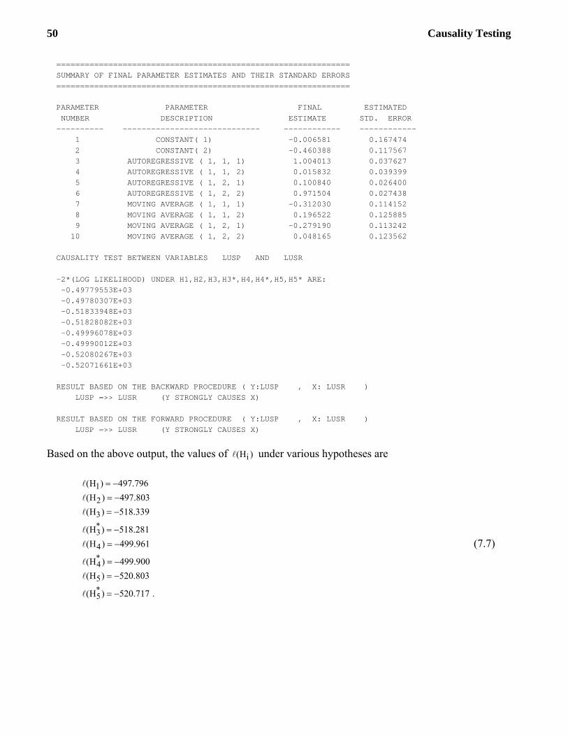
50 Causality Testing
============================================================== SUMMARY OF FINAL PARAMETER ESTIMATES AND THEIR STANDARD ERRORS ============================================================== PARAMETER PARAMETER FINAL ESTIMATED NUMBER DESCRIPTION ESTIMATE STD. ERROR ---------- ----------------------------- ------------ ------------ 1 CONSTANT( 1) -0.006581 0.167474 2 CONSTANT( 2) -0.460388 0.117567 3 AUTOREGRESSIVE ( 1, 1, 1) 1.004013 0.037627 4 AUTOREGRESSIVE ( 1, 1, 2) 0.015832 0.039399 5 AUTOREGRESSIVE ( 1, 2, 1) 0.100840 0.026400 6 AUTOREGRESSIVE ( 1, 2, 2) 0.971504 0.027438 7 MOVING AVERAGE ( 1, 1, 1) -0.312030 0.114152 8 MOVING AVERAGE ( 1, 1, 2) 0.196522 0.125885 9 MOVING AVERAGE ( 1, 2, 1) -0.279190 0.113242 10 MOVING AVERAGE ( 1, 2, 2) 0.048165 0.123562 CAUSALITY TEST BETWEEN VARIABLES LUSP AND LUSR -2*(LOG LIKELIHOOD) UNDER H1,H2,H3,H3*,H4,H4*,H5,H5* ARE: -0.49779553E+03 -0.49780307E+03 -0.51833948E+03 -0.51828082E+03 -0.49996078E+03 -0.49990012E+03 -0.52080267E+03 -0.52071661E+03 RESULT BASED ON THE BACKWARD PROCEDURE ( Y:LUSP , X: LUSR ) LUSP =>> LUSR (Y STRONGLY CAUSES X) RESULT BASED ON THE FORWARD PROCEDURE ( Y:LUSP , X: LUSR ) LUSP =>> LUSR (Y STRONGLY CAUSES X)
Based on the above output, the values of i(H ) under various hypotheses are
1
2
3*3
4*4
5*5
(H ) 497.796(H ) 497.803(H ) 518.339
(H ) 518.281(H ) 499.961
(H ) 499.900(H ) 520.803
(H ) 520.717 .
= −= −= −
= −
= −
= −= −
= −
(7.7)

Causality Testing 51
Summarizing the SCA output of the log likelihood ratio statistics for various pairs of hypotheses and their corresponding 2χ critical values at 5%α = , the following table is constructed:
23 5 3 5 0.05
24 5 4 5 0.05
22 3 2 3 0.05
2 4
LR(H vs H ) (H ) (H ) 2.463 (2) 5.991 (insignificant)
LR(H vs H ) (H ) (H ) 20.842 (2) 5.991 (significant)
LR(H vs H ) (H ) (H ) 20.534 (2) 5.991 (significant)
LR(H vs H )
= − = < χ =
= − = > χ =
= − = > χ =
= 22 4 0.05
21 2 1 2 0.05
22 5 2 5 0.05* *3 3 3 3
(H ) (H ) 2.158 (2) 5.991 (insignificant)
LR(H vs H ) (H ) (H ) 0.008 (1) 3.841 (insignificant)
LR(H vs H ) (H ) (H ) 22.996 (4) 9.488 (significant)
LR(H vs H ) (H ) (H
− = < χ =
= − = < χ =
= − = > χ =
= − 20.05
* * 24 4 4 4 0.05* * 25 5 5 5 0.05
1 5 1 5
) 0.059 (1) 3.841 (insignificant)
LR(H vs H ) (H ) (H ) 0.061 (1) 3.841 (insignificant)
LR(H vs H ) (H ) (H ) 0.086 (1) 3.841 (insignificant)
LR(H vs H ) (H ) (H )
= < χ =
= − = < χ =
= − = < χ =
= − = 20.05 23.007 (5) 11.070 (significant) .> χ =
(7.8)
Using the above likelihood ratio statistics and both the backward and forward procedures suggested by Chen and Lee (1990), the CAUSALTEST concludes is that price strongly causes interest rates as shown in the output of the CAUSALTEST command. More information on the backward and forward procedures used in CAUSALTEST can be found in Chen and Lee (1990) and Liu (2006).
7.5 Causal Relationships between Housing Starts and Houses Sold in the United States (Based on Non-Seasonally Adjusted Series)
In this example, we consider non-seasonally adjusted (NSA) U.S. monthly single-family housing starts and houses sold. The monthly data for these series between January 1963 and December 2003 are shown below.

52 Causality Testing
U.S. monthly single-family housing starts and houses sold (NSA, 1/1963 – 12/2005)
Instead of using the entire series, here we only use the data between January 1986 and December 2003 to illustrate causality testing using vector ARMA models. The series tY and tX in the following discussion are defined as
tY : Non-seasonally adjusted monthly housing starts in U.S. between 1986 and 2003 tX : Non-seasonally adjusted monthly houses sold in U.S. between 1986 and 2003.
During this sub-period, we have 216 observations for each series.
Following vector ARMA model identification procedures, the following seasonal vector ARMA model was obtained:
12 t 12t
12 t
Y( B) ( B)( B )
X∇∇⎡ ⎤
− = − −⎢ ⎥∇∇⎣ ⎦I I I aφ θ Θ . (7.9)

Causality Testing 53
In the above model, the constant term is insignificant and hence omitted from the model. The model is first specified in the SCA System using the MTSMODEL command followed by the CAUSALTEST command
MTSMODEL NAME VARMASEASONAL. SERIES HSTART(1,12),HSOLD(1,12). @ MODEL IS (1-PHI1*B)SERIES=(1-THETA1*B)(1-THETA2*B**12)NOISE.
CAUSALTEST VARMASEASONAL. OUTPUT PRINT(CORR).
----------------------- ERROR COVARIANCE MATRIX ----------------------- 1 2 1 26.917782 2 7.226946 19.205436 ============================================================== SUMMARY OF FINAL PARAMETER ESTIMATES AND THEIR STANDARD ERRORS ============================================================== PARAMETER PARAMETER FINAL ESTIMATED NUMBER DESCRIPTION ESTIMATE STD. ERROR ---------- ----------------------------- ------------ ------------ 1 AUTOREGRESSIVE ( 1, 1, 1) -0.068799 0.103855 2 AUTOREGRESSIVE ( 1, 1, 2) -0.240153 0.200579 3 AUTOREGRESSIVE ( 1, 2, 1) -0.058576 0.068029 4 AUTOREGRESSIVE ( 1, 2, 2) 0.417557 0.087700 5 MOVING AVERAGE ( 1, 1, 1) 0.725354 0.094989 6 MOVING AVERAGE ( 1, 1, 2) -0.726185 0.194046 7 MOVING AVERAGE ( 1, 2, 1) 0.018602 0.035440 8 MOVING AVERAGE ( 1, 2, 2) 0.721436 0.076811 9 SEAS MOVING AVERAGE (12, 1, 1) 0.927476 0.042646 10 SEAS MOVING AVERAGE (12, 1, 2) -0.070954 0.052423 11 SEAS MOVING AVERAGE (12, 2, 1) 0.074544 0.038916 12 SEAS MOVING AVERAGE (12, 2, 2) 0.812825 0.043798 CAUSALITY TEST BETWEEN VARIABLES HSTART AND HSOLD -2*(LOG LIKELIHOOD) UNDER H1,H2,H3,H3*,H4,H4*,H5,H5* ARE: 0.17518177E+04 0.17268096E+04 0.17221825E+04 0.17360510E+04 0.16851187E+04 0.17095935E+04 0.16818872E+04 0.16968655E+04 RESULT BASED ON THE BACKWARD PROCEDURE ( Y:HSTART , X: HSOLD ) HSTART <= HSOLD (Y IS CAUSED BY X) RESULT BASED ON THE FORWARD PROCEDURE ( Y:HSTART , X: HSOLD ) HSTART <= HSOLD (Y IS CAUSED BY X)

54 Causality Testing
Based on the CAUSALTEST output, the values of i(H ) under various hypotheses are
1
2
3*3
4*4
5*5
(H ) 1751.818(H ) 1726.810(H ) 1722.183
(H ) 1736.051(H ) 1685.119
(H ) 1709.594(H ) 1681.887
(H ) 1696.866 .
===
=
=
==
=
(7.10)
Summarizing the SCA output of the log likelihood ratio statistics for various pairs of hypotheses and their corresponding 2χ critical values at 5%α = , the following table is constructed:
23 5 3 5 0.05
24 5 4 5 0.05
22 3 2 3 0.05
2
LR(H vs H ) (H ) (H ) 40.295 (3) 7.815 (significant)
LR(H vs H ) (H ) (H ) 3.231 (3) 7.815 (insignificant)
LR(H vs H ) (H ) (H ) 4.627 (3) 7.815 (insignificant)
LR(H vs H
= − = > χ =
= − = < χ =
= − = < χ =
24 2 4 0.05
21 2 1 2 0.05
22 5 2 5 0.05* *3 3 3
) (H ) (H ) 41.691 (3) 7.815 (significant)
LR(H vs H ) (H ) (H ) 25.008 (1) 3.841 (significant)
LR(H vs H ) (H ) (H ) 44.922 (6) 12.592 (significant)
LR(H vs H ) (H ) (H
= − = > χ =
= − = > χ =
= − = > χ =
= − 23 0.05
* * 24 4 4 4 0.05* * 25 5 5 5 0.05
1 5 1 5
) 13.869 (1) 3.841 (significant)
LR(H vs H ) (H ) (H ) 24.475 (1) 3.841 (significant)
LR(H vs H ) (H ) (H ) 14.978 (1) 3.841 (significant)
LR(H vs H ) (H ) (H ) 69.9
= > χ =
= − = > χ =
= − = > χ =
= − = 20.0531 (7) 14.067 (significant) .> χ =
(7.11)
Using the above likelihood ratio statistics and both the backward and forward procedures suggested by Chen and Lee (1990), the CAUSALTEST concludes that housing starts is caused by houses sold.

CHAPTER 8
INTRODUCTION TO NONLINEAR TIME SERIES ANALYSIS IN THE SCA SYSTEM
Time series models, such as ARIMA and transfer function models discussed in Box and Jenkins (1976) and other literatures, typically assume the model parameters and innovation variances are constant (i.e., invariant) regardless of the time and the values of the series. While the behavior (processes) for a vast variety of real-life time series can be approximated by such constancy models, there are situations that different forms of time series models may be more useful in either understanding the behavior/relationships of the time series, or improving the accuracy of forecasting models. We collectively refer to this class of models as nonlinear time series models. It is useful to note that transfer function models in fact can capture certain types of nonlinear dynamic relationships between output and input time series. However it still assumes the parameters representing such nonlinear relationships remain the same (i.e., constancy parameters) regardless of the time and values of the series.
A classic issue in time series modeling is the non-homogeneity of innovation variances. When the innovation variances increase as the values of the time series increase, a class of power transformation (see e.g., Box and Jenkins 1976) is often find useful in both linearizing the relationships and homogenizing the variances. The issues related to power transformation are discussed in the next chapter (Chapter 9) as well as in Chapter 6. In some situations however (e.g., in financial time series analysis), our primary interest is to model and understand the behavior of innovation variances. Engle (1982), Bollerslev (1986), and others have developed a variety of conditional heteroscedastic models, generally known as ARCH/GARCH or their extended models. Such models are discussed in Chapter 10.
A common and more serious threat to the usability of traditional time series models is the non-constancy of the model parameters. The model parameters may evolve over time without a particular pattern. In some situations, however, the model parameters may remain constant (stable) during particular time frames, or seasons, or within certain ranges of input or output time series. Under such a situation, time-segmented or value-segmented time series models can be useful in the analysis and forecasting of such time series. Value-segmented time series models are commonly referred to as threshold time series models.
In Chapter 11, the TVPEXPLORE command is introduced to examine the potential time-varying (non-constancy) properties of the parameters in a time series model. Depending upon the information obtained in TVPEXPLORE analysis, we can then decide what sort of models could be employed for the next step of analysis. TVPEXPLORE not only provides a convenient method of studying the time-varying properties of estimated parameters, the information that is provides may help the analyst find

56 Introduction to Nonlinear Time Series Analysis in the SCA System
hidden characteristics in the time series that can be useful in business analysis or essential to improve forecasting performance as well.
In Chapter 12, we discuss weighted estimation and forecasting method. This method is employed using the WESTIM and WFORECAST commands. Chapter 12 provides examples to show how WESTIM and WFORECAST commands are useful for time-segmented time series analysis and forecasting. The WESTIM command is very flexible and can be used for value-segmented modeling in various situations.
In Chapter 13, we discuss several special types of value-segmented time series models known as threshold models. In this chapter, examples of threshold autoregressive (TAR) models are shown. Other novel extensions are also discussed such as threshold transfer function models, and general threshold models with more complex noise models that go beyond the typical threshold autoregressive approach. The SCA commands presented in Chapter 13 include TARTEST, TARXTEST, THMTEST, THMEXPLORE, TARESTIM, and TARFORECAST commands.

CHAPTER 9
SEARCH FOR THE BEST POWER TRANSFORMATION FOR TIME SERIES FORECASTING
The Professional Edition (B) of the SCA Statistical System implements new capabilities to search for the best transformation that can be applied to a time series for the purpose of improving forecasting accuracy, linearizing (and thus simplifying) time series models, or improving estimation of intervention effects. In this chapter, the TSEARCH command is discussed. A related command, RETRANSFORM, to retransform forecasts back into original units was presented in an earlier chapter. A few supporting SCA analytic statements are also used to complete the examples. More information on SCA analytic statements is documented in the SCA Reference Manual for Fundamental Capabilities.
In univariate time series analysis, Box and Jenkins (1976) discussed the feasibility of obtaining an ARIMA model with homogenous residual variance based on a time series derived from a power transformed series similar to that proposed in Box and Cox (1964). Using tY to denote the original series with positive value (if tY is non-positive, a positive constant value can be added to tY before the transformation), this class of transformation can be expressed as
ttt
(Y 1) / if 0 Zn(Y ) if 0
λ⎧ − λ λ ≠⎪= ⎨λ =⎪⎩
(9.1)
where tZ is the transformed series, λ (referred to as lambda) is the power value of the transformation, and t=1, 2, …, n. The above formulation of power transformations is continuous in the parameter λ . While the transformation in (9.1) has desirable properties such as continuity of λ at 0, the variances of transformed series are not comparable when 'sλ are different. To address this issue, the following scaled power transformation is recommended by Box and Jenkins (1976), and Ansley, Spivey, and Wrobleski (1977)
1t
tt
(Y 1) / ( Y ) if 0 Z
Y n(Y ) if 0
λ λ−⎧ − λ λ ≠⎪= ⎨λ =⎪⎩
(9.2)
where 1/n1 2 nY (Y Y Y )= ⋅⋅⋅ is the geometric mean of the series. We shall refer to the formulation of
transformation in (9.1) and (9.2) as Type 1 power transformations.
In addition to using the above power transformation, the following formulation of power transformation is also considered
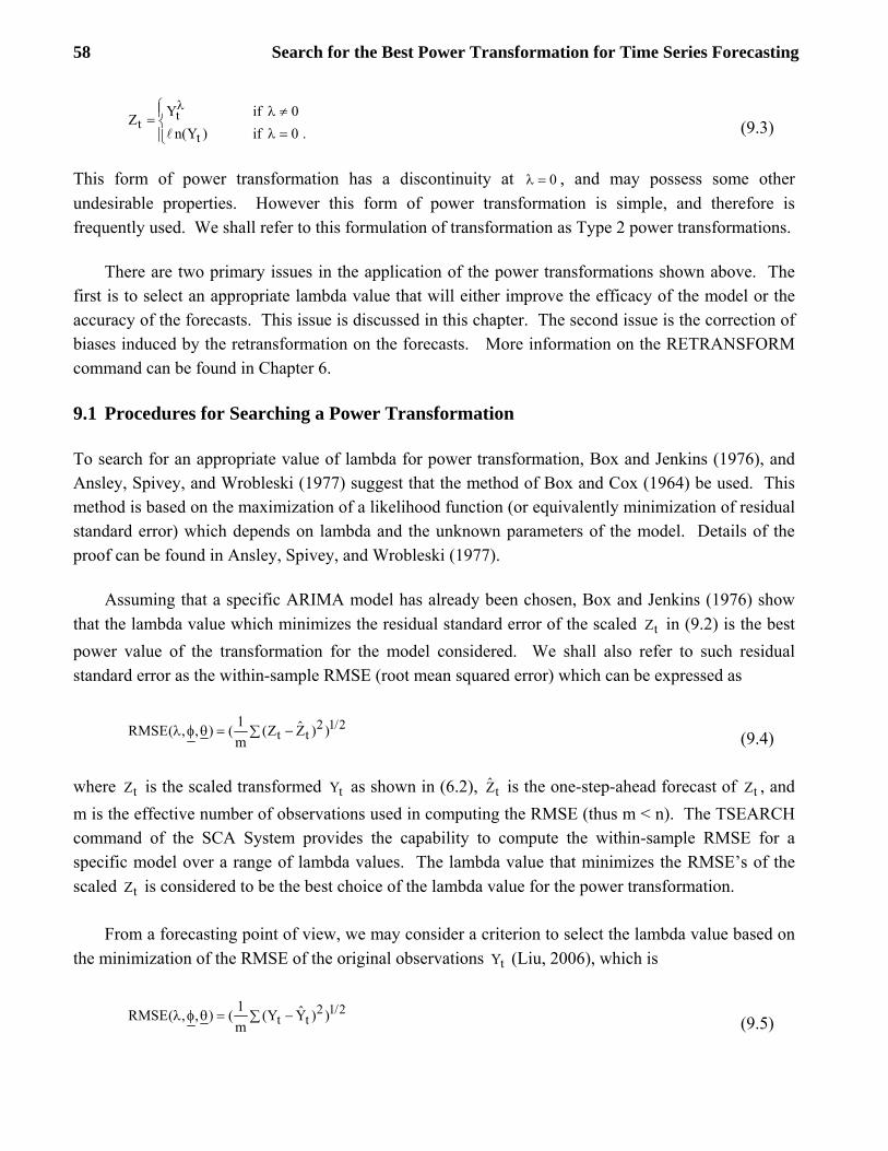
58 Search for the Best Power Transformation for Time Series Forecasting
ttt
Y if 0 Z n(Y ) if 0 .
λ⎧ λ ≠⎪= ⎨λ =⎪⎩
(9.3)
This form of power transformation has a discontinuity at 0λ = , and may possess some other undesirable properties. However this form of power transformation is simple, and therefore is frequently used. We shall refer to this formulation of transformation as Type 2 power transformations.
There are two primary issues in the application of the power transformations shown above. The first is to select an appropriate lambda value that will either improve the efficacy of the model or the accuracy of the forecasts. This issue is discussed in this chapter. The second issue is the correction of biases induced by the retransformation on the forecasts. More information on the RETRANSFORM command can be found in Chapter 6.
9.1 Procedures for Searching a Power Transformation
To search for an appropriate value of lambda for power transformation, Box and Jenkins (1976), and Ansley, Spivey, and Wrobleski (1977) suggest that the method of Box and Cox (1964) be used. This method is based on the maximization of a likelihood function (or equivalently minimization of residual standard error) which depends on lambda and the unknown parameters of the model. Details of the proof can be found in Ansley, Spivey, and Wrobleski (1977).
Assuming that a specific ARIMA model has already been chosen, Box and Jenkins (1976) show that the lambda value which minimizes the residual standard error of the scaled tZ in (9.2) is the best power value of the transformation for the model considered. We shall also refer to such residual standard error as the within-sample RMSE (root mean squared error) which can be expressed as
2 1/2t t
1 ˆRMSE( , , ) ( (Z Z ) )m
λ φ θ = −∑ (9.4)
where tZ is the scaled transformed tY as shown in (6.2), tZ is the one-step-ahead forecast of tZ , and m is the effective number of observations used in computing the RMSE (thus m < n). The TSEARCH command of the SCA System provides the capability to compute the within-sample RMSE for a specific model over a range of lambda values. The lambda value that minimizes the RMSE’s of the scaled tZ is considered to be the best choice of the lambda value for the power transformation.
From a forecasting point of view, we may consider a criterion to select the lambda value based on the minimization of the RMSE of the original observations tY (Liu, 2006), which is
2 1/2t t
1 ˆRMSE( , , ) ( (Y Y ) )m
λ φ θ = −∑ (9.5)

Search for the Best Power Transformation for Time Series Forecasting 59
where tY is the retransformed one-step-ahead forecast tZ . The TSEARCH command also provides such a capability for the determination of the lambda value.
It is useful to note that the value of tY generally increases over time for most business and
economic time series, therefore the forecast error t tˆY Y− also increases over time. Consequently, the
within-sample RMSE based on the original scale (i.e., using RMSE defined in (9.5)) is more influenced by the latter observations of the series and less influenced by the earlier observations. This implicitly imposes the importance of time order in searching the power transformation. This is not the case if the scaled tZ is used in the minimization of RMSE since we expect ( t tˆZ Z− ) to have a similar distribution throughout the entire transformed series. In forecasting, we are primarily interested in the accuracy of the most current forecasts. Hence, the forecasting accuracy (reflected by the one-step-ahead forecast errors) for the latter part of the series is more important than the earlier part. We expect the RMSE criterion in (9.5) to provide a better choice of lambda for forecasting applications compared to the lambda obtained by (9.4).
The power transformation in (9.1) and (9.2) are both Type 1 transformations and are basically the same (see Chapter 6 for the difference between Type 1 and Type 2 power transformation). The only difference between (9.1) and (9.2) is that the transformation in (9.2) is scaled by the geometric mean. Unlike Type 1 power transformations, Type 2 power transformations have a discontinuity at 0λ = , which renders it inappropriate to use when searching for a lambda value based on the minimization of the RMSE of the scaled tZ . However, it is still appropriate to search for a lambda value based on the minimization of the RMSE of the original series tY . This is part of the rationale that leads us to strongly recommend a Type 1 transformation when considering power transformations in time series analysis and forecasting.
We shall use one example to illustrate the search of the lambda value for an appropriate power transformation. Additional examples can be found in Liu (2006).
9.2 Peak Electricity Load Forecasting Example of Power Transformation Search
In this section we provide an example of power transformation in time series analysis using the monthly electricity peak load data in a certain service area of Taiwan. The data analyzed are from January 1982 up to and including December 1999 (a total of 219 monthly observations). The original monthly peak load data (PEAKLOAD) is displayed below.

60 Search for the Best Power Transformation for Time Series Forecasting
Time Series Plot of Monthly Electricity Peak Loads
By examining the above time series plot, we find the first four years of data have a different trend when compared with the rest of the time series. To simplify our discussion, first a power transformation analysis is conducted using the data starting in the fifth year which corresponds to time periods between t=49 and t=192. We reserve the data between t=193 and t=216 for post-sample forecasting comparison. Power transformation analysis that includes the first four years of data can be found in Liu (2006) and will be discussed later in this chapter as well. After performing a preliminary analysis, the following model is chosen for this time series which can be expressed as
12 12
t 1 1 t(1 B)(1 B )Y (1 B)(1 B )a− − = − θ −Θ .
The model is specified in the SCA System using the following TSMODEL command
TSMODEL MODEL1. MODEL IS PEAKLOAD(1,12)=(1)(12)NOISE.
In the above command, MODEL1 is used to reference the specified model in the SCA System. The model reference is subsequently used in the TSEARCH command to find a power value (lambda) which is the best power transformation under this model.
Before the TSEARCH command is employed, an analytic statement is used in the SCA System to assign the value 1 to a variable named VTYPE. This variable will be used in the TSEARCH command shown below.
VTYPE=1 TSEARCH MODEL1. POWER 0.05,-1.0,1.0. FORM VTYPE,GMEAN. @
SPAN 49,192,216. WITHIN-RMSE VPOWER,WRMSEO,WRMSET. @ POST-RMSE VPOWER, PRMSEO, PRMSET.

Search for the Best Power Transformation for Time Series Forecasting 61
In the above TSEARCH command, we use the data between t=49 and t=192 (a total of 144 observations) to determine the lambda value. The last 24 observations (between t=193 and t=216) are reserved for computing the post-sample RMSE for forecasting. This is specified using the SPAN subcommand. The FORM subcommand is used to specify the type of transformation (TYPE=1) and whether the geometric mean should be used to scale the data. We indicate the use of geometric mean scaling by including a variable name (GMEAN is used here) as the second argument. After the TSEARCH command is executed, the GMEAN variable will hold the geometric mean value which can then be used later in an SCA session for retransformation or other applications.
The POWER subcommand is used to specify the range of power values (lambda values) that will be considered. The first argument specifies the increment of the lambda value and the second and third arguments specify the lower and upper bounds of the lambda values.
The WITHIN-RMSE and POST-RMSE subcommands are used to specify the variables to hold information related to the within-sample and post-sample RMSE’s across the range of power values considered. The output results from the TSEARCH command are shown below. Some output has been suppressed for brevity.
THE FOLLOWING ANALYSIS IS BASED ON TIME SPAN 49 THRU 192 THE POST-SAMPLE RMSE IS BASED ON TIME SPAN 193 THRU 216 --------------------------------------------------- POWER TRANSFORMATION USING LAMDA (POWER): -1.0000 --------------------------------------------------- SUMMARY FOR UNIVARIATE TIME SERIES MODEL -- MODEL1 ----------------------------------------------------------------------- VARIABLE TYPE OF ORIGINAL DIFFERENCING VARIABLE OR CENTERED 1 12 PEAKLOAD RANDOM ORIGINAL (1-B ) (1-B ) ----------------------------------------------------------------------- PARAMETER VARIABLE NUM./ FACTOR ORDER CONS- VALUE STD T LABEL NAME DENOM. TRAINT ERROR VALUE 1 PEAKLOAD MA 1 1 NONE .6470 .0665 9.73 2 PEAKLOAD MA 2 12 NONE .5108 .0795 6.42 TOTAL NUMBER OF OBSERVATIONS. . . . . . . . . . . . . . 144 EFFECTIVE NUMBER OF OBSERVATIONS. . . . . . . . . . . . 131 RESIDUAL STANDARD ERROR (WITHOUT OUTLIER ADJUSTMENT). . 0.486509E+03 LAMDA VALUE OF POWER TANSFORMATION= -1.0000 WITHIN-SAMPLE RMSE (UNTRANSFORMED)= 0.651556E+03 N. OF OBS.= 131 POST-SAAMPLE RMSE (UNTRANSFORMED)= 0.734450E+03 N. OF OBS.= 24

62 Search for the Best Power Transformation for Time Series Forecasting
--------------------------------------------------- POWER TRANSFORMATION USING LAMDA (POWER): -0.9500 --------------------------------------------------- SUMMARY FOR UNIVARIATE TIME SERIES MODEL -- MODEL1 ----------------------------------------------------------------------- VARIABLE TYPE OF ORIGINAL DIFFERENCING VARIABLE OR CENTERED 1 12 PEAKLOAD RANDOM ORIGINAL (1-B ) (1-B ) ----------------------------------------------------------------------- PARAMETER VARIABLE NUM./ FACTOR ORDER CONS- VALUE STD T LABEL NAME DENOM. TRAINT ERROR VALUE 1 PEAKLOAD MA 1 1 NONE .6501 .0672 9.68 2 PEAKLOAD MA 2 12 NONE .5228 .0780 6.70 TOTAL NUMBER OF OBSERVATIONS. . . . . . . . . . . . . . 144 EFFECTIVE NUMBER OF OBSERVATIONS. . . . . . . . . . . . 131 RESIDUAL STANDARD ERROR (WITHOUT OUTLIER ADJUSTMENT). . 0.482516E+03 LAMDA VALUE OF POWER TANSFORMATION= -0.9500 WITHIN-SAMPLE RMSE (UNTRANSFORMED)= 0.644508E+03 N. OF OBS.= 131 POST-SAAMPLE RMSE (UNTRANSFORMED)= 0.725407E+03 N. OF OBS.= 24 . . . --------------------------------------------------- POWER TRANSFORMATION USING LAMDA (POWER): 0.9500 --------------------------------------------------- SUMMARY FOR UNIVARIATE TIME SERIES MODEL -- MODEL1 ----------------------------------------------------------------------- VARIABLE TYPE OF ORIGINAL DIFFERENCING VARIABLE OR CENTERED 1 12 PEAKLOAD RANDOM ORIGINAL (1-B ) (1-B ) ----------------------------------------------------------------------- PARAMETER VARIABLE NUM./ FACTOR ORDER CONS- VALUE STD T LABEL NAME DENOM. TRAINT ERROR VALUE 1 PEAKLOAD MA 1 1 NONE .9865 .0097 101.50 2 PEAKLOAD MA 2 12 NONE .5074 .0786 6.46 TOTAL NUMBER OF OBSERVATIONS. . . . . . . . . . . . . . 144 EFFECTIVE NUMBER OF OBSERVATIONS. . . . . . . . . . . . 131 RESIDUAL STANDARD ERROR (WITHOUT OUTLIER ADJUSTMENT). . 0.559287E+03 LAMDA VALUE OF POWER TANSFORMATION= 0.9500 WITHIN-SAMPLE RMSE (UNTRANSFORMED)= 0.564448E+03 N. OF OBS.= 131 POST-SAAMPLE RMSE (UNTRANSFORMED)= 0.620066E+03 N. OF OBS.= 24

Search for the Best Power Transformation for Time Series Forecasting 63
--------------------------------------------------- POWER TRANSFORMATION USING LAMDA (POWER): 1.0000 --------------------------------------------------- SUMMARY FOR UNIVARIATE TIME SERIES MODEL -- MODEL1 ----------------------------------------------------------------------- VARIABLE TYPE OF ORIGINAL DIFFERENCING VARIABLE OR CENTERED 1 12 PEAKLOAD RANDOM ORIGINAL (1-B ) (1-B ) ----------------------------------------------------------------------- PARAMETER VARIABLE NUM./ FACTOR ORDER CONS- VALUE STD T LABEL NAME DENOM. TRAINT ERROR VALUE 1 PEAKLOAD MA 1 1 NONE .9784 .0148 66.30 2 PEAKLOAD MA 2 12 NONE .4975 .0793 6.27 TOTAL NUMBER OF OBSERVATIONS. . . . . . . . . . . . . . 144 EFFECTIVE NUMBER OF OBSERVATIONS. . . . . . . . . . . . 131 RESIDUAL STANDARD ERROR (WITHOUT OUTLIER ADJUSTMENT). . 0.569440E+03 LAMDA VALUE OF POWER TANSFORMATION= 1.0000 WITHIN-SAMPLE RMSE (UNTRANSFORMED)= 0.569440E+03 N. OF OBS.= 131 POST-SAMPLE RMSE (UNTRANSFORMED)= 0.620799E+03 N. OF OBS.= 24
Upon executing the above TSEARCH command, the within-sample RMSE based on the original series (WRMSEO), the within-sample RMSE based on the Box-Cox scaled transformation (WRMSET), and the post-sample RMSE based on the original data (PRMSEO) are stored in the SCA workspace. The PRINT command is used to display the results summary.
PRINT POWER,WRMSEO,WRMSET, PRMSEO.
VARIABLE POWER WRMSEO WRMSET PRMSEO ROW 1 -1.000 651.556 486.509 734.450 2 -.950 644.508 482.516 725.407 3 -.900 636.692 478.575 721.012 4 -.850 629.213 474.988 713.962 5 -.800 621.536 471.678 707.540 6 -.750 614.143 468.559 700.238 7 -.700 606.763 465.690 693.165 8 -.650 599.403 463.020 684.942 9 -.600 592.168 460.623 676.430 10 -.550 585.034 458.505 666.929 11 -.500 578.049 456.673 656.588 12 -.450 571.281 455.184 645.208 13 -.400 564.832 454.070 632.860 14 -.350 558.803 453.378 619.705 15 -.300 553.332 453.161 606.019 16 -.250 548.541 453.449 592.283 17 -.200 544.411 454.277 579.160 18 -.150 541.310 455.652 566.860 19 -.100 539.055 457.570 556.329 20 -.050 537.691 459.996 548.768 21 .000 536.996 462.901 543.140 22 .050 536.918 466.228 539.730 23 .100 537.342 469.926 538.461

64 Search for the Best Power Transformation for Time Series Forecasting
24 .150 538.157 473.938 539.115 25 .200 539.269 478.215 541.400 26 .250 540.602 482.710 544.951 27 .300 542.100 487.387 549.349 28 .350 543.714 492.215 554.173 29 .400 545.399 497.168 559.081 30 .450 547.113 502.223 563.840 31 .500 548.811 507.355 568.290 32 .550 550.447 512.535 572.297 33 .600 551.965 517.718 575.720 34 .650 553.288 522.837 578.394 35 .700 554.289 527.771 580.105 36 .750 554.666 532.236 579.899 37 .800 545.576 526.732 624.905 38 .850 552.012 537.507 619.311 39 .900 558.690 548.670 620.456 40 .950 564.448 559.287 620.066 41 1.000 569.440 569.440 620.799
Based on these results, we obtain a lambda value of 0.05 if the within-sample RMSE based on the original scale is used as the selection criterion. The corresponding post-sample RMSE is 539.730, which is very close to the smallest post-sample RMSE 538.461 (where 0.10λ = ), and much smaller than the post-sample RMSE of 620.799 when no transformation is applied (i.e., when 1.00λ = ). If the within-sample RMSE based on the scaled transformed data is used as a selection criterion for lambda, we obtain a lambda value of -0.30. The corresponding post-sample RMSE is 606.019, which is about 12% higher than the post-sample RMSE if 0.05λ = is used. In the analysis shown above, we find that for forecasting applications, it is better to use the within-sample RMSE based on the original scale as a selection criterion for lambda rather than the traditional Box-Cox criterion which bases lambda selection using the scaled transformed series.
In some situations, the post-sample RMSE for a lambda that was selected based on the scaled transformed series may be higher than the post-sample RMSE of the non-transformed original series. This raises the question about the usefulness of traditional Box-Cox power transformation in forecasting applications. Using all data between t=1 and t=192 (i.e., not excluding the first four years of data), the within-sample RMSE based on the original series (WRMSEO), the within-sample RMSE based on the Box-Cox scaled transformation (WRMSET), and the post-sample RMSE based on the original data (PRMSEO) are computed by the TSEARCH command and summarized below.
POWER WRMSEO WRMSET PRMSEO -1.000 568.140 400.624 770.280 -.950 561.371 395.330 764.340 -.900 555.078 390.197 760.422 -.850 547.730 385.368 755.751 -.800 540.831 381.113 751.246 -.750 533.886 377.020 746.435 -.700 526.602 373.269 740.699 -.650 519.204 369.934 733.382 -.600 511.615 367.009 724.031 -.550 503.967 364.536 711.548 -.500 496.428 362.638 695.359

Search for the Best Power Transformation for Time Series Forecasting 65
-.450 489.414 361.390 674.882 -.400 483.410 360.901 651.183 -.350 478.789 361.197 626.563 -.300 475.758 362.281 603.256 -.250 474.227 364.097 583.136 -.200 473.919 366.562 567.206 -.150 474.520 369.593 555.147 -.100 475.767 373.108 546.523 -.050 477.458 377.048 540.675 .000 479.445 381.366 536.990 .050 481.628 386.023 534.945 .100 483.939 390.997 534.136* .150 486.333 396.270 534.258 .200 488.781 401.831 535.088 .250 491.261 407.671 536.460 .300 493.760 413.786 538.252 .350 496.268 420.172 540.373 .400 498.780 426.830 542.760 .450 501.291 433.758 545.363 .500 504.078 440.968 549.313 .550 506.485 448.433 551.698 .600 509.020 456.188 554.868 .650 511.489 464.219 557.878 .700 513.970 472.537 561.096 .750 516.434 481.143 564.353 .800 518.894 490.043 567.713 .850 521.347 499.242 571.139 .900 523.796 508.745 574.644 .950 526.242 518.557 578.220 1.000 528.685 528.685 581.872
From the above table, we obtain a lambda value of -0.20 if the within-sample RMSE based on the original scale is used as a selection criterion for lambda. The corresponding post-sample RMSE is 567.206. However, if the within-sample RMSE based on the scaled transformed series is used, we obtain a lambda value of -0.40. The corresponding post-sample RMSE is 651.183 which is much larger than the post-sample RMSE 581.872 if no transformation is applied to the time series (i.e., when
1.00λ = ). Such a result gives practitioners reasons to question the usefulness of power transformations in forecasting. The lambda selected based on the original scale does not have this problem. More discussion of this issue can be found in Liu (2006).

66 Search for the Best Power Transformation for Time Series Forecasting

CHAPTER 10
GARCH MODELING AND ANALYSIS
The Professional Edition (B) of the SCA Statistical System includes GARCH modeling, analysis, and forecasting capabilities through SCA WorkBench and the SCAB34S GARCH product. The SCAB34S product is a subset of capabilities from the B34S ProSeries Econometric System. More on the B34S family of products can be found in Stokes (1997). SCAB34S GARCH is included as an integrated component of the Professional Edition (B). The user is directed to the document, General Autoregressive Conditional Heteroscedastic (GARCH) Modeling Using the SCAB34S-GARCH and SCA WorkBench, for a detailed discussion of GARCH capabilities in the SCA System. A detailed and comprehensible discussion of GARCH models can be found in Liu (2006). An example of the ARCH/GARCH modeling environment is displayed below:
The SCA System provides options to estimate a variety of conditional heteroscedastic models including the autoregressive conditional heteroscedastic (ARCH) model of Engle (1982), the generalized ARCH (GARCH) model of Bollerslev (1986), the integrated GARCH (IGARCH) model of Nelson (1990, 1991), the GARCH-M model of Engle, Lilien, and Robins (1987), the GJR-GARCH model of Glosten, Jagannathan, and Runkle (1993), the exponential GARCH (EGARCH) model of Nelson (1991), and a variety of threshold GARCH models discussed in Zachoian (1994) and Tsay (2005). In addition, the non-normal error distributions including Student-t, Cauchy, and GED are supported.

68 GARCH Modeling and Analysis

CHAPTER 11
TIME SERIES MODELS WITH TIME-VARYING PARAMETERS
The Professional Edition (B) of the SCA Statistical System provides capabilities to employ time series models with time-varying parameters. In this chapter, the TVPEXPLORE command is presented. Other commands such as TSMODEL and ESTIMATE are also used to complete the illustrative examples. These additional commands are documented in the SCA reference manual, Forecasting and Time Series Analysis Using the SCA Statistical System, Volume 1.
The TVPEXPLORE command is very useful to explore the stability and time-varying properties of the estimated model parameters. It can also be used to study seasonal effects, structural shifts, and overall model performance as it relates to both parameter estimates and windows of time.
11.1 Example of the TVPEXPLORE Command Using a Day-of-Week Effect Model
To illustrate an application of time-varying parameter analysis through the TVPEXPLORE command, we consider the daily per store sales (DSALES) of a service-related product from January 1, 2004 through December 31, 2006.
Daily Sales (1/1/2004 – 12/31/2006)
The plot reveals that DSALES has a very strong weekly periodic pattern and thus is dominated by strong day-of-week effects. Weekends (Friday to Sunday) have consistently higher sales than weekdays. In addition, Monday, Tuesday,…, and Sunday seem to have their own unique means, often referred to as day-of-week effects. In this example, we are interested in studying the characteristics of the day-of-week effects over time.

70 Time Series Models with Time-varying Parameters
We begin by generating the day-of-week dummy variables using the DOWEEK and DVECTOR commands. The DATE and DSALES variables have been input into the SCA workspace prior to the commands shown below.
DOWEEK DATE. DAYOFWEEK VDOW. DVECTOR VDOW. MAIN-EFFECT X.
The first twenty-one rows of the generated dummy variables (X1 to X6) are now printed along with the DATE, DSALES and VDOW variables for illustration. For more information on the use of the DOWEEK and DVECTOR commands, please refer to Chapter 2.
PRINT VARIABLES DATE, DSALES,VDOW, X1 TO X6. @ FORMAT '2F12.0,7F5.0'. SPAN 1,21.
VARIABLE DATE DSALES VDOW X1 X2 X3 X4 X5 X6 ROW 1 20040101 3632 4 0 0 0 1 0 0 2 20040102 4261 5 0 0 0 0 1 0 3 20040103 4314 6 0 0 0 0 0 1 4 20040104 3257 7 -1 -1 -1 -1 -1 -1 5 20040105 2203 1 1 0 0 0 0 0 6 20040106 2093 2 0 1 0 0 0 0 7 20040107 2220 3 0 0 1 0 0 0 8 20040108 2555 4 0 0 0 1 0 0 9 20040109 4690 5 0 0 0 0 1 0 10 20040110 4413 6 0 0 0 0 0 1 11 20040111 3070 7 -1 -1 -1 -1 -1 -1 12 20040112 1922 1 1 0 0 0 0 0 13 20040113 1981 2 0 1 0 0 0 0 14 20040114 2236 3 0 0 1 0 0 0 15 20040115 2712 4 0 0 0 1 0 0 16 20040116 4869 5 0 0 0 0 1 0 17 20040117 4740 6 0 0 0 0 0 1 18 20040118 3591 7 -1 -1 -1 -1 -1 -1 19 20040119 2379 1 1 0 0 0 0 0 20 20040120 2417 2 0 1 0 0 0 0
21 20040121 2505 3 0 0 1 0 0 0
We now specify a deterministic seasonal regression model with an AR(1) term using the TSMODEL command. The AR(1) term is used to accommodate day-to-day serial correlation. This model is then estimated using the ESTIMATE command.
TSMODEL SALESMDL. MODEL IS @ DSALES=C+(B1)X1+(B2)X2+(B3)X3+(B4)X4+(B5)X5+(B6)X6+1/(1;PH1)NOISE.
ESTIMATE SALESMDL.

Time Series Models with Time-varying Parameters 71
SUMMARY FOR UNIVARIATE TIME SERIES MODEL -- SALESMDL ----------------------------------------------------------------------- VARIABLE TYPE OF ORIGINAL DIFFERENCING VARIABLE OR CENTERED DSALES RANDOM ORIGINAL NONE X1 RANDOM ORIGINAL NONE X2 RANDOM ORIGINAL NONE X3 RANDOM ORIGINAL NONE X4 RANDOM ORIGINAL NONE X5 RANDOM ORIGINAL NONE X6 RANDOM ORIGINAL NONE ----------------------------------------------------------------------- PARAMETER VARIABLE NUM./ FACTOR ORDER CONS- VALUE STD T LABEL NAME DENOM. TRAINT ERROR VALUE 1 C CNST 1 0 NONE 3212.6734 19.8714 161.67 2 B1 X1 NUM. 1 0 NONE -970.1566 10.2090 -95.03 3 B2 X2 NUM. 1 0 NONE -892.6729 10.2113 -87.42 4 B3 X3 NUM. 1 0 NONE -663.1560 10.2075 -64.97 5 B4 X4 NUM. 1 0 NONE -288.0881 10.2013 -28.24 6 B5 X5 NUM. 1 0 NONE 1599.5879 10.1879 157.01 7 B6 X6 NUM. 1 0 NONE 1152.0953 10.1881 113.08 8 PH1 DSALES D-AR 1 1 NONE .7675 .0192 39.95 EFFECTIVE NUMBER OF OBSERVATIONS . . 1095 R-SQUARE . . . . . . . . . . . . . . 0.975 RESIDUAL STANDARD ERROR. . . . . . . 0.152890E+03
The day-of-week effects ( B1 Monday≡ ,…, B6 Saturday≡ ) are estimated as deviations from the overall mean of DSALES (which is represented by C in the model). Since such a model uses the constraint B1+B2+…+B7=0, the Sunday effect is equal to –(B1+B2+…+B6). The use of the above deterministic seasonal model assumes that the day-of-week effects remain constant over time.
The TVPEXPLORE command can be used to explore the validity of the assumption of invariant day-of-week effects for the DSALES series. The WINDOWSIZE subcommand is used to specify the number of time periods in moving window estimation of the model parameters. The window size can be increased or decreased depending upon desired sensitivity in detecting the time-varying properties of the model parameters. In this example, the window size is specified as 84 observations (twelve weeks). Here, the first estimation will be from time span 1 to 84; the second estimation will be from 2 to 85; and so on. The parameter values and their t-values are saved for each estimation window in designated variables. All model parameters that have been specified with labels in the TSMODEL command will accumulate in this manner during the TVPEXPLORE estimation. Note that the first 83 values of the estimated parameters and their t-values are padded with missing values since the initial window size is specified as 84 observations.

72 Time Series Models with Time-varying Parameters
TVPEXPLORE SALESMDL. WINDOWSIZE 84. HOLD VARIANCE(VRNCE)
VARIABLE C STORES PARAMETER ESTIMATES (WITH 1096 VALUES) VARIABLE _C STORES THE t-VALUES OF THE ABOVE ESTIMATES VARIABLE B1 STORES PARAMETER ESTIMATES (WITH 1096 VALUES) VARIABLE _B1 STORES THE t-VALUES OF THE ABOVE ESTIMATES VARIABLE B2 STORES PARAMETER ESTIMATES (WITH 1096 VALUES) VARIABLE _B2 STORES THE t-VALUES OF THE ABOVE ESTIMATES VARIABLE B3 STORES PARAMETER ESTIMATES (WITH 1096 VALUES) VARIABLE _B3 STORES THE t-VALUES OF THE ABOVE ESTIMATES VARIABLE B4 STORES PARAMETER ESTIMATES (WITH 1096 VALUES) VARIABLE _B4 STORES THE t-VALUES OF THE ABOVE ESTIMATES VARIABLE B5 STORES PARAMETER ESTIMATES (WITH 1096 VALUES) VARIABLE _B5 STORES THE t-VALUES OF THE ABOVE ESTIMATES VARIABLE B6 STORES PARAMETER ESTIMATES (WITH 1096 VALUES) VARIABLE _B6 STORES THE t-VALUES OF THE ABOVE ESTIMATES VARIABLE PH1 STORES PARAMETER ESTIMATES (WITH 1096 VALUES) VARIABLE _PH1 STORES THE t-VALUES OF THE ABOVE ESTIMATES VARIABLE VRNCE STORES THE VARIANCE FOR EACH ESTIMATION WINDOW
The above output echoes the names of the variables containing the parameter estimates, associated t-values, and residual variance. As mentioned earlier, the effect of Sunday (B7) can be computed using the following SCA analytic statement
B7= -(B1+B2+B3+B4+B5+B6)
In order to better visualize the time-varying properties of the constant and day-of-week effects, the overall mean of the vector C is computed and added to the day-of-week effects using the following analytic statements
CMEAN=MEAN(C) TB1=CMEAN+B1 TB2=CMEAN+B2 TB3=CMEAN+B3 TB4=CMEAN+B4 TB5=CMEAN+B5 TB6=CMEAN+B6 TB7=CMEAN+B7

Time Series Models with Time-varying Parameters 73
The time-varying properties of the day-of-week effects can now be graphed using the SCAGRAF command or other graphing program.
$1,750
$2,250
$2,750
$3,250
$3,750
$4,250
$4,750
$5,250
1/1/2004 1/1/2005 1/1/2006
Time‐varying Day of Week Effects
FRI
SAT
SUN
THU
WED
TUEMON
CNST
The above plot provides an abundance of information regarding this daily sales series. First, we find that the day-of-week effects are not stable over time. Second, weekends (Friday through Sunday) have higher variability (and higher sales volumes) than weekdays. Third, the estimated constant (labeled as CNST in the graph) reveals that sales are decreased in 2006 in comparison with 2005.
A yearly cyclical pattern is also present. Higher sales typically occur around February and lower sales typically occur around the September or October months. In addition, we find that the distribution of day-of-week effects across the week is somewhat dynamic. For example, during the peak cycle (around February), the relative increase of sales in the weekend periods are greater than the weekday periods. Also, during the yearly cycle with lower sales (around September or October), weekday sales are increasing at a relatively greater rate over weekend sales. Finally, it seems that Friday sales are eroding at a faster rate than other days and the gap between Friday and Saturday sales is somewhat narrowing.
As shown, the use of traditional deterministic models with TVPEXPLORE reveals much about the series at hand that may lead to better operational planning and business decisions. However, with such high instability among the day-of-week effects over time, it would be unwise to rely on such deterministic models for forecasting applications. Therefore, if forecasting is the primary application,

74 Time Series Models with Time-varying Parameters
adaptive models such as ARIMA are better suited. In addition, time-segmented or value-segmented (threshold) time series models may be useful in the analysis and forecasting of such series. A time-segmented model will be applied to the DSALES series to illustrate such application in the next chapter.
The residual variances for the estimation windows were also stored using the HOLD subcommand in the TVPEXPLORE command. Besides exploring the time-varying properties of the day-of-week effects (or other parameter estimates in the model), it may be useful to explore the residual standard errors of the model over time. In the TVPEXPLORE command, the residual variances were stored in the VRNCE variable. We now use the SQRT analytic statement to get the residual standard errors.
STDERR=SQRT(VRNCE)
The residual standard errors (STDERR) can now be plotted using the SCAGRAF program or other graphing program as shown below.
50
100
150
200
1/1/2004 1/1/2005 1/1/2006
Time‐varying Residual Standard Deviation
The plot reveals that the residual standard errors are also not stable over time. The standard errors are relatively high earlier in each year but lower near the end of each year. This may be partially due to holidays and seasonal business conditions. With evidence of cyclical behavior in residual standard errors, we would also expect forecasting accuracy to be highly dependent upon the time of year in

Time Series Models with Time-varying Parameters 75
which it is measured. This information may be important to a business for seasonal planning, and to understand the underlying causes of such cyclical behavior in forecasting accuracy.
11.2 Example of TVPEXPLORE in the Context of Simple Moving Averages
The concept and power behind the TVPEXPLORE command is quite extraordinary. Even the use of a very simple model with the time-varying parameter approach can provide important information. Consider the following simple mean model
t tDSALES C a .= + (11.1)
If the above model is applied to the DSALES series using the traditional estimation method, we obtain C 3217.03= as the estimate of the fixed mean. However, if we employ the TVPEXPLORE command with a moving window size of 84 observations, as in the previous example, we gain information on the year-to-year movement of the mean for the DSALES series similar to that shown in the previous model. Below are the SCA commands for such an analysis.
TSMODEL MEANMDL. MODEL DSALES=C+NOISE. TVPEXPLORE MEANMDL. WINDOWSIZE 84.
In the table below, the first fourteen non-missing constant estimates from the model with day-of-week effects and the above simple mean model are displayed. Rows 1-83 are missing since the initial moving window size was specified as 84.
Row Constant from
Day-of-Week Model Constant from
Simple Mean Model % Difference
84 85 86 87 88 89 90 91 92 93 94 95 96 97
3332.07 3407.06 3382.19 3343.90 3342.44 3378.36 3399.23 3421.24 3438.69 3419.70 3411.95 3403.82 3429.59 3425.50
3361.89 3352.19 3359.52 3360.71 3360.17 3359.57 3362.77 3368.36 3376.23 3382.39 3385.52 3387.66 3392.82 3397.65
-0.89% 1.61% 0.67% -0.50% -0.53% 0.56% 1.07% 1.55% 1.82% 1.09% 0.77% 0.47% 1.07% 0.81%
From the above table, we find the estimates for the mean are very similar in each window. To better illustrate the similarity between these two estimates, the mean estimates from the above two models using time-varying parameter estimation are displayed below.

76 Time Series Models with Time-varying Parameters
$1,750
$2,250
$2,750
$3,250
$3,750
$4,250
$4,750
$5,250
1/1/2004 1/1/2005 1/1/2006
Comparison of Time‐Varying Means (Window Size 84)
Mean Model
DOW Effect Model
From the above graphs, it is evident that the time-varying estimates of the mean are very similar to one another even though the models are of different form. The average difference of these two estimates is 0.9% in relative terms of percent. From the above graph, we can also see the systematic cyclical level movements from year to year. The estimates of time-varying means based on the simple mean model is the same as the traditional “moving average” approach. However, by including the time-varying day-of-week effects in the model (as shown in the first example), we gain more insight into the characteristics of the DSALES series without distorting the information provided by the simple mean model.

CHAPTER 12
WEIGHTED TIME SERIES MODEL ESTIMATION AND FORECASTING
The Professional Edition (B) of the SCA Statistical System includes weighted time series model estimation and weighted forecasting capabilities. The commands WESTIM and WFORECAST are documented in this chapter. These two commands can be employed for both time-segmented and value-segmented analysis and forecasting. Related commands including TARTEST, TARXTEST, TARESTIM, TARFORECAST, THMTEST, and THMEXPLORE are for value-segmented models discussed in the next Chapter. Additional information can be found in Liu (2006).
This chapter includes three examples to illustrate weighted time series model estimation and forecasting. The first example illustrates time-segmented analysis and forecasting of the daily sales series (DSALES), discussed in the previous chapter, by leveraging separate models for weekday and weekend periods. The second example uses stock market data to illustrate how the WESTIM command can be used to discount the effect of atypical sections of data in a time series without disrupting the serial correlations in the data. The third example illustrates how the WESTIM command can be used for a value-segmented (threshold) transfer function model to study the symmetrical (or asymmetrical) elasticity characteristics of new home sales with respect to interest rate increases or decreases.
Statistical modeling is used to capture homogeneous patterns or relationships that may exist in the data. However in time series data, such patterns may be dependent on the day of the week, or the month of the year, often referred to as periodic time series (Cleveland and Tiao, 1979). In other situations, such patterns or relationships may be temporarily disrupted by outliers or transient structural changes. If disruptions are isolated and not exceedingly large, outlier detection and adjustment techniques are sufficient to correct for the biases caused by such disruptions. However if the disruptions are clustered together or if their atypical effects are persistent over a period of time, it may be more appropriate to discount or disregard those portions of the data in time series modeling. In regression analysis, we can accomplish this by simply deleting such portions of the data during model estimation. In time series analysis, however, data cannot be arbitrarily deleted during model estimation due to the existence of serial correlation or seasonality. In this chapter, we introduce a weighted estimation method to facilitate the practice of discounting the effects of certain atypical data in ARIMA and transfer function modeling as well as in periodic time series data.
12.1 Model Estimation Using the Weighted Method
When the parameters in a time series model are estimated, the typical approach is to obtain the final parameter estimates that maximize the log likelihood function, or roughly speaking, minimize the sum of squared errors. For time series models, the sum of squared errors can be generally expressed as

78 Weighted Time Series Model Estimation and Forecasting
1
n 2t
t tˆSSE a
== ∑ (12.1)
where ta is the residual (also referred to as estimated error) for the t-th observation, n is the total number of observations, and 1t is the first residual in the model that can be computed. The above expression is not only appropriate for conditional least squares estimation, but also appropriate for exact maximum likelihood estimation because the entire log likelihood function can be cast in a form as that in (12.1).
In the weighted estimation method, instead of minimizing the sum of squared errors expressed in (12.1), we obtain the parameter estimates that minimize the following weighted sum of squared errors
1
n 2t t
t tˆSSE w a
== ∑ (12.2)
where tw 1= if the residual ta is to be included in the computation of SSE, and tw 0= if the residual ta is to be excluded in the computation of SSE. Even though an ta is excluded in the computation of SSE, it is still used in computing the subsequent ta 's due to the serially correlated nature of time series. Obviously if tw 1= for all t, the weighted estimation method will produce the same estimates as the traditional method. By setting 1 or 0 for the values in the weight variable in (12.2), we can define the relevant segment of time series data to be studied, and obtain the parameter estimates that are optimal for this segment of time series data. We may view the weight variable tw as an instrument for the convenient segmentation of a time series into certain homogenous groupings.
The weighted estimation method has many applications. For example, certain time series may possess a strong month-of-year effect, or day-of-week effect as shown in the previous chapter. By grouping those data that possess similar characteristics (e.g., weekdays and weekends), separate models can be entertained for those data groups which may help in better model estimates and in turn better forecasting performance. In the next section, we will discuss this more by revisiting the DSALES series used to illustrate the TVPEXPLORE command for time-varying parameters. Another use of the weighted estimation method may be to discount a portion of a time series in model estimation that exhibits a radically different pattern from the general series. We can do this by creating a weight variable consisting of zeros that correspond to observations whose effects on parameter estimation are to be discounted, and ones corresponding to observations that otherwise are to receive full weight during estimation.
The weight variable may also assume a more general structure rather than simply 0 and 1 values. A weight value may be varied between 0 and 1 to represent its relative importance. In addition, a weight variable may follow a step function or even a geometric sequence. By varying the structure of the weight variable, we can address a number of applications in time series modeling and forecasting.

Weighted Time Series Model Estimation and Forecasting 79
12.2 Example of Time-varying Day-of-Week Effects in Daily Sales
In this section, we once again consider the daily sales series (DSALES). In Chapter 11, the TVPEXPLORE command was used to gain insight into the time-varying properties of the day-of-week effects of the DSALES series. It was found that weekend periods (Friday through Sunday) possessed different time-varying properties than weekday periods (Monday through Thursday). This leads us to consider whether the ARIMA model for the weekend periods is different from the ARIMA model for the weekday periods. Since sales during the weekend periods are very different from the weekday periods, a segmented model may result in improved forecasting accuracy for both weekdays and weekends. This example illustrates time-segmented models using the WESTIM command to obtain parameter estimates for weekday and weekend periods. The WFORECAST command is then used to combine the forecasts of these two models together.
We begin this illustration of the WESTIM command by creating binary weight variables to indicate weekday and weekend time periods for DSALES. The VDOW variable is a day-of-week indicator variable that was created earlier using the command DOWEEK (see Chapter 11). The following RECODE commands are used to generate the WEEKDAYS and WEEKENDS binary indicator variables.
RECODE VDOW. VALUES (1, 4, 1), (5, 7, 0). NEW WEEKDAYS. RECODE VDOW. VALUES (1, 4, 0), (5, 7, 1). NEW WEEKENDS.
To better understand the binary variables created, the first twenty-one observations of the WEEKDAYS and WEEKENDS indicator variables are printed along with DATE, DSALES, and VDOW.
PRINT DATE, DSALES, VDOW, WEEKDAYS, WEEKENDS. SPAN 1, 21. @ FORMAT '2F10.0, 3F9.0'
VARIABLE DATE DSALES VDOW WEEKDAYS WEEKENDS ROW 1 20040101 3632 4 1 0 2 20040102 4261 5 0 1 3 20040103 4314 6 0 1 4 20040104 3257 7 0 1 5 20040105 2203 1 1 0 6 20040106 2093 2 1 0 7 20040107 2220 3 1 0 8 20040108 2555 4 1 0 9 20040109 4690 5 0 1 10 20040110 4413 6 0 1 11 20040111 3070 7 0 1 12 20040112 1922 1 1 0 13 20040113 1981 2 1 0 14 20040114 2236 3 1 0 15 20040115 2712 4 1 0 16 20040116 4869 5 0 1 17 20040117 4740 6 0 1

80 Weighted Time Series Model Estimation and Forecasting
18 20040118 3591 7 0 1 19 20040119 2379 1 1 0 20 20040120 2338 2 1 0 21 20040121 2450 3 1 0
Following appropriate model identification procedures, a seasonal model of the form
( ) ( ) ( )( )
71 17
t t1
1 B 11 B DSALES a
1 B
−θ −Θ− =
−φ (12.3)
is found to be appropriate for the DSALES series. For comparison purposes, the above model is first estimated using all available data in a traditional manner without discerning between weekday and weekend periods. The model is specified in the SCA System using the TSMODEL command and is then estimated using the ESTIM command below.
TSMODEL SALESMDL. MODEL DSALES(7)=(1)(7)/(1)NOISE. ESTIM SALESMDL. HOLD RESID(RES).
SUMMARY FOR UNIVARIATE TIME SERIES MODEL -- SALESMDL ---------------------------------------------------------------------- VARIABLE TYPE OF ORIGINAL DIFFERENCING VARIABLE OR CENTERED 7 DSALES RANDOM ORIGINAL (1-B ) ----------------------------------------------------------------------- PARAMETER VARIABLE NUM./ FACTOR ORDER CONS- VALUE STD T LABEL NAME DENOM. TRAINT ERROR VALUE 1 DSALES MA 1 1 NONE -.4283 .0357 -11.99 2 DSALES MA 2 7 NONE .5039 .0264 19.09 3 DSALES D-AR 1 1 NONE .5025 .0319 15.77 EFFECTIVE NUMBER OF OBSERVATIONS . . 1088 R-SQUARE . . . . . . . . . . . . . . 0.984 RESIDUAL STANDARD ERROR. . . . . . . 0.120961E+03
The WESTIM command is now employed to estimate the parameters for the weekday model
(Monday through Thursday). In order to maintain separate parameter estimates for the weekday and weekend models, the model in (12.3) is re-specified using the model name WKDAYMDL. The WEEKDAYS indicator variable is specified in the WEIGHT subcommand to obtain weighted parameter estimates for the weekday periods.
WESTIM WKDAYMDL. WEIGHT WEEKDAYS.
SUMMARY FOR UNIVARIATE TIME SERIES MODEL -- WKDAYMDL ----------------------------------------------------------------------- VARIABLE TYPE OF ORIGINAL DIFFERENCING VARIABLE OR CENTERED 7 DSALES RANDOM ORIGINAL (1-B ) -----------------------------------------------------------------------
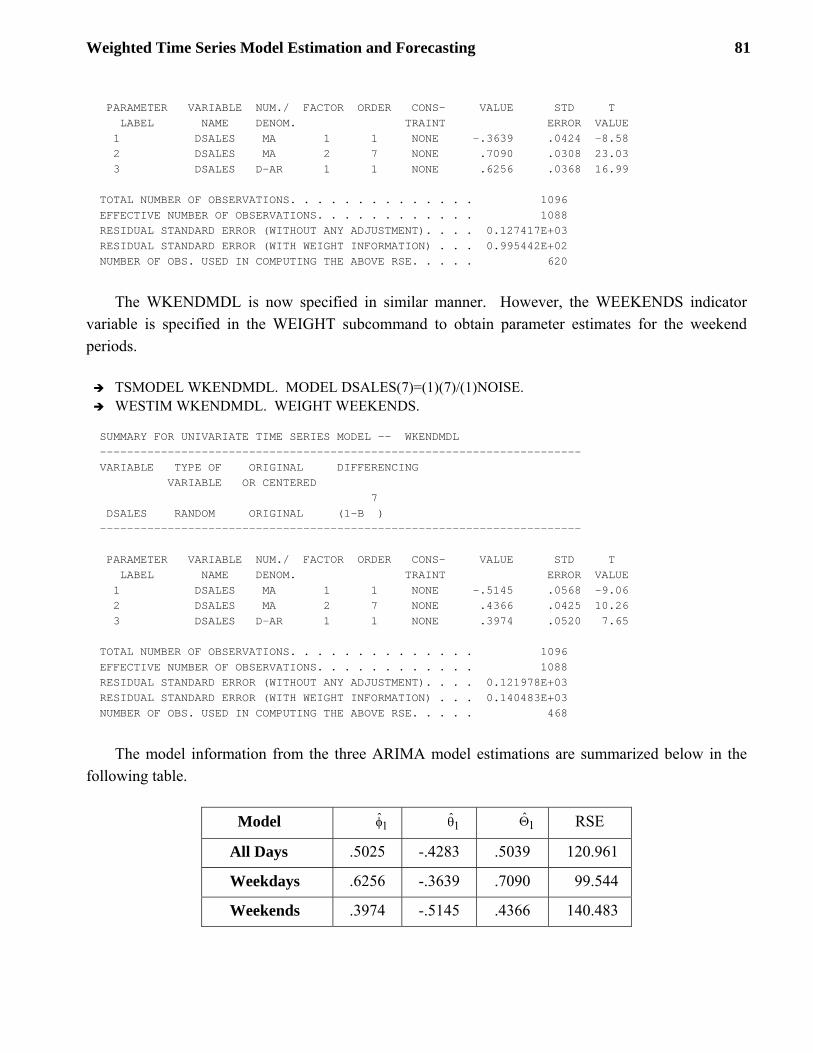
Weighted Time Series Model Estimation and Forecasting 81
PARAMETER VARIABLE NUM./ FACTOR ORDER CONS- VALUE STD T LABEL NAME DENOM. TRAINT ERROR VALUE 1 DSALES MA 1 1 NONE -.3639 .0424 -8.58 2 DSALES MA 2 7 NONE .7090 .0308 23.03 3 DSALES D-AR 1 1 NONE .6256 .0368 16.99 TOTAL NUMBER OF OBSERVATIONS. . . . . . . . . . . . . . 1096 EFFECTIVE NUMBER OF OBSERVATIONS. . . . . . . . . . . . 1088 RESIDUAL STANDARD ERROR (WITHOUT ANY ADJUSTMENT). . . . 0.127417E+03 RESIDUAL STANDARD ERROR (WITH WEIGHT INFORMATION) . . . 0.995442E+02 NUMBER OF OBS. USED IN COMPUTING THE ABOVE RSE. . . . . 620
The WKENDMDL is now specified in similar manner. However, the WEEKENDS indicator
variable is specified in the WEIGHT subcommand to obtain parameter estimates for the weekend periods.
TSMODEL WKENDMDL. MODEL DSALES(7)=(1)(7)/(1)NOISE. WESTIM WKENDMDL. WEIGHT WEEKENDS.
SUMMARY FOR UNIVARIATE TIME SERIES MODEL -- WKENDMDL ----------------------------------------------------------------------- VARIABLE TYPE OF ORIGINAL DIFFERENCING VARIABLE OR CENTERED 7 DSALES RANDOM ORIGINAL (1-B ) ----------------------------------------------------------------------- PARAMETER VARIABLE NUM./ FACTOR ORDER CONS- VALUE STD T LABEL NAME DENOM. TRAINT ERROR VALUE 1 DSALES MA 1 1 NONE -.5145 .0568 -9.06 2 DSALES MA 2 7 NONE .4366 .0425 10.26 3 DSALES D-AR 1 1 NONE .3974 .0520 7.65 TOTAL NUMBER OF OBSERVATIONS. . . . . . . . . . . . . . 1096 EFFECTIVE NUMBER OF OBSERVATIONS. . . . . . . . . . . . 1088 RESIDUAL STANDARD ERROR (WITHOUT ANY ADJUSTMENT). . . . 0.121978E+03 RESIDUAL STANDARD ERROR (WITH WEIGHT INFORMATION) . . . 0.140483E+03 NUMBER OF OBS. USED IN COMPUTING THE ABOVE RSE. . . . . 468
The model information from the three ARIMA model estimations are summarized below in the
following table.
Model 1φ 1θ 1Θ RSE
All Days .5025 -.4283 .5039 120.961
Weekdays .6256 -.3639 .7090 99.544
Weekends .3974 -.5145 .4366 140.483

82 Weighted Time Series Model Estimation and Forecasting
As shown in the above summary table, the parameter estimates are quite different between the weekday and weekend models. In particular, the seasonal moving-average parameter estimate, 1Θ , for the weekday model is much larger than the seasonal parameter estimate for the weekend model. The t-value of 1Θ for the weekday model is also much larger. This information reveals that the week-to-week changes in sales are much more stable for the weekday periods than the weekend periods. Also, the residual standard error (RSE) of the weekday model is clearly smaller than the RSE of the weekend model. Such information is otherwise masked by the averaging effect of the traditional (All Days) model. In operations planning or inventory management applications, the forecasting interval is often as important as the point forecast in determining customer service level and safety stock. The traditional model would result in a larger forecasting interval for weekday periods and a smaller forecasting interval for weekend periods than necessary.
Based on the above results, we may be inclined to leverage models based on weighted estimation to improve forecasting accuracy. The SCA System provides the WFORECAST command to combine forecasts from more than one model using a weighting method. In the WFORECAST command provided below, the WKDAYMDL and WKENDMDL models are forecasted. Prior to executing the WFORECAST command, the forecast dates are generated using the DATEBUILD command and the corresponding day of week information is stored in the variable DAYCODE. The RECODE command can then be used to generate the binary indicator variables for the weekday and weekend models.
DATEBUILD FCSTDATE. BEGIN 2007, 1, 1. NOBS 14. HOLD DOWEEK(DAYCODE). RECODE DAYCODE. VALUES (1,4,1),(5,7,0). NEW FIWKDAY. RECODE DAYCODE. VALUES (1,4,0),(5,7,1). NEW FIWKEND.
The weight variables (FIWKDAY and FIWKEND) specified in the WEIGHTS subcommand in the WFORECAST command below must correspond with the order of the regime models entered. Upon executing the WFORECAST command, interim forecasts are generated for the weekday model and the weekend model. Lastly, the interim forecasts are combined into the final forecasts based on the weight variables. Since the weight variables are of binary form with no overlap between weekday and weekend periods, the final forecasts are a direct copy of the appropriate interim forecasts.
WFORECAST WKDAYMDL, WKENDMDL. @ WEIGHTS FIWKDAY, FIWKEND. NOFS 14.
--------------------------------------------------- MODEL WKDAYMDL: 14 FORECASTS, BEGINNING AT 1096 --------------------------------------------------- TIME FORECAST STD. ERROR ACTUAL IF KNOWN 1097 2374.6762 99.5442 1098 2436.5593 140.0418 1099 2662.9423 153.0013 1100 2965.9725 157.7841 1101 4738.8807 159.6171 1102 4461.5719 160.3289 1103 3467.6502 160.6066

Weighted Time Series Model Estimation and Forecasting 83
1104 2281.2279 164.3494 1105 2378.0958 167.5050 1106 2626.3660 168.7240 1107 2943.0894 169.1988 1108 4724.5645 169.3842 1109 4452.6154 169.4567 1110 3462.0468 169.4851 --------------------------------------------------- MODEL WKENDMDL: 14 FORECASTS, BEGINNING AT 1096 --------------------------------------------------- TIME FORECAST STD. ERROR ACTUAL IF KNOWN 1097 2435.2684 140.4826 1098 2429.8538 190.1211 1099 2685.5587 196.8193 1100 3011.6903 197.8564 1101 4689.1343 198.0197 1102 4387.7981 198.0455 1103 3466.3836 198.0496 1104 2360.6012 213.4665 1105 2400.1805 225.4014 1106 2673.7663 227.2291 1107 3007.0039 227.5164 1108 4687.2719 227.5617 1109 4387.0580 227.5689 1110 3466.0894 227.5700 --------------------------------------------------- COMBINED FORECASTS: 14 FORECASTS, BEGINNING AT 1096 --------------------------------------------------- TIME FORECAST STD. ERROR ACTUAL IF KNOWN 1097 2374.6763 99.5442 1098 2436.5593 140.0418 1099 2662.9424 153.0013 1100 2965.9724 157.7841 1101 4689.1343 198.0197 1102 4387.7983 198.0455 1103 3466.3835 198.0496 1104 2281.2280 164.3494 1105 2378.0957 167.5050 1106 2626.3660 168.7240 1107 2943.0894 169.1988 1108 4687.2720 227.5617 1109 4387.0581 227.5689 1110 3466.0894 227.5700
It is also possible to construct binary indicator variables with non-zero weights that overlap one or more particular forecast periods. By doing so, the final forecast for those particular periods would be computed from the proportional contribution of the weights using the WFORECAST command. For example, it is possible to smooth the transition of forecasts from Thursday to Friday by averaging the Thursday interim forecasts of both the weekday and weekend models. To accomplish this, a new weight variable (FIWKEND) is generated that sets FIWKEND=1 for Thursday through Sunday periods, 0 otherwise. With the FIWKDAY and FIWKEND weight variables overlapping on Thursday, the proportional contribution of forecasts for Thursday periods is 1/(1+1) or 50%. Therefore, the final forecast would be the average of interim forecasts for the weekday and weekend regime models for all Thursday forecasts. Below, the new FIWKEND weight variable is used in the WFORECAST

84 Weighted Time Series Model Estimation and Forecasting
command. Note, that we are still using the regime models that were estimated based on the original WEEKDAYS and WEEKENDS binary indicator variables.
WFORECAST WKDAYMDL,WKENDMDL. WEIGHTS FIWKDAY, FIWKEND. NOFS 14.
--------------------------------------------------- MODEL WKDAYMDL: 14 FORECASTS, BEGINNING AT 1096 --------------------------------------------------- TIME FORECAST STD. ERROR ACTUAL IF KNOWN 1097 2374.6762 99.5442 1098 2436.5593 140.0418 1099 2662.9423 153.0013 1100 2965.9725 157.7841 1101 4738.8807 159.6171 1102 4461.5719 160.3289 1103 3467.6502 160.6066 1104 2281.2279 164.3494 1105 2378.0958 167.5050 1106 2626.3660 168.7240 1107 2943.0894 169.1988 1108 4724.5645 169.3842 1109 4452.6154 169.4567 1110 3462.0468 169.4851 --------------------------------------------------- MODEL WKENDMDL: 14 FORECASTS, BEGINNING AT 1096 --------------------------------------------------- TIME FORECAST STD. ERROR ACTUAL IF KNOWN 1097 2435.2684 140.4826 1098 2429.8538 190.1211 1099 2685.5587 196.8193 1100 3011.6903 197.8564 1101 4689.1343 198.0197 1102 4387.7981 198.0455 1103 3466.3836 198.0496 1104 2360.6012 213.4665 1105 2400.1805 225.4014 1106 2673.7663 227.2291 1107 3007.0039 227.5164 1108 4687.2719 227.5617 1109 4387.0580 227.5689 1110 3466.0894 227.5700 --------------------------------------------------- COMBINED FORECASTS: 14 FORECASTS, BEGINNING AT 1096 --------------------------------------------------- TIME FORECAST STD. ERROR ACTUAL IF KNOWN 1097 2374.6763 99.5442 1098 2436.5593 140.0418 1099 2662.9424 153.0013 1100 2988.8313 178.9455 1101 4689.1343 198.0197 1102 4387.7983 198.0455 1103 3466.3835 198.0496 1104 2281.2280 164.3494 1105 2378.0957 167.5050 1106 2626.3660 168.7240 1107 2975.0466 200.4893 1108 4687.2720 227.5617
Forecast 2988.8313 = (2965.9725*0.50)+(3011.6903*0.50)
Forecast 2975.0466 = (2943.0894*0.50)+(3007.0039*0.50)
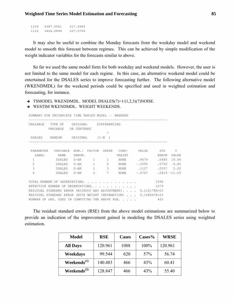
Weighted Time Series Model Estimation and Forecasting 85
1109 4387.0581 227.5689 1110 3466.0894 227.5700
It may also be useful to combine the Monday forecasts from the weekday model and weekend
model to smooth this forecast between regimes. This can be achieved by simple modification of the weight indicator variables for the forecasts similar to above.
So far we used the same model form for both weekday and weekend models. However, the user is not limited to the same model for each regime. In this case, an alternative weekend model could be entertained for the DSALES series to improve forecasting further. The following alternative model (WKENDMDL) for the weekend periods could be specified and used in weighted estimation and forecasting, for instance.
TSMODEL WKENDMDL. MODEL DSALES(7)=1/(1,2,3)(7)NOISE. WESTIM WKENDMDL. WEIGHT WEEKENDS.
SUMMARY FOR UNIVARIATE TIME SERIES MODEL -- WEEKEND ----------------------------------------------------------------------- VARIABLE TYPE OF ORIGINAL DIFFERENCING VARIABLE OR CENTERED 7 DSALES RANDOM ORIGINAL (1-B ) ----------------------------------------------------------------------- PARAMETER VARIABLE NUM./ FACTOR ORDER CONS- VALUE STD T LABEL NAME DENOM. TRAINT ERROR VALUE 1 DSALES D-AR 1 1 NONE .9679 .0485 19.94 2 DSALES D-AR 1 2 NONE -.3390 .0700 -4.84 3 DSALES D-AR 1 3 NONE .1127 .0557 2.02 4 DSALES D-AR 2 7 NONE -.4767 .0414 -11.53 TOTAL NUMBER OF OBSERVATIONS. . . . . . . . . . . . . . 1096 EFFECTIVE NUMBER OF OBSERVATIONS. . . . . . . . . . . . 1079 RESIDUAL STANDARD ERROR (WITHOUT ANY ADJUSTMENT). . . . 0.116178E+03 RESIDUAL STANDARD ERROR (WITH WEIGHT INFORMATION) . . . 0.128847E+03 NUMBER OF OBS. USED IN COMPUTING THE ABOVE RSE. . . . . 463
The residual standard errors (RSE) from the above model estimations are summarized below to
provide an indication of the improvement gained in modeling the DSALES series using weighted estimation.
Model RSE Cases Cases% WRSE
All Days 120.961 1088 100% 120.961
Weekdays 99.544 620 57% 56.74
Weekends(1) 140.483 466 43% 60.41
Weekends(2) 128.847 466 43% 55.40

86 Weighted Time Series Model Estimation and Forecasting
From the above summary table, weighted residual standard errors (WRSE) can be computed based on the effective number of cases in each regime. Since the effective number of cases is slightly different between the two weekend models, the average number of cases (466) is used for comparison purposes. By adding the WRSE values of the weekday model and weekend model, we can compare the relative improvement between the “All Days” model and the segmented models. Depending on the model used for the weekend periods, the weighted estimation provides a relative improvement of 3.2% ((56.74+60.41)/120.961) to 9.3% ((56.74+55.40)/120.961) in residual standard error over the traditional “All Days” model. Further improvements are also possible by refining the weekday model as we have done for the weekend model.
If each day of the week follows its own distinct pattern, an individual model can be employed for each day (Monday, Tuesday,…,Sunday). Such models are known as periodic time series models and have been discussed extensively by Cleveland and Tiao (1979), Tiao and Grupe (1980), and others. In this example, the weekday and weekend periods were grouped because of their similar properties as seen in the day-of-week effects plot presented in the previous chapter.
12.3 Example of Weighted Estimation with Outlier Adjustment Using Stock Market Data
In this section we illustrate the use of weighted estimation in conjunction with joint outlier adjustment. The data used in this example consist of monthly stock market series from January 1976 up to and including December 1991 (a total of 192 observations for each series). The three time series are:
(1) The monthly average of the Standard and Poor's 500 stock index,
(2) The monthly average of long-term government security interest rates (from the Federal Reserve Bulletin), and
(3) The monthly composite index of leading indicators (from Business Conditions Digest).
In this data set, we are interested in understanding how monthly stock prices (reflected by S&P500 index) are influenced by long-term interest rates and general economic conditions (reflected by the monthly composite index of leading indicators).
The data are displayed below and stored in the SCA workspace under the labels SP500, IRLONG and LINDCTR, respectively. From the time plots, we see that SP500 increases steadily until observation 142, at which time it plummets for three consecutive periods. This period corresponds to the stock market crash in October-December 1987. Since these observations behave abruptly, special consideration must be rendered to such data points during model estimation. In the previous example, we were concerned to best accommodate weekday and weekend patterns in the data by developing two regime models. In this example, we are interested in discounting a section of the data because it disrupts the otherwise stable relationship in the data.

Weighted Time Series Model Estimation and Forecasting 87
We will analyze the natural logarithms of all time series. In this way, we can assess the percent change in the response for a 1% change in an explanatory variable. The log transformed series of SP500, IRLONG and LINDCTR are stored in the SCA workspace under the labels LNSP500, LNIRLONG and LNLINDTR respectively.
Time Series Plots of Stock Market Data
SP500IR
LO
NG
LIN
DC
TR

88 Weighted Time Series Model Estimation and Forecasting
Using the LTF method (Liu et. al. 1992) and the data during the first 141 months, we identify the following transfer function model to be appropriate in representing the relationship between S&P500, long-term interest rates and composite leading indicators.
t 1 t 2 t t(1 B)LNSP500 C (1 B)LNIRLONG (1 B)LNINDTR (1 B)a− = +β − +β − + −θ (12.4)
The estimation results for the above model indicate that both long-term interest rates and leading indicators influence stock prices significantly. However in reviewing the time series plots for SP500, IRLONG, and LINDTR, we find that during the period 1980 to 1982 the long-term interest rates are quite high which coincides with the low leading indicator periods. It would be interesting to evaluate the estimation results if this part of the data is disregarded from the analysis. Furthermore we may also wish to lessen the impact of some data points related to the 1987 stock market crash in order to minimize any atypical effects of such a major event. The following GENERATE command is used to create a weight variable (WEIGHT1) that consists of 1's, except for those time periods between t=49 and t=85 (stagnated economy period of 1980-1982), and t=142 and t=147 (stock market crash of 1987). The weights for these time periods are 0's. This weight variable allows us to estimate the parameters with zero weights assigned to those atypical observations.
GENERATE VARIABLE IS WEIGHT1. NROW IS 192. @ VALUES ARE 1 FOR 48, 0 FOR 37, 1 FOR 56, 0 FOR 6, 1 FOR 45.
The model in (12.4) can be specified and estimated using the following TSMODEL and WESTIM commands. In the WESTIM command, the WEIGHT subcommand is used to specify the weight variable (WEIGHT1) that will be employed during model estimation. The OADJUST subcommand is specified with the keyword “JOINT” to employ the joint estimation method of outlier effects. The user also has the option to specify the keyword “SEQUENTIAL” to employ the sequential estimation method of outlier effects, or the keyword “NONE” to not employ outlier detection and estimation.
TSMODEL STOCKMDL. NO SHOW. @ MODEL LNSP500(1)=C+(0)LNIRLONG(1)+(0)LNLINDTR(1)+(1)NOISE.
WESTIM STOCKMDL. WEIGHT IS WEIGHT1. OADJUST JOINT.
SUMMARY FOR UNIVARIATE TIME SERIES MODEL -- STOCKMDL ----------------------------------------------------------------------- VARIABLE TYPE OF ORIGINAL DIFFERENCING VARIABLE OR CENTERED 1 LNSP500 RANDOM ORIGINAL (1-B ) 1 LNLONG RANDOM ORIGINAL (1-B ) 1 LNLEAD RANDOM ORIGINAL (1-B ) ----------------------------------------------------------------------- PARAMETER VARIABLE NUM./ FACTOR ORDER CONS- VALUE STD T LABEL NAME DENOM. TRAINT ERROR VALUE 1 C CNST 1 0 NONE .0069 .0025 2.79

Weighted Time Series Model Estimation and Forecasting 89
2 LNIRLONG NUM. 1 0 NONE -.4752 .0704 -6.75 3 LNLINDTR NUM. 1 0 NONE .4743 .2538 1.87 4 LNSP500 MA 1 1 NONE -.2353 .0807 -2.92 SUMMARY OF OUTLIER DETECTION AND ADJUSTMENT ------------------------------------- TIME ESTIMATE T-VALUE TYPE ------------------------------------- 50 0.081 5.38 AO 69 -0.078 -3.29 LS 81 0.079 3.22 IO 142 -0.127 -5.19 IO 143 -0.136 -5.55 IO 182 0.087 3.53 IO ------------------------------------- TOTAL NUMBER OF OBSERVATIONS. . . . . . . . . . . . . . 192 EFFECTIVE NUMBER OF OBSERVATIONS. . . . . . . . . . . . 191 RESIDUAL STANDARD ERROR (WITHOUT ANY ADJUSTMENT). . . . 0.310057E-01 RESIDUAL STANDARD ERROR (WITH WEIGHT INFORMATION) . . . 0.232833E-01 NUMBER OF OBS. USED IN COMPUTING THE ABOVE RSE. . . . . 148
If we wish to estimate model (12.4) with outlier adjustment but without omitting any data, then the
OESTIM command can be used. In this instance, the following results are obtained.
OESTIM STOCKMDL.
SUMMARY FOR UNIVARIATE TIME SERIES MODEL -- STOCKMDL ----------------------------------------------------------------------- VARIABLE TYPE OF ORIGINAL DIFFERENCING VARIABLE OR CENTERED 1 LNSP500 RANDOM ORIGINAL (1-B ) 1 LNIRLONG RANDOM ORIGINAL (1-B ) 1 LNLINDTR RANDOM ORIGINAL (1-B ) ----------------------------------------------------------------------- PARAMETER VARIABLE NUM./ FACTOR ORDER CONS- VALUE STD T LABEL NAME DENOM. TRAINT ERROR VALUE 1 C CNST 1 0 NONE .0066 .0021 3.13 2 LNIRLONG NUM. 1 0 NONE -.3705 .0506 -7.32 3 LNLINDTR NUM. 1 0 NONE .9559 .1660 5.76 4 LNSP500 MA 1 1 NONE -.2437 .0731 -3.33 SUMMARY OF OUTLIER DETECTION AND ADJUSTMENT ------------------------------------- TIME ESTIMATE T-VALUE TYPE 50 0.075 5.30 AO 69 -0.047 -3.31 AO 73 -0.100 -4.34 IO 81 0.079 3.42 IO 98 -0.071 -3.16 LS 142 -0.124 -5.39 IO 143 -0.122 -5.29 IO 182 0.084 3.63 IO

90 Weighted Time Series Model Estimation and Forecasting
TOTAL NUMBER OF OBSERVATIONS. . . . . . . . . . . . . . 192 EFFECTIVE NUMBER OF OBSERVATIONS. . . . . . . . . . . . 191 RESIDUAL STANDARD ERROR (WITHOUT OUTLIER ADJUSTMENT). . 0.304104E-01 RESIDUAL STANDARD ERROR (WITH OUTLIER ADJUSTMENT) . . . 0.230039E-01
The results from the two commands above reveal several interesting findings. Both estimation results show that long-term interest rates have a strong influence on stock market prices. The former (with weighted estimation) shows that a 1% relative increase in long-term interest rates may decrease the stock prices by 0.4752%, and the latter (without a weight variable) shows that the elasticity due to long-term interest rates is only 0.3705%. More importantly, when weighted estimation is considered (i.e., certain portions of the data have their effects discounted), the leading indicators do not show a significant influence on stock market prices, while the estimation without discounting any data indicates a strong positive relationship. The differences between these results are somewhat inconsistent but reveal quite interesting information. If we examine the time series plots of these three variables carefully, we find the data disregarded during 1980-82 happen to correspond to a low or downward period of composite leading indicators. The rest of the composite leading indicators are generally in an upward trend. When data during 1980-1982 (and stock market crash period) are discounted, the leading indicators become insignificant. This implies that stock prices are not affected significantly by composite leading indicators in typically good economic conditions, but are sensitive to composite leading indicators in severely bad economic conditions (during 1980-82).
It would also be interesting to investigate the results if the WESTIM command without outlier adjustment is used for the model in (12.4) as shown below.
WESTIM STOCKMDL. WEIGHT IS WEIGHT1.
The parameter estimates are summarized below. We find they are rather close to those obtained with outlier adjustment using the WESTIM command. The estimate 2β is only marginally significant. Thus weighted estimation alone alleviates some biases caused by outliers in this example.
( )( )( )( )
1
2
C 0.0073 t 2.87ˆ 0.4926 t 6.68ˆ 0.5775 t 2.17ˆ 0.2257 t 2.77ˆ 0.02318
= =
β = − = −
β = =
θ = − = −
σ =
If we wish to estimate model (12.4) without using the weighted method and without outlier adjustment, then the following standard ESTIM command can be specified
ESTIM STOCKMDL.
The parameter estimates are summarized below:

Weighted Time Series Model Estimation and Forecasting 91
( )( )( )( )
1
2
C 0.0053 t 1.92ˆ 0.3440 t 5.20ˆ 0.8656 t 3.91ˆ 0.2480 t 3.42ˆ 0.030279
= =
β = − = −
β = =
θ = − = −
σ =
The above ESTIM command produces very different estimates of 2β . By discounting the effect of the atypical data using the WESTIM command, the leading indicator has marginal influence on the S&P 500 index. In contrast, by including the atypical periods in model estimation, the leading indicator shows rather significant.
12.4 Example of Value-segmented Analysis Using the HSOLD and BON10Y Series
In this example, a transfer function model is used in conjunction with weighted estimation to study the symmetry of the elasticity estimates between interest rate increases and interest rates decreases. The two original series are presented below. The first graph is monthly sales of new homes (referred to as houses sold hereafter). The second graph is ten-year bond rates. These monthly series span from January 1963 through December 2003, a total of 512 observations for each series.
HSO
LD
B
ON
D10Y

92 Weighted Time Series Model Estimation and Forecasting
Houses sold and the 10-year bond rate exhibits a roughly inverse relationship. We are interested in studying whether an interest rate increases or decreases have similar effect (elasticity) on houses sold. The weighted estimation method can be used effectively for investigating such behavior. Since the bond rate varied greatly during the period under study, we will examine the interest rate elasticity effect across various time spans. These time spans are (1) January 1963 through December 1979 where the bond rate generally increased during the period; (2) January 1980 through December 1985 where the bond rate was unusually high; (3) January 1986 through December 2003 where the bond rate generally declined during the period; and (4) the entire span of data.
Using the LTF identification method, we obtain the following transfer function model between log transformed houses sold ( tHSOLD ) and log transformed bond rate ( tBONDRATE ):
t 1 t 1 1 t(HSOLD ) (BONDRATE ) (1 B)a−∇ = ω ∇ + −θ
Note that the bond rate leads houses sold by one month as shown in the above model. For comparison purposes, the above model is specified using the TSMODEL command and estimated using the standard ESTIM command with all data used.
TSMODEL HSMDL. MODEL IS HSOLD(1)=(1)BOND10Y(1)+(1)NOISE. ESTIM HSMDL. METHOD EXACT.
SUMMARY FOR UNIVARIATE TIME SERIES MODEL -- HSMDL ----------------------------------------------------------------------- VARIABLE TYPE OF ORIGINAL DIFFERENCING VARIABLE OR CENTERED 1 HSOLD RANDOM ORIGINAL (1-B ) 1 BOND10Y RANDOM ORIGINAL (1-B ) ----------------------------------------------------------------------- PARAMETER VARIABLE NUM./ FACTOR ORDER CONS- VALUE STD T LABEL NAME DENOM. TRAINT ERROR VALUE 1 BOND10Y NUM. 1 1 NONE -.5775 .0731 -7.90 2 HSOLD MA 1 1 NONE .2705 .0432 6.26 EFFECTIVE NUMBER OF OBSERVATIONS . . 490 R-SQUARE . . . . . . . . . . . . . . 0.925 RESIDUAL STANDARD ERROR. . . . . . . 0.680262E-01
In this illustrative example, we now consider two different types of weight variables to explore the
elasticity of houses sold. For the first weight variable, the weight is set to 1 if the bond rate in the previous month went down and 0 otherwise (labeled as “Rate-down”). For the second weight variable, the weight is set to 1 if the bond rate in the previous month went up and 0 otherwise (labeled as “Rate-up”). Thus by using the decrease or increase of bond rates, two value-segmented models are formed. Such models are also referred to as threshold models in the literature.
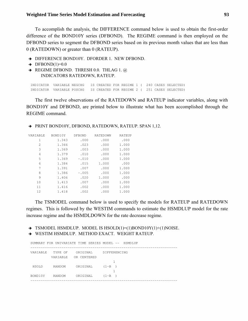
Weighted Time Series Model Estimation and Forecasting 93
To accomplish the analysis, the DIFFERENCE command below is used to obtain the first-order difference of the BOND10Y series (DFBOND). The REGIME command is then employed on the DFBOND series to segment the DFBOND series based on its previous month values that are less than 0 (RATEDOWN) or greater than 0 (RATEUP).
DIFFERENCE BOND10Y. DFORDER 1. NEW DFBOND. DFBOND(1)=0.0 REGIME DFBOND. THRESH 0.0. THLAG 1. @
INDICATORS RATEDOWN, RATEUP.
INDICATOR VARIABLE NEGCHG IS CREATED FOR REGIME 1 ( 240 CASES SELECTED) INDICATOR VARIABLE POSCHG IS CREATED FOR REGIME 2 ( 251 CASES SELECTED)
The first twelve observations of the RATEDOWN and RATEUP indicator variables, along with BOND10Y and DFBOND, are printed below to illustrate what has been accomplished through the REGIME command.
PRINT BOND10Y, DFBOND, RATEDOWN, RATEUP. SPAN 1,12.
VARIABLE BOND10Y DFBOND RATEDOWN RATEUP 1 1.343 .000 .000 .000 2 1.366 .023 .000 1.000 3 1.369 .003 .000 1.000 4 1.379 .010 .000 1.000 5 1.369 -.010 .000 1.000 6 1.384 .015 1.000 .000 7 1.391 .007 .000 1.000 8 1.386 -.005 .000 1.000 9 1.406 .020 1.000 .000 10 1.413 .007 .000 1.000 11 1.416 .002 .000 1.000 12 1.418 .002 .000 1.000
The TSMODEL command below is used to specify the models for RATEUP and RATEDOWN regimes. This is followed by the WESTIM commands to estimate the HSMDLUP model for the rate increase regime and the HSMDLDOWN for the rate decrease regime.
TSMODEL HSMDLUP. MODEL IS HSOLD(1)=(1)BOND10Y(1)+(1)NOISE. WESTIM HSMDLUP. METHOD EXACT. WEIGHT RATEUP.
SUMMARY FOR UNIVARIATE TIME SERIES MODEL -- HSMDLUP ----------------------------------------------------------------------- VARIABLE TYPE OF ORIGINAL DIFFERENCING VARIABLE OR CENTERED 1 HSOLD RANDOM ORIGINAL (1-B ) 1 BOND10Y RANDOM ORIGINAL (1-B ) -----------------------------------------------------------------------

94 Weighted Time Series Model Estimation and Forecasting
PARAMETER VARIABLE NUM./ FACTOR ORDER CONS- VALUE STD T LABEL NAME DENOM. TRAINT ERROR VALUE 1 BOND10Y NUM. 1 1 NONE -.4709 .1122 -4.20 2 HSOLD MA 1 1 NONE .1798 .0642 2.80 TOTAL NUMBER OF OBSERVATIONS. . . . . . . . . . . . . . 492 EFFECTIVE NUMBER OF OBSERVATIONS. . . . . . . . . . . . 490 RESIDUAL STANDARD ERROR (WITHOUT ANY ADJUSTMENT). . . . 0.683972E-01 RESIDUAL STANDARD ERROR (WITH WEIGHT INFORMATION) . . . 0.703243E-01 NUMBER OF OBS. USED IN COMPUTING THE ABOVE RSE. . . . . 250
TSMODEL HSMDLDOWN. MODEL IS HSOLD(1)=(1)BOND10Y(1)+(1)NOISE. WESTIM HSMDLDOWN. METHOD EXACT. WEIGHT RATEDOWN.
SUMMARY FOR UNIVARIATE TIME SERIES MODEL -- HSMDLDOWN ----------------------------------------------------------------------- VARIABLE TYPE OF ORIGINAL DIFFERENCING VARIABLE OR CENTERED 1 HSOLD RANDOM ORIGINAL (1-B ) 1 BOND10Y RANDOM ORIGINAL (1-B ) ----------------------------------------------------------------------- PARAMETER VARIABLE NUM./ FACTOR ORDER CONS- VALUE STD T LABEL NAME DENOM. TRAINT ERROR VALUE 1 BOND10Y NUM. 1 1 NONE -.6750 .0895 -7.54 2 HSOLD MA 1 1 NONE .3922 .0537 7.30 TOTAL NUMBER OF OBSERVATIONS. . . . . . . . . . . . . . 492 EFFECTIVE NUMBER OF OBSERVATIONS. . . . . . . . . . . . 490 RESIDUAL STANDARD ERROR (WITHOUT ANY ADJUSTMENT). . . . 0.686248E-01 RESIDUAL STANDARD ERROR (WITH WEIGHT INFORMATION) . . . 0.644704E-01 NUMBER OF OBS. USED IN COMPUTING THE ABOVE RSE. . . . . 240
From the above estimation results, we find that the elasticity estimate for rate increases is -.4709; the elasticity estimate for rate decreases is -.6750; and the elasticity estimate using standard estimation methods is -.5775. These elasticity estimates are quite different. To study whether the elasticity estimates exhibit such behavior when interest rates are generally increasing (1/1963 – 12/1979), unusually high (1/1980 – 12/1985), or generally decreasing (1/1986 – 12/2003), the above analysis is repeated for these three time periods. The elasticity estimates are presented in the following summary table.

Weighted Time Series Model Estimation and Forecasting 95
Elasticity Estimates Period All Data Rate-up Rate-down
Entire series (1/1963 – 12/2003)
-.5775 -.4709 -.6750
Increasing bond rate period(1/1963 – 12/1979)
-.3979 -.2597 -.6237
Unusually high bond rate period(1/1980 – 12/1985)
-1.1627 -1.0286 -1.2609
Decreasing bond rate period(1/1986 – 12/2003)
-.3951 -.3529 -.4525
In the above estimation results, we are particularly interested in the symmetry or asymmetry of the elasticity estimates. We find that the elasticity of houses sold is consistently greater when the interest rate change is negative (Rate-down) in the four time spans considered. We also find that the highest elasticity of houses sold, regardless of Rate-up or Rate-down regime, was during the high bond rate period.
In this chapter, general weighted estimation was discussed using the WESTIM command along with the WFORECAST command to blend weighted forecasts. It was shown how the REGIME and RECODE commands can be used to generate indicator variables that discern particular regimes for both time-segmented and value-segmented models. In the next chapter, value-segmented models (or threshold models) will be further discussed.

96 Weighted Time Series Model Estimation and Forecasting

CHAPTER 13
THRESHOLD TIME SERIES MODELING AND FORECASTING
The Professional Edition (B) of the SCA Statistical System includes nonlinear time series modeling and forecasting capabilities. The commands TARTEST, TARXTEST, TARESTIM, TARFORECAST, THMTEST, and THMEXPLORE are documented in this chapter. Related commands including WESTIM and WFORECAST were discussed in Chapter 12. Additional information on nonlinear time series analysis can be found in Liu (2006).
In Chapter 12, a value-segmented approach was used to analyze the relationship between houses sold and long-term interest rate. The month-to-month changes in long-term interest rate were segmented into positive and negative cases using zero as the threshold value and one as the threshold lag. The model used was a threshold transfer function model with an MA(1) noise. The WESTIM command was used to estimate the parameters in the threshold transfer function models.
In this chapter, we first discuss a special case of threshold model for the univariate autoregressive case. This class of model is referred to as the threshold autoregressive (TAR) model. TAR models have been studied extensively by Tong (1978, 1983, 1990), Tong and Lim (1980), Maravell (1983), Tsay (1986, 1989), Chen and Tsay (1991, 1993), Tiao and Tsay (1994), and others.
In the next section, we shall cover the nonlinearity test of a time series, the identification of a TAR model for a time series, TAR model estimation, forecasting, and other extensions of such models using the SCA System.
13.1 Threshold Autoregressive Models
A k-regime TAR model for a time series tY with t=1, 2, …, n, can be written as
( )i (i) (i) (i)t t 1 p t p i 1 t d it0 1Y C Y Y a , r Y r− − − −= + φ + ⋅⋅⋅ + φ + ≤ < (13.1)
where i=1,2, …, k, and d is a positive integer often referred to as a threshold lag (or delay parameter). The thresholds i(r ) are non-overlapping intervals on the real line with 0 1 kr r ... r−∞ = < < < = ∞ . The
innovations (i)ta 's are identically and independently distributed random variables for each regime, and
are independent across the regimes with potentially different variances. Even though tY follows a linear AR model in each regime, the overall process for (13.1) is nonlinear when there are at least two regimes with different linear models. This class of models was proposed by Tong (1978, 1983) and Tong and Lim (1980) as alternative models for describing periodic time series. It has certain features that allow it to model time series with limit cycles, jump phenomena, and amplitude dependant frequencies. The TAR model in (13.1) is also referred to as self-exciting threshold autoregressive

98 Threshold Time Series Modeling and Forecasting
(SETAR) model because the AR model in each regime is determined by its own past value. Following the threshold principle, some other models, such as threshold MA models (Wecker 1981, Jolliffe and Kumar 1985), threshold ARMA models (Wang et al., 1984), and adaptive spline threshold autoregression (ASTAR) models (Lewis and Stevens, 1991) have also been proposed.
Using the backshift operator B, the model in (13.1) can be written as
(i) (i) (i) (i)p
p t t1 0(1 B B )Y C a , i 1, 2, ..., k−φ − ⋅⋅ ⋅ − φ = + = (13.2)
or
( ) (i) (i) (i) (i)(i) (i) pt pt0 1B Y C a , with (B) 1 B Bφ = + φ = −φ − ⋅⋅⋅ − φ . (13.3)
In the models (13.1), (13.2), and (13.3), the constant term (i)0C in each regime does not have a
straightforward interpretation. It is more appropriate to write (13.2) and (13.3) in the following form
(i)(i)t t(i) (i) p
p1
1Y C a , i 1,2, ..., k1 B B
= + =− φ − ⋅⋅ ⋅ − φ (13.4)
or
(i)(i)t t(i)
1Y C a(B)
= +φ (13.5)
The constant term (i)C in (13.4) and (13.5) is then the mean for each regime. In some applications, the comparison of the mean values among regimes could be useful and even the focus of a study.
The models in (13.1) through (13.5) can be extended to multiplicative AR models as below:
(i) (i)(i) (i) st t0(B) (B )Y C a , i=1,2, ..., kφ Φ = + (13.6)
or
(i)(i)t t(i) (i) s
1Y C a , i 1, 2, ..., k(B) (B )
= + =φ Φ (13.7)
where (i) s(B )Φ is a stationary seasonal AR polynomial in sB .
More generally, the models in (13.6) and (13.7) can be extended to multiplicative seasonal ARIMA models as

Threshold Time Series Modeling and Forecasting 99
(i) (i)(i) (i) s (i) (i) st t0(B) (B )Y C (B) (B )a , i=1,2, ..., kφ Φ = + θ Θ (13.8)
or
(i) (i) s (i)(i)t t(i) (i) s
(B) (B )Y C a , i=1,2, ..., k(B) (B )
θ Θ= +
φ Φ (13.9)
where (i) (B)θ and (i) s(B )Θ are MA and seasonal MA polynomials in sB and B . In most of the literature, only TAR models in the forms of (13.1) or (13.2) are discussed. We shall also focus on this class of TAR models in this chapter.
There are two important issues involved in building a threshold model. The first is the determination of the threshold lag (d) and the corresponding threshold values. The second is the estimation of the model parameters in each regime. Assuming that the first issue has been resolved, all threshold models discussed can be estimated using the weighted estimation method discussed in Chapter 12.
The TARESTIM command in the SCA System is designed to accommodate the estimation of all models shown above. Unlike threshold AR models, certain assumptions may need to be imposed in order for the estimation of threshold MA or ARIMA models to be valid.
13.2 Nonlinearity Test
Before we pursue building a TAR model, it is prudent to check if the time series under study is nonlinear and therefore warrants consideration of a TAR model. The SCA System employs the TARTEST command that is based on the work of Tsay (1986, 1989, 1991) and others.
Tsay (1986) generalizes the procedure of Keenan (1985) and develops an F-statistic to test a very general class of nonlinear time series. Petruccelli and Davies (1986) use normalized predictive residuals to derive a CUSUM portmanteau test for TAR processes. Tsay (1989) combines the procedures of Keenan (1985), Tsay (1986), and Petruccelli and Davies (1986) and develops another F-statistic specifically to test for alternative TAR models. We shall refer to this particular F-test as TAR-F test. Tsay (1991) further extends the TAR-F test and develops a new F-test by including a larger class of alternative TAR models.
As pointed out in Tsay (1991), the power of a nonlinearity test inevitably will suffer when the class of models considered is too large. Since the class of TAR models is most useful in business and economic applications, we shall primarily use the TAR-F test for checking for nonlinearity of a time series. In addition to the increase in power of the test, Tsay’s TAR-F test also provides useful information for the potential value of the threshold lag (d).

100 Threshold Time Series Modeling and Forecasting
13.3 Arranged Autoregression
The TARTEST is used to obtain the threshold lag and threshold values based on the past values of the series itself. When the threshold variable is an external variable as opposed to past values of the series itself, the TARXTEST command can be used instead. The syntax for these two commands is provided in Appendix B.
The rationale and the procedure for the TAR-F test will be outlined in the following section. The TAR-F test and several other nonlinearity tests use a novel computational procedure called arranged Autoregression (AAR). We shall use a simple example to illustrate this procedure.
Assume that we have a time series tY with eight observations as below:
t 1 2 3 4 5 6 7 8 tY 1.61 0.32 -1.63 -1.70 -0.71 -2.86 -2.40 1.48
Let us also assume the above time series may follow a linear or nonlinear AR(1) model with zero mean which can be written as
t 1 t 1 tY Y a , t=1, 2, , 8−= φ + ⋅⋅⋅ . (13.10)
To obtain the estimate of 1φ under a linear AR(1) model, traditionally we would regress tY on t 1Y − using the following data sequence.
t tY t 1Y − 1 1.61 - - 2 0.32 1.61 3 -1.63 0.32 4 -1.70 -1.63 5 -0.71 -1.70 6 -2.86 -0.71 7 -2.40 -2.86 8 1.48 -2.40
Using the seven complete pairs of data in the above table, the least squares estimate of 1φ in (13.10) is 0.4106.
Now let us assume the above time series follow a TAR(1) model with d=1. We can arrange the data sequence in the above table in ascending order according to the threshold variable t 1Y − . Thus we have the following arranged autoregression data sequence:

Threshold Time Series Modeling and Forecasting 101
t tY t 1Y − 1φ 7 -2.400 -2.860 - - 8 1.480 -2.400 0.2376 5 -.710 -1.700 0.2685 4 -1.700 -1.630 0.3741 6 -2.860 -.710 0.4663 3 -1.630 0.320 0.4379 2 0.320 1.610 0.4106
The above data sequence contains the same information as in the previous table except that the data are ordered by t 1Y − rather than by t. Using the arranged autoregression data, we can compute sequential estimates of 1φ according to the order of t 1Y − . These sequential estimates are listed in the last column of the above table. It is important to note that the last sequential estimate of 1φ (0.4106) is the same as the least squares estimate for the linear AR(1) model using the entire data set.
The sequential estimates of 1φ (based on the ordered threshold variable) and their related statistics are very useful. They can be used to develop nonlinearity tests as well as to identify threshold values. To improve computational efficiency, recursive estimation algorithms are typically used for the computation of autoregressive coefficients. The results under recursive estimation are the same as the straightforward least squares estimates using the same data. In arranged autoregression, the data sequence can be arranged either in ascending order of the threshold variable or in descending order of the threshold variable. We refer to the latter as reverse arranged autoregression (RAAR). This method also provides useful information in identification of threshold values.
13.4 Example of TAR Modeling Using Chickenpox Cases in New York City
To illustrate TAR modeling capabilities in the SCA System, we analyze the number of Chickenpox cases that occurred monthly in New York City from 1949-1972 (Sugilara and May 1990). The natural log transformation is applied to the time series to stabilize the variability. This time series was analyzed using TAR models by Chen and Tsay (1993). The log transformed time series is first brought into the SCA System under the variable named CHICPOX. A time series plot of the log transformed monthly Chickenpox series is shown below. There are a total of 533 observations.

102 Threshold Time Series Modeling and Forecasting
Time Series Plot of the Log Transformed Chickenpox Cases in New York City
CHI
CPOX
Obs 0 50 100 150 200 250 300 350 400 450 500 550
6.6
6.8
7
7.2
7.4
7.6
7.8
8
8.2
CHI CK EN POX CA SES (L OGGED ) I N N EW Y ORK CI T Y (1949-1972)
The TARTEST command is used to examine the nonlinearity of this series using a linear AR(12) as the null hypothesis model.
TARTEST CHICPOX. ARLAGS 1 TO 12. THLAGS 1 TO 12.
Lag F-statistic Degrees of freedom -------- ----------- ------------------ 1 3.73837 13 443 2 3.92756 13 443 3 5.09289 13 443 4 7.24443 13 443 5 6.36462 13 443 6 6.20812 13 443 7 3.56343 13 443 8 2.80965 13 443 9 6.72298 13 443 10 13.54124 13 443 11 12.06614 13 443 12 6.82576 13 443
From the above table, we see that the CHICPOX series shows strong nonlinearity because the F-statistics for all threshold lags are significant at both 5% and 1% levels. The F-statistics for the threshold lag at lags 10, 11, and 12 are particularly large. Because this series consists of monthly data, Chen and Tsay (1993) choose the threshold lag as 12 in their analysis.
Identification of threshold values
After the threshold lag (d) is determined, we can proceed to determine the values of the thresholds for the regimes based on the threshold variable t dY − . Tsay (1989) employs arranged autoregession and recursive estimation to obtain the sequential estimates of autoregressive parameters, their t-ratios, and corresponding estimated variances. These statistics can then be plotted against the threshold variable

Threshold Time Series Modeling and Forecasting 103
t dY − . When a major change is spotted in these scatter plots, it suggests that a regime partition is needed at that threshold value. For convenience, we shall refer to this method of threshold value identification as the arranged autoregression (AAR) method even though the method incorporates ideas more than just arranged autoregression.
In preliminary analysis of the chickenpox series, the autoregressive coefficients for lags 1 and 24 are most significant. Therefore we consider the following linear autoregressive model:
t 0 1 t 1 24 t 24 tY C Y Y a− −= + φ + φ + . (13.11)
To identify the threshold values for the CHICPOX series using the AAR method, we once again employ the TARTEST command. The THLAG is set to 12 and the ARLAGS are specified as 1 and 24 only. The autoregressive parameter estimates, their t-ratios, and corresponding estimated variances are saved in the SCA workspace using the HOLD subcommand.
TARTEST CHICPOX. THLAG 12. ARLAGS 1, 24. @ HOLD THVARIABLE(THVAR,THINDX),PHI(PHIMTX),TPHI(TPHIMTX), @ SIGMAHAT(SIGMA).
The threshold values (in sorted order) are stored under the THVAR variable name. The PHIMTX and TPHIMTX variables store the AR estimates and their corresponding t-values in matrix form. The following SCA matrix operation separates the matrix columns into variables that can be readily used for graphing or further analysis.
PHI1=PHIMTX(.,1) PHI24=PHIMTX(.,2) TPHI1=TPHIMTX(.,1) TPHI24=TPHIMTX(.,2)
Alternatively, the PICK command can be used in place of the matrix operations above to obtain columns of a matrix to create the PHI1, PHI24, TPHI1, and TPHI24 series.
Using the AAR method to obtain the estimates of 1φ , 24φ , and their associated statistics, scatter
plots for the 1φ , 24φ , and their t-ratios versus the threshold variable t 12Y − are displayed. Note that the
range of 1φ and t-ratios of 1φ are different from those of 24φ and the t-ratios of 24ˆ φ . We usually prefer to use the same scale across the estimates of the model parameters (and similarly the t-ratios). In this case however, the ranges for 1φ and 24φ are very different. Therefore, different scales are used in order to display the features of the estimates for each parameter more prominently.
In the identification of threshold values, it is important to focus only on scatter plots that contain significant t-ratios. Scatter plots of insignificant AR coefficients or their t-ratios are counter-

104 Threshold Time Series Modeling and Forecasting
productive. Other important guidelines for the identification of threshold values will be discussed later.
The SCA command to transfer the variables for threshold identification to the SCAGRAF applet is provided below.
GRAPH THVAR, PHI1, PHI24, TPHI1, TPHI24.
The scatter plots are then created using the menu and dialog box graphical user interface of SCAGRAF.
Plots of autoregressive coefficients and their t-ratios versus the threshold variable Yt-12
(chickenpox series with the AAR method)
(a) Arranged autoregression estimates of 1φ (b) Arranged autoregression estimates of 24φ
(c) t-ratios for the estimates of 1φ (d) t-ratios for the estimates of 24φ

Threshold Time Series Modeling and Forecasting 105
By examining the scatter plots for the 1φ estimates and the corresponding t-ratios, we find potential threshold values near 6.92, 7.0, and 7.15. On the other hand, by examining the scatter plots for the 24φ estimates and the corresponding t-ratios, we find potential threshold values near 6.92 and 7.45. Because the threshold 7.0 is very close to 6.92 and because observations greater than 7.45 in the series are limited (particularly in the latter part of the time series), we may conclude the threshold values are 1r 6.92= and 2r 7.15= . While these values are close, they differ from those identified by Chen and Tsay (1993). This discrepancy is due in part that the features for the thresholds in the scatter plots of the chickenpox series are not prominent. Consequently, it is somewhat difficult to exactly identify the threshold values using the AAR method in this example. We shall consider modifications to the AAR method in the next section which may facilitate easier identification of threshold values.
13.5 Modified Methods for the Identification of Threshold Values
One obvious problem in using recursive estimation of arranged autoregression (Tsay, 1989) is the recursive estimates eventually converge to those of the linear autoregressive estimates. Thus the AAR method employed in the previous section is most effective in identifying the first threshold value from the left-hand-side section (lower-end) of the threshold axis. The AAR method may start to lose effectiveness for the coefficients beyond the first threshold. This is due to the confounding (or averaging) effect on the parameter estimates as the estimation range includes more regimes. In this section, we consider two variations of the AAR method.
(A) Reverse Arranged Autoregression Method
One possible way to remedy the AAR method is to consider another set of arranged autoregression estimates based on the values of the threshold variable in descending order (instead of ascending-ordered threshold variable in the original AAR method). Such an approach will allow us to more effectively identify the first threshold value from the right-hand-side section (higher-end) of the threshold axis. We shall refer to such an approach as the Reverse AAR method which is specified in the TARTEST command using the RAAR keyword in the METHOD subcommand.
TARTEST CHICPOX. METHOD RAAR. THLAG 12. ARLAGS 1, 24. @ HOLD THVARIABLE(THVARR,THINDXR), PHI(PHIMTXR), TPHI(TPHIMTXR), @ SIGMAHAT(SIGMAR).
Using the Reverse AAR method, the scatter plots for 1φ , 24φ , and their t-ratios (versus the threshold variables) are displayed below for the chickenpox series. Based on the scatter plots of 1φ estimates and their t-ratios shown in (a) and (c), we can clearly identify threshold values around 7.15 and 7.0. Similarly, when we examine the scatter plots of 24φ estimates and their t-ratios shown in (b) and (d), we can identify threshold values around 7.45, 7.15, and 7.0. The threshold 6.9 is not identified using this method since it is a threshold very close to the end of the reverse arranged autoregression

106 Threshold Time Series Modeling and Forecasting
sequence. In this case, the Reverse AAR method reveals more distinct features for the threshold values in comparison with the AAR method.
Plots of autoregressive coefficients and their t-ratios versus the threshold variable Yt-12
(chickenpox series with the Reverse AAR method)
(a) Arranged autoregression estimates of 1φ (b) Arranged autoregression estimates of 24φ
(c) t-ratios for the estimates of 1φ (d) t-ratios for the estimates of 24φ
(B) Local Autoregression Method
Instead of using recursive estimation which implies all data available up to the potential threshold value are used in estimation, we may use a moving window so that only the data close to the potential threshold value are used to obtain local estimates of the model parameters and their associated statistics (e.g., t-ratios, variances, etc.). We shall refer to this method as the local autoregression (LAR) method. The LAR method is similar to the ALR method proposed in Chen and Tsay (1993). The primary difference is that the LAR method uses linear autoregression estimation for the data
Threshold Time Series Modeling and Forecasting 107
contained within the data window while the ALR method employs nonparametric regression estimation.
The LAR method is available through the THMEXPLORE command. The THMEXPLORE command is used to provide parameter estimates of a model according to the order of the sorted threshold variable. The threshold variable may be sorted in ascending or descending order.
A moving-window-regression estimation is used to explore the potential nonlinearity and threshold values of the model parameters. The THMEXPLORE command can be used with an autoregressive model or a transfer function model. For autoregressive models, this command provides AAR and RAAR methods in addition to the LAR method for the identification of threshold values.
In this command, the model parameters to be estimated must be specified with names (labels). For example, Y=CNST+(BETA1)X1+NOISE where CNST and BETA1 are the parameter estimate names associated with the constant and input variable X1. Furthermore, the model must be expressed in linear regression form using the TSMODEL command with white noise and without any backshift operator. All lagged variables must be created prior to using this command via the LAG command.
The parameter estimates for each data window are stored in the associated names for the parameters as vectors. The lengths of the resulting vectors for the parameter estimates are the same as the length of the output variable. The t-values for the parameter estimates are also stored for each window using the root word of the parameter label preceded by an underscore character (e.g., _CNST and _BETA1). There are estimates at the beginning of the series that are missing due to initial window size. Any parameter estimates that are unavailable (missing) are padded with the missing value code.
As a precursor to using the THMEXPLORE command, a lag 1 and lag 24 is taken on the CHICPOX series and stored as YLAG1 and YLAG24. This is performed using the LAG command.
LAG CHICPOX. NEW YLAG1, YLAG24. LAGS 1, 24.
A model is then specified in linear regression form using the following TSMODEL command. Here, parameter labels (C, PHI1L, and PHI24L) are used in the following model specification command
TSMODEL THMODEL. MODEL IS @ CHICPOX=C+(0;PHI1L)YLAG1+(0;PHI24L)YLAG24+NOISE.
The THMEXPLORE command is employed using the above model with a moving window size of 54 observations, and threshold lag of 12. To accommodate for missing values associated with the lagged variables, the THMEXPLORE command uses the beginning data span as the first row where all variables have non-missing values. The ending data span is similarly set to the last row where all variables have non-missing values.

108 Threshold Time Series Modeling and Forecasting
THMEXPLORE THMODEL. THLAG 12. WINDOWSIZE 54. @ HOLD THVARIABLE(THVL).
VARIABLE THVL STORES THE SORTED THRESHOLD VARIABLE (WITH 509 VALUES) VARIABLE C STORES PARAMETER ESTIMATES (WITH 509 VALUES) VARIABLE _C STORES THE t-VALUES OF THE ABOVE ESTIMATES VARIABLE PHI1L STORES PARAMETER ESTIMATES (WITH 509 VALUES) VARIABLE _PHI1L STORES THE t-VALUES OF THE ABOVE ESTIMATES VARIABLE PHI24L STORES PARAMETER ESTIMATES (WITH 509 VALUES) VARIABLE _PHI24L STORES THE t-VALUES OF THE ABOVE ESTIMATES
The scatter plots for the estimates of 1φ , 24φ , and their t-ratios versus the threshold variable t 12Y − are displayed next. By examining the scatter plots for the 1φ estimates and their t-ratios, we find potential threshold values around 6.92, 7.0, and 7.15 as shown in (a) and (c). On the other hand, by examining the scatter plots for the 24φ estimates and their t-ratios, we find potential threshold values around 6.92 and 7.48 as shown in (d). The results under the LAR method are similar to those of the AAR and Reverse AAR methods. However, the LAR method exhibits the threshold at 6.92 more prominently than the other two methods.

Threshold Time Series Modeling and Forecasting 109
Plots of autoregressive coefficients and their t-ratios versus the threshold variable Yt-12
(chickenpox series with the LAR method)
(a) Arranged autoregression estimates of 1φ (b) Arranged autoregression estimates of 24φ
(c) t-ratios for the estimates of 1φ (d) t-ratios for the estimates of 24φ
(C) Combined Use of the Methods
Following the examples discussed above, we see that all three methods for threshold value identification have their own strengths and weaknesses. The strength of the AAR and the Reverse AAR method is that both methods are effective in the identification of the first threshold value (the lower-end one for the AAR method and the higher-end one for the Reverse AAR method). In addition, we do not need to specify a data window for arranged autoregression estimation which, at times, can be complicated. When a process has only two or three regimes, the combined use of the AAR and Reverse AAR methods will fully identify the threshold values for the TAR model. In practice, a three-regime TAR model is probably more than adequate for most applications. If a process has more than three regimes, an additional application of this combined method may find two additional threshold

110 Threshold Time Series Modeling and Forecasting
values, resulting in a five-regime model. One weakness of these two methods is that these methods may be less effective in identifying subsequent threshold values after the first one.
The LAR method allows us to identify multiple threshold values in one pass. However, the choice of data window size may be complicated depending on the length of the series and the underlying model used for threshold value identification. In addition, the estimates of model parameters and t-ratios are more volatile than the AAR method, particularly if the window size is small. Typically, we need more data when this method is used.
In practice, it is probably prudent to use all three methods in the identification of threshold values. Ideally, we would like to see all three methods confirm one another by identifying the same or similar threshold values.
13.6 Guidelines for the Identification of Threshold Values
(1) It is advisable that extremely large outliers are pre-adjusted before embarking on threshold value identification (or nonlinearity testing). This would avoid volatile changes in the statistics to be examined. Moderate outliers need not be adjusted.
(2) When examining the scatter plots for the AAR method (where the threshold variable is sorted in ascending order), the parameter estimates at the beginning section of the scatter plot (i.e., smallest values in the threshold variable) may not be reliable due to the limited numbers of observations used in parameter estimation. This is often depicted by erratic movements in the scatter plots of parameter estimates and their t-ratios. Consequently, information shown in the beginning section of the scatter plot should be properly discounted in determining possible threshold values. A similar issue is associated with the Reverse AAR method (where the threshold variable is sorted in descending order). Here, the parameter estimates near the right-side of the scatter plot (i.e., largest values in the threshold variable) may not be reliable.
(3) The AAR scatter plots are examined for thresholds from left to right (smallest to largest value in the threshold axis). The first threshold encountered is the most reliable one. Additional thresholds detected after the initial one could still be reliable, but are often confounded by the use of the data in the earlier regime(s) in parameter estimation. Therefore, it is important to examine the Reverse AAR scatter plots for the thresholds on the higher-end of the threshold axis as well. For longer time series, the LAR method should also be considered since the presence of additional thresholds would be masked by thresholds that occur for smaller threshold values (AAR method) or larger threshold values (Reverse AAR method).
(4) Threshold candidates typically are flagged by a persistent increase (or decrease) and then leveling off in the parameter estimates or their t-ratios versus the threshold variable. The vertical range between the beginning of the threshold regime and its eventual stabilization to a new level plays a key role in determining the importance of a particular threshold candidate. It

Threshold Time Series Modeling and Forecasting 111
is imperative to confirm that the parameter estimates have meaningful differences between the levels of two adjacent regimes.
(5) If there is more than one possible threshold candidate in close proximity to each other, select the threshold value that has more prominent features. It is also important to make sure that each threshold regime contains an adequate number of data points to ensure proper parameter estimation.
13.7 TAR Model Estimation
In this section, we consider three types of TAR models for the log transformed time series CHICPOX. The first model type is a conventional TAR model, replicating the work of Chen and Tsay (1993). The second model type is a multiplicative AR model, and the third model type is a “threshold ARIMA” model.
In the paper by Chen and Tsay (1993), the regimes t 12Y 6.85− < , t 126.85 Y 7.21−≤ < , and t 12Y 7.21− > are identified with the underlying model (13.11) using the Functional-Coefficient Autoregression (FAR) approach. In the previous section, we have identified regimes (and hence threshold values) that are very close to the above values. For comparison purpose, the threshold values identified by Chen and Tsay (1993) will be used to illustrate TAR model estimation and forecasting.
Model Type 1
In Chen and Tsay (1993), the following TAR model with threshold lag (delay parameter) of 12 is considered.
( )( )( )
(1) (1) (1) (1) (1) (1)3 9 24t t-12t1 3 9 24 0
(2) (2) (2) (2) (2) (2)2 9 24t t-12t1 2 9 24 0
(3) (3) (3) (3) (3) (3)2 8 9t t-12t1 2 8 9 0
1 B B B B Y a if Y 6.85,
1 B B B B Y a if 6.85 Y 7.21,
1 B B B B Y a if Y 7.21,
− φ −φ − φ − φ = φ + <
− φ − φ − φ − φ = φ + ≤ <
− φ −φ − φ − φ = φ + ≥
The SCA System provides the REGIME command to generate the threshold indicator variables. The threshold indicator variables consist of 0’s and 1’s, where 1 indicates that an observation is in a specific regime and 0 otherwise. The threshold lag is specified in the REGIME command using the THLAG subcommand. In this example, the threshold lag is specified as 12. Two values, 6.85 and 7.21, are specified in the THRESHOLD subcommand, which define the three regimes. The INDICATORS subcommand is used to specify the variables that will store the regime information. Here, REGIME1 represents the regime where t 12Y 6.85− < , REGIME2 represents the regime where
t 126.85 Y 7.21−≤ < , and REGIME3 represents the regime where t 12Y 7.21− ≥ .

112 Threshold Time Series Modeling and Forecasting
The FINDICATOR subcommand is used to hold the extended part of the threshold indicator. The FINDICATOR subcommand should be specified if we intend to perform TAR model forecasting (to be described later). The REGIME command is specified below.
REGIME CHICPOX. THRESHOLD 6.85, 7.21. THLAG 12. @ INDICATORS REGIME1, REGIME2, REGIME3. FINDICATOR FI1, FI2, FI3.
INDICATOR VARIABLE REGIME1 IS CREATED FOR REGIME 1 FINDICATOR VARIABLE FI1 IS CREATED FOR REGIME 1 FOR FORECASTING INDICATOR VARIABLE REGIME2 IS CREATED FOR REGIME 2 FINDICATOR VARIABLE FI2 IS CREATED FOR REGIME 2 FOR FORECASTING INDICATOR VARIABLE REGIME3 IS CREATED FOR REGIME 3 FINDICATOR VARIABLE FI3 IS CREATED FOR REGIME 3 FOR FORECASTING
Once the threshold indicators are constructed, we can now specify the TAR models for the three regimes considered in this example. The TAR models are specified using the TSMODEL command and are estimated using the TARESTIM command. An individual model is specified for each regime. The model information is stored in the SCA System as MODEL1, MODEL2 and MODEL3 (see the TSMODEL command). The SCA commands and output are presented below
Regime 1: Yt-12 < 6.85
TSMODEL MODEL1. MODEL IS (1,3,9,24)CHICPOX=C1+NOISE. TARESTIM MODEL1. REGIME REGIME1.
SUMMARY FOR UNIVARIATE TIME SERIES MODEL -- MODEL1 ----------------------------------------------------------------------- VARIABLE TYPE OF ORIGINAL DIFFERENCING VARIABLE OR CENTERED CHICPOX RANDOM ORIGINAL NONE ----------------------------------------------------------------------- PARAMETER VARIABLE NUM./ FACTOR ORDER CONS- VALUE STD T LABEL NAME DENOM. TRAINT ERROR VALUE 1 C1 CNST 1 0 NONE 2.6329 .4391 6.00 2 CHICPOX AR 1 1 NONE .2848 .0364 7.83 3 CHICPOX AR 1 3 NONE -.0984 .0173 -5.68 4 CHICPOX AR 1 9 NONE .0730 .0182 4.01 5 CHICPOX AR 1 24 NONE .3517 .0630 5.58 TOTAL NUMBER OF OBSERVATIONS. . . . . . . . . . . . . . 533 EFFECTIVE NUMBER OF OBSERVATIONS. . . . . . . . . . . . 509 RESIDUAL STANDARD ERROR (WITHOUT ANY ADJUSTMENT). . . . 0.250641E+00 RESIDUAL STANDARD ERROR (WITH WEIGHT INFORMATION) . . . 0.426755E-01 NUMBER OF OBS. USED IN COMPUTING THE ABOVE RSE. . . . . 135

Threshold Time Series Modeling and Forecasting 113
Regime 2: 6.85 ≤ Yt-12 < 7.21
TSMODEL MODEL2. MODEL IS (1,2,9,24)CHICPOX=C2+NOISE. TARESTIM MODEL2. REGIME REGIME2.
SUMMARY FOR UNIVARIATE TIME SERIES MODEL -- MODEL2 ----------------------------------------------------------------------- VARIABLE TYPE OF ORIGINAL DIFFERENCING VARIABLE OR CENTERED CHICPOX RANDOM ORIGINAL NONE ----------------------------------------------------------------------- PARAMETER VARIABLE NUM./ FACTOR ORDER CONS- VALUE STD T LABEL NAME DENOM. TRAINT ERROR VALUE 1 C2 CNST 1 0 NONE .7203 .6746 1.07 2 CHICPOX AR 1 1 NONE .8700 .1221 7.12 3 CHICPOX AR 1 2 NONE -.5126 .0989 -5.18 4 CHICPOX AR 1 9 NONE .1175 .0438 2.68 5 CHICPOX AR 1 24 NONE .4157 .0708 5.87 TOTAL NUMBER OF OBSERVATIONS. . . . . . . . . . . . . . 533 EFFECTIVE NUMBER OF OBSERVATIONS. . . . . . . . . . . . 509 RESIDUAL STANDARD ERROR (WITHOUT ANY ADJUSTMENT). . . . 0.141528E+00 RESIDUAL STANDARD ERROR (WITH WEIGHT INFORMATION) . . . 0.981392E-01 NUMBER OF OBS. USED IN COMPUTING THE ABOVE RSE. . . . . 117
Regime 3: Yt-12 ≥ 7.21
TSMODEL MODEL3. MODEL IS (1,2,8,9,24)CHICPOX=C3+NOISE. TARESTIM MODEL3. REGIME REGIME3.
SUMMARY FOR UNIVARIATE TIME SERIES MODEL -- MODEL3 ----------------------------------------------------------------------- VARIABLE TYPE OF ORIGINAL DIFFERENCING VARIABLE OR CENTERED CHICPOX RANDOM ORIGINAL NONE ----------------------------------------------------------------------- PARAMETER VARIABLE NUM./ FACTOR ORDER CONS- VALUE STD T LABEL NAME DENOM. TRAINT ERROR VALUE 1 C3 CNST 1 0 NONE .2300 .3551 .65 2 CHICPOX AR 1 1 NONE .8511 .0574 14.83 3 CHICPOX AR 1 2 NONE -.1454 .0519 -2.80 4 CHICPOX AR 1 8 NONE -.1309 .0377 -3.48 5 CHICPOX AR 1 9 NONE .2559 .0350 7.32 6 CHICPOX AR 1 24 NONE .1444 .0362 3.99 TOTAL NUMBER OF OBSERVATIONS. . . . . . . . . . . . . . 533 EFFECTIVE NUMBER OF OBSERVATIONS. . . . . . . . . . . . 509 RESIDUAL STANDARD ERROR (WITHOUT ANY ADJUSTMENT). . . . 0.137159E+00 RESIDUAL STANDARD ERROR (WITH WEIGHT INFORMATION) . . . 0.994496E-01 NUMBER OF OBS. USED IN COMPUTING THE ABOVE RSE. . . . . 25

114 Threshold Time Series Modeling and Forecasting
Conditional least squares estimation is used to estimate the TAR models in the SCA System. The results produced by the SCA System are the same as those presented in Chen and Tsay (1993). SCA estimation results shown after each TARESTIM command are summarized in the table below.
(1) (1) (1) (1) (1) (1)0 1 3 9 24 1(2) (2) (2) (2) (2) (2)0 1 2 9 24 1(3) (3) (3) (3) (3)0 1 2 8 9
ˆ ˆ ˆ ˆ ˆ ˆ2.63 0.28 0.10 0.07 0.35 0.04268
ˆ ˆ ˆ ˆ ˆ ˆ0.72 0.87 0.51 0.12 0.42 0.09814
ˆ ˆ ˆ ˆ ˆ ˆ0.23 0.85 0.15 .13 0.26
φ = φ = φ = − φ = φ = σ =
φ = φ = φ = − φ = φ = σ =
φ = φ = φ = − φ = − φ = φ(3) (3)24 1ˆ0.14 0.09945= σ =
13.8 Forecasting
After the regime models (MODEL1 - MODEL3) are estimated, forecasts can be generated for each model up to the threshold lag (d) using the TARFORECAST command. The threshold lag (delay parameter) is 12 in this example and we will use the thresholds (6.85 and 7.21) reported by Chen and Tsay (1993) in this illustration.
We first input the threshold information into a variable THRSHINFO. The first number is the threshold lag followed by the threshold values. The threshold information is then provided to the TARFORECAST command.
INPUT THRSHINFO. 12 6.85 7.21 END OF DATA
Below, the TARFORECAST command is specified. The NOFS subcommand is used to control the number of forecasts to generate. It is important to note that the number of forecasts cannot exceed the threshold lag value; in this case 12.
TARFORECAST MODEL1,MODEL2,MODEL3. THRESHOLD THRSHINFO. NOFS 12.
--------------------------------------------------- MODEL MODEL1 : 12 FORECASTS, BEGINNING AT 533 --------------------------------------------------- TIME FORECAST STD. ERROR ACTUAL IF KNOWN 534 6.9954 0.0427 535 6.7595 0.0444 536 6.6678 0.0445 537 6.7357 0.0446 538 6.7613 0.0447 539 6.8195 0.0447 540 6.8635 0.0447 541 6.9267 0.0447 542 6.9792 0.0447 543 6.9993 0.0448 544 6.9633 0.0448 545 6.9790 0.0448

Threshold Time Series Modeling and Forecasting 115
--------------------------------------------------- MODEL MODEL2 : 12 FORECASTS, BEGINNING AT 533 --------------------------------------------------- TIME FORECAST STD. ERROR ACTUAL IF KNOWN 534 7.0784 0.0981 535 6.6475 0.1301 536 6.4522 0.1323 537 6.5626 0.1342 538 6.7425 0.1381 539 6.8976 0.1390 540 6.9836 0.1390 541 7.0470 0.1394 542 7.1042 0.1396 543 7.1270 0.1402 544 7.0452 0.1413 545 6.9842 0.1418 --------------------------------------------------- MODEL MODEL3 : 12 FORECASTS, BEGINNING AT 533 --------------------------------------------------- TIME FORECAST STD. ERROR ACTUAL IF KNOWN 534 7.3549 0.0994 535 7.2106 0.1306 536 7.0863 0.1427 537 7.0452 0.1474 538 7.0272 0.1491 539 7.0605 0.1498 540 7.1081 0.1500 541 7.2067 0.1501 542 7.3090 0.1505 543 7.3846 0.1505 544 7.4059 0.1519 545 7.4022 0.1541 --------------------------------------------------- COMBINED FORECASTS: 12 FORECASTS, BEGINNING AT 533 --------------------------------------------------- TIME FORECAST STD. ERROR ACTUAL IF KNOWN 534 7.0784 0.0981 535 6.7595 0.0444 536 6.6678 0.0445 537 6.7357 0.0446 538 6.7613 0.0447 539 6.8195 0.0447 540 6.9836 0.1390 541 7.0470 0.1394 542 7.3090 0.1505 543 7.3846 0.1505 544 7.4059 0.1519 545 7.4022 0.1541
In the above TARFORECAST specification, the regime indicator variables for the forecasts are constructed internally based on the threshold information provided. In some situations, it may be desirable to provide the regime indicator variables for the forecasts directly. The TARFORECAST command allows an alternative specification using the WEIGHT subcommand. When the WEIGHT subcommand is used, more flexibility is possible (e.g., smoothing forecasts for regime transition

116 Threshold Time Series Modeling and Forecasting
periods). The FI1, FI2, and FI3 variables that were generated using the earlier REGIME command can now be used.
TARFORECAST MODEL1,MODEL2,MODEL3. WEIGHT FI1,FI2,FI3. NOFS 12.
The output from this command is not shown since it is the same as the as the TARFORECAST command using the THRESHOLD subcommand above.
Model Type 2
Having replicated the TAR estimation results of Chen and Tsay (1993), we now deviate from the conventional TAR modeling approach and consider a multiplicative autoregressive model. The same threshold lag and regime specifications from the first approach are continued to be used here.
The IARIMA command which provides automatic ARIMA model identification is used to examine the overall behavior of the CHICPOX series without consideration of different regimes. The command and output are shown below.
IARIMA CHICPOX. SEASON 12.
SUMMARY FOR UNIVARIATE TIME SERIES MODEL -- UTSMODEL ----------------------------------------------------------------------- VARIABLE TYPE OF ORIGINAL DIFFERENCING VARIABLE OR CENTERED 12 CHICPOX RANDOM ORIGINAL (1-B ) ----------------------------------------------------------------------- PARAMETER VARIABLE NUM./ FACTOR ORDER CONS- VALUE STD T LABEL NAME DENOM. TRAINT ERROR VALUE 1 CHICPOX MA 1 12 NONE .7300 .0306 23.83 2 CHICPOX D-AR 1 1 NONE .7902 .0272 29.03 TOTAL NUMBER OF OBSERVATIONS . . . . 533 EFFECTIVE NUMBER OF OBSERVATIONS . . 520 RESIDUAL STANDARD ERROR. . . . . . . 0.904489E-01
Upon reviewing the model identified by the IARIMA command, it shows that the seasonal behavior of the time series is represented by the model
( ) ( )12 12t 1 t1 B Y 1 B a− = −Θ (13.12)
which can be approximated by a seasonal AR(2) model. Therefore, the ARIMA model identified by the IARIMA command can be written as

Threshold Time Series Modeling and Forecasting 117
( )( )t t12 241 12 24
1Y C a1 B 1 B B
= +−φ − φ − φ (13.13)
We shall use the model in (13.13) for the three regimes considered in this example. The multiplicative TAR model and regimes are
( )( )
( )( )
( ) ( )
(1)(1)t t-12t(1) (1) (1)12 24
1 12 24
(2)(2)t t-12t(2) (2) (2)12 24
1 12 24
(3)(3)t t-12t(3) (3) (3)12 24
1 12 24
1Y C a if Y 6.85,1 B 1 B B
1Y C a if 6.85 Y 7.21,1 B 1 B B
1Y C a if Y 7.21,1 B 1 B B
= + <− φ −φ − φ
= + ≤ <−φ − φ − φ
= + ≥−φ −φ − φ
(13.14)
In the above multiplicative TAR model, all autoregressive polynomials are specified on the right-hand side of the model. By doing so, the constant terms in the model (i)C is the mean of the associated regime, thus bringing more intuitive meaning to the parameter estimates. This is different from the conventional TAR models, where the constant term (i)
0φ in each regime has no particular meaning.
The models are specified and estimated in the SCA System using the TSMODEL and TARESTIM commands. Following the same steps taken in Approach 1, the SCA commands and output are presented below.
Regime 1: Yt-12 < 6.85
TSMODEL MODEL1. MODEL IS CHICPOX=C1+1/(1)(12,24)NOISE. TARESTIM MODEL1. REGIME REGIME1.
SUMMARY FOR UNIVARIATE TIME SERIES MODEL -- MODEL1 ----------------------------------------------------------------------- VARIABLE TYPE OF ORIGINAL DIFFERENCING VARIABLE OR CENTERED CHICPOX RANDOM ORIGINAL NONE ----------------------------------------------------------------------- PARAMETER VARIABLE NUM./ FACTOR ORDER CONS- VALUE STD T LABEL NAME DENOM. TRAINT ERROR VALUE 1 C1 CNST 1 0 NONE 6.7285 .0329 204.67 2 CHICPOX D-AR 1 1 NONE .2932 .0528 5.55 3 CHICPOX D-AR 2 12 NONE .2712 .1003 2.71 4 CHICPOX D-AR 2 24 NONE .5492 .0698 7.87 TOTAL NUMBER OF OBSERVATIONS. . . . . . . . . . . . . . 533 EFFECTIVE NUMBER OF OBSERVATIONS. . . . . . . . . . . . 508 RESIDUAL STANDARD ERROR (WITHOUT ANY ADJUSTMENT). . . . 0.132016E+00 RESIDUAL STANDARD ERROR (WITH WEIGHT INFORMATION) . . . 0.454842E-01 NUMBER OF OBS. USED IN COMPUTING THE ABOVE RSE. . . . . 135

118 Threshold Time Series Modeling and Forecasting
Regime 2: 6.85 ≤ Yt-12 < 7.21
TSMODEL MODEL2. MODEL IS CHICPOX=C2+1/(1)(12,24)NOISE. TARESTIM MODEL2. REGIME REGIME2.
SUMMARY FOR UNIVARIATE TIME SERIES MODEL -- MODEL2 ----------------------------------------------------------------------- VARIABLE TYPE OF ORIGINAL DIFFERENCING VARIABLE OR CENTERED CHICPOX RANDOM ORIGINAL NONE ----------------------------------------------------------------------- PARAMETER VARIABLE NUM./ FACTOR ORDER CONS- VALUE STD T LABEL NAME DENOM. TRAINT ERROR VALUE 1 C2 CNST 1 0 NONE 7.0727 .3415 20.71 2 CHICPOX D-AR 1 1 NONE .5792 .0874 6.63 3 CHICPOX D-AR 2 12 NONE .3794 .0995 3.81 4 CHICPOX D-AR 2 24 NONE .5536 .0881 6.29 TOTAL NUMBER OF OBSERVATIONS. . . . . . . . . . . . . . 533 EFFECTIVE NUMBER OF OBSERVATIONS. . . . . . . . . . . . 508 RESIDUAL STANDARD ERROR (WITHOUT ANY ADJUSTMENT). . . . 0.972547E-01 RESIDUAL STANDARD ERROR (WITH WEIGHT INFORMATION) . . . 0.104459E+00 NUMBER OF OBS. USED IN COMPUTING THE ABOVE RSE. . . . . 117
Regime 3: Yt-12 ≥ 7.21
TSMODEL MODEL3. MODEL IS CHICPOX=C3+1/(1)(12,24)NOISE. TARESTIM MODEL3. REGIME REGIME3.
SUMMARY FOR UNIVARIATE TIME SERIES MODEL -- MODEL3 ----------------------------------------------------------------------- VARIABLE TYPE OF ORIGINAL DIFFERENCING VARIABLE OR CENTERED CHICPOX RANDOM ORIGINAL NONE ----------------------------------------------------------------------- PARAMETER VARIABLE NUM./ FACTOR ORDER CONS- VALUE STD T LABEL NAME DENOM. TRAINT ERROR VALUE 1 C3 CNST 1 0 NONE 7.7169 .1232 62.64 2 CHICPOX D-AR 1 1 NONE .7926 .0355 22.34 3 CHICPOX D-AR 2 12 NONE .2802 .0530 5.28 4 CHICPOX D-AR 2 24 NONE .4525 .0521 8.69 TOTAL NUMBER OF OBSERVATIONS. . . . . . . . . . . . . . 533 EFFECTIVE NUMBER OF OBSERVATIONS. . . . . . . . . . . . 508 RESIDUAL STANDARD ERROR (WITHOUT ANY ADJUSTMENT). . . . 0.105704E+00 RESIDUAL STANDARD ERROR (WITH WEIGHT INFORMATION) . . . 0.100817E+00 NUMBER OF OBS. USED IN COMPUTING THE ABOVE RSE. . . . . 256
The SCA estimation results shown after each TARESTIM command are summarized in the table below for convenience.
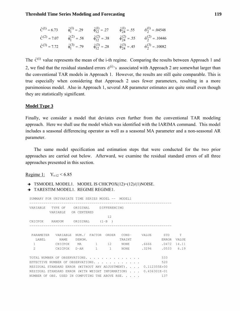
Threshold Time Series Modeling and Forecasting 119
(1) (1) (1) (1)(1)1 12 24 2(2) (2) (2) (2)(2)1 12 24 2(3) (3) (3) (3)(3)1 12 24 2
ˆ ˆ ˆ ˆ ˆC 6.73 .29 .27 .55 .04548
ˆ ˆ ˆ ˆ ˆC 7.07 .58 .38 .55 .10446
ˆ ˆ ˆ ˆ ˆC 7.72 .79 .28 .45 .10082
= φ = φ = φ = σ =
= φ = φ = φ = σ =
= φ = φ = φ = σ =
The (i)C value represents the mean of the i-th regime. Comparing the results between Approach 1 and
2, we find that the residual standard errors (i)ˆ 'sσ associated with Approach 2 are somewhat larger than the conventional TAR models in Approach 1. However, the results are still quite comparable. This is true especially when considering that Approach 2 uses fewer parameters, resulting in a more parsimonious model. Also in Approach 1, several AR parameter estimates are quite small even though they are statistically significant.
Model Type 3
Finally, we consider a model that deviates even further from the conventional TAR modeling approach. Here we shall use the model which was identified with the IARIMA command. This model includes a seasonal differencing operator as well as a seasonal MA parameter and a non-seasonal AR parameter.
The same model specification and estimation steps that were conducted for the two prior approaches are carried out below. Afterward, we examine the residual standard errors of all three approaches presented in this section.
Regime 1: Yt-12 < 6.85
TSMODEL MODEL1. MODEL IS CHICPOX(12)=(12)/(1)NOISE. TARESTIM MODEL1. REGIME REGIME1.
SUMMARY FOR UNIVARIATE TIME SERIES MODEL -- MODEL1 ----------------------------------------------------------------------- VARIABLE TYPE OF ORIGINAL DIFFERENCING VARIABLE OR CENTERED 12 CHICPOX RANDOM ORIGINAL (1-B ) ----------------------------------------------------------------------- PARAMETER VARIABLE NUM./ FACTOR ORDER CONS- VALUE STD T LABEL NAME DENOM. TRAINT ERROR VALUE 1 CHICPOX MA 1 12 NONE .6666 .0472 14.11 2 CHICPOX D-AR 1 1 NONE .3296 .0533 6.19 TOTAL NUMBER OF OBSERVATIONS. . . . . . . . . . . . . . 533 EFFECTIVE NUMBER OF OBSERVATIONS. . . . . . . . . . . . 520 RESIDUAL STANDARD ERROR (WITHOUT ANY ADJUSTMENT). . . . 0.112355E+00 RESIDUAL STANDARD ERROR (WITH WEIGHT INFORMATION) . . . 0.436301E-01 NUMBER OF OBS. USED IN COMPUTING THE ABOVE RSE. . . . . 137
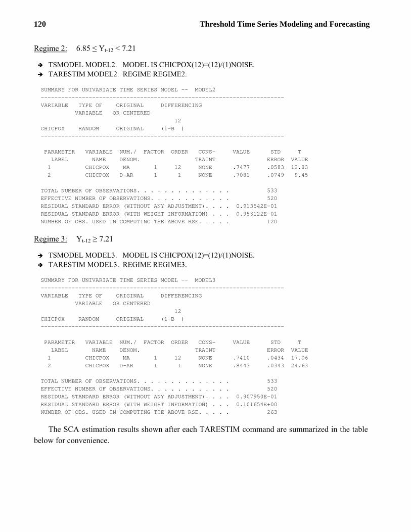
120 Threshold Time Series Modeling and Forecasting
Regime 2: 6.85 ≤ Yt-12 < 7.21
TSMODEL MODEL2. MODEL IS CHICPOX(12)=(12)/(1)NOISE. TARESTIM MODEL2. REGIME REGIME2.
SUMMARY FOR UNIVARIATE TIME SERIES MODEL -- MODEL2 ----------------------------------------------------------------------- VARIABLE TYPE OF ORIGINAL DIFFERENCING VARIABLE OR CENTERED 12 CHICPOX RANDOM ORIGINAL (1-B ) ----------------------------------------------------------------------- PARAMETER VARIABLE NUM./ FACTOR ORDER CONS- VALUE STD T LABEL NAME DENOM. TRAINT ERROR VALUE 1 CHICPOX MA 1 12 NONE .7477 .0583 12.83 2 CHICPOX D-AR 1 1 NONE .7081 .0749 9.45 TOTAL NUMBER OF OBSERVATIONS. . . . . . . . . . . . . . 533 EFFECTIVE NUMBER OF OBSERVATIONS. . . . . . . . . . . . 520 RESIDUAL STANDARD ERROR (WITHOUT ANY ADJUSTMENT). . . . 0.913542E-01 RESIDUAL STANDARD ERROR (WITH WEIGHT INFORMATION) . . . 0.953122E-01 NUMBER OF OBS. USED IN COMPUTING THE ABOVE RSE. . . . . 120
Regime 3: Yt-12 ≥ 7.21
TSMODEL MODEL3. MODEL IS CHICPOX(12)=(12)/(1)NOISE. TARESTIM MODEL3. REGIME REGIME3.
SUMMARY FOR UNIVARIATE TIME SERIES MODEL -- MODEL3 ----------------------------------------------------------------------- VARIABLE TYPE OF ORIGINAL DIFFERENCING VARIABLE OR CENTERED 12 CHICPOX RANDOM ORIGINAL (1-B ) ----------------------------------------------------------------------- PARAMETER VARIABLE NUM./ FACTOR ORDER CONS- VALUE STD T LABEL NAME DENOM. TRAINT ERROR VALUE 1 CHICPOX MA 1 12 NONE .7410 .0434 17.06 2 CHICPOX D-AR 1 1 NONE .8443 .0343 24.63 TOTAL NUMBER OF OBSERVATIONS. . . . . . . . . . . . . . 533 EFFECTIVE NUMBER OF OBSERVATIONS. . . . . . . . . . . . 520 RESIDUAL STANDARD ERROR (WITHOUT ANY ADJUSTMENT). . . . 0.907950E-01 RESIDUAL STANDARD ERROR (WITH WEIGHT INFORMATION) . . . 0.101654E+00 NUMBER OF OBS. USED IN COMPUTING THE ABOVE RSE. . . . . 263
The SCA estimation results shown after each TARESTIM command are summarized in the table below for convenience.

Threshold Time Series Modeling and Forecasting 121
(1) (1) (1)1 12 3(2) (2) (2)1 12 3(3) (3) (3)1 12 3
ˆ ˆ ˆ.33 .67 .04363
ˆ ˆ ˆ.71 .75 .09531
ˆ ˆ ˆ.84 .74 .10165
φ = Θ = σ =
φ = Θ = σ =
φ = Θ = σ =
Upon examining the residual standard errors of the three regimes, we find that the residual standard errors under Model Type 3 are smaller or comparable to the TAR model used by Chen and Tsay (1993) while the number of parameters was reduced by more than half.
In summary, three types of threshold models are presented in this section to address nonlinearity in a time series caused by the presence of multiple regimes in the time series data. The first model type considered was a conventional TAR model that was presented by Chen and Tsay (1993) in their analysis of logged monthly Chickenpox cases in New York City. Their estimation results were replicated using the SCA System in Model Type 1. A second model type was then considered using a multiplicative AR model. In Model Type 2, we specified the autoregressive operators on the right-hand side of the model, giving more meaning to the constant term in the models. The final model type considered was a general threshold ARIMA model. The residual standard errors and the number of parameters in each model (p) for the three threshold model types are presented in the table below.
Model Type
Regime 1 Regime 2 Regime 3
p RSE p RSE p RSE
#1 5 0.04268 5 0.09814 6 0.09945
#2 4 0.04548 4 0.10446 4 0.10082
#3 2 0.04363 2 0.09531 2 0.10165
13.9 Example of TAR Modeling Using the U.S. Real GNP
In this section, a TAR model is used to analyze the quarterly U.S. real GNP series (in 1982 dollars) between the first quarter of 1947 and the first quarter of 1991. Tiao and Tsay (1994) study the growth rate of the U.S. real GNP series (denoted as tDGNP below) with
t t t 1 tDGNP (GNP ) (GNP ) (1 B) (GNP )−= − = −n n n (13.15)
where tGNP is the quarterly real GNP in the t-th quarter and tDGNP is the growth rate between the successive quarters. Due to differencing, the series tDGNP has 176 observations and is displayed below.

122 Threshold Time Series Modeling and Forecasting
Growth rate of U.S. quarterly real GNP (2/1947 – 1/1991)
Using the entire time series, we find that the GNP growth rate ( tDGNP ) can be represented by a MA(2) or an AR(1) model. For purpose of TAR modeling, we consider the following slightly over-parameterized AR(2) model:
t 0 1 t 1 2 t 2 tDGNP C DGNP DGNP a− −= + φ + φ + . (13.16)
The estimates for the parameters of the above model are
0 1 2 aˆ ˆ ˆ ˆC =0.0041 (t=4.13), 0.3304 (t=4.39), 0.1344 (t=1.78), and 0.00986φ = φ = σ = (13.17)
Using this linear AR(2) as the null hypothesis model, the statistics for the TAR-F test for possible nonlinear threshold lags (d) are computed using the TARTEST command. Here, we consider threshold lags from 1 to 6.
TARTEST DGNP. ARLAGS 1, 2. THLAGS 1 TO 6.
Lag F-statistic Degrees of freedom -------- ----------- ------------------ 1 0.36586 3 152 2 3.16414 3 152 3 2.55177 3 151 4 2.65051 3 150 5 1.70234 3 149 6 1.79730 3 148
The above table shows that the linear AR(2) model should be rejected because the F-statistic at d=2 (the largest) is significant at 5% level. Thus a TAR model with d=2 should be considered. If multiple d values are significant, we usually choose the d that has the largest corresponding F-value. In some applications we may select a threshold lag based on additional rationale. For example, if a few significant F statistics are clustered around a seasonal lag, the seasonal lag may be selected instead of a more significant threshold lag due to the seasonality of the particular series.

Threshold Time Series Modeling and Forecasting 123
To identify the threshold values for the DGNP series using the AAR method, the TARTEST command is employed. The THLAG is set to 2 and the ARLAGS are specified as 1 and 2. The autoregressive parameter estimates, their t-ratios, and corresponding estimated variances are saved in the SCA workspace using the HOLD subcommand.
TARTEST DGNP. THLAG 2. ARLAGS 1 TO 2. @ HOLD THVARIABLE(THV,THINDX), PHI(PHIMTX), TPHI(TPHIMTX), @ SIGMAHAT(SIGMA).
The threshold values (in sorted order) are stored under the THV variable name. The PHIMTX and TPHIMTX variables store the AR estimates and their corresponding t-values in matrix form. The following SCA matrix operation separates the matrix columns into variables that can be readily used for graphing or further analysis.
PHI1=PHIMTX(.,1) PHI2=PHIMTX(.,2) TPHI1=TPHIMTX(.,1) TPHI2=TPHIMTX(.,2)
Alternatively, the PICK command can be used in place of the matrix operations above to copy columns of a matrix to create the PHI1, PHI2, TPHI1, and TPHI2 series.
The scatter plots for the estimates (PHI1 and PHI2), and their t-ratios (TPHI1 and TPHI2) versus the threshold variable THV (i.e., t 2DGNP − ) are created using the GRAPH command. The data is transferred to SCAGRAF using the command
GRAPH THV, PHI1, PHI2, TPHI1, TPHI2.
By examining the scatter plots we find that the estimates of 1φ have little variation. On the contrary, the estimates of 2φ vary greatly (between -1.019 and 0.134). Therefore, we shall use the estimates of 2φ and the corresponding t-ratios for identification of threshold values. From (b) and (d), we find the 2φ estimates and their t-ratios change their direction from descending to ascending around
t 2Y 0− = . This suggests that data can be partitioned into two regimes with a threshold at t 2Y 0.0− = . However, if we also use 1φ estimates and their t-ratios to identify threshold values, we find an additional threshold around t 2Y 0.007− = , as shown in (a) and (b). We should keep in mind that this threshold may not be meaningful because the 1φ estimates have little variation between regimes separated by this threshold, as shown in (a).

124 Threshold Time Series Modeling and Forecasting
Plots of autoregressive coefficients and their t-ratios versus the threshold variable Yt-2
(GNP series with the AAR method)
(a) Arranged autoregression estimates of 1φ
(b) Arranged autoregression estimates of 2φ
(c) t-ratios for the estimates of 1φ
(d) t-ratios for the estimates of 2φ
The Reverse AAR method is also applied on the GNP series. Instead of searching for threshold values from left-to-right on the threshold axis, we search for threshold values from right-to-left on the threshold axis when the Reverse AAR method is used. The following TARTEST command is specified using the RAAR method.
TARTEST DGNP. THLAGS 2. ARLAGS 1, 2. HOLD @ THVARIABLE(THVR,THINDXR), PHI(PHIMTXR),TPHI(TPHIMTXR), @ SIGMAHAT(SIGMAR).
The scatter plots for 1φ , 2φ , and their t-ratios versus the threshold variable are displayed below.

Threshold Time Series Modeling and Forecasting 125
Plots of autoregressive coefficients and their t-ratios versus the threshold variable Yt-2
(GNP series with the Reverse AAR method)
(a) Arranged autoregression estimates of 1φ (b) Arranged autoregression estimates of 2φ
(c) t-ratios for the estimates of 1φ (d) t-ratios for the estimates of 2φ
By examining the dominant coefficient 2φ , we find that 2φ and its t-ratios have a major change of
direction around t 2Y 0.0− = as shown in (b) and (d). Similarly, by examining the coefficient 1φ , we find its t-ratios have a major change of direction around t 2Y 0.007− = . These findings confirm the
previous results. Again, the threshold identified based on 2φ is more important than the one based on
1φ .
The THMEXPLORE command can also be used to explore potential thresholds using the local arranged regression (LAR) method. To use the LAR method in the THMEXPLORE, a linear regression model must be specified. The model may be in the form of a lagged regression or in the form of a linear regression model that includes explanatory variables.

126 Threshold Time Series Modeling and Forecasting
For comparison purposes, the LAR method will be used to explore the thresholds of the DGNP series. The THMEXPLORE command with a window size of 60 and threshold lag 2 is used. A lagged regression model will be employed using lags one and two of the DGNP series as input variables. The SCA LAG command is used to create lagged variables of the DGNP series stored as YLAG1 and YLAG2. The command is shown below.
LAG DGNP. NEW YLAG1,YLAG2. LAGS 1, 2.
A model is specified in linear regression form using the following TSMODEL command. Here, parameter labels (C, PHI1L, and PHI2L) are specified in the model command.
TSMODEL THMODEL. MODEL IS @ DGNP=C+(0;PHI1L)YLAG1+(0;PHI2L)YLAG2+NOISE.
The THMEXPLORE command is employed using the above model with a moving window size of 60 observations, and threshold lag of 2.
THMEXPLORE THMODEL. THLAG 2. WINDOWSIZE 60. @ HOLD THVARIABLE(THVL).
VARIABLE THVL STORES THE SORTED THRESHOLD VARIABLE (WITH 174 VALUES) VARIABLE C STORES PARAMETER ESTIMATES (WITH 174 VALUES) VARIABLE _C STORES THE t-VALUES OF THE ABOVE ESTIMATES VARIABLE PHI1L STORES PARAMETER ESTIMATES (WITH 174 VALUES) VARIABLE _PHI1L STORES THE t-VALUES OF THE ABOVE ESTIMATES VARIABLE PHI2L STORES PARAMETER ESTIMATES (WITH 174 VALUES) VARIABLE _PHI2L STORES THE t-VALUES OF THE ABOVE ESTIMATES
Plots of autoregressive coefficients and their t-ratios versus the threshold variable Yt-2 are displayed below.

Threshold Time Series Modeling and Forecasting 127
Plots of autoregressive coefficients and their t-ratios versus the threshold variable Yt-2
(GNP series with the LAR method)
(a) Arranged autoregression estimates of 1φ
(b) Arranged autoregression estimates of 2φ
(c) t-ratios for the estimates of 1φ
(d) t-ratios for the estimates of 2φ
By examining the dominant coefficient 2φ , we find that the estimates of 2φ and their t-ratios have major changes of directions around t 2Y 0.0− = and t 2Y 0.017− = , as shown in (b) and (d). The latter threshold ( t 2Y 0.017− = ) should be ignored since the t-ratios before and after this threshold are all
insignificant. By examining the coefficient 1φ , we find the estimates of 1φ and their t-ratios have a major change of direction around t 2Y 0.007− = . The findings here are also consistent with the previous results.
Now that the appropriate threshold lag and suitable threshold values have been identified, the REGIME command is used to construct the threshold indicator variables. Here, the threshold lag 2 is specified using the THLAG subcommand and the threshold value 0 is specified using the

128 Threshold Time Series Modeling and Forecasting
THRESHOLD subcommand. The threshold indicator variables are stored as REGIME1 and REGIME2.
REGIME DGNP. THLAG 2. THRESHOLD 0. INDICATORS REGIME1, REGIME2.
Using the regime indicators generated above, the following two-regime TAR(2) is specified using the TSMODEL command and estimated using the TARESTIM command as shown below.
Regime 1: Yt-12 <= 0.0
TSMODEL MODEL1. MODEL IS (1,2)DGNP=CNST1+NOISE. TARESTIM MODEL1. REGIME REGIME1.
SUMMARY FOR UNIVARIATE TIME SERIES MODEL -- MODEL1 ----------------------------------------------------------------------- VARIABLE TYPE OF ORIGINAL DIFFERENCING VARIABLE OR CENTERED DGNP RANDOM ORIGINAL NONE ----------------------------------------------------------------------- PARAMETER VARIABLE NUM./ FACTOR ORDER CONS- VALUE STD T LABEL NAME DENOM. TRAINT ERROR VALUE 1 CNST1 CNST 1 0 NONE -.0039 .0033 -1.18 2 DGNP AR 1 1 NONE .4362 .1754 2.49 3 DGNP AR 1 2 NONE -.7873 .3335 -2.36 TOTAL NUMBER OF OBSERVATIONS. . . . . . . . . . . . . . 176 EFFECTIVE NUMBER OF OBSERVATIONS. . . . . . . . . . . . 174 RESIDUAL STANDARD ERROR (WITHOUT ANY ADJUSTMENT). . . . 0.199273E-01 RESIDUAL STANDARD ERROR (WITH WEIGHT INFORMATION) . . . 0.120398E-01 NUMBER OF OBS. USED IN COMPUTING THE ABOVE RSE. . . . . 37
Regime 2: Yt-12 > 0.0
TSMODEL MODEL2. MODEL IS (1,2)DGNP=CNST2+NOISE. TARESTIM MODEL2. REGIME REGIME2.
SUMMARY FOR UNIVARIATE TIME SERIES MODEL -- MODEL2 ----------------------------------------------------------------------- VARIABLE TYPE OF ORIGINAL DIFFERENCING VARIABLE OR CENTERED DGNP RANDOM ORIGINAL NONE ----------------------------------------------------------------------- PARAMETER VARIABLE NUM./ FACTOR ORDER CONS- VALUE STD T LABEL NAME DENOM. TRAINT ERROR VALUE 1 CNST2 CNST 1 0 NONE .0038 .0014 2.71 2 DGNP AR 1 1 NONE .3111 .0792 3.93 3 DGNP AR 1 2 NONE .2014 .1061 1.90
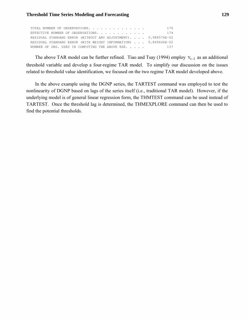
Threshold Time Series Modeling and Forecasting 129
TOTAL NUMBER OF OBSERVATIONS. . . . . . . . . . . . . . 176 EFFECTIVE NUMBER OF OBSERVATIONS. . . . . . . . . . . . 174 RESIDUAL STANDARD ERROR (WITHOUT ANY ADJUSTMENT). . . . 0.988576E-02 RESIDUAL STANDARD ERROR (WITH WEIGHT INFORMATION) . . . 0.869640E-02 NUMBER OF OBS. USED IN COMPUTING THE ABOVE RSE. . . . . 137
The above TAR model can be further refined. Tiao and Tsay (1994) employ t 1Y − as an additional threshold variable and develop a four-regime TAR model. To simplify our discussion on the issues related to threshold value identification, we focused on the two regime TAR model developed above.
In the above example using the DGNP series, the TARTEST command was employed to test the nonlinearity of DGNP based on lags of the series itself (i.e., traditional TAR model). However, if the underlying model is of general linear regression form, the THMTEST command can be used instead of TARTEST. Once the threshold lag is determined, the THMEXPLORE command can then be used to find the potential thresholds.

130 Threshold Time Series Modeling and Forecasting

References
Ansley, C.F. , Spivey, W.A. and Wrobleski, W.J. (1977). A class of transformations for Box-Jenkins seasonal models, Applied Statistics 26: 173-178
Box, G.E.P. and Cox, D.R. (1964). An analysis of transformations, Journal of the Royal Statistical Society, B, 26: 211-243
Box, G.E.P. and Jenkins, G.M. (1970). Time Series Analysis Forecasting and Control, Holden Day.
Chen, C. and Liu, L.-M (1990). Joint estimation of model parameters and outlier effects in time series, Journal of the American Statistical Association 88: 284-297
Chen, R. and Tsay, R.S. (1993). Functional-coefficient autoregressive models, Journal of the American Statistical Association 88: 298-308
Cleveland, W.P. and Tiao, G.C. (1979). Modelling seasonal time series, Revue Economique 32: 107-129
Dickey, D. and Fuller, W.A. (1979). Distribution of estimates fort autoregressive time series with a unit root, Journal of the American Statistical Association 74: 427-431
Dickey, D. and Fuller, W.A. (1981). Likelihood ratio tests for autoregressive time series with a unit root, Econometrics 49: 1057-1072
Diebold, F.X. and Nerlove, M. (1990). Unit roots in econometric time series: a selective survey, Advances in Econometrics, JAI Press 8: 3-69
Enders, W. (1995). Applied Econometric Time Series, Wiley
Guerrero, V.M. (1993). Time-series analysis supported by power transformations, Journal of Forecasting 12: 37-48
Hamilton, J.D. (1994). Time Series Analysis, Princeton University Press
Jolliffe, I.T. and Kumar, K. (1985). Discussion of the paper by Lawrance and Lewis, Journal of the Royal Statistical Society, B, 47: 190-191
Liu and Chen (1991). Recent development of time series analysis in intervention in environmental impact studies, Journal of Environmental Science and Health A26: 1217-1252

Liu, L.-M., Hudak, G.B., Box, G.E.P., Tiao, G.C. and Muller, M.E. (1992). Forecasting and Time Series Analysis Using the SCA Statistical System, Volume 1. Scientific Computing Associates Corp.
Liu, L-M., (2006). Time Series Analysis and Forecast, 2nd Edition, Scientific Computing Associates Corp.
Mills, T.C. (1993). The Econometric Modelling of Financial Time Series, Cambridge University Press
Pankratz, A. and Dudley, U. (1987). Forecasts of power-transformed series, Journal of Forecasting 6: 239-248
Phillips, P. and Perron, P. (1988). Testing for a unit root in time series regression, Biometrica 75: 335-346
Schwert, G.W. (1987). Effects of model specification on test for unit roots in macroeconomic data, Journal of Monetary Economics 20: 73-103
Stokes, H.S. (1997). Specifying and Diagnostically Testing Econometric Models 2nd Edition, Quorum Books
Sugihara, G. and May, R.M. (1990). Nonlinear forecasting as a way of distinguishing chaos from measurement error in time series, Nature 344: 734-741
Tiao, G.C. and Grupe, M.R. (1980). Hidden periodic autoregressive-moving average models in time series data, Biometrica 67: 365-373
Tong, H. (1978). On a threshold model. In Pattern Recognition and Signal Processing, (ed. C.H. Chen). Sijthoff and Noordhoff, Amsterdam.
Tong, H. and Lim, K.S. (1980). Threshold autoregression, limit cycles and cyclical data (with Discussion), Journal of the Royal Statistical Society, B, 42: 245-292
Tong, H. (1983). Threshold Models in Nonlinear Time Series Analysis, Lecture Notes in Statistics 21, Springer, Heidelberg.
Wang, W-Y., Du, J-G, and Xiang, J-T. (1984). Threshold autoregressive moving average model, Computational Mathematics (in Chinese), 4: 414-419
Wecker, W.E. (1981). Asymmetric time series, Journal of the American Statistical Association 76: 16-21

APPENDIX A
SCA COMMAND LIST GROUPED BY FOCUS AND EDITION
This Appendix provides information on the capabilities available in Release 8 of the SCA Statistical System for personal computers. Capabilities are provided in chart form, blocked into the following categories:
• Univariate time series analysis and forecasting • Automatic univariate time series modeling and outlier analysis • Multivariate time series modeling and forecasting • Seasonal adjustment • Transformation and forecasting • Nonlinear time series modeling and forecasting • General statistical analysis • Descriptive statistics • Date handling • Data editing • Input and output • Macro procedures • Utilities • Applets • Graphics Capabilities are listed in alphabetical order by SCA command names within each category.
Specific information regarding a capability (command) presented in this appendix include:
• The command name or system function • A short description for the command • The SCA Edition(s) that include the command • The document reference for the command
For convenience, the user guides that document the SCA commands are designated by letter abbreviations listed below:
(A) SCA Reference Manual for Fundamental Capabilities (B) SCA Reference Manual for General Statistical Analysis (C) Forecasting and Time Series Analysis Using the SCA Statistical System, Volume 1 (D) Forecasting and Time Series Analysis Using the SCA Statistical System, Volume 2 (E) GARCH Modeling using SCAB34S-GARCH and SCA WorkBench (F) New and Enhanced Capabilities in Release 8 of the SCA Statistical System (this document) (G) On-line Syntax Help (Accessible through SCA WorkBench)

134 Appendix A
Univariate Time Series Analysis and Forecasting
Command User Guide
Educationa
l
Practition
er
Profession
al A
Profession
al B
Description
ACF C x x x x Autocorrelation Function
AGGREGATE C x x x x Simple Temporal Aggregation
CCF C x x x x Cross Correlation Function
CCM C,D x x x x Cross Correlation Matrix
CORNER C x x x x Corner Table
CSPECTRA G x x x x Spectral Analysis
EACF C x x x x Extended Autocorrelation Function
ESTIM C x x x x Estimate a time series model
FFILTER G x x x x Band‐pass / Band‐fail Filter
FILTER C x x x x Filter a time series based on model
FORECAST C x x x x Forecast a time series
GFORECST C x x x x General Exponential Smoothing
IACF G x x x x Inverse Autocorrelation Function
IDENTIFY C x x x x ACF & PACF
OUTLIER C x x x x Outlier detection and identification
PACF C x x x x Partial Autocorrelation Function
PSPECTRA G x x x x Spectral Analysis
SIMULATION C x x x x Simulate a time series based on model
RSFILTER F x x x x Seasonal time series model identification
TSMODEL C x x x x Time series model specification
UROOT F x x x x Unit Root tests
WEIGHT C x x x x Pi‐weights and Psi‐weights

Appendix A 135
Automatic Univariate Time Series Analysis and Forecasting
Command User Guide
Edu
cation
al
Practitione
r
Professiona
l A
Professiona
l B
Description
IARIMA D ‐‐ x x x Automatic ARIMA Modeling
IESTIM D ‐‐ x x x Automatic ARIMA & Transfer Function
OESTIM C ‐‐ x x x Joint Outlier Estimation and Adjustment
OFILTER C ‐‐ x x x Outlier Filtering of a Time Series
OFORECST C ‐‐ x x x Outlier Adjusted Forecasting
OUTLIER C ‐‐ x x x Outlier detection and identification
RSFILTER F x x x x Seasonal time series model identification
Multivariate Time Series Analysis and Forecasting
Command
User Guide
Educationa
l
Practition
er
Profession
al A
Profession
al B
Description
CAUSALTEST F ‐‐ ‐‐ x ‐‐ Causality tests
CANONICAL G ‐‐ ‐‐ x ‐‐ Canonical Analysis
CCM D x x x x Cross Correlaton Matrix
ECCM D ‐‐ ‐‐ x ‐‐ Extended Cross Correlation Matrix
MESTIM D ‐‐ ‐‐ x ‐‐ Vector ARMA Model Estimation
IMESTIM D ‐‐ ‐‐ x ‐‐ Automatic Vector ARMA Estimation
MFORECAST D ‐‐ ‐‐ x ‐‐ Vector ARMA Forecasting
MIDEN D ‐‐ ‐‐ x ‐‐ Vector ARMA Model Identification
MSIMULATE D ‐‐ ‐‐ x ‐‐ Vector ARMA Model Simulation
MTSMODEL D ‐‐ ‐‐ x ‐‐ Vector ARMA Model Specification
SCAN G ‐‐ ‐‐ x ‐‐ Vector ARMA Model Identification
SESTIM D ‐‐ ‐‐ x ‐‐ STF Model Estimation
SFORECAST D ‐‐ ‐‐ x ‐‐ STF Model Forecasting
SSIMULATE D ‐‐ ‐‐ x ‐‐ STF Model Simulation
STEPAR D ‐‐ ‐‐ x ‐‐ Step‐wise Autoregressive Fit
STFMODEL D ‐‐ ‐‐ x ‐‐ STF Model Specification

136 Appendix A
Seasonal Adjustment
Command
User Guide
Educationa
l
Practition
er
Profession
al A
Profession
al B
Description
XCD D ‐‐ ‐‐ x ‐‐ Model‐based seasonal adjustment
Transformation and Forecasting
Command
User Guide
Educationa
l
Practition
er
Profession
al A
Profession
al B
Description
RETRANSFORM F ‐‐ x x x Retransform forecasts (unbias)
TSEARCH F ‐‐ ‐‐ ‐‐ x Lambda value search for transformation
Nonlinear Time Series Modeling and Forecasting
Command
User Guide
Educationa
l
Practition
er
Profession
al A
Profession
al B
Description
GARCH E ‐‐ ‐‐ ‐‐ x GARCH modeling and analysis environment
NLTEST F ‐‐ ‐‐ ‐‐ x Nonlinearity testing using LM ARCH test
REGIME F ‐‐ ‐‐ ‐‐ x Generate binary regime indicator variables
SPLINES G * * * * MARSplines, GAM, ACE, other
TARESTIM F ‐‐ ‐‐ ‐‐ x Threshold AR estimation
TARFORECAST F ‐‐ ‐‐ ‐‐ x Threshold AR forecast
TARTEST F ‐‐ ‐‐ ‐‐ x Threshold AR F‐Test and threshold lag search
TARXTEST F ‐‐ ‐‐ ‐‐ x Threshold search using external variable
THMEXPLORE F ‐‐ ‐‐ ‐‐ x Threshold search using arranged regression
THMTEST F ‐‐ ‐‐ ‐‐ x Threshold AR F‐Test and threshold lag search
TSEARCH F ‐‐ ‐‐ ‐‐ x Lambda value search for transformation
TVPEXPLORE F ‐‐ ‐‐ ‐‐ x Time‐varying parameter analysis
WESTIM F ‐‐ ‐‐ ‐‐ x Weighted time series model estimation
WFORECAST F ‐‐ ‐‐ ‐‐ x Weighted forecasting
(*) The SPLINES capability requires the SCAB34S SPLINESproduct.

Appendix A 137
General Statistical Analysis
Command User Guide
Educationa
l
Practition
er
Profession
al A
Profession
al B
Description
CORRELATION B x x x x Display correlation between two variables
CROSSTAB B x x x x Cross tabulation
NONPARAMETRIC B x x x x Non‐parametric statistics
NWAY B x x x x N‐way analysis of variance
OWAY B x x x x One‐way analysis of variance
PTRAN B x x x x Parameter estimation with Box‐Cox transform
RANK B x x x x Convert data into a ranked variable
REGRESS B x x x x Estimate a regression model
TABLE B x x x x Display sample mean and STD of data groups
TTEST B x x x x Two‐sample t‐test
TWAY B x x x x Two‐way analysis of variance
Date Handling
Command
User Guide
Educationa
l
Practition
er
Profession
al A
Profession
al B
Description
DAGGREGATE F ‐‐ x x x Temporal aggregation using date indices
DATEBUILD F ‐‐ x x x Generate date variable
DAYS C ‐‐ x x x Compute number of mondays, etc. in month
DMATRIX G x x x x Generate a design matrix from factor variable
DOWEEK F ‐‐ x x x Day of week associated with date
DVECTOR F ‐‐ x x x Generate dummy variables from factors
EASTER C ‐‐ x x x Generate monthly weights related to Easter

138 Appendix A
Data Editing
Command
User Guide
Educationa
l
Practition
er
Profession
al A
Profession
al B
Description
AGGREGATE A,C x x x x Temporal aggregation using observation index
AUGMENT A x x x x Join variables into a matrix
CHANGE A x x x x Change the values of a variable
DIFFERENCE A,C x x x x Difference a time series
DMATRIX G x x x x Generate a design matrix from factor variable
GENERATE A x x x x Generate a variable using specified sequence
JOIN A x x x x Join variables together as a new variable
LAG A,C x x x x Lag a time series
OMIT A x x x x Omit values or time span in a variables
PATCH A,C x x x x Patch or recode missing values
PERCENT A,C x x x x Generate a percent change variable
PICK A x x x x Pick off columns from a matrix
RANK A x x x x Convert data into a ranked variable
RECODE A x x x x Recode values in a variables to a new value
SELECT A x x x x Select obs. of a variable by value or span
SIMULATE A x x x x Simulate a data with a specified distribution
SORT A x x x x Sort the values of a variable
Descriptive Statistics
Command
User Guide
Educationa
l
Practition
er
Profession
al A
Profession
al B
Description
DESCRIBE B x x x x Display descriptive statistics of a variable
DPLOT G x x x x Dispersion plot (character plot)
GRAPH G x x x x Create graph in SCAGRAF Applet (graphic plot)
HGRAPH G ‐‐ ‐‐ ‐‐ ‐‐ Create graph in SCAB34S Applet (graphic plot)
HISTOGRAM B x x x x Histogram plot (character plot)
LABEL A x x x x Assign one character label to variable name
MPLOT A x x x x Multiple scatter plot (character plot)

Appendix A 139
MTPLOT A x x x x Multiple time series plot (character plot)
MTSPLOT A x x x x Multiple time series plot (character plot)
PARETO A x x x x Pareto plot (character plot)
PLOT A x x x x Scatter plot (character plot)
PPLOT A x x x x Probability plot (character plot)
SHEWHART A x x x x Shewhart plot (character plot)
TPLOT A x x x x Time series plot (character plot)
TSPLOT A x x x x Time series plot (character plot)
Input and Output
Command
User Guide
Educationa
l
Practition
er
Profession
al A
Profession
al B
Description
ASSIGN A x x x x Associate a file with a unit number
BINPUT A x x x x Input dataset using SCA binary format
BSAVE A x x x x Save dataset using SCA binary format
DISPLAY A x x x x Display descriptive text in SCA macro
FINPUT A x x x x Input dataset using SCA meta data format
FREE A x x x x Release a unit number associated with a file
FSAVE A x x x x Save dataset using SCA meta data format
INPUT A x x x x Input data from a flat text file
PRINT A x x x x Print variables
REWIND A x x x x Rewind a unit number associated with a file
SAVE A x x x x Save data in a flat text file format
Macro Procedures
Command
User Guide
Educationa
l
Practition
er
Profession
al A
Profession
al B
Description
CALL A x x x x Call a SCA macro procedure script
PARAMETERS A x x x x Specify symbolic parameters
RETURN A x x x x Return from macro procedure

140 Appendix A
Utilities
Command
User Guide
Educationa
l
Practition
er
Profession
al A
Profession
al B
Description
NEWPAGE A x x x x Force start of new page in SCA output
PROFILE A x x x x Control key settings of SCA System session
RESTART A x x x x Clears the SCA workspace
STOP A x x x x Exit the SCA System session
TIME A x x x x Print date and time
WORKSPACE A x x x x Provides various SCA Workspace utilities
Applets
Command
User Guide
Educationa
l
Practition
er
Profession
al A
Profession
al B
Description
RUN G x x x x Execute an external program
RUNW G x x x x Execute an external program and wait for finish
BUILD G x x x x Write text to a file in free format (control file)
ENDBUILD G x x x x End writing text to a file
COPY G x x x x Copy text from external file into the SCA output
XLSREAD G x x x x Build SCA data macro from Excel file
XLSWRITE G x x x x Write data from a file into Excel
Graphics
Command
User Guide
Educationa
l
Practition
er
Profession
al A
Profession
al B
Description
HGRAPH G * * * * Create graph in SCAB34S Applet (graphic plot)
SCAGRAF G x x x x Create graph in SCAGRAF Applet (graphic plot)
(*) The HGRAPH command requires the SCAB34S product.

APPENDIX B
SCA COMMAND SYNTAX LISTING
This appendix B provides a listing of the syntax for new SCA commands included in Release 8 of the SCA Statistical System. The commands are presented in alphabetical order.
CAUSALTEST
The CAUSALTEST command is used to examine the causal relationships between two time series.
SYNTAX in terms of subcommands and associated argument type(s)
+----------------------------------------------------------------+ | | | CAUSALTEST MODEL model-name. | | PROCEDURE IS w. @ | | ALPHA IS r. | | | | ** Complete list of available subcommands: | | | | CAUSALTEST MODEL model-name. @ | | PROCEDURE IS w. @ | | ALPHA IS r. @ | | STOP-CRITERIA ARE MAXIT(i), LIKELIHOOD(r). @ | | SPAN IS i1, i2. @ | | OUTPUT IS LEVEL(w), PRINT(w1,w2,---), @ | | NOPRINT(w1,w2,---). @ | | | | Required subcommand: MODEL | | | | Legend: v -- variable namel i -- integer value; | | w -- keyword r -- real value | +----------------------------------------------------------------+
Subcommand descriptions
MODEL subcommand The MODEL subcommand is used to specify the name (label) of the vector ARMA model used for causality testing. The name must be a vector ARMA model specified in a previous TSMODEL command.
PROCEDURE subcommand The PROCEDURE subcommand is used to specify the approach employed in causality testing. The keyword, w, may be BACKWARD for the backward procedure, FORWARD for the forward procedure, or BOTH for both backward and forward procedures. The default is BOTH.

142 Appendix B
ALPHA subcommand The ALPHA subcommand is used to specify the significant level employed in conducting all pair-wise tests. The default is 0.05 (i.e., 5%).
STOP subcommand
The STOP subcommand is used to specify the stopping criterion for nonlinear estimation. The argument, i, for the keyword MAXIT specifies the maximum number of iterations (default is i=10), and the argument, r, for the keyword LIKELIHOOD specifies the value of the relative convergence criterion on the likelihood function (default is r=0.001). Estimation iterations will be terminated when the relative change in the value of likelihood function between two successive iterations is less than or equal to the convergence criterion, or if the maximum number of iterations is exceeded.
SPAN subcommand The SPAN subcommand is used to specify the span of time indices, i1 to i2, for which the data will be analyzed. The default is the maximum span available for the series which is the span of the shortest series if all series are not of equal length.
OUTPUT subcommand
The OUTPUT subcommand is used to control the amount of output printed for computed statistics. Control is achieved in a two stage procedure. First a basic LEVEL of output (default NORMAL) is specified. Output may then be increased from this level by use of PRINT (NOPRINT). The keywords for LEVEL and output printed are: BRIEF: likelihood values and their related statistics only NORMAL: same as BRIEF DETAILED: CORR where the reserved words (and keywords for PRINT, NOPRINT) on the right denote:
CORR: the correlation matrix for the parameter estimates. It also activates the display of
detailed information in causality testing.

Appendix B 143
DAGGREGATE
The DAGGREGATE command is used to generate a new time series through the temporal aggregation of a specified time series given a companion date index variable. The generated series will be aggregated into user specified time intervals such as year, quarter, month, week, or day. Aggregation method may be specified as the sum, mean, first, last, high or low of the data values in each date period.
SYNTAX in terms of subcommands and associated argument type(s)
+--------------------------------------------------------------+ | | | DAGGREGATE OLD v1,v2,--- . @ | | NEW v1,v2,--- . @ | | DATE IS v. @ | | METHOD IS w1(w2). | | | | ** Complete list of available subcommands: | | | | DAGGREGATE OLD v1,v2,--- . @ | | NEW v1,v2,--- . @ | | DATE IS v. @ | | METHOD IS w1(w2). @ | | WBEGIN IS i. @ | | COMPRESS/NO COMPRESS. @ | | HOLD DATE(v),NOBS(v1,v2,---),MEAN(v1,v2,---),@ | | STDERR(v1,v2,---). | | | | Required subcommands: OLD, NEW, DATE, METHOD | | | | Legend: v -- variable name; i -- integer value; | | w -- keyword | +--------------------------------------------------------------+
Subcommand descriptions
OLD subcommand The OLD subcommand is used to specify the name(s) of time series variable(s) from which the aggregated time series will be derived. It is a required subcommand.
NEW subcommand The NEW subcommand is used to specify the name(s) of variable(s) to store the aggregated time series. The default are the names specified in the OLD subcommand. It is a required subcommand.
DATE subcommand The DATE subcommand is used to specify the name of the date index variable associated with the original series to be aggregated. The date must be a 8-digit number representing YYYYMMDD where YYYY is year, MM is month, and DD is day. It is a required subcommand.

144 Appendix B
METHOD subcommand The METHOD subcommand is used to specify the aggregation grouping and the summarization or aggregation method. The aggregation grouping keyword (w1) can be specified as YEAR, QUARTER, MONTH, WEEK, or DAY. The aggregation method keyword (w2) can be specified as SUM, MEAN, FIRST, LAST, HIGH, or LOW. It is a required subcommand.
WBEGIN subcommand The WBEGIN subcommand is used to specify the first day of the week which is only applicable to weekly aggregation. For example, the weekly data aggregation will begin on Tuesday if 2 is specified.
COMPRESS subcommand The COMPRESS subcommand is used to specify that the aggregated series shall be stored in compressed form, i.e., aggregated values are not repeated so that the total number of observations are less than that of the original series. This is the typical case. If NO COMPRESS is specified, then the aggregated series will have the same length as the original series. The default is COMPRESS.
HOLD subcommand The HOLD subcommand is used to specify those values computed for particular functions to be retained in the workspace until the end of the session. Only those information desired to be retained need be named. Values are placed in the variable named in parentheses. The default is that none of the values of the above information will be retained after the command is used. The values that may be retained are:
DATE: the new dates associated with the aggregated series. For aggregation in WEEK, the values stored in the DATE variable are 10 digit values where the first 8 digits represent the date for each aggregated value, and the last 2 digits represent the week for the aggregated value.
NOBS: the number of observations in the each aggregated period. This information is useful to evaluate and adjust partially aggregated periods
MEAN: the mean of the observations in the aggregated period.
STDERR: the sample standard deviation of the observations in the aggregated period

Appendix B 145
DATEBUILD
The DATEBUILD command is used to generate a sequence of dates given a beginning period and an ending period. If the ending period is not well defined, the number of dates to create may be specified directly using the NOBS subcommand.
SYNTAX in terms of subcommands and associated argument type(s)
+--------------------------------------------------------------+ | | | DATEBUILD VARIABLE IS v. @ | | BEGIN i1,i2,i3. @ | | END i1,i2,i3. @ | | NOBS IS i. | | | | ** Complete list of available subcommands: | | | | DATEBUILD VARIABLES IS v. @ | | QUARTERLY. @ | | BEGIN i1,i2,i3. @ | | END i1,i2,i3. @ | | NOBS IS i. @ | | OMIT DOWEEK(---),DAY(---),MONTH(---), @ | | QUARTER(---),YEAR(---). @ | | HOLD YEAR(v),QUARTER(v),MONTH(v),DAY(v), @ | | DOWEEK(v). | | | | Required subcommands: VARIABLES, BEGIN, END (or NOBS) | | | | Legend: v -- variable name | | | +--------------------------------------------------------------+
Subcommand descriptions
VARIABLE subcommand The VARIABLE subcommand is used to specify the name of the variable that will hold the newly generated date values.
QUARTERLY subcommand The QUARTERLY subcommand is used to specify that the date variable shall be organized as quarterly dates.
BEGIN subcommand The BEGIN subcommand is used to specify the beginning period for the generated date variable. The first parameter value i1 specifies the beginning year as a 4-digit integer, the second parameter value i2 specifies the beginning month or quarter (if the QUARTERLY subcommand is specified), and the third parameter value i3 specifies the beginning day. If only the year is needed, it is not necessary to provide values for i2 and i3. Similarly, if only year and month is needed, it is not necessary to provide a value for i3.

146 Appendix B
END subcommand The END subcommand is used to specify the ending period for the new date variable. The first parameter value i1 specifies the beginning year as a 4-digit integer, the second parameter value i2 specifies the beginning month or quarter (if the QUARTERLY subcommand is specified), and the third parameter value i3 specifies the beginning day. If only the year is needed, it is not necessary to provide values for i2 and i3. Similarly, if only year and month is needed, it is not necessary to provide a value for i3. The NOBS subcommand can be used instead of the END subcommand if the ending date is not well defined.
NOBS subcommand The NOBS subcommand is used to specify the number of dates that are to be generated starting from the specified beginning date period.
OMIT subcommand The OMIT subcommand is used to specify if certain date periods are to be skipped when building the date variable. For example, weekend dates can be omitted in daily date creation by specifying OMIT DOWEEK(6,7).
HOLD subcommand The HOLD subcommand is used to store the components of the generate date variable into separate variables. The component values that may be retained are:
YEAR: the years associated with the dates generated QUARTER: the quarters associated with the dates generated MONTH: the months associated with the dates generated DAY: the days associated with the dates generated DOWEEK: the day of week associated with the dates generated where Monday=1, Tuesday=2, ...., Sunday=7.

Appendix B 147
DOWEEK
The DOWEEK command is used to evaluate a double-precision date variable and determine the day of week associated with that date. The date variable must be a double precision variable of the form YYYYMMDD where YYYY represents the 4-digit year, MM represents the two-digit month, and DD represents the two-digit day. The command returns 1 for Monday, 2 for Tuesday, 3 for Wednesday, 4 for Thursday, 5 for Friday, 6 for Saturday, and 7 for Sunday.
SYNTAX in terms of subcommands and associated argument type(s)
+--------------------------------------------------------------+ | | | DOWEEK VARIABLE IS v. @ | | DAYOFWEEK IS v. | | | | ** Complete list of available subcommands: | | | | DOWEEK VARIABLE IS v. @ | | DAYOFWEEK IS v. @ | | DATEPARTS IN v1,v2,v3. | | | | Required subcommands: VARIABLES and DAYOFWEEK | | | | Legend: v -- variable name | | | +--------------------------------------------------------------+
Subcommand descriptions
VARIABLE subcommand The VARIABLE subcommand is used to specify the name of the variable whose values represent dates in the form YYYYMMDD. It is a required subcommand.
DAYOFWEEK subcommand The DAYOFWEEK subcommand is used to specify the variable (label) used to hold the associated day of week values. It is a required subcommand.
DATEPARTS subcommand The DATEPARTS subcommand stores the date information into separate variables where years will be saved to first variable name specified, months will be saved to the second variable name, and days will be saved to the third variable name specified.

148 Appendix B
DVECTOR
The DVECTOR command is used to construct a set of dummy variables (design matrix) from the values of factor variables and stores the dummy variables as vector variables. The resultant dummy variables can then be used in subsequent time series modeling and forecasting. Its functionality is similar to that of the DMATRIX command, but the resultant dummy variables are in vector form (as opposed to matrix form) and are more convenient to use in time series modeling and forecasting.
SYNTAX in terms of subcommands and associated argument type(s)
+--------------------------------------------------------------+ | | | DVECTOR VARIABLES ARE v1, v2, ---. @ | | MAIN-EFFECTS ARE v1, v2, ---. | | | | ** Complete list of available subcommands: | | | | DVECTOR VARIABLES ARE v1, v2, ---. @ | | MAIN-EFFECTS ARE v1, v2, ---. @ | | TYPE IS DEVIATION/T11/T10/T01. @ | | INTERACTIONS ARE v1(...), v2(...), ---. | | | | Required subcommands: VARIABLES and MAIN-EFFECTS | | | | Legend: v -- variable name | | | +--------------------------------------------------------------+
Subcommand descriptions
VARIABLES subcommand The VARIABLES subcommand is used to specify the names of the variables whose values are used to define the resultant design matrices. The variables must be categorical and specified as numerical values.
MAIN-EFFECTS subcommand The MAIN-EFFECTS subcommand is used to specify the variables (labels) for holding the resultant dummy variables. One set of dummy variables is constructed for each of the variables specified in the VARIABLES subcommand. Each dummy variable will have as many rows as the original variable. The number of dummy variables generated for each variable may be equal to or one less than the number of categories for the associated variable depending on the choice of the TYPE of design matrix formulation. The number of labels specified in the MAIN-EFFECTS subcommand must be the same as the number of variables specified in the VARIABLES subcommand. The labels specified here are used as the root word in storing the individual dummy variable vectors for the associated main effect. Since SCA has a limit of 8 characters for variable labels, it is important to use short labels of 6 characters or less. For example, if there are 4 categories in a variable and a root word label is specified as QA, the dummy variable vector labels associated with that variable will be assigned as QA1, QA2, and QA3 (and QA4 if TYPE is T11, see below).

Appendix B 149
TYPE subcommand The TYPE subcommand is used to specify the formulation of the design matrix. The keyword DEVIATION will produce a set of dummy variables such that its use in a regression or time series model will provide the estimates of the main-effects as deviations from the overall mean. In this case, there will be (m-1) dummy variables created for the variable where m is the number of categories. The keyword T11 will generate a dummy variable for each category in the variable. In this case, there will be m dummy variables created for the variable. The keyword T10 is similar to T11 except the dummy variable for the last category will not be created. The keyword T01 is also similar to T11 except the dummy variable for the first category will not be created. Both T10 and T01 create (m-1) dummy variables for each associated variable. The default is DEVIATION.
INTERACTION subcommand The INTERACTION subcommand is used to specify the construction of design matrices for interactions. The specification of each interaction is given by v (v1, v2, ---) where 'v' is the variable name (label) used to store the resultant design matrix for an interaction; and "v1, v2, ---" specifies the terms whose cross-products form the interaction, and have been specified previously in the MAIN-EFFECTS subcommand. Note that not all variables specified in the VARIABLES subcommand need be used in this subcommand and more than one interaction matrix can be constructed.

150 Appendix B
IARIMA
The IARIMA command is used to automatically identify an appropriate ARIMA model for a seasonal or non-seasonal time series. It also estimates the parameters of the identified model.
SYNTAX in terms of subcommands and associated argument type(s)
+--------------------------------------------------------------+ | | | IARIMA VARIABLE IS v. @ | | SEASONALITY is i. @ | | SPAN IS i1, i2. @ | | DFORDERS ARE i1, i2, --- . @ | | NODFORDERS i1, i2, --- . | | | | ** Complete list of available subcommands: | | | | IARIMA VARIABLE IS v. @ | | NAME IS model-name @ | | SEASONALITY is i. (PERIOD IS i.) @ | | SPAN IS i1, i2. @ | | DFORDERS ARE i1, i2, --- . @ | | NODFORDERS i1, i2, --- . @ | | CRITERIA r. @ | | DELETE-CONSTANT/NO DELETE. @ | | REPLACE IN model-name. @ | | COMPONENT-SERIES ARE v1,v2,v3. @ | | HOLD RESIDUALS(v),FITTED(v),VARIANCE(v). | | | | Required subcommand: VARIABLE | | | | Legend: v -- variable name; i -- integer value; | | w -- keyword | +--------------------------------------------------------------+
Subcommand descriptions
VARIABLE subcommand The VARIABLE subcommand is used to specify the name of the series for which an ARIMA model will be identified and estimated. It is a required subcommand.
NAME subcommand The NAME subcommand is used to specify a name (label) for the model identified by the IARIMA command. When it is not specified, the default name UTSMODEL is used internally.
SEASONALITY subcommand The SEASONALITY subcommand is used to specify the potential seasonality the series may possess. The seasonality is 4 for quarterly data, 12 for monthly data, and so on. If seasonality is specified but in fact the series is non-seasonal, an appropriate non-seasonal model will still be obtained (assuming that the series is medium to long in length). If a series is seasonal but no seasonality is specified, the identified model will not be appropriate (it is signified by the display of

Appendix B 151
significant sample autocorrelations of residuals). Hence the SEASONALITY is required if the series is seasonal, and optional if the series is non-seasonal. It is safe to specify the potential seasonality if the series is medium to long in length.
PERIOD subcommand The PERIOD subcommand serves the same purpose as the SEASONALITY subcommand. Either PERIOD or SEASONALITY may be used to specify the periodicity or seasonality of a time series, but not both.
SPAN subcommand The SPAN subcommand is used to specify the span of time indices, i1 to i2, for which the data are used to identify and estimate an ARIMA model. The default is the maximum span available for the series.
DFORDER subcommand The DFORDER subcommand is used to specify the differencing order(s) that must be included in the final ARIMA model. In addition to the specified differencing(s), other differencing orders may be included by the IARIMA command in the final ARIMA model if they are found to be necessary. By default, the differencing orders for the ARIMA model of a time series are automatically determined by the IARIMA command. User imposed specification of differencing order(s) may be particularly useful when a time series is short.
NODFORDERS subcommand The NODFORDERS subcommand is used to exclude specific differencing order(s) from being used in the final ARIMA model. By default, the differencing orders for the ARIMA model of a time series are automatically determined by the IARIMA command.
CRITERIA subcommand The CRITERIA subcommand is used to specify the critical value for determining the statistical significance of parameters retained in the model. The default is 1.96 for determining the statistical significance of model parameters.
DELETE-CONSTANT subcommand The DELETE-CONSTANT subcommand is used to specify the manner in which the deletion of the constant term in an ARIMA model is handled. By default (which is DELETE-CONSTANT), the constant term is deleted from the model if it is insignificant, and retained in the model if it is significant. However, if NO DELETE is specified, the constant term will be retained in the model no matter if it is significant or not. The default is DELETE-CONSTANT.
REPLACE subcommand The REPLACE subcommand is used to specify the name of a transfer function model or intervention model for which its ARMA component is to be replaced by the ARIMA model identified by the IARIMA command. The REPLACE subcommand provides a link for the combined use of the IARIMA and IESTIM commands.

152 Appendix B
COMPONENT subcommand The COMPONENT subcommand is used to specify the names of variables to store the residual series, R series (nonseasonal), and S series (seasonal). See SCA manual for the definition of R and S series. The S series will not be generated if the SEASONALITY (or PERIOD) subcommand is not specified.
HOLD subcommand The HOLD subcommand is used to specify those values computed for particular functions to be retained in the workspace until the end of the session. Only those statistics desired to be retained need be named. Values are placed in the variable named in parentheses. The default is that none of the values of the above statistics will be retained after the command is used. The values that may be retained are:
RESIDUALS: the residual series FITTED: the one-step-ahead forecasts (fitted values) of the series VARIANCE: the variance of the noise

Appendix B 153
NLTEST
The NLTEST command performs a non-linear testing of a series using a LaGrange multiplier approach proposed in Engle (1982) to test the null hypothesis that errors do not follow an ARCH process. The test performs a regression of the squared residuals on a constant and q lagged values of the squared residuals. From the regression, the LM test statistic is calculated as (N-q)-R**2. An ARCH process is determined to exist if the LM test exceeds the critical value from a chi-square distribution with q degrees of freedom.
SYNTAX in terms of subcommands and associated argument type(s)
+---------------------------------------------------------------+ | | | ** Complete list of available subcommands: | | | | NLTEST VARIABLE IS v1. @ | | METHOD IS w. @ | | ORDERS ARE i1,i2 ---. @ | | SPAN IS i1,i2. | | | | Required subcommand: | | | | Legend: v -- variable name; i -- integer value; | | w -- keyword; r -- real value | +---------------------------------------------------------------+
Subcommand descriptions
VARIABLE subcommand The VARIABLE subcommand is used to specify the series on which a nonlinear test is conducted.
METHOD subcommand The METHOD subcommand is used to specify the type of nonlinear test to be employed. The valid keywords are LM (LaGrange Multiplier).
ORDERS subcommand The ORDERS subcommand is used to specify the lag order(s) to be tested.
SPAN subcommand The SPAN subcommand is used to specify the span of the series to be considered. The default is all available data.

154 Appendix B
REGIME
The REGIME command is used to generate binary indicator variables based on the thresholds specified for a given time series.
SYNTAX in terms of subcommands and associated argument type(s)
+---------------------------------------------------------------+ | | | REGIME VARIABLE IS v. @ | | THLAG IS i. @ | | THRESHOLDS ARE r1, r2, ---. @ | | INDICATORS ARE v1, v2, v3, ---. | | | | ** Complete list of available subcommands: | | | | REGIME VARIABLE IS v1. @ | | THLAG IS i. @ | | THRESHOLDS ARE r1, r2, ---. @ | | INDICATORS ARE v1, v2, v3, ---. @ | | FINDICATORS ARE v1, v2, v3,---. @ | | EXTEND. / NO EXTEND. | | | | Required subcommand: VARIABLE, THRESHOLDS, INDICATORS | | | | Legend: v -- variable name; i -- integer value; | | w -- keyword; r -- real value | +---------------------------------------------------------------+
Subcommand descriptions
VARIABLE subcommand The VARIABLE subcommand is used to specify the time series whose values will be evaluated in generating the regime indicator variables (i.e., the regime variables).
THLAG subcommand The THLAG subcommand is used to specify the threshold lag that is used to generate the regime variables. The default is 1.
THRESHOLDS subcommand The THRESHOLDS subcommand is used to specify the cut-off values that define the threshold intervals. More than one threshold value may be specified but must be specified in ascending order.
INDICATORS subcommand The INDICATORS subcommand is used to specify the names of the variables that will hold the regime indicator variables. The number of regime indicator variables generated is always one greater than the number of threshold values specified.

Appendix B 155
If two threshold values are specified, three regime indicator variables will be generated. The first regime variable will mark all observations that are less than the first threshold value. The second regime indicator will mark all observations that are greater than or equal to the first threshold value but less than the second threshold value. The third regime indicator will mark all observations that are greater than the second threshold value.
FINDICATORS subcommand The FINDICATORS subcommand is used to specify the names of the regime indicator variables that hold the indicator information that is extended past the length of the time series. These regime indicator variables can then be used for forecasting a TAR model up to threshold lag value specified. The threshold lag must be greater than 0 when using the FINDICATOR subcommand.
EXTEND subcommand The EXTEND subcommand is used to extend the regime indicator variables by the value specified in the THLAG subcommand. The default is NO EXTEND.

156 Appendix B
RETRANSFORM
The RETRANSFORM command is used to retransform forecasts back into original scale when a time series received a power transformation.
SYNTAX in terms of subcommands and associated argument type(s)
+---------------------------------------------------------------+ | | | RETRANSFORM OLD-VARIABLES ARE v1, v2, v3. @ | | FORM IS v1, v2, v3, v4. @ | | NEW-VARIABLES ARE v1, v2, v3. @ | | CRITICAL-VALUE r. @ | | METHOD IS w. | | | | ** Complete list of available subcommands: | | | | RETRANSFORM OLD-VARIABLES ARE v1, v2. @ | | FORM IS v1, v2, v3, v4. @ | | NEW-VARIABLES ARE v1, v2, v3. @ | | CRITICAL-VALUE r. @ | | METHOD IS w. @ | | OUTPUT LEVEL(W),PRINT(...),NOPRINT(...) | | | | Required subcommand: OLD-VARIABLES, FORM | | | | Legend: v -- variable name; i -- integer value; | | w -- keyword; r -- real value | +---------------------------------------------------------------+
Subcommand descriptions
OLD-VARIABLES subcommand The OLD-VARIABLES subcommand is used to specify the forecasts and the forecast standard errors which are based on a transformed time series. The argument, v1, specifies the forecast series. The argument, v2, specifies the standard errors of the forecasts. The argument, v3, specifies a vector containing the actual values for the forecast periods, if known. The actual values should be in original scale (i.e., prior to being transformed). The v3 argument must be the same length as v1. If specified, the result table will be expanded to show the forecast errors, as well as the RMSE and MAPE statistics of the forecasts based on the original scale of the series.
FORM subcommand The FORM subcommand is used to specify the form of retransformation method applied.
The argument, v1, specifies the power (lambda) value associated with the forecasts to be retransformed. This is a required argument.
The argument, v2, is used to specify the type of transformation applied to the transformed forecasts. The v2 argument must pass the value 1 or 2. An explanation of Type 1 and Type 2

Appendix B 157
transformation is provided in the body of the text. If the argument, v2, is not specified, Type 1 transformation form is assumed.
The optional argument, v3, specifies if a constant was added to the original series before it received a power transformation.
The optional argument, v4, specifies if the transformed forecasts were scaled by the geometric mean of the original series, or by any other arbitrary value.
NEW-VARIABLES subcommand The NEW-VARIABLES subcommand is used to specify the Retransformed forecasts and upper/lower confidence limits of the Retransformed forecasts. The argument, v1, specifies the Retransformed forecast series. The arguments, v2 and v3, specify the upper limit and lower limit of the retransformed forecasts, respectively.
CRITICAL-VALUE The CRITICAL-VALUE subcommand is used to specify the critical value for computing the confidence intervals of the Retransformed forecasts. The default is 1.96 (i.e., 95% confidence intervals).
METHOD subcommand The METHOD subcommand is used to specify the method for transforming the forecasts back into original scale. The method may be specified as STRAIGHT or UNBIASED. The default is UNBIASED.
OUTPUT subcommand The OUTPUT subcommand is used to control the amount of output printed for the Retransformed series. Control is achieved in a two stage procedure. First a basic LEVEL of output is specified. Output may then be increased from this level by use of PRINT, or decreased from this level by use of NOPRINT.
The keywords for LEVEL and output printed are:
BRIEF: no output displayed NORMAL: FORECASTS DETAILED: FORECASTS
where the reserved words on the right denote:
FORECAST: the Retransformed forecast
These reserved words are also keywords for PRINT and NOPRINT. The default for LEVEL is NORMAL, or the level specified in the PROFILE command.

158 Appendix B
RSFILTER
The RSFILTER command is used to identify the differencing orders and generate the R and S series for a seasonal time series after differencing. This command provides more detailed information for the identification of seasonal ARIMA models. The R series contains information to represent the behavior for the nonseasonal part of the ARMA process, and the S series contains information to represent the behavior for the seasonal part of the ARMA process.
SYNTAX in terms of subcommands and associated argument type(s)
+--------------------------------------------------------------+ | | | RSFILTER VARIABLE IS v. @ | | NEW-SERIES ARE v1,v2. @ | | SEASONALITY is i. (PERIOD IS i.) | | | | ** Complete list of available subcommands: | | | | RSFILTER VARIABLE IS v. @ | | NEW-SERIES ARE v1,v2. @ | | SEASONALITY is i. (PERIOD IS i.) @ | | DFORDERS ARE i1, i2, --- . @ | | NODFORDERS i1, i2, --- . @ | | SPAN IS i1, i2. | | | | Required subcommand: VARIABLE and NEW-SERIES | | | | Legend: v -- variable name; i -- integer value; | | w -- keyword | +--------------------------------------------------------------+
Subcommand descriptions
VARIABLE subcommand The VARIABLE subcommand is used to specify the name of the time series that will be used for model identification. It is a required subcommand.
NEW-SERIES subcommand The NEW-SERIES subcommand is used to specify the names of variables to store the R (nonseasonal) series and S (seasonal) series. The S series will not be generated if the SEASONALITY (or PERIOD) subcommand is not specified. It is a required subcommand.
SEASONALITY subcommand The SEASONALITY subcommand is used to specify the potential seasonality that the series may possess. The seasonality is 4 for quarterly data, 12 for monthly data, and so on. If a seasonality is specified but in fact the series is nonseasonal, an appropriate nonseasonal model can still be identified from the R series (assuming that the series has a reasonable number of observations). It is safe to specify the potential seasonality if the series is medium to long in length.

Appendix B 159
PERIOD subcommand The PERIOD subcommand serves the same purpose as the SEASONALITY subcommand. Either PERIOD or SEASONALITY may be used to specify the periodicity or seasonality of a time series, but not both.
DFORDER subcommand The DFORDER subcommand is used to specify the differencing order(s) that must be included in the final ARIMA model. In addition to the specified differencing(s), other differencing orders may be included if they are found to be necessary. By default, the differencing orders of a time series are automatically determined by the RSFILTER command. This imposed specification of differencing order(s) may be particularly useful when a time series is short.
NODFORDERS subcommand The NODFORDERS subcommand is used to exclude specific differencing order(s) from being used in the RSFILTER command. By default, the differencing orders for a time series are automatically determined by the RSFILTER command.
SPAN subcommand The SPAN subcommand is used to specify the span of time indices, i1 to i2, for which the data are used to generate the R and S series. The default is the maximum span available for the series.

160 Appendix B
TARESTIM
The TARESTIM command is used to estimate the model parameters of a threshold autoregressive (TAR) model.
SYNTAX in terms of subcommands and associated argument type(s)
+---------------------------------------------------------------+ | | | TARESTIM MODEL model-name. @ | | REGIME IS v1. @ | | HOLD RESIDUALS(v). | | | | ** Complete list of available subcommands: | | | | TARESTIM MODEL model-name. @ | | REGIME IS v1. @ | | SPAN IS i1, i2. @ | | METHOD IS w. @ | | STOP ARE MAXIT(i), LIKELIHOOD(r1), @ | | ESTIMATE(r2), STDEV(r3). @ | | OUTPUT IS LEVEL(w), PRINT(w1, w2, - - -), @ | | NOPRINT(w1, w2, - - -). @ | | HOLD RESIDUALS(v), FITTED(v), VARIANCE(v). | | | | Required subcommand: MODEL | | | | Legend: v -- variable name; i -- integer value; | | w -- keyword; r -- real value | +---------------------------------------------------------------+
Subcommand descriptions
MODEL subcommand The MODEL subcommand is used to specify the label (name) of the model to be estimated. The label must be one specified in a previous TSMODEL command. It is a required subcommand.
REGIME subcommand The REGIME subcommand is used to specify the binary indicator variable that marks the observations associated with a regime.
SPAN subcommand The SPAN subcommand is used to specify the span of time indices, i1 to i2, for which data are analyzed. The default is the maximum span available for the series.
METHOD subcommand The METHOD subcommand is used to specify the method for the computation of the likelihood function used in model estimation. The keyword may be CONDITIONAL for the "conditional" likelihood or EXACT for the "exact" likelihood function. The default is CONDITIONAL.

Appendix B 161
STOP subcommand The STOP subcommand is used to specify the stopping criterion for the nonlinear estimation of parameters.
Estimation is terminated when the relative change in the value of the likelihood function of parameter estimates between two successive iterations is less than or equal to the convergence criterion, or if the maximum number of iterations is reached.
The argument, i, for the keyword MAXIT specifies the maximum number of iterations. The default is i=10.
The argument, r1, for the keyword LIKELIHOOD specifies the value of the relative convergence criterion on the likelihood function. The default is r1 = 0.0001.
The argument, r2, for the keyword ESTIMATE specifies the value of the relative convergence criterion on the parameter estimates. The default is r2 = 0.001.
The argument, r3, for the keyword STDEV specifies the value of the relative convergence criterion on the estimate of the standard deviation in the iteration. This criterion is employed by the SCA System if a constant term is present in the model. The default is r3=0.001 when a constant term is present and the criterion is disabled otherwise. The criterion can be disabled by the user by specifying a negative value for r3. The criterion is enabled if a positive value is specified for r3, even if no constant term is present.
OUTPUT subcommand The OUTPUT subcommand is used to control the amount of output printed for computed statistics. Control is achieved in a two stage procedure. First a basic LEVEV of output is specified. Output may then be increased from this level by use of PRINT, or decreased from this level by use of NOPRINT.
The keywords for LEVEL and output printed are:
BRIEF: estimates and their related statistics only NORMAL: RCORR DETAILED: RCORR, ITERATION, and CORR
where the reserved words on the right denote:
RCORR: the reduced correlation matrix for the parameter estimates ITERATION: the parameter and covariance estimates for each iteration CORR: the correlation matrix for the parameter estimates
These reserved words are also keywords for PRINT and NOPRINT. The default for LEVEL is NORMAL, or the level specified in the PROFILE command.

162 Appendix B
Note: Reduced correlation matrix refers to the display of the correlation matrix of parameter estimates in which all values have no more than two decimal places with those estimates within two standard errors of zero displayed as dots, "." .
HOLD subcommand The HOLD subcommand is used to specify those values computed for particular functions to be retained in the workspace until the end of the session. Only those statistics desired to be retained need be named. Values are placed in the variable named in parentheses. The default is that none of the values of the statistics below will be retained after the command is used. The values that may be retained are:
RESIDUALS: the residual series without outlier adjustment FITTED: the one step-ahead forecasts (fitted values) of the series VARIANCE: the variance of the noise

Appendix B 163
TARFORECAST
The TARFORECAST command is used to compute the forecasts for a threshold autoregressive (TAR) model possessing one or more regimes. Note that there are two alternative syntax specifications. If the WEIGHT subcommand is used, the TARFORECAST command syntax and functionalities are identical to the WFORECAST command.
(1) SYNTAX in terms of subcommands and associated argument type(s)
+---------------------------------------------------------------+ | | | TARFORECAST MODELS ARE model-name1, model-name2, ---. @ | | THRESHOLD IN v. | | | | ** Complete list of available subcommands: | | | | TARFORECAST MODELS ARE model-name1, model-name2, ---. @ | | THVARIABLE IS v. @ | | THRESHOLD IN v. @ | | ORIGIN IS i. @ | | NOFS IS i. @ | | OUTPUT IS PRINT(w1,w2,---), @ | | NOPRINT(w1,w2,---), @ | | HOLD FORECASTS(v), STD_ERRS(v). | | | | Required subcommand: MODEL and THRESHOLD | | | | Legend: v -- variable name; i -- integer value; | | w -- keyword | +---------------------------------------------------------------+
(2) SYNTAX in terms of subcommands and associated argument type(s)
+---------------------------------------------------------------+ | | | TARFORECAST MODELS ARE model-name1, model-name2, ---. @ | | WEIGHTS IN v1, v2, ---. | | | | ** Complete list of available subcommands: | | | | TARFORECAST MODELS ARE model-name1, model-name2, ---. @ | | THVARIABLE IS v. @ | | WEIGHTS IN v1, v2, ---. | | ORIGIN IS i. @ | | NOFS IS i. @ | | OUTPUT IS PRINT(w1,w2,---), @ | | NOPRINT(w1,w2,---), @ | | HOLD FORECASTS(v), STD_ERRS(v). | | | | Required subcommand: MODEL and WEIGHTS | | | | Legend: v -- variable name; i -- integer value; | | w -- keyword | +---------------------------------------------------------------+

164 Appendix B
Subcommand descriptions
MODEL subcommand The MODEL subcommand is used to specify the names (labels) of the AR models for the regimes of a TAR model. The order of the models must correspond to the regimes in ascending order as defined in the THRESHOLD subcommand. It is a required subcommand.
THVARIABLE subcommand The THVARIABLE subcommand is used to specify the name (label) of the threshold variable. The default is the dependant variable in the regime models. The threshold variable can also be specified as any other variable that may or may not be part of the model.
THRESHOLD subcommand The THRESHOLD subcommand is used to specify a vector that contains the threshold lag (delay) and the cut-off values (threshold values) that define the regimes of a TAR model. The first element of the vector specifies the threshold lag. The remaining elements specify the threshold values pertaining to the model regimes. More than one threshold value may be specified, and they must be specified in ascending order. The WEIGHTS subcommand must not be specified if the THRESHOLDS subcommand is used.
WEIGHTS subcommand The WEIGHTS subcommand is used for the alternative syntax specification for the WFORECAST command. The THRESHOLD subcommand must not be specified if the WEIGHTS subcommand is used. By specifying the WEIGHTS subcommand, the TARFORECAST command is the same as the WFORECAST command. The WEIGHTS subcommand is used to specify the weight variables for the models used for forecasting. The minimum length of the weight variables must be equal to the number of forecasts specified in the NOFS subcommand. The values for the forecast weights are typically between 0 and 1, where 0 receives no weight. The weighted forecasts are computed as the proportional contribution of each forecast based on the given weights. For example, if two forecasting models are used in weighted forecasting and the weights for both models are set to 1 at a particular forecast period, the proportional contribution of forecasts for that period is 1/(1+1) or 50%. This can be more generally stated as weight(i) divided by the sum of all weights for a particular period.
ORIGIN subcommand The ORIGIN subcommand is used to specify the time origin for forecasting. The default is the last observation of the series.
NOFS subcommand The NOFS subcommand is used to specify the number of forecasts to be generated. The default is 24 forecasts.

Appendix B 165
OUTPUT subcommand The OUTPUT subcommand is used to control the amount of output printed or plotted for computed statistics. Control is achieved by increasing or decreasing the basic level of output by use of PRINT or NOPRINT, respectively. The keyword for PRINT and NOPRINT is:
FORECAST: forecast values for each time origin
The default condition is PRINT(FORECAST).
HOLD subcommand The HOLD subcommand is used to specify those values computed for particular functions to be retained in the workspace until the end of the session. Only those statistics desired to be retained need be named. Values are placed in the variable named in parenthesis. Default is that none of the values of the above statistics will be retained after the command is executed. The values that may be retained are:
FORECASTS: forecasts at the last time origin STD_ERRS: standard errors of the forecasts at the last time origin

166 Appendix B
TARTEST
The TARTEST command serves two purposes, (1) testing a time series for nonlinearity based on the TAR-F test and other types of tests; and (2) to determine threshold values for a TAR model based on the parameter estimates of the arranged autoregression (AAR) or reverse arranged autoregression (RAAR) method. The latter function can also be performed using the THMEXPLORE command.
If the TARTEST command is being used to determine the threshold values for a TAR model, only a single value in the THLAG subcommand should be specified. In this case, the HOLD subcommand can be used to save the AR estimates, their t-values, and residual standard errors to explore potential threshold values. If a set of THLAGS is specified, it is assumed that the user is searching for the best threshold lag (delay) based on the statistics of nonlinearity tests.
SYNTAX in terms of subcommands and associated argument type(s)
+---------------------------------------------------------------+ | | | (1) Nonlinearity tests | | | | TARTEST VARIABLE IS v. @ | | ARLAGS ARE i1,i2, --- . @ | | THLAGS ARE i1,i2, --- . @ | | METHOD IS w. @ | | STANDARDIZED./NO STANDARDIZED. @ | | PSTART r. @ | | SPAN IS i1, i2. | | | | (2) Obtaining parameter estimates for examination of | | potential threhold values | | | | TARTEST VARIABLE IS v. @ | | ARLAGS ARE i1,i2, --- . @ | | THLAG IS i1. @ | | METHOD IS w. @ | | STANDARDIZED./NO STANDARDIZED. @ | | PSTART r. @ | | SPAN IS i1, i2. @ | | HOLD THVARIABLE(v1,v2),PHI(v),TPHI(v), @ | | SIGMAHAT(v). | | | | Required subcommand: VARIABLE, THLAG, and ARLAGS | | | | Legend: v -- variable name; i -- integer value; | | w -- keyword; r -- real value | +---------------------------------------------------------------+
Subcommand descriptions
VARIABLE subcommand The VARIABLE subcommand is used to specify the name of the series for which the nonlinearity tests will be conducted, or the threshold values will be explored. It is a required subcommand.

Appendix B 167
ARLAGS subcommand The ARLAGS subcommand is used to specify the lag orders of the underlying AR model used for nonlinearity tests. The lags must be consecutive and start with 1 if ALLTESTS is specified in the METHOD subcommand. Otherwise the highest AR order model is used for the ALLTESTS option. Skipping lags are allowed if the AAR or RAAR method is specified. It is a required subcommand.
THLAGS subcommand The THLAGS subcommand is used to specify the threshold lags (delays) considered for the threshold nonlinearity test. If a single threshold lag is specified, then it assumed that the TARTEST command is being used to explore potential threshold values for a TAR model. This is a required subcommand.
METHOD subcommand The METHOD subcommand is used to specify the method for the nonlinearity test. The keywords are AAR (arranged autoregression), RAAR (reverse arranged autoregression), and ALLTESTS. If the TARTEST is used for computation of parameter estimates for determination of threshold values, then only AAR or RAAR can be specified. The default is the AAR method.
SPAN subcommand The SPAN subcommand is used to specify the span of time indices, i1 to i2, for which data are analyzed. The default is the maximum span available for the series.
STANDARDIZED subcommand The STANDARDIZED subcommand is used to specify if the predictive residuals are standardized in the computation of the F-statistics or not. The default is STANDARDIZED.
PSTART subcommand The PSTART subcommand is used to specify the portion of the data used for initial estimates of the model parameters. The default is 0.10 (i.e., 10% of the data).
HOLD subcommand The HOLD subcommand is used to specify those values computed for particular functions to be retained in the workspace until the end of the session. Only those statistics desired to be retained need be named. Values are placed in the variable named in parentheses. The default is that none of the values of the above statistics will be retained after the command is used. The values that may be retained are:
THVARIABLE: arranged threshold variable (v1), and the time index of the sorted variable.
PHI: a matrix that holds the parameter estimates for the autoregressive parameters (in ascending lag order) and the constant term (the last column of the matrix) in the model. The parameter estimates in each column of the matrix can be easily obtained by a simple analytic statement. For example, the statement

168 Appendix B
PHI1=PHIMTX(.,1) will assign the first column of PHIMTX to the vector variable PHI1.
TPHI: a matrix that holds the t-values for the autoregressive and constant terms of the model. Its use is similar to the keyword PHI.
SIGMAHAT: a vector variable that holds the incremental residual standard deviations from the model estimations.

Appendix B 169
TARXTEST
The TARXTEST command is used to test the nonlinearity of a time series and obtain the best threshold lag (delay) when the threshold variable is an exogenous variable, rather than a lag of the dependent variable.
SYNTAX in terms of subcommands and associated argument type(s)
+---------------------------------------------------------------+ | | | TARXTEST VARIABLE IS v. @ | | ARLAGS ARE i1,i2, --- . @ | | THVARIABLE IS v. @ | | THLAGS ARE i1,i2, ... . @ | | METHOD IS w. @ | | STANDARDIZED./NO STANDARDIZED. @ | | PSTART r. @ | | SPAN IS i1, i2. | | | | Required subcommand: VARIABLE, THLAG, THVARIABLE, and | | ARLAGS | | | | Legend: v -- variable name; i -- integer value; | | w -- keyword; r -- real value | +---------------------------------------------------------------+
Subcommand descriptions
VARIABLE subcommand The VARIABLE subcommand is used to specify the name of the series for which the nonlinearity test will be conducted. It is a required subcommand.
ARLAGS subcommand The ARLAGS subcommand is used to specify the lag orders of the underlying AR model used for nonlinearity tests. Skipping lags are allowed. This is a required subcommand.
THVARIABLE subcommand The THVARIABLE subcommand is used to specify the time series served as the threshold variable. The threshold variable is an exogenous variable in this command. This is a required subcommand.
THLAGS subcommand The THLAGS subcommand is used to specify the threshold lags (delays) considered for the threshold nonlinearity test. Lag 0 is allowed in this case. This is a required subcommand.
METHOD subcommand The METHOD subcommand is used to specify the method for the nonlinearity test. The keywords supported are AAR (arranged autoregression) and RAAR (reverse arranged autoregression). The default is the AAR method.

170 Appendix B
STANDARDIZED The STANDARDIZED subcommand is used to specify if the predictive residuals are standardized in the computation of the F-statistics or not. The default is STANDARDIZED.
PSTART subcommand The PSTART subcommand is used to specify the portion of the data used for initial estimates of the model parameters. The default is 0.10 (i.e., 10% of the data).
SPAN subcommand The SPAN subcommand is used to specify the span of time indices, i1 to i2, for which data are analyzed. The default is the maximum span available for the series.

Appendix B 171
THMTEST
The THMTEST command is used to test nonlinearity relationships between time series and obtain the best threshold lag (delay). It is assumed that the specified model has a white noise process.
SYNTAX in terms of subcommands and associated argument type(s)
+---------------------------------------------------------------+ | | | THMTEST VARIABLE IS v. @ | | XVARIABLES ARE v1, v2, ... . @ | | THVARIABLE IS v. @ | | THLAGS ARE i1,i2, ... . @ | | METHOD IS w. @ | | STANDARDIZED./NO STANDARDIZED. @ | | PSTART r. @ | | SPAN IS i1, i2. | | | | Required subcommand: VARIABLE, THLAG, and THVARIABLE | | | | Legend: v -- variable name; i -- integer value; | | w -- keyword; r -- real value | +---------------------------------------------------------------+
Subcommand descriptions
VARIABLE subcommand The VARIABLE subcommand is used to specify the name of the dependent series for which the nonlinearity relationships will be examined. It is a required subcommand.
XVARIABLES subcommand The XVARIABLES subcommand is used to specify the names of the exogenous series in the model for nonlinearity test. This is a required subcommand.
THVARIABLE subcommand The THVARIABLE subcommand is used to specify the time series served as the threshold variable. The threshold variable can be the dependent or any exogenous series. This is a required subcommand.
THLAGS subcommand The THLAGS subcommand is used to specify the threshold lags (delays) considered for the threshold nonlinearity test. Lag 0 is allowed in this case. This is a required subcommand.
METHOD subcommand The METHOD subcommand is used to specify the method for the nonlinearity test. The keywords supported are AAR (arranged autoregression) and RAAR (reverse arranged autoregression). The default is the AAR method.

172 Appendix B
STANDARDIZED The STANDARDIZED subcommand is used to specify if the predictive residuals are standardized in the computation of the F-statistics or not. The default is STANDARDIZED.
PSTART subcommand The PSTART subcommand is used to specify the portion of the data used for initial estimates of the model parameters. The default is 0.10 (i.e., 10% of the data).
SPAN subcommand The SPAN subcommand is used to specify the span of time indices, i1 to i2, for which data are analyzed. The default is the maximum span available for the series.

Appendix B 173
THMEXPLORE
The THMEXPLORE command is used to provide parameter estimates of a model according to the order of the sorted threshold variable. The threshold variable may be sorted in ascending or descending order. A moving-window regression estimation is used to explore the potential nonlinearity and threshold values of the model parameters. The THMEXPLORE command can be used with an autoregressive model or a transfer function model. For autoregressive models, this command provides AAR (arranged autoregression), RAAR (reverse arranged autoregression), and LAR (local arranged autoregression) methods for the identification of threshold values.
In this command, the model parameters to be estimated must be specified with names (labels). For example, Y=CNST+(BETA1)X1+NOISE where CNST and BETA1 are the parameter estimate names associated with the constant and input variable X1. Furthermore, the model must be expressed in linear regression form using the TSMODEL command with white noise and without any backshift operator. All lagged variables must be created prior to using this command via the LAG command.
The parameter estimates for each data window are stored in the associated names for the parameters as vectors. The lengths of the resulting vectors for the parameter estimates are the same as the length of the output variable. The t-values for the parameter estimates are also stored for each window-estimation using the root word of the parameter label preceded by an underscore character (e.g., _CNST and _BETA1). There are estimates at the beginning of the series that are missing due to initial window size. Any parameter estimates that are unavailable (missing) are padded with the missing value code.
SYNTAX in terms of subcommands and associated argument type(s)
+--------------------------------------------------------------+ | | | THMEXPLORE MODEL model-name. @ | | THVARIABLE IS v. @ | | THLAG IS i. @ | | WINDOWSIZE i1,i2. @ | | BEGIN i1,i2. @ | | DESCENDING./NO DESCENDING. @ | | HOLD THVARIABLE(v),SEQUENCE(v),VARIANCE(v). | | | | ** Complete list of available subcommands: | | | | THMEXPLORE MODEL model-name. @ | | THVARIABLE IS v. @ | | THLAG IS i. @ | | WINDOWSIZE i1,i2. @ | | BEGIN i1,i2. @ | | DESCENDING./NO DESCENDING. @ | | SPAN IS i1, i2. @ | | OUTPUT IS LEVEL(w),PRINT(w1,w2,---), @ | | NOPRINT(w1,w2,---). @ | | HOLD THVARIABLE(v),SEQUENCE(v),VARIANCE(v). | | | | Required subcommand: MODEL and THLAG |

174 Appendix B
| | | Legend: v -- variable name; i -- integer value; | | w -- keyword | +--------------------------------------------------------------+
Subcommand descriptions
MODEL subcommand The MODEL subcommand is used to specify the name (label) of the potential threshold model to be explored. The name must be one specified in a previous TSMODEL or IARIMA command. It is a required subcommand.
THVARIABLE subcommand The THVARIABLE subcommand is used to specify the time series serving as the threshold variable. The threshold variable can be an external variable that is not explicitly specified in the model. The default is the dependent variable in the model.
THLAG subcommand The THLAG subcommand is used to specify the threshold lag (delay) for the threshold variable. The user may obtain this value using the TARTEST or TARXTEST command. Lag 0 is allowed if the threshold variable is not the dependent variable in the model. It is a required subcommand.
WINDOWSIZE subcommand The WINDOWSIZE subcommand is used to specify the size of the data window employed in the sorted regression estimation. If i2 is specified, it indicates the increment for the data span of the next data window in sorted regression estimation. It is required to specify the value of i1. The value of i2 is set to the default of 1 if it is not specified.
For autoregressive models, if the window size is set to the maximum data length and the threshold variable is sorted in ascending order, this command produces estimates using the AAR method. Conversely, this command produces estimates using the RAAR method if the threshold variable is in descending order. The LAR method is implied if the window size is not the maximum of the data length.
BEGIN subcommand The BEGIN subcommand is used to specify the data index (i1) where the first moving-window estimation begins. The default sets i1 equal to the value of specified WINDOWSIZE. The code 0 can also be used to indicate that the default value for i1 is the WINDOWSIZE. The value i2 is used to indicate where the moving-window estimation ends. The default is the maximum data length. The code 0 may also be specified to set the default of i2 equal to the maximum data length.
This subcommand must be specified if the WINDOWSIZE is set to the maximum data length.
DESCENDING subcommand The DESCENDING subcommand is used to specify if the sorted regression estimation will be performed according the ascending or descending order of the threshold variable. The default is ascending order (i.e., NO DESCENDING).

Appendix B 175
SPAN subcommand The SPAN subcommand is used to specify the span of time indices, i1 to i2, for which data are analyzed. The default is the maximum span available for the series. The SPAN subcommand will reduce the data prior to applying the settings in the BEGIN subcommand.
OUTPUT subcommand The OUTPUT subcommand is used to control the amount of output displayed for selected statistics. Control is achieved in a two stage procedure. First, a basic LEVEL of output (default NORMAL) is designated. Output may then be increased (decreased) from this level by use of PRINT (NOPRINT).
The keywords for LEVEL and output displayed are:
BRIEF: display information for the estimates and their t-statistics NORMAL: same as BRIEF DETAILED: same as BRIEF
where the keywords on the right denote:
CORR: the correlation matrix for the parameter estimates. It also activates the display of detailed estimation information.
HOLD subcommand The HOLD subcommand is used to specify those values computed for particular functions to be retained in the workspace until the end of the session. Only those statistics desired to be retained need be named. Values are placed in the variable named in parentheses. The default is that none of the values of the above statistics will be retained after the command is used. The values that may be retained are:
THVARIABLE: the sorted threshold variable SEQUENCE: the time index (sequence) of the sorted threshold variable VARIANCE: the estimated variance in each data window

176 Appendix B
TSEARCH
The TSEARCH command is used to search for the power value (lambda) in a time series power transformation given a specified univariate time series model.
SYNTAX in terms of subcommands and associated argument type(s)
+---------------------------------------------------------------+ | | | TSEARCH MODEL model-name. @ | | POWERS r1, r2, r3. @ | | FORM v1, v2. @ | | SPAN i1, i2, i3. @ | | WITHIN-RMSE v1, v2, v3, v4. @ | | POST-RMSE v1, v2, v3. | | | | | | ** Complete list of available subcommands: | | | | TSEARCH MODEL model-name. @ | | POWERS r1, r2, r3. @ | | FORM v1, v2. @ | | RETRANSFORMATION-METHOD w. @ | | WEIGHTS IN v. @ | | RMSE-WEIGHTS IN v. @ | | SPAN i1, i2, i3. @ | | WITHIN-RMSE v1, v2, v3, v3. @ | | POST-RMSE v1, v2, v3. @ | | METHOD IS w. @ | | STOP ARE MAXIT(i), LIKELIHOOD(r1), @ | | ESTIMATE(r2), STDEV(r3). @ | | OUTPUT IS LEVEL(w), PRINT(w1, w2, - - -), @ | | NOPRINT(w1, w2, - - -). @ | | HOLD RESIDUALS(v), FITTED(v), VARIANCE(v). | | | | Required subcommand: MODEL | | | | Legend: v -- variable name; i -- integer value; | | w -- keyword; r -- real value | +---------------------------------------------------------------+
Subcommand descriptions
MODEL subcommand The MODEL subcommand is used to specify the label (name) of the model to be estimated. The label must be one specified in a previous TSMODEL command. It is a required subcommand.
POWERS subcommand The POWERS subcommand is used to specify the range of power (lambda) values to include in the power transformation analysis. The value r1 is the increment of the power value, r2 the beginning value, and r3 the ending value. The default values are 0.5, -1.0 and 1.0 respectively. The number of arguments in this subcommand may be 1, 2 or 3.

Appendix B 177
FORM subcommand The FORM subcommand is used to specify the type of transformation to be applied and whether the geometric mean is to be used to scale the data. The argument, v1, must be a pre-defined value, and v2 should be a new variable (if an existing variable is used, its value will be over-written).
The argument, v1, must pass the value 1 or 2 to control the type of transformation to be applied. The default type is Type 1. An explanation of transformation Type 1 and Type 2 is provided in the body of the text.
The second argument, v2, if specified, indicates the power transformation analysis is to be based on data scaled by its geometric mean. After the command is executed, the v2 argument will store the computed geometric mean of the series. The geometric mean is computed based on all available data in the within-sample span. If the second argument, v2, is not specified then the transformation analysis will be conducted on the original series without scaling.
RETRANSFORM-METHOD subcommand The RETRANSFORM-METHOD subcommand is used to specify the method for computing the one-step-ahead forecasts. The method may be specified as STRAIGHT or UNBIASED. The default is STRAIGHT.
WEIGHTS subcommand The WEIGHT subcommand is used to specify a variable containing the weight for each observation in the time series to be used in estimating the model. The weights variable must be a vector of length greater than or equal to the number of observations in the time series. A weight typically is specified in the range of 0 to 1, where 0 indicates that an observation is to be completely discounted during estimation, and 1 indicates that the observation is not discounted during estimation.
RMSE-WEIGHTS subcommand The RMSE-WEIGHTS subcommand is used to specify a variable containing the weight for each observation in the time series to be used in computing the within-sample RMSE statistics based on the one-step-ahead forecasts. The RMSE-WEIGHTS variable must be a vector of length greater than or equal to the number of observations in the time series. A weight typically is specified in the range of 0 to 1, where 0 indicates that an observation is to be completely discounted when computing the RMSE statistic, and 1 indicates that the observation receives no discounting when computing the RMSE statistic.
SPAN subcommand The SPAN subcommand is used to specify the span of time indices for model estimation and to compute the within-sample RMSE and post-sample RMSE of the one-step-ahead forecasts.
The arguments, i1 and i2, specify the time indices to be used for model estimation and computing the within-sample RMSE. The argument, i3, specifies the ending period used to compute the post-sample RMSE. The beginning period used to compute the post-sample RMSE is implicitly set as the value of i2+1.

178 Appendix B
WITHIN-RMSE subcommand The WITHIN-RMSE subcommand is used to specify the variables to hold information regarding the within-sample RMSE statistics computed over the range of power (lambda) values being analyzed.
The argument, v1, specifies the variable to hold the power (lambda) values searched in the power transformation analysis.
The argument, v2, specifies the variable to hold the RMSE statistics of the one-step-ahead forecasts which are re-transformed into the original scale of the time series. If the RMSE-WEIGHTS subcommand is specified, these RMSE statistics are based on the weights provided. It is recommended that the power value (lambda) be determined based on the within-sample RMSE statistics.
The argument, v3, specifies the variable to hold the RMSE statistics of the one-step-ahead forecasts based on the transformed time series. If the RMSE-WEIGHTS subcommand is specified, these RMSE statistics are based on the weights provided.
The argument, v4, specifies the variable to hold the RMSE statistics of the one-step-ahead forecasts based on the transformed time series. The RMSE statistics are based on all available data associated with the within-sample period where all observations are included (i.e., the RMSE-WEIGHT variable is ignored). If the RMSE-WEIGHTS subcommand is not specified, the RMSE statistics saved in v4 will be the same as the RMSE statistics saved in v3.
POST-RMSE subcommand The POST-RMSE subcommand is used to specify the variables to hold information regarding the post-sample RMSE statistics computed over the range of power (lambda) values being analyzed.
The argument, v1, specifies the variable to hold the power (lambda) values searched in the power transformation analysis.
The argument, v2, specifies the variable to hold the RMSE statistics of the one-step-ahead forecasts which are re-transformed into the original scale of the time series. If the RMSE-WEIGHTS subcommand is specified, these RMSE statistics are based on the weights provided.
The argument, v3, specifies the variable to hold the RMSE statistics of the one-step-ahead forecasts based on the transformed time series. If the RMSE-WEIGHTS subcommand is specified, these RMSE statistics are based on the weights provided.
METHOD subcommand The METHOD subcommand is used to specify the method for the computation of the likelihood function used in model estimation. The keyword may be CONDITIONAL for the “conditional” likelihood or EXACT for the “exact” likelihood function. The default is CONDITIONAL.

Appendix B 179
STOP subcommand The STOP subcommand is used to specify the stopping criterion for the nonlinear estimation of parameters. This estimation is conditional on the most recent outlier adjustment.
Estimation is terminated when the relative change in the value of the likelihood function of parameter estimates between two successive iterations is less than or equal to the convergence criterion, or if the maximum number of iterations is reached.
The argument, i, for the keyword MAXIT specifies the maximum number of iterations. The default is i=10.
The argument, r1, for the keyword LIKELIHOOD specifies the value of the relative convergence criterion on the likelihood function. The default is r1 = 0.0001.
The argument, r2, for the keyword ESTIMATE specifies this value of the relative convergence criterion on the parameter estimates. The default is r2 = 0.001.
The argument, r3, for the keyword STDEV specifies the value of the relative convergence criterion on the estimate of the standard deviation in the iteration. This criterion is employed by the SCA System if a constant term is present in the model. The default is r3=0.001 when a constant term is present and the criterion is disabled otherwise. The criterion can be disabled by the user by specifying a negative value for r3. The criterion is enabled if a positive value is specified for r3, even if no constant term is present.
OUTPUT subcommand The OUTPUT subcommand is used to control the amount of output printed for computed statistics. Control is achieved in a two stage procedure. First a basic LEVEL of output is specified. Output may then be increased from this level by use of PRINT, or decreased from this level by use of NOPRINT.
The keywords for LEVEL and output printed are:
BRIEF: SUMMARY NORMAL: SUMMARY and MODEL DETAILED: SUMMARY, MODEL and FORECAST where the reserved words on the right denote:
SUMMARY: the lambda values and their associate RMSE’s and statistics MODEL: estimated model under each lambda FORECAST: post-sample forecasts These reserved words are also keywords for PRINT and NOPRINT. The default for LEVEL is NORMAL, or the level specified in the PROFILE command.

180 Appendix B
Note: Reduced correlation matrix refers to the display of the correlation matrix of parameter estimates in which all values have no more than two decimal places with those estimates within two standard errors of zero displayed as dots, "." .
HOLD subcommand The HOLD subcommand is used to specify those values computed for particular functions to be retained in the workspace until the end of the session. Only those statistics desired to be retained need be named. Values are placed in the variable named in parentheses. The default is that none of the values of the statistics below will be retained after the command is used. The values that may be retained are:
RESIDUALS: the residual series without outlier adjustment FITTED: the one step-ahead forecasts (fitted values) of the series VARIANCE: the variance of the noise VPOWER: the lambda values IPOWER: the index position of the smallest lambda value in VPOWER

Appendix B 181
TVPEXPLORE
The TVPEXPLORE command is used to provide information for time series models that may possess time-varying parameters. A moving-window estimation method is used to explore the behavior of such models over time. The TVPEXPLORE command can be used with an ARIMA or a transfer function model. In this command, the model parameters to be estimated must be specified with names (labels). For example,
Y=CNST+(0;BETA1)X1+1/(1;PHI)NOISE
where CNST, BETA1 and PHI are the names associated with the model parameters.
The parameter estimates for each data window used are stored in the associated names for the parameters as vectors. The lengths of the resulting vectors for the parameter estimates are the same as the length of the output variable. The t-values for the parameter estimates are also stored for each window estimation using the root word of the parameter label preceded by an underscore character (e.g., _CNST, _BETA1 and _PHI). There are estimates at the beginning of the series that are missing due to initial window size. Any parameter estimates that are unavailable (missing) are padded with the SCA missing value code.
SYNTAX in terms of subcommands and associated argument type(s)
+--------------------------------------------------------------+ | | | TVPEXPLORE MODEL model-name. @ | | WINDOWSIZE i1,i2. @ | | BEGIN i1,i2. @ | | HOLD VARIANCE(v). | | | | ** Complete list of available subcommands: | | | | TVPEXPLORE MODEL model-name. @ | | WINDOWSIZE i1,i2. @ | | BEGIN i1,i2. @ | | SPAN IS i1, i2. @ | | INITIALIZED / NO INITALIZED. @ | | METHOD IS w. @ | | STOP ARE MAXIT(i),LIKELIHOOD(r1),ESTIMATE(r2).@ | | OUTPUT IS LEVEL(w),PRINT(w1,w2,---), @ | | NOPRINT(w1,w2,---). @ | | HOLD VARIANCE(v). | | | | Required subcommand: MODEL | | | | Legend: v -- variable name; i -- integer value; | | w -- keyword | +--------------------------------------------------------------+

182 Appendix B
Subcommand descriptions
MODEL subcommand The MODEL subcommand is used to specify the name (label) of the model to be explored. The name must be one specified in a previous TSMODEL or IARIMA command. It is a required subcommand.
WINDOWSIZE subcommand The WINDOWSIZE subcommand is used to specify the size of data window (i1) in each estimation. If i2 is specified, it indicates the increment for the time span of the next data window in time-varying parameter estimation. It is required to specify the value of i1. The value of i2 is set to the default of 1 if it is not specified.
BEGIN subcommand The BEGIN subcommand is used to specify the time index (i1) where the first moving-window estimation begins. The default sets i1 equal to the value of specified WINDOWSIZE. The code 0 can also be used to indicate that the default value for i1 is the WINDOWSIZE. The value i2 is used to indicate where the moving-window estimation ends. The default is the maximum ending time period. The code 0 may also be specified to set the default of i2 equal to the maximum ending time period.
SPAN subcommand The SPAN subcommand is used to specify the span of time indices, i1 to i2, for which data are analyzed. The default is the maximum span available for the series. The SPAN subcommand will reduce the data prior to applying the settings in the BEGIN subcommand.
INITIALIZED subcommand The INITIALIZED subcommand is used to indicate that each parameter in the model will be initialized (i.e., all set to 0.1 except for the constant term) or not initialized (i.e., parameter values from previous estimation used as starting values for next estimation) for the nonlinear estimation in each data window. The default is INITIALIZED.
METHOD subcommand The METHOD subcommand is used to specify the method for the computation of the likelihood function used in model estimation. The keyword may be CONDITIONAL for the conditional" likelihood or EXACT for the "exact" likelihood function. The default is CONDITIONAL.
STOP subcommand The STOP subcommand is used to specify the stopping criterion for the nonlinear estimation of parameters. Estimation is terminated when the relative change in the value of the likelihood function or parameter estimates between two successive iterations is less than or equal to the convergence criterion, or if the maximum number of iterations is reached.
The argument, i, for the keyword MAXIT specifies the maximum number of iterations. The default is i=10.

Appendix B 183
The argument, r1, for the keyword LIKELIHOOD specifies the value of the relative convergence criterion on the likelihood function. The default is r1 = 0.0001.
The argument, r2, for the keyword ESTIMATE specifies the value of the relative convergence criterion on the parameter estimates. The default is r2 = 0.001.
OUTPUT subcommand The OUTPUT subcommand is used to control the amount of output displayed for selected statistics. Control is achieved in a two stage procedure. First, a basic LEVEL of output (default NORMAL) is designated. Output may then be increased (decreased) from this level by use of PRINT (NOPRINT).
The keywords for LEVEL and output displayed are:
BRIEF: display information for the estimates and their t-statistics NORMAL: same as BRIEF DETAILED: ALLESTIM where the keywords on the right denote: ALLESTIM: the parameter and covariance estimates for each iteration CORR: the correlation matrix for the parameter estimates. It also activates the display of detailed estimation information.
HOLD subcommand The HOLD subcommand is used to specify those values computed for particular functions to be retained in the workspace until the end of the session. Only those statistics desired to be retained need be named. Values are placed in the variable named in parentheses. The default is that none of the values of the above statistics will be retained after the command is used. The values that may be retained are:
VARIANCE: the estimated variance in each data window
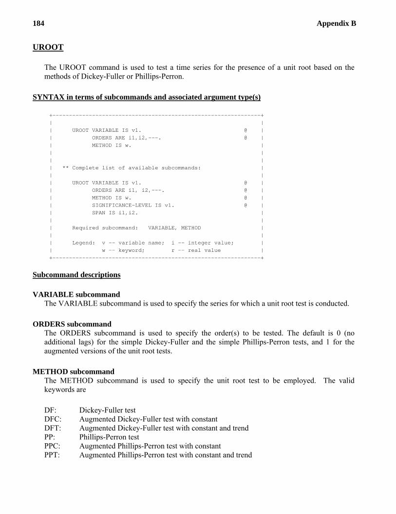
184 Appendix B
UROOT
The UROOT command is used to test a time series for the presence of a unit root based on the methods of Dickey-Fuller or Phillips-Perron.
SYNTAX in terms of subcommands and associated argument type(s)
+---------------------------------------------------------------+ | | | UROOT VARIABLE IS v1. @ | | ORDERS ARE i1,i2,---. @ | | METHOD IS w. | | | | | | ** Complete list of available subcommands: | | | | UROOT VARIABLE IS v1. @ | | ORDERS ARE i1, i2,---. @ | | METHOD IS w. @ | | SIGNIFICANCE-LEVEL IS v1. @ | | SPAN IS i1,i2. | | | | Required subcommand: VARIABLE, METHOD | | | | Legend: v -- variable name; i -- integer value; | | w -- keyword; r -- real value | +---------------------------------------------------------------+
Subcommand descriptions
VARIABLE subcommand The VARIABLE subcommand is used to specify the series for which a unit root test is conducted.
ORDERS subcommand The ORDERS subcommand is used to specify the order(s) to be tested. The default is 0 (no additional lags) for the simple Dickey-Fuller and the simple Phillips-Perron tests, and 1 for the augmented versions of the unit root tests.
METHOD subcommand The METHOD subcommand is used to specify the unit root test to be employed. The valid keywords are
DF: Dickey-Fuller test DFC: Augmented Dickey-Fuller test with constant DFT: Augmented Dickey-Fuller test with constant and trend PP: Phillips-Perron test PPC: Augmented Phillips-Perron test with constant PPT: Augmented Phillips-Perron test with constant and trend

Appendix B 185
SIGNIFICANCE-LEVEL subcommand The SIGNIFICANCE-LEVEL subcommand is used to specify the significance level for the unit root test. The default is set to the 0.05 level. The critical-values for the various tests are interpolated from the tables derived by Dickey and Fuller.
SPAN subcommand The SPAN subcommand is used to specify the span of the series to be considered. The default is all available data.

186 Appendix B
WESTIM
The WESTIM command is used to perform weighted estimation for an ARIMA or transfer function model. The WESTIM command performs model estimation using conditional or exact maximum likelihood estimation. It can also perform joint model estimation with outlier adjustment if specified.
SYNTAX in terms of subcommands and associated argument type(s)
+---------------------------------------------------------------+ | | | WESTIM MODEL model-name. @ | | WEIGHTS IN v. @ | | SPAN IS i1, i2. @ | | HOLD RESIDUALS(v). | | | | ** Complete list of available subcommands: | | | | WESTIM MODEL model-name. @ | | WEIGHTS IN v. @ | | SPAN IS i1, i2. @ | | METHOD IS w. @ | | STOP ARE MAXIT(i), LIKELIHOOD(r1), @ | | ESTIMATE(r2), STDEV(r3). @ | | TYPES ARE w1, w2, - - - . @ | | DELTA IS r. @ | | OSTOP ARE MXOUTLIERS(i1), CRITICAL(r), @ | | MXESTIM(i2). @ | | NEW-SERIES IN v1, v2, v3, v4, v5. @ | | OADJUSTMENT IS w. @ | | STDEV IS w(r). @ | | OUTPUT IS LEVEL(w), PRINT(w1, w2, - - -), @ | | NOPRINT(w1, w2, - - -). @ | | HOLD RESIDUALS(v), FITTED(v), VARIANCE(v). | | | | Required subcommand: MODEL, WEIGHTS | | | | Legend: v -- variable name; i -- integer value; | | w -- keyword; r -- real value | +---------------------------------------------------------------+
Subcommand descriptions
MODEL subcommand The MODEL subcommand is used to specify the label (name) of the model to be estimated. The label must be one specified in a previous TSMODEL command. It is a required subcommand.
WEIGHTS subcommand The WEIGHT subcommand is used to specify a variable containing the weight for each observation in the time series to be used in estimating the univariate time series model. The weights variable must be a vector of length greater than or equal to the number of observations in the time series. A weight typically is specified in the range of 0 to 1, where 0 indicates that an

Appendix B 187
observation is to be completely discounted during estimation, and 1 indicates that the observation is not discounted during estimation.
SPAN subcommand The SPAN subcommand is used to specify the span of time indices, i1 to i2, for which data are analyzed. The default is the maximum span available for the series.
METHOD subcommand The METHOD subcommand is used to specify the method for the computation of the likelihood function used in model estimation. The keyword may be CONDITIONAL for the “conditional” likelihood or EXACT for the “exact” likelihood function. The default is CONDITIONAL.
STOP subcommand The STOP subcommand is used to specify the stopping criterion for the nonlinear estimation of parameters. Estimation is terminated when the relative change in the value of the likelihood function of parameter estimates between two successive iterations is less than or equal to the convergence criterion, or if the maximum number of iterations is reached.
The argument, i, for the keyword MAXIT specifies the maximum number of iterations. The default is i=10.
The argument, r1, for the keyword LIKELIHOOD specifies the value of the relative convergence criterion on the likelihood function. The default is r1 = 0.0001.
The argument, r2, for the keyword ESTIMATE specifies this value of the relative convergence criterion on the parameter estimates. The default is r2 = 0.001.
The argument, r3, for the keyword STDEV specifies the value of the relative convergence criterion on the estimate of the standard deviation in the iteration. This criterion is employed by the SCA System if a constant term is present in the model. The default is r3=0.001 when a constant term is present and the criterion is disabled otherwise. The criterion can be disabled by the user by specifying a negative value for r3. The criterion is enabled if a positive value is specified for r3, even if no constant term is present.
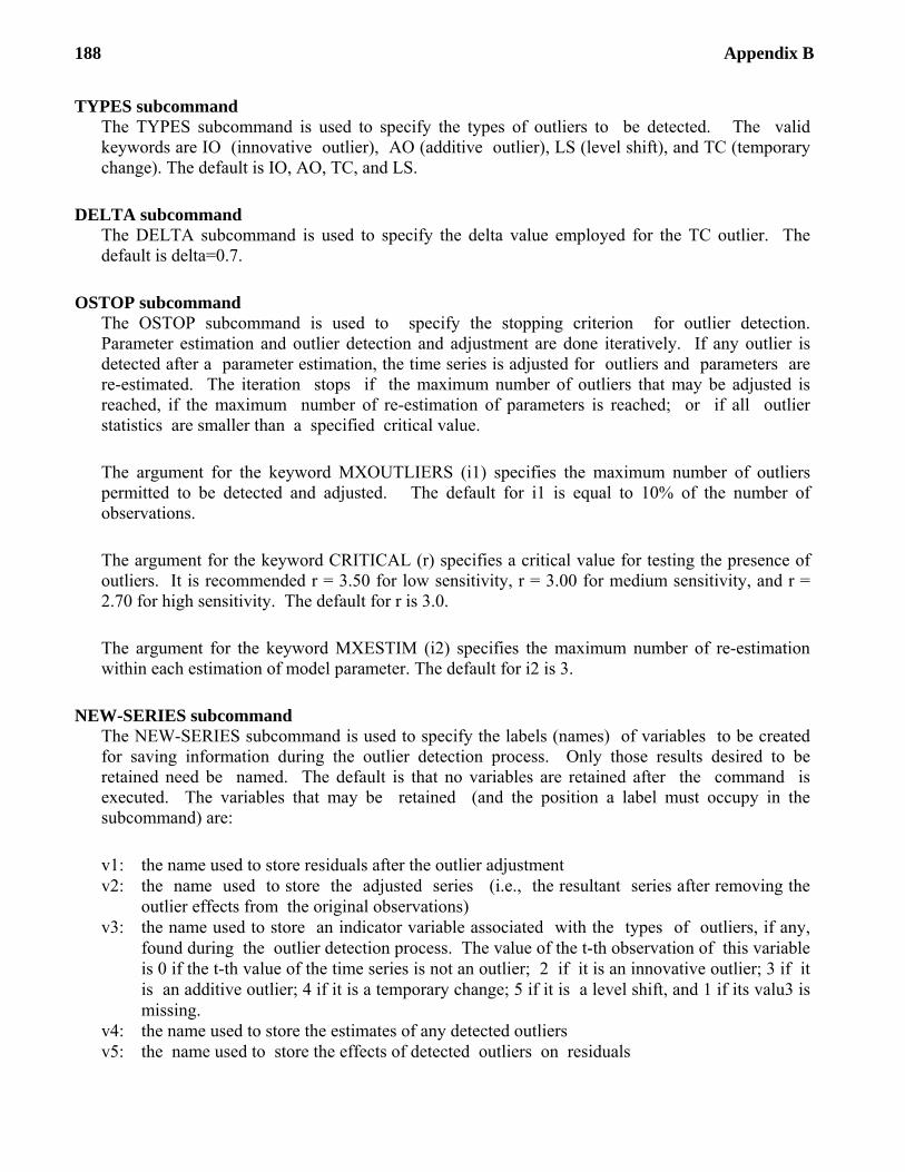
188 Appendix B
TYPES subcommand The TYPES subcommand is used to specify the types of outliers to be detected. The valid keywords are IO (innovative outlier), AO (additive outlier), LS (level shift), and TC (temporary change). The default is IO, AO, TC, and LS.
DELTA subcommand The DELTA subcommand is used to specify the delta value employed for the TC outlier. The default is delta=0.7.
OSTOP subcommand The OSTOP subcommand is used to specify the stopping criterion for outlier detection. Parameter estimation and outlier detection and adjustment are done iteratively. If any outlier is detected after a parameter estimation, the time series is adjusted for outliers and parameters are re-estimated. The iteration stops if the maximum number of outliers that may be adjusted is reached, if the maximum number of re-estimation of parameters is reached; or if all outlier statistics are smaller than a specified critical value.
The argument for the keyword MXOUTLIERS (i1) specifies the maximum number of outliers permitted to be detected and adjusted. The default for i1 is equal to 10% of the number of observations.
The argument for the keyword CRITICAL (r) specifies a critical value for testing the presence of outliers. It is recommended r = 3.50 for low sensitivity, r = 3.00 for medium sensitivity, and r = 2.70 for high sensitivity. The default for r is 3.0.
The argument for the keyword MXESTIM (i2) specifies the maximum number of re-estimation within each estimation of model parameter. The default for i2 is 3.
NEW-SERIES subcommand The NEW-SERIES subcommand is used to specify the labels (names) of variables to be created for saving information during the outlier detection process. Only those results desired to be retained need be named. The default is that no variables are retained after the command is executed. The variables that may be retained (and the position a label must occupy in the subcommand) are:
v1: the name used to store residuals after the outlier adjustment v2: the name used to store the adjusted series (i.e., the resultant series after removing the
outlier effects from the original observations) v3: the name used to store an indicator variable associated with the types of outliers, if any,
found during the outlier detection process. The value of the t-th observation of this variable is 0 if the t-th value of the time series is not an outlier; 2 if it is an innovative outlier; 3 if it is an additive outlier; 4 if it is a temporary change; 5 if it is a level shift, and 1 if its valu3 is missing.
v4: the name used to store the estimates of any detected outliers v5: the name used to store the effects of detected outliers on residuals

Appendix B 189
OADJUSTMENT subcommand The OADJUSTMENT subcommand is used to specify the method of outlier estimation and adjustment. The keyword may be SEQUENTIAL for the sequential method, JOINT for the joint method, and NONE for no outlier detection and adjustment. The default is NONE.
STDEV subcommand The STDEV subcommand is used to specify a method for the estimation of the standard error. TRIM(r) specifies that an r*100% trimmed standard deviation is used (i.e., the top r*100% largest observations, according to absolute values, are excluded from the computation). A specification of TRIM(0.0) indicates that the standard error is computed at each observation (residual) using all data except the current observation. TRIM(0.0) is the default. MAD(r) specifies that the median absolute deviation is used for sigma (i.e., sigma = 1.483*median absolute deviation).
OUTPUT subcommand The OUTPUT subcommand is used to control the amount of output printed for computed statistics. Control is achieved in a two stage procedure. First a basic LEVEL of output is specified. Output may then be increased from this level by use of PRINT, or decreased from this level by use of NOPRINT.
The keywords for LEVEL and output printed are:
BRIEF: estimates and their related statistics only NORMAL: RCORR DETAILED: RCORR, ITERATION, and CORR
where the reserved words on the right denote:
RCORR: the reduced correlation matrix for the parameter estimates ITERATION: the parameter and covariance estimates for each iteration CORR: the correlation matrix for the parameter estimates
These reserved words are also keywords for PRINT and NOPRINT. The default for LEVEL is NORMAL, or the level specified in the PROFILE command.
Note: Reduced correlation matrix refers to the display of the correlation matrix of parameter estimates in which all values have no more than two decimal places with those estimates within two standard errors of zero displayed as dots, "." .
HOLD subcommand The HOLD subcommand is used to specify those values computed for particular functions to be retained in the workspace until the end of the session. Only those statistics desired to be retained need be named. Values are placed in the variable named in parentheses. The default is that none of the values of the statistics below will be retained after the command is used. The values that may be retained are:
RESIDUALS: the residual series without outlier adjustment FITTED: the one step-ahead forecasts (fitted values) of the series VARIANCE: the variance of the noise

190 Appendix B
WFORECAST
The WFORECAST command is used to compute weighted forecasts based on the user specified models. The specified models may include both ARIMA and transfer function models. This command can be used in conjunction with the WESTIM, ESTIM, or other single-equation estimation command in the SCA Statistical System.
SYNTAX in terms of subcommands and associated argument type(s)
+---------------------------------------------------------------+ | | | WFORECAST MODELS ARE model-name1, model-name2, ---. @ | | WEIGHTS ARE v1, v2, ---. | | | | ** Complete list of available subcommands: | | | | WFORECAST MODELS ARE model-name1, model-name2, ---. @ | | WEIGHTS ARE v1, v2, ---. @ | | ORIGIN IS i. @ | | NOFS IS i. @ | | IARIMA ARE v1(model-name), @ | | v2(model-name), --- . @ | | OUTPUT IS PRINT(w1,w2,---), @ | | NOPRINT(w1,w2,---), @ | | HOLD FORECASTS(v), STD_ERRS(v). | | | | Required subcommand: MODEL and WEIGHTS | | | | Legend: v -- variable name; i -- integer value; | | w -- keyword | +---------------------------------------------------------------+
Subcommand descriptions
MODEL subcommand The MODEL subcommand is used to specify the names (labels) of the ARIMA or transfer function models to be used for forecasting. The models must be specified in a previous TSMODEL command.
WEIGHTS subcommand The WEIGHTS subcommand is used to specify the weight variables for the models used for forecasting. The minimum length of the weight variables must be equal to the number of forecasts specified in the NOFS subcommand. The values for the forecast weights are typically between 0 and 1, where 0 receives no weight. The weighted forecasts are computed as the proportional contribution of each forecast based on the given weights. For example, if two forecasting models are used in weighted forecasting and the weights for both models are set to 1 at a particular forecast period, the proportional contribution of forecasts for that period is 1/(1+1) or 50%. This can be more generally stated as weight(i) divided by the sum of all weights for a particular period.

Appendix B 191
ORIGIN subcommand The ORIGIN subcommand is used to specify the time origin for forecasting. The default is the last observation of the series.
NOFS subcommand The NOFS subcommand is used to specify the number of forecasts to be generated. The default is 24 forecasts.
IARIMA subcommand The IARIMA subcommand is used to specify the label associated with the ARIMA model of each stochastic input series. The variable name of each stochastic input series must be entered and in parentheses the name (label) for its ARIMA model.
OUTPUT subcommand The OUTPUT subcommand is used to control the amount of output printed or plotted for computed statistics. Control is achieved by increasing or decreasing the basic level of output by use of PRINT or NOPRINT, respectively. The keyword for PRINT and NOPRINT is:
FORECAST: forecast values for each time origin
The default condition is PRINT(FORECAST).
HOLD subcommand The HOLD subcommand is used to specify those values computed for particular functions to be retained in the workspace until the end of the session. Only those statistics desired to be retained need be named. Values are placed in the variable named in parenthesis. Default is that none of the values of the above statistics will be retained after the command is executed. The values that may be retained are:
FORECASTS: forecasts at the last time origin STD_ERRS: standard errors of the forecasts at the last time origin

192 Appendix B

INDEX
A
AAR, 100, 103, 104, 105, 106, 107, 108, 109, 110, 123, 124,
125, 166, 167, 169, 171, 173, 174
Ansley, 35, 57, 58, 131
Ansley, Spivey, and Wrobleski, 35, 57, 58
arranged Autoregression, 100
Autocorrelation Function
ACF, 18, 19, 21, 22, 23, 24, 25, 26, 27, 28, 34, 134
Automatic ARIMA
IARIMA, 21, 29, 31, 32, 33, 34, 38, 116, 119, 135, 150, 151,
174, 182, 190, 191
B
backshift operator, 98, 107, 173
Barsky and Summers, 48
Bollerslev, 55, 67
Box and Cox, 35, 57, 58
Box and Jenkins, 35, 55, 57, 58
Box‐Cox, 63, 64, 137
C
Canadian real exchange rates, 18
causality, 1, 41, 42, 47, 49, 52, 141, 142
CAUSALTEST, 41, 49, 51, 53, 54, 135, 141
Chen, 3, 41, 42, 49, 51, 54, 97, 101, 102, 105, 106, 111, 114,
116, 121, 131, 132
Chen and Lee, 41, 42, 49, 51, 54
Chickenpox, 101, 102, 121
Cleveland and Tiao, 77, 86
D
Date handling
DAGGREGATE, 5, 11, 12, 13, 137, 143
DATEBUILD, 5, 6, 7, 82, 137, 145
DATEPARTS, 8, 147
DOWEEK, 5, 7, 8, 70, 79, 82, 137, 145, 146, 147
DVECTOR, 5, 9, 10, 70, 137, 148
Davies, 99
day‐of‐week effects, 69, 71, 72, 73, 74, 75, 76, 79, 86
DFORDER, 23, 29, 31, 32, 33, 34, 93, 151, 159
Dickey‐Fuller, 15, 16, 17, 19, 20, 184
Diebold, 17, 131
DSALES, 69, 70, 71, 74, 75, 76, 77, 78, 79, 80, 81, 85
Dudley, 36, 132
E
Edition
Advanced, 1, 4
Educational, 1, 2, 3, 21
Practitioner, 1, 3, 4, 5, 35
Professional, 1, 3, 4, 41, 67, 69, 77, 97
Engle, 55, 67, 153
Engle, Lilien, and Robins, 67
ESTIM, 21, 80, 90, 91, 92, 134, 190
Extended Autocorrelation Function
EACF, 22, 27, 134
F
Feige and Pearce, 42
Fisher, 48
G
GARCH, 1, 2, 4, 55, 67, 133, 136
GENERATE, 11, 88, 138
Gibson paradox, 47, 48, 49
Glosten, Jagannathan, and Runkle, 67
GNP, 21, 32, 38, 121, 122, 124, 125, 127
Granger, 49
Guerrero, 35, 36, 37, 131
H
Hamilton, 17, 131
Haugh, 41, 42
Hillmer and Tiao, 47
Hsiao, 42
I
indicator variable, 79, 80, 81, 160, 188
J
Jolliffe, 98, 131
jump phenomena, 97
K
Kang, 41
Keenan, 99

194
Keynes, 48
Koreisha, 41
Kumar, 98, 131
L
LAG, 107, 126, 138, 173
LAR, 106, 107, 108, 109, 110, 126, 127, 173, 174
Lee and Petruzzi, 48
Lewis, 98, 131
Lim, 97, 132
limit cycles, 97, 132
Liu, 3, 2, 3, 21, 51, 59, 60, 65, 67, 77, 88, 97, 131, 132
local autoregression, 106
M
Maravell, 97
MESTIM, 41, 135
Mills, 16, 132
MTSMODEL, 41, 49, 53, 135
N
Nelson, 48, 67
Nelson and Schwertz, 48
Nerlove, 17, 131
NODFORDER, 23, 29, 32, 33, 34
Nonlinearity tests, 4, 166
non‐normal error distributions, 67
O
OESTIM, 89, 135
P
Pankratz, 35, 36, 132
Partial Autocorrelation Function
PACF, 21, 22, 24, 25, 26, 27, 28, 134
PEAKLOAD, 59, 60, 61, 62, 63
periodic time series, 21, 77, 86, 97
Petruccelli, 99
Phillips‐Perron, 15, 16, 17, 19, 20, 184
PICK, 103, 123, 138
Pierce, 41, 42
Pierce and Haugh, 41
R
RAAR, 101, 105, 107, 124, 166, 167, 169, 171, 173, 174
RECODE, 79, 82, 95, 138
REGIME, 93, 95, 111, 112, 113, 116, 117, 118, 119, 120, 127,
128, 136, 154, 160
residual standard error, 58, 82, 86
residual standard errors, 74, 85, 86, 119, 121, 166
RETRANSFORM, 35, 39, 57, 58, 136, 156, 177
Reverse AAR method, 105, 106, 109, 110, 124
reverse arranged autoregression, 101, 105, 166, 167, 169, 171,
173
RMSE, 58, 59, 60, 61, 62, 63, 64, 156, 176, 177, 178, 179
root mean squared error, 58
S
Sargent, 48
SCA System User Guides, 1
SCAGRAF, 21, 24, 48, 73, 74, 104, 123, 138, 140
Scatter plots, 103
Schwert, 16, 132
Seasonal ARIMA identification
RSFILTER, 21, 22, 23, 25, 26, 29, 31, 32, 33, 34, 38, 134,
135, 158, 159
segmented time series, 1, 4, 55, 56
SETAR, 98
Shiller and Siegel, 48
Sims, 41, 42
SP500, 86, 87, 88
Spivey, and Wrobleski, 35, 57, 58
Stevens, 98
T
TAR, 4, 56, 97, 99, 100, 101, 109, 111, 112, 114, 116, 117, 119,
121, 122, 128, 129, 155, 160, 163, 164, 166, 167
TARESTIM, 56, 77, 97, 99, 112, 113, 114, 117, 118, 119, 120,
128, 136, 160
TAR‐F, 99, 100
TARFORECAST, 56, 77, 97, 114, 115, 116, 136, 163
TARTEST, 56, 77, 97, 99, 100, 102, 103, 105, 122, 123, 124,
136, 166, 167, 174
TARXTEST, 56, 77, 97, 100, 136, 169, 174
Temporal aggregation
DAGGREGATE, 11, 134
THMEXPLORE, 56, 77, 97, 107, 108, 125, 126, 136, 166, 173
THMTEST, 56, 77, 97, 136, 171
threshold, 2, 4, 55, 56, 67, 74, 77, 92, 95, 97, 99, 100, 101, 102,
103, 104, 105, 106, 107, 108, 109, 110, 111, 112, 114, 115,
116, 121, 122, 123, 124, 125, 126, 127, 128, 129, 132, 136,
154, 155, 160, 163, 164, 166, 167, 169, 171, 173, 174, 175
Tiao, 86, 97, 121, 129, 131, 132
Time series model specification

195
TSMODEL, 21, 28, 29, 38, 60, 69, 70, 71, 75, 80, 81, 85, 88,
92, 93, 94, 107, 112, 113, 117, 118, 119, 120, 126, 128,
134, 141, 160, 173, 174, 176, 182, 186, 190
time‐varying parameter, 1, 4
Time‐varying parameter
TVPEXPLORE, 10, 55, 69, 71, 72, 73, 74, 75, 78, 79, 136, 181
Tong, 97, 132
transformation, 2, 3, 4, 35, 36, 38, 39, 49, 55, 57, 58, 59, 60,
61, 63, 64, 101, 136, 156, 157, 176, 177, 178
Transformation
TSEARCH, 35, 36, 57, 58, 59, 60, 61, 63, 136, 176
Tsay, 67, 97, 99, 101, 102, 105, 106, 111, 114, 116, 121, 129,
131
U
Unit root, 2
Unit root test
UROOT, 15, 16, 19, 20, 134, 184
V
value‐segmented, 55, 56, 74, 77, 92, 95, 97
vector ARMA, 4, 35, 41, 47, 49, 52, 141
W
Wang, 98, 132
Wecker, 98, 132
WEIGHT, 80, 81, 85, 88, 90, 93, 94, 112, 113, 115, 116, 117,
118, 119, 120, 128, 129, 134, 163, 177, 178, 186
weighted estimation, 4, 56, 77, 78, 82, 85, 86, 90, 91, 92, 95,
99, 186
WESTIM, 56, 77, 79, 80, 81, 85, 88, 90, 91, 93, 94, 95, 97, 136,
186, 190
WFORECAST, 56, 77, 79, 82, 83, 84, 95, 97, 136, 190
Wicksell, 48
WINDOWSIZE, 71, 72, 75, 108, 126, 173, 174, 181, 182
Z
Zachoian, 67