NEW ALGORITHMS FOR UNCERTAINTY QUANTIFICATION AND ...
201
NEW ALGORITHMS FOR UNCERTAINTY QUANTIFICATION AND NONLINEAR ESTIMATION OF STOCHASTIC DYNAMICAL SYSTEMS A Dissertation by PARIKSHIT DUTTA Submitted to the Office of Graduate Studies of Texas A&M University in partial fulfillment of the requirements for the degree of DOCTOR OF PHILOSOPHY August 2011 Major Subject: Aerospace Engineering
Transcript of NEW ALGORITHMS FOR UNCERTAINTY QUANTIFICATION AND ...

NEW ALGORITHMS FOR UNCERTAINTY QUANTIFICATION AND
NONLINEAR ESTIMATION OF STOCHASTIC DYNAMICAL SYSTEMS
A Dissertation
by
PARIKSHIT DUTTA
Submitted to the Office of Graduate Studies ofTexas A&M University
in partial fulfillment of the requirements for the degree of
DOCTOR OF PHILOSOPHY
August 2011
Major Subject: Aerospace Engineering

NEW ALGORITHMS FOR UNCERTAINTY QUANTIFICATION AND
NONLINEAR ESTIMATION OF STOCHASTIC DYNAMICAL SYSTEMS
A Dissertation
by
PARIKSHIT DUTTA
Submitted to the Office of Graduate Studies ofTexas A&M University
in partial fulfillment of the requirements for the degree of
DOCTOR OF PHILOSOPHY
Approved by:
Chair of Committee, Raktim BhattacharyaCommittee Members, Suman Chakravorty
John L. JunkinsAniruddha Datta
Head of Department, Dimitris C. Lagoudas
August 2011
Major Subject: Aerospace Engineering

iii
ABSTRACT
New Algorithms for Uncertainty Quantification and Nonlinear Estimation of
Stochastic Dynamical Systems. (August 2011)
Parikshit Dutta, B.Tech.; M.Tech., Indian Institute of Technology, Kharagpur
Chair of Advisory Committee: Dr. Raktim Bhattacharya
Recently there has been growing interest to characterize and reduce uncertainty in
stochastic dynamical systems. This drive arises out of need to manage uncertainty
in complex, high dimensional physical systems. Traditional techniques of uncertainty
quantification (UQ) use local linearization of dynamics and assumes Gaussian prob-
ability evolution. But several difficulties arise when these UQ models are applied to
real world problems, which, generally are nonlinear in nature. Hence, to improve per-
formance, robust algorithms, which can work efficiently in a nonlinear non-Gaussian
setting are desired.
The main focus of this dissertation is to develop UQ algorithms for nonlinear
systems, where uncertainty evolves in a non-Gaussian manner. The algorithms devel-
oped are then applied to state estimation of real-world systems. The first part of the
dissertation focuses on using polynomial chaos (PC) for uncertainty propagation, and
then achieving the estimation task by the use of higher order moment updates and
Bayes rule. The second part mainly deals with Frobenius-Perron (FP) operator the-
ory, how it can be used to propagate uncertainty in dynamical systems, and then using
it to estimate states by the use of Bayesian update. Finally, a method to represent the
process noise in a stochastic dynamical system using a finite term Karhunen-Loeve
(KL) expansion is proposed. The uncertainty in the resulting approximated system
is propagated using FP operator.

iv
The performance of the PC based estimation algorithms were compared with
extended Kalman filter (EKF) and unscented Kalman filter (UKF), and the FP oper-
ator based techniques were compared with particle filters, when applied to a duffing
oscillator system and hypersonic reentry of a vehicle in the atmosphere of Mars. It
was found that the accuracy of the PC based estimators is higher than EKF or UKF
and the FP operator based estimators were computationally superior to the particle
filtering algorithms.

v
To my family and my friends

vi
ACKNOWLEDGMENTS
I would like to give special thanks to Dr. Raktim Bhattacharya who has been a
mentor and a friend. His creativity and drive have been essential to the completion of
this work. Secondly, I would like to thank Dr. Suman Chakravorty for his guidance
during my time as graduate student and clarifying several important concepts. I
would also like to thank Dr. John L. Junkins for inspiring me, and helping me build
the fundamental understanding of estimation theory.
My appreciation also goes to all my friends who have been very supportive and
have helped me to maintain my sanity while completing this work. I would especially
like to thank Abhishek, Baljeet, Avinash and Ramesh with whom I have worked and
shared several good times at the CISAR laboratory. Their support and inspiration
were of immense help towards completion of my work. I would also like to thank
several other friends for always being there to share both laughter and hardship.
Last, but not the least I would like to thank my family especially my parents for
everything they have done for me, and my uncle who helped me develop my interest
in science.

vii
TABLE OF CONTENTS
CHAPTER Page
I INTRODUCTION . . . . . . . . . . . . . . . . . . . . . . . . . . 1
A. Background . . . . . . . . . . . . . . . . . . . . . . . . . . 1
B. Contribution of This Dissertation . . . . . . . . . . . . . . 7
II SEQUENTIAL STATE ESTIMATION METHODS . . . . . . . 9
A. Sequential State Estimation for Linear Systems . . . . . . 10
1. Kalman Filter . . . . . . . . . . . . . . . . . . . . . . 11
2. Linear Non-Gaussian Filter . . . . . . . . . . . . . . . 12
B. Sequential State Estimation for Nonlinear Systems . . . . . 14
1. Extended Kalman Filter . . . . . . . . . . . . . . . . . 15
2. Unscented Kalman Filter . . . . . . . . . . . . . . . . 16
3. Particle Filters . . . . . . . . . . . . . . . . . . . . . . 20
a. Step 1: Initialization of the Filter . . . . . . . . . 21
b. Step 2: Propagation . . . . . . . . . . . . . . . . 21
c. Step 3: Update . . . . . . . . . . . . . . . . . . . 22
d. Step 4: State Estimate . . . . . . . . . . . . . . . 22
e. Resampling . . . . . . . . . . . . . . . . . . . . . 23
4. Other Sequential Monte Carlo Methods . . . . . . . . 24
C. A Simple Example . . . . . . . . . . . . . . . . . . . . . . 25
D. Summary of the Chapter . . . . . . . . . . . . . . . . . . . 27
III POLYNOMIAL CHAOS . . . . . . . . . . . . . . . . . . . . . . 31
A. Generalized Polynomial Chaos Theory . . . . . . . . . . . 31
1. Wiener-Askey Orthogonal Polynomials . . . . . . . . . 32
B. Approximation of the Solution of Ordinary Differential
Equations with Uncertainty . . . . . . . . . . . . . . . . . 34
1. Getting the Moments of the States . . . . . . . . . . . 35
2. A Simple Example . . . . . . . . . . . . . . . . . . . . 37
C. Nonlinear State Estimation Using Polynomial Chaos
and Higher Order Moments Update . . . . . . . . . . . . . 39
1. Step 1: Initialization of State . . . . . . . . . . . . . . 40
2. Step 2: Propagation of Uncertainty and Computa-
tion of Prior Moments . . . . . . . . . . . . . . . . . . 40

viii
CHAPTER Page
3. Step 3: Update Phase . . . . . . . . . . . . . . . . . . 41
4. Step 4: Estimation of Posterior Probability Distribution 44
5. Step 5: Generation of Basis Functions . . . . . . . . . 48
D. Nonlinear Estimation Using Polynomial Chaos and Up-
date Using Bayesian Inference . . . . . . . . . . . . . . . . 48
1. Step 1: Initialization of State and Propagation of
Uncertainty . . . . . . . . . . . . . . . . . . . . . . . . 49
2. Step 2: Calculating the Posterior Probability Den-
sity Function . . . . . . . . . . . . . . . . . . . . . . . 49
3. Step 3: Getting the State Estimate . . . . . . . . . . . 50
4. Step 4: Regeneration of Basis Functions . . . . . . . . 51
E. Application to Duffing Oscillator . . . . . . . . . . . . . . 51
1. Results for Estimation with Higher Order Moments
Update . . . . . . . . . . . . . . . . . . . . . . . . . . 51
2. Results for Estimation Using Bayesian Inference . . . 56
F. Application to Hypersonic Reentry . . . . . . . . . . . . . 56
G. Limitations of Polynomial Chaos . . . . . . . . . . . . . . 74
IV THE FROBENIUS-PERRON OPERATOR . . . . . . . . . . . . 76
A. Analysis of Densities in State Space Using Frobenius-
Perron Operator . . . . . . . . . . . . . . . . . . . . . . . . 76
1. Discrete-Time Systems . . . . . . . . . . . . . . . . . 76
2. Continuous-Time Systems . . . . . . . . . . . . . . . . 79
3. Properties of Frobenius-Perron Operator . . . . . . . . 81
B. Method of Characteristics for Solving First Order Lin-
ear Partial Differential Equations . . . . . . . . . . . . . . 81
C. Uncertainty Propagation in Dynamical Systems Using
FP Operator . . . . . . . . . . . . . . . . . . . . . . . . . . 82
1. Accuracy in Prediction of Uncertainty . . . . . . . . . 85
D. Nonlinear Estimation Using Frobenius-Perron Operator . . 88
1. Step 1: Initialization Step . . . . . . . . . . . . . . . . 88
2. Step 2: Propagation Step . . . . . . . . . . . . . . . . 88
3. Step 3: Update Step . . . . . . . . . . . . . . . . . . . 89
4. Step 4: Getting the State Estimate . . . . . . . . . . . 89
5. Step 5: Resampling . . . . . . . . . . . . . . . . . . . 90
E. Application of Nonlinear Estimation Using FP Operator . 90
1. Application to a Duffing Oscillator System . . . . . . 91
2. Application to Three State Vinh’s Equation . . . . . . 94
ix
CHAPTER Page
a. Sensitivity Analysis . . . . . . . . . . . . . . . . . 104
3. Application to Six-State Vinh’s Equation . . . . . . . 108
F. Limitations of Using Frobenius-Perron Operator . . . . . . 110
V THE KARHUNEN LOEVE EXPANSION . . . . . . . . . . . . 116
A. Stochastic Dynamical Systems . . . . . . . . . . . . . . . . 116
1. Solution Methodology . . . . . . . . . . . . . . . . . . 117
2. Uncertainty Propagation in Stochastic Dynamical
Systems . . . . . . . . . . . . . . . . . . . . . . . . . . 119
B. The Karhunen Loeve Expansion Applied to Stochastic
Dynamical Systems . . . . . . . . . . . . . . . . . . . . . . 120
1. KL Expansion of Wiener Process . . . . . . . . . . . . 121
2. KL Expansion Applied to Langevin Equation . . . . . 122
C. Convergence of Solutions . . . . . . . . . . . . . . . . . . . 123
1. Verification of Convergence in Distribution . . . . . . 123
2. Convergence in Mean Square Sense . . . . . . . . . . . 132
D. Karhunen Loeve Frobenius-Perron Formulation . . . . . . . 138
1. Illustrative Examples . . . . . . . . . . . . . . . . . . 139
E. State Estimation Using Karhunen Loeve Expansion and
Frobenius-Perron Operator . . . . . . . . . . . . . . . . . . 140
1. State Estimation of Vanderpol’s Oscillator . . . . . . . 140
2. Application to Hypersonic Reentry . . . . . . . . . . . 142
F. Summary . . . . . . . . . . . . . . . . . . . . . . . . . . . 149
VI CONCLUSIONS AND SCOPE OF FUTURE WORK . . . . . . 150
A. Future Work . . . . . . . . . . . . . . . . . . . . . . . . . . 151
1. Stochastic Control . . . . . . . . . . . . . . . . . . . . 151
2. Multiphysical Dynamical Systems . . . . . . . . . . . 152
3. Dimensional Scaling . . . . . . . . . . . . . . . . . . . 152
REFERENCES . . . . . . . . . . . . . . . . . . . . . . . . . . . . . . . . . . . 154
APPENDIX A . . . . . . . . . . . . . . . . . . . . . . . . . . . . . . . . . . . 171
APPENDIX B . . . . . . . . . . . . . . . . . . . . . . . . . . . . . . . . . . . 177
APPENDIX C . . . . . . . . . . . . . . . . . . . . . . . . . . . . . . . . . . . 182
VITA . . . . . . . . . . . . . . . . . . . . . . . . . . . . . . . . . . . . . . . . 184
x
LIST OF TABLES
TABLE Page
I Algorithm for linear non-Gaussian filtering . . . . . . . . . . . . . . . 14
II Correspondence between choice of polynomials and given distri-
bution of ∆ (Xiu and Karniadakis, 2002) . . . . . . . . . . . . . . . 33
III Explanation and values of the constants for Martian atmosphere
(Sengupta and Bhattacharya, 2008) . . . . . . . . . . . . . . . . . . . 59
IV Scaling constants for base units . . . . . . . . . . . . . . . . . . . . . 60
V Normalization factors for measurements . . . . . . . . . . . . . . . . 61
VI Computational time taken per filtering step for each estimation
algorithm. Listed times are in seconds . . . . . . . . . . . . . . . . . 100
VII Normalization factors used for measurements . . . . . . . . . . . . . 109
VIII Normalization factors used for measurements (six state Vinh’s
equation with noise) . . . . . . . . . . . . . . . . . . . . . . . . . . . 145
IX The first ten Hermite polynomials . . . . . . . . . . . . . . . . . . . 172

xi
LIST OF FIGURES
FIGURE Page
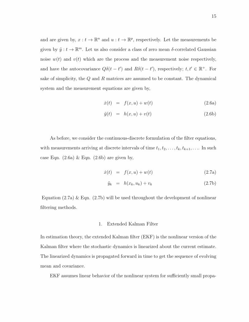
1 Plot of estimation errors and ±3σ limits for a) EKF b) UKF c)
particle filter for the system in Eqn. (2.27a) & Eqn. (2.27b). The
solid lines are estimation errors and the dashed lines are ±3σ limits. 26
2 Plot of estimation errors and ±3σ limits for a) EKF b) UKF c)
particle filter for the system in Eqn. (2.27a) & Eqn. (2.27b). The
measurement update interval is 0.3s. The solid lines are estima-
tion errors and the dashed lines are ±3σ limits. . . . . . . . . . . . 28
3 Plot of square root of difference between evolving variance of each
state and CRLB. The solid line is EKF the starred line is UKF
and the dashed line is particle filter. . . . . . . . . . . . . . . . . . . 29
4 Plots for a) mean b) variance of the Duffing oscillator in Eqn.
(3.10) & Eqn. (3.11) obtained from gPC scheme (solid) and Monte
Carlo (dashed) and linearized dynamics (star-solid) simulations. . . 39
5 Flowchart of polynomial chaos based estimation algorithms. . . . . . 52
6 Evolution initial condition uncertainty for Duffing oscillator. Prob-
ability density functions were obtained using high fidelity Monte
Carlo simulations. . . . . . . . . . . . . . . . . . . . . . . . . . . . . 53
7 Performance of EKF estimators. Dashed lines represent ±3σ lim-
its and the solid line represents error in estimation. . . . . . . . . . . 54
8 Performance of gPC estimators. Dashed lines represent ±3σ lim-
its and the solid line represents error in estimation. . . . . . . . . . . 55
9 Plots for time (x-axis) vs. ±3σ limits (dashed lines) and estima-
tion error (solid lines) (y-axis) for gPC based estimators and EKF
based estimator. . . . . . . . . . . . . . . . . . . . . . . . . . . . . . 57

xii
FIGURE Page
10 (a) Mean and (b) standard deviation of the true system (solid) and
the approximated system (dashed) obtained from Monte Carlo
simulations. . . . . . . . . . . . . . . . . . . . . . . . . . . . . . . . . 63
11 Percentage error in states of the approximated system from true system. 64
12 Performance of (a) EKF and (b) UKF based estimator with true
initial states as [Rm + 61 km 2.42 km/s − 8.91o]T and update
interval of 20s. The dashed lines represent ±3σ limits and the
solid line represents error in estimation. . . . . . . . . . . . . . . . . 66
13 Performance of the gPC based estimator with true initial states
as [Rm + 61 km 2.42 km/s − 8.91o]T and update interval of 20s.
The dashed lines represent ±3σ limits and the solid line represents
error in estimation. . . . . . . . . . . . . . . . . . . . . . . . . . . . . 67
14 Performance of (a) EKF and (b) UKF based estimator with true
initial states as [Rm + 61 km 2.42 km/s − 8.91o]T and update
interval of 40s.The dashed lines represent ±3σ limits and the solid
line represents error in estimation. . . . . . . . . . . . . . . . . . . . 68
15 Performance of the gPC based estimator with true initial states
as [Rm + 61 km 2.42 km/s − 8.91o]T and update interval of 40s.
The dashed lines represent ±3σ limits and the solid line represents
error in estimation. . . . . . . . . . . . . . . . . . . . . . . . . . . . . 69
16 Performance of (a) EKF and (b) UKF based estimator with true
initial states as [Rm + 61 km 2.64 km/s − 8.1o]T and update in-
terval of 20s. The dashed lines represent ±3σ limits and the solid
line represents error in estimation. . . . . . . . . . . . . . . . . . . . 71
17 Performance of the gPC based estimator with true initial states
as [Rm + 61 km 2.64 km/s − 8.1o]T and update interval of 20s.
The dashed lines represent ±3σ limits and the solid line represents
error in estimation. . . . . . . . . . . . . . . . . . . . . . . . . . . . . 72
18 Performance of (a) MCE, (b) MLE and (c) MEE criterion for state
estimates. The true initial states are [Rm + 61 km 2.42 km/s −8.91o]T and update interval is 20s. The dashed lines represent
±3σ limits and the solid line represents error in estimation. . . . . . 73

xiii
FIGURE Page
19 Long term statistics, up to 10 seconds predicted by Monte Carlo
(dashed line) and polynomial chaos (solid line) for the system in
Eqn. (3.10) & Eqn. (3.11). The x-axis represents time and y-axes
are the states. . . . . . . . . . . . . . . . . . . . . . . . . . . . . . . . 75
20 Method of characteristics. Number of samples = 500. System is
Duffing oscillator. The black circle shows the location and the
PDF value (color coded) of an arbitrary sample point at different
time instances. . . . . . . . . . . . . . . . . . . . . . . . . . . . . . . 84
21 Comparison of FP and Monte Carlo based approximation of den-
sity functions. . . . . . . . . . . . . . . . . . . . . . . . . . . . . . . . 86
22 Performance of the estimators with measurement update interval
as 0.3s. . . . . . . . . . . . . . . . . . . . . . . . . . . . . . . . . . . 92
23 Performance of the estimators with measurement update rate as 0.6s. 93
24 Generic particle filter. True initial states are [Rm+61 km 2.64 km/s−8.1o]T and update interval is 20s. The dashed lines represent ±3σ
limits and the solid line represents error in estimation. . . . . . . . . 95
25 Bootstrap filter. True initial states are [Rm + 61 km 2.64 km/s −8.1o]T and update interval is 20s. The dashed lines represent ±3σ
limits and the solid line represents error in estimation. . . . . . . . . 95
26 Performance of the Frobenius-Perron estimator with true initial
states as [Rm + 61 km 2.64 km/s − 8.1o]T and update interval
of 20s. The dashed lines represent ±3σ limits and the solid line
represents error in estimation. . . . . . . . . . . . . . . . . . . . . . 96
27 Plots for√σ2 − CRLB vs. time. In the legend, ’BPF’, ’gPF’
and ’FP’, represent bootstrap filter, generic particle filter and
Frobenius-Perron operator based estimator respectively. . . . . . . . 96
28 Generic particle filter with 7000 particles. True initial states are
[Rm + 61 km 2.64 km/s − 8.1o]T and update interval is 20s. The
dashed lines represent ±3σ limits and the solid line represents
error in estimation. . . . . . . . . . . . . . . . . . . . . . . . . . . . . 97

xiv
FIGURE Page
29 Bootstrap filter with 7000 particles. True initial states are [Rm +
61 km 2.64 km/s −8.1o]T and update interval is 20s. The dashed
lines represent ±3σ limits and the solid line represents error in
estimation. . . . . . . . . . . . . . . . . . . . . . . . . . . . . . . . . 97
30 Generic particle filter with 10000 particles. True initial states are
[Rm + 61 km 2.64 km/s − 8.1o]T and update interval is 20s. The
dashed lines represent ±3σ limits and the solid line represents
error in estimation. . . . . . . . . . . . . . . . . . . . . . . . . . . . . 99
31 Bootstrap filter with 10000 particles. True initial states are [Rm+
61 km 2.64 km/s −8.1o]T and update interval is 20s. The dashed
lines represent ±3σ limits and the solid line represents error in
estimation. . . . . . . . . . . . . . . . . . . . . . . . . . . . . . . . . 99
32 Percentage error in estimation with 7000 particles. True initial
states are [Rm + 61 km 2.64 km/s − 8.1o]T and update interval
is 20s. In the legend, ’BF’, ’gPF’ and ’FP’, represent bootstrap
filter, generic particle filter and Frobenius-Perron operator based
estimator respectively. . . . . . . . . . . . . . . . . . . . . . . . . . . 100
33 Percentage error in estimation with number of particles for FP
based operator (FP), generic particle filter (gPF) and bootstrap
filter (BF), 7000, 20000, and 25000 respectively. True initial states
are [Rm + 61 km 2.64 km/s − 8.1o]T and update interval is 20s. . . 101
34 Plots for 3rd and 4th order moments for particle filter with 100,000
particles- (dashed line) and FP operator based filter with 7000
samples- (solid line). . . . . . . . . . . . . . . . . . . . . . . . . . . . 102
35 Plots for percentage error in 3rd and 4th order moments for boot-
strap filter (BF), generic particle filter (gPF) and FP operator
based filter (FP), all with 7000 particles. Percentage deviation
taken from particle filter with 100,000 particles. . . . . . . . . . . . . 103
36 FP operator based filter with measurement noise 6 × 10⁻⁴I3 in
scaled units (number of samples = 7000). True initial states are
[Rm+61 km 2.64 km/s −8.1o]T . The dashed lines represent ±3σ
limits and the solid line represents error in estimation. . . . . . . . . 105

xv
FIGURE Page
37 FP operator based filter measurement update interval is 40s (num-
ber of samples = 7000). True initial states are [Rm+61 km 2.64 km/s−8.1o]T . The dashed lines represent ±3σ limits and the solid line
represents error in estimation. . . . . . . . . . . . . . . . . . . . . . . 105
38 Generic particle filter with measurement noise 6×10⁻⁴I3 in scaled
units (number of samples = 25000) True initial states are [Rm +
61 km 2.64 km/s −8.1o]T . The dashed lines represent ±3σ limits
and the solid line represents error in estimation. . . . . . . . . . . . . 106
39 Generic particle filter measurement update interval is 40s (number
of samples = 25000). True initial states are [Rm+61 km 2.64 km/s−8.1o]T . The dashed lines represent ±3σ limits and the solid line
represents error in estimation. . . . . . . . . . . . . . . . . . . . . . . 106
40 Bootstrap filter with measurement noise 6 × 10⁻⁴I3 in scaled
units (number of samples = 20000) True initial states are [Rm +
61 km 2.64 km/s −8.1o]T . The dashed lines represent ±3σ limits
and the solid line represents error in estimation. . . . . . . . . . . . . 107
41 Bootstrap filter measurement update interval is 40s (number of
samples = 20000). True initial states are [Rm+61 km 2.64 km/s −8.1o]T . The dashed lines represent ±3σ limits and the solid line
represents error in estimation. . . . . . . . . . . . . . . . . . . . . . . 107
42 Performance of FP operator based filter with 9000 particles, when
applied to six state Vinh’s equation. The dashed lines represent
±3σ limits and the solid line represents error in estimation. . . . . . 111
43 Performance of generic particle filter with 9000 particles, when
applied to six state Vinh’s equation. The dashed lines represent
±3σ limits and the solid line represents error in estimation. . . . . . 112
44 Performance of the bootstrap filter with 9000 particles, when ap-
plied to six state Vinh’s equation. The dashed lines represent ±3σ
limits and the solid line represents error in estimation. . . . . . . . . 113
45 Performance of generic particle filter with 30000 particles, when
applied to six state Vinh’s equation. The dashed lines represent
±3σ limits and the solid line represents error in estimation. . . . . . 114

xvi
FIGURE Page
46 Performance of the bootstrap filter with 25000 particles, when
applied to six state Vinh’s equation. The dashed lines represent
±3σ limits and the solid line represents error in estimation. . . . . . 115
47 Scatter plot of initial and the back-propagated elements for a given
sample. Blue circles are the original sample and the red ones are
the back-propagated sample. . . . . . . . . . . . . . . . . . . . . . . 128
48 Plot of empirical CDF of yj0 and uniform CDF for a given sample. . . 129
49 Plot DM value for all the 100 samples. The samples above the
red and black lines fail when α = 0.05 and 0.01 respectively. . . . . . 129
50 Plot DM value for all the 100 samples for a. N = 76 and b.
N = 91. The samples above the red and black lines fail when
α = 0.05 and 0.01 respectively. . . . . . . . . . . . . . . . . . . . . . 130
51 Plot DM value for all the 100 samples for a. N = 21 and b.
N = 76, with increased M = 1000. The samples above the red
line fails when α = 0.05. . . . . . . . . . . . . . . . . . . . . . . . . . 131
52 Plot of empirical CDF of√MDM (red) and Kolmogorov CDF
(blue). . . . . . . . . . . . . . . . . . . . . . . . . . . . . . . . . . . 131
53 Plot of supx∈R|FMs(x)− FK(x)| vs. Ms . . . . . . . . . . . . . . . . . . 132
54 Uncertainty propagation for Vanderpol’s oscillator Eqn. (5.40)
in top row of each figure, and Duffing oscillator Eqn. (5.41) in
bottom row of each figure. . . . . . . . . . . . . . . . . . . . . . . . . 141
55 ±3σ plots for a) KLFP-based estimator and b) Generic particle
filter. . . . . . . . . . . . . . . . . . . . . . . . . . . . . . . . . . . . 143
56 Estimation errors (solid lines) and ±3σ limits (dashed lines) for
particle filter based estimator. . . . . . . . . . . . . . . . . . . . . . . 146
57 Estimation errors (solid lines) and ±3σ limits (dashed lines) for
estimator using KL expansion and FP operator. . . . . . . . . . . . . 147

xvii
FIGURE Page
58 Plot for univariate marginal density for particle filter (dashed line)
and KL expansion and FP operator based estimator (solid line).
Here h = r −Rm and the y-axis denotes PDF value. . . . . . . . . . 148
59 Plot for bivariate marginal density for particle filter (top row) and
KL expansion and FP operator based estimator (bottom row) for
4 state combinations. Here h = r − Rm. The PDF value is color
coded, red is high PDF and blue is low. . . . . . . . . . . . . . . . . 149
60 Locations of eigenvalues of the system in Eqn. (A.1), when Monte
Carlo approximation is used (red circles) and when PC approxi-
mated dynamics in Eqn. (A.3) is used (blue). . . . . . . . . . . . . . 175
61 PDF of the eigenvalue distribution on the complex plane. Blue
represents low probability regions and red is high probability re-
gion. Eigenvalues represented in black. . . . . . . . . . . . . . . . . . 176
62 Plots for estimation error and ±3σ limits for a) Kalman filter b)
FP operator based estimator c) particle filter. . . . . . . . . . . . . 179
63 Normalized Wasserstein distance between posterior PDFs of Kalman
filter and FP operator based estimator (solid line) and Kalman
filter and particle filter (dashed line). The value of R = 1/2. . . . . . 180
64 Normalized Wasserstein distance between posterior PDFs of Kalman
filter and FP operator based estimator (solid line) and Kalman
filter and particle filter (dashed line). The value of R = 2. . . . . . . 181
65 Normalized Wasserstein distance between posterior PDFs of Kalman
filter and FP operator based estimator (solid line) and Kalman
filter and particle filter (dashed line). The value of R = 4. . . . . . . 181

1
CHAPTER I
INTRODUCTION
A. Background
Uncertainty quantification in stochastic dynamical systems is a challenging field that
has received attention for over a century. Understanding the impact of uncertainty
in complex physical system has become a primary topic of research over the years.
Problems due to uncertainty may arise in myriad areas of application ranging from
robotics (e.g. path planning in an uncertain environment) and astrodynamics (eg.
trajectory estimation of 99942 Aphophis) to structural engineering (e.g. excitation of
a building caused by siesmic events) and petroleum engineering (eg. study of flow of
oil through a reservoir with uncertain porosity). A large class of such problems deal
with uncertainty in physical model and system parameters. Estimation of parame-
ters in this scenario is typically a hard problem due to lack of frequent measurements
and underlying nonlinearities in system dynamics. Thus the evolution of uncertainty,
which can be non Gaussian, needs to be predicted over longer intervals of time. These
issues undermine the validity of the classical linear Gaussian theory. Sequential es-
timation algorithms, based on Monte Carlo (MC) simulations are most commonly
used in such cases. However for systems having three or more dimensions, MC based
techniques may be computationally expensive as ensemble size required to guarantee
convergence, increases exponentially with number of states. Hence a nonlinear esti-
mation algorithm, superior to the existing methods in terms of convergence of errors
and computational complexity is desired.
Estimation of states and parameters for dynamical systems in general, are gen-
The journal model is IEEE Transactions on Automatic Control.

2
erally performed in the Bayesian framework, where uncertainty is represented as
probability density functions (PDF). For linear Gaussian systems, it is possible to get
exact analytical expressions for evolving sequence of moments, which characterizes
the PDF completely. This method is widely know as Kalman filter [1]. For nonlinear
systems exhibiting Gaussian behavior, the system is linearized locally, about the cur-
rent mean, and the covariance is propagated using the approximated linear dynamics.
This method is used in extended Kalman filters (EKF) [2]. It is well known that this
approach performs poorly when the nonlinearities are high, resulting in an unstable
estimator [3, 4, 5, 6]. However, the error in mean and covariance can be reduced if the
uncertainty is propagated, using the nonlinear dynamics, for a minimal set of sample
points, called sigma points. The PDF of the states, characterized by sigma points,
capture the posterior mean and covariance accurately to the third order (Taylor series
expansion) for any nonlinearity with Gaussian behavior. This technique has resulted
in the unscented Kalman filter (UKF) [7]. The aforementioned filters are based on
the premise of Gaussian PDF evolution. If the sensor updates are frequent then EKF
and UKF may yield satisfactory results. However, for nonlinear systems, if the sensor
updates are slow, these filters result in inaccurate estimates [8].
Recently, simulation-based sequential filtering methods, using Monte Carlo sim-
ulations, have been developed to tackle nonlinear system with non-Gaussian uncer-
tainty [9, 10]. Monte Carlo methods involve representing the PDF of the states using
a finite number of samples. The filtering task is obtained by recursively generat-
ing properly weighted samples of the state variable using importance sampling [11].
These filters, based on sequential MC methods are known as Monte Carlo filters [12].
Amongst them, the most widely used is the particle filter [13, 14, 15, 16]. Here en-
semble members or particles are propagated using the nonlinear system dynamics.
These particles with proper weights, determined from the measurements, are used

3
to obtain the state estimate. However, particle filters require a large number of en-
sembles for convergence, leading to higher computational costs [17]. This problem is
tackled through resampling [13, 18, 8]. Particle filters with resampling technique are
commonly known as bootstrap filters [8]. It has been observed that bootstrap filters
introduce other problems like loss of diversity amongst particles [15], if the resampling
is not performed correctly. Recently developed techniques have combined importance
sampling and Markov-Chain-Monte Carlo (MCMC) methods to generate samples to
get better estimates of states and parameters [19]. Several other methods, like reg-
ularized particle filter [20], and filters involving MCMC move step [21], have been
developed to improve sample diversity. At the same time, even with resampling, due
to the simulation based nature of these filters, the ensemble size scales exponentially
with state dimension for large problems [22]. To circumvent this problem, particle
filters based on Rao-Blackwellization have been developed to partially solve the esti-
mation problem analytically [23]. However, its application is limited to systems where
the required partition of the state space is possible. An excellent comparison of the
various nonlinear filtering algorithms is available in ref. [24].
Nonlinear estimation algorithms based on polynomial chaos theory [25] and
Frobenius-Perron operator [26] has been proposed in this work. Polynomial chaos
(PC) is used to approximate any random process as linear combination of orthog-
onal basis functions. The advantage of using PC is that an alternate deterministic
dynamical system can be created from the stochastic system, which is then used to
propagate uncertainty. Polynomial chaos was first introduced by Wiener [27] where
Hermite polynomials were used to model stochastic processes with Gaussian random
variables. According to Cameron and Martin [28], such an expansion converges in the
L2 sense for any arbitrary stochastic process with finite second moment. This applies
to most physical systems. Xiu et al. [29] generalized the result of Cameron-Martin

4
to various continuous and discrete distributions using orthogonal polynomials from
the so-called Askey-scheme [30] and demonstrated L2 convergence in the correspond-
ing Hilbert functional space. This is popularly known as the generalized polynomial
chaos (gPC) framework. The gPC framework has been applied to various applications
including stochastic fluid dynamics [31, 32], stochastic finite elements [25], and solid
mechanics [33, 34]. In the context of nonlinear estimation, polynomial chaos has been
applied by Blanchard et al. [35, 36], where uncertainty prediction was computed us-
ing gPC theory for nonlinear dynamical systems, and estimation was performed using
linear output equations and classical Kalman filtering theory. It has been shown that
PC is computationally more efficient than Monte Carlo simulations [29]. Hence, it is
expected that, the estimation algorithm presented here will be computationally more
efficient than particle filters. However, such an analysis has not been performed, and
is a subject of our future work. Here we have applied gPC theory to estimate states
of a Duffing oscillator and hypersonic vehicle reentering Mars’ atmosphere.
The Frobenius-Perron operator determines the time evolution of probability den-
sity function (PDF) through a system, and as shown later is computationally efficient
than particle filters. The Frobenius-Perron operator has been used in the physics
community to study evolution of uncertainty in dynamical systems [26]. In contin-
uous time, the Frobenius-Perron operator is defined by the Liouville equation [37],
which is the Fokker-Planck equation [38] without the diffusion term. It has been
shown that the Frobenius-Perron operator or the Liouville equation, predicts evolu-
tion of uncertainty in a more computationally efficient manner than Monte Carlo [39].
Based on this fact, we can expect a nonlinear filtering algorithm in this framework
to be computationally more efficient than particle filters. However, it is important to
note that the Frobenius-Perron operator only addresses parametric uncertainty. Use
of Liouville equation to develop a nonlinear filtering algorithm was first presented

5
by Daum et al. [40], where the process of the filtering algorithm has been outlined.
In this work we have applied Frobenius-Perron operator theory to a state estimation
problem arising in hypersonic flights and perform a direct comparison with particle
filters.
The above mentioned uncertainty propagation methods are applicable only when
the dynamical system has initial state or parametric uncertainty. In presence of
process noise, the evolution of densities are given by the Kramers-Moyal expansion
[41]. This is a partial differential equation which characterize PDF propagation in any
nonlinear system having process noise. A special case arises when we limit ourselves
to additive Gaussian white noise as stochastic forcing. Then, the first two terms of
the Kramers-Moyal expansion is sufficient to describe the evolving densities. This
is referred to as the Fokker-Planck equation or Kolmogorov forward equation [42].
There are several methods, by which we can approximately determine the solution
of the Fokker-Plank equation. A brief treatise of the most popular methods can
be found in the book by Riskin [38]. Several methods which deal with numerical
solutions of the Fokker-Planck equation have been developed over the years [43, 44,
45]. The numerical algorithms, intend to solve the Fokker-Planck equation using grid
based methods like FEM, to evaluate the densities in a structured grid [46, 47, 48],
or by using meshfree methods, by evaluating densities at randomly selected points
to get the final PDF [49, 50]. Several researchers have used Monte Carlo based
techniques to get an approximation of the solution of Fokker-Planck equation using
finite number of samples [51, 50]. Another popular technique of solving Fokker-Planck
equation involves approximating the PDF as linear combination of known functions.
Researchers have often used known densities as the basis functions for approximation.
This method is popularly known as kernel density estimation [52]. There are several
techniques which solve the Fokker-Planck equation using this method [53, 54]. One

6
can also use known functions to get a finite dimensional approximation of the operator
generated by the Fokker Planck equation. This method is useful as it converts the
Fokker Planck partial differential equation into an approximate ordinary differential
equation. Kumar et al. presents a method of solving the Fokker Planck equation using
this technique [49, 55]. It has been observed that most of the solution methodologies
perform poorly when the dimensionality of the state space involves is high [56]. This
has been proved for grid based method as the complexity in solving the problem
increases exponentially with dimension [57]. The problem is partially resolved by
the use of sparse grids where a structured grid is used to evaluate the solution at
lesser number of points than the grid based methods [58]. But even with sparse grids,
accuracy of solution become worse with increase in dimensions [59]. For methods using
approximating basis functions, finding the correct basis for evolution is challenging
when one has to deal with high dimensional problem [59]. Hence most of the solution
methods of the Fokker Planck equation suffer from the curse of dimensionality [60].
In this dissertation, we use a methodology based on Frobenius-Perron operator
theory and Karhunen Loeve expansion, to determine the sequence of evolving den-
sities in a stochastic dynamical system. Karhunen Loeve (KL) expansion has been
developed independently by researchers to represent a random process as linear com-
bination of orthogonal functions [61, 62]. KL expansion, expands any random process
as homogeneous products of functions of deterministic and stochastic variables. It is
widely used in physics and fluid mechanics to represent noise in a Langevin equation
and turbulence models [63, 64]. In the context of dynamical systems, it has pri-
marily been used in model reduction and data analysis of complex high dimensional
systems [65, 66, 67]. KL expansion has also found applications in the areas of non-
linear vibrations [68], wavelet analysis [69, 70], and signal processing [71]. However,
its application to problems involving uncertainty propagation in dynamical systems

7
has been limited. Here we use a methodology where the process noise in a system
is represented as a KL expansion of the underlying random process, and then use
Frobenius-Perron operator to propagate uncertainty. We have applied the resulting
uncertainty propagation method, to an estimation problem where we estimate states
of a hypersonic reentry vehicle. The results have been compared with particle filtering
methods.
B. Contribution of This Dissertation
In this dissertation we mainly focus on developing new, efficient algorithms for un-
certainty quantification of dynamical systems and apply them to state estimation
problems. In particular we assume that the uncertainty in the system dynamics is
dependent on random variable, governed by a known PDF. Throughout the disser-
tation our focus is representing the PDF as a continuous function of the underlying
random variable. Although it is possible to extend these results to discrete distribu-
tions, these have not been treated.
The main contribution of this dissertation lies in the application of the proposed
estimation algorithms to real-world problems. The problem that we focus on here is
hypersonic reentry of a vehicle in the atmosphere of Mars. Entry, descent, landing
of a hypersonic vehicle on the surface of Mars is a topic of research receiving much
attention in recent years. The expected mass of the next Mars science mission lab-
oratory is approximately 2800 kilograms at entry, which is required to land within
few kilometers of robotic test sites. The requirement of high accuracy when landing
in proximity of the target region is a key challenge of high mass entry. It is therefore
necessary to estimate states and parameters of the reentry vehicle when uncertainties
are present in initial conditions. High nonlinearity of reentry dynamics, coupled with
8
lack of frequent sensor updates make the estimation problem difficult to solve. In the
subsequent chapters, we develop algorithms to effectively quantify uncertainty for the
reentry vehicle and to estimate states of the reentry vehicle.
In Chapter II, we discuss some of the commonly used state estimation methods.
We first introduce Kalman filter, which is optimal for linear Gaussian systems. Next
we discuss some of the suboptimal algorithms for estimation of nonlinear systems.
Finally we show, through an example how these estimation algorithms perform when
applied to a nonlinear system.
In Chapter III, we introduce polynomial chaos (PC) and develop two relevant
estimation algorithms; one that uses higher order moment updates and other using
Bayesian update. We apply the proposed estimation methodologies to estimate states
of a Duffing oscillator and eventually apply them to state estimation of a hypersonic
reentry vehicle. We compare our results with estimators based on EKF and UKF.
Chapter IV deals with, uncertainty propagation using Frobenius-Perron (FP)
operator theory. We first develop the methodology of uncertainty propagation, and
then we apply the estimation scheme to hypersonic reentry vehicle and compare our
results with particle filters.
In Chapter V, we propose a methodology for uncertainty quantification when
the dynamical system has process noise in it. We use Karhunen Loeve (KL) expan-
sion to represent process noise and then use Frobenius-Perron operator to propagate
uncertainty. We show how the proposed methodology can be used to estimate states
and parameters of a stochastic dynamical system. We apply the methodology to
hypersonic reentry problem and compare the results with particle filter.
Finally in Chapter VI we summarize our conclusions and highlight some future
directions of research.
9
CHAPTER II
SEQUENTIAL STATE ESTIMATION METHODS
State estimation methods is a topic of research that has gained popularity over the
years. The development of estimation methods was pioneered by Gauss, in 18th cen-
tury, when he proposed the method of least squares [72]. In the sequential estimation
setting, Gaussian least squares method used to reduce the estimation error sequen-
tially with each observations, by incrementally correcting the measurements. This
is known as Gaussian least square differential correction (GLSDC) [73]. For nonlin-
ear systems, the dynamics can be linearized about the current estimate, which can
then be used for state estimation purposes. This method is known as nonlinear least
squares [73]. In a probabilistic setting, this method in turn minimizes the variance
of the state estimate from the true value, and hence is called the minimum variance
estimator [74]. However, Gauss did anticipate the need of the most probable esti-
mate of the state rather than one which minimizes the variance [75]. This was first
introduced by R. A. Fisher, in 1912, as the maximum likelihood estimator [76]. It
is interesting to note that if the states follow a Gaussian distribution the minimum
variance and the maximum likelihood estimates are the same.
The first concepts of estimating states of a system, as a consequence of a filtering
problem was proposed independently by Wiener and Kolmogorov, which became pop-
ularly known by the name of Wiener-Kolmogorov filter [77]. In this framework, the
objective was to filter out noise from a signal by minimizing the mean square error.
The filter was formulated both for continuous and discrete observations, which made
it different from the least squares technique, where observations arrived in discrete
time intervals. All these contributions were significant towards the development of
Kalman filter which will be discussed in detail, in the subsequent sections [1].

10
State estimation of dynamical systems is generally done in two steps: a for-
ward step, where the PDF of the states is propagated forward in time, to get the
prior PDF; and an inverse step, where the prior is updated based on observations
to get the posterior PDF. The forward step, generally reduces to propagation of un-
certainty through the stochastic dynamical system, and the inverse step reduces to,
using Bayesian inference [78]. The state estimate is obtained as a result of applying
a desired optimization criterion on the posterior PDF.
In this chapter, we will cover, methodologies for state estimation of dynamical
systems. We will begin with a brief overview of the techniques that are popularly
used and then we will describe in brief the methodologies that has been proposed
in this framework. Finally we would present an example of application of the state
estimation methods discussed in this chapter.
A. Sequential State Estimation for Linear Systems
In this section, we propose a methodology where the dynamical system in question
is a linear system. We consider systems with dynamics and measurements described
by following sets of equations,
x(t) = A(t)x(t) +B(t)u(t) +G(t)w(t) (2.1a)
y(t) = H(t)x(t) + v(t) (2.1b)
where x ∈ Rn are states, u ∈ Rm are controls and y ∈ Rp are observations. A ∈ Rn×n
is the state transition matrix, B ∈ Rn×m is the input coefficient matrix, and H ∈ Rp×n
is the matrix relating states to output. w ∈ Rq and v ∈ Rp are zero mean Gaussian
white noise processes, and G ∈ Rn×q is the process noise coefficient matrix.
We will now describe the formulation of linear state estimation algorithms. We

11
will consider only continuous-discrete cases i.e. the stochastic dynamical system is
propagated continuously and the measurements arrive at discrete time intervals.
1. Kalman Filter
Kalman filter is a sequential state estimation method which gives us exact sequence of
evolving densities for a linear systems with Gaussian uncertainties. It was developed
by R.E. Kalman in 1960 for discrete systems [1]. The continuous time version of this
filter is called the Kalman-Bucy filter which was developed in 1961 [79]. Kalman filter
gives us optimal state estimate for a linear system which takes Gaussian densities to
initially, and the density of the states remains Gaussian throughout the propagation
time. It postulates a dynamical equation for covariance and mean, for the under-
lying Gaussian density function. Thus, the PDF of the states can be completely
characterized evolving sequence of moments.
Given the system in Eqn. (2.1a) and Eqn. (2.1b), we assume that the pro-
cess noise w(t) and the measurement noise v(t) are uncorrelated. Moreover in a
continuous-discrete formulation, the measurement equation is assumed to be discrete.
Hence Eqn. (2.1a) and Eqn. (2.1b) in this case is modified to,
x(t) = A(t)x(t) +B(t)u(t) +G(t)w(t) (2.2a)
yk = Hkxk + vk (2.2b)
The subscript k represents the time instant tk when the measurement is available.
Also E [vk] = 0,∀k ∈ N, E [vkvj] = R δkj, and E [w(t)] = 0,∀t ∈ R+, E [w(t1)w(t2)] =
Q δ(t1 − t2). We will assume that R and Q remain constant.
In a continuous-discrete Kalman filter, the mean µk|k and the covariance Pk|k are
propagated forward in time from current time step, tk to the next step tk+1, when the
measurements are available, to get the prior mean µk+1|k, and covariance Pk+1|k. The

12
prior mean and the covariance are then updated using the Kalman gain K to get the
posterior mean µk+1|k+1 and covariance Pk+1|k+1, which is obtained by minimizing the
error covariance. It is interesting to note that regardless of the optimization criterion
used the optimal estimate for a Kalman filter is the mean of the posterior PDF, hence
xk+1 = µk+1|k+1.
The initial state estimate and covariance are the mean and the covariance of
the initial PDF, i.e. x0 = E [x(t0)] and P0|0 = E [x2(t0)] − E [x(t0)]2. The forward
propagation step, for a Kalman filter essentially consists of two equations for mean
and covariance propagation, which are given by,
µ(t) = A(t)µ(t) +B(t)u(t), with µ(tk) = µk|k (2.3a)
P (t) = A(t)P (t) + P (t)A(t)T +Q, with P (tk) = Pk|k (2.3b)
The update step consists of solving an optimization problem to get the Kalman
gain Kk+1 at step tk+1 and subsequently obtaining the state estimate and the covari-
ance of the posterior PDF. The update equations are given by,
Kk+1 = Pk+1|kHTk+1
(Pk+1Pk+1|kH
Tk+1 +R
)−1(2.4a)
µk+1|k+1 = µk+1|k +Kk+1(yk+1 −Hk+1µk+1|k) (2.4b)
Pk+1|k+1 = (I−Kk+1Hk+1)Pk+1|k (2.4c)
The state estimate is given by the posterior mean i.e. xk+1 = µk+1|k+1.
2. Linear Non-Gaussian Filter
In this section we briefly describe methodology of estimation when the given PDF of
initial states is not a Gaussian distribution. We still deal with linear system hence

13
the PDF of states undergoes only linear transformation while it evolves. Hence then
structure of the PDF is conserved, but due to linear transformation the parameters
by which it is represented changes.
We do not have an optimal estimator for such systems. But we can design a filter
which is suboptimal by approximating the initial PDF using Gaussian Mixture Models
(GMM) [80, 81]. In this framework we represent any PDF as linear combination
of Gaussian PDFs. This method of approximating the density function of states
using other known PDFs is referred to as kernel density estimation (KDE) [52]. For
example, let us consider the set of PDF described of a r-parameter set, given by,
P(α1, α2, . . . , αr), where αiri=1 are the set of parameters. Using GMM this PDF
can be represented as,
P(α1, α2, . . . , αr) =∞∑j=1
βjN (µj,Σj) (2.5)
where βj are constants and N (µj,Σj) are Gaussian PDFs with µj and Σj being mean
and covariance, form a basis for representing such PDFs.
For estimation purposes, if the initial density is given by P(α1, α2, . . . , αr), we
start be representing it in GMM framework using Eqn. (2.5). The expansion in
Eqn. (2.5) is truncated to Nt terms. Each Gaussian basis PDF is propagated using
Eqn. (2.3a) & Eqn. (2.3b) to get the prior mean and covariance, and the update step
involves using Eqn. (2.4a) through Eqn. (2.4c) for each Gaussian PDF. The posterior
state PDF is obtained by using a GMM model with posterior mean and covariance
from update step parameterizing each Gaussian PDF. The essential steps for state
estimation with non-Gaussian initial PDF is given in Table I. Detailed discussion of
estimation using GMM can be found in ref. [82].

14
Table I.: Algorithm for linear non-Gaussian filtering
Step Equations
Initialization P(α1, α2, . . . , αr)(t0) =Nt∑j=1
βjN (µj(t0),Σj(t0)).
Propagation Propagate µj(tk|k) and Σj(tk|k) using Eqn. (2.3a) & Eqn. (2.3b) to
get µj(tk+1|k) and Σj(tk+1|k).
Update Update µj(tk+1|k) and Σj(tk+1|k) using Eqn. (2.4a) through Eqn.
(2.4c) to get µj(tk+1|k+1) and Σj(tk+1|k+1).
Final PDF P(α1, α2, . . . , αr)(tk+1) =Nt∑j=1
βjN (µj(tk+1|k+1),Σj(tk+1|k+1)).
B. Sequential State Estimation for Nonlinear Systems
In this section we will introduce some popular methods of state estimation for non-
linear systems. For nonlinear systems, there exist no estimator that is optimal with
respect to the established optimality criteria [73]. Hence, all the algorithms described
henceforth yield suboptimal solution, using some approximation methods. To judge
the performance of these solutions, there are several metrics that have become useful.
Towards the end of this chapter we will discuss in brief some of the criteria that are
used as a metric to judge the performance of the estimation algorithm, through an
example. We would begin with Kalman filter based methods and then go on to de-
scribe more robust methods which are also known as sequential Monte Carlo (SMC)
methods.
To give a generic flavor to the problem we define the dynamical system and the
observation model in a way such that they can be used in subsequent sections. Let us
consider two real valued functions which are at least once continuously differentiable,
f : (x, u)→ Rn and h : (x, u)→ Rm where f, h ∈ C1, where x, u are states and controls
15
and are given by, x : t→ Rn and u : t→ Rp, respectively. Let the measurements be
given by y : t→ Rm. Let us also consider a class of zero mean δ-correlated Gaussian
noise w(t) and v(t) which are the process and the measurement noise respectively,
and have the autocovariance Qδ(t − t′) and Rδ(t − t′), respectively; t, t′ ∈ R+. For
sake of simplicity, the Q and R matrices are assumed to be constant. The dynamical
system and the measurement equations are given by,
x(t) = f(x, u) + w(t) (2.6a)
y(t) = h(x, u) + v(t) (2.6b)
As before, we consider the continuous-discrete formulation of the filter equations,
with measurements arriving at discrete intervals of time t1, t2, . . . , tk, tk+1, . . .. In such
case Eqn. (2.6a) & Eqn. (2.6b) are given by,
x(t) = f(x, u) + w(t) (2.7a)
yk = h(xk, uk) + vk (2.7b)
Equation (2.7a) & Eqn. (2.7b) will be used throughout the development of nonlinear
filtering methods.
1. Extended Kalman Filter
In estimation theory, the extended Kalman filter (EKF) is the nonlinear version of the
Kalman filter where the stochastic dynamics is linearized about the current estimate.
The linearized dynamics is propagated forward in time to get the sequence of evolving
mean and covariance.
EKF assumes linear behavior of the nonlinear system for sufficiently small propa-

16
gation time, and hence uses the linearized dynamics to propagate uncertainty. Also it
assumes Gaussian PDF evolution, hence mean and covariance of the states are prop-
agated, and updated using Kalman update law. Here, as in the case of Kalman filter,
the mean is the state estimate. The mean and covariance propagation equations are
given by,
˙x(t) = f(x(t), u(t)) with, x(tk) = xk|k (2.8a)
P (t) = F (t)P (t) + P (t)F (t)> +Q with, P (tk) = Pk|k (2.8b)
which are propagated from t ∈ [tk, tk+1].
The update equations are same as that for the Kalman filter which are given by
Eqn. (2.4a) through Eqn. (2.4c), where F (t) and H(t) are Jacobians given by,
F (t) =∂f
∂x|x(t),u(t) H(t) =
∂h
∂x|x(t),u(t)
f and h are functions that were defined in Eqn. (2.6a) & Eqn. (2.6b).
Due to linearization, EKF has been found to accrue errors if the propagation
times are long [83]. Hence for systems where the measurement update are infrequent,
estimation errors are observed to be divergent. Moreover, like its linear counterpart
EKF assumes the PDF evolution is Gaussian which is not always true for a nonlinear
system. It has also been observed that if the initial error estimates are large, the
covariance matrix underestimates the true covariance and the results of EKF are
found to be inconsistent. Though this error can be corrected marginally by selecting
R and Q properly.
2. Unscented Kalman Filter
The unscented Kalman filter (UKF) uses a deterministic sampling technique known as
the unscented transform to pick a minimal set of sample points, called sigma points,
17
around the mean [7]. These sigma points are then propagated through the nonlinear
functions, from which the mean and covariance of the estimate are then recovered. It
has been shown that the result is a filter which more accurately captures the true mean
and covariance, than EKF [84]. In addition, this technique removes the requirement
to explicitly calculate the Jacobians, which, for complex functions, can be a difficult
task in itself.
We will assume the same nonlinear estimation setting as given in Eqn. (2.6a) &
Eqn. (2.6b). In the prediction step of UKF, the estimated state and covariance are
augmented with the mean and covariance of the process noise, i.e.
xak|k = [xTk|k E[wTk+1] ]T (2.9a)
P ak|k =
Pk|k 0
0 Q
(2.9b)
A set of 2L + 1 sigma points is derived from the augmented state and covariance
where L is the dimension of the augmented state. The sigma points are given by,
χ1k|k = xak|k (2.10a)
χik|k = xak|k +(√
(L+ λ)P ak|k
)i, i = 2 . . . L+ 1 (2.10b)
χik|k = xak|k −(√
(L+ λ)P ak|k
)i−L
, i = L+ 2, . . . , 2L+ 1 (2.10c)
where(√
(L+ λ)P ak|k
)i
is the ith column of the matrix square root of (L+ λ)P ak|k.
The quantity λ, is defined as,
λ = α2 (L+ κ)− L (2.11)
where α and κ control the spread of the sigma points. Normal value of α = 10−3 and
κ = 1. However, one may change these constants according to application.

18
The sigma points are propagated using the same equation as given in Eqn. (2.6a),
from time [tk, tk+1] to get χik+1|k. Let g(x, u, w) = f(x, u) + w(t), then
χ(t)i = g(χ(t)i) i = 1 . . . 2L+ 1, with, χ(tk)i = χik|k (2.12)
The weighted sigma points are recombined to produce the predicted prior state and
covariance.
xk+1|k =2L+1∑i=1
W isχ
ik+1|k (2.13a)
Pk+1|k =2L+1∑i=1
W ic [χik+1|k − xk+1|k][χ
ik+1|k − xk+1|k]
T (2.13b)
where the weights for the state and covariance are given by,
W 1s =
λ
L+ λ(2.14a)
W 1c =
λ
L+ λ+ (1− α2 + β) (2.14b)
W is = W i
c =1
2(L+ λ)(2.14c)
β is a constant related to the distribution of the states. For example, if the underlying
distribution is Gaussian then β = 2 is optimal.
The predicted prior state and covariance are augmented as previously, except now
the estimated state vector and the covariance matrix are augmented by the mean and
covariance of the measurement noise.
xak+1|k = [xTk+1|k E[vTk+1] ]T (2.15a)
P ak+1|k =
Pk+1|k 0
0 R
(2.15b)

19
As in the case of propagation step, a set of 2L + 1 sigma points is derived from
the augmented state and covariance (in Eqn. (2.15a) & Eqn. (2.15b)) where L is the
dimension of the augmented state.
χ1k+1|k = xak+1|k (2.16a)
χik+1|k = xak+1|k +(√
(L+ λ)P ak+1|k
)i, i = 2 . . . L+ 1 (2.16b)
χik+1|k = xak+1|k −(√
(L+ λ)P ak+1|k
)i−L
, i = L+ 2, . . . , 2L+ 1 (2.16c)
One can also use the sigma points received after propagation in Eqn. (2.12), given
by,
χk+1|k := [χTk+1|k E[vTk+1] ]T ±√
(L+ λ)Ra (2.17)
where,
Ra =
0 0
0 R
Let, h(χk) = h(xk, uk) + vk be the discrete observation process. Then we get the
weighted sigma points using the following equation,
γik+1 = h(χik+1|k) i = 1 . . . 2L+ 1 (2.18)
The predicted measurements, and their covariance, and also the state covariance are
then received from the weighted sigma points using the equation,
yk+1 =2L+1∑i=1
W isγ
ik+1 (2.19a)
Pyk+1yk+1=
2L+1∑i=1
W ic [γik+1 − yk+!][γ
ik+1 − yk+1]T (2.19b)
Pxk+1yk+1=
2L+1∑i=1
W ic [χik+1|k − xk+1|k][γ
ik+1 − yk+1]T (2.19c)

20
The Kalman gain Kk is then computed using the equation,
Kk+1 = Pxk+1yk+1P−1yk+1yk+1
(2.20)
The posterior state and covariance are then received using the Kalman gain and
the measurements.
xk+1|k+1 = xk+1|k +Kk+1(yk+1 − yk+1) (2.21a)
Pk+1|k+1 = Pk+1|k −Kk+1Pyk+1yk+1KTk+1 (2.21b)
Though UKF provides us with a method, where we can avoid the disadvantages
due to linearization of dynamics but its main drawback is assumption of Gaussian
PDF evolution (i.e. use of Kalman update law). In most real-world situations PDF
evolution is non-Gaussian and UKF has been observed to perform unsatisfactorily in
such cases. The state estimated covariance and the true covariance don’t match and
so the estimator becomes inconsistent. Hence, a state estimation methodology where
the PDF evolution is assumed to be non-Gaussian, is desired.
3. Particle Filters
Particle filters (PF), also known as sequential Monte Carlo methods (SMC), are
sophisticated state estimation techniques based on Monte Carlo simulations. They
are based upon importance sampling theorem [11], where we draw random samples
from a “proposal distribution” based on their “weights”, and propagate using Eqn.
(2.6a) [10]. Particle filters are often used in scenarios where the EKF or UKF fail,
with the advantage that, with sufficiently large number of particles, they approach
the Bayesian optimal estimate, so they can be made more accurate than either the
EKF or UKF. However, when the simulated sample is not sufficiently large, they
21
might suffer from sample impoverishment. The approaches can also be combined by
using a version of the Kalman filter as a proposal distribution for the particle filter.
Let us consider the system given in Eqn. (2.6a) & Eqn. (2.6b). Let the initial
states have the PDF P (x(t = 0)). We follow the following steps in particle filtering.
a. Step 1: Initialization of the Filter
We draw N particles from the domain of initial state x(t = 0) with replacement,
which are given by x0,i, i = 1, 2, · · · , N , where p(x(t0) = x0,i) is the probability of
selection of the ith particle. The initial weights are given by
w0,i =p(x(t0) = x0,i)
N∑j=1
p(x(t = 0) = x0,j)
(2.22)
The state estimate at time t0 is the weighted mean of all particles, i.e. x0 =∑Ni=1 w0,ix0,i. We now perform steps 2 to 4 recursively starting from k = 1.
b. Step 2: Propagation
We now get xk|k−1,i for each particle i, by integrating Eqn. (2.6a) over the interval
[tk−1, tk], with initial states as xk−1|k−1,i.
The particles xk|k−1,i, represent weighted sample which is received from the prior
PDF p(x(tk)|x(tk−1)). Generally it is very difficult to sample from the prior PDF
as its exact analytical representation is unknown. Let us assume a “proposal” PDF
π(x(tk)|x(tk−1)), which is close to the prior PDF and easy to sample from. We sample
N particles from the proposal PDF, which we represent as xk|k,i

22
c. Step 3: Update
We update the weights wk−1,i using Bayesian update rule [78]. We first construct
the likelihood function, pi(yk|x(tk) = xk|k,i) for each particle i, using the Gaussian
measurement noise, and the sensor model as shown in Eqn. (2.6b). It is defined as
pi(yk|x(tk) = xk|k,i) =1√
(2π)m|R|e−
12
(yk−h(xk|k,i))TR−1(yk−h(xk|k,i)) (2.23)
where |R| is the determinant of measurement noise covariance matrix.
The weights are then updated up to a normalizing constant using the equation,
wk,i =pi(yk|x(tk) = xk|k,i)p(x(tk)|x(tk−1))
π(x(tk)|x(tk−1))wk−1,i (2.24)
Note if the proposal density is the prior then Eqn. (2.24) reduces to
wk,i = pi(yk|x(tk) = xk|k,i)wk−1,i
The weights are then normalized to get the final weights
wk,i =wk,iN∑i=1
wk,i
(2.25)
The above method of using a proposal density to obtain the unbiased sample is
often called importance sampling [11].
d. Step 4: State Estimate
We then statistically approximate the state estimate as, (e.g. [15, 16])
xk =N∑i=1
wk,ixk|k,i (2.26)
It should be noted that in the limit of infinitely large N , particle filter gives us

23
asymptotically exact estimate of the state.
e. Resampling
In most practical applications, a large number of the weights, wk,i become negligible
after certain number of recursive steps. This phenomenon is called degeneracy. Hence
a large computational effort is wasted in updating weights making little contribution
towards state estimate. A measure of degeneracy at step k is the effective sample size
[13, 15], given by
Ne =1
N∑i=1
w2k,i
If all but one weight is zero then Ne = 1 indicating degeneracy. We set a threshold
value, Nt for effective number of particles, and resample whenever Ne < Nt. The
resampling is done in following manner.
1. Draw N particles from the current particle set, xk|k,i with probability of selection
as wk,i. Replace the current particle set with the new one.
2. Set wk,i = 1/N for i = 1, 2, · · · , N .
Although resampling step eliminates degeneracy, it can artificially reduce the esti-
mated state variance thus giving erroneous state estimate.
Note that the algorithm presented above is one of the many particle filtering
algorithms in use, but is the most common one. There are several variants of the par-
ticle filtering algorithm depending on application. In next section, we will introduce
in brief, some of the particle filtering algorithms that are most commonly used.

24
4. Other Sequential Monte Carlo Methods
Researchers have developed several SMC methods that would suit their particular
application. These algorithms use Monte Carlo methods for propagation and then
use Bayesian update. They vary within themselves by the choice of proposal PDF or
the resampling method used. In this section we will discuss in brief some of the SMC
methods that are commonly used by practitioners. We will just introduce them and
explain the difference from the algorithm presented in the previous section, without
going into the details of each algorithm.
The algorithm presented in the previous section is often termed as generic particle
filter. There are several variants to this filtering method, namely in the resampling
step. All of them are known by the name of generic PF. For example Arulampalam
et al. , presents a new algorithm, which uses a MCMC based resampling technique
[9]. If we eliminate the resampling step entirely, the algorithm is called sequential
importance sampling (SIS) [85], and if we resample at each step, disregarding the
effective number of particles, the resulting filter is known as sequential importance
resampling (SIR) or bootstrap filter [8].
Resampling is seen to be a major step in particle filtering algorithms as most par-
ticle filters developed suffer from sample impoverishment [15]. Hence, a major effort
has been put to make the resampling step more robust to increase diversity amongst
particles. Hence particle filters like regularized particle filter and MCMC Move step
particle filters have been developed, which use better resampling techniques. But par-
ticle filters, being a simulation based method suffer from the curse of dimensionality,
i.e. the computational cost increases exponentially with increase in state dimension
[22]. To solve this problem, particle filters based on Rao-Blackwellization have been
developed to partially solve the estimation problem analytically [23]. A description

25
of the SMC techniques commonly in use can be found in ref. [15].
C. A Simple Example
We consider a Duffing oscillator system with dynamics and the discrete measurements
given by the equations,
x(t) = −x(t)− 1
4x(t)3 − x(t) + w(t) (2.27a)
yk = x2k + x2
k + vk (2.27b)
where w(t) and v(t) are zero mean process noise with autocorrelation Q = 6× 10⁻²
and R = 6× 10⁻¹, respectively. The initial states of the system are assumed to have
Gaussian PDF with mean and covariance as [1, 1] and diag(1, 1), respectively.
Figure 1 shows plots for estimation error and ±3σ limits for EKF, UKF and
particle filter (PF), when used to estimate states of the system in Eqn. (2.27a)
& Eqn. (2.27b). The solid line represents error in estimation, i.e. how close are
the estimated states to the actual states of the system. The dashed lines represent
±3σ confidence intervals or ±3σ limits. This refers to the confidence level of the
estimated states. It says that the estimation algorithm is 6σ percent confident that
the estimation error will lie within the limits. For a Gaussian distribution, this is a
very high number which is equal to 97.3% [73] . Hence, normal intuition suggests
that the estimation error should lie within the ±3σ limits if the PDF propagation is
assumed to be Gaussian. However, if Gaussian propagation is not assumed, the plots
can be inconclusive in some cases.
In Fig. 1, we assume that the update interval of each measurement is 0.1s. We
observe that the errors are within ±3σ limits, hence we can conclude that all the three
filters are successful in prediction of uncertainty. Moreover we can see that the ±3σ
26
(a) EKF. (b) UKF.
(c) Particle filter.
Fig. 1.: Plot of estimation errors and ±3σ limits for a) EKF b) UKF c) particle filter
for the system in Eqn. (2.27a) & Eqn. (2.27b). The solid lines are estimation errors
and the dashed lines are ±3σ limits.

27
limits and estimation error of the PF converge faster than EKF and UKF. Hence for
the given system PF is superior than EKF or UKF. This is because of the dynamics
is nonlinear and the evolution of PDF is non-Gaussian.
In Fig. 2, we increase the update interval to 0.3s. We can see that the perfor-
mance of PF is better than EKF and UKF. The poor performance of EKF and UKF
is more conspicuous in this case as the linear Gaussian assumption doesn’t hold for
sufficiently long propagation times. Hence for a nonlinear system where PDF evo-
lution is Gaussian particle filters perform the best. This is in agreement with the
theory about sequential state estimation.
As mentioned earlier, ±3σ limits do not provide conclusive evidence of efficacy of
an estimation algorithm if the PDF evolution is non-Gaussian. In such cases Cramer-
Rao bounds can be used as a metric to judge their effectiveness [9]. Cramer-Rao lower
bound (CRLB) gives us a bound for covariance minimization of an estimation algo-
rithm. It says that, given a suboptimal estimation algorithm, minimizing variance,
the posterior variance of that algorithm is lower bounded by CRLB. So better the
estimation algorithm closer the minimum variance solution is to CRLB. In Fig. 3 we
plot the square root of the difference between the Cramer-Rao lower bounds and the
variance for each estimator compared in this section for the system in Eqn. (2.27a) &
Eqn. (2.27b). Clearly it can be seen that PF has a smaller difference than the other
estimators assuming Gaussian PDF evolution. This shows the suitability of PF in a
nonlinear non-Gaussian estimation setting.
D. Summary of the Chapter
In this chapter, we have introduced sequential state estimation techniques for linear
and nonlinear systems, assuming both Gaussian and non-Gaussian PDF evolution.

28
(a) EKF. (b) UKF.
(c) Particle filter.
Fig. 2.: Plot of estimation errors and ±3σ limits for a) EKF b) UKF c) particle filter
for the system in Eqn. (2.27a) & Eqn. (2.27b). The measurement update interval is
0.3s. The solid lines are estimation errors and the dashed lines are ±3σ limits.

29
Fig. 3.: Plot of square root of difference between evolving variance of each state and
CRLB. The solid line is EKF the starred line is UKF and the dashed line is particle
filter.

30
We have shown through an example that nonlinear non-Gaussian estimation tech-
niques are better for systems which are nonlinear in nature. In the following chap-
ters, we will discuss about the estimation algorithms proposed in this dissertation.
For the sake of comparison, we will continuously refer to the algorithms described in
this chapter, and show how the proposed algorithms perform when compared to the
estimation techniques described in this chapter.
31
CHAPTER III
POLYNOMIAL CHAOS∗
Polynomial chaos (PC) is a parametric method based on using orthogonal functionals
to represent random processes that are solutions of dynamic systems with uncertain-
ties. It utilizes families of orthogonal polynomials, which we will refer to as polynomial
chaoses, to approximate the both the functions of random variables which appear in
the equations of motion for a dynamic system as well as the actual solution. In this
chapter, we define the structure of these orthogonal polynomials and present some of
their properties, which will be applied to estimate states of dynamical systems having
uncertainty.
A. Generalized Polynomial Chaos Theory
Let (Ω,F ,M) be a probability space, where Ω is the sample space, F is the σ-algebra
of the subsets of Ω, andM is the probability measure. Let ∆(ω) = (∆1(ω), · · · ,∆d(ω)) :
(Ω,F) → (Rd,Bd) be an Rd-valued continuous random variable, where d ∈ N,
and Bd is the σ-algebra of Borel subsets of Rd. A general second order process
X(ω) ∈ L2(Ω,F ,M) can be expressed in polynomial chaos framework as
X(ω) =∞∑i=0
xiφi(∆(ω)), (3.1)
where ω is the random event and φi(∆(ω)) denotes the generalized polynomial chaos
(gPC) basis function of degree i, in terms of the random variables ∆(ω). Henceforth,
∆ will be use to represent ∆(ω).
∗Reprinted from “Nonlinear Estimation of Hypersonic State Trajectories inBayesian Framework with Polynomial Chaos” by P. Dutta, R. Bhattacharya, 2010.AIAA Journal of Guidance Control and Dynamics , vol. 33, no. 6, pp. 1765–1778,Copyright [2010] by P. Dutta & R. Bhattacharya.

32
1. Wiener-Askey Orthogonal Polynomials
To approximate a stochastic process, a set of orthogonal polynomials will be employed.
In this section, we will present an overview of how to generate such polynomials for
the gPC framework. Given the random variable ∆ with probability density function
(PDF), p(∆), let v = [1,∆,∆2, . . . ,∞]T . The family of orthogonal basis functions
φi(∆) are given by,
φ0(∆) = v0 (3.2a)
φi(∆) = vi −i−1∑k=0
〈vi, φk(∆)〉〈φk(∆), φk(∆)〉
φk(∆) i = 1, . . . ,∞, (3.2b)
where
〈φi, φj〉 =
∫D∆
φiφjp(∆) d∆, (3.3)
where 〈·, ·〉 denotes the inner product with respect to the weight function p(∆), and
D∆ is the domain of the random variable ∆. Note that the weight function for the
inner product here is same as the PDF of ∆.
For example, we take a scalar case i.e. d = 1, let the PDF of ∆ be a standard
normal PDF, then
p(∆) =1
(2π)e−
12
∆T∆,
where ∆ ∈ R. To find the orthogonal polynomials φi(∆)∞i=1, we need to employ the

33
scheme given in Eqn. (3.2a) & Eqn. (3.2b). Hence,
φ0(∆) = 1
φ1(∆) = ∆− 〈∆, 1〉〈1, 1〉
× 1 = ∆
φ2(∆) = ∆2 − 〈∆2, 1〉〈1, 1〉
× 1− 〈∆2,∆〉
〈∆,∆〉×∆ = ∆2 − 1
...
φi(∆) = ∆i −i−1∑k=0
〈∆i, φk(∆)〉〈φk(∆), φk(∆)〉
× φk(∆).
The procedure in Eqn. (3.2a) & Eqn. (3.2b) is the classical Gram-Schmidt Orthog-
onalization [86]. The orthogonal polynomials thus obtained are the members of the
Askey-scheme of polynomials [30], which form a complete basis in the Hilbert space
determined by their corresponding support. Table II summarizes the correspondence
between the orthogonal polynomials for a given PDF of ∆ [29].
Table II.: Correspondence between choice of polynomials and given distribution of ∆
(Xiu and Karniadakis, 2002)
PDF of ∆ φi(∆) of the Wiener-Askey Scheme
Gaussian Hermite
Uniform Legendre
Gamma Laguerre
Beta Jacobi

34
B. Approximation of the Solution of Ordinary Differential Equations with Uncer-
tainty
A dynamical system of the form x = f(x,∆), where x ∈ Rn and random variable
∆ ∈ Rd, representing uncertainty in initial states and parameters, can be solved in the
gPC framework in the following manner. Assume solution of the differential equation
to be x(t,∆). For second order processes, the solution for every component of x ∈ Rn
can be approximated as
xi(t,∆) =N∑j=0
xij(t)φj(∆); i = 1, · · · , n. (3.4)
The above series is truncated after N+1 terms, which is determined by the dimension
d of ∆ and the order r of the orthogonal polynomials φj, satisfying N + 1 =
(d+r)!/d!r!. This expression gives the number of terms in a sequence of multi-variate
polynomials up to order r with d variables.
Substituting the approximate solution into equation of the dynamical system
results in errors which are given by,
ei = ˙xi − fi(x,∆); i = 1, · · · , n.
The approximation in Eqn. (3.4) is optimal in the L2 sense when the projection of
the errors on the orthogonal basis functions are zero, i.e.,
〈ei(t,∆), φj(∆)〉 = 0, (3.5)
for j = 0, · · · , N ; i = 1, · · · , n. Equation (3.5) results in the following n(N + 1)
deterministic ordinary differential equations
xik =
∫D∆
f(∑N
j=0 xij(t)φj(∆),∆)φk(∆)p(∆)d∆∫
D∆φ2k(∆)p(∆)d∆
, (3.6)

35
for i = 1, · · · , n and k = 0, · · · , N . Therefore, the uncertain dynamics in Rn
has been transformed into deterministic dynamics in Rn(N+1). Let us represent
Xpc = [x10 · · · x1N x20 · · · x2N · · ·xn0 · · · xnN ]T . Then Eqn. (3.6) can be written
in a compact form as
Xpc = Fpc(Xpc), (3.7)
where Fpc(Xpc) represents the right hand side of Eqn. (3.6). Equation (3.7) can be
solved using algorithms for ordinary differential equation, to obtain the approximate
stochastic response of the system under consideration.
This method of obtaining Eqn. (3.7) through Eqn. (3.6) is referred to as intrusive
method, and is difficult to compute when f(x,∆) is a non-polynomial function [87].
For such cases, it is better to apply gPC on a suitable polynomial approximation of
f(x,∆).
1. Getting the Moments of the States
Given the gPC expansion we can get the moments of the states of the dynamical
system using the gPC coefficients. For example, using gPC, the mean of any state is

36
given by,
E [x(t)] =
∫D∆
x(t,∆)p(∆)d∆
⇒ E [x(t)] =
∫D∆
N∑i=1
xi(t)φi(∆)p(∆)d∆
=N∑i=1
xi(t)
∫D∆
φi(∆)p(∆)d∆
⇒ E [x(t)] = [x1, x2, . . . , xN ]
〈φ1(∆)〉
〈φ2(∆)〉...
〈φN(∆)〉
. (3.8)
We use a similar methodology to get the second moment of the states.
E[x(t)2
]=
∫D∆
x2(t,∆)p(∆)d∆
⇒ E[x(t)2
]=
∫D∆
N∑i=1
N∑j=1
xi(t)xj(t)φi(∆)φj(∆)p(∆)d∆
=N∑i=1
N∑j=1
xi(t)xj(t)
∫D∆
φi(∆)φj(∆)p(∆)d∆
⇒ E[x(t)2
]= [x1(t), . . . xN(t)]
〈φ1(∆)φ1(∆)〉 . . . 〈φ1(∆)φN(∆)〉
〈φ2(∆)φ1(∆)〉 . . . 〈φ2(∆)φN(∆)〉...
. . ....
〈φN(∆)φ1(∆)〉 . . . 〈φN(∆)φN(∆)〉
x1(t)
...
xN(t)
.
(3.9)
The third and higher order moments of the states can be found similarly using the
gPC coefficients, and the inner product of basis functions. Comprehensive derivation
of moments with explanation of each step can be found in [88].

37
2. A Simple Example
We will now show, using an example, how gPC is used to solve ordinary differential
equations with uncertainty. Let us consider a Duffing oscillator with the following
dynamics,
x1 = x2 (3.10)
x2 = −x1 −1
4x2 − x3. (3.11)
Let the above dynamical system have initial state uncertainty, ∆ := [x1(t = 0), x2(t = 0)]
with PDF p(∆). Let the orthogonal polynomials found using Eqn. (3.2a) & Eqn.
(3.2b) be φi(∆). Then the states at any time t can be represented in gPC framework
as
x1(t) =N∑i=1
x1i(t)φi(∆) (3.12a)
x2(t) =N∑i=1
x2i(t)φi(∆). (3.12b)
Substituting the expressions in Eqn. (3.12a) & Eqn. (3.12b) in Eqn. (3.10) & Eqn.
(3.11), we get
N∑i=1
x1i(t)φi(∆) =N∑i=1
x2i(t)φi(∆) (3.13a)
N∑i=1
x1i(t)φi(∆) =−N∑i=1
x1i(t)φi(∆)− 1
4
N∑i=1
x2i(t)φi(∆)−
N∑j=1
N∑k=1
N∑l=1
x1j(t)x1k(t)x1l(t)φj(∆)φk(∆)φl(∆). (3.13b)

38
Taking inner product with respect to φi(∆) in both sides of Eqn. (3.13a) and Eqn.
(3.13b) and using orthogonality of φi(∆) we have
x1i(t) =x2i(t) ∀i = 1, 2, . . . , N (3.14a)
x2i(t) =− x1i(t)−1
4x2i(t)−
N∑j=1
N∑k=1
N∑l=1
x1j(t)x1k(t)x1l(t)〈φj(∆)φk(∆)φl(∆), φi(∆)〉
〈φi(∆), φi(∆)〉
∀i = 1, 2, . . . , N. (3.14b)
Equation (3.14a) & Eqn. (3.14b) constitute the gPC dynamical system we used
during propagation.
For the Duffing oscillator in Eqn. (3.10) & Eqn. (3.11), we assume that the
initial states follows a standard Normal distribution (µ(t = 0) = [0, 0], Σ(t = 0) =
diag(1, 1)). We plot the mean and variance of the states obtained from gPC and from
linearized dynamics. The state transition matrix of linearized system is given by
A =
0 1
−1− 3x22 −1/4
.The linearized mean (µ) and covariance (Σ) propagation equations are given by,
µ(t) = Aµ(t) (3.15a)
Σ(t) = AΣ(t) + Σ(t)A, (3.15b)
where
µ =
E [x1]
E [x2]
Σ =
E [x21]− E [x1]2 E [x1x2]
E [x1x2] E [x22]− E [x2]2
.We compare the results obtained after application of gPC and propagation of lin-
earized dynamics, to Monte Carlo (MC) simulations. Figure 4 shows the plots for

39
(a) Mean. (b) Variance.
Fig. 4.: Plots for a) mean b) variance of the Duffing oscillator in Eqn. (3.10) & Eqn.
(3.11) obtained from gPC scheme (solid) and Monte Carlo (dashed) and linearized
dynamics (star-solid) simulations.
evolution of mean and covariance. It can be seen that results for gPC and MC match
closely, whereas the for the linearized dynamics, results diverge from that obtained
from MC simulations. Hence, it can be concluded that gPC scheme effectively cap-
tures the evolution of uncertainty in the given nonlinear system.
C. Nonlinear State Estimation Using Polynomial Chaos and Higher Order Moments
Update
Let us consider a nonlinear dynamical system being measured by a nonlinear mea-
surement model. The states are given by x ∈ Rn and the measured outputs are,
y ∈ Rm. The dynamics is governed by,
x = f(x,∆), (3.16a)
y = h(x) + ν, (3.16b)
40
where ν is the measurement noise with ν ∼ N (0, R). The random parameters can
be written as ∆ = [∆x0 ∆ρ]T , where ∆x0 represents initial state uncertainty and ∆ρ
represents uncertainty in system parameters. Let p(∆) be the distribution of ∆.
Estimation algorithms have essentially two steps, the propagation phase and the
update phase. It is assumed that p(∆) is stationary during the propagation phase.
However, the distribution of x(t,∆) will not be stationary due to the dynamics.
Therefore, the distribution of ∆x0 will change after every update phase. The dis-
tribution of ∆ρ will typically not change at all, unless updated externally. Without
loss of generality, here will will consider that the system has only initial state uncer-
tainty. Let us also assume that the measurement updates are available at discrete
time tk, tk+1, . . ..
1. Step 1: Initialization of State
Given the probability density function of the parameters pk(∆) at time tk, the initial
condition for Xpc(tk) at tk can be obtained using the following equation
xij(tk) =
∫D∆
∆x0iφj(∆)pk(∆)d∆ for i = 1, · · · , n; j = 0, · · · , N, (3.17)
where ∆x0 = x(tk,∆). The symbol ∆x0irepresents the ith component of ∆x0 , which
is the random variable associated with initial condition uncertainty.
2. Step 2: Propagation of Uncertainty and Computation of Prior Moments
With initial condition defined by Eqn. (3.17), the system in Eqn. (3.7) is integrated
over the interval [tk, tk+1] to obtain Xpc(tk+1), i.e.
Xpc(tk+1) = Xpc(tk) +
∫ tk+1
tk
Fpc(Xpc(τ))dτ. (3.18)

41
The moments of the random process x(t,∆) at t = tk+1 can be computed from
Xpc(tk+1) as follows. An outline of the derivation of the moments can be found in the
previous section.
M1−i = xi0, (3.19a)
M2−ij =
N∑p=0
N∑q=0
xipxjq〈φpφq〉, (3.19b)
M3−ijk =
N∑p=0
N∑q=0
N∑r=0
xipxjqxkr〈φpφqφr〉, (3.19c)
M4−ijkl =
N∑p=0
N∑q=0
N∑r=0
N∑s=0
xipxjqxkrxls〈φpφqφrφs〉, (3.19d)
and so on; for i, j, k, l = 1, · · · , n. In the above equations xij := xij(tk+1) and M i−
represents the ith prior moment at tk+1. The inner products of the basis functions are
computed with respect to pk(∆), i.e.
〈φpφqφrφs〉 =
∫D∆
φp(∆)φq(∆)φr(∆)φs(∆)pk(∆)d∆.
3. Step 3: Update Phase
We incorporate the measurements y := y(tk) and the prior moments M i− to get the
posterior estimates of the moments, M i+. Here we consider the prior state estimate x−
to be the expected value of x(t,∆) at tk+1, i.e. x− = M1− = E [x]. Also, y− = h(x−).
Let
v = y − h(x−) = h(x) + ν − h(x−).
Using the approach used by Julier et al. [89, 90] and Park et al. [91], we use a linear
Kalman gain K to update the moments. Although updates with nonlinear gains are
also possible, but they were not considered in this dissertation. Linear update law
has also been used by Majji et al. [92] in their design of nonlinear estimators using

42
higher order moment updates. The Kalman gain K is computed as
K = P xv(P vv)−1, (3.20)
where P xvij = E
[xiv
Tj
]and P vv
ij = E[viv
Tj
]. This gain is optimal in the minimum
variance sense. The update equations for the moments are therefore given by,
M1+ = M1− +Kv (3.21a)
M2+ = M2− −KP vvKT (3.21b)
M3+ = M3− + 3K2P xvv − 3KP xxv −K3P vvv (3.21c)
M4+ = M4− − 4KP xxxv + 6K2P xxvv − 4K3P vvvx +K4P vvvv. (3.21d)
The work of Majji et al. [92] and Julier et al. [89], contains complete derivations of
these formula. The fifth and higher order moment update equations can be computed
in a similar fashion, using appropriate prior moments and Kalman gain [89, 92].
The tensors P xv, P vv, P xvv, P xxv, P vvv, P xxvx, P xxvv, P vvvx, and P vvvv can be com-
puted in terms of the gPC coefficients. Here we only the derivations for P xv and P vv,
the other tensors can be calculated in a similar manner. Using this derivation process,
the higher order tensors can be computed very easily. The expressions for P xv and
P vv are
P xv = E[(x− x)(y − y)T
]= E
[xyT
]− xE
[yT]
= E[x(h(x) + ν)T
]− xE
[(h(x) + ν)T
]= E
[xhT (x)
]− xE
[hT (x)
]=
∫D∆
(∑i
xiφi(∆)
)hT
(∑j
xjφj
)pk(∆)d∆
−x∫D∆
hT
(∑j
xjφj(∆)
)pk(∆)d∆, (3.22)

43
where xi = [x1i x2i · · · xni]T . Similarly,
P vv =
∫D∆
h
(∑j
xjφj(∆)
)hT
(∑j
xjφj(∆)
)pk(∆)d∆ +R− yyT . (3.23)
The above expressions for P xv and P vv are dependent on the output function
h(x). If h(x) is polynomial function, the above expressions become functions of M i−.
This is shown through an example in a later section, where we consider the output
equation h(x) = xTx. When h(x) is a transcendental function, computation of the
above integrals cannot be performed directly. One approach would be to expand
h(x) about E [x] in terms of the perturbations, using Taylor series expansion [87],
and obtain a polynomial approximation of h(x). While Taylor series approximation
is straightforward and generally computationally cost effective, it becomes severely
inaccurate when higher order gPC expansions are required to represent the physical
variability [87]. For example, a 5th order Taylor series approximation using 3rd order
gPC expansion would require tensor products of six 3rd order basis functions. This
will result in 18th order polynomials. This will increase if higher order Taylor series
or gPC expansions are used to obtain better approximations. It is well known that
computation of higher order polynomials using finite significant digits representation
of real numbers have associated numerical errors. At the same time, for many non-
linear functions this Taylor series approximation is limited by the theoretical range
of convergence Taylor series. To tackle the problem of inaccuracies in the evaluation
of transcendental functions, using Taylor series expansions, a more robust algorithm
is presented by Debusschere et al. [87]. This method is valid for any non polynomial
function u(ξ) for which du/dξ can be expressed as a rational function of ξ, u(ξ). The
same issues are encountered with f(x,∆), which defines the dynamics of the system.

44
4. Step 4: Estimation of Posterior Probability Distribution
After the update step, we only have the moments of the of the posterior PDF, pk+1(∆)
at time tk+1. Hence it is difficult to estimate pk+1(∆), except when Gaussian behavior
is assumed [93]. In this estimation algorithm, the posterior PDF, is determined using
maximum entropy estimation theory, subject to constraints defined by the posterior
moments M i−. This is the solution of the following optimization problem,
J := maxpk+1(∆)
−∫D∆
pk+1(∆) log(pk+1(∆)) d∆, (3.24)
subject to
C1 :=
∫D∆
∆pk+1(∆) d∆ = M1+, (3.25a)
C2 :=
∫D∆
Q2(∆)pk+1(∆) d∆ = M2+, (3.25b)
C3 :=
∫D∆
Q3(∆)pk+1(∆) d∆ = M3+, (3.25c)
and so on. The symbols Qi(∆) are tensors of polynomials defining the moments cor-
responding to M i+. The functional space of pk+1(∆) is approximated using Gaussian
mixture models (GMM) [80]. GMM are dense in the space of continuous functions
and a sufficiently large mixture can exactly approximate pk+1(∆) [94]. In general,
any parameterization of pk+1(∆) is possible, which is known under the name of kernel
density estimation [95]. Under GMM approximation, pk+1(∆) is parameterized as

45
pk+1(∆) =M∑i=1
αiN (µi,Σi), (3.26)
with αi ∈ R, µi ∈ Rn, Σi = ΣTi ∈ Rn×n and Σi ≥ 0. For computational simplicity, Σi
is assumed to be diagonal, i.e. Σi = diag(σi1 · · · σin). For pk+1(∆) to be a PDF the
following constraints need to be satisfied:∫D∆
pk+1(∆)d∆ = 1⇒M∑i
αi = 1, (3.27)
pk+1(∆) ≥ 0⇒ αi ≥ 0. (3.28)
Equation (3.27) and Eqn. (3.28) together implies
0 ≤ αi ≤ 1. (3.29)
With GMM approximation of pk+1(∆), the integrals in Eqn. (3.24) and Eqn. (3.25a)
through Eqn. (3.25c) can be analytically computed and expressed in terms of the
unknowns αi, µi and Σi. For a given term in the summation in Eqn. (3.26), and
for x ∈ R3, the cost function Ji and the constraints Ci,j, are given by the following
expressions.

46
Ji = αi(log(2)− log(αi) + log(σi1) + log(σi2) + log(σi3) + log(π) + 1)
Ci,1 = µi1αi,
Ci,2 = µi2αi,
Ci,3 = µi3αi,
Ci,4 = µ2i1αi + αiσ
2i1,
Ci,5 = µi1µi2αi,
Ci,6 = µ2i2αi + αiσ
2i2,
Ci,7 = µi1µi3αi,
Ci,8 = µi2µi3αi,
Ci,9 = µ2i3αi + αiσ
2i3,
Ci,10 = µ3i1αi + 3µi1αiσ
2i1,
Ci,11 = µ2i1µi2αi + µi2αiσ
2i1,
Ci,12 = µi1µ2i2αi + µi1αiσ
2i2,
Ci,13 = µ3i2αi + 3µi2αiσ
2i2,
Ci,14 = µ3i3αi + 3µi3αiσ
2i3,
Ci,15 = µi1µ2i3αi + µi1αiσ
2i3,
Ci,16 = µi2µ2i3αi + µi2αiσ
2i3,
Ci,17 = µ2i1µi3αi + µi3αiσ
2i1,
Ci,18 = µi3µ2i2αi + µi3αiσ
2i2,
Ci,19 = µi3µi2µi1α
The expressions in the above equations can also be obtained analytically for
x ∈ Rn. The number of constraints Ci,j needed for x ∈ Rn, is given by the following

47
expression.
dim(Ci,j) =3∑
k=1
(n+ k − 1
k
)∀i = 1, · · · ,M (3.30)
Detailed derivation of the above formula has been omitted here, and can be found in
the literature [96].
If the moments are represented in column form as,
M1+ = [M1+1 ,M1+
2 ,M1+3 ]T
M2+ = [M2+11 , · · · ,M2+
13 ,M2+21 , · · · ,M2+
23 , · · · ]T
M3+ = [M2+111, · · · ,M3+
113,M3+121, · · · ,M3+
123,M3+131, · · · ,M3+
133, · · · ]T .
The cost J in Eqn. (3.24) and constraints Cj in Eqn. (3.25a) through Eqn. (3.25c)
are given by,
J =M∑i=1
Ji
C1 :=M∑i=1
Ci,j = M1+j j = 1, · · · , 3
C2 :=M∑i=1
Ci,j = M2+j−3 j = 4, · · · , 9
C3 :=M∑i=1
Ci,j = M3+j−9 j = 10, · · · , 19.
It can be seen that the cost function is convex in αi and concave in σij. The
constraints are convex in αi and σij, and not all the constraints are convex in µij.
The problem can be made convex by restricting µij ≥ 0, which will require affine
transformation of the state variables and rewriting the dynamics and output equation
in terms of the new variables. The optimization problem, as presented here, can also
be solved as a nonlinear programming problem.

48
5. Step 5: Generation of Basis Functions
Once pk+1(∆) has been estimated using GMM approximations, the basis functions
φi(∆) need to be generated so that they are orthogonal with respect to the new
probability density function. If φi(∆) are orthogonal, the gPC approximations
have exponential convergence and thus are optimal. For any other basis functions,
the approximation is worse than optimal. However, for some applications use of the
same basis functions for all the time steps may provide acceptable results. We use
the Gram-Schmidt procedure to generate the set of basis functions φi(∆) that are
orthogonal with respect to pk+1(∆). Consequently, all the inner products, in the es-
timation algorithm presented, need to be recomputed at every time step.
The estimation algorithm proceeds by repeating steps one to five as described
above.
D. Nonlinear Estimation Using Polynomial Chaos and Update Using Bayesian In-
ference
The estimation algorithm presented in th previous section was based on updating
higher order moments and estimating the posterior PDF. Since, the prior moments
is available, we can directly estimate the prior PDF from moments and then use
Bayesian inference to get the posterior PDF.
In section we use the Bayesian inference to develop the nonlinear estimation al-
gorithm using polynomial chaos theory. At time tk+1, let xk+1(∆) be the random
variable associated with the state, let xk+1 be the state estimate and yk+1 be the
measurement. The objective is to incorporate yk+1 to determine xk+1 , using the
classical Bayesian approach (pg. 377, in ref.[97]). In this framework we first calculate

49
p(yk+1|xk+1(∆) = xk+1), the conditional probability density function of yk+1 , given
the current state estimate xk+1. This function is the likelihood function. Next,we find
the conditional PDF of the state, given yk+1, i.e. p(xk+1(∆)|yk+1), which is the poste-
rior PDF, from the prior PDF and the likelihood function. The state estimate xk+1 is
then determined using the maximum likelihood, minimum-variance or minimum error
criterion from p(xk+1(∆)|yk+1). The algorithm in the context of polynomial chaos is
described next.
1. Step 1: Initialization of State and Propagation of Uncertainty
The first two steps in the Bayesian estimation algorithm using polynomial chaos
theory is the same as the previous algorithm. Given the PDF pk(∆), the initial
states for Xpc(tk) are determined using Eqn. (3.17) . The propagation of uncertainty
is achieved by integrating the system in Eqn. (3.7) over the interval [tk, tk+1] to
obtain Xpc(tk+1). With Xpc(tk+1), higher order moments are obtained as described in
the previous algorithm. With these moments, the prior probability density function
pk+1−(∆) is determined using the Gaussian mixture model, also as described in the
previous algorithm. Polynomial chaos is used only to determine pk+1−(∆). The
following steps are standard steps in Bayesian estimation and have been presented
here for completeness.
2. Step 2: Calculating the Posterior Probability Density Function
First, the likelihood function p(yk+1|xk+1(∆) = xk+1), is constructed assuming Gaus-
sian measurement noise and the sensor model as shown in Eqn. (3.16a) & Eqn.
(3.16b). It is defined as
p(yk+1|xk+1(∆) = xk+1) =1√
(2π)m|R|e−
12
(yk+1−h(xk+1)TR−1(yk+1−h(xk+1), (3.31)
50
where |R| is the determinant of measurement noise covariance matrix.
The posterior probability density function of the states is determined next.
It is given by the density function of the states given the current measurement,
p(xk+1(∆)|yk+1). Using the classical Bayes rule we can write it as,
p(xk+1(∆)|yk+1) =p(yk+1|xk+1(∆) = xk+1)pk+1−(∆)∫
D∆
p(yk+1|xk+1(∆) = xk+1)pk+1−(∆)d∆, (3.32)
where pk+1−(∆) is the prior PDF.
3. Step 3: Getting the State Estimate
Depending on the criterion function for state estimation, we can compute the estimate
xk+1 from p(xk+1(∆)|yk+1) The commonly used criterion are:
1. Maximum likelihood estimate: maximize the probability that xk+1 = xk+1(∆).
This translates to,
xk+1 = mode of p(xk+1(∆)|yk+1).
2. Minimum variance estimate, which translates to,
xk+1 = minxk+1(∆)
∫D∆
||xk+1(∆)− xk+1| |p(xk+1(∆)|yk+1)d∆ = E [xk+1(∆)] .
3. Minimum error estimate, which translates to,
xk+1 = minxk+1(∆)
sup |xk+1(∆)− xk+1| = median of p(xk+1(∆)|yk+1).

51
4. Step 4: Regeneration of Basis Functions
With pk+1(∆) := p(xk+1(∆)|yk+1), the basis functions φi(∆) should be generated
so that they are orthogonal with respect to the new PDF. This step is identical to
Step 5, in the previous algorithm. The estimation algorithm proceeds by repeating
steps one to four as described above.
Here, two algorithms have been proposed based on gPC, which differ in their
update methodology. Flowcharts of the PC based estimation algorithms are shown
in Fig. 5.
E. Application to Duffing Oscillator
We apply the estimation algorithm presented here to the classical Duffing oscillator.
It is a two state system, x = [x1, x2]T , whose dynamical equations are given by Eqn.
(3.10) & Eqn. (3.11). After application of gPC scheme on the dynamical system, the
gPC dynamical system is given by Eqn. (3.14a) & Eqn. (3.14b).
In this example, we consider initial condition uncertainty in x with Gaussian
distribution, i.e. ∆x0 ∼ N (µ,Σ). We use a scalar measurement model for the Duffing
oscillator which is given by
y = xTx+ ν, (3.33)
with E [ν] = 0 and E[ννT
]= 0.006. First, we will show results when we apply higher
order moments update. Results for the estimation algorithm using Bayesian inference
will be discussed next.
1. Results for Estimation with Higher Order Moments Update
In this example we update up to third order moments. Therefore, we only need
to compute the tensors P xv, P vv, P xvv, P xxv, P vvv, which for this system are given in

52
(a) Estimation with higher order moments update.
(b) Estimation using Bayesian inference.
Fig. 5.: Flowchart of polynomial chaos based estimation algorithms.
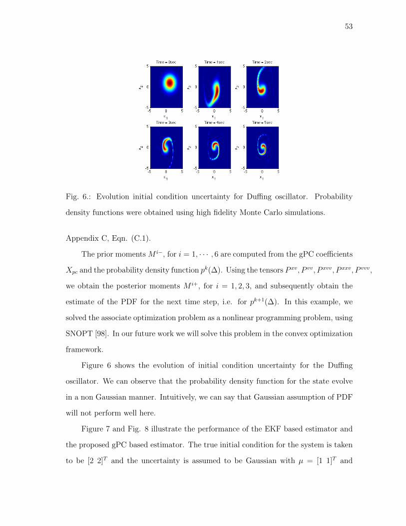
53
Fig. 6.: Evolution initial condition uncertainty for Duffing oscillator. Probability
density functions were obtained using high fidelity Monte Carlo simulations.
Appendix C, Eqn. (C.1).
The prior moments M i−, for i = 1, · · · , 6 are computed from the gPC coefficients
Xpc and the probability density function pk(∆). Using the tensors P xv, P vv, P xvv, P xxv, P vvv,
we obtain the posterior moments M i+, for i = 1, 2, 3, and subsequently obtain the
estimate of the PDF for the next time step, i.e. for pk+1(∆). In this example, we
solved the associate optimization problem as a nonlinear programming problem, using
SNOPT [98]. In our future work we will solve this problem in the convex optimization
framework.
Figure 6 shows the evolution of initial condition uncertainty for the Duffing
oscillator. We can observe that the probability density function for the state evolve
in a non Gaussian manner. Intuitively, we can say that Gaussian assumption of PDF
will not perform well here.
Figure 7 and Fig. 8 illustrate the performance of the EKF based estimator and
the proposed gPC based estimator. The true initial condition for the system is taken
to be [2 2]T and the uncertainty is assumed to be Gaussian with µ = [1 1]T and

54
(a) EKF based estimator with 0.2s update. (b) EKF based estimator with 0.3s up-date.
Fig. 7.: Performance of EKF estimators. Dashed lines represent ±3σ limits and the
solid line represents error in estimation.
Σ = diag(1, 1). Therefore, the initial error in the state estimation is [1 1]T . Figure
7a shows the performance of the EKF based estimator with 0.2 seconds measurement
update. We observe that the errors in estimates go to zero rapidly. However, when
the measurement update interval is increased to 0.3 seconds, the EKF based estimator
performs poorly and the errors do not converge to zero. Figure 8a shows the plots
of the estimator when gPC theory is used to propagate the uncertainty and only the
first two moments are updated, using standard Kalman update law. We observe that
this combination achieves better results than the EKF estimator but is inconsistent
as the errors escape the ±3σ bounds. Figure 8b shows the performance of the gPC
based estimator with third order moment updates, performed every 0.5 seconds. We
observe that errors in the estimates converge to zero rapidly and are within the
±3σ bounds. The EKF based estimator for this case diverges. This highlights the
importance of using nonlinear dynamics for uncertainty propagation along with higher
order moments update for solving nonlinear estimation problems.
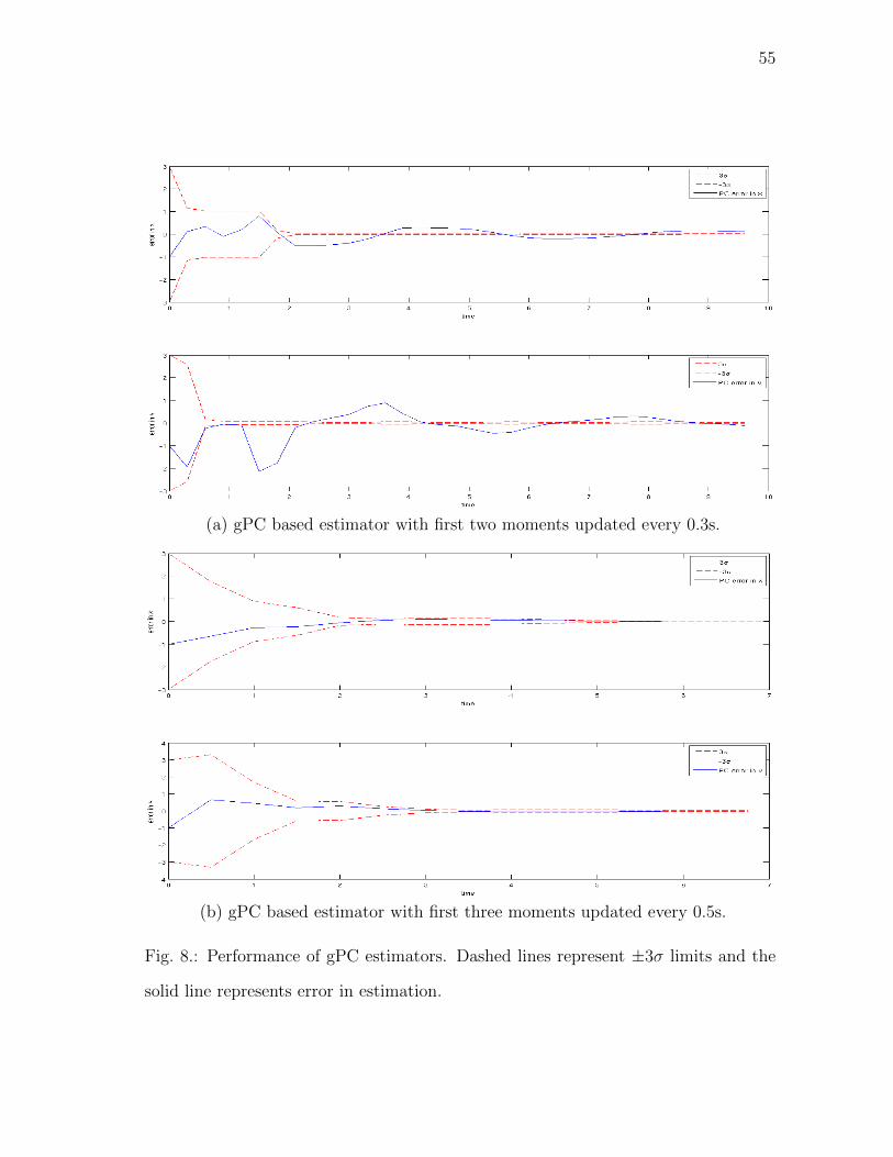
55
(a) gPC based estimator with first two moments updated every 0.3s.
(b) gPC based estimator with first three moments updated every 0.5s.
Fig. 8.: Performance of gPC estimators. Dashed lines represent ±3σ limits and the
solid line represents error in estimation.

56
2. Results for Estimation Using Bayesian Inference
In this section we discuss the results of the application of estimation algorithm that
uses Bayesian inference for update, to the Duffing oscillator in Eqn. (3.10) & Eqn.
(3.11). The true initial states of the system were taken to be [2.5, 2.5]. The initial
state uncertainty was assumed to be Gaussian with mean and covariance matrix given
by
µ =
1
1
Σ2 =
3 0
0 3
.Hence, the initial error in estimation and the initial state uncertainty is larger than the
previous case. Time between each measurement update was taken to be 1s. Figure 9
shows plots for estimation error and ±3σ bounds for minimum covariance, maximum
likelihood and minimum error estimators, and EKF based estimator. It can be seen
that for the PC based estimators, errors converge and are within the ±3σ limits,
whereas for EKF errors diverge and escape outside the ±3σ bounds.
F. Application to Hypersonic Reentry
We apply the estimation algorithm, that uses Bayesian inference for PDF update, to
reentry of a hypersonic vehicle in the atmosphere of Mars. We assume only longi-
tudinal motion of the reentry vehicle here. The simplified dynamics of reentry are
represented by Vinh’s equation [99], in three states - the distance from planet’s cen-
ter r, velocity v, and the flight-path angle γ, or x = [r v γ]T . The equations can be

57
(a) Minimum covariance estimator.
(b) Maximum likelihood estimator.
Fig. 9.: Plots for time (x-axis) vs. ±3σ limits (dashed lines) and estimation error
(solid lines) (y-axis) for gPC based estimators and EKF based estimator.

58
(c) Minimum error estimator.
(d) EKF based estimator.
Fig. 9.: Continued.

59
Table III.: Explanation and values of the constants for Martian atmosphere (Sengupta
and Bhattacharya, 2008)
Description of Constants Value
Radius of Mars Rm = 3397× 103 m
Acceleration due to Gravity of Mars g = 3.71 m/s2
Ballistic Coefficient of the Vehicle Bc = 72.8 kg/m2
Lift-to-Drag Ratio of the Vehicle LD
= 0.3
Density at the Surface of Mars ρ0 = 0.0019 kg/m3
Scale Height for Density Computation h1 = 9.8 km h2 = 20 km
Escape Velocity of Mars vc = 5.027 km/s
written as
r = vsin(γ) (3.34a)
v = − ρv2
2Bc
− gsin(γ) (3.34b)
γ =(vr− g
v
)cos(γ) +
ρ
2Bc
(L
D
)v, (3.34c)
where g is the acceleration due to gravity, Bc is the ballistic coefficient, LD
is the
lift-to-drag ratio of the the vehicle, ρ is the atmospheric density given by
ρ = ρ0e(h2−hh1
),
where ρ0, h1 and h2 are constants depending on the planet’s atmospheric model,
h = r − Rm is the height above planet’s surface and Rm is the radius of the planet.
Choices of the constants in Eqn. (3.34a) through Eqn. (3.34c) used to simulate
reentry in Martian atmosphere are given in Table III [100].
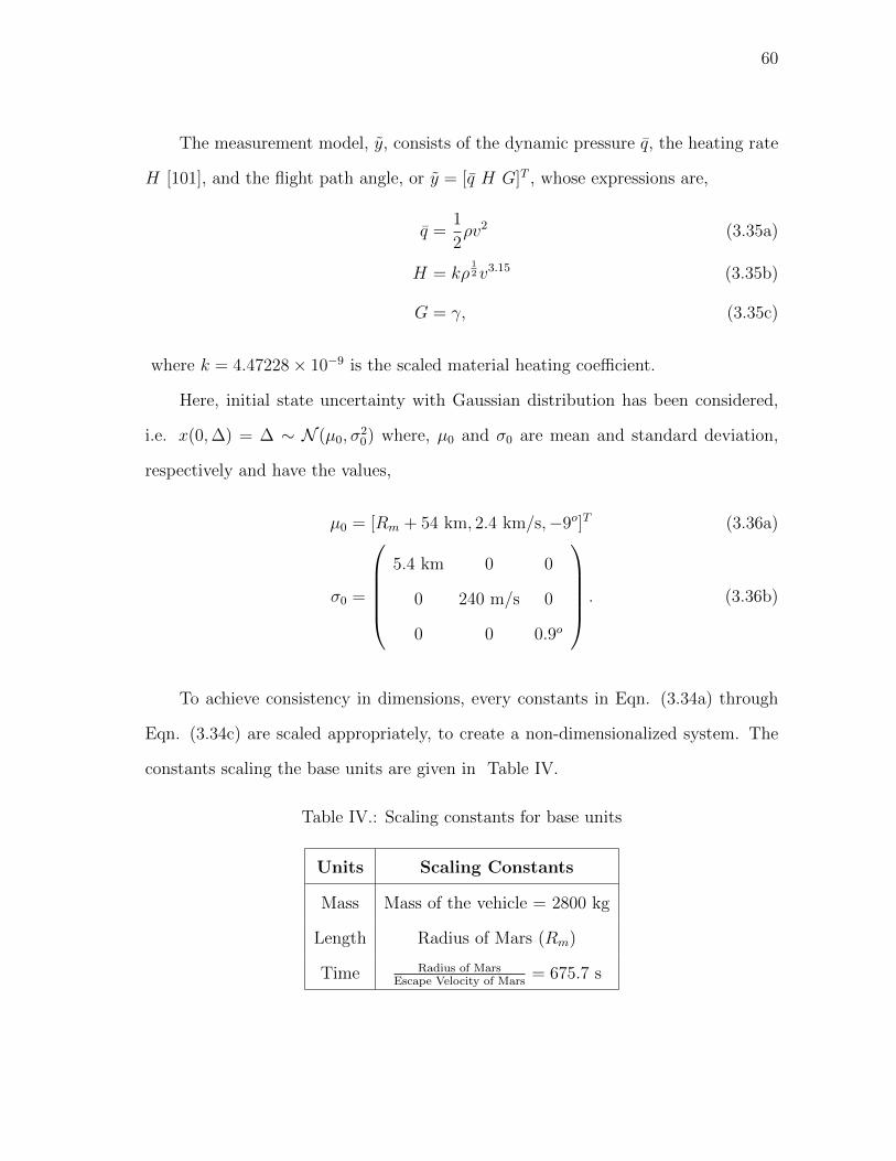
60
The measurement model, y, consists of the dynamic pressure q, the heating rate
H [101], and the flight path angle, or y = [q H G]T , whose expressions are,
q =1
2ρv2 (3.35a)
H = kρ12v3.15 (3.35b)
G = γ, (3.35c)
where k = 4.47228× 10⁻⁹ is the scaled material heating coefficient.
Here, initial state uncertainty with Gaussian distribution has been considered,
i.e. x(0,∆) = ∆ ∼ N (µ0, σ20) where, µ0 and σ0 are mean and standard deviation,
respectively and have the values,
µ0 = [Rm + 54 km, 2.4 km/s,−9o]T (3.36a)
σ0 =
5.4 km 0 0
0 240 m/s 0
0 0 0.9o
. (3.36b)
To achieve consistency in dimensions, every constants in Eqn. (3.34a) through
Eqn. (3.34c) are scaled appropriately, to create a non-dimensionalized system. The
constants scaling the base units are given in Table IV.
Table IV.: Scaling constants for base units
Units Scaling Constants
Mass Mass of the vehicle = 2800 kg
Length Radius of Mars (Rm)
Time Radius of MarsEscape Velocity of Mars
= 675.7 s

61
The measurements are normalized to lie within [−1, 1], so that they have con-
sistent magnitude. The normalization factors used for measurements are given in
Table V. The measurement noise ν is assumed to have mean and covariance as,
Table V.: Normalization factors for measurements
Measurement Normalization Factors
Dynamic Pressure 1.97× 10³ Nm
Heating Rate 0.0231 Jm-s
Flight Path Angle 19.13o
E [ν] = [0, 0, 0]T and R = E[ννT
]= 6× 10⁻⁵I3.
As mentioned before, gPC theory works best, when the nonlinearities are in the
form of polynomials [87, 102]. In this case, the trigonometric and exponential terms
in Eqn. (3.34a) through Eqn. (3.34c) are approximated, with cubic polynomials in
γ and h respectively. For example, let S(γ) be a suitable approximation of sin(γ),
then,
S(γ) = a0 + a1γ + a2γ2 + a3γ
3,
and
S ′(γ) = a1 + 2a2γ + 3a3γ2.
The coefficients of S(γ) are obtained by equating the values of sin(γ) and its deriva-
tive, with S(γ) and S ′(γ) respectively, at the boundaries of γ’s domain. For the

62
present case, γ ∈ [−90o, 0], which yields a system of linear equations given by,
1 −1.57 2.47 −3.88
1 0 0 0
0 1 −3.14 7.40
0 1 0 0
a0
a1
a2
a3
=
−1
0
0
1
,
which can be solved for a0, a1, a2 and a3. The approximation of cos(γ) can be found
in a similar manner.
The approximation of sine and cosine terms for the present case are,
sin(γ) ≈ S(γ) := γ + 0.0574γ2 − 0.1107γ3
cos(γ) ≈ C(γ) := 1− 0.5792γ2 − 0.1107γ3.
Assuming h ∈ [0, 100 km], the exponential density term, is approximated by cu-
bic polynomials, in three different intervals. The approximated density term D(h) ≈
ρ, is given by,
D(h) :=
0.0146− 1.50× 10⁻⁶h+ 5.93× 10⁻¹¹h2 − 8.45× 10⁻¹⁶h3 h ∈ [0, 25km)
0.0080− 4.72× 10⁻⁷h+ 9.59× 10⁻¹²h2 − 6.61× 10⁻¹⁷h3 h ∈ [25km, 50km)
0.0015− 5.2× 10⁻⁸h+ 5.90× 10⁻¹³h2 − 2.20× 10⁻¹⁸h3 h ∈ [50km, 100km)
.
The approximated system can be written as
r = vS(γ) (3.37a)
v = −D(h)v2
2Bc
− gS(γ) (3.37b)
γ =(vr− g
v
)C(γ) +
1
2Bc
(L
D
)v. (3.37c)
Monte Carlo simulations were performed to validate the approximated model.

63
(a) Mean vs. time.
(b) Standard deviation vs. time.
Fig. 10.: (a) Mean and (b) standard deviation of the true system (solid) and the
approximated system (dashed) obtained from Monte Carlo simulations.

64
Fig. 11.: Percentage error in states of the approximated system from true system.
A Gaussian distribution for initial states was assumed, with mean and standard
deviation as given in Eqn. (3.36a) & Eqn. (3.36b). Figure 10 shows the trajectories of
mean and the standard deviations for systems in Eqn. (3.34a) through Eqn. (3.34c)
and Eqn. (3.37a) through Eqn. (3.37c). It can be seen that they are almost identical
for both the systems, although some variation is observed for longer propagation
time. Figure 11 shows the percentage error in approximation of the systems’ states.
From this analysis it can be concluded that the system in Eqn. (3.37a) through Eqn.
(3.37c) is a good approximation of the actual system in Eqn. (3.34a) through Eqn.
(3.34c), for estimation purposes. Clearly a better approximation could be performed
that reduces the growth of error over long time integration. However, with this model,
good results were obtained, for the estimation algorithm. The approximated model is
used to propagate the uncertainty. The “measurements” were obtained by simulating
the actual nonlinear system.

65
To construct the deterministic dynamical system via polynomial chaos as defined
in Eqn. (3.7), inner products of up to six basis functions were required. Detailed
derivation of the augmented dynamics has been omitted from this dissertation and
can be found in Prabhakar et al. [102].
Up to fourth order moments were used, to compute the prior probability density
function from GMM. The prior moments, M i− for i = 1, . . . , 4 were computed from
the gPC coefficients XPC and the inner products 〈φiφj . . .〉 as in Eqn. (3.19a) through
Eqn. (3.19d).
The performance of the proposed estimator was then compared with EKF and
UKF based estimators. For the current analysis, the covariance of the posterior PDF
was minimized to get the state estimate (MCE criterion), which is the mean of the
posterior density function. The initial states of the true system were assumed to be
x(t = 0) = [Rm + 61 km 2.42 km/s − 8.91o]T . Therefore the initial error in state
estimation was [−7 km − 0.02 km/s 0.09o]T . Figure 12 and Fig. 13, show the plots
for error in state estimation where the measurement update interval is 20s. It can
be observed that the errors for gPC based estimator goes to zero rapidly and are
within the ±3σ limits. The EKF based estimator performs poorly and the errors
don’t converge to zero. Also the EKF based estimator is inconsistent as the errors
escape outside ±3σ limits. In case of UKF, the errors for γ and v starts to increase
after a while and the ±3σ limits are divergent.
In Fig. 14 and Fig. 15 the update interval was increased to 40s. It can be seen
that, the errors and the ±3σ bounds for the gPC based estimator converges. The
errors for the EKF based estimator for this case diverges. Although the ±3σ limits
of the UKF based estimator converge, but convergence is slower than gPC based
estimator. The estimation errors for UKF is divergent.
The gPC based estimator works well even for larger errors in initial state es-
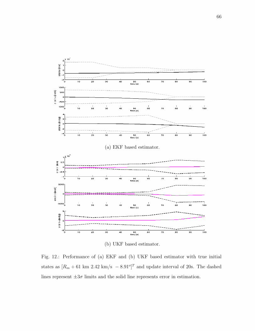
66
(a) EKF based estimator.
(b) UKF based estimator.
Fig. 12.: Performance of (a) EKF and (b) UKF based estimator with true initial
states as [Rm + 61 km 2.42 km/s − 8.91o]T and update interval of 20s. The dashed
lines represent ±3σ limits and the solid line represents error in estimation.

67
Fig. 13.: Performance of the gPC based estimator with true initial states as [Rm +
61 km 2.42 km/s − 8.91o]T and update interval of 20s. The dashed lines represent
±3σ limits and the solid line represents error in estimation.

68
(a) EKF based estimator.
(b) UKF based estimator.
Fig. 14.: Performance of (a) EKF and (b) UKF based estimator with true initial
states as [Rm + 61 km 2.42 km/s − 8.91o]T and update interval of 40s.The dashed
lines represent ±3σ limits and the solid line represents error in estimation.

69
Fig. 15.: Performance of the gPC based estimator with true initial states as [Rm +
61 km 2.42 km/s − 8.91o]T and update interval of 40s. The dashed lines represent
±3σ limits and the solid line represents error in estimation.

70
timation. For plots in Fig. 16 and Fig. 17, the true initial states were [Rm +
61 km 2.64 km/s − 8.1o]T , with v and γ having 10%(= σ) errors in initial estimate.
It can be observed that gPC based estimator achieves convergence of error and re-
mains within ±3σ bounds. For EKF, the errors diverge and escape outside the ±3σ
limits. Hence the EKF based estimator here is inconsistent. The errors for the UKF
based estimator converge but briefly remain outside the ±3σ bounds. For this ex-
ample, the ±3σ limits for UKF are observed to be divergent. This highlights the
advantage of using polynomial chaos for propagation in Bayesian estimation frame-
work over traditional filters based on Gaussian theory.
Figure 18 compares the performance of the three criterion functions used to get
the state estimate. It is observed that ±3σ bounds of MEE criterion converges faster
than MCE and MLE criteria, although the bounds for MLE based estimate diverges
towards the end. The error convergence for MEE is slower MCE and MLE, but errors
are within ±3σ limits for all the criteria. When compared to EKF and UKF, the gPC
based estimators outperform both of them when convergence of errors and ±3σ limits
are considered.

71
(a) EKF based estimator.
(b) UKF based estimator.
Fig. 16.: Performance of (a) EKF and (b) UKF based estimator with true initial
states as [Rm + 61 km 2.64 km/s − 8.1o]T and update interval of 20s. The dashed
lines represent ±3σ limits and the solid line represents error in estimation.

72
Fig. 17.: Performance of the gPC based estimator with true initial states as [Rm +
61 km 2.64 km/s − 8.1o]T and update interval of 20s. The dashed lines represent
±3σ limits and the solid line represents error in estimation.

73
(a) MCE criterion. (b) MLE criterion.
(c) MEE criterion.
Fig. 18.: Performance of (a) MCE, (b) MLE and (c) MEE criterion for state estimates.
The true initial states are [Rm + 61 km 2.42 km/s − 8.91o]T and update interval is
20s. The dashed lines represent ±3σ limits and the solid line represents error in
estimation.

74
G. Limitations of Polynomial Chaos
Polynomial chaos is a good methodology to propagate uncertainty specially in systems
where nonlinearities are in the form of polynomials. But there are certain limitations,
when we use gPC to propagate uncertainty in systems which have non-polynomial
nonlinearities. This is well documented and can be found in the paper by Debusschere
et al. [87]. Moreover polynomial chaos gives us inaccurate results when the statistics
is to predicted for longer durations.
For example Fig. 19 shows first and second moment plots for the system given
by Eqn. (3.10) & Eqn. (3.11) with Gaussian initial state uncertainty have mean and
covariance, µ = [1, 1] and σ = diag(1, 1) respectively. It can be seen that after a while
the PC trajectory diverges from the MC solution, thus proving that PC incurs error
when long term statistics are to be predicted.
Uncertainty propagation using PC is a method, which is based on parameterizing
the random variable, and then approximating the density using a density kernel.
However, a method which propagates density directly without requiring any kind
of parameterization is more desired. Intuitively this nonparametric method should
perform better than PC as it is approximation free. In the next chapter, we present
a methodology to propagate uncertainty in a nonparametric sense.

75
(a) First moment.
(b) Second moment.
Fig. 19.: Long term statistics, up to 10 seconds predicted by Monte Carlo (dashed
line) and polynomial chaos (solid line) for the system in Eqn. (3.10) & Eqn. (3.11).
The x-axis represents time and y-axes are the states.
76
CHAPTER IV
THE FROBENIUS-PERRON OPERATOR∗
In this chapter, we propose a nonlinear estimation technique based on Frobenius-
Perron (FP) operator theory. The Frobenius-Perron operator, also known by the
name of transfer operator or Stochastic Liouville equation (SLE) is a linear operator
that dictates the flow of probability densities in a dynamical system. We introduce
FP operator, then develop theories related to how densities evolve in a dynamical
system with uncertainties present in it. Finally we describe the estimation algorithm,
and apply it to hypersonic reentry problem, while comparing its performance with
particle filters.
A. Analysis of Densities in State Space Using Frobenius-Perron Operator
In this section we introduce the concept of the FP operator and demonstrate, how it
can be used to study evolution of densities of state trajectories. The presentation of
the background on FP operator is deliberately kept informal as the associated theory
is well developed. The interested reader is directed to [26] for a rigorous treatment
of the material presented in this section.
1. Discrete-Time Systems
To establish an intuitive view of the evolution of densities, let us consider one di-
mensional discrete-time system defined by the transformation xk+1 = S(xk), where
S : A 7→ A, and A ⊂ R. Let us pick a large number of N initial states x01, · · · , x0
N
∗Reprinted from “Hypersonic State Estimation Using Frobenius-Perron Operator”by P. Dutta, R. Bhattacharya, 2011. AIAA Journal of Guidance Control and Dy-namics , vol. 34, no. 2, pp. 325–344, Copyright [2011] by P. Dutta & R. Bhattacharya
77
and apply the map S(x) to obtain new states x11 = S(x0
1), · · · , x1N = S(x0
N). Let us
define an indicator function for A as
1A(x) =
1 if x ∈ A,
0 if x 6∈ A.
Also any function f0(x) is a density function. for initial states x01, · · · , x0
N , if for every
interval D0 ⊂ A and µ(D0) 6= 0, the following is true,∫D0
f0(u)du = limN→∞
1
N
N∑i=1
1D0(x0i ), (4.1)
Similarly the density function f1(x) for states x11, · · · , x1
N satisfies, for D1 ⊂ A ,∫D1
f1(u)du = limN→∞
1
N
N∑i=1
1D1(x1i ), (4.2)
The FP operator relates f1 and f0. To define the FP operator, we first introduce the
notion of counterimage of any interval D ⊂ A under transformation operator S. This
is the set of all points that will be in D after one application of S, i.e.,
S−1(D) = x : S(x) ∈ D.
We note that ∀D1 ⊂ A, we have
x1j ∈ D1 ⇐⇒ x0
j ∈ S−1(D1).
Hence D0 = S−1(D1) as x0j ∈ D0. We thus have an important relation, ∀D ⊂ A.
1D(S(x)) = 1S−1(D)(x). (4.3)

78
With Eqn. (4.3) we can write Eqn. (4.2) as∫D1
f1(u)du = limN→∞
1
N
N∑i=1
1S−1(D1)(x0i )
=
∫S−1(D1)
f0(u)du.
The above relation tells us how density of initial states f0 will be transformed to
new density f1 under the transformation S.
Let D1 = [a, x] then, ∫ x
a
f1(u)du =
∫S−1[a,x]
f0(u)du,
and differentiating the above relation with respect to x, we have
f1(x) =d
dx
∫S−1[a,x]
f0(u)du
Clearly, f1 depends on f0, and is usually indicated by writing f1 = Pf0. In general,
the deformation of the density function f(x) defined over [a, x] under transformation
S is given by
Pf(x) =d
dx
∫S−1[a,x]
f(u)du (4.4)
If the transformation S is invertible and differentiable in A, then it must be monotone
in A. In such case Eqn. (4.4) can be written as
Pf(x) =d
dx
∫S−1[a,x]
f(u)du
= f(S−1(x))
∣∣∣∣dS−1(x)
dx
∣∣∣∣ , (4.5)
where absolute value takes into account cases where S−1 is increasing or decreasing.
Equation (4.5) can be generalized for x ∈ Rn by noting that |dS−1(x)/dx| is the
determinant of the Jacobian of dS−1(x)/dx. Time evolution of f(x) can be determined
by recursively applying Eqn. (4.4).

79
2. Continuous-Time Systems
In contrast to discrete time systems, we have uncountably many mappings from initial
to final states, in case of continuous time systems. We will start by defining some
preliminary concepts, on which the development of FP operator theory is based.
Let X be a Hausdorff space and A be the σ−algebra generated by Borel sets of
X .
Definition 1 A dynamical system Stt∈R on X is the family of transformations
St : X → X , t ∈ R, satisfying
• S0(x) = x ∀x ∈ X
• St(St‘(x)) = St+t‘(x) ∀x ∈ X and t, t‘ ∈ R, and
• The mapping (t, x)→ St(x) from R×X → X is continuous.
It is also clear from the properties of Stt∈R that St(S−t(x)) = x and S−t(St(x)) =
x, ∀t ∈ R. Thus, ∀t0 ∈ R, any transformation St0 of the dynamical system Stt∈R,
is invertible.
Remark 1 A semidynamical system is same as a dynamical system except for t ∈
R+.
Let us consider a semidynamical system of the form Stt≥0. Assume a measure
µ(·) on X is given and all transformation St of Stt≥0 are nonsingular, i.e.,
F = A ∈ A : µ(S−1t (A)) = 0 then µ(A) = 0 ∀A ∈ F .
80
Definition 2 The Frobenius-Perron operator Pt : L1(X )→ L1(X ), corresponding to
the transformation St is uniquely defined by∫A
Ptf(x)µ(dx) =
∫S−1(A)
f(x)µ(dx),
where f : X → R is any arbitrary function such that∫X |f(x)|µ(dx) <∞.
We can show [26] that Ptt≥0 is continuous. To show this, note that since
St is invertible, S−1t = S−t. Let J−t be the determinant of the Jacobian of the
transformation S−t. Then, using Eqn. (4.5)
Ptf(x) = f(S−t(x))J−t(x).
Thus, for every continuous f , with compact support,
limt→t0
f(S−t(x))J−t(x) = f(S−t0(x))J−t0(x),
uniformly with respect to x. This implies that,
limt→t0||Ptf − Pt0f || = lim
t→t0
∫X
|Ptf(x)− Pt0f(x)|dx = 0,
Since the integrals are computed over the a bounded set X ⊂ A. Now, because
continuous functions with compact support form a dense subset in L1, this implies
that Ptt≥0 is continuous.
From a computational point of view, this property is important as we will be
using space of continuous functions to approximately solve for Ptt≥0 in R×X .
For a dynamical system of the form
x = F (x); x ∈ X ∈ B(Rn), F : X → X , (4.6)
where B(Rn) refers to Borel sets of Rn and F (x) = [F1(x), · · · , Fn(x)]T . It can

81
be shown that, the definition of the FP operator reduces to the following partial
differential equation (pg. 213, [26]).
∂u
∂t+
n∑i=1
∂(uFi(x))
∂xi= 0, (4.7)
where u(t, x) = Ptf(x).
3. Properties of Frobenius-Perron Operator
Both continuous and discrete time Frobenius-Perron operators have the following
properties, shown here using the notation for continuous time FP operator,
1. Pt(λ1f1 + λ2f2) = λ1Ptf1 + λ2Ptf2, ∀f1, f2 ∈ L1, λ1, λ2 ∈ R.
2. Ptf ≥ 0, if f ≥ 0.
3.∫X Ptf(x)µ(dx) =
∫X f(x)µ(dx), ∀f ∈ L1.
Thus for a fixed t, Pt is a Markov operator.
B. Method of Characteristics for Solving First Order Linear Partial Differential
Equations
Equation (4.7) is a first order linear partial differential equation that can be solved
using method of characteristics. Equation (4.7) can be written as
∂u
∂t+
∂u
∂x1
F1(x) + · · · ∂u∂xn
Fn(x) + u
n∑i=1
∂Fi(x)
∂xi= 0.
Defining G(x, u) := −un∑i=1
∂Fi(x)
∂xi, we get
∂u
∂t+
∂u
∂x1
F1(x) + · · · ∂u∂xn
Fn(x) = G(x, u), (4.8)

82
which is in the standard form. Assuming G(x, u) 6= 0, Eqn. (4.8) can be solved by
solving (n+ 1) coupled ordinary differential equations given by
dx1
dt= F1(x), · · · , dxn
dt= Fn(x), (4.9a)
du
dt= G(x, u). (4.9b)
Substituting the value of G(x, u) in Eqn. (4.9b), we get
du
dt= −u
n∑i=1
∂Fi(x)
∂xi(4.10)
wheren∑i=1
∂Fi(x)
∂xiis the trace of the Jacobian of F (x).
Equation (4.9a) & Eqn. (4.9b) trace out a trajectory in the (n+ 1) dimensional
space spanned by (x1, · · · , xn, u). To make the solution unique, the value of u(t, x)
has to be specified at a given point x(t0) at time t0. The evolution of u(t, x) over
R×X can be determined by specifying u(t, x) over several points in X at time t0. The
trajectories x(t) are called characteristics and Eqn. (4.9a) & Eqn. (4.9b) determine
evolution of u along x(t) [103].
C. Uncertainty Propagation in Dynamical Systems Using FP Operator
Given a dynamical system of the form,
x(t) = g(x(t),∆) (4.11)
where x : R+ → Rn are states and g : Rn × Rq → Rn is a real valued function.
Let ∆ ∈ Rq be the vector of initial and parametric uncertainty. Without loss of
generality, we assume that ∆ represents the set of initial state uncertainty, hence
∆ := x(t = 0) ∈ Rn, and let ∆ ∼ p(∆) = p(x(0)). Using the method of characteristics
to get the equation for evolution of densities as presented in the previous section in

83
Eqn. (4.10), we augment the dynamical system in Eqn. (4.11). The final dynamical
system is given by,
x(t) = g(x(t)) (4.12a)
p(t) = − div [g(x(t))] p(t), (4.12b)
where p : R+ → R denotes the joint density of the states x(t) at a given time t.
The augmented equation has states [x(t), p(t)], which are to be solved with initial
conditions [x(t = 0), p(t = 0)]. Equation (4.12a) & Eqn. (4.12) dictate the evolution
of probability density along the trajectories of a dynamical system with uncertainties.
For example, consider uncertainty propagation due to initial condition uncer-
tainty for the Duffing oscillator model. As shown in Fig. 20, consider the case where
there is initial condition has the mean (1, 1) and standard deviation diag(1, 1). The
distribution is considered to be Gaussian. The initial distribution is sampled using
500 points. The system considered is the same one as used in Eqn. (3.10) & Eqn.
(3.11) . The corresponding differential equation for uncertainty propagation is given
by,
x1 = x2, (4.13a)
x2 = −x1 − x31 −
1
4x2, (4.13b)
p = −p(0 +−1
4) =
1
4p. (4.13c)
The initial conditions for (x1, x2) are given by the locations of the samples. The
initial conditions for p are given by the values of the Gaussian distribution function
at those points. With these initial conditions the above equations are integrated
to obtain (x1(t), x2(t), p(t)). Figure 20 shows the initial values of (x1(t), x2(t), p(t))
and their values at time t = 1s,2s and 3s. The magnitude of p is color coded, with

84
−2 0 2 4−2
0
2
4time = 0 s
x1
x 2
−4 −2 0 2−5
0
5time = 1 s
x1
x 2
−2 0 2 4−5
0
5
10time = 2 s
x1
x 2
−2 0 2 4−10
−5
0
5time = 3 s
x1
x 2
Fig. 20.: Method of characteristics. Number of samples = 500. System is Duffing
oscillator. The black circle shows the location and the PDF value (color coded) of an
arbitrary sample point at different time instances.
red corresponding to large and blue corresponding to small. It can be observed,
this method determines the value of p(t) at the sample locations, (x1, x2) exactly.
However, for intermediate points, the value of p(t) is not known. Several methods
like scattered data interpolation [104] may be used to find the density at intermediate
points, but such an analysis has not been performed in this dissertation. Also, note
that value of p determined at (x1, x2), at some time t, is independent of the number
of samples. Although, increasing the number of samples will improve the accuracy of
the subsequent interpolation. However, in case of Monte Carlo, since the value of p
is approximated using histograms, the accuracy depends on the number of samples.

85
1. Accuracy in Prediction of Uncertainty
Since this method requires selection of points in the state space, one may argue that
this approach is similar to Monte Carlo. The main difference is that in FP operator
the value of the density function is determined along the trajectory and at final time
the value of the density function is known at certain discrete locations. These loca-
tions are values of the state vector at that final time. The value of the density function
over the domain can be then determined using interpolation. In Monte Carlo, same
idea is used except only state equations are integrated. The density function at final
time is determined using histogram techniques, which are sensitive to the number of
sample points taken. Thus for comparable accuracy, many more points will have to be
taken for Monte Carlo based method than for FP based method. As an illustration,
consider Fig. 21. It can be seen that a good approximation of the Gaussian density
function is achieved by taking 25 points and linear interpolation in the case of FP
operator. Whereas for Monte Carlo, at least 1000 points were needed to get the same
level of accuracy. Thus for this one dimensional case, there is a reduction of two orders
of magnitude in the number of sample points required for FP based uncertainty prop-
agation. For higher dimensional case, the benefits will be even more significant. For
high dimensional problems, discrete points can be generated using Halton sequence
[105], and concentrating them in regions with higher importance/features will further
reduce the growth of computational complexity. Other methods for generating smart
samples from a given distribution include sparse grids [106, 107, 58] and mesh-free
adjoint methods [108, 109, 110, 111].

86
(a) PF: 25 samples.
(b) MC: 25 samples.
Fig. 21.: Comparison of FP and Monte Carlo based approximation of density func-
tions.
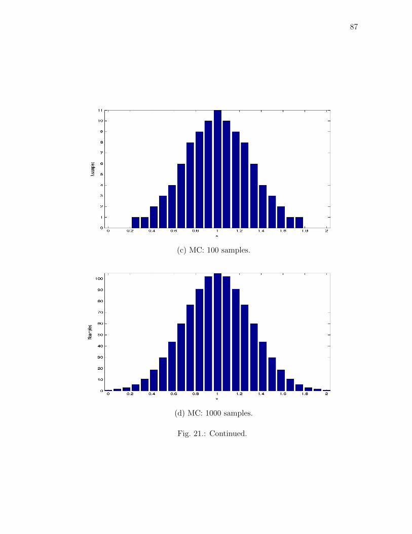
87
(c) MC: 100 samples.
(d) MC: 1000 samples.
Fig. 21.: Continued.

88
D. Nonlinear Estimation Using Frobenius-Perron Operator
The nonlinear estimation setting in this scenario is same as one in Chapter III. We
have an uncertain dynamical system being measured by a nonlinear measurement
model which are given by,
x = g(x,∆), (4.14a)
y = h(x) + ν. (4.14b)
where x ∈ RN are the states and y ∈ Rm are the measurements.
It is assumed that measurements are available at discrete times t0, · · · , tk, tk+1, · · · .
At a given time tk, let xk, yk and pk(·) be the state, measurement and the probabil-
ity density function. Let p−k (·) and p+k (·) denote the prior and the posterior density
functions at time tk. The estimation algorithm is described next, which is similar to
that presented by Daum et al. [40].
1. Step 1: Initialization Step
To begin, the domain D∆ of the initial random variable x0 is discretized. From the
discretized domain, N particles are chosen at random based on the PDF p0(x0) of
the random variable x0. Let the particles be represented by x0,i for i = 1, 2, · · · , N ;
and p0(x0,i) be the value of p0(x) at these particles. The following steps are then
performed recursively starting from k = 1.
2. Step 2: Propagation Step
With initial states at k − 1th step as [xk−1,i pk−1(xk−1,i)]T Eqn. (4.9a) & Eqn. (4.9b)
are integrated for each particle over the interval [tk−1, tk] to get [xk,i, p−k (xk,i)]
T . Note
that p−k (xk,i) obtained by integration are the prior PDF values for xk,i, and hence the

89
superscript.
3. Step 3: Update Step
First the likelihood function, p(yk|xk = xk,i), is determined for each particle i, using
Gaussian measurement noise and sensor model in Eqn. (4.14b). It is defined as
l(yk|xk = xk,i) =1√
(2π)m|R|e−
12
(yk−h(xk,i))TR−1(yk−h(xk,i)), (4.15)
where |R| is the determinant of the covariance matrix of measurement noise.
The posterior probability density function of the states is constructed next, for
each particle i, using classical Bayes rule [78]. It is defined as the density function
of the states given current measurement, i.e. p+k (xk,i) := pk(xk = xk,i|yk). For a
particular particle, xk,i it is given by,
p+k (xk,i) := p(xk = xk,i|yk) =
l(yk|xk = xk,i)p−k (xk = xk,i)
N∑j=1
l(yk|xk = xk,j)p−k (xk = xk,j)
. (4.16)
4. Step 4: Getting the State Estimate
The state estimate for the kth step is then computed depending on the desired com-
putation as given in Bryson and Ho[97]. As in the previous section the commonly
used criteria are the same, which are given by,
1. Maximum-Likelihood Estimate: maximize the probability that xk,i = xk. This
results in xk = mode of p+k (xk,i).
2. Minimum-Variance Estimate: here xk = arg minx∑N
i=1 ||x − xk,i||2 p+k (xk,i) =∑N
i=1 xk,i p+k (xk,i). The estimate is the mean of xk,i.
90
3. Minimum-Error Estimate: minimize maximum |x − xk,i|. This results in x =
median of p+k (xk,i).
Note that though the criteria are the same, their definition in this case are
different, as we have particles selected from discretized domain of the random variable.
Hence we do a Monte Carlo integration [112] to get the state estimate.
5. Step 5: Resampling
Degeneracy of particles can be detected by looking at values of xk,i for which p+k (xk,i) <
ε, where ε 1 and is pre-specified. Existing methods for resampling can be used to
generate new particles from the new distribution p+k (xk,i). For the k + 1th step, new
points and the corresponding posterior density p+k (xk,i) serve as initial states. Qual-
itatively, since we have the exact density information for each particle, this method
is less sensitive to the issue of degeneracy, as, rather than using histograms, we can
directly use the density information. Although, a rigorous analysis of this has not
been done in this dissertation.
E. Application of Nonlinear Estimation Using FP Operator
In this section we apply the estimation algorithm using FP operator to estimate states
of a nonlinear estimation problem. First we will apply the estimation algorithm to
a Duffing oscillator, the will first present results for application to the simplified
hypersonic reentry problem given by three state Vinh’s equation model. Finally the
results of application to the full reentry dynamics will be shown.
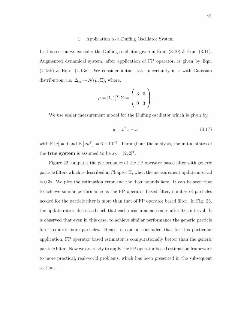
91
1. Application to a Duffing Oscillator System
In this section we consider the Duffing oscillator given in Eqn. (3.10) & Eqn. (3.11).
Augmented dynamical system, after application of FP operator, is given by Eqn.
(4.13b) & Eqn. (4.13c). We consider initial state uncertainty in x with Gaussian
distribution, i.e. ∆x0 ∼ N (µ,Σ), where,
µ = [1, 1]T Σ =
3 0
0 3
.
We use scalar measurement model for the Duffing oscillator which is given by,
y = xTx+ ν, (4.17)
with E [ν] = 0 and E[ννT
]= 6× 10⁻². Throughout the analysis, the initial states of
the true system is assumed to be x0 = [2, 2]T .
Figure 22 compares the performance of the FP operator based filter with generic
particle filters which is described in Chapter II, when the measurement update interval
is 0.3s. We plot the estimation error and the ±3σ bounds here. It can be seen that
to achieve similar performance as the FP operator based filter, number of particles
needed for the particle filter is more than that of FP operator based filter. In Fig. 23,
the update rate is decreased such that each measurement comes after 0.6s interval. It
is observed that even in this case, to achieve similar performance the generic particle
filter requires more particles. Hence, it can be concluded that for this particular
application, FP operator based estimator is computationally better than the generic
particle filter. Now we are ready to apply the FP operator based estimation framework
to more practical, real-world problems, which has been presented in the subsequent
sections.
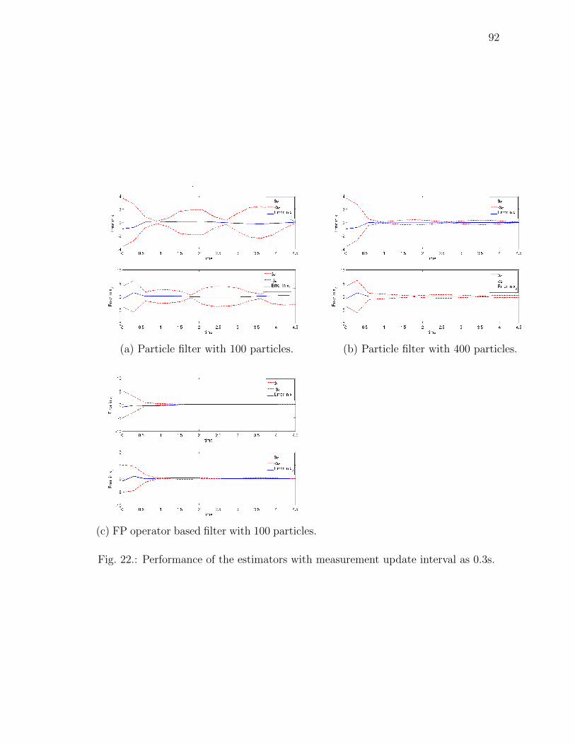
92
(a) Particle filter with 100 particles. (b) Particle filter with 400 particles.
(c) FP operator based filter with 100 particles.
Fig. 22.: Performance of the estimators with measurement update interval as 0.3s.

93
(a) Particle filter with 100 particles. (b) Particle filter with 400 particles.
(c) FP operator based filter with 100 particles.
Fig. 23.: Performance of the estimators with measurement update rate as 0.6s.

94
2. Application to Three State Vinh’s Equation
We consider the dynamical system given in Eqn. (3.34a) through Eqn. (3.34c), with
states x = [r, v, γ], where r is distance from Mars’ center, v is the total velocity
of the reentry vehicle and γ is the flight path angle. The constants have the same
value as given by Table III. The measurement model consist of dynamic pressure
q, heating rate H and the flight path angle γ, whose expressions are given by Eqn.
(3.35a) through Eqn. (3.35c). Initial state uncertainty is assumed to be Gaussian
with mean µ and standard deviation σ given by Eqn. (3.36a) & Eqn. (3.36b). For
consistency in dimensions of the system in Eqn. (3.34a) through Eqn. (3.34c), the
base units of mass, length and time are scaled. The scaling factors used are given
in Table IV. The measurements are normalized such that they lie in [−1, 1], for
consistency in magnitude. The normalization factors used are given in Table V. The
measurement noise ν is assumed to have mean and covariance, E [ν] = [0, 0, 0]T and
R = E[ννT
]= 6× 10⁻⁵I3, respectively, in scaled units.
The performance of the Frobenius-Perron operator based nonlinear estimator is
now compared with generic particle filter and bootstrap filter described in Chapter II,
when applied to hypersonic reentry dynamics. The initial states of the actual system
is taken as [Rm + 61 km 2.64 km/s − 8.1o]T , in this case, with v and γ having 10%
errors in state estimate. The measurement update rate was taken to be 20 seconds.
Figure 24, Fig. 25, and Fig. 26 show the plots for particle filter, the bootstrap filter
and the Frobenius-Perron filter respectively. Figure 27 shows the Cramer-Rao bounds
for the three filters. From these plots it can be seen that all three filters perform
equally well and the errors are within the ±3σ limits. The number of particles used
in these simulations for particle filter, bootstrap filter and the Frobenius-Perron filter
are 25000, 20000 and 7000 respectively.
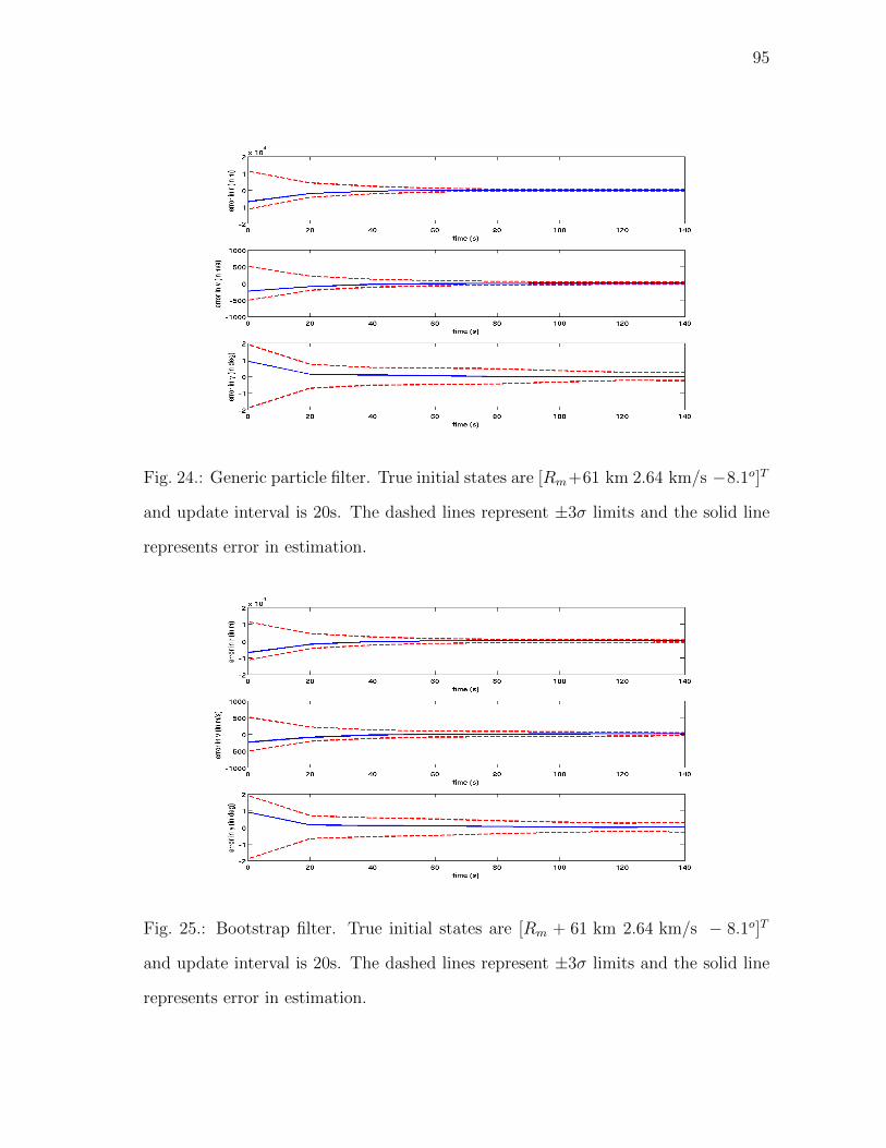
95
Fig. 24.: Generic particle filter. True initial states are [Rm+61 km 2.64 km/s −8.1o]T
and update interval is 20s. The dashed lines represent ±3σ limits and the solid line
represents error in estimation.
Fig. 25.: Bootstrap filter. True initial states are [Rm + 61 km 2.64 km/s − 8.1o]T
and update interval is 20s. The dashed lines represent ±3σ limits and the solid line
represents error in estimation.

96
Fig. 26.: Performance of the Frobenius-Perron estimator with true initial states as
[Rm+61 km 2.64 km/s −8.1o]T and update interval of 20s. The dashed lines represent
±3σ limits and the solid line represents error in estimation.
Fig. 27.: Plots for√σ2 − CRLB vs. time. In the legend, ’BPF’, ’gPF’ and ’FP’,
represent bootstrap filter, generic particle filter and Frobenius-Perron operator based
estimator respectively.

97
Fig. 28.: Generic particle filter with 7000 particles. True initial states are [Rm +
61 km 2.64 km/s −8.1o]T and update interval is 20s. The dashed lines represent ±3σ
limits and the solid line represents error in estimation.
Fig. 29.: Bootstrap filter with 7000 particles. True initial states are [Rm +
61 km 2.64 km/s − 8.1o]T and update interval is 20s. The dashed lines represent
±3σ limits and the solid line represents error in estimation.

98
The particle and the bootstrap filter did not perform as well as the Frobenius-
Perron filter with lesser number of particles. Figure 28 and Fig. 29 show plots for
error covariance and estimation errors for generic particle filter and bootstrap filter
respectively with 7000 particle points. It can bee seen that they do not perform as
well as FP operator based estimator (Fig. 26). In Fig. 30 and Fig. 31 the number
of particles were increased to 10,000 for the particle filter based estimators. Even
then, the performance of the particle filters do not match with FP operator based
estimator’s performance. To substantiate our claim, percentage error vs. time of the
three estimators has been compared here. Figure 32 shows plots when the number
of particles for each estimator is fixed at 7000. It can be seen that the percentage
error in state estimate for FP operator based estimator is lower than the particle filter
based estimators. The performance of the particle filters matches the FP operator
only when the number of particles for generic particle filter is 25000 and for bootstrap
filter is 20000, the percentage error plots for which is shown in Fig. 33.
Thus, it can be said that the Frobenius-Perron filter can achieve the same result
as particle filters using significantly lower number of particles. These simulations were
performed in a Linux machine with Intel R© Pentium D processor. The superiority of
the Frobenius-Perron filter is in the computational time. For each filtering algorithm,
the computational time taken for one filtering step is presented in Table VI. It
can be seen that due to fewer number of particles the Frobenius-Perron filter takes
significantly less computational time.
The FP operator based estimator captures the non-Gaussian PDF evolution al-
most accurately. To show this, time evolution of 3rd and 4th moments of the posterior
PDF for the FP operator based estimator with 7000 particles and a particle filter
with large number of particles (100,000) has been plotted in Fig. 34. It can be seen
that moments for FP operator matches exactly with the particle filter. If, the generic
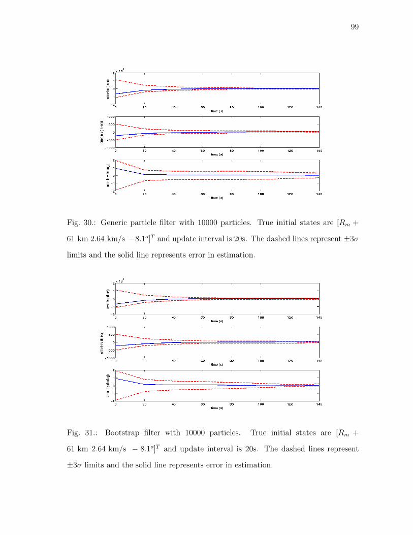
99
Fig. 30.: Generic particle filter with 10000 particles. True initial states are [Rm +
61 km 2.64 km/s −8.1o]T and update interval is 20s. The dashed lines represent ±3σ
limits and the solid line represents error in estimation.
Fig. 31.: Bootstrap filter with 10000 particles. True initial states are [Rm +
61 km 2.64 km/s − 8.1o]T and update interval is 20s. The dashed lines represent
±3σ limits and the solid line represents error in estimation.

100
Fig. 32.: Percentage error in estimation with 7000 particles. True initial states are
[Rm + 61 km 2.64 km/s − 8.1o]T and update interval is 20s. In the legend, ’BF’,
’gPF’ and ’FP’, represent bootstrap filter, generic particle filter and Frobenius-Perron
operator based estimator respectively.
Table VI.: Computational time taken per filtering step for each estimation algorithm.
Listed times are in seconds
FP operator based filter Generic particle filter Bootstrap filter
57.42 s 207.96 s 168.06 s

101
Fig. 33.: Percentage error in estimation with number of particles for FP based oper-
ator (FP), generic particle filter (gPF) and bootstrap filter (BF), 7000, 20000, and
25000 respectively. True initial states are [Rm+61 km 2.64 km/s −8.1o]T and update
interval is 20s.

102
(a) 3rd order moments.
(b) 4th order moments.
Fig. 34.: Plots for 3rd and 4th order moments for particle filter with 100,000 particles-
(dashed line) and FP operator based filter with 7000 samples- (solid line).

103
(a) Percentage error in 3rd order moments.
(b) Percentage error in 4th order moments.
Fig. 35.: Plots for percentage error in 3rd and 4th order moments for bootstrap filter
(BF), generic particle filter (gPF) and FP operator based filter (FP), all with 7000
particles. Percentage deviation taken from particle filter with 100,000 particles.

104
particle filter and bootstrap filter with 7000 particles are compared, it is observed that
they fail to predict non-Gaussian PDF evolution as accurately as the FP operator
based estimator. To show this percentage deviation of the 3rd and 4th order moments
of three estimators from the particle filter with 100,000 particles has been plotted in
Fig. 35. It can be seen that percentage error for the FP operator based estimator
lower than the particle filter based estimators.
a. Sensitivity Analysis
In this section, we perform sensitivity analysis of the FP operator based filter and
the particle filters with respect to measurement noise and measurement update rate.
Figure 36 and Fig. 37 show plots of error covariance and state estimate error for the
FP operator based filter when the measurement noise is 6 × 10⁻⁴I3 in scaled units,
and when the measurement update rate is 40 seconds, respectively. The number of
particles taken here is 7000. To achieve similar performance the generic particle filter
and the bootstrap filter needed 20000 and 25000 particles respectively. The plots for
particle filter are shown in Fig. 38 and Fig. 39 and for the bootstrap filter in Fig. 40
and Fig. 41.

105
Fig. 36.: FP operator based filter with measurement noise 6× 10⁻⁴I3 in scaled units
(number of samples = 7000). True initial states are [Rm + 61 km 2.64 km/s −8.1o]T .
The dashed lines represent ±3σ limits and the solid line represents error in estimation.
Fig. 37.: FP operator based filter measurement update interval is 40s (number of
samples = 7000). True initial states are [Rm + 61 km 2.64 km/s − 8.1o]T . The
dashed lines represent ±3σ limits and the solid line represents error in estimation.
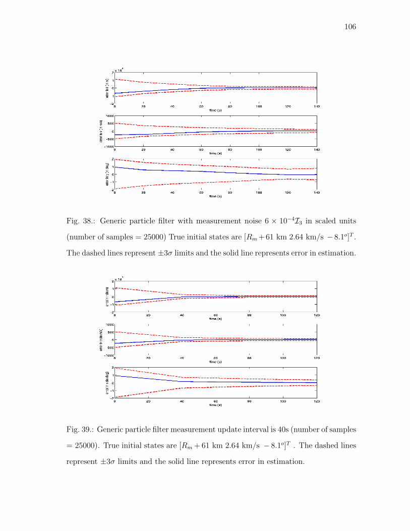
106
Fig. 38.: Generic particle filter with measurement noise 6 × 10⁻⁴I3 in scaled units
(number of samples = 25000) True initial states are [Rm+ 61 km 2.64 km/s −8.1o]T .
The dashed lines represent ±3σ limits and the solid line represents error in estimation.
Fig. 39.: Generic particle filter measurement update interval is 40s (number of samples
= 25000). True initial states are [Rm + 61 km 2.64 km/s − 8.1o]T . The dashed lines
represent ±3σ limits and the solid line represents error in estimation.
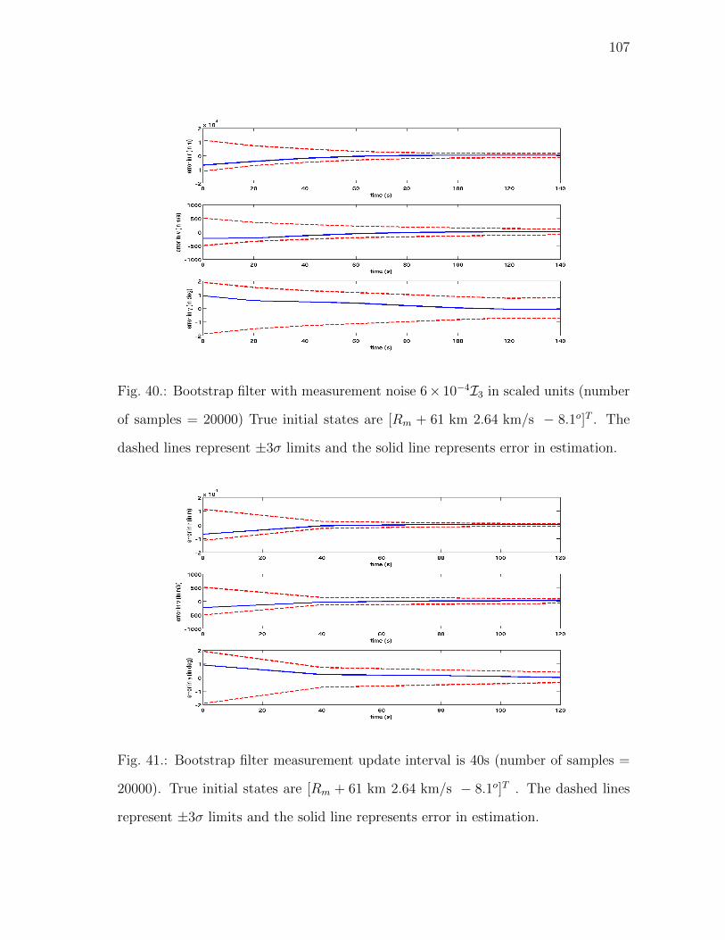
107
Fig. 40.: Bootstrap filter with measurement noise 6× 10⁻⁴I3 in scaled units (number
of samples = 20000) True initial states are [Rm + 61 km 2.64 km/s − 8.1o]T . The
dashed lines represent ±3σ limits and the solid line represents error in estimation.
Fig. 41.: Bootstrap filter measurement update interval is 40s (number of samples =
20000). True initial states are [Rm + 61 km 2.64 km/s − 8.1o]T . The dashed lines
represent ±3σ limits and the solid line represents error in estimation.

108
3. Application to Six-State Vinh’s Equation
The estimation algorithm presented, is then applied to reentry of a hypersonic vehicle
in Mars’ atmosphere, with dynamics governed by six-state Vinh’s equation [101]. The
equation of motion are given by,
r = v sin γ, (4.18a)
θ =v cos γ cos ξ
r cosλ, (4.18b)
λ =v cos γ sin ξ
r, (4.18c)
v = − ρv2
2Bc
− g sin γ − Ω2r cosλ(sin γ cosλ− cos γ sinλ sin ξ), (4.18d)
γ =(vr− g
v
)cos(γ) +
ρ
2Bc
(L
D
)v cosσ + 2Ω cosλ cos ξ
+Ω2r
vcosλ(cos γ cosλ+ sin γ sinλ sin ξ), (4.18e)
ξ =ρ
2Bc
(L
D
)v sinσ − v
rcos γ cos ξ tanλ+ 2Ω(tan γ cosλ sin ξ − sinλ)
− Ω2r
v cos γsinλ cosλ cos ξ, (4.18f)
where θ is the geocentric longitude, λ is the geocentric latitude and ξ is the hypersonic
vehicle’s heading angle. Ω is the angular velocity of Mars given by 7.0882×10⁻⁵ rad/s,
and σ is the bank angle which is taken as 0o in this case.
The measurement model, y, consists measurements of geocentric latitude and
longitude, θ and λ, along with dynamic pressure q, heating rate H, and flight path
angle, γ, whose expressions are given in Eqn. (3.35a) through Eqn. (3.35c). Hence,
the measurement model is given by y = [q H G θ λ]T .
The vehicle’s heading angle ξ, is assumed to have no initial state uncertainty, and
has initial value of 0.0573o. Gaussian initial condition uncertainty, along r, θ, λ, v,&γ

109
is considered, with mean, µ0 and standard deviation σ0 given by
µ0 = [Rm + 54 Km,−60o, 30o, 2.4 Km/s,−9o]T (4.19a)
σ0 =
5.4 Km 0 0 0 0
0 3o 0 0 0
0 0 3o 0 0
0 0 0 240 m/s 0
0 0 0 0 0.9o
. (4.19b)
A nondimensionalized system is created, scaling each constants in Eqn. (4.18a)
through Eqn. (4.18f), using scaling constants given in Table IV. The normalization
factors used for measurements are given in Table VII.
Table VII.: Normalization factors used for measurements
Measurement Normalization Factors
Dynamic Pressure 1.97× 10³ Nm
Heating Rate 0.0231 Jm-s
Flight Path Angle 19.13o
Geocentric Longitude 60.6o
Geocentric Latitude 30.3o
The performance of FP operator based filter is then compared with generic par-
ticle filter and bootstrap filter, when applied to the six-state Vinh’s equation model.
The initial states of the actual system are assumed to be,
[Rm + 61 km,−60.6o, 30.3o, 2.42Km/s,−9.09o, 0.0573o]
in this case, with θ, λ, v, and γ having 1% error in initial state estimate. The

110
measurement update interval is kept fixed at 20 seconds. Figure 42 shows the plot
for FP operator based filter with 9000 samples. Figure 43 and Fig. 44 shows plots for
generic particle filter and bootstrap filter respectively, with same number of particles.
It can be seen that FP operator based estimator performs better than particle filter
based estimators. The errors for the generic particle filter and bootstrap filter diverge
and are not inside the ±3σ limits. Hence, these filters are inconsistent, when same
number of particles as FP operator are taken.
The best performance that was achieved using particle filter and bootstrap filter
is shown in Fig. 45 and Fig. 46 respectively. The number of particles needed for
generic particle filter is 30000 and bootstrap filter is 25000. For particle filter, it
is observed that although the ±3σ bounds converge, the estimation errors escape
outside these limits. For the bootstrap filter, the errors and the ±3σ limits converge,
but for γ the ±3σ bounds diverge towards the end of estimation period.
F. Limitations of Using Frobenius-Perron Operator
Although FP operator provides us with an exact methodology to propagate uncer-
tainty in nonlinear dynamical systems, it has certain limitations. Throughout the
analysis, we have dealt with systems that have only parametric or initial condition
uncertainty. We have neglected the presence of process noise in a system.
For a system with process noise, evolution of densities are governed by the Fokker
Planck operator. Thus Eqn. (4.7) consists of not only the first order, but second order
derivatives too. The next chapter presents a complete treatise of such systems, and
develops a methodology to propagate uncertainty in dynamical systems with process
noise.

111
(a) Plots for r, v and γ.
(b) Plots for θ and λ.
Fig. 42.: Performance of FP operator based filter with 9000 particles, when applied
to six state Vinh’s equation. The dashed lines represent ±3σ limits and the solid line
represents error in estimation.

112
(a) Plots for r, v and γ.
(b) Plots for θ and λ.
Fig. 43.: Performance of generic particle filter with 9000 particles, when applied to
six state Vinh’s equation. The dashed lines represent ±3σ limits and the solid line
represents error in estimation.

113
(a) Plots for r, v and γ.
(b) Plots for θ and λ.
Fig. 44.: Performance of the bootstrap filter with 9000 particles, when applied to
six state Vinh’s equation. The dashed lines represent ±3σ limits and the solid line
represents error in estimation.

114
(a) Plots for r, v and γ.
(b) Plots for θ and λ.
Fig. 45.: Performance of generic particle filter with 30000 particles, when applied to
six state Vinh’s equation. The dashed lines represent ±3σ limits and the solid line
represents error in estimation.
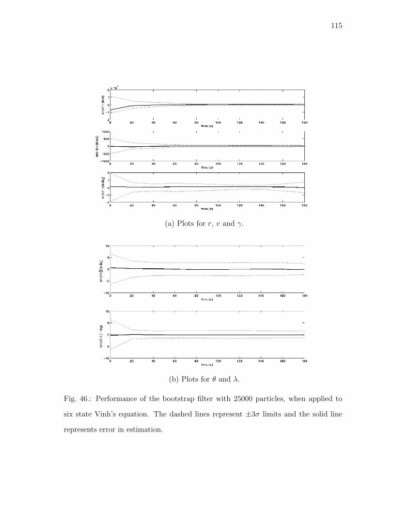
115
(a) Plots for r, v and γ.
(b) Plots for θ and λ.
Fig. 46.: Performance of the bootstrap filter with 25000 particles, when applied to
six state Vinh’s equation. The dashed lines represent ±3σ limits and the solid line
represents error in estimation.

116
CHAPTER V
THE KARHUNEN LOEVE EXPANSION
Up until this point, we have developed theories for uncertainty propagation in dy-
namical systems, which have only parametric or initial state uncertainty. However,
the given model in a dynamical system may not match actual state evolution of the
system. There may be uncertainties coming from unmodeled dynamics, modeling
uncertainties and other phenomena which may be difficult to incorporate in the true
system. Moreover, there may be some uncertainties in the actuation system, which
was ignored during model development. Generally all the above mentioned uncertain-
ties are coupled as one term, in the dynamical equation, which is called stochastic
forcing term or the process noise term.
In this chapter, we will deal with the methodology applied to characterize the
process noise term in an dynamical system. At first we will introduce such dynamical
systems, methodology of solution, and how uncertainty propagates through such sys-
tems. Then, we will describe the Karhunen Loeve (KL) expansion and how it can be
used to represent the process noise term in a stochastic dynamical system, followed
by some applications. Finally we will assess the convergence of the solution of the
dynamical system, to the true solution, when the process noise term is expanded
using a finite term KL expansion.
A. Stochastic Dynamical Systems
Consider the dynamical system given by,
dx (t) = f (x (t) , δ) dt+ g (x (t) , δ) dW (t) , (5.1)

117
where x (t) ∈ Rn is the state vector at time t, δ ∈ Rp is the vector of uncertain
parameters, and dW (t) ∈ Rq, is a random process denoting process noise. The
function f (., .), g (., .) represent the dynamics while the function-valued matrix, g (., .)
denotes noise coupling.
Equation (5.1) is referred to as stochastic dynamical system, or often stochastic
differential equation. We will provide a brief overview of the solution methodologies
of this equation, next.
1. Solution Methodology
Over the years, researchers have done a lot of work regarding solutions of stochastic
differential equations [113, 114, 115, 116, 117]. A complete treatise of the solution
methodology can be found in Øksendal [116]. Most commonly, dW (t) is considered
as a Wiener process [118] with E [W (t)] = 0 and E [W (t)W (t′)] = Qδ(t − t′) for all
t > t′
with t, t′ ∈ R+, where Q ∈ Rq×q is the correlation matrix of the noise. Hence
Eqn. (5.1) can be written as
dx(t)
dt= f (x (t) , δ) + g (x (t) , δ) η(t). (5.2)
Here η(t) is called the Gaussian white noise which is the derivative of the Wiener
process. It has been seen [116], that there exists no process with continuous paths
that satisfy η(t). In other words the Gaussian white noise process is a nowhere
differentiable process. Hence, solving Eqn. (5.2) is a hard problem. In the remainder
of the section, we will try to avoid using Eqn. (5.2), but get some sense of the solution
of the differential equation in Eqn. (5.1).
For general nonlinear systems, the state and the parametric uncertainty can be
expressed as in an extended framework with states z := [x, δ]T ∈ Rn+p. Without loss
of generality, it is assumed that the dynamical system in Eqn. (5.1) has only state

118
uncertainty, hence z = x. The modified equation is given by
dx (t) = f (x (t) , t) dt+ g (x (t) , t) dW (t) . (5.3)
Integrating Eqn. (5.3) till time T , we get
x(T ) = x(0) +
∫ T
0
f (x (t) , t) dt+
∫ T
0
g (x (t) , t) dW (t) . (5.4)
Integral of the type
∫ T
0
g (x (t) , t) dW (t) is called the Ito integral [116]. It is difficult
to solve this integral as the normal rules of Riemann-Stieltjes integration do not hold.
Hence a distance preserving map is done to a space where it can be integrated.
Let x(t) : (Ω,F)→ (Rn,B(Rn)), given t, where B(Rn) is the Borel σ-algebra on
Rn. Then the Ito integral can be written as
∫ T
0
g (ω, t) dW (t), where ω ∈ Ω.
Definition 3 Let V = V (S, T ) be a class of function
f(ω, t) : Ω× [0,∞)→ R,
such that
1. (ω, t) → f(ω, t) is F × B − measurable, where B is the Borel σ-algebra on
[0,∞).
2. f(ω, t) is Ft-adapted.
3. E[∫ T
S
f(ω, t)2dt
]<∞.
Using Ito Isometry (Chapter 3 of [116]), it can be shown that
E
[(∫ T
S
f (ω, t) dW (t)
)2]
= E[∫ T
S
f 2 (ω, t) dt
]∀f ∈ V (S, T ). (5.5)
It can also be shown under certain boundedness conditions, Eqn. (5.3) has unique
solutions. Detailed discussion of this topic has been omitted here and can be found

119
in Øksendal [116].
2. Uncertainty Propagation in Stochastic Dynamical Systems
Given the stochastic dynamical system in Eqn. (5.3), let the initial state random
variable be x(0). Also let us assume that the states x(t) admit a probability density
function (PDF) ρ(x, t), where (x, t) ∈ Rn × [0,∞], with the following properties.
1. Positivity : ρ(x, t) > 0,∀ t & x ∈ Rn.
2. Normalization constraint :
∫ ∞−∞
ρ(x, t)dV = 1,∀t ≥ 0 where dV = dx1dx2 . . . dxn.
Further let the initial state PDF ρ(x, 0) = ρ0 and the PDF at x = ∞, ρ(∞, t) = 0
be known. Then the evolution of uncertainty can be described by the following
linear parabolic partial differential equation which is also called the Fokker Planck
Kolmogorov (FPK) equation,
∂ρ(x, t)
∂t= −
n∑i=1
∂
∂xi(fiρ(x, t)) +
n∑i=1
n∑j=1
∂2
∂xi∂xj
((gQgT
)ijρ(x, t)
). (5.6)
This equation is to be solved with the boundary conditions ρ(0, x) = ρ0 and ρ(t,∞) =
0. Solving the above partial differential equation is computationally hard [55, 38].
Researchers have tried to solve this problem either numerically [119, 120, 44, 43], or by
using some basis function approximation [55, 45]. But all the solution methodologies
suffer from curse of dimensionality [60].
But if there is no stochastic forcing term Eqn. (5.6) reduced to stochastic Li-
ouville equation or Frobenius-Perron operator, whose solution methodology was pre-
sented in previous chapter. Here, we have used an approach of approximating the
process noise term in Eqn. (5.3) using KL expansion. The advantage of such repre-
sentation is that, the PDF evolution in the stochastic dynamical system can be found
using the FP operator. In the following section, we describe the methodology using

120
KL expansion to represent noise in Eqn. (5.3) and solving for the PDF using FP
operator.
B. The Karhunen Loeve Expansion Applied to Stochastic Dynamical Systems
The Karhunen Loeve (KL) expansion is a representation of a stochastic process as
an infinite linear combination of orthogonal functions [61, 62]. The theory of KL
expansion was developed from expanding any random process as a homogeneous
product of functions of deterministic and the stochastic variable. This framework was
first used in physics [63], to represent noise term in the Langevin equation. We will
discuss about this specific application in subsequent sections. In this framework the
class of such functions are chosen from the L2 space, such that the they span the whole
space and are linearly independent. Moreover, such a framework is advantageous as
it helps us analyze the random process in an space where inner product is defined.
Given the random process X(ω, t) where (ω, t) ∈ Ω× [0,∞), Ω being the sample
space, let us define the class of functions φi(t) ∈ L2 satisfying the following properties.
1. 〈φi(t), φj(t)〉 = δij,∀ i, j = 1, 2, . . . ,∞, 〈·, ·〉 represent inner product in L2.
2. span(φ1(t), φ2(t), ...) = span(L2).
Due to the fact that the φi(t) form the basis in L2 space, there are certain
restrictions on the random processes that can be represented in such a framework.
Here, we require that the random process is of second order, or E [X(ω, t)2] <∞,∀ t ∈
[0,∞), and that it is centered, i.e., E [X(ω, t)] = 0,∀ t.
Now, as we have specified the class of approximation functions to be used, we
will define the homogeneous representation of any random process. It is given by,
X(ω, t) =∞∑i=1
ξi(ω)φi(t), (5.7)
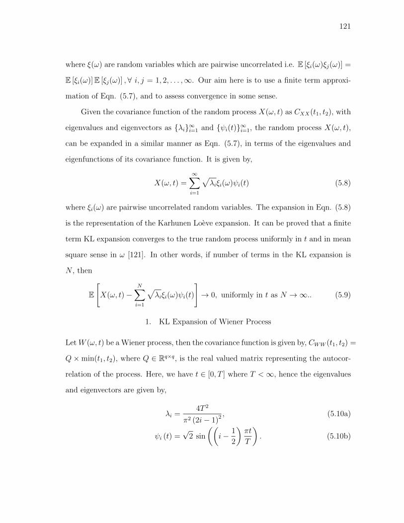
121
where ξ(ω) are random variables which are pairwise uncorrelated i.e. E [ξi(ω)ξj(ω)] =
E [ξi(ω)]E [ξj(ω)] , ∀ i, j = 1, 2, . . . ,∞. Our aim here is to use a finite term approxi-
mation of Eqn. (5.7), and to assess convergence in some sense.
Given the covariance function of the random process X(ω, t) as CXX(t1, t2), with
eigenvalues and eigenvectors as λi∞i=1 and ψi(t)∞i=1, the random process X(ω, t),
can be expanded in a similar manner as Eqn. (5.7), in terms of the eigenvalues and
eigenfunctions of its covariance function. It is given by,
X(ω, t) =∞∑i=1
√λiξi(ω)ψi(t) (5.8)
where ξi(ω) are pairwise uncorrelated random variables. The expansion in Eqn. (5.8)
is the representation of the Karhunen Loeve expansion. It can be proved that a finite
term KL expansion converges to the true random process uniformly in t and in mean
square sense in ω [121]. In other words, if number of terms in the KL expansion is
N , then
E
[X(ω, t)−
N∑i=1
√λiξi(ω)ψi(t)
]→ 0, uniformly in t as N →∞.. (5.9)
1. KL Expansion of Wiener Process
LetW (ω, t) be a Wiener process, then the covariance function is given by, CWW (t1, t2) =
Q×min(t1, t2), where Q ∈ Rq×q, is the real valued matrix representing the autocor-
relation of the process. Here, we have t ∈ [0, T ] where T <∞, hence the eigenvalues
and eigenvectors are given by,
λi =4T 2
π2 (2i− 1)2 , (5.10a)
ψi (t) =√
2 sin
((i− 1
2
)πt
T
). (5.10b)
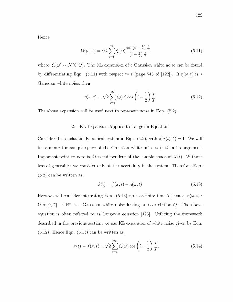
122
Hence,
W (ω, t) =√
2∞∑i=1
ξi(ω)sin(i− 1
2
)tT(
i− 12
)tT
, (5.11)
where, ξi(ω) ∼ N (0, Q). The KL expansion of a Gaussian white noise can be found
by differentiating Eqn. (5.11) with respect to t (page 548 of [122]). If η(ω, t) is a
Gaussian white noise, then
η(ω, t) =√
2∞∑i=1
ξi(ω) cos
(i− 1
2
)t
T(5.12)
The above expansion will be used next to represent noise in Eqn. (5.2).
2. KL Expansion Applied to Langevin Equation
Consider the stochastic dynamical system in Eqn. (5.2), with g(x(t), δ) = 1. We will
incorporate the sample space of the Gaussian white noise ω ∈ Ω in its argument.
Important point to note is, Ω is independent of the sample space of X(t). Without
loss of generality, we consider only state uncertainty in the system. Therefore, Eqn.
(5.2) can be written as,
x(t) = f(x, t) + η(ω, t) (5.13)
Here we will consider integrating Eqn. (5.13) up to a finite time T , hence, η(ω, t) :
Ω × [0, T ] → Rn is a Gaussian white noise having autocorrelation Q. The above
equation is often referred to as Langevin equation [123]. Utilizing the framework
described in the previous section, we use KL expansion of white noise given by Eqn.
(5.12). Hence Eqn. (5.13) can be written as,
x(t) = f(x, t) +√
2∞∑i=1
ξi(ω) cos
(i− 1
2
)t
T. (5.14)

123
Here we will use a finite term approximation of the Eqn. (5.14) and then assess
the convergence of solutions of approximated system to the actual solution. Let the
number of terms in the KL expansion in the RHS of Eqn. (5.14) be N , and the
approximate solution of Eqn. (5.14) be given by xN(t). The approximated system is
then given by,
xN(t) = f(xN , t) +√
2N∑i=1
ξi(ω) cos
(i− 1
2
)t
T. (5.15)
C. Convergence of Solutions
Due to finite term approximation of the process noise in Eqn. (5.13), the solution
obtained after propagation is not error-free. It is well known that, KL expansion
converges in mean square sense, to the underlying stochastic process as N → ∞.
But, same argument cannot be extended regarding the convergence of states xN (t) of
the dynamical system in Eqn. (5.15). To obtain a meaningful solution, there should
be some notion of convergence of the states in Eqn. (5.15) to states in Eqn. (5.13).
Hence, verification of the obtained solution is important in this scenario. Here, first
we will try to verify a weaker notion of convergence, before proving to a stronger
condition on the solutions. We first verify that the solution of Eqn. (5.15) and Eqn.
(5.13) converge in distribution. Then we have proved that under certain conditions,
the solutions converge in mean square sense.
1. Verification of Convergence in Distribution
In this section we have verified that the solution of the approximated dynamical
system converge to the true solution in distribution. Our approach here is mainly ap-
plication specific. Therefore, we have verified that given a dynamical system whether
the solution of the approximated system and the actual system converge in distribu-
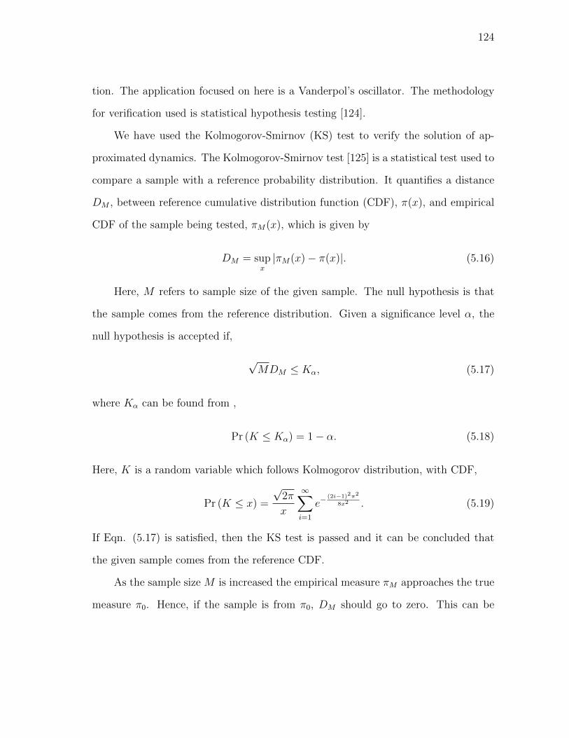
124
tion. The application focused on here is a Vanderpol’s oscillator. The methodology
for verification used is statistical hypothesis testing [124].
We have used the Kolmogorov-Smirnov (KS) test to verify the solution of ap-
proximated dynamics. The Kolmogorov-Smirnov test [125] is a statistical test used to
compare a sample with a reference probability distribution. It quantifies a distance
DM , between reference cumulative distribution function (CDF), π(x), and empirical
CDF of the sample being tested, πM(x), which is given by
DM = supx|πM(x)− π(x)|. (5.16)
Here, M refers to sample size of the given sample. The null hypothesis is that
the sample comes from the reference distribution. Given a significance level α, the
null hypothesis is accepted if,
√MDM ≤ Kα, (5.17)
where Kα can be found from ,
Pr (K ≤ Kα) = 1− α. (5.18)
Here, K is a random variable which follows Kolmogorov distribution, with CDF,
Pr (K ≤ x) =
√2π
x
∞∑i=1
e−(2i−1)2π2
8x2 . (5.19)
If Eqn. (5.17) is satisfied, then the KS test is passed and it can be concluded that
the given sample comes from the reference CDF.
As the sample size M is increased the empirical measure πM approaches the true
measure π0. Hence, if the sample is from π0, DM should go to zero. This can be

125
shown using the Glivenko-Cantelli lemma which states that,
supx∈R|πM − π0| → 0 almost surely. (5.20)
Due to the fact that M <∞, DM is a random variable, and each sample will give us
different DM values. The empirical distribution of√MDM is given by,
πMs (x) =1
Ms
Ms∑i=1
Ix<√MDiM, (5.21)
where Ms is the number of samples and DiM is the DM value for ith sample. Dvoretzky
Kiefer Wolfowitz inequality [126] states that,
Pr
(supx∈R|πMs(x)− πK(x)| > ε
)≤ 2e−2Msε2 ∀ε > 0, (5.22)
where πK(x) is the Kolmogorov CDF in Eqn. (5.19). Hence as Ms → ∞ the test
statistic√MDM exponentially converges in distribution to a Kolmogorov random
variable with rate 2e−2Msε2 . Detailed discussion of KS test can be found in ref.
[125, 127].
In the present case, the analytical representation of CDF at time t = T is not
known. Hence to verify our solution, we back-propagate the sample obtained after
propagation of Eqn. (5.15) at final time T to time t = 0 using the original dynamics
in Eqn. (5.13); and check if the back-propagated sample belongs to the initial CDF.
For simplicity of comparing CDFs we have used inverse transform sampling [128] to
convert the initial samples and samples obtained after back-propagation to uniformly
distributed samples in [0, 1].
Let the initial state, x(0) = x0 ∈ D0, have a CDF π0. Let the elements of
the sample; sampled from the initial CDF be x0,i, i = 1, . . . ,M , and elements after
propagation of Eqn. (5.15) be xT,i. Let the back-propagated sample obtained by

126
propagating Eqn. (5.13) from [T, 0] be x0,i. Here, we claim that, x0,i is a sample
from the initial CDF. Hence, using the KS test, the sample x0,i, is compared with
the initial CDF, for statistical significance. Here, we have used a multivariable KS
test, which is similar to the one presented in [125]. The verification methodology
employed, is described in algorithm 1.
We apply the proposed verification methodology to verify states of the Vander-
pol’s oscillator given by,
x1 (t) = x2 (t) (5.23a)
x2 (t) =(1− x2
1 (t))x2 (t)− x1 (t) + η (ω, t) . (5.23b)
We assume, the initial conditions are normally distributed, with CDF given by,
π0 ∼ N ([0, 0], diag [1, 1]), and the process noise has the autocorrelation Q = 2π. We
obtain Ms = 100 samples, each of sample size M = 500 from π0. The number of
terms in the KL expansion is fixed to N = 21. At first, we pick a sample from the 100
available samples and perform KS test on it. Figure 47 shows plot for the location
of elements initially (x0) and after back-propagation (x0), for the particular sample.
It is observed that the back-propagated sample, is clustered around the origin and
sparseness increases as we move away. This is in agreement with the physical intuition
of random samples drawn from π0 which is a standard normal distribution.
Using the methodology in [125] we obtain uniformly distributed sample y0 =
F (x0) using inverse transform sampling theory [128]. Figure 48 shows the plot of
empirical CDF of yj0 and the uniform CDF for the selected sample. It can be seen
that, visually the CDFs are close to each other. Hence, the value of DM for the
particular sample is expected to be less.

127
Algorithm 1 Verification of solutions of approximated dynamical systems using KL
expansion
Require: Domain D0, CDF π0, of initial parameters, significance level α, sample
size M , number of samples Ms, number of terms in KL expansion N .
1: Calculate Kα using Eqn. (5.17).
2: for j = 1 to Ms do. . Sample number counter.
3: Draw M elements xj0,i at random from D0. . Use Markov Chain Monte
Carlo.
4: Create null hypothesis H0 : π = π0 for the current sample
5: for i = 1 to M do. . Sample element counter.
6: Propagate xj0,i, from t = [0, T ], using Eqn. (5.15) to get xjT,i. . Use of KL
approximated dynamics with number of terms N .
7: Backward propagate xjT,i, from t = [T, 0] using Eqn. (5.13) to get xj0,i. .
Use of original stochastic dynamics.
8: Get yj0,i ← π0(xj0,i) . From inverse transform sampling theory, yj0 is
uniformly distributed in [0, 1].
9: end for
10: Calculate empirical CDF of the current sample yj0, GjM(y)← 1
M
M∑i=1
Iy≤yj0,i .
11: Calculate DjM ← sup
y∈[0,1]
|GjM(y)−G(y)|. . G(y) is the uniform CDF in [0, 1].
12: if DjM ≤ Kα√
Mthen.
13: Accept H0 for the jth sample.
14: else
15: Reject H0 for the jth sample.
16: end if
17: end for . Repeat the same test for the next sample

128
−4 −3 −2 −1 0 1 2 3−4
−3
−2
−1
0
1
2
3
4
x1
x 2
Original Sample
Back−Propagated Sample
Fig. 47.: Scatter plot of initial and the back-propagated elements for a given sample.
Blue circles are the original sample and the red ones are the back-propagated sample.
For the KS test, the value of α is fixed to 0.05. Hence, using Eqn. (5.18) and
Eqn. (5.19), we get Kα/√M = 0.0607. For the given sample, the value of DM was
0.0455. Hence, the null hypothesis, that the sample is drawn from a standard normal
distribution, is accepted with a significance level α = 0.05. Figure 49 shows plots for
DM values for all the 100 samples drawn. The samples above red line fail the test if
α = 0.05 and the samples above the black line fail, if α = 0.01. It is observed that 23
samples fail the test when α = 0.05 and 5 samples fail when α = 0.01. It can be seen
that, as the significance level α, is decreased, the chances that the null hypothesis is
accepted increases.
To get an idea of rate of convergence in solution with number of terms in KL
expansion, N , we plot the DM values by increasing N . Figure 50 shows plot for DM
values for 76 and 91 terms in KL expansion. It was found that with an α = 0.05,

129
Fig. 48.: Plot of empirical CDF of yj0 and uniform CDF for a given sample.
0 20 40 60 80 1000.03
0.04
0.05
0.06
0.07
0.08
0.09
Sample Number
DM
Val
ue
Fig. 49.: Plot DM value for all the 100 samples. The samples above the red and black
lines fail when α = 0.05 and 0.01 respectively.
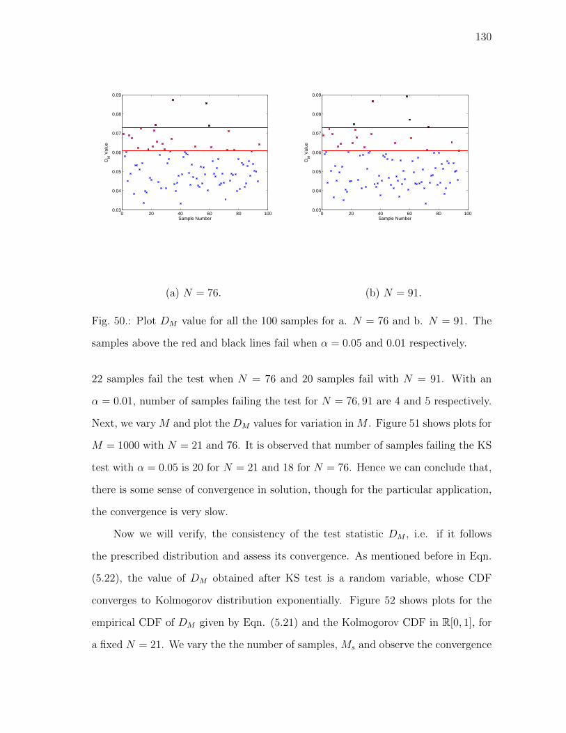
130
0 20 40 60 80 1000.03
0.04
0.05
0.06
0.07
0.08
0.09
Sample Number
DM
Val
ue
(a) N = 76.
0 20 40 60 80 1000.03
0.04
0.05
0.06
0.07
0.08
0.09
Sample Number
DM
Val
ue
(b) N = 91.
Fig. 50.: Plot DM value for all the 100 samples for a. N = 76 and b. N = 91. The
samples above the red and black lines fail when α = 0.05 and 0.01 respectively.
22 samples fail the test when N = 76 and 20 samples fail with N = 91. With an
α = 0.01, number of samples failing the test for N = 76, 91 are 4 and 5 respectively.
Next, we vary M and plot the DM values for variation in M . Figure 51 shows plots for
M = 1000 with N = 21 and 76. It is observed that number of samples failing the KS
test with α = 0.05 is 20 for N = 21 and 18 for N = 76. Hence we can conclude that,
there is some sense of convergence in solution, though for the particular application,
the convergence is very slow.
Now we will verify, the consistency of the test statistic DM , i.e. if it follows
the prescribed distribution and assess its convergence. As mentioned before in Eqn.
(5.22), the value of DM obtained after KS test is a random variable, whose CDF
converges to Kolmogorov distribution exponentially. Figure 52 shows plots for the
empirical CDF of DM given by Eqn. (5.21) and the Kolmogorov CDF in R[0, 1], for
a fixed N = 21. We vary the the number of samples, Ms and observe the convergence

131
0 20 40 60 80 1000.02
0.025
0.03
0.035
0.04
0.045
0.05
0.055
0.06
0.065
0.07
Sample Number
DM
Val
ue
α = 0.05
(a) N = 21.
0 20 40 60 80 1000.02
0.025
0.03
0.035
0.04
0.045
0.05
0.055
0.06
0.065
0.07
Sample Number
DM
Val
ue
α = 0.05
(b) N = 76.
Fig. 51.: Plot DM value for all the 100 samples for a. N = 21 and b. N = 76, with
increased M = 1000. The samples above the red line fails when α = 0.05.
0.8 1 1.2 1.4 1.6 1.8 20
0.1
0.2
0.3
0.4
0.5
0.6
0.7
0.8
0.9
1
Kolmogorov−Smirnov Test Statistic
Cum
ulat
ive
Pro
babi
lity
Dis
trib
utio
n
Fig. 52.: Plot of empirical CDF of√MDM (red) and Kolmogorov CDF (blue).

132
10 20 30 40 50 60 70 80 90 1000.5
0.55
0.6
0.65
0.7
0.75
Number of Samples (Ms)
sup x |F
Ms(x
) −
FK(x
)|
Fig. 53.: Plot of supx∈R|FMs(x)− FK(x)| vs. Ms .
in supx∈R|FMs(x) − FK(x)|. The variation is plotted in Fig. 53. It can be seen that
supx∈R|FMs(x)−FK(x)| decreases exponentially as we increaseMs, which is in compliance
with the theory. Due to the fact that the convergence is in probability but only
one realization of supx∈R|FMs(x) − FK(x)| has been plotted here, we do not observe a
monotonic behavior in convergence. But, there are very few outliers, as the probability
in the left hand side of Eqn. (5.22) can be decreased arbitrarily by varying ε.
2. Convergence in Mean Square Sense
In the last section, we have shown that there is some sense of convergence between
solutions of the approximated system in Eqn. (5.15) and the actual system in Eqn.
(5.13). We will here prove a stronger notion of convergence that the solutions actually
converge in mean square sense. Before, showing that we state the following theorem,
Theorem 1 Let x (ω, t) be the solution of the nonlinear stochastic differential equa-

133
tion (SDE),
dx(t) = f(x, t)dt+ dW (ω, t) (5.24a)
⇒ dx (t)
dt= f (x, t) + η(ω, t), (5.24b)
where f : Rn × [0, T ]→ Rn satisfies the following conditions
1. Non-explosion condition: there exists D ≥ 0, |f (x, t)| < D(1 + |x|) where
x ∈ Rn.
2. Lipschitz condition: there exists C ≥ 0, and x, y ∈ Rn |f (x, t)− f (y, t)| <
C |x− y|.
Let xN (t) be solution of the differential equation, formed by N−term approximation
of η(ω, t) in Eqn. (5.24b), using orthonormal basis, which is given by
dxN (t)
dt= f (xN , t) + ηN(ω, t), (5.25)
where ηN(ω, t) is the N-term approximation and E[∫ T
0
ηN(ω, t)dt
]<∞. Then
limN→∞
E[|x (t)− xN (t)|2
]→ 0, (5.26)
uniformly in t, iff xN (t) is the Karhunen Loeve (KL) expansion of x (t).
Proof Throughout the proof, we will write x(t) as x(ω, t) where ω ∈ Ω is the sample
space of the random process x(t). First we will prove that if Eqn. (5.26) holds then
xN (ω, t) is the KL expansion of x (ω, t).
Let φm(t) be the set of any orthonormal basis, then x (ω, t) can be written as a
convergent series as,
x (ω, t) =∞∑m=1
am(ω)φm(t),

134
without loss of generality we assume am(ω) = bmcm(ω). Hence the above expansion
becomes
x (ω, t) =∞∑m=1
bmcm(ω)φm(t). (5.27)
Let the solution in Eqn. (5.25) be a N−term approximation of x (ω, t) which converge
to true solution in mean square sense, given by
xN (ω, t) =N∑m=1
bmcm(ω)φm(t). (5.28)
Hence the error eN is given by
eN (ω, t) =∞∑
m=N+1
bmcm(ω)φm(t). (5.29)
Projecting x (ω, t) in φm we get
cm(ω) =1
bm
∫ T
0
x(ω, t)φm(t)dt. (5.30)
Hence,
E [eN (ω, t)] =∞∑
m=N+1
∞∑k=N+1
φm(t)φk(t)
∫ T
0
∫ T
0
E [x (ω, t1)x (ω, t2)]φm(t1)φk(t2)dt1dt2
=∞∑
m=N+1
∞∑k=N+1
φm(t)φk(t)
∫ T
0
∫ T
0
Cxx(t1, t2)φm(t1)φk(t2)dt1dt2, (5.31)
where Cxx(t1, t2) is the covariance function of x(ω, t). For uniform convergence of
error in t, the orthonormal basis φm(t) should minimize
∫ T
0
E [eN (ω, t)] dt. So taking
into account orthonormality of φm(t) we get∫ T
0
E [eN (ω, t)] dt =∞∑
m=N+1
∫ T
0
∫ T
0
Cxx(t1, t2)φm(t1)φm(t2)dt1dt2, (5.32)

135
which is to be minimized subject to∫ T
0
φm(t)φk(t)dt = δmk ∀m, k ∈ N. (5.33)
So using the method of Lagrange multipliers our objective function is
F (φm(t)) = minφm(t)
∞∑m=N+1
∫ T
0
∫ T
0
Cxx(t1, t2)φm(t1)φm(t2)dt1dt2
−b2m
(∫ T
0
φm(t)φm(t)dt− 1
), (5.34)
where b2m are the Lagrange multipliers. Differentiating above equation with respect
to φm(t) and setting the derivative to zero we get∫ T
0
[∫ T
0
Cxx(t1, t2)φm(t1)dt1 − b2mφm(t2)
]dt2 = 0 (5.35)
which is satisfied when∫ T
0
Cxx(t1, t2)φm(t1)dt1 = b2mφm(t2) (5.36)
which is the Fredholm integral equation for the random process x (ω, t). Hence φm(t)
and b2m are the eigenfunctions and eigenvalues of Cxx(t1, t2) respectively, which com-
pletes our proof.
Now we will prove that, if xN(ω, t) is the KL expansion of x(ω, t), then to ensure
that solution of Eqn. (5.25) converge to solution of Eqn. (5.24b) in mean square
sense, xN(ω, t) should be the solution of Eqn. (5.25). To prove this, we propose the
following uniqueness conditions on solution of Eqn. (5.24b) and KL expansion of a
random process.
Proposition 1 Given the non-explosion condition and the Lipschitz condition are
satisfied for f (·, ·) in Eqn. (5.24b). Let Z be a random variable, independent of

136
the σ-algebra Fm∞ generated by η(ω, t), t ≥ 0 and E [|Z|2] ≤ ∞. Then the stochastic
differential equation in Eqn. (5.24b) where t ∈ [0, T ], X(ω, 0) = Z has a unique t-
continuous solution x(ω, t) with the property that x(ω, t) is adapted to the filtration
FZt generated by Z and η(ω, t), t ≥ 0 and E[∫ T
0
|x(ω, t)|2dt]≤ ∞.
Proof See [116], Chapter 5.
Proposition 2 The Karhunen Loeve expansion of the random process x(ω, t) given
by x(ω, t) =∞∑m=1
√λmξm(ω)φm(t) is unique.
Proof See [25], Chapter 2.
Let us assume that yN(ω, t) is the KL expansion of x(ω, t). Furthermore assume
that yN(ω, t) 6= xN(ω, t), which is the solution of Eqn. (5.25). Hence, we assume
that although yN(ω, t) is the KL expansion of x(ω, t) it does not satisfy Eqn. (5.25),
whose solution converge to the solution of Eqn. (5.24b) in mean square sense.
Proposition 1 and 2 says that the solution of SDE is unique and any random
process has an unique KL expansion. Also Eqn. (5.25) has unique solution as RHS
of Eqn. (5.25) satisfies Lipschitz condition. This can be proven as follows: for right
hand side of Eqn. (5.25) to be Lipschitz we must have
|f(x, t) + ηN(ω, t)− f(y, t)− ηN(ω, t)| ≤ C |x− y|
⇒ |f(x, t)− f(y, t)| ≤ C |x− y| .
which is true as f(·, ·) satisfies Lipschitz condition.
Hence Eqn. (5.24b) has unique solution which has an unique KL expansion.
Also according to our assumption, the solution of Eqn. (5.25) converge to solution of
Eqn. (5.24b) in mean square sense. This contradicts our assumption that yN(ω, t) 6=
xN(ω, t) as we have proved that Eqn. (5.25) has unique solutions, and for mean

137
square convergence in solutions of Eqn. (5.25) and Eqn. (5.24b), xN(ω, t) must be
the KL expansion of x(ω, t), which completes our proof.
Special Case Let ηN(ω, t) be the N -term KL expansion of η(ω, t). Given by,
ηN(ω, t) =N∑m=1
√ληmξ
Wm (ω)φWm (t). (5.37)
Since ηN(ω, t) is the KL expansion, we have E[∫ T
0
ηN(ω, t)dt
]<∞ [25]. Hence the
solutions of Eqn. (5.25) converge to the solution of Eqn. (5.24b) in mean square
sense. So, we suggest a corollary.
Corollary 2 Given the stochastic differential equation in Eqn. (5.24b), where f(·, ·)
satisfies the non-explosion and the Lipschitz condition, if the N-term approximation
of η(ω, t) in Eqn. (5.25), ηN(ω, t), is given by the KL expansion of η(ω, t) then the
solution of Eqn. (5.25) converges to the solution of Eqn. (5.24b) in mean square
sense.
Using corollary 2 we have showed that if the non-explosion and Lipschitz con-
ditions are satisfied then the solution of Eqn. (5.25) converge to solution of Eqn.
(5.24b) in mean square sense. In other words, if the process noise term in Eqn. (5.13)
is approximated using KL expansion, then the solutions of Eqn. (5.15) and Eqn.
(5.13) converge in mean square sense.
This proof gives us a framework to apply KL expansion to stochastic dynamical
systems. In the next section, we will describe the methodology employed to predict
evolution of probability density in stochastic dynamical systems using this framework.

138
D. Karhunen Loeve Frobenius-Perron Formulation
Let us consider the dynamical system given in Eqn. (5.13) where x ∈ Rn are the
states, having initial CDF π(x, 0) = π0. Let us also assume that the initial CDF
admits a PDF given by ρ0. The stochastic forcing term η(ω, t) in Eqn. (5.13) is
approximated using KL expansion having finite number of terms (N). In the present
case, where η(ω, t) is a Gaussian white noise, the approximation reduces to,
η (ω, t) =√
2N∑i=1
ξi (ω) cos
((i− 1
2
)πt
T
), (5.38)
After substituting the expression in Eqn. (5.38) in Eqn. (5.13) we get the differential
Eqn. (5.15).
Using the methodology given in [129, 130] and as presented in the previous
section, MOC is applied to Eqn. (4.7), and an augmented dynamical system is formed,
with states [xN (t) , ρ (x, t)]T , where ρ (x, t) is the probability density of the states at
time t, and xN (t) = [x1N (t) , . . . , xnN (t)]T . The augmented system is given by,
xN (t) = f (xN , t) +√
2N∑i=1
ξi (ω) cos
((i− 1
2
)πt
T
), (5.39a)
ρ(xN , t) = − div f (xN , t) ρ(xN , t), (5.39b)
where div f (x, t) =n∑i=1
∂f (x, t)
∂xi (t). Equation (5.39a) & Eqn. (5.39b) can be solved
to get the value of ρ (xN , t) along the characteristic curves of Eqn. (4.7). Detailed
discussion of the solution methodology has been presented in the previous section.

139
1. Illustrative Examples
The proposed methodology is applied to a Vanderpol’s oscillator, whose dynamics is
governed by,
x (t) =(1− x2 (t)
)x (t)− x (t) + ξ (t) , (5.40)
and to a Duffing oscillator, with dynamics,
x (t) = 10x (t)− 30x3 (t)− 10x (t) + ξ (t) , (5.41)
with ξ (t) having zero mean and autocorrelation 2πI. The initial state uncertainty,
has a PDF ρ0(z) ∼ N([0, 0]T , diag (1, 1)
)for both the systems in Eqn. (5.40) and
Eqn. (5.41).
Let x1 (t) = x (t) and x2 (t) = x (t), the augmented dynamical system for the
Vanderpol’s oscillator is given by,
x1 (t) = x2 (t) (5.42a)
x2 (t) =(1− x2
1 (t))x2 (t)− x1 (t) + ξ (t) (5.42b)
ρ (x (t)) = −(1− x2
1 (t))ρ (x (t)) , (5.42c)
and for the Duffing oscillator, is given by,
x1 (t) = x2 (t) (5.43a)
x2 (t) = 10x1 (t)− 30x31 (t)− 10x2 (t) + ξ (t) (5.43b)
ρ (x (t)) = 10ρ (x (t)) . (5.43c)
Next, the initial PDF, ρ0 is sampled, with sample size of M = 500. For the Vander-
pol’s oscillator, final time T is 1s, for the Duffing oscillator T = 3s. Number of terms
in the KL expansion is fixed to N = 7. Figure 54 shows the evolution of probability

140
densities with time for the two oscillators. The density value ρ (x, t) is color coded
with red representing high density value and blue representing low. It is observed
that, for the Vanderpol’s oscillator the probability mass accumulates along the limit
cycle and for the Duffing oscillator, we get a bimodal PDF at final time. This is in
agreement with the physical intuition of behavior of these systems.
E. State Estimation Using Karhunen Loeve Expansion and Frobenius-Perron Oper-
ator
We apply the proposed methodology of using Karhunen Loeve and Frobenius-Perron
(KLFP) operator, for uncertainty propagation to estimate states of a nonlinear sys-
tem. The nonlinear estimation algorithm used is same as the one described in the
previous chapter, that uses FP operator. First, we apply this to a Vanderpol’s oscilla-
tor system, then we use the proposed methodology to estimate states of a hypersonic
reentry vehicle. Here, we draw random particles (elements) from the domain D0 of
x(t = 0). Propagation of uncertainty is done using Eqn. (5.39a) & Eqn. (5.39b).
By using this framework for nonlinear estimation purposes, we get the exact value of
prior PDF after propagation. This gives us significant advantage over particle filters
where, generally the prior PDF is approximated using histograms. Bayesian inference
is used to update the posterior PDF from prior for each particle.
1. State Estimation of Vanderpol’s Oscillator
In the present work, the system used is the Vanderpol’s oscillator described by Eqn.
(5.40). We use a nonlinear measurement model which is given by
y (t) = x21 (t) + x2
2 (t) + ζ (t) (5.44)

141
(a) Perspective view of the PDFs along direction(π4, π
4, π
4
).
(b) Top view of the PDFs along direction(π2, π
2, 0).
Fig. 54.: Uncertainty propagation for Vanderpol’s oscillator Eqn. (5.40) in top row
of each figure, and Duffing oscillator Eqn. (5.41) in bottom row of each figure.

142
where ζ (t) is zero mean Gaussian measurement noise with autocorrelation R =
6× 10⁻². The process noise, η (x, t) also considered to have zero mean and an auto-
correlation of Q = 6× 10⁻¹.
We consider the initial state uncertainty to be normally distributed with E [x(0)] =
[0, 0]T and E [x(0)2] = diag (1, 1). It is assumed that the initial states of the actual
system is [0.25, 0.25], with initial error in estimation being [0.25, 0.25]. The measure-
ment update interval was fixed to 0.1s and final time T was assumed to be T = 1s.
The performance of the proposed filter is compared with the generic particle
filter given in [9]. The sample size for each estimator is fixed to 500 elements. The
simulations were performed on a Linux machine with Intel R© Pentium D processor.
Figure 55 shows the ±3σ plots for the estimators. No major difference can be ob-
served in the performance of the estimators as the errors in estimation are within the
±3σ limits and converge. But if we compare the computational time, KLFP-based
estimator takes 58.46s per filtering step, whereas the generic particle filter the time
taken is 284.19s. Thus it can be concluded, given same sample size and the same
processing environment, KLFP-based estimator achieves similar performance as the
generic particle filter, and is almost five times faster than the particle filter based
estimator.
2. Application to Hypersonic Reentry
The state estimation methodology is now applied to estimate states of a hypersonic
reentry vehicle. The equations of motion are described by a six state Vinh’s equation
which is similar to the equations used in the previous section. Here we add process

143
(a) KLFP-based estimator. Magenta: Errorin estimation, black: ±3σ bounds.
(b) Generic particle filter. Blue- Error in esti-mation, red- ±3σ bounds.
Fig. 55.: ±3σ plots for a) KLFP-based estimator and b) Generic particle filter.
noise to states r and v. The equations with process noise are given by,
r =v sin γ + ηr, (5.45a)
θ =v cos γ cos ξ
r cosλ, (5.45b)
λ =v cos γ sin ξ
r(5.45c)
v =− ρv2
2Bc
− g sin γ − Ω2r cosλ(sin γ cosλ− cos γ sinλ sin ξ) + ηv (5.45d)
γ =(vr− g
v
)cos(γ) +
ρ
2Bc
(L
D
)v cosσ
+ 2Ω cosλ cos ξ +Ω2r
vcosλ(cos γ cosλ+ sin γ sinλ sin ξ) (5.45e)
ξ =ρ
2Bc
(L
D
)v sinσ − v
rcos γ cos ξ tanλ
+ 2Ω(tan γ cosλ sin ξ − sinλ)− Ω2r
v cos γsinλ cosλ cos ξ, (5.45f)
where ηr and ηv are zero mean, Gaussian white noises with autocorrelation Q =
6×10⁻², in scaled units. The other constants have the same values as in the previous

144
section. The initial condition uncertainty is assumed to be Gaussian with mean and
covariance given by,
µ0 = [Rm + 54 Km,−60o, 30o, 2.4 Km/s,−9o, 0.0573o]T (5.46a)
σ0 =
5.4 Km 0 0 0 0 0
0 3o 0 0 0 0
0 0 3o 0 0 0
0 0 0 240 m/s 0 0
0 0 0 0 0.9o 0
0 0 0 0 0 0.0057o
. (5.46b)
A nondimensionalized system is constructed by scaling each term in Eqn. (5.45a)
through Eqn. (5.45f) with scaling constants. We use the same scaling constants as
used in previous two section which are given in Table IV.
The measurement model consists of the dynamic pressure q the heating rate H,
the flight path angle γ, and measurements along geocentric longitude and latitude
θ and λ. Here we add another observation where we observe the azimuth angle ξ.
Hence
y =
(q H γ θ λ ξ
)(5.47)
The constants scaling the measurements are given in Table VIII. We assume mea-
surement noise added to each state with constant autocorrelation R = 6× 10⁻¹.
The true states are assumed to be [Rm+61 km,−60.6o, 30.3o, 2.42 km/s,−9.09o,
0.0573o], hence the estimation algorithms start with an initial error. The measurement
update interval is kept fixed at 10 seconds.
Figure 56 shows plots for ±3σ limits and estimation error for particle filter. We
can see that the errors diverge and the ±3σ limits do not converge, for all the states
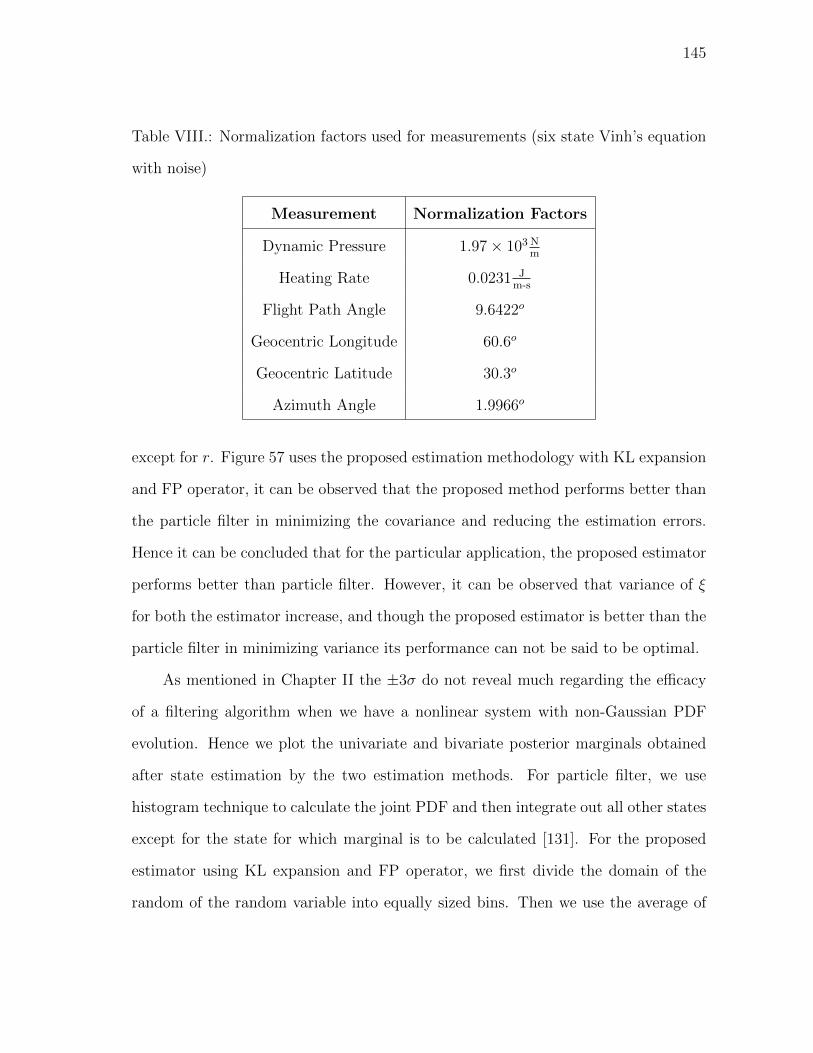
145
Table VIII.: Normalization factors used for measurements (six state Vinh’s equation
with noise)
Measurement Normalization Factors
Dynamic Pressure 1.97× 10³ Nm
Heating Rate 0.0231 Jm-s
Flight Path Angle 9.6422o
Geocentric Longitude 60.6o
Geocentric Latitude 30.3o
Azimuth Angle 1.9966o
except for r. Figure 57 uses the proposed estimation methodology with KL expansion
and FP operator, it can be observed that the proposed method performs better than
the particle filter in minimizing the covariance and reducing the estimation errors.
Hence it can be concluded that for the particular application, the proposed estimator
performs better than particle filter. However, it can be observed that variance of ξ
for both the estimator increase, and though the proposed estimator is better than the
particle filter in minimizing variance its performance can not be said to be optimal.
As mentioned in Chapter II the ±3σ do not reveal much regarding the efficacy
of a filtering algorithm when we have a nonlinear system with non-Gaussian PDF
evolution. Hence we plot the univariate and bivariate posterior marginals obtained
after state estimation by the two estimation methods. For particle filter, we use
histogram technique to calculate the joint PDF and then integrate out all other states
except for the state for which marginal is to be calculated [131]. For the proposed
estimator using KL expansion and FP operator, we first divide the domain of the
random of the random variable into equally sized bins. Then we use the average of

146
(a) Plots for r, v and γ.
(b) Plots for θ, λ and ξ.
Fig. 56.: Estimation errors (solid lines) and ±3σ limits (dashed lines) for particle
filter based estimator.

147
(a) Plots for r, v and γ.
(b) Plots for θ, λ and ξ.
Fig. 57.: Estimation errors (solid lines) and ±3σ limits (dashed lines) for estimator
using KL expansion and FP operator.

148
Fig. 58.: Plot for univariate marginal density for particle filter (dashed line) and KL
expansion and FP operator based estimator (solid line). Here h = r − Rm and the
y-axis denotes PDF value.
the density values of points, obtained after using FP operator, in a bin, to get the
PDF value for that particular bin. Detailed description of this method can be found
in ref. [129].
Figure 58 and Fig. 59 show plots for univariate and bivariate marginal density
respectively, for the two estimators compared in this chapter. There can be 15 state
combinations for bivariate densities, of which we show four combinations. It can be
observed that the dispersion of the particle filter based estimator is more than the
proposed estimator as the histogram approximation of PDF tend to smear out the
probability mass, whereas the proposed estimator captures the concentration of the
probability mass well. Hence it can be seen that proposed estimator is more successful
in capturing the actual reduction uncertainty than the particle filter.

149
Fig. 59.: Plot for bivariate marginal density for particle filter (top row) and KL
expansion and FP operator based estimator (bottom row) for 4 state combinations.
Here h = r −Rm. The PDF value is color coded, red is high PDF and blue is low.
F. Summary
In this section, we present an uncertainty quantification methodology, where the
process noise term is expanded using KL expansion and uncertainty is propagated
using FP operator. We have shown that if in a stochastic dynamical system if the noise
term is approximated using finite term KL expansion the solution of the approximated
dynamics converge to the actual solution in mean square sense. Moreover, we propose
an estimation technique based on Kl expansion and FP operator, and show that the
proposed estimator outperforms particle filter in terms of performance.

150
CHAPTER VI
CONCLUSIONS AND SCOPE OF FUTURE WORK
This dissertation has presented novel methods of uncertainty quantification of non-
linear system with emphasis on state estimation problems. Most of the real-world
systems deal with the problems of high dimensionality, nonlinearity and high uncer-
tainty. Hence, characterization of uncertainty is a difficult task in practice for these
systems. One of the major problems in this scenario is estimation of states and pa-
rameters. Most commonly used estimation algorithms, involve local linearization of
dynamics and assume Gaussian PDF evolution. But due to high nonlinearity of the
real-world systems, estimation becomes a difficult task to achieve.
There are estimation algorithms, based on Monte Carlo methods which alleviate
the problem of nonlinearity. But they have been observed to fail if the state space
dimension is high.
In this work we use the uncertainty quantification methods developed to esti-
mate states and parameters of a nonlinear system. We first present two methods
based on polynomial chaos framework. Polynomial chaos is a method where the any
random process is expanded as a linear combination of orthogonal polynomials of
the underlying random variable. The estimation algorithms use polynomial chaos for
forward propagation of uncertainty, and the update step or the inverse problem is
solved using higher order moment updates, and Bayesian inference. The proposed
method was applied to estimate states of a duffing oscillator and vehicle reentering
the atmosphere of Mars, and its performance was compared with EKF based esti-
mators. It was found that the performance of the PC based estimators was superior
than EKF for the particular application.
Next we presented an algorithm which uses Frobenius-Perron (FP) operator the-
151
ory for propagation of uncertainty. The FP operator given by a partial differential
equation, which dictates the evolution of densities in a dynamical system with para-
metric uncertainty. The power of FP operator is that we know the exact density
values at each sample points after propagation. We have formulated an estimation
algorithm based on FP operator and compared the results to particle filters. It was
found that the FP operator is computationally superior than the particle filtering
based estimators.
Finally we have proposed an estimation algorithm, when the dynamical system
has process noise in it. We use the Karhunen Loeve (KL) expansion to represent pro-
cess noise and then use FP operator based methodology to propagate uncertainty. We
have proved that the solutions of the stochastic differential equation when the noise
is approximated using KL expansion converge in mean square sense to the actual so-
lutions. Finally we have applied the proposed estimation algorithm to estimate states
of a duffing oscillator and Vinh’s equation. It was found that the proposed estimation
method is superior to the particle filtering method for the particular application.
A. Future Work
There are several directions in which one can work towards, from the methodologies
and algorithms developed in this dissertation. In this section we will discuss in brief
some of the future directions of research.
1. Stochastic Control
One of the main use of the methodologies of uncertainty quantification developed in
this dissertation is control of stochastic dynamical system. Up until now, stochastic
control methodologies mainly focus on minimizing the expectation of the underlying
152
cost function, amongst them the linear quadratic Gaussian formulation is widely used
[132]. But there are several systems for which it is difficult to minimize a cost function
based on expected value. In such cases, one can resort to providing performance
guarantees in a weaker sense like in distribution or probabilistic guarantees. The FP
operator technique can play an important role in such cases. One may use the fact
that the uncertainty propagation is exact in this case.
2. Multiphysical Dynamical Systems
More often than not we are faced with systems which are multiphysical in nature.
Dynamics in such systems evolve in different scales and are spatially and temporally
varying. The dynamical system in such cases is described by a partial differential
equation (PDE) [133]. Uncertainty management in such systems in a difficult prob-
lems and faces a lot of challenges, as the measurements are available in different scales
and of different quantities than which we want to estimate. Most of the methods for
quantification of uncertainty involve Monte Carlo (MC) simulations and suffer from
the curse of dimensionality [134]. We have observed that FP operator based method is
computationally superior than MC methods and predicts the uncertainty accurately.
The use of FP operator for parameter estimation and sensitivity analysis of dynami-
cal systems may help reduce the computational burden due to use Monte Carlo and
PDF approximation using histograms.
3. Dimensional Scaling
Almost all of the uncertainty quantification (UQ) algorithms suffer from the curse of
dimensionality. For MC methods the number of sample points needed to obtain a suf-
ficiently good estimate of the quantity of interest increase exponentially with increase
in dimension. Though FP operator was found to better than MC methods for UQ

153
in the particular application discussed in this dissertation, it fails if the dimension-
ality of the state space is very high. We can use dimensional scaling or dimensional
interpolation in such cases.
Dimensional scaling generalizes any system into a N dimensional representation,
and has been widely used in chemical physics [135]. It has been successfully applied to
solve the Schrodinger’s equation to find the ground state energy of a hydrogen atom
[136]. A technique has been intuitively proposed by Daum [137], where dimensional
scaling is used alongside FP operator for UQ in high dimensional systems. We can
use this technique for parameter estimation and uncertainty quantification of several
nonlinear systems, with large state space and high uncertainty.

154
REFERENCES
[1] R.E. Kalman, “A new approach to linear filtering and prediction problems,”
Journal of Basic Engineering, vol. 82, no. 1, pp. 35–45, 1960.
[2] B. Anderson, J.B. Moore, and M. Eslami, “Optimal filtering,” IEEE Transac-
tions on Systems, Man and Cybernetics, vol. 12, no. 2, pp. 235–236, 1982.
[3] G. Evensen, “Using the extended Kalman filter with a multilayer quasi-
geostrophic ocean model,” Journal of Geophysical Research, vol. 97, no. C11,
pp. 17905–17924, 1992.
[4] R.N. Miller, M. Ghil, and F. Gauthiez, “Advanced data assimilation in strongly
nonlinear dynamical systems,” Journal of the Atmospheric Sciences, vol. 51,
no. 8, pp. 1037–1056, 1994.
[5] P. Gauthier, P. Courtier, and P. Moll, “Assimilation of simulated wind lidar
data with a Kalman filter,” Monthly Weather Review, vol. 121, no. 6, pp.
1803–1820, 1993.
[6] F. Bouttier, “A dynamical estimation of forecast error covariances in an as-
similation system,” Monthly Weather Review, vol. 122, no. 10, pp. 2376–2390,
1994.
[7] S.J. Julier and J.K. Uhlmann, “A new extension of the Kalman filter to nonlin-
ear systems,” in Proceedings of Int. Symp. Aerospace/Defense Sensing, Simul.
and Controls, 1997, vol. 3, pp. 182–193.
[8] N.J. Gordon, D.J. Salmond, and A.F.M. Smith, “Novel approach to
nonlinear/non-Gaussian Bayesian state estimation,” in IEE Proceedings on
Radar and Signal Processing, 1993, vol. 140, pp. 107–113.

155
[9] M.S. Arulampalam, S. Maskell, N. Gordon, and T. Clapp, “A tutorial on
particle filters for online nonlinear/non-Gaussian Bayesian tracking,” IEEE
Transactions on Signal Processing, vol. 50, no. 2, pp. 174–188, 2002.
[10] A. Khalil, M.and Sarkar and S. Adhikari, “Nonlinear filters for chaotic oscilla-
tory systems,” Nonlinear Dynamics, vol. 55, pp. 113–137, 2009.
[11] P.W. Glynn and D.L. Iglehart, “Importance sampling for stochastic simula-
tions,” Management Science, pp. 1367–1392, 1989.
[12] G. Kitagawa, “Monte Carlo filter and smoother for non-Gaussian nonlinear
state space models,” Journal of Computational and Graphical Statistics, vol.
5, no. 1, pp. 1–25, 1996.
[13] A. Doucet, S.J. Godsill, and C. Andrieu, “On sequential Monte Carlo sampling
methods for Bayesian filtering,” Statistics and Computing, vol. 10, no. 3, pp.
197–208, 2000.
[14] H. Tanizaki, Nonlinear Filters: Estimation and Applications, Berlin: Springer-
Verlag, 1996.
[15] B. Ristic, S. Arulampalam, and N. Gordon, Beyond the Kalman Filter: Particle
Filters for Tracking Applications, Norwood, MA: Artech House Publishers,
2004.
[16] A. Doucet, N. De Freitas, and N. Gordon, Sequential Monte Carlo Methods in
Practice, New York: Springer-Verlag, 2001.
[17] F. Daum, J. Huang, and R. Co, “Curse of dimensionality and particle filters,”
in Proceedings of IEEE Aerospace Conference, 2003, pp. 4 1979–4 1993.
156
[18] C.S. Manohar and D. Roy, “Monte Carlo filters for identification of nonlinear
structural dynamical systems,” Sadhana Acad. Proc. Eng. Sciences, vol. 31,
pp. 399–427, 2006.
[19] J.S. Liu and R. Chen, “Sequential Monte Carlo methods for dynamic systems,”
Journal of the American Statistical Association, vol. 93, no. 443, pp. 1032–1044,
1998.
[20] N. Oudjane and C. Musso, “Progressive correction for regularized particle
filters,” in Proceedings of the Third International Conference on Information
Fusion. IEEE, 2000, vol. 2, pp. THB2–10.
[21] W.R. Gilks and C. Berzuini, “Following a moving target Monte Carlo inference
for dynamic Bayesian models,” Journal of the Royal Statistical Society: Series
B (Statistical Methodology), vol. 63, no. 1, pp. 127–146, 2001.
[22] C. Snyder, T. Bengtsson, P. Bickel, and J. Anderson, “Obstacles to high-
dimensional particle filtering,” Monthly Weather Review, vol. 136, no. 12, pp.
4629–4640, 2008.
[23] G. Casella and C.P. Robert, “Rao-Blackwellisation of sampling schemes,”
Biometrika, vol. 83, no. 1, pp. 81–94, 1996.
[24] F. Daum and R. Co, “Nonlinear filters: beyond the Kalman filter,” IEEE
Aerospace and Electronic Systems Magazine, vol. 20, no. 8 Part 2, pp. 57–69,
2005.
[25] R. G. Ghanem and P. D. Spanos, Stochastic Finite Elements: A Spectral
Approach, New York: Springer-Verlag, 1991.
157
[26] A. Lasota and M.C. Mackey, Chaos, Fractals, and Noise: Stochastic Aspects
of Dynamics, New York: Springer-Verlag, 1994.
[27] N. Wiener, “The homogeneous chaos,” American Journal of Mathematics, vol.
60, no. 4, pp. 897–936, 1938.
[28] R. H. Cameron and W. T. Martin, “The orthogonal development of nonlinear
functionals in series of Fourier-Hermite functionals,” The Annals of Mathemat-
ics, vol. 48, no. 2, pp. 385–392, 1947.
[29] D. Xiu and G. E. Karniadakis, “The Wiener–Askey polynomial chaos for
stochastic differential equations,” SIAM J. Sci. Comput., vol. 24, no. 2, pp.
619–644, 2002.
[30] R. Askey and J. Wilson, “Some basic hypergeometric polynomials that gen-
eralize Jacobi polynomials,” Memoirs Amer. Math. Soc., vol. 54, no. 314, pp.
1–4, 1985.
[31] T. Y. Hou, W. Luo, B. Rozovskii, and H-M. Zhou, “Wiener chaos expansions
and numerical solutions of randomly forced equations of fluid mechanics,” J.
Comput. Phys., vol. 216, no. 2, pp. 687–706, 2006.
[32] D. Xiu and G. E. Karniadakis, “Modeling uncertainty in flow simulations via
generalized polynomial chaos,” J. Comput. Phys., vol. 187, no. 1, pp. 137–167,
2003.
[33] R. Ghanem and J. Red-Horse, “Propagation of probabilistic uncertainty in
complex physical systems using a stochastic finite element approach,” Phys. D,
vol. 133, no. 1-4, pp. 137–144, 1999.

158
[34] R.G. Ghanem, “Ingredients for a general purpose stochastic finite elements
implementation,” Comput. Methods Appl. Mech. Eng., vol. 168, no. 1-4, pp.
19–34, 1999.
[35] C. Sandu E. D. Blanchard, A. Sandhu, “A polynomial chaos based Bayesian
approach for estimating uncertain parameters of mechanical systems part 1:
Theoretical approach,” Tech. Rep. TR-07-38, Computer Science Department,
Virginia Polytechnic Inst. and State Univ., Blacksburg, VA, 2007.
[36] C. Sandu E. D. Blanchard, A. Sandhu, “A polynomial chaos based Bayesian
approach for estimating uncertain parameters of mechanical systems part 2:
Application to vehicle systems,” Tech. Rep. TR-07-39, Computer Science De-
partment, Virginia Polytechnic Inst. and State Univ., Blacksburg, VA, 2007.
[37] R. Kubo, “Stochastic Liouville equations,” Journal of Mathematical Physics,
vol. 4, pp. 174–183, 1963.
[38] H. Risken, The Fokker-Planck Equation: Methods of Solution and Applica-
tions, Berlin: Springer-Verlag, 1996.
[39] T. Runolfsson and C. Lin, “Computation of uncertainty distributions in com-
plex dynamical systems,” in Proceedings of the American Control Conference.
IEEE Press, 2009, pp. 2458–2463.
[40] F. Daum and M. Krichman, “Non-particle filters,” in Proceedings of SPIE, the
International Society for Optical Engineering, 2006, vol. 6236, pp. 623614 1–
623614 12.
[41] J. Kuczka, P. Hanggi, and A. Gadomski, “Non-Markovian process driven
by quadratic noise: Kramers-Moyal expansion and Fokker-Planck modeling,”
159
Physical Review-Section E-Statistical Physics Plasma Fluids Related Interdis-
cpl Topics, vol. 51, no. 4, pp. 2933–2938, 1995.
[42] AN Kolmogorov, “On analytical methods in the theory of probability,” Uspehi.
Mat. Nauk, vol. 1938, pp. 5–41, 1938.
[43] M.F. Wehner and W.G. Wolfer, “Numerical evaluation of path-integral so-
lutions to Fokker-Planck equations,” Physical Review A, vol. 27, no. 5, pp.
26632670, 1983.
[44] HP Langtangen, “A general numerical solution method for Fokker-Planck equa-
tions with applications to structural reliability,” Probabilistic Engineering Me-
chanics, vol. 6, no. 1, pp. 33–48, 1991.
[45] M. Di Paola and A. Sofi, “Approximate solution of the Fokker-Planck-
Kolmogorov equation,” Probabilistic Engineering Mechanics, vol. 17, no. 4,
pp. 369–384, 2002.
[46] SF Wojtkiewicz and LA Bergman, “Numerical solution of high dimensional
Fokker-Planck equations,” in 8th ASCE Specialty Conference on Probabilistic
Mechanics and Structural Reliability, South Bend, IN, 2000, pp. PMC2000–
167 1–6.
[47] GW Wei, “A unified approach for the solution of the Fokker-Planck equation,”
Journal of Physics A: Mathematical and General, vol. 33, pp. 4935–4953, 2000.
[48] A. Masud and L.A. Bergman, “Application of multi-scale finite element meth-
ods to the solution of the Fokker-Planck equation,” Computer Methods in
Applied Mechanics and Engineering, vol. 194, no. 12-16, pp. 1513–1526, 2005.

160
[49] M. Kumar, P. Singla, S. Chakravorty, and J.L. Junkins, “The partition of
unity finite element approach to the stationary Fokker-Planck equation,” in
AIAA/AAS Astrodynamics Specialist Conference and Exhibit, Keystone, CO,
August 2006, AIAA, Paper 2006-6285.
[50] S.L. Shapiro, “Monte Carlo simulations of the 2+ 1 dimensional Fokker-Planck
equation-Spherical star clusters containing massive, central black holes,” in
Dynamics of Star Clusters: Proceedings of the 113th Symposium of the Inter-
national Astronomical Union, Princeton, NJ, 1985, vol. 113, pp. 373–412.
[51] K. Kikuchi, M. Yoshida, T. Maekawa, and H. Watanabe, “Metropolis Monte
Carlo method as a numerical technique to solve the Fokker–Planck equation,”
Chemical Physics Letters, vol. 185, no. 3-4, pp. 335–338, 1991.
[52] D.W. Scott, Multivariate Density Estimation, vol. 139, New York: Wiley
Online Library, 1992.
[53] M. Magdziarz and A. Weron, “Fractional Fokker-Planck dynamics: Stochastic
representation and computer simulation,” Phys Rev. E, vol. 75, no. 1 Pt 2, pp.
016708 1–016708 6, 2007.
[54] H. Singer, “Parameter estimation of nonlinear stochastic differential equations:
simulated maximum likelihood versus extended Kalman filter and Ito-Taylor
expansion,” Journal of Computational and Graphical Statistics, vol. 11, no. 4,
pp. 972–995, 2002.
[55] M. Kumar, S. Chakravorty, and J.L. Junkins, “A semianalytic meshless ap-
proach to the Fokker-Planck equation with application to hybrid systems,” in
IEEE Conference on Decision and Control. IEEE, 2007, pp. 3078–3083.

161
[56] J. Elf, P. Lotstedt, and P. Sjoberg, “Problems of high dimension in molecular
biology,” in Proceedings of the 19th GAMM-Seminar, Leipzig, Germany, 2003,
pp. 21–30.
[57] J. Rust, “Using randomization to break the curse of dimensionality,” Econo-
metrica, vol. 65, no. 3, pp. 487–516, 1997.
[58] H.J. Bungartz and M. Griem, “Sparse grids,” Acta Numerica, vol. 13, no. 1,
pp. 147–269, 2004.
[59] J. Garcke and M. Griebel, “On the computation of the eigenproblems of hy-
drogen and helium in strong magnetic and electric fields with the sparse grid
combination technique,” Journal of Computational Physics, vol. 165, no. 2, pp.
694–716, 2000.
[60] R. Bellman, Dynamic Programming, Princeton, NJ: Princeton Univ. Press,
1957.
[61] K. Karhunen, “Uber lineare methoden in der wahrscheinlichkeitsrechnung,”
Ann. Acad. Sci. Fennicae. Ser. A. I. Math.-Phys., , no. 37, pp. 1–79, 1947.
[62] M. Loeve, Probability Theory, Vol. II, New York: Springer-Verlag, 1978.
[63] G. Adomian, Nonlinear Stochastic Systems Theory and Applications to
Physics, Norwood, MA: Kluwer Academic Pub, 1989.
[64] D.H. Chambers, R.J. Adrian, P. Moin, D.S. Stewart, and H.J. Sung,
“Karhunen–Loeve expansion of Burger’s model of turbulence,” Physics of Flu-
ids, vol. 31, pp. 2573–2582, 1988.

162
[65] A.J. Newman, “Model reduction via the Karhunen-Loeve expansion Part 1: An
exposition,” Tech. Rep., Institute for Systems Research, University of Mary-
land, College Park, MD, 1996.
[66] A.J. Newman, “Model reduction via the Karhunen-Loeve expansion Part 2:
Some elementary examples,” Tech. Rep., Institute for Systems Research, Uni-
versity of Maryland, College Park, MD, 1996.
[67] S. Lall, J.E. Marsden, and S. Glavaski, “A subspace approach to balanced
truncation for model reduction of nonlinear control systems,” International
Journal of Robust and Nonlinear Control, vol. 12, no. 6, pp. 519–535, 2002.
[68] R. Ghanem and P.D. Spanos, “A stochastic Galerkin expansion for nonlinear
random vibration analysis,” Probabilistic Engineering Mechanics, vol. 8, no.
3-4, pp. 255–264, 1993.
[69] G.W. Wornell, “A Karhunen-Loeve-like expansion for 1/f processes via
wavelets,” IEEE Transactions on Information Theory, vol. 36, no. 4, pp. 859–
861, 1990.
[70] K.K. Phoon, S.P. Huang, and S.T. Quek, “Implementation of Karhunen-Loeve
expansion for simulation using a wavelet-Galerkin scheme,” Probabilistic En-
gineering Mechanics, vol. 17, no. 3, pp. 293–303, 2002.
[71] K.W. Yip and T.S. Ng, “Karhunen-Loeve expansion of the WSSUS channel
output and its application to efficient simulation,” IEEE Journal on Selected
Areas in Communications, vol. 15, no. 4, pp. 640–646, 1997.
[72] C.F. Gauss, Theory of the Motion of the Heavenly Bodies Moving About the
Sun in Conic Sections, Boston: Little, Brown and Comp., 1857.

163
[73] J.L. Crassidis and J.L. Junkins, Optimal Estimation of Dynamic Systems,
vol. 2, Boca Raton, FL: Chapman & Hall, 2004.
[74] C.R. Rao, “Minimum variance quadratic unbiased estimation of variance com-
ponents,” Journal of Multivariate Analysis, vol. 1, no. 4, pp. 445–456, 1971.
[75] H. W. Sorenson, “Least-squares estimation: from Gauss to Kalman,” IEEE
Spectrum, vol. 7, pp. 63–68, July 1970.
[76] R.A. Fisher, “On an absolute criterion for fitting frequency curves,” Statistical
Science, vol. 12, no. 1, pp. 39–41, 1997.
[77] N. Wiener, “Extrapolation, interpolation, and smoothing of stationary time
series with engineering applications,” Bull. Amer. Math. Soc. 56 (1950), 378-
381, vol. 2, no. 9904, pp. 09416–6, 1950.
[78] M. Bayes and M. Price, “An essay towards solving a problem in the doctrine
of chances,” Royal Society of London Philosophical Transactions Series I, vol.
53, pp. 370–418, 1763.
[79] R.E. Kalman and R.S. Bucy, “New results in linear filtering and prediction
theory,” Transactions of the ASME. Series D, Journal of Basic Engineering,
vol. 83, pp. 95–107, 1961.
[80] C.E. Rasmussen, “The infinite Gaussian mixture model,” Advances in Neural
Information Processing Systems, vol. 12, pp. 554–560, 2000.
[81] T.W. Lee and M.S. Lewicki, “The generalized Gaussian mixture model us-
ing ICA,” in International Workshop on Independent Component Analysis,
Helsinki, Finland, 2000, pp. 239–244.

164
[82] R. Chen and J.S. Liu, “Mixture Kalman filters,” Journal of the Royal Statis-
tical Society: Series B (Statistical Methodology), vol. 62, no. 3, pp. 493–508,
2000.
[83] P. Dutta and R. Bhattacharya, “Nonlinear estimation with polynomial chaos
and higher order moment updates,” in Proceedings of American Control Con-
ference, Baltimore, MD, 2010, IEEE, pp. 3142–3147.
[84] E.A. Wan and R. Van Der Merwe, “The unscented Kalman filter for nonlinear
estimation,” in Proceedings of The IEEE Adaptive Systems for Signal Pro-
cessing, Communications, and Control Symposium, Lake Louise, AB, Canada,
2000, IEEE, pp. 153–158.
[85] J.S. Liu, R. Chen, and T. Logvinenko, “A theoretical framework for sequential
importance sampling and resampling,” in Sequential Monte Carlo Methods in
Practice, A. Doucet, N. De Freitas, and N. Gordon, Eds., pp. 225–246. Springer-
Verlag, New York, 2001.
[86] G.B. Arfken and H.J. Weber, Mathematical Methods for Physicists, New York:
Academic Press, 2001.
[87] B. J. Debusschere, H. N. Najm, P. P. Pebay, O. M. Knio, R. G. Ghanem,
and O. P. Le Maıtre, “Numerical challenges in the use of polynomial chaos
representations for stochastic processes,” SIAM J. Sci. Comput., vol. 26, no. 2,
pp. 698–719, 2005.
[88] J. Fisher and R. Bhattacharya, “Linear quadratic regulation of systems with
stochastic parameter uncertainties,” Automatica, vol. 35, no. 12, pp. 2831–
2841, December 2009.

165
[89] S. Julier, J. Uhlmann, and H.F. Durrant-Whyte, “A new method for the non-
linear transformation of means and covariances in filters and estimators,” IEEE
Transactions on Automatic Control, vol. 45, no. 3, pp. 477–482, 2000.
[90] S.J. Julier and J.K. Uhlmann, “Unscented filtering and nonlinear estimation,”
Proceedings of the IEEE, vol. 92, no. 3, pp. 401–422, 2004.
[91] R.S. Park and D.J. Scheeres, “Nonlinear mapping of Gaussian statistics: theory
and applications to spacecraft trajectory design,” Journal of Guidance Control
and Dynamics, vol. 29, no. 6, pp. 1367–1375, 2006.
[92] M. Majji, J. Junkins, and J. D. Turner, “ J th moment extended Kalman filtering
for estimation of nonlinear dynamic systems,” in AIAA Guidance, Navigation
and Control Conference and Exhibit, Honolulu, HI, August 2008, AIAA, Paper
2008-7386.
[93] G. Casella, R.L. Berger, and R.L. Berger, Statistical Inference, Grove, CA:
Duxbury Pacific, 2002.
[94] B.D. Ripley, Pattern Recognition and Neural Networks, Cambridge: Cam-
bridge University Press, 2008.
[95] M. Rosenblatt, “Remarks on some nonparametric estimates of a density func-
tion,” The Annals of Mathematical Statistics, vol. 27, no. 3, pp. 832–837, 1956.
[96] N. Bourbaki, Elements of Mathematics: Commutative Algebra, New York:
Springer Verlag, 1998.
[97] A. E. Bryson and Y. C. Ho, Applied Optimal Control: Optimization, Estima-
tion, and Control, New York: Taylor & Francis, 1975.

166
[98] P.E. Gill, W. Murray, and M.A. Saunders, “SNOPT: An SQP algorithm for
large-scale constrained optimization,” SIAM Journal on Optimization, vol. 12,
no. 4, pp. 979–1006, 2002.
[99] J.S. Chern and N.X. Vinh, “Optimal reentry trajectories of a lifting vehicle,”
Tech. Rep., NASA-CR-3236, NASA, 1980.
[100] P. Sengupta and R. Bhattacharya, “Uncertainty analysis of hypersonic flight
using multi-resolution Markov operators,” in AIAA Guidance Navigation and
Control Conference and Exhibit, Honolulu, HI, August 2008, AIAA, Paper
2008-6298.
[101] K.P. Bollino, I.M. Ross, and D.D. Doman, “Optimal nonlinear feedback guid-
ance for reentry vehicles,” in AIAA Guidance Navigation and Control Confer-
ence and Exhibit, Keystone, CO, August 2006, AIAA, Paper 2006-6074.
[102] A. Prabhakar, J. Fisher, and R. Bhattacharya, “Polynomial chaos based anal-
ysis of probabilistic uncertainty in hypersonic flight dynamics,” Journal of
Guidance, Control, and Dynamics, vol. 33, no. 1, pp. 222–234, 2010.
[103] A.D. Polyanin and V.F. Zaitsev, Handbook of Nonlinear Partial Differential
Equations, Boca Raton, FL: CRC Press, 2004.
[104] R. Franke, “Scattered data interpolation: Tests of some methods,” Math.
Comput., vol. 38, no. 157, pp. 181–200, 1982.
[105] J.H. Halton, “On the efficiency of certain quasi-random sequences of points in
evaluating multi-dimensional integrals,” Numerische Mathematik, vol. 2, no. 1,
pp. 84–90, 1960.

167
[106] F. Nobile, R. Tempone, and C.G. Webster, “A sparse grid stochastic collocation
method for partial differential equations with random input data,” SIAM J.
Numer. Anal., vol. 46, no. 5, pp. 2309–2345, 2008.
[107] C. Zenger, “Sparse grids,” Tech. Rep. TUM-I–9037, Inst. fuer Informatik,
Muenchen Technische Univ., Germany, Munich, Germany, 1997, http://hdl.
handle.net/10068/146730.
[108] R. Becker and R. Rannacher, “An optimal control approach to a posteriori
error estimation in finite element methods,” Acta Numerica, vol. 10, pp. 1–
102, 2003.
[109] M.B. Giles and E. Suli, “Adjoint methods for pdes: a posteriori error analysis
and post-processing by duality,” Acta Numerica, vol. 11, pp. 145–236, 2003.
[110] W. Bangerth and R. Rannacher, Adaptive Finite Element Methods for Differ-
ential Equations, Basel, Switzerland: Birkhauser Verlag, 2003.
[111] F. Daum, M. Krichman, and R. Co, “Meshfree adjoint methods for nonlinear
filtering,” in Proc. of IEEE Aerospace Conference, Woburn,MA, July 2006, pp.
1–16, doi:10.1109/AERO.2006.1655925.
[112] W.R. Gilks, S. Richardson, and D.J. Spiegelhalter, Markov Chain Monte Carlo
in Practice, Boca Raton, FL: Chapman and Hall, 1996.
[113] C.W. Gardiner, Handbook of Stochastic Methods, Berlin: Springer Verlag,
1985.
[114] E. Pardoux and S.G. Peng, “Adapted solution of a backward stochastic differ-
ential equation,” Systems & Control Letters, vol. 14, no. 1, pp. 55–61, 1990.
168
[115] P.E. Kloeden and E. Platen, Numerical Solution of Stochastic Differential Equa-
tions, Berlin: Springer-Verlag, 1992.
[116] B.K. Øksendal, Stochastic Differential Equations: An Introduction with Ap-
plications, Berlin: Springer-Verlag, 2003.
[117] K. Ito and M. Nisio, “On stationary solutions of a stochastic differential equa-
tion,” Kyoto Journal of Mathematics, vol. 4, no. 1, pp. 1–75, 1964.
[118] N. Wiener, Nonlinear Problems in Random Theory, Cambridge, MA: Technol-
ogy Press of Massachusetts Institute of Technology, 1958.
[119] F. Liu, V. Anh, and I. Turner, “Numerical solution of the space fractional
Fokker-Planck equation,” Journal of Computational and Applied Mathematics,
vol. 166, no. 1, pp. 209–219, 2004.
[120] B.F. Spencer and L.A. Bergman, “On the numerical solution of the Fokker-
Planck equation for nonlinear stochastic systems,” Nonlinear Dynamics, vol. 4,
no. 4, pp. 357–372, 1993.
[121] J.L. Brown, “Mean square truncation error in series expansions of random
functions,” Journal of the Society for Industrial and Applied Mathematics, vol.
8, no. 1, pp. 28–32, 1960.
[122] A. Leon-Garcia, Probability and Random Processes for Electrical Engineering,
vol. 87, New York: Addison-Wesley, 1994.
[123] P. Langevin, “On the theory of Brownian motion,” CR Acad. Sci.(Paris), vol.
146, pp. 530–533, 1908.
[124] R. Tempo, G. Calafiore, and F. Dabbene, Randomized Algorithms for Analysis
and Control of Uncertain Systems, London: Springer-Verlag, 2005.

169
[125] A. Justel, D. Pena, and R. Zamar, “A multivariate Kolmogorov-Smirnov test
of goodness of fit,” Statistics & Probability Letters, vol. 35, no. 3, pp. 251–259,
1997.
[126] A. Dvoretzky, J. Kiefer, and J. Wolfowitz, “Asymptotic minimax character of
the sample distribution function and of the classical multinomial estimator,”
The Annals of Mathematical Statistics, vol. 27, no. 3, pp. 642–669, 1956.
[127] R.H.C. Lopes, I. Reid, and P.R. Hobson, “The two-dimensional Kolmogorov-
Smirnov test,” in The XI International Workshop on Advanced Computing
and Analysis Techniques in Physics Research, Nikhef, Amsterdam, Netherlands,
April 2007.
[128] G. Steinbrecher and W.T. Shaw, “Quantile mechanics,” European Journal of
Applied Mathematics, vol. 19, no. 2, pp. 87–112, 2008.
[129] A. Halder and R. Bhattacharya, “Dispersion analysis in hypersonic flight dur-
ing planetary entry using stochastic Liouville equation,” Journal of Guidance,
Control, and Dynamics, vol. 34, no. 2, pp. 459–474, 2011.
[130] P. Dutta and R. Bhattacharya, “Hypersonic state estimation using Frobenius-
Perron operator,” Journal of Guidance, Control, and Dynamics, vol. 34, no. 2,
pp. 325–344, 2011.
[131] K. Pearson, “Contributions to the mathematical theory of evolution. II: Skew
variation in homogeneous material,” Philosophical Transactions of the Royal
Society of London. A, vol. 186, pp. 343–414, 1895.
[132] M. Athans, “The role and use of the stochastic linear-quadratic-gaussian prob-
lem in control system design,” IEEE Transactions on Automatic Control, vol.

170
16, no. 6, pp. 529–552, 1971.
[133] J.G. Michopoulos, C. Farhat, and J. Fish, “Modeling and simulation of multi-
physics systems,” Journal of Computing and Information Science in Engineer-
ing (Transactions of the ASME), vol. 5, no. 3, pp. 198–213, 2005.
[134] L. Biegler, G. Biros, and O. Ghattas, Large-Scale Inverse Problems and Quan-
tification of Uncertainty, vol. 707, West Sussex, UK: John Wiley & Sons, 2011.
[135] D.R. Herschbach, J. Avery, and O. Goscinski, Dimensional Scaling in Chemical
Physics, Norwell, MA: Kluwer Academic Publishers, 1993.
[136] G. Chen, Z. Ding, S.B. Hsu, M. Kim, and J. Zhou, “Mathematical analysis
of a Bohr atom model,” Journal of Mathematical Physics, vol. 47, no. 2, pp.
022107 1–022107 23, 2006.
[137] F. Daum, “Dimensional interpolation for nonlinear filters,” in Proc. of SPIE,
vol. 5913, pp. 59131E 1–59131E 8.
[138] L. Ruschendorf, “The Wasserstein distance and approximation theorems,”
Probability Theory and Related Fields, vol. 70, no. 1, pp. 117–129, 1985.
[139] J.A. Cuesta and C. Matran, “Notes on the Wasserstein metric in Hilbert
spaces,” The Annals of Probability, vol. 17, no. 3, pp. 1264–1276, 1989.

171
APPENDIX A
ANALYSIS OF THE EIGENVALUES OF A POLYNOMIAL CHAOS
APPROXIMATED SYSTEM
In this appendix, we present an eigenvalue analysis of a linear system with para-
metric uncertainty when polynomial chaos (PC) is used to approximate the random
parameter. The main goal here is to show if the eigenvalues of a system are properly
captured through using PC expansion.
We consider a linear system whose dynamics is given by the following equations x1
x2
=
∆ −3
4 −5
x1
x2
(A.1)
where x = [x1, x2]> are the states. ∆ is a random parameter having standard normal
distribution. Our aim here is to get an approximation of the system in Eqn. (A.1) and
to check if the deterministic system have the same eigenvalues as the actual system.
We use Monte Carlo simulation for comparison of eigenvalues.
We start by expanding the states using finite term PC expansion, which are given
by,
x1(t,∆) =N∑i=1
x1i(t)φi(∆) (A.2a)
x2(t,∆) =N∑i=1
x2i(t)φi(∆) (A.2b)
where x1i, x2i, i = 1 . . . , N are PC coefficients. φi(∆) are orthogonal polynomials
which in this particular case are Hermite polynomials. The first ten Hermite polyno-
mials are shown in Table IX.

172
Table IX.: The first ten Hermite polynomials
Number Polynomial
φ0 1
φ1 ∆
φ2 ∆2 − 1
φ3 ∆3 − 3∆
φ4 ∆4 − 6∆2 + 3
φ5 ∆5 − 10∆3 + 15∆
φ6 ∆6 − 15∆4 + 45∆2 − 15
φ7 ∆7 − 21∆5 + 105∆3 − 105∆
φ8 ∆8 − 28∆6 + 210∆4 − 420∆2 + 105
φ9 ∆9 − 36∆7 + 378∆5 − 1260∆3 + 945∆
φ10 ∆10 − 45∆8 + 630∆6 − 3150∆4 + 4725∆2 − 945

173
Let
A =
∫D∆
∆φ21(∆)p(∆)d∆ · · ·
∫D∆
∆φ1(∆)φN(∆)p(∆)d∆
.... . .
...∫D∆
∆φN(∆)φ1(∆)p(∆)d∆ · · ·∫D∆
∆φ2N(∆)p(∆)d∆
,
and,
G =
∫D∆
φ21(∆)p(∆)d∆ · · · 0
.... . .
...
0 · · ·∫D∆
φ2N(∆)p(∆)d∆
,
where D∆ is the domain of ∆ and p(∆) is the standard normal density. After applying
PC to the dynamical system and taking inner products with respect to the basis
functions, the PC dynamical system for Eqn. (A.1) is given by,
d
dt
x11
...
x1N
x21
...
x2N
=
G−1A
... −3I
· · · · · ·
4I... −5I
x11
...
x1N
x21
...
x2N
. (A.3)
We plot the eigenvalues for the dynamical system in Eqn. (A.1) by varying ∆
between its 3σ limits and overlay the eigenvalues of the PC dynamical system in
Eqn. (A.3) on it. Figure 60 shows distribution of eigenvalues for the system in a
complex plane, when 5 terms in the PC expansion are taken. It can be seen that the
eigenvalues of PC dynamics match the eigenvalues of the actual dynamical system.
Next, we increase the number of terms to N = 10. We see that the PC dynamical
system is able to capture the eigenvalue distribution better than the previous case. We
can conclude that, number of eigenvalues represented by PC in the complex plane

174
increases as N is increased. Hence, as N → ∞ the PC dynamical system would
completely represent the eigenvalue distribution of the actual dynamics.
In Fig. 61 we plot the PDF of the eigenvalues in the complex plane with the
color denoting the corresponding density. It can be seen that the densities are sym-
metric about the real line, which is because complex conjugate eigenvalues have same
density. We can not infer the density information from PC approximation. One of
the drawbacks of using the PC to get eigenvalues of a linear system is that we do not
have any PDF information after applying PC.
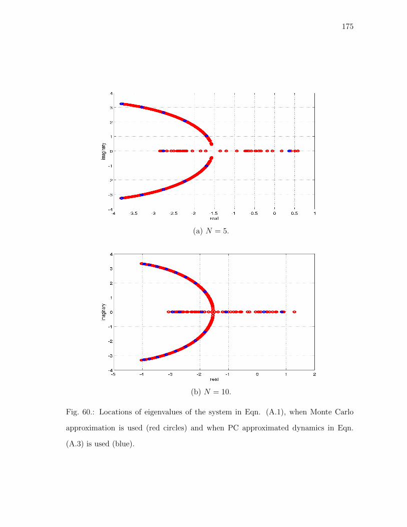
175
(a) N = 5.
(b) N = 10.
Fig. 60.: Locations of eigenvalues of the system in Eqn. (A.1), when Monte Carlo
approximation is used (red circles) and when PC approximated dynamics in Eqn.
(A.3) is used (blue).

176
Fig. 61.: PDF of the eigenvalue distribution on the complex plane. Blue represents
low probability regions and red is high probability region. Eigenvalues represented in
black.

177
APPENDIX B
COMPARISON OF FROBENIUS-PERRON BASED ESTIMATION TO
PARTICLE FILTERS
In this appendix, we compare the FP operator based estimation method to parti-
cle filters, by investigating the posterior PDF obtained by the two methods. We use a
linear system with Gaussian uncertainty for comparison, as we have the exact repre-
sentation of evolving sequence of posterior PDFs through Kalman filter. We compute
the Wasserstein metric [138] of the two posteriors from the posterior obtained from
Kalman filtering.
The Wasserstein metric is a metric comparing the distance between the shapes
of two distributions. Let (M,d) be a metric space. For p ≥ 1, let Pp(M) denote the
collection of all probability measures µ on M with finite pth moment, i.e. for some x0
in M , ∫M
d(x, x0)pdµ(x) <∞
Then the pth Wasserstein distance between two probability measures µ and ν in Pp(M)
is defined as
Wp(µ, ν) =
(inf
γ∈Γ(µ,ν)
∫M×M
d(x, y)p dγ(x, y)
)1/p
, (B.1)
where, Γ(µ, ν) is the set of all pairing of measures (µ, ν) on M × M . Important
property of this metric is that it is commutative i.e. Wp(µ, ν) = Wp(ν, µ). For the
sake of brevity detailed discussion about the Wasserstein metric has been omitted
here and can be found in ref. [139]. If both µ and ν are Gaussian measures, and if
we consider p = 2, requiring the 2nd moment to be finite, then there is an analytical

178
expression of Wasserstein metric given by,
W2(µ, ν) =
√||µ1 − µ2||2 + tr(Σ1) + tr(Σ2)− 2 tr(
√Σ1Σ2
√Σ1)
12 , (B.2)
where µ1, µ2, Σ1 and Σ2 are the means and covariances of each Gaussian measure,
respectively. The Wasserstein metric can be normalized by dividing W2(µ, ν) in Eqn.
(B.2) by the diameter of the Ω space.
Let us consider the linear system given by the following dynamical equations.
x(t) =
−0.05 0
0 −0.05
x(t), (B.3)
where x(t) ∈ R2 are the states. We consider a scalar measurement model given by,
yk = [1 1]xk + vk, (B.4)
where yk are measurements coming at discrete times, and vk is a zero mean delta
correlated discrete Gaussian noise with autocorrelation R.
We assume that the system has Gaussian initial condition uncertainty with mean
and covariance as, 1
1
and
1 0
0 1
,
respectively. The true system is assumed to have initial states [2, 2], hence we start
with an initial error in estimation. We fix the measurement update interval with each
measurement coming every 1s. We run the estimation algorithms for 10s.
Initially, we fix the value of R to 2. Figure 62 shows plots for estimation error
for the Kalman filter, FP operator based filter and particle filter. We can see that
performance of FP operator based estimator is similar to that of the Kalman filter,
in this case.
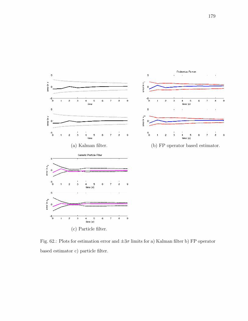
179
(a) Kalman filter. (b) FP operator based estimator.
(c) Particle filter.
Fig. 62.: Plots for estimation error and ±3σ limits for a) Kalman filter b) FP operator
based estimator c) particle filter.

180
Fig. 63.: Normalized Wasserstein distance between posterior PDFs of Kalman filter
and FP operator based estimator (solid line) and Kalman filter and particle filter
(dashed line). The value of R = 1/2.
Figure 63 shows the plot for normalized Wasserstein metric for posterior PDFs,
generated by particle filter and FP operator based estimator, from the posterior PDF
of the Kalman filter when R = 1/2. The propagation time is fixed to 20s. We can
see that the posterior PDF of the FP operator based estimator is closer to Kalman
filter’s posterior than the particle filter. If autocorrelation of noise is increased to
R = 2, the difference in performance of the two estimators become even clearer, as it
can be seen in Fig. 64.
However, if the value of R is increased the estimators perform equally. Figure
65 shows the Wasserstein distance between posterior PDFs of Kalman filter and FP
operator based estimator and Kalman filter and particle filter, when value of R = 4.
It can be seen that the distance from Kalman filter’s posterior PDF increases for both
filters, even if FP operator is nearer than particle filter.
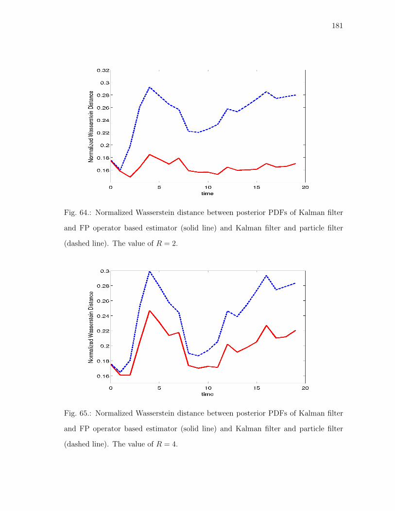
181
Fig. 64.: Normalized Wasserstein distance between posterior PDFs of Kalman filter
and FP operator based estimator (solid line) and Kalman filter and particle filter
(dashed line). The value of R = 2.
Fig. 65.: Normalized Wasserstein distance between posterior PDFs of Kalman filter
and FP operator based estimator (solid line) and Kalman filter and particle filter
(dashed line). The value of R = 4.

182
APPENDIX C
TENSOR CALCULATIONS
This appendix shows the tensor calculations for for finding the prior moments of the
system in Eqn. (3.10) & Eqn. (3.11). After applying gPC to the system, the gPC
dynamical system is given by Eqn. (3.14a) & Eqn. (3.14b). To get the prior higher
order moments, we need to evaluate tensors which are given in section 3 in chapter
III. The tensor calculations for the given problem are as follows.
P xv =
(M3−
111 +M3−122
M3−211 +M3−
222
)−(
M1−1 M2−
11 +M1−1 M2−
22
M1−2 M2−
11 +M1−2 M2−
22
), (C.1a)
P vv = R+M4−1111 +M4−
2222 + 2M4−1122 − 2
((M1−
1 )2 + (M1−2 )2
) (M2−
11 +M2−22
)+((M1−
1 )2 + (M1−2 )2
)2, (C.1b)
P xvv =
(M5−
11111 + 2M5−11122 +M5−
12222
M5−21111 + 2M5−
11222 +M5−22222
)− 2
(M3−
111 +M3−122
M3−211 +M3−
222
)((M1−
1 )2 + (M1−2 )2
)−(
M1−1
M1−2
)(M4−
1111 + 2M4−1122 +M4−
2222) + 2
(M1−
1
M1−2
)((M1−
1 )2 + (M1−2 )2
) (M2−
11 +M2−22
)−R
(M1−
1
M1−2
), (C.1c)
P xxv =
(M4−
1111 +M4−1122 M4−
1112 +M4−1222
M4−1112 +M4−
1222 M4−2211 +M4−
2222
)−(
M3−111 +M3−
122
M3−211 +M3−
222
)(M1−
1
M1−2
)T−(
M2−11 M2−
12
M2−21 M2−
22
)((M1−
1 )2 + (M1−2 )2
)−(
M1−1
M1−2
)(M3−
111 +M3−122
M3−211 +M3−
222
)T+
(M1−
1
M1−2
)(M1−
1
M1−2
)T (M2−
11 +M2−22
)+
(M1−
1
M1−2
)(M1−
1
M1−2
)T ((M1−
1 )2 + (M1−2 )2
)2,
(C.1d)
P vvv = M6−111111 + 3M6−
111122 + 3M6−112222 +M6−
222222 − 3((M1−
1 )2 + (M1−2 )2
)(M4−
1111
+ 2M4−1122 +M4−
2222)− 3((M1−
1 )2 + (M1−2 )2
)R− 3
((M1−
1 )2 + (M1−2 )2
)2(M2−
11 +M2−22 )
−((M1−
1 )2 + (M1−2 )2
)3. (C.1e)

183
Here, M i− are the prior moments which are calculated from the gPC coefficients.
The superscript is the order of the moment and the subscript is the element of the cor-
responding moment tensor. For example M6−112222 represents (1, 1, 2, 2, 2, 2)th member
of the 6th order moment, which happens to be a 6th order tensor.

184
VITA
Parikshit Dutta received his Bachelor of Technology degree in manufacturing sci-
ence and engineering, and Master of Technology in industrial engineering and man-
agement, both in June 2006, as a part of dual degree program, from Indian Institute
of Technology, Kharagpur, India, . He received his Ph.D. in aerospace engineering
from Texas A&M University in August 2011. His research interests lie in the fields
of uncertainty quantification of dynamical systems, estimation theory and sensitivity
analysis, Monte Carlo methods for high dimensional systems, and Bayesian inferential
techniques.
He can be reached via email at [email protected] or at,
Department of Aerospace Engineering,
H.R. Bright Building, Rm. 701, Ross Street - TAMU 3141,
College Station TX 77843-3141.