Paradigm France, 78 av XX corps, 54000 Nancy, France - Emmanuel.Labrunnye@pdgm.com

P-248

New 3D flattened space for seismic interpretation

Emmanuel Labrunye*, Christophe Winkler, Cédric Borges, Jean-Laurent Mallet,

Stanislas Jayr (Paradigm, USA)

Summary

This paper presents a new way of flattening the seismic in 3D using a new space/time framework. The parameterization of the

seismic data is based on the interpreted faults and main stratigraphic events, and a stratigraphic column is used to grant its

geological consistency. The result is a new flattened space where all the horizons are flattened and where any data can be

mapped for visualization. Interpretation can be performed in this flattened space, and the result can be mapped back to the

regular geological space.

Introduction Seismic flattening is a common interpretation technique used to remove structures such as folds or faults to help the interpreter recognizing the geological features. Indeed, by removing the post depositional deformations, it is possible to see the layers as they were emplaced. Such pictures are

sometimes called paleosections (Sheriff, 1991). This is especially useful to interpret complex sedimentological patterns, like meander systems. We present in this paper an iterative method to create a 3D flattened space based on a space/time framework and on the interpretation of the faults and of a limited number of horizons. Any data, like the seismic cube, a well marker or an horizon surface can be shown in this new space to QC or improve the

interpretation.

State of Art of The 3D Seismic Flattening The straightforward way to flatten a seismic cube is to pick an horizon, then to move vertically each seismic trace independently such as the picked horizon becomes flat. It is also possible to consider two reference horizons and to

stretch or squeeze the seismic such as theses horizons become flat. However, unconformities or normal or reverse faults will not be handled correctly. Furthermore the traces where the reference horizons are not interpreted cannot be flattened.

Stark (2005) and de Groot et al. (2006) propose a 3D approach based on an attribute computed from the seismic (respectively phase unwrapping and dip steering cube constrained by some interpreted horizons). This attribute is used to automatically give a relative geologic age to each point of the seismic cube. A 3D cube whose vertical axis represents the age is then computed by resampling the

seismic signal trace by trace for each age value. Hiatus locations appear when there is no seismic data for a given age. Although automated and fully 3D, these methods do not seem to be able to take fault throws into account. The workflow presented by Monsen et al. (2007) uses horizon patches. The goal is not to flattened the seismic itself, but the interpreted horizons. The patches are

extracted from a classification algorithm, and they are given a relative age by a graph analysis of their relative position. The patches are then displayed in a specific 3D viewer where the Z axis is replaced by the age axis. This technique is interesting to understand the geological data but does not allow interpretation of the seismic data in the flattened space.

A New 3D Space/Time Framework Our approach is based on the concept of space/time mathematical framework introduced by Mallet (2004, 2008). It consists in a curvilinear parameterization of the subsurface by creating a uvt-transform. This transformation maps every (x,y,z) point in the geological space to a (u,v,t)

New 3D flattened space

2

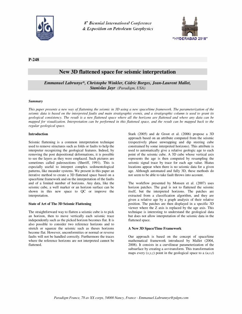
point in the parametric space. The uvt-transform is computed such that (Figure 1):

• An iso-t surface corresponds to a stratigraphic horizons,

i.e. to a seismic event.

• An iso-t is discontinuous across the faults.

Figure 1: Example of uvt-transform corresponding to the

curvilinear parameterization of a reservoir. Courtesy of Numerical

Earth Models EAGE Publications Bv (Mallet, 2008).

The parametric space can be regularly discretized into elementary volumes. A reverse uvt-transform enables the mapping of these volume elements into the geological domain as illustrated in the Figure 2. It can be

demonstrated (Mallet, 2008) that such a transformation minimizes the distortions of the volumes and stratigraphic distances.

Figure 2: Representation of the discretized parametric domain in

the geological space, showing the uvt-transform from xyz-space to

uvt-space and the reverse uvt-transform from uvt-space to xyz-

space. Courtesy of Numerical Earth Models EAGE Publications

Bv (Mallet, 2008).

The u and v coordinates can be considered as the paleogeographic coordinates. By construction, the stratigraphic horizons are unfaulted and unfolded in the parametric space, and the fault displacement is null, whatever the fault type (normal, reverse, strike-slip). If the

transformation is applied to the seismic cube itself, all the seismic events should be perfectly flat: the uvt parametric space can be considered as a 3D flattened space.

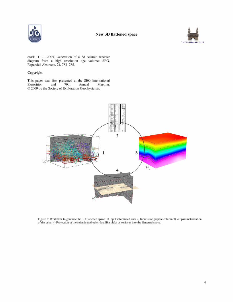
The 3D Flattened Space Workflow The following workflow is proposed to build the flattened space (Figure 3):

1. Interpretation of the faults and of the main stratigraphic events from the seismic data, using manual and/or automatic interpretation tools.

2. Selection of a stratigraphic column, listing the considered stratigraphic events and their relationships. The column may contain sub events not yet interpreted on the seismic. It will be used to associate an age (relative or absolute) to each event and to manage the

missing events. 3. 3D uvt parameterization of the volume, using an

interpolation engine constrained by the given faults, the stratigraphic events and the stratigraphic column.

4. Projection of the seismic cube and of the interpreted data into the flattened space using the uvt-transform.

5. Visualization and interpretation in the flattened space.

The uvt parameterization is the result of a full 3D iterative interpolation in the considered volume. The advantages of this approach are the following:

• The horizons do not need to be fully interpreted along

the seismic. It is possible to pick only some small pieces. Based on the stratigraphic column, the 3D approach ensures a coherent result.

• For the same reasons, there is no need to pick a lot of

horizons. Only the major events and unconformities are required.

• The extraction of any intermediate conformable horizon

is immediate by computing the corresponding iso-t surface.

• The process can be iterated to improve the

parameterization. New data interpreted either from the geological or from the flattened space can be added to locally refine the parameterization.

New 3D flattened space

3

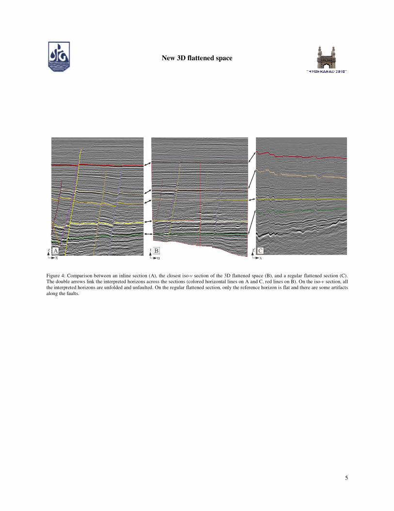
Interpretation in the Flattened Space The Figure 4 compares the initial seismic section (A) with the closest iso-v section of the 3D flattened space (B) and with a section flattened relatively to the yellow horizon

using the straightforward algorithm (C). On the iso-v flattened section, all the input horizons become perfectly flat. The seismic is stretched and squeezed relatively to the horizons. The square section becomes a polygonal section, in which the holes correspond to the missing data on the borders. All the faults throws, where they were defined by interpreted horizons and faults, are null. On the regular flattened section, only the reference horizon is really flat

and the faults are not taken into account. Any data located in the seismic cube can be projected easily in the 3D flattened space by simply applying the uvt-transform. The (x,y,z) coordinates of each point of the data must be replaced by their associated (u,v,t) coordinates during the display in a 3D viewer. As a consequence, any interpretation work performed in the geological space can

also be done in the 3D flattened space: horizon picking, line or surface editing, comparison of the position of the extracted surface and of the well markers, etc. The reverse transformation will be done afterwards to map the added or edited data back to the geological space. If there are enough horizons and if all the faults are correctly interpreted, the flattened seismic should be

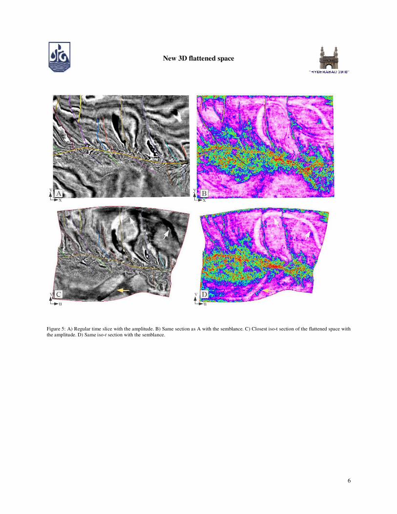
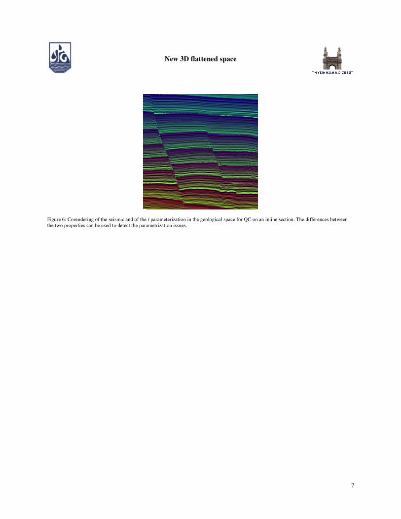
perfectly flat for a given conformable sequence. If it is not the case, it means the interpreter missed an event. This can be detected in the flattened space itself, but also in the geological space. By corendering the t parameterization and the seismic signal in the geological space, it is very easy to check the accuracy of the current parameterization (Figure 6). For optimization purpose, the flattened iso-u, iso-v or iso-t

seismic sections are computed by extracting the seismic texture following the corresponding iso-surface in the geological domain. As this process is quite fast, it is possible to slice the flattened seismic or any flattened seismic attribute in real time without duplicating the seismic volume. These sections are a powerful tool to unveil the complex structures hidden by the faults and folds. For example, the Figure 5 compares a seismic regular

time slice in the geological space with an iso-t section in the flattened space. The channel is very difficult to see in

the regular time slice with the amplitude. The use of the semblance improves the visibility of the channel. In the flattened space, the channel becomes clear on both amplitude and semblance sections (white arrows). Moreover, it is possible to see its extension on the other

side of the fault (yellow arrow).

Conclusion The workflow described in this paper uses a powerful space/time framework approach to compute a fully 3D flattened space from seismic and interpreted data. It is perfectly able to take any faults or any folds into account,

and all the input horizons are flattened together. The geological coherency of the result is controlled by the stratigraphic column and the provided picks or surfaces. Once the 3D flattened space is created, any data located into the seismic cube can be flattened in real time for any interpretation purpose. It opens a new way for 3D flattened interpretation.

Acknowledgements The authors would like to thank Paradigm for permission to publish this paper and specifically all the members of the Paradigm SKUATM project who made this 3D Flattened Space a reality.

References

de Groot, P., G. de Bruin, and N. Hemstra, 2006, How to create and use 3d wheeler transformed seismic volumes: SEG,Expanded Abstracts, 25, 1038–1042. Mallet, J.-L., 2004, Space-time mathematical framework for sedimentary geology: Mathematical geology, 36, 1–32., 2008, Numerical earth models: EAGE publications.

Monsen, E., H. G. Borgos, P. L. Guern, and L. Sonneland, 2007, Geologic-process-controlled interpretation based on 3d wheeler diagram generation: SEG, Expanded Abstracts, 26, 885–889. Sheriff, R. E., 1991, Encyclopedic dictionary of exploration geophysics. Geophysical References Series, No. 1: Sociey of Exploration Geophysics.

New 3D flattened space

4

Stark, T. J., 2005, Generation of a 3d seismic wheeler diagram from a high resolution age volume: SEG, Expanded Abstracts, 24, 782–785.

Copyright

This paper was first presented at the SEG International Exposition and 79th Annual Meeting. © 2009 by the Society of Exploration Geophysicists.

Figure 3: Workflow to generate the 3D flattened space: 1) Input interpreted data 2) Input stratigraphic column 3) uvt parameterization

of the cube. 4) Projection of the seismic and other data like picks or surfaces into the flattened space.

New 3D flattened space

5

Figure 4: Comparison between an inline section (A), the closest iso-v section of the 3D flattened space (B), and a regular flattened section (C).

The double arrows link the interpreted horizons across the sections (colored horizontal lines on A and C, red lines on B). On the iso-v section, all

the interpreted horizons are unfolded and unfaulted. On the regular flattened section, only the reference horizon is flat and there are some artifacts

along the faults.

New 3D flattened space

6

Figure 5: A) Regular time slice with the amplitude. B) Same section as A with the semblance. C) Closest iso-t section of the flattened space with

the amplitude. D) Same iso-t section with the semblance.

New 3D flattened space

7

Figure 6: Corendering of the seismic and of the t parameterization in the geological space for QC on an inline section. The differences between

the two properties can be used to detect the parametrization issues.