NEUTRON STARS AND BLACK HOLES IN SCALAR-TENSOR …
108
NEUTRON STARS AND BLACK HOLES IN SCALAR-TENSOR GRAVITY
Transcript of NEUTRON STARS AND BLACK HOLES IN SCALAR-TENSOR …

NEUTRON STARS AND BLACK HOLES INSCALAR-TENSOR GRAVITY

NEUTRON STARS AND BLACK HOLES IN
SCALAR-TENSOR GRAVITY
By
MICHAEL W. HORBATSCH, M.Sc., B.Sc.
A Thesis
Submitted to the School of Graduate Studies
in Partial Fulfilment of the Requirements
for the Degree
Doctor of Philosophy
McMaster University
c© Copyright by Michael W. Horbatsch, July 2012
DOCTOR OF PHILOSOPHY (2012) McMaster University
(Physics and Astronomy) Hamilton, Ontario
TITLE: Neutron Stars and Black Holes in Scalar-Tensor Gravity
AUTHOR: Michael W. Horbatsch, M.Sc. (McMaster University), B.Sc. (Uni-
versity of Toronto)
SUPERVISOR: Professor Cliff P. Burgess
NUMBER OF PAGES: vi, 101
ii
Abstract
The properties of neutron stars and black holes are investigated within a class
of alternative theories of gravity known as Scalar-Tensor theories, which extend
General Relativity by introducing additional light scalar fields to mediate the
gravitational interaction.
It has been known since 1993 that neutron stars in certain Scalar-Tensor
theories may undergo ‘scalarization’ phase transitions. The Weak Central
Coupling (WCC) expansion is introduced for the purpose of describing scalar-
ization in a perturbative manner, and the leading-order WCC coefficients are
calculated analytically for constant-density stars. Such stars are found to
scalarize, and the critical value of the quadratic scalar-matter coupling pa-
rameter βs = −4.329 for the phase transition is found to be similar to that of
more realistic neutron star models.
The influence of cosmological and galactic effects on the structure of an
otherwise isolated black hole in Scalar-Tensor gravity may be described by in-
corporating the Miracle Hair Growth Formula discovered by Jacobson in 1999,
a perturbative black hole solution with scalar hair induced by time-dependent
boundary conditions at spatial infinity. It is found that a double-black-hole bi-
nary (DBHB) subject to these boundary conditions is inadequately described
by the Eardley Lagrangian and emits scalar dipole radiation.
Combining this result with the absence of observable dipole radiation
from quasar OJ287 (whose quasi-periodic ‘outbursts’ are consistent with the
predictions of a general-relativistic DBHB model at the 6% level) yields the
bound |φ/Mpl| . (16 days)−1 on the cosmological time variation of canonically-
normalized light (m . 10−23 eV) scalar fields at redshift z ∼ 0.3.
iii

Acknowledgements
First and foremost, I would like to thank my supervisor Cliff Burgess for all
his guidance and assistance over the past six years. Additionally, I would like
to thank my future postdoctoral advisor Emanuele Berti, and collaborators
Vitor Cardoso, Leonardo Gualtieri, Ulrich Sperhake, and Justin Alsing, for
taking an interest in my work, inviting me to the University of Mississippi, and
warmly welcoming me to their research team. Moreover, I would like to thank
my parents Marko Horbatsch and Roma Chumak-Horbatsch for their endless
support and motivation, and Ian Graham for a wonderful friendship over the
past few years and provision of nourishing health-giving raw organic food. I
also thank my sister Olenka Horbatsch, my fellow graduate students, and all
other members of the Department of Physics and Astronomy at McMaster.
iv
Contents
1 Outline 1
2 Scalar-Tensor Gravity 4
2.1 Introduction . . . . . . . . . . . . . . . . . . . . . . . . . . . . 4
2.1.1 Motivation from Classical Gravitational Physics . . . . 4
2.1.2 Motivation from High-Energy Physics . . . . . . . . . . 8
2.1.3 Partial Literature Survey . . . . . . . . . . . . . . . . . 9
2.2 Action and Field Equations in the Einstein Frame . . . . . . . 14
2.3 Transformation to the Jordan Frame . . . . . . . . . . . . . . 16
2.4 Conservation Laws . . . . . . . . . . . . . . . . . . . . . . . . 18
2.5 The Weak-Field Limit . . . . . . . . . . . . . . . . . . . . . . 19
3 The Weak-Central-Coupling Formalism 26
3.1 Introduction . . . . . . . . . . . . . . . . . . . . . . . . . . . . 26
3.2 Field Equations . . . . . . . . . . . . . . . . . . . . . . . . . . 29
3.3 Vacuum . . . . . . . . . . . . . . . . . . . . . . . . . . . . . . 31
3.4 Interior . . . . . . . . . . . . . . . . . . . . . . . . . . . . . . . 33
3.5 Matching Conditions . . . . . . . . . . . . . . . . . . . . . . . 36
3.6 The Weak-Central-Coupling (WCC) Expansion . . . . . . . . 39
3.7 Constant-Density Stars . . . . . . . . . . . . . . . . . . . . . . 42
4 Binary Systems 46
4.1 The Non-Relativistic Problem . . . . . . . . . . . . . . . . . . 46
4.2 Introduction to The Relativistic Problem . . . . . . . . . . . . 47
4.3 Formalism . . . . . . . . . . . . . . . . . . . . . . . . . . . . . 48
4.4 Solution of the External Field Equations . . . . . . . . . . . . 50
4.5 Radiation at Infinity . . . . . . . . . . . . . . . . . . . . . . . 52
4.6 Radiation in Massive Brans-Dicke Theory . . . . . . . . . . . 56
4.7 Effective Field Theory . . . . . . . . . . . . . . . . . . . . . . 58
4.7.1 Motivation . . . . . . . . . . . . . . . . . . . . . . . . . 58
4.7.2 Introduction . . . . . . . . . . . . . . . . . . . . . . . . 59
4.7.3 Formalism . . . . . . . . . . . . . . . . . . . . . . . . . 60
v

5 Miracle Hair Growth 64
5.1 Introduction . . . . . . . . . . . . . . . . . . . . . . . . . . . . 64
5.2 Jacobson’s Formula . . . . . . . . . . . . . . . . . . . . . . . . 64
5.3 Double-Black-Hole Binaries . . . . . . . . . . . . . . . . . . . 65
5.4 The Quasar OJ287 . . . . . . . . . . . . . . . . . . . . . . . . 66
6 Summary and Prospects 68
A Mathematical Preliminaries 69
A.1 Units . . . . . . . . . . . . . . . . . . . . . . . . . . . . . . . . 69
A.2 Basic Differential Geometry . . . . . . . . . . . . . . . . . . . 69
A.3 Static Spherically-Symmetric Metrics . . . . . . . . . . . . . . 74
A.4 Variations of the Metric . . . . . . . . . . . . . . . . . . . . . 75
A.5 Conformal Transformations . . . . . . . . . . . . . . . . . . . 76
A.6 Wave Equations and Green’s Functions . . . . . . . . . . . . . 78
A.7 Hypergeometric and Heun Functions . . . . . . . . . . . . . . 79
References 82
vi

PhD Thesis - M. W. Horbatsch McMaster - Physics and Astronomy
1 Outline
Scalar-Tensor theories are alternatives to General Relativity which modify
the widely-accepted theory by introducing additional light scalar particles
to mediate the gravitational interaction while retaining the usual graviton.
The principal motivation for considering these alternatives stems from theo-
retical attempts to unify gravity with quantum mechanics at high energies,
such as string theory, whose low-energy limit has recently been shown to con-
tain scalars sufficiently light to have interesting astrophysical consequences
[9]. Scalar-Tensor theories also play an important role in classical gravita-
tional physics by providing a concrete framework for interpreting tests of rel-
ativistic gravity in the strong-field regime, where a phenomenological theory-
independent interpretation is often problematic.
The subject of this thesis is the structure of highly-relativistic compact
objects, namely, neutron stars and black holes, within Scalar-Tensor theories
of gravity. Two novel theoretical results are obtained — the Weak Central
Coupling (WCC) formalism for the perturbative description of scalarization
phase transitions in neutron stars, developed in section 3, and Miracle Hair
Growth in a double-black-hole binary system induced by cosmological and/or
galactic effects, which is the subject of section 5.
The thesis begins with a comprehensive discussion of the basic proper-
ties of Scalar-Tensor gravity in section 2. In 2.1, the motivation for this theory
stemming from classical gravitational physics on the one hand, and quantum
high-energy physics on the other, is reviewed, and the historical development
of the theory is summarized. A survey of more recent work is also provided,
in order to set the context for the novel theoretical results developed in later
sections. In 2.2 and 2.3, the action and field equations of Scalar-Tensor gravity
are presented in two different mathematical formulations commonly referred
to as the Einstein and Jordan frames, respectively. Conservation laws are dis-
cussed in 2.4, while the weak-field limit is taken in 2.5 in order to identify the
‘physical’ Newton constant G, among other things. This section contains no
new results, and experts should feel free to skip it.
The purpose of section 3 is to develop the Weak Central Coupling
1

PhD Thesis - M. W. Horbatsch McMaster - Physics and Astronomy
(WCC) formalism for the description of neutron star scalarization. The Lan-
dau approach to phase transitions is followed [113], and the coefficients therein
are expressed in terms of perturbative solutions to the equations of stellar
structure. In 3.1, the phenomenon of spontaneous scalarization is explained in
some detail, and the key ideas behind the WCC expansion are introduced. The
field equations for a static spherically-symmetric perfect fluid are obtained in
3.2, and the external vacuum solution is described in 3.3. Subsequently, the
equations of stellar structure are derived in 3.4, and the formulas for matching
their solution to an exterior metric are obtained in 3.5. With all the required
tools in hand, the WCC perturbative expansions are then introduced in 3.6,
and the leading-order coefficients are expressed in terms of perturbative solu-
tions to the equations of stellar structure. This formalism is finally applied
to constant-density stars in 3.7, and the complete leading-order solution is ex-
pressed analytically in terms of Heun functions, enabling one to describe the
scalarization of such stars without numerically solving the equations of stellar
structure.
Section 4 concerns the formalism and analytical approximation meth-
ods employed in the description of a binary inspiral with small size-to-separation
ratio ε ∼ R/D, as a prerequisite for the Miracle Hair Growth described in sec-
tion 5. The non-relativistic two-body problem is briefly reviewed in 4.1, and
the complications arising at the relativistic level are first introduced in 4.2.
The formalism of dividing the two-body problem into the ‘interior’ and ‘ex-
terior’ regions is explained in 4.3, and in particular it is demonstrated how
the boundary conditions simplify in the ‘point-particle’ limit ε → 0. Subse-
quently, the work of Damour and Esposito-Farese [50] on binary systems in
Scalar-Tensor gravity and radiation therefrom is summarized in 4.4 and 4.5, re-
spectively, and the foundations upon which this work was built are explained.
The results of a recent Jordan-frame calculation by Alsing and collaborators
[6] of the radiation flux in massive Scalar-Tensor theory are summarized in 4.6,
and converted to the Einstein frame, confirming in particular that the radi-
ated power is a frame-independent quantity up to re-scaling of units. Finally,
the Effective Field Theory (EFT) approach to the two-body problem initi-
2

PhD Thesis - M. W. Horbatsch McMaster - Physics and Astronomy
ated by Goldberger and Rothstein [78, 80] is motivated and introduced in 4.7.
Omitting the details of Feynman diagrams and power counting, the discussion
focuses on the fundamental role played by the point-particle Lagrangian, its
derivative expansion, and the relation thereof to an expansion in powers of the
size-to-separation ratio ε ∼ R/D. As a prerequisite for the material in section
5, the derivative expansion in Scalar-Tensor gravity is explicitly written down
to second order.
Building heavily on the material of section 4, section 5 discusses the
influence of cosmological and galactic effects on the orbital dynamics of a
double-black-hole binary inspiral in Scalar-Tensor gravity, and the radiation
emitted therefrom. Following a brief introduction in 5.1, it is explained in 5.2
how Jacobson’s Miracle Hair Growth Formula implies that such effects cause
isolated black holes to grow scalar hair. Subsequently, Jacobson’s arguments
are applied to a double-black-hole binary in 5.3, and it is shown that the trun-
cation of the point-particle Lagrangian to zeroth order in the derivative ex-
pansion, namely, the Eardley Lagrangian, is inadequate to describe the orbital
corrections induced by galactic and cosmological effects. While the difficult
problem of calculating these corrections is left for future work, the leading-
order scalar dipole radiation flux is calculated in a relatively straightforward
manner. Finally, in 5.4, an application to quasar OJ287 (which has been suc-
cessfully modelled as a DBHB within GR) is discussed, and a bound on the
cosmological time evolution of light scalar fields at its redshift is obtained.
Finally, the key results are summarized in section 6, and prospects for
future work are discussed.
Mathematical preliminaries and explanations of notation, units, and
conventions, have all been relegated to appendix A.
3
PhD Thesis - M. W. Horbatsch McMaster - Physics and Astronomy
2 Scalar-Tensor Gravity
2.1 Introduction
2.1.1 Motivation from Classical Gravitational Physics
General Relativity, the current widely-accepted standard theory of gravitation,
arose out of the attempt to unify the Newtonian theory of gravity with the
special theory of relativity. Shortly after being formulated by Einstein in
1916, General Relativity was tested in the solar system, and was found to
correctly describe the bending of starlight in the gravitational field of the sun,
as measured by Eddington during a total solar eclipse in 1919. Moreover,
General Relativity was able to explain the anomalous precession of Mercury’s
orbit, which had been a long-standing unsolved problem in celestial mechanics.
Subsequent solar-system tests have become much more precise, and
have confirmed the validity of General Relativity to a high degree of accuracy
[198, 196, 199]. For instance, Very Long Baseline Interferometry (VLBI) [155]
and the Very Long Baseline Array (VLBA) [73] have been used to measure
the deflection of radio waves from distant sources in the sun’s gravitation field,
and have confirmed the validity of General Relativity to a few parts in 104.
According to General Relativity, electromagnetic signals propagating through
a gravitational field experience a time delay [154] in addition to being deflected.
This delay has been measured for radio signals transmitted from Earth to the
Cassini spacecraft, and found to agree with the general-relativistic prediction
to a few parts in 105 [18].
While the accuracy of these solar-system tests is impressive, it is im-
portant to keep in mind that such tests only probe the weak-field, or Post-
Newtonian limit of General Relativity, where relativistic effects are merely
small corrections to Newtonian gravity.
In 1975, a remarkable new testing ground for relativistic gravity was
discovered — the binary pulsar PSR B1913+16 [92, 93, 169], for which Hulse
and Taylor were awarded the Nobel Prize. This system consists of two neutron
stars in a binary orbit, one of which is a pulsar, rotating with a period on the
order of milliseconds, and having a magnetic field whose axis is not aligned
4
PhD Thesis - M. W. Horbatsch McMaster - Physics and Astronomy
with the axis of rotation. This creates a ‘lighthouse effect’, where an observer
on Earth sees radio signals emitted from the pulsar at regular intervals. These
signals are measured by radio telescopes, and the Doppler shift is used to
reconstruct the properties of the orbit. It was found that the reconstructed
orbit agrees beautifully with the predictions of General Relativity [168]. In
particular, a secular decrease of the orbital period due to the emission of
gravitational radiation has been observed. Recent observations of this system
continue to be consistent with the predictions of General Relativity [170, 193,
192].
Subsequently, many other binary pulsars have been discovered, and
their reconstructed orbits all spectacularly agree with the predictions of Gen-
eral Relativity [164, 108]. Of particular interest is the double pulsar PSR
J0737-3039 [110, 105], a binary system consisting of two pulsars. Although one
of the pulsars has a slow rotational period on the order of seconds, its timing
gives access to an orbital parameter that can not be measured in single-pulsar
binary systems.
These binary pulsars typically have orbital periods on the order of
hours, and light-crossing times on the order of seconds, and thus orbital ve-
locities on the order of v/c ∼ 0.0001, implying that the orbital motion may be
described as a perturbation of the non-relativistic Kepler problem. However,
the gravitational fields inside the neutron stars are very strong, and thus the
binary pulsar tests probe some limited aspects of strong-field General Relativ-
ity.
Although the measurement of the decrease of the orbital period of bi-
nary pulsars provides indirect evidence for the existence of gravitational waves,
a major experimental research program is currently being undertaken in or-
der to directly measure these waves on Earth with interferometric detectors
[128, 151]. The ‘first generation’ ground-based detectors (LIGO, VIRGO, GEO
600, and TAMA 300) have taken data, and set upper limits on the amplitudes
of gravitational waves. Since a signal above the background noise has not yet
been detected, the method of matched filtering is employed to look for signals
buried in noise. After carrying out six ‘science runs’, LIGO is currently being
5

PhD Thesis - M. W. Horbatsch McMaster - Physics and Astronomy
upgraded to Advanced LIGO [85], which is planned to become operational in
2014. This upgrade will increase the sensitivity ten-fold, which is expected
to be sufficient to detect a gravitational wave signal above the noise. Similar
‘second generation’ upgrades are planned for the other ground-based detectors.
Since the frequency range of any ground-based detector is fundamen-
tally limited by seismic noise, there exist propoals for ‘third-generation’ de-
tectors, which will eliminate this noise and be sensitive to lower frequencies.
The Einstein Telescope [142] will be cryogenically cooled and located in an
underground facility, whereas eLISA/NGO [7] will be space-based and consist
of three satellites.
One of the most promising sources of gravitational waves are the in-
spiral, merger, and ringdown of a binary system consisting of neutron stars
and/or black holes. During the merger, orbital velocities may approach the
speed of light, and thus, direct gravitational wave detection will test a regime
of General Relativity which has not yet been tested by binary pulsar timing.
It is useful to interpret the results of experiments and observations in a
framework which does not assume General Relativity, or any other particular
theory of gravity, to be correct. For instance, in the weak-field regime it is
possible to express the predictions of a broad class of relativistic theories of
gravity in terms of the Parametrized Post-Newtonian (PPN) phenomenological
parameters [196]. The result of any experiment or observation in a weak-field
setting may then be phrased as a bound on some combination of the PPN
parameters.
For the timing of binary pulsars whose relative orbital velocity is much
slower than the speed of light, i.e. v/c 1, the Parametrized Post-Keplerian
(PPK) formalism may be used to describe the properties of the orbits, and
relate the times-of-emission of pulses to their times-of-arrival on Earth in a
broad class of relativistic theories of gravity [196, 54].
In order to describe the gravitational waveform emitted by a binary
inspiral in a theory-independent manner, Yunes and Pretorius have developed
the Parametrized Post-Einsteinian (PPE) framework [209, 41]. Following an
investigation by Arun [8], this framework was extended to include amplitude
6
PhD Thesis - M. W. Horbatsch McMaster - Physics and Astronomy
corrections due to dipole radiation [39]. However, recent work has revealed
that the PPE framework is not sufficiently general to describe the waveform
in massive Brans-Dicke theory [17].
In regimes where the gravitational fields are strong everywhere, such as
binary systems with v/c approaching unity, it is usually very difficult, if not
downright impossible, to express the predictions of a broad class of relativistic
theories of gravity in terms of a finite set of phenomenological parameters.
Thus, the only practical approach is the explicit construction of well-motivated
alternative theories of gravity, which depend on a finite set of parameters, and
reduce to General Relativity for a specific choice of parameters. Then the
result of any experiment or observation may be phrased as a bound on some
combination of these parameters.
In addition to their crucial role in the interpretation of strong-field ob-
servations, alternative theories of gravity are useful for gaining insight into the
special properties of General Relativity. For example, the Strong Equivalence
Principle (SEP), which holds in General Relativity, states that extended bod-
ies with internal self-gravity respond to an external gravitational field in the
same manner as microscopic test particles [196]. Nordtvedt [119, 120, 118]
was the first to point out that the SEP may be violated in alternative theories
of gravity, and suggest an experimental test by Lunar Laser Ranging (LLR).
The results of this test have confirmed the validity of the SEP to a very high
degree of accuracy [58, 204].
Another special property of General Relativity which breaks down in
most alternative theories is the effacement principle, which states that in a
binary system with v/c 1, the internal structure of the two bodies affects
the orbital motion at a much higher order in v/c than one would have a
priori expected [44]. Thus, the successful general-relativistic description of
the binary pulsar orbits in terms of two neutron star masses, and no other
‘internal’ parameters, is an excellent test of the effacement principle.
7

PhD Thesis - M. W. Horbatsch McMaster - Physics and Astronomy
2.1.2 Motivation from High-Energy Physics
Being a classical field theory, General Relativity is expected to break down
when quantum-gravitational effects become important, that is, when energies
become comparable to the Planck energy Mplc2, or when distance scales be-
come comparable to the Planck length `pl, where
Mpl =
√~cG∼ 1019 GeV
c2, (2.1)
`pl =
√~Gc3∼ 10−35 m . (2.2)
Although such high energies are far outside the range of present-day and any
foreseeable future experimental technologies, the problem of unifying gravity
with quantum mechanics is of great theoretical interest, and has received much
attention over the past few decades. The principal obstacle to the straight-
forward quantization of General Relativity, and most alternative theories of
gravity, is that G has mass dimension −2 in relativistic units, and thus the
resulting quantum field theory of gravity is non-renormalizable, in the sense
that an infinite number of counterterms are required to cancel ultraviolet di-
vergences.
String theory [13], the most popular candidate for a quantum theory
of gravity, solves this problem by postulating that matter is composed of ex-
tended objects with length scale `p called strings rather than point particles
at the fundamental level. This length scale eliminates ultraviolet divergences
by providing a natural high-energy and short-distance cut-off.
In order to be consistent at the quantum level, string theory forces the
number of space-time dimensions to be equal to ten. One way to reconcile
this requirement with the observed four space-time dimensions is to postulate
that space-time is the product of a ‘large’ four-dimensional manifold and an
‘internal’ six-dimensional manifold. In the low-energy limit, an effective four-
dimensional theory is obtained, and the information about the geometry of
the ‘internal’ manifold is encoded in four-dimensional scalar fields. This idea
of ‘compactification’ goes back to Kaluza [100] and Klein [103].
Moreover, string theory incorporates supersymmetry, which predicts,
8

PhD Thesis - M. W. Horbatsch McMaster - Physics and Astronomy
among other things, that the gravitational interaction is mediated not only
by the rank-2 symmetric tensor field of General Relativity, but by an entire
supergravity multiplet. Although its precise structure depends on the type
of supersymmetry considered, this multiplet generically contains a spin-3/2
‘gravitino’ field, and a scalar ‘dilaton’ field.
Thus, the low-energy limit of string theory is not pure General Rela-
tivity, but a more complicated theory of gravity which contains scalar fields.
In order for these scalar fields to mediate long-range forces which are rel-
evant in gravitational physics, they must be either massless, or very light.
Although quantum corrections generically give large masses to scalars, it has
been recently argued that many of the scalar fields predicted by string the-
ory remain sufficiently light to have interesting cosmological and astrophysical
consequences [9].
2.1.3 Partial Literature Survey
Relativistic theories of gravity which contain scalar fields in addition to the
usual metric tensor are generically called Scalar-Tensor, or Tensor-Scalar theo-
ries [50, 25, 158, 75, 40]. Motivated by Mach’s principle and building on earlier
work by Jordan [98, 97] and Fierz [71], Brans and Dicke [24, 26, 57] constructed
the first Scalar-Tensor theory in 1962, now referred to as Brans-Dicke (BD)
gravity, or Jordan-Fierz-Brans-Dicke (JFBD) gravity. It contains one massless
scalar field, and one free parameter ω which determines the strength of inter-
actions between this scalar field and other matter fields. In the limit ω →∞,
General Relativity is recovered. The tests of relativistic gravity within the
solar system described in section 2.1.1 place the bound ω & 40000. Conse-
quently, all the predictions of Brans-Dicke gravity, in both the strong-field
and weak-field regimes, are very close to those of General Relativity. For in-
stance, in 1967 Salmona [150] investigated how the properties of neutron stars
in Brans-Dicke theory differ from those in General Relativity, and found small
corrections which vanish as ω →∞.
Thus, in order to construct a Scalar-Tensor theory whose strong-field
predictions deviate from General Relativity in an interesting manner, while
9
PhD Thesis - M. W. Horbatsch McMaster - Physics and Astronomy
the weak-field limit passes the stringent solar-system tests, it is necessary
to go beyond Brans-Dicke gravity. In the years 1968-1970, Bergmann [15],
Nordtvedt [121], and Wagoner [188], have taken steps in this direction, and
generalized the work of Brans and Dicke by replacing the parameter ω with a
scalar-matter coupling function ω(φ).
Following the discovery of the binary pulsar PSR B1913+16 in 1975,
the predictions of several alternative theories of gravity were compared with
the reconstructed orbit from pulsar timing, and a bound on the Brans-Dicke
parameter ω was obtained [62, 203, 202], while the alternative bimetric theory
of Rosen which contains no free parameters was ruled out [200].
In 1992, Damour and Esposito-Farese generalized Scalar-Tensor grav-
ity to include multiple scalar fields, and worked out the orbital Lagrangian
and radiative energy loss for the N -body problem in these so-called Tensor-
Multi-Scalar theories. They explicitly constructed a two-parameter family of
models T (β′, β′′), which contains two scalar fields, and passes solar system
tests while predicting deviations from General Relativity in the strong-field
regime. Binary pulsar timing data was used to obtain constraints on β′ and
β′′ [50].
In deriving their theoretical results, Damour and Esposito-Farese em-
ployed the ‘Einstein frame’ formulation of Scalar-Tensor gravity, which is
mathematically simpler than the ‘Jordan frame’ formulation used by Clifford
Will and others. There has been a great deal of confusion and controversy in
the literature surrounding the issue of the physical equivalence of the Einstein
and Jordan frames, or lack thereof [19, 35, 72, 69, 38]. The point of view
taken here is that the distinction between these two frames is no different
than the distinction between Cartesian and polar coordinates — all physical
predictions, when worked out carefully, should be independent of the choice
of conformal frame [72, 38]. In fact, in section 4.6, it is explicitly demon-
strated that a recent Jordan-frame calculation of the radiative energy loss [6]
in massive Brans-Dicke theory is consistent with the results of Damour and
Esposito-Farese.
In 1993, Damour and Esposito-Farese investigated stellar structure in
10
PhD Thesis - M. W. Horbatsch McMaster - Physics and Astronomy
the quasi-Brans-Dicke, or ‘quadratic’ model, which contains a single scalar
field whose couplings to matter are determined by the Einstein-frame scalar-
matter coupling function α(ϕ) = αs + βsϕ. They found a phase-transition
phenomenon which is analogous to the spontaneous magnetization of ferro-
magnets at low temperatures, and has been called spontaneous scalarization
[51]. The quantity playing a role analogous to the applied magnetic field
is the ‘applied scalar-matter coupling’ α∞ asymptotically far away from the
star, while the analogue of the magnetization is the scalar-charge-to-mass ratio
Q/M of the star. For non-relativistic stars it may be shown that Q/M = α∞
which vanishes in the limit α∞ → 0, and thus scalarization is not possible. On
the other hand, for a relativistic star, if βs . −4, then scalarization is possible
— there exists a critical mass whose value depends on βs, and relativistic stars
heavier than this critical mass may have finite Q/M in the limit α∞ → 0.
The discovery of scalarization was an important milestone for the study
of stellar structure in Scalar-Tensor gravity, which has motivated much of the
subsequent research. In 1998, the properties of scalarization were further in-
vestigated by Salgado and Sudarsky [148], while Harada employed catastrophe
theory to quasi-analytically verify that scalarized stars are stable against per-
turbations, while non-scalarized stars heavier than the critical scalarization
mass are unstable [83, 84]. These stability properties were also verified by
Novak by means of a direct numerical simulation [122]. Other numerical sim-
ulations of scalarization phenomena have been carried out in [123, 124] and
[2].
In further research, the spontaneous scalarization of boson stars [194],
as well as a possible relation between scalarization and violation of the Weak
Energy Condition (WEC) [195, 149] were investigated.
Subsequently, oscillations of scalarized stars were investigated by Sotani
and Kokkotas [161, 160] and DeDeo and Psaltis [55, 56, 141]. The latter au-
thors used observed redshifts of spectral lines from neutron stars to obtain
the bound βs & −9 on the quasi-Brans-Dicke model. Psaltis has also writ-
ten a more general review on the subject of testing strong-field gravity with
observations in the electromagnetic spectrum [140].
11
PhD Thesis - M. W. Horbatsch McMaster - Physics and Astronomy
It was found that the orbital dynamics of a binary system of scalarized
stars differs substantially from that of non-scalarized stars, and consequently,
the spectacular agreement between the pulsar timing data and General Rel-
ativity places strong constraints on the quasi-Brans-Dicke model. A detailed
analysis yields the bound βs & −5 [68, 66, 67, 65, 64, 53, 63, 52, 49, 20, 106,
74, 89], ruling out a large portion of the theory-space in which scalarization is
possible.
In 2010, an argument claiming that string theory predicts light scalars
with masses in the range 10−33 eV/c2 . . . 10−10 eV/c2 [9] has led to an interest
in massive Scalar-Tensor theories of gravity. For a massive scalar, the super-
radiance mechanism enables a Kerr black hole to develop a non-trivial scalar
field profile at the expense of its rotational energy, leading to potentially ob-
servable phenomena [10, 104, 61]. In the context of a binary system with at
least one rotating black hole, superradiance enables gravitational radiation to
be emitted at the expense of the rotational energy of the black hole rather than
the orbital binding energy, leading to the notion of a floating orbit which ra-
diates without shrinking [36, 207]. Recently, Alsing and collaborators [6] have
calculated the power loss formulas for circular orbits in massive Brans-Dicke
theory, and in further work [17] these results were combined with a Fisher
matrix analysis to obtain prospective bounds on massive Brans-Dicke theory
from future gravitational wave detection, along lines similar to the earlier work
of Will, Scharre, and Yunes [197, 152, 201], Damour and Esposito-Farese [53],
and Yagi and Tanaka [206].
In recent years there has been interest in stars [125], black holes [211,
208, 210], and binary inspirals [205, 166, 159, 127] in extended versions of
Scalar-Tensor gravity motivated by string theory, where the scalar is coupled to
quadratic curvature invariants. The two cases of special interest are Dynamical
Chern Simons (DCS) gravity [94, 3, 4] and Einstein-Dilaton-Gauss-Bonnet
(EDGB) gravity [116, 126], which are distinguished by the fact that the scalar
is coupled to a topological invariant, giving rise to second-order field equations
(which generically are fourth order).
In order to understand gravitational physics in regimes where analyti-
12

PhD Thesis - M. W. Horbatsch McMaster - Physics and Astronomy
cal methods break down, such as the merger or collision of compact objects,
it is necessary to resort to numerical relativity. This mature subfield of gravi-
tational physics is well-developed, and numerous textbooks have been written
on the subject (for example, see [12]). In contrast, numerical simulation in
alternative theories of gravity is relatively uncharted territory. Although the-
oretical work has been carried out to cast the field equations of Scalar-Tensor
gravity into a form suitable for numerical integration [147, 146] four years ago,
it was only very recently that the first results of a binary inspiral simulation
were reported [87]. It was found that whenever the scalar field is given an
initial non-trivial profile, dipole radiation is emitted, and the dynamics dif-
fers very strongly from that of a double-black-hole binary inspiral in General
Relativity. On the other hand, if the initial scalar field profile is turned off,
the dynamics is indistinguishable from that of General Relativity, and dipole
radiation is absent. Future numerical work in Scalar-Tensor gravity, as well as
other alternative theories, has great potential to give insights into the proper-
ties of these theories which are inaccessible by analytical means.
In addition to Brans-Dicke theory and its natural generalizations, which
are the principal subject of this thesis, there exist numerous other approaches
to incorporating light scalar fields in a relativistic theory of gravity. For exam-
ple, the Chameleon mechanism developed by Khoury and Weltman [102] by
building on earlier work of Mota and Barrow [115] employs a matter-dependent
scalar mass to satisfy solar system constraints, whereas the Galileon mecha-
nism developed by Nicolis, Rattazzi, and Trincherini [117] satisfies these con-
straints by incorporating the Vainshtein effect [173] to decouple the scalar field
from matter in gravitationally bound systems. A comprehensive survey of such
alternative approaches is beyond the scope of this thesis.
Another subject beyond the scope of this thesis is cosmology. Although
the effects of cosmology on an double-black-hole binary are investigated in sec-
tion 5, this is implemented in a phenomenological manner, independent of the
details of any particular cosmological model. For a comprehensive introduc-
tion to cosmology in Scalar-Tensor gravity, and motivation therefor, the reader
is referred to the monographs [70] and [16].
13
PhD Thesis - M. W. Horbatsch McMaster - Physics and Astronomy
2.2 Action and Field Equations in the Einstein Frame
The class of Scalar-Tensor theories considered in this thesis is defined by the
following action in the so-called Einstein frame:
S =c4
4πG
∫ddx
c
√−g(R
4− 1
2γab(ϕ)gµν∇µϕ
a∇νϕb −B(ϕ)
)+Sm[Ψ;A2(ϕ)gµν ] , (2.3)
where the units, conventions, and geometrical quantities have been defined in
appendices A.1 and A.2. The ϕa are scalar fields, and a is an index used to
denote coordinates on an N -dimensional target-space with metric γab(ϕ). The
notation used is similar, but not identical, to that of Damour and Esposito-
Farese [50]. In particular, the ‘star’ subscripts used by these authors to denote
Einstein-frame quantities are dropped for brevity. It is always assumed that
boundary terms in actions may be dropped, in other words, one may ‘integrate
by parts’.
The first line of (2.3) is the gravitational action, consisting of kinetic
terms for both the tensor and scalar fields, as well as a scalar potential B(ϕ).
It is the most general coordinate-space-covariant and target-space-covariant
functional of a metric and N scalar fields, expanded in numbers of coordinate-
space derivatives to second order.1 The motivation for such an expansion
comes from effective field theory, which is described in section 4.7.
The second line of (2.3) is the matter action, which functionally depends
on a set of matter fields, denoted collectively by Ψ. The choice of coupling these
matter fields only to the combination A2(ϕ)gµν is motivated by the well-tested
Weak Equivalence Principle (WEP) [196], which states that trajectories of test
particles follow the geodesics of a metric. Moreover, couplings of this form arise
in the low-energy limit of several higher-dimensional models [99, 1, 47, 48].
The tensor and scalar field equations are derived from the requirement
that the action (2.3) be stationary under variations of the metric and scalar
fields, respectively. Using equations (A.46) and (A.42) to find the variations
1A priori, arbitrary functions of ϕ may appear in the kinetic terms. However, these
functions may be eliminated by field redefinitions. Such a redefinition is explicitly carried
out in section 2.3 to put the action into Jordan-frame form.
14
PhD Thesis - M. W. Horbatsch McMaster - Physics and Astronomy
of R and√−g, respectively, and using equation (A.41) to write δgµν in terms
of δgµν , it is found that the tensor field equation is given by
Rµν −1
2Rgµν − 2γab(ϕ)
(∇µϕ
a∇νϕb − 1
2gµνg
ρσ∇ρϕa∇σϕ
b
)+2B(ϕ)gµν =
8πG
c4Tµν , (2.4)
where the Einstein-frame energy-momentum tensor is defined by
T µν =2c√−g
δSm[Ψ;A2(ϕ)gρσ]
δgµν, (2.5)
and with the help of equation (A.41), its lowered-index form may be written
as
Tµν = − 2c√−g
δSm[Ψ;A2(ϕ)gρσ]
δgµν. (2.6)
Contracting the indices in the tensor equation (2.4) yields
R = 2γab(ϕ)gµν∇µϕa∇νϕ
b +4dB(ϕ)
d− 2− 16πGT
(d− 2)c4, (2.7)
where T is the trace of the energy-momentum tensor (2.5), and substituting
this result back in to (2.4) yields the ‘trace-reverse’ form of the tensor field
equation:
Rµν−2γab(ϕ)∇µϕa∇νϕ
b− 4
d− 2B(ϕ)gµν =
8πG
c4
(Tµν −
1
d− 2Tgµν
). (2.8)
Varying the action (2.3) with respect to ϕa yields the scalar field equa-
tion
2ϕa + γabc(ϕ)gµν∇µϕb∇νϕ
c −Ba(ϕ) = −4πG
c4αa(ϕ)T , (2.9)
where
γabc(ϕ) =1
2γad(ϕ)
(∂γcd(ϕ)
∂ϕb+∂γbd(ϕ)
∂ϕc− ∂γbc(ϕ)
∂ϕd
)(2.10)
are the target-space Christoffel symbols, and the derivatives of the functions
A(ϕ) and B(ϕ) are denoted by
αa(ϕ) =d logA(ϕ)
dϕa, Ba(ϕ) =
dB(ϕ)
dϕa. (2.11)
Note that target-space indices are lowered and raised with the metric γab(ϕ)
and its inverse γab(ϕ), respectively. For example, αa(ϕ) = γab(ϕ)αb(ϕ).
15

PhD Thesis - M. W. Horbatsch McMaster - Physics and Astronomy
2.3 Transformation to the Jordan Frame
The essential feature of the Einstein-frame formulation of Scalar-Tensor grav-
ity presented in section 2.2 is the absence of ‘mixed’ kinetic terms of the
form F (ϕ)R in (2.3), which implies that the last two terms in (A.46) may
be neglected when varying the action. Consequently, the Einstein-frame field
equations (2.8) and (2.9) have a very simple mathematical form. However, the
downside is that matter couples to a combination of gµν and ϕ, complicating
the physical interpretation of a given solution to the field equations.
The idea behind the Jordan-frame formulation of Scalar-Tensor gravity
is to write the gravitational action (2.3) in terms of the Jordan-frame metric
gµν = A2(ϕ)gµν , to which matter is universally coupled. This simplifies the
physical interpretation of solutions to the field equations, but the price paid
is that the field equations themselves become substantially more complicated.
A Jordan-frame scalar field φ is introduced, and defined by the require-
ment that the Ricci term of (2.3) take the canonical form c3√−gφR/16π when
written in terms of Jordan-frame variables2, where g and R are the determi-
nant and Ricci scalar, respectively, built out of the Jordan-frame metric gµν .
This requirement implies that
φ =1
GAd−2(ϕ). (2.12)
Whereas the scalar fields ϕa are all on equal footing in the Einstein-
frame gravitational action, the field φ plays a distinguished role in the Jordan-
frame gravitational action, which complicates the Jordan-frame description of
Tensor-Multi-Scalar theories. For simplicity, only the case of a single scalar
field (N = 1) will be considered.
The results of section A.5 (with Ω = A(ϕ)) may be used to calculate
the various geometric objects built out of the Jordan-frame metric gµν . In
particular, equation (A.56), along with (2.12) may be used to write the action
2Note that with this definition of φ, the Jordan-frame quantity φ−1 may be interpreted
as a spacetime-dependent Newton constant. This interpretation has been historically im-
portant in the development of Brans-Dicke theory [24, 26, 57].
16
PhD Thesis - M. W. Horbatsch McMaster - Physics and Astronomy
(2.3) in the Jordan-frame form
S =c4
16π
∫ddx
c
√−g(φR− ω(φ)
φgµν∇µφ∇νφ− V (φ)
)+Sm[Ψ; gµν ] , (2.13)
where
ω(φ) =2
(d− 2)2α2(ϕ)− d− 1
d− 2(2.14)
is the Jordan-frame scalar-matter coupling function, and
V (φ) =4B(ϕ)
GAd(ϕ)(2.15)
is the Jordan-frame scalar potential.
The method described in the section 2.2 may be used to derive the the
Jordan-frame scalar field equation3
R + 2ω(φ)
φ2φ+
(ω′(φ)
φ− ω(φ)
φ2
)gµν∇µφ∇νφ− V ′(φ) = 0 , (2.16)
and tensor field equation
φ
(Rµν −
1
2Rgµν
)− ω(φ)
φ
(∇µφ∇νφ−
1
2gµν g
ρσ∇ρφ∇σφ
)+gµν2φ− ∇µ∇νφ+
1
2V (φ)gµν =
8π
c4Tµν , (2.17)
where the Jordan-frame energy-momentum tensor is defined by
T µν ≡ 2c√−g
δSm[Ψ; gρσ]
δgµν=
T µν
Ad+2(ϕ), (2.18)
and its indices and lowered and raised by gµν and gµν , respectively, so that
Tµν ≡ gµρgνσTρσ = − 2c√
−gδSm[Ψ; gρσ]
δgµν=
TµνAd−2(ϕ)
, (2.19)
and
T µν ≡ gνσTµσ =
T µνAd(ϕ)
. (2.20)
3Alternatively, the Jordan-frame field equations (2.16) and (2.17) may be derived di-
rectly from the Einstein-frame field equations (2.9) and (2.4) by means of the conformal
transformation formulas given in section A.5.
17
PhD Thesis - M. W. Horbatsch McMaster - Physics and Astronomy
Contracting the tensor equation (2.17) yields
φR =ω(φ)
φgµν∇µφ∇νφ+
2(d− 1)
d− 22φ+
dV (φ)
d− 2− 16πT
(d− 2)c4, (2.21)
and susbstituting this result back into (2.17) yields the ‘trace-reverse’ form of
the tensor field equation
φRµν −gµν2φd− 2
− V (φ)gµνd− 2
− ω(φ)
φ∇µφ∇νφ− ∇µ∇νφ
=8π
c4
(Tµν −
gµνT
d− 2
). (2.22)
Equation (2.21) may also be used to exchange the curvature term in the scalar
field equation (2.16) for a ‘matter’ term :(2ω(φ) +
2(d− 1)
d− 2
)2φ+ ω′(φ)gµν∇µφ∇νφ+
d
d− 2V (φ)− φV ′(φ)
=16πT
(d− 2)c4. (2.23)
2.4 Conservation Laws
In relativistic theories of gravity, the equations describing the local flow of
energy and momentum are intricately tied to the contracted form of the second
Bianchi identity, equation (A.19). For the Scalar-Tensor theories constructed
in sections 2.2 and 2.3, the simplest method of deriving these equations involves
working with (A.19) in the Einstein frame, and subsequently transforming the
result to the Jordan frame.
Applying ∇µ to the Einstein-frame tensor field equation (2.4) and using
the Bianchi identity (A.19) yields the Einstein-frame conservation law
∇µ(Tµν + T (ϕ)
µν
)= 0 , (2.24)
where the second term in the brackets denotes an effective energy-momentum
tensor for the scalar fields, given by
T (ϕ)µν =
c4
4πG
([∇µϕ
a∇νϕb − 1
2gµνg
ρσ∇ρϕa∇σϕ
b
]γab(ϕ)−B(ϕ)gµν
).
(2.25)
18

PhD Thesis - M. W. Horbatsch McMaster - Physics and Astronomy
Applying ∇µ to equation (2.25) and using the scalar field equation (2.9) yields
a more explicit form of the conservation law (2.24):
∇µTµν = −∇µT (ϕ)µν = αa(ϕ)T∇νϕ
a . (2.26)
Since matter does not couple to the scalar field φ in the Jordan frame,
it is expected that the Jordan-frame energy-momentum tensor (2.18) is covari-
antly conserved, in other words, the Jordan-frame version of equation (2.24)
should not have a ‘scalar energy-momentum tensor’. In order to demonstrate
this, the covariant derivative of (2.18) is written in terms of Einstein-frame
quantities by means of equations (A.8) and (A.48):
∇µTµν = ∂µT
µν + ΓµµλTλν + ΓνµλT
µλ
= ∇µTµν + Cµ
µλTλν + Cν
µλTµλ , (2.27)
where in the second line, Cλµν denotes the terms proportional to log Ω on the
right-hand side of equation (A.48), which are given by
Cλµν = α(ϕ)
(δλµ∂νϕ+ δλν∂µϕ− gµνgλρ∂ρϕ
). (2.28)
Using equation (2.18) to write T µν in terms of T µν , and also using the Einstein-
frame conservation law (2.26) finally yields the desired result, namely,
∇µTµν = 0 . (2.29)
2.5 The Weak-Field Limit
In order to connect Scalar-Tensor gravity with Newtonian gravity and identify
the physical Newton constant G which is the quantity measured by Cavendish
experiments, it is necessary to take the weak-field limit.
To this end, specialize the construction of sections 2.2 and 2.3 to the
case of a single scalar field (N = 1) with no potential (B(ϕ) = V (φ) = 0).
Consider a ‘weakly-gravitating’ isolated system whose matter distribution in a
globally-defined Minkowskian coordinate system is given by Tµν , and assume
that the solutions to the Scalar-Tensor field equations admit perturbative ex-
pansions of the form
gµν = ηµν + hµν +O(h2) , (2.30)
ϕ = ϕ∞ + ψ +O(ψ2) (2.31)
19
PhD Thesis - M. W. Horbatsch McMaster - Physics and Astronomy
in the Einstein frame, and
gµν = ηµν + hµν +O(h2) , (2.32)
φ = φ∞ + χ+O(χ2) (2.33)
in the Jordan frame, where ϕ∞ and φ∞ are constants, and
ηµν := A2(ϕ∞)ηµν , ηµν := A−2(ϕ∞)ηµν (2.34)
is the ‘Jordan-frame flat metric’.
Assume that all the quadratic terms on the right-hand sides of (2.30)-
(2.33), as well as cross-terms of O(hψ) and O(hχ) may be neglected. It follows
from (2.30) that gµν = ηµν + O(h), and therefore the indices on hµν may be
lowered and raised with the flat metric ηµν and its inverse ηµν , respectively.
For example,
h νµ := gνλhµλ = [ηνλ +O(h)]hµλ = ηνλhµλ . (2.35)
The identity gµνgνλ = δλµ then implies that
gµν = ηµν − hµν . (2.36)
In the Jordan frame, the indices on hµν are lowered and raised with gµν
and gµν by definition, and it follows from the linearization approximation that
one may instead use the flat metric ηµν and its inverse ηµν to lower and raise
these indices. Moreover, the identity gµν gνλ = δλµ implies that
gµν = ηµν − hµν . (2.37)
The Einstein-frame (2.30)-(2.31) and Jordan-frame (2.32)-(2.33) per-
turbative expansions are not independent, but rather are related by gµν =
A2(ϕ)gµν and equation (2.12). Linearizing these relations yields
hµν = A2(ϕ∞)hµν + 2α(ϕ∞)ψηµν , (2.38)
and
φ∞ =1
GAd−2(ϕ∞), (2.39)
χ
φ∞= −(d− 2)α(ϕ∞)ψ , (2.40)
20
PhD Thesis - M. W. Horbatsch McMaster - Physics and Astronomy
respectively. Furthermore, linearizing the relation between the Jordan-frame
and Einstein-frame scalar-matter coupling functions (2.14), and using equa-
tions (2.39)-(2.40) yields
ω(φ∞) =2
(d− 2)2α2(ϕ∞)− d− 1
d− 2, (2.41)
ω′(φ∞) =4GAd−2(ϕ∞)α′(ϕ∞)
(d− 2)3α4(ϕ∞)=
4α′(ϕ∞)
(d− 2)3φ∞α4(ϕ∞), (2.42)
where ω′(φ) := dω(φ)/dφ, and α′(ϕ) := dα(ϕ)/dϕ.
In order to write down the linearized field equations in a simple form
that is readily solved, it is convenient to employ harmonic coordinates, which
are defined by the condition (A.22), or equivalently, (A.23). Linearizing the
latter equation yields
∂µhµν = 0 , (2.43)
where
hµν ≡ hµν −1
2hηµν , (2.44)
is the so-called trace-reverse4 of hµν , and h := ηµνhµν is the trace of hµν .
Linearizing the expression for the Ricci tensor in harmonic coordinates (A.24)
yields
Rµν = −1
22ηhµν , (2.45)
and therefore, the so-called Einstein tensor takes the form
Rµν −1
2Rgµν = −1
22ηhµν , (2.46)
where 2η = ηµν∂µ∂ν is the d’Alembertian operator of the flat Minkowski
metric ηµν . With equation (2.46) in hand, it is now a straightforward matter
to linearize the Einstein-frame field equations (2.4) and (2.9):
2ηhµν = −16πG
c4Tµν , (2.47)
2ηψ = −4πG
c4α(ϕ∞)T . (2.48)
4This nomenclature derives from the identity h := ηµν hµν = −ηµνhµν = −h which holds
when d = 4.
21
PhD Thesis - M. W. Horbatsch McMaster - Physics and Astronomy
Alternatively, one may linearize (2.8) instead of (2.4) to obtain an equation
for hµν rather than hµν :
2ηhµν = −16πG
c4
(Tµν −
Tηµνd− 2
). (2.49)
Note that applying ∂µ to equation (2.47) and using the linearized har-
monic coordinate condition (2.43) yields the linearized conservation law
∂µTµν = 0 , (2.50)
which is consistent with the exact nonlinear conservation law (2.26) because
T = O(ψ).5 The fact that T = O(ψ) also implies that indices on Tµν may
be lowered and raised with the flat metric ηµν and its inverse ηµν , and that
the linearized version of the relations between the Jordan-frame and Einstein-
frame energy-momentum tensors (2.18)-(2.20) is simply
Tµν =Tµν
Ad−2(ϕ∞), T µν =
T µν
Ad+2(ϕ∞), T µν =
T µνAd(ϕ∞)
. (2.51)
Equation (2.51) implies that T = O(ψ) and therefore, indices on Tµν may be
lowered and raised with the flat metric ηµν and its inverse ηµν , respectively.
Equations (2.47)-(2.48) are wave equations in d-dimensional Minkowski
space-time, which may be formally solved by the method of Green’s functions,
as explained in section A.6. In the case d = 4 which is of physical interest, the
Green’s function has the simple form given by equation (A.61), which yields
the following solution of the field equations:
hµν(x0, ~x) =
4G
c4
∫d3~y
Tµν(x0 − |~x− ~y|, ~y)
| ~x− y|, (2.52)
ψ(x0, ~x) =G
c4α(ϕ∞)
∫d3~y
T (x0 − |~x− ~y|, ~y)
|~x− ~y|. (2.53)
If Tµν is time-independent, then the solution to the field equations
may be taken to also be time-independent, and thus the d’Alembertian wave
operator 2η in d-dimensional Minkowski space-time reduces to the Laplacian ∆
in (d−1)-dimensional Euclidean space. The Green’s function for this operator
5This follows from the linearized scalar field equation (2.48).
22
PhD Thesis - M. W. Horbatsch McMaster - Physics and Astronomy
is given by equation (A.62) (with N = d − 1), and therefore the solution to
the field equations is given by
hµν(~x) =16πG
(d− 3)Ωd−2c4
∫dd−1~y
Tµν(~y)
|~x− ~y|d−3, (2.54)
ψ(~x) =4πGα(ϕ∞)
(d− 3)Ωd−2c4
∫dd−1~y
T (~y)
|~x− ~y|d−3, (2.55)
where Ωd−2 is the area of the sphere Sd−2, and is given by equation (A.64).
If the matter distribution is further specialized to pressure-less dust
with mass density ρ, then the form of the energy-momentum becomes particu-
larly simple — T00 = ρc2A2(ϕ∞), and all other components vanish. Using the
relations (2.51), one finds that T00 = −T = ρc2Ad(ϕ∞), which in conjunction
with the solution (2.54)-(2.55) yields
h00(~x) =16πGAd(ϕ∞)
(d− 2)Ωd−2c2
∫dd−1~y
ρ(~y)
|~x− ~y|d−3, (2.56)
h0i(~x) = 0 , (2.57)
hij(~x) = δij ·16πGAd(ϕ∞)
(d− 2)(d− 3)Ωd−2c2
∫dd−1~y
ρ(~y)
|~x− ~y|d−3, (2.58)
ψ(~x) = −4πGα(ϕ∞)Ad(ϕ∞)
(d− 3)Ωd−2c2
∫dd−1~y
ρ(~y)
|~x− ~y|d−3. (2.59)
Equations (2.56)-(2.59) express the solution of the linearized field equations in
a form that is suitable for comparison to Newtonian gravity.
In order to complete the connection with Newtonian gravity, it is neces-
sary to investigate the trajectory of a test particle in the presence of the fields
(2.56)-(2.59). The universal coupling of matter to the Jordan-frame metric
implies that such a trajectory zµ(t) is a geodesic of the Jordan-frame metric,
and thus satisfiesd2zλ
dτ 2+ Γλµν
dzµ
dτ
dzν
dτ= 0 , (2.60)
where τ is the proper time. The first step in evaluating equation (2.60) involves
the calculation of the Jordan-frame Christoffel symbols Γλµν , whose indepen-
dent non-vanishing components (in the weak and static field limit) are found
23
PhD Thesis - M. W. Horbatsch McMaster - Physics and Astronomy
using equation (A.9):
Γ00i = Γi00 = − 1
2A2(ϕ∞)∂ih00 , (2.61)
Γijk =1
2A2(ϕ∞)
(∂jhki + ∂khji − ∂ihjk
). (2.62)
The temporal and spatial components of the geodesic equation (2.60) may
then be written as
d2t/dτ 2
dt/dτ= − 2
c2
d~z
dτ· ~∇UNewt , (2.63)
d2zi
dτ 2= −∂iUNewt ·
(dt
dτ
)2
− Γijkdzj
dτ
dzk
dτ, (2.64)
where the Newtonian potential is identified as
UNewt(~x) = − c2h00(~x)
2A2(ϕ∞). (2.65)
Up to this point, all calculations in this section have employed coor-
dinates xµ in which the Einstein-frame metric asymptotically tends to ηµν =
diag(−1, 1, . . . , 1), while the Jordan-frame metric asymptotically tends to ηµν =
A2(ϕ∞)ηµν (see equations (2.30) and (2.32)). However, in order to identify the
‘physical’ Jordan-frame Newton constant G, it is useful to introduce new co-
ordinates xµ := A(ϕ∞)xµ, in which the Jordan-frame metric asymptotically
tends to ηµν = diag(−1, 1, . . . , 1). Let UNewt and ρ denote the Newtonian po-
tential and mass density in these new coordinates, so that ρ(x) := ρ(x/A(ϕ∞)),
and likewise for UNewt. Combining equations (2.65), (2.38), (2.56), and (2.59)
yields an explicit integral formula for the Newtonian potential, which in hatted
coordinates reads
UNewt(x) = −G∫dd−1y
ρ(y)
|x− y|d−3, (2.66)
where
G =4πGAd−2(ϕ∞)[2(d− 3) + (d− 2)α2(ϕ∞)]
(d− 2)(d− 3)Ωd−2
(2.67)
is the ‘physical’ Jordan-frame Newton constant. This expression simplifies to
G = A2(ϕ∞)(1 + α2(ϕ∞)) (2.68)
24
PhD Thesis - M. W. Horbatsch McMaster - Physics and Astronomy
in the case of physical interest, d = 4. Note that the Newtonian limit of
the geodesic equation (2.63)-(2.64), expressed in ‘hatted’ coordinates, has the
canonical formd2zi
dt2= −∂iUNewt . (2.69)
25
PhD Thesis - M. W. Horbatsch McMaster - Physics and Astronomy
3 The Weak-Central-Coupling Formalism
3.1 Introduction
The purpose of this introductory section is to explain the phenomenon of
spontaneous scalarization and outline the key ideas behind the Weak Central
Coupling (WCC) formalism. The starting point is the definition of the mass
and scalar charge of a possibly strongly-gravitating star, which is motivated by
the asymptotic properties of the gravitational fields of a ‘weakly-gravitating’
object found in section 2.5
To this end, the hyperspherical coordinates described in section A.3 are
employed, and a multipole expansion of equations (2.56)-(2.59) is carried out,
demonstrating that the behaviour of the fields asymptotically far away from
such a body is given by
g00 = −1 +16πGM
(d− 2)Ωd−2c2rd−3+O
(1
rd−2
), (3.1)
g0i = 0 , (3.2)
gij = δij
[1 +
16πGM
(d− 2)(d− 3)Ωd−2c2rd−3
]+O
(1
rd−2
), (3.3)
ϕ = ϕ∞ −4πGQ
(d− 3)Ωd−2c2rd−3+O
(1
rd−2
), (3.4)
where
M := A(ϕ∞)M = Ad(ϕ∞)
∫dd−1~y ρ(~y) (3.5)
is defined to be the Einstein-frame mass of the body,
M :=
∫dd−1y ρ(y) (3.6)
is the ‘physical’ Jordan-frame mass, and
Q :=c2
4πG
∫Sd−2
∂µϕnµdΩd−2 = α(ϕ∞)M (3.7)
is the Einstein-frame ‘scalar charge’, where nµ and dΩµd−2 denote the outward-
pointing normal vector and canonical volume element on Sd−2, respectively.
The important lesson to take away from this analysis is that in the slow-
motion weak-field regime of Scalar-Tensor gravity, the magnitude of scalar ef-
fects relative to tensor effects is determined by the asymptotic value of the
26
PhD Thesis - M. W. Horbatsch McMaster - Physics and Astronomy
scalar-matter coupling, α(ϕ∞). The purpose of this section is to explore
how things change in the strong-field regime, while restricting attention to
static spherically-symmetric isolated bodies for simplicity. It turns out that
an asymptotic expansion of the form (3.1)-(3.4) continues to hold6, however,
the constants M , Q, and ϕ∞ characterizing the asymptotic fields are no longer
given by equations (3.5)-(3.7). In fact, it turns out that in certain Scalar-
Tensor theories, it is possible for the ratio Q/M to be non-zero, and even of
order unity, when α(ϕ∞) = 0. This phenomenon, called spontaneous scalar-
ization, was discovered in 1993 by Damour and Esposito-Farese [51]. The
principal goal of this section is to develop a formalism for describing scalar-
ization perturbatively.
It is possible to expand Q/M in a series of the form [51]
Q
M= α(ϕ∞)
(1 + a1s+ a2s
2 + . . .), (3.8)
where s := GM/Rd−3c2, the compactness of the star, is a dimensionless mea-
sure of the gravitational field strength in the stellar interior, where R denotes
the stellar radius. For instance, Schwarzschild black holes in d = 4 have s = 12,
while neutron stars typically have s ∼ 0.1. It is important to note that all
the properties of a star depend on the scalar boundary condition ϕ∞ imposed
at infinity, and thus, the right-hand side of (3.8) depends on ϕ∞ not only
explicitly, but also implicitly through s. Thus, it may happen that Q/M re-
mains finite in the limit α(ϕ∞) → 0, provided that the series in s diverges
sufficiently rapidly. It is in this sense that spontaneous scalarization has been
called a ‘non-perturbative’ phenomenon [51].
The approach taken in the WCC formalism begins with the observation
that the difficulties in analytically understanding scalarization stem from the
multi-valuedness of (3.8) as a function of ϕ∞. The crucial insight is that an
expansion of Q/M in powers of the central values of the scalar field ϕ0 and
pressure P0 is guaranteed to define a single-valued function. Indeed, for a
given choice of these central values (ϕ0, P0), it is possible to integrate the
equations of stellar structure, match the solution to the exterior metric, and
6This will be demonstrated in section 3.3
27
PhD Thesis - M. W. Horbatsch McMaster - Physics and Astronomy
thus uniquely determine all properties of the star. Therefore, the so-called
Weak-Central-Coupling (WCC) series expansions are employed:
GM
Rd−3c2≡ s = c1 + c2α
20 + c3α
40 +O(α6
0) , (3.9)
α∞ = d1α0 + d2α30 +O(α5
0) , (3.10)
Q/M = e1α0 + e2α30 +O(α5
0) , (3.11)
where α0 := α(ϕ0), α∞ := α(ϕ∞), and the coefficients ci, di and ei are func-
tions of P0. When the cubic terms are neglected, it follows from (3.10)-(3.11)
that Q/M ∝ α∞, and thus scalarization is impossible. However, when the
cubic terms are included, equation (3.10) may be inverted to write α0 in terms
of α∞, d1, and d2 by means of Cardano’s formula [90]. In the limit α∞ → 0,
the expression for α0 simplifies to
α0 = ±√−d1/d2 . (3.12)
Therefore, scalarization is possible whenever d1/d2 < 0, and the criterion for
the onset of scalarization is given by d1 = 0.
Arguments of this type for describing phase transitions go back to Lan-
dau [113], and have been previously put forward in the literature on scalariza-
tion. For instance, the ansatz
M(Q,ϕ∞) = µ(Q)−Qϕ∞ , (3.13)
µ(Q) =1
2a(Mcr − M)Q2 +
1
4bQ4 , (3.14)
was postulated in [52], however, the coefficients a and b were not calculated,
either numerically or analytically. The quantity M denotes the baryonic mass7
of the star, and Mcr is the critical value thereof for the onset of scalarization.
The novelty of the present approach is the development of a formalism
for the systematic calculation of the coefficients ci, di and ei. This formalism is
applied to constant-density stars, for which the i = 1 coefficients are expressed
in terms of Heun functions, and used to demonstrate that such stars exhibit
scalarization.7The baryonic mass is defined to be the total mass of the baryons making up the star
when their gravitational interaction is ‘turned off’. This is a useful quantity because it is
often conserved.
28

PhD Thesis - M. W. Horbatsch McMaster - Physics and Astronomy
3.2 Field Equations
There exist two distinct classes of astrophysical objects with strong internal
gravitational fields — black holes and neutron stars. The former are described
by vacuum solutions of the field equations, whereas the latter may be modelled
by a perfect fluid at zero temperature, characterized by the mass-energy density
ρ and pressure P , as well as a functional relation between these two quantities,
called an equation of state. The purpose of this section is to specialize the field
equations of Scalar-Tensor gravity to such a perfect fluid source, and write
them out explicitly in a suitable coordinate system.
The starting point is the perfect fluid energy-momentum tensor [37],
which has the form
T µν = (ρ+ P/c2)uµuν + P gµν , (3.15)
where uµ is the velocity four-vector of the fluid. For a static spherically-
symmetric fluid, the requirement that uµ must point in the positive time di-
rection, together with the normalization condition
gµν uµuν = −c2 , (3.16)
uniquely determines
u0 =c
A(ϕ)√f, (3.17)
and
u0 := g00u0 = −cA(ϕ)
√f , (3.18)
where the Einstein-frame metric is taken to have the form (A.25).
In order to write down the Einstein-frame field equations (2.8) and
(2.9), it is necessary to calculate the lower-index components and trace of the
Einstein-frame energy momentum tensor, which may be accomplished with
the help of equations (2.19) and (2.20):
T00 = Ad(ϕ)fρc2 , (3.19)
Trr = Ad(ϕ)hP , (3.20)
Tθiθi = Ad(ϕ)Pgθiθi , (3.21)
T = Ad(ϕ)[(d− 1)P − ρc2] . (3.22)
29

PhD Thesis - M. W. Horbatsch McMaster - Physics and Astronomy
It is thus found that the independent non-trivial components of the Einstein-
frame tensor field equation (2.8) are given by
R00 +4
d− 2B(ϕ)f =
8πG
c4(d− 2)Ad(ϕ)f [(d− 3)ρc2 + (d− 1)P ] , (3.23)
Rrr − 2ϕ′2 − 4
d− 2B(ϕ)h =
8πG
c4(d− 2)Ad(ϕ)h(ρc2 − P ) , (3.24)
Rθ1θ1 −4
d− 2B(ϕ)k =
8πG
c4(d− 2)kAd(ϕ)(ρc2 − P ) , (3.25)
while (A.11) may be used to write the Einstein-frame scalar field equation
(2.9) in the form
1√fhk(d−2)/2
(√f
hk(d−2)/2ϕ′
)′−B′(ϕ)
=4πG
c4α(ϕ)Ad(ϕ)(ρc2 − (d− 1)P ) . (3.26)
Substituting into (3.23)-(3.25) the components of the Ricci tensor Rµν given
by equations (A.38)-(A.40) yields
f ′′
2f− f ′2
4f 2− f ′h′
4fh+
(d− 2)f ′k′
4fk+
4
d− 2B(ϕ)h =
8πG
c4(d− 2)Ad(ϕ)h[(d− 3)ρc2 + (d− 1)P ] , (3.27)
−f′′
2f+f ′2
4f 2+f ′h′
4fh+ (d− 2)
(−k
′′
2k+k′2
4k2+k′h′
4kh
)−2ϕ′2 − 4
d− 2B(ϕ)h =
8πG
c4(d− 2)Ad(ϕ)h(ρc2 − P ) , (3.28)
(d− 3)h
k− k′′
2k− (d− 4)k′2
4k2+k′h′
4kh− k′f ′
4kf− 4
d− 2B(ϕ)h =
8πG
c4(d− 2)Ad(ϕ)h(ρc2 − P ) . (3.29)
Thus, the field equations for a static spherically-symmetric perfect fluid
boil down to (3.26)-(3.29), a system of four coupled radial differential equations
for the dependent variables f = −g00, h = grr, k = gθ1θ1 , and ϕ. Note that the
freedom to re-define the radial coordinate allows one to impose a constraint
involving f , h, k, ϕ, and r. For the interior of a star, which is treated in
section 3.4, it is convenient to make the choice k = r2. On the other hand, the
30
PhD Thesis - M. W. Horbatsch McMaster - Physics and Astronomy
solution to the vacuum equations with P = ρ = 0 (described in section 3.3),
which is relevant for describing a black hole or the exterior of a star, is known
analytically in a coordinate system where f = hq for some constant exponent
q. The coordinate transformation required to match the interior and exterior
solutions at a stellar boundary is the subject of section 3.5.
3.3 Vacuum
The field equations (3.26)-(3.29) simplify considerably in the absence of matter,
that is, when P = ρ = 0. To simplify things even further and enable an
analytical solution, it will be assumed that the scalar potential B(ϕ) vanishes.
Under these assumptions, the scalar field equation (3.26) may be im-
mediately integrated, yielding
f
hkd−2ϕ′2 = const . (3.30)
After multiplying through by f/f ′, one finds that the (tt) equation (3.27) may
also be immediately integrated, yielding
f ′2
fhkd−2 = const . (3.31)
These two ‘conservation laws’ imply that
ϕ′ = const× f ′
f. (3.32)
When d = 4, it is not difficult to find the most general solution to the remaining
equations (3.28) and (3.29) by means of standard techniques. However, for
arbitrary d, it appears that there exists no straightforward method of arriving
at the most general solution without making any additional assumptions. One
way to understand why the case d 6= 4 is challenging, is to notice that the k′2
term drops out of (3.29) when d = 4, considerably simplifying this equation.
By means of an ansatz, the following three-parameter class of solutions
31

PhD Thesis - M. W. Horbatsch McMaster - Physics and Astronomy
has been obtained for arbitrary d by Bagchi and Kalyana Rama [11]:
f(ξ) = (1− (ξ0/ξ)d−3)1−(d−3)q , (3.33)
h(ξ) = (1− (ξ0/ξ)d−3)q−1 , (3.34)
k(ξ) = ξ2(1− (ξ0/ξ)d−3)q , (3.35)
ϕ(ξ) = ϕ∞ +p
2log(1− (r0/r)
d−3) , (3.36)
where the constants p and q are related by
2p2 = (d− 2)(2− (d− 3)q)q , (3.37)
and the radial coordinate has been renamed to ξ to distinguish it from the
coordinate used in the interior of a star. Note that it follows from equation
(3.37) that
0 ≤ q ≤ 2
(d− 3)≡ qmax . (3.38)
While the solution (3.33)-(3.36) for arbitrary d is relatively recent, the special
case of d = 4 has been known for a long time. For references to these earlier
works, the reader is referred to the bibliography of [11].
The asymptotic expansions
g00 = −1 + (1− (d− 3)q)(ξ0/ξ)d−3 + . . .
≡ −1 +GM
ξd−3c2+ . . . , (3.39)
ϕ = ϕ∞ −p
2(ξ0/ξ)
d−3 + . . .
≡ ϕ∞ +GQ
ξd−3c2+ . . . , (3.40)
agree with those derived earlier in the weak-field context, namely, equations
(3.1) and (3.4). The ‘hatted’ mass M and scalar charge Q have been introduced
for simplicity of notation, and are related to the corresponding Einstein-frame
quantities by
M =16πM
(d− 2)Ωd−2
, (3.41)
Q = − 4πQ
(d− 3)Ωd−2
. (3.42)
32
PhD Thesis - M. W. Horbatsch McMaster - Physics and Astronomy
For the later purpose of matching to a stellar interior (which is the
subject of section 3.5), it is useful to express the constants (M , Q, ϕ∞) char-
acterizing the vacuum solution in the form
GM
c2=
kd−3
(d− 3)ξd−4
df
dξ, (3.43)
Q
M= − dϕ/dξ
d log f/dξ, (3.44)
ϕ∞ = ϕ− log fdϕ/dξ
d log f/dξ. (3.45)
In order to investigate whether the solution (3.33)-(3.36) may be em-
ployed to describe a black hole, it is necessary to study its behaviour in the
vicinity of ξ = ξ0, which involves the computation of scalar curvature invari-
ants. In General Relativity, where the Ricci scalar vanishes by the vacuum field
equations, one must compute ‘quadratic’ curvature scalars such as RρσµνRρσµν .
However, in Scalar-Tensor gravity, the Ricci scalar may be written in terms of
(∂ϕ)2 by means of (2.7), yielding
R =p2(d− 3)2ξ2d−6
0
2ξ2d−4(1− (ξ0/ξ)d−3)1+q, (3.46)
which is singular at ξ = ξ0 unless q = 0. Thus, the solution (3.33)-(3.36)
may describe a black hole only in the case q = 0, which is nothing other than
the well-known d-dimensional generalization of the Schwazschild black hole.
Statements about vanishing scalar charges of black holes are usually referred
to as ‘no-hair theorems’ [86], and have been recently extended to a broad class
of Scalar-Tensor theories [162]. These theorems generically need to assume
some form of time-independence, as explicitly illustrated by the Miracle Hair
Growth Formula [96] discussed in section 5.
3.4 Interior
In this section, the Einstein-frame field equations for a static spherically-
symmetric perfect fluid (3.26)-(3.29) are simplified. Schwarzschild-like coor-
dinates with k = r2 are employed, and the dependent variables are trans-
formed from (f, h, k, ϕ) to (µ, ν, P, ϕ), where ν = log f = log(−g00), and
33
PhD Thesis - M. W. Horbatsch McMaster - Physics and Astronomy
µ = (1 − h−1)/2 = (1 − grr)/2. It turns out that ν may be eliminated, in
the sense that the µ, P , and ϕ equations form a closed system.
In order to carry out these simplifications, one starts by adding the (tt)
(3.27) and (rr) (3.28) equations to obtain
−k′′
2k+k′2
4k2+f ′k′
4fk+h′k′
4hk− 2
d− 2ϕ′2 =
8πG
c4(d− 2)Ad(ϕ)h(ρc2 + P ) . (3.47)
Adding the (θ1θ1) (3.29) equation to this result yields an equation which does
not depend on P ,
−k′′
k− (d− 5)k′2
4k2+k′h′
2kh− 2
d− 2ϕ′2 + (d− 3)
h
k− 4
d− 2B(ϕ)h
=16πG
c2(d− 2)Ad(ϕ)hρ , (3.48)
whereas subtracting the (θ1θ1) (3.29) equation from (3.47) yields an equation
which allows ν ′ = f ′/f to be eliminated,
ν ′ =2k
k′
((d− 3)
(h
k− k′2
4k2
)+
2ϕ′2 − 4B(ϕ)h+ 16πGAd(ϕ)hP/c4
d− 2
). (3.49)
Writing out the r component of the energy conservation equation (2.26) quickly
yields
P ′ = −(ρc2 + P )
(ν ′
2+ α(ϕ)ϕ′
), (3.50)
a simple result which may also be derived the hard way by starting from
(3.26)-(3.29). Finally, writing out the scalar equation (3.26) and using (3.49)
to eliminate ν ′ = f ′/f yields
ϕ′′ +
(−k
′′
k′+k′
k− 8khB(ϕ)
(d− 2)k′+ 2(d− 3)
h
k′
)ϕ′ −B′(ϕ)h =
4πGAd(ϕ)h
c4
(α(ϕ)(ρc2 − (d− 1)P ) +
4ϕ′k
(d− 2)k′(ρc2 − P )
). (3.51)
This new system of ODEs (3.48)-(3.51) in which the dependent variables are
(h, ν, P, ϕ) and k is regarded as being fixed by a constraint is equivalent to the
original system (3.26)-(3.29).
34
PhD Thesis - M. W. Horbatsch McMaster - Physics and Astronomy
In order to further simplify (3.48)-(3.51), define the radial coordinate
r by the condition k(r) = r2, and define
h(r) =1
1− 2µ(r), µ(r) =
Gm(r)
c2rd−3. (3.52)
Then the h equation (3.48) becomes
rµ′ + (d− 3)µ =1
d− 2(1− 2µ)r2ϕ′2 +
2
d− 2r2B(ϕ) +
8πGAd(ϕ)r2ρ
c2(d− 2), (3.53)
the ν equation (3.49) becomes
ν ′ =2(d− 3)µ
r(1− 2µ)+
2rϕ′2
d− 2− 4rB(ϕ)
(d− 2)(1− 2µ)+
16πGAd(ϕ)rP
c4(1− 2µ)(d− 2), (3.54)
the P equation (3.50) remains unchanged, and the scalar equation (3.51) be-
comes
ϕ′′ + ϕ′(
(d− 2)− 2µ
r(1− 2µ)− 4rB(ϕ)
(d− 2)(1− 2µ)
)− B′(ϕ)
1− 2µ=
4πGAd(ϕ)
c4(1− 2µ)
(α(ϕ)(ρc2 − (d− 1)P ) +
2rϕ′(ρc2 − P )
d− 2
). (3.55)
For a solution regular at the stellar centre, the appropriate initial conditions
are found to be
ν(r = 0) = ν0 , µ(r = 0) = 0 , P (r = 0) = P0 ,
ϕ(r = 0) = ϕ0 , ϕ′(r = 0) = 0 . (3.56)
The final simplification involves casting the ODEs (3.53),(3.54), (3.50),
and (3.55) into dimensionless form, which is useful for both analytical and
numerical work. To this end, write the dimensionful variables as ρ = ρ0ρ,
P = ρ0c2P , B(ϕ) = λζB(ϕ), and r =
√u/ζ, where ρ0 := ρ(r = 0) is the
central mass density, and ζ := 8πGρ0Ad(ϕ0)/c2 has units of inverse length
squared, so that ζ−1/2 sets the scale for the radius of the star. The conformal
factor is written as A(ϕ) = A(ϕ0)A(ϕ).
Under this transformation, the µ equation (3.53) becomes
µ+d− 3
2uµ = 2u
1− 2µ
d− 2ϕ2 +
λB(ϕ)
d− 2+
Ad(ϕ)ρ
2(d− 2), (3.57)
35
PhD Thesis - M. W. Horbatsch McMaster - Physics and Astronomy
where dots denote derivatives with respect to u. The P equation (3.50) be-
comes˙P = −(ρ+ P )
(ν
2+ α(ϕ)ϕ
), (3.58)
the ν equation (3.54) becomes
ν =(d− 3)µ
u(1− 2µ)+
4uϕ2
d− 2− 2λB(ϕ)
(d− 2)(1− 2µ)+
Ad(ϕ)P
(1− 2µ)(d− 2), (3.59)
and finally, the ϕ equation (3.55) becomes
ϕ+d− 1− 4µ
2u(1− 2µ)ϕ− 2λB(ϕ)ϕ
(d− 2)(1− 2µ)− λB′(ϕ)
4u(1− 2µ)
=Ad(ϕ)
8u(1− 2µ)
(α(ϕ)(ρ− (d− 1)P ) +
4uϕ
d− 2(ρ− P )
). (3.60)
The system of ODEs (3.57)-(3.60) is the final simplified dimensionless form
of the Einstein-frame field equations for a static spherically-symmetric perfect
fluid. The appropriate initial conditions for the scalar gradient are given by
ϕ(u = 0) =2λB′(ϕ0) + (1− (d− 1)P0)α(ϕ0)
4(d− 1), (3.61)
where P0 := P (u = 0).
3.5 Matching Conditions
At the surface of a star, it is necessary to match the interior solution described
in section 3.4 to the exterior solution described in section 3.3. This matching
procedure is complicated by the fact that the interior and exterior problems
are formulated using different radial coordinates — the interior coordinate,
denoted by r, is defined by the condition gθ1θ1 = r2, whereas the exterior
coordinate, denoted by ξ, is defined by the condition (3.35), in which k = gθ1θ1 .
Therefore, the relation between r and ξ is given explicitly by
r2 = (1− (ξ0/ξ)d−3)qξ2 . (3.62)
36

PhD Thesis - M. W. Horbatsch McMaster - Physics and Astronomy
Equating the other components of the metric and the scalar field yields the
following matching conditions to be satisfied at the stellar boundary:
−g00 = eν = (1− (ξ0/ξ)d−3)1−(d−3)q , (3.63)
grr =1
1− 2µ= (1− (ξ0/ξ)
d−3)−(1−q)(dξ
dr
)2
, (3.64)
ϕ = ϕ∞ +p
2log(1− (ξ0/ξ)
d−3) . (3.65)
Differentiating equation (3.62) with respect to ξ and combining the result with
equation (3.64) yields
dξ
dr=
(1− (ξ0/ξ)d−3)1−q/2
1− (1− q/qmax)(ξ0/ξ)d−3≥ 0 , (3.66)
√1− 2µ =
1− (1− q/qmax)(ξ0/ξ)d−3√
1− (ξ0/ξ)d−3, (3.67)
where qmax has been defined in equation (3.38).
The ultimate goal of the matching procedure is to express the constants
which characterize the external solution (M, Q, ϕ∞) in terms of the boundary
values of the internal solution (µ(R), ν(R), ϕ(R), ϕ′(R)), where R denotes the
value of the coordinate r at the stellar boundary, (not to be confused with
the Ricci scalar), which is defined by the condition of vanishing pressure —
P (R) = 0.
To achieve this, equations (3.43)-(3.45) are evaluted at the stellar bound-
ary, and then re-written in terms of ‘internal’ quantities. This is a triviality
for the latter two of these equation, since the derivatives with respect to ξ may
be replaced by derivatives with respect to r. On the other hand, more work is
required to express (3.43) in terms of internal quantities, and the desired result
may be obtained by the use of equations (3.66), (3.67), (3.63), and (3.62). It
is found that
GM
c2=
√1− 2µ
Rd−2
d− 3
dν
dreν/2 , (3.68)
Q
M= −dϕ/dr
dν/dr, (3.69)
ϕ∞ = ϕ− ν · dϕ/drdν/dr
. (3.70)
37
PhD Thesis - M. W. Horbatsch McMaster - Physics and Astronomy
In principle, the set of equations (3.68)-(3.70) is the complete solution to the
matching problem. Given an interior solution, the right-hand sides of these
equations may be evaluated at the stellar boundary, and used to determine
the parameters M , Q, and ϕ∞ which characterize the external gravitational
and scalar fields.
However, it turns out that the quantities which appear on the right-
hand sides of equations (3.68)-(3.70) are not all independent, and in particular,
ν(R) and ν ′(R) may be expressed in terms of the other quantities. It is useful
to eliminate ν and its derivative, because the interior ODEs for µ, P , and ϕ,
namely, equations (3.57), (3.58), and (3.60), form a closed system.
While it is fairly straightforward to express ν ′(R) in terms of other
quantities by evaluating equation (3.54) at the stellar boundary,
ν ′(R) =2(d− 3)µ(R)
R(1− 2µ(R))+
2Rϕ′2(R)
d− 2, (3.71)
it takes much more work to carry this out for ν(R). Since the gradients
(eν)′ = −g′00 and ϕ′ are required to be continuous at the stellar boundary,
equations (3.63) and (3.65) may be differentiated and then combined with
(3.66) to yield
ϕ′ =p(d− 3)
2ξ· (1− (ξ0/ξ)
d−3)−q/2(ξ0/ξ)d−3
1− (1− q/qmax)(ξ0/ξ)d−3, (3.72)
ν ′ =(1− (d− 3)q)(d− 3)
ξ· (1− (ξ0/ξ)
d−3)−q/2(ξ0/ξ)d−3
1− (1− q/qmax)(ξ0/ξ)d−3. (3.73)
With these two expressions in hand, it is now a matter of algebra to verify
that one may write
ν = − 2ν ′√ν ′2 + 8(d− 3)ϕ′2/(d− 2)
×arctanh
(√ν ′2 + 8(d− 3)ϕ′2/(d− 2)
ν ′ + 2(d− 3)/R
). (3.74)
Finally, substituting the expressions (3.74) for ν(R) and (3.71) for ν ′(R) into
38
PhD Thesis - M. W. Horbatsch McMaster - Physics and Astronomy
the matching formulas (3.68)-(3.70) and simplifying yields
s :=GM
Rd−3c2=
2K(d− 2)(d− 3)
√1− 2µ
exp
(−KH
arctanhHJ
),(3.75)
Q
M= −(d− 2)(1− 2µ)Rϕ′
2K, (3.76)
ϕ∞ = ϕ(R) +(d− 2)(1− 2µ)Rϕ′
Harctanh
(HJ
), (3.77)
where the following auxilliary quantities have been defined:
K = (d− 2)(d− 3)µ+ (1− 2µ)R2ϕ′2 , (3.78)
H =√K2 + 2(d− 2)(d− 3)(1− 2µ)2R2ϕ′2 , (3.79)
J = (d− 2)(d− 3)(1− µ) +R2ϕ′2(1− 2µ) . (3.80)
From the matching conditions in their final form, (3.75)-(3.80), one deduces
that the quantities s, Q/M , and ϕ∞−ϕ(R) depend only on µ(R) and Rϕ′(R).
3.6 The Weak-Central-Coupling (WCC) Expansion
In this section, it is demonstrated that the quantities characterizing the exter-
nal gravitational and scalar fields of a star, namely, s = GM/Rd−3c2, Q/M ,
and α∞ := α(ϕ∞), admit formal Weak-Central-Coupling (WCC) series expan-
sions in powers of α0 := α(ϕ0) of the type (3.9)-(3.11), and explicit formulas
for the first WCC coefficients c1, d1, and e1 are obtained. For simplicity, atten-
tion is restricted to the ‘quadratic’, or quasi-Brans-Dicke model with vanishing
scalar potential, that is, B(ϕ) = 0, and conformal factor
A(ϕ) = exp
(αs(ϕ− ϕ?) +
1
2βs(ϕ− ϕ?)2
), (3.81)
which leads to the Einstein-frame scalar-matter coupling
α(ϕ) = αs + βs(ϕ− ϕ?) , (3.82)
where ϕ? is an arbitrary constant8.
8This constant is related to the choice of units and drops out of all physical predictions.
39

PhD Thesis - M. W. Horbatsch McMaster - Physics and Astronomy
The first step in the calculation of the WCC coefficients involves an
expansion of the solution to the equations of stellar structure (3.57)-(3.60) in
powers of α0 := α(ϕ0). In order to write down such a series explicitly, it is
useful to ‘move’ the quantity ϕ0 ‘from the initial conditions to the differential
equations’, by shifting and scaling the Einstein-frame scalar field ϕ. To this
end, introduce ψ := (ϕ−ϕ0)/α(ϕ0), which is well-defined as long as α(ϕ0) does
not vanish9. When written in terms of ψ, the equations of stellar structure
(3.57)-(3.60) take the form
µ = −d− 3
2uµ+
2α20u(1− 2µ)ψ2
d− 2+ρedα
20ψ(1+βsψ/2)
2(d− 2), (3.83)
˙P = −(ρ+ P )
(ν
2+ α2
0(1 + βsψ)ψ
), (3.84)
ν =(d− 3)µ
u(1− 2µ)+
4α20uψ
2
d− 2+P edα
20ψ(1+βsψ/2)
(d− 2)(1− 2µ), (3.85)
ψ = −d− 1− 4µ
2u(1− 2µ)ψ
+edα
20ψ(1+βsψ/2)
8u(1− 2µ)
(4u
d− 2ψ(ρ− P )
+ (1 + βsψ)(ρ− (d− 1)P )
), (3.86)
which is readily suited for expansion in powers of α20. It follows from equations
(3.56) and (3.61) that the initial conditions for a solution regular at the stellar
centre are given by
ν(0) = ν0 , µ(0) = 0 , P (0) = P0 ,
ψ(0) = 0 , ψ(0) =1− (d− 1)P0
4(d− 1), (3.87)
9If α(ϕ0) vanishes, then ϕ ≡ ϕ0 solves the scalar equation (3.60), and the remaining
equations reduce to those of General Relativity. On the other hand, if α(ϕ∞) vanishes, it
does not follow that the equations of stellar structure reduce to those of GR, which is the
lesson of scalarization, and the whole motivation behind working with ϕ0 rather than ϕ∞.
40
PhD Thesis - M. W. Horbatsch McMaster - Physics and Astronomy
and therefore, the coefficients of the series
µ = µ(0) + α20µ
(1) + α40µ
(2) + . . . , (3.88)
P = P (0) + α20P
(1) + α40P
(2) + . . . , (3.89)
ψ = ψ(0) + α20ψ
(1) + α40ψ
(2) + . . . , (3.90)
depend only on the parameters βs, P0, and d.10 The stellar boundary, located
at u = U and defined by the condition P (u = U) = 0, may also be expanded
in powers of α20,
U = U (0) + α20U
(1) + α40U
(2) + . . . , (3.91)
where the coefficients in (3.91) are related to those in (3.89) by expansion of
P (U) = 0. For instance,
P (0)(U (0)) = 0 , U (1) = − P(1)(U (0))
˙P (0)(U (0)). (3.92)
The final step involves an expansion of the matching conditions (3.75)-
(3.80) in powers of α20. One may use
Rϕ′(R) = 2Uϕ(U) = 2α0Uψ(U) (3.93)
to re-write these equations in terms of ψ and the dimensionless radial variable
u introduced in section 3.4, and subsequently conclude that the quantities s,
Q/(Mα0), and
F :=ϕ∞ − ϕ0
α0
= ψ(U) +2(d− 2)(1− 2µ)Uψ(U)
Harctanh
(HJ
)(3.94)
all admit series expansions in powers of α20, with coefficients depending on
βs, P0, and d. Finally, converting from ‘hatted’ to ‘physical’ quantities by
means of (3.41)-(3.42) and writing α∞ = α0(1 + βsF) yields the desired WCC
expansions (3.9)-(3.11).
In summary, it has been demonstrated that the coefficients ci, di, and
ei in the WCC series (3.9)-(3.11) may be explicitly calculated in terms of the
10These coefficients also depend on the functional form of the equation of state. An
expansion of ν is not considered because this quantity does not enter into the matching
conditions (3.75)-(3.80) derived in section 3.5.
41

PhD Thesis - M. W. Horbatsch McMaster - Physics and Astronomy
perturbative solutions to the equations of stellar structure (3.83)-(3.86). For
example,
c1 =(d− 2)Ωd−2
8πµ(0) , (3.95)
d1 = 1 + βs
(ψ(0) − U (0)ψ(0)
(d− 3)µ(0)(1− 2µ(0)) log(1− 2µ(0))
), (3.96)
e1 =4(1− 2µ(0))U (0)ψ(0)
(d− 2)µ(0), (3.97)
where the right-hand sides of the above equations are all to be evaluated at
the zeroth-order stellar boundary u = U (0).
3.7 Constant-Density Stars
The purpose of this section is to put some ‘flesh’ on the skeletal framework
developed in the preceeding sections 3.1 - 3.6 by solving the equations of stellar
structure (3.83)-(3.86) and calculating the coefficients of the WCC series (3.9)-
(3.11) to leading order for an explicit model. As in section 3.6, the scalar-
matter coupling is taken to have the ‘quasi-Brans-Dicke’ form (3.82), while
the stellar model employed is that of an ‘incompressible’, or constant-density
star, defined by ρ(r) ≡ ρ0 rather than a functional relation between P and ρ.
The leading-order terms in the series (3.88)-(3.90) may be found by
solving the equations of stellar structure (3.83)-(3.86) in the limit α20 = 0,
namely,
µ(0) = −d− 3
2uµ(0) +
1
2(d− 2), (3.98)
˙P (0) = −(1 + P (0))[(d− 3)(d− 2)µ(0) + uP (0)]
2u(d− 2)(1− 2µ(0)), (3.99)
ψ(0) = −d− 1− 4µ(0)
2u(1− 2µ(0))ψ(0)
+1
8u(1− 2µ(0))
(4u
d− 2ψ(0)(1− P (0))
+ (1 + βsψ(0))(1− (d− 1)P (0))
), (3.100)
42
PhD Thesis - M. W. Horbatsch McMaster - Physics and Astronomy
with initial conditions
µ(0)(0) = 0 , P (0)(0) = P0 , ψ(0)(0) = 0 , (3.101)
and
ψ(0)(0) =1− (d− 1)P0
4(d− 1)(3.102)
at the stellar centre. Equation (3.98), which is self-contained, may be imme-
diately solved to yield
µ(0)(u) =u
(d− 1)(d− 2). (3.103)
This result is substituted into equation (3.99), whose solution may then be
found by standard techniques to be
P (0) =((d− 1)P0 + d− 3)
√1− 2µ(0) − (d− 3)(1 + P0)
(d− 1)(1 + P0)− ((d− 1)P0 + d− 3)√
1− 2µ(0), (3.104)
which vanishes at
U (0) =2(d− 1)(d− 2)P0(d− 3 + (d− 2)P0)
(d− 3 + (d− 1)P0)2. (3.105)
Equations (3.103)-(3.104) describe the famous constant-density stellar solu-
tion in General Relativity which saturates the Buchdahl inequality11 and was
first discovered by Schwarzschild in 1916 [153]. The leading-order ‘scalar cor-
rections’ to this general-relativistic solution are contained in the remaining
equation (3.100), whose solution is considerably more complicated than that
of (3.98)-(3.99)
In the special case of Brans-Dicke theory, namely, βs = 0, equation
(3.100) reduces to a linear first-order equation for ψ(0), whose solution may be
written in terms of the hypergeometric function (A.67),
ψ(0) =(1 + P0)(d− 2)2F1(1
2, d−1
2; d+1
2; 2µ(0))− d(d−3
d−1+ P0)
4(d− 1)√
1− 2µ(0)[(1 + P0)− (d−3d−1
+ P0)√
1− 2µ(0)]. (3.106)
11The general-relativistic Buchdahl inequality, an upper bound on the mass-to-radius ratio
of a star, was initially derived in [28], and its generalization to Scalar-Tensor gravity was
investigated in [172].
43
PhD Thesis - M. W. Horbatsch McMaster - Physics and Astronomy
On the other hand, for βs 6= 0 the change of variables
y = 1 + βsψ(0) , z =
1
2
(1−
√1− 2u
(d−1)(d−2)
)(3.107)
reduces (3.100) to the Heun equation (A.69) with parameters
aH = − 1d−3+(d−1)P0
, qH = − (d−1)(d−2)[1−(d−1)P0]βs4[d−3+(d−1)P0]
, (3.108)
αH = d−12
(1 +
√1− d(d−2)
d−1βs
), βH = d−1
2
(1−
√1− d(d−2)
d−1βs
), (3.109)
and
γH = δH = d−12, εH = 1 . (3.110)
In the latter case, the leading-order WCC coefficients (3.95)-(3.97) are found
to be
c1 =(d− 2)Ωd−2P0(d− 3 + (d− 2)P0)
4π[d− 3 + (d− 1)P0]2, (3.111)
d1 = HeunG− (1 + P0)HeunG′
d− 3 + (d− 1)P0
log
((d− 3)(1 + P0)
d− 3 + (d− 1)P0
), (3.112)
e1 =2(d− 3)(1 + P0)HeunG′(aH , qH ;αH , βH , γH , δH ;Z)
(d− 2)βs[d− 3 + (d− 1)P0], (3.113)
where in (3.112), the arguments of the Heun functions are the same as those
in (3.113) and have been suppressed for brevity. The derivative of the Heun
function (A.71) with respect to its argument is denoted by HeunG′, and
Z =P0
d− 3 + (d− 1)P0
(3.114)
is the value of the radial variable z at the stellar boundary.
Recalling from section 3.1 that the onset of scalarization takes place
when d1 = 0, and evaluating (3.112) in Maple for the case of physical interest,
namely, d = 4, reveals the critical value of βs for this transition to be −4.329
[90], which is similar to that of more realistic neutron star models [51]. The
ability to calculate this critical value by means of special functions without hav-
ing to numerically integrate the equations of stellar structure and employ the
44
PhD Thesis - M. W. Horbatsch McMaster - Physics and Astronomy
shooting method12 is the most remarkable achievement of the Weak-Central-
Coupling formalism13. For other applications, the reader is referred to [90].
12In the numerical integration of the equations of stellar structure, initial conditions are
specified at the stellar centre. In order to obtain a solution with a desired boundary condition
at infinity, it is necessary to vary the initial conditions until the required boundary condition
is obtained to the desired level of accuracy. This procedure is often referred to as the shooting
method.13Note that heuristic analytical methods of estimating the critical value of βs, based
on minimizing an approximate energy functional, or neglecting certain terms in the field
equations, were presented in [51, 52].
45

PhD Thesis - M. W. Horbatsch McMaster - Physics and Astronomy
4 Binary Systems
4.1 The Non-Relativistic Problem
The gravitational two-body problem has a long history, going back to Kepler
and Newton in the 1600s, who obtained the complete solution at the non-
relativistic level [88]. In this limit, the ‘relative’ dynamics decouples from that
of the centre of mass, and is described by the equations of motion
~r = −GM~r
r3, (4.1)
which may be derived from the Lagrangian
L =1
2µv2 +
GMµ
r, (4.2)
where ~r is the relative position vector, and ~v = ~r is its time derivative. The
masses of the two bodies are denoted by M1 and M2, the total mass is denoted
by M = M1 + M2, and the reduced mass is denoted by µ = M1M2/M . On
account of the time-translational and rotational symmetries of the Lagrangian
(4.2), the total mechanical energy,
E =1
2µv2 − GMµ
r, (4.3)
and the angular momentum
~L = µ~r × ~v , (4.4)
are conserved — E = ~L = 0. The famous result for which Kepler is well-
known, is that every bound orbit with E < 0 is a non-precessing14 ellipse with
one of the foci at r = 0, described mathematically by
r =a(1− e2)
1 + e cos θ, (4.5)
where
a =GMµ
2|E|, e =
√1− 2|E|L2
G2M2µ3, (4.6)
14This lack of precession is related to an abstract symmetry of (4.2), and the conservation
of the so-called Laplace-Runge-Lenz vector which points in the direction of the periastron.
46
PhD Thesis - M. W. Horbatsch McMaster - Physics and Astronomy
are the semi-major axis and eccentricity, respectively, and θ is the angle be-
tween the periastron and ~r, as measured in the plane of the motion. Less
well-known is Kepler’s equation describing the motion in time15,
ω(t− t0) = ψ − e sinψ , (4.7)
where
ω =
√GM
a3=
√8|E|3
G2M2µ3(4.8)
is the orbital (angular) frequency, and ψ is an auxilliary variable called the
eccentric anomaly, which is related to r and θ by
r = a(1− e cosψ) , tanθ
2=
√1 + e
1− etan
ψ
2. (4.9)
4.2 Introduction to The Relativistic Problem
The feature of General Relativity (or alternatives) absent in Newtonian gravity
which substantially complicates the two-body problem is the finite propagation
speed of gravity, which leads to gravitational radiation, rendering the orbits
unstable. Due to this instability, the relativistic two-body problem consists
of three successive stages — the inspiral, when the separation between the
bodies greatly exceeds their radii, the merger, when the separation is of the
same order as the radii, and the ringdown, when the two bodies have coalesced
into a single oscillating body which gradually ‘rings’ down to the final state.
A variety of approximation methods have been developed for the purpose of
describing the inspiral and ringdown analytically, whereas the merger is not
amenable to analytical methods and must be treated numerically.
The purpose of this section is to provide a brief overview of the approx-
imation methods employed in the analytical description of a binary inspiral in
Scalar-Tensor gravity. The Einstein-frame approach of Damour and Esposito-
Farese [50] which draws heavily on the methods of [42, 22] is followed, and it is
explicitly checked that the power loss formulas obtained are consistent with the
15This equation may be inverted by means of a Fourier series, the nth coefficient being
proportional to the Bessel function Jn(ne) [190].
47
PhD Thesis - M. W. Horbatsch McMaster - Physics and Astronomy
recent Jordan-frame calculation in massive Scalar-Tensor gravity carried out
by Alsing and collaborators [6], which draws heavily on the methods described
in the book by Clifford Will [196].
4.3 Formalism
The natural dimensionless expansion parameter in a binary inspiral is the size-
to-separation ratio ε ∼ R/D. If the masses of the two bodies have equal order
of magnitude16, i.e. M1 ∼ M2 ∼ M , then the assumption ε 1 implies
GM/Dc2 GM/Rc2 . 1, that is to say, the gravitational fields exterior to
the bodies are weak, whereas the interior fields may be strong, as in the case
of neutron stars and black holes. The obvious way to proceed, is to break
up space-time into three distinct regions — the interiors of the two bodies, in
which the full non-linear field equations are to be solved, and the exterior, in
which a weak-field approximation similar to that described in section 2.5 may
be employed. To formalize this idea, introduce the ‘matching’ length scale
L ∼√RD so that R L D, construct regions of space-time D1 and D2
of radius L enclosing the world-tubes of bodies 1 and 2, respectively, and let
Dext denote the complement of D1∪D2. While the problem of solving the field
equations, both in DA and Dext, is a difficult one17, due to the necessity of
imposing appropriate boundary conditions, a substantial simplification takes
place in the limit ε→ 0.
Indeed, for a dimensionless coordinate system covering DA in which the
size of the Ath body is of order unity, the boundary conditions are imposed
at a radius of order L/R ∼ ε−1/2, which tends to infinity as ε → 0. Thus, in
this limit, the problem to be solved in the interior of DA reduces to that of an
isolated body subject to boundary conditions (gextµν , ϕ
ext) at infinity. Moreover,
the boundary condition for the metric may be reduced to asymptotic flatness
by means of a coordinate transformation.
16Recall thatM := M1+M2 is defined to be the total mass. An extreme mass ratio inspiral
(EMRI) with M1 M2 is treated by perturbing about geodesics, employing methods
beyond the scope of this thesis.17The letter A labels the bodies and runs over 1, 2.
48

PhD Thesis - M. W. Horbatsch McMaster - Physics and Astronomy
Similarly, for a dimensionless coordinate system covering Dext in which
the separation between the bodies is of order unity, the boundary conditions
are imposed on tubes of size L/D ∼ ε1/2, which vanishes in the limit ε → 0.
Thus, in this limit, the tubes shrink down to the worldlines of the two bodies.
In General Relativity, it may be shown [42] that imposing these ‘near-
worldline’ boundary conditions is equivalent to introducing the following fic-
titious source term into the field equations:
T µν(a)(x) =∑A
MA
∫dsA Z(a)(x− zA(sA))
uµuν√−g√−gρσuρuσ/c2
, (4.10)
where zµA(sA) is the arclength-parametrized worldline of body A, and uµA =
dzµA/dsA is its velocity. The function Z(a) which depends on a complex param-
eter a is called the Riesz kernel, and is defined to be
Z(a)(x) =(−ηµνxµxν)(a−d)/2
π(d−2)/22a−1Γ(a/2)Γ((a+ 2− d)/2)(4.11)
for future-directed timelike vectors x, and zero otherwise18. It reduces to the
delta function in the limit a → 0, and serves to regularize divergences19. If
these divergences are disregarded and ZΛ is replaced by δ(4), then the fictitious
energy-momentum tensor (4.10) may be formally derived20 from the ‘point
particle’ matter action
Sm = −∑A
cMA
∫ΓA
dsA , (4.12)
18Equations (4.10) and (4.11) are written in a ‘Minkowskian’ coordinate system xµ glob-
ally defined on Dext. In these coordinates the metric gµν is asymptotically flat, and satisfies
the Kirchoff ‘no-incoming-radiation’ boundary condition at past null infinity.19Taking the limit ε ∼ R/D → 0 essentially amounts to approximating extended bodies by
point particles, and it is well known that a field theory coupled to point sources generically
contains divergences due to the lack of a short-distance cutoff. In equations (4.10) and
(4.11), the parameter a essentially plays the role of such a cutoff. It is taken to zero at
the end of the calculation, and all physical quantities, when calculated carefully, should be
independent of it.20The one-dimensional integral over the worldline ΓA is written as a four-dimensional
integral over the entire space-time, with a delta function restricting the integration variables
to the worldline. This expression is functionally differentiated with respect to gµν , and
equation (2.5) is used to calculate Tµν .
49

PhD Thesis - M. W. Horbatsch McMaster - Physics and Astronomy
where ΓA denotes the worldline of body A.
In Scalar-Tensor gravity, the situation is more complicated. Although
one may introduce fictitious source terms to impose the correct ‘near-worldline’
boundary conditions as in General Relativity, it turns out that these sources
may not be formally derived from a matter action of the form considered in
(2.3) where matter couples solely to the Jordan-frame metric. Rather, the
appropriate action, first written down by Eardley [62] in 1975, has the form
Sm = −∑A
c
∫ΓA
MA(ϕ)dsA , (4.13)
where MA(ϕext) is the Einstein-frame mass21 of body A, found by solving the
field equations in the interior of DA. This action may also be expressed in
terms of Jordan-frame quantities as
Sm = −∑A
c
∫ΓA
MA(ϕ)dsA , (4.14)
where MA(ϕext) := MA(ϕext)/A(ϕext) is the Jordan-frame mass of body A, and
dsA = A(ϕ)dsA is the differential arclength along ΓA measured by the Jordan-
frame metric. In the special case of a ‘weakly-gravitating’ body, the results
of sections 2.5 and 3.1 may be applied in the interior of DA, and thus the
Jordan-frame mass of body A is given by equation (3.6), which is independent
of ϕext. It then follows that the matter action for body A does couple solely to
the Jordan-frame metric, and is of the form considered in (2.3). However, this
need not be the case for strongly gravitating bodies, indicating a violation of
the Strong Equivalence Principle (SEP).
4.4 Solution of the External Field Equations
With the source terms in hand, one turns to the problem of solving the field
equations in Dext. To this end, approximation schemes are employed which
are similar in spirit to those described in section 2.5, but technically more
sophisticated. Whereas the field equations were linearized and all quadratic
21For a strongly-gravitating body, the Einstein-frame mass is defined by the asymptotic
expansion (3.1).
50
PhD Thesis - M. W. Horbatsch McMaster - Physics and Astronomy
terms were dropped in section 2.5, the method employed here may be used to
systematically calculate higher-order corrections.
The starting point is the definition of harmonic coordinates (A.22), in
which the Ricci tensor takes the form (A.24) of a nonlinear wave operator
acting on the metric. Since (A.22) may be written as ∂µgµν = 0, where
gµν ≡gµν√−g
, gµν ≡√−ggµν , (4.15)
is the ‘gothic’ metric, it is useful to work with a perturbative expansion of gµν
(rather than gµν , as was done in section 2.5), so that the harmonic coordinate
condition retains its simple form at all orders. The Post-Minkowskian (PM)
series, written as
gµν = ηµν +Ghµν(1) +G2hµν(2) + . . . , (4.16)
ϕ = ϕ∞ +Gϕ(1) +G2ϕ(2) + . . . , (4.17)
is an expansion in the ‘nonlinearity’ of gravity, where ϕ∞ is the constant
‘background’ value of the scalar field asymptotically far away from the binary
system. At ith order in G, the harmonic coordinate condition simply reads
∂µhµν(i) = 0, while the Einstein-frame field equations (2.8)-(2.9) take the form
2ηhµν(i) = F µν [h(1), . . . , h(i−1), ϕ(1), . . . , ϕ(i−1);mA,ΓA] , (4.18)
2ηϕ(i) = F [h(1), . . . , h(i−1), ϕ(1), . . . , ϕ(i−1);mA,ΓA] , (4.19)
where 2η = ηµν∂µ∂ν is the d’Alembertian operator of the flat Minkowski
metric, and the right-hand sides depend on the lower-order solutions, as well as
the mass functions mA(ϕ) and the worldlines ΓA. Equations (4.18)-(4.19) may
be formally solved by means of the Green’s function (A.60), and in principle
the procedure may be iterated to arbitrarily high order in G.
The harmonic coordinate condition at ith order, ∂µhµν(i) = 0, is a set of
four constraints involving the worldlines, the mass functions, and the solution
up to order i − 1. These constraints may be regarded in some sense as the
O(Gi−1) ‘equations of motion’ that the worldlines must satisfy. In General
Relativity, this has been carefully worked out [42] for i = 4, and moreover,
these constraints have been further expanded in a Post-Newtonian series, that
51

PhD Thesis - M. W. Horbatsch McMaster - Physics and Astronomy
is, an expansion in powers of v/c, to yield the relativistic corrections to the
equations of motion (4.1), up to and including G3/c5, which is the order at
which non-conservative effects first arise [44].
In suitable coordinates, the O(v4/c4) relativistic corrections to the
equations of motion may be derived from a two-body Lagrangian22, whose
symmetries may be employed to decouple the centre-of-mass and relative prob-
lems, and furthermore define the energy and angular momentum, i.e., the rel-
ativistic generalizations of (4.3)-(4.4). Although the mathematical description
of trajectories at this order involves complicated hyperelliptic functions [43],
Damour and Deruelle [45] have shown that shifting the radial coordinate and
introducing ‘relativistic eccentricities’ allows the O(v2/c2) trajectories to be
described by means of the standard Keplerian functions (4.7) and (4.9), pro-
viding the foundation upon which the Parametrized Post Keplerian (PPK)
framework and pulsar timing formula [46, 54] have been built.
At order v5/c5, the equations of motion contain a ‘radiation reaction’
force, and thus may not be derived from a Lagrangian. The rate of energy loss
due to this force has been found to be [44]
dE
dt= −8G3M2µ2
15r4c5[12v2 − 11(~v · r)2] . (4.20)
Moreover, the relative dynamics no longer decouples from that of the centre
of mass, since a system emitting non-symmetric radiation experiences a recoil,
as first pointed out by Bekenstein [14]. In recent years it has been found
that a double-black-hole binary with anti-aligned spins in the orbital plane
experiences a particularly large recoil, which has been called a ‘superkick’
[32, 27, 81, 33, 139, 101, 109, 82, 163].
4.5 Radiation at Infinity
The conventional interpretation of equation (4.20) is that mechanical energy
is converted into ‘gravitational-wave energy’, which then gets ‘radiated out to
infinity’. The purpose of the present section is to make this intuition precise,
22Although this Lagrangian generically depends on positions, velocities, and accelerations,
a special coordinate choice eliminates the acceleration-dependence.
52

PhD Thesis - M. W. Horbatsch McMaster - Physics and Astronomy
and demonstrate that the energy flux through a large sphere at infinity is
given by (4.20). In addition to providing a consistency check of the general-
relativistic result, this method enables one to calculate the power loss in Scalar-
Tensor gravity without the use of equations of motion23.
The principal obstacle to the description of gravitational radiation in
terms of the coordinates xµ and fields (gµν , ϕ) employed in the previous section,
is the non-analyticity of the metric gµν at future null infinity — in an expansion
of the form
gµν(x0, ~x) = ηµν +
kµν(x0 − r, ~x/r)r
+O(
1
r2
), (4.21)
where r = |~x|, terms logarithmic in r appear at high Post-Minkowskian orders,
because the light-cones of gµν along which the waves propagate differ from
those of ηµν [23]. However, it is possible to construct a ‘radiative’ coordinate
system (which is not harmonic) adapted to the light cones of gµν , in which the
metric is analytic at future null infinity [21].
Therefore, it is necessary to break up space-time yet again. A region
Dnear (the near zone) which encloses the binary system is constructed, and
Dfar (the far wave zone) is defined to be its complement. In the latter re-
gion, the radiative coordinates constructed in [21] are employed and denoted
by Xµ = (X0, ~X), while the metric and scalar fields are denoted by Gµν and
Φ, respectively. The solution to the vacuum field equations in Dfar, subject
to past-stationarity and no incoming radiation at past null infinity, has been
obtained in [23] to all orders24 in the Post-Minkowskian expansion. The result-
ing metric depends functionally on an infinite set of multipole moments, which
are functions of the retarded time U = (X0 − | ~X|)/c, and are conventionally
denoted by Mi1···il(U) and Si1···il(U).25 Similarly, the scalar field Φ depends
on an infinite set of multipole moments denoted by Ψi1···il(U). Matching the
23These equations of motion are only known to order v2/c2, and calculating them to
higher order is extremely difficult.24This is made possible by the simplified structure of the Post-Minkowskian field equations
(4.18)-(4.19) in the absence of matter. The solution is first obtained in harmonic coordinates,
and then transformed to radiative coordinates.25Note that these time-dependent multipole moments [34] differ from the frequency-
dependent moments often used in electrodynamics [95]. For a comprehensive introduction
53

PhD Thesis - M. W. Horbatsch McMaster - Physics and Astronomy
radiative fields (Gµν ,Φ) to the near fields (gµν , ϕ) at the boundary leads to
expressions for the multipole moments in terms of integrals over the sources
in Dnear, the first few of which are given by
Mij(U = t) =
∫Dnear
d3~x(xixj − 1
3δij|~x|2
)ρ(t, ~x) +O
(1
c2
), (4.22)
ψ(U = t) =
∫Dnear
d3~x j(t, ~x) +O(
1
c2
), (4.23)
ψi(U = t) =
∫Dnear
d3~x xi j(t, ~x) +O(
1
c2
), (4.24)
ψij(U = t) =
∫Dnear
d3~x (xixj − 13δij|~x|2)j(t, ~x) +O
(1
c2
), (4.25)
in the non-relativistic limit, where ρ = T 00/c2 +O(1/c2) is the mass density,
while j is the source term26 in the scalar field equation
√−g2ϕ = −4πG
c2j . (4.26)
In the particular case of the matter action (4.13), it is found that
ρ(t, ~x) =∑A
MA(ϕ∞)δ(3)(~x− ~zA(t)) +O(
1
c2
), (4.27)
j(t, ~x) = −∑A
M ′A(ϕ∞)δ(3)(~x− ~zA(t)) +O
(1
c2
), (4.28)
where M ′A(ϕ) := dMA(ϕ)/dϕ. By considering the variation of a Tolman-like
integral expression forMA, it may be shown [50] for a static body thatM ′A(ϕ) =
QA(ϕ), where QA is defined by the integral in equation (3.7), or equivalently
by the asymptotic expansion (3.4).
With expressions for the multipole moments in hand, it remains to
express the radiative fields in terms of these moments, and calculate the energy
flow through a large sphere at infinity. The leading-order term in the multipole
expansion of the metric is given by
Gij(U, ~X) = δij +1
R
[2G
c4Mij(U) +O
(1
c5
)]+O
(1
R2
), (4.29)
to multipole expansions in relativistic gravity, the reader is referred to the review of Thorne
[171].26Note that j is generically not equal to
√−gα(ϕ)T on account of the violation of the
Strong Equivalence Principle (SEP).
54

PhD Thesis - M. W. Horbatsch McMaster - Physics and Astronomy
where dots denote derivatives with respect to U , R = | ~X|, and the time-time
and time-space components of the metric vanish in the Transverse Traceless
(TT) gauge. A similar expansion for the scalar field Φ has the form
Φ = ϕ∞ +1
R
[G
c2ψ(U) +
G
c3N iψi(U)
+G
2c4N iN jψij(U) +O
(1
c5
)]+O
(1
R2
), (4.30)
where ~N = ~X/R. The scalar energy flux through a large sphere of radius R?
may be calculated by means of the energy-momentum tensor defined in (2.25),
Fϕ(U) =
∫S2R?
T 0i(ϕ)(U, ~X)NidA
=G
cψ2(U) +
G
3c3
3∑i=1
[ψi(U)]2
+G
30c5
3∑i,j=1
[...ψ ij(U)]2 +O
(1
c7
), (4.31)
where the first three terms describe monopole, dipole, and quadrupole scalar
radiation, respectively, and the limit R? →∞ has been taken so that the 1/R2
terms in (4.30) do not contribute.
The notion of a gravitational energy flux may only be defined in special
circumstances. In particular, given a decomposition of the metric into a ‘back-
ground’ and ‘perturbation’, as in (4.29), the quadratic corrections to equation
(2.46) may be interpreted as an effective gravitational energy-momentum ten-
sor [189, 37]. Employing such a construction and calculating the corresponding
flux, one finds the leading-order contribution
Fg =G
5c5
3∑i,j=1
[...Mij(U)]2 +O
(1
c7
), (4.32)
which is the famous quadrupole formula. The fluxes (4.31)-(4.32) may be
explicitly calculated for a binary system by means of equations (4.22)-(4.25)
and (4.27)-(4.28), and in General Relativity it is found that Fg = −dE/dt,where the right-hand side is given by (4.20), confirming that the mechanical
energy loss is balanced by the radiated power, as promised.
55
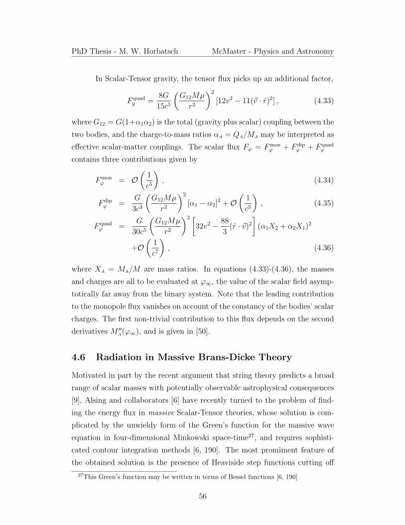
PhD Thesis - M. W. Horbatsch McMaster - Physics and Astronomy
In Scalar-Tensor gravity, the tensor flux picks up an additional factor,
F quadg =
8G
15c5
(G12Mµ
r2
)2
[12v2 − 11(~v · r)2] , (4.33)
where G12 = G(1+α1α2) is the total (gravity plus scalar) coupling between the
two bodies, and the charge-to-mass ratios αA = QA/MA may be interpreted as
effective scalar-matter couplings. The scalar flux Fϕ = Fmonϕ + F dip
ϕ + F quadϕ
contains three contributions given by
Fmonϕ = O
(1
c5
), (4.34)
F dipϕ =
G
3c3
(G12Mµ
r2
)2
[α1 − α2]2 +O(
1
c5
), (4.35)
F quadϕ =
G
30c5
(G12Mµ
r2
)2 [32v2 − 88
3(r · ~v)2
](α1X2 + α2X1)2
+O(
1
c7
), (4.36)
where XA = MA/M are mass ratios. In equations (4.33)-(4.36), the masses
and charges are all to be evaluated at ϕ∞, the value of the scalar field asymp-
totically far away from the binary system. Note that the leading contribution
to the monopole flux vanishes on account of the constancy of the bodies’ scalar
charges. The first non-trivial contribution to this flux depends on the second
derivatives M ′′A(ϕ∞), and is given in [50].
4.6 Radiation in Massive Brans-Dicke Theory
Motivated in part by the recent argument that string theory predicts a broad
range of scalar masses with potentially observable astrophysical consequences
[9], Alsing and collaborators [6] have recently turned to the problem of find-
ing the energy flux in massive Scalar-Tensor theories, whose solution is com-
plicated by the unwieldy form of the Green’s function for the massive wave
equation in four-dimensional Minkowski space-time27, and requires sophisti-
cated contour integration methods [6, 190]. The most promiment feature of
the obtained solution is the presence of Heaviside step functions cutting off
27This Green’s function may be written in terms of Bessel functions [6, 190]
56
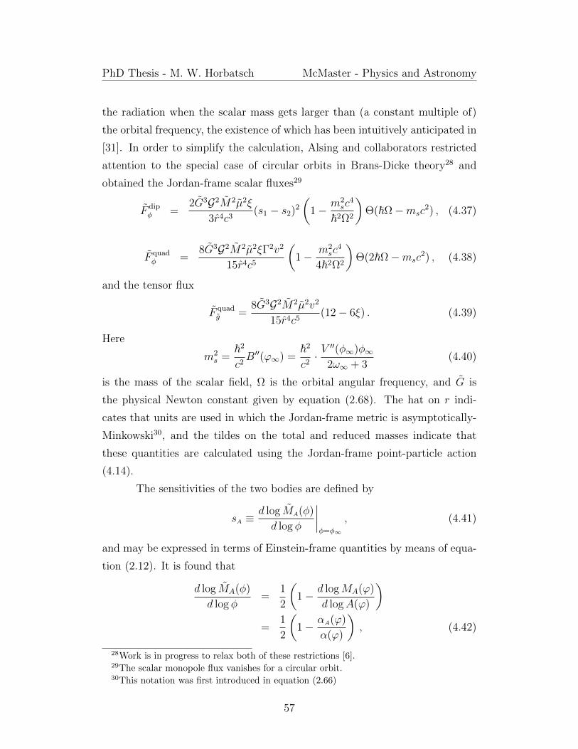
PhD Thesis - M. W. Horbatsch McMaster - Physics and Astronomy
the radiation when the scalar mass gets larger than (a constant multiple of)
the orbital frequency, the existence of which has been intuitively anticipated in
[31]. In order to simplify the calculation, Alsing and collaborators restricted
attention to the special case of circular orbits in Brans-Dicke theory28 and
obtained the Jordan-frame scalar fluxes29
F dipφ =
2G3G2M2µ2ξ
3r4c3(s1 − s2)2
(1− m2
sc4
~2Ω2
)Θ(~Ω−msc
2) , (4.37)
F quadφ =
8G3G2M2µ2ξΓ2v2
15r4c5
(1− m2
sc4
4~2Ω2
)Θ(2~Ω−msc
2) , (4.38)
and the tensor flux
F quadg =
8G3G2M2µ2v2
15r4c5(12− 6ξ) . (4.39)
Here
m2s =
~2
c2B′′(ϕ∞) =
~2
c2· V′′(φ∞)φ∞2ω∞ + 3
(4.40)
is the mass of the scalar field, Ω is the orbital angular frequency, and G is
the physical Newton constant given by equation (2.68). The hat on r indi-
cates that units are used in which the Jordan-frame metric is asymptotically-
Minkowski30, and the tildes on the total and reduced masses indicate that
these quantities are calculated using the Jordan-frame point-particle action
(4.14).
The sensitivities of the two bodies are defined by
sA ≡d log MA(φ)
d log φ
∣∣∣∣φ=φ∞
, (4.41)
and may be expressed in terms of Einstein-frame quantities by means of equa-
tion (2.12). It is found that
d log MA(φ)
d log φ=
1
2
(1− d logMA(ϕ)
d logA(ϕ)
)=
1
2
(1− αA(ϕ)
α(ϕ)
), (4.42)
28Work is in progress to relax both of these restrictions [6].29The scalar monopole flux vanishes for a circular orbit.30This notation was first introduced in equation (2.66)
57

PhD Thesis - M. W. Horbatsch McMaster - Physics and Astronomy
which implies
1− 2sA =αAα∞
. (4.43)
With this result in hand, the constants ξ, G, and Γ appearing in equations
(4.37)-(4.39) may be transformed into the Einstein frame:
ξ :=1
ω∞ + 2=
2α2∞
1 + α2∞, (4.44)
G := 1− ξ(s1 + s2 − 2s1s2) =1 + α1α2
1 + α2∞
, (4.45)
Γ := 1− 2(s1X2 + s2X1) =α1X2 + α2X1
α∞. (4.46)
Finally, upon putting everything together, it is found that31
F dipφ =
GA−2∞
3c3
(G12Mµ
r2
)2
(α1 − α2)2 ×(1− m2
sc4
~2Ω2
)Θ(~Ω−msc
2) , (4.47)
F quadϕ =
16GA−2∞
15c5
(G12Mµv
r2
)2
(α1X2 + α2X1)2 ×(1− m2
sc4
4~2Ω2
)Θ(2~Ω−msc
2) , (4.48)
F quadg =
96GA−2∞
15c5
(G12Mµv
r2
)2
, (4.49)
which is consistent with equations (4.33)-(4.36) in the limit of circular orbits
and a massless scalar, that is, r · ~v → 0 and ms → 0, explicitly confirming the
equivalence of the Einstein-frame and Jordan-frame formulations of Scalar-
Tensor gravity.
4.7 Effective Field Theory
4.7.1 Motivation
In General Relativity, the relativistic corrections to the equations of motion de-
scribed in section 4.4 were calculated in a mathematically well-defined manner
to order v5/c5, by employing the Riesz kernel (4.11) to regularize divergences
31The notation A∞ is short-hand for A(ϕ∞).
58

PhD Thesis - M. W. Horbatsch McMaster - Physics and Astronomy
arising in the point-particle limit [44, 42]. Two independent groups have at-
tempted to extend this calculation to order v6/c6, and both found that the
final equations of motion depend on an undetermined parameter arising in the
regularization procedure. Although initially conjectured that this ambiguity
is related to the physical incompleteness of the point-particle model, it was
later understood how the unknown parameter may be uniquely determined by
means of dimensional regularization. Subsequently, the results obtained by
these two groups were shown to be physically equivalent [22].
Motivated by the desire to obtain an intuitive physical understanding of
these complicated calculations, Goldberger and Rothstein [80, 78, 76] applied
the formalism of Effective Field Theory (EFT) [30] to the gravitational two-
body problem. This approach employs the tools of Quantum Field Theory
(QFT) [112] to handle divergences, and explains in very simple terms why
the traditional Post-Newtonian calculations run into difficulty at order v6/c6.
Moreover, the equations of motion, radiative multipole moments, and power
loss formulas may be calculated by means of Feynman diagrams and power
counting, which drastically reduces the amount of work required to obtain
results at a given Post-Newtonian order [77, 145, 80, 78, 76]. These methods
are particularly useful for incorporating the effects of spin [129, 134, 133, 132,
137, 138, 130, 136, 135] and disspiation [79, 131].
4.7.2 Introduction
Motivated by the separation of scales32 ubiquitous in nature, Effective Field
Theory (EFT) [30] is a framework built upon the axiom that it is always possi-
ble to describe physics at energies E Λ (or length scales r r0) using only
degrees of freedom accessible at those energies (or length scales). The high-
energy (or short-distance) degrees of freedom are ‘integrated out’, and their
effects are encoded into a set of low-energy (or long-distance) phenomenolog-
ical parameters. For instance, hydrodynamics is an effective field theory in
32For example, it is possible to understand the macroscopic properties of fluids without
understanding atomic physics (QED), and the latter may be understood without knowledge
of QCD.
59
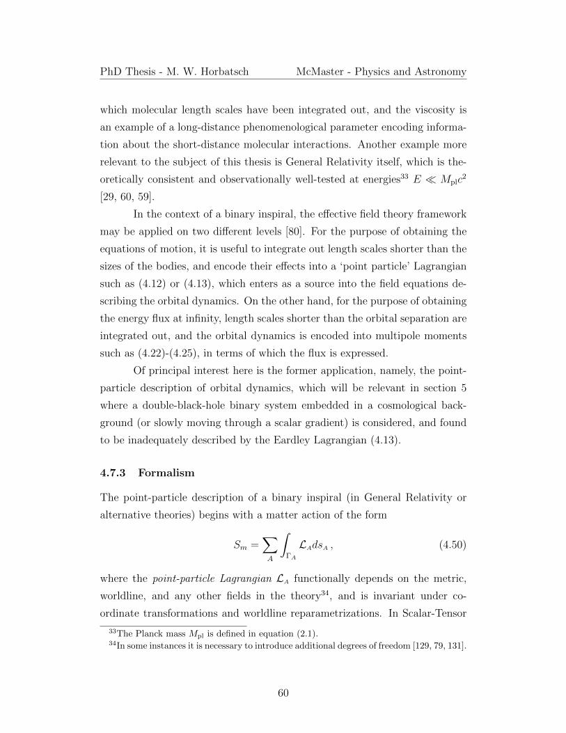
PhD Thesis - M. W. Horbatsch McMaster - Physics and Astronomy
which molecular length scales have been integrated out, and the viscosity is
an example of a long-distance phenomenological parameter encoding informa-
tion about the short-distance molecular interactions. Another example more
relevant to the subject of this thesis is General Relativity itself, which is the-
oretically consistent and observationally well-tested at energies33 E Mplc2
[29, 60, 59].
In the context of a binary inspiral, the effective field theory framework
may be applied on two different levels [80]. For the purpose of obtaining the
equations of motion, it is useful to integrate out length scales shorter than the
sizes of the bodies, and encode their effects into a ‘point particle’ Lagrangian
such as (4.12) or (4.13), which enters as a source into the field equations de-
scribing the orbital dynamics. On the other hand, for the purpose of obtaining
the energy flux at infinity, length scales shorter than the orbital separation are
integrated out, and the orbital dynamics is encoded into multipole moments
such as (4.22)-(4.25), in terms of which the flux is expressed.
Of principal interest here is the former application, namely, the point-
particle description of orbital dynamics, which will be relevant in section 5
where a double-black-hole binary system embedded in a cosmological back-
ground (or slowly moving through a scalar gradient) is considered, and found
to be inadequately described by the Eardley Lagrangian (4.13).
4.7.3 Formalism
The point-particle description of a binary inspiral (in General Relativity or
alternative theories) begins with a matter action of the form
Sm =∑A
∫ΓA
LAdsA , (4.50)
where the point-particle Lagrangian LA functionally depends on the metric,
worldline, and any other fields in the theory34, and is invariant under co-
ordinate transformations and worldline reparametrizations. In Scalar-Tensor
33The Planck mass Mpl is defined in equation (2.1).34In some instances it is necessary to introduce additional degrees of freedom [129, 79, 131].
60
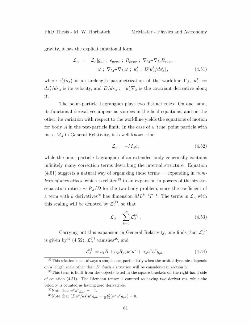
PhD Thesis - M. W. Horbatsch McMaster - Physics and Astronomy
gravity, it has the explicit functional form
LA = LA[gµν ; εµνρσ ; Rρσµν ; ∇λ1···∇λiRρσµν ;
ϕ ; ∇λ1···∇λiϕ ; uλA ; DiuλA/dsiA] , (4.51)
where zλA(sA) is an arclength parametrization of the worldline ΓA, uλA :=
dzλA/dsA is its velocity, and D/dsA := uλA∇λ is the covariant derivative along
it.
The point-particle Lagrangian plays two distinct roles. On one hand,
its functional derivatives appear as sources in the field equations, and on the
other, its variation with respect to the worldline yields the equations of motion
for body A in the test-particle limit. In the case of a ‘true’ point particle with
mass MA in General Relativity, it is well-known that
LA = −MAc , (4.52)
while the point-particle Lagrangian of an extended body generically contains
infinitely many correction terms describing the internal structure. Equation
(4.51) suggests a natural way of organizing these terms — expanding in num-
bers of derivatives, which is related35 to an expansion in powers of the size-to-
separation ratio ε ∼ RA/D for the two-body problem, since the coefficient of
a term with k derivatives36 has dimension MLk+1T−1. The terms in LA with
this scaling will be denoted by L(k)A , so that
LA =∞∑k=0
L(k)A . (4.53)
Carrying out this expansion in General Relativity, one finds that L(0)A
is given by37 (4.52), L(1)A vanishes38, and
L(2)A = a1R + a2Rµνu
µuν + a3uµuνgµν , (4.54)
35This relation is not always a simple one, particularly when the orbital dynamics depends
on a length scale other than D. Such a situation will be considered in section 5.36This term is built from the objects listed in the square brackets on the right-hand side
of equation (4.51). The Riemann tensor is counted as having two derivatives, while the
velocity is counted as having zero derivatives.37Note that uµuνgµν = −1.38Note that (Duµ/ds)uνgµν = 1
2Dds (uµuνgµν) = 0.
61
PhD Thesis - M. W. Horbatsch McMaster - Physics and Astronomy
where uµ is short-hand notation for the covariant derivative Duµ/ds, and the
body labels A on uµ, s, and ai have been suppressed for brevity. Since the
variation of the gravitational action∫d4x√−gR is a linear combination of Rµν
and R (see equation (A.46)), a re-definition of the metric may be employed to
remove the a1 and a2 terms from L(2)A , as explained in the appendix of [76].
A power-counting argument [78] demonstrates that the a1 and a2 terms may
only appear in the equations of motion at orders v6/c6 and higher, explaining
why the traditional approaches ran into difficulties at this order, while the fact
that a1 and a2 may be removed explains why it was possible to surmount these
difficulties39.
Turning to the a3 term quadratic in u, one finds that it may be removed
by redefining the dynamical variables zλA, since the variation of∫L(0)A dsA with
respect to the worldline is proportional to u [37]. Continuing the derivative
expansion to third order, one finds a plethora of terms involving R, ∇R, u,
u, and...u , which the present author has not seen discussed anywhere in the
literature. For instance, Goldberger and Rothstein [76, 79, 80] state that the
first non-redundant terms arise at fourth order in the derivative expansion,
and may be put into the canonical form
L(4)A = cEEµνE
µν + cBBµνBµν , (4.55)
where Eµν := Cµρνσuρuσ andBµν := Cµρνσu
ρuσ are the ‘electric’ and ‘magnetic’
parts of they Weyl tensor, respectively, where Cµρνσ := 12εµρκλC
κλνσ is the dual.
Turning to Scalar-Tensor gravity, it is found that L(0)A is given by the
Eardley Lagrangian (4.13), whereas L(1)A is a total derivative,
L(1)A =
dF (ϕ)
dsA, (4.56)
contributing only a boundary term to the action. Although eight terms are a
39The fact that a1 and a2 may be removed is also an explicit illustration of the principle
of effacement briefly mentioned in section 2.1.1.
62

PhD Thesis - M. W. Horbatsch McMaster - Physics and Astronomy
priori possible at second order,
L(2)A = a1(ϕ)R + a2(ϕ)Rµνu
µuν + a3(ϕ)uµuνgµν
+a4(ϕ)gµν∇µϕ∇νϕ+ a5(ϕ)uµuν∇µϕ∇νϕ
+a6(ϕ)gµν∇µ∇νϕ+ a7(ϕ)uµuν∇µ∇νϕ
+a8(ϕ)uµ∇µϕ , (4.57)
the field redefinition procedure described above may be employed to remove
the a3, a6, and a8 terms, and absorb the a1 and a2 terms into the a4 and a5
terms, respectively [53]. In the latter reference, it was demonstrated that for
bodies which are static and spherically-symmetric when unperturbed, the a4
term is the dominant one in the Post-Newtonian limit.
In summary, the formalism of Effective Field Theory demonstrates that
a derivative expansion of the point-particle Lagrangian is related to an expan-
sion in powers of the size-to-separation ratio ε ∼ R/D for a binary inspiral.
The next section considers an astrophysically interesting situation where the
Eardley Lagrangian (4.13) is inadequate, and it is necessary to go beyond
the zeroth order in this derivative expansion to correctly describe the orbital
dynamics.
63
PhD Thesis - M. W. Horbatsch McMaster - Physics and Astronomy
5 Miracle Hair Growth
5.1 Introduction
The purpose of this section is to construct an astrophysically interesting exam-
ple of a binary inspiral in which the Eardley Lagrangian (4.13) is inadequate to
describe the orbital dynamics, and the derivative expansion explained in 4.7.3
must be taken to higher orders. This may be accomplished by introducing a
new scale into the problem, and the natural candidate is the time scale T over
which the asymptotic background scalar ϕ∞ evolves, which may physically
arise either due to a cosmological embedding [70, 16], or a relative velocity to
an external scalar gradient, such as that sourced by the dark matter distri-
bution of a galaxy. In addition to the size-to-separation ratio ε ∼ R/D, the
orbital dynamics will then depend on the ratios Torb/T and Tint/T, where Torb
is the orbital time scale40, and Tint is the internal time scale41 of the bodies. It
turns out that O(Tint/T) effects cause black holes to grow scalar hair, which
is the subject of the next section.
5.2 Jacobson’s Formula
As discussed in section 3.3, black holes in Scalar-Tensor gravity often fail to
have ‘scalar hair’, and reduce to those of General Relativity. Although it is
not difficult to obtain hairy black-hole solutions, most of these constructions
are irrelevant for astrophysics, since they employ higher dimensions, electro-
magnetic charge, scalar potentials, and combinations thereof42. An interesting
exception is Jacobson’s Miracle Hair Growth Formula, discovered back in 1999
[96], which states that a Schwarzschild43 black hole subject to time-dependent
boundary conditions for the scalar field at spatial infinity grows hair, in other
words, acquires a non-zero scalar charge44 QA. More precisely, if the asymp-
40This quantity may be related to other orbital variables by equation (4.8).41For a black hole of mass M , Tint = GM/c3.42For a few examples, see [165, 156, 5, 111].43The result generalizes to a wide class of black holes in a fairly straightforward manner.44Recall that QA is defined by the integral in equation (3.7), or equivalently by the asymp-
totic expansion (3.4).
64
PhD Thesis - M. W. Horbatsch McMaster - Physics and Astronomy
totic value of the scalar ϕ∞ evolves linearly in time with scale T, that is,
ϕ(t, r = ∞) = t/T + const, and one works to linear order in the ratio45
δ := GMA/Tc3, then the dimensionless quantity characterizing the amount of
hair grown46 is given by
αA :=QA
MA
= 4δ =4GMA
Tc3. (5.1)
On a technical level, the vacuum field equations to be solved boil down
to the wave equation 2ϕ = 0 in a Schwarzschild background upon linearization
in δ, and the scalar field profile giving rise to the hair is the following globally-
defined zero mode of the d’Alembertian operator:
ϕ(t, r) =t
T+ 2δ log
∣∣∣∣1− 2GMA
rc2
∣∣∣∣ , (5.2)
where both terms individually satisfy the linear wave equation, and coefficients
are chosen so that the breakdown of the time coordinate at the horizon is
precisely cancelled by the singularity in the second term, as explained in [96,
91].
5.3 Double-Black-Hole Binaries
In the context of a double-black-hole binary, Jacobson’s formula implies that
both black holes acquire scalar charges given by (5.1) at linear order in δ, and
thus a scalar interaction between the black holes arises at order δ2. To find
the orbital corrections induced by this interaction, it is insufficient to use the
Eardley Lagrangian (4.13), because the mass (or any other physical property)
of a black hole in Scalar-Tensor gravity is invariant under shifts of the scalar
field, implying that the source term δSEardleym /δϕ in the scalar field equation
vanishes.
It follows from the discussion in 4.7.3 that the appropriate point-particle
Lagrangian from which the O(δ2) orbital corrections may be derived has the
45In taking this quantity to be small, one is assuming that the cosmological or galactic
time scale T associated with the evolution of ϕ∞ is much longer than the light crossing time
scale GMA/c3 of the black hole.
46This quantity, initially defined in section 4.5, enters into the power loss formulas (4.33)-
(4.36).
65

PhD Thesis - M. W. Horbatsch McMaster - Physics and Astronomy
general form
LA = −MAc+ (a4gµν + a5u
µuν)∇µϕ∇νϕ+ a7uµuν∇µ∇νϕ , (5.3)
where the coefficients ai do not depend on ϕ on account of the scalar-shift
symmetry of black holes, and may be determined by a matching calculation.
This calculation is reserved for future work, and attention is restricted to the
simpler problem of finding the dipole flux emitted by the accelerating scalar
charges. To leading order in δ and leading Post-Newtonian order, this flux is
given by the second term on the second line of equation (4.31), where the scalar
dipole moment ψi(U) is calculated by means of equation (4.24), in which the
source j is given by (4.28), with zA(t) being the O(δ0) unperturbed trajectory,
and M ′A(ϕ∞) being replaced by QA = αAMA as given by the Jacobson formula
(5.1). Putting everything together yields the final radiated scalar dipole power
F dipϕ =
G3M21M
22
3r4c3[α1 − α2]2 +O
(v5
c5
)+O(δ3) , (5.4)
for a double-black-hole binary in Scalar-Tensor gravity subject to the boundary
conditions ϕ(t, r =∞) = t/T + const.
5.4 The Quasar OJ287
The result (5.4) has a nice application to quasar OJ287, whose light intensity
as a function of time is quasi-periodic, with two ‘bursts’ occurring every 12
years. In 1988, this system was modelled by Sillanpaa and collaborators [157]
as a supermassive black hole binary, with an outburst occurring whenever
the orbit of the lighter black hole punctures the accretion disc of the heavier
companion. Work on the model continued following the outbursts of 1994-5
[107, 176, 167, 178, 143], and the first outburst of 2007 [182, 179, 177, 174]. In
particular, a prediction was made for the date of the second outburst, which
was subsequently verified by observations to within 6% [185]. Further work on
the model [183, 180, 184] has led to an estimate of the spin of the heavier black
hole [187, 181, 175], and it is expected that observations of future outbursts
will yield a test of the no-hair theorem [186].
66
PhD Thesis - M. W. Horbatsch McMaster - Physics and Astronomy
The agreement of the general-relativistic quadrupolar flux F quadg (given
by (4.20)) with the observations of OJ287 implies a bound on the ratio F dipϕ /F quad
g ,
which by means of equations (5.4), (5.1), and (4.20) may be translated into the
bound T & 16 days [91]. Although not impressive by cosmological or galactic
standards, it is quite remarkable that such a bound is even possible, given that
it is completely independent of any assumptions about how the scalar couples
to matter.
67
PhD Thesis - M. W. Horbatsch McMaster - Physics and Astronomy
6 Summary and Prospects
In this thesis, strong-field effects in Scalar-Tensor gravity were investigated,
and two novel results have been presented — The Weak Central Coupling
(WCC) framework for describing neutron star scalarization perturbatively, and
the Miracle Hair Growth in double-black-hole binaries induced by cosmological
and/or galactic effects.
The former has been worked out in the ‘quadratic’ model with confor-
mal factor (3.81) and Einstein-frame scalar-matter coupling (3.82) for simplic-
ity. However, since pulsar timing observations have already ruled out a large
region of the quadratic-model theory-space in which scalarization is allowed
[68, 66, 67, 65, 64, 53, 63, 52, 49, 20, 106, 74, 89], it would be worthwhile to
extend the WCC formalism to more complicated coupling functions, as well
as more general Scalar-Tensor theories such as Einstein-Dilaton-Gauss-Bonet
(EDGB) gravity [116, 126], in which a detailed study of stellar structure has
recently been undertaken [125].
A calculation of the scalar dipole flux emitted by a double-black-hole
binary has led to a bound on galactic and cosmological effects in quasar OJ287
which is interesting in principle, but not very useful in practice. However,
observations of future OJ287 outbursts, as well as direct gravitational wave
observations by second-generation detectors may yield better bounds.
A calculation of theoretical interest which has not yet been under-
taken, is the determination of the coefficients ai in the effective point-particle
Lagrangian (5.3) describing a ‘Jacobson’ black hole with ‘miracle hair’.
68

PhD Thesis - M. W. Horbatsch McMaster - Physics and Astronomy
A Mathematical Preliminaries
The purpose of this section is to establish conventions and notation, and list
the mathematical formulae that are used throughout the thesis.
A.1 Units
The speed of light is denoted by c. In the Einstein-frame formulation of Scalar-
Tensor gravity, the gravitational constant is denoted by G and scalar fields
are denoted by ϕ, while in the Jordan-frame formulation, the gravitational
constant (which is measured in a Cavendish experiment) is denoted by G
while scalar fields are denoted by φ. Geometrical units are not used, and all
factors of G and c are explicitly written. Note that ϕ is dimensionless, while
φ has units of 1/G, where G has units of Ld−1/MT 2 in d dimensions.
A.2 Basic Differential Geometry
The number of space-time dimensions is denoted by d. Although the case d = 4
is of physical interest, results are derived for arbitrary d whenever possible.
Space-time coordinates are denoted by xµ = (x0, xi), where x0 = ct is the time
coordinate, and xi are spatial coordinates. Greek indices run from 0 to d− 1,
and latin indices run from 1 to d − 1. The partial derivative with respect to
xµ is denoted by ∂µ.
The space-time metric is denoted by gµν , and its inverse is denoted by
gµν , so that gµνgνλ = δλµ. Differentiating this identity relates partial derivatives
of the metric to partial derivatives of the inverse metric:
∂λgµν = −gµρgνσ∂λgρσ , ∂λgµν = −gµρgνσ∂λgρσ . (A.1)
Unless stated otherwise, indices are raised and lowered with gµν and gµν , re-
spectively. Signs are chosen so that time-like vectors have negative norm, and
space-like vectors have positive norm. In other words, the metric is ‘mostly
plus’. MTW [114], Carroll [37], and Weinberg [191] all use this same choice of
sign, but some other authors use opposite signs.
69
PhD Thesis - M. W. Horbatsch McMaster - Physics and Astronomy
The flat Minkowski metric is denoted by ηµν . In canonical coordinates
on Minkowski space-time, it takes the form ηµν = diag(−1, 1, . . . , 1). The
notation for symmetrization and antisymmetrization of tensors is given by
T(µ1···µk) =1
k!
∑σ∈Sk
Tµσ(1)···µσ(k) , (A.2)
T[µ1···µk] =1
k!
∑σ∈Sk
(sgnσ)Tµσ(1)···µσ(k) . (A.3)
Note that some authors may omit the factor of k!.
The determinant of the metric, which is negative-definite, is denoted
by g. It appears in the canonical volume element of the space-time manifold,
dV =√−gdx0 · · · dxd−1 ≡
√−gddx , (A.4)
and its derivative may be computed by using the matrix identity log det =
tr log and equation (A.1):
∂λ√−g =
1
2
√−ggµν∂λgµν = −1
2
√−ggµν∂λgµν . (A.5)
The completely antisymmetric Levi-Civita tensor is defined to be
εµ1···µd =√−g · sgn(µ1 · · ·µd) , (A.6)
and its raised-index form is given by
εµ1···µd = − 1√−g· sgn(µ1 · · ·µd) (A.7)
When the partial derivative operator ∂µ acts on a tensor, the resulting
object is generally not a tensor. However, it is possible to define a covariant
derivative operator ∇µ, which maps tensors to tensors, annihilates the metric,
and reduces to the partial derivative operator when acting on scalars. Its
action on single-index tensors is given by
∇µVν = ∂µV
ν + ΓνµλVλ , ∇µVν = ∂µVν − ΓλµνVλ , (A.8)
and its action on multi-index tensors is given by straightforward generaliza-
tions of (A.8), with a +Γ correction term for each upper index, and a −Γ
correction term for each lower index.
70
PhD Thesis - M. W. Horbatsch McMaster - Physics and Astronomy
The Γλµν are called Christoffel symbols. They are not tensors, and they
are constructed to cancel the ‘non-covariant’ parts of ∂µ. An explicit formula
for them may be found by writing out the metric compatibility condition
∇λgµν = 0:
Γλµν =1
2gλσ (∂µgνσ + ∂νgµσ − ∂σgµν) . (A.9)
Contracting equation (A.9) and combining the result with equation (A.5)
yields
Γµµλ =1
2gµν∂λgµν = −1
2gµν∂λg
µν =∂λ√−g√−g
. (A.10)
The d’Alembertian wave operator is defined by 2 ≡ ∇µ∇µ. By means
of equation (A.10), the d’Alembertian of a scalar function f may be written
explicitly in coordinates as
2f = ∂µ∂µf + Γµµν∂
νf
=1√−g
∂µ(√−ggµν∂νf
). (A.11)
When acting on a scalar function f , covariant derivatives commute:
∇µ∇νf = ∇ν∇µf . However, this need not be the case when covariant deriva-
tives act on tensors of higher rank. The failure of covariant derivatives to
commute is quantified by the Riemann curvature tensor Rρσµν , so that for
single-index tensors,
[∇µ,∇ν ]Vρ = Rρ
σµνVσ , [∇µ,∇ν ]Vρ = −Rσ
ρµνVσ , (A.12)
and for multi-index tensors, the action of [∇µ,∇ν ] is given by a straightforward
generalization of equation (A.12), with a +R term for each upper index, and
a −R term for each lower index.
The curvature conventions used are those of MTW [114], Wald [189],
and Carroll [37]. They differ from those of Weinberg [191] by a sign. The
advantage of this choice is that the Ricci scalar curvature (A.18) is positive
on spheres and negative on hyperboloids, in line with intuition. However,
the disadvantage is that in an action, the gravitational kinetic term has the
opposite sign of the kinetic terms of other fields.
71
PhD Thesis - M. W. Horbatsch McMaster - Physics and Astronomy
Using (A.8) to evaluate the left-hand side of one of the equations in
(A.12) yields the following expression for the Riemann tensor in coordinates:
Rρσµν = ∂µΓρνσ − ∂νΓρµσ + ΓρµλΓ
λνσ − ΓρνλΓ
λµσ . (A.13)
It may be shown that the Riemann tensor has the following symmetry prop-
erties under the interchange of two indices:
Rρσµν = −Rρσνµ = −Rσρµν = Rµνρσ . (A.14)
The first equality in (A.14) follows immediately from the definition (A.12),
whereas it takes more work to derive the other two equalities. The Riemann
tensor also satisfies two Bianchi identities, which involve antisymmetrization
over three indices. The first of these is given by
Rρ[σµν] = 0 , (A.15)
and the second is given by
∇[λRρσ]µν = 0 . (A.16)
On account of the symmetries (A.14), there exists only one independent
non-vanishing contraction of the Riemann tensor. It is called the Ricci tensor,
and is defined by
Rµν = Rλµλν . (A.17)
It follows from (A.14) that the Ricci tensor is symmetric: Rµν = Rνµ. It may
be further contracted, to define the Ricci scalar:
R = Rµµ . (A.18)
Writing out and contracting the second Bianchi identity (A.16) yields the
following differential relation between the Ricci tensor and scalar:
∇µ
(Rµν −
1
2Rgµν
)= 0 . (A.19)
The trace-free part of the Riemann tensor, with the Ricci tensor and scalar
‘subtracted out’, is called the Weyl tensor, is given by
Cρσµν = Rρσµν−2
d− 2
(gρ[µRν]σ − gσ[µRν]ρ
)+
2
(d− 1)(d− 2)gρ[µgν]σR , (A.20)
72

PhD Thesis - M. W. Horbatsch McMaster - Physics and Astronomy
and has the same symmetry properties (A.14)-(A.15) as the Riemann tensor
under interchange of indices.
By means of equations (A.13), (A.9), and (A.1), the Ricci tensor (A.17)
may be written explicitly in terms of the metric and its partial derivatives as
Rµν =1
2gρσ(∂ν∂σgµρ − ∂ρ∂σgµν + ∂µ∂ρgνσ − ∂µ∂νgρσ)
+1
4gκλgρσ
(2∂κgµν∂σgρλ − ∂κgµν∂λgρσ
− 2∂νgµκ∂σgρλ + ∂νgµκ∂λgρσ
− 2∂µgνκ∂σgρλ + ∂µgνκ∂λgρσ
+ 2∂σgνλ∂ρgκµ − 2∂σgνλ∂κgρµ
+ ∂µgρλ∂νgσκ). (A.21)
In order to write the above expression as a non-linear wave operator acting
on the metric, it is useful to introduce harmonic coordinates, defined by the
condition
0 = 2xµ =1√−g
∂ν(√−ggµν) . (A.22)
It follows from equation (A.5) and (A.1) that the harmonic coordinate condi-
tion (A.22) is equivalent to
1
2gµν∂ρgµν = ∂σgρσ . (A.23)
Equation (A.23) may be used to simplify equation (A.21), and obtain the
following expression for the Ricci tensor in harmonic coordinates:
Rµν = −1
2gρσ∂ρ∂σgµν
+1
4gκλgρσ
(2∂νgρλ∂σgµκ + 2∂µgρλ∂σgνκ
+ 2∂σgνλ∂ρgκµ − 2∂σgνλ∂κgρµ
− ∂µgρλ∂νgσκ). (A.24)
73

PhD Thesis - M. W. Horbatsch McMaster - Physics and Astronomy
A.3 Static Spherically-Symmetric Metrics
In this section, coordinates for describing static spherically-symmetric bodies
are introduced, and the various curvature tensors are explicitly computed in
these coordinates.
The most general static spherically-symmetric metric may be written
as
ds2 = gµνdxµdxν = −f(r)c2dt2 + h(r)dr2 + k(r)dΩ2 , (A.25)
where the coordinates are xµ = (ct, r, θ1, . . . , θd−2), and dΩ2 is the canonical
line element on Sd−2 in hyperspherical coordinates, namely,
dΩ2 = dθ21 + sin2 θ1dθ
22 + sin2 θ1 sin2 θ2dθ
23 + · · ·
+(sin2 θ1 · · · sin2 θd−3)dθ2d−2 . (A.26)
Note that the functions f and h are dimensionless, while the function k has
units of length squared.
Given this choice of coordinates, it follows from equation (A.9) that
the independent non-vanishing Christoffel symbols are given by
Γ00r =
f ′
2f, (A.27)
Γr00 =f ′
2h, (A.28)
Γrrr =h′
2h, (A.29)
Γrθiθi = − k′
2k· gθiθih
, (A.30)
Γθirθi =k′
2k, (A.31)
Γθjθiθi
=
− cot θjg
θjθjgθiθi : j < i
0 : j ≥ i, (A.32)
Γθjθjθi
=
cot θi : i < j
0 : i ≥ j, (A.33)
where primes denote derivatives with respect to r, and it follows from equa-
tions (A.13) and (A.14) that the independent non-vanishing components of
74
PhD Thesis - M. W. Horbatsch McMaster - Physics and Astronomy
the Riemann tensor are given by
R0r0r = −f
′′
2f+f ′2
4f 2+f ′h′
4fh, (A.34)
R0θi0θi
= −f′k′
4fk
gθiθih
, (A.35)
Rrθirθi
=
(−k
′′
2k+k′2
4k2+h′k′
4hk
)gθiθih
, (A.36)
Rθiθjθiθj
=
(h
k− k′2
4k2
)gθjθjh
(i 6= j) . (A.37)
Carrying out the contraction (A.17) yields the following expressions for the
non-vanishing independent components of the Ricci tensor:
R00 =f
h
(f ′′
2f− f ′2
4f 2− f ′h′
4fh+
(d− 2)f ′k′
4fk
), (A.38)
Rrr = −f′′
2f+f ′2
4f 2+f ′h′
4fh+ (d− 2)
(−k
′′
2k+k′2
4k2+k′h′
4kh
), (A.39)
Rθiθi =
[d− 3 +
k
h
(−k
′′
2k− (d− 4)k′2
4k2+k′h′
4kh− k′f ′
4kf
)]gθiθik
. (A.40)
A.4 Variations of the Metric
In order to derive the field equations from the action in a relativistic theory
of gravity, it is necessary to consider a variation of the metric gµν → gµν +
δgµν , and compute how the various curvature tensors transform under such a
variation. The variations of the metric and its inverse are related by
δgµν = −gµρgνσδgρσ , δgµν = −gµρgνσδgρσ , (A.41)
which is analogous to equation (A.1). The variation of the determinant of the
metric is given by
δ√−g = −1
2
√−ggµνδgµν =
1
2
√−ggµνδgµν , (A.42)
which is analogous to equation (A.5). It follows from equations (A.9), (A.8),
and (A.41) that the variation of the Christoffel symbols is given by
δΓλµν =1
2gλσ (∇µδgνσ +∇νδgµσ −∇σδgµν) . (A.43)
75
PhD Thesis - M. W. Horbatsch McMaster - Physics and Astronomy
The variation of the Riemann curvature tensor is given by
δRρσµν = ∇µδΓ
ρνσ −∇νδΓ
ρµσ
=1
2gρλ([∇µ,∇ν ]δgσλ +∇µ(∇σδgνλ −∇λδgνσ)
−∇ν(∇σδgµλ −∇λδgµσ)), (A.44)
where the first equality follows equations (A.13) and (A.8), and the second
equality follows from equation (A.43). Taking variations of the contractions
of the Riemann tensor, one obtains
δRµν = ∇λδΓλµν −∇νδΓ
λλµ
= ∇λ∇(µδgν)λ −1
22δgµν −
1
2gλρ∇µ∇νδgλρ (A.45)
for the variation of the Ricci tensor, and
δR = −(Rµν + gµν2−∇µ∇ν)δgµν
= (Rµν + gµν2−∇µ∇ν)δgµν (A.46)
for the variation of the Ricci scalar.
A.5 Conformal Transformations
Scalar-tensor theories of gravity have two different mathematical representa-
tions, called the Einstein and Jordan frames. In order to convert between
them, it is necessary to know how the various curvature tensors transform
when the metric is re-scaled by a conformal factor:
gµν = Ω2gµν , gµν = Ω−2gµν , (A.47)
where Ω is a function of space-time. Let Γλµν , ∇µ, 2, Rρσµν , Rµν , and R be
the Christoffel symbols, covariant derivative, d’Alembertian, Riemann tensor,
Ricci tensor, and Ricci scalar, respectively, which are constructed using the
re-scaled metric (A.47). In particular, this means that the indices on Γλµν ,
∇µ, Rρσµν , and Rµν are raised and lowered with the re-scaled metric (A.47).
For example, R = gµνRµν , and Rρσµν = gρλRλσµν .
76
PhD Thesis - M. W. Horbatsch McMaster - Physics and Astronomy
In order to obtain the transformation of the Christoffel symbols, one
uses equations (A.9) and (A.47) to find that
Γλµν =1
2gλσ (∂µgνσ + ∂ν gµσ − ∂σgµν)
= Γλµν + (δλµ∂ν + δλν∂µ − gµνgλρ∂ρ) log Ω . (A.48)
Now to find the transformation of the Riemann tensor, the above result is
combined with equations (A.13) and (A.8), yielding
Rρσµν = ∂µΓρνσ − ∂νΓρµσ + ΓρµλΓ
λνσ − ΓρνλΓ
λµσ
= Rρσµν + 2(δβσδ
α[µδ
ρν] − g
ρβδα[µgν]σ)∇α∇β log Ω
+2(δρ[µδαν]δ
βσ − gρβgσ[µδ
αν] + gσ[µδ
ρν]g
αβ)∇α log Ω∇β log Ω .(A.49)
Contracting equation (A.49) gives the transformation of the Ricci tensor,
Rµν = Rµν −((d− 2)δρµδ
σν + gρσgµν
)∇ρ∇σ log Ω
+(d− 2)(δρµδσν − gρσgµν)∇ρ log Ω∇σ log Ω , (A.50)
and contracting again gives the transformation of the Ricci scalar,
R = Ω−2 [R− 2(d− 1)2 log Ω− (d− 2)(d− 1)gµν∇µ log Ω∇ν log Ω] .(A.51)
Note that in equations (A.48)-(A.50), indices may not be freely moved up and
down, because on the left-hand sides, the re-scaled metric (A.47) is used to
raise and lower indices, whereas on the right-hand sides, the original metric is
used to raise and lower indices.
Let g be the determinant of the re-scaled metric gµν . Its scaling is given
by √−g = Ωd
√−g , (A.52)
and therefore, the d’Alembertian operator acting on a scalar function, (A.11),
transforms according to
2f = ∇µ∇µf
=1√−g
∂µ
(√−ggµν∂νf
)= Ω−2 [2f + (d− 2)gµν∇µ log Ω∇νf ] . (A.53)
77

PhD Thesis - M. W. Horbatsch McMaster - Physics and Astronomy
This relation may be inverted to write 2f in terms of re-scaled quantities:
2f = Ω2[2f − (d− 2)gµν∇µ log Ω∇νf
]. (A.54)
Now, equation (A.54) may be combined with equation (A.51) to write R in
terms of re-scaled quantities:
R = Ω2[R + 2(d− 1)2 log Ω− (d− 1)(d− 2)gµν∇µ log Ω∇ν log Ω
]. (A.55)
It is also useful to write the relation between R and R in the form
R− 2(d− 1)2 log Ω = Ω2[R + (d− 2)(d− 1)gµν∇µ log Ω∇ν log Ω
], (A.56)
since the second term on the left-hand side is a total derivative.
A.6 Wave Equations and Green’s Functions
A useful tool for solving wave equations is the Green’s function G(x, y), which
is defined to be a solution of the wave equation with a point source:
2xG(x, y) = δy(x) , (A.57)
where δy is the Dirac distribution centered on y, which is defined by the con-
ditions δy(x) = 0 for x 6= y, and∫dVxf(x)δy(x) = f(y) (A.58)
for all functions f . The subscripts x on 2 and dV denote that the differ-
entiation and integration is with respect to the coordinate x. Given a wave
equation of the form 2f = j, a solution may be written in terms of Green’s
function as
f(x) =
∫dVyG(x, y)j(y) . (A.59)
Note that in order to uniquely determine G, it is necessary to supplement
equation (A.57) with appropriate boundary conditions.
For a general manifold, the calculation of G is a difficult problem. Even
in flat d-dimensional Minkowski space-time, there is no simple expression for
78
PhD Thesis - M. W. Horbatsch McMaster - Physics and Astronomy
G. However, in the special case d = 4, the Green’s function with ‘retarded’
boundary conditions is given by
G(x, y) = − 1
2πΘ(x0 − y0)δ[(xµ − yµ)(xµ − yµ)] , (A.60)
where Θ is the Heaviside step function, which ensures that ‘signals propagate
forward in time’, and δ is the one-dimensional Dirac distribution on R, which
ensures that ‘signals propagate at the speed of light’.
Writing equation (A.60) explicitly in terms of the space and time com-
ponents of the coordinates yields
G(x, y) = − 1
4π
δ[y0 − (x0 − |~x− ~y|)]|~x− ~y|
. (A.61)
Another operator whose Green’s function has a simple formula is the
d’Alembertian constructed out of the flat metric on the N -dimensional Eu-
clidean space RN , in other words, the Laplacian ∆. It may be shown that
G∆N(~x, ~y) = − 1
(N − 2)ΩN−1|~x− ~y|N−2(A.62)
is a Green’s function for ∆, that is,
∆xG∆N(~x, ~y) = δ(N)(~x− ~y) . (A.63)
where δ(N) is the Dirac distribution on RN . In equation (A.62), ΩN−1 denotes
the area of the sphere SN−1, and is given by
ΩN−1 =2πN/2
Γ(N/2). (A.64)
A.7 Hypergeometric and Heun Functions
In this section, the hypergeometric and Heun differential equations are in-
troduced. Their solutions are needed to describe constant-density stars in
Scalar-Tensor gravity by means of perturbation theory.
Given a linear second-order differential equation with three regular sin-
gular points, it is possible to find a fractional linear transformation which maps
79

PhD Thesis - M. W. Horbatsch McMaster - Physics and Astronomy
the singular points to 0, 1, and ∞, and thus brings the differential equation
into the canonical form
d2y
dz2+
(γ
z+
δ
z − 1
)dy
dz+
αβy
z(z − 1)= 0 , (A.65)
where the coefficients are related by
γ + δ = α + β + 1 . (A.66)
Equation (A.65) is the famous hypergeometric equation, which shows up through-
out theoretical and mathematical physics, and reduces to many well-known
special functions for particular values of α, β, and γ. The regular solution
about z = 0 has the series expansion
2F1(α, β; γ; z) =∞∑k=0
(α)k(β)k(γ)k
zk
k!, (A.67)
where
(x)k =Γ(x+ k)
Γ(x)= x(x+ 1) · · · (x+ k − 1) (A.68)
is the Pochhammer symbol.
Similarly, given a linear second-order differential equation with four
regular singular points, it is possible to find a fractional linear transforma-
tion which maps the singular points to 0, 1, ∞, and a, and thus brings the
differential equation into the canonical form
d2y
dz2+
(γ
z+
δ
z − 1+
ε
z − a
)dy
dz+
αβz − qz(z − 1)(z − a)
y = 0 , (A.69)
where the parameters are related by
γ + δ + ε = α + β + 1 . (A.70)
Equation (A.69) is called the Heun equation [144]. It was first studied by Karl
Heun in 1889, and is not nearly as well-known as the hypergeometric equation.
The regular solution about z = 0 has the series expansion
HeunG(a, q;α, β, γ, δ; z) =∞∑r=0
crzr , (A.71)
80
PhD Thesis - M. W. Horbatsch McMaster - Physics and Astronomy
where the coefficients cr satisfy the recursion relations
−qc0 + aγc1 = 0 , (A.72)
Prcr−1 − (Qr + q)cr +Rrcr+1 = 0 (r ≥ 1) , (A.73)
where
Pr = (r − 1 + α)(r − 1 + β) , (A.74)
Qr = r[(r − 1 + γ)(1 + a) + aδ + ε] , (A.75)
Rr = (r + 1)(r + γ)a . (A.76)
81

PhD Thesis - M. W. Horbatsch McMaster - Physics and Astronomy
References
[1] Andreas Albrecht, C.P. Burgess, F. Ravndal, and C. Skordis. Natural
quintessence and large extra dimensions. Phys.Rev., D65:123507, 2002,
astro-ph/0107573.
[2] Miguel Alcubierre, Juan C. Degollado, Dario Nunez, Milton Ruiz, and
Marcelo Salgado. Dynamic transition to spontaneous scalarization in
boson stars. Phys.Rev., D81:124018, 2010, 1003.4767.
[3] Stephon Alexander and Nicolas Yunes. Chern-Simons Modified Grav-
ity as a Torsion Theory and its Interaction with Fermions. Phys.Rev.,
D77:124040, 2008, 0804.1797.
[4] Stephon Alexander and Nicolas Yunes. Chern-Simons Modified General
Relativity. Phys.Rept., 480:1–55, 2009, 0907.2562.
[5] Masoud Allahverdizadeh and Ken Matsuno. Charged Rotating Kaluza-
Klein Black Holes in Dilaton Gravity. Phys.Rev., D81:044001, 2010,
0908.2484.
[6] Justin Alsing, Emanuele Berti, Clifford M. Will, and Helmut Zaglauer.
Gravitational radiation from compact binary systems in the massive
Brans-Dicke theory of gravity. Phys.Rev., D85:064041, 2012, 1112.4903.
[7] Pau Amaro-Seoane, Sofiane Aoudia, Stanislav Babak, Pierre Binetruy,
Emanuele Berti, et al. eLISA: Astrophysics and cosmology in the milli-
hertz regime. 2012, 1201.3621.
[8] K.G. Arun. Generic bounds on dipolar gravitational radiation from inspi-
ralling compact binaries. Class.Quant.Grav., 29:075011, 2012, 1202.5911.
[9] Asimina Arvanitaki, Savas Dimopoulos, Sergei Dubovsky, Nemanja
Kaloper, and John March-Russell. String Axiverse. Phys.Rev.,
D81:123530, 2010, 0905.4720.
82
PhD Thesis - M. W. Horbatsch McMaster - Physics and Astronomy
[10] Asimina Arvanitaki and Sergei Dubovsky. Exploring the String Axi-
verse with Precision Black Hole Physics. Phys.Rev., D83:044026, 2011,
1004.3558.
[11] Arjun Bagchi and S. Kalyana Rama. Cosmology and static spherically
symmetric solutions in D-dimensional scalar tensor theories: Some Novel
features. Phys.Rev., D70:104030, 2004, gr-qc/0408030.
[12] Thomas W. Baumgarte and Stuart L. Shapiro. Numerical Relativity:
Solving Einstein’s Equations on the Computer. Cambridge University
Press, 2010.
[13] Katrin Becker, Melanie Becker, and John H. Schwarz. String Theory and
M-Theory: A Modern Introduction. Cambridge University Press, 2007.
[14] Jacob D. Bekenstein. Gravitational-Radiation Recoil and Runaway
Black Holes. Astrophys.J., 183:657–664, 1973.
[15] Peter G. Bergmann. Comments on the scalar-tensor theory. Interna-
tional Journal of Theoretical Physics, 1(1):25–36, 1968.
[16] Marcelo Samuel Berman. Introduction to General Relativistic and
Scalar-tensor Cosmologies. Nova Science Pub Inc, 2007.
[17] Emanuele Berti, Leonardo Gualtieri, Michael Horbatsch, and Justin Als-
ing. Light scalar field constraints from gravitational-wave observations
of compact binaries. 2012, 1204.4340.
[18] B. Bertotti, L. Iess, and P. Tortora. A test of general relativity using
radio links with the Cassini spacecraft. Nature, 425:374–376, 2003.
[19] A. Bhadra, K. Sarkar, D.P. Datta, and K.K. Nandi. Brans-Dicke theory:
Jordan versus Einstein frame. Mod.Phys.Lett., A22:367–376, 2007, gr-
qc/0605109.
[20] N.D. Ramesh Bhat, Matthew Bailes, and Joris P.W. Verbiest.
Gravitational-radiation losses from the pulsar-white-dwarf binary PSR
J1141-6545. Phys.Rev., D77:124017, 2008, 0804.0956.
83

PhD Thesis - M. W. Horbatsch McMaster - Physics and Astronomy
[21] Luc Blanchet. Radiative gravitational fields in general relativity. 2.
Asymptotic behaviour at future null infinity. Proc.Roy.Soc.Lond.,
A409:383–399, 1987.
[22] Luc Blanchet. Gravitational radiation from post-Newtonian sources and
inspiralling compact binaries. Living Rev.Rel., 9:4, 2006.
[23] Luc Blanchet and Thibault Damour. Radiative gravitational fields in
general relativity I. general structure of the field outside the source.
Phil.Trans.Roy.Soc.Lond., A320:379–430, 1986.
[24] C. Brans and R. H. Dicke. Mach’s principle and a relativistic theory of
gravitation. Phys. Rev., 124(3):925–935, 1961.
[25] Carl H. Brans. The roots of scalar-tensor theory: an approximate history,
2005, arXiv:gr-qc/0506063.
[26] C.H. Brans. Mach’s Principle and a Relativistic Theory of Gravitation.
II. Phys.Rev., 125:2194–2201, 1962.
[27] Bernd Bruegmann, Jose A. Gonzalez, Mark Hannam, Sascha Husa,
and Ulrich Sperhake. Exploring black hole superkicks. Phys.Rev.,
D77:124047, 2008, 0707.0135.
[28] H. A. Buchdahl. General relativistic fluid spheres. Phys. Rev.,
116(4):1027–1034, 1959.
[29] C.P. Burgess. Quantum gravity in everyday life: General relativity as
an effective field theory. Living Rev.Rel., 7:5, 2004, gr-qc/0311082.
[30] C.P. Burgess. Introduction to Effective Field Theory.
Ann.Rev.Nucl.Part.Sci., 57:329–362, 2007, hep-th/0701053.
[31] C.P. Burgess and J. Cloutier. Astrophysical Evidence for a Weak New
Force? Phys.Rev., D38:2944, 1988.
[32] Manuela Campanelli, Carlos O. Lousto, Yosef Zlochower, and David
Merritt. Large merger recoils and spin flips from generic black-hole bi-
naries. Astrophys.J., 659:L5–L8, 2007, gr-qc/0701164.
84
PhD Thesis - M. W. Horbatsch McMaster - Physics and Astronomy
[33] Manuela Campanelli, Carlos O. Lousto, Yosef Zlochower, and David
Merritt. Maximum gravitational recoil. Phys.Rev.Lett., 98:231102, 2007,
gr-qc/0702133.
[34] W.B. Campbell, J. Macek, and T.A. Morgan. Relativistic Time Depen-
dent Multipole Analysis for Scalar, Electromagnetic, and Gravitational
Fields. Phys.Rev., D15:2156–2164, 1977.
[35] S. Capozziello, P. Martin-Moruno, and C. Rubano. Physical non-
equivalence of the Jordan and Einstein frames. Phys.Lett., B689:117–
121, 2010, 1003.5394.
[36] Vitor Cardoso, Sayan Chakrabarti, Paolo Pani, Emanuele Berti, and
Leonardo Gualtieri. Floating and sinking: The Imprint of massive
scalars around rotating black holes. Phys.Rev.Lett., 107:241101, 2011,
1109.6021.
[37] Sean Carroll. Spacetime and Geometry: An Introduction to General
Relativity. Pearson Education, Addison Wesley, 2004.
[38] Riccardo Catena, Massimo Pietroni, and Luca Scarabello. Einstein and
Jordan reconciled: a frame-invariant approach to scalar-tensor cosmol-
ogy. Phys.Rev., D76:084039, 2007, astro-ph/0604492.
[39] Katerina Chatziioannou, Nicolas Yunes, and Neil Cornish. Model-
Independent Test of General Relativity: An Extended post-Einsteinian
Framework with Complete Polarization Content. 2012, 1204.2585.
[40] Takeshi Chiba, Tomohiro Harada, and Ken-ichi Nakao. Gravita-
tional physics in scalar tensor theories: Tests of strong field gravity.
Prog.Theor.Phys.Suppl., 128:335–372, 1997.
[41] Neil Cornish, Laura Sampson, Nicolas Yunes, and Frans Pretorius. Grav-
itational Wave Tests of General Relativity with the Parameterized Post-
Einsteinian Framework. Phys.Rev., D84:062003, 2011, 1105.2088.
85
PhD Thesis - M. W. Horbatsch McMaster - Physics and Astronomy
[42] T. Damour. Gravitational radiation and the motion of compact bodies.
In N. Deruelle and T. Piran, editors, Gravitational Radiation, pages 59–
144. North-Holland Publishing Company, 1983.
[43] T. Damour. Un nouveau test de la relativite generale. In S. Benenti,
M. Ferraris, and M. Francaviglia, editors, Proceedings of ‘Journees rela-
tivistes 1983’, Torino, May 5-8, 1983, pages 89–110. Pitagora Editrice,
1985.
[44] T. Damour. The problem of motion in newtonian and einsteinian gravity.
In S.W. Hawking and W. Israel, editors, 300 Years of Gravitation, pages
128–198. Cambridge University Press, 1987.
[45] T. Damour and N. Deruelle. General relativistic celestial mechanics
of binary systems. i. the post-newtonian motion. Annales de l’Institut
Henri Poincare, 43:107–132, 1985.
[46] T. Damour and N. Deruelle. General relativistic celestial mechanics
of binary systems. ii. the post-newtonian timing formula. Annales de
l’Institut Henri Poincare, 44:263–292, 1986.
[47] T. Damour and Alexander M. Polyakov. String theory and gravity.
Gen.Rel.Grav., 26:1171–1176, 1994, gr-qc/9411069.
[48] T. Damour and Alexander M. Polyakov. The String dilaton and a least
coupling principle. Nucl.Phys., B423:532–558, 1994, hep-th/9401069.
[49] Thibault Damour. Binary Systems as Test-beds of Gravity Theories.
2007, 0704.0749.
[50] Thibault Damour and Gilles Esposito-Farese. Tensor-multi-scalar theo-
ries of gravitation. Class. Quantum Grav., 9(9):2093, 1992.
[51] Thibault Damour and Gilles Esposito-Farese. Nonperturbative strong
field effects in tensor - scalar theories of gravitation. Phys.Rev.Lett.,
70:2220–2223, 1993.
86

PhD Thesis - M. W. Horbatsch McMaster - Physics and Astronomy
[52] Thibault Damour and Gilles Esposito-Farese. Tensor - scalar gravity
and binary pulsar experiments. Phys.Rev., D54:1474–1491, 1996, gr-
qc/9602056.
[53] Thibault Damour and Gilles Esposito-Farese. Gravitational wave versus
binary - pulsar tests of strong field gravity. Phys.Rev., D58:042001, 1998,
gr-qc/9803031.
[54] Thibault Damour and Joseph H. Taylor. Strong field tests of relativistic
gravity and binary pulsars. Phys.Rev., D45:1840–1868, 1992.
[55] Simon DeDeo and Dimitrios Psaltis. Towards New Tests of Strong-
field Gravity with Measurements of Surface Atomic Line Redshifts from
Neutron Stars. Phys.Rev.Lett., 90:141101, 2003, astro-ph/0302095.
[56] Simon DeDeo and Dimitrios Psaltis. Testing strong-field gravity with
quasiperiodic oscillations. Bull. Am. Astron. Soc., 36, 2004, astro-
ph/0405067.
[57] R. H. Dicke. Mach’s principle and invariance under transformation of
units. Phys. Rev., 125(6):2163–2167, 1962.
[58] J.O. Dickey, P.L. Bender, J.E. Faller, X.X. Newhall, R.L. Ricklefs, et al.
Lunar Laser Ranging: A Continuing Legacy of the Apollo Program.
Science, 265:482–490, 1994.
[59] John F. Donoghue. General relativity as an effective field theory:
The leading quantum corrections. Phys.Rev., D50:3874–3888, 1994, gr-
qc/9405057.
[60] John F. Donoghue. Introduction to the effective field theory description
of gravity. 1995, gr-qc/9512024.
[61] Sergei Dubovsky and Victor Gorbenko. Black Hole Portal into Hidden
Valleys. Phys.Rev., D83:106002, 2011, 1012.2893.
[62] D.M. Eardley. Observable Effects of a Scalar Gravitational Field in a
Binary Pulsar. Astrophys.J., 196:L59–L62, 1975.
87
PhD Thesis - M. W. Horbatsch McMaster - Physics and Astronomy
[63] Gilles Esposito-Farese. Binary pulsar tests of strong field gravity. 1996,
gr-qc/9612039.
[64] Gilles Esposito-Farese. Comparing solar system, binary pulsar, and grav-
itational wave tests of gravity. 1999, gr-qc/9903058.
[65] Gilles Esposito-Farese. Tests of strong field gravity and gravitational
radiation damping in binary pulsar systems. 2000, gr-qc/0011114.
[66] Gilles Esposito-Farese. Tests of scalar-tensor gravity. AIP Conf.Proc.,
736:35–52, 2004, gr-qc/0409081.
[67] Gilles Esposito-Farese. Binary pulsar tests of strong field gravity and
gravitational radiation damping. Proceedings World Scientific, pages
647–666, 2005, gr-qc/0402007.
[68] Gilles Esposito-Farese. Motion in alternative theories of gravity. Fun-
dam.Theor.Phys., 162:461–489, 2011, 0905.2575.
[69] V. Faraoni and E. Gunzig. Einstein frame or Jordan frame?
Int.J.Theor.Phys., 38:217–225, 1999, astro-ph/9910176.
[70] Valerio Faraoni. Cosmology in Scalar-Tensor Gravity. Springer, 2004.
[71] M. Fierz. Uber die physikalische Deutung der erweiterten Gravitations-
theorie P. Jordans. Helvetica Physica Acta, 29:128–134, 1956.
[72] Eanna E. Flanagan. The Conformal frame freedom in theories of gravi-
tation. Class.Quant.Grav., 21:3817, 2004, gr-qc/0403063.
[73] E. Fomalont, S. Kopeikin, G. Lanyi, and J. Benson. Progress in Measure-
ments of the Gravitational Bending of Radio Waves Using the VLBA.
Astrophys.J., 699:1395–1402, 2009, 0904.3992.
[74] Paulo C.C. Freire, Norbert Wex, Gilles Esposito-Farese, Joris P.W. Ver-
biest, Matthew Bailes, et al. The relativistic pulsar-white dwarf binary
PSR J1738+0333 II. The most stringent test of scalar-tensor gravity.
2012, 1205.1450.
88

PhD Thesis - M. W. Horbatsch McMaster - Physics and Astronomy
[75] Yasunori Fujii and Kei-ichi Maeda. The Scalar-Tensor Theory of Grav-
itation. Cambridge University Press, 2007.
[76] Walter D. Goldberger. Les Houches lectures on effective field theories
and gravitational radiation. 2007, hep-ph/0701129.
[77] Walter D. Goldberger and Andreas Ross. Gravitational radiative correc-
tions from effective field theory. Phys.Rev., D81:124015, 2010, 0912.4254.
[78] Walter D. Goldberger and Ira Z. Rothstein. An Effective field the-
ory of gravity for extended objects. Phys.Rev., D73:104029, 2006, hep-
th/0409156.
[79] Walter D. Goldberger and Ira Z. Rothstein. Dissipative effects in the
worldline approach to black hole dynamics. Phys.Rev., D73:104030,
2006, hep-th/0511133.
[80] Walter D. Goldberger and Ira Z. Rothstein. Towers of Gravitational
Theories. Gen.Rel.Grav., 38:1537–1546, 2006, hep-th/0605238.
[81] J.A. Gonzalez, M.D. Hannam, U. Sperhake, Bernd Bruegmann, and
S. Husa. Supermassive recoil velocities for binary black-hole mergers
with antialigned spins. Phys.Rev.Lett., 98:231101, 2007, gr-qc/0702052.
[82] Samuel E. Gralla, Abraham I. Harte, and Robert M. Wald. Bobbing and
Kicks in Electromagnetism and Gravity. Phys.Rev., D81:104012, 2010,
1004.0679.
[83] Tomohiro Harada. Stability analysis of spherically symmetric star in
scalar - tensor theories of gravity. Prog.Theor.Phys., 98:359–379, 1997,
gr-qc/9706014.
[84] Tomohiro Harada. Neutron stars in scalar tensor theories of gravity and
catastrophe theory. Phys.Rev., D57:4802–4811, 1998, gr-qc/9801049.
[85] Gregory M. Harry. Advanced LIGO: The next generation of gravitational
wave detectors. Class.Quant.Grav., 27:084006, 2010.
89
PhD Thesis - M. W. Horbatsch McMaster - Physics and Astronomy
[86] S.W. Hawking. Black holes in the Brans-Dicke theory of gravitation.
Commun.Math.Phys., 25:167–171, 1972.
[87] James Healy, Tanja Bode, Roland Haas, Enrique Pazos, Pablo Laguna,
et al. Late Inspiral and Merger of Binary Black Holes in Scalar-Tensor
Theories of Gravity. 2011, 1112.3928.
[88] John L. Safko Herbert Goldstein, Charles P. Poole. Classical Mechanics.
Addison Wesley, 2001.
[89] M.W. Horbatsch and C.P. Burgess. Model-Independent Comparisons of
Pulsar Timings to Scalar-Tensor Gravity. 2011, 1107.3585.
[90] M.W. Horbatsch and C.P. Burgess. Semi-Analytic Stellar Structure in
Scalar-Tensor Gravity. JCAP, 1108:027, 2011, 1006.4411.
[91] M.W. Horbatsch and C.P. Burgess. Cosmic Black-Hole Hair Growth and
Quasar OJ287. JCAP, 1205:010, 2012, 1111.4009.
[92] R.A. Hulse and J.H. Taylor. Discovery of a pulsar in a binary system.
Astrophys.J., 195:L51–L53, 1975.
[93] Russell A. Hulse. The discovery of the binary pulsar. Rev.Mod.Phys.,
66:699–710, 1994.
[94] R. Jackiw and S.Y. Pi. Chern-Simons modification of general relativity.
Phys.Rev., D68:104012, 2003, gr-qc/0308071.
[95] John David Jackson. Classical Electrodynamics. Wiley, 1998.
[96] Ted Jacobson. Primordial black hole evolution in tensor scalar cosmol-
ogy. Phys.Rev.Lett., 83:2699–2702, 1999, astro-ph/9905303.
[97] P. Jordan. Zum gegenwartigen Stand der Diracschen kosmologischen
Hypothesen. Zeitschrift fur Physik, 157:112–121, 1959.
[98] Pascual Jordan. Formation of the stars and development of the universe.
Nature, 164(4172):637–640, 1949.
90
PhD Thesis - M. W. Horbatsch McMaster - Physics and Astronomy
[99] Kimmo Kainulainen and Daniel Sunhede. Dark energy from large extra
dimensions. Phys.Rev., D73:083510, 2006, astro-ph/0412609.
[100] Th. Kaluza. Zum Unitatsproblem der Physik. Sitzungsberichte der
Preußischen Akademie der Wissenschaften, pages 966–972, 1921.
[101] Drew Keppel, David A. Nichols, Yanbei Chen, and Kip S. Thorne. Mo-
mentum Flow in Black Hole Binaries. I. Post-Newtonian Analysis of
the Inspiral and Spin-Induced Bobbing. Phys.Rev., D80:124015, 2009,
0902.4077.
[102] Justin Khoury and Amanda Weltman. Chameleon fields: Awaiting sur-
prises for tests of gravity in space. Phys.Rev.Lett., 93:171104, 2004,
astro-ph/0309300.
[103] Oskar Klein. Quantentheorie und funfdimensionale Relativitatstheorie.
Zeitschrift fur Physik, 37(12):895–906, 1926.
[104] Hideo Kodama and Hirotaka Yoshino. Axiverse and Black Hole. 2011,
1108.1365.
[105] M. Kramer, Ingrid H. Stairs, R.N. Manchester, M.A. McLaughlin, A.G.
Lyne, et al. Tests of general relativity from timing the double pulsar.
Science, 314:97–102, 2006, astro-ph/0609417.
[106] K. Lazaridis, N. Wex, A. Jessner, M. Kramer, B.W. Stappers, et al.
Generic tests of the existence of the gravitational dipole radiation and
the variation of the gravitational constant. 2009, 0908.0285.
[107] H. J. Lehto and M. J. Valtonen. OJ 287 Outburst Structure and a Binary
Black Hole Model. Astrophys.J., 460:207, March 1996.
[108] D.R. Lorimer. Binary and Millisecond Pulsars. Living Rev.Rel., 11:8,
2008, 0811.0762.
[109] Geoffrey Lovelace, Yanbei Chen, Michael Cohen, Jeffrey D. Kaplan,
Drew Keppel, et al. Momentum flow in black-hole binaries. II. Numer-
91
PhD Thesis - M. W. Horbatsch McMaster - Physics and Astronomy
ical simulations of equal-mass, head-on mergers with antiparallel spins.
Phys.Rev., D82:064031, 2010, 0907.0869.
[110] A.G. Lyne, Marta Burgay, M. Kramer, A. Possenti, R.N. Manchester,
et al. A Double - pulsar system - A Rare laboratory for relativistic gravity
and plasma physics. Science, 303:1153–1157, 2004, astro-ph/0401086.
[111] Cristian Martinez and Ricardo Troncoso. Electrically charged black hole
with scalar hair. Phys.Rev., D74:064007, 2006, hep-th/0606130.
[112] Daniel V. Schroeder Michael E. Peskin. An Introduction to Quantum
Field Theory. Basic Books, 1995.
[113] Birger Bergersen Michael Plischke. Equilibrium Statistical Physics.
World Scientific, 1994.
[114] Charles W. Misner, Kip S. Thorne, and John A. Wheeler. Gravitation.
W. H. Freeman Company, 1973.
[115] David F. Mota and John D. Barrow. Varying alpha in a more realistic
Universe. Phys.Lett., B581:141–146, 2004, astro-ph/0306047.
[116] Filipe Moura and Ricardo Schiappa. Higher-derivative corrected black
holes: Perturbative stability and absorption cross-section in heterotic
string theory. Class.Quant.Grav., 24:361–386, 2007, hep-th/0605001.
[117] Alberto Nicolis, Riccardo Rattazzi, and Enrico Trincherini. The Galileon
as a local modification of gravity. Phys.Rev., D79:064036, 2009,
0811.2197.
[118] K. Nordtvedt. Testing relativity with laser ranging to the moon.
Phys.Rev., 170:1186–1187, 1968.
[119] Kenneth Nordtvedt. Equivalence Principle for Massive Bodies. 1. Phe-
nomenology. Phys.Rev., 169:1014–1016, 1968.
[120] Kenneth Nordtvedt. Equivalence Principle for Massive Bodies. 2. The-
ory. Phys.Rev., 169:1017–1025, 1968.
92
PhD Thesis - M. W. Horbatsch McMaster - Physics and Astronomy
[121] Kenneth Nordtvedt. Post-Newtonian metric for a general class of scalar-
tensor gravitational theories and observational consequences. The As-
trophysical Journal, 161:1059–1067, 1970.
[122] Jerome Novak. Neutron star transition to strong scalar field state in
tensor scalar gravity. Phys.Rev., D58:064019, 1998, gr-qc/9806022.
[123] Jerome Novak. Spherical neutron star collapse in tensor - scalar theory
of gravity. Phys.Rev., D57:4789–4801, 1998, gr-qc/9707041.
[124] Jerome Novak and Jose M. Ibanez. Gravitational waves from the col-
lapse and bounce of a stellar core in tensor scalar gravity. Astrophys.J.,
533:392–405, 2000, astro-ph/9911298.
[125] Paolo Pani, Emanuele Berti, Vitor Cardoso, and Jocelyn Read. Compact
stars in alternative theories of gravity. Einstein-Dilaton-Gauss-Bonnet
gravity. Phys.Rev., D84:104035, 2011, 1109.0928.
[126] Paolo Pani and Vitor Cardoso. Are black holes in alternative theories
serious astrophysical candidates? The Case for Einstein-Dilaton-Gauss-
Bonnet black holes. Phys.Rev., D79:084031, 2009, 0902.1569.
[127] Paolo Pani, Vitor Cardoso, and Leonardo Gualtieri. Gravitational waves
from extreme mass-ratio inspirals in Dynamical Chern-Simons gravity.
Phys.Rev., D83:104048, 2011, 1104.1183.
[128] Matthew Pitkin, Stuart Reid, Sheila Rowan, and Jim Hough. Gravita-
tional Wave Detection by Interferometry (Ground and Space). Living
Rev.Rel., 4:5, 2011, 1102.3355.
[129] Rafael A. Porto. Post-Newtonian corrections to the motion of spinning
bodies in NRGR. Phys.Rev., D73:104031, 2006, gr-qc/0511061.
[130] Rafael A. Porto. New results at 3PN via an effective field theory of
gravity. pages 2493–2496, 2007, gr-qc/0701106.
[131] Rafael A. Porto. Absorption effects due to spin in the worldline approach
to black hole dynamics. Phys.Rev., D77:064026, 2008, 0710.5150.
93

PhD Thesis - M. W. Horbatsch McMaster - Physics and Astronomy
[132] Rafael A. Porto. Next to leading order spin-orbit effects in the motion
of inspiralling compact binaries. Class.Quant.Grav., 27:205001, 2010,
1005.5730.
[133] Rafael A. Porto, Andreas Ross, and Ira Z. Rothstein. Spin induced
multipole moments for the gravitational wave flux from binary inspirals
to third Post-Newtonian order. JCAP, 1103:009, 2011, 1007.1312.
[134] Rafael A. Porto, Andreas Ross, and Ira Z. Rothstein. Spin induced
multipole moments for the gravitational wave amplitude from binary
inspirals to 2.5 Post-Newtonian order. 2012, 1203.2962.
[135] Rafael A. Porto and Ira Z. Rothstein. The Hyperfine Einstein-Infeld-
Hoffmann potential. Phys.Rev.Lett., 97:021101, 2006, gr-qc/0604099.
[136] Rafael A. Porto and Ira Z. Rothstein. Comment on ‘On the next-to-
leading order gravitational spin(1) - spin(2) dynamics’ by J. Steinhoff et
al. 2007, 0712.2032.
[137] Rafael A Porto and Ira Z. Rothstein. Next to Leading Order
Spin(1)Spin(1) Effects in the Motion of Inspiralling Compact Binaries.
Phys.Rev., D78:044013, 2008, 0804.0260.
[138] Rafael A. Porto and Ira Z. Rothstein. Spin(1)Spin(2) Effects in the
Motion of Inspiralling Compact Binaries at Third Order in the Post-
Newtonian Expansion. Phys.Rev., D78:044012, 2008, 0802.0720.
[139] Frans Pretorius. Binary Black Hole Coalescence. 2007, 0710.1338.
[140] Dimitrios Psaltis. Probes and Tests of Strong-Field Gravity with Obser-
vations in the Electromagnetic Spectrum. Living Rev.Rel., 11:9, 2008,
0806.1531.
[141] Dimitrios Psaltis. Testing General Metric Theories of Gravity with
Bursting Neutron Stars. Phys.Rev., D77:064006, 2008, 0704.2426.
94

PhD Thesis - M. W. Horbatsch McMaster - Physics and Astronomy
[142] M. Punturo, M. Abernathy, F. Acernese, B. Allen, N. Andersson, et al.
The Einstein Telescope: A third-generation gravitational wave observa-
tory. Class.Quant.Grav., 27:194002, 2010.
[143] T. Pursimo, L. O. Takalo, A. Sillanpaa, M. Kidger, H. J. Lehto, J. Heidt,
P. A. Charles, et al. Intensive monitoring of OJ 287. Astron. Astrophys.
Suppl., 146:141–155, October 2000.
[144] A. Ronveaux. Heun’s Differential Equations. Oxford University Press,
1995.
[145] Andreas Ross. Multipole expansion at the level of the action. 2012,
1202.4750. 39 pages.
[146] Marcelo Salgado. The Cauchy problem of scalar tensor theories of grav-
ity. Class.Quant.Grav., 23:4719–4742, 2006, gr-qc/0509001.
[147] Marcelo Salgado, David Martinez-del Rio, Miguel Alcubierre, and Dario
Nunez. Hyperbolicity of scalar-tensor theories of gravity. Phys.Rev.,
D77:104010, 2008, 0801.2372.
[148] Marcelo Salgado, Daniel Sudarsky, and Ulises Nucamendi. On sponta-
neous scalarization. Phys.Rev., D58:124003, 1998, gr-qc/9806070.
[149] Marcelo Salgado, Daniel Sudarsky, and Ulises Nucamendi. The Violation
of the weak energy condition, is it generic of spontaneous scalarization?
Phys.Rev., D70:084027, 2004, gr-qc/0402126.
[150] A. Salmona. Effect of Gravitational Scalar Field on High-Density Star
Structure. Phys.Rev., 154:1218–1223, 1967.
[151] B.S. Sathyaprakash and B.F. Schutz. Physics, Astrophysics and Cosmol-
ogy with Gravitational Waves. Living Rev.Rel., 12:2, 2009, 0903.0338.
[152] Paul D. Scharre and Clifford M. Will. Testing scalar tensor gravity using
space gravitational wave interferometers. Phys.Rev., D65:042002, 2002,
gr-qc/0109044.
95
PhD Thesis - M. W. Horbatsch McMaster - Physics and Astronomy
[153] Karl Schwarzschild. Uber das Gravitationsfeld einer Kugel aus inkom-
pressibler Flussigkeit. Sitzungsberichte Preuss. Akad. Wiss., pages 424–
434, 1916.
[154] Irwin I. Shapiro. Fourth Test of General Relativity. Phys.Rev.Lett.,
13:789–791, 1964.
[155] S.S. Shapiro, J.L. Davis, D.E. Lebach, and J.S. Gregory. Measure-
ment of the Solar Gravitational Deflection of Radio Waves using Geode-
tic Very-Long-Baseline Interferometry Data, 1979-1999. Phys.Rev.Lett.,
92:121101, 2004.
[156] A. Sheykhi, M. Allahverdizadeh, Y. Bahrampour, and M. Rahnama.
Asymptotically flat charged rotating dilaton black holes in higher di-
mensions. Phys.Lett., B666:82–85, 2008, 0805.4464.
[157] A. Sillanpaa, S. Haarala, M.J. Valtonen, B. Sundelius, and G.G. Byrd.
OJ 287 - Binary pair of supermassive black holes. Astrophys.J., 325:628–
634, 1988.
[158] T. Singh and L. N. Rai. Scalar-tensor theories of gravitation: Founda-
tions and prospects. General Relativity and Gravitation, 15(9):875–902,
1983.
[159] Carlos F. Sopuerta and Nicolas Yunes. Extreme and Intermediate-Mass
Ratio Inspirals in Dynamical Chern-Simons Modified Gravity. Phys.Rev.,
D80:064006, 2009, 0904.4501.
[160] Hajime Sotani and Kostas D. Kokkotas. Probing strong-field scalar-
tensor gravity with gravitational wave asteroseismology. Phys.Rev.,
D70:084026, 2004, gr-qc/0409066.
[161] Hajime Sotani and Kostas D. Kokkotas. Stellar oscillations in scalar-
tensor theory of gravity. Phys.Rev., D71:124038, 2005, gr-qc/0506060.
[162] Thomas P. Sotiriou and Valerio Faraoni. Black holes in scalar-tensor
gravity. Phys.Rev.Lett., 108:081103, 2012, 1109.6324. v1: 4 pages/ v2:
typos corrected, published version.
96

PhD Thesis - M. W. Horbatsch McMaster - Physics and Astronomy
[163] Ulrich Sperhake, Emanuele Berti, Vitor Cardoso, Frans Pretorius, and
Nicolas Yunes. Superkicks in ultrarelativistic encounters of spinning
black holes. Phys.Rev., D83:024037, 2011, 1011.3281.
[164] Ingrid H. Stairs. Testing general relativity with pulsar timing. Living
Rev.Rel., 6:5, 2003, astro-ph/0307536.
[165] Ivan Zh. Stefanov, Stoytcho S. Yazadjiev, and Michail D. Todorov.
Phases of 4D scalar-tensor black holes coupled to Born-Infeld nonlin-
ear electrodynamics. Mod.Phys.Lett., A23:2915–2931, 2008, 0708.4141.
[166] Leo C. Stein and Nicolas Yunes. Effective Gravitational Wave
Stress-energy Tensor in Alternative Theories of Gravity. Phys.Rev.,
D83:064038, 2011, 1012.3144.
[167] B. Sundelius, M. Wahde, H. J. Lehto, and M. J. Valtonen. A Numerical
Simulation of the Brightness Variations of OJ 287. Astrophys.J., 484:180,
July 1997.
[168] J.H. Taylor and J.M. Weisberg. A new test of general relativity: Grav-
itational radiation and the binary pulsar PS R 1913+16. Astrophys.J.,
253:908–920, 1982.
[169] Joseph H. Taylor. Binary pulsars and relativistic gravity. Rev.Mod.Phys.,
66:711–719, 1994.
[170] Joseph H. Taylor and J.M. Weisberg. Further experimental tests of
relativistic gravity using the binary pulsar PSR 1913+16. Astrophys.J.,
345:434–450, 1989.
[171] K.S. Thorne. Multipole Expansions of Gravitational Radiation.
Rev.Mod.Phys., 52:299–339, 1980.
[172] Tooru Tsuchida, Go Kawamura, and Kazuya Watanabe. A maximum
mass-to-size ratio in scalar-tensor theories of gravity. Progress of Theo-
retical Physics, 100(2):291–313, 1998.
97
PhD Thesis - M. W. Horbatsch McMaster - Physics and Astronomy
[173] A.I. Vainshtein. To the problem of nonvanishing gravitation mass.
Phys.Lett., B39:393–394, 1972.
[174] M. Valtonen, M. Kidger, H. Lehto, and G. Poyner. The structure of the
October/November 2005 outburst in OJ287 and the precessing binary
black hole model. Astron. Astrophys., 477:407–412, January 2008.
[175] M. Valtonen, S. Mikkola, H.J. Lehto, T. Hyvonen, K. Nilsson, et al.
Measuring Black Hole Spin in OJ287. 2010, 1001.1284.
[176] M. J. Valtonen. The OJ 287 binary model and the expected outburst
in November 1995. In L. O. Takalo, editor, Workshop on Two Years of
Intensive Monitoring of OJ 287 and 3C66A, page 64, 1996.
[177] M. J. Valtonen. New Orbit Solutions for the Precessing Binary Black
Hole Model of OJ 287. Astrophys.J., 659:1074–1081, April 2007.
[178] M. J. Valtonen and H. J. Lehto. Outbursts in OJ 287: A New Test for
the General Theory of Relativity. Astrophys.J., 481:L5, May 1997.
[179] M. J. Valtonen, H. J. Lehto, A. Sillanpaa, K. Nilsson, S. Mikkola,
R. Hudec, M. Basta, H. Terasranta, S. Haque, and H. Rampadarath.
Predicting the Next Outbursts of OJ 287 in 2006-2010. Astrophys.J.,
646:36–48, July 2006.
[180] M. J. Valtonen, H. J. Lehto, L. O. Takalo, and A. Sillanpaa. Testing the
1995 Binary Black Hole Model of OJ287. Astrophys.J., 729:33, March
2011.
[181] M. J. Valtonen, S. Mikkola, H. J. Lehto, T. Hyvonen, K. Nilsson, D. Mer-
ritt, A. Gopakumar, H. Rampadarath, R. Hudec, M. Basta, and R. Saun-
ders. Measuring black hole spin in OJ287. Celestial Mechanics and
Dynamical Astronomy, 106:235–243, March 2010, 1001.1284.
[182] M. J. Valtonen, K. Nilsson, A. Sillanpaa, L. O. Takalo, H. J. Lehto, W. C.
Keel, S. Haque, D. Cornwall, and A. Mattingly. The 2005 November
Outburst in OJ 287 and the Binary Black Hole Model. Astrophys.J.,
643:L9–L12, May 2006.
98

PhD Thesis - M. W. Horbatsch McMaster - Physics and Astronomy
[183] M. J. Valtonen, K. Nilsson, C. Villforth, H. J. Lehto, L. O. Takalo,
E. Lindfors, A. Sillanpaa, et al. Tidally Induced Outbursts in OJ 287
during 2005-2008. Astrophys.J., 698:781–785, June 2009.
[184] Mauri Valtonen and Stefano Ciprini. OJ 287 binary black hole system.
2011, 1112.1162.
[185] M.J. Valtonen, H.J. Lehto, K. Nilsson, J. Heidt, L.O. Takalo, et al.
A massive binary black-hole system in OJ 287 and a test of general
relativity. Nature, 452:851–853, 2008, 0809.1280.
[186] M.J. Valtonen, S. Mikkola, H.J. Lehto, A. Gopakumar, R. Hudec, et al.
Testing black hole no-hair theorem with OJ287. Astrophys.J., 742:22,
2011, 1108.5861.
[187] M.J. Valtonen, S. Mikkola, D. Merritt, A. Gopakumar, H.J. Lehto, et al.
Measuring the spin of the primary black hole in OJ287. Astrophys.J.,
709:725–732, 2010, 0912.1209.
[188] Robert V. Wagoner. Scalar-tensor theory and gravitational waves. Phys.
Rev. D, 1(12):3209–3216, 1970.
[189] Robert M. Wald. General Relativity. The University of Chicago Press,
1984.
[190] G. N. Watson. A Treatise on the Theory of Bessel Functions. Merchant
Books, 2008.
[191] Steven Weinberg. Gravitation and Cosmology: Principles and Applica-
tions of the General Theory of Relativity. Wiley, 1972.
[192] J.M. Weisberg, D.J. Nice, and J.H. Taylor. Timing Measurements of the
Relativistic Binary Pulsar PSR B1913+16. Astrophys.J., 722:1030–1034,
2010, 1011.0718.
[193] Joel M. Weisberg and Joseph H. Taylor. Relativistic binary pulsar
B1913+16: Thirty years of observations and analysis. ASP Conf.Ser.,
328:25, 2005, astro-ph/0407149.
99
PhD Thesis - M. W. Horbatsch McMaster - Physics and Astronomy
[194] A.W. Whinnett. Spontaneous scalarization and boson stars. Phys.Rev.,
D61:124014, 2000, gr-qc/9911052.
[195] A.W. Whinnett and Diego F. Torres. Spontaneous violation of the energy
conditions. Astrophys.J., 603:L133–L136, 2004, astro-ph/0401521.
[196] Clifford M. Will. Theory and Experiment in Gravitational Physics. Cam-
bridge University Press, 1993.
[197] Clifford M. Will. Testing scalar - tensor gravity with gravitational wave
observations of inspiraling compact binaries. Phys.Rev., D50:6058–6067,
1994, gr-qc/9406022.
[198] Clifford M. Will. The confrontation between general relativity and ex-
periment. Living Rev. Rel., 9:3, 2005, arXiv:gr-qc/0510072.
[199] Clifford M. Will. Resource Letter PTG-1: Precision Tests of Gravity.
2010, 1008.0296.
[200] Clifford M. Will and Douglas M. Eardley. Dipole gravitational radiation
in Rosen’s theory of gravity - Observable effects in the binary system
PSR 1913+16. Astrophys.J., 212:L91–L94, 1977.
[201] Clifford M. Will and Nicolas Yunes. Testing alternative theories of grav-
ity using LISA. Class.Quant.Grav., 21:4367, 2004, gr-qc/0403100.
[202] Clifford M. Will and Helmut W. Zaglauer. Gravitational Radiation,
Close Binary Systems, and the Brans-Dicke Theory of Gravity. Astro-
phys.J., 346:366, 1989.
[203] C.M. Will. Gravitational Radiation from Binary Systems in Alternative
Metric Theories of Gravity: Dipole Radiation and the Binary Pulsar.
Astrophys.J., 214:826–839, 1977.
[204] James G. Williams, Slava G. Turyshev, and Dale H. Boggs. Progress in
lunar laser ranging tests of relativistic gravity. Phys.Rev.Lett., 93:261101,
2004, gr-qc/0411113.
100

PhD Thesis - M. W. Horbatsch McMaster - Physics and Astronomy
[205] Kent Yagi, Leo C. Stein, Nicolas Yunes, and Takahiro Tanaka. Post-
Newtonian, Quasi-Circular Binary Inspirals in Quadratic Modified Grav-
ity. Phys.Rev., D85:064022, 2012, 1110.5950.
[206] Kent Yagi and Takahiro Tanaka. Constraining alternative theories of
gravity by gravitational waves from precessing eccentric compact binaries
with LISA. Phys.Rev., D81:064008, 2010, 0906.4269.
[207] Nicolas Yunes, Paolo Pani, and Vitor Cardoso. Gravitational Waves
from Extreme Mass-Ratio Inspirals as Probes of Scalar-Tensor Theories.
2011, 1112.3351.
[208] Nicolas Yunes and Frans Pretorius. Dynamical Chern-Simons Modified
Gravity. I. Spinning Black Holes in the Slow-Rotation Approximation.
Phys.Rev., D79:084043, 2009, 0902.4669.
[209] Nicolas Yunes and Frans Pretorius. Fundamental Theoretical Bias
in Gravitational Wave Astrophysics and the Parameterized Post-
Einsteinian Framework. Phys.Rev., D80:122003, 2009, 0909.3328.
[210] Nicolas Yunes and Carlos F. Sopuerta. Perturbations of Schwarzschild
Black Holes in Chern-Simons Modified Gravity. Phys.Rev., D77:064007,
2008, 0712.1028.
[211] Nicolas Yunes and Leo C. Stein. Non-Spinning Black Holes in Alternative
Theories of Gravity. Phys.Rev., D83:104002, 2011, 1101.2921. 7 pages,
submitted to PRD.
101


![Interacting scalar tensor cosmology in light of …arXiv:1502.05952v5 [astro-ph.CO] 27 Jan 2016 Noname manuscript No. (will be inserted by the editor) Interacting scalar tensor cosmology](https://static.fdocuments.us/doc/165x107/5fae6a5920eac96ac106b6af/interacting-scalar-tensor-cosmology-in-light-of-arxiv150205952v5-astro-phco.jpg)