arX

iv:1

507.

0561

3v2

[phy

sics

.ins-

det]

18

Oct

201

5

Neutrino Physics with JUNO

Fengpeng An1, Guangpeng An2, Qi An3, Vito Antonelli4, Eric Baussan5, John Beacom6,

Leonid Bezrukov7, Simon Blyth8, Riccardo Brugnera9, Margherita Buizza Avanzini10,

Jose Busto11, Anatael Cabrera12, Hao Cai13, Xiao Cai2, Antonio Cammi14,15, Guofu Cao2,

Jun Cao∗2, Yun Chang16, Shaomin Chen17, Shenjian Chen18, Yixue Chen19,

Davide Chiesa14,20, Massimiliano Clemenza14,20, Barbara Clerbaux21, Janet Conrad22,

Davide D’Angelo4, Herve De Kerret12, Zhi Deng17, Ziyan Deng2, Yayun Ding2,

Zelimir Djurcic23, Damien Dornic11, Marcos Dracos5, Olivier Drapier10, Stefano Dusini24,

Stephen Dye25, Timo Enqvist26, Donghua Fan27, Jian Fang2, Laurent Favart21,

Richard Ford4, Marianne Goger-Neff28, Haonan Gan29, Alberto Garfagnini9,

Marco Giammarchi4, Maxim Gonchar30, Guanghua Gong17, Hui Gong17, Michel Gonin10,

Marco Grassi2, Christian Grewing31, Mengyun Guan2, Vic Guarino23, Gang Guo32,

Wanlei Guo2, Xin-Heng Guo33, Caren Hagner34, Ran Han19, Miao He2, Yuekun Heng2,

Yee Hsiung8, Jun Hu2, Shouyang Hu35, Tao Hu2, Hanxiong Huang35, Xingtao Huang36,

Lei Huo37, Ara Ioannisian38, Manfred Jeitler39, Xiangdong Ji40, Xiaoshan Jiang2,

Cecile Jollet5, Li Kang41, Michael Karagounis31, Narine Kazarian38, Zinovy Krumshteyn30,

Andre Kruth31, Pasi Kuusiniemi26, Tobias Lachenmaier42, Rupert Leitner43, Chao Li36,

Jiaxing Li44, Weidong Li2, Weiguo Li2, Xiaomei Li35, Xiaonan Li2, Yi Li41, Yufeng Li2,

Zhi-Bing Li45, Hao Liang3, Guey-Lin Lin46, Tao Lin2, Yen-Hsun Lin46, Jiajie Ling47,45,

Ivano Lippi24, Dawei Liu48, Hongbang Liu49, Hu Liu45, Jianglai Liu32, Jianli Liu37,

Jinchang Liu2, Qian Liu50, Shubin Liu3, Shulin Liu2, Paolo Lombardi4, Yongbing Long27,

Haoqi Lu2, Jiashu Lu2, Jingbin Lu51, Junguang Lu2, Bayarto Lubsandorzhiev7,

Livia Ludhova4, Shu Luo52, Vladimir Lyashuk 7, Randolph Mollenberg28, Xubo Ma19,

Fabio Mantovani53, Yajun Mao54, Stefano M. Mari55, William F. McDonough56,

Guang Meng24, Anselmo Meregaglia5, Emanuela Meroni4, Mauro Mezzetto24,

Lino Miramonti4, Thomas Mueller 10, Dmitry Naumov30, Lothar Oberauer28, Juan

Pedro Ochoa-Ricoux57, Alexander Olshevskiy30, Fausto Ortica58, Alessandro Paoloni59,

Haiping Peng3, Jen-Chieh Peng†47, Ezio Previtali14, Ming Qi18, Sen Qian2, Xin Qian60,

Yongzhong Qian61,32, Zhonghua Qin2, Georg Raffelt62, Gioacchino Ranucci4,

Barbara Ricci53, Markus Robens31, Aldo Romani58, Xiangdong Ruan49, Xichao Ruan35,

Giuseppe Salamanna55, Mike Shaevitz63, Valery Sinev 7, Chiara Sirignano9,

Monica Sisti14,20, Oleg Smirnov30, Michael Soiron64, Achim Stahl64, Luca Stanco24,

Jochen Steinmann64, Xilei Sun2, Yongjie Sun3, Dmitriy Taichenachev30, Jian Tang45,

Igor Tkachev7, Wladyslaw Trzaska65, Stefan van Waasen31, Cristina Volpe12, Vit Vorobel43,

Lucia Votano59, Chung-Hsiang Wang16, Guoli Wang37, Hao Wang32, Meng Wang36,

Ruiguang Wang2, Siguang Wang54, Wei Wang45, Yi Wang17, Yi Wang27, Yifang Wang2,

Zhe Wang17, Zheng Wang2, Zhigang Wang2, Zhimin Wang2, Wei Wei2, Liangjian Wen2,

Christopher Wiebusch64, Bjorn Wonsak34, Qun Wu36, Claudia-Elisabeth Wulz39,

Michael Wurm66, Yufei Xi29, Dongmei Xia44, Yuguang Xie2, Zhi-zhong Xing‡2, Jilei Xu2,

Baojun Yan2, Changgen Yang2, Chaowen Yang67, Guang Yang23, Lei Yang41, Yifan Yang21,

Yu Yao31, Ugur Yegin31, Frederic Yermia68, Zhengyun You45, Boxiang Yu2, Chunxu Yu69,

Zeyuan Yu2, Sandra Zavatarelli70, Liang Zhan2, Chao Zhang60, Hong-Hao Zhang45,

1

Jiawen Zhang2, Jingbo Zhang37, Qingmin Zhang71, Yu-Mei Zhang45, Zhenyu Zhang13,

Zhenghua Zhao2, Yangheng Zheng50, Weili Zhong2, Guorong Zhou27, Jing Zhou35,

Li Zhou2, Rong Zhou67, Shun Zhou2, Wenxiong Zhou44, Xiang Zhou13, Yeling Zhou2,

Yufeng Zhou72, and Jiaheng Zou2

1East China University of Science and Technology, Shanghai, China2Institute of High Energy Physics, Beijing, China

3University of Science and Technology of China, Hefei, China4INFN Sezione di Milano and Dipartimento di Fisica dell’Universita di Milano, Milan,

Italy5Institut Pluridisciplinaire Hubert Curien, Universite de Strasbourg, CNRS/IN2P3,

Strasbourg, France6Department of Physics and Department of Astronomy, Ohio State University, Columbus,

OH, USA7Institute for Nuclear Research of the Russian Academy of Sciences, Moscow, Russia

8Department of Physics, National Taiwan University, Taipei, Taiwan, China9Dipartimento di Fisica e Astronomia dell’Universita di Padova and INFN Sezione di

Padova, Padova, Italy10Leprince-Ringuet Laboratory Ecole Polytechnique, Palaiseau Cedex, France

11Centre de Physique des Particules de Marseille, Marseille, France12Astro-Particle Physics Laboratory, CNRS/CEA/Paris7/Observatoire de Paris, Paris,

France13Wuhan University, Wuhan, China

14INFN Sezione Milano Bicocca, Milan, Italy15Politecnico di Milano, Department of Energy, CeSNEF (Enrico Fermi Center for Nuclear

Studies), Milan, Italy16National United University, Miao-Li, Taiwan, China

17Tsinghua University, Beijing, China18Nanjing University, Nanjing, China

19North China Electric Power University, Beijing, China20Department of Physics, University of Milano Bicocca, Milan, Italy

21Universite Libre de Bruxelles, Brussels, Belgium22Massachusetts Institute of Technology, Cambridge, MA, USA

23Argonne National Laboratory, Argonne, IL, USA24INFN Sezione di Padova, Padova, Italy

25Department of Physics and Astronomy, University of Hawaii, Honolulu, HI, USA26Oulu Southern Institute, University of Oulu, Pyhasalmi, Finland

27Wuyi University, Jiangmen, China28Technical University of Munich, Garching, Germany

29Institute of Hydrogeology and Environmental Geology, Chinese Academy of GeologicalSciences, Shijiazhuang, China

30Joint Institute for Nuclear Research, Dubna, Russia31Forschungszentrum Julich GmbH, Central Institute of Engineering, Electronics and

Analytics - Electronic Systems (ZEA-2), Julich, Germany32Shanghai Jiao Tong University, Shanghai, China

33Beijing Normal University, Beijing, China

2

34Institute of Experimental Physics, University of Hamburg, Hamburg, Germany35China Institute of Atomic Energy, Beijing, China

36Shandong University, Jinan, China37Harbin Institute of Technology, Harbin, China38Yerevan Physics Institute, Yerevan, Armenia

39Institute of High Energy Physics, Vienna, Austria40Department of Physics, University of Maryland, College Park, MD, USA

41Dongguan University of Technology, Dongguan, China42Eberhard Karls Universitat Tubingen, Physikalisches Institut, Tubingen, Germany43Charles University, Faculty of Mathematics and Physics, Prague, Czech Republic

44Chongqing University, Chongqing, China45Sun Yat-Sen University, Guangzhou, China

46Institute of Physics National Chiao-Tung University, Hsinchu, Taiwan, China47Department of Physics, University of Illinois at Urbana-Champaign, Urbana, IL, USA

48Department of Physics, University of Houston, Houston, TX, USA49Guangxi University, Nanning, China

50University of Chinese Academy of Sciences, Beijing, China51Jilin University, Changchun, China52Xiamen University, Xiamen, China

53Department of Physics and Earth Science, University of Ferrara and INFN Sezione diFerrara, Ferrara, Italy

54School of Physics, Peking University, Beijing, China55University of Roma Tre and INFN Sezione Roma Tre, Roma, Italy

56Department of Geology, University of Maryland, College Park, MD, USA57Instituto de Fisica, Pontificia Universidad Catolica de Chile, Santiago, Chile

58INFN and University of Perugia - Department of Chemistry, Biology and Biotechnology,Perugia, Italy

59Laboratori Nazionali di Frascati dell’INFN, Roma, Italy60Brookhaven National Laboratory, Upton, NY, USA

61School of Physics and Astronomy, University of Minnesota, Minneapolis, MN, USA62Max Planck Institute for Physics (Werner Heisenberg Institute), Munich, Germany

63Columbia University, New York, NY, USA64III. Physikalisches Institut B, RWTH Aachen University, Aachen, Germany

65Department of Physics, University of Jyvaskyla, Jyvaskyla, Finland66Institute of Physics and EC PRISMA, Johannes-Gutenberg University Mainz, Mainz,

Germany67Sichuan University, Chengdu, China

68SUBATECH, CNRS/IN2P3, Universite de Nantes, Ecole des Mines de Nantes, Nantes,France

69Nankai University, Tianjin, China70INFN Sezione di Genova, Genova, Italy71Xi’an Jiaotong University, Xi’an, China

72Institute of Theoretical Physics, Beijing, China

3

∗Co-editor, Email: caoj@ihep.ac.cn†Co-editor, Email: jcpeng@illinois.edu‡Co-editor, Email: xingzz@ihep.ac.cn

4

Abstract

The Jiangmen Underground Neutrino Observatory (JUNO), a 20 kton multi-purpose under-ground liquid scintillator detector, was proposed with the determination of the neutrino masshierarchy as a primary physics goal. The excellent energy resolution and the large fiducialvolume anticipated for the JUNO detector offer exciting opportunities for addressing many im-portant topics in neutrino and astro-particle physics. In this document, we present the physicsmotivations and the anticipated performance of the JUNO detector for various proposed mea-surements.

Following an introduction summarizing the current status and open issues in neutrino physics,we discuss how the detection of antineutrinos generated by a cluster of nuclear power plantsallows the determination of the neutrino mass hierarchy at a 3-4σ significance with six yearsof running of JUNO. The measurement of antineutrino spectrum with excellent energy resolu-tion will also lead to the precise determination of the neutrino oscillation parameters sin2 θ12,∆m2

21, and |∆m2ee| to an accuracy of better than 1%, which will play a crucial role in the future

unitarity test of the MNSP matrix.The JUNO detector is capable of observing not only antineutrinos from the power plants, but

also neutrinos/antineutrinos from terrestrial and extra-terrestrial sources, including supernovaburst neutrinos, diffuse supernova neutrino background, geoneutrinos, atmospheric neutrinos,and solar neutrinos. As a result of JUNO’s large size, excellent energy resolution, and vertexreconstruction capability, interesting new data on these topics can be collected. For example,a neutrino burst from a typical core-collapse supernova at a distance of 10 kpc would leadto ∼ 5000 inverse-beta-decay events and ∼ 2000 all-flavor neutrino-proton elastic scatteringevents in JUNO, which are of crucial importance for understanding the mechanism of supernovaexplosion and for exploring novel phenomena such as collective neutrino oscillations. Detectionof neutrinos from all past core-collapse supernova explosions in the visible universe with JUNOwould further provide valuable information on the cosmic star-formation rate and the averagecore-collapse neutrino energy spectrum. Antineutrinos originating from the radioactive decay ofUranium and Thorium in the Earth can be detected in JUNO with a rate of ∼ 400 events peryear, significantly improving the statistics of existing geoneutrino event samples. Atmosphericneutrino events collected in JUNO can provide independent inputs for determining the masshierarchy and the octant of the θ23 mixing angle. Detection of the 7Be and 8B solar neutrinoevents at JUNO would shed new light on the solar metallicity problem and examine the transitionregion between the vacuum and matter dominated neutrino oscillations.

Regarding light sterile neutrino topics, sterile neutrinos with 10−5 eV2 < ∆m241 < 10−2 eV2

and a sufficiently large mixing angle θ14 could be identified through a precise measurement ofthe reactor antineutrino energy spectrum. Meanwhile, JUNO can also provide us excellent op-portunities to test the eV-scale sterile neutrino hypothesis, using either the radioactive neutrinosources or a cyclotron-produced neutrino beam.

The JUNO detector is also sensitive to several other beyond-the-standard-model physics.Examples include the search for proton decay via the p → K+ + ν decay channel, search forneutrinos resulting from dark-matter annihilation in the Sun, search for violation of Lorentzinvariance via the sidereal modulation of the reactor neutrino event rate, and search for theeffects of non-standard interactions.

The proposed construction of the JUNO detector will provide a unique facility to addressmany outstanding crucial questions in particle and astrophysics in a timely and cost-effectivefashion. It holds the great potential for further advancing our quest to understanding thefundamental properties of neutrinos, one of the building blocks of our Universe.

5

Contents

1 Introduction 201.1 Neutrino Oscillations in a Nutshell . . . . . . . . . . . . . . . . . . . . . . . . . . . . 20

1.1.1 Flavor mixing and neutrino oscillation probabilities . . . . . . . . . . . . . . . 201.1.2 Known and unknown neutrino oscillation parameters . . . . . . . . . . . . . . 22

1.2 Open Issues of Massive Neutrinos . . . . . . . . . . . . . . . . . . . . . . . . . . . . . 231.2.1 The nature of neutrinos and their mass spectrum . . . . . . . . . . . . . . . . 231.2.2 Lepton flavor mixing pattern and CP violation . . . . . . . . . . . . . . . . . 251.2.3 Extra neutrino species and unitarity tests . . . . . . . . . . . . . . . . . . . . 27

1.3 JUNO Experiment . . . . . . . . . . . . . . . . . . . . . . . . . . . . . . . . . . . . . 281.3.1 Experimental site . . . . . . . . . . . . . . . . . . . . . . . . . . . . . . . . . . 291.3.2 JUNO Detector . . . . . . . . . . . . . . . . . . . . . . . . . . . . . . . . . . . 30

2 Identifying the Neutrino Mass Hierarchy 332.1 Introduction and motivation . . . . . . . . . . . . . . . . . . . . . . . . . . . . . . . . 332.2 Signal and Background . . . . . . . . . . . . . . . . . . . . . . . . . . . . . . . . . . . 38

2.2.1 Reactor neutrino signal . . . . . . . . . . . . . . . . . . . . . . . . . . . . . . 382.2.2 Background estimation . . . . . . . . . . . . . . . . . . . . . . . . . . . . . . . 40

2.3 The MH Sensitivity . . . . . . . . . . . . . . . . . . . . . . . . . . . . . . . . . . . . 422.3.1 Basic Setup and Definition . . . . . . . . . . . . . . . . . . . . . . . . . . . . 422.3.2 Baseline Optimization . . . . . . . . . . . . . . . . . . . . . . . . . . . . . . . 432.3.3 Requirement on the Energy Resolution . . . . . . . . . . . . . . . . . . . . . . 442.3.4 Statistical Interpretation . . . . . . . . . . . . . . . . . . . . . . . . . . . . . . 46

2.4 Systematics . . . . . . . . . . . . . . . . . . . . . . . . . . . . . . . . . . . . . . . . . 482.4.1 Reactor related uncertainties . . . . . . . . . . . . . . . . . . . . . . . . . . . 482.4.2 Detector related uncertainties . . . . . . . . . . . . . . . . . . . . . . . . . . . 492.4.3 Background related uncertainties . . . . . . . . . . . . . . . . . . . . . . . . . 522.4.4 Systematics summary . . . . . . . . . . . . . . . . . . . . . . . . . . . . . . . 52

2.5 MH Sensitivity with Precision |∆m2ee| and |∆m2

µµ| Measurements . . . . . . . . . . . 532.6 Conclusions . . . . . . . . . . . . . . . . . . . . . . . . . . . . . . . . . . . . . . . . . 53

3 Precision Measurements of Neutrinos 553.1 Introduction and motivation . . . . . . . . . . . . . . . . . . . . . . . . . . . . . . . . 553.2 Precision measurements of oscillation parameters . . . . . . . . . . . . . . . . . . . . 583.3 Tests of the standard three-neutrino paradigm . . . . . . . . . . . . . . . . . . . . . . 633.4 Conclusions . . . . . . . . . . . . . . . . . . . . . . . . . . . . . . . . . . . . . . . . . 66

4 Supernova Burst Neutrinos 684.1 Core-collapse supernovae: What, where and when? . . . . . . . . . . . . . . . . . . . 684.2 Neutrino signature of core collapse . . . . . . . . . . . . . . . . . . . . . . . . . . . . 70

4.2.1 Neutrino-driven explosion . . . . . . . . . . . . . . . . . . . . . . . . . . . . . 704.2.2 Three-phase neutrino signal . . . . . . . . . . . . . . . . . . . . . . . . . . . . 72

4.3 Detection channels in JUNO . . . . . . . . . . . . . . . . . . . . . . . . . . . . . . . 744.3.1 Time-integrated event rates . . . . . . . . . . . . . . . . . . . . . . . . . . . . 744.3.2 Elastic neutrino-proton scattering . . . . . . . . . . . . . . . . . . . . . . . . 764.3.3 Backgrounds . . . . . . . . . . . . . . . . . . . . . . . . . . . . . . . . . . . . 794.3.4 Data acquisition . . . . . . . . . . . . . . . . . . . . . . . . . . . . . . . . . . 80

6

4.4 Implications for astrophysics . . . . . . . . . . . . . . . . . . . . . . . . . . . . . . . . 814.4.1 Pre-supernova neutrinos . . . . . . . . . . . . . . . . . . . . . . . . . . . . . . 824.4.2 Locating the supernova . . . . . . . . . . . . . . . . . . . . . . . . . . . . . . 834.4.3 Coincidence with gravitational waves . . . . . . . . . . . . . . . . . . . . . . . 844.4.4 SN nucleosynthesis . . . . . . . . . . . . . . . . . . . . . . . . . . . . . . . . . 84

4.5 Implications for particle physics . . . . . . . . . . . . . . . . . . . . . . . . . . . . . . 854.5.1 Bound on neutrino masses . . . . . . . . . . . . . . . . . . . . . . . . . . . . . 854.5.2 Impact of mass ordering . . . . . . . . . . . . . . . . . . . . . . . . . . . . . . 874.5.3 Collective neutrino oscillations . . . . . . . . . . . . . . . . . . . . . . . . . . 884.5.4 Constraining new physics . . . . . . . . . . . . . . . . . . . . . . . . . . . . . 89

4.6 Summary . . . . . . . . . . . . . . . . . . . . . . . . . . . . . . . . . . . . . . . . . . 89

5 Diffuse Supernova Neutrino Background (DSNB) 905.1 Motivation and Opportunities . . . . . . . . . . . . . . . . . . . . . . . . . . . . . . . 905.2 Parametric DSNB flux spectrum . . . . . . . . . . . . . . . . . . . . . . . . . . . . . 915.3 Signal and background sources in JUNO . . . . . . . . . . . . . . . . . . . . . . . . . 935.4 Expected sensitivity . . . . . . . . . . . . . . . . . . . . . . . . . . . . . . . . . . . . 955.5 Outlook on further studies . . . . . . . . . . . . . . . . . . . . . . . . . . . . . . . . . 975.6 Conclusions . . . . . . . . . . . . . . . . . . . . . . . . . . . . . . . . . . . . . . . . . 97

6 Solar Neutrinos 1006.1 History of solar neutrino experiments . . . . . . . . . . . . . . . . . . . . . . . . . . . 1006.2 Relevant open questions in solar neutrino physics . . . . . . . . . . . . . . . . . . . . 1016.3 Motivation of solar neutrino measurements at JUNO . . . . . . . . . . . . . . . . . . 1026.4 Measurement of low energy solar neutrinos at JUNO . . . . . . . . . . . . . . . . . . 1046.5 Measurement of 8B solar neutrinos at JUNO . . . . . . . . . . . . . . . . . . . . . . 1076.6 Conclusions . . . . . . . . . . . . . . . . . . . . . . . . . . . . . . . . . . . . . . . . . 110

7 Atmospheric Neutrinos 1117.1 Introduction . . . . . . . . . . . . . . . . . . . . . . . . . . . . . . . . . . . . . . . . . 1117.2 Atmospheric Neutrino Oscillations . . . . . . . . . . . . . . . . . . . . . . . . . . . . 1117.3 Detector Performance . . . . . . . . . . . . . . . . . . . . . . . . . . . . . . . . . . . 115

7.3.1 Monte Carlo Simulation . . . . . . . . . . . . . . . . . . . . . . . . . . . . . . 1157.3.2 Reconstruction Potential . . . . . . . . . . . . . . . . . . . . . . . . . . . . . . 1167.3.3 Event Selection and Classification . . . . . . . . . . . . . . . . . . . . . . . . 1187.3.4 Identification of νµ, νµ, νe, and νe for the CP-Violation analysis . . . . . . . . 121

7.4 Atmospheric Neutrino Analysis . . . . . . . . . . . . . . . . . . . . . . . . . . . . . . 1227.4.1 The χ2 Function . . . . . . . . . . . . . . . . . . . . . . . . . . . . . . . . . . 1227.4.2 Neutrino Mass Hierarchy . . . . . . . . . . . . . . . . . . . . . . . . . . . . . 1227.4.3 Atmospheric Mixing Angle θ23 . . . . . . . . . . . . . . . . . . . . . . . . . . 1247.4.4 CP Phase δ . . . . . . . . . . . . . . . . . . . . . . . . . . . . . . . . . . . . 1257.4.5 Summary . . . . . . . . . . . . . . . . . . . . . . . . . . . . . . . . . . . . . . 126

8 Geoneutrinos 1288.1 Introduction . . . . . . . . . . . . . . . . . . . . . . . . . . . . . . . . . . . . . . . . . 1288.2 Expected geoneutrino signal . . . . . . . . . . . . . . . . . . . . . . . . . . . . . . . . 1298.3 The local geology study around JUNO . . . . . . . . . . . . . . . . . . . . . . . . . . 1318.4 Detecting geoneutrino signal . . . . . . . . . . . . . . . . . . . . . . . . . . . . . . . . 134

7

8.5 Reactor antineutrino background . . . . . . . . . . . . . . . . . . . . . . . . . . . . . 1358.6 Non antineutrino background . . . . . . . . . . . . . . . . . . . . . . . . . . . . . . . 1378.7 JUNO potential in measuring geoneutrinos . . . . . . . . . . . . . . . . . . . . . . . 138

8.7.1 Geoneutrino signal assuming chondritic mass Th/U ratio . . . . . . . . . . . 1398.7.2 Potential to measure Th/U ratio . . . . . . . . . . . . . . . . . . . . . . . . . 142

8.8 Directionality measurement . . . . . . . . . . . . . . . . . . . . . . . . . . . . . . . . 1448.9 Conclusions . . . . . . . . . . . . . . . . . . . . . . . . . . . . . . . . . . . . . . . . . 147

9 Sterile Neutrinos 1499.1 Introduction . . . . . . . . . . . . . . . . . . . . . . . . . . . . . . . . . . . . . . . . . 1499.2 Indications of eV-scale sterile neutrinos . . . . . . . . . . . . . . . . . . . . . . . . . 1509.3 Requirements for future measurements . . . . . . . . . . . . . . . . . . . . . . . . . . 1519.4 JUNO potential for light sterile neutrino searches . . . . . . . . . . . . . . . . . . . . 152

9.4.1 Sensitivity using an antineutrino source at the detector center . . . . . . . . . 1539.4.2 Sensitivity with the antineutrino sources outside the detector . . . . . . . . . 154

9.5 Sensitivity of a cyclotron-driven 8Li source (IsoDAR) . . . . . . . . . . . . . . . . . . 1569.6 Sensitivity with reactor antineutrino oscillations . . . . . . . . . . . . . . . . . . . . . 1599.7 Conclusion . . . . . . . . . . . . . . . . . . . . . . . . . . . . . . . . . . . . . . . . . 161

10 Nucleon Decays 16210.1 A brief overview of nucleon decays . . . . . . . . . . . . . . . . . . . . . . . . . . . . 16210.2 Detection principle in liquid scintillator . . . . . . . . . . . . . . . . . . . . . . . . . 16310.3 Signal selection and efficiency . . . . . . . . . . . . . . . . . . . . . . . . . . . . . . . 16510.4 Background estimation . . . . . . . . . . . . . . . . . . . . . . . . . . . . . . . . . . . 16610.5 Sensitivity . . . . . . . . . . . . . . . . . . . . . . . . . . . . . . . . . . . . . . . . . . 167

11 Neutrinos from Dark Matter 16811.1 Introduction . . . . . . . . . . . . . . . . . . . . . . . . . . . . . . . . . . . . . . . . . 16811.2 The neutrino flux from DM annihilation in the Sun . . . . . . . . . . . . . . . . . . . 16911.3 The sensitivities of the JUNO detector . . . . . . . . . . . . . . . . . . . . . . . . . . 17011.4 Summary . . . . . . . . . . . . . . . . . . . . . . . . . . . . . . . . . . . . . . . . . . 173

12 Exotic Searches with Neutrinos 17512.1 Non-standard Interactions . . . . . . . . . . . . . . . . . . . . . . . . . . . . . . . . . 17512.2 Lorentz Invariance Violation . . . . . . . . . . . . . . . . . . . . . . . . . . . . . . . . 18112.3 Discussions . . . . . . . . . . . . . . . . . . . . . . . . . . . . . . . . . . . . . . . . . 185

13 Appendix 18713.1 Reactor Neutrinos . . . . . . . . . . . . . . . . . . . . . . . . . . . . . . . . . . . . . 187

13.1.1 Introduction . . . . . . . . . . . . . . . . . . . . . . . . . . . . . . . . . . . . 18713.1.2 Neutrino flux per fission . . . . . . . . . . . . . . . . . . . . . . . . . . . . . . 18713.1.3 Reactor Power and Fuel Evolution . . . . . . . . . . . . . . . . . . . . . . . . 18813.1.4 Antineutrino Spectrum and Uncertainties . . . . . . . . . . . . . . . . . . . . 18913.1.5 Model Independent Prediction of the Antineutrino Spectrum . . . . . . . . . 192

13.2 Monte Carlo Simulation and Reconstruction . . . . . . . . . . . . . . . . . . . . . . . 19213.2.1 Monte Carlo Simulation . . . . . . . . . . . . . . . . . . . . . . . . . . . . . . 19213.2.2 Reconstruction and performance . . . . . . . . . . . . . . . . . . . . . . . . . 194

13.3 Antineutrino Detection in JUNO . . . . . . . . . . . . . . . . . . . . . . . . . . . . . 196

8

13.4 Backgrounds in JUNO . . . . . . . . . . . . . . . . . . . . . . . . . . . . . . . . . . . 19713.4.1 Cosmic Muons at JUNO experimental site . . . . . . . . . . . . . . . . . . . . 19713.4.2 Neutrons . . . . . . . . . . . . . . . . . . . . . . . . . . . . . . . . . . . . . . 19813.4.3 Cosmogenic Isotopes . . . . . . . . . . . . . . . . . . . . . . . . . . . . . . . . 19813.4.4 Natural Radioactivity . . . . . . . . . . . . . . . . . . . . . . . . . . . . . . . 199

9

List of Figures

1-1 A schematic illustration of the “flavor hierarchy” and “flavor desert” in the fermionmass spectrum at the electroweak scale [38]. Here the neutrino masses are assumedto have a normal ordering. . . . . . . . . . . . . . . . . . . . . . . . . . . . . . . . . . 24

1-2 An illustration of the correlation between Σν and |〈m〉ee| (left panel) and that be-tween Σν and 〈m〉e (right panel) by using the 3σ inputs as given in Table 1.1. Herethe red (blue) region corresponds to the normal (inverted) neutrino mass ordering. . 26

1-3 Location of the JUNO site. The distances to the nearby Yangjiang NPP and Tais-han NPP are both 53 km. Daya Bay NPP is 215 km away. Huizhou and LufengNPPs have not been approved yet. Three metropolises, Hong Kong, Shenzhen, andGuangzhou, are also shown. . . . . . . . . . . . . . . . . . . . . . . . . . . . . . . . 29

1-4 A schematic view of the JUNO detector. . . . . . . . . . . . . . . . . . . . . . . . . 312-1 Illustration for the patterns of normal and inverted neutrino mass hierarchies. . . . . 342-2 Values of the effective Majorana mass |mββ| as a function of the lightest neutrino

mass in the normal (NS, with mmin = m1) and inverted (IS, with mmin = m3)neutrino mass spectra after the measurement of non-zero θ13. The plot is takenfrom [89]. . . . . . . . . . . . . . . . . . . . . . . . . . . . . . . . . . . . . . . . . . . 35

2-3 The current constraints and forecast sensitivity of cosmology to the neutrino massin relation to MH [93]. In the case of an inverted MH in the upper curve, futurecombined cosmological constraints would have a very high-precision detection, with1σ error shown as the blue band. In the case of a normal MH in the lower curve,future cosmology would detect the lowest

∑mν at a level of ∼ 4σ. . . . . . . . . . . 35

2-4 (left panel) The effective mass-squared difference shift ∆m2φ [79] as a function of

baseline (y-axis) and visible prompt energy Evis ≃ Eν−0.8MeV (x-axis). The legendof color code is shown in the right bar, which represents the size of ∆m2

φ in eV2. Thesolid, dashed, and dotted lines represent three choices of detector energy resolutionwith 2.8%, 5.0%, and 7.0% at 1 MeV, respectively. The purple solid line representsthe approximate boundary of degenerate mass-squared difference. (right panel) Therelative shape difference [65,66] of the reactor antineutrino flux for different neutrinoMHs. . . . . . . . . . . . . . . . . . . . . . . . . . . . . . . . . . . . . . . . . . . . . . 36

2-5 The Fourier cosine transform (FCT) (left panel) and Fourier sine transform (FST)(right panel) of the reactor antineutrino energy spectrum. The solid and dashedlines are for the normal MH and the inverted MH, respectively. . . . . . . . . . . . . 37

2-6 The observable νe spectrum (red line) is a product of the antineutrino flux fromreactor and the cross section of inverse beta decay (blue line). The contributionsof four fission isotopes to the antineutrino flux are shown for a typical pressurizedwater reactor. The steps involved in the detection are schematically drawn on thetop of the figure [108]. . . . . . . . . . . . . . . . . . . . . . . . . . . . . . . . . . . . 39

2-7 The MH discrimination ability as the function of the baseline (left panel) and functionof the baseline difference of two reactors (right panel). . . . . . . . . . . . . . . . . . 43

2-8 The comparison of the MH sensitivity for the ideal and actual distributions of thereactor cores. The real distribution gives a degradation of ∆χ2

MH ≃ 5. . . . . . . . . 442-9 The iso-∆χ2

MH contour plot as the function of the event statistics (luminosity) andthe energy resolution, where the vertical dash-dotted line stands for the nominalrunning of six years with 80% signal efficiency. . . . . . . . . . . . . . . . . . . . . . 45

2-10 The T distribution function for the JUNO nominal setup of six year running. . . . . 472-11 Two classes of typical examples for the residual non-linear functions in our simulation. 49

10

2-12 ∆χ2 distribution as functions of the free parameters |∆m2ee|, where the normal MH

is assumed, and the plus (left) and minus (right) signs of the non-linearity curvesin Fig 2-11 are implemented, respectively. The dashed and dotted lines are for thecases with reduced sizes of the non-linearity. . . . . . . . . . . . . . . . . . . . . . . 50

2-13 The non-linearity models with the largest effects of mimicking between the normalMH and inverted MH. . . . . . . . . . . . . . . . . . . . . . . . . . . . . . . . . . . . 50

2-14 Effects of two classes of energy non-linearity models [with plus (left) and minus(right) signs] in determination of the MH with the self-calibration effect, where thenormal MH is assumed. . . . . . . . . . . . . . . . . . . . . . . . . . . . . . . . . . . 51

2-15 Spectra for the antineutrino signal and five kinds of main backgrounds, includingthe accidental, 8He/9Li, fast neutron, and 13C(α, n)16O and geo-neutrinos. . . . . . . 52

2-16 the reactor-only (dashed) and combined (solid) distributions of the ∆χ2 function inEq. (2.9) and Eq. (2.23), where a 1% (left panel) or 1.5% (right panel) relativeerror of ∆m2

µµ is assumed and the CP-violating phase (δ) is assigned to be 90/270

(cos δ = 0) for illustration. The black and red lines are for the true (normal) andfalse (inverted) neutrino MH, respectively. . . . . . . . . . . . . . . . . . . . . . . . 54

3-1 The expected prompt energy spectrum of JUNO with a nominal luminosity for sixyears of data taking with a 20 kt detector and 36 GWth reactor power (a total of100k IBD events). A 3%/

√E energy resolution is assumed. . . . . . . . . . . . . . . 56

3-2 The main properties of the effective mass |mee| as a function of the smallest neutrinomass [121]. Here m denotes the common mass for the quasi-degenerate region andtij = tan θij , sij = sin θij, cij = cos θij. Furthermore, ∆m2

A and ∆m2⊙ stands

for the atmospheric mass-squared difference and the solar mass-squared difference,respectively. . . . . . . . . . . . . . . . . . . . . . . . . . . . . . . . . . . . . . . . . . 57

3-3 The observed neutrino events over the non-oscillation predictions as functions ofLeff (the effective baseline) over E (the neutrino energy) for Super-K [128] atmo-spheric neutrino oscillations (top), KamLAND [129] reactor antineutrino oscillations(middle) and Daya Bay [130] reactor antineutrino oscillations (bottom). They cor-respond to three different modes of effective two-flavor oscillations controlled by(∆m2

32, sin2 2θ23), (∆m

221, sin

2 2θ12) and (∆m231, sin

2 2θ13), respectively. . . . . . . . 593-4 Expected accuracy for sin2 θ12, ∆m

221 and ∆m2

ee after 6 years of running at JUNO(i.e., O(100 k) events). The solid curves are obtained with all other oscillation pa-rameters fixed, while the parameters are set free for the dashed curves. . . . . . . . . 61

3-5 The precision of sin2 θ12 with the rate plus shape information (solid curve) and rate-only information (dashed curve). . . . . . . . . . . . . . . . . . . . . . . . . . . . . . 62

3-6 Dependence of the precision of sin2 θ12, ∆m221 and ∆m2

ee with the neutrino energyresolution. . . . . . . . . . . . . . . . . . . . . . . . . . . . . . . . . . . . . . . . . . 62

3-7 Different realizations of the unitarity violation test of the equation 3.1 in reactorantineutrino oscillations. See the text for details. . . . . . . . . . . . . . . . . . . . . 66

11

4-1 Three phases of neutrino emission from a core-collapse SN, from left to right: (1) In-fall, bounce and initial shock-wave propagation, including prompt νe burst. (2) Ac-cretion phase with significant flavor differences of fluxes and spectra and time vari-ations of the signal. (3) Cooling of the newly formed neutron star, only small flavordifferences between fluxes and spectra. (Based on a spherically symmetric Garchingmodel with explosion triggered by hand during 0.5–0.6 ms [168, 169]. See text fordetails.) We show the flavor-dependent luminosities and average energies as well asthe IBD rate in JUNO assuming either no flavor conversion (curves νe) or completeflavor swap (curves νx). The elastic proton (electron) scattering rate uses all sixspecies and assumes a detection threshold of 0.2 MeV of visible proton (electron)recoil energy. For the electron scattering, two extreme cases of no flavor conversion(curves no osc.) and flavor conversion with a normal neutrino mass ordering (curvesNH) are presented. . . . . . . . . . . . . . . . . . . . . . . . . . . . . . . . . . . . . 73

4-2 The neutrino event spectra with respect to the visible energy Ed in the JUNO de-tector for a SN at 10 kpc, where no neutrino flavor conversions are assumed forillustration and the average neutrino energies are 〈Eνe〉 = 12 MeV, 〈Eνe

〉 = 14 MeVand 〈Eνx〉 = 16 MeV. The main reaction channels are shown together with thethreshold of neutrino energies: (1) IBD (black and solid curve), Ed = Eν −0.8 MeV;(2) Elastic ν-p scattering (red and dashed curve), Ed stands for the recoil energyof proton; (3) Elastic ν-e scattering (blue and double-dotted-dashed curve), Ed de-notes the recoil energy of electron; (4) Neutral-current reaction 12C(ν, ν ′)12C∗ (or-ange and dotted curve), Ed ≈ 15.1 MeV; (5) Charged-current reaction 12C(νe, e

−)12N(green and dotted-dashed curve), Ed = Eν−17.3 MeV; (6) Charged-current reaction12C(νe, e

+)12B (magenta and double-dotted curve), Ed = Eν − 13.9 MeV. . . . . . . 754-3 The light output of a recoiled proton in a LAB-based scintillator detector, where the

Birk’s constant is taken to be kB = 0.0098 cm MeV−1 according to the measurementin Ref. [187]. The energy deposition rates of protons in hydrogen and carbon targetsare taken from the PSTAR database [188], and combined to give the deposition ratein a LAB-based scintillator according to the ratio of their weights in the detector. . . 77

4-4 Event spectrum of the elastic neutrino-proton scattering in JUNO. The averageneutrino energies are 〈Eνe〉 = 12 MeV, 〈Eνe〉 = 14 MeV and 〈Eνx〉 = 16 MeV. Thetotal numbers of events have been calculated by imposing an energy threshold of 0.1or 0.2 MeV. . . . . . . . . . . . . . . . . . . . . . . . . . . . . . . . . . . . . . . . . . 77

4-5 Impact of energy threshold on the elastic ν-p scattering events in JUNO, where theinput parameters are the same as in Fig. 4-4. . . . . . . . . . . . . . . . . . . . . . . 78

4-6 Vertex distribution of the faked events created by coincidence of the PMT dark noiseversus total photoelectrons. The data point and the error bar shows the mean valueand 1 σ uncertainty for the Maxwell-Boltzmann distribution of the radius of thefaked events. . . . . . . . . . . . . . . . . . . . . . . . . . . . . . . . . . . . . . . . . 80

4-7 Maximum IBD rate at JUNO as a function of the distance to a galactic SN. In theupper panel, the shaded range has been obtained by considering a class of SN modelsfrom the Basel [189], Garching [190,191] and Nakazato [192] groups. The insert refersto the SN candidate Betelgeuse with a distance of 0.197 ± 0.045 kpc [144]. In thelower panel, the SN probability in our galaxy has been given according to threedifferent evaluations [141–143]. . . . . . . . . . . . . . . . . . . . . . . . . . . . . . . 81

4-8 The neutrino event rate in JUNO for a massive star of 20 M⊙ at the silicon-burningstage, where the distance is assumed to be 0.2 kpc, the same as that of the nearestpossible SN progenitor Betelgeuse. . . . . . . . . . . . . . . . . . . . . . . . . . . . . 83

12

4-9 The upper bounds on the absolute scale of neutrino masses at the 95% CL for a SN ata distance of D = 5 kpc, 10 kpc, 20 kpc and 50 kpc in the parameterized model fromRef. [213], and a series of numerical models from Ref. [192], in which simulationshave been performed for a progenitor-star mass M = 13, 20, 30 or 50 solar masses,a metallicity Z = 0.02 or 0.004, and a shock revival time trevive = 100 ms or 300 ms.In our calculations, we have chosen fourteen numerical models, since a black hole isformed 842 ms after bounce in two models with M = 30 solar masses and Z = 0.02.See Ref. [192] for more details about the numerical models, and the SN neutrinodata are publicly available at the website http://asphwww.ph.noda.tus.ac.jp/snn/.This figure is taken from Ref. [216] . . . . . . . . . . . . . . . . . . . . . . . . . . . . 87

4-10 Numerical illustration for the splits in neutrino energy spectra after collective oscilla-tions in the case of inverted mass hierarchy [218]. The initial spectra are indicated bydotted curves in the same color as the final ones, where one can observe a completeswap of the antineutrino spectra and a sharp split in the neutrino spectra. . . . . . . 88

5-1 Visible energy spectra of prompt DSNB events for 〈Eνe〉 = 12, 15, 18 and 21 MeV fora fiducial volume of 17 kt (cf. section 5.3). Observation below 11MeV is obstructed bythe overwhelming background from reactor antineutrinos and cosmogenic background. 92

5-2 Prompt DSNB signal (〈Eνe〉 = 15MeV, Φ = Φ0) and background spectra before(left) and after (right) the application of pulse-shape discrimination. The DSNBsignal dominates all backgrounds for a large fraction of the observation window from11 to 30 MeV. . . . . . . . . . . . . . . . . . . . . . . . . . . . . . . . . . . . . . . . . 95

5-3 JUNO’s discovery potential for the DSNB as a function of the mean energy of theSN spectrum 〈Eνe〉 and the DSNB flux normalization Φ (cf. section 5.2). We assume10 yrs measuring time, 5% background uncertainty and a detected event spectrumcorresponding to the sum of signal and background predictions. The significanceis derived from a likelihood fit to the data. The star marks a theoretically well-motivated combination of DSNB parameters (cf. section 5.2). . . . . . . . . . . . . . 98

5-4 Predicted exclusion contour (90% C.L.) if JUNO finds no signal of the DSNB abovebackground. The upper limit is shown as a function of the mean energy of the SNspectrum 〈Eνe〉 and the DSNB flux normalization Φ (cf. section 5.2). It has beenderived from a spectral likelihood fit assuming 5% background uncertainty, 10 yrsof measurement time and Ndet = 〈Nbg〉. The upper limit derived from the Super-Kamiokande results presented in [231] is shown for comparison. . . . . . . . . . . . . 98

6-1 Comparison between theoretical predictions and experimental results for the fluxesof 8B (x-axis) and 7Be (y-axis) solar neutrinos. The black, red, and blue ellipsesrepresent the 1σ allowed regions, respectively in the high-Z, low-Z and low-Z withincreased opacity versions of the SSM. The 1σ experimental results for the two fluxescorrespond to the horizontal and vertical black bars. Updated version of the figurefrom [289]. See also [290] and [291]. . . . . . . . . . . . . . . . . . . . . . . . . . . . . 103

6-2 Comparison between the theoretical predictions for the values of the 8B (x-axis)and 13N + 15O (y-axis) neutrino fluxes derived from different versions of the SSM(high-Z in black, low-Z in red, and low-Z with increased opacity in blue). Theshaded grey vertical region represents the 1σ region compatible with present datafor 8B neutrinos. The horizontal line indicates the Borexino measured CNO fluxlimit. Updated version of the figure from [289]. See also [290,291]. . . . . . . . . . . 104

6-3 The expected singles spectra at JUNO with (a) the “baseline” and (b) the “ideal”radiopurity assumptions listed in Table 6-1. See text for details. . . . . . . . . . . . 106

13

6-4 The simulated background spectra for the cosmogenics isotopes 11C, 10C, and 11Beat JUNO. Furthermore, the expected 8B (ν − e) spectrum is shown for comparison.A reduction of 10C and 11C should be possible by Three-Fold Coincidence but is notapplied in the figure (see text for details). . . . . . . . . . . . . . . . . . . . . . . . . 109

7-1 The differential (νµ + νµ) flux density multiplied with E2 versus energy and zenithangle (left) and flux ratios of different flavors versus energy averaged over all zenithangles (right). . . . . . . . . . . . . . . . . . . . . . . . . . . . . . . . . . . . . . . . 112

7-2 Six relevant oscillograms of oscillation probabilities for atmospheric neutrinos andantineutrinos in the normal hierarchy hypothesis. . . . . . . . . . . . . . . . . . . . . 113

7-3 Maximum variations of oscillation probabilities in the energy and zenith angle planefor P (νe → νµ) ( left) and P (νµ → νµ) (right) cases where we scan the CP phase δfrom 0 to 2π. . . . . . . . . . . . . . . . . . . . . . . . . . . . . . . . . . . . . . . . . 115

7-4 The initial neutrino energy Eν versus the visible energy Evis (upper panels) and theinitial neutrino direction θν versus the µ± direction θµ (lower panels) for all (left)and selected (right) νµ/νµ CC events . . . . . . . . . . . . . . . . . . . . . . . . . . 117

7-5 Left panel: the neutrino and antineutrino per nucleon cross sections for the LStarget [320]. Right panel: the expected spectra as a function of Evis for the 200kton-years exposure. . . . . . . . . . . . . . . . . . . . . . . . . . . . . . . . . . . . 118

7-6 The calculated spectra as a function of Evis/Eν (left) and θµ − θν (right) for theselected FC (green), PC (violet) and all (black) νµ/νµ CC events. The orange linedescribes the Eµ/Eν distribution for the FC events. . . . . . . . . . . . . . . . . . . 119

7-7 The expected FC (left) and PC (right) spectra as a function of the visible energyEvis for the Lµ ≥ 5 m νµ/νµ CC events. The blue and red lines denote νµ and νµ,respectively. . . . . . . . . . . . . . . . . . . . . . . . . . . . . . . . . . . . . . . . . . 120

7-8 The JUNO MH sensitivities from high energy muon neutrino events as a function oflivetime for the true NH (left) and IH (right) hypotheses. . . . . . . . . . . . . . . . 123

7-9 The future optimistic (blue) and pessimistic (red) MH sensitivities as a function oflivetime for the true NH (left) and IH (right) hypotheses. . . . . . . . . . . . . . . . 124

7-10 The JUNO sensitivities to the octant for high energy muon neutrino events as afunction of true θ23 in the true NH (left) and IH (right) cases. . . . . . . . . . . . . 125

7-11 The JUNO’s sensitivities to CP violation for high energy muon neutrino events as afunction of true δ in the NH (left) and IH (right) cases. . . . . . . . . . . . . . . . . 126

7-12 The upper limit of the CP discovery sensitivity of JUNO in ten years. All statisticsof νµ, νµ, νe, and νe in low energy are considered. . . . . . . . . . . . . . . . . . . . . 127

8-1 Geoneutrino signal contribution at JUNO. The cumulative geoneutrino signal andthe percentage contributions of the Bulk Crust, Continental Lithospheric Mantle(CLM) and Mantle are represented as function of the distance from JUNO [332]. . . 129

8-2 (a) Sketch map showing major tectonic units around JUNO. NCC - North ChinaCraton; SCB - South China Block. (b) Regional map showing the distributionof Mesozoic granites in the southeastern South China Block. Dashed purple linesshow the provincial boundaries. (c) Geological map showing the age distributionof Mesozoic granites along the southern coastal region of the Guangdong Province,southeastern China). Stars highlight the plutons. New geochronological results areshown in bold. J-K-Jurassic and Cretaceous; P-T-Permian and Triassic [342]. . . . 132

8-3 Crustal thickness (exclusive water) in the surrounding area of JUNO from CRUST1.0 model, 1 degree [349]. Dashed thick blue line is plate boundary [350]. Thin bluelines denote the main tectonic units. . . . . . . . . . . . . . . . . . . . . . . . . . . . 133

14

8-4 Result of a single toy Monte Carlo for 1-year measurement with fixed chondritic Th/Umass ratio; the bottom plot is in logarithmic scale to show background shapes. Thedata points show the energy spectrum of prompt candidates of events passing IBDselection cuts. The different spectral components are shown as they result from thefit; black line shows the total sum for the best fit. The geoneutrino signal with Th/Ufixed to chondritic ratio is shown in red. The following colour code applies to thebackgrounds: orange (reactor antineutrinos), green (9Li - 8He), blue (accidental),small magenta (α, n). The flat contribution visible in the lower plot is due to fastneutron background. . . . . . . . . . . . . . . . . . . . . . . . . . . . . . . . . . . . 139

8-5 The three plots demonstrate the procedure of the sensitivity study to measuregeoneutrinos in JUNO. In particular, the capability of the fit to reproduce the cor-rect number of geoneutrino events (fixed ratio U/Th ratio) after 1 year live timeafter all cuts. Ten thousand simulations and fits have been performed: the upperleft plot shows the distribution of the number of generated geoneutrino events, whilethe upper right plot the distribution of fit results. Finally, the lower plot gives thedistribution of the ratio between reconstructed and generated number events. . . . 140

8-6 Distribution of the ratios of the reconstructed/generated number of events for geoneu-trinos versus reactor antineutrinos. . . . . . . . . . . . . . . . . . . . . . . . . . . . 142

8-7 Distributions of the ratios between reconstructed and generated number events for1 year lifetime simulations, considering fixed Th/U ratio. Top left: reactor antineu-trinos. Top right: (α, n) background. Bottom left: 9Li - 8He events, Bottom right:accidental coincidences. . . . . . . . . . . . . . . . . . . . . . . . . . . . . . . . . . . 143

8-8 Result of a single toy Monte Carlo for 10-year measurement with Th and U com-ponents left free and independent. The data points show the energy spectrum ofprompt candidates of events passing IBD selection cuts. The different spectral com-ponents are shown as they result from the fit; black line shows the total sum for thebest fit. The U and Th signal are shown in red and black areas, respectively. Thefollowing colour code applies to the backgrounds: orange (reactor antineutrinos),green (9Li - 8He), blue (accidental), small magenta (α, n). . . . . . . . . . . . . . . 145

8-9 Correlations between the ratios of reconstructed-to-generated number of events in5 years of lifetime (after cuts): Top left: U versus reactors antineutrinos. Top right:Th vs reactor antineutrinos. Bottom left: Th versus U. Bottom right: Th versus (α,n) background. . . . . . . . . . . . . . . . . . . . . . . . . . . . . . . . . . . . . . . . 146

8-10 Distribution of the ratio reconstructed-to-generated U/Th ratio for 1 (blue line)and 10 (red line) years of lifetime after cuts. The simulations resulting in zero Thcontribution are not plot here. . . . . . . . . . . . . . . . . . . . . . . . . . . . . . . 147

9-1 Four different scenarios of neutrino mass spectra in the (3+1) scheme, dependingon the neutrino mass hierarchies of three active and one sterile neutrino mass eigen-states. The (2+2) scheme with two separate groups of mass eigenstates are alreadyruled out with the global analysis of solar and atmospheric neutrino data [367]. . . . 149

9-2 Energy and position dependence of the event numbers expected for a 144Ce νe source(50 kCi, 900 days) at the center of the detector. The top row of panels shows thesignal of the antineutrino source without oscillations. The middle row illustratesthe effect of νe → νs oscillations. The bottom row illustrates the event distributionexpected for the reactor antineutrino background. In each row, the left panel showsthe 2-dimension distribution of the event rates as a function of signal energy and thedistance from the source. The middle panels are are one-dimensional projections ofthe energy spectrum, while right panels show the distance distributions. . . . . . . 155

15

9-3 Sensitivity of sin2 2θ14 at the 90% C.L. (for ∆m241 fixed at 1 eV2): Default values

are a running time of 450 days, an energy resolution of 3%/√E(MeV), and a spatial

resolution of 12 cm. While the other values are kept fixed, the left panel showsthe dependence of the sensitivity on the running time, the middle on the energyresolution, and the right on the spatial resolution. . . . . . . . . . . . . . . . . . . . 155

9-4 Sensitivity of a νe disappearance search at JUNO to the oscillation parameters ∆m241

and sin2 2θ14 assuming a 50 kCi 144Ce source at the detector center, with 450 daysof data-taking. We show the 90, 95 and 99% confidence levels, with the reactorantineutrino background taken into account. . . . . . . . . . . . . . . . . . . . . . . . 156

9-5 Sensitivity of a νe disappearance search at JUNO to the oscillation parameters ∆m241

and sin2 2θ14, placing a 100 kCi 144Ce source outside the central detector. We assumea data taking time of 450 days and take the reactor antineutrino background intoaccount. The exclusion limits shown represent 90, 95 and 99% confidence levels. Theallowed regions are taken from the global analysis in Ref. [60]. . . . . . . . . . . . . . 157

9-6 Oscillation signature in the L/E space, with five years running, assuming (top)∆m2(≡ ∆m2

41) = 1.0 eV2 and sin2 2θee(≡ sin2 2θ14) = 0.1 and (bottom) sin2 2θee =0.003. Black points corresponds to the simulation data, while the solid curve repre-sents the oscillation probability without energy and position smearing. Plots fromRef. [382] . . . . . . . . . . . . . . . . . . . . . . . . . . . . . . . . . . . . . . . . . . 158

9-7 The sensitivity of an oscillation search of JUNO@IsoDAR experiment in comparisonto the parameter regions favored by the current anomalies. The blue curve indicatesthe ∆m2(≡ ∆m2

41) vs. sin2 2θee(≡ sin2 2θ14) contours for which the null-oscillationhypothesis can be excluded at more than 5σ with IsoDAR@JUNO after five yearsof data-taking. The light (dark) gray area is the 99% allowed region for the ReactorAnomaly [58] (Global Oscillation Fit [60]) plotted as ∆m2 vs. sin2 2θee. The purplearea is the 99% CL for a combined fit to all νe appearance data [374], plotted as∆m2 vs. sin2 2θeµ(≡ 4 sin2 θ14 sin

2 θ24). Plot is adapted from Ref. [382], . . . . . . . 1599-8 Comparison of the 95% C.L. sensitivities for various combinations of neutrino mass

hierarchies. . . . . . . . . . . . . . . . . . . . . . . . . . . . . . . . . . . . . . . . . . 16010-1 The 90% C.L. limits on the nucleon lifetimes in a variety of two-body decay modes

of the nucleons [401]. Today’s best limits are mostly from the Super-Kamiokandeexperiment using the water Cherenkov detector. . . . . . . . . . . . . . . . . . . . . . 163

10-2 The simulated hit time distribution of photoelectrons (PEs) from a K+ → µ+νµevent at JUNO. . . . . . . . . . . . . . . . . . . . . . . . . . . . . . . . . . . . . . . . 164

10-3 The 90% C.L. sensitivity to the proton lifetime in the decay mode p → K+ + ν atJUNO as a function of time. In comparison, Super-Kamiokande’s sensitivity is alsoprojected to year 2030. . . . . . . . . . . . . . . . . . . . . . . . . . . . . . . . . . . . 167

11-1 The energy-dependent efficiency ǫ(Eν) for selecting muon events with track lengthgreater than 5 m in the detector. . . . . . . . . . . . . . . . . . . . . . . . . . . . . 171

11-2 The efficiency for collecting DM-induced neutrino events from the Sun with the conehalf angle ψ = 10, 20 and 30. . . . . . . . . . . . . . . . . . . . . . . . . . . . . . 172

11-3 The JUNO 2σ sensitivity in 5 years to the spin-dependent cross section σSDχp in 5years. The constraints from the direct detection experiments are also shown forcomparison. . . . . . . . . . . . . . . . . . . . . . . . . . . . . . . . . . . . . . . . . . 173

11-4 The JUNO 2σ sensitivity in 5 years to the spin-independent cross section σSIχp. Therecent constraints from the direct detection experiments are also shown for compar-ison. . . . . . . . . . . . . . . . . . . . . . . . . . . . . . . . . . . . . . . . . . . . . 174

16

12-1 The effects of NSIs in reactor νe spectra at a baseline of 52.5 km [450]. For visual-ization, we set δε1 − δε2 = 0,±0.02 in the upper panel and δε1 − δε3 = 0,±0.4 inthe lower panel. δε1 − δε3 is fixed at zero in the upper panel, and δε1 − δε2 is fixedat zero in the lower panel. The NH is assumed for illustration. . . . . . . . . . . . . 178

12-2 The shifts of mixing angles sin2 θ12 (left) and sin2 θ13 (right) induced by NSIs infitting (θ12, ∆m

221) and (θ13, ∆m

231) to the simulated data [449]. The NSI effects

are neglected in the fitting process. The black diamonds indicate the true values,whereas the crosses correspond to the extracted parameters. The dotted-dashed(green), dotted (yellow), and solid (red) curves stand for the 1σ, 2σ, and 3σ C.L.,respectively. . . . . . . . . . . . . . . . . . . . . . . . . . . . . . . . . . . . . . . . . 179

12-3 The shifts of mass-squared differences induced by NSIs in fitting (∆m221, ∆m2

31)to the simulated data. The left and right panels are illustrated for δε1 − δε2 =−0.54 δU, δε1 − δε3 = −5.60 δU and δε1 − δε2 = +3.00 δU, δε1 − δε3 = +8.06 δUrespectively, with δU = 0.01 [450]. The NSI effects are neglected in the fitting process.179

12-4 The iso-∆χ2 contours for the MH sensitivity as a function of two effective NSI pa-rameters δε1 − δε2 and δε1 − δε3. [450] The NH is assumed for illustration. . . . . . 180

12-5 The experimental constraints on the generic NSI parameters δε1− δε2 and δε1− δε3,where the true values are fixed at δε1−δε2 = δε1−δε3 = 0. [450] The NH is assumedfor illustration. . . . . . . . . . . . . . . . . . . . . . . . . . . . . . . . . . . . . . . . 180

12-6 The definition (left panel) of the sun-centered system [455,456], and definition (rightpanel) of t = 0 in the sun-centered system. . . . . . . . . . . . . . . . . . . . . . . . 183

12-7 The definition of the earth-centered system (left panel) [455, 456], and definition ofthe local coordinate system (right panel). . . . . . . . . . . . . . . . . . . . . . . . . 183

13-1 Neutrino yield per fission, the interaction cross section of the inverse beta decay, andthe observable spectra of the listed isotopes. . . . . . . . . . . . . . . . . . . . . . . . 188

13-2 Simulation of the fission fractions in the Daya Bay and Taishan cores with DRAGONpackages for a normal burnup cycle. The simulation assumes a 18 months refuelingcycle and average disassembly burnup at 45 MW · d/ton. Differences between theDaya Bay and Taishan cores are due to fuel enrichment. . . . . . . . . . . . . . . . 190

13-3 Total p.e. for 1 MeV gamma uniformly generated in the central detector. . . . . . . 19513-4 Vertex resolution as a function of energy (left) and PMT time resolution (right). . . 19513-5 Mountain profile at the JUNO experimental site. . . . . . . . . . . . . . . . . . . . 197

17

List of Tables

1-1 The best-fit values, together with the 1σ, 2σ and 3σ intervals, for the six three-flavorneutrino oscillation parameters from a global analysis of current experimental data [27]. 23

1-2 Summary of the thermal power and baseline to the JUNO detector for the Yangjiang(YJ) and Taishan (TS) reactor cores, as well as the remote reactors of Daya Bay(DYB) and Huizhou (HZ). . . . . . . . . . . . . . . . . . . . . . . . . . . . . . . . . . 30

2-1 The efficiencies of antineutrino selection cuts, signal and backgrounds rates. . . . . 402-2 The MH sensitivity with the JUNO nominal setup of six year running. . . . . . . . . 472-3 Probability ratios with respect to several typical ∆χ2

MH values. . . . . . . . . . . . . 482-4 The background summary table for the analysis of reactor antineutrinos. . . . . . . 512-5 Different contributions for the MH determination. The first column is the statistical-

only scenario with the equal baseline of 52.5 km, the second column considers thereal distribution (dist.) of reactor cores, the third column defines the contributionof remote DYB and HZ NPPs, the fourth column stands for the reduction of thereactor shape uncertainty, the fifth and sixth columns are the contributions of thebackground statistical and shape uncertainties, the seventh column is the enhancedsensitivity from additional information of |∆m2

µµ|. . . . . . . . . . . . . . . . . . . . 533-1 Current precision for the five known oscillation parameters from the dominant ex-

periments and the latest global analysis [29]. . . . . . . . . . . . . . . . . . . . . . . 603-2 Precision of sin2 θ12, ∆m

221 and |∆m2

ee| from the nominal setup to those includingadditional systematic uncertainties. The systematics are added one by one from leftto right. . . . . . . . . . . . . . . . . . . . . . . . . . . . . . . . . . . . . . . . . . . . 63

4-1 Numbers of neutrino events in JUNO for a SN at a typical distance of 10 kpc,where ν collectively stands for neutrinos and antineutrinos of all three flavors andtheir contributions are summed over. Three representative values of the averageneutrino energy 〈Eν〉 = 12 MeV, 14 MeV and 16 MeV are taken for illustration,where in each case the same average energy is assumed for all flavors and neutrinoflavor conversions are not considered. For the elastic neutrino-proton scattering, athreshold of 0.2 MeV for the proton recoil energy is chosen. . . . . . . . . . . . . . . 75

4-2 Neutrino emission from a massive star of 20 M⊙ [197,198]. . . . . . . . . . . . . . . 825-1 Signal and background event rates before and after PSD in 10 years of JUNO data

taking. An energy window 11MeV < Eν < 30MeV and a fiducial volume cutcorresponding to 17 kt have been chosen for background suppression. . . . . . . . . . 95

5-2 The expected detection significance after 10 years of data taking for different DSNBmodels with 〈Eνe〉 ranging from 12MeV to 21MeV (Φ = Φ0). Results are givenbased on either a rate-only or spectral fit analysis and assuming 5% or 20% forbackground uncertainty. . . . . . . . . . . . . . . . . . . . . . . . . . . . . . . . . . . 96

6-1 The requirements of singles background rates for doing low energy solar neutrinomeasurements and the estimated solar neutrino signal rates at JUNO. . . . . . . . . 105

6-2 Cosmogenic radioisotopes . . . . . . . . . . . . . . . . . . . . . . . . . . . . . . . . . 1087-1 The expected event numbers of four samples for 200 kton-years exposure. . . . . . . 121

18

8-1 Geoneutrino signals from U and Th expected in JUNO. The signals from differ-ent reservoirs (CLM = Continental Lithospheric Mantle, LS = Lithosphere, DM= Depleted Mantle, EM = Enriched Mantle) indicated in the first column are inTNU [332]. Total equals Total LS + DM + EM. The mantle signal can span between1-19 TNU according to the composition of the Earth: here the geoneutrino signalproduced by a primitive mantle having m(U)= 8.1 · 1016 kg and m(Th)= 33 · 1016 kgis reported. . . . . . . . . . . . . . . . . . . . . . . . . . . . . . . . . . . . . . . . . . 130

8-2 Systematic uncertainties on the expected reactor antineutrino signal in the totalenergy window. See Eq. (8.3) and accompanying text for details. . . . . . . . . . . . 136

8-3 Main non antineutrino background components assumed in the geoneutrino sensi-tivity study: the rates are intended as number of events per day after all cuts (referto Section 2.2.2). The options of acrylic vessel and balloon have been compared inthe (α, n) background evaluation. . . . . . . . . . . . . . . . . . . . . . . . . . . . . . 137

8-4 Signal and backgrounds considered in the geoneutrino sensitivity study: the numberof expected events for all components contributing to the IBD spectrum in the 0.7- 12 MeV energy region of the prompt signal. We have assumed 80% antineutrinodetection efficiency and 17.2m radial cut (18.35 kton of liquid scintillator, 12.85×1032

target protons). . . . . . . . . . . . . . . . . . . . . . . . . . . . . . . . . . . . . . . 1418-5 Precision of the reconstruction of geoneutrino signal, as it can be obtained in 1, 3,

5, and 10 years of lifetime, after cuts. Different columns refer to the measurementof geoneutrino signal with fixed Th/U ratio, and U and Th signals fit as free andindependent components. The given numbers are the position and RMS of theGaussian fit to the distribution of the ratios between the number of reconstructedand generated events. It can be seen that while the RMS is decreasing with longerdata acquisition time, there are some systematic effects which do not depend on theacquired statistics and are described in text. . . . . . . . . . . . . . . . . . . . . . . . 144

8-6 Parametrization of asymmetric distributions of the reconstructed-to-generated U/Thratio for 1, 3, 5, and 10 years of lifetime after cuts (see examples for 1 and 10 yearson Fig. 8-10). Different columns give the position of the peak, RMS, and the fractionof fits in which Th component converges to zero. . . . . . . . . . . . . . . . . . . . . 144

12-1 The JUNO sensitivity at the 95% confidence level for the effective LIV coefficientsC, and A/B from the effects of spectral distortion and sidereal variation [454]. . . . . 186

13-1 Energy release per fission of the main fissile isotopes. . . . . . . . . . . . . . . . . . . 19013-2 Correlation coefficients of isotope fission fraction uncertainties. . . . . . . . . . . . . 19113-3 Baseline parameters in the JUNO MC simulation. . . . . . . . . . . . . . . . . . . . 19413-4 Factors that impact to the energy resolution. . . . . . . . . . . . . . . . . . . . . . . 19613-5 IBD efficiency of different time cuts from MC simulation. . . . . . . . . . . . . . . . 19613-6 IBD efficiency of different distance cuts from MC simulation. . . . . . . . . . . . . . 19713-7 The simulated muon flux and mean energy at JUNO site. . . . . . . . . . . . . . . . 19713-8 The multiplicity of muons going through JUNO detector. . . . . . . . . . . . . . . . 19813-9 The estimated rates for cosmogenic isotopes in JUNO LS by FLUKA simulation, in

which the oxygen isotopes are neglected. The decay modes and Q values are fromTUNL Nuclear Data Group [479]. . . . . . . . . . . . . . . . . . . . . . . . . . . . . 199

13-10The estimated radioactivity of JUNO detector construction materials. . . . . . . . . 20013-11The estimated radioactivity of JUNO LS. . . . . . . . . . . . . . . . . . . . . . . . . 20113-12The simulated singles rates from different detector components. . . . . . . . . . . . 20113-13The summary of singles rates inside the Fiducial volume from the detector compo-

nents, Radon in water and rock. . . . . . . . . . . . . . . . . . . . . . . . . . . . . . 201

19

1 Introduction

1.1 Neutrino Oscillations in a Nutshell

The standard electroweak model is a successful theory which not only unifies the electromagneticand weak interactions but also explains almost all the phenomena of this nature observed at orbelow the electroweak scale. When this theory was first formulated by Weinberg in 1967 [1], itsparticle content was so economical that the neutrinos were assumed to be massless and hence therewas no lepton flavor mixing. But just one year later the solar neutrinos were observed by Daviset al [2], and a deficit of their flux as compared with the prediction from the standard solar modelwas also established by Bahcall et al [3, 4]. Such an anomaly turned out to be solid evidence fornew physics beyond the standard model, because it was found to be attributed to the neutrinooscillation — a spontaneous and periodic change from one neutrino flavor to another, which doesnot take place unless neutrinos have finite masses and lepton flavors are mixed. Flavor oscillationscan therefore serve as a powerful tool to study the intrinsic properties of massive neutrinos andprobe other kinds of new physics.

1.1.1 Flavor mixing and neutrino oscillation probabilities

In the standard model the fact that the quark fields interact with both scalar and gauge fields leadsto a nontrivial mismatch between their mass and flavor eigenstates, which is just the dynamicalreason for quark flavor mixing and CP violation. Although a standard theory for the origin oftiny neutrino masses has not been established, one may expect a straightforward extension of thestandard model in which the phenomena of lepton flavor mixing and CP violation emerge for asimilar reason. In this case the weak charged-current interactions of leptons and quarks can bewritten as

− Lcc =g√2

(e µ τ)L γ

µ U

ν1ν2ν3

L

W−µ + (u c t)L γ

µ V

dsb

L

W+µ

+ h.c. , (1.1)

where all the fermion fields are the mass eigenstates, U is the 3 × 3 Maki-Nakagawa-Sakata-Pontecorvo (MNSP) matrix [5, 6], and V denotes the 3 × 3 Cabibbo-Kobayashi-Maskawa (CKM)matrix [7, 8]. Note that unitarity is the only but powerful constraint, imposed by the standardmodel itself, on V . This property, together with the freedom of redefining the phases of six quarkfields, allows one to parametrize V in terms of only four independent parameters, such as threemixing angles and one CP-violating phase. In contrast, whether the MNSP matrix U is unitaryor not depends on the mechanism of neutrino mass generation [9] 1. The bottom line is that anypossible deviation of U from unitarity must be small, at most at the percent level, as constrainedby the available experimental data [22, 23]. That is why U is simply assumed to be unitary indealing with current neutrino oscillation data.

Given the basis in which the flavor eigenstates of three charged leptons are identified with their

Editors: Jun Cao (caoj@ihep.ac.cn) and Zhi-zhong Xing (xingzz@ihep.ac.cn)1For example, U is exactly unitary in the type-II seesaw mechanism [10–14], but it is non-unitary in the type-

I [15–20] and type-III [21] seesaw mechanisms due to the mixing of three light neutrinos with some heavy degrees offreedom.

20

mass eigenstates, the flavor eigenstates of three active neutrinos and n sterile neutrinos read as

νeνµντ...

=

Ue1 Ue2 Ue3 · · ·Uµ1 Uµ2 Uµ3 · · ·Uτ1 Uτ2 Uτ3 · · ·...

......

. . .

ν1ν2ν3...

. (1.2)

where νi is a neutrino mass eigenstate with the physical mass mi (for i = 1, 2, · · · , 3 + n). Eq.(1.1) tells us that a να neutrino can be produced from the W+ + ℓ−α → να interaction, and a νβneutrino can be detected through the νβ →W++ℓ−β interaction (for α, β = e, µ, τ). So the να → νβoscillation may happen if the νi beam with energy E ≫ mi travels a proper distance L in vacuum.The amplitude of the να → νβ oscillation turns out to be

A(να → νβ) =∑

i

[A(W+ + ℓ−α → νi) · Prop(νi) ·A(νi →W+ + ℓ−β )

]

=1√

(UU †)αα(UU†)ββ

∑

i

[U∗αi exp

(−im2

iL

2E

)Uβi

](1.3)

in the plane-wave expansion approximation [24, 25], where A(W+ + ℓ−α → νi) = U∗αi/√

(UU †)αα ,Prop(νi) and A(νi →W+ + ℓ−β ) = Uβi/

√(UU †)ββ describe the production of να at the source, the

propagation of free νi over a distance L and the detection of νβ at the detector, respectively. It isthen straightforward to obtain the probability of the να → νβ oscillation P (να → νβ) ≡ |A(να →νβ)|2; i.e.,

P (να → νβ) =

∑

i

|Uαi|2|Uβi|2 + 2∑

i<j

[Re(UαiUβjU

∗αjU

∗βi

)cos∆ij − Im

(UαiUβjU

∗αjU

∗βi

)sin∆ij

]

(UU †)αα(UU†)ββ

,(1.4)

where ∆ij ≡ ∆m2ijL/(2E) with ∆m2

ij ≡ m2i −m2

j . The probability of the να → νβ oscillation caneasily be read off from Eq. (1.4) by making the replacement U → U∗.

As for the “disappearance” reactor antineutrino oscillations to be studied in this Yellow Book,we may simply take α = β = e for Eq. (1.4) and then arrive at

P (νe → νe) = 1− 4(∑

i

|Uei|2)2

∑

i<j

(|Uei|2|Uej|2 sin2

∆m2ijL

4E

). (1.5)

Note that the denominator on the right-hand side of Eq. (1.5) is not equal to unity if there areheavy sterile antineutrinos which mix with the active antineutrinos but do not take part in the flavoroscillations (forbidden by kinematics). Note also that the terrestrial matter effects on P (νe → νe)are negligibly small in most cases, because the typical value of E is only a few MeV and that of Lis usually less than 100 km for a realistic reactor-based νe → νe oscillation experiment.

If the 3× 3 MNSP matrix U is exactly unitary, it can be parametrized in terms of three flavor

21

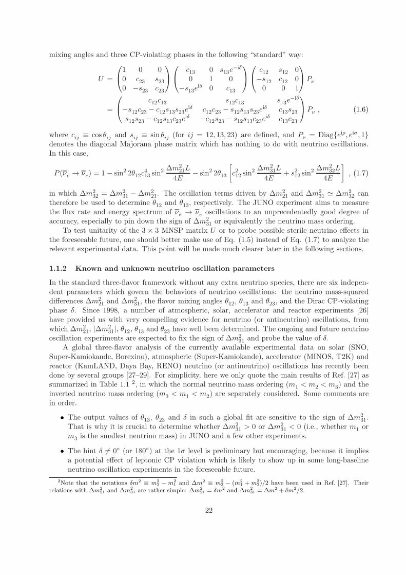
mixing angles and three CP-violating phases in the following “standard” way:

U =

1 0 00 c23 s230 −s23 c23

c13 0 s13e−iδ

0 1 0−s13eiδ 0 c13

c12 s12 0−s12 c12 00 0 1

Pν

=

c12c13 s12c13 s13e−iδ

−s12c23 − c12s13s23eiδ c12c23 − s12s13s23e

iδ c13s23s12s23 − c12s13c23e

iδ −c12s23 − s12s13c23eiδ c13c23

Pν , (1.6)

where cij ≡ cos θij and sij ≡ sin θij (for ij = 12, 13, 23) are defined, and Pν = Diageiρ, eiσ , 1denotes the diagonal Majorana phase matrix which has nothing to do with neutrino oscillations.In this case,

P (νe → νe) = 1− sin2 2θ12c413 sin

2 ∆m221L

4E− sin2 2θ13

[c212 sin

2 ∆m231L

4E+ s212 sin

2 ∆m232L

4E

], (1.7)

in which ∆m232 = ∆m2

31 − ∆m221. The oscillation terms driven by ∆m2

21 and ∆m231 ≃ ∆m2

32 cantherefore be used to determine θ12 and θ13, respectively. The JUNO experiment aims to measurethe flux rate and energy spectrum of νe → νe oscillations to an unprecedentedly good degree ofaccuracy, especially to pin down the sign of ∆m2

31 or equivalently the neutrino mass ordering.To test unitarity of the 3 × 3 MNSP matrix U or to probe possible sterile neutrino effects in

the foreseeable future, one should better make use of Eq. (1.5) instead of Eq. (1.7) to analyze therelevant experimental data. This point will be made much clearer later in the following sections.

1.1.2 Known and unknown neutrino oscillation parameters

In the standard three-flavor framework without any extra neutrino species, there are six indepen-dent parameters which govern the behaviors of neutrino oscillations: the neutrino mass-squareddifferences ∆m2

21 and ∆m231, the flavor mixing angles θ12, θ13 and θ23, and the Dirac CP-violating

phase δ. Since 1998, a number of atmospheric, solar, accelerator and reactor experiments [26]have provided us with very compelling evidence for neutrino (or antineutrino) oscillations, fromwhich ∆m2

21, |∆m231|, θ12, θ13 and θ23 have well been determined. The ongoing and future neutrino

oscillation experiments are expected to fix the sign of ∆m231 and probe the value of δ.

A global three-flavor analysis of the currently available experimental data on solar (SNO,Super-Kamiokande, Borexino), atmospheric (Super-Kamiokande), accelerator (MINOS, T2K) andreactor (KamLAND, Daya Bay, RENO) neutrino (or antineutrino) oscillations has recently beendone by several groups [27–29]. For simplicity, here we only quote the main results of Ref. [27] assummarized in Table 1.1 2, in which the normal neutrino mass ordering (m1 < m2 < m3) and theinverted neutrino mass ordering (m3 < m1 < m2) are separately considered. Some comments arein order.

• The output values of θ13, θ23 and δ in such a global fit are sensitive to the sign of ∆m231.

That is why it is crucial to determine whether ∆m231 > 0 or ∆m2

31 < 0 (i.e., whether m1 orm3 is the smallest neutrino mass) in JUNO and a few other experiments.

• The hint δ 6= 0 (or 180) at the 1σ level is preliminary but encouraging, because it impliesa potential effect of leptonic CP violation which is likely to show up in some long-baselineneutrino oscillation experiments in the foreseeable future.

2Note that the notations δm2 ≡ m22 − m2

1 and ∆m2 ≡ m23 − (m2

1 + m22)/2 have been used in Ref. [27]. Their

relations with ∆m221 and ∆m2

31 are rather simple: ∆m221 = δm2 and ∆m2

31 = ∆m2 + δm2/2.

22

Table 1-1: The best-fit values, together with the 1σ, 2σ and 3σ intervals, for the six three-flavorneutrino oscillation parameters from a global analysis of current experimental data [27].

Parameter Best fit 1σ range 2σ range 3σ range

Normal neutrino mass ordering (m1 < m2 < m3)

∆m221/10

−5 eV2 7.54 7.32 — 7.80 7.15 — 8.00 6.99 — 8.18∆m2

31/10−3 eV2 2.47 2.41 — 2.53 2.34 — 2.59 2.26 — 2.65

sin2 θ12/10−1 3.08 2.91 — 3.25 2.75 — 3.42 2.59 — 3.59

sin2 θ13/10−2 2.34 2.15 — 2.54 1.95 — 2.74 1.76 — 2.95

sin2 θ23/10−1 4.37 4.14 — 4.70 3.93 — 5.52 3.74 — 6.26

δ/180 1.39 1.12 — 1.77 0.00 — 0.16 ⊕ 0.86 — 2.00 0.00 — 2.00

Inverted neutrino mass ordering (m3 < m1 < m2)

∆m221/10

−5 eV2 7.54 7.32 — 7.80 7.15 — 8.00 6.99 — 8.18∆m2

13/10−3 eV2 2.42 2.36 — 2.48 2.29 — 2.54 2.22 — 2.60

sin2 θ12/10−1 3.08 2.91 — 3.25 2.75 — 3.42 2.59 — 3.59

sin2 θ13/10−2 2.40 2.18 — 2.59 1.98 — 2.79 1.78 — 2.98

sin2 θ23/10−1 4.55 4.24 — 5.94 4.00 — 6.20 3.80 — 6.41

δ/180 1.31 0.98 — 1.60 0.00 — 0.02 ⊕ 0.70 — 2.00 0.00 — 2.00

• The possibility θ23 = 45 cannot be excluded at the 2σ level, and thus a more precise deter-mination of θ23 is desirable in order to resolve its octant. The latter is important since it canhelp fix the geometrical structure of the MNSP matrix U .

Note also that |Uµi| = |Uτi| (for i = 1, 2, 3), the so-called µ-τ permutation symmetry of U itself,holds if either the conditions θ13 = 0 and θ23 = 45 or the conditions δ = 90 (or 270) andθ23 = 45 are satisfied. Now that θ13 = 0 has definitely been ruled out by the Daya Bay experiment[30–32], it is imperative to know the values of θ23 and δ as accurately as possible, so as to fix thestrength of µ-τ symmetry breaking associated with the structure of U .

1.2 Open Issues of Massive Neutrinos

There are certainly many open questions in neutrino physics, but here we concentrate on someintrinsic flavor issues of massive neutrinos which may more or less be addressed in the JUNOexperiment.

1.2.1 The nature of neutrinos and their mass spectrum

Question (1): Dirac or Majorana? — If a massive neutrino is the Dirac particle, just like theelectron, then it must be distinguishable from its antiparticle because they possess the oppositelepton numbers. By definition, a massive Majorana neutrino is its own antiparticle [33], leading tolepton number violation as a direct consequence. The tiny masses of three known neutrinos make itextremely difficult to identify their nature, i.e., whether they are the Dirac or Majorana particles.At present the only experimentally feasible way to probe the Majorana nature of massive neutrinosis to observe the neutrinoless double-beta (0νββ) decays of some even-even nuclei, N(A,Z) →N(A,Z + 2) + 2e−, which occur via an exchange of the virtual Majorana neutrinos between two

23

10-6 10-5 10-4 10-3 10-2 10-1 100 101 102 103 104 105 106 107 108 109 1010 1011 1012

1

2

3

eV

3

2

1

TeVGeVMeVkeVmeV

tb

cs

du

Gen

erat

ion

Mass (eV)

e

eV

Figure 1-1: A schematic illustration of the “flavor hierarchy” and “flavor desert” in the fermionmass spectrum at the electroweak scale [38]. Here the neutrino masses are assumed to have anormal ordering.

associated beta decays [34]. The effective neutrino mass term in the 0νββ decay is defined as

〈m〉ee ≡∑

i

(miU

2ei

), (1.8)

which is in general sensitive to all the three neutrino masses (including the sign of ∆m231), two of

the three flavor mixing angles and two of the three CP-violating phases.So far no convincing evidence for an occurrence of the 0νββ decay has been established, al-

though a lot of experimental efforts have been made in the past few decades. Within the standardthree-flavor scheme, the inverted neutrino mass ordering (i.e., ∆m2

31 < 0) or a near neutrino massdegeneracy will allow |〈m〉ee| ≥ 0.01 eV [35–37], perhaps accessible in the next-generation 0νββ-decay experiments.

Question (2): Normal or inverted mass ordering? — Now that ∆m221 > 0 has been fixed

but the sign of ∆m231 remains unknown, we are left with two possibilities for the mass ordering of

three active neutrinos whose family indices are specified by the weak charged-current interactionsin Eq. (1.1): the normal case m1 < m2 < m3 and the inverted case m3 < m1 < m2. The formeris “normal” in the sense that it is parallel to the mass ordering of three charged leptons or threequarks of the same electric charge (i.e., me ≪ mµ ≪ mτ , mu ≪ mc ≪ mt and md ≪ ms ≪ mb, asshown in Fig. 1.1). However, a good (model-independent) theoretical reason for either ∆m2

31 > 0or ∆m2

31 < 0 has been lacking 3.The sign of ∆m2

31 is of fundamental importance because it can impact on many important pro-cesses in particle physics, astrophysics and cosmology. The 0νββ decay is just a typical exampleof this kind. In the atmospheric and long-baseline accelerator neutrino experiments, the behav-iors of flavor oscillations are sensitive to a combination of ∆m2

31 and the terrestrial matter term2√2 GFNeE, where Ne denotes the number density of electrons in the matter background and E is

the neutrino beam energy [39]. The supernova neutrino oscillations are also affected by the sign of∆m2

31 for a similar reason [40]. Meanwhile, the interference effects of two atmospheric mass-squareddifferences in reactor neutrino vacuum oscillations are sensitive to the sign of ∆m2

31 [41]. It is there-fore possible to probe the neutrino mass ordering via the atmospheric, long-baseline accelerator,

3If the neutrino mass ordering is finally found to be inverted, one may always “renormalize” it to m′1 < m′

2 < m′3

by setting m′1 = m3, m

′2 = m1 and m′

3 = m2, equivalent to a transformation (ν1, ν2, ν3) → (ν′2, ν

′3, ν

′1). In this case

the matrix elements of U must be reordered in a self-consistent way: U → U ′, in which U ′α1 = Uα3, U

′α2 = Uα1 and

U ′α3 = Uα2 (for α = e, µ, τ ). Therefore, such a treatment does not change any physical content of massive neutrinos.

24

reactor and supernova neutrino oscillations [42, 43]. On the other hand, the “right” sign of ∆m231

may help the seesaw and leptogenesis mechanisms [44] work well to simultaneously interpret theorigin of tiny neutrino masses and the observed baryon number asymmetry of the Universe [45,46].

Question (3): The absolute mass scale? — Since the flavor oscillations of massive neutrinos areonly sensitive to the neutrino mass-squared differences, a determination of the absolute neutrinomass scale has to rely on some non-oscillation experiments. Searching for the 0νββ decay is oneof the feasible ways for this purpose if massive neutrinos are the Majorana particles, because themagnitude of its effective mass 〈m〉ee is governed by mi as shown in Eq. (1.8). The upper boundof |〈m〉ee| has been set to be about 0.2 eV by the present 0νββ-decay experiments [47], and thesensitivities of the future experiments are likely to reach the meV level [35–37]. Another way is todetect the effective neutrino mass

〈m〉e ≡√∑

i

(m2

i |Uei|2)

(1.9)

in the beta decays, such as 31H → 3

2He + e− + νe. The most promising experiment of this kind isthe KATRIN experiment, which may hopefully probe 〈m〉e with a sensitivity of about 0.2 eV [48].

Furthermore, one may get useful information on the mass scale of light neutrinos from cos-mology and astrophysics. A global analysis of current cosmological data (especially those on thecosmic microwave background and large-scale structures) has actually provided us with the mostpowerful sensitivity to the sum of light neutrino masses,

Σν ≡∑

i

mi . (1.10)

For example, Σν < 0.23 eV has recently been reported by the Planck Collaboration at the 95% con-fidence level [49]. Given the values of ∆m2

21 and |∆m231| extracted from current neutrino oscillation

data, the results of |〈m〉ee|, 〈m〉e and Σν are all sensitive to the sign of ∆m231.

Let us restrict ourselves to the standard three-flavor case to illustrate the correlation amongthe above three effective mass terms in Fig. 1.2, where the 3σ ranges of ∆m2

21, |∆m231|, θ12 and

θ13 as given in Table 1.1 are input, and the CP-violating phases of U are all allowed to vary in the[0, 360) interval.

1.2.2 Lepton flavor mixing pattern and CP violation

Question (4): The octant of θ23? — Although the smallest neutrino mixing angle θ13 has alreadybeen determined in the Daya Bay experiment [30–32], the geometric structure of the 3× 3 MNSPmatrix U cannot be fully fixed until the octant of θ23 and the value of δ are both known. Currentexperimental data strongly support |Uµi| ≃ |Uτi| (for i = 1, 2, 3), i.e., an approximate µ-τ permu-tation symmetry of U itself [50]. In particular, θ23 = 45 is favored in many neutrino mass modelsas a consequence of the exact µ-τ symmetry or some other kinds of flavor symmetries. In this sensethe deviation of θ23 from 45 serves for a useful model discriminator [51,52] and deserves a precisemeasurement in the upcoming atmospheric and long-baseline neutrino oscillation experiments.

Taking account of sin θ12 < 1/√2 and sin θ13 ≪ 1, one may roughly expect |Ue1| > |Uµ3| ∼

|Uτ3| ∼ |Uµ2| ∼ |Uτ2| ∼ |Ue2| > |Uµ1| ∼ |Uτ1| > |Ue3|, where “∼” means that the two MNSP matrixelements are comparable in magnitude. Hence the pattern of U seems to be partly anarchical andpartly hierarchical. In comparison, the CKM quark flavor mixing matrix V is found to possess aclearly hierarchical structure: |Vtb| > |Vud| > |Vcs| ≫ |Vus| > |Vcd| ≫ |Vcb| > |Vts| ≫ |Vtd| > |Vub|since its three mixing angles satisfy ϑ12 ≫ ϑ23 ≫ ϑ13, which should have something to do with thestrong quark mass hierarchies.

25

10−2

10−1

100

10−4

10−3

10−2

10−1

100

10−2

10−1

100

10−4

10−3

10−2

10−1

100

|〈m〉ee| [eV] 〈m〉e [eV]

Σν [eV] Σν [eV]

Figure 1-2: An illustration of the correlation between Σν and |〈m〉ee| (left panel) and that betweenΣν and 〈m〉e (right panel) by using the 3σ inputs as given in Table 1.1. Here the red (blue) regioncorresponds to the normal (inverted) neutrino mass ordering.

Question (5): The Dirac CP-violating phase δ? — In the standard three-flavor scheme thephase parameter δ of U is fundamentally important because it uniquely controls the strength ofleptonic CP and T violation in neutrino oscillations. Under CPT invariance, the CP- and T-violating asymmetries Aαβ ≡ P (να → νβ) − P (να → νβ) = P (να → νβ) − P (νβ → να) in vacuumare explicitly given by

Aαβ = 2 sin 2θ12 cos θ13 sin 2θ13 sin 2θ23 sin δ∑

γ

ǫαβγ sin∆m2

21L

4Esin

∆m231L

4Esin

∆m232L

4E, (1.11)

in which the Greek subscripts run over e, µ and τ . It becomes obvious that CP or T violationis a three-flavor “appearance” effect, and a measurement of this effect will allow us to determinethe value of δ. Given the best-fit values θ12 ≃ 33.7, θ13 ≃ 8.8 and θ23 ≃ 40.7 in the normalneutrino mass ordering case, for example, the coefficient in front of the oscillating term of Aαβ isabout 0.5× sin δ. Current neutrino oscillation data seem to hint at δ ∼ 270 (see Table 1.1) — anencouraging implication of large CP violation in the lepton sector.

In a realistic medium- or long-baseline neutrino oscillation experiment, however, the terrestrialmatter effects may modify the oscillation behaviors and thus affect the determination of δ. Thiskind of contamination is negligible for a variety of experiments provided the neutrino beam energyE and the baseline length L satisfy the condition 10−7 (L/km)2 (GeV/E) ≪ 1. If the unitarityof the 3 × 3 MNSP matrix U is slightly violated due to the existence of extra species of massiveneutrinos, it is also possible for new CP-violating effects to show up in neutrino oscillations [9].

Question (6): The Majorana CP-violating phases ρ and σ? — If the Majorana nature ofmassive neutrinos is finally established through a convincing measurement of the 0νββ decay, onewill be left with a question which is probably most challenging in neutrino physics — how todetermine the CP-violating phases ρ and σ in the standard three-flavor scheme? Because the 0νββdecay is a CP-conserving process, its effective mass term 〈m〉ee can only provide some indirectinformation on the combinations of δ, ρ and σ. Hence a direct determination of ρ and σ dependson the observation of those processes which are both lepton-number-violating and CP-violating.Although the measurement of neutrino-antineutrino oscillations can in principle allow us to probeall the three CP-violating phases and even the absolute neutrino mass scale [53], it is in practice

26

impossible to do such an experiment since the corresponding oscillation probabilities are suppressedby the factors m2

i /E2 . 10−12.

The 3× 3 Majorana neutrino mass matrix Mν can be reconstructed in terms of three neutrinomasses, three flavor mixing angles and three CP-violating phases in the basis where the flavor eigen-states of three charged leptons are identified with their mass eigenstates, and its six independentelements are

〈m〉αβ ≡∑

i

(miUαiUβi

), (1.12)

where α and β run over e, µ and τ . Current experimental constraints on the magnitudes of 〈m〉αβcan be found in Ref. [54]. While a theoretical model is always possible to predict the moduli andphases of 〈m〉αβ , its correctness or wrongness will not be testable until sufficient information aboutthe CP-violating phases of U is experimentally obtained.

1.2.3 Extra neutrino species and unitarity tests

Question (7): Extra light or heavy sterile neutrinos? — One of the fundamental questions in neu-trino physics and cosmology is whether there exist extra species of neutrinos which do not directlyparticipate in the standard weak interactions. Such sterile neutrinos are certainly hypothetical,but their possible existence is either theoretically motivated or experimentally implied [55]. Forexample, the canonical (type-I) seesaw mechanism [15–20] provides an elegant interpretation of thesmall masses of νi (for i = 1, 2, 3) with the help of two or three heavy sterile neutrinos, and thelatter can even help account for the observed matter-antimatter asymmetry of the Universe via theleptogenesis mechanism [44]. On the experimental side, the LSND [56], MiniBooNE [57] and reactorantineutrino [58] anomalies can all be explained as the active-sterile antineutrino oscillations in theassumption of one or two species of sterile antineutrinos whose masses are below 1 eV [59,60]. Fur-thermore, a careful analysis of the existing data on the cosmic microwave background anisotropy,galaxy clustering and supernovae Ia seems to favor one species of sterile neutrinos at the sub-eVmass scale [61–63]. On the other hand, sufficiently long-lived sterile neutrinos in the keV massrange might serve as a good candidate for warm dark matter if they were present in the earlyUniverse [64]. That is why a lot of attention has been paid to sterile neutrinos. No matter howsmall or how large the mass scale of sterile neutrinos is, they are undetectable unless they mix withthree active neutrinos to some extent. The active-sterile neutrino mixing can slightly modify thebehaviors of the standard three-flavor neutrino oscillations, as shown in Eqs. (1.2)—(1.4).

As for the νe → νe oscillation in a reactor antineutrino experiment, its probability P (νe → νe) isgoverned by Eq. (1.5). The heavy sterile antineutrinos do not participate in any flavor oscillations,but they may violate the unitarity of the 3 × 3 MNSP matrix. In comparison, the light sterileantineutrinos can contribute extra oscillation terms to P (νe → νe). The JUNO experiment willtherefore be a good playground to probe or constrain the effects of sterile antineutrinos.

Question (8): Direct and indirect non-unitary effects? — In the presence of small mixingbetween 3 active and n sterile neutrinos, the 3 × 3 MNSP matrix becomes a submatrix of the(3 + n)× (3 + n) unitary matrix which describes the overall flavor mixing effects, as shown in Eq.(1.2). Hence the 3×3 MNSP matrix itself must be non-unitary. From the point of view of neutrinooscillations, one may classify its possible non-unitary effects into three categories [24,25]:

• the indirect non-unitary effect arising from the heavy sterile neutrinos which are kinematicallyforbidden to take part in neutrino oscillations;

• the direct non-unitary effect caused by the light sterile neutrinos which are able to participatein neutrino oscillations;

27

• the interplay of the direct and indirect non-unitary effects in a flavor mixing scenario includingboth light and heavy sterile neutrinos.

An experimental test of the unitarity of the 3× 3 MNSP matrix is therefore important to probe orconstrain the flavor mixing parameters of possible new physics associated with sterile neutrinos, andit can theoretically shed light on the underlying dynamics responsible for neutrino mass generationand lepton flavor mixing (e.g., the 3 × 3 MNSP matrix is exactly unitary in the type-II [10–14]seesaw mechanism but non-unitary in the type-I [15–20] and type-III [21] seesaw mechanisms).

In the quark sector, the unitarity of the CKM matrix V has been tested to an impressive degreeof accuracy. For instance, |Vud|2 + |Vus|2 + |Vub|2 = 0.9999 ± 0.0006 and |Vud|2 + |Vcd|2 + |Vtd|2 =1.000± 0.004 for the first row and column of V , respectively [26]. Hence the room for possible newphysics which may violate the unitarity of V must be extremely small. In comparison, a preliminaryconstraint on the sum of |Ue1|2, |Ue2|2 and |Ue3|2 in the lepton sector is

|Ue1|2 + |Ue2|2 + |Ue3|2 = 0.9979 · · · 0.9998 (1.13)

at the 90% confidence level [22, 23], implying that the 3 × 3 MNSP matrix U is allowed to benon-unitary only at the O(10−3) level. But it should be noted that such a stringent constraintis obtained in the assumption of minimal unitarity violation, and there might be the effects ofunitarity violation at the percent level in the lepton sector. The JUNO experiment will allow us todetermine |Ue1|, |Ue2| and |Ue3| to a much better degree of accuracy via a precision measurementof the νe → νe oscillation, and then examine whether the sum |Ue1|2+ |Ue2|2+ |Ue3|2 deviates fromone or not.

Of course, there are many more open questions, which are more or less associated with massiveneutrinos and their various consequences, in particle physics, astrophysics and cosmology. Typicalexamples of this kind include how to detect the cosmic neutrino (or antineutrino) background, howto detect the supernova neutrino burst and (or) the supernova relic neutrino background, how todetect the ultrahigh-energy cosmic neutrinos, etc. In any case the JUNO experiment is expectedto clarify a part of the flavor issues in the lepton sector and help resolve some of the fundamentalproblems about the origin and evolution of the Universe.

1.3 JUNO Experiment

The Jiangmen Underground Neutrino Observatory (JUNO) is a multi-purpose neutrino experiment.It was proposed in 2008 to determine the neutrino mass hierarchy by detecting reactor antineutrinosfrom the Daya Bay nuclear power plant (NPP) [65–68], thus formerly known as “Daya Bay IIexperiment”. The mass hierarchy determination requires equal baselines from the detector to allreactor cores to avoid cancellation of the oscillation dephasing effect. Due to the complex andunclear layout of the future nuclear power plants in the neighborhood, the experiment was movedto Jiangmen city in Guangdong province in August 2012, and named as JUNO in 2013.

The site location is optimized to have the best sensitivity for the mass hierarchy determination,which is at 53 km from both the Yangjiang and Taishan NPPs [69]. The neutrino detector is aliquid scintillator (LS) detector with a 20 kton fiducial mass, deployed in a laboratory 700 meterunderground. The experimental site and the detector will be described in this section.

The JUNO project was approved by Chinese Academy of Sciences in February 2013. Datataking is expected in 2020.

28

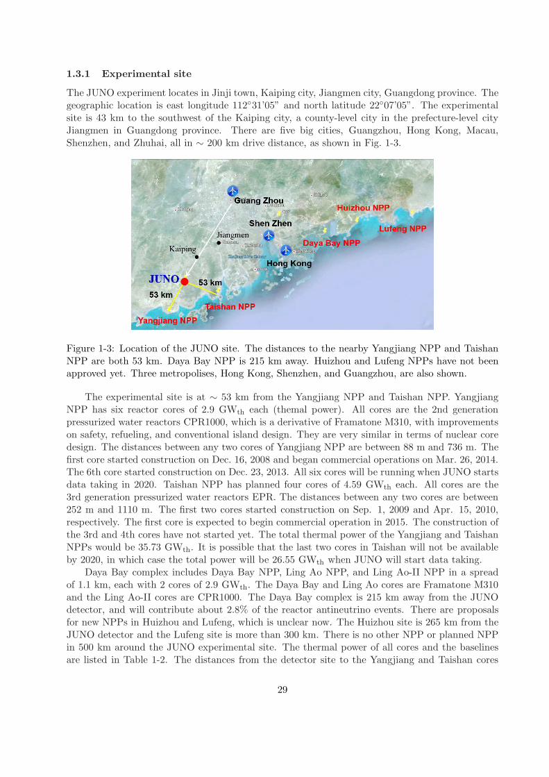
1.3.1 Experimental site

The JUNO experiment locates in Jinji town, Kaiping city, Jiangmen city, Guangdong province. Thegeographic location is east longitude 11231’05” and north latitude 2207’05”. The experimentalsite is 43 km to the southwest of the Kaiping city, a county-level city in the prefecture-level cityJiangmen in Guangdong province. There are five big cities, Guangzhou, Hong Kong, Macau,Shenzhen, and Zhuhai, all in ∼ 200 km drive distance, as shown in Fig. 1-3.

Figure 1-3: Location of the JUNO site. The distances to the nearby Yangjiang NPP and TaishanNPP are both 53 km. Daya Bay NPP is 215 km away. Huizhou and Lufeng NPPs have not beenapproved yet. Three metropolises, Hong Kong, Shenzhen, and Guangzhou, are also shown.

The experimental site is at ∼ 53 km from the Yangjiang NPP and Taishan NPP. YangjiangNPP has six reactor cores of 2.9 GWth each (themal power). All cores are the 2nd generationpressurized water reactors CPR1000, which is a derivative of Framatone M310, with improvementson safety, refueling, and conventional island design. They are very similar in terms of nuclear coredesign. The distances between any two cores of Yangjiang NPP are between 88 m and 736 m. Thefirst core started construction on Dec. 16, 2008 and began commercial operations on Mar. 26, 2014.The 6th core started construction on Dec. 23, 2013. All six cores will be running when JUNO startsdata taking in 2020. Taishan NPP has planned four cores of 4.59 GWth each. All cores are the3rd generation pressurized water reactors EPR. The distances between any two cores are between252 m and 1110 m. The first two cores started construction on Sep. 1, 2009 and Apr. 15, 2010,respectively. The first core is expected to begin commercial operation in 2015. The construction ofthe 3rd and 4th cores have not started yet. The total thermal power of the Yangjiang and TaishanNPPs would be 35.73 GWth. It is possible that the last two cores in Taishan will not be availableby 2020, in which case the total power will be 26.55 GWth when JUNO will start data taking.

Daya Bay complex includes Daya Bay NPP, Ling Ao NPP, and Ling Ao-II NPP in a spreadof 1.1 km, each with 2 cores of 2.9 GWth. The Daya Bay and Ling Ao cores are Framatone M310and the Ling Ao-II cores are CPR1000. The Daya Bay complex is 215 km away from the JUNOdetector, and will contribute about 2.8% of the reactor antineutrino events. There are proposalsfor new NPPs in Huizhou and Lufeng, which is unclear now. The Huizhou site is 265 km from theJUNO detector and the Lufeng site is more than 300 km. There is no other NPP or planned NPPin 500 km around the JUNO experimental site. The thermal power of all cores and the baselinesare listed in Table 1-2. The distances from the detector site to the Yangjiang and Taishan cores

29

are surveyed with a Global Positioning System (GPS) to a precision of 1 meter. All these NPPsare constructed and operated by the China General Nuclear Power Group (CGNPG).

Cores YJ-C1 YJ-C2 YJ-C3 YJ-C4 YJ-C5 YJ-C6

Power (GW) 2.9 2.9 2.9 2.9 2.9 2.9

Baseline(km) 52.75 52.84 52.42 52.51 52.12 52.21

Cores TS-C1 TS-C2 TS-C3 TS-C4 DYB HZ

Power (GW) 4.6 4.6 4.6 4.6 17.4 17.4

Baseline(km) 52.76 52.63 52.32 52.20 215 265

Table 1-2: Summary of the thermal power and baseline to the JUNO detector for the Yangjiang(YJ) and Taishan (TS) reactor cores, as well as the remote reactors of Daya Bay (DYB) andHuizhou (HZ).

In absence of high mountains in the allowed area where the sensitivity to the mass hierarchyis optimized, the detector will be deployed in an underground laboratory under the Dashi hill.The elevation of the hill above the detector is 268 m, and that of the dome and the floor of theunderground experimental hall is -433 m and -460 m, respectively. The detector is located in acylindrical pit. The elevation of the detector center is -481.25 m. Therefore, the vertical overburdenfor the detector is more than 700 m. The experimental hall is designed to have two accesses. Oneis a 616 m-deep vertical shaft, and the other is a 1340 m long tunnel with a slope of 42.5%. Therock is granite. The average rock density along a 650 m borehole is measured to be 2.61 g/cm3.The activities of the 238U, 232Th, and 40K in the rock around the experimental hall are measuredto be 130, 113, and 1062 Bq/kg, respectively. The muon rate and average energy in the JUNOdetector are expected to be 0.0030 Hz/m2 and 215 GeV estimated by simulation with the surveyedmountain profile taken into account.

1.3.2 JUNO Detector

The JUNO detector consists of a central detector, a water Cherenkov detector and a muon tracker.The central detector is a liquid scintillator (LS) detector of 20 kton fiducial mass with an designedenergy resolution of 3%/

√E(MeV). The central detector is submerged in a water pool to be

shielded from natural radioactivity from the surrounding rock and air. The water pool is equippedwith Photomultiplier Tubes (PMTs) to detect the Cherenkov light from cosmic muons, acting as aveto detector. On top of the water pool, there is another muon detector to accurately measure themuon tracks. A schematic view of the JUNO detector is shown in Fig. 1-4. The detector design isstill developing in the carrying on of R&D.

To achieve a 3%/√E(MeV) energy resolution is very challenging. A Monte Carlo simula-

tion has been developed based on the Monte Carlo of the Daya Bay experiment, as described inSec. 13.2.1. The photoelectron yield has been tuned according to the Daya Bay data. To reach therequired energy resolution, the following improvements from Daya Bay have to be accomplished.

• The PMT photocathode covergage ≥ 75%.

• The PMT photocathode quantum efficiency ≥ 35%.

• The attenuation length of the liquid scintillator ≥ 20 m at 430 nm, which corresponds to anabsorption length of 60 m with a Rayleigh scattering length of 30 m 4.

4The Rayleigh scattering length of Linear alkybenzene was measured to be 28.2 ± 1.0 m at 430 nm recently [70]

30

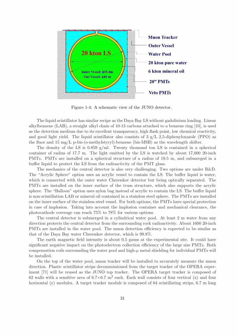
Figure 1-4: A schematic view of the JUNO detector.

The liquid scintillator has similar recipe as the Daya Bay LS without gadolinium loading. Linearalkylbenzene (LAB), a straight alkyl chain of 10-13 carbons attached to a benzene ring [10], is usedas the detection medium due to its excellent transparency, high flash point, low chemical reactivity,and good light yield. The liquid scintillator also consists of 3 g/L 2,5-diphenyloxazole (PPO) asthe fluor and 15 mg/L p-bis-(o-methylstyryl)-benzene (bis-MSB) as the wavelength shifter.

The density of the LS is 0.859 g/ml. Twenty thousand ton LS is contained in a sphericalcontainer of radius of 17.7 m. The light emitted by the LS is watched by about 17,000 20-inchPMTs. PMTs are installed on a spherical structure of a radius of 19.5 m, and submerged in abuffer liquid to protect the LS from the radioactivity of the PMT glass.

The mechanics of the central detector is also very challenging. Two options are under R&D.The “Acrylic Sphere” option uses an acrylic vessel to contain the LS. The buffer liquid is water,which is connected with the outer water Cherenkov detector but being optically separated. ThePMTs are installed on the inner surface of the truss structure, which also supports the acrylicsphere. The “Balloon” option uses nylon bag instead of acrylic to contain the LS. The buffer liquidis non-scintillation LAB or mineral oil contained in a stainless steel sphere. The PMTs are installedon the inner surface of the stainless steel vessel. For both options, the PMTs have special protectionin case of implosion. Taking into account the implosion container and mechanical clearance, thephotocathode coverage can reach 75% to 78% for various options.

The central detector is submerged in a cylindrical water pool. At least 2 m water from anydirection protects the central detector from the surrounding rock radioactivity. About 1600 20-inchPMTs are installed in the water pool. The muon detection efficiency is expected to be similar asthat of the Daya Bay water Cherenkov detector, which is 99.8%.

The earth magnetic field intensity is about 0.5 gauss at the experimental site. It could havesignificant negative impact on the photoelectron collection efficiency of the large size PMTs. Bothcompensation coils surrounding the water pool and high-µ metal shielding for individual PMTs willbe installed.

On the top of the water pool, muon tracker will be installed to accurately measure the muondirection. Plastic scintillator strips decommissioned from the target tracker of the OPERA exper-iment [71] will be reused as the JUNO top tracker. The OPERA target tracker is composed of62 walls with a sensitive area of 6.7×6.7 m2 each. Each wall consists of four vertical (x) and fourhorizontal (y) modules. A target tracker module is composed of 64 scintillating strips, 6.7 m long

31

and 26.4 mm wide. Each strip is read out on both sides by a Hamamatsu 64-channel multi-anodePMT. The total surface which could be covered by the 62 x-y walls is 2783 m2. Radioactivity fromthe surrounding rock of the experimental hall will induce extremely high noise rate in the plasticscintillator strips. Multi-layer design, at least 3 x-y layers, is needed to suppress the radioactivitybackground. Distance between two adjacent super-layers will be between 1 m and 1.5 m. Themuon tracker will cover more than 25% of the area of the top surface of the water pool.

A chimney for calibration operation will connect the central detector to outside from the top.Special radioactivity shielding and muon detector will be designed for the chimney.

32

2 Identifying the Neutrino Mass Hierarchy

2.1 Introduction and motivation

After the discovery of non-zero θ13 in recent reactor [30,31,72,73] and accelerator [74,75] neutrinoexperiments, the present status of the standard three-flavor neutrino oscillation [27–29,76–78] canbe summarized as follows:

• three non-zero mixing angles [26] θ12, θ23, and θ13 in the MNSP [5, 6] lepton mixing matrixhave been measured with the precision from 4% to 10% 1,

• two independent mass-squared differences |∆m231| = |m2

3 −m21| (or |∆m2

32| = |m23 −m2

2|) and∆m2

21 = m22 −m2

1 have been measured with the precision better than 4% [26],

• the neutrino mass hierarchy (i.e., sign of the mass-squared difference ∆m231) is unknown,

• the octant of the mixing angle θ23 (i.e., θ23 < π/4 or θ23 > π/4) is unknown,

• the leptonic CP-violating phase δ in the MNSP matrix is unknown.

Therefore, the determination of the neutrino mass hierarchy and octant of the mixing angle θ23,as well as the measurement of the leptonic CP-violating phase constitutes the main focus of futureneutrino oscillation experiments.

The neutrino mass hierarchy (MH) answers the question whether the third generation (ν3 masseigenstate) is heavier or lighter than the first two generations (ν1 and ν2). As shown in Fig. 2-1,the normal mass hierarchy (NH) refers to m3 > m1 and the inverted mass hierarchy (IH) refers tom3 < m1.

The relatively large value of θ13 has provided excellent opportunities to resolve the MH indifferent neutrino oscillation configurations, which include

• the medium baseline (∼50 km) reactor antineutrino νe → νe oscillation experiments (JUNO [65,66,69,79,80] and RENO-50 [81]),

• the long-baseline accelerator (anti-)neutrino(−)νµ →(−)

νe oscillation experiments (NOνA [82] andDUNE [83]),

• the atmospheric (anti-)neutrino(−)νµ → (−)

νµ oscillation experiments (INO [84], PINGU [85],ORCA [86], DUNE [83] and Hyper-K [87,88]).

While the last two methods depend on the matter effect in neutrino oscillations (the charge-currentinteraction between (anti-)νe and electrons in the matter), the first method with reactor antineutri-nos at a medium baseline only relies on the oscillation interference between ∆m2

31 and ∆m232 with

∆m2ij = m2

i −m2j [65, 66,69,79,80].

Besides the neutrino oscillation experiments of determining the MH, the octant of θ23 and thelepton CP-violating phase, the absolute neutrino mass scale and nature of the massive neutrinos(i.e., the Majorana or Dirac type) are questions of fundamental importance to be answered infuture neutrino non-oscillation probes, including beta decays, neutrinoless double beta decays andcosmological observations.

The determination of the MH has profound impacts on our understanding of the neutrinophysics, neutrino astronomy and neutrino cosmology.

Editors: Yufeng Li (liyufeng@ihep.ac.cn) and Liang Zhan (zhanl@ihep.ac.cn)Major contributor: Xin Qian

1precision in terms of sin2 θ12, sin2 θ23, and sin2 θ13.

33

Normal

m12

solar: 7.5×10-5 eV2

m22

atomospheric:

2.4×10-3 eV2

m32

Inverted

m12

atomospheric:

2.4×10-3 eV2

m22

solar: 7.5×10-5 eV2

m32

νe νµ ντ

Figure 2-1: Illustration for the patterns of normal and inverted neutrino mass hierarchies.

• First, as illustrated in Fig. 2-2 [89], MH helps to define the goal of neutrinoless doublebeta decay (0νββ) search experiments, which aim to reveal whether neutrinos are Dirac orMajorana particles. In particular, the chance to observe 0νββ in the next-generation doublebeta decay experiments is greatly enhanced for an inverted MH and the Majorana natureof massive neutrinos. New techniques beyond the next generation are needed to explore theregion covered by a normal MH.

• Second, MH is a crucial factor for measuring the lepton CP-violating phase. In the long-baseline accelerator (anti-)neutrino oscillation experiments, degenerate solutions for the MHand CP phase emerge, and the wrong MH would give a fake local minimum for the CP phase,thus reduce the significance of the CP measurement. This effect is even more importantfor accelerator neutrino experiments with a shorter baseline such as Hyper-K [87, 88] andMOMENT [90]. Therefore, a determination of the MH independent of the CP phase isimportant for the future prospect of neutrino physics.

• Third, MH is a key parameter of the neutrino astronomy and neutrino cosmology. On onehand, the spectral splits [91] in supernova neutrino fluxes would provide a smoking gun forcollective neutrino oscillations induced by the neutrino self-interaction in the dense environ-ment. The split patterns are significantly different for the normal and inverted MHs. MH isalso important for the supernova nucleosynthesis, where the prediction of the 7Li/11B ratio isalso distinct for different MHs [92]. On the other hand, MH may have important implicationson the cosmological probe of the neutrino mass scale (i.e.,

∑mν). As shown in Fig. 2-3,

in the case of an inverted MH, future combined cosmological constraints would have a veryhigh-precision detection, with 1σ error shown as a blue band. In the case of a normal MH,future cosmology would detect the lowest

∑mν at a level of ∼ 4σ.

• Fourth, MH is one of the most important discriminators for model building of the neutrinomasses and flavor mixing. To understand the origin of neutrino mass generation, the MHinformation is crucial. Due to the similar and complementary aspects of quarks and leptons,the normal MH could be related to the quark mass spectrum and attributed to the rela-tions of Grand Unified Theories (GUTs). On the other hand, the inverted MH predicts anearly-degenerate spectrum between the first and second mass eigenstates, which could be

34

mmin [eV]

|mββ

| [

eV]

NS

IS

Cosm

ological Limit

Current Bound

10−4 10−3 10−2 10−1 110−4

10−3

10−2

10−1

1

1σ2σ3σ

Figure 2-2: Values of the effective Majorana mass |mββ | as a function of the lightest neutrino massin the normal (NS, with mmin = m1) and inverted (IS, with mmin = m3) neutrino mass spectraafter the measurement of non-zero θ13. The plot is taken from [89].

Figure 2-3: The current constraints and forecast sensitivity of cosmology to the neutrino mass inrelation to MH [93]. In the case of an inverted MH in the upper curve, future combined cosmologicalconstraints would have a very high-precision detection, with 1σ error shown as the blue band. Inthe case of a normal MH in the lower curve, future cosmology would detect the lowest

∑mν at a

level of ∼ 4σ.

35

(MeV)visE2 4 6 8 10

L (k

m)

20

40

60

80

100

0.01

0.02

0.03

0.04

0.05

0.06

-310×

Figure 2-4: (left panel) The effective mass-squared difference shift ∆m2φ [79] as a function of

baseline (y-axis) and visible prompt energy Evis ≃ Eν − 0.8MeV (x-axis). The legend of colorcode is shown in the right bar, which represents the size of ∆m2

φ in eV2. The solid, dashed, anddotted lines represent three choices of detector energy resolution with 2.8%, 5.0%, and 7.0% at 1MeV, respectively. The purple solid line represents the approximate boundary of degenerate mass-squared difference. (right panel) The relative shape difference [65, 66] of the reactor antineutrinoflux for different neutrino MHs.

explained in the models with the discrete or U(1) flavor symmetries. Therefore, MH is acritical parameter to understand the origin of neutrino masses and mixing.

JUNO is designed to resolve the neutrino MH using precision spectral measurements of reactorantineutrino oscillations. Before giving the quantitative calculation of the MH sensitivity, we shallbriefly review the principle of this method. The electron antineutrino survival probability in vacuumcan be written as [69,79,94]:

Pνe→νe = 1− sin2 2θ13(cos2 θ12 sin

2∆31 + sin2 θ12 sin2 ∆32)− cos4 θ13 sin

2 2θ12 sin2 ∆21 (2.1)

= 1− 1

2sin2 2θ13

[1−

√1− sin2 2θ12 sin

2 ∆21 cos(2|∆ee| ± φ)]− cos4 θ13 sin

2 2θ12 sin2 ∆21,

where ∆ij ≡ ∆m2ijL/4E, in which L is the baseline, E is the antineutrino energy,

sinφ =c212 sin(2s

212∆21)− s212 sin(2c

212∆21)√

1− sin2 2θ12 sin2 ∆21

, cosφ =c212 cos(2s

212∆21) + s212 cos(2c

212∆21)√

1− sin2 2θ12 sin2∆21

,

and [95,96]

∆m2ee = cos2 θ12∆m

231 + sin2 θ12∆m

232 . (2.2)

The ± sign in the last term of Eq. (2.1) is decided by the MH with plus sign for the normal MHand minus sign for the inverted MH.

In a medium-baseline reactor antineutrino experiment (e.g., JUNO), oscillation of the atmo-spheric mass-squared difference manifests itself in the energy spectrum as the multiple cycles.The spectral distortion contains the MH information, and can be understood with the left panelof Fig. 2-4 which shows the energy and baseline dependence of the extra effective mass-squareddifference,

∆m2φ = 4Eφ/L , (2.3)

36

2/eV2mδ0.002 0.0022 0.0024 0.0026 0.0028

-0.06

-0.04

-0.02

0

0.02

0.04

0.06

0.08

0.1 normal hierarchyinverted hierarchyFCT spectrum

2/eV2mδ0.002 0.0022 0.0024 0.0026 0.0028

-0.08

-0.06

-0.04

-0.02

0

0.02

0.04

0.06

0.08

0.1

0.12normal hierarchy

inverted hierarchyFST spectrum

Figure 2-5: The Fourier cosine transform (FCT) (left panel) and Fourier sine transform (FST)(right panel) of the reactor antineutrino energy spectrum. The solid and dashed lines are for thenormal MH and the inverted MH, respectively.

At baseline of ∼ 50 km, ∆m2φ at the low energy (∼ 3 MeV) is larger than the ∆m2

φ at the high

energy (∼ 6 MeV). For NH, the effective mass-squared difference 2|∆m2ee|+∆m2

φ in Eq. (2.1) at lowenergies will be larger than that at high energies and vice versa for IH, in which the effective mass-squared difference is 2|∆m2

ee| −∆m2φ . Therefore, the advancement or retardance of the oscillation

phase illustrated in the right panel of Fig. 2-4 contains the useful MH information. However, inorder to extract the MH information from the spectral distortion, an excellent energy resolution(3%/

√E), a good understanding of the energy response (better than 1%), and a large statistics

(O(100k) inverse beta decay events) are required.The oscillation interference effect is more evident in the frequency domain after a Fourier

transform of the L/E spectrum of reactor antineutrinos [65, 66, 97]. In Fig 2-5 we illustrate theFourier sine transform (FST) and Fourier cosine transform (FCT) of the reactor antineutrino energyspectrum, where the FST and FCT frequency spectra are defined as

FST(ω) =

∫ tmax

tmin

F (t) sin(ωt)dt , FCT(ω) =

∫ tmax

tmin

F (t) cos(ωt)dt , (2.4)

with ω = 2.54 × ∆m2ij being the frequency, and t = L/E being the variable in the L/E space,

varying from tmin = L/Emax to tmax = L/Emin. F (L/E) is written as

F (L/E) = φ(E)σ(E)Pνe→νe(L/E) , (2.5)

where φ(E), σ(E) and Pνe→νe(L/E) are the reactor antineutrino spectrum, the interaction crosssection and the oscillation probability, respectively. φ(E) and σ(E) will be discussed in the nextsection, and Pνe→νe(L/E) is defined in Eq. (2.1). Distinctive features of the FST and FCT spectrafor normal and inverted MHs can be observed in Fig 2-5. On the FCT spectrum (left panel), avalley appears at the left of the prominent peak for the IH, and a peak appears at the left of thevalley for the NH. On the FST spectrum (right panel), there is a clear valley for the IH, and a clearpeak for NH. Therefore, we can distinguish the MH from the Fourier transform spectra withoutany prior information on the neutrino mass-squared differences. More details on properties of theFCT and FST spectra in the MH determination can be found in Refs. [65, 66].

Beside the aforementioned interference between |∆m231| and |∆m2

32|, the precision measurementof |∆m2

ee| in a medium-baseline reactor experiment can reveal additional information regarding the

37

MH, when combined with the precision |∆m2µµ| measurements from the future muon (anti-)neutrino

disappearance [95,96]. Using the convention of Refs. [69, 95], we have

|∆m2ee| − |∆m2

µµ| = ±∆m221(cos 2θ12 − sin 2θ12 sin θ13 tan θ23 cos δ) , (2.6)

where the positive and negative signs correspond to normal and inverted MHs, respectively. Theprecision measurements of both |∆m2

µµ| and |∆m2ee| would provide new information regarding the

neutrino MH. Therefore, by combining these two types of information (interference and precision|∆m2

ee| measurement), JUNO will have a robust path to resolve the neutrino MH [69].

2.2 Signal and Background

2.2.1 Reactor neutrino signal

Reactor neutrinos are electron antineutrinos emitted from subsequent β-decays of instable fissionfragments. All reactors close to JUNO are pressurized water reactors (PWR), the same type asthe Daya Bay reactors. In these reactors, fissions of four fuel isotopes, 235U, 238U, 239Pu, and241Pu, generate more than 99.7% of the thermal power and reactor antineutrinos. Reactor neutrinofluxes per fission of each isotope are determined by inversion of the measured β spectra of fissionproducts [98–102] or by calculation with the nuclear database [103, 104]. Their fission rates in areactor can be estimated with the core simulation and thermal power measurements. The reactorneutrino flux can be predicted as

Φ(Eν) =Wth∑i fiei

·∑

i

fi · Si(Eν), (2.7)

Where Wth is the thermal power of the reactor, fi, ei, and Si(Eν) are fission fraction, the thermalenergy released in each fission, and the neutrino flux per fission for the i-th isotope, respectively.Such a prediction is expected to carry an uncertainty of 2-3% [30]. Recently, reactor neutrinoexperiments (Daya Bay [105], RENO [106] Double Chooz [107]) found a large discrepancy betweenthe predicted and measured spectra in the 4-6 MeV region. Model independent prediction based onthe new precision measurements could avoid this bias, and might be able to improve the precisionto 1%. Detailed description on the reactor neutrino flux can be found in the Appendix of Sec. 13.

JUNO measures the reactor neutrino signal via the inverse beta decay (IBD) reaction

νe + p→ e+ + n . (2.8)

The reactor antineutrino νe interacts with a proton, creating a positron (e+) and a neutron. Thepositron quickly deposits its energy and annihilates into two 511-keV γ-rays, which gives a promptsignal. The neutron scatters in the detector until being thermalized. It is then captured by aproton ∼ 200 µs later and releases a 2.2-MeV γ-ray. The coincidence of the prompt-delayed signalpair in such a short time significantly reduces backgrounds. Positron carries almost all energy ofthe neutrino in this reaction. Therefore, the observable neutrino spectrum shown in Fig. 2-6 can beobtained from the prompt signal with a ∼ 0.8 MeV shift. With reactors of 36 GW thermal powerat 53 km, a 20-kton LS detector will have 83 IBD events per day.

The accidental background, 8He/9Li, fast neutron and (α, n) background are the major back-grounds for the reactor neutrino oscillation analysis. Fiducial volume cut can significantly reducethe accidental background and the (α, n) background. Energy selection, time coincidence, andvertex correlation of the prompt and delayed signals are required for the reactor antineutrino se-lection to further suppress the accidental background. To reject the cosmogenic backgrounds such

38

Antineutrino Energy (MeV)!

0 ! 1 ! 2 ! 3 ! 4 ! 5 ! 6 ! 7 ! 8 ! 9 !

An

tin

eu

trin

os / M

eV

/ F

issio

n!

0 !

0.1 !

0.2 !

0.3 !

0.4 !

0.5 !

0.6 !

0.7 !

0.8 !

0.9 ! )!2!

Inv

ers

e B

eta

De

ca

y C

ros

s S

ec

tio

n (

cm!

0 !

1 !

2 !

3 !

4 !

-42 !10 !×"

U !235 !

Pu !239 !

U !238 !

Pu !241 !

cro

ss s

ection!

an

tineu

trino

flux!

measured spectrum !

n

Ɣ

Ɣ Ɣ

νe

e+

Figure 2-6: The observable νe spectrum (red line) is a product of the antineutrino flux from reactorand the cross section of inverse beta decay (blue line). The contributions of four fission isotopes tothe antineutrino flux are shown for a typical pressurized water reactor. The steps involved in thedetection are schematically drawn on the top of the figure [108].

as 9Li/8He and fast neutron, muon veto cuts are necessary and need be optimized to reduce theloss of detector live time and dead volume. Detailed discussion on backgrounds will be presentedlater. A set of preliminary antineutrino selection criteria is listed below:

• fiducial volume cut r < 17 m;

• the prompt energy cut 0.7 MeV < Ep < 12 MeV;

• the delayed energy cut 1.9 MeV < Ed < 2.5 MeV;

• time interval between the prompt and delayed signal ∆T <1.0 ms;

• the prompt-delayed distance cut Rp−d <1.5 m;

• Muon veto criteria:

– for muons tagged by Water Pool, veto the whole LS volume for 1.5 ms

– for good tracked muons in central detector and water Cerenkov detector, veto the de-tector volume within Rd2µ < 3 m and Td2µ < 1.2 s

– for the tagged, non-trackable muons in central detector, veto the whole LS volume for1.2 s

The antineutrino selection efficiency due to the fiducial volume is 91.8%. The energy cut, timecut, and vertex cut have efficiencies of 97.8%, 99.1%, and 98.7%, respectively, using Geant4-basedMonte Carlo (MC) studies described in Sec. 13. Assuming 99% muons have good reconstructedtrack, the efficiency of above muon veto cut is estimated to be 83% by using the toy MC method.Tab. 2-1 summarizes the efficiencies of antineutrino selection cuts and the corresponding reductionto various backgrounds, which will be discussed in the next subsection. JUNO will observe 60 IBDevents per day, with about 6% backgrounds.

39

Selection IBD efficiency IBD Geo-νs Accidental 9Li/8He Fast n (α, n)

- - 83 1.5 ∼ 5.7× 104 84 - -

Fiducial volume 91.8% 76 1.4 77 0.1 0.05Energy cut 97.8% 410Time cut 99.1% 73 1.3 71Vertex cut 98.7% 1.1Muon veto 83% 60 1.1 0.9 1.6

Combined 73% 60 3.8

Table 2-1: The efficiencies of antineutrino selection cuts, signal and backgrounds rates.

2.2.2 Background estimation

Accidental background The rate of accidental backgrounds can be calculated as Racc = Rp ·Rd ·∆T , where Rp and Rd are the rate of prompt and delayed signals, respectively, and ∆T is the timecoincidence window. A fiducial volume cut is essential to significantly suppress such background.The accidental background consists of mainly three types of random coincidence: (radioactivity,radioactivity), (radioactivity, cosmogenic isotope) and (radioactivity, spallation neutrons):

• (radioactivity, radioactivity): The singles rate obtained from MC simulation is about 7.6 Hzafter fiducial volume cut (see Sec. 13.4.4),in which the faction of neutron-like signals is ∼8%.Thus the rate of prompt-delayed coincidence within 1.0 ms is ∼ 410/day. In addition, a toyMC study gives a factor of 380 suppression by requiring Rp−d <1.5 m, where Rp−d is thedistance between the prompt-delayed pair, thus the accidental background rate is reduced to1.1/day.

• (radioactivity, cosmogenic isotope): based on the rates of cosmogenic isotopes in Sec. 13.4.3,the neutron-like singles from cosmogenic isotopes is estimated to be ∼340/day. The rate ofaccidental coincidence between radioactivity and those isotopes is <0.01/day after ∆T < 1.0ms and Rp−d <1.5 m cut.

• (radioactivity, spallation neutrons): Though the total rate of spallation neutrons is 1.8 Hz,after 1.5 ms muon veto the rate is reduced to ∼45/day. The coincidence between radioactivityand the residual spallation neutrons is negligible after the time and spatial cut.

Thus the total rate of accidental backgrounds is estimated to be 0.9/day, after taking into accountthe efficiency of muon veto. During data taking, the rate of radioactivity can be precisely monitored,so can the neutron-like events from muon spallation. So the uncertainty of accidental backgroundrate can be controlled within 1% and the uncertainty of spectrum shape is negligible due to thelarge statistics of prompt-like singles.

9Li/8He As noted in Sec. 13.4.3, the β-n decays from cosmogenic 8He and 9Li can mimic IBDinteractions, thus are the most serious correlated background to reactor antineutrinos. The 9Li and8He production cross section is often modelled empirically as being proportional to E0.74

µ , whereEµ is the average energy of the muon at the detector. Considering the cross section measured inthe KamLAND detector [109], 2.2×10−7µ−1g−1cm2 for 9Li and 0.7×10−7µ−1g−1cm2 for 8He, thepredicted 9Li and 8He production rate at JUNO is 150 and 50 per day, respectively. The branchingratio of the β-n decay is 51% for 9Li and 16% for 8He, thus the total rate of β-n decays is 84/day.Taking into account the fiducial volume cut, the rate is reduced to 77/day. The delayed energy cut

40

and time cut efficiencies for 9Li are the same as those for IBDs, as shown in Tab. 2-1, while theprompt energy cut efficiency for 9Li is ∼97%. Thus the background rate is reduced to ∼71/day.The FLUKA simulation results in Tab. 13-9 are smaller than this empirical extrapolation. It ispointed out that scaling with the muon average energy is not as accurate as the scaling with theenergy loss of individual muons, which may explain the differences between the FLUKA-estimatedyields and the empirical extrapolation [308].

In practice, the rate of 9Li/8He can be measured from the distribution of the time since thelast muon using the known decay times for these isotopes [110]. A toy MC based on the simulatedmuon data has been performed, and it’s expected that <3% rate uncertainty can be achieved with6 years data.

The 9Li/8He background is correlated with the parent muon in time and space. The lateraldistance between the muon-induced isotopes and the parent muon trajectory is roughly exponential.The most effective approach to reject 9Li/8He background is to veto a sufficient detector volumealong the muon trajectory for a relative long time, e.g, a few times of the isotope’s lifetime. Muonsthat are accompanied by electromagnetic or hadronic showers, usually named as showering muons,are the dominant producers (>85%) of the radioactive isotopes. With a muon simulation forJUNO, it is found that the showering muon rate is ∼0.5 Hz. The simulation also suggests thatafter producing a shower, the muon still survives and its direction changes negligibly. Thus thecritical issue is how well the muon track reconstruction is, for both non-showering muons andshowering muons.

For single non-showering muon, the track can be reconstructed using the first hit-time onPMTs. The methods to reconstruct the track of showering muons and the tracks in muon bundles(see Sec. 13.4.1) are under development. Initial track can be guessed by using the PMTs near theinjecting point and outgoing point. The locations of spallation neutrons, if there is any, can beused to constrain their parent muon tracks. Particularly, the high multiplicity of spallation neutronsfrom the showering processes can give good estimation of where the showering happens, then it’spossible to veto a spherical volume around the showering point to reject 9Li/8He. If showeringmuons are poorly reconstructed, a whole volume cut is essential to reject the 9Li/8He background.

To estimate the residual 9Li/8He after the muon veto cuts listed in Sec. 2.2.1, we assume theefficiency of good track reconstruction for non-showering muon is more than 99%, based on theexperience from KamLAND. For showering muons, we expect the track reconstruction can alsoreach 99% efficiency. Then the efficiency of the muon veto cuts is estimated to be 83% using toyMC, and 2.3% of 9Li/8He will survive, thus the final residual 9Li and 8He background is 1.6/day.

The uncertainties on the residual 9Li/8He background rate are mainly from the uncertaintyfrom muon track reconstruction and the position reconstruction uncertainty of IBD candidates. Weassume 20% relative uncertainty on the residual background rate. With the full statistics of 9Li/8Heevents, the energy spectrum shape can be measured quite well. We can assign 10% bin-to-bin shapeuncertainty.

Fast neutron The cosmic muons that only passing the surrounding rock of the water pool, aswell as the corner clipping muons with very short track length in water, are not able to be tagged.The energetic neutrons produced by those muons can form a fast neutron background by scatteringoff a proton and then being captured in the LS detector. Based on a full simulation without opticalprocesses, the rate of fast neutrons is estimated to be ∼0.1/day. The signals produced by theenergetic neutrons are found to be concentrated at the top of detector and near the equator wherethe water shielding is minimum. For the MH analysis, we assume the relative rate uncertainty is100%. The prompt energy spectrum is consistent with a flat distribution. The tagged fast-neutrons

41

can actually provide good information about the energy spectrum. In this analysis, we assume theshape uncertainty is 20%.

13C(α, n)16O background The alpha particles from the U, Th radioactivities can react withthe 13C in LS. The 13C(α, n)16O reaction could lead to a correlated background if the neutronis fast enough or there is a gamma from the de-excitation of the 16O excited states. Based onthe estimated natural radioactivity concentrations, the (α, n) background rate is estimated to be0.05/day for the “Acrylic Sphere” option, and 0.01/day for the “Balloon” option due to the lowerU/Th concentration. The highest energy of alpha’s from U/Th is about 9 MeV, and the crosssection of 13C(α, n)16O reaction is known with a ∼20% uncertainty for an alpha with energy <10MeV. Thus if the rate of alpha particles is well measured, the (α, n) background can be predictedprecisely. In this analysis, a 50% relative uncertainty for both the background rate and the energyspectrum shape is conservatively assumed.

Geo-neutrino background Antineutrinos produced from radioactive decays of Th and U insidethe Earth constitute the geo-neutrino flux, which will also contribute to the background of reactorantineutrinos. The total event rate of geo-neutrinos at the JUNO site is 1.5/day, where contribu-tions from Th and U are 23% and 77% respectively. After the IBD efficiency cut, the remaininggeo-neutrino background is 1.1/day. The relative rate uncertainty of geo-neutrinos is estimated as30%, where the crust uncertainty is 18% and the uncertainty of mantle prediction is assumed tobe 100%. Experimentally the rate of geo-neutrinos can be measured with much better precisionusing the JUNO detector itself. Finally, we assume the relative shape uncertainty of geo-neutrinosto be 5%, because the β-decay spectra of Th and U are well known from the nuclear physics. Moredetails on the geo-neutrino prediction and measurement are discussed in Sec. 8.

The background rates and the reduction with the antineutrino selection cuts are summarizedin Tab. 2-1.

2.3 The MH Sensitivity

2.3.1 Basic Setup and Definition

In JUNO simulation, we assume a 20 kt LS detector, and the total thermal power of the two reactorcomplexes as 36 GWth. We use the nominal running time of six years (i.e., 2000 effective days)and a detector energy resolution of 3%/

√E(MeV) as a benchmark. The IBD detection efficiency

is estimated as 73% as show in Tab. 2-1. The energy E is referred as the visible energy of theIBD events [E(MeV) ≃ Eν(MeV) − 0.8]. A normal MH is assumed to be the true one (unlessmentioned explicitly) while the conclusion is the same for the other assumption. The relevantoscillation parameters are taken from the latest global analysis [27,76] as ∆m2

21 = 7.54×10−5 eV−2,(∆m2

31 + ∆m232)/2 = 2.43 × 10−3 eV−2, sin2 θ13 = 0.024 and sin2 θ12 = 0.307. The CP-violating

phase will be specified when needed. Corrections to ∆m221 and sin2 θ12 from terrestrial matter

effects are around 0.5%-1% (see Sec. 3) and the induced uncertainties are negligibly small (< 0.1%).Finally, the reactor antineutrino flux model from ILL and Vogel et al. [98–100, 103] is adopted inour simulation2. Because only two of the three mass-squared differences (∆m2

21, ∆m231 and ∆m2

32)are independent, we choose ∆m2

21 and ∆m2ee [see Eq. (2.2)] as our working parameters.

2We have tried both the old [98–100,103] and new evaluations [101,102] of the reactor antineutrino fluxes. Bothevaluations give consistent results on the MH determination.

42

0 20 40 60 80 100 120 140 1600

5

10

15

20

25

30

6 yearsIdeal distributionE_res = 3%

(MH)

L Km-5 -4 -3 -2 -1 0 1 2 3 4 5

0

5

10

15

20

25

6 yearsL = 52 kmE_res = 3%

(MH)

L km

Figure 2-7: The MH discrimination ability as the function of the baseline (left panel) and functionof the baseline difference of two reactors (right panel).

To obtain the MH sensitivity, we employ the least-squares method and construct a χ2 functionas 3,

χ2REA =

Nbin∑

i=1

[Mi − Ti(1 +∑

k αikǫk)]2

Mi+∑

k

ǫ2kσ2k

, (2.9)

whereMi is the measured neutrino events in the i-th energy bin, Ti is the predicted neutrino eventswith oscillations, σk is the systematic uncertainty, ǫk is the corresponding pull parameter, and αik

is the fraction of neutrino event contribution of the k-th pull parameter to the i-th energy bin. Theconsidered systematic uncertainties include the correlated (absolute) reactor uncertainty (2%), theuncorrelated (relative) reactor uncertainty (0.8%), the spectrum shape uncertainty (1%) and thedetector-related uncertainty (1%). We use 200 equal-size bins for the incoming neutrino energybetween 1.8 MeV and 8.0 MeV.

We fit the spectrum assuming the normal MH or inverted MH with the chisquare method andtake the difference of the minima as a measure of the MH sensitivity. The discriminator of the MHcan be defined as

∆χ2MH = |χ2

min(N)− χ2min(I)|, (2.10)

where the minimization process is implemented for all the relevant oscillation parameters. Notethat two local minima for each MH [χ2

min(N) and χ2min(I)] can be located at different positions of

|∆m2ee|.

2.3.2 Baseline Optimization

The discriminator defined in Eq. (2.10) can be used to obtain the optimal baseline, which areshown in the left panel of Fig. 2-7. A sensitivity of ∆χ2

MH ≃ 16 is obtained for the ideal case withidentical baselines at around 50 km. The impact of the baseline difference due to multiple reactorcores is shown in the right panel of Fig. 2-7, by keeping the baseline of one reactor unchanged andvarying that of another. A rapid oscillatory behavior is observed and demonstrates the importanceof reducing the baseline differences of reactor cores. The worst case is at ∆L ∼ 1.7 km, where the|∆m2

ee| related oscillation is cancelled between two reactors.

3A different definition with the Poisson χ2 function yields the consistent MH sensitivity [79,80].

43

2.34 2.36 2.38 2.40 2.42 2.44 2.46 2.48 2.500

5

10

15

20

25

True MH (ideal) True MH (real) False MH (ideal) False MH (real)

(m

2 ee)

m2ee X10-3 eV2

Normal true MH

Figure 2-8: The comparison of the MH sensitivity for the ideal and actual distributions of thereactor cores. The real distribution gives a degradation of ∆χ2

MH ≃ 5.

Considering the baseline optimization and impact of the baseline difference, we select of theexperimental site. A candidate site was identified by taking account of the physical performanceand detailed geological survey. With the spatial coordinates of the experimental site and reactorcores, the actual power and baseline distributions for the reactor cores of Yangjiang (YJ) andTaishan (TS) NPPs are shown in Tab. 1-2. The remote reactors in the Daya Bay (DYB) andthe possible Huizhou (HZ) NPP are also included. The reduction of sensitivity due to the actualdistribution of reactor cores is shown in Fig. 2-8, which gives a degradation of ∆χ2

MH ≃ 5. Thedegradation includes ∆χ2

MH ≃ 3 due to the baseline differences of Taishan and Yangjiang NPP,and ∆χ2

MH ≃ 1.7 with the inclusion of Daya Bay and Huizhou NPPs. Other NPPs in operationand construction are much further away from the experimental site (larger than 400 km) and canbe neglected in the MH studies (reduction of ∆χ2

MH < 0.2). In all the following, the actual spacialdistribution of reactor cores as shown in Tab. 1-2 is taken into account.

2.3.3 Requirement on the Energy Resolution

The energy resolution as or better than the size of ∆m221/|∆m2

31| is required in order to preciselymeasure both the fast oscillations (driven by ∆m2

31 and ∆m232) and slow oscillation (driven by

∆m221) at a medium baseline. In our nominal setup, the detector energy resolution 3%/

√E(MeV)

is defined from the photon-electron statistics (1200 p.e./MeV), with the energy E defined as thevisible energy of the positron. To show the effects of the energy resolution and event statistics, weillustrate the iso-∆χ2

MH contour plot as a function of the two key factors in Fig. 2-9. The nominalluminosity is defined as the IBD event statistics in Sec. 2.3.1. From the figure, we can observe thatthe energy resolution of 2.6%/

√E(MeV) and 2.3%/

√E(MeV) is required to achieve the sensitivity

of ∆χ2MH ≃ 16 or ∆χ2

MH ≃ 25 with the nominal statistics, respectively. With an increase of thestatistics by 50%, the energy resolution of 2.9%/

√E(MeV) and 2.6%/

√E(MeV) are required to

achieve the same sensitivity of ∆χ2MH ≃ 16 or ∆χ2

MH ≃ 25.For a real experimental environment, there are other important factors beyond the photon-

electron statistics that affect the energy resolution, such as the dark noise from PMT and electronics,the detector non-uniformity and vertex resolution, as well as the PMT charge resolution. A generic

44

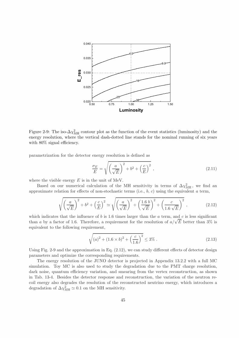
16

9.0

4.0

2536

0.50 0.75 1.00 1.25 1.500.020

0.025

0.030

0.035

0.040

E_res

Luminosity

Figure 2-9: The iso-∆χ2MH contour plot as the function of the event statistics (luminosity) and the

energy resolution, where the vertical dash-dotted line stands for the nominal running of six yearswith 80% signal efficiency.

parametrization for the detector energy resolution is defined as

σEE

=

√(a√E

)2

+ b2 +( cE

)2, (2.11)

where the visible energy E is in the unit of MeV.Based on our numerical calculation of the MH sensitivity in terms of ∆χ2

MH , we find anapproximate relation for effects of non-stochastic terms (i.e., b, c) using the equivalent a term,

√(a√E

)2

+ b2 +( cE

)2≃√(

a√E

)2

+

(1.6 b√E

)2

+

(c

1.6√E

)2

, (2.12)

which indicates that the influence of b is 1.6 times larger than the a term, and c is less significantthan a by a factor of 1.6. Therefore, a requirement for the resolution of a/

√E better than 3% is

equivalent to the following requirement,√

(a)2 + (1.6 × b)2 +( c

1.6

)2≤ 3% . (2.13)

Using Fig. 2-9 and the approximation in Eq. (2.12), we can study different effects of detector designparameters and optimize the corresponding requirements.

The energy resolution of the JUNO detector is projected in Appendix 13.2.2 with a full MCsimulation. Toy MC is also used to study the degradation due to the PMT charge resolution,dark noise, quantum efficiency variation, and smearing from the vertex reconstruction, as shownin Tab. 13-4. Besides the detector response and reconstruction, the variation of the neutron re-coil energy also degrades the resolution of the reconstructed neutrino energy, which introduces adegradation of ∆χ2

MH ≃ 0.1 on the MH sensitivity.

45

2.3.4 Statistical Interpretation

In this section, we shall present a brief summary of the MH statistics and relation to the sensitivity.The following discussion is crucial to properly understand the sensitivity results shown in Fig. 2-8.The determination of MH is equivalent to resolving the sign of ∆m2

31. From the statistics point ofview, the determination of MH is a test to distinguish two discrete hypotheses (NH vs. IH).

First let us employ the commonly used approach in the Frequentist statistics. Given a nullhypothesis H0 and the alternative hypothesis H1, we can choose a test statistic T in order to testwhether data can reject the null hypothesis H0. The confidence level (CL) (1 − α) to reject H0 isrelated to the type-I error rate α, where,

• type-I error rate α is defined as the probability of rejecting the null hypothesis H0, if H0 istrue.

From the definition, one can define the relation between a critical value of the observation Tαc and

the the type-I error rate α as ∫ ∞

Tαc

p(T |H0)dT = α , (2.14)

with p(T |H0) being the probability distribution function of T given that H0 is true. Moreover, wecan further define the conversion between the double-sided Gaussian nσ and the value of α as

α(n) =2√2π

∫ ∞

ndx e−x2/2 = erfc

(n√2

), (2.15)

where erfc(x) is the complementary error function. This definition implies that we identify standarddeviations of 1σ, 2σ, 3σ with a CL (1− α) of 68.27%, 95.45%, 99.73%, respectively.

On the other hand, the power of a given test T is related to the type-II error rate β, where

• type-II error rate β is defined as the probability of accepting the null hypothesis H0, if H1 istrue.

According to the definition, β is calculated as

β = P (T < Tαc |H1) =

∫ Tαc

−∞p(T |H1)dT , (2.16)

where p(T |H1) is the probability distribution function of T assuming the alternative hypothesis H1

is true. β depends on the CL (1−α) at which we want to reject H. A small value of β means thatthe type-II error rate is small, the power of the test (which is defined as 1− β) is large.

Based on different choices of β, one can have different sensitivities, such as the median sensi-tivity [111, 112] (β = 50%) and the crossing sensitivity [112–115] (β = α). The former is definedfor the expected sensitivity of an averaged experiment, and the latter corresponds to the CL atwhich exactly one of the two hypotheses can be rejected. By definition, the crossing sensitivitygives smaller confidence levels than the median sensitivity and is not necessarily connected to whatwould be expected from an designed experiment [112].

For the case of the MH determination at JUNO, we first define our working test statisticssimilar to the discriminator in Eq. (2.10),

T = χ2min(I)− χ2

min(N). (2.17)

According to the derivation in Refs. [112–115], the static T follows the Gaussian distribution with

T = N(±∆χ2

MH, 2√

∆χ2MH

), (2.18)

46

T∆-40 -20 0 20 40

T)

∆P

DF

(

0

0.02

0.04

0.06

0.08

0.1NH MC

IH MC

NH Norm. Approx.

IH Norm. Approx.

Figure 2-10: The T distribution function for the JUNO nominal setup of six year running.

Median sens. Standard sens. Crossing sens.

Normal MH 3.4 σ 3.3 σ 1.9 σ

Inverted MH 3.5 σ 3.4 σ 1.9 σ

Table 2-2: The MH sensitivity with the JUNO nominal setup of six year running.

where the plus (minus) sign holds for the normal (inverted) MH. This distribution is validated withan explicit MC simulation in Fig. 2-10, showing the excellent agreement between the numerical andanalytical calculations.

In Tab 2-2, we show the median sensitivity, standard sensitivity (defined as√

∆χ2MHσ), and

crossing sensitivity respectively for the JUNO nominal setup, where we can see that the commonlydefined standard sensitivity is very close to the median sensitivity and can be regard as the expectedsensitivity of a future experiment.

Before finishing the discussion on this approach, we want to stress that the Frequentist approachdoes not directly address the question how much one MH hypothesis is favored than the otherMH hypothesis given the experimental data. In the MH determination one can choose the nullhypothesis to be the NH, and the alternative hypothesis would be the IH. The result of thishypothesis testing will tell us whether the NH would be rejected or not, given the pre-defined rule.Similarly, one should also perform a second hypothesis testing by choosing null hypothesis to be theIH with the alternative hypothesis being the NH. The result of the second test will tell us whetherthe IH would be rejected or not.

On the other hand, the method of using the Bayesian statistics can tell us the comparison of twoMH hypotheses. The Bayes’ theorem gives the relationship of the posterior probability distributionfunction p(MH|D, I), the prior probability distribution function p(MH|I) and the likelihood functionL(D|MH, I) as

p(MH|D, I) = L(D|MH, I) · p(MH|I)∫L(D|MH, I) · p(MH|I) , (2.19)

47

where D represents the data of a measurement, I is the prior information on the MH hypothesesand the integration are carried out for all the oscillation parameters. Given data from the mea-surement, one can calculate TNH = −2Log[p(NH|D, I)] and TIH = −2Log[p(IH|D, I)]. TNH andTIH are marginalized over all nuisance parameters including unknown parameters and systematicuncertainties of the experiment to obtain Tmag

NH and TmagIH , respectively 4.

Assuming that the prior information of NH vs. IH is 50% vs. 50%, the probability ratioof the IH vs. NH, which is p(IH|D, I) vs. p(NH|D, I), can be calculated as e−∆τ/2 vs. 1, with∆τ = Tmag

IH − TmagNH . As illustrated in Ref. [113], an approximation ∆τ ≈ ∆χ2

MH can be made inpractice. More generally, ∆τ can be explicitly calculated through MC simulations or other advancedintegration techniques. Tab. 2-3 lists a few values of ∆χ2

MH and their corresponding probabilityratios. The final results are then presented in terms of probability ratio which is a natural andsimple way to present results for the MH determination.

∆τ ≈ ∆χ2MH 1 4 9 16 25

p(IH|D, I) vs. p(NH|D, I) 38% vs. 12% vs. 1.1% vs. 0.034% vs. 3.7 ×10−6 vs.62% 88% 98.9% 99.966% 100%

p(IH|D, I)/p(NH|D, I) 0.61 0.136 0.011 3.4×10−4 3.7× 10−6

Table 2-3: Probability ratios with respect to several typical ∆χ2MH values.

2.4 Systematics

In this section, we shall discuss the effects of systematics in the MH measurement in reactor antineu-trino oscillations, which includes the reactor related uncertainties, detector related uncertainties,background related uncertainties and the energy related uncertainties.

2.4.1 Reactor related uncertainties

As discussed before, the MH information is encoded in the spectral shape of reactor antineutrinooscillations. The absolute normalization uncertainty from the reactor flux at the current level hasnegligible impact on the MH determination. Therefore only the reactor-related shape uncertaintyis considered in the following.

We incorporate the shape uncertainty to each bin by modifying the χ2 definition in Eq. (2.9)as follows:

χ2REA =

Nbin∑

i=1

[Mi − Ti(1 +∑

k αikǫk)]2

Mi + (σMi)2+∑

k

ǫ2kσ2k

, (2.20)

where σ denotes the relative (uncorrelated) shape uncertainty. The ∆χ2REA degrades less than 1

when we set the 1% shape uncertainty (σ = 1%), while the degradation is about 2 in ∆χ2REA when

we increase σ to 2%. Therefore, careful estimation and reduction of the energy uncorrelated shapeuncertainties are mandatory to achieve the required sensitivity.

Because the model predictions for the reactor antineutrino spectrum are inconsistent with themeasurement from ongoing reactor experiments (i.e., the bump between 4 ∼ 6 MeV) [105–107].Moreover, a recent theoretical calculation trying to understand the above inconsistency observesadditional high-frequency fine structures [104] in the reactor antineutrino spectrum. Both of the

4In the marginalization process, one integrates the likelihood function over the entire phase space of nuisanceparameters.

48

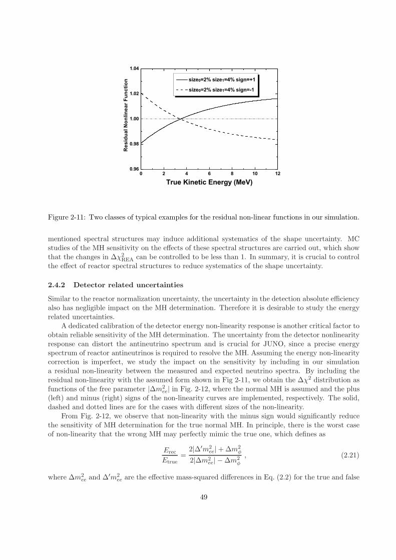
0 2 4 6 8 10 120.96

0.98

1.00

1.02

1.04

size0=2% size1=4% sign=+1

size0=2% size1=4% sign=-1

Res

idua

l Non

linea

r Fun

ctio

n

True Kinetic Energy (MeV)

Figure 2-11: Two classes of typical examples for the residual non-linear functions in our simulation.

mentioned spectral structures may induce additional systematics of the shape uncertainty. MCstudies of the MH sensitivity on the effects of these spectral structures are carried out, which showthat the changes in ∆χ2

REA can be controlled to be less than 1. In summary, it is crucial to controlthe effect of reactor spectral structures to reduce systematics of the shape uncertainty.

2.4.2 Detector related uncertainties

Similar to the reactor normalization uncertainty, the uncertainty in the detection absolute efficiencyalso has negligible impact on the MH determination. Therefore it is desirable to study the energyrelated uncertainties.

A dedicated calibration of the detector energy non-linearity response is another critical factor toobtain reliable sensitivity of the MH determination. The uncertainty from the detector nonlinearityresponse can distort the antineutrino spectrum and is crucial for JUNO, since a precise energyspectrum of reactor antineutrinos is required to resolve the MH. Assuming the energy non-linearitycorrection is imperfect, we study the impact on the sensitivity by including in our simulationa residual non-linearity between the measured and expected neutrino spectra. By including theresidual non-linearity with the assumed form shown in Fig 2-11, we obtain the ∆χ2 distribution asfunctions of the free parameter |∆m2

ee| in Fig. 2-12, where the normal MH is assumed and the plus(left) and minus (right) signs of the non-linearity curves are implemented, respectively. The solid,dashed and dotted lines are for the cases with different sizes of the non-linearity.

From Fig. 2-12, we observe that non-linearity with the minus sign would significantly reducethe sensitivity of MH determination for the true normal MH. In principle, there is the worst caseof non-linearity that the wrong MH may perfectly mimic the true one, which defines as

Erec

Etrue=

2|∆′m2ee|+∆m2

φ

2|∆m2ee| −∆m2

φ

, (2.21)

where ∆m2ee and ∆′m2

ee are the effective mass-squared differences in Eq. (2.2) for the true and false

49

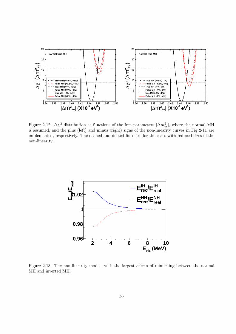
2.34 2.36 2.38 2.40 2.42 2.44 2.46 2.48 2.500

5

10

15

20

25

True MH (+0.5%, +1%) False MH (+0.5%, +1%) True MH (+1%, +2%) False MH (+1%, +2%) true MH (+2%, +4%) False MH (+2%, +4%)

(m

2 ee)

m2ee X10-3 eV2

Normal true MH

2.34 2.36 2.38 2.40 2.42 2.44 2.46 2.48 2.500

5

10

15

20

25

True MH (-0.5%, -1%) False MH (-0.5%, -1%) True MH (-1%, -2%) False MH (-1%, -2%) true MH (-2%, -4%) False MH (-2%, -4%)

(m

2 ee)

m2ee X10-3 eV2

Normal true MH

Figure 2-12: ∆χ2 distribution as functions of the free parameters |∆m2ee|, where the normal MH

is assumed, and the plus (left) and minus (right) signs of the non-linearity curves in Fig 2-11 areimplemented, respectively. The dashed and dotted lines are for the cases with reduced sizes of thenon-linearity.

(MeV)visE2 4 6 8 10

real

/Ere

cE

0.96

0.98

1

1.02realIH/Erec

IHE

realNH/Erec

NHE

Figure 2-13: The non-linearity models with the largest effects of mimicking between the normalMH and inverted MH.

50

2.34 2.36 2.38 2.40 2.42 2.44 2.46 2.48 2.500

5

10

15

20

25

True MH (+0.5%, +1%) False MH (+0.5%, +1%) True MH (+1%, +2%) False MH (+1%, +2%) true MH (+2%, +4%) False MH (+2%, +4%)

(m

2 ee)

m2ee X10-3 eV2

Normal true MH

2.34 2.36 2.38 2.40 2.42 2.44 2.46 2.48 2.500

5

10

15

20

25

True MH (-0.5%, -1%) False MH (-0.5%, -1%) True MH (-1%, -2%) False MH (-1%, -2%) true MH (-2%, -4%) False MH (-2%, -4%)

(m

2 ee)

m2ee X10-3 eV2

Normal true MH

Figure 2-14: Effects of two classes of energy non-linearity models [with plus (left) and minus (right)signs] in determination of the MH with the self-calibration effect, where the normal MH is assumed.

Event type Rate (per day) Rate uncertainty (relative) Shape uncertaintyIBD candidates 60 - -

Geo-νs 1.1 30% 5%Accidental signals 0.9 1% negligible

Fast-n 0.1 100% 20%9Li-8He 1.6 20% 10%

13C(α, n)16O 0.05 50% 50%

Table 2-4: The background summary table for the analysis of reactor antineutrinos.

MHs, respectively. Thanks to the current measurements of the neutrino oscillation parameters, wecan illustrate the specific non-linearity curves for the normal MH and inverted MH in Fig. 2-13.With this residual non-linearity in the measurement of Eq. (2.9), we can obtain the degradation of∆χ2 ≃ 2.5 in agreement with the effect in the right panel of Fig. 2-12.

For the reactor antineutrino experiment at a medium baseline, we can observe multiple peaksof the ∆m2

ee induced oscillation. Each of the peak position carries the information of ∆m2ee. This

redundancy can be used to evaluate the energy scale at different energies, providing a self-calibrationway of measuring the energy non-linearity [69]. To illustrate, we consider a test quadratic non-linearfunction in the prediction of Eq. (2.9), where the coefficients of the function are arbitrary and willbe determined in the fitting. Therefore, in the simplest way, we illustrate the self-calibration effectin Fig. 2-14, where the normal MH is assumed. We observe that the increase and reduction of theMH sensitivity due to unknown energy non-linearity can be resolved to some extent, and consistentsensitivity of the MH determination are obtained. Notice that the width of the ∆χ2 functionsin Fig. 2-14 is broadened, because additional uncertainties from the parameters of test quadraticnon-linearity are introduced.

51

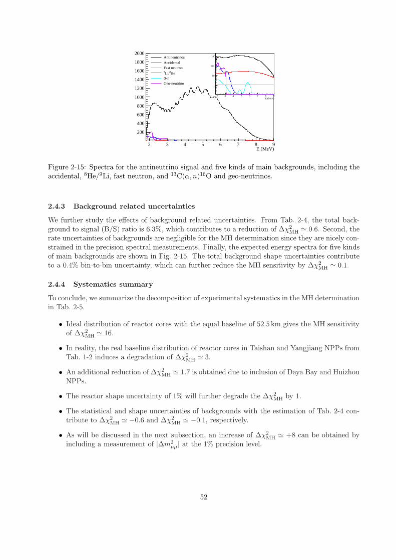
E (MeV)2 3 4 5 6 7 8 9

200

400

600

800

1000

1200

1400

1600

1800

2000Antineutrinos

AccidentalFast neutron

He8Li/9

-nαGeo-neutrino

E (MeV)2 3 4 5 6 7 8 9

1

10

210

310

Figure 2-15: Spectra for the antineutrino signal and five kinds of main backgrounds, including theaccidental, 8He/9Li, fast neutron, and 13C(α, n)16O and geo-neutrinos.

2.4.3 Background related uncertainties

We further study the effects of background related uncertainties. From Tab. 2-4, the total back-ground to signal (B/S) ratio is 6.3%, which contributes to a reduction of ∆χ2

MH ≃ 0.6. Second, therate uncertainties of backgrounds are negligible for the MH determination since they are nicely con-strained in the precision spectral measurements. Finally, the expected energy spectra for five kindsof main backgrounds are shown in Fig. 2-15. The total background shape uncertainties contributeto a 0.4% bin-to-bin uncertainty, which can further reduce the MH sensitivity by ∆χ2

MH ≃ 0.1.

2.4.4 Systematics summary

To conclude, we summarize the decomposition of experimental systematics in the MH determinationin Tab. 2-5.

• Ideal distribution of reactor cores with the equal baseline of 52.5 km gives the MH sensitivityof ∆χ2

MH ≃ 16.

• In reality, the real baseline distribution of reactor cores in Taishan and Yangjiang NPPs fromTab. 1-2 induces a degradation of ∆χ2

MH ≃ 3.

• An additional reduction of ∆χ2MH ≃ 1.7 is obtained due to inclusion of Daya Bay and Huizhou

NPPs.

• The reactor shape uncertainty of 1% will further degrade the ∆χ2MH by 1.

• The statistical and shape uncertainties of backgrounds with the estimation of Tab. 2-4 con-tribute to ∆χ2

MH ≃ −0.6 and ∆χ2MH ≃ −0.1, respectively.

• As will be discussed in the next subsection, an increase of ∆χ2MH ≃ +8 can be obtained by

including a measurement of |∆m2µµ| at the 1% precision level.

52

Stat. Core dist. DYB & HZ Shape B/S (stat.) B/S (shape) |∆m2µµ|

Size 52.5 km Tab. 1-2 Tab. 1-2 1% 6.3% 0.4% 1%

∆χ2MH +16 −3 −1.7 −1 −0.6 −0.1 +(4− 12)

Table 2-5: Different contributions for the MH determination. The first column is the statistical-only scenario with the equal baseline of 52.5 km, the second column considers the real distribution(dist.) of reactor cores, the third column defines the contribution of remote DYB and HZ NPPs,the fourth column stands for the reduction of the reactor shape uncertainty, the fifth and sixthcolumns are the contributions of the background statistical and shape uncertainties, the seventhcolumn is the enhanced sensitivity from additional information of |∆m2

µµ|.

2.5 MH Sensitivity with Precision |∆m2ee| and |∆m2

µµ| Measurements

Due to the intrinsic difference between |∆m2ee| and |∆m2

µµ|, precise measurements of these twomass-squared differences can provide additional sensitivity to MH, besides the sensitivity from theinterference effects. To incorporate the contribution from the |∆m2

µµ| measurement in long-baselinemuon-neutrino oscillation experiments, we define the following the extra pull function

χ2pull(|∆m2

µµ|) =(|∆m2

µµ| − |∆m2µµ|)2

σ2(∆m2µµ)

, (2.22)

where |∆m2µµ| and σ(∆m2

µµ) are the central value and 1σ uncertainty of the measurement. Thecombined χ2 function is defined as

χ2ALL = χ2

REA + χ2pull(|∆m2

µµ|) . (2.23)

Because two of the three mass-squared differences (∆m221, ∆m

231 and ∆m2

32) are independent, wechoose ∆m2

21 and ∆m2ee defined in Eq. (2.2) as the free parameters. Proper values of ∆m2

µµ can becalculated by the relations in Eq. (2.6).

To illustrate the effect of the external |∆m2µµ| measurement, we calculate the separated and

combined χ2 functions in Eqs. (2.9) and (2.23) in Fig. 2-16, where a 1% (left panel) or 1.5% (rightpanel) relative error of ∆m2

µµ is assumed. The black and red lines are for the true (normal) andfalse (inverted) MHs, respectively. The dashed and solid lines are for the reactor-only [in Eq. (2.9)]and combined distributions. Here a fixed CP-violating phase (cos δ = 0) is assumed for illustration.We can get a value of ∆χ2

MH ≃ 10 for the reactor-only analysis in the χ2 method. As for thecontribution from the external |∆m2

µµ| measurement, it is almost negligible if we choose the true(normal) MH in the fitting program. However, if the fitting MH is the false (inverted) one, thecentral value of ∆m2

ee in the χ2pull function will change by two times the difference in Eq. (2.6),

which accordingly results in a significant contribution to the combined χ2 function. Finally wecan achieve ∆χ2

MH ≃ 19 and ∆χ2MH ≃ 14 for the 1% and 1.5% relative errors of the |∆m2

µµ|measurement, respectively. Considering the whole parameter space of δ2MH from 0 to 2π, ∆χ2 canrange from 14 to 22 for the 1% relative precision of |∆m2

µµ| [69].

2.6 Conclusions

The determination of the neutrino mass hierarchy is of great importance in neutrino physics, sincethe MH provides a crucial input for future searches of neutrinoless double beta decays, observation

53

2.34 2.36 2.38 2.40 2.42 2.44 2.46 2.48 2.500

5

10

15

20

25

True MH ( )

False MH ( )

True MH ( )

False MH ( )

(m

2 ee)

m2ee X10-3 eV2

Normal true MH

2.34 2.36 2.38 2.40 2.42 2.44 2.46 2.48 2.500

5

10

15

20

25

True MH ( )

False MH ( )

True MH ( )

False MH ( )

(m

2 ee)

m2ee X10-3 eV2

Normal true MH

Figure 2-16: the reactor-only (dashed) and combined (solid) distributions of the ∆χ2 function inEq. (2.9) and Eq. (2.23), where a 1% (left panel) or 1.5% (right panel) relative error of ∆m2

µµ isassumed and the CP-violating phase (δ) is assigned to be 90/270 (cos δ = 0) for illustration. Theblack and red lines are for the true (normal) and false (inverted) neutrino MH, respectively.

of supernoca neutrino bursts, cosmological probe of neutrino properties, and model building of theneutrino masses and flavor mixing.

Thanks to the relatively large θ13 discovered in recent reactor and accelerator neutrino exper-iments, precise measurements of the reactor antineutrino spectrum at a medium baseline of about50 km can probe the interference effect of two fast oscillation modes (i.e., oscillations induced by∆m2

31 and ∆m232) and sensitive to the neutrino MH. The corresponding sensitivity depends strongly

on the energy resolution, the baseline differences and energy response functions. Moreover, the MHsensitivity can be improved by including a measurement of the effective mass-squared difference inthe long-baseline muon-neutrino disappearance experiment due to flavor dependence of the effectivemass-squared differences.

We have calculated the MH sensitivity at JUNO taking into account the real spatial distributionof reactor complexes, reactor related uncertainties, detector related uncertainties and backgroundrelated uncertainties. We demonstrated that a median sensitivity of ∼ 3σ can be achieved withthe reasonable assumption of the systematics and six years of running. We emphasized that thereactor shape uncertainty and detector non-linearity response, are the important factors to be dealtwith. In addition, we have studied the additional sensitivity by including precision measurementsof |∆m2

µµ| from long baseline muon (anti)neutrino disappearance. A confidence level of ∆χ2MH ∼ 14

(3.7σ) or ∆χ2MH ∼ 19 (4.4σ) can be obtained, for the |∆m2

µµ| uncertainty of 1.5% or 1%.Besides the spectral measurement of reactor antineutrino oscillations, there are other methods

to resolve the MH using the matter-induced oscillation of accelerator or atmospheric neutrinos.Worldwide, there are many ongoing and planed experiments designed in this respect. These in-clude the long baseline accelerator neutrino experiments (i.e. NOνA and DUNE) and atmosphericneutrino experiments (i.e., INO, PINGU, Hyper-K). Using different oscillation patterns, differentneutrino sources and different detector techniques, they are complementary in systematics and con-tain a great amount of synergies. Therefore, the mass hierarchy, being one of the most importantundetermined fundamental parameters in neutrino physics, clearly deserves multiple experimentswith preferably different experimental techniques. A consistent resolution of the MH from all theseexperiments will greatly increase our confidence in the MH determination.

54

3 Precision Measurements of Neutrinos

3.1 Introduction and motivation

JUNO is designed to collect a large number of reactor antineutrino events with excellent energyresolution [3%/

√E(MeV)] and accurate energy determination [better than 1%]. Therefore, besides

the determination of the neutrino mass hierarchy (MH) [69, 79], in 6 years JUNO will also allowa detailed study of various aspects of neutrino oscillations, including the extractions of the mixingparameters θ12, ∆m

221, and |∆m2

ee|, and probe the fundamental properties of neutrino oscillations.JUNO will be:

• the first experiment to simultaneously observe the neutrino oscillation driven by both atmo-spheric and solar neutrino mass-squared differences (Fig. 3-1). The pronounced dip around 3MeV corresponds to the solar ∆m2, and the rapid oscillations correspond to the atmospheric∆m2.

• the first experiment to observe multiple oscillation cycles of the atmospheric ∆m2 (Fig. 3-1).

• the well place to have an unprecedented precision measurement of sin2 θ12, ∆m221 and |∆m2

ee|to better than 1%.

Furthermore, together with long-baseline neutrino experiments (DUNE [83], Hyper-K [87, 88]),JUNO will usher in the new era of precision neutrino oscillation experiments.

It has to be stressed that on top of measuring the oscillation parameters precision tests ofthe oscillation pattern in a model-independent way is also very important to probe new physicsbeyond the Standard Model. The precision measurement of neutrino oscillation parameters is avery powerful tool to test the standard 3-flavor neutrino model (νSM). In particular, precisionmeasurement of the fundamental parameter θ12 will:

• play a crucial role in the future unitarity test of the MNSP matrix U . The combinationof short-baseline reactor antineutrino experiments (e.g., Daya Bay [30]), medium-baselinereactor antineutrino experiments as JUNO and solar neutrino experiments (e.g., SNO [116])will enable the first direct unitarity test of the MNSP matrix [22–24,117]:

|Ue1|2 + |Ue2|2 + |Ue3|2 ?= 1 . (3.1)

With the combination of Daya Bay, JUNO and SNO, the above unitarity condition willbe tested with the precision of 2.5% [117]. The precision is limited by the solar neutrinomeasurements and could be improved to better than 1% with future precision solar neutrinomeasurements.

• narrow down the parameter space of the effective mass (i.e., |mee|) of the neutrinoless doublebeta decay allowing a conclusive test for the scenario of inverted mass hierarchy (IH). In thecase of m3 ≤ 0.05 eV, the minimal value of the effective neutrino mass for IH can be writtenas [118]

|mee|min(IH) ≃ cos2 θ13

√|∆m2

31| cos 2θ12 . (3.2)

Editors: Yufeng Li (liyufeng@ihep.ac.cn)Major contributor: Xin Qian

55

(MeV)promptE2 4 6 8

# of

IBD

per

10

keV

0

50

100

150

200

250

JUNO 100k IBD Events

solar2 m∆

atm2 m∆

Figure 3-1: The expected prompt energy spectrum of JUNO with a nominal luminosity for sixyears of data taking with a 20 kt detector and 36 GWth reactor power (a total of 100k IBD events).A 3%/

√E energy resolution is assumed.

As the uncertainty of sin2 θ12 shrinks from the current level to better than 1%, the lower limitof the effective mass for IH can increase by a factor of two (see Fig. 3-2). In a background-dominated neutrinoless double beta decay experiment, a factor of two improvement in theeffective mass sensitivity corresponds to a combined factor of 16 improvement for the ex-perimental parameters of the running time, detector mass, background level and energy res-olution [119, 120]. Therefore, the precision measurement of sin2 θ12 is crucial for the nextgeneration of the neutrinoless double beta decay experiments, which aim to cover the wholeparameter space corresponding to IH.

• be a powerful discriminator for models of the neutrino masses and mixing. First, θ12 ismore sensitive than other mixing angles to the quantum corrections since ∆m2

21 ≪ |∆m231|.

Therefore, neutrino-mixing models will be better constrained when the accuracy of θ12 isimproved. Second, taking the prediction of the tri-bimaximal mixing (TBM) [122–124] forθ12 as an example:

θTBM12 = arcsin

1√3≃ 35.3 , (3.3)

the value of non-zero θ13 may induce further corrections for θ12. Depending on the sign of θ12corrections, two categories of mixing models, TM1 and TM2, are defined respectively [125].TM1 and TM2 correspond to the mixing matrix keeping the first or second column of TBMunchanged. A measurement of sin2 θ12 better than 1% is a powerful tool to discriminatebetween TM1 and TM2 and may shed light on the mechanism of the neutrino masses andmixing.

The muon (anti)neutrino and electron antineutrino disappearance effectively measure ∆m2µµ

and ∆m2ee [95, 96] (two different combinations of ∆m2

31 and ∆m232), respectively. When combined

with the precision |∆m2µµ| measurements from muon (anti)neutrino disappearance, the precision

measurement of |∆m2ee| will:

56

0.0001 0.001 0.01 0.1 1m @eVD

0.0001

0.001

0.01

0.1

1Èm

eeÈ@e

VD Dm31

2 < 0

Dm312 > 0

0.0001 0.001 0.01 0.1 1m @eVD

0.0001

0.001

0.01

0.1

1Èm

eeÈ@e

VD

hierarchical cancellation quasi−degenerate (only normal)

√∆m2

⊙s212c

213

√∆m2

Ac213 cos 2θ12

m1c212c

213

√∆m2

Ac213

m0

|m(2)ee |nor > |m(3)

ee |nor |m(1)ee |nor > |m(2)

ee |nor

−√

∆m2⊙ +m2

1s212c

213

m01−t212−2s213

1+t212

−√

∆m2A +m2

1s213±

√∆m2

As213

Figure 3-2: The main properties of the effective mass |mee| as a function of the smallest neutrinomass [121]. Here m denotes the common mass for the quasi-degenerate region and tij = tan θij,sij = sin θij, cij = cos θij. Furthermore, ∆m2

A and ∆m2⊙ stands for the atmospheric mass-squared

difference and the solar mass-squared difference, respectively.

• test the mass sum rule:

∆m213 +∆m2

21 +∆m232

?= 0 , (3.4)

which is an important prediction of the νSM. New physics like the light sterile neutrinosor non-standard interactions may induce non-trivial corrections to the effective oscillationfrequencies ∆m2 . Therefore, a precision test of the sum rule is an important probe of newphysics beyond the Standard Model.

• reveal additional information regarding the neutrino mass hierarchy. As discussed in Refs. [69,95], precision measurements of both |∆m2

ee| and |∆m2µµ| would provide new information for

the neutrino mass hierarchy. A quantitative calculation is performed in Ref. [69], illustratinga significant improvement for the sensitivity of the neutrino mass hierarchy. The mediansensitivity is increased from 3 ÷ 3.5σ to 4 ÷ 4.5σ [69] by considering a precision of 1% for|∆m2

µµ|. An individual 1.5% precision is estimated for both T2K [126] and NOνA [82].Therefore, a combined precision level [127] of 1% would be achievable by the moment whenJUNO will start taking data.

In the following sections, the sensitivity of JUNO for precision measurements will be illustrated.Precision measurements of the oscillation parameters will be presented in Sec. 3.2. Moreover, thestrategy for testing the unitarity of the lepton mixing matrix and the contribution of JUNO in thisrespect will be presented in Sec. 3.3. Finally, a summary will be given in Sec. 3.4.

57

3.2 Precision measurements of oscillation parameters

In the standard three-neutrino mixing framework, the relevant mass and mixing parameters forJUNO are θ12, θ13, ∆m2

21 and ∆m2ee (as the linear combination of ∆m2

31 and ∆m232, see the

definition in Eq. (2.2)). In the era of precision measurements, matter effects may not be negligibleand deserve careful evaluations. In the presence of terrestrial matter effects, the survival probabilityof reactor antineutrinos is written as

P (νe → νe) = 1 − sin2 2θm13[cos2 θm12 sin

2∆m31 + sin2 θm12 sin

2 ∆m32

]

− cos4 θm13 sin2 2θm12 sin

2∆m21 , (3.5)

with ∆mij ≡ (λ2i − λ2j)L/4E, and

sin2 2θm12 ≃ sin2 2θ12

(1 + 2

ACC

∆m221

cos 2θ12

),

λ22 − λ21 ≃ ∆m221

(1− ACC

∆m221

cos 2θ12

), (3.6)

and

sin2 2θm13 ∼ sin2 2θ13

[1 +O(

ACC

∆m231

sin2 θ13)

],

λ23 − λ21 ∼ ∆m231

[1 +O(

ACC

∆m231

sin2 θ13)

]. (3.7)

Note that λ2i is the ith energy eigenvalue of the Hamiltonian in matter, and ACC = 2√2EGFNe

with Ne being the electron number density in matter and GF the Fermi constant.. For the typicalneutrino energy E and matter density ρ(x), we obtain

ACC

∆m221

cos 2θ12 ≃ 0.5% × E

4MeV× ρ(x)

3 g/cm,

ACC

∆m231

sin2 θ13 ≃ 1.5× 10−5 × E

4MeV× ρ(x)

3 g/cm. (3.8)

For measurements with precision better than 1%, matter effects are negligible for the atmosphericneutrino oscillation parameters (i.e., θ13 and ∆m2

31), but they are sizable (0.5%-0.1%) for the solarneutrino oscillation parameters (i.e., θ12 and ∆m2

21). Therefore, it is important to consider mattereffects when analyzing the real data. However, matter effects can be neglected for sensitivity studiesas the corrections only affect the central values of oscillation parameters and not the sensitivity ofMH and oscillation parameters.

In the history of neutrino oscillation observations, three different oscillation modes are observedin terms of effective two-flavor oscillations. The Super-Kamiokande Collaboration [128] observedthe oscillation driven by (∆m2

32, sin2 2θ23) in the atmospheric muon neutrino disappearance chan-

nel (shown in the upper panel of Fig. 3-3). Later on, two reactor antineutrino experiments alsopresented the electron antineutrino survival probability as a function of L/E. The middle panel ofFig. 3-3 illustrates the oscillation determined by (∆m2

21, sin2 2θ12) at the KamLAND detector [129]

with almost two complete cycles. The third case is shown in the lower panel of Fig. 3-3, which ischaracterized by (∆m2

31, sin2 2θ13) and observed in the Daya Bay spectral observation [130]. JUNO

could be the first to observe an oscillation pattern containing two independent oscillation frequen-cies and multiple oscillation cycles. Because the reactor-detector distances are almost identical as

58

0

0.2

0.4

0.6

0.8

1

1.2

1.4

1.6

1.8

1 10 102

103

104

L/E (km/GeV)

Dat

a/P

redi

ctio

n (n

ull o

sc.)

(km/MeV)eν/E0L

20 30 40 50 60 70 80 90 100 110

Sur

viva

l Pro

babi

lity

0

0.2

0.4

0.6

0.8

1

eνData - BG - Geo best-fit oscillationν3-

best-fit oscillationν2-

[km/MeV]⟩ν

E⟨ / effL

0 0.2 0.4 0.6 0.8

)e

ν→

eν

P(

0.9

0.95

1EH1

EH2

EH3

Best fit

Figure 3-3: The observed neutrino events over the non-oscillation predictions as functions ofLeff (the effective baseline) over E (the neutrino energy) for Super-K [128] atmospheric neutrinooscillations (top), KamLAND [129] reactor antineutrino oscillations (middle) and Daya Bay [130]reactor antineutrino oscillations (bottom). They correspond to three different modes of effectivetwo-flavor oscillations controlled by (∆m2

32, sin2 2θ23), (∆m221, sin2 2θ12) and (∆m2

31, sin2 2θ13),respectively.

59

∆m221 |∆m2

31| sin2 θ12 sin2 θ13 sin2 θ23Dominant Exps. KamLAND MINOS SNO Daya Bay SK/T2K

Individual 1σ 2.7% [129] 4.1% [131] 6.7% [116] 6% [130] 14% [132,133]

Global 1σ 2.6% 2.7% 4.1% 5.0% 11%

Table 3-1: Current precision for the five known oscillation parameters from the dominant experi-ments and the latest global analysis [29].

required by the MH measurement, antineutrinos from different reactors generate nearly identicalenergy spectra without smearing the oscillation patterns. This represents an important advantagefor extracting the oscillation parameters with high precision. Fig. 3-1 shows the predicted promptenergy spectrum for the IBD events. Multiple oscillation patterns corresponding to the solar andatmospheric ∆m2 scales are clearly visible.

Current precision for five known oscillation parameters are summarized in Table 3-1, whereboth the results from individual experiments and from the latest global analysis [29] are presented.Most of the oscillation parameters have been measured with an accuracy better than 10%. Theleast accurate case is for θ23, where the octant ambiguity hinders a precision determination. Amongthe four oscillation parameters accessible by JUNO, θ13 can not be measured with a precision betterthan the Daya Bay one, which is expected to reach a 4% precision for this smallest mixing angleafter 5 years of running. Therefore, we only discuss the prospect for precision measurements ofθ12,∆m

221, and |∆m2

ee|1.With the nominal setup [69] described in the MH measurement, the expected accuracy for the

three relevant parameters is shown in Fig. 3-4, where the solid lines show the accuracy with allthe other oscillation parameters fixed and the dashed lines show the accuracy with free oscillationparameters. The precision (dashed lines) of 0.54%, 0.24% and 0.27% can be obtained for sin2 θ12,∆m2

21 and ∆m2ee, respectively, after 6 years of running.

Several comments are listed as follows:

• Although only one single detector is considered, the precision on θ12 at the sub-percent levelis achievable because most of the sensitivity is from the spectral information. This propertyis illustrated in Fig. 3-5, showing the θ12 accuracy with both the rate and shape informationand with only the rate information.

• A precision of |∆m2ee| similar to ∆m2

21 is obtained because each fast oscillation cycle givesa statistically independent measurement of |∆m2

ee|. The combined result from the wholespectrum has a high statistical accuracy.

• The baseline differences may affect significantly the precision of θ12 because different baselinescan smear the oscillation pattern. For comparison, the precision of θ12 could be improvedfrom 0.54% to 0.35% if the baselines were identical for JUNO.

• The energy resolution impacts mainly |∆m2ee| because the relevant information is contained

in the fine structure of fast oscillations. A quantitative dependence on the energy resolutionfor all the three oscillation parameters is shown in Fig. 3-6 with energy resolution rangingfrom 2% to 5%.

1There will be two degenerated solutions for |∆m2ee| in case of undetermined MH.

60

Figure 3-4: Expected accuracy for sin2 θ12, ∆m221 and ∆m2

ee after 6 years of running at JUNO(i.e., O(100 k) events). The solid curves are obtained with all other oscillation parameters fixed,while the parameters are set free for the dashed curves.

61

Figure 3-5: The precision of sin2 θ12 with the rate plus shape information (solid curve) and rate-only information (dashed curve).

Figure 3-6: Dependence of the precision of sin2 θ12, ∆m221 and ∆m2

ee with the neutrino energyresolution.

62

Nominal + B2B (1%) + BG + EL (1%) + NL (1%)

sin2 θ12 0.54% 0.60% 0.62% 0.64% 0.67%

∆m221 0.24% 0.27% 0.29% 0.44% 0.59%

|∆m2ee| 0.27% 0.31% 0.31% 0.35% 0.44%

Table 3-2: Precision of sin2 θ12, ∆m221 and |∆m2

ee| from the nominal setup to those includingadditional systematic uncertainties. The systematics are added one by one from left to right.

In the following a study of the effects of important systematic errors, including the bin-to-bin (B2B)energy uncorrelated uncertainty, the energy linear scale (EL) uncertainty and the energy non-linear(NL) uncertainty, will be discussed and the influence of background (BG) will be presented. As abenchmark, 1% precision for all the considered systematic errors is assumed. The background leveland uncertainties are the same as in the previous chapter for the MH determination. In Table 3-2, we show the precision of sin2 θ12, ∆m

221 and |∆m2

ee| from the nominal setup to those includingadditional systematic uncertainties. The systematics are added one by one. Note the energy-relateduncertainties are more important because the sensitivity is mostly from the spectrum distortiondue to neutrino oscillations.

In summary, for the precision measurements of oscillation parameters, we can achieve the preci-sion level of 0.5%−0.7% for the three oscillation parameters sin2 θ12, ∆m

221 and |∆m2

ee|. Therefore,precision tests of the unitarity of the lepton mixing matrix in Eq. (3.1), and the mass sum rule inEq. (3.4) are feasible at unprecedented precision levels.

3.3 Tests of the standard three-neutrino paradigm

In this section, the strategy for testing the standard three-neutrino paradigm including the unitarityof the lepton mixing matrix and the sum rule of the mass-squared differences will be discussed.As only the lepton mixing elements of the electron flavor are accessible in reactor antineutrinooscillations, we here focus on testing the normalization condition in the first row of U as shown inEq. (3.1). It should be noted that the θ12 measurement in JUNO is mainly from the energy spectrummeasurement, and θ13 in Daya Bay is from the relative rate measurement. Therefore, an absoluterate measurement from either reactor antineutrino experiments or solar neutrino experiments isrequired to anchor the total normalization for the first row of U . For the test of the mass sum rule,an additional independent mass-squared difference is needed, where the most promising one is thatfrom the long-baseline accelerator muon-neutrino disappearance channel, i.e., ∆m2

µµ.To explain non-zero neutrino masses in new physics beyond the Standard Model (SM), a large

class of models introduces additional fermion singlets to mix with the SM neutrinos. Thus the fullneutrino mixing matrix will be enlarged, and an effective 3× 3 non-unitary mixing matrix emergeswhen one integrates out all those heavy fermion singlets (i.e., sterile neutrinos). The distinct effectswithin this class of SM extensions are well described by an effective field extension of the SM, calledthe Minimal Unitarity Violation (MUV) scheme. The MUV extension of the SM, characterized bytwo non-renormalizable effective operators, is defined as

LMUV = LSM + δLd=5 + δLd=6

= LSM +1

2cd=5αβ

(Lc

αφ∗)(

φ† Lβ

)+ cd=6

αβ

(Lαφ

)i 6 ∂

(φ†Lβ

)+H.c. , (3.9)

where φ denotes the SM Higgs field, which breaks the electroweak (EW) symmetry spontaneouslyafter acquiring the vacuum expectation value (vev) vEW ≃ 246GeV, and Lα represents the lepton

63

doublets. In addition, we use the notation φ = iτ2φ∗. The dimension-5 operator in Eq. (3.9)

generates nonzero neutrino masses after EW symmetry breaking. On the other hand, the dimension-6 operator contributes to the kinetic terms of neutrinos, which leads to the non-unitary neutrinomixing matrixN after we canonically normalize the kinetic terms with a non-unitary transformationof the neutrino fields. Therefore, we can obtain the effective low-energy Lagrangian in the neutrinomass basis as

LMUV =1

2(νi i ∂/ νi − νcimi νi +H.c.) − g

2√2

(W+

µ lα γµ (1− γ5)Nαi νi +H.c.)

− g

2 cos θW

(Zµ νi γ

µ (1− γ5) (N†N)ij νj +H.c.

)+ . . . (3.10)

where νi denotes the four-component left-handed field for the ith neutrino mass eigenstate, and g isthe coupling constant of the EW interactions. It should be noted that observable consequences ofthe non-unitary neutrino mixing matrix are encoded in the modifications of charged current (CC)and neutral current (NC) interactions of neutrinos in Eq. (3.10).

To test the unitarity violation, we first need a parametrization of the non-unitary neutrinomixing matrix N . Without loss of generality, one can write N as the product of a Hermitianmatrix H and a unitary matrix U :

N = HU ≡ (1 + η)U , (3.11)

where the elements of the η matrix are assumed to be ≪ 1 due to the smallness of the unitarityviolation. Alternatively, one can use the parametrization for the Hermitian combination NN † as

(NN †)αβ = (1αβ + εαβ) , (3.12)

where elements of the ε matrix are again assumed to be ≪ 1, and can be related to the η matrix as

εαβ ≃ 2 ηαβ , (3.13)

up to higher orders of ηαβ and εαβ .Unitarity violation can be tested in both the neutrino oscillation and EW interaction pro-

cesses. There exist significant distinctions for the unitarity tests in the neutrino oscillation andEW interaction processes. For the neutrino oscillations, the neutrino flavors are tagged with thecorresponding charged leptons in the production or detection processes, and the indices for neu-trino mass eigenstates are distinguished using the interference effects. Thus we can determine theindividual elements of the mixing matrix from neutrino oscillations [22, 24, 117]. On the otherhand, in the EW interaction processes, neutrino mass eighstates in the final states are not detectedseparately. The experiment rates correspond to sums over all possible mass eigenstates. Therefore,only the sums of products of the matrix elements (i.e., NN †) are measurable [22,23].

In the following we shall briefly summarize the constraints of non-unitarity from the EWinteraction processes [22,23], which include both high and low energy observables:

• electroweak precision observables, including the weak mixing angle sin2 θW, Z decay param-eters, the W boson mass and decay widths;

• leptonic universality tests;

• rare charged lepton decays (e.g., ℓρ → ℓσγ);

• CKM unitarity;

64

• NuTeV tests of weak interactions;

• low energy measurements of sin2 θW, including parity non-conservation in Cesium, weakcharge of the proton, and Moller scattering.

A global analysis of all above observables is performed to obtain the constraints on the elements ofNN †. At 90% C.L., the constraints are [23]:

∣∣∣NN †∣∣∣ =

0.9979 − 0.9998 < 10−5 < 0.0021< 10−5 0.9996 − 1.0 < 0.0008< 0.0021 < 0.0008 0.9947 − 1.0

, (3.14)

where the best-fit points for the off-diagonal εαβ and for εµµ are at zero, and the preference offlavor-conserving non-unitarity is observed at 90% C.L. for εee and below 90% CL for εττ . Theoff-diagonal non-unitarity parameters are mainly constrained from charged lepton flavor-changingdecays. Particularly, the limit for εeµ is dominated by the measurements of µ → e γ. The slightdeparture from zero for εee is stemmed from the similar discrepancy in the invisible width of the Zboson, and that for εττ is from the internal correlation among εαβ in the MUV scheme. The EWinteraction processes are only sensitive to the elements of NN †. The unitarity test in the form ofN †N can only be inferred indirectly from Eq. (3.14) in the MUV scheme, where a precision level ofaround 3% can be obtained [22]. In this respect, the neutrino oscillations provide us an excellentopportunity to test the unitarity using the direct measurements of mixing matrix elements.

In the neutrino oscillation with a single transition channel, only one combination of the mixingmatrix elements can be extracted from the oscillation amplitude. In addition, an absolute measure-ment of the zero-distance effect gives a direct test of unitarity conditions in NN † or N †N . For theformer case, the global analysis of different oscillation channels is needed to test unitary conditions.As for the latter case, the level of unitarity tests from absolute rate measurements requires betterunderstanding of the uncertainties in the neutrino flux normalization and detector efficiency. Inthe following part, we shall discuss the unique role of JUNO in the global picture of unitarity testsin neutrino oscillations.

For reactor antineutrino oscillations, only the νe survival probability is detectable, which canbe expressed in the MUV scheme as

Pνe→νe =(|Ne1|2 + |Ne2|2 + |Ne3|2

)2

− 4|Ne1|2|Ne2|2 sin2∆21 − 4|Ne3|2(|Ne1|2 sin2 ∆31 + |Ne2|2 sin2 ∆32) , (3.15)

where ∆ij = (m2i −m2

j)L/4E. It has to be noted that the mixing element Nαi is only sensitive tothe absolute measurements, which is directly compared to model predictions of the antineutrinoproduction. To illustrate this effect, we define the effective mixing angles as

sin2 θ13 ≡|Ne3|2

|Ne1|2 + |Ne2|2 + |Ne3|2, tan2 θ12 ≡

|Ne2|2|Ne1|2

. (3.16)

Therefore, we can rewrite Eq. (3.15) as

Pνe→νe =(|Ne1|2 + |Ne2|2 + |Ne3|2

)×[1− cos4 θ13 sin

2 2θ12 sin2 ∆21

− sin2 2θ13(cos2 θ12 sin

2∆31 + sin2 θ12 sin2 ∆32)

]. (3.17)

Comparing to the probability in Eq. (2.1), it can be shown that only the rate normalization factorcontributes to the unitarity test of Eq. (3.1), which mainly includes the uncertainties from the

65

0.8 0.9 1.0 1.1 1.20

2

4

6

8

10

10% Abs 2% Abs 10% Rel 2% Rel

2

|Ne1|2+|Ne2|2+|Ne3|2

Figure 3-7: Different realizations of the unitarity violation test of the equation 3.1 in reactorantineutrino oscillations. See the text for details.

reactor flux normalization and detector efficiency. We refer this scenario as the absolute (Abs)measurement. On the other hand, we can define a relative (Rel) measurement, which combines thereactor spectral measurements of effective mixing parameters in Eq. (3.16) and the solar neutrinomeasurements to test the unitarity violation in an indirect way [117]. In Fig. 3-7, we present the twodifferent scenarios of the unitarity test, which show obvious advantages for the combined analysis,for several considered uncertainties of reactor flux normalization. An additional 1% detector effi-ciency uncertainty is assumed. In the combined analysis, we assume a 4% final projected sensitivityfor sin2 2θ13 at Daya Bay, and a direct measurement of |Ne2|2 of the 4% level at a future SNO-likesolar neutrino experiment. Finally, we may achieve the precision level of 1.2% for unitarity testsin the assumption of a 10% reactor normalization uncertainty, which could present a independenttest of the reactor antineutrino anomaly.

Regarding the test of the mass sum rule in Eq. (3.4), JUNO is a powerful precision tool inmeasuring the two independent mass-squared differences ∆m2

21 and |∆m2ee| as seen in Table 3-2,

and can test the mass sum rule by inclusion of a third independent mass-squared difference inEq. (2.6). Assuming a 1% precision level of |∆m2

µµ|, we can obtain the test of the mass sum rule inEq. (3.4) at better than 1.8%, which represents an important test for the standard three-neutrinoparadigm.

3.4 Conclusions

Precision measurement of the oscillation parameters and test of the standard three-neutrino frame-work constitute another important goal of the JUNO experiment. Among all the six oscillationparameters of neutrino oscillations, JUNO can measure sin2 θ12, ∆m

221 and |∆m2

ee| to the world-leading levels of 0.7%, 0.6%, and 0.5%, respectively. As a powerful detector with huge statistics,unprecedent energy resolution, the precision measurements of oscillation parameters are importantfor discrimination of the neutrino mixing patterns, the search of neutrinoless double beta decay,and test of the standard three-neutrino paradigm. Utilizing these above measurements, JUNO can

66

help in testing the unitarity relation of Eq. (3.1) and the mass sum rule of Eq. (3.4) to the levelsof around 1.2% and 1.8%, respectively. Moreover, JUNO would be the first experiment to simulta-neously observe neutrino oscillations from two different frequencies, and be the first experiment toobserve more than two oscillation cycles.

67

4 Supernova Burst Neutrinos

Measuring the neutrino burst from the next nearby supernova (SN) is a premier target of low-energy neutrino physics and astrophysics. For a typical galactic distance of 10 kpc and typical SNparameters, JUNO will register about 5000 events from inverse beta decay (IBD), νe + p→ n+ e+,comparable to Super-Kamiokande, and many events from complementary channels, notably 2000events from all-flavor elastic neutrino-proton scattering. With more than 300 events from neutrino-electron scattering, JUNO will also be the best detector for SN νe. Such a high-statistics signalcan determine a detailed neutrino “light curve” spectrum, and complete flavor information. Incombination with other neutrino detectors, gravitational-wave detectors, and observations in variouselectromagnetic channels, a detailed astrophysical multi-messenger picture will emerge. In this waythe standard paradigm of stellar core collapse will be confirmed, refuted or extended. The uniqueparticle-physics lessons pioneered by the sparse SN 1987A data for the first time will be madeprecise and will extend to areas that depend on high statistics, good energy resolution, or flavorinformation, notably in the area of neutrino oscillations.

4.1 Core-collapse supernovae: What, where and when?

The baryonic matter in a spiral galaxy like our own Milky Way participates in an on-going cycle ofstar formation, nuclear processing, and ejection into interstellar space. Only low-mass stars withM . 0.85M⊙

1 live longer than the age of the universe of 14 billion years, whereas the progenitors ofcore-collapse SNe (M & 6 ∼ 8M⊙, depending on other parameters such as metallicity [134]) finishafter less than a hundred million years. Intermediate-mass stars lose most of their mass during thered-giant phase in the form of a “stellar wind”, i.e., they mostly “evaporate”, leaving behind a whitedwarf, a sub-M⊙ compact star supported by electron degeneracy pressure. A more massive star, onthe other hand, completes the nuclear reaction chains all the way to iron, forming a degenerate core.It ultimately collapses to nuclear density, ejects the remaining mass in a spectacular SN explosion,and emits 99% of the gravitational binding energy of the newly formed neutron star in the form ofneutrinos and antineutrinos2 of all flavors. The standard paradigm of how a core-collapse implosionreverses to a SN explosion is that a shock wave forms at core bounce, propagates outward, stallsat a radius of 100–200 km, and is finally revived by neutrino energy deposition [135, 136]. If thisneutrino-driven explosion mechanism indeed captures the crucial physics remains open and couldbe tested with a high-statistics SN neutrino observation.

Core-collapse SNe encompass the spectral types Ib, Ic, and II, whereas SNe of Type Ia representa different physical phenomenon [135, 137, 138]. The progenitor consists of a carbon-oxygen whitedwarf, accreting matter from a binary companion until collapse (single degenerate scenario) orof two merging white dwarfs (double degenerate scenario), either way igniting explosive nuclearburning that disrupts the entire star—no stellar remnant survives. This thermonuclear explosionmechanism liberates a comparable amount of visible energy as a core-collapse SN which is driven bygravitational binding energy, liberates about 100 times more energy, but emits 99% of it in the formof neutrinos. The light curves of SNe Ia are very reproducible and they have been extensively usedas cosmological standard candles, whereas core-collapse SNe are dimmer and show more diverselight curves. Core-collapse SNe occur in regions of active star formation, i.e., primarily the gaseous

Editors: Georg Raffelt (raffelt@mpp.mpg.de) and Shun Zhou (zhoush@ihep.ac.cn)Major contributors: Gang Guo, Yufeng Li, Jiashu Lu, and Hao Wang

1In stellar astrophysics, masses are usually measured in units of the solar mass, 1 M⊙ = 1.989 ×1033 g, corre-sponding to 1.20 ×1057 nucleons.

2In the following we will generically use the term “neutrinos” to include both neutrinos and antineutrinos unlesswe explicitly distinguish between them.

68

and dust-filled disks of spiral galaxies, where around 2/3 of all SNe are of core-collapse type. Littlestar formation takes place in elliptical galaxies and they host only SNe Ia [137].

Core collapse may sometimes produce a black hole, but usually the compact remnant is aneutron star with a gravitational mass of up to 2M⊙, often showing up as a pulsar. The collapseof this amount of matter to nuclear density, i.e., to a radius of 12–15 km, liberates 10–20% of itsrest mass as gravitational binding energy, corresponding to some 3 × 1053 erg or 2 × 1059 MeV,exact numbers depending on the final neutron-star mass and the nuclear equation of state. Around99% of this enormous amount of energy emerges as neutrinos, about 1% as kinetic energy of theexplosion, and about 0.01% as light, still outshining the host galaxy. Star formation stronglyfavors low-mass stars, so core-collapse SNe are rare, yet the integrated cosmic energy density of SNneutrinos (the diffuse SN neutrino background or DSNB, see Sec. 5) is comparable to the integratedphoton emission from all stars [139].

While every second a few core-collapse events happen in the visible universe, a JUNO-classdetector covers only our own galaxy and its satellites, such as the Large Magellanic Cloud (LMC)at a distance of 50 kpc, the site of SN 1987A which provided the first and only observed SN neutrinosignal [140]. A SN in Andromeda, at 750 kpc our nearest-neighbor big galaxy, would produce aboutone neutrino event in JUNO. Another SN in the LMC would produce around 200 events, a significantimprovement on the SN 1987A statistics of a total of about two dozen events in three detectors.The most likely place of the next nearby SN, however, is the spiral disk of our own galaxy. Thesolar system is located close to the mid-plane of the disk at a distance of 8.7 kpc from the galacticcenter. The expected SN distance distribution has an average of around 10 kpc, usually taken asthe fiducial distance, where JUNO would register around 5000 events.

However, the distance distribution is broad [141–143] and one cannot expect the next galacticSN to be “average” or “typical”. The distribution drops very quickly at or around 20 kpc, a distancethat would still provide a whopping 103 events. On the other extreme, the distribution becomesvery small at around 2 kpc, where the number of events would be around 105. The nearest possibleSN progenitor is the red supergiant Betelgeuse (Alpha Orionis) at a distance of around 0.2 kpc [144]producing around 107 events. Such a high event rate (∼ 20 MHz at peak) is a big challenge for ahuge liquid scintillator detector like JUNO. The data acquisition system of JUNO will be designedto accommodate as high event rates as possible to maintain the event by event detection.

Observing the next nearby SN in neutrinos is a once-in-a-lifetime opportunity that must not bemissed. The galactic core-collapse SN rate is only one every few decades. It can be estimated fromSN statistics in external galaxies [137, 145, 146], the galactic birth rate of massive stars [147], thepulsar birth rate [148,149], the measured galactic abundance of the radioactive isotope 26Al whichis produced in core-collapse SNe [150], and the historical SN rate over the past millennium [143,151,152]. A weak upper limit is obtained from the non-observation of a neutrino burst other thanSN 1987A since 30 June 1980 when the Baksan Scintillator Telescope (BST) took up operation [153].Together with subsequent neutrino detectors, no galactic SN neutrino burst would have been missedsince that time. Assuming a galactic core-collapse rate of one every 30–40 years, the chances ofobserving a galactic SN burst over ten years of operation is around 30%, a great opportunityfor a world-class fundamental observation. Coordination on detector maintenance with other bigneutrino observatories, such as Super-Kamiokande and IceCube, will help to avoid missing a SN inall neutrino observatories simultaneously.

Our location in the mid-plane of the dust-filled galactic disk implies that visual SN observationsare strongly impeded by obscuration. Therefore, only five historical SNe have been reported in thesecond millennium where the record may be reasonably complete [154]. Moreover, three out of theseevents were of the brighter type Ia (SNe 1006, 1572 and 1604). The two historical core-collapseSNe were the “Chinese SN” of 1054 that has produced the Crab Nebula and Crab Pulsar and

69

SN 1181. The Cas A remnant and non-pulsar hot neutron star may correspond to the uncertainSN observation of 1680 that would bring the historical second-millennium SNe up to six. Thesenumbers are consistent with 2/3 or more of all galactic SNe being of core-collapse type and witha few galactic core-collapse events per century. Today, a galactic SN almost certainly would beobserved in some electromagnetic band, notably in the near infra-red (IR) [143]. Actually, anIR record of the progenitor star almost certainly exists in the Two Micron All Sky Survey. Theneutrino burst occurs several hours before the explosion and optical outburst, leaving time to issuea neutrino alert to the astronomical community. JUNO will join the Supernova Early WarningSystem (SNEWS) [155], a network of neutrino detectors, to participate in this important task.

4.2 Neutrino signature of core collapse

4.2.1 Neutrino-driven explosion

The neutrino signal from the next nearby, probably galactic, core-collapse SN will be picked up bymany detectors that will measure tens to hundreds of events if the SN is at the fiducial distanceof 10 kpc [156]. A completely different level of statistics will be provided by the large detectorsSuper-Kamiokande [157, 158] with around 104 reconstructed events and IceCube [159–161] witharound 106 events of correlated noise increase. JUNO will play in this forefront league of largedetectors that will provide detailed information about the neutrino signal and will have a numberof unique capabilities, similar to the earlier LENA (Low-Energy Neutrino Astronomy) concept [162].However, what is to be expected and what will it tell us?

The standard scenario of core-collapse SN explosion is the delayed, neutrino-driven explosionparadigm of Bethe and Wilson [163,164]. The degenerate core of an evolved massive star becomesunstable by pressure loss due to electron absorption and photon dissociation on heavy nuclei.Usually this happens after completing all nuclear burning stages when the core consists of iron,the most tightly bound nucleus—the class of iron-core SNe. For the smallest progenitor masses ofperhaps 6–8M⊙, the dissociation begins before igniting the final burning stage when the oxygen-neon-magnesium core has become very degenerate—the class of electron-capture or O-Ne-Mg-coreSNe. In both cases, the subsequent implosion on a near free-fall time is halted when nuclear densityof around 3× 1014 g cm−3 is reached and the equation of state stiffens. This sudden “core bounce”forms a shock wave that propagates outward, ramming into the high-Z material that keeps falling inat supersonic speed. Its dissociation absorbs energy and weakens the shock wave until it stagnatesafter reaching a radius of 100–200 km.

The absorption of electrons during infall produces a νe flux until the core reaches densitiesof around 1012 g cm−3. Afterwards neutrinos are trapped and the lepton number stored in theelectron gas can no longer escape. This trapping at relatively low density is caused by the coherenceof neutrino scattering on large nuclei. This effect means that the electron fraction per baryon, Ye,after collapse is around 0.32, not much smaller than that of the pre-collapse core. Most of thistrapped electron-lepton number will eventually escape by diffusion in the form of νe. However, a“prompt νe burst” or “deleptonization burst” lasting around 10 ms (Fig. 4-1), is released when theshock wave passes through the edge of the iron core, dissociates iron, and allows the outer layersto deleptonize by e− + p→ n+ νe.

During the subsequent stalled-shock phase, or standing accretion shock phase, matter keepsfalling in, heating the outer layers of the forming neutron star, and powering strong neutrinoemission. Neutrinos and antineutrinos of all flavors are thermally produced and in addition a νeexcess flux emerges as a result of charged-current electron conversion fed by the electrons of theinfalling material. The neutrino emission region with a thickness of a few tens of km above the

70

proto-neutron star preferentially emits νe and νe. Heavy-flavor neutrino emission emerges froma somewhat deeper and hotter region. Typical neutrino energies of tens of MeV are too low toproduce muon or tau leptons. Therefore, νµ, νµ, ντ and ντ , often collectively denoted as νx, arenot subject to charged-current reactions but rather are produced or absorbed in pairs. During theaccretion phase Lνe and Lνe are similar, but perhaps twice as large as each Lνx (Fig. 4-1).

Neutrinos stream almost freely from the decoupling region or “neutrino sphere”, which howevershould be pictured as a broad region and depends on energy. Still, νe and νe occasionally interactby charged-current reactions on nucleons on their way out, producing electrons and positrons. Thebalance of neutrino energy gain and loss is such that, midway between the neutrino sphere andthe stalling shock wave, a “gain radius” develops such that there is a net gain of energy behindthe shock wave. It is this effect that pumps energy back into this region, builds up pressure, andeventually revives the shock wave: The explosion takes off and the accretion flow is terminated. Theproto-neutron star settles and the subsequent evolution is cooling and deleptonization, a detectablesignal in JUNO lasting of order 10 s.

Numerical simulations, however, do not reliably produce explosions or sufficiently energeticexplosions: neutrinos do not deposit quite enough energy. Spherically symmetric (one-dimensional,1D) simulations produce explosions for the low-mass class of electron-capture SNe, but not for thehigher-mass iron-core SNe. Early exploding models by the Livermore group had enhanced neutrinofluxes by the assumed effect of neutron-finger convection which today is no longer deemed realistic.

However, core-collapse SNe are generically 3D phenomena. The explosion of SN 1987A wasstrongly asymmetric, as seen in electromagnetic observations. Neutron stars often have large “kickvelocities” of several hundreds to thousands of km/s, pointing to strong asymmetries in their birthprocess. 2D and 3D numerical simulations show the evolution of large-scale convective overturnbetween neutron star and standing shock wave after some 100 ms post bounce. Other dynamicalinstabilities have been discovered over the years, notably the standing accretion shock instability(SASI) [165], producing a large-scale sloshing or spiral motion and strong deformations of the shockfront, and very recently the LESA phenomenon (lepton-emission self-sustained asymmetry) [166].Multi-D effects may help with the explosion, for example by allowing the material to absorb moreenergy from the neutrino flux, yet explosions have not been systematically successful. A suite ofaxisymmetric (2D) models shows explosions, but in 3D the same models do not explode in currentsimulations [167].

Systematic 3D simulations with sophisticated multi-flavor Boltzmann neutrino transport areonly beginning and still depend on significant approximations. Therefore, the question remainsif numerical improvements, notably increased spatial resolution, will actually produce systematicexplosions or if entirely new physical ingredients are required as some authors have argued. Inprinciple, these could be of the astrophysical type (rotation, magnetic fields, new hydrodynamicaleffects) or of the particle physics type (e.g., energy transfer to the shock wave by new particles). Itis also not known how strongly the explosion physics depends on details of the progenitor model andif some or many cases also fail in nature, leading to black-hole formation. These failed SNe wouldproduce a strong neutrino signal because the black-hole collapse would occur only after a period ofshock-wave stagnation. The non-observation of a galactic neutrino burst since 1980 provides onlya weak upper limit on the galactic rate of failed SNe.

Core-collapse SNe probably create half of the chemical elements heavier than iron. The con-ditions depend on the proton-to-neutron ratio as well as the entropy in the hot SN outflows whichare determined by neutrinos and particularly by the fluxes and spectra of νe and νe through betaprocesses. Observations of nucleosynthesis yields in SNe provide some information about the condi-tions in this region, and conversely measuring the neutrino flavor-dependent neutrino fluxes providescrucial information on these conditions. Nucleosynthesis in the SN environment, like the explosion

71

mechanism itself, is a major subject of numerical study that would benefit from high-statisticsneutrino data.

4.2.2 Three-phase neutrino signal

If the core-collapse scenario indeed roughly follows the stages described in the previous section,one expects a neutrino signal with three characteristic phases as shown in Fig. 4-1. In a high-statistics observation one should consider these essentially as three different experiments, eachholding different and characteristic lessons for particle- and astrophysics. The shown example is aspherically symmetric model from the Garching group, based on a 27M⊙ model [168, 169]. Theexplosion is triggered “by hand” by quenching the accretion flow between 500–600 ms. The finalneutron-star baryonic mass is 1.762M⊙ and it emits a total of 3.24×1053 erg of energy in neutrinos,corresponding to a mass equivalent of 0.180M⊙. Its final gravitational mass is 1.582M⊙ and thusa typical neutron star. This model is comparable to the example from the Basel group shownin the LENA White Paper [162], except that the Garching models include nucleon recoils in thetreatment of neutrino transport, leading to a much smaller flavor-dependent spread in averageneutrino energies.

For each of the three phases (νe Burst, Accretion, Cooling) we show the luminosities in νe, νe,and νx, where the latter stands for any of νµ, νµ, ντ and ντ , and the average energies. We furthershow the IBD rate in JUNO for two cases: No flavor conversion at all (curves marked νe) andassuming complete flavor conversion (curves marked νx). The actual neutrino flavor conversionslead to an IBD rate lying between the curves of two extreme cases. Finally we show the rate ofelastic proton scattering caused by all six species, assuming a detection threshold for proton recoilsof 0.2 MeV visible energy. More discussions about the detection of SN neutrinos can be found inthe following section. A few comments are in order on the three phases of neutrino signals:

1. Infall, Bounce and Shock Propagation.—During the core collapse, the electron captureon protons and heavy nuclei already starts to produce νe. The first tens of ms after bounce showthe characteristic prompt νe burst, the emission of νe is at first suppressed, and emission of otherflavors only begins. The flux and spectral characteristics are rather reproducible, independentlyof specific assumptions, e.g., concerning the progenitor mass and nuclear equation of state. TheIBD rate shows a characteristic rise-time difference between νe and νx that can be used to diagnoseneutrino flavor conversion.

2. Accretion Phase (Shock Stagnation).—Few tens to few hundreds of ms, depending onprogenitor properties and other parameters. Neutrino emission is powered by accretion flow. Lu-minosities in νe and νe perhaps as much as a factor of two larger than each of the νx fluxes.Pronounced hierarchy of average energies 〈Eνe〉 < 〈Eνe〉 < 〈Eνx〉, energies increasing until explo-sion. Large-scale convection, SASI and LESA build up, implying fast time variations and directionaldependence of the neutrino signal. The luminosity drop at around 200 ms represents the infall ofthe Si/O interface—the accretion rate and therefore luminosity clearly drops afterwards.

3. Cooling.—When the explosion has taken off (here triggered between 500–600 ms by numericallyquenching the accretion flow) the luminosity drops and is subsequently powered by cooling of theproto-neutron star. Approximate luminosity equipartition between species and 〈Eνe〉 < 〈Eνe〉 ∼〈Eνx〉. Number flux of νe enhanced because of de-leptonization.

Finally, it is worth mentioning that there exist alternatives to the delayed, neutrino-drivenexplosion paradigm, such as the acoustic mechanism [170] and magnetohydrodynamically drivenexplosion [171]. A successful explosion could also be triggered by a QCD phase transition [172–174].

72

0

100

200

300

400

0

10

20

30

40

50

60

70

0

2

4

6

8

10

12

14

6

8

10

12

14

16

18

6

8

10

12

14

16

18

6

8

10

12

14

16

18

0

1

2

3

4

5

6

0

1

2

3

4

5

6

0.0

0.2

0.4

0.6

0.8

1.0

1.2

1.4

-20 0 20 40 600.0

0.2

0.4

0.6

0.8

1.0

1.2

1.4

0.0 0.2 0.4 0.6 0.80.0

0.4

0.8

1.2

1.6

0 2 4 6 80.0

0.1

0.2

0.3

0.4

0.5

0.6

x e

Lum

inos

ity [1

051 e

rg/s

]

_

e

_e

e

x

_x

ee

A

vera

ge E

nerg

y [M

eV]

_xe

e

_x

e

e

_x

e

e

IBD

eve

nts i

n JU

NO

/ m

s

e

_x

_

e

_

x

_

e

_ x

_

e (NH)

e (no osc.)

ES

even

ts in

JU

NO

/ m

s

Time [ms]

p

Time [s]

p

e (no osc.)

e (NH)

e Burst CoolingAccretion

Time [s]

p

e (no osc.)

e (NH)

Figure 4-1: Three phases of neutrino emission from a core-collapse SN, from left to right: (1) Infall,bounce and initial shock-wave propagation, including prompt νe burst. (2) Accretion phase withsignificant flavor differences of fluxes and spectra and time variations of the signal. (3) Cooling ofthe newly formed neutron star, only small flavor differences between fluxes and spectra. (Based on aspherically symmetric Garching model with explosion triggered by hand during 0.5–0.6 ms [168,169].See text for details.) We show the flavor-dependent luminosities and average energies as well asthe IBD rate in JUNO assuming either no flavor conversion (curves νe) or complete flavor swap(curves νx). The elastic proton (electron) scattering rate uses all six species and assumes a detectionthreshold of 0.2 MeV of visible proton (electron) recoil energy. For the electron scattering, twoextreme cases of no flavor conversion (curves no osc.) and flavor conversion with a normal neutrinomass ordering (curves NH) are presented.

73

The neutrino signals in all these cases may be quite different from those shown in Fig. 4-1, andthus a high-statistics measurement of time and energy spectra of neutrino events can be used todistinguish one explosion mechanism from another.

4.3 Detection channels in JUNO

4.3.1 Time-integrated event rates

In order to estimate the expected neutrino rates in JUNO, we assume a linear alkylbenzene (LAB)based liquid scintillator and a fiducial mass of 20 kiloton, implying about 1.5 × 1033 target pro-tons. For a typical galactic SN at 10 kpc, there will be more than 5000 neutrino events solelyfrom the IBD channel. Such a high-statistics observation definitely allows us to probe the time-dependent features of SN neutrinos. However, the time-integrated event rates will give a firstimpression on the capability of JUNO detector in SN neutrino detection. For simplicity, instead oftaking the simulated results in Fig. 4-1 as input, we model the time-integrated neutrino spectra asfν(Eν) ∝ Eα

ν exp[−(1 + α)Eν/〈Eν〉] with a nominal index α = 3 and 〈Eν〉 being the average neu-trino energy [175]. Furthermore, a total energy of 3× 1053 erg is assumed to be equally distributedin neutrinos and antineutrinos of three flavors. As the average neutrino energies are both flavor-and time-dependent, we calculate the event rates for three representative values 〈Eν〉 = 12 MeV,14 MeV and 16 MeV, and in each case the average energy is taken to be equal for all flavors sothat one can easily observe the impact of average neutrino energies on the event rates. The totalnumbers of neutrino events for the main channels in JUNO are summarized in Table 4-1, whereno neutrino flavor conversions are considered. For the numerical model introduced in the previoussection, the time-dependent event rates for IBD are displayed in the third row of Fig. 4-1, whilethose for elastic proton and electron scattering are given in the fourth row. The neutrino eventspectra with respect to the visible energy in six main reaction channels are shown in Fig. 4-2. Somecomments on the different signal channels are in order.

(1) The IBD is the dominant channel for SN neutrino detection in both scintillator and water-Cherenkov detectors, in which a large number of free protons are available. In the IBD reaction

νe + p→ e+ + n , (4.1)

the neutrino energy threshold is Ethν = ∆+me ≈ 1.806 MeV, where ∆ ≡ mn −mp ≈ 1.293 MeV is

the neutron-proton mass difference. The energy of the incident neutrino can be reconstructed fromthe positron energy via Eν ≈ Ee +∆. The energy deposition and the annihilation of the positronwith an ambient electron into 0.511-MeV γ’s give rise to a prompt signal. In addition, the neutronis captured on a free proton with an average lifetime of about 200 µs, producing a 2.2-MeV γ.Hence the time coincidence of the prompt and delayed signals increases greatly the tagging power.A precise calculation of the IBD cross section has been performed in Ref. [176,177]. In general, theangular distribution of the positron is nearly isotropic, so it is difficult to extract the directionalinformation of neutrinos. However, the forward shift of the neutron capture vertex may be used tofurther reduce backgrounds and locate the neutrino source [177,178].

(2) As an advantage of the scintillator detector, the charged-current (CC) interaction on 12Ctakes place for both νe and νe via

νe +12C → e− + 12N , (4.2)

νe +12C → e+ + 12B . (4.3)

The energy threshold for νe is 17.34 MeV, while that for νe is 14.39 MeV. The subsequent betadecays of 12B and 12N with a 20.2 ms and 11 ms half-life, respectively, lead to a prompt-delayed

74

Channel TypeEvents for different 〈Eν〉 values

12 MeV 14 MeV 16 MeV

νe + p→ e+ + n CC 4.3 × 103 5.0× 103 5.7× 103

ν + p→ ν + p NC 0.6 × 103 1.2× 103 2.0× 103

ν + e→ ν + e ES 3.6 × 102 3.6× 102 3.6× 102

ν + 12C → ν + 12C∗ NC 1.7 × 102 3.2× 102 5.2× 102

νe +12C → e− + 12N CC 0.5 × 102 0.9× 102 1.6× 102

νe +12C → e+ + 12B CC 0.6 × 102 1.1× 102 1.6× 102

Table 4-1: Numbers of neutrino events in JUNO for a SN at a typical distance of 10 kpc, where νcollectively stands for neutrinos and antineutrinos of all three flavors and their contributions aresummed over. Three representative values of the average neutrino energy 〈Eν〉 = 12 MeV, 14 MeVand 16 MeV are taken for illustration, where in each case the same average energy is assumedfor all flavors and neutrino flavor conversions are not considered. For the elastic neutrino-protonscattering, a threshold of 0.2 MeV for the proton recoil energy is chosen.

0.1

1

10

102

103

104

105

0.2 1 10 20 50

Ed

dN/d

E d [M

eV-1

]

Ed [MeV]

ν-p ES

ν-e ES

12 N CC, Ethν = 17.3 MeV

12 B CC,

Eth

ν=14.4MeV

12C NC, Ethν = 15.1 MeV

IBD, E

th ν=1.8MeV

Figure 4-2: The neutrino event spectra with respect to the visible energy Ed in the JUNO detectorfor a SN at 10 kpc, where no neutrino flavor conversions are assumed for illustration and theaverage neutrino energies are 〈Eνe〉 = 12 MeV, 〈Eνe

〉 = 14 MeV and 〈Eνx〉 = 16 MeV. The mainreaction channels are shown together with the threshold of neutrino energies: (1) IBD (black andsolid curve), Ed = Eν − 0.8 MeV; (2) Elastic ν-p scattering (red and dashed curve), Ed standsfor the recoil energy of proton; (3) Elastic ν-e scattering (blue and double-dotted-dashed curve),Ed denotes the recoil energy of electron; (4) Neutral-current reaction 12C(ν, ν ′)12C∗ (orange anddotted curve), Ed ≈ 15.1 MeV; (5) Charged-current reaction 12C(νe, e

−)12N (green and dotted-dashed curve), Ed = Eν − 17.3 MeV; (6) Charged-current reaction 12C(νe, e

+)12B (magenta anddouble-dotted curve), Ed = Eν − 13.9 MeV.

coincident signal. Hence the charged-current reactions in Eqs. (4.2) and (4.3) provide a possibilityto detect separately νe and νe [179]. The cross section of neutrino interaction on 12C has beencalculated in Ref. [180] by using a direct evaluation of nuclear matrix elements from experimentaldata at that time. Recent calculations based on the nuclear shell model and the random-phase

75

approximation can be found in Ref. [181]. The cross section has been measured in the LSNDexperiment, and the result is well compatible with theoretical calculations [182].

(3) The neutral-current (NC) interaction on 12C is of crucial importance to probe neutrinos ofnon-electron flavors, i.e.,

ν + 12C → ν + 12C∗ , (4.4)

where ν collectively denotes neutrinos and antineutrinos of all three flavors. A 15.11-MeV γ fromthe deexcitation of 12C∗ to its ground state is a clear signal of SN neutrinos. The cross section canbe found in Refs. [180,181], and has also been measured in the LSND experiment [182]. Since theneutrinos of non-electron flavors νx have higher average energies, the neutral-current interaction ismost sensitive to νx, offering a possibility to pin down the flavor content of SN neutrinos. However,the recoil energy of 12C is negligible and the final-state neutrino is invisible to current detectors,implying the impossibility to reconstruct neutrino energy event-by-event in this channel. Note thatthe neutral-current processes are not affected by the neutrino flavor oscillations.

(4) In the elastic scattering (ES) of neutrinos on electrons, the scattered electrons carry thedirectional information of incident neutrinos, and thus can be used to locate the SN. This is ex-tremely important if a SN is hidden in the galactic gas and dust clouds and the optical signal isobscured. The elastic scattering

ν + e− → ν + e− (4.5)

is most sensitive to νe because of its largest cross section, which is particularly useful in detectingthe prompt νe burst. The cross sections of neutrino- and antineutrino-electron elastic scatteringhave been computed and summarized in Ref. [183], where the electroweak radiative corrections arealso included. Unlike water Cherenkov detectors such as Super-Kamiokande, it is challenging fora liquid scintillator detector to determine the SN direction by reconstructing the direction of thescattered electron, unless the PMT time response is quick enough and the detector is preciselyunderstood. For high-energy electrons, it might be possible to make use of Cherenkov light toobtain some directional information.

(5) The elastic scattering of neutrinos on protons has been proposed as a promising channel tomeasure SN neutrinos of non-electron flavors [184,185]:

ν + p→ ν + p . (4.6)

Although the total cross section is about four times smaller than that of the IBD reaction, thecontributions from all the neutrinos and antineutrinos of three flavors will compensate for thereduction of cross section, especially if the average energy of the SN neutrinos is large. In thischannel, the proton recoil energy Tp ≤ 2E2

ν/mp is highly suppressed by the nucleon mass, sothe precise determination of the proton quenching factor and a low energy threshold are requiredto reconstruct neutrino energy and accumulate sufficient statistics. The cross section of elasticneutrino-proton scattering was calculated a long time ago [186], and has been recently simplifiedfor low-energy neutrinos [184]. However, the cross section receives a dominant contribution from theproton axial form factor, which at present is only known with a 30% uncertainty if the strange-quarkcontribution to the nucleon spin is taken into account.

4.3.2 Elastic neutrino-proton scattering

As shown in Refs. [184, 185], it is possible to reconstruct the energy spectrum of νx at a largescintillator detector, which is very important to establish the flavor conversions and the totalenergy of SN neutrinos. Therefore, it is worthwhile to study in more detail the potential of JUNOto detect SN neutrinos in this channel.

76

0

1

2

3

4

5

0 1 2 3 4 5

Que

nche

d K

inet

ic E

nerg

y [M

eV]

Kinetic Energy [MeV]

electron

proton

Figure 4-3: The light output of a recoiled proton in a LAB-based scintillator detector, where theBirk’s constant is taken to be kB = 0.0098 cm MeV−1 according to the measurement in Ref. [187].The energy deposition rates of protons in hydrogen and carbon targets are taken from the PSTARdatabase [188], and combined to give the deposition rate in a LAB-based scintillator according tothe ratio of their weights in the detector.

0.01

0.1

1

10

0.1 1

Evi

sp

dN

/dEvi

sp

[1

03 eve

nts

MeV

-1]

Quenched Proton Energy Evisp [MeV]

νe

ν_

e

4νx

All

2795 (1613) events

above 0.1 (0.2) MeV

JUNO

Figure 4-4: Event spectrum of the elastic neutrino-proton scattering in JUNO. The average neutrinoenergies are 〈Eνe〉 = 12 MeV, 〈Eνe〉 = 14 MeV and 〈Eνx〉 = 16 MeV. The total numbers of eventshave been calculated by imposing an energy threshold of 0.1 or 0.2 MeV.

77

0

500

1000

1500

2000

2500

3000

0.2 0.4 0.6 0.8 1

Tot

al N

umbe

r of

Eve

nts

Threshold of Visible Energy [MeV]

Elastic ν-p Scattering at JUNO

Figure 4-5: Impact of energy threshold on the elastic ν-p scattering events in JUNO, where theinput parameters are the same as in Fig. 4-4.

For a realistic measurement of the neutrino energy spectrum, a low-energy threshold and asatisfactory reconstruction of proton recoil energy are required. The reason is simply that low-energy protons are highly ionizing particles, implying that their energy-loss rate is much highercompared to electrons of the same energy. From Fig. 4-3, one can observe that the light outputof a low-energy proton is significantly quenched relative to an electron losing the same amount ofenergy. The measurement of the proton quenching factor for various liquid scintillators has beenperformed in Ref. [187], and further applied to the SN neutrino detection. For JUNO, the protonquenching factor will be measured for the ultimately implemented scintillator.

In Fig. 4-4, the event spectrum of elastic neutrino-proton scattering in JUNO has been given,where a hierarchical spectrum of average neutrino energies is assumed. It is evident that the eventsare dominated by the heavy-lepton flavors, for which the average energy is higher than that forthe electron flavor. However, as indicated by the sophisticated numerical simulations, the averageenergies of νe and νx are quite similar and larger than that of νe in the late phases (see Fig. 4-1).Whereas the νe spectrum can be well measured in the IBD channel, the νx spectrum can onlybe determined in the neutrino-proton channel. The reconstruction of neutrino energy spectrumallows us to figure out the total energy emitted in neutrinos and to extract the information offlavor conversions. Although the neutrino-proton scattering is most sensitive to the high-energytail of the neutrino spectrum, one can fit the observed data by using a thermal spectrum withan unknown average energy [185]. In JUNO, the total number of events is about 1600 above athreshold of 0.2 MeV and 2800 above 0.1 MeV. Singles from radioactivity will be controlled totens of Hz in the JUNO detector. The major impediment is the coincidence of PMT dark noise,limiting the energy threshold at ∼ 0.3 MeV. A sophisticated trigger approach that rejects low energyevents with vertices at the detector center is under study, which could lower the energy thresholddown to ∼ 0.1 MeV with negligible inefficiency. In Fig. 4-5, the dependence of total events on theenergy threshold is illustrated, where one can see that the events decrease dramatically for a higherenergy threshold. Even at the worst case, the threshold ∼ 0.7 MeV as required by reactor neutrino

78

physics, the neutrino-proton scattering is still the best channel to measure the SN neutrinos ofheavy-lepton flavors. The time-dependent event rate for the Garching SN model has been shownin Fig. 4-1, where one can see that a few tens of proton scattering events can be observed for theprompt νe burst, independently of the flavor oscillations. The reason is simply that the elasticproton scattering is governed by the NC interaction, which is flavor blind.

4.3.3 Backgrounds

There exist various backgrounds for SN neutrino detection, and the backgrounds may vary by thedetector location and type, as well as the signal channel. In general, background is not a seriousconcern for a SN neutrino burst since it lasts only for about 10 seconds. Possible backgroundsources for a given signal channel are natural radioactivities (less than 10 Hz at > 0.7 MeV),cosmogenic backgrounds (∼ 3 Hz muon rate in the JUNO liquid scintillator detector), the SNneutrinos themselves, and other neutrinos. Detailed background estimation can be found in theAppendix.

Inverse beta decay is the major signal channel of the SN burst detection in JUNO. Reactorneutrinos and geo-neutrinos contribute as backgrounds. In a 10-second interval, there will be0.01 IBD from reactors and 0.0002 IBD from geo-neutrinos, which is totally negligible for anydetectable SN. Other backgrounds, such as that from low-energy atmospheric antineutrinos, naturalradioactivities, and cosmogenic isotopes are even smaller.

The other charged-current channels that produce 12N and 12B as delayed signals will not sufferfrom the reactor neutrinos and geo-neutrinos, either. Coincidence of IBD prompt signals from theSN burst is a major obstacle to identify these events, since the delayed signal from the decay of12N or 12B has a long lifetime of tens of ms. Vertex correlation between the prompt e− (e+) andthe delayed 12N (12B) signals can reject the coincidence backgrounds to a negligible level, unlessthe SN neutrino rate is extremely high.

The neutral-current channel that produces a 12C∗ can be identified with the 15.11 MeV γ,which is much higher than the natural radioactivities. There are 0.1 8Li and 0.1 12B/12N in thecosmogenic isotopes in 10 seconds. With the energy selection around 15.11 MeV, they are negligible.The 12C∗ signal locates in the energy region of the IBD prompt signal and the 12N and 12B decaysof the SN neutrinos. Again, rejection can be done with vertex correlation and time correlation ofthe other two types of SN neutrinos.

Backgrounds should be estimated with more care for the elastic neutrino-proton scatteringsince they are singles of low visible energy. In the cosmogenic isotopes, there are 1.9 11C, 0.67B, and 0.6 other longlived isotopes in the 10 seconds interval. Radioactive decays of scintillatormaterials and surroundings lead to the dominant backgrounds. In the energy region from 0.2 to1MeV, it will arise from the β-decay of the noble gas 85Kr and the lead-daughter 210Bi, which isfed by the long-lived isotope 210Pb (τ = 32 yrs). The JUNO baseline design without distillationforesees an activity of 50 µBq/m3 for 85Kr and a concentration of 1.4 × 10−22 g/g for 210Pb. Thecorresponding background rates in the 10 second interval are 10 events of 85Kr and ∼ 70 events of210Bi. Even assuming low spectral energies for the SN neutrinos, the proton recoil signal would bedominating by at least one order of magnitude.

The neutrino-electron scattering has similar backgrounds as the neutrino-proton scattering. Ithas higher visible energy since the quenching effect for the electron is small. If we select only highenergy events, it has much less background than the neutrino-proton scattering.

Faked events created by random coincidences of the PMT dark noise can be rejected by vertexselection. Since the PMT hits are uniformly distributed, the vertex of the faked event is at thedetector center. Fig. 4-6 shows the vertex distribution due to statistical fluctuation versus the

79

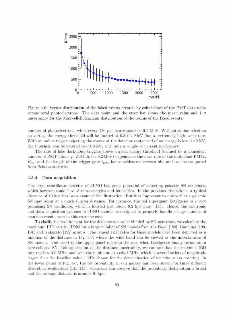
totalPE 0 500 1000 1500 2000 2500

R/m

m

0

500

1000

1500

2000

2500

Figure 4-6: Vertex distribution of the faked events created by coincidence of the PMT dark noiseversus total photoelectrons. The data point and the error bar shows the mean value and 1 σuncertainty for the Maxwell-Boltzmann distribution of the radius of the faked events.

number of photoelectrons, while every 120 p.e. corresponds ∼ 0.1 MeV. Without online selectionon vertex, the energy threshold will be limited at 0.3–0.4 MeV due to extremely high event rate.With an online trigger rejecting the events at the detector center and of an energy below 0.4 MeV,the threshold can be lowered to 0.1 MeV, with only a couple of percent inefficiency.

The rate of fake dark-noise triggers above a given energy threshold (defined by a coincidentnumber of PMT hits, e.g. 240 hits for 0.2MeV) depends on the dark rate of the individual PMTs,Rdn, and the length of the trigger gate tgate for coincidences between hits and can be computedfrom Poisson statistics.

4.3.4 Data acquisition

The large scintillator detector of JUNO has great potential of detecting galactic SN neutrinos,which however could have diverse energies and intensities. In the previous discussions, a typicaldistance of 10 kpc has been assumed for illustration. But it is important to notice that a galacticSN may occur at a much shorter distance. For instance, the red supergiant Betelgeuse is a verypromising SN candidate, which is located just about 0.2 kpc away [144]. Hence, the electronicand data acquisition systems of JUNO should be designed to properly handle a huge number ofneutrino events even in this extreme case.

To clarify the requirement for the detector not to be blinded by SN neutrinos, we calculate themaximum IBD rate in JUNO for a large number of SN models from the Basel [189], Garching [190,191] and Nakazato [192] groups. The largest IBD rates for those models have been depicted as afunction of the distance in Fig. 4-7, where the wide band can be viewed as the uncertainties ofSN models. The insert in the upper panel refers to the case when Betelgeuse finally turns into acore-collapse SN. Taking account of the distance uncertainty, we can see that the maximal IBDrate reaches 100 MHz, and even the minimum exceeds 1 MHz, which is several orders of magnitudelarger than the baseline value 1 kHz chosen for the determination of neutrino mass ordering. Inthe lower panel of Fig. 4-7, the SN probability in our galaxy has been shown for three differenttheoretical evaluations [141–143], where one can observe that the probability distribution is broadand the average distance is around 10 kpc.

80

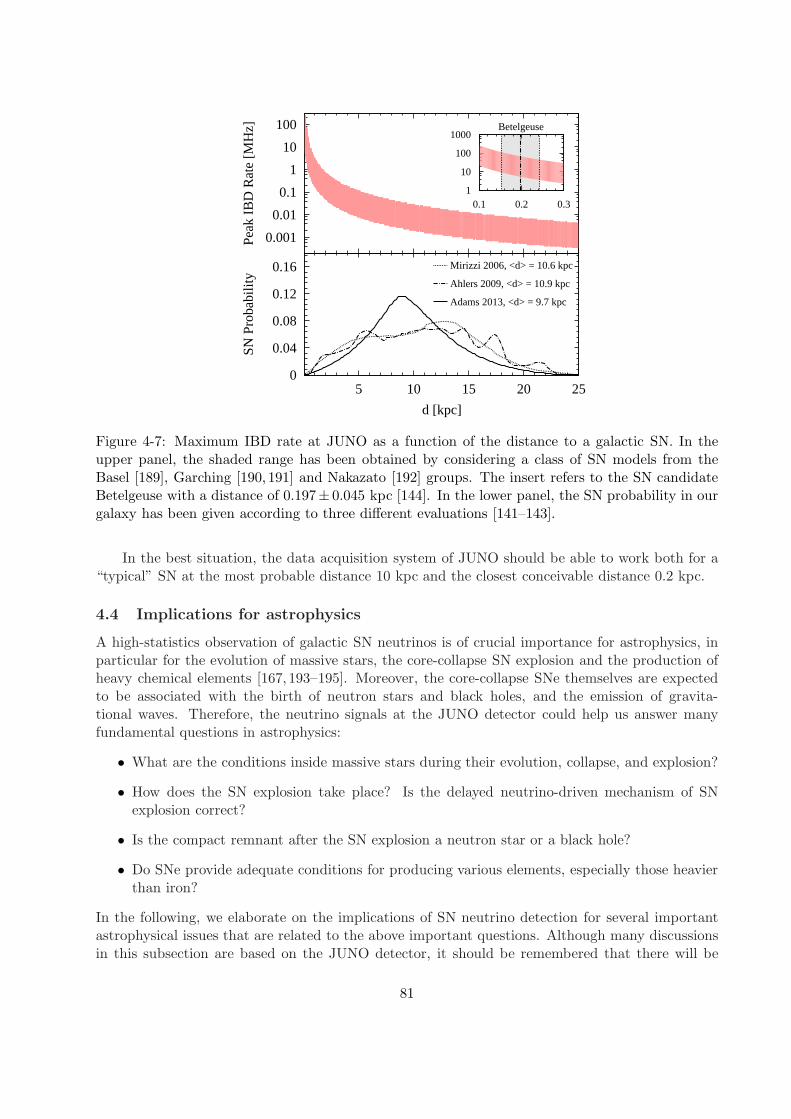
0.001

0.01

0.1

1

10

100

Pea

k IB

D R

ate

[MH

z]

1

10

100

1000

0.1 0.2 0.3

Betelgeuse

0

0.04

0.08

0.12

0.16

5 10 15 20 25

SN

Pro

babi

lity

d [kpc]

Adams 2013, <d> = 9.7 kpc

Mirizzi 2006, <d> = 10.6 kpc

Ahlers 2009, <d> = 10.9 kpc

Figure 4-7: Maximum IBD rate at JUNO as a function of the distance to a galactic SN. In theupper panel, the shaded range has been obtained by considering a class of SN models from theBasel [189], Garching [190, 191] and Nakazato [192] groups. The insert refers to the SN candidateBetelgeuse with a distance of 0.197± 0.045 kpc [144]. In the lower panel, the SN probability in ourgalaxy has been given according to three different evaluations [141–143].

In the best situation, the data acquisition system of JUNO should be able to work both for a“typical” SN at the most probable distance 10 kpc and the closest conceivable distance 0.2 kpc.

4.4 Implications for astrophysics

A high-statistics observation of galactic SN neutrinos is of crucial importance for astrophysics, inparticular for the evolution of massive stars, the core-collapse SN explosion and the production ofheavy chemical elements [167, 193–195]. Moreover, the core-collapse SNe themselves are expectedto be associated with the birth of neutron stars and black holes, and the emission of gravita-tional waves. Therefore, the neutrino signals at the JUNO detector could help us answer manyfundamental questions in astrophysics:

• What are the conditions inside massive stars during their evolution, collapse, and explosion?

• How does the SN explosion take place? Is the delayed neutrino-driven mechanism of SNexplosion correct?

• Is the compact remnant after the SN explosion a neutron star or a black hole?

• Do SNe provide adequate conditions for producing various elements, especially those heavierthan iron?

In the following, we elaborate on the implications of SN neutrino detection for several importantastrophysical issues that are related to the above important questions. Although many discussionsin this subsection are based on the JUNO detector, it should be remembered that there will be

81

several SN neutrino detectors of scintillator, Cherenkov and liquid-argon [83] types in operation atthe same time. Altogether, they will offer us valuable and complementary information.

4.4.1 Pre-supernova neutrinos

Before a massive star collapses and forms a SN, it experiences various “stationary” burning phases.In the standard stellar evolution model, one can obtain the temperature and density for a givenradius at any time. However, it is difficult to test the stellar models solely by using optical ob-servations: photons come out of the core by diffusion, and any information about the core will belost. During the advanced burning stages, the flux of neutrinos becomes much larger than thatof photons. As neutrinos interact only weakly with stellar matter, they record faithfully the innerstructure of the stars. Therefore, the detection of pre-SN neutrinos is vital for the verification ofstellar models.

Inside a massive star neutrinos are produced via thermal processes, out of which the dominantone is e+ + e− → ν + ν [196]. At any given time, a massive star can be divided into manythin layers – each with approximately uniform temperature, density and chemical composition.One calculates neutrino production rate for each layer, and sum over all layers to derive the totalneutrino flux and spectrum. In Table 4-2, neutrino fluxes and average energies at relevant burningstages are listed. The neutrino spectrum at the silicon-burning stage, in contrast with the solarneutrinos (e.g., pp and 8B neutrinos), can be found in Ref. [197, 198]. Generally speaking, theneutrino production rate increases significantly with temperature, and so do the average energiesof neutrinos and antineutrinos. Therefore, the detection of pre-SN neutrinos becomes relativelyeasier for the nuclear burning at later stages.

Burning phase Average energy [MeV] Total energy [erg] Duration [days]

C 0.71 7.0 × 1049 105

Ne 0.99 1.4 × 1050 140O 1.13 1.2 × 1051 180Si 1.85 5.4 × 1050 2

Table 4-2: Neutrino emission from a massive star of 20 M⊙ [197,198].

The IBD reaction is the dominant channel to probe pre-SN neutrinos from massive stars.Fig. 4-8 shows the expected event rates in JUNO for the nearest possible SN progenitor, i.e., thered supergiant Betelgeuse, whose mass is taken to be 20 M⊙ and distance is 0.2 kpc. The salientfeature in the neutrino “light curve” – a quick rise starting at a few hours prior to core collapse –makes the JUNO detector an ultimate pre-warning system of SN explosion. As shown in Fig. 4-8,the rate drops rapidly down to 60 events per day around 0.6 day before SN explosion. The reasonis that the silicon has been burnt out in the center and the core temperature decreases, leading to areduced neutrino production. This dip in the neutrino “light curve” could serve as a discriminatorfor different progenitor star masses. The signal rate is time dependent, and there are about 400events in the whole detector in the last day before core collapse.

Within the same energy window as for reactor neutrinos, any backgrounds of reactor neutrinoexperiments also act as backgrounds for detecting thermal neutrinos from massive stars. Thosestandard backgrounds include 9Li-8He events, fast-n events, accidental coincidences, (α, n) events,geo-neutrinos, and so on. Among all possible νe sources, the reactor neutrino itself could be the mainbackground for pre-SN neutrino detection. The event rates from reactor neutrinos and geoneutrinosare 0.25 and 0.05 per kiloton per day, respectively. Here the expected event rate is estimated inthe energy region 1.8 MeV < E < 3.3 MeV and a 100% detection efficiency is assumed.

82

0

100

200

300

400

500

600

-1.4 -1.2 -1 -0.8 -0.6 -0.4 -0.2 0

Eve

nts

per

Day

Time before Collapse [Days]

Figure 4-8: The neutrino event rate in JUNO for a massive star of 20 M⊙ at the silicon-burningstage, where the distance is assumed to be 0.2 kpc, the same as that of the nearest possible SNprogenitor Betelgeuse.

However, it is worthwhile to point out that the detection of pre-SN neutrinos is only possiblefor a very close progenitor star. For a SN at 10 kpc, the event rate will be reduced by about fourorders of magnitude, rendering the detection of pre-SN neutrinos in JUNO or the detector of similarsize extremely difficult.

4.4.2 Locating the supernova

As mentioned before, the SN neutrinos arrive at the Earth several hours earlier than the opticalsignals, providing an early-time alert to the astronomical community. Moreover, if the opticaldisplay is hidden behind the dense gas and dust clouds of a star-forming region, the neutrino burstwill be a unique tool to locate the SN [199,200].

In general, there are two distinct methods to determine the location. First, the angular cor-relation between the final-state particle and the incident neutrino can be directly fixed in largeCherenkov detectors, such as Super-Kamiokande and its possible upgrade Hyper-Kamiokande. Sec-ond, two detectors separated at a long distance can locate the SN by neutrino triangulation.

According to the kinematics, the outgoing neutrons in the IBD reaction have a forward angulardistribution. For a JUNO-like scintillator detector, it is possible to separately reconstruct thepositions of positron and neutron. Therefore, the direction along the line connecting these twopoints is, at least statistically, related to the neutrino direction [177]. This method has beenused by the CHOOZ experiment to determine the incoming direction of reactor antineutrinos inRef. [178]. It has been found that the direction of the neutrino source can be fixed within a coneof half-aperture angle 18 at the 68% confidence level, based on 2700 collected νe events. For agalactic SN, if the total number of IBD events is about 5000, it is possible to measure the skycoordinates of the SN with an uncertainty of about 9. It is expected that the JUNO detector willdo better in this aspect. In the scintillator detector, it is also possible to observe the Cherenkovlight from electrons, which are boosted to a high velocity in the elastic neutrino-electron scattering,

83

so the direction of recoiled electron can help locate the SN.On the other hand, in neutrino triangulation, the key point is to estimate the neutrino arrival

time and figure out the time delay ∆t between two detectors at the distance d. In this case,the angle θ between the SN direction and the line connecting these two detectors is given bycos θ = ∆t/d, and the uncertainty is dominated by the error in the measurement of ∆t. Takinga detector similar to JUNO with 5000 events and a distance of 30 ms, we obtain an uncertaintyof about δ(cos θ) ∼ 0.21, following the strategy in Ref. [199]. Evidently, the precision for neutrinotriangulation is not comparable to the statistical method.

4.4.3 Coincidence with gravitational waves

Besides neutrinos, the gravitational waves are good messengers to probe the interior of a SN. Agravitational-wave signal provides useful information on non-radial deformation and non-sphericalhydrodynamic motions, whereas a high-statistics neutrino signal allows us to follow directly thedifferent stages of core collapse without additional assumptions. As predicted by all theoreticalSN models, the prompt νe burst is a robust and uniform landmark structure. Since the energythreshold of JUNO can be as low as 0.2 MeV, it offers a unique possibility of identifying thisfeature via elastic electron and proton scattering. One could use the prompt νe burst in JUNO forcoincidence measurements with the gravitational wave burst that may arise at core bounce. Usingthe prompt νe burst could provide an even sharper coincidence than can be achieved with the onsetof the νe signal in Super-Kamiokande and IceCube.

After core collapse, the luminosities of νe and νe in the accretion phase depends on the massinfall rate and thus on the progenitor-dependent structure of the stellar core, with more massivecores producing higher luminosities. During this phase, the luminosity variations are accompaniedby sizable gravitational-wave emission at several hundred Hz, the observation of neutrino andgravitational-wave signals would confirm the presence of violent hydrodynamic instabilities stirringthe accretion flow around the assembling neutron star [201]. Such activity and a several hundredmillisecond delay of the onset of the explosion are expected within the framework of the delayedneutrino-driven mechanism. A pronounced drop of the νe and νe luminosities, followed by a closesimilarity to those of heavy-lepton neutrinos, would finally signal the end of the accretion phaseand the launch of the outgoing SN blast wave. The cooling signature of a nascent neutron star ischaracterized by a monotonic and gradual decline of the neutrino emission. It would be prolongedif additional energy was released by phase transitions in the nuclear matter. Exotic scenarios mightpredict a secondary νe burst, such as a QCD phase transition, or an abrupt end of neutrino emissionif the collapse to a black hole occurred.

4.4.4 SN nucleosynthesis

Another advantage of the JUNO detector is its superior energy resolution, which could help to dis-entangle source-imposed spectral features from those caused by neutrino-flavor conversions. More-over, detecting significant numbers not only of νe but also of νe and heavy-lepton neutrinos wouldyield at least time-averaged spectral information for different emission channels. Conceivably onecould extract information on the neutron-to-proton ratio in the neutrino-processed SN outflows,presently also a sensitive result of numerical modeling of a multitude of complex processes. Therelative abundance of neutrons and protons determines the conditions for nucleosynthesis and areset by competing νe and νe captures, which in turn depend delicately on the relative fluxes andspectral distributions of these neutrinos [195]. A JUNO measurement of a SN burst may offer theonly direct empirical test of the possibility for r-processing in the SN core, except for an extremely

84

challenging in-situ measurement of r-process nuclei in fresh SN ejecta [202].In addition to the r-process for the production of heavy chemical elements, the neutrinos

emitted from the core collapse and the subsequent cooling of the proto-neutron star will interactwith outer layers of the SN, producing some rare nuclei such as 11B and 7Li. This neutrino processis crucially important for the 11B and 7Li production [203–205]. In particular, the SN neutrinosof heavy-lepton flavors, which may have higher average energies, will dominate the generationof galactic light chemical elements. Therefore, the measurement of νx energy spectra at JUNOis necessary to directly pin down whether the neutrino process is really the true mechanism forproducing the present galactic inventory of light nuclei.

One should notice that the flavor oscillations of SN neutrinos, which could lead to modificationof neutrino energy spectra and fluxes, will affect both r- and neutrino processes [206].

4.5 Implications for particle physics

Neutrino signals of a core-collapse SN have also profound implications for elementary particlephysics. If the standard scenario of delayed neutrino-driven explosion is confirmed by future ob-servations of SN neutrinos and the cooling phase of neutrino emission is firmly established, theenergy-loss argument will result in robust and restrictive constraints on a large number of particlephysics models where new weakly-interacting particles are introduced, such as axions, majorons,and sterile neutrinos [207]. Numerous results derived from the sparse SN 1987A data can be refined.

If neutrinos are Majorana particles, spin-flavor conversions caused by the combined action ofmagnetic fields and matter effects can transform some of the prompt νe burst to νe, leading to ahuge inverse-beta signal. Such an observation would provide smoking-gun evidence for neutrinotransition magnetic moments. Non-radiative decays would also produce a νe → νe conversion duringthe prompt burst. On the other hand, null results of observing those conversions will set restrictivebounds on the neutrino transition magnetic moments [208]. In addition, the existence of eV-masssterile neutrinos may have great impact on the supernova explosion and nucleosynthesis [209,210]

The core-collapse SNe serve as laboratories to probe intrinsic properties of neutrinos themselves.The SN neutrino observations will shed light on important fundamental problems in particle physics:

• What is the absolute scale of neutrino masses?

• What is the neutrino mass ordering?

• Are there collective neutrino oscillations?

• Are there exotic neutrino interactions?

In the following, we elaborate on a few important topics that are associated with these fundamentalquestions, and study the role that JUNO will play in this connection.

4.5.1 Bound on neutrino masses

Since neutrinos are massive, their flight time from a SN core to the detector at the Earth will bedelayed, compared to massless particles [211]. For SN neutrinos, the time delay can be written as

∆t(mν , Eν) = 5.14 ms(mν

eV

)2(10 MeV

Eν

)2 D

10 kpc, (4.7)

where Eν is the neutrino energy, and D is the distance between SN and detector. Thus a time-delayat the millisecond level is expected for neutrinos from a typical galactic SN. However, the average

85

energy and luminosity of neutrinos evolve in time, which complicates the extraction of neutrinomass information. In order to derive a mass bound, one has to know the time evolution of neutrinoenergies and fluxes, and take into account neutrino flavor conversions.

The sharply rising and falling luminosity of prompt νe burst can be implemented to probe thetime-delay effects of massive neutrinos, since the time structure is very unique and the characteristictimescale is around tens of milliseconds. However, the total number of neutrino-electron scatteringevents in JUNO is limited and it is impossible to reconstruct neutrino energy, which may reducethe sensitivity to neutrino masses. An abrupt termination of neutrino signals after the black-holeformation should be a perfect scenario to probe absolute neutrino masses [212].

As the IBD is the dominant channel for SN neutrino detection, we concentrate on the νe fluxΦ0νe

in the accretion and cooling phases. In Ref. [213], a simple parametrization of Φ0νe

has beenproposed to capture essential physics of neutrino production and the main features of numericalsimulations. In the cooling phase, the νe flux Φ0

c is parametrized by three model parameters:the initial temperature Tc, the radius of neutrino sphere Rc, and the cooling time scale τc. Moreexplicitly, we have

Φ0c(t, Eν) =

1

4πD2

1

8π2

4πR2

c

E2ν

1 + exp [Eν/Tc(t)]

, (4.8)

where the temperature evolves as Tc(t) = Tc exp[−t/(4τc)]. In the accretion phase, one has tomodel the time evolution of neutron number and positron temperature in order to figure out the νeflux Φ0

a. This can be done by introducing the accretion time scale τa, and requiring the resultantneutrino energy and luminosity to follow numerical simulations. In addition, the initial number ofneutrons depends on an initial accreting massMa, and a thermal energy spectrum of positrons withan initial temperature Ta is reasonable. The flux of νe is determined by the interaction betweenneutrons and positrons, so it can be written as

Φ0a(t, Eν) =

1

4πD2

1

π2

Nn(t)σne+(Eν)

E2e+

1 + exp[Ee+/Ta(t)

], (4.9)

where the average positron energy is evaluated as Ee+ = (Eν − 1.293 MeV)/(1−Eν/mn). For theneutrino energies of our interest (i.e., from 5 to 40 MeV), the cross section is approximately given byσne+(Eν) ≈ 4.8× 10−44 cm2/[1 + Eν/(260 MeV)]. The time evolution of neutron number Nn(t) =0.6Majk(t)T

6a /[1+ t/(0.5 s)]T 6

a (t) and the temperature function Ta(t) = Ta+(0.6 Tc−Ta)(t/τa)2

are properly chosen to ensure a continuous neutrino average energy and to capture the numericalfeatures [213]. Putting all together, the total flux is [213,214]

Φ0νe(t, Eν) = fr(t)Φ

0a(t, Eν) + [1− jk(t)] Φ

0c(t, Eν) , (4.10)

where fr(t) = 1−exp(−t/τr) with the rising time scale τr further introduces fine early time structure,and jk(t) = exp[−(t/τa)

k] with a default value of k = 2 is the time function interpolating theaccretion and cooling phases of neutrino emission.

However, neutrino flavor conversions take place when they propagate from the SN core to thedetector. In particular, the Mikheyev-Smirnov-Wolfenstein (MSW) matter effects in the SN mantlewill significantly change neutrino flavor content. Given a relatively large θ13, the electron antineu-trino flux at the detector is Φνe = cos2 θ12Φ

0νe + sin2 θ12Φ

0νx for normal neutrino mass ordering,

while Φνe = Φ0νx for inverted neutrino mass ordering.

It is now straightforward to figure out the neutrino event rate R(t, E) as a function of emissiontime and neutrino energy, which are related to the detection time and positron energy, given a

86

0.7

0.8

0.9

1.0

1.1

1.2

5 10 20 50

mν

limit

[eV

]

D [kpc]

Parameterized Model

Numerical Models

Figure 4-9: The upper bounds on the absolute scale of neutrino masses at the 95% CL for a SN ata distance of D = 5 kpc, 10 kpc, 20 kpc and 50 kpc in the parameterized model from Ref. [213],and a series of numerical models from Ref. [192], in which simulations have been performed for aprogenitor-star massM = 13, 20, 30 or 50 solar masses, a metallicity Z = 0.02 or 0.004, and a shockrevival time trevive = 100 ms or 300 ms. In our calculations, we have chosen fourteen numericalmodels, since a black hole is formed 842 ms after bounce in two models with M = 30 solar massesand Z = 0.02. See Ref. [192] for more details about the numerical models, and the SN neutrinodata are publicly available at the website http://asphwww.ph.noda.tus.ac.jp/snn/. This figure istaken from Ref. [216]

definite neutrino mass. The strategy is to generate neutrino events, denoted by a detection timeti and a positron energy Ei, according to the event rate R(t, E). The simulated data are fitted bythe event rate with neutrino mass scale mν as an additional parameter. The maximum likelihoodapproach is implemented, and the likelihood function has been constructed by taking account ofevery single event [215]. Assuming a nearly-degenerate neutrino mass spectrum and the normalmass ordering, we obtain a neutrino mass upper bound mν < (0.83 ± 0.24) eV at 95% confidencelevel, where 1σ Gaussian error has been attached to the best-fit value [216]. In order to illustratethe impact of the SN distance on the mass limit, we have calculated the mass bound for differentdistances D = 5 kpc, 10 kpc, 20 kpc and 50 kpc, where the last one corresponds to the case of SN1987A. It is generally expected that a closer SN offers a larger number of neutrino events, implyinga better upper limit on neutrino masses. Furthermore, to take account of SN model uncertainties,we show in Fig. 4-9 the results for the previous parametrized model of SN neutrino fluxes and adozen of numerical SN models. In the latter case, the upper bound could be worsened by 0.15 eVor so, which should be regarded as a kind of systematic uncertainty.

4.5.2 Impact of mass ordering

Flavor conversions of SN neutrinos are very interesting. Neutrinos propagating through the SNmantle and envelope encounter a large range of matter densities, allowing for MSW conversionsdriven first by the neutrino mass-squared difference ∆m2

31 and the mixing angle θ13, and then by

87

E (MeV)0 10 20 30 40 50

Flu

x (a

.u.)

0.0

0.2

0.4

0.6

0.8

1.0

xν

eν

E (MeV)0 10 20 30 40 50

xν

eν

Final fluxes in inverted hierarchy (multi-angle)

Figure 4-10: Numerical illustration for the splits in neutrino energy spectra after collective oscil-lations in the case of inverted mass hierarchy [218]. The initial spectra are indicated by dottedcurves in the same color as the final ones, where one can observe a complete swap of the antineutrinospectra and a sharp split in the neutrino spectra.

∆m221 and θ12. A SN neutrino signal is sensitive to the unknown neutrino mixing parameter: the

ordering of neutrino masses that could be in the normal (NH) or inverted hierarchy (IH). In theformer case, the νe flux outside the SN envelope will be a superposition of both initial νe and νxfluxes, and the ratio between these two components is determined by the mixing angle θ12. In thelatter case, the final νe flux at the Earth will be entirely the initial νx flux. Note in both cases, thefinal fluxes needed to be scaled by the square of SN distance.

Although the difference caused by flavor conversions can be seen from the third row of Fig. 4-1,where the IBD event rate is calculated and the complete flavor conversion has been assumed, itremains to find a model-independent way to extract the information of mass ordering directly fromthe experimental observations. As another example, in the fourth row of Fig. 4-1, we can observethat the neutrino mass ordering significantly affects the event rate of neutrino-electron scattering.One possible way to determine the neutrino mass ordering may be to compare the event rates inthe IBD channel with that of elastic neutrino-proton scattering, since the latter is not changed byflavor conversions.

4.5.3 Collective neutrino oscillations

The picture of SN neutrino oscillations has recently been changed drastically by the insight thatthe neutrino-neutrino refractive effect is crucial. These self-induced collective flavor conversionsoccur within a few hundred km above the neutrino sphere; see Ref. [217] for a review of the recenttorrent of literature on this topic. The most important observational consequence is a swap of theνe and νe spectrum with that of νx and νx in certain energy intervals. The sharp spectral featuresat the edges of these swap intervals are known as “spectral splits”. Their development depends onthe neutrino mass hierarchy as well as on the ordering of the flavor fluxes at the source. Therefore,the split features can depend on time in interesting ways. For instance, in Ref. [218], it has beenshown in the case of inverted neutrino mass hierarchy that SN neutrinos in the accretion phasewill undergo collective oscillations, leading to a complete swap between νe and νx spectra and a

88

sharp split around 7 MeV in the neutrino spectra, as in Fig. 4-10. The average neutrino energies〈Eνe〉 = 10 MeV, 〈Eνe

〉 = 15 MeV and 〈Eνx〉 = 24 MeV, together with a total neutrino energyof 3 × 1053 erg equally distributed in six neutrino species, are assumed. In the case of normalhierarchy, no significant flavor conversions are observed [217,218].

The main problem to detect oscillation features is that one can not rely on detailed theoreticalpredictions of the flavor-dependent fluxes and spectra. Therefore, model-independent signatures arecrucial. One case in point is the energy-dependent modulation of the neutrino survival probabilitycaused by Earth matter effects that occur if SN neutrinos arrive at the detector “from below”. Theappearance of Earth effects depends on the flux and mixing scenario. Therefore, its detection couldgive hints about the primary SN neutrino fluxes, as well as on the neutrino mass hierarchy [219,220].

The excellent energy resolution of JUNO leads to a particular advantage for discovering smallenergy-dependent flux modulations caused by Earth effects, but of course depends on seeing theSN shadowed by the Earth. Additional signatures of flavor conversions can be imprinted by mattereffects of the shock fronts in the SN envelope. The number of events, average energy, or the widthof the spectrum may display dips or peaks for short time intervals. Such signatures yield valuableinformation about shock-wave propagation and the neutrino mass hierarchy [221]. However, realisticchances to detect shock features remain unclear. The flavor-dependent spectral differences in theantineutrino channel are probably small during the cooling phase. Moreover, strong turbulence inthe post-shock regions could affect these signatures [222].

4.5.4 Constraining new physics

It is well known that the stars can be ideal places to constrain new physics scenarios beyond thestandard model of elementary particles [207]. If the standard picture of SN explosion is verifiedby a high-statistics observation, the duration of neutrino signal in the long cooling phase willbe precisely measured. According to the standard energy-loss argument, any weakly-interactingexotic particles that can be copiously produced in the SN core will carry away a large amountof energies, significantly reducing the neutrino signal. To avoid excessive energy loss, the newparticles should be interacting with matter and neutrinos so strongly that they are captured in theSN core, or so weakly that the production of new particles is inefficient. Therefore, by requiring theagreement between observations and theoretical prediction, we can draw restrictive constraints onthe interaction strengths of new elementary particles. This approach has been applied to numerousnew physics scenarios, such as axions, sterile neutrinos, majorons, and hidden photons.

As the neutrino energy spectra and flavors can be determined in future observations of SNneutrinos, new possibilities other than the energy-loss argument will be opened to set bounds onnew physics.

4.6 Summary

A high-statistics detection of neutrinos from a galactic SN will provide us with precious informationabout the explosion mechanism and intrinsic properties of neutrinos themselves. For a galacticSN at a distance of 10 kpc, there are around 5000 events in the IBD channel, 2000 events forelastic neutrino-proton scattering, and 300 events for elastic neutrino-electron scattering in theJUNO detector. The time evolution, energy spectra and flavor contents of SN neutrinos can inprinciple be established and used to verify or disprove the neutrino-driven explosion mechanism.With experimental observations, many interesting questions in astronomy, astrophysics and particlephysics, such as the early warning of SNe, the SN location, SN nucleosynthesis, absolute neutrinomasses and neutrino mass ordering, can hopefully be revised or addressed.

89

5 Diffuse Supernova Neutrino Background (DSNB)

The integrated neutrino flux from all past core-collapse events in the visible universe forms thediffuse supernova neutrino background (DSNB), holding information on the cosmic star-formationrate, the average core-collapse neutrino spectrum, and the rate of failed SNe. The Super-Kamiokandewater Cherenkov detector has provided first limits and eventually may achieve a measurement atthe rate of a few events per year, depending on the implementation of its gadolinium upgrade.A JUNO-class detector has the potential to achieve a comparable measurement, benefitting fromthe excellent intrinsic capabilities of liquid scintillator detectors for antineutrino tagging and back-ground rejection. The most critical background is created by neutral-current interactions of atmo-spheric neutrinos. Depending on the performance of pulse-shape discrimination techniques, thisbackground may prove too high for a clear detection. However, a positive signal at the 3σ levelis conceivable for a 10-year measurement and typical DSNB parameters. A non-detection wouldstrongly improve current limits and exclude a significant range of DSNB parameter space.

5.1 Motivation and Opportunities

While core-collapse SNe are rare, and in a galaxy like our own Milky Way occur only once everyfew decades, the energy release is so large that the integrated neutrino flux from all past SNe, thediffuse SN neutrino background (DSNB), adds up to a large cosmic radiation density [139,223–228].It is comparable to the extra-galactic background light, the photons emitted from all stars, andcorresponds to around 10% of the energy density of the cosmic microwave background. Notethat the big-bang relic neutrinos are today non-relativistic, contributing a small hot dark mattercomponent, so the DSNB is actually the largest cosmic neutrino radiation background, unlessthe lightest mass eigenstate of the big-bang neutrinos remains relativistic after all. It has beenrecognized for a long time that for Eν & 10 MeV, above reactor neutrino energies, the DSNB isthe dominant local anti-neutrino flux. The primary detection channel is inverse-beta decay (IBD),νe + p → n + e+, where the solar νe flux does not contribute even though it reaches up to about15 MeV and dominates in this low-energy range.1 The DSNB flux component in νe is around20 cm−2 s−1, details depending on the cosmic SN rate as a function of redshift and the averagecore-collapse νe flux spectrum, including the effect of flavor conversion.

The DSNB can be detected if backgrounds, notably caused by atmospheric neutrinos, canbe controlled. In this regard, a scintillator detector has an inherent advantage over the water-Cherenkov technique because neutron tagging of IBD events is a generic feature. The most re-strictive current limits on the DSNB derive from Super-Kamiokande I–III without neutron tag-ging [230, 231], already excluding the most extreme models for the DSNB flux spectrum. With acompletely revised data-acquisition system, Super-Kamiokande IV now has limited sensitivity to the2.2MeV γ-ray caused by neutron capture on protons. A new DSNB limit based on this techniquehas recently become available [232], but is not yet competitive with the earlier Super-KamiokandeI–III results. Limits by the much smaller SNO [233] and KamLAND [234] detectors are alsonot competitive. In future, gadolinium as an efficient neutron absorber may be dissolved in Super-Kamiokande [235], a technique currently studied at the EGADS facility [236,237], probably allowingthem to detect the DSNB at a rate of perhaps a few events per year [238]. Super-Kamiokande hasaround 1.5× 1033 protons in its 22.5 kt of fiducial volume for DSNB detection, whereas JUNO has

Editors: Georg Raffelt (raffelt@mpp.mpg.de) and Michael Wurm (michael.wurm@uni-mainz.de)Major contributor: Randolph Mollenberg, Zhimin Wang

1In principle, νe → νe transitions in the Sun caused by spin-flavor transitions of Majorana neutrinos could producea solar background signal in this low-energy range [229].

90

around 1.2 × 1033 protons in the fiducial volume of 17 kt to be used for the DSNB analysis (seebelow). Therefore, JUNO will be comparable and complementary to the Super-Kamiokande effort,and it will be unique if the gadolinium upgrade would not be implemented after all.

Following Ref. [139], the expected DSNB flux depends on two main ingredients, the core-collapse rate as a function of cosmic redshift and the number and spectrum of neutrinos andanti-neutrinos per flavor emitted by an average core-collapse event, including flavor conversioneffects. These quantities bear significant uncertainties. The core-collapse SN rate rises from itslocal value by about an order of magnitude up to redshift z ∼ 1, then levels off and eventuallydecreases [226, 227, 239–242]. If the νe detection threshold is above some 10 MeV, the overalldetection rate is dominated by SNe with z . 1. However, the SN rate predicted from the observedstar-formation rate appears to be systematically a factor of 2 smaller than the directly observedSN rate [242]. Additional contributions likely arise from sub-luminous SNe and from failed SNe,i.e. those core-collapse events leading to a black hole rather than an actual explosion [243–251].Both outcomes lead to a neutrino flux comparable to that of a standard SN.

The total liberated energy in a core collapse depends on the final neutron-star mass and thenuclear equation of state, introducing a significant uncertainty even if we ignore the unknowncontribution by failed SNe. The predicted flux spectra of the different flavors depend on detailsof the neutrino interaction rates and the numerical implementation of neutrino transport. Flavorconversion during neutrino propagation in the SN environment partly swaps the spectra so thatthe detectable νe flux is some combination of the original νe, νµ and ντ fluxes emitted by the SNcore. One expects large variability for most of these effects between different core-collapse eventsbecause of the large range of progenitor masses and other properties.

In principle, the DSNB is a treasure trove of valuable information on the astrophysics of corecollapse, failed SNe and black-hole formation, and flavor-dependent neutrino propagation and flavorconversion. However, a detailed spectral DSNB measurement is clearly out of reach with near-termdetectors of the JUNO and Super-Kamiokande class. Neutrino astronomy is a field in its infancywhere only solar neutrinos have been observed with robust statistical detail. At this stage, the verydetection of the DSNB is the first milestone and will be a fundamental discovery in its own right.

5.2 Parametric DSNB flux spectrum

In this situation, a detailed parameter study of the various DSNB ingredients is not warranted for aJUNO sensitivity forecast. Rather, we follow the practice adopted in the LENA physics study [162]and adopt a simple parametric representation of the DSNB. Its isotropic flux spectrum is given bythe line-of-sight integral over cosmic redshift z

dFνe

dEνe

=c

H0

∫ zmax

0dz

RSN(z)√Ωm (1 + z)3 +ΩΛ

dNνe(E′νe)

dE′νe

. (5.1)

The maximum redshift of star-formation zmax is taken to be 5, but the exact value is irrelevantbecause z . 1 dominates for the detectable part of the spectrum. H0 = 70 km s−1 Mpc−1 is thepresent-day Hubble parameter and c the speed of light. RSN(z) is the redshift-dependent co-movingSN rate, i.e., the number of SNe per year and per cubic-Mpc. The cosmological model is taken tobe flat with a matter-density parameter Ωm = 0.30 and cosmological-constant density parameterΩΛ = 0.70. The cosmological parameters are rather well established, but our results do not directlydepend upon them because they also enter the determination of RSN(z). Finally, dNνe(Eνe)/dEνe

is the total number spectrum of νe from an average core collapse, with flavor-conversion effectsalready included. Note that E′

νe = (1 + z)Eνe is the neutrino energy in the rest frame of a SN atredshift z.

91

For the cosmic SN rate as a function of redshift we specifically adopt the functional formproposed by Porciani and Madau [239] in the form of equations (4) and (5) of reference [226]with the choice f∗ = 1.5. The SN rate in the local universe is thus taken to be RSN(0) =1.25×10−4 yr−1 Mpc−3 in agreement with reference [238]. A different parametrization provided inreference [241] leads to similar DSNB results because the main contribution arises from z . 1 so thatdifferences of RSN(z) at larger redshifts have little impact on the overall result. For each individualcore collapse we assume that, after flavor conversion effects have been included, a total energyEtot = 0.5× 1053 erg is emitted in νe with average energy 〈Eνe〉. While the instantaneous emissionspectra tend to be “pinched”, i.e., less broad than a thermal distribution, the time-averaged spectramay be close to thermal. So we assume a Maxwell-Boltzmann distribution, normalized to tEtot, ofthe form [175,252]

dNνe

dEνe

=0.5× 1053 erg

〈Eνe〉27

2

E2νe

〈Eνe〉3e−3Eνe/〈Eνe 〉 . (5.2)

Overall, this corresponds effectively to a two-parameter representation of the DSNB flux spectrum:one parameter is 〈Eνe〉, the other a global flux normalization Φ which depends on the product ofthe SN rate at z = 0 and the average energy per SN emerging in the form of νe. As a reference forthe flux normalization, we define a default value Φ0 = Etot · RSN(0) that corresponds to the mostlikely SN rate and total energy as described above.

In the following, we will explicitly consider 〈Eνe〉 = 12, 15, 18 and 21 MeV, where the upper endis certainly beyond what is nowadays expected for core-collapse SNe, but is meant to represent anextreme case. Figure 5-1 displays the corresponding DSNB antineutrino energy spectra for JUNO.Depending on 〈Eνe〉, the position of the spectral peak varies around 10MeV. The correspondingevent rate is 0.2–0.5 per (kt·yr) .

prompt event visible energy [MeV]0 5 10 15 20 25 30 35 40 45 50

]-1

yrs

[MeV

.kt

num

ber

of e

vent

s in

170

0

0.05

0.1

0.15 MeV >=12ν<EMeV >=15ν<EMeV >=18ν<EMeV >=21ν<E

Figure 5-1: Visible energy spectra of prompt DSNB events for 〈Eνe〉 = 12, 15, 18 and 21 MeVfor a fiducial volume of 17 kt (cf. section 5.3). Observation below 11MeV is obstructed by theoverwhelming background from reactor antineutrinos and cosmogenic background.

92

5.3 Signal and background sources in JUNO

The following section lines out the expected signal and background sources for the DSNB search inJUNO and proposes a viable analysis strategy based on event selection cuts and event identificationto enable a positive detection of the DSNB in spite of the significant backgrounds. The projectedsensitivity is laid out in section 5.4.

DSNB antineutrino signal. While the DSNB consists of approximately equal fluxes of neutrinosand antineutrinos of all flavors, the primary signal in liquid-scintillator detectors is the IBD reactionνe+p→ e++n. The energy of the interacting antineutrino can be inferred by the signal of promptpositron that is shifted by ∼ 0.8MeV to lower energies. The expected event rates and prompt eventspectra have been derived by the convolution of the DSNB spectrum described in section 5.2 andthe parametrized cross-section proposed in [176]. From this, the expected signal can be derived asa function of the mean energy of the SN spectrum 〈Eνe〉, the flux normalization Φ, the numberof protons contained in the fiducial mass mfid and the detection efficiency εν . For mfid = 17kt,Φ = Φ0 and 〈Eνe〉 ∈ [12; 21] MeV, we expect an event rate of 1.5 to 2.9 events per year. The DSNBsignal spectra of figure 5-1 have been obtained by a toy MC assuming a 3% energy resolution at1MeV.

The DSNB provides a clear coincidence signature of prompt positron and delayed neutroncapture on hydrogen (Eγ = 2.2MeV, τnp ∼ 220µs) which allows for an efficient suppression ofsingle-event background. However, there are several sources of correlated background events thatmust be taken into account when defining the energy window, fiducial volume and pulse shapeselection criteria for DSNB detection (see below). The corresponding visible energy spectra aremostly derived from a modified version of the LENA detector simulation [253] but provide a goodapproximation of the expected signal in JUNO. On the other hand, the background created by fastneutrons is much more dependent on the detector geometry and has therefore been taken from adedicated simulation of the JUNO setup [254].

Reactor antineutrino background. νe’s from neutron-rich fission products provide a large IBDsignal in the energy region below 10MeV that effectively impedes a detection of the DSNB in thisenergy range. Due to the relative proximity to the nuclear power stations at Taishan and Yanjiang,the νe background flux will be large compared to other proposed sites [255].The expected rate is∼ 800 events per (kt·yr). In particular, this will lead to a substantial number of events in the high-energy tail of the reactor νe spectrum that potentially extends to energies as high as 13MeV [255].To avoid this irreducible background, the energy threshold for DSNB detection has been set to avisible energy of 11MeV, indicated by the shaded region in figure 5-1.

Cosmogenic isotopes. The decay events of the βn-emitters 9Li and 8He that are induced bycosmic muons pose with ∼ 70 d−1 a large background for low-energy νe detection. However, thespectral endpoints of both radioisotopes effectively lie below the lower analysis of 11MeV defineddue to the reactor antineutrino signal. Therefore, this background can be safely neglected in thefurther discussion.

Atmospheric neutrino CC interactions. The events created by the IBDs of atmosphericνe’s on the target protons constitute a further source of indiscriminable background and start todominate the DSNB signal for energies of 30MeV and higher. Compared to other sites, Jiangmenis at a low geographical latitude (22.6N), which leads to a relatively low atmospheric ν flux.The corresponding background spectrum of IBD events (scaled from reference [255]) is shown infigure 5-1.

93

Unlike in water Cherenkov detectors, the background rate originating from the CC interactionsof the large flux of atmospheric νµ’s and νµ’s is far less problematic in liquid scintillator. In thisevents, the presence of final state muons can be very efficiently tagged based on both the coincidencetag provided by the Michel electrons and the characteristic pulse shape of muon events. Thisbackground is therefore considered to be negligible in this analysis. However, a determination of apotential residual rate will be addressed in future, more elaborate studies.

Atmospheric neutrino NC interactions. The search for antineutrinos at energies above 8MeVthat has been performed by KamLAND has demonstrated that neutral current reactions of high-energy atmospheric neutrinos in liquid scintillator can result in an IBD-like signature, either byneutron knock-out or by more complicated processes [234]. The corresponding event rate is morethan an one order of magnitude above the DSNB signal in the region of interest. In many cases, a11C-nucleus will remain in the end state of such reactions. Its delayed decay has the potential toreject about 50% of this background. Moreover, a significant reduction can be achieved if pulse-shape discrimination (PSD) techniques are applied to the prompt signal [253]. In the following, weassume that the PSD efficiencies derived for the LENA setup in reference [253] can be transferredwithout loss to JUNO. This approach is supported by the use of identical scintillators and neglectsthe positive impact of the considerably higher light yield in JUNO. In this way, the residual back-ground rate within the observational window can be reduced to 0.6 yr−1 in the fiducial volume,corresponding to εNC = 1.1% of the original rate. In spite of this rather stringent cut, the signalefficiency is still at εν = 50% [253].

Fast neutron (FN) background. Due to the relatively low depth of the JUNO detector cavern(∼ 700m of rock shielding), neutrons created by cosmic muons passing through the rock close-by the detector are relatively frequent and constitute a relevant source of background. Whilespallation neutrons can be easily discarded if the parent muon crosses the outer veto or the waterpool, neutrons from further-out muons have a non-zero probability to pass undetected through theCherenkov veto region and to mimic the IBD signature by a prompt proton recoil and a delayedcapture of the thermalized neutron. Based on a muon flux of ∼ 20 m−2 h−1 and a mean muonenergy of 〈Eµ〉 = 215GeV, the expected FN background rate inside the JUNO target volume is ofthe order of 20 events per year.

Two factors allow a considerable reduction of this background: Because of the finite meanfree path of the neutrons most of the events are concentrated towards the verge of the scintillatorvolume, clustering at the equator and the north pole of the spherical vessel. A soft fiducial volumecut rejecting all events at radii greater than 16.8m reduces the residual background rate to ∼ 1 yr−1

in the remaining target mass of 17 kt. Moreover, the PSD analysis (see above) is sensitive to theprompt proton recoils, decreasing the residual rate to εFN = 1.3% of the initial value, correspondingto a negligible FN rate of ∼ 0.01 yr−1.

Reactor and atmospheric neutrino IBD signals define an observational window reaching from 11to ∼30MeV. Corresponding numbers for signal and background events with and without PSDhave been compiled in table 5-1 for a 10-year measuring period. The beneficial impact of PSD isillustrated in figure 5-2: In the left panel before PSD, atmospheric NC and fast neutron backgroundsdominate the DSNB signal, while they are greatly reduced in the right panel that reflects thesituation after application of the PSD. The signal-to-background ratio is expected to exceed 1:1,creating very favorable conditions for a positive detection of the DSNB.

94

prompt event energy [MeV]10 15 20 25 30 35

]-1

yrs

[MeV

.nu

mbe

r of

eve

nts

in 1

70 k

t

-110

1

10

>=15MeVνDSNB: <E

sum of backgrounds

eνreactor

eνCC atmospheric

νNC atmospheric

fast neutrons

prompt event energy [MeV]10 15 20 25 30 35

]-1

yrs

[MeV

.nu

mbe

r of

eve

nts

in 1

70 k

t

-110

1

10

>=15MeVνDSNB: <E

sum of backgrounds

eνreactor

eνCC atmospheric

νNC atmospheric

fast neutrons

Figure 5-2: Prompt DSNB signal (〈Eνe〉 = 15MeV, Φ = Φ0) and background spectra before (left)and after (right) the application of pulse-shape discrimination. The DSNB signal dominates allbackgrounds for a large fraction of the observation window from 11 to 30 MeV.

Item Rate (no PSD) PSD efficiency Rate (PSD)

Signal 〈Eνe〉 = 12MeV 13 εν = 50% 7〈Eνe〉 = 15MeV 23 12〈Eνe〉 = 18MeV 33 16〈Eνe〉 = 21MeV 39 19

Background reactor νe 0.3 εν = 50% 0.13atm. CC 1.3 εν = 50% 0.7atm. NC 6 · 102 εNC = 1.1% 6.2fast neutrons 11 εFN = 1.3% 0.14Σ 7.1

Table 5-1: Signal and background event rates before and after PSD in 10 years of JUNO datataking. An energy window 11MeV < Eν < 30MeV and a fiducial volume cut corresponding to17 kt have been chosen for background suppression.

5.4 Expected sensitivity

We have investigated two possible approaches for determining the potential of a positive DSNBdetection by JUNO: Optimal sensitivity can be achieved in case the spectral shapes and rates of allbackgrounds are well known, allowing for an energy-dependent fit of signal and background spectrato the data. Alternatively, we investigate a more conservative ansatz where detection significanceis evaluated based on a rate-only analysis inside the observation window. Finally, the dependenceof the sensitivity on the systematic uncertainty associated with the background normalizations isstudied.

Spectral fit. The sensitivity of the DSNB search will depend on the knowledge on spectral

95

shape and normalization of the various background sources. Reactor and atmospheric antineutrinoIBD spectra and fluxes can be extrapolated from the regions outside the observation window andwill play only a minor role for most of the region of interest. For the more important FN andatmospheric NC backgrounds, rates and spectra can probably be determined with good accuracyif the energy-dependent PSD efficiencies are well understood.

Figure 5-3 depicts the significance of a positive DSNB measurement as a function of DSNBparametrization. Both the flux normalization Φ and the mean spectral energy have been variedaround the most probable values Φ0 and 〈Eνe〉 = 15MeV (cf. section 5.2). Assuming 170 kt·yrs ofexposure, event spectra based on the predictions for signal and all background sources have beengenerated for the energy range of 10-40MeV. Based on these data samples, likelihood fits havebeen performed to the spectra above a prompt-event visible energy of 11MeV, with and withoutincluding a contribution from the DSNB2. The likelihood function employed is

L(〈Eνe〉,Φ, fj) =∑

i

−2 log

[P(ni,Φsi +

∑

j

fjbj,i

)]+∑

j

(fj − 1)2

σ2j, (5.3)

where P is the Poissonian probability to obtain ni events in the ith bin based on the prediction forsignal si and backgrounds bj,i, Φ and fj are the spectral normalizations of signal and backgrounds,respectively. The σj are the systematic uncertainties on the background normalization. The profileof figure 5-3 assumes σj = 5%, while table 5-2 also lists the expected sensitivities for σj = 20%.For the favored DSNB parameters, a 3σ evidence for the DSNB signal seems well within reach(cf. table 5-2).

Rate-only analysis. Assuming no accurate knowledge on spectral shapes of signal and back-ground, the detection potential can be calculated based merely on the detected event rate (table5-1). This more conservative analysis is based on the integrated event rates within the nominalobservational window of 11–30MeV. The detection significance is evaluated according to the samelikelihood function (5.3), but assuming only a single energy bin i. Resulting sensitivities are listedin table 5-2. Again, 5% and 20% are considered as systematic uncertainties for the individualbackground contributions. While the sensitivity is in all cases somewhat reduced, a 3σ evidence for〈Eνe〉 = 15MeV can be still expected. Compared to the rate-only result, the inclusion of spectralinformation provides only a mild benefit due to the overall low statistics and the similarity in thespectral shapes of the DSNB and the background dominated by the atmospheric ν NC interactions.

Syst. uncertainty BG 5% 20%

〈Eνe〉 rate only spectral fit rate only spectral fit

12MeV 2.3σ 2.5σ 2.0σ 2.3σ15MeV 3.5σ 3.7σ 3.2σ 3.3σ18MeV 4.6σ 4.8σ 4.1σ 4.3σ21MeV 5.5σ 5.8σ 4.9σ 5.1σ

Table 5-2: The expected detection significance after 10 years of data taking for different DSNBmodels with 〈Eνe〉 ranging from 12MeV to 21MeV (Φ = Φ0). Results are given based on either arate-only or spectral fit analysis and assuming 5% or 20% for background uncertainty.

2In particular, the median sensitivities have been obtained by using the Asimov sample (without statistical fluc-tuations).

96

Upper limit on DSNB flux. If there is no positive detection of the DSNB, the current limitcan be significantly improved. Assuming that the detected event spectrum equals the backgroundexpectation in overall normalization and shape, the upper limit on the DSNB flux above 17.3MeVwould be ∼ 0.2 cm−2 s−1 (90% C.L.) after 10 years for 〈Eνe〉 = 18MeV. This limit is almost anorder of magnitude better than the current value from Super-Kamiokande [231]. In figure 5-4 weshow the corresponding exclusion contour as function of 〈Eνe〉 (90% C.L.).

5.5 Outlook on further studies

A precise estimate of the DSNB detection potential in JUNO requires further studies. Most impor-tant is the determination of the PSD efficiency. The current estimates for the detection potential(section 5.4) are based on the assumption that the pulse-shape cut has the same efficiency as inthe LENA study. But due to the higher light yield in JUNO, the pulse shape cut should actuallybe more efficient. If the signal efficiency can be increased, the information extracted on the DSNBwill be more detailed and might allow us to obtain some information on the spectral mean energy〈Eνe〉. On the other hand, PSD efficiency will also greatly depend on the time resolution of thelight sensors, for which we here assumed a rather optimistic value of 1 ns (1σ). While first stud-ies indicate that a moderate reduction in time resolution will have only a small impact on PSDefficiencies, more detailed investigations are mandatory.

Another important issue that needs to be studied is how precise the expected value for thenumber of background events can be determined. While it is relatively easy to estimate the amountof radioactive, fast-neutron and CC atmospheric background events, the critical task will be todetermine the expected value of the atmospheric NC events after the pulse-shape cut [253].

Finally, it should be investigated whether shape and rate uncertainties of the fast neutronbackground might be constrained by a dedicated muon sampler above the detector. Such a devicewill allow us to track a sample of rock muons and to study the induced signals of particle showersand especially neutrons in the water and scintillator volumes.

5.6 Conclusions

Large liquid-scintillator detectors are probably the most powerful approach to measure the long-sought DSNB. Despite its shallow depth, the relatively small size and the large atmospheric NCbackground, the superior detector properties of JUNO may be able to provide a DSNB detectionat the 3σ level. If no signal is detected, significant limits in the plausible parameter space can beachieved, improving on the existing limits from Super-Kamiokande which has approximately a 50%larger fiducial mass for DSNB detection. In case the gadolinium upgrade of Super-Kamiokande isimplemented, it will have a realistic chance of measuring the DSNB. Adding the measurements ofthe two detectors will roughly double the overall statistics while reducing systematic uncertaintiesdue to the differences in background and detection uncertainties. A combined analysis will eitherprovide a more significant detection or more restrictive limits for the DSNB.

A detailed spectral study of the DSNB will not be possible with detectors of the JUNO orSuper-Kamiokande size. In the more distant future, larger detectors such as the original LENAconcept may be realized. For example, if the megaton Hyper-Kamiokande water Cherenkov detectoris built, Super-Kamiokande might be converted to a 50 kt scintillator observatory.

The neutrino observation of a galactic SN is quite conceivable over the time span until theJUNO measurements have been completed. Such an observation would go a long way to give usconfidence in theoretical expectations of SN neutrino emission parameters, strongly improving onthe sparse SN 1987A data. However, the large variability of core-collapse events, the signal even

97

)> [MeV]eνmean spectral energy <E(12 13 14 15 16 17 18 19 20 21

] 0Φ

flux

norm

aliz

atio

n [

0

0.5

1

1.5

2

σ1

σ2

σ3

σ4

σ5

Figure 5-3: JUNO’s discovery potential for theDSNB as a function of the mean energy of theSN spectrum 〈Eνe〉 and the DSNB flux normal-ization Φ (cf. section 5.2). We assume 10 yrsmeasuring time, 5% background uncertaintyand a detected event spectrum correspondingto the sum of signal and background predic-tions. The significance is derived from a like-lihood fit to the data. The star marks a theo-retically well-motivated combination of DSNBparameters (cf. section 5.2).

)> [MeV]eνmean spectral energy <E(12 13 14 15 16 17 18 19 20 21

] 0Φ

flux

norm

aliz

atio

n [

0

1

2

3

4

5

6Super-Kamiokande

JUNO

Figure 5-4: Predicted exclusion contour(90% C.L.) if JUNO finds no signal of theDSNB above background. The upper limit isshown as a function of the mean energy of theSN spectrum 〈Eνe〉 and the DSNB flux nor-malization Φ (cf. section 5.2). It has beenderived from a spectral likelihood fit assum-ing 5% background uncertainty, 10 yrs of mea-surement time and Ndet = 〈Nbg〉. The upperlimit derived from the Super-Kamiokande re-sults presented in [231] is shown for compari-son.

98

depending on observer direction [166,256], will prevent one from an unambiguous prediction of theaverage core-collapse neutrino emission properties.

In the more distant future, one may therefore construct a multi-megaton detector that canmeasure SN neutrinos out to distances of several Mpc, although only a few events per SN [257].Yet by stacking such measurements, over time one can build up an average νe flux spectrum thatcould be used to interpret DSNB measurements in terms of SN rates, notably failed SNe andblack-hole formation. One possible implementation of such a program could be a dense infill ofthe IceCube detector. At present, the PINGU infill is being considered for studying atmosphericneutrino oscillations, and a further step could bring the energy threshold down to the level requiredfor low-energy neutrino astronomy, the MICA concept [258].

Neutrino astronomy is a field in its infancy and high-statistics observations exist only for solarneutrinos. JUNO will play a leading role in pushing the low-energy frontier of this exciting fieldand may be the first instrument ever to measure low-energy neutrinos from the edge of the visibleuniverse.

99

6 Solar Neutrinos

The Sun is a powerful source of electron neutrinos with the energy of O(1) MeV, produced in thethermonuclear fusion reactions in the solar core. The two fusion reactions involved in combiningfour protons into a 4He nucleus, 4p → 4

2He + 2e+ + 2νe, are known as the pp chain and the CNOcycle. Because the total mass of the four protons is larger than the total mass of the final stateparticles, extra energy is released in the form of photons or of neutrino kinetic energy. The ppchain constitutes around 99% of the neutrino flux out of the Sun, which includes the pp neutrinos,pep neutrinos, hep neutrinos, 7Be neutrinos, and 8B neutrinos. The names of these neutrinos aredefined according to their respective fusion reactions. On the other hand, neutrinos from nucleidecays (i.e., 13N, 15O and 17F) of the CNO cycle are often referred to as the CNO neutrinos.

The study of solar neutrinos has already contributed significantly to the development of ele-mentary particle physics and of astrophysics, reinforcing the synergy between these two disciplines.Over the last decades, together with the atmospheric [259], accelerator [260] and reactor [261]neutrino experiments, the experimental studies using solar neutrinos [262,263] have obtained com-pelling evidence of neutrino oscillations. Nowadays, the issue is not any more to prove that neutrinosare massive and oscillating particles. However, important questions are still open for relevant so-lutions. Besides testing of the Mikheyev-Smirnov-Wolfenstein (MSW) [264, 265] matter effect inparticle physics, we can also improve significantly our knowledge of fundamental solar physics, suchas the mechanism ruling the dynamics of the Sun, the solar metallicity problem, and the agreementbetween solar models and the data from helioseismology.

Using a liquid scintillator detector as KamLAND [261] and Borexino [266] but with a muchlarger mass comparable to the Super-Kamiokande water Cherenkov detector [267], and with avery good energy resolution and hopefully an high radiopurity level, the JUNO experiment canhave the potentiality to contribute significantly to the solar neutrino measurements, both fromthe astrophysical side and the elementary particle side. In this section we discuss the possibilitiesof doing solar neutrino physics at JUNO, with particular attention to the 7Be and 8B neutrinomeasurements.

6.1 History of solar neutrino experiments

The long-standing solar neutrino problem (SNP) was caused by the observed flux deficit in Homes-take [2,268], KamiokaNDE [269], Super-Kamiokande [267], and Gallium experiments (Gallex [270],GNO [271], and SAGE [272]) and it was solved finally by the SNO experiment [273] in 2002. TheSNO results confirmed the validity of the Standard Solar Models (SSM) [274] using the neutralcurrent signal that measured all active neutrino flavors. By comparing these results with the νeflux recovered by the charged current signal, they offered a clear proof of the electron neutrinoconversion into other active flavors [275]. The combination of the SNO result with the previoussolar neutrino experiments defined a complete oscillation solution to the SNP, and together withthe data from the reactor experiment KamLAND [261], the so-called large mixing angle (LMA)solution was found as the correct neutrino mixing parameter set. These results had great impactboth on nuclear astrophysics and on elementary particle physics. In combination with atmosphericneutrino [259] and long baseline accelerator experiments [260], they proved in an undeniable waythat neutrinos oscillate and have non-zero masses. Therefore, they gave the first clear hint of theneed to go beyond the Standard Model of elementary particle physics.

Editors: Emanuela Meroni (emanuela.meroni@mi.infn.it), Lothar Oberauer (lothar.oberauer@tum.de), and ChaoZhang (chao@bnl.gov)

Major contributors: Vito Antonelli, Marco Grassi, Yufeng Li and Lino Miramonti

100

In the last years, the liquid scintillator experiments Borexino and KamLAND reached a lowenergy threshold in the sub-MeV region. The solar 7Be-neutrinos have been measured with highprecision [276,277], and for the first time solar pep and pp neutrinos have been observed [278,279].These measurements allow the new insight into the mechanism of thermal nuclear fusion processesin the center of the Sun. In addition, the predicted MSW matter effect on neutrino oscillations wasfound to be in general agreement with the experimental observations.

Moreover, a global three neutrino analysis [280], including all the solar neutrino experiments(assuming the fluxes predicted by the high-Z version of SSM) and KamLAND data (assuming theCPT invariance), gave the following values for the mixing angles and the mass-squared difference:tan2 θ12 = 0.457+0.038

−0.025 ; sin2 θ13 = 0.023+0.014

−0.018 ;∆m221 = 7.50+0.18

−0.21 × 10−5 eV2 , which are very similarto other global analyses of all neutrino data performed in the three neutrino framework [27–29] andother similar works published in 2012 [76–78].

6.2 Relevant open questions in solar neutrino physics

Despite the great achievements of the last decades, there are still important aspects of solar neutrinophysics to clarify and some questions of great relevance for astrophysics and elementary particlephysics are waiting for definite solutions. The issues can be summarized as the need for a betterdetermination of the oscillation parameters, the solution of the solar metallicity problem, and thedetailed analysis of the energy dependence for the oscillation probability in the region correspondingto the low-energy solar 8B neutrinos.

For the measurements of oscillation parameters, there could be a significant improvement withrespect to the present situation, thanks to the precision measurements of reactor antineutrino oscil-lations at JUNO. As shown in the previous chapters, three of the oscillation parameters, includingthe solar oscillation parameters sin2 θ12, ∆m

221 and the larger mass-squared difference ∆m2

ee (i.e.,a linear combination of ∆m2

31 and ∆m232), can be measured with the precision level of 0.5%−0.7%.

In this respect, one could enter the precision oscillation era in combination with other future longbaseline experiments [83,87,88]. Moreover, solar neutrino oscillations itself can make the indepen-dent measurements of oscillation parameters without the assumption of CPT invariance, which isvery important to test the consistency of the standard three neutrino framework and probe newphysics beyond the Standard Model [281]. As also discussed previously, the combination of thedata from medium baseline reactor antineutrino experiments (like JUNO) and from short baselinereactor (like Daya Bay) and solar experiments can offer a direct unitarity test of the MNSP mixing

matrix, i.e., |Ue1|2 + |Ue2|2 + |Ue3|2 ?= 1. On the other hand, further improvement in the oscillation

parameters from the solar experiment side is difficult in the post-SNO era.Regarding the solar metallicity problem [282,283], so far we have observed neutrinos from the

pp chain and still missing is a measurement of the sub-dominant solar CNO cycle. The best limitsfor its contribution to the solar energy generation are coming so far from the Borexino data, howevera CNO neutrino measurement with the accuracy of about 10% would be necessary to shed light onthe solar metallicity problem, which became apparent within the last years. The former excellentagreement between the SSM and the solar data has been compromised by the revision of the solarsurface heavy-element content from (Z/X) = 0.0229 [284] to (Z/X) = 0.0165 [285], leading to adiscrepancy between the SSM and helioseismology results1. Solution to this puzzle would implyeither to revise the physical inputs of the SSM or to modify the core abundances, in particularthose of C, N, O, Ne, and Ar. In 2009, a complete revision of the solar photospheric abundancesfor nearly all elements has been done [286], including a new three dimensional hydrodynamical

1X and Z are the mass fractions of hydrogen and metals respectively

101

solar atmosphere model with the improved radiative transfer and opacity. The obtained resultsgive a solar abundance (Z/X) = 0.0178. The three different sets of solar abundances, GS98 [284],AGS05 [285], and AGSS09 [286], have been used to construct different versions of the SSM [287].The predictions of these SSM versions differ also for the 8B and 7Be neutrino fluxes. Therefore, apossible improvement at JUNO of the accuracy in the determination of these fluxes, together withdata (coming from other future experiments) about the CNO fluxes could help solving this centralproblem of nuclear astrophysics, which will be explained further in the next subsection.

Coming, finally, to the study of energy dependence of the electron neutrino survival probabil-ity, the vacuum-oscillation and matter-oscillation dominated regions are separated at around 1–3MeV. The continuous solar 8B neutrino spectrum is in principle a perfect tool to study the MSW-modulated energy dependence. According to the standard LMA-MSW solution one would expecta continuous transition between the vacuum and matter related νe-survival probabilities. However,the data of existing detectors did not observe a clear evidence of this up-turn going towards thelow energy part of the solar 8B spectrum, which gave rise to a series of theoretical discussions ofsub-leading non-standard effects of the neutrino survival probability. The Super-Kamiokande datapublished in 2014 [288], including a combined analysis of all the four phases of this experiment,slightly indicated the presence of the up-turn. However, an independent and high-significance testof the up-turn effect would be extremely important to confirm the consistency of the standardLMA-MSW solution, or to indicate any possible deviations from this standard paradigm.

6.3 Motivation of solar neutrino measurements at JUNO

Solar neutrino measurement at JUNO is performed via the elastic neutrino electron scattering.A low energy threshold and a very good energy resolution should be accomplished at JUNO.Due to its much larger volume, significantly larger statistics can be reached as compared withBorexino. The larger detector size will also help suppress external gamma background by defininga fiducial volume and the self-shielding of the detector can be very good, provided that the intrinsicradiopurity of the scintillator is comparable to that reached in Borexino. However, the overburden issignificantly lower with respect to the Gran Sasso underground laboratory of Borexino and thereforeone has to see how cosmogenic background events can be rejected at JUNO. In the following, wediscuss motivations and prospects of the low (i.e., E ∼ 1MeV) and high energy solar neutrinosmeasurements.

A new, accurate and independent measurement of the 7Be flux, that presently is essentiallydetermined by the Borexino data within 5% of accuracy, would be interesting for a precise studyof the vacuum dominated MSW-region. It could also shed some light on the solar metallicityproblem, which is one of the present central astrophysical puzzles [282, 283]. In addition to thealready cited high-Z [284] and low-Z [285, 286] versions of the SSM, in literature one can findalso models in which the effect of reduced metallicity is partially compensated by an increase inthe radiative opacity. In this way it is possible to reproduce the opacity profile and restore agood agreement with helioseismology, but this increased opacity can be only partially justified bytheoretical arguments.

The values of the different solar neutrino fluxes can be used as observables to solve the presentambiguity between the different versions of the SSM (high-Z, low-Z and low-Z with increasedopacity), as shown in Fig. 6-1. The relatively large uncertainty of theoretical models and the factthat present experimental results fall in the middle between different SSM predictions make it im-possible to draw any final conclusion at present. It is also clear that, due to the ambiguity betweenthe high-Z SSM and a low-Z solution with increased opacity, there is the need for complementaryinformation, like the values of CNO neutrino fluxes, that would represent the real breakthrough

102

Figure 6-1: Comparison between theoretical predictions and experimental results for the fluxes of8B (x-axis) and 7Be (y-axis) solar neutrinos. The black, red, and blue ellipses represent the 1σallowed regions, respectively in the high-Z, low-Z and low-Z with increased opacity versions of theSSM. The 1σ experimental results for the two fluxes correspond to the horizontal and vertical blackbars. Updated version of the figure from [289]. See also [290] and [291].

in this field. Nevertheless, a 7Be flux measurement with the reduced uncertainty, possibly com-plemented by a parallel reduction of the theoretical model uncertainties, could give an importantcontribution to the solution of this puzzle, especially in the case of central value moving towardsone of the two solutions (high or low-Z).

A further improved measurement of 7Be solar neutrinos could be also relevant to the searchfor the anomalous magnetic moment of neutrinos. In the Standard Model of electroweak interac-tions the magnetic moments of neutrinos are predicted to be very small, µν ≤ 10−20µB (whereµB = e/2me is the Bohr-magneton), therefore, any significantly larger value of the neutrinomagnetic moment would be a clear signal of new physics [292–294]. The current experimentalupper limit from particle physics experiments on the neutrino anomalous magnetic moment hasbeen obtained by experiments studying reactor antineutrinos [295–297] and it is of the order of∼ 3× 10−11µB. Even more stringent (of almost one order of magnitude lower) indirect limits canbe derived from astrophysical experiments and studies [208, 298]. The Borexino experiment alsostudied the anomalous neutrino magnetic moment, using the data of the elastic scattering of 7Beneutrinos on electrons. Due to the oscillations, the incident neutrinos are a mixture of three flavors,and this means that what is measured is an effective magnetic moment [299]. A further improve-ment of the neutrino effective magnetic moment at JUNO could offer important information [300]complementary to the reactor antineutrino studies and to the astrophysical studies.

A precise measurement of 8B solar neutrino flux from JUNO will also shed light on the metal-licity problem with similar consideration as for the 7Be neutrinos. It is worthwhile to notice that,as shown in Fig. 6-2, even in the case of CNO neutrino fluxes being accurately extracted by thefuture measurements, e.g. in Borexino or SNO+ [301,302], there could still be (in case of low values

103

Figure 6-2: Comparison between the theoretical predictions for the values of the 8B (x-axis) and13N + 15O (y-axis) neutrino fluxes derived from different versions of the SSM (high-Z in black,low-Z in red, and low-Z with increased opacity in blue). The shaded grey vertical region representsthe 1σ region compatible with present data for 8B neutrinos. The horizontal line indicates theBorexino measured CNO flux limit. Updated version of the figure from [289]. See also [290,291].

for these fluxes) an ambiguity in the solution between the low-Z version of the SSM and the low-Zwith increased opacity. Therefore, an additional measurement with the increased accuracy of atleast one of the two fluxes of 8B and 7Be solar neutrinos would be useful to break the degeneracybetween the metallicity and opacity.

The measurement of the 8B solar neutrinos would be relevant also to test the consistencyof the standard LMA-MSW paradigm. A first example is given by the study of the day-nightasymmetry (i.e., defined as ADN). The outcome of the recent Super-Kamiokande analysis [303]found a value of ADN different from zero at 2.7σ and an even more robust hint when combiningwith the SNO data. However, it still needs a confirmation with higher statistical significance. Evenmore compelling information comes from the detailed analysis of the lower energy part of the 8Bneutrino spectrum (around 3 MeV), which corresponds to the transition part between the matterenhanced and vacuum dominated regions. Considering the current ambiguity [288] in the up-turnbehavior of the solar neutrino survival probability, an improved accuracy of this measurement inthe region around 3 MeV would be essential to test the consistency of the LMA-MSW solution anddefinitely exclude (or confirm) more exotic sub-leading effects. Using the liquid scintillator andtaking advantage of the low energy threshold, good energy resolution, low radioactive background,and large statistics, JUNO could be promising to arrive at a definite solution to this problem.

6.4 Measurement of low energy solar neutrinos at JUNO

In this section, we describe in details the requirements for low energy solar neutrino measurement atJUNO, in particular for 7Be neutrinos. The measurement of the higher energy 8B solar neutrinoswill be discussed in the next section. In a liquid scintillator detector such as JUNO, the solar

104

neutrinos of all flavors (via neutrino oscillations) are detected by means of their elastic scatteringoff electrons:

νe,µ,τ + e− → νe,µ,τ + e− . (6.1)

In contrast to the reactor νe IBD reaction where a coincidence signature exists to largely suppressbackground, the detection of solar neutrinos appears as a single flash of light. Only a fractionof the neutrino energy is transferred to the electron, therefore the electron recoil spectrum iscontinuous even in the case of mono-energetic neutrinos. The expected solar neutrino rates atJUNO are summarized in Tab. 6-1. The rates are calculated using the BP05(OP) [304] flux model,convolved with the neutrino-electron elastic scattering cross sections for all flavors. The standardthree neutrino oscillation is applied with the solar LMA-MSW effect included. All the rates areestimated without any energy threshold cuts.

The emission of scintillation light is isotropic and any information about the initial direction ofsolar neutrinos is lost. Neutrino elastic scattering events in a liquid scintillator are thus intrinsicallyindistinguishable on an event-by-event basis from the background due to β or γ decays. Therefore,high radiopurity is required in order for JUNO to have the capability of measuring low energysolar neutrinos. Two internal purity levels are considered in Table 6-1 to calculate the intrinsicradioactive background. The “baseline” column is the minimum requirement of the purity level.The signal-to-background ratio at this level is approximately 1 : 3. The “ideal” column is thepurity level at which the signal-to-background ratio is approximately 2 : 1. As a comparison, the“baseline” requirement is at approximately the KamLAND solar phase purity level (in the cleanestregion) [277], and the “ideal” requirement is at about the Borexino phase-I (before 2010) puritylevel [280]. The exceptions are 238U and 232Th, for which both KamLAND and Borexino havereached better than “ideal” requirement since the beginning.

Table 6-1: The requirements of singles background rates for doing low energy solar neutrinomeasurements and the estimated solar neutrino signal rates at JUNO.

Internal radiopurity requirements

baseline ideal210Pb 5× 10−24 [g/g] 1× 10−24 [g/g]85Kr 500 [counts/day/kton] 100 [counts/day/kton]238U 1× 10−16 [g/g] 1× 10−17 [g/g]

232Th 1× 10−16 [g/g] 1× 10−17 [g/g]40K 1× 10−17 [g/g] 1× 10−18 [g/g]14C 1× 10−17 [g/g] 1× 10−18 [g/g]

Cosmogenic background rates [counts/day/kton]11C 186010C 35

Solar neutrino signal rates [counts/day/kton]

pp ν 13787Be ν 517pep ν 288B ν 4.5

13N/15O/17F ν 7.5/5.4/0.1

The expected cosmogenic 11C and 10C rates given in Table 6-1 are scaled from KamLANDspallation measurements (Table IV of Ref. [109].) As an example, for 11C, the KamLAND mea-surement is 866 × 10−7µ−1g−1cm2. At the JUNO site, the mean muon energy is smaller than

105

KamLAND and the spallation production rate is about 0.9 times lower. The muon rate in thewhole detector (20 kton) is about 3Hz. The mean muon track length is about 23m. The densityis about 0.8 g/cc. Therefore, the scaled 11C rate at JUNO is ∼1000 counts per day per kton. Allother cosmogenic backgrounds are assumed to be minor at the low energy [109,305] and are ignoredin the calculation.

Fig. 6-3 shows the expected singles spectra at JUNO with the “baseline” and the “ideal”radiopurity assumptions listed in Table 6-1. The energy resolution is assumed to be σ(E) =3%×

√E(MeV). For simplicity, no energy non-linearity is applied to the spectrum.

Energy (MeV)0 0.2 0.4 0.6 0.8 1 1.2 1.4 1.6 1.8

coun

ts /

day

/ kto

n / M

eV

-110

1

10

210

310

410

510 Total

νBe 7

ν pep

ν pp

νN 13

νO 15

νF 17

Bi210

Kr85

K40

C14

U238

Th232

C11

C10

(a)

Energy (MeV)0 0.2 0.4 0.6 0.8 1 1.2 1.4 1.6 1.8

coun

ts /

day

/ kto

n / M

eV

-110

1

10

210

310

410

510 Total

νBe 7

ν pep

ν pp

νN 13

νO 15

νF 17

Bi210

Kr85

K40

C14

U238

Th232

C11

C10

(b)

Figure 6-3: The expected singles spectra at JUNO with (a) the “baseline” and (b) the “ideal”radiopurity assumptions listed in Table 6-1. See text for details.

106

In calculating 238U and 232Th decay spectra, secular equilibrium is assumed along the decaychains. The only non-equilibrium isotope considered is 210Pb (and the subsequent 210Bi decay)which has a 22-year half life and could break out of secular equilibrium by Rn contamination.When calculating all beta decay spectra, the Fermi correction, screening correction, finite sizecorrection, and weak magnetism correction are applied to the shape of allowed decay spectrum. Ashape correction to forbidden decays is also applied based on the spin and parity difference betweenthe initial and final states.

A few backgrounds are neglected when calculating the rate and spectrum for Table 6-1 andFig. 6-3: 39Ar rate is assumed to be two orders of magnitude lower than 85Kr (as it is in theair), thus is neglected in the calculation. We assume that the external gamma background canbe removed with fiducial volume cuts. Since the signal rate is high, we assume we can alwaysafford to cut deep into the cleanest region of the detector, therefore only internal radioactivityfrom the liquid scintillator itself is considered. We assume that with FADC waveform analysis,pile-up events can be largely removed and thus are neglected in the calculation. We further assumethat the alpha-decay events (e.g. 210Po and alpha-decays in the 238U and 232Th decay chains) canbe statistically subtracted from the singles spectrum with high precision, using the pulse-shapediscrimination as demonstrated by Borexino [280]. Therefore, only beta and gamma decays areconsidered when calculating the singles spectra. The reactor νe elastic scattering rate is estimatedto be only about 0.5 per day per kton and is neglected in the calculation.

As shown in Fig. 6-3 (a), the only solar neutrino branch that can be observed at the “baseline”purity level is the 7Be solar neutrino, which manifests itself as an edge around Tmax = 665 keVabove the background. The extraction of this signal, however, requires a precise determination ofthe 210Bi background from the spectrum fit. On the other hand, the cosmogenic 11C doesn’t causebackground to the solar 7Be neutrinos, because it undergoes β+ decay, thus has a minimum energyof 1.022 MeV. JUNO’s high energy resolution (3%) makes sure that there is no leakage into the 7Bespectrum. At the “baseline” purity level, besides the dominating 210Bi background coming fromthe decay of 210Pb, 85Kr, 238U, and 40K all contribute non-negligibly in the 7Be signal range, thusneed to be determined by other means (e.g., spectrum fitting, independent sample measurement,coincidence tagging, etc.) Detection of other low enegy solar neutrino branches is difficult. Thesolar pep (and CNO) neutrino signal is overwhelmed by 210Bi at the low energy and by 11C at thehigh energy. The pp solar neutrino signal is overwhelmed by 14C at the low energy and by 210Bi atthe high energy.

Assuming that the “ideal” purity level in Table 6-1 can be achieved (via online distillationand other means), the signal-to-background ratio will be largely improved, as shown in Fig. 6-3(b). The 7Be solar neutrino signal rate will be about three times higher than the total of all otherbackgrounds. The ES scattering edge is clearly visible in Fig. 6-3 (b).

JUNO’s high energy resolution even makes it possible to observe the solar pp neutrinos. Thisis because the intrinsic 14C background ends at 156 keV, therefore there exists a window fromapproximately 160 keV to 230 keV where the pp neutrino flux is the dominating component of thesingles spectrum. It manifests itself as a rising edge above the 7Be solar neutrino spectrum, asshown in Fig. 6-3 (b). The observation of pp solar neutrinos, however, requires a good pulse-shapediscrimination to remove the low energy quenched alpha events, a clean removal of pile-up eventswith waveform analysis, as well as good understanding of low energy noise events.

6.5 Measurement of 8B solar neutrinos at JUNO

The measurement of 8B solar neutrinos with a low energy threshold is possible at JUNO. Due to themuch larger target mass, the counting statistics will be enlarged significantly with respect to the

107

Isotope Decay Type Q-Value Life time Yield [109,305] Rate[MeV] 10−7 (µ g/cm2)−1 [cpd/ kton]

11C β+ 2.0 29.4min 866 186010C β+ 3.7 27.8 s 16.5 3511Be β− 11.5 19.9 s 1.1 2

Table 6-2: List of the cosmogenic radioisotopes whose lifetimes are above 2 s, which are the mainbackgrounds for 8B solar neutrino detection. Shorter-lifetime spallation products can be efficientlysuppressed with proper muon veto cuts (see text for details).

previous liquid scintillator experiments such as Borexino and KamLAND. The higher photoelectronyield makes it possible for JUNO to lower the energy threshold further. Similar to other solarneutrino components, the detection of 8B solar neutrinos is through the neutrino-electron elasticscattering (ES) channel. The signal is a single event in contrast to the prompt-delayed signal pairin the case of reactor antineutrino IBD reaction. Therefore, background need to be controlled toa low level. The intrinsic background, external background, reactor background, and cosmogenicbackground that are relevant for solar 8B neutrino detection will be discussed in the following.

The intrinsic background at high energy is dominated by the decay of 208Tl (Q = 5.0MeV,τ1/2 = 3 min), which comes from the contamination of 232Th in the liquid scintillator. As aninternal radioactive impurity, the total energy from the cascading β- and γ-decays adds up to theQ-value of 5 MeV. This background cannot be removed by the fiducial volume cut. Assuming thatsecular equilibrium is reached, the 208Tl internal background can be measured via the β–α delayedcoincidence from the 212Bi−212Po decay chain and then statistically subtracted. Nonetheless, theinternal 232Th contamination need to be controlled to 10−17 g/g level in order to lower the analysisthreshold to much below 5 MeV.

The external background, at the low energy end, is dominated by the 2.6 MeV γ-rays from 208Tlfrom the PMTs. Higher energy external gamma rays mainly come from the (n, γ) reaction in thesurrounding materials. For example, neutron captures on stainless steel yield 6-MeV and 8.5-MeVgamma rays that can penetrate into the central detector. Energetic neutrons can also excite heavynuclei in the surrounding material and produce high energy gamma rays. The external backgroundcan be efficiently reduced by applying a fiducial volume cut. A preliminary Monte Carlo studyindicates that at least 5m shielding is necessary [306], which will significantly reduce the fiducialmass by more than 50%.

The reactor background arises via elastic scattering (ES) of reactor antineutrinos off electronsin the liquid scintillator. The reactor ES event rate is estimated to be about 0.5 per day per kton,spanning over an energy range from 1 to 8 MeV. In total, the reactor ES background contributionis at about 5% level of the 8B solar neutrino signal. Furthermore, its contribution can be measuredaccurately from the IBD reaction and statistically subtracted with high precision.

Above 5 MeV, the dominant background is caused by the cosmogenic isotopes, which are pro-duced in-situ by spallation reactions of cosmic muons on the carbon nuclei in the liquid scintillator.The muon rate in the 20-kton JUNO central detector is 3Hz. The spallation products are typi-cally unstable and undergo β−/β+ decays. From the Monte Carlo study, the short-lived spallationisotopes (τ ≤∼ 1 s) can be efficiently suppressed by vetoing a cylindrical volume with 1m radiusaround each traversing muon track for 6.5 seconds. Since some of the muon events are muon bun-dles (multiple muons in one event), and some of the muons produce electromagnetic and hadronicshowers (showering muons), good track reconstructions for muon bundles and showering muonsare necessary (see the reactor neutrino chapter for details of muon reconstructions) for an efficient

108

Energy [MeV]0 2 4 6 8 10 12 14

Eve

nts

/ d

ay /

kt

/ 0

.1 M

ev

-410

-310

-210

-110

1

10

210

310

C11

C10

Be11

B8

Figure 6-4: The simulated background spectra for the cosmogenics isotopes 11C, 10C, and 11Be atJUNO. Furthermore, the expected 8B (ν − e) spectrum is shown for comparison. A reduction of10C and 11C should be possible by Three-Fold Coincidence but is not applied in the figure (see textfor details).

rejection of short-lived spallation backgrounds.The remaining long-lived spallation radioisotopes are 11C (β+, τ = 29.4min), 10C (β+, τ =

27.8 s), and 11Be (β−, τ = 19.9 s). Due to the long lifetime, they are difficult to remove withoutlosing a large fraction of detector livetime. Therefore, their rates and spectra need to be measuredaccurately and subtracted. Their decay information, spallation yields, and estimated rates at JUNOare summarized in Table 6-2. The expected rates are scaled from the KamLAND and Borexinospallation measurements [109,305] similarly as described in the previous low energy solar neutrinosection. Their expected energy spectra at JUNO are shown in Fig. 6-4, together with the expected8B solar neutrino signal spectrum. The energy resolution is assumed to be σ(E) = 3%×

√E(MeV).

For simplicity, no energy non-linearity is applied to the spectrum. One can see that due to therelatively shallow depth of JUNO, the long-lived spallation radioisotopes are the major backgroundsources for 8B solar neutrino detection.

Typically, neutrons are produced along with the spallation products. For example, the primaryprocesses to produce the 11C and 10C isotopes are (γ, n) and (π+, np), respectively. Therefore, aThree-Fold Coincidence (cosmic muon, neutron capture, and isotope decay) can be used to furthersuppress the 11C and 10C backgrounds. Since neutrons are captured with a lifetime of about 200µs,the electronics needs to recover within a few microseconds after high-multiplicity events in orderto minimize the dead time and to have a high neutron tagging efficiency. The effect of neutronsleaking out of the scintillation region can be mitigated by a fiducial volume cut. Further rejectionis possible by studying the underlining mechanism of spallation production and possible signatures

109

from them [307,308]. We note that the rates and the spectra of the spallation products can also bemeasured in-situ with enhanced samples by selecting the candidates inside the veto volume closeto the muon tracks.

6.6 Conclusions

The JUNO detector has many advantages in performing solar neutrinos measurements comparedwith previous detectors. Being a liquid scintillator detector similar to Borexino and KamLAND,it has the benefit of high light yield and, therefore, very high energy resolution and low energythreshold. Being a massive 20 kton detector it will have large statistics comparable to the Super-Kamiokande water Cherenkov detector. This makes JUNO an attractive detector to further improvethe measurement precision of various components of the solar neutrino flux, shed light on the solarmetallicity problem, and probe the transition region between the vacuum-dominated and MSW-dominated neutrino oscillations. The solar neutrino measurements, however, demand challenginglylow levels of radio-impurities and accurate determination of cosmogenic backgrounds. Since JUNOis optimized for reactor antineutrino measurements with relatively lenient background requirement,dedicated efforts to realize the low background phase for solar neutrino measurements are necessary.

110

7 Atmospheric Neutrinos

7.1 Introduction

A compelling three-flavor neutrino oscillation framework has been established by various atmo-spheric, solar, reactor, and accelerator neutrino experiments so far. Reviews of the progress can befound in many articles, for example, in Ref. [27]. Precision of the oscillation parameters has beenimproved significantly with recent experiments. However, there are still several major unknownsin neutrino oscillation physics. Many new experiments with various neutrino sources and detectortechnologies are designed to address these questions [309]. Here, we explore the capabilities ofJUNO to determine the neutrino mass hierarchy (MH), the octant of atmospheric mixing angle θ23and the Dirac CP violation phase δ using atmospheric neutrinos.

Atmospheric neutrinos are a very important neutrino source to study the neutrino oscillationphysics. In 1998, the Super-Kamiokande experiment reported the first evidence of neutrino oscilla-tions based on a zenith angle dependent deficit of atmospheric muon neutrinos [259]. Atmosphericneutrinos have a broad range in baseline (15 km ∼ 13000 km) and energy (0.1 GeV ∼ 10 TeV),and contain neutrinos and antineutrinos of all flavors. When they pass through the Earth, theMikheyev-Smirnov-Wolfenstein (MSW) matter effect [264,265] will play a key role in answering theabove three open questions. Super-Kamiokande has reported the preliminary results on these issuesbased on 4538 days of data [132]. Future atmospheric neutrino experiments, such as PINGU [85],ORCA [310] Hyper-Kamiokande [87,88] and INO [84], anticipate improved sensitivities.

The JUNO central detector as a liquid scintillator (LS) calorimeter has a very low energythreshold and can measure atmospheric neutrinos with excellent energy resolution. Characteristicsignals from Michel electrons, neutron captures and unstable daughter nuclei are helpful for theparticle recognition. Note that the JUNO LS detector also has some capabilities to reconstructthe directions of charged leptons in terms of the timing pattern of the first-hit on the PMTs (Seeappendix and Refs. [162,311]). Based on the above capabilities, JUNO is a promising detector foratmospheric neutrino oscillation measurements.

7.2 Atmospheric Neutrino Oscillations

Atmospheric neutrinos are produced in the Earth’s atmosphere as a result of cosmic ray interactionsand the weak decays of secondary mesons, in particular pions and kaons. The competition betweenthe particle’s decay and re-interaction probabilities leads to characteristic shapes for neutrino’senergy spectrum and angular distributions. At energies relevant for JUNO the production of νµand νµ is dominated by the decay chains

π+ → µ+ + νµ, µ+ → e+ + νµ + νe; (7.1)

π− → µ− + νµ, µ− → e− + νµ + νe. (7.2)

At low energies below typically one GeV, all parent particles in the decay chain decay at equal

probability and the expected flux ratios reflect the production ratios of parent mesonsφνµ

φνµ≃ 1,

φνe

φνe≃ 1 and

φνµ+φνµ

φνe+φνe≥ 2. These ratios increase at higher energies as muons are less likely to decay

before hitting ground. The neutrino energy spectrum initially follows the primary cosmic rayspectrum ∝ E−2.7 and becomes steeper at higher energy reflecting the decreasing decay probabilityof parent particles. The angular distribution exhibits a characteristic shape with an increased flux

Editors: Wanlei Guo (guowl@ihep.ac.cn) and Christopher Wiebusch (wiebusch@physik.rwth-aachen.de)Major contributors: Michael Soiron and Zhe Wang

111

towards the horizon due to the effects of the longer path length together with lower interactionprobability at the high altitude. At even higher energies of the order of ∼ 100GeV the decay ofkaons becomes more important, because of their shorter lifetime with respect to pions. The flux ofatmospheric neutrinos has been simulated with increasing precision over the last decades. The fluxof atmospheric muon neutrinos (νµ+ νµ) resulting from the recent calculation [312] is shown in Fig.7-1. An up-down asymmetry appears at sub-GeV energies due to the Earth magnetic field anddepends on the geographical location of the experiment. The suppression of the electron neutrinoflux becomes apparent above about 1GeV. Note that the above calculations show the fluxes atproduction level and do not include flavor oscillations during propagation through the Earth whichare discussed below.

10-1 100 101

Ev [GeV])

−1.0

−0.5

0.0

0.5

1.0

cos(θ)

25

50

75

100

125

150

175

200

φν·E

2[ Ge

V

m2ssr

]

10-1 100 101

E [GeV]

0.5

1.0

1.5

2.0

2.5

3.0

3.5

4.0

4.5

Flux ratio

νµ+νµ/νe+νe

νµ/νµ

νe/νe

Figure 7-1: The differential (νµ + νµ) flux density multiplied with E2 versus energy and zenithangle (left) and flux ratios of different flavors versus energy averaged over all zenith angles (right).

When atmospheric neutrinos propagate in the Earth, the evolution of the flavor eigenstates isgiven by

idνfdt

=

(UM2

2Eνf

U † + V

)νf , (7.3)

with M2 = diag(m21,m

22,m

23) and V = diag(

√2GFNe, 0, 0). For the antineutrinos, Eq. (7.3) is still

valid when replacing the leptonic mixing matrix U → U∗ and the effective potential V → −V . GF

is the Fermi coupling constant and Ne = Yeρ is the electron number density with Ye = 0.466 forthe core and Ye = 0.494 for the mantle [313]. In terms of the PREM Earth density profile [314], wenumerically solve Eq. (7.3) and calculate six typical oscillation probabilities by use of nuCraft [315]for the normal hierarchy (NH) hypothesis as shown in Fig. 7-2. Here we take the Dirac CP phaseδ = 0 and use the current best known values of the following oscillation parameters [27]:

sin2 θ12 = 0.308+0.051−0.049,

sin2 θ13 = 0.0234+0.0061−0.0058,

sin2 θ23 = 0.437+0.187−0.063,

∆m221 = 7.54+0.64

−0.55 × 10−5eV2,

∆m2atm = 2.43+0.18

−0.20 × 10−3eV2, (7.4)

112

Figure 7-2: Six relevant oscillograms of oscillation probabilities for atmospheric neutrinos andantineutrinos in the normal hierarchy hypothesis.

113

where ∆m2atm = m2

3 − (m21 +m2

2)/2. The matter effects for neutrinos traveling through the denseEarth core (cos(θ) ≤ −0.82) is obvious. In particular, in the GeV region the structures strongly dif-fer for neutrinos and antineutrinos, and these structures swap between neutrinos and antineutrinosfor the inverted hierarchy (IH) hypothesis.

A set of analytical expressions of the oscillation probabilities in Fig. 7-2 are very convenientfor us to understand the oscillation features. For illustrative purposes we adopt the “one dominantmass scale” approximation (∆m2

21 ≪ |∆m231|) and have the following formulas [316–319]:

P (νe → νe) ≈ 1− sin2 2θm13 sin2

[1.27(∆m2

31)m L

Eν

]; (7.5)

P (νe → νµ) ≈ P (νµ → νe) ≈ sin2 θ23 sin2 2θm13 sin

2

[1.27(∆m2

31)m L

Eν

]; (7.6)

P (νµ → νµ) ≈ 1− cos2 θm13 sin2 2θ23 sin

2

[1.27

∆m231 +A+ (∆m2

31)m

2

L

Eν

]

− sin2 θm13 sin2 2θ23 sin

2

[1.27

∆m231 +A− (∆m2

31)m

2

L

Eν

]

− sin4 θ23 sin2 2θm13 sin

2

[1.27(∆m2

31)m L

Eν

], (7.7)

where A = 2√2GFNeEν and the superscript m denotes the effective quantities in matter. The

units of L, Eν and ∆m231 are in units of km, GeV and eV2, respectively. The effective mass squared

difference (∆m231)

m and mixing angle sin2 2θm13 are given by

(∆m231)

m = ∆m231

√(cos 2θ13 −A/∆m2

31)2 + sin2 2θ13 , (7.8)

sin2 2θm13 =sin2 2θ13

(cos 2θ13 −A/∆m231)

2 + sin2 2θ13. (7.9)

It should be worthwhile to stress that Eqs. (7.5-7.7) are valid when ∆m221L/Eν ≪ 1, namely

L/Eν ≪ 13263 km/GeV. The expansion in the small parameters (sin θ13 and ∆m221) can be found

in Ref. [318]. For antineutrinos, the corresponding oscillation probabilities P (νe → νe), P (νe → νµ)and P (νµ → νµ) can be derived from Eqs. (7.5-7.9) with A → −A. It is clear that neutrinos andantineutrinos have the same oscillation probabilities for the opposite mass hierarchies:

PNH(να → νβ) = PIH(να → νβ) , PIH(να → νβ) = PNH(να → νβ) . (7.10)

Therefore, one can image the oscillation probabilities in the IH case from Fig. 7-2 if the condition∆m2

21L/Eν ≪ 1 is satisfied.When the matter potential term A≪ |∆m2

31| cos 2θ13 for the downward atmospheric neutrinos(cos(θ) > 0), we may neglect A and obtain the vacuum oscillation probabilities from the aboveequations. Then, these vacuum oscillation probabilities are the same for the NH and IH cases.If A = ∆m2

31 cos 2θ13, the MSW resonance will significantly enhance the effective mixing anglesin2 2θm13 → 1. Note that the MSW resonance enhancement occurs for neutrinos in the normalmass hierarchy and for antineutrinos in the inverted mass hierarchy. The resonance energy can bewritten as

Eν =∆m2

31 cos 2θ13

2√2GFNe

= 32.1GeVg/cm3

ρ

0.5

Ye

∆m231

2.43 × 10−3eV2cos 2θ13 . (7.11)

114

Considering the Earth density profile, we can obtain the resonance energy range Eν ≈ 3− 10 GeVfor the atmospheric neutrinos passing through the Earth. In the resonance case, the oscillationprobabilities in Eqs. (7.5-7.7) have significant differences for the NH and IH hypotheses. Withthe help of Eq. (7.10), we can easily find these differences from Fig.7-2. Therefore the upwardatmospheric neutrinos can be used to probe the neutrino mass hierarchy.

The oscillation probabilities in Eqs. (7.5-7.7) do not include the CP phase δ because we haveignored the subleading terms. Note that these approximated expressions are only valid in the caseof ∆m2

21L/Eν ≪ 1. In order to estimate the impact of the CP phase δ, we numerically calculatethe oscillation probabilities in the neutrino energy and zenith angle plane while scanning δ from0 to 2π. In Fig. 7-3, we plot the maximum variations due to δ for P (νe → νµ) and P (νµ → νµ).Note that P (νµ → νe) and P (νe → νµ) have the same results since

P (να → νβ) = P (νβ → να)(δ → −δ) (7.12)

for constant or symmetric matter density profiles [318]. In addition, the P (νe → νe) case is notsensitive to δ. Since only upward going neutrinos are influenced by matter effects we only seedifferences for these directions as shown in Fig. 7-3. Because the expected rates are higher towardslower energies, we find that the best region to search for the CP phase is the sub-GeV region.

log10(E/GeV)-1 -0.8 -0.6 -0.4 -0.2 0 0.2 0.4 0.6 0.8 1

cos(

Ze

nith

)

-1

-0.8

-0.6

-0.4

-0.2

0

0.2

0.4

0.6

0.8

1

0

0.05

0.1

0.15

0.2

0.25

0.3

0.35

0.4

log10(E/GeV)-1 -0.8 -0.6 -0.4 -0.2 0 0.2 0.4 0.6 0.8 1

cos(

Ze

nith

)

-1

-0.8

-0.6

-0.4

-0.2

0

0.2

0.4

0.6

0.8

1

0

0.05

0.1

0.15

0.2

0.25

0.3

0.35

0.4

Figure 7-3: Maximum variations of oscillation probabilities in the energy and zenith angle planefor P (νe → νµ) ( left) and P (νµ → νµ) (right) cases where we scan the CP phase δ from 0 to 2π.

7.3 Detector Performance

7.3.1 Monte Carlo Simulation

According to the detector properties described in appendix, we simulate atmospheric neutrinoevents using GENIE as generator (Version 2.8.0) [320] and Geant4 for detector simulation. We usethe atmospheric neutrino event generation application in GENIE to generate 5 million events inJUNO detector including oscillation effects and additionally 25 million neutrino events which arelater reweighted using the oscillation probability with nuCraft [315]. Unless otherwise specified,we take the best fit values in Eq. (7.4), δ = 0 and the normal hierarchy to calculate the neutrinooscillation probabilities in this subsection. For the first 5 million simulated events we have performed

115

a full detector simulation where the resulting particles are propagated using the Geant4 simulation[321]. Geant4 then provide various quantities for each neutrino event, such as the event vertexradius Rν , visible energy Evis, charged lepton’s zenith angles θe and θµ, muon track length in theLS Lµ, captured neutron numbers Nn and the Michel electron numbers Ne, etc. The JUNO centraldetector can measure the neutrino energy very well. For illustration, we plot the energy Eν versusthe visible energy in the target region Evis for the νµ/νµ CC interactions in the upper-left panel ofFig. 7-4. Since some particles can escape the LS region with partially deposited energy, one findsEvis ≪ Eν for many events. If the event vertex Rν < 16.7 m and µ± stops in the LS, the Evis

smearing is small as shown in the upper-right panel of Fig. 7-4. In the lower panels of Fig. 7-4,we plot θν versus θµ for all (left) and Lµ ≥ 5 m (right) νµ/νµ CC events. It is found that θµ hassmaller smearing for Lµ ≥ 5 m case.

The expected number of the atmospheric neutrino CC events in every bin of the neutrinoenergy and zenith angle can be expressed as:

Tij,να = 2πMT

cos θi,maxz∫

cos θi,minz

d cos θz

Ej,maxν∫

Ej,minν

dEν Fα(cos θz, Eν)σνα , (7.13)

with

Fα(cos θz, Eν) =∑

l=(e,µ,τ)

cνlφνl · P (νl → να), (7.14)

where να = (νe, νµ, ντ ), M = 20 kton is the LS target mass, T is the exposure time, cos θi,min/maxz

and Ej,min/maxν are the borders of the bin i, j in zenith angle and energy. Unless otherwise specified,

the 200 kton-years exposure will be used in this section. φνl are the initial atmospheric neutrinofluxes from Ref. [312]. For the flux normalization terms cνl , we set cνe = cνµ = 1 and cντ = 0. σνα isthe να per nucleon CC cross section [320] as shown in left panel of Fig. 7-5. Here we have consideredthat the LS target includes 12% 1H and 88% 12C. Considering the different cross sections, fluxes andoscillation probabilities the above expression applies also to antineutrinos. Applying it to JUNOwe find that 8662 νµ CC events, 3136 νµ CC events, 6637 νe CC events, 2221 νe CC events, 90ντ CC events, 44 ντ CC events and a total of 12255 NC events. Comparing the event numbersper bin of the MC simulation and theoretical prediction, we determine the weight value for everyMC event. Then the expected event sample can be obtained for the given neutrino interaction andoscillation parameters. In the right panel of Fig. 7-5, we plot the expected spectra as a functionof the visible energy Evis. Note that 88.5% of the NC events have visible energies smaller than 1.0GeV since the final state neutrino does not deposit energy and the final state hadrons have largequenching effect.

7.3.2 Reconstruction Potential

The JUNO central detector can measure the visible energy Evis of atmospheric neutrinos very well.In the Geant4 detector simulation, we have considered the quenching effect for different final stateparticles. The visible energy resolution depends on the statistical fluctuation in the scintillationphoton emission and the quenching fluctuation. Here we assume σEvis

= 0.01√Evis/GeV for the

following analysis. The JUNO central detector can also reconstruct the track direction of theenergetic charged particle by use of the time profile per PMT. The scintillation lights are emittedisotropically for every energy deposition point of the track. However, the first photon arriving at

116

Figure 7-4: The initial neutrino energy Eν versus the visible energy Evis (upper panels) and theinitial neutrino direction θν versus the µ± direction θµ (lower panels) for all (left) and selected(right) νµ/νµ CC events

any PMT from this track are not isotropic when the energetic particle travels faster than light inthe LS [311]. This first photon surface coinciding with the Cherenkov surface is directly correlatedwith the particle position and its time evolution hence includes all information about the track.With the help of the above principle, one may reconstruct the cosmic muon direction and suppressthe corresponding backgrounds. More importantly, we can measure the charged lepton directionfor the atmospheric neutrino CC events.

We have made a toy MC simulation for single muon tracks in the JUNO’s central detector. Forthe track reconstruction, algorithms using the first photons registered in each PMT show promising

117

0.1 1 100.0

0.1

0.2

0.3

0.4

0.5

0.6

0.7

0.8

0.9

1.0

-

--

e CC

CC

CC

e CC

CC

CC

NC

NC

/ E (

10-3

8 cm

2 GeV

-1)

E (GeV)

-

0 2 4 6 8 10 12 14 16 18 20100

101

102

103

104

-

e CC

CC

CC

e CC

CC

CC

NC

-

Eve

nts

/ 0.5

GeV

Evis

(GeV)

-

Figure 7-5: Left panel: the neutrino and antineutrino per nucleon cross sections for the LS tar-get [320]. Right panel: the expected spectra as a function of Evis for the 200 kton-years exposure.

results for JUNO (See the appendix for details). It is found that the direction and track lengthLµ resolutions mainly depend on the intrinsic PMT timing resolution. If it is better than 4 ns,the muon track length resolution is better than 0.5% and the angular resolution is better than 1

when Lµ ≥ 5 m. For 1 m < Lµ < 5 m, Lµ and angular resolution are better than 1% and 10,respectively.

In the atmospheric neutrino CC interactions, the final states consist of a charged lepton andseveral hadrons. The charged lepton takes on average about 60% of the initial neutrino energyand several hadronic particles will share the residual energy. The existence of hadronic final stateparticles will have a negative effect on the expected resolutions for the charged lepton direction.On the other hand, these hadronic particles can also affect the charged lepton flavor recognitioneven if the signals from the single µ± track and e± shower have clear differences. In addition,a substantial fraction of π± (γ from π0 → γγ) from the NC interactions will be misidentified asµ± (e±) [162]. In this case, the π± or γ direction will be reconstructed as the charged leptondirection and the atmospheric neutrino NC events become the main backgrounds. Note that thedirection reconstruction, lepton flavor recognition and misidentification efficiencies have not beenfully explored so far [162,322,323]. The related studies are under way.

To significantly increase the muon recognition capability and suppress the misidentificationefficiencies, we select tracks with a length of at least a few meters. The final state hadrons (p, nand π±) usually have the shorter track length than µ± since they would undergo hadronic inter-actions. For the JUNO LS, the nuclear and pion interaction lengths are about 0.9m and 1.3m,respectively. The electromagnetic shower from e± and π0 will not give a very long track becauseof the 0.5m radiation length. It is clear that muons with longer track lengths are easier to identifyand reconstruct.

7.3.3 Event Selection and Classification

To identify charged leptons, we conservatively require a track length of ≥ 5 m and only considerthe νµ/νµ CC events. The selection efficiency of Lµ ≥ 5 m is 29.2% for a MC sample of 11798 νµ/νµCC events. For these selected events, we assume that the final state µ± can be fully reconstructedand identified. The corresponding µ± angular resolution is assumed to be 1. Note that the Michel

118

electron from µ± decay can also help us to optimize the algorithm for distinguishing muon trackfrom electron shower. For the selected CC events, the NC backgrounds are negligible based on thefollowing three reasons. Firstly, event rates for the NC interaction is far lower than those from theνµ/νµ CC interactions for Evis > 1 GeV as shown in the right panel of Fig. 7-5. This is becausethat the NC events are suppressed due to the E−2.7

ν energy dependence of the neutrino flux andhadron quenching effect for a given visible energy. Secondly, the energetic π± production rates arelargely suppressed since several hadrons share this visible energy. Finally, it is very rare for theseπ± to produce a long straight track for the 1.3m pion interaction length. As shown in right panelof Fig. 7-5, the ντ/ντ CC backgrounds can also be ignored when we consider the 17.36% branchingratio of τ− → µ−νµντ .

According to the characteristics of the reconstructed muon track, the selected νµ and νµ CCevents will be classified as fully contained (FC) or partially contained (PC) events, where FC andPC refers to muon track being fully or partially contained in the LS region. Note that the Michelelectron can also help us to distinguish the FC from PC events. For the specified sample we find1932 FC and 1510 PC events with Lµ ≥ 5 m. The FC sample (green line) has a better correlationbetween Evis and Eν than those from the PC (violet line) sample and all 11798 events (black line)as shown in left panel of Fig. 7-6. Here we have also plotted the spectrum (orange line) of the FCsample as a function of the µ± visible energy Eµ over Eν . It is found that the PC events in theJUNO LS detector and the FC events in the Cherenkov detector have the similar energy smearing.As shown in the right panel of Fig. 7-6, the PC sample has the smaller angle smearing θµ − θνthan the FC sample and all νµ/νµ CC events. We will focus on the 1932 FC and 1510 PC eventswith Lµ ≥ 5 m and plot their expected spectra as a function of Evis in Fig. 7-7. The FC and PCsamples include 67.7% and 63.6% νµ, respectively.

ν/EvisE0 0.1 0.2 0.3 0.4 0.5 0.6 0.7 0.8 0.9 1

Eve

nts

/ 0.0

1

0

50

100

150

200

250

300

350

(Degree)νθ - µθ-80 -60 -40 -20 0 20 40 60 80

Eve

nts

/ 1 D

egre

e

0

50

100

150

200

250

Figure 7-6: The calculated spectra as a function of Evis/Eν (left) and θµ − θν (right) for theselected FC (green), PC (violet) and all (black) νµ/νµ CC events. The orange line describes theEµ/Eν distribution for the FC events.

119

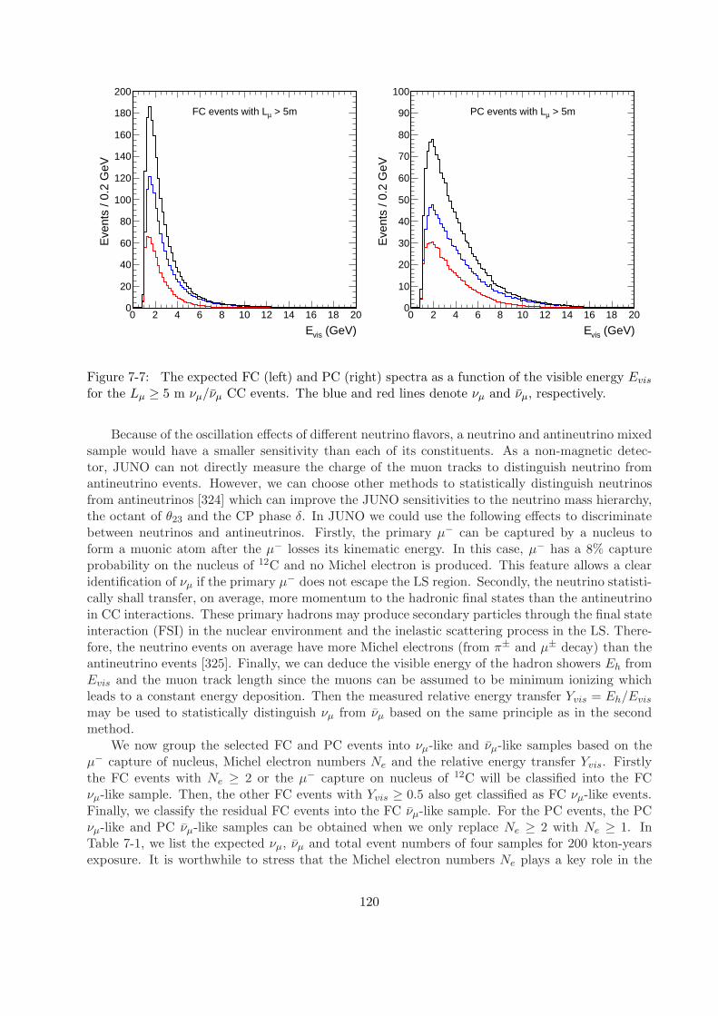
(GeV)visE0 2 4 6 8 10 12 14 16 18 20

Eve

nts

/ 0.2

GeV

0

20

40

60

80

100

120

140

160

180

200

> 5mµFC events with L

(GeV)visE0 2 4 6 8 10 12 14 16 18 20

Eve

nts

/ 0.2

GeV

0

10

20

30

40

50

60

70

80

90

100

> 5mµPC events with L

Figure 7-7: The expected FC (left) and PC (right) spectra as a function of the visible energy Evis

for the Lµ ≥ 5 m νµ/νµ CC events. The blue and red lines denote νµ and νµ, respectively.

Because of the oscillation effects of different neutrino flavors, a neutrino and antineutrino mixedsample would have a smaller sensitivity than each of its constituents. As a non-magnetic detec-tor, JUNO can not directly measure the charge of the muon tracks to distinguish neutrino fromantineutrino events. However, we can choose other methods to statistically distinguish neutrinosfrom antineutrinos [324] which can improve the JUNO sensitivities to the neutrino mass hierarchy,the octant of θ23 and the CP phase δ. In JUNO we could use the following effects to discriminatebetween neutrinos and antineutrinos. Firstly, the primary µ− can be captured by a nucleus toform a muonic atom after the µ− losses its kinematic energy. In this case, µ− has a 8% captureprobability on the nucleus of 12C and no Michel electron is produced. This feature allows a clearidentification of νµ if the primary µ− does not escape the LS region. Secondly, the neutrino statisti-cally shall transfer, on average, more momentum to the hadronic final states than the antineutrinoin CC interactions. These primary hadrons may produce secondary particles through the final stateinteraction (FSI) in the nuclear environment and the inelastic scattering process in the LS. There-fore, the neutrino events on average have more Michel electrons (from π± and µ± decay) than theantineutrino events [325]. Finally, we can deduce the visible energy of the hadron showers Eh fromEvis and the muon track length since the muons can be assumed to be minimum ionizing whichleads to a constant energy deposition. Then the measured relative energy transfer Yvis = Eh/Evis

may be used to statistically distinguish νµ from νµ based on the same principle as in the secondmethod.

We now group the selected FC and PC events into νµ-like and νµ-like samples based on theµ− capture of nucleus, Michel electron numbers Ne and the relative energy transfer Yvis. Firstlythe FC events with Ne ≥ 2 or the µ− capture on nucleus of 12C will be classified into the FCνµ-like sample. Then, the other FC events with Yvis ≥ 0.5 also get classified as FC νµ-like events.Finally, we classify the residual FC events into the FC νµ-like sample. For the PC events, the PCνµ-like and PC νµ-like samples can be obtained when we only replace Ne ≥ 2 with Ne ≥ 1. InTable 7-1, we list the expected νµ, νµ and total event numbers of four samples for 200 kton-yearsexposure. It is worthwhile to stress that the Michel electron numbers Ne plays a key role in the

120

above classification. For example, the selection Ne ≥ 2 will result in 524 νµ and 62 νµ events inthe FC νµ-like sample. In addition to the above event classification, we have also performed asimplified classification in track-like and point-like events. Track-like events are all CC νµ eventswith an inelasticity Eh/Eν < 0.65. All other interactions are called point-like, because the cascadeat the interaction vertex dominates the visible energy. This classification based on 25 millionsimulation events will be used for the pessimistic analysis of the MH sensitivity.

νµ events νµ events Total events νµ purity

FC νµ-like 656 83 739 88.8%

FC νµ-like 652 541 1193 54.6%

PC νµ-like 577 166 743 77.7%

PC νµ-like 383 384 767 50.0%

Table 7-1: The expected event numbers of four samples for 200 kton-years exposure.

7.3.4 Identification of νµ, νµ, νe, and νe for the CP-Violation analysis

As shown in Fig. 7-3, the sub-GeV region is most sensitive to the CP phase δ. Below 100 MeV, thecurrent atmospheric neutrino flux prediction has a large uncertainty, and the discrepancy betweenmodels can be as large as 50%. Therefore, it is a difficult region to study. Above 100 MeV, theCC quasi elastic processes are open for νµ and νe. Around 300 MeV, the CC resonance productionprocess is open. In this case, the final states include the charged lepton, pions and the daughternuclei. For a liquid scintillator detector, which is weak in detecting multiple tracks for the sub-GeVneutrino events, it is also difficult to distinguish µ± (e±) from π± (π0).

For the identification of the sub-GeV νµ, νµ, νe, and νe, the [100, 300] MeV region is veryinteresting since it may be a region with relatively low background. For example, the final stateµ− will on average take 74% of the initial 200 MeV energy in the νµ CC interaction. It is possiblefor us to reconstruct the track length and direction of the charged lepton as discussed in appendix.Besides the quenching effect, the energy of µ± and e± can be measured. Another advantage ofthe [100, 300] MeV region is that we may distinguish neutrinos from antineutrinos by use of thedifferent daughter nuclei. In the [100, 300] MeV region, the νe and νe CC processes can be writtenas

12C(νe, e+)12B∗, 12C(νe, e

+)12B(g.s.), (7.15)12C(νe, e

−)12N∗, 12C(νe, e−)12N(g.s.), (7.16)

where the ground states 12N(g.s.) and 12B(g.s.) can be identified by the JUNO detector since theyhave different lifetimes and Q-values. The excited states 12B∗ and 12N∗ have characteristic decaymodes. For example, 12N∗ may decay into a proton and a 11C. The β+ decay of 11C can beidentified since JUNO has a very low energy threshold. JUNO can also detect νe through IBDprocess p(νe, e

+)n. The same principle can be applied to νµ and νµ. The final state muon with a2.2 µs lifetime can decay into a Michel electron plus neutrinos. This delayed coincidence featurecan be used to distinguish muon neutrinos. In this case, a triple coincidence from prompt muonproduction, the Michel electron from muon decay, and the decay of the daughter nuclei are required.

It is promising to use double (triple) coincidence detection for νe and νe (νµ and νµ), and torely on different daughter nuclei to distinguish neutrinos from antineutrinos. However it is veryhard to precisely predict the cross sections for different daughter nuclei in present nuclear structuremodels. Some experiments only measure the ground state cross section. Studies on the particle

121

identification and reconstruction are in progress for the [100, 300] MeV atmospheric neutrinos.Therefore the NC and CC backgrounds are not yet certain. In the [100, 300] MeV region, we shalltake the idealized assumptions and only present a very optimistic upper limit of the JUNO detectorfor the CP research.

7.4 Atmospheric Neutrino Analysis

7.4.1 The χ2 Function

In the following we will investigate different data samples using the visible neutrino energy Evis

and the µ± zenith angle θµ. For most of the analysis we will use a χ2 function, where we adopt thePoisson form:

χ2 = 2∑

ij

[Tij −Nij +Nij ln

Nij

Tij

]+

4∑

k=1

ξ2k , (7.17)

with

Tij = Tij

(1 +

4∑

k=1

πkijξk

), (7.18)

where the subscripts i and j run over the energy and angle bins, respectively. For the range−1 ≤ cos θµ ≤ 1, the number of bins is chosen to be 10, namely a bin width of 0.2. Then we dividethe visible energy into several bins and require the experimental event numbers Nij ≥ 5 for everybin. Adopting a set of oscillation parameters as the true values, we can calculate Nij based onthe MC efficiency per bin. The expected event numbers Tij can be obtained from Eq. (7.13) withany input values of oscillation parameters. Using the method of pulls, we take into account theneutrino flux and cross section systematic uncertainties [326]. The pull variable ξ1 describes the10% normalization error of neutrino cross section. ξ2 is the pull for the overall 20% neutrino fluxerror. ξ3 and ξ4 parameterize the 5% uncertainties on the energy and zenith angle dependence ofatmospheric neutrino fluxes, respectively. The “coupling” πkij describes the fractional change of Tijwhen the corresponding uncertainty has 1σ deviation. Finally, we minimize χ2 over the above fourpull variables for a set of input oscillation parameters and derive the best-fit minimal χ2(test). Forthe test NH and IH hypotheses, the difference ∆χ2 = |χ2(IH)− χ2(NH)| will be used to calculatethe JUNO MH sensitivity with Nσ =

√∆χ2.

7.4.2 Neutrino Mass Hierarchy

As discussed in Sec. 7.2, νµ and νµ have opposite contributions to the MH sensitivity in theabsence of the charge identification. That is because P (νµ → νµ) and P (νe → νµ) in the NH case isapproximately equal to the corresponding antineutrino oscillation probabilities in the IH case. Dueto different fluxes and cross sections one expects a higher neutrino rate compared to antineutrinoswhich allows a measurement of the MH without distinguishing between the two. The statisticalseparation of νµ and νµ events in Sec. 7.3.3 will obviously improve the sensitivity further.

For the upward atmospheric neutrinos, the oscillation probabilities P (νµ → νµ) and P (νe → νµ)in the NH and IH cases have obvious differences due to the MSW resonance effect. These differencescan be easily found from Eqs. (7.6-7.7) and Fig. 7-2 with the help of Eq. (7.10). It is clear thatthe approximated oscillation probabilities P (νµ → νµ) and P (νe → νµ) in Eqs. (7.6-7.7) do notdepend on θ12, δ and ∆m2

21. In addition, the MH sensitivity is also insensitive to θ13 since the

122

effective mixing angle sin2 2θm13 will approach 1 in the MSW resonance case. Unless otherwisespecified, we shall take θ12, θ13 and ∆m2

21 at their best values of Eq. (7.4), and the CP violationphase δ = 0 for the following analysis. Here we will analyze the dependence on θ23 and ∆m2

atm.For three typical sin2 θ23 = 0.4, 0.5, 0.6, we have calculated the theoretical and experimental eventnumbers per bin through varying ∆m2

atm. Then the JUNO MH sensitivity can be determinedfrom Eqs. (7.17) and (7.18). The minimal ∆χ2 has been found at ∆m2

atm = −2.40 × 10−3eV2 and∆m2

atm = 2.47 × 10−3eV2 for the true ∆m2atm = 2.43 × 10−3eV2 and ∆m2

atm = −2.43 × 10−3eV2,respectively. Using the two values as the test ∆m2

atm, we calculate the MH sensitivity as a functionof livetime as shown in Fig. 7-8. It is found that JUNO has a 0.9σ MH sensitivity with 10 year dataand sin2 θ23 = 0.5. The larger sin2 θ23 gives better MH sensitivity. In the absence of the statisticalseparation of neutrinos and antineutrinos, about 20% reduction of the JUNO MH sensitivity isexpected.

2 4 6 8 10 12 14 16 18 200.0

0.5

1.0

1.5

2.0

2.5

3.0

Sen

sitiv

ity (

)

Livetime (year)

sin2 23 = 0.4

sin2 23 = 0.5

sin2 23 = 0.6

Normal Hierarchy

2 4 6 8 10 12 14 16 18 200.0

0.5

1.0

1.5

2.0

2.5

3.0

Sen

sitiv

ity (

)

Livetime (year)

sin2 23 = 0.4

sin2 23 = 0.5

sin2 23 = 0.6

Inverted Hierarchy

Figure 7-8: The JUNO MH sensitivities from high energy muon neutrino events as a function oflivetime for the true NH (left) and IH (right) hypotheses.

In the following, we will discuss an optimistic estimation for the neutrino mass hierarchy basedon few reasonable assumptions. Firstly, the νe/νe CC events can be identified and reconstructedvery well in the e± visible energy Ee

vis > 1 GeV and Yvis < 0.5 case. Secondly, we extend theselection condition Lµ > 5m to Lµ > 3m for the νµ/νµ CC events. Finally, we replace the chargedlepton direction with the neutrino direction for this physical analysis and assume 10 angularresolution. As shown in Fig. 7-9, we numerically calculate the optimistic MH sensitivities fromνµ/νµ (dashed lines) and νe/νe (dotted lines) with a fixed sin2 θ23 = 0.5. It is found that the νµ/νµcontributions have a small enhancement with respect to the results in Fig. 7-8. The νe/νe eventshave the larger sensitivities than νµ/νµ events since most of νe/νe events can deposit their energiesin the LS region. The selected νe/νe events only are divided into two samples in terms of the Michelelectron number Ne = 0 and Ne ≥ 1. The combined sensitivities can reach 1.8 σ and 2.6 σ for 10and 20 year data, respectively. Note that the predicted MH sensitivity will have a 13% reductionwhen we take 20 angular resolution.

Before the JUNO particle reconstruction and identification capabilities are fully understood,we should consider a more pessimistic case. For this analysis we adopt a different analytical methodand assume that it will be only possible to distinguish muon tracks from other cascading events. Wetherefore divide the data into the point-like and track-like samples. The track-like sample containsonly νµ/νµ CC events with a Eh/Eν < 0.65 inelasticity and the point-like sample all other CC

123

2 4 6 8 10 12 14 16 18 200.0

0.5

1.0

1.5

2.0

2.5

3.0

Sen

sitiv

ity (

)

Livetime (year)

Electron neutrinos Point-like Muon neutrinos Track-like Electron+Muon Point+Track

Normal Hierarchy

2 4 6 8 10 12 14 16 18 200.0

0.5

1.0

1.5

2.0

2.5

3.0

Sen

sitiv

ity (

)

Livetime (year)

Electron neutrinos Point-like Muon neutrinos Track-like Electron+Muon Point+Track

Inverted Hierarchy

Figure 7-9: The future optimistic (blue) and pessimistic (red) MH sensitivities as a function oflivetime for the true NH (left) and IH (right) hypotheses.

and NC events. Here we do not consider the statistical separation of neutrinos and antineutrinos,and do not discriminate the FC and PC events. In contrast to the optimistic case, we take the5%

√Evis and 37.2/

√Eν for the visible energy and the neutrino direction resolutions, respectively.

37.2/√Eν corresponds to the mean angle between the lepton and neutrino directions. In order to

calculate the MH sensitivity we weight a simulated dataset of 25 million events according to thebest fit parameters [27] of both NH and IH hierarchies. For the experimental event numbers Nij inEq. (7.17), we dice pseudo experiments for each hierarchy using a poisson distribution. This yieldsthe Gaussian distributed χ2 values. The MH sensitivity under the assumption that one hierarchyis true is the distance between the expectation values µtrue and µfalse expressed in units of thefalse hierarchy standard deviation σfalse. The estimated sensitivity Nσ = |µtrue − µfalse|/σfalse canbe seen in Fig. 7-9. After a 10 year measurement one would expect a 1.0σ combined sensitivityfrom the point and track-like samples. The results are pessimistic compared to the optimistic casewhich is mostly due to the assumed angular uncertainties. Additionally, the sensitivity of the point-like sample is decreased by a high contamination of NC events and deep inelastic muon neutrinointeractions while the track-like sample has a higher uncertainty on energy resolution due to a highnumber of PC events.

7.4.3 Atmospheric Mixing Angle θ23

For the atmospheric mixing angle θ23, the MINOS disappearance data indicates a non-maximalθ23 [131]. However, the T2K disappearance data prefer a nearly maximal mixing θ23 = 45 [133].It is an open question whether or not θ23 is maximal. If θ23 deviates from 45, one can getboth the lower octant (LO) θ23 < 45 and higher octant (HO) θ23 > 45 solutions, because theνµ/νµ survival probability is mainly sensitive to the sin2 2θ23 terms of Eq. (7.7) for the MINOSand T2K experiments. When the MSW resonance happens, the sin4 θ23 term in Eq. (7.7) will beenlarged due to sin2 2θm13 → 1. Then the sin4 θ23 term can help us to distinguish the θ23 octantsince sin4 θ23 is different for the θ23 and π/2 − θ23 solutions. In addition, we should consider theoscillation probability P (νe → νµ) which is proportional to sin2 θ23 as shown in Eq. (7.6). It isworthwhile to stress that the octant sensitivity from antineutrinos (neutrinos) is largely suppressedby sin2 2θm13 → sin2 2θ13 when we take the NH (IH) hypothesis as the true mass hierarchy. Therefore

124

the statistical separation of neutrinos and antineutrinos can suppress the statistical errors andimprove the octant sensitivity.

For the octant analysis, we assume a prior knowledge of mass hierarchy and hence considerthe normal (inverted) hierarchy as the true hierarchy. For a given true θ23, we take the correctoctant solution θ23 and the wrong octant solution π/2 − θ23 as the test values to calculate thebest fit minimal difference ∆χ2 = χ2(π/2 − θ23) − χ2(θ23). Then we can derive the JUNO octantsensitivity

√∆χ2. In Fig. 7-10, we have plotted the JUNO sensitivities to the octant for the true

NH and IH cases. The wrong θ23 octant could be ruled out at 1.8σ (NH) and 0.9σ (IH) for thetrue θ23 = 35. Note that the inverted hierarchy has the smaller octant sensitivity than the normalhierarchy, because neutrinos have more events than antineutrinos as shown in Fig. 7-7 and theMSW resonance occurs in the NH (IH) case for neutrinos (antineutrinos). We have also consideredthe ∆m2

atm impact on the octant sensitivity. As shown in Fig. 7-10, the JUNO octant sensitivityhas a weak dependence on ∆m2

atm.

36 38 40 42 44 46 48 50 52 540.0

0.5

1.0

1.5

2.0

Sen

sitiv

ity (

)

True 23 (degree)

m2atm = 2.2*10-3 eV2

m2atm = 2.4*10-3 eV2

m2atm = 2.6*10-3 eV2

Normal Hierarchy

36 38 40 42 44 46 48 50 52 540.0

0.5

1.0

1.5

2.0

Sen

sitiv

ity (

)

True 23 (degree)

m2atm = -2.2*10-3 eV2

m2atm = -2.4*10-3 eV2

m2atm = -2.6*10-3 eV2

Inverted Hierarchy

Figure 7-10: The JUNO sensitivities to the octant for high energy muon neutrino events as afunction of true θ23 in the true NH (left) and IH (right) cases.

7.4.4 CP Phase δ

As shown in Fig. 7-3, both P (νe → νµ) and P (νµ → νµ) can be used to measure the CP phase δ.However only the appearance oscillation probabilities are possible for us to discover the CP violationphenomenon, because P (να → να) = P (να → να) from the CPT invariance. The disappearanceP (νµ → νµ) only contain the cos δ terms which are invariant in the CP transformation (δ → −δ).The appearance P (νe → νµ) includes both sin δ and cos δ terms as shown in the approximatedexpressions of Ref. [318]. The sin δ terms can help us to discover the CP violation phenomenon,namely P (να → νβ) 6= P (να → νβ). Note that δ = 0 and δ = π correspond to the CP conservation.For a given true δ, the CP violation sensitivity comes from whether or not it can be distinguishedfrom the CP conservation. We take δ = 0 and δ = π as the test values to calculate the best fitminimal differences ∆χ2

0 = χ2(0) − χ2(δ) and ∆χ2π = χ2(π) − χ2(δ). Then we define the minimal

value of√

∆χ20 and

√∆χ2

π as the JUNO CP violation sensitivity. Since the sin δ terms have theopposite signs for neutrinos and antineutrinos, the statistical separation of νµ and νµ signals willimprove the sensitivity.

In Sec. 7.3.3, we have required Lµ ≥ 5 m which means the νµ and νµ energy is larger than 0.9

125

GeV. For these high energy νµ and νµ, the oscillation probabilities P (νµ → νµ) and P (νe → νµ) aresensitive to the CP phase δ as shown in Fig. 7-3. However the kinematical smearing will obviouslysuppress the CP violation sensitivity. As shown in Fig. 7-11, the JUNO sensitivity to CP violationis very small for these high energy νµ and νµ events where we have taken the best fit values of∆m2

atm. It is found that different sin2 θ23 can change the predicted sensitivity.

0.0 0.5 1.0 1.5 2.00.00

0.05

0.10

0.15

0.20

0.25

0.30

Sen

sitiv

ity (

)

True ( )

sin2 23 = 0.4

sin2 23 = 0.5

sin2 23 = 0.6

Normal Hierarchy

0.0 0.5 1.0 1.5 2.00.00

0.05

0.10

0.15

0.20

0.25

0.30

Sen

sitiv

ity (

)True ( )

sin2 23 = 0.4

sin2 23 = 0.5

sin2 23 = 0.6

Inverted Hierarchy

Figure 7-11: The JUNO’s sensitivities to CP violation for high energy muon neutrino events as afunction of true δ in the NH (left) and IH (right) cases.

The lower energy [100, 300] MeV neutrinos have more sensitivity to measure CP phase δ asshown in Fig. 7-3. With the techniques discussed in Sec. 7.3.4, it is possible to pursue such ameasurement. The major uncertainty comes from the lack of knowledge of the daughter nuclei,which might spoil the idea. There might be also some backgrounds from the NC and CC processesof high energy neutrinos. An estimate of the maximal JUNO sensitivity is made by ignoring theabove unknowns. The pure statistical sensitivity of JUNO detector in ten years is shown in Fig.7-12 where all νµ, νµ, νe, and νe are considered. Direction reconstruction of electron and muonis not crucial, because it is only weakly correlated to the initial neutrino direction at these lowenergies.

7.4.5 Summary

We have investigated atmospheric neutrinos in JUNO and discussed their contributions to theMH, octant and CP violation. In terms of the reconstruction potential of the JUNO detector,we conservatively use the atmospheric νµ and νµ with the track length larger than 5 m for ourphysical analysis. These events have been classified into the FC νµ-like, FC νµ-like, PC νµ-like andPC νµ-like samples based on the µ± track and the statistical charge separation. Our numericalresults have shown that the JUNO’s MH sensitivity can reach 0.9 σ for a 200 kton-years exposureand sin2 θ23 = 0.5, which is complementary to the JUNO reactor neutrino results. The wrong θ23octant could be ruled out at 1.8σ (0.9σ) for the true normal (inverted) hierarchy and θ23 = 35.It is found that the JUNO sensitivity to CP violation is very small when we only consider thehigh energy νµ and νµ. In contrast to the high energy neutrinos, the low energy neutrinos maygive the dominant contributions to the CP violation sensitivity even if we do not use the directioninformation. In our analysis of the high-energy neutrino events, all νe/νe and the sub-GeV νµ/νµdata have been discarded from the conservative point of view. According to the optimistic and

126

]π [CP

δ0 0.2 0.4 0.6 0.8 1 1.2 1.4 1.6 1.8 2

]σC

PV

Dis

cove

ry S

igni

fican

ce L

evel

[

0

0.5

1

1.5

2

2.5

3

3.5

backgroundeνwith

Figure 7-12: The upper limit of the CP discovery sensitivity of JUNO in ten years. All statisticsof νµ, νµ, νe, and νe in low energy are considered.

pessimistic estimations, atmospheric neutrinos in JUNO may give a better sensitivity to the masshierarchy. In the future, we shall investigate the particle reconstruction and identification of theJUNO detector in detail. In addition, we shall analyze the upward through-going and stoppingmuon events those are produced by atmospheric neutrinos in the rock and water pool. The futureatmospheric neutrino exploration in JUNO can also help us to probe new physics beyond thestandard model, such as the non-standard neutrino interactions, sterile neutrinos and new longrange forces, etc.

127

8 Geoneutrinos

8.1 Introduction

For half a century we have established with considerable precision the Earth’s surface heat flow as46± 3TW [327,328]. However we are vigorously debating what fraction of this power comes fromprimordial versus radioactive sources. This debate touches on the composition of the Earth, thequestion of chemical layering in the mantle, the nature of mantle convection, the energy neededto drive plate tectonics, and the power source of the geodynamo, which powers the magnetospherethat shields the Earth from the harmful cosmic ray flux.

Over the last decade particle physicists have detected the Earth’s geoneutrino flux [329, 330],electron antineutrinos that are derived from naturally occurring, radioactive beta-decay eventsinside the Earth [223, 331]. Matter, including the Earth, is mostly transparent to these elusivemessengers that reveal the sources of heat inside the Earth as they virtually escape detection, beingthat the Earth’s geoneutrino flux is some 106 cm−2 s−1. However, by detecting a few particles peryears we are now measuring the geoneutrino flux from thorium and uranium inside the planet,which in turn allows us to estimate the amount of radiogenic power driving the Earth’s engine.

Today we are experiencing a renaissance in neutrino studies, in part driven by the fact that15 years ago physicists revealed the phenomenon of neutrino oscillations and thus the fact thatneutrinos have non-zero mass. Neutrino science is now bringing us fundamental insights into thenature of nuclear reactions, revealing for us the nuclear fusion in the core of the sun, nuclear fissionin man-made nuclear reactors, and identifying our planet’s nuclear fuel cycle, as reflected in theheat produced during radioactive decay. Geology is the fortunate recipient of the particle physicists’efforts to detect the Earth’s emission of geoneutrinos.

How does geoneutrino detection serve the geological community and what transformationalinsights will it bring? It directly estimates the radiogenic heating in the Earth from thorium anduranium. These elements, along with potassium, account for more than 99% of the radiogenicheat production in the Earth. This component, along with the primordial energy of accretion andcore segregation, define the total planetary power budget of the planet. By defining the absoluteabundance of Th and U in the Earth, with accuracy and precision, we can:

1. define the building blocks, the chondritic meteorites, that formed the Earth,

2. resolve ever vexing paradoxes (e.g. 4He-heat flow, Ar budget and degassing) that fuel thedebates of compositionally layered mantle structures or not,

3. discriminate models of parameterized mantle convection that define the thermal evolution(dT/dt) of the Earth,

4. potentially identify and characterize deep, hidden reservoirs (or not) in the mantle, and

5. fix the radiogenic contribution to the terrestrial heat flow.

Moreover, such studies can place stringent limits on the power of any natural nuclear reactor in ornear the Earth’s core.

Editors: Ran Han (hanran@ncepu.edu.cn), Livia Ludhova (ludhova@gmail.com), and Bill McDonough (mc-donoug@umd.edu)

Major contributors: Fabio Mantovani, Barbara Ricci, Liangjian Wen, Oleg Smirnov, Yufei Xi, and SandraZavatarelli

128

8.2 Expected geoneutrino signal

The amount of U and Th and their distribution in a reservoir (e.g. crust and mantle) affects theintegrated geoneutrino flux at a location on the Earth’s surface. The unoscillated geoneutrino fluxproduced by a source volume ∆V at the detector position1 can be calculated with:

Φ(∆V ) =1

4π

∫

∆Vd3r

A(−→r )|−→R −−→r |2

, (8.1)

where A is the rate of geoneutrinos produced in the volume ∆V , which depends on density, an-tineutrino production rates per unit mass and U and Th abundances. The intensity of the fluxdepends on the inverse-square of the distance to the sources, and thus the crust surrounding thedetector, which contains a relative small amount of the Earth’s U and Th budget, gives a largecontribution to the signal. It is predicted that the first ∼ 500 km from the KamLAND detectorcontributes about 50% of the measured geoneutrino signal, with this volume containing ∼ 0.1% ofthe total crustal U and Th mass [332]. For the JUNO site it is predicted that the first 550 km fromthe detector contribute some 50% of the measured geoneutrino signal (Fig. 8-1).

Figure 8-1: Geoneutrino signal contribution at JUNO. The cumulative geoneutrino signal and thepercentage contributions of the Bulk Crust, Continental Lithospheric Mantle (CLM) and Mantleare represented as function of the distance from JUNO [332].

The geophysical structure of the global crustal model described in [333] takes into accountdata from different studies: body wave studies using reflection and refraction methods, surfacewave dispersion studies and gravity surveys. On the basis of this model, the expected geoneutrinosignal at JUNO, which originates from the U and Th in the global Bulk Crust (BC) and in the

1In the case of detector near the Earth surface |−→R | is the radius of the Earth.

129

Continental Lithospheric Mantle (CLM), are SBC = 28.2+5.2−4.5 TNU 2 and SCLM = 2.1+2.9

−1.3 TNUrespectively (Tab. 8-1) [332]. The 1σ asymmetric uncertainties reflect the propagation of non-Gaussian distributions of U and Th abundances in the deep BC and CLM, together with theGaussian distributions of the errors associated with the geophysical inputs.

Table 8-1: Geoneutrino signals from U and Th expected in JUNO. The signals from differentreservoirs (CLM = Continental Lithospheric Mantle, LS = Lithosphere, DM = Depleted Mantle,EM = Enriched Mantle) indicated in the first column are in TNU [332]. Total equals Total LS +DM + EM. The mantle signal can span between 1-19 TNU according to the composition of theEarth: here the geoneutrino signal produced by a primitive mantle having m(U)= 8.1 · 1016 kg andm(Th)= 33 · 1016 kg is reported.

S(U) S(Th) S(U+Th)

Bulk crust 21.3+4.8−4.2 6.6+1.9

−1.2 28.2+5.2−4.5

CLM 1.3+2.4−0.9 0.4+1.0

−0.3 2.1+2.9−1.3

Total LS 23.2+5.9−4.8 7.3+2.4

−1.5 30.9+6.5−5.2

DM 4.1 0.8 4.9

EM 2.9 0.9 3.8

Total 30.3+5.9−4.8 9.0+2.4

−1.5 39.7+6.5−5.2

The Total predicted geoneutrino signal at JUNO STOT = 39.7+6.5−5.2 TNU [332], which is obtained

assuming a predicted Mantle contribution of SM ∼9 TNU according to a mass balance argument.The adopted mantle model, divided into two spherically symmetric domains (Depleted Mantle andEnriched Mantle), refers to a Bulk Silicate Earth based on a primitive mantle having U and Thmass of m(U)= 8.1·1016 kg and m(Th)= 33·1016 kg, respectively [331]. Alternatively, another classof Earth models [334], with a global composition similar to that observed in enstatite chondrites,is characterized by smaller amounts of U and Th (i.e. m(U) = 4.9 · 1016 kg and m(Th) = 20 · 1016kg). Consequently, assuming the same lithospheric contribution and mass balance arguments, thismodel has a minimum signal from the mantle of SM ∼1 TNU [335]. On the other hand, modelsbased on the energetics of mantle convection and on the observed surface heat loss [336] require ahigh concentration of U and Th in the primitive mantle (e.g. m(U) = 12.5 · 1016 kg and m(Th)= 52 · 1016 kg). In this scenario the present mantle signal could reach SM ∼19 TNU. Ranges ofgeoneutrino signals produced by symmetric and asymmetric distributions of U and Th in the mantleare extensively discussed in [337]. The present crustal models are affected by uncertainties that arecomparable to the mantle’s contribution: this comes mainly from understanding the abundanceand distribution of Th and U in the regional crystalline rocks. Upper crustal estimates for Thand U abundances vary by 10% and 22%, respectively, whereas larger uncertainties exist for their

2TNU: Terrestrial Neutrino Units. 1 TNU = 1 event/yr/1032 target protons, which is approximately the numberof free protons in 1 kiloton liquid scintillation.

130

estimates in middle and lower crustal lithologies [333].Thus, to understand the relative contributions from the crust and mantle to the total geoneu-

trino signal at JUNO an accurate estimation of the geoneutrino flux from the crustal region sur-rounding JUNO is a priority. Detailed geological, geochemical, and geophysical studies were per-formed in the areas surrounding the KamLAND detector at Kamioka, Japan [338,339], the Borexinodetector at Gran Sasso, Italy [340], and the SNO+ detector at Sudbury, Canada [341]. The presentgeoneutrino flux prediction for JUNO [332] is recognized as being a first step and is not based ondata specifically from the local region. This estimate was generated from a set of global databases,including a compositional estimate of the average upper crust, physical structure of crustal rocks,and models of the seismic and gravity properties of the crust (see [333]). To improve upon theaccuracy and precision of this estimate, future studies of JUNO will necessarily require input fromgeological, geochemical and geophysical studies of the area surrounding JUNO, up to some 550 kmaway from the detector. The survey distance from the JUNO detector can be fixed by resolutionstudies, with trade offs between distance, limits on uncertainty, and costs of survey.

Thus, a refined model for predicting the geoneutrino flux at JUNO is needed. To meet thisneed, an integrated effort is required and will involve an exciting and collaborative research effortbetween particle physicists and Earth scientists.

8.3 The local geology study around JUNO

The JUNO detector is to be built near the southern continental margin of China close to the SouthChina Sea (Fig. 8-2). This passive margin area has an extensive continental shelf and representsthe transition between continental and oceanic plates.

The JUNO detector will accumulate a signal from the regional distribution of Th and U, aswell as from the rest of the planet. The local contribution (the immediate several hundred km ofcrust surrounding the detector) typically contributes about half of the signal at the detector. So itwill be important for the geological community to map out carefully and identify the abundanceand distribution of Th and U in this region. Models for calculating the total geoneutrino signalfrom an area surrounding a detector and the rest of the planet requires extensive integration ofspatially resolved local geological, geochemical, and geophysical data that is then integrated intoa global model for the distribution of geoneutrino sources. Detailed characterization of the localregion also brings additional fundamental benefits to the geoscience community.

Eastern China is documented, relative to a global perspective, as being a region of elevatedheat flow and the Guangdong province specifically, has hot springs and anomalously high heat flowzones associated with deep crustal fractures and fluid flow. Regionally, southern and southeasternChina have large surface areas covered with Mesozoic (circa 250 to 70 million years ago) granitescontaining high concentrations of K, Th and U (the heat producing elements) (Fig. 8-2b).

The Jurassic (∼ 160 million years old) high-K granites are ubiquitous, extending from thecontinental interior to the coastal area [343] and possess the highest amount of heat producingelements. The petrogenesis of granitic rocks and the tectonic evolution in the southeastern Chinacontinue to attract attention (e.g., [343–348]) as they are a relevant source of economic minerals andgeothermal energy. Lithologically the granites are heterogeneous, rich in heat producing elements,and important source rocks producing geoneutrinos [332].

The thickness of the continental crust immediately surrounding JUNO has been modeled usingCRUST 2.0 and 1.0 [332, 333, 349]; it varies between 26 and 32 km (Fig. 8-3). At some 350km distance to the south of JUNO, the oceanic crust outcrops (approximately 8 km thick andcontaining ∼ 1/10 of the concentration of Th and U as compared to the continental crust) andwill contribute approximately to 0.2% of the total expected geoneutrino signal. On the basis of

131

Figure 8-2: (a) Sketch map showing major tectonic units around JUNO. NCC - North China Cra-ton; SCB - South China Block. (b) Regional map showing the distribution of Mesozoic granites inthe southeastern South China Block. Dashed purple lines show the provincial boundaries. (c) Ge-ological map showing the age distribution of Mesozoic granites along the southern coastal region ofthe Guangdong Province, southeastern China). Stars highlight the plutons. New geochronologicalresults are shown in bold. J-K-Jurassic and Cretaceous; P-T-Permian and Triassic [342].

132

Figure 8-3: Crustal thickness (exclusive water) in the surrounding area of JUNO from CRUST 1.0model, 1 degree [349]. Dashed thick blue line is plate boundary [350]. Thin blue lines denote themain tectonic units.

133

an existing global reference model for the Earth [333], an initial estimate of the local geoneutrinosignal expected at JUNO is SLOC = 17.4+3.3

−2.8 TNU [332]. This flux contribution corresponds to∼44% of the expected geoneutrino signal at JUNO and exceeds the signal from the whole mantle.The 2 × 2 region including and to the north of JUNO is the area with the greatest thicknessof sediments and crystalline crust and it alone has been identified as contributing ∼27% of thegeoneutrino signal [332]. Thus, these early studies have identified significant regional targets thatwill require further intensive research to predict better the JUNO geoneutrino signal.

The main tasks for predicting the JUNO geoneutrino signal include surveys and descriptions ofthe geology, seismology, heat flow, and geochemistry of the regional lithosphere (the Earth’s outerconductive layer that includes the crust and the mechanically coupled layer of mantle beneathit). Geological surveys define the surface lithologies, major structures, and geological provenances.Seismological surveys include refraction and reflection mapping, receiver function and ambient noisetomography of the crust and lithospheric mantle; these studies provide a 3-dimensional image ofthe structures of the deep crust and lithospheric mantle, specifically in terms of major boundariesand the vertical and horizontal variations in density, acoustic velocity and Poisson’s ratio. Heatflow surveys will map out the surface variation in heat flow, as well as the heat production andthermal conductivity of the immediate lithologies, and from this develop models of near surfaceproductivity versus reduced heat flow. Gravity surveys record the variations in density structureof the lithosphere and mantle; these surveys can be coupled with heat flow and seismic surveysto cross check and refine models of the lithosphere. Finally a wide range of geochemical studies,including mapping the spatial variations in the abundance of K, Th and U, local helium gas fluxmeasurements, and gamma ray spectroscopy, will define the nature and composition of the nearsurface and set up the potential for projecting the 3-dimensional variation in the abundances ofthese elements at depth.

In addition to these survey studies it is vitally important to involve computational geologicalstudies, where all of the geological, geophysical and geochemical data are geo-located into anintegrated, 3-dimensional model that is the essential physical and chemical database of the Earthsystem. The global and regional contributions of the geoneutrino flux need to be predicted forthe area surrounding the JUNO detector, as have been previously done at the existing detectorsKamLAND (Japan) [338,339], Borexino (Italy) [340] and SNO+ (Canada) [341].

The area of Kaiping, China, the site of the JUNO experiment, is close to the continental marginof south China. Beyond the shores of this area is a significant region of continental shelf. Thisregional study therefore represents a golden opportunity to investigate in detail a passive continentalmargin, a tectonic boundary that we know little of its nature. These broad continental marginstypically host considerable petroleum reserves and thus understanding their nature and structuremight provide critical insights into identifying further energy resources. Moreover, integration ofthe matrix of geophysical, geochemical and geological data into a single, self-consistent solution isrequired in order to calculate the geoneutrino flux at JUNO.

8.4 Detecting geoneutrino signal

The full strength of geoneutrino studies comes from the synergistic activities of geology and physics,neither acting independently of the other and both accepting the challenge of knowing better theEarth and its secrets. These studies represent the ultimate opportunity for geologists and particlephysicists to independently measure and test our predictions of the structure and composition ofthe planet’s interior [329]. Thus, by 2020, when the JUNO detector will be built and begin datataking, we will have our best prediction of the expected signal. At that time we will wait and seewhat the measurement reveals. It is a rare moment in geology where we predict and then receive

134

independent assessment of the strength of our prediction.Detectors like JUNO are sited deep underground and are enormous (20 kiloton) structures;

their size enhances their potential for detection and their overburden shields them from cosmic rayfluxes. These factors, combined with their ultra-clean construction, will allow these detectors toextract the geoneutrino signal.

Geoneutrinos from 238U and 232Th (not those from 235U and 40K) are above threshold for theclassical antineutrino (νe) detection reaction, the inverse beta decay (IBD) on free protons (p):

νe + p→ e+ + n− 1.806 MeV. (8.2)

The characteristic temporal and spatial coincidence of prompt positron (e+) and delayed neutron(n) flash events offers a clean signature that resolves them from background signals.

The first geoneutrino measurements were reported in 2005 by the KamLAND team [351], wherethey recorded 25 events over two years of exposure. The KamLAND detector is sited deep in theJapanese Alps, opposite Tokyo, on the island of Honshu and is 1 kiloton in scale. Another activedetector is the Borexino experiment, located beneath the Apennine Mountains near the town ofL’Aquila in Italy. This detector, which is smaller (300 tons), reported in 2010 its measurementof the Earth’s geoneutrino flux at the 99.997% C.L (5σ) [352]. Both experiments provided newupdated measurements [329, 330], on the occasion of the inter-disciplinary Neutrino Geoscienceconference series, in 2013 held in Takayama, Japan.

A third, new detector, SNO+ is a re-deployed Sudbury Neutrino Observatory. It is a secondkiloton detector and it is situated in Sudbury, Ontario, Canada, on the ancient stable SuperiorCraton [353]. JUNO will then join these detectors in 2020, being 20 times larger than all theexisting devices. In its first year of operation, JUNO will record more geoneutrino events thanall other detectors combined will have accumulated to that time. Before discussing the detectionof geoneutrino events we will discuss the various experimental backgrounds coming from nuclearreactors and other sources.

8.5 Reactor antineutrino background

Determination of the expected signal from reactor νe’s requires a wide set of information, spanningfrom characteristics of nuclear cores placed around the world to neutrino properties. In this section,the number of expected reactor events and the corresponding spectral shape have been calculatedas follows:

Nev = ǫNp τ

Nreact∑

r=1

Pr

4πL2r

< LFr > ×∫dEνe

4∑

i=1

piQiφi(Eνe)σ(Eνe)Pee(Eνe , θ, Lr), (8.3)

where ǫ is the detection efficiency, Np is the number of target protons, and τ is the data-taking time.The index r cycles over the number of reactors considered: Pr is the nominal thermal power, Lr isthe reactor-detector distance, < LFr > indicates the average Load Factor (LF) 3 in the period τ ,Eνe is the antineutrino energy. The index i stands for the different nuclear-fuel components (235U,238U, 239Pu, 241Pu), pi is the power fraction, Qi is the energy released per fission of the componenti, and φi(Eν) is the antineutrino energy spectrum originated by the fission of component i. σ(Eνe)is the inverse-beta-decay cross section. Pee is the energy-dependent survival probability of electronantineutrinos traveling the baseline Lr, for mixing parameters θ = (δm2, ∆m2, sin2 θ12, sin

2 θ13).

3Load Factor reflects the ratio between the delivered and the nominal reactor power. The shut-down periods aretaken into account.

135

We express the expected reactor antineutrino signal in unit of TNU, same as the geoneutrinos.This means that in Eq. (8.3) we assume a 100% detection efficiency for a detector containingNp = 1032 target protons and operating continuously for τ = 1 year. We consider all the nuclearcores in the world operating in the year 2013, plus all the cores of the Taishan and Yangjiangnuclear power plants that will enter operation in 2020. Information on the nominal thermal powerand Load Factor for each existing nuclear core comes from the International Agency of AtomicEnergy (IAEA) [354]. For each core the distance Lr has been calculated taking into account theposition of the JUNO detector (22.12 N, 112.52 E) [69] and the positions of all the cores in theworld according to the database adopted in [355]. For the future Taishan and Yangjiang nuclearplants, we considered the thermal power of 18.4 GW and 17.4 GW, the distance of 52.7 and 53.0km, respectively, and we assumed 80% Load Factor. Typical power fractions for the PWR andBWR type reactors are adopted to be equal to the averaged value of the Daya Bay nuclear cores:235U : 238U : 239Pu : 241Pu = 0.577 : 0.076 : 0.295 : 0.052. As in [329], we have considered forthe European reactors using Mixed OXide technology that 30% of their thermal power originatesfrom the fuel with power fractions 0.000 : 0.080 : 0.708 : 0.212, respectively and for the cores in theworld using heavy-water moderator pi = 0.543 : 0.024 : 0.411 : 0.022, respectively.

The φi(Eνe) energy spectra are taken from [102], theQi energy released per fission of componenti are from [356], and the interaction cross section σ(Eνe) for inverse beta decay reaction is from [176].For the vacuum survival probability Pee and the corresponding mixing parameters we adopt themost recent determinations by Capozzi et al. [27] for the Normal Hierarchy.

Tab 8-2 gives an overview of different contributions to the total error on the expected reactorantineutrino signal in the total energy window (1.8 MeV < Eνe < 10 MeV).

Table 8-2: Systematic uncertainties on the expected reactor antineutrino signal in the total energywindow. See Eq. (8.3) and accompanying text for details.

Source Error Source Error[%] [%]

Fuel composition 1.0 sin2 θ12 3.6φi(Eνe) 3.4 sin2 θ13 0.21Pr 2.0 ∆m2 < 10−2

σ(Eνe) 0.4 δm2 1.2Qi 0.09

Total 5.6

The error due to the fuel composition reflects the possible differences among different coresand the unknown stage of burn-up in each of them. This error is determined as the variance ofa uniform distribution, assumed for different signals calculated with the sets of power fractionsavailable in the literature (see Tab. 1 of [355]).

The uncertainty due to φi(Eνe) energy spectra is very conservatively quoted as 3.4%, which isdetermined as the difference in the expected signal computed with the reference spectra of [102]and with the spectra published by [357].

The uncertainty due to the thermal power Pr is conservatively assumed to be 2%. Althoughthermal powers can be measured at sub-percent level, the adopted uncertainty reflects the reg-ulatory specifications for Japan and United States (see e.g., Refs. [358] and [359]), furthermoreallowing to account for the fact that the Load Factors reported in the IAEA database refer to theelectrical power and not to the thermal one.

136

Table 8-3: Main non antineutrino background components assumed in the geoneutrino sensitivitystudy: the rates are intended as number of events per day after all cuts (refer to Section 2.2.2).The options of acrylic vessel and balloon have been compared in the (α, n) background evaluation.

Background type Rate after IBD+ Uncertainty Uncertaintymuon cuts in Rate in Shape[events/day] [%] [%]

9Li - 8He 1.6 20 10Fast neutrons 0.1 100 20Accidental events 0.9 1 negl.13C(α, n)16O (acrylic vessel) 0.05 50 5013C(α, n)16O (ballon) 0.01 50 50

The effect of the uncertainties of oscillation parameters is calculated by varying each parameterone at the time in the 1σ range and assuming a uniform distribution of the obtained signals; notethat the dominant contribution arises from the θ12 mixing angle. A more extensive treatment ofthe uncertainties can be found in [355], where a Monte Carlo based approach has been adopted inthe determination of the uncertainty budget as well as of the signal central values.

In conclusion, the expected reactor antineutrino signal in the total energy window is (1569 ±88)TNU 4. The signal in the geoneutrino energy window (1.8 MeV < Eνe < 3.27 MeV) is (351 ±27)TNU, where the Taishan and Yangjiang nuclear power stations contribute more than 90% ofthe total.

We want to stress that JUNO will measure neutrino oscillations parameters with unprece-dented precision. Thus, as a consequence, the total error on the expected antineutrino flux will bestrongly reduced. In the geoneutrino sensitivity studies presented here, we have adopted the 5.6%uncertainty, since it reflects the current knowledge of the estimation of the reactor antineutrinobackground for JUNO geoneutrino measurement. As we will discuss below, the reactor antineu-trino background is not constrained and is kept as a free fit parameter in our simulations of possibleJUNO geoneutrino measurements. Thus, the error on the predicted reactor-antineutrino rate en-ters the simulations only as a parameter defining the signal-to-background ratio. We have checked,that considering an error of 2.4% (instead of 5.6%) does not significantly change our results ongeoneutrino sensitivity.

8.6 Non antineutrino background

The coincidence tag used in the νe-detection is a very powerful tool in background suppression.Nevertheless, the event rate expected from geoneutrino interactions is quite small (few hundreds ofevents/year) and a number of non antineutrino background events faking geoneutrino interactionshas to be properly accounted for in the sensitivity study.

A detailed description of expected background in JUNO is given elsewhere. Here we brieflysummarise the most relevant backgrounds for the geoneutrino analysis. They can be divided intothree main categories:

• Cosmic-muons spallation products, namely:

4The signal value dose not include the matter effect in the neutrino-oscillation mechanism, which represents anadditional increase of +1.1% with respect to the vacuum oscillation. Furthermore, the contribution of antineutrinosemitted from spent nuclear fuel (SNF) can be considered as +1.9% signal increase [360]

137

– 9Li and 8He isotopes decaying in (β + neutron) branches perfectly mimicking antineu-trino interactions;

– fast neutrons able to penetrate through construction materials and giving a delayedcoincidence if scattered off by one or many protons before being captured;

• Accidental coincidences of non-correlated events.

• Backgrounds induced by radioactive contaminants of scintillator and detector materials. Inparticular, alpha particles emitted in the 238U and 232Th decay chains or by off-equilibrium210Po can induce 13C (α, n)16O reactions on the scintillator 13C nuclides. In these interactions,the prompt signal can be induced by three different processes: i) de-excitation of 16O nuclides,if produced in an excited state; ii) 4 MeV γ ray from the de-excitation of 12C excited byneutron, and iii) protons scattered off by the thermalizing neutron before its capture.

In the second column of Tab. 8-3 the rates of events surviving the IBD selection cuts andmuon cuts are reported. The muon cut properly vetoes in time and space the detector after eachmuon crossing the water pool or the central detector and it is effective in reducing the 9Li and 8Hebackgrounds by a factor 44 (refer to Tab. 2-1).

A fiducial volume of 18.35 ktons corresponding to a radial cut of R = 17.2m was chosen since itis particularly effective in reducing the accidental background mostly arising from 238U/232Th/40Kcontamination of the acrylic vessel, PMT’s glass, steel supports, and copper fasteners.

In the (α, n) background evaluation, the options of acrylic vessel (238U: 10 ppt, 232Th: 10 ppt)and ballon (238U: 2 ppt, 232Th: 4 ppt) have been compared: after the fiducial volume cut, thecorresponding (α, n) event rates of 0.05 counts/day and negligible were found, respectively. A 10−15

g/g 238U/232Th contamination of the liquid scintillator would be responsible for less than 0.01 (α,n) events/day. Considering the 210Pb contamination of the scintillator of the order of 1.4 · 10−22

g/g, the α-decay rate of 210Po in equilibrium with 210Pb would give a negligible contribution to (α,n) background.

8.7 JUNO potential in measuring geoneutrinos

JUNO will be able to detect geoneutrinos in spite of the noticeable background coming from varioussources - and mainly from nearby nuclear power plants. In order to assess the detectability andthe measurement accuracy, the predicted total antineutrino spectrum (signal and backgrounds) hasbeen studied under different possible conditions. The expected geoneutrino signal, as well as reactorantineutrino and non-antineutrino backgrounds have been described above in this section. Forconvenience, Tab. 8-4 summarizes the number of expected events for all components contributingto the IBD spectrum in the 0.7 - 12 MeV energy region of the prompt signal. We have assumed80% antineutrino detection efficiency and 17.2m radial cut (18.35 kton of liquid scintillator). In thesimulations described below, we have considered Gaussian distributions for all spectral componentsaccording to this table. For simplicity, this is valid also for the geoneutrino signal, taking the meanof the left and right variances described above as the variance of symmetric Gaussian.

The main assumptions concerning the signal searched for (U and Th chains in the Earth,assumed to be in secular equilibrium) are the ones about their relative value (the Th/U ratio). Onepossibility, described in Sec. 8.7.1, is to consider in the analysis the fixed chondritic mass Th/U ratioof 3.9. Because the cross-section of the IBD detection interaction increases with energy, the ratioof the signals expected in the detector is Th/U = 0.27. The other obvious choice in the analysis,described in Sec. 8.7.2, is to leave both Th and U contributions free and independent (keeping both

138

Visible energy [MeV]1 2 3 4 5 6 7 8 9 10

Eve

nt /

225

keV

0

50

100

150

200

250

300

350

400

450

Visible energy [MeV]1 2 3 4 5 6 7 8 9 10

Eve

nt /

225

keV

-210

-110

1

10

210

310

Figure 8-4: Result of a single toy Monte Carlo for 1-year measurement with fixed chondritic Th/Umass ratio; the bottom plot is in logarithmic scale to show background shapes. The data pointsshow the energy spectrum of prompt candidates of events passing IBD selection cuts. The differentspectral components are shown as they result from the fit; black line shows the total sum for thebest fit. The geoneutrino signal with Th/U fixed to chondritic ratio is shown in red. The followingcolour code applies to the backgrounds: orange (reactor antineutrinos), green (9Li - 8He), blue(accidental), small magenta (α, n). The flat contribution visible in the lower plot is due to fastneutron background.

chains in secular equilibrium) and to study if the relative Th/U signal ratio is compatible with theexpected chondritic mass ratio.

8.7.1 Geoneutrino signal assuming chondritic mass Th/U ratio

We have simulated several thousand possible JUNO geoneutrino measurements using a toy MonteCarlo. In each simulation, we have attributed to each spectral component a rate randomly extractedfrom the Gaussian distributions according to Tab. 8-4. We have used theoretical spectral shapesfor geoneutrinos; Th and U components were summed in a proportion according to chondritic massTh/U ratio of 3.9. The method of calculation of reactor antineutrino spectrum was described inSec. 8.5. For non-antineutrino backgrounds (accidental coincidences, (α, n), 9Li - 8He) we haveused spectral shapes as they have been measured in Daya Bay. For fast neutrons, we have used asimple flat spectral shape.

In the simulations we have not included the shape uncertainties of the reactor neutrino spec-trum. The shape uncertainty for the Huber-Muller model is about 2% in average. Recently thereactor neutrino experiments, Daya Bay, Double Chooz, and RENO, have found discrepancies be-tween the observed shape and the models, especially in the 4-6 MeV region. With these highprecision measurements, it is possible to constrain the shape of the reactor neutrino spectrum to1%. Comparing to the statistic uncertainty of the reactor spectrum (several percent for each bin),the shape uncertainty is not critical for this sensitivity study.

The possible precision of geoneutrino measurement under these conditions was evaluated for1, 3, 5, and 10 years of full live time after cuts, including muon-veto cuts that require 17% loss ofreal DAQ time.

Figure 8-4 shows one of the possible total spectra (geoneutrinos and backgrounds) as simu-lated assuming a data taking period of one year (full livetime after cuts), with Th/U fixed at the

139

Entries 10000Mean 408.4RMS 59.96Constant 3.3± 267.4 Mean 0.6± 408.3 Sigma 0.43± 59.06

Number of generated geoneutrino events

0 100 200 300 400 500 600 700

Num

ber

of e

ntrie

s

0

50

100

150

200

250

Entries 10000Mean 408.4RMS 59.96Constant 3.3± 267.4 Mean 0.6± 408.3 Sigma 0.43± 59.06

Entries 10000Mean 391.7RMS 93.4Constant 2.1± 170.1 Mean 0.9± 392 Sigma 0.67± 92.43

Number of geoneutrino events resulting from the fit0 100 200 300 400 500 600 700

Num

ber

of e

ntrie

s

0

20

40

60

80

100

120

140

160

180Entries 10000Mean 391.7RMS 93.4Constant 2.1± 170.1 Mean 0.9± 392 Sigma 0.67± 92.43

Entries 10000

Mean 0.9587

RMS 0.1777

Constant 3.2± 258.6

Mean 0.0018± 0.9585 Sigma 0.001± 0.174

Number of geoneutrino events: fit / generated0 0.2 0.4 0.6 0.8 1 1.2 1.4 1.6 1.8 2

Num

ber

of e

ntrie

s

0

50

100

150

200

250

300 Entries 10000

Mean 0.9587

RMS 0.1777

Constant 3.2± 258.6

Mean 0.0018± 0.9585 Sigma 0.001± 0.174

Figure 8-5: The three plots demonstrate the procedure of the sensitivity study to measure geoneutri-nos in JUNO. In particular, the capability of the fit to reproduce the correct number of geoneutrinoevents (fixed ratio U/Th ratio) after 1 year live time after all cuts. Ten thousand simulations andfits have been performed: the upper left plot shows the distribution of the number of generatedgeoneutrino events, while the upper right plot the distribution of fit results. Finally, the lower plotgives the distribution of the ratio between reconstructed and generated number events.

140

Table 8-4: Signal and backgrounds considered in the geoneutrino sensitivity study: the number ofexpected events for all components contributing to the IBD spectrum in the 0.7 - 12 MeV energyregion of the prompt signal. We have assumed 80% antineutrino detection efficiency and 17.2mradial cut (18.35 kton of liquid scintillator, 12.85 × 1032 target protons).

Source Events/year

Geoneutrinos 408± 60U chain 311± 55Th chain 92± 37Reactors 16100 ± 900Fast neutrons 36.5± 36.59Li - 8He 657± 13013C(α, n)16O 18.2± 9.1Accidental coincidences 401± 4

chondritic value. After the simulation, the data are fit with the same spectral components used inthe data generation. The amplitudes of geoneutrino and reactor antineutrino components are leftas free fit parameters, while the non-antineutrino background components are constrained to theirexpectation value within ±1σ range.

This procedure was then repeated 10,000 times for 1, 3, 5, and 10 years of lifetime aftercuts, as it is demonstrated in Fig. 8-5 for a specific case of 1 year. The upper left plot shows thenumber of geoneutrino events randomly generated in each simulation; the Gaussian fit is compatiblewith the values from the first input of Tab. 8-4. The upper right plot is the distribution of theabsolute number of reconstructed geoneutrino events as resulting from the fit. The goodness of theprocedure can be appreciated by the third plot, showing the distribution of ratios, calculated foreach simulation, between the number of geoneutrinos reconstructed by the fit and the true numberof generated events. This distribution is centered at about 0.96, thus systematically shifted tolower values by about 4% with respect to an ideal case centered at 1. Considering the width of thisdistribution, an error of about 17% is expected for the JUNO geoneutrino measurement, assuminga fixed U/Th ratio and one year statistics (after cuts). The correlation between geoneutrinosand reactor antineutrinos is demonstrated in Fig. 8-6 showing the distribution of the ratios of thereconstructed/generated number of events for geoneutrinos versus reactor antineutrinos for 1 yearlifetime after cuts.

The distributions of ratios between reconstructed and generated number events for reactorantineutrinos and for (α, n), 9Li - 8He, and accidental backgrounds are shown in Fig. 8-7. The-4% systematic shift in the reconstruction of geoneutrino signal (see lower part of Fig. 8-5) ismostly due to the correlation with reactor antineutrino background: 0.1% overestimate of thereactor background corresponds to 4% decrease in the reconstructed geoneutrino signal. The (α, n)background tends to be overestimated and is correlated with the 9Li - 8He background. Backgrounddue to the accidental coincidences is well reconstructed.

This analysis has been repeated also for 3, 5, and 10 years of lifetime (after cuts). The precisionof the geoneutrino measurement with fixed Th/U ratio is summarised in the 2nd column of Tab 8-5.As it can be seen, the -4% systematic shift in the reconstruction of the geoneutrino signal remainsalso for long data taking periods. The width of the distributions of the reconstructed/generatednumber of geoneutrino events decreases, and thus the statistical error on the measurement decreases

141

Number of reactor antineutrino events: fit / genearted0.96 0.97 0.98 0.99 1 1.01 1.02 1.03 1.04 1.05 1.06

Num

ber

of g

eone

utrin

os: f

it / g

ener

ated

0

0.2

0.4

0.6

0.8

1

1.2

1.4

1.6

1.8

2Entries 10000Mean x 1.001Mean y 0.9587RMS x 0.006466RMS y 0.1777

0

10

20

30

40

50

60Entries 10000Mean x 1.001Mean y 0.9587RMS x 0.006466RMS y 0.1777

Figure 8-6: Distribution of the ratios of the reconstructed/generated number of events for geoneu-trinos versus reactor antineutrinos.

with higher statistics, as expected. With 1, 3, 5, and 10 years of data, this error amounts to 17,10, 8, and 6%, respectively.

8.7.2 Potential to measure Th/U ratio

The large size of the JUNO detector and the significant number of geoneutrino events recorded eachyear offers the potential to measure individually the U and Th contributions. The same study asdescribed in Sec. 8.7.1 has been repeated, but this time the constraint on the Th/U chondritic ratiohas been removed and we allowed independent contributions from the two main natural radioactivechains. The Th and U signal has been generated from Gaussian distributions according to Tab. 8-4.As an example, Fig. 8-8 shows the spectrum that could be obtained in 10 years of the JUNO data(after cuts).

The precision of the free U and Th signal measurements for 1, 3, 5, and 10 years of lifetime aresummarised in the 3rd and 4th columns of Tab 8-5, respectively. One year of data collection wouldresult in a a significant statistical error on the estimates of both U and Th, while the situationimproves greatly with time. On the other hand, a systematic bias, at the level of 3% overestimateof the U signal and 20% underestimate of the Th signal is not eliminated with increased statistics.This is due to the correlations among different spectral components, as it is demonstrated on Fig. 8-9 for 5 years of lifetime after cuts. The correlation between U and reactor antineutrinos is strongerthan between Th and reactor antineutrinos (top plots). The correlation between U and Th is quitestrong (bottom left). The (α, n) background gets overestimated but is not strongly correlated withTh (and neither U), as it is shown on the bottom right plot, but it is correlated with 9Li - 8Hebackground.

Accordingly, we have studied how well we can reconstruct the U/Th ratio. Figure 8-10 showsthe asymmetric distribution of the ratio reconstructed-to-generated U/Th ratio for 1 and 10 yearsof lifetime after cuts, excluding simulations in which the Th contribution converges to 0. Tab. 8-6

142

Entries 10000

Mean 1.001

RMS 0.006458

Constant 2.7± 213.5

Mean 0.000± 1.001 Sigma 0.000047± 0.006326

Number of reactor antineutrinos: fit / generated0.97 0.98 0.99 1 1.01 1.02 1.03

Ent

ries

0

50

100

150

200

250 Entries 10000

Mean 1.001

RMS 0.006458

Constant 2.7± 213.5

Mean 0.000± 1.001 Sigma 0.000047± 0.006326

Entries 10000Mean 1.462

RMS 0.8363

/ n) events: fit / generatedαNumber of (

0 0.5 1 1.5 2 2.5 3 3.5 4 4.5 5

Ent

ries

0

20

40

60

80

100

120

140

160

180

200

220

240 Entries 10000Mean 1.462

RMS 0.8363

Entries 10000Mean 1.005RMS 0.1144

He events: fit / generated8Li-9Number of

0.5 0.6 0.7 0.8 0.9 1 1.1 1.2 1.3 1.4 1.5

Ent

ries

0

50

100

150

200

250 Entries 10000Mean 1.005RMS 0.1144

Entries 10000

Mean 0.9991

RMS 0.01212

Number of accidental background events: fit / generated0.95 0.96 0.97 0.98 0.99 1 1.01 1.02 1.03 1.04 1.05

Ent

ries

0

20

40

60

80

100

120

140

160

180

200Entries 10000

Mean 0.9991

RMS 0.01212

Figure 8-7: Distributions of the ratios between reconstructed and generated number events for1 year lifetime simulations, considering fixed Th/U ratio. Top left: reactor antineutrinos. Topright: (α, n) background. Bottom left: 9Li - 8He events, Bottom right: accidental coincidences.

143

Table 8-5: Precision of the reconstruction of geoneutrino signal, as it can be obtained in 1, 3, 5, and10 years of lifetime, after cuts. Different columns refer to the measurement of geoneutrino signalwith fixed Th/U ratio, and U and Th signals fit as free and independent components. The givennumbers are the position and RMS of the Gaussian fit to the distribution of the ratios between thenumber of reconstructed and generated events. It can be seen that while the RMS is decreasingwith longer data acquisition time, there are some systematic effects which do not depend on theacquired statistics and are described in text.

Number of years U + Th (fixed chondritic Th/U ratio) U (free) Th (free)

1 0.96 ± 0.17 1.02± 0.32 0.83± 0.603 0.96 ± 0.10 1.03± 0.20 0.80± 0.385 0.96 ± 0.08 1.03± 0.16 0.80± 0.2810 0.96 ± 0.06 1.03± 0.11 0.80± 0.19

Table 8-6: Parametrization of asymmetric distributions of the reconstructed-to-generated U/Thratio for 1, 3, 5, and 10 years of lifetime after cuts (see examples for 1 and 10 years on Fig. 8-10). Different columns give the position of the peak, RMS, and the fraction of fits in which Thcomponent converges to zero.

Number of years Peak position RMS Fits with Th(fit) = 0[%]

1 0.7 2.43 8.23 0.9 2.23 3.65 1.0 2.22 2.710 1.1 1.84 1.8

parametrizes such distributions for 1, 3, 5, and 10 years of lifetime after cuts and gives position ofthe peak, left and right RMS. The last column shows the fraction of fits in which the Th componentconverges to zero. We can see, that at least few years of lifetime are required in order to measurethe Th/U ratio.

8.8 Directionality measurement

The average forward shift of neutrons in the direction of incoming antineutrinos have been observedby reactor experiments (i.e. by CHOOZ collaboration [178]). More recent theoretical considerationswith respect to the geoneutrino detection can be found in [361]. The basic idea is to search forthe statistical displacement of the capture vertex of the neutron with respect to the vertex of the

prompt positron event (−−→∆R =

−−−−−→Rprompt −

−−−−−→Rdelayed).

The neutron from the inverse beta decay of geoneutrino carries energy up to tens of keV andis emitted in a relatively narrow range (below ∼ 55 degrees [361]) of angles around the incomingantineutrino. Emitted neutron is thermalized and then captured on hydrogen in liquid scintillator.The average forward displacement of the neutron capture vertex is about 1.7 cm, as observed byCHOOZ for reactor neutrinos, while the spread due to neutron drifting is about 10 cm. The gravityof energy deposit in liquid scintillator of the gamma released by the neutron capture will further

144

Visible energy [MeV]1 2 3 4 5 6 7 8 9 10

Eve

nt /

225

keV

0

500

1000

1500

2000

2500

3000

3500

4000

Figure 8-8: Result of a single toy Monte Carlo for 10-year measurement with Th and U componentsleft free and independent. The data points show the energy spectrum of prompt candidates of eventspassing IBD selection cuts. The different spectral components are shown as they result from thefit; black line shows the total sum for the best fit. The U and Th signal are shown in red andblack areas, respectively. The following colour code applies to the backgrounds: orange (reactorantineutrinos), green (9Li - 8He), blue (accidental), small magenta (α, n).

145

N (reactor antineutrinos): fit / generated0.985 0.99 0.995 1 1.005 1.01 1.015 1.02

N (

U e

vent

s): f

it / g

ener

ated

0

0.2

0.4

0.6

0.8

1

1.2

1.4

1.6

0

2

4

6

8

10

12

14

16

18

20

N (reactor antineutrinos): fit / generated0.985 0.99 0.995 1 1.005 1.01 1.015 1.02

N (

Th

even

ts):

fit /

gen

erat

ed

0

0.2

0.4

0.6

0.8

1

1.2

1.4

1.6

0

2

4

6

8

10

N (U events): fit / generated0 0.2 0.4 0.6 0.8 1 1.2 1.4 1.6

N (

Th

even

ts):

fit /

gen

erat

ed

0

0.2

0.4

0.6

0.8

1

1.2

1.4

1.6

1.8

2

0

2

4

6

8

10

12

14

16

, n) events): fit / generatedαN ((0 0.5 1 1.5 2 2.5 3 3.5 4 4.5 5

N (

Th

even

ts):

fit /

gen

erat

ed

0

0.2

0.4

0.6

0.8

1

1.2

1.4

1.6

1.8

2

0

2

4

6

8

10

Figure 8-9: Correlations between the ratios of reconstructed-to-generated number of events in5 years of lifetime (after cuts): Top left: U versus reactors antineutrinos. Top right: Th vs reactorantineutrinos. Bottom left: Th versus U. Bottom right: Th versus (α, n) background.

146

U/Th (fit) / U/Th (gen)0 1 2 3 4 5 6 7 8

Ent

ries

0

100

200

300

400

500

600

700

800

900

Figure 8-10: Distribution of the ratio reconstructed-to-generated U/Th ratio for 1 (blue line) and10 (red line) years of lifetime after cuts. The simulations resulting in zero Th contribution are notplot here.

smear the vertex by about 20 cm, together with the vertex reconstruction resolution, a few to 10cm for JUNO. The prompt event has relatively smaller vertex smearing, a few cm due to the energydeposit and a few to 10 cm due to vertex reconstruction. Given the small displacement (∼1.7 cm)and the large intrinsic smearing (∼25 cm), the direction of the reconstructed antineutrino is onlymeaningful statistically and needs large statistics.

The positron is almost isotropic in direction with respect to the incoming antineutrino. Itcan not provide directional information of the antineutrino directly. Optimistically, if the PMTtime response is good enough, JUNO could reconstruct the direction of the positron, which couldconstrain the reconstruction of the neutron displacement since kinematically they are in the sameplane. A simulation shows that the reconstructed direction of a supernova could be improved from11.2 to 8.6 with 5000 events.

Because the direction to the reactors in JUNO is known, it looks promising exploiting the fit of

displacement (−−→∆R) distribution with predicted separate distributions from geo and reactor neutri-

nos in conjunction with the spectral fit. An attempt to separate the crust and mantle geoneutrinocomponents could be made. Both tasks need extensive MC studies.

8.9 Conclusions

JUNO represents a fantastic opportunity to measure geoneutrinos. Its unprecedented size andsensitivity allows for the recording of 300 to 500 geoneutrino interactions per year. In approximatelysix months JUNO would match the present world sample of recorded geoneutrino interactions, whichis less than 150 events.

This contribution investigates the prospects for extracting the geoneutrino signal at JUNO fromthe considerable background of reactor antineutrinos and non-antineutrino sources. Using a wellconstrained estimate of the reactor signal and reasonable estimates of the non-antineutrino sources,

147

the conclusion of the presented analysis is that geoneutrinos are indeed observable at JUNO. Thisencouraging result motivates continued studies of the potential to perform neutrino geoscience withJUNO.

With this illumination of the potential importance of JUNO to geological sciences it becomesimportant to explore fully the sensitivity of JUNO to geoneutrino observations. For example,radiogenic heating in the mantle, which is closely related to the mantle geoneutrino signal, is ofcritical geological significance. Maximizing the precision of the mantle geoneutrino measurementat JUNO requires detailed knowledge of the uranium and thorium content in the crust withinseveral hundreds of kilometers of JUNO. Moreover, the statistical power of the geoneutrino signalat JUNO enables a measurement of the thorium to uranium ratio, which provides valuable insightto the Earth’s origin and evolution.

Fully realizing JUNO’s potential contributions to neutrino geosciences recommends the follow-ing studies: detailed investigations of the sensitivity of JUNO to geoneutrinos, including refiningdetails of the geoneutrino signal and background Monte Carlo; and a geological examination of thelocal crust.

In summary, this contribution reveals the unprecedented opportunity to explore the origin andthermal evolution of the Earth by recording geoneutrino interactions with JUNO. It motivatescontinued studies to fully realize the indicated potential. There is an experienced and dedicatedcommunity of neutrino geoscientists that is eager to take advantage of this unique opportunity.

148

9 Sterile Neutrinos

9.1 Introduction

Sterile neutrinos are hypothesized gauge singlets of the Standard Model. They do not participatein standard weak interactions but couple to the active neutrinos through non-zero mixing betweenactive and sterile flavors. Heavy sterile neutrinos featuring masses near the Grand Unified Theory(GUT) scale can explain the smallness of the three active neutrino masses via the traditional type-Iseesaw mechanism [15–20], and play a pivotal role in the leptogenesis explanation of the cosmologicalmatter-antimatter asymmetry [44,46]. On the other hand, light sterile neutrinos are also a hot topicin particle physics and cosmology. A sterile neutrino at the keV mass scale is a promising candidatefor Warm Dark Matter [362]. Moreover, sterile neutrinos at the eV or sub-eV scale [93,363] are well-motivated by the short-baseline neutrino oscillation anomalies, which include the LSND [56] andMiniBooNE [57] νµ → νe event excess, the Reactor Antineutrino Anomaly [58,101] and the Galliumanomaly [364]. Finally, the standard LMA-MSW solution [264, 265] of solar neutrino oscillationspredicts an energy-dependent variation (upturn) in the mid-energy regime of the solar neutrinospectrum that is not observed in current solar neutrino data [116,288]. A hypothetical super-lightsterile neutrino at the ∆m2 scale of O(10−5) eV2 has been proposed to explain the suppression ofthe upturn in the 5-MeV region [365,366].

In the following, we investigate JUNO’s potential to search for sterile neutrino oscillation with∆m2 values on the scale of eV2 andO(10−5) eV2. For the former case, we consider both a radioactive(anti-)neutrino source inside or near the JUNO detector and a cyclotron-produced neutrino beamto directly test the short baseline anomalies. For the latter one, an additional ∆m2 near the solarmass-squared difference could be discovered in JUNO by studying reactor antineutrino oscillationsas the experiment is very sensitive to both the solar and atmospheric mass-squared differences.We will restrict ourselves to the simplest (3 + 1) scheme, which includes three active and onesterile neutrino mass eigenstate. Depending on the neutrino mass hierarchy, there are four differentscenarios of neutrino mass spectra, which are shown in Fig. 9-1.

eν µν τν

sν

1ν2ν

3ν

4νS + NH

A(a) NH

3ν

2ν

1ν

4νS + NH

A(b) IH

eν µν τν

sν

4ν

1ν2ν

3νS + IH

A(c) NH

4ν

3ν

1ν2νS + IH

A(d) IH

Figure 9-1: Four different scenarios of neutrino mass spectra in the (3+1) scheme, depending onthe neutrino mass hierarchies of three active and one sterile neutrino mass eigenstates. The (2+2)scheme with two separate groups of mass eigenstates are already ruled out with the global analysisof solar and atmospheric neutrino data [367].

According to the general expression in Eq. 1.5, the electron (anti)neutrino survival probability

Editors: Yufeng Li (liyufeng@ihep.ac.cn), Weili Zhong (zhongwl@ihep.ac.cn)Major contributors: Janet Conrad, Chao Li, Jiajie Ling, Gioacchino Ranucci, and Mike Shaevitz

149

in the (3+1) scheme is given by

P ((−)νe →

(−)νe ) = 1− 4

3∑

i=1

4∑

j>i

|Uei|2|Uej|2 sin2∆m2

jiL

4E, (9.1)

where U is the neutrino mixing matrix defined in Eq. 1.2, and ∆m2ji ≡ m2

j −m2i for (1 ≤ i < j ≤ 4).

For the elements of U, we define Ue1 ≡ cos θ14 cos θ13 cos θ12 , Ue2 ≡ cos θ14 cos θ13 sin θ12 , Ue3 ≡cos θ14 sin θ13 , and Ue4 ≡ sin θ14. Using the mixing angles defined above, the survival probabilityin Eq. 9.1 can be written as

P ((−)νe →

(−)νe ) = 1 − cos4 θ14 cos

4 θ13 sin2 2θ12 sin

2 ∆21

− cos4 θ14 sin2 2θ13(cos

2 θ12 sin2∆31 + sin2 θ12 sin

2 ∆32)

− cos4 θ13 sin2 2θ14(cos

2 θ12 sin2∆41 + sin2 θ12 sin

2 ∆42)

− sin2 θ13 sin2 2θ14 sin

2∆43 , (9.2)

with ∆ij ≡ ∆m2ijL/4E. The oscillation parameters from the three neutrino framework [26] are

assumed to remain unchanged by the inclusion of the light sterile neutrino.In the case of an eV-scale sterile neutrino, we can simplify Eq. 9.1 to an effective two-neutrino

survival probability,

P ((−)νe →

(−)νe ) = 1− sin2 2θ14 sin

2 ∆m241L

4E, (9.3)

and the neutrino transition probability to

P ((−)νµ →(−)

νe ) = 4 sin2 θ14 sin2 θ24 sin

2 ∆m241L

4E, (9.4)

with θ24 being a further active-sterile mixing angle defined by |Uµ4|2 ≡ sin2 θ24. Comparing the

above oscillation probabilities, the amplitudes of the(−)νe → (−)

νe and(−)νµ → (−)

νe channels are relatedwith each other. A test of one of these channels can be used to restrict the other and vice versa.

9.2 Indications of eV-scale sterile neutrinos

In the past decades, there has been a number of experimental results that appear as anomalies inthe context of the standard three-neutrino framework. This includes,

• the event excess of electron antineutrinos in a muon antineutrino beam [56] in the LSNDexperiment;

• the event excess of electron antineutrinos in a muon antineutrino beam [57] in the MiniBooNEexperiment;

• the antineutrino rate deficit in reactor short-baseline experiments based on a recent evaluationof the reactor antineutrino flux model [58,101];

• the neutrino rate deficit in the calibration runs performed with radioactive sources in theGallium solar neutrino experiments [364].

It is quite interesting that all the above anomalies can be consistently described by short-baselineoscillations via a ∆m2 of around 1 eV2. Given that solar neutrino oscillations indicate a value of∆m2

21 ≃ 7.5 × 10−5 eV2 and atmospheric neutrino oscillations correspond to |∆m231| ≃ 2.4 × 10−3

150

eV2, the new mass-squared difference requires a fourth neutrino mass and thus also flavor eigenstate.However, results from the Large Electron-Positron collider (LEP) at CERN on the invisible decaywidth of Z bosons show that there are only three species of light neutrinos coupling to the Zfeaturing masses lower than half of the Z mass [368]. Therefore, the fourth neutrino flavor, if itexists, must be a sterile neutrino without direct coupling to standard model gauge bosons.

The LSND experiment used a pion decay-at-rest beam in the 20-60 MeV energy range tostudy neutrino oscillations at a baseline of 30 meters. Within the muon antineutrino beam, LSNDobserved an excess of electron-antineutrino events. The statistical significance of the observedexcess is about 3.8 σ [56]. In the follow-up, the MiniBooNE experiment was designed to test theLSND signal at a similar L/E ratio but both baseline and energy larger by about one order ofmagnitude. The result observed by MiniBooNE was inconclusive with regards to the LSND signalas there was no νe excess observed in the same L/E region. However, an anomalous excess wasidentified in the low-energy bins [57].

In the electron (anti-)neutrino disappearance channel, the recent re-evaluations of the reactorantineutrino spectrum resulted in a 3% increase in the interaction rates expected for neutrino de-tectors with respect to earlier calculations. Meanwhile, the experimental value for neutron lifetimedecreased, which in turn implied a larger inverse β-decay cross section. Including previously-neglected effects on the rate expectation caused by long-lived isotopes not reaching equilibriumin a nuclear reactor core during the detector running time, the overall expectation value for theantineutrino rate from nuclear reactors increased by about 6%. As a result, more than 30 yearsof data from short-baseline reactor antineutrino experiments, which formerly agreed well with theflux prediction, featured now an apparent 6% deficit in their electron antineutrino event rates.

Another hint consistent with short-baseline oscillations arose from the source calibrations per-formed for the radio-chemical Gallium experiments for solar neutrino detection. High-intensitysources based on the radioisotopes 51Cr and 37Ar, which both decay via electron capture and emitmono-energetic electron neutrinos, were placed in close proximity to the detector and the resultingevent rates were measured. Compared to the rates predicted based on the source strengths andreaction cross-sections, a 5-20% deficit of the measured count rate was observed.

At the same time, a number of measurements disfavor the interpretation of a sterile neutrinostate with a mass of around 1 eV. Neither muon neutrino disappearance in MINOS [369], norelectron neutrino appearance was observed in KARMEN [370], NOMAD [371], ICARUS [372] andOPERA [373]. Several global analyses [59, 60, 374] that include all the available short-baselinedata show strong tension between the appearance and disappearance data. A careful analysis ofthe existing data on the cosmic microwave background (CMB) anisotropies, galaxy clustering andsupernovae Ia seems to favor one additional sterile neutrino species at the sub-eV mass scale [61–63].However, the full thermalization of the additional degree of freedom before the CMB decoupling isdisfavored.

In summary, a number of short baseline neutrino experiments support the sterile neutrinohypothesis, but some others do not. Considering the ambiguity of the available data, an unambigu-ous confirmation or refusal of the existence of light sterile neutrinos by a dedicated short-baselineoscillation experiments is a pressing requirement.

9.3 Requirements for future measurements

The neutrino community is engaging itself in an experimental effort to confirm or defy the existenceof light sterile neutrinos (or an equivalent mechanism which would be consistent with the observedphenomena). In this context, the question arises how to define satisfactory criteria for a positivemeasurement. The current situation seems to suggest that a mere rate excess or deficit, although

151

statistically significant, may not be sufficient. Therefore, future experiments are required to test theanomalies with as little model-dependence as possible and by complementary methods to obtainas complete a picture as possible.

Future short-baseline accelerator neutrino experiments, such as the three detector short-baselineneutrino oscillation program laid out for the Fermilab Booster neutrino beam [375], will use charged-current reactions to observe both appearance and disappearance signals. Meanwhile, reactor an-tineutrino experiments may provide a charged-current measurement of the baseline-dependence ofνe disappearance oscillations, as has been recently demonstrated by the Daya Bay experiment [376].Currently, a new strategy emerges based on experiments with high-intensity radioactive neutrinosources at large liquid-scintillator detectors. The intense sources currently proposed are eitherbased on electron-capture nuclei emitting mono-energetic electron neutrinos detected via elasticscattering of electrons or on high-endpoint β−-emitters providing a sizable flux of electron antineu-trinos above the detection threshold of the inverse beta decay. Corresponding experiments likeSOX [377] or CeLAND [378] provide a test of both the distance and energy dependence expectedfor short-baseline oscillations. If very low energy thresholds were reached, a detection of all activeneutrino flavors via neutral-current coherent scattering might become available, providing the mostdirect test of active-neutrino disappearance. Only multiple experiments using different channelswill allow for a robust interpretation of the data as sterile neutrino oscillations. In addition, cos-mological constraints [93] as well as a direct neutrino mass measurement at KATRIN [379] mayprovide the final orthogonal check for the existence of light sterile neutrinos.

Under the assumption of CPT invariance, the νe disappearance parameter space must containthe νµ → νe appearance parameter space. This is because CPT invariance requires that P (νµ →νe) = P (νe → νµ) and P (νe → νe) = P (νe → νe). However, it must also hold P (νe → νe) > P (νe →νµ), since the latter is only a single appearance channel. Thus, if a νe disappearance experimentsuch as IsoDAR@JUNO will provide sufficient sensitivity to cover the entire parameter space forthe observation of νµ → νe appearance, this experiment offers a decisive test.

9.4 JUNO potential for light sterile neutrino searches

The JUNO experiment is designed to deploy a single (far) detector at baselines of about 53 km fromboth the Yangjiang and Taishan NPPs. Without an additional near detector, reactor antineutrinooscillations cannot be used to search for eV-scale sterile neutrinos. However, the diameter of theJUNO central detector will be around 35 meters, which is perfectly suitable for a short-baselineoscillation experiment with a radioactive neutrino source sensitive to eV-scale sterile neutrinos.

Source-based initiatives add a complementary approach to the reactor and accelerator shortbaseline programs because of both the purity of their source and the possibility to probe the baseline-dependence of the oscillation signal. In addition, source-based experiments are less susceptibleto uncertainties arising from the normalization of both flux and cross-section. The possibility toperform orthogonal measurements by using multiple detection channels (i.e. elastic, neutral current,and charged current scattering) may provide the necessary orthogonal measurement to positivelyclaim the existence of sterile neutrinos.

However, the production of MCi neutrino sources (e.g., 51Cr, 37Ar) depends on reactor facilitiesfor irradiation, while kCi antineutrino sources (e.g., 144Ce-144Pr) are based on fission isotopeswon from spent nuclear fuel. Therefore, they can only be produced in countries that feature thecorresponding facilities for the reprocessing of nuclear fuel. Further, short half-lives and regulatoryissues complicate the transport of such sources, especially across international borders.

There are two basic options for the radioactive sources that can be deployed in a liquid scin-tillator detector like JUNO: A monochromatic νe emitter, such as 51Cr or 37Ar, or a νe emitter

152

with a continuous β-spectrum. Regarding the former case, the signature is provided by νe elasticscattering off electrons in the LS target. This signature can be mimicked by beta-decays or theCompton scattering of gamma-rays induced by radioactive and cosmogenic background sources andas well the elastic scattering of solar neutrinos. Especially if deployed outside of the detector target,an oscillation experiment with a νe source requires a very high source activity of 5 − 10MCi toovercome these backgrounds. In the second approach, νe are detected via the inverse beta decay, inwhich the delayed coincidence signature of positron and neutron provides efficient rejection powerfor the above-mentioned backgrounds. Therefore, we focus our studies on this second option.

A suitable νe source must feature a Qβ value larger than 1.8 MeV (i.e., threshold of the inversebeta decay) and a sufficiently long lifetime τ1/2 (≥ 1 month) to allow for the production andtransportation to the detector. All candidate sources that have been proposed feature a long-livedlow-Q nucleus that decays to a short-lived high-Q nucleus (e.g. [380]). Several suitable pairs havebeen identified:

• 144Ce-144Pr, with Qβ(Pr)=2.996 MeV and τ1/2(Ce)=285 d,

• 106Ru-106Rh, with Qβ(Rh)=3.54 MeV and τ1/2(Ru)=372 d,

• 90Sr-90Y, with Qβ(Y)=2.28 MeV and τ1/2(Sr)=28.9 y,

• 42Ar-42K, with Qβ(K)=3.52 MeV and τ1/2(Ar)=32.9 y,

The first three candidates are common fission products from nuclear reactors, which can be ex-tracted from spent fuel rods. Since the Qβ of 144Ce is larger than that of 90Sr, and the chemicalproduction of 144Ce is easier than for 106Ru, we will focus in the following on a 144Ce-144Pr νe sourceto study the sensitivity of a sterile neutrino search in JUNO. This source can be either positionedat the center of the detector or outside the central detector, right next to the wall of the detectorvessel.

9.4.1 Sensitivity using an antineutrino source at the detector center

In this section, we study the deployment of a 144Ce-144Pr νe antineutrino source featuring an energyspectrum S(Eν), a mean lifetime τ , and an initial activity A0 = 50 kCi. The source is encapsulatedby a tungsten and copper shielding sphere and positioned at the detector center. We consider arunning time te and a detection efficiency of 76% . The expected number of inverse beta decayinteractions at radius R from the source and energy Eν can be written as

d2N(R,Eν)

dRdEν= A0 · n · σ(Eν) · S(Eν) · P (R,Eν)

∫ te

0e−t/τdt; (9.5)

where n is the number density of free protons in the detector target, 6.4×1028 protons/m3 forJUNO, σ(Eν) is the IBD cross-section, and P (R,Eν) is the oscillation probability given in Eq. 9.1.

The radius range considered for the oscillation search ranges from 1 m to 16 m with respectto the source. The total event number from inverse beta decays will reach 2 × 105 for 900 days ofdata taking. The main background will be caused by coincidences among the 2.185 MeV gammarays emitted in the decay of 144Pr with a branching ratio of 0.7% branch. This background willbe reduced by a factor of 5 × 109 when shielded by 33 cm of tungsten and 2 cm of copper. Theremaining background is mainly given by the reactor antineutrinos emitted from the Taishan andYangjiang reactor cores. Corresponding event numbers can be derived based on the respectivethermal powers (total power of 35.8 GW) and baselines given in Tab. 1-2.

153

The expected sensitivity has been calculated based on a standard least-squares function,

χ2 =∑

i

∑

j

(Nobs

i,j −N expi,j

)2

N expi,j

(1 + σ2bN

expi,j

) +

(αs

σs

)2

+

(αr

σr

)2

+

(αd

σd

)2

, (9.6)

where the indices i and j refer to bins in the detected energy and position respectively. Nobsi,j is the

antineutrino events detected in each bin, including the possible sterile neutrino oscillation effect.The expected number of events assuming no sterile neutrino oscillation N exp

i,j is the sum of eventsfrom the source Sexp

i,j and the background from reactor antineutrinos Rexpi,j :

N expi,j = (1 + αd)[(1 + αs)S

expi,j + (1 + αr)R

expi,j ] . (9.7)

For the observed and expected number of events, the survival probabilities for reactor and sourceantineutrinos are both calculated with the full 3+1 scheme oscillation probability assuming normalhierarchies for three active and one sterile mass eigenstates (as shown in panel (a) of Fig. 9-1).The expected number of events is allowed to vary within the systematic uncertainties via nuisanceparameters. αd accounts for detector efficiency variations (σd, 2%), while αs and αr account for thesource (σs, 2%) and reactor (σd, 3%) normalization uncertainties. In addition, σb is the bin-to-binuncertainty of 0.3%.

Fig. 9-2 shows the distance and energy distributions expected for the antineutrino source signal(first row) as well as the reactor antineutrino background (third row). The second row illustrates thespectral features introduced by the presence of short-baseline disappearance oscillations, assuming amass-squared difference of ∆m2

41 = 1 eV2, and an active-sterile mixing ampltiude of sin2 2θ14 = 0.1.Based on the above χ2 function, we have performed a scan of the sensitivity to sin2 2θ14 as a functionof running time, energy resolution and spatial resolution, assuming a fixed mass-squared difference∆m2

41 is 1 eV2. The results are shown in Fig. 9-3. As the default value for the calculation of thefinal sensitivity, we choose 450 days as a practical data-taking time, a spatial resolution of 12 cmaccording to the current detector design, and an energy resolution of 3%/

√E(MeV). When varying

these parameters, the resulting sensitivity shows only weak dependence on the spatial resolution,while the dependence on the energy resolution is significant.

Assuming these default values, the final sensitivity as a function of both sin2 2θ14 and ∆m241 is

shown in Fig. 9-4. Despite the lower activity of the source and a shorter running time, JUNO willsurpass the sensitivity of CeLAND [378] in the ∆m2

41 region from 0.1 to 10 eV2.

9.4.2 Sensitivity with the antineutrino sources outside the detector

In case the kCi 144Ce source is deployed outside the central detector, we determine the sensitivityof a sterile neutrino search following the approach described in [381] . Specifically, the sensitivityis quantified using a χ2 analysis along the lines of Eq. 9.6. The corresponding exclusion contourshave been derived using the null-oscillation hypothesis, in which the observed event number Nobs

i,j

is calculated assuming the absence of oscillations. On the other hand, the predicted N expi,j profile

includes the possibility of short-baseline oscillations with the oscillation parameters ∆m241 and

sin2 2θ14. The background from reactor antineutrinos is included in the analysis. The uncorrelatedsystematic bin-to-bin error is assumed to be 2%, and an additional pull term has been included toquantify the uncertainty in the knowledge of the source intensity, which has been set to 1.5%. Otherinputs used in the calculations are the distance from the center of the detector, 20 m, the strengthof the source, 100 kCi, the overall data taking period, 1.5 years, and the spatial resolution, 12 cm.For illustration, the energy resolution is set to be 5%/

√E(MeV) here as that of the Borexino

154

energy (MeV)2 2.2 2.4 2.6 2.8

radi

us (

m)

2

4

6

8

10

12

14

16

100

200

300

400

500

600

energy (MeV)2 2.2 2.4 2.6 2.8

2000

4000

6000

8000

10000

12000

14000

radius (m)

2 4 6 8 10 12 14 167600

7800

8000

8200

8400

8600

8800

9000

9200

9400

energy (MeV)2 2.2 2.4 2.6 2.8

radi

us (

m)

2

4

6

8

10

12

14

16

100

200

300

400

500

600

energy (MeV)2 2.2 2.4 2.6 2.8

2000

4000

6000

8000

10000

12000

radius (m)

2 4 6 8 10 12 14 167600

7800

8000

8200

8400

8600

8800

9000

9200

9400

energy (MeV)2 2.2 2.4 2.6 2.8

radi

us (

m)

2

4

6

8

10

12

14

16

10

20

30

40

50

60

energy (MeV)2 2.2 2.4 2.6 2.8

150

200

250

300

350

400

450

radius (m)

2 4 6 8 10 12 14 160

100

200

300

400

500

600

700

800

900

Figure 9-2: Energy and position dependence of the event numbers expected for a 144Ce νe source(50 kCi, 900 days) at the center of the detector. The top row of panels shows the signal of theantineutrino source without oscillations. The middle row illustrates the effect of νe → νs oscillations.The bottom row illustrates the event distribution expected for the reactor antineutrino background.In each row, the left panel shows the 2-dimension distribution of the event rates as a functionof signal energy and the distance from the source. The middle panels are are one-dimensionalprojections of the energy spectrum, while right panels show the distance distributions.

days0 200 400 600 800 1000 1200

14

θ2

2sin

0.01

0.02

0.03

0.04

0.05

position resolution (m)0 0.05 0.1 0.15 0.2 0.25 0.3

14

θ2

2sin

0.012

0.013

0.014

0.015

0.016

0.017

0.018

0.019

0.02

0.021

E(MeV)×energy resolution 0 0.05 0.1 0.15 0.2 0.25 0.3

14

θ2

2sin

0.012

0.013

0.014

0.015

0.016

0.017

0.018

0.019

0.02

0.021

Figure 9-3: Sensitivity of sin2 2θ14 at the 90% C.L. (for ∆m241 fixed at 1 eV2): Default values are a

running time of 450 days, an energy resolution of 3%/√E(MeV), and a spatial resolution of 12 cm.

While the other values are kept fixed, the left panel shows the dependence of the sensitivity on therunning time, the middle on the energy resolution, and the right on the spatial resolution.

155

Figure 9-4: Sensitivity of a νe disappearance search at JUNO to the oscillation parameters ∆m241

and sin2 2θ14 assuming a 50 kCi 144Ce source at the detector center, with 450 days of data-taking.We show the 90, 95 and 99% confidence levels, with the reactor antineutrino background taken intoaccount.

detector. The exclusion contours, stemming from Eq. 9.6 and reported in Fig. 9-5, are obtainedwith the 90, 95 and 99% C.L. of the χ2 distribution for two degrees of freedom.

Comparing to the experiment placing the antineutrino source at the detector center as describedbefore, the sensitivity in sin2 2θ14 seems comparable. Note, however, that the experiment withthe external source assumes a twice higher source activity as well as slightly different systematicuncertainties.

9.5 Sensitivity of a cyclotron-driven 8Li source (IsoDAR)

IsoDAR@JUNO uses the decay of cyclotron-produced 8Li as a pure νe source located at shortdistance from the JUNO detector. The combination of high antineutrino flux and the large targetvolume of the JUNO detector allows the experiment to make an extremely sensitive search forantineutrino disappearance in the parameter region favored by the sterile-neutrino anomalies. Basedon the small spatial diameter of the 8Li production region and the excellent position resolution ofJUNO, such an experiment will be able to detect oscillations by observing the rate deficit thatis induced by the oscillation wave as a function of the ratio of distance over energy (L/E). Ananalysis of survival probabilities in L/E is well suited to detect oscillations but also highly effectivein reducing the systematic uncertainties introduced by background and flux normalizations. Inthe following, we investigate the sensitivity of IsoDAR@JUNO for the oscillation parameter rangeindicated by the current experimental anomalies.

Neutrino source. A 60 MeV/amu cyclotron accelerator produces deuterons that impinge on aberyllium target, such producing copious amounts of neutrons. The target is surrounded on all

156

0.01

0.1

1

10

100

0.01 0.1 1

'm

241

Sin22T14

144Ce100kCir 20mfromcentrer 1.5yearsr 1.5%precisionon

intensityr en.res.5%@1MeVr binrtorbinuncorrelatederr.2%

Anomaliesglobalregion90%

Anomaliesglobalregion95%Anomaliesglobalregion99%95%exclusioncontour

99%exclusioncontour90%exclusioncontour

FromarXiv:1308.5288

Figure 9-5: Sensitivity of a νe disappearance search at JUNO to the oscillation parameters ∆m241

and sin2 2θ14, placing a 100 kCi 144Ce source outside the central detector. We assume a data takingtime of 450 days and take the reactor antineutrino background into account. The exclusion limitsshown represent 90, 95 and 99% confidence levels. The allowed regions are taken from the globalanalysis in Ref. [60].

sides by a high-purity (99.99%) 7Li sleeve, where neutron capture results in 8Li production. Thesubsequent β−-decay of the 8Li nuclei created produces an isotropic νe flux with an average energy of∼6.5 MeV and an endpoint of ∼13 MeV. The spatial extension of the source leads to an uncertaintyof 40 cm (1σ) regarding the origin of the antineutrinos emitted. The source requires substantialiron and concrete shielding to contain the neutrons that escape the 7Li sleeve. For this analysis,we assume that the center of the source is located 5.0 m from the edge of the active region ofJUNO. Electron antineutrinos are observed via the inverse beta decay (IBD), νe+p→ e++n. Theneutrino energy is reconstructed from the visible energy of the positron: Eν = Ee+ +0.8 MeV. Thevertex position is reconstructed using the arrival time of the scintillation light. For the preliminaryanalysis published in Ref. [382], the following parameters have been used for JUNO:

• an active target of 34.5 m in diameter, with a fiducial volume of 20 ktons.

• PMTs are located at a diameter of 37.5 m.

• Veto region extends 1.5 m beyond the PMTs

• rock overburden corresponding to ∼ 2000 m.w.e.

• an energy resolution of 3%/√E(MeV).

• a vertex resolution of 12 cm/√E(MeV).

The analysis for the sterile-neutrino sensitivity follows the method presented in Ref. [383], thatassumes anormalization uncertainty of 5% and a detection efficiency of 90%. Since L and E canbe measured rather precisely, this analysis exploits the L/E dependence of the possible oscillationprobability to estimate the ∆m2

41-sin2 2θ14 regions where the null-oscillation hypothesis can be

excluded at the 5σ confidence level.

157

0.850

0.900

0.950

1.000

Ob

served

/P

red

icte

d

∆m2 = 1.0 eV

2

sin22θee = 0.1

0.994

0.997

1.000

0 5 10 15

L/E (m/MeV)

Ob

served

/P

red

icte

d

∆m2 = 1.0 eV

2

sin22θee = 0.003

Figure 9-6: Oscillation signature in the L/E space, with five years running, assuming (top) ∆m2(≡∆m2

41) = 1.0 eV2 and sin2 2θee(≡ sin2 2θ14) = 0.1 and (bottom) sin2 2θee = 0.003. Black pointscorresponds to the simulation data, while the solid curve represents the oscillation probabilitywithout energy and position smearing. Plots from Ref. [382]

We assume 5 years of running time. Fig. 9-6 shows example oscillation waves for parametercombinations motivated by the global oscillation analyses for sterile neutrinos. The parametersfor the top example are ∆m2

41 = 1.0 eV2 and sin2 2θ14 = 0.1, which corresponds to the allowedparameter region for νe disappearance derived in Ref. [60]. The bottom example assumes parametervalues of ∆m2

41 = 1.0 eV2 and sin2 2θ14 = 0.003, which is a solution in agreement with the allowedregion for the νµ → νe appearance signal [374]. The bottom plot illustrates that even for the lowestvalues sin2 2θeµ(≡ 4 sin2 θ14 sin

2 θ24) allowed by the LSND anomaly, IsoDAR@JUNO will be ableto definitively map out the oscillation wave.

Fig. 9-7 shows the sensitivity curve for IsoDAR@JUNO (blue line). Such an experiment couldnot only perform a decisive test of the parameter regions favored by the reactor anomaly (lightgray) and the corresponding global analysis region for electron-flavor disappearance in a (3+1)model (dark gray). It also covers completely the “global νe appearance” region (purple) at asignificance level greater than 5σ. If no oscillation signal was observed, sterile neutrinos mixingcould be excluded at 5σ level as the cause of all of the present anomalies, including LSND andMiniBooNE. In case of a positive detection of short-baseline oscillations, the precise measurementof the L/E dependence will allow to quantify the emerging oscillation pattern in order to trace thecomplicated wave behavior and assess the consistency with oscillation models featuring one (3+1)or two (3+2) sterile in addition to the three active neutrino flavors. Currently, there are no otherexperiments proposed that would match the sensitivity of IsoDAR@JUNO.

158

0.01

0.1

1

10

100

0.001 0.01 0.1 1

sin22θee or sin

22θeµ

∆m

2 (

eV

2)

IsoDAR

@JUNO

Reactor

Anomaly

Global

Fit

Figure 9-7: The sensitivity of an oscillation search of JUNO@IsoDAR experiment in comparisonto the parameter regions favored by the current anomalies. The blue curve indicates the ∆m2(≡∆m2

41) vs. sin2 2θee(≡ sin2 2θ14) contours for which the null-oscillation hypothesis can be excluded

at more than 5σ with IsoDAR@JUNO after five years of data-taking. The light (dark) gray area isthe 99% allowed region for the Reactor Anomaly [58] (Global Oscillation Fit [60]) plotted as ∆m2

vs. sin2 2θee. The purple area is the 99% CL for a combined fit to all νe appearance data [374],plotted as ∆m2 vs. sin2 2θeµ(≡ 4 sin2 θ14 sin

2 θ24). Plot is adapted from Ref. [382],

9.6 Sensitivity with reactor antineutrino oscillations

Super-light sterile neutrinos on a ∆m2 scale of O(10−5) eV2 [387, 388] could be discovered notonly by a precision measurement of the solar MSW-LMA oscillation transition region but also bya medium-baseline reactor neutrino experiment such as JUNO. In the following, we will study thesensitivity of a corresponding search in JUNO.

The JUNO detector, a 20 kton liquid scintillator detector, is located at a baseline of 53 kmfrom two reactor complexes, with a total thermal power of 36 GW. The targeted energy resolutionis 3%/

√E(MeV). We assume the uncertainty of the absolute energy scale for positron signals is

similar to the Daya Bay experiment [32], which corresponds to about 1% between 1 and 10 MeV.With 6 years of running at full reactor power, a total of ∼ 100,000 IBD events will be collected. Thereactor neutrino data will be used to determine the mass hierarchy as well as precision measurementof three oscillation parameters. However, if super-light sterile neutrinos exist, additional distortioncould be observed in the reactor neutrino spectrum.

For the three active neutrinos, two neutrino mass hierarchies are still allowed by experiment.They are usually referred to as the normal mass hierarchy if m3 > m1, and inverted mass hierarchyif m3 < m1. Similarly, there are also two possible mass orderings for the new sterile neutrinomass eigenstate, m4, with respect to m1. Following the convention, we define m4 > m1 as thesterile neutrino normal mass hierarchy, and m4 < m1 as the inverted mass hierarchy. In orderto distinguish those two arrangements, we denote the conventional active neutrino normal andinverted mass hierarchies as NHA and IHA, and NHS and IHS for the sterile neutrino cases. Asillustrated in Fig. 9-1, there are in the extended case four possible combinations for the neutrinomass hierarchy. Note that since the JUNO experiment has a 3-4σ medium sensitivity to determinethe mass hierarchy of the active neutrinos we may end up with only two scenarios.

159

14θ22sin

3−10 2−10 1−10 1

)2

| (e

V41

2m

∆|

6−10

5−10

4−10

3−10

2−10

1−10

1

95% C.L. Sensitivity

S+NHANH

S+NHAIH

S+IHANH

S+IHAIH

Daya Bay 2017

Figure 9-8: Comparison of the 95% C.L. sensitivities for various combinations of neutrino masshierarchies.

In order to calculate the sensitivity for oscillations into super-light sterile neutrinos, we followthe method used in the Daya Bay reactor sterile neutrino search [390]. A binned log-likelihoodmethod is adopted with nuisance parameters reflecting the uncertainty on the detector responseand a covariance matrix encapsulating the reactor flux uncertainties as given in the Huber [101]and Mueller [102] flux models. Since there is no near detector to constrain the flux [391], the rateuncertainty of the reactor neutrino flux was enlarged to 6%. The fit uses |∆m2

32| = (2.41± 0.10)×10−3eV2 [131]. The values of sin2 2θ14, sin

2 2θ13, sin2 2θ12, ∆m

241 and ∆m2

32 are unconstrained.Fig. 9-8 shows the 95% C.L. sensitivity contours in the oscillation parameters sin2 2θ14 and |∆m2

41|for different combinations of the neutrino mass hierarchy. The search is most sensitive rin the region10−5 < |∆m2

41| < 10−2 eV2. For the region of |∆m241| > 10−2 eV2, the fast oscillation pattern is

smeared out in energy as the detector resolution is no longer sufficient. Therefore, the sensitivity inthis region depends only on the uncertainty of the flux normalization, and no further informationon |∆m2

41| can be obtained.For different mass hierarchies, there are some clearly distinctive features. For the sterile neu-

trino normal hierarchy NHS, there appears a large dip in sensitivity at |∆m241| = 7 × 10−5eV2.

This is caused by |∆m241| ≈ ∆m2

21 as the masses of m4 and m2 become degenerate. How-ever, this degeneracy is broken for other mass configurations that result in a different valueof |∆m2

42|. As shown in Fig. 9-1, for the NHS case, |∆m242| = |∆m2

41| − ∆m221; and for the

IHS case, |∆m242| = |∆m2

41| + ∆m221. According to the oscillation probability in Eq. 9.1, the

|Ue2|2|Ue4|2 sin2(∆m242L/4E) term becomes quite different for those two cases. Interestingly, there

is a smaller dip structure at |∆m241| = 2.4 × 10−3eV2 for all neutrino mass hierarchies. Similarly

when masses m4 and m3 become degenerate at |∆m241| ≈ |∆m2

31|, |∆m243| itself is different for the

four cases. However, the oscillation term associated with |∆m243|, |Ue3|2|Ue4|2 sin2(∆m2

43L/4E), issuppressed by the smallness of |Ue3|2 ≈ 0.02, compared with |Ue2|2 ≈ 0.3 for the case of degeneracyof m2 and m4. Since JUNO has sensitivity to the active neutrino mass hierarchy determination,the dip structure shows up at slightly different locations for the NHA and IHA cases.

In summary, the precision measurement of reactor antineutrino oscillations in JUNO provides

160

sensitivity to search for super-light sterile neutrinos at a ∆m2 scale of O(10−5) eV2. The mostsensitive region is located at 10−5 < |∆m2

41| < 10−2 eV2. If it is combined with the results ofthe sterile neutrino search conducted by the Daya Bay experiment [390], which is sensitive to10−3 < |∆m2

41| < 0.3 eV2, the sensitive region will cover about four orders of magnitude in |∆m241|,

from 10−5 eV2 to 0.3 eV2. Combined with one of the experiment approaches searching for eV-scale sterile neutrinos that have been described above, the whole region of interest for light sterileneutrinos can be covered.

9.7 Conclusion

The JUNO detector has multiple advantages in searching for light sterile neutrinos, including itslarge dimensions, unprecedent energy resolution and excellent position accuracy. Placing a 50 to100 kCi source of antineutrinos extracted from spent reactor fuel, inside or outside the detector fora 1.5 year run, JUNO is sensitive to the entire global analysis region for electron-flavor disappear-ance in the (3+1) scheme, at a more than 3σ confidence level. It has the greatest sensitivity for 0.1- 10 eV2-scale sterile neutrinos among all current and planned experiments with various proposedsources. Using a 8Li antineutrino source produced from a 60 MeV/amu cyclotron accelerator (Iso-DAR@JUNO) located 5 m away from the detector would provide sensitivity to 1 eV2-scale sterileneutrinos. Assuming 5 years of data-taking, the sensitivity curve of IsoDAR@JUNO covers theallowed reactor anomaly region, the 3+1 scheme global analysis region for electron-flavor disap-pearance, and the global νe appearance region (i.e., all present anomaly regions) at a greater than5σ confidence level. In addition to the excellent sensitivity to 1 eV2-scale light sterile neutrinos, theJUNO experiment can search for super-light sterile neutrinos at the ∆m2 scale of O(10−5) eV2 usingreactor antineutrinos. With a total of 100,000 IBD events from reactor antineutrinos collected over 6years of full-power running, the most sensitive region is 10−5 < |∆m2

41| < 10−2 eV2. Combined withthe sterile neutrino exclusion region of the Daya Bay experiment, i.e., 10−3 < |∆m2

41| < 0.3 eV2,the JUNO experiment will have good sensitivity across the entire range of light sterile neutrinosearches, about seven orders of magnitude in |∆m2

41|, when using antineutrinos both from sourcesand reactors.

161

10 Nucleon Decays

Being a large liquid scintillator detector deep underground, JUNO is in an excellent position tosearch for nucleon decays. In particular, in the SUSY-favored decay channel p → K+ + ν, JUNOwill be competitive with or complementary to those experiments using either water Cherenkov orliquid argon detectors.

10.1 A brief overview of nucleon decays

To explain the observed matter-antimatter asymmetry of the universe, baryon number violationis one of the prerequisites [392]. However, there has been no experimental evidence for baryonnumber violation. Unlike the electric charge, the baryon number is only a global symmetry in theStandard Model (SM) and its natural extensions. In many Grand Unified Theories (GUTs) thatunify strong and weak interactions, baryon number conservation is only an approximate symmetry(i.e., it is slightly broken). A recent review of the GUT models can be found in Ref. [393]. Thegauge coupling unification scale of such GUT models is typically of the order of 1016 GeV, whichcan never be touched by any man-made particle accelerators in the foreseeable future. Fortunately,an indirect experimental test of the GUTs is possible through an observation of the proton decays— one of the unique predictions of the GUTs.

The first experiment in search of the proton decay dates back to 1954, when Reines et al[394] set a lower limit on the lifetime of protons with the help of a 300-liter liquid scintillatordetector: τ > 1022 yrs. Since then many larger-scale experiments, such as Kolar Gold Field [395],NUSEX [396], FREJUS [397], SOUDAN [398], IMB [399] and Kamiokande [400], have been donefor this purpose. Today the largest running experiment of this kind is the Super-Kamiokande, a50 kton (22.5 kton fiducial mass) water Cherenkov detector located in Kamioka in Japan. Thanksto these experiments, the lower bound on the lifetime of the proton has been improved by manyorders of magnitude in the past 60 years.

The two decay modes which have often been searched for are p → π0e+ and p → K+ν. Thefirst one is expected to be the leading mode in many GUTs, in particular in those non-SUSY GUTswhich typically predict the lifetime of the proton to be about 1035 yrs. This decay mode has alsobeen constrained to the best degree of accuracy because of the high efficiency and backgroundrejection of the water Cherenkov detectors. The current limit is τ(p → π0e+) > 1.4 × 1034 yrs at90% C.L. from the Super-Kamiokande experiment [401].

In comparison, the decay mode p → K+ν is favored by a number of SUSY GUTs whichtypically predict the lifetime of the proton to be less than a few × 1034 yrs. The search for thismode in a large water Cherenkov detector is hindered by the decay kinematics. The momentumof the K+ in this two-body decay is 339 MeV/c (kinetic energy of 105 MeV), which is below theCherenkov threshold in water. Therefore, both of the final-state particles are invisible. Nonetheless,the daughter particles originating from the two main decay channels of K+ (i.e., K+ → µ+νµ andK+ → π+π0) can be reconstructed in a water Cherenkov detector. A photon-tagging techniquefrom the de-excitation of 15N, which is emitted from the decay of a proton bound in 16O, can befurther used to increase the detection efficiency. But the overall efficiency remains rather low in awater Cherenkov detector. Today’s best limit is τ(p→ K+ν) > 5.9×1033 yrs at 90% C.L. reportedby the Super-Kamiokande collaboration [401].

There are some other decay modes of the proton, which are also interesting from a theoreticalpoint of view. In some GUTs, for example, the branching ratios of p → µ+π0 and p → e+η are ofthe order of 10—20%. Note that the lifetime of bound neutrons is expected to be comparable with

Editor: Chao Zhang (chao@bnl.gov)

162

that of protons. The 90% C.L. limits on the nucleon lifetimes in various two-body decay modes ofthe nucleons are graphically presented in Fig. 10-1. Most of the most stringent limits are achievedfrom the Super-Kamiokande experiment [402–404].Antilepton + Meson Two-Body Modes

!"#$

!"##

!"#%

!"#$%& '()*#+ ,%-."/%&$) 012

&'()*+,-./

!#3)(4,

0(!(+1(""

0(!(#1($"

2(!(%(&

0(!(+1(3 "

2(!(+1(3 4

2(!(#1(3 4

0(!(%(3 1

2(!(%(3 "

0(!(+1(35)67$/"

2(!(%(35)67$/"

0(!(%(35)67$/1

0(!(#1(""

2(!(#1("4

0(!(%("1

2(!(%(""

0(!(e1('

0(!(#1('

2(!(%('

0(!(+1($"

2(!(+1($4

2(!(%($"

0(!(+1(&

0(!(#1(&

2(!(+1("4

2(!(#1($4

0(!(%($1

0(!(#1(3 "

!"#8

2(!(+4(3 1

Figure 10-1: The 90% C.L. limits on the nucleon lifetimes in a variety of two-body decay modes ofthe nucleons [401]. Today’s best limits are mostly from the Super-Kamiokande experiment usingthe water Cherenkov detector.

The Super-Kamiokande detector (22.5 kt) and the future Hyper-Kamiokande detector (560 kt)are certainly larger than the JUNO detector (20 kt) in mass. Compared with the water Cherenkovdetectors, however, the liquid scintillator detectors have the unique advantages in detecting someproton decay modes, in particular p→ K+ν [405]. The tagging efficiency for the proton decay canbe largely improved due to the large scintillation signal created by the K+ itself, which is invisiblein a water Cherenkov detector. For most other decay modes, the liquid scintillator does not provideany immediate advantages over water in the aspects of the signal efficiency and background. Thuswe shall mainly focus on the p→ K+ν channel in the following.

10.2 Detection principle in liquid scintillator

Let us focus on the p→ K+ν channel. The protons in the JUNO detector are from both hydrogenand carbon nuclei. Using the Daya Bay liquid scintillator as a reference, the H-to-C molar ratio is1.639. For a 20 kt fiducial volume detector, the number of protons from hydrogen (free protons) is1.45 × 1033, and that from carbon (bound protons) is 5.30 × 1033.

p→ K+ν is a two-body decay. If the decaying proton is from hydrogen, then it decays at rest.In this case the kinetic energy of K+ is fixed to be 105 MeV, which yields a prompt signal in the

163

liquid scintillator. The K+ meson has a lifetime of 12.4 nanoseconds and can quickly decay via thefollowing major channels:

• K+ → µ+νµ (63.43%),

• K+ → π+π0 (21.13%),

• K+ → π+π+π− (5.58%),

• K+ → π0e+νe (4.87%),

• K+ → π+π0π0 (1.73%).

We mainly consider the two most important decay modes: K+ → µ+νµ and K+ → π+π0. In eithercase there is a shortly delayed (∼12 ns) signal from the daughter particle(s). If the K+ mesondecays into µ+νµ, the delayed signal comes from µ+, which has a fixed kinetic energy of 152 MeVas required by kinematics. Then the decay µ+ → e+νeνµ happens about 2.2 µs later, leading to thethird long-delayed signal with a well-known (Michel electron) energy spectrum. If the K+ mesondecays into π+π0, the π+ deposits its kinetic energy (108 MeV) and the π0 instantaneously decaysinto two gamma rays with the sum of the energies equal to the total energy of π0 (246 MeV). Thedelayed signal includes all of the aforementioned deposited energies. Then the π+ meson decaysprimarily into µ+νµ. The µ

+ itself has very low kinetic energy (4.1 MeV), but it decays into e+νeνµabout 2.2 µs later, yielding the third long-delayed decay positron signal. The simulated hit timedistribution of a K+ → µ+νµ event is shown in Figure. 10-2, which displays a clear three-foldcoincidence.

Figure 10-2: The simulated hit time distribution of photoelectrons (PEs) from a K+ → µ+νµ eventat JUNO.

If a proton decays in a carbon nucleus, the nuclear effects have to be taken into account. Inparticular, the binding energy and Fermi motion modify the decaying proton’s effective mass andmomentum, leading to a change of the kinematics of the decay process. In Ref. [405], the limitingvalues for the ranges of the kinetic energy of K+ are calculated to be 25.1—198.8 MeV for protonsin the s-state and 30.0—207.2 MeV for protons in the p-state. The K+ meson may also rescatterinside the nucleus, producing the intranuclear cascades. This possibility has been discussed inRef. [406].

In summary, the signatures of p→ K+ν in the JUNO experiment are:

• A prompt signal from K+ and a delayed signal from its decay daughters with a time coinci-dence of 12 ns.

164

• Both the prompt and delayed signals have well-defined energies.

• There is one and only one decay positron with a time coincidence of 2.2 µs from the promptsignals.

The time coincidence and well-defined energies provide a powerful tool to reject the background,which is crucial in the search for proton decays.

10.3 Signal selection and efficiency

Because the decay time of K+ is very short (i.e., about 12 ns), the signal pulses from K+ andfrom its daughter particles (e.g. µ+) will typically be in fast sequence or even partially overlapped.A fast response and high resolution waveform digitizer (e.g. a Giga-Hz flash ADC) is required toseparate the prompt and delayed signals. Even so, if the K+ decays early, the prompt and delayedpulses may mix together and will resemble a single muon event from the quasi-elastic interactionsof atmospheric muon neutrinos.

The combined photon hit time distribution recorded by all the PMTs can be used to distinguisha two-pulse event (the signal of proton decays) from a one-pulse event (the atmospheric muonneutrino background). The hit time distribution depends on the scintillation light time profile, lightyield, light attenuation, PMT time jitter and electronic signal response. Here we use Ref. [405]as a baseline for the efficiency estimation. In Ref. [405] a pulse shape discrimination criterion(∆T15%−85%) is constructed using the time difference between the moments for which the pulsereaches 15% and 85% of the maximum pulse height. ∆T15%−85% is typically longer for a two-pulse signal-like event than a one-pulse background-like event. A cut at ∆T15%−85% > 7 ns retains65% of the signals while rejecting 99.995% of the muon background induced by the quasi-elasticinteractions of atmospheric neutrinos.

Scaled from the Super-Kamiokande detector [407], the upper limit on the charged-currentinteraction rate of atmospheric muon neutrinos in the related energy range is estimated to be4.8 × 10−2 MeV−1kt−1y−1. Further background rejection can be achieved by an energy cut onthe two shortly correlated events, i.e. the sum of the deposited energies (Esum) from K+ and thedaughter particles of its decay. For K+ → µ+νµ, Esum includes EK+ (105 MeV) and Eµ+ (152MeV), a total of 257 MeV. For K+ → π+π0, Esum includes EK+ (105 MeV), Eπ+ (108 MeV)and Eπ0→γγ (246 MeV), a total of 459 MeV. When defining the visible energy window, one has totake into account that the light output is quenched, especially for heavy ionizing particles. Thequenching mechanism can be reasonably well described by the Birk’s formula:

dE

dx

∣∣∣∣dep

=dE

dx

(1 + kB · dE

dx

)−1

, (10.1)

where kB is around 0.01 cm/MeV for typical liquid scintillators. A cut of 150 MeV < Esum <650 MeV retains 99% of the signals [405]. In a more realistic simulation, the hadronic interactionswill reduce the energy resolution and slightly decrease the energy cut efficiency. The backgroundrate from the quasi-elastic interactions of atmospheric muon neutrinos in this 500 MeV energywindow is estimated to be at most 0.024 yr−1 by taking into account the previously described pulseshape discrimination.

In the proton decay p→ K+ν, there will be only a single decay positron from the decay of µ+

— the descendant of K+. This is in contrast with most of the hadronic processes from atmosphericneutrinos that produce kaons, which are the potential backgrounds of the proton decay. Apartfrom kaons, there are some other hadrons produced from these processes, such as Λ0. By requiring

165

precisely one single decay positron, we can efficiently reject the backgrounds producing more thanone decay positron. We require µ+ to decay later than 100 ns to prevent its light leaking into Esum,also to separate it from the daughter positron. We further require the energy of the decay positronto be larger than 1 MeV to reduce the contribution from random coincidences with the radioactivebackground events. The efficiency of the decay positron cut is estimated to be 99%. The totalsignal efficiency by combining the pulse shape cut, energy cut and decay positron cut, is estimatedto be 64%.

10.4 Background estimation

In the search of a rare event, such as the proton decay, the understanding of the background iscrucial. JUNO is located deep underground with an overburden of ∼1900 m.w.e, thus the cosmic-muon-related background is largely suppressed. The muon rate in the detector is about 3 Hz withthe average muon energy of about 215 GeV. The outer muon system can efficiently veto muonswhich are in the energy range that can mimic the events of p → K+ν, as well as any short-livedparticles and isotopes produced by the muon spallation. For the long-lived isotopes, their betadecays are in the low energy region (< 20 MeV) and do not cause any background to the protondecay. On the other hand, neutral particles (e.g., neutrons, neutral kaons and Λ0 particles producedby muons outside the veto system) can penetrate the scintillator before being tagged. These neutralparticles have energy spectra extending from a few MeV to a few GeV [408]. Fast neutrons willbe thermalized inside the detector and captured on hydrogen within 200 µs. The capture processemits a 2.2 MeV gamma ray and can be used to veto fast neutrons. The lack of the decay e+ signalfurther reduces the fast neutron background to a negligible level. The production of Λ0 is about10−4 relative to the production of neutrons [408] therefore is negligible. Finally, K0

L could mimica signal event either through the charge exchange and converting to a K+ in the detector, or viaits decay (e.g., K0

L → π+e−νe and K0L → π−e+νe) with the right amount of deposited energy. The

production rate of K0L is estimated to be about 1:500 relative to that of the neutron in Ref. [408].

However, due to the passive shielding from the water pool, we expect a stronger suppression of theK0

L (and Λ0) background as compared with the estimate given in Ref. [408].This leaves atmospheric neutrinos as the main background for the proton decay search. The

background from νµn→ µ−p and νµp→ µ+n has been discussed in the previous subsection. Sucha background can be largely rejected by combining the prompt energy cut and the pulse shape cut.The background rate from the quasi-elastic interactions of atmospheric muon neutrinos is estimatedto be 0.024 yr−1. The charged-current single pion production has smaller cross sections and canbe further suppressed by the decay positron cut, and hence it is negligible.

Now let us consider the neutrino-triggered production of strange particles, in particular with theK+ mesons in the final state. The first category is relevant for the processes in which the strangenessis conserved (i.e., ∆S = 0). The typical process of this kind is νµn→ µ−K+Λ0. In such processes aΛ0 particle is usually produced. The Λ0 decays shortly (τΛ0 = 0.26 ns) primarily via Λ0 → pπ− andΛ0 → nπ0. The decay daughters of Λ0 combined with µ−,K+ result in a larger prompt signal thanthat expected from a true proton decay. These events can be further rejected because there are threeor more decay electrons or positrons from the decay chains. The second category is associated withthe processes in which the strangeness is not conserved. The representative process of this kind isνµp→ µ−K+p. Although the cross sections of such processes are Cabbibo-suppressed as comparedwith those ∆S = 0 reactions, they are the potential background events in case the prompt energyis similar to the expectation from the proton decay and one of the decay electrons is missed dueto the low pulse height or the overlap with the prompt signal. Such a background can be largelyremoved if sophisticated particle ID algorithms can be developed to distinguish a muon-like event

166

from a kaon-like event in the scintillator (e.g., using the Cherenkov and range information). Herewe simply scale the result obtained in Ref. [405]. The estimated background in this channel thatproduces strange particles in the final state is 0.026 yr−1. The total background, combining thequasi-elastic channel, is estimated to be 0.05 yr−1.

10.5 Sensitivity

The sensitivity to the proton lifetime can be expressed as

τ(p → K+ + ν) = NpTRǫ

S, (10.2)

where Np = 6.75 × 1033 is the total number of protons, T is the measurement time which isassumed to be 10 years, R = 84.5% is the branching ratio of the K+ decays being included inthe analysis, ǫ = 65% is the total signal efficiency, and S is the upper limit on the number ofsignal events at a certain confidence interval which depends on the number of observed events andthe expected number of background events. We follow the Feldman-Cousins approach [409] in ouranalysis. The expected background is 0.5 events in 10 years. If no event is observed, the 90% C.L.upper limit is S = 1.94. The corresponding sensitivity to the proton lifetime is τ > 1.9× 1034 yrs.This represents “a factor of three” improvement over today’s best limit from the Super-Kamiokandeexperiment [401], and starts to approach the region of interest predicted by some GUT models [393].

In a realistic experiment, the sensitivity may decrease if there is an upward fluctuation of thebackground. In the case that one event is observed (30% probability), the 90% C.L. upper limit isS = 3.86. The corresponding sensitivity to the proton lifetime is τ > 9.6× 1033 yrs. If two eventsare observed (7.6% probability), the sensitivity is further reduced to τ > 6.8 × 1033 yrs.

Year1995 2000 2005 2010 2015 2020 2025 2030 2035 2040

Life

time

Sen

sitiv

ity (

90%

C.L

.)

3310

3410

3510+ + Kν →p

Super-K 22.5 kt

JUNO 20 kt

Figure 10-3: The 90% C.L. sensitivity to the proton lifetime in the decay mode p → K+ + ν atJUNO as a function of time. In comparison, Super-Kamiokande’s sensitivity is also projected toyear 2030.

In Figure. 10-3 we plot the 90% C.L. sensitivity to the proton lifetime in the decay modep → K+ + ν at JUNO as a function of time. Due to the high efficiency in measuring this mode,JUNO’s sensitivity will surpass Super-Kamiokande’s in only 3 years since its data taking.

167

11 Neutrinos from Dark Matter

11.1 Introduction

The existence of non-baryonic dark matter (DM) in the Universe has been well established byastronomical observations. For most spiral galaxies, the rotation curve of stars or gas far fromthe galactic center does not decline with increasing distance but rather stays as a constant. Thisstrongly indicates the existence of a massive dark halo which envelops the galactic disk and extendswell beyond the size of the visible part of the galaxy [410]. At cluster scales, the mass of a clusterdetermined by the radial velocity distribution [411,412], or the gravitational lensing of backgroundgalaxies in the cluster [413], or the measurements of the X-ray temperature of hot gas in the cluster,is typically an order of magnitude larger than that inferred from the visible part of the cluster.The observation of the bullet cluster (1E0657-558) [414] and the large-scale structure filament insuperclusters (Abell 222/223) [415] also strongly support the existence of DM.

The most accurate determination of the DM energy density comes from the measurement ofthe anisotropy of the cosmic microwave background. The recent measurement gives [49]

ΩDMh2 = 0.1198 ± 0.0026 , (11.1)

where h = 0.673± 0.012 is the Hubble constant. The contribution from baryonic matter is Ωbh2 =

0.02207 ± 0.00027 [49]. Thus DM contributes to nearly 85% of the total mass in the Universe.The DM candidate must be stable on he cosmological time scale, and must only have very

weak interactions with ordinary matter and electromagnetic radiation. The N-body simulationssuggest that DM particles should be cold (or non-relativistic) at the time of galaxy formation. TheStandard Model (SM) of particle physics, although extremely successful in explaining the data, cannot provide a viable cold DM candidate. In the particle content of the SM, only the neutrinos areelectromagnetically neutral and interact with matter very weakly. However, the relic density ofthe neutrinos is too low today: Ωνh

2 ≤ 0.0062 at 95% CL [49], and they could only serve as hot(or relativistic) DM particles in the early Universe. Therefore, the existence of cold DM is also astriking indication of new physics beyond the SM.

A widely studied class of DM candidates are the Weakly Interacting Massive Particles (WIMPs).The masses of WIMPs are in the range of O(1) GeV to O(1) TeV, and their interaction strengthswith the SM particles are around the weak interaction scale. Such WIMPs can naturally fit theobserved DM density through decoupling from the thermal equilibrium with electromagnetic radia-tion fields, which is due to the expansion and cooling of the early Universe. Well-motivated WIMPcandidates exist in the supersymmetric (SUSY) extensions of the SM. If the R-parity is conserved,the lightest neutral supersymmetric particle (LSP) is stable and can be a cold DM candidate. TheLSP can be the lightest neutralino or sneutrino, and the latter is stringently constrained by thedirect detection experiments. In models with universal extra dimensions, the Kaluza-Klein (KK)excitations of the SM particles have odd KK-parity while the SM particles are all KK-even. Thusthe lightest neutral KK excitation particle (LKP) is stable and can be a WIMP. A possible DMcandidate of this kind is the first KK excitation of the hypercharge field B(1). In a variety of thelittle Higgs models, a new discrete symmetry T is introduced to avoid the constraints from theelectroweak precision measurements. The lightest T -odd particle is also a viable WIMP candidate.Besides the well-motivated WIMP candidates, one can construct “minimal” DM models, such asthe SM singlet scalar models, singlet fermion models, etc. The motivation of such DM modelsdoes not seem to be compelling, but they can have rich phenomenology. Non-WIMP candidates,

Editor: Guey-Lin Lin (glin@mail.nctu.edu.tw)Major contributors: Wanlei Guo, Yen-Hsun Lin, and Yufeng Zhou

168

such as the primordial black holes, axions and keV sterile neutrinos, also exist and attract someattentions [416]. Gravitinos and axionos, the respective supersymmetric partners of gravitons andaxions, can be the cold DM candidates with the relic density obtained through the nonthermalprocesses.

DM can be detected either directly or indirectly. The former is to observe the nucleus recoilas DM interacts with the target nuclei in the detector, and the latter is to detect the final-stateparticles resulting from DM annihilation or decays. A direct detection of DM is possible becausethe DM particles constantly bombard the Earth as the Earth sweeps through the local halos. Someof the direct detection experiments have observed the preliminary excesses of candidate events overknown backgrounds, such as DAMA [417], CoGeNT [418–420], CRESS-II [421], and CDMS-Si [422].In contrast, other experiments have only obtained stringent upper limits on DM, such as those fromXENON100 [423,424], LUX [425], superCDMS [426], SIMPLE [427], and CDEX [428].

DM can be indirectly detected by measuring the cosmic-ray particle fluxes which may receiveextra contributions from DM annihilation or decays in the galactic halo. The recent measurementsby PAMELA [429], ATIC-2 [430], Fermi-LAT [431], and AMS-02 [432] have indicated an excess inthe fraction of cosmic-ray positrons, but whether it points to DM or not remains an open question.

DM can also be detected indirectly by looking for the neutrino signature from DM annihilationor decays in the galactic halo, the Sun or the Earth. In particular, the search for the DM-inducedneutrino signature from the Sun has given quite tight constraints on the spin-dependent (SD)DM-proton scattering cross section σSDχp [433]. In the following we shall study the sensitivities of

the JUNO detector to σSDχp and spin-independent (SI) DM-proton scattering cross section σSIχp byfocusing on the neutrino signature from the Sun as well.

11.2 The neutrino flux from DM annihilation in the Sun

To facilitate our discussions, let us define dNfνα/dEν as the energy spectrum of να (for α = e, µ, τ)

produced per DM annihilation χχ → f f in the Sun. The differential neutrino flux of flavor β (forβ = e, µ, τ) arriving at the terrestrial neutrino detector is

dΦDMνβ

dEν= Pνα→ν

β(Eν ,D)

ΓA

4πD2

∑

f

Bfχ

dNfνα

dEν, (11.2)

where ΓA is the DM annihilation rate, Bfχ is the branching ratio for the DM annihilation channel

χχ → f f , D is the distance between the source and detector, and Pνα→νβ(Eν ,D) is the neutrino

oscillation probability from the source to the detector. Pνα→νβ(Eν ,D) can be calculated with the

best fit neutrino oscillation parameters given by Ref. [27]. The DM annihilation rate ΓA can bedetermined by the following argument. When the Sun sweeps through the DM halo, a WIMP couldcollide with matter inside the Sun and lose its speed. If the WIMP speed becomes less than itsescape velocity, the WIMP can be captured by the Sun’s gravitational force and then sinks intothe core of the Sun. After a long period of accumulation, WIMPs inside the Sun can begin toannihilate into the SM particles at an appreciable rate. Among the final states of DM annihilation,neutrinos can be detected by a neutrino telescope, such as the JUNO detector. Defining N(t) asthe number of WIMPs in the Sun at time t, we have

dN

dt= Cc − CaN

2 − CeN , (11.3)

where Cc is the capture rate, CaN2 is the annihilation rate, and CeN is the evaporation rate. It

has been shown that WIMPs with masses below 3 to 4 GeV may evaporate from the Sun [434–437].

169

The critical mass scale for WIMP evaporation may be raised by about 1 GeV if the WIMP self-interaction is taken into account [438]. In this case Eq. (11.3) should be modified by including theself-interaction effect. Here we shall not address the issue of DM self-interaction.

Taking the nominal values of Cc, Ca and Ce, one can show that the total DM number in theSun has already reached to the equilibrium, i.e., the right hand side of Eq. (11.3) vanishes.. For themass range in which DM evaporation is negligible (i.e., Ce → 0), it is easy to see that ΓA(t) = Cc/2,i.e., the DM annihilation rate in this case only depends on the capture rate Cc. Since Cc dependson the DM-nucleon scattering cross section and the chemical composition of the Sun, the constrainton the SD cross section σSDχp and that on the SI cross section σSIχp can be extracted by searching forthe DM-induced neutrinos from the Sun.

For spin-dependent (SD) interactions, the capture rate is given by [439,440]

CSDc ≃ 3.35 × 1024 s−1

(ρ0

0.3 GeV/cm3

)(270 km/s

v

)3(GeV

mχ

)2

×(

σSDH10−6 pb

), (11.4)

where ρ0 is the local DM density, v is the velocity dispersion, σSDH ≡ σSDχp is the SD DM-hydrogenscattering cross section, and mχ is the DM mass. The capture rate for spin-independent (SI)scattering behaves like [439,440]

Cc ∝ρ0

GeV cm−3× km s−1

v× GeV

mχ×σSIχppb

×∑

Ai

F ∗Ai(mχ), (11.5)

with Ai the atomic number of chemical element i in the Sun, F ∗Ai(mχ) is the product of various

factors including the mass fraction of element i, the gravitational potential for element i, kinematicsuppression factor, form factor, and a factor of reduced mass.

The DM evaporation rate in the Sun, Ce, has been well investigated in Refs. [435, 437]. Herewe do not discuss it further since we shall focus on the DM mass range in which the neutrino fluxfrom the Sun is not suppressed.

11.3 The sensitivities of the JUNO detector

In general, DM inside the Sun can annihilate into leptons, quarks and gauge bosons. The neutrinoflux results from the decays of such final-state particles. Here we consider two annihilation channelsχχ→ τ+τ− and χχ→ νν as a benchmark. We shall focus on the detection of muon-neutrino fluxfrom the above two annihilation channels. Hence we consider track events induced by chargedcurrent interactions of νµ and νµ. The differential muon-neutrino flux arriving at the terrestrialneutrino detector can be calculated with the help of Eq. (11.2). For simplicity, we set the branchingfraction Bτ,ν

χ = 1. We employ WimpSim [441] with a total of 50,000 Monte Carlo generated events.The muon-neutrino event rate in the detector reads

NDM =

∫ mχ

Eth

dΦDMν

dEνAν(Eν) dEν dΩ , (11.6)

where Eth is the detector’s threshold energy, dΦDMν /dEν is the muon-neutrino flux from DM an-

nihilation, Aν is the detector’s effective area, and Ω is the solid angle. The angular resolution ofmuon-neutrino track event has been presented in Chapter 7. It is shown there that, to reconstructthe muon direction in a good precision, one requires the muon track length to be greater than 5 m

170

within the JUNO detector. In such a condition, the angular resolution of the muon track is betterthan 1. This sets the lower limit of νµ (νµ) energy to be about 1 GeV. Hence we set Eth = 1 GeV.The effective area of the JUNO detector is expressed as

Aν(Eν) =MLS

(NA

m

)[npσνp(Eν) + nnσνn(Eν)] ǫ(Eν) , (11.7)

where MLS is the target mass of the JUNO detector, NA is the Avogadro constant, m is the massof liquid scintillator per mole, np and nn are the number of protons and neutrons, respectively, ina liquid scintillator molecule, σνp and σνn are the neutrino-proton and neutrino-neutron scatteringcross sections, respectively, and ǫ(Eν) is the energy-dependent efficiency for selecting muon eventswith track length greater than 5 m in the detector. This efficiency has been studied in Chap. 7where ǫ is found to be less than 1% for Eν = 1 GeV and it is greater than 70% for Eν > 5 GeV.We plot the efficiency ǫ(Eν) in Fig. 11-1. The selected track events are classified as fully contained(FC) and partially contained (PC) events. PC events begin to dominate FC events for Eν > 5GeV. At Eν = 20 GeV, NPC/NFC > 10.

1.0 10.05.02.0 20.03.01.5 15.07.00.0

0.2

0.4

0.6

0.8

1.0

EΝ @GeVD

ΕHEΝL

Figure 11-1: The energy-dependent efficiency ǫ(Eν) for selecting muon events with track lengthgreater than 5 m in the detector.

The effective area for anti-neutrino interactions can be calculated by the same equation withthe replacements σνp → σνp and σνn → σνn. We use the results in [320] for the above cross sectionsin our interested energy range 1 GeV ≤ Eν ≤ 20 GeV. Here we take ρ = 0.86 g/cm3 for thedensity of liquid scintillator which has been used in the Daya Bay experiment. The mass fractionsof carbon and hydrogen in the liquid scintillator are taken to be 88% and 12%, respectively. Thesefractions are also quoted from those used in the Daya Bay experiment. As the neutrinos propagatefrom the source to the detector, they encounter the high-density medium in the Sun, the vacuum

171

in space, and the Earth medium. The matter effects on neutrino oscillations have been consideredin Pνα→ν

βin Eq. (11.2).

The atmospheric background event rate can also be calculated by using Eq. (11.6) withdΦDM

ν /dEν replaced by the atmospheric neutrino flux. Hence

Natm =

∫ Emax

Eth

dΦatmν

dEνAν(Eν) dEν dΩ . (11.8)

In our calculations the atmospheric neutrino flux dΦatmν /dEν is quoted from Refs. [442, 443]. We

set Emax = mχ so as to compare with the DM signal. The threshold energy Eth is taken to be 1GeV.

To estimate the JUNO sensitivity to the DM-induced neutrino flux from the Sun, we focuson events coming from a chosen solid angle range surrounding the direction of the Sun. The solidangle range ∆Ω is related to the half angle of the observation cone by ∆Ω = 2π(1− cosψ). Due tothe spreading of muon direction relative to the direction of original νµ, which has been extensivelystudied in Chap.7, there is an efficiency factor corresponding to each choice of ψ for collectingthe neutrino events from the Sun. This collection efficiency is plotted in Fig. 11-2. We choose

Ψ = 30°Ψ = 20°Ψ = 10°

1.0 10.05.02.0 20.03.01.5 15.07.0

0.0

0.2

0.4

0.6

0.8

1.0

EΝ @GeVD

Col

lect

ion

effic

ienc

y

Figure 11-2: The efficiency for collecting DM-induced neutrino events from the Sun with the conehalf angle ψ = 10, 20 and 30.

ψ = 30 for our sensitivity calculation since the collection efficiency is greater than 80% for therelevant DM mass range, mχ > 3 GeV. The DM-induced neutrino event rate given by Eq. (11.6) isthen corrected by the collection efficiency. The sensitivities to σSDχp and σSIχp are taken to be the 2σsignificance for 5 years of data taking. We extract the sensitivities using

s√s+ b

= 2.0 , (11.9)

172

ΧΧ®ΝΝ

ΧΧ®Τ+Τ-

5 10 15 20

10-40

10-39

10-38

10-37

10-36

mΧ @GeVD

ΣΧ

pS

D@c

m2 D

SIMPLECOUPP

PICASSO

Figure 11-3: The JUNO 2σ sensitivity in 5 years to the spin-dependent cross section σSDχp in 5years. The constraints from the direct detection experiments are also shown for comparison.

where s is the DM signal, b is the atmospheric background, and 2.0 refers to the 2σ detectionsignificance. The results of our sensitivity calculations are given in Fig. 11-3 and Fig. 11-4. It isclearly seen that the JUNO sensitivities to σSD,SI

χp through χχ→ νν channel are essentially identicalto those through χχ→ τ+τ− channel. This follows from our definition of sensitivity as the excess oftotal neutrino event rate integrated from Eth to mχ. If we consider the spectral feature of χχ→ νν

annihilation channel, the JUNO sensitivities to σSD,SIχp can be significantly improved. In Fig. 11-3

one can see that the JUNO sensitivity to σSDχp is much better than the current direct detectionconstraints set by COUPP [444], SIMPLE [427] and PICASSO [445] experiments. For mχ < 3GeV, the sensitivity becomes poor due to the DM evaporation from the Sun. Fig. 11-4 shows thatthe direct detection experiments, such as XENON100 [423], LUX [425] and CDMSlite [446], can setvery stringent constraints on σSIχp for mχ > 7 GeV. On the other hand, JUNO is more sensitive thanthe direct detection experiments for mχ < 7 GeV. This advantage continues until the evaporationmass scale.

11.4 Summary

In this chapter we first reviewed the developments of dark matter physics and the status of darkmatter detection search. We then discussed the sensitivities of the JUNO detector to spin-dependentDM-nucleon scattering cross section σSDχp and the spin-independent one σSIχp by searching for DM-induced neutrino events from the core of the Sun. The sensitivities are calculated based upon theexcess of neutrino events beyond the atmospheric background. We focus on muon neutrino eventsresulting from DM annihilation channels χχ→ τ+τ− and χχ→ νν. We select those events with themuon track length greater than 5 m within the detector. In such a case, the direction of the muontrack can be reconstructed with an accuracy better than 1. To search for DM-induced neutrinoevents from the Sun, we choose an observation cone with a cone half angle ψ = 30. We have found

173

ΧΧ®ΝΝ

ΧΧ®Τ+Τ-

5 10 15 20

10-43

10-42

10-41

10-40

mΧ @GeVD

ΣΧ

pS

I@c

m2 D

LUX

XENO

N100

CDMSlite

Figure 11-4: The JUNO 2σ sensitivity in 5 years to the spin-independent cross section σSIχp. Therecent constraints from the direct detection experiments are also shown for comparison.

that JUNO sensitivity to σSDχp is much better than the current direct detection constraints. In the

case of σSIχp, JUNO is competitive with direct detection experiments for mχ < 7 GeV.

174

12 Exotic Searches with Neutrinos

The standard three-neutrino mixing paradigm, characterized by two mass-squared differences (∆m221

and ∆m231), three mixing angles (θ12, θ13 and θ23) and one Dirac CP-violating phase δ, can describe

most of the phenomena of solar, atmospheric, reactor, and accelerator neutrino oscillations [26].However, other new physics mechanisms can operate at a sub-leading level, and may appear at thestage of precision measurements of neutrino oscillations.

Among different possibilities, the hypotheses of light sterile neutrinos, unitarity violation, non-standard interactions (NSIs), and Lorentz invariance violation (LIV), are of particular importanceat JUNO.

• The light sterile neutrinos in light of short baseline oscillation anomalies have attracted activeresearch attention in both the experimental searches and phenomenological implications. AtJUNO, the hypothesis of light sterile neutrinos could be tested either using radioactive sourcesor with reactor antineutrinos. This part is thoroughly explored in Sec. 9.

• Unitarity violation in the lepton mixing matrix is the generic consequence of a large classof seesaw models, where the light active neutrinos are mixed with heavy fermion degrees offreedom. Tests of unitarity violation have been discussed in Sec. 3.3 in the MUV framework.

• High-dimensional operators from the new physics contributions can affect the neutrino oscil-lation in the form of NSIs [281,447–450], which emerge as effective four fermion interactionsafter integrating out the heavy particles beyond the SM. NSIs can modify both the neu-trino production and detection processes, and induce shifts for both the mixing angles andmass-squared differences at reactor antineutrino oscillations.

• LIV is one of the most important evidence for Quantum Gravity [451]. The low energyphenomena of LIV can be systematically studied in the framework of the Standard ModelExtension (SME) [452,453]. In reactor antineutrino experiments, LIV can be tested in termsof both the spectral distortion and sidereal variation effects [454].

In this section, we shall concentrate on the tests of NSIs and LIV at JUNO with reactor antineutrinooscillations. We shall also give brief discussions on other aspects of exotic searches beyond the SM.

12.1 Non-standard Interactions

NSIs can occur in the neutrino production, propagation and detection processes in the experimentsof neutrino oscillations. The NSI effects in the propagation process are negligible because of thesuppression of the neutrino energy and terrestrial matter density. The neutrino and antineutrinostates produced in the source and observed in the detector are superpositions of neutrino andantineutrino flavor states [449,450]

|νsα〉 =1

N sα

(|να〉+

∑

β

ǫsαβ|νβ〉), |νsα〉 =

1

N sα

(|να〉+

∑

β

ǫs∗αβ|νβ〉),

〈νdβ | =1

Ndβ

(〈νβ|+

∑

α

ǫdαβ〈να|), 〈νdβ| =

1

Ndβ

(〈νβ|+

∑

α

ǫd∗αβ〈να|), (12.1)

where ǫsαβ and ǫdαβ denote the NSI parameters at the source and detector, respectively, and

N sα =

√∑β |δαβ + ǫsαβ|2, Nd

β =√∑

α |δαβ + ǫdαβ |2 (12.2)

Editor: Yufeng Li (liyufeng@ihep.ac.cn)

175

are normalization factors. In order to measure the average and difference between neutrino pro-duction and detection processes, we introduce two sets of new NSI parameters as

ǫαβ = (ǫsαβ + ǫd∗βα)/2 , δǫαβ = (ǫsαβ − ǫd∗βα)/2 , (12.3)

to rewrite the NSI effects.Including the NSI effects at the source and detector, the amplitude of the να → να transition

can be written as

Aαα = 〈νdα|e−iHL|νsα〉 =∑

βγ

〈νdα|νγ〉〈νγ |e−iHL|νβ〉〈νβ|νsα〉 = (δγα + ǫd∗γα)Aβγ(δαβ + ǫs∗αβ),(12.4)

where L is the baseline, and

Aβγ = 〈νγ |e−iHL|νβ〉 =∑

i

U∗γiUβi exp

(−im

2iL

2E

)(12.5)

is the amplitude of νβ → νγ without NSIs. It is useful to define

Uαi =1

Nα

∑

β

(δαβ + ǫ∗αβ)Uβi, δUαi =1

Nα

∑

β

δǫ∗αβUβi, (12.6)

where

Nα =√∑

β |δαβ + ǫαβ|2 =√N s

αNdα +O(δǫ2) , (12.7)

and∑

i |Uαi|2 = 1 is required. Thus we can obtain Aαα as

Aαα =∑

i

(U − δU)∗αi(U + δU)αi exp

(−im

2iL

2E

)+O(δǫ2) , (12.8)

and the survival probability for να → να is expressed as

Pαα = |Aαα|2 = 1− 4∑

i<j

|Uαi|2|Uαj |2[sin2∆ji + Im

(δUαi

Uαi

− δUαj

Uαj

)sin 2∆ji

]+O(δǫ2) .(12.9)

Due to the smallness of δUαi/Uαi, we can rewrite the above equation as

Pαα = 1− 4∑

i<j

|Uαi|2|Uαj |2 sin2 ∆αji +O(δǫ2) (12.10)

with

∆αji = ∆ji + Im

(δUαi

Uαi

− δUαj

Uαj

). (12.11)

For the effective mass-squared differences we have

∆m2αji (E/L) = ∆m2

ji + Im

(δUαi

Uαi

− δUαj

Uαj

)4E

L, (12.12)

176

which is an energy/baseline- and flavor-dependent effective quantity.With Eq. (12.10) we have obtained a standard-like expression for the antineutrino survival

probability in vacuum in the presence of NSIs. The corresponding NSI effects are encoded in theeffective mass and mixing parameters. The average parts induce constant shifts for the neutrinomixing elements, and the difference parts generate energy and baseline dependent corrections tothe mass-squared differences.

In reactor antineutrino oscillations, only the electron antineutrino survival probability is rele-vant because of the high threshold of the µ/τ production. We can rewrite Pee with these effectivemixing parameters as

Pee = 1 − c413 sin2 2θ12[sin

2 ∆21 + (δε1 − δε2) sin 2∆21]

− c212 sin2 2θ13[sin

2 ∆31 + (δε1 − δε3) sin 2∆31]

− s212 sin2 2θ13[sin

2 ∆32 + (δε2 − δε3) sin 2∆32] +O(δǫ2)

= 1 − c413 sin2 2θ12 sin

2 ∆21 − c212 sin2 2θ13 sin

2 ∆31

− s212 sin2 2θ13 sin

2 ∆32 +O(δε2) , (12.13)

with

∆ji = ∆ji + δεi − δεj ,

δε1 =Im(δUe1)

c12c13, δε2 =

Im(δUe2)

s12c13, δε3 =

Im(δUe3)

s13, (12.14)

where the superscript α = e in ∆eji has been ignored, and the effective mixing angles θ13 and θ12

are defined through s13 = |Ue3| and s12 = |Ue2|/c13. Correspondingly we have |Ue1| = c12c13 byusing the normalization relation |Ue1|2 + |Ue2|2 + |Ue3|2 = 1.

The average part ǫ can be treated as constant shifts to mixing angles θ12 and θ13, and thedifference part δǫ leads to energy- and baseline-dependent shifts to the mass-squared differences∆m2

ji as

∆m2ji(E/L) = ∆m2

ji + (δεi − δεj)4E/L . (12.15)

However, only two combinations of the three parameters δεi contribute to the oscillation probabilitythanks to the relation (δε2 − δε3) = (δε1 − δε3) − (δε1 − δε2). It is notable that one cannotdistinguish the effects of mixing angle shifts from the scenario of three neutrino mixing using reactorantineutrino oscillation experiments. On the other hand, the shifts of mass-squared differences areclearly observable due to the baseline- and energy-dependent corrections in the reactor antineutrinospectrum.

Following the nominal setup defined in the MH sensitivity study, we numerically show theNSI effects at JUNO. We illustrate how the NSI effects shift the mixing angles and mass-squareddifferences, how it influences the mass ordering measurement and to what extent we can constrainthe NSI parameters. The relevant oscillation parameters are θ12, θ13, ∆m

221 and ∆m2

ee and theNSI parameters are δε1 − δε2, δε1 − δε3. We directly employ the mixing angles measured in recentreactor antineutrino experiments as our effective mixing angles, which can be shown as

sin2 2θ13 = sin2 2θD13 = 0.084, tan2 θ12 = tan2 θK12 = 0.481 , (12.16)

where the measured mixing angles θD13 and θK12 are from Daya Bay [130] and KamLAND [330],respectively. On the other hand, because the current uncertainties of mass-squared differences

177

Figure 12-1: The effects of NSIs in reactor νe spectra at a baseline of 52.5 km [450]. For visual-

ization, we set δε1 − δε2 = 0,±0.02 in the upper panel and δε1 − δε3 = 0,±0.4 in the lower panel.

δε1 − δε3 is fixed at zero in the upper panel, and δε1 − δε2 is fixed at zero in the lower panel. The

NH is assumed for illustration.

from Daya Bay and KamLAND are much larger than the NSI corrections, we simply take themeasured mass-squared differences as the true parameters,

∆m2ee = ∆m2D

ee = 2.44× 10−3 eV2 , (12.17)

∆m221 = ∆m2K

21 = 7.54× 10−5 eV2. (12.18)

We show the effects of NSIs in the reactor νe spectra at a baseline of 52.5 km in Fig. 12-1, where theinfluences of δε1− δε2 and δε1− δε3 are presented in the upper panel and lower panel, respectively.In the upper panel, we fix δε1 − δε3 = 0 and find that non-zero δε1 − δε2 introduces the spectraldistortion to the slow oscillation term ∆21. For δε1 − δε2 = 0.02, the spectrum is suppressed in thehigh energy region with E > 3 MeV and enhanced for the low energy range 2 MeV < E < 3 MeV.In comparison, negative δε1− δε2 gives the opposite effect on the spectrum distortion. In the lowerpanel, we set δε1 − δε2 = 0 and observe that δε1 − δε3 can affect the spectral distribution for thefast oscillation term ∆31. The non-trivial NSI effects will contribute a small phase advancement orretardance to the fast oscillation depending on the sign of δε1 − δε3.

The NSI-induced shifts of mixing angles and mass squared differences are presented in Figs. 12-2 and 12-3 respectively, where the true scenario is the generic scenario with the NSI effects, andthe best-fit values of θ12, θ13, ∆m

221 and ∆m2

31 are obtained from the minimization process withoutthe NSI effects. One can observe from Fig. 12-2 that the average part (i.e., εeµ = 0.02) of NSIsintroduces constant shifts of θ12 and θ13 [449]. On the other hand, from Fig. 12-3, the differencepart of NSIs induce the shifts to ∆m2

21 and ∆m231, where the left and right panels are illustrated

for δε1 − δε2 = −0.54 δU, δε1 − δε3 = −5.60 δU and δε1 − δε2 = +3.00 δU, δε1 − δε3 = +8.06 δUrespectively, with δU = 0.01 [450].

Next we shall discuss the NSI effects on the MH measurement. The iso-∆χ2 contours areillustrated in Fig. 12-4 for the MH sensitivity as a function of two effective NSI parameters δε1−δε2and δε1 − δε3. The NH is assumed for illustration. We can learn from the figure that the smallerδε1 − δε2 and larger δε1 − δε3 will reduce the possibility of the MH measurement. If δε1 − δε2decreases by 0.03 or δε1 − δε3 increases by 0.05, ∆χ2 will be suppressed by 2 units.

Finally we want to present the constraints on NSI parameters with JUNO. In our calculation,

178

7.48

7.5

7.52

7.54

7.56

7.58

7.6

0.28 0.29 0.3 0.31 0.32 0.33

∆ m

2 21 [

10-5

eV

2 ]

sin2 θ12

εeµ = 0.02

♦

2.41

2.415

2.42

2.425

2.43

2.435

2.44

2.445

2.45

0.01 0.015 0.02 0.025 0.03 0.035 0.04

∆ m

2 31 [

10-3

eV

2 ]sin2 θ13

εeµ = 0.02

♦

Figure 12-2: The shifts of mixing angles sin2 θ12 (left) and sin2 θ13 (right) induced by NSIs in

fitting (θ12, ∆m221) and (θ13, ∆m

231) to the simulated data [449]. The NSI effects are neglected in

the fitting process. The black diamonds indicate the true values, whereas the crosses correspond

to the extracted parameters. The dotted-dashed (green), dotted (yellow), and solid (red) curves

stand for the 1σ, 2σ, and 3σ C.L., respectively.

2.42 2.44 2.46 2.48 2.50 2.527.45

7.50

7.55

7.60

7.65

7.70

7.75

m231 (10-3 eV2)

m2 2

1 (1

0-5 e

V2 )

99.7% C.L.95.5% C.L.

68.3% C.L.

2.42 2.44 2.46 2.48 2.50 2.527.45

7.50

7.55

7.60

7.65

7.70

7.75

m231 (10-3 eV2)

m2 2

1 (1

0-5 e

V2 )

99.7% C.L.95.5% C.L.

68.3% C.L.

Figure 12-3: The shifts of mass-squared differences induced by NSIs in fitting (∆m221, ∆m

231) to

the simulated data. The left and right panels are illustrated for δε1 − δε2 = −0.54 δU, δε1 − δε3 =

−5.60 δU and δε1 − δε2 = +3.00 δU, δε1 − δε3 = +8.06 δU respectively, with δU = 0.01 [450]. The

NSI effects are neglected in the fitting process.

179

Figure 12-4: The iso-∆χ2 contours for the MH sensitivity as a function of two effective NSI param-

eters δε1 − δε2 and δε1 − δε3. [450] The NH is assumed for illustration.

-0.02 -0.01 0.00 0.01 0.02-0.4

-0.3

-0.2

-0.1

0.0

0.1

0.2

0.3

0.4

99.7% C.L.95.5% C.L.

68.3% C.L.

Figure 12-5: The experimental constraints on the generic NSI parameters δε1 − δε2 and δε1 − δε3,

where the true values are fixed at δε1−δε2 = δε1−δε3 = 0. [450] The NH is assumed for illustration.

180

the true NSI parameters are taken as δε1−δε2 = δε1−δε3 = 0, but the corresponding fitted ones arefree. The constraints on the NSI parameters are shown in Fig. 12-5, where the limits on these twoparameters are at the 1σ, 2σ, 3σ confidence levels respectively. For δε1− δε2, the precision is muchbetter than 1%. However, the precision for δε1 − δε3 is around the 10% level. JUNO is designedfor a precision spectral measurement at the oscillation maximum of ∆m2

21. From Eq. (12.13), theprecision for δε1 − δε2 can be compatible with that of sin2 2θ12, where a sub-percent level can beachieved. On the other hand, the precision for sin2 2θ13 is also at the 10% level, also consistent withthat of δε1 − δε3 in our numerical simulation. Because δε1 − δε3 is suppressed by sin θ13, the abovetwo constraints are actually compatible if we consider the physical NSI parameters δǫαβ defined inEq. (12.3).

12.2 Lorentz Invariance Violation

Special Relativity is a fundamental theory describing the Lorentz space-time symmetry, which isa consequence of the homogeneous and isotropic space-time and the relativity principle amongdifferent inertial frames. Although Lorentz invariance has been widely accepted, well-motivatedmodels with LIV are anticipated from the principle of Quantum Gravity [451]. As one of the mostimportant low energy phenomena, neutrino oscillations provide an opportunity to test the Lorentzinvariance violation.

The low energy phenomena of LIV can be systematically studied in the framework of theStandard Model Extension (SME) [452,453], which includes all possible LIV terms formed by theSM fields in the Lagrangian,

LLV ≃ −(aL)µψLγµψL − (cL)µνψLiγ

µ∂νψL. (12.19)

Notice that aL violates both the Lorentz and CPT symmetries, but cL is CPT-even and only violatesthe Lorentz invariance. Although the LIV coefficients are very small due to the suppression factorof the order of the electro-weak scale divided by the Planck scale (i.e., 10−17), they provide anaccessible test to the Planck scale physics.

The SME framework predicts distinct behaviors of neutrino flavor conversions, which are dif-ferent from the standard picture of three neutrino oscillations. The transition probability dependson the ratio of neutrino propagation baseline L to energy E (i.e., L/E) in the standard oscillationframework, but in the SME it depends on either L or L×E for the contribution induced by aL orcL. On the other hand, LIV also predicts the breakdown of space-time’s isotropy, which manifestsas a sidereal modulation of the neutrino events for experiments with both the neutrino source anddetector fixed on the earth. The sidereal time is defined on the basis of the orientation of the earthwith respect to the sun-centered reference inertial frame. At JUNO both the sidereal variation andspectral distortion effects will be employed to test the LV. We shall analyze the LIV effects in thereference frame of the sun [455,456] and present the sensitivity of JUNO to LIV coefficients.

According to the SME, the effective Hamiltonian for Lorentz violating neutrino oscillations iswritten as [457]

Hαβ =1

E

[m2

2+ (aL)µp

µ + (cL)µνpµpν

]

αβ

, (12.20)

where E and pµ are the neutrino energy and 4-momentum, α and β are flavor indices, and (m2)αβ =Udiag(m2

1,m22,m

23)U

† is the mass-squared matrix in the flavor basis. To derive the oscillationprobabilities from the Hamiltonian, we employ the perturbation treatment [458] to factorize theLIV part from the conventional neutrino oscillation part.

181

By defining δH = [(aL)µpµ + (cL)µνp

µpν ]/E and taking the perturbative expansion, we derivethe time evolution operator as

S = e−iHt =(e−iH0t−iδHt eiH0t

)e−iH0t =

(1− i

∫ t0 dt1 e

−iH0t1 δH eiH0t1 + · · ·)S(0) . (12.21)

Therefore, the oscillation probability is expanded as

Pα→β = |Sαβ|2 =∣∣∣S(0)

αβ

∣∣∣2+ 2Re

[(S

(0)αβ )

∗S(1)αβ

]= P

(0)α→β + P

(1)α→β . (12.22)

In particular, the expression of P(1)α→β can be written as [458]

P(1)α→β =

∑

i,j

∑

ρ,σ

2L Im[(S

(0)αβ )

∗UαiU∗ρi τij δHρσ Uσj U

∗βj

], (12.23)

with

τij =

exp −iEiL when i = j

exp −iEiL − exp −iEjL−i(Ei − Ej)L

when i 6= j. (12.24)

δHρσ is required to be real when ρ = σ and δHρσ = δH∗σρ when ρ 6= σ. For the former case the

LIV terms can be extracted directly as

P(1)α→β =

∑

i,j

∑

ρ=σ

2L Im[(S

(0)αβ )

∗UαiU∗ρi τij Uσj U

∗βj

]δHρσ . (12.25)

On the other hand, the LIV terms with ρ 6= σ can be expressed as

P(1)α→β =

∑

i,j

∑

ρ6=σ

L Im[(S

(0)αβ )

∗UαiUρi τij Uσj Uβj(δHρσ + δHσρ)]

=∑

i,j

∑

ρ6=σ

2L Im[(S

(0)αβ )

∗UαiUρi τij Uσj Uβj

]ReδHρσ ,

(12.26)

where the CP-violating phase in the MNSP matrix has been neglected for simplicity. We notice fromEqs. (12.25) and (12.26) that contributions from the mass term and LIV terms can be factorized.Therefore, we define the quantity Iρσαβ as an indicator of the sensitivity to δHρσ in a certain oscillationchannel Pα→β,

Iρσαβ =∑

i,j

2L Im[(S

(0)αβ )

∗UαiUρi τij Uσj Uβj

]. (12.27)

This indicator can be used to understand the distinct properties of different LIV components δHρσ

in the following numerical analysis.Since the LIV coefficients (aL)µ and (cL)µν are direction-dependent, a reference frame should be

specified when an experiment is going to report the LIV results. The sun-centered system [455,456]can take on this responsibility, which is depicted in the left panel of Fig. 12-6 and defined in thefollowing way:

• Point S is the center of the sun;

• The Z axis has the same direction as the earth’s rotational axis, so the X-Y plane is parallelto the earth’s equator;

182

Winter

Solstice

Summer

Solstice

Vernal Equinox

Autumnal Equinox

Z

X

Y

Winter

Solstice

Summer

Solstice

Vernal Equinox

Autumnal Equinox

Z

X

Y

= 0

Figure 12-6: The definition (left panel) of the sun-centered system [455,456], and definition (right

panel) of t = 0 in the sun-centered system.

X

Y

Z

x

y

z

O

O

x

y

z

Figure 12-7: The definition of the earth-centered system (left panel) [455, 456], and definition of

the local coordinate system (right panel).

183

• The X axis is parallel to the vector pointed from the sun to the autumnal equinox, while theY axis completes the right-handed system.

In a terrestrial experiment, the direction of neutrino propagation is described by its componentsalong the X,Y,Z axes (i.e., NX , NY and NZ). For convenience, the origin of the sun-centeredsystem can be defined to sit in the center of the earth O due to the invariance of spatial translation,as shown in the left panel of Fig. 12-7. In order to express NX , NY and NZ in terms of localgeographical information, a local coordinate system (x, y, z) is also introduced:

• point O′ is the site of the neutrino source, and χ (i.e., the angle between OO′ and Z axis)denotes its colatitude;

• the z axis is defined to be upward;

• the x and y axes point to the south and east, respectively.

In the local coordinate system depicted in the right panel of Fig. 12-7, the direction of neutrinopropagation is parameterized by two angles, of which θ is the angle between the beam directionand z axis and φ is the angle between the beam direction and x axis.

Because the neutrino source and detector are fixed on the earth, the rotation of the earth willinduce a periodic change of the neutrino propagation directions relative to the standard referenceframe, with an angular frequency ω = 2π/Ts. Here Ts ≃ 23 h 56 min is the period of a siderealday. For this reason, a reference time origin should be specified. Without loss of generality, we canset the local midnight when the earth arrives at the autumnal equinox to be t = 0 (see the rightpanel of Fig. 12-6). At this moment, the x-z plane coincides with the X-Z plane, resulting in thecoordinate transformation between the coordinate in the sun-centered system and that in the localsystem as

NX = cosχ sin θ cosφ+ sinχ cos θ,

NY = sin θ sinφ,

NZ = − sinχ sin θ cosφ+ cosχ cos θ.

(12.28)

Therefore, the direction of neutrino propagation pµ = (1, pX , pY , pZ) is a periodic function of thetime t

pX = NX cosωt− NY sinωt,

pY = NX cosωt+ NY sinωt,

pZ = NZ .

(12.29)

Accordingly, δHρσ can be decomposed as

δHρσ = Cρσ + (As)ρσ sinωt+ (Ac)ρσ cosωt+(Bs)ρσ sin 2ωt+ (Bc)ρσ cos 2ωt.

(12.30)

Note that the above coefficients (i.e., C, As, Ac, Bs and Bc) are linear combinations of the LIVcoefficients (aL)µ and (cL)µν . As, Ac, Bs and Bc (written as A/B for short) associated terms aretime-dependent and can induce periodic variations for the oscillation probability. On the otherhand, the C term can modify the absolute value of the oscillation probability with unconventionalenergy and baseline dependence, while the contributions of A/B cancel out in a full sidereal period.

In our numerical calculation of the JUNO sensitivity to LIV coefficients, we take the samesetup as that in the MH studies when using the spectral information. However, we simplify thereactor complexes in Yangjiang and Taishan NPPs as two virtual reactors with equal baselines (i.e.,

184

52.5 km). When we discuss the sidereal variation of IBD event rates, a sidereal day is divided into24 bins. Notice that a normalization factor has a negligible effect in the sidereal variation analysis.Thus we only consider the statistical uncertainty and the time-dependent uncorrelated uncertaintyof the 1% level for this study.

The upper limits at the 95% confidence level for those LIV coefficients responsible for thespectral distortion (i.e., Ceff

ρσ ) are listed in the first row of Tab. 12-1. The relative differences in thepower of constraining these six coefficients can be understood by the quantity defined in Eq. (12.27),which indicates that the flavor components with larger Iαβ will get more severe constraints. The

95% upper limits for those LIV coefficients from the sidereal variation (i.e., A/Beffρσ) are listed

in the second row of Tab. 12-1, where the ττ component gets the worst sensitivity, but the eτcoefficient turns out to be the most severely constrained parameter. The order of magnitude forA/Beff

ρσ is 10−24 GeV, which is much smaller than that for Ceffρσ (i.e., 10−22 GeV). This is because

the uncertainties of the spectrum and oscillation parameters do not enter the sidereal variation ofIBD events.

It is straightforward to transfer the limits for Ceffρσ andA/Beff

ρσ to that for each space component ofthe physical parameters aµL and cµνL . Using the real positions of the reactor cores and experiment site,we can present explicit relations between the effective parameters and the physical parameters [454].The expansion coefficients for antineutrinos coming from Yangjiang are given as follows:

(C∗ρσ)1 = −aTρσ + 0.81 aZρσ + [ 0.42 cTT

ρσ − 0.48 cZZρσ ] E,

((As)∗ρσ)1 = −0.49 aXρσ − 0.33 aYρσ − [ 0.98 cTX

ρσ + 0.65 cTYρσ − 0.79 cXZ

ρσ − 0.52 cY Zρσ ] E,

((Ac)∗ρσ)1 = −0.33 aXρσ + 0.49 aYρσ − [ 0.65 cTX

ρσ − 0.98 cTYρσ − 0.52 cXZ

ρσ + 0.79 cY Zρσ ] E,

((Bs)∗ρσ)1 = −0.16 cXX

ρσ + 0.16 cY Yρσ + 0.13 cXY

ρσ ,

((Bc)∗ρσ)1 = −0.067 cXX

ρσ + 0.067 cY Yρσ + 0.32 cXY

ρσ .

(12.31)

Meanwhile, expansion coefficients for antineutrinos coming from Taishan are given as

(C∗ρσ)2 = −aTρσ + 0.41 aZρσ − [ 0.59 cTT

ρσ − 0.25 cZZρσ ] E,

((As)∗ρσ)2 = 0.90 aXρσ − 0.17 aYρσ + [ 1.8 cTX

ρσ − 0.34 cTYρσ − 0.73 cXZ

ρσ + 0.14 cY Zρσ ] E,

((Ac)∗ρσ)2 = −0.17 aXρσ − 0.90 aYρσ − [ 0.34 cTX

ρσ + 1.8 cTYρσ − 0.14 cXZ

ρσ − 0.73 cY Zρσ ] E,

((Bs)∗ρσ)2 = 0.15 cXX

ρσ − 0.15 cY Yρσ + 0.77 cXY

ρσ ,

((Bc)∗ρσ)2 = −0.39 cXX

ρσ + 0.39 cY Yρσ − 0.30 cXY

ρσ .

(12.32)

Here the subscript “L” for aL and cL is omitted for simplicity.One should keep in mind that the degrees of freedom in aµL and cµνL are much larger than

those in the effective LIV coefficients. In order to obtain independent constraints, it is thus morereasonable to use the effective coefficients. On the other hand, it is better to derive the limits ofaµL and cµνL when we compare and combine the limits from different oscillation experiments.

12.3 Discussions

Besides the exotic search with the reactor neutrino oscillation, there are many other possibilities inthe aspect of new physics studies.

Rare decays and similar processes related to the baryon number and lepton number violation,constitute a large group of fundamental issues in the new physics searches beyond the SM. Future

185

Ceffee Ceff

eµ Ceffeτ Ceff

µµ Ceffµτ Ceff

ττ

10−22 GeV 1.5 0.5 0.4 4.4 3.4 1.1

A/Beffee A/Beff

eµ A/Beffeτ A/Beff

µµ A/Beffµτ A/Beff

ττ

10−24 GeV 3.7 3.7 2.7 5.4 6.6 11.6

Table 12-1: The JUNO sensitivity at the 95% confidence level for the effective LIV coefficients C,and A/B from the effects of spectral distortion and sidereal variation [454].

prospects of nucleon decays at JUNO are discussed in Sec. 10, with the special attention to thep → K+ + ν channel of proton decays. Solar and supernova neutrino studies at JUNO alsoprovide us useful astrophysical probes for testing new physics scenarios, among which tests ofneutrino electromagnetic properties are of fundamental importance [300]. In solar neutrinos, effectsof neutrino magnetic dipole moments could appear in the νe-e scattering cross section and spin-flavor precession mechanism. Through the solar 7Be and 8B neutrino observations at JUNO, theneutrino magnetic moment can be tested at a level comparable to that using reactor antineutrinos.On the other hand, with the high-precision supernova neutrino detection at JUNO, it might bepossible to reveal the collective spin-flavor oscillation effects with the Majorana transition magneticmoments as small as 10−22 µB [459,460].

In summary, as a multi-purpose underground neutrino observatory, JUNO will provide us theunique opportunity to study new physics beyond the SM.

186

13 Appendix

13.1 Reactor Neutrinos

13.1.1 Introduction

Reactor neutrinos are electron antineutrinos that emitted from subsequent β-decays of instablefission fragments. All reactors close to JUNO are pressurized water reactors (PWR). In thesereactors, fission of four fuel isotopes, 235U, 238U, 239Pu, and 241Pu, makes up more than 99.7% ofthe thermal power and reactor antineutrinos. Reactor neutrino fluxes per fission of each isotopeare determined by inversion of the measured β spectra of fissioning [98–102] or by calculationwith nuclear database [103, 104]. Their fission rates in a reactor can be estimated with the coresimulation and the thermal power measurements. Therefore, the reactor neutrino flux can bepredicted as Φ(Eν) =

∑i FiSi(Eν), where Fi is the fission rate of isotope i and Si(Eν) is the

neutrino flux per fission, summing over the four isotopes [358]. Such a prediction is expected tocarry an uncertainty of 2-3% [30–32]. Recently, reactor neutrino experiments (i.e., Daya Bay [105],RENO [106] Double Chooz [107]) found a large discrepancy between the predicted and measuredspectra in 4-6 MeV. Model independent prediction based on the new precision measurements couldavoid this bias, and might be able to improve the precision to 1%.

13.1.2 Neutrino flux per fission

Neutrino flux per fission for each isotope could be calculated by superposing thousands of betadecays of the fission fragments. However, such a first-principle calculation is challenging due tomissing or inaccurate data even with modern nuclear databases. In general the uncertainty is∼ 10% [103].

Several direct measurements were done at ILL in 1980s to determine the neutrino fluxes andenergy spectra of the thermal fissile isotopes 235U, 239Pu and 241Pu. In these measurements, samplefoils were placed into a reactor and exposed to neutrons for one or two days. A high precisionelectron spectrometer recorded the emitted β spectra, which were then inverted to the antineutrinospectra by fitting the observed β spectra to a set of 30 virtual β-branches. With the Q-value and thebranching ratios of the virtual β-branches, the corresponding neutrino spectra could be computedout [98–100].

These measurements didn’t include 238U which fissions only with fast neutrons. A theoreticalcalculation of the 238U neutrino spectrum has been computed by Vogel et al. [103]. Since 238Ucontributes only ∼ 10% antineutrinos in a typical PWR, the error by using this calculated 238Uneutrino spectrum should be less than 1%. The neutrino fluxes per fission of the four isotopesdetermined in above literature, which is called ILL+Vogel model, are shown in Fig. 13-1. Theinverted neutrino spectrum were compared with the Bugey-3 data [461] and showed reasonableagreement in both the total rate and energy spectrum.

The neutrino flux per fission was recently improved by Huber [101], in which the ILL β spectrawere re-analyzed with higher order corrections in the β decay spectrum taken into account. Thespectrum of 238U was also updated with an ab initio calculation by Mueller et al. [102]. Comparingto the ILL+Vogel model, the Huber+Mueller model shows a 3.5% increase in total flux and a smallexcess in the high energy part of the spectra. The flux uncertainty is reduced to 2% from 2.7% of

Editors: Jun Cao (caoj@ihep.ac.cn), Miao He (hem@ihep.ac.cn), Liangjian Wen (wenlj@ihep.ac.cn), and Weili

Zhong (zhongwl@ihep.ac.cn)

Major Contributors: Ziyan Deng and Xinying Li

187

the ILL+Vogel model. The upward shift in the total flux introduces tension with short baselinereactor neutrino experiments, which is called Reactor Neutrino Anomaly [58].

The reactor antineutrinos are generally detected via the inverse beta decay (IBD) reactionνe + p → n+ e+. The reaction cross section σ(Eν) is calculated to the order of 1/M in Ref. [177].The observable reactor neutrino spectrum is the multiplication of the neutrino flux per fission andthe cross section, which is shown in Fig. 13-1 for the four isotopes.

energy (MeV)eν1 2 3 4 5 6 7 8 9 10

)-1

fissi

on-1

(M

eVeν

Num

ber

of

0

0.5

1

1.5

2

2.5

3 )-2

Cro

ss s

ectio

n (c

m

0

2

4

6

8

10-4210×

U235

U238

Pu239

Pu241

Cross section

Figure 13-1: Neutrino yield per fission, the interaction cross section of the inverse beta decay, and

the observable spectra of the listed isotopes.

13.1.3 Reactor Power and Fuel Evolution

Fission rates of isotopes (at nominal power) as a function of time, as well as the fuel composition,can be obtained via core simulation. Since the fission rates are correlated with the reactor power,normally we use fission fraction in the core simulation, which is the ratio of the fission rate ofan isotope over the total fission rate. Fresh fuel contains only uranium. The plutonium isotopesare gradually generated via the neutron capture of 238U and the subsequent evolution. Generallya PWR core refuels every 12-18 months, and replaces 1/4 to 1/3 fuel assemblies each time. Todescribe the fuel evolution as a function of time, burnup of the fuel is defined as

B(t) =W ·DMinit-U

, (13.1)

where W is the fission power of the fuel, D is the fissioning days, and Minit-U is the initial mass ofthe uranium. The unit of the burnup is MW · d/ton. Since a fuel assembly will stay in the core for3-4 refueling cycles, and fuel assemblies have different burnup, a more convenient variable “cycleburnup” is defined to describe the aging of a reactor core within a refueling cycle. The cycle burnuphas the same expression as Eq. (13.1), but with W being the total nuclear power of the reactorcore, D being the fissioning days since the beginning of the refueling cycle, and Minit-U being thetotal initial uranium mass in the reactor core. Cycle burnup can be calculated by using the dailythermal power which are obtained by the power monitoring system.

The most accurate thermal power measurement is the Secondary Heat Balance method. De-tailed description of this measurement can be found, for example, in Ref. [462]. It is an offline

188

measurement, normally done weekly or monthly. Primary Heat Balance test are online thermalpower measurement. Normally it is calibrated to the Secondary Heat Balance measurement weekly.Daya Bay power plants control the difference between these two measurements to less than 0.1%of the full power. This data is good for neutrino flux analysis. To 0.1% level, it can be takenas the Secondary Heat Balance measurement. The power plants also monitor the ex-core neutronflux, which gives the nuclear power. This monitoring is online, for safety and reactor operationcontrol. It is normally calibrated to the Primary Heat Balance measurement daily. The ex-coreneutron measurement is less accurate, controlled to be less than 1.5% of the full power by the DayaBay power plant. Using the Primary Heat Balance measurement, the thermal power uncertainty isestimated to be 0.5% per core for the Daya Bay experiment [30–32]. The Yangjiang and TaishanNPPs use similar reactors as the Daya Bay NPP. The power uncertainty is also taken as 0.5% forJUNO in the analyses.

The reactor power plants simulate the fuel evolution in every refueling cycle to reconfigure thelocation of the fuel assemblies of different burnup in the core. Simulations are done for possibleconfigurations before the refueling to optimize the safety factor and operation efficiency, and areredone with actual power history and in-core neutron flux measurements to better estimate theburnup of the fuel assemblies when the cycle completes. Fission fraction and fuel compositioncan be extracted from these simulations. The simulation is performed by Daya Bay power plantswith a validated and licensed commercial software SCIENCE developed by CEA, France. Its corecomponent is APOLLO2 [463]. Uncertainties of the simulation were estimated by comparing thesimulated fuel composition at different burnup with isotopic analyses of spent fuel samples takingfrom the reactors. The uncertainties of the fission fractions reported by SCIENCE are estimated tobe ∼ 5%. Another simulation package based on DRAGON [464], a public available software, wasdeveloped by the Daya Bay experiment to cross check the simulation done by the power plant andto evaluate the correlation of uncertainties.

The Yangjiang reactors are CPR1000+. The nuclear cores are almost identical to the DayaBay cores (Framatone M310) and Ling Ao cores (CP1000, a derivative of M310). The fresh fuelenrichment is ∼ 4.5%. A refueling cycle lasts for 12-18 months. The Taishan reactors use the EPRtechnology of the French AREVA company. The fresh fuel enrichment is about 7.44%. A refuelingcycle could be 18-22 months. When refueling for a new cycle, the fuel elements are configured in thereactor core around the center as symmetrical as possible, which makes the center of gravity beingstable at the core center. The fission fractions versus burnup for the Tainshan core are simulatedwith DRAGON packages, and compared to the Daya Bay core, as shown in Fig. 13-2. Due to thedifferent enrichment, there are slight differences between the Daya Bay (Yangjiang) core and theTaishan core. The uncertainty of the fission fraction will be taken as 5% for both core types, whilefurther investigation will be done in the future.

13.1.4 Antineutrino Spectrum and Uncertainties

With the thermal power Wth and fission fractions of four main isotopes fi, the expected neutrinoflux emitted from a reactor is predicted as:

Φ(Eν) =Wth∑i fiei

·∑

i

fi · Si(Eν), (13.2)

Where ei and Si(Eν) are the thermal energy released in each fission and the neutrino flux perfission for the i-th isotope, respectively. Eq. (13.2) is equivalent to the expression

∑i FiSi(Eν) in

the introduction since Wth/∑

i fiei is the total fission rate, and the fission rate of the i-th isotopeis Fi =Wth/

∑i fiei · fi.

189

!

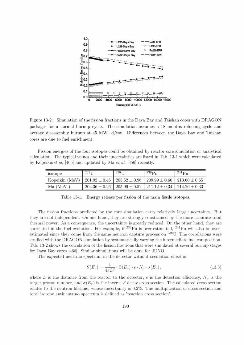
Figure 13-2: Simulation of the fission fractions in the Daya Bay and Taishan cores with DRAGON

packages for a normal burnup cycle. The simulation assumes a 18 months refueling cycle and

average disassembly burnup at 45 MW · d/ton. Differences between the Daya Bay and Taishan

cores are due to fuel enrichment.

Fission energies of the four isotopes could be obtained by reactor core simulation or analyticalcalculation. The typical values and their uncertainties are listed in Tab. 13-1 which were calculatedby Kopeikinet al. [465] and updated by Ma et al. [356] recently.

isotope 235U 238U 239Pu 241Pu

Kopeikin (MeV) 201.92 ± 0.46 205.52 ± 0.96 209.99 ± 0.60 213.60 ± 0.65

Ma (MeV ) 202.36 ± 0.26 205.99 ± 0.52 211.12 ± 0.34 214.26 ± 0.33

Table 13-1: Energy release per fission of the main fissile isotopes.

The fission fractions predicted by the core simulation carry relatively large uncertainty. Butthey are not independent. On one hand, they are strongly constrained by the more accurate totalthermal power. As a consequence, the uncertainty is greatly reduced. On the other hand, they arecorrelated in the fuel evolution. For example, if 239Pu is over-estimated, 241Pu will also be over-estimated since they come from the same neutron capture process on 238U. The correlations werestudied with the DRAGON simulation by systematically varying the intermediate fuel composition.Tab. 13-2 shows the correlation of the fission fractions that were simulated at several burnup stagesfor Daya Bay cores [466]. Similar simulations will be done for JUNO.

The expected neutrino spectrum in the detector without oscillation effect is

S(Eν) =1

4πL2· Φ(Eν) · ǫ ·Np · σ(Eν) , (13.3)

where L is the distance from the reactor to the detector, ǫ is the detection efficiency, Np is thetarget proton number, and σ(Eν) is the inverse β decay cross section. The calculated cross sectionrelates to the neutron lifetime, whose uncertainty is 0.2%. The multiplication of cross section andtotal isotope antineutrino spectrum is defined as ’reaction cross section’.

190

235U 238U 239Pu 241Pu235U 1.0 -0.22 -0.53 -0.18238U -0.22 1.0 0.18 0.26239Pu -0.53 0.18 1.0 0.49241Pu -0.18 0.26 0.49 1.0

Table 13-2: Correlation coefficients of isotope fission fraction uncertainties.

In ILL measurements, fissile samples were exposed in neutrons for one to two days. Therefore,the beta decays from some of the long-lived fission fragments not reaching equilibrium were missedin the ILL measurements. The long lived fission fragments accumulate in core during operationand contribute an extra antineutrino flux at low energy. This effect can be evaluated with nucleardatabase by using the cumulative yields of the known long-lived ( e.g. lifetime longer than 10hours) fission fragments which has Q-values above the inverse β decay threshold (1.8 MeV ) [102].On the other hand, after refueling the reactor cores, the spent fuel taken out from the previouscycle are moved to a cooling pool adjacent to the core. The long-lived isotopes will continue decayand generate antineutrinos. This contributions to the total antineutrinos can also be evaluated byusing the cumulative yields [360, 467–470]. The contribution to IBD events from off-equilibriumof long-lived isotopes in reactor cores and from spent fuel pools in the Daya Bay experiment wereevaluated to be both less than 0.3%. The uncertainties of them were taken as 100%, or 0.3% interms of the total IBD events. For JUNO experiment, the similar calculation could be done withthe reactor core and spent fuel pool information. The total neutrino spectrum should then bemodified by including the contributions from the off-equilibrium long-lived isotopes in reactor coresand from the spent fuel pools,

Sν(Eν) = S(Eν) + SoffEq + SSNF . (13.4)

The event rate of the IBD reactions in the k-th energy bin [Emink , Emax

k ] of a detector fromseveral reactor cores is given by

Rk(Eν) =∑

r

1

4πL2r

· W rth∑

i fri e

ri

·∑

i

f ri

∫ Emaxk

Emink

·Si(Eν) · σ(Eν)dEν · ǫ ·Np , (13.5)

where k is the bin index and r is the index of the reactor cores.The flux uncertainties can be propagated using Eq. (13.5). The reaction cross section uncer-

tainties are considered to be correlated between isotopes. The reactor-related uncertainties arecategorized into the reactor-correlated ones and reactor-uncorrelated ones, respectively. The corre-lated uncertainties includes those from energy per fission (0.2%) and reaction cross section (2.7%).The uncorrelated uncertainties are the combination of the thermal power (0.5%), fission fraction(0.6% with the thermal power constraint and correlation among isotopes), off-Equilibrium (0.3%)and spent fuel (0.3%).

The shape uncertainties can also be propagated using Eq. (13.5). There are two categoriesbasically, energy dependent and energy independent uncertainties. The energy independent uncer-tainties are same as flux uncertainties, such as power and fission energies. The energy dependentuncertainties includes the uncertainties of antineutrino flux per fission of each fuel isotope, theuncertainties of off-equilibrium and SNF corrections, and the uncertainties introduced by fission

191

fraction uncertainty. These energy dependent uncertainties are categorized as bin-to-bin corre-lated and uncorrelated uncertainties. The 235U, 239Pu and 241Pu spectra have both bin-to-binuncorrelated uncertainties (statistical uncertainties) and bin-to-bin correlated uncertainties (sys-tematic uncertainties from ILL measurements, and beta-antineutrino conversion), while the 238Uspectrum only has bin-to-bin correlated uncertainties since it is from theoretical calculation. Theoff-equilibrium uncertainties, spent fuel uncertainties and fission fraction uncertainties are treatedas energy correlated, but reactor uncorrelated.

13.1.5 Model Independent Prediction of the Antineutrino Spectrum

Recently, Daya Bay [105], RENO [106] Double Chooz [107] have found significant local inconsis-tency (at 4 ∼ 6 MeV) between the measured reactor neutrino spectrum and the predicted spectrum,no matter using the ILL+Vogel or the Huber+Mueller flux model. The largest deviation reaches∼ 10%, significantly larger than the expected uncertainty 2-3%. In 2014, there were new evalua-tions of the shape uncertainties of the antineutrino flux per fission from ILL measurement, whichclaimed that the uncertainties of the inversion from the β spectra to the antineutrino spectrum isunderestimated. The energy dependent uncertainty should be no less than 4% [391]. Further more,the latest calculation of the antineutrino flux per fission with the β branch information in databaseof the fission fragments indicates similar local structure of isotope antineutrino spectrum as themeasurements in the reactor antineutrino experiments [104].

One possible way to do more precise prediction of the expected antineutrino spectrum for JUNOis to use the measured positron spectrum of the Daya Bay experiment directly. The principle is totreat Daya Bay as a virtual near detector of the JUNO experiment. The reactor cores of Yangjiangand Taishan will be constructed and operated by the same company as Daya Bay. Similar coretechnology and simulation enable a virtual near/far relative measurement, where the reactor relateduncertainties are almost cancelled, and the relative detector uncertainties between near and far siteis the main contribution of final uncertainty. Detector simulation would help to determine therelative uncertainty of energy scale between the antineutrino detectors of JUNO and Daya Bay.The current absolute energy scale uncertainty of Daya Bay is within 1% and the energy non-linearityhas been determined to ∼ 1%.

We expect that the shape uncertainties of the measured positron spectrum for JUNO could bedetermined to 1% with further studies. As an alternative method, the antineutrino spectrum fromunfolding of the direct measurement of Daya Bay could be also used for spectrum prediction. Theunfolded spectrum is independent of the Daya Bay detector effect, could be used more generally,such as comparing with different reactor models of antineutrino spectrum, and predicting themeasured positron spectrum by applying their own detector effects of the experiments [105].

13.2 Monte Carlo Simulation and Reconstruction

13.2.1 Monte Carlo Simulation

A Geant4 [321, 472] based computer simulation (Monte Carlo, MC) of the detectors and readoutelectronics is used to study the detector response and optimize the detector design. It consists of fivecomponents: kinematic generator, detector simulation, electronics simulation, trigger simulationand readout simulation. The JUNO MC is developed based on the Daya Bay MC simulation, whichhas been carefully tuned to match observed detector distributions, such as the liquid scintillatorlight yield, charge response, and energy non-linearity.

The antineutrino generator reads from a database that stored the reactor antineutrino spectra.

192

The cosmic muons in the underground laboratory are simulated using a digitized topographicmap of the site and Muon Simulation Code [473] (MUSIC), which calculates the energy loss andmultiple scattering due to the rock overburden. The muon generator for Geant4 reads randomlyfrom a library of muon events generated with MUSIC. The software generators for the calibrationsources and the simulation of the decay sequences for natural radionuclides found in our detectorsare customized based on data from the ENDF database [474].

All physical processes in Geant4 relevant to the reactor neutrino experiment have been vali-dated. The gamma spectra of neutron capture and muon capture on many nuclei are incorrectlymodeled in Geant4. Since a systematic correction is complex, we implement corrections on a caseby case basis. Furthermore, the simulation of thermal neutron scattering is improved by consideringthe molecular binding energy of the scattering nuclei.

The details of the electronics simulation can be found in Ref. [475, 476]. Using the timingand number of photoelectron (p.e.) generated in PMTs, an analog signal pulse for each PMT isgenerated and tracked through the digitization process, taking into account the non-linearity, darkrate, pre-pulsing, after-pulsing and ringing of the waveform. The simulated analog pulse is thenused as input to a trigger system simulation.

Most of the properties of the detector materials are borrowed from the Daya Bay experiment.The elemental concentrations of the liquid scintillator were measured and incorporated into theMC. All relevant optical properties of the detector components are derived from measurements,including refractive indices of the liquids as well as the acrylic or nylon components, time constantsand photon emission spectra of the liquid scintillator, and the reflectivity of the detector materials.Photon absorption and re-emission processes in liquid scintillator are modeled based on measure-ments in order to properly simulate the propagation of scintillation photons and contributions fromCherenkov process.

The major differences from the Daya Bay MC include the detector geometry, the attenuationlength and the rayleigh scattering length of the liquid scintillator, and the PMT geometry andquantum efficiency. The detector is spherical, of a diameter of 35.4 m for the liquid scintillatorcontainer. Currently there are two options for the central detector to be determined with R&D.One use an acrylic ball as the LS container. PMTs are installed on a truss and look inward in thewater buffer. The water cherenkov detector for muon veto is optically separated from the waterbuffer for the center detector. Another option is a nylon balloon as the LS container. PMTs areinstalled on the inner wall of a stainless steel sphere and shielded with non-scintillation liquid.Both options are implemented in the MC and simulated to compare the detector performance. Toachieve an energy resolution of 3%/

√E, 17746 20-inch PMTs corresponding to 77% photocathode

coverage are used. The quantum efficiency is set to be 35%. The attenuation length of the LS is setto be 20 m, larger than 15 m for the Daya Bay. Recently we have measured the rayleigh scatteringlength of the liquid scintillator to be ∼ 30 m. The light yield of the liquid scintillator is tuned tothe data of the Daya Bay detector. We find that the 3%/

√E energy resolution is achieved with

the above settings. Therefore, they served as the requirements for the JUNO detector design. Thebaseline parameters of the JUNO MC are shown in Tab. 13-3, as well as in the following.

Detector dimensions. The scintillator volume is 35.4 m in diameter, surrounded by a buffermedium with a thickness of 1.5 m, either water in the acrylic ball option or non-scintillation oil inthe balloon option. PMTs are assumed to be 20-inch PMTs, with their bulk center located at 19.5m in radius. The number of PMTs is 17746. The water pool, as the cherenkov detector for muons,is a cylinder of 42.5 m in diameter and 42.5 m in height.

Light emission. The light yield of the liquid scintillator is about 10000 photons per MeV.The exact value may vary by the order of 10% depending on the scintillator solvent and fluorconcentrations. For different settings in the simulation, we normalize the light yield to the response

193

target mass 20 kt

target radius 17.7 m

target density 0.856 g/cm3

mass fraction of C 0.8792

mass fraction of H 0.1201

light yield 10400 /MeV

birks1 6.5 × 10−3 g/cm2/MeV

birks2 1.5 × 10−6 (g/cm2/MeV)2

emission time τ1 4.93 ns

emission time τ2 20.6 ns

emission time τ3 190 ns

τ1 weight 0.799

τ2 weight 0.171

τ3 weight 0.03

attenuation length 20 m

absorption length 60 m

rayleigh scat. length 30 m

optical coverage 75%

quantum efficiency 35%

Table 13-3: Baseline parameters in the JUNO MC simulation.

of the Daya Bay detector. The light output also depends on the energy loss rate dE/dx of theionizing particle, resulting in a quenched visible energy. This effect is taken into account by theBirks’ law,

Quenched Energy =Energy Deposit

1 +C1dEdx + C2

(dEdx

)2 . (13.6)

The light is emitted following a time profile described by a superposition of exponential decays. Thesimulation uses a description of three components with time constants τ1, τ2, and τ3, respectively.

Light propagation. The scintillation light is produced in a relatively broad span of wave-lengths. The emission spectrum of liquid scintillator is from the Daya Bay measurements. Thephoton absorption, re-emission, and Rayleigh scattering are simulated.

Light detection. The baseline design for JUNO assumes an photocathode coverage of 77%and 35% peak quantum efficiency of the PMTs. The quantum efficiency spectrum is scaled fromthe Daya Bay PMTs.

Based on these configurations, the p.e. yield per deposited energy can be obtained as a functionof the vertex position inside the target volume. The p.e. yield significantly depends on vertex posi-tion, the transparency of liquid scintillator container, and the refractive indices of liquid materials,as shown in Figure 13-3.

13.2.2 Reconstruction and performance

Since the energy of the reactor antineutrino is mainly below 10 MeV, it can be approximated asa point-like source in the JUNO detector. The vertex can be determined by the measurement of

194

)3(m3R0 1000 2000 3000 4000 5000 6000

tota

l p.e

.

0

200

400

600

800

1000

1200

1400

Acrylic-Option

Balloon-Option(PE_PA film)

Balloon-Option(ETFE film)

Figure 13-3: Total p.e. for 1 MeV gamma uniformly generated in the central detector.

the time of flight to each PMT. In case of multiple photoelectrons that hit on the same PMT, onlythe first hit time is used in the reconstruction because the latter ones may be distorted due to theresponse of electronics. The vertex resolution depends on the PMT time resolution as well as thetime spread of the light emission of the liquid scintillator.

The performance of the vertex reconstruction is studied using single γ or positron uniformlydistributed in the detector. Fig. 13-4 (left) shows the vertex resolution as a function of visibleenergy, assuming a PMT time resolution of 1 ns. Fig. 13-4 (right) shows the impact of the PMTtime resolution. It dominates the vertex performance when larger than 4 ns, while the decay timeof the scintillation light becomes significant when it is better than 2 ns.

(MeV)trueE1 2 3 4 5 6 7 8

sigm

a(m

m)

35

40

45

50

55

60

65

70

75

80PMT time resolution: 1ns

(ns)restime0 1 2 3 4 5 6 7 8

(mm

)re

sve

rtex

60

80

100

120

140

160

180

P=0MeV e+

Figure 13-4: Vertex resolution as a function of energy (left) and PMT time resolution (right).

The visible energy in the detector is reconstructed by comparing the measured charge of eachPMT with the expectation, which relies on the event vertex, the light emission and propagation,and the photon detection with PMTs. The energy solution as a function of the visible energy canbe described with a 3-parameter function

σ

E=

√(p0√E

)2

+ p21 +(p2E

)2, (13.7)

where E refers to the visible energy in MeV, p0 is the leading term dominated by the photonstatistics, p1 and p2 come from detector effects such as PMT dark noise, variation of the PMT QE,

195

and the reconstructed vertex smearing. Toy MC samples are generated to study each term, whichis shown in Tab. 13-4.

effects p0 p1 p2

statistical fluctuation 2.68 0 0

PMT charge resolution(30%) 2.8 0 0

PMT dark noise(50kHz per PMT) 2.68 0 0.9

PMT QE difference(20%) 2.68 0.26 0

vertex smearing(11cm @1MeV) 2.68 0.17 0

Table 13-4: Factors that impact to the energy resolution.

Muon tracking is important for the cosmogenic background rejection and the atmosphericneutrino study. Similar to the vertex reconstruction, a track is determined by the the first hittime of each PMT. For the muons that go through the detector, the PMTs around the injectionpoint and the outgoing point see more lights and form two clusters, which can be used to estimatethe initial tracking parameters. Toy MC samples are used to estimate the tracking performance.Assuming the intrinsic PMT time resolution is better than 4 ns, for a muon track longer than 5 m(i.e. > 1 GeV), the track length resolution is better than 0.5% and the angular resolution is betterthan 1 degree. For a muon track between 1 m and 5 m (i.e. 0.2 GeV < E < 1 GeV), the tracklength resolution is better than 1% and the angular resolution is better than 10 degree. Trackingof electrons and identification of muon/electron are still under development.

13.3 Antineutrino Detection in JUNO

Antineutrinos from reactors are detected by LS via the inverse beta decay reaction (shorten as IBDin the following contents):

νe + p→ e+ + n

The prompt positron signal and delayed neutron capture signal constitute an anti-neutrino event.In LS, neutron are captured by free protons or Carbon with a capture time of ∼216µs obtained byMC simulation. The delayed signal, 2.2 MeV γ-ray emitted after neutron captured on proton, canbe contaminated by the natural radioactivity. Thus, a triple-coincidence criteria of energy, timeand space is necessary to suppress the accidental background.

Full MC simulation and reconstruction is performed to obtain the antineutrino detection effi-ciency. The efficiency of (0.7 MeV, 12 MeV) energy cut on prompt signal is 100%. The efficiencyof (1.9 MeV, 2.5 MeV) cut on the delayed signal is 97.8%, and the in-efficiency is mainly due toneutron-capture on Carbon. The efficiency for different time-, and space- correlation cuts are listedin Tab. 13-5 and Tab. 13-6.

Time Cut (µs) 300 500 1000 1500 2000

Efficiency (%) 74.55 89.57 98.68 99.49 99.60

Table 13-5: IBD efficiency of different time cuts from MC simulation.

196

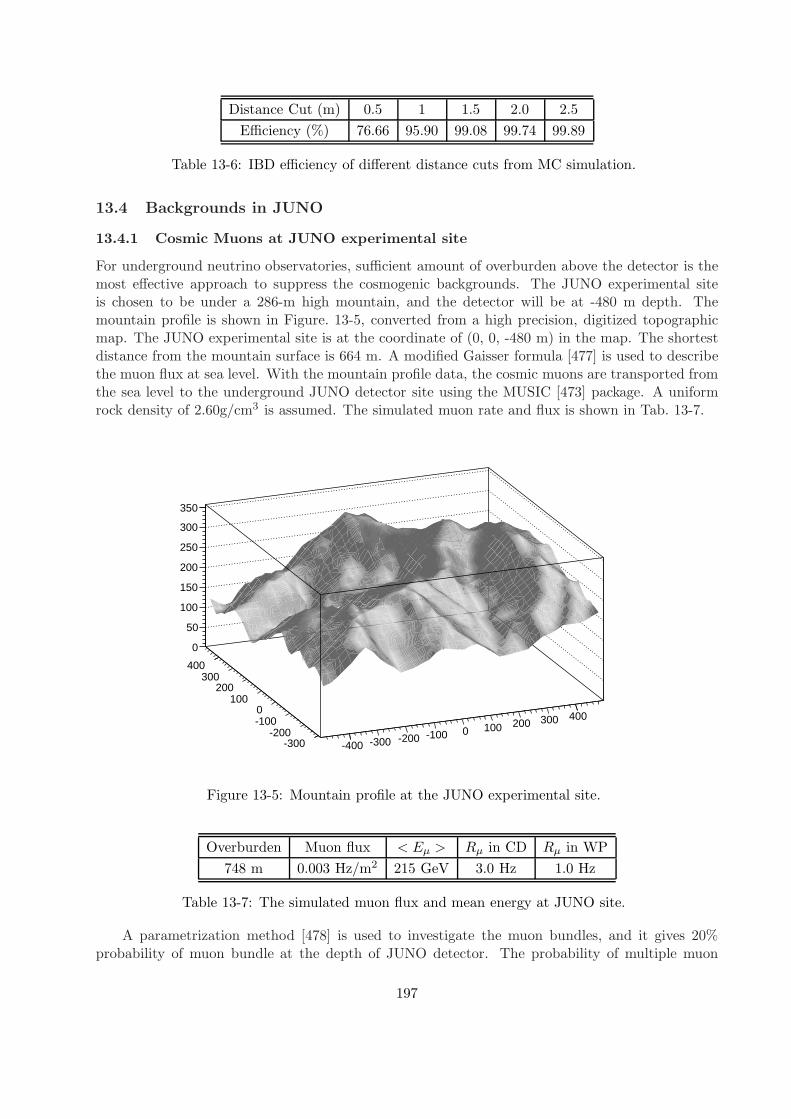
Distance Cut (m) 0.5 1 1.5 2.0 2.5

Efficiency (%) 76.66 95.90 99.08 99.74 99.89

Table 13-6: IBD efficiency of different distance cuts from MC simulation.

13.4 Backgrounds in JUNO

13.4.1 Cosmic Muons at JUNO experimental site

For underground neutrino observatories, sufficient amount of overburden above the detector is themost effective approach to suppress the cosmogenic backgrounds. The JUNO experimental siteis chosen to be under a 286-m high mountain, and the detector will be at -480 m depth. Themountain profile is shown in Figure. 13-5, converted from a high precision, digitized topographicmap. The JUNO experimental site is at the coordinate of (0, 0, -480 m) in the map. The shortestdistance from the mountain surface is 664 m. A modified Gaisser formula [477] is used to describethe muon flux at sea level. With the mountain profile data, the cosmic muons are transported fromthe sea level to the underground JUNO detector site using the MUSIC [473] package. A uniformrock density of 2.60g/cm3 is assumed. The simulated muon rate and flux is shown in Tab. 13-7.

-400 -300 -200 -100 0 100 200 300 400

-300-200

-1000

100200

300400

0

50

100

150

200

250

300

350

Figure 13-5: Mountain profile at the JUNO experimental site.

Overburden Muon flux < Eµ > Rµ in CD Rµ in WP

748 m 0.003 Hz/m2 215 GeV 3.0 Hz 1.0 Hz

Table 13-7: The simulated muon flux and mean energy at JUNO site.

A parametrization method [478] is used to investigate the muon bundles, and it gives 20%probability of muon bundle at the depth of JUNO detector. The probability of multiple muon

197

bundle reduces to 10% after taking into account the JUNO detector geometry. MC simulationindicates the muons in the bundle are almost in parallel within 0.2. The multiplicity of muonsgoing through JUNO detector is shown in Table. 13-8.

Multiplicity 1 2 3 4 5 6

Fraction 89.6% 7.7% 1.8% 0.6% 0.3% 0.07%

Table 13-8: The multiplicity of muons going through JUNO detector.

13.4.2 Neutrons

The neutron production depends on the muon flux and the average energy at the JUNO detector.Full muon simulation using Geant4 gives ∼1.8 Hz spallation neutrons in JUNO LS.

Neutron produced by muons passing through the JUNO LS will be tagged with almost 100%efficiency. Neutron produced in water buffer can be tagged with an efficiency of 99.8%, since theirparent muons pass through the muon systems. The 0.2% inefficiency is mainly from the cornerclipping muons. The tagged neutrons can be rejected by sufficient time veto after the tagged muonsto suppress the possible correlated background.

Neutrons produced by the un-tagged corner clipping muons and in the surrounding rocks arisefrom the muons missing muon systems, have to traverse at least 3.2 m for the “Sphere Acrylic”option (or 2.5 m for “Balloon” option) to reach JUNO LS. The “un-tagged” neutrons can enterLS and produce prompt proton-recoil signal then captured by H or C in LS. These events, namelythe fast neutron events, can mimic the anti-neutrino signal as correlated backgrounds. A full MCsimulation is performed to propagate the neutrons produced by cosmic muons in water pool andsurrounding rocks, and the fast neutrons mimicking the anti-neutrino events are estimated to be∼0.1/day.

13.4.3 Cosmogenic Isotopes

In the liquid scintillator, the energetic cosmic muons and subsequent showers can interact with 12Cand produce radioactive isotopes with Z ≤ 6 by electromagnetic or hadronic processes. Amongthem, 9Li and 8He with half-lives of 0.178 s and 0.119 s, respectively, are the most serious correlatedbackground source to reactor anti-neutrinos, because they can decay by emitting both a beta anda neutron which mimics as an anti-neutrino signal. The estimation of 9Li and 8He is discussedin detail in Section 2.2.2. Other isotopes, such as 11Li, 12Be, 14B, 16C, 17N and 18N, are alsobeta-neutron emitters but have much less contribution to the background.

The other long-lived cosmogenic isotopes have beta decay without an accompanying neutron.They can not form correlated backgrounds by themselves but can contribute the neutron-like signalif they have beta decay energy in the 1.9-2.5 MeV range. Measuring the isotopes production yield inJUNO detector is useful for understanding the muon shower spallation processes. The rates of thosecosmogenic radioactive isotopes from FLUKA MC simulation are listed in Table. 13-9. Recentlythere are measurements from KamLAND [109] and Borexino [305]. Physics-driven model is builtto analyze the cosmogenic backgrounds in Super-K [307,308], which could significantly reduce thebackgrounds, and also increase the live time by well defining the shower position. Cosmogenicbackgrounds in JUNO detector will be elaborated with these studies.

198

Isotopes Q (MeV) T1/2 Rate (per day)3H 0.0186 (β−) 12.31 year 1.14×104

6He 3.508 (β−) 0.807 s 5447Be QEC=0.862 (10.4% γ, Eγ = 0.478) 53.22 day 54388He 10.66 (β−γ : 84%), 8.63 (β−n : 16%) 0.119 s 118Li 16.0 (β−) 0.839 s 9388B 16.6 (β+) 0.770 s 2259Li 13.6 (β− : 49%), 11.94 (β−n : 51%) 0.178 s 949C 15.47 (β+p : 61.6%, β+α : 38.4%) 0.126 s 31

10Be 0.556 (β−) 1.51e6 year 141910C 2.626 (β+γ) 19.29 s 48211Li 20.55 (β−n : 83%, β−2n : 4.1%) 0.00875 s 0.0611Be 11.51 (β−γ : 96.9%), 2.85 (β−α : 3.1%) 13.76 s 2411C 0.960 (β+) 20.36 min 1.62×104

12Be 11.708 (β−γ, β−n : 0.5%) 0.0215 s 0.4512B 13.37 (β−γ) 0.0202 s 96612N 16.316 (β+γ) 0.0110 s 1713B 13.437 (β−γ) 0.0174 s 1213N 1.198 (β+) 9.965 min 1914B 20.644 (β−γ, β−n : 6.1%) 0.0126 s 0.02114C 0.156 (β−) 5730 year 13215C 9.772 (β−) 2.449 s 0.616C 8.010 (β−n : 99%) 0.747 s 0.01216N 10.42 (β−γ) 7.130 s 1317N 8.680 (β−γ : 5%), 4.536 (β−n : 95%) 4.173 s 0.4218N 13.896 (β−γ : 93%), 5.851 (β−n : 7%) 0.620 s 0.009

neutron 155 000

Table 13-9: The estimated rates for cosmogenic isotopes in JUNO LS by FLUKA simulation, in

which the oxygen isotopes are neglected. The decay modes and Q values are from TUNL Nuclear

Data Group [479].

13.4.4 Natural Radioactivity

Natural radioactivity exists in the material of JUNO detector components and its surroundings.Particular care need be taken to select low radioactivity materials and design the passive shielding tocontrol the radioactivity background. For JUNO experiment, the radioactivity comes from varioussources. For simplicity, the radioactive isotopes 238U, 232Th, 222Rn, 85Kr, 60Co, 40K are shorten asU, Th, Rn, Kr, Co, K in the following text. The radioactive sources include:

• U/Th/K in the rocks around the detector hall

• U/Th/K and Rn dissolved in the water buffer

• U/Th/K/Co in the stainless steel (vessel or strut)

199

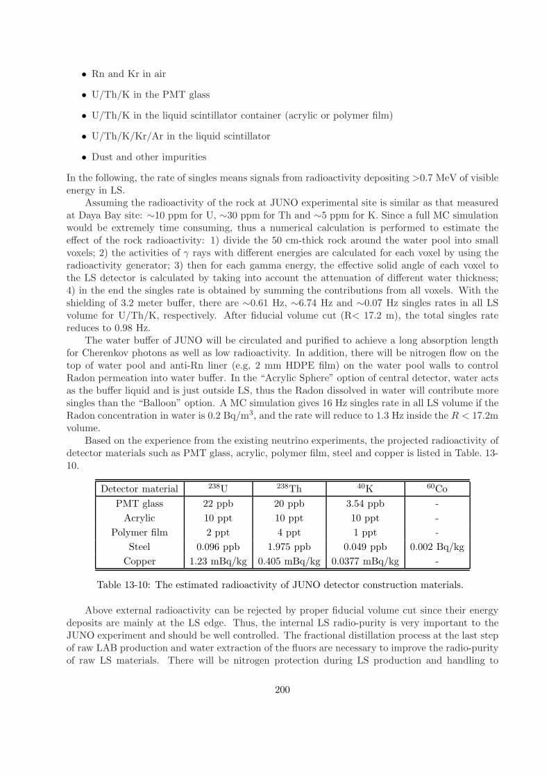
• Rn and Kr in air

• U/Th/K in the PMT glass

• U/Th/K in the liquid scintillator container (acrylic or polymer film)

• U/Th/K/Kr/Ar in the liquid scintillator

• Dust and other impurities

In the following, the rate of singles means signals from radioactivity depositing >0.7 MeV of visibleenergy in LS.

Assuming the radioactivity of the rock at JUNO experimental site is similar as that measuredat Daya Bay site: ∼10 ppm for U, ∼30 ppm for Th and ∼5 ppm for K. Since a full MC simulationwould be extremely time consuming, thus a numerical calculation is performed to estimate theeffect of the rock radioactivity: 1) divide the 50 cm-thick rock around the water pool into smallvoxels; 2) the activities of γ rays with different energies are calculated for each voxel by using theradioactivity generator; 3) then for each gamma energy, the effective solid angle of each voxel tothe LS detector is calculated by taking into account the attenuation of different water thickness;4) in the end the singles rate is obtained by summing the contributions from all voxels. With theshielding of 3.2 meter buffer, there are ∼0.61 Hz, ∼6.74 Hz and ∼0.07 Hz singles rates in all LSvolume for U/Th/K, respectively. After fiducial volume cut (R< 17.2 m), the total singles ratereduces to 0.98 Hz.

The water buffer of JUNO will be circulated and purified to achieve a long absorption lengthfor Cherenkov photons as well as low radioactivity. In addition, there will be nitrogen flow on thetop of water pool and anti-Rn liner (e.g, 2 mm HDPE film) on the water pool walls to controlRadon permeation into water buffer. In the “Acrylic Sphere” option of central detector, water actsas the buffer liquid and is just outside LS, thus the Radon dissolved in water will contribute moresingles than the “Balloon” option. A MC simulation gives 16 Hz singles rate in all LS volume if theRadon concentration in water is 0.2 Bq/m3, and the rate will reduce to 1.3 Hz inside the R < 17.2mvolume.

Based on the experience from the existing neutrino experiments, the projected radioactivity ofdetector materials such as PMT glass, acrylic, polymer film, steel and copper is listed in Table. 13-10.

Detector material 238U 238Th 40K 60Co

PMT glass 22 ppb 20 ppb 3.54 ppb -

Acrylic 10 ppt 10 ppt 10 ppt -

Polymer film 2 ppt 4 ppt 1 ppt -

Steel 0.096 ppb 1.975 ppb 0.049 ppb 0.002 Bq/kg

Copper 1.23 mBq/kg 0.405 mBq/kg 0.0377 mBq/kg -

Table 13-10: The estimated radioactivity of JUNO detector construction materials.

Above external radioactivity can be rejected by proper fiducial volume cut since their energydeposits are mainly at the LS edge. Thus, the internal LS radio-purity is very important to theJUNO experiment and should be well controlled. The fractional distillation process at the last stepof raw LAB production and water extraction of the fluors are necessary to improve the radio-purityof raw LS materials. There will be nitrogen protection during LS production and handling to

200

suppress Radon contamination. In addition, the residual Radon contamination will lead to non-equilibrium isotope 210Pb (and the subsequent 210Bi decay) which has 22-year half life. The 210Pbisotope is the dominant background in searching solar neutrinos, as discussed in Section.6. On-linepurification, such as distillation, is required to remove 210Pb from LS to open the opportunity toobserve 7Be solar neutrino. In the JUNO experiment, an initial purity level of 10−15 g/g U/Th,10−16 g/g K and 1.4 · 10−22 g/g 210Pb can be achieved without distillation. After setting up theon-line distillation, we believe two orders of magnitude better purity level can be achieved: 10−17

g/g U/Th, 10−18 g/g K and 10−24 g/g 210Pb. The purity level of other isotope such as 85Kr and39Ar is also listed.

LS 238U 238Th 40K 210Pb 85Kr 39Ar

No distillation 10−15 g/g 10−15 g/g 10−16 g/g 1.4 · 10−22 g/g 50 µBq/m3 50 µBq/m3

After distillation 10−17 g/g 10−17 g/g 10−18 g/g 10−24 g/g 1 µBq/m3 -

Table 13-11: The estimated radioactivity of JUNO LS.

Full MC simulation is performed to obtain the singles rates from LS and other detector con-struction materials. Taking the “Acrylic Sphere” option of central detector, the singles rates indifferent volumes are listed in Table. 13-12.

Fiducial Cut LS (Hz) PMT (Hz) Acrylic (Hz) Strut (Hz) Fastener (Hz) Sum (Hz)

R<17.7 m 2.39 2.43 69.23 0.89 0.82 75.75

R<17.6 m 2.35 1.91 41.27 0.66 0.55 46.74

R<17.5 m 2.31 1.03 21.82 0.28 0.32 25.75

R<17.4 m 2.27 0.75 12.23 0.22 0.19 15.66

R<17.3 m 2.24 0.39 6.47 0.13 0.12 9.33

R<17.2 m 2.20 0.33 3.61 0.083 0.087 6.31

R<17.1 m 2.16 0.23 1.96 0.060 0.060 4.47

R<17.0 m 2.12 0.15 0.97 0.009 0.031 3.28

Table 13-12: The simulated singles rates from different detector components.

A fiducial volume cut is necessary to reject the external radioactivity thus reduce the accidentalbackground and (α, n) background, as discussed in Section.2. The total singles rate will reduce to∼7.6 Hz if applying an R< 17.2 m fiducial volume cut, as shown in Table. 13-13.

Fiducial Cut Detector Components Radon in water Rock Total

R<17.2 m 6.3 Hz 1.3 Hz 0.98 Hz 7.63 Hz

Table 13-13: The summary of singles rates inside the Fiducial volume from the detector components,

Radon in water and rock.

201

Acknowledgement

The JUNO Experiment is supported by the Chinese Academy of Sciences, the Ministry of Scienceand Technology of China, the National Natural Science Foundation of China, Shanghai Jiao TongUniversity, and Tsinghua University in China, the Belgian Fonds de la Recherche Scientifique,FNRS in Belgium, the Charles University in Prague, Czech Republic, the CNRS National Instituteof Nuclear and Particle Physics (IN2P3) in France, the Deutsche Forschungsgemeinschaft (DFG),Helmholtz Alliance for Astroparticle Physics (HAP), and Helmholtz Gemeinschaft (HGF) in Ger-many, the Istituto Nazionale di Fisica Nucleare (INFN) in Italy, the Joint Institute for NuclearResearch (JINR) in Russia, and the NSFC-RFBR joint research program. We acknowledge thegenerous support of the Guangdong provincial government and the Jiangmen and Kaiping Munic-ipal Government. We are grateful for the ongoing cooperation from the China General NuclearPower Group (CGNPC).

202

References

[1] S. Weinberg, Phys. Rev. Lett. 19, 1264 (1967).

[2] R. Davis, Jr., D. S. Harmer and K. C. Hoffman, Phys. Rev. Lett. 20, 1205 (1968).

[3] J. N. Bahcall, N. A. Bahcall and G. Shaviv, Phys. Rev. Lett. 20, 1209 (1968).

[4] J. N. Bahcall, W. F. Huebner, S. H. Lubow, P. D. Parker and R. K. Ulrich, Rev. Mod. Phys.54, 767 (1982).

[5] Z. Maki, M. Nakagawa and S. Sakata, Prog. Theor. Phys. 28, 870 (1962).

[6] B. Pontecorvo, Sov. Phys. JETP 26, 984 (1968) [Zh. Eksp. Teor. Fiz. 53, 1717 (1967)].

[7] N. Cabibbo, Phys. Rev. Lett. 10, 531 (1963).

[8] M. Kobayashi and T. Maskawa, Prog. Theor. Phys. 49, 652 (1973).

[9] Z. z. Xing and S. Zhou, “Neutrinos in particle physics, astronomy and cosmology,” Springer-Verlag, Berlin Heidelberg (2011).

[10] W. Konetschny and W. Kummer, Phys. Lett. B 70, 433 (1977).

[11] M. Magg and C. Wetterich, Phys. Lett. B 94, 61 (1980).

[12] T. P. Cheng and L. F. Li, Phys. Rev. D 22, 2860 (1980).

[13] G. Lazarides, Q. Shafi and C. Wetterich, Nucl. Phys. B 181, 287 (1981).

[14] R. N. Mohapatra and G. Senjanovic, Phys. Rev. D 23, 165 (1981).

[15] P. Minkowski, Phys. Lett. B 67, 421 (1977).

[16] T. Yanagida, in Proceedings of the Workshop on Unified Theory and the Baryon Number ofthe Universe, edited by O. Sawada and A. Sugamoto (KEK, Tsukuba, 1979), p. 95.

[17] M. Gell-Mann, P. Ramond, and R. Slansky, in Supergravity, edited by P. van Nieuwenhuizenand D. Freedman (North Holland, Amsterdam, 1979), p. 315.

[18] S. L. Glashow, in Quarks and Leptons, edited by M. Levy et al. (Plenum, New York, 1980),p. 707.

[19] R. N. Mohapatra and G. Senjanovic, Phys. Rev. Lett. 44, 912 (1980).

[20] J. Schechter and J. W. F. Valle, Phys. Rev. D 22, 2227 (1980).

[21] R. Foot, H. Lew, X. G. He and G. C. Joshi, Z. Phys. C 44, 441 (1989).

[22] S. Antusch, C. Biggio, E. Fernandez-Martinez, M. B. Gavela and J. Lopez-Pavon, JHEP0610, 084 (2006) [hep-ph/0607020].

[23] S. Antusch and O. Fischer, JHEP 1410, 94 (2014) [arXiv:1407.6607 [hep-ph]].

[24] Z. z. Xing, Phys. Lett. B 718, 1447 (2013) [arXiv:1210.1523 [hep-ph]].

203

[25] Y. F. Li and S. Luo, arXiv:1508.00052 [hep-ph].

[26] K. A. Olive et al. [Particle Data Group Collaboration], Chin. Phys. C 38, 090001 (2014).

[27] F. Capozzi, G. L. Fogli, E. Lisi, A. Marrone, D. Montanino and A. Palazzo, Phys. Rev. D89, 093018 (2014) [arXiv:1312.2878 [hep-ph]].

[28] D. V. Forero, M. Tortola and J. W. F. Valle, Phys. Rev. D 90, no. 9, 093006 (2014)[arXiv:1405.7540 [hep-ph]].

[29] M. C. Gonzalez-Garcia, M. Maltoni and T. Schwetz, JHEP 1411, 052 (2014) [arXiv:1409.5439[hep-ph]].

[30] F. P. An et al. [Daya Bay Collaboration], Phys. Rev. Lett. 108, 171803 (2012)[arXiv:1203.1669 [hep-ex]].

[31] F. P. An et al. [Daya Bay Collaboration], Chin. Phys. C 37, 011001 (2013) [arXiv:1210.6327[hep-ex]].

[32] F. P. An et al. [Daya Bay Collaboration], Phys. Rev. Lett. 112, 061801 (2014)[arXiv:1310.6732 [hep-ex]].

[33] E. Majorana, Nuovo Cim. 14, 171 (1937).

[34] W. H. Furry, Phys. Rev. 56, 1184 (1939).

[35] W. Rodejohann, Int. J. Mod. Phys. E 20, 1833 (2011) [arXiv:1106.1334 [hep-ph]].

[36] S. Dell’Oro, S. Marcocci and F. Vissani, Phys. Rev. D 90, no. 3, 033005 (2014)[arXiv:1404.2616 [hep-ph]].

[37] S. M. Bilenky and C. Giunti, Int. J. Mod. Phys. A 30, no. 04n05, 1530001 (2015)[arXiv:1411.4791 [hep-ph]].

[38] Y. F. Li and Z. z. Xing, Phys. Lett. B 695, 205 (2011) [arXiv:1009.5870 [hep-ph]].

[39] J. Bernabeu, S. Palomares Ruiz and S. T. Petcov, Nucl. Phys. B 669, 255 (2003) [hep-ph/0305152].

[40] A. S. Dighe and A. Y. Smirnov, Phys. Rev. D 62, 033007 (2000) [hep-ph/9907423].

[41] S. T. Petcov and M. Piai, Phys. Lett. B 533, 94 (2002) [hep-ph/0112074].

[42] X. Qian and P. Vogel, Prog. Part. Nucl. Phys. 83, 1 (2015) [arXiv:1505.01891 [hep-ex]].

[43] R. B. Patterson, arXiv:1506.07917 [hep-ex].

[44] M. Fukugita and T. Yanagida, Phys. Lett. B 174, 45 (1986).

[45] W. Buchmuller, P. Di Bari and M. Plumacher, Annals Phys. 315, 305 (2005) [hep-ph/0401240].

[46] S. Davidson, E. Nardi and Y. Nir, Phys. Rept. 466, 105 (2008) [arXiv:0802.2962 [hep-ph]].

[47] M. Agostini et al. [GERDA Collaboration], Phys. Rev. Lett. 111, no. 12, 122503 (2013)[arXiv:1307.4720 [nucl-ex]].

204

[48] L. Bornschein [KATRIN Collaboration], eConf C 030626, FRAP14 (2003) [hep-ex/0309007].

[49] P. A. R. Ade et al. [Planck Collaboration], Astron. Astrophys. 571, A16 (2014)[arXiv:1303.5076 [astro-ph.CO]].

[50] Z. z. Xing and S. Zhou, Phys. Lett. B 737, 196 (2014) [arXiv:1404.7021 [hep-ph]].

[51] S. Luo and Z. z. Xing, Phys. Rev. D 90, no. 7, 073005 (2014) [arXiv:1408.5005 [hep-ph]].

[52] Y. L. Zhou, arXiv:1409.8600 [hep-ph].

[53] Z. z. Xing and Y. L. Zhou, Phys. Rev. D 88, 033002 (2013) [arXiv:1305.5718 [hep-ph]].

[54] Z. z. Xing, Z. h. Zhao and Y. L. Zhou, arXiv:1504.05820 [hep-ph].

[55] K. N. Abazajian, M. A. Acero, S. K. Agarwalla, A. A. Aguilar-Arevalo, C. H. Albright,S. Antusch, C. A. Arguelles and A. B. Balantekin et al., arXiv:1204.5379 [hep-ph].

[56] A. Aguilar-Arevalo et al. [LSND Collaboration], Phys. Rev. D 64, 112007 (2001) [hep-ex/0104049].

[57] A. A. Aguilar-Arevalo et al. [MiniBooNE Collaboration], Phys. Rev. Lett. 105, 181801 (2010)[arXiv:1007.1150 [hep-ex]].

[58] G. Mention, M. Fechner, T. Lasserre, T. A. Mueller, D. Lhuillier, M. Cribier and A. Le-tourneau, Phys. Rev. D 83, 073006 (2011) [arXiv:1101.2755 [hep-ex]].

[59] J. Kopp, P. A. N. Machado, M. Maltoni and T. Schwetz, JHEP 1305, 050 (2013)[arXiv:1303.3011 [hep-ph]].

[60] C. Giunti, M. Laveder, Y. F. Li and H. W. Long, Phys. Rev. D 88, 073008 (2013)[arXiv:1308.5288 [hep-ph]].

[61] J. Hamann, S. Hannestad, G. G. Raffelt, I. Tamborra and Y. Y. Y. Wong, Phys. Rev. Lett.105, 181301 (2010) [arXiv:1006.5276 [hep-ph]].

[62] J. Hamann, S. Hannestad, G. G. Raffelt and Y. Y. Y. Wong, JCAP 1109, 034 (2011)[arXiv:1108.4136 [astro-ph.CO]].

[63] E. Giusarma, M. Corsi, M. Archidiacono, R. de Putter, A. Melchiorri, O. Mena and S. Pan-dolfi, Phys. Rev. D 83, 115023 (2011) [arXiv:1102.4774 [astro-ph.CO]].

[64] P. Bode, J. P. Ostriker and N. Turok, Astrophys. J. 556, 93 (2001) [astro-ph/0010389].

[65] L. Zhan, Y. Wang, J. Cao and L. Wen, Phys. Rev. D 78, 111103 (2008) [arXiv:0807.3203[hep-ex]].

[66] L. Zhan, Y. Wang, J. Cao and L. Wen, Phys. Rev. D 79, 073007 (2009) [arXiv:0901.2976[hep-ex]].

[67] Yifang Wang, talk at ICFA seminar, (2008). http://www-conf.slac.stanford.edu/

icfa2008/Yifang_Wang_102808.pdf

[68] Jun Cao, talk at Neutrino Telescope, (2009). http://neutrino.pd.infn.it/NEUTEL09/

Talks/Cao.pdf

205

[69] Y. F. Li, J. Cao, Y. Wang and L. Zhan, Phys. Rev. D 88, 013008 (2013) [arXiv:1303.6733[hep-ex]].

[70] Q. Liu, X. Zhou, W. Huang, Y. Zhang, W. Wu, W. Luo, M. Yu and Y. Zheng et al., Nucl.Instrum. Meth. A 795, 284 (2015) [arXiv:1504.01001 [physics.ins-det]].

[71] T. Adam, E. Baussan, K. Borer, J. E. Campagne, N. Con-Sen, C. de La Taille, N. Dick andM. Dracos et al., Nucl. Instrum. Meth. A 577, 523 (2007) [physics/0701153].

[72] Y. Abe et al. [Double Chooz Collaboration], Phys. Rev. Lett. 108, 131801 (2012)[arXiv:1112.6353 [hep-ex]].

[73] J. K. Ahn et al. [RENO Collaboration], Phys. Rev. Lett. 108, 191802 (2012) [arXiv:1204.0626[hep-ex]].

[74] K. Abe et al. [T2K Collaboration], Phys. Rev. Lett. 107, 041801 (2011) [arXiv:1106.2822[hep-ex]].

[75] P. Adamson et al. [MINOS Collaboration], Phys. Rev. Lett. 107, 181802 (2011)[arXiv:1108.0015 [hep-ex]].

[76] G. L. Fogli, E. Lisi, A. Marrone, D. Montanino, A. Palazzo and A. M. Rotunno, Phys. Rev.D 86, 013012 (2012) [arXiv:1205.5254 [hep-ph]].

[77] D. V. Forero, M. Tortola and J. W. F. Valle, Phys. Rev. D 86, 073012 (2012) [arXiv:1205.4018[hep-ph]].

[78] M. C. Gonzalez-Garcia, M. Maltoni, J. Salvado and T. Schwetz, JHEP 1212, 123 (2012)[arXiv:1209.3023 [hep-ph]].

[79] X. Qian, D. A. Dwyer, R. D. McKeown, P. Vogel, W. Wang and C. Zhang, Phys. Rev. D 87,033005 (2013) [arXiv:1208.1551 [physics.ins-det]].

[80] A. B. Balantekin, H. Band, R. Betts, J. J. Cherwinka, J. A. Detwiler, S. Dye, K. M. Heegerand R. Johnson et al., arXiv:1307.7419 [hep-ex].

[81] S. B. Kim, arXiv:1412.2199 [hep-ex].

[82] D. S. Ayres et al. [NOνA Collaboration], hep-ex/0503053.

[83] C. Adams et al. [LBNE Collaboration], arXiv:1307.7335 [hep-ex].

[84] S. Ahmed et al. [ICAL Collaboration], arXiv:1505.07380 [physics.ins-det].

[85] M. G. Aartsen et al. [IceCube PINGU Collaboration], arXiv:1401.2046 [physics.ins-det].

[86] V. Van Elewyck [KM3NeT Collaboration], J. Phys. Conf. Ser. 598, 012033 (2015).

[87] K. Abe, T. Abe, H. Aihara, Y. Fukuda, Y. Hayato, K. Huang, A. K. Ichikawa and M. Ikedaet al., arXiv:1109.3262 [hep-ex].

[88] K. Abe et al. [Hyper-Kamiokande Proto- Collaboration], PTEP 2015, no. 5, 053C02 (2015)[arXiv:1502.05199 [hep-ex]].

206

[89] S. M. Bilenky and C. Giunti, Mod. Phys. Lett. A 27, 1230015 (2012) [arXiv:1203.5250 [hep-ph]].

[90] J. Cao, M. He, Z. L. Hou, H. T. Jing, Y. F. Li, Z. H. Li, Y. P. Song and J. Y. Tang et al.,Phys. Rev. ST Accel. Beams 17, 090101 (2014) [arXiv:1401.8125 [physics.acc-ph]].

[91] G. G. Raffelt and A. Y. Smirnov, Phys. Rev. D 76, 081301 (2007) [Phys. Rev. D 77, 029903(2008)] [arXiv:0705.1830 [hep-ph]].

[92] T. Kajino, G. J. Mathews and T. Hayakawa, J. Phys. G 41, 044007 (2014).

[93] K. N. Abazajian et al. Astropart. Phys. 63, 66 (2015) [arXiv:1309.5383 [astro-ph.CO]].

[94] H. Minakata, H. Nunokawa, S. J. Parke and R. Zukanovich Funchal, Phys. Rev. D 76, 053004(2007) [Phys. Rev. D 76, 079901 (2007)] [hep-ph/0701151].

[95] H. Nunokawa, S. J. Parke and R. Zukanovich Funchal, Phys. Rev. D 72, 013009 (2005)[hep-ph/0503283].

[96] A. de Gouvea, J. Jenkins and B. Kayser, Phys. Rev. D 71, 113009 (2005) [hep-ph/0503079].

[97] J. Learned, S. T. Dye, S. Pakvasa and R. C. Svoboda, Phys. Rev. D 78, 071302 (2008)[hep-ex/0612022].

[98] F. Von Feilitzsch, A. A. Hahn and K. Schreckenbach, Phys. Lett. B 118, 162 (1982).

[99] K. Schreckenbach, G. Colvin, W. Gelletly and F. Von Feilitzsch, Phys. Lett. B 160, 325(1985).

[100] A. A. Hahn, K. Schreckenbach, G. Colvin, B. Krusche, W. Gelletly and F. Von Feilitzsch,Phys. Lett. B 218, 365 (1989).

[101] P. Huber, Phys. Rev. C 84, 024617 (2011) [Phys. Rev. C 85, 029901 (2012)] [arXiv:1106.0687[hep-ph]].

[102] T. A. Mueller, D. Lhuillier, M. Fallot, A. Letourneau, S. Cormon, M. Fechner, L. Giot andT. Lasserre et al., Phys. Rev. C 83, 054615 (2011) [arXiv:1101.2663 [hep-ex]].

[103] P. Vogel, G. K. Schenter, F. M. Mann and R. E. Schenter, Phys. Rev. C 24, 1543 (1981).

[104] D. A. Dwyer and T. J. Langford, Phys. Rev. Lett. 114, 012502 (2015) [arXiv:1407.1281[nucl-ex]].

[105] W. L. Zhong, for Daya Bay collaboration, talk at ICHEP 2014; F. P. An, for Daya Bay collab-oration, talk at NuFact 2014; See also L. Zhan [Daya Bay Collaboration], arXiv:1506.01149[hep-ex].

[106] S. H. Seo [RENO Collaboration], arXiv:1410.7987 [hep-ex].

[107] Y. Abe et al. [Double Chooz Collaboration], JHEP 1410, 086 (2014) [JHEP 1502, 074 (2015)][arXiv:1406.7763 [hep-ex]].

[108] P. Vogel, L. Wen and C. Zhang, Nature Communications 6, 6935 (2015) [arXiv:1503.01059[hep-ex]].

207

[109] S. Abe et al. [KamLAND Collaboration], Phys. Rev. C 81, 025807 (2010) [arXiv:0907.0066[hep-ex]].

[110] L. Wen, J. Cao, K. Luk, Y. Ma, Y. Wang and C. Yang, Nucl. Instrum. Meth. A 564, 471(2006) [hep-ex/0604034].

[111] T. Schwetz, Phys. Lett. B 648, 54 (2007) [hep-ph/0612223].

[112] M. Blennow, P. Coloma, P. Huber and T. Schwetz, JHEP 1403, 028 (2014) [arXiv:1311.1822[hep-ph]].

[113] X. Qian, A. Tan, W. Wang, J. J. Ling, R. D. McKeown and C. Zhang, Phys. Rev. D 86,113011 (2012) [arXiv:1210.3651 [hep-ph]].

[114] S. F. Ge, K. Hagiwara, N. Okamura and Y. Takaesu, JHEP 1305, 131 (2013) [arXiv:1210.8141[hep-ph]].

[115] E. Ciuffoli, J. Evslin and X. Zhang, JHEP 1401, 095 (2014) [arXiv:1305.5150 [hep-ph]].

[116] B. Aharmim et al. [SNO Collaboration], Phys. Rev. C 88, 025501 (2013) [arXiv:1109.0763[nucl-ex]].

[117] X. Qian, C. Zhang, M. Diwan and P. Vogel, arXiv:1308.5700 [hep-ex].

[118] M. Lindner, A. Merle and W. Rodejohann, Phys. Rev. D 73, 053005 (2006) [hep-ph/0512143].

[119] A. Dueck, W. Rodejohann and K. Zuber, Phys. Rev. D 83, 113010 (2011) [arXiv:1103.4152[hep-ph]].

[120] S. F. Ge and W. Rodejohann, arXiv:1507.05514 [hep-ph].

[121] W. Rodejohann, J. Phys. G 39, 124008 (2012) [arXiv:1206.2560 [hep-ph]].

[122] P. F. Harrison, D. H. Perkins and W. G. Scott, Phys. Lett. B 530, 167 (2002) [hep-ph/0202074].

[123] Z. z. Xing, Phys. Lett. B 533, 85 (2002) [hep-ph/0204049].

[124] X. G. He and A. Zee, Phys. Lett. B 560, 87 (2003) [hep-ph/0301092].

[125] C. H. Albright andW. Rodejohann, Eur. Phys. J. C 62, 599 (2009) [arXiv:0812.0436 [hep-ph]].

[126] Y. Itow et al. [T2K Collaboration], hep-ex/0106019.

[127] S. K. Agarwalla, S. Prakash and W. Wang, arXiv:1312.1477 [hep-ph].

[128] Y. Ashie et al. [Super-Kamiokande Collaboration], Phys. Rev. Lett. 93, 101801 (2004) [hep-ex/0404034].

[129] A. Gando et al. [KamLAND Collaboration], Phys. Rev. D 83, 052002 (2011) [arXiv:1009.4771[hep-ex]].

[130] F. P. An et al. [Daya Bay Collaboration], arXiv:1505.03456 [hep-ex].

[131] P. Adamson et al. [MINOS Collaboration], Phys. Rev. Lett. 110, 251801 (2013)[arXiv:1304.6335 [hep-ex]].

208

[132] R. Wendell [Super-Kamiokande Collaboration], arXiv:1412.5234 [hep-ex].

[133] K. Abe et al. [T2K Collaboration], Phys. Rev. Lett. 112, 181801 (2014) [arXiv:1403.1532[hep-ex]].

[134] N. Langer, Ann. Rev. Astron. Astrophys. 50, 107 (2012) [arXiv:1206.5443].

[135] A. Burrows, Nature 403, 727 (2000).

[136] H.-Th. Janka, Ann. Rev. Nucl. Part. Sci. 62, 407 (2012) [arXiv:1206.2503].

[137] E. Cappellaro and M. Turatto, Astrophys. Space Sci. Libr. 264, 199 (2001) [astro-ph/0012455].

[138] P. A. Mazzali, F. K. Ropke, S. Benetti and W. Hillebrandt, Science 315, 825 (2007) [astro-ph/0702351].

[139] J. F. Beacom, Ann. Rev. Nucl. Part. Sci. 60, 439 (2010) [arXiv:1004.3311].

[140] M. Koshiba, Phys. Rept. 220, 229 (1992).

[141] A. Mirizzi, G. G. Raffelt and P. D. Serpico, JCAP 0605, 012 (2006) [astro-ph/0604300].

[142] M. Ahlers, P. Mertsch and S. Sarkar, Phys. Rev. D 80, 123017 (2009) [arXiv:0909.4060].

[143] S. M. Adams, C. S. Kochanek, J. F. Beacom, M. R. Vagins and K. Z. Stanek, Astrophys. J.778, 164 (2013) [arXiv:1306.0559].

[144] G. M. Harper, A. Brown and E. F. Guinan, Astron. J. 135, 1430 (2008).

[145] S. van den Bergh and R. D. McClure, Astrophys. J. 425, 205 (1994).

[146] W. Li, R. Chornock, J. Leaman, A. V. Filippenko, D. Poznanski, X. Wang, M. Ganeshalingamand F. Mannucci, Mon. Not. R. Astron. Soc. 412, 1473 (2011) [arXiv:1006.4613].

[147] B. C. Reed, Astron. J. 130, 1652 (2005) [astro-ph/0506708].

[148] C.-A. Faucher-Giguere and V. M. Kaspi, Astrophys. J. 643, 332 (2006) [astro-ph/0512585].

[149] E. F. Keane and M. Kramer, Mon. Not. R. Astron. Soc. 391, 2009 (2008) [arXiv:0810.1512].

[150] R. Diehl et al., Nature 439, 45 (2006).

[151] R. G. Strom, Astron. Astrophys. 288, L1 (1994).

[152] G. A. Tammann, W. Loffler and A. Schroder, Astrophys. J. Suppl. 92, 487 (1994).

[153] E. N. Alekseev et al., Zh. Eksp. Teor. Fiz. 104, 2897 (1993) [J. Exp. Theor. Phys. 77, 339(1993)].

[154] D. A. Green and F. R. Stephenson, Lect. Notes Phys. 598, 7 (2003) [astro-ph/0301603].

[155] P. Antonioli et al., New J. Phys. 6, 114 (2004) [astro-ph/0406214]. For the SNEWS projecthomepage see http://snews.bnl.gov/

[156] K. Scholberg, Ann. Rev. Nucl. Part. Sci. 62, 81 (2012).

209

[157] K. Abe et al. (Super-Kamiokande Collaboration), Nucl. Instrum. Meth. A 737, 253 (2014).

[158] T. Mori (for Super-Kamiokande Collaboration), Nucl. Instrum. Meth. A 732, 316 (2013).

[159] R. Abbasi et al. (IceCube Collaboration), Astron. Astrophys. 535, A109 (2011).

[160] M. Salathe, M. Ribordy and L. Demirors, Astropart. Phys. 35, 485 (2012).

[161] M. G. Aartsen et al. (IceCube Collaboration), arXiv: 1309.7008.

[162] M. Wurm et al. (LENA Collaboration), Astropart. Phys. 35, 685 (2012) [arXiv:1104.5620].

[163] H. A. Bethe and J. Wilson, R., Astrophys. J. 295, 14 (1985).

[164] H. A. Bethe, Rev. Mod. Phys. 62, 801 (1990).

[165] J. M. Blondin, A. Mezzacappa and C. DeMarino, Astrophys. J. 584, 971 (2003) [astro-ph/0210634].

[166] I. Tamborra, F. Hanke, H. T. Janka, B. Mller, G. G. Raffelt and A. Marek, Astrophys. J.792, no. 2, 96 (2014) [arXiv:1402.5418].

[167] H.-Th. Janka, F. Hanke, L. Hudepohl, A. Marek, B. Muller and M. Obergaulinger, PTEP2012, 01A309 (2012) [arXiv:1211.1378].

[168] L. Hudepohl, PhD Thesis, Technische Universitat Munchen (2013). Neutrino model data canbe made available upon request at http://www.mpa-garching.mpg.de/ccsnarchive/

[169] A. Mirizzi, I. Tamborra, H. T. Janka, N. Saviano, K. Scholberg, R. Bollig, L. Hudepohl andS. Chakraborty, arXiv:1508.00785 [astro-ph.HE].

[170] A. Burrows, E. Livne, L. Dessart, C. Ott and J. Murphy, Astrophys. J. 640, 878 (2006)[astro-ph/0510687].

[171] S. Akiyama, J. C. Wheeler, D. L. Meier and I. Lichtenstadt, Astrophys. J. 584, 954 (2003)[astro-ph/0208128].

[172] N. A. Gentile, M. B. Aufderheide, G. J. Mathews, F. D. Swesty and G. M. Fuller, Astrophys.J. 414, 701 (1993).

[173] Z. G. Dai, Q. H. Peng and T. Lu, Astrophys. J. 440, 815 (1995).

[174] I. Sagert, T. Fischer, M. Hempel, G. Pagliara, J. Schaffner-Bielich, A. Mezzacappa, F.-K. Thielemann and M. Liebendorfer, Phys. Rev. Lett. 102, 081101 (2009) [arXiv:0809.4225].

[175] M. Th. Keil, G. G. Raffelt and H.-Th. Janka, Astrophys. J. 590, 971 (2003) [astro-ph/0208035].

[176] A. Strumia and F. Vissani, Phys. Lett. B 564, 42 (2003) [astro-ph/0302055].

[177] P. Vogel and J. F. Beacom, Phys. Rev. D 60, 053003 (1999) [hep-ph/9903554].

[178] M. Apollonio et al. [CHOOZ Collaboration], Phys. Rev. D 61, 012001 (2000) [hep-ex/9906011].

[179] R. Laha, J. F. Beacom and S. K. Agarwalla, arXiv:1412.8425.

210

[180] M. Fukugita, Y. Kohyama and K. Kubodera, Phys. Lett. B 212, 139 (1988).

[181] C. Volpe, N. Auerbach, G. Colo, T. Suzuki and N. Van Giai, Phys. Rev. C 62, 015501 (2000)[nucl-th/0001050].

[182] L. B. Auerbach et al. [LSND Collaboration], Phys. Rev. C 64, 065501 (2001) [hep-ex/0105068].

[183] W. J. Marciano and Z. Parsa, J. Phys. G 29, 2629 (2003) [hep-ph/0403168].

[184] J. F. Beacom, W. M. Farr and P. Vogel, Phys. Rev. D 66, 033001 (2002) [hep-ph/0205220].

[185] B. Dasgupta and J. F. Beacom, Phys. Rev. D 83, 113006 (2011) [arXiv:1103.2768].

[186] S. Weinberg, Phys. Rev. D 5, 1412 (1972).

[187] B. von Krosigk, L. Neumann, R. Nolte, S. Rottger and K. Zuber, Eur. Phys. J. C 73, 2390(2013) [arXiv:1301.6403].

[188] PSTAR Database: http://physics.nist.gov/PhysRefData/Star/Text/PSTAR.html

[189] T. Fischer, S. C. Whitehouse, A. Mezzacappa, F.-K. Thielemann and M. Liebendorfer, As-tron. Astrophys. 517, A80 (2010) [arXiv:0908.1871].

[190] R. Buras, H. T. Janka, M. Rampp and K. Kifonidis, Astron. Astrophys. 457, 281 (2006)[astro-ph/0512189].

[191] P. D. Serpico, S. Chakraborty, T. Fischer, L. Hudepohl, H. T. Janka and A. Mirizzi, Phys.Rev. D 85, 085031 (2012) [arXiv:1111.4483 [astro-ph.SR]].

[192] K. Nakazato, K. Sumiyoshi, H. Suzuki, T. Totani, H. Umeda and S. Yamada, Astrophys. J.Suppl. 205, 2 (2013) [arXiv:1210.6841].

[193] A. Burrows, Rev. Mod. Phys. 85, 245 (2013) [arXiv:1210.4921 [astro-ph.SR]].

[194] G. M. Fuller, R. Mayle, B. S. Meyer, and J. R. Wilson, Astrophys. J. 389, 517 (1992).

[195] Y. Z. Qian, G. M. Fuller, G. J. Mathews, R. Mayle, J. R. Wilson and S. E. Woosley, Phys.Rev. Lett. 71, 1965 (1993).

[196] N. Itoh, H. Hayashi, A. Nishikawa and Y. Kohyama, Astrophys. J. Suppl. 102, 411 (1996).

[197] A. Odrzywolek, M. Misiaszek and M. Kutschera, Astropart. Phys. 21, 303 (2004) [astro-ph/0311012].

[198] A. Odrzywolek and A. Heger, Acta Phys. Polon. B 41, 1611 (2010).

[199] J. F. Beacom and P. Vogel, Phys. Rev. D 60, 033007 (1999) [astro-ph/9811350].

[200] R. Tomas, D. Semikoz, G. G. Raffelt, M. Kachelrieß and A. S. Dighe, Phys. Rev. D 68,093013 (2003) [hep-ph/0307050].

[201] E. Muller, M. Rampp, R. Buras, H.-Th. Janka and D. H. Shoemaker, Astrophys. J. 603, 221(2004) [astro-ph/0309833].

[202] Y. Z. Qian, Prog. Part. Nucl. Phys. 50, 153 (2003) [astro-ph/0301422].

211

[203] S. E. Woosley, D. H. Hartmann, R. D. Hoffman and W. C. Haxton, Astrophys. J. 356, 272(1990).

[204] A. Heger, E. Kolbe, W. C. Haxton, K. Langanke, G. Martınez-Pinedo and S. E. Woosley,Phys. Lett. B 606, 258 (2005) [astro-ph/0307546].

[205] T. Yoshida, T. Kajino and D. H. Hartmann, Phys. Rev. Lett. 94, 231101 (2005) [astro-ph/0505043].

[206] M. R. Wu, Y. Z. Qian, G. Martınez-Pinedo, T. Fischer and L. Huther, Phys. Rev. D 91, no.6, 065016 (2015) [arXiv:1412.8587].

[207] G. G. Raffelt, Stars as Laboratories for Fundamental Physics (Chicago University Press,Chicago, 1996).

[208] G. G. Raffelt, Phys. Rept. 320, 319 (1999).

[209] I. Tamborra, G. G. Raffelt, L. Hudepohl and H.-Th. Janka, JCAP 1201, 013 (2012)[arXiv:1110.2104].

[210] M. R. Wu, T. Fischer, L. Huther, G. Martınez-Pinedo and Y. Z. Qian, Phys. Rev. D 89,061303 (2014) [arXiv:1305.2382].

[211] G. T. Zatsepin, Pisma Zh. Eksp. Teor. Fiz. 8, 333 (1968).

[212] J. F. Beacom, R. N. Boyd and A. Mezzacappa, Phys. Rev. Lett. 85, 3568 (2000) [hep-ph/0006015].

[213] G. Pagliaroli, F. Vissani, M. L. Costantini and A. Ianni, Astropart. Phys. 31, 163 (2009)[arXiv:0810.0466].

[214] G. Pagliaroli, F. Vissani, E. Coccia and W. Fulgione, Phys. Rev. Lett. 103, 031102 (2009)[arXiv:0903.1191].

[215] G. Pagliaroli, F. Rossi-Torres and F. Vissani, Astropart. Phys. 33, 287 (2010)[arXiv:1002.3349].

[216] J. S. Lu, J. Cao, Y. F. Li and S. Zhou, JCAP 1505, 044 (2015) [arXiv:1412.7418].

[217] H. Duan, G. M. Fuller and Y. Z. Qian, Ann. Rev. Nucl. Part. Sci. 60, 569 (2010)[arXiv:1001.2799].

[218] G. L. Fogli, E. Lisi, A. Marrone and A. Mirizzi, JCAP 0712, 010 (2007) [arXiv:0707.1998].

[219] A. S. Dighe, M. T. Keil and G. G. Raffelt, JCAP 0306, 005 (2003) [hep-ph/0303210].

[220] A. S. Dighe, M. T. Keil and G. G. Raffelt, JCAP 0306, 006 (2003) [hep-ph/0304150].

[221] R. Tomas, M. Kachelriess, G. Raffelt, A. Dighe, H.-T. Janka and L. Scheck, JCAP 0409, 015(2004) [astro-ph/0407132].

[222] E. Borriello, S. Chakraborty, H. T. Janka, E. Lisi and A. Mirizzi, JCAP 1411, no. 11, 030(2014) [arXiv:1310.7488].

[223] L. M. Krauss, S. L. Glashow and D. N. Schramm, Nature 310, 191 (1984).

212

[224] G. S. Bisnovatyi-Kogan and S. F. Seidov, Annals N. Y. Acad. Sci. 422, 319 (1984).

[225] S. E. Woosley, J. R. Wilson and R. Mayle, Astrophys. J. 302, 19 (1986).

[226] S. Ando and K. Sato, New J. Phys. 6, 170 (2004) [astro-ph/0410061].

[227] C. Lunardini, Astropart. Phys. 26, 190 (2006) [astro-ph/0509233].

[228] C. Lunardini and I. Tamborra, JCAP 1207, 012 (2012) [arXiv:1205.6292].

[229] G. Raffelt and T. Rashba, Phys. Atom. Nucl. 73, 609 (2010) [arXiv:0902.4832].

[230] M. Malek et al. (Super-Kamiokande Collaboration), Phys. Rev. Lett. 90, 061101 (2003) [hep-ex/0209028].

[231] K. Bays et al. (Super-Kamiokande Collaboration), Phys. Rev. D 85, 052007 (2012)[arXiv:1111.5031].

[232] H. Zhang et al. (Super-Kamiokande Collaboration), Astropart. Phys. 60, 41 (2014)[arXiv:1311.3738].

[233] B. Aharmim et al. (SNO Collaboration), Astrophys. J. 653, 1545 (2006) [hep-ex/0607010].

[234] A. Gando et al. (KamLAND Collaboration), Astrophys. J. 745, 193 (2012) [arXiv:1105.3516].

[235] J. F. Beacom and M. R. Vagins, Phys. Rev. Lett. 93, 171101 (2004) [hep-ph/0309300].

[236] H. Watanabe et al. (Super-Kamiokande Collaboration), Astropart. Phys. 31, 320 (2009)[arXiv:0811.0735].

[237] M. R. Vagins, Nucl. Phys. Proc. Suppl. 229–232, 325 (2012).

[238] S. Horiuchi, J. F. Beacom and E. Dwek, Phys. Rev. D 79, 083013 (2009) [arXiv:0812.3157].

[239] C. Porciani and P. Madau, Astrophys. J. 548, 522 (2001) [astro-ph/0008294].

[240] A. M. Hopkins and J. F. Beacom, Astrophys. J. 651, 142 (2006) [astro-ph/0601463].

[241] H. Yuksel, M. D. Kistler, J. F. Beacom and A. M. Hopkins, Astrophys. J. 683, L5 (2008)[arXiv:0804.4008].

[242] S. Horiuchi, J. F. Beacom, C. S. Kochanek, J. L. Prieto, K. Z. Stanek and T. A. Thompson,Astrophys. J. 738, 154 (2011) [arXiv:1102.1977].

[243] A. Heger, C. L. Fryer, S. E. Woosley, N. Langer and D. H. Hartmann, Astrophys. J. 591,288 (2003) [astro-ph/0212469].

[244] T. Fischer, S. C. Whitehouse, A. Mezzacappa, F.-K. Thielemann and M. Liebendorfer, As-tron. Astrophys. 499, 1 (2009) [arXiv:0809.5129].

[245] K. Nakazato, K. Sumiyoshi, H. Suzuki and S. Yamada, Phys. Rev. D 78, 083014 (2008);Erratum ibid. 79, 069901 (2009) [arXiv:0810.3734].

[246] C. S. Kochanek, J. F. Beacom, M. D. Kistler, J. L. Prieto, K. Z. Stanek, T. A. Thompsonand H. Yuksel, Astrophys. J. 684, 1336 (2008) [arXiv:0802.0456].

213

[247] C. Lunardini, Phys. Rev. Lett. 102, 231101 (2009) [arXiv:0901.0568].

[248] E. O’Connor and C. D. Ott, Astrophys. J. 730, 70 (2011) [arXiv:1010.5550].

[249] M. Ugliano, H.-T. Janka, A. Marek and A. Arcones, Astrophys. J. 757, 69 (2012)[arXiv:1205.3657].

[250] J. G. Keehn and C. Lunardini, Phys. Rev. D 85, 043011 (2012) [arXiv:1012.1274].

[251] C. S. Kochanek, Astrophys. J. 785, 28 (2014) [arXiv:1308.0013].

[252] I. Tamborra, B. Muller, L. Hudepohl, H.-T. Janka and G. Raffelt, Phys. Rev. D 86, 125031(2012) [arXiv:1211.3920].

[253] R. M?llenberg, F. von Feilitzsch, D. Hellgartner, L. Oberauer, M. Tippmann, V. Zimmer,J. Winter and M. Wurm, Phys. Rev. D 91, no. 3, 032005 (2015) [arXiv:1409.2240 [astro-ph.IM]].

[254] Jilei Xu, “Rock Neutron Background Simulation”, JUNO General Meeting, Guangzhou(2015)

[255] M. Wurm, F. von Feilitzsch, M. Goger-Neff, K. A. Hochmuth, T. Marrodan Undagoitia,L. Oberauer and W. Potzel, Phys. Rev. D 75, 023007 (2007) [astro-ph/0701305].

[256] I. Tamborra, G. Raffelt, F. Hanke, H.-T. Janka and B. Muller, Phys. Rev. D 90, 045032(2014) [arXiv:1406.0006].

[257] M. D. Kistler, H. Yuksel, S. Ando, J. F. Beacom and Y. Suzuki, Phys. Rev. D 83, 123008(2011) [arXiv:0810.1959].

[258] A. Gross (for the IceCube/PINGU Collaboration), Talk at the NNN 2013 Conference,Kashiwa, Japan, (2013).

[259] Y. Fukuda et al. [Super-Kamiokande Collaboration], Phys. Rev. Lett. 81 (1998) 1562.

[260] M. H. Ahn et al. [K2K Collaboration], Phys. Rev. Lett. 90 (2003) 041801.

[261] K. Eguchi et al. [KamLAND Collaboration], Phys. Rev. Lett. 90, 021802 (2003) [hep-ex/0212021].

[262] W. C. Haxton, R. G. Hamish Robertson and A. M. Serenelli, Ann. Rev. Astron. Astrophys.51, 21 (2013) [arXiv:1208.5723 [astro-ph.SR]].

[263] V. Antonelli, L. Miramonti, C. Pena Garay and A. Serenelli, Adv. High Energy Phys. 2013,351926 (2013) [arXiv:1208.1356 [hep-ex]].

[264] L. Wolfenstein, Phys. Rev. D 17, 2369 (1978).

[265] S. P. Mikheev and A. Y. Smirnov, Sov. J. Nucl. Phys. 42, 913 (1985) [Yad. Fiz. 42, 1441(1985)].

[266] G. Alimonti et al. [Borexino Collaboration], Nucl. Instrum. Meth. A 600, 568 (2009)[arXiv:0806.2400 [physics.ins-det]].

214

[267] Y. Fukuda et al. [Super-Kamiokande Collaboration], Phys. Rev. Lett. 81, 1158 (1998) [Phys.Rev. Lett. 81, 4279 (1998)] [hep-ex/9805021].

[268] B. T. Cleveland, T. Daily, R. Davis, Jr., J. R. Distel, K. Lande, C. K. Lee, P. S. Wildenhainand J. Ullman, Astrophys. J. 496, 505 (1998).

[269] K. S. Hirata et al. [Kamiokande-II Collaboration], Phys. Rev. Lett. 63, 16 (1989).

[270] W. Hampel et al. [GALLEX Collaboration], Phys. Lett. B 447, 127 (1999).

[271] M. Altmann et al. [GNO Collaboration], Phys. Lett. B 616, 174 (2005) [hep-ex/0504037].

[272] J. N. Abdurashitov et al. [SAGE Collaboration], Phys. Rev. Lett. 83, 4686 (1999) [astro-ph/9907131].

[273] N. Jelley, A. B. McDonald and R. G. H. Robertson, Ann. Rev. Nucl. Part. Sci. 59, 431 (2009).

[274] J. N. Bahcall and M. H. Pinsonneault, Phys. Rev. Lett. 92, 121301 (2004) [astro-ph/0402114].

[275] Q. R. Ahmad et al. [SNO Collaboration], Phys. Rev. Lett. 87, 071301 (2001) [nucl-ex/0106015].

[276] C. Arpesella et al. [Borexino Collaboration], Phys. Rev. Lett. 101, 091302 (2008)[arXiv:0805.3843 [astro-ph]].

[277] A. Gando et al. [KamLAND Collaboration], arXiv:1405.6190 [hep-ex].

[278] G. Bellini et al. [Borexino Collaboration], Phys. Rev. Lett. 108, 051302 (2012)[arXiv:1110.3230 [hep-ex]].

[279] G. Bellini et al. [BOREXINO Collaboration], Nature 512, 383 (2014).

[280] G. Bellini et al. [Borexino Collaboration], Phys. Rev. D 89, 112007 (2014) [arXiv:1308.0443[hep-ex]].

[281] T. Ohlsson, Rept. Prog. Phys. 76, 044201 (2013) [arXiv:1209.2710 [hep-ph]].

[282] F. L. Villante, A. M. Serenelli, F. Delahaye and M. H. Pinsonneault, Astrophys. J. 787, 13(2014) [arXiv:1312.3885 [astro-ph.SR]].

[283] M. Bergemann and A. Serenelli, arXiv:1403.3097 [astro-ph.SR].

[284] N. Grevesse and A. J. Sauval, Space Sci. Rev. 85, 161 (1998).

[285] M. Asplund, N. Grevesse and J. Sauval, Nucl. Phys. A 777, 1 (2006) [ASP Conf. Ser. 336,25 (2005)] [astro-ph/0410214].

[286] M. Asplund, N. Grevesse, A. J. Sauval and P. Scott, Ann. Rev. Astron. Astrophys. 47, 481(2009) [arXiv:0909.0948 [astro-ph.SR]].

[287] A. Serenelli, S. Basu, J. W. Ferguson and M. Asplund, Astrophys. J. 705, L123 (2009)[arXiv:0909.2668 [astro-ph.SR]].

[288] A. Renshaw [Super-Kamiokande Collaboration], Phys. Procedia 61, 345 (2015)[arXiv:1403.4575 [hep-ex]].

215

[289] A. M. Serenelli, talk given at “A special Borexino event - Borexino Mini-Workshop”, GranSasso, (2014).

[290] K. Zuber, PoS NICXII , 012 (2012).

[291] A. M. Serenelli, Astrophys. Space Sci. 328, 13 (2010) [arXiv:0910.3690 [astro-ph.SR]].

[292] M. B. Voloshin, Phys. Rev. Lett. 105, 201801 (2010) [Phys. Rev. Lett. 106, 059901 (2011)][arXiv:1008.2171 [hep-ph]].

[293] C. Giunti and A. Studenikin, arXiv:1403.6344 [hep-ph].

[294] C. Broggini, C. Giunti and A. Studenikin, Adv. High Energy Phys. 2012, 459526 (2012)[arXiv:1207.3980 [hep-ph]].

[295] A. G. Beda, V. B. Brudanin, V. G. Egorov, D. V. Medvedev, V. S. Pogosov, E. A. Shevchik,M. V. Shirchenko and A. S. Starostin et al., Phys. Part. Nucl. Lett. 10, 139 (2013).

[296] H. T. Wong et al. [TEXONO Collaboration], Phys. Rev. D 75, 012001 (2007) [hep-ex/0605006].

[297] Z. Daraktchieva et al. [MUNU Collaboration], Phys. Lett. B 615, 153 (2005) [hep-ex/0502037].

[298] N. Viaux, M. Catelan, P. B. Stetson, G. Raffelt, J. Redondo, A. A. R. Valcarce and A. Weiss,Phys. Rev. Lett. 111, 231301 (2013) [arXiv:1311.1669 [astro-ph.SR]].

[299] J. F. Beacom and P. Vogel, Phys. Rev. Lett. 83, 5222 (1999) [hep-ph/9907383].

[300] C. Giunti, K. A. Kouzakov, Y. F. Li, A. V. Lokhov, A. I. Studenikin and S. Zhou,arXiv:1506.05387 [hep-ph].

[301] C. Kraus et al. [SNO+ Collaboration], Prog. Part. Nucl. Phys. 64, 273 (2010).

[302] M. Mottram [SNO+ Collaboration], PoS EPS -HEP2013, 524 (2013).

[303] A. Renshaw et al. [Super-Kamiokande Collaboration], Phys. Rev. Lett. 112, 091805 (2014)[arXiv:1312.5176 [hep-ex]].

[304] J. N. Bahcall, A. M. Serenelli and S. Basu, Astrophys. J. 621, L85 (2005) [astro-ph/0412440].

[305] G. Bellini et al. [Borexino Collaboration], JCAP 1308, 049 (2013) [arXiv:1304.7381[physics.ins-det]].

[306] R. Mollenberg, “Monte Carlo Study of Solar 8B Neutrinos and the Diffuse Su-pernova Neutrino Background in LENA,” PhD thesis, TU Munchen (2013). seehttp://mediatum.ub.tum.de/node?id=1175550

[307] S. W. Li and J. F. Beacom, Phys. Rev. C 89, 045801 (2014) [arXiv:1402.4687 [hep-ph]].

[308] S. W. Li and J. F. Beacom, Phys. Rev. D 91, 105005 (2015) [arXiv:1503.04823 [hep-ph]].

[309] A. de Gouvea et al. [Intensity Frontier Neutrino Working Group Collaboration],arXiv:1310.4340 [hep-ex].

216

[310] U. F. Katz [KM3NeT Collaboration], [arXiv:1402.1022 [astro-ph.IM]].

[311] J. G. Learned, arXiv:0902.4009 [hep-ex].

[312] M. Honda, T. Kajita, K. Kasahara and S. Midorikawa, Phys. Rev. D 83, 123001 (2011)[arXiv:1102.2688 [astro-ph.HE]].

[313] E. Lisi and D. Montanino, Phys. Rev. D 56, 1792 (1997) [hep-ph/9702343].

[314] A. M. Dziewonski and D. L. Anderson, Phys. Earth Planet. Interiors 25, 297 (1981).

[315] M. Wallraff and C. Wiebusch, arXiv:1409.1387 [astro-ph.IM].

[316] A. Cervera, A. Donini, M. B. Gavela, J. J. Gomez Cadenas, P. Hernandez, O. Mena andS. Rigolin, Nucl. Phys. B 579, 17 (2000) [Nucl. Phys. B 593, 731 (2001)] [hep-ph/0002108].

[317] M. Freund, Phys. Rev. D 64, 053003 (2001) [hep-ph/0103300].

[318] E. K. Akhmedov, R. Johansson, M. Lindner, T. Ohlsson and T. Schwetz, JHEP 0404, 078(2004) [hep-ph/0402175].

[319] S. Choubey and P. Roy, Phys. Rev. D 73, 013006 (2006) [hep-ph/0509197].

[320] C. Andreopoulos, A. Bell, D. Bhattacharya, F. Cavanna, J. Dobson, S. Dytman, H. Gallagherand P. Guzowski et al., Nucl. Instrum. Meth. A 614, 87 (2010) [arXiv:0905.2517 [hep-ph]].

[321] S. Agostinelli et al. [GEANT4 Collaboration], Nucl. Instrum. Meth. A 506, 250 (2003).

[322] J. Peltoniemi, arXiv:0909.4974 [physics.ins-det].

[323] J. Peltoniemi, arXiv:0911.4876 [hep-ex].

[324] P. Huber and T. Schwetz, Phys. Lett. B 669, 294 (2008) [arXiv:0805.2019 [hep-ph]].

[325] K. Abe et al. [Super-Kamiokande Collaboration], Phys. Rev. Lett. 107, 241801 (2011)[arXiv:1109.1621 [hep-ex]].

[326] M. C. Gonzalez-Garcia and M. Maltoni, Phys. Rev. D 70, 033010 (2004) [hep-ph/0404085].

[327] C. Jaupart, S. Labrosse, and J. C. Mareschal, “Temperatures, Heat and Energy in the Mantleof the Earth”, In: Bercovici, Schubert, eds. Treatise on Geophysics, vol. 7: Mantle dynamics.Elsevier B-V, 253-303 (2007).

[328] J. H. Davies and D. R. Davies, Solid Earth 1, 5 (2010).

[329] G. Bellini et al. [Borexino Collaboration], Phys. Lett. B 722, 295 (2013) [arXiv:1303.2571[hep-ex]].

[330] A. Gando et al. [KamLAND Collaboration], Phys. Rev. D 88, 033001 (2013) [arXiv:1303.4667[hep-ex]].

[331] W. F. McDonough, J. G. Learned and S. T. Dye, Phys. Today 65N3, 46 (2012).

[332] V. Strati, M. Baldoncini, I. Callegari, F. Mantovani, W. F. McDonough, B. Ricci andG. Xhixha, Progress in Earth and Planetary Science 2, 1 (2015).

217

[333] Y. Huang et al., Geochemistry Geophysics Geosystems 14, 2003 (2013).

[334] M. Javoy et al., Earth Planet. Sci. Lett. 293, 259 (2010).

[335] G. Fiorentini, G. L. Fogli, E. Lisi, F. Mantovani and A. M. Rotunno, Phys. Rev. D 86, 033004(2012) [arXiv:1204.1923 [hep-ph]].

[336] D.L. Turcotte and G. Schubert, “Geodynamics, Applications of Continuum Physics to Geo-logical Problems”, second ed., Cambridge University Press (2002).

[337] O. Sramek, W. F. McDonough, E. S. Kite, V. Lekic, S. Dye and S. Zhong, Earth Planet. Sci.Lett. 361, 356 (2013) [arXiv:1207.0853 [physics.geo-ph]].

[338] S. Enomoto et al., Earth Planet. Sci. Lett. 258, 147 (2007).

[339] G. Fiorentini, M. Lissia, F. Mantovani and R. Vannucci, Phys. Rev. D 72, 033017 (2005)[hep-ph/0501111].

[340] M. Coltorti, R. Boraso, F. Mantovani, M. Morsilli, G. Fiorentini, A. Riva, G. Rusciadelliand R. Tassinari et al., Geochim. Cosmochim. Acta 75, 2271 (2011) [arXiv:1102.1335 [astro-ph.EP]].

[341] Y. Huang, V. Strati, F. Mantovani, S. B. Shirey, R. L. Rudnick and W. F. McDonough,Geochem. Geophys. Geosyst. 15, 3925 (2014) [arXiv:1404.6692 [physics.geo-ph]].

[342] H-Q. Huang, et al., J. Asian Earth Sci. 74, 280 (2013).

[343] X. M. Zhou, W. X. Li., Tectonophysics 326, 269 (2000).

[344] S. A. Gilder et al., J. Geophysical Research 101, B7, 16137 (1996).

[345] Y. L. Niu, Geological J. China Universities, 11, 9 (2005).

[346] X. Zhou et al., Episodes, 29, 26 (2006).

[347] Z-X. Li, X-H. Li, Geology, 35, 179 (2007).

[348] Y-T. Yang, Earth Sci. Reviews, 126, 96 (2013).

[349] G. Laske, G. Masters, Z. Ma, and M. Pasyanos, Geophys. Research Abstracts, 15, 2658(2013).

[350] C. DeMets et al., Geophys. J. International, 101, 425 (1990).

[351] T. Araki, S. Enomoto, K. Furuno, Y. Gando, K. Ichimura, H. Ikeda, K. Inoue and Y. Kishi-moto et al., Nature 436, 499 (2005).

[352] G. Bellini et al. [Borexino Collaboration], Phys. Lett. B 687, 299 (2010) [arXiv:1003.0284[hep-ex]].

[353] M. C. Chen, Earth Moon Planets 99, 221 (2006).

[354] J. Mandula, Nuclear Power Engeneering Section, IAEA-PRIS database 2013.

[355] M. Baldoncini, I. Callegari, G. Fiorentini, F. Mantovani, B. Ricci, V. Strati and G. Xhixha,Phys. Rev. D 91, 065002 (2015) [arXiv:1411.6475 [physics.ins-det]].

218

[356] X. B. Ma, W. L. Zhong, L. Z. Wang, Y. X. Chen and J. Cao, Phys. Rev. C 88, no. 1, 014605(2013) [arXiv:1212.6625 [nucl-ex]].

[357] P. Huber and T. Schwetz, Phys. Rev. D 70, 053011 (2004) [hep-ph/0407026].

[358] J. Cao, Nucl. Phys. Proc. Suppl. 229-232, 205 (2012) [arXiv:1101.2266 [hep-ex]].

[359] Z. Djurcic, J. A. Detwiler, A. Piepke, V. R. Foster, Jr., L. Miller and G. Gratta, J. Phys. G36, 045002 (2009) [arXiv:0808.0747 [hep-ex]].

[360] B. Zhou, X. C. Ruan, Y. B. Nie, Z. Y. Zhou, F. P. An and J. Cao, Chin. Phys. C 36, 1(2012).

[361] M. Batygov, Earth, Moon, and Planets 183, 192 (2006).

[362] A. Kusenko, Phys. Rept. 481, 1 (2009) [arXiv:0906.2968 [hep-ph]].

[363] S. Gariazzo, C. Giunti, M. Laveder, Y. F. Li and E. M. Zavanin, arXiv:1507.08204 [hep-ph].

[364] C. Giunti and M. Laveder, Phys. Rev. C 83, 065504 (2011) [arXiv:1006.3244 [hep-ph]].

[365] P. C. de Holanda and A. Y. Smirnov, Phys. Rev. D 69, 113002 (2004) [hep-ph/0307266].

[366] P. C. de Holanda and A. Y. Smirnov, Phys. Rev. D 83, 113011 (2011) [arXiv:1012.5627[hep-ph]].

[367] M. Maltoni, T. Schwetz, M. A. Tortola and J. W. F. Valle, Nucl. Phys. B 643, 321 (2002)[hep-ph/0207157].

[368] S. Schael et al. [ALEPH and DELPHI and L3 and OPAL and SLD and LEP ElectroweakWorking Group and SLD Electroweak Group and SLD Heavy Flavour Group Collaborations],Phys. Rept. 427, 257 (2006) [hep-ex/0509008].

[369] A. Sousa [MINOS and MINOS+ Collaborations], arXiv:1502.07715 [hep-ex].

[370] B. Armbruster et al. [KARMEN Collaboration], Phys. Rev. D 65, 112001 (2002) [hep-ex/0203021].

[371] P. Astier et al. [NOMAD Collaboration], Phys. Lett. B 570, 19 (2003) [hep-ex/0306037].

[372] M. Antonello et al. [ICARUS Collaboration], Eur. Phys. J. C 73, 2599 (2013) [arXiv:1307.4699[hep-ex]].

[373] N. Agafonova et al. [OPERA Collaboration], JHEP 1307, 004 (2013) [JHEP 1307, 085(2013)] [arXiv:1303.3953 [hep-ex]].

[374] J. M. Conrad, C. M. Ignarra, G. Karagiorgi, M. H. Shaevitz and J. Spitz, Adv. High EnergyPhys. 2013, 163897 (2013) [arXiv:1207.4765 [hep-ex]].

[375] M. Antonello et al. [MicroBooNE and LAr1-ND and ICARUS-WA104 Collaborations],arXiv:1503.01520 [physics.ins-det].

[376] D. A. Dwyer, K. M. Heeger, B. R. Littlejohn and P. Vogel, Phys. Rev. D 87, no. 9, 093002(2013) [arXiv:1109.6036 [hep-ex]].

219

[377] G. Bellini et al. [Borexino Collaboration], JHEP 1308, 038 (2013) [arXiv:1304.7721[physics.ins-det]].

[378] A. Gando, Y. Gando, S. Hayashida, H. Ikeda, K. Inoue, K. Ishidoshiro, H. Ishikawa andM. Koga et al., arXiv:1312.0896 [physics.ins-det].

[379] A. S. Riis and S. Hannestad, JCAP 1102, 011 (2011) [arXiv:1008.1495 [astro-ph.CO]].

[380] V. N. Kornoukhov, ITEP-90-94.

[381] M. Cribier, M. Fechner, T. Lasserre, A. Letourneau, D. Lhuillier, G. Mention, D. Franco andV. Kornoukhov et al., Phys. Rev. Lett. 107, 201801 (2011) [arXiv:1107.2335 [hep-ex]].

[382] J. M. Conrad and M. H. Shaevitz, Phys. Rev. D 89, 057301 (2014) [arXiv:1310.3857 [hep-ex]].

[383] S. K. Agarwalla, J. M. Conrad and M. H. Shaevitz, JHEP 1112, 085 (2011) [arXiv:1105.4984[hep-ph]].

[384] B. Aharmim et al. [SNO Collaboration], Phys. Rev. Lett. 101, 111301 (2008) [arXiv:0806.0989[nucl-ex]].

[385] J. Hosaka et al. [Super-Kamiokande Collaboration], Phys. Rev. D 73, 112001 (2006) [hep-ex/0508053].

[386] S. Abe et al. [KamLAND Collaboration], Phys. Rev. Lett. 100, 221803 (2008)[arXiv:0801.4589 [hep-ex]].

[387] P. Bakhti and Y. Farzan, JHEP 1310, 200 (2013) [arXiv:1308.2823 [hep-ph]].

[388] I. Girardi, D. Meloni, T. Ohlsson, H. Zhang and S. Zhou, JHEP 1408, 057 (2014)[arXiv:1405.6540 [hep-ph]].

[389] A. Palazzo, JHEP 1310, 172 (2013) [arXiv:1308.5880 [hep-ph]].

[390] F. P. An et al. [Daya Bay Collaboration], Phys. Rev. Lett. 113, 141802 (2014)[arXiv:1407.7259 [hep-ex]].

[391] A. C. Hayes, J. L. Friar, G. T. Garvey, G. Jungman and G. Jonkmans, Phys. Rev. Lett. 112,202501 (2014) [arXiv:1309.4146 [nucl-th]].

[392] A. D. Sakharov, JETP Lett. 5, 27 (1967) [Pisma Zh. Eksp. Teor. Fiz. 5, 36 (1967)].

[393] P. Nath and P. Fileviez Perez, Phys. Rept. 441, 191 (2007) [hep-ph/0601023].

[394] F. Reines, C. L. Cowan and M. Goldhaber, Phys. Rev. 96, 1157 (1954).

[395] M. R. Krishnaswamy, M. G. K. Menon, N. K. Mondal, V. S. Narasimham, B. V. Sreekantan,N. Ito, S. Kawakami and Y. Hayashi et al., Phys. Lett. B 106, 339 (1981).

[396] G. Battistoni, E. Bellotti, C. Bloise, G. Bologna, P. Campana, C. Castagnoli, V. Chiarellaand O. Cremonesi et al., Nucl. Instrum. Meth. A 245, 277 (1986).

[397] C. Berger et al. [FREJUS Collaboration], Nucl. Instrum. Meth. A 262, 463 (1987).

[398] J. L. Thron, Nucl. Instrum. Meth. A 283, 642 (1989).

220

[399] R. Becker-Szendy, C. B. Bratton, D. R. Cady, D. Casper, R. Claus, S. T. Dye, W. Gajewskiand M. Goldhaber et al., Nucl. Instrum. Meth. A 324, 363 (1993).

[400] K. S. Hirata et al. [Kamiokande-II Collaboration], Phys. Lett. B 220, 308 (1989).

[401] E. Kearns, talk presented at the ISOUP Symposium (2013).

[402] H. Nishino et al. [Super-Kamiokande Collaboration], Phys. Rev. D 85, 112001 (2012)[arXiv:1203.4030 [hep-ex]].

[403] C. Regis et al. [Super-Kamiokande Collaboration], Phys. Rev. D 86, 012006 (2012)[arXiv:1205.6538 [hep-ex]].

[404] K. Abe et al. [Super-Kamiokande Collaboration], Phys. Rev. Lett. 113, no. 12, 121802 (2014)[arXiv:1305.4391 [hep-ex]].

[405] T. M. Undagoitia, F. von Feilitzsch, M. Goger-Neff, C. Grieb, K. A. Hochmuth, L. Oberauer,W. Potzel and M. Wurm, Phys. Rev. D 72, 075014 (2005) [hep-ph/0511230].

[406] D. Stefan and A. M. Ankowski, Acta Phys. Polon. B 40, 671 (2009) [arXiv:0811.1892 [nucl-th]].

[407] Y. Hayato et al. [Super-Kamiokande Collaboration], Phys. Rev. Lett. 83, 1529 (1999) [hep-ex/9904020].

[408] A. Bueno, Z. Dai, Y. Ge, M. Laffranchi, A. J. Melgarejo, A. Meregaglia, S. Navas andA. Rubbia, JHEP 0704, 041 (2007) [hep-ph/0701101].

[409] G. J. Feldman and R. D. Cousins, Phys. Rev. D 57, 3873 (1998) [physics/9711021[physics.data-an]].

[410] V. C. Rubin and W. K. Ford, Jr., Astrophys. J. 159, 379 (1970).

[411] F. Zwicky, Helv. Phys. Acta 6, 110 (1933).

[412] F. Zwicky, Astrophys. J. 86, 217 (1937).

[413] H. Hoekstra, H. Yee and M. Gladders, New Astron. Rev. 46, 767 (2002) [astro-ph/0205205].

[414] D. Clowe, M. Bradac, A. H. Gonzalez, M. Markevitch, S. W. Randall, C. Jones and D. Zarit-sky, Astrophys. J. 648, L109 (2006) [astro-ph/0608407].

[415] J. P. Dietrich, N. Werner, D. Clowe, A. Finoguenov, T. Kitching, L. Miller and A. Simionescu,Nature 487, 202 (2012) [arXiv:1207.0809 [astro-ph.CO]].

[416] J. L. Feng, Ann. Rev. Astron. Astrophys. 48, 495 (2010) [arXiv:1003.0904 [astro-ph.CO]].

[417] R. Bernabei et al. [DAMA and LIBRA Collaborations], Eur. Phys. J. C 67, 39 (2010)[arXiv:1002.1028 [astro-ph.GA]].

[418] C. E. Aalseth et al. [CoGeNT Collaboration], Phys. Rev. Lett. 106, 131301 (2011)[arXiv:1002.4703 [astro-ph.CO]].

[419] C. E. Aalseth et al. [CoGeNT Collaboration], Phys. Rev. Lett. 107, 141301 (2011)[arXiv:1106.0650 [astro-ph.CO]].

221

[420] C. E. Aalseth et al. [CoGeNT Collaboration], arXiv:1401.3295 [astro-ph.CO].

[421] G. Angloher et al., Eur. Phys. J. C 72, 1971 (2012) [arXiv:1109.0702 [astro-ph.CO]].

[422] R. Agnese et al. [CDMS Collaboration], Phys. Rev. Lett. 111, 251301 (2013) [arXiv:1304.4279[hep-ex]].

[423] E. Aprile et al. [XENON100 Collaboration], Phys. Rev. Lett. 109, 181301 (2012)[arXiv:1207.5988 [astro-ph.CO]].

[424] E. Aprile et al. [XENON100 Collaboration], Phys. Rev. Lett. 111, 021301 (2013)[arXiv:1301.6620 [astro-ph.CO]].

[425] D. S. Akerib et al. [LUX Collaboration], Phys. Rev. Lett. 112, 091303 (2014) [arXiv:1310.8214[astro-ph.CO]].

[426] R. Agnese et al. [SuperCDMS Collaboration], Phys. Rev. Lett. 112, 241302 (2014)[arXiv:1402.7137 [hep-ex]].

[427] M. Felizardo et al. (SIMPLE Collaboration), Phys. Rev. Lett. 108, 201302 (2012)[arXiv:1106.3014 [astro-ph.CO]].

[428] Q. Yue et al. [CDEX Collaboration], Phys. Rev. D 90, 091701 (2014) [arXiv:1404.4946 [hep-ex]].

[429] O. Adriani et al. [PAMELA Collaboration], Nature 458, 607 (2009) [arXiv:0810.4995 [astro-ph]].

[430] J. Chang et al., Nature 456, 362 (2008).

[431] A. A. Abdo et al. [Fermi LAT Collaboration], Phys. Rev. Lett. 102, 181101 (2009)[arXiv:0905.0025 [astro-ph.HE]].

[432] M. Aguilar et al. [AMS Collaboration], Phys. Rev. Lett. 110, 141102 (2013).

[433] M. G. Aartsen et al. [IceCube Collaboration], Phys. Rev. Lett. 110, 131302 (2013).

[434] L. M. Krauss, M. Srednicki and F. Wilczek, Phys. Rev. D 33, 2079 (1986).

[435] K. Griest and D. Seckel, Nucl. Phys. B 283, 681 (1987) [Erratum-ibid. B 296, 1034 (1988)].

[436] M. Nauenberg, Phys. Rev. D 36, 1080 (1987).

[437] A. Gould, Astrophys. J. 321, 560 (1987).

[438] C. S. Chen, F. F. Lee, G. L. Lin and Y. H. Lin, JCAP 1410, 049 (2014) [arXiv:1408.5471[hep-ph]].

[439] G. Jungman, M. Kamionkowski and K. Griest, Phys. Rept. 267, 195 (1996) [hep-ph/9506380].

[440] G. Bertone, D. Hooper and J. Silk, Phys. Rept. 405, 279 (2005) [hep-ph/0404175].

[441] M. Blennow, J. Edsjo and T. Ohlsson, JCAP 0801, 021 (2008).

[442] M. G. Aartsen et al. [IceCube Collaboration], Phys. Rev. Lett. 110, 151105 (2013).

222

[443] M. Honda, M. S. Athar, T. Kajita, K. Kasahara and S. Midorikawa, arXiv:1502.03916 [astro-ph.HE].

[444] E. Behnke et al. [COUPP Collaboration], Phys. Rev. D 86, 052001 (2012) [arXiv:1204.3094[astro-ph.CO]].

[445] S. Archambault et al. [PICASSO Collaboration], Phys. Lett. B 711, 153 (2012)[arXiv:1202.1240 [hep-ex]].

[446] R. Agnese et al. [SuperCDMS Collaboration], Phys. Rev. Lett. 112, 041302 (2014)[arXiv:1309.3259 [physics.ins-det]].

[447] S. Antusch, J. P. Baumann and E. Fernandez-Martinez, Nucl. Phys. B 810, 369 (2009)[arXiv:0807.1003 [hep-ph]].

[448] N. Severijns, M. Beck and O. Naviliat-Cuncic, Rev. Mod. Phys. 78, 991 (2006) [nucl-ex/0605029].

[449] T. Ohlsson, H. Zhang and S. Zhou, Phys. Lett. B 728, 148 (2014) [arXiv:1310.5917 [hep-ph]].

[450] Y. F. Li and Y. L. Zhou, Nucl. Phys. B 888, 137 (2014) [arXiv:1408.6301 [hep-ph]].

[451] V. A. Kostelecky and S. Samuel, Phys. Rev. D 39, 683 (1989).

[452] D. Colladay and V. A. Kostelecky, Phys. Rev. D 55, 6760 (1997) [hep-ph/9703464].

[453] D. Colladay and V. A. Kostelecky, Phys. Rev. D 58, 116002 (1998) [hep-ph/9809521].

[454] Y. F. Li and Z. h. Zhao, Phys. Rev. D 90, no. 11, 113014 (2014) [arXiv:1409.6970 [hep-ph]].

[455] V. A. Kostelecky and M. Mewes, Phys. Rev. Lett. 87, 251304 (2001) [hep-ph/0111026].

[456] V. A. Kostelecky and M. Mewes, Phys. Rev. D 66, 056005 (2002) [hep-ph/0205211].

[457] V. A. Kostelecky and M. Mewes, Phys. Rev. D 69, 016005 (2004) [hep-ph/0309025].

[458] J. S. Diaz, V. A. Kostelecky and M. Mewes, Phys. Rev. D 80, 076007 (2009) [arXiv:0908.1401[hep-ph]].

[459] A. de Gouvea and S. Shalgar, JCAP 1210, 027 (2012) [arXiv:1207.0516 [astro-ph.HE]].

[460] A. de Gouvea and S. Shalgar, JCAP 1304, 018 (2013) [arXiv:1301.5637 [astro-ph.HE]].

[461] B. Achkar, R. Aleksan, M. Avenier, G. Bagieu, J. Bouchez, R. Brissot, J. F. Cavaignac andJ. Collot et al., Phys. Lett. B 374, 243 (1996).

[462] Imrpoving Pressurized Water Reactor Performance Through Instrumentation: ApplicationCase of Reducing Uncertainties on Thermal Power, EPRI report prepared by Electricite deFrance, 2001; Application of Orifice Plates for Measurement of Feedwater Flow, EPRI reportprepared by Electricite de France, 2001.

[463] R. Sanchez et al., Nuclear Engineering and Technology 42, 474 (2010).

[464] G. Marleau, A. Hebert and R. Roy, A User Guide for DRAGON. Report IGE-174 Rev. 5(2000).

223

[465] V. Kopeikin, L. Mikaelyan and V. Sinev, Phys. Atom. Nucl. 67, 1892 (2004) [Yad. Fiz. 67,1916 (2004)] [hep-ph/0410100].

[466] X. B. Ma, L. Z. Wang, Y. X. Chen, W. L. Zhong and F. P. An, arXiv:1405.6807 [nucl-ex].

[467] V. I. Kopeikin, L. A. Mikaelyan and V. V. Sinev, Phys. Atom. Nucl. 64, 849 (2001) [Yad.Fiz. 64, 914 (2001)] [hep-ph/0110290].

[468] V. N. Afanasev, V. V. Barmin, A. A. Burenkov, V. I. Demekhin, A. G. Dolgolenko,A. S. Gerasimov, V. S. Goryachev and Y. I. Povarov et al., Phys. Atom. Nucl. 66, 500(2003) [Yad. Fiz. 66, 527 (2003)].

[469] V. Kopeikin, L. Mikaelyan and V. Sinev, Phys. Atom. Nucl. 69, 185 (2006) [hep-ph/0412044].

[470] F. P. An, X. C. Tian, L. Zhan and J. Cao, Chin. Phys. C 33, 711 (2009).

[471] A. C. Hayes, J. L. Friar, G. T. Garvey, G. Jungman, G. Jonkmans, Phys. Rev. Lett. bf 112,202501 (2014).

[472] J. Allison, K. Amako, J. Apostolakis, H. Araujo, P. A. Dubois, M. Asai, G. Barrand andR. Capra et al., IEEE Trans. Nucl. Sci. 53, 270 (2006).

[473] P. Antonioli, C. Ghetti, E. V. Korolkova, V. A. Kudryavtsev and G. Sartorelli, Astropart.Phys. 7, 357 (1997) [hep-ph/9705408].

[474] See the website: http://www-nds.iaea.org/exfor/endf.htm

[475] W. Q. Jiang, S. D. Gu, J. Joseph, D. W. Liu, K. B. Luk, H. Steiner, Z. Wang and Q. Wu,Chin. Phys. C 36, 235 (2012).

[476] S. Jetter, D. Dwyer, W. Q. Jiang, D. W. Liu, Y. F. Wang, Z. M. Wang and L. J. Wen, Chin.Phys. C 36, 733 (2012).

[477] X. Guo et al. [Daya Bay Collaboration], hep-ex/0701029.

[478] Y. Becherini, A. Margiotta, M. Sioli and M. Spurio, Astropart. Phys. 25, 1 (2006) [hep-ph/0507228].

[479] Triangular Universities Nuclear Laboratory (TUNL), the Nuclear Data Evaluation Group:http://www.tunl.duke.edu/nucldata/

224