NeuroSolutions Help - Aertia

1

Table of Contents

Preface 32 About On-line Help ........................................................................................ 32 Acknowledgments ......................................................................................... 32

Product Information 33 Contacting NeuroDimension.......................................................................... 33 NeuroSolutions Technical Support................................................................ 34 NeuroDimension Products and Services....................................................... 35 Level Restrictions .......................................................................................... 39 Evaluation Mode............................................................................................ 40 NeuroSolutions Pricing .................................................................................. 41 NeuroSolutions University Site License Pricing ............................................ 41 Ordering Information...................................................................................... 41

Getting Started 42 System Requirements ................................................................................... 42 Running the Demos....................................................................................... 42 What to do after Running the Demos ............................................................ 45 Frequently Asked Questions (FAQ) .............................................................. 45 Terms to Know............................................................................................... 51

Main Window........................................................................................... 51 Inspector ........................................................................................... 52

Breadboards............................................................................................ 53 Neural Components ................................................................................ 54 Toolbars and Palettes ............................................................................. 54 Selection and Stamping Modes .............................................................. 54 Temporary License ................................................................................. 55

Menus & Toolbars ......................................................................................... 55 File Menu & Toolbar Commands ............................................................ 55 Edit Menu & Toolbar Commands............................................................ 56 Alignment Menu & Toolbar Commands.................................................. 57 Windows Menu & Toolbar Commands .................................................. 59 Component Menu.................................................................................... 59 Tools ....................................................................................................... 60

Tools Menu Commands ................................................................... 60 Control Menu & Toolbar Commands................................................ 61 Macro Menu & Toolbar Commands ................................................. 63 Customize Toolbars Page ................................................................ 63

Component Palettes ........................................................................................................................64 Command Toolbars .........................................................................................................................65

Customize Buttons Page.................................................................. 65 View ........................................................................................................ 66

View Menu........................................................................................ 66 Macro Bars.............................................................................................. 67 Status Bar ............................................................................................... 69 Help......................................................................................................... 69

Help Menu & Toolbar Commands .................................................... 69 Activate Software Panel ................................................................... 71

User Options.................................................................................................. 72 Options Window...................................................................................... 72 Options Workspace Page ....................................................................... 72

2

Options Save Page ................................................................................. 73 Examples ....................................................................................................... 75

Example 1 - Toolbar Manipulation .......................................................... 75 Example 2 - Component Manipulation.................................................... 75 Example 3 - Inspecting a Component's Parameters .............................. 76

Simulations 77 Simulations .................................................................................................... 77 Introduction to Neural Network Simulations .................................................. 78

What Are Artificial Neural Networks........................................................ 78 A Prototype Problem............................................................................... 79

Ingredients of a Simulation ............................................................................ 80 Formulation of the problem..................................................................... 80 Data Collection and Coding .................................................................... 80 Getting Data into the Network................................................................. 81 Cross Validation ...................................................................................... 82 Network Topology ................................................................................... 83 Network Training..................................................................................... 85 Probing.................................................................................................... 87 Running the Simulation........................................................................... 87

Concepts 87 Concepts........................................................................................................ 87 NeuroSolutions Structure .............................................................................. 88

NeuroSolutions Structure........................................................................ 88 Palettes ................................................................................................... 88 Breadboard ............................................................................................. 89

NeuroSolutions Graphical User Interface (GUI) ............................................ 90 NeuroSolutions Graphical User Interface (GUI) ..................................... 90 Logic of the Interface............................................................................... 90 Components............................................................................................ 91 The Inspector .......................................................................................... 91 Single-Click vs. Double-Click .................................................................. 92 File Open Dialog Box .............................................................................. 93 Save As Dialog Box ................................................................................ 93 Toolbars and Palettes ............................................................................. 93 Title Bar................................................................................................... 94 Scroll Bars............................................................................................... 94 Network Construction.............................................................................. 95

Network Construction ....................................................................... 95 Stamping........................................................................................... 95 Manipulating Components................................................................ 95 Replacing Axons and Synapses....................................................... 96 Connectors ....................................................................................... 96 Cabling.............................................................................................. 97 Stacking............................................................................................ 98

Network Access ...................................................................................... 98 Network Access................................................................................ 98 Probes .............................................................................................. 99 Data Input/Output ........................................................................... 100 Transmitters and Receivers............................................................ 101

Network Simulation ............................................................................... 101 Network Simulation......................................................................... 101

Application Window Commands ........................................................... 101

3

Size command (System menu) 101

Move command (Control menu) 102 Minimize command (application Control menu) ............................. 102

Maximize command (System menu) 102

Close command (Control menus) 102

Restore command (Control menu) 103

Switch to command (application Control menu) 103 Generating Source Code............................................................................. 104

Generating Source Code ...................................................................... 104 Customized Components ............................................................................ 104

Customized Components...................................................................... 104 Testing the Network..................................................................................... 105

The TestingWizard................................................................................ 105 Freezing the Network Weights.............................................................. 105 Cross Validation .................................................................................... 105 Production Data Set .............................................................................. 106 Sensitivity Analysis................................................................................ 106 Confusion Matrix ................................................................................... 106 Correlation Coefficient .......................................................................... 107 ROC Matrix ........................................................................................... 108 Performance Measures......................................................................... 109

Practical Simulation Issues.......................................................................... 110 Practical Simulation Issues ................................................................... 110 Associating a File Extension with an Editor .......................................... 111 Data Preparation ................................................................................... 111 Normalization File ................................................................................. 112 Forms of Backpropagation.................................................................... 113 Probing.................................................................................................. 114 Saving and Fixing Network Weights ..................................................... 114 Weights File .......................................................................................... 114 Saving Network Data ............................................................................ 119 Stop Criteria .......................................................................................... 119 Constructing Learning Dynamics .......................................................... 119 Simulating Recurrent Networks ............................................................ 120 Component Naming Conventions ......................................................... 120 Coordinating Unsupervised and Supervised Learning ......................... 122

Organization of NeuroSolutions................................................................... 122 Organization of NeuroSolutions ............................................................ 122 Activation Family ................................................................................... 123 Activation Family ................................................................................... 123

Axon Family.................................................................................... 125 MemoryAxon Family....................................................................... 126 FuzzyAxon Family .......................................................................... 128 ErrorCriteria Family ........................................................................ 129 Synapse Family .............................................................................. 131

Backprop Family ................................................................................... 132 Backprop Family ................................................................................... 132

BackAxon Family............................................................................ 133 BackMemoryAxon Family............................................................... 135 BackSynapse Family ...................................................................... 137

4

GradientSearch Family ......................................................................... 138 GradientSearch Family ......................................................................... 138 Controls Family ..................................................................................... 140 Controls Family ..................................................................................... 140

ActivationControl Family................................................................. 141 BackpropControl Family ................................................................. 143

Unsupervised Family............................................................................. 144 Unsupervised Family............................................................................. 144

Hebbian Family............................................................................... 145 Competitive Family ......................................................................... 146 Kohonen Family.............................................................................. 147

Probe Family ......................................................................................... 148 Probe Family ......................................................................................... 148 Input Family........................................................................................... 149 Input Family........................................................................................... 149 Transmitter Family ................................................................................ 150

Transmitter Family.......................................................................... 150 Schedule Family.................................................................................... 151 Schedule Family.................................................................................... 151

Introduction to Neural Computation 152 Introduction to NeuroComputation .............................................................. 152 Introduction to Neural Computation............................................................. 153

Introduction to NeuroComputation........................................................ 153 History of Neural Networks ................................................................... 153 What are Artificial Neural Networks ...................................................... 154 Neural Network Solutions ..................................................................... 155

Neural Network Analysis ............................................................................. 156 Neural Network Analysis....................................................................... 156 Neural Network Taxonomies................................................................. 158 Learning Paradigms.............................................................................. 160

Learning Paradigms ....................................................................... 160 Cost Function ................................................................................. 161 Gradient Descent............................................................................ 162

Constraining the Learning Dynamics.................................................... 167 Constraining the Learning Dynamics ............................................. 167

Practical Issues of Learning ........................................................................ 169 Practical Issues of Learning.................................................................. 169 Training Set........................................................................................... 169 Network Size ......................................................................................... 170 Learning Parameters............................................................................. 170 Stop Criteria .......................................................................................... 171

Unsupervised Learning................................................................................ 172 Unsupervised learning .......................................................................... 172

Support Vector Machines ............................................................................ 175 Support Vector Machines...................................................................... 175

Dynamic Networks....................................................................................... 177 Dynamic Networks ................................................................................ 177

Famous Neural Topologies ......................................................................... 178 Famous Neural Topologies................................................................... 178 Perceptron............................................................................................. 178 Multilayer Perceptron ............................................................................ 179 Madaline................................................................................................ 181 Radial Basis Function Networks ........................................................... 181 Associative Memories ........................................................................... 182 Jordan/Elman Networks........................................................................183

5

Hopfield Network................................................................................... 184 Principal Component Analysis Networks .............................................. 185 Kohonen Self-Organizing Maps (SOFM) .............................................. 186 Adaptive Resonance Theory (ART) ...................................................... 188 Fukushima............................................................................................. 188 Time Lagged Recurrent Networks ........................................................ 188

Tutorials 191 Tutorials Chapter ......................................................................................... 191 Running NeuroSolutions.............................................................................. 191 Signal Generator Example .......................................................................... 192

Signal Generator Example.................................................................... 192 Construction Rules................................................................................ 193 Stamping Components ......................................................................... 194 On-line Help .......................................................................................... 194 Connectors............................................................................................ 194 Selecting and Configuring a Component .............................................. 195 Arranging Icons ..................................................................................... 195 Connecting Components ...................................................................... 196 The Cursor ............................................................................................ 196 Component Compatibility...................................................................... 196 Bringing in the Function Generators ..................................................... 197 Stacking Components........................................................................... 197 Accessing the Component Hierarchy.................................................... 198 Access Points........................................................................................ 199 Displaying the Output Waveform .......................................................... 199 Opening the Display Window................................................................ 200 Controlling Data Flow............................................................................ 200 Configuring the Controller ..................................................................... 200 Running the Signal Generator Example ............................................... 201 Things to Try with the Signal Generator ............................................... 202 What You have Learned from the Signal Generator Example ............. 203

Combination of Data Sources Example ...................................................... 204 Combination of Data Sources Example................................................ 204 Constructing a McCulloch-Pitts Processing Element............................ 204 Preparing Files for Input into NeuroSolutions ....................................... 205 Things to Try with the Combination of Data Sources Example ............ 207 What You have Learned from the Combination of Data Sources Example208

The Perceptron and Multilayer Perceptron.................................................. 208 Perceptron and Multilayer Perceptron Example ................................... 208 Perceptron Topology............................................................................. 208 Constructing the Learning Dynamics of a Perceptron .......................... 209 Alternate Procedure for Constructing the Learning Dynamics of a Perceptron 211 Selecting the Learning Paradigm.......................................................... 212 Running the Perceptron ........................................................................ 213 MLP Construction.................................................................................. 214 Running the MLP .................................................................................. 215 Things to Try with the Perceptron and Multilayer Perceptron Example 216 What You have Learned from the Perceptron and Multilayer Perceptron Example.............................................................................................................. 217

Associator Example..................................................................................... 218 Associator Example .............................................................................. 218 Building the Associator ......................................................................... 218 Things to Try with the Associator.......................................................... 222 What you have Learned from the Associator Example......................... 222

Filtering Example......................................................................................... 223

6

Filtering Example .................................................................................. 223 Constructing A Linear Filter .................................................................. 223 Things to Try with the Linear Filter........................................................ 225 Adaptive Network Construction............................................................. 226 Running the Adaptive Network ............................................................. 226 Things to Try with the Adaptive Network .............................................. 227 What You have Learned from the Filter Example................................. 230

Recurrent Neural Network Example............................................................ 230 Recurrent Neural Network Example ..................................................... 230 Creating the Recurrent Topology.......................................................... 230 Fixed Point Learning ............................................................................. 232 Running the Recurrent Network............................................................ 233 Things to Try with the Recurrent Network ............................................ 235 What You have Learned from the Recurrent Network Example........... 238

Frequency Doubler Example....................................................................... 238 Frequency Doubler Example ................................................................ 238 Creating the Frequency Doubler Network ............................................ 238 Configuration of the Trajectory.............................................................. 240 Running the Frequency Doubler Network............................................. 240 Using the Gamma Model to Double the Frequency.............................. 241 Visualizing the State Space .................................................................. 243 Things to Try with the Frequency Doubler Network.............................. 245 What You have Learned from the Frequency Doubler Example .......... 247

Unsupervised Learning Example ................................................................ 248 Unsupervised Learning Example .......................................................... 248 Introduction to Unsupervised Learning ................................................. 248 Noise Reduction with Oja's or Sanger's Learning................................. 249 Things to Try with the Unsupervised Network ...................................... 250 What You have Learned from the Unsupervised Learning Example.... 252

Principle Component Analysis Example...................................................... 252 Principal Component Analysis Example ............................................... 252 Introduction to Principal Component Analysis ...................................... 252 Running the PCA Network .................................................................... 252 Things to Try with the PCA Network ..................................................... 254 What You have Learned from the Principal Component Analysis Example 254

Competitive Learning Example.................................................................... 254 Competitive Learning Example ............................................................. 254 Introduction to Competitive Learning .................................................... 254 Constructing the Competitive Network.................................................. 255 Things to Try with the Competitive Network ......................................... 257 What You have Learned from the Competitive Learning Example....... 259

Kohonen Self Organizing Feature Map (SOFM) Example .......................... 260 Kohonen Self Organizing Feature Map (SOFM) Example.................... 260 Introduction to SOFM Example............................................................. 260 SOFM Network Construction ................................................................ 260 Running the SOFM Network ................................................................. 261 Things to Try with the SOFM Network .................................................. 262 What you have Learned from the Kohonen SOFM Example ............... 262

Character Recognition Example.................................................................. 262 Character Recognition Example ........................................................... 262 Introduction to Character Recognition Example ................................... 263 Constructing the Counterpropagation Network..................................... 263 Running the Counterpropagation Network ........................................... 264 Things to Try with the Counterpropagation Network ............................ 265 What You have Learned from the Character Recognition Example..... 266

Pattern Recognition Example...................................................................... 266

7

Pattern Recognition Example ............................................................... 266 Introduction to Pattern Recognition Example ....................................... 267 Constructing the Pattern Recognition Network..................................... 267 Running the Pattern Recognition Network............................................ 269 What you have Learned from the Pattern Recognition Example.......... 270

Time Series Prediction Example ................................................................. 270 Time Series Prediction Example........................................................... 270 Introduction to Time Series Prediction Example................................... 270 Constructing the TLRN Network ........................................................... 271 Running the TLRN Network .................................................................. 272 What You have Learned from the Time Series Prediction Example .... 272

Neural Network Components 272 Components ................................................................................................ 272 Engine Family .............................................................................................. 273 Activation Family ......................................................................................... 273

Axon Family .......................................................................................... 273 Axon................................................................................................ 273 BiasAxon......................................................................................... 274 CombinerAxon................................................................................ 275 GaussianAxon ................................................................................ 276 LinearAxon ..................................................................................... 277 LinearSigmoidAxon ........................................................................ 278 LinearTanhAxon ............................................................................. 279 NormalizedAxon ............................................................................. 280 NormalizedSigmoidAxon ................................................................ 281 SigmoidAxon .................................................................................. 282 SoftMaxAxon .................................................................................. 283 TanhAxon ....................................................................................... 284 ThresholdAxon ............................................................................... 285 WinnerTakeAllAxon ........................................................................ 286 Access Points ................................................................................. 287

Axon Family Access Points ...........................................................................................................287 DLL Implementation ....................................................................... 288

Axon DLL Implementation .............................................................................................................288 BiasAxon DLL Implementation ......................................................................................................289 GaussianAxon DLL Implementation ..............................................................................................289 LinearAxon DLL Implementation ...................................................................................................290 LinearSigmoidAxon DLL Implementation.......................................................................................291 LinearTanhAxon DLL Implementation ...........................................................................................292 SigmoidAxon DLL Implementation.................................................................................................293 SoftMaxAxon DLL Implementation ................................................................................................293 TanhAxon DLL Implementation .....................................................................................................294 ThresholdAxon DLL Implementation..............................................................................................295 WinnerTakeAllAxon DLL Implementation ......................................................................................296

Examples........................................................................................ 297 Axon Example ...............................................................................................................................297 BiasAxon Example.........................................................................................................................298 GaussianAxon Example ................................................................................................................299 LinearAxon Example......................................................................................................................300 LinearSigmoidAxon Example.........................................................................................................301 LinearTanhAxon Example .............................................................................................................302 SigmoidAxon Example...................................................................................................................303 SoftMaxAxon Example ..................................................................................................................304 TanhAxon Example .......................................................................................................................305 ThresholdAxon Example................................................................................................................306 WinnerTakeAllAxon Example ........................................................................................................307

Macro Actions................................................................................. 308

8

Axon ..............................................................................................................................................308 Axon Macro Actions.......................................................................................................................308 setRows.........................................................................................................................................309 cols ................................................................................................................................................309 fireNext ..........................................................................................................................................309 fireNextOnReset ............................................................................................................................310 rows ...............................................................................................................................................310 setCols...........................................................................................................................................310 setDimensions ...............................................................................................................................310 setFireNext ....................................................................................................................................311 setFireNextOnReset ......................................................................................................................311 Gaussian Axon ..............................................................................................................................312 GaussianAxon Macro Actions........................................................................................................312 assignCenters................................................................................................................................312 assignVariance ..............................................................................................................................312 neighbors.......................................................................................................................................312 setEngineData ...............................................................................................................................313 setNeighbors .................................................................................................................................313 Linear Axon ...................................................................................................................................313 LinearAxon Macro Actions.............................................................................................................313 beta................................................................................................................................................314 setBeta ..........................................................................................................................................314 setWeightMean..............................................................................................................................314 setWeightVariance.........................................................................................................................315 weightMean ...................................................................................................................................315 weightVariance ..............................................................................................................................315 Winner Take All Axon ....................................................................................................................315 WinnerTakeAllAxon Macro Actions................................................................................................315 maxWinner ....................................................................................................................................316 setMaxWinner................................................................................................................................316

Inspectors.............................................................................................. 316 Axon Inspector................................................................................ 316 GaussianAxon Inspector ................................................................ 317 WinnerTakeAllAxon Inspector ........................................................ 319

Engine Inspector............................................................................................................................320 Soma Family Inspector ......................................................................... 322

Transfer Function Inspector............................................................ 323 Drag and Drop....................................................................................... 324

Axon Family Drag and Drop ........................................................... 324 MemoryAxon Family ............................................................................. 324

ContextAxon ................................................................................... 324 GammaAxon................................................................................... 325 IntegratorAxon ................................................................................ 326 LaguarreAxon ................................................................................. 327 SigmoidContextAxon ...................................................................... 328 SigmoidIntegratorAxon................................................................... 329 TanhContextAxon........................................................................... 330 TanhIntegratorAxon........................................................................ 331 TDNNAxon ..................................................................................... 332 DLL Implementation ....................................................................... 333

ContextAxon DLL Implementation .................................................................................................333 GammaAxon DLL Implementation.................................................................................................333 IntegratorAxon DLL Implementation ..............................................................................................334 LaguarreAxon DLL Implementation ...............................................................................................335 SigmoidContextAxon DLL Implementation ....................................................................................336 SigmoidIntegratorAxon DLL Implementation .................................................................................337 TanhContextAxon DLL Implementation .........................................................................................338 TanhIntegratorAxon DLL Implementation ......................................................................................339 TDNNAxon DLL Implementation ...................................................................................................339

Examples........................................................................................ 340

9

IntegratorAxon Example ................................................................................................................340 TanhIntegratorAxon Example ........................................................................................................341 SigmoidIntegratorAxon Example ...................................................................................................342 ContextAxon Example ...................................................................................................................344 SigmoidContextAxon Example ......................................................................................................345 TanhContextAxon Example ...........................................................................................................346 GammaAxon Example...................................................................................................................347 LaguarreAxon Example .................................................................................................................348 TDNNAxon Example......................................................................................................................349

Inspectors ....................................................................................... 350 TDNNAxon Inspector.....................................................................................................................350 Feedback Inspector .......................................................................................................................351

Macro Actions................................................................................. 352 TDNN Axon ...................................................................................................................................352 TDNNAxon Macro Actions.............................................................................................................352 setTapDelay ..................................................................................................................................353 setTaps..........................................................................................................................................353 tapDelay ........................................................................................................................................353 taps................................................................................................................................................353

FuzzyAxon Family................................................................................. 354 BellFuzzyAxon................................................................................ 354 GaussianFuzzyAxon....................................................................... 355 DLL Implementation ....................................................................... 355

GaussianFuzzyAxon DLL Implementation.....................................................................................355 BellFuzzyAxon DLL Implementation ..............................................................................................357

Inspectors ....................................................................................... 358 FuzzyAxon Inspector .....................................................................................................................358

Synapse Family..................................................................................... 358 ArbitrarySynapse ............................................................................ 358 CombinerSynapse .......................................................................... 359 ContractorSynapse......................................................................... 360 ExpanderSynapse .......................................................................... 361 ModularSynapse............................................................................. 362 FullSynapse.................................................................................... 363 SVMOutputSynapse ....................................................................... 364 Synapse.......................................................................................... 364 Access Points ................................................................................. 365

Synapse Family Access Points......................................................................................................365 DLL Implementation ....................................................................... 366

FullSynapse DLL Implementation ..................................................................................................366 Synapse DLL Implementation........................................................................................................367

Drag and Drop ................................................................................ 368 Synapse Family Drag and Drop.....................................................................................................368

Inspectors ....................................................................................... 368 ArbitrarySynapse Inspector ...........................................................................................................368 CombinerSynapse Inspector .........................................................................................................370 ContractorSynapse Inspector ........................................................................................................371 ExpanderSynapse Inspector..........................................................................................................372 ModularSynapse Inspector ............................................................................................................372 Synapse Inspector .........................................................................................................................373

Macro Actions................................................................................. 374 ArbitrarySynapse ...........................................................................................................................374 ArbitrarySynapse Macro Actions....................................................................................................374 autoconnect ...................................................................................................................................374 disconnectAll .................................................................................................................................375 forward...........................................................................................................................................375 nConnections.................................................................................................................................375 removeConnections.......................................................................................................................376 setAutoconnect ..............................................................................................................................376 setForward.....................................................................................................................................377

10

setNConnections ...........................................................................................................................377 toggleInputNeuron .........................................................................................................................377 toggleOutputNeuron ......................................................................................................................377 FullSynapse...................................................................................................................................378 Synapse.........................................................................................................................................378 Synapse Macro Actions .................................................................................................................378 delay ..............................................................................................................................................378 inputConnector ..............................................................................................................................378 outputConnector ............................................................................................................................379 setDelay.........................................................................................................................................379

Macro Actions ....................................................................................... 379 Soma .............................................................................................. 379

Soma Macro Actions......................................................................................................................379 networkJog ....................................................................................................................................380 networkRandomize ........................................................................................................................380 setEngineData ...............................................................................................................................380 setWeightsFixed ............................................................................................................................381 setWeightMean..............................................................................................................................381 setWeightsSave.............................................................................................................................381 setWeightVariance.........................................................................................................................382 weightsFixed..................................................................................................................................382 weightMean ...................................................................................................................................382 weightsSave ..................................................................................................................................382 weightVariance ..............................................................................................................................383 Backprop Family.......................................................................................... 383

BackAxon Family .................................................................................. 383 BackAxon........................................................................................ 383 BackBiasAxon ................................................................................ 384 BackCombinerAxon........................................................................ 385 BackLinearAxon ............................................................................. 386 BackNormalizedAxon ..................................................................... 387 BackNormalizedSigmoidAxon ........................................................ 387 BackSigmoidAxon .......................................................................... 388 BackTanhAxon ............................................................................... 389 BackCriteriaControl ........................................................................ 390 BackBellFuzzyAxon........................................................................ 391 BackGaussianFuzzyAxon............................................................... 392 Access Points ................................................................................. 393

BackAxon Family Access Points ...................................................................................................393 DLL Implementation ....................................................................... 394

BackAxon DLL Implementation .....................................................................................................394 BackBiasAxon DLL Implementation...............................................................................................395 BackLinearAxon DLL Implementation............................................................................................395 BackSigmoidAxon DLL Implementation.........................................................................................396 BackTanhAxon DLL Implementation .............................................................................................397 BackBellFuzzyAxon DLL Implementation ......................................................................................398 BackGaussianFuzzyAxon DLL Implementation.............................................................................399

Inspectors ....................................................................................... 401 BackLinearAxon Inspector.............................................................................................................401

Macro Actions................................................................................. 401 Back Linear Axon...........................................................................................................................401 BackLinearAxon Macro Actions.....................................................................................................401 offset..............................................................................................................................................402 setOffset ........................................................................................................................................402

BackMemoryAxon Family ..................................................................... 402 BackContextAxon ........................................................................... 402 BackGammaAxon........................................................................... 403 BackLaguarreAxon ......................................................................... 404 BackIntegratorAxon ........................................................................ 405

11

BackSigmoidContextAxon.............................................................. 406 BackSigmoidIntegratorAxon........................................................... 407 BackTanhContextAxon................................................................... 407 BackTanhIntegratorAxon................................................................ 408 BackTDNNAxon ............................................................................. 409 DLL Implementation ....................................................................... 410

BackContextAxon DLL Implementation .........................................................................................410 BackGammaAxon DLL Implementation.........................................................................................410 BackIntegratorAxon DLL Implementation ......................................................................................411 BackLaguarreAxon DLL Implementation .......................................................................................412 BackSigmoidContextAxon DLL Implementation ............................................................................414 BackSigmoidIntegratorAxon DLL Implementation .........................................................................414 BackTanhContextAxon DLL Implementation .................................................................................415 BackTanhIntegratorAxon DLL Implementation ..............................................................................416 BackTDNNAxon DLL Implementation............................................................................................417

BackSynapse Family............................................................................. 418 BackArbitrarySynapse.................................................................... 418 BackFullSynapse............................................................................ 419 BackSynapse.................................................................................. 419 DLL Implementation ....................................................................... 420

BackFullSynapse DLL Implementation ..........................................................................................420 BackSynapse DLL Implementation................................................................................................421

Drag and Drop....................................................................................... 422 Backprop Family Drag and Drop .................................................... 422

Controls Family............................................................................................ 423 StaticControl.......................................................................................... 423 BackStaticControl.................................................................................. 424 DynamicControl..................................................................................... 424 BackDynamicControl............................................................................. 426 GeneticControl ...................................................................................... 427 Access Points........................................................................................ 428

StaticControl Access Points ........................................................... 428 GeneticControl Access Points........................................................ 428

Drag and Drop....................................................................................... 428 Controls Drag and Drop.................................................................. 428

Inspectors.............................................................................................. 429 Exemplar Weighting Inspector ....................................................... 429 Progress Display Inspector............................................................. 430 Weights Inspector........................................................................... 431 StaticControl Inspector ................................................................... 433 Termination Inspector..................................................................... 435 DynamicControl Inspector .............................................................. 436 Iterative Prediction Inspector .......................................................... 437 Backpropagation Inspector (Dynamic) ........................................... 438 Teacher Forcing Inspector.............................................................. 439 BackStaticControl Inspector (Static)............................................... 440 Code Generation Inspector ............................................................ 442 Auto Macros Inspector.................................................................... 444 GeneticControl Inspector................................................................ 445 Genetic Operators Inspector .......................................................... 447 Genetic Termination Inspector ....................................................... 450

Windows................................................................................................ 451 Simulation Progress Window.......................................................... 451 Optimization Log Window............................................................... 452

Macro Actions ....................................................................................... 453 Back Dynamic Control .................................................................... 453

BackDynamicControl Macro Actions..............................................................................................453

12

backpropOffset ..............................................................................................................................453 setBackpropOffset .........................................................................................................................453

Back Static Control ......................................................................... 453 BackStaticControl Macro Actions...................................................................................................453 allocateBackpropPlane ..................................................................................................................455 batch..............................................................................................................................................455 costWeightingActive ......................................................................................................................455 custom ...........................................................................................................................................455 freeALL ..........................................................................................................................................456 freeBackpropPlane ........................................................................................................................456 gradientClass.................................................................................................................................456 gradientWeightingActive ................................................................................................................456 learning..........................................................................................................................................457 learningOnReset............................................................................................................................457 setBatch.........................................................................................................................................457 setCostWeightingActive.................................................................................................................458 setCustom .....................................................................................................................................458 setForceLearning...........................................................................................................................458 setGradientClass ...........................................................................................................................458 setGradientClassName..................................................................................................................459 setGradientWeightingActive ..........................................................................................................459 setLearning....................................................................................................................................459 setLearningOnReset......................................................................................................................460 setUpdateEvery .............................................................................................................................460 setWeightingFilePath.....................................................................................................................460 updateEvery ..................................................................................................................................461 weightingFilePath ..........................................................................................................................461

Dynamic Control ............................................................................. 461 DynamicControl Macro Actions......................................................................................................461 fixedPointMode..............................................................................................................................462 samples .........................................................................................................................................462 setFixedPointMode........................................................................................................................462 setSamples....................................................................................................................................462 setZeroState ..................................................................................................................................463 setZeroStateEpoch ........................................................................................................................463 zeroState .......................................................................................................................................463 zeroStateEpoch .............................................................................................................................464

Static Control .................................................................................. 464 StaticControl Macro Actions ..........................................................................................................464 activeDataSet ................................................................................................................................467 autoIncrement................................................................................................................................467 closeMacro ....................................................................................................................................467 codeGenProjectPath......................................................................................................................467 codeGenTargetPath ......................................................................................................................468 compileSourceCode ......................................................................................................................468 debugSourceCode.........................................................................................................................468 dither..............................................................................................................................................468 dualName ......................................................................................................................................469 elapsedTimeInSeconds .................................................................................................................469 epochCounter ................................................................................................................................469 epochs ...........................................................................................................................................469 epochsPerTest ..............................................................................................................................470 executableFilePath ........................................................................................................................470 exemplarCounter ...........................................................................................................................470 exemplars ......................................................................................................................................470 forceWindowOnTop.......................................................................................................................471 learning..........................................................................................................................................471 jogNetworkWeights........................................................................................................................471 loadWeights...................................................................................................................................471 openMacro.....................................................................................................................................472 pauseNetwork................................................................................................................................472 postRunMacro ...............................................................................................................................472

13

preRunMacro.................................................................................................................................473 randomizeNetworkWeights............................................................................................................473 resetNetwork .................................................................................................................................473 runCompiledCode..........................................................................................................................473 runNetwork ....................................................................................................................................474 runSensitivity .................................................................................................................................474 saveWeights ..................................................................................................................................474 setActiveDataSet ...........................................................................................................................474 setAutoIncrement...........................................................................................................................475 setCloseMacro...............................................................................................................................475 setCodeGenProjectPath ................................................................................................................475 setCodeGenTargetPath.................................................................................................................476 setDither ........................................................................................................................................476 setEpochCounter ...........................................................................................................................476 setEpochs......................................................................................................................................477 setEpochsPerTest .........................................................................................................................477 setExemplarCounter ......................................................................................................................477 setExemplars.................................................................................................................................478 setForceWindowOnTop .................................................................................................................478 setLearning....................................................................................................................................478 setOpenMacro ...............................................................................................................................478 setPostRunMacro ..........................................................................................................................479 setPreRunMacro............................................................................................................................479 setShowExemplars ........................................................................................................................479 setUpdateDisplayByEpoch ............................................................................................................480 setUpdateDisplayEvery .................................................................................................................480 setUseName..................................................................................................................................480 setXValDataSet .............................................................................................................................480 setZeroOnReset ............................................................................................................................481 showExemplars .............................................................................................................................481 stepEpoch......................................................................................................................................481 stepExemplar.................................................................................................................................482 stopNetwork...................................................................................................................................482 updateDisplayByEpoch..................................................................................................................482 updateDisplayEvery.......................................................................................................................482 useName .......................................................................................................................................483 xValDataSet...................................................................................................................................483 zeroOnReset .................................................................................................................................483 ErrorCriteria Family ..................................................................................... 484

L1Criterion............................................................................................. 484 L2Criterion............................................................................................. 485 L2TemporalCriterion ............................................................................. 486 LpCriterion............................................................................................. 487 LinfinityCriterion .................................................................................... 487 SVML2Criterion..................................................................................... 488 Access Points........................................................................................ 489

ErrorCriteria Access Points ............................................................ 489 DLL Implementation.............................................................................. 491

L1Criterion DLL Implementation..................................................... 491 L2Criterion DLL Implementation..................................................... 492 LinfinityCriterion DLL Implementation ............................................ 492 DeltaBarDelta DLL Implementation................................................ 493

Drag and Drop....................................................................................... 494 ErrorCriteria Drag and Drop ........................................................... 494

Inspectors.............................................................................................. 495 ErrorCriteria Inspector .................................................................... 495 L2TemporalCriterion Inspector....................................................... 496

Macro Actions ....................................................................................... 498 Criterion .......................................................................................... 498

Criterion Macro Actions .................................................................................................................498

14

autoSave .......................................................................................................................................499 averageOverUpdates.....................................................................................................................499 bestCost ........................................................................................................................................499 checkCostEvery.............................................................................................................................499 onIncrease.....................................................................................................................................500 reportEvery ....................................................................................................................................500 setAutoSave ..................................................................................................................................500 setAverageOverUpdates ...............................................................................................................501 setBestCost ...................................................................................................................................501 setCheckCostEvery .......................................................................................................................501 setOnIncrease ...............................................................................................................................502 setReportEvery..............................................................................................................................502 setTrainTest...................................................................................................................................502 trainTest.........................................................................................................................................503 GradientSearch Family................................................................................ 503

ConjugateGradient ................................................................................ 503 DeltaBarDelta........................................................................................ 505 Momentum ............................................................................................ 506 Quickprop.............................................................................................. 507 Step....................................................................................................... 508 SVMStep ............................................................................................... 509 Access Points........................................................................................ 510

Momentum Access Points .............................................................. 510 Quickprop Access Points................................................................ 510 Step Access Points......................................................................... 510

DLL Implementation.............................................................................. 511 Momentum DLL Implementation .................................................... 511 Quickprop DLL Implementation...................................................... 512 Step DLL Implementation............................................................... 513

Drag and Drop....................................................................................... 514 GradientSearch Drag and Drop...................................................... 514

Inspectors.............................................................................................. 514 DeltaBarDelta Inspector ................................................................. 514 Momentum Inspector...................................................................... 515 Step Inspector ................................................................................ 516

Macro Actions ....................................................................................... 517 Delta Bar Delta ............................................................................... 517

DeltaBarDelta Macro Actions.........................................................................................................517 beta................................................................................................................................................518 kappa.............................................................................................................................................518 setBeta ..........................................................................................................................................518 setKappa .......................................................................................................................................519 setZeta...........................................................................................................................................519 zeta................................................................................................................................................519

Momentum...................................................................................... 520 Momentum Macro Actions .............................................................................................................520 momentumRate .............................................................................................................................520 setMomentumRate ........................................................................................................................520

Step ................................................................................................ 520 Step Macro Actions........................................................................................................................520 broadcastBumpStep ......................................................................................................................521 bumpStep ......................................................................................................................................521 individualSteps ..............................................................................................................................521 normalized .....................................................................................................................................522 setIndividualSteps..........................................................................................................................522 setNormalized................................................................................................................................522 setStepSize ...................................................................................................................................523 stepSize.........................................................................................................................................523 Input Family ................................................................................................. 523

15

Access................................................................................................... 523 Function ................................................................................................ 524 Noise ..................................................................................................... 524 DLLInput................................................................................................ 526 DLLPreprocessor .................................................................................. 526 OLEInput ............................................................................................... 527 File ........................................................................................................ 527

File .................................................................................................. 527 Translators...................................................................................... 529

ASCII Translator ............................................................................................................................529 Binary Translator ...........................................................................................................................529 Bitmap Translator ..........................................................................................................................530 Column-Formatted ASCII Translator .............................................................................................530 DLL Translator ...............................................................................................................................532 Translator Customize.....................................................................................................................532 Column Translator Customize .......................................................................................................532

DLL Implementation ....................................................................... 535 File DLL Implementation................................................................................................................535

Inspectors ....................................................................................... 536 File Inspector .................................................................................................................................536 Data Sets Inspector .......................................................................................................................537

File Macro Actions .......................................................................... 538 File Macro Actions .........................................................................................................................538 activeDataSet ................................................................................................................................541 activeFileName..............................................................................................................................542 activeFilePath ................................................................................................................................542 activeTranslatorName....................................................................................................................542 addFile...........................................................................................................................................542 associateActiveFile ........................................................................................................................543 beginCustomizeOfActiveFile..........................................................................................................543 binaryEncodingForSymbols...........................................................................................................543 columnCountForActiveFile.............................................................................................................544 columnTagForActiveFile ................................................................................................................544 customizeActiveFile .......................................................................................................................544 dataSetCount.................................................................................................................................545 dataSetForActiveFile .....................................................................................................................545 dataSetNameAt .............................................................................................................................545 dataSetUsedForNormalization.......................................................................................................545 durationForActiveFile.....................................................................................................................546 endCustomizeOfActiveFile ............................................................................................................546 expandedColumnCountForActiveFile ............................................................................................546 fileCount ........................................................................................................................................546 filePathAt .......................................................................................................................................547 generateSymbolFile.......................................................................................................................547 matchPEsWithColumns .................................................................................................................547 normalizationFileName ..................................................................................................................547 normalizationFilePath ....................................................................................................................548 normalizationFileReadOnly............................................................................................................548 numericForActiveFile .....................................................................................................................548 offsetForActiveFile .........................................................................................................................549 removeActiveFile ...........................................................................................................................549 removeAllFiles ...............................................................................................................................549 segmentForActiveFile ....................................................................................................................549 setActiveDataSet ...........................................................................................................................550 setActiveFileNameAndDataSet .....................................................................................................550 setActiveFilePath ...........................................................................................................................550 setActiveTranslatorName ..............................................................................................................551 setBinaryEncodingForSymbols......................................................................................................551 setColumnTagForActiveFile ..........................................................................................................551 setDataSetForActiveFile ................................................................................................................552 setDataSetUsedForNormalization .................................................................................................552

16

setDurationForActiveFile ...............................................................................................................552 setNormalizationFilePath...............................................................................................................553 setNormalizationFileReadOnly ......................................................................................................553 setNumericForActiveFile................................................................................................................553 setOffsetForActiveFile ...................................................................................................................554 setSegmentForActiveFile...............................................................................................................554 setSkipForActiveFile ......................................................................................................................554 setSymbolFilePath.........................................................................................................................555 setSymbolFileReadOnly ................................................................................................................555 setSymbolForActiveFile .................................................................................................................555 setUseDefaultTranslatorForActiveFile ...........................................................................................556 skipForActiveFile ...........................................................................................................................556 symbolFileName............................................................................................................................556 symbolFilePath ..............................................................................................................................556 symbolFileReadOnly......................................................................................................................557 symbolForActiveFile ......................................................................................................................557 toggleColumnForActiveFile............................................................................................................557 translate.........................................................................................................................................558 translateIfNeeded ..........................................................................................................................558 translatorCount ..............................................................................................................................558 translatorNameAt...........................................................................................................................558 useDefaultTranslatorForActiveFile.................................................................................................559 verifiedSamples .............................................................................................................................559

Access Points........................................................................................ 559 Preprocessor Access Points........................................................... 559 Access Access Points .................................................................... 560

DLL Implementation.............................................................................. 560 Function DLL Implementation......................................................... 560 Noise DLL Implementation ............................................................. 561 DLLInput DLL Implementation........................................................ 561 DLLPreprocessor & DLLPostprocessor DLL Implementation ........ 562

Drag and Drop....................................................................................... 563 Access Drag and Drop ................................................................... 563 Input Drag and Drop ....................................................................... 563

Inspectors.............................................................................................. 563 Function Inspector .......................................................................... 563 Noise Inspector............................................................................... 565 Stream Inspector ............................................................................ 566 Access Inspector ............................................................................ 568 Associate File ................................................................................. 570

Macro Actions ....................................................................................... 572 Access ............................................................................................ 572

Access Macro Actions ...................................................................................................................572 accessDataSet ..............................................................................................................................572 accessedComponent .....................................................................................................................573 activeAccessPoint..........................................................................................................................573 autoWindow...................................................................................................................................573 codeNormalizesData .....................................................................................................................573 flashFileMode ................................................................................................................................574 normalizeDataFile..........................................................................................................................574 setAccessDataSet .........................................................................................................................574 setActiveAccessPoint ....................................................................................................................575 setAutoWindow..............................................................................................................................575 setCodeNormalizesData................................................................................................................575 setFlashFileMode ..........................................................................................................................576 setNormalizeDataFile ....................................................................................................................576

Function.......................................................................................... 576 Function Macro Actions .................................................................................................................576 amplitude .......................................................................................................................................577 offset..............................................................................................................................................577

17

phaseShift......................................................................................................................................577 setAmplitude..................................................................................................................................577 setOffset ........................................................................................................................................578 setPhaseShift ................................................................................................................................578

Noise............................................................................................... 578 Noise Macro Actions......................................................................................................................578 mean..............................................................................................................................................579 regenerateData..............................................................................................................................579 setMean.........................................................................................................................................579 setRegenerateData........................................................................................................................580 setVariance....................................................................................................................................580 variance .........................................................................................................................................580

Multi Channel Stream..................................................................... 580 MultiChannelStream Macro Actions...............................................................................................580 activeChannel ................................................................................................................................582 amplitudeForChannel ....................................................................................................................582 broadcast.......................................................................................................................................583 channels ........................................................................................................................................583 dataSource ....................................................................................................................................583 endChannel ...................................................................................................................................584 incrementActiveChannel................................................................................................................584 incrementEndChannel ...................................................................................................................584 inject ..............................................................................................................................................584 lowerBound....................................................................................................................................585 networkReset.................................................................................................................................585 normalize .......................................................................................................................................585 normalizeByChannel......................................................................................................................585 offsetForChannel ...........................................................................................................................586 resetAll...........................................................................................................................................586 samples .........................................................................................................................................586 saveStream ...................................................................................................................................587 scale ..............................................................................................................................................587 setActiveChannel...........................................................................................................................587 setAmplitude..................................................................................................................................588 setBroadcast..................................................................................................................................588 setDataSource...............................................................................................................................588 setEndChannel ..............................................................................................................................588 setInject .........................................................................................................................................589 setLowerBound..............................................................................................................................589 setNormalize..................................................................................................................................589 setNormalizeByChannel ................................................................................................................590 setOffset ........................................................................................................................................590 setSamples....................................................................................................................................590 setScale.........................................................................................................................................591 setStreamOn .................................................................................................................................591 setUpperBound..............................................................................................................................591 streamOn.......................................................................................................................................592 upperBound ...................................................................................................................................592

OLE Input........................................................................................ 592 OLEInput Macro Actions................................................................................................................592 setEngineData ...............................................................................................................................592 setNormalizationFilePath...............................................................................................................593 Probe Family................................................................................................ 593

StaticProbe Family ................................................................................ 593 StaticProbe Family ......................................................................... 593 BarChart ......................................................................................... 594 DataGraph ...................................................................................... 594 DataWriter....................................................................................... 595 DataStorage ................................................................................... 596 Hinton ............................................................................................. 597 ImageViewer................................................................................... 598

18

MatrixEditor .................................................................................... 598 MatrixViewer................................................................................... 599 DLLPostprocessor .......................................................................... 600 Access Points ................................................................................. 601

DataStorage Access Points ...........................................................................................................601 Postprocessor Access Points ........................................................................................................601

DLL Implementation ....................................................................... 601 Static Probe DLL Implementation ..................................................................................................601

Drag and Drop ................................................................................ 602 Static Probe Family Drag and Drop ...............................................................................................602

Inspectors ....................................................................................... 602 BarChart Inspector.........................................................................................................................602 DataGraph Inspector .....................................................................................................................603 DataWriter Inspector......................................................................................................................605 DataStorage Inspector...................................................................................................................606 Hinton Inspector.............................................................................................................................607 ImageViewer Inspector ..................................................................................................................608 Label Inspector ..............................................................................................................................609

Windows ......................................................................................... 610 BarChart Window...........................................................................................................................610 DataGraph Window .......................................................................................................................611 DataWriter Window........................................................................................................................612 Hinton Window ..............................................................................................................................612 ImageViewer Window....................................................................................................................613 MatrixEditor Window......................................................................................................................614 MatrixViewer Window ....................................................................................................................614

Macro Actions................................................................................. 615 Bar Chart .......................................................................................................................................615 BarChart Macro Actions.................................................................................................................615 barSize ..........................................................................................................................................615 setBarSize .....................................................................................................................................616 Data Writer ....................................................................................................................................616 DataWriter Macro Actions..............................................................................................................616 bufferSize ......................................................................................................................................617 clear...............................................................................................................................................617 clearBeforeRun..............................................................................................................................617 dumpFile........................................................................................................................................618 filePath...........................................................................................................................................618 fileType ..........................................................................................................................................618 fontSize..........................................................................................................................................618 inputEnabled..................................................................................................................................619 mergeProbeName .........................................................................................................................619 saveText ........................................................................................................................................619 scientificNotation............................................................................................................................620 setBufferSize .................................................................................................................................620 setClearBeforeRun ........................................................................................................................620 setDumpFile ..................................................................................................................................620 setFilePath.....................................................................................................................................621 setFileType ....................................................................................................................................621 setFontSize....................................................................................................................................621 setInputEnabled.............................................................................................................................622 setMergeProbeName.....................................................................................................................622 setScientificNotation ......................................................................................................................622 setTranspose.................................................................................................................................623 transpose.......................................................................................................................................623 Data Storage .................................................................................................................................623 DataStorage Macro Actions...........................................................................................................623 bufferLength ..................................................................................................................................623 messageEvery...............................................................................................................................624 setBufferLength .............................................................................................................................624 setMessageEvery ..........................................................................................................................624

19

Hinton ............................................................................................................................................625 Hinton Macro Actions.....................................................................................................................625 setSquareSize ...............................................................................................................................625 squareSize.....................................................................................................................................625 Image Viewer.................................................................................................................................625 ImageViewer Macro Actions ..........................................................................................................625 loadPaletteBeforeRun....................................................................................................................626 restorePaletteAfterRun ..................................................................................................................626 saveImageToBitmap......................................................................................................................626 setLoadPaletteBeforeRun..............................................................................................................627 setRestorePaletteAfterRun ............................................................................................................627 Label..............................................................................................................................................627 Label Macro Actions ......................................................................................................................627 accessRows ..................................................................................................................................628 activeNeuron .................................................................................................................................629 autosizing ......................................................................................................................................629 decrementNeuron..........................................................................................................................629 enableLabels .................................................................................................................................629 fileForColumnHeadings .................................................................................................................630 fontHeight ......................................................................................................................................630 incrementNeuron ...........................................................................................................................630 label ...............................................................................................................................................630 labelSize ........................................................................................................................................631 loadColumnHeadings ....................................................................................................................631 setAccessRows .............................................................................................................................631 setActiveNeuron ............................................................................................................................632 setAutosizing .................................................................................................................................632 setEnableLabels ............................................................................................................................632 setFileForColumnHeadings ...........................................................................................................632 setFontHeight ................................................................................................................................633 setLabel .........................................................................................................................................633 setLabelSize ..................................................................................................................................633 setShowLabels ..............................................................................................................................634 setWantsColumn ...........................................................................................................................634 showLabels....................................................................................................................................634 wantsColumn.................................................................................................................................635

TemporalProbe Family.......................................................................... 635 TemporalProbe Family ................................................................... 635 MegaScope .................................................................................... 635 ScatterPlot ...................................................................................... 636 Access Points ................................................................................. 637

MegaScope Access Points ............................................................................................................637 Drag and Drop ................................................................................ 637

Temporal Probe Drag and Drop ....................................................................................................637 Inspectors ....................................................................................... 637

Scope Inspector.............................................................................................................................637 Sweep Inspector ............................................................................................................................639 ScatterPlot Inspector .....................................................................................................................640 StateSpaceProbe Inspector...........................................................................................................641 3DProbe Inspector.........................................................................................................................642

Windows ......................................................................................... 643 MegaScope Window......................................................................................................................643 ScatterPlot Window .......................................................................................................................644 StateSpaceProbe Window.............................................................................................................645

Macro Actions................................................................................. 646 Mega Scope ..................................................................................................................................646 MegaScope Macro Actions............................................................................................................646 amplitude .......................................................................................................................................647 autoscaleChannel ..........................................................................................................................647 autoSetUpChannels.......................................................................................................................648 horizontalPos.................................................................................................................................648

20

horizontalPosSamples ...................................................................................................................648 multiplier ........................................................................................................................................648 scale ..............................................................................................................................................649 setAmplitude..................................................................................................................................649 setHorizontalPos............................................................................................................................649 setHorizontalPosSamples..............................................................................................................649 setMultiplier ...................................................................................................................................650 setScale.........................................................................................................................................650 setSweepMult ................................................................................................................................650 setSweepRate ...............................................................................................................................651 setSweepScale..............................................................................................................................651 setVerticalPos................................................................................................................................651 setVerticalPosVolts........................................................................................................................652 sweepMult .....................................................................................................................................652 sweepRate.....................................................................................................................................652 sweepScale ...................................................................................................................................652 verticalPos .....................................................................................................................................653 verticalPosVolts .............................................................................................................................653 Scatter Plot ....................................................................................................................................653 ScatterPlot Macro Actions .............................................................................................................653 autoSetUpChannels.......................................................................................................................654 decrementXChannel ......................................................................................................................654 dotSize...........................................................................................................................................655 incrementXChannel .......................................................................................................................655 performAutoscale...........................................................................................................................655 setDotSize .....................................................................................................................................656 setXChannel ..................................................................................................................................656 setXMaxScale................................................................................................................................656 setXMinScale.................................................................................................................................656 setYMaxScale................................................................................................................................657 setYMinScale.................................................................................................................................657 xChannel .......................................................................................................................................657 xMaxScale .....................................................................................................................................658 xMinScale ......................................................................................................................................658 yMaxScale .....................................................................................................................................658 yMinScale ......................................................................................................................................658 Temporal Probe.............................................................................................................................659 TemporalProbe Macro Actions ......................................................................................................659 activeChannel ................................................................................................................................659 autoSetUpChannels.......................................................................................................................660 broadcast.......................................................................................................................................660 decrementChannel ........................................................................................................................660 grid.................................................................................................................................................660 incrementChannel..........................................................................................................................661 setActiveChannel...........................................................................................................................661 setBroadcast..................................................................................................................................661 setColor .........................................................................................................................................662 setGrid ...........................................................................................................................................662 setVisible .......................................................................................................................................662 visible.............................................................................................................................................663

3DProbe Family .................................................................................... 663 3DProbe Family.............................................................................. 663 StateSpaceProbe ........................................................................... 663 Macro Actions................................................................................. 664

3D Probe .......................................................................................................................................664 3DProbe Macro Actions.................................................................................................................664 amplitude .......................................................................................................................................665 autoscale .......................................................................................................................................666 distance .........................................................................................................................................666 offset..............................................................................................................................................666 phi..................................................................................................................................................666 reset...............................................................................................................................................667

21

setAmplitude..................................................................................................................................667 setAutoscale ..................................................................................................................................667 setPhi.............................................................................................................................................668 setShowCube ................................................................................................................................668 setShowDots .................................................................................................................................668 setShowLines ................................................................................................................................668 setSquareCube..............................................................................................................................669 setTheta.........................................................................................................................................669 showCube......................................................................................................................................669 showDots.......................................................................................................................................670 showLines......................................................................................................................................670 squareCube ...................................................................................................................................670 theta...............................................................................................................................................670 setDistance....................................................................................................................................671 setOffset ........................................................................................................................................671 State Space Probe.........................................................................................................................671 StateSpaceProbe Macro Actions...................................................................................................671 displacement .................................................................................................................................672 history ............................................................................................................................................672 setDisplacement ............................................................................................................................672 setHistory.......................................................................................................................................673

Drag and Drop....................................................................................... 673 Inspectors.............................................................................................. 673

Probe Inspector .............................................................................. 673 Macro Actions ....................................................................................... 675

Access ............................................................................................ 675 Probe .............................................................................................. 675

Probe Macro Actions .....................................................................................................................675 autoNormalize ...............................................................................................................................676 dataLength.....................................................................................................................................676 dataWidth ......................................................................................................................................676 denormalizeFromFile .....................................................................................................................677 displayEvery ..................................................................................................................................677 fixWindowTitle ...............................................................................................................................677 getProbeData ................................................................................................................................677 maxNormValue..............................................................................................................................678 minNormValue...............................................................................................................................678 normalizationFilePath ....................................................................................................................678 setAutoNormalize ..........................................................................................................................678 setDenormalizeFromFile................................................................................................................679 setDisplayEvery .............................................................................................................................679 setFixWindowTitle..........................................................................................................................679 setMaxNormValue .........................................................................................................................680 setMinNormValue ..........................................................................................................................680 setNormalizationFilePath...............................................................................................................680 setWindowTitle ..............................................................................................................................681 tileWindow .....................................................................................................................................681 tileWindowBelow............................................................................................................................682 tileWindowNextTo..........................................................................................................................682 windowTitle....................................................................................................................................683 Transformer Family ..................................................................................... 683

Transformer Family ............................................................................... 683 SpectralTransform................................................................................. 683 Transformer........................................................................................... 684 Access Points........................................................................................ 685

Transformer Access Points ............................................................ 685 DLL Implementation.............................................................................. 685

Transformer DLL Implementation................................................... 685 Inspectors.............................................................................................. 686

SpectralTransform Inspector .......................................................... 686

22

Display Inspector ............................................................................ 687 Drag and Drop....................................................................................... 689 Macro Actions ....................................................................................... 689

Spectral Transform......................................................................... 689 SpectralTransform Macro Actions..................................................................................................689 fftSize.............................................................................................................................................689 linear..............................................................................................................................................689 overlap...........................................................................................................................................690 segments .......................................................................................................................................690 setFFTSize ....................................................................................................................................690 setLinear........................................................................................................................................691 setOverlap .....................................................................................................................................691 setSegments..................................................................................................................................691 setWindowSize ..............................................................................................................................692 windowSize....................................................................................................................................692

Access ............................................................................................ 692 Schedule Family .......................................................................................... 692

ExpScheduler........................................................................................ 692 LinearScheduler .................................................................................... 693 LogScheduler ........................................................................................ 694 DLL Implementation.............................................................................. 695

ExpScheduler DLL Implementation................................................ 695 LinearScheduler DLL Implementation ............................................ 695 LogScheduler DLL Implementation ................................................ 696

Inspectors.............................................................................................. 697 Schedule Inspector......................................................................... 697

Drag and Drop....................................................................................... 698 Access Points........................................................................................ 698 Macro Actions ....................................................................................... 698

Scheduler........................................................................................ 698 Scheduler Macro Actions...............................................................................................................698 beta................................................................................................................................................698 maximum .......................................................................................................................................699 minimum ........................................................................................................................................699 setBeta ..........................................................................................................................................699 setMaximum ..................................................................................................................................699 setMinimum ...................................................................................................................................700 setStart ..........................................................................................................................................700 setStop ..........................................................................................................................................700 start................................................................................................................................................701 stop................................................................................................................................................701

Access ............................................................................................ 701 Transmitter Family....................................................................................... 701

ControlTransmitter Family..................................................................... 701 ControlTransmitter Family .............................................................. 701 DeltaTransmitter ............................................................................. 702 ThresholdTransmitter ..................................................................... 702 Access Points ................................................................................. 703

ThresholdTransmitter Access Points .............................................................................................703 DLL Implementation ....................................................................... 703

ThresholdTransmitter DLL Implementation....................................................................................703 Inspectors ....................................................................................... 705

ThresholdTransmitter Inspector .....................................................................................................705 Macro Actions................................................................................. 707

Threshold Transmitter....................................................................................................................707 ThresholdTransmitter Macro Actions .............................................................................................707 absoluteValue................................................................................................................................708 beta................................................................................................................................................708 initialValue .....................................................................................................................................708

23

lessThan ........................................................................................................................................708 multBy............................................................................................................................................709 setAbsoluteValue...........................................................................................................................709 setBeta ..........................................................................................................................................709 setInitialValue ................................................................................................................................710 setLessThan ..................................................................................................................................710 setMultBy.......................................................................................................................................710 setThreshold..................................................................................................................................711 setThresholdDecay........................................................................................................................711 setThresholdType..........................................................................................................................711 threshold........................................................................................................................................712 thresholdDecay..............................................................................................................................712 thresholdType................................................................................................................................712

DataTransmitters Family....................................................................... 713 DataTransmitter Family .................................................................. 713 DataStorageTransmitter ................................................................. 713

Inspectors.............................................................................................. 714 Transmitter Inspector...................................................................... 714

Drag and Drop....................................................................................... 715 Access Points........................................................................................ 715 Transmitter Macro Actions .................................................................... 715

Transmitter Macro Actions.............................................................. 715 toggleConnection............................................................................ 715 setParameter .................................................................................. 715

Unsupervised Family ................................................................................... 716 HebbianFull ........................................................................................... 716 OjasFull ................................................................................................. 717 SangersFull ........................................................................................... 718 SVMInputSynapse ................................................................................ 719 Competitive Family................................................................................ 719

StandardFull ................................................................................... 719 ConscienceFull ............................................................................... 720 Access Points ................................................................................. 721

ConscienceFull Access Points.......................................................................................................721 DLL Implementation ....................................................................... 722

Competitive DLL Implementation...................................................................................................722 Inspectors ....................................................................................... 723

Conscience Inspector ....................................................................................................................723 Competitive Inspector ....................................................................................................................723

Macro Actions................................................................................. 724 Competitive Full .............................................................................................................................724 CompetitiveFull Macro Actions ......................................................................................................724 metric.............................................................................................................................................724 setMetric ........................................................................................................................................724 Conscience Full .............................................................................................................................725 ConscienceFull Macro Actions ......................................................................................................725 beta................................................................................................................................................725 gamma...........................................................................................................................................725 setBeta ..........................................................................................................................................726 setGamma .....................................................................................................................................726

Kohonen Family .................................................................................... 726 DiamondKohonen........................................................................... 726 LineKohonen .................................................................................. 727 SquareKohonen.............................................................................. 728 Access Points ................................................................................. 729

Kohonen Access Points.................................................................................................................729 DLL Implementation ....................................................................... 730

DiamondKohonen DLL Implementation .........................................................................................730 LineKohonen DLL Implementation.................................................................................................731

24

SquareKohonen DLL Implementation............................................................................................732 Inspectors ....................................................................................... 734

Kohonen Inspector.........................................................................................................................734 Macro Actions................................................................................. 735

Kohonen Full .................................................................................................................................735 KohonenFull Macro Actions...........................................................................................................735 neighborhood.................................................................................................................................735 setNeighborhood ...........................................................................................................................735

Access Points........................................................................................ 735 Unsupervised Access Points.......................................................... 735 HebbianFull Access Points............................................................. 736

DLL Implementation.............................................................................. 736 HebbianFull DLL Implementation ................................................... 736 OjasFull DLL Implementation ......................................................... 737 SangersFull DLL Implementation ................................................... 738

Drag and Drop....................................................................................... 739 Unsupervised Drag and Drop......................................................... 739

Inspectors.............................................................................................. 740 Rate Inspector ................................................................................ 740 SVMInputSynapse Inspector .......................................................... 741

Macro Actions ....................................................................................... 741 Unsupervised Full........................................................................... 741

UnsupervisedFull Macro Actions ...................................................................................................741 learning..........................................................................................................................................742 learningOnReset............................................................................................................................742 setLearning....................................................................................................................................742 setLearningOnReset......................................................................................................................743 setStepSize ...................................................................................................................................743 stepSize.........................................................................................................................................743 Inspectors .................................................................................................... 744

Genetic Parameters Inspector .............................................................. 744 Engine Macro Actions.................................................................................. 745

Engine Macro Actions ........................................................................... 745 activateDLL ........................................................................................... 747 baseEngineOnDocument...................................................................... 747 bottom ................................................................................................... 748 className ............................................................................................ 748 closeEngineWindow.............................................................................. 748 connectTo ............................................................................................. 748 delete .................................................................................................... 749 dllActive................................................................................................. 749 dllName ................................................................................................. 749 dllPath ................................................................................................... 750 engineAtAccessPoint ............................................................................ 750 fixToSuperengine.................................................................................. 750 fixName ................................................................................................. 750 isDescendant ........................................................................................751 isKindOf................................................................................................. 751 isMemberOf........................................................................................... 751 isMemberOf........................................................................................... 752 isSubengine .......................................................................................... 752 keepWindowActive................................................................................ 752 left.......................................................................................................... 753 moveBy ................................................................................................. 753 moveEngineWindow ............................................................................. 753 moveOn................................................................................................. 754 moveTo ................................................................................................. 754

25

name ..................................................................................................... 754 openEngineWindow .............................................................................. 755 right ....................................................................................................... 755 setDLLName ......................................................................................... 755 setFixName........................................................................................... 755 setFixToSuperengine............................................................................ 756 setKeepWindowActive .......................................................................... 756 setName................................................................................................ 756 sizeEngineWindow................................................................................ 757 subengines............................................................................................ 757 top ......................................................................................................... 757

Dialog Components 758 DialogEngine Family.................................................................................... 758

DialogEngine Family ............................................................................. 758 ArrowEngine.......................................................................................... 758 MacroEngine Family ............................................................................. 759

MacroEngine Family....................................................................... 759 TextBoxEngine ............................................................................... 759 ButtonEngine .................................................................................. 760 EditEngine ...................................................................................... 761 Drag and Drop ................................................................................ 761

MacroEngine Family Drag and Drop..............................................................................................761 Inspectors ....................................................................................... 761

Text Box Inspector.........................................................................................................................761 Edit Inspector.................................................................................................................................762 Macro Inspector .............................................................................................................................763

Macro Actions................................................................................. 764 Edit Engine ....................................................................................................................................764 EditEngine Macro Actions..............................................................................................................764 autosize .........................................................................................................................................766 bold................................................................................................................................................766 borderType ....................................................................................................................................766 editModeEnabled...........................................................................................................................767 fontSize..........................................................................................................................................767 height.............................................................................................................................................767 italic ...............................................................................................................................................767 padding..........................................................................................................................................768 position ..........................................................................................................................................768 setAutosize ....................................................................................................................................768 setBackgroundColor ......................................................................................................................768 setBold...........................................................................................................................................769 setBorderType ...............................................................................................................................769 setColor .........................................................................................................................................769 setEditModeEnabled......................................................................................................................770 setFontSize....................................................................................................................................770 setHeight .......................................................................................................................................770 setItalic ..........................................................................................................................................771 setPadding.....................................................................................................................................771 setPosition .....................................................................................................................................771 setText...........................................................................................................................................772 setTextFromFile.............................................................................................................................772 setTransparent ..............................................................................................................................772 setUnderlined ................................................................................................................................773 setWidth.........................................................................................................................................773 sizeToFit ........................................................................................................................................773 text.................................................................................................................................................773 transparent ....................................................................................................................................774 underlined......................................................................................................................................774

26

width ..............................................................................................................................................774 Macro Engine ................................................................................................................................775 MacroEngine Macro Actions..........................................................................................................775 macroAction...................................................................................................................................775 macroPath .....................................................................................................................................775 runMacro .......................................................................................................................................775 setMacroAction..............................................................................................................................776 setMacroPath ................................................................................................................................776

Drag and Drop....................................................................................... 776 ArrowEngine Drag and Drop .......................................................... 776

The Theory 777 The Theory .................................................................................................. 777 Contributions to the Theory of Neural Networks ......................................... 777 Introduction to the Theory Chapter.............................................................. 777 Equation-based Modeling............................................................................ 779 Object-oriented Modeling of Neural Networks............................................. 782

Object-oriented Modeling of Neural Networks ...................................... 782 Static ANNs........................................................................................... 784 Dynamic ANNs...................................................................................... 785 Learning Dynamics ............................................................................... 789 Error Criterion........................................................................................ 792 Gradient Search Methodology .............................................................. 793 Implications for ANN Simulations.......................................................... 793 Ideal Simulation Environments ............................................................. 795

Code Generation 796 Code Generation ......................................................................................... 796 Introduction to Code Generation ................................................................. 796 System Requirements for Code Generation ............................................... 796 Code Generation User Interface ................................................................. 797 Behind the Scenes of C++ Code Generation .............................................. 797 Network Input/Output for Generated Code.................................................. 797 A Simple Example of Code Generation....................................................... 799 Limitations of Code Generation................................................................... 800 Generating DLL Source Code ..................................................................... 800 Porting the Generated Code........................................................................ 800 Examples of Integrating the Generated C++ Code ..................................... 801

Examples of Integrating the Generated C++ Code............................... 801 Code Generation Example - Keyboard Input using Function Calls ...... 801 Code Generation Example - ASCII File Input using Function Calls ..... 803 Code Generation Example - ASCII File Input using a File Component 804

Dynamic Link Libraries (DLLs) 805 Dynamic Link Libraries (DLLs) .................................................................... 805 Introduction to DLLs .................................................................................... 805 System Requirements for creating DLLs..................................................... 806 Structure of a DLL ....................................................................................... 806 How to Use DLLs......................................................................................... 806 User Interface of the DLL Feature............................................................... 807 Behind the Scenes of DLLs ......................................................................... 807 Perform Sub-Protocol .................................................................................. 808

Perform Sub-Protocol............................................................................ 808 DLL Example......................................................................................... 808

Memory Management Sub-Protocol............................................................ 810 Memory Management Sub-protocol...................................................... 810

27

The DLLData Structure ......................................................................... 810 Adding Adaptable Weights to the Instance Data .................................. 812 Adding Parameters to the Instance Data.............................................. 813 Adding User-Defined Data .................................................................... 814 Memory Management of Instance Data................................................ 814 Creating Global Variables ..................................................................... 816

Breadboard Sub-Protocol ............................................................................ 817 Breadboard Sub-Protocol ..................................................................... 817

DLL Examples ............................................................................................. 818 DLL Examples....................................................................................... 818 Axon ...................................................................................................... 819

Adjustable Transfer Function Slope DLL Example ........................ 819 TanhAxon with Gain DLL Example ................................................ 821

Synapse ................................................................................................ 823 Subset FullSynapse DLL Example................................................. 823 Locally-Connected Synapse DLL Example.................................... 825

ErrorCriterion......................................................................................... 828 Loser Learn All DLL Example......................................................... 828

GradientSearch ..................................................................................... 829 DeltaBarDelta with Limited Step DLL Example.............................. 829 DeltaBarDelta with Exponential Step DLL Example....................... 831

General Input and Postprocessor ......................................................... 831 Strange Attractor DLL Example...................................................... 831 Logistic Map DLL Example............................................................. 833 Discriminant Function DLL Example .............................................. 835 Scaling DLL Example ..................................................................... 839

Function Generator ............................................................................... 842 Sawtooth DLL Example .................................................................. 842 Triangle DLL Example .................................................................... 842 Square DLL Example ..................................................................... 843 Decayed Sine DLL Example .......................................................... 843 Pulse DLL Example ........................................................................ 844

Noise Generator.................................................................................... 845 Gaussian DLL Example.................................................................. 845 Decayed Gaussian DLL Example .................................................. 845 Decayed Uniform DLL Example ..................................................... 846

File ........................................................................................................ 847 Binary DLL Example....................................................................... 847 Binary Float DLL Example.............................................................. 847 Binary Integer DLL Example .......................................................... 849 Binary Short DLL Example ............................................................. 849 Binary Character DLL Example...................................................... 850

Preprocessor......................................................................................... 851 Averaging Filter DLL Example........................................................ 851 Decimator Filter DLL Example ....................................................... 852 Extractor DLL Example................................................................... 854

Postprocessor and Probe ..................................................................... 856 Confusion Matrix DLL Example...................................................... 856

Transformer........................................................................................... 861 Derivative DLL Example ................................................................. 861 Autocorrelation DLL Example......................................................... 862 Crosscorrelation DLL Example....................................................... 863

Customizing NeuroSolutions Components using DLLs .............................. 864 Customizing an Activation Component ................................................. 864

Customizing an Activation Component using DLLs ....................... 864 Customizing an Axon using DLLs .................................................. 865

28

Customizing a Synapse using DLLs............................................... 865 Customizing an ErrorCriterion Component ........................................... 866

Customizing an ErrorCriterion using DLLs ..................................... 866 Customizing a Gradient Search Component ........................................ 866

Customizing a Gradient Search component using DLLs ............... 866 Customizing an Input Component......................................................... 867

Customizing an Input Component using DLLs............................... 867 Customizing a General Input using DLLs....................................... 867 Customizing a Function using DLLs............................................... 867 Customizing a Noise using DLLs ................................................... 868 Customizing a File using DLLs....................................................... 868 Customizing a Preprocessor or Postprocessor using DLLs........... 868

Customizing a Probe Component ........................................................ 869 Customizing a Probe Component using DLLs ............................... 869 Customizing a General Probe using DLLs ..................................... 869 Customizing a Transformer using DLLs ......................................... 869

Customizing a Scheduler Component .................................................. 869 Customizing a Scheduler using DLLs ............................................ 869

Customizing a Transmitter Component ................................................ 870 Customizing a Transmitter using DLLs .......................................... 870

Customizing an Unsupervised Component .......................................... 870 Customizing an Unsupervised component using DLLs.................. 870

DLL Protocols 871 Axon Family Protocols................................................................................. 871

PerformAxonProtocol ............................................................................ 871 PerformBiasAxon Protocol.................................................................... 872 PerformLinearAxon Protocol................................................................. 874

MemoryAxon Family Protocols.................................................................... 876 PerformContextAxon Protocol .............................................................. 876 PerformGammaAxon Protocol .............................................................. 877 PerformTDNNAxon Protocol................................................................. 879

FuzzyAxon Family Protocols ....................................................................... 882 PerformFuzzyAxon Protocol ................................................................. 882

Synapse Family Protocols ........................................................................... 884 PerformFullSynapse Protocol ............................................................... 884 PerformSynapse Protocol ..................................................................... 886

BackAxon Family Protocols......................................................................... 887 PerformBackAxon Protocol................................................................... 887 PerformBackBiasAxon Protocol............................................................ 889 PerformBackLinearAxon Protocol......................................................... 891 PerformBackFuzzyAxon Protocol ......................................................... 892

BackMemoryAxon Family Protocols............................................................ 895 PerformBackContextAxon Protocol ...................................................... 895 PerformBackGammaAxon Protocol ...................................................... 897 PerformBackTDNNAxon Protocol......................................................... 899

BackSynapse Protocols............................................................................... 902 PerformBackFullSynapse Protocol ....................................................... 902 PerformBackSynapse Protocol ............................................................. 904

ErrorCriteria Family Protocols ..................................................................... 906 PerformCriterion Protocol ..................................................................... 906

GradientSearch Family Protocols................................................................ 907 PerformDeltaBarDelta Protocol............................................................. 907 PerformMomentum Protocol ................................................................. 909 PerformQuickprop Protocol................................................................... 911 PerformStep Protocol............................................................................ 913

29

Input Family Protocols ................................................................................. 915 PerformFile Protocol ............................................................................. 915 PerformFunction Protocol ..................................................................... 916 PerformNoise Protocol.......................................................................... 918 PerformInput Protocol ........................................................................... 919 PerformPrePost Protocol ...................................................................... 920

StaticProbe Family Protocols ...................................................................... 922 PerformOutput Protocol ........................................................................ 922

Transformer Family Protocols ..................................................................... 923 PerformTransform Protocol................................................................... 923

Schedule Family Protocols .......................................................................... 925 PerformScheduler Protocol................................................................... 925

ControlTransmitter Family Protocols ........................................................... 926 PerformThresholdTransmitter Protocol................................................. 926

Unsupervised Family Protocols ................................................................... 928 PerformUnsupervised Protocol ............................................................. 928

Competitive Family Protocols ...................................................................... 930 PerformCompetitive Protocol ................................................................ 930

Kohonen Family Protocols........................................................................... 932 PerformKohonen Protocol..................................................................... 932

Macros 934 Macro Introduction....................................................................................... 934 Macro Language.......................................................................................... 935

Macro Language ................................................................................... 935 Active Breadboard Macro Actions......................................................... 935 Application Macro Actions..................................................................... 938

MacroWizard Window.................................................................................. 939 MacroWizard Window ........................................................................... 939 MacroWizard List Page......................................................................... 940 MacroWizard Edit Page ........................................................................ 941 MacroWizard Debug Page....................................................................942 MacroWizard Watch Page .................................................................... 943

Application Macro Actions ........................................................................... 944 breadboards .......................................................................................... 944 closeBreadboard................................................................................... 944 horizontalResolution.............................................................................. 944 maximize ............................................................................................... 944 minimize ................................................................................................ 945 moveWindow......................................................................................... 945 newBreadboard..................................................................................... 945 openBreadboard ................................................................................... 945 pathFromActiveBreadboard .................................................................. 946 pathFromMacro..................................................................................... 946 pathFromNS.......................................................................................... 946 pathFromWizard.................................................................................... 946 restore ................................................................................................... 947 runSubMacro......................................................................................... 947 runWizard.............................................................................................. 947 setUserParameter ................................................................................. 948 sizeWindow........................................................................................... 948 sleep...................................................................................................... 948 verticalResolution.................................................................................. 948 strcat ..................................................................................................... 949 displayInspector .................................................................................... 949 openApplicationDocument .................................................................... 949

30

closeApplication .................................................................................... 950 activateBreadboard............................................................................... 950 runExecutable ....................................................................................... 950 openDefaultEditorWithFile .................................................................... 950

Active Breadboard Macro Actions ............................................................... 951 alignBottom ........................................................................................... 951 alignLeft................................................................................................. 951 alignRight .............................................................................................. 951 alignTop ................................................................................................ 951 animatePointX....................................................................................... 951 animatePointY....................................................................................... 952 centerHorizontal .................................................................................... 952 centerObjects ........................................................................................ 952 centerVertical ........................................................................................ 952 copySelection........................................................................................ 953 copyToFile............................................................................................. 953 cutSelection........................................................................................... 953 deleteObject .......................................................................................... 953 deleteSelection...................................................................................... 954 distributeHorizontal ............................................................................... 954 distributeVertical.................................................................................... 954 isModified .............................................................................................. 954 lockWindowUpdate ............................................................................... 954 maximize ............................................................................................... 955 minimize ................................................................................................ 955 moveAnimatePointBy............................................................................ 955 moveSelectionBy .................................................................................. 955 moveToBack ......................................................................................... 956 moveToFront......................................................................................... 956 onBreadboard ....................................................................................... 956 pasteFromFile ....................................................................................... 956 pasteToSelection .................................................................................. 957 pathName.............................................................................................. 957 replaceWith ........................................................................................... 957 restore ................................................................................................... 958 runMacro ............................................................................................... 958 save....................................................................................................... 958 saveAs .................................................................................................. 958 select..................................................................................................... 958 selectKind.............................................................................................. 959 selectMembers...................................................................................... 959 selectRespondingTo ............................................................................. 959 sendDataToEngine ............................................................................... 960 setAnimatePoint .................................................................................... 960 setAnimatePointBottomLeft .................................................................. 960 setPromptToSaveModifications ............................................................ 961 showOpenProbes.................................................................................. 961 sizeWindow........................................................................................... 961 stampAndMove ..................................................................................... 962 stampOnAndMove ................................................................................ 962 stampOnMoveAndName....................................................................... 962 title......................................................................................................... 962 unlockWindowUpdate ........................................................................... 963 unselect................................................................................................. 963 stampOnAndMoveAtAccessPoint ......................................................... 963 setTitle................................................................................................... 963

31

setPathName ........................................................................................ 964 setEditModeEnabledForTextAndButtons.............................................. 964 promptToSaveModifications ................................................................. 964

OLE Automation 965 OLE Automation Introduction ...................................................................... 965 Sample Visual Basic Project Demonstrating OLE Automation ................... 965 Sample Visual C++ Project Demonstrating OLE Automation ..................... 966

References 967 References .................................................................................................. 967

32

Preface About On-line Help

NeuroSolutions

Program version: 4.30

Help version: 4.30

Help Release Date: 02/20/04

Download the latest release from: http://www.neurosolutions.com/downloads/documentation.html

Acknowledgments

NeuroSolutions is the product of significant effort by everyone at NeuroDimension, Incorporated. The various technical and theoretical achievements present in this package are to be attributed to: NeuroSolutions

Designed and written by Curt Lefebvre, in collaboration with Jose Principe. NeuroSolutions - Components

The various components were developed by Curt Lefebvre, David Samson, Neil Euliano and Gary Lynn.

NeuroSolutions - Wizards

The NeuralExpert, NeuralBuilder and TestingWizard were developed by Dan Wooten, Neil Euliano, and Gary Lynn.

NeuroSolutions - Documentation

The manual and on-line help was written by Jose Principe, Curt Lefebvre, Gary Lynn, Craig Fancourt and Dan Wooten.

NeuroSolutions - Demos

The demo was constructed by Craig Fancourt, Mark Allen, and Curt Lefebvre. NeuroSolutions for Excel Add-in

NeuroSolutions for Excel was developed by Dan Wooten and Richard Madden, in collaboration with Curt Lefebvre.

Custom Solution Wizard

33

The Custom Solution Wizard was developed by Dan Wooten, Jason Gerstenburger, Jeremy Purvis and Gary Lynn.

The following personnel deserve special mention for their individual contributions: Steven A. Reid

For believing in, and financially supporting, this product through its extensive development phase. Matt Kochtan

For the exceptional work done in maintaining and enhancing the NeuroDimension web site.

Product Information Contacting NeuroDimension

NeuroDimension, Inc.

1800 N. Main Street, Suite D4

Gainesville, FL 32609

www.nd.com

Sales and Information

Place an Order 1-800-634-3327 (Option 1)

Questions about our Products 1-800-634-3327 (Option 2)

Fax 352-377-9009

Email [email protected]

Calls Outside U.S. 352-377-5144

Technical Support

34

Bug Reports, Installation Problems, and Priority Support 1-800-634-3327 (Option 0)

All Other Technical Support 352-377-1542

Fax 352-377-9009


Calls Outside U.S. 352-377-1542

Before contacting technical support, please attempt to answer any questions by first consulting the following resources:

• The printed manual (if applicable) • The on-line help • The Frequently Asked Questions (FAQ)

The latest versions of the on-line help and FAQ can always be found at the NeuroDimension web site: .

NeuroSolutions Technical Support

Included with Evaluation/Demo Software Toll-free line for bug reports and installation problems

Included with Purchased Software Toll-free line for bug reports and installation problems 1 year unlimited email, fax and phone support (toll line)

Contact Information

Bug Reports, Installation Problems and Priority Support 1-800-634-3327 (Option 0)

All other Technical Support (352) 377-1542

Fax (352) 377-9009


Calls Outside U.S. (352) 377-1542

Please have your invoice number ready when calling and include your invoice number in all fax, email, or written correspondence.

35

Note that the technical support described above is for questions regarding the software package. Neural network experts are on staff and available for consulting on an hourly basis. Consulting rates are dependent on the specifics of the problem.

NeuroDimension Products and Services

NeuroSolutions

There are six levels of NeuroSolutions, all of which allow you to implement your own neural models. The Educator, our entry level version, is intended for those who want to learn about neural networks and work with MLPs. The Users version extends the Educator with a variety of neural models for static pattern recognition applications. The Consultants version offers enhanced models that support dynamic pattern recognition, time-series prediction and process control problems.

The Professional version adds ANSI C++ compatible code generation, allowing you to embed NeuroSolutions’ algorithms into your own applications (including learning). Furthermore, this version allows any simulation prototyped within NeuroSolutions to be run on other platforms, e.g. faster computers or embedded real time systems. The Developer versions allow you to extend the functionality of NeuroSolutions by integrating your own neural network, preprocessing, control, and input/output algorithms.

NeuroSolutions for Excel

NeuroSolutions for Excel is an Excel Add-in that integrates with any of the six levels of NeuroSolutions to provide a very powerful environment for manipulating your data, generating reports, and running batches of experiments.

The Custom Solution Wizard

The Custom Solution Wizard is a program that will take any neural network created with NeuroSolutions and automatically generate and compile a Dynamic Link Library (DLL) for that network, which you can then embed into your own application.

NeuroSolutions for MATLAB

NeuroSolutions for MATLAB is a neural network toolbox for MATLAB. The toolbox features 15 flexible neural models, 5 learning algorithms and a host of useful utilities that enable you to employ the power of neural networks to solve complicated real-world problems. The NeuroSolutions toolbox is a valuable addition to MATLAB’s technical computing capabilities allowing you to leverage the power of NeuroSolutions inside MATLAB. All the capabilities are integrated into MATLAB through an easy-to-use interface, which requires "next to no knowledge" of neural networks to begin using.

The toolbox is also integrated with NeuroSolutions which enables you to build custom networks in NeuroSolutions and utilize them inside MATLAB using the NeuroSolutions for MATLAB interface.

The Genetic Server/Library The Genetic Server and Genetic Library provide a general purpose API for genetic algorithm design. Genetic Server is an ActiveX component that can be used to easily build a custom genetic application in Visual Basic. Genetic Library is a C++ library that can be used for building custom genetic applications in C++.

36

TradingSolutions TradingSolutions is a financial analysis and investment program that combines traditional technical analysis with state-of-the-art neural network and genetic algorithm technologies. Use any combination of financial indicators in conjunction with advanced neural networks and genetic algorithms to create remarkably effective trading models.

Consulting

Neural network and genetic algorithm experts are on staff and available for Consulting on an hourly basis. Consulting rates are dependent upon the specifics of the problem. To obtain an estimate for consulting, please email your problem specifics to [email protected].

Training Courses

Twice a year NeuroDimension holds a course in Orlando, Florida to teach both the theory of neural networks and use of NeuroSolutions. The course uses interactive hypertext material that allows a "learn by doing" methodology. For more information on the course content and the date of the next scheduled course offering, please visit http://www.neurosolutions.com/products/course/.

Priority Support Package

The priority support package is a valuable service that can be added to the purchase of any NeuroDimension product anytime within the first 30 days of product purchase. This service provides the following benefits:

Priority treatment for all support issues

Guaranteed bug fixes within 5 business days

Toll-free line for all calls

Free minor and major upgrades

The annual subscription price for the Priority Support Package is 30% of the purchase price of the product to be covered.

NeuroSolutions Feature Summary by Level

Educator Unrestricted Topologies

Multilayer perceptrons (MLPs)

Generalized feedforward networks

User-defined network topologies

Up to 50 neurons per layer

Up to 2 hidden layers Learning Paradigms

Backpropagation Competitive Advantage

32-bit code

37

Faster simulations

Icon-based graphical user interface

Extensive probing capabilities

Users Unrestricted Topologies

All topologies of the Educator

Modular networks

Jordan-Elman networks

Self Organizing Feature Map nets

Radial Basis Function networks

Neuro-Fuzzy

Support Vector Machines (SVM)

Up to 500 neurons per layer

Up to 6 hidden layers Additional Features

Genetic Parameter Optimization Learning Paradigms

Backpropagation

Unsupervised Learning

Hebbian

Oja’s

Sanger’s

Competitive

Kohonen Competitive Advantage

More neurons per layer

More neural models to choose from

More unsupervised learning rules

Consultants Additional Topologies

Hopfield networks

Time Delay Neural Networks

Time-Lag Recurrent Networks

Unrestricted User-defined network topologies

Over 90 components to build from

A virtually infinite number of possible networks Learning Paradigms

38

All paradigms of Users version

Recurrent backpropagation

Backpropagation through time Competitive Advantage

Modular design allowing user-defined network topologies

Dynamic systems modeling

Time-Lag Recurrent Networks

Professional Additional Features

ANSI C++ Source Code generation

Embed networks into your own applications

Train networks on faster computers

Developers Additional Features

User-defined dynamic link libraries

Customized neural components

Nonlinearities

Interconnection matrices

Gradient search procedures

Error criteria

Unsupervised learning rules

Memory structures

Customized input

Customized output

Customized parameter scheduling

Developers Lite Features

All features of the Developers version except for ANSI C++ Source Code generation

NeuroSolutions for Excel Features

Visual Data Selection

Data Preprocessing and Analysis

Batch Training and Parameter Optimization

Sensitivity Analysis

39

Automated Report Generation

Custom Solution Wizard Features

Encapsulate any NeuroSolutions NN into a Dynamic Link Library (DLL)

Use the DLL to embed a NN into your own Visual Basic, Microsoft Excel, Microsoft Access or Visual C++ application

Support for both Recall and Learning networks available

Simple protocol for sending the input data and retrieving the network response

Genetic Library/Server Features

Provides a general purpose API for genetic algorithm design

Genetic Server 1.0 is an ActiveX component that can be used to easily build a custom genetic application in Visual Basic

Genetic Library 1.0 is a C++ library that can be used for building custom genetic applications in C++

There are no royalties for distributing applications built with the ActiveX component or the library

TradingSolutions Features

Download data directly from the Internet or import from a variety of other sources

Get up and running fast with animated demonstrations and step-by-step tutorials

Perform calculations on a single security or multiple securities at once

Model optimal actions and predict future prices with exclusive time-based neural networks

Implement your own functions, systems, and complete trading solutions

Evaluate trading models for profit potential using historical back-testing

Optimize your models for maximum profit

Level Restrictions

All levels of NeuroSolutions use the same executable. The software detects the level you are licensed for by reading a code from the attached hardware key or from a password stored on the file system. The restrictions for each of the levels are summarized in the table below.

Level Restrictions Restriction Type

Evaluation Always in Evaluation Mode Evaluation Mode

Educator ContextAxon

UnsupervisedFull

Evaluation Mode

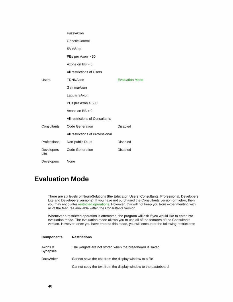
40

FuzzyAxon

GeneticControl

SVMStep

PEs per Axon > 50

Axons on BB > 5

All restrictions of Users

Users TDNNAxon

GammaAxon

LaguarreAxon

PEs per Axon > 500

Axons on BB > 9

All restrictions of Consultants

Evaluation Mode

Consultants Code Generation

All restrictions of Professional

Disabled

Professional Non-public DLLs Disabled

Developers Lite

Code Generation Disabled

Developers None

Evaluation Mode

There are six levels of NeuroSolutions (the Educator, Users, Consultants, Professional, Developers Lite and Developers versions). If you have not purchased the Consultants version or higher, then you may encounter restricted operations. However, this will not keep you from experimenting with all of the features available within the Consultants version.

Whenever a restricted operation is attempted, the program will ask if you would like to enter into evaluation mode. The evaluation mode allows you to use all of the features of the Consultants version. However, once you have entered this mode, you will encounter the following restrictions:

Components Restrictions

Axons & Synapses

The weights are not stored when the breadboard is saved

DataWriter Cannot save the text from the display window to a file

Cannot copy the text from the display window to the pasteboard

41

Cannot redirect the probed data to a file

ImageViewer Cannot save the probed image to a bitmap file

Criterion Cannot automatically save the best network weights to a file

StaticControl & DynamicControl

Cannot save the network weights to a weights file

The source code generation feature produces incomplete source code

All Neural Components

Cannot create, compile, or debug a DLL

Can only load DLLs created by NeuroDimension

Macro Bars Cannot create a new Macro Bar or delete an existing one

Some of the tutorials within the on-line help require some advanced features available only in the higher-level versions. By allowing the program to switch to evaluation mode when prompted, you will be able to work through all of the tutorials within the text.

Note: If you have not activated your copy of NeuroSolutions within 60 days from the time of installation then the evaluation software will expire.

NeuroSolutions Pricing

The latest pricing for all NeuroDimension products can be found on our web site at: http://www.nd.com/neurosolutions/pricing.html.

Note: If you do not have access to the Internet, see the Contacting NeuroDimension topic for information on how to contact NeuroDimension via phone, fax and mail.

NeuroSolutions University Site License Pricing

The latest university site license pricing for NeuroDimension products can be found on our web site at: http://www.nd.com/neurosolutions/univsite.html.

Note: If you do not have access to the Internet, see the Contacting NeuroDimension topic for information on how to contact NeuroDimension via phone, fax and mail.

Ordering Information

NeuroDimension products can be ordered using any of the following 3 methods:

42

1 Place the order on-line using our SECURE order entry system. 2 Download and print the latest order form then fax the completed form to 352-377-9009, or mail it to:

NeuroDimension, Inc.

Order Processing Department

1800 N. Main Street, Suite #D4

Gainesville, FL 32609-8606

3 Phone in your order (800-634-3327 or 352-377-5144) Monday through Friday between the hours of 8:30 AM and 5:00 PM EST.

We accept payment by credit card (Visa, MasterCard or American Express), wire transfer, or prepayment by check or money order.

Note: In order to use the links within this topic, you must be connected to the Internet.

Getting Started System Requirements

Before installing NeuroSolutions, you should verify that the configuration of your system meets the following minimum specifications:

Operating System Windows 95/98/Me/NT/2000

Memory 16MB RAM (32MB recommended)

Hard Drive 40MB free space

Video 640x480 with 256 colors (800x600 with 16M colors recommended)

Running the Demos

43

The best way to get an overview of the features provided by NeuroSolutions is to run the demos. These demos present a series of examples in neural computing in an attempt to illustrate the broad range of capabilities NeuroSolutions has to offer.

All demos are live! Each one starts with random initial conditions and learns on-line. Since most of the examples deal with highly nonlinear problems, they may get stuck in local minima. In such cases, simply run the simulation a couple of times.

Demo selection panel

44

To display the Demo Panel, select the Demos item from the Help menu. To run a demo, make a selection by pressing one of the demo buttons followed by the Run button. The two buttons at the bottom are the exception; they do not use the Run button.

A running demo

These demos are designed to be interactive. Many of the panels have edit cells that allow you to modify the network parameters and buttons to run the simulation or single-step through an epoch.

These demos are also not very restrictive. At any time during the presentation you are able to manipulate the breadboard by, adding a component, removing a component or changing a component’s parameters with the inspector. This can be advantageous in that you can learn a lot about the software by experimenting with the components. However, changing the state of the breadboard may result in a failure for the remainder of the demo, since the demos were designed with the assumption that no changes would be made. If the demo does fail, simply re-run the demo from the demo selection panel and do not make any changes to the components as you are stepping through the panels.

It is important to note that the demos are nothing more than NeuroSolutions macros. In other words, you the user have the same the same tools at your disposal that we had to create this demo. To take a look at the macro source code, open one of the macro files (*.nsm) within the Demos subdirectory of NeuroSolutions using the MacroWizard (under the "Tools" menu).

Once you have run the demos for NeuroSolutions, you should have a good idea of the broad range of capabilities provided by the base software. The next step you will want to take is to run the demo for NeuroSolutions for Excel. There is a button at the bottom of the NeuroSolutions demo panel that

45

will launch this demo for you, or you can click here . Note that both NeuroSolutions for Excel and Microsoft Excel (97 or higher) need be installed for this demo to work.

What to do after Running the Demos

After running the demos you will want to read the Getting Started Manual. This document steps you through the process of building a neural network with the NeuralExpert and NeuralBuilder utilities. The examples are written based on sample data included with the software, but you can use your own data instead. Click here to open the electronic version of this manual.

One possible starting point for building your own networks is to use the Demos. Simply run one of the demos that closely resembles the topology you want to use, then step through the panels until the network is constructed. From there you can load your own data into the File component(s) and make any other parameter and/or topology modifications that you wish. One you have made the desired changes, save the breadboard to a file for future use.

If you have purchased or are interested in purchasing NeuroSolutions for Excel, then you will want to read the Getting Started chapter of the NeuroSolutions for Excel help file. Click here to open this documentation.

Included with the full installation of NeuroSolutions is an introductory chapter of an electronic book entitled Neural Systems: Fundamentals Through Simulations by Principe, Lefebvre, and Euliano. If you want to read this chapter and work through the simulations, then select "Interactive Book" from the Help menu. Please visit the Interactive Book page of the NeuroDimension web site for more information on this revolutionary teaching tool.

Frequently Asked Questions (FAQ)

General What is NeuroSolutions?

NeuroSolutions is the premier neural network simulation environment. What is a neural network?

A neural network is an adaptable system that can learn relationships through repeated presentation of data, and is capable of generalizing to new, previously unseen data. Some networks are supervised, in that a human must determine what the network should learn from the data. Other networks are unsupervised, in that the way they organize information is hard-coded into their architecture.

What do you use a neural network for?

Neural networks are used for both regression and classification. In regression, the outputs represent some desired, continuously valued transformation of the input patterns. In classification, the objective is to assign the input patterns to one of several categories or classes, usually represented by outputs restricted to lie in the range from 0 to 1, so that they represent the probability of class membership.

Why are neural networks so powerful?

46

For regression, it can be shown that neural networks can learn any desired input-output mapping if they have sufficient numbers of processing elements in the hidden layer(s). For classification, neural networks can learn the Bayesian posterior probability of correct classification.

What is the NeuralBuilder?

The NeuralBuilder is an external program that aids the user in neural network design and setup. It automatically constructs any of the eight most popular neural architectures, including file and probe specifications.

What is NeuroSolutions for Excel?

NeuroSolutions for Excel is an Excel add-in that allows the user to construct, train, and test neural networks entirely from Excel. The user simply selects columns of data as input or target, and rows of data as training, testing, or cross-validation. NeuroSolutions for Excel then sends messages to NeuroSolutions in order to train or test a network.

Algorithms How does NeuroSolutions implement neural networks?

NeuroSolutions adheres to the so-called local additive model. Under this model, each component can activate and learn using only its own weights and activations, and the activations of its neighbors. This lends itself very well to object orientated modeling, since each component can be a separate object that sends and receives messages. This in turn allows for a graphical user interface (GUI) with icon based construction of networks.

What algorithm does NeuroSolutions use to train recurrent networks?

NeuroSolutions uses the back-propagation through time (BPTT) algorithm, which "unfolds" a dynamic net at each time step into an equivalent feed-forward net.

How does NeuroSolutions implement Radial Basis Function (RBF) networks?

The centers and widths of the Gaussian axons are determined from the cluster centers of the data, which are found through an unsupervised clustering algorithm. The weights from the Gaussian axons to the output layer are then determined through supervised learning with a desired signal.

Can I implement my own algorithms?

Yes, the easiest way to modify NeuroSolutions is through Dynamic Link Libraries (DLL’s), available with the Developer’s Lite and Developer’s levels. Every component has default code, which can be generated and edited from the "Engine" property page, and then compiled with MS Visual C++.

Platforms and OS Issues What operating systems does NeuroSolutions run on?

The full GUI environment of NeuroSolutions runs under Windows NT and Windows95. Are there versions of NeuroSolutions for the Macintosh, Sun, etc.?

Not at present, and there are no immediate plans for porting the GUI environment to other platforms (see the next question).

Does NeuroSolutions run under Unix?

Yes, NeuroSolutions runs under Unix, but without the GUI environment. The source code license provides the user with the complete NeuroSolutions’ core algorithmic code, either as a pre-compiled library or raw source code to be compiled by the user. The easiest way to make use of the library is to use the code

47

generation capabilities of the Professional and Developer’s versions, which generate source code from the GUI breadboard. Alternatively, the user can write code that calls the library.

How can I communicate with NeuroSolutions from another program?

NeuroSolutions is an OLE compatible server, which means it can be controlled by any OLE client, such as MS Excel or an MS Visual Basic application. The OLE commands take advantage of NeuroSolutions’ macro language. Two of our other products, the "NeuralBuilder" and "NeuroSolutions for Excel", control NeuroSolutions externally as clients in this way.

Network Components What do Axons do?

The Axon family sums all incoming vectors from multiple connections, and then applies a transfer function to the sum.

What does the plain blank Axon do?

This Axon acts the same as all other Axons, except its transfer function is the identity function.

What does a Full Synapse do?

A Full Synapse takes its input and multiplies it by a matrix. If a delay is specified, the output is delayed by that many time steps.

What’s does the straight Synapse do?

Using the Straight synapse to connect two Axons is exactly the same as making a direct connection between them, except it gives the additional option of specifying a delay.

What is that 2nd network that seems to lie on top of the main network?

This is the backpropagation network. Every Axon and Synapse has a corresponding BackAxon and BackSynapse that attaches to the upper right corner of the corresponding forward component. Data flows forward from the input to the output through the forward propagation network. The criterion compares the output with the desired response, and computers the error. The error is then injected into the backpropagation network, and the data flows through this network, back towards the original input.

In the control palette, what’s the difference between the clocks with one and two dials?

The clocks with one dial are for use with static networks, where the complete forward activation and back-propagation cycle can be completed in the same time step. The clocks with two dials are dynamic controllers for use with dynamic networks (see the next question).

When do I need to use the dynamic controllers?

You need to use the dynamic controllers anytime your network has a feedback loop with an adaptable weight(s). This includes the Gamma and Laguarre Axons, which are components that have internal feedback loops with an adaptable weight. You also need the dynamic controllers whenever a component with delays is used at any point in the network other than the input layer. For example, you can use a static controller for a network with a TDNN Axon (tapped delay line) at the input layer, but you must use a dynamic controller if the TDNN Axon is in the hidden layer.

Constructing Networks How do I connect two components on the breadboard?

There are two ways. The easiest way is to left-click select the "from" component, and then right-click select the "to" component, and choose "Connect To" from the menu. The other way is to manually grab the male

48

connector of the "from" component, and drag it over the female component of the "to" component, and release it.

How do I move or delete a connection?

First, of the two components connected by the connector, identify the "to" component. Then, identify where the male end of the connector joins with the female receptor of the "to" component. To move it, left-click select it, and then left-click drag it to a new location. To delete it, right-click select it and choose delete from the menu.

How can I make a connector follow a path instead of straight line?

First, move the male end of the connector to the first way-point on your path (see the previous question). Then, while holding down the shift key, drag the end of the connector to the next way-point. Continue in this fashion until the connector follows the desired path. Finally, drag the male end of the connector over the female receptor of the "to" component.

Why can’t I connect a Synapse to multiple Axons?

In NeuroSolutions, only Axons can branch. Thus, you can connect a single Axon to multiple Synapses but not the opposite.

When I try to create a recurrency in my network, why do I get a message that there’s an infinite loop in the data flow?

NeuroSolutions is a discrete-time simulator, and thus any recurrent loops must have a delay. Otherwise, the components in the loop would fire in sequence forever without ever advancing the time. In NeuroSolutions, Synapses implement the delays, and can be changed from the inspector’s Synapse property page. Setting at least one Synapse in your recurrent loop to a delay of one or greater will solve the problem.

What’s the meaning of "stacked access"?

When you put one component on another, such as placing a probe on a file component, its access is said to be "stacked", in that the data it receives (or sends) comes from (or goes to) the same access point as the component below it. Note that a stacked component only communicates with those components that are below it, not above it.

Editing Networks What is the Inspector?

The inspector is a panel that displays component specific information that the user can edit.

How do I bring up the Inspector for a particular component?

Right-click on the component and choose "Properties". You can also left-click select the component and then use the keyboard combination Alt-Enter.

How can I simultaneously edit the parameters of several components?

Right-click select the first component and, if the inspector is not already open, choose properties from the menu. Then hold down the shift key while left-click selecting the remaining components. Any changes you make in the inspector will be reflected in all selected components, as long as they all have the same parameter. For example, you can simultaneously change the number of PE’s of a group of Axons, even if they have different transfer functions (tanh, sigmoid, etc.).

In the Axon family, what is the meaning of "Rows" and "Cols" of PE’s on the Axon property page?

The PE’s of an Axon can be arranged as a matrix for display purposes, such as viewing the activations as an image. However, for calculation purposes, NeuroSolutions only cares about the

49

total number of PE’s, given by rows times columns, and this is the number shown on the "Axon" property page. If you don’t care about arranging the Axon’s activations as a matrix, just set the "Rows:" of PE’s. Note that some Axons have a "Transfer Function" property page with a "PEs" edit box, which is the same as the "Rows:" edit box.

Why can’t I change the number of PE’s of an output Axon?

The number of PE’s of the last Axon in a supervised network are completely determined by the number of PE’s of the Criteria.

Why can’t I change the dimensions of a Synapse?

The dimensions of a Synapse are completely determined by the two axons to which it is connected.

In the forward controller’s Inspector, why can’t I choose the number of exemplars/epoch?

For file input, the number of exemplars is entirely determined by the number of data points in the input file divided by the number of PE’s of the input axon. For other input, such as the function generator, you can set the number of exemplars.

What’s the standard naming convention?

All components on the breadboard must have distinct names. NeuroSolutions provides default names, which can be viewed or changed in the Inspector’s "Engine" property page. The standard naming convention is a set of suggested names for components based on their place and function within the network. The suggested names can be found in the on-line help index under "naming".

Why should I name my components according to the standard convention?

Following the standard naming convention means that you can use the same macros with any network, and that weight files and generated code will be easier to read.

File Management How do I feed a test set through the network?

First, go to the "File List" property page of the input file, click "Add…", and choose your test set. When the "Associate File" panel appears, choose "Testing" under the "Data Sets" list. If your test set has an associated desired file and you want to view error information, repeat the above steps for the desired file. Then, go to the "Static" property page of the forward controller, and choose "Testing" in the "Active Data Set" pull down menu. This automatically turns off learning. From the "Access" property page of the output probe, switch the "Access Data Set" to "Testing". You may then run the test set.

How do I split a file into a training set and a test set?

Add the file as usual from the File List property page of the File Inspector. It will be added as a Training data set by default. Click "Customize…" and then, within the "Data Segmentation" area of the resulting pop-up window, click the "Segment" box, and choose the offset and duration of the Training set. Then add the same file to the Data Set list, but this time as a test set (see the previous question). With the Testing file highlighted in the Data Set list, click "Customize…" again, and then the "Segment" box, and set the offset and duration to a different region of the file. These procedures must be applied to both the input and desired files. In addition, make sure you change your probe’s Access Data Set (see question H.2).

Note that this technique can only be used to split files into contiguous regions. To split a file randomly, use NeuroSolutions for Excel, or some other external pre-processor.

How can I train a network to do prediction of a data set without using multiple files?

Add the input file as usual from the File List property page of the File Inspector. Click "Customize…" and then, within the "Data Segmentation" area of the resulting pop-up window,

50

click the "Segment" box. Leave the offset at zero. If you are predicting P steps in advance, and your file has N exemplars, enter the difference N-P as the duration. Then add the desired file and click "Customize…". Click the "Segment" box and enter P as the offset and the difference N-P as the duration.

This process of setting up prediction is much simpler in the NeuralBuilder. Consider using it if your network is one of the default architectures it constructs.

What is the normalization file?

NeuroSolutions can scale and shift your data so that it fits in any range. This can be set from the "Stream" property page of the File Inspector. The normalization file is where NeuroSolutions stores the scale and bias parameters. You can view, select, and resave the normalization file under a different name from the "Data Sets" property page.

How do I denormalize the network output?

Place a probe on the network output, and go to the "Probe" property page, and check the box "Denormalize from Normalization File". Then choose the file that is used to normalize the desired output.

What is the meaning of the various NeuroSolutions extensions?

The extension "nsb" indicates a breadboard, "nsm" is for a macro, "nsn" is used for a normalization file, and "nsw" indicates a weight file.

Running Networks Why doesn’t anything happen when I hit the Start button?

NeuroSolutions now keeps track of the total number of epochs trained. After a training run, if you wish to continue training, you must increase the epochs in the "Static" property page of the forward controller, or reset the network and start over.

When using a test data set, why don’t I see anything happening in the probes?

All probes have an access property page, where you can set the "Access Data Set", through a pull-down menu, to "All", "Cross-Validation", "Training", or "Testing". The default setting is "Training", and thus you need to set it to either "All" or "Testing".

If I "fix" a component’s weights in the "Soma" property page, are they permanently frozen?

No, fixing a component’s weights simply means that they can’t be randomized. The component can, however, still learn and improve its weight estimates.

How can I freeze a component’s weights while allowing others to learn?

For supervised components, set the associated gradient descent component’s learning rate to zero. For unsupervised components, set the learning rate of the component itself to zero.

What’s the difference between randomize and jog in the control panel?

Randomize alters the weights according to a uniform distribution with the given mean and range. Jog alters the weights around their current value, using the given range. Jog can be useful during training to nudge a network out of a local minima.

51

Terms to Know Main Window

From the Start menu of Windows (the lower-left corner of your screen), select "Programs" then "NeuroSolutions 4". The icon represents the NeuroSolutions program. Double-click on this icon to begin or click the following shortcut to run NeuroSolutions.

Once the program is launched you will see the main window of NeuroSolutions. The top of the window contains the main menus. These are used to issue commands to the program. The icons just below the menus are the toolbars. These buttons are shortcuts to the menu commands. The icons at the bottom of the main window represent neural components. All NeuroSolutions components are grouped into families and reside on palettes, which are very similar to toolbars. The sub-windows are referred to as the breadboards. These are the NeuroSolutions "documents" and it is where the network construction and simulations take place. This multi-document interface (MDI) allows you to run multiple simulations simultaneously.

52

The NeuroSolutions Main Window

Inspector

The Inspector is a window that is used to view and modify the parameters of the selected component(s) on the breadboard. Within the Inspector are multiple property pages, each page containing a different set of parameters. The pages are selected by clicking on the labeled tabs at the top of the Inspector window. To display the inspector window, select Inspector item of the View menu, or right-click on the component (to bring up the Component menu) and select the Properties item.

53

Axon Inspector

Breadboards

From the File menu select the New item. The blank window that appears is referred to as a breadboard. This is a simulation "document", similar to a document in your word processing program. The breadboard contains all of the information that defines an experiment. When the breadboard is saved to disk, all of the components, connections, parameters and (optionally) weights are stored.

The breadboard is where the network construction and simulation takes place. Networks can be automatically constructed using the NeuralBuilder utility or they can be built from scratch by selecting components from palettes and stamping them on a breadboard. Note that networks constructed with the NeuralBuilder can later be customized by removing components and/or adding new ones from the palettes.

Multiple breadboards can be opened at one time, allowing you to run multiple simulations simultaneously. To select between the breadboards you can click on the breadboard window (if it is not hidden), or use the Window menu. To maximize a breadboard to fill the entire workspace, simply double-click on the title bar of the breadboard window.

Breadboard containing a MLP

54

Neural Components

Each neural component encapsulates the functionality of a particular piece of a neural network. A working neural network simulation requires the interconnection of many different components.

As mentioned above, the NeuralBuilder utility automates the construction process of many popular neural networks. There may be times when you will want to create a network from scratch, or to add components to a network created by the NeuralBuilder. This is done by selecting components from palettes and stamping them onto the breadboard.

Axon component

Toolbars and Palettes

Both the toolbars and palettes are control bars that can be positioned anywhere on the screen. These control bars are also dockable, meaning that they have the ability to be attached or "docked" along any edge of the main window.

Both the toolbars and palettes have a feature called tooltips. On palettes, tooltips display the name of an icon’s component. To activate the tooltip for an icon, simply hold the mouse cursor over the icon for a couple of seconds.

Axon Palette

The Customize Toolbars Page is used to toggle the visibility of toolbars. This feature is available so that only the palettes and toolbars used most often occupy the screen area. This page also allows you to switch between large and small buttons (the sample toolbar shown above contains small buttons). The contents of the toolbars is fully customizable within the Customize Buttons Page.

See Also

Selection and Stamping Modes

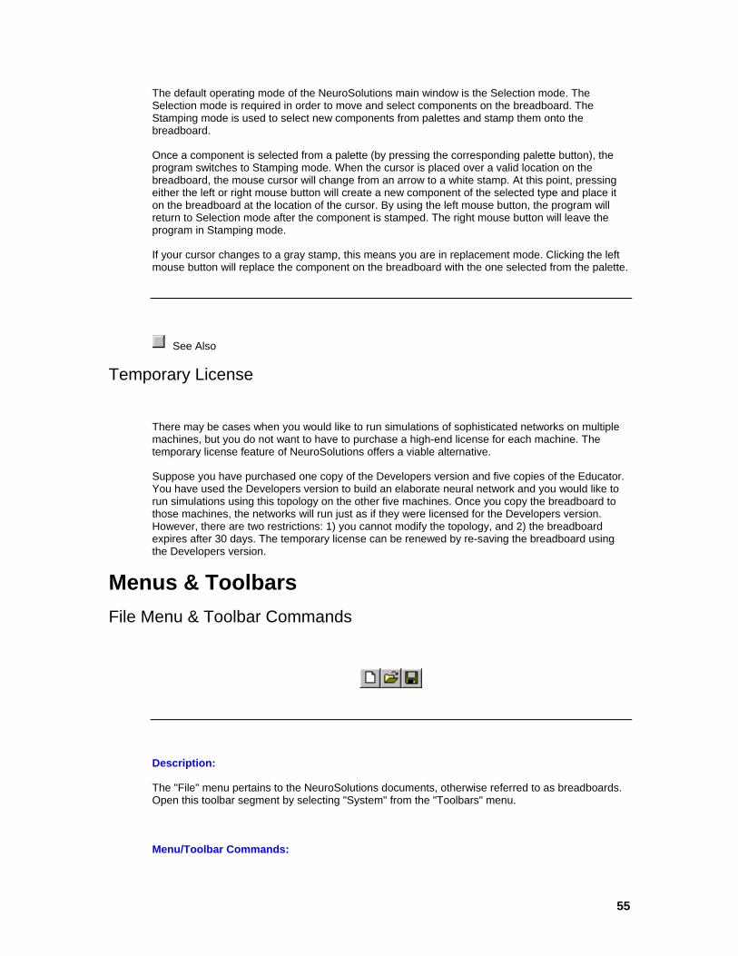
55

The default operating mode of the NeuroSolutions main window is the Selection mode. The Selection mode is required in order to move and select components on the breadboard. The Stamping mode is used to select new components from palettes and stamp them onto the breadboard.

Once a component is selected from a palette (by pressing the corresponding palette button), the program switches to Stamping mode. When the cursor is placed over a valid location on the breadboard, the mouse cursor will change from an arrow to a white stamp. At this point, pressing either the left or right mouse button will create a new component of the selected type and place it on the breadboard at the location of the cursor. By using the left mouse button, the program will return to Selection mode after the component is stamped. The right mouse button will leave the program in Stamping mode.

If your cursor changes to a gray stamp, this means you are in replacement mode. Clicking the left mouse button will replace the component on the breadboard with the one selected from the palette.

See Also

Temporary License

There may be cases when you would like to run simulations of sophisticated networks on multiple machines, but you do not want to have to purchase a high-end license for each machine. The temporary license feature of NeuroSolutions offers a viable alternative.

Suppose you have purchased one copy of the Developers version and five copies of the Educator. You have used the Developers version to build an elaborate neural network and you would like to run simulations using this topology on the other five machines. Once you copy the breadboard to those machines, the networks will run just as if they were licensed for the Developers version. However, there are two restrictions: 1) you cannot modify the topology, and 2) the breadboard expires after 30 days. The temporary license can be renewed by re-saving the breadboard using the Developers version.

Menus & Toolbars File Menu & Toolbar Commands

Description:

The "File" menu pertains to the NeuroSolutions documents, otherwise referred to as breadboards. Open this toolbar segment by selecting "System" from the "Toolbars" menu.

Menu/Toolbar Commands:

56

New

Creates a new breadboard (document) and opens it as a separate window.

Open

Opens an existing breadboard (document) as a separate window. The file is specified using the File Open dialog box.

Close

Closes the active breadboard (document). If there have been any changes to the breadboard since the last save then you will be given the option to save the breadboard before closing.

Save

Use this command to save the active document to its current name and directory. When you save a document for the first time, NeuroSolutions displays the Save As dialog box so you can name your document. If you want to change the name and directory of an existing document before you save it, choose the "Save As" command (see below).

Save As

Use this command to save and name the active document. NeuroSolutions displays the Save As dialog box so you can name your document.

Recent Files

Use the numbers and filenames listed at the bottom of the File menu to open the last four documents you closed. Choose the number that corresponds with the document you want to open.

Exit

Ends your NeuroSolutions session. You can also use the Close button ( ) of the NeuroSolutions main window. You will be prompted to save documents with unsaved changes.

Edit Menu & Toolbar Commands

Description:

The "Edit" menu contains commands for manipulating the components on the breadboard. Open this toolbar segment by selecting "System" from the "Toolbars" menu.


57

Undo

Reverses the most recent change to the breadboard. To return the breadboard its original state, issue the Undo command a second time.

Cut

Removes the currently selected components from the breadboard and puts them on the clipboard. This command is unavailable if there are no components currently selected. Cutting data to the clipboard replaces the contents previously stored there.

Copy

Copies the currently selected components onto the clipboard. This command is unavailable if there are no components currently selected. Copying data to the clipboard replaces the contents previously stored there.

Paste

Inserts a copy of the clipboard contents at the insertion point. This command is unavailable if the clipboard is empty or if a valid insertion point has not been selected.

Delete

Removes the currently selected components from the breadboard. This command is unavailable if there are no components currently selected.

Copy to File

Copies the currently selected components to the selected Clipboard file (*.nsc). This command is unavailable if there are no components currently selected.

Paste from File

Inserts the contents of the selected Clipboard file (*.nsc) at the insertion point. This command is unavailable if the clipboard is empty or if a valid insertion point has not been selected.

Selection Cursor

Use this command to switch the cursor from the stamping mode to the selection mode.

Alignment Menu & Toolbar Commands

58

Description:

This toolbar is used for arranging the components on the breadboard. Open this toolbar by selecting "Alignment" from the "Toolbars" menu. These alignment commands can also be found under the "Alignment" menu.


Align Left

Moves the selected components so that the left borders all have the same x coordinate on the breadboard.

Align Right

Moves the selected components so that the right borders all have the same x coordinate on the breadboard.

Align Top

Moves the selected components so that the top borders all have the same y coordinate on the breadboard.

Align Bottom

Moves the selected components so that the bottom borders all have the same y coordinate on the breadboard.

Space Across

Distributes the selected components within the horizon tal space between the left-most selected component and the right-most selected component.

Space Down

Distributes the selected components within the vertical space between the top selected component and the bottom selected component.

Center Horizontal

Moves the selected components horizontally to the center of the visible portion of the breadboard.

Center Vertical

Moves the selected components vertically to the center of the visible portion of the breadboard.

Center Objects

Moves the selected components so that their centers all have the same x coordinate on the breadboard.

Bring To Front

59

Moves selected component in front of any other components sharing the same space.

Send To Back

Moves selected component behind any other components sharing the same space.

Windows Menu & Toolbar Commands

Description:

The "Windows" menu contains commands for manipulating the breadboard (document) windows.


New Window

Opens a new window with the same contents as the active window. This feature allows you to view/modify two sections of the same breadboard at once.

Cascade

Displays all breadboards in windows that do overlap.

Tile

Displays all breadboards in windows that do not overlap.

Arrange Icons

Arranges the minimized versions of the windows along the bottom of the application workspace.

Currently Open Breadboards

Activates the window of the selected breadboard.

Component Menu

The component menu is used to issue commands specific to a particular component or group of components. To issue a command for an individual component on the breadboard, click the right mouse button while the cursor is on top of the component and select the menu item for the command. To issue a command for a group of components, you must first select the components (see Logic of the Interface) before right-clicking to display the menu.

Menu Item Description

60

Properties Displays the inspector window, which is used to view/modify the component’s parameters.

Connect to Connects the previously selected component to the selected component.

Cut See Edit Menu

Copy See Edit Menu

Paste See Edit Menu

Delete Removes the selected component(s) from the breadboard.

Copy to File Writes the selected component(s) to a user-specified clipboard (*.nsc) file.

Paste from File Pastes the component(s) stored in a user-specified clipboard file (*.nsc) onto the breadboard.

Insert New Object

Displays a list of object types available on your system. Once a type is selected, the appropriate OLE-compliant application will be launched and a new object of that type will be embedded into the NeuroSolutions breadboard.

Tools

Tools Menu Commands

Description:

The "Tools" menu contains macro and control commands. It also provides short cuts to wizard programs such as the NeuralBuilder.


NeuralBuilder

Launches the NeuralBuilder neural network construction utility. The user steps through a series of panels to specify the topology, input data, learning parameters and probing. The network is then constructed and ready for simulations.

NSForExcel

Launches NeuroSolutions for Excel. This Excel add-in can be used in conjunction with any level of NeuroSolutions to simplify and enhance the process of getting data in and out of the network. Both NeuroSolutions for Excel and Microsoft Excel must be installed in order for this toolbar button to function.

CustomSolutionWizard

61

Launches the Custom Solution Wizard. This utility will take any neural network created with NeuroSolutions and automatically generate and compile a Dynamic Link Library (DLL) for that network, which you can then embed into your own application. The Custom Solution Wizard must be installed in order for this toolbar button to function.

NeuralExpert

Launches the NeuralExpert neural network contruction utility. This is similar to the NeuralBuilder, but it is much simpler to use. It asks the user a series of questions about their problem and then intelligently builds a neural network based on the size and type of problem specified.

TestingWizard

Launches the TestingWizard. This utility provides an easy way to produce the network output for a new dataset once the training phase has been completed. The network output can be displayed within a window or saved to a file.

MacroWizard

Opens the MacroWizard Window.

Record Macro

See Macro Menu & Toolbar Commands.

Control

See Control Menu & Toolbar Commands.

Customize

See Customize Toolbars Page.

Options

See Options Window.

Add

Opens a file selection panel to select an executable file. A menu cell is created that when selected will execute this file.

Remove

Opens a panel listing the user-defined tools. Select from this list to remove one of the tools from the Tools menu.

Control Menu & Toolbar Commands

62

Description:

This toolbar allows you to perform global data flow operations on the network. Open this toolbar by selecting "Control" from the "Toolbars" menu. These control commands can also be found within the "Tools" menu.

Toolbar Commands:

Start

Begins an experiment defined by the Control component on the breadboard. If this button is disabled, then the experiment has run to completion and the network must either be reset (see below) or the epochs must be increased (see the Static property page).

Pause

Pauses the simulation after finishing the current epoch.

Reset

Resets the experiment by resetting the epoch and exemplar counters, and randomizing the network weights. Note that when the Learning switch from the Static property page is off, the weights are not randomized when the network is reset

Zero Counters

Sets the Epoch and Exemplar counters to zero without resetting the network.

Step Epoch

Runs the simulation for one epoch.

Step Exemplar

Runs the simulation for one exemplar.

Randomize

Randomizes the network weights. The mean and variance of the randomization is defined within the Soma property page of each component that has adaptable weights.

Jog

Alters all network weights by a random value. The variance of the randomization is defined within the Soma property page of each component that has adaptable weights.

Hide Windows

When this button is selected (pressed down), all display windows are hidden from view. When the button is de-selected (popped up), the display windows are restored to their original state.

63

See Also

Macro Menu & Toolbar Commands

Description:

This toolbar is used to issue commands associated with the MacroWizard. Open this toolbar by selecting "Macro" from the "Toolbars" menu. These macro commands can also be found within the "Tools" menu.

Toolbar Commands:

MacroWizard

Displays the MacroWizard window.

Record New

Opens a panel for entering a macro name, creates a new macro with the specified name, and begins recording the macro.

Stop

Stops the macro recording process and displays the MacroWizard Edit Page.

Pause

Pauses the macro recording process. Press the button again to resume recording.

Customize Toolbars Page

A palette contains a group of neural components belonging to the same family. A toolbar contains shortcut buttons to the various menu commands. The Customize Toolbars page allows you to toggle the visibility of the various palettes and toolbars, as well as adding new ones and customizing the appearance.

64

Component Palettes Menu Item Description

Axon Contains the processing elements (PEs) and activation functions of the network.

Backprop Backpropagation components, which backpropagate the error through the network and compute weight gradients.

Controls Control the data flow of the network.

Dialog Text boxes, edit cells and buttons.

ErrorCriteria Produce a measure of error based on the output and desired signal of the network.

GradientSearch Updates the weights of the network based on first order gradient information.

Input Bring data into the network, either by generating it or by reading it from the file system.

MemoryAxon Axons that store information over time.

Probes Graph the parameters and data contained within the network.

Schedule Components that modify the network’s parameters during an experiment.

65

Synapse Connect axons together and contain the weights of the network.

Transmitter Transmit data and control messages from one component to another.

Unsupervised Family

Synapses whose weights are updated based on unsupervised learning rules.

Command Toolbars Menu Item Description

Alignment Commands used to align components on the breadboard.

Control Commands used to control the simulation.

Macro Commands used to record and manipulate macros.

Necessities The most commonly used commands taken from several toolbars.

System Commands that are common to most Windows programs.

Tools Shortcuts to wizards and related programs.

Options:

Show Tooltips

This feature will display the full name of the command/component when the cursor is placed over the toolbar/palette button. Cool Look

This feature diplays the toolbar/palette button in 3-D only when the cursor is placed over it. Large Buttons

Displays a larger version of the toolbar/palette buttons, which includes the names of the commands/components.

See also Customize Buttons Page

Customize Buttons Page

The Customize Buttons page allows you to select which tool buttons should be displayed on each toolbar.

66

To add a button to a toolbar/palette, select the category of the command/component and then drag the desired button to the location in the toolbar/palette that you would like it displayed. Note: You must drag the button to the actual toolbar/palette -- not to the category list.

To remove a button, simply drag the button from the toolbar/palette to an emply place on the screen (while the Customize Buttons page is displayed).

See also Customize Toolbars Page

View

View Menu

This menu is used to toggle the visibility of the selected toolbar or window. Menu Item Description

Custom Macro Bars

Commands that are defined with user-defined macros. The default installation includes a set of sample macro bars.

67

Status Bar Section of the main window that indicates the current state of the system.

Inspector Window to view/modify the component parameters.

Console Window that displays the log of error and diagnostic messages.

New Macro Bar Creates a blank Macro Bar with the user-specified name.

Macro Bars

Macros can be run from the MacroWizard, a MacroEngine or a Macro Bar. Macro bars allow you to easily run macros directly from the main window of NeuroSolutions. Simply clicking a button on a macro bar will run the associated Macro.

To create a new macro bar, select "New Macro Bar…" from the View Menu and enter a name for the bar. A new macro bar with a blank button should appear. Right-click on this bar to configure the buttons. Left-click on a button while holding down the shift key to move the button within the toolbar.

Macro Bar Commands (right-click to display menu): Add Button

Adds a blank button to the macro bar. Delete Button

Deletes the selected button from the macro bar. Name Button

Opens a dialog box for entering the name of the selected button. Assign Macro

Opens a file selected panel for selecting the macro file (*.nsm) to associate with the button. Edit Macro

Opens the MacroWizard Edit Page with the associated macro loaded. Delete Macro Bar

Deletes the macro bar and removes its entry from the View Menu.

The default installation of NeuroSolutions includes three macro bars, which can be found at the top of the View Menu. Below is a summary of the default macros.

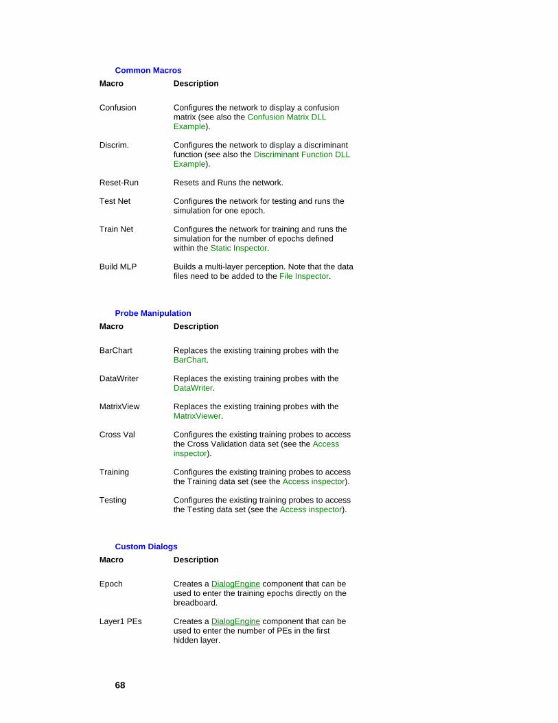
68

Common Macros Macro Description

Confusion Configures the network to display a confusion matrix (see also the Confusion Matrix DLL Example).

Discrim. Configures the network to display a discriminant function (see also the Discriminant Function DLL Example).

Reset-Run Resets and Runs the network.

Test Net Configures the network for testing and runs the simulation for one epoch.

Train Net Configures the network for training and runs the simulation for the number of epochs defined within the Static Inspector.

Build MLP Builds a multi-layer perception. Note that the data files need to be added to the File Inspector.

Probe Manipulation Macro Description

BarChart Replaces the existing training probes with the BarChart.

DataWriter Replaces the existing training probes with the DataWriter.

MatrixView Replaces the existing training probes with the MatrixViewer.

Cross Val Configures the existing training probes to access the Cross Validation data set (see the Access inspector).

Training Configures the existing training probes to access the Training data set (see the Access inspector).

Testing Configures the existing training probes to access the Testing data set (see the Access inspector).

Custom Dialogs Macro Description

Epoch Creates a DialogEngine component that can be used to enter the training epochs directly on the breadboard.

Layer1 PEs Creates a DialogEngine component that can be used to enter the number of PEs in the first hidden layer.

69

Layer1 Mom. Creates a DialogEngine component that can be used to enter the momentum of the first hidden layer.

Layer1 Step Creates a DialogEngine component that can be used to enter the step size of the first hidden layer.

Output Mom. Creates a DialogEngine component that can be used to enter the momentum of the output layer.

Output Step Creates a DialogEngine component that can be used to enter the step size of the output layer.

Status Bar

The status bar is displayed at the bottom of the NeuroSolutions window. To display or hide the status bar, select the "Status Bar" item within the View Menu.

The left side of the status bar describes the action in progress or the action associated with the current cursor position. The right areas of the status bar indicate which of the following keys are latched down:

Indicator Description

CAP The Caps Lock key is latched down.

NUM The Num Lock key is latched down.

SCRL The Scroll Lock key is latched down.

Help

Help Menu & Toolbar Commands

Description:

70

The "Help" menu contains commands for displaying the on-line help, the about panel, and the demos.


NeuroSolutions Help

Displays the main window for the on-line help system. From there you can find the documentation by the table of contents, keyword index, or content search.

Context Help

When you click this toolbar button or menu item, the mouse cursor will change to an arrow and question mark. Click somewhere inside one of the windows of NeuroSolutions and the help topic will be shown for that specific item.

Getting Started Manual

This is the online version of the printed manual that comes with all licensed copies of NeuroSolutions. It is recommended that new users read this manual before reading the main NeuroSolutions Help.

About NeuroSolutions

Display the copyright notice and version number of your copy of NeuroSolutions.

Demos

Use this command to run the NeuroSolutions Demo. This will show a panel that contains a number of macros that demonstrate some of the capabilities of the program. Once an example is complete, the breadboard can be modified and additional experiments can be run.

Interactive Book

Opens the introductory chapter of an electronic book entitled Neural Systems: Fundamentals Through Simulations by Principe, Lefebvre, and Euliano. Please visit the Interactive Book page of the NeuroDimension web site for more information on the entire publication.

Open ND Web Page

Opens the home page of NeuroDimension (http://www.nd.com) using the default browser.

Technical Support

Opens the Tech Support Help Page.

Activate Software

Opens the Activate Software Panel, which displays the serial number for your installation and allows you to enter in the activation codes needed to upgrade the software from the evaluation level to the level you have purchased.

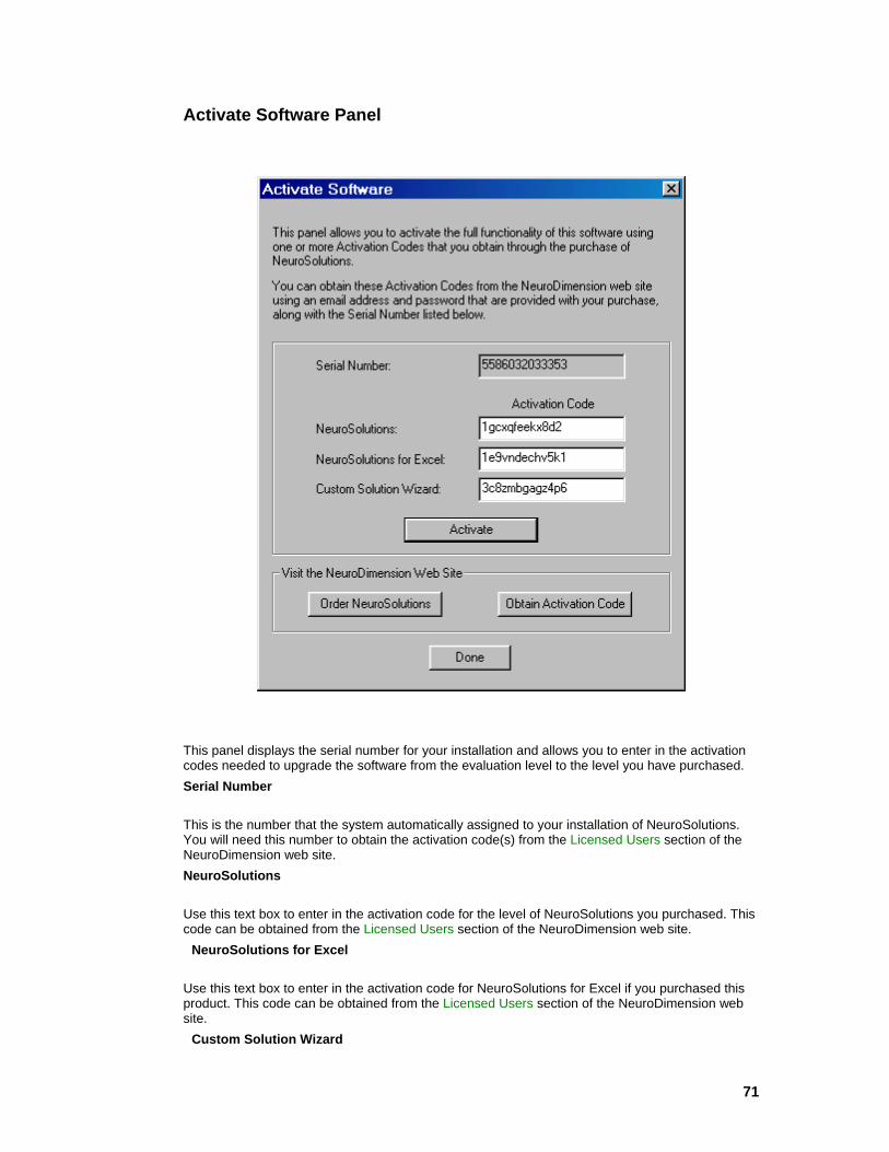
71

Activate Software Panel

This panel displays the serial number for your installation and allows you to enter in the activation codes needed to upgrade the software from the evaluation level to the level you have purchased. Serial Number

This is the number that the system automatically assigned to your installation of NeuroSolutions. You will need this number to obtain the activation code(s) from the Licensed Users section of the NeuroDimension web site. NeuroSolutions

Use this text box to enter in the activation code for the level of NeuroSolutions you purchased. This code can be obtained from the Licensed Users section of the NeuroDimension web site.

NeuroSolutions for Excel

Use this text box to enter in the activation code for NeuroSolutions for Excel if you purchased this product. This code can be obtained from the Licensed Users section of the NeuroDimension web site.

Custom Solution Wizard

72

Use this text box to enter in the activation code for the Custom Solution Wizard if you purchased this product. This code can be obtained from the Licensed Users section of the NeuroDimension web site. Activate

Once you have entered in the activation codes for the products you purchased, click this button to save these codes. If the codes are correct, the software will be activated to the proper level. To verify the level is correct, select "About NeuroSolutions" from the NeuroSolutions Help menu.

User Options Options Window

This window is used to view/modify the user preference settings. These settings are stored in the file "NeuroSolutions.ini" located within the Windows directory. OK

Saves all changes and closes the window. Cancel

Closes the window and discards all changes that have not yet been applied. Apply

Saves all changes and keeps the window open. Help

Displays the on-line help for the selected options page.

See Also

Options Workspace Page

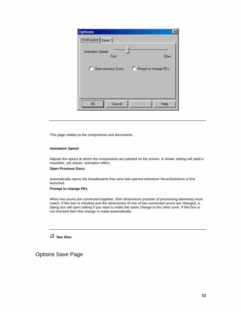
73

This page relates to the components and documents.

Animation Speed

Adjusts the speed at which the components are painted on the screen. A slower setting will yield a smoother, yet slower, animation effect. Open Previous Docs.

Automatically opens the breadboards that were last opened whenever NeuroSolutions is first launched. Prompt to change PEs

When two axons are connected together, their dimensions (number of processing elements) must match. If this box is checked and the dimensions of one of two connected axons are changed, a dialog box will open asking if you want to make the same change to the other axon. If this box is not checked then this change is made automatically.

See Also

Options Save Page

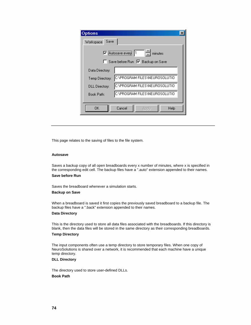
74

This page relates to the saving of files to the file system.

Autosave

Saves a backup copy of all open breadboards every x number of minutes, where x is specified in the corresponding edit cell. The backup files have a ".auto" extension appended to their names. Save before Run

Saves the breadboard whenever a simulation starts. Backup on Save

When a breadboard is saved it first copies the previously saved breadboard to a backup file. The backup files have a ".back" extension appended to their names. Data Directory

This is the directory used to store all data files associated with the breadboards. If this directory is blank, then the data files will be stored in the same directory as their corresponding breadboards. Temp Directory

The input components often use a temp directory to store temporary files. When one copy of NeuroSolutions is shared over a network, it is recommended that each machine have a unique temp directory. DLL Directory

The directory used to store user-defined DLLs. Book Path

75

The directory where the Interactive Book files are stored. If you purchased this product then this directory should be on your CD-ROM drive. Otherwise, this directory will be a sub-directory of your NeuroSolutions installation and will contain only the files for the first chapter.

See Also

Examples Example 1 - Toolbar Manipulation

The figure below shows the default toolbar. Try moving this toolbar by beginning a drag operation with the mouse cursor just to the right of the right-most button. Drag the toolbar to the center of the main window and release. This toolbar is no longer attached to the main window. Try moving the main window to verify this.

Default Toolbar

Now drag the toolbar to the right border of the main window. As you drag the toolbar across, you should see the border change from a horizontal orientation to a vertical one. At this point, release the mouse button. The toolbar should now be docked on the right side of the main window. Both toolbars and palettes can be docked at any of the four borders of the main window.

Move the mouse cursor to the button with the button labeled "NBuilder". After leaving it there for about a half of a second, a small yellow box with the text "NeuralBuilder" will appear. This is the button’s tooltip.

Select "Customize" within the Tools menu to view the list of available palettes. Click on the Axon check box to display the Axon palette. You may move this palette as described above.

See Also

Example 2 - Component Manipulation

During the previous example you displayed the Axon palette. Select the left-most (or top-most if the palette is arranged vertically) button on this palette. You have now selected the Axon component. Move the mouse cursor over the breadboard and click the left mouse button. This should have placed an Axon component on the breadboard. From the Probes palette, select the left-most (or top-most) button. Now move the mouse cursor over the Axon on the breadboard and click the left mouse button. You have now placed a MatrixViewer probe on the Axon. At this point there is little

76

to probe since you are missing key elements of the network. This exercise is only intended to be a brief introduction to component manipulation.

MatrixViewer attached to an Axon.

See Also

Example 3 - Inspecting a Component's Parameters

During the previous example you placed an Axon and a MatrixViewer on the breadboard. If you stamped the MatrixViewer using the right mouse button, then you are still in Stamping mode. If this is the case, you will first need to click the following button from the System toolbar:

Selection Cursor toolbar button

This changes the mouse cursor from Stamping mode to Selection mode. Now when you click the mouse on the breadboard, you will not stamp a new component as you did earlier. Move the mouse over the Axon on the breadboard and single-click. A square should appear around the Axon to indicate that this component is selected.

From the View menu, select the Inspector item. This should display the Inspector window containing the parameter settings for the Axon component that you just selected. Click the tab buttons at the top of the Inspector window to switch between the three property pages of the Axon. From the breadboard, single click on the MatrixViewer’s icon to make it the selected component. Note that the Inspector has been updated to reflect the parameter settings of the MatrixViewer component.

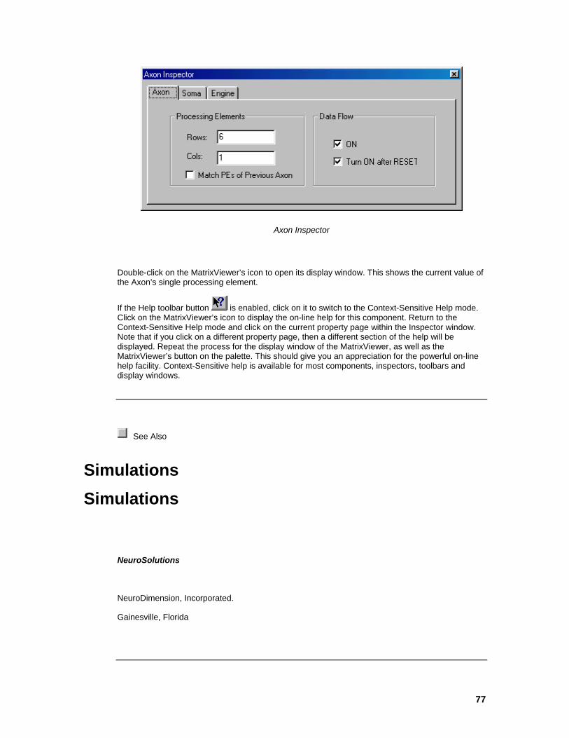
77

Axon Inspector

Double-click on the MatrixViewer’s icon to open its display window. This shows the current value of the Axon’s single processing element.

If the Help toolbar button is enabled, click on it to switch to the Context-Sensitive Help mode. Click on the MatrixViewer’s icon to display the on-line help for this component. Return to the Context-Sensitive Help mode and click on the current property page within the Inspector window. Note that if you click on a different property page, then a different section of the help will be displayed. Repeat the process for the display window of the MatrixViewer, as well as the MatrixViewer’s button on the palette. This should give you an appreciation for the powerful on-line help facility. Context-Sensitive help is available for most components, inspectors, toolbars and display windows.

See Also

Simulations Simulations

NeuroSolutions

NeuroDimension, Incorporated.

Gainesville, Florida

78

Purpose

This chapter describes general principles useful in simulating neural networks, and motivates the step by step procedure utilized later in the Manual. After reading this chapter, the user should have a better understanding of the power of neural networks and how they can be effectively used to solve real world problems.

Introduction to Neural Network Simulations What Are Artificial Neural Networks

Before delving into the solution of real world problems using neural networks, a definition of neural networks will be presented. It is important to know the conditions under which this style of problem solving excels and what its limitations are.

At the core of neural computation are the concepts of distributed, adaptive and nonlinear computing. Neural networks perform computation in a very different way than conventional computers, where a single central processing unit sequentially dictates every piece of the action. Neural networks are built from a large number of very simple processing elements that individually deal with pieces of a big problem. A processing element (PE) simply multiplies an input by a set of weights, and nonlinearly transforms the result into an output value (table lookup). The principles of computation at the PE level are deceptively simple. The power of neural computation comes from the massive interconnection among the PEs, which share the load of the overall processing task, and from the adaptive nature of the parameters (weights) that interconnect the PEs.

Normally, a neural network will have several layers of PEs. This chapter only covers the most basic feedforward architecture, the multilayer perceptron (MLP). Other feedforward architectures as well as those with recurrent connections are addressed in the Tutorials chapter.

The diagram below illustrates a simple MLP. The circles are the PEs arranged in layers. The left column is the input layer, the middle column is the hidden layer, and the right column is the output layer. The lines represent weighted connections (i.e., a scaling factor) between PEs.

A simple multilayer perceptron

By adapting its weights, the neural network works towards an optimal solution based on a measurement of its performance. For supervised learning, the performance is explicitly measured

79

in terms of a desired signal and an error criterion. For the unsupervised case, the performance is implicitly measured in terms of a learning law and topology constraints.

A Prototype Problem

Sleep staging is a quantitative measure to evaluate sleep. Sleep disorders are becoming quite common, probably due to the stress of modern living. Sleep is not a uniform process. The brain goes through well defined patterns of activity that have been catalogued by researchers. Insomnia is a disruption of this normal pattern, and can be diagnosed by analyzing sleep patterns. Normally these patterns are divided into five stages plus awake (sleep stage 0). Sleep staging is a time consuming and extremely expensive task, because the expert must score every minute of a multichannel tracing (1,200 feet of paper) recorded during the whole night. For these reasons, there is great interest in automating this procedure.

In order to score sleep automatically, it is necessary to measure specific waveforms in the brain (alpha, beta, sigma spindles, delta, theta waves) along with additional indicators (two rapid eye movements -- REM 1 and 2, and muscle artifact).

This example illustrates the type of problem that is best solved by a neural network. After much training the human expert is able to classify the sleep stages based on the input signals, but it would be impossible for that person to come up with an algorithm to automate the process. A neural network is able to perform such a classification by extracting information from the data, without any prior knowledge.

The table below shows a segment of the brain wave sensor data. The first column contains the time, in minutes, of each reading, and the next eight columns contain the eight sensor readings. The last column is the sleep stage, scored by the sleep researcher, for each minute of the experiment.

Sleep Staging Data

Min ? ? ? ? ? MA REM 1 REM 2 Stage

37 0 0 25 1 16 0 6 0 1

38 0 0 25 2 14 0 1 0 1

39 0 0 29 3 13 0 4 0 2

40 0 0 29 1 8 0 5 0 1

41 0 0 32 2 8 0 2 0 0

42 0 0 29 1 8 0 1 1 1

The problem is to find the best mapping from the input patterns (the eight sensors) to the desired response (one of six sleep stages). The neural network will produce from each set of inputs a set of outputs. Given a random set of initial weights, the outputs of the network will be very different from the desired classifications. As the network is trained, the weights of the system are continually adjusted to incrementally reduce the difference between the output of the system and the desired response. This difference is referred to as the error and can be measured in different ways. The most common measurement is the mean squared error (MSE). The MSE is the average of the squares of the difference between each output PE and the true sleep stage (desired output).

80

This simple example illustrates the basic ingredients required in neural computation. The network requires input data and a desired response to each input. The more data presented to the network, the better its performance will be. Neural networks take this input-output data, apply a learning rule and extract information from the data. Unlike other technologies that try to model the problem, artificial neural networks (ANNs) learn from the input data and the error. The network tries to adjust the weights to minimize the error. Therefore, the weights embody all of the information extracted during learning.

Essential to this learning process is the repeated presentation of the input-output patterns. If the weights change too fast, the conditions previously learned will be rapidly forgotten. If the weights change too slowly, it will take a long time to learn complicated input-output relations. The rate of learning is problem dependent and must be judiciously chosen.

Each PE in the ANN will simply produce a nonlinear weighted sum of inputs. A good network output (i.e. a response with small error) is the right combinations of each individual PE response. Learning seeks to find this combination. In so doing, the network is discovering patterns in the input data that can solve the problem.

It is interesting that these basic principles are very similar to the ones used by biological intelligence. Information is gained and structured from experience, without explicit formulation. This is one of the exciting aspects of neural computation. These are probably the same principles utilized by evolution to construct intelligent beings. Like biological systems, ANNs can solve difficult problems that are not mathematically formulated. The systematic application of the learning rule guides the system to find the best possible solution.

Ingredients of a Simulation Formulation of the problem

As in the example given, one needs a well defined problem domain. In our everyday life we are bombarded with situations so complex that we do not have analytical ways to solve them. Some examples are: the best way to invest your money in a diversified portfolio, the prediction of your company’s next quarterly sales, repairs to your car which maximize its commercial value, who is going to win the football game. Note that in each one of these cases, there is a clearly defined problem. Once you have a crisp definition, the next step is to select the input variables and the desired responses. Here you always use common sense to select the variables that are relevant for the problem. As an example, using your birthday to forecast the weather is probably not a valuable variable. One should seek variables and conditions that appear relevant to the problem being analyzed. One should also seek data that cover a wide spectrum of cases. If the ANN does not see an equilibrated set of cases, its output will be ‘biased’. Since ANNs learn from the data, the data must be valid for the results to be meaningful.

Sometimes the desired response is unknown. For instance, what is the desired response for a stock prediction problem? Everyday there is a stock price, so the history of the prices can be used as a basis for making a prediction. If the network can do this reliably for every day in the past, then it may also be able to predict tomorrow’s stock price.

NeuroSolutions implements the basic building blocks of neural computation, such as multi-layer perceptrons, Jordan and Elman networks, radial basis function (also called probabilistic) networks, principal component analysis networks, self-organizing feature map networks, and time-lagged recurrent networks. With these neural models one can solve virtually any problem where a neural network solution has been reported. See the on-line documentation of the NeuralBuilder for more information on these models.

Data Collection and Coding

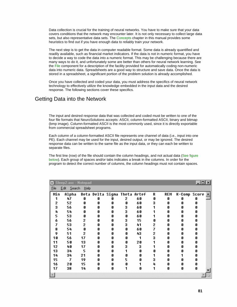
81

Data collection is crucial for the training of neural networks. You have to make sure that your data covers conditions that the network may encounter later. It is not only necessary to collect large data sets, but also representative data sets. The Concepts chapter in this manual provides some heuristics to find out if you have enough data to reliably train your network.

The next step is to get the data in computer readable format. Some data is already quantified and readily available, such as financial market indicators. If the data is not in numeric format, you have to decide a way to code the data into a numeric format. This may be challenging because there are many ways to do it, and unfortunately some are better than others for neural network learning. See the File component for a description of the facility provided for automatically coding non-numeric data into numeric data. Spreadsheets are a good way to structure and save data. Once the data is stored in a spreadsheet, a significant portion of the problem solution is already accomplished.

Once you have collected and coded your data, you must address the specifics of neural network technology to effectively utilize the knowledge embedded in the input data and the desired response. The following sections cover these specifics.

Getting Data into the Network

The input and desired response data that was collected and coded must be written to one of the four file formats that NeuroSolutions accepts: ASCII, column-formatted ASCII, binary and bitmap (bmp image). Column-formatted ASCII is the most commonly used, since it is directly exportable from commercial spreadsheet programs.

Each column of a column-formatted ASCII file represents one channel of data (i.e., input into one PE). Each channel may be used for the input, desired output, or may be ignored. The desired response data can be written to the same file as the input data, or they can each be written to separate files.

The first line (row) of the file should contain the column headings, and not actual data (See figure below). Each group of spaces and/or tabs indicates a break in the columns. In order for the program to detect the correct number of columns, the column headings must not contain spaces.

82

Example of a column-formatted ASCII file

The remaining lines contain the individual samples of data. The data elements (values) are separated by spaces and/or tabs. The number of data elements for each line must match the number of column headings from the first line. The data elements can be either numeric or symbolic. There is a facility to automatically convert symbolic data to numeric data.

The remaining three file types are simply read as a sequential stream of floating-point values. Non-formatted ASCII files contain numeric value separated by tabs and/or spaces. Any non-numeric values are simply ignored. Bitmap files can be either 16-color or 256-color. Each pixel of the image is converted to a value from 0 to 1, based on its intensity level. Binary files contain raw data, such that each 4-byte segment contains a floating-point value. Many numerical software packages export their data to this type of format.

Cross Validation

During training, the input and desired data will be repeatedly presented to the network. As the network learns, the error will drop towards zero. Lower error, however, does not always mean a better network. It is possible to overtrain a network.

Cross validation is a highly recommended criterion for stopping the training of a network. Although highly recommended, it is not required. One will often want to try several networks using just training data in order to see which works best, and then use cross validation for the final training.

When using cross validation, the next step is to decide how to divide your data into a training set and a validation set, also called the test set. The network is trained with the training set, and the performance checked with the test set. The neural network will find the input-output map by repeatedly analyzing the training set. This is called the network training phase. Most of the neural network design effort is spent in the training phase. Training is normally slow because the network’s weights are being updated based on the error information. At times, training will strain the patience of the designer. But a carefully controlled training phase is indispensable for good performance, so be patient. NeuroSolutions’ code was written to take maximum advantage of your computer’s resources. Hardware accelerators for NeuroSolutions that are totally transparent to the user are forthcoming.

There is a need to monitor how well the network is learning. One of the simplest methods is to observe how the cost, which is the square difference between the network’s output and the desired response, changes over training iterations. This graph of the output error versus iteration is called the learning curve. The figure below shows a typical learning curve. Note that in principle the learning curve decreases exponentially to zero or a small constant. One should be satisfied with a small error. How small depends upon the situation, and your judgment must be used to find what error value is appropriate for your problem. The training phase also holds the key to an accurate solution, so the criterion to stop training must be very well delineated. The goal of the stop criterion is to maximize the network’s generalization.

83

Typical learning curve

It is relatively easy to adapt the weights in the training phase to provide a good solution to the training data. However, the best test for a network’s performance is to apply data that it has not yet seen. Take a stock prediction example. One can train the network to predict the next day’s stock price using data from the previous year. This is the training data. But what is really needed is to use the trained network to predict tomorrow’s price.

To test the network one must freeze the weights after the training phase and apply data that the network has not seen before. If the training is successful and the network’s topology is correct, it will apply its ‘past experience’ to this data and still produce a good solution. If this is the case, then the network will be able to generalize based on the training set.

What is interesting is that a network with enough weights will always learn the training set better as the number of iterations is increased. However, neural network researchers have found that this decrease in the training set error was not always coupled to better performance in the test set. When the network is trained too much, the network ‘memorizes’ the training patterns and does not generalize well.

A practical way to find a point of better generalization is to set aside a small percentage (around 10%) of the training set and use it for cross validation. One should monitor the error in the training set and the validation set. When the error in the validation set increases, the training should be stopped because the point of best generalization has been reached. Cross validation is one of the most powerful methods to stop the training. Other methods are discussed under Network Training.

Network Topology

After taking care of the data collection and organization of the training sets, one must select the network’s topology. An understanding of the topology as a whole is needed before the number of hidden layers and the number of PEs in each layer can be estimated. This discussion will focus on multilayer perceptrons (MLPs) because they are the most common.

A multilayer perceptron with two hidden layers is a universal mapper. A universal mapper means that if the number of PEs in each layer and the training time is not constrained, then mathematicians can prove that the network has the power of solving any problem. This is a very important result but it is only an existence proof, so it does not say how such networks can be designed. The problem left to the experimentalist (like you) is to find out what is the right

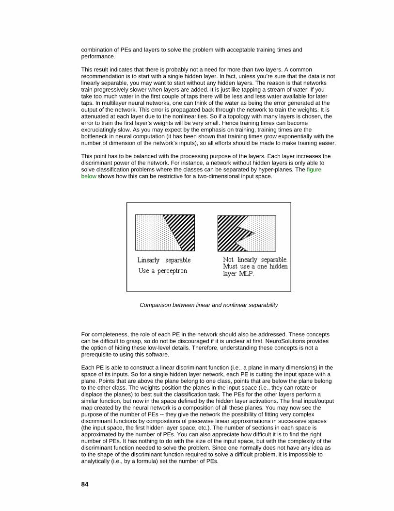
84

combination of PEs and layers to solve the problem with acceptable training times and performance.

This result indicates that there is probably not a need for more than two layers. A common recommendation is to start with a single hidden layer. In fact, unless you’re sure that the data is not linearly separable, you may want to start without any hidden layers. The reason is that networks train progressively slower when layers are added. It is just like tapping a stream of water. If you take too much water in the first couple of taps there will be less and less water available for later taps. In multilayer neural networks, one can think of the water as being the error generated at the output of the network. This error is propagated back through the network to train the weights. It is attenuated at each layer due to the nonlinearities. So if a topology with many layers is chosen, the error to train the first layer’s weights will be very small. Hence training times can become excruciatingly slow. As you may expect by the emphasis on training, training times are the bottleneck in neural computation (it has been shown that training times grow exponentially with the number of dimension of the network’s inputs), so all efforts should be made to make training easier.

This point has to be balanced with the processing purpose of the layers. Each layer increases the discriminant power of the network. For instance, a network without hidden layers is only able to solve classification problems where the classes can be separated by hyper-planes. The figure below shows how this can be restrictive for a two-dimensional input space.

Comparison between linear and nonlinear separability

For completeness, the role of each PE in the network should also be addressed. These concepts can be difficult to grasp, so do not be discouraged if it is unclear at first. NeuroSolutions provides the option of hiding these low-level details. Therefore, understanding these concepts is not a prerequisite to using this software.

Each PE is able to construct a linear discriminant function (i.e., a plane in many dimensions) in the space of its inputs. So for a single hidden layer network, each PE is cutting the input space with a plane. Points that are above the plane belong to one class, points that are below the plane belong to the other class. The weights position the planes in the input space (i.e., they can rotate or displace the planes) to best suit the classification task. The PEs for the other layers perform a similar function, but now in the space defined by the hidden layer activations. The final input/output map created by the neural network is a composition of all these planes. You may now see the purpose of the number of PEs -- they give the network the possibility of fitting very complex discriminant functions by compositions of piecewise linear approximations in successive spaces (the input space, the first hidden layer space, etc.). The number of sections in each space is approximated by the number of PEs. You can also appreciate how difficult it is to find the right number of PEs. It has nothing to do with the size of the input space, but with the complexity of the discriminant function needed to solve the problem. Since one normally does not have any idea as to the shape of the discriminant function required to solve a difficult problem, it is impossible to analytically (i.e., by a formula) set the number of PEs.

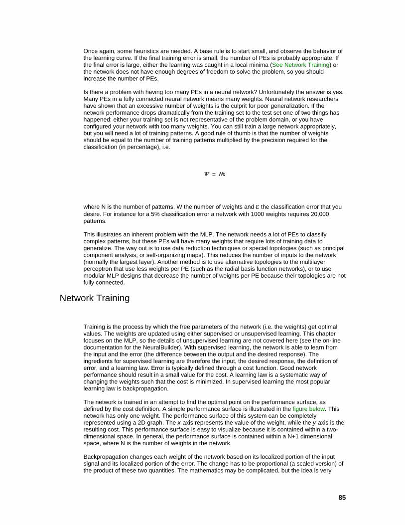
85

Once again, some heuristics are needed. A base rule is to start small, and observe the behavior of the learning curve. If the final training error is small, the number of PEs is probably appropriate. If the final error is large, either the learning was caught in a local minima (See Network Training) or the network does not have enough degrees of freedom to solve the problem, so you should increase the number of PEs.

Is there a problem with having too many PEs in a neural network? Unfortunately the answer is yes. Many PEs in a fully connected neural network means many weights. Neural network researchers have shown that an excessive number of weights is the culprit for poor generalization. If the network performance drops dramatically from the training set to the test set one of two things has happened: either your training set is not representative of the problem domain, or you have configured your network with too many weights. You can still train a large network appropriately, but you will need a lot of training patterns. A good rule of thumb is that the number of weights should be equal to the number of training patterns multiplied by the precision required for the classification (in percentage), i.e.

where N is the number of patterns, W the number of weights and ε the classification error that you desire. For instance for a 5% classification error a network with 1000 weights requires 20,000 patterns.

This illustrates an inherent problem with the MLP. The network needs a lot of PEs to classify complex patterns, but these PEs will have many weights that require lots of training data to generalize. The way out is to use data reduction techniques or special topologies (such as principal component analysis, or self-organizing maps). This reduces the number of inputs to the network (normally the largest layer). Another method is to use alternative topologies to the multilayer perceptron that use less weights per PE (such as the radial basis function networks), or to use modular MLP designs that decrease the number of weights per PE because their topologies are not fully connected.

Network Training

Training is the process by which the free parameters of the network (i.e. the weights) get optimal values. The weights are updated using either supervised or unsupervised learning. This chapter focuses on the MLP, so the details of unsupervised learning are not covered here (see the on-line documentation for the NeuralBuilder). With supervised learning, the network is able to learn from the input and the error (the difference between the output and the desired response). The ingredients for supervised learning are therefore the input, the desired response, the definition of error, and a learning law. Error is typically defined through a cost function. Good network performance should result in a small value for the cost. A learning law is a systematic way of changing the weights such that the cost is minimized. In supervised learning the most popular learning law is backpropagation.

The network is trained in an attempt to find the optimal point on the performance surface, as defined by the cost definition. A simple performance surface is illustrated in the figure below. This network has only one weight. The performance surface of this system can be completely represented using a 2D graph. The x-axis represents the value of the weight, while the y-axis is the resulting cost. This performance surface is easy to visualize because it is contained within a two-dimensional space. In general, the performance surface is contained within a N+1 dimensional space, where N is the number of weights in the network.

Backpropagation changes each weight of the network based on its localized portion of the input signal and its localized portion of the error. The change has to be proportional (a scaled version) of the product of these two quantities. The mathematics may be complicated, but the idea is very

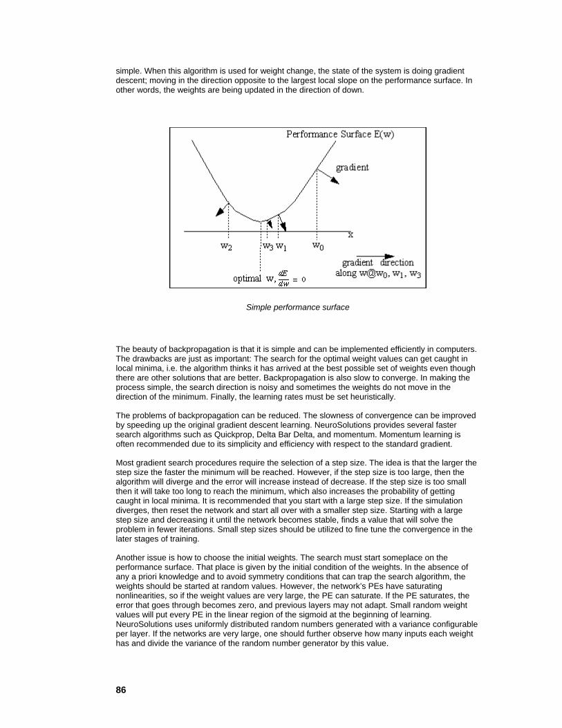
86

simple. When this algorithm is used for weight change, the state of the system is doing gradient descent; moving in the direction opposite to the largest local slope on the performance surface. In other words, the weights are being updated in the direction of down.

Simple performance surface

The beauty of backpropagation is that it is simple and can be implemented efficiently in computers. The drawbacks are just as important: The search for the optimal weight values can get caught in local minima, i.e. the algorithm thinks it has arrived at the best possible set of weights even though there are other solutions that are better. Backpropagation is also slow to converge. In making the process simple, the search direction is noisy and sometimes the weights do not move in the direction of the minimum. Finally, the learning rates must be set heuristically.

The problems of backpropagation can be reduced. The slowness of convergence can be improved by speeding up the original gradient descent learning. NeuroSolutions provides several faster search algorithms such as Quickprop, Delta Bar Delta, and momentum. Momentum learning is often recommended due to its simplicity and efficiency with respect to the standard gradient.

Most gradient search procedures require the selection of a step size. The idea is that the larger the step size the faster the minimum will be reached. However, if the step size is too large, then the algorithm will diverge and the error will increase instead of decrease. If the step size is too small then it will take too long to reach the minimum, which also increases the probability of getting caught in local minima. It is recommended that you start with a large step size. If the simulation diverges, then reset the network and start all over with a smaller step size. Starting with a large step size and decreasing it until the network becomes stable, finds a value that will solve the problem in fewer iterations. Small step sizes should be utilized to fine tune the convergence in the later stages of training.

Another issue is how to choose the initial weights. The search must start someplace on the performance surface. That place is given by the initial condition of the weights. In the absence of any a priori knowledge and to avoid symmetry conditions that can trap the search algorithm, the weights should be started at random values. However, the network’s PEs have saturating nonlinearities, so if the weight values are very large, the PE can saturate. If the PE saturates, the error that goes through becomes zero, and previous layers may not adapt. Small random weight values will put every PE in the linear region of the sigmoid at the beginning of learning. NeuroSolutions uses uniformly distributed random numbers generated with a variance configurable per layer. If the networks are very large, one should further observe how many inputs each weight has and divide the variance of the random number generator by this value.

87

The stop criteria for learning are very important. The stop criterion based on the error of the cross validation set was explained earlier. Other methods limit the total number of iterations (hence the training time), stopping the training regardless of the networks performance. Another method stops training when the error reaches a given value. Since the error is a relative quantity, and the length of time needed for the simulation to get there is unknown, this may not be the best stop criterion. Another alternative is to stop on incremental error. This method stops the training at the point of diminishing returns, when an iteration is only able to decrease the error by a negligible amount. However, the training can be prematurely stopped with this criterion because performance surfaces may have plateaus where the error changes very little from iteration to iteration.

Probing

A successful neural network simulation requires the specification of many parameters. The performance is highly dependent on the choice of these parameters. A productive way to assess the adequacy of the chosen parameters is to observe the signals that flow inside the network. NeuroSolutions has an amazingly powerful set of probing tools. One can observe signals flowing in the network, weights changing, errors being propagated, and most importantly the cost, all while the network is working. This means that you do not need to wait until the end of training to find out that the learning rate was set too high.

All probes within NeuroSolutions belong to one of two categories -- static probes and temporal probes. The big difference is that the first kind access instantaneous data, while the second access the data over a window in time. The temporal probes have a buffer that stores past values, so one can visualize the signals as they change during learning. Fourier transforms provide a look at the frequency composition of such signals. There is also a probe that provides a 3-D representation of the state space.

Running the Simulation

The simulation of a network in NeuroSolutions requires the orchestration of many pieces. When you run the simulation you should start by checking if the data is being correctly fed into the network by placing probes on the input sources. Likewise you should verify the desired signal.

Another important aspect is to check if the learning rates are sufficiently low to avoid divergence. Divergence will usually occur during the beginning of training. You might place a matrix viewer on the first synapse to see if the weights are changing. Observing a steady decrease of the cost is the best overall indicator (the temperature) that everything is progressing well.

Note that with a lot of the probes open, you are stealing computing cycles from the simulations. Therefore once you are convinced that the training is OK, you should momentarily stop the simulation and close the probe windows. Minimally you should leave the matrix viewer to report the cost, or even better to attach a scope to the cost, such that you can have the history of the learning during the length of the simulation. At this point you can leave the simulation unattended until the stop criterion halts the simulation.

You now have to decide if the learning was successful or not. Most of the time, the first check is to see if the cost is within what you think is appropriate for your application. In the affirmative case, you should save your network. Remember that all the information gathered by the network from the input data is contained in the weights. So you should save the weights, along with the topology. The weights are saved by default.

Concepts Concepts

88

NeuroSolutions



Purpose

This chapter links neural network theory with the principles and components embodied within NeuroSolutions. It will provide an abstract tour of the NeuroSolutions components while motivating their application to neural network simulations.

NeuroSolutions Structure NeuroSolutions Structure

NeuroSolutions consists of two major parts: the main window and the neural network components. The main window includes the ability to load, create and save the document, which is called the breadboard. The neural components are used to construct neural network topologies and are organized into palettes that can be attached to the main window.

Palettes

Breadboard

Palettes

Palettes provide organized storage for neural components. Since NeuroSolutions is object-oriented, the program modules that implement the neural component functionality are naturally organized in code hierarchies that have common ancestry. Each member of the hierarchy increases the functionality of its ancestors. Each branch in the code hierarchy has a specific function in the neural network simulations.

NeuroSolutions associates an icon to each neural component. The user interacts with these icons within a graphical user interface (GUI) to construct and simulate neural topologies. The components are organized into families and stored within palettes. Select the Palettes menu from the NeuroSolutions main window to see a list of the component families.

Networks are constructed by simply selecting components from the palettes and stamping them onto the breadboard. Palettes that are used frequently can be docked (attached) to the main window (see Toolbar Manipulation).

89

Example of a palette

Breadboard

NeuroSolutions has one document type, the breadboard. Simulations are constructed and run on breadboards. With NeuroSolutions, designing a neural network is very similar to prototyping an electronic circuit. With an electronic circuit, components such as resistors, capacitors and inductors are first arranged on a breadboard. NeuroSolutions instead uses neural components such as axons, synapses and probes. The components are then connected together to form a circuit. The electronic circuit passes electrons between its components. The circuit (i.e., neural network) of NeuroSolutions passes activity between its components, and is termed a data flow machine. Finally, the circuit is tested by inputting data and probing the systems' response at various points. An electronic circuit would use an instrument, such as an oscilloscope, for this task. A NeuroSolutions network uses one or more of its components within the probes family (e.g., the MegaScope).

Networks are constructed on a breadboard by selecting components from the palettes, stamping them on the breadboard, and then interconnecting them to form a network topology. Once the topology is established and its components have been configured, a simulation can be run. An example of a functional breadboard is illustrated in the figure below.

Example of a breadboard (single hidden layer MLP)

New breadboards are created by selecting New from the File menu. This will create a blank breadboard titled "Breadboard1.nsb". The new breadboard can later be saved. Saving a breadboard saves the topology, the configuration of each component and (optionally) their weights. Therefore, a breadboard may be saved at any point during training and then restored later. The saving of weights is a parameter setting for each component that contains adaptive weights. This parameter can be set for all components on the breadboard or just selected ones.

90

NeuroSolutions Graphical User Interface (GUI) NeuroSolutions Graphical User Interface (GUI)

Logic of the Interface

Components

The Inspector

Single-Click vs. Double-Click

Network Construction

Network Access

Network Simulation

Logic of the Interface

User interaction with NeuroSolutions follows very simple and clear principles:

Each neural component is represented by an icon.

Single-clicking on a component's icon will display its Inspector window. A component's inspector is where the user can inspect and alter any variables of the component.

Double-clicking on a component's icon will open its animation window, if such a window exist. Animation windows allow components to display data while a simulation is running.

Single-clicking on a component's icon with the help cursor will display its on-line help quick reference page.

Networks are constructed by placing and interconnecting components on a breadboard.

Components are created by selecting them from palettes and stamping them onto the breadboard. Components can be removed from the topology by means of the cut operation.

During a stamp operation, the cursor will indicate whether stamping the component in its present location is valid. These operations and their corresponding mouse cursor are as follows:

A stamp indicates that the selected palette component can be copied to the present mouse location.

A move cursor means that the component is under mouse control (drag).

A circle with a slanted line means that the component can not be copied to the present mouse position.

A gray stamp indicates that the selected palette component can be used to replace the component at the present mouse location.

Stamping by pressing the left mouse button will stamp a single component and return to selection mode.

Stamping by pressing the right mouse button will stamp a single component and remain in stamping mode. This allows multiple copies of the same component to be stamped easily.

The Selection Cursor toolbar button is used to switch from stamping mode to selection mode. Several components can be selected at the same time by pressing the Shift key and mousing down on the component. Another method is to select a rectangular region of the breadboard, which then selects all components that lie within. A box is drawn around each of the selected components.

91

Selected components can be cut, copied, pasted or moved. The multiple-selection feature is also used to broadcast parameter changes made in one component’s inspector to a group of components.

Components

The building blocks used to create, control and inspect neural networks are referred to as components. Each component is represented by an icon. An example is the Axon, which corresponds to the icon illustrated in the figure below.

Icon for the Axon

Each component is concisely described within the Components chapter. You will find the component’s function (with an equation if appropriate), how to manipulate and configure it (via its inspector), where it can "live" (be stamped), and how to access its data (access points). You can

reach the help for a component by selecting the help cursor and then selecting the component that you want help on.

The Inspector

The Inspector window is the tool used to configure individual components. If for any reason the Inspector window is closed, it can be re-opened by selecting Inspector from the View menu. Single-clicking on any component will highlight it (put a square around it) and load its property pages into the Inspector window. The name of the inspected component is displayed at the top of the Inspector window. This procedure is referred to as selecting a component.

The Inspector window has a folder organization (see figure belowHIDD_NAXONINSPECTOR), reflecting the hierarchical organization of the code (inheritance in object-oriented parlance). The name of the hierarchy level is placed on the tab of the folder. The highest ancestor is the right most tab. This system of inspecting components minimizes the number of windows open at any given time. A single breadboard may have hundreds of components. If each component used space on the screen for user interaction, the entire screen would quickly become cluttered. After a while this convention becomes natural and easy to use.

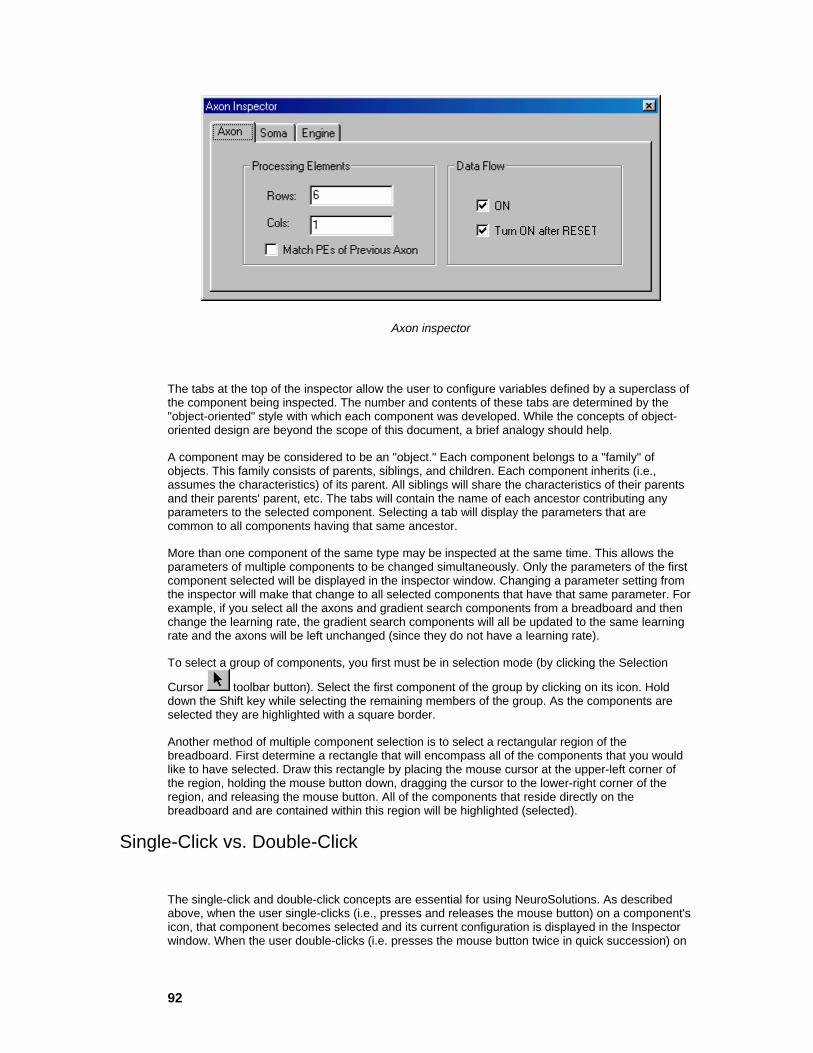
92

Axon inspector

The tabs at the top of the inspector allow the user to configure variables defined by a superclass of the component being inspected. The number and contents of these tabs are determined by the "object-oriented" style with which each component was developed. While the concepts of object-oriented design are beyond the scope of this document, a brief analogy should help.

A component may be considered to be an "object." Each component belongs to a "family" of objects. This family consists of parents, siblings, and children. Each component inherits (i.e., assumes the characteristics) of its parent. All siblings will share the characteristics of their parents and their parents' parent, etc. The tabs will contain the name of each ancestor contributing any parameters to the selected component. Selecting a tab will display the parameters that are common to all components having that same ancestor.

More than one component of the same type may be inspected at the same time. This allows the parameters of multiple components to be changed simultaneously. Only the parameters of the first component selected will be displayed in the inspector window. Changing a parameter setting from the inspector will make that change to all selected components that have that same parameter. For example, if you select all the axons and gradient search components from a breadboard and then change the learning rate, the gradient search components will all be updated to the same learning rate and the axons will be left unchanged (since they do not have a learning rate).

To select a group of components, you first must be in selection mode (by clicking the Selection

Cursor toolbar button). Select the first component of the group by clicking on its icon. Hold down the Shift key while selecting the remaining members of the group. As the components are selected they are highlighted with a square border.

Another method of multiple component selection is to select a rectangular region of the breadboard. First determine a rectangle that will encompass all of the components that you would like to have selected. Draw this rectangle by placing the mouse cursor at the upper-left corner of the region, holding the mouse button down, dragging the cursor to the lower-right corner of the region, and releasing the mouse button. All of the components that reside directly on the breadboard and are contained within this region will be highlighted (selected).

Single-Click vs. Double-Click

The single-click and double-click concepts are essential for using NeuroSolutions. As described above, when the user single-clicks (i.e., presses and releases the mouse button) on a component's icon, that component becomes selected and its current configuration is displayed in the Inspector window. When the user double-clicks (i.e. presses the mouse button twice in quick succession) on

93

any component, NeuroSolutions will select the component and attempt to open any windows that the component may have. Component windows allow components to display data while a simulation is running. If the inspector is hidden and the component’s window is already open (or it doesn’t have a window), then double-clicking on the component will bring the inspector into view.

File Open Dialog Box

The following options allow you to specify which breadboard to open: File Name

Type or select the filename of the breadboard you want to open. This box lists files with the extension you select in the List Files of Type box. List Files of Type

Select the file type you want to open. Since NeuroSolutions only document type is the breadboard, you should find your files with the ".nsb" extension. Drives

Select the drive in which NeuroSolutions stores the breadboard that you want to open. Directories

Select the directory in which NeuroSolutions stores the breadboard that you want to open. Network...

Choose this button to connect to a network location, assigning it a new drive letter.

Save As Dialog Box

The following options allow you to specify the name and location of the file you're about to save: File Name

Type a new filename to save a document with a different name. A filename can contain up to eight characters and an extension of up to three characters. NeuroSolutions adds the extension you specify in the Save File As Type box. Drives

Select the drive in which you want to store the document. Directories

Select the directory in which you want to store the document. Network...

Choose this button to connect to a network location, assigning it a new drive letter.

Toolbars and Palettes

94

Both the toolbars and palettes are control bars that can be positioned any where on the screen. These control bars are also dockable, meaning that they have the ability to be attached or "docked" to the main window.

Both the toolbars and palettes have a feature called tooltips. Tooltips provide a means for labeling the buttons with a name in addition to the icons.

The Toolbars menu and the Palettes menu are used to toggle the visibility of the control bars. This feature is available so that only the palettes and toolbars used most often occupy the screen area.

Title Bar

The title bar is located along the top of a window. It contains the name of the application and document.

To move the window, drag the title bar. Note: You can also move dialog boxes by dragging their title bars.

A title bar may contain the following elements:

Application Control-menu button

Maximize button

Minimize button

Close Button

Name of the application

Name of the document

Scroll Bars

Displayed at the right and bottom edges of the breadboard. The scroll boxes inside the scroll bars indicate your vertical and horizontal location in the document. You can use the mouse to scroll to other parts of the breadboard.

95



Components are selected from palettes and stamped on the breadboard. The network topology is specified by interconnecting components via male and female connectors. This topology is then tested by injecting data into and probing output from components via access points.

The following sections describe each step in this simulation process.

Stamping

Manipulating Components

Replacing Axons and Synapses

Connectors

Cabling

Stacking

Stamping

The method used to copy components from palettes to breadboards is by selecting and stamping. Selecting is accomplished by clicking on the component’s button on the palette. The cursor then becomes a stamp, and the component can be copied many times on the breadboard by clicking on a specific location. Note that some components cannot be stamped directly on the breadboard and can only be stamped on top of other components.

To switch from stamping mode back to selection mode, click the Selection Cursor button from the main toolbar (see figure below).

Toolbar button used to switch to selection mode

Manipulating Components

Moving a component is very straightforward. Select the component by clicking on its icon. Holding down the mouse button will make the cursor change to a move cursor. While the mouse button is down, the component will track the location of the cursor. Release the mouse button to place the component at a new location.

Copying a component will create a clone with the exact same configuration. To copy a component,

select it and click the Copy toolbar button. Then select where the clone should reside; click on

96

the breadboard or component where the copy should be placed. Then click the Paste toolbar button to create the clone. If the Paste button is disabled (grayed-out), that means that the component can not be pasted on the selected location. Copied components that reside directly on the breadboard must be pasted on the breadboard. Copied components that are attached to other components must be pasted onto other components.

These concepts get a bit more complicated, and more powerful, when a component is connected to other components on the breadboard. There are basically two methods for connecting components: through connectors and stacking. When a component is moved or copied, all components stacked on top of it will also be moved or copied. Components attached by connectors will be disconnected during a copy, except for those connections made between the copied components. However, connectors will be disconnected when a component is removed from the breadboard.

Replacing Axons and Synapses

There will often be times when you would like to change the transfer function or memory structure of an Axon, or change a fully connected Synapse to a sparsely connected one. This requires that you replace a component, which can be inconvenient when other components are attached and connected. The component replace feature automatically swaps an Axon or Synapse and re-establishes all of the attachments and connections. Simply select the new component from the palette, place your cursor over the component to replace (notice that the cursor changes to a gray stamp), and click the left mouse button.

Connectors

Constructing a network topology is equivalent to assigning the order in which data flows through network components. Data flow connections are made using male and female connectors. These connectors have the icons illustrated in the figure below.

Male Connector Female Connector

Connections are formed by dragging a MaleConnector over a FemaleConnector and releasing the mouse button (dropping). The cursor will turn to a move cursor when a male is dragged over an available female. Otherwise the forbidden sign will show up. The icon for a male connected to a female is shown in the figure below.

Connection

There is also a shortcut for making a connection between two components. First, select the source component (by single-clicking the left mouse button), then single click the destination component with the right mouse button to bring up the Component Menu. Select the "Connect to" menu item.

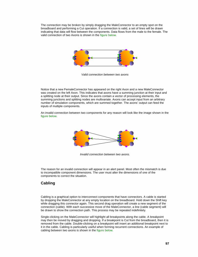
97

The connection may be broken by simply dragging the MaleConnector to an empty spot on the breadboard and performing a Cut operation. If a connection is valid, a set of lines will be drawn indicating that data will flow between the components. Data flows from the male to the female. The valid connection of two Axons is shown in the figure below.

Valid connection between two axons

Notice that a new FemaleConnector has appeared on the right Axon and a new MaleConnector was created on the left Axon. This indicates that axons have a summing junction at their input and a splitting node at their output. Since the axons contain a vector of processing elements, the summing junctions and splitting nodes are multivariate. Axons can accept input from an arbitrary number of simulation components, which are summed together. The axons’ output can feed the inputs of multiple components.

An invalid connection between two components for any reason will look like the image shown in the figure below.

Invalid connection between two axons.

The reason for an invalid connection will appear in an alert panel. Most often the mismatch is due to incompatible component dimensions. The user must alter the dimensions of one of the components to correct the situation.

Cabling

Cabling is a graphical option to interconnect components that have connectors. A cable is started by dropping the MaleConnector at any empty location on the breadboard. Hold down the Shift key while dragging this connector again. This second drag operation will create a new segment of the connection (cable). With each successive move of the MaleConnector, a line (cable segment) will be drawn to show the connection path. This process may be repeated indefinitely.

Single-clicking on the MaleConnector will highlight all breakpoints along the cable. A breakpoint may then be moved by dragging and dropping. If a breakpoint is Cut from the breadboard, then it is removed from the cable. Double-clicking on a breakpoint will insert an additional breakpoint next to it in the cable. Cabling is particularly useful when forming recurrent connections. An example of cabling between two axons is shown in the figure below.

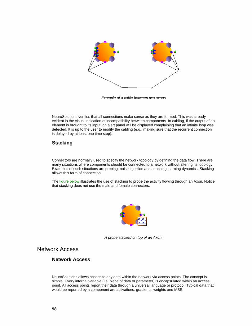
98

Example of a cable between two axons

NeuroSolutions verifies that all connections make sense as they are formed. This was already evident in the visual indication of incompatibility between components. In cabling, if the output of an element is brought to its input, an alert panel will be displayed complaining that an infinite loop was detected. It is up to the user to modify the cabling (e.g., making sure that the recurrent connection is delayed by at least one time step).

Stacking

Connectors are normally used to specify the network topology by defining the data flow. There are many situations where components should be connected to a network without altering its topology. Examples of such situations are probing, noise injection and attaching learning dynamics. Stacking allows this form of connection.

The figure below illustrates the use of stacking to probe the activity flowing through an Axon. Notice that stacking does not use the male and female connectors.

A probe stacked on top of an Axon.

Network Access

Network Access

NeuroSolutions allows access to any data within the network via access points. The concept is simple. Every internal variable (i.e. piece of data or parameter) is encapsulated within an access point. All access points report their data through a universal language or protocol. Typical data that would be reported by a component are activations, gradients, weights and MSE.

99

Components that understand this protocol belong to the Access family. Access components attach to access points through stacking. Any component with accessible data will report its available access points to an Access component during the stamping operation. If the component being stamped has a compatible access point, then the cursor will turn to a stamp. The Probe stacked on top of an Axon figure illustrates a MatrixViewer that has been placed on an Axon.

Since each component may have more than one access point, the desired access point must be selected from a list. This list is contained within the Access property page of the stacked component’s inspector (see The Inspector).

The inspector for the MatrixViewer allows the user to select between the activity and pre-activity access reported by the Axon. This inspector is illustrated in the figure below.

Available access points of the Axon component

All Access components have an access point called Stacked access. This access point allows data to be simultaneously used by more than one Access component. In the above example, another probe can be dropped on top of the MatrixViewer using its Stacked access to visualize the data in a different way.

Probes

Data Input/Output

Transmitters and Receivers

Probes

Probes are one family of components that speak the Access protocol. Each probe provides a unique way of visualizing the data provided by access points. Consider an access point presenting a fully connected matrix of weights. You could view this data instantaneously as a matrix of numbers or you could view this data over time as weight tracks. What is important here is that NeuroSolutions provides an extensive set of visualization tools that can be attached to any data within the network.

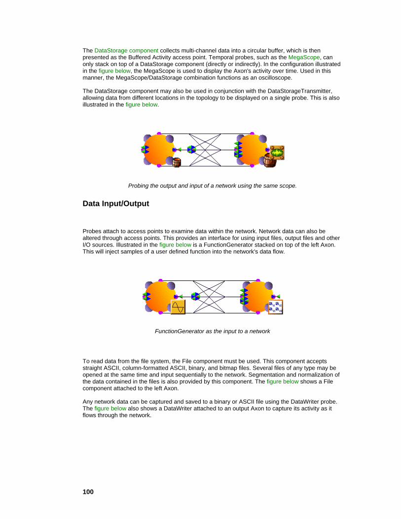
100

The DataStorage component collects multi-channel data into a circular buffer, which is then presented as the Buffered Activity access point. Temporal probes, such as the MegaScope, can only stack on top of a DataStorage component (directly or indirectly). In the configuration illustrated in the figure below, the MegaScope is used to display the Axon's activity over time. Used in this manner, the MegaScope/DataStorage combination functions as an oscilloscope.

The DataStorage component may also be used in conjunction with the DataStorageTransmitter, allowing data from different locations in the topology to be displayed on a single probe. This is also illustrated in the figure below.

Probing the output and input of a network using the same scope.

Data Input/Output

Probes attach to access points to examine data within the network. Network data can also be altered through access points. This provides an interface for using input files, output files and other I/O sources. Illustrated in the figure below is a FunctionGenerator stacked on top of the left Axon. This will inject samples of a user defined function into the network's data flow.

FunctionGenerator as the input to a network

To read data from the file system, the File component must be used. This component accepts straight ASCII, column-formatted ASCII, binary, and bitmap files. Several files of any type may be opened at the same time and input sequentially to the network. Segmentation and normalization of the data contained in the files is also provided by this component. The figure below shows a File component attached to the left Axon.

Any network data can be captured and saved to a binary or ASCII file using the DataWriter probe. The figure below also shows a DataWriter attached to an output Axon to capture its activity as it flows through the network.

101

A File component to read data in and a DataWriter probe to write data out

Transmitters and Receivers

Both connectors and stacking provide local communication between components. There are situations where a global communication channel is necessary, either to send/receive data or for control. NeuroSolutions provides a family of components, called Transmitters, to implement global communications. These components use access points to globally transmit data, or to send global messages based on local decisions. Several components can receive data or control messages that alter their normal operation. This allows very sophisticated tasks to be implemented, such as adaptive learning rates, nonuniform relaxation, and error-based stop criteria.

Network Simulation

Network Simulation

When a network is "run", data will flow one sample at a time from the input components, through the network topology, and into the output components. The standard data flow is from left to right, but this depends on how the components are connected together. Note that the NeuroSolutions main window has no menu options for controlling the simulation. This is done strictly at the component level using members of the Controls family.

Application Window Commands Size command (System menu)

Use this command to display a four-headed arrow so you can size the active window with the arrow keys.

After the pointer changes to the four-headed arrow:

1 Press one of the DIRECTION keys (left, right, up, or down arrow key) to move the pointer to the border you want to move.

2 Press a DIRECTION key to move the border.

3 Press ENTER when the window is the size you want.

102

Note: This command is unavailable if you maximize the window.

Shortcut

Mouse: Drag the size bars at the corners or edges of the window.

Move command (Control menu)

Use this command to display a four-headed arrow so you can move the active window or dialog box with the arrow keys.

Note: This command is unavailable if you maximize the window.

Shortcut

Keys: CTRL+F7

Minimize command (application Control menu)

Use this command to reduce the NeuroSolutions window to an icon.

Shortcut

Mouse: Click the minimize icon on the title bar.

Keys: ALT+F9

Maximize command (System menu)

Use this command to enlarge the active window to fill the available space.

Shortcut

Mouse: Click the maximize icon on the title bar; or double-click the title bar.

Keys: CTRL+F10 enlarges a document window.

Close command (Control menus)

103

Use this command to close the active window or dialog box.

Double-clicking a Control-menu box is the same as choosing the Close command.

Note: If you have multiple windows open for a single document, the Close command on the document Control menu closes only one window at a time. You can close all windows at once with the Close command on the File menu.

Shortcut

Keys: ALT+F4 exits NeuroSolutions

Restore command (Control menu)

Use this command to return the active window to its size and position before you chose the Maximize or Minimize command.

Switch to command (application Control menu)

Use this command to display a list of all open applications. Use this "Task List" to switch to or close an application on the list.

Shortcut

Keys: CTRL+ESC

Dialog Box Options

When you choose the Switch To command, you will be presented with a dialog box with the following options:

Task List

Select the application you want to switch to or close. Switch To

Makes the selected application active. End Task

Closes the selected application. Cancel

Closes the Task List box. Cascade

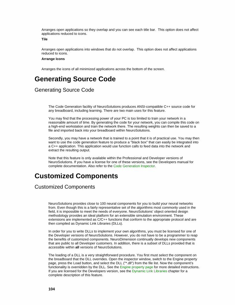
104

Arranges open applications so they overlap and you can see each title bar. This option does not affect applications reduced to icons. Tile

Arranges open applications into windows that do not overlap. This option does not affect applications reduced to icons. Arrange Icons

Arranges the icons of all minimized applications across the bottom of the screen.

Generating Source Code Generating Source Code

The Code Generation facility of NeuroSolutions produces ANSI-compatible C++ source code for any breadboard, including learning. There are two main uses for this feature.

You may find that the processing power of your PC is too limited to train your network in a reasonable amount of time. By generating the code for your network, you can compile this code on a high-end workstation and train the network there. The resulting weights can then be saved to a file and imported back into your breadboard within NeuroSolutions.

Secondly, you may have a network that is trained to a point that it is of practical use. You may then want to use the code generation feature to produce a "black box" that can easily be integrated into a C++ application. This application would use function calls to feed data into the network and extract the resulting output.

Note that this feature is only available within the Professional and Developer versions of NeuroSolutions. If you have a license for one of these versions, see the Developers manual for complete documentation. Also refer to the Code Generation Inspector.

Customized Components Customized Components

NeuroSolutions provides close to 100 neural components for you to build your neural networks from. Even though this is a fairly representative set of the algorithms most commonly used in the field, it is impossible to meet the needs of everyone. NeuroSolutions’ object oriented design methodology provides an ideal platform for an extensible simulation environment. These extensions are implemented as C/C++ functions that conform to the appropriate protocol and are then compiled as Dynamic Link Libraries (DLLs).

In order for you to write DLLs to implement your own algorithms, you must be licensed for one of the Developer versions of NeuroSolutions. However, you do not have to be a programmer to reap the benefits of customized components. NeuroDimension continually develops new components that are public to all Developer customers. In addition, there is a subset of DLLs provided that is accessible within all versions of NeuroSolutions.

The loading of a DLL is a very straightforward procedure. You first must select the component on the breadboard that the DLL overrides. Open the inspector window, switch to the Engine property page, press the Load button, and select the DLL ("*.dll") from the file list. Now the component’s functionality is overridden by the DLL. See the Engine property page for more detailed instructions. If you are licensed for the Developers version, see the Dynamic Link Libraries chapter for a complete description of this feature.

105

Testing the Network The TestingWizard

After training a network, you will want to test the network performance on data that the network was not trained with. The TestingWizard automates this procedure by providing an easy way to produce the network output for the testing dataset that you defined within the NeuralExpert or NeuralBuilder, or on a new dataset not yet defined.

To launch the TestingWizard from within NeuroSolutions go to the Tools menu and choose "TestingWizard" or click the "Testing" toolbar button. If your breadboard was built with the NeuralExpert, you may alternatively click the "Test" button in the upper-left corner of the breadboard.

Online help is available from all TestingWizard panels. To access help, click the Help button in the lower left corner of the wizard.

Freezing the Network Weights

The method that the TestingWizard uses for freezing the network weights is to turn off the Learning switch from the Static page of the activation control inspector. This method is easy but not very efficient because the error is still computed, even though the weights are not modified. This method is convenient for times when you just want to run a small test set through your network, where efficiency is not a concern.

To run a fixed network most efficiently, the Backprop and Gradient Search planes, as well as the ErrorCriteria component, should be removed from the breadboard. First save the breadboard so that you can easily return to the learning state. Press the Free All Backprop button of the Backpropagation page of the backprop control inspector to discard these learning planes automatically. The fixed network is now ready to run.

Cross Validation

Cross validation computes the error in a test set at the same time that the network is being trained with the training set. It is known that the MSE will keep decreasing in the training set, but may start to increase in the test set. This happens when the network starts "memorizing" the training patterns. The Termination page of the activation control inspector can be used to monitor the cross validation set error and automatically stop the network when it is not improving.

The easiest way to understand the mechanics of cross validation is to use the NeuralBuilder or NeuralExpert to build a simple network that has cross validation. The Static Inspector is used to configure the switching between the testing and training phases of the simulation. The File components each contain a Training data set and a Cross-Validation data set (see the Data Set property page). The Cross-Validation data can either be a different segment of the same file, or a different file. There is an additional set of Probes and a ThresholdTransmitter for monitoring the cross validation phase of the simulation. Observe the Access Data Set setting of the Access property page for these components.

106

Production Data Set

Once you have trained and tested a network and have determined that the network adequately models your data, you may want to then put that network into production. In doing so, you will have input data but no desired data. The data set to use for this case is the "Production" data set. The easiest way to configure a Production set is to run the TestingWizard and specify an input data file but no desired data file.

Sensitivity Analysis

As you are training a network, you may want to know the effect that each of the network inputs is having on the network output. This provides feedback as to which input channels are the most significant. From there, you may decide to prune the input space by removing the insignificant channels. This will reduce the size of the network, which in turn reduces the complexity and the training times.

Sensitivity analysis is a method for extracting the cause and effect relationship between the inputs and outputs of the network. The network learning is disabled during this operation such that the network weights are not affected. The basic idea is that the inputs to the network are shifted slightly and the corresponding change in the output is reported either as a percentage or a raw difference.

The activation control component generates the input data for the sensitivity analysis by temporarily increasing the input by a small value (dither). The corresponding change in output is the sensitivity data, which is reported by the ErrorCriteria component and displayed by an attached probe.

To configure a network to report the sensitivity data, simply stamp a StaticProbe component on either the "Sensitivity", "Raw Sensitivity", or "Overall Sensitivity" Access Point of the ErrorCriteria component. Double-click the icon of the probe to open its display window. Once you have trained the network, open the Static Inspector, select the "Active Data Set" to perform the sensitivity operation on, specify the "Dither", then click the "Perform" button. The display window of the probe should be updated with the calculated sensitivity data.

Probing the "Sensitivity" access point with a MatrixViewer will display a matrix of values, each corresponding to the percentage effect that a particular input has on a particular output. Each row represents a single input and each column represents a single output. Note that the total for each column (output channel) sums to 100 percent. Likewise, the "Raw Sensitivity" access point produces a matrix, but each value corresponding to the raw difference between the outputs for the dithered and non-dithered inputs. Probing the "Overall Sensitivity" access point with a MatrixViewer will display a column of values, each corresponding to the percentage effect that a particular input has on the output vector as a whole (the sum of all output channels).

Confusion Matrix

A confusion matrix is a simple methodology for displaying the classification results of a network. The confusion matrix is defined by labeling the desired classification on the rows and the predicted classifications on the columns. For each exemplar, a 1 is added to the cell entry defined by (desired classification, predicted classification). Since we want the predicted classification to be the same as the desired classification, the ideal situation is to have all the exemplars end up on the diagonal cells of the matrix (the diagonal that connects the upper-left corner to the lower right). Observe these two examples:

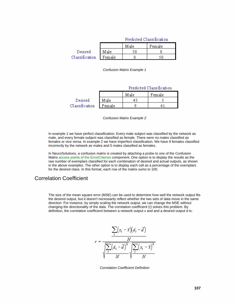
107

Confusion Matrix Example 1

Confusion Matrix Example 2

In example 1 we have perfect classification. Every male subject was classified by the network as male, and every female subject was classified as female. There were no males classified as females or vice versa. In example 2 we have imperfect classification. We have 9 females classified incorrectly by the network as males and 5 males classified as females.

In NeuroSolutions, a confusion matrix is created by attaching a probe to one of the Confusion Matrix access points of the ErrorCriterion component. One option is to display the results as the raw number of exemplars classified for each combination of desired and actual outputs, as shown in the above examples. The other option is to display each cell as a percentage of the exemplars for the desired class. In this format, each row of the matrix sums to 100.

Correlation Coefficient

The size of the mean square error (MSE) can be used to determine how well the network output fits the desired output, but it doesn't necessarily reflect whether the two sets of data move in the same direction. For instance, by simply scaling the network output, we can change the MSE without changing the directionality of the data. The correlation coefficient (r) solves this problem. By definition, the correlation coefficient between a network output x and and a desired output d is:

Correlation Coefficient Definition

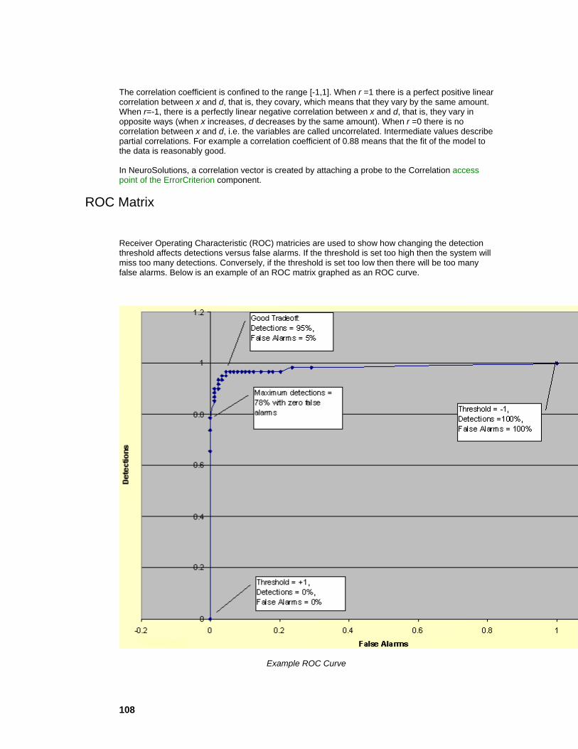
108

The correlation coefficient is confined to the range [-1,1]. When r =1 there is a perfect positive linear correlation between x and d, that is, they covary, which means that they vary by the same amount. When r=-1, there is a perfectly linear negative correlation between x and d, that is, they vary in opposite ways (when x increases, d decreases by the same amount). When r =0 there is no correlation between x and d, i.e. the variables are called uncorrelated. Intermediate values describe partial correlations. For example a correlation coefficient of 0.88 means that the fit of the model to the data is reasonably good.

In NeuroSolutions, a correlation vector is created by attaching a probe to the Correlation access point of the ErrorCriterion component.

ROC Matrix

Receiver Operating Characteristic (ROC) matricies are used to show how changing the detection threshold affects detections versus false alarms. If the threshold is set too high then the system will miss too many detections. Conversely, if the threshold is set too low then there will be too many false alarms. Below is an example of an ROC matrix graphed as an ROC curve.

Example ROC Curve

109

In NeuroSolutions, a ROC matrix is created by attaching a probe to the ROC access point of the ErrorCriterion component. The matrix contains three columns: 1) the detection threshold, 2) the percentage of detections classified correctly, and 3) the percentage of non-detections incorrectly classified as detections (i.e., false alarms). The ouput channel and the number of thresholds are defined within the error criteria inspector.

Performance Measures

The Performance Meassures access point of the ErrorCriterion component provides six values that can be used to measure the performance of the network for a particular data set. MSE

The mean squared error is simply two times the average cost (see the access points of the ErrorCriterion component.) The formula for the mean squared error is:

NMSE

The normalized mean squared error is defined by the following formula:

r

The correlation coefficient. % Error

The percent error is defined by the following formula:

110

Note that this value can easily be misleading. For example, say that your output data is in the range of 0 to 100. For one exemplar your desired output is 0.1 and your actual output is 0.2. Even though the two values are quite close, the percent error for this exemplar is 100. AIC

Akaike's information criterion (AIC) is used to measure the tradeoff between training performance and network size. The goal is to minimize this term to produce a network with the best generalization:

MDL

Rissanen's minimum description length (MDL) criterion is similar to the AIC in that it tries to combine the model’s error with the number of degrees of freedom to determine the level of generalization. The goal is to minimize this term:

Practical Simulation Issues Practical Simulation Issues

Data Preparation

Forms of Backpropagation

Probing

Saving and Fixing Network Weights

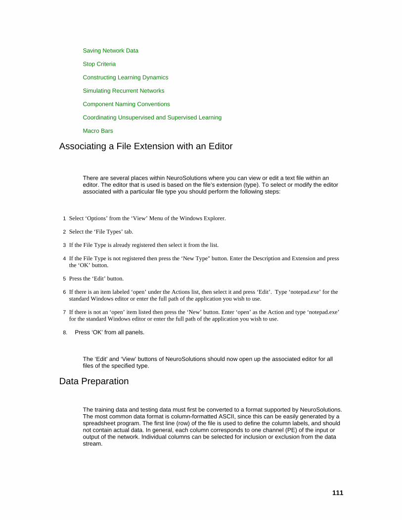
111

Saving Network Data

Stop Criteria

Constructing Learning Dynamics

Simulating Recurrent Networks

Component Naming Conventions

Coordinating Unsupervised and Supervised Learning

Macro Bars

Associating a File Extension with an Editor

There are several places within NeuroSolutions where you can view or edit a text file within an editor. The editor that is used is based on the file’s extension (type). To select or modify the editor associated with a particular file type you should perform the following steps:

1 Select ‘Options’ from the ‘View’ Menu of the Windows Explorer.

2 Select the ‘File Types’ tab.

3 If the File Type is already registered then select it from the list.

4 If the File Type is not registered then press the ‘New Type" button. Enter the Description and Extension and press the ‘OK’ button.

5 Press the ‘Edit’ button.

6 If there is an item labeled ‘open’ under the Actions list, then select it and press ‘Edit’. Type ‘notepad.exe’ for the standard Windows editor or enter the full path of the application you wish to use.

7 If there is not an ‘open’ item listed then press the ‘New’ button. Enter ‘open’ as the Action and type ‘notepad.exe’ for the standard Windows editor or enter the full path of the application you wish to use.

8. Press ‘OK’ from all panels.

The ‘Edit’ and ‘View’ buttons of NeuroSolutions should now open up the associated editor for all files of the specified type.

Data Preparation

The training data and testing data must first be converted to a format supported by NeuroSolutions. The most common data format is column-formatted ASCII, since this can be easily generated by a spreadsheet program. The first line (row) of the file is used to define the column labels, and should not contain actual data. In general, each column corresponds to one channel (PE) of the input or output of the network. Individual columns can be selected for inclusion or exclusion from the data stream.

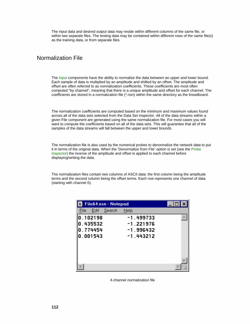
112

The input data and desired output data may reside within different columns of the same file, or within two separate files. The testing data may be contained within different rows of the same file(s) as the training data, or from separate files.

Normalization File

The Input components have the ability to normalize the data between an upper and lower bound. Each sample of data is multiplied by an amplitude and shifted by an offset. The amplitude and offset are often referred to as normalization coefficients. These coefficients are most often computed "by channel", meaning that there is a unique amplitude and offset for each channel. The coefficients are stored in a normalization file (*.nsn) within the same directory as the breadboard.

The normalization coefficients are computed based on the minimum and maximum values found across all of the data sets selected from the Data Set Inspector. All of the data streams within a given File component are generated using the same normalization file. For most cases you will want to compute the coefficients based on all of the data sets. This will guarantee that all of the samples of the data streams will fall between the upper and lower bounds.

The normalization file is also used by the numerical probes to denormalize the network data to put it in terms of the original data. When the ‘Denormalize from File’ option is set (see the Probe Inspector) the inverse of the amplitude and offset is applied to each channel before displaying/writing the data.

The normalization files contain two columns of ASCII data: the first column being the amplitude terms and the second column being the offset terms. Each row represents one channel of data (starting with channel 0).

4-channel normalization file

113

These coefficients are calculated using the following formula:

Amp(i) = (UpperBound - LowerBound) / (Max(i) - Min(i))

Off(i) = UpperBound - Amp(i) * Max(i)

where Max(i) and Min(i) are the maximum and minimum values found within channel i, and UpperBound and LowerBound are the values entered within the Stream Inspector.

The Input components normalize the data using the following formula:

Data(i) = Amp(i) * Data(i) + Off(i)

The Probe components then use the following formula to denormalize the data:

Data(i) = (Data(i) - Off(i)) / Amp(i)

Forms of Backpropagation

Backpropagation can either be synchronized in Static, Trajectory or Fixed Point modes.

Static

Static backpropagation assumes that the output of a network is strictly a function of its present input (i.e., the network topology is static). In this case, the gradients and sensitivities are only dependent on the error and activations from the current time step. Trajectory

Training a network in Trajectory mode assumes that each exemplar has a temporal dimension defined by its forward samples (period), and that there exists some desired response for the network's output over this period. The network is first run forward in time over the entire period, during which an error is determined between the network's output and the desired response. Then the network is run backwards for a prescribed number of samples (defined by the

samples/exemplar of the BackDynamicControl ) to compute the gradients and sensitivities. This forward/backward pass is considered a single exemplar. Fixed Point

Fixed Point mode assumes that each exemplar represents a static pattern that is to be embedded as a fixed point of a recurrent network. Here the terms forward samples and backward samples can be thought of as the forward relaxation period and backward relaxation period, respectively. All inputs are held constant while the network is repeatedly fired during its forward relaxation period, specified by the samples/exemplar of the DynamicControl component. Note that there are no

114

guarantees that the forward activity of the network will relax to a fixed point, or even relax at all. After the network has relaxed, an error is determined and held as constant input to the backpropagation layer. Similarly, the error is backpropagated through the backprop plane for its backward relaxation period, specified by the samples/exemplar of the BackDynamicControl

. This forward/backward relaxation is considered to be one exemplar.

Probing

Probing is a fundamental concept of NeuroSolutions. Each probe provides a unique way of visualizing the data available throughout the network. Here are some hints on how to use probing to better guide the simulations:

Monitor the progression of learning by observing the output means square error.

Judiciously select learning parameters by observing if the learning curve oscillates or is too flat.

Monitor a component’s weights and/or activities to see if they did not change from their initial values during learning. These features can indicate redundant units.

Try to understand how the network learned its task, by observing how the waveforms change when they pass through the neural topology (particularly useful in dynamic nets).

Saving and Fixing Network Weights

Once a network is trained, its weights can be saved along with the breadboard. Each component with adaptive weights is responsible for saving them. The Soma property page of a component’s inspector contains a Save Weights switch. When the breadboard is saved to a file, the current weight settings (of all components with the Save switch set) are stored along with the components. By default, the Save switch is set on all components. When the breadboard is later re-loaded, the training can them resume from where it had left off.

There is also an option within the StaticControl Inspector for saving all adaptive weights of the network to a NeuroSolutions Weights File. This allows a convenient interface with which to extract trained network weights to be used by another application, or to save the weights of several trials and keep the best results.

The Soma property page also contains a Fix Weights switch. This switch protects the component weights from being modified by the global commands of the controller (i.e., Reset, Randomize and Jog). This switch is useful when you want to set the values of a component’s weight matrix (using the MatrixEditor) and have those values stay fixed while the rest of the network is trained. Note that if there is a gradient search component attached, then the learning rate must be set to zero for the weights to remain fixed.

Weights File

The NeuroSolutions weights file is used to store the weights, biases and internal states of each component on the breadboard. This file has several uses:

Save the best weights of a training session (see "Save Best" within the ErrorCriteria Inspector).

Save multiple states of the network (see "Auto Increment" within the Weights Inspector).

115

Stores the state of the network to be retrieved by the Generated C++ Source Code.

Allows one to implement their own recall network by looking up the formulas for the components and using the parameters stored in the weights file.

The default extension for NeuroSolutions weights files is "nsw", but the "Save Best" feature of the ErrorCriteria components stores the file with a "bst" extension. The file consists of a sequence of component definitions, one for each component on the breadboard containing adaptive weights. The file format for individual component definitions is as follows:

#NAME CLASS

SIZE

WEIGHTS

STATES

All component definitions begin with the # delimiter. Immediately following this delimiter is the component’s name and the component’s class. The component's name is reported in the Engine property page of its inspector. The user can alter this name in order to match specific names within a weights file, but the name entered will be checked to verify that it is unique to the current breadboard. The component’s class must appear as reported by the title bar of its inspector (displayed at the top of the inspector window).

The next lines following the component’s class is reserved for a set of numbers defining the component’s size. The contents of these lines will depend on the type of component.

The next line contains the actual values of the weights. All Somas will store their adaptive weights in the following format:

N w(1) w(2) .... w(N)

where N is the total number of weights and w(i) represents each individual weight in integer, floating point or exponential format.

The last line contains any parameters that determine the internal state of the component such as momentum or delayed activity. Most components do not include this line.

Size Definitions

Axon Family

All axons will store their number of rows and columns in the following format:

ROW_COUNT COL_COUNT

Tapped MemoryAxon Family

116

All tapped memory axons will store their number of taps, rows and columns in the following format:

TAP_COUNT

ROW_COUNT COL_COUNT

ArbitrarySynapse Component

This component will store its user-defined connections in the following format:

m

FROM_INDEX(1) n(1) TO_INDEX(1) TO_INDEX(2) ... TO_INDEX(n(1))

FROM_INDEX(2) n(2) TO_INDEX(1) TO_INDEX(2) ... TO_INDEX(n(2))

: :

: :

FROM_INDEX(m) n(m) TO_INDEX(1) TO_INDEX(2) ... TO_INDEX(n(m))

where m is the total number of feeding indices and n(i) is the total number of indices that the feeding index FROM_INDEX(i) is connected to. Each TO_INDEX is connected to the FROM_INDEX by an adaptive weight. The total number of weights is the sum of the n(i)’s.

FullSynapse Family

The number of weights of a fully-connected Synapse is determined by the dimensions of the Axons that it is connected to. For this reason, there is no size field stored for these components.

Weights Definitions

ArbitrarySynapse Component

This component stores its weights in the order that the "TO_INDEX" indices are listed (see above).

FullSynapse Family

These components store their weights in the following order:

w(1,1) w(1,2) … w(1,N) w(2,1) w(2,2) … w(2,N) … w(M,1) w(M,2) … w(M,N)

where w(i,j) is the weight connecting output processing element i to input processing element j. M is the total number of outputs and N is the total number of inputs (see the Soma Family Inspector).

117

GammaAxon Component

This component uses the weights line to store its gamma coefficents, one for each processing element (see the GammaAxon component definition page).

LaguarreAxon Component

This component uses the weights line to store its Laguarre coefficents, one for each processing element (see the LaguarreAxon component definition page).

BiasAxon Family

These components use the weights line to store their biases, one for each processing element (see the BiasAxon component definition page).

Feedback Family

These components use the weights line to store their time constants, one for each processing element (see the Feedback Family Inspector).

State Definitions

Input Components

This component uses the weights file to store its normalization coefficients, which are used to normalize the input data. These are the same coefficents stored in the associated Normalization File. Note that these coefficients are used by the generated C++ source code, but are ignored when using the weights file within the NeuroSolutions interface.

Probe Components

This component uses the weights file to store its normalization coefficients, which are used to denormalize the probed data. These are the same coefficents stored in the associated Normalization File. Note that these coefficients are used by the generated C++ source code, but are ignored when using the weights file within the NeuroSolutions interface.

Tapped MemoryAxon Family

All tapped memory axons store the values of each individual memory element in the following format:

ELEMENT_COUNT e(1,1) e(1,2) … e(1,N) e(2,1) e(2,2) … e(2,N) … e(T,1) e(T,2) … e(T,N)

118

where e(i,j) is the value of the memory element for tap i and processing element j. T is the number of taps (see the TDNNAxon Inspector) and N is the total number of processing elements of the axon ("Rows" times "Columns" defined within the Soma Family Inspector).

Feedback Family

These components store the delayed activities (the activities from the previous time step), one for each processing element. The format for this line is as follows:

PE_COUNT a(1) a(2) … a(N)

where a(i) is the delayed activity for processing element i and N is the number of processing elements of the axon ("Rows" times "Columns" defined within the Soma Family Inspector).

FullSynapse Family

When there is a delay specified (see the Synapse Inspector), these components store the delayed inputs (the inputs from the previous time step), one for each processing element of the axon that is feeding the synapse. The format for this line is as follows:

PE_COUNT a(1) a(2) … a(N)

where a(i) is the delayed activity for processing element i and N is the number of processing elements of the feeding axon ("Rows" times "Columns" defined within the Soma Family Inspector).

Momentum Component

This components stores the momentum parameters (see the Momentum component reference), one for each processing element. The format for this line is as follows:

PE_COUNT m(1) m(2) … m(N)

where m(i) is the momentum parameter for processing element i and N is the number of processing elements of the attached Activation component.

Quickprop Component

This components stores the momentum parameters (see the Momentum component reference) and the second order derivative parameters (see the Quickprop component reference). The format for these lines is as follows:

119

PE_COUNT d(1) d(2) … d(N)

PE_COUNT m(1) m(2) … m(N)

where d(i) is the second order derivative for processing element i , m(i) is the momentum parameter for processing element i and N is the number of processing elements of the attached Activation component.

Saving Network Data

Any data that can be probed can also be stored to an ASCII or binary file by attaching a DataWriter

probe. The DataWriter probe functions similar to the MatrixViewer probe . It displays the probed data within a display window. From the DataWriter inspector, there is an option to specify a file on the file system. Once this is set, then all data that passes through the attached access point is displayed and written to the file.

Stop Criteria

The StaticControl and the DynamicControl components contain a parameter for the maximum number of training epochs. This parameter assigns a stop criterion. Other stop criteria can be specified that will supersede this criterion.

The stop criterion of unsupervised components is often based on the amount of weight change between epochs. Once this change (for all weights) reaches some threshold then the unsupervised training is terminated.

The stop criteria for supervised training is usually based on the mean squared error (MSE). Most often the training is set to terminate when the MSE drops to some threshold. Another approach is to terminate when the change in the error between epochs is less than some threshold.

NeuroSolutions also provides a cross validation method to stop the training. Cross validation utilizes the error in the test set. Even though the MSE of the training set will keep decreasing throughout the simulation, at some point the MSE of the test set will begin to rise. This is an indication that the network has begun to overtrain or "memorize" the training patterns. The network can be automatically terminated at this point to insure the best generalization.

The stop criteria just summarized are the most commonly used. NeuroSolutions provides the flexibility to specify a wide range of stop criteria using components from the Transmitter family.

Constructing Learning Dynamics

The BackStaticControl and the BackDynamicControl components provide a mechanism for automatically adding or removing the Backprop and the GradientSearch planes. This is used to specify whether or not the weights are to be frozen (i.e., when testing the network). The Remove button from the corresponding inspector will remove the two planes and the Add button will create two new planes. Note that the type of GradientSearch components created is based on the menu selection from the inspector. The learning rates for these components will be set to default values and not those from the previous training session.

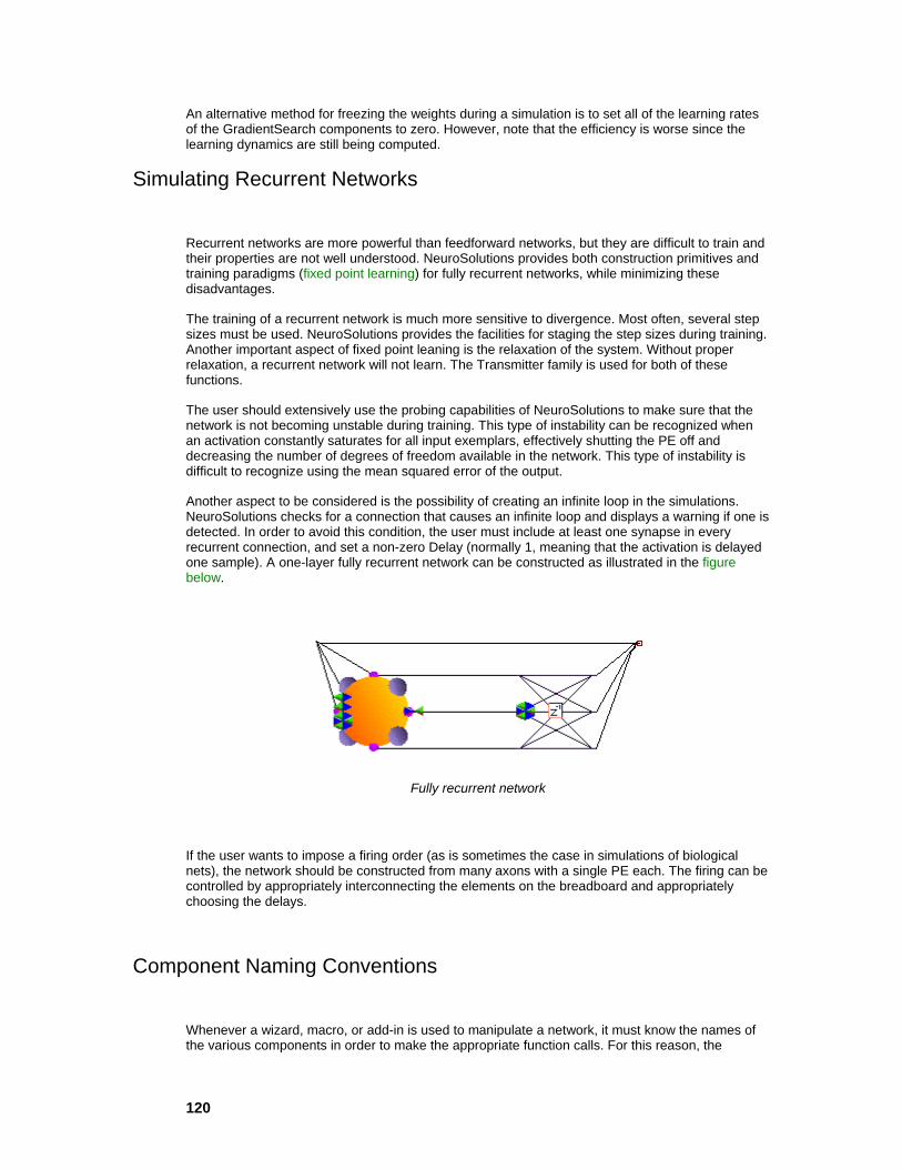
120

An alternative method for freezing the weights during a simulation is to set all of the learning rates of the GradientSearch components to zero. However, note that the efficiency is worse since the learning dynamics are still being computed.

Simulating Recurrent Networks

Recurrent networks are more powerful than feedforward networks, but they are difficult to train and their properties are not well understood. NeuroSolutions provides both construction primitives and training paradigms (fixed point learning) for fully recurrent networks, while minimizing these disadvantages.

The training of a recurrent network is much more sensitive to divergence. Most often, several step sizes must be used. NeuroSolutions provides the facilities for staging the step sizes during training. Another important aspect of fixed point leaning is the relaxation of the system. Without proper relaxation, a recurrent network will not learn. The Transmitter family is used for both of these functions.

The user should extensively use the probing capabilities of NeuroSolutions to make sure that the network is not becoming unstable during training. This type of instability can be recognized when an activation constantly saturates for all input exemplars, effectively shutting the PE off and decreasing the number of degrees of freedom available in the network. This type of instability is difficult to recognize using the mean squared error of the output.

Another aspect to be considered is the possibility of creating an infinite loop in the simulations. NeuroSolutions checks for a connection that causes an infinite loop and displays a warning if one is detected. In order to avoid this condition, the user must include at least one synapse in every recurrent connection, and set a non-zero Delay (normally 1, meaning that the activation is delayed one sample). A one-layer fully recurrent network can be constructed as illustrated in the figure below.

Fully recurrent network

If the user wants to impose a firing order (as is sometimes the case in simulations of biological nets), the network should be constructed from many axons with a single PE each. The firing can be controlled by appropriately interconnecting the elements on the breadboard and appropriately choosing the delays.

Component Naming Conventions

Whenever a wizard, macro, or add-in is used to manipulate a network, it must know the names of the various components in order to make the appropriate function calls. For this reason, the

121

following naming conventions have been defined in order to identify each component based on its particular function within the topology. It is recommended that you name your components according to these conventions if you plan to use a wizard, macro, or add-in with your network. It is important to note that the names should begin with a lower case letter, but that the remaining words should be capitalized (e.g., trainingCostProbe).

Naming Conventions

Family Template Comments

Input #File # = {input, desired}

Axon #%Axon # = {input, output, context, unsupervised, memory1, memory2, …, hidden1, hidden2, …}

% = {Lower}

The ‘Lower’ tag is only used if there are two axons in the same layer (e.g., a modular network).

The ‘context’ tag is signifies a layer of context units, such as those found in a Jordan/Elman network.

The ‘unsupervised’ tag signifies the axon fed by the unsupervisedSynapse of a hybrid network (see below).

The ‘memory’ tag signifies a TDNNAxon, as found in the TLRN network.

Synapse #%Synapse # = {output, unsupervised, hidden1, hidden2, …}

% = {Lower}

The ‘Lower’ tag is only used if there are two synapses in the same layer (e.g., a modular network).

The ‘context’ tag is signifies a connection to a contextAxon (see above).

The ‘unsupervised’ tag signifies the unsupervised component of a hybrid network (e.g., PCA, RBF, SOFM).

%To#Synapse % = name of component feeding the synapse

# = name of the component that the synapse feeds

The second template is used for connections between non-adjacent layers (e.g., Modular and Generalized Feedforward networks).

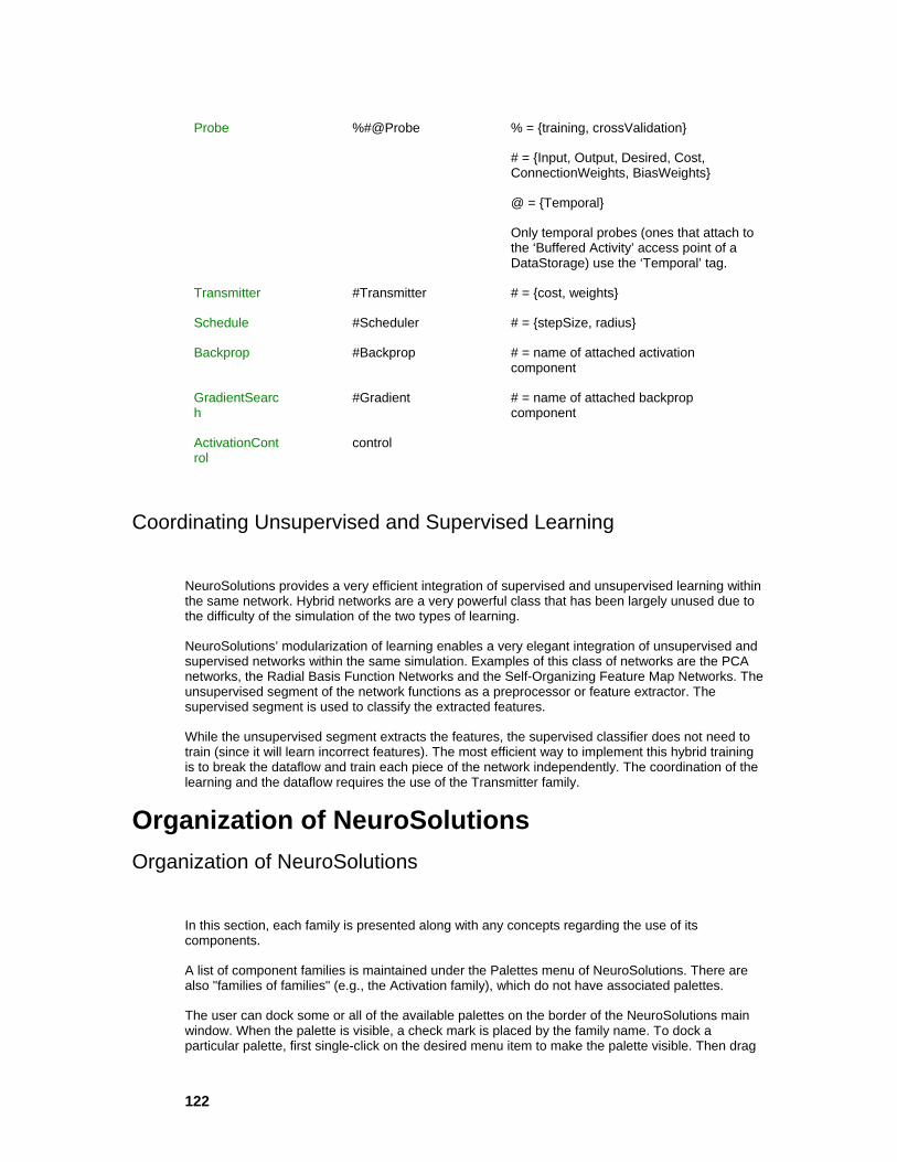
122

Probe %#@Probe % = {training, crossValidation}

# = {Input, Output, Desired, Cost, ConnectionWeights, BiasWeights}

@ = {Temporal}

Only temporal probes (ones that attach to the ‘Buffered Activity’ access point of a DataStorage) use the ‘Temporal’ tag.

Transmitter #Transmitter # = {cost, weights}

Schedule #Scheduler # = {stepSize, radius}

Backprop #Backprop # = name of attached activation component

GradientSearch

#Gradient # = name of attached backprop component

ActivationControl

control

Coordinating Unsupervised and Supervised Learning

NeuroSolutions provides a very efficient integration of supervised and unsupervised learning within the same network. Hybrid networks are a very powerful class that has been largely unused due to the difficulty of the simulation of the two types of learning.

NeuroSolutions’ modularization of learning enables a very elegant integration of unsupervised and supervised networks within the same simulation. Examples of this class of networks are the PCA networks, the Radial Basis Function Networks and the Self-Organizing Feature Map Networks. The unsupervised segment of the network functions as a preprocessor or feature extractor. The supervised segment is used to classify the extracted features.

While the unsupervised segment extracts the features, the supervised classifier does not need to train (since it will learn incorrect features). The most efficient way to implement this hybrid training is to break the dataflow and train each piece of the network independently. The coordination of the learning and the dataflow requires the use of the Transmitter family.

Organization of NeuroSolutions Organization of NeuroSolutions

In this section, each family is presented along with any concepts regarding the use of its components.

A list of component families is maintained under the Palettes menu of NeuroSolutions. There are also "families of families" (e.g., the Activation family), which do not have associated palettes.

The user can dock some or all of the available palettes on the border of the NeuroSolutions main window. When the palette is visible, a check mark is placed by the family name. To dock a particular palette, first single-click on the desired menu item to make the palette visible. Then drag

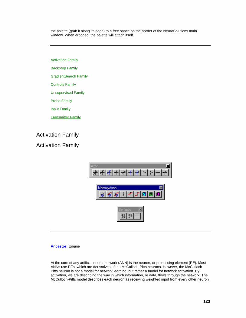
123

the palette (grab it along its edge) to a free space on the border of the NeuroSolutions main window. When dropped, the palette will attach itself.

Activation Family

Backprop Family

GradientSearch Family

Controls Family

Unsupervised Family

Probe Family

Input Family

Transmitter Family

Activation Family

Activation Family

Ancestor: Engine

At the core of any artificial neural network (ANN) is the neuron, or processing element (PE). Most ANNs use PEs, which are derivatives of the McCulloch-Pitts neurons. However, the McCulloch-Pitts neuron is not a model for network learning, but rather a model for network activation. By activation, we are describing the way in which information, or data, flows through the network. The McCulloch-Pitts model describes each neuron as receiving weighted input from every other neuron

124

in the network, applying a non-linear threshold and presenting its output for the others to input. The activation of data through a first order McCulloch-Pitts neuron is defined by the following equation,

where xi(t) represents a neurons activity, ? is a nonlinearity and wij is a connection weight linking PEj to PEi..

Time t is discrete, and it relates to one simulation step. This equation means that the next value of the activation is obtained from the values of the other activations of PEj at the previous time step. If the first order model is generalized to any discrete time delay d, more sophisticated models for the neuron can be implemented from multiple first order models, as given by,

Neural networks are constructed by first defining the neuron interconnections, and then assigning a learning procedure to adapt its weights. The Activation family only addresses the interconnection of PEs to form a neural network topology. A network constructed from Activation components contains no inherent procedure for learning, but rather supports a general communications protocol such that components belonging to various learning procedure families can adapt its weights.

The McCulloch-Pitts model describes a network topology with a fully interconnected set of neurons (i.e., each neuron feeds all of the others). In practice, ANN topologies typically interconnect distributed clusters, or layers of PEs. For this reason, each component in the Activation family will operate on a layer, or vector of PEs. This leads to very efficient simulations.

Activation family components model the McCulloch-Pitts neuron by dividing its functionality into a temporally discrete linear map, and an instantaneous nonlinear map.

A Special Note for Neurobiologists

Many of the terms used in NeuroSolutions have different meanings than when used in a biological context. This section is included to help neurobiologists avoid confusion by explicitly listing these differences.

In NeuroSolutions, the term "soma" refers to a parent, or archetypal class of elements. Both "synapse" and "axon" are derivative classes of "soma". There is no specific "soma" element used in the construction of NeuroSolutions breadboards.

The term "axon" in NeuroSolutions refers to an element that integrates its input weights and creates an output. Often this is a nonlinear process. The NeuroSolutions "axon" more closely resembles the combination of the neuronal dendrites, soma, and axon hillock in neurobiology.

"Synapse" in NeuroSolutions refers to the principal element that transmits information between NeuroSolutions "axons". These "synapses" are more like the combined axon and synapses of neurobiology. A NeuroSolutions "synapse" can be connected to many NeuroSolutions "axons", and is therefore similar to a highly branched, or arborized, neurobiological axon. A biological synapse is functionally similar to a single weight in NeuroSolutions.

125

Members:

Axon Family

MemoryAxon Family

Synapse Family

See Also

Axon Family

Axon family palette

Ancestor: Activation Family

Artificial neural networks are constructed by interconnecting processing elements (PEs) which mimic the biological nerve cell, or neuron. NeuroSolutions divides the functionality of a neuron into two disjoint operations: a nonlinear instantaneous map, which mimics the neuron’s threshold characteristics; and a linear map applied across an arbitrary discrete time delay, which mimics the neuron’s synaptic interconnections. The Axon family implements common variations on the nonlinear instantaneous maps employed by neural models. Each axon represents a layer, or vector, of PEs. All axons will also be equipped with a summing junction at their input and a splitting node at their output. This allows multiple components to feed an axon, which then processes their accumulated activity. It is important to notice the difference between this sum of activity vectors, and the weighted sum of products depicted by the McCulloch-Pitts neuron model (see Activation family). The latter is implemented as a linear map by the other functional division of the neuron, the Synapse family.

For generality, an axon's map may actually be either linear or nonlinear. However, components in the Axon family typically apply a nonlinear instantaneous map, as given by,

126

where yi(t) is the axon's output, xi(t) is an accumulation of input activity from other components, is an internal weight or coefficient and represents an arbitrary functional map. We call

the activation function, and the on-line help for a particular axon gives the definition of this map for that axon.

All members of the Axon family accumulate input from, and provide output to, an arbitrary number of activation components. In other words, each axon has a summing junction at its input and a splitting node at its output. This functionality is illustrated by the following block diagram:

The mapping for the PE of the Axon class.

Axons can receive input from, and provide output to both axons and synapse within the network.

Members:

Axon

BiasAxon

GaussianAxon

LinearAxon

LinearSigmoidAxon

LinearTanhAxon

SigmoidAxon

SoftMaxAxon

TanhAxon

ThresholdAxon

WinnerTakeAllAxon

See Also

MemoryAxon Family

127

MemoryAxon family palette

Ancestor: Axon

Members of the MemoryAxon family encapsulate a local memory structure into a single axon. They store a history of the input vector, which is contained within memory taps. MemoryAxons still belong to the Axon family (even though they are contained within a separate palette), but they diverge slightly from typical axon functionality. Most axons provide some form of an instantaneous map. A MemoryAxon's activation function is not instantaneous, but has been wrapped for efficiency into an axon.

Tapped MemoryAxons also diverge from the Axon family by having more outputs than inputs. In fact, if there are n inputs and K taps (K-1 delay elements), then the MemoryAxon will have n*K outputs. MemoryAxons can be best described by using a z-domain (frequency domain) activation function. All MemoryAxons will be defined by their activation function given by:

Tapped MemoryAxons will use a tap activation function as given by:

with the topological understanding illustrated in the figure below.

128

Block diagram of a memory axon

The index k refers to the tap value.

Probing the Output:

When attaching a MatrixViewer or MatrixEditor to an Axon without memory, the vector of PEs is displayed as a matrix of rows and columns based on the Rows and Cols parameters set within the Axon’s inspector. When probing a member of the MemoryAxon family, the number of columns displayed is the number of channels (Rows*Cols). The number of rows displayed is the number of Taps entered in the inspector. Therefore, each column represents data stored in a given channel’s memory taps.

Members:

ContextAxon

GammaAxon

IntegratorAxon

LaguarreAxon

SigmoidIntegratorAxon

TanhContextAxon

TanhIntegratorAxon

TDNNAxon

FuzzyAxon Family

FuzzyAxon family palette

129

Ancestor: Axon

Members of the FuzzyAxon family contain a set of membership functions (MFs) for each input processing element. The parameters of the membership functions are stored within the weight vector of the FuzzyAxon. The number of membership functions per processing element is specified within the FuzzyAxon inspector. The number of outputs is computed by taking the number of membership functions per processing element and raising it to the Nth power, where N is the number of inputs.

Activation Function:

The output of a FuzzyAxon is computed using the following formula:

where i = input index

j = output index

xi = input i

wij = weights (MF parameters) corresponding to the jth MF of input i

MF = membership function of the particular subclass of FuzzyAxon

Members:

BellFuzzyAxon

GaussianFuzzyAxon

ErrorCriteria Family

ErrorCriteria family palette

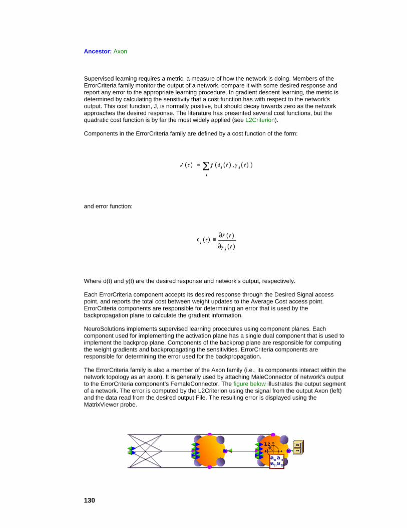
130

Ancestor: Axon

Supervised learning requires a metric, a measure of how the network is doing. Members of the ErrorCriteria family monitor the output of a network, compare it with some desired response and report any error to the appropriate learning procedure. In gradient descent learning, the metric is determined by calculating the sensitivity that a cost function has with respect to the network's output. This cost function, J, is normally positive, but should decay towards zero as the network approaches the desired response. The literature has presented several cost functions, but the quadratic cost function is by far the most widely applied (see L2Criterion).

Components in the ErrorCriteria family are defined by a cost function of the form:

and error function:

Where d(t) and y(t) are the desired response and network's output, respectively.

Each ErrorCriteria component accepts its desired response through the Desired Signal access point, and reports the total cost between weight updates to the Average Cost access point. ErrorCriteria components are responsible for determining an error that is used by the backpropagation plane to calculate the gradient information.

NeuroSolutions implements supervised learning procedures using component planes. Each component used for implementing the activation plane has a single dual component that is used to implement the backprop plane. Components of the backprop plane are responsible for computing the weight gradients and backpropagating the sensitivities. ErrorCriteria components are responsible for determining the error used for the backpropagation.

The ErrorCriteria family is also a member of the Axon family (i.e., its components interact within the network topology as an axon). It is generally used by attaching MaleConnector of network's output to the ErrorCriteria component’s FemaleConnector. The figure below illustrates the output segment of a network. The error is computed by the L2Criterion using the signal from the output Axon (left) and the data read from the desired output File. The resulting error is displayed using the MatrixViewer probe.

131

Output segment of a network (activation plane only)

Members:

L1Criterion

L2Criterion

LpCriterion

LinfinityCriterion

User Interaction:

Macro Actions

See Also

Synapse Family

Synapse family palette


Artificial neural networks are constructed by interconnecting processing elements (PEs) which mimic the biological nerve cell, or neuron. NeuroSolutions divides the functionality of a neuron into two disjoint operations: a nonlinear instantaneous map, which mimics the neuron’s threshold characteristics; and a linear map applied across an arbitrary discrete time delay, which mimics the neuron’s synaptic interconnections. The Synapse family implements the dynamic linear mapping characteristics of the neuron. A synapse connects two layers of PEs (axons). A synapse will receive input from, and provide output to, components belonging to the Axon family.

If a synapse is connected between two axons, then these axons represent distributed layers of PEs within a network. If the synapse's input and output are applied to the same axon, then the axon PEs are recurrently interconnected as described by the McCulloch-Pitts model. The concept of interconnected layers of distributed PEs is fundamental to neural network theory. The interconnection is normally defined by an interconnection matrix. In theory, any network topology can be specified through a single interconnection matrix. In practice, however, it is impractical to burden an already computationally expensive task with "connect by zero" operations. It makes

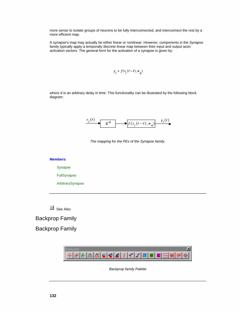
132

more sense to isolate groups of neurons to be fully interconnected, and interconnect the rest by a more efficient map.

A synapse's map may actually be either linear or nonlinear. However, components in the Synapse family typically apply a temporally discrete linear map between their input and output axon activation vectors. The general form for the activation of a synapse is given by:

where d is an arbitrary delay in time. This functionality can be illustrated by the following block diagram:

The mapping for the PEs of the Synapse family.

Members:

Synapse

FullSynapse

ArbitrarySynapse

See Also

Backprop Family

Backprop Family

Backprop family Palette

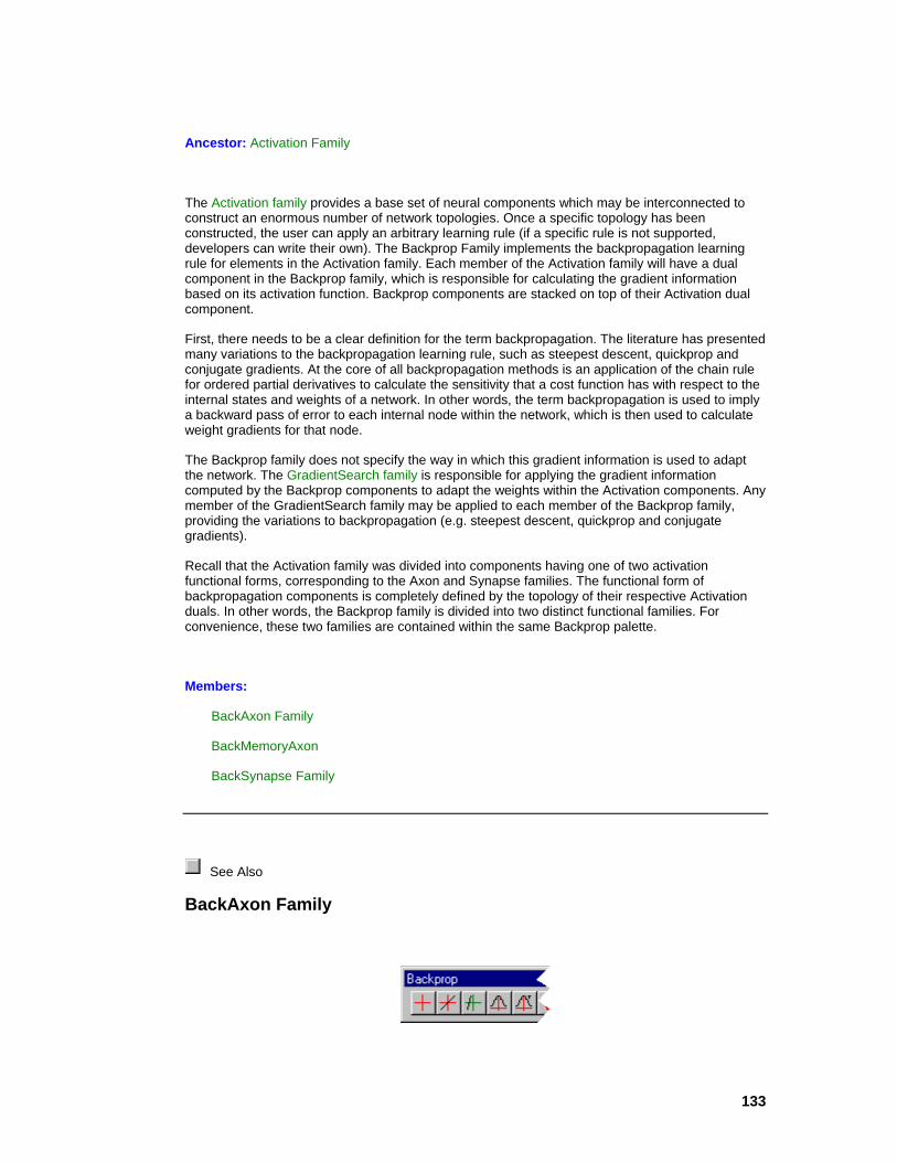
133


The Activation family provides a base set of neural components which may be interconnected to construct an enormous number of network topologies. Once a specific topology has been constructed, the user can apply an arbitrary learning rule (if a specific rule is not supported, developers can write their own). The Backprop Family implements the backpropagation learning rule for elements in the Activation family. Each member of the Activation family will have a dual component in the Backprop family, which is responsible for calculating the gradient information based on its activation function. Backprop components are stacked on top of their Activation dual component.

First, there needs to be a clear definition for the term backpropagation. The literature has presented many variations to the backpropagation learning rule, such as steepest descent, quickprop and conjugate gradients. At the core of all backpropagation methods is an application of the chain rule for ordered partial derivatives to calculate the sensitivity that a cost function has with respect to the internal states and weights of a network. In other words, the term backpropagation is used to imply a backward pass of error to each internal node within the network, which is then used to calculate weight gradients for that node.

The Backprop family does not specify the way in which this gradient information is used to adapt the network. The GradientSearch family is responsible for applying the gradient information computed by the Backprop components to adapt the weights within the Activation components. Any member of the GradientSearch family may be applied to each member of the Backprop family, providing the variations to backpropagation (e.g. steepest descent, quickprop and conjugate gradients).

Recall that the Activation family was divided into components having one of two activation functional forms, corresponding to the Axon and Synapse families. The functional form of backpropagation components is completely defined by the topology of their respective Activation duals. In other words, the Backprop family is divided into two distinct functional families. For convenience, these two families are contained within the same Backprop palette.

Members:

BackAxon Family

BackMemoryAxon

BackSynapse Family

See Also

BackAxon Family

134

BackAxon section of the Backprop family Palette

Ancestor: Backprop Family

Members of the Axon family implement the instantaneous nonlinear threshold characteristics of the neuron, and its members are constrained to a standard activation functional form. Thus components implementing backpropagation for axons will also share a common functional form.

Backpropagation requires that all members of the BackAxon family perform two operations. First, given an error at their output, BackAxons must calculate gradient information for all adaptive weights within their dual components (i.e. from the Axon family). Second, they must derive the relative error at their input to be backpropagated to any components which precedes them. Recall the standard activation function for members of the Axon family (see equation). Similarly, members of the BackAxon Family can be defined by a backward sensitivity function (error) as given by,

Each member of the Axon family was completely defined through its activation function. Similarly, members of the BackAxon family can be defined by a backward sensitivity function (error) as given by:

and a weight gradient function of the form:

where and are sensitivities, is the weight gradient, ' denote derivatives, and J is the cost function. The error propagation can be illustrated by the block diagram in the figure below.

135

BackAxon functionality

Each BackAxon will assign its error function, and weight gradient function,

.

Members:

BackAxon

BackBiasAxon

BackLinearAxon

BackSigmoidAxon

BackTanhAxon

BackMemoryAxon Family

See Also


BackMemoryAxon section of the Backprop family Palette

Ancestor: BackAxon Family

136

Members of the MemoryAxon family encapsulate a local memory structure into a single axon. MemoryAxons do not use time domain equations to describe their activation, but instead use z-domain tap activation equations. Similarly BackMemoryAxons are defined by a z-domain sensitivity function given by,

Tapped MemoryAxons are defined by a z-domain tap sensitivity function,

A topological perspective for the tapped components is illustrated in the figure below. Each

individual pair of activations (i.e., , ) is treated as in the backward sensitivity equation and the weight gradient equation.

Block diagram for BackMemoryAxons

Members:

BackContextAxon

BackGammaAxon

BackLaguarreAxon

BackIntegratorAxon

137

BackSigmoidContextAxon

BackSigmoidIntegratorAxon

BackTanhContextAxon

BackTanhIntegratorAxon

BackTDNNAxon

See Also

BackSynapse Family

BackSynapse section of the Backprop family Palette

Ancestor: Backprop Family

Neural network topologies are constructed by interconnecting components that mimic the biological neuron. Members of the Synapse family implement the linear dynamic characteristics of the neuron, and its members are constrained to a standard activation functional form. Thus components implementing backpropagation for synapse will also share a common functional form.

Backpropagation requires that all members of the BackSynapse family perform two operations. First, given an error at their output, BackSynapses must calculate gradient information for all adaptive weights within their family of dual components (i.e., the Synapse family). Second, they must derive the relative error (the sensitivities) at their input to be backpropagated to any components which precedes them. Recall the equation for the standard activation function for members of the Synapse family. Similarly, members of the BackSynapse family can be defined by a backward sensitivity function as given by:

Each member of the Synapse family was completely defined through its activation function. Similarly, members of the BackSynapse family can be defined by a backward sensitivity function (error) of the form:

138

and a weight gradient function of the form:

The error propagation can be illustrated by the block diagram in the figure below.

BackSynapse block diagram

Each BackSynapse is defined by an error function and weight gradient function.

Members:

BackSynapse

BackFullSynapse

BackArbitrarySynapse

See Also



139

GradientSearch family palette

Ancestor: Engine

Components in the GradientSearch family search a network’s performance surface in an attempt to find the global minima. Recall that the Activation family is responsible for passing activity forward through the network, and the Backprop family is responsible for passing an error backwards, in addition to calculating weight gradients. The GradientSearch family will use the weight gradients provided by the Backprop family to update the weights of the Activation family. This is depicted by the general form for the weight update equation given in the equation below.

Conceptually, members of the Activation family are interconnected to form the network topology, which in turn fixes the performance surface topography. Members of the Backprop family act as a level, i.e. given the current location in weight space, they estimate the direction of a minima or valley within the performance surface. Members of the GradientSearch family move the location (by updating the weights) based on this estimated direction in an attempt to minimize the error.

There are many methods for searching the performance surface based on first order gradient information (e.g., steepest descent, quickprop and conjugate gradients), as well as several methods for deriving these gradients (e.g., static backpropagation, backpropagation through time and real time recurrent learning). This is the motivation for separating gradient calculations from weight updates.

A GradientSearch component can be stacked on top of any member of the Backprop family that contains weights (see figure below). This allows the GradientSearch component to access the errors and gradients of the Backprop component, as well as the activities and weights of the Activation component.

Network with Activation, Backprop and GradientSearch planes

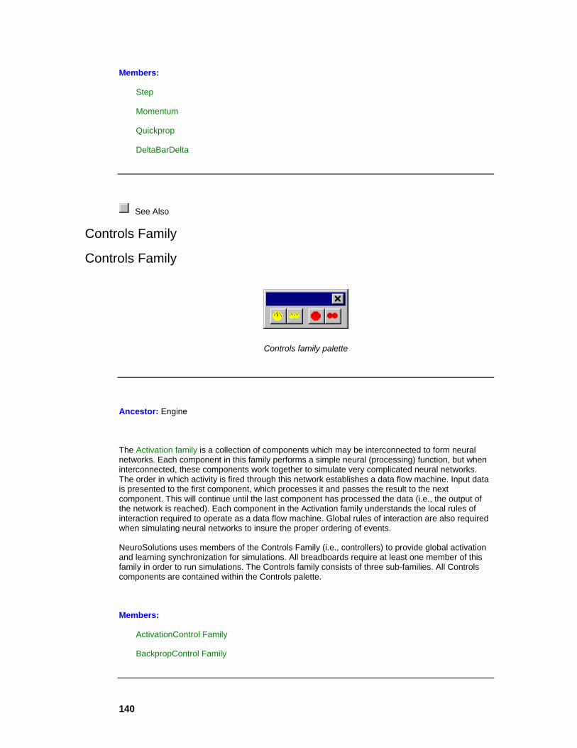
140

Members:

Step

Momentum

Quickprop

DeltaBarDelta

See Also

Controls Family

Controls Family

Controls family palette

Ancestor: Engine

The Activation family is a collection of components which may be interconnected to form neural networks. Each component in this family performs a simple neural (processing) function, but when interconnected, these components work together to simulate very complicated neural networks. The order in which activity is fired through this network establishes a data flow machine. Input data is presented to the first component, which processes it and passes the result to the next component. This will continue until the last component has processed the data (i.e., the output of the network is reached). Each component in the Activation family understands the local rules of interaction required to operate as a data flow machine. Global rules of interaction are also required when simulating neural networks to insure the proper ordering of events.

NeuroSolutions uses members of the Controls Family (i.e., controllers) to provide global activation and learning synchronization for simulations. All breadboards require at least one member of this family in order to run simulations. The Controls family consists of three sub-families. All Controls components are contained within the Controls palette.

Members:

ActivationControl Family

BackpropControl Family

141

See Also

ActivationControl Family

The ActivationControl family consists of the StaticControl and DynamicControl components. These components are responsible for synchronizing the presentation of data to a neural network. The activation of network simulations are divided into experiments, epochs, exemplars and forward samples. The StaticControl component is only capable of controlling static network topologies, while the DynamicControl component supports both static and dynamic topologies.

The outputs of a static network are only a function of its inputs and states at the current instant in time. This relationship can be depicted by the equation

where y(t) are the network's outputs, i(t) are inputs, x(t) are internal nodes and w are the weights.

The outputs of a dynamic network can be a function of its inputs and internal states at the present time, as well as its states at any past instant in time. This is defined by

Note that static networks are a special case of dynamic where T is set to zero.

An example may be the best method for explaining the settings available on the inspectors of these two components. Assume that you have designed a dynamic network for isolated speech recognition. In particular, you wish to train the network to recognize the digits 0-9. These digits have been individually spoken into a microphone and properly sampled. Each digit is completely contained within an isolated segment consisting of 8000 samples. To complete the training set, this process was repeated 100 times for each digit.

The term samples, refers to the individual pieces of temporal information. An exemplar is a complete pattern of samples (e.g., each spoken digit), which may be static or temporal. The temporal dimension of an exemplar is defined by its Samples/Exemplar (in this case 8000). Static problems will have one sample per exemplar. An epoch refers to the set of all exemplars to be presented during the training of a network (e.g., all 100 exemplars of each of the 10 digits). Thus an epoch is defined by assigning the Exemplars/Epoch (1000 in our example). A neural network experiment will consist of the repeated presentation of an epoch to the network until it has sufficiently trained. Thus an experiment is defined by assigning the Epochs/Experiment.

142

Inspector for the DynamicControl component

The StaticControl inspector does not contain the Samples/Exemplar parameter. This is because every sample corresponds to one exemplar. A simple example of a static case is the XOR problem. The XOR table is composed of 4 cases. You train an MLP to solve the XOR by presenting the 4 cases 100 times. Here an exemplar is one of the four entries of the XOR table. An epoch consists of the four patterns (Exemplars/Epoch = 4). The experiment consists of 100 presentations of each of the 4 cases (Epochs/Experiment = 100).

Inspector for the StaticControl component

The ActivationControl family is also responsible for cross validation of the network during learning. It does this by sending a second set of data through the network during the training, while temporarily freezing the network weights.

All Access components have the ability to choose the data set to access. Each probe can be assigned to monitor a particular data set. Furthermore, a transmitter can make control decisions based on one of the data sets, e.g. stopping training after the error in the cross validation set has fallen below a given threshold.

143

Members:

StaticControl

DynamicControl

See Also

BackpropControl Family

The BackpropControl family consists of the BackStaticControl and the

BackDynamicControl components. They are responsible for synchronizing components in the backpropagation plane. There are two distinct synchronization paradigms for backpropagation. Synchronization refers to the way in which the network processes sensitivity (error) data. The ActivationControl family divides simulations into experiments, epochs, exemplars and samples. The BackpropControl family further defines a simulation by the number of backward samples per exemplar and the number of exemplars per weight update. Backpropagation can either be synchronized in Static, Trajectory or Fixed-Point modes.

The BackStaticControl component is used in conjunction with the StaticControl component. Static backpropagation assumes that the output of a network is strictly a function of its present input (i.e., the network topology is static). In this case, the gradients and sensitivities are only dependent on the error and activations from the current time step. The Exemplars/Update field of the BackStaticControl inspector is the number of patterns presented to the networks before a weight update is computed. If the weights are updated after every exemplar (Exemplars/Update = 1), then this is termed on-line learning. If the weights are update after every epoch (Exemplars/Update = Exemplars/Epoch in the activation control component), then this is termed batch learning.

BackStaticControl inspector

144

Note that for linear systems, static backpropagation is equivalent to least mean squares (LMS). If a network does not have any recurrent connections (i.e., the network is feed-forward) but has a dynamic component such as a TDNNAxon, then the sensitivity that the output has with respect to any internal node is strictly a function of that node at present time. Therefore, static backpropagation can still be used even though the network topology is dynamic.

The BackDynamicControl component is used in conjunction with the DynamicControl component. These components allow for Trajectory and Fixed-Point learning. Training a network in Trajectory mode assumes that each exemplar has a temporal dimension defined by its forward samples (period), and that there exists some desired response for the network's output over this period. The network is first run forward in time over the entire period, during which an error is determined between the network's output and the desired response. Then the network is run backwards for a prescribed number of samples (defined by the Samples/Exemplar of the BackDynamicControl inspector) to compute the gradients and sensitivities. This forward/backward pass is considered a single exemplar. As with the static case, the Exemplars/Update field specifies how many times this process is repeated before the weight gradients are applied to the weights.

Fixed Point mode assumes that each exemplar represents a static pattern that is to be embedded as a fixed point of a recurrent network. Here the terms forward samples and backward samples can be thought of as the forward relaxation period and backward relaxation period, respectively. All inputs are held constant while the network is repeatedly fired during its forward relaxation period, specified by the Samples/Exemplar of the DynamicControl component. There are no guarantees that the forward activity of the network will relax to a fixed point, or even relax at all. If the network becomes unstable or gets stuck in a limit cycle, simply randomize the weights and try again. Of course, a clever researcher will start the network from initial conditions that are known to be stable (as in the case of symmetric weights). After the network has relaxed, an error is determined and held as constant input to the backpropagation layer. Similarly, the error is backpropagated through the backprop plane for its backward relaxation period, specified by the Samples/Exemplar of the BackDynamicControl inspector. This forward/backward relaxation is considered to be one exemplar. Again, the Exemplars/Update specifies how often to update the weights.

Members:

BackStaticControl

BackDynamicControl

See Also

Unsupervised Family

Unsupervised Family

Unsupervised family palette.

145

Ancestor: Level

Unsupervised learning trains based on internal constraints, so no desired signal is used during training. This should not be confused with not having a desired response. The way in which the network responds to input data is pre-encoded into the learning procedure.

Unsupervised learning is only meaningful if there is redundancy in the input data. Without redundancy it is impossible to find any patterns or features. Unsupervised networks extract knowledge by exploring redundancy. In this sense, knowledge and information are exact opposites; information can be measured by a signal’s lack of redundancy.

Unsupervised learning is normally applied to a single layer of weighted connections. In NeuroSolutions, this corresponds to the Synapse family. Therefore, all components in the Unsupervised family are also members of the Synapse family. Unlike supervised procedures, unsupervised components do not require a dedicated network controller. These components insert themselves into the data flow during the network's forward activation. The weights of the synapse are adapted internally with every sample of data flowing through the network. Supervised and unsupervised components may be intermixed within a single network.

Within the Unsupervised palette are three sub-families summarized below. All components in the Unsupervised family can be functionally described through a weight update function in the form of the equation below.

where η is the step size specified within the Learning Rateproperty page.

Members:

Hebbian Family

Competitive Family

User Interface:

Macro Actions

Hebbian Family

The Hebbian learning is correlation learning. The elements of this family utilize directly the product of its local input and output to derive the weight updates. NeuroSolutions implements straight Hebbian (Hebbian, anti-Hebbian, forced-Hebbian) and normalized Hebbian (Oja and Sanger). The last two types have an inherent normalization. These three components are HebbianFull, OjasFull and SangersFull.

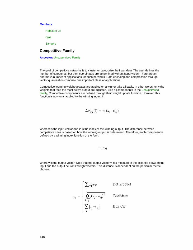
146

Members:

HebbianFull

Ojas

Sangers

Competitive Family

Ancestor: Unsupervised Family

The goal of competitive networks is to cluster or categorize the input data. The user defines the number of categories, but their coordinates are determined without supervision. There are an enormous number of applications for such networks. Data encoding and compression through vector quantization comprise one important class of applications.

Competitive learning weight updates are applied on a winner take all basis. In other words, only the weights that feed the most active output are adjusted. Like all components in the Unsupervised family, Competitive components are defined through their weight update function. However, this function is now only applied to the winning index, i*.

where x is the input vector and i* is the index of the winning output. The difference between competitive rules is based on how the winning output is determined. Therefore, each component is defined by a winning index function of the form,

i* = f(y)

where y is the output vector. Note that the output vector y is a measure of the distance between the input and the output neurons’ weight vectors. This distance is dependent on the particular metric chosen.

147

The Competitive family consists of two components, StandardFull and ConscienceFull. The first component implements the standard competitive rule summarized above. With this rule, there are cases when one PE will win the competition too much, causing the output to be skewed. The second component implements the "competitive with a conscience" learning rule. This rule adds a bias term to balance the competition, which reduces this problem.

The components of the Competitive family are often used in conjunction with a WinnerTakeAllAxon. This component will extract the winning PE of the competition. For the Dot Product metric, the winning PE is the one with the maximum value. For the other two metrics, the winning PE is the one with the minimum value.

Members:

StandardFull

ConscienceFull

Kohonen Family

User Interface:

Macro Actions

Kohonen Family

Ancestor: Competitive Family

The Kohonen family is an enhancement of the Competitive family. It extends the competition over spatial neighborhoods. While competitive learning only updates the weights of the winning PE, in Kohonen learning the weights in a neighborhood of the winning PE are also updated. NeuroSolutions implements a 1D neighborhood and two types of 2D neighborhoods. Both the neighborhood and the learning rates can be set to decay as the network learns.

The Kohonen components use the same weight update as used for the competitive components, and they all use a conscience bias to determine the winning index. The difference is that a neighborhood of PEs around the winning output are updated along with the winning PE.

The reference page of each component contains an illustration of its neighborhood for a neighborhood size of 2. Both the neighborhood size and learning rate are available on the component’s inspector. These parameters can also be scheduled to decay during the simulations.

Members:

DiamondKohonen

LineKohonen

SquareKohonen

148

User Interface:

Macro Actions

Probe Family

Probe Family

Probes family palette

Ancestor: Access Family

Probing is a fundamental concept of NeuroSolutions. Since it is very difficult to mathematically describe the complex signal transformations occurring in highly nonlinear systems, neural networks are often used as "black boxes". However in a simulation environment, considerable insight can be gained by observing activations and weights at the input, output and internal nodes during training. The learning curve (i.e., how the output MSE decreases with training) is a paradigmatic display of the importance of probing.

Analyzing the activity within PEs tends to be almost exclusively applied to output components. In NeuroSolutions, the user has the ability to place probes on ANY component in the network. Each probe provides a unique way of visualizing the data available at a component’s access points. It is obvious that on-line visualization of learning (i.e., visualizing the MSE or other network parameters during the simulations) is a time savings feature. Maladjustments in learning parameter settings can be observed early in the simulation, and corrected. Another useful feature of probing is the added understanding that the user gets about the path that the network takes to arrive at a working solution (see Frequency Doubler Example).

The core idea of probing is to extract data from signal paths for visualization, and further processing, without disturbing the network topology. Probing will require additional clock cycles, but NeuroSolutions allows the user to set how often the display is refreshed. If the user does not take into account the interval between display cycles, probing can significantly hinder the simulation speed.

In NeuroSolutions, whenever a component has data to monitor (e.g., activity, weights and learning rates) it reports the data through a standard protocol. In this way, all NeuroSolutions components speak the same language. No matter what the data represents, it is reported through the same protocol. This is the same protocol that all probes speak, allowing the same data to be visualized in many formats.

The Probes Family consists of static probes, temporal probes and transformers. The static probes accept instantaneous data from component access points. Temporal probes are used to observe data that has been collected and stored over a number of simulation clock cycles. Transformer probes transform the data collected at temporal access points (e.g., a spectral estimator based on the Fast Fourier Transform). The results of these transformations are then presented as another temporal access point.

149

Members:

StaticProbe Family

TemporalProbe Family

Transformer Family

User Interaction:

Macro Actions

Input Family

Input Family

Input family palette


The Input family links NeuroSolutions with the computer file system for input, and also provides testing signals (signal generators and noise sources) for the simulations. This is done by feeding data to an access point of the attached network component.

These components are most often used to generate an input signal and a desired output signal. This is implemented by attaching an Input component to the Pre-Activity access point of the input Axon and another Input component at the Desired Signal access point of the ErrorCriterion component.

The internal data input format in NeuroSolutions is a multi-channel stream. The number of channels is determined by the number of PEs contained within the component stacked below. The data stream for an input component is stored as a binary pattern file (*.nsp) within the same directory as the breadboard. When the input component is a File, a data stream is generated for each unique data set defined in the file list.

The function of the File component is to translate other file formats to data streams stored as pattern files. Presently there is support for ASCII, column-formatted ASCII, binary, and bitmap file formats. Multiple files of mixed type can be translated simultaneously within the same File component. There are also provisions for normalization, segmentation and symbolic translation of input files.

The Function component is a function generator, used for testing network topologies. It produces periodic waveforms of a variety of types. The waveforms can be the same for all channels or they can differ between them.

150

The Noise component provides the ability to inject noise into network components. By attaching a Noise component to another component, all data that flows through the selected access point has a noise factor added in. This component provides both a uniformly distributed noise source and a Gaussian distributed noise source. For both of these, the mean and variance of the noise is adjustable and can vary between channels.

The DLLInput component is used to inject data into the network from a DLL. This is similar to using the DLL capability of the Function component, except that this data is not cyclical.

The DLLPreprocessor component is used to preprocess the data sent from the component stacked on the Preprocessor access point using a DLL. The DLL retrieves the data one sample at a time and passes the processed data to the component attached below.

Members:

Function

File

Noise

DLLInput

DLLPreprocessor

OLEInput

Transmitter Family

Transmitter Family

Transmitters family palette.


The purpose of the Transmitter Family is to provide global communications between the various network components. This is necessary because each network component is an isolated entity that only knows how to communicate with its immediate neighbors on the breadboard, via access points and connectors. A transmitter transmits control messages or data based on the data that passes through the access point of the attached component. In this way, data may be transmitted between components that are not connected by the topology, or a component’s parameters may be altered based on the data of a remote component.

151

Many of the components that are on the breadboard will have message that can be sent to them. When a transmitter is inspected, all of these messages are shown and any or all of them may be sent. Some of these messages may have a parameter that must be sent with the message. These parameters may be set using the inspector. The parameters will be of one of three types: a floating point number, (i.e. 34.5322 or -3.21e5) an integer number, (i.e. 1322, -5, -132) or a boolean. (i.e. TRUE or FALSE) The parameters type is determined by the message.

If a component has messages, they will be shown in the inspector page of their respective on-line help screens. The messages are shown in the following manner:

(Message(parameter))

Members:

DataTransmitter Family

ControlTransmitter Family

User Interface:

Macro Actions

Schedule Family

Schedule Family

Scheduler family palette


The Scheduler family implements a graded change of a parameter during learning. This operation is very important in neurocomputing in order to modify the behavior of learning throughout the experiment. For instance, it may be advisable to start learning with a high learning rate or over a large neighborhood, and during learning slowly decrease the learning rate and the neighborhood size to consolidate (i.e., fine-tune) the learning. This is most important in Kohonen self-organizing feature maps and other unsupervised topologies.

The Scheduler family consists of the three components, LinearScheduler, LogScheduler and ExpScheduler. These components differ by the formula used to increase/decrease the parameter

152

from one iteration to the next (i.e., a linear, logarithmic or exponential function). Each component is defined by a recursive schedule equation of the form,

where β is a parameter available on each component’s inspector.

Members:

ExpScheduler

LinearScheduler

LogScheduler

User Interface:

Macro Actions

Introduction to Neural Computation Introduction to NeuroComputation

NeuroSolutions



Purpose

NeuroSolutions is a highly advanced simulation environment capable of supporting users with varying levels of expertise. A conceptual understanding of the fundamentals of Neural Network Theory is deemed necessary. Our purpose here is not to provide a substitute for the already voluminous literature in this area, but to set pointers to key articles, making explicit the level of user knowledge required. This chapter provides a "guided tour" of neural network principles.

153

Introduction to Neural Computation Introduction to NeuroComputation

History of Neural Networks

What are Artificial Neural Networks

Neural Network Solutions

History of Neural Networks

Neural Networks are an expanding and interdisciplinary field bringing together mathematicians, physicists, neurobiologists, brain scientists, engineers, and computer scientists. Seldom has a field of study coalesced from so much individual expertise, bringing a tremendous momentum to neural network research and creating many challenges.

One unsolved challenge in this field is the definition of a common language for neural network researchers with very different backgrounds. Another, to compile a list of key papers which pleases everyone, has only recently been accomplished, see Arbib, 1995. However, for the sake of pragmatism, we present some key landmarks below.

Neural network theory started with the first discoveries about brain cellular organization, by Ramon Y. Cajal and Charles S. Sherrington at the turn of the century. The challenge was immediately undertaken to discover the principles that would make a complex interconnection of relatively simple elements produce information processing at an intelligent level. This challenge is still with us today.

The work of the neuroanatomists has grown into a very rich field of science cataloguing the interconnectivity of the brain, its physiology and biochemistry [Eccles, Szentagothai], and its function [Hebb]. The work of McCulloch and Pitts on the modeling of the neuron as a threshold logic unit, and Caia-niello on neurodynamics merit special mention because they respectively led to the analysis of neural circuits as switching devices and as nonlinear dynamic systems. More recently, brain scientists began studying the underlying principles of brain function [Braitenberg, Marr, Pellionisz, Willshaw, Rumelhart, Freeman, Grossberg], and even implications to philosophy [Churchland].

Key books are Freeman’s "Mass Activation of the Nervous System", Eccles et al "The Cerebellum as a Neural Machine", Shaw and Palm’s "Brain theory" (collection of key papers), Churchland "NeuroPhilosophy", and Sejnowski and Churchland "The Computational Brain".

The theoretical neurobiologists’ work also interested computer scientists and engineers. The principles of computation involved in the interconnection of simple elements led to cellular automata [Von Neumann], were present in Norbert Wiener’s work on cybernetics and laid the ground for artificial intelligence [Minsky, Arbib]. This branch is often referred to as artificial neural networks, and will be the one reviewed here.

There are a few compilations of key papers on ANN’s, for the technically motivated reader. We mention the MIT Press Neuro Computing III, the IEEE Press Artificial Neural Networks and the book on Parallel models of Associative memories by Erlbaum.

154

Patrick Simpson’s book has an extensive reference list of key papers, and provides one possible taxonomy of neural computation.

The DARPA book provides an early account of neural network applications and issues.

Several books present the neural network computation paradigm at different technical levels:

Hertz, Krogh and Palmer’s "Introduction to the Theory of Neural Computation" (Addison Wesley, 1991) has probably one of the most thorough coverages of neural models, but requires a strong mathematical background.

Zurada’s "Introduction to Artificial Neural Systems" (West, 1992) and Kung’s "Digital Neural Networks" (Prentice Hall) are good texts for readers with an engineering background. Haykin’s book is encyclopedic, providing an extensive coverage of neural network theory and its links to signal processing.

An intermediate text is the Rumelhart and McClelland PDP Edition from MIT Press.

Freeman and Skapura, and Caudill and Butler are two recommended books for the least technically oriented reader.

In terms of magazines with state-of-the art technical papers, we mention "Neural Computation", "Neural Networks" and "IEEE Trans. Neural Networks".

Proceedings of the NIPS (Neuro Information Processing Systems) Conference, the Snowbird Conference, the Joint Conferences on Neural Networks and the World Congress are valuable sources of up-to-date technical information.

An initial goal in neural network development was modeling memory as the collective property of a group of processing elements [von der Marlburg, Willshaw, Kohonen, Anderson, Shaw, Palm, Hopfield, Kosko]. Caianiello, Grossberg and Amari studied the principles of neural dynamics. Rosenblatt created the perceptron for data driven (nonparametric) pattern recognition, and Fukushima, the cognitron. Widrow’s adaline (adaptive linear element) found applications and success in communication systems. Hopfield’s analogy of computation as a dynamic process captured the importance of distributed systems. Rumelhart and McClelland’s compilation of papers in the PDP (Parallel Distributive Processing) book, opened up the field for a more general audience. From the first International Joint Conference on Neural Networks held in San Diego, 1987, the field exploded.

What are Artificial Neural Networks

Artificial neural networks (ANN) are highly distributed interconnections of adaptive nonlinear processing elements (PEs). When implemented in digital hardware, the PE is a simple sum of products followed by a nonlinearity (McCulloch-Pitts neuron). An artificial neural network is nothing but a collection of interconnected PEs (see figure below). The connection strengths, also called the network weights, can be adapted such that the network’s output matches a desired response.

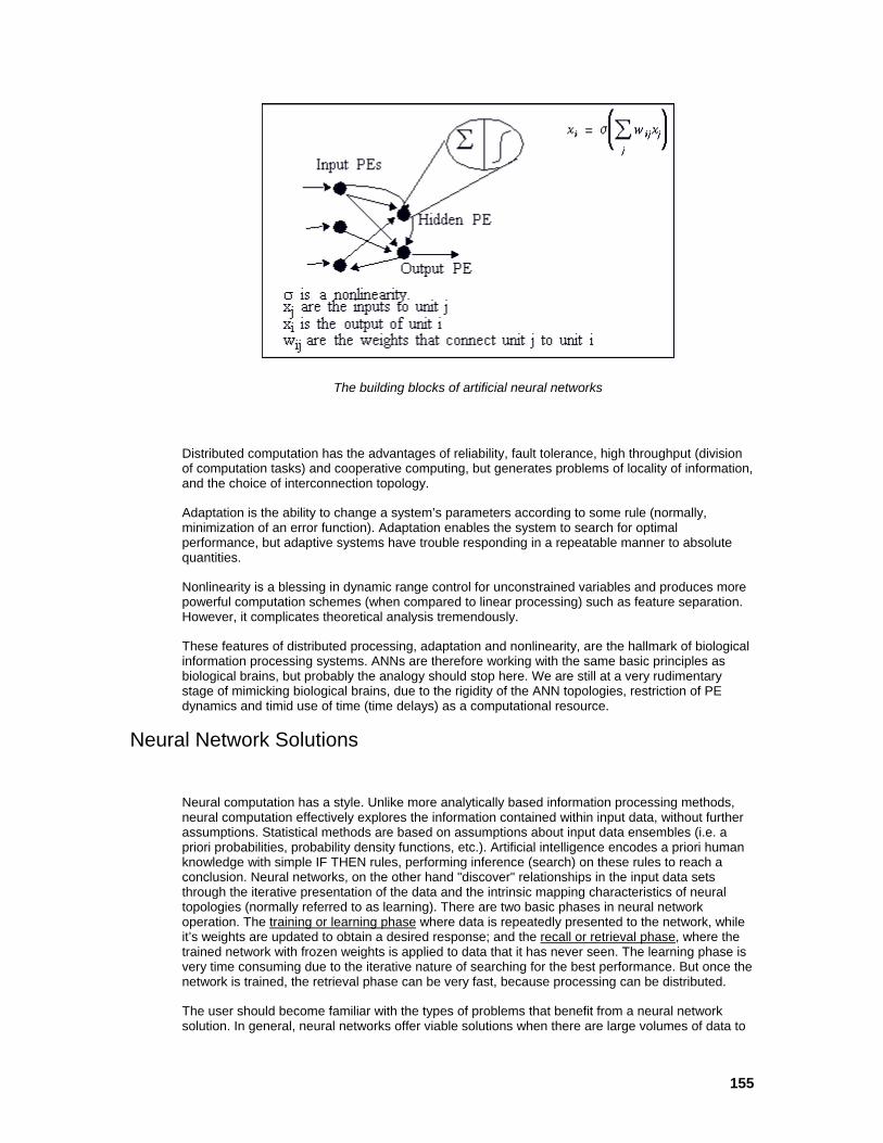
155

The building blocks of artificial neural networks

Distributed computation has the advantages of reliability, fault tolerance, high throughput (division of computation tasks) and cooperative computing, but generates problems of locality of information, and the choice of interconnection topology.

Adaptation is the ability to change a system’s parameters according to some rule (normally, minimization of an error function). Adaptation enables the system to search for optimal performance, but adaptive systems have trouble responding in a repeatable manner to absolute quantities.

Nonlinearity is a blessing in dynamic range control for unconstrained variables and produces more powerful computation schemes (when compared to linear processing) such as feature separation. However, it complicates theoretical analysis tremendously.

These features of distributed processing, adaptation and nonlinearity, are the hallmark of biological information processing systems. ANNs are therefore working with the same basic principles as biological brains, but probably the analogy should stop here. We are still at a very rudimentary stage of mimicking biological brains, due to the rigidity of the ANN topologies, restriction of PE dynamics and timid use of time (time delays) as a computational resource.

Neural Network Solutions

Neural computation has a style. Unlike more analytically based information processing methods, neural computation effectively explores the information contained within input data, without further assumptions. Statistical methods are based on assumptions about input data ensembles (i.e. a priori probabilities, probability density functions, etc.). Artificial intelligence encodes a priori human knowledge with simple IF THEN rules, performing inference (search) on these rules to reach a conclusion. Neural networks, on the other hand "discover" relationships in the input data sets through the iterative presentation of the data and the intrinsic mapping characteristics of neural topologies (normally referred to as learning). There are two basic phases in neural network operation. The training or learning phase where data is repeatedly presented to the network, while it’s weights are updated to obtain a desired response; and the recall or retrieval phase, where the trained network with frozen weights is applied to data that it has never seen. The learning phase is very time consuming due to the iterative nature of searching for the best performance. But once the network is trained, the retrieval phase can be very fast, because processing can be distributed.

The user should become familiar with the types of problems that benefit from a neural network solution. In general, neural networks offer viable solutions when there are large volumes of data to

156

train the neural network. When a problem is difficult (or impossible) to formulate analytically and experimental data can be obtained, then a neural network solution is normally appropriate.

The major applications of ANNs are the following:

Pattern classifiers: The necessity of a data set in classes is a very common problem in information processing. We find it in quality control, financial forecasting, laboratory research, targeted marketing, bankruptcy prediction, optical character recognition, etc. ANNs of the feedforward type, normally called multilayer perceptrons (MLPs) have been applied in these areas because they are excellent functional mappers (these problems can be formulated as finding a good input-output map). The article by Lippman is an excellent review of MLPs.

Associative memories: Human memory principles seem to be of this type. In an associative memory, inputs are grouped by common characteristics, or facts are related. Networks implementing associative memory belong generally to the recurrent topology type, such as the Hopfield network or the bidirectional associative memory. However, there are simpler associative memories such as the linear or nonlinear feedforward associative memories. A good overview of associative memories is a book edited by Anderson et al, Kohonen’s book (for the more technically oriented), or Freeman and Skapura book for the beginner.

Feature extractors: This is also an important building block for intelligent systems. An important aspect of information processing is simply to use relevant information, and discard the rest. This is normally accomplished in a pre-processing stage. ANNs can be used here as principal component analyzers, vector quantizers, or clustering networks. They are based on the idea of competition, and normally have very simple one-layer topologies. Good reviews are presented in Kohonen’s, and in Hertz et al book.

Dynamic networks: A number of important engineering applications require the processing of time-varying information, such as speech recognition, adaptive control, time series prediction, financial forecasting, radar/sonar signature recognition and nonlinear dynamic modeling. To cope with time varying signals, neural network topologies have to be enhanced with short term memory mechanisms. This is probably the area where neural networks will provide an undisputed advantage, since other technologies are far from satisfactory. This area is still in a research stage. The books of Hertz and Haykin present a reasonable overview, and the paper of deVries and Principe covers the basic theory.

Notice that a lot of real world problems fall in this category, ranging from classification of irregular patterns, forecasting, noise reduction and control applications. Humans solve problems in a very similar way. They observe events to extract patterns, and then make generalizations based on their observations.

Neural Network Analysis Neural Network Analysis

At the highest level of neural network analysis is the neural model. Neural models represent dynamic behavior. What we call neural networks are nothing but special topologies (realizations) of neural models.

The most common neural model is the additive model [Amari, Grossberg, Carpenter]. The neurodynamical equation is

157

where is the eventual input to the i-th unit, τ is the time constant of the unit, σ a nonlinearity, and are the interconnection weights. Notice that in this model the weights do not depend explicitly on the input. This model gives rise to the most common neural networks (the multilayer perceptron and the Hopfield networks). Another neural model is Grossberg’s shunting model, where the weights depend directly on the inputs.

An ANN is an interconnection of PEs as depicted in the Building Blocks of ANN figure. In the figure below, a more detailed view of one of the PEs is shown.

The McCulloch-Pitts processing element

Two basic blocks can be identified: a linear map, the weighted sum of activations from other units (implemented as a sum of products) which produces the local variable given by

and an instantaneous nonlinear map that transforms to the output variable xi, the activation of i-th PE, given by

158

Here are the weights feeding the i-th PE, is the activation of the j-th PE, and the summation runs over all the PEs that feed the i-th PE.

In general, the form of the nonlinearity is a smooth, monotonically increasing and saturating function. Smooth nonlinearities are required when error backpropagation learning is used. The figure below shows some commonly used nonlinearities and their equations.

Some commonly used nonlinearities

Neural Network Taxonomies

Learning Paradigms

Constraining the Learning Dynamics

Neural Network Taxonomies

A neural network is no more than an interconnection of PEs. The form of the interconnection provides one of the key variables for dividing neural networks into families. Let us begin with the most general case, the fully connected neural network. By definition any PE can feed or receive

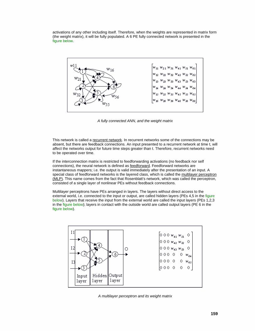
159

activations of any other including itself. Therefore, when the weights are represented in matrix form (the weight matrix), it will be fully populated. A 6 PE fully connected network is presented in the figure below.

A fully connected ANN, and the weight matrix

This network is called a recurrent network. In recurrent networks some of the connections may be absent, but there are feedback connections. An input presented to a recurrent network at time t, will affect the networks output for future time steps greater than t. Therefore, recurrent networks need to be operated over time.

If the interconnection matrix is restricted to feedforwarding activations (no feedback nor self connections), the neural network is defined as feedforward. Feedforward networks are instantaneous mappers; i.e. the output is valid immediately after the presentation of an input. A special class of feedforward networks is the layered class, which is called the multilayer perceptron (MLP). This name comes from the fact that Rosenblatt’s network, which was called the perceptron, consisted of a single layer of nonlinear PEs without feedback connections.

Multilayer perceptrons have PEs arranged in layers. The layers without direct access to the external world, i.e. connected to the input or output, are called hidden layers (PEs 4,5 in the figure below). Layers that receive the input from the external world are called the input layers (PEs 1,2,3 in the figure below); layers in contact with the outside world are called output layers (PE 6 in the figure below).

A multilayer perceptron and its weight matrix

160

Notice that most entries in the weight matrix of an MLP are zero. In particular, any feedforward network has at least the main diagonal, and the elements below it populated with zeros. Feedforward neural networks are therefore a special case of recurrent networks. Implementing partially connected topologies with the fully connected system and then zeroing weights is very inefficient, but unfortunately is sometimes done.

Learning Paradigms

Learning Paradigms

The process of modifying network parameters to improve performance is normally called learning. Learning in ANN’s can also be thought of as a second set of dynamics, because the network parameters will evolve in time according to some rules.

Consider the 6 PE MLP in A Multilayer Perceptron and its Weight Matrix figure. Assume that inputs are currents, and the weights are potentiometers that the user can control. For this example, the PEs can be thought of simply as being transistors. The goal is to obtain a value of 1 volt at the output, when several different currents are presented to the network. What the user would do is the following: start by connecting one of the inputs, and check the value at the output. If the value is not 1 volt, then some of the potentiometers will have to be changed until the goal state is reached. Then a second input is presented, and the process repeated until the desired response is obtained for all the inputs. When a neural network is trained, this very process of changing the weights is automated.

Learning requires several ingredients. First, as the network parameters change, the performance should improve. Therefore, the definition of a measure of performance is required. Second, the rules for changing the parameters should be specified. Third, this procedure (of training the network) should be done with known data.

The application of a performance measure produces another important taxonomic division in ANNs. When the performance function is based on the definition of an error measure, learning is said to be supervised. Normally the error is defined as the difference of the output of the ANN and a pre-specified external desired signal. In engineering applications where the desired performance is known, supervised learning paradigms become very important.

The other class of learning methods modify the network weights according to some pre-specified internal rules of interaction (unsupervised learning). There is therefore no "external teacher". This is the reason unsupervised learning is also called self-organization. Self-organization may be very appropriate for feature discovery (feature extraction) in complex signals with redundancy. A third intermediate class of learning is called reinforcement learning. In reinforcement learning the external teacher just indicates the quality (good or bad) of the response. Reinforcement learning is still in a research phase, but it may hold the key to on-line learning (i.e. with the present sample).

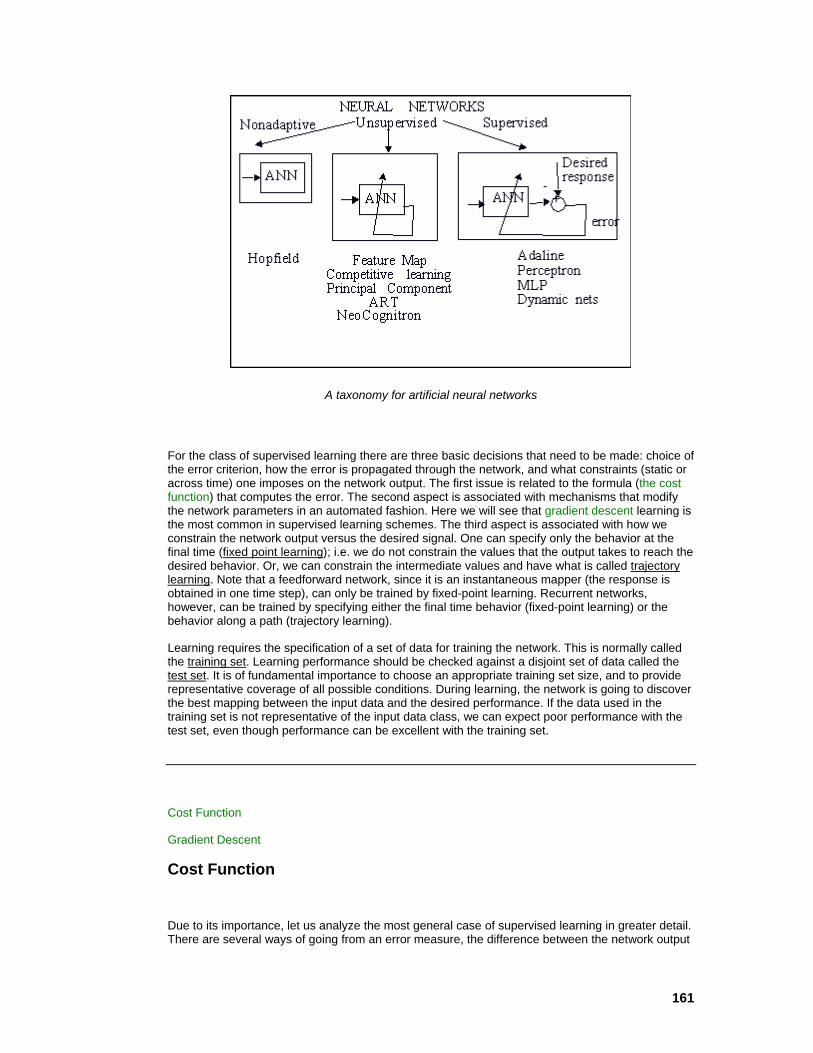
161

A taxonomy for artificial neural networks

For the class of supervised learning there are three basic decisions that need to be made: choice of the error criterion, how the error is propagated through the network, and what constraints (static or across time) one imposes on the network output. The first issue is related to the formula (the cost function) that computes the error. The second aspect is associated with mechanisms that modify the network parameters in an automated fashion. Here we will see that gradient descent learning is the most common in supervised learning schemes. The third aspect is associated with how we constrain the network output versus the desired signal. One can specify only the behavior at the final time (fixed point learning); i.e. we do not constrain the values that the output takes to reach the desired behavior. Or, we can constrain the intermediate values and have what is called trajectory learning. Note that a feedforward network, since it is an instantaneous mapper (the response is obtained in one time step), can only be trained by fixed-point learning. Recurrent networks, however, can be trained by specifying either the final time behavior (fixed-point learning) or the behavior along a path (trajectory learning).

Learning requires the specification of a set of data for training the network. This is normally called the training set. Learning performance should be checked against a disjoint set of data called the test set. It is of fundamental importance to choose an appropriate training set size, and to provide representative coverage of all possible conditions. During learning, the network is going to discover the best mapping between the input data and the desired performance. If the data used in the training set is not representative of the input data class, we can expect poor performance with the test set, even though performance can be excellent with the training set.

Cost Function

Gradient Descent

Cost Function

Due to its importance, let us analyze the most general case of supervised learning in greater detail. There are several ways of going from an error measure, the difference between the network output

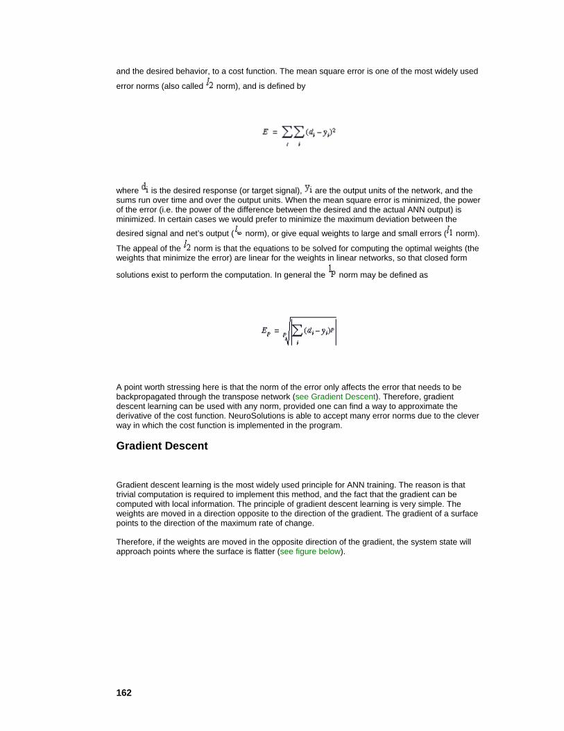
162

and the desired behavior, to a cost function. The mean square error is one of the most widely used

error norms (also called norm), and is defined by

where is the desired response (or target signal), are the output units of the network, and the sums run over time and over the output units. When the mean square error is minimized, the power of the error (i.e. the power of the difference between the desired and the actual ANN output) is minimized. In certain cases we would prefer to minimize the maximum deviation between the

desired signal and net’s output ( norm), or give equal weights to large and small errors ( norm).

The appeal of the norm is that the equations to be solved for computing the optimal weights (the weights that minimize the error) are linear for the weights in linear networks, so that closed form

solutions exist to perform the computation. In general the norm may be defined as

A point worth stressing here is that the norm of the error only affects the error that needs to be backpropagated through the transpose network (see Gradient Descent). Therefore, gradient descent learning can be used with any norm, provided one can find a way to approximate the derivative of the cost function. NeuroSolutions is able to accept many error norms due to the clever way in which the cost function is implemented in the program.

Gradient Descent

Gradient descent learning is the most widely used principle for ANN training. The reason is that trivial computation is required to implement this method, and the fact that the gradient can be computed with local information. The principle of gradient descent learning is very simple. The weights are moved in a direction opposite to the direction of the gradient. The gradient of a surface points to the direction of the maximum rate of change.

Therefore, if the weights are moved in the opposite direction of the gradient, the system state will approach points where the surface is flatter (see figure below).

163

Gradient descent in one dimension

In the figure above, let us assume that the first point is . The gradient along x at points to the right, so we move to the left, to At , the gradient still points to the right, so we move to . Now the gradient points to the left. so we move to the right. The bottom of the bowl is also the flat region of the surface. So, at least for the convex surface depicted, moving in a direction opposite that of the gradient moves in the direction of the smallest curvature. The weights that correspond to the point of minimum error are the optimal weights.

Widrow showed that in order to implement gradient descent in a linear distributed network (called an adaptive filter, see figure below) each of the weights (indexed by i) should be modified according to

where ? is a sufficiently small constant (the learning rate parameter), is the error (the difference between the desired response and the actual system response) at iteration step k, is the input value to the weight i at iteration k, and is the value of weight i at iteration k.

This is the LMS (least mean square) algorithm. The basic idea behind the LMS algorithm is a simplification of computing the gradient. Instead of averaging a lot of samples to obtain an accurate representation of the gradient as indicated by the l2 cost equation, the LMS only uses the present sample to estimate the gradient. Therefore one only needs to take the derivative of the present difference between the desired signal and the present output with respect to the PE weights, which simply becomes the multiplication of the present error by the input at each PE. This estimate is unbiased, so although noisy, it will converge to the correct value.

Notice that only two multiplications and one addition are necessary per weight to implement this equation, which is computationally very efficient. Notice also that all the necessary information (input and local error) is available locally to the weight. These are the two features of gradient descent that make it so appealing for ANN learning, but as with most things in the real world, there are some shortcomings.

164

The adaptive linear combiner (FIR filter)

The problem is with the existence of multiple minima (non-convex surfaces) that can trap the adaptation, and with difficulty in choosing appropriate leaning constants for fast convergence (see figure below).

A non-convex performance surface

Notice that, from the point of view of the gradient, a local minimum and the global minimum are indistinguishable, i.e. in both cases the gradient will be zero.

In nonlinear systems such as the ANN PE, the easy LMS rule must be modified to account for the nonlinearity. This gives rise to the delta rule, and this principle was known for a long time in sensitivity analysis. If one wants to compute the sensitivity of one quantity (E) with respect to another (w), related by a function (f(w)), as long as the function f is differentiable, the chain rule can be used, i.e.

165

Now we can understand why we required the nonlinearity of the PE to be monotonic and smooth, otherwise the first term of the equation could not be computed. If we apply this principle to the error at the output of the ith PE with respect to the weights, we see that

The first term is the derivative of the instantaneous mapper which will be denoted as σ'’ . The

second term gives the LMS rule applied to the weight (i.e. having as input and error ), i.e.

Delta rule learning is just an application of these principles repeated over and over again for each PE in the network. The problem that was faced by early ANN researchers when they tried to extrapolate this simple procedure to multilayer perceptrons was the fact that the desired signal in the hidden layers of the network was not known explicitly. It turns out that when the error is considered as a signal that is propagated from the output of the net to the input, one can reason that the error reaching a given node should be distributed proportionally to the strength of the weights connecting to that node (just think of an electrical signal being propagated through a resistive network where the weights are the conductances or resistors). This is the principle behind the backpropagation algorithm.

A relevant aspect of this methodology, which can be considered a contribution of ANN research to the theory of optimization, is the way the gradients are computed. In optimization, the method of forward perturbation is normally used to compute the gradient, which implies a massive computation of partial derivatives (see real time recurrent learning below). It has been shown repeatedly by ANN researchers, however that gradients can also be computed by propagating the error through the transpose network (or dual) and multiplying it locally with the activation residing at the node (see figure below). The transpose network is obtained from the original network by changing the direction of signal flow and switching the summing junctions with the nodes.

166

Relation between a network and its transpose (dual)

It turns out that this is a much more efficient procedure for computing the gradients than forward activation of the sensitivities. Moreover, the backpropagation procedure is not restricted to feedforward networks. A recurrent network can also benefit from the same backpropagation principle, and the backpropagation principle can even be applied to problems where the gradients have to be computed over time. NeuroSolutions extensively uses this simplification.

Note that in the backpropagation procedure there is an intrinsic data flow. First, the inputs are propagated forward through the network to reach the output. The output error is computed as the difference between the desired output and the current system output. Then errors are propagated back through the network up to the first layer after which the delta rule can be applied to each network PE.

Normally, the backpropagation equations are written in a much more complicated manner because one has to mathematically formulate the composition of intermediate errors. But these equations cloud a very simple and uniform principle. All the PEs compute the gradient in the same manner as expressed by the delta rule. When the transpose network is used to propagate the error, a routine computing the backpropagation procedure only needs to know about the delta rule, because the complication of propagating the error up to the unit is naturally taken care of by the transpose network. This is the way NeuroSolutions implements the backpropagation procedure.

A final note about backpropagation that needs to be covered is the functional form of the propagated error. Notice that the error passing across a PE is multiplied by the derivative of the nonlinearity taken at the operating value given by the PE activation. Practically, one does not need to explicitly compute the derivative of the nonlinearity since it can be given as a function of the operating point.

We know that the nonlinearity is a saturating function. Therefore, the derivative of large activations (positive or negative) will produce an attenuation in the propagated error. Since the weights will be modified proportionally to the magnitude of the error, one can expect that learning speed decreases

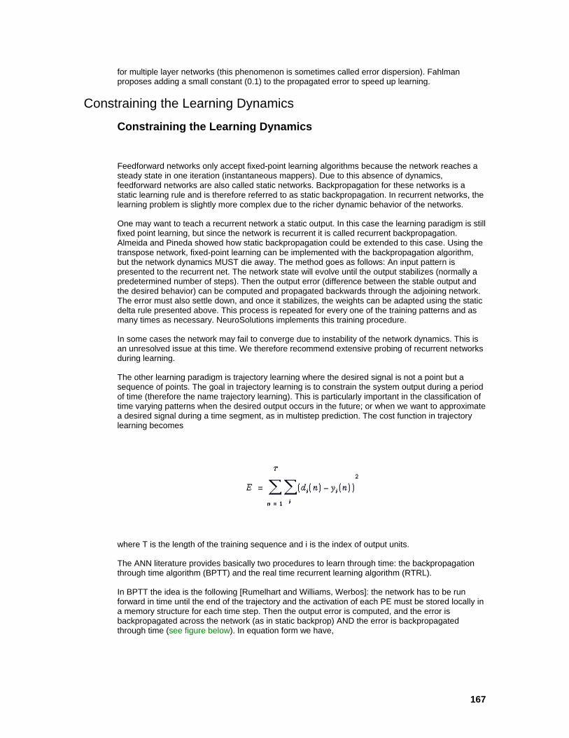
167

for multiple layer networks (this phenomenon is sometimes called error dispersion). Fahlman proposes adding a small constant (0.1) to the propagated error to speed up learning.



Feedforward networks only accept fixed-point learning algorithms because the network reaches a steady state in one iteration (instantaneous mappers). Due to this absence of dynamics, feedforward networks are also called static networks. Backpropagation for these networks is a static learning rule and is therefore referred to as static backpropagation. In recurrent networks, the learning problem is slightly more complex due to the richer dynamic behavior of the networks.

One may want to teach a recurrent network a static output. In this case the learning paradigm is still fixed point learning, but since the network is recurrent it is called recurrent backpropagation. Almeida and Pineda showed how static backpropagation could be extended to this case. Using the transpose network, fixed-point learning can be implemented with the backpropagation algorithm, but the network dynamics MUST die away. The method goes as follows: An input pattern is presented to the recurrent net. The network state will evolve until the output stabilizes (normally a predetermined number of steps). Then the output error (difference between the stable output and the desired behavior) can be computed and propagated backwards through the adjoining network. The error must also settle down, and once it stabilizes, the weights can be adapted using the static delta rule presented above. This process is repeated for every one of the training patterns and as many times as necessary. NeuroSolutions implements this training procedure.

In some cases the network may fail to converge due to instability of the network dynamics. This is an unresolved issue at this time. We therefore recommend extensive probing of recurrent networks during learning.

The other learning paradigm is trajectory learning where the desired signal is not a point but a sequence of points. The goal in trajectory learning is to constrain the system output during a period of time (therefore the name trajectory learning). This is particularly important in the classification of time varying patterns when the desired output occurs in the future; or when we want to approximate a desired signal during a time segment, as in multistep prediction. The cost function in trajectory learning becomes

where T is the length of the training sequence and i is the index of output units.

The ANN literature provides basically two procedures to learn through time: the backpropagation through time algorithm (BPTT) and the real time recurrent learning algorithm (RTRL).

In BPTT the idea is the following [Rumelhart and Williams, Werbos]: the network has to be run forward in time until the end of the trajectory and the activation of each PE must be stored locally in a memory structure for each time step. Then the output error is computed, and the error is backpropagated across the network (as in static backprop) AND the error is backpropagated through time (see figure below). In equation form we have,

168

where (n) is the error propagated by the transpose network across the network and through time. Since the activations x(n) in the forward pass have been stored, the gradient across time can be reconstructed by simple addition. This procedure is naturally implemented in NeuroSolutions.

Construction of the gradient in Backpropagation through time.

The other procedure for implementing trajectory learning is based on a very different concept. It is called real time recurrent learning [Williams and Zipser] and is a natural extension of the gradient computation in adaptive signal processing and control theory. The idea is to compute, at each time step, ALL the sensitivities, i.e. how much a change in one weight will affect the activation of all the

PEs of the network. Since there are weights in a fully connected net, and for each we have to keep track of N derivatives this is a very computationally intensive procedure (we further need N multiplications to compute each gradient). However, notice that we can perform the computation at each time step, so the storage requirements are not a function of the length of the trajectory. At the end of the trajectory, we can multiply these sensitivities by the error signal and compute the gradient along the trajectory (see figure below). In equation form we write the gradient as

where (n) is the output of the network. We can compute the derivative of the activation recursively as

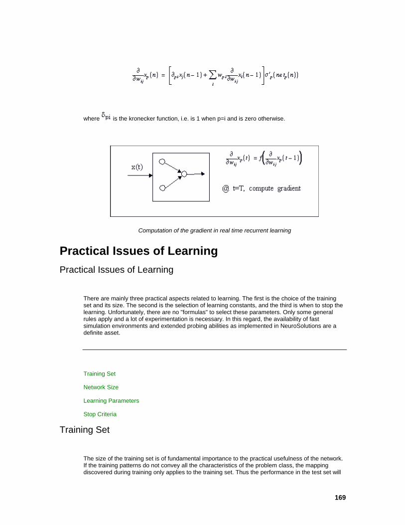
169

where is the kronecker function, i.e. is 1 when p=i and is zero otherwise.

Computation of the gradient in real time recurrent learning

Practical Issues of Learning Practical Issues of Learning

There are mainly three practical aspects related to learning. The first is the choice of the training set and its size. The second is the selection of learning constants, and the third is when to stop the learning. Unfortunately, there are no "formulas" to select these parameters. Only some general rules apply and a lot of experimentation is necessary. In this regard, the availability of fast simulation environments and extended probing abilities as implemented in NeuroSolutions are a definite asset.

Training Set

Network Size

Learning Parameters

Stop Criteria

Training Set

The size of the training set is of fundamental importance to the practical usefulness of the network. If the training patterns do not convey all the characteristics of the problem class, the mapping discovered during training only applies to the training set. Thus the performance in the test set will

170

be much worse than the training set performance. The only general rules that can be formulated are to use a lot of data and use representative data. If you do not have lots of data to train the ANN, then the ANN paradigm is probably not the best solution to solve your problem. Understanding of the problem to be solved is of fundamental importance in this step.

Another aspect of proper training is related to the relation between training set size and number of weights in the ANN. If the number of training examples is smaller than the number of weights, one can expect that the network may "hard code" the solution, i.e. it may allocate one weight to each training example. This will obviously produce poor generalization (i.e the ability to link unseen examples to the classes defined from the training examples). We recommend that the number of training examples be at least double the number of network weights.

When there is a big discrepancy between the performance in the training set and test set, we can suspect deficient learning. Note that one can always expect a drop in performance from the training set to the test set. We are referring to a large drop in performance (more than 10~15%). In cases like this we recommend increasing the training set size and/or produce a different mixture of training and test examples.

Network Size

At our present stage of knowledge, establishing the size of a network is more efficiently done through experimentation. The theory of generalization addresses this issue, but it is still difficult to apply in practical settings [VP dimension, Vapnik]. The issue is the following: The number of PEs in the hidden layer is associated with the mapping ability of the network. The larger the number, the more powerful the network is. However, if one continues to increase the network size, there is a point where the generalization gets worse. This is due to the fact that we may be over-fitting the training set, so when the network works with patterns that it has never seen before the response is unpredictable. The problem is to find the smallest number of degrees of freedom that achieves the required performance in the TEST set.

One school of thought recommends starting with small networks and increasing their size until the performance in the test set is appropriate. Fahlman proposes a method of growing neural topologies (the cascade correlation) that ensures a minimal number of weights, but the training can be fairly long. An alternate approach is to start with a larger network, and remove some of the weights. There are a few techniques, such as weight decay, that partially automate this idea [Weigend, LeCun]. The weights are allowed to decay from iteration to iteration, so if a weight is small, its value will tend to zero and can be eliminated.

In NeuroSolutions the size of the network can be controlled by probing the hidden layer weight activations with the scopes. When the value of an activation is small, does not change during learning, or is highly correlated with another activation, then the size of the hidden layer can be decreased.

Learning Parameters

The control of the learning parameters is an unsolved problem in ANN research (and for that matter in optimization theory). The point is that one wants to train as fast as possible and reach the best performance. Increasing the learning rate parameter will decrease the training time, but will also increase the possibility of divergence, and of rattling around the optimal value. Since the weight correction is dependent upon the performance surface characteristics and learning rate, to obtain constant learning, an adaptive learning parameter is necessary. We may even argue that what is necessary is a strategy where the learning rate is large in the beginning of the learning task and progressively decays towards the end of adaptation. Modification of learning rates is possible under certain circumstances, but a lot of other parameters are included that also need to be experimentally set. Therefore, these procedures tend to be brittle and the gains are problem dependent (see the work of Fahlman, LeCun, and Silva and Almeida, for a review). NeuroSolutions

171

enables versatile control of the learning rates by implementing adaptive schemes [Jacob] and Fahlman’s quickprop [Fahlman].

The conventional approach is to simply choose the learning rate and a momentum term. The momentum term imposes a "memory factor" on the adaptation, and has been shown to speedup adaptation while avoiding local minima trapping to a certain extent. Thus, the learning equation becomes

where γ is a constant (normally set between 0.5 and 0.9), and µ is the learning rate.

Jacob’s delta bar delta is also a versatile procedure, but requires more care in specification of the learning parameters. The idea is the following: when there are consecutive iterations that produce the same sign of weight update, the learning rate is too small. On the other hand, if consecutive iterations produce weight updates that have opposite signs, the learning rate is too fast. Jacob proposed the following formulas for learning rate updates:

where η is the learning rate for each weight, (n) is the gradient and

where ξ is a small constant.

One other option available to the researcher is when to perform the weight updates. Updates can be performed at the end of presentation of all the elements of the training set (batch learning) or at each iteration (real time). The first modality "smoothes" the gradient and may give faster learning for noisy data, however it may also average the gradient to zero and stall learning. Modification of the weights at each iteration with a small learning rate may be preferable most of the time.

Stop Criteria

The third problem is how to stop the learning. Stop criteria are all based on monitoring the mean square error. The curve of the MSE as a function of time is called the learning curve. The most used criterion is probably to choose the number of iterations, but we can also preset the final error.

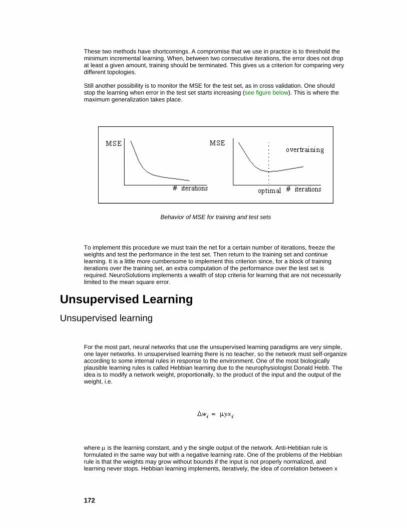
172

These two methods have shortcomings. A compromise that we use in practice is to threshold the minimum incremental learning. When, between two consecutive iterations, the error does not drop at least a given amount, training should be terminated. This gives us a criterion for comparing very different topologies.

Still another possibility is to monitor the MSE for the test set, as in cross validation. One should stop the learning when error in the test set starts increasing (see figure below). This is where the maximum generalization takes place.

Behavior of MSE for training and test sets

To implement this procedure we must train the net for a certain number of iterations, freeze the weights and test the performance in the test set. Then return to the training set and continue learning. It is a little more cumbersome to implement this criterion since, for a block of training iterations over the training set, an extra computation of the performance over the test set is required. NeuroSolutions implements a wealth of stop criteria for learning that are not necessarily limited to the mean square error.

Unsupervised Learning Unsupervised learning

For the most part, neural networks that use the unsupervised learning paradigms are very simple, one layer networks. In unsupervised learning there is no teacher, so the network must self-organize according to some internal rules in response to the environment. One of the most biologically plausible learning rules is called Hebbian learning due to the neurophysiologist Donald Hebb. The idea is to modify a network weight, proportionally, to the product of the input and the output of the weight, i.e.

where µ is the learning constant, and y the single output of the network. Anti-Hebbian rule is formulated in the same way but with a negative learning rate. One of the problems of the Hebbian rule is that the weights may grow without bounds if the input is not properly normalized, and learning never stops. Hebbian learning implements, iteratively, the idea of correlation between x

173

and y (the input and output of the weight). This principle can even be applied with the input and a desired signal, as in heteroassociation (forced Hebbian).

A very effective normalization of the Hebbian rule has been proposed by Oja, and reads

For linear networks, one can show that Oja’s rule finds the principal component of the input data, i.e. it implements what is called an eigenfilter. A common name for the eigenfilter is matched filter, which is known to maximize the signal to noise ratio. Hence, Oja’s rule produces a system that is optimal and can be used for feature extraction.

This network can be extended to M multiple output units and extract, in order, the M principal components of the input [Sanger], yielding

where

Principal Component Analysis is a very powerful feature representation method. PCA projects the data cluster on a set of orthogonal axes that best represent the input at each order. It can be shown that PCA is solving an eigenvalue problem. This can be accomplished with linear algebra techniques, but here we are doing the same thing using on-line, adaptive techniques.

Another unsupervised learning paradigm is competitive learning. The idea of competitive learning is that the output PEs compete to be on all the time (winner-take-all). This is accomplished by creating inhibitory connections among the output PEs. Competitive learning networks cluster the input patterns, and can therefore be used in data reduction through vector quantization. One can describe competitive learning as a sort of Hebbian learning applied to the output node that wins the competition among all the output nodes. First, only one of the output units can be active at a given time (called the winner), which is defined as the PE that has the largest summed input. If the weights to each PE are normalized, then this choice takes the winner as the unit closest to the

input vector x in the norm sense, i.e.

174

where means the winning PE. For the winning PE, the weights are updated as

which displaces the weight vector towards the input pattern (inputs are assumed normalized). Several other distance metrics can also be used, and the Euclidean seems the one that is more robust. These types of networks have been applied successfully to vector quantization schemes, since they can search the code books in parallel.

The problem with competitive learning is that the same unit may always win the competition. One way to handle this problem is to create a second competitive mechanism, where each unit keeps track of how many times it wins the competition. The units that win the competition too often are penalized. This second competition is called conscience. To implement conscience each PE must count how often it wins the competition by

where is one or zero. The constant β is normally small (0.001). The current bias for the unit is computed as

where 1/N measures the equal firing rate for an N PE net. γ is normally large (for -1/+1 normalized

data γ should be 1). The value of is subtracted from the distance function that selects the winner. This gives the ability to use all the PEs, but distorts the a priori probability of the classes.

Feature mapping is closely related to competitive learning networks. In feature mapping the output units are arranged in a geometric configuration (normally a 2D space). The goal is to map a multidimensional vector onto this 2D space while preserving neighborhoods. This can be achieved with an extension of competitive learning, where PEs in a neighborhood of the winning PE also have their weights updated according to the distance to the winning PE. The update rules read,

where

175

is a neighborhood function that decays like a Gaussian, and the variance and learning rate are made time varying to speed up the convergence.

Support Vector Machines Support Vector Machines

The support vector machine (SVM) in NeuroSolutions is a new kind of classifier that is motivated by two concepts. First, transforming data into a high-dimensional space can transform complex problems (with complex decision surfaces) into simpler problems that can use linear discriminant functions. Second, SVMs are motivated by the concept of training and using only those inputs that are near the decision surface since they provide the most information about the classification.

The first step in a SVM is transforming the data into a high-dimensional space. In NeuroSolutions this is done using a Radial Basis Function (RBF) network that places a gaussian at each data sample. Thus, the feature space becomes as large as the number of samples. The RBF, however, uses backpropagation to train a linear combination of the gaussians to produce the final result. The SVM in NeuroSolutions, however, uses the idea of large margin classifiers for training. This decouples the capacity of the classifier from the input space and at the same time provides good generalization. This is an ideal combination for classification. The learning algorithm is based on the Adatron algorithm extended to the RBF network. The Adatron algorithm can be easily extended to the RBF network by substituting the inner product of patterns in the input space by the kernel function, leading to the following quadratic optimization problem:

We can then define

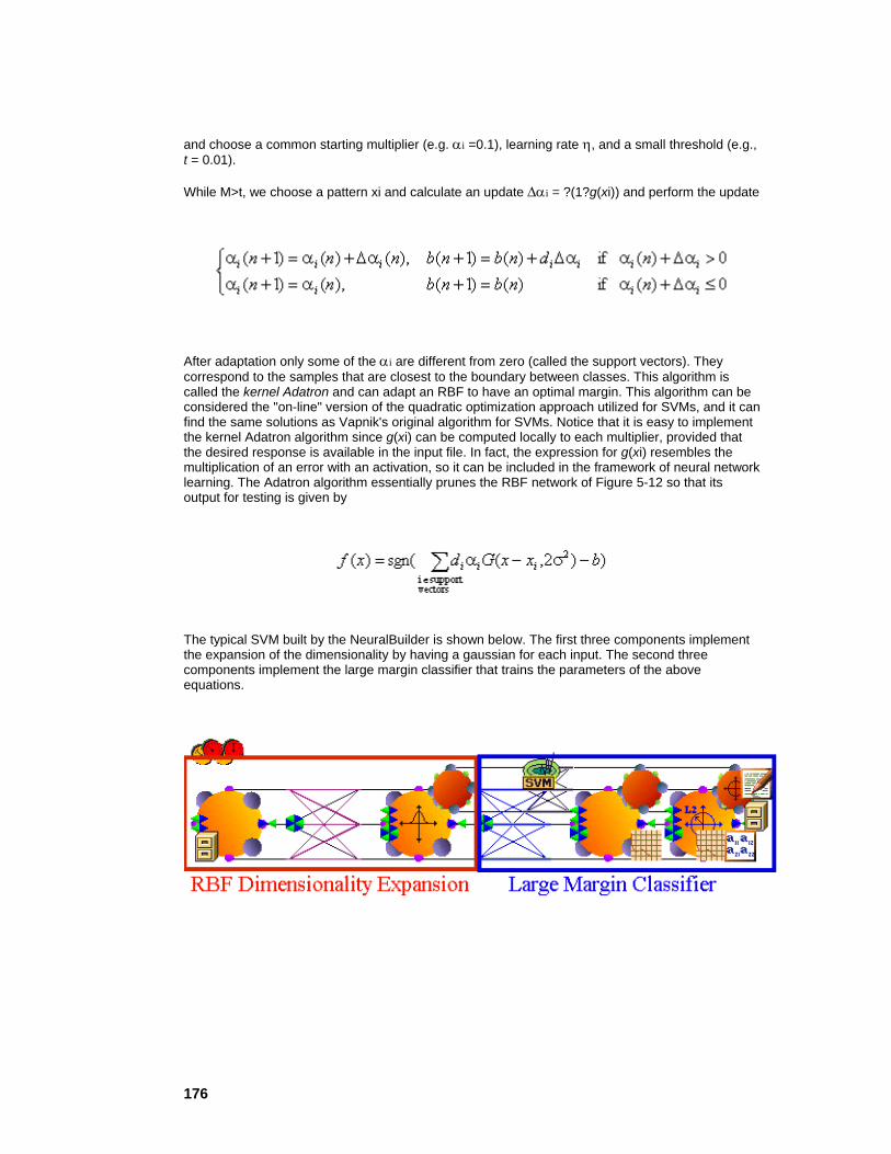
176

and choose a common starting multiplier (e.g. αi =0.1), learning rate η, and a small threshold (e.g., t = 0.01).

While M>t, we choose a pattern xi and calculate an update ∆αi = ?(1?g(xi)) and perform the update

After adaptation only some of the αi are different from zero (called the support vectors). They correspond to the samples that are closest to the boundary between classes. This algorithm is called the kernel Adatron and can adapt an RBF to have an optimal margin. This algorithm can be considered the "on-line" version of the quadratic optimization approach utilized for SVMs, and it can find the same solutions as Vapnik's original algorithm for SVMs. Notice that it is easy to implement the kernel Adatron algorithm since g(xi) can be computed locally to each multiplier, provided that the desired response is available in the input file. In fact, the expression for g(xi) resembles the multiplication of an error with an activation, so it can be included in the framework of neural network learning. The Adatron algorithm essentially prunes the RBF network of Figure 5-12 so that its output for testing is given by

The typical SVM built by the NeuralBuilder is shown below. The first three components implement the expansion of the dimensionality by having a gaussian for each input. The second three components implement the large margin classifier that trains the parameters of the above equations.

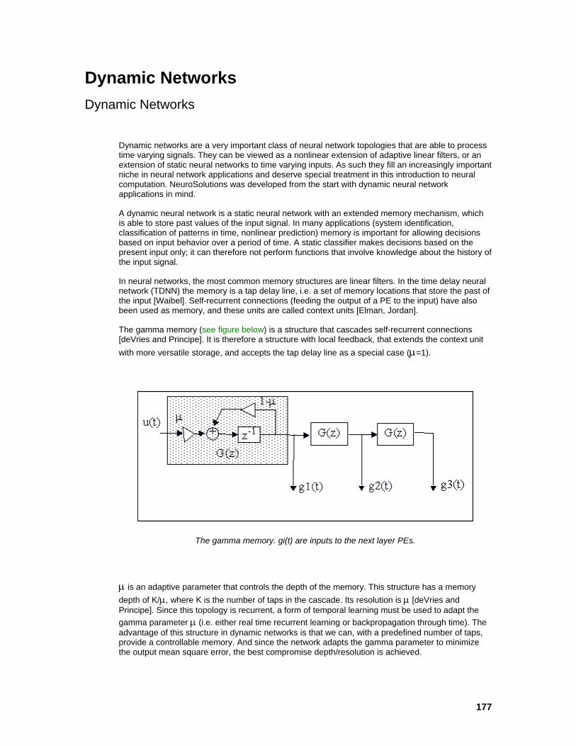
177

Dynamic Networks Dynamic Networks

Dynamic networks are a very important class of neural network topologies that are able to process time varying signals. They can be viewed as a nonlinear extension of adaptive linear filters, or an extension of static neural networks to time varying inputs. As such they fill an increasingly important niche in neural network applications and deserve special treatment in this introduction to neural computation. NeuroSolutions was developed from the start with dynamic neural network applications in mind.

A dynamic neural network is a static neural network with an extended memory mechanism, which is able to store past values of the input signal. In many applications (system identification, classification of patterns in time, nonlinear prediction) memory is important for allowing decisions based on input behavior over a period of time. A static classifier makes decisions based on the present input only; it can therefore not perform functions that involve knowledge about the history of the input signal.

In neural networks, the most common memory structures are linear filters. In the time delay neural network (TDNN) the memory is a tap delay line, i.e. a set of memory locations that store the past of the input [Waibel]. Self-recurrent connections (feeding the output of a PE to the input) have also been used as memory, and these units are called context units [Elman, Jordan].

The gamma memory (see figure below) is a structure that cascades self-recurrent connections [deVries and Principe]. It is therefore a structure with local feedback, that extends the context unit with more versatile storage, and accepts the tap delay line as a special case (µ=1).

The gamma memory. gi(t) are inputs to the next layer PEs.

µ is an adaptive parameter that controls the depth of the memory. This structure has a memory depth of K/µ, where K is the number of taps in the cascade. Its resolution is µ [deVries and Principe]. Since this topology is recurrent, a form of temporal learning must be used to adapt the gamma parameter µ (i.e. either real time recurrent learning or backpropagation through time). The advantage of this structure in dynamic networks is that we can, with a predefined number of taps, provide a controllable memory. And since the network adapts the gamma parameter to minimize the output mean square error, the best compromise depth/resolution is achieved.

178

The gamma memory can be applied to the input (focused gamma memory), to the hidden PEs or to the output PEs. In each case it will store the activations of the respective PEs and use their past values to compute the net output. A dynamic neural network with the gamma memory is called the gamma neural model. The gamma neural model can be applied to classification of time varying patterns, signal detection, prediction of chaotic time series, and identification of nonlinear systems.

Famous Neural Topologies Famous Neural Topologies

Perceptron

Multilayer Perceptron

Madaline

Radial Basis Function Networks

Associative Memories

Jordan/Elman Networks

Hopfield Network

Principal Component Analysis Networks

Kohonen Self-Organizing Maps (SOFM)

Adaptive Resonance Theory (ART)

Fukushima

Time Lagged Recurrent Networks

Perceptron

The perceptron was probably the first successful neurocomputer (Rosenblatt 1957). Rosenblatt constructed the MARK I for binary image classification. The perceptron is nothing but a feedforward neural network with no hidden units. Its information processing abilities are limited. It can only discriminate among linearly separable classes, i.e. classes that could be separated by hyperplanes. The appeal of the perceptron was Rosenblatt’s proof that it is trainable (for linearly separable classes) in a finite number of steps. The Perceptron learning rule is very simple:

Present a pattern. If the output is the desired output, do nothing. If the response is wrong, from the units that are active, change their weights towards the desired response. Repeat the process until all the units have acceptable outputs.

The delta rule (simplified backpropagation) can also be applied to the perceptron, but perceptron learning is faster and more stable if the patterns are linearly separable. Even today (more than 30 years later), the perceptron and its learning rule have appeal. Recently the perceptron learning rule was revisited to provide acceptable results even when the patterns were not linearly separable. We can implement a perceptron as a special case (no hidden layer) of a multilayer perceptron.

179

Multilayer Perceptron

The multilayer perceptron (MLP) is one of the most widely implemented neural network topologies. The article by Lippman is probably one of the best references for the computational capabilities of MLPs. Generally speaking, for static pattern classification, the MLP with two hidden layers is a universal pattern classifier. In other words, the discriminant functions can take any shape, as required by the input data clusters. Moreover, when the weights are properly normalized and the output classes are normalized to 0/1, the MLP achieves the performance of the maximum a posteriori receiver, which is optimal from a classification point of view [Makhoul]. In terms of mapping abilities, the MLP is believed to be capable of approximating arbitrary functions. This has been important in the study of nonlinear dynamics [Lapedes and Farber], and other function mapping problems.

MLPs are normally trained with the backpropagation algorithm [Rumelhart et al]. In fact the renewed interest in ANNs was in part triggered by the existence of backpropagation. The LMS learning algorithm proposed by Widrow can not be extended to hidden PEs, since we do not know the desired signal there. The backpropagation rule propagates the errors through the network and allows adaptation of the hidden PEs.

Two important characteristics of the multilayer perceptron are: its nonlinear processing elements (PEs) which have a nonlinearity that must be smooth (the logistic function and the hyperbolic tangent are the most widely used); and their massive interconnectivity (i.e. any element of a given layer feeds all the elements of the next layer).

The multilayer perceptron is trained with error correction learning, which means that the desired response for the system must be known. In pattern recognition this is normally the case, since we have our input data labeled, i.e. we know which data belongs to which experiment.

Error correction learning works in the following way: From the system response at PE i at iteration

n, (n), and the desired response (n) for a given input pattern an instantaneous error (n) is defined by

Using the theory of gradient descent learning, each weight in the network can be adapted by correcting the present value of the weight with a term that is proportional to the present input and error at the weight, i.e.

The local error (n) can be directly computed from (n) at the output PE or can be computed as a weighted sum of errors at the internal PEs. The constant η is called the step size. This procedure is called the backpropagation algorithm.

Backpropagation computes the sensitivity of a cost functional with respect to each weight in the network, and updates each weight proportional to the sensitivity. The beauty of the procedure is that it can be implemented with local information and requires just a few multiplications per weight, which is very efficient. Because this is a gradient descent procedure, it only uses the local

180

information so can be caught in local minima. Moreover, the procedure is inherently noisy since we are using a poor estimate of the gradient, causing slow convergence.

Momentum learning is an improvement to the straight gradient descent in the sense that a memory term (the past increment to the weight) is used to speed up and stabilize convergence. In momentum learning the equation to update the weights becomes

where α is the momentum. Normally α should be set between 0.1 and 0.9.

Training can be implemented in two ways: Either we present a pattern and adapt the weights (on-line training), or we present all the patterns in the input file (an epoch), accumulate the weight updates, and then update the weights with the average weight update. This is called batch learning. They are theoretically equivalent, but the former sometimes has advantages in tough problems (many similar input -output pairs).

To start backpropagation, we need to load an initial value for each weight (normally a small random value), and proceed until some stopping criterion is met. The three most common are: to cap the number of iterations, to threshold the output mean square error, or to use cross validation. Cross validation is the more powerful of the three since it stops the training at the point of best generalization (i.e. the performance in the test set) is obtained. To implement cross validation one must put aside a small part of the training data (10%) and use it to see how the trained network is doing (e.g. every 100 training epochs, test the net with a validation set). When the performance starts to degrade in the validation set, training should be stopped.

Checking the progress of learning is fundamental in any iterative training procedure. The learning curve (how the mean square error evolves with the training iteration) is such a quantity. We can judge the difficulty of the task, and how to control the learning parameters from the learning curve. When the learning curve is flat, the step size should be increased to speed up learning. On the other hand, when the learning curve oscillates up and down the step size should be decreased. In the extreme, the error can go steadily up, showing that learning is unstable. At this point the network should be reset. When the learning curve stabilizes after many iterations at an error level that is not acceptable, it is time to rethink the network topology (more hidden PEs or more hidden layers, or a different topology altogether) or the training procedure (other more sophisticated gradient search techniques).

We present below a set of heuristics that will help decrease the training times and, in general, produce better performance.

Normalize your training data.

Use the tanh nonlinearity instead of the logistic function.

Normalize the desired signal to be just below the output nonlinearity rail voltages (i.e. if you use the tanh, use desired signals of +/- 0.9 instead of +/- 1).

Set the step size higher towards the input (i.e. for a one hidden layer MLP, set the step size at 0.05 in the synapse between the input and hidden layer, and 0.01 in the synapse between the hidden and output layer).

Initialize the net’s weights in the linear region of the nonlinearity (divide the standard deviation of the random noise source by the fan-in of each PE).

Use more sophisticated learning methods (quick prop or delta bar delta).

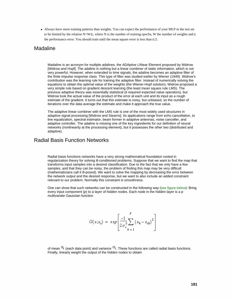
181

Always have more training patterns than weights. You can expect the performance of your MLP in the test set to be limited by the relation N>W/ε, where N is the number of training epochs, W the number of weights and ε the performance error. You should train until the mean square error is less than ε/2.

Madaline

Madaline is an acronym for multiple adalines, the ADAptive LINear Element proposed by Widrow [Widrow and Hopf]. The adaline is nothing but a linear combiner of static information, which is not very powerful. However, when extended to time signals, the adaline becomes an adaptive filter of the finite impulse response class. This type of filter was studied earlier by Wiener (1949). Widrow’s contribution was the learning rule for training the adaptive filter. Instead of numerically solving the equations to obtain the optimal value of the weights (the Wiener-Hopf solution), Widrow proposed a very simple rule based on gradient descent learning (the least mean square rule LMS). The previous adaptive theory was essentially statistical (it required expected value operators), but Widrow took the actual value of the product of the error at each unit and its input as a rough estimate of the gradient. It turns out that this estimate is noisy, but unbiased, so the number of iterations over the data average the estimate and make it approach the true value.

The adaptive linear combiner with the LMS rule is one of the most widely used structures in adaptive signal processing [Widrow and Stearns]. Its applications range from echo cancellation, to line equalization, spectral estimator, beam former in adaptive antennas, noise canceller, and adaptive controller. The adaline is missing one of the key ingredients for our definition of neural networks (nonlinearity at the processing element), but it possesses the other two (distributed and adaptive).

Radial Basis Function Networks

Radial basis functions networks have a very strong mathematical foundation rooted in regularization theory for solving ill-conditioned problems. Suppose that we want to find the map that transforms input samples into a desired classification. Due to the fact that we only have a few samples, and that they can be noisy, the problem of finding this map may be very difficult (mathematicians call it ill-posed). We want to solve the mapping by decreasing the error between the network output and the desired response, but we want to also include an added constraint relevant to our problem. Normally this constraint is smoothness.

One can show that such networks can be constructed in the following way (see figure below): Bring every input component (p) to a layer of hidden nodes. Each node in the hidden layer is a p multivariate Gaussian function

of mean (each data point) and variance . These functions are called radial basis functions. Finally, linearly weight the output of the hidden nodes to obtain

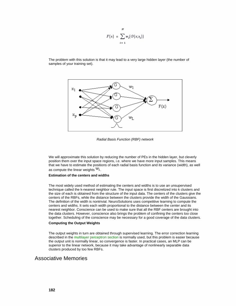
182

The problem with this solution is that it may lead to a very large hidden layer (the number of samples of your training set).

Radial Basis Function (RBF) network

We will approximate this solution by reducing the number of PEs in the hidden layer, but cleverly position them over the input space regions, i.e. where we have more input samples. This means that we have to estimate the positions of each radial basis function and its variance (width), as well as compute the linear weights . Estimation of the centers and widths

The most widely used method of estimating the centers and widths is to use an unsupervised technique called the k-nearest neighbor rule. The input space is first discretized into k clusters and the size of each is obtained from the structure of the input data. The centers of the clusters give the centers of the RBFs, while the distance between the clusters provide the width of the Gaussians. The definition of the width is nontrivial. NeuroSolutions uses competitive learning to compute the centers and widths. It sets each width proportional to the distance between the center and its nearest neighbor. Conscience can be used to make sure that all the RBF centers are brought into the data clusters. However, conscience also brings the problem of confining the centers too close together. Scheduling of the conscience may be necessary for a good coverage of the data clusters. Computing the Output Weights

The output weights in turn are obtained through supervised learning. The error correction learning described in the multilayer perceptron section is normally used, but this problem is easier because the output unit is normally linear, so convergence is faster. In practical cases, an MLP can be superior to the linear network, because it may take advantage of nonlinearly separable data clusters produced by too few RBFs.

Associative Memories

183

Steinbuch was a cognitive scientist and one of the pioneering researchers in distributed computation. His interests were in associative memories, i.e. devices that could learn associations among dissimilar binary objects. He implemented the learnmatrix, where a set of binary inputs is fed to a matrix of resistors, producing a set of binary outputs. The outputs are 1 if the sum of the inputs is above a given threshold, zero otherwise. The weights (which were binary) were updated by using several very simple rules based on Hebbian learning. But the interesting thing is that the asymptotic capacity of this network is rather high and easy to determine (I= [Willshaw]).

The linear associative memory was proposed by several researchers [Anderson, Kohonen]. It is a very simple device with one layer of linear units that maps N inputs (a point in N dimensional space) onto M outputs (a point in M dimensional space). In terms of signal processing, this network does nothing but a projection operation of a vector in N dimensional space to a vector in M dimensional space.

This projection is achieved by the weight matrix. The weight matrix can be computed analytically: it is the product of the output with the pseudo inverse of the input [Kohonen]. In terms of linear algebra, what we are doing is computing the outer product of the input vector with the output vector. This solution can be approximated by Hebbian learning and the approximation is quite good if the input patterns are orthogonal. Widrow’s LMS rule can also be used to compute a good approximation of W even for the case of non-orthogonal patterns [Hecht-Nielsen].

Jordan/Elman Networks

The theory of neural networks with context units can be analyzed mathematically only for the case of linear PEs. In this case the context unit is nothing but a very simple lowpass filter. A lowpass filter creates an output that is a weighted (average) value of some of its more recent past inputs. In the case of the Jordan context unit, the output is obtained by summing the past values multiplied by the scalar as shown in the figure below.

Context unit response

Notice that an impulse event x(n) (i.e. x(0)=1, x(n)=0 for n>0) that appears at time n=0, will disappear at n=1. However, the output of the context unit is t1 at n=1, t2 at n=2, etc. This is the reason these context units are called memory units, because they "remember" past events. t should be less than 1, otherwise the context unit response gets progressively larger (unstable).

The Jordan network and the Elman network combine past values of the context units with the present inputs to obtain the present net output. The input to the context unit is copied from the network layer, but the outputs of the context unit are incorporated in the net through adaptive weights. NeuroSolutions uses straight backpropagation to adapt all the network weights. In the NeuralBuilder, the context unit time constant is pre-selected by the user. One issue in these nets is that the weighting over time is kind of inflexible since we can only control the time constant (i.e. the exponential decay). Moreover, a small change in t is reflected in a large change in the weighting (due to the exponential relationship between time constant and amplitude). In general, we do not know how large the memory depth should be, so this makes the choice of t problematic, without a

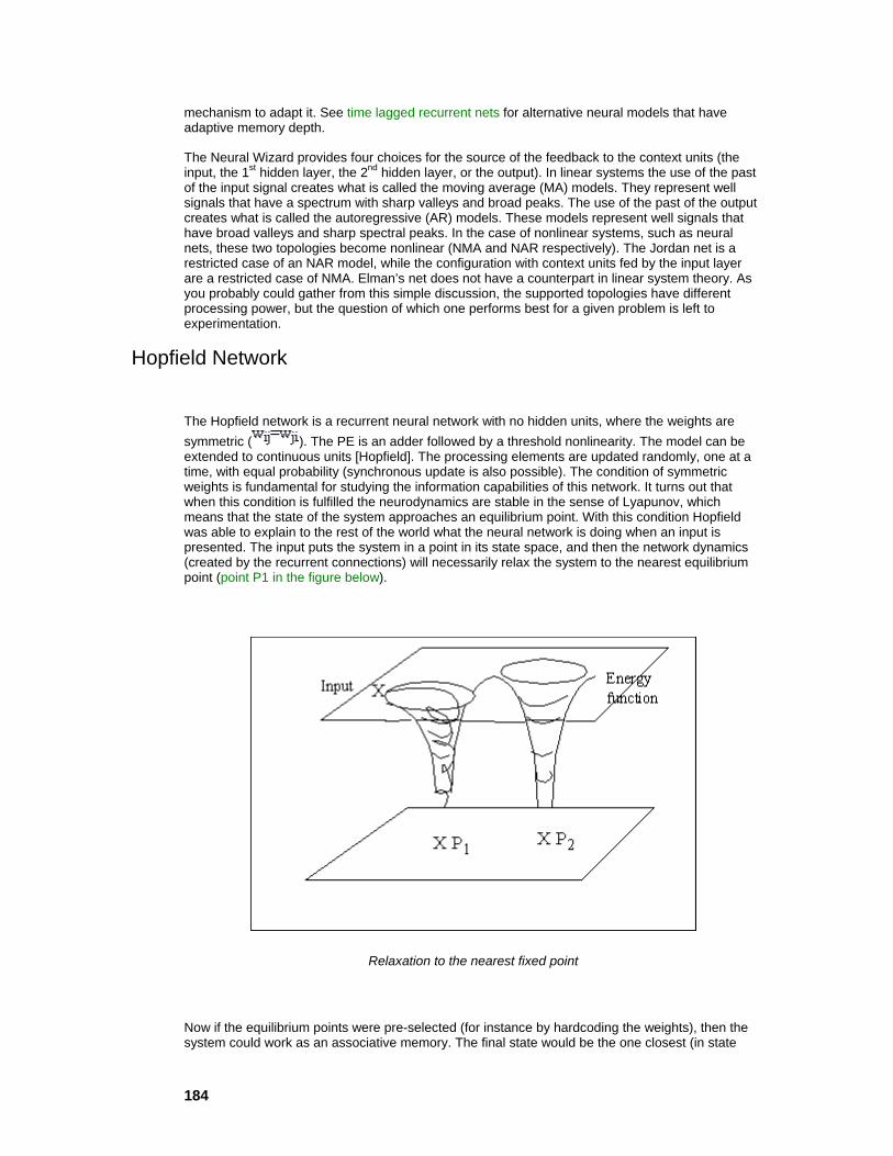
184

mechanism to adapt it. See time lagged recurrent nets for alternative neural models that have adaptive memory depth.

The Neural Wizard provides four choices for the source of the feedback to the context units (the input, the 1st hidden layer, the 2nd hidden layer, or the output). In linear systems the use of the past of the input signal creates what is called the moving average (MA) models. They represent well signals that have a spectrum with sharp valleys and broad peaks. The use of the past of the output creates what is called the autoregressive (AR) models. These models represent well signals that have broad valleys and sharp spectral peaks. In the case of nonlinear systems, such as neural nets, these two topologies become nonlinear (NMA and NAR respectively). The Jordan net is a restricted case of an NAR model, while the configuration with context units fed by the input layer are a restricted case of NMA. Elman’s net does not have a counterpart in linear system theory. As you probably could gather from this simple discussion, the supported topologies have different processing power, but the question of which one performs best for a given problem is left to experimentation.

Hopfield Network

The Hopfield network is a recurrent neural network with no hidden units, where the weights are symmetric ( ). The PE is an adder followed by a threshold nonlinearity. The model can be extended to continuous units [Hopfield]. The processing elements are updated randomly, one at a time, with equal probability (synchronous update is also possible). The condition of symmetric weights is fundamental for studying the information capabilities of this network. It turns out that when this condition is fulfilled the neurodynamics are stable in the sense of Lyapunov, which means that the state of the system approaches an equilibrium point. With this condition Hopfield was able to explain to the rest of the world what the neural network is doing when an input is presented. The input puts the system in a point in its state space, and then the network dynamics (created by the recurrent connections) will necessarily relax the system to the nearest equilibrium point (point P1 in the figure below).

Relaxation to the nearest fixed point

Now if the equilibrium points were pre-selected (for instance by hardcoding the weights), then the system could work as an associative memory. The final state would be the one closest (in state

185

space) to that particular input. We could then classify the input or recall it using content addressable properties. In fact, such a system is highly robust to noise, also displaying pattern completion properties. Very possibly, biological memory is based on identical principles. The structure of the hippocampus is very similar to the wiring of a Hopfield net (outputs of one unit fed to all the others). In a Hopfield net if one asks where the memory is, the answer has to be in the set of weights. The Hopfield net, therefore, implements a nonlinear associative memory, which is known to have some of the features of human memory; (e.g. highly distributed, fault tolerance, graceful degradation, and finite capacity).

Most Hopefield net applications are in optimization, where a mapping of the energy function to the cost function of the user’s problem must be established and the weights pre-computed. The weights in the Hopfield network can be computed using Hebbian learning, which guarantees a stable network. Recurrent backpropagation can also be used to compute the weights, but in this case, there is no guarantee that the weights are symmetric (hence the system may be unstable). NeuroSolutions can implement the Hopfield net and train it with fixed-point learning or Hebbian learning.

The "brain state in a box" [Anderson] can be considered as a special case of the Hopfield network where the state of the system is confined to the unit hypercube, and the system attractors are the vertices of the cube. This network has been successfully used for categorization of the inputs.


The fundamental problem in pattern recognition is to define data features that are important for the classification (feature extraction). One wishes to transform our input samples into a new space (the feature space) where the information about the samples is retained, but the dimensionality is reduced. This will make the classification job much easier.

Principal component analysis (PCA) also called Karhunen-Loeve transform of Singular Value Decomposition (SVD) is such a technique. PCA finds an orthogonal set of directions in the input space and provides a way of finding the projections into these directions in an ordered fashion. The first principal component is the one that has the largest projection (we can think that the projection is the shadow of our data cluster in each direction). The orthogonal directions are called the eigenvectors of the correlation matrix of the input vector, and the projections the corresponding eigenvalues.

Since PCA orders the projections, we can reduce the dimensionality by truncating the projections to a given order. The reconstruction error is equal to the sum of the projections (eigenvalues) left out. The features in the projection space become the eigenvalues. Note that this projection space is linear.

PCA is normally done by analytically solving an eigenvalue problem of the input correlation function. However, Sanger and Oja demonstrated (see Unsupervised Learning) that PCA can be accomplished by a single layer linear neural network trained with a modified Hebbian learning rule.

Let us consider the network shown in the figure below. Notice that the network has p inputs (we assume that our samples have p components) and m<p linear output PEs. The output is given by

To train the weights, we will use the following modified Hebbian rule

186

where η is the step size.

PCA network

What is interesting in this network is that we are computing the eigenvectors of the correlation function of the input without ever computing the correlation function. Sanger showed that this learning procedure converges to the correct solution, i.e. the weights of the PCA network approach the first m principal components of the input data matrix. The outputs are therefore related to the eigenvalues and can be used as input to another neural networks for classification.

PCA networks can be used for data compression, providing the best m linear features. They can also be used for data reduction in conjunction with multilayer perceptron classifiers. In this case, however, the separability of the classes is not always guaranteed. If the data clusters are sufficiently separated, yes, but if the classes are on top of each other, the PCA will get the largest projections, but the separability can be in some of the other projections. Another problem with linear PCA networks is outlying data points. Outliers will distort the estimation of the eigenvectors and create skewed data projections. Nonlinear networks are better able to handle this case.

The importance of PCA analysis is that the number of inputs for the MLP classifier can be reduced a lot, which positively impacts the number of required training patterns, and the training times of the classifier.

Kohonen Self-Organizing Maps (SOFM)

As was stated previously, one of the most important issues in pattern recognition is feature extraction. Since this is such a crucial step, different techniques may provide a better fit to our problem. An alternative to the PCA concept is the self-organizing feature map.

The ideas of SOFM are rooted in competitive learning networks. These nets are one layer nets with linear PEs but use a competitive learning rule. In such nets there is one and only one winning PE for every input pattern (i.e. the PE whose weights are closest to the input pattern). In competitive

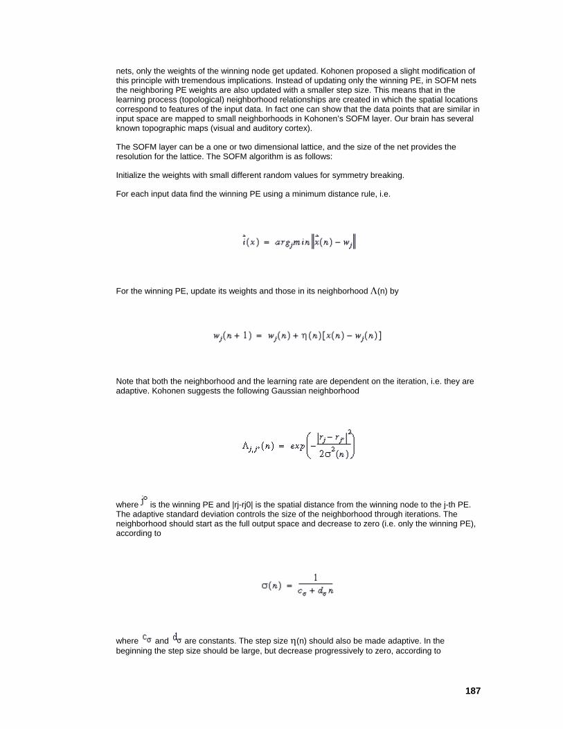
187

nets, only the weights of the winning node get updated. Kohonen proposed a slight modification of this principle with tremendous implications. Instead of updating only the winning PE, in SOFM nets the neighboring PE weights are also updated with a smaller step size. This means that in the learning process (topological) neighborhood relationships are created in which the spatial locations correspond to features of the input data. In fact one can show that the data points that are similar in input space are mapped to small neighborhoods in Kohonen’s SOFM layer. Our brain has several known topographic maps (visual and auditory cortex).

The SOFM layer can be a one or two dimensional lattice, and the size of the net provides the resolution for the lattice. The SOFM algorithm is as follows:

Initialize the weights with small different random values for symmetry breaking.

For each input data find the winning PE using a minimum distance rule, i.e.

For the winning PE, update its weights and those in its neighborhood Λ(n) by

Note that both the neighborhood and the learning rate are dependent on the iteration, i.e. they are adaptive. Kohonen suggests the following Gaussian neighborhood

where is the winning PE and |rj-rj0| is the spatial distance from the winning node to the j-th PE. The adaptive standard deviation controls the size of the neighborhood through iterations. The neighborhood should start as the full output space and decrease to zero (i.e. only the winning PE), according to

where and are constants. The step size η(n) should also be made adaptive. In the beginning the step size should be large, but decrease progressively to zero, according to

188

where and are also problem dependent constants.

The idea of these adaptive constants is to guarantee, in the early stages of learning, plasticity and recruitment of units to form local neighborhoods and, in the later stages of learning, stability and fine-tuning of the map. These issues are very difficult to study theoretically, so heuristics have to be included in the definition of these values.

Once the SOFM stabilizes, its output can be fed to an MLP to classify the neighborhoods. Note that in so doing we have accomplished two things: first, the input space dimensionality has been reduced and second, the neighborhood relation will make the learning of the MLP easier and faster because input data is now structured.

Adaptive Resonance Theory (ART)

Adaptive resonance theory proposes to solve the stability-plasticity dilemma present in competitive learning. Grossberg and co-workers [Grossberg, Carpenter] add a new parameter (vigilance parameter) that controls the degree of similarity between stored patterns and the current input. When the input is sufficiently dissimilar to the stored patterns, a new unit is created in the network for the input. There are two ART models, one for binary patterns and one for continuous valued patterns. This is a highly sophisticated network that achieves good performance, but the network parameters need to be well tuned. It is not supported in NeuroSolutions.

Fukushima

Fukushima [Fukushima] proposed the Neocognitron, a hierarchical network for image processing that achieves rotation, scale, translation and distortion invariance up to a certain degree. The principle of a Fukushima network is a pyramid of two layer networks (one, feature extractor and the other, position readjusting) with specific connections that create feature detectors at increasing space scales. The feature detector layer is a competitive layer with neighborhoods where the input features are recognized. It is not supported in NeuroSolutions

Time Lagged Recurrent Networks

TLRNs with the memory layer confined to the input can also be thought of as input preprocessors. But now the problem is representation of the information in time instead of the information among the input patterns, as in the PCA network. When we have a signal in time (such as a time series of financial data, or a signal coming from a sensor monitoring an industrial process) we do not know a priori where, in time, the relevant information is. Processing of the signal can be used here in a general sense, and can be substituted for prediction, identification of dynamics, or classification.

A brute force approach is to use a long time window. But this method does not work in practice because it creates very large networks that are difficult or impossible to train (particularly if the data is noisy). TLRNs are therefore a very good alternative to this brute force approach. The other class of models that have adaptive memory are the recurrent neural networks. However, these nets are very difficult to train and require more advanced knowledge of neural network theory.

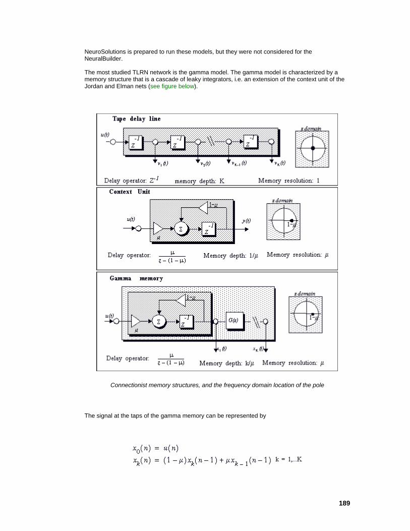
189

NeuroSolutions is prepared to run these models, but they were not considered for the NeuralBuilder.

The most studied TLRN network is the gamma model. The gamma model is characterized by a memory structure that is a cascade of leaky integrators, i.e. an extension of the context unit of the Jordan and Elman nets (see figure below).

Connectionist memory structures, and the frequency domain location of the pole

The signal at the taps of the gamma memory can be represented by

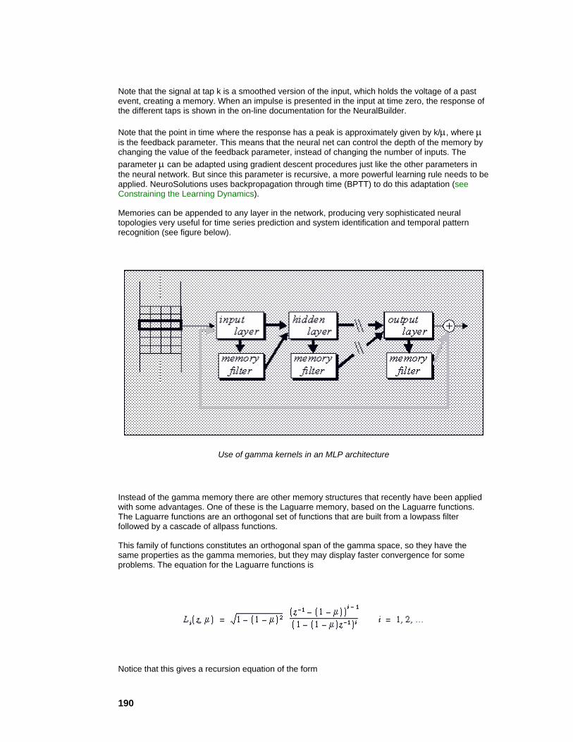
190

Note that the signal at tap k is a smoothed version of the input, which holds the voltage of a past event, creating a memory. When an impulse is presented in the input at time zero, the response of the different taps is shown in the on-line documentation for the NeuralBuilder.

Note that the point in time where the response has a peak is approximately given by k/µ, where µ is the feedback parameter. This means that the neural net can control the depth of the memory by changing the value of the feedback parameter, instead of changing the number of inputs. The parameter µ can be adapted using gradient descent procedures just like the other parameters in the neural network. But since this parameter is recursive, a more powerful learning rule needs to be applied. NeuroSolutions uses backpropagation through time (BPTT) to do this adaptation (see Constraining the Learning Dynamics).

Memories can be appended to any layer in the network, producing very sophisticated neural topologies very useful for time series prediction and system identification and temporal pattern recognition (see figure below).

Use of gamma kernels in an MLP architecture

Instead of the gamma memory there are other memory structures that recently have been applied with some advantages. One of these is the Laguarre memory, based on the Laguarre functions. The Laguarre functions are an orthogonal set of functions that are built from a lowpass filter followed by a cascade of allpass functions.

This family of functions constitutes an orthogonal span of the gamma space, so they have the same properties as the gamma memories, but they may display faster convergence for some problems. The equation for the Laguarre functions is

Notice that this gives a recursion equation of the form

191

where u(n) is the input signal.

Tutorials Tutorials Chapter

NeuroSolutions



Purpose

This chapter is a collection of hands-on examples. Our purpose is to explain the core concepts of NeuroSolutions by showing them to you. You will be guided through the construction of network topologies at increasing levels of difficulty. Upon completion, you are expected to be able to construct similar topologies by analogy.

Running NeuroSolutions Windows 3.1, 3.11, NT

In the Program Manager of Windows, there are two icons within the program group labeled NeuroSolutions. The question mark represents the on-line help for the program. This can be

launched separately or from within NeuroSolutions. The cluster represents the NeuroSolutions program. Double-click on this icon or click the following shortcut to run NeuroSolutions. Windows 95

In the Start Menu of Windows 95, there are two icons within the folder labeled NeuroSolutions. The book represents the on-line help for the program. This can be launched separately or from within

192

NeuroSolutions. The icon represents the NeuroSolutions program. Double-click on this icon to begin or click the following shortcut to run NeuroSolutions.

The NeuroSolutions MainWindow will appear in the center of the display. The Inspector window will also appear in the lower right corner of your display; this is where you will configure all NeuroSolutions components.

A good way to get started with NeuroSolutions is to run through the various demos. The demos can be accessed by selecting Utilities/Run Demo from the MainMenu bar. This contains a list of demos, each of which is similar to one of the breadboards constructed in the following examples. It is recommended that you refer to these breadboards for ideas on solving your particular problem. By taking the time to work through the following examples, a much better understanding of the concepts behind NeuroSolutions will be obtained.

NeuroSolutions after program launch

Signal Generator Example Signal Generator Example

193

Purpose - This example creates a simple system for generating composite waveforms. The purpose of this example is to illustrate how components are interconnected, data is injected into the network, data is probed within the network and how the simulation is controlled.

Components Introduced - Axon, MaleConnector, FemaleConnector, FunctionGenerator, MegaScope, DataStorage and StaticControl.

Concepts Introduced - Connecting components, palettes, breadboards, the Inspector, stacking components, component selection, access points, probing data, data buffers, data flow and cut & paste.

STEPS

Construction Rules

Stamping Components

On-line Help

Connectors

Selecting and Configuring a Component

Arranging Icons

Connecting Components

The Cursor

Component Compatibility

Bringing in the Function Generators

Stacking Components

Accessing the Component Hierarchy

Access Points

Displaying the Output Waveform

Opening the Display Window

Controlling Data Flow

Configuring the Controller

Running the Signal Generator Example

Things to Try with the Signal Generator

What You have Learned from the Signal Generator Example

Construction Rules

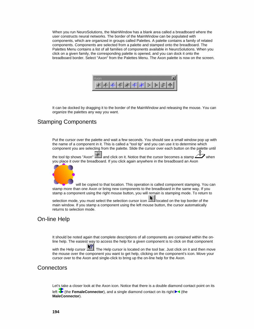
194

When you run NeuroSolutions, the MainWindow has a blank area called a breadboard where the user constructs neural networks. The border of the MainWindow can be populated with components, which are organized in groups called Palettes. A palette contains a family of related components. Components are selected from a palette and stamped onto the breadboard. The Palettes Menu contains a list of all families of components available in NeuroSolutions. When you click on a given family, the corresponding palette is opened, and you can dock it onto the breadboard border. Select "Axon" from the Palettes Menu. The Axon palette is now on the screen.

It can be docked by dragging it to the border of the MainWindow and releasing the mouse. You can organize the palettes any way you want.

Stamping Components

Put the cursor over the palette and wait a few seconds. You should see a small window pop up with the name of a component in it. This is called a "tool tip" and you can use it to determine which component you are selecting from the palette. Slide the cursor over each button on the palette until

the tool tip shows "Axon" and click on it. Notice that the cursor becomes a stamp when you place it over the breadboard. If you click again anywhere in the breadboard an Axon

will be copied to that location. This operation is called component stamping. You can stamp more than one Axon or bring new components to the breadboard in the same way. If you stamp a component using the right mouse button, you will remain is stamping mode. To return to

selection mode, you must select the selection cursor icon located on the top border of the main window. If you stamp a component using the left mouse button, the cursor automatically returns to selection mode.

On-line Help

It should be noted again that complete descriptions of all components are contained within the on-line help. The easiest way to access the help for a given component is to click on that component

with the Help cursor . The Help cursor is located on the tool bar. Just click on it and then move the mouse over the component you want to get help, clicking on the component’s icon. Move your cursor over to the Axon and single-click to bring up the on-line help for the Axon.

Connectors

Let’s take a closer look at the Axon icon. Notice that there is a double diamond contact point on its left (the FemaleConnector), and a single diamond contact on its right (the MaleConnector).

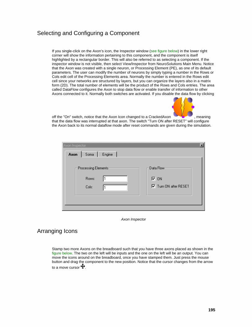
195

Selecting and Configuring a Component

If you single-click on the Axon’s icon, the Inspector window (see figure below) in the lower right corner will show the information pertaining to this component, and the component is itself highlighted by a rectangular border. This will also be referred to as selecting a component. If the inspector window is not visible, then select View/Inspector from NeuroSolutions Main Menu. Notice that the Axon was created with a single neuron, or Processing Element (PE), as one of its default parameters. The user can modify the number of neurons by simply typing a number in the Rows or Cols edit cell of the Processing Elements area. Normally the number is entered in the Rows edit cell since your networks are structured by layers, but you can organize the layers also in a matrix form (2D). The total number of elements will be the product of the Rows and Cols entries. The area called DataFlow configures the Axon to stop data flow or enable transfer of information to other Axons connected to it. Normally both switches are activated. If you disable the data flow by clicking

off the "On" switch, notice that the Axon Icon changed to a CrackedAxon , meaning that the data flow was interrupted at that axon. The switch "Turn ON after RESET" will configure the Axon back to its normal dataflow mode after reset commands are given during the simulation.

Axon Inspector

Arranging Icons

Stamp two more Axons on the breadboard such that you have three axons placed as shown in the figure below. The two on the left will be inputs and the one on the left will be an output. You can move the icons around on the breadboard, once you have stamped them. Just press the mouse button and drag the component to the new position. Notice that the cursor changes from the arrow to a move cursor .

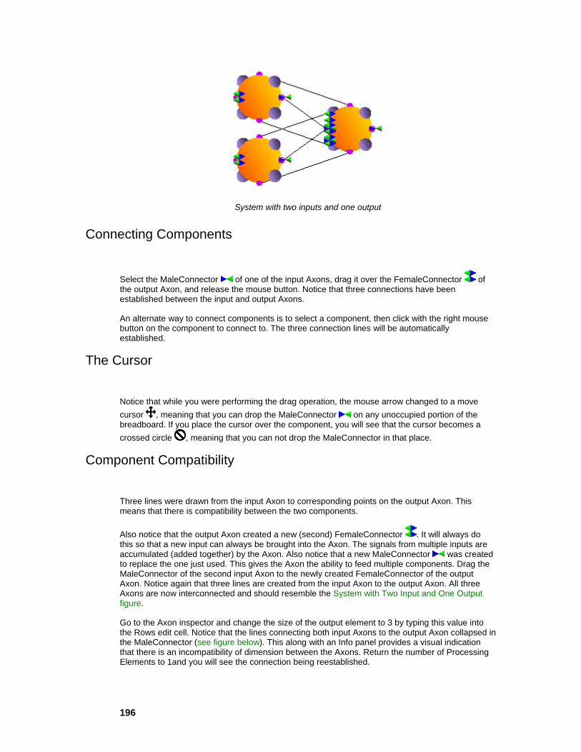
196

System with two inputs and one output

Connecting Components

Select the MaleConnector of one of the input Axons, drag it over the FemaleConnector of the output Axon, and release the mouse button. Notice that three connections have been established between the input and output Axons.

An alternate way to connect components is to select a component, then click with the right mouse button on the component to connect to. The three connection lines will be automatically established.

The Cursor

Notice that while you were performing the drag operation, the mouse arrow changed to a move cursor , meaning that you can drop the MaleConnector on any unoccupied portion of the breadboard. If you place the cursor over the component, you will see that the cursor becomes a crossed circle , meaning that you can not drop the MaleConnector in that place.

Component Compatibility

Three lines were drawn from the input Axon to corresponding points on the output Axon. This means that there is compatibility between the two components.

Also notice that the output Axon created a new (second) FemaleConnector . It will always do this so that a new input can always be brought into the Axon. The signals from multiple inputs are accumulated (added together) by the Axon. Also notice that a new MaleConnector was created to replace the one just used. This gives the Axon the ability to feed multiple components. Drag the MaleConnector of the second input Axon to the newly created FemaleConnector of the output Axon. Notice again that three lines are created from the input Axon to the output Axon. All three Axons are now interconnected and should resemble the System with Two Input and One Output figure.

Go to the Axon inspector and change the size of the output element to 3 by typing this value into the Rows edit cell. Notice that the lines connecting both input Axons to the output Axon collapsed in the MaleConnector (see figure below). This along with an Info panel provides a visual indication that there is an incompatibility of dimension between the Axons. Return the number of Processing Elements to 1and you will see the connection being reestablished.

197

Attempted connection among Axons of differing dimensions

Bringing in the Function Generators

Now that the network topology is established, you will connect a function generator to the input Axons. Select Palettes/Input from the Palettes menu and dock it on the MainWindow border. Stamp

the FunctionGenerator icon onto one of the input Axons.

Input Family Palette

Stacking Components

Notice that the cursor turns to the stamp only over the Axons. This means that the FunctionGenerator can not be dropped directly onto the breadboard, but only over accepting components. The FunctionGenerator will attach to one of the corners of the Axon. If you select the FunctionGenerator, its inspector will be shown.

198

FunctionGenerator inspector

For each PE in the Axon, you can choose the type of signal, along with its frequency, amplitude, sampling rate, offset and phase shift. Click on the button showing the sinewave and type 20 in the Samples/Cycle edit cell. A sinewave of 20 samples per cycle was just programmed.

Accessing the Component Hierarchy

At the top of the Inspector you will find several tabs. Each tab represents another page of parameters that can be configured for this component. This allows you to change the other attributes of the FunctionGenerator. The attributes you are viewing are specific to the class FunctionGenerator. By selecting the Stream tab, you will see the attributes that pertain to a class called Stream, from which FunctionGenerator was derived. Notice that it is currently configured to Accumulate Data on the Network, i.e. it will add the signal from the FunctionGenerator to the accumulated input of the Axon. The option Overwrite data will discard the accumulated input and replace it with the injected signal. Since the Axon has no other input, this setting is not important for this example. Notice also that the generated data can be normalized and that it can also be saved to disk.

Now select the Access tab to view the attributes that configure how the FunctionGenerator communicates with the component. In particular this tells you about the data format and the access points available for the component the Function Generator is stacked on.

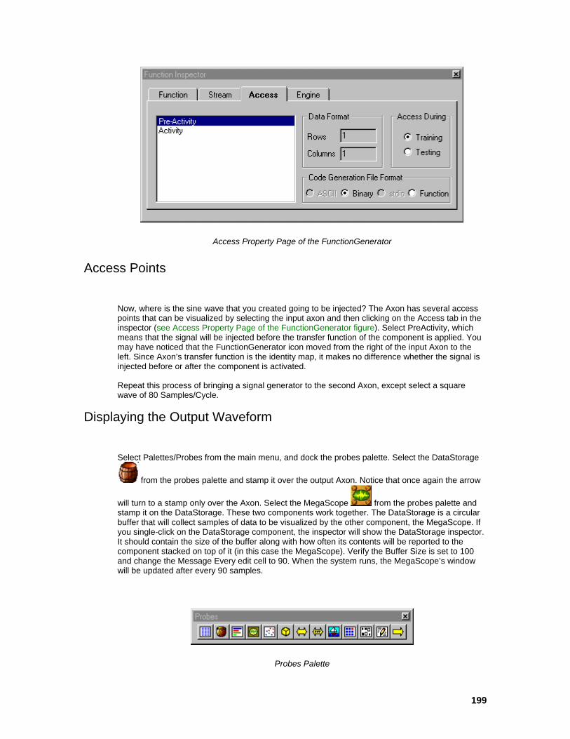
199

Access Property Page of the FunctionGenerator

Access Points

Now, where is the sine wave that you created going to be injected? The Axon has several access points that can be visualized by selecting the input axon and then clicking on the Access tab in the inspector (see Access Property Page of the FunctionGenerator figure). Select PreActivity, which means that the signal will be injected before the transfer function of the component is applied. You may have noticed that the FunctionGenerator icon moved from the right of the input Axon to the left. Since Axon’s transfer function is the identity map, it makes no difference whether the signal is injected before or after the component is activated.

Repeat this process of bringing a signal generator to the second Axon, except select a square wave of 80 Samples/Cycle.

Displaying the Output Waveform

Select Palettes/Probes from the main menu, and dock the probes palette. Select the DataStorage

from the probes palette and stamp it over the output Axon. Notice that once again the arrow

will turn to a stamp only over the Axon. Select the MegaScope from the probes palette and stamp it on the DataStorage. These two components work together. The DataStorage is a circular buffer that will collect samples of data to be visualized by the other component, the MegaScope. If you single-click on the DataStorage component, the inspector will show the DataStorage inspector. It should contain the size of the buffer along with how often its contents will be reported to the component stacked on top of it (in this case the MegaScope). Verify the Buffer Size is set to 100 and change the Message Every edit cell to 90. When the system runs, the MegaScope’s window will be updated after every 90 samples.

Probes Palette

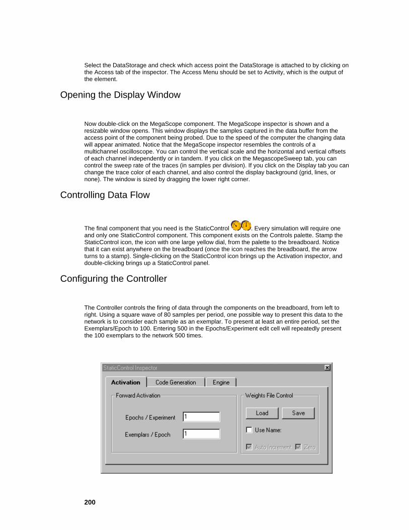
200

Select the DataStorage and check which access point the DataStorage is attached to by clicking on the Access tab of the inspector. The Access Menu should be set to Activity, which is the output of the element.

Opening the Display Window

Now double-click on the MegaScope component. The MegaScope inspector is shown and a resizable window opens. This window displays the samples captured in the data buffer from the access point of the component being probed. Due to the speed of the computer the changing data will appear animated. Notice that the MegaScope inspector resembles the controls of a multichannel oscilloscope. You can control the vertical scale and the horizontal and vertical offsets of each channel independently or in tandem. If you click on the MegascopeSweep tab, you can control the sweep rate of the traces (in samples per division). If you click on the Display tab you can change the trace color of each channel, and also control the display background (grid, lines, or none). The window is sized by dragging the lower right corner.

Controlling Data Flow

The final component that you need is the StaticControl . Every simulation will require one and only one StaticControl component. This component exists on the Controls palette. Stamp the StaticControl icon, the icon with one large yellow dial, from the palette to the breadboard. Notice that it can exist anywhere on the breadboard (once the icon reaches the breadboard, the arrow turns to a stamp). Single-clicking on the StaticControl icon brings up the Activation inspector, and double-clicking brings up a StaticControl panel.

Configuring the Controller

The Controller controls the firing of data through the components on the breadboard, from left to right. Using a square wave of 80 samples per period, one possible way to present this data to the network is to consider each sample as an exemplar. To present at least an entire period, set the Exemplars/Epoch to 100. Entering 500 in the Epochs/Experiment edit cell will repeatedly present the 100 exemplars to the network 500 times.

201

ActivationControl inspector

The StaticControl panel has 5 buttons. The 1st button toggles between Run and Stop and is used to initiate or stop the simulation. The Reset button resets the experiment by zeroing all counters, the activations, and reloading the weights with random values. The Jog button just jogs the component's weights. The Exemplar button allows you to single step the simulations. Whereas, the Epoch button presents an entire epoch upon each click. Notice also that there are counters under the exemplar and epoch buttons.

Running the Signal Generator Example

Click on the Run Button of the StaticControl panel. Notice the MegaScope is displaying the addition of the square and sine waves. The Epochs counter in the StaticControl panel will show you the number of epochs that have elapsed. You have just run your first simulation—a rather simplistic simulation but be patient. You can go back to the FunctionGenerator and change the waveforms and view the effect on the MegaScope. Every time you want to make a modification in the system, simply press Stop, modify the component and press Run again. An error will sound if you try to make a modification while the simulation is running. You should get familiar with the controls of the MegaScope. It is recommended that you adjust the controls and view the affect of the modifications in the MegaScope window. (see the figure below for the completed network configuration or load the file EX1.NSB)

202

Signal generator simulation

Things to Try with the Signal Generator

Disconnecting Components

Take one of the input Axon’s MaleConnectors and remove it from the output Axon by dropping it over the middle of the output Axon. Notice that the connection between the Axon components disappeared, i.e. they were disconnected. An alternate way to disconnect components is to select

the MaleConnector and then click on the scissors icon on the tool bar. The scissors will always remove the selected component from the breadboard. Reestablish the connection by dragging the MaleConnector of the input Axon to the output FemaleConnector. Cables

If you drop a MaleConnector directly on the breadboard, lines will be established from the Axon to that point. You can create cables linking the Axons in this way. Every time you drag the MaleConnector while holding the shift key, a new section of the cable will be created. This is very handy when building recurrent neural networks. You can modify the cable path by first selecting the MaleConnector of the cable. This will display all of the points used to define the cable. Dragging

203

intermediate points of the cable will redefine the cable’s path. Note that all components included in the Axon palette obey these simple rules of interconnection.

Forming a connection using cables

Remove one of the Axons by clicking on it’s icon (this selects the component) and clicking on the scissors icon. Instead of stamping both Axons and both FunctionGenerators from the palettes, you can construct just one Axon/FunctionGenerator combination and then copy it to get a second set.

Select the Axon to be copied, click on the copy button on the toolbar, click on an empty spot

on the breadboard, and click on the paste button . A new copy is formed on the breadboard. Notice that the FunctionGenerator was also copied. Copying a component will also copy all components that are stacked on top of it. More important, you see that the parameter settings correspond to the ones you had selected for the original Axon and not the default values.

There is another way to create a composite signal generator. Throw away one of the input Axons (by selecting it and cutting), bring from the Input palette another FunctionGenerator and drop it on top of the one residing on the Axon. Using the FunctionGenerator inspector, you will see that under Access the Active Access Point is set to StackedAccess, i.e. both FunctionGenerators are sharing the same access point. This circuit will perform as the one previously constructed.

Try saving the breadboard by selecting File/Save from the NeuroSolutions MainMenu, or clicking

on the disk icon . A Save panel will then allow you to give a name to the breadboard, and will save it to a file. The breadboard can now be re-opened by selecting File/Open from the MainMenu, or simply clicking on the open icon from the tool bar. The breadboard is ready to run; press run on the StaticControl window.

What You have Learned from the Signal Generator Example

You have learned the basic rules for connecting and disconnecting components of the Axon class. You have also learned how to modify the dimension of Axons (i.e., their number of PEs) and hopefully you were able to appreciate the inspector, since it encapsulates all information regarding the selected component on the breadboard.

You were able to inject data into the network by means of FunctionGenerators attached to Axon access points. You were also able to view the output of the system by attaching a MegaScope/DataStorage to the output Axon. You learned that some components have several access points for both injecting and retrieving data. Finally, you learned how to use the StaticControl component to set up the parameters of the experiment. It is recommended that you refer to the Concepts chapter if any portion of this example was unclear.

204

Combination of Data Sources Example Combination of Data Sources Example

Purpose - Combination of information is fundamental in neurocomputing. By feeding data into a series of weights, NeuroSolutions implements virtually all models used in neurocomputing. NeuroSolutions combines (linearly or nonlinearly) independent data sources or several delayed versions of the same source. This example demonstrates the construction of such topologies.

Components Introduced - ThresholdAxon, FullSynapse, TanhAxon, MatrixEditor, MatrixViewer, File.

Concepts Introduced - Nonlinear elements, McCulloch-Pitts neuron, weight inspection and manipulation, probing data, file input.

STEPS

Constructing a McCulloch-Pitts Processing Element

Preparing Files for Input into NeuroSolutions

Things to Try with the Combination of Data Sources Example

What You have Learned from the Combination of Data Sources Example

Constructing a McCulloch-Pitts Processing Element

Select File/New from the Main Menu. Go to the Axon palette and stamp an Axon and a ThresholdAxon to the breadboard. Drop the ThresholdAxon to the right of the Axon. The ThresholdAxon component corresponds to a nonlinear element that clips the values of its input at +/- 1. This element creates an output that is a logic value as used in digital computers (-1 is normally the zero voltage).

Synapse Palette

From the Synapse palette, select and stamp the FullSynapse (the one with lines connecting all the points) to the breadboard between the two other components (see figure below). The FullSynapse

implements full connectivity between two axons. The FullSynapse provides the

205

scalar values (combination weights) that multiply each input. Select the Axon and enter 2 in the Processing Element form cell of the inspector. This creates two processing elements in the input layer. Connect the Axon to the FullSynapse by dragging the MaleConnector of the Axon to the FemaleConnector of the FullSynapse. Then connect the MaleConnector of the FullSynapse to the FemaleConnector of the ThresholdAxon. This structure (FullSynapse followed by the ThresholdAxon) implements a McCulloch-Pitts processing element (neuron) with two inputs. Go to the Soma property page of the inspector to verify that the FullSynapse has two weights.

Implementation of a McCulloch-Pitts neuron

Go to the Probes palette, select and stamp a MatrixEditor to the FullSynapse, and place it at the WeightsAccess point. Double-click on the MatrixEditor icon and a row vector with two values will appear. This MatrixEditor window allows us to observe, and change the network weights. For this example, enter 1 in each form cell of the window. Now select the FullSynapse and display it’s inspector. Under the Soma tab, click on the Fix switch. This will keep the weight values unchanged during the full simulation, even when the Randomize button on the StaticControl is pressed. You have to do a similar thing to the bias (i.e., free parameter, weight) of the ThresholdAxon. Place the MatrixEditor over this component, select the Weights Access in the inspector, and enter the value -1.2 in the MatrixEditor window. Also set the Fix button of the ThresholdAxon in the corresponding inspector. Remove the MatrixEditor from the network. What you have done can be translated as the following: the data input to the Axon will be multiplied by 1, added in the ThresholdAxon, and internally compared with the threshold. If the bias (weight) of the ThresholdAxon is set at -1.2, the threshold will be 1.2. If the input to the ThresholdAxon is larger than this value, the output will be 1. If smaller, the output will be -1.

Preparing Files for Input into NeuroSolutions

The last thing to do in this example is to prepare the input files that will contain the input patterns. For this simple case, you will use the ASCII column format. Using the Windows NotePad Editor

(click here to run ), create a file with the format shown in the figure below. The four lines will have the numbers specifying the coordinates of the input points (two per line).

206

An ASCII input file

When you store an ASCII file for NeuroSolutions, name it with the extension ".ASC". Save the file in your home directory and call it "XOR_IN.ASC". Next establish the link between NeuroSolutions

and these files. From the Input palette, select and stamp a File component to the input Axon, and select it to show the corresponding inspector. Click on the Add button and an Add panel will appear on the screen. Find the "XOR_IN.ASC" file using the browser and double-click on the file name. This name will be copied to the inspector. Click the Translate button to convert the ASCII characters to a data stream. The inspector will provide statistics regarding the length of the file (4 exemplars) and the type of data under the Stream tab. Now from the Access level, select the access point to be Pre-Activity, since you want this file to be the input to the network.

In order to run the input data through the McCulloch-Pitts processing element you need to select and stamp a StaticControl component to the breadboard. Select the StaticControl to show its inspector and enter 4 in the exemplar/epoch cell. This is done because the XOR problem has four exemplars. Notice that each exemplar feeds two channels. Before you simulate this network, think about how you want to visualize the results. To view the input and the output values use the

MatrixViewer .

From the Probes palette, stamp the MatrixViewer on the input Axon. Double click on the icon to open the corresponding window. In the inspector set the Stacked Access, such that you can observe the data that is input to the network. Stamp another copy of the MatrixViewer to the ThresholdAxon, double click to open the window, and set the access point to Activity, i.e. the output of the network.

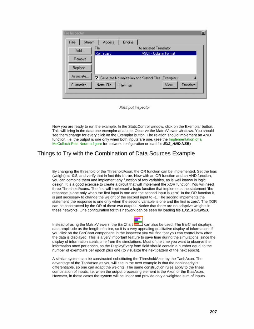
207

FileInput inspector

Now you are ready to run the example. In the StaticControl window, click on the Exemplar button. This will bring in the data one exemplar at a time. Observe the MatrixViewer windows. You should see them change for every click on the Exemplar button. The relation should implement an AND function, i.e. the output is one only when both inputs are one. (see the Implementation of a McCulloch-Pitts Neuron figure for network configuration or load file EX2_AND.NSB)

Things to Try with the Combination of Data Sources Example

By changing the threshold of the ThresholdAxon, the OR function can be implemented. Set the bias (weight) at -0.8, and verify that in fact this is true. Now with an OR function and an AND function, you can combine them and implement any function of two variables, as is well known in logic design. It is a good exercise to create a circuit that will implement the XOR function. You will need three ThresholdAxons. The first will implement a logic function that implements the statement ‘the response is one only when the first input is one and the second input is zero’. In the OR function it is just necessary to change the weight of the second input to -1. The second implements the statement ‘the response is one only when the second variable is one and the first is zero’. The XOR can be constructed by the OR of these two outputs. Notice that there are no adaptive weights in these networks. One configuration for this network can be seen by loading file EX2_XOR.NSB.

Instead of using the MatrixViewers, the BarChart can also be used. The BarChart displays data amplitude as the length of a bar, so it is a very appealing qualitative display of information. If you click on the BarChart component, in the inspector you will find that you can control how often the data is displayed. This is a very important feature to save time during the simulations, since the display of information steals time from the simulations. Most of the time you want to observe the information once per epoch, so the DisplayEvery form field should contain a number equal to the number of exemplars per epoch plus one (to visualize the next pattern of the next epoch).

A similar system can be constructed substituting the ThresholdAxon by the TanhAxon. The advantage of the TanhAxon as you will see in the next example is that the nonlinearity is differentiable, so one can adapt the weights. The same construction rules apply to the linear combination of inputs, i.e. when the output processing element is the Axon or the BiasAxon. However, in these cases the system will be linear and provide only a weighted sum of inputs.

208

What You have Learned from the Combination of Data Sources Example

You have learned how to construct nonlinear and linear weighting of input data. This is a fundamental piece of neurocomputing. You have also learned how to visualize and manipulate network parameters with the MatrixEditor. You have linked for the first time NeuroSolutions with the computer file system by means of the File component.

The Perceptron and Multilayer Perceptron Perceptron and Multilayer Perceptron Example

Purpose - In this example you will construct your first adaptive network—the perceptron. You will repeat the AND function, but now the network will learn how to select the weights and the bias of the components by itself. This will be accomplished using backpropagation, one of the most useful learning rules. Later you will construct a network to learn the XOR problem.

Components Introduced - SigmoidAxon, L2Criterion, BackTanhAxon, BackSigmoidAxon, BackFullSynapse, BackAxon, BackStaticControl, Momentum, BackCriteriaControl, Quickprop.

Concepts Introduced - Cost function (mean square error), backpropagation of error, dual network (backprop plane), gradient search (weight updating), automatic creation of the backprop plane, learning paradigms, divergence, hidden layers, broadcasting of parameter changes.

STEPS

Perceptron Topology

Constructing the Learning Dynamics of a Perceptron

Alternate Procedure for Constructing the Learning Dynamics of a Perceptron

Selecting the Learning Paradigm

Running the Perceptron

MLP Construction

Running the MLP

Things to Try with the Perceptron and Multilayer Perceptron Example

What You have Learned from the Perceptron and Multilayer Perceptron Example

Perceptron Topology

The perceptron is one of the most famous neural network topologies (see Perceptron). Its major difference with respect to the McCulloch-Pitts model seen in the previous example is the use of smooth nonlinearities and adaptive weights. So this is the first adaptive system that you have encountered. Here you will construct the perceptron using the SigmoidAxon.

209

With a new breadboard, stamp from the Axon Palette one Axon for the input, a FullSynapse, and

the SigmoidAxon , which implements a smooth nonlinearity also called the logistic map. Interconnect all the elements as before. Select the number of processing elements in the Axon as two.

ErrorCriteria Palette

Select Palette/ErrorCriteria from the Main Menu. Go to the ErrorCriteria palette and choose the L2Criterion. This cost function implements the mean square error—the most widely used error

metric. Now place the L2Criterion to the right of the SigmoidAxon, then make the connection between them. The L2Criterion will compare the desired response with the network input, compute the error power and give it to other components that handle error backpropagation.

From the Probes palette, select and stamp a MatrixViewer on the L2Criterion and set the access point to Average Cost. Double-clicking on the MatrixViewer will open up a window. Since you are probing the L2Criterion at its average cost access point, this window will display the learning curve, i.e. how the mean square error evolves during learning. The MatrixEditor probe could also be used, but it would slow the simulations since it allows editing at every epoch.

The perceptron with the L2criterion attached

Constructing the Learning Dynamics of a Perceptron

There are two basic ways to create the learning dynamics. Start out by docking the Backprop palette. Each of these components is a dual of a component on the Axon and Synapse palettes. The reason for this can be found in the theory of learning dynamics (see Backprop Family). When backpropagation trains a neural network, the error can be thought of as being injected at the output of the network, and propagated through a dual network of the original topology. The dual topology has the same weights but switches splitting nodes with summing junctions.

210

Backprop palette

A closer look at the Backprop palette shows that there are two icons with bell shaped curves. One is the BackTanhAxon that corresponds to the hyperbolic tangent nonlinearity, and the other is the BackSigmoidAxon corresponding to the logistic function. All Backprop components will be stacked on top of their activation duals. Bring in the BackAxon, the BackSigmoidAxon, and repeat the process for the BackFullSynapse. Notice that lines are automatically drawn between the BackAxon and the BackFullSynapse. By adding the BackCriteriaControl, you have created a network capable of learning. The error can now flow from the output to every component in the network, allowing the program to compute local error gradients.

Addition of the backprop plane to propagate the error

There are several ways that the activation and error can be combined to compute the weight updates. Therefore, you must specify what type of gradient search you want by selecting a

component from the GradientSearch palette. There is the Step (straight LMS), the

Momentum (LMS with momentum, the most widely used in neural computing), the

Quickprop (Fahlman’s quick prop) and the DeltaBarDelta (adaptive step sizes).

You have to place one of these gradient procedures on every activity component that contains adaptive weights.

211

Momentum inspector

In the perceptron example, the only elements that have adaptive weights are the FullSynapse and the SigmoidAxon (a bias term), so you need to drag the Momentum to these two components. From the Momentum inspector, enter a momentum of 0.9 and set the step size to 1.

Alternate Procedure for Constructing the Learning Dynamics of a Perceptron

Before moving on, consider a second alternative to the construction of backprop plane or of learning dynamics. Since there is a tight relationship between the original topology and the backpropagation topology used for learning, the learning network is unequivocally defined by the original topology (there is a duality between the two). Therefore, NeuroSolutions can AUTOMATICALLY construct the learning network. This facility is included in the BackStaticControl component.

From the Controls palette, you will recognize the BackStaticControl as the red dial component. After stamping a StaticControl on the breadboard, select the BackStaticControl from the palette and stamp it over the StaticControl.

At the bottom of the BackStaticControl inspector, you can find the Backpropagation Plane box. There are two buttons—one that adds the backprop plane and one that removes the backprop plane. You also have the ability to select on the scroll panel the class of gradient search that you want using the pull down menu. Verify that this is set to Momentum. Now press the Remove button and observe that the backprop plane that you constructed disappears from the breadboard.

By pressing the Add button, the backprop plane is automatically constructed for us. Since the original topology had weights in the FullSynapse and SigmoidAxon, two new GradientSearches were created. Since they are new components, you still need to set the Step Size and the Momentum values in the corresponding inspector. This facility of NeuroSolutions is very powerful. By decoupling the learning dynamics from the original topology, several important goals are simultaneously achieved. First, the learning becomes extremely fast because you are giving each element the ability to learn (see Learning Dynamics). This leads to very efficient and compact code. Second, the weights can be easily frozen for testing by freeing the learning plane. This speeds up the simulations tremendously once the network has learned.

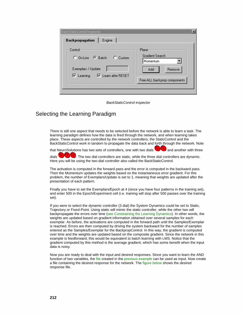
212

BackStaticControl inspector

Selecting the Learning Paradigm

There is still one aspect that needs to be selected before the network is able to learn a task. The learning paradigm defines how the data is fired through the network, and when learning takes place. These aspects are controlled by the network controllers; the StaticControl and the BackStaticControl work in tandem to propagate the data back and forth through the network. Note

that NeuroSolutions has two sets of controllers, one with two dials and another with three

dials . The two dial controllers are static, while the three dial controllers are dynamic. Here you will be using the two-dial controller also called the BackStaticControl.

The activation is computed in the forward pass and the error is computed in the backward pass. Then the Momentum updates the weights based on the instantaneous error gradient. For this problem, the number of Exemplars/Update is set to 1, meaning that weights are updated after the presentation of each pattern.

Finally you have to set the Exemplars/Epoch at 4 (since you have four patterns in the training set), and enter 500 in the Epoch/Experiment cell (i.e. training will stop after 500 passes over the training set).

If you were to select the dynamic controller (3 dial) the System Dynamics could be set to Static, Trajectory or Fixed-Point. Using static will mimic the static controller, while the other two will backpropagate the errors over time (see Constraining the Learning Dynamics). In other words, the weights are updated based on gradient information obtained over several samples for each exemplar. As before, the activations are computed in the forward path until the Samples/Exemplar is reached. Errors are then computed by driving the system backward for the number of samples entered as the Samples/Exemplar for the BackpropControl. In this way, the gradient is computed over time and the weights are updated based on the composite gradient. Since the network in this example is feedforward, this would be equivalent to batch learning with LMS. Notice that the gradient computed by this method is the average gradient, which has some benefit when the input data is noisy.

Now you are ready to deal with the input and desired responses. Since you want to learn the AND function of two variables, the file created in the previous example can be used as input. Now create a file containing the desired response for the network. The figure below shows the desired response file.

213

An ASCII desired response file

Note that the inputs and desired data must be aligned in order for the network to learn the desired task. You have to stamp a File component on the input Axon (Pre-Activity Access point), and another File component on the L2Criterion for the desired response (Desired Access point).

Construction of the Perceptron Example

Running the Perceptron

In order to analyze the performance of the network, select and stamp a MegaScope/DataStorage over the MatrixViewer that has access to the average cost. Configure the buffer size to 100 and report the error every sample. This will show the learning curve. Now you are ready to start the simulation. Click on the run button of the StaticControl and the simulation will start. Note that the error starts large, but then decreases steadily to a very small value (<0.01) meaning that the network learned the task.

It is interesting to verify the weights found after learning the AND task. Select and stamp a MatrixViewer on the FullSynapse, and select the weight Access. You will see that both weights are large and positive, and the bias of the SigmoidAxon is large and negative, just like you expect after running the previous example. (see Construction of the Perceptron Example figure for network configuration or load the file EX3_AND.NSB)

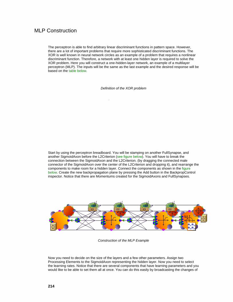
214

MLP Construction

The perceptron is able to find arbitrary linear discriminant functions in pattern space. However, there are a lot of important problems that require more sophisticated discriminant functions. The XOR is well known in neural network circles as an example of a problem that requires a nonlinear discriminant function. Therefore, a network with at least one hidden layer is required to solve the XOR problem. Here you will construct a one-hidden-layer network, an example of a multilayer perceptron (MLP). The inputs will be the same as the last example and the desired response will be based on the table below.

Definition of the XOR problem

Start by using the perceptron breadboard. You will be stamping on another FullSynapse, and another SigmoidAxon before the L2Criterion (see figure below). You will have to break the connection between the SigmoidAxon and the L2Criterion. (by dragging the connected male connector of the SigmoidAxon over the center of the L2Criterion and dropping it), and rearrange the components to make room for a hidden layer. Connect the components as shown in the figure below. Create the new backpropagation plane by pressing the Add button in the BackpropControl inspector. Notice that there are Momentums created for the SigmoidAxons and FullSynapses.

Construction of the MLP Example

Now you need to decide on the size of the layers and a few other parameters. Assign two Processing Elements to the SigmoidAxon representing the hidden layer. Now you need to select the learning rates. Notice that there are several components that have learning parameters and you would like to be able to set them all at once. You can do this easily by broadcasting the changes of

215

one component to similar components. Select one of the Momentums, and while pressing the shift key click on the other Momentums. They will be all selected. Use a Step Size of 1 and a Momentum of 0.9. Verify that these parameters were broadcast to the other Momentums by clicking on each component and observing its corresponding inspector. You will keep the learning in batch mode.

The last thing to do in this example is to prepare the "desired" file, which will contain the patterns for the desired signal according to the table above. You have to create a file called XOR_DES.ASC, as shown in the "out" column of the table above and link it to the File placed over the L2Criterion. The first step is to remove the previous file, and add the new one, using the same procedure as explained in the Combination of Data Sources example. Before running the example, you should determine what it is that you want to probe. As usual, you should monitor the output mean square error just to make sure that the network is converging. Stamp a MatrixViewer on the L2Criterion. You should also bring a MegaScope/DataStorage to the input axon and stamp it on the Activity point. This way you can verify that the data is firing in the appropriate order. Configure the DataStorage to Message Every 10 samples.

Running the MLP

Double-click on the MegaScope. You will see that you have two channels, since the input has two channels. You may want to move the Channel 1 signal so that it doesn’t overlap the Channel 2 signal. This can be accomplished by using the Vertical offset slider or the Autoset Channels button. Open the StaticControl panel. If you click on the Exemplar button several times, you should see two waveforms being displayed—one that looks like a triangular wave and the other more like a square wave (you may need to adjust the Vertical Scale and Samples/division to match the display shown in the figure below). By looking at the XOR table, you can interpret the alternating 0’s and 1’s in each column as being square waves of different frequencies. You may want to adjust the settings of the MegaScope to magnify the waveforms. Verify that the input is being correctly read. You can now move the MegaScope/DataStorage to the output Axon to observe the output of the network through the learning process. Run the network and observe that in the beginning the MegaScope at the output will display a wave that is irregular, but that it will converge to a periodic square wave. At the same time, the error will decrease to almost zero. The network will most often learn the XOR problem in less than 150 iterations (depending on the initial conditions). The network may have to be jogged several times if it appears to have settled in a local minima. An example of a network solution for this problem using an MLP can be seen by loading file EX3_XORS.NSB.

216

Training a MLP to learn the XOR problem

Things to Try with the Perceptron and Multilayer Perceptron Example

Move the MegaScope/DataStorage to the left FullSynapse and select the Weight access point, such that you can track the weights through learning. Now randomize the weights and run the network again. Observe that the weight tracks are constant in the beginning, but that there is a quick inflection and both weight tracks go in opposite directions. This is the most general behavior of weights for networks that learn this problem, but other solutions are possible depending upon the initial conditions.

217

Tracking the values of the weights during training

If one wants to smooth out the learning curve, you can use batch learning. Batch learning adapts the weights after the presentation and calculation of the gradients for the full training set (four patterns). You can implement batch learning by going to the BackStaticControl Inspector and selecting the Batch radio button. Reset the network and run it again. You will see that now the learning curve is very smooth, which shows the steady decrease of the error through learning.

You can also see the effect of different gradient update rules on the learning speed. Choose Quickprop and repeat the experiment. Choose the Step and repeat the experiment. The idea is to compare the speed of adaptation of each rule.

What You have Learned from the Perceptron and Multilayer Perceptron Example

You were able to create a system that was able to adapt its weights to approximate a desired signal. To do this, it had to be able to determine the error between the output and the desired signal. By attaching an L2Criterion to the output and attaching a desired signal to the L2Criterion, the system had the error criteria it needed. This error had to be backpropagated through the network to determine error gradients. This gradient was computed and the weights were updated by attaching a Momentum to the FullSynapse. After running the system, you observed that it was able to learn the AND table with no difficulty.

You were able to create the backprop plane automatically using the BackStaticControl. This can save you the several steps required to stamp each of the backprop components individually. You also learned a little more about the probing capabilities of NeuroSolutions. The MatrixViewer is similar to the MatrixEditor except that it runs faster because it does not give you the ability to modify the data.

You have also constructed an MLP with the ability to solve a problem that is not linearly separable. You did this by using nonlinear processing elements (SigmoidAxons) for the hidden and output layers of the network. You were able to give the network the problem (the input and the corresponding desired output) by creating ASCII text files and linking them in to the system (by means of the File component).

218

You also learned how to broadcast the parameter changes of one component to other components on the breadboard by choosing the appropriate scope of the broadcast; this feature can be a real time-saver.

Associator Example Associator Example

Purpose - The purpose of this example is to provide an easy introduction to the use of hetero-association, and to show the speed of NeuroSolutions.

Components Introduced - ArbitrarySynapse, ImageViewer, Noise.

Concepts Introduced - Hetero-association in distributed systems, the use of images in simulations, testing systems for immunity to noise.

STEPS

Building the Associator

Things to Try with the Associator

What you have Learned from the Associator Example

Building the Associator

In this example you will be building a simple linear associative memory, trained with gradient descent learning. The task is to associate the images of three people (48x48) with their corresponding initials (30x7). The images are provided with the package. This example also shows the efficiency of the NeuroSolutions code, as you will see the training happen in front of your eyes.

Linear associative memories are probably one of the oldest forms of artificial neural networks. Their advantage is that they can be understood mathematically (since they are linear systems), they are easy and fast to train, but they are not immune to noise. Please see Associative Memories for a review of linear associative memories. Normally, linear associative memories are either trained with Hebbian learning or computed using the outer-product. But more recently, it has been shown that they can also be trained with gradient descent learning when the desired signal is known. This method has an advantage in that the training approaches the minimum norm solution.

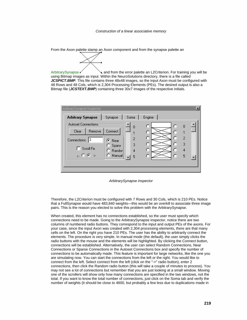
219

Construction of a linear associative memory

From the Axon palette stamp an Axon component and from the synapse palette an

ArbitrarySynapse , and from the error palette an L2Criterion. For training you will be using Bitmap images as input. Within the NeuroSolutions directory, there is a file called JCSPICT.BMP. This file contains three 48x48 images, so the input Axon must be configured with 48 Rows and 48 Cols, which is 2,304 Processing Elements (PEs). The desired output is also a Bitmap file (JCSTEXT.BMP) containing three 30x7 images of the respective initials.

ArbitrarySynapse inspector

Therefore, the L2Criterion must be configured with 7 Rows and 30 Cols, which is 210 PEs. Notice that a FullSynapse would have 483,840 weights—this would be an overkill to associate three image pairs. This is the reason you elected to solve this problem with the ArbitrarySynapse.

When created, this element has no connections established, so the user must specify which connections need to be made. Going to the ArbitrarySynapse inspector, notice there are two columns of numbered radio buttons. They correspond to the input and output PEs of the axons. For your case, since the input Axon was created with 2,304 processing elements, there are that many cells on the left. On the right you have 210 PEs. The user has the ability to arbitrarily connect the elements. The procedure is very simple. In manual mode (the default), the user simply clicks the radio buttons with the mouse and the elements will be highlighted. By clicking the Connect button, connections will be established. Alternatively, the user can select Random Connections, Near Connections or Sparse Connections in the Autoset Connections box and specify the number of connections to be automatically made. This feature is important for large networks, like the one you are simulating now. You can start the connections from the left or the right. You would like to connect from the left. Select connect from the left (click on the "->" radio button), enter 2 connections, then click the Random radio button (this will take a couple of minutes to process). You may not see a lot of connections but remember that you are just looking at a small window. Moving one of the scrollers will show only how many connections are specified in the two windows, not the total. If you want to know the total number of connections, just click on the Soma tab and verify the number of weights (it should be close to 4600, but probably a few less due to duplications made in

220

the randomization process). As you will see, this is more than enough to associate the pairs of patterns given.

Now go to the Input palette, stamp a File component onto the input Axon, and attach it to the Pre-Activity Access point. In the Combination of Data Sources example, you used the File component to input ASCII data into your network. This component also accepts Bitmap image data (8 bits, without alpha channels). From the File list box of the File inspector, the user can manipulate files or translators. A translator is a program that reads data from one of the accepted formats to a stream, which is the format that NeuroSolutions processes. Presently there are translators for ASCII(.ASC), ASCII- Column Format, Binary and Bitmap (.BMP) files. Data can be read from several files, and the data types can be mixed.

FileInput inspector

To open the image data file, click on the Add button and select JCSPICT.BMP from the Open panel. The name will be copied to the FileInput inspector. In order to translate it to a stream, click the Translate button. Notice that the inspector tells you the number of samples in the file in the Stream level. You also have the ability to Customize the file. Normalize the data (between the values of Lower and Upper), or to extract a Segment (using Offset and Duration). By not normalizing, the translator has converted the pixels of the three images into a stream of 6912 floating point values ranging from 0 (black) to 1 (white). Now perform the same procedure using the file JCSTEXT.BMP and attaching it to the Desired Access point of the L2Criterion.

To complete the example, you need to stamp a MatrixViewer on the Average Cost Access of the

L2Criterion to create an MSE probe. Also needed are two ImageViewers , one to the input Axon’s Activity Access point and the other to the Pre-Activity Access point of the L2Criterion. From the ImageViewer inspector, set to Display Every sample. You would also like the normalization to be Automatic because it will guarantee the correct gray (or color) scale. You will also need to set the parameters for the second ImageViewer in the same way. Double click on these ImageViewers to open their windows.

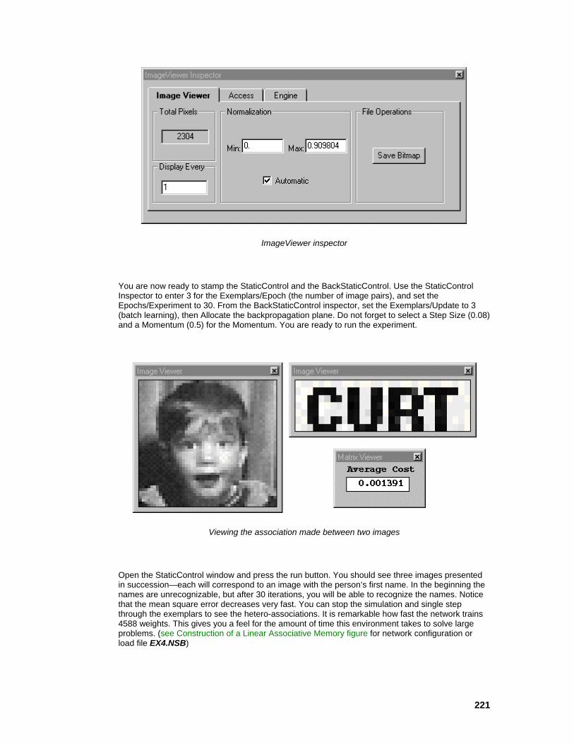
221

ImageViewer inspector

You are now ready to stamp the StaticControl and the BackStaticControl. Use the StaticControl Inspector to enter 3 for the Exemplars/Epoch (the number of image pairs), and set the Epochs/Experiment to 30. From the BackStaticControl inspector, set the Exemplars/Update to 3 (batch learning), then Allocate the backpropagation plane. Do not forget to select a Step Size (0.08) and a Momentum (0.5) for the Momentum. You are ready to run the experiment.

Viewing the association made between two images

Open the StaticControl window and press the run button. You should see three images presented in succession—each will correspond to an image with the person’s first name. In the beginning the names are unrecognizable, but after 30 iterations, you will be able to recognize the names. Notice that the mean square error decreases very fast. You can stop the simulation and single step through the exemplars to see the hetero-associations. It is remarkable how fast the network trains 4588 weights. This gives you a feel for the amount of time this environment takes to solve large problems. (see Construction of a Linear Associative Memory figure for network configuration or load file EX4.NSB)

222

Things to Try with the Associator

One obvious thing to try is to go back to the ArbitrarySynapse and test other possible wiring combinations to see when the wiring density fails. Another interesting aspect is the weak noise immunity of this type of memory. Since it is a linear system, a small amount of noise may disturb

the associations. You can verify this by stamping a Noise component from the Input palette on the File attached to the input Axon.

Noise inspector

From the Noise inspector you can control the Variance and Mean of the noise source, and you can also have the option to add the noise source to the existing signal (accumulate), or overwrite it (i.e. disconnect the other signal source and replace it with just noise). Select Accumulate Data on Network from the Stream tab.

Choose a small Variance of 0.3 (make sure that it is set to Change All Channels) and set the Step Size to 0 such that the weights will remain fixed. By single-stepping through the iterations, you will see that the images of the faces are still somewhat recognizable. You will also see that the system is still able to make the associations. The reason is that 3500 weights provide enough redundancy to overcome the noise. Now try decreasing the number of weights, but not so much that the wiring density fails. Re-train the network and re-test with the noise. Was the system more susceptible to the noise? Why?

What you have Learned from the Associator Example

You were able to build a system that could associate a set of large images with a set of much smaller images. You did this by implementing a simple linear associative memory and trained it with gradient descent learning. Since the system only required a fraction of the weights of a FullSynapse, you instead used the ArbitrarySynapse with random connections. You were able to input the images into the system using the bmp translator of the File component. While running the system you were able to view the input image and its corresponding output image with the ImageViewer probe. You were also introduced to the UniformNoise component and how it can be used to test your system for immunity to noise.

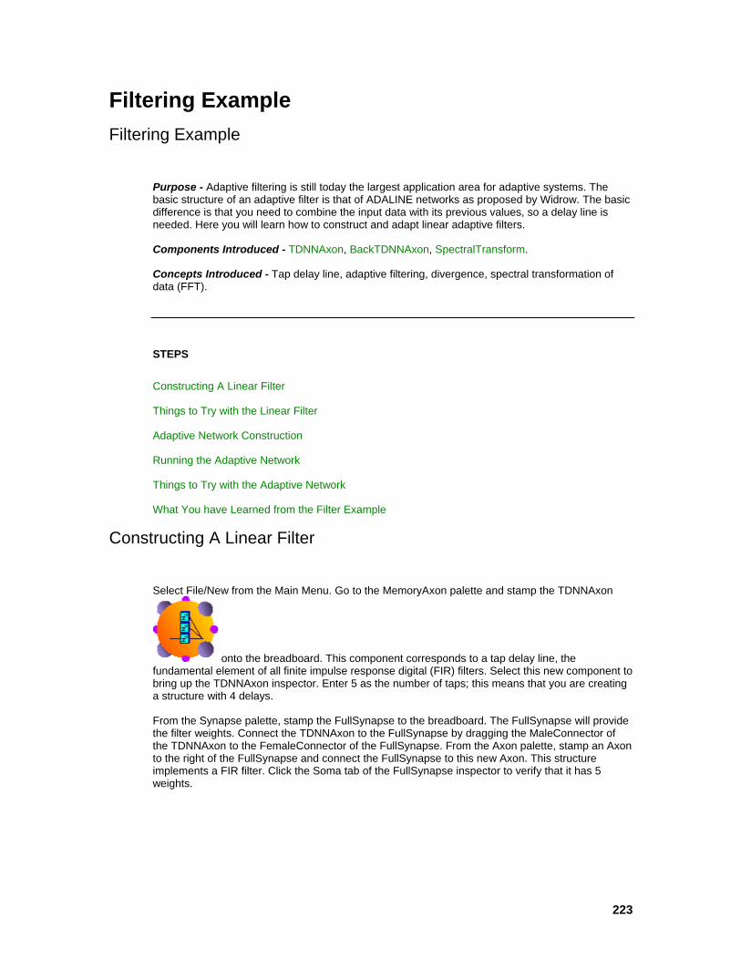
223

Filtering Example Filtering Example

Purpose - Adaptive filtering is still today the largest application area for adaptive systems. The basic structure of an adaptive filter is that of ADALINE networks as proposed by Widrow. The basic difference is that you need to combine the input data with its previous values, so a delay line is needed. Here you will learn how to construct and adapt linear adaptive filters.

Components Introduced - TDNNAxon, BackTDNNAxon, SpectralTransform.

Concepts Introduced - Tap delay line, adaptive filtering, divergence, spectral transformation of data (FFT).

STEPS

Constructing A Linear Filter

Things to Try with the Linear Filter

Adaptive Network Construction

Running the Adaptive Network

Things to Try with the Adaptive Network

What You have Learned from the Filter Example

Constructing A Linear Filter

Select File/New from the Main Menu. Go to the MemoryAxon palette and stamp the TDNNAxon

onto the breadboard. This component corresponds to a tap delay line, the fundamental element of all finite impulse response digital (FIR) filters. Select this new component to bring up the TDNNAxon inspector. Enter 5 as the number of taps; this means that you are creating a structure with 4 delays.

From the Synapse palette, stamp the FullSynapse to the breadboard. The FullSynapse will provide the filter weights. Connect the TDNNAxon to the FullSynapse by dragging the MaleConnector of the TDNNAxon to the FemaleConnector of the FullSynapse. From the Axon palette, stamp an Axon to the right of the FullSynapse and connect the FullSynapse to this new Axon. This structure implements a FIR filter. Click the Soma tab of the FullSynapse inspector to verify that it has 5 weights.

224

Implementation of a Linear Filter

Now go to the Input palette and stack two FunctionGenerators on the Pre-Activity point of the TDNNAxon. Select a sinewave of 8 Samples/Cycle on one FunctionGenerator and a sinewave of 20 Samples/Cycle on the other.

Next go to the Probes palette and stamp a MegaScope/DataStorage on the output Axon, placing it on the Activity access point. Select a StaticControl from the Controls palette and stamp it on the breadboard, set the Exemplars/Epoch to 100, and verify that the Epochs/Experiment is set to 500. Run the network. The waveform in the MegaScope will probably appear complex. The reason is that the sum of input sinusoids is being filtered by a random set of weights.

Go to the Probes palette, stamp a MatrixEditor to the FullSynapse, and place it at the Weight access point. Double-click on the MatrixEditor icon and a row vector with 5 values will appear. This MatrixEditor window allows us to observe, and change the filter weights. While running the network, click the Jog button of the StaticControl window. You should see the values in the MatrixEditor change and the waveform on the MegaScope should also change.

Say you want to produce a specified frequency response by implementing a simple bandstop filter. Stop the simulation and enter in the Matrix Editor the values 1,0,0,0,1. This implements the filter

which is known to have zeros at ?/4, ??/4, 5?/4, and 7?/4. Therefore, an 8 samples per cycle sinewave will be totally attenuated by this filter. In fact, you should see a perfect sinewave at the output that corresponds to the 20 samples per cycle sinewave generator.

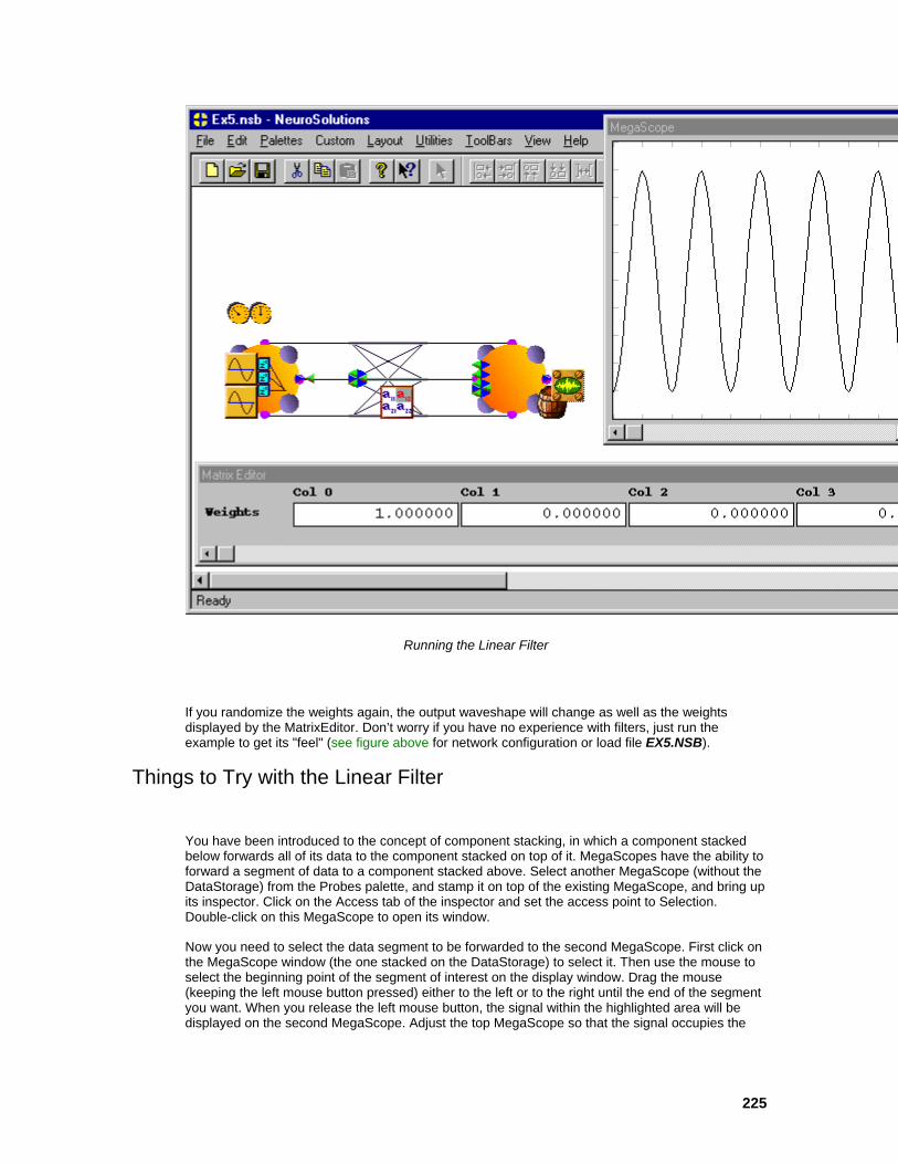
225

Running the Linear Filter

If you randomize the weights again, the output waveshape will change as well as the weights displayed by the MatrixEditor. Don’t worry if you have no experience with filters, just run the example to get its "feel" (see figure above for network configuration or load file EX5.NSB).

Things to Try with the Linear Filter

You have been introduced to the concept of component stacking, in which a component stacked below forwards all of its data to the component stacked on top of it. MegaScopes have the ability to forward a segment of data to a component stacked above. Select another MegaScope (without the DataStorage) from the Probes palette, and stamp it on top of the existing MegaScope, and bring up its inspector. Click on the Access tab of the inspector and set the access point to Selection. Double-click on this MegaScope to open its window.

Now you need to select the data segment to be forwarded to the second MegaScope. First click on the MegaScope window (the one stacked on the DataStorage) to select it. Then use the mouse to select the beginning point of the segment of interest on the display window. Drag the mouse (keeping the left mouse button pressed) either to the left or to the right until the end of the segment you want. When you release the left mouse button, the signal within the highlighted area will be displayed on the second MegaScope. Adjust the top MegaScope so that the signal occupies the

226

entire display. When you run the simulation again, you should see the top MegaScope mirroring the selected segment of the bottom MegaScope.

This exercise may not seem that interesting, but you will find that this ability to select segments of data for further processing and/or probing is a powerful feature that you will likely find very useful. For instance, you will later be introduced to a component that will perform a Fast Fourier Transform (FFT) on the data. Using a MegaScope, you are able to select a portion the signal (i.e. how many periods) from which to construct the FFT. Notice also that the more windows open the slower the simulations run. So a compromise between simulation speed and visualization tools is needed.

Adaptive Network Construction

You will use the same network but now you will let the weights adapt according to a given desired response. From the ErrorCriteria palette, choose the L2Criterion—the most widely used error metric. Now place the L2Criterion to the right of the output Axon, then make the connection between them. From the Probes palette, select the MatrixViewer and stamp it on the L2Criterion and set the access point to Average Cost.

Attaching the L2Criterion to the output

Now select the BackStaticControl and stamp it over the StaticControl. Use the BackStaticControl Inspector to add the backpropagation components. Select the On-Line radio button from within the BackStaticControl Inspector. From within the Static Control Inspector, set the Exemplars/Epoch to 80. Set the Step Size to .1 in the Momentum Inspector. Within the DataStorage Inspector, set the Message Every form cell to 80. Make a copy of the 20 samples/cycle input FunctionGenerator and place it over the L2Criterion. Now select the access point to be Desired access. Effectively, you are telling the ADALINE to output a signal that is equal to a sine with 20 samples per cycle. This adaptive system will then try to approximate the filter that you hand-coded for the previous example.

Running the Adaptive Network

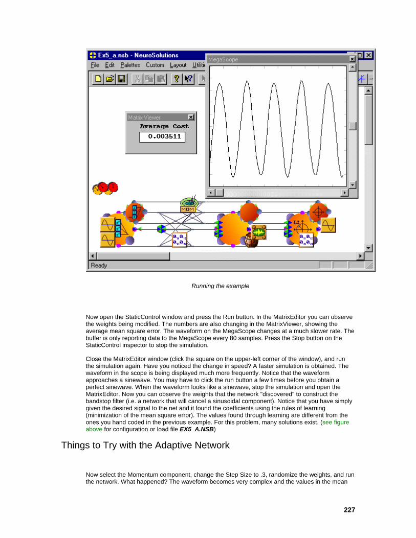
227

Running the example

Now open the StaticControl window and press the Run button. In the MatrixEditor you can observe the weights being modified. The numbers are also changing in the MatrixViewer, showing the average mean square error. The waveform on the MegaScope changes at a much slower rate. The buffer is only reporting data to the MegaScope every 80 samples. Press the Stop button on the StaticControl inspector to stop the simulation.

Close the MatrixEditor window (click the square on the upper-left corner of the window), and run the simulation again. Have you noticed the change in speed? A faster simulation is obtained. The waveform in the scope is being displayed much more frequently. Notice that the waveform approaches a sinewave. You may have to click the run button a few times before you obtain a perfect sinewave. When the waveform looks like a sinewave, stop the simulation and open the MatrixEditor. Now you can observe the weights that the network "discovered" to construct the bandstop filter (i.e. a network that will cancel a sinusoidal component). Notice that you have simply given the desired signal to the net and it found the coefficients using the rules of learning (minimization of the mean square error). The values found through learning are different from the ones you hand coded in the previous example. For this problem, many solutions exist. (see figure above for configuration or load file EX5_A.NSB)

Things to Try with the Adaptive Network

Now select the Momentum component, change the Step Size to .3, randomize the weights, and run the network. What happened? The waveform becomes very complex and the values in the mean

228

square error window become extremely large. Stop the simulation. The step size was selected too large and the iterations are simply diverging (i.e. the operating point of the network departs further and further from the optimal solution).

Select a new Step Size of 0.1 in the Momentum Inspector. Now go back to the Probes palette, select a second MegaScope/DataStorage, and place it over the MatrixViewer attached to the L2Criterion (the MSE probe). Verify that the access point of the DataStorage is Stacked access (i.e. it is reading the value reported by the MatrixViewer). Have the buffer message after every 10 samples. You have constructed a probe that will display the learning curve for this network.

Randomize the weights and run the simulation again. What do you see? The MegaScope connected to the MatrixViewer is showing a very complex waveform—the instantaneous error through iteration. Notice that the largest value of the waveform is steadily decreasing. After 5 epochs (400 exemplars) the MegaScope connected to the output is displaying a waveform very close to a sinewave, and the error is decreasing to zero very fast. After 15 epochs (1200 exemplars) the network basically learned the task. Randomize the weights again and re-run the network just to see the effect of the initialization on the speed of adaptation.

Now let the system learn this task with batch learning. From the BackStaticControl inspector, select the Batch radio button. This means that you are using 80 exemplars to learn (the setting of the Exemplars/Epoch form cell in the StaticControl Inspector). Also, select a new Step Size of .5 in the Momentum Inspector.

Randomize the weights and run the simulation. What happened? Notice that now the learning curve is much smoother than with the on-line system, decreasing steadily to zero. Also notice that the system basically learns the task in 150 epochs. But don’t forget that in each epoch has the gradient has the contribution of 80 samples. Another aspect that must be stressed is that the simulation with batch learning is more efficient. In the way that the code is implemented, the activations and errors are being stored in memory, and the switching between forward and backward task is less frequent. This will be addressed in later sections.

The final test with this example is to show a little more of the phenomenal probing abilities of the

package. From the Probes palette, stamp the SpectralTransform over the MegaScope on the output Axon (we will call this the output MegaScope). Stamp another MegaScope on top of this component. This MegaScope will enable us to visualize the spectrum of the network’s output WHILE the network is learning. Just double click on this MegaScope to open its corresponding window.

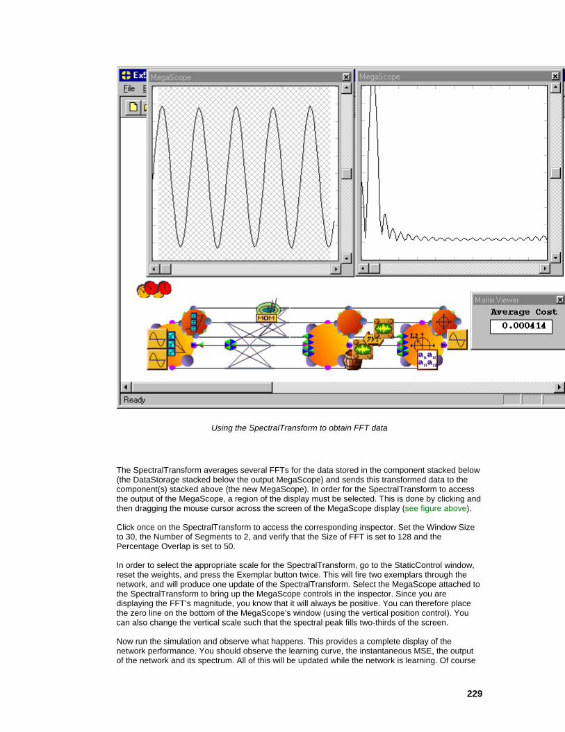
229

Using the SpectralTransform to obtain FFT data

The SpectralTransform averages several FFTs for the data stored in the component stacked below (the DataStorage stacked below the output MegaScope) and sends this transformed data to the component(s) stacked above (the new MegaScope). In order for the SpectralTransform to access the output of the MegaScope, a region of the display must be selected. This is done by clicking and then dragging the mouse cursor across the screen of the MegaScope display (see figure above).

Click once on the SpectralTransform to access the corresponding inspector. Set the Window Size to 30, the Number of Segments to 2, and verify that the Size of FFT is set to 128 and the Percentage Overlap is set to 50.

In order to select the appropriate scale for the SpectralTransform, go to the StaticControl window, reset the weights, and press the Exemplar button twice. This will fire two exemplars through the network, and will produce one update of the SpectralTransform. Select the MegaScope attached to the SpectralTransform to bring up the MegaScope controls in the inspector. Since you are displaying the FFT’s magnitude, you know that it will always be positive. You can therefore place the zero line on the bottom of the MegaScope’s window (using the vertical position control). You can also change the vertical scale such that the spectral peak fills two-thirds of the screen.

Now run the simulation and observe what happens. This provides a complete display of the network performance. You should observe the learning curve, the instantaneous MSE, the output of the network and its spectrum. All of this will be updated while the network is learning. Of course

230

simulations become a little slower this way, but the insight obtained with this arrangement of probes is often worth the performance penalty.

Notice that the SpectralTransform is very sensitive to the accuracy of the output. The MSE is already very low, but the MegaScope still displays a predominant second harmonic stating that the learning is not yet complete. After approximately 500 epochs, the spectrum consistently displays a single peak and you can say that learning is complete. (see figure above for network configuration or load file EX5_FFT.NSB)

What You have Learned from the Filter Example

In this example you have learned more fundamentals of interconnecting elements. By making the appropriate connection, you were able to feed the taps of the TDNNAxon to the weights of the FullSynapse. You were able to manipulate the values of those weights by randomizing them, or by setting them manually with the MatrixEditor. This manipulation of the weights defined the frequency response of the filter.

You also have learned how to automatically adapt the filter weights by providing a cost function and a desired signal. The constructed network worked as an adaptive interference chancellor, widely used in communications and instrumentation. You have seen that you can adapt the coefficients on-line or in batch mode, and that if you are not careful the adaptation may diverge.

You have also learned how to compute and display Fast Fourier Transforms with NeuroSolutions. This is very important for engineering applications.

Recurrent Neural Network Example Recurrent Neural Network Example

Purpose - In this example you will learn how to construct a recurrent neural network. You will then train this network to learn the exclusive-or problem.

Components Introduced - DeltaTransmitter.

Concepts Introduced - Delay operators, feedback loops, fixed point learning algorithms, network stability, probing for appropriate learning, dynamic relaxation.

STEPS

Creating the Recurrent Topology

Fixed Point Learning

Running the Recurrent Network

Things to Try with the Recurrent Network

What You have Learned from the Recurrent Network Example

Creating the Recurrent Topology

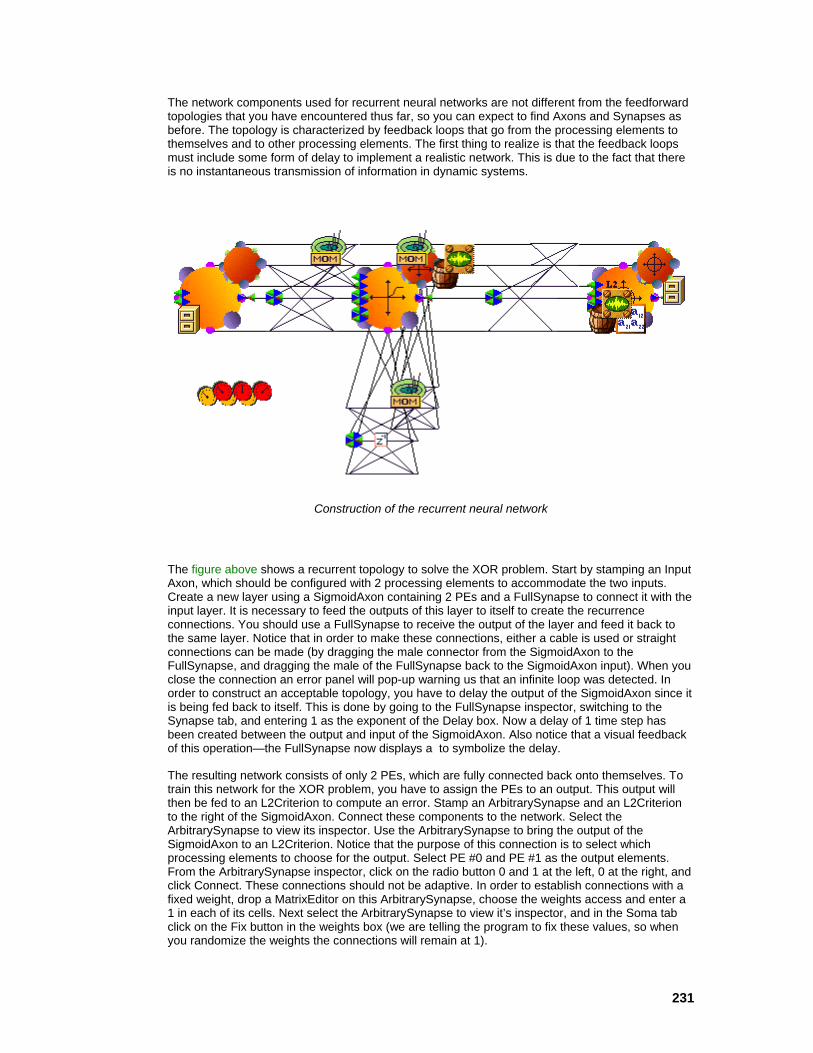
231

The network components used for recurrent neural networks are not different from the feedforward topologies that you have encountered thus far, so you can expect to find Axons and Synapses as before. The topology is characterized by feedback loops that go from the processing elements to themselves and to other processing elements. The first thing to realize is that the feedback loops must include some form of delay to implement a realistic network. This is due to the fact that there is no instantaneous transmission of information in dynamic systems.

Construction of the recurrent neural network

The figure above shows a recurrent topology to solve the XOR problem. Start by stamping an Input Axon, which should be configured with 2 processing elements to accommodate the two inputs. Create a new layer using a SigmoidAxon containing 2 PEs and a FullSynapse to connect it with the input layer. It is necessary to feed the outputs of this layer to itself to create the recurrence connections. You should use a FullSynapse to receive the output of the layer and feed it back to the same layer. Notice that in order to make these connections, either a cable is used or straight connections can be made (by dragging the male connector from the SigmoidAxon to the FullSynapse, and dragging the male of the FullSynapse back to the SigmoidAxon input). When you close the connection an error panel will pop-up warning us that an infinite loop was detected. In order to construct an acceptable topology, you have to delay the output of the SigmoidAxon since it is being fed back to itself. This is done by going to the FullSynapse inspector, switching to the Synapse tab, and entering 1 as the exponent of the Delay box. Now a delay of 1 time step has been created between the output and input of the SigmoidAxon. Also notice that a visual feedback of this operation—the FullSynapse now displays a to symbolize the delay.

The resulting network consists of only 2 PEs, which are fully connected back onto themselves. To train this network for the XOR problem, you have to assign the PEs to an output. This output will then be fed to an L2Criterion to compute an error. Stamp an ArbitrarySynapse and an L2Criterion to the right of the SigmoidAxon. Connect these components to the network. Select the ArbitrarySynapse to view its inspector. Use the ArbitrarySynapse to bring the output of the SigmoidAxon to an L2Criterion. Notice that the purpose of this connection is to select which processing elements to choose for the output. Select PE #0 and PE #1 as the output elements. From the ArbitrarySynapse inspector, click on the radio button 0 and 1 at the left, 0 at the right, and click Connect. These connections should not be adaptive. In order to establish connections with a fixed weight, drop a MatrixEditor on this ArbitrarySynapse, choose the weights access and enter a 1 in each of its cells. Next select the ArbitrarySynapse to view it’s inspector, and in the Soma tab click on the Fix button in the weights box (we are telling the program to fix these values, so when you randomize the weights the connections will remain at 1).

232

To provide the input and desired response you can use two FileInput components with the input and output files created for the XOR problem. These should be stamped respectively at the input Axon and at the L2Criterion. You are now ready to establish the training protocol of fixed-point learning.

Fixed Point Learning

Fixed-point learning is an extension of static backpropagation that is used to embed fixed points into recurrent systems. See the Constraining the learning Dynamics for details. There are several steps involved in fixed-point learning. First, there is the forward propagation of the activations. This has to be done for a certain number of time steps, since the network has its own dynamics (this is called the relaxation period). After the net stabilizes, an error can be computed at the output in the normal way. Then the error is propagated backward through the dual network, and once again it must be fed several times to allow the network to relax. After relaxation, the error at each PE can be multiplied by the relaxed activation to update the weights.

As per this explanation, you have to select the relaxation time both in the forward and

backpropagation planes. Stamp a DynamicControl on the breadboard and then a

BackDynamicControl over the DynamicControl. Select the Fixed Point radio button in the DynamicControl Inspector. Notice that within the DynamicControl Inspector there are 3 form cells: the Epochs/Experiment, the Exemplars/Epoch and the Samples/Exemplar. You should select respectively 1000, 4 (since you have 4 patterns for the XOR), and 10. This means that each sample will be repeatedly presented to the network 10 times to let the output relax.

DynamicControl inspector

This parameter is crucial for stable learning. If the network is not relaxed enough, the output activation will not be the steady state value and will produce an erroneous error estimate. A MegaScope/DataStorage should be used here on the SigmoidAxon to help set and monitor the relaxation period through learning. A more efficient method will be presented later using the transmitters.

Now you have to do a similar thing for the BackDynamicControl. From the BackDynamicControl inspector, observe the Samples/Exemplar and the Exemplars/Update. You should match the Samples/Exemplar of the forward plane and select the Exemplars/Update to 4 for this XOR problem.

233

While here, you should also allocate the backprop plane by selecting Momentum and clicking the Add button. The gradient search can be selected by typing the appropriate method or simply using the default. Notice that all the components with adaptive weights will be provided with a backprop component and a gradient search component. Since the weight of the output ArbitrarySynapse should not be adapted, remove the corresponding Momentum from the breadboard.

Now add the probes needed to monitor the learning. If probing was important for the static networks, it is now ESSENTIAL. In our opinion, one of the reasons recurrent systems are not as popular as static systems is the difficulty of the learning dynamics. With probing, a lot of the guesswork can be taken away by simply visualizing the appropriate variables. With learning, all of the information is carried to the backprop plane (the errors), so place a MegaScope/DataStorage on the BackSigmoidAxon and choose the Activity point. This probe will monitor the errors during learning. Use a MatrixViewer as a mean square error probe. Note that since the network is recurrent, you can expect transient behavior between the different input patterns.

Now select the Learning Rate. Start with a large Step Size of 0.5 and a Momentum of 0.8. Turn off normalization.

Running the Recurrent Network

You are now ready to run the example. Open the MegaScopes, the MatrixViewer, and run the network. The MSE error starts large (~.4) and quickly should approach ~ 0.25. This problem has a plateau around this value of MSE (the linear solution). The problem is to get over this part of the performance surface. If a smaller step size or momentum is selected, very probably the adaptation will be caught in the local minimum. On the other hand, these two parameters are too large towards the end of adaptation. Therefore, the user must stop the training and drastically reduce both the step size and the momentum after the knee. It is recommended to interrupt the learning just after the MSE drops below 0.2, and reduce the Learning Rate at this point to 0.05 Step Size and 0.1 Momentum. It should be pointed out that this inherent ability to have real time monitoring of parameters is a distinctive advantage of NeuroSolutions. Furthermore, you will learn how to use transmitters to automate these changes in learning rates. (see Construction of the Recurrent Neural Network figure for network configuration or load file EX6.NSB)

Before continuing the simulation, an important concept relating to the relaxation of the network needs to be mentioned. In the beginning of learning, the network relaxes almost immediately as can be observed by the flat top and bottom of the error signal waveforms. Towards the end of learning, you will notice that the backpropagated error has longer and longer transients. It is therefore necessary to increase the relaxation time to ensure that the transients die away before the comparison with the desired signal is done.

234

Probing the state of the system after learning

When you observed the MegaScopes on the initial run, you should have seen that initially the output signal did not resemble the desired response. To verify this, just go to the desired signal file

to see the sequence of values you entered. Alternatively, use a DataStorageTransmitter to project the desired response of the forward activation MegaScope. If you are not yet familiar with this component, you will learn about it in later sections. Now that you have reached the plateau and have modified the parameters, continue the simulation. The MSE should decrease steadily and you should see a square wave, which does resemble the desired signal such that the length of the pulse is the relaxation time that you chose.

Some extra comments are pertinent at this time. First, training a recurrent system is not trivial and requires appropriate tools like the ones provided in NeuroSolutions. Don’t give up if the network seems to get stuck in a local minimum. Try increasing the momentum, but be prepared for "picky" training and a lot of instabilities (i.e. the network will blow up frequently). When this occurs, you will need to reset the network. Resetting clears all storage locations (activations) and randomizes the weights. Note that randomization of the weights alone is not sufficient, since in a recurrent system the output depends on the initial state of the activations. Finely tuned, the network learns in less than 800-1000 steps. Remember that each training pattern is presented repeatedly to the net during relaxation, so training time is longer than for a multi-layer perceptron (MLP).

235

Notice in the figure above that the amplitude of the backpropagated error signal observed using the MegaScope becomes larger towards the end of adaptation (this is normally, but not necessarily observed). Also notice the large values of the weights. This is one feature of recurrent systems (due to the feedback connections, the output error can be small but internally the backpropagated error can be large), and it is one of the reasons they are more difficult to adapt. Notice that the error is not as small as the one achieved with a static system, the reason being the dynamic behavior of the net output (i.e. the transients). What you gain with a recurrent system is the insensitivity it has towards input noise. You observed a disadvantage of the system as it nears adaptation; the network weights become large requiring the step size to be reduced proportionally.

Things to Try with the Recurrent Network

This is the perfect example to introduce the transmitter family. The transmitters are a class of objects that test for a particular condition and perform global communications within a breadboard. Transmitters have a lot of potential applications, but here they will be used to control the relaxation time (i.e. the number of samples/exemplar) of the network in the forward and backward planes. Above you had to control the relaxation time conservatively, by imposing a fixed relaxation period. But the relaxation can be controlled by measuring the differential between two consecutive iterations. When the difference is smaller than a given threshold you can assume that the system stabilized. This produces an enormous savings in training time for a recurrent system. Now you can include the transmitters in your recurrent system.

Using transmitters to dynamically control the relaxation period

Dock the Transmitters palette, and select the DeltaTransmitter . The idea is to place one DeltaTransmitter in the forward plane to monitor the network output and to notify the breadboard controller when to stop firing. To accomplish this, attach it to the Pre-Activity access point of the L2Criterion.

From the Transmitter tab of the DeltaTransmitter inspector, select DynamicControl within the Receivers box and double-click on end samples within the Actions box. The selection should be preceded by a C, denoting that the connection has been made. You have configured the DeltaTransmitter so that after every sample, it will check to see if the change (delta) in activation

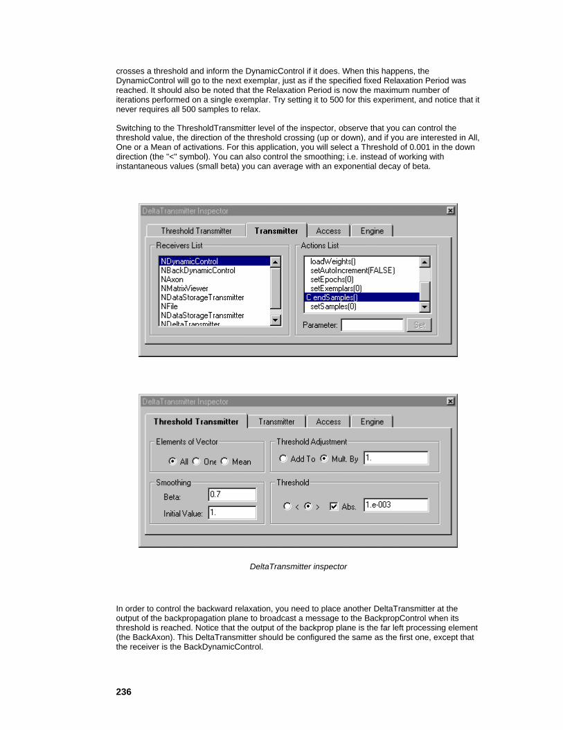
236

crosses a threshold and inform the DynamicControl if it does. When this happens, the DynamicControl will go to the next exemplar, just as if the specified fixed Relaxation Period was reached. It should also be noted that the Relaxation Period is now the maximum number of iterations performed on a single exemplar. Try setting it to 500 for this experiment, and notice that it never requires all 500 samples to relax.

Switching to the ThresholdTransmitter level of the inspector, observe that you can control the threshold value, the direction of the threshold crossing (up or down), and if you are interested in All, One or a Mean of activations. For this application, you will select a Threshold of 0.001 in the down direction (the "<" symbol). You can also control the smoothing; i.e. instead of working with instantaneous values (small beta) you can average with an exponential decay of beta.

DeltaTransmitter inspector

In order to control the backward relaxation, you need to place another DeltaTransmitter at the output of the backpropagation plane to broadcast a message to the BackpropControl when its threshold is reached. Notice that the output of the backprop plane is the far left processing element (the BackAxon). This DeltaTransmitter should be configured the same as the first one, except that the receiver is the BackDynamicControl.

237

You are ready to use the DeltaTransmitters to train the recurrent net. Starting with the large step sizes, notice that the training goes much faster. The MegaScope shows that the length of the pulses becomes much shorter, meaning that the network relaxes very fast because the differential increment of 0.01 is reached very quickly. You should interrupt the training when the MSE drops below 0.2 to decrease the Step Size to 0.05 and Momentum to 0.1. Continue training and you will observe that the relaxation time increases quite a bit towards the end of training, meaning that the net requires more iterations to reach the steady state. With the transmitters, relax the network only as much as needed to achieve the incremental condition. However, notice that to achieve a MSE on the order of 0.08, you will have to set the threshold at 1.e-6 or less, otherwise the network does not relax sufficiently, possibly resulting in instability.

Distorted input to the XOR problem

Configuration for testing generalization

Another thing to test is the generalization ability of this network. Recall that one of the advantages of recurrent systems is their ability to handle noise very well. In order to experiment with this characteristic, distort the input signal by adding a noise source to the input (see figure above). Then set the learning rates to zero (in the trained network), and pass the distorted XOR data through the net. It is clear that the network is able to reproduce the XOR output for these distorted inputs. You

238

may want to try this same experiment for the perceptron that you constructed earlier so that you can compare the two network topologies.

What You have Learned from the Recurrent Network Example

In this example, you were exposed to the concept of recurrent networks, and you learned how to train one to solve the XOR problem using fixed point learning. Fixed-point learning is an extension of backpropagation for recurrent networks. You were able to setup the controllers for fixed point learning, and you learned the importance of probing to appropriately train recurrent systems.

You were also exposed to the DeltaTransmitter, which allowed you to dynamically adapt the relaxation period based on the incremental difference in the activations. This allowed you to run the network more efficiently, since you were not forced to make a conservative estimate on the number of iterations needed to relax. At the end, you were able to verify the noise immunity of this recurrent system.

Frequency Doubler Example Frequency Doubler Example

Purpose - The purpose of the frequency doubler example is to introduce the topic of trajectory learning, so useful in the recognition of time varying patterns such as speech recognition, adaptive controls, and time series prediction. Here you will learn how to design and train a dynamic network to double the frequency of a sinewave.

Components Introduced - GammaAxon, LaguarreAxon, BiasAxon, StateSpaceProbe, DataStorageTransmitter, IntegratorAxon.

Concepts Introduced - Trajectory learning, dynamic neural networks, comparison of memory structures.

STEPS

Creating the Frequency Doubler Network

Configuration of the Trajectory

Running the Frequency Doubler Network

Using the Gamma Model to Double the Frequency

Visualizing the State Space

Things to Try with the Frequency Doubler Network

What You have Learned from the Frequency Doubler Example

Creating the Frequency Doubler Network

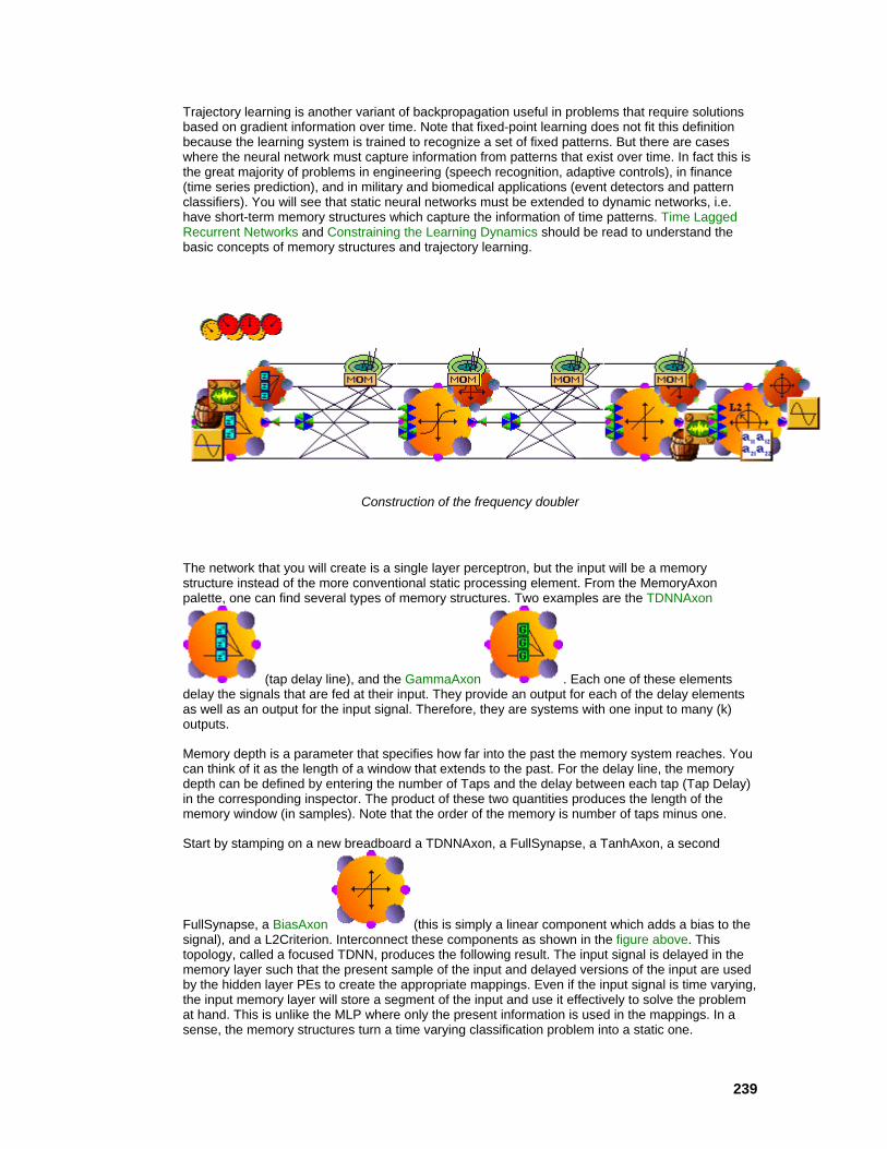
239

Trajectory learning is another variant of backpropagation useful in problems that require solutions based on gradient information over time. Note that fixed-point learning does not fit this definition because the learning system is trained to recognize a set of fixed patterns. But there are cases where the neural network must capture information from patterns that exist over time. In fact this is the great majority of problems in engineering (speech recognition, adaptive controls), in finance (time series prediction), and in military and biomedical applications (event detectors and pattern classifiers). You will see that static neural networks must be extended to dynamic networks, i.e. have short-term memory structures which capture the information of time patterns. Time Lagged Recurrent Networks and Constraining the Learning Dynamics should be read to understand the basic concepts of memory structures and trajectory learning.

Construction of the frequency doubler

The network that you will create is a single layer perceptron, but the input will be a memory structure instead of the more conventional static processing element. From the MemoryAxon palette, one can find several types of memory structures. Two examples are the TDNNAxon

(tap delay line), and the GammaAxon . Each one of these elements delay the signals that are fed at their input. They provide an output for each of the delay elements as well as an output for the input signal. Therefore, they are systems with one input to many (k) outputs.

Memory depth is a parameter that specifies how far into the past the memory system reaches. You can think of it as the length of a window that extends to the past. For the delay line, the memory depth can be defined by entering the number of Taps and the delay between each tap (Tap Delay) in the corresponding inspector. The product of these two quantities produces the length of the memory window (in samples). Note that the order of the memory is number of taps minus one.

Start by stamping on a new breadboard a TDNNAxon, a FullSynapse, a TanhAxon, a second

FullSynapse, a BiasAxon (this is simply a linear component which adds a bias to the signal), and a L2Criterion. Interconnect these components as shown in the figure above. This topology, called a focused TDNN, produces the following result. The input signal is delayed in the memory layer such that the present sample of the input and delayed versions of the input are used by the hidden layer PEs to create the appropriate mappings. Even if the input signal is time varying, the input memory layer will store a segment of the input and use it effectively to solve the problem at hand. This is unlike the MLP where only the present information is used in the mappings. In a sense, the memory structures turn a time varying classification problem into a static one.

240

One of the issues is to determine the memory depth (how far into the past is the information relevant for your application?). In this case, the definition of the memory depth is simple because you want to duplicate the frequency of a sinewave. Therefore, you have to give to the dynamic net a number of samples that corresponds roughly to one fourth the period of the slower wave (at least), such that the net "sees" the doubling of frequency. To solve this problem, the net has to combine the input samples in the window and produce new values that match the double of the frequency, all of which is done over time (i.e. the samples keep on changing). Frequency doubling of a sinewave is intrinsically a nonlinear problem that no linear system can solve.

Now stamp two FunctionGenerators, one on the input (TDNNAxon Pre-Activity access) and the other to the L2Criterion to be used as the desired signal. Select the input to be a sinewave of 40 Samples/Cycle and the desired output to be a sinewave of 20 Samples/Cycle. From the TDNNAxon inspector, enter a memory depth of 10 Taps and a Tap Delay of 1. The hidden layer (TanhAxon) should have 2 PEs. Stamp a DynamicControl on the breadboard and a BackDynamicControl on the DynamicControl. Now Allocate the backprop plane and start with an initial estimate of the learning rate to be 0.4 for the normalized Step Size and 0.5 for the Momentum. Stamp two MegaScopes/DataStorages to verify the performance of the network—one on the input and the other on the output (set them to Message Every 80 samples, so that the display of the waveforms is steady). Stamp an MSE probe (MatrixViewer) on the output to monitor the learning.

Configuration of the Trajectory

The goal of the trajectory configuration is to use the information of an input section and train the classifier to minimize the fitting error between the network output and the desired trajectory. Notice that to solve this problem, the network needs information along time. For this problem, you need to accumulate the gradient information during at least one period of the slowest wave. You will elect to accumulate over two periods (80 samples) and backpropagate the errors 70 (the trajectory length minus the memory depth) samples in the past. You propose this length to avoid feeding in erroneous values associated with the initial conditions. Learning becomes more stable with this selection.

After selecting the DynamicControl, select Trajectory within the System Dynamics box, enter 80 as the number of Samples/Exemplar, and 1,000 as the number of Epochs/Experiment. This means that you have only two periods of the sinewave that will be repeatedly used for learning. Since the sinewave is periodic, the number of Exemplars/Epoch can be set to 1. Otherwise, this number would be associated with the length of the input data (divided by the Samples/Exemplar used). You have to go to the BackDynamicControl to establish how far into the past to propagate the errors. As explained above, you will select 70 for the Samples/Exemplar and 1 for the Exemplars/Update, meaning that you will update the weights every time you backpropagate the error through time. (see Construction of the Frequency Doubler figure for network configuration or load file EX7.NSB)

Running the Frequency Doubler Network

Be sure to open the MegaScopes and calibrate them. Within 200 iterations the network should learn this task. At first the output waveform looks distorted, but then the second peak corresponding to the doubling of frequency appears and the display stabilizes. The errors decrease to very small values, showing that the task has been learned.

It is recommended that you try changing the memory size. If you decrease it too much the doubling of frequency will not be complete. If you increase it, the task is learned a little faster with respect to the number of iterations, but the actual processing time increases since there are more weights to compute. Try decreasing the number of Taps to 5 and increasing the Tap Delay to 2. What this does is cut the number of free parameters (weights) in half, but you still span the same segment of the signal (with only half of the resolution). You may think that the net will not learn the task with 5 taps, but you will see that what counts most in temporal signal processing with dynamic neural nets is the memory depth (which is still 10). By running the simulation again, you will see that the net

241

again learns the doubling of the frequency. If the time window size is not properly adjusted, you may end up with a very powerful multi-layer net (one with lots of PEs) which may still not be able to learn the task.

In order to help in the determination of the more appropriate memory depth, the gamma memory was introduced in neural computation. It is a memory structure that is more versatile than the tap delay line, since it is recursive. This means that during learning, the network can change one parameter (the gamma parameter) to adapt the memory depth. So, with the gamma memory, there are less problems associated with the choice of the memory size, since the net is able to adapt the compromise of memory depth and memory resolution.

Using the Gamma Model to Double the Frequency

Now substitute the TDNNAxon with the GammaAxon and assign it 5 Taps with a Tap Delay of 1. Remember to also attach a BackGammaAxon and a Momentum, since the GammaAxon has one parameter that is adaptive (the gamma parameter). Re-attach the FunctionGenerator and stamp the MegaScope/DataStorage on the WeightsAccess point of the GammaAxon. You will be observing the adaptation of the gamma parameter during learning, so change the Buffer Size of the DataStorage to 250 and have it Message Every 4 iterations. The gamma parameter requires a slower adaptation rate (it is a recursive parameter), so configure the corresponding Momentum to have a Step Size of 0.1 and a Momentum of 0.5.

Run the experiment. Notice that the gamma parameter always starts at 1 (you may have to autoscale the MegaScope with the first few iterations). For this value, the gamma memory defaults to the tap delay line of the same number of taps. So you are starting with the previous case which was difficult to learn. Notice that during adaptation the gamma parameter decreases, meaning that longer memory depths are being searched (memory depth = number of taps / gamma parameter). When the gamma parameter stabilizes (at around 0.5), notice that the output MegaScope displays the expected waveform with double the original frequency. This means that the task was solved by the static classifier attached to the gamma memory structure, just after the correct memory depth was reached.

Now make the problem even harder. Reduce the number of taps to 3. Notice that to provide the same memory depth the gamma parameter must even go to smaller values. Resume the training without randomizing the weights. You will find out that the problem is still solvable, and that the gamma parameter reduces to an even smaller value (~0.3). This versatility of the gamma memory—having the ability to choose an appropriate compromise memory depth/resolution for a given memory size—has been shown to be very important in dynamic modeling with neural networks.

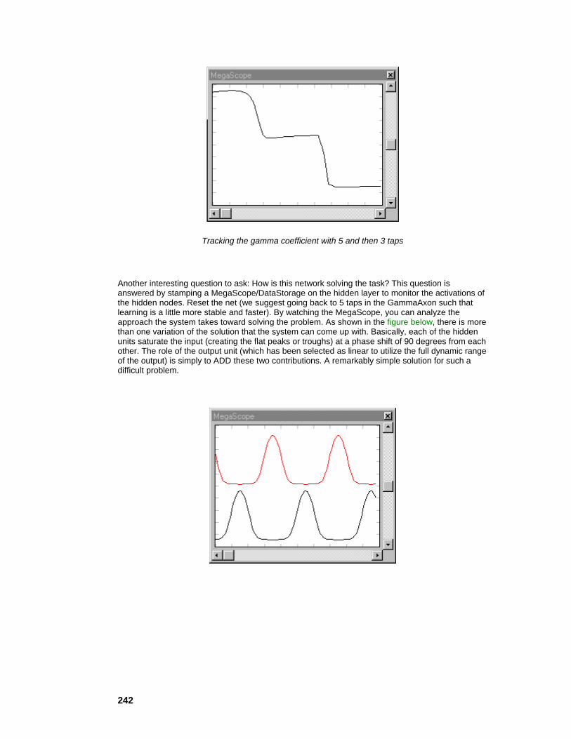
242

Tracking the gamma coefficient with 5 and then 3 taps

Another interesting question to ask: How is this network solving the task? This question is answered by stamping a MegaScope/DataStorage on the hidden layer to monitor the activations of the hidden nodes. Reset the net (we suggest going back to 5 taps in the GammaAxon such that learning is a little more stable and faster). By watching the MegaScope, you can analyze the approach the system takes toward solving the problem. As shown in the figure below, there is more than one variation of the solution that the system can come up with. Basically, each of the hidden units saturate the input (creating the flat peaks or troughs) at a phase shift of 90 degrees from each other. The role of the output unit (which has been selected as linear to utilize the full dynamic range of the output) is simply to ADD these two contributions. A remarkably simple solution for such a difficult problem.

243

Activations of the two hidden layer PEs after learning (two runs)

Visualizing the State Space

You will now introduce a different way of looking at the waveforms by using the StateSpaceProbe

. This probe is particularly valuable in dynamic system analysis, because it provides a way to visualize the evolution of the state of the system that is producing the output waveform.

In state space, the axes are the amplitude of the signal and its derivatives. You will restrict your display to 3-D (the amplitude, the first derivative, and the second derivative). For instance, a sinewave in state space corresponds to a circle. Now the interesting question: How does the state of the neural network change while it learns to double the frequency of the input?

Go to the Probes palette, stamp a StateSpaceProbe, and place it over the output MegaScope at the Selection Access point. This means that the segment of data that you select from the MegaScope (by dragging the mouse across the window) will be passed to the StateSpaceProbe. Select the entire contents of the window as the data segment (be sure to calibrate the MegaScope to display the entire segment stored in the DataStorage).

StateSpaceProbe inspector

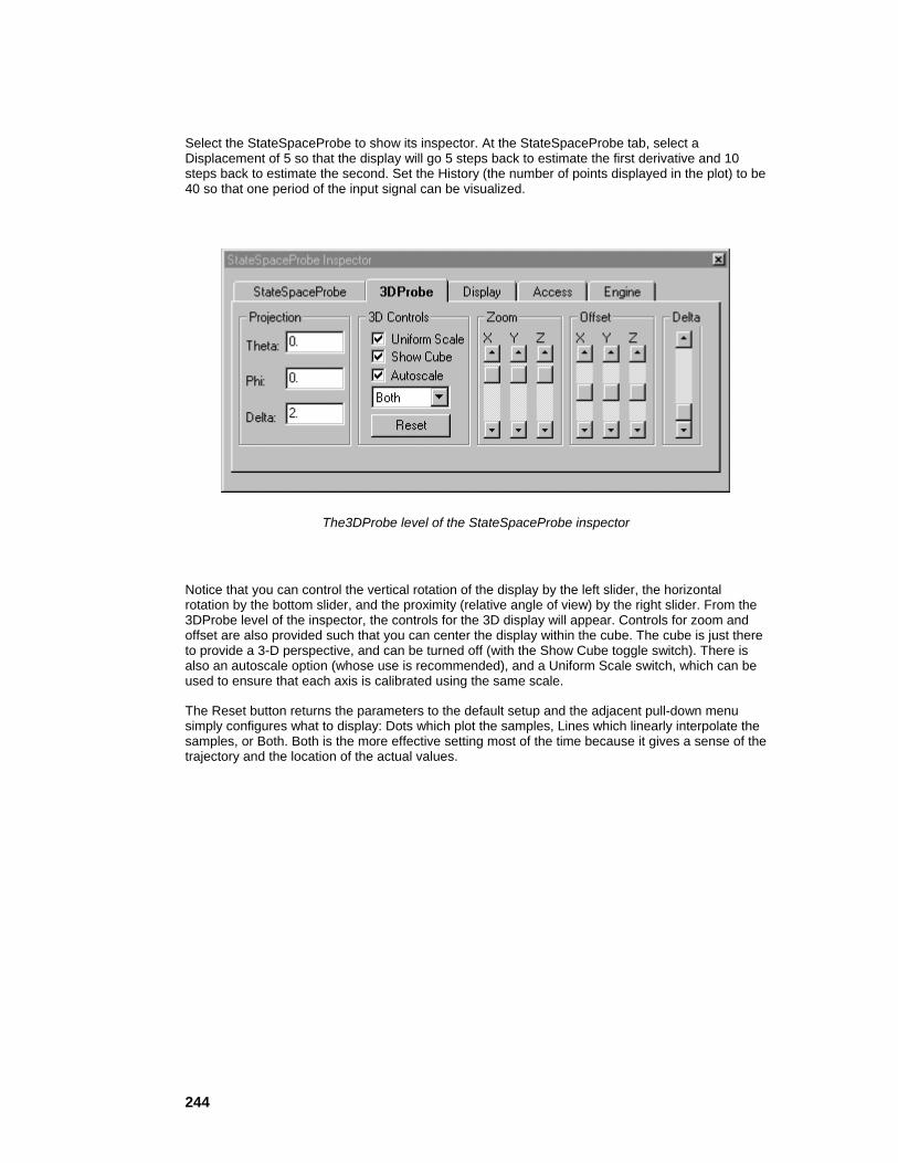
244

Select the StateSpaceProbe to show its inspector. At the StateSpaceProbe tab, select a Displacement of 5 so that the display will go 5 steps back to estimate the first derivative and 10 steps back to estimate the second. Set the History (the number of points displayed in the plot) to be 40 so that one period of the input signal can be visualized.

The3DProbe level of the StateSpaceProbe inspector

Notice that you can control the vertical rotation of the display by the left slider, the horizontal rotation by the bottom slider, and the proximity (relative angle of view) by the right slider. From the 3DProbe level of the inspector, the controls for the 3D display will appear. Controls for zoom and offset are also provided such that you can center the display within the cube. The cube is just there to provide a 3-D perspective, and can be turned off (with the Show Cube toggle switch). There is also an autoscale option (whose use is recommended), and a Uniform Scale switch, which can be used to ensure that each axis is calibrated using the same scale.

The Reset button returns the parameters to the default setup and the adjacent pull-down menu simply configures what to display: Dots which plot the samples, Lines which linearly interpolate the samples, or Both. Both is the more effective setting most of the time because it gives a sense of the trajectory and the location of the actual values.

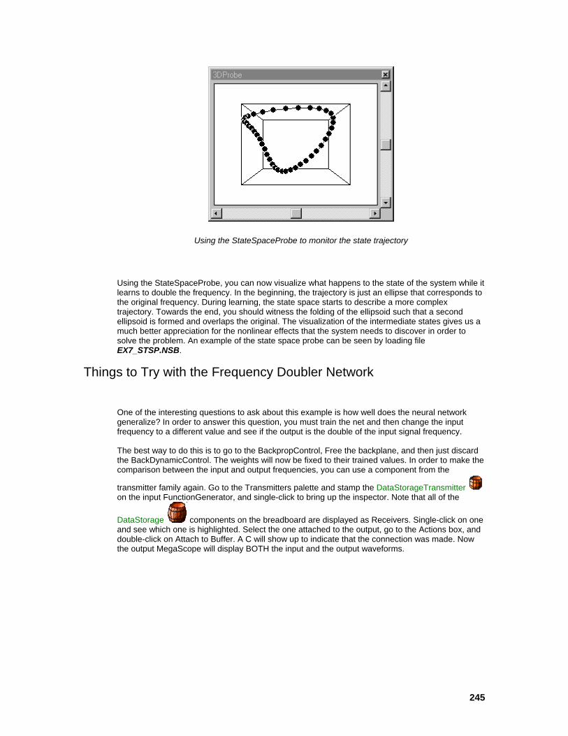
245

Using the StateSpaceProbe to monitor the state trajectory

Using the StateSpaceProbe, you can now visualize what happens to the state of the system while it learns to double the frequency. In the beginning, the trajectory is just an ellipse that corresponds to the original frequency. During learning, the state space starts to describe a more complex trajectory. Towards the end, you should witness the folding of the ellipsoid such that a second ellipsoid is formed and overlaps the original. The visualization of the intermediate states gives us a much better appreciation for the nonlinear effects that the system needs to discover in order to solve the problem. An example of the state space probe can be seen by loading file EX7_STSP.NSB.

Things to Try with the Frequency Doubler Network

One of the interesting questions to ask about this example is how well does the neural network generalize? In order to answer this question, you must train the net and then change the input frequency to a different value and see if the output is the double of the input signal frequency.

The best way to do this is to go to the BackpropControl, Free the backplane, and then just discard the BackDynamicControl. The weights will now be fixed to their trained values. In order to make the comparison between the input and output frequencies, you can use a component from the

transmitter family again. Go to the Transmitters palette and stamp the DataStorageTransmitter on the input FunctionGenerator, and single-click to bring up the inspector. Note that all of the

DataStorage components on the breadboard are displayed as Receivers. Single-click on one and see which one is highlighted. Select the one attached to the output, go to the Actions box, and double-click on Attach to Buffer. A C will show up to indicate that the connection was made. Now the output MegaScope will display BOTH the input and the output waveforms.

246

Viewing both the input and output using the DataStorageTransmitter

You are now ready to do comparisons. With a network properly trained, you should be able to go from 10 up to 100 Samples/Period and obtain a fairly good doubling of the frequency. This shows the generalization ability of this network. Of course, if you choose a square wave the method breaks down, simply because the relation between the data samples is very different. If you try a triangular wave, you will verify that the network is still able to double the frequency, but as you might expect, the corners will be rounded. It is recommended that you substitute the GammaAxon

by the LaguarreAxon and repeat the experiment. The Laguarre tends to be a little faster than the Gamma kernel.

It is also interesting to contrast this solution of the frequency doubler (using the input memory plane of a delay line) with a solution that instead, uses the memory by recurrency. One experiment is to substitute the input memory layer with context units creating a Jordan net.

247

A frequency doubler using recurrent hidden units

The figure above shows another possible configuration for solving the frequency doubling problem, but using "context units" that hold the values of the input units (Elman’s architecture). Use an IntegratorAxon for the context units which integrates the input signals, and a TanhAxon as the hidden layer with 2 PEs. At the input use an Axon with a single input. Use a FullSynapse to bring the output of each context unit to each hidden unit. The breadboard is shown in the figure above. The parameters of the trajectory learning should be as before, except that now you should use the same value for Samples/Exemplar for both the DynamicControl and BackDynamicControl (since a memory depth does not apply anymore).

This is a recurrent net, but you will not adapt the time constant of the context unit nor the connections of the input to the context units. Fix the time constant at 0.8. In order to keep this value, you should discard the gradient descent that will automatically be placed on the component when the backplane is allocated. Also select Fixed within the weights box under the Soma tab of the inspector. In this way, static backpropagation can be used. Choose the initial Step Size to be 1.0 and Momentum to be 0.6 for all Momentums. Learning progresses very fast. Looking at the MegaScope you will see that one of the parts of the sinewave is already there, but the other half appears very quickly. In the StateSpaceProbe you see that the double ellipsoid is still not present.

It is interesting to compare this solution with the gamma memory. Note that here the memory necessary to learn the problem is given by the context units, because they integrate the past. See figure above for configuration or load EX7_RECU.NSB.

Actual output vs. desired output for the recurrent frequency doubler

What You have Learned from the Frequency Doubler Example

The system you created was one that should have provided an introduction to trajectory learning. It was able to take a sinewave as input and produce a sinewave, which was doubled in frequency—not a trivial problem. At first, this was done using a tap delay line. You found that the system could still learn the problem after you reduced the number of taps, but kept the memory depth the same. You then substituted in a gamma delay line, which allowed you to use still fewer taps. You also constructed a system with context units, which replaced the memory structures of the delay lines with recurrent connections to provide memory. You found that this approach was well suited to solve this problem.

248

You were introduced to a few more components of NeuroSolutions. The StateSpaceProbe is a useful tool in dynamic systems, because it allows you to visualize the evolution of the system state in 3D. The DataStorageTransmitter is a useful tool for probing in that it allows you to transmit a signal from a remote component to a probe. The context units are important components for learning in time.

Unsupervised Learning Example Unsupervised Learning Example

Purpose - The purpose of this example is to discuss and present the unsupervised learning paradigms available in NeuroSolutions. You will present the Hebbian (including the normalized versions), the Sanger’s and the Oja’s rules. You will see that unsupervised learning has the appeal of preprocessing and feature extraction.

Components Introduced - OjasFull, SangersFull, HebbianFull.

Concepts Introduced - Unsupervised learning topologies (straight Hebbian, anti-Hebbian, Oja’s rule, and Sanger’s rule).

STEPS

Introduction to Unsupervised Learning

Noise Reduction with Oja's or Sanger's Learning

Things to Try with the Unsupervised Network

What You have Learned from the Unsupervised Learning Example

Introduction to Unsupervised Learning

Unsupervised learning is particularly well suited to perform feature extraction. There are a lot of problems where you do not know a priori the desired signal, nor what are the most important features of a given signal. This happens in compression, in signal and noise separation, and in feature extraction problems.

Unsupervised learning networks are normally very simple topologies that utilize the idea of correlation between input and output to process signals. It turns out that correlation can be easily implemented in a neural network through Hebbian learning. Most of the unsupervised learning rules, in one way or another, are based on Hebbian learning.

Hebbian learning has a slight problem of producing unbounded network weights (weights that keep increasing with each iteration). To compensate for this, you can either normalize the input data, clip the weights, or normalize the weights. The last idea is the more general, so extensions to the Hebbian learning (Oja’s rule or Sanger’s rule) are the recommended learning rules.

In Hebbian type learning, the weights are modified according to the product of the input and output at the weight, implying that there is no desired signal. Hence, it is not necessary to propagate the signal forward and the error backward, as in gradient descent learning. In terms of network construction, these networks are normally very simple in that they consist of a single layer of components.

249

NeuroSolutions provides five Hebbian type learning rules: straight Hebbian, anti-Hebbian, forced Hebbian, Oja’s rule, and Sanger’s rule. Please read the Unsupervised Learning topic to learn more about them.

Unsupervised palette

Noise Reduction with Oja's or Sanger's Learning

There are many types of applications that try to reduce the amount of noise in a signal. This can be accomplished through linear filtering if the noise and signal spectra do not overlap. Utilize the idea of principal components to extract the signal from noise.

If the signal is viewed as a vector, the principal components are basically the directions of the signal vector in signal space. Broadband noise totally fills in the signal space, so it has components in every direction. The signal normally exists in a subspace of lower dimension. Hence, if it is possible to project the signal plus noise on the subspace built from the principal components of the signal, then less noise power will be present and the signal will be less distorted.

This simple geometric projection can be achieved with Oja’s or Sanger’s rule applied to a single layer of linear components, simply because these two learning rules extract the principal components of the input signal. This means that the weight vectors of the network are the principal components, and the outputs are the projection of the input along these directions.

The figure below depicts the example that you will be building with NeuroSolutions. The network has a single layer of linear units (built from the Axon and an Ojas). You will be using a FunctionGenerator as your input, but since these unsupervised rules are static, you will need a TDNNAxon at the input layer. Therefore, the memory unit will transform the time signals into static patterns of a length equal to the size of the memory. Stamp a TDNNAxon on a new breadboard.

Construction of an unsupervised system using Oja’s rule

Select a memory of 10 Taps. The output will have a single PE. Stamp an Axon to the right of the TDNNAxon. The input to this network will be a sinewave of 20 Samples/Cycle added to uniformly distributed noise. Stamp a Function component on the Pre-Activity access of the TDNNAxon. Select a Noise component from the Input palette, stamp it over the FunctionGenerator and verify that the Variance is set to 1.

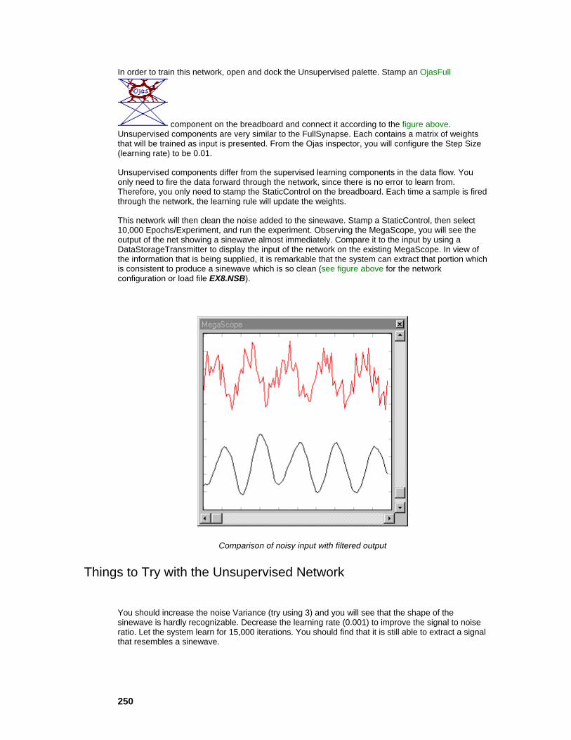
250

In order to train this network, open and dock the Unsupervised palette. Stamp an OjasFull

component on the breadboard and connect it according to the figure above. Unsupervised components are very similar to the FullSynapse. Each contains a matrix of weights that will be trained as input is presented. From the Ojas inspector, you will configure the Step Size (learning rate) to be 0.01.

Unsupervised components differ from the supervised learning components in the data flow. You only need to fire the data forward through the network, since there is no error to learn from. Therefore, you only need to stamp the StaticControl on the breadboard. Each time a sample is fired through the network, the learning rule will update the weights.

This network will then clean the noise added to the sinewave. Stamp a StaticControl, then select 10,000 Epochs/Experiment, and run the experiment. Observing the MegaScope, you will see the output of the net showing a sinewave almost immediately. Compare it to the input by using a DataStorageTransmitter to display the input of the network on the existing MegaScope. In view of the information that is being supplied, it is remarkable that the system can extract that portion which is consistent to produce a sinewave which is so clean (see figure above for the network configuration or load file EX8.NSB).

Comparison of noisy input with filtered output

Things to Try with the Unsupervised Network

You should increase the noise Variance (try using 3) and you will see that the shape of the sinewave is hardly recognizable. Decrease the learning rate (0.001) to improve the signal to noise ratio. Let the system learn for 15,000 iterations. You should find that it is still able to extract a signal that resembles a sinewave.

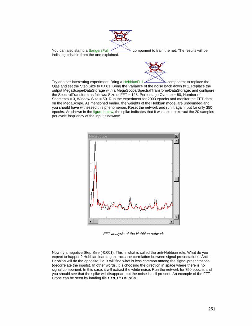
251

You can also stamp a SangersFull component to train the net. The results will be indistinguishable from the one explained.

Try another interesting experiment. Bring a HebbianFull component to replace the Ojas and set the Step Size to 0.001. Bring the Variance of the noise back down to 1. Replace the output MegaScope/DataStorage with a MegaScope/SpectralTransform/DataStorage, and configure the SpectralTransform as follows: Size of FFT = 128, Percentage Overlap = 50, Number of Segments = 3, Window Size = 50. Run the experiment for 2000 epochs and monitor the FFT data on the MegaScope. As mentioned earlier, the weights of the Hebbian model are unbounded and you should have witnessed this phenomenon. Reset the network and run it again, but for only 350 epochs. As shown in the figure below, the spike indicates that it was able to extract the 20 samples per cycle frequency of the input sinewave.

FFT analysis of the Hebbian network

Now try a negative Step Size (-0.001). This is what is called the anti-Hebbian rule. What do you expect to happen? Hebbian learning extracts the correlation between signal presentations. Anti-Hebbian will do the opposite, i.e. it will find what is less common among the signal presentations (decorrelate the inputs). In other words, it is choosing the direction in space where there is no signal component. In this case, it will extract the white noise. Run the network for 750 epochs and you should see that the spike will disappear, but the noise is still present. An example of the FFT Probe can be seen by loading file EX8_HEBB.NSB.

252

What You have Learned from the Unsupervised Learning Example

You have been introduced to four of the five Hebbian type learning rules provided by NeuroSolutions. Using Oja’s or Sanger’s rule, you were able to construct a simple network which could filter out much of the noise from a distorted sinewave. By analyzing the FFT using Hebbian learning, you were able to see the extraction of the sinewave. You were then able to extract the noise (which eliminated the sinewave) using the anti-Hebbian model. You also verified the unbounded nature of the weights using the straight Hebbian rule.

Principle Component Analysis Example Principal Component Analysis Example

Purpose - You will show that Sanger’s and Oja’s perform principal component analysis. To verify the extraction of the principle components, you will re-combine the extracted signals to approximate the original input.

Components Introduced - OjasFull, SangersFull.

Concepts Introduced - Principal component analysis, forced Hebbian learning.

STEPS

Introduction to Principal Component Analysis

Running the PCA Network

Things to Try with the PCA Network

What You have Learned from the Principal Component Analysis Example

Introduction to Principal Component Analysis

You will now perform principal component analysis on a complex waveform using Sanger’s and Oja’s rules. In this respect, Sanger’s is better because it always outputs the components in order.

The problem is to input a square wave to a one layer linear network with several outputs, train it with Sanger ‘s rule and observe the waveforms at the outputs. As you may know, a square wave is built from the addition of multiple sinewaves at the harmonics of the fundamental frequency, properly weighted and shifted. The Fourier series computes this decomposition.

Sanger’s and Oja’s networks can also provide a very similar decomposition. During learning, the weights will find the orthogonal directions (eigenvectors) associated with the square wave. The outputs will then be the projections on these directions. For a square wave, you can expect to find an infinite number of directions (infinite harmonics). For each frequency, you can expect to find two sinusoidal components that are orthogonal (just like the sine and the cosine).

Running the PCA Network

253

Starting from the Unsupervised Learning example, discard the Noise, increase the size of the TDNNAxon to have 30 Taps (once again to have a stable "view" of the input), drop the Ojas and replace it with a Sangers, and enlarge the output Axon to have 6 PEs. Configure the Step Size to 0.001, just to make sure that learning is accurate (it will be a bit slower). Change your input signal from a sine wave to a square wave of 20 Samples/Cycle. (see figure below for network configuration or load file EX9.NSB)

Configuration of PCA network

Observing the output MegaScope (run the network a few iterations and then autoscale), you will see that after training the output units will show pairs of sinusoids of the fundamental frequency and their odd harmonics. As expected, the sinusoids of a given frequency are orthogonal (when one reaches the peak the other goes through zero). Notice that there is an intrinsic ordering to the decomposition. The first two units give the slower components, followed by the next higher frequency, etc. You will not get this feature with Oja’s. It is remarkable that this network performed principal component analysis (sometimes also called singular value decomposition or Karhunen Loeve transforms) just using the correlation information, but you can expect this from the theory. The only difference with respect to the theoretical methods is that the amplitudes of the waves (which are associated through the power with the eigenvalues) are not estimated correctly.

Probing the activations to verify the principal component extraction

254

Things to Try with the PCA Network

Substitute the Sangers with the Ojas and verify that the principal components are not ordered. An interesting aspect can be found by adding all the six outputs using a FullSynapse and an Axon and plotting the result with another MegaScope. Fix the amplitude of this FullSynapse by dropping the MatrixEditor and entering 1 into every weight. Run the network again (without randomizing). If the amplitudes were right, the resulting wave should approximate the initial square wave built from three harmonics. You can play with the multiplicative constants to see if you get a square wave.

What You have Learned from the Principal Component Analysis Example

You were able to verify that both the Sanger’s and Oja’s rules can be used to extract the principle components from a complex waveform such as a square wave. The advantage of the Sanger’s model is that it produces components in order, where Oja’s does not. You were able to verify that these components could be re-combined to approximate the original signal. You tried this first by straight addition of the signals, but since the amplitudes of the principal components produced are not accurate, the result did not resemble a square wave.

Competitive Learning Example Competitive Learning Example

Purpose - You will introduce the principles of competitive learning by creating a system that is able to represent centers of clusters.

Components Introduced - StandardFull, ConscienceFull, ScatterPlot.

Concepts Introduced - The purpose of competitive learning, interpretation of scatter data.

STEPS

Introduction to Competitive Learning

Constructing the Competitive Network

Things to Try with the Competitive Network

What You have Learned from the Competitive Learning Example

Introduction to Competitive Learning

Competitive learning is a rather important unsupervised learning method. It enables the adaptive system to cluster input data into classes. There are a lot of engineering applications related to clustering, such as vector quantization and classification. In classification, one may want to divide the input data set into clusters and use their centers to represent the different classes. Competitive learning provides exactly this functionality. The user must decide how many classes the data has,

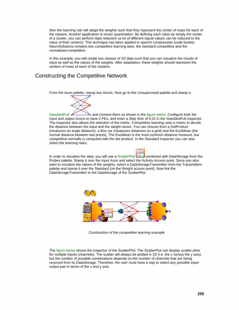
255

then the learning rule will adapt the weights such that they represent the center of mass for each of the classes. Another application is vector quantization. By defining each class as simply the center of a cluster, you can perform data reduction (a lot of different signal values can be reduced to the value of their centers). This technique has been applied to speech compression (code books). NeuroSolutions contains two competitive learning laws, the standard competitive and the normalized competitive.

In this example, you will create two classes of 2D data such that you can visualize the clouds of input as well as the values of the weights. After adaptation, these weights should represent the centers of mass of each of the clusters.

Constructing the Competitive Network

From the Axon palette, stamp two Axons. Now go to the Unsupervised palette and stamp a

StandardFull and connect them as shown in the figure below. Configure both the input and output Axons to have 2 PEs, and enter a Step Size of 0.01 in the StandardFull inspector. The inspector also allows the selection of the metric. Competitive learning uses a metric to decide the distance between the input and the weight vector. You can choose from a DotProduct (measures an angle distance), a Box car (measures distances on a grid) and the Euclidean (the normal distance between two points). The Euclidean is the most common distance measure, but competitive normally is computed with the dot product. In the Standard inspector you can also select the learning rates.

In order to visualize the data, you will use a ScatterPlot combined with DataStorage from the Probes palette. Stamp it over the input Axon and select the Activity Access point. Since you also want to visualize the values of the weights, select a DataStorageTransmitter from the Transmitters palette and stamp it over the Standard (on the Weight access point). Now link the DataStorageTransmitter to the DataStorage of the ScatterPlot.

Construction of the competitive learning example

The figure below shows the inspector of the ScatterPlot. The ScatterPlot can display scatter plots for multiple inputs (channels). The scatter will always be plotted in 2D (i.e. the x versus the y axis), but the number of possible combinations depends on the number of channels that are being received from its DataStorage. Therefore, the user must have a way to select any possible input-output pair in terms of the x and y axis.

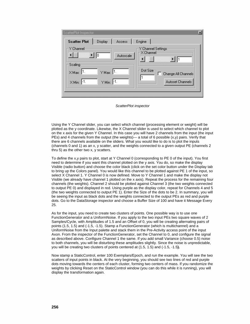
256

ScatterPlot inspector

Using the Y Channel slider, you can select which channel (processing element or weight) will be plotted as the y coordinate. Likewise, the X Channel slider is used to select which channel to plot on the x axis for the given Y Channel. In this case you will have 2 channels from the input (the input PEs) and 4 channels from the output (the weights)— a total of 6 possible (x,y) pairs. Verify that there are 6 channels available on the sliders. What you would like to do is to plot the inputs (channels 0 and 1) as an x, y scatter, and the weights connected to a given output PE (channels 2 thru 5) as the other two x, y scatters.

To define the x,y pairs to plot, start at Y Channel 0 (corresponding to PE 0 of the input). You first need to determine if you want this channel plotted on the y axis. You do, so make the display Visible (radio button) and choose the color black (click on the set color button under the Display tab to bring up the Colors panel). You would like this channel to be plotted against PE 1 of the input, so select X Channel 1. Y Channel 0 is now defined. Move to Y Channel 1 and make the display not Visible (we already have channel 1 plotted on the x axis). Repeat the process for the remaining four channels (the weights). Channel 2 should be plotted against Channel 3 (the two weights connected to output PE 0) and displayed in red. Using purple as the display color, repeat for Channels 4 and 5 (the two weights connected to output PE 1). Enter the Size of the dots to be 2. In summary, you will be seeing the input as black dots and the weights connected to the output PEs as red and purple dots. Go to the DataStorage inspector and choose a Buffer Size of 100 and have it Message Every 25.

As for the input, you need to create two clusters of points. One possible way is to use one FunctionGenerator and a UniformNoise. If you apply to the two input PEs two square waves of 2 Samples/Cycle, with Amplitudes of 1.5 and an Offset of 0, you will be creating alternating pairs of points (1.5, 1.5) and (-1.5, -1.5). Stamp a FunctionGenerator (which is multichannel) and a UniformNoise from the Input palette and stack them in the Pre-Activity access point of the input Axon. From the inspector of the FunctionGenerator, set the Channel to 0, and configure the signal as described above. Configure Channel 1 the same. If you add small Variance (choose 0.5) noise to both channels, you will be disturbing these amplitudes slightly. Since the noise is unpredictable, you will be creating two clusters of points centered at (1.5, 1.5) and (-1.5, -1.5).

Now stamp a StaticControl, enter 100 Exemplars/Epoch, and run the example. You will see the two scatters of input points in black. At the very beginning, you should see two lines of red and purple dots moving towards the centers of each cluster, forming two centers of mass. If you randomize the weights by clicking Reset on the StaticControl window (you can do this while it is running), you will display the transformation again.

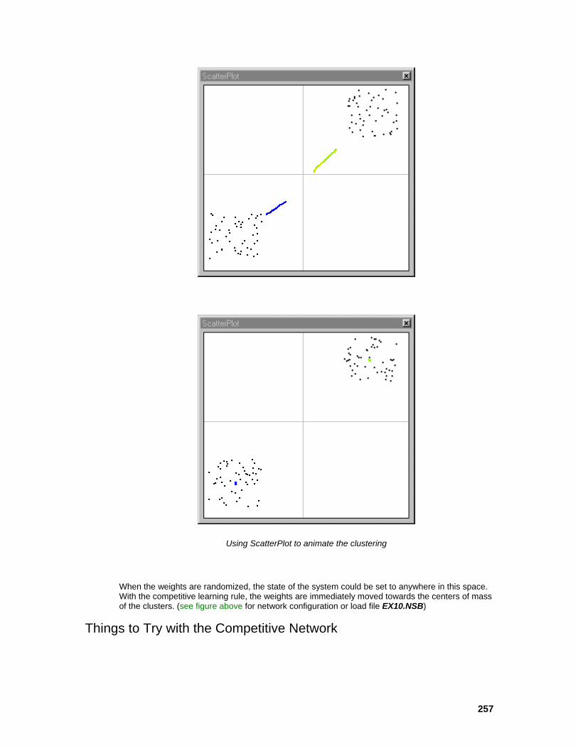
257

Using ScatterPlot to animate the clustering

When the weights are randomized, the state of the system could be set to anywhere in this space. With the competitive learning rule, the weights are immediately moved towards the centers of mass of the clusters. (see figure above for network configuration or load file EX10.NSB)

Things to Try with the Competitive Network

258

Try setting the Phase of one of the FunctionGenerators to 180. What do you expect to happen? Run the network again (without randomizing) and you should discover that the clusters are now moved to the other two quadrants and that the centers were still found.

You can see the effect of a bad selection of the initial number of clusters by selecting 3 output PEs. Since you have only two clusters of points, the third output unit will have its weights put half way between the other two, giving an erroneous result (you could interpret it as meaning that there are three clusters of data).

Now enter an offset of 2 in the FunctionGenerator. (You will have to autoscale the ScatterPlot to see both clusters.) Notice that the clusters now are not symmetrical with respect to the origin. Try to run the competitive network again. What do you find? The weights no longer go to the centers of the clusters. This is due to the dot product metric selected in the competitive. You can still solve the problem if you select Euclidean in the competitive level of the inspector of the competitive component. An alternative to solve this new problem is to use a new component, the

ConscienceFull . Select this component from the Unsupervised palette and use it to replace the StandardFull. The Conscience is a mechanism that keeps track of the number of times that a PE wins the competition. It is a competitive mechanism of its own. The two parameters in the ConscienceFull Inspector are beta (small value 0.001) and gamma (normally between 1 and 20). Try to solve the problem again, with the ConscienceFull component, and see that it can be solved easily.

Another interesting experiment is to take out the competitive learning rule and substitute it with the Sanger’s rule that you covered in the Principal Components Analysis example. Set the step size to 0.1. You should keep the input exactly as is. The purpose is to show how a change in the learning rule affects the information extracted from the same input. Can you foresee what will happen?

Competitive learning gave us the centers of the clusters. Sanger’s provides the principal directions for the data sets (principal components). Therefore, the weights of the FullSynapse should now seek a point on the unit circle (since the input is normalized) in the direction of the principal axis of the data clusters. These are the directions where the data projections are the largest. For this case, these can be obtained by drawing a line between the centers of the clusters and its perpendicular (the bisectors of the quadrants).

Keep the same learning rate and the same ScatterPlot settings. By running the example, you will see the larger dots representing the weights move towards the first quadrant bisector and the fourth quadrant bisector, as expected.

259

Principal components displayed with the ScatterPlot

If you randomize the weights during learning, you will see the weights jump to a random position and then track to the previous locations. By stopping the simulation and switching to the FunctionGenerator inspector, you can change the parameters of the waveforms. By choosing the triangular wave, you will find that the clusters of points move to the second and fourth quadrant. Immediately after, the synaptic weights will travel to the first and fourth quadrants.

What You have Learned from the Competitive Learning Example

260

You were able to construct a system that could take two clusters of data and find their centers of mass. You did this using the standard competitive learning rule, which updated the weights to represent the centers. You were able to visualize the learning process by plotting the input data and the centers using the ScatterPlot. You also saw the importance of selecting an appropriate number of clusters; otherwise the system may not perform well.

Kohonen Self Organizing Feature Map (SOFM) Example Kohonen Self Organizing Feature Map (SOFM) Example

Purpose - Kohonen self-organizing map is a very important component in self-organization because it preserves topological neighborhoods from the input space to the output space (neural field).

Components Introduced - LineKohonen, DiamondKohonen, SquareKohonen, WinnerTakeAllAxon, LinearScheduler.

Concepts Introduced - SOFM and scheduling of learning parameters.

STEPS

Introduction to SOFM Example

SOFM Network Construction

Running the SOFM Network

Things to Try with the SOFM Network

What you have Learned from the Kohonen SOFM Example

Introduction to SOFM Example

This example will build a self-organizing feature map (SOFM) from a 2D space into a 2D space. The input is a cloud of samples that are organized in a circle around the origin. The idea is to create a SOFM that will adequately represent this cloud of points in input space. The SOFM discretizes the input probability density function. Notice that you are going to do this with several different types of neighborhoods, and just a few PEs.

SOFM Network Construction

Start with an Axon, a LineKohonen and a WinnerTakeAllAxon as shown in the figure below. Set the number of PEs in the Axon to 2. The LineKohonenFull Synapse creates a line of PEs. The WinnerTakeAllAxon is a component that wins the competition in the

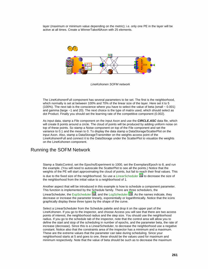
261

layer (maximum or minimum value depending on the metric); i.e. only one PE in the layer will be active at all times. Create a WinnerTakeAllAxon with 25 elements.

LineKohonen SOFM network

The LineKohonenFull component has several parameters to be set. The first is the neighborhood, which normally is set at between 100% and 70% of the linear size of the layer. Here set it to 5 (100%). The next tab is the conscience where you have to select the value of beta (small ~ 0.001) and gamma (large ~1 and 20). The next choice is the type of matrix used, which should select as dot Product. Finally you should set the learning rate of the competitive component (0.002).

As input data, stamp a File component on the input Axon and use the CIRCLE.ASC data file, which will create 8 points around a circle. The cloud of points will be produced by adding uniform noise on top of these points. So stamp a Noise component on top of the File component and set the variance to 0.1 and the mean to 0. To display the data stamp a DataStorage/ScatterPlot on the input Axon. Also, stamp a DataStorageTransmitter on the weights access point of the LineKohonenFull and connect it to the DataStorage under the ScatterPlot to visualize the weights on the LineKohonen component.

Running the SOFM Network

Stamp a StaticControl, set the Epochs/Experiment to 1000, set the Exemplars/Epoch to 8, and run the example. (You will need to autoscale the ScatterPlot to see all the points.) Notice that the weights of the PE will start approximating the cloud of points, but fail to reach their final values. This is due to the fixed size of the neighborhood. So use a LinearScheduler to decrease the size of the neighborhood from the initial value to a neighborhood of 1.

Another aspect that will be introduced in this example is how to schedule a component parameter. This function is implemented by the Schedule family. There are three schedulers, the LinearScheduler, the ExpScheduler , and the LogScheduler . As the names indicate, they decrease or increase the parameter linearly, exponentially or logarithmically. Notice that the icons graphically display these three types by the shape of the curve.

Select a LinearScheduler from the Schedule palette and drop it on the upper part of the LineKohonen. If you go to the inspector, and choose Access you will see that there are two access points of interest, the neighborhood radius and the step size. You should use the neighborhood radius. If you go to the schedule tab of the inspector, note that the control area will allow you to define the start and stop of the scheduling in number of epochs, and the parameter beta, the rate of increase (decrease). Since this is a LinearScheduler, to decrease the neighborhood use a negative constant. Notice also that the constraints area of the inspector has a minimum and a maximum. These are the extreme values that the parameter can take during scheduling. Since your neighborhood starts at 5 and goes to one, these should be the values used for maximum and minimum respectively. Note that the value of beta should be such as to decrease the maximum

262

value to the minimum in the number of epochs selected (i.e., beta = -0.0025). Put a MatrixViewer on top of the scheduler just to visualize the neighborhood parameter. Running the example again, you will see that the number of points in the display split when the neighborhood parameter passes through integer values, creating a much better approximation of the cloud of points.

Things to Try with the SOFM Network

You can change the neighborhood from LineKohonenFull to DiamondKohonen (4

nearest neighbors) or SquareKohonen (8 nearest neighbors). You will find out that the splitting of neighborhoods is much more readily apparent. Experiment with the size of the original neighborhood. If the original neighborhood is large, learning will be much slower, but all weights are brought to the cloud of points. Smaller neighborhoods make learning faster, but you loose some PEs. An example of using the SquareKohonenFull can be seen by loading file EX11.NSB. The example in this file also illustrates some of the versatile customizing features of the ScatterPlot probe in NeuroSolutions.

What you have Learned from the Kohonen SOFM Example

You have learned what the self organizing map is, and how to create one. There are a few parameters that need to be defined in the Kohonen components. For a more in depth treatment, see Kohonen Self-Organizing Maps. You also learned how to schedule parameters, like for instance the neighborhood using the LinearScheduler.

Character Recognition Example Character Recognition Example

Purpose - The purpose of this example is to show how non-conventional neural models can be easily simulated in NeuroSolutions. You will construct a counterpropagation network, which will integrate the unsupervised and supervised learning paradigms.

Components Introduced - SangersFull, ImageViewer, Noise, HebbianFull.

Concepts Introduced - Integration of supervised and unsupervised learning models.

STEPS

Introduction to Character Recognition Example

Constructing the Counterpropagation Network

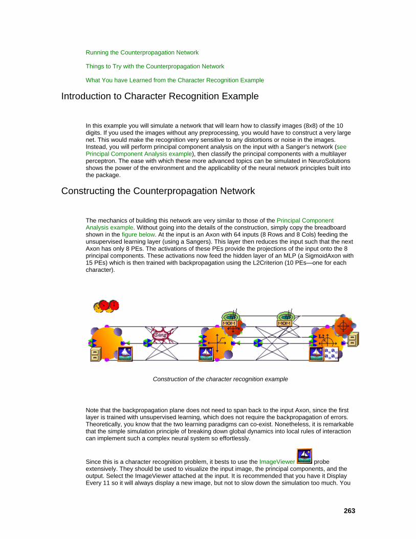
263

Running the Counterpropagation Network

Things to Try with the Counterpropagation Network

What You have Learned from the Character Recognition Example

Introduction to Character Recognition Example

In this example you will simulate a network that will learn how to classify images (8x8) of the 10 digits. If you used the images without any preprocessing, you would have to construct a very large net. This would make the recognition very sensitive to any distortions or noise in the images. Instead, you will perform principal component analysis on the input with a Sanger’s network (see Principal Component Analysis example), then classify the principal components with a multilayer perceptron. The ease with which these more advanced topics can be simulated in NeuroSolutions shows the power of the environment and the applicability of the neural network principles built into the package.

Constructing the Counterpropagation Network

The mechanics of building this network are very similar to those of the Principal Component Analysis example. Without going into the details of the construction, simply copy the breadboard shown in the figure below. At the input is an Axon with 64 inputs (8 Rows and 8 Cols) feeding the unsupervised learning layer (using a Sangers). This layer then reduces the input such that the next Axon has only 8 PEs. The activations of these PEs provide the projections of the input onto the 8 principal components. These activations now feed the hidden layer of an MLP (a SigmoidAxon with 15 PEs) which is then trained with backpropagation using the L2Criterion (10 PEs—one for each character).

Construction of the character recognition example

Note that the backpropagation plane does not need to span back to the input Axon, since the first layer is trained with unsupervised learning, which does not require the backpropagation of errors. Theoretically, you know that the two learning paradigms can co-exist. Nonetheless, it is remarkable that the simple simulation principle of breaking down global dynamics into local rules of interaction can implement such a complex neural system so effortlessly.

Since this is a character recognition problem, it bests to use the ImageViewer probe extensively. They should be used to visualize the input image, the principal components, and the output. Select the ImageViewer attached at the input. It is recommended that you have it Display Every 11 so it will always display a new image, but not to slow down the simulation too much. You

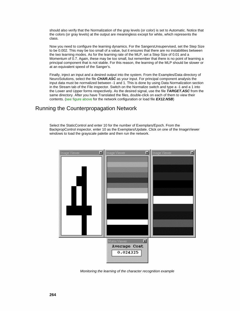
264

should also verify that the Normalization of the gray levels (or color) is set to Automatic. Notice that the colors (or gray levels) at the output are meaningless except for white, which represents the class.

Now you need to configure the learning dynamics. For the SangersUnsupervised, set the Step Size to be 0.002. This may be too small of a value, but it ensures that there are no instabilities between the two learning modes. As for the learning rate of the MLP, set a Step Size of 0.01 and a Momentum of 0.7. Again, these may be too small, but remember that there is no point of learning a principal component that is not stable. For this reason, the learning of the MLP should be slower or at an equivalent speed of the Sanger’s.

Finally, inject an input and a desired output into the system. From the Examples/Data directory of NeuroSolutions, select the file CHAR.ASC as your input. For principal component analysis the input data must be normalized between -1 and 1. This is done by using Data Normalization section in the Stream tab of the File inspector. Switch on the Normalize switch and type a -1 and a 1 into the Lower and Upper forms respectively. As the desired signal, use the file TARGET.ASC from the same directory. After you have Translated the files, double-click on each of them to view their contents. (see figure above for the network configuration or load file EX12.NSB)

Running the Counterpropagation Network

Select the StaticControl and enter 10 for the number of Exemplars/Epoch. From the BackpropControl inspector, enter 10 as the Exemplars/Update. Click on one of the ImageViewer windows to load the grayscale palette and then run the network.

Monitoring the learning of the character recognition example

265

You will see the patterns being flashed through the network and the mean square error decreasing. After 400 epochs, the ImageViewer at the output of the net should be displaying an upward scrolling white bar, meaning that the highest activation corresponds to the desired pattern. Training can continue (try 800 epochs) until basically all the outputs are dark except the desired one, proving that the net has learned the task well.

This example shows how a robust pre-processing sub-system can decrease the size of the nets required to learn a large task. It also has the added advantage of creating a system that is fairly immune to noise.

Things to Try with the Counterpropagation Network

An interesting experiment is to stop the learning and add noise to the input. Just stack a Noise

component from the Input palette on the File component at the input. Set the Variance (of all channels) to 0.2. Now set the learning on the Sanger’s to 0, Free the backprop plane, and discard the BackStaticControl. Now run the net again with the frozen weights. You will not be able to recognize many of the characters due to the noise, but notice that the white bar is still scrolling as it did before, meaning that there is enough information within the principal components to still accurately classify the patterns.

Testing the classification ability of the system by using a noisy input

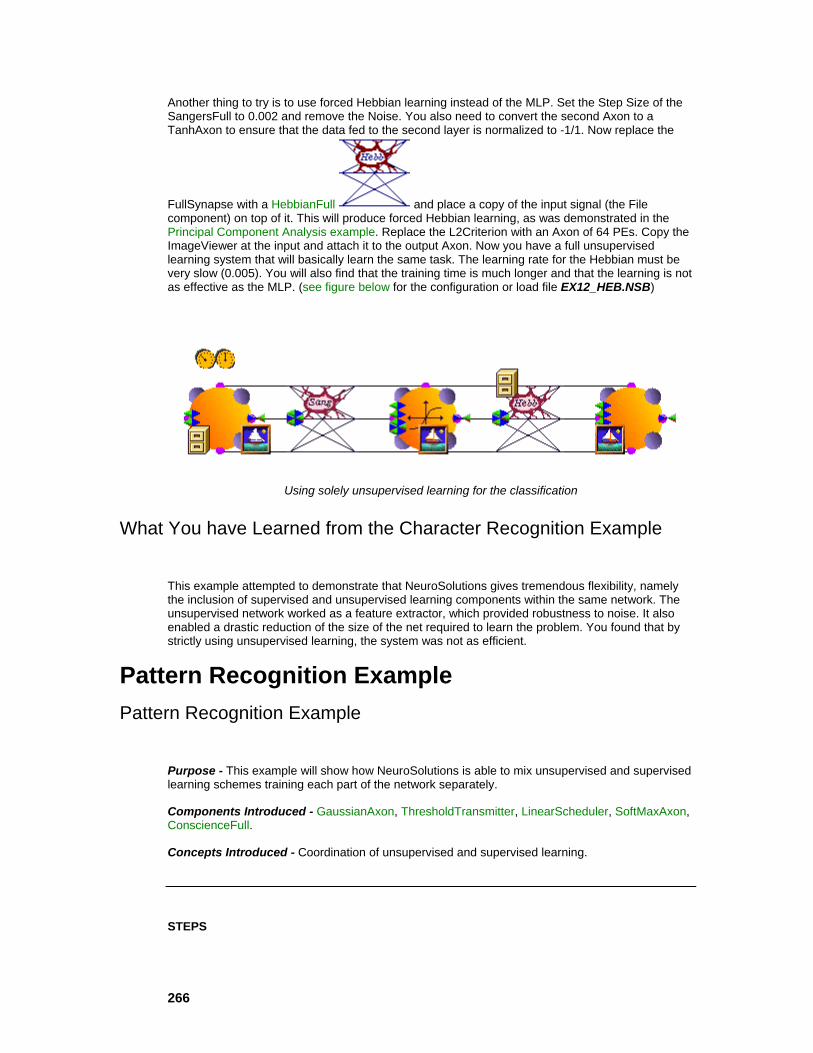
266

Another thing to try is to use forced Hebbian learning instead of the MLP. Set the Step Size of the SangersFull to 0.002 and remove the Noise. You also need to convert the second Axon to a TanhAxon to ensure that the data fed to the second layer is normalized to -1/1. Now replace the

FullSynapse with a HebbianFull and place a copy of the input signal (the File component) on top of it. This will produce forced Hebbian learning, as was demonstrated in the Principal Component Analysis example. Replace the L2Criterion with an Axon of 64 PEs. Copy the ImageViewer at the input and attach it to the output Axon. Now you have a full unsupervised learning system that will basically learn the same task. The learning rate for the Hebbian must be very slow (0.005). You will also find that the training time is much longer and that the learning is not as effective as the MLP. (see figure below for the configuration or load file EX12_HEB.NSB)

Using solely unsupervised learning for the classification

What You have Learned from the Character Recognition Example

This example attempted to demonstrate that NeuroSolutions gives tremendous flexibility, namely the inclusion of supervised and unsupervised learning components within the same network. The unsupervised network worked as a feature extractor, which provided robustness to noise. It also enabled a drastic reduction of the size of the net required to learn the problem. You found that by strictly using unsupervised learning, the system was not as efficient.

Pattern Recognition Example Pattern Recognition Example

Purpose - This example will show how NeuroSolutions is able to mix unsupervised and supervised learning schemes training each part of the network separately.

Components Introduced - GaussianAxon, ThresholdTransmitter, LinearScheduler, SoftMaxAxon, ConscienceFull.

Concepts Introduced - Coordination of unsupervised and supervised learning.

STEPS

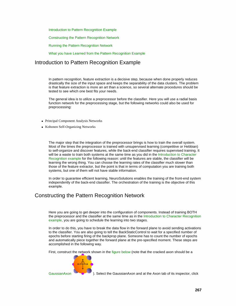
267

Introduction to Pattern Recognition Example

Constructing the Pattern Recognition Network

Running the Pattern Recognition Network

What you have Learned from the Pattern Recognition Example

Introduction to Pattern Recognition Example

In pattern recognition, feature extraction is a decisive step, because when done properly reduces drastically the size of the input space and keeps the separability of the data clusters. The problem is that feature extraction is more an art than a science, so several alternate procedures should be tested to see which one best fits your needs.

The general idea is to utilize a preprocessor before the classifier. Here you will use a radial basis function network for the preprocessing stage, but the following networks could also be used for preprocessing:


Kohonen Self-Organizing Networks

The major step that the integration of the preprocessor brings is how to train the overall system. Most of the times the preprocessor is trained with unsupervised learning (competitive or Hebbian) to self-organize and discover features, while the back-end classifier requires supervised training. It will be a waste to train both systems at the same time as you did in the Introduction to Character Recognition example for the following reason: until the features are stable, the classifier will be learning the wrong thing. You can choose the learning rates of the classifier much slower than those of the feature extractor, but the point is that in terms of computation you are training both systems, but one of them will not have stable information.

In order to guarantee efficient learning, NeuroSolutions enables the training of the front-end system independently of the back-end classifier. The orchestration of the training is the objective of this example.

Constructing the Pattern Recognition Network

Here you are going to get deeper into the configuration of components. Instead of training BOTH the preprocessor and the classifier at the same time as in the Introduction to Character Recognition example, you are going to schedule the learning into two stages.

In order to do this, you have to break the data flow in the forward plane to avoid sending activations to the classifier. You are also going to tell the BackStaticControl to wait for a specified number of epochs before starting firing of the backprop plane. Someone has to count the number of epochs and automatically piece together the forward plane at the pre-specified moment. These steps are accomplished in the following way.

First, construct the network shown in the figure below (note that the cracked axon should be a

GaussianAxon ). Select the GaussianAxon and at the Axon tab of its inspector, click

268

off the data flow ON and Turn ON after RESET switches. Notice that the Axon will crack (as shown in the figure below) meaning that the dataflow is interrupted. Also, in the Transfer Function tab, set the number of PE’s to 3.

Now click on the BackStaticControl to access its inspector. Click off the two switches Learning and Learn after RESET. This means that when you press the reset switch supervised learning will not start automatically. Notice that the red double dial was transformed to a single gray dial to demonstrate that its functionality has been changed.

Construction of the pattern recognition network

Now that these features are disabled, something must turn them on at the right time. Towards that

goal, you will use a ThresholdTransmitter . Select the ThresholdTransmitter above the StaticController and open its corresponding inspector. Set the threshold to 10, and click the greater than (>) switch. This means that when the controller epoch counts pass 10 the ThresholdTransmitter will broadcast a command. The problem is who is going to listen?

If you go to the Transmitter tab of the ThresholdTransmitter inspector, you will find a list of possible receivers of the message. First select the GaussianAxon as the receiver (note that the components are listed in the order in which they were pasted on the breadboard). After clicking on it, the action list will display the possible actions. Select the setFireNext action. If this action says (FALSE) you will need to set it to true by typing TRUE in the Parameter form cell and pressing the set button. Now, enable this action by double clicking the setFireNext(TRUE) line. Notice that a "C" will appear meaning that a connection was made. Now, when the ThresholdTransmitter fires, the Axon will turn on data flow and the right side of the topology (the classifier) will be able to learn. Select the assignCenters() and assignVariance() actions and double click them to connect them also. This will assign the centers and the variance of the GaussianAxon based on the weights when the ThresholdTransmitter fires.

Now select the ConscienceFull as the receiver. Double click the action setLearning(FALSE). This will stop the learning in the preprocessor section when the ThresholdTransmitter fires. You also need to enable the backpropagation learning for the classifier section when the ThresholdTransmitter fires. To do this, select the BackStaticControl as the receiver and double click the setLearning(TRUE) action.

269

Transmitter Inspector

Next, you need to schedule the learning rate of the ConscienceFull component. It should be decreased linearly. Click on the LinearScheduler above the ConscienceFull component to open its inspector. Within the Access tab, select the Unsupervised Step Size as the access point. Going back to the schedule tab, you should set the start epoch to 1 and the end epoch to 10 in this case, since the unsupervised run was set above at 10 iterations.

You still have to tell the scheduler how you want to schedule the parameter. In this case you want to decrease the learning rate, so beta should be a negative value. How negative depends on the annealing rate that you want. The right side of the inspector displays two constraint values, a minimum and a maximum. In this case the maximum should be chosen equal to the initial setting of the ConscienceFull learning rate (use .01). The minimum constraint is the smallest learning rate that you want for this application (use .001). Now beta can be easily computed, because it should decrease the step size from the maximum to the minimum in 10 iterations. The value of beta can be approximated, since the bounds are always met. Data that can be used for training this network are located in files FAULT.ASC for the input file and FAULTT.ASC for the desired file.

Running the Pattern Recognition Network

Now you are ready to run the pattern recognition network. Before pressing the run button, notice that the dataflow is interrupted by the cracked axon after the ConscienceFull, i.e. you will train the RBF preprocessor for 10 iterations alone, and then the classifier for another 40 iterations (for Epochs/Experiment = 50).

Notice that the scheduler value starts at 0.01 and decreases linearly. Notice also that the cost is at zero (for the first 10 Epochs), signaling that the classifier is not learning. When the epoch counter passes over 10, the cracked Axon is reconstructed into a GaussianAxon, and the MSE starts changing. Notice how much slower the epoch counter becomes. This is the reason you implemented all these features, to make the simulations much more efficient.

If you stamp and open a Hinton over the ConscienceFull, you will find that during the first 10 iterations the weights are changing, fast at first, then very slowly since the learning rates are being decreased be the LinearScheduler. After 10 iterations, the Hinton diagram will become unchanged, signaling that the weights quit adapting.

270

The procedure just described also applies to a PCA network and a Kohonen SOFM Network. You should try these networks to have a feel for how they behave (see Construction of the Pattern Recognition Network figure for the configuration or load the file EX13.NSB).

What you have Learned from the Pattern Recognition Example

In this example you have learned a very important lesson on how to combine data flow for unsupervised and supervised learning. The synchronization aspects that were described in this example are very valuable to design sophisticated simulations.

Time Series Prediction Example Time Series Prediction Example

Purpose - The purpose of this example is to show how artificial neural networks can be used to predict chaotic time series. To show this, you will construct a time lagged recurrent net (TLRN) that will be designed to predict the next point (or the next few points ahead) of a time series.

Components Introduced - LinearAxon, LaguarreAxon.

Concepts Introduced - Performing dynamic modeling with time lagged recurrent neural (TLRN) networks.

STEPS

Introduction to Time Series Prediction Example

Constructing the TLRN Network

Running the TLRN Network

What You have Learned from the Time Series Prediction Example

Introduction to Time Series Prediction Example

Dynamic modeling is the process of identifying the system that produced a time series, assumed to be created by a dynamically system. You will be using a time series produced by the Mackey-Glass system, having a delay of 30. This system is mildly chaotic for this choice of delay (largest Lyapunov exponent of 0.02 bits/sec).

Our goal is to predict the Mackey-Glass system using a time lagged recurrent neural network. A time lagged recurrent network has the static PEs substituted by PEs with short term memories, such as the gamma, the Laguarre or the tap delay line.

How can you construct and train such an ANN system? The core idea is that you should train the ANN as a nonlinear predictor, i.e. the input is delayed by L samples before being presented to the net, and the input signal without delays becomes the desired response. Since it is best to match a time series, and as long as the network is recurrent, you should use trajectory learning as your learning paradigm. For the case of prediction with a net using TDNNAxon (tap delay line) memory structures, trajectory learning is equivalent to static backpropagation in batch mode (the batch is

271

the length of the trajectory), but as soon as you have a net that is recurrent, this equivalency no longer holds.

Constructing the TLRN Network

Stamp a LaguarreAxon for the input, a TanhAxon, another LaguarreAxon, a

LinearAxon , and two FullSynapse components and connect them as shown in the figure below. Note that the Laguarre is a local recurrent memory structure. Set the number of taps of the LaguarreAxon at the input to 4. Set the number of taps of the LaguarreAxon in the hidden layer to 2. Set the number of PEs of the TanhAxon to 8 (thus, you must also set the number of Rows of the hidden layer LaguarreAxon to 8). You will use the L2Criterion and Trajectory learning as the gradient descent paradigm (using a Normalized Step Size of 0.5 and Momentum Rate of 0.7 except for the Momentum components above the two BackLaguarreAxons for which you should use a Step Size of .05 and a Momentum Rate of .1). Stamp a DynamicControl and use a trajectory (Samples/Exemplar in the DynamicControl) of 50 samples and set the Exemplars/Epoch to 6. Set the back trajectory (Samples/Exemplar in the BackDynamicControl) to 50 samples. The gradients will be updated at each exemplar (verify that the Exemplars/Update is set to 1). Now stamp two File components and use the file MG300.ASC as both the input and the desired signal. This is a well-known chaotic time series. Offset the desired signal file by three samples, which can be accomplished by pressing the customize button in file property page of the File inspector. This will show a panel where you should click the segment switch on, enter 3 in the offset, and enter 300 as the duration. This same procedure should be done with the input file, except use 0 offset and 300 duration. Set the Normalize switch for both the input and desired signal and enter -1 and 1 for the Lower and Upper values of the normalization range, respectively.

Construction of the prediction network

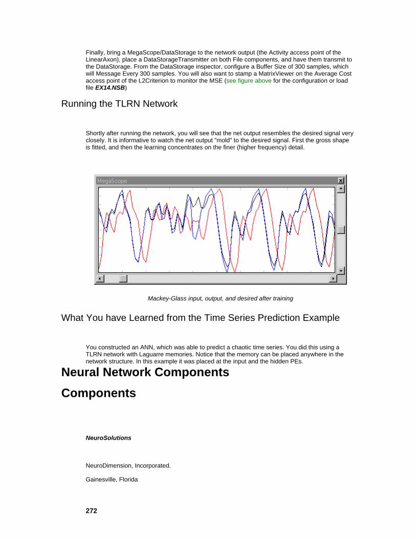
272

Finally, bring a MegaScope/DataStorage to the network output (the Activity access point of the LinearAxon), place a DataStorageTransmitter on both File components, and have them transmit to the DataStorage. From the DataStorage inspector, configure a Buffer Size of 300 samples, which will Message Every 300 samples. You will also want to stamp a MatrixViewer on the Average Cost access point of the L2Criterion to monitor the MSE (see figure above for the configuration or load file EX14.NSB)

Running the TLRN Network

Shortly after running the network, you will see that the net output resembles the desired signal very closely. It is informative to watch the net output "mold" to the desired signal. First the gross shape is fitted, and then the learning concentrates on the finer (higher frequency) detail.

Mackey-Glass input, output, and desired after training

What You have Learned from the Time Series Prediction Example

You constructed an ANN, which was able to predict a chaotic time series. You did this using a TLRN network with Laguarre memories. Notice that the memory can be placed anywhere in the network structure. In this example it was placed at the input and the hidden PEs.

Neural Network Components Components

NeuroSolutions



273

Purpose

This chapter provides a detailed description of each component available in NeuroSolutions.

Engine Family

Ancestor: ImageView Family

All NeuroSolutions components will belong to the Engine family. Being an Engine provides communication and control of inspectors and animation windows. The Engine inspector provides the ability to have the component's animation window opened after the component is unarchived, and the ability to fix components to their superengine.

User Interaction:

Inspector

Macro Actions

Activation Family Axon Family

Axon

Family: Axon Family

Superclass: Soma

Backprop Dual: BackAxon

Description:

274

The Axon simply performs an identity map between its input and output activity. The Axon is the first member of the Axon family, and all subsequent members will subclass its functionality. Furthermore, each subclass will use the above icon with a graph of their activation function superimposed on top.


User Interaction:

Drag and Drop

Inspector

Access Points

Example

DLL Implementation

Macro Actions

See Also

BiasAxon

Family: Axon Family

Superclass: Axon

Backprop Dual: BackBiasAxon

Description:

The BiasAxon simply provides a bias term, which may be adapted. Most nonlinear axons are subclasses of this component in order to inherit this bias characteristic.

275


Note: The Weights access point of the BiasAxon provides access to the Bias vector ( in the above equation).

User Interaction:

Drag and Drop

Inspector

Access Points

Example

DLL Implementation

See Also

CombinerAxon

Family: Axon Family

Superclass: Axon

Backprop Dual: BackCombinerAxon

Description: The CombinerAxon multiplies each neuron from the top half of the Axon with the corresponding neuron from the bottom half of the Axon and overwrites the activity of the top neuron with this

276

product. This Axon has twice as many inputs as it has outputs. This component is normally used within the neural-fuzzy architecture built by the NeuralBuilder.


where N is equal to the number of input PEs and i < N/2.

User Interaction:

Inspector

Drag and Drop

Access Points

GaussianAxon

Family: Axon Family

Superclass: LinearAxon

Backprop Dual: None

Description:

The GaussianAxon implements a radial basis function layer. There is a significant difference between the GaussianAxon and other members of the Axon family. The GaussianAxon only responds significantly to a local area of the input space (where the peak of the Gaussian is located). It is therefore considered to be a local function approximator. The center of the Gaussian is controlled using the bias weight inherited from the BiasAxon, and its width using the β parameter inherited from the LinearAxon.


277

Note: The Weights access point of the GaussianAxon provides access to the Bias vector ( in the above equation). These weights control the locations of the centers of the Gaussian functions.

User Interaction:

Drag and Drop

Inspector

Access Points

Example

DLL Implementation

Macro Actions

LinearAxon

Family: Axon Family

Superclass: BiasAxon

Backprop Dual: BackLinearAxon

Description:

The LinearAxon implements a linear axon with slope and offset control. It is therefore more powerful than the BiasAxon (because it implements an affine transform). The bias is inherited from the BiasAxon and can be adapted, but the slope is controlled by an additional parameter β, which is not adaptive.


278

Note: The Weights access point of the LinearAxon provides access to the Bias vector ( in the above equation).

User Interaction:

Drag and Drop

Inspector

Access Points

Example

DLL Implementation

Macro Actions

LinearSigmoidAxon

Family: Axon Family


Backprop Dual: BackSigmoidAxon

Description:

The LinearSigmoidAxon substitutes the intermediate portion of the sigmoid by a line of slope β, making it a piecewise linear approximation of the sigmoid. This PE has an input-output map that is discontinuous, so it is not recommended for learning. However, when used with the BackSigmoidAxon it can learn. This component is more computationally efficient that the SigmoidAxon (it is much easier to compute the map).


279

where is the scaled and offset activity inherited from the LinearAxon.

Note: The Weights access point of the LinearSigmoidAxon provides access to the Bias vector ( in the above equation).

User Interaction:

Drag and Drop

Inspector

Access Points

Example

DLL Implementation

LinearTanhAxon

Family: Axon Family


Backprop Dual: BackTanhAxon

Description:

The LinearTanhAxon substitutes the intermediate portion of the tanh by a line of slope β, making it a piecewise linear approximation of the tanh. This PE has an input-output map that is discontinuous, so it is not recommended for learning. However, when used with the BackTanhAxon

280

it can learn. This component is more computationally efficient that the TanhAxon (it is much easier to compute the map).



Note: The Weights access point of the LinearTanhAxon provides access to the Bias vector ( in the above equation).

User Interaction:

Drag and Drop

Inspector

Access Points

Example

DLL Implementation

NormalizedAxon

Family: Axon Family

Superclass: Axon

Backprop Dual: BackNormalizedAxon

281

Description: The NormalizedSigmoidAxon divides each neuron by the sum of the inputs. This component is normally used within the neural-fuzzy architecture built by the NeuralBuilder.


User Interaction:

Inspector

Drag and Drop

Access Points

NormalizedSigmoidAxon

Family: Axon Family

Superclass: SigmoidAxon

Backprop Dual: BackNormalizedSigmoidAxon

Description: The NormalizedSigmoidAxon applies a scaled and biased sigmoid function to each neuron in the layer. The scaling factor and bias are inherited from the SigmoidAxon. In addition, each neuron is scaled by the ratio of the neuron's input to the sum of the inputs. This component is normally used within the neural-fuzzy architecture built by the NeuralBuilder.


282

where is the activation function inherited from the SigmoidAxon.

User Interaction:

Inspector

Drag and Drop

Access Points

SigmoidAxon

Family: Axon Family


Backprop Dual: BackSigmoidAxon

Description:

The SigmoidAxon applies a scaled and biased sigmoid function to each neuron in the layer. The scaling factor and bias are inherited from the LinearAxon. The range of values for each neuron in the layer is between 0 and 1. Such nonlinear elements provide a network with the ability to make soft decisions.


283


Note: The Weights access point of the SigmoidAxon provides access to the Bias vector ( in the above equation).

User Interaction:

Inspector

Drag and Drop

Access Points

Example

DLL Implementation

SoftMaxAxon

Family: Axon Family


Description:

The SoftMaxAxon is a component used to interpret the output of the neural net as a probability. In order for a set of numbers to constitute a probability density function, their sum must equal one.

Often the output of a neural network produces a similarity measure. In order to convert this similarity measure to a probability, the SoftMaxAxon is used at the output of the network.


284


Note: The Weights access point of the SoftMaxAxon provides access to the Bias vector ( in the above equation).

User Interaction:

Drag and Drop

Inspector

Access Points

Example

DLL Implementation

TanhAxon

Family: Axon Family


Backprop Dual: BackTanhAxon

Description:

The TanhAxon applies a bias and tanh function to each neuron in the layer. This will squash the range of each neuron in the layer to between -1 and 1. Such nonlinear elements provide a network with the ability to make soft decisions.


285


Note: The Weights access point of the TanhAxon provides access to the Bias vector ( in the above equation).

User Interaction:

Inspector

Drag and Drop

Access Points

Example

DLL Implementation

ThresholdAxon

Family: Axon Family


Description:

The ThresholdAxon will output a 1 if the input plus bias are positive and -1 otherwise. Such nonlinear elements provide a network with the ability to implement hard decision functions.


286

where is the offset activity inherited from the BiasAxon.

Note: The Weights access point of the ThresholdAxon provides access to the Bias vector ( in the above equation).

User Interaction:

Inspector

Drag and Drop

Access Points

Example

DLL Implementation

WinnerTakeAllAxon

Family: Axon Family

Superclass: Axon

Description:

The winner-take-all is a special type of Axon that ensures that only one PE is active at all times (the winner). So the output of all the PEs of that layer are compared, and the one that is largest (or smallest) wins the competition.


287

User Interaction:

Drag and Drop

Inspector

Access Points

Example

DLL Implementation

Macro Actions

Access Points

Axon Family Access Points

Family: Axon Family

Access points allow simulation components that are not part of the neural network topology to probe and/or alter data flowing through the network. All members of the Axon family share a standard functional form. The sub-system block diagram given in Axon Family depicted this functionality. Access to data flowing through any axon is provided at the following three access points,

Pre-Activity Access:

Attaches the Access component to the vector sum just prior to applying the activation function . It is important to realize that this access point does not correspond to any physical

storage within the simulation. In other words, data may be injected or probed as activity flows

288

through the network, but is then immediately lost. Trying to alter the pre-activity out of sync with the network data flow will actually alter the data storage for Activity Access.

Activity Access:

Attaches the Access component to the vector of activity immediately after the function map

Weights Access:

All adaptive weights within the axon are reported by attaching to Weight Access. This data may be reported in vector or matrix form, depending on how the axon stores it. If a component does not have any weights, this access point will not appear in the inspector.

Winning PE Access (WinnerTakeAllAxon only):

With a "winner-take-all" output of a Self-Organizing Map (SOM), the winning PE gets a value of 1 and all the others get a value of 0. This access point provides the numeric value of the winning PE.

See Also

DLL Implementation

Axon DLL Implementation

Component: Axon

Protocol: PerformAxon

Description:

The Axon component does not modify the data fed into the processing elements (PEs).

Code: void performAxon( DLLData *instance, // Pointer to instance data (may be NULL) NSFloat *data, // Pointer to the layer of PEs int rows, // Number of rows of PEs in the layer int cols // Number of columns of PEs in the layer

289

) { }

BiasAxon DLL Implementation

Component: BiasAxon

Protocol: PerformBiasAxon

Description:

The BiasAxon component adds a bias term to each processing element (PE). The bias vector contains the bias term for each PE and can be thought of as the Axon’s adaptable weights.

Code: void performBiasAxon( DLLData *instance, // Pointer to instance data (may be NULL) NSFloat *data, // Pointer to the layer of PEs int rows, // Number of rows of PEs in the layer int cols // Number of columns of PEs in the layer NSFloat *bias // Pointer to the layer's bias vector ) { int i, length=rows*cols; for (i=0; i<length; i++) data[i] += bias[i]; }

GaussianAxon DLL Implementation

290

Component: GaussianAxon

Protocol: PerformLinearAxon

Description:

The GaussianAxon applies a gaussian function to each neuron in the layer. The bias vector determines the center of the gaussian for each PE, and the beta term determines the width of the gaussian for all PEs. The range of values for each neuron in the layer is between 0 and 1.

Code: void performLinearAxon( DLLData *instance, // Pointer to instance data (may be NULL) NSFloat *data, // Pointer to the layer of PEs int rows, // Number of rows of PEs in the layer int cols // Number of columns of PEs in the layer NSFloat *bias // Pointer to the layer's bias vector NSFloat beta // Slope gain scalar, same for all PEs ) { int i, length=rows*cols; for (i=0; i<length; i++) { data[i] += bias[i]; data[i] = (NSFloat)exp(-beta*data[i]*data[i]); } }

LinearAxon DLL Implementation

Component: LinearAxon


Description:

291

The LinearAxon component adds to the functionality of the BiasAxon by adding a beta term that is the same for all processing elements (PEs). This scalar specifies the slope of the linear transfer function.

Code: void performLinearAxon( DLLData *instance, // Pointer to instance data (may be NULL) NSFloat *data, // Pointer to the layer of PEs int rows, // Number of rows of PEs in the layer int cols // Number of columns of PEs in the layer NSFloat *bias // Pointer to the layer's bias vector NSFloat beta // Slope gain scalar, same for all PEs ) { int i, length=rows*cols; for (i=0; i<length; i++) data[i] = beta*data[i] + bias[i]; }

LinearSigmoidAxon DLL Implementation

Component: LinearSigmoidAxon


Description:

The implementation for the LinearSigmoidAxon is the same as that of the LinearAxon except that the transfer function is clipped at 0 and 1.

Code: void performLinearAxon( DLLData *instance, // Pointer to instance data (may be NULL) NSFloat *data, // Pointer to the layer of PEs int rows, // Number of rows of PEs in the layer int cols // Number of columns of PEs in the layer NSFloat *bias // Pointer to the layer's bias vector

292

NSFloat beta // Slope gain scalar, same for all PEs ) { int i, length=rows*cols; for (i=0; i<length; i++) { data[i] = beta*data[i] + bias[i]; if (data[i] < 0.0f) data[i] = 0.0f; else if (data[i] > 1.0f) data[i] = 1.0f; } }

LinearTanhAxon DLL Implementation

Component: LinearTanhAxon


Description:

The implementation for the LinearTanhAxon is the same as that of the LinearAxon except that the transfer function is clipped at -1 and 1.

Code: void performLinearAxon( DLLData *instance, // Pointer to instance data (may be NULL) NSFloat *data, // Pointer to the layer of PEs int rows, // Number of rows of PEs in the layer int cols // Number of columns of PEs in the layer NSFloat *bias // Pointer to the layer's bias vector NSFloat beta // Slope gain scalar, same for all PEs ) { int i, length=rows*cols; for (i=0; i<length; i++) { data[i] = beta*data[i] + bias[i];

293

if (data[i] < -1.0f) data[i] = -1.0f; else if (data[i] > 1.0f) data[i] = 1.0f; } }

SigmoidAxon DLL Implementation

Component: SigmoidAxon


Description:

The SigmoidAxon applies a scaled and biased sigmoid function to each neuron in the layer. The range of values for each neuron in the layer is between 0 and 1.

Code: void performLinearAxon( DLLData *instance, // Pointer to instance data (may be NULL) NSFloat *data, // Pointer to the layer of PEs int rows, // Number of rows of PEs in the layer int cols // Number of columns of PEs in the layer NSFloat *bias // Pointer to the layer's bias vector NSFloat beta // Slope gain scalar, same for all PEs ) { int i, length=rows*cols; for (i=0; i<length; i++) data[i] = 1.0f / (1.0f + (NSFloat)exp(-(beta*data[i] + bias[i]))); }

SoftMaxAxon DLL Implementation

294

Component: SoftMaxAxon


Description:

The SoftMaxAxon is a component used to interpret the output of the neural net as a probability, such that the sum of the outputs is equal to one. Unlike the WinnerTakeAllAxon, this component outputs positive values for the non-maximum PEs. The beta term determines how hard or soft the max function is. A high beta corresponds to a harder max; meaning that the PE with the highest value is accentuated compared to the other PEs. The bias vector has no effect on this component. The range of values for each neuron in the layer is between 0 and 1.

Code: void performLinearAxon( DLLData *instance, // Pointer to instance data (may be NULL) NSFloat *data, // Pointer to the layer of PEs int rows, // Number of rows of PEs in the layer int cols // Number of columns of PEs in the layer NSFloat *bias // Pointer to the layer's bias vector NSFloat beta // Slope gain scalar, same for all PEs ) { int i, length=rows*cols; NSFloat sum=(NSFloat)0.0; for (i=0; i<length; i++) { data[i] = beta*data[i]; sum += data[i] = (NSFloat)exp(data[i]); } for (i=0; i<length; i++) data[i] /= sum; }

TanhAxon DLL Implementation

295

Component: TanhAxon


Description:

The TanhAxon applies a scaled and biased hyperbolic tangent function to each neuron in the layer. The range of values for each neuron in the layer is between -1 and 1.

Code: void performLinearAxon( DLLData *instance, // Pointer to instance data (may be NULL) NSFloat *data, // Pointer to the layer of PEs int rows, // Number of rows of PEs in the layer int cols // Number of columns of PEs in the layer NSFloat *bias // Pointer to the layer's bias vector NSFloat beta // Slope gain scalar, same for all PEs ) { int i, length=rows*cols; for (i=0; i<length; i++) data[i] = (NSFloat)tanh(beta*data[i] + bias[i]); }

ThresholdAxon DLL Implementation

Component: ThresholdAxon

Protocol: PerformBiasAxon

Description:

The ThresholdAxon component uses the bias term of each processing element (PE) as a threshold. If the value of a given PE is less than or equal to its corresponding threshold, then this value is set to -1. Otherwise, the PE’s value is set to 1.

296

Code: void performBiasAxon( DLLData *instance, // Pointer to instance data (may be NULL) NSFloat *data, // Pointer to the layer of PEs int rows, // Number of rows of PEs in the layer int cols // Number of columns of PEs in the layer NSFloat *bias // Pointer to the layer's bias vector ) { int i, length=rows*cols; for (i=0; i<length; i++) { data[i] += bias[i]; data[i] = data[i] > 0? (NSFloat)1.0: (NSFloat)-1.0; } }

WinnerTakeAllAxon DLL Implementation

Component: WinnerTakeAllAxon

Protocol: PerformAxon

Description:

The WinnerTakeAllAxon component determines the processing element (PE) with the highest value and declares it as the winner. It then sets the value of the winning PE to 1 and the rest to 0.

Code: void performAxon( DLLData *instance, // Pointer to instance data NSFloat *data, // Pointer to the layer of PEs int rows, // Number of rows of PEs in the layer int cols // Number of columns of PEs in the layer ) { register int i, length=rows*cols, winner=0;

297

for (i=1; i<length; i++) if (data[i] > data[winner]) winner = i; for (i=0; i<length; i++) data[i] = (NSFloat)0.0; data[winner] = (NSFloat)1.0; }

Examples

Axon Example

Component: Axon

The Axon’s activation function is the identity map. It is normally used just as a storage unit. Recall however, that all axons have a summing junction at their input and a node junction at their output. The Axon will often be used purely to accumulate/distribute vectors of activity to/from other network components.

The figure below illustrates the output of an Axon with a ramp function as the input. The ramp in this example provides a sweep of 100 points from [-1,1). Notice that the output is equal to the input as expected. To experiment with this example, load the breadboard AxonExample.nsb.

298

BiasAxon Example

Component: BiasAxon

The BiasAxon will typically be used at the network's output, or as a superclass of most nonlinear axons. There are very few applications requiring the BiasAxon class, rather than a subclass, to be instantiated and used directly.

The figure below illustrates the output of a BiasAxon with a ramp function as the input. The ramp in this example provides a sweep of 100 points from [-1,1). The Bias has been set to .5 by stamping a MatrixEditor on the Weights access point of the BiasAxon and entering .5 (see figure below). Increasing the Bias has the affect of shifting the output up while decreasing the Bias has the affect of shifting the output down. Notice that the output is equal to the input plus the Bias as expected. To experiment with this example, load the breadboard BiasAxonExample.nsb.

299

GaussianAxon Example


The GaussianAxon is at the core of the network topology called Radial Basis Function (RBF). It has been shown that with a sufficient number of PEs, the RBF outputs can be linearly combined to produce any input-output map.

The figure below illustrates the output of a GaussianAxon with a ramp function as the input. The ramp in this example provides a sweep of 100 points from [-1,1). The Bias has been set to -.25 by stamping a MatrixEditor on the Weights access point of the GaussianAxon and entering -.25 (see figure below). Increasing the Bias has the affect of shifting the center of the Gaussian function to the left while decreasing the Bias has the affect of shifting the center of the Gaussian function to the right. The width of the Gaussian function is controlled through the choice of Beta within the Transfer Function property page of the GaussianAxon Inspector. Increasing Beta decreases the width and vice versa. Notice that the output is a Gaussian function as expected. To experiment with this example, load the breadboard GaussianAxonExample.nsb.

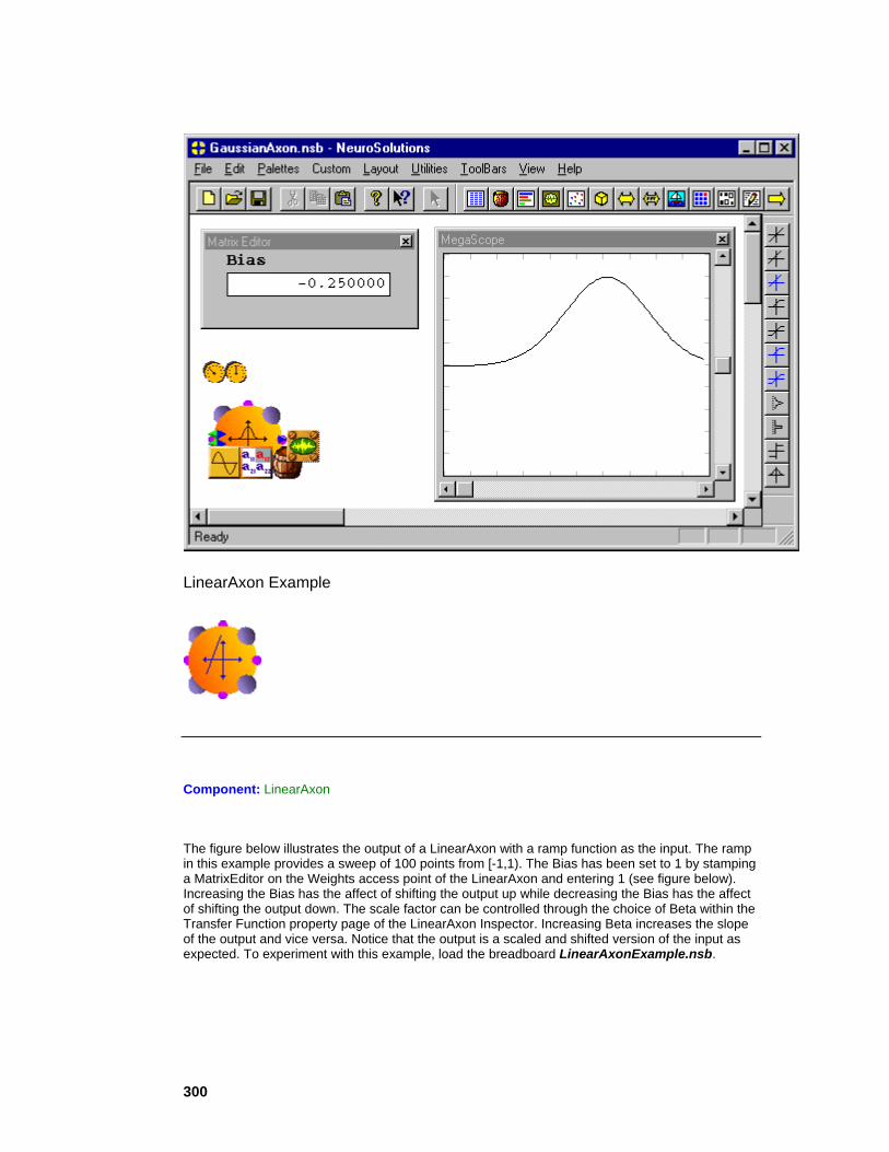
300

LinearAxon Example

Component: LinearAxon

The figure below illustrates the output of a LinearAxon with a ramp function as the input. The ramp in this example provides a sweep of 100 points from [-1,1). The Bias has been set to 1 by stamping a MatrixEditor on the Weights access point of the LinearAxon and entering 1 (see figure below). Increasing the Bias has the affect of shifting the output up while decreasing the Bias has the affect of shifting the output down. The scale factor can be controlled through the choice of Beta within the Transfer Function property page of the LinearAxon Inspector. Increasing Beta increases the slope of the output and vice versa. Notice that the output is a scaled and shifted version of the input as expected. To experiment with this example, load the breadboard LinearAxonExample.nsb.

301

LinearSigmoidAxon Example

Component: LinearSigmoidAxon

The figure below illustrates the output of a LinearSigmoidAxon with a ramp function as the input. The ramp in this example provides a sweep of 100 points from [-2,2). The Bias has been set to 0 by stamping a MatrixEditor on the Weights access point of the LinearSigmoidAxon and entering 0 (see figure below). Increasing the Bias has the affect of shifting the knee of the output to the left while decreasing the Bias has the affect of shifting the knee of the output to the right. The slope of the linear region can be controlled through the choice of Beta within the Transfer Function property page of the LinearSigmoidAxon Inspector. Increasing Beta increases the slope of the linear region and vice versa. Of course, increasing Beta also decreases the range of the inputs that the PE can accept without saturating and vice versa. To experiment with this example, load the breadboard LinearSigmoidAxonExample.nsb.

302

LinearTanhAxon Example

Component: LinearTanhAxon

The figure below illustrates the output of a LinearTanhAxon with a ramp function as the input. The ramp in this example provides a sweep of 100 points from [-3,3). The Bias has been set to 1 by stamping a MatrixEditor on the Weights access point of the LinearTanhAxon and entering 1 (see figure below). Increasing the Bias has the affect of shifting the knee of the output to the left while decreasing the Bias has the affect of shifting the knee of the output to the right. The slope of the linear region can be controlled through the choice of Beta within the Transfer Function property page of the LinearTanhAxon Inspector. Increasing Beta increases the slope of the linear region and vice versa. Of course, increasing Beta also decreases the range of the inputs that the PE can accept without saturating and vice versa. To experiment with this example, load the breadboard LinearTanhAxonExample.nsb.

303

SigmoidAxon Example

Component: SigmoidAxon

The SigmoidAxon will typically be used as hidden and output layers in MLP topologies. If used in the output layer, it is important to verify that the desired signal is normalized to between 0 and 1.

The figure below illustrates the output of a SigmoidAxon with a ramp function as the input. The ramp in this example provides a sweep of 100 points from [-6,6). The Bias has been set to 1.5 by stamping a MatrixEditor on the Weights access point of the SigmoidAxon and entering 1.5 (see figure below). Increasing the Bias has the affect of shifting the knee of the output to the left while decreasing the Bias has the affect of shifting the knee of the output to the right. The slope of the linear region can be controlled through the choice of Beta within the Transfer Function property page of the SigmoidAxon Inspector. Increasing Beta increases the slope of the linear region and vice versa. Of course, increasing Beta also decreases the range of the inputs that the PE can accept without saturating and vice versa. To experiment with this example, load the breadboard SigmoidAxonExample.nsb.

304

SoftMaxAxon Example

Component: SoftMaxAxon

The SoftMaxAxon component should be used as the output of any MLP to allow interpretation of the output as a probability, as normally is the case in classification.

The figure below illustrates the 3 outputs (grouped at the top of the MegaScope) of a SoftMaxAxon (3 PEs) with a sine function, a triangle function, and a ramp function as the inputs (grouped at the bottom of the MegaScope). Notice that at any point in time, the 3 outputs sum to one that is required for each of the outputs to be interpreted as a probability. To experiment with this example, load the breadboard SoftMaxAxonExample.nsb.

305

TanhAxon Example

Component: TanhAxon

The TanhAxon will typically be used as hidden and output layers in MLP topologies. If used in the output layer, it is important to verify that the desired signal is normalized to between -1 and 1.

The figure below illustrates the output of a TanhAxon with a ramp function as the input. The ramp in this example provides a sweep of 100 points from [-6,6). The Bias has been set to -1.5 by stamping a MatrixEditor on the Weights access point of the TanhAxon and entering -1.5 (see figure below). Increasing the Bias has the affect of shifting the knee of the output to the left while decreasing the Bias has the affect of shifting the knee of the output to the right. The slope of the linear region can be controlled through the choice of Beta within the Transfer Function property page of the TanhAxon Inspector. Increasing Beta increases the slope of the linear region and vice versa. Of course, increasing Beta also decreases the range of the inputs that the PE can accept without

306

saturating and vice versa. To experiment with this example, load the breadboard TanhAxonExample.nsb.

ThresholdAxon Example

Component: ThresholdAxon

The ThresholdAxon will typically be used as hidden layers in non-adaptive (hardwired) topologies such as the Hopfield net and McCulloch-Pitts models.

The figure below illustrates the output of a ThresholdAxon with a ramp function as the input. The ramp in this example provides a sweep of 100 points from [-1,1). The Bias has been set to .5 by stamping a MatrixEditor on the Weights access point of the ThresholdAxon and entering .5 (see figure below). Increasing the Bias has the affect of shifting the knee of the output to the left while decreasing the Bias has the affect of shifting the knee of the output to the right. With the Bias set to .5 as in the figure below, this means that any input less than -.5 will be output as -1 and any input

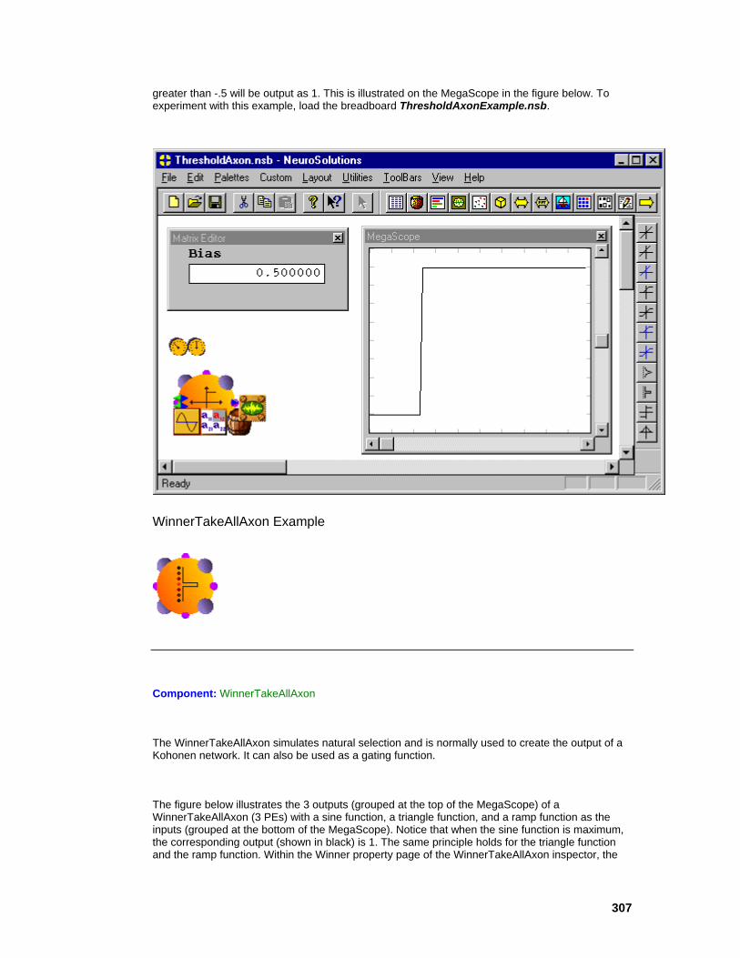
307

greater than -.5 will be output as 1. This is illustrated on the MegaScope in the figure below. To experiment with this example, load the breadboard ThresholdAxonExample.nsb.

WinnerTakeAllAxon Example


The WinnerTakeAllAxon simulates natural selection and is normally used to create the output of a Kohonen network. It can also be used as a gating function.

The figure below illustrates the 3 outputs (grouped at the top of the MegaScope) of a WinnerTakeAllAxon (3 PEs) with a sine function, a triangle function, and a ramp function as the inputs (grouped at the bottom of the MegaScope). Notice that when the sine function is maximum, the corresponding output (shown in black) is 1. The same principle holds for the triangle function and the ramp function. Within the Winner property page of the WinnerTakeAllAxon inspector, the

308

user can choose whether the maximum value or the minimum value wins. To experiment with this example, load the breadboard WinnerTakeAllAxonExample.nsb.

Macro Actions

Axon

Axon Macro Actions Overview Superclass Macro Actions

Action Description cols The number of columns of PE’s for the Axon. fireNext Returns the current "Data Flow ON" setting fireNextOnReset Returns the current "Turn Data Flow ON after RESET" setting rows The number of rows of PE’s for the Axon. setCols Sets the number of columns of PE’s for the Axon. setDimensions Sets the number of rows and columns of PE’s for the Axon. setFireNext Sets the "Data Flow ON" setting.

309

setFireNextOnReset Sets the "Turn Data Flow ON after RESET" setting. setRows Sets the number of rows of PE’s for the axon.

setRows Overview Macro Actions

Syntax

componentName.setRows(rows)

Parameters Type Description return void componentName Name defined on the engine property page. rows int Number of rows of PE’s for the Axon (see "Rows" within the Axon Inspector ).

cols Overview Macro Action

Syntax

componentName.cols()

Parameters Type Description return int Number of columns of PE’s for the Axon (see "Cols" within the Axon Inspector ). componentName Name defined on the engine property page.

fireNext Overview Macro Actions

Syntax

componentName.fireNext()

Parameters Type Description return BOOL When TRUE, data flows through the axon (see "Data Flow On" within the Axon Inspector). componentName Name defined on the engine property page.

310

fireNextOnReset Overview Macro Actions

Syntax

componentName.fireNextOnReset()

Parameters Type Description return BOOL When TRUE, data flow resumes after the network is reset (see "Turn Data Flow On After Reset" within the Axon Inspector ). componentName Name defined on the engine property page.

rows Overview Macro Actions

Syntax

componentName.rows()

Parameters Type Description return int Number of rows of PE’s for the Axon (see "Rows" within the Axon Inspector ). componentName Name defined on the engine property page.

setCols Overview Macro Actions

Syntax

componentName.setCols(cols)

Parameters Type Description return void componentName Name defined on the engine property page. cols int The number of columns of PE’s for the Axon (see "Cols" within the Axon Inspector).

setDimensions Overview Macro Actions

311

Syntax

componentName.setDimensions(rows, cols)

Parameters Type Description return void componentName Name defined on the engine property page. rows int Number of rows of PE’s for the Axon (see "Rows" within the Axon Inspector ). cols int The number of columns of PE’s for the Axon (see "Cols" within the Axon Inspector).

setFireNext Overview Macro Actions

Syntax

componentName.setFireNext(fireNext)

Parameters Type Description return void componentName Name defined on the engine property page. fireNext BOOL When TRUE, data flows through the axon (see "Data Flow On" within the Axon Inspector).

setFireNextOnReset Overview Macro Actions

Syntax

componentName.setFireNextOnReset(fireNextOnReset)

Parameters Type Description return void componentName Name defined on the engine property page. fireNextOnReset BOOL When TRUE, data flow resumes after the network is reset (see "Data Flow Turn On After Reset" within the Axon Inspector ).

312

Gaussian Axon

GaussianAxon Macro Actions Overview Superclass Macro Actions

Action Description assignCenters Sets the centers (weights) of the Axon’s PEs from the FullSynapse that is feeding it. assignVariance Sets the widths of the Axon’s PEs from the FullSynapse that is feeding it. neighbors Returns the nearest neighbors setting (P).

setEngineData Sets the gaussian widths (β) for each of the axon's processing elements. setNeighbors Sets the nearest neighbors setting (P).

assignCenters Overview Macro Actions

Syntax

componentName.assignCenters()

Parameters Type Description return void componentName Name defined on the engine property page.

assignVariance Overview Macro Actions

Syntax

componentName.assignVariance()


neighbors Overview Macro Actions

Syntax

componentName.neighbors()

Parameters Type Description

313

return int Number of nearest neighbors for computation of variance (see "P" within the GaussianAxon Inspector ). componentName Name defined on the engine property page.

setEngineData Overview Macro Actions

Syntax

componentName.setEngineData(data)

Parameters Type Description return void componentName Name defined on the engine property page. data variant An array of single-precision floating point values that contains the gaussian widths (β) for each of the axon's processing elements (see "Variance" within the GaussianAxon Inspector ).

setNeighbors Overview Macro Actions

Syntax

componentName.setNeighbors(neighbors)

Parameters Type Description return void componentName Name defined on the engine property page. neighbors int Number of nearest neighbors for computation of variance (see "P" within the GaussianAxon Inspector ).

Linear Axon

LinearAxon Macro Actions Overview Superclass Macro Actions

Action Description beta Returns the Beta value. setBeta Sets the Beta value. setWeightMean Sets the Bias Mean value. setWeightVariance Sets the Bias Variance value.

314

weightMean Returns the Bias Mean value. weightVariance Returns the Bias Variance value.

beta Overview Macro Actions

Syntax

componentName.beta()

Parameters Type Description return float The slope of the nonlinearities for all PE’s (see "Beta" within the TransferFunction Inspector ). componentName Name defined on the engine property page.

setBeta Overview Macro Actions

Syntax

componentName.setBeta(beta)

Parameters Type Description return void componentName Name defined on the engine property page. beta float The slope of the nonlinearities for all PE’s (see "Beta" within the TransferFunction Inspector ).

setWeightMean Overview Macro Actions

Syntax

componentName.setWeightMean(weightMean)

Parameters Type Description return void componentName Name defined on the engine property page. weightMean float The mean of the bias values when the weights are randomized (see "Bias Mean" within the TransferFunction Inspector ).

315

setWeightVariance Overview Macro Actions

Syntax

componentName.setWeightVariance(weightVariance)

Parameters Type Description return void componentName Name defined on the engine property page. weightVariance float The variance of the bias values when the weights are randomized (see "Bias Variance" within the TransferFunction Inspector ).

weightMean Overview Macro Actions

Syntax

componentName.weightMean()

Parameters Type Description return float The mean of the bias values when the weights are randomized (see "Bias Mean" within the TransferFunction Inspector ). componentName Name defined on the engine property page.

weightVariance OverviewMacro Actions

Syntax

componentName.weightVariance()

Parameters Type Description return float The variance of the bias values when the weights are randomized (see "Bias Variance" within the TransferFunction Inspector ). componentName Name defined on the engine property page.

Winner Take All Axon

WinnerTakeAllAxon Macro Actions Overview Superclass Macro Actions

Action Description maxWinner Returns TRUE if PE with maximum value is the winner, or FALSE if PE with

316

minimum value is the winner. setMaxWinner Sets the maxWinner setting above.

maxWinner Overview Macro Actions

Syntax

componentName.maxWinner()

Parameters Type Description return BOOL When TRUE, the neuron with the largest value is the winner of the competition (see "Maximum/Minimum Value is Winner" within the WinnerTakeAllAxon Inspector ). componentName Name defined on the engine property page.

setMaxWinner Overview Macro Actions

Syntax

componentName.setMaxWinner(maxWinner)

Parameters Type Description return void componentName Name defined on the engine property page. maxWinner BOOL When TRUE, the neuron with the largest value is the winner of the competition (see "Maximum/Minimum Value is Winner" within the WinnerTakeAllAxon Inspector ).

Inspectors

Axon Inspector

Family: Axon Family

Superclass Inspector: Soma Family Inspector

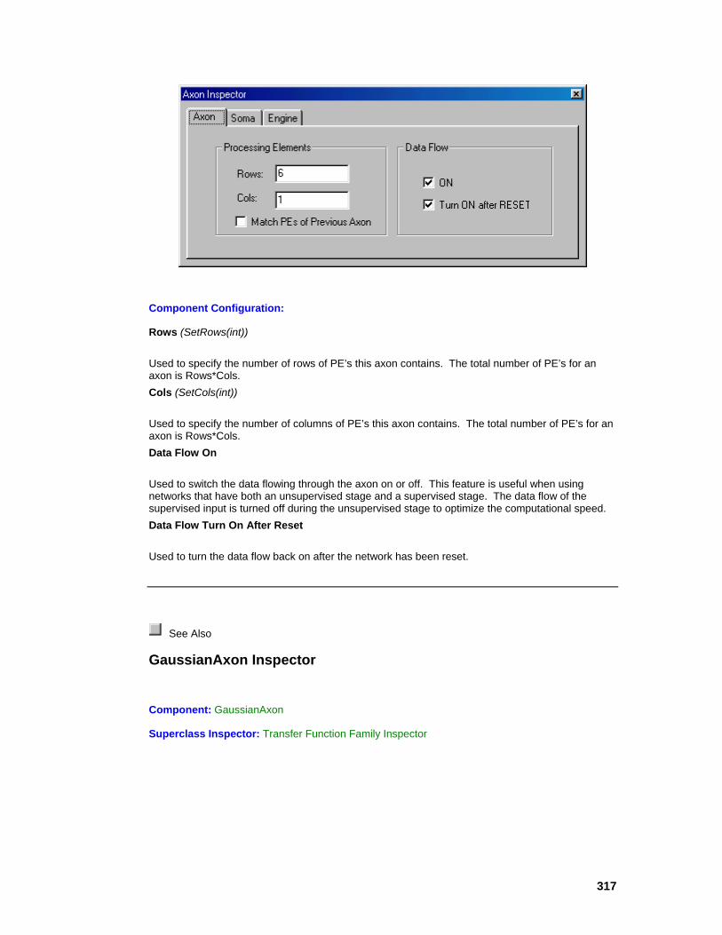
317

Component Configuration:

Rows (SetRows(int))

Used to specify the number of rows of PE’s this axon contains. The total number of PE’s for an axon is Rows*Cols. Cols (SetCols(int))

Used to specify the number of columns of PE’s this axon contains. The total number of PE’s for an axon is Rows*Cols. Data Flow On

Used to switch the data flowing through the axon on or off. This feature is useful when using networks that have both an unsupervised stage and a supervised stage. The data flow of the supervised input is turned off during the unsupervised stage to optimize the computational speed. Data Flow Turn On After Reset

Used to turn the data flow back on after the network has been reset.

See Also

GaussianAxon Inspector


Superclass Inspector: Transfer Function Family Inspector

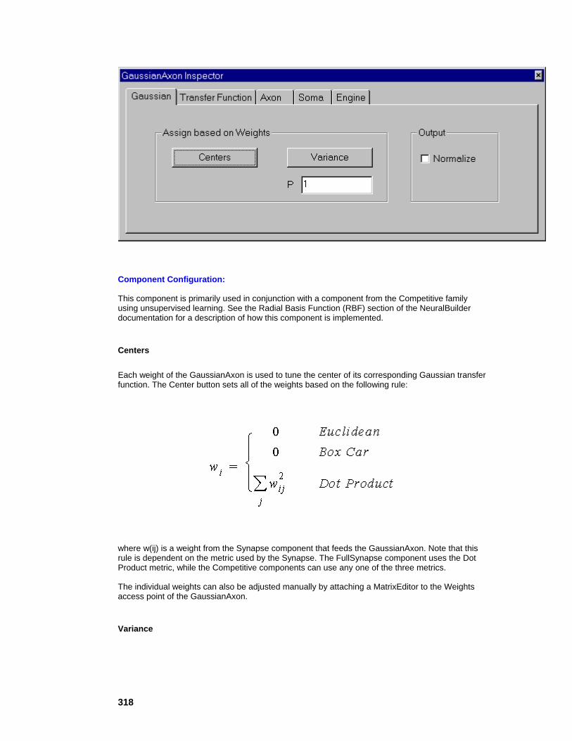
318


This component is primarily used in conjunction with a component from the Competitive family using unsupervised learning. See the Radial Basis Function (RBF) section of the NeuralBuilder documentation for a description of how this component is implemented.

Centers

Each weight of the GaussianAxon is used to tune the center of its corresponding Gaussian transfer function. The Center button sets all of the weights based on the following rule:

where w(ij) is a weight from the Synapse component that feeds the GaussianAxon. Note that this rule is dependent on the metric used by the Synapse. The FullSynapse component uses the Dot Product metric, while the Competitive components can use any one of the three metrics.

The individual weights can also be adjusted manually by attaching a MatrixEditor to the Weights access point of the GaussianAxon.

Variance

319

The GaussianAxon has a width parameter (β) for each PE. This parameter is used to specify the variance (i.e., the width) of the Gaussian transfer function for the given PE. The Variance button sets all of the PE widths based on the following formula:

where the Synapse weight w(kj) is one of the P nearest neighbors to the weight w(ij).

The individual widths can also be adjusted manually by attaching a MatrixEditor to the Widths access point of the GaussianAxon.

P (SetP(int))

This parameter sets the number of nearest neighbors that are averaged together when computing the variance of the Gaussian transfer functions (see above). If this is set low and there are clusters of centers that are relatively close together, then the resulting widths will often be too small (filtering out important data). If P is set high, then many of the neighbors will be averaged together and the resulting widths may be too high (blending the Gaussians together).

Normalize (SetNormalize(Bool))

This switch determines whether the output is normalized. If the output is normalized, then the sum of all the activations is equal to one. This can be useful for Generalized Regression and Probabilistic networks.

WinnerTakeAllAxon Inspector


Superclass Inspector: Axon Inspector

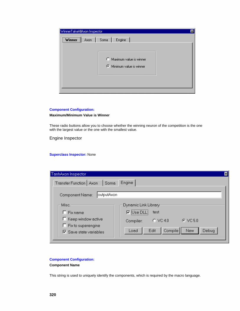
320

Component Configuration: Maximum/Minimum Value is Winner

These radio buttons allow you to choose whether the winning neuron of the competition is the one with the largest value or the one with the smallest value.

Engine Inspector

Superclass Inspector: None

Component Configuration: Component Name

This string is used to uniquely identify the components, which is required by the macro language.

321

Fix Name

When this switch is on, the component’s name will not be modified by NeuroSolutions. Keep Window Active

When this switch is on, the window associated with this component will stay open even if the "Hide Windows" command is issued (see Control Menu & Toolbar Commands). Fix to Superengine

When this switch is on, the component may not be dragged from where it sits on the breadboard. Use DLL

Turning this switch on will attempt to link the selected DLL, thus overriding the functionality of the base component with that defined by the selected DLL. When this switch is off, the selected DLL is ignored. The DLL is selected using the New or Load buttons. Load

This button will display a file selection panel, from which a DLL is selected. The file may be the DLL itself, or the corresponding source file (with a .c or .cpp extension). Note that the DLL will only be active when the Use DLL switch is on. Edit

This button will open an editor containing the source code for the selected DLL. From there, the code may be modified and saved for the next Compile. Note that the editor used is specified by associating the .c or .cpp file extension with it. See the Windows documentation for more information on associating files to applications. Compile

This button will update the selected DLL by compiling the corresponding source code. Note that the directory containing the command line compiler (nmake.exe) must be included in the search path. See the Windows documentation for information on setting the Path environment variable. New

This button brings up a panel for entering the name of a new DLL. From there, the source code for the selected component is copied to the appropriate work directory under the new name. The functionality of the default DLL will, in most cases, be the same as the base component. To modify this functionality you must first Edit the source code and then Compile the DLL. Note that the DLL will only be active when the Use DLL switch is on. Debug

This feature is used to run the DLL through the development environment in order to debug it. The first thing this button does is create a makefile for the DLL and copies it to the "DLLTest" directory. This project is then compiled in "debug" mode and the release version of the DLL is replaced by the debug version. Next, the development environment is launched and the running instance of NeuroSolutions is linked into the debugger. Now you can set breakpoints within the DLL source code and run the network. Note that when you stop the debugger then you are also quitting NeuroSolutions.

Save state variables

Some neural components have internal states the affect their input/output map. By saving the state variables with the breadboard, the results will be repeatable between identical experiments. The components that have state variables include: BackContextAxon, BackTDNNAxon, ContextAxon, Momentum, Quickprop, Step, Synapse, and TDNNAxon.

322

See Also

Soma Family Inspector

Superclass Inspector: Engine Inspector

Component Configuration: Inputs

This cell reports the number of PEs within the Axon that are attached to the Synapse's input. This value cannot be modified. Outputs

This cell reports the number of PEs within the Axon attached to the Synapse's output. This value cannot be modified. Weights

This text reports the number of weights within the Activation component. For Axon components, the weights are referred to as the biases (one for each PE). The number of weights within a FullSynapse is equal to Inputs*Outputs. Save

This switch forces the weights to be saved whenever the breadboard is saved. Note that this switch only corresponds to the weights of this component and not the entire breadboard. To change this setting for the entire network, first select all Activation components (by holding down the Shift key while selecting). Fix

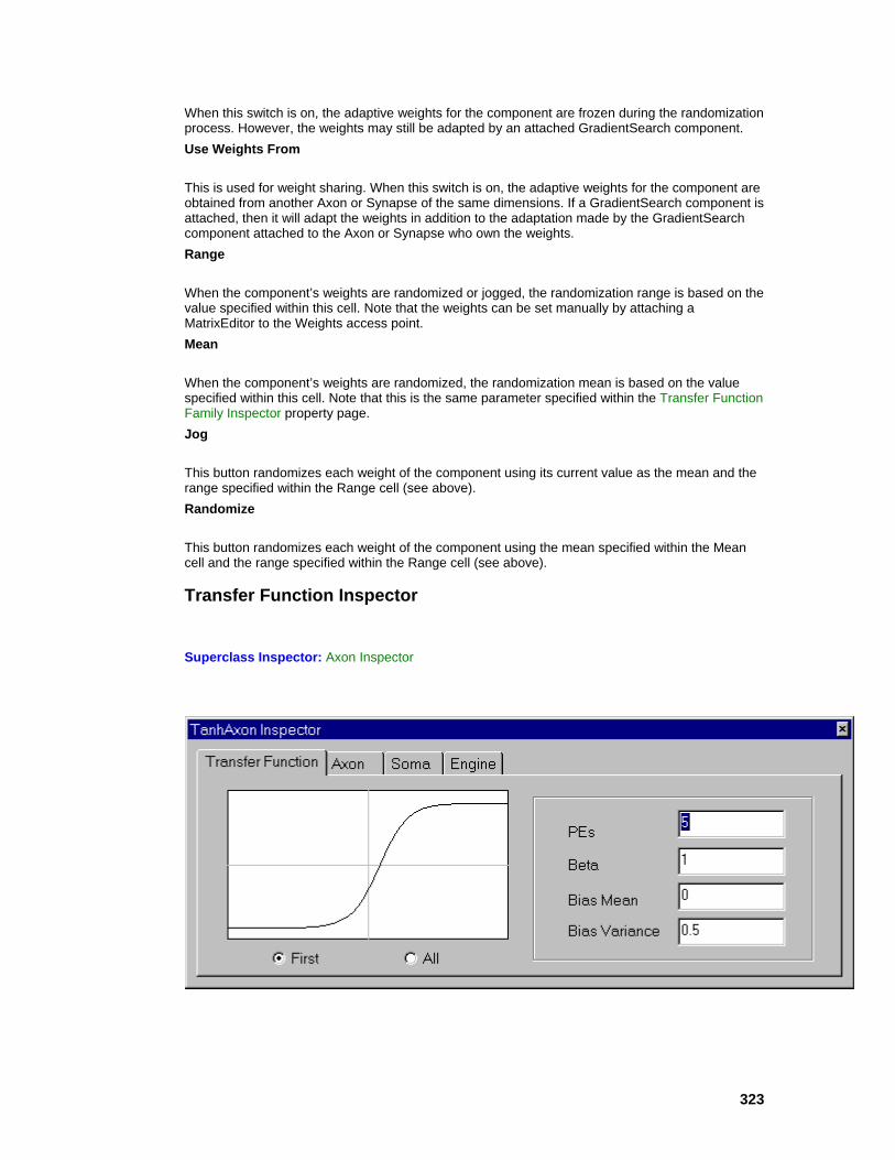
323

When this switch is on, the adaptive weights for the component are frozen during the randomization process. However, the weights may still be adapted by an attached GradientSearch component. Use Weights From

This is used for weight sharing. When this switch is on, the adaptive weights for the component are obtained from another Axon or Synapse of the same dimensions. If a GradientSearch component is attached, then it will adapt the weights in addition to the adaptation made by the GradientSearch component attached to the Axon or Synapse who own the weights. Range

When the component’s weights are randomized or jogged, the randomization range is based on the value specified within this cell. Note that the weights can be set manually by attaching a MatrixEditor to the Weights access point. Mean

When the component’s weights are randomized, the randomization mean is based on the value specified within this cell. Note that this is the same parameter specified within the Transfer Function Family Inspector property page. Jog

This button randomizes each weight of the component using its current value as the mean and the range specified within the Range cell (see above). Randomize

This button randomizes each weight of the component using the mean specified within the Mean cell and the range specified within the Range cell (see above).

Transfer Function Inspector


324

Component Configuration PE’s

This cell can be used to alter the total number of PEs for the component. Beta (SetBeta(float))

The cell is used to specify the slope (?) of the nonlinearities for all PEs. Refer to the activation function of the particular Axon component for the specifics of its use. Bias Mean

When the network is randomized, the biases are randomized based on a mean and a variance. This cell specifies the mean of the randomization. Note that the biases can be set manually by attaching a MatrixEditor to the Weights access point. Bias Variance

When the network is randomized, the biases are randomized based on a mean and a variance. This cell specifies the variance of the randomization and is the same parameter that appears within the Soma property page. Note that the biases can be set manually by attaching a MatrixEditor to the Weights access point.

Drag and Drop

Axon Family Drag and Drop

Axons are base components on the breadboard. This means that they must be dropped directly onto an empty breadboard location.

See Also

MemoryAxon Family

ContextAxon

Family: MemoryAxon Family


Backprop Dual: BackContextAxon

325

Description:

The ContextAxon integrates with a time constant the activity received by each PE in the layer. This operation implements a (non-normalized) feedback from the scaled output of the PE to its input. The ContextAxon is very similar to the IntegratorAxon, except that in this family the activity can have instantaneous jumps, which will taper off according to the defined time constant. The gain factor β is inherited from the LinearAxon. The time constant is implemented by the Axon’s weight vector, i.e. τ = . This allows each PE to have its own time constant, each of which can be adapted.


Note: The Weights access point of the ContextAxon provides access to the time constant vector ( in the above equation).

User Interaction:

Drag and Drop

Inspector

Access Points

Example

DLL Implementation

GammaAxon


Superclass: TDNNAxon

Backprop Dual: BackGammaAxon

326

Description:

The GammaAxon provides a recursive memory of the input signals past. Note that the axon receives a vector of inputs, therefore the GammaAxon implements a vector memory structure. The memory depth is equal to K/µ, where K is the number of taps and µ is the Gamma coefficient. The Gamma coefficient is implemented by the axon’s weight vector, i.e. τ = . This allows each PE to have its own coefficient, each of which can be adapted. The delay between taps, τ, is an adjustable parameter of the component.

Tap Activation Function:

Note: The Weights access point of the GammaAxon provides access to the Gamma coefficient vector ( in the above equation).

User Interaction:

Drag and Drop

Inspector

Access Point

Example

DLL Implementation

IntegratorAxon


Superclass: ContextAxon

Backprop Dual: BackIntegratorAxon

327

Description:

The IntegratorAxon integrates with a time constant the activity received by each PE in the layer. This operation implements a normalized feedback from the scaled output of the PE to its input. The IntegratorAxon is very similar to the ContextAxon, except that in this family the activity cannot have instantaneous jumps. The gain factor β is inherited from the LinearAxon. The time constant is implemented by the axons weight vector, i.e. τ = . This allows each PE to have its own time constant, each of which can be adapted.


Note: The Weights access point of the IntegratorAxon provides access to the time constant vector ( in the above equation).

User Interaction:

Drag and Drop

Inspector

Access Points

Example

DLL Implementation

LaguarreAxon



Backprop Dual: BackLaguarreAxon

328

Description:

The LaguarreAxon memory structure is built from a low-pass filter with a pole at z = (1-µ), followed by a cascade of K all-pass functions. This provides a recursive memory of the input signal’s past. Notice that the axon receives a vector of inputs, therefore the LaguarreAxon implements a vector memory structure. The memory depth is equal to K/µ, where K is the number of taps and is the Laguarre coefficient. The Laguarre coefficient is implemented by the axon’s weight vector, i.e. µ =

. This allows each PE to have its own coefficient, each of which can be adapted. The delay between taps, τ, is an adjustable parameter of the component.


Note: The Weights access point of the LaguarreAxon provides access to the Laguarre coefficient vector ( in the above equation).

User Interaction:

Drag and Drop

Inspector

Access Point

Example

DLL Implementation

SigmoidContextAxon



329

Backprop Dual: BackSigmoidContextAxon

Description:

The SigmoidContextAxon is very similar to the ContextAxon, except that the transfer function of each PE is a sigmoid (i.e., saturates at 0 and 1) and the feedback is taken from this output.


The input data is transformed by a SigmoidAxon followed by a ContextAxon.

Note: The Weights access point of the SigmoidContextAxon provides access to the time constant vector. There is no Bias as in the SigmoidAxon.

User Interaction:

Drag and Drop

Inspector

Access Point

Example

DLL Implementation

SigmoidIntegratorAxon


Superclass: IntegratorAxon

Backprop Dual: BackSigmoidIntegratorAxon

Description:

The SigmoidIntegratorAxon implements the self-feedback of the SigmoidAxon. So it is a nonlinear integrator, because its output activity saturates at 0 or 1.

330


The input data is transformed by a SigmoidAxon followed by an IntegratorAxon.

Note: The Weights access point of the SigmoidIntegratorAxon provides access to the time constant vector. There is no Bias as in the SigmoidAxon.

User Interaction:

Drag and Drop

Inspector

Access Point

Example

DLL Implementation

TanhContextAxon



Backprop Dual: BackTanhContextAxon

Description:

Description: The TanhContextAxon is very similar to the ContextAxon, except that the feedback is taken from the output of tanh PE, i.e. it will saturate at +/- 1.


The input data is transformed by a ContextAxon followed by a TanhAxon.

331

Note: The Weights access point of the TanhContextAxon provides access to the time constant vector. There is no Bias as in the TanhAxon.

User Interaction:

Drag and Drop

Inspector

Access Point

Example

DLL Implementation

TanhIntegratorAxon



Backprop Dual: BackTanhIntegratorAxon

Description:

The TanhIntegratorAxon implements the self-feedback of the TanhAxon. So it is a nonlinear integrator, because its output activity saturates at +/- 1.


The input data is transformed by an IntegratorAxon followed by a TanhAxon.

Note: The Weights access point of the TanhIntegratorAxon provides access to the time constant vector. There is no Bias as in the TanhAxon.

User Interaction:

332

Drag and Drop

Inspector

Access Point

Example

DLL Implementation

TDNNAxon


Superclass: Axon

Backprop Dual: BackTDNNAxon

Description:

The TDNNAxon is a multi-channel tapped delay line memory structure. The number of sample delays between each tap, defined by τ, may be varied, allowing memory depth and the number of taps to be decoupled. This forms a local memory whose length (depth) is equal to the number of taps minus 1, times the tap delay, times the sampling period. Notice that the axon receives a vector of inputs, therefore the TDNNAxon implements multiple tapped delay line (TDL) memory structures.


User Interaction:

Drag and Drop

Inspector

Access Points

Example

333

DLL Implementation

Macro Actions

DLL Implementation

ContextAxon DLL Implementation

Component: ContextAxon

Protocol: PerformContextAxon

Description:

The ContextAxon integrates the activity received by each PE in the layer using an adaptable time constant. Each PE within the data vector is computed by adding the product of the PE’s time constant and the activity of the PE at the previous time step to the current activity. This sum is then multiplied by a user-defined scaling factor.

Code: void performContextAxon( DLLData *instance, // Pointer to instance data (may be NULL) NSFloat *data, // Pointer to the layer of PEs int rows, // Number of rows of PEs in the layer int cols // Number of columns of PEs in the layer NSFloat *delayedData, // Pointer to a delayed PE layer NSFloat *tau, // Pointer to a vector of time constants NSFloat beta // Linear scaling factor (user-defined) ) { int i, length=rows*cols; for (i=0; i<length; i++) data[i] = beta * (data[i] + tau[i] * delayedData[i]); }

GammaAxon DLL Implementation

334

Component: GammaAxon

Protocol: PerformGammaAxon

Description:

The GammaAxon is a multi-channel tapped delay line with a Gamma memory structure. With a straight tapped delay line (TDNNAxon), each memory tap (PE) within the data vector is computed by simply copying the value from the previous tap of the delayedData vector. With the GammaAxon, a given tap within data vector is computed by taking a fraction (gamma) of the value from the previous tap of the delayedData vector and adding it with a fraction (1-gamma) of the same tap. The first PE of each channel (tap[0]) is simply the channel’s input and is not modified.

Code: void performGammaAxon( DLLData *instance, // Pointer to instance data (may be NULL) NSFloat *data, // Pointer to the layer of PEs int rows, // Number of rows of PEs in the layer int cols // Number of columns of PEs in the layer NSFloat *delayedData, // Pointer to a delayed PE layer int taps // Number of memory taps NSFloat *gamma // Pointer to vector of gamma coefficients ) { register int i,j,k,length=rows*cols; for (i=0; i<length; i++) for (j=1; j<taps; j++) { k = i + j*length; data[k] = gamma[i]*delayedData[k-length] + (1-gamma[i])*delayedData[k]; } }

IntegratorAxon DLL Implementation

335

Component: IntegratorAxon


Description:

The IntegratorAxon is very similar to the BackLaguarreAxon DLL Implementation, except that the feedback connection is normalized. Each PE within the data vector is computed by adding the product of the PE’s time constant and the activity of the PE at the previous time step to the product of current activity times 1 minus the time constant. This sum is then multiplied by a user-defined scaling factor.

Code: void performContextAxon( DLLData *instance, // Pointer to instance data (may be NULL) NSFloat *data, // Pointer to the layer of PEs int rows, // Number of rows of PEs in the layer int cols // Number of columns of PEs in the layer NSFloat *delayedData, // Pointer to a delayed PE layer NSFloat *tau, // Pointer to a vector of time constants NSFloat beta // Linear scaling factor (user-defined) ) { int i, length=rows*cols; for (i=0; i<length; i++) data[i] = (NSFloat)(beta * ((1.0-tau[i])*data[i] + tau[i]*delayedData[i])); }

LaguarreAxon DLL Implementation

Component: LaguarreAxon

Protocol: PerformGammaAxon

336

Description:

The LaguarreAxon is a multi-channel tapped delay line similar to the GammaAxon. The difference is that this algorithm provides an orthogonal span of the memory space.

Code: void performGammaAxon( DLLData *instance, // Pointer to instance data (may be NULL) NSFloat *data, // Pointer to the layer of PEs int rows, // Number of rows of PEs in the layer int cols // Number of columns of PEs in the layer NSFloat *delayedData, // Pointer to a delayed PE layer int taps // Number of memory taps NSFloat *gamma // Pointer to vector of gamma coefficients ) { register int i,j,k,length=rows*cols; for (i=0; i<length; i++) { NSFloat gain = (NSFloat)pow(1-pow(gamma[i], 2), 0.5); for (j=1; j<taps; j++) { k = i + j*length; data[k] = delayedData[k-length] + gamma[i]*delayedData[k]; if (j==1) data[k] *= gain; else data[k] -= gamma[i]*data[k-length]; } } }

SigmoidContextAxon DLL Implementation

Component: SigmoidContextAxon


Description:

337

The SigmoidContextAxon is very similar to the ContextAxon, except that the transfer function of each PE is a sigmoid (i.e., saturates at 0 and 1) and the feedback is taken from this output.

Code: void performContextAxon( DLLData *instance, // Pointer to instance data (may be NULL) NSFloat *data, // Pointer to the layer of PEs int rows, // Number of rows of PEs in the layer int cols // Number of columns of PEs in the layer NSFloat *delayedData, // Pointer to a delayed PE layer NSFloat *tau, // Pointer to a vector of time constants NSFloat beta // Linear scaling factor (user-defined) ) { int i, length=rows*cols; for (i=0; i<length; i++) { data[i] = beta * (data[i] + tau[i] * delayedData[i]); data[i] = (NSFloat)(1.0/(1.0+exp(-data[i]))); } }

SigmoidIntegratorAxon DLL Implementation

Component: SigmoidIntegratorAxon


Description:

The SigmoidIntegratorAxon is very similar to the IntegratorAxon, except that the transfer function of each PE is a sigmoid (i.e., saturates at 0 and 1) and the feedback is taken from this output.

Code: void performContextAxon( DLLData *instance, // Pointer to instance data (may be NULL) NSFloat *data, // Pointer to the layer of PEs int rows, // Number of rows of PEs in the layer

338

int cols // Number of columns of PEs in the layer NSFloat *delayedData, // Pointer to a delayed PE layer NSFloat *tau, // Pointer to a vector of time constants NSFloat beta // Linear scaling factor (user-defined) ) { int i, length=rows*cols; for (i=0; i<length; i++) { data[i] = beta * ((1-tau[i])*data[i] + tau[i]*delayedData[i]); data[i] = 1/(1+(NSFloat)exp(-data[i])); } }

TanhContextAxon DLL Implementation

Component: TanhContextAxon


Description:

The TanhContextAxon is very similar to the ContextAxon, except that the transfer function of each PE is a hyperbolic tangent (i.e., saturates at -1 and 1) and the feedback is taken from this output.

Code: void performContextAxon( DLLData *instance, // Pointer to instance data (may be NULL) NSFloat *data, // Pointer to the layer of PEs int rows, // Number of rows of PEs in the layer int cols // Number of columns of PEs in the layer NSFloat *delayedData, // Pointer to a delayed PE layer NSFloat *tau, // Pointer to a vector of time constants NSFloat beta // Linear scaling factor (user-defined) ) { int i, length=rows*cols; for (i=0; i<length; i++)

339

data[i] = (NSFloat)tanh(beta * (data[i] + tau[i] * delayedData[i])); }

TanhIntegratorAxon DLL Implementation

Component: TanhIntegratorAxon


Description:

The TanhIntegratorAxon is very similar to the IntegratorAxon, except that the transfer function of each PE is a hyperbolic tangent (i.e., saturates at -1 and 1) and the feedback is taken from this output.

Code: void performContextAxon( DLLData *instance, // Pointer to instance data (may be NULL) NSFloat *data, // Pointer to the layer of PEs int rows, // Number of rows of PEs in the layer int cols // Number of columns of PEs in the layer NSFloat *delayedData, // Pointer to a delayed PE layer NSFloat *tau, // Pointer to a vector of time constants NSFloat beta // Linear scaling factor (user-defined) ) { for (i=0; i<length; i++) data[i] = (NSFloat)tanh(beta * ((1-tau[i])*data[i] + tau[i]*delayedData[i])); }

TDNNAxon DLL Implementation

340

Component: TDNNAxon

Protocol: PerformTDNNAxon

Description:

The TDNNAxon is a multi-channel tapped delay line memory structure. For each memory tap (PE) within the data vector, the value is copied from the previous tap of the delayedData vector. The first PE of each channel (tap[0]) is simply the channel’s input and is not modified.

Code: void performTDNNAxon( DLLData *instance, // Pointer to instance data (may be NULL) NSFloat *data, // Pointer to the layer of PEs int rows, // Number of rows of PEs in the layer int cols // Number of columns of PEs in the layer NSFloat *delayedData, // Pointer to a delayed PE layer int taps // Number of memory taps ) { register int i,j,k,length=rows*cols; for (i=0; i<length; i++) for (j=1; j<taps; j++) { k = i + j*length; data[k] = delayedData[k-length]; } }

Examples

IntegratorAxon Example

Component: IntegratorAxon

341

The IntegratorAxon can be used as a context unit in Jordan or Elman nets. Its function is to integrate the past activity. It can also be used as an integrator PE at the output of a net.

The figure below illustrates the impulse response (the output for an impulse at the input) of the IntegratorAxon. The red curve on the MegaScope is the input impulse, whereas the black and blue curves illustrate the IntegratorAxon output with time constants of .7 and .5 respectively. The time constant can be accessed by stamping a matrix editor on the Weights access point of the IntegratorAxon (as shown in the figure below) or it can be accessed directly on the Feedback property page of the IntegratorAxon inspector. Notice that increasing the time constant has the affect of increasing the memory depth. To experiment with this example, load the breadboard IntegratorAxonExample.nsb.

TanhIntegratorAxon Example

Component: TanhIntegratorAxon

342

The TanhIntegratorAxon can be used as a context unit in Jordan or Elman nets. Its function is to integrate the past activity. It can also be used as an integrator PE at the output of a net. A signal fed into a TanhIntegratorAxon is processed by an IntegratorAxon followed by a TanhAxon. Note that the Weights access point of the TanhIntegratorAxon provides access to the Time Constant (not the Bias as with the TanhAxon).

The figure below illustrates the impulse response (the output for an impulse at the input) of the TanhIntegratorAxon. The red curve on the MegaScope is the input impulse, whereas the black and blue curves illustrate the TanhIntegratorAxon output with time constants of .7 and .5 respectively. The time constant can be accessed by stamping a matrix editor on the Weights access point of the TanhIntegratorAxon (as shown in the figure below) or it can be accessed directly on the Feedback property page of the TanhIntegratorAxon inspector. Notice that increasing the time constant has the affect of increasing the memory depth. To experiment with this example, load the breadboard TanhIntegratorAxonExample.nsb.

SigmoidIntegratorAxon Example

343

Component: SigmoidIntegratorAxon

The SigmoidIntegratorAxon can be used as a context unit in Jordan or Elman nets. Its function is to integrate the past activity. It can also be used as an integrator PE at the output of a net. A signal fed into a SigmoidIntegratorAxon is processed by a SigmoidAxon followed by an IntegratorAxon. Note that the Weights access point of the SigmoidIntegratorAxon provides access to the Time Constant (not the Bias as with the SigmoidAxon). To experiment with this example, load the breadboard SigmoidIntegratorAxonExample.nsb.

344

ContextAxon Example

Component: ContextAxon

The ContextAxon is normally used in Jordan or Elman nets.

The figure below illustrates the impulse response (the output for an impulse at the input) of the ContextAxon. The red curve on the MegaScope is the input impulse, whereas the black and blue curves illustrate the ContextAxon output with time constants of .9 and .6 respectively. The time constant can be accessed by stamping a matrix editor on the Weights access point of the ContextAxon (as shown in the figure below) or it can be accessed directly on the Feedback property page of the ContextAxon inspector. Notice that increasing the time constant has the affect of increasing the memory depth. To experiment with this example, load the breadboard ContextAxonExample.nsb.

345

SigmoidContextAxon Example

Component: SigmoidContextAxon

The SigmoidContextAxon is normally used in Jordan or Elman nets. A signal fed into a SigmoidContextAxon is processed by a SigmoidAxon followed by a ContextAxon. Note that the Weights access point of the SigmoidContextAxon provides access to the Time Constant (not the Bias as with the SigmoidAxon). To experiment with this example, load the breadboard SigmoidContextAxonExample.nsb.

346

TanhContextAxon Example

Component: TanhContextAxon

The TanhContextAxon is normally used in Jordan or Elman nets. A signal fed into a TanhContextAxon is processed by a ContextAxon followed by a TanhAxon. Note that the Weights access point of the TanhContextAxon provides access to the Time Constant (not the Bias as with the TanhAxon).

The figure below illustrates the impulse response (the output for an impulse at the input) of the TanhContextAxon. The red curve on the MegaScope is the input impulse, whereas the black and blue curves illustrate the TanhContextAxon output with time constants of .9 and .6 respectively. The time constant can be accessed by stamping a matrix editor on the Weights access point of the TanhContextAxon (as shown in the figure below) or it can be accessed directly on the Feedback property page of the TanhContextAxon inspector. Notice that increasing the time constant has the affect of increasing the memory depth. To experiment with this example, load the breadboard TanhContextAxonExample.nsb.

347

GammaAxon Example

Component: GammaAxon

The GammaAxon is typically used as an input layer when processing temporal sequences. This allows the temporal signal to be presented directly to the network without preprocessing or segmentation. The GammaAxon finds the best compromise between time resolution vs. memory depth for the application. When used with Axon, the GammaAxon extends the Adaline to a recursive adaptive linear filter.

The figure below illustrates the impulse response (the output for an impulse at the input) of each of the taps of a 5 tap GammaAxon. Notice that the output of the first tap (black) is just an impulse. This is because the input and the first tap are directly connected. In general, the point in time where the response has a peak is approximately given by k/? where ? is the Gamma Coefficient and k is the tap number (note that the directly connected first tap is number 0). In this example ? has been set to .5 by stamping a MatrixEditor on the Weights access point of the GammaAxon and entering .5 (see figure below). Thus, the depth of the memory can be controlled by adjusting the value of ?

348

(i.e. increasing ? decreases the memory depth and vice versa). To experiment with this example, load the breadboard GammaAxonExample.nsb.

LaguarreAxon Example

Component: LaguarreAxon

The LaguarreAxon is typically used as an input layer when processing temporal sequences. This allows the temporal signal to be presented directly to the network without preprocessing or segmentation.

The figure below illustrates the impulse response (the output for an impulse at the input) of each of the taps of a 5 tap LaguarreAxon. Notice that the output of the first tap (black) is just an impulse. This is because the input and the first tap are directly connected. In general, the point in time where

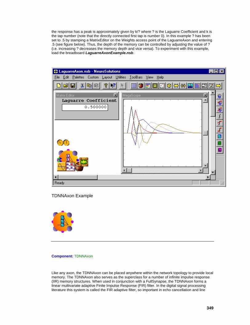
349

the response has a peak is approximately given by k/? where ? is the Laguarre Coefficient and k is the tap number (note that the directly connected first tap is number 0). In this example ? has been set to .5 by stamping a MatrixEditor on the Weights access point of the LaguarreAxon and entering .5 (see figure below). Thus, the depth of the memory can be controlled by adjusting the value of ? (i.e. increasing ? decreases the memory depth and vice versa). To experiment with this example, load the breadboard LaguarreAxonExample.nsb.

TDNNAxon Example

Component: TDNNAxon

Like any axon, the TDNNAxon can be placed anywhere within the network topology to provide local memory. The TDNNAxon also serves as the superclass for a number of infinite impulse response (IIR) memory structures. When used in conjunction with a FullSynapse, the TDNNAxon forms a linear multivariate adaptive Finite Impulse Response (FIR) filter. In the digital signal processing literature this system is called the FIR adaptive filter, so important in echo cancellation and line

350

equalization. It is important to remember that this multivariate FIR filter can also be made adaptive, so NeuroSolutions can also implement adaptive linear filter simulations.

The figure below shows the output of each of the taps of a 3 tap TDNNAxon, with a triangle function as the input. The input is also set up to display on the MegaScope but it is completely covered by the by the output of the first tap (red) since the first tap and the input are directly connected. The second and third taps are simply time-delayed versions of the input as shown in the figure. The length of the tap delay can be set within the TDNN property page of the TDNNAxon inspector. To experiment with this example, load the breadboard TDNNAxonExample.nsb.

Inspectors

TDNNAxon Inspector



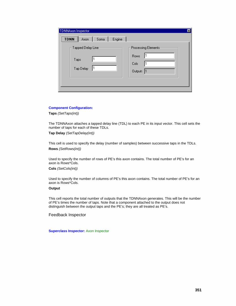
351

Component Configuration: Taps (SetTaps(int))

The TDNNAxon attaches a tapped delay line (TDL) to each PE in its input vector. This cell sets the number of taps for each of these TDLs. Tap Delay (SetTapDelay(int))

This cell is used to specify the delay (number of samples) between successive taps in the TDLs. Rows (SetRows(int))

Used to specify the number of rows of PE’s this axon contains. The total number of PE’s for an axon is Rows*Cols. Cols (SetCols(int))

Used to specify the number of columns of PE’s this axon contains. The total number of PE’s for an axon is Rows*Cols. Output

This cell reports the total number of outputs that the TDNNAxon generates. This will be the number of PE’s times the number of taps. Note that a component attached to the output does not distinguish between the output taps and the PE’s; they are all treated as PE’s.

Feedback Inspector


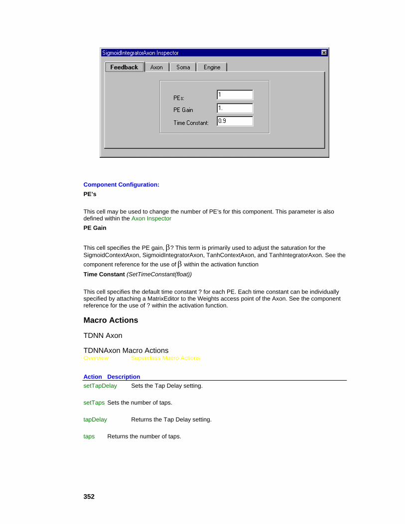
352

Component Configuration: PE’s

This cell may be used to change the number of PE’s for this component. This parameter is also defined within the Axon Inspector PE Gain

This cell specifies the PE gain, β? This term is primarily used to adjust the saturation for the SigmoidContextAxon, SigmoidIntegratorAxon, TanhContextAxon, and TanhIntegratorAxon. See the component reference for the use of β within the activation function Time Constant (SetTimeConstant(float))

This cell specifies the default time constant ? for each PE. Each time constant can be individually specified by attaching a MatrixEditor to the Weights access point of the Axon. See the component reference for the use of ? within the activation function.

Macro Actions

TDNN Axon

TDNNAxon Macro Actions Overview Superclass Macro Actions

Action Description setTapDelay Sets the Tap Delay setting. setTaps Sets the number of taps. tapDelay Returns the Tap Delay setting. taps Returns the number of taps.

353

setTapDelay Overview Macro Actions

Syntax

componentName.setTapDelay(tapDelay)

Parameters Type Description return void componentName Name defined on the engine property page. tapDelay int The delay (number of samples) between successive taps in the TDLs (see "Tap Delay" within the TDNNAxon Inspector ).

setTaps Overview Macro Actions

Syntax

componentName.setTaps(taps)

Parameters Type Description return void componentName Name defined on the engine property page. taps int The number of taps for each tapped delay line (TDL) (see "Taps" within the TDNNAxon Inspector ).

tapDelay Overview Macro Actions

Syntax

componentName.tapDelay()

Parameters Type Description return int The delay (number of samples) between successive taps in the TDLs (see "Tap Delay" within the TDNNAxon Inspector ). componentName Name defined on the engine property page.

taps Overview Macro Actions

Syntax

componentName.taps()

354

Parameters Type Description return int The number of taps for each tapped delay line (TDL) (see "Taps" within the TDNNAxon Inspector ). componentName Name defined on the engine property page.

FuzzyAxon Family

BellFuzzyAxon

Family: FuzzyAxon Family

Superclass: Axon

Description:

The BellFuzzyAxon is a type of FuzzyAxon that uses a bell-shaped curve as its membership function. Each membership function takes 3 parameters, which are stored in the weight vector of the BellFuzzyAxon.

Membership Function:

User Interaction:

Drag and Drop

Inspector

Access Points

DLL Implementation

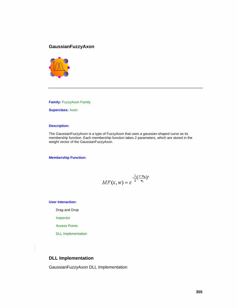
355

GaussianFuzzyAxon

Family: FuzzyAxon Family

Superclass: Axon

Description:

The GaussianFuzzyAxon is a type of FuzzyAxon that uses a gaussian-shaped curve as its membership function. Each membership function takes 2 parameters, which are stored in the weight vector of the GaussianFuzzyAxon.

Membership Function:

User Interaction:

Drag and Drop

Inspector

Access Points

DLL Implementation

DLL Implementation

GaussianFuzzyAxon DLL Implementation

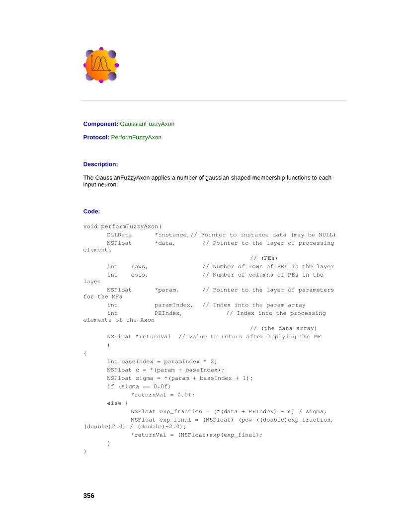
356

Component: GaussianFuzzyAxon

Protocol: PerformFuzzyAxon

Description:

The GaussianFuzzyAxon applies a number of gaussian-shaped membership functions to each input neuron.

Code: void performFuzzyAxon( DLLData *instance,// Pointer to instance data (may be NULL) NSFloat *data, // Pointer to the layer of processing elements // (PEs) int rows, // Number of rows of PEs in the layer int cols, // Number of columns of PEs in the layer NSFloat *param, // Pointer to the layer of parameters for the MFs int paramIndex, // Index into the param array int PEIndex, // Index into the processing elements of the Axon // (the data array) NSFloat *returnVal // Value to return after applying the MF ) { int baseIndex = paramIndex * 2; NSFloat c = *(param + baseIndex); NSFloat sigma = *(param + baseIndex + 1); if (sigma == 0.0f) *returnVal = 0.0f; else { NSFloat exp_fraction = (*(data + PEIndex) - c) / sigma; NSFloat exp_final = (NSFloat) (pow ((double)exp_fraction, (double)2.0) / (double)-2.0); *returnVal = (NSFloat)exp(exp_final); } }

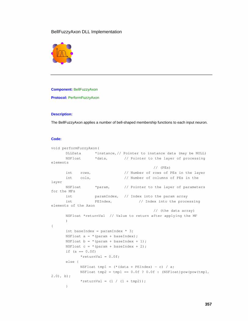
357

BellFuzzyAxon DLL Implementation

Component: BellFuzzyAxon

Protocol: PerformFuzzyAxon

Description:

The BellFuzzyAxon applies a number of bell-shaped membership functions to each input neuron.

Code: void performFuzzyAxon( DLLData *instance,// Pointer to instance data (may be NULL) NSFloat *data, // Pointer to the layer of processing elements // (PEs) int rows, // Number of rows of PEs in the layer int cols, // Number of columns of PEs in the layer NSFloat *param, // Pointer to the layer of parameters for the MFs int paramIndex, // Index into the param array int PEIndex, // Index into the processing elements of the Axon // (the data array) NSFloat *returnVal // Value to return after applying the MF ) { int baseIndex = paramIndex * 3; NSFloat a = *(param + baseIndex); NSFloat b = *(param + baseIndex + 1); NSFloat c = *(param + baseIndex + 2); if (a == 0.0f) *returnVal = 0.0f; else { NSFloat tmp1 = (*(data + PEIndex) - c) / a; NSFloat tmp2 = tmp1 == 0.0f ? 0.0f : (NSFloat)pow(pow(tmp1, 2.0), b); *returnVal = (1 / (1 + tmp2)); }

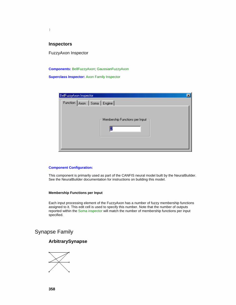
358

}

Inspectors

FuzzyAxon Inspector

Components: BellFuzzyAxon; GaussianFuzzyAxon

Superclass Inspector: Axon Family Inspector


This component is primarily used as part of the CANFIS neural model built by the NeuralBuilder. See the NeuralBuilder documentation for instructions on building this model.

Membership Functions per Input

Each input processing element of the FuzzyAxon has a number of fuzzy membership functions assigned to it. This edit cell is used to specify this number. Note that the number of outputs reported within the Soma inspector will match the number of membership functions per input specified.

Synapse Family

ArbitrarySynapse

359

Family: Synapse Family

Superclass: Synapse

Description:

The ArbitrarySynapse provides an arbitrarily connected linear map between its input and output axons. Since each axon contains a vector of processing elements (PEs), the ArbitrarySynapse is capable of connecting any PE in the input axon to an arbitrary PE in the output axon. The connections can be either established manually or automatically to form common interconnection patterns.


The ArbitrarySynapse does not have a predefined activation function. We know that the map is linear, but the interconnections are arbitrarily defined by the user.

Note: The Weights access point will provide the connection weights in vector form.

User Interaction:

Drag and Drop

Inspector

Access Points

Macro Actions

CombinerSynapse


Superclass: Synapse

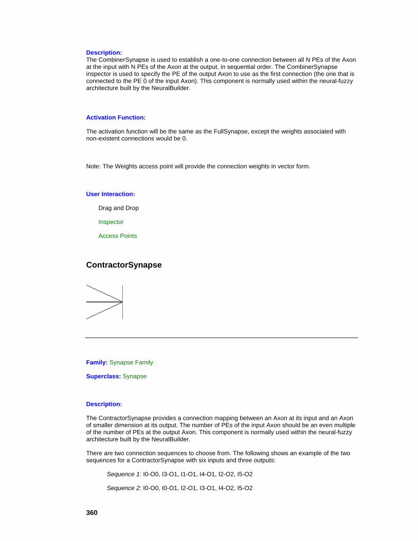
360

Description: The CombinerSynapse is used to establish a one-to-one connection between all N PEs of the Axon at the input with N PEs of the Axon at the output, in sequential order. The CombinerSynapse inspector is used to specify the PE of the output Axon to use as the first connection (the one that is connected to the PE 0 of the input Axon). This component is normally used within the neural-fuzzy architecture built by the NeuralBuilder.


The activation function will be the same as the FullSynapse, except the weights associated with non-existent connections would be 0.


User Interaction:

Drag and Drop

Inspector

Access Points

ContractorSynapse


Superclass: Synapse

Description:

The ContractorSynapse provides a connection mapping between an Axon at its input and an Axon of smaller dimension at its output. The number of PEs of the input Axon should be an even multiple of the number of PEs at the output Axon. This component is normally used within the neural-fuzzy architecture built by the NeuralBuilder.

There are two connection sequences to choose from. The following shows an example of the two sequences for a ContractorSynapse with six inputs and three outputs:

Sequence 1: I0-O0, I3-O1, I1-O1, I4-O1, I2-O2, I5-O2


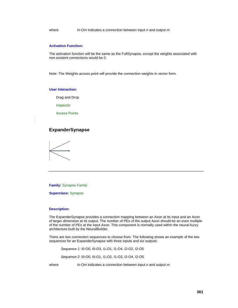
361

where In-Om indicates a connection between input n and output m




User Interaction:

Drag and Drop

Inspector

Access Points

ExpanderSynapse


Superclass: Synapse

Description:

The ExpanderSynapse provides a connection mapping between an Axon at its input and an Axon of larger dimension at its output. The number of PEs of the output Axon should be an even multiple of the number of PEs at the input Axon. This component is normally used within the neural-fuzzy architecture built by the NeuralBuilder.

There are two connection sequences to choose from. The following shows an example of the two sequences for an ExpanderSynapse with three inputs and six outputs:



where In-Om indicates a connection between input n and output m

362




User Interaction:

Drag and Drop

Inspector

Access Points

ModularSynapse


Superclass: Synapse

Description:

The ModularSynapse breaks up the neurons of the Axon at its input into equal sized groups, or modules. The neurons of the Axon at the output are also divided into the same number of groups, although the number of neurons per group may be different depending on the number of PEs of the Axon. This Synapse then provides a full interconnection between the corresponding modules of the two Axons. The number of modules is specified within the ModularSynapse inspector. This component is normally used within the neural-fuzzy architecture built by the NeuralBuilder.




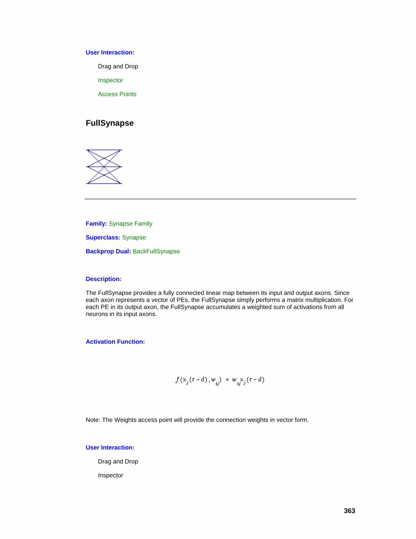
363

User Interaction:

Drag and Drop

Inspector

Access Points

FullSynapse


Superclass: Synapse

Backprop Dual: BackFullSynapse

Description:

The FullSynapse provides a fully connected linear map between its input and output axons. Since each axon represents a vector of PEs, the FullSynapse simply performs a matrix multiplication. For each PE in its output axon, the FullSynapse accumulates a weighted sum of activations from all neurons in its input axons.



User Interaction:

Drag and Drop

Inspector

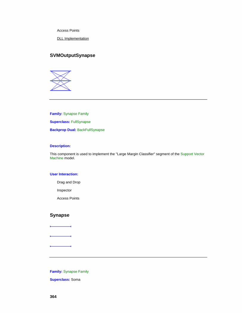
364

Access Points

DLL Implementation

SVMOutputSynapse


Superclass: FullSynapse

Backprop Dual: BackFullSynapse

Description:

This component is used to implement the "Large Margin Classifier" segment of the Support Vector Machine model.

User Interaction:

Drag and Drop

Inspector

Access Points

Synapse


Superclass: Soma

365

Backprop Dual: BackSynapse

Description:

The Synapse applies an identity map between its input and output axons. Since this map is one to one, the axons must have the same number of processing elements. The Synapse is the first member of the Synapse family, and all subsequent members will subclass its functionality.


User Interaction:

Drag and Drop

Inspector

Access Points

DLL Implementation

Macro Actions

See Also

Access Points

Synapse Family Access Points


Access points allow simulation components that are not part of the neural network topology to probe and/or alter data flowing through the network. All members of the Synapse family share a standard functional form. The sub-system block diagram given in diagram depicted this functionality. Access to data flowing through any synapse is provided at the following two access points,

366

Activity Access:

Attaches the NSAccess component to the input axon's activity vector just prior to applying the delay and activation function . It is important to realize that the data reported by this access point actually belongs to the input axon, possibly delayed in time.

Weight Access:

All adaptive weights within the synapse are reported by attaching to Weight Access. This data may be reported in vector or matrix form, depending on how the synapse stores it.

See Also

DLL Implementation

FullSynapse DLL Implementation

Component: FullSynapse

Protocol: PerformFullSynapse

Description:

The FullSynapse component is similar to the Synapse except that the FullSynapse implements a fully-connected linear map from its input to its output, while the Synapse implements only a one-to-one mapping. This mapping requires a matrix of weights, which is adaptable by the Gradient Search components. For each PE in its output axon, the FullSynapse accumulates a weighted sum of activations from all neuron in its input axon.

Code:

367

void performFullSynapse( DLLData *instance, // Pointer to instance data (may be NULL) NSFloat *input, // Pointer to the input layer of PEs int inRows, // Number of rows of PEs in the input layer int inCols, // Number of columns of PEs in the input layer NSFloat *output, // Pointer to the output layer int outRows, // Number of rows of PEs in the output layer int outCols // Number of columns of PEs in the output layer NSFloat *weights // Pointer to the fully-connected weight matrix ) { int i, j, inCount=inRows*inCols, outCount=outRows*outCols; for (i=0; i<outCount; i++) for (j=0; j<inCount; j++) output[i] += W(i,j)*input[j]; }

Synapse DLL Implementation

Component: Synapse

Protocol: PerformSynapse

Description:

The Synapse component simply takes each PE from the Axon feeding the Synapse’s input and adds its activity to the corresponding PE of the Axon at the Synapse’s output. The delay between the input and output is defined by the user within the Synapse Inspector (see Synapse Family). Note that the activity is accumulated at the output for the case of a summing junction (i.e., connection that is fed by multiple Synapses) at the output Axon. Also note that if there is a different number of input PEs than output PEs, then the extra ones are ignored.

Code: void performSynapse( DLLData *instance, // Pointer to instance data (may be NULL) NSFloat *input, // Pointer to the input layer of PEs int inRows, // Number of rows of PEs in the input layer

368

int inCols, // Number of columns of PEs in the input layer NSFloat *output, // Pointer to the output layer int outRows, // Number of rows of PEs in the output layer int outCols // Number of columns of PEs in the output layer ) { int i, inCount=inRows*inCols, outCount=outRows*outCols, count = inCount<outCount? inCount: outCount; for (i=0; i<count; i++) output[i] += input[i]; }

Drag and Drop

Synapse Family Drag and Drop

Synapses are base components on the breadboard. This means that they must be dropped directly onto an empty breadboard location.

See Also

Inspectors

ArbitrarySynapse Inspector

Component: ArbitrarySynapse

Superclass Inspector: Synapse Inspector

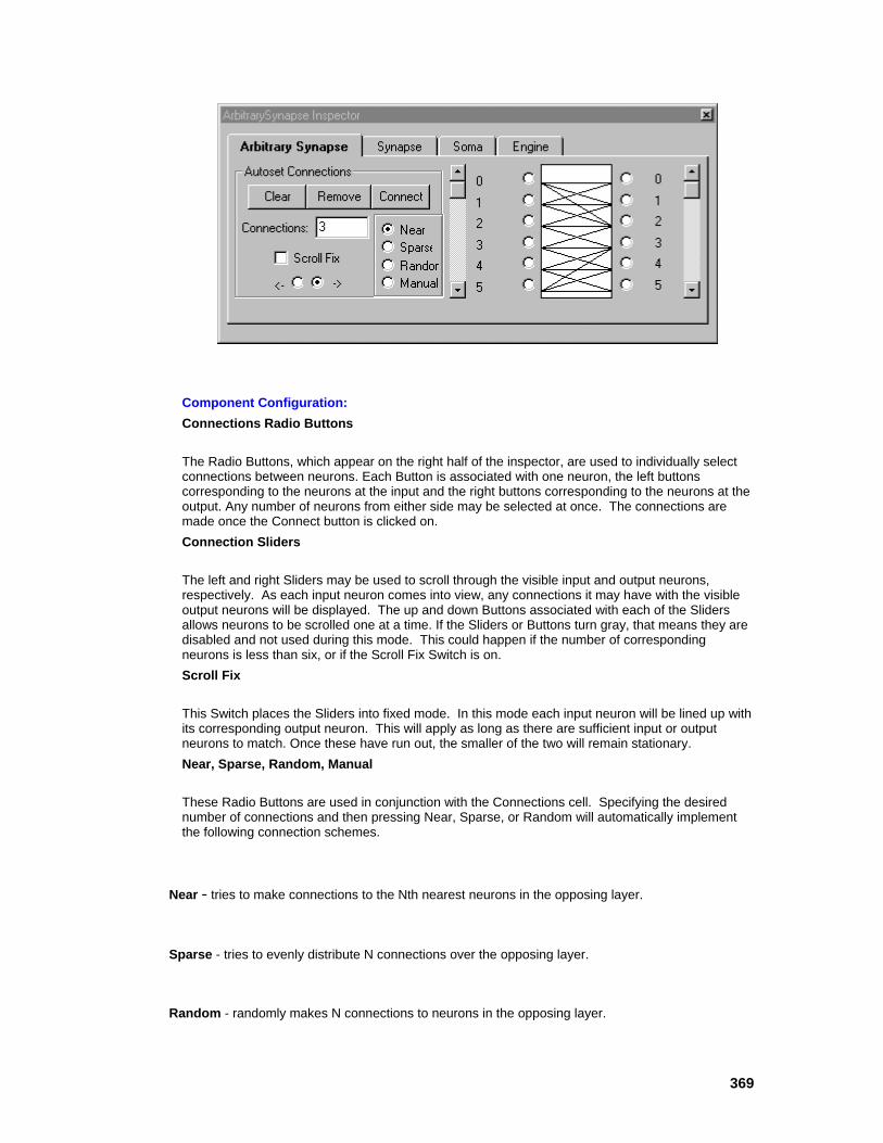
369

Component Configuration: Connections Radio Buttons

The Radio Buttons, which appear on the right half of the inspector, are used to individually select connections between neurons. Each Button is associated with one neuron, the left buttons corresponding to the neurons at the input and the right buttons corresponding to the neurons at the output. Any number of neurons from either side may be selected at once. The connections are made once the Connect button is clicked on. Connection Sliders

The left and right Sliders may be used to scroll through the visible input and output neurons, respectively. As each input neuron comes into view, any connections it may have with the visible output neurons will be displayed. The up and down Buttons associated with each of the Sliders allows neurons to be scrolled one at a time. If the Sliders or Buttons turn gray, that means they are disabled and not used during this mode. This could happen if the number of corresponding neurons is less than six, or if the Scroll Fix Switch is on. Scroll Fix

This Switch places the Sliders into fixed mode. In this mode each input neuron will be lined up with its corresponding output neuron. This will apply as long as there are sufficient input or output neurons to match. Once these have run out, the smaller of the two will remain stationary. Near, Sparse, Random, Manual

These Radio Buttons are used in conjunction with the Connections cell. Specifying the desired number of connections and then pressing Near, Sparse, or Random will automatically implement the following connection schemes.

Near - tries to make connections to the Nth nearest neurons in the opposing layer.

Sparse - tries to evenly distribute N connections over the opposing layer.

Random - randomly makes N connections to neurons in the opposing layer.

370

Once the connection scheme has been chosen, the connections will change under the following conditions: 1) the number of Connections is changed by typing a new number in the Connections cell, or 2) the number of neurons in either the input or output layer are changed, or 3) the component is loaded from a saved breadboard. Note that the third condition can be avoided (i.e., the individual connections will be stored with the breadboard instead of regenerated) by selecting the Manual radio button after the automated connections have been made (but before saving the breadboard).

Pressing the Manual button will allow arbitrarily selected connections to be made. Arbitrary "adding" or "pruning" of connections may be done at any time as long as the Manual Button is highlighted. This works by selecting the input and output neurons, then clicking either the Connect or Remove button. Connections

This cell is used to indicate how many connections should be made from each neuron when using the automatic connection schemes (See above description). From Left, From Right

These radio buttons are used to determine which direction the automatic connection schemes should use when computing which neurons to connect from and to. Connect

This button is used to make connections between arbitrarily selected neurons. When this button is pressed, every highlighted input neuron will be connected to every highlighted output neuron. Clear

Pressing this button will remove all connections. Remove

This button is used to remove connections between neurons. When this button is pressed, every highlighted input neuron will be disconnected from each of the highlighted output neurons.

CombinerSynapse Inspector

Component: CombinerSynapse


371

Component Configuration: Starting PE

This specifies the PE of the Axon at the output to use as the first connection (the one that is connected to the PE 0 of the input Axon). The remaining connections are then made in sequential order (e.g., input PE 1 connects to output PE "Starting+1").

ContractorSynapse Inspector

Component: ContractorSynapse


Component Configuration: Connection Sequence

372

These Radio Buttons are used to specify the connection mapping between the input and output PEs of the ExpanderSynapse. The button labeled "123123123" corresponds to the Sequence 1 example given within the ContractorSynapse component definition page and the button labeled "111222333" corresponds to the Sequence 2 example.

ExpanderSynapse Inspector

Component: ExpanderSynapse


Component Configuration: Connection Sequence

These Radio Buttons are used to specify the connection mapping between the input and output PEs of the ExpanderSynapse. The button labeled "123123123" corresponds to the Sequence 1 example given within the ExpanderSynapse component definition page and the button labeled "111222333" corresponds to the Sequence 2 example.

ModularSynapse Inspector

Component: ModularSynapse


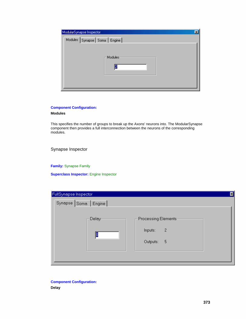
373

Component Configuration: Modules

This specifies the number of groups to break up the Axons' neurons into. The ModularSynapse component then provides a full interconnection between the neurons of the corresponding modules.

Synapse Inspector



Component Configuration: Delay

374

A synapse applies an arbitrary activation function to the activity of an axon at its input, and passes the result to an axon at its output. The activation function can be applied to the input axon's current activity, or its activity at any previous instant in time. The Delay cell allows the user to connect the synapse to delayed versions of the input axon's activity. All recurrent connections on a breadboard will require at least one synapse with a delay greater than zero. Inputs

This cell reports the number of PEs within the Axon attached to the Synapse's input. This value cannot be modified from this location. Outputs

This cell reports the number of PEs within the Axon attached to the Synapse's output. This value cannot be modified from this location.

See Also

Macro Actions

ArbitrarySynapse

ArbitrarySynapse Macro Actions Overview Superclass Macro Actions

Action Description autoconnect Returns the autoconnect setting (Near, Sparse, Random, or Manual). disconnectAll Removes all connections between neurons. forward Returns the connection direction setting (left to right or right to left). nConnections Returns the number of connections setting. removeConnections Removes connections between neurons. setAutoconnect Sets the autoconnect setting (Near, Sparse, Random, or Manual). setForward Sets the connection direction setting (left to right or right to left). setNConnections Sets the number of connections setting. toggleInputNeuron Selects/deselects specific input neurons to be used in the next connection. toggleOutputNeuron Selects/deselects specific output neurons to be used in the next connection.

autoconnect Overview Macro Actions

375

Syntax

componentName.autoconnect()

Parameters Type Description return int Current autoconnect setting (see "Near, Sparse, Random, Manual" within the ArbitrarySynapse Inspector ). 0 = Near 1 = Sparse 2 = Random 3 = Manual componentName Name defined on the engine property page.

disconnectAll Overview Macro Actions

Syntax

componentName.disconnectAll()


forward Overview Macro Actions

Syntax

componentName.forward()

Parameters Type Description return BOOL True if current direction setting is from left to right (see "From Left, From Right" within the ArbitrarySynapse Inspector ). componentName Name defined on the engine property page.

nConnections Overview Macro Actions

376

Syntax

componentName.nConnections()

Parameters Type Description return int The current number of connections from each neuron (see "Connections" within the ArbitrarySynapse Inspector ). componentName Name defined on the engine property page.

removeConnections Overview Macro Actions

Syntax

componentName.removeConnections()


setAutoconnect Overview Macro Actions

Syntax

componentName.setAutoconnect(autoconnect)

Parameters Type Description return void componentName Name defined on the engine property page. autoconnect int New autoconnect setting (see "Near, Sparse, Random, Manual" within the ArbitrarySynapse Inspector ). 0 = Near 1 = Sparse 2 = Random 3 = Manual

377

setForward Overview Macro Actions

Syntax

componentName.setForward(forward)

Parameters Type Description return void componentName Name defined on the engine property page. forward BOOL True if new direction setting is from left to right (see "From Left, From Right" within the ArbitrarySynapse Inspector ).

setNConnections Overview Macro Actions

Syntax

componentName.setNConnections(nConnections)

Parameters Type Description return void componentName Name defined on the engine property page. nConnections int The current number of connections from each neuron (see "Connections" within the ArbitrarySynapse Inspector ).

toggleInputNeuron Overview Macro Actions

Syntax

componentName.toggleInputNeuron(neuronPos)

Parameters Type Description return void componentName Name defined on the engine property page. neuronPos int Index of the input neuron to be selected/deselected for the next connection (see "Connections Radio Buttons" within the ArbitrarySynapse Inspector ).

toggleOutputNeuron Overview Macro Actions

378

Syntax

componentName.toggleOutputNeuron(neuronPos)

Parameters Type Description return void componentName Name defined on the engine property page. neuronPos int Index of the output neuron to be selected/deselected for the next connection (see "Connections Radio Buttons" within the ArbitrarySynapse Inspector ).

FullSynapse

Synapse

Synapse Macro Actions Overview Superclass Macro Actions

Action Description delay Returns the Delay setting. inputConnector Returns the name of the Axon attached to the Synapse's input. outputConnector Returns the name of the Axon attached to the Synapse's output. setDelay Sets the Delay setting.

delay Overview Macro Actions

Syntax

componentName.delay()

Parameters Type Description return int The Synapse’s delay in samples (see "Delay" within the Synapse Inspector ). componentName Name defined on the engine property page.

inputConnector Overview Macro Actions

Syntax

componentName.inputConnector()

379

Parameters Type Description return string The name of the Axon attached to the Synapse's input. componentName Name defined on the engine property page.

outputConnector Overview Macro Actions

Syntax

componentName.outputConnector()

Parameters Type Description return string The name of the Axon attached to the Synapse's output. componentName Name defined on the engine property page.

setDelay Overview Macro Actions

Syntax

componentName.setDelay(delay)

Parameters Type Description return void componentName Name defined on the engine property page. delay int The Synapse’s delay in samples (see "Delay" within the Synapse Inspector ).

Macro Actions

Soma

Soma Macro Actions Overview Superclass Macro Actions

Action Description networkJog Randomizes each weight of the component using its current value as the mean and the variance specified within the Variance cell. networkRandomize Randomizes each weight of the component using the mean specified within the Mean cell and the variance specified within the Variance cell. setEngineData Sets the soma's weights. setWeightMean Sets the Mean value for the weight randomization.

380

setWeightsFixed Sets the Fix Weights setting. setWeightsSave Sets the Save Weights setting. setWeightVariance Sets the Variance value for the weight randomization. weightMean Returns the Mean value for the weight randomization. weightsFixed Returns the Fix Weights setting. weightsSave Returns the Save Weights setting. weightVariance Returns the Variance value for the weight randomization.

networkJog Overview Macro Actions

Syntax

componentName.networkJog()


networkRandomize Overview Macro Actions

Syntax

componentName.networkRandomize()



Syntax



381

data variant An array of single-precision floating point values that contains the soma's weights.

setWeightsFixed Overview Macro Actions

Syntax

componentName.setWeightsFixed(weightsFixed)

Parameters Type Description return void componentName Name defined on the engine property page. weightsFixed BOOL When TRUE, the adaptive weights for the component are frozen during the randomization process (see "Fix Weights" within the Soma Family Inspector ).

setWeightMean Overview Macro Actions

Syntax

componentName.setWeightMean(weightMean)

Parameters Type Description return void componentName Name defined on the engine property page. weightMean float The randomization mean for the component weights (see "Mean" within the Soma Family Inspector ).

setWeightsSave Overview Macro Actions

Syntax

componentName.setWeightsSave(weightsSave)

Parameters Type Description return void componentName Name defined on the engine property page. weightSave BOOL When TRUE, the weights will be saved when the breadboard is saved (see "Save" within the Soma Family Inspector ).

382

setWeightVariance Overview Macro Actions

Syntax

componentName.setWeightVariance(weightVariance)

Parameters Type Description return void componentName Name defined on the engine property page. weightVariance float The randomization variance for the component weights (see "Variance" within the Soma Family Inspector).

weightsFixed Overview Macro Actions

Syntax

componentName.weightsFixed()

Parameters Type Description return BOOL When TRUE, the adaptive weights for the component are frozen during the randomization process (see "Fix Weights" within the Soma Family Inspector ). componentName Name defined on the engine property page.

weightMean Overview Macro Actions

Syntax

componentName.weightMean()

Parameters Type Description return float The randomization mean for the component weights (see "Mean" within the Soma Family Inspector ). componentName Name defined on the engine property page.

weightsSave Overview Macro Actions

Syntax

componentName.weightsSave()

383

Parameters Type Description return BOOL When TRUE, the weights will be saved when the breadboard is saved (see "Save" within the Soma Family Inspector ). componentName Name defined on the engine property page.

weightVariance Overview Macro Actions

Syntax

componentName.weightVariance()

Parameters Type Description return float The randomization variance for the component weights (see "Variance" within the Soma Family Inspector). componentName Name defined on the engine property page.

Backprop Family BackAxon Family

BackAxon

Family: BackAxon Family

Superclass: Axon

Activation Dual: Axon

Sensitivity Function:

384

Gradient Function:

No weights

User Interaction:

Drag and Drop

Inspector

Access Points

DLL Implementation

BackBiasAxon



Activation Dual: BiasAxon


Gradient Function:

385

User Interaction:

Drag and Drop

Inspector

Access Points

DLL Implementation

BackCombinerAxon


Superclass: BackAxon

Activation Dual: CombinerAxon


where i < N/2, and

where i >= N/2.

Gradient Function:

No weights to update.

User Interaction:

Drag and Drop

Inspector

386

Access Points

DLL Implementation

BackLinearAxon


Superclass: BackBiasAxon

Activation Dual: LinearAxon

Description:

The BackLinearAxon is the companion component for the LinearAxon that implements learning. It basically allows for the adaptation of the bias weight. The slope can be scheduled or user modified.


Gradient Function:

User Interaction:

Drag and Drop

Inspector

Access Points

387

DLL Implementation

Macro Actions

BackNormalizedAxon



Activation Dual: NormalizedAxon


Gradient Function:

No weights to update.

User Interaction:

Drag and Drop

Inspector

Access Points

DLL Implementation

BackNormalizedSigmoidAxon

388


Superclass: BackSigmoidAxon

Activation Dual: NormalizedSigmoidAxon


where is the sensitivity function of the BackSigmoidAxon.

Gradient Function:

Same as the BackSigmoidAxon.

User Interaction:

Drag and Drop

Inspector

Access Points

DLL Implementation

BackSigmoidAxon

389


Superclass: BackLinearAxon

Activation Duals: SigmoidAxon, LinearSigmoidAxon


where O is the Nonlinearity Derivative Offset .

Gradient Function:

User Interaction:

Drag and Drop

Inspector

Access Points

DLL Implementation

BackTanhAxon

390



Activation Duals: TanhAxon, LinearTanhAxon


where O is the Nonlinearity Derivative Offset .

Gradient Function:

User Interaction:

Drag and Drop

Inspector

Access Points

DLL Implementation

BackCriteriaControl



Activation Dual: ErrorCriteria Family

391

Description:

The BackCriteriaControl is designed to stack on top of any member of the ErrorCriteria family, and communicate with the Backprop components to perform backpropagation.

User Interaction:

Drag and Drop

Inspector

Access Points

BackBellFuzzyAxon



Activation Dual: BellFuzzyAxon

Description:

The BackBellFuzzyAxon is the companion component for the BellFuzzyAxon that implements learning. It basically allows for the adaptation of the three parameters of each of the membership functions.


Gradient Function:

392

where wi = weight (MF parameter)

User Interaction:

Drag and Drop

Inspector

Access Points

DLL Implementation

BackGaussianFuzzyAxon



Activation Dual: GaussianFuzzyAxon

393

Description:

The BackGaussianFuzzyAxon is the companion component for the GaussianFuzzyAxon that implements learning. It basically allows for the adaptation of the two parameters of each of the membership functions.


Gradient Function:

where wi = weight (MF parameter)

User Interaction:

Drag and Drop

Inspector

Access Points

DLL Implementation

Access Points

BackAxon Family Access Points

Family:BackAxon Family

394

Pre-Activity Gradients Access:

Attaches the Access component to the vector sum just prior to applying the activation function . It is important to realize that this access point does not correspond to any physical

storage within the simulation. In other words, data may be injected or probed as activity flows through the network, but is then immediately lost. Trying to alter the pre-activity out of sync with the network data flow will actually alter the data storage for Activity Access.

Activity Gradients Access:

Attaches the Access component to the vector of activity immediately after the function map .

Weights Gradients Access:


DLL Implementation

BackAxon DLL Implementation

Component: BackAxon

Protocol: PerformBackAxon

Description:

Since the Axon component does not modify the data fed into the processing elements (PEs), the BackAxon component does not modify the sensitivity vector. The Axon component does not have any adaptable weights, so there is no gradient vector to compute.

Code: void performBackAxon( DLLData *instance, // Pointer to instance data (may be NULL) DLLData *dualInstance, // Pointer to forward axon’s instance data NSFloat *data, // Pointer to the layer of PEs int rows, // Number of rows of PEs in the layer int cols, // Number of columns of PEs in the layer NSFloat *error // Pointer to the sensitivity vector ) {

395

}

BackBiasAxon DLL Implementation

Component: BackBiasAxon

Protocol: PerformBackBiasAxon

Description:

Since the partial of the BiasAxon’s cost with respect to its activity is 1, the sensitivity vector is not modified. The partial of the BiasAxon’s cost with respect to its weight vector is used to compute the gradient vector. This vector is simply an accumulation of the error.

Code: void performBackBiasAxon( DLLData *instance, // Pointer to instance data DLLData *dualInstance, // Pointer to forward axon’s instance data NSFloat *data, // Pointer to the layer of PEs int rows, // Number of rows of PEs in the layer int cols, // Number of columns of PEs in the layer NSFloat *error // Pointer to the sensitivity vector NSFloat *gradient // Pointer to the bias gradient vector ) { int i, length=rows*cols; if (gradient) for (i=0; i<length; i++) gradient[i] += error[i]; }

BackLinearAxon DLL Implementation

396

Component: BackLinearAxon

Protocol: PerformBackLinearAxon

Description:

The partial of the LinearAxon’s cost with respect to its activity is the sensitivity from the previous layer times beta. The partial of the LinearAxon’s cost with respect to its weight vector is used to compute the gradient vector. As with the BiasAxon, this vector is simply an accumulation of the error.

Code: void performBackLinearAxon( DLLData *instance, // Pointer to instance data DLLData *dualInstance, // Pointer to forward axon’s instance data NSFloat *data, // Pointer to the layer of PEs int rows, // Number of rows of PEs in the layer int cols, // Number of columns of PEs in the layer NSFloat *error // Pointer to the sensitivity vector NSFloat *gradient // Pointer to the bias gradient vector NSFloat beta // Slope gain scalar, same for all PEs ) { int i, length=rows*cols; for (i=0; i<length; i++) { error[i] *= beta; if (gradient) gradient[i] += error[i]; } }

BackSigmoidAxon DLL Implementation

Component: BackSigmoidAxon


Description:

397

The partial of the SigmoidAxon’s cost with respect to its activity is used to compute the sensitivity vector. The partial of the SigmoidAxon’s cost with respect to its weight vector is used to compute the gradient vector. As with the BiasAxon, this vector is simply an accumulation of the error.

Code: void performBackLinearAxon( DLLData *instance, // Pointer to instance data DLLData *dualInstance, // Pointer to forward axon’s instance data NSFloat *data, // Pointer to the layer of PEs int rows, // Number of rows of PEs in the layer int cols, // Number of columns of PEs in the layer NSFloat *error // Pointer to the sensitivity vector NSFloat *gradient // Pointer to the bias gradient vector NSFloat beta // Slope gain scalar, same for all PEs ) { int i, length=rows*cols; for (i=0; i<length; i++) { error[i] *= beta*(data[i]*(1.0f-data[i]) + 0.1f); if (gradient) gradient[i] += error[i]; } }

BackTanhAxon DLL Implementation

Component: BackTanhAxon


Description:

The partial of the TanhAxon’s cost with respect to its activity is used to compute the sensitivity vector. The partial of the TanhAxon’s cost with respect to its weight vector is used to compute the gradient vector. As with the BiasAxon, this vector is simply an accumulation of the error.

Code: void performBackLinearAxon( DLLData *instance, // Pointer to instance data

398

DLLData *dualInstance, // Pointer to forward axon’s instance data NSFloat *data, // Pointer to the layer of PEs int rows, // Number of rows of PEs in the layer int cols, // Number of columns of PEs in the layer NSFloat *error // Pointer to the sensitivity vector NSFloat *gradient // Pointer to the bias gradient vector NSFloat beta // Slope gain scalar, same for all PEs ) { int i, length=rows*cols; for (i=0; i<length; i++) { error[i] *= beta*(1.0f - data[i]*data[i] + 0.1f); if (gradient) gradient[i] += error[i]; } }

BackBellFuzzyAxon DLL Implementation

Component: BackBellFuzzyAxon

Protocol: PerformBackFuzzyAxon

Description: The BellFuzzyAxon has three parameters for each membership function. This function computes the partial of each of those parameters with respect to the input value corresponding to the winning membership function.

Code: void performBackFuzzyAxon( DLLData *instance, // Pointer to instance data (may be NULL) DLLData *dualInstance,// Pointer to forward axon’s instance data // (may be NULL) NSFloat *data, // Pointer to the layer of processing // elements (PEs) int rows, // Number of rows of PEs in the layer int cols, // Number of columns of PEs in

399

the layer NSFloat *error, // Pointer to the sensitivity vector NSFloat *param, // Pointer to the layer of parameters for the // MFs int paramIndex, // Index of the MF parameter int winnerIndex, // Index of the winning MF NSFloat winnerVal, // Value of the winning Input NSFloat *returnVal // Return value ) { NSFloat b; NSFloat c; NSFloat tmp1; NSFloat tmp2; NSFloat denom; NSFloat a = *(param + winnerIndex); if (a == 0.0f) *returnVal = 0.0f; b = *(param + winnerIndex + 1); c = *(param + winnerIndex + 2); tmp1 = (winnerVal - c)/a; tmp2 = tmp1 == 0 ? 0 : (NSFloat)pow(pow(tmp1, 2.0), b); denom = (1 + tmp2)*(1 + tmp2); if (paramIndex == winnerIndex) *returnVal = (2*b*tmp2/(a*denom)); if (paramIndex == (winnerIndex + 1)) { if (tmp1 == 0) *returnVal = 0.0f; else *returnVal = ((NSFloat)-log(tmp1*tmp1)*tmp2/denom); } if (paramIndex == (winnerIndex + 2)) { if (winnerVal == c) *returnVal = 0.0f; else *returnVal = (2*b*tmp2/((winnerVal - c)*(denom))); } }

BackGaussianFuzzyAxon DLL Implementation

400

Component: BackGaussianFuzzyAxon

Protocol: PerformBackFuzzyAxon

Description: The GaussianFuzzyAxon has two parameters for each membership function. This function computes the partial of each of those parameters with respect to the input value corresponding to the winning membership function.

Code: void performBackFuzzyAxon( DLLData *instance, // Pointer to instance data (may be NULL) DLLData *dualInstance,// Pointer to forward axon’s instance data // (may be NULL) NSFloat *data, // Pointer to the layer of processing // elements (PEs) int rows, // Number of rows of PEs in the layer int cols, // Number of columns of PEs in the layer NSFloat *error, // Pointer to the sensitivity vector NSFloat *param, // Pointer to the layer of parameters for the // MFs int paramIndex, // Index of the MF parameter int winnerIndex, // Index of the winning MF NSFloat winnerVal, // Value of the winning Input NSFloat *returnVal // Return value ) { NSFloat c = *(param + winnerIndex); NSFloat sigma = *(param + winnerIndex + 1); if (sigma == 0.0f) *returnVal = 0.0f; else { NSFloat exp_fraction = (winnerVal - c) / sigma; NSFloat exp_final = (NSFloat)(pow (exp_fraction, 2.0) / -2.0); NSFloat fwrd_activation = (NSFloat)exp (exp_final); if (paramIndex == winnerIndex) { NSFloat deriv_fwrd = (NSFloat)((winnerVal - c) / pow (sigma, 2.0)); *returnVal = fwrd_activation * deriv_fwrd; } if (paramIndex == (winnerIndex + 1)) {

401

NSFloat deriv_fwrd = (NSFloat)(pow ( (winnerVal - c), 2.0) / pow (sigma, 3.0)); *returnVal = fwrd_activation * deriv_fwrd; } } }

Inspectors

BackLinearAxon Inspector

Component: BackLinearAxon


Component Configuration: Nonlinearity Derivative Offset

This offset is added to computed sensitivities in order to avoid a zero error, which could result in a flat learning curve.

Macro Actions

Back Linear Axon

BackLinearAxon Macro Actions Overview Superclass Macro Actions

Action Description

402

offset Returns the nonlinearity derivative offset. setOffset Sets the nonlinearity derivative offset.

offset Overview Macro Actions

Syntax

componentName.offset()

Parameters Type Description return float The nonlinearity derivative offset (see the BackLinearAxon Inspector). componentName Name defined on the engine property page.

setOffset Overview Macro Actions

Syntax

componentName.setOffset(offset)

Parameters Type Description return void componentName Name defined on the engine property page. offset float The nonlinearity derivative offset (see the BackLinearAxon Inspector).


BackContextAxon


403


Activation Dual: ContextAxon


Gradient Function:

User Interaction:

Drag and Drop

Inspector

Access Points

DLL Implementation

BackGammaAxon


Superclass: BackTDNNAxon

Activation Dual: GammaAxon

Tap Sensitivity Function:

404

Gradient Function:

User Interaction:

Drag and Drop

Inspector

Access Points

DLL Implementation

BackLaguarreAxon


Superclass: BackTDNNAxon

Activation Dual: LaguarreAxon


405

Gradient Function:

User Interaction:

Drag and Drop

Inspector

Access Points

DLL Implementation

BackIntegratorAxon


Superclass: BackContextAxon

Activation Dual: IntegratorAxon


Gradient Function:

406

User Interaction:

Drag and Drop

Inspector

Access Points

DLL Implementation

BackSigmoidContextAxon



Activation Dual: SigmoidContextAxon


See BackSigmoidAxon and BackContextAxon

Gradient Function:

See BackContextAxon

User Interaction:

Drag and Drop

Inspector

Access Points

DLL Implementation

407

BackSigmoidIntegratorAxon


Superclass: BackIntegratorAxon

Activation Dual: SigmoidIntegratorAxon


See BackSigmoidAxon and BackIntegratorAxon

Gradient Function:

See BackIntegratorAxon

User Interaction:

Drag and Drop

Inspector

Access Points

DLL Implementation

BackTanhContextAxon


408


Activation Dual: TanhContextAxon


See BackTanhAxon and BackContextAxon

Gradient Function:

See BackContextAxon

User Interaction:

Drag and Drop

Inspector

Access Points

DLL Implementation

BackTanhIntegratorAxon


Superclass: BackIntegratorAxon

Activation Dual: TanhIntegratorAxon


See BackTanhAxon and BackIntegratorAxon

Gradient Function:

409

See BackIntegratorAxon

User Interaction:

Drag and Drop

Inspector

Access Points

DLL Implementation

BackTDNNAxon



Activation Dual: TDNNAxon


Gradient Function:

No weights

User Interaction:

Drag and Drop

Inspector

Access Points

DLL Implementation

410

DLL Implementation

BackContextAxon DLL Implementation

Component: BackContextAxon

Protocol: PerformBackContextAxon

Description:

The gradient information is computed to update the time constants and the sensitivity vector is computed for the backpropagation.

Code: void performBackContextAxon( DLLData *instance, // Pointer to instance data (may be NULL) DLLData *dualInstance, // Pointer to forward axon’s instance data NSFloat *error, // Pointer to the current sensitivity vector int rows, // Number of rows of PEs in the layer int cols, // Number of columns of PEs in the layer NSFloat *delayedError, // Pointer to the delayed error vector NSFloat *data, // Pointer to the layer of PEs NSFloat *tau, // Pointer to a vector of time constants NSFloat beta, // Linear scaling factor (user-defined) NSFloat *gradient // Pointer to the tau gradient vector ) { int i, length=rows*cols; for (i=0; i<length; i++) { error[i] = beta*(data[i] + tau[i]*delayedError[i]); if (gradient) gradient[i] += delayedError[i]*beta*data[i]; } }

BackGammaAxon DLL Implementation

411

Component: BackGammaAxon

Protocol: PerformBackGammaAxon

Description:

The gradient information is computed to update the gamma coefficients and the sensitivity vector is computed for the backpropagation.

Code: void performBackGammaAxon( DLLData *instance, // Pointer to instance data (may be NULL) DLLData *dualInstance, // Pointer to forward axon’s instance data NSFloat *error, // Pointer to the current sensitivity vector int rows, // Number of rows of PEs in the layer int cols, // Number of columns of PEs in the layer NSFloat *delayedError, // Pointer to the delayed error vector int taps, // Number of memory taps (user-defined) NSFloat *data // Pointer to the layers of (PEs) NSFloat *gamma, // Pointer to vector of gamma coefficients NSFloat *gradient // Pointer to the gamma gradient vector ) { register int i,j,k,length=rows*cols; for (i=0; i<length; i++) for (j=1; j<taps; j++) { k = i + j*length; error[k-length] += gamma[i]*delayedError[k]; error[k] += (1.0f-gamma[i])*delayedError[k]; if (gradient) gradient[i] += delayedError[k]*(data[k-length]-data[k]); } }

BackIntegratorAxon DLL Implementation

412

Component: BackIntegratorAxon


Description:


Code: void performBackContextAxon( DLLData *instance, // Pointer to instance data (may be NULL) DLLData *dualInstance, // Pointer to forward axon’s instance data NSFloat *error, // Pointer to the current sensitivity vector int rows, // Number of rows of PEs in the layer int cols, // Number of columns of PEs in the layer NSFloat *delayedError, // Pointer to the delayed error vector NSFloat *data, // Pointer to the layer of PEs NSFloat *tau, // Pointer to a vector of time constants NSFloat beta, // Linear scaling factor (user-defined) NSFloat *gradient // Pointer to the tau gradient vector ) { int i, length=rows*cols; for (i=0; i<length; i++) { error[i] = beta*((1.0f-tau[i])*data[i] + tau[i]*delayedError[i]); if (gradient) gradient[i] += delayedError[i]*beta*data[i]; } }

BackLaguarreAxon DLL Implementation

413

Component: BackLaguarreAxon

Protocol: PerformBackGammaAxon DLL Protocol

Description:

The gradient information is computed to update the gamma coefficients and the sensitivity vector is computed for the backpropagation.

Code: void performBackGammaAxon( DLLData *instance, // Pointer to instance data (may be NULL) DLLData *dualInstance, // Pointer to forward axon’s instance data NSFloat *error, // Pointer to the current sensitivity vector int rows, // Number of rows of PEs in the layer int cols, // Number of columns of PEs in the layer NSFloat *delayedError, // Pointer to the delayed error vector int taps, // Number of memory taps (user-defined) NSFloat *data // Pointer to the layers of (PEs) NSFloat *gamma, // Pointer to vector of gamma coefficients NSFloat *gradient // Pointer to the gamma gradient vector ) { register int i,j,k,length=rows*cols; NSFloat gain; for (i=0; i<length; i++) { gain = (NSFloat)pow(1-pow(gamma[i], 2.0f), 0.5f); for (j=1; j<taps; j++) { k = i + j*length; error[k-length] += delayedError[k]; error[k] += gamma[i]*delayedError[k]; if (gradient) gradient[i] += delayedError[k]*data[k]; if (j==1) error[k] *= gain; else { error[k-length] -= gamma[i]*error[k]; if (gradient) gradient[i] -= error[k]*data[k-length]; } } } }

414

BackSigmoidContextAxon DLL Implementation

Component: BackSigmoidContextAxon


Description:


Code: void performBackContextAxon( DLLData *instance, // Pointer to instance data (may be NULL) DLLData *dualInstance, // Pointer to forward axon’s instance data NSFloat *error, // Pointer to the current sensitivity vector int rows, // Number of rows of PEs in the layer int cols, // Number of columns of PEs in the layer NSFloat *delayedError, // Pointer to the delayed error vector NSFloat *data, // Pointer to the layer of PEs NSFloat *tau, // Pointer to a vector of time constants NSFloat beta, // Linear scaling factor (user-defined) NSFloat *gradient // Pointer to the tau gradient vector ) { int i, length=rows*cols; for (i=0; i<length; i++) { error[i] *= data[i]*(1.0f-data[i]) + 0.1f; error[i] = beta*(data[i] + tau[i]*delayedError[i]); if (gradient) gradient[i] += delayedError[i]*beta*data[i]; } }

BackSigmoidIntegratorAxon DLL Implementation

415

Component: BackSigmoidIntegratorAxon


Description:


Code: void performBackContextAxon( DLLData *instance, // Pointer to instance data (may be NULL) DLLData *dualInstance, // Pointer to forward axon’s instance data NSFloat *error, // Pointer to the current sensitivity vector int rows, // Number of rows of PEs in the layer int cols, // Number of columns of PEs in the layer NSFloat *delayedError, // Pointer to the delayed error vector NSFloat *data, // Pointer to the layer of PEs NSFloat *tau, // Pointer to a vector of time constants NSFloat beta, // Linear scaling factor (user-defined) NSFloat *gradient // Pointer to the tau gradient vector ) { int i, length=rows*cols; for (i=0; i<length; i++) { error[i] *= data[i]*(1.0f-data[i]) + 0.1f; error[i] = beta*((1.0f-tau[i])*data[i] + tau[i]*delayedError[i]); if (gradient) gradient[i] += delayedError[i]*beta*data[i]; } }

BackTanhContextAxon DLL Implementation

416

Component: BackTanhContextAxon


Description:


Code: void performBackContextAxon( DLLData *instance, // Pointer to instance data (may be NULL) DLLData *dualInstance, // Pointer to forward axon’s instance data NSFloat *error, // Pointer to the current sensitivity vector int rows, // Number of rows of PEs in the layer int cols, // Number of columns of PEs in the layer NSFloat *delayedError, // Pointer to the delayed error vector NSFloat *data, // Pointer to the layer of PEs NSFloat *tau, // Pointer to a vector of time constants NSFloat beta, // Linear scaling factor (user-defined) NSFloat *gradient // Pointer to the tau gradient vector ) { int i, length=rows*cols; for (i=0; i<length; i++) { error[i] *= 1.0f - data[i]*data[i] + 0.1f; error[i] = beta*(data[i] + tau[i]*delayedError[i]); if (gradient) gradient[i] += delayedError[i]*beta*data[i]; } }

BackTanhIntegratorAxon DLL Implementation

Component: BackTanhIntegratorAxon

417


Description:


Code: void performBackContextAxon( DLLData *instance, // Pointer to instance data (may be NULL) DLLData *dualInstance, // Pointer to forward axon’s instance data NSFloat *error, // Pointer to the current sensitivity vector int rows, // Number of rows of PEs in the layer int cols, // Number of columns of PEs in the layer NSFloat *delayedError, // Pointer to the delayed error vector NSFloat *data, // Pointer to the layer of PEs NSFloat *tau, // Pointer to a vector of time constants NSFloat beta, // Linear scaling factor (user-defined) NSFloat *gradient // Pointer to the tau gradient vector ) { int i, length=rows*cols; for (i=0; i<length; i++) { error[i] *= 1.0f - error[i]*error[i] + 0.1f; error[i] = beta*((1.0f-tau[i])*error[i] + tau[i]*delayedError[i]); if (gradient) gradient[i] += delayedError[i]*beta*data[i]; } }

BackTDNNAxon DLL Implementation

Component: BackTDNNAxon

Protocol: PerformBackTDNNAxon

Description:

418

Since the TDNNAxon has no adaptable weights, there is no gradient information to compute. The sensitivity vector is computed by taking the backpropagated error from each PE and adding the delayedError from the next tap.

Code: void performBackTDNNAxon( DLLData *instance, // Pointer to instance data (may be NULL) DLLData *dualInstance, // Pointer to forward axon’s instance data NSFloat *error, // Pointer to the current sensitivity vector int rows, // Number of rows of PEs in the layer int cols, // Number of columns of PEs in the layer NSFloat *delayedError, // Pointer to the delayed error vector int taps, // Number of memory taps (user-defined) NSFloat *data // Pointer to the layers of (PEs) ) { register int i,j,k,length=rows*cols; for (i=0; i<length; i++) for (j=1; j<taps; j++) { k = i + j*length; error[k-length] += delayedError[k]; } }

BackSynapse Family

BackArbitrarySynapse

Family: BackSynapse Family

Superclass: BackSynapse

Activation Dual: ArbitrarySynapse

Sensitivity Function and Gradient Function:

There is no pre-specified map for the ArbitrarySynapse. This component will backpropagate the sensitivities and gradients for any user defined connections within its dual component.

419

User Interaction:

Drag and Drop

Inspector

Access Points

BackFullSynapse


Superclass: BackSynapse

Activation Dual: FullSynapse


Gradient Function:

User Interaction:

Drag and Drop

Inspector

Access Points

DLL Implementation

BackSynapse

420


Superclass: Synapse

Activation Dual: Synapse


Gradient Function:

No weights

User Interaction:

Drag and Drop

Inspector

Access Points

DLL Implementation

DLL Implementation

BackFullSynapse DLL Implementation

Component: BackFullSynapse

421

Protocol: PerformBackFullSynapse

Description:

The gradient of the weight going from the jth PE of the input BackAxon to the ith PE of the output BackAxon is the product of the error at the ith PE of the input BackAxon and the activity of the jth PE of the output BackAxon’s activation dual component.

The error at the ith PE of the output BackAxon is the sum of the products of each weight connected to that PE and the corresponding error at the input BackAxon. Note that the input and output are reversed from the activation dual (i.e., the Synapse).

Code: void performBackFullSynapse( DLLData *instance, // Pointer to instance data (may be NULL) DLLData *dualInstance, // Pointer to forward axon’s instance data NSFloat *errorIn, // Pointer to the input error layer of PEs int inRows, // Number of rows of PEs in the input layer int inCols, // Number of columns of PEs at the input NSFloat *errorOut, // Pointer to the output error layer int outRows, // Number of rows of PEs in the output layer int outCols, // Number of columns of PEs at the output NSFloat *input // Pointer to output PEs of forward synapse NSFloat *weights, // Pointer to fully-connected weight matrix NSFloat *gradients // Pointer to the weight gradient matrix ) { int i, j, inCount=inRows*inCols, outCount=outRows*outCols; for (i=0; i<outCount; i++) for (j=0; j<inCount; j++) { errorOut[i] += W(j,i)*errorIn[j]; if (gradients) Wg(j,i) += errorIn[j]*input[i]; } }

BackSynapse DLL Implementation

422

Component: BackSynapse

Protocol: PerformBackSynapse

Description:

Since the Synapse component has no adaptable weights, there is no gradient information computed. The sensitivity vector is computed by taking the error from the previous backprop layer and adding it to the error at the next backprop layer. Note that the error is accumulated at the output for the case of a splitting node (i.e., connection that feeds multiple Synapses) at the Axon that feeds the activation dual component (i.e., the Synapse).

The delay between the output and input is defined by the user within the inspector of the activation dual (see Back Synapse Family). Note that the input and output are reversed from the activation dual (i.e., the Synapse).

Code: void performBackSynapse( DLLData *instance, // Pointer to instance data (may be NULL) DLLData *dualInstance, // Pointer to forward axon’s instance data NSFloat *errorIn, // Pointer to the input error layer of PEs int inRows, // Number of rows of PEs in the input layer int inCols, // Number of columns of PEs at the input NSFloat *errorOut, // Pointer to the output error layer int outRows, // Number of rows of PEs in the output layer int outCols, // Number of columns of PEs at the output NSFloat *input // Pointer to output PEs of forward synapse ) { int i, inCount=inRows*inCols, outCount=outRows*outCols, count=inCount<outCount? inCount: outCount; for (i=0; i<count; i++) errorOut[i] += errorIn[i]; }

Drag and Drop

Backprop Family Drag and Drop

Each member of the Backprop family was custom developed to perform backpropagation for a component in the Activation family. There is a one-to-one association between members of the Backprop family and the adaptive Activation components. The Activation component associated with any Backprop member will be referred to as its Activation dual. Each member of the Backprop family must be dropped directly on its activation dual, or a subclass of its dual.

423

See Also

Controls Family StaticControl

Family: Controls Family

Superclass: Control

Description:

The StaticControl implements data flow for static backpropagation. It expects a static input and a static desired response, from which an error is obtained. The error is propagated through the dual system (backprop plane).

The user-defined options are limited to the number of patterns in the training set (exemplars/epoch) and the number of training cycles (epochs/experiment). The Control Toolbar contains controls to start/stop the simulation, reset the network (randomize the weights and clear the activations), and jog the weights (alter them by a small random value). The user can also single-step through the presentation of patterns either one exemplar at a time or one epoch at a time using the Static property page.

The StaticControl allows a Cross Validation data set to flow through a network during learning, without affecting the updating of the weights.

User Interaction:

Drag and Drop

Inspector

Toolbar

Window

Access Points

Macro Actions

424

See Also

Schedule Family

BackStaticControl


Superclass: Control

Description:

The BackStaticControl component is used in conjunction with the StaticControl component. Static backpropagation assumes that the output of a network is strictly a function of its present input (i.e., the network topology is static). In this case, the gradients and sensitivities are only dependent on the error and activations from the current time step. Note that static backpropagation can be used with temporal problems when using components with internal memory taps (e.g., TDNNAxon).

The user specifies the number of patterns to be presented to the network before a weight update is computed. If the weights are updated after every exemplar (exemplars/update = 1), then this is termed on-line learning. If the weights are update after every epoch (exemplars/update = exemplars/epoch), then this is termed batch learning.

This component also has a facility for automatically constructing or removing the learning dynamics (the backprop and gradient search planes) from the network. This provides an efficient means of switching a network between testing and training modes.

User Interaction:

Drag and Drop

Inspector

Macro Actions

See Also

DynamicControl

425


Superclass: Control

Description:

The DynamicControl component is responsible for synchronizing the presentation of data to a neural network. The activation of all network simulations are divided into experiments, epochs, exemplars and forward samples. The DynamicControl component is capable of controlling both static and dynamic network topologies and is an extension of the StaticControl component.

The outputs of a static network are only a function of its inputs and states at the current instant in time. This relationship can be depicted by the following equation:

y(t) = f(i(t), x(t), w)

where y(t) are the network's outputs, i(t) are inputs, x(t) are internal nodes and w are its weights.

The outputs of a dynamic network can be a function of its inputs and internal states at the present time step, as well as its states at any past instant in time. This is illustrated by:

y(t) = f(i(t), x(t), x(t-1), ... , x(t-T), w)

The term forward samples refers to the individual pieces of temporal information. An exemplar is a complete pattern of samples. The temporal dimension of an exemplar is defined by the number of samples/exemplar. Note that the temporal dimension of a static network is one. An epoch refers to the set of all exemplars to be presented during the training of a network. A neural network experiment consists of the repeated presentation of an epoch to the network until it has sufficiently trained.

Like the StaticControl, the DynamicControl allows a Cross Validation data set to flow through a network during learning, without affecting the updating of the weights.

User Interaction:

Drag and Drop

Inspector

Toolbar

Macro Actions

426

See Also

BackDynamicControl


Superclass: Control

Description:

The BackDynamicControl and BackStaticControl components are responsible for the synchronization of components implementing the backpropagation learning rule (i.e., the backpropagation plane). There are two distinct synchronization paradigms for backpropagation. Synchronization refers to the way in which the network processes sensitivity (error) data. The ActivationControl family divides simulations into experiments, epochs, exemplars and forward samples. The BackDynamicControl further defines a simulation by the number of backward samples per exemplar and the number of exemplars per update. As with the static case, the exemplars/update specifies how many times this process is repeated before the weight gradients are applied to the weights. Backpropagation can either be synchronized in Static, Trajectory or Fixed Point modes.

Static backpropagation requires that the samples/exemplar of both the DynamicControl and the BackDynamicControl be set to one. See the reference for BackStaticControl for a description of static backpropagation.

Training a network in Trajectory mode assumes that each exemplar has a temporal dimension defined by its forward samples (period), and that there exists some desired response for the network's output over this period. The network is first run forward in time over the entire period, during which an error is determined between the network's output and the desired response. Then the network is run backwards for a prescribed number of samples (defined by the samples/exemplar of the BackDynamicControl) to compute the gradients and sensitivities. This forward/backward pass is considered a single exemplar.

Fixed Point mode assumes that each exemplar represents a static pattern that is to be embedded as a fixed point of a recurrent network. Here the terms forward samples and backward samples can be thought of as the forward relaxation period and backward relaxation period, respectively. All inputs are held constant while the network is repeatedly fired during its forward relaxation period, specified by the samples/exemplar of the DynamicControl component. Note that there are no guarantees that the forward activity of the network will relax to a fixed point, or even relax at all. After the network has relaxed, an error is determined and held as constant input to the backpropagation layer. Similarly, the error is backpropagated through the backprop plane for its backward relaxation period, specified by the samples/exemplar of the BackDynamicControl. This forward/backward relaxation is considered to be one exemplar.

User Interaction:

Drag and Drop

Inspector

427

Macro Actions

See Also

GeneticControl


Superclass: Control

Description:

The GeneticControl component implements a genetic algorithm to optimize one or more parameters within the neural network. The most common parameters to optimize are the input columns, the number of hidden PEs, number of memory taps, and the learning rates. Many other network parameters are available for optimization.

Genetic Algorithms are general-purpose search algorithms based upon the principles of evolution observed in nature. Genetic algorithms combine selection, crossover, and mutation operators with the goal of finding the best solution to a problem. They search for this optimal solution until a specified termination criterion is met. In NeuroSolutions the criteria used to evaluate the fitness of each potential solution is the lowest cost achieved during the training run.

The solution to a problem is called a chromosome. A chromosome is made up of a collection of genes, which are simply the neural network parameters to be optimized. A genetic algorithm creates an initial population (a collection of chromosomes) and then evaluates this population by training a neural network for each chromosome. It then evolves the population through multiple generations (using the genetic operators discussed above) in the search for the best network parameters.

User Interaction:

Drag and Drop

Inspector

Window

428

Access Points

StaticControl Access Points

Family: Activation Control Family

Epochs: This access point reports the number of epochs that have been run during a given simulation. This number may be used to transmit messages at various points during leaning.

Exemplars:

This access point reports the number of exemplars that have been run during the current epoch. This number may be used to transmit messages at various points during leaning.

GeneticControl Access Points

Family: Activation Control Family

Best Fitness: Reports the fitness of the chromosome with the lowest value. In other words, this is the lowest Average Cost reported by the ErrorCriterion since the beginning of the genetic run.

Average Fitness:

Reports the average fitness of all of the chromosomes in the current population. Note that the fitness is the Average Cost reported by the ErrorCriterion.

SD Fitness:

Reports the standard deviation fitness of all of the chromosomes in the current population. Note that the fitness is the Average Cost reported by the ErrorCriterion.

Worst Fitness:

Reports the fitness of the chromosome with the highest value. Note that the fitness is the Average Cost reported by the Error Criterion.

Generations:

Reports the generation number. Note that this value is also reported within the Simulation Progress window.

Drag and Drop

Controls Drag and Drop

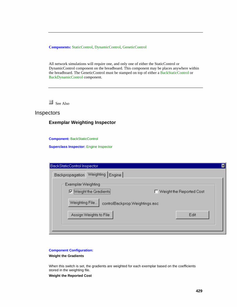
429

Components: StaticControl, DynamicControl, GeneticControl

All network simulations will require one, and only one of either the StaticControl or DynamicControl component on the breadboard. This component may be places anywhere within the breadboard. The GeneticControl must be stamped on top of either a BackStaticControl or BackDynamicControl component.

See Also

Inspectors

Exemplar Weighting Inspector

Component: BackStaticControl


Component Configuration: Weight the Gradients

When this switch is set, the gradients are weighted for each exemplar based on the coefficients stored in the weighting file. Weight the Reported Cost

430

When this switch is set, the computation of the reported cost is weighted for each exemplar based on the coefficients stored in the weighting file. Weighting File

Opens a file dialog box to select the path of the exemplar weighting file. This file should contain one row for each exemplar of the training set. Each row contains a single floating point value representing the weighting coefficient for the exemplar. The higher the value, the more the error for the exemplar changes the gradient and/or cost (1.0 is the default). Assign Weights to File

Computes the default weights for the weighting file based on the following formula:

Wi = y/(x*Zi)

where Zi = # of exemplars for output class i

Wi = weight for output class i

x = # of classes

y = # of exemplars

This function only works properly when the outputs are unary encoded (i.e., each output class is represented by a unique output PE). Edit

Opens the weighting file using the default text editor.

Progress Display Inspector

Components: StaticControl, DynamicControl


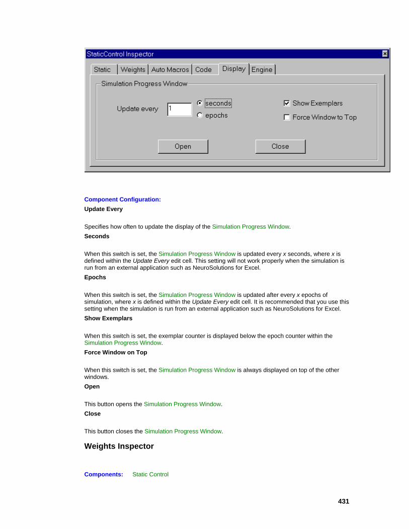
431

Component Configuration: Update Every

Specifies how often to update the display of the Simulation Progress Window. Seconds

When this switch is set, the Simulation Progress Window is updated every x seconds, where x is defined within the Update Every edit cell. This setting will not work properly when the simulation is run from an external application such as NeuroSolutions for Excel. Epochs

When this switch is set, the Simulation Progress Window is updated after every x epochs of simulation, where x is defined within the Update Every edit cell. It is recommended that you use this setting when the simulation is run from an external application such as NeuroSolutions for Excel. Show Exemplars

When this switch is set, the exemplar counter is displayed below the epoch counter within the Simulation Progress Window. Force Window on Top

When this switch is set, the Simulation Progress Window is always displayed on top of the other windows. Open

This button opens the Simulation Progress Window. Close

This button closes the Simulation Progress Window.

Weights Inspector

Components: Static Control

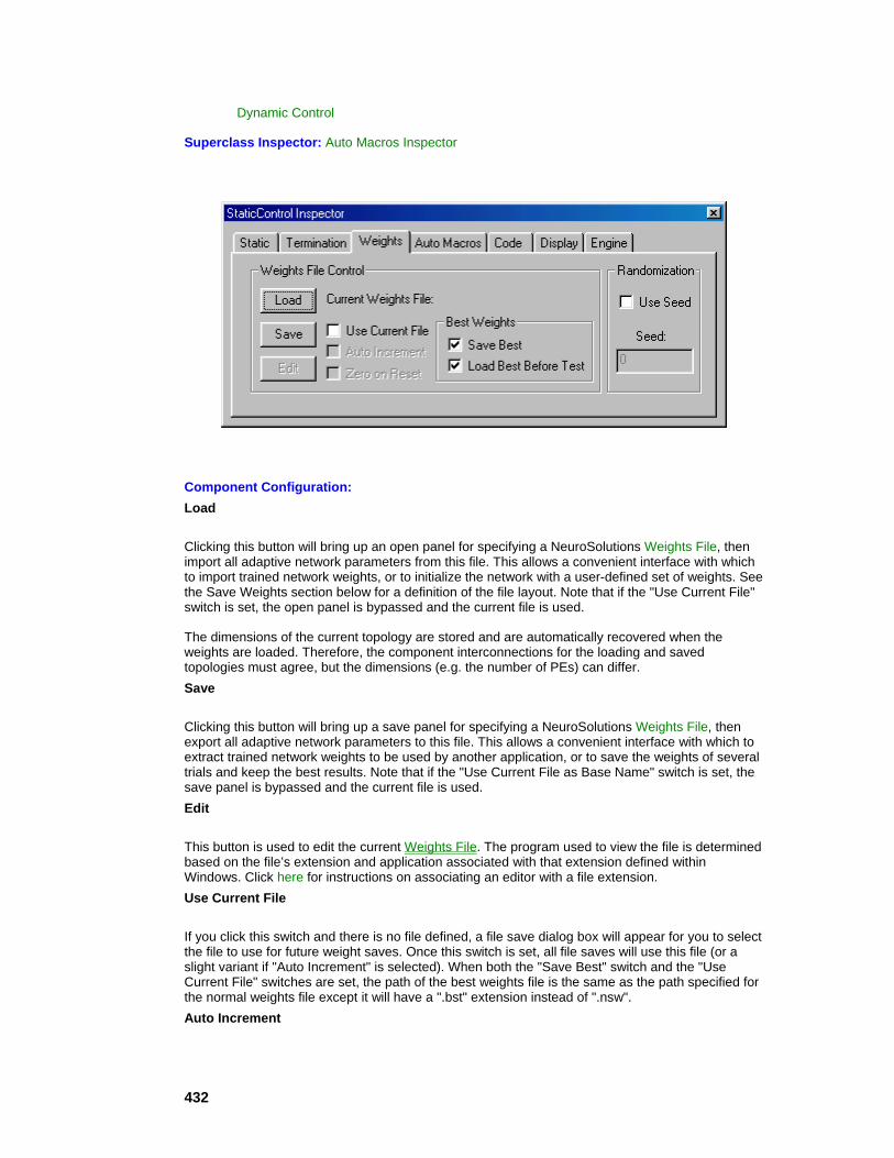
432

Dynamic Control

Superclass Inspector: Auto Macros Inspector

Component Configuration: Load

Clicking this button will bring up an open panel for specifying a NeuroSolutions Weights File, then import all adaptive network parameters from this file. This allows a convenient interface with which to import trained network weights, or to initialize the network with a user-defined set of weights. See the Save Weights section below for a definition of the file layout. Note that if the "Use Current File" switch is set, the open panel is bypassed and the current file is used.

The dimensions of the current topology are stored and are automatically recovered when the weights are loaded. Therefore, the component interconnections for the loading and saved topologies must agree, but the dimensions (e.g. the number of PEs) can differ. Save

Clicking this button will bring up a save panel for specifying a NeuroSolutions Weights File, then export all adaptive network parameters to this file. This allows a convenient interface with which to extract trained network weights to be used by another application, or to save the weights of several trials and keep the best results. Note that if the "Use Current File as Base Name" switch is set, the save panel is bypassed and the current file is used. Edit

This button is used to edit the current Weights File. The program used to view the file is determined based on the file’s extension and application associated with that extension defined within Windows. Click here for instructions on associating an editor with a file extension. Use Current File

If you click this switch and there is no file defined, a file save dialog box will appear for you to select the file to use for future weight saves. Once this switch is set, all file saves will use this file (or a slight variant if "Auto Increment" is selected). When both the "Save Best" switch and the "Use Current File" switches are set, the path of the best weights file is the same as the path specified for the normal weights file except it will have a ".bst" extension instead of ".nsw". Auto Increment

433

When this switch is turned on, a counter is incremented each time the weights are loaded or saved. This counter is appended onto the base file name defined (see above). Note the "Use Current File" switch must be set in order for this switch to be enabled. Zero on Reset

This switch specifies whether or not the file name counter (see above) will be set to zero when the network is reset. Note that the "Use Name" switch must be set in order for this switch to be enabled. Save Best

This switch specifies that the best weights (the weights that produced the lowest error) are automatically saved during training. This switch is tied to the "Save Best" switch of the ErrorCriteria inspector – see this page for all of the configuration options of this feature. Load Best on Test

If this switch is set and there is an ErrorCriteria component on the breadboard and the Learning switch of the Static page of the inspector is turned off (the default for the Testing set), then the best weights stored during training are automatically loaded just before the network is run. Use Seed

When this switch is set, the randomization of the weights is seeded the same each time, allowing you to start with the same initial conditions for multiple experiments. Seed

This is the value used to seed the weight randomization when the "Use Seed" switch is set.

See Also

StaticControl Inspector


Dynamic Control

Superclass Inspector: Termination Inspector

434

Component Configuration: Epochs / Run (SetEpochs(int))

This cell specifies the maximum number of epochs to run (i.e., training cycles) before the simulation stops. Note that the simulation can also be stopped manually with the Control Toolbar, or automatically using one or more Transmitters. Exemplars / Epoch

This cell specifies the number of exemplars that comprise one epoch of data (i.e., the number of patterns in the training set). This value is automatically determined from the exemplars reported by the File components and cannot be modified by the user. Epochs / Cross Val.

This cell specifies the number of training epochs between each cross validation epoch. The higher this number, the less often the network is tested. Learning

This switch enables/disables the learning for the entire network (for the active data set). It does this by setting the Learning switch of the BackpropControl component and any Unsupervised components. Note that when the learning is disabled, the weights are not randomized when the network is reset (see Control Toolbar). Active Data Set

This cell is used to select the currently active data set. The available data sets are detemined from the File components on the breadboard. Cross Validation Data Set

This cell is used to select the data set that is used for the Cross Validation portion of the simulation. The available data sets are detemined from the File components on the breadboard. If "None" is selected then cross validation is not performed. Epoch

Runs the simulation for a duration of one epoch. Exemplar

435

Runs the simulation for a duration of one exemplar. Perform

Performs the Sensitivity Analysis operation. Dither

The amount that the inputs are dithered during the Sensitivity Analysis operation.

See Also

Termination Inspector


Dynamic Control

Superclass Inspector: Weights Inspector

Component Configuration: Terminate after (setTerminateWOImprovement(bool))

In general, the error of the cross validation set will initially drop with the error of the training set. Once the network begins to "memorize" the training set, the cross validation error will begin to rise. When this switch is set, the training will stop if the cross validation error has not reached a new low value within the specified number of epochs. It is important to note that the weights can automatically be saved at the point of lowest cross validation error even if the simulation stops many epochs afterwards. See the Weights page of the inspector for more information. Epochs w/o improvement in cross val. Error (setMaxEpochsWoImprovement(int))

This cell specifies the number of epochs to let the network run without improvement in the cross validation error, as described above.

436

DynamicControl Inspector

Component: DynamicControl

Superclass Inspector: Iterative Prediction Inspector

Component Configuration: Samples / Exemplar (SetSamples(int))

The term forward samples refers to the individual pieces of temporal information. An exemplar is a complete pattern of samples. The temporal dimension of an exemplar is defined by this cell. Note that this value is 1 for static networks. Static

This radio button forces the number of samples/exemplar to be 1. Note that this is equivalent to using the StaticControl component. Fixed Point

This radio button sets the network synchronization to be in fixed point mode. See the DynamicControl reference for an explanation of this mode. Trajectory

This radio button sets the network synchronization to be in trajectory mode. See the DynamicControl reference for an explanation of this mode. Zero state between exemplars

437

When this switch is turned on and an exemplar has completed, all components that store internal states (e.g., MemoryAxons, delayed Synapses) will have those states set to zero before the next exemplar. Zero state between epochs

When this switch is turned on and an epoch has completed, all components that store internal states (e.g., MemoryAxons, delayed Synapses) will have those states set to zero before the next epoch.

See Also

Iterative Prediction Inspector

Component: DynamicControl

Superclass Inspector: Static Inspector

Component Configuration: Enable (setEnableIP(bool))

Enables interative prediction mode. Interative prediction is a process by which the first input sample of each trajectory is read from the network input and the remaining input samples of the trajectory are obtained from the network output. Note that if teacher forcing is enabled (see the Teacher page of the BackDynamicControl inspector) then the number of input samples read from the network input may vary. Trajectory Length (setSamples(int))

The length of the prediction trajectory in samples. This value determines the number of exemplars per epoch (# of exemplars = # samples in file - trajectory length + 1). Note that any change made to the Trajectory Length field will be reflected in the Samples/Exemplar field of the Dynamic page of the inspector. Input Data Source (setInputDataSourceName(string))

438

The component name of the Input component used for the network input. Note that a component's name can be found within the Engine page of its inspector. Desired Data Source (setDesiredDataSourceName(string))

The component name of the Input component used for the desired output of the network. Note that a components name can be found within the Engine page of its inspector. Output Axon (setOutputAxonName(string))

The component name of the Axon component used for the network output. Note that a components name can be found within the Engine page of its inspector.

Backpropagation Inspector (Dynamic)

Component: BackDynamicControl

Superclass Inspector: Teacher Forcing Inspector

Component Configuration: Samples/Exemplar

Training for an exemplar in Trajectory mode requires that the network first be run forward in time for the number of samples specified by the samples/exemplar of the DynamicControl Inspector. An error is determined between the network's output and the desired response. Then the network is run backwards for a prescribed number of samples to compute the gradients and sensitivities. This number of backpropagation samples is defined within this cell.

For Fixed Point mode the terms forward samples and backward samples can be thought of as the forward relaxation period and backward relaxation period, respectively. All inputs are held constant while the network is repeatedly fired during its forward relaxation period, specified by the samples/exemplar of the DynamicControl Inspector. After the network has relaxed, an error is determined and held as constant input to the backpropagation layer. Similarly, the error is

439

backpropagated through the backprop plane for its backward relaxation period, specified by the value within this cell.

Note than the value within this cell cannot exceed the samples/exemplar of the DynamicControl Inspector. On-Line, Batch, Custom (SetMode(int))

See BackStaticControl Inspector Exemplars/Update (SetExemplars(int))

See BackStaticControl Inspector Learning (Turn learning on(); Turn learning off(); Toggle learning())

See BackStaticControl Inspector Learn after RESET

See BackStaticControl Inspector Gradient Search

See BackStaticControl Inspector Add (AddBackprop())

See BackStaticControl Inspector Remove Button (RemoveBackprop())

See BackStaticControl Inspector Free All Backprop Components

See BackStaticControl Inspector (Force Learning())

See BackStaticControl Inspector

See Also

Teacher Forcing Inspector

Component: BackDynamicControl

Superclass Inspector: Exemplar Weighting Inspector

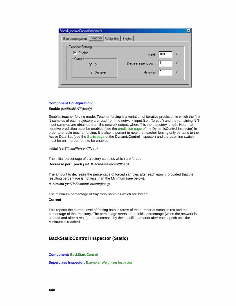
440

Component Configuration: Enable (setEnableTF(bool))

Enables teacher forcing mode. Teacher forcing is a variation of iterative prediction in which the first N samples of each trajectory are read from the network input (i.e., "forced") and the remaining N-T input samples are obtained from the network output, where T is the trajectory length. Note that iterative prediction must be enabled (see the prediction page of the DynamicControl inspector) in order to enable teacher forcing. It is also important to note that teacher forcing only pertains to the Active Data Set (see the Static page of the DynamicControl inspector) and the Learning switch must be on in order for it to be enabled.

Initial (setTfInitialPercent(float))

The initial percentage of trajectory samples which are forced. Decrease per Epoch (setTfDecreasePercent(float))

The amount to decrease the percentage of forced samples after each epoch, provided that the resulting percentage is not less than the Minimum (see below). Minimum (setTfMinimumPercent(float))

The minimum percentage of trajectory samples which are forced. Current

This reports the current level of forcing both in terms of the number of samples (N) and the percentage of the trajectory. The percentage starts at the Initial percentage (when the network is created and after a reset) then decreases by the specified amount after each epoch until the Minimum is reached.

BackStaticControl Inspector (Static)

Component: BackStaticControl

Superclass Inspector: Exemplar Weighting Inspector

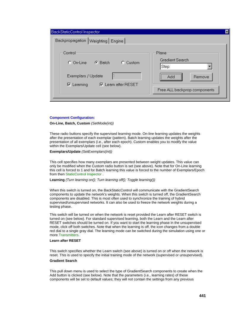
441

Component Configuration: On-Line, Batch, Custom (SetMode(int))

These radio buttons specify the supervised learning mode. On-line learning updates the weights after the presentation of each exemplar (pattern). Batch learning updates the weights after the presentation of all exemplars (i.e., after each epoch). Custom enables you to modify the value within the Exemplars/Update cell (see below). Exemplars/Update (SetExemplars(int))

This cell specifies how many exemplars are presented between weight updates. This value can only be modified when the Custom radio button is set (see above). Note that for On-Line learning this cell is forced to 1 and for Batch learning this value is forced to the number of Exemplars/Epoch from then StaticControl Inspector . Learning (Turn learning on(); Turn learning off(); Toggle learning())

When this switch is turned on, the BackStaticControl will communicate with the GradientSearch components to update the network’s weights. When this switch is turned off, the GradientSearch components are disabled. This is most often used to synchronize the training of hybrid supervised/unsupervised networks. It can also be used to freeze the network weights during a testing phase.

This switch will be turned on when the network is reset provided the Learn after RESET switch is turned on (see below). For standard supervised learning, both the Learn and the Learn after RESET switches should be turned on. If you want to start the learning phase in the unsupervised mode, click off both switches. Note that when the learning is off, the icon changes from a double red dial to a single gray dial. The learning mode can be switched during the simulation using one or more Transmitters. Learn after RESET

This switch specifies whether the Learn switch (see above) is turned on or off when the network is reset. This is used to specify the initial training mode of the network (supervised or unsupervised). Gradient Search

This pull down menu is used to select the type of GradientSearch components to create when the Add button is clicked (see below). Note that the parameters (i.e., learning rates) of these components will be set to default values; they will not contain the settings from any previous

442

GradientSearch components. In order to change the learning procedure for an existing network, click the Remove button, select the Gradient Search procedure, and click the Add button. Add (AddBackprop())

When this button is clicked, a Backprop and GradientSearch component will be attached to each Activation component that has adaptable weights. Each Backprop component is automatically selected to be the dual of the corresponding Activation component. The type of GradientSearch components is specified with the Gradient Search pull down menu (see above). Note that this function only adds these components if none exist; you must Remove (see below) the old Backprop and GradientSearch components before adding new ones. Remove (RemoveBackprop())

When this button is clicked, all Backprop and GradientSearch components will be removed from the breadboard. This will freeze the network weights, but still allow you to monitor the network error. Free All Backprop Components

In addition to the components removed by the Remove button, this button will remove the ErrorCriterion and the BackStaticControl component. This will freeze the network weights and eliminate the overhead of the error computation. (Force Learning())

This transmitter action requires that the Learning switch be turned off. When this message is received, the Learning is turned on, the error of the current exemplar is backpropagated, and the learning is turned back off. By attaching a ThresholdTransmitter to the Cost access point of the ErrorCriteria component, this message can be sent when the error for a given exemplar is above a certain threshold. This way, only those patterns that the network has not yet sufficiently learned will be used to update the weights. This can significantly speed the convergence.

Recall that the number of Exemplars/Update specifies how often the GradientSearch components update their weights. It may be important to note that the exemplar count is only incremented when the error is backpropagated. Therefore, forced learning may take several epochs of training before the weights are updated, even though the learning is set to batch mode.

See Also

Code Generation Inspector


Superclass Inspector: Progress Display Inspector

443


This property page is used to generate, compile and run C++ source code for the current breadboard. Target

Sets the target platform by selecting a library definition file (".nsl" extension) from a file selection panel. This will copy the appropriate header (".h" extension), library (".lib" extension), and makefile (".mak" extension) to the directory of the active project. Note that libraries for platforms other than Windows are sold separately and may be obtained by Contacting NeuroDimension Project Name

Displays the name of the currently active project. This is used to name the source file (".cpp" extension), weight file (".nsw" extension) and executable file (".exe" extension). The current project is switched by clicking on either the Open or New button. Load Weights before Run

When this flag is set, the generated code will include instructions for loading the weights from the weight file ("ProjectName.nsw") before running the simulation, allowing you to continue training from a previously saved state. These weights could be from a previous run of the C++ project (see Save Weights after Run below), or they could be from a previous run of the NeuroSolutions breadboard (see Save Weights within the StaticControl Inspector ). Save Weights after Run

When this flag is set, the generated code will include instructions for saving the weights to the weight file ("ProjectName.nsw") after running the simulation. These weights could be used by a future run of the C++ project (see above), or they could be loaded into the NeuroSolutions breadboard (see Load Weights within the StaticControl Inspector Generate

Clicking this button generates the C++ source code for the current state of the breadboard and saves it to the source file ("ProjectName.cpp"). Once the code is generated, press the Compile button and then the Run button to test the generated code. If the code does not perform as expected, press the Debug button to load the project into the C++ development environment. Compile

444

Clicking this button compiles the C++ source code and saves the result to the executable file ("ProjectName.exe"). Note that the directory containing the command line compiler ("nmake.exe") must be included in the search path. See the Windows documentation for information on the Path environment variable. Run

Clicking this button runs the executable file ("ProjectName.exe") within a DOS window. The data from the probes will be displayed if they are configured to write to the standard output (seeAccess inspector ). Edit

Clicking this button opens an editor window and loads the C++ source file ("ProjectName.cpp"). From here you can modify the generated code, save the file, and then Compile and Run the project. Note that the ".cpp" file extension must be associated with an editor application for this to work. See the Windows documentation for more information on associating files to applications. Open

Sets the current project by selecting an existing source file (".cpp" extension) from a file selection panel. Note that the Generate button will overwrite this file with the source code for the current breadboard. New

Sets the current project by creating a new source file (".cpp" extension) from a file selection panel. This will automatically Generate the code for the existing breadboard and save it to the new source file ("ProjectName.cpp"). Debug

This launches the development environment and loads the makefile for the current project. From there, you will need to build a debug version of the project. Presently, this integration is only available for the MS Visual C++ 4.0 and 5.0 compilers.

Auto Macros Inspector


Superclass Inspector: Code Generation Inspector

445

Component Configuration: Open

Displays a file selection panel to specify the macro that will be run automatically when the breadboard is opened. Close

Displays a file selection panel to specify the macro that will be run automatically when the breadboard is closed. Reset

Displays a file selection panel to specify the macro that will be run automatically when the network is Reset. Post-Run

Displays a file selection panel to specify the macro that will be run automatically when the simulation has been Paused or run to completion.

GeneticControl Inspector

Component: GeneticControl

Superclass Inspector: Genetic Operators Inspector

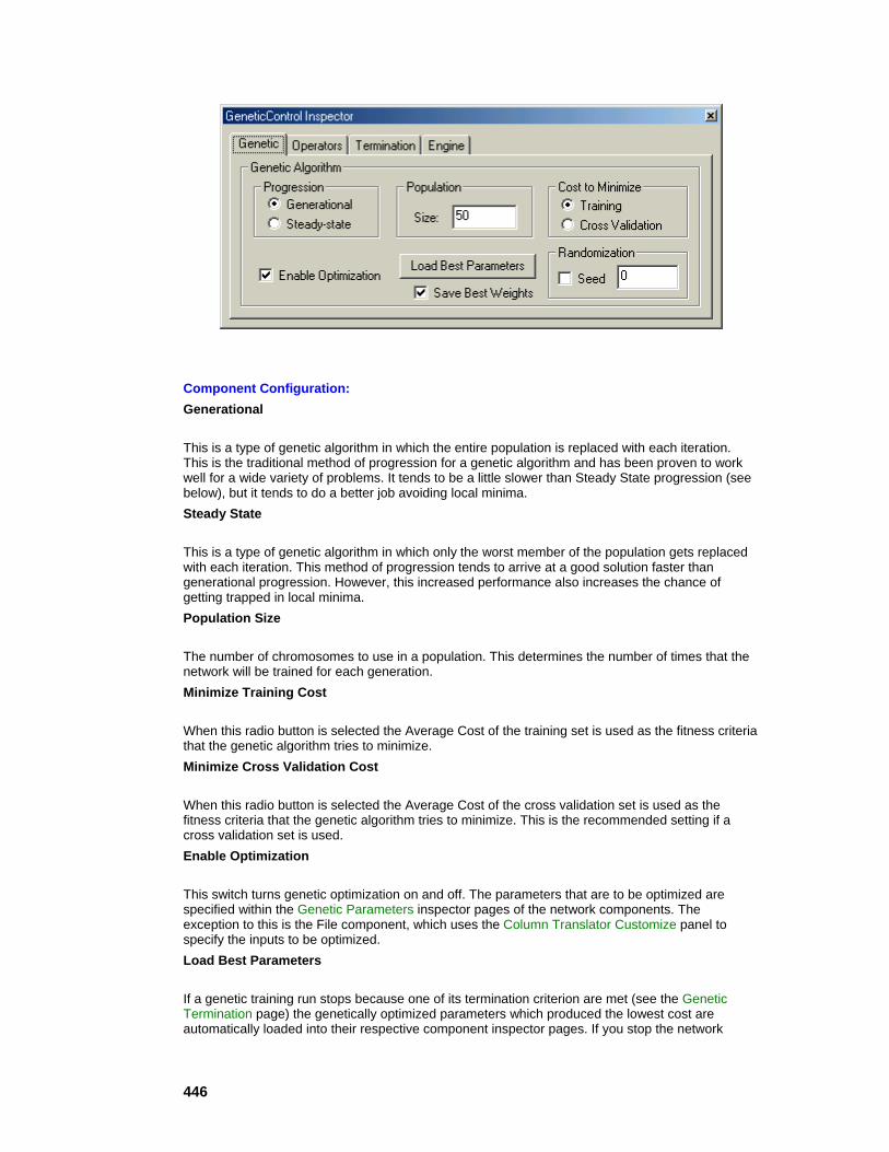
446

Component Configuration: Generational

This is a type of genetic algorithm in which the entire population is replaced with each iteration. This is the traditional method of progression for a genetic algorithm and has been proven to work well for a wide variety of problems. It tends to be a little slower than Steady State progression (see below), but it tends to do a better job avoiding local minima. Steady State

This is a type of genetic algorithm in which only the worst member of the population gets replaced with each iteration. This method of progression tends to arrive at a good solution faster than generational progression. However, this increased performance also increases the chance of getting trapped in local minima. Population Size

The number of chromosomes to use in a population. This determines the number of times that the network will be trained for each generation. Minimize Training Cost

When this radio button is selected the Average Cost of the training set is used as the fitness criteria that the genetic algorithm tries to minimize. Minimize Cross Validation Cost

When this radio button is selected the Average Cost of the cross validation set is used as the fitness criteria that the genetic algorithm tries to minimize. This is the recommended setting if a cross validation set is used. Enable Optimization

This switch turns genetic optimization on and off. The parameters that are to be optimized are specified within the Genetic Parameters inspector pages of the network components. The exception to this is the File component, which uses the Column Translator Customize panel to specify the inputs to be optimized. Load Best Parameters

If a genetic training run stops because one of its termination criterion are met (see the Genetic Termination page) the genetically optimized parameters which produced the lowest cost are automatically loaded into their respective component inspector pages. If you stop the network

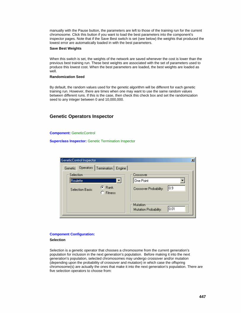
447

manually with the Pause button, the parameters are left to those of the training run for the current chromosome. Click this button if you want to load the best parameters into the component’s inspector pages. Note that if the Save Best switch is set (see below) the weights that produced the lowest error are automatically loaded in with the best parameters. Save Best Weights

When this switch is set, the weights of the network are saved whenever the cost is lower than the previous best training run. These best weights are associated with the set of parameters used to produce this lowest cost. When the best parameters are loaded, the best weights are loaded as well. Randomization Seed

By default, the random values used for the genetic algorithm will be different for each genetic training run. However, there are times when one may want to use the same random values between different runs. If this is the case, then check this check box and set the randomization seed to any integer between 0 and 10,000,000.

Genetic Operators Inspector


Superclass Inspector: Genetic Termination Inspector

Component Configuration: Selection

Selection is a genetic operator that chooses a chromosome from the current generation’s population for inclusion in the next generation’s population. Before making it into the next generation’s population, selected chromosomes may undergo crossover and/or mutation (depending upon the probability of crossover and mutation) in which case the offspring chromosome(s) are actually the ones that make it into the next generation’s population. There are five selection operators to choose from:

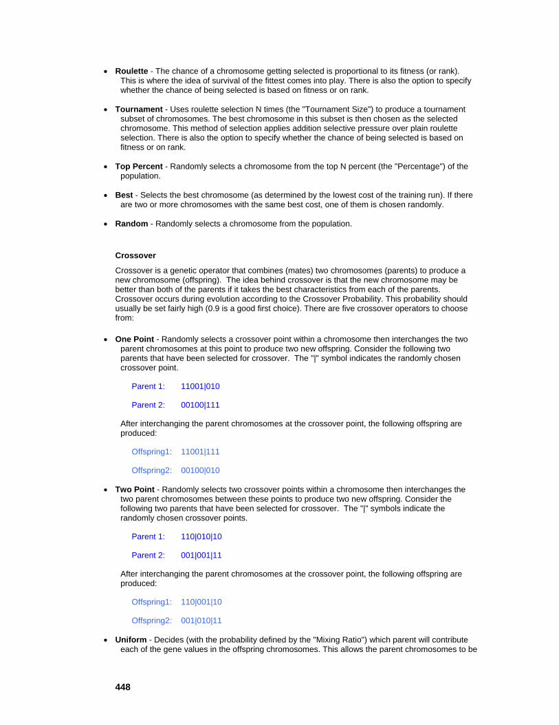
448

• Roulette - The chance of a chromosome getting selected is proportional to its fitness (or rank). This is where the idea of survival of the fittest comes into play. There is also the option to specify whether the chance of being selected is based on fitness or on rank.

• Tournament - Uses roulette selection N times (the "Tournament Size") to produce a tournament subset of chromosomes. The best chromosome in this subset is then chosen as the selected chromosome. This method of selection applies addition selective pressure over plain roulette selection. There is also the option to specify whether the chance of being selected is based on fitness or on rank.

• Top Percent - Randomly selects a chromosome from the top N percent (the "Percentage") of the population.

• Best - Selects the best chromosome (as determined by the lowest cost of the training run). If there are two or more chromosomes with the same best cost, one of them is chosen randomly.

• Random - Randomly selects a chromosome from the population.

Crossover

Crossover is a genetic operator that combines (mates) two chromosomes (parents) to produce a new chromosome (offspring). The idea behind crossover is that the new chromosome may be better than both of the parents if it takes the best characteristics from each of the parents. Crossover occurs during evolution according to the Crossover Probability. This probability should usually be set fairly high (0.9 is a good first choice). There are five crossover operators to choose from:

• One Point - Randomly selects a crossover point within a chromosome then interchanges the two parent chromosomes at this point to produce two new offspring. Consider the following two parents that have been selected for crossover. The "|" symbol indicates the randomly chosen crossover point.

Parent 1: 11001|010

Parent 2: 00100|111

After interchanging the parent chromosomes at the crossover point, the following offspring are produced:

Offspring1: 11001|111

Offspring2: 00100|010

• Two Point - Randomly selects two crossover points within a chromosome then interchanges the two parent chromosomes between these points to produce two new offspring. Consider the following two parents that have been selected for crossover. The "|" symbols indicate the randomly chosen crossover points.

Parent 1: 110|010|10

Parent 2: 001|001|11

After interchanging the parent chromosomes at the crossover point, the following offspring are produced:

Offspring1: 110|001|10

Offspring2: 001|010|11

• Uniform - Decides (with the probability defined by the "Mixing Ratio") which parent will contribute each of the gene values in the offspring chromosomes. This allows the parent chromosomes to be

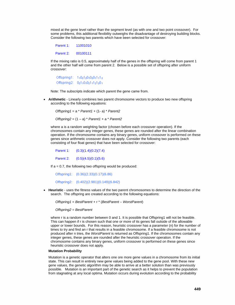
449

mixed at the gene level rather than the segment level (as with one and two point crossover). For some problems, this additional flexibility outweighs the disadvantage of destroying building blocks. Consider the following two parents which have been selected for crossover:

Parent 1: 11001010

Parent 2: 00100111

If the mixing ratio is 0.5, approximately half of the genes in the offspring will come from parent 1 and the other half will come from parent 2. Below is a possible set of offspring after uniform crossover:

Note: The subscripts indicate which parent the gene came from.

• Arithmetic - Linearly combines two parent chromosome vectors to produce two new offspring according to the following equations:

Offspring1 = a * Parent1 + (1- a) * Parent2

Offspring2 = (1 – a) * Parent1 + a * Parent2

where a is a random weighting factor (chosen before each crossover operation). If the chromosomes contain any integer genes, these genes are rounded after the linear combination operation. If the chromosome contains any binary genes, uniform crossover is performed on these genes since arithmetic crossover does not apply. Consider the following two parents (each consisting of four float genes) that have been selected for crossover:

Parent 1: (0.3)(1.4)(0.2)(7.4)

Parent 2: (0.5)(4.5)(0.1)(5.6)

If a = 0.7, the following two offspring would be produced:

Offspring1: (0.36)(2.33)(0.17)(6.86)

Offspring2: (0.402)(2.981)(0.149)(6.842)

• Heuristic - uses the fitness values of the two parent chromosomes to determine the direction of the search. The offspring are created according to the following equations:

Offspring1 = BestParent + r * (BestParent – WorstParent)

Offspring2 = BestParent

where r is a random number between 0 and 1. It is possible that Offspring1 will not be feasible. This can happen if r is chosen such that one or more of its genes fall outside of the allowable upper or lower bounds. For this reason, heuristic crossover has a parameter (n) for the number of times to try and find an r that results in a feasible chromosome. If a feasible chromosome is not produced after n tries, the WorstParent is returned as Offspring1. If the chromosomes contain any integer genes, these genes are rounded after the heuristic crossover operation. If the chromosome contains any binary genes, uniform crossover is performed on these genes since heuristic crossover does not apply.

Mutation Probability

Mutation is a genetic operator that alters one ore more gene values in a chromosome from its initial state. This can result in entirely new gene values being added to the gene pool. With these new gene values, the genetic algorithm may be able to arrive at a better solution than was previously possible. Mutation is an important part of the genetic search as it helps to prevent the population from stagnating at any local optima. Mutation occurs during evolution according to the probability

450

defined in this cell. This probability should usually be set fairly low (0.01 is a good first choice). If it is set too high, the search will turn into a primitive random search. Note that the mutation type is defined within the Genetic Parameters inspector page for the components with parameters to be optimized.

Genetic Termination Inspector



Description:

A genetic training run will run until the user stops the network with the Pause button, or until one of the three termination criteria described below are met. When the network terminates due to one of these criterion, the best parameters (those that produced the lowest cost) are automatically loaded into the network. See the GeneticControl page if you want to manually load in the best network parameters.

Component Configuration: Maximum Generations

This cell specifies the maximum number of generations that will be run until the simulation is stopped. Termination Type

You may choose one of these four termination methods or "None".

• Fitness Threshold - Stops the evolution when the best fitness in the current population becomes less than the fitness "Threshold" and the objective is set to minimize the fitness.

• Fitness Convergence - Stops the evolution when the fitness is deemed as converged. Two filters of different lengths are used to smooth the best fitness across the generations. When the

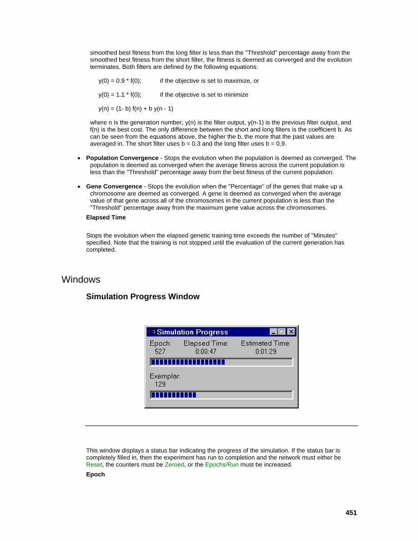
451

smoothed best fitness from the long filter is less than the "Threshold" percentage away from the smoothed best fitness from the short filter, the fitness is deemed as converged and the evolution terminates. Both filters are defined by the following equations:

y(0) = 0.9 * f(0); if the objective is set to maximize, or

y(0) = 1.1 * f(0); if the objective is set to minimize

y(n) = (1- b) f(n) + b y(n - 1)

where n is the generation number, y(n) is the filter output, y(n-1) is the previous filter output, and f(n) is the best cost. The only difference between the short and long filters is the coefficient b. As can be seen from the equations above, the higher the b, the more that the past values are averaged in. The short filter uses b = 0.3 and the long filter uses b = 0.9.

• Population Convergence - Stops the evolution when the population is deemed as converged. The population is deemed as converged when the average fitness across the current population is less than the "Threshold" percentage away from the best fitness of the current population.

• Gene Convergence - Stops the evolution when the "Percentage" of the genes that make up a chromosome are deemed as converged. A gene is deemed as converged when the average value of that gene across all of the chromosomes in the current population is less than the "Threshold" percentage away from the maximum gene value across the chromosomes.

Elapsed Time

Stops the evolution when the elapsed genetic training time exceeds the number of "Minutes" specified. Note that the training is not stopped until the evaluation of the current generation has completed.

Windows

Simulation Progress Window

This window displays a status bar indicating the progress of the simulation. If the status bar is completely filled in, then the experiment has run to completion and the network must either be Reset, the counters must be Zeroed, or the Epochs/Run must be increased. Epoch

452

Display of the current epoch count. Exemplar

Display of the current exemplar count. If this is not displayed then switch the "Show Exemplars" setting within the Progress Display Inspector . Sample

Display of the current sample count (DynamicControl only). Elapsed Time

Display of the total time (H::MM::SS) that the simulation has run. Time Remaining

Display of the estimated time remaining (H::MM::SS) until the maximum number of epochs (or generations) is reached. Generation

When genetic optimization is enabled (see the GeneticControl inspector) this will show the current generation number of the genetic training.

See Also

Optimization Log Window

During genetic optimization, the values of the user-specified neural network parameters are set before each training pass based on the contents of the current chromosome. This window displays each of the optimized parameter settings for each training pass, along with the fitness (the best average cost of the training).

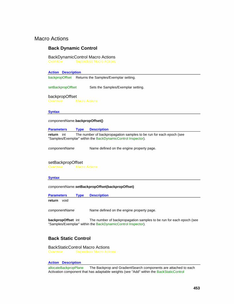
453

Macro Actions

Back Dynamic Control

BackDynamicControl Macro Actions Overview Superclass Macro Actions

Action Description backpropOffset Returns the Samples/Exemplar setting. setBackpropOffset Sets the Samples/Exemplar setting.

backpropOffset Overview Macro Actions

Syntax

componentName.backpropOffset()

Parameters Type Description return int The number of backpropagation samples to be run for each epoch (see "Samples/Exemplar" within the BackDynamicControl Inspector). componentName Name defined on the engine property page.

setBackpropOffset Overview Macro Actions

Syntax

componentName.setBackpropOffset(backpropOffset)

Parameters Type Description return void componentName Name defined on the engine property page. backpropOffset int The number of backpropagation samples to be run for each epoch (see "Samples/Exemplar" within the BackDynamicControl Inspector).

Back Static Control

BackStaticControl Macro Actions Overview Superclass Macro Actions

Action Description allocateBackpropPlane The Backprop and GradientSearch components are attached to each Activation component that has adaptable weights (see "Add" within the BackStaticControl

454

Inspector). batch Returns the Batch learning mode setting. costWeightingActive Returns the "Weight the Reported Cost" setting. custom Returns the Custom learning mode setting. freeALL Removes all ErrorCriterion, BackStaticControl, Backprop, and GradientSearch components from the breadboard (see "Free All Backprop Components" within the BackStaticControl Inspector ). freeBackpropPlane Removes all Backprop and GradientSearch components from the breadboard (see "Remove" within the BackStaticControl Inspector). gradientClass Returns the class name of the GradientSearch components that are added when the allocateBackpropPlane function is called (see above). gradientWeightingActive Returns the "Weight the Gradients" setting. learning Returns FALSE if the GradientSearch components are disabled. learningOnReset Returns the "Learning after RESET" setting. setBatch Sets the learning mode to Batch.

setCostWeightingActive Sets the "Weight the Reported Cost" setting.

setCustom Sets the learning mode to Custom. setForceLearning Sets the Learning to on, backpropagates the error of the current exemplar, and then turns off the Learning. setGradientClass Allows the user to select GradientSearch components from a pull down menu and then add or remove them from the project. setGradientClassName Sets the class name of the GradientSearch components that are added when the allocateBackpropPlane function is called (see above). setGradientWeightingActive Sets the "Weight the Gradients" setting. setLearning Set to FALSE to disable the GradientSearch components. setLearningOnReset Sets the "Learning after RESET" setting. setUpdateEvery Sets the Exemplar/Update setting. setWeightingFilePath Sets the path of the exemplar weighting file. updateEvery Returns the Exemplar/Update setting.

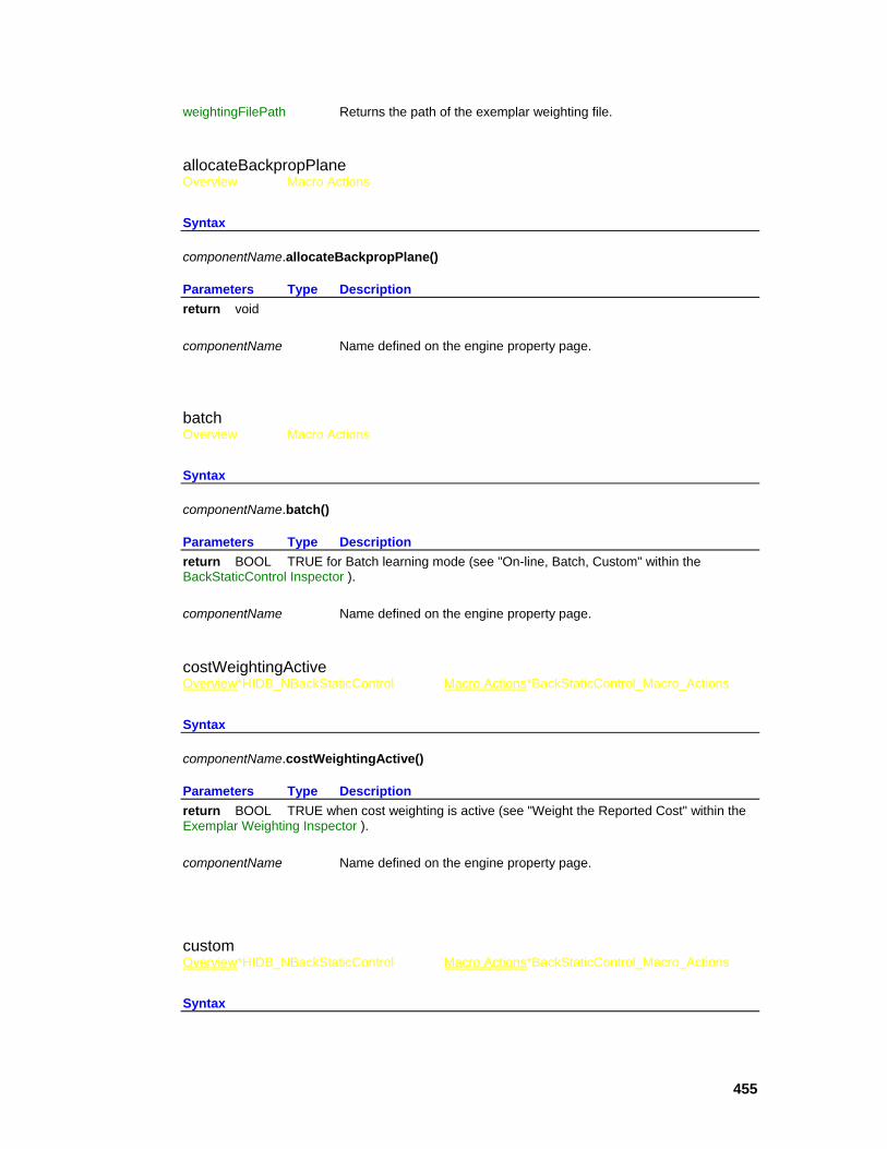
455

weightingFilePath Returns the path of the exemplar weighting file.

allocateBackpropPlane Overview Macro Actions

Syntax

componentName.allocateBackpropPlane()


batch Overview Macro Actions

Syntax

componentName.batch()

Parameters Type Description return BOOL TRUE for Batch learning mode (see "On-line, Batch, Custom" within the BackStaticControl Inspector ). componentName Name defined on the engine property page.

costWeightingActive Overview*HIDB_NBackStaticControl Macro Actions*BackStaticControl_Macro_Actions

Syntax

componentName.costWeightingActive()

Parameters Type Description return BOOL TRUE when cost weighting is active (see "Weight the Reported Cost" within the Exemplar Weighting Inspector ). componentName Name defined on the engine property page.

custom Overview*HIDB_NBackStaticControl Macro Actions*BackStaticControl_Macro_Actions

Syntax

456

componentName.custom()

Parameters Type Description return BOOL TRUE for Custom learning mode (see "On-line, Batch, Custom" within the BackStaticControl Inspector ). componentName Name defined on the engine property page.

freeALL Overview Macro Actions

Syntax

componentName.freeAll()


freeBackpropPlane Overview Macro Actions

Syntax

componentName.freeBackpropPlane()


gradientClass Overview Macro Actions

Syntax

componentName.gradientClass()

Parameters Type Description return String The class name of the GradientSearch components to be added (see the "Gradient Search" pull down menu within the BackStaticControl Inspector). componentName Name defined on the engine property page.

gradientWeightingActive Overview Macro Actions

Syntax

457

componentName.gradientWeightingActive()

Parameters Type Description return BOOL TRUE if gradient weighting is active (see the "Weight the Gradients" switch of the Exemplar Weighting Inspector). componentName Name defined on the engine property page.

learning Overview Macro Actions

Syntax

componentName.learning()

Parameters Type Description return BOOL TRUE if the GradientSearch components are enabled (see "Learning" within the BackStaticControl Inspector ). componentName Name defined on the engine property page.

learningOnReset Overview Macro Actions

Syntax

componentName.learningOnReset()

Parameters Type Description return BOOL TRUE sets the learning flag to TRUE when the network is reset (see "Learning after RESET" within the BackStaticControl Inspector). componentName Name defined on the engine property page.

setBatch Overview Macro Actions

Syntax

componentName.setBatch(batch)

Parameters Type Description return void componentName Name defined on the engine property page. batch BOOL TRUE for batch learning mode (see "On-line, Batch, Custom" within the BackStaticControl Inspector).

458

setCostWeightingActive Overview Macro Actions

Syntax

componentName.setCostWeightingActive(costWeightingActive)

Parameters Type Description return void componentName Name defined on the engine property page. costWeightingActive BOOL TRUE when cost weighting is active (see "Weight the Reported Cost" within the Exemplar Weighting Inspector ).

setCustom Overview Macro Actions

Syntax

componentName.setCustom(custom)

Parameters Type Description return void componentName Name defined on the engine property page. custom BOOL TRUE for custom learning mode (see "On-line, Batch, Custom" within the BackStaticControl Inspector).

setForceLearning Overview Macro Actions

Syntax

componentName.setForceLearning(forceLearning)

Parameters Type Description return BOOL TRUE sets the Learning to on, backpropagates the error of the current exemplar, and then turns off the Learning. componentName Name defined on the engine property page.

setGradientClass Overview Macro Actions

Syntax

459

componentName.setGradientClass(gradientClass)

Parameters Type Description return void componentName Name defined on the engine property page. gradientClass When selected, allows the user to select GradientSearch components from a pull down menu and then add or remove them from the project (see "Gradient Search" within the BackStaticControl Inspector).

setGradientClassName Overview Macro Actions

Syntax

componentName.setGradientClassName(gradientClassName)

Parameters Type Description return string The class name of the GradientSearch components to be added (see the "Gradient Search" pull down menu within the BackStaticControl Inspector). componentName Name defined on the engine property page.

setGradientWeightingActive Overview Macro Actions

Syntax

componentName.setGradientWeightingActive(gradientWeightingActive)

Parameters Type Description return void componentName Name defined on the engine property page. gradientWeightingActive BOOL TRUE if gradient weighting is active (see the "Weight the Gradients" switch of the Exemplar Weighting Inspector).

setLearning Overview Macro Actions

Syntax

componentName.setLearning(learning)

Parameters Type Description return void

460

componentName Name defined on the engine property page. learning BOOL TRUE if the GradientSearch components are enabled (see "Learning" within the BackStaticControl Inspector ).

setLearningOnReset Overview Macro Actions

Syntax

componentName.setLearningOnReset(learningOnReset)

Parameters Type Description return void componentName Name defined on the engine property page. learningOnReset BOOL TRUE sets the learning flag to TRUE when the network is reset (see "Learning after RESET" within the BackStaticControl Inspector).

setUpdateEvery Overview Macro Actions

Syntax

componentName.setUpdateEvery(updateEvery)

Parameters Type Description return void componentName Name defined on the engine property page. updateEvery int The number of exemplars presented between weight updates (see "Exemplars/Update" within the BackStaticControl Inspector ). .

setWeightingFilePath Overview Macro Actions

Syntax

componentName.setWeightingFilePath(weightingFilePath)

Parameters Type Description return void componentName Name defined on the engine property page. weightingFilePath String The path of the weighting file (see the "Weighting File" button within the Exemplar Weighting Inspector).

461

updateEvery Overview Macro Actions

Syntax

componentName.updateEvery()

Parameters Type Description return int The number of exemplars presented between weight updates (see "Exemplars/Update" within the BackStaticControl Inspector ). componentName Name defined on the engine property page.

weightingFilePath Overview Macro Actions

Syntax

componentName.weightingFilePath()

Parameters Type Description return String The path of the weighting file (see the "Weighting File" button within the Exemplar Weighting Inspector). componentName Name defined on the engine property page.

Dynamic Control

DynamicControl Macro Actions Overview Superclass Macro Actions

Action Description fixedPointMode Returns TRUE if activation mode is set to "Fixed Point". samples Returns the "Samples/Exemplar" setting. setFixedPointMode Set to TRUE to change activation mode to "Fixed Point". setSamples Sets the "Samples/Exemplar" setting. setZeroState Sets the "Zero state between exemplars" setting. setZeroStateEpoch Sets the "Zero state between epochs" setting. zeroState Returns the "Zero state between exemplars" setting. zeroStateEpoch Returns the "Zero state between epochs" setting.

462

fixedPointMode Overview Macro Actions

Syntax

componentName.fixedPointMode()

Parameters Type Description return BOOL TRUE if activation mode is Fixed Point, FALSE is activation mode is Trajectory (see "Fixed Point" within the DynamicControl Inspector ). componentName Name defined on the engine property page.

samples Overview Macro Actions

Syntax

componentName.samples()

Parameters Type Description return int The temporal dimension of an exemplar (see "Samples/Exemplar" within the DynamicControl Inspector). componentName Name defined on the engine property page.

setFixedPointMode Overview Macro Actions

Syntax

componentName.setFixedPointMode(fixedPointMode)

Parameters Type Description return void componentName Name defined on the engine property page. fixedPointMode BOOL TRUE if activation mode is Fixed Point, FALSE is activation mode is Trajectory (see "Fixed Point" within the DynamicControl Inspector ).

setSamples Overview Macro Actions

Syntax

componentName.setSamples(samples)


463

componentName Name defined on the engine property page. samples int The temporal dimension of an exemplar (see "Samples/Exemplar" within the DynamicControl Inspector).

setZeroState Overview Macro Actions

Syntax

componentName.setZeroState(zeroState)

Parameters Type Description return void componentName Name defined on the engine property page. zeroState BOOL If TRUE, then all components storing internal states (e.g., MemoryAxons, delayed Synapses) will be set to zero prior to the next exemplar (see "Zero state between exemplars" within the DynamicControl Inspector).

setZeroStateEpoch Overview Macro Actions

Syntax

componentName.setZeroStateEpoch(zeroState)

Parameters Type Description return void componentName Name defined on the engine property page. zeroState BOOL If TRUE, then all components storing internal states (e.g., MemoryAxons, delayed Synapses) will be set to zero prior to the next epoch (see "Zero state between epochs" within the DynamicControl Inspector).

zeroState Overview Macro Actions

Syntax

componentName.zeroState()

Parameters Type Description return BOOL If TRUE, then all components storing internal states (e.g., MemoryAxons, delayed Synapses) will be set to zero prior to the next exemplar (see "Zero state between exemplars" within the DynamicControl Inspector).

464

componentName Name defined on the engine property page.

zeroStateEpoch Overview Macro Actions

Syntax

componentName.zeroStateEpoch()

Parameters Type Description return BOOL If TRUE, then all components storing internal states (e.g., MemoryAxons, delayed Synapses) will be set to zero prior to the next epoch (see "Zero state between epoch" within the DynamicControl Inspector). componentName Name defined on the engine property page.

Static Control

StaticControl Macro Actions Overview Superclass Macro Actions

Action Description activeDataSet Returns the "Active Data Set" name. autoIncrement Returns the "Auto Increment" setting. closeMacro Returns the path of the macro that is run when the breadboard is closed. codeGenProjectPath Returns the path of the generated source code (*.cpp) file. codeGenTargetPath Returns the path of the library definition (*.nsl) file. compileSourceCode Compiles the C++ source code and saves the result to the executable file ("ProjectName.exe"). debugSourceCode Launches the development environment and loads the makefile for the current project from which the user can build a debug version of the project.

dither Sets the "Dither" setting used by the sensitivity analysis function.

dualName Returns the name of the attached backprop control component.

elapsedTimeInSeconds Returns the amount of time (in seconds) the simulation has been run. epochCounter Returns the number of epochs the simulation has been run.

465

epochs Returns the "Epochs/Run" setting. epochsPerTest Returns the "Epochs/Cross Val." setting. executableFilePath Returns the path of the executable file ("ProjectName.exe") for the code generation project. exemplarCounter Returns the number of exemplars the simulation has been run. exemplars Returns the "Exemplars/Epoch" setting. forceWindowOnTop Returns the "Force Window on Top" setting. jogNetworkWeights Alters the weights by a small random value. learning Returns the state of learning for the entire network (enabled or disabled). loadWeights Imports all adaptive network parameters from the specified weights file. openMacro Returns the path of the macro that is automatically run when the breadboard is opened. pauseNetwork Halts the simultation. postRunMacro Returns the path of the macro that is automatically run when the simulation concludes. preRunMacro Returns the path of the macro that is automatically run when the network is reset. randomizeNetworkWeights Randomizes the network weights. resetNetwork Randomizes the network weights, zeroes the counters and clears the activations. runCompiledCode Runs the executable file ("ProjectName.exe") within a DOS window. runNetwork Starts the simulation. runSensitivity Performs the sensitivity analysis function. saveWeights Exports all adaptive network parameters to the specified weights file. setActiveDataSet Sets the "Active Data Set" name. setAutoIncrement Sets the "Auto Increment" setting. setCloseMacro Sets the path of the macro that is run when the breadboard is closed. setCodeGenProjectPath Sets the path of the generated source code (*.cpp) file. setCodeGenTargetPath Sets the path of the library definition (*.nsl) file.

466

setDither Sets the "Dither" setting used by the sensitivity analysis function. setEpochCounter Sets the current epoch of the experiment. setEpochs Sets the "Epochs/Run" setting. setEpochsPerTest Sets the "Epochs/Cross Val." Setting. setExemplarCounter Sets the current exemplar of the experiment. setExemplars Sets the "Exemplars/Epoch" setting. setForceWindowOnTop Sets the "Force Window on Top" setting. setLearning Sets the state of learning for the entire network (enabled or disabled). setOpenMacro Sets the path of the macro that is automatically run when the breadboard is opened. setPostRunMacro Sets the path of the macro that is automatically run when the simulation concludes. setPreRunMacro Sets the path of the macro that is automatically run when the network is reset. setShowExemplars Sets the "Show Exemplars" setting. setUpdateDisplayByEpoch Set to TRUE to update the progress display based on epochs, and FALSE to update based on seconds. setUpdateDisplayEvery Sets the "Update every" setting. setUseName Sets the "Use Current File as Base Name" setting. setXValDataSet Sets the data set used for the Cross Validation portion of the simulation. setZeroOnReset Sets the "Zero on Reset" setting for the weights file name counter. showExemplars Returns the "Show Exemplars" setting. stepEpoch Runs the simulation for a duration of one epoch. stepExemplar Runs the simulation for a duration of one exemplar. updateDisplayByEpoch Runs the simulation for a duration of one epoch. updateDisplayEvery Returns the "Update every" setting. useName Returns the "Use Current File as Base Name" setting. xValDataSet Returns the data set used for the Cross Validation portion of the simulation.

467

zeroOnReset Returns the "Zero on Reset" setting for the weights file name counter.

activeDataSet Overview Macro Actions

Syntax

componentName.activeDataSet()

Parameters Type Description return string The name of the active data set (see "Active Data Set" within the StaticControl Inspector). componentName Name defined on the engine property page.

autoIncrement Overview Macro Actions

Syntax

componentName.autoIncrement()

Parameters Type Description return BOOL TRUE if the name counter is incremented each time the weights are loaded or saved (see the Weights Inspector). componentName Name defined on the engine property page.

closeMacro Overview Macro Actions

Syntax

componentName.closeMacro()

Parameters Type Description return string The path of the macro that is run when the breadboard is closed (see the Auto Macros Inspector ). componentName Name defined on the engine property page.

codeGenProjectPath Overview Macro Actions

Syntax

componentName.codeGenProjectPath()


468

return String The path of the generated source code (*.cpp) file (see "Project" within the Code Generation Inspector). componentName Name defined on the engine property page.

codeGenTargetPath Overview Macro Actions

Syntax

componentName.codeGenTargetPath()

Parameters Type Description return String The path of the library definition (*.nsl) file (see "Target" within the Code Generation Inspector). componentName Name defined on the engine property page.

compileSourceCode Overview Macro Actions

Syntax

componentName.compileSourceCode()


debugSourceCode Overview Macro Actions

Syntax

componentName.debugSourceCode()


dither Overview Macro Actions

Syntax

469

componentName.dither()

Parameters Type Description return float The dither value used to perform the sensitivity analysis function (see the Static Inspector). componentName Name defined on the engine property page.

dualName Overview Macro Actions

Syntax

componentName.dualName()

Parameters Type Description return string The name of the attached backprop control component. componentName Name defined on the engine property page.

elapsedTimeInSeconds Overview Macro Actions

Syntax

componentName.elapsedTimeInSeconds()

Parameters Type Description return int The number of seconds that the simulation has been running. componentName Name defined on the engine property page.

epochCounter Overview Macro Actions

Syntax

componentName.epochCounter()

Parameters Type Description return int The number of epochs that the simulation has completed (see the Simulation Progress Window). componentName Name defined on the engine property page.

epochs Overview Macro Actions

470

Syntax

componentName.epochs()

Parameters Type Description return int The maximum number of epochs to run before the simulation stops (see "Epochs/Run" within the Static Inspector). componentName Name defined on the engine property page.

epochsPerTest Overview Macro Actions

Syntax

componentName.epochsPerTest()

Parameters Type Description return int The number of epochs between each cross validation cycle (see "Epochs/Cross Val" within the the Static Inspector). componentName Name defined on the engine property page.

executableFilePath Overview Macro Actions

Syntax

componentName.executableFilePath()

Parameters Type Description return string The path of the executable file ("ProjectName.exe") for the code generation project. componentName Name defined on the engine property page.

exemplarCounter Overview Macro Actions

Syntax

componentName.exemplarCounter()

Parameters Type Description return int The number of exemplars that the simulation has completed in the current epoch (see the Simulation Progress Window). componentName Name defined on the engine property page.

exemplars Overview Macro Actions

471

Syntax

componentName.exemplars()

Parameters Type Description return int The number of exemplars that comprise one epoch of the data set (see "Exemplars/Epoch" within the StaticControl Inspector). componentName Name defined on the engine property page.

forceWindowOnTop Overview Macro Actions

Syntax

componentName.forceWindowOnTop()

Parameters Type Description return BOOL TRUE if the Simulation Progress Window is forced on top. componentName Name defined on the engine property page.


Syntax

componentName.learning()

Parameters Type Description return BOOL TRUE if learning is enabled for the entire network (see "Learning" within the StaticControl Inpsector). componentName Name defined on the engine property page.

jogNetworkWeights Overview Macro Actions

Syntax

componentName.jogNetworkWeights()


loadWeights Overview Macro Actions

472

Syntax

componentName.loadWeights(weightsPath)

Parameters Type Description return void componentName Name defined on the engine property page. weightsPath string Path of the weights file to load (see the Weights Inspector). If the path is blank and the "useName" flag is set, then the current file path is used.

openMacro Overview Macro Actions

Syntax

componentName.openMacro()

Parameters Type Description return string The path of the macro that is run when the breadboard is opened (see the Auto Macros Inspector ). componentName Name defined on the engine property page.

pauseNetwork Overview Macro Actions

Syntax

componentName.pauseNetwork()


postRunMacro Overview Macro Actions

Syntax

componentName.postRunMacro()

Parameters Type Description return string The path of the macro that is run when the simulation concludes (see the Auto Macros Inspector ).

473


preRunMacro Overview Macro Actions

Syntax

componentName.preRunMacro()

Parameters Type Description return string The path of the macro that is run when the network is reset (see the Auto Macros Inspector ). componentName Name defined on the engine property page.

randomizeNetworkWeights Overview Macro Actions

Syntax

componentName.randomizeNetworkWeights()


resetNetwork Overview Macro Actions

Syntax

componentName.resetNetwork()


runCompiledCode Overview Macro Actions

Syntax

componentName.runCompiledCode()


474


runNetwork Overview Macro Actions

Syntax

componentName.runNetwork()


runSensitivity Overview Macro Actions

Syntax

componentName.runSensitivity()


saveWeights Overview Macro Actions

Syntax

componentName.saveWeights(weightsPath)

Parameters Type Description return void componentName Name defined on the engine property page. weightsPath string Path of the weights file to save (see the Weights Inspector). If the path is blank and the "useName" flag is set, then the current file path is used.

setActiveDataSet Overview Macro Actions

475

Syntax

componentName.setActiveDataSet(activeDataSet)

Parameters Type Description return void componentName Name defined on the engine property page. activeDataSet string The name of the active data set (see "Active Data Set" within the StaticControl Inspector).

setAutoIncrement Overview Macro Actions

Syntax

componentName.setAutoIncrement(autoIncrement)

Parameters Type Description return void componentName Name defined on the engine property page. autoIncrement BOOL TRUE if the name counter is incremented each time the weights are loaded or saved (see the Weights Inspector).

setCloseMacro Overview Macro Actions

Syntax

componentName.setCloseMacro(closeMacro)

Parameters Type Description return void componentName Name defined on the engine property page. closeMacro string The path of the macro that is run when the breadboard is closed (see the Auto Macros Inspector ).

setCodeGenProjectPath Overview Macro Actions

Syntax

componentName.setCodeGenProjectPath(codeGenProjectPath)


476

return void componentName Name defined on the engine property page. codeGenProjectPath String The path of the generated source code (*.cpp) file (see "Project" within the Code Generation Inspector).

setCodeGenTargetPath Overview Macro Actions

Syntax

componentName.setCodeGenTargetPath(codeGenTargetPath)

Parameters Type Description return void componentName Name defined on the engine property page. codeGenTargetPath String The path of the library definition (*.nsl) file (see "Target" within the Code Generation Inspector).

setDither Overview Macro Actions

Syntax

componentName.setDither(dither)

Parameters Type Description return Float The dither value used to perform the sensitivity analysis function (see the Static Inspector). componentName Name defined on the engine property page.

setEpochCounter Overview Macro Actions

Syntax

componentName.setEpochCounter(epochCounter)

Parameters Type Description return void componentName Name defined on the engine property page. epochCounter int The epoch number that the simulation will start at (see the Simulation

477

Progress Window).

setEpochs Overview Macro Actions

Syntax

componentName.setEpochs(epoch)

Parameters Type Description return void componentName Name defined on the engine property page. epochs int The maximum number of epochs to run (i.e., training cycles) before the simulation stops (see "Epochs/Run" within the StaticControl Inspector).

setEpochsPerTest Overview Macro Actions

Syntax

componentName.setEpochsPerTest(epochsPerTest)

Parameters Type Description return void componentName Name defined on the engine property page. epochsPerTest int The number of epochs between each cross validation cycle (see "Epochs/Cross Val" within the the Static Inspector).

setExemplarCounter Overview Macro Actions

Syntax

componentName.setExemplarCounter(exemplarCounter)

Parameters Type Description return void componentName Name defined on the engine property page. exemplarCounter int The exemplar number that the simulation will start at (see the Simulation Progress Window).

478

setExemplars Overview Macro Actions

Syntax

componentName.setExemplars(exemplars)

Parameters Type Description return void componentName Name defined on the engine property page. exemplars int The number of exemplars that comprise one epoch of the data set (see "Exemplars/Epoch" within the StaticControl Inspector).

setForceWindowOnTop Overview Macro Actions

Syntax

componentName.setForceWindowOnTop(forceWindowOnTop)

Parameters Type Description return void componentName Name defined on the engine property page. forceWindowOnTop BOOL TRUE if the Simulation Progress Window is forced on top.


Syntax

componentName.setLearning(learning)

Parameters Type Description return void componentName Name defined on the engine property page. learning BOOL TRUE if learning is enabled for the entire network (see "Learning" within the StaticControl Inpsector).

setOpenMacro Overview Macro Actions

Syntax

componentName.setOpenMacro(openMacro)

479

Parameters Type Description return void componentName Name defined on the engine property page. openMacro string The path of the macro that is run when the breadboard is opened (see the Auto Macros Inspector ).

setPostRunMacro Overview Macro Actions

Syntax

componentName.setPostRunMacro(postRunMacro)

Parameters Type Description return void componentName Name defined on the engine property page. postRunMacro string The path of the macro that is run when the simulation concludes (see the Auto Macros Inspector ).

setPreRunMacro Overview Macro Actions

Syntax

componentName.setPreRunMacro(preRunMacro)

Parameters Type Description return void componentName Name defined on the engine property page. preRunMacro string The path of the macro that is run when network is reset (see the Auto Macros Inspector ).

setShowExemplars Overview Macro Actions

Syntax

componentName.setShowExemplars(showExemplars)

Parameters Type Description return void componentName Name defined on the engine property page. showExemplars BOOL TRUE if the exemplars are displayed in the Simulation Progress Window.

480

setUpdateDisplayByEpoch Overview Macro Actions

Syntax

componentName.setUpdateDisplayByEpoch(updateDisplayByEpoch)

Parameters Type Description return void componentName Name defined on the engine property page. updateDisplayByEpoch BOOL TRUE if the display of the Simulation Progress Window is updated based on the number of epochs since the last display (see the Progress Display Inspector ).

setUpdateDisplayEvery Overview Macro Actions

Syntax

componentName.setUpdateDisplayEvery(updateDisplayEvery)

Parameters Type Description return void componentName Name defined on the engine property page. updateDisplayEvery int The value used to specify how often the Simulation Progress Window is updated (see the Progress Display Inspector ).

setUseName Overview Macro Actions

Syntax

componentName.setUseName(useName)

Parameters Type Description return void componentName Name defined on the engine property page. useName BOOL Sets the base name for the auto-saving of the weights file (see "Use Name" within the Weights Inspector).

setXValDataSet Overview Macro Actions

481

Syntax

componentName.setXValDataSet(xValDataSet)

Parameters Type Description return void componentName Name defined on the engine property page. xValDataSet string The name of the cross validation data set (see "Cross Validation Data Set" within the StaticControl Inspector).

setZeroOnReset Overview Macro Actions

Syntax

componentName.setZeroOnReset(zeroOnReset)

Parameters Type Description return void componentName Name defined on the engine property page. zeroOnReset BOOL TRUE if the file name counter is zeroed when the network is reset (see "Zero" within the Weights Inspector).

showExemplars Overview Macro Actions

Syntax

componentName.showExemplars()

Parameters Type Description return BOOL TRUE if the exemplars are displayed in the Simulation Progress Window). componentName Name defined on the engine property page.

stepEpoch Overview Macro Actions

Syntax

componentName.stepEpoch()


482

stepExemplar Overview Macro Actions

Syntax

componentName.stepExemplar()


stopNetwork Overview Macro Actions

Syntax

componentName.stopNetwork()


updateDisplayByEpoch Overview Macro Actions

Syntax

componentName.updateDisplayByEpoch()

Parameters Type Description return BOOL TRUE if the display of the Simulation Progress Window is updated based on the number of epochs since the last display (see the Progress Display Inspector ). componentName Name defined on the engine property page.

updateDisplayEvery Overview Macro Actions

Syntax

componentName.updateDisplayEvery()

Parameters Type Description return int The value used to specify how often the Simulation Progress Window is updated (see the Progress Display Inspector ). componentName Name defined on the engine property page.

483

useName Overview Macro Actions

Syntax

componentName.useName()

Parameters Type Description return BOOL Sets the base name for the auto-saving of the weights file (see "Use Name" within the Weights Inspector). componentName Name defined on the engine property page.

xValDataSet Overview Macro Actions

Syntax

componentName.xValDataSet()

Parameters Type Description return string The name of the cross validation data set (see "Cross Validation Data Set" within the StaticControl Inspector). componentName Name defined on the engine property page.

zeroOnReset Overview Macro Actions

Syntax

componentName.zeroOnReset()

Parameters Type Description return BOOL TRUE if the file name counter is zeroed when the network is reset (see "Zero" within the Weights Inspector). componentName Name defined on the engine property page.

484

ErrorCriteria Family L1Criterion

Family: ErrorCriteria Family

Superclass: NS Criterion Engine

Description:

The L1CriterionEngine implements the absolute value cost function. This criterion is mostly applied to networks processing binary data. The error reported to the supervised learning procedure will simply be the sign of the difference between the network's output and desired response.

Cost Function:

Error Function:

User Interaction:

Drag and Drop

Inspector

Access points

DLL Implementation

485

L2Criterion


Superclass: CriterionEngine

Description:

The L2Criterion implements the quadratic cost function. This is by far the most applied cost function in adaptive systems. The error reported to the supervised learning procedure is simply the squared Euclidean distance between the network's output and the desired response.

Cost Function:

Error Function:

User Interaction:

Drag and Drop

Inspector

Access Points

DLL Implementation

486

L2TemporalCriterion



Description:

The L2TemporalCriterion is a variant of the L2Criterion that can weight different aspects of temporal (time-series) data differently. Descriptions of the various weighting factors are described within the L2TemporalCriterion Inspector.

Cost Function:

where w is the weighting factor.

Error Function:

User Interaction:

Drag and Drop

Inspector

Access Points

487

LpCriterion



Description:

The LpCriterion is similar to the L2Criterion, except that the order of the cost function is determined by the user-defined constant, p.

Cost Function:

Error Function:

User Interaction:

Drag and Drop

Inspector

Access Points

DLL Implementation

LinfinityCriterion

488



Description:

The LinfinityCriterion is actually an approximation to the Linfinity norm. Instead of globally searching the output of a network for its maximum error, the LinfinityCriterion locally emphasizes large errors in each output. This is done by applying the tan function to the clipped error reported by the L2Criterion class.

Cost Function:

Error Function:

User Interaction:

Drag and Drop

Inspector

Access Points

DLL Implementation

SVML2Criterion

489


Superclass: L2Criterion

Description:


Cost Function:

User Interaction:

Drag and Drop

Inspector

Access Points

Access Points

ErrorCriteria Access Points


Superclass Access Points: Axon Family Access Points

Pre-Activity Access:

Attaches the Access component to the network output vector (y). Note that this is the same as attaching to the Activity access point of the output Axon.

Desired Signal Access:

490

Attaches an input Access component to the desired response vector (d). This access point is the only means for providing the ErrorCriteria component with its desired input. Typically network input components such as the Function or File will be attached here.

Activity Access:

Attaches the Access component to the network error vector (d-y).

Cost Access:

This access point reports one half of the cost of the network's output ((d-y)2) instantaneously with each input. Only output Access components should be attached here.

Average Cost Access:

This access point reports one half of the average cost of the network's output ((d-y)2) since the last weight update or epoch (depending on the ErrorCriteria Inspector property page settings). Only output Access components should be attached here.

Raw Sensitivity Access:

Produces a matrix of values containing the raw Sensitivity information for each input/output combination.

Sensitivity Access:

Produces a matrix of values containing the Sensitivity information for each input/output combination, computed as a percentage such that the sum of all sensitivity values for a particular output totals 100.

Overall Sensitivity Access:

Produces a vector of values containing the Sensitivity information for each input, averaged across all of the outputs and computed as a percentage such that the sum of all sensitivity values totals 100.

Confusion Matrix (Totals) Access:

Produces a confusion matrix in which each cell contains the raw number of exemplars classified for the corresponding combination of desired and actual outputs.

Confusion Matrix (Percentages) Access:

Produces a confusion matrix in which each cell contains the percentage of exemplars classified for the corresponding combination of desired and actual outputs, relative to the total number of exemplars for the given desired output class.

Correlation Access:

This access point reports the correlation coefficients for each network output.

ROC Access:

This access point reports the Receiver Operating Characteristic (ROC) matrix for a given output channel.

Performance Measures Access:

This access point reports six different performance measures of the network for the given data set.

491

See Also

DLL Implementation

L1Criterion DLL Implementation

Component: L1Criterion

Protocol: PerformCriterion

Description:

The L1CriterionEngine implements the absolute value cost function. The error reported to the supervised learning procedure (costDerivative) is simply the sign of the difference between the network's output and desired response, for each output PE. The cost returned is the accumulation of the absolute differences between the output and the desired response, for all output PEs.

Code: NSFloat performCriterion( DLLData *instance, // Pointer to instance data (may be NULL) NSFloat *costDerivative, // Pointer to output sensitivity vector int rows, // Number of rows of PEs in the layer int cols, // Number of columns of PEs in the layer NSFloat *output, // Pointer to output layer of the network NSFloat *desired // Pointer to desired output vector ) { int i,length=rows*cols; NSFloat cost=0.0f; for (i=0; i<length; i++) { costDerivative[i] = desired[i] - output[i] >= 0? (NSFloat)-1.0 : (NSFloat)1.0; cost += (NSFloat)fabs(desired[i] - output[i]); } return cost; }

492


Component: L2Criterion


Description:

The L2CriterionEngine implements the quadratic cost function. The error reported to the supervised learning procedure (costDerivative) is simply the squared Euclidean distance between the net work's output and the desired response, for each output PE. The cost returned is the accumulation of the squared error, for all output PEs.

Code: NSFloat performCriterion( DLLData *instance, // Pointer to instance data (may be NULL) NSFloat *costDerivative, // Pointer to output sensitivity vector int rows, // Number of rows of PEs in the layer int cols, // Number of columns of PEs in the layer NSFloat *output, // Pointer to output layer of the network NSFloat *desired // Pointer to desired output vector ) { int i,length=rows*cols; NSFloat cost=0.0f; for (i=0; i<length; i++) { costDerivative[i] = desired[i] - output[i]; cost += costDerivative[i]*costDerivative[i]; } return cost; }

LinfinityCriterion DLL Implementation

493

Component: LinfinityCriterion


Description:

The LinfinityCriterionEngine implements an approximation to the Linfinity norm cost function. The error reported to the supervised learning procedure (costDerivative) is simply the hyperbolic tangent of the difference between the network's output and desired response, for each output PE. This results in a local emphasis on large errors. The cost returned is the accumulation of the error, for all output PEs.

Code: NSFloat performCriterion( DLLData *instance, // Pointer to instance data (may be NULL) NSFloat *costDerivative, // Pointer to output sensitivity vector int rows, // Number of rows of PEs in the layer int cols, // Number of columns of PEs in the layer NSFloat *output, // Pointer to output layer of the network NSFloat *desired // Pointer to desired output vector ) { int i,length=rows*cols; NSFloat cost=0.0f; for (i=0; i<length; i++) { costDerivative[i] = (NSFloat)tan(desired[i] - output[i]); cost += (NSFloat)fabs(costDerivative[i]); } return cost; }

DeltaBarDelta DLL Implementation

Component: DeltaBarDelta

Protocol: PerformDeltaBarDelta

494

Description:

The implementation of the DeltaBarDelta component computes the step size for each of the weights based on the gradient from the backprop component, a smoothed version of the gradient (smoothedGradient), and three constants (beta, kappa, and zeta) defined by the user within the DeltaBarDelta inspector. This function is responsible for updating both the step and smoothedGradient vectors. Note that the updating of the weights uses the standard Momentum rule, and is performed by the component itself.

Code: void performDeltaBarDelta( DLLData *instance, // Pointer to instance data NSFloat *step, // Pointer to vector of learning rates int length, // Length of learning rate vector NSFloat *smoothedGradient, // Smoothed gradient vector NSFloat *gradient, // Gradient vector from backprop comp. NSFloat beta, // Multiplicative constant NSFloat kappa, // Additive constant NSFloat zeta // Smoothing factor ) { register int i; for (i=0; i<length; i++) { if (smoothedGradient[i]*gradient[i] > 0) step[i] += kappa; else if (smoothedGradient[i]*gradient[i] < 0) step[i] -= beta*step[i]; smoothedGradient[i] = (1-zeta)*gradient[i] + zeta*smoothedGradient[i]; } }

Drag and Drop

ErrorCriteria Drag and Drop

ErrorCriteria are members of the Axon family, therefore they may also be dropped anywhere on a breadboard. However, members of the ErrorCriteria family must be connected to the output of the network. If the network has more than one output and more than one desired response, then there will be multiple ErrorCriteria.

See Also

495

Inspectors

ErrorCriteria Inspector



Component Configuration: Average Cost for

The number of weight updates or epochs, as defined by the network controller, per cost report. The individual cost estimates of each update/epoch are averaged over this period. Weight Updates

Specifies the weight update as the metric for the cost report (default). Epochs

Specifies the epoch as the metric for the cost report. This is useful for when you have the network weights, but still want to report the average cost using the trained network. Save Best

Saves the set of weights with the lowest average cost to the Weights File "xxx.bst", where xxx is the name of the current breadboard. The weight file can instead be assigned within the Weights Inspector and it can be configured to increment the file name each time the file is saved. The saved weight file can then be loaded from the Weights Inspector. Note that the current breadboard must be assigned to a file (using Save As) before this feature can be activated. Sampling Every

Specifies how often to check the error to see if it dropped below the Saved error. If the learning curve is very erratic, then this value should be low to avoid missing a set of weights with low error. If the error continually decreases, then this value should be higher so that there is less time spent writing the weights to disk. Note that the error is checked when the network is stopped regardless of this parameter setting.

496

On Increase

Saves the weights only when the error of the current sampling is higher than the previous sampling, but still lower than the error from the previous save. In other words, the system only saves the weights as an increase in error is detected. This is often more efficient because the weights are only saved at the valleys of the learning curve. Training

Saves the best weights based on the error of the training set. Cross Validation

Saves the best weights based on the error of the cross validation set. Saved error

Reports the error of the set of saved weights. Confusion Threshold

When there is only one network output and there is a probe attached to one of the confusion matrix access points, this edit cell allows you to specify the threshold to use to differentiate between the two classes represented by the single output. ROC Channel

The ROC matrix (produced by attaching a probe to the ROC access point) can only display the detections and false alarms for a singe output at a time. This edit cell allows you to specifiy which output PE to use. ROC Thresholds

The ROC matrix (produced by attaching a probe to the ROC access point) consists of one row for each threshold generated. The thresholds are equally partitioned across the data range specified by the normalized data range of the input component (see the Stream inspector). The edit cell specifies the number of thresholds generated within the data range.

L2TemporalCriterion Inspector


Superclass Inspector: ErrorCriteria Inspector

497

Component Configuration: Recency of Observation

This criterion weights the error of the exemplars at the end of the data series more heavily than those at the beginning of the data series. This is useful when predicting time series in which the conditions may be changing over time, such as predictions based on long-term historical data. The amount of weighting is determined by the Discount Rate. Direction of Change

This criterion weights the error of the exemplars whose output is the opposite sign of the desired output more heavily than those whose signs match. This is useful for applications such as trading, when being on the right side of the trade is the most important. There is one weighting specified for exemplars with outputs in the Right Direction and another weighting for exemplars with outputs in the Wrong Direction. Magnitude of Change

This criterion weights the error of the exemplars whose output is far from the desired output more heavily than those with an output and desired output that are close. This is useful for learning infrequent data that has a desired value that is not the same as most of the desired values. However, this may result in less accuracy overall. There is one weighting specified for exemplars with outputs with a Large Change from the desired output and another weighting for exemplars with outputs with a Small Change from the desired output. Data Pre-Differenced

Check this box if the output data is a measurement of the difference between the current exemplar and the previous exemplar. Discount Rate

This parameter is used when the Recency of Observation box is checked. The higher this value, the more weight is given to the errors produced by the recent data (the data at the end of the series). Right Direction

This parameter is used when the Direction of Change box is checked. The higher this value, the more weight is given to the errors produced by the output having the same sign as the desired output. Wrong Direction

498

This parameter is used when the Direction of Change box is checked. The higher this value, the more weight is given to the errors produced by the output having the opposite sign as the desired output. Large Change

This parameter is used when the Magnitude of Change box is checked. The higher this value, the more weight is given to the errors produced by exemplars in which the difference between the output and the desired output is large. Small Change

This parameter is used when the Magnitude of Change box is checked. The higher this value, the more weight is given to the errors produced by exemplars in which the difference between the output and the desired output is small.

Macro Actions

Criterion

Criterion Macro Actions Overview Superclass Macro Actions

Action Description autoSave Returns the "Save Best" setting. averageOverUpdates Returns TRUE when the "Weight Update" is the metric for the cost reporting, otherwise "Epochs" is the metric. bestCost Returns the "Saved error" setting. checkCostEvery Returns the "Sampling Every" setting. onIncrease Returns the Auto-save weights "On Increase" setting. reportEvery Returns "Average cost for" setting. setAutoSave Sets the "Save Best" setting. setAverageOverUpdates Set to TRUE when the "Weight Update" is the metric for the cost reporting, otherwise "Epochs" is the metric. setBestCost Sets the "Saved error" setting. setCheckCostEvery Sets the "Sampling Every" setting. setOnIncrease Sets the Auto-save weights "On Increase" setting. setReportEvery Sets "Average cost for" setting. setTrainTest Sets to TRUE to auto-save on the "Training" set, or FALSE to auto-save on the "Cross Validation" set.

499

trainTest Returns TRUE to auto-save on the "Training" set, or FALSE to auto-save on the "Cross Validation" set.

autoSave Overview Macro Actions

Syntax

componentName.autosave()

Parameters Type Description return BOOL When TRUE, the weights with the lowest average cost are saved (see "Save Best" within the ErrorCriteria Inspector). componentName Name defined on the engine property page.

averageOverUpdates Overview Macro Actions

Syntax

componentName.averageOverUpdates()

Parameters Type Description return BOOL When TRUE, the weight update is the metric for the cost report (see "Weight Update" within the ErrorCriteria Inspector). Otherwise, the epoch is used as the metric. componentName Name defined on the engine property page.

bestCost Overview Macro Actions

Syntax

componentName.bestCost()

Parameters Type Description return float The lowest cost that has been achieved (see "Saved Error" within the ErrorCriteria Inspector). componentName Name defined on the engine property page.

checkCostEvery Overview Macro Actions

Syntax

500

componentName.checkCostEvery()

Parameters Type Description return int How often the error is sampled to see if it has dropped below the Saved error (see "Sampling Every" within the ErrorCriteria Inspector). componentName Name defined on the engine property page.

onIncrease Overview Macro Actions

Syntax

componentName.onIncrease()

Parameters Type Description return BOOL When TRUE, the weights are saved when an increase in error is detected (see "On Increase" within the ErrorCriteria Inspector). componentName Name defined on the engine property page.

reportEvery Overview Macro Actions

Syntax

componentName.reportEvery()

Parameters Type Description return int How often the cost is averaged (see "Average Cost for" within the ErrorCriteria Inspector). componentName Name defined on the engine property page.

setAutoSave Overview Macro Actions

Syntax

componentName.setAutoSave(autoSave)


501

autoSave BOOL When TRUE, the weights with the lowest average cost are saved (see "Save Best" within the ErrorCriteria Inspector).

setAverageOverUpdates Overview Macro Actions

Syntax

componentName.setAverageOverUpdates(averageOverUpdates)

Parameters Type Description return void componentName Name defined on the engine property page. averageOverUpdates BOOL When TRUE, the weight update is the metric for the cost report (see "Weight Update" within the ErrorCriteria Inspector). Otherwise, the epoch is used as the metric.

setBestCost Overview Macro Actions

Syntax

componentName.setBestCost(bestCost)

Parameters Type Description return void componentName Name defined on the engine property page. bestCost float The lowest cost that has been achieved (see "Saved Error" within the ErrorCriteria Inspector).

setCheckCostEvery Overview Macro Actions

Syntax

componentName.setCheckCostEvery(checkCostEvery)

Parameters Type Description return void componentName Name defined on the engine property page. checkCostEvery int How often the error is sampled to see if it has dropped below the Saved error (see "Sampling Every" within the ErrorCriteria Inspector).

502

setOnIncrease Overview Macro Actions

Syntax

componentName.setOnIncrease(onIncrease)

Parameters Type Description return void componentName Name defined on the engine property page. onIncrease BOOL When TRUE, the weights are saved when an increase in error is detected (see "On Increase" within the ErrorCriteria Inspector).

setReportEvery Overview Macro Actions

Syntax

componentName.setReportEvery(reportEvery)

Parameters Type Description return void componentName Name defined on the engine property page. reportEvery int How often the cost is averaged (see "Average Cost for" within the ErrorCriteria Inspector).

setTrainTest Overview Macro Actions

Syntax

componentName.setTrainTest(trainTest)

Parameters Type Description return void componentName Name defined on the engine property page. trainTest BOOL When TRUE, the auto-save will be performed on the "Training" set (see "Training" within the ErrorCriteria Inspector). Otherwise, the auto-save will be performed on the "Cross Validation" set.

503

trainTest Overview Macro Actions

Syntax

componentName.trainTest()

Parameters Type Description return BOOL When TRUE, the auto-save will be performed on the "Training" set (see "Training" within the ErrorCriteria Inspector). Otherwise, the auto-save will be performed on the "Cross Validation" set. componentName Name defined on the engine property page.

GradientSearch Family ConjugateGradient

Family: GradientSearch Family

Superclass: GradientEngine

Description:

NeuroSolutions ConjugateGradient gradient descent component uses the "scaled conjugate gradient" learning algorithm. It is a member of a class of learning algorithms called "second order methods".

Standard gradient descent algorithms (like "step" and "momentum") use only the local approximation of the slope of the performance surface (error versus weights) to determine the best direction to move the weights in order to lower the error. Second order methods use or approximate second derivatives (the curvature instead of just the slope) of the performance surface to determine the weight update. If the performance surface is quadratic (which is only true in general for linear systems), then using a second order method can find the exact minimum in one step. In nonlinear systems like neural networks, you will generally still need multiple steps. Each step, however, will typically lower the error much more than a standard gradient descent step. The problem with second order methods is that they require many more computations for each weight update. An algorithm that makes many poor decisions may perform better on average than a much slower algorithm that makes very good decisions.

Weight Update Equations:

The conjugate gradient method is an excellent tradeoff between speed of computation and performance. The conjugate gradient method can move to the minimum of a N-dimensional

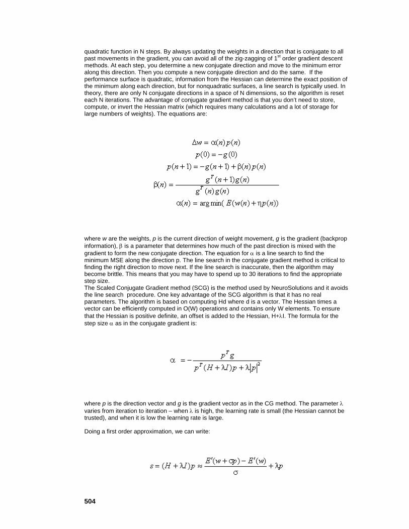
504

quadratic function in N steps. By always updating the weights in a direction that is conjugate to all past movements in the gradient, you can avoid all of the zig-zagging of 1st order gradient descent methods. At each step, you determine a new conjugate direction and move to the minimum error along this direction. Then you compute a new conjugate direction and do the same. If the performance surface is quadratic, information from the Hessian can determine the exact position of the minimum along each direction, but for nonquadratic surfaces, a line search is typically used. In theory, there are only N conjugate directions in a space of N dimensions, so the algorithm is reset each N iterations. The advantage of conjugate gradient method is that you don’t need to store, compute, or invert the Hessian matrix (which requires many calculations and a lot of storage for large numbers of weights). The equations are:

where w are the weights, p is the current direction of weight movement, g is the gradient (backprop information), β is a parameter that determines how much of the past direction is mixed with the gradient to form the new conjugate direction. The equation for α is a line search to find the minimum MSE along the direction p. The line search in the conjugate gradient method is critical to finding the right direction to move next. If the line search is inaccurate, then the algorithm may become brittle. This means that you may have to spend up to 30 iterations to find the appropriate step size. The Scaled Conjugate Gradient method (SCG) is the method used by NeuroSolutions and it avoids the line search procedure. One key advantage of the SCG algorithm is that it has no real parameters. The algorithm is based on computing Hd where d is a vector. The Hessian times a vector can be efficiently computed in O(W) operations and contains only W elements. To ensure that the Hessian is positive definite, an offset is added to the Hessian, H+λI. The formula for the step size α as in the conjugate gradient is:

where p is the direction vector and g is the gradient vector as in the CG method. The parameter λ varies from iteration to iteration – when λ is high, the learning rate is small (the Hessian cannot be trusted), and when it is low the learning rate is large.

Doing a first order approximation, we can write:

505

which means that you can replace the Hessian calculations with one additional evaluation of the gradients (backprop pass). The parameter λ must be set to ensure that the H+λI is positive definite so that the denominator of α will always be positive. If the value of the denominator is negative, we

increase λ by a value λ so that it will be positive. Additionally, we adjust λ based upon how closely the current point in the performance surface approximates a quadratic – if the performance surface is far from quadratic, we should increase λ resulting in a smaller step size. The value ∆ is used to determine "closeness to quadratic" and is estimated via:

If ∆ is less than zero, the change in the MSE will rise and the algorithm says to not change the weights (in my experience, however, it seems to work better if you do change the weights). If ∆ is less than .25 you multiply λ by 4, if it is greater than .75 (very quadratic) you multiply λ by .5.

This algorithm requires a number of global scalar computations. All matrix calculations can be done locally (parallel). It also requires one backprop pass to compute E’(w+sp) and one forward pass to compute E(w+αp). Conjugate Gradient learning in NeuroSolutions requires that the network learn in batch mode. In general, each Conjugate Gradient batch weight update will take twice as long as a standard batch weight update (using step or momentum gradient search).

User Interaction:

Drag and Drop

DeltaBarDelta


Superclass: Step

Description:

Delta-Bar-Delta is an adaptive step-size procedure for searching a performance surface. The step size and momentum are adapted according to the previous values of the error at the PE. If the current and past weight updates are both of the same sign, it increases the learning rate linearly. The reasoning is that if the weight is being moved in the same direction to decrease the error, then it will get there faster with a larger step size. If the updates have different signs, this is an indication

506

that the weight has been moved too far. When this happens, the learning rate decreases geometrically to avoid divergence.

Step Size Update Equation:

where:

κ= Additive constant

β= Multiplicative constant

λ= Smoothing factor

Weight Update Equation:

See Momentum

User Interaction:

Drag and Drop

Inspector

Access Points

DLL Implementation

Macro Actions

Momentum

507


Superclass: Step

Description:

Step components try to find the bottom of a performance surface by taking steps in the direction estimated by the attached backprop component. Network learning can be very slow if the step size is small, and can oscillate or diverge if it is chosen too large. To further complicate matters, a step size that works well for one location in weight space may be unstable in another.

The Momentum provides the gradient descent with some inertia, so that it tends to move along a direction that is the average estimate for down. The amount of inertia (i.e., how much of the past to average over) is dictated by the momentum parameter, ρ. The higher the momentum, the more it smoothes the gradient estimate and the less effect a single change in the gradient has on the weight change. The major benefit is the added ability to break out of local minima that a Step component might otherwise get caught in. Note that oscillations may occur if the momentum is set too high.

The momentum parameter is the same for all weights of the attached component. An access point has been provided for the step size and momentum allowing access for adaptive and scheduled learning rate procedures.


User Interaction:

Drag and Drop

Inspector

Access Points

DLL Implementation

Macro Actions

Quickprop

508


Superclass: Momentum

Description:

The Quickprop implements Fahlman's quickprop algorithm. It is a gradient search procedure that has been shown to be very fast in a multitude of problems. It basically uses information about the second order derivative of the performance surface to accelerate the search.

User Interaction:

Drag and Drop

Inspector

Access Points

DLL Implementation

Step


Superclass: GradientEngine

Description:

Gradient descent learning rules, e.g. backpropagation and real time recurrent learning, provide first order gradient information about the network's performance surface. In other words, they estimate which way is up. The most straightforward way of reaching the bottom (the minima) given which way is up, is to move in the opposite direction. With this scenario, the only variable is the step size, i.e. how far should it move before obtaining another directional estimate. If the steps are too small, then it will take too long to get there. If the steps are too large, then it may overshoot the bottom, causing it to rattle or even diverge.

509

The Step uses this procedure to adapt the weights of the Activation component that it is stacked on. The Step’s inspector allows the user to set a default step size for all weights within the Activation component. The step sizes of individual weights can be specified by attaching at MatrixEditor to the Learning Rate access point and modifying the default values. This access point can be used to adapt and/or schedule the step sizes during the simulation.


User Interaction:

Drag and Drop

Inspector

Access Points

DLL Implementation

Macro Actions

See Also

SVMStep


Superclass: Step

Description:


510

User Interaction:

Drag and Drop

Inspector

Access Points

Momentum Access Points

Component: Momentum

Superclass Access Points: Step Access Points

Momentum Access:

The Momentum Access provides a static access point to individually set the momentum of each weight, or to adaptively change the learning rates.

Delta Gradient Access:

The Delta Gradient Access provides a static access point to individually view the delta gradient of each weight.

Quickprop Access Points

Component: Quickprop

Superclass Access Points: DeltaBarDelta

Local Sensitivity Delta Access:

The Local Sensitivity Access reports the current state sensitivity minus the last state sensitivity used by the quickprop algorithm.

Step Access Points

Family: Step

Superclass Access Points: None

Learning Rate:

The Step Access provides a static access point to individually set the step size of each weight, or to adaptively change the learning rates.

511

See Also

DLL Implementation

Momentum DLL Implementation

Component: Momentum

Protocol: PerformMomentum

Description:

The implementation of the Momentum component is similar to that of the Step component, except that there is the addition of a momentum term and a vector containing the previous weight change (delta). The delta for a given weight is computed by taking product of the momentum rate and the weight’s previous delta and adding it to the product of the step size and the weight’s gradient. Note that this function is responsible for updating the delta vector as well as the weights vector.

Code: void performMomentum( DLLData *instance, // Pointer to instance data NSFloat *weights, // Pointer to the vector of weights int length, // Length of the weight vector NSFloat *gradient, // Pointer to vector of gradients NSFloat *step, // Pointer to the learning rate/s BOOL individual // Indicates whether there is one learning rate // for all weights (FALSE), or each weight has // its own learning rate (TRUE) NSFloat *delta, // Last weight Update NSFloat momentum // Momentum rate for all weights ) { register int i; for (i=0; i<length; i++) weights[i] += delta[i] = momentum*delta[i] + step[individual?i:0]*gradient[i]; }

512

Quickprop DLL Implementation

Component: Quickprop

Protocol: PerformQuickprop

Description:

The implementation of the Quickprop component is similar to that of the Momentum component, except that the momentum rate is unique to each weight. This vector is computed from the gradient information from the previous (lastGradient) and current (gradient) weight updates. The absolute value of the individual momentum terms is limited by the defaultMomentum defined by the user within the inspector. Note that this vector could have been allocated as local storage, but it is passed as a parameter for efficiency reasons. This function is responsible for updating the lastGradient vector as well as the delta and weights vectors.

Code: void performQuickprop( DLLData *instance, // Pointer to instance data NSFloat *weights, // Pointer to the vector of weights int length, // Length of the weight vector NSFloat *gradient, // Pointer to vector of gradients NSFloat *step, // Pointer to the learning rate/s BOOL individual // Indicates whether there is one learning // rate for all weights (FALSE), or each // weight has its own learning rate (TRUE) NSFloat *delta, // Last weight Update NSFloat defaultMomentum, // Max momentum rate for all weights NSFloat *momentum, // Individual momentum rate for each weight NSFloat *lastGradient // Previous weight gradient vector ) { register int i; for (i=0; i<length; i++) { momentum[i] = gradient[i]/(lastGradient[i] - gradient[i]); if (momentum[i] > defaultMomentum) momentum[i] = defaultMomentum; if (momentum[i] < -defaultMomentum) momentum[i] = -defaultMomentum;

513

delta[i] = momentum[i]*delta[i] + lastGradient[i]*(gradient[i]<0?0:step[individual?i:0]*gradient[i]); weights[i] += delta[i]; lastGradient[i] = gradient[i]; } }

Step DLL Implementation

Component: Step

Protocol: PerformStep

Description:

The Step component simply increments each weight by its corresponding gradient times a step size. Note that the step size can either be specific to a particular weight or it can be the same for all weights.

Code: void performStep( DLLData *instance, // Pointer to instance data NSFloat *weights, // Pointer to the vector of weights int length, // Length of the weight vector NSFloat *gradient, // Pointer to vector of gradients NSFloat *step, // Pointer to the learning rate/s BOOL individual // Indicates whether there is one learning rate // for all weights (FALSE), or each weight has // its own learning rate (TRUE) ) { register int i; if (!individual) for (i=0; i<length; i++) weights[i] += step[individual?i:0] * gradient[i]; }

514

Drag and Drop

GradientSearch Drag and Drop

Neural network topologies are constructed by dropping components from the Activation family directly onto the breadboard. Gradient descent learning dynamics are attached by dropping gradient descent components, e.g. components from the Backprop family, on top of their respective dual Activation component. The GradientSearch components are then dropped directly on top of these gradient descent components. In other words, three layers are required for networks using gradient descent learning. Each gradient descent learning family will have a controller within the Control family, e.g. the StaticBackpropControl component. Each controller is capable of automatically generating the gradient descent and GradientSearch layers once the Activation layer has been constructed.

See Also

Inspectors

DeltaBarDelta Inspector

Component: DeltaBarDelta

Superclass Inspector: NSEngineInspector

Component Configuration: Additive (SetAdditive(float))

515

This cell is used to specify the additive constant (κ), specified within the DeltaBarDelta component reference. Multiplicative (SetMult(float))

This cell is used to specify the multiplicative constant (β), specified within the DeltaBarDelta component reference. Smoothing (SetSmoothing(float))

This cell is used to specify the smoothing factor (ζ), specified within the DeltaBarDelta component reference.

Momentum Inspector

Component: Momentum


Component Configuration: Step Size (SetStepSize(float))

This cell sets the default step size for all weights within the Activation component. If the step size is adjusted during an experiment through an adaptive or scheduled procedure, then it will be reset to this default value each time the weights are randomized. Note that the individual step sizes can be modified by setting the Individual switch (see below), attaching a MatrixEditor to the Momentum component, and editing the values within the display window of the probe. Normalized

When this switch is turned on, the step size is normalized by dividing the number entered in the Step Size cell (see above) by the number of exemplars/update (see BackStaticControl). Individual

When this switch is turned on, the step sizes can be set individually by attaching a MatrixEditor to the Momentum component and editing the values within the display window of the probe. Note that

516

when this switch is set the step sizes are not restored to their default value when the network is reset. Momentum Rate (SetMomentum(float))

This cell sets the default momentum for all weights within the Activation component. If the momentum is altered during an experiment through an adaptive or scheduled procedure, then it will be reset to this default value whenever the weights of the Momentum component are randomized. Up

Raises the step sizes of all Gradient Search components on the breadboard by the percentage specified within the cell. Down

Lowers the step sizes of all Gradient Search components on the breadboard by the percentage specified within the cell. Decay Weights

The idea in weight elimination is to create a driving force that will attempt to decrease all the weights to zero during adaptation. If the input-output map requires some large weights, learning will keep bumping up the important weights, but the ones that are not important will be driven to zero, thus reducing the number of free parameters in the network. This idea is called weight decay. When this switch is set, weight decay is enabled such that the product of the current weight and the Decay Rate (see below) is subtracted from the weight adaptation formula for the Momentum component. Decay Rate

This cell specifies the decay rate to use in the weight decay algorithm described above.

Step Inspector

Component: Step


517


This cell sets the default step size for all weights within the Activation component. If the step size is adjusted during an experiment through an adaptive or scheduled procedure, then it will be reset to this default value each time the weights are randomized. Note that the individual step sizes can be modified by setting the Individual switch (see below), attaching a MatrixEditor to the Step component, and editing the values within the display window of the probe. Normalized

When this switch is turned on, the step size is normalized by dividing the number entered in the Step Size cell (see above) by the number of exemplars/update (see BackStaticControl). Individual

When this switch is turned on, the step sizes can be set individually by attaching a MatrixEditor to the Step component and editing the values within the display window of the probe. Note that when this switch is set the step sizes are not restored to their default value when the network is reset. Up

Bumps up the step sizes of all Gradient Search components on the breadboard by the percentage specified within the cell. Down

Bumps down the step sizes of all Gradient Search components on the breadboard by the percentage specified within the cell. Decay Weights

The idea in weight elimination is to create a driving force that will attempt to decrease all the weights to zero during adaptation. If the input-output map requires some large weights, learning will keep bumping up the important weights, but the ones that are not important will be driven to zero, thus reducing the number of free parameters in the network. This idea is called weight decay. When this switch is set, weight decay is enabled such that the product of the current weight and the Decay Rate (see below) is subtracted from the weight adaptation formula for the Step component. Decay Rate

This cell specifies the decay rate to use in the weight decay algorithm described above.

Macro Actions

Delta Bar Delta

DeltaBarDelta Macro Actions Overview Superclass Macro Actions

Action Description

beta Returns the multiplicative constant (β).

kappa Returns the additive constant (κ).

518

setBeta Sets the multiplicative constant (β).

setKappa Sets the additive constant (κ).

setZeta Sets the smoothing factor (ζ).

zeta Returns the smoothing factor (ζ).


Syntax

componentName.beta()


return float The multiplicative constant (β), specified within the DeltaBarDelta component reference (see "Multiplicative" within the DeltaBarDelta Inspector). componentName Name defined on the engine property page.

kappa Overview Macro Actions

Syntax

componentName.kappa()


return float The additive constant (κ), specified within the DeltaBarDelta component reference (see "Additive" within the DeltaBarDelta Inspector). componentName Name defined on the engine property page.


Syntax

componentName.setBeta(beta)


519


beta float The multiplicative constant (β), specified within the DeltaBarDelta component reference (see "Multiplicative" within the DeltaBarDelta Inspector).

setKappa Overview Macro Actions

Syntax

componentName.setKappa(kappa)


kappa float The additive constant (κ), specified within the DeltaBarDelta component reference (see "Additive" within the DeltaBarDelta Inspector).

setZeta Overview Macro Actions

Syntax

componentName.setZeta(zeta)


zeta float The smoothing factor (ζ), specified within the DeltaBarDelta component reference (see "Smoothing" within the DeltaBarDelta Inspector).

zeta Overview Macro Actions

Syntax

componentName.zeta()


return float The smoothing factor (ζ), specified within the DeltaBarDelta component reference (see "Smoothing" within the DeltaBarDelta Inspector). componentName Name defined on the engine property page.

520

Momentum

Momentum Macro Actions Overview Superclass Macro Actions

Action Description momentumRate Returns the momentum setting. setMomentumRate Sets the momentum setting.

momentumRate Overview Macro Actions

Syntax

componentName.momentumRate()

Parameters Type Description return float The default momentum for all weights within the Activation component (see "Momentum Rate" within the Momentum Inspector). componentName Name defined on the engine property page.

setMomentumRate Overview Macro Actions

Syntax

componentName.setMomentumRate(momentumRate)

Parameters Type Description return void componentName Name defined on the engine property page. momentumRate float The default momentum for all weights within the Activation component (see "Momentum Rate" within the Momentum Inspector).

Step

Step Macro Actions Overview Superclass Macro Actions

Action Description broadcastBumpStep Bumps the step size of all Gradient Search components on the breadboard up or down by a percentage.

521

bumpStep Bumps the step size up or down by a percentage. individualSteps Returns the "Individual" setting. normalized Returns the "Normalize" setting. setIndividualSteps Sets the "Individual" setting. setNormalized Sets the "Normalize" setting. setStepSize Sets the step size setting. stepSize Returns the step size setting.

broadcastBumpStep Overview Macro Actions

Syntax

componentName.broadcastBumpStep(percentage)

Parameters Type Description return void componentName Name defined on the engine property page. percentage float Percentage to change the step size for all the GradientSearch components (see "Up" and "Down" within the Step Inspector).

bumpStep Overview Macro Actions

Syntax

componentName.bumpStep(percentage)

Parameters Type Description return void componentName Name defined on the engine property page. percentage float Percentage to change the step size (see "Up" and "Down" within the Step Inspector).

individualSteps Overview Macro Actions

522

Syntax

componentName.individualSteps()

Parameters Type Description return BOOL TRUE if the step sizes can be set individually for each weight (see "Individual" within the Step Inspector). componentName Name defined on the engine property page.

normalized Overview Macro Actions

Syntax

componentName.normalized()

Parameters Type Description return BOOL TRUE if the step size is divided by the number of exemplars/update (see "Normalized" within the Step Inspector). componentName Name defined on the engine property page.

setIndividualSteps Overview Macro Actions

Syntax

componentName.setIndividualSteps(individualSteps)

Parameters Type Description return void componentName Name defined on the engine property page. individualSteps BOOL TRUE if the step sizes can be set individually for each weight (see "Individual" within the Step Inspector).

setNormalized Overview Macro Actions

Syntax

componentName.setNormalized(normalized)


523

componentName Name defined on the engine property page. normalized BOOL TRUE if the step size is divided by the number of exemplars/update (see "Normalized" within the Step Inspector).

setStepSize Overview Macro Actions

Syntax

componentName.setStepSize(stepSize)

Parameters Type Description return void componentName Name defined on the engine property page. stepSize float The default step size for all weights within the Activation component (see "Step Size" within the Step Inspector).

stepSize Overview Macro Actions

Syntax

componentName.stepSize()

Parameters Type Description return float The default step size for all weights within the Activation component (see "Step Size" within the Step Inspector). componentName Name defined on the engine property page.

Input Family Access

Ancestor: Engine Family

The purpose the Access family is to allow its members to access data provided by components through access points. This family uses an inspector to show which access points are available and provides a means for selecting one.

524

User Interaction:

Access Points

Access inspector

Macro Actions

Function

Family: Input Family

Superclass: MultiChannelStream

Description:

The Function component is used to create a variety of waveforms that can be used as input for neural networks. These inputs include impulses, square waves, sine waves, triangle waves, sawtooth waves, and user-defined functions via Dynamic Link Libraries (DLLs). The signals are specified by their amplitude, frequency, offset, and phase shift.

Function is a multi-channel component that can produce a different waveform for each neuron. The number of channels is dictated by the size (the number of PEs) of the network component that is being accessed. Each channel can have different amplitude, offset, and phase shift. However, all channels of a given function component must have the same frequency. If different frequencies are desired for different channels, the Function components may be stacked on top of each other such that each provides a unique input frequency.

User Interaction:

Drag and Drop

Inspector

Access Points

DLL Implementation

Macro Actions

Noise

525



Description:

The Noise component is used to inject random noise sources into an attached component. This component is most often used to test a network’s sensitivity to noise. The noise sources can have a uniform or a Gaussian distribution, or a user-defined distribution via a Dynamic Link Library (DLL). The noise signals are specified by their mean and variance.

Noise is a multi-channel component that can produce a different noise source for each neuron. The number of channels is dictated by the size (the number of PEs) of the network component that is being accessed. Each channel can have different mean and variance, as well as a different distribution.

The stream of noise data (of a user-defined size) is usually generated once and recycled throughout the simulations. There is an option for the data to be continually regenerated so that the noise is more random.

Noise Functions:

Uniform:

Gaussian:

where

x = a pseudo-random random floating point value between 0 and 1

σ = is the square root of the variance

µ = is the mean

User Interaction:

Drag and Drop

Inspector

DLL Implementation

526

Macro Actions

DLLInput



Description:

The DLLInput component is used to inject data into the network from a DLL. This is similar to using the DLL capability of the Function component, except that this data is not cyclical. One important use for this feature is to retrieve input data from external hardware (such as a analog-to-digital converter) by including the data acquisition code within the performInput function call.

DLLInput is a multi-channel component. The number of channels is dictated by the size (the number of PEs) of the network component that is being accessed. Each call to the performInput function requires that the implementation generate one sample of data for each channel.

User Interaction:

Drag and Drop

Access Points

DLL Implementation

DLLPreprocessor



Description:

The DLLPreprocessor component is used to preprocess the data sent from the component stacked on the Preprocessor access point. It requires that a DLL be loaded within the Engine property page

527

of the component’s inspector. The DLL retrieves the data one sample at a time and passes the processed data to the component attached below.

User Interaction:

Drag and Drop

Access Points

DLL Implementation

OLEInput



Description:

The OLEInput component is used to inject data into the network from an external program using the Object Linking and Embedding (OLE) protocol. To send data to the component you need to pass a variant array of floating point values to the sendDataToEngine function.

OLEInput is a multi-channel component. The number of channels is dictated by the size (the number of PEs) of the network component that is being accessed. The number of elements in the array passed to the sendDataToEngine function should be equal to the number of PEs times the number of input samples (exemplars).

User Interaction:

Drag and Drop

Access Points

Macro Actions

File

File

528



Description:

The File component reads data from the computer’s file system. Presently there is support for ASCII, column-formatted ASCII, binary, and bitmap file formats (see the Associate File panel). Multiple files of mixed type can be translated simultaneously within the same File component. There are also provisions for normalization and segmentation of input files.

Column-formatted ASCII is the most commonly used, since it is directly exportable from commercial spreadsheet programs. Each column of a column-formatted ASCII file represents one channel of data (i.e., input into one PE). The first line (row) of the file contains the column headings, and the remaining lines contain the samples of data. The data elements can be either numeric or symbolic. There is a facility to automatically convert symbolic data to numeric data (see Column-Formatted ASCII Translator).

The remaining three file types are simply read as a sequential stream of floating-point values. Non-formatted ASCII files contain numeric value separated by delimeters (see ASCII Translator). Any non-numeric values are simply ignored. Bitmap files can be either 16-color or 256-color. Each pixel of the image is converted to a value from 0 to 1, based on its intensity level. Binary files contain raw data, such that each 4-byte segment contains a floating-point value. Many numerical software packages export their data to this type of format.

The translation process for large ASCII files may be very time consuming. For this reason, each translated data stream is automatically stored in the same directory as the breadboard as a binary pattern file (.nsp). This way, the file(s) only need to be re-translated when the data set or component configuration has changed.

Each unique data set within a File component has its own data stream. The data is read from the stream of the currently active data set and sequentially fed to the PEs of the component stacked below. A data set that is translated to a stream that has 100 data elements could be used to feed 10 samples to a 10-PE axon, or 20 samples to a 5-PE axon. Note that it could also feed 9 samples to an 11-PE axon, but that the last data element would be discarded.

The File component can be configured to normalize the data based on a set of normalization coefficients. These coefficients consist of an amplitude and an offset term for each channel of the File component, and they can be generated automatically or read from a previously generated and/or modified Normalization File.

User Interaction:

Drag and Drop

Inspector

Access Points

DLL Implementation

Macro Actions

529

Translators

ASCII Translator

This translator reads all numeric data from an ASCII file and ignores all non-numeric information. The numeric data must be separated by any of the delimiters listed below and may be in floating point, scientific, or integer format.

Delimiters:

ASCII Char

-------- -------

9 <tab>

10 <line break>

32 <space>

34 "

44 ,

58 :

59 ;

96 `

There are also several other less common ASCII characters that are also interpreted as delimeters:

0, 1, 2, 3, 4, 5, 6, 7, 8, 11, 12, 13, 14, 15, 16, 17, 18, 19, 20, 21, 22, 23, 24, 25, 26, 27, 28, 29, 30, 31, 127, 128, 129, 141, 142, 143, 144, 157, 158, 160

See Also

Binary Translator

This translator reads files that are in a standard binary format. This format specifies that each floating point value is stored within 4 bytes of the file. This is the same format used by the pattern files (*.nsp) generated for each data set of the file (see File).

530

See Also

Bitmap Translator

This translator reads a 16-color, 256-color or 24-bit bitmap and translates the image into a stream of intensity values (i.e., gray levels) ranging from 0 to 1. These values are obtained by averaging the RGB values from each of the pixels and dividing by 255 (the maximum RGB value).

See Also

Column-Formatted ASCII Translator

Each column of a column-formatted ASCII file represents one channel of data (i.e., input into one PE). The first line (row) of the file should contain the column headings, and not actual data. Each group of delimiters (see ASCII Translator) indicates a break in the columns. In order for the program to detect the correct number of columns, the column headings must not contain any delimiters.

The remaining lines contain the individual samples of data. The data elements (values) are separated by delimiters. The number of data elements for each line must match the number of column headings from the first line. The data elements can be either numeric or symbolic.

When there are multiple data files within the same File component using the Column-Formatted ASCII Translator, the column selections apply to all of these files. For this reason, the column headings of the included columns must match across all files and be arranged in the same order. If NeuroSolutions detects that the ordering of the included columns differs between the files, then an option will be given to run a utility that will match the column ordering for you.

The translator handles symbolic columns by reading the symbol definitions from the symbol translation file (*.nss), stored in the same directory as the breadboard. This file can be automatically generated from the columns that have been declared as symbolic (see Column Translator Customize). This file is generated by extracting the symbols from all of the data files associated with the Column-Formatted ASCII Translator. The format of the symbol translation file is as follows:

Symb1 N1 Val1 Val2 . . . ValN1 Head1 Head2 . . .

Symb2 N2 Val1 Val2 . . . ValN2 Head1 Head2 . . .

: : : : : : :

: : : : : : :

SymbM NM Val1 Val2 . . . ValNM Head1 Head2 . . .

#Labels

Head1 N1 Symb1 Symb2 . . . SymbN1

Head2 N2 Symb1 Symb2 . . . SymbN2

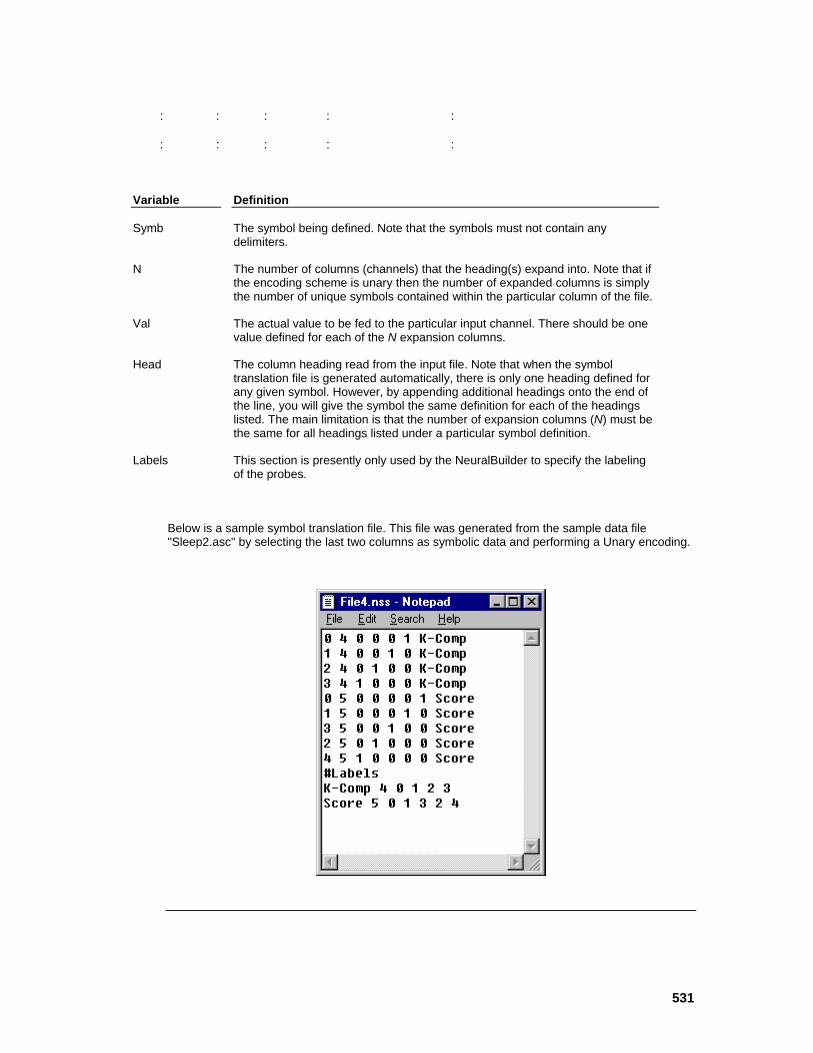
531

: : : : :

: : : : :

Variable Definition

Symb The symbol being defined. Note that the symbols must not contain any delimiters.

N The number of columns (channels) that the heading(s) expand into. Note that if the encoding scheme is unary then the number of expanded columns is simply the number of unique symbols contained within the particular column of the file.

Val The actual value to be fed to the particular input channel. There should be one value defined for each of the N expansion columns.

Head The column heading read from the input file. Note that when the symbol translation file is generated automatically, there is only one heading defined for any given symbol. However, by appending additional headings onto the end of the line, you will give the symbol the same definition for each of the headings listed. The main limitation is that the number of expansion columns (N) must be the same for all headings listed under a particular symbol definition.

Labels This section is presently only used by the NeuralBuilder to specify the labeling of the probes.

Below is a sample symbol translation file. This file was generated from the sample data file "Sleep2.asc" by selecting the last two columns as symbolic data and performing a Unary encoding.

532

See Also

DLL Translator

The DLL translator uses a user-defined dynamic link library (DLL) to translate either a text or binary file into a data stream. The DLL is specified within the Engine property page of the File inspector. Note that the DLL must be loaded in order to use the DLL translator.

See Also

Translator Customize

This panel used to customize the way in which the translator translates the selected file. All translators have the ability to extract a segment of the file’s data.

Segment

When this switch is turned on, the first Offset exemplars are skipped, the next Duration exemplars are read from the file, and the remaining exemplars are skipped. Offset

This cell is used to specify the number of exemplars to skip before reading the first exemplar. Duration

This cell is used to specify the number of exemplars of the segment.

Column Translator Customize

This panel used to customize the way in which the Column-Formatted ASCII Translator translates the selected file. Like all other translators, this has the ability to extract a segment of the file’s data. It also provides a facility for selecting columns for inclusion to, or exclusion from, the translation

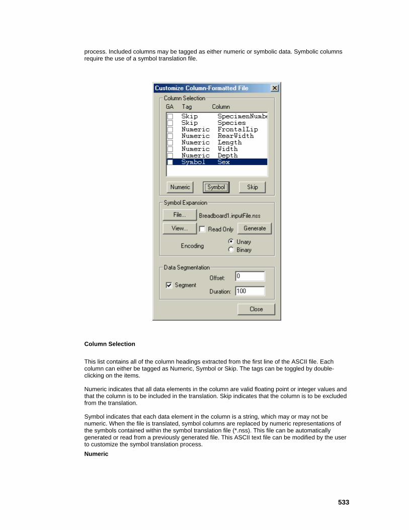
533

process. Included columns may be tagged as either numeric or symbolic data. Symbolic columns require the use of a symbol translation file.

Column Selection

This list contains all of the column headings extracted from the first line of the ASCII file. Each column can either be tagged as Numeric, Symbol or Skip. The tags can be toggled by double-clicking on the items.

Numeric indicates that all data elements in the column are valid floating point or integer values and that the column is to be included in the translation. Skip indicates that the column is to be excluded from the translation.

Symbol indicates that each data element in the column is a string, which may or may not be numeric. When the file is translated, symbol columns are replaced by numeric representations of the symbols contained within the symbol translation file (*.nss). This file can be automatically generated or read from a previously generated file. This ASCII text file can be modified by the user to customize the symbol translation process. Numeric

534

This button is used to set the tags of the selected item(s) from the Column Selection list to Numeric. Numeric indicates that all data elements in the column are valid floating point or integer values and that the column is to be included in the translation. Symbol

This button is used to set the tags of the selected item(s) from the Column Selection list to Symbol. Symbol indicates that each data element in the column is a string, which may or may not be numeric. When the file is translated, symbol columns are replaced by numeric representations of the symbols contained within the symbol translation file (*.nss). Skip

This button is used to set the tags of the selected item(s) from the Column Selection list to Skip. Skip indicates that the column is to be excluded from the translation. GA

There are times when you are not sure whether or not an input column provides useful information to the network. By tagging a set of inputs as "GA", a genetic algorithm will try various permutations of includes and skips among these inputs in an attempt to produce the lowest error. Once the optimization training run is complete and the best parameters are loaded into the network, the column list will reflect which genetically optimized input columns were included. Note that the GeneticControl component must have optimization enabled (see the GeneticControl inspector) before the selected inputs will be optimized on the next training run. File Name

This button brings up a panel to enter the file name (including the extension) of the symbol translation file that is generated or read on translation. This ASCII file contains the definitions for each unique symbol contained within the tagged columns of all data files using the Column-Formatted ASCII Translator). Note that there must be at least one column tagged as Symbol in order for this button to be enabled. Read Only

If there is at least one column tagged as Symbol, then this switch specifies how the symbol file is used. If the switch is off (the default), the symbol file is generated when the Customize panel is closed, or after the associated data files are modified. If the switch is on, the symbols are read from an existing symbol file during translation (see Column-Formatted ASCII Translator). Unary

This encoding scheme adds an additional channel for each unique symbol found in the column. Each expanded channel of a given symbol column represents one symbol; a 1 indicating the symbol is present and a 0 indicating the symbol is absent. In other words, each exemplar will have one channel set to 1 and the remaining columns will be set to 0. Note that this switch is only enabled when the Read Only switch is off and there is at least one column tagged as Symbol. Binary

This encoding scheme adds log N (base 2) channels, where N is the number of unique symbols found in the column. Each symbol is represented by a unique binary number. Note that this switch is only enabled when the Read Only switch is off and there is at least one column tagged as Symbol. View

This button is used to view the current state of the symbol translation file (see Column-Formatted ASCII Translator). The program used to view the file is determined based on the file’s extension and application associated with that extension defined within Windows. Click here for instructions on associating an editor with a file extension.

535

Generate

This button generates the symbol translation file based on the columns tagged as Symbol and will overwrite the existing file if it exists. If the symbol file has not been generated by the time the Customize panel is closed, then the file is generated automatically. Note that this switch is only enabled when the Read Only switch is off and there is at least one column tagged as Symbol. Segment

See Translator Customize Offset

See Translator Customize Duration

See Translator Customize

See Also

DLL Implementation

File DLL Implementation

Component: File

Protocol: PerformFile

Description:

The File component contains four base translators: 1) ASCII, 2) Column-formatted ASCII, 3) binary, and 4) bitmap. The DLL capability of the File component allows you to write your own translator. The default functionality of the DLL translator is a very basic ASCII translator. It will read a file containing only space-delimited numbers.

Code: BOOL performFile( DLLData *instance, // Pointer to instance data (may be NULL) FILE *file, // Pointer to the opened file NSFloat *sample // Location to place next sample )

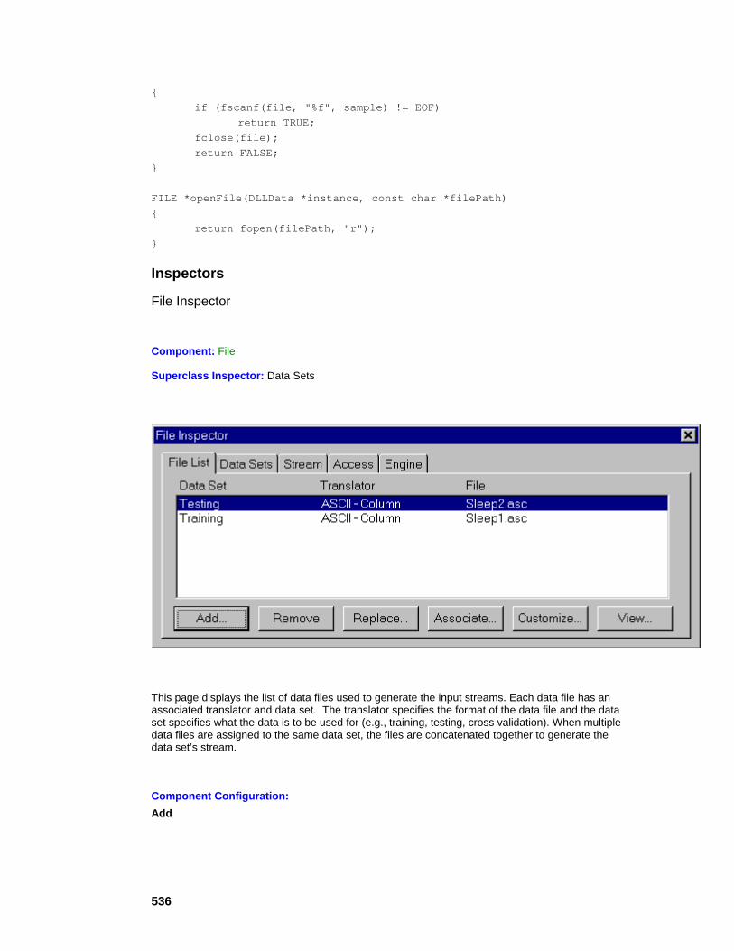
536

{ if (fscanf(file, "%f", sample) != EOF) return TRUE; fclose(file); return FALSE; } FILE *openFile(DLLData *instance, const char *filePath) { return fopen(filePath, "r"); }

Inspectors

File Inspector

Component: File

Superclass Inspector: Data Sets

This page displays the list of data files used to generate the input streams. Each data file has an associated translator and data set. The translator specifies the format of the data file and the data set specifies what the data is to be used for (e.g., training, testing, cross validation). When multiple data files are assigned to the same data set, the files are concatenated together to generate the data set’s stream.

Component Configuration: Add

537

This button displays a file selection panel for adding a file to the list. The Associate File panel is then displayed for you to specifiy the translator and data set to associate with the file. Each unique data set added will have an associated pattern file (.nsp) that contains the raw data stream. Remove

This button removes the currently selected file from the file list. Replace

This button displays a file selection panel for replacing the currently selected file from the list. Associate

This button displays the Associate File panel. This panel is used to associate a translator and a data set with the selected data file. The file list displays the current associations. Customize

This button displays a panel used to customize the way in which the translator translates the selected file. Some translators have different parameter settings than others (see the Translator Customize and Column Translator Customize panels). All translators have the ability to extract a segment of the file’s data. View

This button is used to view the selected file. The program used to view the file is determined based on the file’s extension and application associated with that extension defined within Windows. Click here for instructions on associating an editor with a file extension.

See Also

Data Sets Inspector

Component: File

Superclass Inspector: Stream

538

This page displays the list of data sets used to generate the Normalization File and the number of exemplars read from the active data set. The normalization coefficients will be computed across all data sets by default. To use multiple data sets for the normalization coefficients, hold down the Control key or Shift key while selecting the items from the list.

Component Configuration: Generate Normalization File

If the File component is configured to normalize the data (see the Stream Inspector), then this switch specifies how the Normalization File is used. If the switch is on (the default), the normalization file is generated when the File component performs a translation. If the switch is off, the normalization coefficients are read from an existing normalization file during translation. Norm. File

This button brings up a panel to enter the file name (including the extension) of the Normalization File that is generated or read on translation (see above). Note that the Normalize switch (see the Stream Inspector) must be switched on in order for this button to be enabled. View

This button is used to view the current state of the Normalization File. The program used to view the file is determined based on the file’s extension and application associated with that extension defined within Windows. Click here for instructions on associating an editor with a file extension. Translate

This button translates the files for the active data set and generates the corresponding data stream. Once the file has been translated, the number of exemplars are displayed.

File Macro Actions

File Macro Actions Overview Superclass Macro Actions

Action Description

539

activeDataSet Returns the selected "Active Data Set". activeFileName Returns the name of the currently selected file in the File List. activeFilePath Returns the full path of the currently selected file in the File List. activeTranslatorName Returns the translator name of the currently selected file in the File List. addFile Adds a file to the File List. associateActiveFile Associates a translator and a data set with the currently selected file in the File List. beginCustomizeOfActiveFile This function is called before any changes are made to the parameters within the Translator Customize and Column Translator Customize panels. binaryEncodingForSymbols Returns TRUE if the "Encoding Scheme" is set to "Binary" and FALSE if it is set to "Unary". columnCountForActiveFile Returns the number of selected columns within the active file. columnTagForActiveFile Returns a code based on how the specified column is tagged (0 = "Skip", 1 = "Numeric", 2 = "Symbol"). customizeActiveFile Displays either the Translator Customize or Column Translator Customize panel depending on the translator used for the active file. dataSetCount Returns the number of unique data sets within the File List. dataSetForActiveFile Returns the data set of the file selected within the File List. dataSetNameAt Returns the data set at the specified index, where 0 <= index < dataSetCount. dataSetUsedForNormalization TRUE if the specified data set is used to calculate the normalization coefficients. durationForActiveFile Returns the "Duration" setting for the currently selected file in the File List. endCustomizeOfActiveFile This function is called after any changes are made to the parameters within the Translator Customize and Column Translator Customize panels. expandedColumnCountForActiveFile Returns the number of selected columns, plus the number of additional columns added for symbolic data, within the active file. fileCount Returns the number of files listed with the File List. filePathAt Returns the full file path of a file in the File List, specified by an index number, where 0 <= index < fileCount. generateSymbolFile Generates a symbol file based on the columns tagged as "Symbol".

540

matchPEsWithColumns Sets the number of rows of the attached Axon component to match that of the number of selected columns. normalizationFileName Returns the name of the "Normalization File" (with extension). normalizationFilePath Returns the full path of the "Normalization File". normalizationFileReadOnly Returns the "Read Only" setting. numericForActiveFile Returns TRUE if the specified column of the active file is tagged as "Numeric". offsetForActiveFile Returns the "Offset" setting for the currently selected file in the File List. removeActiveFile Removes the currently selected file from the file list. removeAllFiles Removes all files from the file list. segmentForActiveFile Returns the "Segment" setting for the currently selected file in the File List. setActiveDataSet Sets the "Active Data Set" selection. setActiveFileNameAndDataSet Selects the active file in the File List given the file's name and data set. setActiveFilePath Selects the active file in the File List given the file's path. setActiveTranslatorName Associates the specified translator with the active file. setBinaryEncodingForSymbols Set to TRUE to set the "Encoding Scheme" to "Binary" and FALSE to set it to "Unary". setColumnTagForActiveFile Tags the specified column (0 = "Skip", 1 = "Numeric", 2 = "Symbol"). setDataSetForActiveFile Sets the data set of the file selected within the File List. setDataSetUsedForNormalization TRUE if the specified data set is used to calculate the normalization coefficients. setDurationForActiveFile Sets the "Duration" setting for the currently selected file in the File List. setNormalizationFilePath Sets the full path of the "Normalization File". setNormalizationFileReadOnly Sets the "Read Only" setting. setNumericForActiveFile Tags the specified columns of the active file as "Numeric". setOffsetForActiveFile Sets the "Offset" setting for the active file. setSegmentForActiveFile Sets the "Segment" setting for the currently selected file in the File List.

541

setSkipForActiveFile Tags the specified columns of the active file as "Skip". setSymbolFilePath Sets the path of the "Symbol Expansion" file. setSymbolFileReadOnly Sets the "Read Only" setting of the "Symbol Expansion" file. setSymbolForActiveFile Tags the specified columns of the active file as "Symbol". setUseDefaultTranslatorForActiveFile TRUE sets the "Set as default for all files of type" setting, and FALSE set the "Set only for file" setting. skipForActiveFile Returns TRUE if the specified column of the active file is tagged as "Skip". symbolFileName Returns the name (with extension) of the "Symbol Expansion" file. symbolFilePath Returns the path of the "Symbol Expansion" file. symbolFileReadOnly Returns the "Read Only" setting of the "Symbol Expansion" file. symbolForActiveFile Returns TRUE if the specified column of the active file is tagged as "Symbol". toggleColumnForActiveFile Toggles the column setting for the active file from "Skip" to "Numeric" to "Symbol". translate Translates the files for the active data set and generates the corresponding data stream. translateIfNeeded Performs the translate operation only if the data files have changed since the last translation. translatorCount Returns the number of available translators. translatorNameAt Returns the translator at the specified index, where 0 <= index < translatorCount. useDefaultTranslatorForActiveFile Returns TRUE if the "Set as default for all files of type" setting is active, and FALSE if the "Set only for file" setting is active. verifiedSamples Performs a translation if needed and returns the number of samples in the active data set.

activeDataSet Overview Macro Actions

Syntax

componentName. activeDataSet()


542

return string The data set used when a "translate" operation is performed (see "Translate" within the Data Set Inspector ). componentName Name defined on the engine property page.

activeFileName Overview Macro Actions

Syntax

componentName. activeFileName()

Parameters Type Description return string The name of the currently selected file in the File List (see the File Inspector ). componentName Name defined on the engine property page.

activeFilePath Overview Macro Actions

Syntax

componentName. activeFilePath()

Parameters Type Description return string The path of the currently selected file in the File List (see the File Inspector ). componentName Name defined on the engine property page.

activeTranslatorName Overview Macro Actions

Syntax

componentName. activeTranslatorName()

Parameters Type Description return string The translator name of the currently selected file in the File List (see the Associate File panel). componentName Name defined on the engine property page.

addFile Overview Macro Actions

Syntax

543

componentName. addFile(path, dialogMode)

Parameters Type Description return BOOL TRUE if the operation completed successfully. componentName Name defined on the engine property page.

path string The full path of the file to add to the File List (see "Add" within the File Inspector).

dialogMode BOOL TRUE to display error and warning messages and FALSE to supress them.

associateActiveFile Overview Macro Actions

Syntax

componentName. associateActiveFile()

Parameters Type Description return BOOL Returns TRUE if the association was made and FALSE if the user cancelled the operation. componentName Name defined on the engine property page.

beginCustomizeOfActiveFile Overview Macro Actions

Syntax

componentName. beginCustomizeOfActiveFile()


binaryEncodingForSymbols Overview Macro Actions

Syntax

componentName. binaryEncodingForSymbols()

Parameters Type Description return BOOL TRUE uses an encoding scheme that adds log N (base 2) channels, where N is

544

the number of unique symbols found in the column. FALSE uses a unary encoding scheme that adds N channels (see "Encoding Scheme" within the Column Translator Customize panel). componentName Name defined on the engine property page.

columnCountForActiveFile Overview Macro Actions

Syntax

componentName. columnCountForActiveFile()

Parameters Type Description return int The number of selected columns within the active file. componentName Name defined on the engine property page.

columnTagForActiveFile Overview Macro Actions

Syntax

componentName. columnTagForActiveFile(index)

Parameters Type Description return int The code based on how the specified column is tagged (0 = "Skip", 1 = "Numeric", 2 = "Symbol"). componentName Name defined on the engine property page.

index int The column index (0 <= index < columnCountForActiveFile).

customizeActiveFile Overview Macro Actions

Syntax

componentName. customizeActiveFile(aString)

Parameters Type Description return string componentName Name defined on the engine property page. aString string The window title for the customize panel (blank to use the default title).

545

dataSetCount Overview Macro Actions

Syntax

componentName. dataSetCount()

Parameters Type Description return int The number of unique data sets defined (see the Data Set Inspector). componentName Name defined on the engine property page.

dataSetForActiveFile Overview Macro Actions

Syntax

componentName. dataSetForActiveFile()

Parameters Type Description return string The data set of the file selected within the File List (see the File Inspector ). componentName Name defined on the engine property page.

dataSetNameAt Overview Macro Actions

Syntax

componentName. dataSetNameAt(index)

Parameters Type Description return string The data set at the specified index (see the Data Set Inspector). componentName Name defined on the engine property page. index int The index of the data set list (0 <= index < dataSetCount).

dataSetUsedForNormalization Overview Macro Actions

Syntax

componentName. dataSetUsedForNormalization(dataset)

Parameters Type Description return BOOL TRUE if the specified dataset has been selected to be included in the calculation of the normalization coefficients (see the Data Set Inspector).

546

componentName Name defined on the engine property page. dataset string The data set name.

durationForActiveFile Overview Macro Actions

Syntax

componentName. durationForActiveFile()

Parameters Type Description return int The number of samples of the segment (see "Duration" within the Translator Customize and Column Translator Customize panels). componentName Name defined on the engine property page.

endCustomizeOfActiveFile Overview Macro Actions

Syntax

componentName. endCustomizeOfActiveFile()

Parameters Type Description return BOOL TRUE if the customization operation was successful. componentName Name defined on the engine property page.

expandedColumnCountForActiveFile Overview Macro Actions

Syntax

componentName. expandedColumnCountForActiveFile()

Parameters Type Description return int The number of selected columns, plus the number of additional columns added for symbolic data, within the active file. componentName Name defined on the engine property page.

fileCount Overview Macro Actions

Syntax

547

componentName. fileCount()

Parameters Type Description return int The number of files listed with the File List (see the File Inspector ). componentName Name defined on the engine property page.

filePathAt Overview Macro Actions

Syntax

componentName. filePathAt(index)

Parameters Type Description return string The path of the specified file within the File List (see the File Inspector ). componentName Name defined on the engine property page.

index int The index of the file within the File List (0<= index < fileCount).

generateSymbolFile Overview Macro Actions

Syntax

componentName. generateSymbolFile()


matchPEsWithColumns Overview Macro Actions

Syntax

componentName. matchPEsWithColumns()


normalizationFileName Overview Macro Actions

548

Syntax

componentName. normalizationFileName()

Parameters Type Description return string The name (with extension) of the file that stores the normalization coefficients (see "Generate Normalization File" within the Data Set Inspector ). componentName Name defined on the engine property page.

normalizationFilePath Overview Macro Actions

Syntax

componentName. normalizationFilePath()

Parameters Type Description return string The full path of the file that stores the normalization coefficients (see "Generate Normalization File" within the Data Set Inspector ). componentName Name defined on the engine property page.

normalizationFileReadOnly Overview Macro Actions

Syntax

componentName. normalizationFileReadOnly()

Parameters Type Description return BOOL FALSE if the normalization file is to be generated from the current data (see "Generate Normalization File" within the Data Set Inspector ). componentName Name defined on the engine property page.

numericForActiveFile Overview Macro Actions

Syntax

componentName. numericForActiveFile(index)

Parameters Type Description return BOOL TRUE if the specified column of the active file is tagged as "Numeric" (see the Column Translator Customize panel). componentName Name defined on the engine property page.

index int The column index of the active file (0 <= index < columnCount).

549

offsetForActiveFile Overview Macro Actions

Syntax

componentName. offsetForActiveFile()

Parameters Type Description return int The number of samples to offset the segment (see "Offset" within the Translator Customize and Column Translator Customize panels). componentName Name defined on the engine property page.

removeActiveFile Overview Macro Actions

Syntax

componentName. removeActiveFile()


removeAllFiles Overview Macro Actions

Syntax

componentName. removeAllFiles()


segmentForActiveFile Overview Macro Actions

Syntax

componentName. segmentForActiveFile()


550

return BOOL TRUE if the active file is segmented (see "Segment" within the Translator Customize and Column Translator Customize panels). componentName Name defined on the engine property page.

setActiveDataSet Overview Macro Actions

Syntax

componentName. setActiveDataSet(activeDataSet)

Parameters Type Description return void componentName Name defined on the engine property page. activeDataSet string The data set used when a "translate" operation is performed (see "Translate" within the Data Set Inspector ).

setActiveFileNameAndDataSet Overview Macro Actions

Syntax

componentName. setActiveFileNameAndDataSet(name, dataSet)

Parameters Type Description return void componentName Name defined on the engine property page. name string The name of the file to select from the File List (see the File Inspector ). dataSet string The data set of the file to select from the File List (see the File Inspector ).

setActiveFilePath Overview Macro Actions

Syntax

componentName. setActiveFilePath(activeFilePath)


551

activeFilePath string The path of the currently selected file in the File List (see the File Inspector ).

setActiveTranslatorName Overview Macro Actions

Syntax

componentName. setActiveTranslatorName(activeTranslatorName)

Parameters Type Description return void componentName Name defined on the engine property page. activeTranslatorName string The translator name of the currently selected file in the File List (see the Associate File panel).

setBinaryEncodingForSymbols Overview Macro Actions

Syntax

componentName. setBinaryEncodingForSymbols(binaryEncodingForSymbols)

Parameters Type Description return void componentName Name defined on the engine property page. binaryEncodingForSymbols BOOL TRUE uses an encoding scheme that adds log N (base 2) channels, where N is the number of unique symbols found in the column. FALSE uses a unary encoding scheme that adds N channels (see "Encoding Scheme" within the Column Translator Customize panel).

setColumnTagForActiveFile Overview Macro Actions

Syntax

componentName. setColumnTagForActiveFile(beginIndex, endIndex, tag)

Parameters Type Description return void componentName Name defined on the engine property page. beginIndex int The first column of the block to tag (0 <= beginIndex < columnCount).

552

endIndex int The last column of the block to tag (0 <= endIndex < columnCount). tag int A code indicating how to tag the block of columns (0 = "Skip", 1 = "Numeric", 2 = "Symbol" – see the Column Translator Customize panel).

setDataSetForActiveFile Overview Macro Actions

Syntax

componentName. setDataSetForActiveFile(dataSet)

Parameters Type Description return void componentName Name defined on the engine property page. dataSet string The data set to associate with the active file (see the Associate File panel).

setDataSetUsedForNormalization Overview Macro Actions

Syntax

componentName. setDataSetUsedForNormalization(dataSet, aBool)

Parameters Type Description return void componentName Name defined on the engine property page. dataSet string The name of the data set to include/exclude from the normalization calculation (see the Data Set Inspector ). aBool BOOL TRUE includes the file and FALSE excludes the file.

setDurationForActiveFile Overview Macro Actions

Syntax

componentName. setDurationForActiveFile(duration)

Parameters Type Description return void componentName Name defined on the engine property page. durationint The number of samples of the segment (see "Duration" within the Translator

553

Customize and Column Translator Customize panels).

setNormalizationFilePath Overview Macro Actions

Syntax

componentName. setNormalizationFilePath(normalizationFilePath)

Parameters Type Description return void componentName Name defined on the engine property page. normalizationFilePath string The full path of the file that stores the normalization coefficients (see "Generate Normalization File" within the Data Set Inspector ).

setNormalizationFileReadOnly Overview Macro Actions

Syntax

componentName. setNormalizationFileReadOnly(normalizationFileReadOnly)

Parameters Type Description return void componentName Name defined on the engine property page. normalizationFileReadOnly BOOL FALSE if the normalization file is to be generated from the current data (see "Generate Normalization File" within the Data Set Inspector ).

setNumericForActiveFile Overview Macro Actions

Syntax

componentName. setNumericForActiveFile(beginIndex, endIndex)

Parameters Type Description return void componentName Name defined on the engine property page. beginIndex int The column index of the first column of the block to tag as "Numeric" (0 <= beginIndex < columnCount – see the Column Translator Customize panel). endIndex int The column index of the last column of the block to tag as "Numeric" (0 <= endIndex < columnCount – see the Column Translator Customize panel).

554

setOffsetForActiveFile Overview Macro Actions

Syntax

componentName. setOffsetForActiveFile(offsetForActiveFile)

Parameters Type Description return void componentName Name defined on the engine property page. offsetForActiveFile int The number of samples to offset the segment (see "Offset" within the Translator Customize and Column Translator Customize panels).

setSegmentForActiveFile Overview Macro Actions

Syntax

componentName. setSegmentForActiveFile(segmentForActiveFile)

Parameters Type Description return void componentName Name defined on the engine property page. segmentForActiveFile BOOL TRUE if the active file is segmented (see "Segment" within the Translator Customize and Column Translator Customize panels).

setSkipForActiveFile Overview Macro Actions

Syntax

componentName. setSkipForActiveFile(beginIndex, endIndex)

Parameters Type Description return void componentName Name defined on the engine property page. beginIndex int The column index of the first column of the block to tag as "Skip" (0 <= beginIndex < columnCount – see the Column Translator Customize panel). endIndex int The column index of the last column of the block to tag as "Skip" (0 <= endIndex < columnCount – see the Column Translator Customize panel).

555

setSymbolFilePath Overview Macro Actions

Syntax

componentName. setSymbolFilePath(symbolFilePath)

Parameters Type Description return void componentName Name defined on the engine property page. symbolFilePath string The path of the file used to store the symbol translation table (see "File Name" with the Column Translator Customize panel).

setSymbolFileReadOnly Overview Macro Actions

Syntax

componentName. setSymbolFileReadOnly(symbolFileReadOnly)

Parameters Type Description return void componentName Name defined on the engine property page. symbolFileReadOnly BOOL FALSE if the symbol file is to be generated from the current data (see "Read Only" within the Column Translator Customize panel).

setSymbolForActiveFile Overview Macro Actions

Syntax

componentName. setSymbolForActiveFile(beginIndex, endIndex)

Parameters Type Description return void componentName Name defined on the engine property page. beginIndex int The column index of the first column of the block to tag as "Symbol" (0 <= beginIndex < columnCount – see the Column Translator Customize panel). endIndex int The column index of the last column of the block to tag as " Symbol" (0 <= endIndex < columnCount – see the Column Translator Customize panel).

556

setUseDefaultTranslatorForActiveFile Overview Macro Actions

Syntax

componentName. setUseDefaultTranslatorForActiveFile(aBool)

Parameters Type Description return void componentName Name defined on the engine property page. aBool BOOL TRUE sets the selected translator as the default translator for all files of the selected extension, and FALSE uses the selected translator only for the active file (see "Set as default for all files" and "Set only for file" within the Associate File panel).

skipForActiveFile Overview Macro Actions

Syntax

componentName. skipForActiveFile(index)

Parameters Type Description return BOOL TRUE if the specified column of the active file is tagged as "Skip" (see the Column Translator Customize panel). componentName Name defined on the engine property page. index int The column index of the active file (0 <= index < columnCount).

symbolFileName Overview Macro Actions

Syntax

componentName. symbolFileName()

Parameters Type Description return BOOL The name (with extension) of the file used to store the symbol translation table (see "File Name" with the Column Translator Customize panel). componentName Name defined on the engine property page.

symbolFilePath Overview Macro Actions

Syntax

557

componentName. symbolFilePath()

Parameters Type Description return string The path of the file used to store the symbol translation table (see "File Name" with the Column Translator Customize panel). componentName Name defined on the engine property page.

symbolFileReadOnly Overview Macro Actions

Syntax

componentName. symbolFileReadOnly()

Parameters Type Description return BOOL FALSE if the symbol file is to be generated from the current data (see "Read Only" within the Column Translator Customize panel). componentName Name defined on the engine property page.

symbolForActiveFile Overview Macro Actions

Syntax

componentName. symbolForActiveFile(index)

Parameters Type Description return BOOL TRUE if the specified column of the active file is tagged as "Symbol" (see the Column Translator Customize panel). componentName Name defined on the engine property page. index int The column index of the active file (0 <= index < columnCount).

toggleColumnForActiveFile Overview Macro Actions

Syntax

componentName. toggleColumnForActiveFile()


558

beginIndex int The column index of the first column of the block to toggle the selection from "Skip" to "Numeric" to "Symbol" (0 <= beginIndex < columnCount – see the Column Translator Customize panel). endIndex int The column index of the last column of the block to toggle the selection from "Skip" to "Numeric" to "Symbol" (0 <= endIndex < columnCount – see the Column Translator Customize panel).

translate Overview Macro Actions

Syntax

componentName. translate()


translateIfNeeded Overview Macro Actions

Syntax

componentName. translateIfNeeded()


translatorCount Overview Macro Actions

Syntax

componentName. translatorCount()

Parameters Type Description return int The number of available translators componentName Name defined on the engine property page.

translatorNameAt Overview Macro Actions

Syntax

559

componentName. translatorNameAt(index)

Parameters Type Description return string The translator at the specified index (see the Associate File panel). componentName Name defined on the engine property page.

index int The index of the translator list (0 <= index < translatorCount).

useDefaultTranslatorForActiveFile Overview Macro Actions

Syntax

componentName. useDefaultTranslatorForActiveFile()

Parameters Type Description return BOOL TRUE indicates that the selected translator is used as the default translator for all files of the selected extension, and FALSE indicates that the selected translator is used only for the active file (see "Set as default for all files" and "Set only for file" within the Associate File panel). componentName Name defined on the engine property page.

verifiedSamples Overview Macro Actions

Syntax

componentName. verifiedSamples()

Parameters Type Description return int The number of samples in the active data set. componentName Name defined on the engine property page.

Access Points

Preprocessor Access Points

Family: Access Family

Superclass Access Points: Access Points

560

Preprocessor Input:

Members of the Access family that are stacked on a preprocessor component will report a Preprocessor Input access point. The component attached to this access point feeds its data to the preprocessor, which in turn processes the data and feeds the component attached below.

See Also

Access Access Points


Superclass Access Points: None

Stacked Access:

Members of the NSAccess family stack on components that report an access point. NSAccess members themselves report an access point called Stacked Access. The stacked access point allows more than one NSAccess component to access data at the same access point. Therefore the user can stack other NSAccess components on top of this one.

DLL Implementation

Function DLL Implementation

Component: Function

Protocol: PerformFunction

Description:

The base Function component has five built-in waveforms. The default waveform for New DLLs of this type is the sinewave. The perform function simply returns the sine of the angle x.

Code: NSFloat performFunction( DLLData *instance, // Pointer to instance data (may be NULL)

561

NSFloat x // Current angle in radians ) { return (NSFloat)sin(x); }

Noise DLL Implementation

Component: Noise

Protocol: PerformNoise

Description:

The base Noise component has two built-in waveforms. The default distribution for New DLLs of this type is uniform. The perform function simply generates a random number given the mean and variance.

Code: NSFloat performNoise( DLLData *instance, // Pointer to instance data (may be NULL) NSFloat variance, // Variance set within components inspector NSFloat mean // Mean set within components inspector ) { return ((NSFloat)sqrt(3*variance)*(NSFloat)(((NSFloat)rand()/RAND_MAX)-0.5)+mean); }

DLLInput DLL Implementation

Component: DLLInput

Protocol: PerformInput

562

Description:

The DLLInput component is used to inject data into the network from a DLL. This is similar to using the DLL capability of the Function component, except that this data is not cyclical. One important use for this feature is to retrieve input data from external hardware (such as an analog-to-digital converter) by including the data acquisition code within the performInput function call.

The default implementation of this DLL simply fills the input buffer with zeros.

Code: void performInput( DLLData *instance, // Pointer to instance data (may be NULL) NSFloat *data, // Pointer to the data int rows, // Number of rows of data int cols // Number of cols of data ) { int i,j; for (i=0; i<rows; i++) for (j=0; j<cols; j++) data[i][j] = 0.0f; // You define your own input source. }

DLLPreprocessor & DLLPostprocessor DLL Implementation

Components: DLLPreprocessor, DLLPostprocessor

Protocol: PerformPrePost

Description:

The DLLPreprocessor and DLLPreprocessor components use the same protocol because their functionality is very similar. The DLLPreprocessor is an input component that processes the input data (using the Preprocessor access point) and injects it into the network. Conversely, the DLLPostprocessor is a probe that processes data coming out of the network before sending it to another probe (using the Postprocessor access point).

The default implementation of these DLLs simply copies the data coming in to the data going out.

Code:

563

BOOL performPrePost( DLLData *instance, // Pointer to instance data (may be NULL) NSFloat *input // Pointer to the input data NSFloat *output, // Pointer to the output data int rows, // Number of rows of data int cols // Number of cols of data ) { int i, length=rows*cols; for (i=0; i<length; i++) output[i] += input[i]; return TRUE; // Return whether to inject this sample or // to call performPrePost with another sample }

Drag and Drop

Access Drag and Drop

Components in the Access family will extract, inspect, or inject data reported by components via access points. There are two basic forms of access points, static and temporal. An access point may also be restricted to injecting of extracting data. The user however, is sheltered from these complexities. When an Access component is dragged over top of another component, the mouse cursor will change from a "not" sign to a stamp if the component will be accepted.

To find out what access points a component reports, reference its on-line help. Each component that has access points will have a section describing them.

Input Drag and Drop

The members of the Input family are designed to inject data into the network via component access points. These components can be dropped on any network component with an available static input access point. The members of this family can also be stacked, allowing accumulated input from multiple sources. Alternatively, stacking allows a probe to monitor the injected data.

Inspectors

Function Inspector

Component: Function

Superclass Inspector: Access inspector

564

Component Configuration: Amplitude FormCell (SetAmplitude(float))

This cell is used to specify the amplitude of the generated signal. Offset (SetOffset(float))

This cell is used to specify the offset of the generated signal. Phase (SetPhase(int))

This cell is used to specify the phase shift (in degrees) of the generated signal. Waveform (SetFunction(int))

These six buttons are used to select the waveform of the generated signal. The five base functions are the Sine, Square, Triangle, Sawtooth, and Impulse. The sixth button uses the loaded DLL defined within the Engine property page of the inspector (see Customizing a Function). This button is inactive if no DLL is loaded. Apply to Current Channel

When the Channel Properties of the Function component are changed, those changes apply to all channels by default. When this radio button is selected, only the properties for a single channel are modified. This channel is specified using the Current Channel cell or slider. Thru Channel

When this radio button is selected, the Channel Properties for a range of channels can be modified at once. The default range is all channels. This range can be modified using the Current Channel and Thru Channel cells or sliders. Samples/Cycle

Each channel consists of one period (i.e., cycle) of its respective function. This cell specifies how many samples are generated for each channel. The total stream length is then the number of Channels times the number of Samples/Channel. Note that this parameter always applies to all channels, unlike the parameters within the Channel Properties box. Frequency (SetFrequency(float))

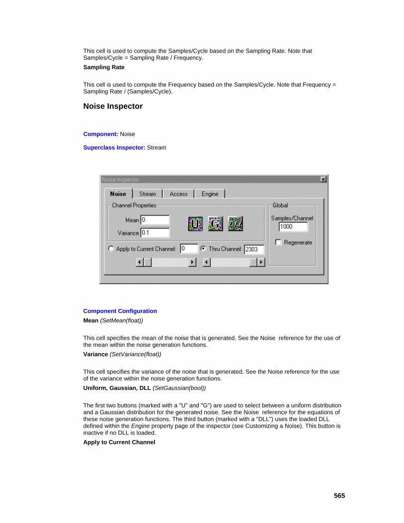
565

This cell is used to compute the Samples/Cycle based on the Sampling Rate. Note that Samples/Cycle = Sampling Rate / Frequency. Sampling Rate

This cell is used to compute the Frequency based on the Samples/Cycle. Note that Frequency = Sampling Rate / (Samples/Cycle).

Noise Inspector

Component: Noise

Superclass Inspector: Stream

Component Configuration Mean (SetMean(float))

This cell specifies the mean of the noise that is generated. See the Noise reference for the use of the mean within the noise generation functions. Variance (SetVariance(float))

This cell specifies the variance of the noise that is generated. See the Noise reference for the use of the variance within the noise generation functions. Uniform, Gaussian, DLL (SetGaussian(bool))

The first two buttons (marked with a "U" and "G") are used to select between a uniform distribution and a Gaussian distribution for the generated noise. See the Noise reference for the equations of these noise generation functions. The third button (marked with a "DLL") uses the loaded DLL defined within the Engine property page of the inspector (see Customizing a Noise). This button is inactive if no DLL is loaded. Apply to Current Channel

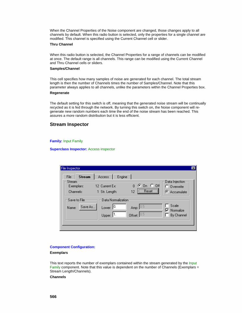
566

When the Channel Properties of the Noise component are changed, those changes apply to all channels by default. When this radio button is selected, only the properties for a single channel are modified. This channel is specified using the Current Channel cell or slider. Thru Channel

When this radio button is selected, the Channel Properties for a range of channels can be modified at once. The default range is all channels. This range can be modified using the Current Channel and Thru Channel cells or sliders. Samples/Channel

This cell specifies how many samples of noise are generated for each channel. The total stream length is then the number of Channels times the number of Samples/Channel. Note that this parameter always applies to all channels, unlike the parameters within the Channel Properties box. Regenerate

The default setting for this switch is off, meaning that the generated noise stream will be continually recycled as it is fed through the network. By turning this switch on, the Noise component will re-generate new random numbers each time the end of the noise stream has been reached. This assures a more random distribution but it is less efficient.

Stream Inspector



Component Configuration: Exemplars

This text reports the number of exemplars contained within the stream generated by the Input Family component. Note that this value is dependent on the number of Channels (Exemplars = Stream Length/Channels). Channels

567

This is the number of channels (i.e., PEs) reported by the component attached below. Current Exemplar

This text reports the exemplar that is to be read next from the stream. Note that for efficiency reasons, this display is only updated when the inspector is switched to this property page. Stream Length

This text reports the length of the stream (i.e., the number of floating point values) generated by the Input Family component. Reset

This button resets the stream to start reading from the beginning. Note that the stream is also reset every time the network is reset. On, Off (SetOn(bool))

These radio buttons are used to turn the stream on or off. This is useful for when you want to temporarily stop the data flow without having to remove the Input component. Overwrite / Accumulate (SetOverwrite(bool))

These radio buttons specify whether or not the stream data is to overwrite the data within the access point of the attached component. If not, the stream data is added to (i.e., accumulated with) the accessed data. This is useful for stacking several inputs onto one access point. Save As

This button displays a file selection panel, which is used to specify a file name for saving the stream in binary format. This is most useful for large ASCII files where the translation process may be very time consuming. Once the file is translated, the stream can be saved to a separate binary file and used in place of the ASCII file. Binary files are processed much more efficiently than ASCII files. Normalize

This switch is used to turn the data normalization on or off. When using a File component, the normalization coefficients (amplitude and offset) for each channel are contained within the specified Normalization File. By Channel

A series of numbers is normalized by first detecting the minimum and maximum values from the selected Data Sets. The resulting scale and offset is then applied to all data elements of the series. When this switch is turned on, each channel is an independent series with its own scaling and offset factor calculated from the channel’s minimum and maximum values. When this switch is turned off, the entire stream is the series and all numbers are normalized using the scaling and offset calculated from the stream’s minimum and maximum values. Note that this switch is only enabled when normalization is active and the Generate switch from the File Inspector is set (applies only to the File component). Lower, Upper

These cells define the upper and lower bounds of the normalization. Once the stream is normalized, all data elements from the selected Data Sets will fall within this range. Note that this switch is only enabled when the normalization is active and the Generate switch from the File Inspector is set (applies only to the File component). Scale

568

This switch is used to turn the data scaling on or off. The scaling is defined for the entire stream using the Amplitude and Offset cells (see below). Amplitude, Offset

These cells define the amplitude and offset of the scaling operation. When scaling is active, these cells are enabled so that the user can specify these parameters. When normalization is active, these cells cannot be modified. Instead, they report the offset and scaling that were applied to generate the normalized stream (unless the normalization is By Channel).

Access Inspector


Component Configuration: Available Access Points

569

The list on the left half of the inspector contains all available access points for the component attached below. The highlighted item is the access point that this component is currently attached to. To change the access point, simply single click on the item in the list. Rows

This cell contains the number of rows that is reported by the access point of the attached component. This value can only be modified from the inspector of that component. Cols

This cell contains the number of columns that is reported by the access point of the attached component. This value can only be modified from the inspector of that component. Auto Window

When this switch is set, the component’s display window automatically hides itself whenever the Access Data Set (see below) is not the Active Data Set (see Static Inspector). Access Data Set

Access components can display (and/or modify) the data of a single data set, "All" data sets, or the "Active" data set (specified from the Static Inspector). Normally the Probe components are configured to display the data for the active data set and the File components are configured to inject the data for all data sets. When a cross validation set is used, then an additional set of probe components can be added and configured to access only the cross validation data. ASCII

This option is only applicable to the Probe and File components that are included within a Code Generation User Interface project. For probes, this specifies that the data passed through this component is written to an ASCII file. For inputs, this specifies that the input data is read from an ASCII file. Note that this input file is automatically created by NeuroSolutions when the source code is generated. Binary

This option is only applicable to the Probe and Input components that are included within a Code Generation User Interface project. For probes, this specifies that the data passed through this component is written to a binary file. For inputs, this specifies that the input data is read from a binary file. Note that this input file is automatically created by NeuroSolutions when the source code is generated. Stdio

This option is only applicable to the Probe components that are included within a Code Generation User Interface project. This specifies that the data passed through this component is sent to the standard output, which is normally a DOS shell. Function

This option is only applicable to the Probe and Input components that are included within a Code Generation User Interface project. For probes, this specifies that its data is sent to a function instead of a file or the standard I/O. For each exemplar of output, a pointer to the output data is passed as a parameter within the function call. For inputs, this specifies that each exemplar of input data is retrieved by calling a function, instead of reading from a file. The implementation of the function computes and/or retrieves the data and stores it to the floating point array passed as a parameter.

This option applies only to the Probe and Input components that are included within a Code Generation User Interface project. For probes, this specifies that its data is sent to a function. For each exemplar of output, a pointer to the output data is passed as a parameter within the function call. For inputs, this specifies that each exemplar of input data is retrieved by calling a function. The

570

function computes and/or retrieves the data and stores it to the floating point array passed as a parameter. Generated Code Normalizes the Data

This option is only applicable to the Input components that are included within a Code Generation User Interface project. When this switch is set and "ASCII" is selected, the generated data file will not be normalized and the generated code will perform the normalization as the data is read. When this switch is set and "Function" is selected the data that is defined by the user-defined function will be normalized by the generated code after the function returns. Note that this switch is only enabled if the "Normalize" switch is turned on from the Stream Inspector and the Code Generation File Format is either "ASCII" or "Function". Normalize the Data File

This option is only applicable to the Input components that are included within a Code Generation User Interface project. This switch specifies that the generated file will contain normalized data. This is always true for "Binary" files, so this switch is only enabled for "ASCII" files. Note that the switch is only enabled if the "Normalize" switch is turned on from the Stream Inspector. Denormalize

This option is only applicable to the Probe components that are included within a Code Generation User Interface project. This switch specifies that the data passed through this component is denormalized before it is written to the file or sent to the function. Note that the "Denormalize from Normalization File" switch of the Probe Inspector must be on for this switch to be enabled.

Associate File

This panel is used to map a data file to one of the file translators provided and to select the data set that the data belongs to. Select a translator by single-clicking on an item within the Available Translators list and select the data set by single-clicking on an item within the Data Sets list.

571

Set as default for all files

When this button is set and the OK button is pressed, all input files with the same extension will use the selected translator for reading their data.

Set only for file

When this button is set and the OK button is pressed, only the selected file will use the selected translator for reading its data.

New

The default data sets are Testing, Training and Cross Validation. You may define your own data set by pressing this button and entering the data set name.

Translators:

ASCII Translator

Binary Translator

Bitmap Translator

Column-Formatted ASCII Translator

DLL Translator

572

See Also

Macro Actions

Access

Access Macro Actions Overview Superclass Macro Actions

Action Description accessDataSet Returns the "Access Data Set" setting. accessedComponent Returns name of the component whose data is being accessed. activeAccessPoint Returns the access point that the component is attached to. autoWindow Returns the "Auto-Window" setting. codeNormalizesData Returns the "Generated Code Normalizes the Data" setting for File components or the "Denormalize" setting for Probe components. flashFileMode Returns the "Code Generation File Format" setting (0=ASCII, 1=Binary, 2=Stdio, 3=Function). normalizeDataFile Returns the "Normalize the Data File" setting. setAccessDataSet Sets the "Access Data Set" setting. setActiveAccessPoint Sets the access point that the component is attached to. setAutoWindow Sets the "Auto-Window" setting. setCodeNormalizesData Sets the "Generated Code Normalizes the Data" setting for File components or the "Denormalize" setting for Probe components. setFlashFileMode Sets the "Code Generation File Format" setting (0=ASCII, 1=Binary, 2=Stdio, 3=Function). setNormalizeDataFile Sets the "Normalize the Data File" setting.

accessDataSet Overview Macro Actions

Syntax

componentName. accessDataSet()

Parameters Type Description return string The name of the data set to display and/or modify, or "All" for all data sets (see "Access Data Set" within the Access Inspector).

573


accessedComponent Overview Macro Actions

Syntax

componentName. accessedComponent()

Parameters Type Description return string The name of the component whose data is being accessed. componentName Name defined on the engine property page.

activeAccessPoint Overview Macro Actions

Syntax

componentName. activeAccessPoint()

Parameters Type Description return string The access point that the component is attached to (see "Available Access Points" within the Access Inspector). componentName Name defined on the engine property page.

autoWindow Overview Macro Actions

Syntax

componentName. autoWindow()

Parameters Type Description return BOOL When TRUE, the component’s display window automatically hides itself whenever the accessDataSet is not the active data set (see "Auto Window" within the Access Inspector). componentName Name defined on the engine property page.

codeNormalizesData Overview Macro Actions

Syntax

componentName. codeNormalizesData()

574

Parameters Type Description return BOOL When TRUE and the component is a File, the generated data file will not be normalized and the generated code will perform the normalization as the data is read (see "Generated Code Normalizes the Data" within the Access Inspector). When TRUE and the component is a Probe, the data passed through the access point is denormalized before it is written to the file or sent to the function (see "Denormalize" within the Access Inspector). componentName Name defined on the engine property page.

flashFileMode Overview Macro Actions

Syntax

componentName. flashFileMode()

Parameters Type Description return int The file format that is used by the generated code when writing/reading the data (0=ASCII, 1=Binary, 2=Stdio, 3=Function -- see "Binary", "ASCII", "Stdio", and "Function" within the Access Inspector). componentName Name defined on the engine property page.

normalizeDataFile Overview Macro Actions

Syntax

componentName. normalizeDataFile()

Parameters Type Description return BOOL When TRUE, the generated file will contain normalized data (see "Normalize the Data File" within the Access Inspector). componentName Name defined on the engine property page.

setAccessDataSet Overview Macro Actions

Syntax

componentName. setAccessDataSet(accessDataSet)

Parameters Type Description return void componentName Name defined on the engine property page. accessDataSet string The name of the data set to display and/or modify, or "All" for all data

575

sets (see "Access Data Set" within the Access Inspector).

setActiveAccessPoint Overview Macro Actions

Syntax

componentName. setActiveAccessPoint(activeAccessPoint)

Parameters Type Description return void componentName Name defined on the engine property page. activeAccessPoint string The access point that the component is attached to (see "Available Access Points" within the Access Inspector).

setAutoWindow Overview Macro Actions

Syntax

componentName. setAutoWindow(autoWindow)

Parameters Type Description return void componentName Name defined on the engine property page. autoWindow BOOL When TRUE, the component’s display window automatically hides itself whenever the accessDataSet is not the active data set (see "Auto Window" within the Access Inspector).

setCodeNormalizesData Overview Macro Actions

Syntax

componentName. setCodeNormalizesData(normalize)

Parameters Type Description return void componentName Name defined on the engine property page. normalize BOOL When TRUE and the component is a File, the generated data file will not be normalized and the generated code will perform the normalization as the data is read (see "Generated Code Normalizes the Data" within the Access Inspector). When TRUE and the component is a Probe, the data passed through the access point is denormalized before it is written to the file or sent to the function (see "Denormalize" within the Access Inspector).

576

setFlashFileMode Overview Macro Actions

Syntax

componentName. setFlashFileMode(flashFileMode)

Parameters Type Description return void componentName Name defined on the engine property page. flashFileMode int The file format that is used by the generated code when writing/reading the data (0=ASCII, 1=Binary, 2=Stdio, 3=Function -- see "Binary", "ASCII", "Stdio", and "Function" within the Access Inspector).

setNormalizeDataFile Overview Macro Actions

Syntax

componentName. setNormalizeDataFile(normalize)

Parameters Type Description return void componentName Name defined on the engine property page. normalize BOOL When TRUE, the generated file will contain normalized data (see "Normalize the Data File" within the Access Inspector).

Function

Function Macro Actions Overview Superclass Macro Actions

Action Description amplitude Returns the "Amplitude" parameter. offset Returns the "Offset" parameter. phaseShift Returns the "Phase" parameter. setAmplitude Sets the "Amplitude" parameter. setOffset Sets the "Offset" parameter.

577

setPhaseShift Sets the "Phase" parameter.

amplitude Overview Macro Actions

Syntax

componentName. amplitude()

Parameters Type Description return float The amplitude of the generated signal (see "Amplitude Form Cell" within the Function Inspector). componentName Name defined on the engine property page.


Syntax

componentName. offset()

Parameters Type Description return float The offset of the generated signal (see "Offset" within the Function Inspector). componentName Name defined on the engine property page.

phaseShift Overview Macro Actions

Syntax

componentName. phaseShift()

Parameters Type Description return float The phase shift (in degrees) of the generated signal (see "Phase" within the Function Inspector). componentName Name defined on the engine property page.

setAmplitude Overview Macro Actions

Syntax

578

componentName. setAmplitude(amplitude)

Parameters Type Description return void componentName Name defined on the engine property page. amplitude float The amplitude of the generated signal (see "Amplitude Form Cell" within the Function Inspector).


Syntax

componentName. setOffset(offset)

Parameters Type Description return void componentName Name defined on the engine property page. offset float The offset of the generated signal (see "Offset" within the Function Inspector).

setPhaseShift Overview Macro Actions

Syntax

componentName. setPhaseShift(phaseShift)

Parameters Type Description return void componentName Name defined on the engine property page. phaseShift float The phase shift (in degrees) of the generated signal (see "Phase" within the Function Inspector).

Noise

Noise Macro Actions Overview Superclass Macro Actions

Action Description mean Returns the "Mean" parameter. regenerateData Returns the "Regenerate" setting.

579

setMean Sets the "Mean" parameter. setRegenerateData Sets the "Regenerate" setting. setVariance Sets the "Variance" parameter. variance Returns the "Variance" parameter.

mean Overview Macro Actions

Syntax

componentName. mean()

Parameters Type Description return float The mean of the noise that is generated (see "Mean" within the Noise Inspector). componentName Name defined on the engine property page.

regenerateData Overview Macro Actions

Syntax

componentName. regenerateData()

Parameters Type Description return BOOL TRUE will re-generate random numbers at the end of each noise stream (see "Regenerate" within the Noise Inspector). componentName Name defined on the engine property page.

setMean Overview Macro Actions

Syntax

componentName. setMean(mean)

Parameters Type Description return void componentName Name defined on the engine property page. mean float The mean of the noise that is generated (see "Mean" within the Noise Inspector).

580

setRegenerateData Overview Macro Actions

Syntax

componentName. setRegenerateData(regenerateData)

Parameters Type Description return void componentName Name defined on the engine property page. regenerateData BOOL TRUE will re-generate random numbers at the end of each noise stream (see "Regenerate" within the Noise Inspector).

setVariance Overview Macro Actions

Syntax

componentName. setVariance(variance)

Parameters Type Description return void componentName Name defined on the engine property page. variance float The variance of the noise that is generated (see "Variance" within the Noise Inspector).

variance Overview Macro Actions

Syntax

componentName. variance()

Parameters Type Description return float The variance of the noise that is generated (see "Variance" within the Noise Inspector). componentName Name defined on the engine property page.

Multi Channel Stream

MultiChannelStream Macro Actions Overview Superclass Macro Actions

Action Description

581

activeChannel Returns the "Current Channel" parameter. amplitudeForChannel Returns the normalization amplitude for the specified channel. broadcast Returns TRUE if the "Thru Channel" radio button is set and FALSE if the "Apply to Current Channel" radio button is set. channels Returns the number of data channels. dataSource Returns the name of the data source for the active channel ("NGaussianNoise", "NUniformNoise", "NDLLNoise", "NSinWaveFunction", "NSquareWaveFunction", "NTriangleWaveFunction", "NSawtoothFunction", "NImpulseFunction", or "NDLLFunction"). endChannel Returns the "Thru Channel" parameter. incrementActiveChannel Increments the "Current Channel" parameter by the specified amount. incrementEndChannel Increments the "Thru Channel" parameter by the specified amount. inject Returns TRUE if the data injection is set to "Accumulate" and FALSE if it is set to "Overwrite". lowerBound Returns the "Lower" bound parameter of the data normalization. networkReset Resets the IO stream. normalize Returns the "Normalize" setting. normalizeByChannel Returns the "By Channel" setting. offsetForChannel Returns the normalization offset for the specified channel. resetAll Resets all input components on the breadboard. samples Returns the number of "Samples/Channel" (Noise) or the "Samples/Cycle" (Function). saveStream Saves the stream as a binary to file to specified path. scale Returns the "Scale" setting. setActiveChannel Sets the "Current Channel" parameter. setAmplitude Sets the "Amplitude" setting for the active channel. setBroadcast Set to TRUE to set the "Thru Channel" radio button and FALSE to set the "Apply to Current Channel" radio button. setDataSource Sets the name of the data source for the active channel ("NGaussianNoise", "NUniformNoise", "NDLLNoise", "NSinWaveFunction", "NSquareWaveFunction", "NTriangleWaveFunction", "NSawtoothFunction", "NImpulseFunction", or "NDLLFunction").

582

setEndChannel Sets the "Thru Channel" parameter. setInject Set to TRUE for the data injection to be set to "Accumulate" and FALSE if it is to be set to "Overwrite". setLowerBound Sets the "Lower" bound parameter of the data normalization. setNormalize Sets the "Normalize" setting. setNormalizeByChannel Sets the "By Channel" setting. setOffset Sets the "Offset" setting for the active channel. setSamples Sets the number of "Samples/Channel" (Noise) or the "Samples/Cycle" (Function). setScale Sets the "Scale" setting. setStreamOn TRUE sets the stream "On" and FALSE sets the stream "Off". setUpperBound Sets the "Upper" bound parameter of the data normalization. streamOn Returns TRUE if the stream is "On" and FALSE if the stream is "Off". upperBound Returns the "Upper" bound parameter of the data normalization.

activeChannel Overview Macro Actions

Syntax

componentName. activeChannel()

Parameters Type Description return int The first channel of the specified range used to change the channel parameters (see "Apply to Current Channel" within the Function Inspector or Noise Inspector). componentName Name defined on the engine property page.

amplitudeForChannel Overview Macro Actions

Syntax

componentName. amplitudeForChannel(index)

Parameters Type Description return float The normalization amplitude (stored in the Normalization File) for the specified channel, or the amplitude of the scaling operation (see "Amplitude/Offset" within the Stream

583

Inspector ). componentName Name defined on the engine property page. index int The channel index (0 <= index < channels).

broadcast Overview Macro Actions

Syntax

componentName. broadcast()

Parameters Type Description return BOOL TRUE if the changes to the channel setting are made to a block of channels and FALSE if they are only to be made to the active channel (see "Apply to Current Channel" and "Thru Channel" within the Function Inspector or Noise Inspector). componentName Name defined on the engine property page.

channels Overview Macro Actions

Syntax

componentName. channels()

Parameters Type Description return int The number of data channels. componentName Name defined on the engine property page.

dataSource Overview Macro Actions

Syntax

componentName. dataSource()

Parameters Type Description return string The name of the data source for the active channel ("NGaussianNoise", "NUniformNoise", "NDLLNoise", "NSinWaveFunction", "NSquareWaveFunction", "NTriangleWaveFunction", "NSawtoothFunction", "NImpulseFunction", or "NDLLFunction" – see the function/noise buttons within the Function Inspector or Noise Inspector). componentName Name defined on the engine property page.

584

endChannel Overview Macro Actions

Syntax

componentName. endChannel()

Parameters Type Description return int The last channel of the specified range used to change the channel parameters (see "Apply to Current Channel" within the Function Inspector or Noise Inspector). componentName Name defined on the engine property page.

incrementActiveChannel Overview Macro Actions

Syntax

componentName. incrementActiveChannel(increment)

Parameters Type Description return void componentName Name defined on the engine property page. increment int The amount to increment the activeChannel by.

incrementEndChannel Overview Macro Actions

Syntax

componentName. incrementEndChannel(increment)

Parameters Type Description return void componentName Name defined on the engine property page. increment int The amount to increment the endChannel by.

inject Overview Macro Actions

Syntax

componentName. inject()

585

Parameters Type Description return BOOL TRUE to accumulate the injected data on the stream and FALSE to overwrite it (see "Overwrite" and "Accumulate" within the Stream Inspector ). componentName Name defined on the engine property page.

lowerBound Overview Macro Actions

Syntax

componentName. lowerBound()

Parameters Type Description return float The lower bound of the normalization calculation (see "Lower" within the Stream Inspector ). componentName Name defined on the engine property page.

networkReset Overview Macro Actions

Syntax

componentName. networkReset()


normalize Overview Macro Actions

Syntax

componentName. normalize()

Parameters Type Description return BOOL TRUE if normalization is active (see "Normalize" within the Stream Inspector ). componentName Name defined on the engine property page.

normalizeByChannel Overview Macro Actions

586

Syntax

componentName. normalizeByChannel()

Parameters Type Description return BOOL TRUE if the normalization is calculated for each individual channel and FALSE if it is calculated across all channels (see "By Channel" within the Stream Inspector ). componentName Name defined on the engine property page.

offsetForChannel Overview Macro Actions

Syntax

componentName. offsetForChannel(index)

Parameters Type Description return int The normalization offset (stored in the Normalization File) for the specified channel, or the offset of the scaling operation (see "Amplitude/Offset" within the Stream Inspector ). componentName Name defined on the engine property page.

index int The channel index (0 <= index < channels).

resetAll Overview Macro Actions

Syntax

componentName. resetAll()


samples Overview Macro Actions

Syntax

componentName. samples()

Parameters Type Description return int The number of samples that defines the Function or Noise component (see

587

"Samples/Channel" within the Noise Inspector or "Samples/Cycle" within the Function Inspector). componentName Name defined on the engine property page.

saveStream Overview Macro Actions

Syntax

componentName. saveStream(path)


path string The full path of the file to save the binary stream to.

scale Overview Macro Actions

Syntax

componentName. scale()

Parameters Type Description return BOOL TRUE if scaling is active (see "Scale" within the Stream Inspector ). componentName Name defined on the engine property page.

setActiveChannel Overview Macro Actions

Syntax

componentName. setActiveChannel(activeChannel)

Parameters Type Description return void componentName Name defined on the engine property page. activeChannel int The first channel of the specified range used to change the channel parameters (see "Apply to Current Channel" within the Function Inspector or Noise Inspector).

588


Syntax

componentName. setAmplitude(amplitude)

Parameters Type Description return void componentName Name defined on the engine property page. amplitude float The amplitude of the scaling operation (see "Amplitude/Offset" within the Stream Inspector ).

setBroadcast Overview Macro Actions

Syntax

componentName. setBroadcast(broadcast)

Parameters Type Description return void componentName Name defined on the engine property page. broadcast BOOL TRUE if the changes to the channel setting are made to a block of channels and FALSE if they are only to be made to the active channel (see "Apply to Current Channel" and "Thru Channel" within the Function Inspector or Noise Inspector).

setDataSource Overview Macro Actions

Syntax

componentName. setDataSource(dataSource)

Parameters Type Description return void componentName Name defined on the engine property page. dataSource string The name of the data source for the active channel ("NGaussianNoise", "NUniformNoise", "NDLLNoise", "NSinWaveFunction", "NSquareWaveFunction", "NTriangleWaveFunction", "NSawtoothFunction", "NImpulseFunction", or "NDLLFunction" – see the function/noise buttons within the Function Inspector or Noise Inspector).

setEndChannel Overview Macro Actions

589

Syntax

componentName. setEndChannel(endChannel)

Parameters Type Description return void componentName Name defined on the engine property page. endChannel int The last channel of the specified range used to change the channel parameters (see "Apply to Current Channel" within the Function Inspector or Noise Inspector).

setInject Overview Macro Actions

Syntax

componentName. setInject(inject)

Parameters Type Description return void componentName Name defined on the engine property page. inject BOOL TRUE to accumulate the injected data on the stream and FALSE to overwrite it (see "Overwrite" and "Accumulate" within the Stream Inspector ).

setLowerBound Overview Macro Actions

Syntax

componentName. setLowerBound(lowerBound)

Parameters Type Description return void componentName Name defined on the engine property page. lowerBound float The lower bound of the normalization calculation (see "Lower" within the Stream Inspector ).

setNormalize Overview Macro Actions

Syntax

componentName. setNormalize(normalize)


590

return void componentName Name defined on the engine property page. normalize BOOL TRUE if normalization is active (see "Normalize" within the Stream Inspector ).

setNormalizeByChannel Overview Macro Actions

Syntax

componentName. setNormalizeByChannel(normalizeByChannel)

Parameters Type Description return void componentName Name defined on the engine property page. normalizeByChannel BOOL TRUE if the normalization is calculated for each individual channel and FALSE if it is calculated across all channels (see "By Channel" within the Stream Inspector ).


Syntax

componentName. setOffset(offset)

Parameters Type Description return void componentName Name defined on the engine property page. offset float The offset of the scaling operation (see "Amplitude/Offset" within the Stream Inspector ).

setSamples Overview Macro Actions

Syntax

componentName. setSamples(samples)


591

samples int The number of samples that defines the Function or Noise component (see "Samples/Channel" within the Noise Inspector or "Samples/Cycle" within the Function Inspector).

setScale Overview Macro Actions

Syntax

componentName. setScale(scale)

Parameters Type Description return void componentName Name defined on the engine property page. scale BOOL TRUE if scaling is active (see "Scale" within the Stream Inspector ).

setStreamOn Overview Macro Actions

Syntax

componentName. setStreamOn(streamOn)

Parameters Type Description return void componentName Name defined on the engine property page. streamOn BOOL TRUE if the stream is turned on (see "On, Off" within the Stream Inspector ).

setUpperBound Overview Macro Actions

Syntax

componentName. setUpperBound(upperBound)

Parameters Type Description return void componentName Name defined on the engine property page. upperBound float The upper bound of the normalization calculation (see "Upper" within the Stream Inspector ).

592

streamOn Overview Macro Actions

Syntax

componentName. streamOn()

Parameters Type Description return BOOL TRUE if the stream is turned on (see "On, Off" within the Stream Inspector ). componentName Name defined on the engine property page.

upperBound Overview Macro Actions

Syntax

componentName. upperBound()

Parameters Type Description return float The upper bound of the normalization calculation (see "Upper" within the Stream Inspector ). componentName Name defined on the engine property page.

OLE Input

OLEInput Macro Actions Overview Superclass Macro Actions

Action Description setEngineData Sets the input data to be injected into the network. setNormalizationFilePath Sets the path of the file containing the normalization coeffiecients.


Syntax



593

data variant An array of single-precision floating point values that contains the input data to be injected into the network.


Syntax

componentName.setNormalizationFilePath(normalizationFilePath)

Parameters Type Description return void componentName Name defined on the engine property page. normalizationFilePath string The path of the file containing the normalization coeffiecients. Once this function is called with a valid normalization file the component is automatically configured to normalize the incoming data before injecting it into the network. If this function is not called then the data is not altered before being injected.

Probe Family StaticProbe Family

StaticProbe Family

Ancestor: Probe Family

The StaticProbe family is a collection of components that are used to observe instantaneous data at the various access points of the components.

Members:

BarChart

DataGraph

DataWriter

DataStorage

DLLPostprocessor

Hinton

ImageViewer

MatrixEditor

594

MatrixViewer

BarChart

Family: StaticProbe Family

Superclass: NSProbe

Description:

The BarChart probe creates a view for observing numeric data as a series of horizontal bars. The length of the bars is proportional to the magnitude of the data being probed. The scale used to display the bars may be changed manually, or automatically. Each bar can be labeled for clarity.

BarCharts are useful for classification problems that have a reasonably small (less than 25) number of outputs. By attaching one to the system output and another to the desired output, one can compare the longest bar of the two probes to see if they match for each exemplar.

Every time that data passes through the component attached below, the BarChart can refresh its display to reflect this data. This can consume a large percentage of the processing cycles used for the simulation. For this reason, there is a parameter used to specify how often the display is refreshed.

User Interaction:

Drag and Drop

Inspector

Window

Access Points

DLL Implementation

Macro Actions

See Also

DataGraph

595


Superclass: NSProbe

Description:

The DataGraph displays temporal data as a set of signal traces -- values (vertical axis) over time (horizontal axis). It is similar in functionality to the MegaScope, except it is much easier to use and includes labels on the X and Y axes so that you can get a better quantitative perspective on the probed data. It is important to note that even though this displays temporal data, it is still a static probe, meaning that it does not need to be stacked on top of a DataStorage component.

User Interaction:

Drag and Drop

Inspector

Window

Access Points

DLL Implementation

DataWriter


Superclass: NSProbe

Description:

The DataWriter provides a means to collect static data from network components during the simulations. This component displays the data using an editable window. Moreover, this data may then be edited and/or saved into ASCII or binary file. The DataWriter is useful in situations where one wants to save simulation data for further analysis or for report generation (by cutting and pasting in other documents).

Data can be written to a file using the DataWriter in one of two ways. The first approach is to specify the file name and type (ASCII or binary) before the simulation is run. As data is fired

596

through the access point of the component attached below, it is simultaneously written to the specified file. Note that the display window does not need to be opened for the data to be collected.

The second approach is to first run the simulation with the display window open. This text window displays the data as it is being fired through the attached component. Once the simulation is complete, the contents of the display window can be edited (if needed), then the file name is specified and window’s text is saved in ASCII format.

Note that there is a limit to the amount of data that can be stored within the display window, thus limiting the size of file that can be generated by this second approach. The size of the file generated by the first approach is limited only by the amount of available disk space on the computer system.

User Interaction:

Drag and Drop

Inspector

Window

Access Points

DLL Implementation

Macro Actions

DataStorage


Superclass: NSProbe

Description:

Data flows through network simulations one sample at a time. Several probes display a sequence of data samples over time. Rather than requiring each of these TemporalProbes to store and maintain data, the DataStorage component was developed.

The DataStorage component collects data from an access point of the component attached below and stores it in a circular buffer. A circular buffer of size n stores the most recent n samples of data. The size of the buffer is user-defined. This buffer is accessible to members of the TemporalProbe family by means of the Buffered Activity access point. A TemporalProbe uses this buffer to display the data over time.

597

The DataStorage component periodically sends a message to the components stacked above so that they can re-process the data or refresh their displays. How often this message is sent is specified within the DataStorage component. Note that if this message is sent too often, then the attached probes will consume a high percentage of the processing cycles of the simulation.

User Interaction:

Drag and Drop

Inspector

Access Points

DLL Implementation

Macro Actions

See Also

Hinton


Superclass: NSProbe

Description:

The Hinton probe creates a view for observing numeric data as a matrix of squares. The size of the squares is proportional to the magnitude (the absolute value) of the data being probed. Positive values are displayed as solid squares while negative values are displayed as outlined squares. The scale used to display the squares may be changed manually, or automatically.

This probe is often used to display a weight matrix. Its design makes it easy to detect patterns and symmetries in the data.

User Interaction:

Drag and Drop

Inspector

Window

Access Points

598

DLL Implementation

See Also

ImageViewer


Superclass: NSProbe

Description:

The ImageViewer component provides the ability to display static data reported by a network component as a 256-level gray-scale image. The dimensions of the component attached below dictate the dimensions of the image. The range of floating-point values within the probed data can be specified or automatically computed. The data is normalized based on this range and used to compute the intensity levels of the individual pixels.

An image shown in the display window can be saved as a bitmap (.bmp) file.

User Interaction:

Drag and Drop

Inspector

Window

Access Points

DLL Implementation

Macro Actions

MatrixEditor

599


Superclass: NSProbe

Description:

The MatrixEditor is similar to the MatrixViewer in that it can be used to observe static data as a numerical matrix. However, this component also allows the user to modify the data at the attached access point. Any modifications will be reflected in the simulation.

There are two consequences to this ability. First, the MatrixEditor slows down the simulations because it allows for user input. The MatrixViewer should be used for cases when the data only needs to be observed and not modified. Second, this probe allows for direct user interaction with the network simulations at any stage. This concept is very powerful, but can also be dangerous if unintended changes are made. Caution is recommended when using this probe, since it has the ability to overwrite previous values.

User Interaction:

Drag and Drop

Inspector

Window

Access Points

DLL Implementation

See Also

MatrixViewer


Superclass: NSProbe

Description:

The MatrixViewer is used to observe instantaneous data as a numerical matrix. The dimensions of matrix is dictated by the dimensions of the component stacked below. The data may not be manipulated in any way. If editing is desired, the MatrixEditor should be used. Note that the

600

MatrixViewer does not slow down the simulations as much as the MatrixEditor, since it only displays the data.

User Interaction:

Drag and Drop

Inspector

Window

Access Points

DLL Implementation

See Also

DLLPostprocessor


Superclass: NSProbe

Description:

The DLLPostprocessor component is used to process the data sent from the component stacked below, and send the processed data to the component attached above using the Postprocessor access point. This is a static probe, meaning that it processes the data of the attached component one sample at a time. It is implemented using DLLs, thus requiring that a DLL be loaded within the Engine Inspector property page of the DLLPostprocessor inspector.

User Interaction:

Drag and Drop

Access Points

DLL Implementation

601

Access Points

DataStorage Access Points

Component: DataStorage

Superclass: Probe

Buffered Activity Access:

This is an access point which is created by the DataStorage class which allow Temporal Probes to display a block of data. This block of data is collected and stored in a circular buffer for each iteration of the simulation. The user defines the size of this buffer. The buffer can be multi-channel depending upon the number of processing elements of the network component.

See Also

Postprocessor Access Points


Superclass Access Points: Access Points

Postprocessor Output:

Members of the Access family that are stacked on a postprocessor component will report a Postprocessor Output access point. A component attached to this access point retrieves processed data from a postprocessor component attached to the network.

See Also

DLL Implementation

Static Probe DLL Implementation

Component: StaticProbe Family

Protocol: PerformOutput

Description:

602

The static probes are used to display instantaneous network data. DLLs can be used with these components to implement customized display routines or to send the output data to other processes/applications.

Each call to performOutput contains the next exemplar of data accessed by the probe. The default implementation of this DLL simply copies each element of the data buffer to the local variable myOutput. The return value of TRUE indicates that the display of the base probe component should remain active.

Code: performOutput( DLLData *instance, // Pointer to instance data (may be NULL) NSFloat *data, // Pointer to the data int rows, // Number of rows of data int cols // Number of cols of data ) { int i,j; NSFloat myOutput; for (i=0; i<rows; i++) for (j=0; j<cols; j++) myOutput = data(i,j); // You define your own output source. // Return whether or not the output component should still work return TRUE; }

Drag and Drop

Static Probe Family Drag and Drop

The Static Probe Family was designed to examine instantaneous data that are presented by network components. Hence, any network component that has an instantaneous access point accepts a probe from the Static Probe family. Members of this family can be dropped on any of these components.

See Also

Inspectors

BarChart Inspector

Component: BarChart

Superclass Inspector: Label Inspector

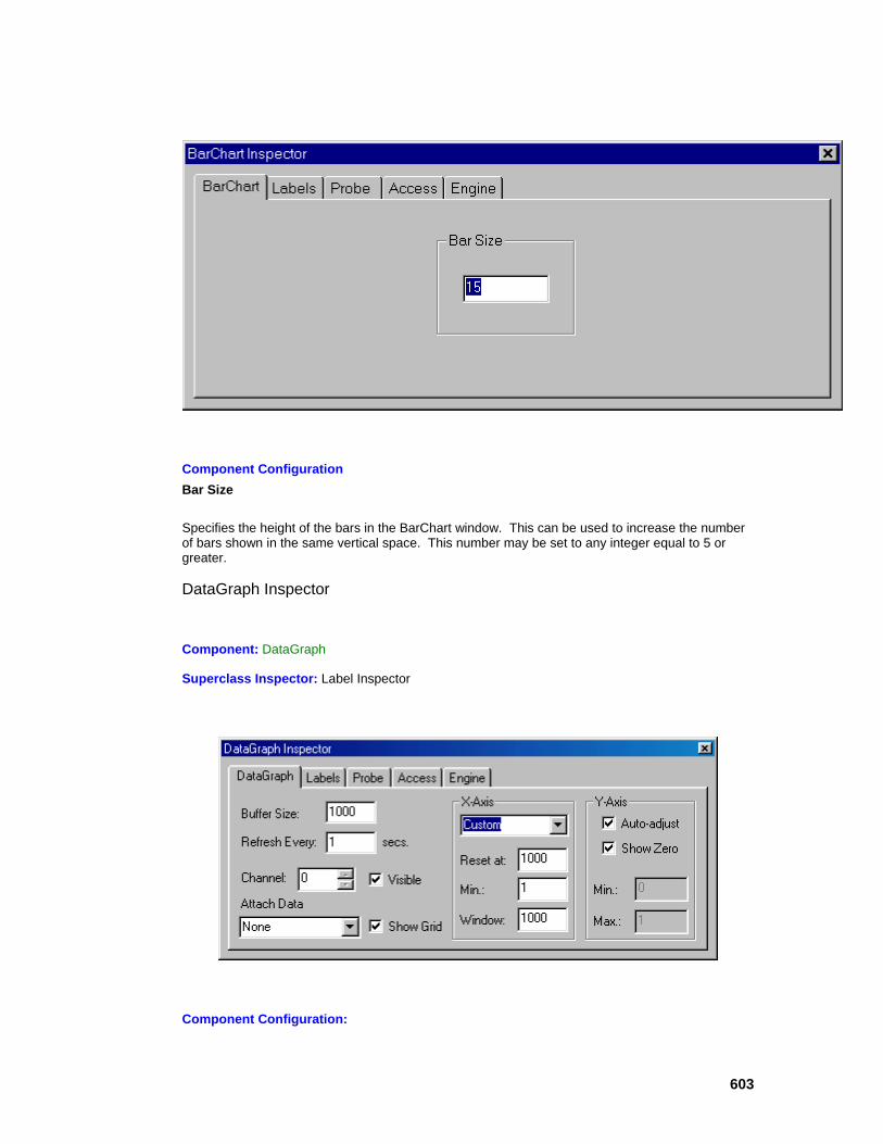
603

Component Configuration Bar Size

Specifies the height of the bars in the BarChart window. This can be used to increase the number of bars shown in the same vertical space. This number may be set to any integer equal to 5 or greater.

DataGraph Inspector

Component: DataGraph



604

Buffer Size

The buffer size form cell sets the size of a circular buffer where samples of data are stored over time to be displayed in the window. While there is no limit to the size of this buffer, be aware that memory will be allocated from the system to store the data. This number can be any integer greater than one. Note that when the X-axis is set to "Epochs", "Exemplars" or "Samples", this cell is grayed out and the value is set automatically based on the size of the data set or the settings of the controller. Refresh Every

Specifies how often to update the display with the latest data. Channel Visible

All channels of data are displayed by default. To remove a channel from the display, select the channel number in the edit cell and uncheck the Visible switch. Attach Data

This pull down menu contains a list of the other Label probes on the breadboard. When one of these probes is selected, the data from that probe is displayed in the DataGraph window along with the data probed directly by the DataGraph. This is useful for displaying the network output and the desired output in the same graph. Show Grid

Displays horizontal and vertical gridlines on the graph. X-Axis

There are several options available for specifying the X-axis of the graph:

Epochs – This is commonly used for probing the error curve, in which the X-axis corresponds to the epoch number. When this option is selected the Buffer Size is automatically set to the maximum number of epochs specified within the StaticControl inspector.

Exemplars – This is commonly used for probing the output, in which the X-axis corresponds to the exemplar number of the current epoch. When this option is selected the Buffer Size is automatically set to the number of exemplars per epoch shown within the StaticControl inspector.

Samples – This is commonly used for dynamic networks, in which there are multiple samples per exemplar. The X-axis corresponds to the sample number of the current epoch. When this option is selected the Buffer Size is automatically set to the number of samples per exemplar times the number of exemplars per epoch specified within the StaticControl inspector and the DynamicControl inspector.

Generations – This is commonly used for probing the error curve during a genetic training run, in which the X-axis corresponds to the generation number. When this option is selected the Buffer Size must be specified manually.

Custom – This is commonly used for probing the cross validation set. The X-axis is an internal counter that is not tied to a counter on the controller. When this option is selected the Buffer Size must be specified manually.

Reset At

This option is only applicable when using a Custom X-axis. When the X-axis counter reaches the value specified in this cell, then the counter is reset to 1. Minimum X

Specifies the left-most data point on the graph. This value can also be set using the zoom feature of the DataGraph window. Window

605

Specifies the window size, or the number of data points to display on the graph beginning with the Minimum. This value can also be set using the zoom feature of the DataGraph window. Auto-adjust

This option automatically adjusts the scale of the Y-axis to fit the data being probed. Show Zero

When the auto-adjust is active, this option specifies that 0 always be included in the Y-axis even if it is not part of the displayed data. Minimum Y

Specifies the bottom of the Y-axis. This parameter is only available when the Auto-adjust switch is turned off. Maximum Y

Specifies the top of the Y-axis. This parameter is only available when the Auto-adjust switch is turned off.

DataWriter Inspector

Component: DataWriter


Component Configuration: Clear Contents

Clears the present edit buffer contents. Clear Before Run

606

Specifies whether or not the edit buffer is cleared each time a network simulation is run. Input Enabled

Enables/disables the writing of the accessed data to the edit buffer. Buffer Size

Sets the maximum number of data points that can be stored in the edit window at any given time. Note that the display window will simply ignore the new data once the buffer is full. Font Size

Sets the point size of the font used in the edit window. Scientific Notation

Displays and outputs the data using scientific notation. Transpose Matrix

Most Axons are configured to be a one-dimensional vector with N rows and 1 column. However, you will most often want to display each exemplar of data as a single row, so that each PE is represented by a column of values. Setting this switch transposes the display matrix for this purpose. Save Text to File

Opens a Save panel to select a file name. Once a name is selected, the ASCII text contained within the data buffer is written to this file. Dump Raw Data to File

Opens a Save panel to select a file name. Once the name is selected and the switch is set, all data that passes through the attached access point is written to this file. This file may be of type ASCII or binary. Set

Opens a Save panel to change the file used to store the probed data. ASCII

Set the output file to be of type ASCII. Binary

Set the output file to be of type binary. Attach Data From

When a probe component name is selected from this combo-box, the data from that component is appended to the data from the DataWriter. This is normally used to display/write the output of the network side-by-side with the desired output. There are three requirements for activating this combo-box: 1) the DataWriter must be accessing the Desired Signal of an ErrorCriterion component, 2) the number of columns of the ErrorCriterion must be equal to 1, and 3) the "Transpose Matrix" option must be selected (see above).

DataStorage Inspector

607

Component: DataStorage

Superclass Inspector: Probe inspector

Component Configuration: Buffer Size

The buffer size form cell sets the size of a circular buffer where samples of data are stored for other components to examine. While there is no limit to the size of this buffer, be aware that memory will be allocated from the system to store the data. This number can be any integer greater than zero. Message Every

The data storage class will send a message to all probes that are attached to it's Temporal Access point telling them that the data samples contained in the DataStorage are available. The periodicity of this message is controlled by the number entered in the Message Every form cell. Setting this value is very important for creating "animations" of the data as it changes. This value will make attached probes respond to the changes in the data only as often as desired. Since the probes tend to slow the computational process, it is helpful to increase the value of Message Every so that the probes respond less frequently. It accepts any integer greater than or equal to one.

Hinton Inspector

Component: Hinton


608

Component Configuration: Square Size

Specifies the maximum size of the squares in the Hinton window. This can be used to increase the number of squares shown in the same space. This number may be set to any integer equal to 5 or greater.

ImageViewer Inspector

Component: ImageViewer


Component Configuration: TotalPixels

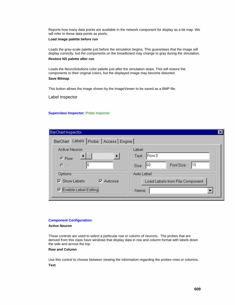
609

Reports how many data points are available in the network component for display as a bit map. We will refer to these data points as pixels. Load image palette before run

Loads the gray-scale palette just before the simulation begins. This guarantees that the image will display correctly, but the components on the breadboard may change to gray during the simulation. Restore NS palette after run

Loads the NeuroSolutions color palette just after the simulation stops. This will restore the components to their original colors, but the displayed image may become distorted. Save Bitmap

This button allows the image shown by the ImageViewer to be saved as a BMP file.

Label Inspector


Component Configuration: Active Neuron

These controls are used to select a particular row or column of neurons. The probes that are derived from this class have windows that display data in row and column format with labels down the side and across the top. Row and Column

Use this control to choose between viewing the information regarding the probes rows or columns. Text

610

Displays the label that corresponds to the Active Neuron. The Active Neuron is set using the Active Neuron slider/field and the Row and Column radio buttons as described above. The labels may only be changed if the Enable Label Editing switch is set. Show Labels

This switch enables the user to view, or remove, the labels in the probe window.

Enable Label Editing

This switch determines if user definable labels should be used in place of the computer generated ones. Be careful when using this feature on probe windows that are displaying very large amounts of data. When this switch is enabled, memory is allocated for each row and column showing in the probe window. Autosizing

This switch controls the autosizing feature of the probes that are derived from this class. By changing the size of the probes window, the maximum number of rows and columns can more easily be displayed. This window will change size whenever the number of neurons being probed changes. Label Size

This form cell determines how much space should be allocated for the row labels. Choosing this number too small could place the probes main view over the labels, making them impossible to read. This number is in pixels and can be any positive integer. Font Size

This control allows the user to change the font size of the labels. Sometimes the font size of the data shown in the probe window of this class can be changed as well. Load Labels from File Component

This button will load the column headings from the selected File component into the label cells of the probe. Note that the Enable Label Editing switch must be switched on to enable this button. Name

Selects the name of the File component that contains the column headings corresponding to the probed data. Note that the File must use the Column-Formatted ASCII Translator in order to extract the column headings.

Windows

BarChart Window

Component: BarChart

Superclass: TemporalProbe

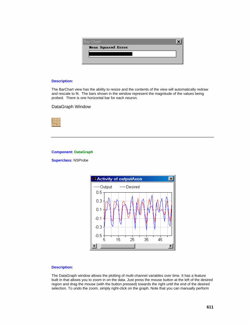
611

Description:

The BarChart view has the ability to resize and the contents of the view will automatically redraw and rescale to fit. The bars shown in the window represent the magnitude of the values being probed. There is one horizontal bar for each neuron.

DataGraph Window

Component: DataGraph

Superclass: NSProbe

Description:

The DataGraph window allows the plotting of multi-channel variables over time. It has a feature built in that allows you to zoom in on the data. Just press the mouse button at the left of the desired region and drag the mouse (with the button pressed) towards the right until the end of the desired selection. To undo the zoom, simply right-click on the graph. Note that you can manually perform

612

the zoom and unzoom operations by changing the "Min" and "Window" parameters within the inspector.

DataWriter Window

Component: DataWriter

Superclass: NSProbe

Description:

The DataWriter view is a full-fledged Editor Window, and as such it has the ability to be edited. Once the data has been collected, its contents may be cut, and pasted as desired. Also, additional text may be added for comments. Since this view may be saved as rich text, any font style and size may be used.

Hinton Window

Component: Hinton

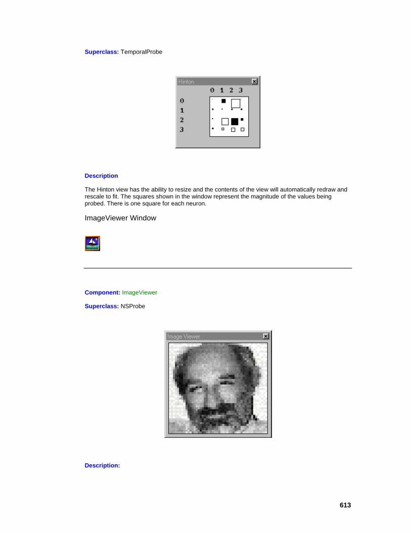
613


Description

The Hinton view has the ability to resize and the contents of the view will automatically redraw and rescale to fit. The squares shown in the window represent the magnitude of the values being probed. There is one square for each neuron.

ImageViewer Window

Component: ImageViewer

Superclass: NSProbe

Description:

614

The ImageViewer view has the ability to be resized and the contents of the view will automatically redraw and rescale to fit. The image shown in the view can be saved as a BMP file.

MatrixEditor Window

Component: MatrixEditor

Superclass: NSProbe

Description:

Each Cell in the MatrixEditor view can be selected and. The changes will affect the corresponding parameters in the network component being probed.

Let us assume that in this case the network component is a FullSynapse, and the MatrixEditor was attached to the Weights access point. So we are displaying the weight matrix between two layers.

Row i show the weights connected to the i-th output processing element. Column j show the weights connected to the j-th input processing element. So this conforms to the traditional assignment used in neural networks.

MatrixViewer Window

Component: MatrixViewer

Superclass: NSProbe

615

Description:

The MatrixViewer view has the ability to resize and the contents of the view will automatically redraw and rescale to fit. The contents of the view can not be changed. The font of the view may be changed by highlighting the text and using the font Panel.

Let us assume that in this case the network component is a FullSynapse, and the MatrixEditor access point was the Weights access point. So we are displaying the weight matrix between two layers.

Row i show the weights connected to the i-th output processing element. Column j show the weights connected to the j-th input processing element. So this conforms to the traditional assignment used in neural networks.

Macro Actions

Bar Chart

BarChart Macro Actions Overview Superclass Macro Actions

Action Description barSize Returns the "Bar Size" setting. setBarSize Sets the "Bar Size" setting.

barSize Overview Macro Actions

Syntax

componentName.barSize()

Parameters Type Description return int The height of the bars in the BarChart window (see "Bar Size" within the BarChart Inspector). componentName Name defined on the engine property page.

616

setBarSize Overview Macro Actions

Syntax

componentName.setBarSize(barSize)

Parameters Type Description return void componentName Name defined on the engine property page. barSize int The height of the bars in the BarChart window (see "Bar Size" within the BarChart Inspector).

Data Writer

DataWriter Macro Actions Overview Superclass Macro Actions

Action Description bufferSize Returns the "Buffer Size" setting. clear Clears the contents of the edit buffer. clearBeforeRun Returns the "Clear Before Run" setting. dumpFile Returns the "Dump Raw Data to File" setting. filePath Returns the path of the dump file. fileType Returns the file type of the dump file (0=Binary, 1=ASCII). fontSize Returns the "Font Size" setting. inputEnabled Returns the "Input Enabled" setting. mergeProbeName Returns the "Attach Data From" setting. saveText Saves the ASCII text contained within the data buffer to the specified file.

scientificNotation Returns the "Scientific Notation" setting.

setBufferSize Sets the "Buffer Size" setting. setClearBeforeRun Sets the "Clear Before Run" setting. setDumpFile Sets the "Dump Raw Data to File" setting.

617

setFilePath Sets the path of the dump file. setFileType Sets the file type of the dump file (0=Binary, 1=ASCII). SetFontSize Sets the "Font Size" setting. setInputEnabled Sets the "Input Enabled" setting. setMergeProbeName Sets the "Attach Data From" setting. setScientificNotation Sets the "Scientific Notation" setting. setTranspose Sets the "Transpose" setting. transpose Returns the "Transpose" setting.

bufferSize Overview Macro Actions

Syntax

componentName.bufferSize()

Parameters Type Description return int The maximum number of data points that can be stored in the edit window at any given time (see "Buffer Size" within the DataWriter Inspector). componentName Name defined on the engine property page.

clear Overview Macro Actions

Syntax

componentName.clear()


clearBeforeRun Overview Macro Actions

Syntax

componentName.clearBeforeRun()

618

Parameters Type Description return BOOL When TRUE, the edit buffer is cleared each time a network simulation is run (see "Clear Before Run" within the DataWriter Inspector). componentName Name defined on the engine property page.

dumpFile Overview Macro Actions

Syntax

componentName.dumpFile()

Parameters Type Description return BOOL When TRUE, all data that passes through the attached access point is written to the file path (see "Dump Raw Data to File" within the DataWriter Inspector). componentName Name defined on the engine property page.

filePath Overview Macro Actions

Syntax

componentName.filePath()

Parameters Type Description return string The path of the dump file (see "Save Text to File" and "Dump Raw Data to File" within the DataWriter Inspector). componentName Name defined on the engine property page.

fileType Overview Macro Actions

Syntax

componentName.fileType()

Parameters Type Description return int The file type of the dump file (0=Binary, 1=ASCII – see "Binary" and "ASCII' within the DataWriter Inspector). componentName Name defined on the engine property page.

fontSize Overview Macro Actions

619

Syntax

componentName.fontSize()

Parameters Type Description return int The point size of the font used in the edit window (see "Font Size" within the DataWriter Inspector). componentName Name defined on the engine property page.

inputEnabled Overview Macro Actions

Syntax

componentName.inputEnabled()

Parameters Type Description return BOOL When TRUE, the accessed data is written to the edit buffer (see "Input Enabled" within the DataWriter Inspector). componentName Name defined on the engine property page.

mergeProbeName Overview Macro Actions

Syntax

componentName.mergeProbeName()

Parameters Type Description return string The component name of the probe that is attaching its data to the DataWriter (see "Attach Data From" within the DataWriter Inspector). componentName Name defined on the engine property page.

saveText Overview Macro Actions

Syntax

componentName.saveText(filePath)

Parameters Type Description return void componentName Name defined on the engine property page. filePath string The ASCII text contained within the data buffer is written to this file (see "Save Text to File" within the DataWriter Inspector).

620

scientificNotation Overview Macro Actions

Syntax

componentName.scientificNotation()

Parameters Type Description return BOOL When TRUE, the data is displayed and/or written in scientific notation (see "Scientific Notation" within the DataWriter Inspector). componentName Name defined on the engine property page.

setBufferSize Overview Macro Actions

Syntax

componentName.setBufferSize(bufferSize)

Parameters Type Description return void componentName Name defined on the engine property page. bufferSize int The maximum number of data points that can be stored in the edit window at any given time (see "Buffer Size" within the DataWriter Inspector).

setClearBeforeRun Overview Macro Actions

Syntax

componentName.setClearBeforeRun(clearBeforeRun)

Parameters Type Description return void componentName Name defined on the engine property page. clearBeforeRun BOOL When TRUE, the edit buffer is cleared each time a network simulation is run (see "Clear Before Run" within the DataWriter Inspector).

setDumpFile Overview Macro Actions

Syntax

componentName.setDumpFile(dumpFile)

621

Parameters Type Description return void componentName Name defined on the engine property page. dumpFile BOOL When TRUE, all data that passes through the attached access point is written to the file path (see "Dump Raw Data to File" within the DataWriter Inspector).

setFilePath Overview Macro Actions

Syntax

componentName.setFilePath(filePath)

Parameters Type Description return void componentName Name defined on the engine property page. filePath string The path of the dump file (see "Save Text to File" and "Dump Raw Data to File" within the DataWriter Inspector).

setFileType Overview Macro Actions

Syntax

componentName.setFileType(fileType)

Parameters Type Description return void componentName Name defined on the engine property page. fileType int The file type of the dump file (0=Binary, 1=ASCII – see "Binary" and "ASCII' within the DataWriter Inspector).

setFontSize Overview Macro Actions

Syntax

componentName.setFontSize(fontSize)


622

fontSize int The point size of the font used in the edit window (see "Font Size" within the DataWriter Inspector).

setInputEnabled Overview Macro Actions

Syntax

componentName.setInputEnabled(inputEnabled)

Parameters Type Description return void componentName Name defined on the engine property page. inputEnabled BOOL When TRUE, the accessed data is written to the edit buffer (see "Input Enabled" within the DataWriter Inspector).

setMergeProbeName Overview Macro Actions

Syntax

componentName.setMergeProbeName(nameString)

Parameters Type Description return void componentName Name defined on the engine property page. nameString string The component name of the probe that is attaching its data to the DataWriter (see "Attach Data From" within the DataWriter Inspector).

setScientificNotation Overview Macro Actions

Syntax

componentName.setScientificNotation(scientificNotation)

Parameters Type Description return void componentName Name defined on the engine property page. scientificNotation BOOL When TRUE, the data is displayed and/or written in scientific notation (see "Scientific Notation" within the DataWriter Inspector).

623

setTranspose Overview Macro Actions

Syntax

componentName.setTranspose(transpose)

Parameters Type Description return void componentName Name defined on the engine property page. transpose BOOL When TRUE, the rows and columns are interchanged such that each PE is represented by a column of values in the display window (see "Transpose Matrix" within the DataWriter Inspector).

transpose Overview Macro Actions

Syntax

componentName.transpose()

Parameters Type Description return BOOL When TRUE, the rows and columns are interchanged such that each PE is represented by a column of values in the display window (see "Transpose Matrix" within the DataWriter Inspector). componentName Name defined on the engine property page.

Data Storage

DataStorage Macro Actions Overview Superclass Macro Actions

Action Description bufferLength Returns the "Buffer Size" setting. messageEvery Returns the "Message Every" setting. setBufferLength Sets the "Buffer Size" setting. setMessageEvery Sets the "Message Every" setting.

bufferLength Overview Macro Actions

624

Syntax

componentName.bufferLength()

Parameters Type Description return int The size of the circular buffer in samples (see "Buffer Size" within the DataStorage Inspector). componentName Name defined on the engine property page.

messageEvery Overview Macro Actions

Syntax

componentName.messageEvery()

Parameters Type Description return int The periodicity at which the attached probes are notified that the data samples contained in the DataStorage are available (see "Message Every" within the DataStorage Inspector). componentName Name defined on the engine property page.

setBufferLength Overview Macro Actions

Syntax

componentName.setBufferLength(bufferLength)

Parameters Type Description return void componentName Name defined on the engine property page. bufferLength int The size of the circular buffer in samples (see "Buffer Size" within the DataStorage Inspector).

setMessageEvery Overview Macro Actions

Syntax

componentName.setMesageEvery(messageEvery)


625

messageEvery int The periodicity at which the attached probes are notified that the data samples contained in the DataStorage are available (see "Message Every" within the DataStorage Inspector).

Hinton

Hinton Macro Actions Overview Superclass Macro Actions

Action Description setSquareSize Sets the "Square Size" setting. squareSize Returns the "Square Size" setting.

setSquareSize Overview Macro Actions

Syntax

componentName.setSquareSize(sqareSize)

Parameters Type Description return void componentName Name defined on the engine property page. squareSize int The maximum size of the squares in the probe window (see "Square Size" within the Hinton Inspector).

squareSize Overview Macro Actions

Syntax

componentName.squareSize()

Parameters Type Description return int The maximum size of the squares in the probe window (see "Square Size" within the Hinton Inspector). componentName Name defined on the engine property page.

Image Viewer

ImageViewer Macro Actions Overview Superclass Macro Actions

626

Action Description loadPaletteBeforeRun Returns the "Load image palette before run" setting. restorePaletteAfterRun Returns the "Restore NS palette after run" setting. saveImageToBitmap Saves the image shown in the display window to the specified BMP file. setLoadPaletteBeforeRun Sets the "Load image palette before run" setting. setRestorePaletteAfterRun Sets the "Restore NS palette after run" setting.

loadPaletteBeforeRun Overview Macro Actions

Syntax

componentName.loadPaletteBeforeRun()

Parameters Type Description return BOOL When TRUE, the gray-scale palette is loaded just before the simulation begins in an effort to guarantee that the image will display correctly (see "Load image palette before run" within the ImageViewer Inspector). componentName Name defined on the engine property page.

restorePaletteAfterRun Overview Macro Actions

Syntax

componentName.restorePaletteAfterRun()

Parameters Type Description return BOOL When TRUE, the original NeuroSolutions palette will be restored at the completion of the simulation (see "Restore NS palette after run" within the ImageViewer Inspector). componentName Name defined on the engine property page.

saveImageToBitmap Overview Macro Actions

Syntax

componentName.saveImageToBitmap(filePath)

Parameters Type Description return void Saves the image shown by the ImageViewer as a BMP file (see "Save Bitmap" within the ImageViewer Inspector).

627

componentName Name defined on the engine property page. filePath string Saves the image shown by the ImageViewer to this BMP file (see "Save Bitmap" within the ImageViewer Inspector).

setLoadPaletteBeforeRun Overview Macro Actions

Syntax

componentName.setLoadPaletteBeforeRun(loadPaletteBeforeRun)

Parameters Type Description return void componentName Name defined on the engine property page. loadPaletteBeforeRun BOOL When TRUE, the gray-scale palette is loaded just before the simulation begins in an effort to guarantee that the image will display correctly (see "Load image palette before run" within the ImageViewer Inspector).

setRestorePaletteAfterRun Overview Macro Actions

Syntax

componentName.setRestorePaletteAfterRun(restorePaletteAfterRun)

Parameters Type Description return void componentName Name defined on the engine property page. restorePaletteAfterRun BOOL When TRUE, the original NeuroSolutions palette will be restored at the completion of the simulation (see "Restore NS palette after run" within the ImageViewer Inspector).

Label

Label Macro Actions Overview Superclass Macro Actions

Action Description accessRows Returns TRUE if the "Rows" radio button is set and FALSE if the "Cols" radio button is set. activeNeuron Returns the "Active Neuron" setting.

628

autosizing Returns the "Autosize" setting. decrementNeuron Decreases the "Active Neuron" setting by one. enableLabels Returns the "Enable Label Editing" setting. fileForColumnHeadings Returns the "Auto Label Name" setting. fontHeight Returns the "Font Size" setting. incrementNeuron Increases the "Active Neuron" setting by one. label Returns the label "Text" that corresponds to the active neuron. labelSize Returns the "Size" setting. loadColumnHeadings Loads the column headings from the File component specifed by fileForColumnHeadings. setAccessRows Set to TRUE to set the "Rows" radio button and "FALSE" to set the "Cols" radio button. setActiveNeuron Sets the "Active Neuron" setting. setAutosizing Sets the "Autosize" setting. setEnableLabels Sets the "Enable Label Editing" setting. setFileForColumnHeadings Sets the "Auto Label Name" setting. setFontHeight Sets the "Font Size" setting. setLabel Sets the label "Text" that corresponds to the active neuron. setLabelSize Sets the "Size" setting. setShowLabels Sets the "Show Labels" setting. setWantsColumn Set to TRUE to force the probe to allow editing of the column labels. showLabels Returns the "Show Labels" setting. wantsColumn Returns TRUE if the probe is forced to allow editing of the column labels.

accessRows Overview Macro Actions

Syntax

629

componentName.accessRows()

Parameters Type Description return BOOL TRUE if the active neuron pertains to the probe window's row and FALSE if it pertains to the window's column (see "Active Neuron" and "Row and Column" within the Label Inspector). componentName Name defined on the engine property page.

activeNeuron Overview Macro Actions

Syntax

componentName.activeNeuron()

Parameters Type Description return int The row or column which is being viewed/modified (see "Active Neuron" within the Label Inspector). componentName Name defined on the engine property page.

autosizing Overview Macro Actions

Syntax

componentName.autosizing()

Parameters Type Description return BOOL When TRUE, the maximum number of rows and columns is more easily be displayed by changing the size of the probe's window (see "Autosizing" within the Label Inspector). componentName Name defined on the engine property page.

decrementNeuron Overview Macro Actions

Syntax

componentName.decrementNeuron()


enableLabels Overview Macro Actions

630

Syntax

componentName.enableLabels()

Parameters Type Description return BOOL When TRUE, the labels are user definable as opposed to computer generated (see "Enable Label Editing" within the Label Inspector). componentName Name defined on the engine property page.

fileForColumnHeadings Overview Macro Actions

Syntax

componentName.fileForColumnHeadings()

Parameters Type Description return string The name of the File component that contains the column headings corresponding to the probed data (see "Name" within the Label Inspector). componentName Name defined on the engine property page.

fontHeight Overview Macro Actions

Syntax

componentName.fontHeight()

Parameters Type Description return int The font height of the labels (see "Font Size" within the Label Inspector). componentName Name defined on the engine property page.

incrementNeuron Overview Macro Actions

Syntax

componentName.incrementNeuron()


label Overview Macro Actions

631

Syntax

componentName.label()

Parameters Type Description return string The label text corresponding to the Active Neuron (see "Text" within the Label Inspector). componentName Name defined on the engine property page.

labelSize Overview Macro Actions

Syntax

componentName.labelSize()

Parameters Type Description return int The amount of space allocated for the row labels (see "Label Size" within the Label Inspector). componentName Name defined on the engine property page.

loadColumnHeadings Overview Macro Actions

Syntax

componentName.loadColumnHeadings()


setAccessRows Overview Macro Actions

Syntax

componentName.setAccessRows(accessRows)

Parameters Type Description return void componentName Name defined on the engine property page. accessRows BOOL TRUE if the active neuron pertains to the probe window's row and FALSE if it pertains to the window's column (see "Active Neuron" and "Row and Column" within the Label Inspector).

632

setActiveNeuron Overview Macro Actions

Syntax

componentName.setActiveNeuron(activeNeuron)

Parameters Type Description return void componentName Name defined on the engine property page. activeNeuron int The row or column which is being viewed/modified (see "Active Neuron" within the Label Inspector).

setAutosizing Overview Macro Actions

Syntax

componentName.setAutosizing(autosizing)

Parameters Type Description return void componentName Name defined on the engine property page. autosizing BOOL When TRUE, the maximum number of rows and columns is more easily be displayed by changing the size of the probe's window (see "Autosizing" within the Label Inspector).

setEnableLabels Overview Macro Actions

Syntax

componentName.setEnableLabels(enableLabels)

Parameters Type Description return void componentName Name defined on the engine property page. enableLabels BOOL When TRUE, the labels are user definable as opposed to computer generated (see "Enable Label Editing" within the Label Inspector).

setFileForColumnHeadings Overview Macro Actions

633

Syntax

componentName.setFileForColumnHeadings(fileForColumnHeadings)

Parameters Type Description return void componentName Name defined on the engine property page. fileForColumnHeadings string The name of the File component that contains the column headings corresponding to the probed data (see "Name" within the Label Inspector).

setFontHeight Overview Macro Actions

Syntax

componentName.setFontHeight(fontHeight)

Parameters Type Description return void componentName Name defined on the engine property page. fontHeight int The font height of the labels (see "Font Size" within the Label Inspector).

setLabel Overview Macro Actions

Syntax

componentName.setLabel(label)

Parameters Type Description return void componentName Name defined on the engine property page. label string The label text corresponding to the Active Neuron (see "Text" within the Label Inspector).

setLabelSize Overview Macro Actions

Syntax

componentName.setLabelSize(labelSize)

634

Parameters Type Description return void componentName Name defined on the engine property page. labelSize int The amount of space allocated for the row labels (see "Label Size" within the Label Inspector).

setShowLabels Overview Macro Actions

Syntax

componentName.setShowLabels(showLabels)

Parameters Type Description return void componentName Name defined on the engine property page. showLabels BOOL When TRUE, the labels are displayed in the probe window (see "Show Labels" within the Label Inspector).

setWantsColumn Overview Macro Actions

Syntax

componentName.setWantsColumn(wantsColumn)

Parameters Type Description return void componentName Name defined on the engine property page. wantsColumn BOOL When TRUE, the probe is forced to allow editing of the column labels.

showLabels Overview Macro Actions

Syntax

componentName.showLabels(labels)

Parameters Type Description return BOOL When TRUE, the labels are displayed in the probe window (see "Show Labels" within the Label Inspector). componentName Name defined on the engine property page.

635

wantsColumn Overview Macro Actions

Syntax

componentName.wantsColumn()

Parameters Type Description return BOOL Forces the probe to allow editing of column labels. componentName Name defined on the engine property page.



Ancestor: Probe Family

The TemporalProbe family is a collection of components for observing data that has been collected from a network component over a number of simulation iterations. This enables the TemporalProbe components to process or display data over time. TemporalProbes require that they be attached to a component having a temporal access point.

Members:

MegaScope

ScatterPlot

3DProbe Family

Transformer Family

User Interface:

Macro Actions

MegaScope

636

Family: TemporalProbe Family


Description:

The MegaScope probe is a fully functional multi-channel oscilloscope. It has the ability to display temporal data as a set of signal traces -- values (vertical axis) over time (horizontal axis). These traces can be manipulated in a variety of ways (e.g., amplitude and time scales, position, and color).

The length (number of samples) within each trace is specified by the size of the buffer within the attached temporal access point. The refresh rate of the display is specified by the DataStorage component used to collect the network data.

Other TemporalProbes may attach to the Selection access point of the MegaScope to access a segment of the displayed data. This segment is specified by selecting (highlighting) a portion of the display window.

User Interaction:

Drag and Drop

Inspector

Window

Access Points

Macro Actions

ScatterPlot

Family: TemporalProbe Family


Description:

The ScatterPlot is a probe that takes the data from a temporal access point and plots one channel’s data against the data of one of the other channels. Multiple pairs of channels can be specified. The data from each pair is used as the X and Y coordinates of a two-dimensional graph. Since the points are displayed over a number of samples (i.e., across time), the data is represented as a scatter plot.

User Interaction:

637

Drag and Drop

Inspector

Window

Macro Actions

Access Points

MegaScope Access Points

Component: MegaScope


Selection Access:

This is an access point to a region of data that has selected (highlighted) in the MegaScope view. The data that passes through this selected region will be passed to any component connected to this access point.

Drag and Drop

Temporal Probe Drag and Drop

The Temporal Probe Family was designed to examine data that has been collected for a period of time. This data block is presented as a temporal access point. The primary component that is responsible for data collection is DataStorage. Any component in this family must be placed on a DataStorage or another TemporalProbe.

Inspectors

Scope Inspector


Superclass Inspector: Sweep Inspector

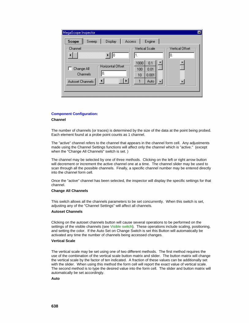
638

Component Configuration: Channel

The number of channels (or traces) is determined by the size of the data at the point being probed. Each element found at a probe point counts as 1 channel.

The "active" channel refers to the channel that appears in the channel form cell. Any adjustments made using the Channel Settings functions will affect only the channel which is "active." (except when the "Change All Channels" switch is set. )

The channel may be selected by one of three methods. Clicking on the left or right arrow button will decrement or increment the active channel one at a time. The channel slider may be used to scan through all the possible channels. Finally, a specific channel number may be entered directly into the channel form cell.

Once the "active" channel has been selected, the inspector will display the specific settings for that channel. Change All Channels

This switch allows all the channels parameters to be set concurrently. When this switch is set, adjusting any of the "Channel Settings" will affect all channels. Autoset Channels

Clicking on the autoset channels button will cause several operations to be performed on the settings of the visible channels (see Visible switch). These operations include scaling, positioning, and setting the color. If the Auto Set on Change Switch is set this Button will automatically be activated any time the number of channels being accessed changes. Vertical Scale

The vertical scale may be set using one of two different methods. The first method requires the use of the combination of the vertical scale button matrix and slider. The button matrix will change the vertical scale by the factor of ten indicated. A fraction of these values can be additionally set with the slider. When using this method the form cell will report the exact value of vertical scale. The second method is to type the desired value into the form cell. The slider and button matrix will automatically be set accordingly. Auto

639

Clicking on this button will automatically set the vertical scaling so that the active trace will vertically fill the view. Vertical Offset

The vertical offset may be set in one of two ways. First, the slider may be used to move the trace. Using this method the trace may only be moved from the top of the view to the bottom of the view. The vertical offset form cell will display the offset in the correct units specified by the vertical scale. The other way to set the vertical offset is by typing the offset directly into the vertical offset form cell. The offset should be entered in terms of the scale currently being used. For example, if the scale is set to10/div and 10 is entered into the vertical offset form cell, the trace will be shifted up one division. Horizontal Offset

The horizontal offset is set in the same fashion as the vertical offset. The only difference is that here the samples/division are used to compute the value in the horizontal offset form cell.

Sweep Inspector


Superclass Inspector: Display Inspector

Component Configuration: Samples/Division

The number of samples per division is a control of the time scale. It sets the number of samples in each of the ten time divisions across the horizontal axis. These divisions can be seen by displaying lines or a grid (see Grid Pull Down Menu ).

The samples per division may be set using one of two different methods. The first method requires the use of the combination of the samples/div button matrix and slider. The button matrix will change the samples/div by the factor of ten indicated. A fraction of these values can be additionally set with the slider. When using this method the form cell will report the exact value of samples/div. The other way to set the samples/div is to type the desired value into the form cell. The slider and button matrix will automatically be set accordingly.

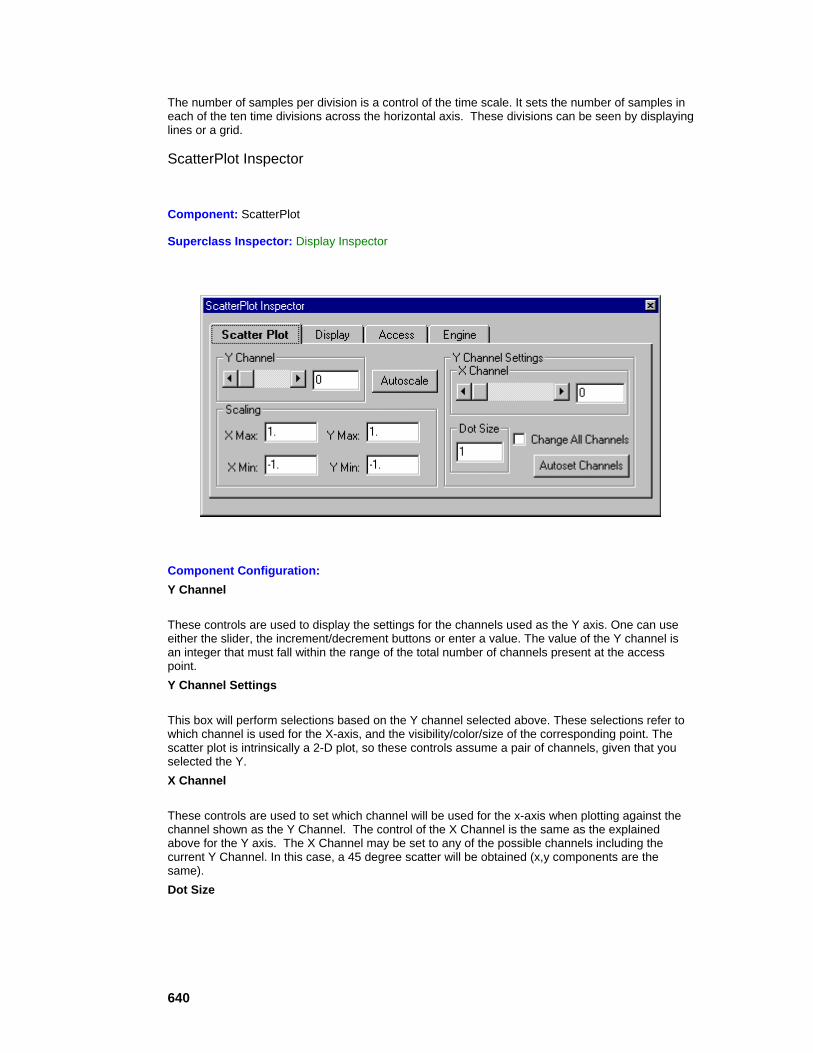
640

The number of samples per division is a control of the time scale. It sets the number of samples in each of the ten time divisions across the horizontal axis. These divisions can be seen by displaying lines or a grid.

ScatterPlot Inspector

Component: ScatterPlot


Component Configuration: Y Channel

These controls are used to display the settings for the channels used as the Y axis. One can use either the slider, the increment/decrement buttons or enter a value. The value of the Y channel is an integer that must fall within the range of the total number of channels present at the access point. Y Channel Settings

This box will perform selections based on the Y channel selected above. These selections refer to which channel is used for the X-axis, and the visibility/color/size of the corresponding point. The scatter plot is intrinsically a 2-D plot, so these controls assume a pair of channels, given that you selected the Y. X Channel

These controls are used to set which channel will be used for the x-axis when plotting against the channel shown as the Y Channel. The control of the X Channel is the same as the explained above for the Y axis. The X Channel may be set to any of the possible channels including the current Y Channel. In this case, a 45 degree scatter will be obtained (x,y components are the same). Dot Size

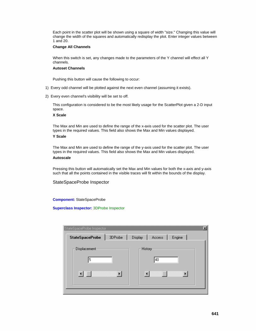
641

Each point in the scatter plot will be shown using a square of width "size." Changing this value will change the width of the squares and automatically redisplay the plot. Enter integer values between 1 and 20. Change All Channels

When this switch is set, any changes made to the parameters of the Y channel will effect all Y channels. Autoset Channels

Pushing this button will cause the following to occur:

1) Every odd channel will be plotted against the next even channel (assuming it exists).

2) Every even channel's visibility will be set to off.

This configuration is considered to be the most likely usage for the ScatterPlot given a 2-D input space. X Scale

The Max and Min are used to define the range of the x-axis used for the scatter plot. The user types in the required values. This field also shows the Max and Min values displayed. Y Scale

The Max and Min are used to define the range of the y-axis used for the scatter plot. The user types in the required values. This field also shows the Max and Min values displayed. Autoscale

Pressing this button will automatically set the Max and Min values for both the x-axis and y-axis such that all the points contained in the visible traces will fit within the bounds of the display.

StateSpaceProbe Inspector

Component: StateSpaceProbe

Superclass Inspector: 3DProbe Inspector

642

Component Configuration: Displacement

The displacement is used to select ?, i.e. how far apart the samples used to create the input matrix are taken from the original signal. This value may be any integer greater than zero. Low values tend to create a state space plot that is elongated along the first quadrant bisector. Too large a value of displacement destroys the organization of the data. History

The history is used to determine how many samples will be shown in the display. This value may be any integer greater than zero. Normally it is related to the size of the buffer or features in the data that one wants to observe (such as periodicity’s).

3DProbe Inspector



Component Configuration: Zoom

The zoom sliders scale the image when projecting it in the 3DProbe. Each dimension may be adjusted separately. Pressing the reset button will return these values to the defaults. Offset

The offset sliders create an offset when projecting the image in the 3DProbe. Each dimension may be adjusted separately. Pressing the reset button will return these values to the defaults.

∆

643

The ? slider allows control of the apparent viewing angle of the image within 3D probes. This occurs because the ∆ slider mimics the change of view with distance in the real world. Uniform Scale

The Uniform Scale switch, when set, will create a uniform scale on all X, Y, and Z dimensions. This is done so that the image contained within the 3D probes will not be distorted by varying scale. Show Cube

The Show Cube switch, when set, will show a cube along the axis. This is known to increase the 3D effect of the display. Autoscale

The Autoscale switch, when set, will scale the X, Y, and Z dimensions independently so that the image will fill the cube. Reset

The reset button will return all sliders to the default positions. Lines/Dots/Both

The Lines/Dots/Both menu allows three different ways of viewing the data. The image may be viewed by connecting the data samples with lines, drawing dots on the location of the data sample in space, or both. Projection Matrix

The Projection Matrix shows the values of ??????and???used to project the 3 dimensional data onto the screen. The user can enter a selection directly into these fields.

Windows

MegaScope Window



644

Description:

The MegaScope view allows the plotting of multi-channel variables over time. The MegaScope view accepts further selection of a portion of the plotted data, which is accomplished with the mouse. Just press the mouse button at the left of the desired region and drag the mouse (with the button pressed) towards the right until the end of the desired selection.

The data in this region can be accessed by other probes. All data that passes through this region will automatically be forwarded to attached temporal probes. The Slider and Buttons at the bottom of the view allow the unseen data to be scrolled to the visible region.

ScatterPlot Window

Component: ScatterPlot


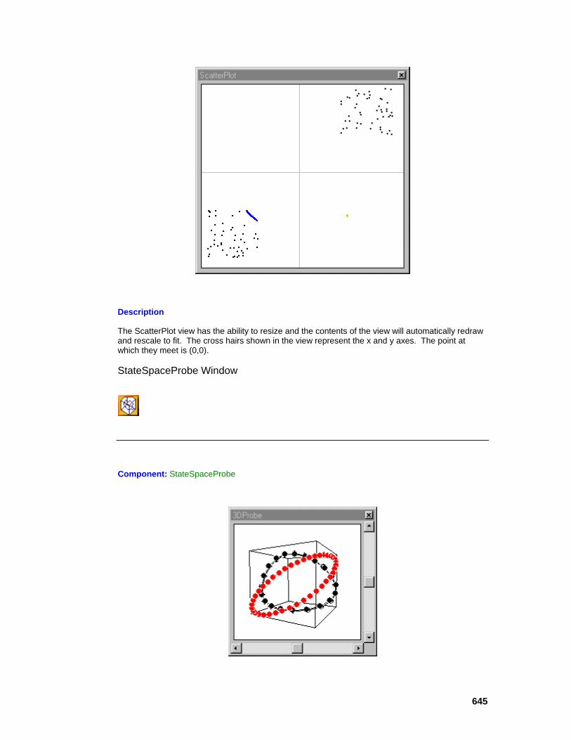
645

Description

The ScatterPlot view has the ability to resize and the contents of the view will automatically redraw and rescale to fit. The cross hairs shown in the view represent the x and y axes. The point at which they meet is (0,0).

StateSpaceProbe Window


646

Description:

The StateSpaceProbe uses the above window to display its data. This window is opened by double-clicking on the StateSpaceProbe icon.

Φ Slider

The Φ slider (horizontal slider) allows the image in the StateSpaceProbe window to be rotated around the horizontal axis. The image may be rotated 90 degrees in either direction.

Θ Slider

The Θ slider (vertical slider) allows the image in StateSpaceProbe window to be rotated around the vertical axis. The image may be rotated 180 degrees in either direction.

Macro Actions

Mega Scope

MegaScope Macro Actions Overview Superclass Macro Actions

Action Description amplitude Returns the "Vertical Scale" setting. autoscaleChannel Automatically adjusts scale setting. autoSetUpChannels Automatically adjusts the MegaScope settings so that all of the traces can be viewed at once. horizontalPos Returns the value of the "Horizontal Offset" scroller. horizontalPosSamples Returns the value of the "Horizontal Offset" edit cell. multiplier Returns the "Vertical Scale" setting. scale Returns the exponent of the "Vertical Scale" setting (3=1000, 2=100, 1=10, 0=1, -1=0.1, -2=0.01, -3=0.001). setAmplitude Sets the "Vertical Scale" setting and automatically adjusts the scale. setHorizontalPos Sets the value of the "Horizontal Offset" scroller. setHorizontalPosSamples Sets the value of the "Horizontal Offset" edit cell. setMultiplier Sets the "Vertical Scale" setting. setScale Sets the exponent of the "Vertical Scale" setting (3=1000, 2=100, 1=10, 0=1, -1=0.1, -2=0.01, -3=0.001).

647

setSweepMult Sets the sweep multiplier ([sweep rate] = [sweep multiplier] * 10 ^ [sweep scale]). setSweepRate Sets the "Samples/Division" setting (sweep rate). setSweepScale Sets the sweep scale ([sweep rate] = [sweep multiplier] * 10 ^ [sweep scale]). setVerticalPos Sets the "Vertical Offset" scroller value. setVerticalPosVolts Sets the "Vertical Offset" edit cell value. sweepMult Returns the sweep multiplier (Sample/Division = [sweep multiplier] * 10 ^ [sweep scale]). sweepRate Returns the "Samples/Division" setting (sweep rate). sweepScale Returns the sweep scale ([sweep rate] = [sweep multiplier] * 10 ^ [sweep scale]). verticalPos Returns the "Vertical Offset" scroller value. verticalPosVolts Returns the "Vertical Offset" edit cell value.


Syntax

componentName.amplitude()

Parameters Type Description return float The vertical scaling factor (see "Vertical Scale" of the Scope Inspector). componentName Name defined on the engine property page.

autoscaleChannel Overview Macro Actions

Syntax

componentName.autoscaleChannel()


648

autoSetUpChannels Overview Macro Actions

Syntax

componentName.autoSetUpChannels()


horizontalPos Overview Macro Actions

Syntax

componentName.horizontalPos()

Parameters Type Description return float The position of the scroller used to adjust the horizontal offset (see "Horizontal Offset" within the Scope Inspector). componentName Name defined on the engine property page.

horizontalPosSamples Overview Macro Actions

Syntax

componentName.horizontalPosSamples()

Parameters Type Description return float The value of the edit cell used to set the horizontal offset (see "Horizontal Offset" within the Scope Inspector). componentName Name defined on the engine property page.

multiplier Overview Macro Actions

Syntax

componentName.multiplier()

Parameters Type Description return float The vertical scaling factor (see "Vertical Scale" within the Scope Inspector).

649


scale Overview Macro Actions

Syntax

componentName.scale()

Parameters Type Description return int The exponent of the vertical scaling factor (3=1000, 2=100, 1=10, 0=1, -1=0.1, -2=0.01, -3=0.001 – see "Vertical Scale" within the Scope Inspector). componentName Name defined on the engine property page.


Syntax

componentName.setAmplitude(amplitude)

Parameters Type Description return void componentName Name defined on the engine property page. amplitude float The vertical scaling factor (see "Vertical Scale" of the Scope Inspector).

setHorizontalPos Overview Macro Actions

Syntax

componentName.setHorizontalPos(horizontalPos)

Parameters Type Description return void componentName Name defined on the engine property page. horizontalPos float The position of the scroller used to adjust the horizontal offset (see "Horizontal Offset" within the Scope Inspector).

setHorizontalPosSamples Overview Macro Actions

Syntax

650

componentName.setHorizontalPosSamples(horizontalPosSamples)

Parameters Type Description return float componentName Name defined on the engine property page. HorizontalPosSamples float The value of the edit cell used to set the horizontal offset (see "Horizontal Offset" within the Scope Inspector).

setMultiplier Overview Macro Actions

Syntax

componentName.setMultiplier(multiplier)

Parameters Type Description return void componentName Name defined on the engine property page. multiplier float The vertical scaling factor (see "Vertical Scale" within the Scope Inspector).

setScale Overview Macro Actions

Syntax

componentName.setScale(scale)

Parameters Type Description return void componentName Name defined on the engine property page. scale int The exponent of the vertical scaling factor (3=1000, 2=100, 1=10, 0=1, -1=0.1, -2=0.01, -3=0.001 – see "Vertical Scale" within the Scope Inspector).

setSweepMult Overview Macro Actions

Syntax

componentName.setSweepMult(sweepMult)


651

return void componentName Name defined on the engine property page. sweepMult float The sweep multiplier ([sweep rate] = [sweep multiplier] * 10 ^ [sweep scale] – see "Samples/Division" with the Sweep Inspector).

setSweepRate Overview Macro Actions

Syntax

componentName.setSweepRate(sweepRate)

Parameters Type Description return void componentName Name defined on the engine property page. sweepRate float The sweep rate ([sweep rate] = [sweep multiplier] * 10 ^ [sweep scale] – see "Samples/Division" with the Sweep Inspector).

setSweepScale Overview Macro Actions

Syntax

componentName.setSweepScale(sweepScale)

Parameters Type Description return void componentName Name defined on the engine property page. sweepScale int The sweep scale ([sweep rate] = [sweep multiplier] * 10 ^ [sweep scale] – see "Samples/Division" with the Sweep Inspector).

setVerticalPos Overview Macro Actions

Syntax

componentName.setVerticalPos(verticalPos)


652

verticalPos float The position of the scroller used to adjust the vertical offset (see "Vertical Offset" within the Scope Inspector).

setVerticalPosVolts Overview Macro Actions

Syntax

componentName.setVerticalPosVolts(verticalPosVolts)

Parameters Type Description return void componentName Name defined on the engine property page. verticalPosVolts float The value of the edit cell used to define the vertical offset (see "Vertical Offset" within the Scope Inspector).

sweepMult Overview Macro Actions

Syntax

componentName.sweepMult()

Parameters Type Description return float The sweep multiplier ([sweep rate] = [sweep multiplier] * 10 ^ [sweep scale] – see "Samples/Division" with the Sweep Inspector). componentName Name defined on the engine property page.

sweepRate Overview Macro Actions

Syntax

componentName.sweepRate()

Parameters Type Description return float The sweep rate ([sweep rate] = [sweep multiplier] * 10 ^ [sweep scale] – see "Samples/Division" with the Sweep Inspector). componentName Name defined on the engine property page.

sweepScale Overview Macro Actions

653

Syntax

componentName.sweepScale()

Parameters Type Description return int The sweep scale ([sweep rate] = [sweep multiplier] * 10 ^ [sweep scale] – see "Samples/Division" with the Sweep Inspector). componentName Name defined on the engine property page.

verticalPos Overview Macro Actions

Syntax

componentName.verticalPos()

Parameters Type Description return float The position of the scroller used to adjust the vertical offset (see "Vertical Offset" within the Scope Inspector). componentName Name defined on the engine property page.

verticalPosVolts Overview Macro Actions

Syntax

componentName.verticalPosVolts()

Parameters Type Description return float The value of the edit cell used to define the vertical offset (see "Vertical Offset" within the Scope Inspector). componentName Name defined on the engine property page.

Scatter Plot

ScatterPlot Macro Actions Overview Superclass Macro Actions

Action Description autoSetUpChannels Automatically sets every odd channel to be plotted against the next even channel (assuming it exists), and every even channel’s visibility will be set to off (see "Autoset Channels" within the ScatterPlot Inspector). decrementXChannel Decreases the "X Channel" setting by one (see "X Channel" within the ScatterPlot Inspector).

654

dotSize Returns the "Dot Size" setting. incrementXChannel Increases the "X Channel" setting by one (see "X Channel" within the ScatterPlot Inspector). performAutoscale Sets the Max and Min values for both the x-axis and y-axis such that all the points contained in the visible traces will fit within the bounds of the display (see "Autoscale" within the ScatterPlot Inspector). setDotSize Sets the "Dot Size" setting. setXChannel Sets the "X Channel" setting. setXMaxScale Sets the "X Max" setting. setXMinScale Sets the "X Min" setting. setYMaxScale Sets the "Y Max" setting. setYMinScale Sets the "Y Min" setting. xChannel Returns the "X Channel" setting. xMaxScale Returns the "X Max" setting. xMinScale Returns the "X Min" setting. yMaxScale Returns the "Y Max" setting. yMinScale Returns the "Y Min" setting.


Syntax

componentName.autoSetUpChannels()


decrementXChannel Overview Macro Actions

655

Syntax

componentName. decrementXChannel()


dotSize Overview Macro Actions

Syntax

componentName. dotSize()

Parameters Type Description return int The width of the squares in the display window (see "Dot Size" within the ScatterPlot Inspector). componentName Name defined on the engine property page.

incrementXChannel Overview Macro Actions

Syntax

componentName. incrementXChannel()


performAutoscale Overview Macro Actions

Syntax

componentName. performAutoscale()


656

setDotSize Overview Macro Actions

Syntax

componentName. setDotSize(dotSize)

Parameters Type Description return void componentName Name defined on the engine property page. dotSize int The width of the squares in the display window (see "Dot Size" within the ScatterPlot Inspector).

setXChannel Overview Macro Actions

Syntax

componentName. setXChannel(xChannel)

Parameters Type Description return void componentName Name defined on the engine property page. xChannel int The channel that will be used for the x-axis when plotting against the channel shown as the "Y Channel" (see "X Channel" within the ScatterPlot Inspector).

setXMaxScale Overview Macro Actions

Syntax

componentName. setXMaxScale(xMaxScale)

Parameters Type Description return void componentName Name defined on the engine property page. xMaxScale float The maximum value used to define the range of the x-axis on the scatter plot (see "X Scale" within the ScatterPlot Inspector).

setXMinScale Overview Macro Actions

Syntax

657

componentName. setXMinScale(xMinScale)

Parameters Type Description return void componentName Name defined on the engine property page. xMinScale float The minimum value used to define the range of the x-axis on the scatter plot (see "X Scale" within the ScatterPlot Inspector).

setYMaxScale Overview Macro Actions

Syntax

componentName. setYMaxScale(yMaxScale)

Parameters Type Description return void componentName Name defined on the engine property page. yMaxScale float The maximum value used to define the range of the y-axis on the scatter plot (see "Y Scale" within the ScatterPlot Inspector).

setYMinScale Overview Macro Actions

Syntax

componentName. setYMinScale(yMinScale)

Parameters Type Description return void componentName Name defined on the engine property page. yMinScale float The minimum value used to define the range of the y-axis on the scatter plot (see "Y Scale" within the ScatterPlot Inspector).

xChannel Overview Macro Actions

Syntax

componentName.xChannel()

Parameters Type Description return int The channel that will be used for the x-axis when plotting against the channel

658

shown as the "Y Channel" (see "X Channel" within the ScatterPlot Inspector). componentName Name defined on the engine property page.

xMaxScale Overview Macro Actions

Syntax

componentName. xMaxScale()

Parameters Type Description return float The maximum value used to define the range of the x-axis on the scatter plot (see "X Scale" within the ScatterPlot Inspector). componentName Name defined on the engine property page.

xMinScale Overview Macro Actions

Syntax

componentName. xMinScale()

Parameters Type Description return float The minimum value used to define the range of the x-axis on the scatter plot (see "X Scale" within the ScatterPlot Inspector). componentName Name defined on the engine property page.

yMaxScale Overview Macro Actions

Syntax

componentName. yMaxScale()

Parameters Type Description return float The maximum value used to define the range of the x-axis on the scatter plot (see "X Scale" within the ScatterPlot Inspector). componentName Name defined on the engine property page.

yMinScale Overview Macro Actions

659

Syntax

componentName. yMinScale()

Parameters Type Description return float The minimum value used to define the range of the y-axis on the scatter plot (see "Y Scale" within the ScatterPlot Inspector). componentName Name defined on the engine property page.

Temporal Probe

TemporalProbe Macro Actions Overview Superclass Macro Actions

Action Description activeChannel Returns the "Channel" setting. autoSetUpChannels Automatically sets the scaling, positioning, color settings (see "Autoset Channels" within the Display Inspector). broadcast Returns the "Change All Channels" setting. decrementChannel Decreases the "Channel" setting by one (see "Channel" within the Display Inspector). grid Returns the "Grid" setting (0="None", 1="Lines", 2="Grid"). incrementChannel Increases the "Channel" setting by one (see "Channel" within the Display Inspector). setActiveChannel Sets the "Channel" setting. setBroadcast Sets the "Change All Channels" setting. setColor Sets the "Color" setting (Hex value 0x00bbggrr). setGrid Sets the "Grid" setting (0="None", 1="Lines", 2="Grid").. setVisible Sets the "Visible" setting. visible Returns the "Visible" setting.

activeChannel Overview Macro Actions

Syntax

componentName. activeChannel()

660

Parameters Type Description return int The current channel used by the "Channel Settings" (see "Channel" within the Display Inspector). componentName Name defined on the engine property page.


Syntax

componentName. autoSetUpChannels()


broadcast Overview Macro Actions

Syntax

componentName. broadcast()

Parameters Type Description return BOOL TRUE if the changes made to the current channel are also made to all channels (see "Autoset Channels" within the Display Inspector). componentName Name defined on the engine property page.

decrementChannel Overview Macro Actions

Syntax

componentName. decrementChannel()


grid Overview Macro Actions

661

Syntax

componentName. grid()

Parameters Type Description return int Specifies whether or not the view is segmented into 10 equal divisions (0="None", 1="Lines", 2="Grid" – see "Grid" within the Display Inspector). componentName Name defined on the engine property page.

incrementChannel Overview Macro Actions

Syntax

componentName. incrementChannel()


setActiveChannel Overview Macro Actions

Syntax

componentName. setActiveChannel(activeChannel)

Parameters Type Description return void componentName Name defined on the engine property page. activeChannel int The current channel used by the "Channel Settings" (see "Channel" within the Display Inspector).

setBroadcast Overview Macro Actions

Syntax

componentName. setBroadcast(broadcast)


662

broadcast BOOL TRUE if the changes made to the current channel are also made to all channels (see "Autoset Channels" within the Display Inspector).

setColor Overview Macro Actions

Syntax

componentName. setColor(color)

Parameters Type Description return void componentName Name defined on the engine property page. color int value has the following hexadecimal form: 0x00bbggrr. The low-order byte contains a value for the relative intensity of red; the second byte contains a value for green; and the third byte contains a value for blue. The high-order byte must be zero. The maximum value for a single byte is 0xFF.

setGrid Overview Macro Actions

Syntax

componentName. setGrid(grid)

Parameters Type Description return void componentName Name defined on the engine property page. grid int Specifies whether or not the view is segmented into 10 equal divisions (0="None", 1="Lines", 2="Grid" – see "Grid" within the Display Inspector).

setVisible Overview Macro Actions

Syntax

componentName. setVisible(visible)

Parameters Type Description return void componentName Name defined on the engine property page. visible int TRUE if the trace for the activeChannel is visible (see "Visible" within the Display Inspector).

663

visible Overview Macro Actions

Syntax

componentName. visible()

Parameters Type Description return int TRUE if the trace for the activeChannel is visible (see "Visible" within the Display Inspector). componentName Name defined on the engine property page.

3DProbe Family

3DProbe Family

Ancestor: TemporalProbe Family

The 3DProbe family is a collection of components for observing the data in a given network as a three dimensional projection. The members of the family determine the way in which the data is projected. Members of the 3DProbe family have the ability to rotate and scale the projection. The points can be plotted using dots, connected lines, or both.

Members:

StateSpaceProbe

User Interaction:

Macro Actions

StateSpaceProbe

Family: 3DProbe Family

Superclass: 3DProbe

664

Description:

The StateSpaceProbe provides a 3D state space representation of a sequence x based on the matrix given below. This matrix is created using the history, n, of input data at some displacement, τ. The output of this matrix is displayed using the abilities inherited from 3DProbe.

aij = x0 x? x2?

x1 x1+? x1+2?

. . .

. . .

xn-2? xn-? xn

A state space trajectory represents a 3-D plot of the time evolution of the state of the system that generated the data. Here the generated data is that contained within the attached temporal access point. The StateSpaceProbe displays the signal against approximations of its first and second derivatives. This tool is very useful for dynamic system analysis.

User Interaction:

Drag and Drop

Inspector

Window

Access Points

Macro Actions

Macro Actions

3D Probe

3DProbe Macro Actions Overview Superclass Macro Actions

Action Description amplitude Returns the "Amplitude" setting. autoscale Returns the "Autoscale" setting. distance Returns the "Delta" setting. offset Returns the "Offset" setting for the specified axis.

665

phi Returns the "Phi setting. reset Returns all dimension values to their original, default positions. setAmplitude Sets the "Amplitude" setting. setAutoscale Sets the "Autoscale" setting. setDistance Sets the "Delta" setting. setOffset Sets the "Offset" setting for the specified axis. setPhi Sets the "Phi setting. setShowCube Sets the "Show Cube" setting. setShowDots Set to TRUE for the "Dots" or "Both" settings. setShowLines Set to TRUE for the "Lines" or "Both" settings. setSquareCube Sets the "Uniform Scale" setting. setTheta Sets the "Theta" setting. showCube Returns the "Show Cube" setting. showDots Returns TRUE for the "Dots" or "Both" settings. showLines Returns TRUE for the "Lines" or "Both" settings. squareCube Returns the "Uniform Scale" setting. theta Returns the "Theta" setting.


Syntax

componentName.amplitude(axis)

Parameters Type Description return float Amplitude of the scaling function (see "Zoom" within the 3DProbe Inspector). componentName Name defined on the engine property page.

666

Axis int Axis to query (X=0, Y=1, Z=2).

autoscale Overview Macro Actions

Syntax

componentName.autoscale()

Parameters Type Description return BOOL When TRUE, the X, Y, and Z dimensions will scale independently so that the image will fill the cube (see "Autoscale" within the 3DProbe Inspector). componentName Name defined on the engine property page.

distance Overview Macro Actions

Syntax

componentName.distance()

Parameters Type Description return float The apparent viewing angle of the image (see "Delta" within the 3DProbe Inspector). componentName Name defined on the engine property page.


Syntax

componentName.offset()

Parameters Type Description return float Offset of the scaling function (see " Offset" within the 3DProbe Inspector). componentName Name defined on the engine property page. Axis int Axis to query (X=0, Y=1, Z=2).

phi Overview Macro Actions

Syntax

667

componentName.phi()

Parameters Type Description return float Parameter used to project the 3 dimensional data onto the screen (see "Projection Matrix" within the 3DProbe Inspector). componentName Name defined on the engine property page.

reset Overview Macro Actions

Syntax

componentName.reset()



Syntax

componentName.setAmplitude(amplitude,axis)

Parameters Type Description return void componentName Name defined on the engine property page. amplitude float Amplitude of the scaling function (see "Zoom" within the 3DProbe Inspector). Axis int Axis to change (X=0, Y=1, Z=2).

setAutoscale Overview Macro Actions

Syntax

componentName.setAutoscale(autoscale)

Parameters Type Description return void componentName Name defined on the engine property page. autoscale BOOL When TRUE, the X, Y, and Z dimensions will scale independently so

668

that the image will fill the cube (see "Autoscale" within the 3DProbe Inspector).

setPhi Overview Macro Actions

Syntax

componentName.setPhi(phi)

Parameters Type Description return void componentName Name defined on the engine property page. phi float Parameter used to project the 3 dimensional data onto the screen (see "Projection Matrix" within the 3DProbe Inspector).

setShowCube Overview Macro Actions

Syntax

componentName.setShowCube(showCube)

Parameters Type Description return void componentName Name defined on the engine property page. showCube BOOL When TRUE, a cube will be displayed along the axis (see "Show Cube" within the 3DProbe Inspector).

setShowDots Overview Macro Actions

Syntax

componentName.setShowDots(showDots)

Parameters Type Description return void componentName Name defined on the engine property page. showDots BOOL When TRUE, the location of the data samples in space are displayed through a series of dots (see "Lines/Dots/Both" within the 3DProbe Inspector).

setShowLines Overview Macro Actions

669

Syntax

componentName.setShowLines(showLines)

Parameters Type Description return void componentName Name defined on the engine property page. showLines BOOL When TRUE, the location of the data samples in space are displayed through a series of lines connecting the points (see "Lines/Dots/Both" within the 3DProbe Inspector).

setSquareCube Overview Macro Actions

Syntax

componentName.setSquareCube(squareCube)

Parameters Type Description return void componentName Name defined on the engine property page. squareCube BOOL When TRUE, the image within the 3D probes will not be distorted by varying scale (see "Uniform Scale" within the 3DProbe Inspector).

setTheta Overview Macro Actions

Syntax

componentName.setTheta(theta)

Parameters Type Description return void componentName Name defined on the engine property page. theta float Parameter used to project the 3 dimensional data onto the screen (see "Projection Matrix" within the 3DProbe Inspector).

showCube Overview Macro Actions

Syntax

componentName.showCube()

670

Parameters Type Description return BOOL When TRUE, a cube will be displayed along the axis (see "Show Cube" within the 3DProbe Inspector). componentName Name defined on the engine property page.

showDots Overview Macro Actions

Syntax

componentName.showDots()

Parameters Type Description return BOOL When TRUE, the location of the data samples in space are displayed through a series of dots (see "Lines/Dots/Both" within the 3DProbe Inspector). componentName Name defined on the engine property page.

showLines Overview Macro Actions

Syntax

componentName.showLines()

Parameters Type Description return BOOL When TRUE, the location of the data samples in space are displayed through a series of lines connecting the points (see "Lines/Dots/Both" within the 3DProbe Inspector). componentName Name defined on the engine property page.

squareCube Overview Macro Actions

Syntax

componentName.squareCube()

Parameters Type Description return BOOL When TRUE, the image within the 3D probes will not be distorted by varying scale (see "Uniform Scale" within the 3DProbe Inspector). componentName Name defined on the engine property page.

theta Overview Macro Actions

671

Syntax

componentName.theta()

Parameters Type Description return float Parameter used to project the 3 dimensional data onto the screen (see "Projection Matrix" within the 3DProbe Inspector). componentName Name defined on the engine property page.

setDistance Overview Macro Actions

Syntax

componentName.setDistance(distance)

Parameters Type Description return void componentName Name defined on the engine property page. distance float The apparent viewing angle of the image (see "Delta" within the 3DProbe Inspector).


Syntax

componentName.setOffset(offset)

Parameters Type Description return void componentName Name defined on the engine property page. amplitude float Offset of the scaling function (see "Offset" within the 3DProbe Inspector). Axis int Axis to change (X=0, Y=1, Z=2).

State Space Probe

StateSpaceProbe Macro Actions Overview Superclass Macro Actions

Action Description displacement Returns the "Displacement" setting.

672

history Returns the "History" setting. setDisplacement Sets the "Displacement" setting. setHistory Sets the "History" setting.

displacement Overview Macro Actions

Syntax

componentName. displacement()


return int The displacement τ, i.e. how far apart the samples used to create the input matrix are taken from the original signal (see "Displacement" within the StateSpaceProbe Inspector). componentName Name defined on the engine property page.

history Overview Macro Actions

Syntax

componentName. history()

Parameters Type Description return int The number of samples that will be shown in the display (see "History" within the StateSpaceProbe Inspector). componentName Name defined on the engine property page.

setDisplacement Overview Macro Actions

Syntax

componentName. setDisplacement(displacement)


displacement int The displacement τ, i.e. how far apart the samples used to create the

673

input matrix are taken from the original signal (see "Displacement" within the StateSpaceProbe Inspector).

setHistory Overview Macro Actions

Syntax

componentName. setHistory(history)

Parameters Type Description return void componentName Name defined on the engine property page. history int The number of samples that will be shown in the display (see "History" within the StateSpaceProbe Inspector).

Drag and Drop

Inspectors

Probe Inspector

Superclass Inspector: Access Inspector

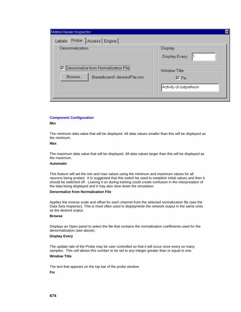
674

Component Configuration Min

The minimum data value that will be displayed. All data values smaller than this will be displayed as the minimum. Max

The maximum data value that will be displayed. All data values larger than this will be displayed as the maximum. Automatic

This feature will set the min and max values using the minimum and maximum values for all neurons being probed. It is suggested that this switch be used to establish initial values and then it should be switched off. Leaving it on during training could create confusion in the interpretation of the data being displayed and it may also slow down the simulation. Denormalize from Normalization File

Applies the inverse scale and offset for each channel from the selected normalization file (see the Data Sets Inspector). This is most often used to display/write the network output in the same units as the desired output. Browse

Displays an Open panel to select the file that contains the normalization coefficients used for the denormalization (see above). Display Every

The update rate of the Probe may be user controlled so that it will occur once every so many samples. This cell allows this number to be set to any integer greater than or equal to one. Window Title

The text that appears on the top bar of the probe window. Fix

675

When this switch is set, the title of the probe window can be fixed to a user-specified string (see "Window Title" above).

Macro Actions

Access

Probe

Probe Macro Actions Overview Superclass Macro Actions

Action Description autoNormalize Returns the "Automatic" setting. dataLength Returns the number of rows of formatted data. dataWidth Returns the number of columns of formatted data. denormalizeFromFile Returns the "Denormalize from Normalization File" setting. displayEvery Returns the "Display Every" setting. fixWindowTitle Returns the "Fix Window Title" setting. getProbeData Returns the probe data as a variant array. maxNormValue Returns the "View Range Max" setting. minNormValue Returns the "View Range Min" setting. normalizationFilePath Returns the normalization file path used for the denormalization. setAutoNormalize Sets the "Automatic" setting. setDenormalizeFromFile Sets the "Denormalize from Normalization File" setting setDisplayEvery Sets the "Display Every" setting. setFixWindowTitle Sets the "Fix Window Title" setting. setMaxNormValue Sets the "View Range Max" setting. setMinNormValue Sets the "View Range Min" setting. SetNormalizationFilePath Sets the normalization file path used for the denormalization.

setWindowTitle Sets the title of the probe window.

676

tileWindow Sizes and positions the probe window based on the position parameters given. tileWindowBelow Sizes and positions the probe window based on the position parameters given and the name of the probe to be placed below. tileWindowNextTo

Sizes and positions the probe window based on the position parameters given and the name of the probe to be placed next to.

windowTitle Returns the title of the probe window.

autoNormalize Overview Macro Actions

Syntax

componentName.autoNormalize()

Parameters Type Description return BOOL When TRUE, the min and max values are automatically determined from the data being probed (see "Automatic" within the Probe Inspector). componentName Name defined on the engine property page.

dataLength Overview Macro Actions

Syntax

componentName.dataLength()

Parameters Type Description return int The number of rows of formatted data. componentName Name defined on the engine property page.

dataWidth Overview Macro Actions

Syntax

componentName.dataWidth()


677

return int The number of columns of formatted data. componentName Name defined on the engine property page.

denormalizeFromFile Overview Macro Actions

Syntax

componentName.denormalizeFromFile()

Parameters Type Description return BOOL When TRUE, the inverse scale and offset is applied to each channel based on the normalization file (see "Denormalize from Normalization File" within the Probe Inspector). componentName Name defined on the engine property page.

displayEvery Overview Macro Actions

Syntax

componentName.displayEvery()

Parameters Type Description return int The update rate of the probe (see "Display Every" within the Probe Inspector). componentName Name defined on the engine property page.

fixWindowTitle Overview Macro Actions

Syntax

componentName.fixWindowTitle()

Parameters Type Description return BOOL When TRUE, the title of the probe window can be fixed to a user-specified string (see "Fix" within the Probe Inspector). componentName Name defined on the engine property page.

getProbeData Overview Macro Actions

Syntax

componentName.getProbeData()

Parameters Type Description return variant Variant array of floating point values containing the data being probed. For static

678

probes, the dimensions of the array are dataWidth by dataLength. For the DataStorage component, the dimensions of the array are dataWidth by dataLength by bufferLength. componentName Name defined on the engine property page.

maxNormValue Overview Macro Actions

Syntax

componentName.maxNormValue()

Parameters Type Description return float The maximum data value that will be displayed (see "Max" within the Probe Inspector). componentName Name defined on the engine property page.

minNormValue Overview Macro Actions

Syntax

componentName.minNormValue()

Parameters Type Description return float The minimum data value that will be displayed (see "Min" within the Probe Inspector). componentName Name defined on the engine property page.

normalizationFilePath Overview Macro Actions

Syntax

componentName.normalizationFilePath()

Parameters Type Description return string The path of the normalization file used for denormalization (see "Denormalize from Normalization File" within the Probe Inspector). componentName Name defined on the engine property page.

setAutoNormalize Overview Macro Actions

679

Syntax

componentName.setAutoNormalize(autoNormalize)

Parameters Type Description return void componentName Name defined on the engine property page . autoNormalize BOOL When TRUE, the min and max values are automatically determined from the data being probed (see "Automatic" within the Probe Inspector).

setDenormalizeFromFile Overview Macro Actions

Syntax

componentName.setDenormalizeFromFile(denormalizeFromFile)

Parameters Type Description return void componentName Name defined on the engine property page. denormalizeFromFile BOOL When TRUE, the inverse scale and offset is applied to each channel based on the normalization file (see "Denormalize from Normalization File" within the Probe Inspector).

setDisplayEvery Overview Macro Actions

Syntax

componentName.setDisplayEvery(displayEvery)

Parameters Type Description return void componentName Name defined on the engine property page. displayEvery int The update rate of the probe (see "Display Every" within the Probe Inspector).

setFixWindowTitle Overview Macro Actions

Syntax

680

componentName.setFixWindowTitle(fixWindowTitle)

Parameters Type Description return void componentName Name defined on the engine property page. fixWindowTitle BOOL When TRUE, the title of the probe window can be fixed to a user-specified string (see "Fix" within the Probe Inspector).

setMaxNormValue Overview Macro Actions

Syntax

componentName.setMaxNormValue(maxNormValue)

Parameters Type Description return void componentName Name defined on the engine property page. maxNormValue float The maximum data value that will be displayed (see "Max" within the Probe Inspector).

setMinNormValue Overview Macro Actions

Syntax

componentName.setMinNormValue(minNormValue)

Parameters Type Description return void componentName Name defined on the engine property page. minNormValue float The minimum data value that will be displayed (see "Min" within the Probe Inspector).


Syntax

componentName.setNormalizationFilePath(normalizationFilePath)

681

Parameters Type Description return void componentName Name defined on the engine property page. normalizationFilePath string The path of the normalization file used for denormalization (see "Denormalize from Normalization File" within the Probe Inspector).

setWindowTitle Overview Macro Actions

Syntax

componentName.setWindowTitle(windowTitle)

Parameters Type Description return void componentName Name defined on the engine property page. windowTitle String The title of the probe window (see "Window Title" of the Probe Inspector page).

tileWindow Overview Macro Actions

Syntax

componentName.tileWindow(probeNumHoriz, totalProbesHoriz, probeNumVert, totalProbesVert)


probeNumHoriz int The horizontal position of the probe window. This value can be between 1 (the left side of the screen) and totalProbesHoriz (the right side of the screen). totalProbesHoriz int The inverse horizontal width of the probe window. A value of 1 would be the width of the entire screen, 2 would be 1/2 of the screen width, 3 would be 1/3 of the screen width, etc. probeNumVert int The vertical position of the probe window. This value can be between 1 (the top of the screen) and totalProbesVert (the bottom of the screen). totalProbesVert int The inverse vertical height of the probe window. A value of 1 would be the height of the entire screen, 2 would be 1/2 of the screen height, 3 would be 1/3 of the screen height, etc.

682

tileWindowBelow Overview Macro Actions

Syntax

componentName.tileWindowBelow(aboveName, probeNum, totalProbes, height)

Parameters Type Description return void componentName Name defined on the engine property page. aboveName string Name of the probe whose window will be directly above this probe window. probeNum int The horizontal position of the probe window. This value can be between 1 (the left side of the screen) and totalProbesHoriz (the right side of the screen). totalProbes int The inverse horizontal width of the probe window. A value of 1 would be the width of the entire screen, 2 would be 1/2 of the screen width, 3 would be 1/3 of the screen width, etc. height int The height as a percentage of the horizontal width. A value of 100 will produce a square window, a value of 200 will produce a rectangular window that is twice as high as it is wide, and a value of 0 will use a default height.

tileWindowNextTo Overview Macro Actions

Syntax

componentName.tileWindowNextTo(nextName, probeNum, totalProbes, height)

Parameters Type Description return void componentName Name defined on the engine property page. nextName string Name of the probe whose window will be directly to the left of this probe window. probeNum int The horizontal position of the probe window. This value can be between 1 (the left side of the screen) and totalProbesHoriz (the right side of the screen). totalProbes int The inverse horizontal width of the probe window. A value of 1 would be the width of the entire screen, 2 would be 1/2 of the screen width, 3 would be 1/3 of the screen width, etc. height int The height as a percentage of the horizontal width. A value of 100 will produce a square window, a value of 200 will produce a rectangular window that is twice as high as it is wide, and a value of 0 will use a default height.

683

windowTitle Overview Macro Actions

Syntax

componentName.windowTitle()

Parameters Type Description return String The title of the probe window (see "Window Title" of the Probe Inspector page). componentName Name defined on the engine property page.

Transformer Family Transformer Family

Ancestor: TemporalProbe Family

The Transformer family is a collection of components that transform temporal data. The data may be transformed into any format. An example of a transform is a periodogram (a spectral estimator based on the Fast Fourier Transform). The results of the transformations are presented as a temporal access point to attached components. The dimensionality of the data at this access point is completely defined by the specific Transformer component.

The actual segment of data used for the transformation is contained within the temporal access point of the component attached below. If the Transformer is attached to a MegaScope (at the Selection access point), then the segment of data is specified by the selection made within the MegaScope’s display window.

Members:

SpectralTransform

Transformer

SpectralTransform

Family: Transformer Family

684

Superclass: Transformer

Description:

The SpectralTransform is used to compute periodograms from temporal data. These periodograms are generated using an averaging of windowed Fast Fourier Transforms (FFT's). The FFT is computed based on a number of parameters (e.g., FFT size, window size, percentage overlap and number of segments). This component is normally used in conjunction with a MegaScope by attaching to its Selection access point to access a segment of the displayed data. This segment is specified by selecting (highlighting) a portion of the MegaScope’s display window.

The problem of spectral estimation is the resolution/stability dilemma. One needs more (averaged) segments to improve the variance of the estimator (which improves with N, the number of segments being averaged). But when doing this for the same spectral resolution (number of points of the FFT) there is a need for more data samples. If there is not enough data, you may need to overlap the segments and/or augment (pad) each data window with zeros. You may have to settle for a worse spectral estimate by decreasing either the FFT size or number of segments.

User Interaction:

Drag and Drop

Inspector

Access Points

Macro Actions

Transformer

Family: Transformer Family

Superclass: Transformer

Description:

The Transformer is a temporal probe that receives a copy of the buffered data sent from the component stacked below, and transforms this data. This transformed data is then used by the component attached to its Transform access point. It is implemented using DLLs, thus requiring that a DLL be loaded within the Engine Inspector property page of the Transformer inspector.

User Interaction:

Drag and Drop

Access Points

685

DLL Implementation

Access Points

Transformer Access Points

Component: Transformer


Transform Access:

This access point is created by all subclasses of the transformer class. It presents the result of the conversion performed by subclasses on temporal data. The dimensions of this access point are completely determined by the subclass.

See Also

DLL Implementation

Transformer DLL Implementation

Component: Transformer

Protocol: PerformTransform

Description:

The Transformer component is used to transform the data sent from the component stacked below, and send the transformed data to the component attached above using the Transform access point. This is a temporal probe meaning that it processes the data stored within the attached DataStorage.

The default DLL implementation of this component simply transforms all of the data to zeros.

Code: BOOL performTransform(

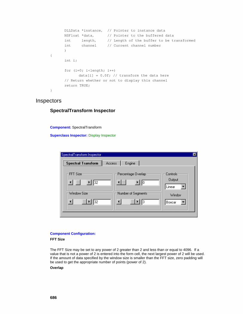
686

DLLData *instance, // Pointer to instance data NSFloat *data, // Pointer to the buffered data int length, // Length of the buffer to be transformed int channel // Current channel number ) { int i; for (i=0; i<length; i++) data[i] = 0.0f; // transform the data here // Return whether or not to display this channel return TRUE; }

Inspectors

SpectralTransform Inspector

Component: SpectralTransform


Component Configuration: FFT Size

The FFT Size may be set to any power of 2 greater than 2 and less than or equal to 4096. If a value that is not a power of 2 is entered into the form cell, the next largest power of 2 will be used. If the amount of data specified by the window size is smaller than the FFT size, zero padding will be used to get the appropriate number of points (power of 2). Overlap

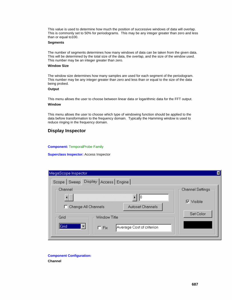
687

This value is used to determine how much the position of successive windows of data will overlap. This is commonly set to 50% for periodograms. This may be any integer greater than zero and less than or equal to100. Segments

The number of segments determines how many windows of data can be taken from the given data. This will be determined by the total size of the data, the overlap, and the size of the window used. This number may be an integer greater than zero. Window Size

The window size determines how many samples are used for each segment of the periodogram. This number may be any integer greater than zero and less than or equal to the size of the data being probed. Output

This menu allows the user to choose between linear data or logarithmic data for the FFT output. Window

This menu allows the user to choose which type of windowing function should be applied to the data before transformation to the frequency domain. Typically the Hamming window is used to reduce ringing in the frequency domain.

Display Inspector

Component: TemporalProbe Family

Superclass Inspector: Access Inspector

Component Configuration: Channel

688

The number of channels (or traces) is determined by the size of the data at the point being probed. Each neuron found at an access point counts as 1 channel.

The "active" channel refers to the channel that appears in the channel form cell. Any adjustments made using the Channel Settings functions will affect only the channel which is "active." (except when the "Change All Channels" switch is set)

The channel may be selected by one of three methods. Clicking on the left or right arrow button will decrement or increment the active channel one at a time. The channel slider may be used to scan through all the possible channels. Finally, a specific channel number may be entered directly into the channel form cell.

Once the "active" channel has been selected, the inspector will display the specific settings for that channel. Change All Channels

This switch allows all the channels parameters to be set concurrently. When this switch is set, adjusting any of the "Channel Settings" will affect all channels. Autoset Channels

Clicking on the autoset channels button will cause several operations to be performed on the settings of the visible channels. These operations include scaling, positioning, and setting the color.

Each of the visible channels is scaled and positioned so that each can be observed while not interfering with the others. The color of each channel is also set uniquely. Grid

The None/Lines/Grid pull down menu allows the view to be segmented into 10 equal divisions. These divisions are used by the scaling and position to determine a relative placement of the data. Visible

This is a switch (toggle) that makes the current channel appear in the view. Set Color

The color may be set by activating the color panel and choosing a color. To activate the color panel click once on the Set Color button. When the color panel appears, select the color of your preference. The color of the view will change accordingly. Window Title

The text that appears on the top bar of the probe window. Fix

When this switch is set, the title of the probe window can be fixed to a user-specified string (see "Window Title" above).

689

Drag and Drop

Macro Actions

Spectral Transform

SpectralTransform Macro Actions Overview Superclass Macro Actions

Action Description fftSize Returns the "FFT Size" setting. linear Returns TRUE if the output is "Linear", FALSE if the output is "Log". overlap Returns the "Percentage Overlap" setting. segments Returns the "Number of Segments" setting. setFFTSize Sets the "FFT Size" setting. setLinear Set to TRUE if the output is "Linear", FALSE if the output is "Log". setOverlap Sets the "Percentage Overlap" setting. setSegments Sets the "Number of Segments" setting. setWindowSize Sets the "Window Size" setting. windowSize Returns the "Window Size" setting.

fftSize Overview Macro Actions

Syntax

componentName. fftSize()

Parameters Type Description return int This value may be any power of 2 greater than 2 and less than or equal to 4096 (see "FFT Size" within the SpectralTransform Inspector). componentName Name defined on the engine property page.

linear Overview Macro Actions

Syntax

690

componentName. linear()

Parameters Type Description return BOOL TRUE if the output is "Linear and FALSE if the output is "Log" (see "Output" within the SpectralTransform Inspector). componentName Name defined on the engine property page.

overlap Overview Macro Actions

Syntax

componentName. overlap()

Parameters Type Description return int The value used to determine how much the position of successive windows of data will overlap (see "Overlap" within the SpectralTransform Inspector). componentName Name defined on the engine property page.

segments Overview Macro Actions

Syntax

componentName. segments()

Parameters Type Description return int The number of windows of data that can be taken from the probed data (see "Segments" within the SpectralTransform Inspector). componentName Name defined on the engine property page.

setFFTSize Overview Macro Actions

Syntax

componentName. setFFTSize(fftSize)

Parameters Type Description return void componentName Name defined on the engine property page. fftSize int This value may be any power of 2 greater than 2 and less than or equal to 4096. If the value is not a power of 2, the next largest power of 2 will be used (see "FFT Size" within the

691

SpectralTransform Inspector).

setLinear Overview Macro Actions

Syntax

componentName. setLinear(linear)

Parameters Type Description return void componentName Name defined on the engine property page. linear BOOL TRUE if the output is "Linear and FALSE if the output is "Log" (see "Output" within the SpectralTransform Inspector).

setOverlap Overview Macro Actions

Syntax

componentName. setOverlap(overlap)

Parameters Type Description return void componentName Name defined on the engine property page. overlap int The value used to determine how much the position of successive windows of data will overlap (see "Overlap" within the SpectralTransform Inspector).

setSegments Overview Macro Actions

Syntax

componentName. setSegments(segments)

Parameters Type Description return void componentName Name defined on the engine property page. segments int The number of windows of data that can be taken from the probed data (see "Segments" within the SpectralTransform Inspector).

692

setWindowSize Overview Macro Actions

Syntax

componentName. setWindowSize(windowSize)

Parameters Type Description return void componentName Name defined on the engine property page. windowSize int The number of samples are used for each segment of the periodogram (see "Window Size" within the SpectralTransform Inspector).

windowSize Overview Macro Actions

Syntax

componentName. windowSize()

Parameters Type Description return int The number of samples are used for each segment of the periodogram (see "Window Size" within the SpectralTransform Inspector). componentName Name defined on the engine property page.

Access

Schedule Family ExpScheduler

Family: Schedule Family

Superclass: NSSchedule

Description:

693

The ExpScheduler receives a parameter and modifies it exponentially (either using an increasing or decreasing value) during a predetermined number of epochs. It has a maximum and minimum constraint that will be met at all times during the scheduling operation.

Schedule Equation:

User Interaction:

Drag and Drop

Inspector

Access Points

DLL Implementation

See Also

LinearScheduler



Description:

The linear scheduler receives a parameter and modifies it linearly (increase or decrease) during a predetermined number of epochs. It has a maximum and minimum constraint that will be met at all times during the scheduling operation.

Schedule Equation:

694

User Interaction:

Drag and Drop

Inspector

Access Points

DLL Implementation

See Also

LogScheduler



Description:

The LogScheduler receives a parameter and modifies it logarithmically (either using an increasing or decreasing value) during a predetermined number of epochs. It has a maximum and minimum constraint that will be met at all times during the scheduling operation.

Schedule Equation:

User Interaction:

Drag and Drop

Inspector

Access Points

DLL Implementation

695

See Also

DLL Implementation

ExpScheduler DLL Implementation

Component: ExpScheduler

Protocol: PerformScheduler

Description:

This function is called after each epoch that has scheduling active (specified by the user within the Scheduler inspector). It simply multiplies each PE within data by beta and copies the result back into data. Note that the component itself handles the clipping if the data exceeds the boundaries specified by the user.

Code: BOOL performScheduler( DLLData *instance, // Pointer to instance data (may be NULL) NSFloat *data, // Pointer to the data to be scheduled int length, // Number of elements in scheduled data vector NSFloat beta // Scheduler parameter (specified by user) ) { int i; for (i=0; i<length; i++) data[i] = beta*data[i]; }

LinearScheduler DLL Implementation

696

Component: LinearScheduler


Description:

This function is called after each epoch that has scheduling active (specified by the user within the Scheduler inspector). It simply increments each PE within data by beta. Note that the component itself handles the clipping if the data exceeds the boundaries specified by the user.

Code: BOOL performScheduler( DLLData *instance, // Pointer to instance data (may be NULL) NSFloat *data, // Pointer to the data to be scheduled int length, // Number of elements in scheduled data vector NSFloat beta // Scheduler parameter (specified by user) ) { int i; for (i=0; i<length; i++) data[i] += beta; }

LogScheduler DLL Implementation

Component: LogScheduler


Description:

This function is called after each epoch that has scheduling active (specified by the user within the Scheduler inspector). It simply decrements each PE within data by beta over data. Note that the component itself handles the clipping if the data exceeds the boundaries specified by the user.

Code: BOOL performScheduler( DLLData *instance, // Pointer to instance data (may be NULL) NSFloat *data, // Pointer to the data to be scheduled

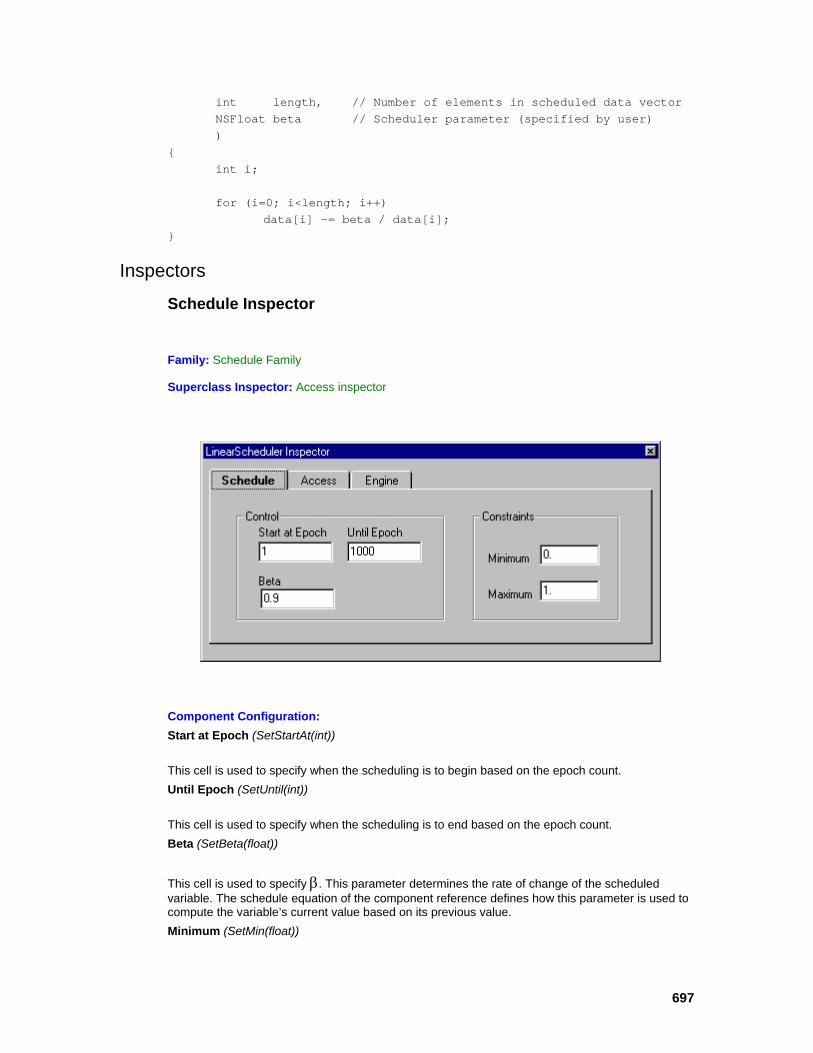
697

int length, // Number of elements in scheduled data vector NSFloat beta // Scheduler parameter (specified by user) ) { int i; for (i=0; i<length; i++) data[i] -= beta / data[i]; }

Inspectors

Schedule Inspector



Component Configuration: Start at Epoch (SetStartAt(int))

This cell is used to specify when the scheduling is to begin based on the epoch count. Until Epoch (SetUntil(int))

This cell is used to specify when the scheduling is to end based on the epoch count. Beta (SetBeta(float))

This cell is used to specify β. This parameter determines the rate of change of the scheduled variable. The schedule equation of the component reference defines how this parameter is used to compute the variable’s current value based on its previous value. Minimum (SetMin(float))

698

The cell specifies the minimum value at which the scheduled variable will be set. Maximum (SetMax(float))

The cell specifies the maximum value at which the scheduled variable will be set.

Drag and Drop

Access Points

Macro Actions

Scheduler

Scheduler Macro Actions Overview Superclass Macro Actions

Action Description beta Returns the "Beta" (β) setting. maximum Returns the "Maximum" setting. minimum Returns the "Minimum" setting. setBeta Sets Returns the "Beta" (β) setting. setMaximum Sets the "Maximum" setting. setMinimum Sets the "Minimum" setting. setStart Sets the "Start at Epoch" setting. setStop Sets the "Until Epoch" setting. start Returns the "Start at Epoch" setting. stop Returns the "Until Epoch" setting.


Syntax

componentName. beta()

Parameters Type Description return float The rate of change of the scheduled variable, or β (see "Beta" within the Schedule Inspector). componentName Name defined on the engine property page.

699

maximum Overview Macro Actions

Syntax

componentName. maximum()

Parameters Type Description return float The maximum value at which the scheduled variable will be set (see "Maximum" within the Schedule Inspector ). componentName Name defined on the engine property page.

minimum Overview Macro Actions

Syntax

componentName. minimum()

Parameters Type Description return float The minimum value at which the scheduled variable will be set (see "Minimum" within the Schedule Inspector). componentName Name defined on the engine property page.


Syntax

componentName. setBeta(beta)

Parameters Type Description return void componentName Name defined on the engine property page. beta float The rate of change of the scheduled variable, or β (see "Beta" within the Schedule Inspector).

setMaximum Overview Macro Actions

Syntax

componentName. setMaximum(maximum)

700

Parameters Type Description return void componentName Name defined on the engine property page. maximum float The maximum value at which the scheduled variable will be set (see "Maximum" within the Schedule Inspector ).

setMinimum Overview Macro Actions

Syntax

componentName. setMinimum(minimum)

Parameters Type Description return void componentName Name defined on the engine property page. minimum float The minimum value at which the scheduled variable will be set (see "Minimum" within the Schedule Inspector).

setStart Overview Macro Actions

Syntax

componentName. setStart(start)

Parameters Type Description return void componentName Name defined on the engine property page. start int The number of epochs to run before the scheduling begins (see "Start at Epoch" within the Schedule Inspector).

setStop Overview Macro Actions

Syntax

componentName. setStop(stop)


701

stop int The number of epochs to run before the scheduling ends (see "Until Epoch" within the Schedule Inspector).

start Overview Macro Actions

Syntax

componentName. start()

Parameters Type Description return int The number of epochs to run before the scheduling begins (see "Start at Epoch" within the Schedule Inspector). componentName Name defined on the engine property page.

stop Overview Macro Actions

Syntax

componentName. stop()

Parameters Type Description return int The number of epochs to run before the scheduling ends (see "Until Epoch" within the Schedule Inspector). componentName Name defined on the engine property page.

Access

Transmitter Family ControlTransmitter Family

ControlTransmitter Family

Ancestor: Transmitter Family

The ControlTransmitter family provides the ability to transmit control messages to components on the breadboard. Members of the ControlTransmitter family monitor the data at the access point of the attached component. When the data meets the set of conditions specified by the ControlTransmitter, it will send one or more control messages to one or more components on the breadboard.

702

The action taken for a particular message is determined by the receiving components. This enables a component to have an outside source control its actions during an experiment.

Members:

ThresholdTransmitter

DeltaTransmitter

DeltaTransmitter

Family: ControlTransmitter Family

Superclass: ThresholdTransmitter

Description:

The DeltaTransmitter sends control messages to other network components on the breadboard based on the change in the data of the attached component from one iteration to the next. The control messages are sent when the change in the data between successive iterations crosses a specified threshold. There are several ways to specify this boundary based on the type and value of the threshold and the filtering performed on the accessed data. The threshold can be specified to move (i.e., incremented, decremented, or scaled by a constant) each time the boundary is crossed.

User Interaction:

Drag and Drop

Inspector

Access Points

ThresholdTransmitter

Family: ControlTransmitter Family

Superclass: Transmitter

703

Description:

The ThresholdTransmitter sends control messages to other network components on the breadboard based on the data of the attached component. The control messages are sent when the data crosses a specified threshold. There are several ways to specify this boundary based on the type and value of the threshold and the filtering performed on the accessed data. The threshold can be specified to move (i.e., incremented, decremented, or scaled by a constant) each time the boundary is crossed.

User Interaction:

Drag and Drop

Inspector

Access Points

DLL Implementation

Macro Actions

Access Points

ThresholdTransmitter Access Points

Component: ThresholdTransmitter

Superclass: Access Points

Weighted Average Access:

The Weighted Average Access reports the output of the smoothing filter used to estimate the point at which the threshold is crossed. The smoothing filter is constructed using parameters defined in the ThresholdTransmitter Inspector

Threshold Access:

This provides access to the value of threshold used to initiate message transmission. This value may be adapted during training by using a Scheduler.

See Also

DLL Implementation

ThresholdTransmitter DLL Implementation

704


Protocol: PerformThresholdTransmitter

Description:

The ThresholdTransmitter sends control messages to other network compo nents on the breadboard based on the data of the attached component. The con trol messages are sent when the function below returns a YES. This function scans through the data and returns a YES if the data has crossed the threshold specifications contained within the last three parameters. Otherwise, the function returns a NO.

Code: BOOL performThresholdTransmitter( DLLData *instance, // Pointer to instance data (may be NULL) NSFloat *data, // Pointer to the data at the access point int rows, // Number of rows of PEs in the layer int cols, // Number of columns of PEs in the layer NSFloat threshold, // Threshold specified by user BOOL lessThan, // Less than/greater than state (user-specified) int type // Threshold type, 0=All 1=One 2=Average ) { int length=rows*cols; switch (type) { case 0: if (lessThan) return allLessThan(data,length,threshold); return !oneLessThan(data,length,threshold); break; case 1: if (lessThan) return oneLessThan(data,length,threshold); return !allLessThan(data,length,threshold); break; case 2: if (lessThan) return averageLessThan(data,length,threshold); return !averageLessThan(data,length,threshold); break; } return NO; } BOOL oneLessThan(NSFloat *data, int length, NSFloat threshold) {

705

register int i; for (i=0; i<length; i++) if (data[i] < threshold) return YES; return NO; } BOOL allLessThan(NSFloat *data, int length, NSFloat threshold) { register int i; for (i=0; i<length; i++) if (data[i] > threshold) return NO; return YES; } BOOL averageLessThan(NSFloat *data, int length, NSFloat threshold) { register int i; register NSFloat average = (NSFloat)0.0; for (i=0; i<length; i++) average += data[i]; return (average /= length) < threshold; }

Inspectors

ThresholdTransmitter Inspector


Superclass Inspector: Transmitter Inspector

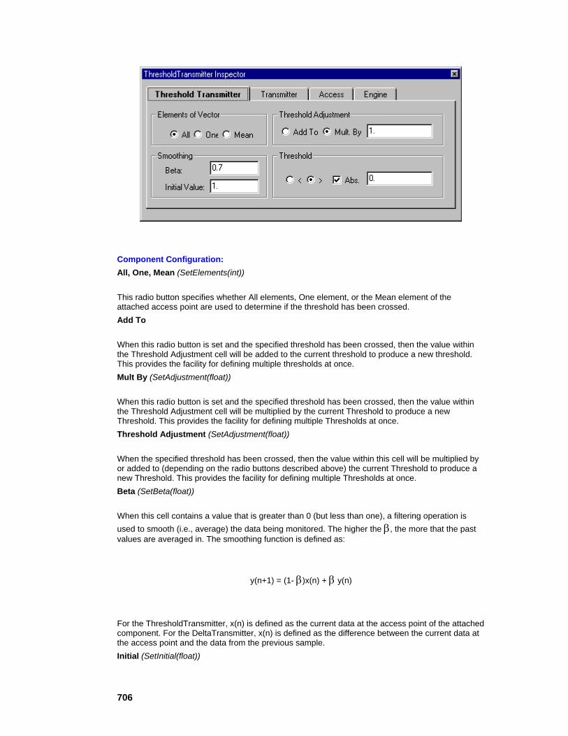
706

Component Configuration: All, One, Mean (SetElements(int))

This radio button specifies whether All elements, One element, or the Mean element of the attached access point are used to determine if the threshold has been crossed. Add To

When this radio button is set and the specified threshold has been crossed, then the value within the Threshold Adjustment cell will be added to the current threshold to produce a new threshold. This provides the facility for defining multiple thresholds at once. Mult By (SetAdjustment(float))

When this radio button is set and the specified threshold has been crossed, then the value within the Threshold Adjustment cell will be multiplied by the current Threshold to produce a new Threshold. This provides the facility for defining multiple Thresholds at once. Threshold Adjustment (SetAdjustment(float))

When the specified threshold has been crossed, then the value within this cell will be multiplied by or added to (depending on the radio buttons described above) the current Threshold to produce a new Threshold. This provides the facility for defining multiple Thresholds at once. Beta (SetBeta(float))

When this cell contains a value that is greater than 0 (but less than one), a filtering operation is used to smooth (i.e., average) the data being monitored. The higher the β, the more that the past values are averaged in. The smoothing function is defined as:

y(n+1) = (1- β)x(n) + β y(n)

For the ThresholdTransmitter, x(n) is defined as the current data at the access point of the attached component. For the DeltaTransmitter, x(n) is defined as the difference between the current data at the access point and the data from the previous sample. Initial (SetInitial(float))

707

This cell specifies y(0), the initial value of the filtering operation (see above). <, > (SetLessThan(bool))

These radio buttons specify whether the crossing occurs when the data is greater than or less than the Threshold value. Abs (SetAbs(bool))

When this switch is on, the threshold is based on the absolute value of the data. Threshold (SetThreshold(float))

This cell is used to specify the initial value of the threshold. This value may change during the course of the simulation using the Threshold Adjustment parameters described above.

Macro Actions

Threshold Transmitter

ThresholdTransmitter Macro Actions Overview Superclass Macro Actions

Action Description absoluteValue Returns the "Abs." setting. beta Returns the "Beta" setting. initialValue Returns the "Initial Value" setting. lessThan Returns TRUE if the crossing occurs when the data is less than the Threshold value and FALSE if the crossing occurs when the data is greater than the Threshold value. multBy Returns TRUE if the "Mult. By" switch is on and FALSE if the "Add To" switch is on. setAbsoluteValue Sets the "Abs." setting. setBeta Sets the "Beta" setting. setInitialValue Sets the "Initial Value" setting. setLessThan Set to TRUE if the crossing occurs when the data is less than the Threshold value and FALSE if the crossing occurs when the data is greater than the Threshold value. setMultBy Set to TRUE to turn the "Mult. By" switch on and FALSE to turn the "Add To" switch on. setThreshold Sets the "Threshold" setting. setThresholdDecay Sets the "Threshold Adjustment" setting. setThresholdType Sets the "Elements of Vector" setting (0 = "All", 1 = "One", 2 = "Average"). threshold Returns the "Threshold" setting.

708

thresholdDecay Returns the "Threshold Adjustment" setting. thresholdType Returns the "Elements of Vector" setting (0 = "All", 1 = "One", 2 = "Average").

absoluteValue Overview Macro Actions

Syntax

componentName. absoluteValue()

Parameters Type Description return BOOL TRUE if the threshold is based on the absolute value of the data (see "Abs." within the ThresholdTransmitter Inspector). componentName Name defined on the engine property page.


Syntax


Parameters Type Description return float The smoothing factor of the filtering operation (see "Beta" within the ThresholdTransmitter Inspector). componentName Name defined on the engine property page.

initialValue Overview Macro Actions

Syntax

componentName. initialValue()

Parameters Type Description return float Specifies y(0), the initial value of the filtering operation (see "Initial Value" within the ThresholdTransmitter Inspector). componentName Name defined on the engine property page.

lessThan Overview Macro Actions

709

Syntax

componentName. lessThan()

Parameters Type Description return int TRUE specifies that crossing occurs when the data is less than the Threshold value and FALSE specifies that crossing occurs when the data is greater than the Threshold value (see "<,>" within the ThresholdTransmitter Inspector). componentName Name defined on the engine property page.

multBy Overview Macro Actions

Syntax

componentName. multBy()

Parameters Type Description return BOOL When TRUE and the specified threshold has been crossed, then the Threshold Adjustment value will be multiplied by the current Threshold to produce a new Threshold. When FALSE and the specified threshold has been crossed, then the Threshold Adjustment value will be added to the current Threshold to produce a new Threshold. (see "Mult By" and "Add to" within the ThresholdTransmitter Inspector). componentName Name defined on the engine property page.

setAbsoluteValue Overview Macro Actions

Syntax

componentName. setAbsoluteValue(absoluteValue)

Parameters Type Description return void componentName Name defined on the engine property page. absoluteValue BOOL TRUE if the threshold is based on the absolute value of the data (see "Abs." within the ThresholdTransmitter Inspector).


Syntax


710

Parameters Type Description return void componentName Name defined on the engine property page. beta float The smoothing factor of the filtering operation (see "Beta" within the ThresholdTransmitter Inspector).

setInitialValue Overview Macro Actions

Syntax

componentName. setInitialValue(initialValue)

Parameters Type Description return void componentName Name defined on the engine property page. initialValue float Specifies y(0), the initial value of the filtering operation (see "Initial Value" within the ThresholdTransmitter Inspector).

setLessThan Overview Macro Actions

Syntax

componentName. setLessThan(lessThan)

Parameters Type Description return void componentName Name defined on the engine property page. lessThan int TRUE specifies that crossing occurs when the data is less than the Threshold value and FALSE specifies that crossing occurs when the data is greater than the Threshold value (see "<,>" within the ThresholdTransmitter Inspector).

setMultBy Overview Macro Actions

Syntax

componentName. setMultBy(multBy)


711

componentName Name defined on the engine property page. multBy BOOL When TRUE and the specified threshold has been crossed, then the Threshold Adjustment value will be multiplied by the current Threshold to produce a new Threshold. When FALSE and the specified threshold has been crossed, then the Threshold Adjustment value will be added to the current Threshold to produce a new Threshold. (see "Mult By" and "Add to" within the ThresholdTransmitter Inspector).

setThreshold Overview Macro Actions

Syntax

componentName. setThreshold(threshold)

Parameters Type Description return void componentName Name defined on the engine property page. threshold float The threshold value (see "Threshold" within the ThresholdTransmitter Inspector).

setThresholdDecay Overview Macro Actions

Syntax

componentName. setThresholdDecay(thresholdDecay)

Parameters Type Description return void componentName Name defined on the engine property page. thresholdDecay float The amount to muliply by or add to the Threshold value when the threshold has been crossed (see "Threshold Adjustment" within the ThresholdTransmitter Inspector).

setThresholdType Overview Macro Actions

Syntax

componentName. setThresholdType(thresholdType)


712

thresholdType int Specifies whether All elements, One element, or the Mean element of the attached access point are used to determine if the threshold has been crossed (0 = "All", 1 = "One", 2 = "Average" -- see "All, One, Mean" within the ThresholdTransmitter Inspector).

threshold Overview Macro Actions

Syntax

componentName. threshold()

Parameters Type Description return float The threshold value (see "Threshold" within the ThresholdTransmitter Inspector). componentName Name defined on the engine property page.

thresholdDecay Overview Macro Actions

Syntax

componentName. thresholdDecay()

Parameters Type Description return float The amount to muliply by or add to the Threshold value when the threshold has been crossed (see "Threshold Adjustment" within the ThresholdTransmitter Inspector). componentName Name defined on the engine property page.

thresholdType Overview Macro Actions

Syntax

componentName. thresholdType()

Parameters Type Description return int Specifies whether All elements, One element, or the Mean element of the attached access point are used to determine if the threshold has been crossed (0 = "All", 1 = "One", 2 = "Average" -- see "All, One, Mean" within the ThresholdTransmitter Inspector). componentName Name defined on the engine property page.

713

DataTransmitters Family

DataTransmitter Family

Ancestor: Transmitter Family

DataTransmitters provide a means of globally transmitting data between various network access points. This is most often used as a means of displaying data from separate network locations within the same probe window.

Members:

DataStorageTransmitter

DataStorageTransmitter

Family: DataTransmitter Family

Superclass: Transmitter

Description:

The DataStorageTransmitter acts as a remote data collector for one or more DataStorage components. A single DataStorage component can collect data from a number of DataStorageTransmitters placed anywhere on the breadboard. This feature is useful when comparing the signals of various points of the network by displaying all of the data within the same probe window.

As the DataStorageTransmitter accesses the data of its attached component, this data is transmitted to the DataStorage components. Each DataStorage component uses this transmitted data as if it were obtained from additional channels of its attached component.

Note that there is a limitation to the use of the DataStorageTransmitter. A DataStorageTransmitter will not work properly if a DataStorage component is accessing its data at a different interval than that which the DataStorageTransmitter is receiving.

User Interaction:

Drag and Drop

Inspector

Access Points

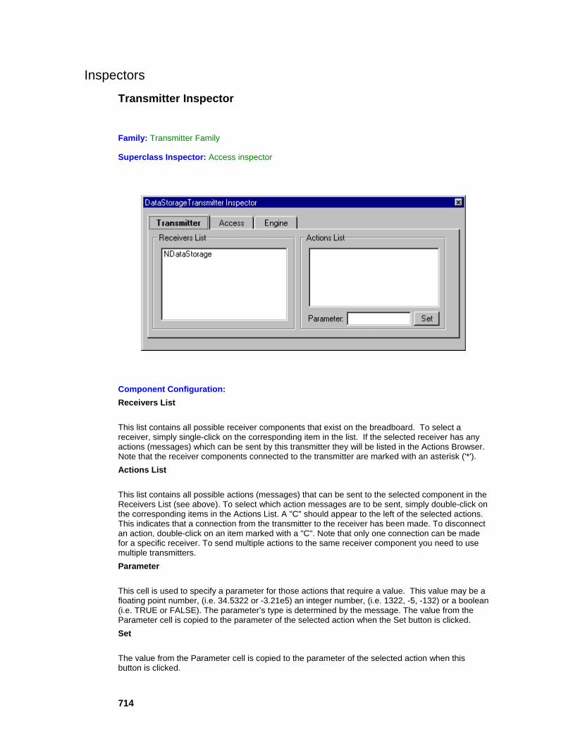
714

Inspectors

Transmitter Inspector

Family: Transmitter Family


Component Configuration: Receivers List

This list contains all possible receiver components that exist on the breadboard. To select a receiver, simply single-click on the corresponding item in the list. If the selected receiver has any actions (messages) which can be sent by this transmitter they will be listed in the Actions Browser. Note that the receiver components connected to the transmitter are marked with an asterisk ('*'). Actions List

This list contains all possible actions (messages) that can be sent to the selected component in the Receivers List (see above). To select which action messages are to be sent, simply double-click on the corresponding items in the Actions List. A "C" should appear to the left of the selected actions. This indicates that a connection from the transmitter to the receiver has been made. To disconnect an action, double-click on an item marked with a "C". Note that only one connection can be made for a specific receiver. To send multiple actions to the same receiver component you need to use multiple transmitters. Parameter

This cell is used to specify a parameter for those actions that require a value. This value may be a floating point number, (i.e. 34.5322 or -3.21e5) an integer number, (i.e. 1322, -5, -132) or a boolean (i.e. TRUE or FALSE). The parameter’s type is determined by the message. The value from the Parameter cell is copied to the parameter of the selected action when the Set button is clicked. Set

The value from the Parameter cell is copied to the parameter of the selected action when this button is clicked.

715

Drag and Drop

Access Points

Transmitter Macro Actions

Transmitter Macro Actions Overview Superclass Macro Actions

Action Description toggleConnection Connects or disconnects the specified action of the specified component. setParameter Sets a parameter for those actions that require a value.

toggleConnection Overview Macro Actions

Syntax

componentName. toggleConnection(name, action)

Parameters Type Description return BOOL TRUE if the action is connected upon completion and FALSE if it is not. componentName Name defined on the engine property page. name string The name of the component to connect to (see "Receivers List" within the Transmitter Inspector ). action string The action (function name) to connect to (see "Actions List" within the Transmitter Inspector ).

setParameter Overview Macro Actions

Syntax

componentName. setParameter(name, action, parameter)


name string The name of the component to connect to (see "Receivers List" within the Transmitter Inspector ). action string The action (function name) to connect to (see "Actions List" within the

716

Transmitter Inspector ).

parameter string The parameter associated with the specified component and action (see "Parameter" within the Transmitter Inspector ).

Unsupervised Family HebbianFull

Family: Unsupervised Family

Superclass: NSUnsupervised

Description:

Hebbian learning adjusts a synapse's weights such that its output reflects its familiarity with an input. The more probable an input, the larger the output will become, at least on average. Unfortunately, plain Hebbian learning continually strengthens its weights without bound (unless the input data is properly normalized). There are only a few applications for plain Hebbian learning; however, almost every unsupervised and competitive learning procedure can be considered Hebbian in nature.

The HebbianFull component adapts its weights according to either the plain Hebbian or forced Hebbian learning rules. In forced Hebbian, the output of the component is substituted by a desired response for the purpose of weight update. The desired response is accepted via an access point. Forced Hebbian learning is clearly not an unsupervised routine, but in the context of data flow and control it fits nicely into the unsupervised family. This type of learning has been applied to heteroassociation.

Anti-Hebbian learning is simply Hebbian with a negative step size, h. It is interesting to note that the least mean squares (LMS) adaptation procedure, which is commonly used in engineering, is simply the sum of anti-Hebbian and forced Hebbian learning.

Weight Update Function: Plain Hebbian:

717

Forced Hebbian:

User Interaction:

Drag and Drop

Inspector

Access Points

DLL Implementation

OjasFull



Description:

Oja's unsupervised learning is simply a procedure for plain Hebbian learning with constrained weight vector growth. This procedure adds a weight decay proportional to the output squared. Oja's rule finds a unit weight vector that maximizes the mean square output. For zero mean data this is equivalent to principal component analysis.

Weight Update Function:

718

where xj is the input, yi is the output, O is the set of all output indices, wij the weight and h the step size.

User Interaction:

Drag and Drop

Inspector

Access Points

DLL Implementation

SangersFull



Description:

Sanger's unsupervised learning is simply a procedure for plain Hebbian learning with constrained weight vector growth. This learning procedure is known to perform principal component analysis. Furthermore, the principal components are extracted in order, with respect to the output unit ordering.


User Interaction:

Drag and Drop

Inspector

719

Access Points

DLL Implementation

SVMInputSynapse



Description:

This component is used to implement the "RBF Dimensionality Expansion" segment of the Support Vector Machine model.

User Interaction:

Drag and Drop

Inspector

Access Points

Competitive Family

StandardFull

Family: Competitive Family

Superclass: NSCompetitive

720

Description:

The StandardFull is a component that implements competitive learning. The weights of a single winning neuron will be moved towards the input.


i* = maxi (yi)

User Interaction:

Drag and Drop

Inspector

Access Points

DLL Implementation

ConscienceFull

Family: Competitive Family

Superclass: Standard

Description:

The ConscienceFull is a special type of competitive learning that keeps track of how often the outputs win the competition with the goal of equilibrating the winnings (i.e., each unit in a set of N will win the competition 1/N on average). This implements a second level of competition among the elements to determine which PE is going to be updated. It avoids the common occurrence in competitive learning that one element (or a subset) may always win the competition.


721

where b is a bias vector created by the conscience mechanism. The bias for each output is computed based upon the output’s frequency of winning,

Here Γ is a parameter on the inspector that controls the amount of bias to apply, K is the number of

outputs, and is the output’s frequency of winning. Running frequency estimates are given by,

where β is a smoothing parameter also set by the component’s inspector.

User Interaction:

Drag and Drop

Inspector

Access Points

DLL Implementation

Macro Actions

Access Points

ConscienceFull Access Points

Component: ConscienceFull

Superclass: Unsupervised Access Points

Bias Access:

This Access point the bias that each processing element has against it’s winning the competition.

Frequency Access:

The current estimate of how often each PE is winning the competition.

722

DLL Implementation

Competitive DLL Implementation

Components: StandardFull, ConscienceFull

Protocol: PerformCompetitive

Description:

The StandardFull and ConscienceFull components implement competitive learning. The ConscienceFull component differs from the StandardFull in that the former adds a bias (i.e., a "conscience") to the competition with the goal of equilibrating the winnings. Note that this second level of competition is performed by the ConscienceFull component to determine the winner, and is not part of code below. This code updates the weights that are connected to the winning output PE.

Code: void performCompetitive( DLLData *instance, // Pointer to instance data (may be NULL) NSFloat *input, // Pointer to the input layer of PEs int inRows, // Number of rows of PEs in the input layer int inCols, // Number of columns of PEs in the input layer NSFloat *output, // Pointer to the output layer int outRows, // Number of rows of PEs in the output layer int outCols // Number of columns of PEs in the output layer NSFloat *weights // Pointer to the fully-connected weight matrix NSFloat step // Learning rate int winner // Index of winning PE ) { int i, inCount=inRows*inCols, outCount=outRows*outCols; for (i=0; i<inCount; i++) W(winner,i) += step*(input[i] - W(winner,i)); }

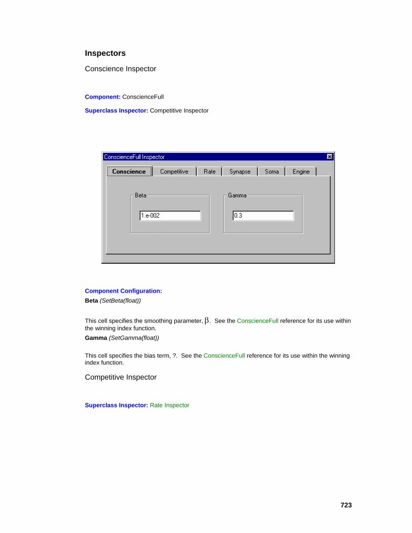
723

Inspectors

Conscience Inspector

Component: ConscienceFull

Superclass Inspector: Competitive Inspector

Component Configuration: Beta (SetBeta(float))

This cell specifies the smoothing parameter, β. See the ConscienceFull reference for its use within the winning index function. Gamma (SetGamma(float))

This cell specifies the bias term, ?. See the ConscienceFull reference for its use within the winning index function.

Competitive Inspector

Superclass Inspector: Rate Inspector

724

Component Configuration: Metric

This pull-down menu is used to select the distance metric used by the competitive algorithm. See the Competitive Family reference for a summary of the available metrics.

Macro Actions

Competitive Full

CompetitiveFull Macro Actions Overview Superclass Macro Actions

Action Description setMetric Sets the "Metric" setting. metric Returns the "Metric" setting.

metric Overview Macro Actions

Syntax

componentName. metric()

Parameters Type Description return int The distance metric used by the competitive algorithm (0 = " Dot Product", 1 = " Euclidean", 2 = " Box Car" -- see "Metric" within the Competitive Inspector ). componentName Name defined on the engine property page.

setMetric Overview Macro Actions

725

Syntax

componentName. setMetric(metric)


metric int The distance metric used by the competitive algorithm (0 = " Dot Product", 1 = " Euclidean", 2 = " Box Car" -- see "Metric" within the Competitive Inspector ).

Conscience Full

ConscienceFull Macro Actions Overview Superclass Macro Actions

Action Description

beta Returns the smoothing parameter, β.

gamma Returns the bias term, γ.

setBeta Sets the smoothing parameter, β.

setGamma Sets the bias term, γ.


Syntax



return float The smoothing parameter, β (see "Beta" within the ConscienceFull Inspector). componentName Name defined on the engine property page.

gamma Overview Macro Actions

Syntax

componentName. gamma()

726


return float The bias term, γ (see "Gamma" within the ConscienceFull Inspector). componentName Name defined on the engine property page.


Syntax



beta float The smoothing parameter, β (see "Beta" within the ConscienceFull Inspector).

setGamma Overview Macro Actions

Syntax

componentName. setGamma(gamma)


gamma float The bias term, γ (see "Gamma" within the ConscienceFull Inspector).

Kohonen Family

DiamondKohonen

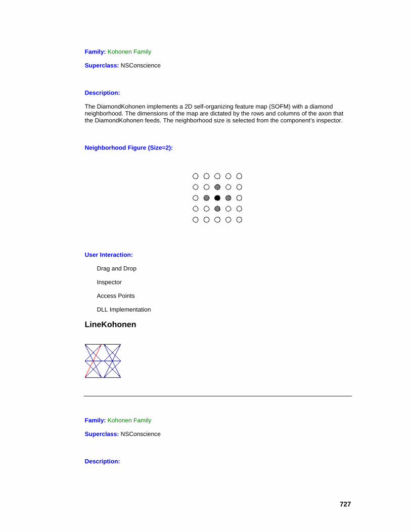
727

Family: Kohonen Family

Superclass: NSConscience

Description:

The DiamondKohonen implements a 2D self-organizing feature map (SOFM) with a diamond neighborhood. The dimensions of the map are dictated by the rows and columns of the axon that the DiamondKohonen feeds. The neighborhood size is selected from the component’s inspector.

Neighborhood Figure (Size=2):

User Interaction:

Drag and Drop

Inspector

Access Points

DLL Implementation

LineKohonen



Description:

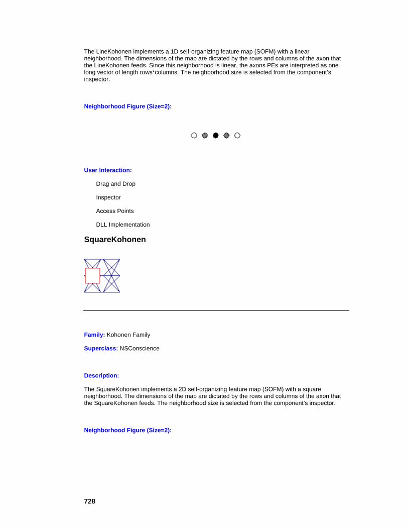
728

The LineKohonen implements a 1D self-organizing feature map (SOFM) with a linear neighborhood. The dimensions of the map are dictated by the rows and columns of the axon that the LineKohonen feeds. Since this neighborhood is linear, the axons PEs are interpreted as one long vector of length rows*columns. The neighborhood size is selected from the component’s inspector.


User Interaction:

Drag and Drop

Inspector

Access Points

DLL Implementation

SquareKohonen



Description:

The SquareKohonen implements a 2D self-organizing feature map (SOFM) with a square neighborhood. The dimensions of the map are dictated by the rows and columns of the axon that the SquareKohonen feeds. The neighborhood size is selected from the component’s inspector.


729

User Interaction:

Drag and Drop

Inspector

Access Points

DLL Implementation

Access Points

Kohonen Access Points


Superclass: ConscienceFull Access Points

Neighborhood Radius Access:

The size of the Neighborhood currently being used. This value may be adapted during training by using a Scheduler.

Component Plane Access:

This access point allows you to view only the weights from a single input (from the multi-dimensional input vector) to all the PEs, in order to see how that input varies from cluster to cluster. For example, if there are regions in the Self-Organizing Map (SOM) where the weights for a particular input are very high, then we can say that all the inputs clustered in that PE have a high value for that input. If all of the values for a particular input are approximately the same, then this particular input has no influence on the clustering. Note that the plane number is selected from the Kohonen inspector page.

Frequency Access: When evaluating the clustering in a Self-Organizing Map (SOM) it is important to understand the mapping done. Typically, the number of SOM PEs is much larger than the number of clusters expected. This allows multiple PEs to capture one logical cluster. What you expect to see in the SOM map is groups of PEs representing a single cluster of the input. The question is how to determine where the clusters are in your SOM. This access point provides a histogram of win frequencies, which gives information to help determine the clustering.

You can think of the SOM as stretching its 2-D grid of PEs over the range of inputs (input space). Inside a cluster, the PEs will be close together since all the inputs in that area are similar. Often times you will have "dead PEs" that will get left in "empty" areas of the input space because they do not win any competitions. By finding these dead PEs, you can locate the borders of the clustering inside your SOM.

730

Unified Distance Access: Another way to determine the clustering in a Self-Organizing Map (SOM) is by looking at the distance between PE cluster centers. The weights from the input to each PE gives the PE cluster centers of the SOM. Inside a cluster of inputs, SOM PEs will be close to each other. Between SOM PEs the SOM map will have to stretch its PEs to map from one input cluster to the next. By finding large distances between neighboring PEs we should be able to find where inputs are clustered in the SOM. Large distances imply an input cluster boundary. Remember, in a square SOM, there are distances from one PE to each of its 8 neighbors.

This access point produces the distance from each PE to its neighbors. Looking for large distances (light values on an ImageViewer probe, or large black squares on a Hinton probe) shows input cluster boundaries.

Quantization Metric Access: This access point produces the average quantization error, which measures the "goodness" of fit of a clustering algorithm. It is the average distance between each input and the winning PE. If the quantization error is large, then the winning PE is not a good representation of the input. If it is small, then the input is very close to the winning PE. Remember, that by increasing the number of PEs you will almost always get lower quantization errors even though the clustering may logically not be much better. Also, changing the input will affect the best quantization error possible. The quantization error is best for comparing the clustering capabilities between multiple trainings of the same Self-Organizing Map (SOM) on the same input.

See Also

DLL Implementation

DiamondKohonen DLL Implementation

Component: DiamondKohonen

Protocol: PerformKohonen

Description:

The DiamondKohonen component implements a 2D self-organizing feature map (SOFM) with a diamond neighborhood. The dimensions of the map are dictated by the dimensions of the axon that the LineKohonen feeds (outRows and outCols). The neighborhood size is defined by the user within the component’s inspector.

Code:

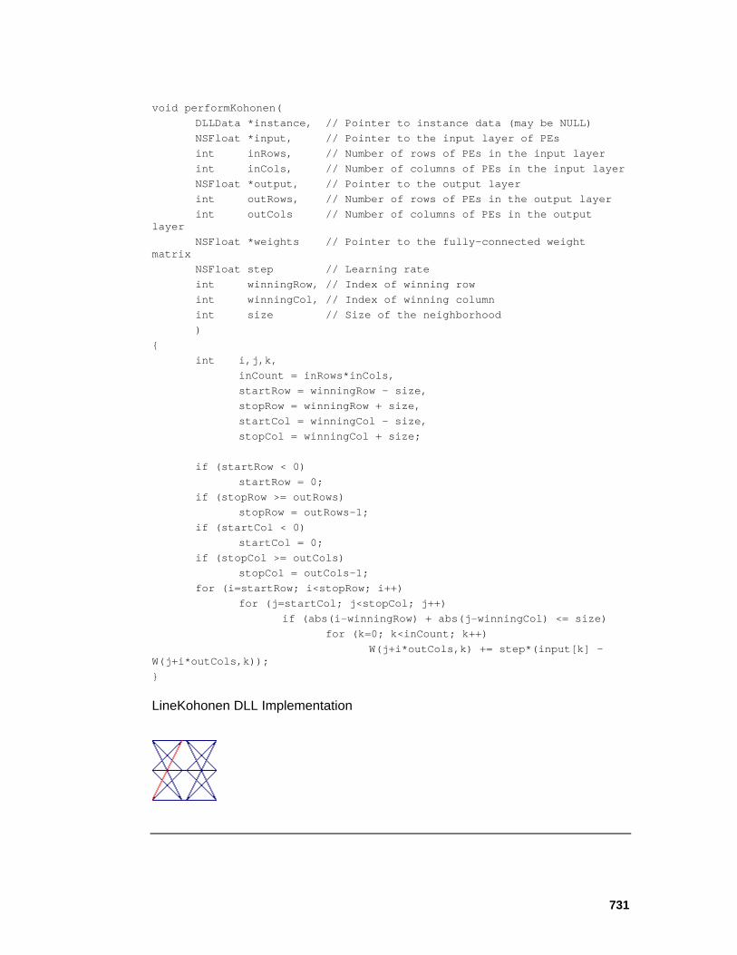
731

void performKohonen( DLLData *instance, // Pointer to instance data (may be NULL) NSFloat *input, // Pointer to the input layer of PEs int inRows, // Number of rows of PEs in the input layer int inCols, // Number of columns of PEs in the input layer NSFloat *output, // Pointer to the output layer int outRows, // Number of rows of PEs in the output layer int outCols // Number of columns of PEs in the output layer NSFloat *weights // Pointer to the fully-connected weight matrix NSFloat step // Learning rate int winningRow, // Index of winning row int winningCol, // Index of winning column int size // Size of the neighborhood ) { int i,j,k, inCount = inRows*inCols, startRow = winningRow - size, stopRow = winningRow + size, startCol = winningCol - size, stopCol = winningCol + size; if (startRow < 0) startRow = 0; if (stopRow >= outRows) stopRow = outRows-1; if (startCol < 0) startCol = 0; if (stopCol >= outCols) stopCol = outCols-1; for (i=startRow; i<stopRow; i++) for (j=startCol; j<stopCol; j++) if (abs(i-winningRow) + abs(j-winningCol) <= size) for (k=0; k<inCount; k++) W(j+i*outCols,k) += step*(input[k] - W(j+i*outCols,k)); }

LineKohonen DLL Implementation

732

Component: LineKohonen


Description:

The LineKohonen component implements a 1D self-organizing feature map (SOFM) with a linear neighborhood. The dimensions of the map are dictated by the vector length (outRows*outCols) of the axon that the LineKohonen feeds. The neighborhood size is defined by the user within the component’s inspector.

Code: void performKohonen( DLLData *instance, // Pointer to instance data (may be NULL) NSFloat *input, // Pointer to the input layer of PEs int inRows, // Number of rows of PEs in the input layer int inCols, // Number of columns of PEs in the input layer NSFloat *output, // Pointer to the output layer int outRows, // Number of rows of PEs in the output layer int outCols // Number of columns of PEs in the output layer NSFloat *weights // Pointer to the fully-connected weight matrix NSFloat step // Learning rate int winningRow, // Index of winning row int winningCol, // Index of winning column int size // Size of the neighborhood ) { int i,j, inCount = inRows*inCols, outCount = outRows * outCols, winner = winningCol + winningRow*outCols, start = winner - size, stop = winner + size; if (start < 0) start = 0; if (stop >= outCount) stop = outCount-1; for (i=start; i<=stop; i++) for (j=0; j<inCount; j++) W(i,j) += step*(input[j] - W(i,j)); }

SquareKohonen DLL Implementation

733

Component: SquareKohonen


Description:

The SquareKohonen component implements a 2D self-organizing feature map (SOFM) with a square neighborhood. The dimensions of the map are dictated by the dimensions of the axon that the LineKohonen feeds (outRows and outCols). The neighborhood size is defined by the user within the component’s inspector.

Code: void performKohonen( DLLData *instance, // Pointer to instance data (may be NULL) NSFloat *input, // Pointer to the input layer of PEs int inRows, // Number of rows of PEs in the input layer int inCols, // Number of columns of PEs in the input layer NSFloat *output, // Pointer to the output layer int outRows, // Number of rows of PEs in the output layer int outCols // Number of columns of PEs in the output layer NSFloat *weights // Pointer to the fully-connected weight matrix NSFloat step // Learning rate int winningRow, // Index of winning row int winningCol, // Index of winning column int size // Size of the neighborhood ) { int i,j,k, inCount = inRows*inCols, startRow = winningRow - size, stopRow = winningRow + size, startCol = winningCol - size, stopCol = winningCol + size; if (startRow < 0) startRow = 0; if (stopRow >= outRows) stopRow = outRows-1; if (startCol < 0)

734

startCol = 0; if (stopCol >= outCols) stopCol = outCols-1; for (i=startRow; i<=stopRow; i++) for (j=startCol; j<=stopCol; j++) for (k=0; k<inCount; k++) W(j+i*outCols,k) += step*(input[k] - W(j+i*outCols,k)); }

Inspectors

Kohonen Inspector

Superclass Inspector: Conscience Inspector

Component Configuration: Neighborhood (SetNeighborhood(int))

This cell specifies the size of the spatial neighborhood used by the Kohonen algorithm. See the Neighborhood Figure section of the component reference for its use of this parameter. Beta (SetBeta(float))

See Conscience Inspector Gamma (SetGamma(float))

See Conscience Inspector Component Plane (setComponentPlane(int))

Used to select the plane displayed by the probe attached to the Component Plane access point.

735

Macro Actions

Kohonen Full

KohonenFull Macro Actions Overview Superclass Macro Actions

Action Description neighborhood Returns the "Neighborhood" setting. setNeighborhood Sets the "Neighborhood" setting.

neighborhood Overview Macro Actions

Syntax

componentName. neighborhood()

Parameters Type Description return int The size of the spatial neighborhood used by the Kohonen algorithm (see "Neighborhood" within the Kohonen Inspector). componentName Name defined on the engine property page.

setNeighborhood Overview Macro Actions

Syntax

componentName. setNeighborhood(neighborhood)

Parameters Type Description return void componentName Name defined on the engine property page. neighborhood int The size of the spatial neighborhood used by the Kohonen algorithm (see "Neighborhood" within the Kohonen Inspector).

Access Points

Unsupervised Access Points


Superclass: None

736

Activity Access:

Attaches the Access component to the vector of activity immediately after the function map

Weights Access:


Unsupervised Step Size:

This Access point reports the step size being used by the Unsupervised component. This value may be adapted during training by using a Scheduler.

Forced Access:

This access point is used to input a desired response to an unsupervised component. It is currently only implemented for the Hebbian and StandardFull components. For the Hebbian component, the learning rule becomes Forced Hebbian. For the StandardFull component, the learning rule becomes Learning Vector Quantization (LVQ), if the desired signal is the class labels of the clusters.

See Also

HebbianFull Access Points

Component: HebbianFull

Superclass: Unsupervised Access Points

Forced Access:

This Access point allows a desired response to be input to the Hebbian component, transforming the learning rule to Forced Hebbian.

DLL Implementation

HebbianFull DLL Implementation

737

Component: HebbianFull

Protocol: PerformUnsupervised

Description:

The HebbianFull component implements Plain Hebbian and Forced Hebbian learning. Each weight of the fully-connected matrix is adjusted by adding the product of the activity at the output PE, the activity at the input PE, and the step size.

Code: void performUnsupervised( DLLData *instance, // Pointer to instance data (may be NULL) NSFloat *input, // Pointer to the input layer of PEs int inRows, // Number of rows of PEs in the input layer int inCols, // Number of columns of PEs in the input layer NSFloat *output, // Pointer to the output layer int outRows, // Number of rows of PEs in the output layer int outCols // Number of columns of PEs in the output layer NSFloat *weights // Pointer to the fully-connected weight matrix NSFloat step // Learning rate ) { int i, j, inCount=inRows*inCols, outCount=outRows*outCols; for (j=0; j<inCount; j++) for (i=0; i<outCount; i++) W(i,j) += step*input[j]*output[i]; }

OjasFull DLL Implementation

Component: OjasFull


738

Description:

OjasFull implements plain Hebbian learning with constrained weight vector growth. This procedure adds a weight decay proportional to the output squared. The implementation is similar to that of the DLL Implementation component, except that each input PE term used to compute the weight change is reduced by the sum of products of the output PEs and the weights connected to the given input.

Code: void performUnsupervised( DLLData *instance, // Pointer to instance data (may be NULL) NSFloat *input, // Pointer to the input layer of PEs int inRows, // Number of rows of PEs in the input layer int inCols, // Number of columns of PEs in the input layer NSFloat *output, // Pointer to the output layer int outRows, // Number of rows of PEs in the output layer int outCols // Number of columns of PEs in the output layer NSFloat *weights // Pointer to the fully-connected weight matrix NSFloat step // Learning rate ) { int i, j, inCount=inRows*inCols, outCount=outRows*outCols; NSFloat partialSum; for (j=0; j<inCount; j++) { partialSum = (NSFloat)0; for (i=0; i<outCount; i++) partialSum += output[i] * W(i,j); for (i=0; i<outCount; i++) W(i,j) += step*output[i]*(input[j] - partialSum); } }

SangersFull DLL Implementation

Component: SangersFull


739

Description:

SangersFull implements principal component analysis. It does this with a plain Hebbian weight update rule while constraining the growth of the weight vector, similar to the DLL Implementation component. The difference is that the range of the summation has changed, resulting in an ordering of the principal components.

Code: void performUnsupervised( DLLData *instance, // Pointer to instance data (may be NULL) NSFloat *input, // Pointer to the input layer of PEs int inRows, // Number of rows of PEs in the input layer int inCols, // Number of columns of PEs in the input layer NSFloat *output, // Pointer to the output layer int outRows, // Number of rows of PEs in the output layer int outCols // Number of columns of PEs in the output layer NSFloat *weights // Pointer to the fully-connected weight matrix NSFloat step // Learning rate ) int i, j, inCount=inRows*inCols, outCount=outRows*outCols; NSFloat partialSum; for (j=0; j<inCount; j++) { partialSum = (NSFloat)0; for (i=0; i<outCount; i++) { partialSum += output[i] * W(i,j); W(i,j) += step*output[i]*(input[j] - partialSum); } } }

Drag and Drop

Unsupervised Drag and Drop

All components in the Unsupervised family must be dropped directly on a component from the Synapse family. The unsupervised component will then be positioned in the upper left corner of the synapse.

See Also

740

Inspectors

Rate Inspector



This cell is used to specify the step size parameter, η. See the component reference for its use within the weight update function. Learning (Turn learning on(); Turn learning off(); Toggle learning())

When this switch is turned on, the weights of this unsupervised component will be adapted. When this switch is turned off, the weights are frozen. This is most often used to synchronize the training of hybrid supervised/unsupervised networks.

This switch will be turned on when the network is reset provided the Learn after RESET switch is turned on (see below). For standard unsupervised learning, both the Learn and the Learn after RESET switches should be turned on. Note that when the learning is off, the icon changes to that of the FullSynapse to indicate the freezing of the weights. The learning mode can be switched during the simulation using one or more Transmitters. Learn after RESET

This switch specifies whether the Learn switch (see above) is turned on or off when the network is reset. Normalize Weights

This switch is only active for the HebbianFull, OjasFull, and SangersFull components. If activated, then each weight vector in the weight matrix is normalized to have an L2 norm of unity after each weight update. It is most commonly used with the OjasFull and SangersFull components, with a negative learning rate, to compute the smallest principal component. Store Hopefield Weights

741

This button works only with the HebbianFull component with a desired signal at the forced access point. It is used to calculate, in a single pass, the weights of a Hopefield net.

SVMInputSynapse Inspector

Superclass Inspector: Step Inspector


The output vector y is a measure of the distance between the input and the output neurons’ weight vectors. This distance is dependent on the particular metric chosen: Dot Product

Euclidean

Macro Actions

Unsupervised Full

UnsupervisedFull Macro Actions Overview Superclass Macro Actions

Action Description learning Returns the "Learning" setting.

742

learningOnReset Returns the "Learning on Reset" setting. setLearning Sets the "Learning" setting. setLearningOnReset Sets the "Learning on Reset" setting.

setStepSize Sets the "Step Size" parameter, η.

stepSize Returns the "Step Size" parameter, η.


Syntax

componentName. learning()

Parameters Type Description return BOOL TRUE if the weights of the unsupervised component are adapted (see "Learning" within the Learning Rate Inspector). componentName Name defined on the engine property page.

learningOnReset Overview Macro Actions

Syntax

componentName. learningOnReset()

Parameters Type Description return BOOL TRUE forces the Learn switch on when the network is reset (see "Learn after RESET" within the Learning Rate Inspector). componentName Name defined on the engine property page.


Syntax

componentName. setLearning(learning)


743

return void componentName Name defined on the engine property page. learning BOOL TRUE if the weights of the unsupervised component are adapted (see "Learning" within the Learning Rate Inspector).

setLearningOnReset Overview Macro Actions

Syntax

componentName. setLearningOnReset(learningOnReset)

Parameters Type Description return void componentName Name defined on the engine property page. learningOnReset BOOL TRUE forces the Learn switch on when the network is reset (see "Learn after RESET" within the Learning Rate Inspector).

setStepSize Overview Macro Actions

Syntax

componentName. setStepSize(stepSize)


stepSize float The step size parameter, η (see "Step Size" within the Learning Rate Inspector).

stepSize Overview Macro Actions

Syntax

componentName. stepSize()


return float The step size parameter, η (see "Step Size" within the Learning Rate Inspector). componentName Name defined on the engine property page.

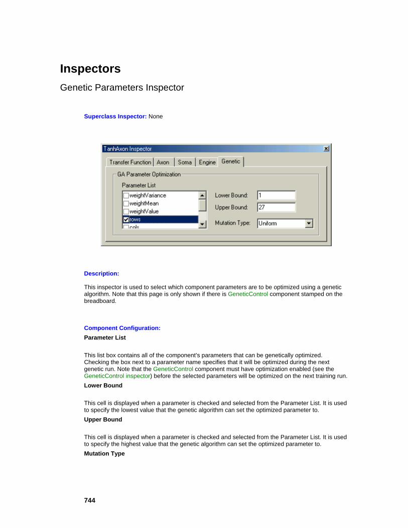
744

Inspectors Genetic Parameters Inspector

Superclass Inspector: None

Description:

This inspector is used to select which component parameters are to be optimized using a genetic algorithm. Note that this page is only shown if there is GeneticControl component stamped on the breadboard.

Component Configuration: Parameter List

This list box contains all of the component’s parameters that can be genetically optimized. Checking the box next to a parameter name specifies that it will be optimized during the next genetic run. Note that the GeneticControl component must have optimization enabled (see the GeneticControl inspector) before the selected parameters will be optimized on the next training run. Lower Bound

This cell is displayed when a parameter is checked and selected from the Parameter List. It is used to specify the lowest value that the genetic algorithm can set the optimized parameter to. Upper Bound

This cell is displayed when a parameter is checked and selected from the Parameter List. It is used to specify the highest value that the genetic algorithm can set the optimized parameter to. Mutation Type

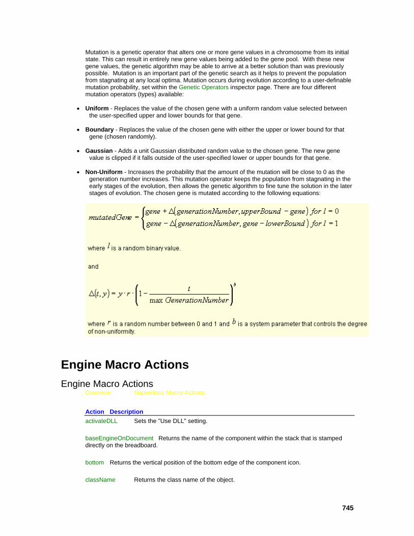
745

Mutation is a genetic operator that alters one or more gene values in a chromosome from its initial state. This can result in entirely new gene values being added to the gene pool. With these new gene values, the genetic algorithm may be able to arrive at a better solution than was previously possible. Mutation is an important part of the genetic search as it helps to prevent the population from stagnating at any local optima. Mutation occurs during evolution according to a user-definable mutation probability, set within the Genetic Operators inspector page. There are four different mutation operators (types) available:

• Uniform - Replaces the value of the chosen gene with a uniform random value selected between the user-specified upper and lower bounds for that gene.

• Boundary - Replaces the value of the chosen gene with either the upper or lower bound for that gene (chosen randomly).

• Gaussian - Adds a unit Gaussian distributed random value to the chosen gene. The new gene value is clipped if it falls outside of the user-specified lower or upper bounds for that gene.

• Non-Uniform - Increases the probability that the amount of the mutation will be close to 0 as the generation number increases. This mutation operator keeps the population from stagnating in the early stages of the evolution, then allows the genetic algorithm to fine tune the solution in the later stages of evolution. The chosen gene is mutated according to the following equations:

Engine Macro Actions Engine Macro Actions

Overview Superclass Macro Actions

Action Description activateDLL Sets the "Use DLL" setting. baseEngineOnDocument Returns the name of the component within the stack that is stamped directly on the breadboard. bottom Returns the vertical position of the bottom edge of the component icon. className Returns the class name of the object.

746

closeEngineWindow Closes the window associated with the component (e.g., the display window of a probe). connectTo Establishes a connection to the specified component on the breadboard. delete Deletes the component. dllActive Returns the "Use DLL" setting. dllName Returns the name (excluding extension) of the DLL associated with the component. dllPath Returns the full file path of the DLL associated with the component. engineAtAccessPoint Returns the name of the component attached to the specified access point. fixName Returns the "Fix Name" setting. fixToSuperengine Returns the "Fix to superengine" setting. isDescendant Returns TRUE if the specified component is directly or indirectly attached below. isKindOf Returns TRUE if the component is a member of the specified class or is a member of a sub-class of the specified class. isMemberOf Returns TRUE if the component is a member of the specified class. isOfLevel Returns TRUE if the component is a member of the specified level. isSubengine Returns TRUE if the specified component is directly or indirectly attached above. keepWindowActive Returns the "Keep Window Active" setting. left Returns the horizontal position of the left edge of the component icon. moveBy Moves the component icon by the specified x and y offsets. moveEngineWindow Moves the component's associated window to the specified location on the screen. moveOn Detaches the component from its existing location and re-attaches it to the specified component. moveTo Moves the component icon to the specified location on the breadboard. name Returns the "Component Name". openEngineWindow Opens the window associated with the component (e.g., the display window of a probe). right Returns the horizontal position of the right edge of the component icon.

747

setDLLName Sets the name of the DLL to associate with the component. The directory is specifed within the Options Window.

setFixName Sets the "Fix Name" setting.

setFixToSuperengine Sets the "Fix to superengine" setting. setKeepWindowActive Sets the "Keep window active" setting. setName Sets the "Component name" setting. sizeEngineWindow Sets the height and width of the window associated with the component. subengines Returns a variant array containing the names of all components attached on top of the component. top Returns the vertical position of the top edge of the component icon.

activateDLL Overview Macro Actions

Syntax

componentName. activateDLL(setSwitch, perform)


setSwitch BOOL TRUE to turn the "Use DLL" switch on and FALSE to turn the switch off (see " Use DLL" within the Engine Inspector ).

perform BOOL TRUE to perform the load/unload operation at the time the switch is set. This is normally set to TRUE.

baseEngineOnDocument Overview Macro Actions

Syntax

componentName. baseEngineOnDocument()

748

Parameters Type Description return string The name of the component within the stack that is stamped directly on the breadboard. componentName Name defined on the engine property page.

bottom Overview Macro Actions

Syntax

componentName. bottom()

Parameters Type Description return int The vertical position of the bottom edge of the component icon componentName Name defined on the engine property page.

className Overview Macro Actions

Syntax

componentName. className()

Parameters Type Description return string The class name of the object. componentName Name defined on the engine property page.

closeEngineWindow Overview Macro Actions

Syntax

componentName. closeEngineWindow()


connectTo Overview Macro Actions

749

Syntax

componentName. connectTo(name)

Parameters Type Description return void componentName Name defined on the engine property page. name string The name of the component to connect to.

delete Overview Macro Actions

Syntax

componentName. delete()


dllActive Overview Macro Actions

Syntax

componentName. dllActive()

Parameters Type Description return BOOL TRUE if the associated DLL is being used (see " Use DLL" within the Engine Inspector ). componentName Name defined on the engine property page.

dllName Overview Macro Actions

Syntax

componentName. dllName()

Parameters Type Description return string The name (excluding extension) of the DLL associated with the component. componentName Name defined on the engine property page.

750

dllPath Overview Macro Actions

Syntax

componentName. dllPath()

Parameters Type Description return string The full path of the DLL associated with the component. componentName Name defined on the engine property page.

engineAtAccessPoint Overview Macro Actions

Syntax

componentName. engineAtAccessPoint(access)

Parameters Type Description return string The name of the component attached to the specified access point. componentName Name defined on the engine property page.

access string The name of the access point.

fixToSuperengine Overview Macro Actions

Syntax

componentName. fixToSuperengine()

Parameters Type Description return BOOL TRUE if the component cannot be moved from the attached component (see "Fix to Superengine" within the Engine Inspector). componentName Name defined on the engine property page.

fixName Overview Macro Actions

Syntax

751

componentName. fixName()

Parameters Type Description return BOOL TRUE if the component's cannot be modified automatically by NeuroSolutions (see "Fix Name" within the Engine Inspector). componentName Name defined on the engine property page.

isDescendant Overview Macro Actions

Syntax

componentName. isDescendant(name)

Parameters Type Description return BOOL TRUE if the specified component is directly or indirectly attached below. componentName Name defined on the engine property page.

name string The component name.

isKindOf Overview Macro Actions

Syntax

componentName. isKindOf(class)

Parameters Type Description return BOOL TRUE if the component is a member of the specified class or is a member of a sub-class of the specified class. componentName Name defined on the engine property page.

class string The class name.

isMemberOf Overview Macro Actions

Syntax

componentName. isMemberOf(class)


752

return BOOL TRUE if the component is a member of the specified class. componentName Name defined on the engine property page.

class string The class name.

isMemberOf Overview Macro Actions

Syntax

componentName. isOfLevel(level)

Parameters Type Description return BOOL TRUE if the component is a member of the specified level. componentName Name defined on the engine property page.

level string The component level. Possible values are: "Activity", "Backprop", "Control" and "Gradient".

isSubengine Overview Macro Actions

Syntax

componentName. isSubengine(name)

Parameters Type Description return BOOL TRUE if the specified component is directly or indirectly attached above. componentName Name defined on the engine property page.

name string The component name.

keepWindowActive Overview Macro Actions

Syntax

componentName. keepWindowActive()

Parameters Type Description return BOOL TRUE if the window associated with this component will stay open (see "Keep window active" within the Engine Inspector).

753


left Overview Macro Actions

Syntax

componentName. left()

Parameters Type Description return int The horizontal position of the left edge of the component icon. componentName Name defined on the engine property page.

moveBy Overview Macro Actions

Syntax

componentName. moveBy(x, y)


x int The horizontal offset to move the component icon by.

y int The vertical offset to move the component icon by.

moveEngineWindow Overview Macro Actions

Syntax

componentName. moveEngineWindow(x, y)


x int The new horizontal location of the left edge of the window associated with the

754

component.

y int The new vertical location of the top edge of the window associated with the component.

moveOn Overview Macro Actions

Syntax

componentName. moveOn(name)


name string The name of the component to attach to.

moveTo Overview Macro Actions

Syntax

componentName. moveTo(x, y)

Parameters Type Description return void componentName Name defined on the engine property page. x int The new horizontal location of the left edge of the component icon.

y int The new vertical location of the top edge of the component icon.

name Overview Macro Actions

Syntax

componentName. name()

Parameters Type Description return string The name of the component (see "Component name" within the Engine Inspector ). componentName Name defined on the engine property page.

755

openEngineWindow Overview Macro Actions

Syntax

componentName. openEngineWindow()


right Overview Macro Actions

Syntax

componentName. right()

Parameters Type Description return int The horizontal position of the right edge of the component icon. componentName Name defined on the engine property page.

setDLLName Overview Macro Actions

Syntax

componentName. setDLLName(dllName, dllPath)

Parameters Type Description return void componentName Name defined on the engine property page. dllName string The name (without extension) of the DLL associated with the component. dllPath string The full path of the DLL associated with the component.

setFixName Overview Macro Actions

Syntax

756

componentName. setFixName(fixName)

Parameters Type Description return void componentName Name defined on the engine property page. fixName BOOL TRUE if the component's cannot be modified automatically by NeuroSolutions (see "Fix Name" within the Engine Inspector).

setFixToSuperengine Overview Macro Actions

Syntax

componentName. setFixToSuperengine(fixToSuperengine)

Parameters Type Description return void componentName Name defined on the engine property page. fixToSuperengine BOOL TRUE if the component cannot be moved from the attached component (see "Fix to Superengine" within the Engine Inspector).

setKeepWindowActive Overview Macro Actions

Syntax

componentName. setKeepWindowActive(keepWindowActive)

Parameters Type Description return void componentName Name defined on the engine property page. keepWindowActive BOOL TRUE if the window associated with this component will stay open (see "Keep window active" within the Engine Inspector).

setName Overview Macro Actions

Syntax

componentName. setName(name)


757

return void componentName Name defined on the engine property page. name string The name of the component (see "Component name" within the Engine Inspector ).

sizeEngineWindow Overview Macro Actions

Syntax

componentName. sizeEngineWindow(cx, cy)

Parameters Type Description return void componentName Name defined on the engine property page. cx int The new width of the window associated with the component.

cy int The new height of the window associated with the component.

subengines Overview Macro Actions

Syntax

componentName. subengines()

Parameters Type Description return variant An array containing the names of all components attached on top of the component. componentName Name defined on the engine property page.

top Overview Macro Actions

Syntax

componentName. top()

Parameters Type Description return int The vertical position of the top edge of the component icon.

758


Dialog Components DialogEngine Family DialogEngine Family

DialogEngine family palette.

Ancestor: Engine Family

This family allows you to enhance a breadboard with user interface components. These components can be used to build presentations, demonstrations, or a high-level interface for the end users of the network.

Members:

MacroEngine Family

ArrowEngine

ArrowEngine

Family: MacroEngine Family

Superclass: NEngine

Description:

759

This component acts as a pointing device and is mainly used for demonstration purposes.

User Interaction:

Drag and Drop

Inspector

MacroEngine Family

MacroEngine Family

Ancestor: DialogEngine Family

Each of these components can have a macro associated with them. The component can be configured to run the macro whenever the user single-clicks on it. The associated macro can also be triggered using a Transmitter and the "runMacro" action.

Most NeuroSolutions components are selected by single-clicking on them. By default, the MacroEngine components are configured to either run a macro or switch to edit mode after a single-click. To select a MacroEngine component when it is in this state, select the region around the component by pressing the mouse button while pointing at the upper left corner, dragging it down to the lower right corner, and releasing (see Logic of the Interface).

Members:

TextBoxEngine

ButtonEngine

EditEngine

User Interface:

Macro Action

See Also

TextBoxEngine

760


Superclass: NEditEngine

Description:

This component is used to place descriptive text on the breadboard, often for demonstration purposes. The border around the text can be modified, as well as the background color.

User Interaction:

Drag and Drop

Inspector

ButtonEngine


Superclass: NEditEngine

Description:

This component is a button that is normally associated with a macro. By default, the macro is run when the user single-clicks on the button.

User Interaction:

Drag and Drop

Inspector

761

EditEngine


Superclass: NMacroEngine

Description:

This component is an edit cell that allows the user to enter in a value. The value entered can be obtained by calling the ‘text()’ macro function of the EditEngine component.

User Interaction:

Drag and Drop

Inspector

Macro Actions

Drag and Drop

MacroEngine Family Drag and Drop

MacroEngines are base components on the breadboard. This means that they must be dropped directly onto an empty breadboard location.

Inspectors

Text Box Inspector

Superclass Inspector: Edit Inspector

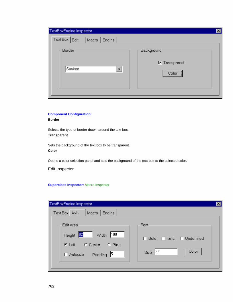
762

Component Configuration: Border

Selects the type of border drawn around the text box. Transparent

Sets the background of the text box to be transparent. Color

Opens a color selection panel and sets the background of the text box to the selected color.

Edit Inspector

Superclass Inspector: Macro Inspector

763

Component Configuration: Height

The height of the edit area. Width

The width of the edit area. Left

Sets the text to be left justified within the edit area. Center

Sets the text to be centered within the edit area. Right

Sets the text to be right justified within the edit area. Autosize

Sizes the edit area based to the size of the text. As the text is edited, the window resizes with each keystroke. Padding

Sets the amount of spacing between the text and the edit area border. Bold

Sets the font to be bold. Italic

Sets the font to be italic. Underlined

Sets the font to be underlined. Size

Sets the font size. Color

Opens a color selection panel and sets the text to the selected color.

Macro Inspector


764

Component Configuration: Browse

Displays a file selection panel for setting the macro to associate with this object. The associated macro is run whenever this object is clicked on (provided that the "Run" switch is set – see below). Edit

Displays the MacroWizard_Debug_Page for the associated macro. Select

When this switch is set, the component is selected when it is clicked on. To select the component when this switch is not set, select the region around the component (see Logic of the Interface). Run

When this switch is set, the associated macro is run when the component is clicked on. Edit

When this switch is set, the edit mode is activated when the component is clicked on.

Macro Actions

Edit Engine

EditEngine Macro Actions Overview Superclass Macro Actions

Action Description autosize Returns the "Edit Area Autosize" setting. bold Returns the "Font Bold" setting.

765

borderType Returns the "Border" setting (0=None, 5=Raised, 6=Etched Edge, 9=Bumped Edge, 10=Sunken). editModeEnabled Returns the "Edit Mode Enabled" setting. fontSize Returns the "Font Size" setting. height Returns the "Edit Area Height" setting. italic Returns the "Font Italic" setting. padding Returns the "Edit Area Padding" setting. position Returns the position setting for the text within the edit area (0=Left, 1=Center, 2=Right). setAutosize Sets the "Edit Area Autosize" setting. setBackgroundColor Sets the "Background Color" setting. setBold Sets the "Font Bold" setting. setBorderType Sets the "Border" setting (0=None, 5=Raised, 6=Etched Edge, 9=Bumped Edge, 10=Sunken). setColor Sets the "Font Color" setting. setEditModeEnabled Sets the "Edit Mode Enabled" setting. setFontSize Sets the "Font Size" setting. setHeight Sets the "Edit Area Height" setting. setItalic Sets the "Font Italic" setting. setPadding Sets the "Edit Area Padding" setting. setPosition Sets the position setting for the text within the edit area (0=Left, 1=Center, 2=Right). setText Sets the text to be placed within the edit box. setTextFromFile Allows the user to read the text to be placed within the text box from an ASCII text file. setTransparent Sets the "Background Transparent" setting. setUnderlined Sets the "Font Underlined" setting. setWidth Sets the "Edit Area Width" setting. sizeToFit Sizes the edit area based on the size of the text.

766

Text Returns the edit box text. transparent Returns the "Background Transparent" setting. underlined Returns the "Font Underlined" setting. width Returns the "Edit Area Width" setting.

autosize Overview Macro Actions

Syntax

componentName. autosize()

Parameters Type Description return BOOL When TRUE, the edit box size automatically adjusts based on the amount of text (see "Autosize" within the EditEngine Inspector). componentName Name defined on the engine property page.

bold Overview Macro Actions

Syntax

componentName. bold()

Parameters Type Description return BOOL When TRUE, the font type is bold (see "Bold" within the EditEngine Inspector). componentName Name defined on the engine property page.

borderType Overview Macro Actions

Syntax

componentName. borderType()

Parameters Type Description return int The border type of a text box (0=None, 5=Raised, 6=Etched Edge, 9=Bumped Edge, 10=Sunken -- see "Border" within the TextBoxEngine Inspector). componentName Name defined on the engine property page.

767

editModeEnabled Overview Macro Actions

Syntax

componentName. editModeEnabled()

Parameters Type Description return BOOL When TRUE, the text of the edit box may be edited (see "Edit Mode Enabled" within the EditEngine Inspector). componentName Name defined on the engine property page.

fontSize Overview Macro Actions

Syntax

componentName. fontSize()

Parameters Type Description return int The point size of the font (see "Size" within the EditEngine Inspector). componentName Name defined on the engine property page.

height Overview Macro Actions

Syntax

componentName. height()

Parameters Type Description return int The height of the edit area (see "Height" within the EditEngine Inspector). componentName Name defined on the engine property page.

italic Overview Macro Actions

Syntax

componentName. italic()


768

return BOOL When TRUE, the font type is italic (see "Italic" within the EditEngine Inspector). componentName Name defined on the engine property page.

padding Overview Macro Actions

Syntax

componentName. padding()

Parameters Type Description return int The amount of spacing between the text and the edit area border (see "Padding" within the EditEngine Inspector). componentName Name defined on the engine property page.

position Overview Macro Actions

Syntax

componentName. position()

Parameters Type Description return int The position of the text within the edit area (0=Left, 1=Center, 2=Right -- see "Left", "Center", and "Right" within the EditEngine Inspector). componentName Name defined on the engine property page.

setAutosize Overview Macro Actions

Syntax

componentName. setAutosize(autosize)

Parameters Type Description return void componentName Name defined on the engine property page. autosize BOOL When TRUE, the edit box size automatically adjusts based on the amount of text (see "Autosize" within the EditEngine Inspector).

setBackgroundColor Overview Macro Actions

769

Syntax

componentName. setBackgroundColor(red, green, blue)

Parameters Type Description return void componentName Name defined on the engine property page. red int The amount of red (0 to 255) in the background color of the text box (see "Color" within the TextBoxEngine Inspector). green int The amount of green (0 to 255) in the background color of the text box (see "Color" within the TextBoxEngine Inspector). blue int The amount of blue (0 to 255) in the background color of the text box (see "Color" within the TextBoxEngine Inspector).

setBold Overview Macro Actions

Syntax

componentName. setBold(bold)

Parameters Type Description return void componentName Name defined on the engine property page. bold BOOL When TRUE, the font type is bold (see "Bold" within the EditEngine Inspector).

setBorderType Overview Macro Actions

Syntax

componentName. setBorderType(borderType)

Parameters Type Description return void componentName Name defined on the engine property page. borderType int The border type of a text box (0=None, 5=Raised, 6=Etched Edge, 9=Bumped Edge, 10=Sunken -- see "Border" within the TextBoxEngine Inspector).

setColor Overview Macro Actions

770

Syntax

componentName. setColor(red, green, blue)

Parameters Type Description return void componentName Name defined on the engine property page. red int The amount of red (0 to 255) in the font color of the text (see "Color" within the EditEngine Inspector). green int The amount of green (0 to 255) in the font color of the text (see "Color" within the EditEngine Inspector). blue int The amount of blue (0 to 255) in the font color of the text (see "Color" within the EditEngine Inspector).

setEditModeEnabled Overview Macro Actions

Syntax

componentName. setEditModeEnabled(editModeEnabled)

Parameters Type Description return void componentName Name defined on the engine property page. editModeEnabled BOOL When TRUE, the text of the edit box may be edited (see "Edit Mode Enabled" within the EditEngine Inspector).

setFontSize Overview Macro Actions

Syntax

componentName. setFontSize(fontSize)

Parameters Type Description return void componentName Name defined on the engine property page. fontSize int The point size of the font (see "Size" within the EditEngine Inspector).

setHeight Overview Macro Actions

Syntax

771

componentName. setHeight(height)

Parameters Type Description return void componentName Name defined on the engine property page. height int The height of the edit area (see "Height" within the EditEngine Inspector).

setItalic Overview Macro Actions

Syntax

componentName. setItalic(italic)

Parameters Type Description return void componentName Name defined on the engine property page. italic BOOL When TRUE, the font type is italic (see "Italic" within the EditEngine Inspector).

setPadding Overview Macro Actions

Syntax

componentName. setPadding(padding)

Parameters Type Description return void componentName Name defined on the engine property page. padding int The amount of spacing between the text and the edit area border (see "Padding" within the EditEngine Inspector).

setPosition Overview Macro Actions

Syntax

componentName. setPosition(position)


772

componentName Name defined on the engine property page. position int The position of the text within the edit area (0=Left, 1=Center, 2=Right -- see "Left", "Center", and "Right" within the EditEngine Inspector).

setText Overview Macro Actions

Syntax

componentName. setText(text)

Parameters Type Description return void componentName Name defined on the engine property page. text string The text to be placed within the edit box.

setTextFromFile Overview Macro Actions

Syntax

componentName. setTextFromFile(path, index)


path string The full path name of the ASCII file that contains the edit box text. index int The index indicating which string to extract. The strings are delimited by a '#' immediately followed by the name of the EditEngine component that will use the text. For example, an index of 3 will find the string following the fourth (because it is zero-based) occurance of #name where name is the engine name found within the Engine Inspector.

setTransparent Overview Macro Actions

Syntax

componentName. setTransparent(transparent)


773

transparent BOOL When TRUE, the background color of the text box is transparent (see "Transparent" within the TextBoxEngine Inspector).

setUnderlined Overview Macro Actions

Syntax

componentName. setUnderlined(underlined)

Parameters Type Description return void componentName Name defined on the engine property page. underlined BOOL When TRUE, the font type is underlined (see "Underlined" within the EditEngine Inspector).

setWidth Overview Macro Actions

Syntax

componentName. setWidth(width)

Parameters Type Description return void componentName Name defined on the engine property page. width int The width of the edit area (see "Width" within the EditEngine Inspector).

sizeToFit Overview Macro Actions

Syntax

componentName. sizeToFit()


text Overview Macro Actions

774

Syntax

componentName. text()

Parameters Type Description return string The text to be placed within the text box. componentName Name defined on the engine property page.

transparent Overview Macro Actions

Syntax

componentName. transparent()

Parameters Type Description return BOOL When TRUE, the background color of the text box is transparent (see "Transparent" within the TextBoxEngine Inspector). componentName Name defined on the engine property page.

underlined Overview Macro Actions

Syntax

componentName. underlined()

Parameters Type Description return BOOL When TRUE, the font type is underlined (see "Underlined" within the EditEngine Inspector). componentName Name defined on the engine property page.

width Overview Macro Actions

Syntax

componentName. width()

Parameters Type Description return int The width of the edit area (see "Width" within the EditEngine Inspector). componentName Name defined on the engine property page.

775

Macro Engine

MacroEngine Macro Actions Overview Superclass Macro Actions

Action Description macroAction Returns the "On single-click" setting (0="Select", 1="Run", 2="Edit"). macroPath Returns the full file path of the macro associated with the dialog component. runMacro Runs the macro specified by macroPath. setMacroAction Sets the "On single-click" setting (0="Select", 1="Run", 2="Edit"). setMacroPath Sets the full file path of the macro associated with the dialog component.

macroAction Overview Macro Actions

Syntax

componentName. macroAction()

Parameters Type Description return int The action to be taken when the dialog component is clicked on (0="Select", 1="Run", 2="Edit" -- see "On single-click" within the MacroEngine Inspector). componentName Name defined on the engine property page.

macroPath Overview Macro Actions

Syntax

componentName. macroPath()

Parameters Type Description return string The full file path of the macro associated with the dialog component (see "Macro Path" within the MacroEngine Inspector). componentName Name defined on the engine property page.

runMacro Overview Macro Actions

Syntax

776

componentName. runMacro()


setMacroAction Overview Macro Actions

Syntax

componentName. setMacroAction(macroAction)

Parameters Type Description return void componentName Name defined on the engine property page. macroAction int The action to be taken when the dialog component is clicked on (0="Select", 1="Run", 2="Edit" -- see "On single-click" within the MacroEngine Inspector).

setMacroPath Overview Macro Actions

Syntax

componentName. setMacroPath(macroPath)

Parameters Type Description return void componentName Name defined on the engine property page. macroPath string The full file path of the macro associated with the dialog component (see "Macro Path" within the MacroEngine Inspector).

Drag and Drop

ArrowEngine Drag and Drop

ArrowEngines are unique in that they can stamp on top of an existing component, or they can be dropped directly onto an empty breadboard location.

777

The Theory The Theory

NeuroSolutions



Purpose

The purpose of this chapter is to present the theoretical contributions of NeuroSolutions for the simulation of artificial neural networks. We will discuss how the global network dynamics and the learning dynamics are broken down into local rules of interaction. We also show the equations implemented at the processing level for activation and error backpropagation, and how they are encapsulated in objects. Finally, we show how the objects communicate with each other in planes of activation and how orchestration of the data flow implements the learning paradigms.

Contributions to the Theory of Neural Networks

NeuroSolutions was designed based on the principle of local rules of interactions among simple neural components. This is one of the principles generally accepted in biological neural networks, but very seldom do artificial simulations effectively explore the idea. Moreover, it was necessary to formulate the equation based neural network theory into this new formalism.

Another contribution to the theory of neural computation is the division of neural networks into functional blocks. NeuroSolutions builds neural networks from families of components, and implements simulations using planes of activations and a data flow concept. The families of components naturally translate the parameters needed to configure neural networks and learning paradigms. This is a crucial aspect in the integration of the user interface with the simulation code. The planes of activation implement, for ultimate efficiency, both the neural network dynamics and the learning dynamics.

Due to its object-oriented nature, NeuroSolutions specifies what components do and how components interact with each other, rather than specifying rigid implementation of functions as in conventional programming. Therefore a simulation environment of unparalleled versatility and power has been achieved. This part of the manual presents, in sufficient detail, the contributions.

Introduction to the Theory Chapter

778

The simulation of artificial neural networks (ANNs) is an increasingly important research area. This is due to the demanding computer bandwidth of ANN implementations coupled with the need to experimentally test topologies and parameters. This compensates, in part, a lack of thorough theoretical characterization of ANNs. The need to address real world applications implies a requirement for simulating very large networks. The simulation environments must not only be fast and efficient, but also user friendly and upgradeable, enabling thorough experimental validation. With the computational bandwidth requirements, brute force implementation can give unrealistic computation times, even using supercomputers. Careful planning and fine-tuning of the code has been a necessity for ANN implementations in digital computers.

At first we looked at the problem from a mere engineering perspective, i.e. to find what computational models were most natural for an efficient implementation of ANN topologies. Our conclusion is that an object-oriented programming paradigm conforms to topologies made up of aggregates of similar elements instantiated as many times as necessary. Along the way we found out that object-oriented concepts provide an alternate and equivalent description of ANN paradigms much more appropriate for simulating ANN topologies.

An ANN model is described by a set of dynamic equations. Being adaptive systems, ANNs require a second set of dynamic equations for learning. Although these equations translate the potential and concepts of the theoretical model very well, they suffer from a key shortcoming. ANNs are implemented in digital computers or other hardware through topologies. A given ANN model may produce several topologies. For each topology the equation-based description applies, but at the expense of brute force calculations and exaggerated storage requirements.

Consider the multilayer perceptron (MLP) [Lippman, 1987] and Hopfield network [Hopfield, 1982]. As topologies, they differ substantially (one is feedforward while the other is recurrent), but they are two implementations for the additive model (in the sense of Grossberg [Grossberg, 1983]). Therefore, if a useful implementation for the additive model is developed in a digital computer, it can implement an MLP and a Hopfield network indiscriminately (or any other recurrent topology). The implementations, however, will be very inefficient since, in the MLP, the feedback connections are set at zero, while the connections in recurrent networks are normally sparse. The same argument applies to learning dynamics, i.e. gradient descent learning for these two networks. Furthermore, when implementing the learning rules one ends up with two distinctly different learning procedures, since the MLP is static and the Hopfield network is recurrent.

This example may be generalized to show that learning equations are specific to topologies and becomes obvious when the transpose network is used to propagate errors and compute gradients (one of the leading contributions from neural network theory to gradient descent learning). It may seem that for the sake of efficiency we are restricted to customized simulation environments, with code specifically written for each network topology and learning paradigm. But we think otherwise, and NeuroSolutions is a "living proof" of such beliefs.

The major goal of this document is to present a simulation environment for neural networks which consists of a mixture of feedforward and recurrent sub-networks, trained with static backpropagation, fixed point learning, or backpropagation through time (BPTT). In our opinion, the equation based modeling, so widespread in ANNs, has an alternate and equivalent formulation, which we call object-oriented modeling, and which is far more natural for computer, based simulations of ANNs. Object-oriented modeling is achieved by the execution of an ordered sequence of formal procedures. At present, we utilize digital computers as the engines for object-oriented modeling. This equivalence is predicated on the well known but often overlooked fact that ANN interactions are BOTH local to space (finite elemental topologies) and to time neighborhoods (finite data operators), which we refer to as being local in time and in space. The equation-based modeling does not explore this natural fact, but object-oriented modeling does. Neural network behavior can be easily encoded into local dynamic rules of interaction. These elementary rules are simply replicated across the network. In this sense the ANN with its learning rules operates as a cellular automaton or a lattice in time and space.

A lattice in mathematics is a partially ordered set (with some constraints [Birkhoff, 1948]). Here we will be using the term to represent an ensemble of ordered computations that can be mapped to sites in a graph. Some of these sites may also require ordered computations in time (such as linear filtering operations), so the overall simulation structure is a coupled lattice.

779

Equation-based Modeling

Every neural network researcher has been faced with the problem of translating equations that describe ANN dynamics to computer programs that implement the network topology. The synthetic power and formalism embedded in a mathematical expression is hard to beat, and has been extensively used for characterizing the global dynamics of neural models. Until the advent of computers, mathematics was the most utilized formal descriptive system. We should remember, however, that computer languages are also formal systems and possess the same properties.

A computer algorithm describes a relationship as precisely as a mathematical formula. The problem is one of choosing the representation that best suits our needs. We do not dispute that at the modeling level, equations are the best way to translate global dynamic properties of the interactions. But does this extrapolate to implementations, i.e. to neural network simulations? Let us examine this point in more detail using the additive model as an example [Amari, 1972, Grossberg, 1973]. In modeling, dynamics are described by coupled sets of first order nonlinear differential equations of the form,

where is the systems state vector, is a dynamic map, is an external input,

represents internal system parameters and is a desired trajectory for the system’s state. A neural model is adopted by selecting a distributed set of dynamic mapping

functions for the system’s state vector. For the additive model, we have,

where is the time constant of the ith processing element and is its input-output transfer function.

In a block diagram this can be illustrated as the block additive model in the figure below (all quantities are vectors). Although this model is very general, notice that the activation at node i only depends explicitly on the present input. This feature is undesirable for a large class of problems such as the classification of time varying signals (speech, control, and prediction). One way of modifying the additive model is to substitute the multiplications by convolutions in time

780

This model has been called the convolution model [deVries and Principe, 1992], and allows the ANN activations to depend explicitly upon the past of the input signal and/or model states. The convolution is a linear operation, so conceptually one can picture the neural activations being stored into a general linear filter, which unfortunately has a growing number of coefficients.

Gamma neural model as a prewired additive model

The convolution model can be approximated by fixed order structures [deVries and Principe, 1992]. They showed that the gamma neural model,

for sufficiently large K can approximate the convolution model as close as necessary. These equations can be easily extended to discrete time [deVries and Principe, 1992]. Special cases of this recursive memory structure are the tapped delay line for µ =1 (utilized in the time domain neural network- TDNN, [Lang et al, 1990]), and context unit for K=1 [Jordan, 1986].

A neural network is an implementation of a neural model. Normally a topology is assigned by choosing specific forms of the weight matrix (i.e. fully populated weight matrices give rise to recurrent nets, and when all the weights with i?j are zero, feedforward nets).

The learning dynamics in the N-dimensional dynamic system of the equation above also involves translating equations to network topologies, although some papers have been written with the word

781

"general" in the title [Thrun and Smieja, 1991]. When present, the vector is used to represent the target values for the desired output. In this framework, learning consists of adjusting the weight values such that the desired output is obtained. Notice that this output can be a function of time, or a constant value.

When the goal is to match a desired response, a metric must be established in the error, i.e. the difference between the desired and actual output. This problem has been extensively studied in adaptive signal processing [Haykin, 1991] and optimal control [Bryson and Ho, 1975]. The standard metric chosen is the L2 norm (mean square error), and the method normally used to minimize this error is gradient descent. In gradient descent learning, network coefficients are updated according to the formula,

where E is an error functional, and η is the learning rate.

In order to proceed we must know more about the problem under different learning methods (static backpropagation [Rumelhart et al, 1986], fixed point learning [Pineda, Almeida, 1987], backpropagation through time [Werbos, 1990], and real time recurrent learning [William and Zipser, 1989). For one thing, the error is a function of the network output, which is coupled directly to the network topology. The desired signal can be a constant (fixed point) or time varying (a trajectory). This implies two possibilities: either the network is feedforward and the desired signal and network inputs are static, in which case the gradient computations are independent of time; or the network is recurrent and/or the desired signal is time dependent in which case the gradient computation becomes time dependent. Normally in the ANN literature, these cases are divided into the learning methods mentioned above. A detailed discussion of the methods is outside the scope of this work. What we want to stress is the following facts: First, the network topology affects the equations that compute the gradients. Second, in all these methods, the gradient can be computed with local information, both spatially and temporally.

Let us summarize what we have reviewed. In the figure below (left half) we show diagrammatically how the analysis progressed, from the model to the topology (network), to the learning system. The network is a special implementation of the model. Since learning uses the network it will also become a special case for each topology. For this reason we believe that if a new topology encapsulates a unique feature of the neural model, it will always require a special set of equations to describe it.

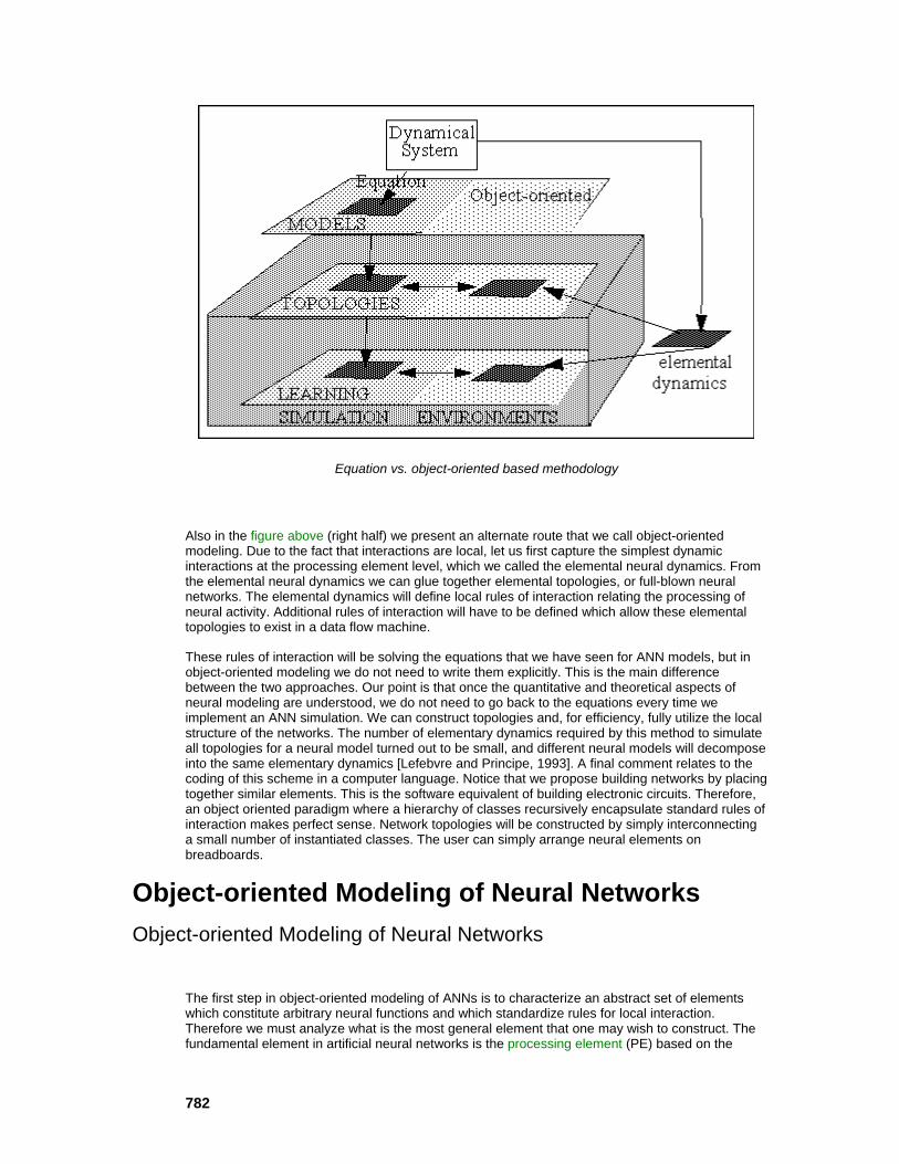
782

Equation vs. object-oriented based methodology

Also in the figure above (right half) we present an alternate route that we call object-oriented modeling. Due to the fact that interactions are local, let us first capture the simplest dynamic interactions at the processing element level, which we called the elemental neural dynamics. From the elemental neural dynamics we can glue together elemental topologies, or full-blown neural networks. The elemental dynamics will define local rules of interaction relating the processing of neural activity. Additional rules of interaction will have to be defined which allow these elemental topologies to exist in a data flow machine.

These rules of interaction will be solving the equations that we have seen for ANN models, but in object-oriented modeling we do not need to write them explicitly. This is the main difference between the two approaches. Our point is that once the quantitative and theoretical aspects of neural modeling are understood, we do not need to go back to the equations every time we implement an ANN simulation. We can construct topologies and, for efficiency, fully utilize the local structure of the networks. The number of elementary dynamics required by this method to simulate all topologies for a neural model turned out to be small, and different neural models will decompose into the same elementary dynamics [Lefebvre and Principe, 1993]. A final comment relates to the coding of this scheme in a computer language. Notice that we propose building networks by placing together similar elements. This is the software equivalent of building electronic circuits. Therefore, an object oriented paradigm where a hierarchy of classes recursively encapsulate standard rules of interaction makes perfect sense. Network topologies will be constructed by simply interconnecting a small number of instantiated classes. The user can simply arrange neural elements on breadboards.

Object-oriented Modeling of Neural Networks Object-oriented Modeling of Neural Networks

The first step in object-oriented modeling of ANNs is to characterize an abstract set of elements which constitute arbitrary neural functions and which standardize rules for local interaction. Therefore we must analyze what is the most general element that one may wish to construct. The fundamental element in artificial neural networks is the processing element (PE) based on the

783

abstraction of the biological neuron proposed by McCulloch and Pitts. The PE used in neural networks has two primary responsibilities: it receives a sum of weighted input activations, and then passes the accumulated activity through a nonlinear instantaneous mapping to produce its output. A neural network can be viewed as a coupled lattice of PEs, i.e. an ordered set of computations.

We define the Axon class which receives the activity from other network elements, implements a nonlinear mapping to its own activity (usually a sigmoid) and holds the resulting activation for other elements to acquire. Since artificial neural networks are so highly interconnected, we will consider for efficiency each Axon to consist of a vector of functionally identical PEs. In other words, there will be a vector of activity associated with each Axon, and our rules of local interaction are mathematically expressed in vector notation (all capitals refer to vectors). The standard local interaction defined by the Axon class can be represented as,

where is the input , is a set of weights for the Axon’s activity (i.e. biases) and

is an arbitrary mapping (usually nonlinear).

A second class of elements called Synapse will take the activity presented by an Axon, apply another mapping (usually the linear weighted sum) and present the result to another Axon. A Synapse is the element that performs linking between lattice sites, and will be represented by a labeled arrow on diagrams. For now we will assume the linear mapping required in additive models when representing the standard interaction defined by the Synapse class,

where and are the respective Axon activity vectors, is a set of

weights for the Synapse class (normally the network weights) and is an arbitrary mapping (usually linear).

All neural elements implemented in NeuroSolutions will belong to either the Axon or Synapse class. For practical reasons we will define the Soma class as representing all neural elements and the ordering of the computations. Thus Axon and Synapse are both subclasses of Soma. We have seen that Axon and Synapse implement the basic McCulloch and Pitts neuron defining rules for computing and passing local activity. As an illustration, the Static ANNs section addresses the construction of a static network, the multilayer perceptron, with our basic elements.

Details Behind Object-Oriented Modeling of Neural Networks:

Static ANNs

Dynamic ANNs

Learning Dynamics

784

Error Criterion

Gradient Search Methodology

Implications for ANN Simulations

Ideal Simulation Environments

Static ANNs

A MLP is a layered feedforward network belonging to the additive model (see additive model equation). The equation in discrete time that defines this topology can be re-written for each PE, yielding

where there are PEs in layer l. If we examine this equation we see two elementary mappings. A linear map between adjacent layers (represented by the weight matrix W), and a nonlinear map (represented by the nonlinearity σ ()) between activity received and activity stored at a single layer. Notice that the form of these maps exactly fit those defined by Axon and Synapse. Implementing the maps for Axon and Synapse as,

where = and is a fully populated matrix of weights, provides all of the elementary dynamics required to construct any MLP. The figure below illustrates the lattice arrangement for a one hidden layer MLP. Note that in this figure we are representing vector quantities.

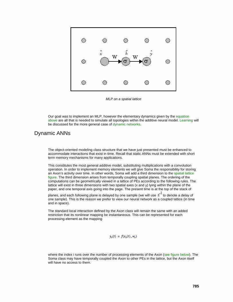
785

MLP on a spatial lattice

Our goal was to implement an MLP, however the elementary dynamics given by the equation above are all that is needed to simulate all topologies within the additive neural model. Learning will be discussed for the more general case of dynamic networks.

Dynamic ANNs

The object-oriented modeling class structure that we have just presented must be enhanced to accommodate interactions that exist in time. Recall that static ANNs must be extended with short term memory mechanisms for many applications.

This constitutes the most general additive model, substituting multiplications with a convolution operation. In order to implement memory elements we will give Soma the responsibility for storing an Axon’s activity over time. In other words, Soma will add a third dimension to the spatial lattice figure. The third dimension arises from temporally coupling spatial planes. The ordering of the computations can be geometrically viewed in a lattice of PEs according to the following rules. The lattice will exist in three dimensions with two spatial axes (x and y) lying within the plane of the paper, and one temporal axis going into the page. The present time is at the top of the stack of

planes, and each following plane is delayed by one sample (we will use to denote a delay of one sample). This is the reason we prefer to view our neural network as a coupled lattice (in time and in space).

The standard local interaction defined by the Axon class will remain the same with an added restriction that its nonlinear mapping be instantaneous. This can be represented for each processing element as the mapping

where the index i runs over the number of processing elements of the Axon (see figure below). The Soma class may have temporally coupled the Axon to other PEs in the lattice, but the Axon itself will have no access to them.

786

The mapping for the PE of the Axon class

The Synapse class will now take the activity presented by one of the coupled PEs for an Axon, apply its linear mapping and present the result to an Axon in the present temporal plane, i.e. the front face of the lattice. This interaction can be represented as,

where d is a delay that represents which temporal plane the Synapse attaches to (see figure below). For each processing element of the Synapse we will have the mapping

The mapping for the PE of the Synapse Class

Recall that Axon and Synapse are both subclasses of Soma. Since Soma performed temporal coupling of the Axon, it can provide Synapse with access to coupled sites. It is important to realize that the temporal coupling performed by Soma is inherent to all network elements and it is hidden from each one of them. Axon and Synapse have no explicit understanding of time. Axon performs a mapping from a node on the lattice to that same node, while Synapse performs its mapping from a node on the lattice to another node on the lattice. As far as Axon and Synapse are concerned, these mappings are between static nodes.

787

As an illustration, lets implement the focused gamma neural network using this coupled lattice. A focused gamma network is a topology that has a gamma memory structure in the input layer (storing traces of the input signal) followed by an MLP [Principe et al, 1992]. If we examine the gamma neural model equation, we see that the gamma neural model is simply an additive model with gamma memory structures inserted for arbitrary states. Let us take a closer look at a discrete version of the gamma memory structure,

Within this equation we see two delayed synaptic maps, one between adjacent memory states ( is a function of activation at the previous time) and one recurrently feeding each memory state onto itself ( is a function of at the previous time). However both of these maps follow the same elementary form given by,

where is a vector of coefficients. In other words, this Synapse will apply a bijective (one-to-one and onto) linear map between Axon sites in the lattice. We can immediately construct the

lattice for a focused gamma network as in the figure below. In this figure, (t) is the input, (t)

represents the hidden layer and (t) is the network output.

Notice that the recursive nature of the gamma memory could in principle require an extension of the instantaneous mapping properties of the Axon class. In the proposed distribution of dynamics the Axon has no knowledge of temporal information, the Soma is responsible for handling time.

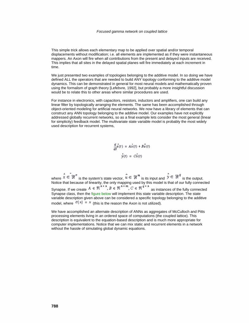
788

Focused gamma network on coupled lattice

This simple trick allows each elementary map to be applied over spatial and/or temporal displacements without modification; i.e. all elements are implemented as if they were instantaneous mappers. An Axon will fire when all contributions from the present and delayed inputs are received. This implies that all sites in the delayed spatial planes will fire immediately at each increment in time.

We just presented two examples of topologies belonging to the additive model. In so doing we have defined ALL the operators that are needed to build ANY topology conforming to the additive model dynamics. This can be demonstrated in general for most neural models and mathematically proven using the formalism of graph theory [Lefebvre, 1992], but probably a more insightful discussion would be to relate this to other areas where similar procedures are used.

For instance in electronics, with capacitors, resistors, inductors and amplifiers, one can build any linear filter by topologically arranging the elements. The same has been accomplished through object-oriented modeling for artificial neural networks. We now have a library of elements that can construct any ANN topology belonging to the additive model. Our examples have not explicitly addressed globally recurrent networks, so as a final example lets consider the most general (linear for simplicity) feedback model. The multivariate state variable model is probably the most widely used description for recurrent systems,

where is the system’s state vector, is its input and is the output. Notice that because of linearity, the only mapping used by this model is that of our fully connected

Synapse. If we create as instances of the fully connected Synapse class, then the figure below will implement this state variable description. The state variable description given above can be considered a specific topology belonging to the additive model, where (this is the reason the Axon is not utilized).

We have accomplished an alternate description of ANNs as aggregates of McCulloch and Pitts processing elements living in an ordered space of computations (the coupled lattice). This description is equivalent to the equation-based description and is much more appropriate for computer implementations. Notice that we can mix static and recurrent elements in a network without the hassle of simulating global dynamic equations.

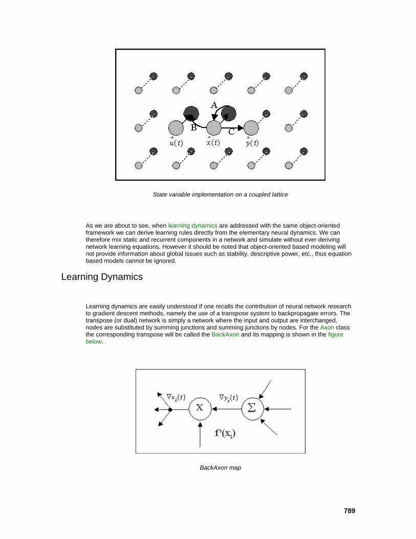
789

State variable implementation on a coupled lattice

As we are about to see, when learning dynamics are addressed with the same object-oriented framework we can derive learning rules directly from the elementary neural dynamics. We can therefore mix static and recurrent components in a network and simulate without ever deriving network learning equations. However it should be noted that object-oriented based modeling will not provide information about global issues such as stability, descriptive power, etc., thus equation based models cannot be ignored.

Learning Dynamics

Learning dynamics are easily understood if one recalls the contribution of neural network research to gradient descent methods, namely the use of a transpose system to backpropagate errors. The transpose (or dual) network is simply a network where the input and output are interchanged, nodes are substituted by summing junctions and summing junctions by nodes. For the Axon class the corresponding transpose will be called the BackAxon and its mapping is shown in the figure below.

BackAxon map

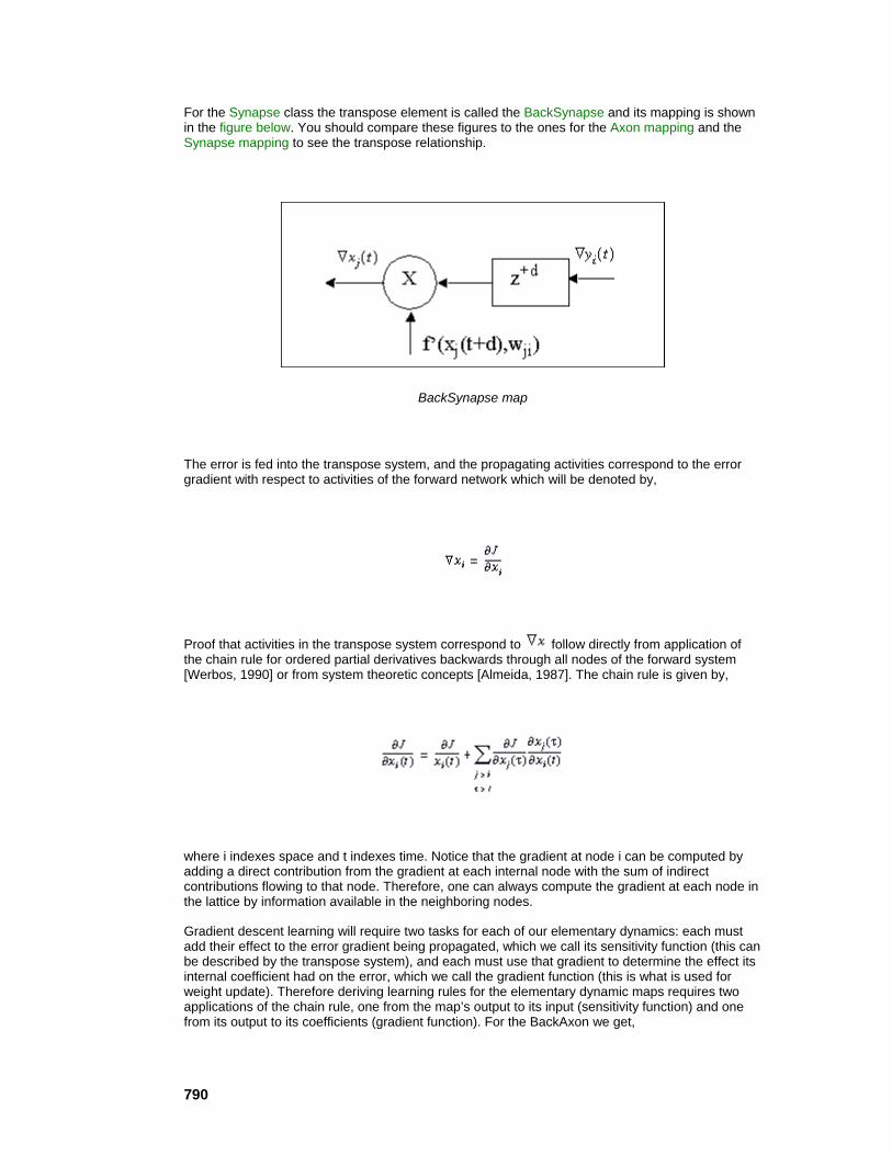
790

For the Synapse class the transpose element is called the BackSynapse and its mapping is shown in the figure below. You should compare these figures to the ones for the Axon mapping and the Synapse mapping to see the transpose relationship.

BackSynapse map

The error is fed into the transpose system, and the propagating activities correspond to the error gradient with respect to activities of the forward network which will be denoted by,

Proof that activities in the transpose system correspond to follow directly from application of the chain rule for ordered partial derivatives backwards through all nodes of the forward system [Werbos, 1990] or from system theoretic concepts [Almeida, 1987]. The chain rule is given by,

where i indexes space and t indexes time. Notice that the gradient at node i can be computed by adding a direct contribution from the gradient at each internal node with the sum of indirect contributions flowing to that node. Therefore, one can always compute the gradient at each node in the lattice by information available in the neighboring nodes.

Gradient descent learning will require two tasks for each of our elementary dynamics: each must add their effect to the error gradient being propagated, which we call its sensitivity function (this can be described by the transpose system), and each must use that gradient to determine the effect its internal coefficient had on the error, which we call the gradient function (this is what is used for weight update). Therefore deriving learning rules for the elementary dynamic maps requires two applications of the chain rule, one from the map’s output to its input (sensitivity function) and one from its output to its coefficients (gradient function). For the BackAxon we get,

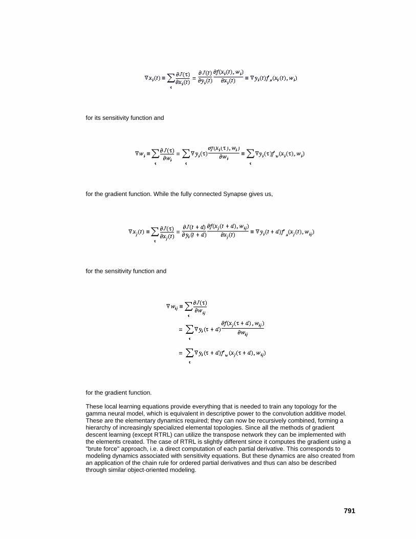
791

for its sensitivity function and

for the gradient function. While the fully connected Synapse gives us,

for the sensitivity function and

for the gradient function.

These local learning equations provide everything that is needed to train any topology for the gamma neural model, which is equivalent in descriptive power to the convolution additive model. These are the elementary dynamics required; they can now be recursively combined, forming a hierarchy of increasingly specialized elemental topologies. Since all the methods of gradient descent learning (except RTRL) can utilize the transpose network they can be implemented with the elements created. The case of RTRL is slightly different since it computes the gradient using a "brute force" approach, i.e. a direct computation of each partial derivative. This corresponds to modeling dynamics associated with sensitivity equations. But these dynamics are also created from an application of the chain rule for ordered partial derivatives and thus can also be described through similar object-oriented modeling.

792

There are several important benefits to this approach that we have tried to illustrate through these examples. First, learning was derived directly from the elementary maps (of the Axon and Synapse classes). Therefore, once you have arranged elements on the lattice, the learning dynamics can be implemented by simply reversing the direction of data flow and replacing each elementary dynamic with its learning equivalent.

Backpropagation network on coupled lattice

The figure above illustrates the transpose network for the focused gamma network figure. Notice that time runs backwards in this network. This process of constructing the learning network can be automated by the simulation environment, thus the user simply constructs the feedforward network without ever having to address learning.

When modeling is based on equations, one generally wants to characterize the dynamics for a broad class of systems. But, when implementing the individual systems, these models are constrained by assigning a specific topology. In object-oriented modeling one always assigns only those elemental maps which are required, thus the implementations are always efficient.

Error Criterion

Another aspect that should be emphasized in the proposed object-oriented modeling is that as long as gradient descent is used, only the output errors injected into the network depend upon the error criterion. The output error depends intrinsically on the cost function used, but the criterion does not say how errors are propagated inside the net. Our method therefore uncouples error propagation inside the net from the error criterion. This is very important because the network elements used for learning do not change with a change in criterion (e.g. mean square error to Kulback Liebler, Lp norms, etc.). The elements only know how to map input signals to output signals, independent of the methods used to create these signals. This is due to the separation of functions achieved through local rules of interaction.

Conceptually, variants of this implementation can lead to other types of learning such as reinforcement learning [Sutton] and the local rules of interaction fit naturally unsupervised learning methods.

793

Gradient Search Methodology

Another aspect crucial to neural network learning is the choice of gradient search methodology. The theory of gradient descent learning (a method of unconstrained optimization) is full of strategies to search a performance surface. Basically, they all revolve around the idea of how to use the gradient information to compute the weight update. Backpropagation directly utilizes the product of the error and the input activation at the processing element to compute the weight update. But in neural networks, several methods have been proposed to speed up backpropagation and undoubtedly many more will be devised in the future.

NeuroSolutions encapsulates gradient search methodology in a plane - the gradient search plane - which also corresponds to a family of components. Presently, we have only implemented the most common search methods, such as simple gradient, momentum learning, and Fahlman’s quickprop [Fahlman]. But other first order methods such as conjugate gradient and pseudo second order methods such the diagonal approximations to the Hebbian [LeCun] can be easily implemented.

Implications for ANN Simulations

Effectively, the ANN and learning dynamics exist in two parallel, disjoint planes, the forward plane and the backpropagation plane. They use the same elements, and their topology is related by the adjoining theorem. The user specifies only the forward topology, because this topology unequivocally defines the backpropagation plane (the adjoining network).

Moreover, the two planes are uncoupled throughout the network. They only become coupled externally at the output by the error criterion. The error criterion injects into the backpropagation plane the composite error determined by the instantaneous error (difference between the desired signal and the network output). The error criterion therefore has the role of supervisor between the two planes.

In order to adapt the weights, a method of computing the weight update is needed. We saw that this is the role of the gradient search components.

These facts lead to a very appealing representation of elements in our simulation model. Each learning neural network can be thought of as a juxtaposition of three independent planes, the activation (forward) plane, the learning (backward) plane, and the gradient search plane with the first two coupled through the error criterion (see figure below).

We believe that this natural division of functionality derived from an in-depth analysis of neural network theory, provides unparalleled power for neural network simulations. It makes neural network construction conceptually easy and basically does not impose unnecessary constraints.

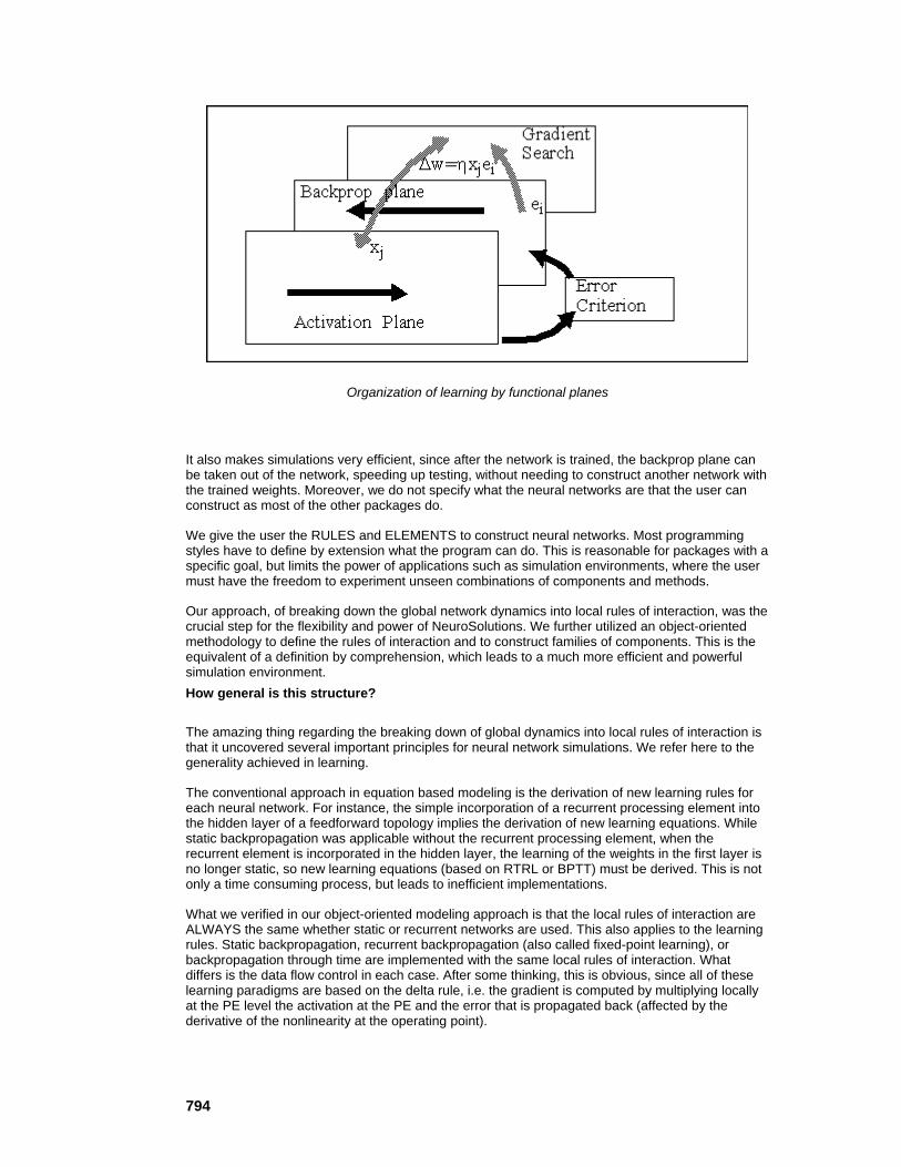
794

Organization of learning by functional planes

It also makes simulations very efficient, since after the network is trained, the backprop plane can be taken out of the network, speeding up testing, without needing to construct another network with the trained weights. Moreover, we do not specify what the neural networks are that the user can construct as most of the other packages do.

We give the user the RULES and ELEMENTS to construct neural networks. Most programming styles have to define by extension what the program can do. This is reasonable for packages with a specific goal, but limits the power of applications such as simulation environments, where the user must have the freedom to experiment unseen combinations of components and methods.

Our approach, of breaking down the global network dynamics into local rules of interaction, was the crucial step for the flexibility and power of NeuroSolutions. We further utilized an object-oriented methodology to define the rules of interaction and to construct families of components. This is the equivalent of a definition by comprehension, which leads to a much more efficient and powerful simulation environment. How general is this structure?

The amazing thing regarding the breaking down of global dynamics into local rules of interaction is that it uncovered several important principles for neural network simulations. We refer here to the generality achieved in learning.

The conventional approach in equation based modeling is the derivation of new learning rules for each neural network. For instance, the simple incorporation of a recurrent processing element into the hidden layer of a feedforward topology implies the derivation of new learning equations. While static backpropagation was applicable without the recurrent processing element, when the recurrent element is incorporated in the hidden layer, the learning of the weights in the first layer is no longer static, so new learning equations (based on RTRL or BPTT) must be derived. This is not only a time consuming process, but leads to inefficient implementations.

What we verified in our object-oriented modeling approach is that the local rules of interaction are ALWAYS the same whether static or recurrent networks are used. This also applies to the learning rules. Static backpropagation, recurrent backpropagation (also called fixed-point learning), or backpropagation through time are implemented with the same local rules of interaction. What differs is the data flow control in each case. After some thinking, this is obvious, since all of these learning paradigms are based on the delta rule, i.e. the gradient is computed by multiplying locally at the PE level the activation at the PE and the error that is propagated back (affected by the derivative of the nonlinearity at the operating point).

795

In static backpropagation, only the present time activation and error are used, so learning progresses by alternating toward propagation of the activations and backward propagating of the instantaneous errors.

In recurrent backpropagation, activations are fed forward UNTIL a fixed value is achieved. Only then is the error computed and propagated backwards. Again, the error activations must be stable before the delta rule is applied, so relaxation of the error is also needed. But once these two conditions are met, the delta rule is used at the PE level to adapt the weights.

In backpropagation through time, the goal is to compute the gradient over the trajectory. Since the gradient decomposes over time, this can be achieved by computing instantaneous gradients at each component and summing the effect over time. So during BPTT the activation is sent through the net and each PE stores its activation locally for the entire length of the trajectory. At each step the network output is also computed and stored. At the end of the trajectory the errors are generated at the output and a vector of errors is input to the transpose networks. The local error activation is then multiplied to the corresponding activation obtained in the feedforward flow, and the delta rule applied at the component level. The net weight update is composed of instantaneous weight updates.

Therefore, in NeuroSolutions these three procedures became one in terms of local rules of interaction (the delta rule). This does not depend on whether the network is static or recurrent. What differs is the firing of activation and errors through the network, a global data control issue.

Another remarkable feature of the local rules of interaction is that supervised and unsupervised learning rules can be INTERMIXED anywhere in the network. These mixed learning rules have only now attracted the attention of neural researchers.

Ideal Simulation Environments

Let us now consider an ideal neural network simulation environment. If we had such an environment, it would have to be flexible. We would want to be able to construct any network topology (static or recurrent), and then train with any learning rule. We want a single network to be able to simultaneously learn under more than one learning rule. Finally, when determining an error, for learning rules that belong to a supervised learning paradigm, we want to be able to assign arbitrary and user-defined criteria.

This ideal simulation environment should also be efficient. It should minimize its storage requirements and maximize code efficiency based upon the network topology we present it. Furthermore, it should allow us to interface with faster hardware platforms.

User friendliness is also very important. Even though some users may want to develop their own network elements by writing source code, others will want to use elements that were provided with the environment, or elements that more ambitious users give them, by simply grabbing their icon off some component palette. Analogous to prototyping electronic circuits, we want to construct network topologies by placing neural components on a breadboard and establishing connections.

We should then be allowed to inspect and alter each element on a breadboard, as well as place runtime probes to graphically monitor any activations or adapting coefficients within the network. In particular, in experimental research areas such as neural networks where the theory is being developed, the user should have extended probing facilities to understand and control the quality of the simulations.

Finally, this environment should inherently demand constructive development. User defined network components should utilize all source code previously developed for similar elements. After a breadboard has been developed, we would like to be able to collapse it and use it as a component in another network on a separate breadboard. This process could continue indefinitely, providing an inherently modular simulation environment.

Although this ideal environment may seem unrealistic, we have created it in NeuroSolutions.

796

Code Generation Code Generation

NeuroSolutions



Purpose

This chapter describes the Code Generation facility available within the Professional and Developers versions of NeuroSolutions. This feature enables the user to compile and run a neural network on another platform. In addition, the generated code can be integrated into custom C/C++ user applications.

Introduction to Code Generation

The Code Generation facility of NeuroSolutions produces ANSI-compatible C++ source code for any breadboard, including learning. This allows a simulation prototyped within the GUI of Windows to be run on other hardware platforms. In addition, NeuroSolutions' networks can be easily integrated into user applications.

It is important to note that the generated code is not completely self-contained. For any given platform that you are compiling under, you must have the corresponding libraries that the source code is compiled against. The libraries for Visual C++ are included with the Professional and Developer levels, while the libraries for other platforms must be compiled by the user after purchasing the Source Code License.

System Requirements for Code Generation

NeuroSolutions was developed using Microsoft’s Visual C++. The interface for the code generation has been tightly integrated with this development environment. This allows you to compile, run, and debug your C++ application right from NeuroSolutions. Please contact NeuroDimension for a list of other C++ compilers that are supported.

The generated C++ code is portable to other platforms and other compilers (provided that you are licensed for the NeuroSolutions Source Code License). This version of NeuroSolutions is not able

797

to communicate with those compilers, so you will be required to integrate the generated source code into the development environment manually.

Code Generation User Interface

The interface to the Code Generation facility is contained within the Code Generation property

page of the StaticControl or DynamicControl inspector. This page allows you to Compile, Run, and Debug the C++ project right from NeuroSolutions.

Behind the Scenes of C++ Code Generation

Within the NeuroSolutions directory is a sub-directory named "CodeGen". It contains the configuration files for each of the supported compilers. For each compiler there are several configuration files. Here is a summary of these files for Visual C++ 6.0:

Msvc60.cmp Commands issued to the Windows 95 operating system when the "Compile" button is pressed.

Msvc60.cmp.NT Commands issued to the Windows NT operating system when the "Compile" button is pressed.

Msvc60.dbg Makefile used when the "Debug" button is pressed.

Msvc60.h The header file for the NeuroSolutions class library that the generated code links against.

Msvc60.lib The NeuroSolutions class library that the generated code links against.

Msvc60.mak The makefile used when the "Compile" button is pressed.

Msvc60.nsl Contains the configuration information for the Visual C++ compiler. This is the file that is selected when choosing the "Target" from the Code Generation property page.

Msvc60.run Commands issued to the operating system when the "Run" button is pressed.

Whenever a new project is created the library ("NS.lib"), header file ("NSLib.h") and makefile ("BreadboardName.mak") are copied to the project directory. The makefile is modified slightly to include the appropriate files and directories for the project.

Network Input/Output for Generated Code

Since the Input and Probe components are dependent on the Windows environment, special consideration must be given to the network input/output when generating portable source code. Inputs

798

When the code for a breadboard is generated, NeuroSolutions stores a binary file for each Input component on the breadboard by default. These binary files contain the data that is feed into the network on the breadboard. The generated source code includes statements to read from these files.

This default may be overridden from the Access property page of the Input component (see the on-line help). By switching the Code Generation File Format switch to Function, the generated code will call a user-defined function for its input instead. This function is called every time a new sample of data is required by the attached component. The implementation of the function computes and/or retrieves the data sample and stores it within the floating point array passed as a parameter. Outputs

During a simulation, each probe on the breadboard will send its output to one of four locations, based on the settings of the Code Generation File Format switches from the Access property page of the component. The Stdio switch sends the output to the standard output, which is normally a DOS window. The ASCII and Binary switches will write the probe’s output to a file of the corresponding type. The Function switch is similar to that of the Input component, except the implementation of the function reads from the floating-point array instead of writing to it. This data may then be displayed, processed, and/or sent to another application. File Names used within the Generated Code

When a file type is selected (ASCII or Binary) from the Access page of either an Input or Probe component, the data associated with this component is written to a file. The prefix of the file name is "in" for Inputs and "out" for Probes. Appended onto the prefix is the component's name (see the Engine property page within the on-line help of the component’s inspector). The file extension is "bin" for binary files and "asc" for ASCII files. Function Prototype

void axonXXXAccess( NSFloat *data, // Buffer to read from/write to int rows, // Number of rows in buffer int cols // Number of cols in buffer );

where, data

Pointers to a block of floating point numbers that contain the processing elements (PEs) of the attached component. For Input components this buffer is written to and for Probe components it is read from. The size of this buffer is rows*cols*sizeof(NSFloat). rows

The number of rows of processing elements (PEs) of the component attached below. cols

The number of columns of processing elements (PEs) of the component attached below.

An empty function is automatically generated for every Input or Probe component on the breadboard that has Function specified as its Code Generation File Format within the Access property page. The prototype for the functions are identical for both Input components and Probe components. The function implementations differ in that Input components write to the data buffer and Probe components read from this buffer. Note that the "XXX" of the function name corresponds to the name of the component attached below (the one accessing the data buffer).

799

A Simple Example of Code Generation

The following example demonstrates how you would go about generating and compiling the code for a simple MLP.

Step 1: Build the Network

Use the NeuralBuilder to build a 1-hidden-layer MLP. Set the input file to "xor.asc" such that the x and y columns are the input and the z column is the output. From the Probe Configuration panel, disable all probes except the MegaScope at the error.

Step 2: Configure the Network Output

Select the Access property page from the DataStorage inspector and verify that the Code Generation File Format is set to stdio. This will send the mean squared error (MSE) from each epoch to the standard output (a DOS window). Also verify that the probes at the networks input, output and desired access points are all sending their data to binary files. Step 3: Create the Project

From the Code Generation property page of the StaticControl inspector, press the New button. Select the directory and file name of the source code to be generated (it must have a ".cpp" extension). It is highly recommended that you create the project in an empty directory, since a number of files will be created along with the source file. This will make clean up much easier. Click the Edit button to view the generated code.

Step 4: Compile and Run

Press the Compile button. A DOS window displays the status of the compile, then prompts you to press any key to close the window. Now press the Run button. This brings up another DOS window

800

and displays a series of floating point numbers. These numbers are the decreasing error values for each epoch, indicating that the network was able to learn the XOR problem. Try sending the networks input and output to stdio as well, then press the Generate, Compile and Run buttons (in that order) to observe how your changes affected the running of the network from the command line.

Limitations of Code Generation

The source code generation facility was designed to produce a self-contained block of code that can easily be ported to faster platforms. This code can also be easily integrated within a C/C++ application by implementing input/output functions. Both the porting and the integration tasks should not require any modification to the generated code. However, since you have the header file ("NSLib.h") and the NeuroSolutions class library ("NS.lib"), you can experiment with manual modifications to the generated code. For this version of NeuroSolutions, there is no documentation for the class library and NeuroDimension will not be able to provide technical support for code modifications that you make.

The only components that are not supported are the probes, since they use Windows-specific functions for their displays. Instead, the probes write to either the standard output, an ASCII file, a binary file, or a floating point array passed as a function parameter.

There is also a limitation with the use of the transmitters when generating code, in that not all of the actions are supported. If you try to generate code for a breadboard containing a transmitter, NeuroSolutions will check to make sure that all of the items selected within the Actions List of the Transmitter property page are supported. If not, a panel will be displayed to warn you that the unsupported action will be ignored.

Generating DLL Source Code

If the current breadboard contains one or more DLLs, then NeuroSolutions will automatically integrate those customized components into the generated source code. It does this by extracting the code from the DLL source, and copying it into the source code for the code generation project. An additional statement is generated within the main() routine (setDLL), which establishes the link between the base component and the DLL functions.

The function names have the component’s name (from the Engine property page of the component’s inspector) appended to them. This forces each DLL implementation to use unique function names to prevent overlap between DLLs using the same protocol.

There is one limitation to this feature: the only functions that are copied are the perform, alloc, and free. These are the only functions that will get called automatically by the NeuroSolutions classes. Any additional functions or global variables that are used by the DLL implementation must be copied to the generated source file by hand. This limitation will be removed for the next release.

Porting the Generated Code

The Code Generation feature of NeuroSolutions produces C++ code that can be compiled on a number of ANSI-compatible compilers under various hardware platforms. However, this code does require the source code for the NeuroSolutions class library ("NS.lib"). Contact NeuroDimension for information on purchasing a license for this code.

Some operating systems store the bytes of binary files in reverse from MS DOS/Windows. This may require that the binary input files generated by NeuroSolutions be byte-swapped in order for

801

these files to be read correctly on another platform. This operation is performed automatically when these lines are commented out of the header file ("NSLib.h"):

#define PC

#define MS_VISUAL

The library source code includes a template makefile, which enable you to easily import the generated source code and compile the project from the command line. Please refer to the readme file of the library source code for instructions on compiling the NeuroSolutions class library.

Examples of Integrating the Generated C++ Code Examples of Integrating the Generated C++ Code

The Code Generation feature of NeuroSolutions produces C++ code that will run a neural network simulation without making any modifications to the code. However, if you want to integrate the network into another application then some code modifications will be required. This section offers three simple examples using an MLP to solve the XOR problem. All of the files needed for these examples are contained within the directory "CodeGen\Examples".

To see an overview of the three example programs, run the program "MainMenu.exe". The files you will be prompted for are "XorInput.asc", "Xor2Out.asc", and "XorDesir.asc" (for the input, network output, and desired output, respectively).

Getting Started

Before integrating a network into an application, you most often will train the network within the graphical user environment of NeuroSolutions. Open the breadboard "xortrain.nsb". Reset and run the network to verify that the error approaches zero and the network output approaches either -1 or 1.

After 100 epochs, the weights are ready for use. From the StaticControl property page, save the weights to the file "xor.nsw". This Weights File will be used by all three example programs.

Example 1: Keyboard Input using Function Calls (recall)

Example 2: ASCII File Input using Function Calls (recall)

Example 3: ASCII File Input using File Component (learning)

Code Generation Example - Keyboard Input using Function Calls

The following example demonstrates how to generate code for a recall network (one with no learning). Two functions are added to the code to read the input from the keyboard and write the network output to the screen. The initial weights are obtained by running the network from the Example Introduction or Example 3.

802

Step 1: Load the Network

Open the breadboard "xor1and2.nsb". This is the same topology as "xortrain.nsb", except all of the components used for learning have been removed. Step 2: Configure the Network Input

Select the Access property page from the File inspector and verify that the Code Generation File Format is set to Function. This will create an empty function named inInputFileAccess ("inputFile" is the component's name), which will be called every time the network needs an exemplar of input data.

Step 3: Configure the Network Output

Select the Access property page from the DataWriter inspector and verify that the Code Generation File Format is set to Function. This will create an empty function named outDataWriterAccess, which will be called every time the network generates an exemplar of output data. Step 4: Create the Project

From the Code Generation property page of the StaticControl inspector, press the New button. Select the directory and enter the name of the new source code file to be generated (Note: do not overwrite the existing source files "xor1.cpp", "xor2.cpp", or "xor3.cpp"). Note that the Load weights before run switch is set, so that code will be included to read from the default weights file ("xor1.nsw"). Click the Edit button to view the generated code. Step 5: Modify the Code

The generated functions need to be written in order to inject data into and extract data out of the network. Open the file "xor1.cpp" within an ASCII editor. Note that code has been added to read the input from the standard input (the keyboard) and write the output to the standard output (the screen). The weights file to load has been changed to "xor.nsw". You could insert this code into the project you created, but to save time you should instead Open this project from the Code Generation property page. Note that if you click the Generate button, then the modified code will be deleted. Step 6: Compile and Run

803

Press the Compile button. If the program is not up to date, a DOS window displays the status of the compile, then prompts you to press any key to close the window. Now press the Run button. This brings up another DOS window and prompts you for the next exemplar of input data. Enter "1 -1" and the program will display the corresponding network output. Type "exit" when you finish entering the input data.

Next Example

Code Generation Example - ASCII File Input using Function Calls

The following example demonstrates how to generate code for a recall network (one with no learning). Two functions are added to the code to read the input from an ASCII File and write the network output to another ASCII file. There is also code added outside of the functions to open and close the files. The initial weights are obtained by running the network from either the Example Introduction or Example 3.


See Example 1 Step 2: Configure the Network Input

See Example 1 Step 3: Configure the Network Output

See Example 1 Step 4: Create the Project

See Example 1 Step 5: Modify the Code

The generated functions need to be written in order to inject data into and extract data out of the network. Open the file "xor2.cpp" within an ASCII editor. Note that code has been added in several places within the source file. Search on the strings "(Begin)" and "(End)" to find these code segments. You could insert this code into the project you created, but to save time you should instead Open this project from the Code Generation property page. Note that if you click the Generate button, then the modified code will be deleted. Step 6: Compile and Run

Press the Compile button. If the program is not up to date, a DOS window displays the status of the compile, then prompts you to press any key to close the window. Now press the Run button. This brings up another DOS window and prompts you for the name of input file. Type in "XorInput.asc" and press enter. Enter "Xor2Out.asc" as the output file. The network runs until the end of the input file is reached (or 100 epochs, whichever comes first). Open the output file within an editor to observe the network output for the 4 exemplars of input data.

Special Note

804

The purpose of this example is to demonstrate how to inject data using a global variable. In this case the variable was a file pointer, but it could have just as easily been a pointer to external data. You do not have to write these functions to simply read from and write to a file (see Example Introduction or Example 3).

Next Example

Next Example

Code Generation Example - ASCII File Input using a File Component

The following example demonstrates how to generate code for a network with learning. This is useful for when you want to train a network on a faster computer, use the trained weights within a recall network (one without learning). The code for the File components has been modified to read ASCII instead of binary data. There is also code added to prompt the user to load the weights and to set the number of training epochs. The weights are automatically saved to "xor.nsw".


Open the breadboard "xor3.nsb". This is the same topology as "xortrain.nsb", except that there is only one probe used to monitor the error. Select the Access property page from the DataWriter inspector and verify that the Code Generation File Format is set to Stdio. This will write the average cost for each epoch to the standard output. Step 2: Configure the Network Input/Output

Select the Access property page from the input File inspector and verify that the Code Generation File Format is set to Binary. This will later be modified within the code to read from an ASCII instead of a binary file. Repeat for the desired output file. Step 3: Create the Project

From the Code Generation property page of the StaticControl inspector, press the New button. Select the directory and enter the name of the new source code file to be generated (Reminder: do not overwrite the existing source files "xor1.cpp", "xor2.cpp", or "xor3.cpp"). Note that both the Load weights before run and the Save weights after run switches are set, so that code will be included to read from and write to the default weights file ("xor3.nsw"). Click the Edit button to view the generated code. Step 4: Modify the Code

We would like to modify the generated code so that the program reads from ASCII files instead of binary ones. We would also like to use the same weights file as the recall networks ("xor.nsw" instead of the default of "xor3.nsw"). Open the file "xor3.cpp" within an ASCII editor. Note that code has been added and removed in several places within the source file. Search on the strings "(Begin)" and "(End)" to find these code segments. You could insert this code into the project you created, but to save time you should instead Open this project from the Code Generation property page. Note that if you click the Generate button, then the modified code will be deleted. Step 5: Compile and Run

Press the Compile button. If the program is not up to date, a DOS window displays the status of the compile, then prompts you to press any key to close the window. Now press the Run button. This brings up another DOS window and prompts you for the name of input file. Type in "XorInput.asc"

805

and press enter. Enter "XorDesir.asc" as the desired output file. Run the first simulation with randomized weights for 500 epochs. Run the program again using the same training files, but load the weights from the previous simulation. Note that the error starts out where the last simulation started and drops further from there.

Things to Try

Run one of the recall networks (Example 1 or Example 2) again. Observe the network response with the set of weights that you just trained.

Dynamic Link Libraries (DLLs) Dynamic Link Libraries (DLLs)

NeuroSolutions



Purpose

This chapter describes the Dynamic Link Library facility available within the Developers versions of NeuroSolutions. This feature extends NeuroSolutions with a set of utilities that enable the user to customize neural components by writing C functions. These new components can utilize all of the basic features of the package, creating an extensible and flexible simulation environment.

Introduction to DLLs

NeuroSolutions utilizes an object oriented design methodology. This design is responsible for the power and flexibility of the package, and it also allows for a user extensible simulation environment. The need for an open simulation environment is clear. During the design process, the user is confronted with a large number of unknowns that may require new solutions. It would be impossible to develop a set of neural components that would meet every user’s needs. An alternate approach is to let the user define their own modifications to the base components included within the environment. Dynamic Link Libraries (DLLs) are the mechanism used for these component modifications.

Dynamic Link Libraries are used to create user-defined components. This is done by writing one or more C functions belonging to the base component’s protocol, thus overriding the component’s functionality. The DLLs are typically implemented as C functions, but C++ may also be used. The source code files for all customized components are included within the "DLLSys" directory. When you create a new DLL, the default source code for the overridden component is copied to the

806

"DLLCust" directory. This allows the user to start from familiar ground, providing the source code for how the current component was implemented. The user then simply modifies this source code to meet his or her particular needs, and re-compiles.

A word of caution should be raised. Since the user is able to modify the data variables used by NeuroSolutions, some C programming knowledge is certainly required. Care must be taken when working with pointers to data vectors in order to prevent errors from occurring outside of the scope of the DLL.

System Requirements for creating DLLs

NeuroSolutions was developed using Microsoft’s Visual C++. The interface for the creation of DLLs has been tightly integrated with this development environment. This allows you to compile, run, and debug your DLLs within NeuroSolutions.

Structure of a DLL

Every neural component within NeuroSolutions is implemented as a C++ object. Each object shares much of its code with other objects belonging to the same family. The unique functionality of an object is normally contained within a couple of C++ functions.

NeuroSolutions developers extends each base component with a DLL protocol and the corresponding default DLL source code that conforms to this protocol. This means that the user has access to a source code implementation of the component selected. This source code can be used as a starting point to make your modifications.

There are three sub-protocols available to each DLL implementation:

Perform sub-protocol

Memory management sub-protocol

Breadboard sub-protocol

The perform sub-protocol (required on every DLL) handles the actual functionality of the component. The prototype function name is prefixed with perform, followed by the component’s protocol name. The memory management sub-protocol (optional in the DLL) handles the allocation and freeing of any data stored within a particular instance of a DLL. The two prototype function names are prefixed with alloc and free, followed by the component’s protocol name. The breadboard sub-protocol (optional in the DLL) contains function prototypes used for synchronizing a DLL with the various stages of the simulation. The prototype function names are the same for all DLLs. The ability to modify NeuroSolutions components increases with each one of the sub-protocols, but it is also coupled with a more detailed and complex interaction that requires more programming skills.

How to Use DLLs

The first step towards utilizing DLLs is to select a NeuroSolutions component that has a functionality similar to the one you seek. Most of the times this is an easy task. However, a thorough knowledge of the NeuroSolutions components is necessary.

We suggest that you consult the Components chapter of NeuroSolutions Manual Volume II, where we provide a mathematical description of the functionality of each component in NeuroSolutions. You should select the component that has the closest mathematical description to the one you

807

want to build. In particular, you should seek a component with the same number of parameters. For instance, the Axon family has several components. If you want to create a new nonlinearity without a bias term, you can select the Axon. If you want your new nonlinearity to have a bias, you should use the BiasAxon instead. If you want to create a new memory structure, you should use the TDNNAxon.

Once you have found the component, bring it to the breadboard and go to the Engine level of its Inspector. Clicking on the New button will create source code for a new DLL with an implementation that is identical to that of the selected component. Details will be given below. Here we will simply address the steps of the design.

Next, simply open the new DLL for the component (the Edit button) to observe the DLL implementation of the selected component. Looking at the perform sub-protocol, try to figure out how the source code implements the selected component, and then identify the piece that you want to modify to create your new component.

Modify the C code to implement the functionality that you desire. Compile the C code and make sure that the code compiles without error. Finally, link the new component with the package (with the Use DLL switch). Once properly linked, the component’s icon will have DLL stamped on it. Your new component contains all of the features of its base component, so it can utilize all the NeuroSolutions features, e.g. probes.

If you want to not only modify the functionality of a component but also add new variables, or deeper modifications, you also can. As you might expect the procedure is more involved, but we designed an environment that is very flexible. Please see the examples for a more in depth look at DLL design.

User Interface of the DLL Feature

The interface to the Dynamic Link Library facility is contained within the Engine property page of every component’s inspector.

Behind the Scenes of DLLs

Within the NeuroSolutions directory are two sub-directories used for DLLs: DLLCust and DLLSys. DLLSys contains the source code and compiled DLLs for most of the base components within NeuroSolutions. These files are arranged based on the protocol that they conform to.

The DLLCust directory is where the user-defined DLLs are stored. When a new DLL is created, the DLL and source code file of the base component are copied from the DLLSys directory to the DLLCust directory. Note that the sub-directory structure is preserved such that the user-defined DLLs are arranged based on the protocol that they conform to.

The DLLSys directory also contains a few other files that are used to compile the DLLs:

DebugMakefile.v60 Visual C++ 6.0 makefile used to compile the DLL after the "Debug" button is pressed. DebugMakefile.v50 Visual C++ 5.0 makefile used to compile the DLL after the "Debug" button is pressed.

DLLTest.dsp The Visual C++ project file used when the "Debug" button is pressed.

Global.h Global variables included by NSDLL.h.

808

Makefile.v60 Visual C++ 6.0 makefile used to compile the DLL after the "Compile" button is pressed.

Makefile.v50 Visual C++ 5.0 makefile used to compile the DLL after the " Compile " button is pressed.

NSDLL.h Header file included by all DLLs.

Perform Sub-Protocol Perform Sub-Protocol

The modifications to the base NeuroSolutions components have several degrees, depending on how extensive the new properties differ from the old ones. The perform sub-protocol implements the component’s basic functionality. Hence, the simplest type of modification involves a change of the functionality of the base component’s perform function without altering the structure of the component parameters or data.

Every DLL must have at least one perform sub-protocol. You can recognize the perform sub-protocol in the code by the function: void performComponentName(...) { ... }

which is normally followed by only a few lines of code that implement the component functionality. This is the part you have to concentrate on rewriting. In order to make the code more readable, the beginning and end of the block are commented.

DLL Example

One of the more common uses of DLLs is to customize the activation function of an Axon. Suppose that the TanhAxon component were not included within NeuroSolutions. The following example demonstrates how you would go about adding this component.

Step 1: Build a Network

Use the NeuralBuilder to build a 1-hidden-layer MLP. Set the input file to "xor.asc" such that the x and y columns are the input and the z column is the desired response. Change the transfer function of the layers from a TanhAxon to a LinearAxon. Build the network, and try running it. As expected, the network is not able to solve the xor problem when the simulation was run. Step 2: Create a New Component

You need to enhance the LinearAxon in order to have the network solve this problem. You will do this by implementing a hyperbolic tangent transfer function.

Select the LinearAxon at the hidden layer and open its inspector. From the Engine property page, click the New button. A panel for the new DLLs name will open. Enter "MyTanh" as the DLL name. A copy of the LinearAxon’s DLL source code has been saved under this new name. NeuroSolutions created automatically the file bkMyTanh for backpropagation support for this new component.

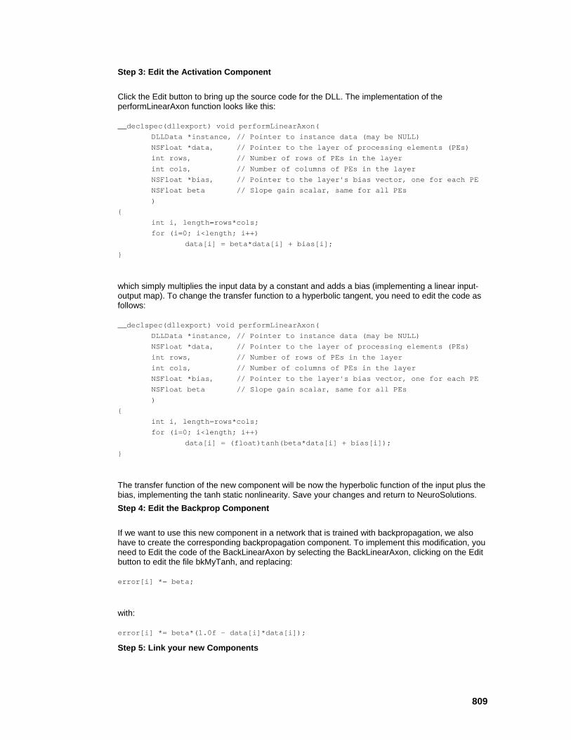
809

Step 3: Edit the Activation Component

Click the Edit button to bring up the source code for the DLL. The implementation of the performLinearAxon function looks like this: __declspec(dllexport) void performLinearAxon( DLLData *instance, // Pointer to instance data (may be NULL) NSFloat *data, // Pointer to the layer of processing elements (PEs) int rows, // Number of rows of PEs in the layer int cols, // Number of columns of PEs in the layer NSFloat *bias, // Pointer to the layer's bias vector, one for each PE NSFloat beta // Slope gain scalar, same for all PEs ) { int i, length=rows*cols; for (i=0; i<length; i++) data[i] = beta*data[i] + bias[i]; }

which simply multiplies the input data by a constant and adds a bias (implementing a linear input-output map). To change the transfer function to a hyperbolic tangent, you need to edit the code as follows: __declspec(dllexport) void performLinearAxon( DLLData *instance, // Pointer to instance data (may be NULL) NSFloat *data, // Pointer to the layer of processing elements (PEs) int rows, // Number of rows of PEs in the layer int cols, // Number of columns of PEs in the layer NSFloat *bias, // Pointer to the layer's bias vector, one for each PE NSFloat beta // Slope gain scalar, same for all PEs ) { int i, length=rows*cols; for (i=0; i<length; i++) data[i] = (float)tanh(beta*data[i] + bias[i]); }

The transfer function of the new component will be now the hyperbolic function of the input plus the bias, implementing the tanh static nonlinearity. Save your changes and return to NeuroSolutions. Step 4: Edit the Backprop Component

If we want to use this new component in a network that is trained with backpropagation, we also have to create the corresponding backpropagation component. To implement this modification, you need to Edit the code of the BackLinearAxon by selecting the BackLinearAxon, clicking on the Edit button to edit the file bkMyTanh, and replacing: error[i] *= beta;

with: error[i] *= beta*(1.0f - data[i]*data[i]);

Step 5: Link your new Components

810

Select the LinearAxon and click the Use DLL switch from the Engine property page. Notice that NeuroSolutions automatically detected that you had modified the DLLs source code and is prompting you to first compile it. Press YES to compile the source code. Once this step is completed you will be prompted to compile the DLL for the BackLinearAxon. Your new components are now linked with the rest of the package, as illustrated by the DLL stamps on their icons. Step 6: Use DLL for the Output Layer

Select the LinearAxon at the output layer and click the Load button. Select "MyTanh.dll" from the file selection panel. The corresponding backprop DLL is automatically loaded as well. Now both layers have the LinearAxon overridden with the hyperbolic tangent transfer function. Click on the Transfer Function property page of the Inspector to verify that the transfer function has changed. When you run the simulation, the network will now solve the xor problem.

Memory Management Sub-Protocol Memory Management Sub-protocol

When a new instance of a component is created, NeuroSolutions automatically creates the variables needed to implement the component. If the modifications do not change the component’s data structure, as in the previous example, we do not have to worry about memory management. However, for more in-depth DLLs, the developer may want to add to the component’s data structure. The purpose of this section is to explain the concepts and the details needed to add variables to a base component.

The DLLData Structure

Adding Adaptable Weights to the Instance Data

Adding Parameters to the Instance Data

Adding User-Defined Data

Memory Management of Instance Data

Creating Global Variables

The DLLData Structure

The DLLData structure is used to store the weights, parameters, and user-defined data that is specific to a particular instance of a DLL component. A pointer to this structure is passed by NeuroSolutions to all implementation functions of the DLL. This data structure is divided in three parts:

the weights

the parameters

the user-defined data

The reason for this division in the data structure is due to the way components interact within the NeuroSolutions environment. Weights are updated by the gradient descent components, and we would like developers to be able to add adaptable weights to their components without having to write the code for gradient search procedures, which are already implemented with NeuroSolutions. Likewise, parameters are displayed and modified within NeuroSolutions’ Inspector window, so there is no point in requiring developers to write their own code for this purpose. In general, user

811

defined data structures cannot be supported by NeuroSolutions, so you will have to write the code associated with this data. Next we present the general DLL data structure.

Data Structure typedef struct { NSFloat *data; int length; } DLLWeights; typedef struct { char parameters[5][3][64]; char parameterNames[5][3][64]; } DLLParameters; typedef struct { DLLWeights *weights; DLLParameters *parameters; void *userData; } DLLData;

The data variables that are available to the user are: data

Pointer to a floating point array containing the user-defined weights. This pointer is accessed by calling the getWeights function defined within "NSDLL.H". Note that the memory is allocated and freed within NeuroSolutions. length

The number of weights stored within data. This number is specified when the weights are allocated (by calling the setWeights function defined within "NSDLL.H"). parameters

Storage for 15 parameter values -- 5 rows and 3 columns. The values are set using the setBoolParameter, setIntParameter, setFloatParameter, and setStringParameter functions defined within "NSDLL.H". These values are converted if needed and stored as strings. The parameter values are retrieved using the getBoolParameter, getIntParameter, getFloatParameter, and getStringParameter functions. parameterNames

Storage for 15 parameter names, corresponding to the 15 parameter values. These are used as labels within the DLL property page of the Inspector window. weights

Pointer to the DLLWeights structure that holds the user-defined weights. This structure is allocated by calling the setWeights function defined within "NSDLL.H" parameters

Pointer to the DLLParameters structure that holds the user-defined parameters. This structure is allocated during the first call to the setParameterName function defined within "NSDLL.H". userData

812

Pointer to a user-defined block of data. The memory is allocated and freed by the user, and the pointer is updated by calling the setUserData function defined within "NSDLL.H".

See Also

Adding Adaptable Weights to the Instance Data

There may be times when you want to add an adaptable weight vector to a component that already has a set of adaptable weights. Recall that a TanhAxon has a bias vector (because it is a subclass of BiasAxon), which may be adapted during learning. The beta term (the slope of the tanh function) is not adaptable and is the same for all PEs. Suppose that you want to have a unique beta for each PE and that these terms should be adaptable. This is a case where an instance weight vector is needed (see Adjustable Transfer Function Slope DLL Example).

An instance weight vector is defined by making a call to the setWeights function within the alloc function of the DLL: __declspec(dllexport) DLLData *allocLinearAxon( DLLData* oldInstance, // Pointer to the last instance if reallocating int rows, // Number of rows of PEs in the layer int cols // Number of columns of PEs in the layer ) { DLLData *instance = allocDLLInstance(oldInstance); setWeights(instance, rows*cols); return instance; }

The setWeights function simply allocates a vector of weights of the specified size, and inserts it within the instance of DLLData. The memory for the weights is automatically freed when the instance is freed (by calling freeDLLInstance from the freeInstance function of the DLL). Note that the implementation of all DLL functions can be found within the "NSDll.h" header file.

The weights are automatically adapted the same way as the base component’s weights. The attached Backprop component will compute the gradients and sensitivities for both sets of weights, and the Gradient Search component will update all of the weights based on the computed gradients. Note that adaptable instance weights only apply to members of the Axon and Synapse families.

If an Axon or Synapse has a vector of adaptable weights, then the component’s backpropagation dual must have a corresponding set of gradients. These gradients are treated as weights in an identical manner to that of the activation dual.

Within the perform function of a DLL, you obtain a pointer to the weight vector by using the getWeights function call:

NSFloat *beta = getWeights(instance);

From there you access the individual weights by indexing into the array (e.g., beta[i]).

813

Adding Parameters to the Instance Data

Each component has a set of parameters that are specified by the user within the various property pages of the inspector window. The creation of custom components using DLLs will often require additional user-defined parameters. For this reason, a facility has been included for you to specify up to 15 parameters that are accessible to the user from the DLL property page of the Inspector.

A parameter set is initialized by making calls to the setParameterName functions within the alloc function of the DLL: __declspec(dllexport) DLLData *allocProtocolName( DLLData *oldInstance, // Pointer to the last instance if reallocating int rows, // Number of rows of PEs in the layer int cols // Number of columns of PEs in the layer ) { DLLData *instance = allocDLLInstance(oldInstance); setParameterName(instance, 1, 1, "Amplitude", FALSE); setFloatParameter(instance, 1, 1, 11.0f, FALSE); setParameterName(instance, 2, 1, "Phase", FALSE); setIntParameter(instance, 2, 1, 180, FALSE); return instance; }

The protocol for the setParameterName function is as follows: void setParameterName( DLLData *instance, // Pointer to instance data storing parameters int row, // Inspector row to display parameter int col, // Inspector column to display parameter char *name, // Inspector label for parameter BOOL realloc // Reallocate instance data when value changes );

The parameter names and values are stored as part of the instance data structure. The row and col refer to the parameter’s position within the inspector. The number of parameters stored is static (5 rows and 3 columns), but only the ones initialized with this function are displayed within the inspector. The name is used to label the parameter within the inspector. The realloc flag is used to indicate whether or not this parameter affects the structure of the instance data. If realloc is set to TRUE, then the instance data is reallocated (i.e., the DLL receives a call to the alloc function) every time the value of the parameter changes. Note that the implementation of setParameterName, as well as all other DLL functions, can be found within the "NSDLL.H" header file.

A default value for each parameter is normally set within the alloc function as well, using one of the following function calls: void setBoolParameter (DLLData *instance, int row, int col, BOOL boolValue, BOOL force); void setIntParameter (DLLData *instance, int row, int col, int intValue, BOOL force); void setFloatParameter (DLLData *instance, int row, int col, NSFloat floatValue, BOOL force); void setStringParameter (DLLData *instance, int row, int col, char *stringValue, BOOL force);

814

If the force flag is set to FALSE, then the parameter is only assigned if the current setting is undefined (blank). Otherwise, the parameter is always set to the specified value. This flag should always be set for FALSE for parameter initialization in order to avoid overwriting a previously specified value.

Here is an example of how a parameter’s value is retrieved and used: int i, length=rows*cols; NSFloat amplitude = getFloatParameter(instance, 1, 1); for (i=0; i<length; i++) data[i] = (NSFloat)amplitude*data[i];

The function prototypes for retrieving the parameter values are similar to those used to set them: int getIntParameter(DLLData *instance, int row, int col); BOOL getBoolParameter(DLLData *instance, int row, int col); NSFloat getFloatParameter(DLLData *instance, int row, int col); char *getStringParameter(DLLData *instance, int row, int col);

See Also

Adding User-Defined Data

During the definition of your new components you may have necessity to define instance variables and data. NeuroSolutions will maintain a pointer to this data for each instance of the DLL component. You are responsible for allocating this data during the alloc sub-protocol, freeing it during the free sub-protocol, and interpreting it during the perform sub-protocol. NeuroSolutions only maintains a single pointer, so all user-defined data must be organized within a single data structure.

For example, if you wanted each instance of your component to contain an integer variable called length and a floating point array called dataArray, then you should define the following data structure within your DLL:

typedef struct { int length; float *dataArray; } MyData;

Memory Management of Instance Data Allocation

An instance of a DLL is allocated when the DLL is first loaded, and it is reallocated whenever the component itself is reallocated (e.g., the number of PEs change), or the instance data is reallocated due to a change in a specially-tagged instance parameter. (Note that the instance parameter is tagged by setting realloc=TRUE when calling the setParameterName function.) Whenever a DLL instance is allocated or reallocated, the DLL’s instance allocation function is called.

815

There are three types of instance data that are available within the DLLData structure: weights, parameters, and user data. The following instance allocation implementation is an example of a DLL that uses all three types: __declspec(dllexport) DLLData *allocLinearAxon( DLLData *oldInstance, // Pointer to the last instance if reallocating int rows, // Number of rows of PEs in the layer int cols // Number of columns of PEs in the layer ) { int i, length = rows*cols; DLLData *instance = allocDLLInstance(oldInstance); setWeights(instance, rows*cols); setParameterName(instance, 2, 1, "Gain", TRUE); setFloatParameter(instance, 2, 1, 1.0f, FALSE); NSFloat *myData = (NSFloat *)calloc(rows*cols, sizeof(NSFloat)); setUserData(instance, myData); return instance; }

The call to allocDLLInstance allocates a new DLLData structure. If it is allocated for the first time, then the three members of the structure are all set to NULL. If it is a reallocation (oldInstance != NULL), then the parameters and weights of the old instance are preserved in the new structure.

The call to setWeights sets the number of instance weights that NeuroSolutions will allocate. The first call to setParameterName allocates the memory needed to store 15 instance parameters (5 rows and 3 columns). Only the first call to setFloatParameter sets the parameter value (since the force flag is set to FALSE). This preserves the parameter values during a reallocation.

The memory management for the user data is the responsibility of the DLL author. Any block of data may be allocated for use by a particular instance. The call to setUserData stores the pointer to the data block within the DLLData structure. The prototype for this function as defined within "NSDLL.H" is: void setUserData(DLLData *instance, void *userData);

Deallocation

An instance of a DLL is deallocated when the DLL is unloaded, or when the instance has been reallocated.

The following instance deallocation implementation corresponds to the allocation implementation above: __declspec(dllexport) void freeLinearAxon(DLLData *instance) { free(getUserData(instance)); freeDLLInstance(instance); }

The prototype for the getUserData function as defined within "NSDLL.H" is: void *getUserData(DLLData *instance);

Note that the user data is the only memory that the DLL author is responsible for freeing directly; the freeDLLInstance function handles the rest.

816

See Also

Creating Global Variables

A very powerful concept that is supported in the DLLs is the global variable. Global variables allow several component DLLs to share the same memory. The user must declare global variables at the top of the DLL. When there are several components using the same DLL, the system only loads the DLL into memory once. In other words, all of those components share the same memory space when accessing the DLL. For this reason, any global variables that are declared within the DLL are global to all instances using the DLL.

Example

Stamp two TanhAxons on a blank breadboard and bring up the inspector for one of them. From the Engine property page click the New button and enter "MyAxon" as the DLL name. Edit the code as follows: NSFloat myBeta = 0.01f; __declspec(dllexport) void performLinearAxon( DLLData *instance, // Pointer to instance data (may be NULL) NSFloat *data, // Pointer to the layer of processing elements (PEs) int rows, // Number of rows of PEs in the layer int cols, // Number of columns of PEs in the layer NSFloat *bias, // Pointer to the layer's bias vector, one for each PE NSFloat beta // Slope gain scalar, same for all PEs ) { int i, length=rows*cols; for (i=0; i<length; i++) { data[i] = (NSFloat)tanh(myBeta*data[i] + bias[i]); myBeta += 0.01f; } }

In this code myBeta is a global variable since it is defined before the perform function. Click the Compile button to create and load this DLL. Select the other TanhAxon and click the Load button from the Engine property page. Select the "MyAxon" DLL that you have just compiled. Now both components are sharing the same DLL. Select the Transfer Function property page to observe the effect of the global variable. Note that NeuroSolutions computes this graph by making consecutive calls to performLinearAxon, thus the slope of the hyperbolic tangent function (myBeta) increases with every point that is plotted. Now view the Transfer Function property page of the other TanhAxon. It plotted the function based on the value of myBeta computed by the first TanhAxon. Switch back and forth between the two components to observe the increasing slope of the transfer function.

If these two DLL instances were placed in a network, then the slope would increase twice for each sample of data run through the network because each instantiated object would be incrementing the same variable.

817

See Also

Breadboard Sub-Protocol Breadboard Sub-Protocol

The breadboard sub-protocol addresses the need to synchronize DLLs with the rest of the simulation environment. This is an important feature for the functionality of the reconfigured component since there are a lot of messages from the simulation environment that have to be attended to by any component, such as reset, zeroing of counters at the end of epoch, updating of weights in batch mode, etc.

NeuroSolutions will call all of the functions that are implemented during the appropriate times, and pass a pointer to The DLLData Structure as the first parameter. Below we present the synchronization function calls available to the DLLs.

// Called after the current epoch has completed __declspec(dllexport) void epochEnded( DLLData *instance, int epoch // Current epoch count ); // Called after the current exemplar has completed __declspec(dllexport) void exemplarEnded( DLLData *instance, int exemplar // Current exemplar count ); // Called after the Run button is pressed __declspec(dllexport) void fireGetReady(DLLData *instance); // Called after fireGetReady(); return FALSE to abort the Run __declspec(dllexport) BOOL fireIsReady(DLLData *instance); // Called after the simulation has stopped __declspec(dllexport) void fireConclude(DLLData *instance); // Called after the weights have been jogged (Controller button) __declspec(dllexport) void networkJog(DLLData *instance); // Called after the network weights are randomized (Controller button) __declspec(dllexport) void networkRandomize(DLLData *instance); // Called after the network has been reset (Controller button) __declspec(dllexport) void networkReset(DLLData *instance); // Called before the network weights are updated __declspec(dllexport) void prepareToUpdateWeights(DLLData *instance); // Called after the network weights have been updated __declspec(dllexport) void updateWeights(DLLData *instance);

818

DLL Examples DLL Examples

In the following we will present several important examples to illustrate the use of DLL features. For each example we explicitly state the feature that is being illustrated, and the code is compared with the base NeuroSolutions component to emphasize the differences, and how the new functionality was implemented. We present examples to reconfigure components belonging to all the NeuroSolutions families. The following summarizes all of the examples:

Axon

Adjustable sigmoid - illustrates the addition of adaptable weights

Adjustable hyperbolic tangent - illustrates the addition of adaptable weights

Adjustable linear - illustrates the addition of adaptable weights

TanhAxon with gain - illustrates the addition of a parameter Synapse

Subset FullSynapse - illustrates the addition of adaptable weights

Locally-Connected Synapse - illustrates configuration ErrorCriterion

Loser learn all - illustrates configuration GradientSearch

DeltaBarDelta with limited step - illustrates configuration

DeltaBarDelta with exponential step - illustrates configuration General Input and Postprocessor

Strange attractor - illustrates configuration

Logistic function - illustrates configuration

Discriminant function - illustrates configuration

Scaling - illustrates configuration Function Generator

Sawtooth - illustrates configuration

Triangle - illustrates configuration

Square - illustrates configuration

Decayed Sine - illustrates configuration

Pulse - illustrates configuration Noise Generator

Gaussian - illustrates configuration

Decayed Gaussian - illustrates configuration

Decayed Uniform - illustrates configuration File

819

Binary - illustrates configuration

Binary float - illustrates configuration

Binary Integer - illustrates configuration

Binary Short - illustrates configuration

Binary character - illustrates configuration Preprocessor

Averaging filter - illustrates configuration

Decimator filter - illustrates configuration

Extractor - illustrates configuration Postprocessor and Probe

Confusion matrix - illustrates global variables Transformer

Derivative - illustrates configuration

Autocorrelation - illustrates configuration

Crosscorrelation - illustrates configuration

Axon

Adjustable Transfer Function Slope DLL Example

Within the "DLLCUST/BiasAxon" directory are three DLL examples entitled "adjtana", "adjsiga", and "adjlina". These DLLs implement specialized versions of the TanhAxon, SigmoidAxon, and LinearAxon, respectively, to demonstrate the use of instance weights.

Each of the base components has a bias vector (because they are subclasses of BiasAxon) that may be adapted during learning. However, the beta term (the slope of the transfer function) is not adaptable and is the same for all PEs. These DLLs use adaptable instance weights to maintain a unique beta for each PE. The backpropagation dual components ("bkadjtan", "bkadjsig", and "bkadjlin") have a corresponding set of weights that store the gradient information, which is used to adapt the beta terms of the activation dual.

The instance weight vectors for both the activation and backpropagation components are allocated and freed as follows: DLLData *allocBiasAxon( DLLData *oldInstance, // Pointer to the last instance if reallocating int rows, // Number of rows of PEs in the layer int cols // Number of columns of PEs in the layer ) { DLLData *instance = allocDLLInstance(oldInstance); setWeights(instance, rows*cols); return instance; } void freeBiasAxon (DLLData *instance) { freeDLLInstance(instance); }

820

All three DLLs have very similar implementations, so only the code for hyperbolic tangent will be shown here. Refer to the sample source code for the implementations of the other two.

The implementation for the activation DLL ("adjtana") is as follows: void performBiasAxon( DLLData *instance, // Pointer to instance data NSFloat *data, // Pointer to the layer of processing elements (PEs) int rows, // Number of rows of PEs in the layer int cols, // Number of columns of PEs in the layer NSFloat *bias // Pointer to the layer's bias vector, one for each PE ) { int i, length=rows*cols; NSFloat *beta = getWeights(instance); for (i=0; i<length; i++) { if (beta[i] < 0.5f) beta[i] = 0.5f; data[i] = (NSFloat)tanh(beta[i]*data[i] + bias[i]); } }

Compare this with the implementation for the base component (TanhAxon): int i, length=rows*cols; for (i=0; i<length; i++) data[i] = (NSFloat)tanh(beta*data[i] + bias[i]);

The weight vector is stored within the DLLData structure and the pointer is obtained with the getWeights function. The weights are accessed by indexing the floating point array.

Note that there is minimum value forced on each beta term. When the network is reset, the weights are randomized to a value between -1 and 1. The beta term must be greater than zero. The higher the beta, the steeper the slope and the more discriminating the function becomes. A value of 0.5 was chosen as a minimum value for this starting point. Most often, the network will adapt to a higher value.

The implementation for the backpropagation DLL ("bkadjtan") is as follows: void performBackBiasAxon( DLLData *instance, // Pointer to instance data DLLData *dualInstance, // Pointer to the forward axons instance data NSFloat *data, // Pointer to the layer of processing elements (PEs) int rows, // Number of rows of PEs in the layer int cols, // Number of columns of PEs in the layer NSFloat *error, // Pointer to the sensitivity vector NSFloat *gradient // Pointer to the bias gradient vector ) { int i,length=rows*cols; NSFloat *beta = getWeights(dualInstance); NSFloat *betaGradient = getWeights(instance); for (i=0; i<length; i++) { error[i] *= beta[i]*(1.0f - data[i]*data[i] + 0.1f); if (gradient)

821

gradient[i] += error[i]; if (betaGradient) betaGradient[i] += error[i]*data[i]; } }

Compare this with the implementation for the base component (BackTanhAxon): int i, length=rows*cols; for (i=0; i<length; i++) { error[i] *= beta*(1.0f - data[i]*data[i] + 0.1f); if (gradient) gradient[i] += error[i]; }

The only differences are that the beta term is unique to each PE and that the gradient information for the beta vector is computed along with the gradient information for the Axon’s weights.

See Also

TanhAxon with Gain DLL Example

Within the "DLLCUST/LinAxon" directory is a DLL example entitled "gaintanh" and its corresponding backprop dual "bkgainta". This DLL implements a specialized version of the TanhAxon to demonstrate the use of instance parameters.

The transfer function of the base TanhAxon produces an output that ranges from -1 to 1. There are cases when you may want to have the output scaled to match that of the original data. This would be one use for a TanhAxon component that is enhanced with a gain factor.

The gain parameter is stored within the instance data of the activation component (the TanhAxon). It is initialized within the allocLinearAxon function as follows: DLLData *allocLinearAxon( DLLData *oldInstance, // Pointer to the last instance if reallocating int rows, // Number of rows of PEs in the layer int cols // Number of columns of PEs in the layer ) { DLLData *instance = allocDLLInstance(oldInstance); setParameterName(instance, 2, 1, "Gain"); setFloatParameter(instance, 2, 1, 1.0f, FALSE); return instance; }

The two function calls set the label on the inspector to "Gain" and set the default value to 1.0. The call to setParameterName must occur before the call to setFloatParameter in order to allocate memory for the parameters. Note that since the parameters are stored with the instance data, that memory is automatically freed when the freeDllInstance function is called.

822

The implementation for the activation DLL ("gaintanh") is as follows: void performLinearAxon( DLLData *instance, // Pointer to instance data NSFloat *data, // Pointer to the layer of processing elements (PEs) int rows, // Number of rows of PEs in the layer int cols, // Number of columns of PEs in the layer NSFloat *bias, // Pointer to the layer's bias vector, one for each PE NSFloat beta // Slope gain scalar, same for all PEs ) { int i, length=rows*cols; NSFloat gain = getFloatParameter(instance, 2, 1); for (i=0; i<length; i++) data[i] = (NSFloat)gain*tanh(beta*data[i] + bias[i]); }

Compare this with the implementation for the base component (TanhAxon): int i, length=rows*cols; for (i=0; i<length; i++) data[i] = (NSFloat)tanh(beta*data[i] + bias[i]);

The gain parameter is stored within the DLLData structure and the value is obtained with the getFloatParameter function. The activation function is simply multiplied by this parameter to produce the scaled result.

The implementation for the backpropagation DLL ("bkgainta") is as follows: void performBackLinearAxon( DLLData *instance, // Pointer to instance data DLLData *dualInstance, // Pointer to the forward axons instance data NSFloat *data, // Pointer to the layer of processing elements (PEs) int rows, // Number of rows of PEs in the layer int cols, // Number of columns of PEs in the layer NSFloat *error, // Pointer to the sensitivity vector NSFloat *gradient, // Pointer to the bias gradient vector NSFloat beta // Slope gain scalar, same for all PEs ) { int i, length=rows*cols; NSFloat gain = getFloatParameter(dualInstance, 2, 1); for (i=0; i<length; i++) { error[i] *= gain*beta*(1.0f - data[i]*data[i] + 0.1f); if (gradient) gradient[i] += error[i]; } }

Compare this with the implementation for the base component (BackTanhAxon): int i, length=rows*cols; for (i=0; i<length; i++) { error[i] *= beta*(1.0f - data[i]*data[i] + 0.1f);

823

if (gradient) gradient[i] += error[i]; }

The backprop component does not need to store its own gain parameter. Instead, it retrieves it from the activation dual component by passing the dualInstance pointer to the getFloatParameter function.

See Also

Synapse

Subset FullSynapse DLL Example

Within the "DLLCUST/Synapse" directory is a DLL example entitled "subsyn" and its corresponding backprop DLL, "bksubsyn". These DLLs implement a specialized version of the Synapse component to demonstrate connectivity customization using instance parameters.

When connecting two Axons of differing size together using the base Synapse component, all N PEs of the smaller Axon are connected to the first N PEs of the larger Axon. This DLL provides more flexibility by letting the user specify a subset of PEs from one Axon that is to be connected to the other Axon.

The user has three parameters to work with from the DLL property page of the inspector. The Input parameter specifies which Axon to select the segment of PEs from -- the input (Input=TRUE) or output (Input=FALSE). The segment begins with the Start PE and ends with the Start+Length-1 PE. These PEs are connected to the other Axon in order starting with PE 0. DLLData *allocSynapse( DLLData *oldInstance, // Pointer to the last instance if reallocating int inRows, // Number of rows of PEs in the input layer int inCols, // Number of columns of PEs in the input layer int outRows, // Number of rows of PEs in the output layer int outCols // Number of columns of PEs in the output layer ) { BOOL subInput; int maxLength, start, length; DLLData *instance = allocDLLInstance(oldInstance); setParameterName(instance, 1, 1, "Input", TRUE); setBoolParameter(instance, 1, 1, TRUE, FALSE); setParameterName(instance, 2, 1, "Start", TRUE); setIntParameter(instance, 2, 1, 0, FALSE); setParameterName(instance, 3, 1, "Length", TRUE); setIntParameter(instance, 3, 1, 1, FALSE); subInput = getBoolParameter(instance, 1, 1); maxLength = subInput? inRows*inCols: outRows*outCols; start = getIntParameter(instance, 2, 1); if (inRows && inCols && outRows && outCols) { if (start >= maxLength) start = maxLength-1;

824

length = getIntParameter(instance, 3, 1); if (start+length > maxLength) length = maxLength-start; if (!subInput) if (length > inRows*inCols) length = inRows*inCols; } else start = length = 0; setBoolParameter(instance, 1, 1, subInput, TRUE); setIntParameter(instance, 2, 1, start, TRUE); setIntParameter(instance, 3, 1, length, TRUE); return instance; }

The call to freeDLLInstance handles the freeing of the instance parameters: void freeInstance(DLLData *instance) { freeDLLInstance(instance); }

The implementation for the activation DLL ("subsyn") is as follows: void performSynapse( DLLData *instance, // Pointer to instance data NSFloat *input, // Pointer to the input layer of PEs int inRows, // Number of rows of PEs in the input layer int inCols, // Number of columns of PEs in the input layer NSFloat *output, // Pointer to the output layer int outRows, // Number of rows of PEs in the output layer int outCols // Number of columns of PEs in the output layer ) { BOOL subInput = getBoolParameter(instance, 1, 1); int i, inCount = subInput? getIntParameter(instance, 3, 1): inRows*inCols, outCount = !subInput? getIntParameter(instance, 3, 1): outRows*outCols, start = getIntParameter(instance, 2, 1), count = inCount<outCount? inCount: outCount; if (subInput) for (i=0; i<count; i++) output[i] += input[i+start]; else for (i=0; i<count; i++) output[i+start] += input[i]; }

Compare this with the implementation for the base component (Synapse): int i, inCount=inRows*inCols, outCount=outRows*outCols, count = inCount<outCount? inCount: outCount;

825

for (i=0; i<count; i++) output[i] += input[i];

The implementation for the backpropagation DLL ("bksubsyn") is as follows: void performBackSynapse( DLLData *instance, // Pointer to instance data DLLData *dualInstance // Pointer to the forward synapses instance data NSFloat *errorIn, // Pointer to the input error layer of PEs int inRows, // Number of rows of PEs in the input layer int inCols, // Number of columns of PEs in the input layer NSFloat *errorOut, // Pointer to the output error layer int outRows, // Number of rows of PEs in the output layer int outCols, // Number of columns of PEs in the output layer NSFloat *input // Pointer to output layer of forward synapse ) { BOOL subInput = getBoolParameter(dualInstance, 1, 1); int i, inCount = !subInput? getIntParameter(dualInstance, 3, 1): inRows*inCols, outCount = subInput? getIntParameter(dualInstance, 3, 1): outRows*outCols, start = getIntParameter(dualInstance, 2, 1), count = inCount<outCount? inCount: outCount; if (subInput) for (i=0; i<count; i++) errorOut[i+start] += errorIn[i]; else for (i=0; i<count; i++) errorOut[i] += errorIn[i+start]; }

Compare this with the implementation for the base component (BackSynapse): int i, inCount=inRows*inCols, outCount=outRows*outCols, count=inCount<outCount? inCount: outCount; for (i=0; i<count; i++) errorOut[i] += errorIn[i];

See Also

Locally-Connected Synapse DLL Example

Within the "DLLCUST/Synapse" directory is a DLL example entitled "localsyn" and its corresponding backprop DLL, "bklocals". These DLLs implement a specialized version of the Synapse component to demonstrate connectivity customization using instance weights.

826

A common problem with using a fully-connected neural network for image processing problems is that even a modest sized image requires an enormous number of weights. One way to solve this problem is to replace the fully-connected matrix of weights at the first layer with one that is only locally-connected. For instance, if the input image is 400x400 pixels and the first hidden layer is a 40x40 PE Axon, then each PE of the hidden layer would be fed by a 10x10 matrix of weighted connections from the input. In this way, much of the spatial information of the image is preserved while the number of weights is drastically reduced (from 256,000,000 for the fully-connected case down to 160,000 for the locally-connected case).

The instance weight vectors for both the activation and backpropagation components are allocated and freed as follows:

DLLData *allocSynapse( DLLData *oldInstance, // Pointer to the last instance if reallocating int inRows, // Number of rows of PEs in the input layer int inCols, // Number of columns of PEs in the input layer int outRows, // Number of rows of PEs in the output layer int outCols // Number of columns of PEs in the output layer ) { DLLData *instance = allocDLLInstance(oldInstance); int colSize = (int)inCols/outCols, colRemainder = inCols-outCols*colSize, rowSize = (int)inRows/outRows, rowRemainder = inRows-outRows*rowSize, totalWeights = outRows*outCols*rowSize*colSize + outRows*rowSize*colRemainder + outCols*colSize*rowRemainder + rowRemainder*colRemainder; setWeights(instance, totalWeights); return instance; }

The number of weights to allocate is based on ratio of input PEs to output PEs. This algorithm takes into account the case when the rows or columns do not divide evenly.

The call to freeDLLInstance handles the freeing of the instance weights: void freeSynapse(DLLData *instance) { freeDLLInstance(instance); }

The implementation for the activation DLL ("localsyn") is as follows: void performSynapse( DLLData *instance, // Pointer to instance data NSFloat *input, // Pointer to the input layer of PEs int inRows, // Number of rows of PEs in the input layer int inCols, // Number of columns of PEs in the input layer NSFloat *output, // Pointer to the output layer int outRows, // Number of rows of PEs in the output layer int outCols // Number of columns of PEs in the output layer ) { int i, j, k, l, startRow, stopRow, startCol, stopCol,

827

colSize = (int)inCols/outCols, colRemainder = inCols-outCols*colSize, rowSize = (int)inRows/outRows, rowRemainder = inRows-outRows*rowSize; NSFloat *weights = getWeights(instance); for (i=0; i<outRows; i++) for (j=0; j<outCols; j++) { startRow = rowSize*i; if (i == outRows-1) stopRow = inRows; else stopRow = rowSize*(i+1); startCol = colSize*j; if (j == outCols-1) stopCol = inCols; else stopCol = colSize*(j+1); for (k=startRow; k<stopRow; k++) for (l=startCol; l<stopCol; l++) out(i,j) += *weights++ * in(k,l); } }

Compare this with the implementation for the base component (Synapse): int i, inCount=inRows*inCols, outCount=outRows*outCols, count = inCount<outCount? inCount: outCount; for (i=0; i<count; i++) output[i] += input[i];

The implementation for the backpropagation DLL ("bklocals") is as follows: void performBackSynapse( DLLData *instance, // Pointer to instance data DLLData *dualInstance // Pointer to the forward synapses instance data NSFloat *errorIn, // Pointer to the input error layer of PEs int inRows, // Number of rows of PEs in the input layer int inCols, // Number of columns of PEs in the input layer NSFloat *errorOut, // Pointer to the output error layer int outRows, // Number of rows of PEs in the output layer int outCols, // Number of columns of PEs in the output layer NSFloat *input // Pointer to output layer of forward synapse ) { int i, j, k, l, startRow, stopRow, startCol, stopCol, colSize = (int)outCols/inCols, colRemainder = outCols-inCols*colSize, rowSize = (int)outRows/inRows, rowRemainder = outRows-inRows*rowSize; NSFloat *weights = getWeights(dualInstance); NSFloat *gradients = getWeights(instance); for (i=0; i<inRows; i++) for (j=0; j<inCols; j++) {

828

startRow = rowSize*i; if (i == inRows-1) stopRow = outRows; else stopRow = rowSize*(i+1); startCol = colSize*j; if (j == inCols-1) stopCol = outCols; else stopCol = colSize*(j+1); for (k=startRow; k<stopRow; k++) for (l=startCol; l<stopCol; l++) { out(k,l) += *weights++ * in(i,j); *gradients++ += in(i,j) * activity(k,l); } } }

Compare this with the implementation for the base component (BackSynapse): int i, inCount=inRows*inCols, outCount=outRows*outCols, count=inCount<outCount? inCount: outCount; for (i=0; i<count; i++) errorOut[i] += errorIn[i];

See Also

ErrorCriterion

Loser Learn All DLL Example

Within the "DLLCUST/ErrCrit" directory is a DLL example entitled "loserlrn". This DLL implements a modified version of the L2Criterion. Instead of backpropagating the sensitivities for all output PEs, this algorithm only passes back the sensitivity data for the PE that has the highest error. The rest of the sensitivity vector is forced to zero. NSFloat performCriterion( DLLData *instance, // Pointer to instance data (may be NULL) NSFloat *costDerivative, // Pointer to the cost derivative vector, // i.e. output sensitivity int rows, // Number of rows of PEs in the layer int cols, // Number of columns of PEs in the layer NSFloat *output, // Pointer to the output layer of the network NSFloat *desired // Pointer to the desired output vector, same // length as output layer ) { int i,maxInt=0,length=rows*cols;

829

NSFloat cost = 0.0f; for (i=0; i<length; i++) { costDerivative[i] = desired[i] - output[i]; cost += costDerivative[i]*costDerivative[i]; if (fabs(costDerivative[i]) > fabs(costDerivative[maxInt])) maxInt = i; } for (i=0; i<length; i++) if (i != maxInt) costDerivative[i] = 0.0f; return cost; }

Compare this with the implementation for the base component (L2Criterion): int i,length=rows*cols; NSFloat cost=0.0f; for (i=0; i<length; i++) { costDerivative[i] = desired[i] - output[i]; cost += costDerivative[i]*costDerivative[i]; } return cost;

See Also

GradientSearch

DeltaBarDelta with Limited Step DLL Example

Within the "DLLCUST/DeltaBar" directory is a DLL example entitled "limitdbd". This DLL implements a modified version of the DeltaBarDelta. The base DeltaBarDelta component has an adaptive step size. In some cases, this step size may grow too large and make the network unstable. This DLL uses an instance parameter to allow the user to specify the maximum step size that any PE can have. This parameter is defined within the allocation function: DLLData *allocDeltaBarDelta( DLLData *oldInstance, // Pointer to the last instance if reallocating int length, // Length of the weight vector BOOL individual // Indicates whether their is one learning rate for //all weights (FALSE), // or each weight has its own learning rate ) { DLLData *instance = allocDLLInstance(oldInstance); setParameterName(instance, 2, 1, "Max Step", TRUE); setFloatParameter(instance, 2, 1, 0.1f, FALSE); if (getFloatParameter(instance, 2, 1) < 0) setFloatParameter(instance, 2, 1, 0.0f, TRUE); return instance; }

830

The parameter (stepMax) is then used to limit the step size of each PE: void performDeltaBarDelta( DLLData *instance, // Pointer to instance data (may be NULL) NSFloat *step, // Pointer to vector of learning rates for each // weight int length, // Length of learning rate vector NSFloat momentum, // Momentum rate for all weights NSFloat *delta, // Last weight Update NSFloat *gradient, // Gradient vector from backprop component NSFloat *smoothedGradient, // Smoothed gradient vector NSFloat beta, // Multiplicative constant NSFloat kappa, // Additive constant NSFloat zeta // Smoothing factor ) { int i; NSFloat stepMax = getFloatParameter(instance, 2, 1); for (i=0; i<length; i++) { if (smoothedGradient[i]*gradient[i] > 0) step[i] += kappa; else if (smoothedGradient[i]*gradient[i] < 0) step[i] -= beta*step[i]; if (step[i] > stepMax) step[i] = stepMax; smoothedGradient[i] = (1-zeta)*gradient[i] + zeta*smoothedGradient[i]; } }

Compare this with the implementation for the base component (DeltaBarDelta): int i; for (i=0; i<length; i++) { if (smoothedGradient[i]*gradient[i] > 0) step[i] += kappa; else if (smoothedGradient[i]*gradient[i] < 0) step[i] -= beta*step[i]; smoothedGradient[i] = (1-zeta)*gradient[i] + zeta*smoothedGradient[i]; }

See Also

831

DeltaBarDelta with Exponential Step DLL Example

Within the "DLLCUST/DeltaBar" directory is a DLL example entitled "expdbd". This DLL further modifies the DeltaBarDelta with Limited Step example. It simply multiplies kappa by an exponential term when computing the step sizes. void performDeltaBarDelta( DLLData *instance, // Pointer to instance data (may be NULL) NSFloat *step, // Pointer to vector of learning rates for each // weight int length, // Length of learning rate vector NSFloat momentum, // Momentum rate for all weights NSFloat *delta, // Last weight Update NSFloat *gradient, // Gradient vector from backprop component NSFloat *smoothedGradient, // Smoothed gradient vector NSFloat beta, // Multiplicative constant NSFloat kappa, // Additive constant NSFloat zeta // Smoothing factor ) { int i; NSFloat gamma = getFloatParameter(instance, 2, 1); NSFloat stepMax = getFloatParameter(instance, 3, 1); for (i=0; i<length; i++) { if (smoothedGradient[i]*gradient[i] > 0) step[i] += kappa * (NSFloat)exp(-gamma*fabs(smoothedGradient[i])); else if (smoothedGradient[i]*gradient[i] < 0) step[i] -= beta*step[i]; if (step[i] > stepMax) step[i] = stepMax; smoothedGradient[i] = (1-zeta)*gradient[i] + zeta*smoothedGradient[i]; } }

See Also

General Input and Postprocessor

Strange Attractor DLL Example

Within the "DLLCUST/PrePost" directory is a DLL example entitled "strange". This DLL implements a strange attractor using the DLLInput component.

832

A strange attractor is a chaotic system whose path in phase space is fully determined, but never recurs. The particular attractor implemented by this DLL is represented by the following 3 equations:

x[n+1] = sin(a*y[n]) - z[n]cos(b*x[n])

y[n+1] = z[n]sin(c*x[n]) - cos(d*y[n])

z[n+1] = sin(x[n])

The user specifies the 4 constants (a, b, c, and d) and the starting point (x[0], y[0], and z[0]). The system state described by the 3-D point and the constants will ultimately converge to the attractor after enough iterations.

The implementation of the strange attractor requires the use of 7 user-defined parameters (the 4 constants and the starting point) and 3 instance variables (the previous x, y, and z). void performInput( DLLData *instance, // Pointer to instance data (may be NULL) NSFloat *data, // Pointer to the data int rows, // Number of rows of data int cols // Number of cols of data ) { int i; NSFloat a = getFloatParameter(instance, 1, 1); NSFloat b = getFloatParameter(instance, 2, 1); NSFloat c = getFloatParameter(instance, 3, 1); NSFloat d = getFloatParameter(instance, 4, 1); NSFloat *lastResult = (NSFloat*)getUserData(instance); data[0] = (NSFloat)(sin(a*lastResult[1]) - lastResult[2]*cos(b*lastResult[0])); if (rows*cols > 1) { data[1] = (NSFloat)(lastResult[2]*sin(c*lastResult[0]) - cos(d*lastResult[1])); if (rows*cols > 2) { data[2] = (NSFloat)sin(lastResult[0]); lastResult[2] = data[2]; } lastResult[1] = data[1]; } lastResult[0] = data[0]; } void networkReset( DLLData *instance // Pointer to instance data (may be NULL) ) { int i; NSFloat Xo = getFloatParameter(instance, 1, 2); NSFloat Yo = getFloatParameter(instance, 2, 2); NSFloat Zo = getFloatParameter(instance, 3, 2); NSFloat *lastData = (NSFloat*)getUserData(instance); lastData[0] = Xo;

833

lastData[1] = Yo; lastData[2] = Zo; } DLLData *allocInput( DLLData *oldInstance, // Pointer to the last instance if reallocating int rows, // Number of rows of data int cols // Number of cols of data ) { DLLData *instance = allocDLLInstance(oldInstance); setUserData(instance, calloc(3, sizeof(NSFloat))); setParameterName(instance, 1, 1, "a", FALSE); setFloatParameter(instance, 1, 1, 2.24f, FALSE); setParameterName(instance, 2, 1, "b", FALSE); setFloatParameter(instance, 2, 1, 0.43f, FALSE); setParameterName(instance, 3, 1, "c", FALSE); setFloatParameter(instance, 3, 1, -0.65f, FALSE); setParameterName(instance, 4, 1, "d", FALSE); setFloatParameter(instance, 4, 1, -2.43f, FALSE); setParameterName(instance, 1, 2, "Xo", FALSE); setFloatParameter(instance, 1, 2, 0.0f, FALSE); setParameterName(instance, 2, 2, "Yo", FALSE); setFloatParameter(instance, 2, 2, 0.0f, FALSE); setParameterName(instance, 3, 2, "Zo", FALSE); setFloatParameter(instance, 3, 2, 0.0f, FALSE); networkReset(instance); return instance; } void freeInput(DLLData *instance) { if (getUserData(instance)) free(getUserData(instance)); freeDLLInstance(instance); }

See Also

Logistic Map DLL Example

Within the "DLLCUST/PrePost" directory is a DLL example entitled "logistic". This DLL implements a logistic map using the DLLInput component.

This logistic map is a simple difference equation that produces widely varying time series (constant periodic, quasi-periodic, and chaotic) depending upon the value of the parameter R:

R=0.8 - Signal decays to 0

R=2.9 - Alternating decay to a value greater than 0

834

R=3.2 - Cycle of period 2

R=3.5 - Cycle of period 4

R>4 - Chaos

The user specifies the value of R and the initial value of the series (seed). The implementation requires the use of 2 user-defined parameters and an instance data structure that stores the result from the last computation. typedef struct { NSFloat *data; int length; } ResultData; void performInput( DLLData *instance, // Pointer to instance data (may be NULL) NSFloat *data, // Pointer to the data int rows, // Number of rows of data int cols // Number of cols of data ) { int i; NSFloat constant = getFloatParameter(instance, 2, 1); ResultData *results = (ResultData*)getUserData(instance); for (i=0; i<results->length; i++) data[i] = results->data[i] = constant * results->data[i] * (1 - results->data[i]); } void networkReset( DLLData *instance // Pointer to instance data (may be NULL) ) { int i; NSFloat seed = getFloatParameter(instance, 3, 1); ResultData *results = (ResultData*)getUserData(instance); for (i=0; i<results->length; i++) results->data[i] = seed; } DLLData *allocInput( DLLData *oldInstance, // Pointer to the last instance if reallocating int rows, // Number of rows of data int cols // Number of cols of data ) { DLLData *instance = allocDLLInstance(oldInstance); ResultData *results = calloc(1,sizeof(ResultData)); results->length = rows*cols; results->data = calloc(results->length, sizeof(NSFloat)); setUserData(instance, results); setParameterName(instance, 2, 1, "Constant", FALSE); setFloatParameter(instance, 2, 1, 4.0f, FALSE); setParameterName(instance, 3, 1, "Seed", FALSE);

835

setFloatParameter(instance, 3, 1, 0.4f, FALSE); networkReset(instance); return instance; } void freeInput(DLLData *instance) { ResultData *results = (ResultData*)getUserData(instance); if (results) { free(results->data); free(results); } freeDLLInstance(instance); }

See Also

Discriminant Function DLL Example

Within the "DLLCUST/PrePost" directory is a DLL example entitled "discrim". This DLL is used to map the discriminant function between two input channels. It does this by scanning through a range of input values and plotting the network’s output. This example demonstrates the customization of the Postprocessor and Input components. It is also a good example of how global variables are used to share data between two DLLs.

Using the DLL

In order to understand the source code for this DLL, you should start by seeing it in action. Using the NeuralBuilder, build a MLP using the file "XOR.ASC" as the input file. Tag the x and y columns as Input and the z column as Desired. Leave the rest of the default settings and Build the network. Run the simulation to verify that the network easily learns the XOR problem.

Remove all of the probes except the MegaScope/DataStorage at the error. Attach a DLLPostprocessor at the Activity access point of the output TanhAxon. From the Engine property page of the DLLPostprocessor, load the "discrim" DLL. From the DLL property page, set the number of Steps to 30. From the Access property page, set the Access During switch to Testing. Stamp an ImageViewer on top of the DLLPostprocessor at the Postprocessor Output access point and open its window. This will display a 30x30 image.

Stamp a StaticTestSetControl on top of the BackStaticControl. Set the Training Epochs / Test to 1 (to display after every epoch) and the Exemplars / Epoch to 900 (the number of points that are plotted).

Stack a DLLInput on top of the input File. From the Engine property page of the DLLInput, load the same DLL ("DLLCUST\PrePost\discrim.dll"). Keep the default settings of the DLL property page. From the Access property page, set the Access During switch to Testing. Reset and run the network.

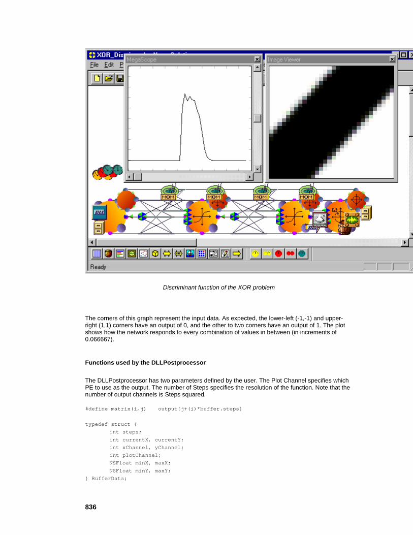
836

Discriminant function of the XOR problem

The corners of this graph represent the input data. As expected, the lower-left (-1,-1) and upper-right (1,1) corners have an output of 0, and the other to two corners have an output of 1. The plot shows how the network responds to every combination of values in between (in increments of 0.066667).

Functions used by the DLLPostprocessor

The DLLPostprocessor has two parameters defined by the user. The Plot Channel specifies which PE to use as the output. The number of Steps specifies the resolution of the function. Note that the number of output channels is Steps squared. #define matrix(i,j) output[j+(i)*buffer.steps] typedef struct { int steps; int currentX, currentY; int xChannel, yChannel; int plotChannel; NSFloat minX, maxX; NSFloat minY, maxY; } BufferData;

837

BufferData buffer = {0, 0, 0, 0, 0, 0, 0.0f, 0.0f, 0.0f, 0.0f}; BOOL performPrePost( DLLData *instance, // Pointer to instance data (may be NULL) NSFloat *input, // Pointer to the input data NSFloat *output, // Pointer to the output data int rows, // Number of rows of data int cols, // Number of cols of data BOOL preprocessor // Flag to indicate whether this is a preprocessor // or postprocessor ) { matrix(buffer.currentX++, buffer.currentY) = input[buffer.plotChannel]; if (buffer.currentX >= buffer.steps) { buffer.currentX = 0; if (++buffer.currentY >= buffer.steps) { buffer.currentY = 0; return TRUE; } } return FALSE; // Return whether to inject this sample or to call // performPrePost with another sample } void networkReset( DLLData *instance // Pointer to instance data (may be NULL) ) { buffer.currentX = 0; buffer.currentY = 0; } DLLData *allocPrePost( DLLData *oldInstance, // Pointer to the last instance if reallocating int *rows, // Number of rows of data attached above -- can be // changed. The default is the number of rows // attached below. int *cols, // Number of cols of data attached above -- can be // changed. The default is the number of cols // attached below. BOOL preprocessor // Flag to indicate whether this is a preprocessor // or postprocessor ) { DLLData *instance = allocDLLInstance(oldInstance); if (preprocessor) MessageBox(NULL, "Confusion matrix should only be used as a postprocessor", "Warning", MB_OK); setParameterName(instance, 2, 1, "Steps", TRUE); setIntParameter(instance, 2, 1, 10, FALSE); setParameterName(instance, 3, 1, "Plot Channel", TRUE); setIntParameter(instance, 3, 1, 0, FALSE);

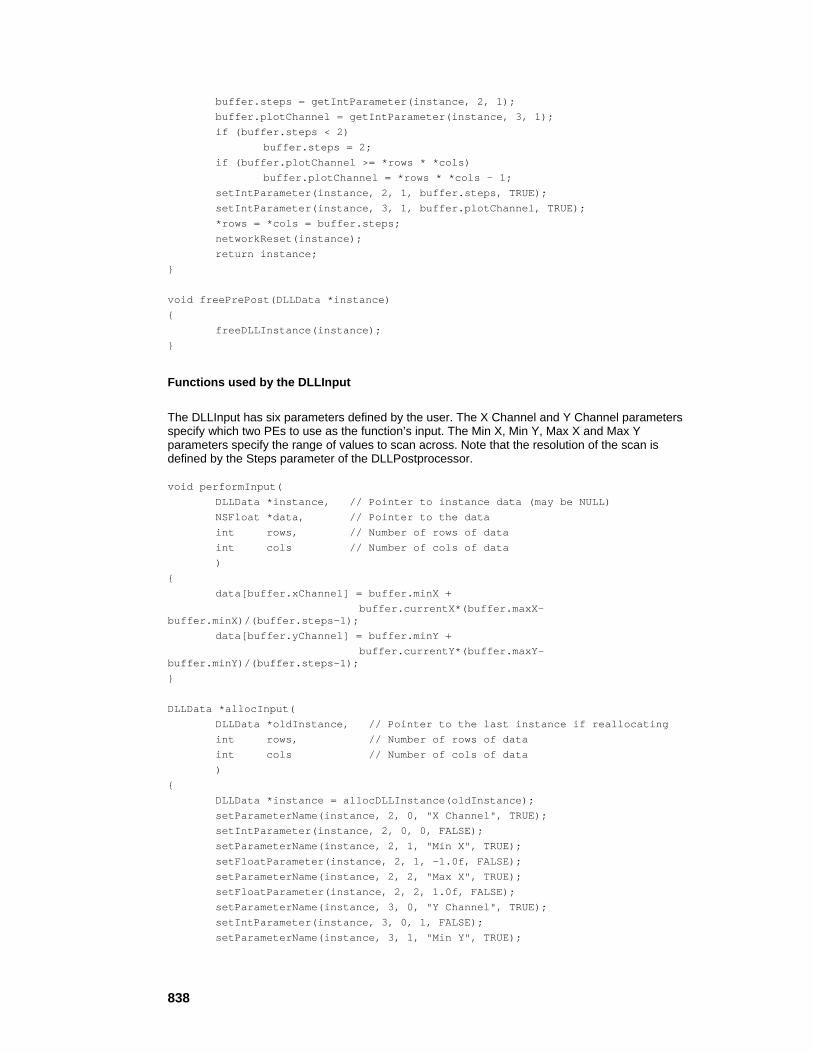
838

buffer.steps = getIntParameter(instance, 2, 1); buffer.plotChannel = getIntParameter(instance, 3, 1); if (buffer.steps < 2) buffer.steps = 2; if (buffer.plotChannel >= *rows * *cols) buffer.plotChannel = *rows * *cols - 1; setIntParameter(instance, 2, 1, buffer.steps, TRUE); setIntParameter(instance, 3, 1, buffer.plotChannel, TRUE); *rows = *cols = buffer.steps; networkReset(instance); return instance; } void freePrePost(DLLData *instance) { freeDLLInstance(instance); }

Functions used by the DLLInput

The DLLInput has six parameters defined by the user. The X Channel and Y Channel parameters specify which two PEs to use as the function’s input. The Min X, Min Y, Max X and Max Y parameters specify the range of values to scan across. Note that the resolution of the scan is defined by the Steps parameter of the DLLPostprocessor. void performInput( DLLData *instance, // Pointer to instance data (may be NULL) NSFloat *data, // Pointer to the data int rows, // Number of rows of data int cols // Number of cols of data ) { data[buffer.xChannel] = buffer.minX + buffer.currentX*(buffer.maxX-buffer.minX)/(buffer.steps-1); data[buffer.yChannel] = buffer.minY + buffer.currentY*(buffer.maxY-buffer.minY)/(buffer.steps-1); } DLLData *allocInput( DLLData *oldInstance, // Pointer to the last instance if reallocating int rows, // Number of rows of data int cols // Number of cols of data ) { DLLData *instance = allocDLLInstance(oldInstance); setParameterName(instance, 2, 0, "X Channel", TRUE); setIntParameter(instance, 2, 0, 0, FALSE); setParameterName(instance, 2, 1, "Min X", TRUE); setFloatParameter(instance, 2, 1, -1.0f, FALSE); setParameterName(instance, 2, 2, "Max X", TRUE); setFloatParameter(instance, 2, 2, 1.0f, FALSE); setParameterName(instance, 3, 0, "Y Channel", TRUE); setIntParameter(instance, 3, 0, 1, FALSE); setParameterName(instance, 3, 1, "Min Y", TRUE);

839

setFloatParameter(instance, 3, 1, -1.0f, FALSE); setParameterName(instance, 3, 2, "Max Y", TRUE); setFloatParameter(instance, 3, 2, 1.0f, FALSE); buffer.xChannel = getIntParameter(instance, 2, 0); buffer.minX = getFloatParameter(instance, 2, 1); buffer.maxX = getFloatParameter(instance, 2, 2); buffer.yChannel = getIntParameter(instance, 3, 0); buffer.minY = getFloatParameter(instance, 3, 1); buffer.maxY = getFloatParameter(instance, 3, 2); if (buffer.minX >= buffer.maxX) buffer.maxX = buffer.minX + 0.1f; if (buffer.minY >= buffer.maxY) buffer.maxY = buffer.minY + 0.1f; if (buffer.xChannel >= rows*cols) buffer.xChannel = rows*cols-1; if (buffer.yChannel >= rows*cols) buffer.yChannel = rows*cols-1; setIntParameter(instance, 2, 0, buffer.xChannel, TRUE); setFloatParameter(instance, 2, 2, buffer.maxX, TRUE); setIntParameter(instance, 3, 0, buffer.yChannel, TRUE); setFloatParameter(instance, 3, 2, buffer.maxY, TRUE); networkReset(instance); return instance; } void freeInput(DLLData *instance) { freeDLLInstance(instance); }

See Also

Scaling DLL Example

Within the "DLLCUST/PrePost" directory is a DLL example entitled "scale". This DLL provides the ability to apply a scale and an offset to either the input or output data. This is most commonly used to denormalize the network output to match the units of the desired response data.

Using the DLL

This DLL is public to all versions of NeuroSolutions. Below is a procedure for using this DLL to denormalize your output data. From a working neural network, perform the following steps:

Remove the probe attached to the Activity access point of the Axon at the network output.

Stamp a DLLPostprocessor probe where the old probe was.

Stamp a copy of the old probe on the DLLPostprocessor and move it to the Postprocessor Output access point.

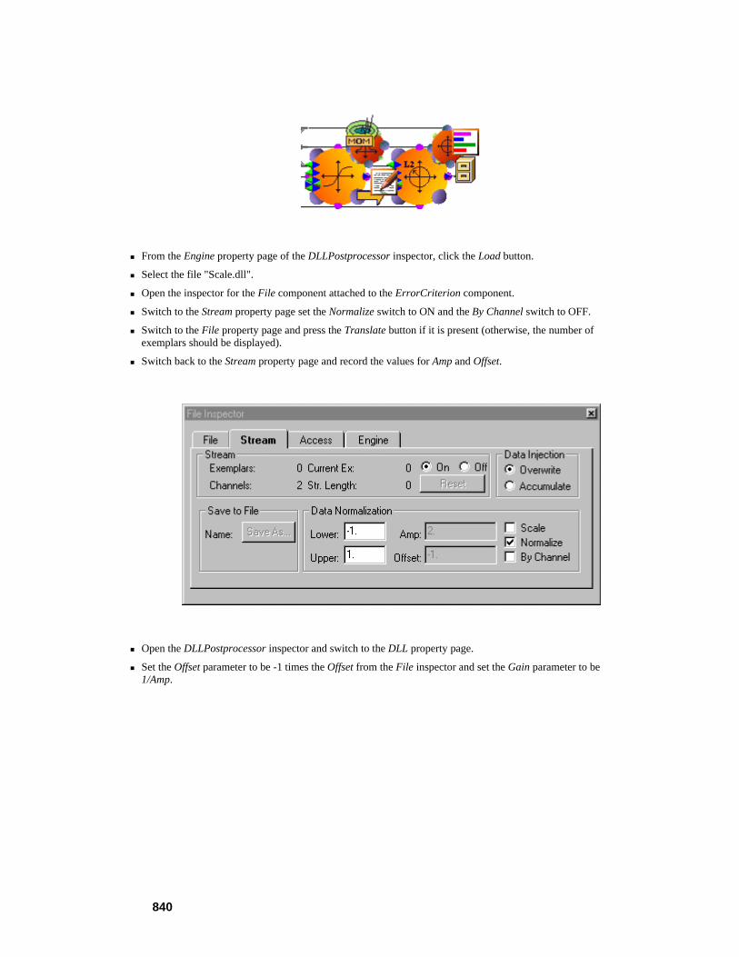
840

From the Engine property page of the DLLPostprocessor inspector, click the Load button.

Select the file "Scale.dll".

Open the inspector for the File component attached to the ErrorCriterion component.

Switch to the Stream property page set the Normalize switch to ON and the By Channel switch to OFF.

Switch to the File property page and press the Translate button if it is present (otherwise, the number of exemplars should be displayed).

Switch back to the Stream property page and record the values for Amp and Offset.

Open the DLLPostprocessor inspector and switch to the DLL property page.

Set the Offset parameter to be -1 times the Offset from the File inspector and set the Gain parameter to be 1/Amp.

841

Run the network. The displayed output data should be denormalized to match the desired output data.

How the DLL is Implemented

This DLL has 2 instance parameters. The Gain specifies the multiplicative constant and the Offset specifies the additive constant. BOOL performPrePost( DLLData *instance, // Pointer to instance data (may be NULL) NSFloat *input // Pointer to the input data NSFloat *output, // Pointer to the output data int rows, // Number of rows of data int cols, // Number of cols of data BOOL preprocessor // Flag to indicate whether this is a preprocessor or postprocessor ) { int i, length=rows*cols; float gain = getFloatParameter(instance, 2, 1); float offset = getFloatParameter(instance, 3, 1); for (i=0; i<length; i++) output[i] += gain*(input[i] + offset); return TRUE; } DLLData *allocPrePost( DLLData *oldInstance, // Pointer to the last instance if reallocating int *rows, // Number of rows of data attached above -- can be // changed. The default is the number of rows // attached below. int *cols, // Number of cols of data attached above -- can be // changed. The default is the number of cols // attached below. BOOL preprocessor // Flag to indicate whether this is a preprocessor // or postprocessor ) {

842

DLLData *instance = allocDLLInstance(oldInstance); setParameterName(instance, 2, 1, "Gain", FALSE); setFloatParameter(instance, 2, 1, 1.0f, FALSE); setParameterName(instance, 3, 1, "Offset", FALSE); setFloatParameter(instance, 3, 1, 0.0f, FALSE); return instance; } void freePrePost(DLLData *instance) { freeDLLInstance(instance); }

See Also

Function Generator

Sawtooth DLL Example

Within the "DLLCUST/Function" directory there is an example entitled "sawtooth". This DLL implements a sawtooth waveform that is built into the base Function component. Note that the sine is the default waveform for the Function DLLs and is defined within the "DLLSYS/Function" directory.

The implementation of this function is very straight forward -- given the angle in radians, compute the output of the function. NSFloat performFunction( DLLData *instance, // Pointer to instance data (may be NULL) NSFloat x // Current angle in radians ) { return (NSFloat)((x - PI)/PI); }

See Also

Triangle DLL Example

Within the "DLLCUST/Function" directory there is an example entitled "triangle". This DLL implements a triangle waveform that is built in to the base Function component. Note that the sine is the default waveform for the Function DLLs and is defined within the "DLLSYS/Function" directory.

The implementation of this function is very straight forward -- given the angle in radians, compute the output of the function.

843

NSFloat performFunction( DLLData *instance, // Pointer to instance data (may be NULL) NSFloat x // Current angle in radians ) { return (NSFloat)(x<PI? x/PI: (-x + 2*PI)/PI); }

See Also

Square DLL Example

Within the "DLLCUST/Function" directory there is an example entitled "square". This DLL implements a square waveform that is built in to the base Function component. Note that the sine is the default waveform for the Function DLLs and is defined within the "DLLSYS/Function" directory.

The implementation of this function is very straight forward -- given the angle in radians, compute the output of the function. NSFloat performFunction( DLLData *instance, // Pointer to instance data (may be NULL) NSFloat x // Current angle in radians ) { return x<PI? 1.0f: -1.0f; }

See Also

Decayed Sine DLL Example

The "decaysin" DLL implements a decayed sinewave function. This requires the use of two additional user parameters and an additional instance variable. The cycles parameter specifies how many sub-cycles are contained within each cycle of the function. The decay parameter is a floating point number between 0 and 1 that specifies how fast the output decays (decay rate). The amplitudeDecay variable is used to store the current level of decay. NSFloat performFunction( DLLData *instance, // Pointer to instance data (may be NULL) NSFloat x // Current angle in radians ) { int cycles = getIntParameter(instance, 3, 1); NSFloat decay = getFloatParameter(instance, 2, 1); NSFloat *amplitudeDecay = getUserData(instance); NSFloat function = (NSFloat)(*amplitudeDecay*sin(cycles*x));

844

*amplitudeDecay *= decay; return function; } void getReadyToFire( DLLData *instance // Pointer to instance data (may be NULL) ) { NSFloat *amplitudeDecay = getUserData(instance); *amplitudeDecay = 1.0f; } DLLData *allocFunction( DLLData *oldInstance // Pointer to the last instance if reallocating ) { DLLData *instance = allocDLLInstance(oldInstance); setParameterName(instance, 3, 1, "Cycles", FALSE); setIntParameter(instance, 3, 1, 5, FALSE); setParameterName(instance, 2, 1, "Decay", FALSE); setFloatParameter(instance, 2, 1, 0.9f, FALSE); setUserData(instance, malloc(sizeof(NSFloat))); return instance; } void freeFunction(DLLData *instance) { free((NSFloat*)getUserData(instance)); freeDLLInstance(instance); }

See Also

Pulse DLL Example

The "pulse" DLL implements a pulse function. This requires the use of an additional user parameter. The width parameter is a floating point number between 0 and 1. The function returns a 1 if the current angle (x) is less than the width and 0 otherwise. NSFloat performFunction( DLLData *instance, // Pointer to instance data (may be NULL) NSFloat x // Current angle in radians ) { NSFloat width = getFloatParameter(instance, 2, 1); return x<width? 1.0f: 0; } DLLData *allocFunction( DLLData *oldInstance // Pointer to the last instance if reallocating )

845

{ DLLData *instance = allocDLLInstance(oldInstance); setParameterName(instance, 2, 1, "Width", FALSE); setFloatParameter(instance, 2, 1, 0.1f, FALSE); return instance; } void freeFunction(DLLData *instance) { freeDLLInstance(instance); }

See Also

Noise Generator

Gaussian DLL Example

Within the "DLLCUST/Noise" directory is a DLL example entitled "gaussian". This DLL implements one of the noise generators built into the base Noise component. Note that the uniform is the default distribution for the Noise DLLs and is defined within the "DLLSYS/Noise" directory.

The implementation of this function is very straightforward; given the mean and variance specified by the user, generate a random number. NSFloat performNoise( DLLData *instance, // Pointer to instance data (may be NULL) NSFloat variance, // Variance set within components inspector NSFloat mean // Mean set within components inspector ) { return (variance*(NSFloat)(sqrt(-2*log((NSFloat)rand()/ RAND_MAX))*cos(2*PI*((NSFloat)rand()/RAND_MAX))) + mean); }

See Also

Decayed Gaussian DLL Example

Within the "DLLCUST/Noise" directory is a DLL example entitled "decgaus". The "decgaus" DLL implements a decayed version of its base counterpart. This requires the use of one additional user parameter and an additional instance variable. The decay parameter is a floating point number between 0 and 1 that specifies how fast the variance decays (decay rate). The varianceDecay variable is used to store the current level of decay. NSFloat performNoise(

846

DLLData *instance, // Pointer to instance data (may be NULL) NSFloat variance, // Variance set within components inspector NSFloat mean // Mean set within components inspector ) { NSFloat decay = getFloatParameter(instance, 2, 1); NSFloat *varianceDecay = getUserData(instance); NSFloat noise = (variance * *varianceDecay* (NSFloat)(sqrt(-2*log((NSFloat)rand()/RAND_MAX))* cos(2*PI*((NSFloat)rand()/RAND_MAX))) + mean); *varianceDecay *= decay; return noise; } void getReadyToFire( DLLData *instance // Pointer to instance data (may be NULL) ) { NSFloat *varianceDecay = getUserData(instance); *varianceDecay = 1.0f; } DLLData *allocNoise( DLLData *oldInstance // Pointer to the last instance if reallocating ) { DLLData *instance = allocDLLInstance(oldInstance); setParameterName(instance, 2, 1, "Decay", FALSE); setFloatParameter(instance, 2, 1, 0.9f, FALSE); setUserData(instance, malloc(sizeof(NSFloat))); return instance; } void freeNoise(DLLData *instance) { free((NSFloat*)getUserData(instance)); freeDLLInstance(instance); }

See Also

Decayed Uniform DLL Example

Within the "DLLCUST/Noise" directory is a DLL example entitled "decunifm". The "decunifm" DLL implements a decayed version of its base counterpart. The structure of the implementation matches that of the decayed gaussian DLL. NSFloat performNoise( DLLData *instance, // Pointer to instance data (may be NULL) NSFloat variance, // Variance set within components inspector NSFloat mean // Mean set within components inspector

847

) { NSFloat decay = getFloatParameter(instance, 2, 1); NSFloat *varianceDecay = getUserData(instance); NSFloat noise = ((NSFloat)sqrt(3*variance * *varianceDecay)* (NSFloat)(((NSFloat)rand()/RAND_MAX)-0.5)+mean); *varianceDecay *= decay; return noise; }

See Also

File

Binary DLL Example

Within the "DLLCUST/File" directory is a DLL example entitled "binary". This DLL implements the binary translator that is built into the base File component. Note that the ASCII translator is the default for the File DLLs and is defined within the "DLLSYS/File" directory.

The implementation of this function is very straightforward -- the fileOpen function opens the file and the performFile function reads the next floating point number. BOOL performFile( DLLData *instance, // Pointer to instance data (may be NULL) FILE *file, // Pointer to the opened file NSFloat *sample // Location to place next sample ) { if (fread(sample, sizeof(NSFloat), 1, (FILE*)file)) return TRUE; fclose((FILE*)file); return FALSE; } FILE *openFile(DLLData *instance, const char *filePath) { return fopen(filePath, "rb"); }

See Also

Binary Float DLL Example

848

Within the "DLLCUST/File" directory is a DLL example entitled "binfloat". The "binfloat" DLL is a specialized version of the binary translator. It allows the user to specify a segment of the data to read. This requires the use of two additional integer parameters and an additional instance variable. The offset parameter specifies how many samples to skip from the beginning of the file and the duration parameter specifies how many samples to read. The durationCount variable is used to store the number of samples that have been skipped so far. BOOL performFile( DLLData *instance, // Pointer to instance data (may be NULL) FILE *file, // Pointer to the opened file NSFloat *sample // Location to place next sample ) { int duration = getIntParameter(instance, 2, 1); int *durationCount = (int*)getUserData(instance); if ((!duration || ((*durationCount)++ < duration)) && fread(sample, sizeof(NSFloat), 1, (FILE*)file)) return TRUE; *durationCount = 0; fclose((FILE*)file); return FALSE; } FILE *openFile( DLLData *instance, // Pointer to instance data (may be NULL) const char *filePath // Full path of file to be opened ) { NSFloat *buffer; FILE *file = fopen(filePath, "rb"); int offset = getIntParameter(instance, 1, 1); if (offset) { buffer = malloc(offset*sizeof(NSFloat)); fread(buffer, sizeof(NSFloat), offset, file); free(buffer); } return file; } DLLData *allocFile( DLLData *oldInstance // Pointer to the last instance if reallocating ) { DLLData *instance = allocDLLInstance(oldInstance); setParameterName(instance, 1, 1, "Offset", FALSE); setIntParameter(instance, 1, 1, 0, FALSE); setParameterName(instance, 2, 1, "Duration", FALSE); setIntParameter(instance, 2, 1, 0, FALSE); setUserData(instance, calloc(1,sizeof(int))); return instance; } void freeFile(DLLData *instance) { free((int*)getUserData(instance)); freeDLLInstance(instance); }

849

See Also

Binary Integer DLL Example

Within the "DLLCUST/File" directory is a DLL example entitled "binint". The "binint" DLL is a specialized version of the binary translator. It allows the user to specify a segment of the data to read. This requires the use of two additional integer parameters and an additional instance variable. The offset parameter specifies how many samples to skip from the beginning of the file and the duration parameter specifies how many samples to read. The durationCount variable is used to store the number of samples that have been skipped so far. This translator reads binary data stored as integers (4-bytes). BOOL performFile( DLLData *instance, // Pointer to instance data (may be NULL) FILE *file, // Pointer to the opened file NSFloat *sample // Location to place next sample ) { int duration = getIntParameter(instance, 2, 1); int *durationCount = (int*)getUserData(instance); int typedSample; if ((!duration || ((*durationCount)++ < duration)) && fread(&typedSample, sizeof(int), 1, (FILE*)file)) { *sample = (NSFloat)typedSample; return TRUE; } *durationCount = 0; fclose((FILE*)file); return FALSE; }

See Also

Binary Short DLL Example

Within the "DLLCUST/File" directory is a DLL example entitled "binshort". The "binshort" DLL is a specialized version of the binary translator. It allows the user to specify a segment of the data to read. This requires the use of two additional integer parameters and an additional instance variable. The offset parameter specifies how many samples to skip from the beginning of the file and the duration parameter specifies how many samples to read. The durationCount variable is used to store the number of samples that have been skipped so far. This translator reads binary data stored as short integers (2-bytes). BOOL performFile( DLLData *instance, // Pointer to instance data (may be NULL) FILE *file, // Pointer to the opened file NSFloat *sample // Location to place next sample

850

) { int duration = getIntParameter(instance, 2, 1); int *durationCount = (int*)getUserData(instance); short typedSample; if ((!duration || ((*durationCount)++ < duration)) && fread(&typedSample, sizeof(short), 1, (FILE*)file)) { *sample = (NSFloat)typedSample; return TRUE; } *durationCount = 0; fclose((FILE*)file); return FALSE; }

See Also

Binary Character DLL Example

Within the "DLLCUST/File" directory is a DLL example entitled "binchar". The "binchar" DLL is a specialized version of the binary translator. It allows the user to specify a segment of the data to read. This requires the use of two additional integer parameters and an additional instance variable. The offset parameter specifies how many samples to skip from the beginning of the file and the duration parameter specifies how many samples to read. The durationCount variable is used to store the number of samples that have been skipped so far. This translator reads binary data stored as characters (1-byte). BOOL performFile( DLLData *instance, // Pointer to instance data (may be NULL) FILE *file, // Pointer to the opened file NSFloat *sample // Location to place next sample ) { int duration = getIntParameter(instance, 2, 1); int *durationCount = (int*)getUserData(instance); char typedSample; if ((!duration || ((*durationCount)++ < duration)) && fread(&typedSample, sizeof(char), 1, (FILE*)file)) { *sample = (NSFloat)typedSample; return TRUE; } *durationCount = 0; fclose((FILE*)file); return FALSE; }

See Also

851

Preprocessor

Averaging Filter DLL Example

Within the "DLLCUST/PrePost" directory is a DLL examples entitled "average". This DLL implements an averaging filter, which averages the last N samples of input for each channel and writes the result to the output for each call to performPrePost. This requires the use of a user-defined parameter (N) and a vector of instance data (bufferData) to store the past samples. #define buffer(i, j) bufferData->data[j+(i)*bufferData->length] typedef struct { int length; NSFloat *data; } AverageData; BOOL performPrePost( DLLData *instance, // Pointer to instance data (may be NULL) NSFloat *input // Pointer to the input data NSFloat *output, // Pointer to the output data int rows, // Number of rows of data int cols // Number of cols of data BOOL preprocessor // Flag to indicate preprocessor or postprocessor ) { int i, j; int N = getIntParameter(instance, 2, 1); AverageData *bufferData = getUserData(instance); NSFloat result; for (i=N-1; i>0; i--) for (j=0; j<bufferData->length; j++) buffer(i,j) = buffer(i-1,j); for (j=0; j<bufferData->length; j++) buffer(0,j) = input[j]; if (!preprocessor) //Zero output buffer if postprocessor (since it is local) for (j=0; j<bufferData->length; j++) output[j] = 0.0f; for (j=0; j<bufferData->length; j++) { result = 0.0f; for (i=0; i<N; i++) result += buffer(i,j); output[j] += result/N; } return TRUE; } void networkReset( DLLData *instance // Pointer to instance data (may be NULL) ) { int i, j; int N = getIntParameter(instance, 2, 1); AverageData *bufferData = getUserData(instance); for (i=0; i<N; i++)

852

for (j=0; j<bufferData->length; j++) buffer(i,j) = 0.0f; } DLLData *allocPrePost( DLLData *oldInstance, // Pointer to the last instance if reallocating int *rows, // Number of rows of data attached above -- can be // changed. The default is the number of rows // attached below. int *cols, // Number of cols of data attached above -- can be // changed. The default is the number of cols // attached below. BOOL preprocessor // Flag to indicate whether this is a preprocessor // or postprocessor ) { DLLData *instance = allocDLLInstance(oldInstance); AverageData *bufferData = calloc(1,sizeof(AverageData)); setParameterName(instance, 2, 1, "N", TRUE); setIntParameter(instance, 2, 1, 4, FALSE); bufferData->length = *rows * *cols; bufferData->data = calloc(bufferData->length* getIntParameter(instance, 2, 1), sizeof(NSFloat)); setUserData(instance, bufferData); return instance; } void freePrePost(DLLData *instance) { AverageData *bufferData = getUserData(instance); if (bufferData) { free(bufferData->data); free(bufferData); } freeDLLInstance(instance); }

See Also

Decimator Filter DLL Example

Within the "DLLCUST/PrePost" directory is a DLL examples entitled "decimate". This DLL implements a decimator filter, which reduces the amount of input data by skipping samples. In order to keep as much of the input information as possible, the samples are averaged together to produce the output. This is similar to the averaging filter except that the implementation passes the results to the output one out of every N calls to performPrePost instead of every call. For the other N-1 calls, it simply stores the input into the bufferData vector. The boolean value returned is used to specify when to process the output. #define buffer(i, j) bufferData->data[j+(i)*bufferData->length]

853

typedef struct { int length; NSFloat *data; } AverageData; BOOL performPrePost( DLLData *instance, // Pointer to instance data (may be NULL) NSFloat *input // Pointer to the input data NSFloat *output, // Pointer to the output data int rows, // Number of rows of data int cols, // Number of cols of data BOOL preprocessor // Flag to indicate a preprocessor or postprocessor ) { int i, j; int N = getIntParameter(instance, 2, 1); DecimatorData *bufferData = getUserData(instance); NSFloat result; for (i=N-1; i>0; i--) for (j=0; j<bufferData->length; j++) buffer(i,j) = buffer(i-1,j); for (j=0; j<bufferData->length; j++) buffer(0,j) = input[j]; if (++bufferData->count >= N) { bufferData->count = 0; if (!preprocessor) //Zero buffer if postprocessor (since it is local) for (j=0; j<bufferData->length; j++) output[j] = 0.0f; for (j=0; j<bufferData->length; j++) { result = 0.0f; for (i=0; i<N; i++) result += buffer(i,j); output[j] = result/N; } return TRUE; } return FALSE; } void networkReset( DLLData *instance // Pointer to instance data (may be NULL) ) { int i, j; int N = getIntParameter(instance, 2, 1); DecimatorData *bufferData = getUserData(instance); for (i=0; i<N; i++) for (j=0; j<bufferData->length; j++) buffer(i,j) = 0.0f; bufferData->count = 0; } DLLData *allocPrePost( DLLData *oldInstance, // Pointer to the last instance if reallocating int *rows, // Number of rows of data attached above -- can be

854

// changed. The default is the number of rows // attached below. int *cols, // Number of cols of data attached above -- can be // changed. The default is the number of cols // attached below. BOOL preprocessor // Flag to indicate whether this is a preprocessor // or postprocessor ) { DLLData *instance = allocDLLInstance(oldInstance); DecimatorData *bufferData = calloc(1,sizeof(DecimatorData)); setParameterName(instance, 2, 1, "N", TRUE); setIntParameter(instance, 2, 1, 4, FALSE); bufferData->length = *rows * *cols; bufferData->data = calloc(bufferData->length* getIntParameter(instance, 2, 1), sizeof(NSFloat)); setUserData(instance, bufferData); return instance; } void freePrePost(DLLData *instance) { DecimatorData *bufferData = getUserData(instance); if (bufferData) { free(bufferData->data); free(bufferData); } freeDLLInstance(instance); }

See Also

Extractor DLL Example

Within the "DLLCUST/PrePost" directory is a DLL example entitled "extract". This DLL provides the ability to extract a subset of channels from the input and copy them to a subset of output channels. This example also demonstrates how on-line parameter verification is implemented.

This DLL has 4 instance parameters. The fromLength or toLength (depending on the value of the preprocessor flag of the allocPrePost function) specifies the number of channels for the component stacked above by setting the rows and cols of the allocPrePost function. The fromStart parameter specifies the first channel of input to extract and the fromStop parameter specifies the last channel of input (the rest of the input channels are ignored). The toStart parameter specifies the channel of output that will be mapped to the fromStart channel of input. The remaining extracted input channels are mapped sequentially to the output from this point. Therefore, there is no need to specify a toStop parameter (since toStop = toStart + fromStop - toStop). BOOL performPrePost( DLLData *instance, // Pointer to instance data (may be NULL) NSFloat *input // Pointer to the input data NSFloat *output, // Pointer to the output data

855

int rows, // Number of rows of data int cols, // Number of cols of data BOOL preprocessor // Flag to indicate preprocessor or postprocessor ) { int i; int fromLength = getIntParameter(instance, 2, 0); int fromStart = getIntParameter(instance, 2, 1); int fromStop = getIntParameter(instance, 2, 2); int toStart = getIntParameter(instance, 3, 1); if (!preprocessor) //Zero buffer if postprocessor (since it is local) for (i=0; i<bufferData->length; i++) output[i] = 0.0f; for (i=0; i<=fromStop-fromStart; i++) output[toStart+i] += input[fromStart+i]; return TRUE; } DLLData *allocPrePost( DLLData *oldInstance, // Pointer to the last instance if reallocating int *rows, // Number of rows of data attached above -- can be // changed. The default is the number of rows // attached below. int *cols, // Number of cols of data attached above -- can be // changed. The default is the number of cols // attached below. BOOL preprocessor // Flag to indicate whether this is a preprocessor // or postprocessor ) { DLLData *instance = allocDLLInstance(oldInstance); int fromLength, toLength, fromStart, fromStop, toStart, returnMax; setParameterName(instance, 2, 1, "From Start", TRUE); setIntParameter(instance, 2, 1, 0, FALSE); setParameterName(instance, 2, 2, "From Stop", TRUE); setIntParameter(instance, 2, 2, 0, FALSE); setParameterName(instance, 3, 1, "To Start", TRUE); setIntParameter(instance, 3, 1, 0, FALSE); if (preprocessor) { setParameterName(instance, 2, 0, "From Length", TRUE); setIntParameter(instance, 2, 0, 1, FALSE); returnMax = fromLength = getIntParameter(instance, 2, 0); toLength = *rows * *cols; } else { setParameterName(instance, 2, 0, "To Length", TRUE); setIntParameter(instance, 2, 0, 1, FALSE); fromLength = *rows * *cols; returnMax = toLength = getIntParameter(instance, 2, 0); } if (fromLength < 1) fromLength = 1; fromStart = getIntParameter(instance, 2, 1); if (fromStart >= fromLength) fromStart = fromLength - 1; fromStop = getIntParameter(instance, 2, 2);

856

if (fromStop < fromStart) fromStop = fromStart; if (fromStop >= fromLength) fromStop = fromLength - 1; toStart = getIntParameter(instance, 3, 1); if (toStart >= toLength) toStart = toLength - 1; if (toStart > toLength - (fromStop-fromStart+1)) fromStop = fromStart + (toLength-toStart-1); setIntParameter(instance, 2, 1, fromStart, TRUE); setIntParameter(instance, 2, 2, fromStop, TRUE); setIntParameter(instance, 3, 1, toStart, TRUE); setIntParameter(instance, 2, 0, returnMax, TRUE); *rows = returnMax; *cols = 1; return instance; } void freePrePost(DLLData *instance) { freeDLLInstance(instance); }

See Also

Postprocessor and Probe

Confusion Matrix DLL Example

Within the "DLLCUST/PrePost" directory is a DLL example entitled "confuse". This DLL is used to determine the percentage of correctly classified exemplars for each output class. This example demonstrates the customization of the Postprocessor and Probe components. It is also a good example of how global variables are used to share data between two DLLs.

Using the DLL

In order to understand the source code for this DLL, you should start by seeing it in action. Run the Character Recognition example from the NeuroSolutions Demo Panel (press Run Demo from the Utilities menu). Quit the demo after the network has run the first experiment. You now have a fully functioning network to work from.

Remove all of the probes except the MegaScope/DataStorage at the error. Attach a DLLPostprocessor at the Activity access point of the SoftMaxAxon (the network output). From the Engine property page of the DLLPostprocessor, load the "confuse" DLL. Switch to the DLL page of the inspector and enter "TRUE" if you want the output classes computed as percentages or "FALSE" if you want the raw tallies for each output class. Attach a MatrixViewer on top of the DLLPostprocessor at the Postprocessor Output access point and open its window. Stack a Hinton on top of the MatrixViewer and open its window. Reset and run the network.

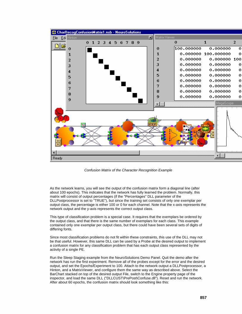
857

Confusion Matrix of the Character Recognition Example

As the network learns, you will see the output of the confusion matrix form a diagonal line (after about 100 epochs). This indicates that the network has fully learned the problem. Normally, this matrix will consist of output percentages (if the "Percentages" DLL parameter of the DLLPostprocessor is set to "TRUE"), but since the training set consists of only one exemplar per output class, the percentage is either 100 or 0 for each channel. Note that the x-axis represents the network output and the y-axis represents the correct output class.

This type of classification problem is a special case. It requires that the exemplars be ordered by the output class, and that there is the same number of exemplars for each class. This example contained only one exemplar per output class, but there could have been several sets of digits of differing fonts.

Since most classification problems do not fit within these constraints, this use of the DLL may not be that useful. However, this same DLL can be used by a Probe at the desired output to implement a confusion matrix for any classification problem that has each output class represented by the activity of a single PE.

Run the Sleep Staging example from the NeuroSolutions Demo Panel. Quit the demo after the network has run the first experiment. Remove all of the probes except for the error and the desired output, and set the Epochs/Experiment to 100. Attach to the network output a DLLPostprocessor, a Hinton, and a MatrixViewer, and configure them the same way as described above. Select the BarChart stacked on top of the desired output File, switch to the Engine property page of the inspector, and load the same DLL ("DLLCUST\PrePost\Confuse.dll"). Reset and run the network. After about 60 epochs, the confusion matrix should look something like this:

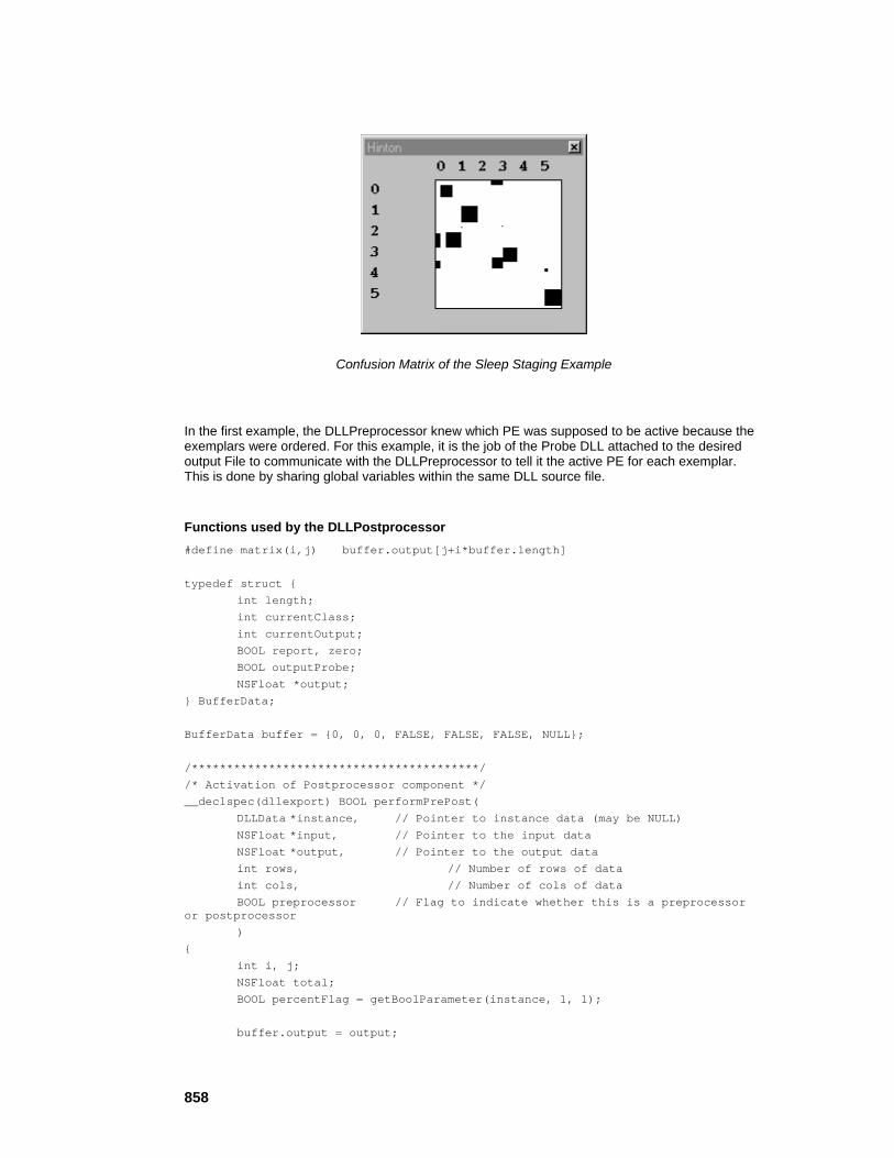
858

Confusion Matrix of the Sleep Staging Example

In the first example, the DLLPreprocessor knew which PE was supposed to be active because the exemplars were ordered. For this example, it is the job of the Probe DLL attached to the desired output File to communicate with the DLLPreprocessor to tell it the active PE for each exemplar. This is done by sharing global variables within the same DLL source file.

Functions used by the DLLPostprocessor #define matrix(i,j) buffer.output[j+i*buffer.length] typedef struct { int length; int currentClass; int currentOutput; BOOL report, zero; BOOL outputProbe; NSFloat *output; } BufferData; BufferData buffer = {0, 0, 0, FALSE, FALSE, FALSE, NULL}; /*****************************************/ /* Activation of Postprocessor component */ __declspec(dllexport) BOOL performPrePost( DLLData *instance, // Pointer to instance data (may be NULL) NSFloat *input, // Pointer to the input data NSFloat *output, // Pointer to the output data int rows, // Number of rows of data int cols, // Number of cols of data BOOL preprocessor // Flag to indicate whether this is a preprocessor or postprocessor ) { int i, j; NSFloat total; BOOL percentFlag = getBoolParameter(instance, 1, 1); buffer.output = output;

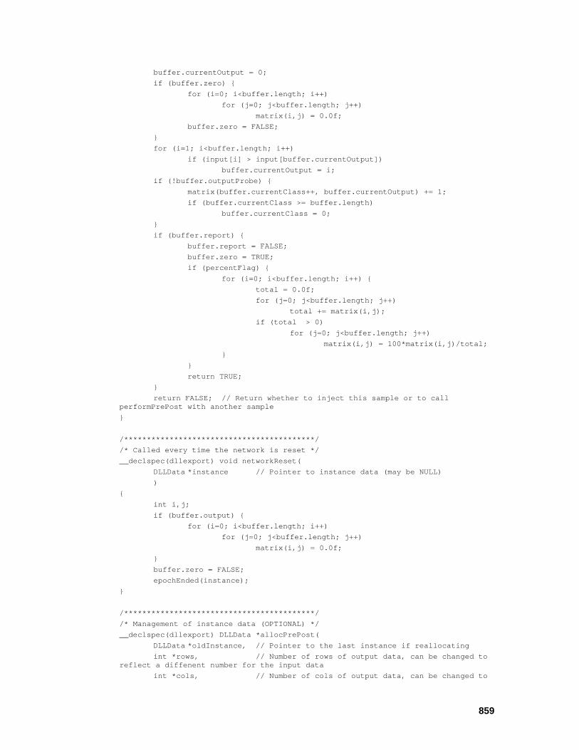
859

buffer.currentOutput = 0; if (buffer.zero) { for (i=0; i<buffer.length; i++) for (j=0; j<buffer.length; j++) matrix(i,j) = 0.0f; buffer.zero = FALSE; } for (i=1; i<buffer.length; i++) if (input[i] > input[buffer.currentOutput]) buffer.currentOutput = i; if (!buffer.outputProbe) { matrix(buffer.currentClass++, buffer.currentOutput) += 1; if (buffer.currentClass >= buffer.length) buffer.currentClass = 0; } if (buffer.report) { buffer.report = FALSE; buffer.zero = TRUE; if (percentFlag) { for (i=0; i<buffer.length; i++) { total = 0.0f; for (j=0; j<buffer.length; j++) total += matrix(i,j); if (total > 0) for (j=0; j<buffer.length; j++) matrix(i,j) = 100*matrix(i,j)/total; } } return TRUE; } return FALSE; // Return whether to inject this sample or to call performPrePost with another sample } /******************************************/ /* Called every time the network is reset */ __declspec(dllexport) void networkReset( DLLData *instance // Pointer to instance data (may be NULL) ) { int i,j; if (buffer.output) { for (i=0; i<buffer.length; i++) for (j=0; j<buffer.length; j++) matrix(i,j) = 0.0f; } buffer.zero = FALSE; epochEnded(instance); } /******************************************/ /* Management of instance data (OPTIONAL) */ __declspec(dllexport) DLLData *allocPrePost( DLLData *oldInstance, // Pointer to the last instance if reallocating int *rows, // Number of rows of output data, can be changed to reflect a diffenent number for the input data int *cols, // Number of cols of output data, can be changed to

860

reflect a diffenent number for the input data BOOL preprocessor // Flag to indicate whether this is a preprocessor or postprocessor ) { DLLData *instance = allocDLLInstance(oldInstance); int size = *rows * *cols; if (preprocessor) MessageBox(NULL, "Confusion matrix should only be used as a postprocessor", "Warning", MB_OK); *rows = *cols = size; buffer.length = size; buffer.report = FALSE; buffer.zero = FALSE; setParameterName(instance, 1, 1, "Percent", FALSE); setBoolParameter(instance, 1, 1, FALSE, FALSE); return instance; } __declspec(dllexport) void freePrePost(DLLData *instance) { buffer.output = NULL; }

Functions used by the Probe /**********************************/ /* Activation of output component */ __declspec(dllexport) BOOL performOutput( DLLData *instance, // Pointer to instance data (may be NULL) NSFloat *data, // Pointer to the data int rows, // Number of rows of data int cols // Number of cols of data ) { int i,j; if (buffer.zero) { for (i=0; i<buffer.length; i++) for (j=0; j<buffer.length; j++) matrix(i,j) = 0.0f; buffer.zero = FALSE; } if (buffer.output) { buffer.currentClass = 0; for (i=1; i<buffer.length; i++) if (data[i] > data[buffer.currentClass]) buffer.currentClass = i; matrix(buffer.currentClass, buffer.currentOutput) += 1; } return TRUE; } /************************************/

861

/* Called at the end of every epoch */ __declspec(dllexport) void epochEnded( DLLData *instance // Pointer to instance data (may be NULL) ) { if (!buffer.outputProbe) buffer.currentClass = 0; buffer.report = TRUE; } __declspec(dllexport) DLLData *allocOutput( DLLData *oldInstance, // Pointer to the last instance if reallocating int rows, // Number of rows of data int cols // Number of cols of data ) { buffer.outputProbe = TRUE; return NULL; } __declspec(dllexport) void freeOutput(DLLData *instance) { buffer.outputProbe = FALSE; }

See Also

Transformer

Derivative DLL Example

Within the "DLLCUST/transfrm" directory there is a DLL example entitled "deriv". This DLL demonstrates how to implement a signal transformer. The "deriv" DLL performs a simple derivative approximation by outputting the difference between each pair of successive samples. It performs this operation on each channel independently.

There is no instance data required for this operation, so the instance allocation and deallocation functions are omitted. The implementation for the perform function is as follows: BOOL performTransform( DLLData *instance, // Pointer to instance data NSFloat *data, // Pointer to the buffered data int length, // Length of the buffer to be transformed int channel // Current channel number ) { int i; for (i=length-1; i>0; i--) data[i] = data[i] - data[i-1];

862

// Return whether or not to display this channel return TRUE; }

This algorithm simply starts at the last sample in the buffer and scans backward while computing the difference between the samples. Note that this function is called once for each channel, since each channel has its own data buffer. The function returns TRUE to indicate that the probe attached to this DLL should display all channels.

See Also

Autocorrelation DLL Example

Within the "DLLCUST/transfrm" directory there is a DLL example entitled "autocorr". This DLL demonstrates how to implement a signal transformer. The "autocorr" DLL performs an autocorrelation operation on each channel independently. There is no instance data required for this operation, so the instance allocation and deallocation functions are omitted. The implementation for the perform function is as follows: BOOL performTransform( DLLData *instance, // Pointer to instance data NSFloat *data, // Pointer to the buffered data int length, // Length of the buffer to be transformed int channel // Current channel number ) { int i,j, start=0, stop=length; NSFloat *corr = (NSFloat*)calloc(length, sizeof(NSFloat)); for (i=0; i<length; i++) { for (j=start; j<stop; j++) corr[i] += data[j]*data[j-start]; start++; } for (i=0; i<length; i++) data[i] = corr[i]; free(corr); // Return whether or not to display this channel return TRUE; }

This algorithm scans through the data buffer while storing the computed correlation information in the corr buffer. Then the corr buffer is copied to the data buffer to produce the output of the Transformer. The function returns TRUE to indicate that the probe attached to this DLL should display all channels.

See Also

863

Crosscorrelation DLL Example

Within the "DLLCUST/transfrm" directory there is a DLL example entitled "crosscor". This DLL demonstrates how to implement a signal transformer. The "crosscor" DLL performs a crosscorrelation operation between two channels of the data buffer to produce a single channel of output. The two channels are selected by the user from the DLL property page of the inspector. These instance parameters are defined within the instance allocation function: DLLData *allocTransform( DLLData *oldInstance, // Pointer to the last instance if reallocating int length, // Length of the buffer to be transformed int channels // Number of channels to be transformed ) { DLLData *instance = allocDLLInstance(oldInstance); setParameterName(instance, 2, 1, "Chan X"); setIntParameter(instance, 2, 1, 0, FALSE); setParameterName(instance, 2, 2, "Chan Y"); setIntParameter(instance, 2, 2, 1, FALSE); return instance; }

The perform function is implemented as follows: BOOL performTransform( DLLData *instance, // Pointer to instance data NSFloat *data, // Pointer to the buffered data int length, // Length of the buffer to be transformed int channel // Current channal number ) { NSFloat *corr, *firstChannel=(NSFloat*)getUserData(instance); BOOL displayChannel=FALSE; int i, j, start=0, channel1=getIntParameter(instance, 2, 1), channel2=getIntParameter(instance, 2, 2); if ((channel == channel1) || (channel == channel2)) { if (channel1 == channel2) firstChannel = data; if (firstChannel) { corr = (NSFloat*)calloc(length, sizeof(NSFloat)); for (i=0; i<length; i++) { for (j=start; j<length; j++) corr[i] += data[j]*firstChannel[j-start]; start++; } for (i=0; i<length; i++) data[i] = corr[i]; setUserData(instance, NULL); displayChannel = TRUE; free(corr); } else setUserData(instance, data); } return displayChannel;

864

}

This algorithm is similar to that of the autocorrelation, except that the correlation is based on two channels instead of one. The two channel numbers are defined by the user and stored as instance parameters. Also, there is only one channel displayed by the Probe attached to the DLL instead of displaying an output channel for every input channel.

Recall that each call to performTransform represents only one channel of data. In order to use the data from two channels at once, the DLL must store a pointer to the data of the first correlation channel. The call to setUserData stores this pointer as part of the instance data. When performTransform is called during the second correlation channel, then getUserData is called to retrieve the data pointer of the first correlation channel.

Once the correlation is computed based on the two channels, the corr buffer is copied the data buffer. This is the only time that the data should be displayed by the probe attached to the DLL. This is why displayChannel is set to TRUE after the correlation has been computed. Note that this only occurs when channel is equal to the second correlation channel.

See Also

Customizing NeuroSolutions Components using DLLs Customizing an Activation Component

Customizing an Activation Component using DLLs Introduction

Activation components consist of the Axon and Synapse families. Customizing any of these components for supervised learning requires the creation of a DLL for both the activation component and the corresponding backprop dual.

To get started, simply build a breadboard that contains an activation/backprop pair that closely resembles the components that you want to create. Select the activation component and press the New button from the Engine Inspector property page of the inspector. This will create a DLL that matches the functionality of the base component. Edit the source code to change the functionality and press the Compile button.

When an activation DLL is created, the default DLL for the corresponding backprop component is automatically created (assuming that the backprop component is attached). Edit and Compile the source code for the backprop component. Run the network to test your new components. Activation

Within the DLLData structure containing The DLLData Structure, there is a mechanism for storing Adding Adaptable Weights to the Instance Data . These weights are in addition to any weights that are contained within the base component. Backprop

The responsibility of the backprop component is to compute the gradients and sensitivities (the gradient and error vectors) for the activation component. If the activation component contains

865

adaptable weights within its instance data, then the backprop component must also allocate a corresponding weight vector and use it to store the computed gradients.

See Also

Customizing an Axon using DLLs Protocols:

Activation

PerformAxon DLL Protocol

PerformBiasAxon DLL Protocol

PerformContextAxon DLL Protocol

PerformGammaAxon DLL Protocol

PerformLinearAxon DLL Protocol

PerformTDNNAxon DLL Protocol

Backprop

PerformBackAxon DLL Protocol

PerformBackBiasAxon DLL Protocol

PerformBackContextAxon DLL Protocol

PerformBackGammaAxon DLL Protocol

PerformBackLinearAxon DLL Protocol

PerformBackTDNNAxon DLL Protocol

Examples:

Adjustable sigmoid

Adjustable hyperbolic tangent

Adjustable linear

TanhAxon with gain

Customizing a Synapse using DLLs Protocols:

Activation

PerformSynapse DLL Protocol

866

PerformFullSynapse DLL Protocol

Backprop

PerformBackSynapse DLL Protocol

PerformBackFullSynapse DLL Protocol

Examples:

Locally-Connected Synapse DLL Example

Subset FullSynapse DLL Example

Customizing an ErrorCriterion Component

Customizing an ErrorCriterion using DLLs Description:

ErrorCriteria DLLs are used to customize the computation of the backpropagated sensitivities and the cost (error).

Protocols:

PerformCriterion DLL Protocol

Examples:

Loser Learn All DLL Example

Customizing a Gradient Search Component

Customizing a Gradient Search component using DLLs Description:

ErrorCriterion DLLs are used to customize the computation of the backpropagated sensitivities and the cost (error).

Protocols:

PerformDeltaBarDelta DLL Protocol

PerformMomentum DLL Protocol

PerformQuickprop DLL Protocol

PerformStep DLL Protocol

867

Examples:

DeltaBarDelta with Limited Step DLL Example

DeltaBarDelta with Exponential Step DLL Example

Customizing an Input Component

Customizing an Input Component using DLLs Introduction:

The base components of the Input family consist of a function generator (Function), a noise generator (Noise), and a file reader (File). Each of these components can be customized by implementing a DLL. There are two additional input components that require the use of a DLL in order to function: the DLLInput and the DLLPreprocessor. The first allows you to inject any data into the network through a function call and the second is used to preprocess the data from another Input source before it is injected into the network.

To get started, simply stamp an Axon on the breadboard, then stamp one of the Input components on the PreActivity access point of the Axon. Stamp a StaticControl on the breadboard and set the Exemplars/Epoch to 1000. Stamp a MegaScope/DataStorage pair on the Activity access point of the Axon. Select the Input component and press the New button from the Engine Inspector property page of the inspector. This will create a copy of the default DLL for the base component. Edit the source code to change the functionality and press the Compile button. Run the network and monitor the MegaScope display to test your DLL.

See Also

Customizing a General Input using DLLs Protocols:

PerformInput DLL Protocol

Examples:

Strange attractor

Logistic function


Customizing a Function using DLLs Protocols:

PerformFunction DLL Protocol

Examples:

Sawtooth

868

Triangle

Square

Decayed Sine

Pulse

Customizing a Noise using DLLs Protocols:

PerformNoise DLL Protocol

Examples:

Gaussian

Decayed Gaussian

Decayed Uniform

Customizing a File using DLLs Protocols:

PerformFile DLL Protocol

Examples:

Binary

Binary float

Binary Integer

Binary Short

Binary character

Customizing a Preprocessor or Postprocessor using DLLs Protocols:

PerformPrePost DLL Protocol

Examples:

Averaging Filter DLL Example

Extractor DLL Example

Scaling


869


Customizing a Probe Component

Customizing a Probe Component using DLLs Introduction:

Any data that is accessed by a Static Probe can be forwarded on to a function within a DLL conforming to thePerformOutput DLL Protocol . This protocol is passive, meaning that it does not alter the network data. To process static data for further use by other static probes, the DLLPostprocessor component is used in conjunction with a DLL conforming to the PerformPrePost DLL Protocol To process buffered data for use by the TemporalProbe Family , the Transformer component is used in conjunction with a DLL conforming to the PerformTransform DLL Protocol .

See Also

Customizing a General Probe using DLLs Protocols:

PerformOutput DLL Protocol

Examples:


Customizing a Transformer using DLLs Protocols:

PerformTransform DLL Protocol

Examples:

Derivative

Autocorrelation

Crosscorrelation

Customizing a Scheduler Component

Customizing a Scheduler using DLLs Description:

Scheduler DLLs are used to customize the scheduling of internal network parameters (i.e., processing elements). The DLL implementation applies a function of beta to the vector of PEs.

Protocols:

870

PerformScheduler DLL Protocol

Examples:

There are no DLL examples available for the Schedulers. Instead, use the DLL implementations of the base components as a reference:




Customizing a Transmitter Component

Customizing a Transmitter using DLLs Description:

DLLs for Transmitters are currently restricted to the ThresholdTransmitter. The DLL implementation returns a boolean value indicating whether or not the user-defined threshold has been crossed during a particular exemplar.

Protocols:

PerformThresholdTransmitter DLL Protocol

Examples:

There are no DLL examples available for the ThresholdTransmitter. Instead, use the DLL implementation of the base component as a reference:


Customizing an Unsupervised Component

Customizing an Unsupervised component using DLLs

The Unsupervised components are Synapses that update their own weights. The basis for implementing an Unsupervised DLL is to modify the matrix of weights given a matrix of PEs at the input, a matrix of PEs at the output, and a user-defined step size. The performCompetitive and performKohonen protocols pass additional parameters that are specific to those algorithms.

Protocols:

PerformUnsupervised DLL Protocol

PerformCompetitive DLL Protocol

PerformKohonen DLL Protocol

871

Examples:

There are no DLL examples available for the Unsupervised family. Instead, use the DLL implementations of the base components as a reference:

Competitive DLL Implementation







DLL Protocols Axon Family Protocols PerformAxonProtocol

Description:

This protocol is used for members of the Axon family that do not contain any adaptable weights, nor parameters.

DLL Prototype:

void performAxon( DLLData *instance, // Pointer to instance data (may be NULL) NSFloat *data, // Pointer to the layer of PEs int rows, // Number of rows of PEs in the layer int cols // Number of columns of PEs in the layer );

Variables: instance

Pointer to data that is specific to a particular instance (copy) of a component. Instance data is used to store parameters, adaptive weights, and user defined structures for each copy of a component using the DLL on the breadboard. See The DLLData Structure for documentation on the DLLData structure. data

872

Pointer to a block of floating point numbers that contain the Axon’s processing elements (PEs). The size of the block in bytes is rows*cols*sizeof(NSFloat), and the floating point values are arranged in row-major order. rows

The number of rows of processing elements contained within the Axon, as specified within the component’s inspector. cols

The number of columns of processing elements contained within the Axon, as specified within the component’s inspector.

Memory Management Protocol:

DLLData *allocAxon( DLLData *oldInstance, // Pointer to last instance if reallocating int rows, // Number of rows of PEs in the layer int cols // Number of columns of PEs in the layer ) { DLLData *instance = NULL; return instance; } void freeAxon(DLLData *instance) { freeDLLInstance(instance); }

Component Implementations:

Axon DLL Implementation

WinnerTakeAllAxon DLL Implementation

See Also

PerformBiasAxon Protocol

Description:

This protocol is used for members of the Axon family that contain an adaptable bias vector, one bias term for each of the Axon’s PEs.

873

DLL Prototype: void performBiasAxon( DLLData *instance, // Pointer to instance data NSFloat *data, // Pointer to the layer of PEs int rows, // Number of rows of PEs in the layer int cols // Number of columns of PEs in the layer NSFloat *bias // Pointer to the layer's bias vector );

Variables: instance




The number of columns of processing elements contained within the Axon, as specified within the component’s inspector. bias

Pointer to a block of floating point numbers that contain the bias term for each of the Axon’s processing elements (PEs). The size and structure of the block match that of data.

Memory Management Protocol: DLLData *allocBiasAxon( DLLData *oldInstance, // Pointer to last instance if reallocating int rows, // Number of rows of PEs in the layer int cols // Number of columns of PEs in the layer ) { DLLData *instance = NULL; return instance; } void freeBiasAxon(DLLData *instance) {

874

freeDLLInstance(instance); }


BiasAxon DLL Implementation

ThresholdAxon DLL Implementation

See Also

PerformLinearAxon Protocol

Description:

This protocol is used for members of the Axon family that have all of the parameters contained within the PerformBiasAxon DLL Protocol protocol, in addition to a beta term. This term is the same for all PEs and is used to specify the slope of the Axon’s transfer function.

DLL Prototype: void performLinearAxon( DLLData *instance, // Pointer to instance data NSFloat *data, // Pointer to the layer of PEs int rows, // Number of rows of PEs in the layer int cols // Number of columns of PEs in the layer NSFloat *bias // Pointer to the layer's bias vector NSFloat beta // Slope gain scalar, same for all PEs );

Variables: instance

Pointer to data that is specific to a particular instance (copy) of a component. Instance data is used to store parameters, adaptive weights, and user defined structures for each copy of a component using the DLL on the breadboard. The DLLData Structure for documentation on the DLLData structure. data


875


The number of columns of processing elements contained within the Axon, as specified within the component’s inspector. bias

Pointer to a block of floating point numbers that contain the bias term for each of the Axon’s processing elements (PEs). The size and structure of the block match that of data. beta

A scalar that is applied to all PEs to provide the slope of the transfer function.

Memory Management Prototypes: DLLData *allocLinearAxon( DLLData *oldInstance, // Pointer to last instance if reallocating int rows, // Number of rows of PEs in the layer int cols // Number of columns of PEs in the layer ) { DLLData *instance = NULL; return instance; } void freeLinearAxon(DLLData *instance) { freeDLLInstance(instance); }


LinearAxon DLL Implementation

LinearSigmoidAxon DLL Implementation

LinearTanhAxon DLL Implementation

SigmoidAxon DLL Implementation

TanhAxon DLL Implementation

GaussianAxon DLL Implementation

See Also

876

MemoryAxon Family Protocols PerformContextAxon Protocol

Description:

This protocol is used for members of the MemoryAxon family that have a vector of adaptable time constants, one for each processing element (PE), and a user-defined scaling factor that is applied to all PEs.

DLL Prototype: void performContextAxon( DLLData *instance, // Pointer to instance data (may be NULL) NSFloat *data, // Pointer to the layer of PEs int rows, // Number of rows of PEs in the layer int cols // Number of columns of PEs in the layer NSFloat *delayedData, // Pointer to a delayed PE layer NSFloat *tau, // Pointer to a vector of time constants NSFloat beta // Linear scaling factor (user-defined) );

Variables: instance


Pointer to a block of floating point numbers that contain the MemoryAxon’s processing elements (PEs). The size of the block in bytes is rows*cols*sizeof(NSFloat), and the floating point values are arranged in row-major order. rows


The number of columns of processing elements contained within the Axon, as specified within the component’s inspector. delayedData

Pointer to a block of floating point numbers that contains the state of data one time step back. The size and structure of the block match that of data. tau

877

Pointer to a vector of adaptable time constants, one for each processing element. Each of these constants determines the memory depth for the corresponding PE. beta

Scaling factor that is specified by the user within the ContextAxon inspector.

Memory Management Protocol: DLLData *allocContextAxon( DLLData *oldInstance, // Pointer to last instance if reallocating int rows, // Number of rows of PEs in the layer int cols // Number of columns of PEs in the layer ) { DLLData *instance = NULL; return instance; } void freeContextAxon(DLLData *instance) { freeDLLInstance(instance); }


ContextAxon DLL Implementation

IntegratorAxon DLL Implementation

SigmoidContextAxon DLL Implementation

TanhContextAxon DLL Implementation

SigmoidIntegratorAxon DLL Implementation

TanhIntegratorAxon DLL Implementation

See Also

PerformGammaAxon Protocol

Description:

This protocol is used for members of the MemoryAxon family that have a vector of memory taps and an adaptable Gamma coefficient for each input channel. Components conforming to this protocol are responsible for updating the data vector, given the gamma coefficient vector and the delayedData vector. The latter contains the state of the taps τ time steps back. The tap delay τ is specified by the user within the TDNNAxon’s inspector and is not included within the prototype.

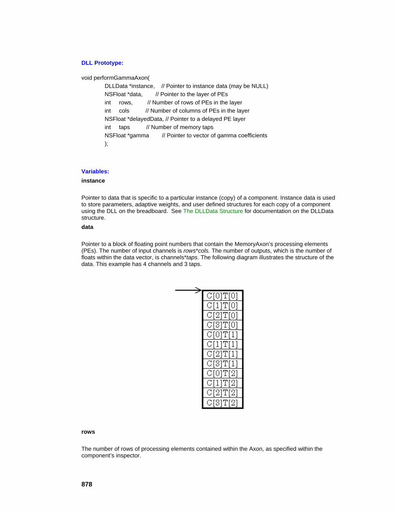
878

DLL Prototype: void performGammaAxon( DLLData *instance, // Pointer to instance data (may be NULL) NSFloat *data, // Pointer to the layer of PEs int rows, // Number of rows of PEs in the layer int cols // Number of columns of PEs in the layer NSFloat *delayedData, // Pointer to a delayed PE layer int taps // Number of memory taps NSFloat *gamma // Pointer to vector of gamma coefficients );

Variables: instance


Pointer to a block of floating point numbers that contain the MemoryAxon’s processing elements (PEs). The number of input channels is rows*cols. The number of outputs, which is the number of floats within the data vector, is channels*taps. The following diagram illustrates the structure of the data. This example has 4 channels and 3 taps.

rows

The number of rows of processing elements contained within the Axon, as specified within the component’s inspector.

879

cols


Pointer to a block of floating point numbers that contains the state of data τ time steps back. The tap delay τ is specified by the user within the TDNNAxon’s inspector and is not included within the prototype. The size and structure of the block match that of data. taps

The number of memory taps stored for each channel. Note that the total number of PEs is rows*cols*taps. gamma

Pointer to the vector of adaptable Gamma coefficients, one for each input channel (rows*cols).

Memory Management Prototypes: DLLData *allocGammaAxon ( DLLData *oldInstance, // Pointer to last instance if reallocating int rows, // Number of rows of PEs in the layer int cols // Number of columns of PEs in the layer int taps // Number of taps attached to each channel ) { DLLData *instance = NULL; return instance; } void freeGammaAxon(DLLData *instance) { freeDLLInstance(instance); }


GammaAxon DLL Implementation

LaguarreAxon DLL Implementation

See Also

PerformTDNNAxon Protocol

880

Description:

This protocol is used for members of the MemoryAxon family that have a vector of memory taps for each input channel. Components conforming to this protocol are responsible for updating this vector, given a second vector that contains the state of the taps τ time steps back. The tap delay τ is specified by the user within the TDNNAxon’s inspector and is not included within the prototype.

DLL Prototype: void performTDNNAxon( DLLData *instance, // Pointer to instance data (may be NULL) NSFloat *data, // Pointer to the layer of PEs int rows, // Number of rows of PEs in the layer int cols // Number of columns of PEs in the layer NSFloat *delayedData, // Pointer to a delayed PE layer int taps // Number of memory taps );

Variables: instance



881

rows



Pointer to a block of floating point numbers that contains the state of data τ time steps back. The tap delay τ is specified by the user within the TDNNAxon’s inspector and is not included within the prototype. The size and structure of the block match that of data. taps

The number of memory taps stored for each channel. Note that the total number of PEs is rows*cols*taps.

Memory Management Prototypes: DLLData *allocTDNNAxon( DLLData *oldInstance, // Pointer to last instance if reallocating int rows, // Number of rows of PEs in the layer int cols // Number of columns of PEs in the layer int taps // Number of taps attached to each channel ) { DLLData *instance = NULL; return instance; } void freeTDNNAxon(DLLData *instance) { freeDLLInstance(instance); }


TDNNAxon DLL Implementation

Example:

882

A TDNNAxon with 1 channel and three taps is fed 6 samples of data. The first row of the table is tap[0], which is the Axon’s input. Each column of the table shows that state of the 3 taps at a given instant in time. Compare the two tables and note how the tap delay τ determines the memory depth.

It is worth pointing out how the delayedData vector fits into this example. If τ is set to 1, then delayedData would point to a block containing the values found in the time=4 column of the first table. Likewise, If τ is set to 2, then delayedData would point to a block containing the values found in the time=3 column of the second table.

See Also

FuzzyAxon Family Protocols PerformFuzzyAxon Protocol

Description:

This protocol is used for members of the FuzzyAxon family that have all of the parameters contained within the PerformAxon DLL Protocol protocol, with the addition of four parameters.

DLL Prototype: void performFuzzyAxon( DLLData *instance, // Pointer to instance data (may be NULL) NSFloat *data, // Pointer to the layer of processing elements (PEs) int rows, // Number of rows of PEs in the layer int cols, // Number of columns of PEs in the layer NSFloat *param, // Pointer to the layer of parameters for the MFs int paramIndex, // Index into the param array int PEIndex, // Index into the processing elements of the

883

Axon // (the data array) NSFloat *returnVal // Value to return after applying the MF );

Variables: instance




The number of columns of processing elements contained within the Axon, as specified within the component’s inspector. param

Pointer to a block of floating point numbers that contain the set of membership function parameters for each of the Axon’s input processing elements (PEs). paramIndex

The base index into the parameter array. PEIndex

The index of the current input PE that is being calculated. returnVal

Pointer to a floating point value, used to store the result of the membership function calculation.

Memory Management Prototypes: DLLData *allocFuzzyAxon( DLLData *oldInstance, // Pointer to last instance if reallocating int rows, // Number of rows of PEs in the layer int cols // Number of columns of PEs in the layer ) { DLLData *instance = NULL; return instance;

884

} void freeFuzzyAxon(DLLData *instance) { freeDLLInstance(instance); }


BellFuzzyAxon DLL Implementation

GaussianFuzzyAxon DLL Implementation

Synapse Family Protocols PerformFullSynapse Protocol

Description:

This protocol is similar to the PerformSynapse DLL Protocol protocol except that the Synapse also contains a matrix of adaptable weights. This matrix is used to provide a fully-connected linear mapping between the PEs of the Axon at the input of the Synapse and the PEs of the Axon at the output of the Synapse.

DLL Prototype: void performFullSynapse( DLLData *instance, // Pointer to instance data (may be NULL) NSFloat *input, // Pointer to the input layer of PEs int inRows, // Number of rows of PEs in the input layer int inCols, // Number of columns of PEs in the input layer NSFloat *output, // Pointer to the output layer int outRows, // Number of rows of PEs in the output layer int outCols // Number of columns of PEs in the output layer NSFloat *weights // Pointer to the fully-connected weight matrix );

Variables: instance

Pointer to data that is specific to a particular instance (copy) of a component. Instance data is used to store parameters, adaptive weights, and user defined structures for each copy of a component using the DLL on the breadboard. Memory Management of Instance Data for documentation on the DLLData structure. input

885

Pointer to a block of floating point numbers that contain the feeding Axon’s processing elements (PEs). The size of the block in bytes is inRows*inCols*sizeof(NSFloat), and the floating point values are arranged in row-major order. inRows

The number of rows of processing elements contained within the feeding Axon, as specified within its inspector. inCols

The number of columns of processing elements contained within the feeding Axon, as specified within its inspector. output

Pointer to a block of floating point numbers that contain the processing elements (PEs) of the Axon that is being fed by the Synapse. The size of the block in bytes is outRows*outCols*sizeof(NSFloat), and the floating point values are arranged in row-major order. outRows

The number of rows of processing elements contained within the Axon that is being fed by the Synapse, as specified within the Axon’s inspector. outCols

The number of columns of processing elements contained within the Axon that is being fed by the Synapse, as specified within the Axon’s inspector. weights

Pointer to a block of floating point numbers that contain the adaptable weights of the Synapse. The size of the block in bytes is inRows*inCols*outRows*outCols*sizeof(NSFloat), and the floating point values are arranged in input-major order.

Memory Management Prototypes: DLLData *allocFullSynapse( DLLData *oldInstance, // Pointer to last instance if reallocating int inRows, // Number of rows of PEs in the input layer int inCols, // Number of columns of PEs in input layer int outRows, // Number of rows of PEs in the output layer int outCols // Number of columns of PEs in output layer ) { DLLData *instance = NULL; return instance; } void freeFullSynapse(DLLData *instance) { freeDLLInstance(instance); }

886


FullSynapse DLL Implementation

See Also

PerformSynapse Protocol

Description:

This protocol is used for members of the Synapse family that simply provide a one-to-one mapping from the inputs to the outputs. The delay between the input and output is defined by the user within the Synapse Inspector (see Synapse Family).

DLL Prototype: void performSynapse( DLLData *instance, // Pointer to instance data (may be NULL) NSFloat *input, // Pointer to the input layer of PEs int inRows, // Number of rows of PEs in the input layer int inCols, // Number of columns of PEs in the input layer NSFloat *output, // Pointer to the output layer int outRows, // Number of rows of PEs in the output layer int outCols // Number of columns of PEs in the output layer );

Variables: instance

Pointer to data that is specific to a particular instance (copy) of a component. Instance data is used to store parameters, adaptive weights, and user defined structures for each copy of a component using the DLL on the breadboard. See The DLLData Structure for documentation on the DLLData structure. input



The number of columns of processing elements contained within the feeding Axon, as specified within its inspector.

887

output



The number of columns of processing elements contained within the Axon that is being fed by the Synapse, as specified within the Axon’s inspector.

Memory Management Prototypes: DLLData *allocSynapse( DLLData *oldInstance, // Pointer to last instance if reallocating int inRows, // Number of rows of PEs in the input layer int inCols, // Number of columns of PEs in input layer int outRows, // Number of rows of PEs in the output layer int outCols // Number of columns of PEs in output layer ) { DLLData *instance = NULL; return instance; } void freeSynapse(DLLData *instance) { freeDLLInstance(instance); }


Synapse DLL Implementation

See Also

BackAxon Family Protocols PerformBackAxon Protocol

Description:

888

This protocol is used to backpropagate the error of its dual Axon component. Note that the Axon does not contain any adaptable weights.

DLL Prototype: void performBackAxon( DLLData *instance, // Pointer to instance data (may be NULL) DLLData *dualInstance, // Pointer to forward axon’s instance data NSFloat *data, // Pointer to the layer of PEs in the axon int rows, // Number of rows of PEs in the layer int cols, // Number of columns of PEs in the layer NSFloat *error // Pointer to the sensitivity vector )

Variables: instance

Pointer to data that is specific to a particular instance (copy) of a component. Instance data is used to store parameters, adaptive weights, and user defined structures for each copy of a component using the DLL on the breadboard. The DLLData Structure for documentation on the DLLData structure. dualInstance

Pointer to data that may have been allocated for the dual component in the activation plane (i.e., the Axon). See The DLLData Structure for documentation on the DLLData structure. data



The number of columns of processing elements contained within the Axon, as specified within the component’s inspector. error

Pointer to a block of floating point numbers that contain the sensitivity information for each of the Axon’s processing elements (PEs). In other words, this is the error that gets backpropagated through the network. The size and structure of the block match that of data.

Memory Management Prototypes: DLLData *allocBackAxon( DLLData *oldInstance, // Pointer to last instance if reallocating

889

int rows, // Number of rows of PEs in the layer int cols // Number of columns of PEs in the layer ) { DLLData *instance = NULL; return instance; } void freeBackAxon(DLLData *instance) { freeDLLInstance(instance); }


BackAxon DLL Implementation

See Also

PerformBackBiasAxon Protocol

Description:

This protocol is used to compute the backpropagated error vector and the bias gradient vector of its dual Axon component, which conforms to the PerformBiasAxon DLL Protocol .

DLL Prototype: void performBackBiasAxon( DLLData *instance, // Pointer to instance data (may be NULL) DLLData *dualInstance, // Pointer to forward axon’s instance data NSFloat *data, // Pointer to the layer of PEs in the axon int rows, // Number of rows of PEs in the layer int cols, // Number of columns of PEs in the layer NSFloat *error // Pointer to the sensitivity vector NSFloat *gradient // Pointer to the bias gradient vector );

Variables: instance

Pointer to data that is specific to a particular instance (copy) of a component. Instance data is used to store parameters, adaptive weights, and user defined structures for each copy of a component

890

using the DLL on the breadboard. See The DLLData Structure for documentation on the DLLData structure. dualInstance

Pointer to data that may have been allocated for the dual component in the activation plane (i.e., the BiasAxon). See The DLLData Structure for documentation on the DLLData structure. data




Pointer to a block of floating point numbers that contain the sensitivity information for each of the Axon’s processing elements (PEs). In other words, this is the error that gets backpropagated through the network. The size and structure of the block match that of data. gradient

Pointer to a block of floating point numbers that contain the gradient information for each of the Axon’s weights (i.e., bias terms). Note that this is the vector that is used by the Gradient Search components. The size and structure of the block match that of bias.

Memory Management Prototypes: DLLData *allocBackBiasAxon( DLLData *oldInstance, // Pointer to last instance if reallocating int rows, // Number of rows of PEs in the layer int cols // Number of columns of PEs in the layer ) { DLLData *instance = NULL; return instance; } void freeBackBiasAxon(DLLData *instance) { freeDLLInstance(instance); }


BackBiasAxon DLL Implementation

891

See Also

PerformBackLinearAxon Protocol

Description:

This protocol is used to compute the backpropagated error vector and the bias gradient vector of its dual Axon component, which conforms to the PerformLinearAxon DLL Protocol protocol.

DLL Prototype: void performBackLinearAxon( DLLData *instance, // Pointer to instance data DLLData *dualInstance, // Pointer to forward axon’s instance data NSFloat *data, // Pointer to the layer of PEs int rows, // Number of rows of PEs in the layer int cols, // Number of columns of PEs in the layer NSFloat *error // Pointer to the sensitivity vector NSFloat *gradient // Pointer to the bias gradient vector NSFloat beta // Slope gain scalar, same for all PEs );

Variables: instance

Pointer to data that is specific to a particular instance (copy) of a component. Instance data is used to store parameters, adaptive weights, and user defined structures for each copy of a component using the DLL on the breadboard. See The DLLData Structure for documentation on the DLLData structure. dualInstance

Pointer to data that may have been allocated for the dual component in the activation plane (i.e., the LinearAxon). See The DLLData Structure for documentation on the DLLData structure. data



892


Pointer to a block of floating point numbers that contain the sensitivity information for each of the Axon’s processing elements (PEs). In other words, this is the error that gets backpropagated through the network. The size and structure of the block match that of data. gradient

Pointer to a block of floating point numbers that contain the gradient information for each of the Axon’s weights (i.e., bias terms). Note that this the vector that is used by the Gradient Search components. The size and structure of the block match that of bias. beta

A scalar that is applied to all PEs to provide the slope of the Axon’s transfer function.

Memory Management Prototypes: DLLData *allocBackLinearAxon( DLLData *oldInstance, // Pointer to last instance if reallocating int rows, // Number of rows of PEs in the layer int cols // Number of columns of PEs in the layer ) { DLLData *instance = NULL; return instance; } void freeBackLinearAxon(DLLData *instance) { freeDLLInstance(instance); }


BackLinearAxon DLL Implementation

BackTanhAxon DLL Implementation

BackSigmoidAxon DLL Implementation

See Also

PerformBackFuzzyAxon Protocol

Description:

893

This protocol is used to compute the gradient for the specified parameter of the membership function of its dual Axon component, which conforms to the PerformFuzzyAxon DLL Protocol protocol.

DLL Prototype: void performBackFuzzyAxon( DLLData *instance, // Pointer to instance data (may be NULL) DLLData *dualInstance, // Pointer to forward axon’s instance data (may be NULL) NSFloat *data, // Pointer to the layer of processing elements (PEs) int rows, // Number of rows of PEs in the layer int cols, // Number of columns of PEs in the layer NSFloat *error, // Pointer to the sensitivity vector NSFloat *param, // Pointer to the layer of parameters for the MFs int paramIndex, // Index of the MF parameter int winnerIndex, // Index of the winning MF NSFloat winnerVal, // Value of the winning Input NSFloat *returnVal // Return value );

Variables: instance


Pointer to data that may have been allocated for the dual component in the activation plane (i.e., the LinearAxon). See The DLLData Structure for documentation on the DLLData structure. data




894

Pointer to a block of floating point numbers that contain the sensitivity information for each of the Axon’s processing elements (PEs). In other words, this is the error that gets backpropagated through the network. The size and structure of the block match that of data. param

Pointer to a block of floating point numbers that contain the set of membership function parameters for each of the dual Axon’s input processing elements (PEs). paramIndex

The index into the parameter array that specifies the parameter whose derivative needs to be calculated. winnerIndex

The index of the dual Axon's membership function which produced the minimum value (i.e., the winning MF). winnerVal

The dual Axon's input PE value corresponding to the membership function which produced the minimum value (i.e., the winning MF). returnVal

The return value, which is the gradient (derivative) for the specified membership function parameter.

Memory Management Prototypes: DLLData *allocBackFuzzyAxon( DLLData *oldInstance, // Pointer to the last instance if reallocating DLLData *dualInstance, // Pointer to forward axon’s instance data (may be NULL) int rows, // Number of rows of PEs in the layer int cols // Number of columns of PEs in the layer ) { DLLData *instance = allocDLLInstance(oldInstance); return instance; } void freeBackFuzzyAxon(DLLData *instance) { freeDLLInstance(instance); }


BackBellFuzzyAxon DLL Implementation

BackGaussianFuzzyAxon DLL Implementation

895

BackMemoryAxon Family Protocols PerformBackContextAxon Protocol

Description:

This protocol is used to compute the backpropagated error vector and the gamma gradient vector of its dual MemoryAxon component, which conforms to the PerformContextAxon DLL Protocol protocol.

DLL Prototype: void performBackContextAxon( DLLData *instance, // Pointer to instance data (may be NULL) DLLData *dualInstance, // Pointer to forward axon’s instance data NSFloat *error, // Pointer to the current sensitivity vector int rows, // Number of rows of PEs in the layer int cols, // Number of columns of PEs in the layer NSFloat *delayedError, // Pointer to the delayed error vector NSFloat *data, // Pointer to the layer of PEs NSFloat *tau, // Pointer to a vector of time constants NSFloat beta, // Linear scaling factor (user-defined) NSFloat *gradient // Pointer to the tau gradient vector );

Variables: instance


Pointer to data that may have been allocated for the dual component in the activation plane (i.e., the ContextAxon). See The DLLData Structure for documentation on the DLLData structure. error

Pointer to a block of floating point numbers that contain the sensitivity information for each of the MemoryAxon’s processing elements (PEs). In other words, this is the error that gets backpropagated through the network. The size and structure of the block match that of data. rows


896

The number of columns of processing elements contained within the Axon, as specified within the component’s inspector. delayedError

Pointer to a block of floating point numbers that contains the state of error one time step back. The size and structure of the block match that of error. data

Pointer to a block of floating point numbers that contain the PEs of the activation dual (i.e., the ContextAxon). The size of the block in bytes is rows*cols*sizeof(NSFloat), and the floating point values are arranged in row-major order. tau

Pointer to the vector of adaptable time constants contained within the activation dual (i.e., the ContextAxon). These constants are adapted by the attached Gradient Search component by using the gradient vector.

beta

Scaling factor that is specified by the user within the ContextAxon inspector. gradient

Pointer to a block of floating point numbers that contain the gradient information for each of the ContextAxon’s time constants. Note that this is the vector that is used by the Gradient Search components. The size and structure of the block match that of tau.

Memory Management Prototypes: DLLData *allocBackContextAxon( DLLData *oldInstance, // Pointer to last instance if reallocating int rows, // Number of rows of PEs in the layer int cols // Number of columns of PEs in the layer ) { DLLData *instance = NULL; return instance; } void freeBackContextAxon(DLLData *instance) { freeDLLInstance(instance); }


BackContextAxon DLL Implementation

BackIntegratorAxon DLL Implementation

BackSigmoidContextAxon DLL Implementation

BackTanhContextAxon DLL Implementation

897

BackSigmoidIntegratorAxon DLL Implementation

BackTanhIntegratorAxon DLL Implementation

See Also

PerformBackGammaAxon Protocol

Description:

This protocol is used to compute the backpropagated error vector and the gamma gradient vector of its dual MemoryAxon component, which conforms to the PerformGammaAxon DLL Protocol protocol.

DLL Prototype: void performBackGammaAxon( DLLData *instance, // Pointer to instance data (may be NULL) DLLData *dualInstance, // Pointer to forward axon’s instance data NSFloat *error, // Pointer to the current sensitivity vector int rows, // Number of rows of PEs in the layer int cols, // Number of columns of PEs in the layer NSFloat *delayedError, // Pointer to the delayed error vector int taps, // Number of memory taps (user-defined) NSFloat *data // Pointer to the layers of (PEs) NSFloat *gamma, // Pointer to vector of gamma coefficients NSFloat *gradient // Pointer to the gamma gradient vector );

Variables: instance


Pointer to data that may have been allocated for the dual component in the activation plane (i.e., the GammaAxon). See The DLLData Structure for documentation on the DLLData structure. error

Pointer to a block of floating point numbers that contain the sensitivity information for each of the MemoryAxon’s processing elements (PEs). In other words, this is the error that gets backpropagated through the network. The size and structure of the block match that of data.

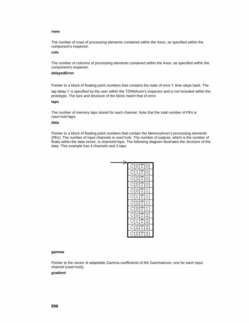
898

rows



Pointer to a block of floating point numbers that contains the state of error τ time steps back. The tap delay τ is specified by the user within the TDNNAxon’s inspector and is not included within the prototype. The size and structure of the block match that of error. taps

The number of memory taps stored for each channel. Note that the total number of PEs is rows*cols*taps. data


gamma

Pointer to the vector of adaptable Gamma coefficients of the GammaAxon, one for each input channel (rows*cols). gradient

899

Pointer to a block of floating point numbers that contain the gradient information for each of the GammaAxon’s gamma coefficients. Note that this is the vector that is used by the Gradient Search components. The size and structure of the block match that of gamma.

Memory Management Prototypes: DLLData *allocBackGammaAxon( DLLData *oldInstance, // Pointer to last instance if reallocating int rows, // Number of rows of PEs in the layer int cols // Number of columns of PEs in the layer int taps // Number of taps attached to each channel ) { DLLData *instance = NULL; return instance; } void freeBackGammaAxon(DLLData *instance) { freeDLLInstance(instance); }


BackGammaAxon DLL Implementation

BackLaguarreAxon DLL Implementation

See Also

PerformBackTDNNAxon Protocol

Description:

This protocol is used to compute the backpropagated error vector of its dual MemoryAxon component, which conforms to the PerformTDNNAxon DLL Protocol protocol.

DLL Prototype: void performBackTDNNAxon( DLLData *instance, // Pointer to instance data (may be NULL) DLLData *dualInstance, // Pointer to forward axon’s instance data NSFloat *error, // Pointer to the current sensitivity vector int rows, // Number of rows of PEs in the layer int cols, // Number of columns of PEs in the layer

900

NSFloat *delayedError, // Pointer to the delayed error vector int taps, // Number of memory taps (user-defined) NSFloat *data // Pointer to the layers of (PEs) );

Variables: instance


Pointer to data that may have been allocated for the dual component in the activation plane (i.e., the TDNNAxon). See The DLLData Structure for documentation on the DLLData structure. error

Pointer to a block of floating point numbers that contain the sensitivity information for each of the MemoryAxon’s processing elements (PEs). In other words, this is the error that gets backpropagated through the network. The size and structure of the block match that of data. rows



Pointer to a block of floating point numbers that contains the state of error τ time steps back. The tap delay τ is specified by the user within the TDNNAxon’s inspector and is not included within the prototype. The size and structure of the block match that of error. taps

The number of memory taps stored for each channel. Note that the total number of PEs is rows*cols*taps. data


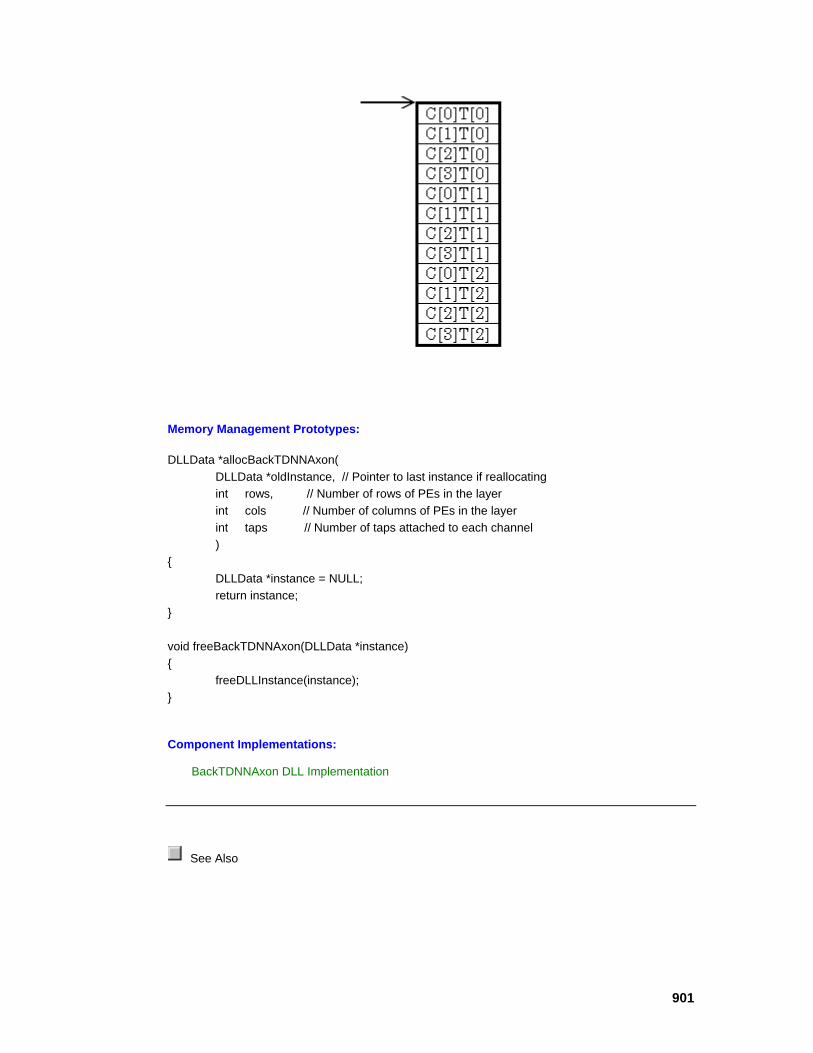
901

Memory Management Prototypes: DLLData *allocBackTDNNAxon( DLLData *oldInstance, // Pointer to last instance if reallocating int rows, // Number of rows of PEs in the layer int cols // Number of columns of PEs in the layer int taps // Number of taps attached to each channel ) { DLLData *instance = NULL; return instance; } void freeBackTDNNAxon(DLLData *instance) { freeDLLInstance(instance); }


BackTDNNAxon DLL Implementation

See Also

902

BackSynapse Protocols PerformBackFullSynapse Protocol

Description:

This protocol is used to compute the weight gradient matrix and the backpropagated error vector of its dual Synapse component, which conforms to the PerformFullSynapse DLL Protocol protocol. Note that the input and output are reversed from that of the activation dual component.

DLL Prototype: void performBackFullSynapse( DLLData *instance, // Pointer to instance data (may be NULL) DLLData *dualInstance, // Pointer to forward axon’s instance data NSFloat *errorIn, // Pointer to the input error layer of PEs int inRows, // Number of rows of PEs in the input layer int inCols, // Number of columns of PEs at the input NSFloat *errorOut, // Pointer to the output error layer int outRows, // Number of rows of PEs in the output layer int outCols, // Number of columns of PEs at the output NSFloat *input // Pointer to output PEs of forward synapse NSFloat *weights, // Pointer to fully-connected weight matrix NSFloat *gradients // Pointer to the weight gradient matrix );

Variables: instance


Pointer to data that may have been allocated for the dual component in the activation plane (i.e., the Synapse). The DLLData Structure for documentation on the DLLData structure. errorIn

Pointer to the sensitivity vector of the PerformBackAxon DLL Protocol component that is feeding the BackSynapse. The size and structure of the block match that of output from the activation dual component. inRows

The number of rows of processing elements associated with the BackAxon component that is feeding the BackSynapse, as specified within the corresponding Axon’s inspector. inCols

903

The number of columns of processing elements associated with the BackAxon component that is feeding the BackSynapse, as specified within the corresponding Axon’s inspector. errorOut

Pointer to the sensitivity vector of the PerformBackAxon DLL Protocol component the BackSynapse is feeding. In other words, this is the error that gets backpropagated through the network. The size and structure of the block match that of input from the activation dual component. outRows

The number of rows of processing elements associated with the BackAxon component that the BackSynapse is feeding, as specified within the corresponding Axon’s inspector. outCols

The number of columns of processing elements associated with the BackAxon component that the BackSynapse is feeding, as specified within the corresponding Axon’s inspector. input

Pointer to a block of floating point numbers that contain the PEs of the activation dual (i.e., the Synapse) at its output. The size of the block in bytes is inRows*inCols*sizeof(NSFloat), and the floating point values are arranged in row-major order. weights

Pointer to a block of floating point numbers that contain the adaptable weights of the activation dual component (see PerformFullSynapse DLL Protocol ). gradient

Pointer to a block of floating point numbers that contain the matrix of gradients for each of the Synapse’s weights. Note that this is the matrix that is used by the Gradient Search components. The size and structure of the block match that of weights.

Memory Management Prototypes: DLLData *allocBackFullSynapse( DLLData *oldInstance, // Pointer to last instance if reallocating int inRows, // Number of rows of PEs in the input layer int inCols, // Number of columns of PEs in input layer int outRows, // Number of rows of PEs in the output layer int outCols // Number of columns of PEs in output layer ) { DLLData *instance = NULL; return instance; } void freeBackFullSynapse(DLLData *instance) { freeDLLInstance(instance); }

904


BackFullSynapse DLL Implementation

See Also

PerformBackSynapse Protocol

Description:

This protocol is used to compute the backpropagated error vector of its dual Synapse component, which conforms to the PerformSynapse DLL Protocol protocol. The delay between the output and input is defined by the user within the inspector of the activation dual (see BackSynapse Family). Note that the input and output are reversed from that of the activation dual component.

DLL Prototype: void performBackSynapse( DLLData *instance, // Pointer to instance data (may be NULL) DLLData *dualInstance, // Pointer to forward axon’s instance data NSFloat *errorIn, // Pointer to the input error layer of PEs int inRows, // Number of rows of PEs in the input layer int inCols, // Number of columns of PEs at the input NSFloat *errorOut, // Pointer to the output error layer int outRows, // Number of rows of PEs in the output layer int outCols, // Number of columns of PEs at the output NSFloat *input // Pointer to output PEs of forward synapse );

Variables: instance


Pointer to data that may have been allocated for the dual component in the activation plane (i.e., the Synapse). See The DLLData Structure for documentation on the DLLData structure. errorIn

Pointer to the sensitivity vector of the PerformBackAxon DLL Protocol component that is feeding the BackSynapse. The size and structure of the block match that of output from the activation dual component. inRows

905

The number of rows of processing elements associated with the BackAxon component that is feeding the BackSynapse, as specified within the corresponding Axon’s inspector. inCols

The number of columns of processing elements associated with the BackAxon component that is feeding the BackSynapse, as specified within the corresponding Axon’s inspector. errorOut

Pointer to the sensitivity vector of the PerformBackAxon DLL Protocol component the BackSynapse is feeding. In other words, this is the error that gets backpropagated through the network. The size and structure of the block match that of input from the activation dual component. outRows

The number of rows of processing elements associated with the BackAxon component that the BackSynapse is feeding, as specified within the corresponding Axon’s inspector. outCols

The number of columns of processing elements associated with the BackAxon component that the BackSynapse is feeding, as specified within the corresponding Axon’s inspector. input

Pointer to a block of floating point numbers that contain the PEs of the activation dual (i.e., the Synapse) at its output. The size of the block in bytes is inRows*inCols*sizeof(NSFloat), and the floating point values are arranged in row-major order.

Memory Management Prototypes: DLLData *allocBackSynapse( DLLData *oldInstance, // Pointer to last instance if reallocating int inRows, // Number of rows of PEs in the input layer int inCols, // Number of columns of PEs in input layer int outRows, // Number of rows of PEs in the output layer int outCols // Number of columns of PEs in output layer ) { DLLData *instance = NULL; return instance; } void freeBackSynapse(DLLData *instance) { freeDLLInstance(instance); }


BackSynapse DLL Implementation

906

See Also

ErrorCriteria Family Protocols PerformCriterion Protocol

Description:

This protocol is used for members of the ErrorCriterion family. Implementations of this protocol are responsible for computing the output sensitivity vector, which is the error used for the backpropagation. The function returns the accumulated cost based on the particular criterion.

DLL Prototype: NSFloat performCriterion( DLLData *instance, // Pointer to instance data (may be NULL) NSFloat *costDerivative, // Pointer to output sensitivity vector int rows, // Number of rows of PEs in the layer int cols, // Number of columns of PEs in the layer NSFloat *output, // Pointer to output layer of the network NSFloat *desired // Pointer to desired output vector );

Variables: instance

Pointer to data that is specific to a particular instance (copy) of a component. Instance data is used to store parameters, adaptive weights, and user defined structures for each copy of a component using the DLL on the breadboard. The DLLData Structure for documentation on the DLLData structure. error

Pointer to a block of floating point numbers that contain the sensitivity information for each of the processing elements (PEs) of the Axon at the output of the network. In other words, this is the error that gets backpropagated through the network. The size and structure of the block match that of output. rows

The number of rows of processing elements contained within the ErrorCriterion component. Note that this should match the number of rows of the feeding Axon. cols

The number of columns of processing elements contained within the ErrorCriterion component. Note that this should match the number of columns of the feeding Axon. output

907

Pointer to a block of floating point numbers that contain the processing elements (PEs) at the output of the network. The size of the block in bytes is rows*cols*sizeof(NSFloat), and the floating point values are arranged in row-major order. desired

Pointer to a block of floating point numbers that contain the desired response of the corresponding processing elements (PEs) at the output of the network. The size and structure of the block match that of output.

Memory Management Protocol: DLLData *allocCriterion( DLLData *oldInstance, // Pointer to last instance if reallocating int rows, // Number of rows of PEs in the layer int cols // Number of columns of PEs in the layer ) { DLLData *instance = NULL; return instance; } void freeCriterion(DLLData *instance) { freeDLLInstance(instance); }




LinfinityCriterion DLL Implementation

See Also

GradientSearch Family Protocols PerformDeltaBarDelta Protocol

Description:

The implementation of this protocol is responsible for computing the step size for each of the weights based on the gradient from the backprop component, a smoothed version of the gradient (smoothedGradient), and three constants (beta, kappa, and zeta) defined by the user within the DeltaBarDelta inspector. The implementation is also responsible for computing the

908

smoothedGradient vector. Note that the component itself implements the standard Momentum DLL Implementation rule using the step sizes computed within the function.

DLL Prototype: void performDeltaBarDelta( DLLData *instance, // Pointer to instance data NSFloat *step, // Pointer to vector of learning rates int length, // Length of learning rate vector NSFloat *smoothedGradient, // Smoothed gradient vector NSFloat *gradient, // Gradient vector from backprop comp. NSFloat beta, // Multiplicative constant NSFloat kappa, // Additive constant NSFloat zeta // Smoothing factor );

Variables: instance

Pointer to data that is specific to a particular instance (copy) of a component. Instance data is used to store parameters, adaptive weights, and user defined structures for each copy of a component using the DLL on the breadboard. See The DLLData Structure for documentation on the DLLData structure. step

Pointer to a block of floating point numbers that contain the learning rates (i.e., step sizes) for each of the weights. This vector is computed within the protocol implementation and is used by the component itself for the standard Momentum weight update. length

The number of weights. smoothedGradient

Pointer to a block of floating point numbers that contain the gradient information applied to a smoothing filter. This vector is computed by the protocol implementation. The size and structure of the block match that of gradient. gradient

Pointer to a block of floating point numbers that contain the gradient information for each of the weights of the attached activation component. This vector is used in conjunction with the smoothedGradient vector to compute the step vector. beta

Multiplicative constant specified by the user within the DeltaBarDelta inspector (see equation within DeltaBarDelta). kappa

Additive constant specified by the user within the DeltaBarDelta inspector (see equation within DeltaBarDelta).

909

zeta

Smoothing factor specified by the user within the DeltaBarDelta inspector (see equation within DeltaBarDelta).

Memory Management Prototypes: DLLData *allocDeltaBarDelta( DLLData *oldInstance, // Pointer to last instance if reallocating int length, // Length of the weight vector BOOL individual // Indicates whether their is one learning // rate for all weights (FALSE), or each // weight has its own learning rate (TRUE) ) { DLLData *instance = NULL; return instance; } void freeDeltaBarDelta(DLLData *instance) { freeDLLInstance(instance); }


DeltaBarDelta DLL Implementation

See Also

PerformMomentum Protocol

Description:

This protocol is similar to the PerformStep DLL Protocol protocol, except that there is the addition of a momentum term and a vector containing the previous weight change (delta). These terms are used in conjunction with the step size and gradient information to adjust the weights. This weight adjustment is the new delta and the implementation of this function is responsible for updating this vector as well as the weights vector.

DLL Prototype: void performMomentum( DLLData *instance, // Pointer to instance data NSFloat *weights, // Pointer to the vector of weights

910

int length, // Length of the weight vector NSFloat *gradient, // Pointer to vector of gradients NSFloat *step, // Pointer to the learning rate/s BOOL individual // Indicates whether there is one learning rate // for all weights (FALSE), or each weight has // its own learning rate (TRUE) NSFloat *delta, // Last weight Update NSFloat momentum // Momentum rate for all weights );

Variables: instance

Pointer to data that is specific to a particular instance (copy) of a component. Instance data is used to store parameters, adaptive weights, and user defined structures for each copy of a component using the DLL on the breadboard. See The DLLData Structure for documentation on the DLLData structure. weights

Pointer to a block of floating point numbers that contain the weights of the attached activation component. This vector is adjusted by the GradientSearch component. The size of the block in bytes is length*sizeof(NSFloat). length

The number of elements contained within the weights vector. gradient

Pointer to a block of floating point numbers that contain the gradient information for each of the weights of the attached activation component. This vector is used to determine the amount to adjust the weights. The size and structure of the block match that of weights. step

Pointer to a block of floating point numbers that contain the learning rates (i.e., step sizes) for each of the weights. If individual is set to TRUE, then this block contains only one floating-point number, which is the step size for all of the weights. individual

Flag to indicate whether the step pointer contains only one floating point number, which is the step size for all of the weights (individual=FALSE), or length floating point numbers, which are the individual step sizes for each of the weights (individual=TRUE). delta

Pointer to a block of floating point numbers that contain the previous update (i.e., delta) for each of the weights. The implementation of this function is responsible for updating this vector before returning. momentum

Scalar containing the momentum rate applied to all weight updates.

911

Memory Management Prototypes: DLLData *allocMomentum( DLLData *oldInstance, // Pointer to last instance if reallocating int length, // Length of the weight vector BOOL individual // Indicates whether their is one learning // rate for all weights (FALSE), or each // weight has its own learning rate (TRUE) ) { DLLData *instance = NULL; return instance; } void freeMomentum(DLLData *instance) { freeDLLInstance(instance); }


Momentum DLL Implementation

See Also

PerformQuickprop Protocol

Description:

This protocol is similar to the PerformMomentum DLL Protocol protocol, except that the momentum rate is unique to each weight. Note that this vector could have been allocated as local storage, but it is passed as a parameter for efficiency reasons. The defaultMomentum is defined by the user within the inspector. The lastGradient is a pointer to a block containing the previous state of gradient. This function is responsible for updating the lastGradient vector as well as the delta and weights vectors.

DLL Prototype: void performQuickprop( DLLData *instance, // Pointer to instance data NSFloat *weights, // Pointer to the vector of weights int length, // Length of the weight vector NSFloat *gradient, // Pointer to vector of gradients NSFloat *step, // Pointer to the learning rate/s BOOL individual // Indicates whether there is one learning // rate for all weights (FALSE), or each

912

// weight has its own learning rate (TRUE) NSFloat *delta, // Last weight Update NSFloat defaultMomentum, // Max momentum rate for all weights NSFloat *momentum, // Individual momentum rate for each weight NSFloat *lastGradient // Previous weight gradient vector );

Variables: instance






Flag to indicate whether the step pointer contains only one floating point number, which is the step size for all of the weights (individual=FALSE), or length floating point numbers, which are the individual step sizes for each of the weights (individual=TRUE). delta

Pointer to a block of floating point numbers that contain the previous update (i.e., delta) for each of the weights. The implementation of this function is responsible for updating this vector before returning. defaultMomentum

Scalar containing the momentum rate entered by the user within the inspector. The quickprop algorithm uses this parameter as the maximum that the absolute value of each element within the momentum vector can be. momentum

913

Pointer to a block of floating point numbers used to store the momentum rates for each of the weights. Note that this vector could have been allocated as local storage, but it is passed as a parameter for efficiency reasons. lastGradient

Pointer to a block of floating point numbers that contain the previous state of the gradient vector. This pointer must be maintained by the protocol’s implementation.

Memory Management Prototypes: DLLData *allocQuickprop( DLLData *oldInstance, // Pointer to last instance if reallocating int length, // Length of the weight vector BOOL individual // Indicates whether their is one learning // rate for all weights (FALSE), or each // weight has its own learning rate (TRUE) ) { DLLData *instance = NULL; return instance; } void freeQuickprop(DLLData *instance) { freeDLLInstance(instance); }


Quickprop DLL Implementation

See Also

PerformStep Protocol

Description:

This protocol is used to update the weight vector of the attached Activation component given the gradient information from the corresponding Backprop component. The learning rate is solely determined by the step size, which can be unique to each weight or the same for all weights.

DLL Prototype: void performStep( DLLData *instance, // Pointer to instance data

914

NSFloat *weights, // Pointer to the vector of weights int length, // Length of the weight vector NSFloat *gradient, // Pointer to vector of gradients NSFloat *step, // Pointer to the learning rate/s BOOL individual // Indicates whether there is one learning rate // for all weights (FALSE), or each weight has // its own learning rate (TRUE) );

Variables: instance






Flag to indicate whether the step pointer contains only one floating point number, which is the step size for all of the weights (individual=FALSE), or length floating point numbers, which are the individual step sizes for each of the weights (individual=TRUE).

Memory Management Prototypes: DLLData *allocStep( DLLData *oldInstance, // Pointer to last instance if reallocating int length, // Length of the weight vector BOOL individual // Indicates whether their is one learning // rate for all weights (FALSE), or each // weight has its own learning rate (TRUE) )

915

{ DLLData *instance = NULL; return instance; } void freeStep(DLLData *instance) { freeDLLInstance(instance); }


Step DLL Implementation

See Also

Input Family Protocols PerformFile Protocol

Description:

This protocol is used to implement a customized file translator. The responsibility of the performFile implementation is to read the next floating-point value from the file. The function returns a TRUE if a value was read and a FALSE if the end-of-file was reached.

DLL Prototype: BOOL performFile( DLLData *instance, // Pointer to instance data (may be NULL) FILE *file, // Pointer to the opened file NSFloat *sample // Location to place next sample );

Variables: instance

Pointer to data that is specific to a particular instance (copy) of a component. Instance data is used to store parameters and user defined structures for each copy of a component using a particular DLL on the breadboard. See The DLLData Structure for documentation on the DLLData structure. file

Pointer returned by the openFile function of the DLL. sample

916

Pointer to the storage used to return the next floating-point value read from the file.

Initialization Prototype:

This function takes in the path name of the input file and returns a pointer to the opened file. FILE *openFile( DLLData *instance, // Pointer to instance data (may be NULL) const char *filePath // Full path of file to be opened );

Memory Management Protocol: DLLData *allocFile( DLLData *oldInstance // Pointer to the last instance if reallocating ) { DLLData *instance = NULL; return instance; } void freeFile(DLLData *instance) { freeDLLInstance(instance); }


File DLL Implementation

See Also

PerformFunction Protocol

Description:

This protocol is used to define a periodic wave to be used as an input source.

DLL Prototype: NSFloat performFunction( DLLData *instance, // Pointer to instance data (may be NULL) NSFloat x // Current angle in radians

917

);

Variables: instance

Pointer to data that is specific to a particular instance (copy) of a component. Instance data is used to store parameters and user defined structures for each copy of a component using a particular DLL on the breadboard. See The DLLData Structure for documentation on the DLLData structure.

x

The current angle in radians. Each time the perform function is called, this angle is incremented by NeuroSolutions based on the number of Samples/Cycle specified by the user within the Function inspector.


This function is used to initialize any instance variables before a new cycle of input is generated. Note that this is different from (and called before) the global prototype, fireGetReady(). void getReadyToFire( DLLData *instance // Pointer to instance data (may be NULL) );

Memory Management Protocol: DLLData *allocFunction( DLLData *oldInstance // Pointer to the last instance if reallocating ) { DLLData *instance = NULL; return instance; } void freeFunction(DLLData *instance) { freeDLLInstance(instance); }


Function DLL Implementation

See Also

918

PerformNoise Protocol

Description:

This protocol is used to generate a noise source.

DLL Prototype: NSFloat performNoise( DLLData *instance, // Pointer to instance data (may be NULL) NSFloat variance, // Variance set within components inspector NSFloat mean // Mean set within components inspector );

Variables: instance

Pointer to data that is specific to a particular instance (copy) of a component. Instance data is used to store parameters and user defined structures for each copy of a component using a particular DLL on the breadboard. See The DLLData Structure for documentation on the DLLData structure. variance

The variance of the generated noise defined by the user within the Noise inspector. mean

The mean of the generated noise defined by the user within the Noise inspector.


This function is used to initialize any instance variables before a new segment of noise data is generated. Note that this is different from (and called before) the global prototype, fireGetReady(). void getReadyToFire( DLLData *instance // Pointer to instance data (may be NULL) );

Memory Management Protocol: DLLData *allocNoise( DLLData *oldInstance // Pointer to the last instance if reallocating ) { DLLData *instance = NULL; return instance; }

919

void freeNoise(DLLData *instance) { freeDLLInstance(instance); }


Noise DLL Implementation

See Also

PerformInput Protocol

Description:

This protocol is used to inject data into the network. The implementation of the performInput function computes the next sample of data for each of the input channels (PEs of the attached component) and writes the floating-point values to the data vector.

DLL Prototype: void performInput( DLLData *instance, // Pointer to instance data (may be NULL) NSFloat *data, // Pointer to the data int rows, // Number of rows of data int cols // Number of cols of data );

Variables: instance

Pointer to data that is specific to a particular instance (copy) of a component. Instance data is used to store parameters and user defined structures for each copy of a component using a particular DLL on the breadboard. See The DLLData Structure for documentation on the DLLData structure. data

Pointer to a block of floating point numbers that contain the processing elements (PEs) of the attached component. This is where the next sample of data is written to. The size of the block in bytes is rows*cols*sizeof(NSFloat), and the floating point values are arranged in row-major order. rows

The number of rows of processing elements contained within the attached component, as specified within the component’s inspector.

920

cols

The number of columns of processing elements contained within the attached component, as specified within the component’s inspector.

Memory Management Protocol: DLLData *allocInput( DLLData *oldInstance // Pointer to the last instance if reallocating int rows, // Number of rows of data int cols // Number of cols of data ) { DLLData *instance = allocDLLInstance(oldInstance); return instance; } void freeInput(DLLData *instance) { freeDLLInstance(instance); }


DLLInput DLL Implementation

See Also

PerformPrePost Protocol

Description:

This protocol is used for both preprocessing of network input as well as postprocessing of network output. The implementation of the performPrePost function reads the data from input and writes the processed data to output. The function returns a TRUE if the output is to be passed on to the next component, or FALSE if more data needs to be processed (more calls to performPrePost).

It is important to understand the distinction between the preprocessor and postprocessor modes. The preprocessor gets its input from an Input component stacked above, and its output is the vector of processing elements of the component stacked below. The preprocessed output is normally accumulated to the existing activity (e.g., data[i] = data[i] + preprocessedData[i]), in order allow other components to inject data into the same component. The postprocessor’s input is the vector of PEs of the component stacked below and its output is a locally-stored vector, which is used by a Probe attached above. Note that this vector is not automatically zeroed, so that it can be used to store the postprocessed data from the previous call to performPrePost.

921

DLL Prototype: BOOL performPrePost( DLLData *instance, // Pointer to instance data (may be NULL) NSFloat *input, // Pointer to the input data NSFloat *output, // Pointer to the output data int rows, // Number of rows of data int cols, // Number of cols of data BOOL preprocessor // Flag to indicate whether this is a preprocessor // or postprocessor );

Variables: instance

Pointer to data that is specific to a particular instance (copy) of a component. Instance data is used to store parameters and user defined structures for each copy of a component using a particular DLL on the breadboard. See The DLLData Structure for documentation on the DLLData structure. input

Pointer to a block of floating point numbers that contain the processing elements (PEs) of the attached component that is feeding data into the processor. For the DLLPreprocessor, this is the component stacked above (using the Preprocessor access point) and for the DLLPostprocessor, this is the component stacked below. Note that for the DLLPostprocessor, the size of this vector is fixed based on the size of the component stacked below (rows*cols*sizeof(NSFloat). For the DLLPreprocessor, the size of this vector defaults to the size of output, but can be modified within the allocPrePost function. output

Pointer to a block of floating point numbers that contain the processing elements (PEs) of the attached component that is retrieving data from the processor. For the DLLPostprocessor, this is the component stacked above (using the Postprocessor access point) and for the DLLPreprocessor, this is the component stacked below. Note that for the DLLPreprocessor, the size of this vector is fixed based on the size of the component stacked below (rows*cols*sizeof(NSFloat). For the DLLPostprocessor, the size of this vector defaults to the size of input, but can be modified within the allocPrePost function. rows

The number of rows of processing elements contained within the attached component that is fixed in size (i.e., the component stacked below). cols

The number of columns of processing elements contained within the attached component that is fixed in size (i.e., the component stacked below). preprocessor

Flag to indicate if the component using the DLL is a DLLPreprocessor (TRUE) or a DLLPostprocessor (FALSE).

Memory Management Protocol:

922

DLLData *allocPrePost( DLLData *oldInstance, // Pointer to the last instance if reallocating int *rows, // Number of rows of data attached above -- can be // changed. The default is the number of rows // attached below. int *cols, // Number of cols of data attached above -- can be // changed. The default is the number of cols // attached below. BOOL preprocessor // Flag to indicate whether this is a preprocessor // or postprocessor ); void freePrePost(DLLData *instance) { freeDLLInstance(instance); }


DLLPreprocessor and DLLPostprocessor DLL Implementation

See Also

StaticProbe Family Protocols PerformOutput Protocol

Description:

This protocol is used to extract the data accessed by a static Probe. Each call to performOutput contains a single sample (of rows*cols PEs) of output data. This DLL is intended to be passive, meaning that the data vector should not be modified. The return value indicates whether the base Probe component is active (TRUE) or not (FALSE).

DLL Prototype: BOOL performOutput( DLLData *instance, // Pointer to instance data (may be NULL) NSFloat *data, // Pointer to the data int rows, // Number of rows of data int cols // Number of cols of data );

923

Variables: instance


Pointer to a block of floating point numbers containing one sample of output for all channels (rows*cols). rows

The number of rows contained within data. cols

The number of cols contained within data.

Memory Management Protocol: DLLData *allocOutput( DLLData *oldInstance, // Pointer to the last instance if reallocating int rows, // Number of rows of data int cols // Number of cols of data ) { DLLData *instance = allocDLLInstance(oldInstance); return instance; } void freeOutput(DLLData *instance) { freeDLLInstance(instance); }


Static Probe DLL Implementation

See Also

Transformer Family Protocols PerformTransform Protocol

924

Description:

This protocol is used to transform temporal output data. For each sample of data to be processed, the performTransform function is called once for each channel. The caller copies its buffer (of length samples) to the data buffer for that particular channel. The implementation then processes the data and writes the transformed data back to the same buffer. The return value specifies whether or not the data for the particular channel is to be displayed by the component stacked on the Transformer Access Points access point.

DLL Prototype: BOOL performTransform( DLLData *instance, // Pointer to instance data NSFloat *data, // Pointer to the buffered data int length, // Length of the buffer to be transformed int channel // Current channel number );

Variables: instance


Pointer to a block of floating point numbers containing the output for a single channel over time. This buffer is also used for writing the transformed data. The size of the buffer is length*sizeof(NSFloat). length

The number of samples stored in the data buffer. channel

The channel number that corresponds to the data buffer. Note that for each sample of output, the performTransform function is called once for each channel.

Memory Management Protocol: DLLData *allocTransform( int length, // Length of the buffer to be transformed int channels // Number of channels to be transformed ) void freeTransform(DLLData *instance) { if (instance) free(instance); }

925


Transformer DLL Implementation

See Also

Schedule Family Protocols PerformScheduler Protocol

Description:

This protocol is implemented by members of the Scheduler family. The function is called during each epoch that has scheduling active (specified by the user within the Scheduler inspector). The implementation simply applies a function of beta to the vector of data. Note that the base component automatically handles the clipping if the data exceeds the boundaries specified by the user.

DLL Prototype: BOOL performScheduler( DLLData *instance, // Pointer to instance data (may be NULL) NSFloat *data, // Pointer to the data to be scheduled int length, // Number of elements in scheduled data vector NSFloat beta // Scheduler parameter (specified by user) );

Variables: instance


Pointer to a block of floating point numbers that contain the processing elements (PEs) of the attached component at a particular access point. This is the data that is modified (i.e., scheduled) by the Scheduler component. The size of the block in bytes is length*sizeof(NSFloat). length

The number of processing elements contained within the attached component at a particular access point. beta

926

User-specified parameter that is used to define the rate of change of the scheduling function.

Memory Management Protocol: DLLData *allocScheduler( DLLData *oldInstance, // Pointer to last instance if reallocating int length // Number of PEs in scheduled data vector ) { DLLData *instance = NULL; return instance; } void freeScheduler(DLLData *instance) { freeDLLInstance(instance); }





See Also

ControlTransmitter Family Protocols PerformThresholdTransmitter Protocol

Description:

This protocol is used by ThresholdTransmitter components to signal when a threshold has been crossed by returning a TRUE from the function. The implementation of this protocol scans through the values within data, and determines if the user-defined threshold (specified by the threshold, lessThan, and type parameters) has been crossed.

DLL Prototype: BOOL performThresholdTransmitter( DLLData *instance, // Pointer to instance data (may be NULL) NSFloat *data, // Pointer to the data at the access point int rows, // Number of rows of PEs in the layer

927

int cols, // Number of columns of PEs in the layer NSFloat threshold, // Threshold specified by user BOOL lessThan, // Less than/greater than state (user-specified) int type // Threshold type, 0=All 1=One 2=Average );

Variables: instance


Pointer to a block of floating point numbers that contain the processing elements (PEs) of the attached component at a particular access point. The size of the block in bytes is rows*cols*sizeof(NSFloat), and the floating point values are arranged in row-major order. rows

The number of rows of processing elements contained within the attached component at a particular access point. cols

The number of cols of processing elements contained within the attached component at a particular access point. threshold

Threshold value specified by the user within the ThresholdTransmitter inspector. lessThan

Flag to indicate whether the crossing occurs when the data is greater than (lessThan=FALSE) or less than (lessThan=TRUE) the threshold value. This flag is specified by the user within the ThresholdTransmitter inspector. type

Flag to indicate whether All elements (type=0), One element (type=1), or the Mean element (type=2) of the attached access point are used to determine if the threshold has been crossed. This flag is specified by the user within the ThresholdTransmitter inspector.

Memory Management Protocol: DLLData *allocThresholdTransmitter( DLLData *oldInstance, // Pointer to last instance if reallocating int rows, // Number of rows of PEs in the layer int cols // Number of columns of PEs in the layer ) { DLLData *instance = NULL;

928

return instance; } void freeThresholdTransmitter(DLLData *instance) { freeDLLInstance(instance); }



See Also

Unsupervised Family Protocols PerformUnsupervised Protocol

Description:

This protocol is similar to the PerformSynapse DLL Protocol protocol, except that there is an additional parameter for the learning rate (for all PEs). Note that the weight matrix is adapted by the DLL implementation of the Unsupervised component, instead of an attached BackSynapse component as required by supervised learning.

DLL Prototype: void performUnsupervised( DLLData *instance, // Pointer to instance data (may be NULL) NSFloat *input, // Pointer to the input layer of PEs int inRows, // Number of rows of PEs in the input layer int inCols, // Number of columns of PEs in the input layer NSFloat *output, // Pointer to the output layer int outRows, // Number of rows of PEs in the output layer int outCols // Number of columns of PEs in the output layer NSFloat *weights // Pointer to the fully-connected weight matrix NSFloat step // Learning rate );

Variables: instance

Pointer to data that is specific to a particular instance (copy) of a component. Instance data is used to store parameters, adaptive weights, and user defined structures for each copy of a component

929

using the DLL on the breadboard. See The DLLData Structure for documentation on the DLLData structure. input







Pointer to a block of floating point numbers that contain the adaptable weights of the Synapse. The size of the block in bytes is inRows*inCols*outRows*outCols*sizeof(NSFloat), and the floating point values are arranged in input-major order. Note that this matrix is adapted by the Unsupervised component itself. step

A scalar used to specify the learning rate of the unsupervised procedure.

Memory Management Prototypes: DLLData *allocUnsupervised( DLLData *oldInstance, // Pointer to last instance if reallocating int inRows, // Number of rows of PEs in the input layer int inCols, // Number of columns of PEs in input layer int outRows, // Number of rows of PEs in the output layer int outCols // Number of columns of PEs in output layer ) { DLLData *instance = NULL; return instance;

930

} void freeUnsupervised(DLLData *instance) { freeDLLInstance(instance); }





See Also

Competitive Family Protocols PerformCompetitive Protocol

Description:

This protocol is similar to the PerformUnsupervised DLL Protocol protocol, except that there is an additional parameter that contains the winning PE at the output. Implementations of this protocol are responsible for updating the weights, which are normally only those connected to the winning PE. Note that this protocol is used for both Standard Competitive learning and Competitive with a Conscience, since the computation of the winning PE is made by the component itself.

DLL Prototype: void performCompetitive( DLLData *instance, // Pointer to instance data (may be NULL) NSFloat *input, // Pointer to the input layer of PEs int inRows, // Number of rows of PEs in the input layer int inCols, // Number of columns of PEs in the input layer NSFloat *output, // Pointer to the output layer int outRows, // Number of rows of PEs in the output layer int outCols // Number of columns of PEs in the output layer NSFloat *weights // Pointer to the fully-connected weight matrix NSFloat step // Learning rate int winner // Index of winning PE );

Variables:

931

instance









A scalar used to specify the learning rate of the unsupervised procedure. winner

The index of the winning PE within output.

Memory Management Prototypes: DLLData *allocCompetitive( DLLData *oldInstance, // Pointer to last instance if reallocating int inRows, // Number of rows of PEs in the input layer

932

int inCols, // Number of columns of PEs in input layer int outRows, // Number of rows of PEs in the output layer int outCols // Number of columns of PEs in output layer ) { DLLData *instance = NULL; return instance; } void freeCompetitive(DLLData *instance) { freeDLLInstance(instance); }


StandardFull

ConscienceFull

See Also

Kohonen Family Protocols PerformKohonen Protocol

Description:

This protocol is similar to the PerformUnsupervised DLL Protocol protocol, except that there are two parameters to specify the location of the winning PE, and a third that contains the neighborhood size specified by the user within the component’s inspector.

DLL Prototype: void performKohonen( DLLData *instance, // Pointer to instance data (may be NULL) NSFloat *input, // Pointer to the input layer of PEs int inRows, // Number of rows of PEs in the input layer int inCols, // Number of columns of PEs in the input layer NSFloat *output, // Pointer to the output layer int outRows, // Number of rows of PEs in the output layer int outCols // Number of columns of PEs in the output layer NSFloat *weights // Pointer to the fully-connected weight matrix NSFloat step // Learning rate int winningRow, // Index of winning row int winningCol, // Index of winning column

933

int size // Size of the neighborhood );

Variables: instance









A scalar used to specify the learning rate of the unsupervised procedure. winningRow

The row index of the winning PE within output. winningCol

934

The column index of the winning PE within output. size

The neighborhood size specified by the user within the component’s inspector.

Memory Management Prototypes: DLLData *allocKohonen( DLLData *oldInstance, // Pointer to last instance if reallocating int inRows, // Number of rows of PEs in the input layer int inCols, // Number of columns of PEs in input layer int outRows, // Number of rows of PEs in the output layer int outCols // Number of columns of PEs in output layer ) { DLLData *instance = NULL; return instance; } void freeKohonen(DLLData *instance) { freeDLLInstance(instance); }





See Also

Macros Macro Introduction

The NeuroSolutions' macro language consists of hundreds of function calls, which are available to you as the user to create and run very elaborate scripts of operations. To see the power of the macros, try Running the Demos – they were created entirely with macros.

It is usually quite simple to create these scripts using the "Record at Cursor" button of the MacroWizard Edit Page. However, more complex macros require that you write some commands

935

manually. For this reason, you will need to become familiar with the reference pages of the Macro Language.

See Also

Macro Language Macro Language

Each component on the breadboard has a set of macro commands that are associated with it. The easiest way to bring up the reference page for these commands is to perform the following steps:

Click on the "Context Help" button of the Help Toolbar.

Click on the desired component to display its main help page.

Scroll down to the bottom of the page and click on "Macro Actions". Note: if there is not a "Macro Actions" link then you will want to go to the help page for the component's superclass (the superclass link is at the top of the page).

From there you see a summary of each function specific to that component. You can click on a particular function to view its syntax and parameter descriptions. You can also click on the "Superclass Macro Actions" link at the top to view the other functions that are supported by the component.

To issue a component-specific command from a macro you simply need to precede the function name by the component name (see "Component Name" within the Engine Inspector ) and a period ('.').

In addition to the component-specific macro commands, there are commands that allow you to control the active breadboard and the NeuroSolutions application. To issue these commands from a macro you simply need to precede the function name by "activeBreadboard." or "application." respectively.

See Also

Active Breadboard Macro Actions Overview

Action Description alignBottom Moves the selected components so that the bottom borders all have the same y coordinate on the breadboard. alignLeft Moves the selected components so that the left borders all have the same x coordinate on the breadboard. alignRight Moves the selected components so that the right borders all have the same x coordinate on the breadboard. alignTop Moves the selected components so that the top borders all have the same y

936

coordinate on the breadboard. animatePointX Returns the x-coordinate of the animate point (the location of the next stamped component). animatePointY Returns the y-coordinate of the animate point (the location of the next stamped component). centerHorizontal Moves the selected components horizontally to the center of the visible portion of the breadboard. centerObjects Moves the selected components so that their centers all have the same x coordinate on the breadboard.

centerVertical Moves the selected components vertically to the center of the visible portion of the breadboard.

copySelection Assigns the currently selected component(s) to the pasteboard. copyToFile Copies the currently selected components to the specified Clipboard file (*.nsc). cutSelection Assigns the currently selected component(s) to the pasteboard and removes the components from the breadboard. deleteObject Removes the specified named component from the breadboard. deleteSelection Removes the currently selected component(s) from the breadboard. distributeHorizontal Distributes the selected components within the horizontal space between the left-most selected component and the right-most selected component. distributeVertical Distributes the selected components within the vertical space between the top selected component and the bottom selected component. isModified Returns TRUE if the breadboard has been modified since the last save. lockWindowUpdate Puts the breadboard in a state such that the display is not updated as the macro statements are being executed. Returns TRUE if the statement executed successfully. maximize Maximizes the breadboard window within the NeuroSolutions window. minimize Minimizes the breadboard window within the NeuroSolutions window. moveAnimatePointBy Moves the animate point (the location of the next stamped component) by the specifed horizontal and vertical offsets. moveSelectionBy Moves the selected components by the specifed horizontal and vertical offsets. moveToBack Moves selected component behind all other components sharing the same space.

937

moveToFront Moves selected component in front of all other components sharing the same space. onBreadboard Returns TRUE if the specified named component exists on the breadboard. pasteFromFile Places the contents of the specified Clipboard file (*.nsc) at the animate point. pasteToSelection Copies the contents of the pasteboard to the breadboard at the animate point. pathName Returns the full path of the breadboard file. promptToSaveModifications Returns TRUE if the user is to be prompted to save the breadboard modifications when closing the document. replaceWith Replaces the specified named component with a new component of the specified class. restore Restores the breadboard window to its original size. runMacro Runs the specified macro file. save Saves the breadboard file. If the breadboard has not yet been saved then a Save As dialog box opens to specify the file name and location. saveAs Saves the breadboard to the specified file path. select Selects the named component. The previously selected components can either be included or not. selectKind Selects all components that are members of a specified class, or members a sub-class of that class. selectMembers Selects all components that are members of a specified class. selectRespondingTo Selects all components that respond to the specified function name. sendDataToEngine Passes data to the setEngineData function of the specified component. setAnimatePoint Sets the animate point (the location of the next stamped component). setAnimatePointBottomLeft Sets the animate point (the location of the next stamped component) relative to the bottom-left corner of the breadboard. setEditModeEnabledForTextAndButtons Set to TRUE to enable the text of the TextBoxEngine and the ButtonEngine components to be edited by the user. setPathName Sets the full path of the breadboard file. setPromptToSaveModifications Set to TRUE if the user is to be prompted to save the breadboard modifications when closing the document.

938

setTitle Sets the breadboard's title (the string displayed in the title bar of a frame window).

showOpenProbes Set to TRUE to display the windows of all probes on the breadboard, and set to FALSE to hide them. sizeWindow Sizes the breadboard window to the specified width and height. stampAndMove Creates a new component of the specified class and sets the component name. stampOnAndMove Creates a new component of the specified class and stamps it on top of the specified named component. stampOnMoveAndName Creates a new component of the specified class, stamps it on top of the specified named component and names the new component. stampOnAndMoveAtAccessPoint Creates a new component of the specified class and stamps it on top of the specified named component at the specified access point. title Returns the breadboard's title (the string displayed in the title bar of a frame window). unlockWindowUpdate Puts the breadboard in a state such that the display is updated as the macro statements are being executed. unselect Unselects the name component from those that are selected.

Application Macro Actions Overview

Action Description

activateBreadboard Sets the breadboard with the specified name (with extension) as the active document.

breadboards Sets the breadboard with the specified name (without extension) as the active document. closeApplication Closes the NeuroSolutions program. closeBreadboard Closes the active breadboard. displayInspector Opens or closes the inspector window. horizontalResolution Returns the number of horizontal pixels of the user's desktop area. maximize Maximizes the NeuroSolutions window. minimize Minimizes the NeuroSolutions window. moveWindow Moves the upper-left corner of the NeuroSolutions window to the specified location.

939

newBreadboard Creates an empty breadboard window. openApplicationDocument Opens a file into an application based on the file's extension. openBreadboard Opens a breadboard given the full path of the file. openDefaultEditorWithFile Opens a file into an application based on the file's extension, and allows the user to select an application if one is not associated. pathFromActiveBreadboard Returns the full path of a file given the path relative to the active breadboard. pathFromMacro Returns the full path of a file given the path relative to the current macro file. pathFromNS Returns the full path of a file given the path relative to the NeuroSolutions executable. pathFromWizard Returns the full path of a file given the path relative to the executable of the specifed wizard (found in the Tools Menu of NeuroSolutions). restore Restores the NeuroSolutions window. runExecutable Lauches an executable file given its path. runWizard Lauches a wizard given its name (found in the Tools Menu of NeuroSolutions). runSubMacro Runs the specified macro within the currently running macro. setUserParameter Sets one of 10 user-defined string parameters. sizeWindow Sizes the NeuroSolutions window to the specified height and width. sleep Halts processing for a set number of milliseconds. strcat Returns the concatenation of the two passed strings. verticalResolution Returns the number of vertical pixels of the user's desktop area.

MacroWizard Window MacroWizard Window

This window is used to select, edit, record, run and debug NeuroSolutions macro files (*.nsm). Macro files contain a series of macro commands, each of which correspond to a user interface command (e.g., stamping a component or changing a component parameter). This very powerful yet simple programming language allows you to write very elaborate scripts, which can be run from within NeuroSolutions or from other OLE server applications such as Excel.

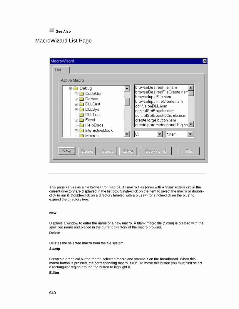
940

See Also

MacroWizard List Page

This page serves as a file browser for macros. All macro files (ones with a "nsm" extension) in the current directory are displayed in the list box. Single-click on the item to select the macro or double-click to run it. Double-click on a directory labeled with a plus (+) (or single-click on the plus) to expand the directory tree.

New

Displays a window to enter the name of a new macro. A blank macro file (*.nsm) is created with the specified name and placed in the current directory of the macro browser. Delete

Deletes the selected macro from the file system. Stamp

Creates a graphical button for the selected macro and stamps it on the breadboard. When this macro button is pressed, the corresponding macro is run. To move this button you must first select a rectangular region around the button to highlight it. Editor

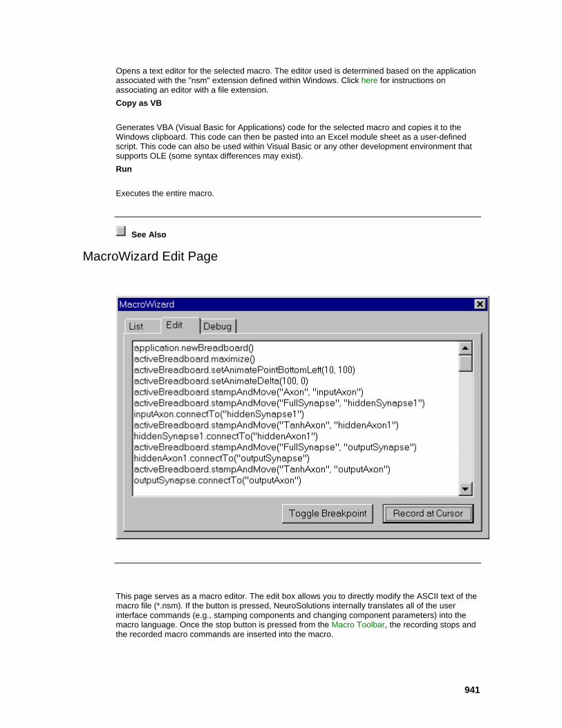
941

Opens a text editor for the selected macro. The editor used is determined based on the application associated with the "nsm" extension defined within Windows. Click here for instructions on associating an editor with a file extension. Copy as VB

Generates VBA (Visual Basic for Applications) code for the selected macro and copies it to the Windows clipboard. This code can then be pasted into an Excel module sheet as a user-defined script. This code can also be used within Visual Basic or any other development environment that supports OLE (some syntax differences may exist). Run

Executes the entire macro.

See Also

MacroWizard Edit Page

This page serves as a macro editor. The edit box allows you to directly modify the ASCII text of the macro file (*.nsm). If the button is pressed, NeuroSolutions internally translates all of the user interface commands (e.g., stamping components and changing component parameters) into the macro language. Once the stop button is pressed from the Macro Toolbar, the recording stops and the recorded macro commands are inserted into the macro.

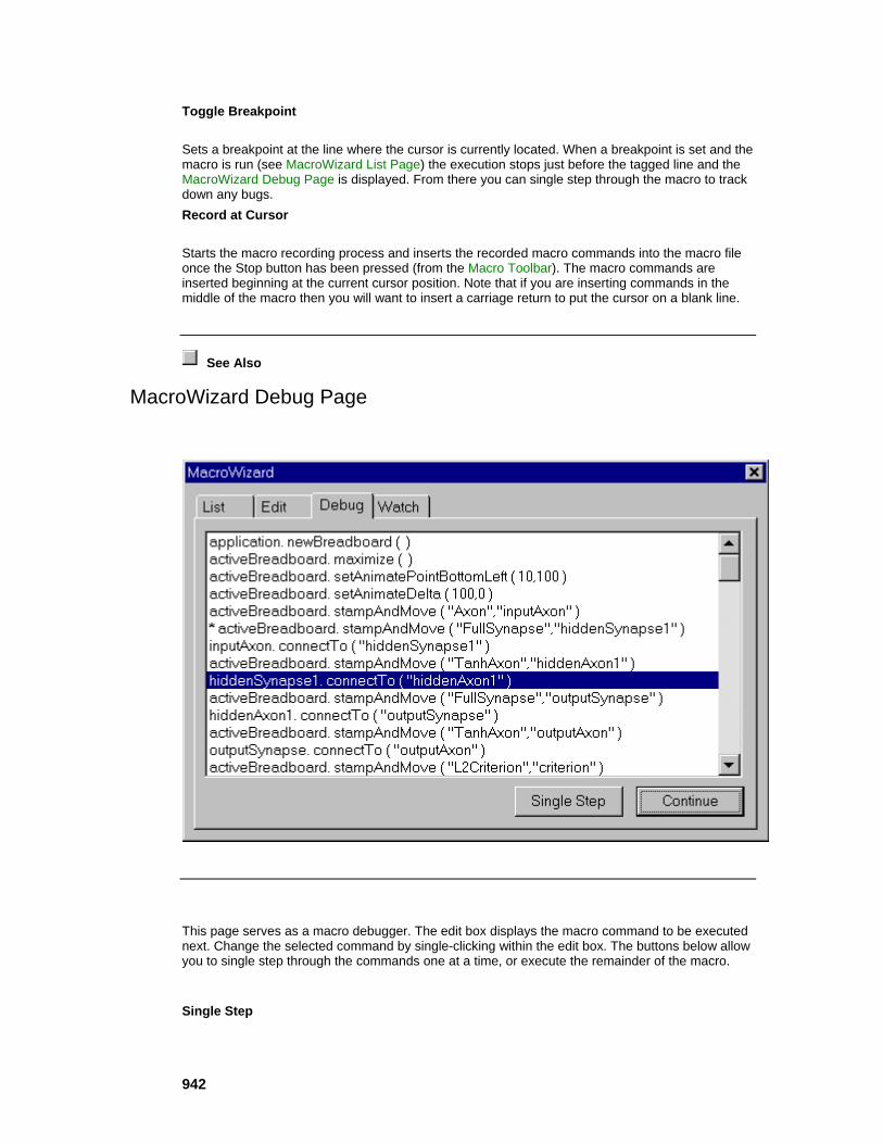
942

Toggle Breakpoint

Sets a breakpoint at the line where the cursor is currently located. When a breakpoint is set and the macro is run (see MacroWizard List Page) the execution stops just before the tagged line and the MacroWizard Debug Page is displayed. From there you can single step through the macro to track down any bugs. Record at Cursor

Starts the macro recording process and inserts the recorded macro commands into the macro file once the Stop button has been pressed (from the Macro Toolbar). The macro commands are inserted beginning at the current cursor position. Note that if you are inserting commands in the middle of the macro then you will want to insert a carriage return to put the cursor on a blank line.

See Also

MacroWizard Debug Page

This page serves as a macro debugger. The edit box displays the macro command to be executed next. Change the selected command by single-clicking within the edit box. The buttons below allow you to single step through the commands one at a time, or execute the remainder of the macro.

Single Step

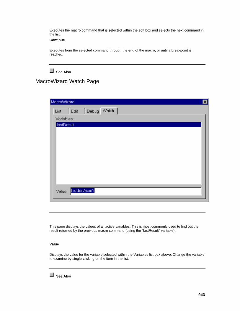
943

Executes the macro command that is selected within the edit box and selects the next command in the list. Continue

Executes from the selected command through the end of the macro, or until a breakpoint is reached.

See Also

MacroWizard Watch Page

This page displays the values of all active variables. This is most commonly used to find out the result returned by the previous macro command (using the "lastResult" variable).

Value

Displays the value for the variable selected within the Variables list box above. Change the variable to examine by single-clicking on the item in the list.

See Also

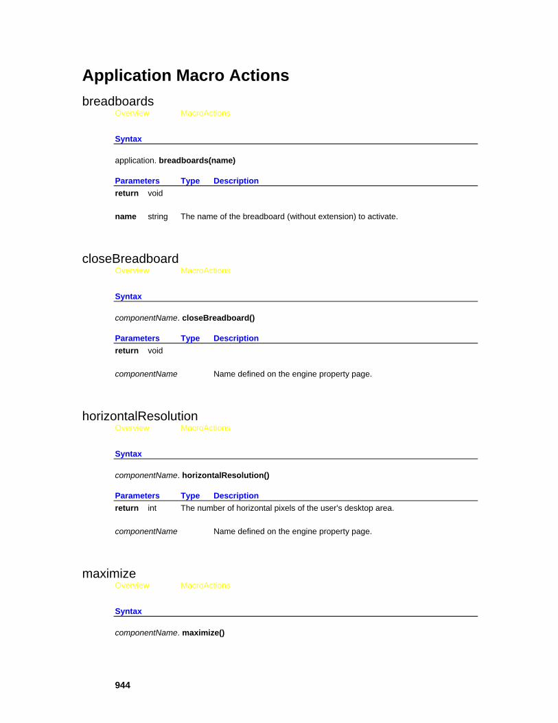
944

Application Macro Actions breadboards

Overview MacroActions

Syntax

application. breadboards(name)

Parameters Type Description return void name string The name of the breadboard (without extension) to activate.

closeBreadboard Overview MacroActions

Syntax

componentName. closeBreadboard()


horizontalResolution Overview MacroActions

Syntax

componentName. horizontalResolution()

Parameters Type Description return int The number of horizontal pixels of the user's desktop area. componentName Name defined on the engine property page.

maximize Overview MacroActions

Syntax

componentName. maximize()

945


minimize Overview MacroActions

Syntax

application. minimize()


moveWindow Overview MacroActions

Syntax

application. moveWindow(x, y)

Parameters Type Description return void x int The new x-coordinate for the upper-left corner of the NeuroSolutions window.

y int The new y-coordinate for the upper-left corner of the NeuroSolutions window.

newBreadboard Overview MacroActions

Syntax

application. newBreadboard()


openBreadboard Overview MacroActions

Syntax

946

application. openBreadboard(path)

Parameters Type Description return void path string The full path of the breadboard file to open.

pathFromActiveBreadboard Overview MacroActions

Syntax

application. pathFromActiveBreadboard(relativePath)

Parameters Type Description return string The full path of the file. relativePath string The file path relative to the active breadboard.

pathFromMacro Overview MacroActions

Syntax

application. pathFromMacro(relativePath)

Parameters Type Description return string The full path of the file. relativePath string The file path relative to the currently running macro.

pathFromNS Overview MacroActions

Syntax

application. pathFromNS(relativePath)

Parameters Type Description return string The full path of the file. relativePath string The file path relative to the NeuroSolutions executable.

pathFromWizard Overview MacroActions

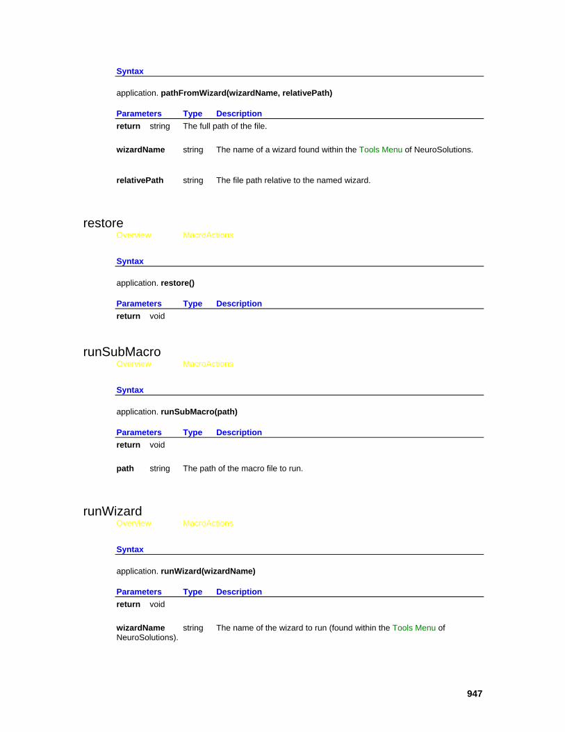
947

Syntax

application. pathFromWizard(wizardName, relativePath)

Parameters Type Description return string The full path of the file. wizardName string The name of a wizard found within the Tools Menu of NeuroSolutions.

relativePath string The file path relative to the named wizard.

restore Overview MacroActions

Syntax

application. restore()


runSubMacro Overview MacroActions

Syntax

application. runSubMacro(path)

Parameters Type Description return void path string The path of the macro file to run.

runWizard Overview MacroActions

Syntax

application. runWizard(wizardName)

Parameters Type Description return void wizardName string The name of the wizard to run (found within the Tools Menu of NeuroSolutions).

948

setUserParameter Overview MacroActions

Syntax

application. setUserParameter(index, aString)

Parameters Type Description return void index int The index of the parameter array (0 <= index <= 9).

aString string The user-defined parameter.

sizeWindow Overview MacroActions

Syntax

application. sizeWindow(cx, cy)


cx int The new width of the NeuroSolutions window.

cy int The new height of the NeuroSolutions window.

sleep Overview MacroActions

Syntax

application. sleep(time)

Parameters Type Description return void time int The number of milliseconds to halt the processing for.

verticalResolution Overview MacroActions

Syntax

949

application. verticalResolution()

Parameters Type Description return int The number of vertical pixels of the user's desktop area.

strcat Overview MacroActions

Syntax

application. strcat(str1, str2)

Parameters Type Description return string The concatenation of str1 and str2. str1 string The left half of the concatenated string.

str2 string The right half of the concatenated string.

displayInspector Overview MacroActions

Syntax

application. displayInspector(show)

Parameters Type Description return void show BOOL TRUE to show the inspector window and FALSE to hide it.

openApplicationDocument Overview MacroActions

Syntax

application. openApplicationDocument(path)

Parameters Type Description return void path string Full path of the document file to open.

950

closeApplication Overview MacroActions

Syntax

application. closeApplication()


activateBreadboard Overview MacroActions

Syntax

application. activateBreadboard(name)

Parameters Type Description return void name string The name of the breadboard (with extension) to activate.

runExecutable Overview MacroActions

Syntax

application. runExecutable(path)

Parameters Type Description return voie path string The full path of the executable file to run.

openDefaultEditorWithFile Overview MacroActions

Syntax

application. openDefaultEditorWithFile(path)

Parameters Type Description return void path string Full path of the document file to open.

951

Active Breadboard Macro Actions alignBottom

Overview Macro Actions

Syntax

activeBreadboard. alignBottom()


alignLeft Overview Macro Actions

Syntax

activeBreadboard. alignLeft()


alignRight Overview Macro Actions

Syntax

activeBreadboard. alignRight()


alignTop Overview Macro Actions

Syntax

activeBreadboard. alignTop()


animatePointX Overview Macro Actions

952

Syntax

activeBreadboard. animatePointX()

Parameters Type Description return int The x-coordinate of the animate point (the location of the next stamped component).

animatePointY Overview Macro Actions

Syntax

activeBreadboard. animatePointY()

Parameters Type Description return int The y-coordinate of the animate point (the location of the next stamped component).

centerHorizontal Overview Macro Actions

Syntax

activeBreadboard. centerHorizontal()


centerObjects Overview Macro Actions

Syntax

activeBreadboard. centerObjects()


centerVertical Overview Macro Actions

Syntax

activeBreadboard. centerVertical()

953


copySelection Overview Macro Actions

Syntax

activeBreadboard. copySelection()


copyToFile Overview Macro Actions

Syntax

activeBreadboard. copyToFile(path)


path string The path of the clipboard file (*.nsc) to copy the currently selected components to (see "Copy to File" within the Edit Menu and Toolbar Commands page).

cutSelection Overview Macro Actions

Syntax

activeBreadboard. cutSelection()


deleteObject Overview Macro Actions

Syntax

activeBreadboard. deleteObject()


954

deleteSelection Overview Macro Actions

Syntax

activeBreadboard. deleteSelection()


distributeHorizontal Overview Macro Actions

Syntax

activeBreadboard. distributeHorizontal()


distributeVertical Overview Macro Actions

Syntax

activeBreadboard. distributeVertical()


isModified Overview Macro Actions

Syntax

activeBreadboard. isModified()

Parameters Type Description return BOOL TRUE if the breadboard has been modified since it was last saved.

lockWindowUpdate Overview Macro Actions

955

Syntax

activeBreadboard. lockWindowUpdate()

Parameters Type Description return void Returns TRUE if the statement executed successfully.

maximize Overview Macro Actions

Syntax

activeBreadboard. maximize()


minimize Overview Macro Actions

Syntax

activeBreadboard. minimize()


moveAnimatePointBy Overview Macro Actions

Syntax

activeBreadboard. moveAnimatePointBy(x, y)

Parameters Type Description return void x int The horizontal offset to move the animate point by. y int The vertical offset to move the animate point by.

moveSelectionBy Overview Macro Actions

Syntax

956

activeBreadboard. moveSelectionBy(x, y)


x int The horizontal offset to move the selected components by. y int The vertical offset to move the selected components by.

moveToBack Overview Macro Actions

Syntax

activeBreadboard. moveToBack()


moveToFront Overview Macro Actions

Syntax

activeBreadboard. moveToFront()


onBreadboard Overview Macro Actions

Syntax

activeBreadboard. onBreadboard(name)

Parameters Type Description return BOOL TRUE if the named component is on the breadboard. name string The component name.

pasteFromFile Overview Macro Actions

957

Syntax

activeBreadboard. pasteFromFile(path)

Parameters Type Description return void path string The Clipboard file (*.nsc) path that contains the components to paste (see "Paste from File" within the Edit Menu and Toolbar Commands page).

pasteToSelection Overview Macro Actions

Syntax

activeBreadboard. pasteToSelection()


pathName Overview Macro Actions

Syntax

activeBreadboard. pathName()

Parameters Type Description return string The full path of the breadboard file.

replaceWith Overview Macro Actions

Syntax

activeBreadboard. replaceWith(name, class)

Parameters Type Description return void name string The name of the component to replace.

class string The class of the new component.

958

restore Overview Macro Actions

Syntax

activeBreadboard. restore()


runMacro Overview Macro Actions

Syntax

activeBreadboard. runMacro(path)

Parameters Type Description return void path string The full path of the macro file to run.

save Overview Macro Actions

Syntax

activeBreadboard. save()


saveAs Overview Macro Actions

Syntax

activeBreadboard. saveAs(path)

Parameters Type Description return void path string The full path of the breadboard file.

select Overview Macro Actions

959

Syntax

activeBreadboard. select(name, keep)

Parameters Type Description return void name string The name of the component to select. keep BOOL TRUE to add the component to the previous selection and FALSE to make the component the only selection.

selectKind Overview Macro Actions

Syntax

activeBreadboard. selectKind(class, keep)

Parameters Type Description return void class string The class name of the components to select. keep BOOL TRUE to add the component to the previous selection and FALSE to make the component the only selection.

selectMembers Overview Macro Actions

Syntax

activeBreadboard. selectMembers(class, keep)

Parameters Type Description return void class string The class name of the components to select. keep BOOL TRUE to add the component to the previous selection and FALSE to make the component the only selection.

selectRespondingTo Overview Macro Actions

Syntax

activeBreadboard. selectRespondingTo(forYes, action, keep)


960

return void forYes BOOL TRUE to select only those components that return a non-null value from the function. action string The name of the function. keep BOOL TRUE to add the component to the previous selection and FALSE to make the component the only selection.

sendDataToEngine Overview Macro Actions

Syntax

activeBreadboard. sendDataToEngine(data, component)

Parameters Type Description return void data variant Data to pass to the setEngineData function (see the reference pages for the OLEInput, Soma, and the GaussianAxon). component string The name of the component to pass the data to.

setAnimatePoint Overview Macro Actions

Syntax

activeBreadboard. setAnimatePoint(x, y)

Parameters Type Description return void x int The horizontal location of the animate point (the location of the next stamped component). y int The vertical location of the animate point (the location of the next stamped component).

setAnimatePointBottomLeft Overview Macro Actions

Syntax

activeBreadboard. setAnimatePointBottomLeft(x, y)


961

return void x int The horizontal location of the animate point (the location of the next stamped component). y int The vertical location of the animate point (the location of the next stamped component) relative to the bottom of the breadboard window.

setPromptToSaveModifications Overview Macro Actions

Syntax

activeBreadboard. setPromptToSaveModifications(aBool)

Parameters Type Description return void aBool BOOL TRUE if the user is to be prompted to save the breadboard modifications when closing the document.

showOpenProbes Overview Macro Actions

Syntax

activeBreadboard. showOpenProbes(aBool)

Parameters Type Description return voie aBool BOOL TRUE to display the windows of all probes on the breadboard, and FALSE to hide them.

sizeWindow Overview Macro Actions

Syntax

activeBreadboard. sizeWindow(cx, cy)

Parameters Type Description return void cx int The new width of the breadboard window. cy int The new height of the breadboard window.

962

stampAndMove Overview Macro Actions

Syntax

activeBreadboard. stampAndMove(class, name)

Parameters Type Description return void class string The class of the new component to be created. name string The name of the new component.

stampOnAndMove Overview Macro Actions

Syntax

activeBreadboard. stampOnAndMove(class, name)

Parameters Type Description return void class string The class of the new component to be created. name string The name of the component to stamp the new component on top of.

stampOnMoveAndName Overview Macro Actions

Syntax

activeBreadboard. stampOnMoveAndName(class, onName, newName)

Parameters Type Description return void class string The class of the new component to be created. onName string The name of the component to stamp the new component on top of. newName string The name of the new component.

title Overview Macro Actions

963

Syntax

activeBreadboard. title()

Parameters Type Description return string The breadboard's title (the string displayed in the title bar of a frame window).

unlockWindowUpdate Overview Macro Actions

Syntax

activeBreadboard. unlockWindowUpdate()


unselect Overview Macro Actions

Syntax

activeBreadboard. unselect(name)

Parameters Type Description return void name string The name of the component to remove from the selection group.

stampOnAndMoveAtAccessPoint Overview Macro Actions

Syntax

activeBreadboard. stampOnAndMoveAtAccessPoint(class, name, access)

Parameters Type Description return void class string The class of the new component to be created. name string The name of the component to stamp the new component on top of. access string The name of the access point to attach the new component to.

setTitle Overview Macro Actions

964

Syntax

activeBreadboard. setTitle(title)

Parameters Type Description return void title string The new title of the breadboard window.

setPathName Overview Macro Actions

Syntax

c activeBreadboard. setPathName(pathName)

Parameters Type Description return void pathName string The new pathname of the breadboard file.

setEditModeEnabledForTextAndButtons Overview Macro Actions

Syntax

activeBreadboard. setEditModeEnabledForTextAndButtons(bool)

Parameters Type Description return void bool BOOL TRUE to allow the user to change the text of the TextBoxEngine and ButtonEngine components.

promptToSaveModifications Overview Macro Actions

Syntax

activeBreadboard. promptToSaveModifications()

Parameters Type Description return BOOL TRUE if the user is to be prompted to save changes when closing the breadboard.

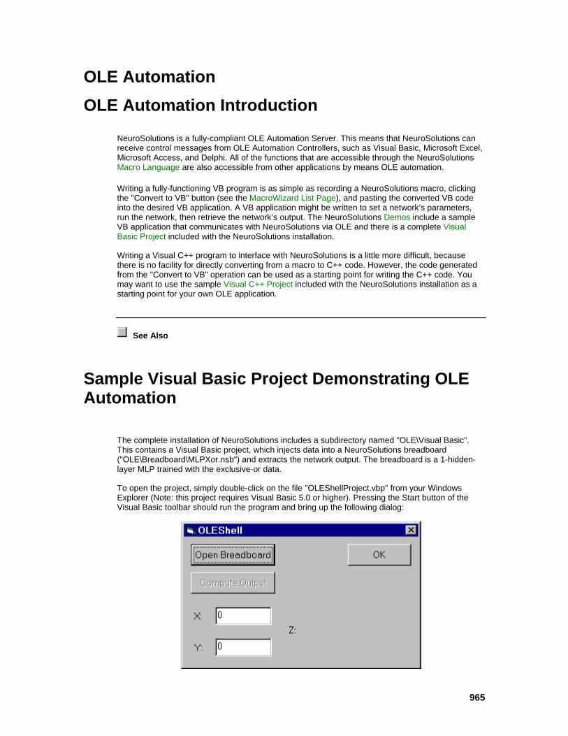
965

OLE Automation OLE Automation Introduction

NeuroSolutions is a fully-compliant OLE Automation Server. This means that NeuroSolutions can receive control messages from OLE Automation Controllers, such as Visual Basic, Microsoft Excel, Microsoft Access, and Delphi. All of the functions that are accessible through the NeuroSolutions Macro Language are also accessible from other applications by means OLE automation.

Writing a fully-functioning VB program is as simple as recording a NeuroSolutions macro, clicking the "Convert to VB" button (see the MacroWizard List Page), and pasting the converted VB code into the desired VB application. A VB application might be written to set a network’s parameters, run the network, then retrieve the network’s output. The NeuroSolutions Demos include a sample VB application that communicates with NeuroSolutions via OLE and there is a complete Visual Basic Project included with the NeuroSolutions installation.

Writing a Visual C++ program to interface with NeuroSolutions is a little more difficult, because there is no facility for directly converting from a macro to C++ code. However, the code generated from the "Convert to VB" operation can be used as a starting point for writing the C++ code. You may want to use the sample Visual C++ Project included with the NeuroSolutions installation as a starting point for your own OLE application.

See Also

Sample Visual Basic Project Demonstrating OLE Automation

The complete installation of NeuroSolutions includes a subdirectory named "OLE\Visual Basic". This contains a Visual Basic project, which injects data into a NeuroSolutions breadboard ("OLE\Breadboard\MLPXor.nsb") and extracts the network output. The breadboard is a 1-hidden-layer MLP trained with the exclusive-or data.

To open the project, simply double-click on the file "OLEShellProject.vbp" from your Windows Explorer (Note: this project requires Visual Basic 5.0 or higher). Pressing the Start button of the Visual Basic toolbar should run the program and bring up the following dialog:

966

Click the "Open Breadboard" button, enter two values between –1 and 1, then click the "Compute Output" button. Notice that the network output displayed on the NeuroSolutions probe is copied to the dialog box.

The code is pretty self-explanatory, however there are a few points worth mentioning:

The "NSApp" variable is the NeuroSolutions Application object.

The "NSBB" variable is the Active Breadboard object.

The sendDataToEngine function is what is used to inject the X and Y values into the network.

The getProbeData function is what is used to extract the Z value from the network.

See Also

Sample Visual C++ Project Demonstrating OLE Automation

The complete installation of NeuroSolutions includes a subdirectory named "OLE\VC++". This contains a Visual C++ project, which injects data into a NeuroSolutions breadboard ("OLE\Breadboard\MLPXor.nsb") and extracts the network output. The breadboard is a 1-hidden-layer MLP trained with the exclusive-or data.

To open the project simply double-click on the file " OLEShell.dsw" from your Windows Explorer (Note: this project requires Visual C++ 5.0 or higher). Press F7 to build the project, then press F5 to run the program, which should bring up the following dialog:

Click the "Open Breadboard" button, enter two values between –1 and 1, then click the "Compute Output" button. Notice that the network output displayed on the NeuroSolutions probe is copied to the dialog box.

The code is pretty self-explanatory, however there are a few points worth mentioning:

967

The " m_nsApp" variable is the NeuroSolutions Application object.

The " m_nsObject" variable is the Active Breadboard object.

The sendDataToEngine function is what is used to inject the X and Y values into the network.

The getProbeData function is what is used to extract the Z value from the network.

See Also

References References

Almeida L. "A learning rule in perceptrons with feedback in a combinatorial environment." 1st IEEE Int. Conf. Neural Networks 2, 609-618, 1987.

Amari S. "Characteristics of random nets of analog neuron-like elements." IEEE Trans. Syst. Man Cybern. SMC-2,5, 643-657, 1972.

Anderson J. and Rosenfeld E. NeuroComputing: Foundations for Research. MIT Press, (vol I, 1988), (vol II, 1990).

Anderson J. "The BSB model: a simple nonlinear autoassociative neural network." In Associative Neural Memories, (ed. Hassoun). Oxford Press, pp77-103, 1993.

Arbib M. Brains, Machines and Mathematics. Springer Verlag, 1987.

Baldi P. "Gradient descent learning algorithms: a general overview." (submitted to IEEE Trans. Neural Networks, 1992).

Braitenberg V. "Functional interpretation of cerebellar histology." Nature 190, 539-540, 1961.

Birkhoff G. Lattice Theory. American Mathematical Society, 1967.

Bryson A. and Ho Y. Applied Optimal Control, Optimization, Estimation and Control. Hemispheric publishing Co., New York, 1975.

Caianiello E. "Outline of a theory of thought-processes and thinking machines." Journal of Theoretical Biology 2, 204-235, 1961.

Carpenter G. and Grossberg S. Pattern Recognition by Self-organizing Neural Networks. MIT Press, 1991.

Cox R. Object Oriented Programming. Addison Wesley, 1987.

Churchland P. Neurophilosophy: Towards a Unified Science of the Mind/Brain. MIT Press, 1986.

DARPA Neural Network Study. AFCEA, 1988.

deVries B. and Principe J. "The gamma model - A new neural model for temporal processing." Neural Networks 5(4), 565-576, 1992.

Eccles J., Ito M. and Szentagothai J. The Cerebellum as a Neuronal Machine. Springer Verlag, 1967.

Elman J. "Finding structure in time." Cognitive science 14, 179-211, 1990.

968

Freeman W. Mass Activation in the Nervous System. Academic Press, 1975.

Freeman J. and Sakura D. Neural Networks: Algorithms, Applications, and Programming Techniques. Addison-Wesley, 1991.

Fukushima K. "Neocognitron: a self-organizing neural network model for a mechanism of pattern recognition unaffected by shift in position." Biological Cybernetics 36, 193-202, 1980.

Grossberg S. Studies of Mind and Brain. Dordrecht, Holland, 1982.

Grossberg S. and Cohen M. "Absolute stability of global pattern formation and parallel memory storage by competitive neural networks." IEEE Trans. on Syst. Man Cybern. SMC-13, 815-826, 1983.

Haykin S. Adaptive Filter Theory. Prentice-Hall, Englewood Cliffs, 1991.

Haykin S. Neural Networks, a Comprehensive Foundation. MacMillan, 1994.

Hebb D. The Organization of Behavior. Wiley, New York, 1949.

Hecht-Nielsen R. NeuroComputing. Addison Wesley, 1990.

Hertz J., Krogh A. and Palmer R. Introduction to the Theory of Neural Networks. Addison Wesley, 1991.

Hopfield J. "Neural networks and physical systems with emergent collective computational abilities." Proc. Natl. Acad. Sci. (USA) 79, 2554-2558, 1982.

Jacobs R. "Increased rates of convergence through learning rate adaptation." Neural Networks 1, 295-307, 1988.

Jordan M. "Attractor dynamics and parallelism in a connectionist sequential machine." Proc. 8th Annual Conf. on Cognition Science Society, pp 531-546, 1986.

Kohonen T. Self Organization and Associative Memory. Springer Verlag, 1988.

Kohonen T. "The self-organizing map." Proc. IEEE 78, 1464-1480, 1990.

Kosko B. Neural Networks and Fuzzy Systems. Prentice Hall, 1992.

Kung S.Y. Digital Neural Networks. Prentice Hall, 1993.

Lang K., Waibel A. and Hinton G. "A time delay neural network architecture for isolated word recognition." Neural Networks 3(1), 23-44, 1990.

Lapedes A. and Farber R. "Nonlinear signal processing using neural networks: prediction, and system modelling." LA-VR-87-2662, Los Alamos, 1987.

LeCun Y., Denker J., Henderson D., Howard R., Hubbard W. and Jackel L. "Handwritten digit recognition with a backpropagation network." In Advances in Neural Information Processing Systems 2, (ed. Touretsky), pp 396-404, 1990.

Lefebvre C. and Principe J. "Object-oriented artificial neural network implementations." World Cong. Neural Networks 4, 436-439, 1993.

Lefebvre C. An Object-Oriented Methodology for the Analysis of Artificial Neural Networks. Masters Thesis, University of Florida, 1992.

Lippman R. "An introduction to computing with neural nets." IEEE Trans. ASSP Magazine 4, 4-22, 1987.

Little W. and Shaw G. "Analytical study of the memory storage capacity of a neural network." Mathematical Biosciences 39, 281-290, 1978.

969

Makhoul J. "Pattern recognition properties of neural networks." Proc. 1991 IEEE Workshop on Neural Networks for Signal Processing, pp 173-187, 1992.

Marr D. "A theory of cerebellar cortex." Journal of Physiology 202, 437-470, 1969.

McCulloch W. and Pitts W. "A logical calculus of the ideas imminent in the nervous activity." Bulletin of Mathematical Biophysics 5, 115-133, 1943.

Minsky M. and Papert S. Perceptrons. MIT Press, 1969.

NeXTStep Operating System, NeXT Computer Documentation, 1991.

Oja E. "A simplified neuron modeled as a principal component analyzer." J. of mathematical biology 15, 267- 273, 1982.

Palm G. "On associative memory." Biological Cybernetics 36, 19-31, 1980.

Pineda F. "Generalization of backpropagation to recurrent neural networks." Physical Rev. Let. 59, 2229-2232, 1987.

Pellionisz A. and Llinas R. "Brain modeling by tensor network theory and computer simulation." NeuroScience 4, 323-348, 1979.

Principe J., deVries B., Kuo J. and Oliveira P. " Modeling applications with the focused gamma network." In Neural Information Processing Systems 4, (eds. Moody, Hanson, Touretsky), pp121-126, Morgan Kaufmann, 1992.

Ramon y Cajal S. Histologie du systeme nerveux de l’homme et des vertebres. Tome I and II, Paris, 1911.

Rosenblatt F. "The perceptron: a probabilistic model for information storage and organization in the brain." Physiological Review 65, 386-408, 1958.

Rumelhart D. and McClelland J. (eds.) Parallel Distributed Processing. vol I, II, MIT Press, 1987.

Rumelhart D., Hinton G. and Williams R. "Learning internal representations by error propagation." In Parallel Distributed Processing, (eds. Rumelhart and McClelland), MIT Press, 1986.

Sanchez-Sinencio E. and Lau C. Artificial Neural Networks. IEEE Press, 1992.

Sanger T. "Optimal unsupervised learning in a single layer linear feedforward network." Neural Networks 12, 459-473, 1989.

Sejnowski T., Koch C. and Churchland P. "Computational Neuroscience." Science 241, 1299-1306, 1988.

Shaw G. and Palm G. (eds.) Brain Theory. World Scientific, 1988.

Sherrington C. The Integrative Action of the Nervous System. Yale Press, 1906.

Simpson P. Artificial Neural Systems. Pergamon Press, 1990.

Silva F., Almeida L. "Speeding up backpropagation." In Advanced Neural Computers, (ed. Eckmiller), pp 151-160.

Steinbuch K. "Die Lernmatrix." Kybernetik 1, 36-45, 1961.

Sutton R. "Learning to predict by the methods of temporal differences." Machine Learning 3, 9-44, 1988.

Thrun S. and Smieja F. "A general feedforward algorithm for gradient descent learning in connectionist networks." Int. Rep. German National Res. Center Comp. Sci., 1991.

970

Von der Marlsburg C. "Network self-organization." In Introduction to Neural and Electronic Computing, (eds. Zornetzer, Davis, Lau), pp 421-432, Academic Press, 1990.

Von Neumann J. The Computer and the Brain. Yale Press, 1958.

Weigend A., Rumelhart D. and Huberman B. "Generalization by weight elimination with applications to forecasting." In Advances in Neural Information Processing Systems 3, (eds. Lippman, Moody, Touretsky), pp 875-882, 1991.

Werbos P. "Backpropagation through time: what it does and how to do it." Proc. IEEE 78(10), 1990.

Wiener N. Cybernetics. Wiley, 1961.

Widrow B. and Hoff M. Adaptive Switching Circuits. IRE Wescon Rept. 4, 1960.

Widrow B. and Lehr M. "30 years of adaptive neural networks: perceptron, madaline and backpropagation." Proc. IEEE 78, 1415-1442, 1990.

Widrow B. and Stearns S. Adaptive Signal Processing. Prentice-Hall, 1985.

Williams R. and Zipser D. "A learning algorithm for continually running fully recurrent neural networks." Neural Computation 1, 270-280, 1989.

Willshaw D. "Holography, associative memory and inductive generalization." In Parallel Models of Associative Memory, (eds. Hinton, Anderson). pp83-104, Lawrence Erlbaum, 1981.

Zurada J. Artificial Neural Systems. West, 1992

971

Index

3 3DProbe.................................................................................................................. 642, 663 Macro Actions......................................................... 664, 665, 666, 667, 668, 669, 670, 671

A About .......................................................................................................................... 32, 70 Absolute value ................................................................................................................ 707 absoluteValue................................................................................................................. 708 Access ........................................................................ 98, 99, 523, 524, 560, 563, 568, 569 Macro Actions................................................................................. 572, 573, 574, 575, 576 Access Points .287, 365, 393, 428, 489, 510, 559, 601, 637, 685, 703, 721, 729, 735, 736 accessDataSet ............................................................................................................... 572 accessedComponent...................................................................................................... 573 accessRows.................................................................................................................... 628 Accumulate ................................................................................................................... 567 Acknowledgments ............................................................................................................ 32 Action.............................................................................................................................. 714 Activate............................................................................................................................ 72 activateBreadboard ........................................................................................................ 950 activateDLL..................................................................................................................... 747 Activation ........................................................................................................ 123, 124, 864 Activation Code .......................................................................................................... 71, 72 ActivationControl ............................................................................................................ 141 Active Breadboard Macro Actions .................................................................................. 935 Active Neuron ....................................................................................................... 609, 610 activeAccessPoint .......................................................................................................... 573 activeBreadboard ........................................................................................................... 935 ActiveBreadboard Macro Actions.................951, 952, 953, 954, 955, 956, 957, 958, 959, 960, 961, 962, 963 activeChannel ......................................................................................................... 582, 659 activeDataSet ......................................................................................................... 467, 541 activeFileName............................................................................................................... 542 activeFilePath ................................................................................................................. 542 activeNeuron................................................................................................................... 629 activeTranslatorName .................................................................................................... 542 Adaptive.......................................................................................................................... 188 Add................................................................................................. 439, 441, 442, 536, 706 addFile ............................................................................................................................ 542 Additive.................................................................................................................. 514, 515 Adjustment.............................................................................................................. 706, 707 AIC.................................................................................................................................. 110 alignBottom..................................................................................................................... 951 alignLeft .......................................................................................................................... 951 Alignment.......................................................................................................................... 58 alignRight........................................................................................................................ 951 alignTop.......................................................................................................................... 951 allocateBackpropPlane................................................................................................... 455 amplitude ........................................................................................................ 577, 647, 665 Amplitude ...................................................................................................................... 568

972

Amplitude FormCell ..................................................................................................... 564 amplitudeForChannel ..................................................................................................... 582 animatePointX ................................................................................................................ 951 animatePointY ................................................................................................................ 952 Application Macro Actions................................................................................. 938, 944, 945, 947, 948 ArbitrarySynapse ............................................................................................ 359, 368, 431 Macro Actions......................................................................................... 374, 375, 376, 377 Arrange ............................................................................................................................ 59 Arrow .............................................................................................................................. 758 ArrowEngine ........................................................................................................... 758, 776 ART................................................................................................................................. 188 Artificial ................................................................................................................... 154, 155 ASCII .............................................................................. 529, 530, 532, 533, 534, 569, 606 assignCenters................................................................................................................. 312 assignVariance ............................................................................................................... 312 Associate ........................................................................................................ 111, 537, 570 associateActiveFile......................................................................................................... 543 Associative Memory ....................................................................................................... 183 Associator ....................................................................................................................... 218 Example.......................................................................................................................... 218 Attach............................................................................................................................. 604 Auto ........................................................................................................ 444, 638, 640, 687 Auto Increment ............................................................................................................. 432 autoconnect .................................................................................................................... 375 autoIncrement................................................................................................................. 467 autoNormalize ................................................................................................................ 676 autoSave......................................................................................................................... 499 autoscale ........................................................................................................................ 666 autoscaleChannel........................................................................................................... 647 autoSetUpChannels ....................................................................................... 648, 654, 660 autosize .......................................................................................................................... 766 Autosize......................................................................................................................... 763 autosizing........................................................................................................................ 629 Autosizing ..................................................................................................................... 610 autoWindow.................................................................................................................... 573 Average Cost................................................................................................................. 495 averageOverUpdates ..................................................................................................... 499 Axon................125, 126, 273, 274, 287, 288, 297, 308, 309, 316, 317, 324, 819, 821, 865 Macro Actions......................................................................................... 308, 309, 310, 311 Axon Example ................................................................................................................ 297

B Back.................................................................................................................................. 57 BackArbitrarySynapse .................................................................................................... 418 BackAxon........................................................................................ 134, 135, 383, 393, 394 BackBellFuzzyAxon................................................................................................ 391, 398 BackBiasAxon ........................................................................................................ 384, 395 BackCombinerAxon........................................................................................................ 385 BackContextAxon ................................................................................................... 402, 410 BackCriteriaControl ........................................................................................................ 391 BackDynamicControl ...................................................................................... 426, 438, 439 Macro Action................................................................................................................... 453 Macro Actions................................................................................................................. 453 BackFullSynapse.................................................................................................... 419, 420 BackGammaAxon................................................................................................... 403, 410

973

BackGaussianFuzzyAxon....................................................................................... 393, 399 Background..................................................................................................................... 762 BackIntegratorAxon ................................................................................................ 405, 412 BackLaguarreAxon ................................................................................................. 404, 412 BackLinearAxon ............................................................................................. 386, 395, 401 Macro Actions......................................................................................................... 401, 402 BackMemoryAxon .......................................................................................................... 135 BackNormalizedAxon ..................................................................................................... 387 BackNormalizedSigmoidAxon ........................................................................................ 387 Backprop......................................................................................................... 132, 133, 422 Backpropagation............................................................................. 113, 114, 438, 439, 440 BackpropControl ............................................................................................................. 143 backpropOffset ............................................................................................................... 453 BackSigmoidAxon .................................................................................................. 388, 396 BackSigmoidContextAxon...................................................................................... 406, 414 BackSigmoidIntegratorAxon................................................................................... 407, 414 BackStaticControl ................................................................................... 424, 429, 441, 442 Macro Actions......................................................... 453, 455, 456, 457, 458, 459, 460, 461 BackStaticControl Macro Actions ................................................................................... 453 BackSynapse.......................................................................................... 137, 138, 420, 421 BackTanhAxon ....................................................................................................... 389, 397 BackTanhContextAxon........................................................................................... 407, 415 BackTanhIntegratorAxon........................................................................................ 408, 416 BackTDNNAxon ..................................................................................................... 409, 417 Bar Size.......................................................................................................................... 603 BarChart ......................................................................................................... 594, 603, 611 Macro Actions......................................................................................................... 615, 616 barSize............................................................................................................................ 615 baseEngineOnDocument ............................................................................................... 747 batch ............................................................................................................................... 455 Batch.............................................................................................................. 439, 441, 442 beginCustomizeOfActiveFile .......................................................................................... 543 Behind the Scenes of C++ Code Generation ................................................................. 797 Behind the Scenes of DLLs ............................................................................................ 807 BellFuzzyAxon........................................................................................................ 354, 357 Best......................................................................................................................... 432, 433 bestCost.......................................................................................................................... 499 beta................................................................................................. 314, 518, 698, 708, 725 Beta ................................................................................................ 324, 697, 705, 723, 734 Bias ................................................................................................................................ 324 Bias Axon Example ........................................................................................................ 298 BiasAxon................................................................................................. 274, 275, 289, 298 Binary...................................................................................................... 529, 534, 569, 606 binaryEncodingForSymbols............................................................................................ 543 Bitmap..................................................................................................................... 530, 609 bold ................................................................................................................................. 766 Bold................................................................................................................................ 763 Border ............................................................................................................................ 762 borderType ..................................................................................................................... 766 bottom............................................................................................................................. 748 Bottom .............................................................................................................................. 58 Breadboard............................................................................................. 53, 56, 59, 89, 817 Macro Actions................................................................................................................. 935 breadboards.................................................................................................................... 944 broadcast ................................................................................................................ 583, 660 broadcastBumpStep ....................................................................................................... 521

974

Browse........................................................................................................................... 764 Buffer ............................................................................................................................. 604 Buffer Size ............................................................................................................. 606, 607 bufferLength.................................................................................................................... 623 bufferSize........................................................................................................................ 617 bumpStep ....................................................................................................................... 521 Button ............................................................................................................................. 760 ButtonEngine .................................................................................................................. 760 Buttons........................................................................................................................ 65, 66

C Cabling........................................................................................................................ 97, 98 Cascade............................................................................................................................ 59 Center .............................................................................................................. 58, 318, 763 centerHorizontal ............................................................................................................. 952 centerObjects.................................................................................................................. 952 centerVertical.................................................................................................................. 952 Channel..........................................................564, 565, 566, 567, 638, 640, 641, 687, 688 channels ......................................................................................................................... 583 Character Recognition.................................................................................................... 262 Example.......................................................................................................................... 262 checkCostEvery.............................................................................................................. 499 Chromosome .................................................................................................................. 452 Classification................................................................................................... 106, 107, 108 className...................................................................................................................... 748 clear ................................................................................................................................ 617 Clear....................................................................................................................... 370, 605 clearBeforeRun............................................................................................................... 617 Click .................................................................................................................................. 92 Clipboard .......................................................................................................................... 60 Close .............................................................................................................................. 445 closeApplication.............................................................................................................. 950 closeBreadboard ............................................................................................................ 944 closeEngineWindow ....................................................................................................... 748 closeMacro ..................................................................................................................... 467 Code ............................................................................................................... 104, 443, 444 Code Generation ....................................442, 796, 797, 798, 799, 800, 801, 802, 803, 804 Code Generation Chapter .............................................................................................. 796 Purpose ......................................................................................................................... 796 codeGenProjectPath ...................................................................................................... 467 codeGenTargetPath ....................................................................................................... 468 codeNormalizesData ...................................................................................................... 573 Coefficients ............................................................................................................. 112, 113 Color ............................................................................................................... 688, 762, 763 cols ................................................................................................................................. 309 Cols................................................................................................................. 316, 351, 569 Column ................................................................................... 530, 531, 533, 534, 609, 610 Column headings............................................................................................................ 610 columnCountForActiveFile ............................................................................................. 544 columnTagForActiveFile................................................................................................. 544 CombinerAxon................................................................................................................ 275 CombinerSynapse .................................................................................................. 360, 370 Competitive............................................................................................. 146, 147, 722, 724 Competitive Learning...................................................................................................... 254 Example.......................................................................................................................... 254 CompetitiveFull

975

Macro Actions................................................................................................................. 724 Compile.................................................................................................................. 321, 443 compileSourceCode ....................................................................................................... 468 Component ..................................................................................................................... 121 Component Menu ............................................................................................................. 59 Components ............................................................................................. 54, 75, 91, 95, 96 Adding............................................................................................................................... 95 Manipulating ..................................................................................................................... 95 Replacing.......................................................................................................................... 96 Components Chapter ..................................................................................................... 272 Purpose ......................................................................................................................... 273 Concepts Chapter............................................................................................................. 87 Purpose ........................................................................................................................... 88 Confusion Matrix..................................................................................... 106, 107, 857, 858 Conjugate ....................................................................................................... 503, 504, 505 ConjugateGradient ......................................................................................................... 503 Connect ............................................................................................................................ 60 Connection ............................................................................................ 369, 370, 371, 372 Connectors ....................................................................................................................... 96 connectTo....................................................................................................................... 748 Conscience..................................................................................................................... 723 ConscienceFull ....................................................................................................... 720, 721 Macro Actions......................................................................................................... 725, 726 Constraint ....................................................................................................................... 167 Contact ............................................................................................................................. 33 Contents ........................................................................................................................... 70 ContextAxon ................................................................................................... 325, 333, 344 Context-sensitive .............................................................................................................. 69 ContractorSynapse................................................................................................. 360, 371 Contributions................................................................................................................... 777 to the theory of Neural Networks.................................................................................... 777 Control .............................................................................................................. 62, 434, 435 Controls ............................................................................................................ 60, 140, 428 ControlTransmitter.......................................................................................................... 701 Conventions.................................................................................................................... 121 Copy ........................................................................................................................... 57, 60 copySelection ................................................................................................................. 953 copyToFile ...................................................................................................................... 953 correlation....................................................................................................................... 109 Correlation .............................................................................................................. 107, 108 Cost........................................................................................................................ 429, 430 Cost Function ................................................................................................................. 162 costWeightingActive ....................................................................................................... 455 Criteria ............................................................................................................ 119, 171, 172 Criterion .......................................................................................................................... 792 Macro Actions......................................................................... 498, 499, 500, 501, 502, 503 Cross Validation ......................................................................................... 82, 83, 105, 434 Cube............................................................................................................................... 643 Current........................................................................................................................... 567 Cursor ............................................................................................................................... 57 custom ............................................................................................................................ 456 Custom .................................................................................................................. 439, 441 Custom Solution Wizard ................................................................................................... 61 Customize................................................................... 65, 66, 104, 532, 533, 534, 535, 537 customizeActiveFile........................................................................................................ 544 Cut .............................................................................................................................. 56, 59

976

cutSelection .................................................................................................................... 953 Cycle............................................................................................................................... 563

D Data ........................................................................................................................ 100, 101 Coding .............................................................................................................................. 81 Collection.......................................................................................................................... 81 Injection ............................................................................................................................ 81 Input/Output .................................................................................................................... 100 Preparation ..................................................................................................................... 111 Saving............................................................................................................................. 119 Data Flow....................................................................................................................... 317 Data Set.......................................................................................... 434, 528, 538, 569, 570 Data: ........................................................................................................... 80, 81, 111, 119 DataGraph .............................................................................................. 595, 604, 605, 611 dataLength...................................................................................................................... 676 dataSetCount.................................................................................................................. 545 dataSetForActiveFile ...................................................................................................... 545 dataSetNameAt .............................................................................................................. 545 dataSetUsedForNormalization ....................................................................................... 545 dataSource ..................................................................................................................... 583 DataStorage............................................................................................ 596, 597, 601, 607 Macro Actions......................................................................................................... 623, 624 DataStorageTransmitter ................................................................................................. 713 DataTransmitter .............................................................................................................. 713 dataWidth........................................................................................................................ 676 DataWriter....................................................................................................... 595, 606, 612 Macro Actions......................................................... 616, 617, 618, 619, 620, 621, 622, 623 Debug............................................................................................................. 321, 444, 942 debugSourceCode.......................................................................................................... 468 decrementChannel ......................................................................................................... 660 decrementNeuron........................................................................................................... 629 decrementXChannel....................................................................................................... 654 Default............................................................................................................................ 571 delay ............................................................................................................................... 378 Delay............................................................................................................... 351, 373, 374 delete .............................................................................................................................. 749 Delete ............................................................................................................................... 59 deleteObject.................................................................................................................... 953 deleteSelection ............................................................................................................... 954 Delta ............................................................................................................................... 642 DeltaBarDelta ................................................................................................. 494, 505, 515 Macro Actions................................................................................................. 517, 518, 519 DeltaTransmitter ............................................................................................................. 702 Demo .................................................................................................................... 43, 44, 45 Denormalize.................................................................................................... 112, 113, 674 denormalizeFromFile...................................................................................................... 677 Dialog................................................................................................ 93, 758, 759, 760, 761 DialogEngine .................................................................................................................. 758 DiamondKohonen................................................................................................... 727, 730 disconnectAll................................................................................................................... 375 Discriminant Function ............................................................................................. 835, 836 displacement................................................................................................................... 672 Displacement ................................................................................................................ 642 Display .................................................................................................... 431, 609, 674, 688 displayEvery ................................................................................................................... 677

977

displayInspector.............................................................................................................. 949 distance .......................................................................................................................... 666 distributeHorizontal......................................................................................................... 954 distributeVertical ............................................................................................................. 954 dither............................................................................................................................... 469 Division ................................................................................................................... 639, 640 DLL 104, 288, 289, 290, 291, 292, 293, 294, 295, 296, 321, 333, 335, 336, 337, 338, 339, 355, 357, 366, 367, 394, 395, 396, 397, 398, 399, 410, 411, 413, 414, 415, 416, 417, 420, 421, 491, 492, 493, 511, 512, 513, 532, 535, 560, 561, 562, 565, 602, 685, 695, 696, 703, 722, 730, 731, 732, 736, 738, 739, 800, 806, 807, 808, 809, 810, 811, 812, 813, 814, 815, 816, 817, 818, 864, 865, 866, 867, 868, 869, 870, 871 DLL Chapter ................................................................................................................... 805 Purpose ......................................................................................................................... 805 DLL Example .819, 821, 823, 825, 828, 829, 831, 833, 835, 842, 843, 844, 845, 846, 847, 848, 849, 850, 851, 852, 854, 856, 861, 862, 863 dllActive .......................................................................................................................... 749 DLLData.................................................................................................................. 810, 811 DLLInput ................................................................................................................. 526, 562 dllName........................................................................................................................... 749 dllPath............................................................................................................................. 750 DLLPostprocessor .......................................................................................... 562, 600, 601 DLLPreprocessor............................................................................................ 526, 559, 562 DLLScaling ..................................................................................................................... 839 Document ................................................................................................................... 56, 59 Dot.................................................................................................................................. 741 Dot Size.......................................................................................................................... 640 dotSize............................................................................................................................ 655 Down ...................................................................................................................... 516, 517 dualName ....................................................................................................................... 469 Dump.............................................................................................................................. 606 dumpFile ......................................................................................................................... 618 Duration ................................................................................................................. 532, 535 durationForActiveFile...................................................................................................... 546 Dynamic.................................................................................................. 177, 436, 437, 788 DynamicControl ................................................ 61, 425, 430, 431, 433, 435, 436, 437, 444 Macro Actions......................................................................................... 461, 462, 463, 464 Dynamics ........................................................................................................................ 120

E Edit.................................................................................... 56, 321, 444, 761, 763, 764, 941 EditEngine ...................................................................................................................... 761 Macro Actions.........................................764, 766, 767, 768, 769, 770, 771, 772, 773, 774 editModeEnabled............................................................................................................ 767 Editor .............................................................................................................................. 111 elapsedTimeInSeconds .................................................................................................. 469 enableLabels .................................................................................................................. 629 endChannel .................................................................................................................... 584 endCustomizeOfActiveFile ............................................................................................. 546 Engine..................................................................................................................... 273, 320 Macro Actions.........................745, 747, 748, 749, 750, 751, 752, 753, 754, 755, 756, 757 engineAtAccessPoint...................................................................................................... 750 Epoch...................................................................................................... 434, 435, 495, 697 epochCounter ................................................................................................................. 469 epochs ............................................................................................................................ 470 Epochs................................................................................................................... 431, 452 epochsPerTest ............................................................................................................... 470

978

Equation-based Modeling............................................................................................... 779 error ....................................................................................................................... 109, 110 Error................................................................................................................................ 792 ErrorCriteria .................................................................... 129, 130, 489, 490, 494, 495, 496 ErrorCriterion .......................................................................................................... 828, 866 Euclidean....................................................................................................................... 741 Evaluation................................................................................................................... 40, 41 Example.75, 76, 79, 80, 193, 204, 208, 218, 223, 230, 238, 248, 252, 254, 260, 262, 266, 270, 297, 298, 299, 300, 301, 302, 303, 304, 305, 306, 307, 308, 341, 342, 343, 344, 345, 346, 347, 348, 349, 350, 799, 801, 803, 804, 805, 808, 818, 839 Associator ....................................................................................................................... 218 Character Recognition............................................................................................ 262, 263 Combination of Data Sources......................................................................................... 204 Competitive Learning...................................................................................................... 254 Filtering ........................................................................................................................... 223 Frequency Doubler ......................................................................................................... 238 Pattern Recognition ........................................................................................................ 267 Perceptron and Multilayer Perceptron............................................................................ 208 Principal Component Analysis........................................................................................ 252 Recurrent ........................................................................................................................ 230 Self Organizing Feature Map.......................................................................................... 260 Signal Generator ............................................................................................................ 193 Unsupervised Learning................................................................................................... 248 executableFilePath ......................................................................................................... 470 Exemplar.........................................429, 430, 434, 435, 436, 437, 438, 440, 441, 442, 567 exemplarCounter ............................................................................................................ 470 exemplars ....................................................................................................................... 471 Exemplars.............................................................................................................. 431, 451 expandedColumnCountForActiveFile............................................................................. 546 ExpanderSynapse .................................................................................................. 361, 372 ExpScheduler ......................................................................................................... 693, 695 Extension........................................................................................................................ 111

F Family .....................................................128, 129, 141, 142, 143, 145, 273, 523, 758, 759 3DProbe.......................................................................................................................... 663 Activation ........................................................................................................................ 123 ActivationControl .................................................................................................... 141, 142 Axon................................................................................................................................ 125 BackAxon........................................................................................................................ 133 BackMemoryAxon .......................................................................................................... 135 Backprop......................................................................................................................... 132 BackpropControl ............................................................................................................. 143 BackSynapse.................................................................................................................. 137 Competitive..................................................................................................................... 146 Controls .......................................................................................................................... 140 ControlTransmitter.......................................................................................................... 701 DataTransmitter .............................................................................................................. 713 DialogEngine .................................................................................................................. 758 ErrorCriteria .................................................................................................................... 129 GradientSearch .............................................................................................................. 138 Hebbian .......................................................................................................................... 145 Input................................................................................................................................ 149 Kohonen ......................................................................................................................... 147 MacroEngine................................................................................................................... 759 MemoryAxon................................................................................................................... 126

979

Probe .............................................................................................................................. 148 Schedule......................................................................................................................... 151 StaticProbe ..................................................................................................................... 593 Synapse.......................................................................................................................... 131 TemporalProbe............................................................................................................... 635 Transformer .................................................................................................................... 683 Transmitter...................................................................................................................... 150 Unsupervised.................................................................................................................. 144 Family: ...123, 125, 126, 129, 131, 132, 133, 135, 137, 138, 140, 144, 146, 147, 148, 149, 150, 151, 593, 635, 663, 683, 701, 713 FAQ .................................................................................................................................. 45 Feedback........................................................................................................................ 351 FFT Size ......................................................................................................................... 686 fftSize.............................................................................................................................. 689 File ...56, 112, 114, 115, 117, 149, 528, 529, 530, 531, 532, 533, 534, 535, 536, 537, 570, 571, 606, 610, 803, 804, 805, 847, 848, 849, 850, 868 Macro Actions 538, 541, 542, 543, 544, 545, 546, 547, 548, 549, 550, 551, 552, 553, 554, 555, 556, 557, 558, 559 fileCount.......................................................................................................................... 546 fileForColumnHeadings .................................................................................................. 630 filePath............................................................................................................................ 618 filePathAt ........................................................................................................................ 547 fileType ........................................................................................................................... 618 Filtering ........................................................................................................................... 223 Example.......................................................................................................................... 223 fireNext ........................................................................................................................... 309 fireNextOnReset ............................................................................................................. 310 Fitness ............................................................................................................................ 428 Fix ........................................................................................................... 105, 114, 321, 322 Fixed Point...................................................................................................... 113, 114, 436 fixedPointMode............................................................................................................... 462 fixName........................................................................................................................... 750 fixToSuperengine ........................................................................................................... 750 fixWindowTitle ................................................................................................................ 677 flashFileMode ................................................................................................................. 574 Font ........................................................................................................................ 610, 763 Font Size........................................................................................................................ 606 fontHeight ....................................................................................................................... 630 fontSize................................................................................................................... 618, 767 Force ...................................................................................................................... 431, 439 Force Learning ............................................................................................................... 440 forceWindowOnTop........................................................................................................ 471 Form ................................................................................................................................. 42 Formulation....................................................................................................................... 80 forward............................................................................................................................ 375 Free ........................................................................................................................ 439, 442 freeALL ........................................................................................................................... 456 freeBackpropPlane ......................................................................................................... 456 Freeze............................................................................................................................. 105 Freezing.......................................................................................................................... 105 Frequency.............................................................................................................. 564, 565 Frequency Doubler ......................................................................................................... 238 Example.......................................................................................................................... 238 Front ................................................................................................................................. 59 Fukushima ...................................................................................................................... 188 FullSynapse.................................................................................................... 363, 366, 431

980

function ........................................................................................................................... 358 Function ..........................................524, 560, 564, 569, 570, 802, 803, 842, 843, 844, 867 Macro Actions................................................................................................. 576, 577, 578 fuzzy ...............................................................275, 280, 281, 359, 360, 361, 362, 391, 392 Fuzzy .............................................................................................................. 128, 354, 355 FuzzyAxon.............................................................................. 128, 129, 355, 357, 358, 882

G Gain................................................................................................................................ 352 gamma............................................................................................................................ 725 Gamma................................................................................................................... 723, 734 GammaAxon................................................................................................... 326, 334, 347 Gaussian........................................................................................................................ 565 GaussianAxon ........................................................................ 276, 277, 290, 299, 318, 319 Macro Actions......................................................................................................... 312, 313 GaussianAxon Example ................................................................................................. 299 GaussianFuzzyAxon............................................................................................... 355, 356 General ................................................................................................................... 867, 869 General Input and Postprocessor................................................................... 831, 833, 835 Generate......................................................................................................... 443, 535, 538 generateSymbolFile........................................................................................................ 547 Generation.............................................................................................................. 104, 442 Genetic ...................................427, 428, 445, 446, 447, 448, 449, 450, 451, 452, 744, 745 GeneticControl................................................................................ 427, 428, 445, 447, 450 getProbeData ................................................................................................................. 677 Global Variables ............................................................................................................. 816 Gradient .................................................................................................. 430, 503, 504, 505 Gradient Descent.................................................................................................... 162, 163 Gradient Search .................................................................................... 439, 441, 442, 793 gradientClass.................................................................................................................. 456 GradientSearch .............................................................................. 139, 514, 829, 831, 866 gradientWeightingActive................................................................................................. 456 Graph.............................................................................................................................. 594 Graphical User Interface................................................................................................... 90 grid.................................................................................................................................. 660 Grid ................................................................................................................................ 688 GUI ................................................................................................................................... 90

H Hebbian .......................................................................................................................... 145 HebbianFull..................................................................................................... 716, 736, 737 height .............................................................................................................................. 767 Height............................................................................................................................. 763 Help ............................................................................................................................ 32, 70 Hide .................................................................................................................................. 62 Hinton ............................................................................................................. 597, 608, 613 Macro Actions................................................................................................................. 625 history ............................................................................................................................. 672 History..................................................................................................................... 153, 642 Hopfield................................................................................................................... 184, 185 Horizontal Offset............................................................................................................. 639 horizontalPos.................................................................................................................. 648 horizontalPosSamples.................................................................................................... 648 horizontalResolution ....................................................................................................... 944 Hybrid ............................................................................................................................. 122

981

I I/O ................................................................................................................................... 797 Icon ................................................................................................................................... 59 ImageViewer................................................................................... 598, 608, 609, 613, 614 Macro Actions................................................................................................. 625, 626, 627 incrementActiveChannel................................................................................................. 584 incrementChannel .......................................................................................................... 661 incrementEndChannel .................................................................................................... 584 incrementNeuron ............................................................................................................ 630 incrementXChannel ........................................................................................................ 655 Individual................................................................................................................. 515, 517 individualSteps ............................................................................................................... 521 Initial ...................................................................................................................... 706, 707 initialValue ...................................................................................................................... 708 inject ............................................................................................................................... 584 Input................................................................................................ 149, 322, 374, 563, 867 Input/Output .................................................................................................................... 797 inputConnector ............................................................................................................... 378 inputEnabled................................................................................................................... 619 Inspector ....52, 60, 76, 77, 91, 92, 316, 317, 319, 320, 322, 323, 350, 351, 358, 369, 370, 371, 372, 373, 401, 429, 430, 433, 435, 436, 437, 438, 439, 441, 442, 443, 444, 446, 447, 450, 495, 496, 514, 515, 516, 536, 537, 563, 564, 565, 566, 567, 568, 569, 602, 603, 605, 607, 608, 609, 637, 638, 639, 640, 641, 642, 673, 686, 687, 688, 697, 705, 714, 723, 734, 740, 744, 745, 761, 762, 763 Instance Data ......................................................................................... 812, 813, 814, 815 Integration....................................................................................................... 801, 803, 804 IntegratorAxon ................................................................................................ 327, 335, 341 IntegratorAxon Example ................................................................................................. 340 Interface............................................................................................................ 90, 797, 807 Introduction............................................................................................... 78, 153, 934, 965 Introduction to NeuroComputation Chapter.................................................................... 152 Purpose ......................................................................................................................... 152 isDescendant.................................................................................................................. 751 isKindOf .......................................................................................................................... 751 isMemberOf .................................................................................................................... 751 isModified........................................................................................................................ 954 isOfLevel......................................................................................................................... 752 isSubengine.................................................................................................................... 752 italic................................................................................................................................. 768 Italic................................................................................................................................ 763 Iterative ................................................................................................................... 437, 440

J Jog ............................................................................................................................ 61, 323 jogNetworkWeights......................................................................................................... 471 Jordan/Elman ................................................................................................................. 183 Famous Neural Topology ............................................................................................... 183

K kappa .............................................................................................................................. 518 keepWindowActive ......................................................................................................... 752 Keyboard ........................................................................................................................ 801 Kohonen ......................................................................................................... 147, 729, 734 KohonenFull Macro Actions................................................................................................................. 735

982

L L1Criterion .............................................................................................................. 484, 491 L2Criterion .............................................................................................................. 485, 492 L2TemporalCriterion............................................................................................... 486, 496 label ................................................................................................................................ 631 Label ............................................................................................................................... 610 Macro Actions......................................................... 627, 628, 629, 630, 631, 632, 633, 634 labelSize ......................................................................................................................... 631 LaguarreAxon ......................................................................................... 328, 336, 348, 349 Language........................................................................................................................ 935 learning ........................................................................................................... 457, 471, 742 Learning.119, 120, 160, 161, 167, 168, 169, 172, 173, 174, 175, 434, 439, 441, 442, 740, 789, 790, 791, 792 Paradigms....................................................................................................................... 160 Parameters ............................................................................................................. 170, 171 Practical Issues .............................................................................................................. 169 Unsupervised.......................................................................................................... 172, 173 Learning Rate ................................................................................................................. 740 Learning:................................................................................................................. 169, 170 learningOnReset..................................................................................................... 457, 742 left ................................................................................................................................... 753 Left............................................................................................................................ 58, 763 lessThan ......................................................................................................................... 708 Level ........................................................................................................................... 71, 72 License ............................................................................................................................. 55 Limitations....................................................................................................................... 800 linear ............................................................................................................................... 689 LinearAxon.............................................................................................. 277, 278, 291, 300 Macro Actions................................................................................................. 313, 314, 315 LinearAxon Example ...................................................................................................... 300 LinearScheduler ..................................................................................................... 693, 695 LinearSigmoidAxon ........................................................................................ 278, 279, 291 LinearSigmoidAxon;Example ......................................................................................... 301 LinearTanhAxon ..................................................................................... 279, 280, 292, 302 LinearTanhAxon Example .............................................................................................. 302 LineKohonen........................................................................................................... 728, 732 LinfinityCriterion...................................................................................................... 488, 492 List .................................................................................................................................. 940 Load ....................................................................................................... 321, 432, 433, 610 Load weights................................................................................................................. 443 loadColumnHeadings ..................................................................................................... 631 loadPaletteBeforeRun .................................................................................................... 626 loadWeights .................................................................................................................... 471 lockWindowUpdate......................................................................................................... 954 Log.................................................................................................................................. 452 LogScheduler.......................................................................................................... 694, 696 Lower ............................................................................................................................. 567 lowerBound..................................................................................................................... 585 LpCriterion ...................................................................................................................... 487

M Machine .................................................................................................. 364, 488, 509, 741 Machines ................................................................................................................ 175, 719 Macro.............................................................................. 60, 61, 63, 67, 445, 759, 760, 764 macroAction.................................................................................................................... 775

983

MacroEngine........................................................................................................... 759, 761 Macro Actions......................................................................................................... 775, 776 macroPath ...................................................................................................................... 775 Macros .................................................................................................................... 934, 935 MacroWizard..................................................................................... 63, 939, 940, 942, 943 Madaline ......................................................................................................................... 181 Manual ................................................................................................................... 369, 370 matchPEsWithColumns.................................................................................................. 547 Matrix ............................................................................................................................. 606 MatrixEditor............................................................................................................. 599, 614 MatrixViewer ................................................................................................... 599, 600, 615 maximize................................................................................................................. 944, 955 maximum ........................................................................................................................ 699 Maximum ................................................................................................................ 319, 698 maxNormValue............................................................................................................... 678 maxWinner...................................................................................................................... 316 MDL ................................................................................................................................ 110 mean............................................................................................................................... 579 Mean....................................................................................................... 323, 324, 565, 706 mean squared error ........................................................................................................ 109 Measurement.................................................................................................................. 109 MegaScope............................................................................................. 636, 637, 639, 644 Macro Actions................................................................. 647, 648, 649, 650, 651, 652, 653 MegaScope Macro Actions............................................................................................. 646 membership .................................................................................................................. 358 Memory Management............................................................................................. 810, 815 MemoryAxon........................................................................................................... 127, 128 Menu....................................................................................... 55, 56, 58, 59, 60, 61, 63, 70 Component ................................................................................................................. 59, 60 Palettes....................................................................................................................... 63, 64 View ............................................................................................................................ 65, 66 Menu:.............................................................................................................. 59, 63, 65, 66 mergeProbeNames ........................................................................................................ 619 Message......................................................................................................................... 607 messageEvery................................................................................................................ 624 metric .............................................................................................................................. 724 Metric ............................................................................................................................. 724 minimize.................................................................................................................. 945, 955 minimum ......................................................................................................................... 699 Minimum ......................................................................................................... 319, 697, 698 minNormValue................................................................................................................ 678 MLP ................................................................................................................ 180, 181, 208 Example.......................................................................................................................... 208 Famous Neural Topology ............................................................................................... 179 Mode........................................................................................................................... 40, 41 Modeling ......................................................................................................... 779, 782, 783 Equation-based ...................................................................................................... 779, 782 Modes ............................................................................................................................... 54 ModularSynapse..................................................................................................... 362, 373 Modules ......................................................................................................................... 373 Momentum...................................................................................... 507, 510, 511, 515, 516 Macro Actions................................................................................................................. 520 Momentum Rate............................................................................................................ 516 momentumRate .............................................................................................................. 520 Mouse ............................................................................................................................... 92 moveAnimatePointBy ..................................................................................................... 955

984

moveBy........................................................................................................................... 753 moveEngineWindow....................................................................................................... 753 moveOn .......................................................................................................................... 754 moveSelectionBy............................................................................................................ 955 moveTo........................................................................................................................... 754 moveToBack................................................................................................................... 956 moveToFront .................................................................................................................. 956 moveWindow .................................................................................................................. 945 MSE ................................................................................................................................ 109 multiBy ............................................................................................................................ 709 MultiChannelStream Macro Actions.........................580, 582, 583, 584, 585, 586, 587, 588, 589, 590, 591, 592 Multilayer Perceptron.............................................................................................. 179, 208 Example.......................................................................................................................... 208 Famous Neural Topology ............................................................................................... 179 Multiplicative ................................................................................................................. 515 multiplier ......................................................................................................................... 648 Multiply............................................................................................................................ 705

N name............................................................................................................................... 754 Name ...................................................................................................................... 320, 321 Naming ........................................................................................................................... 121 nConnections.................................................................................................................. 375 Near................................................................................................................................ 369 neighborhood.................................................................................................................. 735 Neighborhood ............................................................................................................... 734 neighbors ........................................................................................................................ 313 Network................................................................................................................... 156, 158 Access .............................................................................................................................. 98 Analysis .......................................................................................................... 105, 106, 156 Construction...................................................................................................................... 95 Simulation....................................................................................................................... 101 Size................................................................................................................................. 170 Network:...................................................................................... 95, 98, 101, 105, 106, 170 networkJog ..................................................................................................................... 380 networkRandomize......................................................................................................... 380 networkReset.................................................................................................................. 585 Networks......................................................................................................................... 177 Dynamic.................................................................................................................. 177, 178 Recurrent ........................................................................................................................ 120 Networks:........................................................................................................................ 120 Neural ....................................................................................................................... 54, 178 Topologies ...................................................................................................................... 178 Neural Network....................................................................... 153, 154, 155, 156, 158, 159 History............................................................................................................................. 153 Solutions ......................................................................................................................... 155 Taxonomies .................................................................................................................... 158 NeuralBuilder .............................................................................................................. 60, 61 NeuralExpert..................................................................................................................... 61 NeuroComputation ......................................................................................................... 153 NeuroDimension......................................................................................................... 33, 34 NeuroSolutions ....................................................................................................... 191, 192 Running .......................................................................................................................... 191 NeuroSolutions for Excel .................................................................................................. 60 New..................................................................................................... 56, 59, 321, 444, 571

985

newBreadboard .............................................................................................................. 945 NMSE ............................................................................................................................. 109 Noise....................................................................... 525, 561, 565, 566, 845, 846, 847, 868 Macro Actions................................................................................................. 578, 579, 580 Norm.File ........................................................................................................................ 537 Normalization.......................................................................................................... 112, 538 Normalization file.......................................................................................................... 674 normalizationFileName................................................................................................... 547 normalizationFilePath ............................................................................................. 548, 678 normalizationFileReadOnly ............................................................................................ 548 normalize ........................................................................................................................ 585 Normalize........................................................................................................ 112, 113, 567 normalizeByChannel ...................................................................................................... 585 normalized .............................................................................................................. 109, 522 Normalized ............................................................................................................ 515, 517 normalizeDataFile........................................................................................................... 574 NormalizedAxon ............................................................................................................. 280 NormalizedSigmoidAxon ................................................................................................ 281 Notation ......................................................................................................................... 606 NSN ................................................................................................................................ 112 NSP ........................................................................................................................ 149, 527 Numeric .................................................................................................................. 533, 534 numericForActiveFile...................................................................................................... 548

O Object ............................................................................................................................... 60 Object-oriented Modeling ............................................................................................... 782 Off........................................................................................................................... 567, 568 offset ............................................................................................................... 402, 577, 666 Offset ............................................................................. 401, 532, 535, 564, 567, 568, 642 offsetForActiveFile.......................................................................................................... 549 offsetForChannel ............................................................................................................ 586 OjasFull................................................................................................................... 717, 738 OLE........................................................................................................... 59, 527, 965, 966 OLEInput......................................................................................................................... 527 Macro Actions......................................................................................................... 592, 593 On ................................................................................................................... 566, 567, 568 onBreadboard................................................................................................................. 956 onIncrease...................................................................................................................... 500 On-Line .................................................................................................................. 439, 441 Open ..................................................................................................... 55, 56, 93, 444, 445 openApplicationDocument.............................................................................................. 949 openBreadboard............................................................................................................. 945 openDefaultEditorWithFile.............................................................................................. 950 openEngineWindow........................................................................................................ 755 openMacro...................................................................................................................... 472 Operators................................................................................................................ 447, 448 Optimization.................................................................................... 427, 446, 447, 450, 452 Optimize.......................................................................................................................... 744 Options ....................................................................................................................... 72, 73 Order................................................................................................................................. 42 Organization ................................................................................................................... 122 Output ..................................................................................................... 322, 351, 374, 687 outputConnector ............................................................................................................. 379 overlap ............................................................................................................................ 690 Overlap .................................................................................................................. 686, 687

986

Overwrite ....................................................................................................................... 567

P padding ........................................................................................................................... 768 Padding.......................................................................................................................... 763 Palette............................................................................................................. 54, 75, 89, 93 Paradigms....................................................................................................................... 160 Parameter ....................................................................................................... 427, 714, 761 Parameters ............................................................................................................. 744, 813 Password.......................................................................................................................... 71 Paste .......................................................................................................................... 57, 60 pasteFromFile................................................................................................................. 956 pasteToSelection............................................................................................................ 957 pathFromActiveBreadboard............................................................................................ 946 pathFromMacro .............................................................................................................. 946 pathFromNS ................................................................................................................... 946 pathFromWizard ............................................................................................................. 946 pathName ....................................................................................................................... 957 Pattern .................................................................................................................... 149, 528 Pattern Recognition ........................................................................................................ 266 Example.......................................................................................................................... 266 Pause.......................................................................................................................... 61, 63 pauseNetwork................................................................................................................. 472 PCA ................................................................................................................ 185, 186, 252 Example.......................................................................................................................... 252 Famous Neural Topology ............................................................................................... 185 PE ........................................................................................................................... 323, 352 Perceptron .............................................................................................................. 178, 208 Example.......................................................................................................................... 208 Perform........................................................................................................................... 808 Performance ........................................................................................................... 109, 110 performAutoscale ........................................................................................................... 655 PerformAxon................................................................................................... 288, 296, 871 PerformBackAxon................................................................................................... 394, 887 PerformBackBiasAxon............................................................................................ 395, 889 PerformBackContextAxon ...................................................... 410, 411, 414, 415, 416, 895 PerformBackFullSynapse ....................................................................................... 420, 902 PerformBackFuzzyAxon ................................................................................. 398, 399, 892 PerformBackGammaAxon.............................................................................. 410, 413, 897 PerformBackLinearAxon......................................................................... 395, 396, 397, 891 performBackSynapse ............................................................................................. 823, 825 PerformBackSynapse............................................................................................. 421, 904 PerformBackTDNNAxon......................................................................................... 417, 899 performBiasAxon ............................................................................................................ 819 PerformBiasAxon............................................................................................ 289, 295, 872 PerformCompetitive................................................................................................ 722, 930 PerformContextAxon ...................................................... 333, 334, 336, 337, 338, 339, 876 performCriterion.............................................................................................................. 828 PerformCriterion ............................................................................................. 491, 492, 906 performDeltaBarDelta............................................................................................. 829, 831 PerformDeltaBarDelta ............................................................................................ 493, 907 performFile...................................................................................................... 847, 849, 850 PerformFile ..................................................................................................... 532, 535, 915 PerformFullSynapse ............................................................................................... 366, 884 performFunction ............................................................................................. 842, 843, 844 PerformFunction ..................................................................................................... 560, 916

987

PerformFuzzyAxon ......................................................................................... 355, 357, 882 performGammaAxon ...................................................................................................... 877 PerformGammaAxon.............................................................................................. 333, 335 performInput ........................................................................................................... 831, 833 PerformInput ........................................................................................................... 562, 919 PerformKohonen .................................................................................... 730, 731, 732, 932 performLinearAxon ......................................................................................................... 821 PerformLinearAxon......................................................... 289, 290, 291, 292, 293, 294, 874 PerformMomentum................................................................................................. 511, 909 performNoise .......................................................................................................... 845, 846 PerformNoise.......................................................................................................... 561, 918 performOutput ................................................................................................................ 856 PerformOutput ........................................................................................................ 602, 922 performPrePost .............................................................................. 837, 851, 852, 854, 859 PerformPrePost .............................................................................................. 563, 839, 920 PerformQuickprop .................................................................................................. 512, 911 PerformScheduler........................................................................................... 695, 696, 925 PerformStep............................................................................................................ 513, 913 performSynapse ..................................................................................................... 823, 825 PerformSynapse..................................................................................................... 367, 886 PerformTDNNAxon................................................................................................. 339, 879 PerformThresholdTransmitter................................................................................. 703, 926 performTransform........................................................................................... 861, 862, 864 PerformTransform .................................................................................................. 685, 923 PerformUnsupervised............................................................................. 736, 737, 738, 928 Phase.............................................................................................................................. 564 phaseShift....................................................................................................................... 577 phi ................................................................................................................................... 666 Pixel ................................................................................................................................ 608 Pointer ............................................................................................................................ 758 Porting ............................................................................................................................ 800 position ........................................................................................................................... 768 Postprocessor......................................................................................................... 601, 868 Postprocessor and Probe............................................................................................... 856 Post-run ......................................................................................................................... 445 postRunMacro ................................................................................................................ 472 Practical .......................................................................................................................... 110 Prediction................................................................................................................ 437, 440 Preferences ...................................................................................................................... 72 Preprocessor .................................................................. 560, 851, 852, 853, 854, 855, 868 preRunMacro.................................................................................................................. 473 Pricing............................................................................................................................... 41 Principal Component Analysis................................................................................ 185, 252 Example.......................................................................................................................... 252 Famous Neural Topology ............................................................................................... 185 Print .................................................................................................................................. 55 probe....................................................................................................................... 602, 637 Probe ...................................................................................................... 148, 674, 675, 869 Macro Actions......................................................... 675, 676, 677, 678, 679, 680, 681, 682 Probes ...................................................................................................................... 99, 100 Probing ..................................................................................................................... 87, 114 Product .......................................................................................................................... 741 Production....................................................................................................................... 106 Progress ......................................................................................................... 431, 451, 452 Project..................................................................................................................... 443, 444 Projection ...................................................................................................................... 643

988

promptToSaveModifications ........................................................................................... 964 Properties ......................................................................................................................... 59 Protocol..808, 810, 817, 871, 872, 874, 876, 877, 880, 882, 884, 886, 888, 889, 891, 893, 895, 897, 899, 902, 903, 904, 906, 907, 908, 909, 911, 913, 915, 916, 918, 919, 920, 922, 924, 925, 926, 928, 930, 932 Purpose ..................................................................... 78, 87, 152, 191, 272, 777, 796, 805 Code Generation Chapter .............................................................................................. 796 Components Chapter ..................................................................................................... 272 Concepts Chapter............................................................................................................. 87 DLL Chapter ................................................................................................................... 805 Introduction to NeuroComputation Chapter.................................................................... 152 Theory Chapter............................................................................................................... 777 Tutorials Chapter ............................................................................................................ 191

Q Questions.......................................................................................................................... 45 Quickprop ............................................................................................................... 508, 512 Quicprop ......................................................................................................................... 510

R Radial Basis Function..................................................................................................... 182 Famous Neural Topology ............................................................................................... 181 Radio Button................................................................................................................... 370 Random ......................................................................................................................... 369 Randomize................................................................................................................ 61, 323 randomizeNetworkWeights............................................................................................. 473 RBF................................................................................................................................. 181 Famous Neural Topology ............................................................................................... 181 Read Only .............................................................................................................. 534, 535 Receiver.................................................................................................................. 108, 714 Receivers........................................................................................................................ 101 Recent files ....................................................................................................................... 55 Record ............................................................................................................................. 63 Recurrent ................................................................................................................ 120, 230 Example.......................................................................................................................... 230 References ..................................................................................................................... 967 Refresh .......................................................................................................................... 604 Regenerate .................................................................................................................... 566 regenerateData............................................................................................................... 579 Regression...................................................................................................................... 107 Remove .......................................................................................................... 370, 442, 537 Remove Button ............................................................................................................. 439 removeActiveFile ............................................................................................................ 549 removeAllFiles ................................................................................................................ 549 removeConnections........................................................................................................ 376 Replace .......................................................................................................................... 537 replaceWith..................................................................................................................... 957 reportEvery ..................................................................................................................... 500 Requirement ................................................................................................................... 806 Requirements ................................................................................................................... 42 reset................................................................................................................................ 667 Reset ........................................................................................................ 62, 445, 567, 740 resetAll............................................................................................................................ 586 resetNetwork................................................................................................................... 473 restore..................................................................................................................... 947, 958

989

restorePaletteAfterRun ................................................................................................... 626 Restriction Level ................................................................................................................................. 39 right................................................................................................................................. 755 Right ......................................................................................................................... 58, 763 Right-click ......................................................................................................................... 59 ROC........................................................................................................................ 108, 109 Row................................................................................................. 316, 350, 568, 609, 610 rows ................................................................................................................................ 310 Run................................................................................................. 434, 443, 444, 445, 764 runCompiledCode........................................................................................................... 473 runExecutable................................................................................................................. 950 runMacro................................................................................................................. 775, 958 runNetwork ..................................................................................................................... 474 Running ............................................................................................................................ 87 runSensitivity .................................................................................................................. 474 runSubMacro .................................................................................................................. 947 runWizard ....................................................................................................................... 947

S Sample............................................................................................ 436, 438, 563, 565, 639 samples .................................................................................................................. 462, 586 Samples.......................................................................................................................... 430 Sampling................................................................................................................ 495, 496 Sampling Rate ................................................................................................................ 565 SangersFull............................................................................................................. 718, 739 save ................................................................................................................................ 958 Save............................................................................ 56, 74, 114, 119, 322, 432, 433, 567 Save As ............................................................................................................................ 93 Save Best....................................................................................................................... 495 Save Text ....................................................................................................................... 606 Save weights .................................................................................................................. 443 saveAs............................................................................................................................ 958 Saved error.................................................................................................................... 496 saveImageToBitmap....................................................................................................... 626 saveStream..................................................................................................................... 587 saveText ......................................................................................................................... 619 saveWeights ................................................................................................................... 474 scale ....................................................................................................................... 587, 649 Scale............................................................................................................... 567, 642, 643 ScatterPlot ...................................................................................................... 636, 641, 645 Macro Actions......................................................................... 653, 654, 655, 656, 657, 658 Schedule......................................................................................................... 152, 697, 869 Scheduler Macro Actions......................................................................................... 698, 699, 700, 701 scientificNotation ............................................................................................................ 620 Scope.............................................................................................................................. 637 Scroll................................................................................................................................. 94 Scroll Fix ......................................................................................................................... 369 Seconds......................................................................................................................... 431 Segment ................................................................................................................. 532, 535 segmentForActiveFile..................................................................................................... 549 segments ........................................................................................................................ 690 Segments....................................................................................................................... 687 select .............................................................................................................................. 959 Select ............................................................................................................................. 764

990

Selection..................................................................................................................... 55, 57 selectKind ....................................................................................................................... 959 selectMembers ............................................................................................................... 959 selectRespondingTo....................................................................................................... 959 Self Organizing Feature Map.......................................................................................... 260 Example.......................................................................................................................... 260 Self Organizing Maps ..................................................................................................... 729 Self-Organizing Feature Map ......................................................................................... 186 Famous Neural Topology ............................................................................................... 186 Sensitivity........................................................................................................................ 106 sentDataToEngine.......................................................................................................... 960 Sequence............................................................................................................... 371, 372 Serial Number................................................................................................................... 71 Set .......................................................................................................................... 606, 714 setAbsoluteValue............................................................................................................ 709 setAccessDataSet .......................................................................................................... 574 setAccessRows .............................................................................................................. 631 setActiveAccessPoint ..................................................................................................... 575 setActiveChannel.................................................................................................... 587, 661 setActiveDataSet .................................................................................................... 474, 550 setActiveFileNameAndDataSet ...................................................................................... 550 setActiveFilePath............................................................................................................ 550 setActiveNeuron ............................................................................................................. 632 setActiveTranslatorName ............................................................................................... 551 setAmplitude........................................................................................... 577, 588, 649, 667 setAnimatePoint ............................................................................................................. 960 setAnimatePointBottomLeft ............................................................................................ 960 setAutoconnect............................................................................................................... 376 setAutoIncrement ........................................................................................................... 475 setAutoNormalize ........................................................................................................... 678 setAutoSave ................................................................................................................... 500 setAutoscale ................................................................................................................... 667 setAutosize ..................................................................................................................... 768 setAutoSizing.................................................................................................................. 632 setAutoWindow............................................................................................................... 575 setAverageOverUpdates ................................................................................................ 501 setBackgroundColor ....................................................................................................... 768 setBackpropOffset .......................................................................................................... 453 setBarSize ...................................................................................................................... 616 setBatch.......................................................................................................................... 457 setBestCost .................................................................................................................... 501 setBeta............................................................................................ 314, 518, 699, 709, 726 setBinaryEncodingForSymbols ...................................................................................... 551 setBold............................................................................................................................ 769 setBoradcast................................................................................................................... 661 setBorderType ................................................................................................................ 769 setBroadcast................................................................................................................... 588 setBufferLength .............................................................................................................. 624 setBufferSize .................................................................................................................. 620 setCheckCostEvery ........................................................................................................ 501 setClearBeforeRun ......................................................................................................... 620 setCloseMacro................................................................................................................ 475 setCodeGenProjectPath................................................................................................. 475 setCodeGenTargetPath.................................................................................................. 476 setCodeNormalizesData................................................................................................. 575 setColor .................................................................................................................. 662, 769

991

setCols............................................................................................................................ 310 setColumnTagForActiveFile ........................................................................................... 551 setCostWeightingActive.................................................................................................. 458 setCustom....................................................................................................................... 458 setDataSetForActiveFile................................................................................................. 552 setDataSetUsedForNormalization.................................................................................. 552 setDataSource................................................................................................................ 588 setDelay.......................................................................................................................... 379 setDenormalizeFromFile ................................................................................................ 679 setDimensions ................................................................................................................ 310 setDisplacement ............................................................................................................. 672 setDisplayEvery.............................................................................................................. 679 setDistance..................................................................................................................... 671 setDither ......................................................................................................................... 476 setDLLName................................................................................................................... 755 setDotSize ...................................................................................................................... 656 setDumpFile.................................................................................................................... 620 setDurationForActiveFile ................................................................................................ 552 setEditModeEnabled ...................................................................................................... 770 setEditModeEnabledForTextAndButtons ....................................................................... 964 setEnableLabels ............................................................................................................. 632 setEndChannel ............................................................................................................... 588 setEngineData ........................................................................................................ 313, 592 setEpochCounter............................................................................................................ 476 setEpochs....................................................................................................................... 477 setEpochsPerTest .......................................................................................................... 477 setExemplarCounter....................................................................................................... 477 setExemplars.................................................................................................................. 478 setFFTSize ..................................................................................................................... 690 setFileForColumnHeadings ............................................................................................ 632 setFilePath...................................................................................................................... 621 setFileType ..................................................................................................................... 621 setFireNext ..................................................................................................................... 311 setFireNextOnReset ....................................................................................................... 311 setFixedPointMode......................................................................................................... 462 setFixName..................................................................................................................... 755 setFixToSuperengine ..................................................................................................... 756 setFixWindowTitle .......................................................................................................... 679 setFlashFileMode ........................................................................................................... 576 setFontHeight ................................................................................................................. 633 setFontSize............................................................................................................. 621, 770 setForceLearning............................................................................................................ 458 setForceWindowOnTop.................................................................................................. 478 setForward...................................................................................................................... 377 setGamma ...................................................................................................................... 726 setGradientClass ............................................................................................................ 458 setGradientClassName .................................................................................................. 459 setGradientWeightingActive ........................................................................................... 459 setGrid ............................................................................................................................ 662 setHeight......................................................................................................................... 770 setHistory........................................................................................................................ 673 setHorizontalPos ............................................................................................................ 649 setHorizontalPosSamples .............................................................................................. 649 setIndividualSteps .......................................................................................................... 522 setInitialValue ................................................................................................................. 710 setInject .......................................................................................................................... 589

992

setInputEnabled.............................................................................................................. 622 setItalic............................................................................................................................ 771 setKappa......................................................................................................................... 519 setKeepWindowActive.................................................................................................... 756 setLabel .......................................................................................................................... 633 setLabelSize ................................................................................................................... 633 setLearning..................................................................................................... 459, 478, 742 setLearningOnReset............................................................................................... 460, 743 setLessThan ................................................................................................................... 710 setLinear ......................................................................................................................... 691 setLoadPaletteBeforeRun .............................................................................................. 627 setLowerBound............................................................................................................... 589 setMacroAction............................................................................................................... 776 setMacroPath ................................................................................................................. 776 setMaximum ................................................................................................................... 699 setMaxNormValue .......................................................................................................... 680 setMaxWinner................................................................................................................. 316 setMean.......................................................................................................................... 579 setMergeProbeName ..................................................................................................... 622 setMessageEvery ........................................................................................................... 624 setMetric ......................................................................................................................... 724 setMinimum .................................................................................................................... 700 setMinNormValue ........................................................................................................... 680 setMomentumRate ......................................................................................................... 520 setMultBy........................................................................................................................ 710 setMultiplier..................................................................................................................... 650 setName ......................................................................................................................... 756 setNConnections ............................................................................................................ 377 setNeighborhood ............................................................................................................ 735 setNeighbors................................................................................................................... 313 setNormalizationFilePath................................................................................ 553, 593, 680 setNormalizationFileReadOnly ....................................................................................... 553 setNormalize................................................................................................................... 589 setNormalizeByChannel ................................................................................................. 590 setNormalized................................................................................................................. 522 setNormalizeDataFile ..................................................................................................... 576 setNumericForActiveFile ................................................................................................ 553 setOffset ................................................................................................. 402, 578, 590, 671 setOffsetForActiveFile .................................................................................................... 554 setOnIncrease ................................................................................................................ 502 setOpenMacro ................................................................................................................ 478 setOverlap ...................................................................................................................... 691 setPadding...................................................................................................................... 771 setParameter .................................................................................................................. 715 setPathName.................................................................................................................. 964 setPhaseShift.................................................................................................................. 578 setPhi.............................................................................................................................. 668 setPosition ...................................................................................................................... 771 setPostRunMacro ........................................................................................................... 479 setPreRunMacro............................................................................................................. 479 setPromptToSaveModifications...................................................................................... 961 setRegenerateData ........................................................................................................ 580 setReportEvery............................................................................................................... 502 setRestorePaletteAfterRun............................................................................................. 627 setRows.......................................................................................................................... 309 setSamples............................................................................................................. 462, 590

993

setScale .................................................................................................................. 591, 650 setScientificNotation ....................................................................................................... 622 setSegmentForActiveFile ............................................................................................... 554 setSegments................................................................................................................... 691 setShowCube ................................................................................................................. 668 setShowDots................................................................................................................... 668 setShowExemplars......................................................................................................... 479 setShowLabels ............................................................................................................... 634 setShowLines ................................................................................................................. 668 setSkipForActiveFile....................................................................................................... 554 setSquareCube............................................................................................................... 669 setSquareSize ................................................................................................................ 625 setStart ........................................................................................................................... 700 setStepSize............................................................................................................. 523, 743 setStop............................................................................................................................ 700 setStreamOn................................................................................................................... 591 setSweepMulti ................................................................................................................ 650 setSweepRate ................................................................................................................ 651 setSweepScale............................................................................................................... 651 setSymbolFilePath.......................................................................................................... 555 setSymbolFileReadOnly ................................................................................................. 555 setSymbolForActiveFile.................................................................................................. 555 setTapDelay.................................................................................................................... 353 setTaps ........................................................................................................................... 353 setText ............................................................................................................................ 772 setTextFromFile.............................................................................................................. 772 setTheta.......................................................................................................................... 669 setThreshold................................................................................................................... 711 setThresholdDecay......................................................................................................... 711 setThresholdType........................................................................................................... 711 setTitle ............................................................................................................................ 963 setTrainTest.................................................................................................................... 502 setTransparent ............................................................................................................... 772 setTranspose.................................................................................................................. 623 setUnderlined ................................................................................................................. 773 setUpdateDisplayByEpoch............................................................................................. 480 setUpdateDisplayEvery .................................................................................................. 480 setUpdateEvery .............................................................................................................. 460 setUpperBound............................................................................................................... 591 setUseDefaultTranslatorForActiveFile............................................................................ 556 setUseName................................................................................................................... 480 setUserParameter .......................................................................................................... 948 setVariance..................................................................................................................... 580 setVerticalPos................................................................................................................. 651 setVerticalPosVolts......................................................................................................... 652 setVisible ........................................................................................................................ 662 setWantsColumn ............................................................................................................ 634 setWeightingFilePath...................................................................................................... 460 setWeightMean....................................................................................................... 314, 381 setWeightsFixed ............................................................................................................. 381 setWeightsSave.............................................................................................................. 381 setWeightVariance ................................................................................................. 315, 382 setWidth.......................................................................................................................... 773 setWindowSize ............................................................................................................... 692 setWindowTitle ............................................................................................................... 681 setXChannel ................................................................................................................... 656

994

setXMaxScale................................................................................................................. 656 setXMinScale.................................................................................................................. 656 setXValDataSet .............................................................................................................. 480 setYMaxScale................................................................................................................. 657 setYMinScale.................................................................................................................. 657 setZeroOnReset ............................................................................................................. 481 setZeroState ................................................................................................................... 463 setZeroStateEpoch......................................................................................................... 463 setZeta............................................................................................................................ 519 Show .............................................................................................................................. 431 showCube....................................................................................................................... 669 showDots ........................................................................................................................ 670 showExemplars .............................................................................................................. 481 showLabels..................................................................................................................... 634 showLines....................................................................................................................... 670 showOpenProbes ........................................................................................................... 961 SigmoidAxon........................................................................................... 282, 283, 293, 303 SigmoidAxon Example ................................................................................................... 303 SigmoidContextAxon ...................................................................................... 329, 337, 345 SigmoidIntegratorAxon ........................................................................... 329, 330, 337, 343 Simulation................................................................... 77, 87, 101, 451, 452, 793, 794, 795 Size................................................................................................................. 686, 687, 763 sizeEngineWindow ......................................................................................................... 757 sizeToFit ......................................................................................................................... 773 sizeWindow............................................................................................................. 948, 961 Skip......................................................................................................................... 533, 534 skipForActiveFile ............................................................................................................ 556 sleep ............................................................................................................................... 948 Sliders............................................................................................................................ 369 Smoothing....................................................................................................................... 515 SOFM ..................................................................................................... 186, 187, 188, 260 Example.......................................................................................................................... 260 Famous Neural Topology ............................................................................................... 186 SoftMaxAxon .......................................................................................... 283, 284, 294, 304 SoftMaxAxon Example ................................................................................................... 304 SOM........................................................................................................................ 729, 730 Soma .............................................................................................................................. 322 Macro Actions................................................................................. 379, 380, 381, 382, 383 Source Code................................................................................................................... 104 Space ......................................................................................................................... 58, 59 Sparse............................................................................................................................ 369 SpectralTransform .................................................................................................. 684, 686 Macro Actions......................................................................................... 689, 690, 691, 692 Square Size ................................................................................................................... 608 squareCube .................................................................................................................... 670 SquareKohonen...................................................................................................... 728, 733 squareSize...................................................................................................................... 625 Stacking ............................................................................................................................ 98 Stamp ............................................................................................................................... 59 stampAndMove............................................................................................................... 962 Stamping............................................................................................................... 55, 75, 95 stampOnAndMove.......................................................................................................... 962 stampOnAndMoveAtAccessPoint .................................................................................. 963 stampOnMoveAndName ................................................................................................ 962 StandardFull ................................................................................................................... 720 start................................................................................................................................. 701

995

Start................................................................................................................................ 697 Starting .......................................................................................................................... 371 StateSpaceProbe ................................................................................... 641, 645, 646, 664 Macro Actions................................................................................................. 671, 672, 673 Static............................................................................................................... 113, 436, 784 Static Probe .................................................................................................................... 601 StaticControl ............................................................. 61, 423, 428, 430, 431, 433, 435, 444 Macro Actions.464, 467, 468, 469, 470, 471, 473, 474, 475, 477, 478, 480, 481, 482, 483 StaticProbe ..................................................................................................................... 593 Status.............................................................................................................................. 451 Status Bar ......................................................................................................................... 69 Stdio............................................................................................................................... 569 Step ........................................................................................................ 508, 510, 513, 517 Macro Actions......................................................................................... 520, 521, 522, 523 Step Size........................................................................................................ 515, 517, 740 stepEpoch....................................................................................................................... 481 stepExemplar.................................................................................................................. 482 stepSize .................................................................................................................. 523, 743 stop ................................................................................................................................. 701 Stop .................................................................................................... 61, 63, 119, 171, 172 stopNetwork.................................................................................................................... 482 strcat ............................................................................................................................... 949 Stream ............................................................................................................ 566, 567, 568 Stream Length............................................................................................................... 567 streamOn........................................................................................................................ 592 Structure ................................................................................................................... 88, 806 subengines ..................................................................................................................... 757 Superengine .................................................................................................................. 321 Supervised...................................................................................................................... 122 Support ........................................................................... 175, 176, 364, 489, 509, 719, 741 SVM................................................................................ 175, 176, 364, 488, 509, 719, 741 SVMInputSynapse.................................................................................................. 719, 741 SVML2Criterion .............................................................................................................. 488 SVMOutputSynapse ....................................................................................................... 364 SVMStep......................................................................................................................... 509 Sweep............................................................................................................................. 639 sweepMult....................................................................................................................... 652 sweepRate...................................................................................................................... 652 sweepScale .................................................................................................................... 652 Symbol.................................................................................................... 531, 533, 534, 535 symbolFileName............................................................................................................. 556 symbolFilePath ............................................................................................................... 556 symbolFileReadOnly ...................................................................................................... 557 symbolForActiveFile ....................................................................................................... 557 Synapse..........................131, 132, 364, 365, 366, 367, 368, 373, 374, 823, 825, 827, 866 Macro Actions......................................................................................................... 378, 379 System.............................................................................................................................. 42 System Requirements for Code Generation .................................................................. 796

T TanhAxon ............................................................................................... 284, 285, 295, 305 TanhAxon Example ........................................................................................................ 305 TanhContextAxon................................................................................... 330, 331, 338, 346 TanhIntegratorAxon........................................................................................ 331, 339, 342 Tap ................................................................................................................................. 351 tapDelay.......................................................................................................................... 353

996

taps ................................................................................................................................. 354 Target............................................................................................................................. 443 TDNN Axon Example ..................................................................................................... 349 TDNNAxon...................................................................................... 332, 340, 349, 350, 351 Macro Actions......................................................................................................... 352, 353 Teacher .......................................................................................................................... 440 Technical Support....................................................................................................... 34, 35 temporal time-series ...................................................................................................................... 486 Temporal................................................................................................................. 496, 595 TemporalProbe............................................................................................................... 635 Macro Actions................................................................................. 659, 660, 661, 662, 663 Temporary ........................................................................................................................ 55 Terminate....................................................................................................................... 435 Termination..................................................................................................................... 450 Testing .................................................................................... 105, 106, 107, 108, 109, 495 TestingWizard........................................................................................................... 61, 105 text .................................................................................................................................. 774 Text................................................................................................................................. 760 Text Box.......................................................................................................................... 762 TextBoxEngine ............................................................................................................... 759 Theory Chapter............................................................................................................... 777 Introduction..................................................................................................................... 777 Purpose ......................................................................................................................... 777 theta................................................................................................................................ 670 threshold ......................................................................................................................... 712 Threshold................................................................................................................ 706, 707 ThresholdAxon ....................................................................................... 285, 286, 295, 306 ThresholdAxon Example ................................................................................................ 306 thresholdDecay............................................................................................................... 712 ThresholdTransmitter ..................................................................................... 703, 704, 706 Macro Actions......................................................................... 707, 708, 709, 710, 711, 712 thresholdType................................................................................................................. 712 Tile .................................................................................................................................... 59 tileWindow ...................................................................................................................... 681 tileWindowBelow ............................................................................................................ 682 tileWindowNextTo........................................................................................................... 682 Time ............................................................................................................................... 452 Time Constant............................................................................................................... 352 Time Lagged Recurrent.................................................................................................. 188 Famous Neural Topology ............................................................................................... 188 Time Series Prediction ................................................................................................... 270 title .................................................................................................................................. 963 Title ................................................................................................................................... 94 TLRN ...................................................................................................................... 189, 270 Famous Neural Topology ............................................................................................... 188 toggleColumnForActiveFile ............................................................................................ 557 toggleConnection............................................................................................................ 715 toggleInputNeuron .......................................................................................................... 377 toggleOutputNeuron ....................................................................................................... 377 Toolbar.................................................................................... 54, 55, 56, 58, 62, 63, 75, 93 Toolbars...................................................................................................................... 63, 65 Tools ................................................................................................................................. 61 top................................................................................................................................... 757 Top.................................................................................................................................... 58 Topics ............................................................................................................................... 69

997

Topologies ...................................................................................................................... 178 Neural ............................................................................................................................. 178 Topology..................................................................................................................... 83, 84 Training................................................................................................. 85, 86, 87, 435, 496 Training Set ............................................................................................................ 169, 170 trainTest.......................................................................................................................... 503 Trajectory................................................................................................................ 113, 436 Transfer .......................................................................................................................... 323 Transformer .................................................................... 683, 684, 685, 861, 862, 863, 869 translate .......................................................................................................................... 558 Translate........................................................................................................................ 538 translateIfNeeded ........................................................................................................... 558 Translator................................................................................ 527, 529, 530, 532, 535, 571 translatorCount ............................................................................................................... 558 translatorNameAt............................................................................................................ 558 Transmitter...................................................................................... 150, 151, 705, 714, 870 Macro Actions................................................................................................................. 715 Transmitters.................................................................................................................... 101 transparent...................................................................................................................... 774 Transparent ................................................................................................................... 762 transpose........................................................................................................................ 623 Transpose...................................................................................................................... 606 Tutorials Chapter ............................................................................................................ 191 Purpose ......................................................................................................................... 191

U Unary.............................................................................................................................. 534 Underline ........................................................................................................................ 762 underlined....................................................................................................................... 774 Undo ................................................................................................................................. 57 Uniform .......................................................................................................................... 565 University Site License ..................................................................................................... 41 unlockWindowUpdate..................................................................................................... 963 unselect .......................................................................................................................... 963 Unsupervised.......................................................... 122, 144, 145, 172, 735, 736, 739, 870 Unsupervised Learning................................................................................................... 248 Example.......................................................................................................................... 248 UnsupervisedFull Macro Actions................................................................................................. 741, 742, 743 Until................................................................................................................................ 697 Up ........................................................................................................................... 516, 517 Update ............................................................................................................ 438, 441, 442 updateDisplayByEpoch .................................................................................................. 482 updateDisplayEvery........................................................................................................ 482 updateEvery.................................................................................................................... 461 Upgrade............................................................................................................................ 71 Upper ............................................................................................................................. 567 upperBound .................................................................................................................... 592 URL................................................................................................................................... 55 useDefaultTranslatorForActiveFile ................................................................................. 559 useName ........................................................................................................................ 483 User .................................................................................................................................. 72 User-Defined Data.......................................................................................................... 814

998

V variance .......................................................................................................................... 580 Variance......................................................................................... 318, 319, 322, 324, 565 VB ................................................................................................................................... 965 Vector ..................................................................................... 175, 364, 489, 509, 719, 741 verifiedSamples .............................................................................................................. 559 Version.............................................................................................................................. 32 Versions............................................................................................................................ 35 Vertical Offset ................................................................................................................. 639 Vertical Scale.......................................................................................................... 638, 639 verticalPos ...................................................................................................................... 653 verticalPosVolts .............................................................................................................. 653 verticalResolution ........................................................................................................... 948 View................................................................................................................ 534, 537, 538 View Menu.................................................................................................................. 66, 69 View Range .................................................................................................................... 673 visible.............................................................................................................................. 663 Visible ............................................................................................................................. 688 Visual Basic .................................................................................................................... 965 Visual C++ ...................................................................................................................... 966

W wantsColumn.................................................................................................................. 635 Watch.............................................................................................................................. 943 Waveform ...................................................................................................................... 564 Weight Update................................................................................................................ 495 Weighting................................................................................................................ 429, 430 weightingFilePath ........................................................................................................... 461 weightMean ............................................................................................................ 315, 382 Weights...................................................105, 114, 115, 116, 117, 322, 323, 432, 433, 812 Fixing .............................................................................................................................. 114 Saving............................................................................................................................. 114 Weights:.......................................................................................................................... 114 weightsFixed................................................................................................................... 382 weightsSave ................................................................................................................... 382 weightVariance ....................................................................................................... 315, 383 width ............................................................................................................................... 774 Width.............................................................................................................................. 763 Window.............................72, 451, 452, 611, 612, 613, 614, 643, 644, 646, 686, 687, 939 Main ............................................................................................................................ 51, 52 Window: ............................................................................................................................ 51 Windows ........................................................................................................................... 59 windowSize..................................................................................................................... 692 windowTitle ..................................................................................................................... 683 Winner............................................................................................................................ 320 WinnerTakeAllAxon ................................................................................ 286, 296, 307, 319 Macro Actions......................................................................................................... 315, 316 WinnerTakeAllAxon Example......................................................................................... 307 Workspace........................................................................................................................ 72 WWW................................................................................................................................ 55

X X ..................................................................................................................................... 640 X-Axis ............................................................................................................................. 604 xChannel......................................................................................................................... 657

999

xMaxScale ...................................................................................................................... 658 xMinScale ....................................................................................................................... 658 xValDataSet.................................................................................................................... 483

Y Y ............................................................................................................................. 640, 641 Y-Axis ............................................................................................................................. 605 yMaxScale ...................................................................................................................... 658 yMinScale ....................................................................................................................... 658

Z Zero ................................................................................................................................ 433 Zero state............................................................................................................... 436, 437 zeroOnReset................................................................................................................... 483 zeroState ........................................................................................................................ 463 zeroStateEpoch .............................................................................................................. 464 zeta ................................................................................................................................. 519 Zoom .............................................................................................................................. 642

NeuroSolutions Help - Aertia

Documents

Transcript of NeuroSolutions Help - Aertia