Neural networksTraining neural networks - empirical risk minimization

NEURAL NETWORK2

Topics: multilayer neural network• Could have L hidden layers:‣ layer input activation for k>0

‣ hidden layer activation (k from 1 to L):

‣ output layer activation (k=L+1):...

Feedforward neural network

Hugo LarochelleD

´

epartement d’informatique

Universit

´

e de Sherbrooke

hugo.larochelle@usherbrooke.ca

September 6, 2012

Abstract

Math for my slides “Feedforward neural network”.

• a(x) = b+P

i wixi = b+w

>x

• h(x) = g(a(x)) = g(b+P

i wixi)

• x

1

xd

• w

• {

• g(·) b

• h(x) = g(a(x))

• a(x) = b

(1) +W

(1)

x

⇣a(x)i = b

(1)

i

Pj W

(1)

i,j xj

⌘

• o(x) = g

(out)(b(2) +w

(2)

>x)

1

Feedforward neural network

Hugo LarochelleD

´

epartement d’informatique

Universit

´

e de Sherbrooke

hugo.larochelle@usherbrooke.ca

September 6, 2012

Abstract

Math for my slides “Feedforward neural network”.

• a(x) = b+P

i wixi = b+w

>x

• h(x) = g(a(x)) = g(b+P

i wixi)

• x

1

xd

• w

• {

• g(·) b

• h(x) = g(a(x))

• a(x) = b

(1) +W

(1)

x

⇣a(x)i = b

(1)

i

Pj W

(1)

i,j xj

⌘

• o(x) = g

(out)(b(2) +w

(2)

>x)

1

...

Feedforward neural network

Hugo LarochelleD

´

epartement d’informatique

Universit

´

e de Sherbrooke

hugo.larochelle@usherbrooke.ca

September 6, 2012

Abstract

Math for my slides “Feedforward neural network”.

• a(x) = b+

Pi wixi = b+w

>x

• h(x) = g(a(x)) = g(b+

Pi wixi)

• x

1

xd b w

1

wd

• w

• {

• g(a) = a

• g(a) = sigm(a) =

1

1+exp(�a)

• g(a) = tanh(a) =

exp(a)�exp(�a)exp(a)+exp(�a) =

exp(2a)�1

exp(2a)+1

• g(a) = max(0, a)

• g(a) = reclin(a) = max(0, a)

• g(·) b

• W

(1)

i,j b

(1)

i xj h(x)i

• h(x) = g(a(x))

• a(x) = b

(1)

+W

(1)

x

⇣a(x)i = b

(1)

i

Pj W

(1)

i,j xj

⌘

• o(x) = g

(out)

(b

(2)

+w

(2)

>x)

1

1

1

...... 1

......

...

• p(y = c|x)

• o(a) = softmax(a) =

hexp(a1)Pc exp(ac)

. . .

exp(aC)Pc exp(ac)

i>

• f(x)

• h

(1)

(x) h

(2)

(x) W

(1)

W

(2)

W

(3)

b

(1)

b

(2)

b

(3)

• a

(k)(x) = b

(k)+W

(k)h

(k�1)

x (h

(0)

= x)

• h

(k)(x) = g(a

(k)(x))

• h

(L+1)

(x) = o(a

(L+1)

(x)) = f(x)

2

• p(y = c|x)

• o(a) = softmax(a) =

hexp(a1)Pc exp(ac)

. . .

exp(aC)Pc exp(ac)

i>

• f(x)

• h

(1)

(x) h

(2)

(x) W

(1)

W

(2)

W

(3)

b

(1)

b

(2)

b

(3)

• a

(k)(x) = b

(k)+W

(k)h

(k�1)

x (h

(0)

= x)

• h

(k)(x) = g(a

(k)(x))

• h

(L+1)

(x) = o(a

(L+1)

(x)) = f(x)

2

• p(y = c|x)

• o(a) = softmax(a) =

hexp(a1)Pc exp(ac)

. . .

exp(aC)Pc exp(ac)

i>

• f(x)

• h

(1)

(x) h

(2)

(x) W

(1)

W

(2)

W

(3)

b

(1)

b

(2)

b

(3)

• a

(k)(x) = b

(k)+W

(k)h

(k�1)

x (h

(0)

(x) = x)

• h

(k)(x) = g(a

(k)(x))

• h

(L+1)

(x) = o(a

(L+1)

(x)) = f(x)

2

• p(y = c|x)

• o(a) = softmax(a) =

hexp(a1)Pc exp(ac)

. . .

exp(aC)Pc exp(ac)

i>

• f(x)

• h

(1)

(x) h

(2)

(x) W

(1)

W

(2)

W

(3)

b

(1)

b

(2)

b

(3)

• a

(k)(x) = b

(k)+W

(k)h

(k�1)

x (h

(0)

(x) = x)

• h

(k)(x) = g(a

(k)(x))

• h

(L+1)

(x) = o(a

(L+1)

(x)) = f(x)

2

• p(y = c|x)

• o(a) = softmax(a) =

hexp(a1)Pc exp(ac)

. . .

exp(aC)Pc exp(ac)

i>

• f(x)

• h

(1)

(x) h

(2)

(x) W

(1)

W

(2)

W

(3)

b

(1)

b

(2)

b

(3)

• a

(k)(x) = b

(k)+W

(k)h

(k�1)

x (h

(0)

(x) = x)

• h

(k)(x) = g(a

(k)(x))

• h

(L+1)

(x) = o(a

(L+1)

(x)) = f(x)

2

• p(y = c|x)

• o(a) = softmax(a) =

hexp(a1)Pc exp(ac)

. . .

exp(aC)Pc exp(ac)

i>

• f(x)

• h

(1)

(x) h

(2)

(x) W

(1)

W

(2)

W

(3)

b

(1)

b

(2)

b

(3)

• a

(k)(x) = b

(k)+W

(k)h

(k�1)

x (h

(0)

(x) = x)

• h

(k)(x) = g(a

(k)(x))

• h

(L+1)

(x) = o(a

(L+1)

(x)) = f(x)

2

• p(y = c|x)

• o(a) = softmax(a) =

hexp(a1)Pc exp(ac)

. . .

exp(aC)Pc exp(ac)

i>

• f(x)

• h

(1)

(x) h

(2)

(x) W

(1)

W

(2)

W

(3)

b

(1)

b

(2)

b

(3)

• a

(k)(x) = b

(k)+W

(k)h

(k�1)

x (h

(0)

(x) = x)

• h

(k)(x) = g(a

(k)(x))

• h

(L+1)

(x) = o(a

(L+1)

(x)) = f(x)

2

• p(y = c|x)

• o(a) = softmax(a) =

hexp(a1)Pc exp(ac)

. . .

exp(aC)Pc exp(ac)

i>

• f(x)

• h

(1)

(x) h

(2)

(x) W

(1)

W

(2)

W

(3)

b

(1)

b

(2)

b

(3)

• a

(k)(x) = b

(k)+W

(k)h

(k�1)

x (h

(0)

(x) = x)

• h

(k)(x) = g(a

(k)(x))

• h

(L+1)

(x) = o(a

(L+1)

(x)) = f(x)

2

• p(y = c|x)

• o(a) = softmax(a) =

hexp(a1)Pc exp(ac)

. . .

exp(aC)Pc exp(ac)

i>

• f(x)

• h

(1)

(x) h

(2)

(x) W

(1)

W

(2)

W

(3)

b

(1)

b

(2)

b

(3)

• a

(k)(x) = b

(k)+W

(k)h

(k�1)

x (h

(0)

(x) = x)

• h

(k)(x) = g(a

(k)(x))

• h

(L+1)

(x) = o(a

(L+1)

(x)) = f(x)

2

• p(y = c|x)

• o(a) = softmax(a) =

hexp(a1)Pc exp(ac)

. . .

exp(aC)Pc exp(ac)

i>

• f(x)

• h

(1)

(x) h

(2)

(x) W

(1)

W

(2)

W

(3)

b

(1)

b

(2)

b

(3)

• a

(k)(x) = b

(k)+W

(k)h

(k�1)

x (h

(0)

(x) = x)

• h

(k)(x) = g(a

(k)(x))

• h

(L+1)

(x) = o(a

(L+1)

(x)) = f(x)

2

• p(y = c|x)

• o(a) = softmax(a) =

hexp(a1)Pc exp(ac)

. . .

exp(aC)Pc exp(ac)

i>

• f(x)

• h

(1)

(x) h

(2)

(x) W

(1)

W

(2)

W

(3)

b

(1)

b

(2)

b

(3)

• a

(k)(x) = b

(k)+W

(k)h

(k�1)

x (h

(0)

(x) = x)

• h

(k)(x) = g(a

(k)(x))

• h

(L+1)

(x) = o(a

(L+1)

(x)) = f(x)

2

Feedforward neural network

Hugo LarochelleD

´

epartement d’informatique

Universit´e de Sherbrooke

hugo.larochelle@usherbrooke.ca

September 13, 2012

Abstract

Math for my slides “Feedforward neural network”.

• f(x)

• l(f(x(t);✓), y(t))

• r✓l(f(x(t);✓), y(t))

• ⌦(✓)

• r✓⌦(✓)

• f(x)c = p(y = c|x)

• x

(t) y(t)

• l(f(x), y) = �P

c 1(y=c) log f(x)c = � log f(x)y =

•

@

f(x)c� log f(x)y =

�1(y=c)

f(x)y

rf(x) � log f(x)y =

�1

f(x)y[1(y=0), . . . , 1(y=C�1)]

>

=

�e(c)

f(x)y

1

• p(y = c|x)

• o(a) = softmax(a) =

hexp(a1)Pc exp(ac)

. . .

exp(aC)Pc exp(ac)

i>

• f(x)

• h

(1)

(x) h

(2)

(x) W

(1)

W

(2)

W

(3)

b

(1)

b

(2)

b

(3)

• a

(k)(x) = b

(k)+W

(k)h

(k�1)

(x) (h

(0)

(x) = x)

• h

(k)(x) = g(a

(k)(x))

• h

(L+1)

(x) = o(a

(L+1)

(x)) = f(x)

2

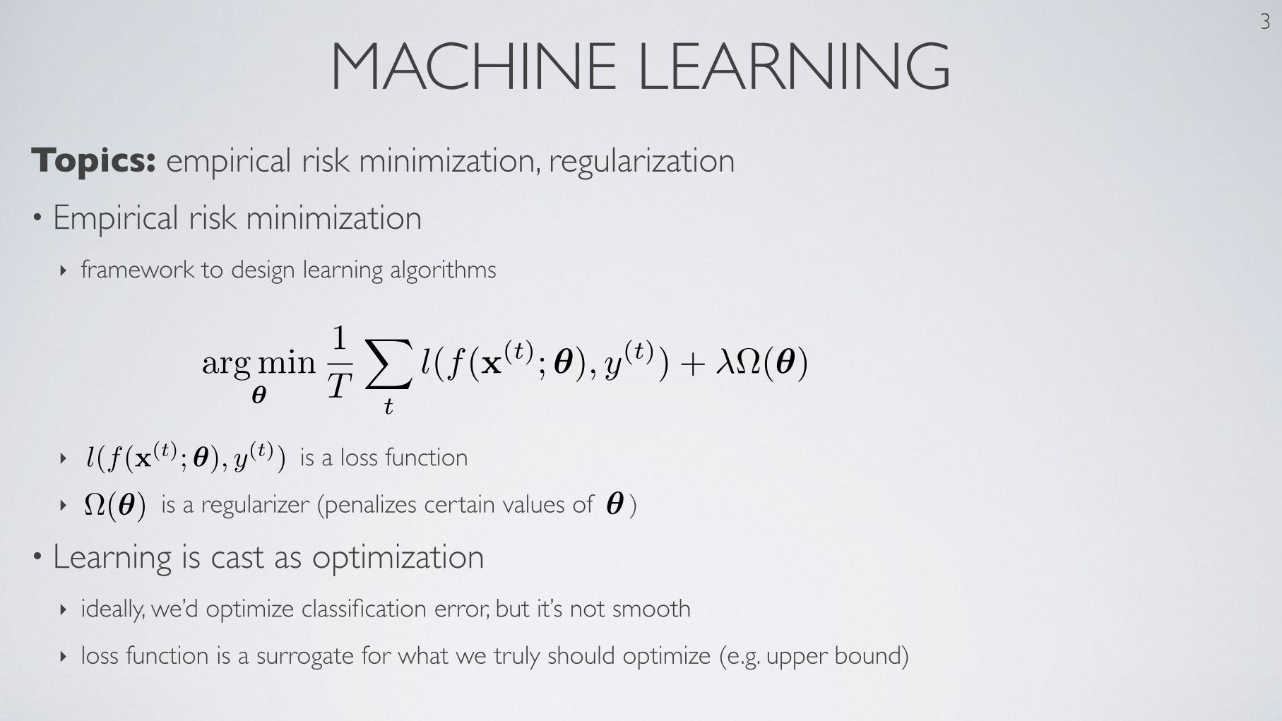
MACHINE LEARNING3

Topics: empirical risk minimization, regularization• Empirical risk minimization‣ framework to design learning algorithms

‣ is a loss function

‣ is a regularizer (penalizes certain values of )

• Learning is cast as optimization‣ ideally, we’d optimize classification error, but it’s not smooth

‣ loss function is a surrogate for what we truly should optimize (e.g. upper bound)

• bµ =

1T

Pt x

(t)

• b�2=

1T�1

Pt(x

(t) � bµ)2

• b⌃ =

1T�1

Pt(x

(t) � bµ)(x(t) � bµ)>

• E[

bµ] = µ E[b�2] = �2

E

hb⌃

i= ⌃

• bµ�µpb�2/T

• µ 2 bµ±�1.96p

b�2/T

•b✓ = argmax

✓p(x(1), . . . ,x(T )

)

•p(x(1), . . . ,x(T )

) =

Y

t

p(x(t))

• T�1T

b⌃ =

1T

Pt(x

(t) � bµ)(x(t) � bµ)>

Machine learning

• Supervised learning example: (x, y) x y

• Training set: Dtrain= {(x(t), y(t))}

• f(x;✓)

• Dvalid Dtest

•argmin

✓

1

T

X

t

l(f(x(t);✓), y(t)) + �⌦(✓)

5

• bµ =

1T

Pt x

(t)

• b�2=

1T�1

Pt(x

(t) � bµ)2

• b⌃ =

1T�1

Pt(x

(t) � bµ)(x(t) � bµ)>

• E[

bµ] = µ E[b�2] = �2

E

hb⌃

i= ⌃

• bµ�µpb�2/T

• µ 2 bµ±�1.96p

b�2/T

•b✓ = argmax

✓p(x(1), . . . ,x(T )

)

•p(x(1), . . . ,x(T )

) =

Y

t

p(x(t))

• T�1T

b⌃ =

1T

Pt(x

(t) � bµ)(x(t) � bµ)>

Machine learning

• Supervised learning example: (x, y) x y

• Training set: Dtrain= {(x(t), y(t))}

• f(x;✓)

• Dvalid Dtest

•argmin

✓

1

T

X

t

l(f(x(t);✓), y(t)) + �⌦(✓)

• l(f(x(t);✓), y(t))

• ⌦(✓)

5

• bµ =

1T

Pt x

(t)

• b�2=

1T�1

Pt(x

(t) � bµ)2

• b⌃ =

1T�1

Pt(x

(t) � bµ)(x(t) � bµ)>

• E[

bµ] = µ E[b�2] = �2

E

hb⌃

i= ⌃

• bµ�µpb�2/T

• µ 2 bµ±�1.96p

b�2/T

•b✓ = argmax

✓p(x(1), . . . ,x(T )

)

•p(x(1), . . . ,x(T )

) =

Y

t

p(x(t))

• T�1T

b⌃ =

1T

Pt(x

(t) � bµ)(x(t) � bµ)>

Machine learning

• Supervised learning example: (x, y) x y

• Training set: Dtrain= {(x(t), y(t))}

• f(x;✓)

• Dvalid Dtest

•argmin

✓

1

T

X

t

l(f(x(t);✓), y(t)) + �⌦(✓)

• l(f(x(t);✓), y(t))

• ⌦(✓)

5

• bµ =

1T

Pt x

(t)

• b�2=

1T�1

Pt(x

(t) � bµ)2

• b⌃ =

1T�1

Pt(x

(t) � bµ)(x(t) � bµ)>

• E[

bµ] = µ E[b�2] = �2

E

hb⌃

i= ⌃

• bµ�µpb�2/T

• µ 2 bµ±�1.96p

b�2/T

•b✓ = argmax

✓p(x(1), . . . ,x(T )

)

•p(x(1), . . . ,x(T )

) =

Y

t

p(x(t))

• T�1T

b⌃ =

1T

Pt(x

(t) � bµ)(x(t) � bµ)>

Machine learning

• Supervised learning example: (x, y) x y

• Training set: Dtrain= {(x(t), y(t))}

• f(x;✓)

• Dvalid Dtest

•argmin

✓

1

T

X

t

l(f(x(t);✓), y(t)) + �⌦(✓)

• l(f(x(t);✓), y(t))

• ⌦(✓)

• � = � 1T

Ptr✓l(f(x

(t);✓), y(t))� �r✓⌦(✓)

• ✓ ✓ +�

5

MACHINE LEARNING4

Topics: stochastic gradient descent (SGD)• Algorithm that performs updates after each example‣ initialize ( )

‣ for N iterations- for each training example

✓

✓

• To apply this algorithm to neural network training, we need‣ the loss function

‣ a procedure to compute the parameter gradients

‣ the regularizer (and the gradient )

‣ initialization method

• bµ =

1T

Pt x

(t)

• b�2=

1T�1

Pt(x

(t) � bµ)2

• b⌃ =

1T�1

Pt(x

(t) � bµ)(x(t) � bµ)>

• E[

bµ] = µ E[b�2] = �2

E

hb⌃

i= ⌃

• bµ�µpb�2/T

• µ 2 bµ±�1.96p

b�2/T

•b✓ = argmax

✓p(x(1), . . . ,x(T )

)

•p(x(1), . . . ,x(T )

) =

Y

t

p(x(t))

• T�1T

b⌃ =

1T

Pt(x

(t) � bµ)(x(t) � bµ)>

Machine learning

• Supervised learning example: (x, y) x y

• Training set: Dtrain= {(x(t), y(t))}

• f(x;✓)

• Dvalid Dtest

•argmin

✓

1

T

X

t

l(f(x(t);✓), y(t)) + �⌦(✓)

• l(f(x(t);✓), y(t))

• ⌦(✓)

• � = � 1T

Ptr✓l(f(x

(t);✓), y(t))� �r✓⌦(✓)

• ✓ ✓ +�

• {x 2 Rd | rx

f(x) = 0}

• v

>r2x

f(x)v > 0 8v

• v

>r2x

f(x)v < 0 8v

• � = �r✓l(f(x(t);✓), y(t))� �r✓⌦(✓)

5

• bµ =

1T

Pt x

(t)

• b�2=

1T�1

Pt(x

(t) � bµ)2

• b⌃ =

1T�1

Pt(x

(t) � bµ)(x(t) � bµ)>

• E[

bµ] = µ E[b�2] = �2

E

hb⌃

i= ⌃

• bµ�µpb�2/T

• µ 2 bµ±�1.96p

b�2/T

•b✓ = argmax

✓p(x(1), . . . ,x(T )

)

•p(x(1), . . . ,x(T )

) =

Y

t

p(x(t))

• T�1T

b⌃ =

1T

Pt(x

(t) � bµ)(x(t) � bµ)>

Machine learning

• Supervised learning example: (x, y) x y

• Training set: Dtrain= {(x(t), y(t))}

• f(x;✓)

• Dvalid Dtest

•argmin

✓

1

T

X

t

l(f(x(t);✓), y(t)) + �⌦(✓)

• l(f(x(t);✓), y(t))

• ⌦(✓)

• � = � 1T

Ptr✓l(f(x

(t);✓), y(t))� �r✓⌦(✓)

• ✓ ✓ +�

• {x 2 Rd | rx

f(x) = 0}

• v

>r2x

f(x)v > 0 8v

• v

>r2x

f(x)v < 0 8v

• � = �r✓l(f(x(t);✓), y(t))� �r✓⌦(✓)

• (x

(t), y(t))

5

• bµ =

1T

Pt x

(t)

• b�2=

1T�1

Pt(x

(t) � bµ)2

• b⌃ =

1T�1

Pt(x

(t) � bµ)(x(t) � bµ)>

• E[

bµ] = µ E[b�2] = �2

E

hb⌃

i= ⌃

• bµ�µpb�2/T

• µ 2 bµ±�1.96p

b�2/T

•b✓ = argmax

✓p(x(1), . . . ,x(T )

)

•p(x(1), . . . ,x(T )

) =

Y

t

p(x(t))

• T�1T

b⌃ =

1T

Pt(x

(t) � bµ)(x(t) � bµ)>

Machine learning

• Supervised learning example: (x, y) x y

• Training set: Dtrain= {(x(t), y(t))}

• f(x;✓)

• Dvalid Dtest

•argmin

✓

1

T

X

t

l(f(x(t);✓), y(t)) + �⌦(✓)

• l(f(x(t);✓), y(t))

• ⌦(✓)

• � = � 1T

Ptr✓l(f(x

(t);✓), y(t))� �r✓⌦(✓)

• ✓ ✓ +�

5

•argmin

✓

1

T

X

t

l(f(x(t);✓), y(t)) + �⌦(✓)

• l(f(x(t);✓), y(t))

• ⌦(✓)

• � = � 1T

Ptr✓l(f(x

(t);✓), y(t))� �r✓⌦(✓)

• ✓ ✓ + ↵ �

• {x 2 Rd | rx

f(x) = 0}

• v

>r2x

f(x)v > 0 8v

• v

>r2x

f(x)v < 0 8v

• � = �r✓l(f(x(t);✓), y(t))� �r✓⌦(✓)

• (x

(t), y(t))

• f⇤ f

6

• X

�1X = I

• (X>)i,j = Xj,i

• det (X) =Q

i Xi,i

• det (X>) = det (X)

• det (X�1) = det (X)�1

• det (X(1)X

(2)) = det (X(1)) det (X(2))

• X

> = X

�1

• v

>Xv > 0

• �

• {x(t)}

• 9w, t

⇤x

(t⇤) =P

t 6=t⇤ wtx(t)

• R(X) = {x 2 Rh | 9w x =P

j wjX·,j}

• {x 2 Rh | x /2 R(X)}

• {�i,ui | Xui = �iui et u

>i uj = 1i=j}

• X =P

i �iuiu>i

• det (X) =Q

i �i

• �i > 0

•@

@x

f(x, y) = lim�!0

f(x+�, y)� f(x, y)

�

•@

@y

f(x, y) = lim�!0

f(x, y +�)� f(x, y)

�

Machine learning

• Supervised learning example: (x, y)

• Training set: Dtrain = {(xt, yt}

•

2

training epoch =

iteration over all examples

Feedforward neural network

Hugo LarochelleD

´

epartement d’informatique

Universit´e de Sherbrooke

hugo.larochelle@usherbrooke.ca

September 13, 2012

Abstract

Math for my slides “Feedforward neural network”.

• f(x)

• l(f(x(t);✓), y(t))

• r✓l(f(x(t);✓), y(t))

• ⌦(✓)

• r✓⌦(✓)

• f(x)c = p(y = c|x)

• x

(t) y(t)

• l(f(x), y) = �P

c 1(y=c) log f(x)c = � log f(x)y =

•

@

f(x)c� log f(x)y =

�1(y=c)

f(x)y

rf(x) � log f(x)y =

�1

f(x)y[1(y=0), . . . , 1(y=C�1)]

>

=

�e(c)

f(x)y

1

Feedforward neural network

Hugo LarochelleD

´

epartement d’informatique

Universit´e de Sherbrooke

hugo.larochelle@usherbrooke.ca

September 13, 2012

Abstract

Math for my slides “Feedforward neural network”.

• f(x)

• l(f(x(t);✓), y(t))

• r✓l(f(x(t);✓), y(t))

• ⌦(✓)

• r✓⌦(✓)

• f(x)c = p(y = c|x)

• x

(t) y(t)

• l(f(x), y) = �P

c 1(y=c) log f(x)c = � log f(x)y =

•

@

f(x)c� log f(x)y =

�1(y=c)

f(x)y

rf(x) � log f(x)y =

�1

f(x)y[1(y=0), . . . , 1(y=C�1)]

>

=

�e(c)

f(x)y

1

Feedforward neural network

Hugo LarochelleD

´

epartement d’informatique

Universit´e de Sherbrooke

hugo.larochelle@usherbrooke.ca

September 13, 2012

Abstract

Math for my slides “Feedforward neural network”.

• f(x)

• l(f(x(t);✓), y(t))

• r✓l(f(x(t);✓), y(t))

• ⌦(✓)

• r✓⌦(✓)

• f(x)c = p(y = c|x)

• x

(t) y(t)

• l(f(x), y) = �P

c 1(y=c) log f(x)c = � log f(x)y =

•

@

f(x)c� log f(x)y =

�1(y=c)

f(x)y

rf(x) � log f(x)y =

�1

f(x)y[1(y=0), . . . , 1(y=C�1)]

>

=

�e(c)

f(x)y

1

Feedforward neural network

Hugo LarochelleD

´

epartement d’informatique

Universit´e de Sherbrooke

hugo.larochelle@usherbrooke.ca

September 13, 2012

Abstract

Math for my slides “Feedforward neural network”.

• f(x)

• l(f(x(t);✓), y(t))

• r✓l(f(x(t);✓), y(t))

• ⌦(✓)

• r✓⌦(✓)

• f(x)c = p(y = c|x)

• x

(t) y(t)

• l(f(x), y) = �P

c 1(y=c) log f(x)c = � log f(x)y =

•

@

f(x)c� log f(x)y =

�1(y=c)

f(x)y

rf(x) � log f(x)y =

�1

f(x)y[1(y=0), . . . , 1(y=C�1)]

>

=

�e(c)

f(x)y

1

Feedforward neural network

Hugo LarochelleD

´

epartement d’informatique

Universit´e de Sherbrooke

hugo.larochelle@usherbrooke.ca

September 13, 2012

Abstract

Math for my slides “Feedforward neural network”.

• f(x)

• ✓ ⌘ {W(1),b(1), . . . ,W(L+1),b(L+1)}

• l(f(x(t);✓), y(t))

• r✓l(f(x(t);✓), y(t))

• ⌦(✓)

• r✓⌦(✓)

• f(x)c = p(y = c|x)

• x

(t) y(t)

• l(f(x), y) = �P

c 1(y=c) log f(x)c = � log f(x)y =

•

@

f(x)c� log f(x)y =

�1(y=c)

f(x)y

rf(x) � log f(x)y =

�1

f(x)y[1(y=0), . . . , 1(y=C�1)]

>

=

�e(c)

f(x)y

1