Neural Networks

Reading: Chapter 3 in Nilsson text

Lab: Work on assignment 2 (due 19th in class)

The Brain -- A Paradox

The brain consists of 10^11 neurons, each of which is connected to 10^4 neighbors

Each neuron is slow (1 millisecond to respond to new stimulus)

Yet, the brain is astonishingly fast at perceptual tasks (e.g. recognize a face)

The brain can also store and retrieve prodigious amounts of multi-media information

The brain uses a very different computing architecture: parallel distributed processing

A brief history of neural networks

1960-65: Perceptron model developed by Rosenblatt

1969: Perceptron model analyzed by Minksy and Papert

1975: Werbos thesis at Harvard lays the roots for multi-layer neural networks

1985: 2 vol. Book on parallel distributed processing 1990: Neural networks enter mainstream

applications (stock market, OCR, robotics)

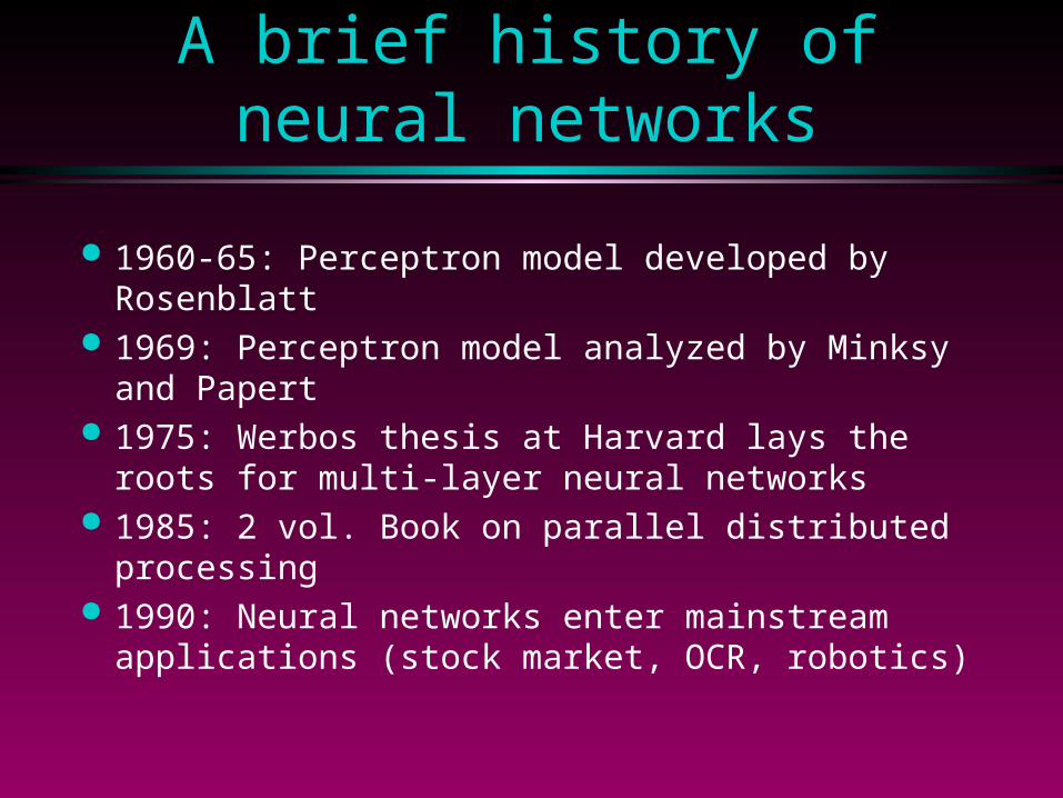
ALVINN: A Neural Net that Drives a

Truck (Pomerleau)

Object Recognition using Neural Networks

(Georgios Theocharous et al.)

Network learns to predict direction and distance to trash can

Training Methods

Single threshold-logic units: Perceptron training rule Widrow-hoff method

Gradient descent methods Arbitrary feedforward neural networks

Sigmoid activation function (smooth nonlinearity) Backpropagation algorithm

Threshold-logic Units

w1

w2

wn

Threshold(nonlinear)

Out

otherwise0

if11

f

xwf i

n

ii

x1

x2

xn

Inputs

TLU’s define hyperplane

Denote the input vector by X = (x0,x1,x2,…,xn)(Note n+1 inputs, where x0 is always set to 1)

Denote the weight vector by W = (w0,w1,…,wn) (note w0 is the threshold weight)

Output = 0 if X*W < 0, else Output = 1

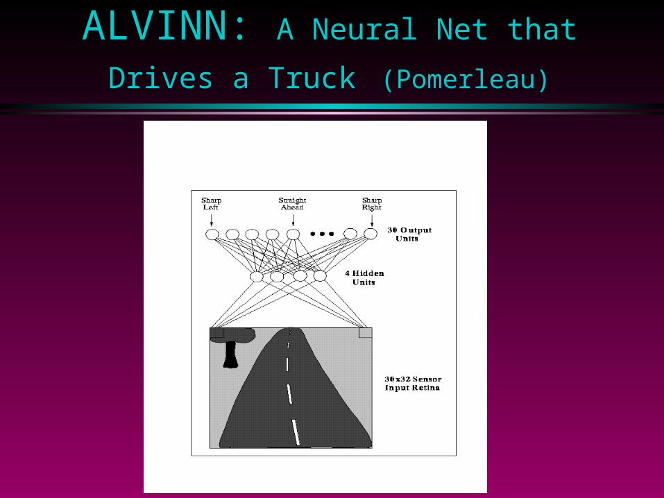
For n=2, this is the equation of a line in 2D

w0 + w1*x1 + w2*x2 = 0x2 = -(w1/w2)*x1 + (-w0/w2)

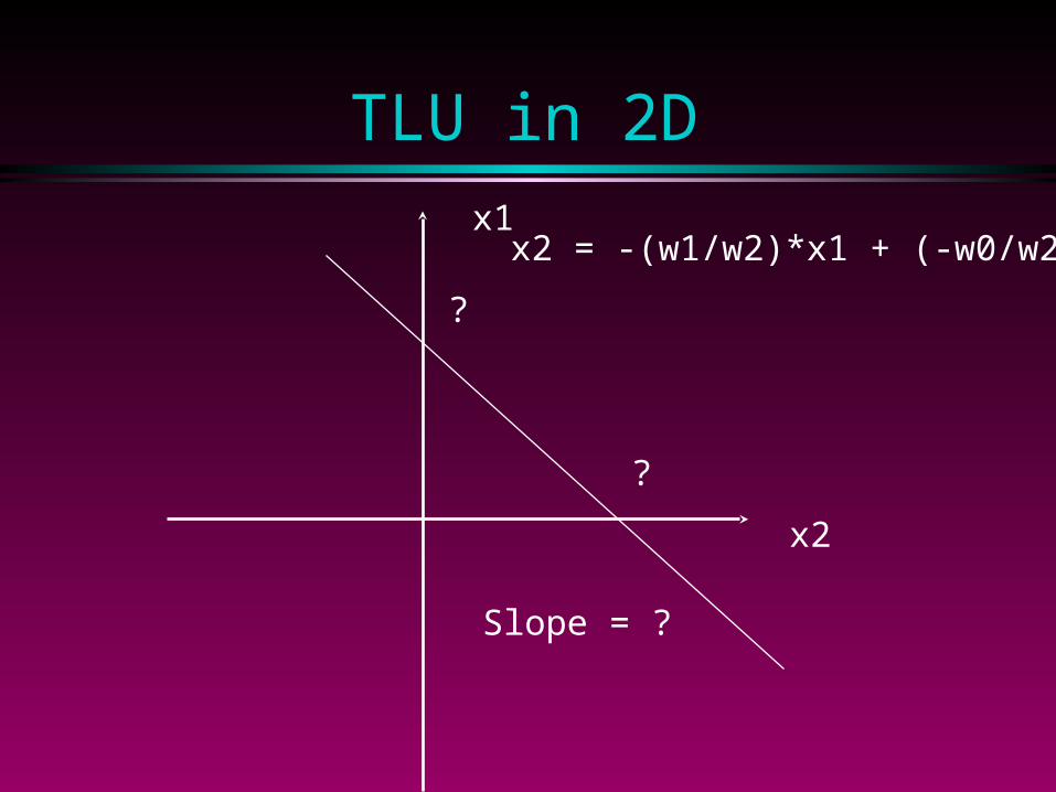
TLU in 2D

x2

x1

?

Slope = ?

?

x2 = -(w1/w2)*x1 + (-w0/w2)

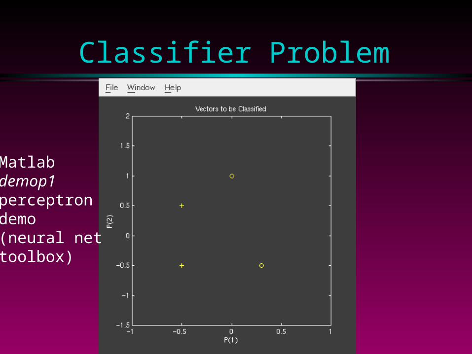
Classifier Problem

Matlabdemop1perceptrondemo (neural nettoolbox)

Initial Classifier

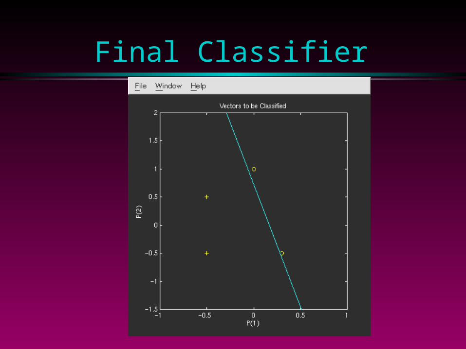
Final Classifier

Error Plot

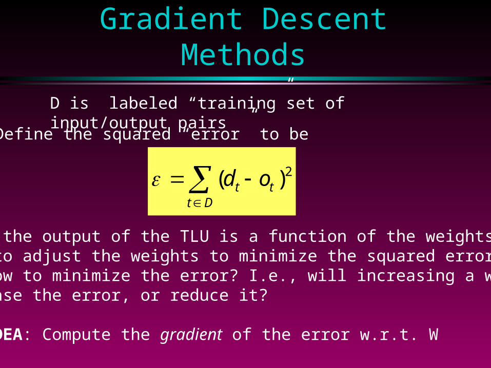
Gradient Descent Methods

Define the squared “error” to be

2)( tDt

t od

D is labeled “training”set of input/output pairs

Since the output of the TLU is a function of the weights W, we want to adjust the weights to minimize the squared error. But how to minimize the error? I.e., will increasing a weight increase the error, or reduce it?

KEY IDEA: Compute the gradient of the error w.r.t. W

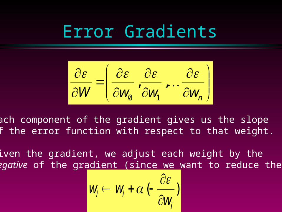
Error Gradients

nwwwW

,,

10

Each component of the gradient gives us the slopeof the error function with respect to that weight.

Given the gradient, we adjust each weight by thenegative of the gradient (since we want to reduce the error).

)(i

ii www

Learning by Gradient Descent

A boomboxwith manyunlabeled volume& tone controls

Sound output

Which way to turn each control to reduce the volume?

Antennainput

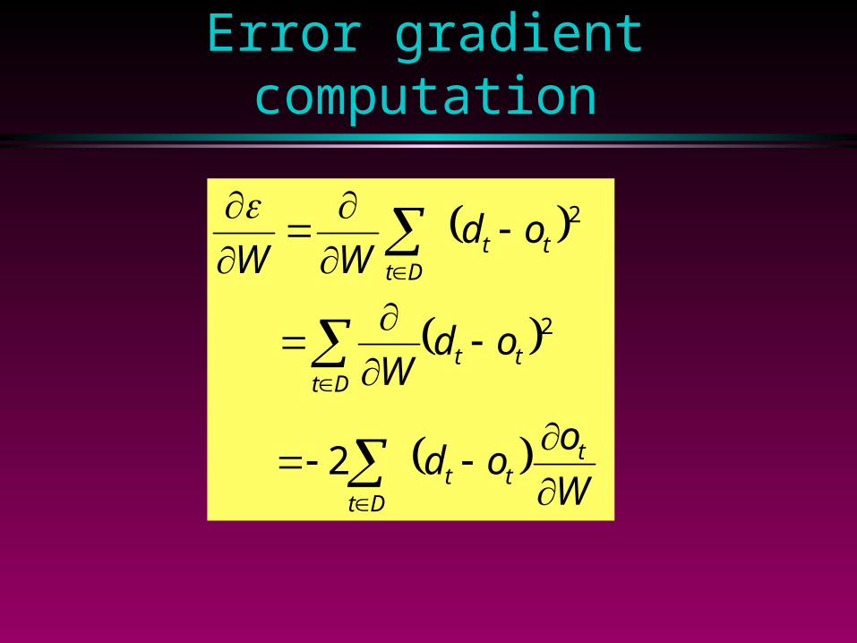
Error gradient computation

W

ood

odW

odWW

ttt

Dt

ttDt

ttDt

2

2

2

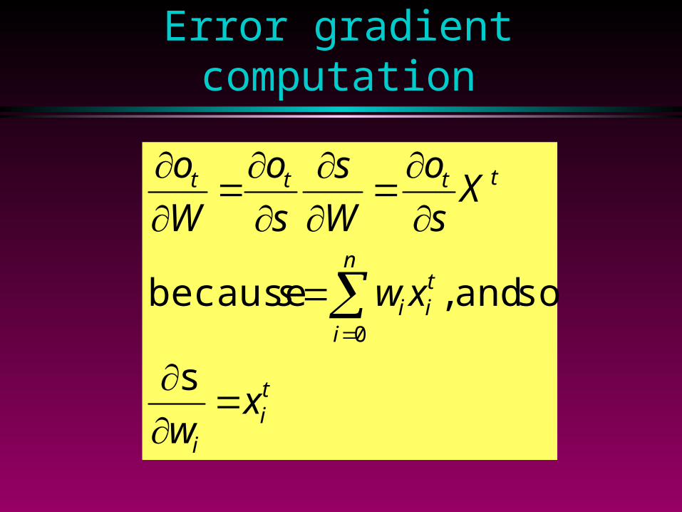
Error gradient computation

ti

i

ti

n

ii

tttt

xw

xws

Xs

o

W

s

s

o

W

o

s

so and ,because0

Threshold Units without thresholding

Let the output of the unit be simply be the weighted sum.We ignore the thresholding, and train the weights such thatan output of 1 is produced exactly, and an output of 0 isreplaced by an output of -1. In this case, we get that

1s

ot

tt

tt XodW

2

The error gradient then becomes

Widrow-Hoff Training Method(Batch)

1. Set the weights to small random values (e.g. between -.1 and .1)2. Set the learning rate to some small fixed positive value (.1). 3. Repeat // until training error is low enough Set error = 0; diff = 0; For each training example e begin error = error + square(d[e] - o[e]); for j=0 to N do diff = diff + (d[e] - o[e])*x[j,e]; end for j=0 to N do w[j] = w[j] + diff; // x[0,e] is always 1 until error < desired_value. 4. Store weight vector w in a file.

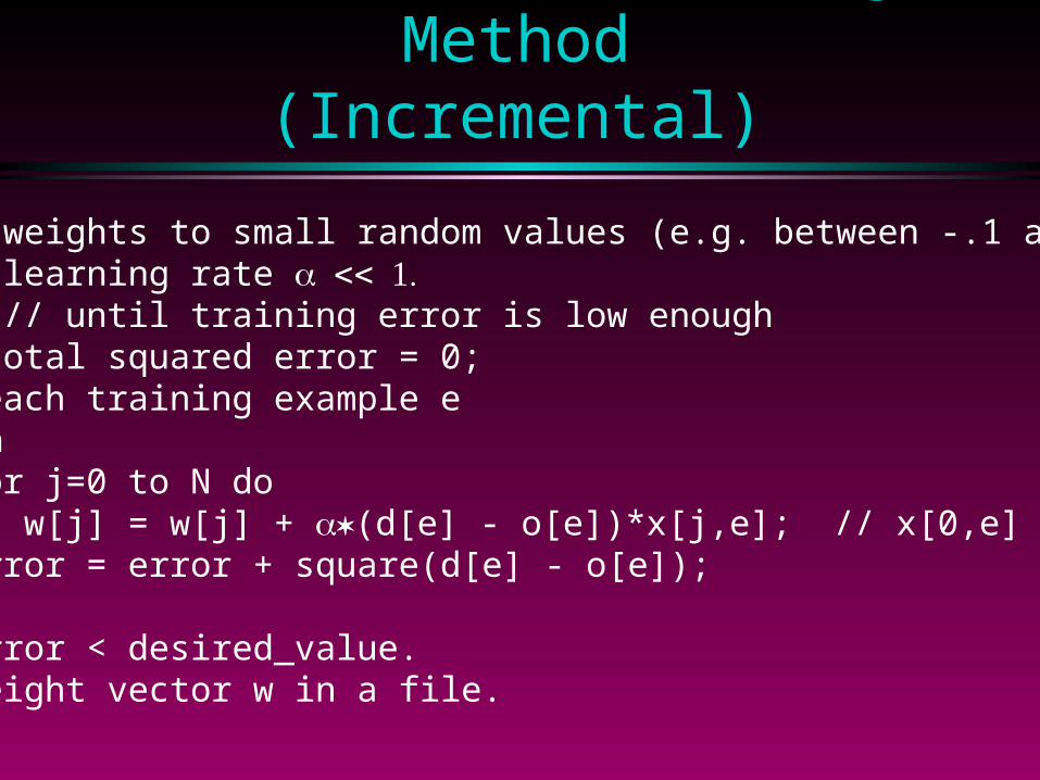
Widrow-Hoff Training Method(Incremental)

1. Set the weights to small random values (e.g. between -.1 and .1)2. Set the learning rate 3. Repeat // until training error is low enough Set total squared error = 0; For each training example e begin for j=0 to N do w[j] = w[j] + (d[e] - o[e])*x[j,e]; // x[0,e] is always 1 error = error + square(d[e] - o[e]); end until error < desired_value. 4. Store weight vector w in a file.

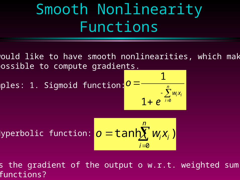
Smooth Nonlinearity Functions

We would like to have smooth nonlinearities, which makeit possible to compute gradients.

Examples: 1. Sigmoid function:

2. Hyperbolic function:

n

iiixw

e

o

01

1

)tanh(0

n

iiixwo

What is the gradient of the output o w.r.t. weighted sum s for these functions?

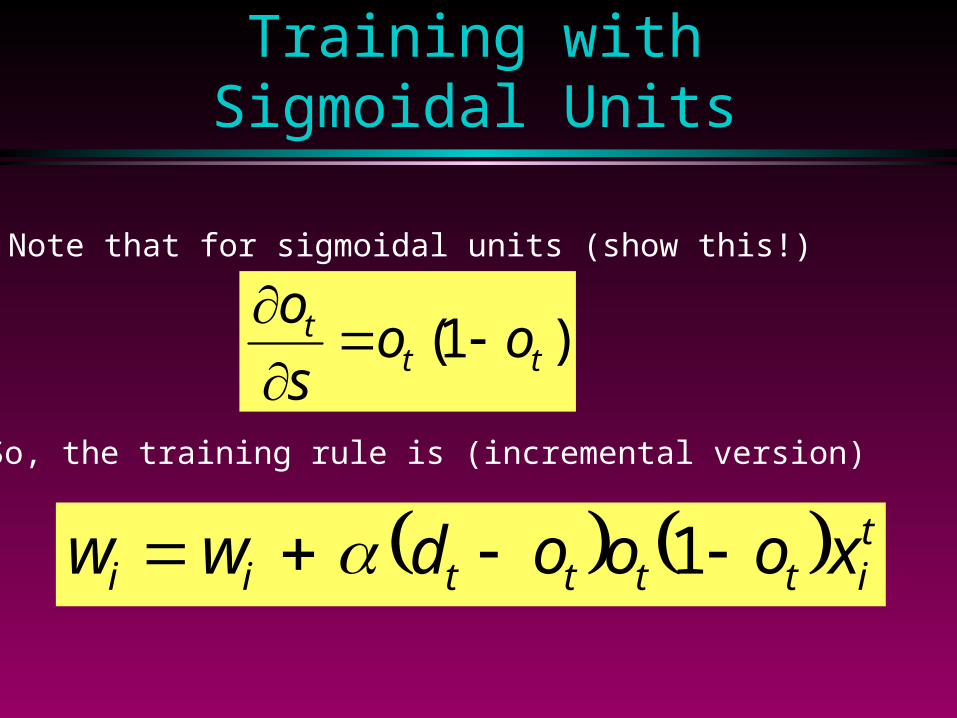
Training with Sigmoidal Units

Note that for sigmoidal units (show this!)

)1( ttt oos

o

So, the training rule is (incremental version)

tittttii xooodww 1