Neural Networks : Basics - University of Ottawapetriu/NN_basics-tutorial.pdf · Neural Networks :...

Emil M. Petriu

School of Electrical Engineering and Computer Science

University of Ottawa

http://www.site.uottawa.ca/~petriu/

[email protected]

Neural Networks :

Basics

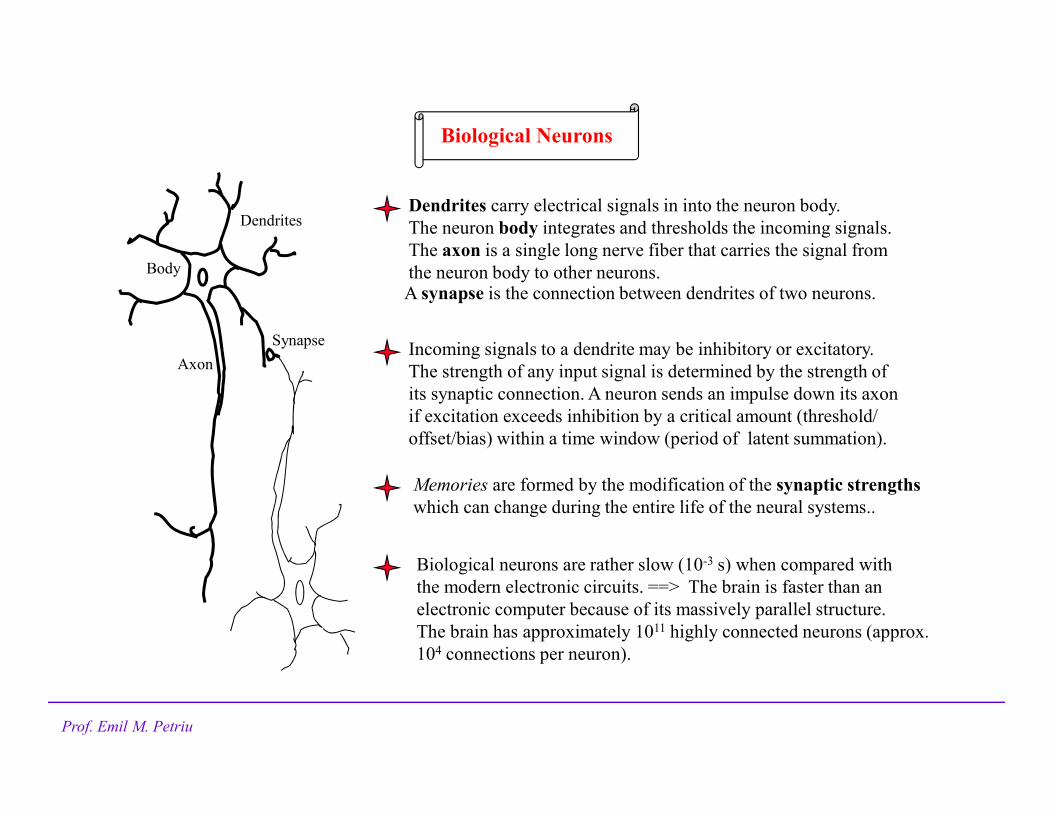
Biological Neurons

Incoming signals to a dendrite may be inhibitory or excitatory.

The strength of any input signal is determined by the strength of

its synaptic connection. A neuron sends an impulse down its axon

if excitation exceeds inhibition by a critical amount (threshold/

offset/bias) within a time window (period of latent summation).

Biological neurons are rather slow (10-3 s) when compared with

the modern electronic circuits. ==> The brain is faster than an

electronic computer because of its massively parallel structure.

The brain has approximately 1011 highly connected neurons (approx.

104 connections per neuron).

Dendrites carry electrical signals in into the neuron body.

The neuron body integrates and thresholds the incoming signals.

The axon is a single long nerve fiber that carries the signal from

the neuron body to other neurons.

Memories are formed by the modification of the synaptic strengths

which can change during the entire life of the neural systems..

Body

Axon

Dendrites

Synapse

A synapse is the connection between dendrites of two neurons.

Prof. Emil M. Petriu

W. McCulloch & W. Pitts (1943) the first theory on the fundamentals of neural computing

(neuro-logicalnetworks) “A Logical Calculus of the Ideas Immanent in Nervous Activity”

==> McCulloch-Pitts neuron model; (1947) “How We Know Universals” - an essay on networks

capable of recognizing spatial patterns invariant of geometric transformations.

Cybernetics: attempt to combine concepts from biology, psychology, mathematics, and engineering.

1940s

Natural components of mind-like machines are simple abstractions based on the behavior

of biological nerve cells, and such machines can be built by interconnecting such elements.

Historical Sketch of Neural Networks

D.O. Hebb (1949) “The Organization of Behavior” the first theory of psychology on conjectures

about neural networks (neural networks might learn by constructing internal representations of

concepts in the form of “cell-assemblies” - subfamilies of neurons that would learn to support one

another’s activities). ==> Hebb’s learning rule: “When an axon of cell A is near enough to excite a

cell B and repeatedly or persistently takes part in firing it, some growth process or metabolic change

takes place in one or both cells such that A’s efficiency, as one of the cells firing B, is increased.”


1950s

Cybernetic machines developed as specific architectures to perform specific functions.

==> “machines that could learn to do things they aren’t built to do”

M. Minsky (1951) built a reinforcement-based network learning system.

F. Rosenblatt (1958) the first practical Artificial Neural Network (ANN) - the perceptron, “The

Perceptron: A Probabilistic Model for Information Storage and Organization in the Brain.”.

IRE Symposium “The Design of Machines to Simulate the Behavior of the Human Brain” (1955)

with four panel members: W.S. McCulloch, A.G. Oettinger, O.H. Schmitt, N. Rochester, invited

questioners: M. Minsky, M. Rubinoff, E.L. Gruenberg, J. Mauchly, M.E. Moran, W. Pitts, and the

moderator H.E. Tompkins.

By the end of 50s, the NN field became dormant because of the new AI advances based on

serial processing of symbolic expressions.


1960s

Connectionism (Neural Networks) - versus - Symbolism (Formal Reasoning)

B. Widrow & M.E. Hoff (1960) “Adaptive Switching Circuits” presents an adaptive percepton-like

network. The weights are adjusted so to minimize the mean square error between the actual and desired

output ==> Least Mean Square (LMS) error algorithm. (1961) Widrow and his students “Generalization

and Information Storage in Newtworks of Adaline “Neurons.”

M. Minsky & S. Papert (1969) “Perceptrons” a formal analysis of the percepton networks explaining

their limitations and indicating directions for overcoming them ==> relationship between the perceptron’s

architecture and what it can learn: “no machine can learn to recognize X unless it poses some scheme

for representing X.”

Limitations of the perceptron networks led to the pessimist view of the NN field as having

no future ==> no more interest and funds for NN research!!!


1970s

Memory aspects of the Neural Networks.

T. Kohonen (1972) “Correlation Matrix Memories” a mathematical oriented paper proposing a

correlation matrix model for associative memory which is trained, using Hebb’s rule, to learn

associations between input and output vectors.

J.A. Anderson (1972) “A Simple Neural Network Generating an Interactive Memory” a physiological

oriented paper proposing a “linear associator” model for associative memory, using Hebb’s rule, to learn

associations between input and output vectors.

S. Grossberg (1976) “Adaptive Pattern Classification and Universal Recording: I. Parallel Development

and Coding of Neural Feature Detectors”describes a self-organizing NN model of the visual system

consisting of a short-term and long term memory mechanisms. ==> continuous-time competitive

network that forms a basis for the Adaptive Resonance Theory (ART) networks.


1980s

Revival of Learning Machine.

D.E. Rumelhart & J.L. McClelland, eds. (1986) “Parallel Distributed Processing: Explorations in the

Microstructure of Cognition: Explorations in the Microstructure of Cognition” represents a milestone

in the resurgence of NN research.

International Neural Network Society (1988) …. IEEE Tr. Neural Networks (1990).

J.A. Anderson & E. Rosenfeld (1988) “Neurocomputing: Foundations of Research” contains over forty

seminal papers in the NN field.

DARPA Neural Network Study(1988) a comprehensive review of the theory and applications of the

Neural Networks.

[Minsky]: “The marvelous powers of the brain emerge not from any single, uniformly structured

connectionst network but from highly evolved arrangements of smaller, specialized networks

which are interconnected in very specific ways.”


Artificial Neural Networks (ANN)

McCulloch-Pitts model of an artificial neuron

y = f ( w1. p1 +…+ wj

. pj +... wR. pR + b)

wjpj

w1p1

wRpR

.

.

.

.

.

.

ΣΣΣΣ f yz

b

Some transfer functions “f”

Hard Limit: y = 0 if z<0

y = 1 if z>=00

1

y

z

Symmetrical: y = -1 if z<0

Hard Limit y = +1 if z>=00

1

y

z

-1

Log-Sigmoid:

y =1/(1+e-z)0

1

y

z

Linear:

y = z0

y

zp = (p1, … , pR)T is the input column-vector

W = (w1, … , wR) is the weight row-vector

y = f (W. p + b)

*) The bias b can be treated as a weight whose input is always 1.


The Architecture of an ANN� Number of inputs and outputs of the network;

� Number of layers;

� How the layers are connected to each other;

� The transfer function of each layer;

� Number of neurons in each layer;ANNs map input/stimulus values

to output/response values: Y= F (P).

Intelligent systems generalize:

their behavioral repertoires exceed

their experience. An intelligent

system is said to have a creative

behaviour if it provides appropriate

responses when faced with new stimuli. Usually the new stimuli

P’ resemble known stimuli P and their corresponding responses

Y’ resemble known/learned responses Y.

Measure of system’s F creativity:

Volume of “stimuli ball BP “

Volume of “response ball BY”

BP

P

P’B

Y

Y

Y’

Y’= F (P’)

Y= F (P)


Most of the mapping functions can be implemented by a two-layer ANN: a sigmoid layer feeding a

linear output layer.

ANNs with biases can represent relationships between inputs and outputs than networks

without biases.

Feed-forward ANNs cannot implement temporal relationships. Recurrent ANNs have internal

feedback paths that allow them to exhibit temporal behaviour.

Feed-forward architecture with three layers

N (1,1)

N (1,R1)

p1

.

.

.

pR

.

.

.

N (2,1)

N (2,R2)

.

.

.

y(1,1)

y(1,R1)

N (3,1)

N (3,R3)

.

.

.

y(2,1)

y(2,R2)

y (3,1)

y (3,R3)

Layer 1 Layer 2 Layer 3N (1)

N (R)

.

.

.

y(1)

y(R)

.

.

.

Recurrent architecture (Hopfield NN)

The ANN is usually supplied with an initial

input vector and then the outputs are used

as inputs for each succeeding cycle.


Learning Rules (Training Algorithms)

Supervised Learning

Procedure/algorithm to adjust the weights and biases

in order for the ANN to perform the desired task.

wj

. . .

ΣΣΣΣ f yz

b

Learning

Rule

e = t-ye t

pj

( j= 1,…,R)

. . .

For a given training set of pairs

{p(1),t(1)},...,{p(n),t(n)}, where p(i)

is an instance of the input vector and

t(i) is the corresponding target

value for the output y, the learning

rule calculates the updated value of

the neuron weights and bias.

Reinforcement Learning

Similar to supervised learning - instead of being provided with the correct output value for each given

input, the algorithm is only provided with a given grade/score as a measure of ANN’s performance.

Unsupervised Learning

The weight and unbiased are adjusted based on inputs only. Most algorithms of this type learn to

cluster input patterns into a finite number of classes. ==> e.g. vector quantization applications


THE PERCEPTRON

The perceptron is a neuron with a hard limit transfer function and a weight adjustment mechanism

(“learning”) by comparing the actual and the expected output responses for any given input /stimulus.

[Minski] “Perceptrons make decisions/determine whether or not event fits a certain pattern

by adding up evidence obtained from many small experiments”

Frank Rosenblatt (1958), Marvin Minski & Seymour Papert (1969)

wjpj

w1p1

wRpR

.

.

.

.

.

.

ΣΣΣΣ yz

b

f

0

1

Perceptrons are well suited for

pattern classification/recognition.

The weight adjustment/training

mechanism is called the perceptron

learning rule.

y = f (W. p + b)

NB: W is a row-vector and p is a column-vector.


� Supervised learning

t <== the target value

e = t-y <== the errorwjpj

w1p1

wRpn

.

.

.

.

.

.

ΣΣΣΣ yz

b

f

0

1

p = (p1, … , pR)T is the input column-vector

W = (x1, … , xR) is the weight row-vector

Because of the perceptron’s hard limit

transfer function y, t, e can take only

binary values

Perceptron learning rule:

Wnew = Wold + e.pT

bnew = bold + e

if e = 1, then Wnew = Wold + p , bnew = bold + 1;

if e = -1, then Wnew = Wold - p , bnew = bold - 1 ;

if e = 0, then Wnew = Wold .

Perceptron Learning Rule


The hard limit transfer function (threshold function) provides the ability to classify input vectors

by deciding whether an input vector belongs to one of two linearly separable classes.

w1p1

w2p2

ΣΣΣΣ yz

bf

0

1

Two-Input Perceptronp2

p10

-b / w2

-b / w1

( z = 0 )

w1. p1 + w2

. p2 + b =0

y = sign (b) y = sign (-b)

The two classes (linearly separable regions) in the two-dimensional

input space (p1, p2) are separated by the line of equation z = 0.

y = hardlim (z) = hardlim{ [w1 , w2] . [p1 , p2]

T + b}

The boundary is always orthogonal to the weight vector W.

W


� Example #1: Teaching a two-input perceptron to classify five input vectors into two classes

p(1) = (0.6, 0.2)T

t(1) = 1

p(2) = (-0.2, 0.9)T

t(2) = 1

p(3) = (-0.3, 0.4)T

t(3) = 0

p(4) = (0.1, 0.1)T

t(4) = 0

p(5) = (0.5, -0.6)T

t(5) = 0

p1

p2

1

1

-1

-1

P=[0.6 -0.2 -0.3 0.1 0.5;

0.2 0.9 0.4 0.1 -0.6];

T=[1 1 0 0 0];

W=[-2 2];

b=-1;

plotpv(P,T);

plotpc(W,b);

nepoc=0

Y=hardlim(W*P+b);

while any(Y~=T)

Y=hardlim(W*P+b);

E=T-Y;

[dW,db]= learnp(P,E);

W=W+dW;

b=b+db;

nepoc=nepoc+1;

disp(‘epochs=‘),disp(nepoc),

disp(W), disp(b);

plotpv(P,T);

plotpc(W,b);

end

The MATLAB solution is:


� Example #1:

After nepoc = 11

(epochs of training

starting from an

initial weight vectorW=[-2 2] and a

bias b=-1)

the weights are:

w1 = 2.4

w2 = 3.1

and the bias is:

b = -2

-0.8 -0.6 -0.4 -0.2 0 0.2 0.4 0.6 0.8 1 1.2-1.5

-1

-0.5

0

0.5

1

1.5

2Input Vector Classification

p1

p2


� The larger an input vector p is, the larger is its effect on the weight vector W during the learning process

Long training times can be caused by the presence of an “outlier,” i.e. an input vector

whose magnitude is much larger, or smaller, than other input vectors.

Normalized perceptron learning rule,

the effect of each input vector on the

weights is of the same magnitude:

Wnew = Wold + e.pT / p

bnew = bold + e

Perceptron Networks for Linearly Separable Vectors

The hard limit transfer function of the perceptron provides the ability to classify input vectors

by deciding whether an input vector belongs to one of two linearly separable classes.

p

2

p

110

1

ANDp

2

p

110

1

OR

W = [ 2 2 ]

b = -3

W = [ 2 2 ]

b = -1

p = [ 0 0 1 1 ;

0 1 0 1 ]

tAND =[ 0 0 0 1 ]

p = [ 0 0 1 1 ;

0 1 0 1 ]

tOR = [ 0 1 1 1 ]


Three-Input Perceptron

w1p1

w2p2ΣΣΣΣ

yz

bf

0

1

w3p3

y =hardlim ( z )

= hardlim{ [w1 , w2 ,w3] .

[p1 , p2 p3]T + b}

-2-1

0

1

2

-2

-1

0

1

2

-2

-1

0

1

2

p1

p2

p3

P = [ -1 1 1 -1 -1 1 1 -1;

-1 -1 1 1 -1 -1 1 1;

-1 -1 -1 -1 1 1 1 1]

T = [ 0 1 0 0 1 1 1 0 ]

EXAMPLE

The two classes in

the 3-dimensional

input space (p1, p2, p3)

are separated by the

plane of equation z = 0.


One-layer multi-perceptron classification of linearly separable patterns

-3 -2 -1 0 1 2-3

-2

-1

0

1

2

3

4

3

p1

p2

0 2 4 6 810

-20

10-15

10-10

10-5

100

105

# Epochs

Err

or

Demo P3 in the “MATLAB Neural Network

Toolbox - User’s Guide”

T = [ 1 1 1 0 0 1 1 1 0 0;

0 0 0 0 0 1 1 1 1 1 ]

00 = O ; 10 = +

01 = * ; 11 = x

P = [ 0.1 0.7 0.8 0.8 1.0 0.3 0.0 -0.3 -0.5 -1.5;

1.2 1.8 1.6 0.6 0.8 0.5 0.2 0.8 -1.5 -1.3 ]

R = 2 inputs

S = 2 neurons

Where:

R = # Inputs

S = # Neurons

MATLAB representation:

W

SxR

b

Sx1R

p

Rx1

1

z

Sx1

Sx1

y

Input Perceptron Layer

y = hardlim(W*p+b)

ΣΣΣΣ


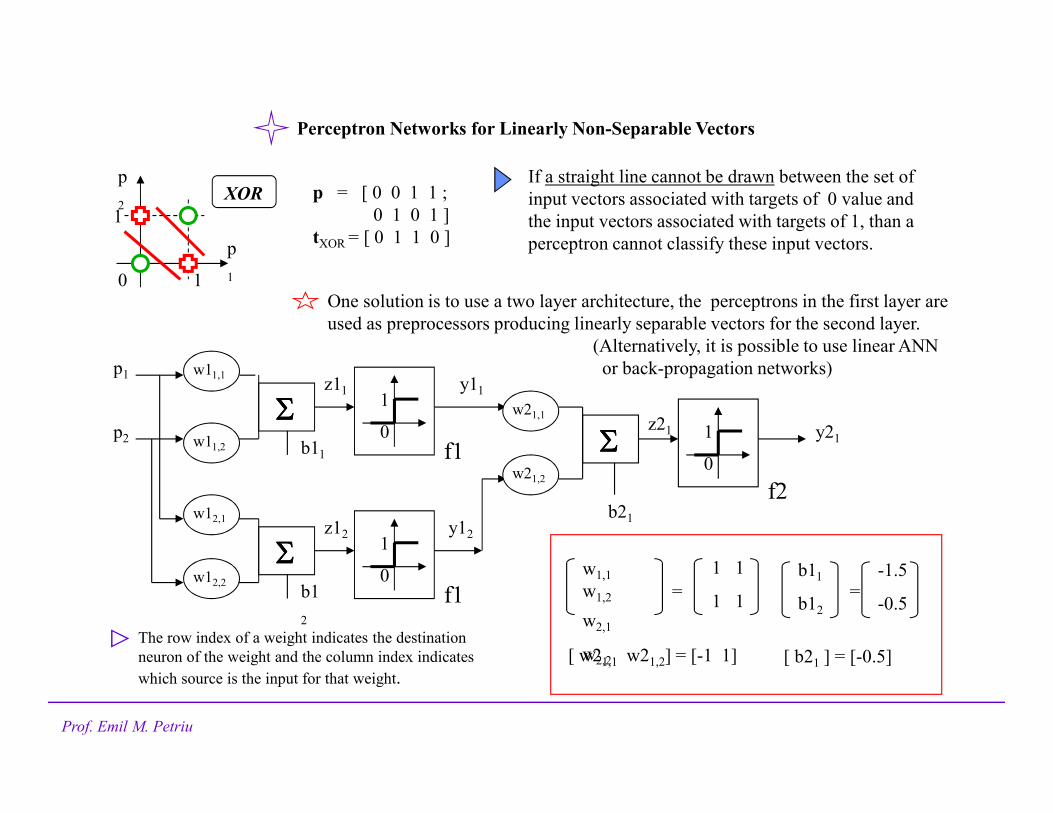
p = [ 0 0 1 1 ;

0 1 0 1 ]

tXOR = [ 0 1 1 0 ]

XORp

2

p

110

1

If a straight line cannot be drawn between the set of

input vectors associated with targets of 0 value and

the input vectors associated with targets of 1, than a

perceptron cannot classify these input vectors.

1 1

1 1

w1,1

w1,2

w2,1

w2,2

=

b11

b12

-1.5

-0.5=

[ w21,1 w21,2] = [-1 1] [ b21 ] = [-0.5]

One solution is to use a two layer architecture, the perceptrons in the first layer are

used as preprocessors producing linearly separable vectors for the second layer.

(Alternatively, it is possible to use linear ANN

or back-propagation networks)w11,1

ΣΣΣΣy11z11

b11 f10

1

ΣΣΣΣy12z12

b1

2

f10

1

p1

p2 ΣΣΣΣ y21z21

b21

f2

0

1w11,2

w12,1

w12,2

w21,2

w21,1

Perceptron Networks for Linearly Non-Separable Vectors

The row index of a weight indicates the destination

neuron of the weight and the column index indicates

which source is the input for that weight.


LINEAR NEURAL NETWORKS (ADALINE NETWORKS)

Widrow-Hoff Learning Rule ( The �� Rule )

wj

. . .

ΣΣΣΣy(y = z)

b

LMS

Learning Rulee = t-ye t

pj

( j= 1,…,R)

. . .

( ADALINE <== ADAptive LInear NEuron )

(NB: E[…] denotes the “expected value”; p is column vector)

The LMS algorithm will adjust ADALINE’s weights

and biases in such away to minimize the mean-square-

error E [e2] between all sets of the desired response

and network’s actual response:

E [ (t-y)2 ] = E [ (t - (w1 … wR b) . (p1 … pR 1)T )2 ]

= E [ (t - W . p)2 ]

Where: R = # Inputs, S = # Neurons

W

SxR

b

Sx1R

p

Rx1

1

z

Sx1

Sx1

y

Input Linear Neuron Layer

y = purelin(W*p+b)

ΣΣΣΣ

� Linear neurons have a linear transfer functionthat

allows to use a Least Mean-Square (LMS) procedure

- Widrow-Hoff learning rule- to adjust weights and

biases according to the magnitude of errors.

� Linear neurons suffer from the same limitation as the

perceptron networks: they can only solve linearly

separable problems.


>> Widrow-Hoff algorithm

As t(k) and p(k) - both affecting e(k) - are independent of W(k), we obtain the final expression of the

Widrow-Hoff learning rule:

W(k+1) = W (k) + 2.µ.e(k). p(k)

where µ the “learning rate” and e(k) = t(k)-y(k) = t(k)-W(k) . p(k)

b(k+1) = b(k) +2.µ.e(k)

The input cross-

correlation matrix

The cross-correlation

between the input vector

and its associated target.

If the input correlation matrix is positive

the LMS algorithm will converge as there will

a unique minimum of the mean square error.

E [ e2 ] = E [ (t - W . p)2 ] = {as for deterministic signals the expectation becomes a time-average}

= E[t2] - 2.W . E[t.p] + W . E[p.pT] . WT

The weight vector is then modified in the direction that decreases the error:

W k W K W k W k e kk

e k

W k

e k

W k( ) ( ) ( ) ( ) ( )* ( )

( )

( )

( )+ = − • ∇ = − • = − • •1 22

µ µ µ∂

∂

∂

∂

[ ]∇ = =k

e k

W k

e k

w k

e k

w k

e k

b kR

* ( )

( )

( )

( )

( )

( )

( )

( ). . . ,∂

∂

∂

∂

∂

∂

∂

∂

2 2

1

2 2

� The W-H rule is an iterative algorithm uses the “steepest-descent” method to reduce the mean-square-error.

The key point of the W-H algorithm is that it replaces E[e2] estimation by the squared error of the iteration k:

e2(k). At each iteration step k it estimates the gradient of this error k with respect to W as a vector consisting

of the partial derivatives of e2(k) with respect to each weight:


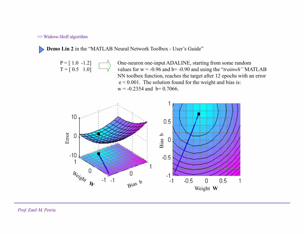
>> Widrow-Hoff algorithm

Demo Lin 2 in the “MATLAB Neural Network Toolbox - User’s Guide”

P = [ 1.0 -1.2]

T = [ 0.5 1.0]

One-neuron one-input ADALINE, starting from some random

values for w = -0.96 and b= -0.90 and using the “trainwh” MATLAB

NN toolbox function, reaches the target after 12 epochs with an error

e < 0.001. The solution found for the weight and bias is:

w = -0.2354 and b= 0.7066.

Err

or

Bia

s b

Weight W


BackBackBackBack----Propagation Learning Propagation Learning Propagation Learning Propagation Learning ---- The Generalized The Generalized The Generalized The Generalized � � � � RuleRuleRuleRule

P. Werbos (Ph.D. thesis 1974);

D. Parker (1985), Yann Le Cun(1985),

D. Rumelhart, G. Hinton, R. Williams (1986)

Two-layer ANN that can approximate

any function with a finite number of

of discontinuities, arbitrarily

well, given sufficient neurons

in the hidden layer.

e2= (t-y2) = (t- purelin

(W2*tansig(W1*p

+b1) +b2))

The error is an indirect

function of the weights

in the hidden layers.

� Back-propagation ANNs often have one or more hidden layers of

sigmoid neurons followed by an output layer of linear neurons.

Linear Neuron Layer

W2

S2xS1

b2

S2x1

z2

S2x1

S2x1

y2

y2 = purelin(W2*y1+b2)

1

y1 = tansig(W1*p+b1)

W1

S1xR

b1

S1x1R

p

Rx1

1

z1

S1x1

S1x1

y1

Input Sigmoid Neuron Layer

ΣΣΣΣ ΣΣΣΣ

� Single layer ANNs are suitable to only solving linearly separable classification problems. Multiple feed-

forward layers can give an ANN greater freedom. Any reasonable function can be modeled by a two layer

architecture: a sigmoid layer feeding a linear output layer.

� Single layer ANNs are only able to solve linearly Widrow-Hoff learning applies to single layer networks.

==> generalized W-H algorithm (∆ -rule) ==> back-propagation learning.


>>Back-Propagation

e = (t - yN)

t

e

R

p

Rx1

Input

Phase I : The input vector is propagated forward (fed-

forward) trough the consecutive layers of the ANN.

y

NSN x 1

Phase II : The errors are recursively back-propagated

trough the layers and appropriate weight changes are

made. Because the output error is an indirect function

of the weights in the hidden layers, we have to use the

“chain rule” of calculus when calculating the derivatives

with respect to the weights and biases in the hidden layers.

These derivatives of the squared error are computed first

at the last (output) layer and then propagated backward

from layer to layer using the “chain rule.”

∆Wj | j= N, N-1, …,1,0

� Back-propagation is an iterative steepest descent algorithm, in which the performance index

is the mean square error E [e2] between the desired response and network’s actual response:


-1 -0.5 0 0.5 1

-1

-0.5

0

0.5

1

Input vector P

Tar

get

vec

tor

T

0 50 100 150 200 250 300 350 400 45010

-2

10-1

100

101

Epochs

Err

or

EXAMPLE: Function Approximation by Back-Propagation

Linear Neuron Layer

W2

S2xS1

b2

S2x1

z2

S2xQ

S2x1

y2

y2 = purelin(W2*y1+b2)

1

y1 = tansig(W1*P+b1)

W1

S1xQ

b1

S1x1Q

P

RxQ

1

z1

S1xQ

S1x1

y1

Input Sigmoid Neuron Layer

ΣΣΣΣ ΣΣΣΣR

S1 S2

R = 1 input

S1 = 5 neurons

in layer #1

S2 = 1 neuron

in layer #2

Q = 21 input

vectors

Demo BP4 in the” MATLAB Neural

Network Toolbox User’s Guide”

The back-propagation algorithm took 454 epochs to

approximate the 21 target vectors with an error < 0.02


Hardware Neural Network

Architectures


ANNs / Neurocomputers ==>architectures optimized for neuron model implementation

� general-purpose, able to emulate a wide range of NN models;

� special-purpose, dedicated to a specific NN model.

ANN VLSI Architectures:

• analog ==> compact,high speed,

asynchronous, no quantization

errors, convenient weight “+”and “X”;

• digital ==> more efifcient VLSI technology,

robust, convenient weight storage;

Pulse Data Representation:

• Pulse Amplitude Modulation (PAM) -

not satisfactory for NN processing;

• Pulse Width Modulation (PWM);

• Pulse Frequency Modulation (PFM).

Number of nodes

0

103

106

109

1012

103 106 109 1012 Node complexity

[VLSI area/node]

RAMs

Special-purpose neurocomputers

General-purpose neurocomputers

Systolic arrays

Computational arays

Conventional parallel

computers

Sequential computers

[from P. Treleaven, M. Pacheco, M. Vellasco,

“VLSI Architectures for Neural Networks,”

IEEE Micro, Dec. 1989, pp. 8-27]

Pulse Stream ANNs: combination of

different pulse data representation methods

and opportunistic use of both analog and

digital implementation techniques.

Hardware NNs consisting of a collection of simple neuron circuits provide the massive

computational parallelism allowing for a higher modelling speed.


HARDWARE NEURAL NETWORK ARCHITECTURES USING RANDOM-PULSE DATA REPRESENTATION

Looking for a model to prove that algebraic operations with analog variables can be performed by

logical gates, von Neuman advanced in 1956 the idea of representing analog variables by the mean

rate of random-pulse streams [J. von Neuman, “Probabilistic logics and the synthesis of reliable

organisms from unreliable components,” in Automata Studies, (C.E. Shannon, Ed.), Princeton, NJ,

Princeton University Press, 1956].

The “random-pulse machine” concept, [S.T. Ribeiro, “Random-pulse machines,” IEEE Trans. Electron.

Comp., vol. EC-16, no. 3, pp. 261-276,1967], a.k.a. "noise computer“, "stochastic computing“, “dithering”

deals with analog variables represented by the mean rate of random-pulse streams allowing to use digital

circuits to perform arithmetic operations. This concept presents a good tradeoff between the electronic

circuit complexity and the computational accuracy. The resulting neural network architecture has a high

packing density and is well suited for very large scale integration (VLSI).

Interactive VE applications require real-time rendering

of complex NN models


ΣF

Y = F [ w X ]Σj=1

m

.j iij

SY

NA

PS

E

SY

NA

PS

E

SY

NA

PS

E

. . .. . . X mX 1 X i

wmj

wij

w1j

Neuron Structure

FS+VFS-V

FS FSXQ

p.d.f.

of VR

1

2 FS.

-FS

+FS

1

V

X

0

-1

VRQ1-BIT QUANTIZER

X-FS

+FS

XQ

X

0

1

-1

XQ

CLOCKCLK

VRP

ANALOG RANDOM

SIGNAL GENERATOR

-FS +FS0

R

p(R)1

2 FS

+

+VR

V

R

One-Bit “Analog / Random Pulse” Converter

� HARDWARE HARDWARE HARDWARE HARDWARE ANNANNANNANN USING RANDOMUSING RANDOMUSING RANDOMUSING RANDOM----PULSE DATA REPRESENTATIONPULSE DATA REPRESENTATIONPULSE DATA REPRESENTATIONPULSE DATA REPRESENTATION

[ E.M. Petriu, K. Watanabe, T. Yeap, "Applications of Random-Pulse Machine Concept toNeural Network Design," IEEE Trans. Instrum. Meas., Vol. 45, No.2, pp.665-669, 1996. ]


CLK

UP

DOWN

PN -BIT

UP/DOWN

COUNTER

D

N -BIT

SHIFT

REGISTER

“Random Pulse / Digital” Converter using a Moving Average Algorithm

>>> Random-Pulse Hardware ANN

1 OUT_OF m

DEMULTIPLEXER

RANDOM NUMBER

GENERATOR

S1SjSm

CLK

Y = (X1+...+Xm)/m

y

x1

xj

xm

X1

Xj

Xm

Random Pulse Addition



SYNAPSE ADDRESS

DECODER

S mpS ijS 11

2 -BIT SHIFT

REGISTER

n

......

wij

RANDOM- PULSE

MULTIPLICATION

DT = w Xij ij

.i

SYNAPSE

MODE

DATIN SYNADD

Xi

Random Pulse Implementation of a Synapse

RANDOM-PULSE/DIGITAL

INTERFACECLK*

ACTIVATION FUNCTION F

DIGITAL/RANDOM-PULSE

CONVERTER

Y = F [ w X ]Σj=1

m

.j iij

... ...

RANDOM-PULSE ADDITION

DTmjDTijDT1j

ΣΣΣΣ

Neuron Body Structure


32 266 5003.2

1

1.2

x2is

x2ditis

x2RQis

42

dZis

dHis

dLis

MAVx2RQis

is

Moving Average ‘Random Pulse -to- Digital ” Conversion



32 266 5008.2

3.5

1.2

x1is

x1RQis

41.5

MAVx1RQis

dZ1is

x2is

3

x2RQis

44.5

MAVx2RQis

3

dZ2is

x1is

x2is

6

SUMRQXis

47.5

MAVSUMRQXis

6

dZSis

dHis

dLis

is


Random Pulse Addition


32 144 2569.2

4

1.2

x1is

x1ditis

x1RQis

42

dZis

dHis

dLis

w1is

3.5

dZis

3.5

W1is

45

x1W1RQis

46.5

MAVx1W1RQis

8

dZis

8

is


Random Pulse Multiplication


� HARDWARE HARDWARE HARDWARE HARDWARE ANNANNANNANN USING MULTIUSING MULTIUSING MULTIUSING MULTI----BIT RANDOMBIT RANDOMBIT RANDOMBIT RANDOM----DATA REPRESENTATIONDATA REPRESENTATIONDATA REPRESENTATIONDATA REPRESENTATION

Generalized b-bit analog/random-data conversion and its quantization characteristics

[ E.M. Petriu, L. Zhao, S.R. Das, and A. Cornell, "Instrumentation Applications of Random-Data Representation," Proc. IMTC/2000, IEEE Instrum. Meas. Technol. Conf., pp. 872-877, Baltimore, MD, May 2000]

[ L. Zhao, "Random Pulse Artificial Neural Network Architecture," M.A.Sc. Thesis, University of Ottawa, 1998]

VR

V

RVRQ

CLOCKCLK

VRP

b-BIT

QUANTIZER

X XQ

ANALOG RANDOM

SIGNAL

GENERATOR

-∆/2 0

R

p(R)

1/∆

+∆/2

+

+

.(k+0.5) ∆(k-0.5) ∆.

XQ

X

k

k+1

k-1

0

β ∆.

1/∆p.d.f.

of VR

∆/2∆/2

β ∆. (1- β) ∆.

.V= (k-β) ∆

k ∆.


0 10 20 30 40 50 60 700

0.02

0.04

0.06

0.08

0.1

0.12

0.14

0.16

0.18

Moving average window size

Mean s

qu

are

err

or

1-Bit

2-Bit

Mean square errors function of the moving average window size

Quantization levels Relative mean square error

2 72.23

3 5.75

4 2.75

... ...

8 1.23

... ...

analog 1


RANDOM

NUMBER

GENERATOR

1-OUT OF-m

DEMULTIPLEXER

.

.

.

.

.

.

CLK

... ... Sm

S1

Si

mX

1X

iX Z =

(X +...+X )/mmi

b

b

b

b

b

b

b

Stochastic adder for random-data.


2-bit random-data multiplier.

Y

X

1

01

-1

10

0

0010-1

-1

10

1

01

0

00011

0

00

0

00

0

00000

100100

-110

XLSB

XMSB Z

LSB

ZMSB

YLSB

YLSB


0 100 200 300 400 500-2

-1

0

1

2multiplication

0 100 200 300 400 500-2

-1

0

1

2

weightinput

product

Example of 2-bit random-data multiplication.


SYNAPSE

ADDRESS

DECODER

S mpS ijS 11

N-STAGE

DELAY

LINE

......

wij

DT = w Xij ij.

i

SYNAPSE

MODE

DATIN SYNADD X i

MULTIPLICATION

b

b

b

b

b

... ...

RANDOM-DATA ADDER

DT mj DT

ij DT 1j

Σ

RANDOM-DATA / DIGITAL

CLK

DIGITAL / RANDOM-DATA

ACTIVATION FUNCTION

F

Y = F [ w X ] j Σ

j=1

m .

i ij

Multi-bit random-data implementation of a neuron body.

Multi-bit random-data implementation of a synapse



Auto-associative memory NN architecture

P1, t1 P2, t2 P3, t3

Training set

30

P

30x1

30x30

n

30x1

a

30x1W

)*hardlim( PWa =

Recovery of 30% occluded patterns


Neural Networks : Basics - University of Ottawapetriu/NN_basics-tutorial.pdf · Neural Networks :...

Documents

Transcript of Neural Networks : Basics - University of Ottawapetriu/NN_basics-tutorial.pdf · Neural Networks :...