Neural Network Toolbox™ Reference - UQAC · Neural Network Toolbox™ Reference R2013a Mark...
473
Neural Network Toolbox™ Reference R2013a Mark Hudson Beale Martin T. Hagan Howard B. Demuth
Transcript of Neural Network Toolbox™ Reference - UQAC · Neural Network Toolbox™ Reference R2013a Mark...
Neural Network Toolbox™
Reference
R2013a
Mark Hudson BealeMartin T. HaganHoward B. Demuth
How to Contact MathWorks
www.mathworks.com Webcomp.soft-sys.matlab Newsgroupwww.mathworks.com/contact_TS.html Technical Support
[email protected] Product enhancement [email protected] Bug [email protected] Documentation error [email protected] Order status, license renewals, [email protected] Sales, pricing, and general information
508-647-7000 (Phone)
508-647-7001 (Fax)
The MathWorks, Inc.3 Apple Hill DriveNatick, MA 01760-2098For contact information about worldwide offices, see the MathWorks Web site.
Neural Network Toolbox™ Reference
© COPYRIGHT 1992–2013 by The MathWorks, Inc.The software described in this document is furnished under a license agreement. The software may be usedor copied only under the terms of the license agreement. No part of this manual may be photocopied orreproduced in any form without prior written consent from The MathWorks, Inc.
FEDERAL ACQUISITION: This provision applies to all acquisitions of the Program and Documentationby, for, or through the federal government of the United States. By accepting delivery of the Programor Documentation, the government hereby agrees that this software or documentation qualifies ascommercial computer software or commercial computer software documentation as such terms are usedor defined in FAR 12.212, DFARS Part 227.72, and DFARS 252.227-7014. Accordingly, the terms andconditions of this Agreement and only those rights specified in this Agreement, shall pertain to and governthe use, modification, reproduction, release, performance, display, and disclosure of the Program andDocumentation by the federal government (or other entity acquiring for or through the federal government)and shall supersede any conflicting contractual terms or conditions. If this License fails to meet thegovernment’s needs or is inconsistent in any respect with federal procurement law, the government agreesto return the Program and Documentation, unused, to The MathWorks, Inc.
Trademarks
MATLAB and Simulink are registered trademarks of The MathWorks, Inc. Seewww.mathworks.com/trademarks for a list of additional trademarks. Other product or brandnames may be trademarks or registered trademarks of their respective holders.
Patents
MathWorks products are protected by one or more U.S. patents. Please seewww.mathworks.com/patents for more information.

Revision HistoryJune 1992 First printingApril 1993 Second printingJanuary 1997 Third printingJuly 1997 Fourth printingJanuary 1998 Fifth printing Revised for Version 3 (Release 11)September 2000 Sixth printing Revised for Version 4 (Release 12)June 2001 Seventh printing Minor revisions (Release 12.1)July 2002 Online only Minor revisions (Release 13)January 2003 Online only Minor revisions (Release 13SP1)June 2004 Online only Revised for Version 4.0.3 (Release 14)October 2004 Online only Revised for Version 4.0.4 (Release 14SP1)October 2004 Eighth printing Revised for Version 4.0.4March 2005 Online only Revised for Version 4.0.5 (Release 14SP2)March 2006 Online only Revised for Version 5.0 (Release 2006a)September 2006 Ninth printing Minor revisions (Release 2006b)March 2007 Online only Minor revisions (Release 2007a)September 2007 Online only Revised for Version 5.1 (Release 2007b)March 2008 Online only Revised for Version 6.0 (Release 2008a)October 2008 Online only Revised for Version 6.0.1 (Release 2008b)March 2009 Online only Revised for Version 6.0.2 (Release 2009a)September 2009 Online only Revised for Version 6.0.3 (Release 2009b)March 2010 Online only Revised for Version 6.0.4 (Release 2010a)September 2010 Online only Revised for Version 7.0 (Release 2010b)April 2011 Online only Revised for Version 7.0.1 (Release 2011a)September 2011 Online only Revised for Version 7.0.2 (Release 2011b)March 2012 Online only Revised for Version 7.0.3 (Release 2012a)September 2012 Online only Revised for Version 8.0 (Release 2012b)March 2013 Online only Revised for Version 8.0.1 (Release 2013a)


Contents
Functions — Alphabetical List
1
Index
v

vi Contents

1
Functions — AlphabeticalList
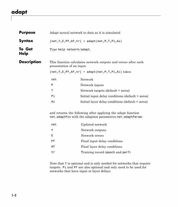
adapt
Purpose Adapt neural network to data as it is simulated
Syntax [net,Y,E,Pf,Af,tr] = adapt(net,P,T,Pi,Ai)
To GetHelp
Type help network/adapt.
Description This function calculates network outputs and errors after eachpresentation of an input.
[net,Y,E,Pf,Af,tr] = adapt(net,P,T,Pi,Ai) takes
net Network
P Network inputs
T Network targets (default = zeros)
Pi Initial input delay conditions (default = zeros)
Ai Initial layer delay conditions (default = zeros)
and returns the following after applying the adapt functionnet.adaptFcn with the adaption parameters net.adaptParam:
net Updated network
Y Network outputs
E Network errors
Pf Final input delay conditions
Af Final layer delay conditions
tr Training record (epoch and perf)
Note that T is optional and is only needed for networks that requiretargets. Pi and Pf are also optional and only need to be used fornetworks that have input or layer delays.
1-2
adapt
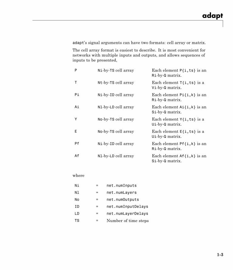
adapt’s signal arguments can have two formats: cell array or matrix.
The cell array format is easiest to describe. It is most convenient fornetworks with multiple inputs and outputs, and allows sequences ofinputs to be presented,
P Ni-by-TS cell array Each element P{i,ts} is anRi-by-Q matrix.
T Nt-by-TS cell array Each element T{i,ts} is aVi-by-Q matrix.
Pi Ni-by-ID cell array Each element Pi{i,k} is anRi-by-Q matrix.
Ai Nl-by-LD cell array Each element Ai{i,k} is anSi-by-Q matrix.
Y No-by-TS cell array Each element Y{i,ts} is aUi-by-Q matrix.
E No-by-TS cell array Each element E{i,ts} is aUi-by-Q matrix.
Pf Ni-by-ID cell array Each element Pf{i,k} is anRi-by-Q matrix.
Af Nl-by-LD cell array Each element Af{i,k} is anSi-by-Q matrix.
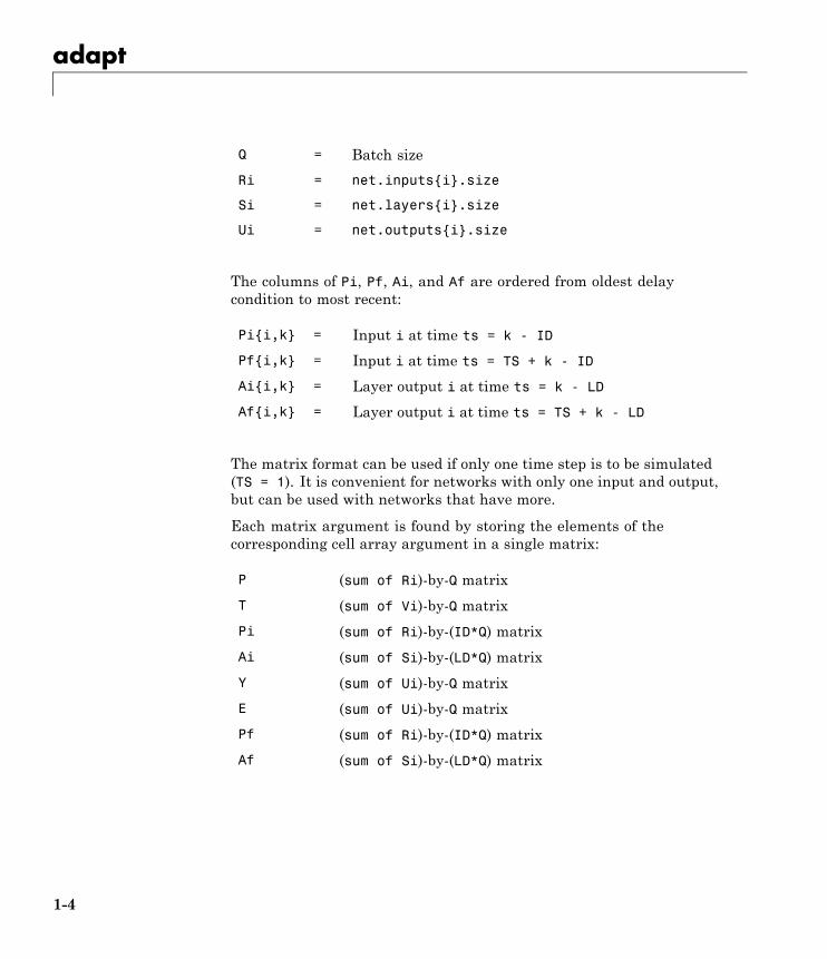
where
Ni = net.numInputs
Nl = net.numLayers
No = net.numOutputs
ID = net.numInputDelays
LD = net.numLayerDelays
TS = Number of time steps
1-3
adapt
Q = Batch size
Ri = net.inputs{i}.size
Si = net.layers{i}.size
Ui = net.outputs{i}.size
The columns of Pi, Pf, Ai, and Af are ordered from oldest delaycondition to most recent:
Pi{i,k} = Input i at time ts = k - ID
Pf{i,k} = Input i at time ts = TS + k - ID
Ai{i,k} = Layer output i at time ts = k - LD
Af{i,k} = Layer output i at time ts = TS + k - LD
The matrix format can be used if only one time step is to be simulated(TS = 1). It is convenient for networks with only one input and output,but can be used with networks that have more.
Each matrix argument is found by storing the elements of thecorresponding cell array argument in a single matrix:
P (sum of Ri)-by-Q matrix
T (sum of Vi)-by-Q matrix
Pi (sum of Ri)-by-(ID*Q) matrix
Ai (sum of Si)-by-(LD*Q) matrix
Y (sum of Ui)-by-Q matrix
E (sum of Ui)-by-Q matrix
Pf (sum of Ri)-by-(ID*Q) matrix
Af (sum of Si)-by-(LD*Q) matrix
1-4
adapt
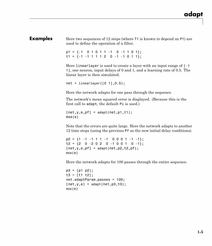
Examples Here two sequences of 12 steps (where T1 is known to depend on P1) areused to define the operation of a filter.
p1 = {-1 0 1 0 1 1 -1 0 -1 1 0 1};t1 = {-1 -1 1 1 1 2 0 -1 -1 0 1 1};
Here linearlayer is used to create a layer with an input range of [-11], one neuron, input delays of 0 and 1, and a learning rate of 0.5. Thelinear layer is then simulated.
net = linearlayer([0 1],0.5);
Here the network adapts for one pass through the sequence.
The network’s mean squared error is displayed. (Because this is thefirst call to adapt, the default Pi is used.)
[net,y,e,pf] = adapt(net,p1,t1);mse(e)
Note that the errors are quite large. Here the network adapts to another12 time steps (using the previous Pf as the new initial delay conditions).
p2 = {1 -1 -1 1 1 -1 0 0 0 1 -1 -1};t2 = {2 0 -2 0 2 0 -1 0 0 1 0 -1};[net,y,e,pf] = adapt(net,p2,t2,pf);mse(e)
Here the network adapts for 100 passes through the entire sequence.
p3 = [p1 p2];t3 = [t1 t2];net.adaptParam.passes = 100;[net,y,e] = adapt(net,p3,t3);mse(e)
1-5
adapt
The error after 100 passes through the sequence is very small. Thenetwork has adapted to the relationship between the input and targetsignals.
Algorithms adapt calls the function indicated by net.adaptFcn, using the adaptionparameter values indicated by net.adaptParam.
Given an input sequence with TS steps, the network is updated asfollows: Each step in the sequence of inputs is presented to the networkone at a time. The network’s weight and bias values are updated aftereach step, before the next step in the sequence is presented. Thus thenetwork is updated TS times.
See Also sim | init | train | revert
1-6
adaptwb
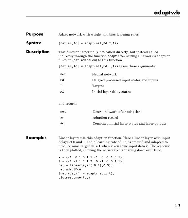
Purpose Adapt network with weight and bias learning rules
Syntax [net,ar,Ac] = adapt(net,Pd,T,Ai)
Description This function is normally not called directly, but instead calledindirectly through the function adapt after setting a network’s adaptionfunction (net.adaptFcn) to this function.
[net,ar,Ac] = adapt(net,Pd,T,Ai) takes these arguments,
net Neural network
Pd Delayed processed input states and inputs
T Targets
Ai Initial layer delay states
and returns
net Neural network after adaption
ar Adaption record
Ac Combined initial layer states and layer outputs
Examples Linear layers use this adaption function. Here a linear layer with inputdelays of 0 and 1, and a learning rate of 0.5, is created and adapted toproduce some target data t when given some input data x. The responseis then plotted, showing the network’s error going down over time.
x = {-1 0 1 0 1 1 -1 0 -1 1 0 1};t = {-1 -1 1 1 1 2 0 -1 -1 0 1 1};net = linearlayer([0 1],0.5);net.adaptFcn[net,y,e,xf] = adapt(net,x,t);plotresponse(t,y)
1-7

adaptwb
See Also adapt
1-8
adddelay
Purpose Add delay to neural network response
Syntax net = adddelay(net,n)
Description net = adddelay(net,n) takes these arguments,
net Neural network
n Number of delays
and returns the network with input delay connections increased, andoutput feedback delays decreased, by the specified number of delays n.The result is a network which behaves identically, except that outputsare produced n timesteps later.
If the number of delays n is not specified, a default of one delay is used.
Examples Here a time delay network is created, trained and simulated in itsoriginal form on an input time series X and target series T. It is thensimulated with a delay removed and then added back. These first andthird outputs will be identical, while the second will be shifted by onetimestep.
[X,T] = simpleseries_dataset;net = timedelaynet(1:2,20);[Xs,Xi,Ai,Ts] = preparets(net,X,T);net = train(net,Xs,Ts,Xi);y1 = net(Xs)net2 = removedelay(net);[Xs,Xi,Ai,Ts] = preparets(net2,X,T);y2 = net2(Xs,Xi)net3 = adddelay(net2)[Xs,Xi,Ai,Ts] = preparets(net3,X,T);y3 = net3(Xs,Xi)
See Also closeloop | openloop | removedelay
1-9
boxdist
Purpose Distance between two position vectors
Syntax d = boxdist(pos)
Description boxdist is a layer distance function that is used to find the distancesbetween the layer’s neurons, given their positions.
d = boxdist(pos) takes one argument,
pos N-by-S matrix of neuron positions
and returns the S-by-S matrix of distances.
boxdist is most commonly used with layers whose topology functionis gridtop.
Examples Here you define a random matrix of positions for 10 neurons arrangedin three-dimensional space and then find their distances.
pos = rand(3,10);d = boxdist(pos)
NetworkUse
To change a network so that a layer’s topology uses boxdist, setnet.layers{i}.distanceFcn to 'boxdist'.
In either case, call sim to simulate the network with boxdist.
Algorithms The box distance D between two position vectors Pi and Pj from a set ofS vectors is
Dij = max(abs(Pi-Pj))
See Also dist | linkdist | mandist | sim
1-10
bttderiv
Purpose Backpropagation through time derivative function
Syntax bttderiv('dperf_dwb',net,X,T,Xi,Ai,EW)bttderiv('de_dwb',net,X,T,Xi,Ai,EW)
Description This function calculates derivatives using the chain rule from anetwork’s performance back through the network, and in the case ofdynamic networks, back through time.
bttderiv('dperf_dwb',net,X,T,Xi,Ai,EW) takes these arguments,
net Neural network
X Inputs, an RxQ matrix (or NxTS cell array of RixQmatrices)
T Targets, an SxQ matrix (or MxTS cell array ofSixQ matrices)
Xi Initial input delay states (optional)
Ai Initial layer delay states (optional)
EW Error weights (optional)
and returns the gradient of performance with respect to the network’sweights and biases, where R and S are the number of input and outputelements and Q is the number of samples (and N and M are the numberof input and output signals, Ri and Si are the number of each input andoutputs elements, and TS is the number of timesteps).
bttderiv('de_dwb',net,X,T,Xi,Ai,EW) returns the Jacobian oferrors with respect to the network’s weights and biases.
Examples Here a feedforward network is trained and both the gradient andJacobian are calculated.
[x,t] = simplefit_dataset;net = feedforwardnet(20);
1-11
bttderiv
net = train(net,x,t);y = net(x);perf = perform(net,t,y);gwb = bttderiv('dperf_dwb',net,x,t)jwb = bttderiv('de_dwb',net,x,t)
See Also defaultderiv | fpderiv | num2deriv | num5deriv | staticderiv
1-12
cascadeforwardnet
Purpose Cascade-forward neural network
Syntax cascadeforwardnet(hiddenSizes,trainFcn)
Description Cascade-forward networks are similar to feed-forward networks,but include a connection from the input and every previous layer tofollowing layers.
As with feed-forward networks, a two-or more layer cascade-networkcan learn any finite input-output relationship arbitrarily well givenenough hidden neurons.
cascadeforwardnet(hiddenSizes,trainFcn) takes these arguments,
hiddenSizes Row vector of one or more hidden layer sizes(default = 10)
trainFcn Training function (default = 'trainlm')
and returns a new cascade-forward neural network.
Examples Here a cascade network is created and trained on a simple fittingproblem.
[x,t] = simplefit_dataset;net = cascadeforwardnet(10);net = train(net,x,t);view(net)y = net(x)perf = perform(net,y,t)
See Also feedforwardnet
1-13
catelements
Purpose Concatenate neural network data elements
Syntax catelements(x1,x2,...,xn)[x1; x2; ... xn]
Description catelements(x1,x2,...,xn) takes any number of neural networkdata values, and merges them along the element dimension (i.e., thematrix row dimension).
If all arguments are matrices, this operation is the same as [x1; x2;... xn].
If any argument is a cell array, then all non-cell array arguments areenclosed in cell arrays, and then the matrices in the same positions ineach argument are concatenated.
Examples This code concatenates the elements of two matrix data values.
x1 = [1 2 3; 4 7 4]x2 = [5 8 2; 4 7 6; 2 9 1]y = catelements(x1,x2)
This code concatenates the elements of two cell array data values.
x1 = {[1:3; 4:6] [7:9; 10:12]; [13:15] [16:18]}x2 = {[2 1 3] [4 5 6]; [2 5 4] [9 7 5]}y = catelements(x1,x2)
See Also nndata | numelements | getelements | setelements | catsignals |catsamples | cattimesteps
1-14
catsamples
Purpose Concatenate neural network data samples
Syntax catsamples(x1,x2,...,xn)[x1 x2 ... xn]catsamples(x1,x2,...,xn,'pad',v)
Description catsamples(x1,x2,...,xn) takes any number of neural network datavalues, and merges them along the samples dimension (i.e., the matrixcolumn dimension).
If all arguments are matrices, this operation is the same as [x1 x2... xn].
If any argument is a cell array, then all non-cell array arguments areenclosed in cell arrays, and then the matrices in the same positions ineach argument are concatenated.
catsamples(x1,x2,...,xn,'pad',v) allows samples with varyingnumbers of timesteps (columns of cell arrays) to be concatenated bypadding the shorter time series with the value v, until they are thesame length as the longest series. If v is not specified, then the valueNaN is used, which is often used to represent unknown or don’t-careinputs or targets.
Examples This code concatenates the samples of two matrix data values.
x1 = [1 2 3; 4 7 4]x2 = [5 8 2; 4 7 6]y = catsamples(x1,x2)
This code concatenates the samples of two cell array data values.
x1 = {[1:3; 4:6] [7:9; 10:12]; [13:15] [16:18]}x2 = {[2 1 3; 5 4 1] [4 5 6; 9 4 8]; [2 5 4] [9 7 5]}y = catsamples(x1,x2)
Here the samples of two cell array data values, with unequal numbersof timesteps, are concatenated.
1-15
catsamples
x1 = {1 2 3 4 5};x2 = {10 11 12};y = catsamples(x1,x2,'pad')
See Also nndata | numsamples | getsamples | setsamples | catelements |catsignals | cattimesteps
1-16
catsignals
Purpose Concatenate neural network data signals
Syntax catsignals(x1,x2,...,xn){x1; x2; ...; xn}
Description catsignals(x1,x2,...,xn) takes any number of neural network datavalues, and merges them along the element dimension (i.e., the cellrow dimension).
If all arguments are matrices, this operation is the same as {x1; x2;...; xn}.
If any argument is a cell array, then all non-cell array arguments areenclosed in cell arrays, and the cell arrays are concatenated as [x1;x2; ...; xn].
Examples This code concatenates the signals of two matrix data values.
x1 = [1 2 3; 4 7 4]x2 = [5 8 2; 4 7 6]y = catsignals(x1,x2)
This code concatenates the signals of two cell array data values.
x1 = {[1:3; 4:6] [7:9; 10:12]; [13:15] [16:18]}x2 = {[2 1 3; 5 4 1] [4 5 6; 9 4 8]; [2 5 4] [9 7 5]}y = catsignals(x1,x2)
See Also nndata | numsignals | getsignals | setsignals | catelements |catsamples | cattimesteps
1-17
cattimesteps
Purpose Concatenate neural network data timesteps
Syntax cattimesteps(x1,x2,...,xn){x1 x2 ... xn}
Description cattimesteps(x1,x2,...,xn) takes any number of neural networkdata values, and merges them along the element dimension (i.e., thecell column dimension).
If all arguments are matrices, this operation is the same as {x1 x2... xn}.
If any argument is a cell array, all non-cell array arguments areenclosed in cell arrays, and the cell arrays are concatenated as [x1x2 ... xn].
Examples This code concatenates the elements of two matrix data values.
x1 = [1 2 3; 4 7 4]x2 = [5 8 2; 4 7 6]y = cattimesteps(x1,x2)
This code concatenates the elements of two cell array data values.
x1 = {[1:3; 4:6] [7:9; 10:12]; [13:15] [16:18]}x2 = {[2 1 3; 5 4 1] [4 5 6; 9 4 8]; [2 5 4] [9 7 5]}y = cattimesteps(x1,x2)
See Also nndata | numtimesteps | gettimesteps | settimesteps |catelements | catsignals | catsamples
1-18
cellmat
Purpose Create cell array of matrices
Syntax cellmat(A,B,C,D,v)
Description cellmat(A,B,C,D,v) takes four integer values and one scalar value v,and returns an A-by-B cell array of C-by-D matrices of value v. If thevalue v is not specified, zero is used.
Examples Here two cell arrays of matrices are created.
cm1 = cellmat(2,3,5,4)cm2 = cellmat(3,4,2,2,pi)
See Also nndata
1-19
closeloop
Purpose Convert neural network open-loop feedback to closed loop
Syntax net = closeloop(net)
Description net = closeloop(net) takes a neural network and closes anyopen-loop feedback. For each feedback output i whose propertynet.outputs{i}.feedbackMode is 'open', it replaces its associatedfeedback input and their input weights with layer weight connectionscoming from the output. The net.outputs{i}.feedbackModeproperty is set to 'closed', and the net.outputs{i}.feedbackInputproperty is set to an empty matrix. Finally, the value ofnet.outputs{i}.feedbackDelays is added to the delays of the feedbacklayer weights (i.e., to the delays values of the replaced input weights).
Examples Here a NARX network is designed in open-loop form and then convertedto closed-loop form.
[X,T] = simplenarx_dataset;net = narxnet(1:2,1:2,10);[Xs,Xi,Ai,Ts] = preparets(net,X,{},T);net = train(net,Xs,Ts,Xi,Ai);view(net)Yopen = net(Xs,Xi,Ai)net = closeloop(net)view(net)[Xs,Xi,Ai,Ts] = preparets(net,X,{},T);Ycloesed = net(Xs,Xi,Ai);
See Also noloop | openloop
1-20
combvec
Purpose Create all combinations of vectors
Syntax combvec(A1,A2...)
Description combvec(A1,A2...) takes any number of inputs,
A1 Matrix of N1 (column) vectors
A2 Matrix of N2 (column) vectors
and returns a matrix of (N1*N2*...) column vectors, where thecolumns consist of all possibilities of A2 vectors, appended to A1 vectors,etc.
Examples a1 = [1 2 3; 4 5 6];a2 = [7 8; 9 10];a3 = combvec(a1,a2)
1-21

compet
Purpose Competitive transfer function
GraphandSymbol
Syntax A = compet(N,FP)info = compet('code')
Description compet is a neural transfer function. Transfer functions calculate alayer’s output from its net input.
A = compet(N,FP) takes N and optional function parameters,
N S-by-Q matrix of net input (column) vectors
FP Struct of function parameters (ignored)
and returns the S-by-Qmatrix A with a 1 in each column where the samecolumn of N has its maximum value, and 0 elsewhere.
info = compet('code') returns information according to the codestring specified:
compet('name') returns the name of this function.
compet('output',FP) returns the [min max] output range.
compet('active',FP) returns the [min max] active input range.
compet('fullderiv') returns 1 or 0, depending on whether dA_dN isS-by-S-by-Q or S-by-Q.
compet('fpnames') returns the names of the function parameters.
compet('fpdefaults') returns the default function parameters.
1-22
compet
Examples Here you define a net input vector N, calculate the output, and plotboth with bar graphs.
n = [0; 1; -0.5; 0.5];a = compet(n);subplot(2,1,1), bar(n), ylabel('n')subplot(2,1,2), bar(a), ylabel('a')
Assign this transfer function to layer i of a network.
net.layers{i}.transferFcn = 'compet';
See Also sim | softmax
1-23
competlayer
Purpose Competitive layer
Syntax competlayer(numClasses,kohonenLR,conscienceLR)
Description Competitive layers learn to classify input vectors into a given number ofclasses, according to similarity between vectors, with a preference forequal numbers of vectors per class.
competlayer(numClasses,kohonenLR,conscienceLR) takes thesearguments,
numClasses Number of classes to classify inputs (default= 5)
kohonenLR Learning rate for Kohonen weights (default =0.01)
conscienceLR Learning rate for conscience bias (default =0.001)
and returns a competitive layer with numClasses neurons.
Examples Here a competitive layer is trained to classify 150 iris flowers into 6classes.
inputs = iris_dataset;net = competlayer(6);net = train(net,inputs);view(net)outputs = net(inputs);classes = vec2ind(outputs);
See Also selforgmap | patternnet | lvqnet
1-24
con2seq
Purpose Convert concurrent vectors to sequential vectors
Syntax S = con2seq(b)S = con2seq(b,TS)
Description Neural Network Toolbox™ software arranges concurrent vectors witha matrix, and sequential vectors with a cell array (where the secondindex is the time step).
con2seq and seq2con allow concurrent vectors to be converted tosequential vectors, and back again.
S = con2seq(b) takes one input,
b R-by-TS matrix
and returns one output,
S 1-by-TS cell array of R-by-1 vectors
S = con2seq(b,TS) can also convert multiple batches,
b N-by-1 cell array of matrices with M*TS columns
TS Time steps
and returns
S N-by-TS cell array of matrices with M columns
Examples Here a batch of three values is converted to a sequence.
p1 = [1 4 2]p2 = con2seq(p1)
1-25

con2seq
Here, two batches of vectors are converted to two sequences with twotime steps.
p1 = {[1 3 4 5; 1 1 7 4]; [7 3 4 4; 6 9 4 1]}p2 = con2seq(p1,2)
See Also seq2con | concur
1-26
concur
Purpose Create concurrent bias vectors
Syntax concur(B,Q)
Description concur(B,Q)
B S-by-1 bias vector (or an Nl-by-1 cell array of vectors)
Q Concurrent size
and returns an S-by-B matrix of copies of B (or an Nl-by-1 cell arrayof matrices).
Examples Here concur creates three copies of a bias vector.
b = [1; 3; 2; -1];concur(b,3)
NetworkUse
To calculate a layer’s net input, the layer’s weighted inputs must becombined with its biases. The following expression calculates the netinput for a layer with the netsum net input function, two input weights,and a bias:
n = netsum(z1,z2,b)
The above expression works if Z1, Z2, and B are all S-by-1 vectors.However, if the network is being simulated by sim (or adapt or train) inresponse to Q concurrent vectors, then Z1 and Z2 will be S-by-Q matrices.Before B can be combined with Z1 and Z2, you must make Q copies of it.
n = netsum(z1,z2,concur(b,q))
See Also con2seq | netprod | netsum | seq2con | sim
1-27
configure
Purpose Configure network inputs and outputs to best match input and targetdata
Syntax net = configure(net,x,t)net = configure(net,x)net = configure(net,'inputs',x,i)net = configure(net,'outputs',t,i)
Description Configuration is the process of setting network input and output sizesand ranges, input preprocessing settings and output postprocessingsettings, and weight initialization settings to match input and targetdata.
Configuration must happen before a network’s weights and biases canbe initialized. Unconfigured networks are automatically configured andinitialized the first time train is called. Alternately, a network canbe configured manually either by calling this function or by settinga network’s input and output sizes, ranges, processing settings, andinitialization settings properties manually.
net = configure(net,x,t) takes input data x and target data t, andconfigures the network’s inputs and outputs to match.
net = configure(net,x) configures only inputs.
net = configure(net,'inputs',x,i) configures the inputs specifiedwith the index vector i. If i is not specified all inputs are configured.
net = configure(net,'outputs',t,i) configures the outputsspecified with the index vector i. If i is not specified all targets areconfigured.
Examples Here a feedforward network is created and manually configured for asimple fitting problem (as opposed to allowing train to configure it).
[x,t] = simplefit_dataset;net = feedforwardnet(20); view(net)net = configure(net,x,t); view(net)
1-28

configure
See Also isconfigured | unconfigure | init | train
1-29
confusion
Purpose Classification confusion matrix
Syntax [c,cm,ind,per] = confusion(targets,outputs)
Description [c,cm,ind,per] = confusion(targets,outputs) takes these values:
targets S-by-Q matrix, where each column vector contains asingle 1 value, with all other elements 0. The indexof the 1 indicates which of S categories that vectorrepresents.
outputs S-by-Q matrix, where each column contains values inthe range [0,1]. The index of the largest element inthe column indicates which of S categories that vectorrepresents.
and returns these values:
c Confusion value = fraction of samples misclassified
cm S-by-S confusion matrix, where cm(i,j) is the numberof samples whose target is the ith class that wasclassified as j
ind S-by-S cell array, where ind{i,j} contains the indices ofsamples with the ith target class, but jth output class
per S-by-4 matrix, where each row summarizes fourpercentages associated with the ith class:
per(i,1) false negative rate
= (false negatives)/(all output negatives)
per(i,2) false positive rate
= (false positives)/(all output positives)
per(i,3) true positive rate
= (true positives)/(all output positives)
per(i,4) true negative rate
= (true negatives)/(all output negatives)
1-30
confusion
[c,cm,ind,per] = confusion(TARGETS,OUTPUTS) takes these values:
targets 1-by-Q vector of 1/0 values representing membership
outputs S-by-Q matrix, of value in [0,1] interval, where valuesgreater than or equal to 0.5 indicate class membership
and returns these values:
c Confusion value = fraction of samples misclassified
cm 2-by-2 confusion matrix
ind 2-by-2 cell array, where ind{i,j} contains the indicesof samples whose target is 1 versus 0, and whose outputwas greater than or equal to 0.5 versus less than 0.5
per 2-by-4 matrix where each ith row represents thepercentage of false negatives, false positives, truepositives, and true negatives for the class andout-of-class
Examples load simpleclass_datasetnet = newpr(simpleclassInputs,simpleclassTargets,20);net = train(net,simpleclassInputs,simpleclassTargets);simpleclassOutputs = sim(net,simpleclassInputs);[c,cm,ind,per] = ...confusion(simpleclassTargets,simpleclassOutputs)
See Also plotconfusion | roc
1-31
convwf
Purpose Convolution weight function
Syntax Z = convwf(W,P)dim = convwf('size',S,R,FP)dw = convwf('dw',W,P,Z,FP)info = convwf('code')
Description Weight functions apply weights to an input to get weighted inputs.
Z = convwf(W,P) returns the convolution of a weight matrix W andan input P.
dim = convwf('size',S,R,FP) takes the layer dimension S, inputdimension R, and function parameters, and returns the weight size.
dw = convwf('dw',W,P,Z,FP) returns the derivative of Z with respectto W.
info = convwf('code') returns information about this function. Thefollowing codes are defined:
'deriv' Name of derivative function
'fullderiv' Reduced derivative = 2, full derivative = 1,linear derivative = 0
'pfullderiv' Input: reduced derivative = 2, full derivative =1, linear derivative = 0
'wfullderiv' Weight: reduced derivative = 2, full derivative= 1, linear derivative = 0
'name' Full name
'fpnames' Returns names of function parameters
'fpdefaults' Returns default function parameters
Examples Here you define a random weight matrix W and input vector P andcalculate the corresponding weighted input Z.
1-32
convwf
W = rand(4,1);P = rand(8,1);Z = convwf(W,P)
NetworkUse
To change a network so an input weight uses convwf, setnet.inputWeight{i,j}.weightFcn to 'convwf'. For a layer weight,set net.layerWeight{i,j}.weightFcn to 'convwf'.
In either case, call sim to simulate the network with convwf.
1-33
defaultderiv
Purpose Default derivative function
Syntax defaultderiv('dperf_dwb',net,X,T,Xi,Ai,EW)defaultderiv('de_dwb',net,X,T,Xi,Ai,EW)
Description This function chooses the recommended derivative algorithm for thetype of network whose derivatives are being calculated. For staticnetworks, defaultderiv calls staticderiv; for dynamic networks itcalls bttderiv to calculate the gradient and fpderiv to calculate theJacobian.
defaultderiv('dperf_dwb',net,X,T,Xi,Ai,EW) takes thesearguments,
net Neural network
X Inputs, an R-by-Q matrix (or N-by-TS cell array ofRi-by-Q matrices)
T Targets, an S-by-Q matrix (or M-by-TS cell array ofSi-by-Q matrices)
Xi Initial input delay states (optional)
Ai Initial layer delay states (optional)
EW Error weights (optional)
and returns the gradient of performance with respect to the network’sweights and biases, where R and S are the number of input and outputelements and Q is the number of samples (or N and M are the number ofinput and output signals, Ri and Si are the number of each input andoutputs elements, and TS is the number of timesteps).
defaultderiv('de_dwb',net,X,T,Xi,Ai,EW) returns the Jacobian oferrors with respect to the network’s weights and biases.
Examples Here a feedforward network is trained and both the gradient andJacobian are calculated.
1-34
defaultderiv
[x,t] = simplefit_dataset;net = feedforwardnet(10);net = train(net,x,t);y = net(x);perf = perform(net,t,y);dwb = defaultderiv('dperf_dwb',net,x,t)
See Also bttderiv | fpderiv | num2deriv | num5deriv | staticderiv
1-35
disp
Purpose Neural network properties
Syntax disp(net)
To GetHelp
Type help network/disp.
Description disp(net) displays a network’s properties.
Examples Here a perceptron is created and displayed.
net = newp([-1 1; 0 2],3);disp(net)
See Also display | sim | init | train | adapt
1-36
display
Purpose Name and properties of neural network variables
Syntax display(net)
To GetHelp
Type help network/display.
Description display(net) displays a network variable’s name and properties.
Examples Here a perceptron variable is defined and displayed.
net = newp([-1 1; 0 2],3);display(net)
display is automatically called as follows:
net
See Also disp | sim | init | train | adapt
1-37
dist
Purpose Euclidean distance weight function
Syntax Z = dist(W,P,FP)dim = dist('size',S,R,FP)dw = dist('dw',W,P,Z,FP)D = dist(pos)info = dist('code')
Description Weight functions apply weights to an input to get weighted inputs.
Z = dist(W,P,FP) takes these inputs,
W S-by-R weight matrix
P R-by-Q matrix of Q input (column) vectors
FP Struct of function parameters (optional,ignored)
and returns the S-by-Q matrix of vector distances.
dim = dist('size',S,R,FP) takes the layer dimension S, inputdimension R, and function parameters, and returns the weight size[S-by-R].
dw = dist('dw',W,P,Z,FP) returns the derivative of Z with respectto W.
dist is also a layer distance function which can be used to find thedistances between neurons in a layer.
D = dist(pos) takes one argument,
pos N-by-S matrix of neuron positions
and returns the S-by-S matrix of distances.
info = dist('code') returns information about this function. Thefollowing codes are supported:
1-38
dist
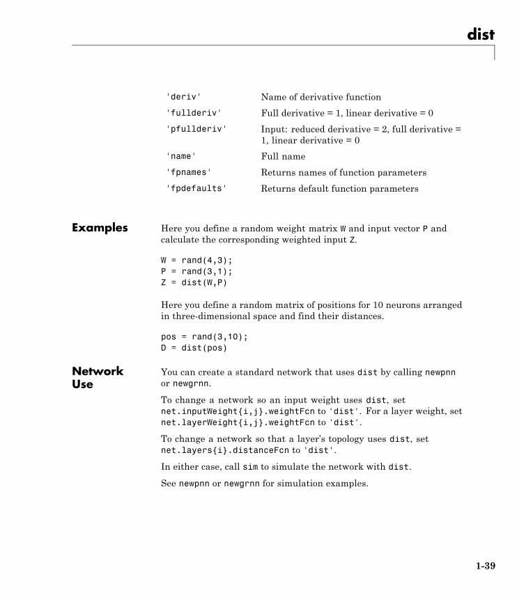
'deriv' Name of derivative function
'fullderiv' Full derivative = 1, linear derivative = 0
'pfullderiv' Input: reduced derivative = 2, full derivative =1, linear derivative = 0
'name' Full name
'fpnames' Returns names of function parameters
'fpdefaults' Returns default function parameters
Examples Here you define a random weight matrix W and input vector P andcalculate the corresponding weighted input Z.
W = rand(4,3);P = rand(3,1);Z = dist(W,P)
Here you define a random matrix of positions for 10 neurons arrangedin three-dimensional space and find their distances.
pos = rand(3,10);D = dist(pos)
NetworkUse
You can create a standard network that uses dist by calling newpnnor newgrnn.
To change a network so an input weight uses dist, setnet.inputWeight{i,j}.weightFcn to 'dist'. For a layer weight, setnet.layerWeight{i,j}.weightFcn to 'dist'.
To change a network so that a layer’s topology uses dist, setnet.layers{i}.distanceFcn to 'dist'.
In either case, call sim to simulate the network with dist.
See newpnn or newgrnn for simulation examples.
1-39

dist
Algorithms The Euclidean distance d between two vectors X and Y is
d = sum((x-y).^2).^0.5
See Also sim | dotprod | negdist | normprod | mandist | linkdist
1-40
distdelaynet
Purpose Distributed delay network
Syntax distdelaynet(delays,hiddenSizes,trainFcn)
Description Distributed delay networks are similar to feedforward networks, exceptthat each input and layer weights has a tap delay line associated withit. This allows the network to have a finite dynamic response to timeseries input data. This network is also similar to the time delay neuralnetwork (timedelaynet), which only has delays on the input weight.
distdelaynet(delays,hiddenSizes,trainFcn) takes thesearguments,
delays Row vector of increasing 0 or positive delays(default = 1:2)
hiddenSizes Row vector of one or more hidden layer sizes(default = 10)
trainFcn Training function (default = 'trainlm')
and returns a distributed delay neural network.
Examples Here a distributed delay neural network is used to solve a simple timeseries problem.
[X,T] = simpleseries_dataset;net = distdelaynet({1:2,1:2},10)[Xs,Xi,Ai,Ts] = preparets(net,X,T)net = train(net,Xs,Ts,Xi,Ai);view(net)Y = net(Xs,Xi,Ai);perf = perform(net,Y,Ts)
See Also preparets | removedelay | timedelaynet | narnet | narxnet
1-41
divideblock
Purpose Divide targets into three sets using blocks of indices
Syntax [trainInd,valInd,testInd] = divideblock(Q,trainRatio,valRatio,testRatio)
Description [trainInd,valInd,testInd] =divideblock(Q,trainRatio,valRatio,testRatio) separatestargets into three sets: training, validation, and testing. It takesthe following inputs:
Q Number of targets to divide up.
trainRatio Ratio of targets for training. Default = 0.7.
valRatio Ratio of targets for validation. Default = 0.15.
testRatio Ratio of targets for testing. Default = 0.15.
and returns
trainInd Training indices
valInd Validation indices
testInd Test indices
Examples [trainInd,valInd,testInd] = divideblock(3000,0.6,0.2,0.2);
NetworkUse
Here are the network properties that define which data divisionfunction to use, what its parameters are, and what aspects of targetsare divided up, when train is called.
net.divideFcnnet.divideParamnet.divideMode
See Also divideind | divideint | dividerand | dividetrain
1-42
divideind
Purpose Divide targets into three sets using specified indices
Syntax [trainInd,valInd,testInd] = divideind(Q,trainInd,valInd,testInd)
Description [trainInd,valInd,testInd] =divideind(Q,trainInd,valInd,testInd) separates targets into threesets: training, validation, and testing, according to indices provided. Itactually returns the same indices it receives as arguments; its purposeis to allow the indices to be used for training, validation, and testing fora network to be set manually.
It takes the following inputs,
Q Number of targets to divide up
trainInd Training indices
valInd Validation indices
testInd Test indices
and returns
trainInd Training indices (unchanged)
valInd Validation indices (unchanged)
testInd Test indices (unchanged)
Examples [trainInd,valInd,testInd] = ...divideind(3000,1:2000,2001:2500,2501:3000);
NetworkUse
Here are the network properties that define which data divisionfunction to use, what its parameters are, and what aspects of targetsare divided up, when train is called.
1-43

divideind
net.divideFcnnet.divideParamnet.divideMode
See Also divideblock | divideint | dividerand | dividetrain
1-44
divideint
Purpose Divide targets into three sets using interleaved indices
Syntax [trainInd,valInd,testInd] = divideint(Q,trainRatio,valRatio,testRatio)
Description [trainInd,valInd,testInd] =divideint(Q,trainRatio,valRatio,testRatio) separatestargets into three sets: training, validation, and testing. It takesthe following inputs,
Q Number of targets to divide up.
trainRatio Ratio of vectors for training. Default = 0.7.
valRatio Ratio of vectors for validation. Default = 0.15.
testRatio Ratio of vectors for testing. Default = 0.15.
and returns
trainInd Training indices
valInd Validation indices
testInd Test indices
Examples [trainInd,valInd,testInd] = divideint(3000,0.6,0.2,0.2);
NetworkUse
Here are the network properties that define which data divisionfunction to use, what its parameters are, and what aspects of targetsare divided up, when train is called.
net.divideFcnnet.divideParamnet.divideMode
See Also divideblock | divideind | dividerand | dividetrain
1-45
dividerand
Purpose Divide targets into three sets using random indices
Syntax [trainInd,valInd,testInd] = dividerand(Q,trainRatio,valRatio,testRatio)
Description [trainInd,valInd,testInd] =dividerand(Q,trainRatio,valRatio,testRatio) separatestargets into three sets: training, validation, and testing. It takesthe following inputs,
Q Number of targets to divide up.
trainRatio Ratio of vectors for training. Default = 0.7.
valRatio Ratio of vectors for validation. Default = 0.15.
testRatio Ratio of vectors for testing. Default = 0.15.
and returns
trainInd Training indices
valInd Validation indices
testInd Test indices
Examples [trainInd,valInd,testInd] = dividerand(3000,0.6,0.2,0.2);
NetworkUse
Here are the network properties that define which data divisionfunction to use, what its parameters are, and what aspects of targetsare divided up, when train is called.
net.divideFcnnet.divideParamnet.divideMode
See Also divideblock | divideind | divideint | dividetrain
1-46
dividetrain
Purpose Assign all targets to training set
Syntax [trainInd,valInd,testInd] = dividetrain(Q,trainRatio,valRatio,testRatio)
Description [trainInd,valInd,testInd] =dividetrain(Q,trainRatio,valRatio,testRatio) assigns all targetsto the training set and no targets to either the validation or test sets. Ittakes the following inputs,
Q Number of targets to divide up.
and returns
trainInd Training indices equal to 1:Q
valInd Empty validation indices, []
testInd Empty test indices, []
Examples [trainInd,valInd,testInd] = dividetrain(3000);
NetworkUse
Here are the network properties that define which data divisionfunction to use, what its parameters are, and what aspects of targetsare divided up, when train is called.
net.divideFcnnet.divideParamnet.divideMode
See Also divideblock | divideind | divideint | dividerand
1-47
dotprod
Purpose Dot product weight function
Syntax Z = dotprod(W,P,FP)dim = dotprod('size',S,R,FP)dw = dotprod('dw',W,P,Z,FP)info = dotprod('code')
Description Weight functions apply weights to an input to get weighted inputs.
Z = dotprod(W,P,FP) takes these inputs,
W S-by-R weight matrix
P R-by-Q matrix of Q input (column) vectors
FP Struct of function parameters (optional,ignored)
and returns the S-by-Q dot product of W and P.
dim = dotprod('size',S,R,FP) takes the layer dimension S, inputdimension R, and function parameters, and returns the weight size[S-by-R].
dw = dotprod('dw',W,P,Z,FP) returns the derivative of Z with respectto W.
info = dotprod('code') returns information about this function.The following codes are defined:
'deriv' Name of derivative function
'pfullderiv' Input: reduced derivative = 2, full derivative =1, linear derivative = 0
'wfullderiv' Weight: reduced derivative = 2, full derivative= 1, linear derivative = 0
1-48
dotprod
'name' Full name
'fpnames' Returns names of function parameters
'fpdefaults' Returns default function parameters
Examples Here you define a random weight matrix W and input vector P andcalculate the corresponding weighted input Z.
W = rand(4,3);P = rand(3,1);Z = dotprod(W,P)
NetworkUse
You can create a standard network that uses dotprod by callingfeedforwardnet.
To change a network so an input weight uses dotprod, setnet.inputWeight{i,j}.weightFcn to 'dotprod'. For a layer weight,set net.layerWeight{i,j}.weightFcn to 'dotprod'.
In either case, call sim to simulate the network with dotprod.
See Also sim | dist | feedforwardnet | negdist | normprod
1-49
elliotsig
Purpose Elliot symmetric sigmoid transfer function
Syntax A = elliotsig(N)
Description Transfer functions convert a neural network layer’s net input into itsnet output.
A = elliotsig(N) takes an S-by-Q matrix of S N-element net inputcolumn vectors and returns an S-by-Q matrix A of output vectors, whereeach element of N is squashed from the interval [-inf inf] to theinterval [-1 1] with an “S-shaped” function.
The advantage of this transfer function over other sigmoids is that it isfast to calculate on simple computing hardware as it does not requireany exponential or trigonometric functions. Its disadvantage is that itonly flattens out for large inputs, so its effect is not as local as othersigmoid functions. This might result in more training iterations, orrequire more neurons to achieve the same accuracy.
Examples Calculate a layer output from a single net input vector:
n = [0; 1; -0.5; 0.5];a = elliotsig(n);
Plot the transfer function:
n = -5:0.01:5;plot(n, elliotsig(n))set(gca,'dataaspectratio',[1 1 1],'xgrid','on','ygrid','on')
For a network you have already defined, change the transfer functionfor layer i:
net.layers{i}.transferFcn = 'elliotsig';
See Also elliot2sig | logsig | tansig
1-50
elliot2sig
Purpose Elliot 2 symmetric sigmoid transfer function
Syntax A = elliot2sig(N)
Description Transfer functions convert a neural network layer’s net input into itsnet output. This function is a variation on the original Elliot sigmoidfunction. It has a steeper slope, closer to tansig, but is not as smooth atthe center.
A = elliot2sig(N) takes an S-by-Q matrix of S N-element net inputcolumn vectors and returns an S-by-Q matrix A of output vectors, whereeach element of N is squashed from the interval [-inf inf] to theinterval [-1 1] with an “S-shaped” function.
The advantage of this transfer function over other sigmoids is that it isfast to calculate on simple computing hardware as it does not requireany exponential or trigonometric functions. Its disadvantage is that itdeparts from the classic sigmoid shape around zero.
Examples Calculate a layer output from a single net input vector:
n = [0; 1; -0.5; 0.5];a = elliot2sig(n);
Plot the transfer function:
n = -5:0.01:5;plot(n, elliot2sig(n))set(gca,'dataaspectratio',[1 1 1],'xgrid','on','ygrid','on')
For a network you have already defined, change the transfer functionfor layer i:
net.layers{i}.transferFcn = 'elliot2sig';
See Also elliotsig | logsig | tansig
1-51
elmannet
Purpose Elman neural network
Syntax elmannet(layerdelays,hiddenSizes,trainFcn)
Description Elman networks are feedforward networks (feedforwardnet) with theaddition of layer recurrent connections with tap delays.
With the availability of full dynamic derivative calculations (fpderivand bttderiv), the Elman network is no longer recommended except forhistorical and research purposes. For more accurate learning try timedelay (timedelaynet), layer recurrent (layrecnet), NARX (narxnet),and NAR (narnet) neural networks.
Elman networks with one or more hidden layers can learn any dynamicinput-output relationship arbitrarily well, given enough neurons in thehidden layers. However, Elman networks use simplified derivativecalculations (using staticderiv, which ignores delayed connections) atthe expense of less reliable learning.
elmannet(layerdelays,hiddenSizes,trainFcn) takes thesearguments,
layerdelays Row vector of increasing 0 or positive delays(default = 1:2)
hiddenSizes Row vector of one or more hidden layer sizes(default = 10)
trainFcn Training function (default = 'trainlm')
and returns an Elman neural network.
Examples Here an Elman neural network is used to solve a simple time seriesproblem.
[X,T] = simpleseries_dataset;net = elmannet(1:2,10);[Xs,Xi,Ai,Ts] = preparets(net,X,T);
1-52
elmannet
net = train(net,Xs,Ts,Xi,Ai);view(net)Y = net(Xs,Xi,Ai);perf = perform(net,Ts,Y)
See Also preparets | removedelay | timedelaynet | layrecnet | narnet| narxnet
1-53
errsurf
Purpose Error surface of single-input neuron
Syntax errsurf(P,T,WV,BV,F)
Description errsurf(P,T,WV,BV,F) takes these arguments,
P 1-by-Q matrix of input vectors
T 1-by-Q matrix of target vectors
WV Row vector of values of W
BV Row vector of values of B
F Transfer function (string)
and returns a matrix of error values over WV and BV.
Examples p = [-6.0 -6.1 -4.1 -4.0 +4.0 +4.1 +6.0 +6.1];t = [+0.0 +0.0 +.97 +.99 +.01 +.03 +1.0 +1.0];wv = -1:.1:1; bv = -2.5:.25:2.5;es = errsurf(p,t,wv,bv,'logsig');plotes(wv,bv,es,[60 30])
See Also plotes
1-54
extendts
Purpose Extend time series data to given number of timesteps
Syntax extendts(x,ts,v)
Description extendts(x,ts,v) takes these values,
x Neural network time series data
ts Number of timesteps
v Value
and returns the time series data either extended or truncated tomatch the specified number of timesteps. If the value v is specified,then extended series are filled in with that value, otherwise they areextended with random values.
Examples Here, a 20-timestep series is created and then extended to 25 timestepswith the value zero.
x = nndata(5,4,20);y = extendts(x,25,0)
See Also nndata | catsamples | preparets
1-55
feedforwardnet
Purpose Feedforward neural network
Syntax feedforwardnet(hiddenSizes,trainFcn)
Description Feedforward networks consist of a series of layers. The first layerhas a connection from the network input. Each subsequent layer hasa connection from the previous layer. The final layer produces thenetwork’s output.
Feedforward networks can be used for any kind of input to outputmapping. A feedforward network with one hidden layer and enoughneurons in the hidden layers, can fit any finite input-output mappingproblem.
Specialized versions of the feedforward network include fitting(fitnet) and pattern recognition (patternnet) networks. Avariation on the feedforward network is the cascade forward network(cascadeforwardnet) which has additional connections from the inputto every layer, and from each layer to all following layers.
feedforwardnet(hiddenSizes,trainFcn) takes these arguments,
hiddenSizes Row vector of one or more hidden layer sizes(default = 10)
trainFcn Training function (default = 'trainlm')
and returns a feedforward neural network.
Examples Here a feedforward neural network is used to solve a simple problem.
[x,t] = simplefit_dataset;net = feedforwardnet(10)net = train(net,x,t);view(net)y = net(x);perf = perform(net,y,t)
1-56

feedforwardnet
See Also fitnet | patternnet | cascadeforwardnet
1-57
fitnet
Purpose Function fitting neural network
Syntax fitnet(hiddenSizes,trainFcn)
Description Fitting networks are feedforward neural networks (feedforwardnet)used to fit an input-output relationship.
fitnet(hiddenSizes,trainFcn) takes these arguments,
hiddenSizes Row vector of one or more hidden layer sizes(default = 10)
trainFcn Training function (default = 'trainlm')
and returns a fitting neural network.
Examples Here a fitting neural network is used to solve a simple problem.
[x,t] = simplefit_dataset;net = fitnet(10)net = train(net,x,t);view(net)y = net(x);perf = perform(net,y,t)
See Also feedforwardnet | nftool
1-58
fixunknowns
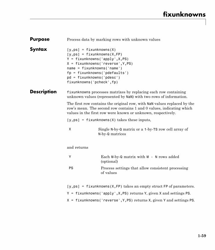
Purpose Process data by marking rows with unknown values
Syntax [y,ps] = fixunknowns(X)[y,ps] = fixunknowns(X,FP)Y = fixunknowns('apply',X,PS)X = fixunknowns('reverse',Y,PS)name = fixunknowns('name')fp = fixunknowns('pdefaults')pd = fixunknowns('pdesc')fixunknowns('pcheck',fp)
Description fixunknowns processes matrixes by replacing each row containingunknown values (represented by NaN) with two rows of information.
The first row contains the original row, with NaN values replaced by therow’s mean. The second row contains 1 and 0 values, indicating whichvalues in the first row were known or unknown, respectively.
[y,ps] = fixunknowns(X) takes these inputs,
X Single N-by-Q matrix or a 1-by-TS row cell array ofN-by-Q matrices
and returns
Y Each M-by-Q matrix with M - N rows added(optional)
PS Process settings that allow consistent processingof values
[y,ps] = fixunknowns(X,FP) takes an empty struct FP of parameters.
Y = fixunknowns('apply',X,PS) returns Y, given X and settings PS.
X = fixunknowns('reverse',Y,PS) returns X, given Y and settings PS.
1-59
fixunknowns
name = fixunknowns('name') returns the name of this processmethod.
fp = fixunknowns('pdefaults') returns the default processparameter structure.
pd = fixunknowns('pdesc') returns the process parameterdescriptions.
fixunknowns('pcheck',fp) throws an error if any parameter is illegal.
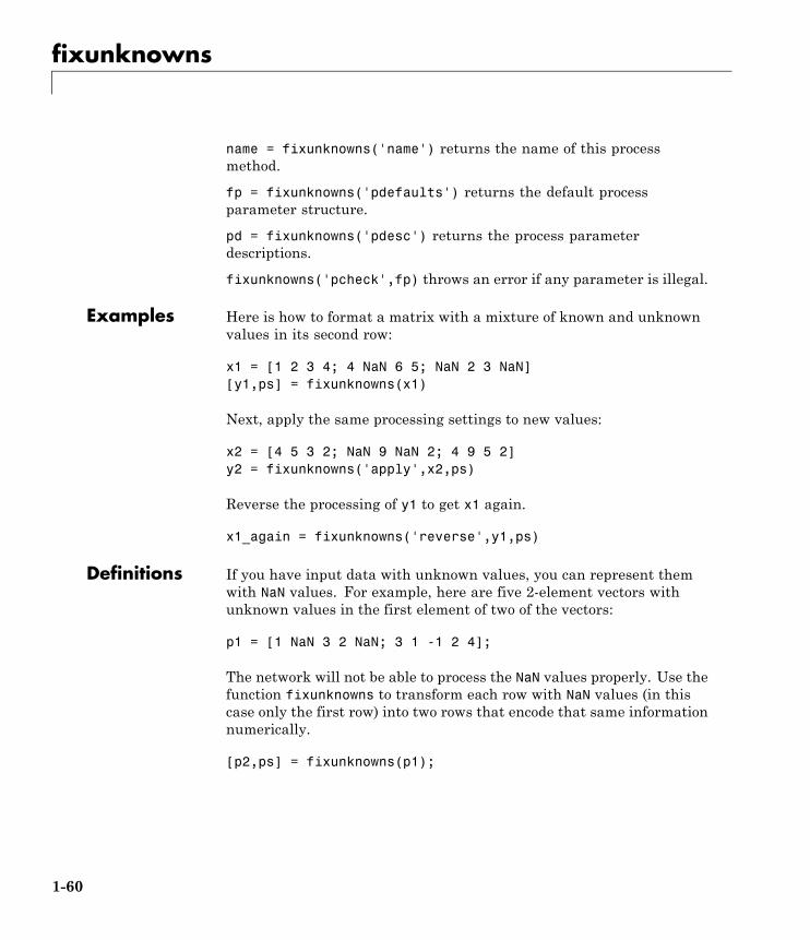
Examples Here is how to format a matrix with a mixture of known and unknownvalues in its second row:
x1 = [1 2 3 4; 4 NaN 6 5; NaN 2 3 NaN][y1,ps] = fixunknowns(x1)
Next, apply the same processing settings to new values:
x2 = [4 5 3 2; NaN 9 NaN 2; 4 9 5 2]y2 = fixunknowns('apply',x2,ps)
Reverse the processing of y1 to get x1 again.
x1_again = fixunknowns('reverse',y1,ps)
Definitions If you have input data with unknown values, you can represent themwith NaN values. For example, here are five 2-element vectors withunknown values in the first element of two of the vectors:
p1 = [1 NaN 3 2 NaN; 3 1 -1 2 4];
The network will not be able to process the NaN values properly. Use thefunction fixunknowns to transform each row with NaN values (in thiscase only the first row) into two rows that encode that same informationnumerically.
[p2,ps] = fixunknowns(p1);
1-60
fixunknowns
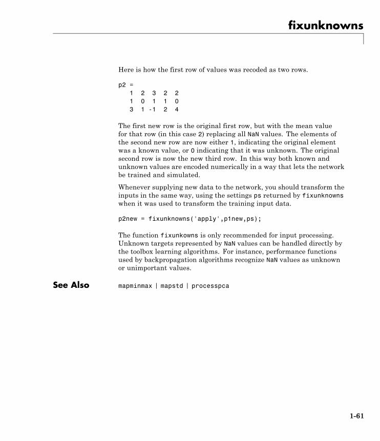
Here is how the first row of values was recoded as two rows.
p2 =1 2 3 2 21 0 1 1 03 1 -1 2 4
The first new row is the original first row, but with the mean valuefor that row (in this case 2) replacing all NaN values. The elements ofthe second new row are now either 1, indicating the original elementwas a known value, or 0 indicating that it was unknown. The originalsecond row is now the new third row. In this way both known andunknown values are encoded numerically in a way that lets the networkbe trained and simulated.
Whenever supplying new data to the network, you should transform theinputs in the same way, using the settings ps returned by fixunknownswhen it was used to transform the training input data.
p2new = fixunknowns('apply',p1new,ps);
The function fixunkowns is only recommended for input processing.Unknown targets represented by NaN values can be handled directly bythe toolbox learning algorithms. For instance, performance functionsused by backpropagation algorithms recognize NaN values as unknownor unimportant values.
See Also mapminmax | mapstd | processpca
1-61
formwb
Purpose Form bias and weights into single vector
Syntax formwb(net,b,IW,LW)
Description formwb(net,b,IW,LW) takes a neural network and bias b, input weightIW, and layer weight LW values, and combines the values into a singlevector.
Examples Here a network is created, configured, and its weights and biasesformed into a vector.
[x,t] = simplefit_dataset;net = feedforwardnet(10);net = configure(net,x,t);wb = formwb(net,net.b,net.IW,net.LW)
See Also getwb | setwb | separatewb
1-62
fpderiv
Purpose Forward propagation derivative function
Syntax fpderiv('dperf_dwb',net,X,T,Xi,Ai,EW)fpderiv('de_dwb',net,X,T,Xi,Ai,EW)
Description This function calculates derivatives using the chain rule from inputs tooutputs, and in the case of dynamic networks, forward through time.
fpderiv('dperf_dwb',net,X,T,Xi,Ai,EW) takes these arguments,
net Neural network
X Inputs, an R-by-Q matrix (or N-by-TS cell array ofRi-by-Q matrices)
T Targets, an S-by-Q matrix (or M-by-TS cell array ofSi-by-Q matrices)
Xi Initial input delay states (optional)
Ai Initial layer delay states (optional)
EW Error weights (optional)
and returns the gradient of performance with respect to the network’sweights and biases, where R and S are the number of input and outputelements and Q is the number of samples (or N and M are the number ofinput and output signals, Ri and Si are the number of each input andoutputs elements, and TS is the number of timesteps).
fpderiv('de_dwb',net,X,T,Xi,Ai,EW) returns the Jacobian of errorswith respect to the network’s weights and biases.
Examples Here a feedforward network is trained and both the gradient andJacobian are calculated.
[x,t] = simplefit_dataset;net = feedforwardnet(20);net = train(net,x,t);
1-63
fpderiv
y = net(x);perf = perform(net,t,y);gwb = fpderiv('dperf_dwb',net,x,t)jwb = fpderiv('de_dwb',net,x,t)
See Also bttderiv | defaultderiv | num2deriv | num5deriv | staticderiv
1-64
fromnndata
Purpose Convert data from standard neural network cell array form
Syntax fromnndata(x,toMatrix,columnSample,cellTime)
Description fromnndata(x,toMatrix,columnSample,cellTime) takes thesearguments,
net Neural network
toMatrix True if result is to be in matrix form
columnSample True if samples are to be represented as columns,false if rows
cellTime True if time series are to be represented as a cellarray, false if represented with a matrix
and returns the original data reformatted accordingly.
Examples Here time-series data is converted from a matrix representation tostandard cell array representation, and back. The original data consistsof a 5-by-6 matrix representing one time-series sample consisting ofa 5-element vector over 6 timesteps arranged in a matrix with thesamples as columns.
x = rands(5,6)columnSamples = true; % samples are by columns.cellTime = false; % time-steps represented by a matrix, not cell.[y,wasMatrix] = tonndata(x,columnSamples,cellTime)x2 = fromnndata(y,wasMatrix,columnSamples,cellTime)
Here data is defined in standard neural network data cell form.Converting this data does not change it. The data consists of three timeseries samples of 2-element signals over 3 timesteps.
x = {rands(2,3); rands(2,3); rands(2,3)}columnSamples = true;cellTime = true;[y,wasMatrix] = tonndata(x)
1-65

fromnndata
x2 = fromnndata(y,wasMatrix,columnSamples)
See Also tonndata
1-66
gadd
Purpose Generalized addition
Syntax gadd(a,b)
Description This function generalizes matrix addition to the addition of cell arraysof matrices combined in an element-wise fashion.
gadd(a,b) takes two matrices or cell arrays, and adds them in anelement-wise manner.
Examples Here matrix and cell array values are added.
gadd([1 2 3; 4 5 6],[10;20])gadd({1 2; 3 4},{1 3; 5 2})gadd({1 2 3 4},{10;20;30})
See Also gsubtract | gmultiply | gdivide | gnegate | gsqrt
1-67
gdivide
Purpose Generalized division
Syntax gdivide(a,b)
Description This function generalizes matrix element-wise division to the division ofcell arrays of matrices combined in an element-wise fashion.
gdivide(a,b) takes two matrices or cell arrays, and divides them inan element-wise manner.
Examples Here matrix and cell array values are added.
gdivide([1 2 3; 4 5 6],[10;20])gdivide({1 2; 3 4},{1 3; 5 2})gdivide({1 2 3 4},{10;20;30})
See Also gadd | gsubtract | gmultiply | gnegate | gsqrt
1-68
gensim
Purpose Generate Simulink block for neural network simulation
Syntax gensim(net,st)
To GetHelp
Type help network/gensim.
Description gensim(net,st) creates a Simulink® system containing a block thatsimulates neural network net.
gensim(net,st) takes these inputs:
net Neural network
st Sample time (default = 1)
and creates a Simulink system containing a block that simulates neuralnetwork net with a sampling time of st.
If net has no input or layer delays (net.numInputDelays andnet.numLayerDelays are both 0), you can use –1 for st to get a networkthat samples continuously.
Examples [x,t] = simplefit_dataset;net = feedforwardnet(10);net = train(net,x,t)gensim(net)
1-69
getelements
Purpose Get neural network data elements
Syntax getelements(x,ind)
Description getelements(x,ind) returns the elements of neural network data xindicated by the indices ind. The neural network data may be in matrixor cell array form.
If x is a matrix, the result is the ind rows of x.
If x is a cell array, the result is a cell array with as many columnsas x, whose elements (1,i) are matrices containing the ind rows of[x{:,i}].
Examples This code gets elements 1 and 3 from matrix data:
x = [1 2 3; 4 7 4]y = getelements(x,[1 3])
This code gets elements 1 and 3 from cell array data:
x = {[1:3; 4:6] [7:9; 10:12]; [13:15] [16:18]}y = getelements(x,[1 3])
See Also nndata | numelements | setelements | catelements | getsamples |gettimesteps | getsignals
1-70
getsamples
Purpose Get neural network data samples
Syntax getsamples(x,ind)
Description getsamples(x,ind) returns the samples of neural network data xindicated by the indices ind. The neural network data may be in matrixor cell array form.
If x is a matrix, the result is the ind columns of x.
If x is a cell array, the result is a cell array the same size as x, whoseelements are the ind columns of the matrices in x.
Examples This code gets samples 1 and 3 from matrix data:
x = [1 2 3; 4 7 4]y = getsamples(x,[1 3])
This code gets elements 1 and 3 from cell array data:
x = {[1:3; 4:6] [7:9; 10:12]; [13:15] [16:18]}y = getsamples(x,[1 3])
See Also nndata | numsamples | setsamples | catsamples | getelements |gettimesteps | getsignals
1-71
getsignals
Purpose Get neural network data signals
Syntax getsignals(x,ind)
Description getsignals(x,ind) returns the signals of neural network data xindicated by the indices ind. The neural network data may be in matrixor cell array form.
If x is a matrix, ind may only be 1, which will return x, or [] which willreturn an empty matrix.
If x is a cell array, the result is the ind rows of x.
Examples This code gets signal 2 from cell array data:
x = {[1:3; 4:6] [7:9; 10:12]; [13:15] [16:18]}y = getsignals(x,2)
See Also nndata | numsignals | setsignals | catsignals | getelements |getsamples | gettimesteps
1-72
getsiminit
Purpose Get Simulink neural network block initial input and layer delays states
Syntax [xi,ai] = getsiminit(sysName,netName,net)
Description [xi,ai] = getsiminit(sysName,netName,net) takes thesearguments,
sysName The name of the Simulink system containing theneural network block
netName The name of the Simulink neural network block
net The original neural network
and returns,
xi Initial input delay states
ai Initial layer delay states
Examples Here a NARX network is designed. The NARX network has a standardinput and an open-loop feedback output to an associated feedback input.
[x,t] = simplenarx_dataset;net = narxnet(1:2,1:2,20);view(net)[xs,xi,ai,ts] = preparets(net,x,{},t);net = train(net,xs,ts,xi,ai);y = net(xs,xi,ai);
Now the network is converted to closed-loop, and the data is reformattedto simulate the network’s closed-loop response.
net = closeloop(net);view(net)[xs,xi,ai,ts] = preparets(net,x,{},t);
1-73
getsiminit
y = net(xs,xi,ai);
Here the network is converted to a Simulink system with workspaceinput and output ports. Its delay states are initialized, inputs X1defined in the workspace, and it is ready to be simulated in Simulink.
[sysName,netName] = gensim(net,'InputMode','Workspace',...'OutputMode','WorkSpace','SolverMode','Discrete');
setsiminit(sysName,netName,net,xi,ai,1);x1 = nndata2sim(x,1,1);
Finally the initial input and layer delays are obtained from the Simulinkmodel. (They will be identical to the values set with setsiminit.)
[xi,ai] = getsiminit(sysName,netName,net);
See Also gensim | setsiminit | nndata2sim | sim2nndata
1-74
gettimesteps
Purpose Get neural network data timesteps
Syntax gettimesteps(x,ind)
Description gettimesteps(x,ind) returns the timesteps of neural network datax indicated by the indices ind. The neural network data may be inmatrix or cell array form.
If x is a matrix, ind can only be 1, which will return x; or [], which willreturn an empty matrix.
If x is a cell array the result is the ind columns of x.
Examples This code gets timestep 2 from cell array data:
x = {[1:3; 4:6] [7:9; 10:12]; [13:15] [16:18]}y = gettimesteps(x,2)
See Also nndata | numtimesteps | settimesteps | cattimesteps |getelements | getsamples | getsignals
1-75
getwb
Purpose Get network weight and bias values as single vector
Syntax getwb(net)
Description getwb(net) returns a neural network’s weight and bias values as asingle vector.
Examples Here a feedforward network is trained to fit some data, then its biasand weight values are formed into a vector.
[x,t] = simplefit_dataset;net = feedforwardnet(20);net = train(net,x,t);wb = getwb(net)
See Also setwb | formwb | separatewb
1-76

gmultiply
Purpose Generalized multiplication
Syntax gmultiply(a,b)
Description This function generalizes matrix multiplication to the multiplication ofcell arrays of matrices combined in an element-wise fashion.
gmultiply(a,b) takes two matrices or cell arrays, and multiplies themin an element-wise manner.
Examples Here matrix and cell array values are added.
gmultiply([1 2 3; 4 5 6],[10;20])gmultiply({1 2; 3 4},{1 3; 5 2})gmultiply({1 2 3 4},{10;20;30})
See Also gadd | gsubtract | gdivide | gnegate | gsqrt
1-77
gnegate
Purpose Generalized negation
Syntax gnegate(x)
Description This function generalizes matrix negation to the negation of cell arraysof matrices combined in an element-wise fashion.
gnegate(x) takes a matrix or cell array of matrices, and negates thematrices.
Examples Here is an example of negating a cell array:
x = {[1 2; 3 4],[1 3; 5 2]};y = gnegate(x);y{1}, y{2}
See Also gadd | gsubtract | gdivide | gmultiply | gsqrt
1-78
gpu2nndata
Purpose Reformat neural data back from GPU
Syntax X = gpu2nndata(Y,Q)X = gpu2nndata(Y)X = gpu2nndata(Y,Q,N,TS)
Description Training and simulation of neural networks require that matrices betransposed. But they do not require (although they are more efficientwith) padding of column length so that each column is memory aligned.This function copies data back from the current GPU and reverses thistransform. It can be used on data formatted with nndata2gpu or onthe results of network simulation.
X = gpu2nndata(Y,Q) copies the QQ-by-N gpuArray Y into RAM, takesthe first Q rows and transposes the result to get an N-by-Q matrixrepresenting Q N-element vectors.
X = gpu2nndata(Y) calculates Q as the index of the last row in Y thatis not all NaN values (those rows were added to pad Y for efficient GPUcomputation by nndata2gpu). Y is then transformed as before.
X = gpu2nndata(Y,Q,N,TS) takes a QQ-by-(N*TS) gpuArray where N isa vector of signal sizes, Q is the number of samples (less than or equal tothe number of rows after alignment padding QQ), and TS is the numberof time steps.
The gpuArray Y is copied back into RAM, the first Q rows are taken, andthen it is partitioned and transposed into an M-by-TS cell array, where Mis the number of elements in N. Each Y{i,ts} is an N(i)-by-Q matrix.
Examples Copy a matrix to the GPU and back:
x = rand(5,6)[y,q] = nndata2gpu(x)x2 = gpu2nndata(y,q)
Copy from the GPU a neural network cell array data representingfour time series, each consisting of five time steps of 2-element and3-element signals.
1-79

gpu2nndata
x = nndata([2;3],4,5)[y,q,n,ts] = nndata2gpu(x)x2 = gpu2nndata(y,q,n,ts)
See Also nndata2gpu
1-80
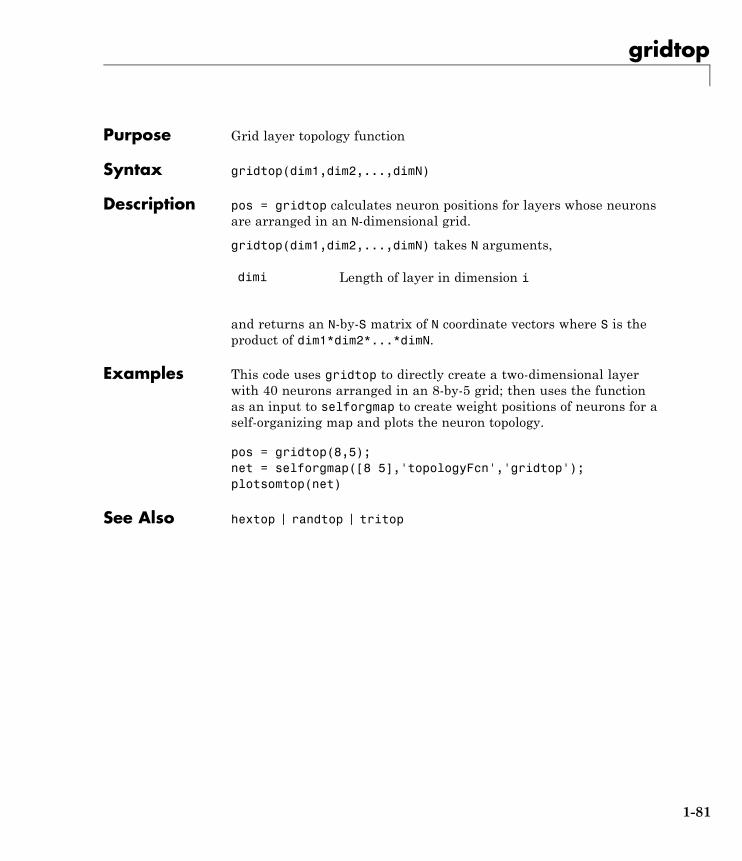
gridtop
Purpose Grid layer topology function
Syntax gridtop(dim1,dim2,...,dimN)
Description pos = gridtop calculates neuron positions for layers whose neuronsare arranged in an N-dimensional grid.
gridtop(dim1,dim2,...,dimN) takes N arguments,
dimi Length of layer in dimension i
and returns an N-by-S matrix of N coordinate vectors where S is theproduct of dim1*dim2*...*dimN.
Examples This code uses gridtop to directly create a two-dimensional layerwith 40 neurons arranged in an 8-by-5 grid; then uses the functionas an input to selforgmap to create weight positions of neurons for aself-organizing map and plots the neuron topology.
pos = gridtop(8,5);net = selforgmap([8 5],'topologyFcn','gridtop');plotsomtop(net)
See Also hextop | randtop | tritop
1-81
gsqrt
Purpose Generalized square root
Syntax gsqrt(x)
Description This function generalizes matrix element-wise square root to the squareroot of cell arrays of matrices combined in an element-wise fashion.
gsqrt(x) takes a matrix or cell array of matrices, and takes theelement-wise square root of the matrices.
Examples Here is an example of taking the element-wise square root of a cellarray:
gsqrt({1 2; 3 4},{1 3; 5 2})
See Also gadd | gsubtract | gdivide | gmultiply | gnegate
1-82
gsubtract
Purpose Generalized subtraction
Syntax gsubtract(a,b)
Description This function generalizes matrix subtraction to the subtraction of cellarrays of matrices combined in an element-wise fashion.
gsubtract(a,b) takes two matrices or cell arrays, and subtracts themin an element-wise manner.
Examples Here matrix and cell array values are added.
gsubtract([1 2 3; 4 5 6],[10;20])gsubtract({1 2; 3 4},{1 3; 5 2})gsubtract({1 2 3 4},{10;20;30})
See Also gadd | gmultiply | gdivide | gnegate | gsqrt
1-83
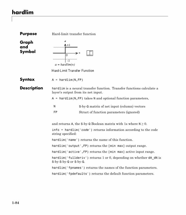
hardlim
Purpose Hard-limit transfer function
GraphandSymbol
Syntax A = hardlim(N,FP)
Description hardlim is a neural transfer function. Transfer functions calculate alayer’s output from its net input.
A = hardlim(N,FP) takes N and optional function parameters,
N S-by-Q matrix of net input (column) vectors
FP Struct of function parameters (ignored)
and returns A, the S-by-Q Boolean matrix with 1s where N ≥ 0.
info = hardlim('code') returns information according to the codestring specified:
hardlim('name') returns the name of this function.
hardlim('output',FP) returns the [min max] output range.
hardlim('active',FP) returns the [min max] active input range.
hardlim('fullderiv') returns 1 or 0, depending on whether dA_dN isS-by-S-by-Q or S-by-Q.
hardlim('fpnames') returns the names of the function parameters.
hardlim('fpdefaults') returns the default function parameters.
1-84
hardlim
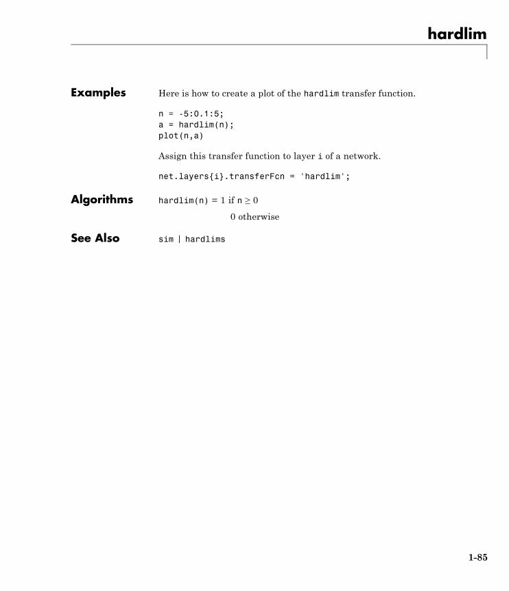
Examples Here is how to create a plot of the hardlim transfer function.
n = -5:0.1:5;a = hardlim(n);plot(n,a)
Assign this transfer function to layer i of a network.
net.layers{i}.transferFcn = 'hardlim';
Algorithms hardlim(n) = 1 if n ≥ 0
0 otherwise
See Also sim | hardlims
1-85
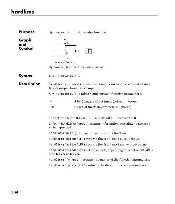
hardlims
Purpose Symmetric hard-limit transfer function
GraphandSymbol
Syntax A = hardlims(N,FP)
Description hardlims is a neural transfer function. Transfer functions calculate alayer’s output from its net input.
A = hardlims(N,FP) takes N and optional function parameters,
N S-by-Q matrix of net input (column) vectors
FP Struct of function parameters (ignored)
and returns A, the S-by-Q +1/–1 matrix with +1s where N ≥ 0.
info = hardlims('code') returns information according to the codestring specified:
hardlims('name') returns the name of this function.
hardlims('output',FP) returns the [min max] output range.
hardlims('active',FP) returns the [min max] active input range.
hardlims('fullderiv') returns 1 or 0, depending on whether dA_dN isS-by-S-by-Q or S-by-Q.
hardlims('fpnames') returns the names of the function parameters.
hardlims('fpdefaults') returns the default function parameters.
1-86
hardlims
Examples Here is how to create a plot of the hardlims transfer function.
n = -5:0.1:5;a = hardlims(n);plot(n,a)
Assign this transfer function to layer i of a network.
net.layers{i}.transferFcn = 'hardlims';
Algorithms hardlims(n) = 1 if n ≥ 0, –1 otherwise.
See Also sim | hardlim
1-87

hextop
Purpose Hexagonal layer topology function
Syntax hextop(dim1,dim2,...,dimN)
Description hextop calculates the neuron positions for layers whose neurons arearranged in an N-dimensional hexagonal pattern.
hextop(dim1,dim2,...,dimN) takes N arguments,
dimi Length of layer in dimension i
and returns an N-by-S matrix of N coordinate vectors where S is theproduct of dim1*dim2*...*dimN.
Examples This code creates and displays a two-dimensional layer with 40 neuronsarranged in an 8-by-5 hexagonal pattern.
pos = hextop(8,5);net = selforgmap([8 5],'topologyFcn','hextop');plotsomtop(net)
See Also gridtop | randtop | tritop
1-88
ind2vec
Purpose Convert indices to vectors
Syntax ind2vec(ind)
Description ind2vec and vec2ind allow indices to be represented either bythemselves, or as vectors containing a 1 in the row of the index theyrepresent.
ind2vec(ind) takes one argument,
ind Row vector of indices
and returns a sparse matrix of vectors, with one 1 in each column, asindicated by ind.
Examples Here four indices are defined and converted to vector representation.
ind = [1 3 2 3]vec = ind2vec(ind)
See Also vec2ind
1-89
init
Purpose Initialize neural network
Syntax net = init(net)
To GetHelp
Type help network/init.
Description net = init(net) returns neural network net with weight and biasvalues updated according to the network initialization function,indicated by net.initFcn, and the parameter values, indicated bynet.initParam.
Examples Here a perceptron is created, and then configured so that its input,output, weight, and bias dimensions match the input and target data.
x = [0 1 0 1; 0 0 1 1];t = [0 0 0 1];net = perceptron;net = configure(net,x,t);net.iw{1,1}net.b{1}
Training the perceptron alters its weight and bias values.
net = train(net,x,t);net.iw{1,1}net.b{1}
init reinitializes those weight and bias values.
net = init(net);net.iw{1,1}net.b{1}
The weights and biases are zeros again, which are the initial valuesused by perceptron networks.
1-90
init
Algorithms init calls net.initFcn to initialize the weight and bias valuesaccording to the parameter values net.initParam.
Typically, net.initFcn is set to 'initlay', which initializes eachlayer’s weights and biases according to its net.layers{i}.initFcn.
Backpropagation networks have net.layers{i}.initFcn set to'initnw', which calculates the weight and bias values for layer i usingthe Nguyen-Widrow initialization method.
Other networks have net.layers{i}.initFcn set to 'initwb', whichinitializes each weight and bias with its own initialization function. Themost common weight and bias initialization function is rands, whichgenerates random values between –1 and 1.
See Also sim | adapt | train | initlay | initnw | initwb | rands | revert
1-91
initcon
Purpose Conscience bias initialization function
Syntax initcon (S,PR)
Description initcon is a bias initialization function that initializes biases forlearning with the learncon learning function.
initcon (S,PR) takes two arguments,
S Number of rows (neurons)
PR R-by-2 matrix of R = [Pmin Pmax] (default = [1 1])
and returns an S-by-1 bias vector.
Note that for biases, R is always 1. initcon could also be used toinitialize weights, but it is not recommended for that purpose.
Examples Here initial bias values are calculated for a five-neuron layer.
b = initcon(5)
NetworkUse
You can create a standard network that uses initcon to initializeweights by calling competlayer.
To prepare the bias of layer i of a custom network to initialize withinitcon,
1 Set net.initFcn to 'initlay'. (net.initParam automaticallybecomes initlay’s default parameters.)
2 Set net.layers{i}.initFcn to 'initwb'.
3 Set net.biases{i}.initFcn to 'initcon'.
To initialize the network, call init.
1-92
initcon
Algorithms learncon updates biases so that each bias value b(i) is a function ofthe average output c(i) of the neuron i associated with the bias.
initcon gets initial bias values by assuming that each neuron hasresponded to equal numbers of vectors in the past.
See Also competlayer | init | initlay | initwb | learncon
1-93
initlay
Purpose Layer-by-layer network initialization function
Syntax net = initlay(net)info = initlay('code')
Description initlay is a network initialization function that initializes each layer iaccording to its own initialization function net.layers{i}.initFcn.
net = initlay(net) takes
net Neural network
and returns the network with each layer updated.
info = initlay('code') returns useful information for eachsupported code string:
'pnames' Names of initialization parameters
'pdefaults' Default initialization parameters
initlay does not have any initialization parameters.
NetworkUse
You can create a standard network that uses initlay by callingfeedforwardnet, cascadeforwardnet, and many other networkfunctions.
To prepare a custom network to be initialized with initlay,
1 Set net.initFcn to 'initlay'. This sets net.initParam to theempty matrix [], because initlay has no initialization parameters.
2 Set each net.layers{i}.initFcn to a layer initialization function.(Examples of such functions are initwb and initnw.)
To initialize the network, call init.
1-94

initlay
Algorithms The weights and biases of each layer i are initialized according tonet.layers{i}.initFcn.
See Also cascadeforwardnet | feedforwardnet | init | initnw | initwb
1-95
initlvq
Purpose LVQ weight initialization function
Syntax initlvq('configure',x)initlvq('configure',net,'IW',i,j,settings)initlvq('configure',net,'LW',i,j,settings)initlvq('configure',net,'b',i,)
Description initlvq('configure',x) takes input data x and returns initializationsettings for an LVQ weights associated with that input.
initlvq('configure',net,'IW',i,j,settings) takes a network,and indices indicating an input weight to layer i from input j, and thatweights settings, and returns new weight values.
initlvq('configure',net,'LW',i,j,settings) takes a network,and indices indicating a layer weight to layer i from layer j, and thatweights settings, and returns new weight values.
initlvq('configure',net,'b',i,) takes a network, and an indexindicating a bias for layer i, and returns new bias values.
See Also lvqnet | init
1-96
initnw
Purpose Nguyen-Widrow layer initialization function
Syntax net = initnw(net,i)
Description initnw is a layer initialization function that initializes a layer’s weightsand biases according to the Nguyen-Widrow initialization algorithm.This algorithm chooses values in order to distribute the active region ofeach neuron in the layer approximately evenly across the layer’s inputspace. The values contain a degree of randomness, so they are not thesame each time this function is called.
initnw requires that the layer it initializes have a transfer functionwith a finite active input range. This includes transfer functions suchas tansig and satlin, but not purelin, whose active input range is theinfinite interval [-inf, inf]. Transfer functions, such as tansig, willreturn their active input range as follows:
activeInputRange = tansig('active')activeInputRange =
-2 2
net = initnw(net,i) takes two arguments,
net Neural network
i Index of a layer
and returns the network with layer i’s weights and biases updated.
There is a random element to Nguyen-Widrow initialization. Unless thedefault random generator is set to the same seed before each call toinitnw, it will generate different weight and bias values each time.
NetworkUse
You can create a standard network that uses initnw by callingfeedforwardnet or cascadeforwardnet.
To prepare a custom network to be initialized with initnw,
1-97
initnw
1 Set net.initFcn to 'initlay'. This sets net.initParam to theempty matrix [], because initlay has no initialization parameters.
2 Set net.layers{i}.initFcn to 'initnw'.
To initialize the network, call init.
Algorithms The Nguyen-Widrow method generates initial weight and bias valuesfor a layer so that the active regions of the layer’s neurons aredistributed approximately evenly over the input space.
Advantages over purely random weights and biases are
• Few neurons are wasted (because all the neurons are in the inputspace).
• Training works faster (because each area of the input space hasneurons). The Nguyen-Widrow method can only be applied to layers
- With a bias
- With weights whose weightFcn is dotprod
- With netInputFcn set to netsum
- With transferFcn whose active region is finite
If these conditions are not met, then initnw uses rands to initialize thelayer’s weights and biases.
See Also cascadeforwardnet | feedforwardnet | init | initlay | initwb
1-98
initsompc
Purpose Initialize SOM weights with principal components
Syntax weights = initsom(inputs,dimensions,positions)weights = initsom(inputs,dimensions,topologyFcn)
Description initsompc initializes the weights of an N-dimensional self-organizingmap so that the initial weights are distributed across the spacespanned by the most significant N principal components of the inputs.Distributing the weight significantly speeds up SOM learning, as themap starts out with a reasonable ordering of the input space.
weights = initsom(inputs,dimensions,positions) takes thesearguments:
inputs R-by-Q matrix of Q R-element input vectors
dimensions D-by-1 vector of positive integer SOM dimensions
positions D-by-Smatrix of S D-dimension neuron positions
and returns the following:
weights S-by-R matrix of weights
weights = initsom(inputs,dimensions,topologyFcn) is analternative specifying the name of a layer topology function insteadof positions. topologyFcn is called with dimensions to obtainpositions.
Examples inputs = rand(2,100)+[2;3]*ones(1,100);dimensions = [3 4];positions = gridtop(dimensions);weights = initsompc(inputs,dimensions,positions);
See Also gridtop | hextop | randtop
1-99
initwb
Purpose By weight and bias layer initialization function
Syntax initwb(net,i)
Description initwb is a layer initialization function that initializes a layer’s weightsand biases according to their own initialization functions.
initwb(net,i) takes two arguments,
net Neural network
i Index of a layer
and returns the network with layer i’s weights and biases updated.
NetworkUse
You can create a standard network that uses initwb by callingperceptron or linearlayer.
To prepare a custom network to be initialized with initwb,
1 Set net.initFcn to 'initlay'. This sets net.initParam to theempty matrix [], because initlay has no initialization parameters.
2 Set net.layers{i}.initFcn to 'initwb'.
3 Set each net.inputWeights{i,j}.initFcn to a weight initializationfunction. Set each net.layerWeights{i,j}.initFcn to a weightinitialization function. Set each net.biases{i}.initFcn to a biasinitialization function. (Examples of such functions are rands andmidpoint.)
To initialize the network, call init.
Algorithms Each weight (bias) in layer i is set to new values calculated according toits weight (bias) initialization function.
See Also init | initlay | initnw | linearlayer | perceptron
1-100
initzero
Purpose Zero weight and bias initialization function
Syntax W = initzero(S,PR)b = initzero(S,[1 1])
Description W = initzero(S,PR) takes two arguments,
S Number of rows (neurons)
PR R-by-2 matrix of input value ranges = [Pmin Pmax]
and returns an S-by-R weight matrix of zeros.
b = initzero(S,[1 1]) returns an S-by-1 bias vector of zeros.
Examples Here initial weights and biases are calculated for a layer with twoinputs ranging over [0 1] and [-2 2] and four neurons.
W = initzero(5,[0 1; -2 2])b = initzero(5,[1 1])
NetworkUse
You can create a standard network that uses initzero to initialize itsweights by calling newp or newlin.
To prepare the weights and the bias of layer i of a custom networkto be initialized with midpoint,
1 Set net.initFcn to 'initlay'. (net.initParam automaticallybecomes initlay’s default parameters.)
2 Set net.layers{i}.initFcn to 'initwb'.
3 Set each net.inputWeights{i,j}.initFcn to 'initzero'.
4 Set each net.layerWeights{i,j}.initFcn to 'initzero'.
5 Set each net.biases{i}.initFcn to 'initzero'.
1-101

initzero
To initialize the network, call init.
See help newp and help newlin for initialization examples.
See Also initwb | initlay | init
1-102
isconfigured
Purpose Indicate if network inputs and outputs are configured
Syntax [flag,inputflags,outputflags] = isconfigured(net)
Description [flag,inputflags,outputflags] = isconfigured(net) takes aneural network and returns three values,
flag True if all network inputs and outputs areconfigured (have non-zero sizes)
inputflags Vector of true/false values for eachconfigured/unconfigured input
outputflags Vector of true/false values for eachconfigured/unconfigured output
Examples Here are the flags returned for a new network before and after beingconfigured:
net = feedforwardnet;[flag,inputFlags,outputFlags] = isconfigured(net)[x,t] = simplefit_dataset;net = configure(net,x,t);[flag,inputFlags,outputFlags] = isconfigured(net)
See Also configure | unconfigure
1-103
layrecnet
Purpose Layer recurrent neural network
Syntax layrecnet(layerDelays,hiddenSizes,trainFcn)
Description Layer recurrent neural networks are similar to feedforward networks,except that each layer has a recurrent connection with a tap delayassociated with it. This allows the network to have an infinite dynamicresponse to time series input data. This network is similar to the timedelay (timedelaynet) and distributed delay (distdelaynet) neuralnetworks, which have finite input responses.
layrecnet(layerDelays,hiddenSizes,trainFcn) takes thesearguments,
layerDelays Row vector of increasing 0 or positive delays(default = 1:2)
hiddenSizes Row vector of one or more hidden layer sizes(default = 10)
trainFcn Training function (default = 'trainlm')
and returns a layer recurrent neural network.
Examples Use a layer recurrent neural network to solve a simple time seriesproblem:
[X,T] = simpleseries_dataset;net = layrecnet(1:2,10)[Xs,Xi,Ai,Ts] = preparets(net,X,T)net = train(net,Xs,Ts,Xi,Ai);view(net)Y = net(Xs,Xi,Ai);perf = perform(net,Y,Ts)
See Also preparets | removedelay | distdelaynet | timedelaynet | narnet| narxnet
1-104
learncon
Purpose Conscience bias learning function
Syntax [dB,LS] = learncon(B,P,Z,N,A,T,E,gW,gA,D,LP,LS)info = learncon('code')
Description learncon is the conscience bias learning function used to increase thenet input to neurons that have the lowest average output until eachneuron responds approximately an equal percentage of the time.
[dB,LS] = learncon(B,P,Z,N,A,T,E,gW,gA,D,LP,LS) takes severalinputs,
B S-by-1 bias vector
P 1-by-Q ones vector
Z S-by-Q weighted input vectors
N S-by-Q net input vectors
A S-by-Q output vectors
T S-by-Q layer target vectors
E S-by-Q layer error vectors
gW S-by-R gradient with respect to performance
gA S-by-Q output gradient with respect to performance
D S-by-S neuron distances
LP Learning parameters, none, LP = []
LS Learning state, initially should be = []
and returns
dB S-by-1 weight (or bias) change matrix
LS New learning state
1-105
learncon
Learning occurs according to learncon’s learning parameter, shownhere with its default value.
LP.lr - 0.001 Learning rate
info = learncon('code') returns useful information for eachsupported code string:
'pnames' Names of learning parameters
'pdefaults' Default learning parameters
'needg' Returns 1 if this function uses gW or gA
Neural Network Toolbox 2.0 compatibility: The LP.lr described aboveequals 1 minus the bias time constant used by trainc in the NeuralNetwork Toolbox 2.0 software.
Examples Here you define a random output A and bias vector W for a layer withthree neurons. You also define the learning rate LR.
a = rand(3,1);b = rand(3,1);lp.lr = 0.5;
Because learncon only needs these values to calculate a bias change(see “Algorithm” below), use them to do so.
dW = learncon(b,[],[],[],a,[],[],[],[],[],lp,[])
NetworkUse
To prepare the bias of layer i of a custom network to learn withlearncon,
1 Set net.trainFcn to 'trainr'. (net.trainParam automaticallybecomes trainr’s default parameters.)
1-106
learncon
2 Set net.adaptFcn to 'trains'. (net.adaptParam automaticallybecomes trains’s default parameters.)
3 Set net.inputWeights{i}.learnFcn to 'learncon'
4 Set each net.layerWeights{i,j}.learnFcn to 'learncon'..(Each weight learning parameter property is automatically set tolearncon’s default parameters.)
To train the network (or enable it to adapt),
1 Set net.trainParam (or net.adaptParam) properties as desired.
2 Call train (or adapt).
Algorithms learncon calculates the bias change db for a given neuron by firstupdating each neuron’s conscience, i.e., the running average of itsoutput:
c = (1-lr)*c + lr*a
The conscience is then used to compute a bias for the neuron that isgreatest for smaller conscience values.
b = exp(1-log(c)) - b
(learncon recovers C from the bias values each time it is called.)
See Also learnk | learnos | adapt | train
1-107
learngd
Purpose Gradient descent weight and bias learning function
Syntax [dW,LS] = learngd(W,P,Z,N,A,T,E,gW,gA,D,LP,LS)info = learngd('code')
Description learngd is the gradient descent weight and bias learning function.
[dW,LS] = learngd(W,P,Z,N,A,T,E,gW,gA,D,LP,LS) takes severalinputs:
W S-by-R weight matrix (or S-by-1 bias vector)
P R-by-Q input vectors (or ones(1,Q))
Z S-by-Q output gradient with respect to performance xQ weighted input vectors
N S-by-Q net input vectors
A S-by-Q output vectors
T S-by-Q layer target vectors
E S-by-Q layer error vectors
gW S-by-R gradient with respect to performance
gA S-by-Q output gradient with respect to performance
D S-by-S neuron distances
LP Learning parameters, none, LP = []
LS Learning state, initially should be []
and returns
dW S-by-R weight (or bias) change matrix
LS New learning state
1-108
learngd
Learning occurs according to learngd’s learning parameter, shownhere with its default value.
LP.lr - 0.01 Learning rate
info = learngd('code') returns useful information for eachsupported code string:
'pnames' Names of learning parameters
'pdefaults' Default learning parameters
'needg' Returns 1 if this function uses gW or gA
Examples Here you define a random gradient gW for a weight going to a layerwith three neurons from an input with two elements. Also define alearning rate of 0.5.
gW = rand(3,2);lp.lr = 0.5;
Because learngd only needs these values to calculate a weight change(see “Algorithm” below), use them to do so.
dW = learngd([],[],[],[],[],[],[],gW,[],[],lp,[])
NetworkUse
You can create a standard network that uses learngd with newff,newcf, or newelm. To prepare the weights and the bias of layer i of acustom network to adapt with learngd,
1 Set net.adaptFcn to 'trains'. net.adaptParam automaticallybecomes trains’s default parameters.
2 Set each net.inputWeights{i,j}.learnFcn to 'learngd'. Seteach net.layerWeights{i,j}.learnFcn to 'learngd'. Setnet.biases{i}.learnFcn to 'learngd'. Each weight and bias
1-109
learngd
learning parameter property is automatically set to learngd’s defaultparameters.
To allow the network to adapt,
1 Set net.adaptParam properties to desired values.
2 Call adapt with the network.
See help newff or help newcf for examples.
Algorithms learngd calculates the weight change dW for a given neuron from theneuron’s input P and error E, and the weight (or bias) learning rate LR,according to the gradient descent dw = lr*gW.
See Also adapt | learngdm | train
1-110
learngdm
Purpose Gradient descent with momentum weight and bias learning function
Syntax [dW,LS] = learngdm(W,P,Z,N,A,T,E,gW,gA,D,LP,LS)info = learngdm('code')
Description learngdm is the gradient descent with momentum weight and biaslearning function.
[dW,LS] = learngdm(W,P,Z,N,A,T,E,gW,gA,D,LP,LS) takes severalinputs,
W S-by-R weight matrix (or S-by-1 bias vector)
P R-by-Q input vectors (or ones(1,Q))
Z S-by-Q weighted input vectors
N S-by-Q net input vectors
A S-by-Q output vectors
T S-by-Q layer target vectors
E S-by-Q layer error vectors
gW S-by-R gradient with respect to performance
gA S-by-Q output gradient with respect to performance
D S-by-S neuron distances
LP Learning parameters, none, LP = []
LS Learning state, initially should be = []
and returns
dW S-by-R weight (or bias) change matrix
LS New learning state
1-111
learngdm
Learning occurs according to learngdm’s learning parameters, shownhere with their default values.
LP.lr - 0.01 Learning rate
LP.mc - 0.9 Momentum constant
info = learngdm('code') returns useful information for each codestring:
'pnames' Names of learning parameters
'pdefaults' Default learning parameters
'needg' Returns 1 if this function uses gW or gA
Examples Here you define a random gradient G for a weight going to a layer withthree neurons from an input with two elements. Also define a learningrate of 0.5 and momentum constant of 0.8:
gW = rand(3,2);lp.lr = 0.5;lp.mc = 0.8;
Because learngdm only needs these values to calculate a weight change(see “Algorithm” below), use them to do so. Use the default initiallearning state.
ls = [];[dW,ls] = learngdm([],[],[],[],[],[],[],gW,[],[],lp,ls)
learngdm returns the weight change and a new learning state.
1-112
learngdm
NetworkUse
You can create a standard network that uses learngdm with newff,newcf, or newelm.
To prepare the weights and the bias of layer i of a custom network toadapt with learngdm,
1 Set net.adaptFcn to 'trains'. net.adaptParam automaticallybecomes trains’s default parameters.
2 Set each net.inputWeights{i,j}.learnFcn to 'learngdm'. Seteach net.layerWeights{i,j}.learnFcn to 'learngdm'. Setnet.biases{i}.learnFcn to 'learngdm'. Each weight and biaslearning parameter property is automatically set to learngdm’sdefault parameters.
To allow the network to adapt,
1 Set net.adaptParam properties to desired values.
2 Call adapt with the network.
See help newff or help newcf for examples.
Algorithms learngdm calculates the weight change dW for a given neuron from theneuron’s input P and error E, the weight (or bias) W, learning rate LR, andmomentum constant MC, according to gradient descent with momentum:
dW = mc*dWprev + (1-mc)*lr*gW
The previous weight change dWprev is stored and read from the learningstate LS.
See Also adapt | learngd | train
1-113
learnh
Purpose Hebb weight learning rule
Syntax [dW,LS] = learnh(W,P,Z,N,A,T,E,gW,gA,D,LP,LS)info = learnh('code')
Description learnh is the Hebb weight learning function.
[dW,LS] = learnh(W,P,Z,N,A,T,E,gW,gA,D,LP,LS) takes severalinputs,
W S-by-R weight matrix (or S-by-1 bias vector)
P R-by-Q input vectors (or ones(1,Q))
Z S-by-Q weighted input vectors
N S-by-Q net input vectors
A S-by-Q output vectors
T S-by-Q layer target vectors
E S-by-Q layer error vectors
gW S-by-R gradient with respect to performance
gA S-by-Q output gradient with respect to performance
D S-by-S neuron distances
LP Learning parameters, none, LP = []
LS Learning state, initially should be = []
and returns
dW S-by-R weight (or bias) change matrix
LS New learning state
Learning occurs according to learnh’s learning parameter, shown herewith its default value.
1-114
learnh
LP.lr - 0.01 Learning rate
info = learnh('code') returns useful information for each codestring:
'pnames' Names of learning parameters
'pdefaults' Default learning parameters
'needg' Returns 1 if this function uses gW or gA
Examples Here you define a random input P and output A for a layer with atwo-element input and three neurons. Also define the learning rate LR.
p = rand(2,1);a = rand(3,1);lp.lr = 0.5;
Because learnh only needs these values to calculate a weight change(see “Algorithm” below), use them to do so.
dW = learnh([],p,[],[],a,[],[],[],[],[],lp,[])
NetworkUse
To prepare the weights and the bias of layer i of a custom network tolearn with learnh,
1 Set net.trainFcn to 'trainr'. (net.trainParam automaticallybecomes trainr’s default parameters.)
2 Set net.adaptFcn to 'trains'. (net.adaptParam automaticallybecomes trains’s default parameters.)
3 Set each net.inputWeights{i,j}.learnFcn to 'learnh'.
1-115
learnh
4 Set each net.layerWeights{i,j}.learnFcn to 'learnh'. (Eachweight learning parameter property is automatically set to learnh’sdefault parameters.)
To train the network (or enable it to adapt),
1 Set net.trainParam (or net.adaptParam) properties to desiredvalues.
2 Call train (adapt).
Algorithms learnh calculates the weight change dW for a given neuron from theneuron’s input P, output A, and learning rate LR according to the Hebblearning rule:
dw = lr*a*p'
References Hebb, D.O., The Organization of Behavior, New York, Wiley, 1949
See Also learnhd | adapt | train
1-116
learnhd
Purpose Hebb with decay weight learning rule
Syntax [dW,LS] = learnhd(W,P,Z,N,A,T,E,gW,gA,D,LP,LS)info = learnhd('code')
Description learnhd is the Hebb weight learning function.
[dW,LS] = learnhd(W,P,Z,N,A,T,E,gW,gA,D,LP,LS) takes severalinputs,
W S-by-R weight matrix (or S-by-1 bias vector)
P R-by-Q input vectors (or ones(1,Q))
Z S-by-Q weighted input vectors
N S-by-Q net input vectors
A S-by-Q output vectors
T S-by-Q layer target vectors
E S-by-Q layer error vectors
gW S-by-R gradient with respect to performance
gA S-by-Q output gradient with respect to performance
D S-by-S neuron distances
LP Learning parameters, none, LP = []
LS Learning state, initially should be = []
and returns
dW S-by-R weight (or bias) change matrix
LS New learning state
Learning occurs according to learnhd’s learning parameters, shownhere with default values.
1-117
learnhd
LP.dr - 0.01 Decay rate
LP.lr - 0.1 Learning rate
info = learnhd('code') returns useful information for each codestring:
'pnames' Names of learning parameters
'pdefaults' Default learning parameters
'needg' Returns 1 if this function uses gW or gA
Examples Here you define a random input P, output A, and weights W for a layerwith a two-element input and three neurons. Also define the decayand learning rates.
p = rand(2,1);a = rand(3,1);w = rand(3,2);lp.dr = 0.05;lp.lr = 0.5;
Because learnhd only needs these values to calculate a weight change(see “Algorithm” below), use them to do so.
dW = learnhd(w,p,[],[],a,[],[],[],[],[],lp,[])
NetworkUse
To prepare the weights and the bias of layer i of a custom network tolearn with learnhd,
1 Set net.trainFcn to 'trainr'. (net.trainParam automaticallybecomes trainr’s default parameters.)
2 Set net.adaptFcn to 'trains'. (net.adaptParam automaticallybecomes trains’s default parameters.)
1-118
learnhd
3 Set each net.inputWeights{i,j}.learnFcn to 'learnhd'.
4 Set each net.layerWeights{i,j}.learnFcn to 'learnhd'. (Eachweight learning parameter property is automatically set to learnhd’sdefault parameters.)
To train the network (or enable it to adapt),
1 Set net.trainParam (or net.adaptParam) properties to desiredvalues.
2 Call train (adapt).
Algorithms learnhd calculates the weight change dW for a given neuron from theneuron’s input P, output A, decay rate DR, and learning rate LR accordingto the Hebb with decay learning rule:
dw = lr*a*p' - dr*w
See Also learnh | adapt | train
1-119

learnis
Purpose Instar weight learning function
Syntax [dW,LS] = learnis(W,P,Z,N,A,T,E,gW,gA,D,LP,LS)info = learnis('code')
Description learnis is the instar weight learning function.
[dW,LS] = learnis(W,P,Z,N,A,T,E,gW,gA,D,LP,LS) takes severalinputs,
W S-by-R weight matrix (or S-by-1 bias vector)
P R-by-Q input vectors (or ones(1,Q))
Z S-by-Q weighted input vectors
N S-by-Q net input vectors
A S-by-Q output vectors
T S-by-Q layer target vectors
E S-by-Q layer error vectors
gW S-by-R gradient with respect to performance
gA S-by-Q output gradient with respect to performance
D S-by-S neuron distances
LP Learning parameters, none, LP = []
LS Learning state, initially should be = []
and returns
dW S-by-R weight (or bias) change matrix
LS New learning state
Learning occurs according to learnis’s learning parameter, shownhere with its default value.
1-120
learnis
LP.lr - 0.01 Learning rate
info = learnis('code') returns useful information for each codestring:
'pnames' Names of learning parameters
'pdefaults' Default learning parameters
'needg' Returns 1 if this function uses gW or gA
Examples Here you define a random input P, output A, and weight matrix W fora layer with a two-element input and three neurons. Also define thelearning rate LR.
p = rand(2,1);a = rand(3,1);w = rand(3,2);lp.lr = 0.5;
Because learnis only needs these values to calculate a weight change(see “Algorithm” below), use them to do so.
dW = learnis(w,p,[],[],a,[],[],[],[],[],lp,[])
NetworkUse
To prepare the weights and the bias of layer i of a custom networkso that it can learn with learnis,
1 Set net.trainFcn to 'trainr'. (net.trainParam automaticallybecomes trainr’s default parameters.)
2 Set net.adaptFcn to 'trains'. (net.adaptParam automaticallybecomes trains’s default parameters.)
3 Set each net.inputWeights{i,j}.learnFcn to 'learnis'.
1-121
learnis
4 Set each net.layerWeights{i,j}.learnFcn to 'learnis'. (Eachweight learning parameter property is automatically set to learnis’sdefault parameters.)
To train the network (or enable it to adapt),
1 Set net.trainParam (net.adaptParam) properties to desired values.
2 Call train (adapt).
Algorithms learnis calculates the weight change dW for a given neuron from theneuron’s input P, output A, and learning rate LR according to the instarlearning rule:
dw = lr*a*(p'-w)
References Grossberg, S., Studies of the Mind and Brain, Drodrecht, Holland,Reidel Press, 1982
See Also learnk | learnos | adapt | train
1-122
learnk
Purpose Kohonen weight learning function
Syntax [dW,LS] = learnk(W,P,Z,N,A,T,E,gW,gA,D,LP,LS)info = learnk('code')
Description learnk is the Kohonen weight learning function.
[dW,LS] = learnk(W,P,Z,N,A,T,E,gW,gA,D,LP,LS) takes severalinputs,
W S-by-R weight matrix (or S-by-1 bias vector)
P R-by-Q input vectors (or ones(1,Q))
Z S-by-Q weighted input vectors
N S-by-Q net input vectors
A S-by-Q output vectors
T S-by-Q layer target vectors
E S-by-Q layer error vectors
gW S-by-R gradient with respect to performance
gA S-by-Q output gradient with respect to performance
D S-by-S neuron distances
LP Learning parameters, none, LP = []
LS Learning state, initially should be = []
and returns
dW S-by-R weight (or bias) change matrix
LS New learning state
Learning occurs according to learnk’s learning parameter, shown herewith its default value.
1-123
learnk
LP.lr - 0.01 Learning rate
info = learnk('code') returns useful information for each codestring:
'pnames' Names of learning parameters
'pdefaults' Default learning parameters
'needg' Returns 1 if this function uses gW or gA
Examples Here you define a random input P, output A, and weight matrix W fora layer with a two-element input and three neurons. Also define thelearning rate LR.
p = rand(2,1);a = rand(3,1);w = rand(3,2);lp.lr = 0.5;
Because learnk only needs these values to calculate a weight change(see “Algorithm” below), use them to do so.
dW = learnk(w,p,[],[],a,[],[],[],[],[],lp,[])
NetworkUse
To prepare the weights of layer i of a custom network to learn withlearnk,
1 Set net.trainFcn to 'trainr'. (net.trainParam automaticallybecomes trainr’s default parameters.)
2 Set net.adaptFcn to 'trains'. (net.adaptParam automaticallybecomes trains’s default parameters.)
3 Set each net.inputWeights{i,j}.learnFcn to 'learnk'.
1-124
learnk
4 Set each net.layerWeights{i,j}.learnFcn to 'learnk'. (Eachweight learning parameter property is automatically set to learnk’sdefault parameters.)
To train the network (or enable it to adapt),
1 Set net.trainParam (or net.adaptParam) properties as desired.
2 Call train (or adapt).
Algorithms learnk calculates the weight change dW for a given neuron from theneuron’s input P, output A, and learning rate LR according to theKohonen learning rule:
dw = lr*(p'-w), if a ~= 0; = 0, otherwise
References Kohonen, T., Self-Organizing and Associative Memory, New York,Springer-Verlag, 1984
See Also learnis | learnos | adapt | train
1-125
learnlv1
Purpose LVQ1 weight learning function
Syntax [dW,LS] = learnlv1(W,P,Z,N,A,T,E,gW,gA,D,LP,LS)info = learnlv1('code')
Description learnlv1 is the LVQ1 weight learning function.
[dW,LS] = learnlv1(W,P,Z,N,A,T,E,gW,gA,D,LP,LS) takes severalinputs,
W S-by-R weight matrix (or S-by-1 bias vector)
P R-by-Q input vectors (or ones(1,Q))
Z S-by-Q weighted input vectors
N S-by-Q net input vectors
A S-by-Q output vectors
T S-by-Q layer target vectors
E S-by-Q layer error vectors
gW S-by-R gradient with respect to performance
gA S-by-Q output gradient with respect to performance
D S-by-S neuron distances
LP Learning parameters, none, LP = []
LS Learning state, initially should be = []
and returns
dW S-by-R weight (or bias) change matrix
LS New learning state
Learning occurs according to learnlv1’s learning parameter, shownhere with its default value.
1-126
learnlv1
LP.lr - 0.01 Learning rate
info = learnlv1('code') returns useful information for each codestring:
'pnames' Names of learning parameters
'pdefaults' Default learning parameters
'needg' Returns 1 if this function uses gW or gA
Examples Here you define a random input P, output A, weight matrix W, andoutput gradient gA for a layer with a two-element input and threeneurons. Also define the learning rate LR.
p = rand(2,1);w = rand(3,2);a = compet(negdist(w,p));gA = [-1;1; 1];lp.lr = 0.5;
Because learnlv1 only needs these values to calculate a weight change(see “Algorithm” below), use them to do so.
dW = learnlv1(w,p,[],[],a,[],[],[],gA,[],lp,[])
NetworkUse
You can create a standard network that uses learnlv1 with lvqnet.To prepare the weights of layer i of a custom network to learn withlearnlv1,
1 Set net.trainFcn to 'trainr'. (net.trainParam automaticallybecomes trainr’s default parameters.)
2 Set net.adaptFcn to 'trains'. (net.adaptParam automaticallybecomes trains’s default parameters.)
1-127
learnlv1
3 Set each net.inputWeights{i,j}.learnFcn to 'learnlv1'.
4 Set each net.layerWeights{i,j}.learnFcn to 'learnlv1'.(Each weight learning parameter property is automatically set tolearnlv1’s default parameters.)
To train the network (or enable it to adapt),
1 Set net.trainParam (or net.adaptParam) properties as desired.
2 Call train (or adapt).
Algorithms learnlv1 calculates the weight change dW for a given neuron from theneuron’s input P, output A, output gradient gA, and learning rate LR,according to the LVQ1 rule, given i, the index of the neuron whoseoutput a(i) is 1:
dw(i,:) = +lr*(p-w(i,:)) if gA(i) = 0;= -lr*(p-w(i,:)) ifgA(i) = -1
See Also learnlv2 | adapt | train
1-128
learnlv2
Purpose LVQ2.1 weight learning function
Syntax [dW,LS] = learnlv2(W,P,Z,N,A,T,E,gW,gA,D,LP,LS)info = learnlv2('code')
Description learnlv2 is the LVQ2 weight learning function.
[dW,LS] = learnlv2(W,P,Z,N,A,T,E,gW,gA,D,LP,LS) takes severalinputs,
W S-by-R weight matrix (or S-by-1 bias vector)
P R-by-Q input vectors (or ones(1,Q))
Z S-by-Q weighted input vectors
N S-by-Q net input vectors
A S-by-Q output vectors
T S-by-Q layer target vectors
E S-by-Q layer error vectors
gW S-by-R weight gradient with respect to performance
gA S-by-Q output gradient with respect to performance
D S-by-S neuron distances
LP Learning parameters, none, LP = []
LS Learning state, initially should be = []
and returns
dW S-by-R weight (or bias) change matrix
LS New learning state
Learning occurs according to learnlv2’s learning parameter, shownhere with its default value.
1-129
learnlv2
LP.lr - 0.01 Learning rate
LP.window - 0.25 Window size (0 to 1, typically 0.2 to 0.3)
info = learnlv2('code') returns useful information for each codestring:
'pnames' Names of learning parameters
'pdefaults' Default learning parameters
'needg' Returns 1 if this function uses gW or gA
Examples Here you define a sample input P, output A, weight matrix W, and outputgradient gA for a layer with a two-element input and three neurons.Also define the learning rate LR.
p = rand(2,1);w = rand(3,2);n = negdist(w,p);a = compet(n);gA = [-1;1; 1];lp.lr = 0.5;
Because learnlv2 only needs these values to calculate a weight change(see “Algorithm” below), use them to do so.
dW = learnlv2(w,p,[],n,a,[],[],[],gA,[],lp,[])
NetworkUse
You can create a standard network that uses learnlv2 with lvqnet.
To prepare the weights of layer i of a custom network to learn withlearnlv2,
1 Set net.trainFcn to 'trainr'. (net.trainParam automaticallybecomes trainr’s default parameters.)
1-130
learnlv2
2 Set net.adaptFcn to 'trains'. (net.adaptParam automaticallybecomes trains’s default parameters.)
3 Set each net.inputWeights{i,j}.learnFcn to 'learnlv2'.
4 Set each net.layerWeights{i,j}.learnFcn to 'learnlv2'.(Each weight learning parameter property is automatically set tolearnlv2’s default parameters.)
To train the network (or enable it to adapt),
1 Set net.trainParam (or net.adaptParam) properties as desired.
2 Call train (or adapt).
Algorithms learnlv2 implements Learning Vector Quantization 2.1, which worksas follows:
For each presentation, if the winning neuron i should not have won,and the runnerup j should have, and the distance di between thewinning neuron and the input p is roughly equal to the distance dj fromthe runnerup neuron to the input p according to the given window,
min(di/dj, dj/di) > (1-window)/(1+window)
then move the winning neuron i weights away from the input vector,and move the runnerup neuron j weights toward the input according to
dw(i,:) = - lp.lr*(p'-w(i,:))dw(j,:) = + lp.lr*(p'-w(j,:))
See Also learnlv1 | adapt | train
1-131

learnos
Purpose Outstar weight learning function
Syntax [dW,LS] = learnos(W,P,Z,N,A,T,E,gW,gA,D,LP,LS)info = learnos('code')
Description learnos is the outstar weight learning function.
[dW,LS] = learnos(W,P,Z,N,A,T,E,gW,gA,D,LP,LS) takes severalinputs,
W S-by-R weight matrix (or S-by-1 bias vector)
P R-by-Q input vectors (or ones(1,Q))
Z S-by-Q weighted input vectors
N S-by-Q net input vectors
A S-by-Q output vectors
T S-by-Q layer target vectors
E S-by-Q layer error vectors
gW S-by-R weight gradient with respect to performance
gA S-by-Q output gradient with respect to performance
D S-by-S neuron distances
LP Learning parameters, none, LP = []
LS Learning state, initially should be = []
and returns
dW S-by-R weight (or bias) change matrix
LS New learning state
Learning occurs according to learnos’s learning parameter, shownhere with its default value.
1-132
learnos
LP.lr - 0.01 Learning rate
info = learnos('code') returns useful information for each codestring:
'pnames' Names of learning parameters
'pdefaults' Default learning parameters
'needg' Returns 1 if this function uses gW or gA
Examples Here you define a random input P, output A, and weight matrix W fora layer with a two-element input and three neurons. Also define thelearning rate LR.
p = rand(2,1);a = rand(3,1);w = rand(3,2);lp.lr = 0.5;
Because learnos only needs these values to calculate a weight change(see “Algorithm” below), use them to do so.
dW = learnos(w,p,[],[],a,[],[],[],[],[],lp,[])
NetworkUse
To prepare the weights and the bias of layer i of a custom network tolearn with learnos,
1 Set net.trainFcn to 'trainr'. (net.trainParam automaticallybecomes trainr’s default parameters.)
2 Set net.adaptFcn to 'trains'. (net.adaptParam automaticallybecomes trains’s default parameters.)
3 Set each net.inputWeights{i,j}.learnFcn to 'learnos'.
1-133
learnos
4 Set each net.layerWeights{i,j}.learnFcn to 'learnos'. (Eachweight learning parameter property is automatically set to learnos’sdefault parameters.)
To train the network (or enable it to adapt),
1 Set net.trainParam (or net.adaptParam) properties to desiredvalues.
2 Call train (adapt).
Algorithms learnos calculates the weight change dW for a given neuron from theneuron’s input P, output A, and learning rate LR according to the outstarlearning rule:
dw = lr*(a-w)*p'
References Grossberg, S., Studies of the Mind and Brain, Drodrecht, Holland,Reidel Press, 1982
See Also learnis | learnk | adapt | train
1-134
learnp
Purpose Perceptron weight and bias learning function
Syntax [dW,LS] = learnp(W,P,Z,N,A,T,E,gW,gA,D,LP,LS)info = learnp('code')
Description learnp is the perceptron weight/bias learning function.
[dW,LS] = learnp(W,P,Z,N,A,T,E,gW,gA,D,LP,LS) takes severalinputs,
W S-by-R weight matrix (or b, and S-by-1 bias vector)
P R-by-Q input vectors (or ones(1,Q))
Z S-by-Q weighted input vectors
N S-by-Q net input vectors
A S-by-Q output vectors
T S-by-Q layer target vectors
E S-by-Q layer error vectors
gW S-by-R weight gradient with respect to performance
gA S-by-Q output gradient with respect to performance
D S-by-S neuron distances
LP Learning parameters, none, LP = []
LS Learning state, initially should be = []
and returns
dW S-by-R weight (or bias) change matrix
LS New learning state
info = learnp('code') returns useful information for each codestring:
1-135
learnp
'pnames' Names of learning parameters
'pdefaults' Default learning parameters
'needg' Returns 1 if this function uses gW or gA
Examples Here you define a random input P and error E for a layer with atwo-element input and three neurons.
p = rand(2,1);e = rand(3,1);
Because learnp only needs these values to calculate a weight change(see “Algorithm” below), use them to do so.
dW = learnp([],p,[],[],[],[],e,[],[],[],[],[])
NetworkUse
You can create a standard network that uses learnp with newp.
To prepare the weights and the bias of layer i of a custom network tolearn with learnp,
1 Set net.trainFcn to 'trainb'. (net.trainParam automaticallybecomes trainb’s default parameters.)
2 Set net.adaptFcn to 'trains'. (net.adaptParam automaticallybecomes trains’s default parameters.)
3 Set each net.inputWeights{i,j}.learnFcn to 'learnp'.
4 Set each net.layerWeights{i,j}.learnFcn to 'learnp'.
5 Set net.biases{i}.learnFcn to 'learnp'. (Each weight and biaslearning parameter property automatically becomes the emptymatrix, because learnp has no learning parameters.)
To train the network (or enable it to adapt),
1-136
learnp
1 Set net.trainParam (or net.adaptParam) properties to desiredvalues.
2 Call train (adapt).
See help newp for adaption and training examples.
Algorithms learnp calculates the weight change dW for a given neuron from theneuron’s input P and error E according to the perceptron learning rule:
dw = 0, if e = 0= p', if e = 1= -p', if e = -1
This can be summarized as
dw = e*p'
References Rosenblatt, F., Principles of Neurodynamics, Washington, D.C., SpartanPress, 1961
See Also adapt | learnpn | train
1-137
learnpn
Purpose Normalized perceptron weight and bias learning function
Syntax [dW,LS] = learnpn(W,P,Z,N,A,T,E,gW,gA,D,LP,LS)info = learnpn('code')
Description learnpn is a weight and bias learning function. It can result infaster learning than learnp when input vectors have widely varyingmagnitudes.
[dW,LS] = learnpn(W,P,Z,N,A,T,E,gW,gA,D,LP,LS) takes severalinputs,
W S-by-R weight matrix (or S-by-1 bias vector)
P R-by-Q input vectors (or ones(1,Q))
Z S-by-Q weighted input vectors
N S-by-Q net input vectors
A S-by-Q output vectors
T S-by-Q layer target vectors
E S-by-Q layer error vectors
gW S-by-R weight gradient with respect to performance
gA S-by-Q output gradient with respect to performance
D S-by-S neuron distances
LP Learning parameters, none, LP = []
LS Learning state, initially should be = []
and returns
dW S-by-R weight (or bias) change matrix
LS New learning state
1-138
learnpn
info = learnpn('code') returns useful information for each codestring:
'pnames' Names of learning parameters
'pdefaults' Default learning parameters
'needg' Returns 1 if this function uses gW or gA
Examples Here you define a random input P and error E for a layer with atwo-element input and three neurons.
p = rand(2,1);e = rand(3,1);
Because learnpn only needs these values to calculate a weight change(see “Algorithm” below), use them to do so.
dW = learnpn([],p,[],[],[],[],e,[],[],[],[],[])
NetworkUse
You can create a standard network that uses learnpn with newp.
To prepare the weights and the bias of layer i of a custom network tolearn with learnpn,
1 Set net.trainFcn to 'trainb'. (net.trainParam automaticallybecomes trainb’s default parameters.)
2 Set net.adaptFcn to 'trains'. (net.adaptParam automaticallybecomes trains’s default parameters.)
3 Set each net.inputWeights{i,j}.learnFcn to 'learnpn'.
4 Set each net.layerWeights{i,j}.learnFcn to 'learnpn'.
5 Set net.biases{i}.learnFcn to 'learnpn'. (Each weight andbias learning parameter property automatically becomes the emptymatrix, because learnpn has no learning parameters.)
1-139
learnpn
To train the network (or enable it to adapt),
1 Set net.trainParam (or net.adaptParam) properties to desiredvalues.
2 Call train (adapt).
See help newp for adaption and training examples.
Algorithms learnpn calculates the weight change dW for a given neuron from theneuron’s input P and error E according to the normalized perceptronlearning rule:
pn = p / sqrt(1 + p(1)^2 + p(2)^2) + ... + p(R)^2)dw = 0, if e = 0
= pn', if e = 1= -pn', if e = -1
The expression for dW can be summarized as
dw = e*pn'
Limitations Perceptrons do have one real limitation. The set of input vectors mustbe linearly separable if a solution is to be found. That is, if the inputvectors with targets of 1 cannot be separated by a line or hyperplanefrom the input vectors associated with values of 0, the perceptron willnever be able to classify them correctly.
See Also adapt | learnp | train
1-140
learnsom
Purpose Self-organizing map weight learning function
Syntax [dW,LS] = learnsom(W,P,Z,N,A,T,E,gW,gA,D,LP,LS)info = learnsom('code')
Description learnsom is the self-organizing map weight learning function.
[dW,LS] = learnsom(W,P,Z,N,A,T,E,gW,gA,D,LP,LS) takes severalinputs,
W S-by-R weight matrix (or S-by-1 bias vector)
P R-by-Q input vectors (or ones(1,Q))
Z S-by-Q weighted input vectors
N S-by-Q net input vectors
A S-by-Q output vectors
T S-by-Q layer target vectors
E S-by-Q layer error vectors
gW S-by-R weight gradient with respect to performance
gA S-by-Q output gradient with respect to performance
D S-by-S neuron distances
LP Learning parameters, none, LP = []
LS Learning state, initially should be = []
and returns
dW S-by-R weight (or bias) change matrix
LS New learning state
Learning occurs according to learnsom’s learning parameters, shownhere with their default values.
1-141
learnsom
LP.order_lr 0.9 Ordering phase learning rate
LP.order_steps 1000 Ordering phase steps
LP.tune_lr 0.02 Tuning phase learning rate
LP.tune_nd 1 Tuning phase neighborhooddistance
info = learnsom('code') returns useful information for each codestring:
'pnames' Names of learning parameters
'pdefaults' Default learning parameters
'needg' Returns 1 if this function uses gW or gA
Examples Here you define a random input P, output A, and weight matrix W fora layer with a two-element input and six neurons. You also calculatepositions and distances for the neurons, which are arranged in a 2-by-3hexagonal pattern. Then you define the four learning parameters.
p = rand(2,1);a = rand(6,1);w = rand(6,2);pos = hextop(2,3);d = linkdist(pos);lp.order_lr = 0.9;lp.order_steps = 1000;lp.tune_lr = 0.02;lp.tune_nd = 1;
Because learnsom only needs these values to calculate a weight change(see “Algorithm” below), use them to do so.
ls = [];
1-142
learnsom
[dW,ls] = learnsom(w,p,[],[],a,[],[],[],[],d,lp,ls)
NetworkUse
You can create a standard network that uses learnsom with newsom.
1 Set net.trainFcn to 'trainr'. (net.trainParam automaticallybecomes trainr’s default parameters.)
2 Set net.adaptFcn to 'trains'. (net.adaptParam automaticallybecomes trains’s default parameters.)
3 Set each net.inputWeights{i,j}.learnFcn to 'learnsom'.
4 Set each net.layerWeights{i,j}.learnFcn to 'learnsom'.
5 Set net.biases{i}.learnFcn to 'learnsom'. (Each weight learningparameter property is automatically set to learnsom’s defaultparameters.)
To train the network (or enable it to adapt):
1 Set net.trainParam (or net.adaptParam) properties to desiredvalues.
2 Call train (adapt).
Algorithms learnsom calculates the weight change dW for a given neuron from theneuron’s input P, activation A2, and learning rate LR:
dw = lr*a2*(p'-w)
where the activation A2 is found from the layer output A, neurondistances D, and the current neighborhood size ND:
a2(i,q) = 1, if a(i,q) = 1= 0.5, if a(j,q) = 1 and D(i,j) <= nd= 0, otherwise
1-143
learnsom
The learning rate LR and neighborhood size NS are altered through twophases: an ordering phase and a tuning phase.
The ordering phases lasts as many steps as LP.order_steps. Duringthis phase LR is adjusted from LP.order_lr down to LP.tune_lr, andND is adjusted from the maximum neuron distance down to 1. It isduring this phase that neuron weights are expected to order themselvesin the input space consistent with the associated neuron positions.
During the tuning phase LR decreases slowly from LP.tune_lr, andND is always set to LP.tune_nd. During this phase the weights areexpected to spread out relatively evenly over the input space whileretaining their topological order, determined during the ordering phase.
See Also adapt | train
1-144
learnsomb
Purpose Batch self-organizing map weight learning function
Syntax [dW,LS] = learnsomb(W,P,Z,N,A,T,E,gW,gA,D,LP,LS)info = learnsomb('code')
Description learnsomb is the batch self-organizing map weight learning function.
[dW,LS] = learnsomb(W,P,Z,N,A,T,E,gW,gA,D,LP,LS) takes severalinputs:
W S-by-R weight matrix (or S-by-1 bias vector)
P R-by-Q input vectors (or ones(1,Q))
Z S-by-Q weighted input vectors
N S-by-Q net input vectors
A S-by-Q output vectors
T S-by-Q layer target vectors
E S-by-Q layer error vectors
gW S-by-R gradient with respect to performance
gA S-by-Q output gradient with respect to performance
D S-by-S neuron distances
LP Learning parameters, none, LP = []
LS Learning state, initially should be = []
and returns the following:
dW S-by-R weight (or bias) change matrix
LS New learning state
Learning occurs according to learnsomb’s learning parameter, shownhere with its default value:
1-145
learnsomb
LP.init_neighborhood 3 Initial neighborhood size
LP.steps 100 Ordering phase steps
info = learnsomb('code') returns useful information for each codestring:
'pnames' Returns names of learning parameters.
'pdefaults' Returns default learning parameters.
'needg' Returns 1 if this function uses gW or gA.
Examples This example defines a random input P, output A, and weight matrixW for a layer with a 2-element input and 6 neurons. This example alsocalculates the positions and distances for the neurons, which appear ina 2-by-3 hexagonal pattern.
p = rand(2,1);a = rand(6,1);w = rand(6,2);pos = hextop(2,3);d = linkdist(pos);lp = learnsomb('pdefaults');
Because learnsom only needs these values to calculate a weight change(see Algorithm).
ls = [];[dW,ls] = learnsomb(w,p,[],[],a,[],[],[],[],d,lp,ls)
NetworkUse
You can create a standard network that uses learnsomb withselforgmap. To prepare the weights of layer i of a custom networkto learn with learnsomb:
1-146
learnsomb
1 Set NET.trainFcn to 'trainr'. (NET.trainParam automaticallybecomes trainr’s default parameters.)
2 Set NET.adaptFcn to 'trains'. (NET.adaptParam automaticallybecomes trains’s default parameters.)
3 Set each NET.inputWeights{i,j}.learnFcn to 'learnsomb'.
4 Set each NET.layerWeights{i,j}.learnFcn to 'learnsomb'.(Each weight learning parameter property is automatically set tolearnsomb’s default parameters.)
To train the network (or enable it to adapt):
1 Set NET.trainParam (or NET.adaptParam) properties as desired.
2 Call train (or adapt).
Algorithms learnsomb calculates the weight changes so that each neuron’s newweight vector is the weighted average of the input vectors that theneuron and neurons in its neighborhood responded to with an outputof 1.
The ordering phase lasts as many steps as LP.steps.
During this phase, the neighborhood is gradually reduced from amaximum size of LP.init_neighborhood down to 1, where it remainsfrom then on.
See Also adapt | selforgmap | train
1-147
learnwh
Purpose Widrow-Hoff weight/bias learning function
Syntax [dW,LS] = learnwh(W,P,Z,N,A,T,E,gW,gA,D,LP,LS)info = learnwh('code')
Description learnwh is the Widrow-Hoff weight/bias learning function, and is alsoknown as the delta or least mean squared (LMS) rule.
[dW,LS] = learnwh(W,P,Z,N,A,T,E,gW,gA,D,LP,LS) takes severalinputs,
W S-by-R weight matrix (or b, and S-by-1 bias vector)
P R-by-Q input vectors (or ones(1,Q))
Z S-by-Q weighted input vectors
N S-by-Q net input vectors
A S-by-Q output vectors
T S-by-Q layer target vectors
E S-by-Q layer error vectors
gW S-by-R weight gradient with respect to performance
gA S-by-Q output gradient with respect to performance
D S-by-S neuron distances
LP Learning parameters, none, LP = []
LS Learning state, initially should be = []
and returns
dW S-by-R weight (or bias) change matrix
LS New learning state
1-148
learnwh
Learning occurs according to learnwh’s learning parameter, shownhere with its default value.
LP.lr0.01
Learning rate
info = learnwh('code') returns useful information for each codestring:
'pnames' Names of learning parameters
'pdefaults' Default learning parameters
'needg' Returns 1 if this function uses gW or gA
Examples Here you define a random input P and error E for a layer with atwo-element input and three neurons. You also define the learningrate LR learning parameter.
p = rand(2,1);e = rand(3,1);lp.lr = 0.5;
Because learnwh only needs these values to calculate a weight change(see “Algorithm” below), use them to do so.
dW = learnwh([],p,[],[],[],[],e,[],[],[],lp,[])
NetworkUse
You can create a standard network that uses learnwh withlinearlayer.
To prepare the weights and the bias of layer i of a custom network tolearn with learnwh,
1 Set net.trainFcn to 'trainb'. net.trainParam automaticallybecomes trainb’s default parameters.
1-149
learnwh
2 Set net.adaptFcn to 'trains'. net.adaptParam automaticallybecomes trains’s default parameters.
3 Set each net.inputWeights{i,j}.learnFcn to 'learnwh'.
4 Set each net.layerWeights{i,j}.learnFcn to 'learnwh'.
5 Set net.biases{i}.learnFcn to 'learnwh'. Each weight and biaslearning parameter property is automatically set to learnwh’s defaultparameters.
To train the network (or enable it to adapt),
1 Set net.trainParam (net.adaptParam) properties to desiredvalues.
2 Call train (adapt).
Algorithms learnwh calculates the weight change dW for a given neuron from theneuron’s input P and error E, and the weight (or bias) learning rate LR,according to the Widrow-Hoff learning rule:
dw = lr*e*pn'
References Widrow, B., and M.E. Hoff, “Adaptive switching circuits,” 1960 IREWESCON Convention Record, New York IRE, pp. 96–104, 1960
Widrow, B., and S.D. Sterns, Adaptive Signal Processing, New York,Prentice-Hall, 1985
See Also adapt | linearlayer | train
1-150
linearlayer
Purpose Linear layer
Syntax linearlayer(inputDelays,widrowHoffLR)
Description Linear layers are single layers of linear neurons. They may be static,with input delays of 0, or dynamic, with input delays greater than 0.They can be trained on simple linear time series problems, but oftenare used adaptively to continue learning while deployed so they canadjust to changes in the relationship between inputs and outputs whilebeing used.
If a network is needed to solve a nonlinear time series relationship, thenbetter networks to try include timedelaynet, narxnet, and narnet.
linearlayer(inputDelays,widrowHoffLR) takes these arguments,
inputDelays Row vector of increasing 0 or positive delays(default = 1:2)
widrowHoffLR Widrow-Hoff learning rate (default = 0.01)
and returns a linear layer.
If the learning rate is too small, learning will happen very slowly.However, a greater danger is that it may be too large and learningwill become unstable resulting in large changes to weight vectors anderrors increasing instead of decreasing. If a data set is available whichcharacterizes the relationship the layer is to learn, the maximum stablelearning rate can be calculated with maxlinlr.
Examples Here a linear layer is trained on a simple time series problem.
x = {0 -1 1 1 0 -1 1 0 0 1};t = {0 -1 0 2 1 -1 0 1 0 1}net = linearlayer(1:2,0.01)[Xs,Xi,Ai,Ts] = preparets(net,X,T)net = train(net,Xs,Ts,Xi,Ai);view(net)
1-151

linearlayer
Y = net(Xs,Xi);perf = perform(net,Ts,Y)
See Also preparets | removedelay | timedelaynet | narnet | narxnet
1-152
linkdist
Purpose Link distance function
Syntax d = linkdist(pos)
Description linkdist is a layer distance function used to find the distances betweenthe layer’s neurons given their positions.
d = linkdist(pos) takes one argument,
pos N-by-S matrix of neuron positions
and returns the S-by-S matrix of distances.
Examples Here you define a random matrix of positions for 10 neurons arrangedin three-dimensional space and find their distances.
pos = rand(3,10);D = linkdist(pos)
NetworkUse
You can create a standard network that uses linkdist as a distancefunction by calling selforgmap.
To change a network so that a layer’s topology uses linkdist, setnet.layers{i}.distanceFcn to 'linkdist'.
In either case, call sim to simulate the network with dist.
Algorithms The link distance D between two position vectors Pi and Pj from a set ofS vectors is
Dij = 0, if i == j= 1, if (sum((Pi-Pj).^2)).^0.5 is <= 1= 2, if k exists, Dik = Dkj = 1= 3, if k1, k2 exist, Dik1 = Dk1k2 = Dk2j = 1= N, if k1..kN exist, Dik1 = Dk1k2 = ...= DkNj = 1= S, if none of the above conditions apply
1-153

linkdist
See Also dist | mandist | selforgmap | sim
1-154
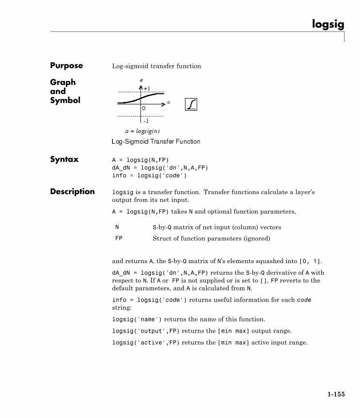
logsig
Purpose Log-sigmoid transfer function
GraphandSymbol
Syntax A = logsig(N,FP)dA_dN = logsig('dn',N,A,FP)info = logsig('code')
Description logsig is a transfer function. Transfer functions calculate a layer’soutput from its net input.
A = logsig(N,FP) takes N and optional function parameters,
N S-by-Q matrix of net input (column) vectors
FP Struct of function parameters (ignored)
and returns A, the S-by-Q matrix of N’s elements squashed into [0, 1].
dA_dN = logsig('dn',N,A,FP) returns the S-by-Q derivative of A withrespect to N. If A or FP is not supplied or is set to [], FP reverts to thedefault parameters, and A is calculated from N.
info = logsig('code') returns useful information for each codestring:
logsig('name') returns the name of this function.
logsig('output',FP) returns the [min max] output range.
logsig('active',FP) returns the [min max] active input range.
1-155
logsig
logsig('fullderiv') returns 1 or 0, depending on whether dA_dN isS-by-S-by-Q or S-by-Q.
logsig('fpnames') returns the names of the function parameters.
logsig('fpdefaults') returns the default function parameters.
Examples Here is the code to create a plot of the logsig transfer function.
n = -5:0.1:5;a = logsig(n);plot(n,a)
Assign this transfer function to layer i of a network.
net.layers{i}.transferFcn = 'logsig';
Algorithms logsig(n) = 1 / (1 + exp(-n))
See Also sim | tansig
1-156
lvqnet
Purpose Learning vector quantization neural network
Syntax lvqnet(hiddenSize,lvqLR,lvqLF)
Description LVQ (learning vector quantization) neural networks consist of twolayers. The first layer maps input vectors into clusters that are foundby the network during training. The second layer maps merges groupsof first layer clusters into the classes defined by the target data.
The total number of first layer clusters is determined by the numberof hidden neurons. The larger the hidden layer the more clusters thefirst layer can learn, and the more complex mapping of input to targetclasses can be made. The relative number of first layer clusters assignedto each target class are determined according to the distribution oftarget classes at the time of network initialization. This occurs whenthe network is automatically configured the first time train is called,or manually configured with the function configure, or manuallyinitialized with the function init is called.
lvqnet(hiddenSize,lvqLR,lvqLF) takes these arguments,
hiddenSize Size of hidden layer (default = 10)
lvqLR LVQ learning rate (default = 0.01)
lvqLF LVQ learning function (default = 'learnlv1')
and returns an LVQ neural network.
The other option for the lvq learning function is learnlv2.
Examples Here, an LVQ network is trained to classify iris flowers.
[x,t] = iris_dataset;net = lvqnet(10)net = train(net,x,t);view(net)y = net(x);
1-157

lvqnet
perf = perform(net,y,t)classes = vec2ind(y)
See Also preparets | removedelay | timedelaynet | narnet | narxnet
1-158
lvqoutputs
Purpose LVQ outputs processing function
Syntax [X,settings] = lvqoutputs(X)X = lvqoutputs('apply',X,PS)X = lvqoutputs('reverse',X,PS)dx_dy = lvqoutputs('dx_dy',X,X,PS)
Description [X,settings] = lvqoutputs(X) returns its argument unchanged,but stores the ratio of target classes in the settings for use by initlvqto initialize weights.
X = lvqoutputs('apply',X,PS) returns X.
X = lvqoutputs('reverse',X,PS) returns X.
dx_dy = lvqoutputs('dx_dy',X,X,PS) returns the identityderivative.
See Also lvqnet | initlvq
1-159
mae
Purpose Mean absolute error performance function
Syntax perf = mae(E,Y,X,FP)
Description mae is a network performance function. It measures networkperformance as the mean of absolute errors.
perf = mae(E,Y,X,FP) takes E and optional function parameters,
E Matrix or cell array of error vectors
Y Matrix or cell array of output vectors (ignored)
X Vector of all weight and bias values (ignored)
FP Function parameters (ignored)
and returns the mean absolute error.
dPerf_dx = mae('dx',E,Y,X,perf,FP) returns the derivative of perfwith respect to X.
info = mae('code') returns useful information for each code string:
mae('name') returns the name of this function.
mae('pnames') returns the names of the training parameters.
mae('pdefaults') returns the default function parameters.
Examples Create and configure a perceptron to have one input and one neuron:
net = perceptron;net = configure(net,0,0);
The network is given a batch of inputs P. The error is calculated bysubtracting the output A from target T. Then the mean absolute error iscalculated.
p = [-10 -5 0 5 10];t = [0 0 1 1 1];
1-160
mae
y = net(p)e = t-yperf = mae(e)
Note that mae can be called with only one argument because the otherarguments are ignored. mae supports those arguments to conform to thestandard performance function argument list.
NetworkUse
You can create a standard network that uses mae with perceptron.
To prepare a custom network to be trained with mae, setnet.performFcn to 'mae'. This automatically sets net.performParamto the empty matrix [], because mae has no performance parameters.
In either case, calling train or adapt, results in mae being used tocalculate performance.
See Also mse | perceptron
1-161
mandist
Purpose Manhattan distance weight function
Syntax Z = mandist(W,P)D = mandist(pos)
Description mandist is the Manhattan distance weight function. Weight functionsapply weights to an input to get weighted inputs.
Z = mandist(W,P) takes these inputs,
W S-by-R weight matrix
P R-by-Q matrix of Q input (column) vectors
and returns the S-by-Q matrix of vector distances.
mandist is also a layer distance function, which can be used to find thedistances between neurons in a layer.
D = mandist(pos) takes one argument,
pos S row matrix of neuron positions
and returns the S-by-S matrix of distances.
Examples Here you define a random weight matrix W and input vector P andcalculate the corresponding weighted input Z.
W = rand(4,3);P = rand(3,1);Z = mandist(W,P)
Here you define a random matrix of positions for 10 neurons arrangedin three-dimensional space and then find their distances.
pos = rand(3,10);D = mandist(pos)
1-162
mandist
NetworkUse
To change a network so an input weight uses mandist, setnet.inputWeight{i,j}.weightFcn to 'mandist'. For a layer weight,set net.layerWeight{i,j}.weightFcn to 'mandist'.
To change a network so a layer’s topology uses mandist, setnet.layers{i}.distanceFcn to 'mandist'.
In either case, call sim to simulate the network with dist. See newpnnor newgrnn for simulation examples.
Algorithms The Manhattan distance D between two vectors X and Y is
D = sum(abs(x-y))
See Also dist | linkdist | sim
1-163
mapminmax
Purpose Process matrices by mapping row minimum and maximum values to[-1 1]
Syntax [Y,PS] = mapminmax(X,YMIN,YMAX)[Y,PS] = mapminmax(X,FP)Y = mapminmax('apply',X,PS)X = mapminmax('reverse',Y,PS)dx_dy = mapminmax('dx_dy',X,Y,PS)
Description mapminmax processes matrices by normalizing the minimum andmaximum values of each row to [YMIN, YMAX].
[Y,PS] = mapminmax(X,YMIN,YMAX) takes X and optional parameters
X N-by-Q matrix or a 1-by-TS row cell array of N-by-Qmatrices
YMIN Minimum value for each row of Y (default is –1)
YMAX Maximum value for each row of Y (default is +1)
and returns
Y Each M-by-Q matrix (where M == N) (optional)
PS Process settings that allow consistent processing ofvalues
[Y,PS] = mapminmax(X,FP) takes parameters as a struct: FP.ymin,FP.ymax.
Y = mapminmax('apply',X,PS) returns Y, given X and settings PS.
X = mapminmax('reverse',Y,PS) returns X, given Y and settings PS.
dx_dy = mapminmax('dx_dy',X,Y,PS) returns the reverse derivative.
1-164
mapminmax
Examples Here is how to format a matrix so that the minimum and maximumvalues of each row are mapped to default interval [-1,+1].
x1 = [1 2 4; 1 1 1; 3 2 2; 0 0 0][y1,PS] = mapminmax(x1)
Next, apply the same processing settings to new values.
x2 = [5 2 3; 1 1 1; 6 7 3; 0 0 0]y2 = mapminmax('apply',x2,PS)
Reverse the processing of y1 to get x1 again.
x1_again = mapminmax('reverse',y1,PS)
Algorithms It is assumed that X has only finite real values, and that the elementsof each row are not all equal. (If xmax=xmin or if either xmax or xminare non-finite, then y=x and no change occurs.)
y = (ymax-ymin)*(x-xmin)/(xmax-xmin) + ymin;
Definitions Before training, it is often useful to scale the inputs and targets so thatthey always fall within a specified range. The function mapminmaxscales inputs and targets so that they fall in the range [–1,1]. Thefollowing code illustrates how to use this function.
[pn,ps] = mapminmax(p);[tn,ts] = mapminmax(t);net = train(net,pn,tn);
The original network inputs and targets are given in the matrices pand t. The normalized inputs and targets pn and tn that are returnedwill all fall in the interval [–1,1]. The structures ps and ts contain thesettings, in this case the minimum and maximum values of the originalinputs and targets. After the network has been trained, the ps settingsshould be used to transform any future inputs that are applied to thenetwork. They effectively become a part of the network, just like thenetwork weights and biases.
1-165
mapminmax
If mapminmax is used to scale the targets, then the output of the networkwill be trained to produce outputs in the range [–1,1]. To convert theseoutputs back into the same units that were used for the original targets,use the settings ts. The following code simulates the network that wastrained in the previous code, and then converts the network outputback into the original units.
an = sim(net,pn);a = mapminmax('reverse',an,ts);
The network output an corresponds to the normalized targets tn. Theunnormalized network output a is in the same units as the originaltargets t.
If mapminmax is used to preprocess the training set data, thenwhenever the trained network is used with new inputs they should bepreprocessed with the minimum and maximums that were computedfor the training set stored in the settings ps. The following code appliesa new set of inputs to the network already trained.
pnewn = mapminmax('apply',pnew,ps);anewn = sim(net,pnewn);anew = mapminmax('reverse',anewn,ts);
For most networks, including feedforwardnet, these steps are doneautomatically, so that you only need to use the sim command.
See Also fixunknowns | mapstd | processpca
1-166
mapstd
Purpose Process matrices by mapping each row’s means to 0 and deviations to 1
Syntax [Y,PS] = mapstd(X,ymean,ystd)[Y,PS] = mapstd(X,FP)Y = mapstd('apply',X,PS)X = mapstd('reverse',Y,PS)dx_dy = mapstd('dx_dy',X,Y,PS)
Description mapstd processes matrices by transforming the mean and standarddeviation of each row to ymean and ystd.
[Y,PS] = mapstd(X,ymean,ystd) takes X and optional parameters,
X N-by-Q matrix or a 1-by-TS row cell array of N-by-Qmatrices
ymean Mean value for each row of Y (default is 0)
ystd Standard deviation for each row of Y (default is 1)
and returns
Y Each M-by-Q matrix (where M == N) (optional)
PS Process settings that allow consistent processing ofvalues
[Y,PS] = mapstd(X,FP) takes parameters as a struct: FP.ymean,FP.ystd.
Y = mapstd('apply',X,PS) returns Y, given X and settings PS.
X = mapstd('reverse',Y,PS) returns X, given Y and settings PS.
dx_dy = mapstd('dx_dy',X,Y,PS) returns the reverse derivative.
Examples Here you format a matrix so that the minimum and maximum values ofeach row are mapped to default mean and STD of 0 and 1.
1-167
mapstd
x1 = [1 2 4; 1 1 1; 3 2 2; 0 0 0][y1,PS] = mapstd(x1)
Next, apply the same processing settings to new values.
x2 = [5 2 3; 1 1 1; 6 7 3; 0 0 0]y2 = mapstd('apply',x2,PS)
Reverse the processing of y1 to get x1 again.
x1_again = mapstd('reverse',y1,PS)
Algorithms It is assumed that X has only finite real values, and that the elements ofeach row are not all equal.
y = (x-xmean)*(ystd/xstd) + ymean;
Definitions Another approach for scaling network inputs and targets is to normalizethe mean and standard deviation of the training set. The functionmapstd normalizes the inputs and targets so that they will have zeromean and unity standard deviation. The following code illustrates theuse of mapstd.
[pn,ps] = mapstd(p);[tn,ts] = mapstd(t);
The original network inputs and targets are given in the matrices p andt. The normalized inputs and targets pn and tn that are returned willhave zero means and unity standard deviation. The settings structuresps and ts contain the means and standard deviations of the originalinputs and original targets. After the network has been trained, youshould use these settings to transform any future inputs that areapplied to the network. They effectively become a part of the network,just like the network weights and biases.
If mapstd is used to scale the targets, then the output of the networkis trained to produce outputs with zero mean and unity standarddeviation. To convert these outputs back into the same units that were
1-168
mapstd
used for the original targets, use ts. The following code simulates thenetwork that was trained in the previous code, and then converts thenetwork output back into the original units.
an = sim(net,pn);a = mapstd('reverse',an,ts);
The network output an corresponds to the normalized targets tn. Theunnormalized network output a is in the same units as the originaltargets t.
If mapstd is used to preprocess the training set data, then wheneverthe trained network is used with new inputs, you should preprocessthem with the means and standard deviations that were computed forthe training set using ps. The following commands apply a new set ofinputs to the network already trained:
pnewn = mapstd('apply',pnew,ps);anewn = sim(net,pnewn);anew = mapstd('reverse',anewn,ts);
For most networks, including feedforwardnet, these steps are doneautomatically, so that you only need to use the sim command.
See Also fixunknowns | mapminmax | processpca
1-169
maxlinlr
Purpose Maximum learning rate for linear layer
Syntax lr = maxlinlr(P)lr = maxlinlr(P,'bias')
Description maxlinlr is used to calculate learning rates for linearlayer.
lr = maxlinlr(P) takes one argument,
P R-by-Q matrix of input vectors
and returns the maximum learning rate for a linear layer without a biasthat is to be trained only on the vectors in P.
lr = maxlinlr(P,'bias') returns the maximum learning rate fora linear layer with a bias.
Examples Here you define a batch of four two-element input vectors and find themaximum learning rate for a linear layer with a bias.
P = [1 2 -4 7; 0.1 3 10 6];lr = maxlinlr(P,'bias')
See Also learnwh | linearlayer
1-170
meanabs
Purpose Mean of absolute elements of matrix or matrices
Syntax [m,n] = meanabs(x)
Description [m,n] = meanabs(x) takes a matrix or cell array of matrices andreturns,
m Mean value of all absolute finite values
n Number of finite values
If x contains no finite values, the mean returned is 0.
Examples m = meanabs([1 2;3 4])[m,n] = meanabs({[1 2; NaN 4], [4 5; 2 3]})
See Also meansqr | sumabs | sumsqr
1-171
meansqr
Purpose Mean of squared elements of matrix or matrices
Syntax [m,n] = meansqr(x)
Description [m,n] = meansqr(x) takes a matrix or cell array of matrices andreturns,
m Mean value of all squared finite values
n Number of finite values
If x contains no finite values, the mean returned is 0.
Examples m = meansqr([1 2;3 4])[m,n] = meansqr({[1 2; NaN 4], [4 5; 2 3]})
See Also meanabs | sumabs | sumsqr
1-172
midpoint
Purpose Midpoint weight initialization function
Syntax W = midpoint(S,PR)
Description midpoint is a weight initialization function that sets weight (row)vectors to the center of the input ranges.
W = midpoint(S,PR) takes two arguments,
S Number of rows (neurons)
PR R-by-Q matrix of input value ranges = [Pmin Pmax]
and returns an S-by-R matrix with rows set to (Pmin+Pmax)'/2.
Examples Here initial weight values are calculated for a five-neuron layer withinput elements ranging over [0 1] and [-2 2].
W = midpoint(5,[0 1; -2 2])
NetworkUse
You can create a standard network that uses midpoint to initializeweights by calling newc.
To prepare the weights and the bias of layer i of a custom network toinitialize with midpoint,
1 Set net.initFcn to 'initlay'. (net.initParam automaticallybecomes initlay’s default parameters.)
2 Set net.layers{i}.initFcn to 'initwb'.
3 Set each net.inputWeights{i,j}.initFcn to 'midpoint'. Set eachnet.layerWeights{i,j}.initFcn to 'midpoint'.
To initialize the network, call init.
See Also initwb | initlay | init
1-173
minmax
Purpose Ranges of matrix rows
Syntax pr = minmax(P)
Description pr = minmax(P) takes one argument,
P R-by-Q matrix
and returns the R-by-2 matrix PR of minimum and maximum valuesfor each row of P.
Alternatively, P can be an M-by-N cell array of matrices. Each matrixP{i,j} should have Ri rows and Q columns. In this case, minmaxreturns an M-by-1 cell array where the mth matrix is an Ri-by-2 matrixof the minimum and maximum values of elements for the matrix onthe ith row of P.
Examples P = [0 1 2; -1 -2 -0.5]pr = minmax(P)P = {[0 1; -1 -2] [2 3 -2; 8 0 2]; [1 -2] [9 7 3]};pr = minmax(P)
1-174
mse
Purpose Mean squared normalized error performance function
Syntax perf = mse(net,t,y,ew)
Description mse is a network performance function. It measures the network’sperformance according to the mean of squared errors.
perf = mse(net,t,y,ew) takes these arguments:
net Neural network
t Matrix or cell array of targets
y Matrix or cell array of outputs
ew Error weights (optional)
and returns the mean squared error.
This function has two optional parameters, which are associated withnetworks whose net.trainFcn is set to this function:
• 'regularization' can be set to any value between 0 and 1. Thegreater the regularization value, the more squared weights andbiases are included in the performance calculation relative to errors.The default is 0, corresponding to no regularization.
• 'normalization' can be set to 'none' (the default); 'standard',which normalizes errors between -2 and 2, corresponding tonormalizing outputs and targets between -1 and 1; and 'percent',which normalizes errors between -1 and 1. This feature is useful fornetworks with multi-element outputs. It ensures that the relativeaccuracy of output elements with differing target value ranges aretreated as equally important, instead of prioritizing the relativeaccuracy of the output element with the largest target value range.
You can create a standard network that uses mse with feedforwardnetor cascadeforwardnet. To prepare a custom network to be trainedwith mse, set net.performFcn to 'mse'. This automatically sets
1-175
mse
net.performParam to a structure with the default optional parametervalues.
Examples Here a two-layer feedforward network is created and trained topredict median house prices using the mse performance function and aregularization value of 0.01, which is the default performance functionfor feedforwardnet.
[x,t] = house_dataset;net = feedforwardnet(10);net.performFcn = 'mse'; % Redundant, MSE is defaultnet.performParam.regularization = 0.01;net = train(net,x,t);y = net(x);perf = perform(net,t,y);
Alternately, you can call this function directly.
perf = mse(net,x,t,'regularization',0.01);
See Also mae
1-176
narnet
Purpose Nonlinear autoregressive neural network
Syntax narnet(feedbackDelays,hiddenSizes,trainFcn)
Description NAR (nonlinear autoregressive) neural networks can be trained topredict a time series from that series past values.
narnet(feedbackDelays,hiddenSizes,trainFcn) takes thesearguments,
feedbackDelays Row vector of increasing 0 or positive delays(default = 1:2)
hiddenSizes Row vector of one or more hidden layer sizes(default = 10)
trainFcn Training function (default = 'trainlm')
and returns a NAR neural network.
Examples Here a NAR network is used to solve a simple time series problem.
T = simplenar_dataset;net = narnet(1:2,10)[Xs,Xi,Ai,Ts] = preparets(net,{},{},T)net = train(net,Xs,Ts,Xi,Ai);view(net)Y = net(Xs,Xi);perf = perform(net,Ts,Y)
See Also preparets | removedelay | timedelaynet | narnet | narxnet
1-177
narxnet
Purpose Nonlinear autoregressive neural network with external input
Syntax narxnet(inputDelays,feedbackDelays,hiddenSizes,trainFcn)
Description NARX (Nonlinear autoregressive with external input) networks canlearn to predict one time series given past values of the same timeseries, the feedback input, and another time series, called the externalor exogenous time series.
narxnet(inputDelays,feedbackDelays,hiddenSizes,trainFcn)takes these arguments,
inputDelays Row vector of increasing 0 or positive delays(default = 1:2)
feedbackDelays Row vector of increasing 0 or positive delays(default = 1:2)
hiddenSizes Row vector of one or more hidden layer sizes(default = 10)
trainFcn Training function (default = 'trainlm')
and returns a NARX neural network.
Examples Here a NARX neural network is used to solve a simple time seriesproblem.
[X,T] = simpleseries_dataset;net = narxnet(1:2,1:2,10)[Xs,Xi,Ai,Ts] = preparets(net,X,{},T)net = train(net,Xs,Ts,Xi,Ai);view(net)Y = net(Xs,Xi,Ai);perf = perform(net,Ts,Y)
Here the NARX network is simulated in closed loop form.
1-178
narxnet
netc = closeloop(net);view(netc)[Xs,Xi,Ai,Ts] = preparets(netc,X,{},T);y = netc(Xs,Xi,Ai)
Here the NARX network is used to predict the next output a timestepahead of when it will actually appear.
netp = removedelay(net);view(netp)[Xs,Xi,Ai,Ts] = preparets(netp,X,{},T);y = netp(Xs,Xi,Ai)
See Also closeloop | narnet | openloop | preparets | removedelay |timedelaynet
1-179
nctool
Purpose Neural network classification or clustering tool
Syntax nctool
Description nctool opens the neural network clustering GUI.
Algorithms nctool leads you through solving a clustering problem using aself-organizing map. The map forms a compressed representation ofthe inputs space, reflecting both the relative density of input vectorsin that space, and a two-dimensional compressed representation of theinput-space topology.
1-180
negdist
Purpose Negative distance weight function
Syntax Z = negdist(W,P)dim = negdist('size',S,R,FP)dw = negdist('dz_dw',W,P,Z,FP)
Description negdist is a weight function. Weight functions apply weights to aninput to get weighted inputs.
Z = negdist(W,P) takes these inputs,
W S-by-R weight matrix
P R-by-Q matrix of Q input (column) vectors
FP Row cell array of function parameters (optional,ignored)
and returns the S-by-Q matrix of negative vector distances.
dim = negdist('size',S,R,FP) takes the layer dimension S, inputdimension R, and function parameters, and returns the weight size[S-by-R].
dw = negdist('dz_dw',W,P,Z,FP) returns the derivative of Z withrespect to W.
Examples Here you define a random weight matrix W and input vector P andcalculate the corresponding weighted input Z.
W = rand(4,3);P = rand(3,1);Z = negdist(W,P)
1-181
negdist
NetworkUse
You can create a standard network that uses negdist by callingcompetlayer or selforgmap.
To change a network so an input weight uses negdist, setnet.inputWeight{i,j}.weightFcn to 'negdist'. For a layer weight,set net.layerWeight{i,j}.weightFcn to 'negdist'.
In either case, call sim to simulate the network with negdist.
Algorithms negdist returns the negative Euclidean distance:
z = -sqrt(sum(w-p)^2)
See Also competlayer | dist | dotprod | selforgmap | sim
1-182
netinv
Purpose Inverse transfer function
Syntax A = netinv(N,FP)
Description netinv is a transfer function. Transfer functions calculate a layer’soutput from its net input.
A = netinv(N,FP) takes inputs
N S-by-Q matrix of net input (column) vectors
FP Struct of function parameters (ignored)
and returns 1/N.
info = netinv('code') returns information about this function. Thefollowing codes are supported:
netinv('name') returns the name of this function.
netinv('output',FP) returns the [min max] output range.
netinv('active',FP) returns the [min max] active input range.
netinv('fullderiv') returns 1 or 0, depending on whether dA_dN isS-by-S-by-Q or S-by-Q.
netinv('fpnames') returns the names of the function parameters.
netinv('fpdefaults') returns the default function parameters.
Examples Here you define 10 five-element net input vectors N and calculate A.
n = rand(5,10);a = netinv(n);
Assign this transfer function to layer i of a network.
net.layers{i}.transferFcn = 'netinv';
1-183

netinv
See Also tansig | logsig
1-184
netprod
Purpose Product net input function
Syntax N = netprod({Z1,Z2,...,Zn})info = netprod('code')
Description netprod is a net input function. Net input functions calculate a layer’snet input by combining its weighted inputs and biases.
N = netprod({Z1,Z2,...,Zn}) takes
Zi S-by-Q matrices in a row cell array
and returns an element-wise product of Z1 to Zn.
info = netprod('code') returns information about this function.The following codes are supported:
'deriv' Name of derivative function
'fullderiv' Full N-by-S-by-Q derivative = 1, element-wiseS-by-Q derivative = 0
'name' Full name
'fpnames' Returns names of function parameters
'fpdefaults' Returns default function parameters
Examples Here netprod combines two sets of weighted input vectors(user-defined).
Z1 = [1 2 4;3 4 1];Z2 = [-1 2 2; -5 -6 1];Z = {Z1,Z2};N = netprod({Z})
1-185
netprod
Here netprod combines the same weighted inputs with a bias vector.Because Z1 and Z2 each contain three concurrent vectors, threeconcurrent copies of B must be created with concur so that all sizesmatch.
B = [0; -1];Z = {Z1, Z2, concur(B,3)};N = netprod(Z)
NetworkUse
You can create a standard network that uses netprod by calling newpnnor newgrnn.
To change a network so that a layer uses netprod, setnet.layers{i}.netInputFcn to 'netprod'.
In either case, call sim to simulate the network with netprod. Seenewpnn or newgrnn for simulation examples.
See Also sim | netsum | concur
1-186
netsum
Purpose Sum net input function
Syntax N = netsum({Z1,Z2,...,Zn},FP)info = netsum('code')
Description netsum is a net input function. Net input functions calculate a layer’snet input by combining its weighted inputs and biases.
N = netsum({Z1,Z2,...,Zn},FP) takes Z1 to Zn and optional functionparameters,
Zi S-by-Q matrices in a row cell array
FP Row cell array of function parameters (ignored)
and returns the elementwise sum of Z1 to Zn.
info = netsum('code') returns information about this function. Thefollowing codes are supported:
netsum('name') returns the name of this function.
netsum('type') returns the type of this function.
netsum('fpnames') returns the names of the function parameters.
netsum('fpdefaults') returns default function parameter values.
netsum('fpcheck', FP) throws an error for illegal functionparameters.
netsum('fullderiv') returns 0 or 1, depending on whether thederivative is S-by-Q or N-by-S-by-Q.
Examples Here netsum combines two sets of weighted input vectors and a bias.You must use concur to make B the same dimensions as Z1 and Z2.
z1 = [1 2 4; 3 4 1}z2 = [-1 2 2; -5 -6 1]b = [0; -1]
1-187
netsum
n = netsum({z1,z2,concur(b,3)})
Assign this net input function to layer i of a network.
net.layers(i).netFcn = 'compet';
Use feedforwardnet or cascadeforwardnet to create a standardnetwork that uses netsum.
See Also cascadeforwardnet | feedforwardnet | netprod | netinv
1-188
network
Purpose Create custom neural network
Syntax net = networknet = network(numInputs,numLayers,biasConnect,inputConnect,
layerConnect,outputConnect)
To GetHelp
Type help network/network.
Description network creates new custom networks. It is used to create networksthat are then customized by functions such as feedforwardnet andnarxnet.
net = network without arguments returns a new neural network withno inputs, layers or outputs.
net =network(numInputs,numLayers,biasConnect,inputConnect,layerConnect,outptakes these optional arguments (shown with default values):
numInputs Number of inputs, 0
numLayers Number of layers, 0
biasConnect numLayers-by-1 Boolean vector, zeros
inputConnect numLayers-by-numInputs Boolean matrix,zeros
layerConnect numLayers-by-numLayers Boolean matrix,zeros
outputConnect 1-by-numLayers Boolean vector, zeros
and returns
net New network with the given property values
1-189
network
Properties Architecture Properties
net.numInputs 0 or a positiveinteger
Number of inputs.
net.numLayers 0 or a positiveinteger
Number of layers.
net.biasConnect numLayer-by-1Boolean vector
If net.biasConnect(i) is 1,then layer i has a bias, andnet.biases{i} is a structuredescribing that bias.
net.inputConnect numLayer-by-numInputsBoolean vector
If net.inputConnect(i,j) is1, then layer i has a weightcoming from input j, andnet.inputWeights{i,j} isa structure describing thatweight.
net.layerConnect numLayer-by-numLayersBoolean vector
If net.layerConnect(i,j) is1, then layer i has a weightcoming from layer j, andnet.layerWeights{i,j} isa structure describing thatweight.
net.numInputs 0 or a positiveinteger
Number of inputs.
net.numLayers 0 or a positiveinteger
Number of layers.
net.biasConnect numLayer-by-1Boolean vector
If net.biasConnect(i) is 1,then layer i has a bias, andnet.biases{i} is a structuredescribing that bias.
1-190
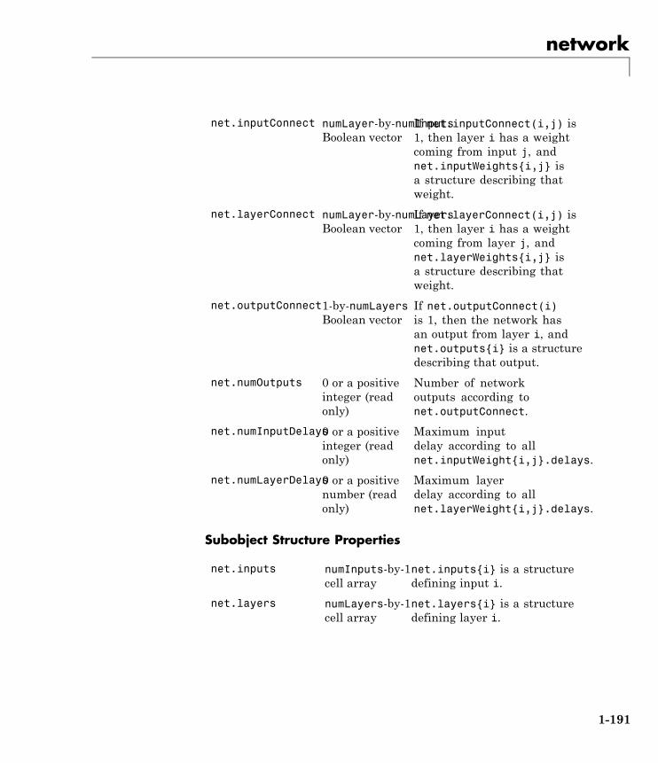
network
net.inputConnect numLayer-by-numInputsBoolean vector
If net.inputConnect(i,j) is1, then layer i has a weightcoming from input j, andnet.inputWeights{i,j} isa structure describing thatweight.
net.layerConnect numLayer-by-numLayersBoolean vector
If net.layerConnect(i,j) is1, then layer i has a weightcoming from layer j, andnet.layerWeights{i,j} isa structure describing thatweight.
net.outputConnect1-by-numLayersBoolean vector
If net.outputConnect(i)is 1, then the network hasan output from layer i, andnet.outputs{i} is a structuredescribing that output.
net.numOutputs 0 or a positiveinteger (readonly)
Number of networkoutputs according tonet.outputConnect.
net.numInputDelays0 or a positiveinteger (readonly)
Maximum inputdelay according to allnet.inputWeight{i,j}.delays.
net.numLayerDelays0 or a positivenumber (readonly)
Maximum layerdelay according to allnet.layerWeight{i,j}.delays.
Subobject Structure Properties
net.inputs numInputs-by-1cell array
net.inputs{i} is a structuredefining input i.
net.layers numLayers-by-1cell array
net.layers{i} is a structuredefining layer i.
1-191
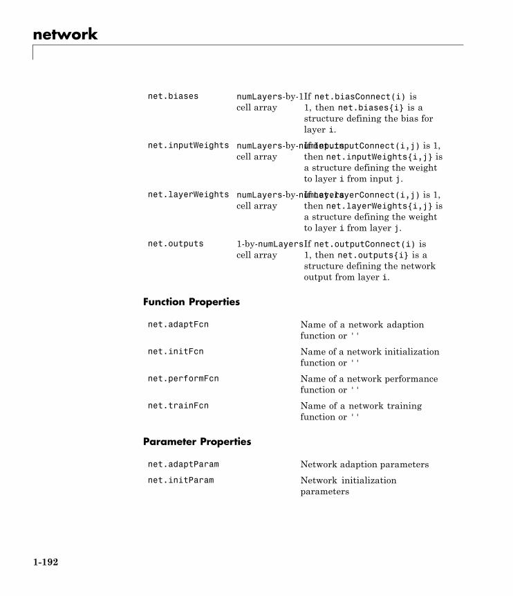
network
net.biases numLayers-by-1cell array
If net.biasConnect(i) is1, then net.biases{i} is astructure defining the bias forlayer i.
net.inputWeights numLayers-by-numInputscell array
If net.inputConnect(i,j) is 1,then net.inputWeights{i,j} isa structure defining the weightto layer i from input j.
net.layerWeights numLayers-by-numLayerscell array
If net.layerConnect(i,j) is 1,then net.layerWeights{i,j} isa structure defining the weightto layer i from layer j.
net.outputs 1-by-numLayerscell array
If net.outputConnect(i) is1, then net.outputs{i} is astructure defining the networkoutput from layer i.
Function Properties
net.adaptFcn Name of a network adaptionfunction or ''
net.initFcn Name of a network initializationfunction or ''
net.performFcn Name of a network performancefunction or ''
net.trainFcn Name of a network trainingfunction or ''
Parameter Properties
net.adaptParam Network adaption parameters
net.initParam Network initializationparameters
1-192
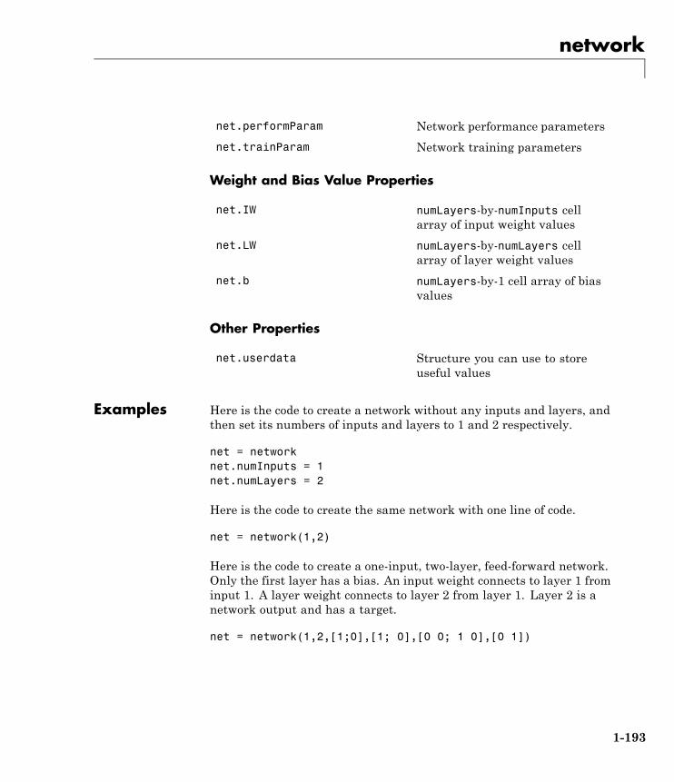
network
net.performParam Network performance parameters
net.trainParam Network training parameters
Weight and Bias Value Properties
net.IW numLayers-by-numInputs cellarray of input weight values
net.LW numLayers-by-numLayers cellarray of layer weight values
net.b numLayers-by-1 cell array of biasvalues
Other Properties
net.userdata Structure you can use to storeuseful values
Examples Here is the code to create a network without any inputs and layers, andthen set its numbers of inputs and layers to 1 and 2 respectively.
net = networknet.numInputs = 1net.numLayers = 2
Here is the code to create the same network with one line of code.
net = network(1,2)
Here is the code to create a one-input, two-layer, feed-forward network.Only the first layer has a bias. An input weight connects to layer 1 frominput 1. A layer weight connects to layer 2 from layer 1. Layer 2 is anetwork output and has a target.
net = network(1,2,[1;0],[1; 0],[0 0; 1 0],[0 1])
1-193
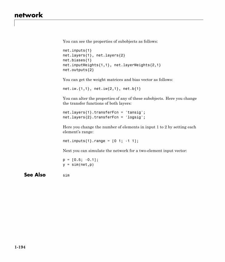
network
You can see the properties of subobjects as follows:
net.inputs{1}net.layers{1}, net.layers{2}net.biases{1}net.inputWeights{1,1}, net.layerWeights{2,1}net.outputs{2}
You can get the weight matrices and bias vector as follows:
net.iw.{1,1}, net.iw{2,1}, net.b{1}
You can alter the properties of any of these subobjects. Here you changethe transfer functions of both layers:
net.layers{1}.transferFcn = 'tansig';net.layers{2}.transferFcn = 'logsig';
Here you change the number of elements in input 1 to 2 by setting eachelement’s range:
net.inputs{1}.range = [0 1; -1 1];
Next you can simulate the network for a two-element input vector:
p = [0.5; -0.1];y = sim(net,p)
See Also sim
1-194
newgrnn
Purpose Design generalized regression neural network
Syntax net = newgrnn(P,T,spread)
Description Generalized regression neural networks (grnns) are a kind of radialbasis network that is often used for function approximation. grnns canbe designed very quickly.
net = newgrnn(P,T,spread) takes three inputs,
P R-by-Q matrix of Q input vectors
T S-by-Q matrix of Q target class vectors
spread Spread of radial basis functions (default = 1.0)
and returns a new generalized regression neural network.
The larger the spread, the smoother the function approximation. Tofit data very closely, use a spread smaller than the typical distancebetween input vectors. To fit the data more smoothly, use a largerspread.
Properties newgrnn creates a two-layer network. The first layer has radbasneurons, and calculates weighted inputs with dist and net input withnetprod. The second layer has purelin neurons, calculates weightedinput with normprod, and net inputs with netsum. Only the first layerhas biases.
newgrnn sets the first layer weights to P', and the first layer biasesare all set to 0.8326/spread, resulting in radial basis functions thatcross 0.5 at weighted inputs of +/– spread. The second layer weightsW2 are set to T.
Examples Here you design a radial basis network, given inputs P and targets T.
P = [1 2 3];T = [2.0 4.1 5.9];
1-195
newgrnn
net = newgrnn(P,T);
The network is simulated for a new input.
P = 1.5;Y = sim(net,P)
References Wasserman, P.D., Advanced Methods in Neural Computing, New York,Van Nostrand Reinhold, 1993, pp. 155–61
See Also sim | newrb | newrbe | newpnn
1-196
newlind
Purpose Design linear layer
Syntax net = newlind(P,T,Pi)
Description net = newlind(P,T,Pi) takes these input arguments,
P R-by-Q matrix of Q input vectors
T S-by-Q matrix of Q target class vectors
Pi 1-by-ID cell array of initial input delay states
where each element Pi{i,k} is an Ri-by-Q matrix, and the default =[]; and returns a linear layer designed to output T (with minimumsum square error) given input P.
newlind(P,T,Pi) can also solve for linear networks with input delaysand multiple inputs and layers by supplying input and target data incell array form:
P Ni-by-TS cellarray
Each element P{i,ts} is anRi-by-Q input matrix
T Nt-by-TS cellarray
Each element P{i,ts} is a Vi-by-Qmatrix
Pi Ni-by-ID cellarray
Each element Pi{i,k} is anRi-by-Q matrix, default = []
and returns a linear network with ID input delays, Ni network inputs,and Nl layers, designed to output T (with minimum sum square error)given input P.
Examples You want a linear layer that outputs T given P for the followingdefinitions:
P = [1 2 3];T = [2.0 4.1 5.9];
1-197
newlind
Use newlind to design such a network and check its response.
net = newlind(P,T);Y = sim(net,P)
You want another linear layer that outputs the sequence T given thesequence P and two initial input delay states Pi.
P = {1 2 1 3 3 2};Pi = {1 3};T = {5.0 6.1 4.0 6.0 6.9 8.0};net = newlind(P,T,Pi);Y = sim(net,P,Pi)
You want a linear network with two outputs Y1 and Y2 that generatesequences T1 and T2, given the sequences P1 and P2, with three initialinput delay states Pi1 for input 1 and three initial delays states Pi2for input 2.
P1 = {1 2 1 3 3 2}; Pi1 = {1 3 0};P2 = {1 2 1 1 2 1}; Pi2 = {2 1 2};T1 = {5.0 6.1 4.0 6.0 6.9 8.0};T2 = {11.0 12.1 10.1 10.9 13.0 13.0};net = newlind([P1; P2],[T1; T2],[Pi1; Pi2]);Y = sim(net,[P1; P2],[Pi1; Pi2]);Y1 = Y(1,:)Y2 = Y(2,:)
Algorithms newlind calculates weight W and bias B values for a linear layer frominputs P and targets T by solving this linear equation in the leastsquares sense:
[W b] * [P; ones] = T
See Also sim
1-198
newpnn
Purpose Design probabilistic neural network
Syntax net = newpnn(P,T,spread)
Description Probabilistic neural networks (PNN) are a kind of radial basis networksuitable for classification problems.
net = newpnn(P,T,spread) takes two or three arguments,
P R-by-Q matrix of Q input vectors
T S-by-Q matrix of Q target class vectors
spread Spread of radial basis functions (default = 0.1)
and returns a new probabilistic neural network.
If spread is near zero, the network acts as a nearest neighbor classifier.As spread becomes larger, the designed network takes into accountseveral nearby design vectors.
Examples Here a classification problem is defined with a set of inputs P and classindices Tc.
P = [1 2 3 4 5 6 7];Tc = [1 2 3 2 2 3 1];
The class indices are converted to target vectors, and a PNN is designedand tested.
T = ind2vec(Tc)net = newpnn(P,T);Y = sim(net,P)Yc = vec2ind(Y)
Algorithms newpnn creates a two-layer network. The first layer has radbasneurons, and calculates its weighted inputs with dist and its net inputwith netprod. The second layer has compet neurons, and calculates its
1-199
newpnn
weighted input with dotprod and its net inputs with netsum. Onlythe first layer has biases.
newpnn sets the first-layer weights to P', and the first-layer biasesare all set to 0.8326/spread, resulting in radial basis functions thatcross 0.5 at weighted inputs of +/– spread. The second-layer weightsW2 are set to T.
References Wasserman, P.D., Advanced Methods in Neural Computing, New York,Van Nostrand Reinhold, 1993, pp. 35–55
See Also sim | ind2vec | vec2ind | newrb | newrbe | newgrnn
1-200
newrb
Purpose Design radial basis network
Syntax net = newrb(P,T,goal,spread,MN,DF)
Description Radial basis networks can be used to approximate functions. newrbadds neurons to the hidden layer of a radial basis network until it meetsthe specified mean squared error goal.
net = newrb(P,T,goal,spread,MN,DF) takes two of these arguments,
P R-by-Q matrix of Q input vectors
T S-by-Q matrix of Q target class vectors
goal Mean squared error goal (default = 0.0)
spread Spread of radial basis functions (default = 1.0)
MN Maximum number of neurons (default is Q)
DF Number of neurons to add between displays(default = 25)
and returns a new radial basis network.
The larger spread is, the smoother the function approximation. Toolarge a spread means a lot of neurons are required to fit a fast-changingfunction. Too small a spread means many neurons are required to fit asmooth function, and the network might not generalize well. Call newrbwith different spreads to find the best value for a given problem.
Examples Here you design a radial basis network, given inputs P and targets T.
P = [1 2 3];T = [2.0 4.1 5.9];net = newrb(P,T);
The network is simulated for a new input.
P = 1.5;
1-201
newrb
Y = sim(net,P)
Algorithms newrb creates a two-layer network. The first layer has radbas neurons,and calculates its weighted inputs with dist and its net input withnetprod. The second layer has purelin neurons, and calculates itsweighted input with dotprod and its net inputs with netsum. Bothlayers have biases.
Initially the radbas layer has no neurons. The following steps arerepeated until the network’s mean squared error falls below goal.
1 The network is simulated.
2 The input vector with the greatest error is found.
3 A radbas neuron is added with weights equal to that vector.
4 The purelin layer weights are redesigned to minimize error.
See Also sim | newrbe | newgrnn | newpnn
1-202
newrbe
Purpose Design exact radial basis network
Syntax net = newrbe(P,T,spread)
Description Radial basis networks can be used to approximate functions. newrbevery quickly designs a radial basis network with zero error on thedesign vectors.
net = newrbe(P,T,spread) takes two or three arguments,
P RxQ matrix of Q R-element input vectors
T SxQ matrix of Q S-element target class vectors
spread Spread of radial basis functions (default = 1.0)
and returns a new exact radial basis network.
The larger the spread is, the smoother the function approximation willbe. Too large a spread can cause numerical problems.
Examples Here you design a radial basis network given inputs P and targets T.
P = [1 2 3];T = [2.0 4.1 5.9];net = newrbe(P,T);
The network is simulated for a new input.
P = 1.5;Y = sim(net,P)
Algorithms newrbe creates a two-layer network. The first layer has radbasneurons, and calculates its weighted inputs with dist and its net inputwith netprod. The second layer has purelin neurons, and calculatesits weighted input with dotprod and its net inputs with netsum. Bothlayers have biases.
1-203
newrbe
newrbe sets the first-layer weights to P', and the first-layer biases areall set to 0.8326/spread, resulting in radial basis functions that cross0.5 at weighted inputs of +/– spread.
The second-layer weights IW{2,1} and biases b{2} are found bysimulating the first-layer outputs A{1} and then solving the followinglinear expression:
[W{2,1} b{2}] * [A{1}; ones] = T
See Also sim | newrb | newgrnn | newpnn
1-204
nftool
Purpose Neural network fitting tool
Syntax nftool
Description nftool opens the neural network fitting tool GUI.
Algorithms nftool leads you through solving a data fitting problem, solving it witha two-layer feed-forward network trained with Levenberg-Marquardt.
See Also nntool
1-205
nncell2mat
Purpose Combine neural network cell data into matrix
Syntax [y,i,j] nncell2mat(x)
Description [y,i,j] nncell2mat(x) takes a cell array of matrices and returns,
y Cell array formed by concatenating matrices
i Array of row sizes
ji Array of column sizes
The row and column sizes returned by nncell2mat can be used toconvert the returned matrix back into a cell of matrices with mat2cell.
Examples Here neural network data is converted to a matrix and back.
c = {rands(2,3) rands(2,3); rands(5,3) rands(5,3)};[m,i,j] = nncell2mat(c)c3 = mat2cell(m,i,j)
See Also nndata | nnsize
1-206
nncorr
Purpose Crross correlation between neural network time series
Syntax nncorr(a,b,maxlag,'flag')
Description nncorr(a,b,maxlag,'flag') takes these arguments,
a Matrix or cell array, with columns interpreted astimesteps, and having a total number of matrixrows of N.
b Matrix or cell array, with columns interpreted astimesteps, and having a total number of matrixrows of M.
maxlag Maximum number of time lags
flag Type of normalization (default = 'none')
and returns an N-by-M cell array where each {i,j} element is a2*maxlag+1 length row vector formed from the correlations of aelements (i.e., matrix row) i and b elements (i.e., matrix column) j.
If a and b are specified with row vectors, the result is returned inmatrix form.
The options for the normalization flag are:
• 'biased'— scales the raw cross-correlation by 1/N.
• 'unbiased'— scales the raw correlation by 1/(N-abs(k)), where kis the index into the result.
• 'coeff'— normalizes the sequence so that the correlations at zerolag are 1.0.
• 'none' — no scaling. This is the default.
Examples Here the autocorrelation of a random 1-element, 1-sample, 20-timestepsignal is calculated with a maximum lag of 10.
1-207
nncorr
a = nndata(1,1,20)aa = nncorr(a,a,10)
Here the cross-correlation of the first signal with another random2-element signal are found, with a maximum lag of 8.
b = nndata(2,1,20)ab = nncorr(a,b,8)
See Also confusion | regression
1-208
nndata
Purpose Create neural network data
Syntax nndata(N,Q,TS,v)
Description nndata(N,Q,TS,v) takes these arguments,
N Vector of M element sizes
Q Number of samples
TS Number of timesteps
v Scalar value
and returns an M-by-TS cell array where each row i has N(i)-by-Q sizedmatrices of value v. If v is not specified, random values are returned.
You can access subsets of neural network data with getelements,getsamples, gettimesteps, and getsignals.
You can set subsets of neural network data with setelements,setsamples, settimesteps, and setsignals.
You can concatenate subsets of neural network data with catelements,catsamples, cattimesteps, and catsignals.
Examples Here four samples of five timesteps, for a 2-element signal consistingof zero values is created:
x = nndata(2,4,5,0)
To create random data with the same dimensions:
x = nndata(2,4,5)
Here static (1 timestep) data of 12 samples of 4 elements is created.
x = nndata(4,12)
1-209

nndata
See Also nnsize | tonndata | fromnndata | nndata2sim | sim2nndata
1-210
nndata2gpu
Purpose Format neural data for efficient GPU training or simulation
Syntax nndata2gpu(x)[Y,Q,N,TS] = nndata2gpu(X)nndata2gpu(X,PRECISION)
Description nndata2gpu requires Parallel Computing Toolbox™.
nndata2gpu(x) takes an N-by-Q matrix X of Q N-element column vectors,and returns it in a form for neural network training and simulationon the current GPU device.
The N-by-Q matrix becomes a QQ-by-N gpuArray where QQ is Q roundedup to the next multiple of 32. The extra rows (Q+1):QQ are filledwith NaN values. The gpuArray has the same precision ('single' or'double') as X.
[Y,Q,N,TS] = nndata2gpu(X) can also take an M-by-TS cell array ofM signals over TS time steps. Each element of X{i,ts} should be anNi-by-Q matrix of Q Ni-element vectors, representing the ith signalvector at time step ts, across all Q time series. In this case, thegpuArray Y returned is QQ-by-(sum(Ni)*TS). Dimensions Ni, Q, and TSare also returned so they can be used with gpu2nndata to perform thereverse formatting.
nndata2gpu(X,PRECISION) specifies the default precision of thegpuArray, which can be 'double' or 'single'.
Examples Copy a matrix to the GPU and back:
x = rand(5,6)[y,q] = nndata2gpu(x)x2 = gpu2nndata(y,q)
Copy neural network cell array data, representing four time series, eachconsisting of five time steps of 2-element and 3-element signals:
x = nndata([2;3],4,5)[y,q,n,ts] = nndata2gpu(x)
1-211

nndata2gpu
x2 = gpu2nndata(y,q,n,ts)
See Also gpu2nndata
1-212
nndata2sim
Purpose Convert neural network data to Simulink time series
Syntax nndata2sim(x,i,q)
Description nndata2sim(x,i,q) takes these arguments,
x Neural network data
i Index of signal (default = 1)
q Index of sample (default = 1)
and returns time series q of signal i as a Simulink time series structure.
Examples Here random neural network data is created with two signals having4 and 3 elements respectively, over 10 timesteps. Three such seriesare created.
x = nndata([4;3],3,10);
Now the second signal of the first series is converted to Simulink form.
y_2_1 = nndata2sim(x,2,1)
See Also nndata | sim2nndata | nnsize
1-213
nnsize
Purpose Number of neural data elements, samples, timesteps, and signals
Syntax [N,Q,TS,M] = nnsize(X)
Description [N,Q,TS,M] = nnsize(X) takes neural network data x and returns,
N Vector containing the number of element sizes foreach of M signals
Q Number of samples
TS Number of timesteps
M Number of signals
If X is a matrix, N is the number of rows of X, Q is the number of columns,and both TS and M are 1.
If X is a cell array, N is an Sx1 vector, where M is the number of rowsin X, and N(i) is the number of rows in X{i,1}. Q is the number ofcolumns in the matrices in X.
Examples This code gets the dimensions of matrix data:
x = [1 2 3; 4 7 4][n,q,ts,s] = nnsize(x)
This code gets the dimensions of cell array data:
x = {[1:3; 4:6] [7:9; 10:12]; [13:15] [16:18]}[n,q,ts,s] = nnsize(x)
See Also nndata | numelements | numsamples | numsignals | numtimesteps
1-214
nnstart
Purpose Neural network getting started GUI
Syntax nnstart
Description nnstart opens a window with launch buttons for neural network fitting,pattern recognition, clustering and time series wizards. It also provideslinks to lists of data sets, examples, and other useful information forgetting started.
See Also nctool | nftool | nprtool | ntstool
1-215

nntool
Purpose Open Network/Data Manager
Syntax nntool
Description nntool opens the Network/Data Manager window, which allows you toimport, create, use, and export neural networks and data.
1-216
nntraintool
Purpose Neural network training tool
Syntax nntraintool
Description nntraintool opens the neural network training GUI.
This function can be called to make the training GUI visible beforetraining has occurred, after training if the window has been closed, orjust to bring the training GUI to the front.
Network training functions handle all activity within the trainingwindow.
To access additional useful plots, related to the current or last networktrained, during or after training, click their respective buttons in thetraining window.
1-217
noloop
Purpose Remove neural network open- and closed-loop feedback
Syntax net = noloop(net)
Description net = noloop(net) takes a neural network and returns the networkwith open- and closed-loop feedback removed.
For outputs i, where net.outputs{i}.feedbackMode is 'open', thefeedback mode is set to 'none', outputs{i}.feedbackInput is set tothe empty matrix, and the associated network input is deleted.
For outputs i, where net.outputs{i}.feedbackMode is 'closed', thefeedback mode is set to 'none'.
Examples Here a NARX network is designed. The NARX network has a standardinput and an open-loop feedback output to an associated feedback input.
[X,T] = simplenarx_dataset;net = narxnet(1:2,1:2,20);[Xs,Xi,Ai,Ts] = preparets(net,X,{},T);net = train(net,Xs,Ts,Xi,Ai);view(net)Y = net(Xs,Xi,Ai)
Now the network is converted to no loop form. The output and secondinput are no longer associated.
net = noloop(net);view(net)[Xs,Xi,Ai] = preparets(net,X,T);Y = net(Xs,Xi,Ai)
See Also closeloop | openloop
1-218
normc
Purpose Normalize columns of matrix
Syntax normc(M)
Description normc(M) normalizes the columns of M to a length of 1.
Examples m = [1 2; 3 4];normc(m)ans =
0.3162 0.44720.9487 0.8944
See Also normr
1-219
normprod
Purpose Normalized dot product weight function
Syntax Z = normprod(W,P,FP)dim = normprod('size',S,R,FP)dw = normprod('dz_dw',W,P,Z,FP)
Description normprod is a weight function. Weight functions apply weights to aninput to get weighted inputs.
Z = normprod(W,P,FP) takes these inputs,
W S-by-R weight matrix
P R-by-Q matrix of Q input (column) vectors
FP Row cell array of function parameters(optional, ignored)
and returns the S-by-Q matrix of normalized dot products.
dim = normprod('size',S,R,FP) takes the layer dimension S, inputdimension R, and function parameters, and returns the weight size[S-by-R].
dw = normprod('dz_dw',W,P,Z,FP) returns the derivative of Z withrespect to W.
Examples Here you define a random weight matrix W and input vector P andcalculate the corresponding weighted input Z.
W = rand(4,3);P = rand(3,1);Z = normprod(W,P)
1-220
normprod
NetworkUse
You can create a standard network that uses normprod by callingnewgrnn.
To change a network so an input weight uses normprod, setnet.inputWeight{i,j}.weightFcn to 'normprod'. For a layer weight,set net.layerWeight{i,j}.weightFcn to 'normprod'.
In either case, call sim to simulate the network with normprod. Seenewgrnn for simulation examples.
Algorithms normprod returns the dot product normalized by the sum of the inputvector elements.
z = w*p/sum(p)
See Also dotprod
1-221

normr
Purpose Normalize rows of matrix
Syntax normr(M)
Description normr(M) normalizes the rows of M to a length of 1.
Examples m = [1 2; 3 4];normr(m)ans =
0.4472 0.89440.6000 0.8000
See Also normc
1-222
nprtool
Purpose Neural network pattern recognition tool
Syntax nprtool
Description nprtool opens the neural network pattern-recognition GUI.
Algorithms nprtool leads you through solving a pattern-recognition classificationproblem using a two-layer feed-forward patternnet network withsigmoid output neurons.
See Also nctool | nftool | ntstool
1-223
ntstool
Purpose Neural network time series tool
Syntax ntstoolntstool('close')
Description ntstool opens the neural network time series wizard and leads youthrough solving a fitting problem using a two-layer feed-forwardnetwork.
ntstool('close') closes the wizard.
See Also nctool | nftool | nprtool
1-224
num2deriv
Purpose Numeric two-point network derivative function
Syntax num2deriv('dperf_dwb',net,X,T,Xi,Ai,EW)num2deriv('de_dwb',net,X,T,Xi,Ai,EW)
Description This function calculates derivatives using the two-point numericderivative rule.
dydx
y x dx y xdx
= + −( ) ( )
This function is much slower than the analytical (non-numerical)derivative functions, but is provided as a means of checking theanalytical derivative functions. The other numerical function,num5deriv, is slower but more accurate.
num2deriv('dperf_dwb',net,X,T,Xi,Ai,EW) takes these arguments,
net Neural network
X Inputs, an RxQ matrix (or NxTS cell array ofRixQ matrices)
T Targets, an SxQ matrix (or MxTS cell array ofSixQ matrices)
Xi Initial input delay states (optional)
Ai Initial layer delay states (optional)
EW Error weights (optional)
and returns the gradient of performance with respect to the network’sweights and biases, where R and S are the number of input and outputelements and Q is the number of samples (and N and M are the numberof input and output signals, Ri and Si are the number of each input andoutputs elements, and TS is the number of timesteps).
num2deriv('de_dwb',net,X,T,Xi,Ai,EW) returns the Jacobian oferrors with respect to the network’s weights and biases.
1-225
num2deriv
Examples Here a feedforward network is trained and both the gradient andJacobian are calculated.
[x,t] = simplefit_dataset;net = feedforwardnet(20);net = train(net,x,t);y = net(x);perf = perform(net,t,y);dwb = num2deriv('dperf_dwb',net,x,t)
See Also bttderiv | defaultderiv | fpderiv | num5deriv | staticderiv
1-226
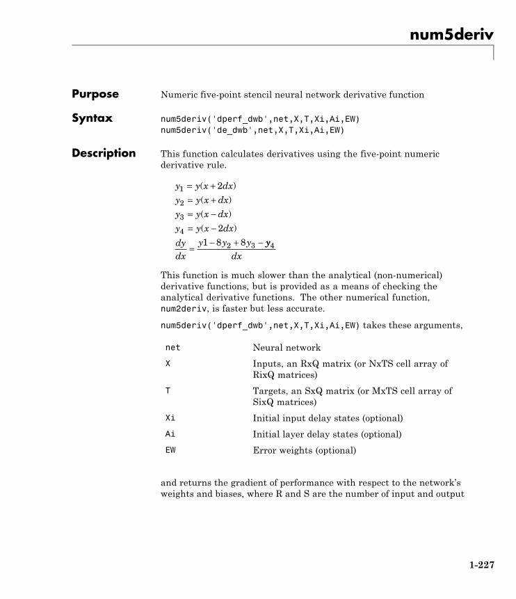
num5deriv
Purpose Numeric five-point stencil neural network derivative function
Syntax num5deriv('dperf_dwb',net,X,T,Xi,Ai,EW)num5deriv('de_dwb',net,X,T,Xi,Ai,EW)
Description This function calculates derivatives using the five-point numericderivative rule.
y y x dx
y y x dx
y y x dx
y y x dx
dydx
y y y
1
2
3
4
2 3
2
2
1 8 8
= += += −= −
=− + −
( )
( )
( )
( )
yydx
4
This function is much slower than the analytical (non-numerical)derivative functions, but is provided as a means of checking theanalytical derivative functions. The other numerical function,num2deriv, is faster but less accurate.
num5deriv('dperf_dwb',net,X,T,Xi,Ai,EW) takes these arguments,
net Neural network
X Inputs, an RxQ matrix (or NxTS cell array ofRixQ matrices)
T Targets, an SxQ matrix (or MxTS cell array ofSixQ matrices)
Xi Initial input delay states (optional)
Ai Initial layer delay states (optional)
EW Error weights (optional)
and returns the gradient of performance with respect to the network’sweights and biases, where R and S are the number of input and output
1-227
num5deriv
elements and Q is the number of samples (and N and M are the numberof input and output signals, Ri and Si are the number of each input andoutputs elements, and TS is the number of timesteps).
num5deriv('de_dwb',net,X,T,Xi,Ai,EW) returns the Jacobian oferrors with respect to the network’s weights and biases.
Examples Here a feedforward network is trained and both the gradient andJacobian are calculated.
[x,t] = simplefit_dataset;net = feedforwardnet(20);net = train(net,x,t);y = net(x);perf = perform(net,t,y);dwb = num5deriv('dperf_dwb',net,x,t)
See Also bttderiv | defaultderiv | fpderiv | num2deriv | staticderiv
1-228
numelements
Purpose Number of elements in neural network data
Syntax numelements(x)
Description numelements(x) takes neural network data x in matrix or cell arrayform, and returns the number of elements in each signal.
If x is a matrix the result is the number of rows of x.
If x is a cell array the result is an S-by-1 vector, where S is the numberof signals (i.e., rows of X), and each element S(i) is the number ofelements in each signal i (i.e., rows of x{i,1}).
Examples This code calculates the number of elements represented by matrix data:
x = [1 2 3; 4 7 4]n = numelements(x)
This code calculates the number of elements represented by cell data:
x = {[1:3; 4:6] [7:9; 10:12]; [13:15] [16:18]}n = numelements(x)
See Also nndata | nnsize | getelements | setelements | catelements |numsamples | numsignals | numtimesteps
1-229
numfinite
Purpose Number of finite values in neural network data
Syntax numfinite(x)
Description numfinite(x) takes a matrix or cell array of matrices and returnsthe number of finite elements in it.
Examples x = [1 2; 3 NaN]n = numfinite(x)
x = {[1 2; 3 NaN] [5 NaN; NaN 8]}n = numfinite(x)
See Also numnan | nndata | nnsize
1-230
numnan
Purpose Number of NaN values in neural network data
Syntax numnan(x)
Description numnan(x) takes a matrix or cell array of matrices and returns thenumber of NaN elements in it.
Examples x = [1 2; 3 NaN]n = numnan(x)
x = {[1 2; 3 NaN] [5 NaN; NaN 8]}n = numnan(x)
See Also numnan | nndata | nnsize
1-231
numsamples
Purpose Number of samples in neural network data
Syntax numsamples(x)
Description numsamples(x) takes neural network data x in matrix or cell arrayform, and returns the number of samples.
If x is a matrix, the result is the number of columns of x.
If x is a cell array, the result is the number of columns of the matricesin x.
Examples This code calculates the number of samples represented by matrix data:
x = [1 2 3; 4 7 4]n = numsamples(x)
This code calculates the number of samples represented by cell data:
x = {[1:3; 4:6] [7:9; 10:12]; [13:15] [16:18]}n = numsamples(x)
See Also nndata | nnsize | getsamples | setsamples | catsamples |numelements | numsignals | numtimesteps
1-232
numsignals
Purpose Number of signals in neural network data
Syntax numsignals(x)
Description numsignals(x) takes neural network data x in matrix or cell arrayform, and returns the number of signals.
If x is a matrix, the result is 1.
If x is a cell array, the result is the number of rows in x.
Examples This code calculates the number of signals represented by matrix data:
x = [1 2 3; 4 7 4]n = numsignals(x)
This code calculates the number of signals represented by cell data:
x = {[1:3; 4:6] [7:9; 10:12]; [13:15] [16:18]}n = numsignals(x)
See Also nndata | nnsize | getsignals | setsignals | catsignals |numelements | numsamples | numtimesteps
1-233
numtimesteps
Purpose Number of time steps in neural network data
Syntax numtimesteps(x)
Description numtimesteps(x) takes neural network data x in matrix or cell arrayform, and returns the number of signals.
If x is a matrix, the result is 1.
If x is a cell array, the result is the number of columns in x.
Examples This code calculates the number of time steps represented by matrixdata:
x = [1 2 3; 4 7 4]n = numtimesteps(x)
This code calculates the number of time steps represented by cell data:
x = {[1:3; 4:6] [7:9; 10:12]; [13:15] [16:18]}n = numtimesteps(x)
See Also nndata | nnsize | gettimesteps | settimesteps | cattimesteps |numelements | numsamples | numsignals
1-234
openloop
Purpose Convert neural network closed-loop feedback to open loop
Syntax net = openloop(net)
Description net = openloop(net) takes a neural network and opens anyclosed-loop feedback. For each feedback output i whose propertynet.outputs{i}.feedbackMode is 'closed', it replaces its associatedfeedback layer weights with a new input and input weight connections.The net.outputs{i}.feedbackMode property is set to 'open', and thenet.outputs{i}.feedbackInput property is set to the index of thenew input. Finally, the value of net.outputs{i}.feedbackDelays issubtracted from the delays of the feedback input weights (i.e., to thedelays values of the replaced layer weights).
Examples Here a NARX network is designed in open-loop form and then convertedto closed-loop form, then converted back.
[X,T] = simplenarx_dataset;net = narxnet(1:2,1:2,10);[Xs,Xi,Ai,Ts] = preparets(net,X,{},T);net = train(net,Xs,Ts,Xi,Ai);view(net)Yopen = net(Xs,Xi,Ai)net = closeloop(net)view(net)[Xs,Xi,Ai,Ts] = preparets(net,X,{},T);Yclosed = net(Xs,Xi,Ai);net = openloop(net)view(net)[Xs,Xi,Ai,Ts] = preparets(net,X,{},T);Yopen = net(Xs,Xi,Ai)
See Also closeloop | noloop
1-235
patternnet
Purpose Pattern recognition network
Syntax patternnet(hiddenSizes,trainFcn)
Description Pattern recognition networks are feedforward networks that can betrained to classify inputs according to target classes. The target data forpattern recognition networks should consist of vectors of all zero valuesexcept for a 1 in element i, where i is the class they are to represent.
patternnet(hiddenSizes,trainFcn) takes these arguments,
hiddenSizes Row vector of one or more hidden layer sizes(default = 10)
trainFcn Training function (default = 'trainscg')
and returns a pattern recognition neural network.
Examples Here a pattern recognition network is designed to classify iris flowers.
[x,t] = iris_dataset;net = patternnet(10)net = train(net,x,t);view(net)y = net(x);perf = perform(net,t,y)classes = vec2ind(y)
See Also lvqnet | competlayer | selforgmap | nprtool
1-236
perceptron
Purpose Perceptron
Syntax perceptron(hardlimitTF,perceptronLF)
Syntax
Description Perceptrons are simple single-layer binary classifiers, which divide theinput space with a linear decision boundary.
Perceptrons are provide for historical interest. For much better resultsuse patternnet, which can solve non-linearly separable problems.Sometimes when people refer to perceptrons they are referring tofeed-forward pattern recognition networks, such as patternnet. Butthe original perceptron, described here, can solve only very simpleproblems.
Perceptrons can learn to solve a narrow class of classification problems.Their significance is they have a simple learning rule and were one ofthe first neural networks to reliably solve a given class of problems.
perceptron(hardlimitTF,perceptronLF) takes these arguments,
hardlimitTF Hard limit transfer function (default ='hardlim')
perceptronLF Perceptron learning rule (default ='learnp')
and returns a perceptron.
In addition to the default hard limit transfer functions, perceptrons canbe created with the hardlims transfer function. The other option for theperceptron learning rule is learnpn.
Examples Here a perceptron is used to solve a very simple classification logical-ORproblem.
x = [0 0 1 1; 0 1 0 1];
1-237
perceptron
t = [0 1 1 1];net = perceptron;net = train(net,x,t);view(net)y = net(x);
See Also preparets | removedelay | timedelaynet | narnet | narxnet
1-238
perform
Purpose Calculate network performance
Syntax perform(net,t,y,ew)
Description perform(net,t,y,ew) takes these arguments,
net Neural network
t Target data
y Output data
ew Error weights (default = {1})
and returns network performance calculated according to thenet.performFcn and net.performParam property values.
The target and output data must have the same dimensions. The errorweights may be the same dimensions as the targets, in the most generalcase, but may also have any of its dimension be 1. This gives theflexibilty of defining error weights across any dimension desired.
Error weights can be defined by sample, output element, time step,or network output:
ew = [1.0 0.5 0.7 0.2]; % Across 4 samplesew = [0.1; 0.5; 1.0]; % Across 3 elementsew = {0.1 0.2 0.3 0.5 1.0}; % Across 5 timestepsew = {1.0; 0.5}; % Across 2 outputs
The may also be defined across any combination, such as across twotime-series (i.e. two samples) over four timesteps.
ew = {[0.5 0.4],[0.3 0.5],[1.0 1.0],[0.7 0.5]};
In the general case, error weights may have exactly the samedimensions as targets, in which case each target value will have anassociated error weight.
1-239
perform
The default error weight treats all errors the same.
ew = {1}
Examples Here a simple fitting problem is solved with a feed-forward networkand its performance calculated.
[x,t] = simplefit_dataset;net = feedforwardnet(20);net = train(net,x,t);y = net(x);perf = perform(net,t,y)
See Also train | configure | init
1-240
plotconfusion
Purpose Plot classification confusion matrix
Syntax plotconfusion(targets,outputs)plotconfusion(targets1,outputs1,'name1',...)
Description plotconfusion(targets,outputs) displays the classificationconfusion grid.
plotconfusion(targets1,outputs1,'name1',...) displays a seriesof plots.
Examples load simpleclass_datasetnet = patternnet(20);net = train(net,simpleclassInputs,simpleclassTargets);simpleclassOutputs = sim(net,simpleclassInputs);plotconfusion(simpleclassTargets,simpleclassOutputs);
1-241
plotep
Purpose Plot weight-bias position on error surface
Syntax H= plotep(W,B,E)H = plotep(W,B,E,H)
Description plotep is used to show network learning on a plot already created byplotes.
H= plotep(W,B,E) takes these arguments,
W Current weight value
B Current bias value
E Current error
and returns a vector H, containing information for continuing the plot.
H = plotep(W,B,E,H) continues plotting using the vector H returnedby the last call to plotep.
H contains handles to dots plotted on the error surface, so they can bedeleted next time, as well as points on the error contour, so they can beconnected.
See Also errsurf | plotes
1-242
ploterrcorr
Purpose Plot autocorrelation of error time series
Syntax ploterrcorr(error)ploterrcorr(errors,'outputIndex',outIdx)
Description ploterrcorr(error) takes an error time series and plots theautocorrelation of errors across varying lags.
ploterrcorr(errors,'outputIndex',outIdx) uses the optionalproperty name/value pair to define which output error autocorrelationis plotted. The default is 1.
Examples Here a NARX network is used to solve a time series problem.
[X,T] = simplenarx_dataset;net = narxnet(1:2,20);[Xs,Xi,Ai,Ts] = preparets(net,X,{},T);net = train(net,Xs,Ts,Xi,Ai);Y = net(Xs,Xi,Ai);E = gsubtract(Ts,Y);ploterrcorr(E)
See Also plotinerrcorr | plotresponse
1-243
ploterrhist
Purpose Plot error histogram
Syntax ploterrhist(e)ploterrhist(e1,'name1',e2,'name2',...)ploterrhist(...,'bins',bins)
Description ploterrhist(e) plots a histogram of error values e.
ploterrhist(e1,'name1',e2,'name2',...) takes any number oferrors and names and plots each pair.
ploterrhist(...,'bins',bins) takes an optional propertyname/value pair which defines the number of bins to use in thehistogram plot. The default is 20.
Examples Here a feedforward network is used to solve a simple fitting problem:
[x,t] = simplefit_dataset;net = feedforwardnet(20);net = train(net,x,t);y = net(x);e = t - y;ploterrhist(e,'bins',30)
See Also plotconfusion | ploterrcorr | plotinerrcorr
1-244
plotes
Purpose Plot error surface of single-input neuron
Syntax plotes(WV,BV,ES,V)
Description plotes(WV,BV,ES,V) takes these arguments,
WV 1-by-N row vector of values of W
BV 1-by-M row vector of values of B
ES M-by-N matrix of error vectors
V View (default = [-37.5, 30])
and plots the error surface with a contour underneath.
Calculate the error surface ES with errsurf.
Examples p = [3 2];t = [0.4 0.8];wv = -4:0.4:4; bv = wv;ES = errsurf(p,t,wv,bv,'logsig');plotes(wv,bv,ES,[60 30])
See Also errsurf
1-245

plotfit
Purpose Plot function fit
Syntax plotfit(NET,INPUTS,TARGETS)plotfit(targets1,inputs1,'name1',...)
Description plotfit(NET,INPUTS,TARGETS) plots the output function of a networkacross the range of the inputs INPUTS and also plots target TARGETS andoutput data points associated with values in INPUTS. Error bars showthe difference between outputs and INPUTS.
The plot appears only for networks with one input.
Only the first output/targets appear if the network has more than oneoutput.
plotfit(targets1,inputs1,'name1',...) displays a series of plots.
Examples load simplefit_datasetnet = fitnet(20);[net,tr] = train(net,simplefitInputs,simplefitTargets);plotfit(net,simplefitInputs,simplefitTargets);
See Also plottrainstate
1-246
plotinerrcorr
Purpose Plot input to error time-series cross correlation
Syntax plotinerrcorr(x,e)plotinerrcorr(...,'inputIndex',inputIndex)plotinerrcorr(...,'outputIndex',outputIndex)
Description plotinerrcorr(x,e) takes an input time series x and an error timeseries e, and plots the autocorrelation of inputs to errors across varyinglags.
plotinerrcorr(...,'inputIndex',inputIndex) optionally defineswhich input element is being correlated and plotted. The default is 1.
plotinerrcorr(...,'outputIndex',outputIndex) optionally defineswhich error element is being correlated and plotted. The default is 1.
Examples Here a NARX network is used to solve a time series problem.
[X,T] = simplenarx_dataset;net = narxnet(1:2,20);[Xs,Xi,Ai,Ts] = preparets(net,X,{},T);net = train(net,Xs,Ts,Xi,Ai);Y = net(Xs,Xi,Ai);E = gsubtract(Ts,Y);ploterrcorr(E)plotinerrcorr(Xs,E)
See Also ploterrcorr | plotresponse | ploterrhist
1-247
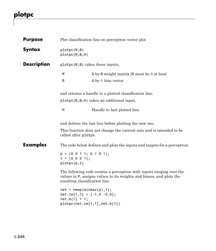
plotpc
Purpose Plot classification line on perceptron vector plot
Syntax plotpc(W,B)plotpc(W,B,H)
Description plotpc(W,B) takes these inputs,
W S-by-R weight matrix (R must be 3 or less)
B S-by-1 bias vector
and returns a handle to a plotted classification line.
plotpc(W,B,H) takes an additional input,
H Handle to last plotted line
and deletes the last line before plotting the new one.
This function does not change the current axis and is intended to becalled after plotpv.
Examples The code below defines and plots the inputs and targets for a perceptron:
p = [0 0 1 1; 0 1 0 1];t = [0 0 0 1];plotpv(p,t)
The following code creates a perceptron with inputs ranging over thevalues in P, assigns values to its weights and biases, and plots theresulting classification line.
net = newp(minmax(p),1);net.iw{1,1} = [-1.2 -0.5];net.b{1} = 1;plotpc(net.iw{1,1},net.b{1})
1-248

plotpc
See Also plotpv
1-249
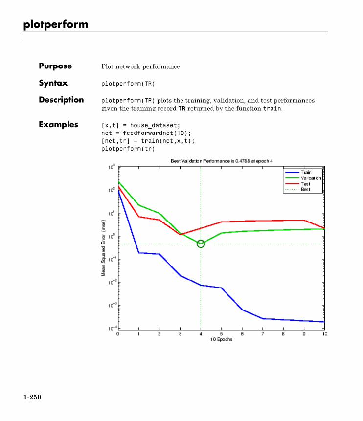
plotperform
Purpose Plot network performance
Syntax plotperform(TR)
Description plotperform(TR) plots the training, validation, and test performancesgiven the training record TR returned by the function train.
Examples [x,t] = house_dataset;net = feedforwardnet(10);[net,tr] = train(net,x,t);plotperform(tr)
1-250

plotperform
See Also plottrainstate
1-251
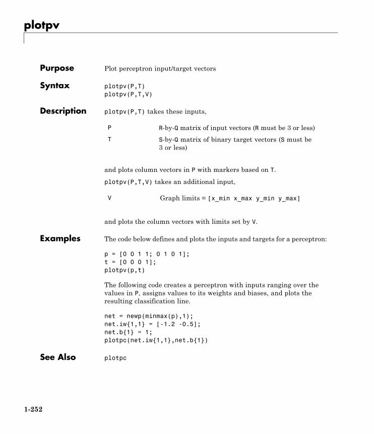
plotpv
Purpose Plot perceptron input/target vectors
Syntax plotpv(P,T)plotpv(P,T,V)
Description plotpv(P,T) takes these inputs,
P R-by-Q matrix of input vectors (R must be 3 or less)
T S-by-Q matrix of binary target vectors (S must be3 or less)
and plots column vectors in P with markers based on T.
plotpv(P,T,V) takes an additional input,
V Graph limits = [x_min x_max y_min y_max]
and plots the column vectors with limits set by V.
Examples The code below defines and plots the inputs and targets for a perceptron:
p = [0 0 1 1; 0 1 0 1];t = [0 0 0 1];plotpv(p,t)
The following code creates a perceptron with inputs ranging over thevalues in P, assigns values to its weights and biases, and plots theresulting classification line.
net = newp(minmax(p),1);net.iw{1,1} = [-1.2 -0.5];net.b{1} = 1;plotpc(net.iw{1,1},net.b{1})
See Also plotpc
1-252
plotregression
Purpose Plot linear regression
Syntax plotregression(targets,outputs)plotregression(targs1,outs1,'name1',targs2,outs2,'name2',...)
Description plotregression(targets,outputs) plots the linear regression oftargets relative to outputs.
plotregression(targs1,outs1,'name1',targs2,outs2,'name2',...)generates multiple plots.
Examples [x,t] = simplefit_dataset;net = feedforwardnet(10);net = train(net,x,t);y = net(x);plotregression(t,y,'Regression')
1-253
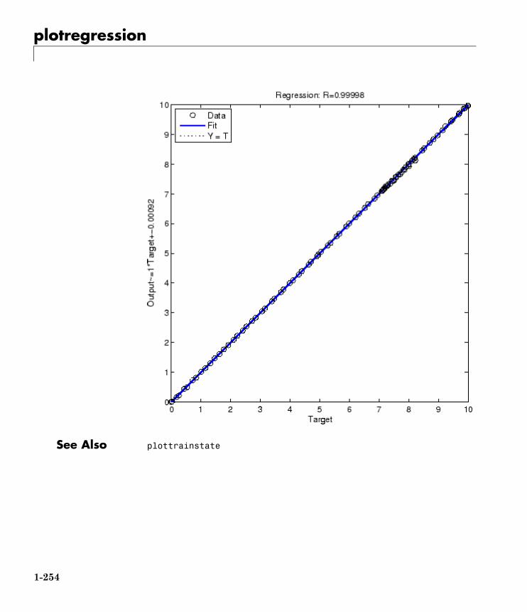
plotregression
See Also plottrainstate
1-254
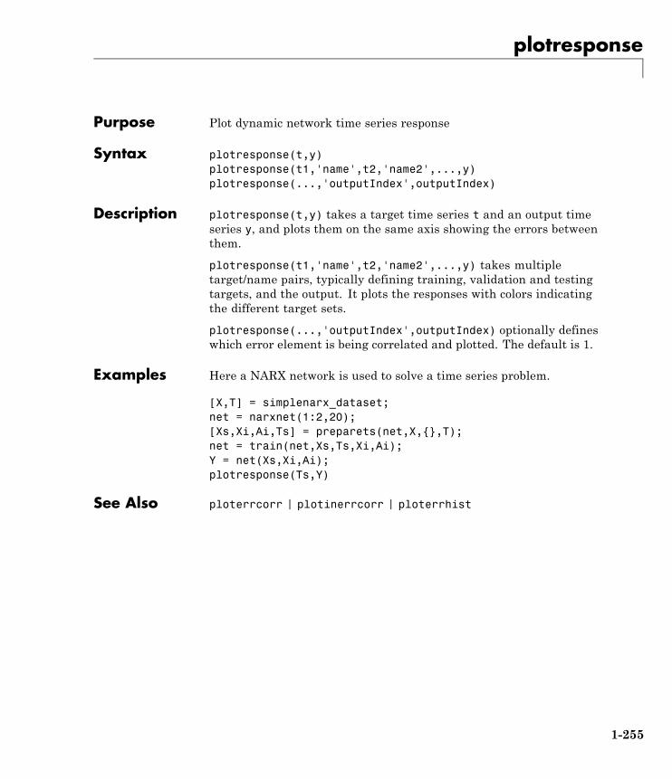
plotresponse
Purpose Plot dynamic network time series response
Syntax plotresponse(t,y)plotresponse(t1,'name',t2,'name2',...,y)plotresponse(...,'outputIndex',outputIndex)
Description plotresponse(t,y) takes a target time series t and an output timeseries y, and plots them on the same axis showing the errors betweenthem.
plotresponse(t1,'name',t2,'name2',...,y) takes multipletarget/name pairs, typically defining training, validation and testingtargets, and the output. It plots the responses with colors indicatingthe different target sets.
plotresponse(...,'outputIndex',outputIndex) optionally defineswhich error element is being correlated and plotted. The default is 1.
Examples Here a NARX network is used to solve a time series problem.
[X,T] = simplenarx_dataset;net = narxnet(1:2,20);[Xs,Xi,Ai,Ts] = preparets(net,X,{},T);net = train(net,Xs,Ts,Xi,Ai);Y = net(Xs,Xi,Ai);plotresponse(Ts,Y)
See Also ploterrcorr | plotinerrcorr | ploterrhist
1-255
plotroc
Purpose Plot receiver operating characteristic
Syntax plotroc(targets,outputs)plotroc(targets1,outputs2,'name1',...)
Description plotroc(targets,outputs) plots the receiver operating characteristicfor each output class. The more each curve hugs the left and top edgesof the plot, the better the classification.
plotroc(targets1,outputs2,'name1',...) generates multiple plots.
Examples load simplecluster_datasetnet = patternnet(20);net = train(net,simpleclusterInputs,simpleclusterTargets);simpleclusterOutputs = sim(net,simpleclusterInputs);plotroc(simpleclusterTargets,simpleclusterOutputs);
1-256
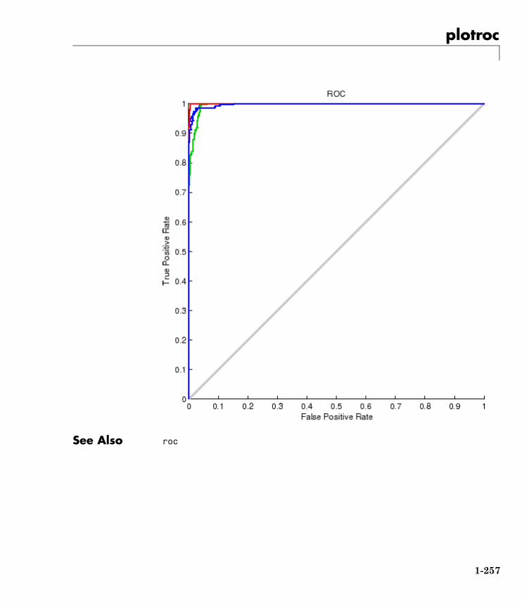
plotroc
See Also roc
1-257
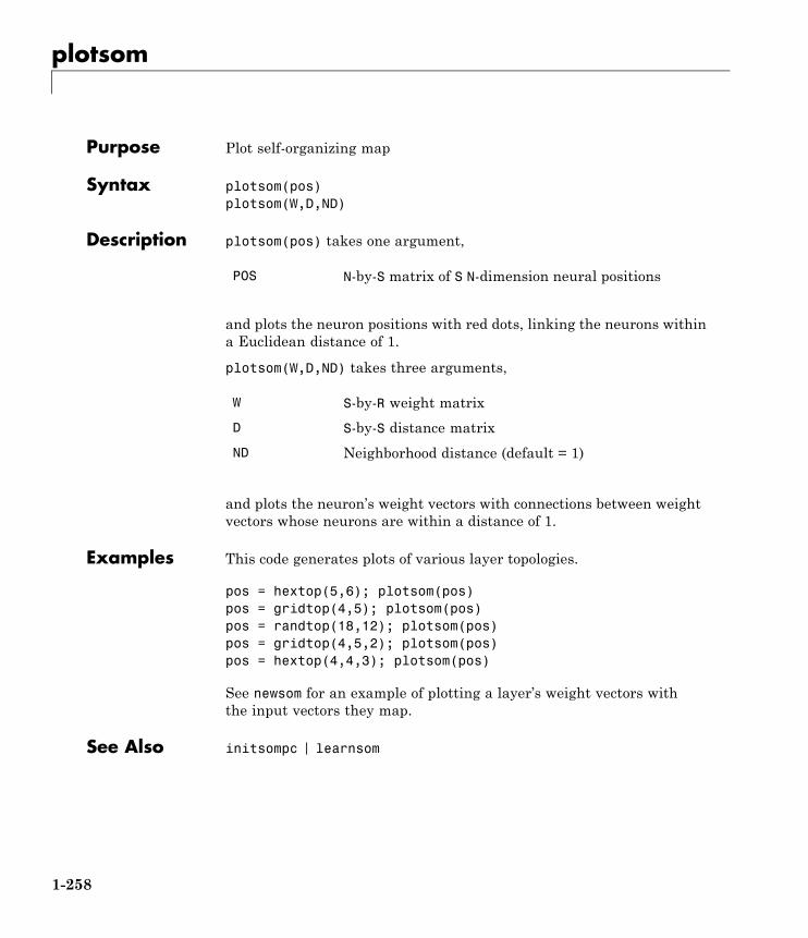
plotsom
Purpose Plot self-organizing map
Syntax plotsom(pos)plotsom(W,D,ND)
Description plotsom(pos) takes one argument,
POS N-by-S matrix of S N-dimension neural positions
and plots the neuron positions with red dots, linking the neurons withina Euclidean distance of 1.
plotsom(W,D,ND) takes three arguments,
W S-by-R weight matrix
D S-by-S distance matrix
ND Neighborhood distance (default = 1)
and plots the neuron’s weight vectors with connections between weightvectors whose neurons are within a distance of 1.
Examples This code generates plots of various layer topologies.
pos = hextop(5,6); plotsom(pos)pos = gridtop(4,5); plotsom(pos)pos = randtop(18,12); plotsom(pos)pos = gridtop(4,5,2); plotsom(pos)pos = hextop(4,4,3); plotsom(pos)
See newsom for an example of plotting a layer’s weight vectors withthe input vectors they map.
See Also initsompc | learnsom
1-258
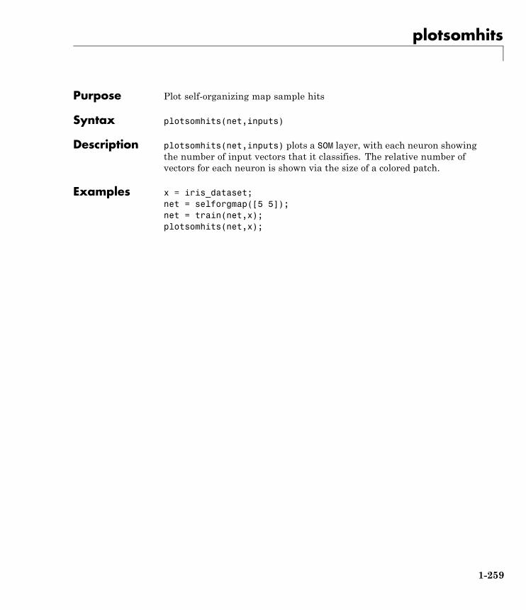
plotsomhits
Purpose Plot self-organizing map sample hits
Syntax plotsomhits(net,inputs)
Description plotsomhits(net,inputs) plots a SOM layer, with each neuron showingthe number of input vectors that it classifies. The relative number ofvectors for each neuron is shown via the size of a colored patch.
Examples x = iris_dataset;net = selforgmap([5 5]);net = train(net,x);plotsomhits(net,x);
1-259
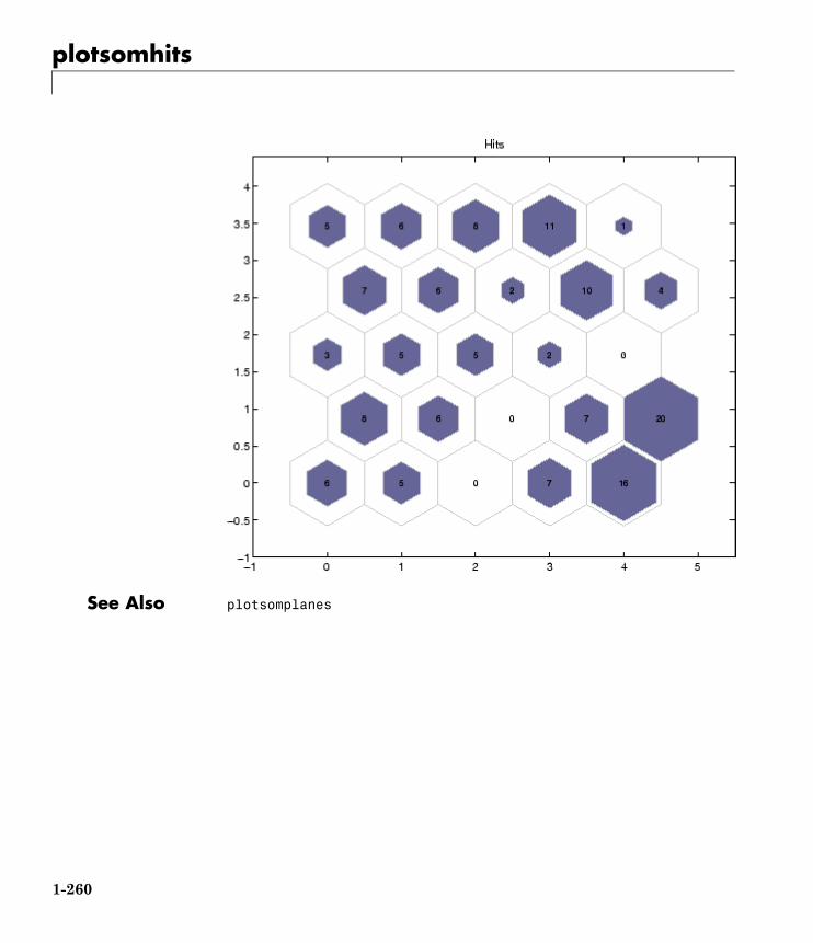
plotsomhits
See Also plotsomplanes
1-260
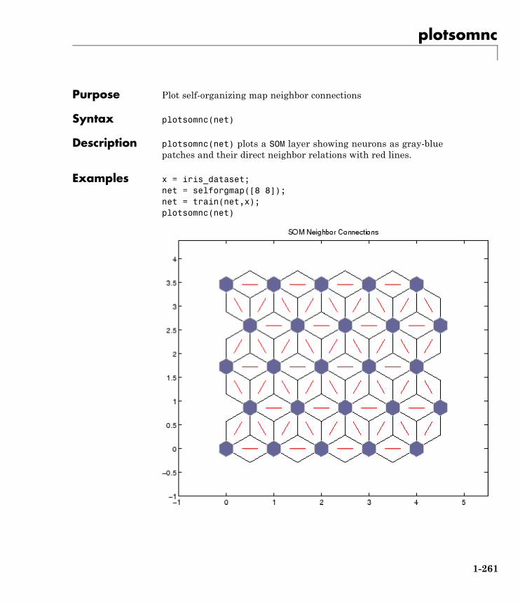
plotsomnc
Purpose Plot self-organizing map neighbor connections
Syntax plotsomnc(net)
Description plotsomnc(net) plots a SOM layer showing neurons as gray-bluepatches and their direct neighbor relations with red lines.
Examples x = iris_dataset;net = selforgmap([8 8]);net = train(net,x);plotsomnc(net)
1-261

plotsomnc
See Also plotsomnd | plotsomplanes | plotsomhits
1-262
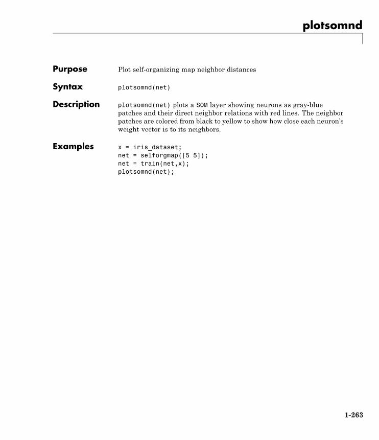
plotsomnd
Purpose Plot self-organizing map neighbor distances
Syntax plotsomnd(net)
Description plotsomnd(net) plots a SOM layer showing neurons as gray-bluepatches and their direct neighbor relations with red lines. The neighborpatches are colored from black to yellow to show how close each neuron’sweight vector is to its neighbors.
Examples x = iris_dataset;net = selforgmap([5 5]);net = train(net,x);plotsomnd(net);
1-263
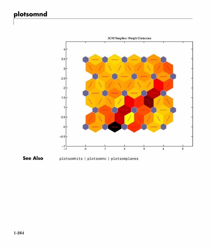
plotsomnd
See Also plotsomhits | plotsomnc | plotsomplanes
1-264
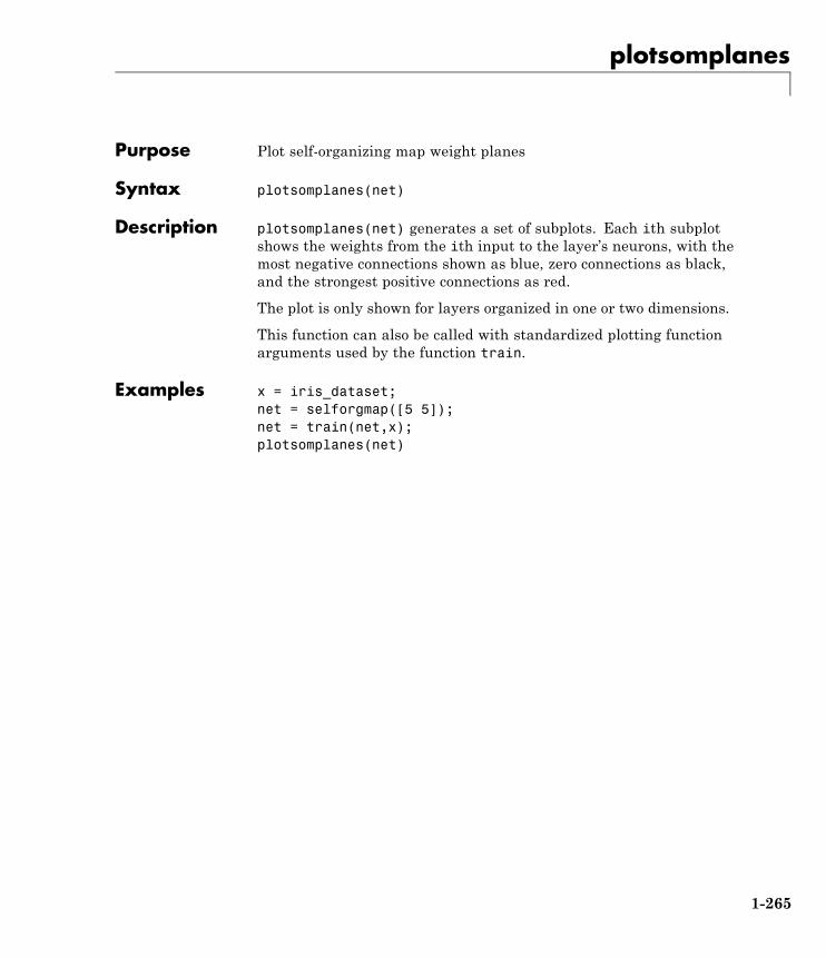
plotsomplanes
Purpose Plot self-organizing map weight planes
Syntax plotsomplanes(net)
Description plotsomplanes(net) generates a set of subplots. Each ith subplotshows the weights from the ith input to the layer’s neurons, with themost negative connections shown as blue, zero connections as black,and the strongest positive connections as red.
The plot is only shown for layers organized in one or two dimensions.
This function can also be called with standardized plotting functionarguments used by the function train.
Examples x = iris_dataset;net = selforgmap([5 5]);net = train(net,x);plotsomplanes(net)
1-265
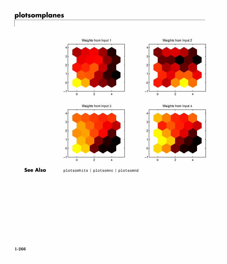
plotsomplanes
See Also plotsomhits | plotsomnc | plotsomnd
1-266
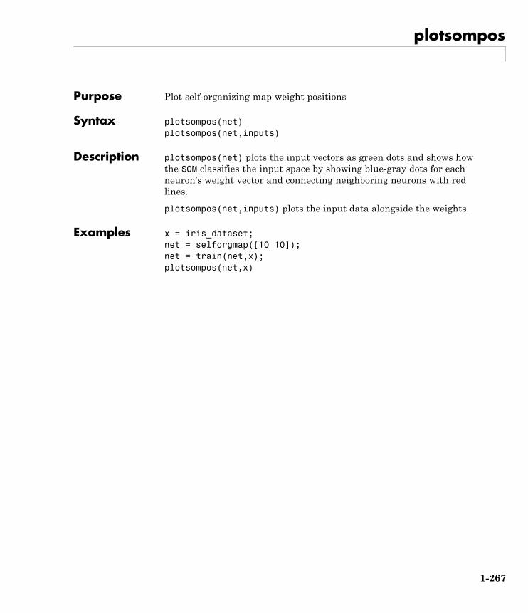
plotsompos
Purpose Plot self-organizing map weight positions
Syntax plotsompos(net)plotsompos(net,inputs)
Description plotsompos(net) plots the input vectors as green dots and shows howthe SOM classifies the input space by showing blue-gray dots for eachneuron’s weight vector and connecting neighboring neurons with redlines.
plotsompos(net,inputs) plots the input data alongside the weights.
Examples x = iris_dataset;net = selforgmap([10 10]);net = train(net,x);plotsompos(net,x)
1-267
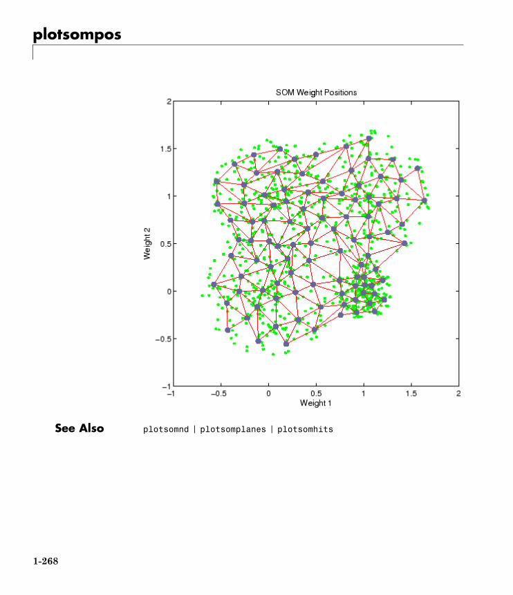
plotsompos
See Also plotsomnd | plotsomplanes | plotsomhits
1-268
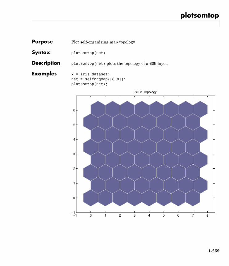
plotsomtop
Purpose Plot self-organizing map topology
Syntax plotsomtop(net)
Description plotsomtop(net) plots the topology of a SOM layer.
Examples x = iris_dataset;net = selforgmap([8 8]);plotsomtop(net);
1-269

plotsomtop
See Also plotsomnd | plotsomplanes | plotsomhits
1-270
plottrainstate
Purpose Plot training state values
Syntax plottrainstate(tr)
Description plottrainstate(tr) plots the training state from a training record trreturned by train.
Examples [x,t] = house_dataset;net = feedforwardnet(10);[net,tr] = train(net,x,t);plottrainstate(tr)
1-271

plottrainstate
See Also plotfit | plotperform | plotregression
1-272
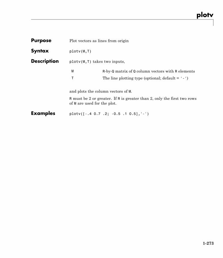
plotv
Purpose Plot vectors as lines from origin
Syntax plotv(M,T)
Description plotv(M,T) takes two inputs,
M R-by-Q matrix of Q column vectors with R elements
T The line plotting type (optional; default = '-')
and plots the column vectors of M.
R must be 2 or greater. If R is greater than 2, only the first two rowsof M are used for the plot.
Examples plotv([-.4 0.7 .2; -0.5 .1 0.5],'-')
1-273
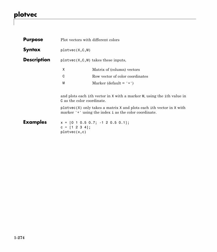
plotvec
Purpose Plot vectors with different colors
Syntax plotvec(X,C,M)
Description plotvec(X,C,M) takes these inputs,
X Matrix of (column) vectors
C Row vector of color coordinates
M Marker (default = '+')
and plots each ith vector in X with a marker M, using the ith value inC as the color coordinate.
plotvec(X) only takes a matrix X and plots each ith vector in X withmarker '+' using the index i as the color coordinate.
Examples x = [0 1 0.5 0.7; -1 2 0.5 0.1];c = [1 2 3 4];plotvec(x,c)
1-274
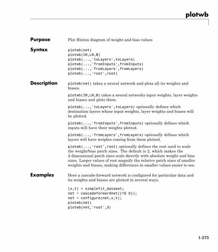
plotwb
Purpose Plot Hinton diagram of weight and bias values
Syntax plotwb(net)plotwb(IW,LW,B)plotwb(...,'toLayers',toLayers)plotwb(...,'fromInputs',fromInputs)plotwb(...,'fromLayers',fromLayers)plotwb(...,'root',root)
Description plotwb(net) takes a neural network and plots all its weights andbiases.
plotwb(IW,LW,B) takes a neural networks input weights, layer weightsand biases and plots them.
plotwb(...,'toLayers',toLayers) optionally defines whichdestination layers whose input weights, layer weights and biases willbe plotted.
plotwb(...,'fromInputs',fromInputs) optionally defines whichinputs will have their weights plotted.
plotwb(...,'fromLayers',fromLayers) optionally defines whichlayers will have weights coming from them plotted.
plotwb(...,'root',root) optionally defines the root used to scalethe weight/bias patch sizes. The default is 2, which makes the2-dimensional patch sizes scale directly with absolute weight and biassizes. Larger values of root magnify the relative patch sizes of smallerweights and biases, making differences in smaller values easier to see.
Examples Here a cascade-forward network is configured for particular data andits weights and biases are plotted in several ways.
[x,t] = simplefit_dataset;net = cascadeforwardnet([15 5]);net = configure(net,x,t);plotwb(net)plotwb(net,'root',3)
1-275
plotwb
plotwb(net,'root',4)plotwb(net,'toLayers',2)plotwb(net,'fromLayers',1)plotwb(net,'toLayers',2,'fromInputs',1)
See Also plotsomplanes
1-276
pnormc
Purpose Pseudonormalize columns of matrix
Syntax pnormc(X,R)
Description pnormc(X,R) takes these arguments,
X M-by-N matrix
R (Optional) radius to normalize columns to (default= 1)
and returns X with an additional row of elements, which results in newcolumn vector lengths of R.
Caution For this function to work properly, the columns of X mustoriginally have vector lengths less than R.
Examples x = [0.1 0.6; 0.3 0.1];y = pnormc(x)
See Also normc | normr
1-277
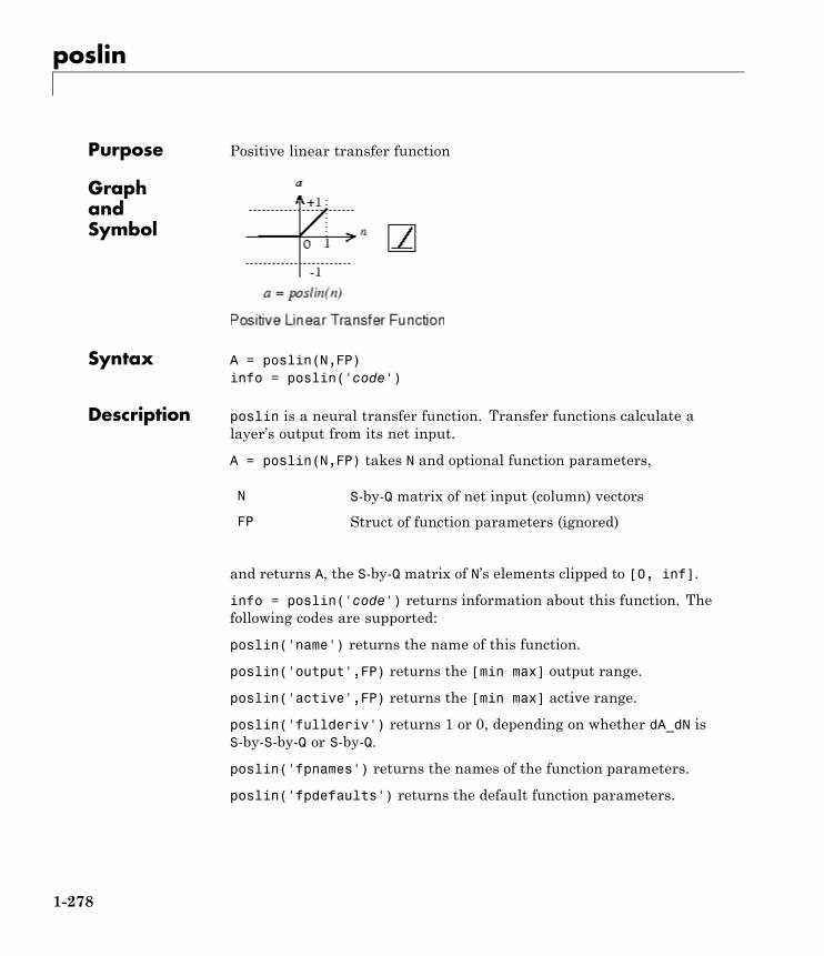
poslin
Purpose Positive linear transfer function
GraphandSymbol
Syntax A = poslin(N,FP)info = poslin('code')
Description poslin is a neural transfer function. Transfer functions calculate alayer’s output from its net input.
A = poslin(N,FP) takes N and optional function parameters,
N S-by-Q matrix of net input (column) vectors
FP Struct of function parameters (ignored)
and returns A, the S-by-Q matrix of N’s elements clipped to [0, inf].
info = poslin('code') returns information about this function. Thefollowing codes are supported:
poslin('name') returns the name of this function.
poslin('output',FP) returns the [min max] output range.
poslin('active',FP) returns the [min max] active range.
poslin('fullderiv') returns 1 or 0, depending on whether dA_dN isS-by-S-by-Q or S-by-Q.
poslin('fpnames') returns the names of the function parameters.
poslin('fpdefaults') returns the default function parameters.
1-278
poslin
Examples Here is the code to create a plot of the poslin transfer function.
n = -5:0.1:5;a = poslin(n);plot(n,a)
Assign this transfer function to layer i of a network.
net.layers{i}.transferFcn = 'poslin';
NetworkUse
To change a network so that a layer uses poslin, setnet.layers{i}.transferFcn to 'poslin'.
Call sim to simulate the network with poslin.
Algorithms The transfer function poslin returns the output n if n is greater than orequal to zero and 0 if n is less than or equal to zero.
poslin(n) = n, if n >= 0= 0, if n <= 0
See Also sim | purelin | satlin | satlins
1-279
preparets
Purpose Prepare input and target time series data for network simulation ortraining
Syntax [Xs,Xi,Ai,Ts,EWs,shift] = preparets(net,Xnf,Tnf,Tf,EW)
Description This function simplifies the normally complex and error prone task ofreformatting input and target time series. It automatically shifts inputand target time series as many steps as are needed to fill the initialinput and layer delay states. If the network has open loop feedback,then it copies feedback targets into the inputs as needed to define theopen loop inputs.
Each time a new network is designed, with different numbers of delaysor feedback settings, preparets can be called to reformat input andtarget data accordingly. Also, each time a network is transformedwith openloop, closeloop, removedelay or adddelay, this functioncan reformat the data accordingly.
[Xs,Xi,Ai,Ts,EWs,shift] = preparets(net,Xnf,Tnf,Tf,EW) takesthese arguments,
net Neural network
Xnf Non-feedback inputs
Tnf Non-feedback targets
Tf Feedback targets
EW Error weights (default = {1})
and returns,
Xs Shifted inputs
Xi Initial input delay states
Ai Initial layer delay states
Ts Shifted targets
1-280
preparets
EWs Shifted error weights
shift The number of timesteps truncated from thefront of X and T in order to properly fill Xi and Ai.
Examples Here a time-delay network with 20 hidden neurons is created, trainedand simulated.
net = timedelaynet(20);view(net)[X,T] = simpleseries_dataset;[Xs,Xi,Ai,Ts] = preparets(net,X,T);net = train(net,Xs,Ts);Y = net(Xs,Xi,Ai)
Here a NARX network is designed. The NARX network has a standardinput and an open-loop feedback output to an associated feedback input.
[X,T] = simplenarx_dataset;net = narxnet(1:2,1:2,20);view(net)[Xs,Xi,Ai,Ts] = preparets(net,X,{},T);net = train(net,Xs,Ts,Xi,Ai);y = net(Xs,Xi,Ai);
Now the network is converted to closed loop, and the data is reformattedto simulate the network’s closed-loop response.
net = closeloop(net);view(net)[Xs,Xi,Ai] = preparets(net,X,{},T);y = net(Xs,Xi,Ai);
See Also adddelay | closeloop | narnet | narxnet | openloop | removedelay| timedelaynet
1-281
processpca
Purpose Process columns of matrix with principal component analysis
Syntax [Y,PS] = processpca(X,maxfrac)[Y,PS] = processpca(X,FP)Y = processpca('apply',X,PS)X = processpca('reverse',Y,PS)name = processpca('name')fp = processpca('pdefaults')names = processpca('pdesc')processpca('pcheck',fp);
Description processpca processes matrices using principal component analysis sothat each row is uncorrelated, the rows are in the order of the amountthey contribute to total variation, and rows whose contribution to totalvariation are less than maxfrac are removed.
[Y,PS] = processpca(X,maxfrac) takes X and an optional parameter,
X N-by-Q matrix or a 1-by-TS row cell array ofN-by-Q matrices
maxfrac Maximum fraction of variance for removed rows(default is 0)
and returns
Y Each N-by-Q matrix with N - M rows deleted(optional)
PS Process settings that allow consistent processingof values
[Y,PS] = processpca(X,FP) takes parameters as a struct:FP.maxfrac.
Y = processpca('apply',X,PS) returns Y, given X and settings PS.
1-282
processpca
X = processpca('reverse',Y,PS) returns X, given Y and settings PS.
name = processpca('name') returns the name of this process method.
fp = processpca('pdefaults') returns default process parameterstructure.
names = processpca('pdesc') returns the process parameterdescriptions.
processpca('pcheck',fp); throws an error if any parameter is illegal.
Examples Here is how to format a matrix with an independent row, a correlatedrow, and a completely redundant row so that its rows are uncorrelatedand the redundant row is dropped.
x1_independent = rand(1,5)x1_correlated = rand(1,5) + x_independent;x1_redundant = x_independent + x_correlatedx1 = [x1_independent; x1_correlated; x1_redundant][y1,ps] = processpca(x1)
Next, apply the same processing settings to new values.
x2_independent = rand(1,5)x2_correlated = rand(1,5) + x_independent;x2_redundant = x_independent + x_correlatedx2 = [x2_independent; x2_correlated; x2_redundant];y2 = processpca('apply',x2,ps)
Reverse the processing of y1 to get x1 again.
x1_again = processpca('reverse',y1,ps)
Algorithms Values in rows whose elements are not all the same value are set to
y = 2*(x-minx)/(maxx-minx) - 1;
Values in rows with all the same value are set to 0.
1-283
processpca
Definitions In some situations, the dimension of the input vector is large, but thecomponents of the vectors are highly correlated (redundant). It is usefulin this situation to reduce the dimension of the input vectors. Aneffective procedure for performing this operation is principal componentanalysis. This technique has three effects: it orthogonalizes thecomponents of the input vectors (so that they are uncorrelated witheach other), it orders the resulting orthogonal components (principalcomponents) so that those with the largest variation come first, and iteliminates those components that contribute the least to the variationin the data set. The following code illustrates the use of processpca,which performs a principal-component analysis using the processingsetting maxfrac of 0.02.
[pn,ps1] = mapstd(p);[ptrans,ps2] = processpca(pn,0.02);
The input vectors are first normalized, using mapstd, so that they havezero mean and unity variance. This is a standard procedure when usingprincipal components. In this example, the second argument passedto processpca is 0.02. This means that processpca eliminates thoseprincipal components that contribute less than 2% to the total variationin the data set. The matrix ptrans contains the transformed inputvectors. The settings structure ps2 contains the principal componenttransformation matrix. After the network has been trained, thesesettings should be used to transform any future inputs that are appliedto the network. It effectively becomes a part of the network, just likethe network weights and biases. If you multiply the normalized inputvectors pn by the transformation matrix transMat, you obtain thetransformed input vectors ptrans.
If processpca is used to preprocess the training set data, thenwhenever the trained network is used with new inputs, you shouldpreprocess them with the transformation matrix that was computed forthe training set, using ps2. The following code applies a new set ofinputs to a network already trained.
pnewn = mapstd('apply',pnew,ps1);pnewtrans = processpca('apply',pnewn,ps2);
1-284
processpca
a = sim(net,pnewtrans);
Principal component analysis is not reliably reversible. Therefore it isonly recommended for input processing. Outputs require reversibleprocessing functions.
Principal component analysis is not part of the default processing forfeedforwardnet. If you wish to add this, you can use the followingcommand:
net.inputs{1}.processFcns{end+1} = 'processpca';
See Also fixunknowns | mapminmax | mapstd
1-285
prune
Purpose Delete neural inputs, layers, and outputs with sizes of zero
Syntax [net,pi,pl,po] = prune(net)
Description This function removes zero-sized inputs, layers, and outputs from anetwork. This leaves a network which may have fewer inputs andoutputs, but which implements the same operations, as zero-sizedinputs and outputs do not convey any information.
One use for this simplification is to prepare a network with zero sizedsubobjects for Simulink, where zero sized signals are not supported.
The companion function prunedata can prune data to remain consistentwith the transformed network.
[net,pi,pl,po] = prune(net) takes a neural network and returns
net The same network with zero-sized subobjectsremoved
pi Indices of pruned inputs
pl Indices of pruned layers
po Indices of pruned outputs
Examples Here a NARX dynamic network is created which has one external inputand a second input which feeds back from the output.
net = narxnet(20);view(net)
The network is then trained on a single random time-series problemwith 50 timesteps. The external input happens to have no elements.
X = nndata(0,1,50);T = nndata(1,1,50);[Xs,Xi,Ai,Ts] = preparets(net,X,{},T);net = train(net,Xs,Ts);
1-286

prune
The network and data are then pruned before generating a Simulinkdiagram and initializing its input and layer states.
[net2,pi,pl,po] = prune(net);view(net)[Xs2,Xi2,Ai2,Ts2] = prunedata(net,pi,pl,po,Xs,Xi,Ai,Ts)[sysName,netName] = gensim(net);setsiminit(sysName,netName,Xi2,Ai2)
See Also prunedata | gensim
1-287
prunedata
Purpose Purpose
Syntax [Xp,Xip,Aip,Tp] = prunedata(pi,pl,po,X,Xi,Ai,T)
Description This function prunes data to be consistent with a network whosezero-sized inputs, layers, and outputs have been removed with prune.
One use for this simplification is to prepare a network with zero-sizedsubobjects for Simulink, where zero-sized signals are not supported.
[Xp,Xip,Aip,Tp] = prunedata(pi,pl,po,X,Xi,Ai,T) takes thesearguments,
pi Indices of pruned inputs
pl Indices of pruned layers
po Indices of pruned outputs
X Input data
Xi Initial input delay states
Ai Initial layer delay states
T Target data
and returns the pruned inputs, input and layer delay states, and targets.
Examples Here a NARX dynamic network is created which has one external inputand a second input which feeds back from the output.
net = narxnet(20);view(net)
The network is then trained on a single random time-series problemwith 50 timesteps. The external input happens to have no elements.
X = nndata(0,1,50);T = nndata(1,1,50);
1-288
prunedata
[Xs,Xi,Ai,Ts] = preparets(net,X,{},T);net = train(net,Xs,Ts);
The network and data are then pruned before generating a Simulinkdiagram and initializing its input and layer states.
[net2,pi,pl,po] = prune(net);view(net)[Xs2,Xi2,Ai2,Ts2] = prunedata(net,pi,pl,po,Xs,Xi,Ai,Ts)[sysName,netName] = gensim(net);setsiminit(sysName,netName,Xi2,Ai2)
See Also prune | gensim
1-289
purelin
Purpose Linear transfer function
GraphandSymbol
Syntax A = purelin(N,FP)info = purelin('code')
Description purelin is a neural transfer function. Transfer functions calculate alayer’s output from its net input.
A = purelin(N,FP) takes N and optional function parameters,
N S-by-Q matrix of net input (column) vectors
FP Struct of function parameters (ignored)
and returns A, an S-by-Q matrix equal to N.
info = purelin('code') returns useful information for eachsupported code string:
purelin('name') returns the name of this function.
purelin('output',FP) returns the [min max] output range.
purelin('active',FP) returns the [min max] active input range.
purelin('fullderiv') returns 1 or 0, depending on whether dA_dN isS-by-S-by-Q or S-by-Q.
purelin('fpnames') returns the names of the function parameters.
purelin('fpdefaults') returns the default function parameters.
1-290
purelin
Examples Here is the code to create a plot of the purelin transfer function.
n = -5:0.1:5;a = purelin(n);plot(n,a)
Assign this transfer function to layer i of a network.
net.layers{i}.transferFcn = 'purelin';
Algorithms a = purelin(n) = n
See Also sim | satlin | satlins
1-291
quant
Purpose Discretize values as multiples of quantity
Syntax quant(X,Q)
Description quant(X,Q) takes two inputs,
X Matrix, vector, or scalar
Q Minimum value
and returns values from X rounded to nearest multiple of Q.
Examples x = [1.333 4.756 -3.897];y = quant(x,0.1)
1-292
radbas
Purpose Radial basis transfer function
GraphandSymbol
Syntax A = radbas(N,FP)
Description radbas is a neural transfer function. Transfer functions calculate alayer’s output from its net input.
A = radbas(N,FP) takes one or two inputs,
N S-by-Q matrix of net input (column) vectors
FP Struct of function parameters (ignored)
and returns A, an S-by-Q matrix of the radial basis function appliedto each element of N.
Examples Here you create a plot of the radbas transfer function.
n = -5:0.1:5;a = radbas(n);plot(n,a)
Assign this transfer function to layer i of a network.
net.layers{i}.transferFcn = 'radbas';
1-293
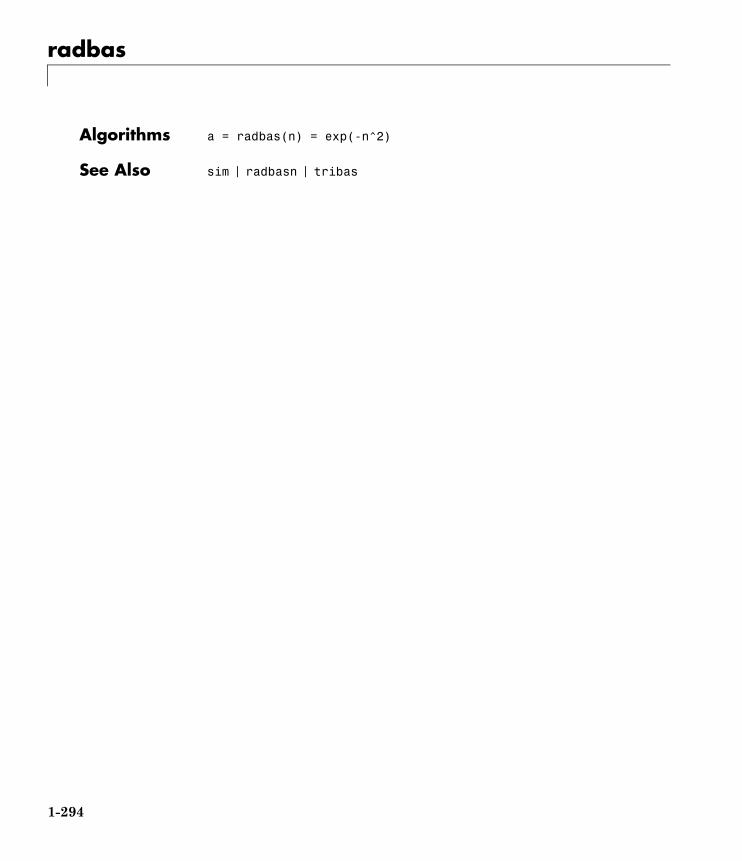
radbas
Algorithms a = radbas(n) = exp(-n^2)
See Also sim | radbasn | tribas
1-294
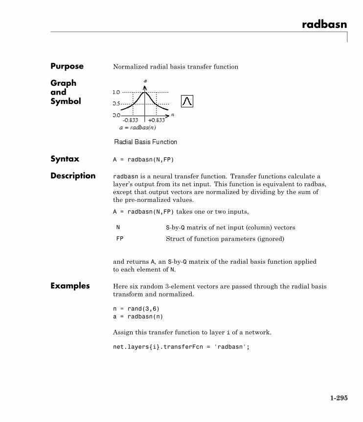
radbasn
Purpose Normalized radial basis transfer function
GraphandSymbol
Syntax A = radbasn(N,FP)
Description radbasn is a neural transfer function. Transfer functions calculate alayer’s output from its net input. This function is equivalent to radbas,except that output vectors are normalized by dividing by the sum ofthe pre-normalized values.
A = radbasn(N,FP) takes one or two inputs,
N S-by-Q matrix of net input (column) vectors
FP Struct of function parameters (ignored)
and returns A, an S-by-Q matrix of the radial basis function appliedto each element of N.
Examples Here six random 3-element vectors are passed through the radial basistransform and normalized.
n = rand(3,6)a = radbasn(n)
Assign this transfer function to layer i of a network.
net.layers{i}.transferFcn = 'radbasn';
1-295

radbasn
Algorithms a = radbasn(n) = exp(-n^2) / sum(exp(-n^2))
See Also sim | radbas | tribas
1-296
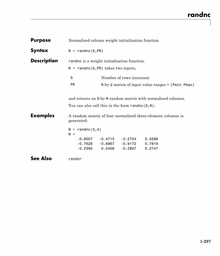
randnc
Purpose Normalized column weight initialization function
Syntax W = randnc(S,PR)
Description randnc is a weight initialization function.
W = randnc(S,PR) takes two inputs,
S Number of rows (neurons)
PR R-by-2 matrix of input value ranges = [Pmin Pmax]
and returns an S-by-R random matrix with normalized columns.
You can also call this in the form randnc(S,R).
Examples A random matrix of four normalized three-element columns isgenerated:
M = randnc(3,4)M =
-0.6007 -0.4715 -0.2724 0.5596-0.7628 -0.6967 -0.9172 0.7819-0.2395 0.5406 -0.2907 0.2747
See Also randnr
1-297
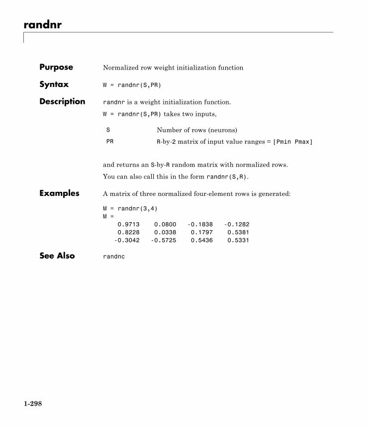
randnr
Purpose Normalized row weight initialization function
Syntax W = randnr(S,PR)
Description randnr is a weight initialization function.
W = randnr(S,PR) takes two inputs,
S Number of rows (neurons)
PR R-by-2 matrix of input value ranges = [Pmin Pmax]
and returns an S-by-R random matrix with normalized rows.
You can also call this in the form randnr(S,R).
Examples A matrix of three normalized four-element rows is generated:
M = randnr(3,4)M =
0.9713 0.0800 -0.1838 -0.12820.8228 0.0338 0.1797 0.5381
-0.3042 -0.5725 0.5436 0.5331
See Also randnc
1-298
rands
Purpose Symmetric random weight/bias initialization function
Syntax W = rands(S,PR)M = rands(S,R)v = rands(S)
Description rands is a weight/bias initialization function.
W = rands(S,PR) takes
S Number of neurons
PR R-by-2 matrix of R input ranges
and returns an S-by-R weight matrix of random values between –1 and 1.
M = rands(S,R) returns an S-by-R matrix of random values. v =rands(S) returns an S-by-1 vector of random values.
Examples Here, three sets of random values are generated with rands.
rands(4,[0 1; -2 2])rands(4)rands(2,3)
NetworkUse
To prepare the weights and the bias of layer i of a custom network tobe initialized with rands,
1 Set net.initFcn to 'initlay'. (net.initParam automaticallybecomes initlay’s default parameters.)
2 Set net.layers{i}.initFcn to 'initwb'.
3 Set each net.inputWeights{i,j}.initFcn to 'rands'.
4 Set each net.layerWeights{i,j}.initFcn to 'rands'.
5 Set each net.biases{i}.initFcn to 'rands'.
1-299

rands
To initialize the network, call init.
See Also randsmall | randnr | randnc | initwb | initlay | init
1-300
randsmall
Purpose Small random weight/bias initialization function
Syntax W = randsmall(S,PR)M = rands(S,R)v = rands(S)
Description randsmall is a weight/bias initialization function.
W = randsmall(S,PR) takes
S Number of neurons
PR R-by-2 matrix of R input ranges
and returns an S-by-R weight matrix of small random values between–0.1 and 0.1.
M = rands(S,R) returns an S-by-R matrix of random values. v =rands(S) returns an S-by-1 vector of random values.
Examples Here three sets of random values are generated with rands.
randsmall(4,[0 1; -2 2])randsmall(4)randsmall(2,3)
NetworkUse
To prepare the weights and the bias of layer i of a custom network tobe initialized with rands,
1 Set net.initFcn to 'initlay'. (net.initParam automaticallybecomes initlay’s default parameters.)
2 Set net.layers{i}.initFcn to 'initwb'.
3 Set each net.inputWeights{i,j}.initFcn to 'randsmall'.
4 Set each net.layerWeights{i,j}.initFcn to 'randsmall'.
1-301

randsmall
5 Set each net.biases{i}.initFcn to 'randsmall'.
To initialize the network, call init.
See Also rands | randnr | randnc | initwb | initlay | init
1-302
randtop
Purpose Random layer topology function
Syntax pos = randtop(dim1,dim2,...,dimN)
Description randtop calculates the neuron positions for layers whose neurons arearranged in an N-dimensional random pattern.
pos = randtop(dim1,dim2,...,dimN) takes N arguments,
dimi Length of layer in dimension i
and returns an N-by-S matrix of N coordinate vectors, where S is theproduct of dim1*dim2*...*dimN.
Examples This code creates and displays a two-dimensional layer with neuronsarranged in a random pattern.
pos = randtop(8,5);net = selforgmap([8 5],'topologyFcn','randtop');plotsomtop(net)
See Also gridtop | hextop | tritop
1-303
regression
Purpose Linear regression
Syntax [r,m,b] = regression(t,y)[r,m,b] = regression(t,y,'one')
Description [r,m,b] = regression(t,y) takes these arguments,
t Target matrix or cell array data with a total ofN matrix rows
y Output matrix or cell array data of the same size
and returns these outputs,
r Regression values for each of the N matrix rows
m Slope of regression fit for each of the N matrixrows
b Offset of regression fit for each of the N matrixrows
[r,m,b] = regression(t,y,'one') combines all matrix rows beforeregressing, returning single scalar regression, slope and offset values.
Examples Here a feedforward network is trained and regression performed on itstargets and outputs.
[x,t] = simplefit_dataset;net = feedforwardnet(20);net = train(net,x,t);y = net(x);[r,m,b] = regression(t,y)plotregression(t,y)
See Also plotregression | confusion
1-304
removeconstantrows
Purpose Process matrices by removing rows with constant values
Syntax [Y,PS] = removeconstantrows(X,max_range)[Y,PS] = removeconstantrows(X,FP)Y = removeconstantrows('apply',X,PS)X = removeconstantrows('reverse',Y,PS)
Description removeconstantrows processes matrices by removing rows withconstant values.
[Y,PS] = removeconstantrows(X,max_range) takes X and an optionalparameter,
X Single N-by-Q matrix or a 1-by-TS row cell arrayof N-by-Q matrices
max_range Maximum range of values for row to be removed(default is 0)
and returns
Y Each M-by-Q matrix with N - M rows deleted(optional)
PS Process settings that allow consistent processingof values
[Y,PS] = removeconstantrows(X,FP) takes parameters as a struct:FP.max_range.
Y = removeconstantrows('apply',X,PS) returns Y, given X andsettings PS.
X = removeconstantrows('reverse',Y,PS) returns X, given Y andsettings PS.
1-305
removeconstantrows
Examples Here is how to format a matrix so that the rows with constant valuesare removed.
x1 = [1 2 4; 1 1 1; 3 2 2; 0 0 0][y1,PS] = removeconstantrows(x1)
Next, apply the same processing settings to new values.
x2 = [5 2 3; 1 1 1; 6 7 3; 0 0 0]y2 = removeconstantrows('apply',x2,PS)
Reverse the processing of y1 to get x1 again.
x1_again = removeconstantrows('reverse',y1,PS)
See Also fixunknowns | mapminmax | mapstd | processpca
1-306
removedelay
Purpose Remove delay to neural network’s response
Syntax net = removedelay(net,n)
Description net = removedelay(net,n) takes these arguments,
net Neural network
n Number of delays
and returns the network with input delay connections decreased, andoutput feedback delays increased, by the specified number of delays n.The result is a network which behaves identically, except that outputsare produced n timesteps later.
If the number of delays n is not specified, a default of one delay is used.
Examples Here a time delay network is created, trained and simulated in itsoriginal form on an input time series X and target series T. It is then witha delay removed and then added back. These first and third outputswill be identical, while the second will be shifted by one timestep.
[X,T] = simpleseries_dataset;net = timedelaynet(1:2,20);[Xs,Xi,Ai,Ts] = preparets(net,X,T);net = train(net,Xs,Ts,Xi);y1 = net(Xs)net2 = removedelay(net);[Xs,Xi,Ai,Ts] = preparets(net2,X,T);y2 = net2(Xs,Xi)net3 = adddelay(net2)[Xs,Xi,Ai,Ts] = preparets(net3,X,T);y3 = net3(Xs,Xi)
See Also adddelay | closeloop | openloop
1-307
removerows
Purpose Process matrices by removing rows with specified indices
Syntax [Y,PS] = removerows(X,'ind',ind)[Y,PS] = removerows(X,FP)Y = removerows('apply',X,PS)X = removerows('reverse',Y,PS)dx_dy = removerows('dx',X,Y,PS)dx_dy = removerows('dx',X,[],PS)name = removerows('name')fp = removerows('pdefaults')names = removerows('pdesc')removerows('pcheck',FP)
Description removerows processes matrices by removing rows with the specifiedindices.
[Y,PS] = removerows(X,'ind',ind) takes X and an optionalparameter,
X N-by-Q matrix or a 1-by-TS row cell array ofN-by-Q matrices
ind Vector of row indices to remove (default is [])
and returns
Y Each M-by-Q matrix, where M == N-length(ind)(optional)
PS Process settings that allow consistent processingof values
[Y,PS] = removerows(X,FP) takes parameters as a struct: FP.ind.
Y = removerows('apply',X,PS) returns Y, given X and settings PS.
X = removerows('reverse',Y,PS) returns X, given Y and settings PS.
1-308
removerows
dx_dy = removerows('dx',X,Y,PS) returns the M-by-N-by-Q derivativeof Y with respect to X.
dx_dy = removerows('dx',X,[],PS) returns the derivative, lessefficiently.
name = removerows('name') returns the name of this process method.
fp = removerows('pdefaults') returns the default process parameterstructure.
names = removerows('pdesc') returns the process parameterdescriptions.
removerows('pcheck',FP) throws an error if any parameter is illegal.
Examples Here is how to format a matrix so that rows 2 and 4 are removed:
x1 = [1 2 4; 1 1 1; 3 2 2; 0 0 0][y1,ps] = removerows(x1,'ind',[2 4])
Next, apply the same processing settings to new values.
x2 = [5 2 3; 1 1 1; 6 7 3; 0 0 0]y2 = removerows('apply',x2,ps)
Reverse the processing of y1 to get x1 again.
x1_again = removerows('reverse',y1,ps)
Algorithms In the reverse calculation, the unknown values of replaced rows arerepresented with NaN values.
See Also fixunknowns | mapminmax | mapstd | processpca
1-309
revert
Purpose Change network weights and biases to previous initialization values
Syntax net = revert (net)
Description net = revert (net) returns neural network net with weight and biasvalues restored to the values generated the last time the network wasinitialized.
If the network is altered so that it has different weight and biasconnections or different input or layer sizes, then revert cannot set theweights and biases to their previous values and they are set to zerosinstead.
Examples Here a perceptron is created with input size set to 2 and number ofneurons to 1.
net = perceptron;net.inputs{1}.size = 2;net.layers{1}.size = 1;
The initial network has weights and biases with zero values.
net.iw{1,1}, net.b{1}
Change these values as follows:
net.iw{1,1} = [1 2];net.b{1} = 5;net.iw{1,1}, net.b{1}
You can recover the network’s initial values as follows:
net = revert(net);net.iw{1,1}, net.b{1}
See Also init | sim | adapt | train
1-310
roc
Purpose Receiver operating characteristic
Syntax [tpr,fpr,thresholds] = roc(targets,outputs)
Description The receiver operating characteristic is a metric used to check thequality of classifiers. For each class of a classifier, roc applies thresholdvalues across the interval [0,1] to outputs. For each threshold, twovalues are calculated, the True Positive Ratio (the number of outputsgreater or equal to the threshold, divided by the number of one targets),and the False Positive Ratio (the number of outputs less than thethreshold, divided by the number of zero targets).
You can visualize the results of this function with plotroc.
[tpr,fpr,thresholds] = roc(targets,outputs) takes thesearguments:
targets S-by-Q matrix, where each column vectorcontains a single 1 value, with all other elements0. The index of the 1 indicates which of Scategories that vector represents.
outputs S-by-Q matrix, where each column containsvalues in the range [0,1]. The index of thelargest element in the column indicates which ofS categories that vector presents. Alternately,1-by-Q vector, where values greater or equal to0.5 indicate class membership, and values below0.5, nonmembership.
and returns these values:
1-311
roc
tpr 1-by-S cell array of 1-by-N true-positive/positiveratios.
fpr 1-by-S cell array of 1-by-N false-positive/negativeratios.
thresholds 1-by-S cell array of 1-by-N thresholds overinterval [0,1].
roc(targets,outputs) takes these arguments:
targets 1-by-Q matrix of Boolean values indicating classmembership.
outputs S-by-Q matrix, of values in [0,1] interval, wherevalues greater than or equal to 0.5 indicate classmembership.
and returns these values:
tpr 1-by-N vector of true-positive/positive ratios.
fpr 1-by-N vector of false-positive/negative ratios.
thresholds 1-by-N vector of thresholds over interval [0,1].
Examples load iris_datasetnet = patternnet(20);net = train(net,irisInputs,irisTargets);irisOutputs = sim(net,irisInputs);[tpr,fpr,thresholds] = roc(irisTargets,irisOutputs)
See Also plotroc | confusion
1-312
sae
Purpose Sum absolute error performance function
Syntax perf = sae(net,t,y,ew)[...] = sae(...,'regularization',regularization)[...] = sae(...,'normalization',normalization)[...] = sae(...,'squaredWeighting',squaredWeighting)[...] = sae(...,FP)
Description sae is a network performance function. It measures performanceaccording to the sum of squared errors.
perf = sae(net,t,y,ew) takes these input arguments and optionalfunction parameters,
net Neural network
t Matrix or cell array of target vectors
y Matrix or cell array of output vectors
ew Error weights (default = {1})
and returns the sum squared error.
This function has three optional function parameters that can bedefined with parameter name/pair arguments, or as a structure FPargument with fields having the parameter name and assigned theparameter values:
[...] = sae(...,'regularization',regularization)
[...] = sae(...,'normalization',normalization)
[...] = sae(...,'squaredWeighting',squaredWeighting)
[...] = sae(...,FP)
• regularization — can be set to any value between the default of0 and 1. The greater the regularization value, the more squaredweights and biases are taken into account in the performancecalculation.
1-313
sae
• normalization — can be set to the default 'absolute', or'normalized' (which normalizes errors to the [+2 -2] rangeconsistent with normalized output and target ranges of [-1 1]) or'percent' (which normalizes errors to the range [-1 +1]).
• squaredWeighting — can be set to the default false, for applyingerror weights to absolute errors, or false for applying error weights tothe squared errors before squaring.
Examples Here a network is trained to fit a simple data set and its performancecalculated
[x,t] = simplefit_dataset;net = fitnet(10,'trainscg');net.performFcn = 'sae';net = train(net,x,t)y = net(x)e = t-yperf = sae(net,t,y)
NetworkUse
To prepare a custom network to be trained with sae, setnet.performFcn to 'sae'. This automatically sets net.performParamto the default function parameters.
Then calling train, adapt or perform will result in sae being usedto calculate performance.
1-314
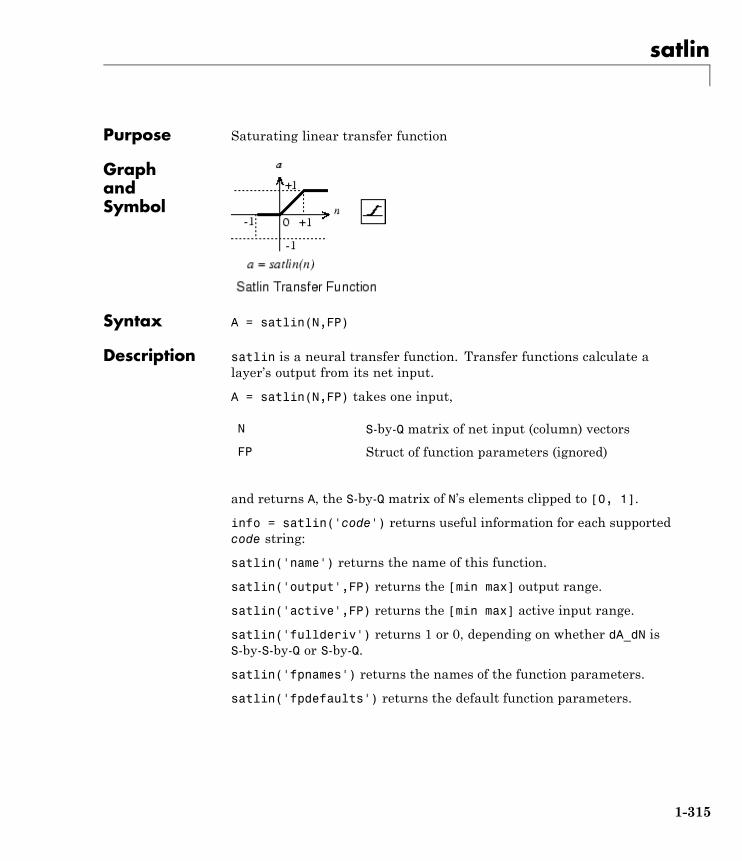
satlin
Purpose Saturating linear transfer function
GraphandSymbol
Syntax A = satlin(N,FP)
Description satlin is a neural transfer function. Transfer functions calculate alayer’s output from its net input.
A = satlin(N,FP) takes one input,
N S-by-Q matrix of net input (column) vectors
FP Struct of function parameters (ignored)
and returns A, the S-by-Q matrix of N’s elements clipped to [0, 1].
info = satlin('code') returns useful information for each supportedcode string:
satlin('name') returns the name of this function.
satlin('output',FP) returns the [min max] output range.
satlin('active',FP) returns the [min max] active input range.
satlin('fullderiv') returns 1 or 0, depending on whether dA_dN isS-by-S-by-Q or S-by-Q.
satlin('fpnames') returns the names of the function parameters.
satlin('fpdefaults') returns the default function parameters.
1-315
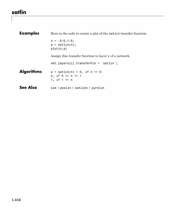
satlin
Examples Here is the code to create a plot of the satlin transfer function.
n = -5:0.1:5;a = satlin(n);plot(n,a)
Assign this transfer function to layer i of a network.
net.layers{i}.transferFcn = 'satlin';
Algorithms a = satlin(n) = 0, if n <= 0n, if 0 <= n <= 11, if 1 <= n
See Also sim | poslin | satlins | purelin
1-316
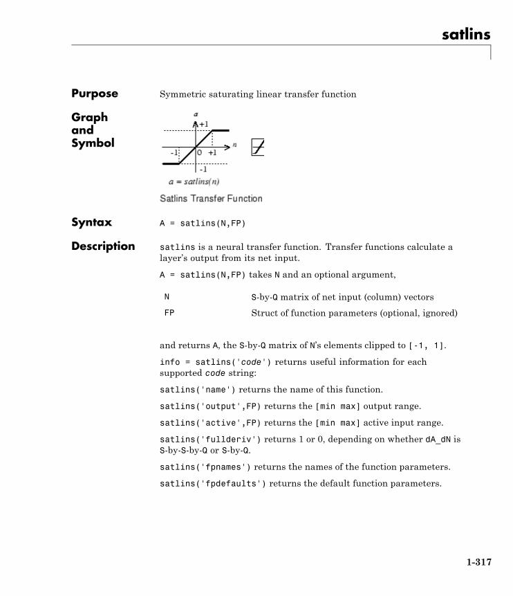
satlins
Purpose Symmetric saturating linear transfer function
GraphandSymbol
Syntax A = satlins(N,FP)
Description satlins is a neural transfer function. Transfer functions calculate alayer’s output from its net input.
A = satlins(N,FP) takes N and an optional argument,
N S-by-Q matrix of net input (column) vectors
FP Struct of function parameters (optional, ignored)
and returns A, the S-by-Q matrix of N’s elements clipped to [-1, 1].
info = satlins('code') returns useful information for eachsupported code string:
satlins('name') returns the name of this function.
satlins('output',FP) returns the [min max] output range.
satlins('active',FP) returns the [min max] active input range.
satlins('fullderiv') returns 1 or 0, depending on whether dA_dN isS-by-S-by-Q or S-by-Q.
satlins('fpnames') returns the names of the function parameters.
satlins('fpdefaults') returns the default function parameters.
1-317
satlins
Examples Here is the code to create a plot of the satlins transfer function.
n = -5:0.1:5;a = satlins(n);plot(n,a)
Algorithms satlins(n) = -1, if n <= -1n, if -1 <= n <= 11, if 1 <= n
See Also sim | satlin | poslin | purelin
1-318
scalprod
Purpose Scalar product weight function
Syntax Z = scalprod(W,P)dim = scalprod('size',S,R,FP)dw = scalprod('dw',W,P,Z,FP)
Description scalprod is the scalar product weight function. Weight functions applyweights to an input to get weighted inputs.
Z = scalprod(W,P) takes these inputs,
W 1-by-1 weight matrix
P R-by-Q matrix of Q input (column) vectors
and returns the R-by-Q scalar product of W and P defined by Z = w*P.
dim = scalprod('size',S,R,FP) takes the layer dimension S, inputdimension R, and function parameters, and returns the weight size[1-by-1].
dw = scalprod('dw',W,P,Z,FP) returns the derivative of Z withrespect to W.
Examples Here you define a random weight matrix W and input vector P andcalculate the corresponding weighted input Z.
W = rand(1,1);P = rand(3,1);Z = scalprod(W,P)
NetworkUse
To change a network so an input weight uses scalprod, setnet.inputWeight{i,j}.weightFcn to 'scalprod'.
For a layer weight, set net.layerWeight{i,j}.weightFcn to'scalprod'.
In either case, call sim to simulate the network with scalprod.
1-319

scalprod
See help newp and help newlin for simulation examples.
See Also dotprod | sim | dist | negdist | normprod
1-320
selforgmap
Purpose Self-organizing map
Syntax selforgmap(dimensions,coverSteps,initNeighbor,topologyFcn,distanceFcn)
Description Self-organizing maps learn to cluster data based on similarity, topology,with a preference (but no guarantee) of assigning the same numberof instances to each class.
Self-organizing maps are used both to cluster data and to reduce thedimensionality of data. They are inspired by the sensory and motormappings in the mammal brain, which also appear to automaticallyorganizing information topologically.
selforgmap(dimensions,coverSteps,initNeighbor,topologyFcn,distanceFcn)takes these arguments,
dimensions Row vector of dimension sizes (default = [88])
coverSteps Number of training steps for initial coveringof the input space (default = 100)
initNeighbor Initial neighborhood size (default = 3)
topologyFcn Layer topology function (default = 'hextop')
distanceFcn Neuron distance function (default ='linkdist')
and returns a self-organizing map.
Examples Here a self-organizing map is used to cluster a simple set of data.
x = simplecluster_dataset;net = selforgmap([8 8])net = train(net,x);view(net)y = net(x);
1-321

selforgmap
classes = vec2ind(y)
See Also lvqnet | competlayer | nctool
1-322
separatewb
Purpose Separate biases and weight values from weight/bias vector
Syntax [b,IW,LW] = separatewb(net,wb)
Description [b,IW,LW] = separatewb(net,wb) takes two arguments,
net Neural network
wb Weight/bias vector
and returns
b Cell array of bias vectors
IW Cell array of input weight matrices
LW Cell array of layer weight matrices
Examples Here a feedforward network is trained to fit some data, then its bias andweight values formed into a vector. The single vector is then redividedinto the original biases and weights.
[x,t] = simplefit_dataset;net = feedforwardnet(20);net = train(net,x,t);wb = formwb(net,net.b,net.iw,net.lw)[b,iw,lw] = separatewb(net,wb)
See Also getwb | formwb | setwb
1-323
seq2con
Purpose Convert sequential vectors to concurrent vectors
Syntax b = seq2con(s)
Description Neural Network Toolbox software represents batches of vectors with amatrix, and sequences of vectors with multiple columns of a cell array.
seq2con and con2seq allow concurrent vectors to be converted tosequential vectors, and back again.
b = seq2con(s) takes one input,
s N-by-TS cell array of matrices with M columns
and returns
b N-by-1 cell array of matrices with M*TS columns
Examples Here three sequential values are converted to concurrent values.
p1 = {1 4 2}p2 = seq2con(p1)
Here two sequences of vectors over three time steps are converted toconcurrent vectors.
p1 = {[1; 1] [5; 4] [1; 2]; [3; 9] [4; 1] [9; 8]}p2 = seq2con(p1)
See Also con2seq | concur
1-324
setelements
Purpose Set neural network data elements
Syntax setelements(x,i,v)
Description setelements(x,i,v) takes these arguments,
x Neural network matrix or cell array data
i Indices
v Neural network data to store into x
and returns the original data x with the data v stored in the elementsindicated by the indices i.
Examples This code sets elements 1 and 3 of matrix data:
x = [1 2; 3 4; 7 4]v = [10 11; 12 13];y = setelements(x,[1 3],v)
This code sets elements 1 and 3 of cell array data:
x = {[1:3; 4:6] [7:9; 10:12]; [13:15] [16:18]}v = {[20 21 22; 23 24 25] [26 27 28; 29 30 31]}y = setelements(x,[1 3],v)
See Also nndata | numelements | getelements | catelements | setsamples |setsignals | settimesteps
1-325
setsamples
Purpose Set neural network data samples
Syntax setsamples(x,i,v)
Description setsamples(x,i,v) takes these arguments,
x Neural network matrix or cell array data
i Indices
v Neural network data to store into x
and returns the original data x with the data v stored in the samplesindicated by the indices i.
Examples This code sets samples 1 and 3 of matrix data:
x = [1 2 3; 4 7 4]v = [10 11; 12 13];y = setsamples(x,[1 3],v)
This code sets samples 1 and 3 of cell array data:
x = {[1:3; 4:6] [7:9; 10:12]; [13:15] [16:18]}v = {[20 21; 22 23] [24 25; 26 27]; [28 29] [30 31]}y = setsamples(x,[1 3],v)
See Also nndata | numsamples | getsamples | catsamples | setelements |setsignals | settimesteps
1-326
setsignals
Purpose Set neural network data signals
Syntax setsignals(x,i,v)
Description setsignals(x,i,v) takes these arguments,
x Neural network matrix or cell array data
i Indices
v Neural network data to store into x
and returns the original data x with the data v stored in the signalsindicated by the indices i.
Examples This code sets signal 2 of cell array data:
x = {[1:3; 4:6] [7:9; 10:12]; [13:15] [16:18]}v = {[20:22] [23:25]}y = setsignals(x,2,v)
See Also nndata | numsignals | getsignals | catsignals | setelements |setsamples | settimesteps
1-327
setsiminit
Purpose Set neural network Simulink block initial conditions
Syntax setsiminit(sysName,netName,net,xi,ai,Q)
Description setsiminit(sysName,netName,net,xi,ai,Q) takes these arguments,
sysName The name of the Simulink system containing theneural network block
netName The name of the Simulink neural network block
net The original neural network
xi Initial input delay states
ai Initial layer delay states
Q Sample number (default is 1)
and sets the Simulink neural network blocks initial conditions asspecified.
Examples Here a NARX network is designed. The NARX network has a standardinput and an open loop feedback output to an associated feedback input.
[x,t] = simplenarx_dataset;net = narxnet(1:2,1:2,20);view(net)[xs,xi,ai,ts] = preparets(net,x,{},t);net = train(net,xs,ts,xi,ai);y = net(xs,xi,ai);
Now the network is converted to closed loop, and the data is reformattedto simulate the network’s closed loop response.
net = closeloop(net);view(net)[xs,xi,ai,ts] = preparets(net,x,{},t);y = net(xs,xi,ai);
1-328
setsiminit
Here the network is converted to a Simulink system with workspaceinput and output ports. Its delay states are initialized, inputs X1defined in the workspace, and it is ready to be simulated in Simulink.
[sysName,netName] = gensim(net,'InputMode','Workspace',...'OutputMode','WorkSpace','SolverMode','Discrete');
setsiminit(sysName,netName,net,xi,ai,1);x1 = nndata2sim(x,1,1);
Finally the initial input and layer delays are obtained from the Simulinkmodel. (They will be identical to the values set with setsiminit.)
[xi,ai] = getsiminit(sysName,netName,net);
See Also gensim | getsiminit | nndata2sim | sim2nndata
1-329
settimesteps
Purpose Set neural network data timesteps
Syntax settimesteps(x,i,v)
Description settimesteps(x,i,v) takes these arguments,
x Neural network matrix or cell array data
i Indices
v Neural network data to store into x
and returns the original data x with the data v stored in the timestepsindicated by the indices i.
Examples This code sets timestep 2 of cell array data:
x = {[1:3; 4:6] [7:9; 10:12]; [13:15] [16:18]}v = {[20:22; 23:25]; [25:27]}y = settimesteps(x,2,v)
See Also nndata | numtimesteps | gettimesteps | cattimesteps |setelements | setsamples | setsignals
1-330
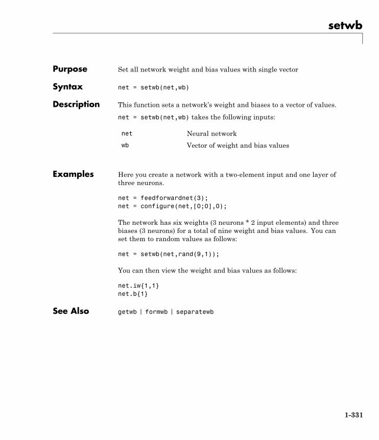
setwb
Purpose Set all network weight and bias values with single vector
Syntax net = setwb(net,wb)
Description This function sets a network’s weight and biases to a vector of values.
net = setwb(net,wb) takes the following inputs:
net Neural network
wb Vector of weight and bias values
Examples Here you create a network with a two-element input and one layer ofthree neurons.
net = feedforwardnet(3);net = configure(net,[0;0],0);
The network has six weights (3 neurons * 2 input elements) and threebiases (3 neurons) for a total of nine weight and bias values. You canset them to random values as follows:
net = setwb(net,rand(9,1));
You can then view the weight and bias values as follows:
net.iw{1,1}net.b{1}
See Also getwb | formwb | separatewb
1-331
sim
Purpose Simulate neural network
Syntax [Y,Xf,Af] = sim(net,X,Xi,Ai,T)[Y,Xf,Af] = sim(net,{Q TS},Xi,Ai)[Y,...] = sim(net,...,'useParallel',...)[Y,...] = sim(net,...,'useGPU',...)[Y,...] = sim(net,...,'showResources',...)[Ycomposite,...] = sim(net,Xcomposite,...)[Ygpu,...] = sim(net,Xgpu,...)
To GetHelp
Type help network/sim.
Description sim simulates neural networks.
[Y,Xf,Af] = sim(net,X,Xi,Ai,T) takes
net Network
X Network inputs
Xi Initial input delay conditions (default = zeros)
Ai Initial layer delay conditions (default = zeros)
T Network targets (default = zeros)
and returns
Y Network outputs
Xf Final input delay conditions
Xf Final layer delay conditions
sim is usually called implicitly by calling the neural network as afunction. For instance, these two expressions return the same result:
1-332
sim
y = sim(net,x,xi,ai)y = net(x,xi,ai)
Note that arguments Xi, Ai, Xf, and Af are optional and need only beused for networks that have input or layer delays.
The signal arguments can have two formats: cell array or matrix.
The cell array format is easiest to describe. It is most convenient fornetworks with multiple inputs and outputs, and allows sequences ofinputs to be presented:
X Ni-by-TS cellarray
Each element X{i,ts} is an Ri-by-Qmatrix.
Xi Ni-by-ID cellarray
Each element Xi{i,k} is an Ri-by-Qmatrix.
Ai Nl-by-LD cellarray
Each element Ai{i,k} is an Si-by-Qmatrix.
T No-by-TS cellarray
Each element X{i,ts} is a Ui-by-Qmatrix.
Y No-by-TS cellarray
Each element Y{i,ts} is a Ui-by-Qmatrix.
Xf Ni-by-ID cellarray
Each element Xf{i,k} is an Ri-by-Qmatrix.
Af Nl-by-LD cellarray
Each element Af{i,k} is an Si-by-Qmatrix.
where
Ni = net.numInputs
Nl = net.numLayers
No = net.numOutputs
D = net.numInputDelays
1-333
sim
LD = net.numLayerDelays
TS = Number of time steps
Q = Batch size
Ri = net.inputs{i}.size
Si = net.layers{i}.size
Ui = net.outputs{i}.size
The columns of Xi, Ai, Xf, and Af are ordered from oldest delaycondition to most recent:
Xi{i,k} = Input i at time ts = k - ID
Xf{i,k} = Input i at time ts = TS + k - ID
Ai{i,k} = Layer output i at time ts = k - LD
Af{i,k} = Layer output i at time ts = TS + k - LD
The matrix format can be used if only one time step is to be simulated(TS = 1). It is convenient for networks with only one input and output,but can also be used with networks that have more.
Each matrix argument is found by storing the elements of thecorresponding cell array argument in a single matrix:
X (sum of Ri)-by-Q matrix
Xi (sum of Ri)-by-(ID*Q) matrix
Ai (sum of Si)-by-(LD*Q) matrix
T (sum of Ui)-by-Q matrix
Y (sum of Ui)-by-Q matrix
1-334
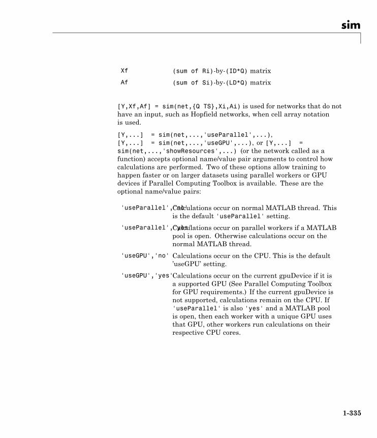
sim
Xf (sum of Ri)-by-(ID*Q) matrix
Af (sum of Si)-by-(LD*Q) matrix
[Y,Xf,Af] = sim(net,{Q TS},Xi,Ai) is used for networks that do nothave an input, such as Hopfield networks, when cell array notationis used.
[Y,...] = sim(net,...,'useParallel',...),[Y,...] = sim(net,...,'useGPU',...), or [Y,...] =sim(net,...,'showResources',...) (or the network called as afunction) accepts optional name/value pair arguments to control howcalculations are performed. Two of these options allow training tohappen faster or on larger datasets using parallel workers or GPUdevices if Parallel Computing Toolbox is available. These are theoptional name/value pairs:
'useParallel','no'Calculations occur on normal MATLAB thread. Thisis the default 'useParallel' setting.
'useParallel','yes'Calculations occur on parallel workers if a MATLABpool is open. Otherwise calculations occur on thenormal MATLAB thread.
'useGPU','no' Calculations occur on the CPU. This is the default’useGPU’ setting.
'useGPU','yes'Calculations occur on the current gpuDevice if it isa supported GPU (See Parallel Computing Toolboxfor GPU requirements.) If the current gpuDevice isnot supported, calculations remain on the CPU. If'useParallel' is also 'yes' and a MATLAB poolis open, then each worker with a unique GPU usesthat GPU, other workers run calculations on theirrespective CPU cores.
1-335
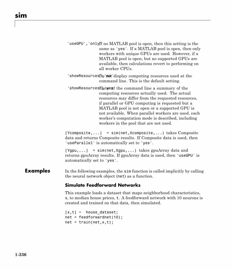
sim
'useGPU','only'If no MATLAB pool is open, then this setting is thesame as 'yes'. If a MATLAB pool is open, then onlyworkers with unique GPUs are used. However, if aMATLAB pool is open, but no supported GPUs areavailable, then calculations revert to performing onall worker CPUs.
'showResources','no'Do not display computing resources used at thecommand line. This is the default setting.
'showResources','yes'Show at the command line a summary of thecomputing resources actually used. The actualresources may differ from the requested resources,if parallel or GPU computing is requested but aMATLAB pool is not open or a supported GPU isnot available. When parallel workers are used, eachworker’s computation mode is described, includingworkers in the pool that are not used.
[Ycomposite,...] = sim(net,Xcomposite,...) takes Compositedata and returns Composite results. If Composite data is used, then'useParallel' is automatically set to 'yes'.
[Ygpu,...] = sim(net,Xgpu,...) takes gpuArray data andreturns gpuArray results. If gpuArray data is used, then 'useGPU' isautomatically set to 'yes'.
Examples In the following examples, the sim function is called implicitly by callingthe neural network object (net) as a function.
Simulate Feedforward Networks
This example loads a dataset that maps neighborhood characteristics,x, to median house prices, t. A feedforward network with 10 neurons iscreated and trained on that data, then simulated.
[x,t] = house_dataset;net = feedforwardnet(10);net = train(net,x,t);
1-336
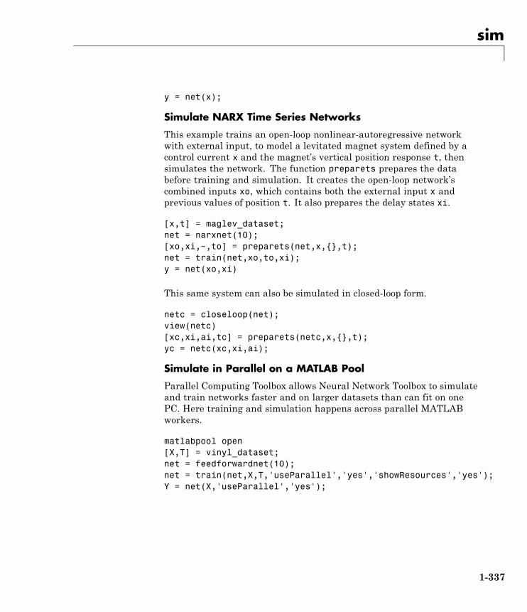
sim
y = net(x);
Simulate NARX Time Series Networks
This example trains an open-loop nonlinear-autoregressive networkwith external input, to model a levitated magnet system defined by acontrol current x and the magnet’s vertical position response t, thensimulates the network. The function preparets prepares the databefore training and simulation. It creates the open-loop network’scombined inputs xo, which contains both the external input x andprevious values of position t. It also prepares the delay states xi.
[x,t] = maglev_dataset;net = narxnet(10);[xo,xi,~,to] = preparets(net,x,{},t);net = train(net,xo,to,xi);y = net(xo,xi)
This same system can also be simulated in closed-loop form.
netc = closeloop(net);view(netc)[xc,xi,ai,tc] = preparets(netc,x,{},t);yc = netc(xc,xi,ai);
Simulate in Parallel on a MATLAB Pool
Parallel Computing Toolbox allows Neural Network Toolbox to simulateand train networks faster and on larger datasets than can fit on onePC. Here training and simulation happens across parallel MATLABworkers.
matlabpool open[X,T] = vinyl_dataset;net = feedforwardnet(10);net = train(net,X,T,'useParallel','yes','showResources','yes');Y = net(X,'useParallel','yes');
1-337
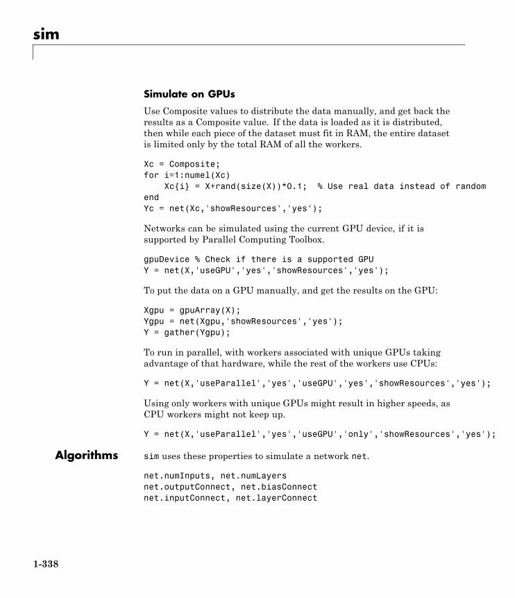
sim
Simulate on GPUs
Use Composite values to distribute the data manually, and get back theresults as a Composite value. If the data is loaded as it is distributed,then while each piece of the dataset must fit in RAM, the entire datasetis limited only by the total RAM of all the workers.
Xc = Composite;for i=1:numel(Xc)
Xc{i} = X+rand(size(X))*0.1; % Use real data instead of randomendYc = net(Xc,'showResources','yes');
Networks can be simulated using the current GPU device, if it issupported by Parallel Computing Toolbox.
gpuDevice % Check if there is a supported GPUY = net(X,'useGPU','yes','showResources','yes');
To put the data on a GPU manually, and get the results on the GPU:
Xgpu = gpuArray(X);Ygpu = net(Xgpu,'showResources','yes');Y = gather(Ygpu);
To run in parallel, with workers associated with unique GPUs takingadvantage of that hardware, while the rest of the workers use CPUs:
Y = net(X,'useParallel','yes','useGPU','yes','showResources','yes');
Using only workers with unique GPUs might result in higher speeds, asCPU workers might not keep up.
Y = net(X,'useParallel','yes','useGPU','only','showResources','yes');
Algorithms sim uses these properties to simulate a network net.
net.numInputs, net.numLayersnet.outputConnect, net.biasConnectnet.inputConnect, net.layerConnect
1-338
sim
These properties determine the network’s weight and bias values andthe number of delays associated with each weight:
net.IW{i,j}net.LW{i,j}net.b{i}net.inputWeights{i,j}.delaysnet.layerWeights{i,j}.delays
These function properties indicate how sim applies weight and biasvalues to inputs to get each layer’s output:
net.inputWeights{i,j}.weightFcnnet.layerWeights{i,j}.weightFcnnet.layers{i}.netInputFcnnet.layers{i}.transferFcn
See Also init | adapt | train | revert
1-339
sim2nndata
Purpose Convert Simulink time series to neural network data
Syntax sim2nndata(x)
Description sim2nndata(x) takes either a column vector of values or a Simulinktime series structure and converts it to a neural network data timeseries.
Examples Here a random Simulink 20-step time series is created and converted.
simts = rands(20,1);nnts = sim2nndata(simts)
Here a similar time series is defined with a Simulink structure andconverted.
simts.time = 0:19simts.signals.values = rands(20,1);simts.dimensions = 1;nnts = sim2nndata(simts)
See Also nndata | nndata2sim
1-340
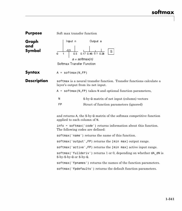
softmax
Purpose Soft max transfer function
GraphandSymbol
Syntax A = softmax(N,FP)
Description softmax is a neural transfer function. Transfer functions calculate alayer’s output from its net input.
A = softmax(N,FP) takes N and optional function parameters,
N S-by-Q matrix of net input (column) vectors
FP Struct of function parameters (ignored)
and returns A, the S-by-Q matrix of the softmax competitive functionapplied to each column of N.
info = softmax('code') returns information about this function.The following codes are defined:
softmax('name') returns the name of this function.
softmax('output',FP) returns the [min max] output range.
softmax('active',FP) returns the [min max] active input range.
softmax('fullderiv') returns 1 or 0, depending on whether dA_dN isS-by-S-by-Q or S-by-Q.
softmax('fpnames') returns the names of the function parameters.
softmax('fpdefaults') returns the default function parameters.
1-341
softmax
Examples Here you define a net input vector N, calculate the output, and plotboth with bar graphs.
n = [0; 1; -0.5; 0.5];a = softmax(n);subplot(2,1,1), bar(n), ylabel('n')subplot(2,1,2), bar(a), ylabel('a')
Assign this transfer function to layer i of a network.
net.layers{i}.transferFcn = 'softmax';
Algorithms a = softmax(n) = exp(n)/sum(exp(n))
See Also sim | compet
1-342
srchbac
Purpose 1-D minimization using backtracking
Syntax [a,gX,perf,retcode,delta,tol] = srchbac(net,X,Pd,Tl,Ai,Q,TS,dX,gX,perf,dperf,delta,TOL,ch_perf)
Description srchbac is a linear search routine. It searches in a given direction tolocate the minimum of the performance function in that direction. Ituses a technique called backtracking.
[a,gX,perf,retcode,delta,tol] =srchbac(net,X,Pd,Tl,Ai,Q,TS,dX,gX,perf,dperf,delta,TOL,ch_perf)takes these inputs,
net Neural network
X Vector containing current values of weights andbiases
Pd Delayed input vectors
Tl Layer target vectors
Ai Initial input delay conditions
Q Batch size
TS Time steps
dX Search direction vector
gX Gradient vector
perf Performance value at current X
dperf Slope of performance value at current X in directionof dX
delta Initial step size
tol Tolerance on search
ch_perf Change in performance on previous step
1-343
srchbac
and returns
a Step size that minimizes performance
gX Gradient at new minimum point
perf Performance value at new minimum point
retcode Return code that has three elements. Thefirst two elements correspond to the numberof function evaluations in the two stages ofthe search. The third element is a returncode. These have different meanings fordifferent search algorithms. Some might notbe used in this function.
0 Normal
1 Minimum step taken
2 Maximum step taken
3 Beta condition not met
delta New initial step size, based on the currentstep size
tol New tolerance on search
Parameters used for the backstepping algorithm are
alpha Scale factor that determines sufficient reductionin perf
beta Scale factor that determines sufficiently largestep size
low_lim Lower limit on change in step size
up_lim Upper limit on change in step size
maxstep Maximum step length
1-344
srchbac
minstep Minimum step length
scale_tol Parameter that relates the tolerance tol to theinitial step size delta, usually set to 20
The defaults for these parameters are set in the training functionthat calls them. See traincgf, traincgb, traincgp, trainbfg, andtrainoss.
Dimensions for these variables are
Pd No-by-Ni-by-TScell array
Each element P{i,j,ts} is aDij-by-Q matrix.
Tl Nl-by-TS cellarray
Each element P{i,ts} is aVi-by-Q matrix.
V Nl-by-LD cellarray
Each element Ai{i,k} is anSi-by-Q matrix.
where
Ni = net.numInputs
Nl = net.numLayers
LD = net.numLayerDelays
Ri = net.inputs{i}.size
Si = net.layers{i}.size
Vi = net.targets{i}.size
Dij = Ri *length(net.inputWeights{i,j}.delays)
Examples Here is a problem consisting of inputs p and targets t to be solved witha network.
1-345
srchbac
p = [0 1 2 3 4 5];t = [0 0 0 1 1 1];
A two-layer feed-forward network is created. The network’s inputranges from [0 to 10]. The first layer has two tansig neurons,and the second layer has one logsig neuron. The traincgf networktraining function and the srchbac search function are to be used.
Create and Test a Network
net = newff([0 5],[2 1],{'tansig','logsig'},'traincgf');a = sim(net,p)
Train and Retest the Network
net.trainParam.searchFcn = 'srchbac';net.trainParam.epochs = 50;net.trainParam.show = 10;net.trainParam.goal = 0.1;net = train(net,p,t);a = sim(net,p)
NetworkUse
You can create a standard network that uses srchbac with newff,newcf, or newelm.
To prepare a custom network to be trained with traincgf, using theline search function srchbac,
1 Set net.trainFcn to 'traincgf'. This sets net.trainParam totraincgf’s default parameters.
2 Set net.trainParam.searchFcn to 'srchbac'.
The srchbac function can be used with any of the following trainingfunctions: traincgf, traincgb, traincgp, trainbfg, trainoss.
1-346
srchbac
Algorithms srchbac locates the minimum of the performance function in the searchdirection dX, using the backtracking algorithm described on page 126and 328 of Dennis and Schnabel’s book, noted below.
References Dennis, J.E., and R.B. Schnabel, Numerical Methods for UnconstrainedOptimization and Nonlinear Equations, Englewood Cliffs, NJ,Prentice-Hall, 1983
Definitions The backtracking search routine srchbac is best suited to use withthe quasi-Newton optimization algorithms. It begins with a stepmultiplier of 1 and then backtracks until an acceptable reduction inthe performance is obtained. On the first step it uses the value ofperformance at the current point and a step multiplier of 1. It alsouses the value of the derivative of performance at the current point toobtain a quadratic approximation to the performance function alongthe search direction. The minimum of the quadratic approximationbecomes a tentative optimum point (under certain conditions) and theperformance at this point is tested. If the performance is not sufficientlyreduced, a cubic interpolation is obtained and the minimum of the cubicinterpolation becomes the new tentative optimum point. This process iscontinued until a sufficient reduction in the performance is obtained.
The backtracking algorithm is described in Dennis and Schnabel. Itis used as the default line search for the quasi-Newton algorithms,although it might not be the best technique for all problems.
See Also srchcha | srchgol | srchhyb
1-347
srchbre
Purpose 1-D interval location using Brent’s method
Syntax [a,gX,perf,retcode,delta,tol] = srchbre(net,X,Pd,Tl,Ai,Q,TS,dX,gX,perf,dperf,delta,tol,ch_perf)
Description srchbre is a linear search routine. It searches in a given direction tolocate the minimum of the performance function in that direction. Ituses a technique called Brent’s technique.
[a,gX,perf,retcode,delta,tol] =srchbre(net,X,Pd,Tl,Ai,Q,TS,dX,gX,perf,dperf,delta,tol,ch_perf)takes these inputs,
net Neural network
X Vector containing current values of weights andbiases
Pd Delayed input vectors
Tl Layer target vectors
Ai Initial input delay conditions
Q Batch size
TS Time steps
dX Search direction vector
gX Gradient vector
perf Performance value at current X
dperf Slope of performance value at current X in directionof dX
delta Initial step size
tol Tolerance on search
ch_perf Change in performance on previous step
1-348
srchbre
and returns
a Step size that minimizes performance
gX Gradient at new minimum point
perf Performance value at new minimum point
retcode Return code that has three elements. Thefirst two elements correspond to the numberof function evaluations in the two stages ofthe search. The third element is a returncode. These have different meanings fordifferent search algorithms. Some might notbe used in this function.
0 Normal
1 Minimum step taken
2 Maximum step taken
3 Beta condition not met
delta New initial step size, based on the currentstep size
tol New tolerance on search
Parameters used for the Brent algorithm are
alpha Scale factor that determines sufficient reductionin perf
beta Scale factor that determines sufficiently largestep size
bmax Largest step size
scale_tol Parameter that relates the tolerance tol to theinitial step size delta, usually set to 20
1-349
srchbre
The defaults for these parameters are set in the training functionthat calls them. See traincgf, traincgb, traincgp, trainbfg, andtrainoss.
Dimensions for these variables are
Pd No-by-Ni-by-TScell array
Each element P{i,j,ts} is aDij-by-Q matrix.
Tl Nl-by-TS cell array Each element P{i,ts} is aVi-by-Q matrix.
Ai Nl-by-LD cell array Each element Ai{i,k} is anSi-by-Q matrix.
where
Ni = net.numInputs
Nl = net.numLayers
LD = net.numLayerDelays
Ri = net.inputs{i}.size
Si = net.layers{i}.size
Vi = net.targets{i}.size
Dij = Ri *length(net.inputWeights{i,j}.delays)
Examples Here is a problem consisting of inputs p and targets t to be solved witha network.
p = [0 1 2 3 4 5];t = [0 0 0 1 1 1];
A two-layer feed-forward network is created. The network’s inputranges from [0 to 10]. The first layer has two tansig neurons,
1-350
srchbre
and the second layer has one logsig neuron. The traincgf networktraining function and the srchbac search function are to be used.
Create and Test a Network
net = newff([0 5],[2 1],{'tansig','logsig'},'traincgf');a = sim(net,p)
Train and Retest the Network
net.trainParam.searchFcn = 'srchbre';net.trainParam.epochs = 50;net.trainParam.show = 10;net.trainParam.goal = 0.1;net = train(net,p,t);a = sim(net,p)
NetworkUse
You can create a standard network that uses srchbre with newff,newcf, or newelm. To prepare a custom network to be trained withtraincgf, using the line search function srchbre,
1 Set net.trainFcn to 'traincgf'. This sets net.trainParam totraincgf’s default parameters.
2 Set net.trainParam.searchFcn to 'srchbre'.
The srchbre function can be used with any of the following trainingfunctions: traincgf, traincgb, traincgp, trainbfg, trainoss.
Algorithms srchbre brackets the minimum of the performance function in thesearch direction dX, using Brent’s algorithm, described on page 46 ofScales (see reference below). It is a hybrid algorithm based on thegolden section search and the quadratic approximation.
References Scales, L.E., Introduction to Non-Linear Optimization, New York,Springer-Verlag, 1985
1-351
srchbre
Definitions Brent’s search is a linear search that is a hybrid of the golden sectionsearch and a quadratic interpolation. Function comparison methods,like the golden section search, have a first-order rate of convergence,while polynomial interpolation methods have an asymptotic rate thatis faster than superlinear. On the other hand, the rate of convergencefor the golden section search starts when the algorithm is initialized,whereas the asymptotic behavior for the polynomial interpolationmethods can take many iterations to become apparent. Brent’s searchattempts to combine the best features of both approaches.
For Brent’s search, you begin with the same interval of uncertaintyused with the golden section search, but some additional points arecomputed. A quadratic function is then fitted to these points and theminimum of the quadratic function is computed. If this minimum iswithin the appropriate interval of uncertainty, it is used in the nextstage of the search and a new quadratic approximation is performed. Ifthe minimum falls outside the known interval of uncertainty, then astep of the golden section search is performed.
See [Bren73] for a complete description of this algorithm. Thisalgorithm has the advantage that it does not require computation of thederivative. The derivative computation requires a backpropagationthrough the network, which involves more computation than aforward pass. However, the algorithm can require more performanceevaluations than algorithms that use derivative information.
See Also srchbac | srchcha | srchgol | srchhyb
1-352
srchcha
Purpose 1-D minimization using Charalambous’ method
Syntax [a,gX,perf,retcode,delta,tol] = srchcha(net,X,Pd,Tl,Ai,Q,TS,dX,gX,perf,dperf,delta,tol,ch_perf)
Description srchcha is a linear search routine. It searches in a given direction tolocate the minimum of the performance function in that direction. Ituses a technique based on Charalambous’ method.
[a,gX,perf,retcode,delta,tol] =srchcha(net,X,Pd,Tl,Ai,Q,TS,dX,gX,perf,dperf,delta,tol,ch_perf)takes these inputs,
net Neural network
X Vector containing current values of weights andbiases
Pd Delayed input vectors
Tl Layer target vectors
Ai Initial input delay conditions
Q Batch size
TS Time steps
dX Search direction vector
gX Gradient vector
perf Performance value at current X
dperf Slope of performance value at current X in directionof dX
delta Initial step size
tol Tolerance on search
ch_perf Change in performance on previous step
1-353
srchcha
and returns
a Step size that minimizes performance
gX Gradient at new minimum point
perf Performance value at new minimum point
retcode Return code that has three elements. Thefirst two elements correspond to the numberof function evaluations in the two stages ofthe search. The third element is a returncode. These have different meanings fordifferent search algorithms. Some might notbe used in this function.
0 Normal
1 Minimum step taken
2 Maximum step taken
3 Beta condition not met
delta New initial step size, based on the currentstep size
tol New tolerance on search
Parameters used for the Charalambous algorithm are
alpha Scale factor that determines sufficient reduction inperf
beta Scale factor that determines sufficiently large stepsize
gama Parameter to avoid small reductions in performance,usually set to 0.1
scale_tol Parameter that relates the tolerance tol to theinitial step size delta, usually set to 20
1-354
srchcha
The defaults for these parameters are set in the training functionthat calls them. See traincgf, traincgb, traincgp, trainbfg, andtrainoss.
Dimensions for these variables are
Pd No-by-Ni-by-TScell array
Each element P{i,j,ts} is aDij-by-Q matrix.
Tl Nl-by-TS cellarray
Each element P{i,ts} is aVi-by-Q matrix.
Ai Nl-by-LD cellarray
Each element Ai{i,k} is anSi-by-Q matrix.
where
Ni = net.numInputs
Nl = net.numLayers
LD = net.numLayerDelays
Ri = net.inputs{i}.size
Si = net.layers{i}.size
Vi = net.targets{i}.size
Dij = Ri *length(net.inputWeights{i,j}.delays)
Examples Here is a problem consisting of inputs p and targets t to be solved witha network.
p = [0 1 2 3 4 5];t = [0 0 0 1 1 1];
1-355
srchcha
A two-layer feed-forward network is created. The network’s inputranges from [0 to 10]. The first layer has two tansig neurons,and the second layer has one logsig neuron. The traincgf networktraining function and the srchcha search function are to be used.
Create and Test a Network
net = newff([0 5],[2 1],{'tansig','logsig'},'traincgf');a = sim(net,p)
Train and Retest the Network
net.trainParam.searchFcn = 'srchcha';net.trainParam.epochs = 50;net.trainParam.show = 10;net.trainParam.goal = 0.1;net = train(net,p,t);a = sim(net,p)
NetworkUse
You can create a standard network that uses srchcha with newff,newcf, or newelm.
To prepare a custom network to be trained with traincgf, using theline search function srchcha,
1 Set net.trainFcn to 'traincgf'. This sets net.trainParam totraincgf’s default parameters.
2 Set net.trainParam.searchFcn to 'srchcha'.
The srchcha function can be used with any of the following trainingfunctions: traincgf, traincgb, traincgp, trainbfg, trainoss.
Algorithms srchcha locates the minimum of the performance function in the searchdirection dX, using an algorithm based on the method described inCharalambous (see reference below).
1-356
srchcha
References Charalambous, C., “Conjugate gradient algorithm for efficient trainingof artificial neural networks,” IEEE Proceedings, Vol. 139, No. 3, June,1992, pp. 301–310.
Definitions The method of Charalambous, srchcha, was designed to be used incombination with a conjugate gradient algorithm for neural networktraining. Like srchbre and srchhyb, it is a hybrid search. It uses acubic interpolation together with a type of sectioning.
See [Char92] for a description of Charalambous’ search. This routineis used as the default search for most of the conjugate gradientalgorithms because it appears to produce excellent results for manydifferent problems. It does require the computation of the derivatives(backpropagation) in addition to the computation of performance, but itovercomes this limitation by locating the minimum with fewer steps.This is not true for all problems, and you might want to experimentwith other line searches.
See Also srchbac | srchbre | srchgol | srchhyb
1-357
srchgol
Purpose 1-D minimization using golden section search
Syntax [a,gX,perf,retcode,delta,tol] = srchgol(net,X,Pd,Tl,Ai,Q,TS,dX,gX,perf,dperf,delta,tol,ch_perf)
Description srchgol is a linear search routine. It searches in a given direction tolocate the minimum of the performance function in that direction. Ituses a technique called the golden section search.
[a,gX,perf,retcode,delta,tol] =srchgol(net,X,Pd,Tl,Ai,Q,TS,dX,gX,perf,dperf,delta,tol,ch_perf)takes these inputs,
net Neural network
X Vector containing current values of weights andbiases
Pd Delayed input vectors
Tl Layer target vectors
Ai Initial input delay conditions
Q Batch size
TS Time steps
dX Search direction vector
gX Gradient vector
perf Performance value at current X
dperf Slope of performance value at current X in directionof dX
delta Initial step size
tol Tolerance on search
ch_perf Change in performance on previous step
1-358
srchgol
and returns
a Step size that minimizes performance
gX Gradient at new minimum point
perf Performance value at new minimum point
retcode Return code that has three elements. Thefirst two elements correspond to the numberof function evaluations in the two stages ofthe search. The third element is a returncode. These have different meanings fordifferent search algorithms. Some might notbe used in this function.
0 Normal
1 Minimum step taken
2 Maximum step taken
3 Beta condition not met
delta New initial step size, based on the currentstep size
tol New tolerance on search
Parameters used for the golden section algorithm are
alpha Scale factor that determines sufficient reductionin perf
bmax Largest step size
scale_tol Parameter that relates the tolerance tol to theinitial step size delta, usually set to 20
1-359
srchgol
The defaults for these parameters are set in the training functionthat calls them. See traincgf, traincgb, traincgp, trainbfg, andtrainoss.
Dimensions for these variables are
Pd No-by-Ni-by-TScell array
Each element P{i,j,ts} is aDij-by-Q matrix.
Tl Nl-by-TS cellarray
Each element P{i,ts} is aVi-by-Q matrix.
Ai Nl-by-LD cellarray
Each element Ai{i,k} is anSi-by-Q matrix.
where
Ni = net.numInputs
Nl = net.numLayers
LD = net.numLayerDelays
Ri = net.inputs{i}.size
Si = net.layers{i}.size
Vi = net.targets{i}.size
Dij = Ri * length(net.inputWeights{i,j}.delays)
Examples Here is a problem consisting of inputs p and targets t to be solved witha network.
p = [0 1 2 3 4 5];t = [0 0 0 1 1 1];
A two-layer feed-forward network is created. The network’s inputranges from [0 to 10]. The first layer has two tansig neurons,
1-360
srchgol
and the second layer has one logsig neuron. The traincgf networktraining function and the srchgol search function are to be used.
Create and Test a Network
net = newff([0 5],[2 1],{'tansig','logsig'},'traincgf');a = sim(net,p)
Train and Retest the Network
net.trainParam.searchFcn = 'srchgol';net.trainParam.epochs = 50;net.trainParam.show = 10;net.trainParam.goal = 0.1;net = train(net,p,t);a = sim(net,p)
NetworkUse
You can create a standard network that uses srchgol with newff,newcf, or newelm.
To prepare a custom network to be trained with traincgf, using theline search function srchgol,
1 Set net.trainFcn to 'traincgf'. This sets net.trainParam totraincgf’s default parameters.
2 Set net.trainParam.searchFcn to 'srchgol'.
The srchgol function can be used with any of the following trainingfunctions: traincgf, traincgb, traincgp, trainbfg, trainoss.
Algorithms srchgol locates the minimum of the performance function in thesearch direction dX, using the golden section search. It is based on thealgorithm as described on page 33 of Scales (see reference below).
References Scales, L.E., Introduction to Non-Linear Optimization, New York,Springer-Verlag, 1985
1-361
srchgol
Definitions The golden section search srchgol is a linear search that does notrequire the calculation of the slope. This routine begins by locating aninterval in which the minimum of the performance function occurs.This is accomplished by evaluating the performance at a sequence ofpoints, starting at a distance of delta and doubling in distance eachstep, along the search direction. When the performance increasesbetween two successive iterations, a minimum has been bracketed. Thenext step is to reduce the size of the interval containing the minimum.Two new points are located within the initial interval. The values ofthe performance at these two points determine a section of the intervalthat can be discarded, and a new interior point is placed within the newinterval. This procedure is continued until the interval of uncertainty isreduced to a width of tol, which is equal to delta/scale_tol.
See [HDB96], starting on page 12-16, for a complete description of thegolden section search. Try the Neural Network Design demonstrationnnd12sd1 [HDB96] for an illustration of the performance of the goldensection search in combination with a conjugate gradient algorithm.
See Also srchbac | srchbre | srchcha | srchhyb
1-362
srchhyb
Purpose 1-D minimization using a hybrid bisection-cubic search
Syntax [a,gX,perf,retcode,delta,tol] = srchhyb(net,X,Pd,Tl,Ai,Q,TS,dX,gX,perf,dperf,delta,tol,ch_perf)
Description srchhyb is a linear search routine. It searches in a given direction tolocate the minimum of the performance function in that direction.It uses a technique that is a combination of a bisection and a cubicinterpolation.
[a,gX,perf,retcode,delta,tol] =srchhyb(net,X,Pd,Tl,Ai,Q,TS,dX,gX,perf,dperf,delta,tol,ch_perf)takes these inputs,
net Neural network
X Vector containing current values of weights andbiases
Pd Delayed input vectors
Tl Layer target vectors
Ai Initial input delay conditions
Q Batch size
TS Time steps
dX Search direction vector
gX Gradient vector
perf Performance value at current X
dperf Slope of performance value at current X in directionof dX
delta Initial step size
tol Tolerance on search
ch_perf Change in performance on previous step
1-363
srchhyb
and returns
a Step size that minimizes performance
gX Gradient at new minimum point
perf Performance value at new minimum point
retcode Return code that has three elements. Thefirst two elements correspond to the numberof function evaluations in the two stages ofthe search. The third element is a returncode. These have different meanings fordifferent search algorithms. Some might notbe used in this function.
0 Normal
1 Minimum step taken
2 Maximum step taken
3 Beta condition not met
delta New initial step size, based on the currentstep size
tol New tolerance on search
Parameters used for the hybrid bisection-cubic algorithm are
alpha Scale factor that determines sufficient reductionin perf
beta Scale factor that determines sufficiently largestep size
bmax Largest step size
scale_tol Parameter that relates the tolerance tol to theinitial step size delta, usually set to 20
1-364
srchhyb
The defaults for these parameters are set in the training functionthat calls them. See traincgf, traincgb, traincgp, trainbfg, andtrainoss.
Dimensions for these variables are
Pd No-by-Ni-by-TScell array
Each element P{i,j,ts} is aDij-by-Q matrix.
Tl Nl-by-TS cellarray
Each element P{i,ts} is aVi-by-Q matrix.
Ai Nl-by-LD cellarray
Each element Ai{i,k} is anSi-by-Q matrix.
where
Ni = net.numInputs
Nl = net.numLayers
LD = net.numLayerDelays
Ri = net.inputs{i}.size
Si = net.layers{i}.size
Vi = net.targets{i}.size
Dij = Ri * length(net.inputWeights{i,j}.delays)
Examples Here is a problem consisting of inputs p and targets t to be solved witha network.
p = [0 1 2 3 4 5];t = [0 0 0 1 1 1];
A two-layer feed-forward network is created. The network’s inputranges from [0 to 10]. The first layer has two tansig neurons,
1-365
srchhyb
and the second layer has one logsig neuron. The traincgf networktraining function and the srchhyb search function are to be used.
Create and Test a Network
net = newff([0 5],[2 1],{'tansig','logsig'},'traincgf');a = sim(net,p)
Train and Retest the Network
net.trainParam.searchFcn = 'srchhyb';net.trainParam.epochs = 50;net.trainParam.show = 10;net.trainParam.goal = 0.1;net = train(net,p,t);a = sim(net,p)
NetworkUse
You can create a standard network that uses srchhyb with newff,newcf, or newelm.
To prepare a custom network to be trained with traincgf, using theline search function srchhyb,
1 Set net.trainFcn to 'traincgf'. This sets net.trainParam totraincgf’s default parameters.
2 Set net.trainParam.searchFcn to 'srchhyb'.
The srchhyb function can be used with any of the following trainingfunctions: traincgf, traincgb, traincgp, trainbfg, trainoss.
Algorithms srchhyb locates the minimum of the performance function in the searchdirection dX, using the hybrid bisection-cubic interpolation algorithmdescribed on page 50 of Scales (see reference below).
References Scales, L.E., Introduction to Non-Linear Optimization, New YorkSpringer-Verlag, 1985
1-366
srchhyb
Definitions Like Brent’s search, srchhyb is a hybrid algorithm. It is a combinationof bisection and cubic interpolation. For the bisection algorithm, onepoint is located in the interval of uncertainty, and the performanceand its derivative are computed. Based on this information, half ofthe interval of uncertainty is discarded. In the hybrid algorithm, acubic interpolation of the function is obtained by using the value of theperformance and its derivative at the two endpoints. If the minimum ofthe cubic interpolation falls within the known interval of uncertainty,then it is used to reduce the interval of uncertainty. Otherwise, a stepof the bisection algorithm is used.
See [Scal85] for a complete description of the hybrid bisection-cubicsearch. This algorithm does require derivative information, so itperforms more computations at each step of the algorithm than thegolden section search or Brent’s algorithm.
See Also srchbac | srchbre | srchcha | srchgol
1-367
sse
Purpose Sum squared error performance function
Syntax perf = sse(net,t,y,ew)[...] = sse(...,'regularization',regularization)[...] = sse(...,'normalization',normalization)[...] = sse(...,'squaredWeighting',squaredWeighting)[...] = sse(...,FP)
Description sse is a network performance function. It measures performanceaccording to the sum of squared errors.
perf = sse(net,t,y,ew) takes these input arguments and optionalfunction parameters,
net Neural network
t Matrix or cell array of target vectors
y Matrix or cell array of output vectors
ew Error weights (default = {1})
and returns the sum squared error.
This function has three optional function parameters which can bedefined with parameter name/pair arguments, or as a structure FPargument with fields having the parameter name and assigned theparameter values.
[...] = sse(...,'regularization',regularization)
[...] = sse(...,'normalization',normalization)
[...] = sse(...,'squaredWeighting',squaredWeighting)
[...] = sse(...,FP)
• regularization — can be set to any value between the default of0 and 1. The greater the regularization value, the more squaredweights and biases are taken into account in the performancecalculation.
1-368
sse
• normalization — can be set to the default 'absolute', or'normalized' (which normalizes errors to the [+2 -2] rangeconsistent with normalized output and target ranges of [-1 1]) or'percent' (which normalizes errors to the range [-1 +1]).
• squaredWeighting — can be set to the default true, for applyingerror weights to squared errors; or false for applying error weightsto the absolute errors before squaring.
Examples Here a network is trained to fit a simple data set and its performancecalculated
[x,t] = simplefit_dataset;net = fitnet(10);net.performFcn = 'sse';net = train(net,x,t)y = net(x)e = t-yperf = sse(net,t,y)
NetworkUse
To prepare a custom network to be trained with sse, setnet.performFcn to 'sse'. This automatically sets net.performParamto the default function parameters.
Then calling train, adapt or perform will result in sse being usedto calculate performance.
1-369
staticderiv
Purpose Static derivative function
Syntax staticderiv('dperf_dwb',net,X,T,Xi,Ai,EW)staticderiv('de_dwb',net,X,T,Xi,Ai,EW)
Description This function calculates derivatives using the chain rule from thenetworks performance or outputs back to its inputs. For time seriesdata and dynamic networks this function ignores the delay connectionsresulting in a approximation (which may be good or not) of the actualderivative. This function is used by Elman networks (elmannet) whichis a dynamic network trained by the static derivative approximationwhen full derivative calculations are not available. As full derivativesare calculated by all the other derivative functions, this function is notrecommended for dynamic networks except for research into trainingalgorithms.
staticderiv('dperf_dwb',net,X,T,Xi,Ai,EW) takes thesearguments,
net Neural network
X Inputs, an RxQ matrix (or NxTS cell array of RixQmatrices)
T Targets, an SxQ matrix (or MxTS cell array of SixQmatrices)
Xi Initial input delay states (optional)
Ai Initial layer delay states (optional)
EW Error weights (optional)
and returns the gradient of performance with respect to the network’sweights and biases, where R and S are the number of input and outputelements and Q is the number of samples (and N and M are the numberof input and output signals, Ri and Si are the number of each input andoutputs elements, and TS is the number of timesteps).
1-370
staticderiv
staticderiv('de_dwb',net,X,T,Xi,Ai,EW) returns the Jacobian oferrors with respect to the network’s weights and biases.
Examples Here a feedforward network is trained and both the gradient andJacobian are calculated.
[x,t] = simplefit_dataset;net = feedforwardnet(20);net = train(net,x,t);y = net(x);perf = perform(net,t,y);gwb = staticderiv('dperf_dwb',net,x,t)jwb = staticderiv('de_dwb',net,x,t)
See Also bttderiv | defaultderiv | fpderiv | num2deriv
1-371
sumabs
Purpose Sum of absolute elements of matrix or matrices
Syntax [s,n] = sumabs(x)
Description [s,n] = sumabs(x) takes a matrix or cell array of matrices andreturns,
s Sum of all absolute finite values
n Number of finite values
If x contains no finite values, the sum returned is 0.
Examples m = sumabs([1 2;3 4])[m,n] = sumabs({[1 2; NaN 4], [4 5; 2 3]})
See Also meanabs | meansqr | sumsqr
1-372
sumsqr
Purpose Sum of squared elements of matrix or matrices
Syntax [s,n] = sumsqr(x)
Description [s,n] = sumsqr(x) takes a matrix or cell array of matrices andreturns,
s Sum of all squared finite values
n Number of finite values
If x contains no finite values, the sum returned is 0.
Examples m = sumsqr([1 2;3 4])[m,n] = sumsqr({[1 2; NaN 4], [4 5; 2 3]})
See Also meanabs | meansqr | sumabs
1-373
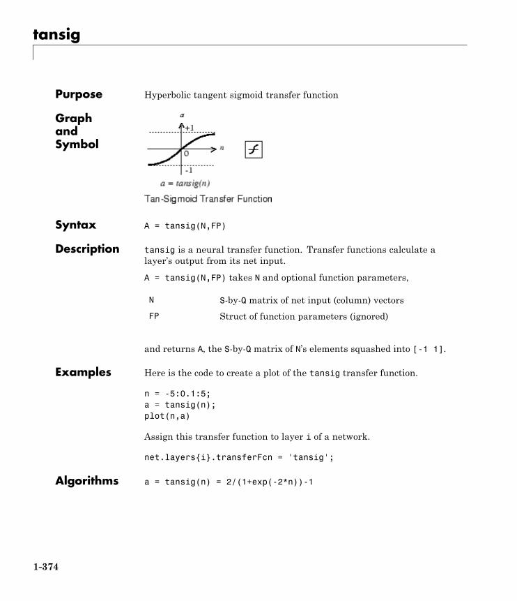
tansig
Purpose Hyperbolic tangent sigmoid transfer function
GraphandSymbol
Syntax A = tansig(N,FP)
Description tansig is a neural transfer function. Transfer functions calculate alayer’s output from its net input.
A = tansig(N,FP) takes N and optional function parameters,
N S-by-Q matrix of net input (column) vectors
FP Struct of function parameters (ignored)
and returns A, the S-by-Q matrix of N’s elements squashed into [-1 1].
Examples Here is the code to create a plot of the tansig transfer function.
n = -5:0.1:5;a = tansig(n);plot(n,a)
Assign this transfer function to layer i of a network.
net.layers{i}.transferFcn = 'tansig';
Algorithms a = tansig(n) = 2/(1+exp(-2*n))-1
1-374
tansig
This is mathematically equivalent to tanh(N). It differs in that it runsfaster than the MATLAB implementation of tanh, but the results canhave very small numerical differences. This function is a good tradeofffor neural networks, where speed is important and the exact shape ofthe transfer function is not.
References Vogl, T.P., J.K. Mangis, A.K. Rigler, W.T. Zink, and D.L. Alkon,“Accelerating the convergence of the backpropagation method,”Biological Cybernetics, Vol. 59, 1988, pp. 257–263
See Also sim | logsig
1-375
tapdelay
Purpose Shift neural network time series data for tap delay
Syntax tapdelay(x,i,ts,delays)
Description tapdelay(x,i,ts,delays) takes these arguments,
x Neural network time series data
i Signal index
ts Timestep index
delays Row vector of increasing zero or positive delays
and returns the tap delay values of signal i at timestep ts given thespecified tap delays.
Examples Here a random signal x consisting of eight timesteps is defined, and atap delay with delays of [0 1 4] is simulated at timestep 6.
x = num2cell(rand(1,8));y = tapdelay(x,1,6,[0 1 4])
See Also nndata | extendts | preparets
1-376
timedelaynet
Purpose Time delay neural network
Syntax timedelaynet(inputDelays,hiddenSizes,trainFcn)
Description Time delay networks are similar to feedforward networks, except thatthe input weight has a tap delay line associated with it. This allows thenetwork to have a finite dynamic response to time series input data.This network is also similar to the distributed delay neural network(distdelaynet), which has delays on the layer weights in addition tothe input weight.
timedelaynet(inputDelays,hiddenSizes,trainFcn) takes thesearguments,
inputDelays Row vector of increasing 0 or positive delays(default = 1:2)
hiddenSizes Row vector of one or more hidden layer sizes(default = 10)
trainFcn Training function (default = 'trainlm')
and returns a time delay neural network.
Examples Here a time delay neural network is used to solve a simple time seriesproblem.
[X,T] = simpleseries_dataset;net = timedelaynet(1:2,10)[Xs,Xi,Ai,Ts] = preparets(net,X,T)net = train(net,Xs,Ts,Xi,Ai);view(net)Y = net(Xs,Xi,Ai);perf = perform(net,Ts,Y)
See Also preparets | removedelay | distdelaynet | narnet | narxnet
1-377
tonndata
Purpose Convert data to standard neural network cell array form
Syntax [y,wasMatrix] = tonndata(x,columnSamples,cellTime)
Description [y,wasMatrix] = tonndata(x,columnSamples,cellTime) takes thesearguments,
x Matrix or cell array of matrices
columnSamples True if original samples are oriented as columns,false if rows
cellTime True if original samples are columns of cell, falseif they are store in matrix
and returns
y Original data transformed into standard neuralnetwork cell array form
wasMatrix True if original data was a matrix (as apposedto cell array)
If columnSamples is false, then matrix x or matrices in cell array x willbe transposed, so row samples will now be stored as column vectors.
If cellTime is false, then matrix samples will be separated into columnsof a cell array so time originally represented as vectors in a matrix willnow be represented as columns of a cell array.
The returned value wasMatrix can be used by fromnndata to reversethe transformation.
Examples Here data consisting of six timesteps of 5-element vectors is originallyrepresented as a matrix with six columns is converted to standardneural network representation and back.
1-378

tonndata
x = rand(5,6)[y,wasMatrix] = tonndata(x,true,false)x2 = fromnndata(y,wasMatrix,columnSamples,cellTime)
See Also nndata | fromnndata | nndata2sim | sim2nndata
1-379
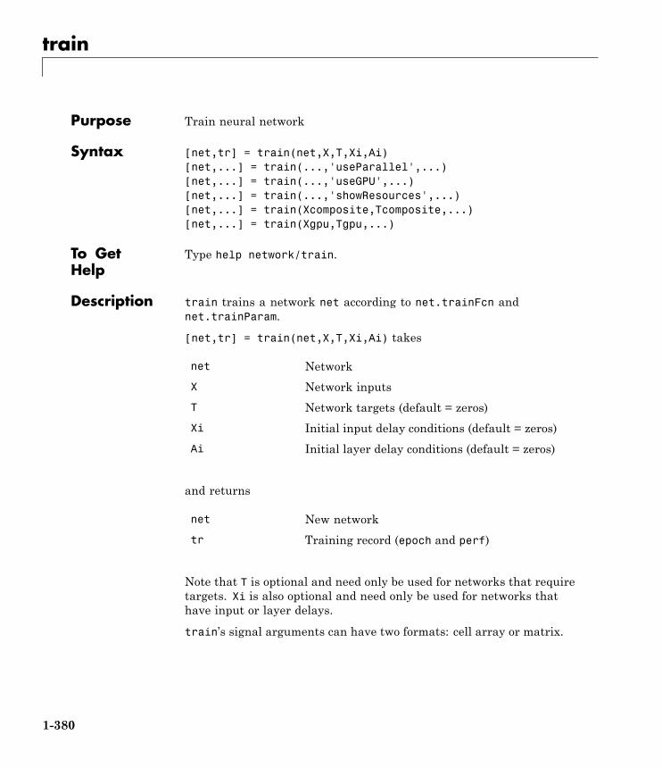
train
Purpose Train neural network
Syntax [net,tr] = train(net,X,T,Xi,Ai)[net,...] = train(...,'useParallel',...)[net,...] = train(...,'useGPU',...)[net,...] = train(...,'showResources',...)[net,...] = train(Xcomposite,Tcomposite,...)[net,...] = train(Xgpu,Tgpu,...)
To GetHelp
Type help network/train.
Description train trains a network net according to net.trainFcn andnet.trainParam.
[net,tr] = train(net,X,T,Xi,Ai) takes
net Network
X Network inputs
T Network targets (default = zeros)
Xi Initial input delay conditions (default = zeros)
Ai Initial layer delay conditions (default = zeros)
and returns
net New network
tr Training record (epoch and perf)
Note that T is optional and need only be used for networks that requiretargets. Xi is also optional and need only be used for networks thathave input or layer delays.
train’s signal arguments can have two formats: cell array or matrix.
1-380
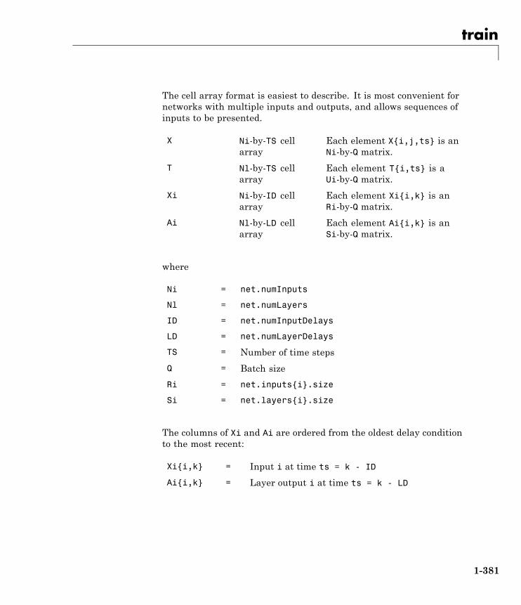
train
The cell array format is easiest to describe. It is most convenient fornetworks with multiple inputs and outputs, and allows sequences ofinputs to be presented.
X Ni-by-TS cellarray
Each element X{i,j,ts} is anNi-by-Q matrix.
T Nl-by-TS cellarray
Each element T{i,ts} is aUi-by-Q matrix.
Xi Ni-by-ID cellarray
Each element Xi{i,k} is anRi-by-Q matrix.
Ai Nl-by-LD cellarray
Each element Ai{i,k} is anSi-by-Q matrix.
where
Ni = net.numInputs
Nl = net.numLayers
ID = net.numInputDelays
LD = net.numLayerDelays
TS = Number of time steps
Q = Batch size
Ri = net.inputs{i}.size
Si = net.layers{i}.size
The columns of Xi and Ai are ordered from the oldest delay conditionto the most recent:
Xi{i,k} = Input i at time ts = k - ID
Ai{i,k} = Layer output i at time ts = k - LD
1-381
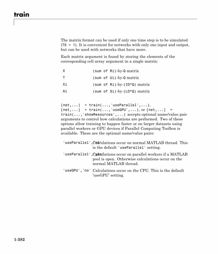
train
The matrix format can be used if only one time step is to be simulated(TS = 1). It is convenient for networks with only one input and output,but can be used with networks that have more.
Each matrix argument is found by storing the elements of thecorresponding cell array argument in a single matrix:
X (sum of Ri)-by-Q matrix
T (sum of Ui)-by-Q matrix
Xi (sum of Ri)-by-(ID*Q) matrix
Ai (sum of Si)-by-(LD*Q) matrix
[net,...] = train(...,'useParallel',...),[net,...] = train(...,'useGPU',...), or [net,...] =train(...,'showResources',...) accepts optional name/value pairarguments to control how calculations are performed. Two of theseoptions allow training to happen faster or on larger datasets usingparallel workers or GPU devices if Parallel Computing Toolbox isavailable. These are the optional name/value pairs:
'useParallel','no'Calculations occur on normal MATLAB thread. Thisis the default 'useParallel' setting.
'useParallel','yes'Calculations occur on parallel workers if a MATLABpool is open. Otherwise calculations occur on thenormal MATLAB thread.
'useGPU','no' Calculations occur on the CPU. This is the default’useGPU’ setting.
1-382
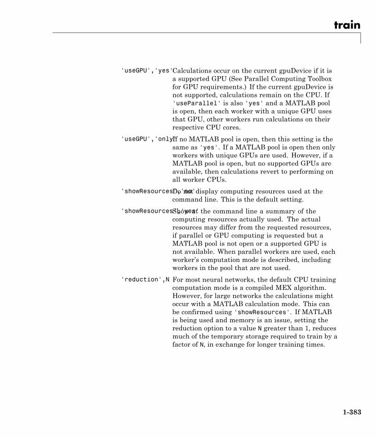
train
'useGPU','yes'Calculations occur on the current gpuDevice if it isa supported GPU (See Parallel Computing Toolboxfor GPU requirements.) If the current gpuDevice isnot supported, calculations remain on the CPU. If'useParallel' is also 'yes' and a MATLAB poolis open, then each worker with a unique GPU usesthat GPU, other workers run calculations on theirrespective CPU cores.
'useGPU','only'If no MATLAB pool is open, then this setting is thesame as 'yes'. If a MATLAB pool is open then onlyworkers with unique GPUs are used. However, if aMATLAB pool is open, but no supported GPUs areavailable, then calculations revert to performing onall worker CPUs.
'showResources','no'Do not display computing resources used at thecommand line. This is the default setting.
'showResources','yes'Show at the command line a summary of thecomputing resources actually used. The actualresources may differ from the requested resources,if parallel or GPU computing is requested but aMATLAB pool is not open or a supported GPU isnot available. When parallel workers are used, eachworker’s computation mode is described, includingworkers in the pool that are not used.
'reduction',N For most neural networks, the default CPU trainingcomputation mode is a compiled MEX algorithm.However, for large networks the calculations mightoccur with a MATLAB calculation mode. This canbe confirmed using 'showResources'. If MATLABis being used and memory is an issue, setting thereduction option to a value N greater than 1, reducesmuch of the temporary storage required to train by afactor of N, in exchange for longer training times.
1-383
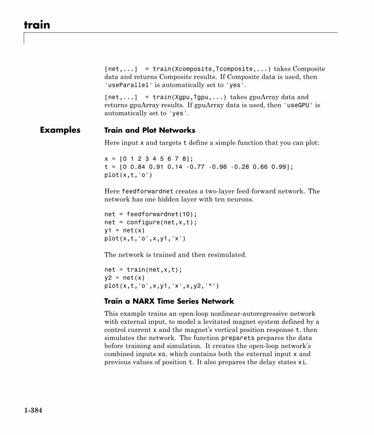
train
[net,...] = train(Xcomposite,Tcomposite,...) takes Compositedata and returns Composite results. If Composite data is used, then'useParallel' is automatically set to 'yes'.
[net,...] = train(Xgpu,Tgpu,...) takes gpuArray data andreturns gpuArray results. If gpuArray data is used, then 'useGPU' isautomatically set to 'yes'.
Examples Train and Plot Networks
Here input x and targets t define a simple function that you can plot:
x = [0 1 2 3 4 5 6 7 8];t = [0 0.84 0.91 0.14 -0.77 -0.96 -0.28 0.66 0.99];plot(x,t,'o')
Here feedforwardnet creates a two-layer feed-forward network. Thenetwork has one hidden layer with ten neurons.
net = feedforwardnet(10);net = configure(net,x,t);y1 = net(x)plot(x,t,'o',x,y1,'x')
The network is trained and then resimulated.
net = train(net,x,t);y2 = net(x)plot(x,t,'o',x,y1,'x',x,y2,'*')
Train a NARX Time Series Network
This example trains an open-loop nonlinear-autoregressive networkwith external input, to model a levitated magnet system defined by acontrol current x and the magnet’s vertical position response t, thensimulates the network. The function preparets prepares the databefore training and simulation. It creates the open-loop network’scombined inputs xo, which contains both the external input x andprevious values of position t. It also prepares the delay states xi.
1-384
train
[x,t] = maglev_dataset;net = narxnet(10);[xo,xi,~,to] = preparets(net,x,{},t);net = train(net,xo,to,xi);y = net(xo,xi)
This same system can also be simulated in closed-loop form.
netc = closeloop(net);view(netc)[xc,xi,ai,tc] = preparets(netc,x,{},t);yc = netc(xc,xi,ai);
Train a Network in Parallel on a MATLAB Pool
Parallel Computing Toolbox allows Neural Network Toolbox to simulateand train networks faster and on larger datasets than can fit on onePC. Here training and simulation happens across parallel MATLABworkers.
matlabpool open[X,T] = vinyl_dataset;net = feedforwardnet(10);net = train(net,X,T,'useParallel','yes','showResources','yes');Y = net(X);
Train a Network on GPUs
Use Composite values to distribute the data manually, and get back theresults as a Composite value. If the data is loaded as it is distributedthen while each piece of the dataset must fit in RAM, the entire datasetis limited only by the total RAM of all the workers.
Xc = Composite;Tc = Composite;for i=1:numel(Xc)
Xc{i} = X+rand(size(X))*0.1; % (Use real data insteadTc{i} = T+rand(size(T))*0.1; % of random data)
endnet = train(net,Xc,Tc);
1-385
train
Yc = net(Xc);
Networks can be trained using the current GPU device, if it is supportedby Parallel Computing Toolbox.
net = train(net,X,T,'useGPU','yes');y = net(X);
To put the data on a GPU manually:
Xgpu = gpuArray(X);Tgpu = gpuArray(T);net = train(net,Xgpu,Tgpu);Ygpu = net(Xgpu);Y = gather(Ygpu);
To run in parallel, with workers associated with unique GPUs takingadvantage of that hardware, while the rest of the workers use CPUs:
net = train(net,X,T,'useParallel','yes','useGPU','yes');y = net(X);
Using only workers with unique GPUs might result in higher speed, asCPU workers might not keep up.
net = train(net,X,T,'useParallel','yes','useGPU','only');Y = net(X);
Algorithms train calls the function indicated by net.trainFcn, using the trainingparameter values indicated by net.trainParam.
Typically one epoch of training is defined as a single presentation of allinput vectors to the network. The network is then updated according tothe results of all those presentations.
Training occurs until a maximum number of epochs occurs, theperformance goal is met, or any other stopping condition of the functionnet.trainFcn occurs.
1-386
train
Some training functions depart from this norm by presenting only oneinput vector (or sequence) each epoch. An input vector (or sequence)is chosen randomly for each epoch from concurrent input vectors (orsequences). competlayer returns networks that use trainru, a trainingfunction that does this.
See Also init | revert | sim | adapt
1-387
trainb
Purpose Batch training with weight and bias learning rules
Syntax net.trainFcn = 'trainb'[net,tr] = train(net,...)
Description trainb is not called directly. Instead it is called by train for networkswhose net.trainFcn property is set to 'trainb', thus:
net.trainFcn = 'trainb'
[net,tr] = train(net,...)
trainb trains a network with weight and bias learning rules with batchupdates. The weights and biases are updated at the end of an entirepass through the input data.
Training occurs according to trainb’s training parameters, shown herewith their default values:
net.trainParam.epochs 100 Maximum number of epochs to train
net.trainParam.goal 0 Performance goal
net.trainParam.max_fail 5 Maximum validation failures
net.trainParam.show 25 Epochs between displays (NaN for nodisplays)
net.trainParam.showCommandLinefalse Generate command-line output
net.trainParam.showWindow true Show training GUI
net.trainParam.time inf Maximum time to train in seconds
NetworkUse
You can create a standard network that uses trainb by callinglinearlayer.
To prepare a custom network to be trained with trainb,
1 Set net.trainFcn to 'trainb'. This sets net.trainParam totrainb’s default parameters.
1-388
trainb
2 Set each net.inputWeights{i,j}.learnFcn to a learning function.Set each net.layerWeights{i,j}.learnFcn to a learning function.Set each net.biases{i}.learnFcn to a learning function. (Weightand bias learning parameters are automatically set to default valuesfor the given learning function.)
To train the network,
1 Set net.trainParam properties to desired values.
2 Set weight and bias learning parameters to desired values.
3 Call train.
Algorithms Each weight and bias is updated according to its learning function aftereach epoch (one pass through the entire set of input vectors).
Training stops when any of these conditions is met:
• The maximum number of epochs (repetitions) is reached.
• Performance is minimized to the goal.
• The maximum amount of time is exceeded.
• Validation performance has increased more than max_fail timessince the last time it decreased (when using validation).
See Also linearlayer | train
1-389
trainbfg
Purpose BFGS quasi-Newton backpropagation
Syntax net.trainFcn = 'trainbfg'[net,tr] = train(net,...)
Description trainbfg is a network training function that updates weight and biasvalues according to the BFGS quasi-Newton method.
net.trainFcn = 'trainbfg'
[net,tr] = train(net,...)
Training occurs according to trainbfg’s training parameters, shownhere with their default values:
net.trainParam.epochs 100 Maximum number of epochs totrain
net.trainParam.showWindow 0 Show training window
net.trainParam.show 25 Epochs between displays (NaN forno displays)
net.trainParam.showCommandLine 0 Generate command-line output
net.trainParam.goal 0 Performance goal
net.trainParam.time inf Maximum time to train inseconds
net.trainParam.min_grad 1e-6 Minimum performance gradient
net.trainParam.max_fail 5 Maximum validation failures
net.trainParam.searchFcn 'srchcha' Name of line search routine touse
Parameters related to line search methods (not all used for all methods):
1-390
trainbfg
net.trainParam.scal_tol 20 Divide into delta to determine tolerance forlinear search.
net.trainParam.alpha 0.001 Scale factor that determines sufficientreduction in perf
net.trainParam.beta 0.1 Scale factor that determines sufficiently largestep size
net.trainParam.delta 0.01 Initial step size in interval location step
net.trainParam.gama 0.1 Parameter to avoid small reductions inperformance, usually set to 0.1 (see srch_cha)
net.trainParam.low_lim 0.1 Lower limit on change in step size
net.trainParam.up_lim 0.5 Upper limit on change in step size
net.trainParam.maxstep 100 Maximum step length
net.trainParam.minstep 1.0e-6 Minimum step length
net.trainParam.bmax 26 Maximum step size
net.trainParam.batch_frag 0 In case of multiple batches, they are consideredindependent. Any nonzero value implies afragmented batch, so the final layer’s conditionsof a previous trained epoch are used as initialconditions for the next epoch.
NetworkUse
You can create a standard network that uses trainbfg withfeedfowardnet or cascadeforwardnet. To prepare a custom networkto be trained with trainbfg:
1 Set NET.trainFcn to 'trainbfg'. This sets NET.trainParam totrainbfg’s default parameters.
2 Set NET.trainParam properties to desired values.
In either case, calling train with the resulting network trains thenetwork with trainbfg.
1-391
trainbfg
Examples Here a neural network is trained to predict median house prices.
[x,t] = house_dataset;net = feedforwardnet(10,'trainbfg');net = train(net,x,t);y = net(x)
Algorithms trainbfg can train any network as long as its weight, net input, andtransfer functions have derivative functions.
Backpropagation is used to calculate derivatives of performance perfwith respect to the weight and bias variables X. Each variable isadjusted according to the following:
X = X + a*dX;
where dX is the search direction. The parameter a is selected tominimize the performance along the search direction. The line searchfunction searchFcn is used to locate the minimum point. The firstsearch direction is the negative of the gradient of performance. Insucceeding iterations the search direction is computed according tothe following formula:
dX = -H\gX;
where gX is the gradient and H is a approximate Hessian matrix. Seepage 119 of Gill, Murray, and Wright (Practical Optimization, 1981) fora more detailed discussion of the BFGS quasi-Newton method.
Training stops when any of these conditions occurs:
• The maximum number of epochs (repetitions) is reached.
• The maximum amount of time is exceeded.
• Performance is minimized to the goal.
• The performance gradient falls below min_grad.
• Validation performance has increased more than max_fail timessince the last time it decreased (when using validation).
1-392
trainbfg
References Gill, Murray, & Wright, Practical Optimization, 1981
Definitions Newton’s method is an alternative to the conjugate gradient methodsfor fast optimization. The basic step of Newton’s method is
x x A gk k k k+−= −11
where Ak−1 is the Hessian matrix (second derivatives) of the
performance index at the current values of the weights and biases.Newton’s method often converges faster than conjugate gradientmethods. Unfortunately, it is complex and expensive to compute theHessian matrix for feedforward neural networks. There is a class ofalgorithms that is based on Newton’s method, but which does notrequire calculation of second derivatives. These are called quasi-Newton(or secant) methods. They update an approximate Hessian matrix ateach iteration of the algorithm. The update is computed as a function ofthe gradient. The quasi-Newton method that has been most successfulin published studies is the Broyden, Fletcher, Goldfarb, and Shanno(BFGS) update. This algorithm is implemented in the trainbfg routine.
The BFGS algorithm is described in [DeSc83]. This algorithm requiresmore computation in each iteration and more storage than the conjugategradient methods, although it generally converges in fewer iterations.The approximate Hessian must be stored, and its dimension is n x n,where n is equal to the number of weights and biases in the network.For very large networks it might be better to use Rprop or one ofthe conjugate gradient algorithms. For smaller networks, however,trainbfg can be an efficient training function.
See Also cascadeforwardnet | feedforwardnet | traingdm | traingda |traingdx | trainlm | trainrp | traincgf | traincgb | trainscg |traincgp | trainoss
1-393
trainbfgc
Purpose BFGS quasi-Newton backpropagation for use with NN model referenceadaptive controller
Syntax [net,TR,Y,E,Pf,Af,flag_stop] = trainbfgc(net,P,T,Pi,Ai,epochs,TS,Q)
info = trainbfgc(code)
Description trainbfgc is a network training function that updates weight and biasvalues according to the BFGS quasi-Newton method. This function iscalled from nnmodref, a GUI for the model reference adaptive controlSimulink block.
[net,TR,Y,E,Pf,Af,flag_stop] =trainbfgc(net,P,T,Pi,Ai,epochs,TS,Q) takes these inputs,
net Neural network
P Delayed input vectors
T Layer target vectors
Pi Initial input delay conditions
Ai Initial layer delay conditions
epochs Number of iterations for training
TS Time steps
Q Batch size
and returns
net Trained network
TR Training record of various values over eachepoch:
TR.epoch Epoch number
TR.perf Training performance
1-394
trainbfgc
TR.vperf Validation performance
TR.tperf Test performance
Y Network output for last epoch
E Layer errors for last epoch
Pf Final input delay conditions
Af Collective layer outputs for last epoch
flag_stop Indicates if the user stopped the training
Training occurs according to trainbfgc’s training parameters, shownhere with their default values:
net.trainParam.epochs 100 Maximum number of epochs to train
net.trainParam.show 25 Epochs between displays (NaN for no displays)
net.trainParam.goal 0 Performance goal
net.trainParam.time inf Maximum time to train in seconds
net.trainParam.min_grad 1e-6 Minimum performance gradient
net.trainParam.max_fail 5 Maximum validation failures
net.trainParam.searchFcn 'srchbacx'Name of line search routine to use
Parameters related to line search methods (not all used for all methods):
net.trainParam.scal_tol 20 Divide into delta to determine tolerance forlinear search.
net.trainParam.alpha 0.001 Scale factor that determines sufficientreduction in perf
net.trainParam.beta 0.1 Scale factor that determines sufficiently largestep size
net.trainParam.delta 0.01 Initial step size in interval location step
1-395
trainbfgc
net.trainParam.gama 0.1 Parameter to avoid small reductions inperformance, usually set to 0.1 (see srch_cha)
net.trainParam.low_lim 0.1 Lower limit on change in step size
net.trainParam.up_lim 0.5 Upper limit on change in step size
net.trainParam.maxstep 100 Maximum step length
net.trainParam.minstep 1.0e-6 Minimum step length
net.trainParam.bmax 26 Maximum step size
info = trainbfgc(code) returns useful information for each codestring:
'pnames' Names of training parameters
'pdefaults' Default training parameters
Algorithms trainbfgc can train any network as long as its weight, net input, andtransfer functions have derivative functions. Backpropagation is used tocalculate derivatives of performance perf with respect to the weight andbias variables X. Each variable is adjusted according to the following:
X = X + a*dX;
where dX is the search direction. The parameter a is selected tominimize the performance along the search direction. The line searchfunction searchFcn is used to locate the minimum point. The firstsearch direction is the negative of the gradient of performance. Insucceeding iterations the search direction is computed according tothe following formula:
dX = -H\gX;
1-396
trainbfgc
where gX is the gradient and H is an approximate Hessian matrix. Seepage 119 of Gill, Murray, and Wright (Practical Optimization, 1981) fora more detailed discussion of the BFGS quasi-Newton method.
Training stops when any of these conditions occurs:
• The maximum number of epochs (repetitions) is reached.
• The maximum amount of time is exceeded.
• Performance is minimized to the goal.
• The performance gradient falls below min_grad.
• Precision problems have occurred in the matrix inversion.
References Gill, Murray, and Wright, Practical Optimization, 1981
1-397
trainbr
Purpose Bayesian regulation backpropagation
Syntax net.trainFcn = 'trainbr'[net,tr] = train(net,...)
Description trainbr is a network training function that updates the weight and biasvalues according to Levenberg-Marquardt optimization. It minimizes acombination of squared errors and weights, and then determines thecorrect combination so as to produce a network that generalizes well.The process is called Bayesian regularization.
net.trainFcn = 'trainbr'
[net,tr] = train(net,...)
Training occurs according to trainbr’s training parameters, shownhere with their default values:
net.trainParam.epochs 100 Maximum number of epochs to train
net.trainParam.goal 0 Performance goal
net.trainParam.mu 0.005 Marquardt adjustment parameter
net.trainParam.mu_dec 0.1 Decrease factor for mu
net.trainParam.mu_inc 10 Increase factor for mu
net.trainParam.mu_max 1e10 Maximum value for mu
net.trainParam.max_fail 5 Maximum validation failures
net.trainParam.mem_reduc 1 Factor to use for memory/speed tradeoff
net.trainParam.min_grad 1e-10 Minimum performance gradient
net.trainParam.show 25 Epochs between displays (NaN for nodisplays)
net.trainParam.showCommandLine 0 Generate command-line output
net.trainParam.showWindow 1 Show training GUI
net.trainParam.time inf Maximum time to train in seconds
1-398
trainbr
NetworkUse
You can create a standard network that uses trainbr withfeedforwardnet or cascadeforwardnet. To prepare a custom networkto be trained with trainbr,
1 Set NET.trainFcn to 'trainbr'. This sets NET.trainParam totrainbr’s default parameters.
2 Set NET.trainParam properties to desired values.
In either case, calling train with the resulting network trains thenetwork with trainbr. See feedforwardnet and cascadeforwardnetfor examples.
Examples Here is a problem consisting of inputs p and targets t to be solved witha network. It involves fitting a noisy sine wave.
p = [-1:.05:1];t = sin(2*pi*p)+0.1*randn(size(p));
A feed-forward network is created with a hidden layer of 2 neurons.
net = feedforwardnet(2,'trainbr');
Here the network is trained and tested.
net = train(net,p,t);a = net(p)
Algorithms trainbr can train any network as long as its weight, net input, andtransfer functions have derivative functions.
Bayesian regularization minimizes a linear combination of squarederrors and weights. It also modifies the linear combination so thatat the end of training the resulting network has good generalizationqualities. See MacKay (Neural Computation, Vol. 4, No. 3, 1992, pp.415 to 447) and Foresee and Hagan (Proceedings of the International
1-399
trainbr
Joint Conference on Neural Networks, June, 1997) for more detaileddiscussions of Bayesian regularization.
This Bayesian regularization takes place within theLevenberg-Marquardt algorithm. Backpropagation is used tocalculate the Jacobian jX of performance perf with respect to theweight and bias variables X. Each variable is adjusted according toLevenberg-Marquardt,
jj = jX * jXje = jX * EdX = -(jj+I*mu) \ je
where E is all errors and I is the identity matrix.
The adaptive value mu is increased by mu_inc until the change shownabove results in a reduced performance value. The change is then madeto the network, and mu is decreased by mu_dec.
The parameter mem_reduc indicates how to use memory and speed tocalculate the Jacobian jX. If mem_reduc is 1, then trainlm runs thefastest, but can require a lot of memory. Increasing mem_reduc to 2 cutssome of the memory required by a factor of two, but slows trainlmsomewhat. Higher values continue to decrease the amount of memoryneeded and increase the training times.
Training stops when any of these conditions occurs:
• The maximum number of epochs (repetitions) is reached.
• The maximum amount of time is exceeded.
• Performance is minimized to the goal.
• The performance gradient falls below min_grad.
• mu exceeds mu_max.
Limitations This function uses the Jacobian for calculations, which assumes thatperformance is a mean or sum of squared errors. Therefore networks
1-400
trainbr
trained with this function must use either the mse or sse performancefunction.
References MacKay, Neural Computation, Vol. 4, No. 3, 1992, pp. 415–447
Foresee and Hagan, Proceedings of the International Joint Conferenceon Neural Networks, June, 1997
See Also cascadeforwardnet | feedforwardnet | traingdm | traingda |traingdx | trainlm | trainrp | traincgf | traincgb | trainscg |traincgp | trainbfg
1-401
trainbu
Purpose Batch unsupervised weight/bias training
Syntax net.trainFcn = 'trainbu'[net,tr] = train(net,...)
Description trainbu trains a network with weight and bias learning rules withbatch updates. Weights and biases updates occur at the end of an entirepass through the input data.
trainbu is not called directly. Instead the train function calls it fornetworks whose NET.trainFcn property is set to 'trainbu', thus:
net.trainFcn = 'trainbu'
[net,tr] = train(net,...)
Training occurs according to trainbu training parameters, shown herewith the following default values:
net.trainParam.epochs 100 Maximum number of epochs to train
net.trainParam.show 25 Epochs between displays (NaN for nodisplays)
net.trainParam.showCommandLine false Generate command-line output
net.trainParam.showGUI true Show training GUI
net.trainParam.time inf Maximum time to train in seconds
Validation and test vectors have no impact on training for this function,but act as independent measures of network generalization.
NetworkUse
You can create a standard network that uses trainbu by callingselforgmap. To prepare a custom network to be trained with trainb:
1 Set NET.trainFcn to 'trainbu'. (This option sets NET.trainParamto trainbu default parameters.)
2 Set each NET.inputWeights{i,j}.learnFcn to a learning function.
1-402
trainbu
3 Set each NET.layerWeights{i,j}.learnFcn to a learning function.
4 Set each NET.biases{i}.learnFcn to a learning function. (Weightand bias learning parameters are automatically set to default valuesfor the given learning function.)
To train the network:
1 Set NET.trainParam properties to desired values.
2 Set weight and bias learning parameters to desired values.
3 Call train.
See selforgmap for training examples.
Algorithms Each weight and bias updates according to its learning function aftereach epoch (one pass through the entire set of input vectors).
Training stops when any of these conditions is met:
• The maximum number of epochs (repetitions) is reached.
• Performance is minimized to the goal.
• The maximum amount of time is exceeded.
• Validation performance has increased more than max_fail timessince the last time it decreased (when using validation).
See Also train | trainb
1-403
trainc
Purpose Cyclical order weight/bias training
Syntax net.trainFcn = 'trainc'[net,tr] = train(net,...)
Description trainc is not called directly. Instead it is called by train for networkswhose net.trainFcn property is set to 'trainc', thus:
net.trainFcn = 'trainc'
[net,tr] = train(net,...)
trainc trains a network with weight and bias learning rules withincremental updates after each presentation of an input. Inputs arepresented in cyclic order.
Training occurs according to trainc’s training parameters, shown herewith their default values:
net.trainParam.epochs 100 Maximum number of epochs to train
net.trainParam.goal 0 Performance goal
net.trainParam.max_fail 5 Maximum validation failures
net.trainParam.show 25 Epochs between displays (NaN for nodisplays)
net.trainParam.showCommandLine false Generate command-line output
net.trainParam.showWindow true Show training GUI
net.trainParam.time inf Maximum time to train in seconds
NetworkUse
You can create a standard network that uses trainc by callingcompetlayer. To prepare a custom network to be trained with trainc,
1 Set net.trainFcn to 'trainc'. This sets net.trainParam totrainc’s default parameters.
1-404
trainc
2 Set each net.inputWeights{i,j}.learnFcn to a learning function.Set each net.layerWeights{i,j}.learnFcn to a learning function.Set each net.biases{i}.learnFcn to a learning function. (Weightand bias learning parameters are automatically set to default valuesfor the given learning function.)
To train the network,
1 Set net.trainParam properties to desired values.
2 Set weight and bias learning parameters to desired values.
3 Call train.
See newp for training examples.
Algorithms For each epoch, each vector (or sequence) is presented in order to thenetwork, with the weight and bias values updated accordingly aftereach individual presentation.
Training stops when any of these conditions is met:
• The maximum number of epochs (repetitions) is reached.
• Performance is minimized to the goal.
• The maximum amount of time is exceeded.
See Also competlayer | train
1-405
traincgb
Purpose Conjugate gradient backpropagation with Powell-Beale restarts
Syntax net.trainFcn = 'traincgb'[net,tr] = train(net,...)
Description traincgb is a network training function that updates weight andbias values according to the conjugate gradient backpropagation withPowell-Beale restarts.
net.trainFcn = 'traincgb'
[net,tr] = train(net,...)
Training occurs according to traincgb’s training parameters, shownhere with their default values:
net.trainParam.epochs 100 Maximum number of epochs to train
net.trainParam.show 25 Epochs between displays (NaN for nodisplays)
net.trainParam.showCommandLine 0 Generate command-line output
net.trainParam.showWindow 1 Show training GUI
net.trainParam.goal 0 Performance goal
net.trainParam.time inf Maximum time to train in seconds
net.trainParam.min_grad 1e-6 Minimum performance gradient
net.trainParam.max_fail 5 Maximum validation failures
net.trainParam.searchFcn 'srchcha'Name of line search routine to use
Parameters related to line search methods (not all used for all methods):
net.trainParam.scal_tol 20 Divide into delta to determine tolerance forlinear search.
net.trainParam.alpha 0.001 Scale factor that determines sufficient reductionin perf
1-406
traincgb
net.trainParam.beta 0.1 Scale factor that determines sufficiently largestep size
net.trainParam.delta 0.01 Initial step size in interval location step
net.trainParam.gama 0.1 Parameter to avoid small reductions inperformance, usually set to 0.1 (see srch_cha)
net.trainParam.low_lim 0.1 Lower limit on change in step size
net.trainParam.up_lim 0.5 Upper limit on change in step size
net.trainParam.maxstep 100 Maximum step length
net.trainParam.minstep 1.0e-6 Minimum step length
net.trainParam.bmax 26 Maximum step size
NetworkUse
You can create a standard network that uses traincgb withfeedforwardnet or cascadeforwardnet.
To prepare a custom network to be trained with traincgb,
1 Set net.trainFcn to 'traincgb'. This sets net.trainParam totraincgb’s default parameters.
2 Set net.trainParam properties to desired values.
In either case, calling train with the resulting network trains thenetwork with traincgb.
Examples Here a neural network is trained to predict median house prices.
[x,t] = house_dataset;net = feedforwardnet(10,'traincgb');net = train(net,x,t);y = net(x)
Algorithms traincgb can train any network as long as its weight, net input, andtransfer functions have derivative functions.
1-407
traincgb
Backpropagation is used to calculate derivatives of performance perfwith respect to the weight and bias variables X. Each variable isadjusted according to the following:
X = X + a*dX;
where dX is the search direction. The parameter a is selected tominimize the performance along the search direction. The line searchfunction searchFcn is used to locate the minimum point. The firstsearch direction is the negative of the gradient of performance. Insucceeding iterations the search direction is computed from the newgradient and the previous search direction according to the formula
dX = -gX + dX_old*Z;
where gX is the gradient. The parameter Z can be computed in severaldifferent ways. The Powell-Beale variation of conjugate gradient isdistinguished by two features. First, the algorithm uses a test todetermine when to reset the search direction to the negative of thegradient. Second, the search direction is computed from the negativegradient, the previous search direction, and the last search directionbefore the previous reset. See Powell,Mathematical Programming, Vol.12, 1977, pp. 241 to 254, for a more detailed discussion of the algorithm.
Training stops when any of these conditions occurs:
• The maximum number of epochs (repetitions) is reached.
• The maximum amount of time is exceeded.
• Performance is minimized to the goal.
• The performance gradient falls below min_grad.
• Validation performance has increased more than max_fail timessince the last time it decreased (when using validation).
References Powell, M.J.D., “Restart procedures for the conjugate gradient method,”Mathematical Programming, Vol. 12, 1977, pp. 241–254
1-408
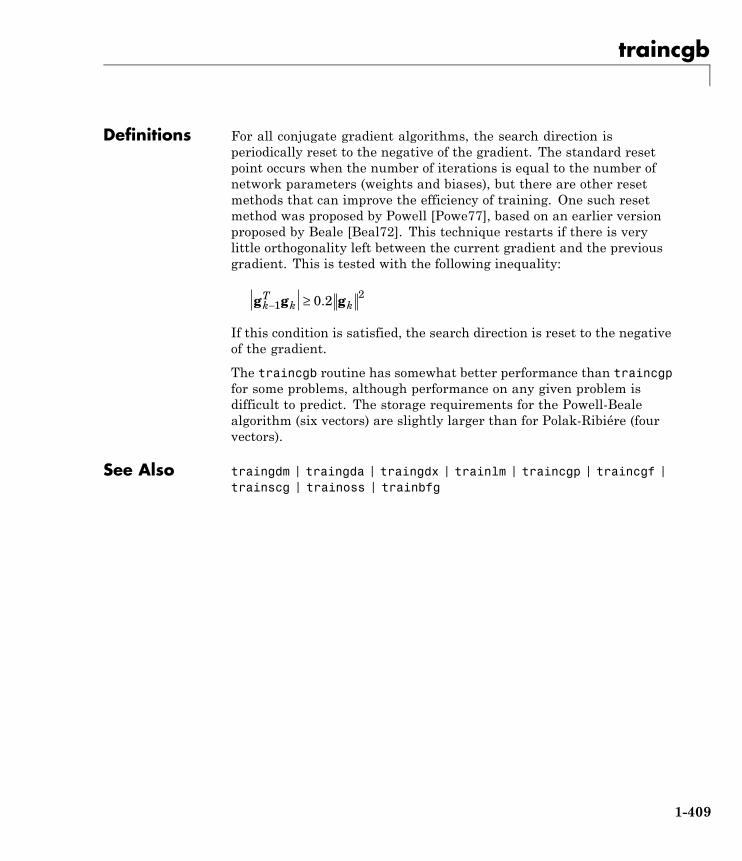
traincgb
Definitions For all conjugate gradient algorithms, the search direction isperiodically reset to the negative of the gradient. The standard resetpoint occurs when the number of iterations is equal to the number ofnetwork parameters (weights and biases), but there are other resetmethods that can improve the efficiency of training. One such resetmethod was proposed by Powell [Powe77], based on an earlier versionproposed by Beale [Beal72]. This technique restarts if there is verylittle orthogonality left between the current gradient and the previousgradient. This is tested with the following inequality:
g g gkT
k k− ≥120 2.
If this condition is satisfied, the search direction is reset to the negativeof the gradient.
The traincgb routine has somewhat better performance than traincgpfor some problems, although performance on any given problem isdifficult to predict. The storage requirements for the Powell-Bealealgorithm (six vectors) are slightly larger than for Polak-Ribiére (fourvectors).
See Also traingdm | traingda | traingdx | trainlm | traincgp | traincgf |trainscg | trainoss | trainbfg
1-409
traincgf
Purpose Conjugate gradient backpropagation with Fletcher-Reeves updates
Syntax net.trainFcn = 'traincgf'[net,tr] = train(net,...)
Description traincgf is a network training function that updates weight andbias values according to conjugate gradient backpropagation withFletcher-Reeves updates.
net.trainFcn = 'traincgf'
[net,tr] = train(net,...)
Training occurs according to traincgf’s training parameters, shownhere with their default values:
net.trainParam.epochs 100 Maximum number of epochs to train
net.trainParam.show 25 Epochs between displays (NaN for nodisplays)
net.trainParam.showCommandLine 0 Generate command-line output
net.trainParam.showWindow 1 Show training GUI
net.trainParam.goal 0 Performance goal
net.trainParam.time inf Maximum time to train in seconds
net.trainParam.min_grad 1e-6 Minimum performance gradient
net.trainParam.max_fail 5 Maximum validation failures
net.trainParam.searchFcn 'srchcha'Name of line search routine to use
Parameters related to line search methods (not all used for all methods):
net.trainParam.scal_tol 20 Divide into delta to determine tolerance forlinear search.
net.trainParam.alpha 0.001 Scale factor that determines sufficientreduction in perf
1-410
traincgf
net.trainParam.beta 0.1 Scale factor that determines sufficiently largestep size
net.trainParam.delta 0.01 Initial step size in interval location step
net.trainParam.gama 0.1 Parameter to avoid small reductions inperformance, usually set to 0.1 (see srch_cha)
net.trainParam.low_lim 0.1 Lower limit on change in step size
net.trainParam.up_lim 0.5 Upper limit on change in step size
net.trainParam.maxstep 100 Maximum step length
net.trainParam.minstep 1.0e-6 Minimum step length
net.trainParam.bmax 26 Maximum step size
NetworkUse
You can create a standard network that uses traincgf withfeedforwardnet or cascadeforwardnet.
To prepare a custom network to be trained with traincgf,
1 Set net.trainFcn to 'traincgf'. This sets net.trainParam totraincgf’s default parameters.
2 Set net.trainParam properties to desired values.
In either case, calling train with the resulting network trains thenetwork with traincgf.
Examples Here a neural network is trained to predict median house prices.
[x,t] = house_dataset;net = feedforwardnet(10,'traincgf');net = train(net,x,t);y = net(x)
Algorithms traincgf can train any network as long as its weight, net input, andtransfer functions have derivative functions.
1-411
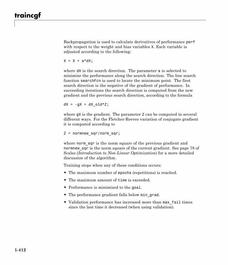
traincgf
Backpropagation is used to calculate derivatives of performance perfwith respect to the weight and bias variables X. Each variable isadjusted according to the following:
X = X + a*dX;
where dX is the search direction. The parameter a is selected tominimize the performance along the search direction. The line searchfunction searchFcn is used to locate the minimum point. The firstsearch direction is the negative of the gradient of performance. Insucceeding iterations the search direction is computed from the newgradient and the previous search direction, according to the formula
dX = -gX + dX_old*Z;
where gX is the gradient. The parameter Z can be computed in severaldifferent ways. For the Fletcher-Reeves variation of conjugate gradientit is computed according to
Z = normnew_sqr/norm_sqr;
where norm_sqr is the norm square of the previous gradient andnormnew_sqr is the norm square of the current gradient. See page 78 ofScales (Introduction to Non-Linear Optimization) for a more detaileddiscussion of the algorithm.
Training stops when any of these conditions occurs:
• The maximum number of epochs (repetitions) is reached.
• The maximum amount of time is exceeded.
• Performance is minimized to the goal.
• The performance gradient falls below min_grad.
• Validation performance has increased more than max_fail timessince the last time it decreased (when using validation).
1-412
traincgf
References Scales, L.E., Introduction to Non-Linear Optimization, New York,Springer-Verlag, 1985
Definitions All the conjugate gradient algorithms start out by searching in thesteepest descent direction (negative of the gradient) on the firstiteration.
p g0 0= −
A line search is then performed to determine the optimal distance tomove along the current search direction:
x x pk k k k+ =1 α
Then the next search direction is determined so that it is conjugate toprevious search directions. The general procedure for determining thenew search direction is to combine the new steepest descent directionwith the previous search direction:
p g pk k k k= − + −β 1
The various versions of the conjugate gradient algorithm aredistinguished by the manner in which the constant βk is computed. Forthe Fletcher-Reeves update the procedure is
βkkT
k
kT
k
=− −
g g
g g1 1
This is the ratio of the norm squared of the current gradient to the normsquared of the previous gradient.
See [FlRe64] or [HDB96] for a discussion of the Fletcher-Reevesconjugate gradient algorithm.
The conjugate gradient algorithms are usually much faster thanvariable learning rate backpropagation, and are sometimes fasterthan trainrp, although the results vary from one problem to another.The conjugate gradient algorithms require only a little more storage
1-413
traincgf
than the simpler algorithms. Therefore, these algorithms are good fornetworks with a large number of weights.
Try the Neural Network Design demonstration nnd12cg [HDB96] for anillustration of the performance of a conjugate gradient algorithm.
See Also traingdm | traingda | traingdx | trainlm | traincgb | trainscg |traincgp | trainoss | trainbfg
1-414
traincgp
Purpose Conjugate gradient backpropagation with Polak-Ribiére updates
Syntax net.trainFcn = 'traincgp'[net,tr] = train(net,...)
Description traincgp is a network training function that updates weight andbias values according to conjugate gradient backpropagation withPolak-Ribiére updates.
net.trainFcn = 'traincgp'
[net,tr] = train(net,...)
Training occurs according to traincgp’s training parameters, shownhere with their default values:
net.trainParam.epochs 100 Maximum number of epochs to train
net.trainParam.show 25 Epochs between displays (NaN for nodisplays)
net.trainParam.showCommandLine 0 Generate command-line output
net.trainParam.showWindow 1 Show training GUI
net.trainParam.goal 0 Performance goal
net.trainParam.time inf Maximum time to train in seconds
net.trainParam.min_grad 1e-6 Minimum performance gradient
net.trainParam.max_fail 5 Maximum validation failures
net.trainParam.searchFcn 'srchcha'Name of line search routine to use
Parameters related to line search methods (not all used for all methods):
net.trainParam.scal_tol 20 Divide into delta to determine tolerance forlinear search.
net.trainParam.alpha 0.001 Scale factor that determines sufficient reductionin perf
1-415
traincgp
net.trainParam.beta 0.1 Scale factor that determines sufficiently largestep size
net.trainParam.delta 0.01 Initial step size in interval location step
net.trainParam.gama 0.1 Parameter to avoid small reductions inperformance, usually set to 0.1 (see srch_cha)
net.trainParam.low_lim 0.1 Lower limit on change in step size
net.trainParam.up_lim 0.5 Upper limit on change in step size
net.trainParam.maxstep 100 Maximum step length
net.trainParam.minstep 1.0e-6 Minimum step length
net.trainParam.bmax 26 Maximum step size
NetworkUse
You can create a standard network that uses traincgp withfeedforwardnet or cascadeforwardnet. To prepare a custom networkto be trained with traincgp,
1 Set net.trainFcn to 'traincgp'. This sets net.trainParam totraincgp’s default parameters.
2 Set net.trainParam properties to desired values.
In either case, calling train with the resulting network trains thenetwork with traincgp.
Examples Examples
Here a neural network is trained to predict median house prices.
[x,t] = house_dataset;net = feedforwardnet(10,'traincgp');net = train(net,x,t);y = net(x)
1-416
traincgp
Algorithms traincgp can train any network as long as its weight, net input, andtransfer functions have derivative functions.
Backpropagation is used to calculate derivatives of performance perfwith respect to the weight and bias variables X. Each variable isadjusted according to the following:
X = X + a*dX;
where dX is the search direction. The parameter a is selected tominimize the performance along the search direction. The line searchfunction searchFcn is used to locate the minimum point. The firstsearch direction is the negative of the gradient of performance. Insucceeding iterations the search direction is computed from the newgradient and the previous search direction according to the formula
dX = -gX + dX_old*Z;
where gX is the gradient. The parameter Z can be computed in severaldifferent ways. For the Polak-Ribiére variation of conjugate gradient, itis computed according to
Z = ((gX - gX_old)'*gX)/norm_sqr;
where norm_sqr is the norm square of the previous gradient, andgX_old is the gradient on the previous iteration. See page 78 of Scales(Introduction to Non-Linear Optimization, 1985) for a more detaileddiscussion of the algorithm.
Training stops when any of these conditions occurs:
• The maximum number of epochs (repetitions) is reached.
• The maximum amount of time is exceeded.
• Performance is minimized to the goal.
• The performance gradient falls below min_grad.
• Validation performance has increased more than max_fail timessince the last time it decreased (when using validation).
1-417
traincgp
References Scales, L.E., Introduction to Non-Linear Optimization, New York,Springer-Verlag, 1985
Definitions Another version of the conjugate gradient algorithm was proposed byPolak and Ribiére. As with the Fletcher-Reeves algorithm, traincgf,the search direction at each iteration is determined by
p g pk k k k= − + −β 1
For the Polak-Ribiére update, the constant βk is computed by
βkkT
k
kT
k
=Δ −
− −
g g
g g1
1 1
This is the inner product of the previous change in the gradient with thecurrent gradient divided by the norm squared of the previous gradient.See [FlRe64] or [HDB96] for a discussion of the Polak-Ribiére conjugategradient algorithm.
The traincgp routine has performance similar to traincgf. It isdifficult to predict which algorithm will perform best on a givenproblem. The storage requirements for Polak-Ribiére (four vectors) areslightly larger than for Fletcher-Reeves (three vectors).
See Also traingdm | traingda | traingdx | trainlm | trainrp | traincgf |traincgb | trainscg | trainoss | trainbfg
1-418
traingd
Purpose Gradient descent backpropagation
Syntax net.trainFcn = 'traingd'[net,tr] = train(net,...)
Description traingd is a network training function that updates weight and biasvalues according to gradient descent.
net.trainFcn = 'traingd'
[net,tr] = train(net,...)
Training occurs according to traingd’s training parameters, shownhere with their default values:
net.trainParam.epochs 10 Maximum number of epochs to train
net.trainParam.goal 0 Performance goal
net.trainParam.showCommandLine 0 Generate command-line output
net.trainParam.showWindow 1 Show training GUI
net.trainParam.lr 0.01 Learning rate
net.trainParam.max_fail 5 Maximum validation failures
net.trainParam.min_grad 1e-10 Minimum performance gradient
net.trainParam.show 25 Epochs between displays (NaN for nodisplays)
net.trainParam.time inf Maximum time to train in seconds
NetworkUse
You can create a standard network that uses traingd withfeedforwardnet or cascadeforwardnet. To prepare a custom networkto be trained with traingd,
1 Set net.trainFcn to 'traingd'. This sets net.trainParam totraingd’s default parameters.
1-419
traingd
2 Set net.trainParam properties to desired values.
In either case, calling train with the resulting network trains thenetwork with traingd.
See help feedforwardnet and help cascadeforwardnet for examples.
Algorithms traingd can train any network as long as its weight, net input, andtransfer functions have derivative functions.
Backpropagation is used to calculate derivatives of performance perfwith respect to the weight and bias variables X. Each variable isadjusted according to gradient descent:
dX = lr * dperf/dX
Training stops when any of these conditions occurs:
• The maximum number of epochs (repetitions) is reached.
• The maximum amount of time is exceeded.
• Performance is minimized to the goal.
• The performance gradient falls below min_grad.
• Validation performance has increased more than max_fail timessince the last time it decreased (when using validation).
Definitions The batch steepest descent training function is traingd. The weightsand biases are updated in the direction of the negative gradient ofthe performance function. If you want to train a network using batchsteepest descent, you should set the network trainFcn to traingd,and then call the function train. There is only one training functionassociated with a given network.
There are seven training parameters associated with traingd:
• epochs
• show
1-420
traingd
• goal
• time
• min_grad
• max_fail
• lr
The learning rate lr is multiplied times the negative of the gradientto determine the changes to the weights and biases. The larger thelearning rate, the bigger the step. If the learning rate is made too large,the algorithm becomes unstable. If the learning rate is set too small,the algorithm takes a long time to converge. See page 12-8 of [HDB96]for a discussion of the choice of learning rate.
The training status is displayed for every show iterations of thealgorithm. (If show is set to NaN, then the training status is neverdisplayed.) The other parameters determine when the training stops.The training stops if the number of iterations exceeds epochs, if theperformance function drops below goal, if the magnitude of the gradientis less than mingrad, or if the training time is longer than time seconds.max_fail, which is associated with the early stopping technique, isdiscussed in Improving Generalization.
The following code creates a training set of inputs p and targets t. Forbatch training, all the input vectors are placed in one matrix.
p = [-1 -1 2 2; 0 5 0 5];t = [-1 -1 1 1];
Create the feedforward network.
net = feedforwardnet(3,'traingd');
In this simple example, turn off a feature that is introduced later.
net.divideFcn = '';
1-421
traingd
At this point, you might want to modify some of the default trainingparameters.
net.trainParam.show = 50;net.trainParam.lr = 0.05;net.trainParam.epochs = 300;net.trainParam.goal = 1e-5;
If you want to use the default training parameters, the precedingcommands are not necessary.
Now you are ready to train the network.
[net,tr] = train(net,p,t);
The training record tr contains information about the progress oftraining.
Now you can simulate the trained network to obtain its response to theinputs in the training set.
a = net(p)a =
-1.0026 -0.9962 1.0010 0.9960
Try the Neural Network Design demonstration nnd12sd1 [HDB96]for an illustration of the performance of the batch gradient descentalgorithm.
See Also traingdm | traingda | traingdx | trainlm
1-422
traingda
Purpose Gradient descent with adaptive learning rate backpropagation
Syntax net.trainFcn = 'traingda'[net,tr] = train(net,...)
Description traingda is a network training function that updates weight and biasvalues according to gradient descent with adaptive learning rate.
net.trainFcn = 'traingda'
[net,tr] = train(net,...)
Training occurs according to traingda’s training parameters, shownhere with their default values:
net.trainParam.epochs 10 Maximum number of epochs to train
net.trainParam.goal 0 Performance goal
net.trainParam.lr 0.01 Learning rate
net.trainParam.lr_inc 1.05 Ratio to increase learning rate
net.trainParam.lr_dec 0.7 Ratio to decrease learning rate
net.trainParam.max_fail 5 Maximum validation failures
net.trainParam.max_perf_inc 1.04 Maximum performance increase
net.trainParam.min_grad 1e-10 Minimum performance gradient
net.trainParam.show 25 Epochs between displays (NaN for nodisplays)
net.trainParam.showCommandLine 0 Generate command-line output
net.trainParam.showWindow 1 Show training GUI
net.trainParam.time inf Maximum time to train in seconds
NetworkUse
You can create a standard network that uses traingda withfeedforwardnet or cascadeforwardnet. To prepare a custom networkto be trained with traingda,
1-423
traingda
1 Set net.trainFcn to 'traingda'. This sets net.trainParam totraingda’s default parameters.
2 Set net.trainParam properties to desired values.
In either case, calling train with the resulting network trains thenetwork with traingda.
See help feedforwardnet and help cascadeforwardnet for examples.
Algorithms traingda can train any network as long as its weight, net input, andtransfer functions have derivative functions.
Backpropagation is used to calculate derivatives of performance dperfwith respect to the weight and bias variables X. Each variable isadjusted according to gradient descent:
dX = lr*dperf/dX
At each epoch, if performance decreases toward the goal, then thelearning rate is increased by the factor lr_inc. If performance increasesby more than the factor max_perf_inc, the learning rate is adjustedby the factor lr_dec and the change that increased the performanceis not made.
Training stops when any of these conditions occurs:
• The maximum number of epochs (repetitions) is reached.
• The maximum amount of time is exceeded.
• Performance is minimized to the goal.
• The performance gradient falls below min_grad.
• Validation performance has increased more than max_fail timessince the last time it decreased (when using validation).
Definitions With standard steepest descent, the learning rate is held constantthroughout training. The performance of the algorithm is very sensitiveto the proper setting of the learning rate. If the learning rate is set
1-424
traingda
too high, the algorithm can oscillate and become unstable. If thelearning rate is too small, the algorithm takes too long to converge. Itis not practical to determine the optimal setting for the learning ratebefore training, and, in fact, the optimal learning rate changes duringthe training process, as the algorithm moves across the performancesurface.
You can improve the performance of the steepest descent algorithm ifyou allow the learning rate to change during the training process. Anadaptive learning rate attempts to keep the learning step size as largeas possible while keeping learning stable. The learning rate is maderesponsive to the complexity of the local error surface.
An adaptive learning rate requires some changes in the trainingprocedure used by traingd. First, the initial network output and errorare calculated. At each epoch new weights and biases are calculatedusing the current learning rate. New outputs and errors are thencalculated.
As with momentum, if the new error exceeds the old error by more thana predefined ratio, max_perf_inc (typically 1.04), the new weightsand biases are discarded. In addition, the learning rate is decreased(typically by multiplying by lr_dec = 0.7). Otherwise, the new weights,etc., are kept. If the new error is less than the old error, the learningrate is increased (typically by multiplying by lr_inc = 1.05).
This procedure increases the learning rate, but only to the extentthat the network can learn without large error increases. Thus, anear-optimal learning rate is obtained for the local terrain. When alarger learning rate could result in stable learning, the learning rate isincreased. When the learning rate is too high to guarantee a decreasein error, it is decreased until stable learning resumes.
Try the Neural Network Design demonstration nnd12vl [HDB96] for anillustration of the performance of the variable learning rate algorithm.
Backpropagation training with an adaptive learning rate isimplemented with the function traingda, which is called just liketraingd, except for the additional training parameters max_perf_inc,
1-425
traingda
lr_dec, and lr_inc. Here is how it is called to train the previoustwo-layer network:
p = [-1 -1 2 2; 0 5 0 5];t = [-1 -1 1 1];net = feedforwardnet(3,'traingda');net.trainParam.lr = 0.05;net.trainParam.lr_inc = 1.05;net = train(net,p,t);y = net(p)
See Also traingd | traingdm | traingdx | trainlm
1-426
traingdm
Purpose Gradient descent with momentum backpropagation
Syntax net.trainFcn = 'traingdm'[net,tr] = train(net,...)
Description traingdm is a network training function that updates weight and biasvalues according to gradient descent with momentum.
net.trainFcn = 'traingdm'
[net,tr] = train(net,...)
Training occurs according to traingdm’s training parameters, shownhere with their default values:
net.trainParam.epochs 10 Maximum number of epochs to train
net.trainParam.goal 0 Performance goal
net.trainParam.lr 0.01 Learning rate
net.trainParam.max_fail 5 Maximum validation failures
net.trainParam.mc 0.9 Momentum constant
net.trainParam.min_grad 1e-10 Minimum performance gradient
net.trainParam.show 25 Epochs between showing progress
net.trainParam.showCommandLine 0 Generate command-line output
net.trainParam.showWindow 1 Show training GUI
net.trainParam.time inf Maximum time to train in seconds
NetworkUse
You can create a standard network that uses traingdm withfeedforwardnet or cascadeforwardnet. To prepare a custom networkto be trained with traingdm,
1 Set net.trainFcn to 'traingdm'. This sets net.trainParam totraingdm’s default parameters.
1-427
traingdm
2 Set net.trainParam properties to desired values.
In either case, calling train with the resulting network trains thenetwork with traingdm.
See help feedforwardnet and help cascadeforwardnet for examples.
Algorithms traingdm can train any network as long as its weight, net input, andtransfer functions have derivative functions.
Backpropagation is used to calculate derivatives of performance perfwith respect to the weight and bias variables X. Each variable isadjusted according to gradient descent with momentum,
dX = mc*dXprev + lr*(1-mc)*dperf/dX
where dXprev is the previous change to the weight or bias.
Training stops when any of these conditions occurs:
• The maximum number of epochs (repetitions) is reached.
• The maximum amount of time is exceeded.
• Performance is minimized to the goal.
• The performance gradient falls below min_grad.
• Validation performance has increased more than max_fail timessince the last time it decreased (when using validation).
Definitions In addition to traingd, there are three other variations of gradientdescent.
Gradient descent with momentum, implemented by traingdm, allowsa network to respond not only to the local gradient, but also to recenttrends in the error surface. Acting like a lowpass filter, momentumallows the network to ignore small features in the error surface. Withoutmomentum a network can get stuck in a shallow local minimum. Withmomentum a network can slide through such a minimum. See page12–9 of [HDB96] for a discussion of momentum.
1-428
traingdm
Gradient descent with momentum depends on two training parameters.The parameter lr indicates the learning rate, similar to the simplegradient descent. The parameter mc is the momentum constant thatdefines the amount of momentum. mc is set between 0 (no momentum)and values close to 1 (lots of momentum). A momentum constant of 1results in a network that is completely insensitive to the local gradientand, therefore, does not learn properly.)
p = [-1 -1 2 2; 0 5 0 5];t = [-1 -1 1 1];net = feedforwardnet(3,'traingdm');net.trainParam.lr = 0.05;net.trainParam.mc = 0.9;net = train(net,p,t);y = net(p)
Try the Neural Network Design demonstration nnd12mo [HDB96] for anillustration of the performance of the batch momentum algorithm.
See Also traingd | traingda | traingdx | trainlm
1-429
traingdx
Purpose Gradient descent with momentum and adaptive learning ratebackpropagation
Syntax net.trainFcn = 'traingdx'[net,tr] = train(net,...)
Description traingdx is a network training function that updates weight and biasvalues according to gradient descent momentum and an adaptivelearning rate.
net.trainFcn = 'traingdx'
[net,tr] = train(net,...)
Training occurs according to traingdx’s training parameters, shownhere with their default values:
net.trainParam.epochs 10 Maximum number of epochs to train
net.trainParam.goal 0 Performance goal
net.trainParam.lr 0.01 Learning rate
net.trainParam.lr_inc 1.05 Ratio to increase learning rate
net.trainParam.lr_dec 0.7 Ratio to decrease learning rate
net.trainParam.max_fail 5 Maximum validation failures
net.trainParam.max_perf_inc 1.04 Maximum performance increase
net.trainParam.mc 0.9 Momentum constant
net.trainParam.min_grad 1e-10 Minimum performance gradient
net.trainParam.show 25 Epochs between displays (NaN for nodisplays)
net.trainParam.showCommandLine 0 Generate command-line output
net.trainParam.showWindow 1 Show training GUI
net.trainParam.time inf Maximum time to train in seconds
1-430
traingdx
NetworkUse
You can create a standard network that uses traingdx withfeedforwardnet or cascadeforwardnet. To prepare a custom networkto be trained with traingdx,
1 Set net.trainFcn to 'traingdx'. This sets net.trainParam totraingdx’s default parameters.
2 Set net.trainParam properties to desired values.
In either case, calling train with the resulting network trains thenetwork with traingdx.
See help feedforwardnet and help cascadeforwardnet for examples.
Algorithms traingdx can train any network as long as its weight, net input, andtransfer functions have derivative functions.
Backpropagation is used to calculate derivatives of performance perfwith respect to the weight and bias variables X. Each variable isadjusted according to gradient descent with momentum,
dX = mc*dXprev + lr*mc*dperf/dX
where dXprev is the previous change to the weight or bias.
For each epoch, if performance decreases toward the goal, then thelearning rate is increased by the factor lr_inc. If performance increasesby more than the factor max_perf_inc, the learning rate is adjustedby the factor lr_dec and the change that increased the performanceis not made.
Training stops when any of these conditions occurs:
• The maximum number of epochs (repetitions) is reached.
• The maximum amount of time is exceeded.
• Performance is minimized to the goal.
• The performance gradient falls below min_grad.
1-431
traingdx
• Validation performance has increased more than max_fail timessince the last time it decreased (when using validation).
Definitions The function traingdx combines adaptive learning rate with momentumtraining. It is invoked in the same way as traingda, except that it hasthe momentum coefficient mc as an additional training parameter.
See Also traingd | traingda | traingdm | trainlm
1-432
trainlm
Purpose Levenberg-Marquardt backpropagation
Syntax net.trainFcn = 'trainlm'[net,tr] = train(net,...)
Description trainlm is a network training function that updates weight and biasvalues according to Levenberg-Marquardt optimization.
trainlm is often the fastest backpropagation algorithm in the toolbox,and is highly recommended as a first-choice supervised algorithm,although it does require more memory than other algorithms.
net.trainFcn = 'trainlm'
[net,tr] = train(net,...)
Training occurs according to trainlm’s training parameters, shownhere with their default values:
net.trainParam.epochs 1000 Maximum number of epochs to train
net.trainParam.goal 0 Performance goal
net.trainParam.max_fail 6 Maximum validation failures
net.trainParam.min_grad 1e-7 Minimum performance gradient
net.trainParam.mu 0.001 Initial mu
net.trainParam.mu_dec 0.1 mu decrease factor
net.trainParam.mu_inc 10 mu increase factor
net.trainParam.mu_max 1e10 Maximum mu
net.trainParam.show 25 Epochs between displays (NaN for nodisplays)
net.trainParam.showCommandLine 0 Generate command-line output
net.trainParam.showWindow 1 Show training GUI
net.trainParam.time inf Maximum time to train in seconds
1-433
trainlm
Validation vectors are used to stop training early if the networkperformance on the validation vectors fails to improve or remains thesame for max_fail epochs in a row. Test vectors are used as a furthercheck that the network is generalizing well, but do not have any effecton training.
trainlm is the default training function for several network creationfunctions including newcf, newdtdnn, newff, and newnarx.
NetworkUse
You can create a standard network that uses trainlm withfeedforwardnet or cascadeforwardnet.
To prepare a custom network to be trained with trainlm,
1 Set net.trainFcn to 'trainlm'. This sets net.trainParam totrainlm’s default parameters.
2 Set net.trainParam properties to desired values.
In either case, calling train with the resulting network trains thenetwork with trainlm.
See help feedforwardnet and help cascadeforwardnet for examples.
Examples Here a neural network is trained to predict median house prices.
[x,t] = house_dataset;net = feedforwardnet(10,'trainlm');net = train(net,x,t);y = net(x)
Algorithms trainlm supports training with validation and test vectors if thenetwork’s NET.divideFcn property is set to a data division function.Validation vectors are used to stop training early if the networkperformance on the validation vectors fails to improve or remains thesame for max_fail epochs in a row. Test vectors are used as a furthercheck that the network is generalizing well, but do not have any effecton training.
1-434
trainlm
trainlm can train any network as long as its weight, net input, andtransfer functions have derivative functions.
Backpropagation is used to calculate the Jacobian jX of performanceperf with respect to the weight and bias variables X. Each variable isadjusted according to Levenberg-Marquardt,
jj = jX * jXje = jX * EdX = -(jj+I*mu) \ je
where E is all errors and I is the identity matrix.
The adaptive value mu is increased by mu_inc until the change aboveresults in a reduced performance value. The change is then made to thenetwork and mu is decreased by mu_dec.
The parameter mem_reduc indicates how to use memory and speed tocalculate the Jacobian jX. If mem_reduc is 1, then trainlm runs thefastest, but can require a lot of memory. Increasing mem_reduc to 2 cutssome of the memory required by a factor of two, but slows trainlmsomewhat. Higher states continue to decrease the amount of memoryneeded and increase training times.
Training stops when any of these conditions occurs:
• The maximum number of epochs (repetitions) is reached.
• The maximum amount of time is exceeded.
• Performance is minimized to the goal.
• The performance gradient falls below min_grad.
• mu exceeds mu_max.
• Validation performance has increased more than max_fail timessince the last time it decreased (when using validation).
Definitions Like the quasi-Newton methods, the Levenberg-Marquardt algorithmwas designed to approach second-order training speed without havingto compute the Hessian matrix. When the performance function has
1-435
trainlm
the form of a sum of squares (as is typical in training feedforwardnetworks), then the Hessian matrix can be approximated as
H = JTJ
and the gradient can be computed as
g = JTe
where J is the Jacobian matrix that contains first derivatives of thenetwork errors with respect to the weights and biases, and e is a vectorof network errors. The Jacobian matrix can be computed through astandard backpropagation technique (see [HaMe94]) that is much lesscomplex than computing the Hessian matrix.
The Levenberg-Marquardt algorithm uses this approximation to theHessian matrix in the following Newton-like update:
x x J J I J ek kT T
+−= − +11[ ]μ
When the scalar µ is zero, this is just Newton’s method, using theapproximate Hessian matrix. When µ is large, this becomes gradientdescent with a small step size. Newton’s method is faster and moreaccurate near an error minimum, so the aim is to shift toward Newton’smethod as quickly as possible. Thus, µ is decreased after each successfulstep (reduction in performance function) and is increased only when atentative step would increase the performance function. In this way,the performance function is always reduced at each iteration of thealgorithm.
The original description of the Levenberg-Marquardt algorithm isgiven in [Marq63]. The application of Levenberg-Marquardt to neuralnetwork training is described in [HaMe94] and starting on page 12-19 of[HDB96]. This algorithm appears to be the fastest method for trainingmoderate-sized feedforward neural networks (up to several hundredweights). It also has an efficient implementation in MATLAB® software,because the solution of the matrix equation is a built-in function, so itsattributes become even more pronounced in a MATLAB environment.
1-436
trainlm
Try the Neural Network Design demonstration nnd12m [HDB96] foran illustration of the performance of the batch Levenberg-Marquardtalgorithm.
Limitations This function uses the Jacobian for calculations, which assumes thatperformance is a mean or sum of squared errors. Therefore, networkstrained with this function must use either the mse or sse performancefunction.
1-437
trainoss
Purpose One-step secant backpropagation
Syntax net.trainFcn = 'trainoss'[net,tr] = train(net,...)
Description trainoss is a network training function that updates weight and biasvalues according to the one-step secant method.
net.trainFcn = 'trainoss'
[net,tr] = train(net,...)
Training occurs according to trainoss’s training parameters, shownhere with their default values:
net.trainParam.epochs 100 Maximum number of epochs to train
net.trainParam.show 25 Epochs between displays (NaN for nodisplays)
net.trainParam.showCommandLine 0 Generate command-line output
net.trainParam.showWindow 1 Show training GUI
net.trainParam.goal 0 Performance goal
net.trainParam.time inf Maximum time to train in seconds
net.trainParam.min_grad 1e-6 Minimum performance gradient
net.trainParam.max_fail 5 Maximum validation failures
net.trainParam.searchFcn 'srchcha'Name of line search routine to use
Parameters related to line search methods (not all used for all methods):
net.trainParam.scal_tol 20 Divide into delta to determine tolerance forlinear search.
net.trainParam.alpha 0.001 Scale factor that determines sufficient reductionin perf
1-438
trainoss
net.trainParam.beta 0.1 Scale factor that determines sufficiently largestep size
net.trainParam.delta 0.01 Initial step size in interval location step
net.trainParam.gama 0.1 Parameter to avoid small reductions inperformance, usually set to 0.1 (see srch_cha)
net.trainParam.low_lim 0.1 Lower limit on change in step size
net.trainParam.up_lim 0.5 Upper limit on change in step size
net.trainParam.maxstep 100 Maximum step length
net.trainParam.minstep 1.0e-6 Minimum step length
net.trainParam.bmax 26 Maximum step size
NetworkUse
You can create a standard network that uses trainoss withfeedforwardnet or cascadeforwardnet. To prepare a custom networkto be trained with trainoss:
1 Set net.trainFcn to 'trainoss'. This sets net.trainParam totrainoss’s default parameters.
2 Set net.trainParam properties to desired values.
In either case, calling train with the resulting network trains thenetwork with trainoss.
Examples Here a neural network is trained to predict median house prices.
[x,t] = house_dataset;net = feedforwardnet(10,'trainoss');net = train(net,x,t);y = net(x)
Algorithms trainoss can train any network as long as its weight, net input, andtransfer functions have derivative functions.
1-439
trainoss
Backpropagation is used to calculate derivatives of performance perfwith respect to the weight and bias variables X. Each variable isadjusted according to the following:
X = X + a*dX;
where dX is the search direction. The parameter a is selected tominimize the performance along the search direction. The line searchfunction searchFcn is used to locate the minimum point. The firstsearch direction is the negative of the gradient of performance. Insucceeding iterations the search direction is computed from the newgradient and the previous steps and gradients, according to thefollowing formula:
dX = -gX + Ac*X_step + Bc*dgX;
where gX is the gradient, X_step is the change in the weights on theprevious iteration, and dgX is the change in the gradient from the lastiteration. See Battiti (Neural Computation, Vol. 4, 1992, pp. 141–166)for a more detailed discussion of the one-step secant algorithm.
Training stops when any of these conditions occurs:
• The maximum number of epochs (repetitions) is reached.
• The maximum amount of time is exceeded.
• Performance is minimized to the goal.
• The performance gradient falls below min_grad.
• Validation performance has increased more than max_fail timessince the last time it decreased (when using validation).
References Battiti, R., “First and second order methods for learning: Betweensteepest descent and Newton’s method,” Neural Computation, Vol. 4,No. 2, 1992, pp. 141–166
Definitions Because the BFGS algorithm requires more storage and computationin each iteration than the conjugate gradient algorithms, there is need
1-440
trainoss
for a secant approximation with smaller storage and computationrequirements. The one step secant (OSS) method is an attempt tobridge the gap between the conjugate gradient algorithms and thequasi-Newton (secant) algorithms. This algorithm does not store thecomplete Hessian matrix; it assumes that at each iteration, the previousHessian was the identity matrix. This has the additional advantagethat the new search direction can be calculated without computing amatrix inverse.
The one step secant method is described in [Batt92]. This algorithmrequires less storage and computation per epoch than the BFGSalgorithm. It requires slightly more storage and computation perepoch than the conjugate gradient algorithms. It can be considereda compromise between full quasi-Newton algorithms and conjugategradient algorithms.
See Also traingdm | traingda | traingdx | trainlm | trainrp | traincgf |traincgb | trainscg | traincgp | trainbfg
1-441
trainr
Purpose Random order incremental training with learning functions
Syntax net.trainFcn = 'trainr'[net,tr] = train(net,...)
Description trainr is not called directly. Instead it is called by train for networkswhose net.trainFcn property is set to 'trainr', thus:
net.trainFcn = 'trainr'
[net,tr] = train(net,...)
trainr trains a network with weight and bias learning rules withincremental updates after each presentation of an input. Inputs arepresented in random order.
Training occurs according to trainr’s training parameters, shown herewith their default values:
net.trainParam.epochs 100 Maximum number of epochs to train
net.trainParam.goal 0 Performance goal
net.trainParam.show 25 Epochs between displays (NaN for nodisplays)
net.trainParam.showCommandLine 0 Generate command-line output
net.trainParam.showWindow 1 Show training GUI
net.trainParam.time inf Maximum time to train in seconds
NetworkUse
You can create a standard network that uses trainr by callingcompetlayer or selforgmap. To prepare a custom network to betrained with trainr,
1 Set net.trainFcn to 'trainr'. This sets net.trainParam totrainr’s default parameters.
2 Set each net.inputWeights{i,j}.learnFcn to a learning function.
1-442
trainr
3 Set each net.layerWeights{i,j}.learnFcn to a learning function.
4 Set each net.biases{i}.learnFcn to a learning function. (Weightand bias learning parameters are automatically set to default valuesfor the given learning function.)
To train the network,
1 Set net.trainParam properties to desired values.
2 Set weight and bias learning parameters to desired values.
3 Call train.
See help competlayer and help selforgmap for training examples.
Algorithms For each epoch, all training vectors (or sequences) are each presentedonce in a different random order, with the network and weight and biasvalues updated accordingly after each individual presentation.
Training stops when any of these conditions is met:
• The maximum number of epochs (repetitions) is reached.
• Performance is minimized to the goal.
• The maximum amount of time is exceeded.
See Also train
1-443
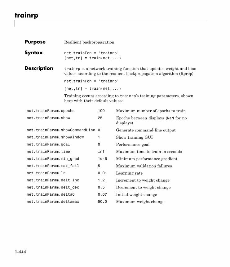
trainrp
Purpose Resilient backpropagation
Syntax net.trainFcn = 'trainrp'[net,tr] = train(net,...)
Description trainrp is a network training function that updates weight and biasvalues according to the resilient backpropagation algorithm (Rprop).
net.trainFcn = 'trainrp'
[net,tr] = train(net,...)
Training occurs according to trainrp’s training parameters, shownhere with their default values:
net.trainParam.epochs 100 Maximum number of epochs to train
net.trainParam.show 25 Epochs between displays (NaN for nodisplays)
net.trainParam.showCommandLine 0 Generate command-line output
net.trainParam.showWindow 1 Show training GUI
net.trainParam.goal 0 Performance goal
net.trainParam.time inf Maximum time to train in seconds
net.trainParam.min_grad 1e-6 Minimum performance gradient
net.trainParam.max_fail 5 Maximum validation failures
net.trainParam.lr 0.01 Learning rate
net.trainParam.delt_inc 1.2 Increment to weight change
net.trainParam.delt_dec 0.5 Decrement to weight change
net.trainParam.delta0 0.07 Initial weight change
net.trainParam.deltamax 50.0 Maximum weight change
1-444
trainrp
NetworkUse
You can create a standard network that uses trainrp withfeedforwardnet or cascadeforwardnet.
To prepare a custom network to be trained with trainrp,
1 Set net.trainFcn to 'trainrp'. This sets net.trainParam totrainrp’s default parameters.
2 Set net.trainParam properties to desired values.
In either case, calling train with the resulting network trains thenetwork with trainrp.
Examples Here is a problem consisting of inputs p and targets t to be solved witha network.
p = [0 1 2 3 4 5];t = [0 0 0 1 1 1];
A two-layer feed-forward network with two hidden neurons and thistraining function is created.
Create and test a network.
net = feedforwardnet(2,'trainrp');
Here the network is trained and retested.
net.trainParam.epochs = 50;net.trainParam.show = 10;net.trainParam.goal = 0.1;net = train(net,p,t);a = net(p)
See help feedforwardnet and help cascadeforwardnet for otherexamples.
1-445
trainrp
Algorithms trainrp can train any network as long as its weight, net input, andtransfer functions have derivative functions.
Backpropagation is used to calculate derivatives of performance perfwith respect to the weight and bias variables X. Each variable isadjusted according to the following:
dX = deltaX.*sign(gX);
where the elements of deltaX are all initialized to delta0, and gX isthe gradient. At each iteration the elements of deltaX are modified.If an element of gX changes sign from one iteration to the next, thenthe corresponding element of deltaX is decreased by delta_dec. If anelement of gX maintains the same sign from one iteration to the next,then the corresponding element of deltaX is increased by delta_inc.See Riedmiller, Proceedings of the IEEE International Conference onNeural Networks (ICNN), San Francisco, 1993, pp. 586 to 591.
Training stops when any of these conditions occurs:
• The maximum number of epochs (repetitions) is reached.
• The maximum amount of time is exceeded.
• Performance is minimized to the goal.
• The performance gradient falls below min_grad.
• Validation performance has increased more than max_fail timessince the last time it decreased (when using validation).
References Riedmiller, Proceedings of the IEEE International Conference on NeuralNetworks (ICNN), San Francisco, 1993, pp. 586–591
Definitions Multilayer networks typically use sigmoid transfer functions in thehidden layers. These functions are often called “squashing” functions,because they compress an infinite input range into a finite outputrange. Sigmoid functions are characterized by the fact that their slopesmust approach zero as the input gets large. This causes a problem whenyou use steepest descent to train a multilayer network with sigmoid
1-446
trainrp
functions, because the gradient can have a very small magnitude and,therefore, cause small changes in the weights and biases, even thoughthe weights and biases are far from their optimal values.
The purpose of the resilient backpropagation (Rprop) training algorithmis to eliminate these harmful effects of the magnitudes of the partialderivatives. Only the sign of the derivative can determine the directionof the weight update; the magnitude of the derivative has no effecton the weight update. The size of the weight change is determinedby a separate update value. The update value for each weight andbias is increased by a factor delt_inc whenever the derivative of theperformance function with respect to that weight has the same sign fortwo successive iterations. The update value is decreased by a factordelt_dec whenever the derivative with respect to that weight changessign from the previous iteration. If the derivative is zero, the updatevalue remains the same. Whenever the weights are oscillating, theweight change is reduced. If the weight continues to change in the samedirection for several iterations, the magnitude of the weight changeincreases. A complete description of the Rprop algorithm is given in[ReBr93].
The following code recreates the previous network and trains it usingthe Rprop algorithm. The training parameters for trainrp are epochs,show, goal, time, min_grad, max_fail, delt_inc, delt_dec, delta0,and deltamax. The first eight parameters have been previouslydiscussed. The last two are the initial step size and the maximum stepsize, respectively. The performance of Rprop is not very sensitive tothe settings of the training parameters. For the example below, thetraining parameters are left at the default values:
p = [-1 -1 2 2;0 5 0 5];t = [-1 -1 1 1];net = feedforwardnet(3,'trainrp');net = train(net,p,t);y = net(p)
rprop is generally much faster than the standard steepest descentalgorithm. It also has the nice property that it requires only a modest
1-447
trainrp
increase in memory requirements. You do need to store the updatevalues for each weight and bias, which is equivalent to storage of thegradient.
See Also traingdm | traingda | traingdx | trainlm | traincgp | traincgf |traincgb | trainscg | trainoss | trainbfg
1-448
trainru
Purpose Unsupervised random order weight/bias training
Syntax net.trainFcn = 'trainru'[net,tr] = train(net,...)
Description trainru is not called directly. Instead it is called by train for networkswhose net.trainFcn property is set to 'trainru', thus:
net.trainFcn = 'trainru'
[net,tr] = train(net,...)
trainru trains a network with weight and bias learning rules withincremental updates after each presentation of an input. Inputs arepresented in random order.
Training occurs according to trainr’s training parameters, shown herewith their default values:
net.trainParam.epochs 100 Maximum number of epochs to train
net.trainParam.goal 0 Performance goal
net.trainParam.show 25 Epochs between displays (NaN for nodisplays)
net.trainParam.showCommandLine 0 Generate command-line output
net.trainParam.showWindow 1 Show training GUI
net.trainParam.time Inf Maximum time to train in seconds
NetworkUse
To prepare a custom network to be trained with trainru,
1 Set net.trainFcn to 'trainr'. This sets net.trainParam totrainru’s default parameters.
2 Set each net.inputWeights{i,j}.learnFcn to a learning function.
3 Set each net.layerWeights{i,j}.learnFcn to a learning function.
1-449
trainru
4 Set each net.biases{i}.learnFcn to a learning function. (Weightand bias learning parameters are automatically set to default valuesfor the given learning function.)
To train the network,
1 Set net.trainParam properties to desired values.
2 Set weight and bias learning parameters to desired values.
3 Call train.
Algorithms For each epoch, all training vectors (or sequences) are each presentedonce in a different random order, with the network and weight and biasvalues updated accordingly after each individual presentation.
Training stops when any of these conditions is met:
• The maximum number of epochs (repetitions) is reached.
• The maximum amount of time is exceeded.
See Also train | trainr
1-450
trains
Purpose Sequential order incremental training with learning functions
Syntax net.trainFcn = 'trains'[net,tr] = train(net,...)
Description trains is not called directly. Instead it is called by train for networkswhose net.trainFcn property is set to 'trains', thus:
net.trainFcn = 'trains'
[net,tr] = train(net,...)
trains trains a network with weight and bias learning rules withsequential updates. The sequence of inputs is presented to the networkwith updates occurring after each time step.
This incremental training algorithm is commonly used for adaptiveapplications.
NetworkUse
You can create a standard network that uses trains for adapting bycalling perceptron or linearlayer.
To prepare a custom network to adapt with trains,
1 Set net.adaptFcn to 'trains'. This sets net.adaptParam totrains’s default parameters.
2 Set each net.inputWeights{i,j}.learnFcn to a learning function.Set each net.layerWeights{i,j}.learnFcn to a learning function.Set each net.biases{i}.learnFcn to a learning function. (Weightand bias learning parameters are automatically set to default valuesfor the given learning function.)
To allow the network to adapt,
1 Set weight and bias learning parameters to desired values.
2 Call adapt.
1-451
trains
See help perceptron and help linearlayer for adaption examples.
Algorithms Each weight and bias is updated according to its learning function aftereach time step in the input sequence.
See Also train | trainb | trainc | trainr
1-452
trainscg
Purpose Scaled conjugate gradient backpropagation
Syntax net.trainFcn = 'trainscg'[net,tr] = train(net,...)
Description trainscg is a network training function that updates weight and biasvalues according to the scaled conjugate gradient method.
net.trainFcn = 'trainscg'
[net,tr] = train(net,...)
Training occurs according to trainscg’s training parameters, shownhere with their default values:
net.trainParam.epochs 100 Maximum number of epochs to train
net.trainParam.show 25 Epochs between displays (NaN for nodisplays)
net.trainParam.showCommandLine 0 Generate command-line output
net.trainParam.showWindow 1 Show training GUI
net.trainParam.goal 0 Performance goal
net.trainParam.time inf Maximum time to train in seconds
net.trainParam.min_grad 1e-6 Minimum performance gradient
net.trainParam.max_fail 5 Maximum validation failures
net.trainParam.sigma 5.0e-5 Determine change in weight for secondderivative approximation
net.trainParam.lambda 5.0e-7 Parameter for regulating theindefiniteness of the Hessian
NetworkUse
You can create a standard network that uses trainscg withfeedforwardnet or cascadeforwardnet. To prepare a custom networkto be trained with trainscg,
1-453
trainscg
1 Set net.trainFcn to 'trainscg'. This sets net.trainParam totrainscg’s default parameters.
2 Set net.trainParam properties to desired values.
In either case, calling train with the resulting network trains thenetwork with trainscg.
Examples Here is a problem consisting of inputs p and targets t to be solved witha network.
p = [0 1 2 3 4 5];t = [0 0 0 1 1 1];
A two-layer feed-forward network with two hidden neurons and thistraining function is created.
net = feedforwardnet(2,'trainscg');
Here the network is trained and retested.
net = train(net,p,t);a = net(p)
See help feedforwardnet and help cascadeforwardnet for otherexamples.
Algorithms trainscg can train any network as long as its weight, net input, andtransfer functions have derivative functions. Backpropagation is usedto calculate derivatives of performance perf with respect to the weightand bias variables X.
The scaled conjugate gradient algorithm is based on conjugatedirections, as in traincgp, traincgf, and traincgb, but this algorithmdoes not perform a line search at each iteration. See Moller (NeuralNetworks, Vol. 6, 1993, pp. 525–533) for a more detailed discussion ofthe scaled conjugate gradient algorithm.
Training stops when any of these conditions occurs:
1-454
trainscg
• The maximum number of epochs (repetitions) is reached.
• The maximum amount of time is exceeded.
• Performance is minimized to the goal.
• The performance gradient falls below min_grad.
• Validation performance has increased more than max_fail timessince the last time it decreased (when using validation).
References Moller, Neural Networks, Vol. 6, 1993, pp. 525–533
See Also traingdm | traingda | traingdx | trainlm | trainrp | traincgf |traincgb | trainbfg | traincgp | trainoss
1-455
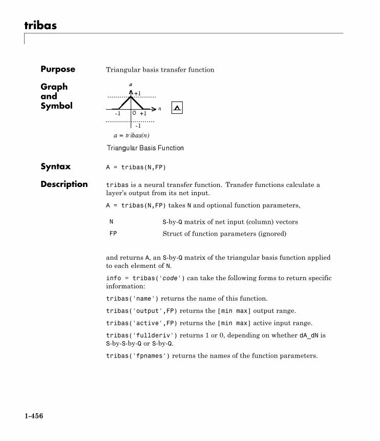
tribas
Purpose Triangular basis transfer function
GraphandSymbol
Syntax A = tribas(N,FP)
Description tribas is a neural transfer function. Transfer functions calculate alayer’s output from its net input.
A = tribas(N,FP) takes N and optional function parameters,
N S-by-Q matrix of net input (column) vectors
FP Struct of function parameters (ignored)
and returns A, an S-by-Q matrix of the triangular basis function appliedto each element of N.
info = tribas('code') can take the following forms to return specificinformation:
tribas('name') returns the name of this function.
tribas('output',FP) returns the [min max] output range.
tribas('active',FP) returns the [min max] active input range.
tribas('fullderiv') returns 1 or 0, depending on whether dA_dN isS-by-S-by-Q or S-by-Q.
tribas('fpnames') returns the names of the function parameters.
1-456
tribas
tribas('fpdefaults') returns the default function parameters.
Examples Here you create a plot of the tribas transfer function.
n = -5:0.1:5;a = tribas(n);plot(n,a)
Assign this transfer function to layer i of a network.
net.layers{i}.transferFcn = 'tribas';
Algorithms a = tribas(n) = 1 - abs(n), if -1 <= n <= 1= 0, otherwise
See Also sim | radbas
1-457
tritop
Purpose Triangle layer topology function
Syntax pos = triptop(dim1,dim2,...,dimN)
Description tritop calculates neuron positions for layers whose neurons arearranged in an N-dimensional triangular grid.
pos = triptop(dim1,dim2,...,dimN) takes N arguments,
dimi Length of layer in dimension i
and returns an N-by-S matrix of N coordinate vectors, where S is theproduct of dim1*dim2*...*dimN.
Examples This code creates and displays a two-dimensional layer with 40 neuronsarranged in an 8-by-5 triangular grid.
pos = tritop(8,5);net = selforgmap([8 5],'topologyFcn','tritop');plotsomtop(net)
See Also gridtop | hextop | randtop
1-458
unconfigure
Purpose Unconfigure network inputs and outputs
Syntax unconfigure(net)unconfigure(net, 'inputs', i)unconfigure(net, 'outputs', i)
Description unconfigure(net) returns a network with its input and output sizesset to 0, its input and output processing settings and related weightinitialization settings set to values consistent with zero-sized signals.The new network will be ready to be reconfigured for data of the sameor different dimensions than it was previously configured for.
unconfigure(net, 'inputs', i) unconfigures the inputs indicated bythe indices i. If no indices are specified, all inputs are unconfigured.
unconfigure(net, 'outputs', i) unconfigures the outputs indicatedby the indices i. If no indices are specified, all outputs are unconfigured.
Examples Here a network is configured for a simple fitting problem, and thenunconfigured.
[x,t] = simplefit_dataset;net = fitnet(10);view(net)net = configure(net,x,t);view(net)net = unconfigure(net)view(net)
See Also configure | isconfigured
1-459
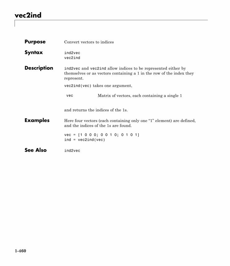
vec2ind
Purpose Convert vectors to indices
Syntax ind2vecvec2ind
Description ind2vec and vec2ind allow indices to be represented either bythemselves or as vectors containing a 1 in the row of the index theyrepresent.
vec2ind(vec) takes one argument,
vec Matrix of vectors, each containing a single 1
and returns the indices of the 1s.
Examples Here four vectors (each containing only one “1” element) are defined,and the indices of the 1s are found.
vec = [1 0 0 0; 0 0 1 0; 0 1 0 1]ind = vec2ind(vec)
See Also ind2vec
1-460

view
Purpose View neural network
Syntax view(net)
Description view(net) launches a window that shows your neural network(specified in net) as a graphical diagram.
1-461

view
1-462
Index
IndexAadapt function 1-2
Bbacktracking search 1-347boxdist function 1-10Brent’s search 1-352
Ccascadeforwardnet function 1-13catelements function 1-14catsamples function 1-15catsignals function 1-17cattimesteps function 1-18cellmat function 1-19Charalambous’ search 1-357closeloop function 1-20combvec function 1-21compet function 1-22competlayer function 1-24con2seq function 1-25concur function 1-27configure function 1-28confusion function 1-30conjugate gradient algorithms
Fletcher-Reeves update 1-413Polak-Ribi\x8e re update 1-418Powell-Beale restarts 1-409
convwf function 1-32
Ddefaultderiv function 1-34demonstrations
nnd12cg 1-414nnd12m 1-437nnd12mo 1-429nnd12sd1 1-362
nnd12sd1 batch gradient 1-422nnd12vl 1-425
disp function 1-36display function 1-37dist function 1-38distdelaynet function 1-41divideblock function 1-42divideind function 1-43divideint function 1-45dividerand function 1-46dividetrain function 1-47dotprod function 1-48
Eelliot2sig function 1-51elliotsig function 1-50elmannet function 1-52errsurf function 1-54extendts function 1-55
Ffeedforwardnet function 1-56fitnet function 1-58fixunknowns function 1-59Fletcher-Reeves update 1-413formwb function 1-62fpderiv function 1-63fromnndata function 1-65
Ggadd function 1-67gdivide function 1-68gensim function 1-69getelements function 1-70getsamples function 1-71getsignals function 1-72getsiminit function 1-73gettimesteps function 1-75
Index-1
Index
getwb function 1-76gmultiply function 1-77gnegate function 1-78golden section search 1-362gpu2nndata function 1-79gradient descent algorithm
batch 1-420gridtop function 1-81gsqrt function 1-82gsubtract function 1-83
Hhardlim function 1-84hardlims function 1-86hextop function 1-88hybrid bisection cubic search 1-367
Iind2vec function 1-89init function 1-90initcon function 1-92initial step size function 1-447initlay function 1-94initlvq function 1-96initnw function 1-97initsompc function 1-99initwb function 1-100initzero function 1-101input vectors
dimension reduction 1-284isconfigured function 1-103
JJacobian matrix 1-436
Llayrecnet function 1-104
learncon function 1-105learngd function 1-108learngdm function 1-111learnh function 1-114learnhd function 1-117learning rates
adaptive 1-425optimal 1-425
learnis function 1-120learnk function 1-123learnlv1 function 1-126learnlv2 function 1-129learnos function 1-132learnp function 1-135learnpn function 1-138learnsom function 1-141learnwh function 1-148Levenberg-Marquardt algorithm 1-435line search functions
backtracking search 1-347Brent’s search 1-352Charalambous’ search 1-357golden section search 1-362hybrid bisection cubic search 1-367
linearlayer function 1-151linkdist function 1-153logsig function 1-155lvqnet function 1-157lvqoutputs function 1-159
Mmae function 1-160mandist function 1-162mapminmax function 1-164mapstd function 1-167maximum step size function 1-447maxlinlr function 1-170meanabs function 1-171meansqr function 1-172
Index-2
Index
midpoint function 1-173minmax function 1-174mse function 1-175
Nnarnet function 1-177narxnet function 1-178nctool function 1-180negdist function 1-181netinv function 1-183netprod function 1-185netsum function 1-187network function 1-189newgrnn function 1-195newlind function 1-197newpnn function 1-199newrb function 1-201newrbe function 1-203Newton’s method 1-436nftool function 1-205nncell2mat function 1-206nncorr function 1-207nndata function 1-209nndata2gpu function 1-211nndata2sim function 1-213nnsize function 1-214nnstart function 1-215nntool function 1-216nntraintool function 1-217noloop function 1-218normalization
inputs and targets 1-165mean and standard deviation 1-168
normc function 1-219normprod function 1-220normr function 1-222nprtool function 1-223ntstool function 1-224num2deriv function 1-225
num5deriv function 1-227numelements function 1-229numfinite function 1-230numnan function 1-231numsamples function 1-232numsignals function 1-233numtimesteps function 1-234
Oone step secant algorithm 1-441openloop function 1-235
Ppatternnet function 1-236perceptron function 1-237perform function 1-239plotconfusion function 1-241plotep function 1-242ploterrcorr function 1-243ploterrhist function 1-244plotes function 1-245plotfit function 1-246plotinerrcorr function 1-247plotpc function 1-248plotperform function 1-250plotpv function 1-252plotresponse function 1-255plotroc function 1-256plotsom function 1-258plotsomhits function 1-259plotsomnc function 1-261plotsomnd function 1-261 1-263plotsomplanes function 1-265plotsompos function 1-267plotsomtop function 1-269plottrainstate function 1-271plotv function 1-273plotvec function 1-274
Index-3
Index
plotwb function 1-275pnormc function 1-277Polak-Ribi\x8e re update 1-418poslin function 1-278Powell-Beale restarts 1-409preparets function 1-280principal component analysis 1-284processpca function 1-282prune function 1-286prunedata function 1-288purelin function 1-290
Qquant function 1-292quasi-Newton algorithm 1-347
Rradbas function 1-293radbasn function 1-295randnc function 1-297randnr function 1-298rands function 1-299randtop function 1-303regression function 1-304removeconstantrows function 1-305removerows function 1-308revert function 1-310
Ssae function 1-313satlin function 1-315satlins function 1-317scalprod function 1-319selforgmap function 1-321separatewb function 1-323seq2con function 1-324setelements function 1-325setsamples function 1-326
setsignals function 1-327setsiminit function 1-328settimesteps function 1-330setwb function 1-331sim function 1-332sim2nndata function 1-340soft max transfer function 1-341softmax function 1-341squashing functions 1-446srchbac function 1-343srchbre function 1-348srchcha function 1-353srchgol function 1-358srchhyb function 1-363sse function 1-368staticderiv function 1-370sumabs function 1-372sumsqr function 1-373
Ttansig function 1-374tapdelay function 1-376timedelaynet function 1-377tonndata function 1-378train function 1-380trainb function 1-388trainbfg function 1-390trainbfgc function 1-394trainbr function 1-398trainc function 1-404traincgb function 1-406traincgf function 1-410traincgp function 1-415traingd function 1-419traingda function 1-423traingdm function 1-427traingdx function 1-430trainlm function 1-433trainoss function 1-438
Index-4
Index
trainr function 1-442trainrp function 1-444trainru function 1-449trains function 1-451trainscg function 1-453transformation matrix 1-284tribas function 1-456tritop function 1-458
Uunconfigure function 1-459
Vvariable learning rate algorithm 1-425vec2ind function 1-460view function 1-461
Index-5