Int. J. Appl. Math. Comput. Sci., 2012, Vol. 22, No. 3, 669–684DOI: 10.2478/v10006-012-0050-5

NEURAL NETWORK SEGMENTATION OF IMAGES FROM STAINEDCUCURBITS LEAVES WITH COLOUR SYMPTOMS OF

BIOTIC AND ABIOTIC STRESSES

JAROSŁAW GOCŁAWSKI ∗, JOANNA SEKULSKA-NALEWAJKO ∗, ELZBIETA KUZNIAK ∗∗

∗ Institute of Applied Computer ScienceŁodz University of Technology, Stefanowskiego 18/22, 90-924 Łodz, Poland

e-mail: jgoclaw,jsekulska@kis.p.lodz.pl

∗∗Department of Plant Physiology and BiochemistryUniversity of Łodz, Banacha 12/16, 90-237 Łodz, Poland

e-mail: elkuz@biol.uni.lodz.pl

The increased production of Reactive Oxygen Species (ROS) in plant leaf tissues is a hallmark of a plant’s reaction tovarious environmental stresses. This paper describes an automatic segmentation method for scanned images of cucurbitsleaves stained to visualise ROS accumulation sites featured by specific colour hues and intensities. The leaves placedseparately in the scanner view field on a colour background are extracted by thresholding in the RGB colour space, thencleaned from petioles to obtain a leaf blade mask. The second stage of the method consists in the classification of withinmask pixels in a hue-saturation plane using two classes, determined by leaf regions with and without colour products of theROS reaction. At this stage a two-layer, hybrid artificial neural network is applied with the first layer as a self-organisingKohonen type network and a linear perceptron output layer (counter propagation network type). The WTA-based, fastcompetitive learning of the first layer was improved to increase clustering reliability. Widrow–Hoff supervised trainingused at the output layer utilises manually labelled patterns prepared from training images. The generalisation ability of thenetwork model has been verified by K-fold cross-validation. The method significantly accelerates the measurement of leafregions containing the ROS reaction colour products and improves measurement accuracy.

Keywords: image segmentation, colour space, morphological processing, image thresholding, artificial neural network,WTA learning, Widrow–Hoff learning, Cucurbita species, plant stress, ROS detection.

1. Introduction

Recently, leaf image analysis systems have been used forquantifying stress symptoms. They can be alternative ac-curate methods for subjective visual assessment (James,1971) or biochemical methods (Cheeseman, 2006), whichdo not allow obtaining detailed data of stress symptomdistribution in leaves. A lot of automated methods of leafanalysis are based on common software packages, e.g.,quantifying infection of fungus Colletotrichum destruc-tivum in Nicotiana benthamiana and other plant specieswas done by the freely available Scion Image application(Wijekoon et al., 2008). This popular, general purpose im-age analyser requires time-consuming operations or sub-stantial knowledge for appropriate macros building to ex-tract the diseased regions. In that case, the authors consid-ered only grey-level images to identify bright leaf blade

profiles and dark diseased areas inside of them by simple,global thresholdings.

Symptoms of infection include leaf discolouration(usually white or dark), thus making it possible to directquantification. However, a common feature of plant re-sponse to biotic and abiotic stresses is the increased pro-duction of Reactive Oxygen Species (ROS), which arevisible in leaf tissues as specific colour regions only af-ter histochemical detection. These histochemical meth-ods allow obtaining detailed data on in situ ROS distri-bution and accumulation in different leaf parts, thus en-abling better comparison of various treatments. How-ever, ROS detected histochemically have been often as-sessed semi-quantitative by visual estimation (Huang etal., 2010). Recently, image analysis methods have beendeveloped and applied to the quantification of the products

670 J. Gocławski et al.

of ROS-mediated histochemical reactions in plant tissues(Soukupova and Albrechtova, 2003).

The authors of this paper have been faced with theidentification of the sites of ROS generation in pumpkinand cucumber leaves subjected to abiotic stresses (droughtand salinity) and infected with a pathogen. The subjects ofquantification were regions of accumulation of two ROSspecies: superoxide anion radical and hydrogen peroxide,visible after leaf staining as blue or red-brown spots, re-spectively. In histochemically stained and then cleared(chlorophyll free) leaves, these regions differ from theintact leaf tissues by colour hue and saturation values.The colour features and multidimensionality of the fea-ture space suggest using the colour space instead of grey-levels and a formal classifier, e.g., with an ANN (ArtificialNeural Network) instead of thresholding. So far, LVQ(Linear Vector Quantization) type neural networks havebeen successfully applied to many classification problemslike blood cell recognition (Tabrizi et al., 2010) or seaflooracoustic images segmentation (Tang et al., 2007). The au-thors propose the use of a slightly modified self-clusteringWTA (Winner Takes All) network (Kohonen 1990; 2001)concatenated with a linear perceptron layer type (Widrowet al., 1988; Hagan et al., 2009). Using a sufficient num-ber of clusters, the network can recognise all visible leafstaining colours and then combine them in two groups: in-tact blade areas and the concentration regions of the stressreaction. For a network of such a type, these groups donot need to be assumed as linearly separated, which is notguaranteed in the examined populations. The capabilitiesof using Kohonen networks in image segmentation in theL∗u∗v∗ colour space have already been studied (Ong etal., 2002).

2. Plant material and leaf preparing

The material for image analysis consisted of the leavesof cucumber and pumpkin plants cultivated under growthchamber conditions. A set of five-week-old plants wasused for abiotic stress treatments. Plants were sub-jected to water deficit (drought stress) or irrigated with50 mM NaCl (salt stress) for seven days. The sec-ond group of plants were not treated with abiotic factors.Then each group was divided into two subsets: controland inoculated with the pathogenic fungus Erysiphe ci-choracearum. The plants were analyzed five days afterinoculation. Detached leaves were examined accordingto Unger et al. (2005) for superoxide anion radical (O−

2 )visualisation and to Thordal-Christensen et al. (1997) forhydrogen peroxide (H2O2) detection. After staining andclearing in ethanol, leaves became almost white, as a re-sult of chlorophyll removal, and colour products of histo-chemical reactions of O−

2 and H2O2 were visible as blueand red-brown spots, respectively.

3. Image preprocessing

The stained leaf images have been acquired in a simplecomputer measurement system consisting of a standarddesktop scanner connected to a dual core PC with a 32-bit Windows 7 operating system. The leaf blade imagesstored in JPEG files are subject to classification designedby the authors to detect stress response regions. Both im-age preprocessing and pixel classification methods havebeen developed in the MATLAB environment and im-plemented in the form of MATLAB functions as well asC++ functions contained in MEX files (The MathworksInc., 2011a). The purposes of preprocessing are to extracta leaf blade and to eliminate a leaf petiole. The mechan-ical cut-off of the petiole is often difficult to do withoutinjuring or even partially damaging the leaf tissue.

3.1. Leaf blade extraction. To simplify the separationof a leaf blade from the image background, it is assumedthat the background has a highly saturated uniform colourdifferent from any colour appearing inside of the stainedleaf blade. Blue and red backgrounds made of plasticsheets have been applied respectively for leaves with red-brown and blue spots inside. The images are typicallyscanned at the resolution of 200 dpi and colour depth24 bit/px. In each of them, at least a 50 px backgroundmargin must be preserved. The main image processingsteps of leaf blade extraction are depicted in Fig. 1 as aflow diagram. The image background colour BC is testedinside of the rectangle window W placed in the upper-leftcorner of the background margin. With the assumptionsabove, this colour indicates one of the two possible colourgroups of the ROS reaction. It is estimated as

BC =

B if EIB(W ) > k · EIR(W ),R otherwise,

(1)

where E· signifies the expected value, IR(W ), IB(W )mean the red and blue components of the true colour im-age IRGB in the rectangular window W [50× 50] px, andk = 1.5 is an arbitrarily chosen constant value. The dif-ference of image colour components IBC and IG (green)exposes a highly saturated background colour BC andmakes the resulting grey-level image independent of po-tential background intensity variations. The global thresh-olding of IBC − IG provides the inversion of a binary leafblade mask image IM :

IM =∼ T(IBC − IG), (2)

where T denotes the Otsu thresholding operator (Otsu,1979). After the thresholding (Eqn. (2)), the binary im-age IM can be considered the set of white objects Oiof 8-adjacent pixels on a black background. All potential“holes” in the leaf mask object should be removed by aflood-fill operation on 4-adjacent background pixels. In

Neural network segmentation of images from stained cucurbits leaves . . . 671

the MATLAB environment it is represented by the func-tion imfill (The Mathworks Inc., 2011b) equivalent to theoperation in Eqn. (3):

∀ (x, y) ∈ ext(OF ), IM (x, y) = 1, (3)

where ext(OF ) means the exterior of the 4-adjacent blackpixels object OF ⊂∼ IM including the image frame.Only one object Om from the set Oi with the greatest

Fig. 1. Flow diagram of the algorithm providing the binarymask of a leaf image.

area Am is preserved as a leaf blade mask. Objects withsmaller areas are spurious data and must be eliminated as

(x, y) ∈ O ∧ AO < Am ⇒ IM (x, y) = 0. (4)

3.2. Leaf petiole elimination. In the tested populationof stained leaves a petiole is usually the place of a highconcentration of dye, but biologists ignore this part of leafduring visual estimation of a plant’s stress. Therefore, inthe presented algorithm the petiole is removed from theleaf mask image IM by the method shown in Fig. 4. Basedon the observation of leaf mask contours, the authors no-ticed that the petiole is always the most protruding part ofevery leaf. They formulated the hypothesis that the peti-ole tip can be distinguished as a leaf contour point withthe highest curvature value. The hypothesis was success-fully verified in the tested population of leaves. The leafcontour C(Om) has been found by a left-most search for

P0 P

p

Fig. 2. Example leaf image with the white contour overlappedon the edge of a leaf mask, P0: the contour starting pixel,Pp: petiole tip pixel.

Fig. 3. Description of contour points and vectors for curvaturecomputation. Letter symbols explained in the text.

leaf mask edge points in eight directions (Gonzalez andWoods, 2008),

C(Om) = LML([P0, . . . , PN−1]). (5)

Figure 2 shows an example image with a markedwhite contour found around the leaf mask according tothe rule in Eqn. (5). For each contour point Pi, i ∈[0, . . . , N − 1], the local curvature is represented as thebending angle θi computed by (Du Buf and Bayer, 2002)

θi =1M

M∑j=1

arccosaj · bj

|aj | · |bj | , (6)

where aj = Pi−jPi and bj = PiPi+j are vectors asshown in Fig. 3, aj · bj is the vector inner product andM is the half size of an averaging mask. This mask rep-resents a built-in low-pass filter smoothing the curvature

672 J. Gocławski et al.

Fig. 4. Flow diagram of the algorithm eliminating a leaf petiole.

P0 P

p

Fig. 5. Example leaf image with the contour part used to cal-culate the curvature θi. P0: contour starting pixel, Pp:petiole tip pixel.

values θi evaluated along a leaf mask contour. This fil-tering is necessary due to the high sensitivity of θi to anycontour ripples. The value of M was chosen experimen-tally in relation to the leaf contour length N as

M = 2.5/100× N. (7)

A proper selection of the value M plays a key role

0 200 400 600 800 1000−150

−100

−50

0

50

100

150

i − contour pixel index

θ [°

]− c

urv

atu

re

Pp

Fig. 6. Example curvature plot θ(i) along the section of the leafcontour shown in Fig. 5

in the detection of petiole protrusion. Each of the scannedleaves is assumed to be placed horizontally in the field ofview with its tip on the left side (Fig. 5). Then leaf maskcontour tracing begins at the leaf’s tip P0 and runs throughthe petiole tip Pp located close to half the length of thecontour N/2. Therefore only the curvature of 30% of thecontour pixels around PN/2 ∈ [Pi1 , Pi2 ] is considered.The petiole tip pixel Pp is determined as

Pp = arg max θi, i ∈ [i1, i2]. (8)

An example curvature plot with the global maximumcorresponding to the contour part in Fig. 5 is depicted inFig. 6. The petiole tip pixel Pp is only used as a markerof the petiole region. This region belongs to the set of leafmask edge protrusion objects obtained by morphologicaloperations expressed by

I ′M = IM\(IM SR1) SR2 , (9)

where SR1 used in opening represents a circular structur-ing element with the radius R1, which must be greaterthan the half of the maximal petiole width. Erosion bySR2 additionally shrinks reminded objects to improvepetiole separation from other protrusions. After enu-meration (labelling) of these objects (The MathworksInc., 2011b), the petiole can be found as the labelled ob-ject Lm closest to the point of the maximum curvature Pp

(Eqns. (10) and (11)),

IL(Li) = LBL(I ′M ), (10)

Lm = arg min ρi(Li, Pp). (11)

The leaf mask without a petiole has been evaluatedin Eqn. (12) as the logical product of the whole leaf maskIM and the binary petiole image∼ T(IL(Lm)) previouslydilated by the disk structuring element SR2 ,

IM = IM∩ ∼ (T(IL(Lm)) ⊕ SR2), (12)

where ⊕ represents a dilation operator.

Neural network segmentation of images from stained cucurbits leaves . . . 673

4. Neural network model design andvalidation

The second stage of the algorithm involves the classifica-tion of leaf blade pixels (inside the mask of image IM ) inthe following two groups:

• the sites of ROS generation in leaf tissues visualisedafter staining,

• the regions of intact leaf tissue with other colours.

4.1. Feature space selection. The observation ofstained leaf blade images leads to the conclusion that ROSaccumulation areas can be distinguished from other leafregions by their colour features. Depending on the ROStype (O−

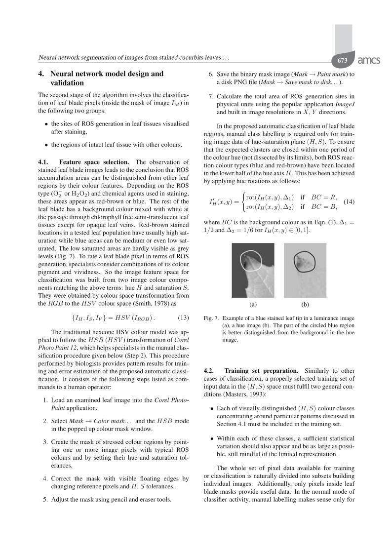
2 or H2O2) and chemical agents used in staining,these areas appear as red-brown or blue. The rest of theleaf blade has a background colour mixed with white atthe passage through chlorophyll free semi-translucent leaftissues except for opaque leaf veins. Red-brown stainedlocations in a tested leaf population have usually high sat-uration while blue areas can be medium or even low sat-urated. The low saturated areas are hardly visible as greylevels (Fig. 7). To rate a leaf blade pixel in terms of ROSgeneration, specialists consider combinations of its colourpigment and vividness. So the image feature space forclassification was built from two image colour compo-nents matching the above terms: hue H and saturation S.They were obtained by colour space transformation fromthe RGB to the HSV colour space (Smith, 1978) as

IH , IS , IV = HSV (IRGB) . (13)

The traditional hexcone HSV colour model was ap-plied to follow the HSB (HSV ) transformation of CorelPhoto Paint 12, which helps specialists in the manual clas-sification procedure given below (Step 2). This procedureperformed by biologists provides pattern results for train-ing and error estimation of the proposed automatic classi-fication. It consists of the following steps listed as com-mands to a human operator:

1. Load an examined leaf image into the Corel Photo-Paint application.

2. Select Mask → Color mask. . . and the HSB modein the popped up colour mask window.

3. Create the mask of stressed colour regions by point-ing one or more image pixels with typical ROScolours and by setting their hue and saturation tol-erances.

4. Correct the mask with visible floating edges bychanging reference pixels and H , S tolerances.

5. Adjust the mask using pencil and eraser tools.

6. Save the binary mask image (Mask → Paint mask) toa disk PNG file (Mask → Save mask to disk. . . ).

7. Calculate the total area of ROS generation sites inphysical units using the popular application ImageJand built in image resolutions in X , Y directions.

In the proposed automatic classification of leaf bladeregions, manual class labelling is required only for train-ing image data of hue-saturation plane (H, S). To ensurethat the expected clusters are closed within one period ofthe colour hue (not dissected by its limits), both ROS reac-tion colour types (blue and red-brown) have been locatedin the lower half of the hue axis H . This has been achievedby applying hue rotations as follows:

I ′H(x, y) =

rot(IH(x, y), Δ1) if BC = R,

rot(IH(x, y), Δ2) if BC = B,(14)

where BC is the background colour as in Eqn. (1), Δ1 =1/2 and Δ2 = 1/6 for IH(x, y) ∈ [0, 1].

(a) (b)

Fig. 7. Example of a blue stained leaf tip in a luminance image(a), a hue image (b). The part of the circled blue regionis better distinguished from the background in the hueimage.

4.2. Training set preparation. Similarly to othercases of classification, a properly selected training set ofinput data in the (H, S) space must fulfil two general con-ditions (Masters, 1993):

• Each of visually distinguished (H, S) colour classesconcentrating around particular patterns discussed inSection 4.1 must be included in the training set.

• Within each of these classes, a sufficient statisticalvariation should also appear and be as large as possi-ble, still mindful of the limited representation.

The whole set of pixel data available for trainingor classification is naturally divided into subsets buildingindividual images. Additionally, only pixels inside leafblade masks provide useful data. In the normal mode ofclassifier activity, manual labelling makes sense only for

674 J. Gocławski et al.

a single image or at most a few images in the tested pop-ulation. They must contain most colour hues and satu-rations existing in the population to classify every imageitem sufficiently well. Keeping in mind that the networkas a whole finally recognises two classes, the very approx-imate identification of these classes and the statistical de-viations of their data have been considered. All exam-ined leaf populations included both strongly and weaklystressed leaf samples (control group), so in all cases a sin-gle image with a medium stressed leaf could be found andused as the training set. The training image can be selectedintuitively, by a visual assessment of images or using aheuristic formula of training the ability factor fi proposedin Eqn. (16). The expression for fi applies the weightedvariances of a leaf blade histogram in the (H, S) space.They are computed inside and between two output colourclasses c1 and c2, coarsely identified before the final clas-sification. It is assumed that the training image with theindex

it = arg max fi (15)

will maximise

fi = kf

(2∑

k=1

pi(ck)si(ck) + kg σi(c1, c2))

, (16)

where

si(ck) =2∑

j=1

kj

Q(i,ck)∑q=1

(xij(ck, q) − xij(ck))2 ,

pi(ck) is the probability of the (H, S) class ck, si(ck)is a weighted variance inside of the i-th image class ck,σi(c1, c2) is the i-th image between-class variance, kf be-ing a scaling constant, kg is the participation rate of thebetween-class variance, xij(ck, q) is the q-th input datain the j-th dimension of the i-th image for the class ck,xij(ck) is the mean data value in the class ck and the j-thdimension of the image i.

Table 1. Training ability factors fi for the example populationof images with the maximum and minimum values un-derlined.

Image Train abilityi fi

1 1.83592 2.72223 2.59784 3.92835 1.21176 3.69537 0.50668 2.59039 1.5800

10 1.4347

The two classes c1 and c2 used in Eqn. (16) wereobtained by applying the kmeans algorithm (Forgy, 1965)

to the input data x = [x1, x2], x1 = IH(p), and x2 =IS(p) taken from hue and saturation image componentsIH , IS of any pixel p as follows:

c1, c2 = kmeans (x, Nc) , (17)

where Nc = 2 is the required number of classes. Thecomputed values fi for an example population of 10 im-ages are given in Table 1 and two images with extreme fi

are illustrated in Figs. 8(a) and (b). For the data in this ta-ble the coefficients in Eqns. (16) and (17) are kf = 1/256,kg = 0.1, k1 = 1, k2 = 1.44. There seems to be

(a) (b)

Fig. 8. Selected images corresponding to the minimum andmaximum values of fi from Table 1: the image withfmax featured by the noticeable variances of (H,S)within and between the two basic colour classes ck, k =1, 2 in Eqn. (17) (a), another leaf image with fmin andthe same variances of small values (b). Darker leaf bladeregions are blue and bluish-grey, respectively, in the im-ages (a) and (b).

no danger of network overfitting in the learning processbecause of the large number of training feature vectorsderived from pixel colours inside of a leaf blade mask.The scanned leaf images typically have a size of about1000 × 1000 pixels and a leaf blade occupies about halfof the image area. The first network layer proposed inSection 4.3 with two inputs and 8–12 neurons has only16–24 vector weights. The second layer with one neu-ron has the same amount of weights as the number offirst layer outputs, which gives a total of maximum 36weights to learn. So the number of data is incomparablylarger than four times of the total network weights num-ber recommended by practitioners as the minimum datalimit to avoid overfitting (Masters, 1993). Neverthelessthe proposed network model is tested for overfitting byK-fold cross-validation described below. When experi-ments suggest that the selected training image does notrepresent sufficiently colour subclasses or their variations,giving unaccepted classification errors, further imageswith the highest fi factors can be applied to additionaltraining.

4.3. Structure of a neural network. The proposedmodel of the classifier applies a two-layer neural net-work of the counter propagation type (Hecht-Nielsen et

Neural network segmentation of images from stained cucurbits leaves . . . 675

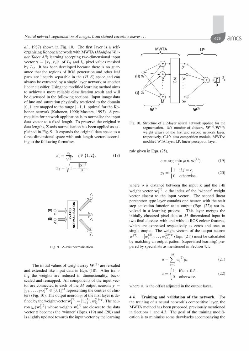
al., 1987) shown in Fig. 10. The first layer is a self-organising Kohonen network with MWTA (Modified Win-ner Takes All) learning accepting two-dimensional inputvector x = [x1, x2]T of IH and IS pixel values maskedby IM . It has been developed because there is no guar-antee that the regions of ROS generation and other leafparts are linearly separable in the (H, S) space and canalways be extracted by a single layer network or anotherlinear classifier. Using the modified learning method aimsto achieve a more reliable classification result and willbe discussed in the following sections. Input image dataof hue and saturation physically restricted to the domain[0, 1] are mapped to the range [−1, 1] optimal for the Ko-honen network (Kohonen, 1990; Masters, 1993). A pre-requisite for network application is to normalise the inputdata vector to a fixed length. To preserve the original xdata lengths, Z-axis normalisation has been applied as ex-plained in Fig. 9. It expands the original data space to athree-dimensional space with unit length vectors accord-ing to the following formulae:

x′i =

xi√2, i ∈ 1, 2, (18)

x′3 =

√1 − ||x||2

2.

Fig. 9. Z-axis normalisation.

The initial values of weight array W(1) are rescaledand extended like input data in Eqn. (18). After train-ing the weights are reduced in dimensionality, back-scaled and remapped. All components of the input vec-tor are connected to each of the M output neurons y =[y1, . . . , yM ]T ∈ [0, 1]M representing the centres of clus-ters (Fig. 10). The output neuron yi of the first layer is de-fined by the weight vector w(1)

i = [w(1)i1 , w

(1)i2 ]T . The neu-

ron yc(w(1)c ) whose weights w(1)

c are closest to the datavector x becomes the ‘winner’ (Eqns. (19) and (20)) andis slightly updated towards the input vector by the learning

Fig. 10. Structure of a 2-layer neural network applied for thesegmentation. M : number of clusters, W(1),W(2):weight arrays of the first and second network layer,respectively, CM : data competition module, MWTA:modified WTA layer, LP: linear perceptron layer.

rule given in Eqn. (25),

c = arg mini

ρ(x,w(1)i ), (19)

yj =

1 if j = c,

0 otherwise,(20)

where ρ is distance between the input x and the i-thweight vector w(1)

i , c the index of the ‘winner’ weightvector closest to the input vector. The second linearperceptron type layer contains one neuron with the stairstep activation function at its output (Eqn. (22)) not in-volved in a learning process. This layer merges theinitially clustered pixel data at M -dimensional input intwo final classes: with and without ROS colour features,which are expressed respectively as zeros and ones atsingle output. The weight vectors of the output neuronw(2) = [w(2)

1 , . . . , w(2)M ]T (Eqn. (21)) must be calculated

by matching an output pattern (supervised learning) pre-pared by specialists as mentioned in Section 4.1,

u =M∑i=0

w(2)i yi, (21)

z =

1 if u > 0.5,

0 otherwise.(22)

where y0 is the offset adjusted in the output layer.

4.4. Training and validation of the network. Forthe training of a neural network’s competitive layer, theMWTA method has been proposed, previously mentionedin Sections 1 and 4.3. The goal of the training modifi-cation is to minimise some drawbacks accompanying the

676 J. Gocławski et al.

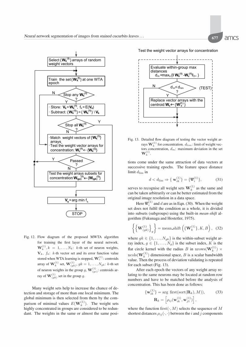
standard WTA algorithm (Kohonen, 2001). All changeshave been made between the consecutive epochs of stan-dard WTA learning as shown in Fig. 12.

The WTA training procedure begins with random ini-tialisation of the weight vectors w(1)

i representing initialclass centres, collected the weight array W(1). They areselected by uniform, no-replacement, random samplingfrom indexes of the Q data samples entered in one epoch,

w(1)i (0) = rand(1, . . . , Q), i ∈ 1, . . . , M. (23)

For the proposed MWTA method its start is extendedto the set W(1) of several weight vector arrays han-dled independently according to the WTA rule duringone epoch. Given the pixel feature input vector x(q)normalised in three dimensions, the output neurons withweights w(1)

i (q) from array W(1)i compete to match to

this vector using the dissimilarity measure (Rubner etal., 2001) as the Euclidean distance:

‖x(q) − w(1)c (q)‖ = min

i‖x(q) − w(1)

i (q)‖, (24)

where w(1)c (q) is the weight vector winning competition at

the presentation of the q-th datum. The weights of winnerneuron yc are then modified according to the rule

w(1)i (r) =

⎧⎪⎪⎪⎪⎨⎪⎪⎪⎪⎩

w(1)i (q) + α(1)

[x(q) − w(1)

i (q)]

if i = c,

w(1)i (q)

if i = c,

(25)

where r = q + 1. The aim of WTA learning is to find theminimum quantisation error E(W(1)) at the approxima-tion of all input data vectors x by M weight vectors (orneurons) shown in Fig. 10.

Using the Euclidean metric, this error can be ex-pressed as

E(W(1)

)= max

c

1Q

Q∑q=1

‖x(q) − w(1)c (q)‖2, (26)

where Q is the number of data vectors in one epoch,w(1)

c (q), c ∈ 1, . . . , M is the weight of neuron win-ning at the presentation of the x(q) vector. The learningprocess described in Eqn. (25) ensures only the conver-gence to a local minimum, when the learning rate α(1) issmall enough. The learning rate has been experimentallychosen as a constant value α(1) = 0.002 to ensure goodand fast convergence of the algorithm. The stopping crite-rion at the local minimum of E(W(1)) exploits the effectof neuron position (weight) stabilisation around the mini-mum and is expressed by Eqn. (27):

maxi

‖Δw(1)i (ep)‖ < ε, (27)

Δw(1)i (ep) = w(1)

i (ep) − w(1)i (ep − 1),

(28)

Fig. 11. Example plot of W(1)(ep) weight stabilisation duringMWTA training for validation using (H,S) pixel dataof the image from Fig. 8(a). W(1)(ep) represents theselected sequence of weights convergent to the mini-mum quantisation error E(W(1)) (Eqn. (26)).

where i ∈ 1, . . . , M, ε represents the weights im-provement limit and ep the epoch number (Fig. 11). Thenumber of convergence steps to fulfil the above criterionis varying and depends on the randomly selected start-ing weights (Eqn. (23)). To limit the time of learning,the following additional condition of maximum allowableepochs EP is imposed on the convergence limit:

ep < EP. (29)

During each epoch of WTA training all valid sets(arrays) of weight vectors W(1)

k = [w(1)i ]k, k =

1, . . . , Nk, i = 1, . . . , M, are independently moved to-wards the nearest class centres minimizing the error func-tion in Eqn. (26). Each of them also comes under the stop-ping criterion given above. After stopping, the currentlyfixed weight sets are stored for final solution analysis (ar-rays Vk in Fig. 12). All of still shifted sets are testedfor their possible concentrations in the input data space.Sufficiently concentrated groups of weight arrays are re-placed by the concentration centres before the next train-ing epoch. It is expected that with the successive trainingepochs the weight arrays W(1)

k will concentrate around

the different local minima of E(W(1)k ) existing in the op-

timisation task considered. The measure of this concen-tration is taken as the maximum deviation d of wik setelements from weight set centres wi as given in Eqn. (30):

d = maxk,i

‖w(1)ik − w(1)

i ‖, (30)

w(1)i =

1Nk

Nk∑k=1

w(1)ik , i = 1 . . .M,

where d is the deviation of the weight set, −w(1)i is the

mean weight vector of i-th neuron, w(1)ik stands for the

weights of i-th neuron from the weight set W(1)k .

Neural network segmentation of images from stained cucurbits leaves . . . 677

Fig. 12. Flow diagram of the proposed MWTA algorithm

for training the first layer of the neural network.

W(1)k , k = 1, . . . , Nk: k-th set of neuron weights,

Vk, fk: k-th vector set and its error function value

stored when WTA learning is stopped, W(1)c : centroids

array of W(1)k set, W(1)

(gk), gk = 1, . . . , Ngk: k-th set

of neuron weights in the group g, W(1)

(gc): centroids ar-

ray of W(1)(gk) set in the group g.

Many weight sets help to increase the chance of de-tection and storage of more than one local minimum. Theglobal minimum is then selected from them by the com-parison of minimal values E(W(1)

k ). The weight setshighly concentrated in groups are considered to be redun-dant. The weights in the same or almost the same posi-

Fig. 13. Detailed flow diagram of testing the vector weight ar-rays W

(1)k for concentration. dlim: limit of weight vec-

tors concentration, dm: maximum deviation in the setW

(1)k .

tions come under the same attraction of data vectors atsuccessive training epochs. The feature space distancelimit dlim in

d < dlim ⇒ w(1)ik = w(1)

i , (31)

serves to recognise all weight sets W(1)k as the same and

can be taken arbitrarily or can be better estimated from theoriginal image resolution in a data space.

Here w(1)i and d are as in Eqn. (30). When the weight

set does not fulfil the condition as a whole, it is dividedinto subsets (subgroups) using the built-in mean-shift al-gorithm (Fukunaga and Hostetler, 1975).

W(1)(gk)

g

= mean shift

(W(1)

k , K, B)

, (32)

where gk ∈ 1, . . . , Ngk is the within-subset weight ar-ray index, g ∈ 1, . . . , Ng is the subset index, K is the

flat circle kernel with the radius B in nrows(W(1)k ) ×

ncols(W(1)k ) dimensional space, B is a scalar bandwidth

value. Then the process of deviation validating is repeatedfor each subset (Fig. 13).

After each epoch the vectors of any weight array re-lating to the same neurons may be located at random rownumbers and have to be matched before the analysis ofconcentration. This has been done as follows:

w(1)ik = arg first(sort(Rk), M)), (33)

Rk =[ρij(w

(1)ik ,w(1)

j1 )],

where the function first(·, M) selects the sequence of Mshortest distances ρij(·, ·) between the i and j components

678 J. Gocławski et al.

of the first and k-th weight vector sets previously sorted inascending order.

To train the output layer MWTA self-clustering mustbe first finished and its vector weights be fixed.

The network’s linear layer is to minimise the error(Kohonen, 2001; Osowski, 2006)

E(W(2)) =1Q

Q∑q=1

‖δ(q)‖2, (34)

δ(q) = t(q) − W(2)y(q),

as a quadratic function of weight matrix W(2), wheret(q) signifies the q-th vector of the image pattern, y(q)is the q-th output vector of the self-organised layer, δ(q)is the error between the q-th pattern and output vectors,q ∈ 1, . . . , Q, Q is the number of data vectors per oneepoch.

An example behaviour of E(W(2)) is shown inFig. 14. To minimise this error, the Widrow–Hoff method

Fig. 14. Example plot of the mean square error vs. the epochnumber in supervised learning of the network linearlayer.

has been used for learning (Eqn. (35)). It applies agradient-like adjustment for each example from the train-ing set,

w(2)ij (q + 1) = w

(2)ij (q) + 2α(2) · δi(q) · yj(q), (35)

where w(2)ij is the weight between the j-th input and the

i-th output of the second network layer, yj(q) is the j-th component of the M-dimensional output vector of theWTA layer. The symbol α(2) means the maximum stablelearning rate (Fukunaga and Hostetler, 1975):

α(2) =1

λmax (YYT), (36)

where λmax(·) is the maximum eigenvalue, Y is the hor-izontal array [(M + 1) × Q] of Q input vectors provided

Fig. 15. Components of the neural network classifier model.PP: preprocessing module, NN: neural network mod-ule, LP: linear perceptron.

to the neural network from Fig. 10 in one epoch.To verify the network generalisation ability, quintuple

cross-validation has been carried out on the vectorisedhue, saturation of leaf blade data x = [x1, x2]T in severaltraining images with manually labelled patterns (Fig. 15).The folding routine implements the MATLAB functioncrossvalind, which returns randomly generated indices fora K-fold cross-validation of Q data items,

ix1, ix2k = crossvalind(′Kfold ′, Q, K), (37)

where k = 1, . . . , K is the fold number, ix1, ix2 are re-spectively training and testing index vectors with valuesin 1, . . . , Q for cross-validation of Q data. The pre-sented algorithm divides leaf blade pixels into the classof ROS coloured ones and others, which gives four possi-ble results in comparison with pattern data. The resultsare counted in separate elements of confusion matrices(Masters, 1993), whose model is shown in Fig. 16.

In K-fold cross-validation, only, K estimates of clas-sification errors can obtained. To achieve better estima-tion performance, K-fold cross-validation can be exe-cuted several times with the data or their indices reshuffledbefore each round (Du Buf and Bayer, 2002; Refaeilzadeh

Neural network segmentation of images from stained cucurbits leaves . . . 679

et al., 2009). As a result of the cross-validation, confusionmatrices are computed for the classified data from trainedimages. The matrices include separate counts of all pos-sible classification results. The confusion matrix based

Fig. 16. Structure of the confusion matrix for classification intotwo classes. TNF : true negative fraction, FNF : falsenegative fraction, FPF : false positive fraction, TPF :true positive fraction.

factors selected to estimate classification method qualityare

PE =FPF

TNF + FPF, (38)

NE =FNF

FNF + TPF, (39)

ER =FNF + FPF∑

F, (40)

where∑

F denotes the sum of all fraction counts, PEis the false positive error rate, NE is the false negativeerror rate, ER is the classifier error rate. The last factoris used to validate the proposed classifier. The process ofpreparing the classifier model is shown as the flowchart inFig. 15.

5. Experimental results

5.1. Experiment framework. The proposed segmen-tation algorithm with neural network classification wasdeveloped in the MATLAB 2008a environment as men-tioned in Section 3. The code of the preprocessing stagewas written as MATLAB scripts with the intensive useof vectorisation techniques. The colour space transforma-tion, image thresholding, edge detection, tracing and themorphological extraction of the leaf blade mask (Figs. 1and 4) apply appropriate functions built in the Image Pro-cessing Toolbox (The Mathworks Inc., 2011b). To in-crease the network training speed, the clustering of thefirst layer as well as the supervised learning of the secondlayer were written as C++ functions in MEX files com-piled with Visual Studio Express 2008 (The MathworksInc., 2011a). The prepared algorithm was executed on

a PC with a dual core processor Intel Core (TM)2 DuoT5750 2 GHz, 4 GB RAM and the operating system Win-dows 7.

Segmentation by the presented method was per-formed on 12 images of single leaves with visible ROSaccumulation regions. The images were read from JPEGfiles, where they had been stored after scanning. Threeleaf images, with the best training ability values fi

(Eqn. (16)), one with blue and two with red-brown re-gions, were chosen as training data. They represent leavesof different plant species (cucumber, pumpkin) affectedby the combinations of pathogen and additional stress fac-tors (e.g., drought). The execution of the proposed seg-mentation algorithm is independent of the type of stress,as long as the colour symptoms in leaves are similar in hueand saturation. At the preprocessing stage of the segmen-tation only the leaves from two groups are distinguished,determined by the ROS types (O−

2 or H2O2). The binarypattern images of regions with stress response were manu-ally labelled to enable supervised learning of the classifieroutput layer (Fig. 15).

To initially assess the classifier quality 5-fold cross-validation was performed for the two different training im-ages from Figs. 17 and 20, representing different ROStypes. Then the cardinalities of training vector sets weretaken respectively as 4/5 of the values 498473 and 387693equal to the pixel number of each leaf blade.

Fig. 17. Example of a pumpkin leaf image undergoing segmen-tation, with blue stained regions of ROS reaction prod-ucts visible as darker pixels. Image size: 844×952 px,depth: 24 bit/px, leaf blade area: 498473 px.

680 J. Gocławski et al.

Fig. 18. Segmentation result for the image from Fig. 17 with theclass of ROS stained pixels shown as white regions.

Fig. 19. Manually labelled pattern for the image from Fig. 17with the class of ROS stained pixels shown as whiteregions and a grey image background.

5.2. Discussion of the results. The classifier errorrates ER at five-fold cross-validation for the training im-ages from Fig. 17 (Fig. 18) and Fig. 20 (Fig. 21) are visu-alised in Fig. 23. Small values of the errors in the range

Fig. 20. Example of a cucumber leaf image before segmen-tation with red-brown stained regions of ROS reac-tion products visible as darker pixels. Image size:1180 × 1182 px, depth: 24 bit/px, leaf blade area:387693 px.

Fig. 21. Segmentation result for the image from Fig. 20 with theseparated class of ROS stained pixels shown as whiteregions.

[0.9, 1.6]% confirm the proper training of the classifier,free of the overfitting phenomenon. The classification er-rors in the segmentation of 12 example images mentionedin Section 5.1 are listed in Table 2. The classification waspreceded by three network trainings with images repre-senting differently stained leaf groups. Each of the train-ings involved the H, S feature data of all leaf blade pixels.

Neural network segmentation of images from stained cucurbits leaves . . . 681

Fig. 22. Manually labelled pattern for the image from Fig. 20with the class of ROS stained pixels shown as whiteregions and a grey image background.

Fig. 23. Example plots of the error rates ER computed accord-ing to Eqn. (40) at five-fold cross-validation for imagesin Fig. 18 (plot 1) and Fig. 21 (plot 2).

Classification errors were evaluated for all these images,whose binary patterns were manually labelled for this pur-pose (Figs. 19 and 22). The computed error rates ER varyfrom 0.24% to 2.77% (mean 1.42%), which means goodcompliance with the patterns. False positive errors (mean1.49%) are regarded as less important than false negativeerrors (mean 2.30%), because further studies of dye con-centration in the stained areas enable detection of this typeof errors.

It should be emphasised that sometimes manual iden-tification of stained foliar areas can be ambiguous, whichgives different possible patterns for one image. In suchcases the pattern variant closest to the automatic classifi-

Table 2. List of classification errors derived from the confusionmatrix.

Image False positive False negative Classifiernumber error rate error rate error rate

PE [%] NE [%] ER [%]

1 2.39 0.01 1.362 2.25 0.01 1.773 1.79 0.18 1.594 3.04 0.19 2.775 0.08 8.64 0.246 0.75 0.03 0.567 1.22 0.00 0.958 1.45 1.83 1.529 0.10 3.47 0.97

10 1.60 6.22 1.9411 1.20 5.30 1.3912 1.87 3.78 1.92

Table 3. Example learning times for the images from Figs. 18and 21, respectively. The learning times of layer 1 arecalculated for Nk = 10 initial neuron weight sets.

Image NN learning timenumber layer 1 layer 2

(validation) [s] [s]

1(1) 29.95 0.971(2) 43.18 0.761(3) 27.63 0.611(4) 33.61 0.551(5) 30.08 0.632(1) 18.90 3.942(2) 17.69 2.702(3) 17.58 3.442(4) 19.84 4.232(5) 15.86 4.46

cation results was taken into account. The accuracy of fi-nal classification results was accepted by specialists iden-tifying the sites of ROS accumulation in stained leaves.The execution times of MWTA self-clustering and linearperceptron supervised learning registered in the examplecross-validation are listed in Table 3 for M = 8 MWTAlayer neurons and Nk = 10 weight vector sets. The av-erage clustering times computed from time data shown inTable 3 are about 33 s and 18 s respectively, for the train-ing images from Figs. 17 and 20. The times can be differ-ent because of different leaf areas and (H, S) distributionsas well as the random starting values of MWTA initialweight vectors. The MWTA training with 10 initial weightsets lasts on average 4 to 5 times longer than the classicWTA learning of the same tested image population. Thisis the cost of increasing the chance to achieve the globalminimum of the clustering error in the first layer.

Because MWTA consists of partially independenttasks of weight arrays correction, they can be executed asparallel threads with GPU computing applying CUDA or

682 J. Gocławski et al.

Open CL technology (Sanders and Kandrot, 2011). Thiswill be the subject of future research. The MWTA (Nk =10) classification errors shown in Table 2 are of the sameorder as in the case of applying classic WTA (Nk = 1)when each of these methods stops at the same weight ar-ray W(1) indicating the global minimum of E(W(1)) asgiven in Eqn. (26). If the WTA method reaches only a lo-cal, but not the global, minimum of E(W(1)), the errorrates of classification can be relatively high.

It may happen for some types of error functions withdifferent local and global minima, whose shapes are ex-plicitly unknown and a single initial weight array in theWTA algorithm is randomly selected. The high error val-ues can also appear when this array has been accidentallylocalised far from the nearest minimum of E(W(1)) andthe minimisation process has been broken by the limitednumber of allowable iterations. In the series of 100 train-ings with the classic WTA method applied to four imageswith high ability factors fi (Eqn. (16)), increased classifi-cation errors up to ER ≈ 6 − 7% appeared on average in1 per 12 times. Two of the four tested images are shownin Figs. 17 and 20. All trainings were limited to 60 epochsat the clustering stage and had the convergence conditionε (Section 5.3).

The training of the linear perceptron layer with themaximum learning rate (Eqn. (36)) is much faster (0.7 sand 3.8 s on average). It should be remembered that thelearning process refers only to the small number of train-ing images and the rest of each image population is in-tended for the classification, typically 10 to 20 times fasterthan the learning.

5.3. Algorithm parameters. The developed algorithmhas a series of parameters, which can be tuned if necessaryto achieve good adaptation to different image classes. Thepreprocessing involves two parameters:

• R1 = 20: the radius of the structuring element usedat the image IM opening (Eqn. (9)) to cut off a leaf’spetiole, above half an expected petiole width,

• R2 = 4: the radius of the structuring element used atthe auxiliary erosion/dilation (Eqns. (9) and (12)) forthe isolation of leaf edge protrusions.

The most important parameters of NN-classification are

• M = 8: the number of clusters (output neurons) inthe first layer,

• Nk = 10: the number of initial weight vector sets forMWTA training,

• α(1) = 0.002: the learning rate of the MWTA layer,

• ε = 10−10: the limit of the weight vector locationerror maxi ‖Δw(1)

i (ep)‖ in the clustering layer,

• EP = 60: the allowed number of epochs at cluster-ing,

• ε = 0.01: the limit of the mean square learning errorE(W(2)) in the output layer,

• EP = 100: the allowed number of epochs at outputlearning,

• B = 0.002: mean-shift bandwidth,

• dlim = 0.004: distance limit for MWTA weight con-centration.

The number of first layer clusters M = 8 was se-lected as the lowest number of neurons for which the aver-age classification error ER of 12 tested images from Ta-ble 2 stops to decrease at the value near 1.4% (Fig. 24).A further enlargement of M is then useless and only in-creases the computational effort. In this paper only the

4 6 8 10 121

1.5

2

2.5

3

M- 1st layer neurons

ER

[%]-cl

assi

fica

tion

erro

r

Fig. 24. Plot of a mean classification error ER vs. the numberM of neurons in the neural network’s first layer.

correctness of the image segmentation method has beenverified. To take full advantage of the results in biologicalresearch, the comparison with classic biochemical meth-ods is necessary. The quantitative segmentation resultsexpressed as the areas of ROS reaction products in plantleaves will be statistically compared with the results ofbiochemical analysis in the future.

6. Conclusions

A method for automatic segmentation of cucurbits leaveswas presented. It aims to detect the blade regions con-taining the colour products of ROS the reaction. Countingand measurements of these areas are of basic importancefor biologists defining the degree of the plant response tobiotic and abiotic stress, and it is a terminal stage of thecomplex biological experiment. In this case, ROS mea-surement can verify the influence (positive or negative) ofabiotic factors (salinity and drought) on pathogen infec-tion. The results of experiments can give a suggestion formodification of cultivation conditions, and thus provide a

Neural network segmentation of images from stained cucurbits leaves . . . 683

natural protection of cucurbits against fungal disease. Allleaf pixel classification errors collected in Table 2 fall inthe range acceptable by biologists. The execution is alsofaster than manual labelling. This indicates the usefulnessof the proposed method for the extraction and area mea-surement of ROS accumulation sites in stained leaves.

The proposed algorithm consists of preprocessingand classification stages. The preprocessing includes leafblade detection and leaf petiole elimination using proce-dures shown in the flow diagrams in Figs. 1 and 4. Thesecond stage of the algorithm applies a two-layer neuralnetwork of the counter propagation type to classify hueand saturation data of leaf blade pixels. The first networklayer has been trained using the new MWTA (modifiedWTA) method (Fig. 12), which needs more time to exe-cute than original WTA learning, but instead gives a muchhigher certainty of correct classification due to the use ofseveral initial neuron weight arrays. At the training phaseof the neural network’s first layer the neuron weight arraysare systematically replaced by their centres when they suf-ficiently concentrate around the local minima of the quan-tisation error function (Eqn. 25). Finally, only the solutionproviding the global minimum is selected.

The accuracy of leaf pixels classification obtainedwith the proposed method is sufficient to estimate the levelof plant reaction stress in the examined populations. Inthe paper only a counter propagation network type wasconsidered to replace manual classification of leaf bladepixels. The possible comparison of the proposed solu-tion with other neural network types to find the optimalarchitecture and training methods is out of the scope ofthis paper and will be the subject of future research. Theproposed segmentation method of leaf images with ROSreaction colour products is fully automatic except for theneural network training phase, which requires manual la-belling of single pattern images. Therefore it is faster thanany manual labelling of every image using general pur-pose graphic applications and also more free of human er-rors, which improves overall segmentation accuracy. Im-plementation of the segmentation algorithm requires onlythe MATLAB environment with the Image ProcessingToolbox and low cost hardware (a personal computer anda desktop scanner), which should be accessible in eachresearch laboratory.

ReferencesCheeseman, J.M. (2006). Hydrogen peroxide concentrations in

leaves under natural conditions, Journal of ExperimentalBotany 57(10): 2435–2444.

Du Buf, H. and Bayer, M. (Eds.) (2002). Automatic DiatomIdentification, World Scientific Publishing, New York,NY/London/Singapore/Hong Kong.

Forgy, E. (1965). Cluster analysis of multivariate data: Effi-ciency vs. interpretability of classification, Biometrics 21:768–769.

Fukunaga, K. and Hostetler, L. (1975). The estimation of thegradient of a density function, with applications in pat-tern recognition, IEEE Transactions on Information The-ory 21(1): 32–40.

Gonzalez, R.C. and Woods, R.E. (2008). Digital Image Process-ing, 3rd Edn., Prentice Hall, Upper Saddle River, NJ.

Hagan, M.T., Demuth, H. B. and Beale, M.H. (2009). NeuralNetwork Design, University of Colorado, Denver, CO,Chapter 10, http://www.personeel.unimaas.nl/westra/Education/ANO/10widrow_hoff.pdf

Hecht-Nielsen, R. (1987). Counterpropagation networks, Ap-plied Optics 26(23): 4979–4984.

Huang, CX-S., Liu, J-H. and Chen, X-J. (2010). Overexpressionof PtrABF gene, a bZIP transcription factor isolated fromPoncirus trifoliata, enhances dehydration and drought tol-erance in tobacco via scavenging ROS and modulating ex-pression of stress-responsive genes, BMC Plant Biology10: 1–18, paper 230, http://www.biomedcentral.com/1471-2229/10/230.

James, W.C. (1971). An illustrated series of assessment keys forplant diseases, their preparation and usage, Canadian PlantDisease Survey 51(2): 39–65.

Kohonen, T. (1990). The self-organising map, Proceedings ofIEEE 78(9): 1464–1479.

Kohonen, T. (2001). Self-organizing Maps, 3rd Edn., Springer-Verlag, Berlin/ Heidelberg/New York, NY.

Masters, T. (1993) Practical Neural Network Recipes in C++,Academic Press Inc., San Diego, CA.

Ong, S., Yeo, N., Lee, K., Venkatesh, Y. and Cao, D. (2002).Segmentation of color images using a two-stage self-organizing network, Image and Vision Computing 20(4):279–289.

Osowski, S. (2006). Neural Networks for Information Process-ing, Warsaw University of Technology Press, Warsaw, (inPolish).

Otsu, N. (1979). A threshold selection method from gray-levelhistograms, IEEE Transactions on Systems, Man, and Cy-bernetics 9(1): 62–66.

Refaeilzadeh, P., Tang, L. and Liu, H., (2009). Cross-validation,Encyclopedia of Database Systems, Springer PublishingCompany, New York, NY, pp. 532–538,

Rubner, Y., Puzicha, J., Tomasi, C. and Buhmann J.M. (2001).Empirical evaluation of dissimilarity measures for colorand texture, Computer Vision and Image Understanding84(1): 25–43.

Sanders, J. and Kandrot, E. (2011). CUDA by Example:An Introduction to General-Purpose GPU Programming,Addison-Wesley, New York, NY/London.

Smith, A.R. (1978). Color gamut transform pairs, ComputerGraphics 12(3): 12–19.

Soukupova, J. and Albrechtova, J. (2003). Image analysis—Toolfor quantification of histochemical detection of phenoliccompounds, lignin and peroxidases in needles of Norwayspruce, Biologia Plantarum 46(4): 595–601.

684 J. Gocławski et al.

Tabrizi, P.R., Rezatofighi, S.H. and Yazdanpanah, M.J. (2010).Using PCA and LVQ neural network for automatic recog-nition of five types of white blood cells, Engineering inMedicine and Biology Society (EMBC), 2010 Annual Inter-national Conference of the IEEE, Teheran, Iran, pp. 5593–5596.

Tang, Q-H., Liu, B-H., Chen, Y-Q., Zhou, X-H. and Ding, J-S. (2007). Application of LVQ neural network combinedwith the genetic algorithm in acoustic seafloor classifica-tion, Chinese Journal Geophysics 50(1): 313–319.

The Mathworks Inc. (2011a). MEX-files guide, http://www.mathworks.com/support/tech-notes/1600/1605.html

The Mathworks Inc. (2011b). Image processing toolbox user’sguide, http://www.mathworks.com//help/toolbox/images/

Thordal-Christensen, H., Zhang, Z., Wei, Y.D. and Collinge,D.B. (1997). Subcellular localization of H2O2 in plants.H2O2 accumulation in papillae and hypersensitive re-sponse during the barley-powdery mildew interaction,Plant Journal 11(6): 1187–1194.

Unger, Ch., Kleta, S., Jandl, G. and Tiedemann, A. (2005).Suppression of the defence-related oxidative burst in beanleaf tissue and bean suspension cells by the necrotrophicpathogen Botrytus cinerea, Journal of Phytopathology153(1): 15–26.

Wijekoon, C.P., Goodwin, P.H. and Hsiang, T. (2008). Quantify-ing fungal infection of plant leaves by digital image analy-sis using Scion Image software, Journal of MicrobiologicalMethods 74(2–3): 94–101.

Widrow, B., Winter, R.G. and Baxter, R.A. (1988). Layeredneural nets for pattern recognition, IEEE Transactions onAcoustics, Speech and Signal Processing 36(7): 1109–1118.

Jarosław Gocławski received the M.S.E. de-gree in electronics in 1977 and then the Ph.D. de-gree in 1986, both from the Electrical Faculty ofthe Technical University of Łodz, Poland. From1977 to 1989 he worked on image processing,analysis and tomographic reconstruction as a lec-turer at the Institute of Electronics of the Tech-nical University of Łodz. From 1989 to 2005 hewas employed at the Informatics Department inthe IMAL company in Łodz, where he worked

on the design of specialised software and hardware image processing so-lutions for medicine and biology. Since 2006 he has been a lecturer at theComputer Engineering Department of the Technical University of Łodz.His research interests include image processing and analysis for the pur-pose of measurements in textile industry and the biology of plants. In thelast three years he has co-authored several journal and conference papersin these areas.

Joanna Sekulska-Nalewajko received theM.Sc. degree in environmental biology in 1996and then the Ph.D. degree in phycology and hy-drobiology in 2001, both at the Faculty of Biol-ogy and Environmental Protection, University ofŁodz, Poland. In 2001 she was employed at theComputer Engineering Department of the Tech-nical University of Łodz. Since 2005 she hasbeen an assistant professor there. She works ondiatom ecology in modern and past inland wa-

ter environments. Another research interest of hers is concerned withbiological image analysis for diagnostic purposes. She is an author ofseveral papers on this topic.

Elzbieta Kuzniak received M.Sc. degree in biology in 1986 and thePh.D. in plant physiology in 1994 from the Faculty of Biology and En-vironmental Protection, University of Łodz, Poland. In 2005, she waspromoted to the present position of an assistant professor in the Depart-ment of Plant Physiology and Biochemistry, University of Łodz. Hercurrent research interest focuses on the roles of reactive oxygen speciesand antioxidants in plant-pathogen interactions.

Received: 12 September 2011Revised: 18 March 2012