![arXiv:1802.08948v2 [cs.CV] 27 Feb 2018 · 2Megvii Technology Inc. 3National University of Singapore flvpyuan, yaocong2010g@gmail.com, wwh@megvii.com, eleyans@nus.edu.sg, xbai@hust.edu.cn](https://static.fdocuments.us/doc/165x107/603b0603a9cba406e8723ef9/arxiv180208948v2-cscv-27-feb-2018-2megvii-technology-inc-3national-university.jpg)
Neural Network Mar. 2019 Approximation [email protected] Low ...
93
Transcript of Neural Network Mar. 2019 Approximation [email protected] Low ...

Motivation● Faster Inference
○ Latency critical scenarios■ VR/AR, UGV/UAV
○ Saves time and energy
● Faster Training○ Higher iteration speed○ Saves life
● Smaller size○ storage size○ memory footprint
Lee Sedol v.s. AlphaGo-Lee (48 TPU)1.5 kWatt83 Watt


Neural Network

Machine Learning as Optimization
● Supervised learning○ is the parameter○ is output, X is input○ y is ground truth○ d is the objective function
● Unsupervised learning○ some oracle function r: low rank, sparse, K

Machine Learning as Optimization
● Regularized supervised learning○
● Probabilistic interpretation○ d measures conditional probability○ r measures prior probability○ Probability approach is more constrained than the
optimization-approach due to normalization problem■ Not easy to represent uniform distribution over [0,
\infty]

● Can be solved by an ODE:○ Discretizing with step length we get gradient
descent with learning rate ○
● Convergence proof
Gradient descent
Derive

Linear Regression
●○○○ x is input, \hat{y} is prediction, y is
ground truth.○ W with dimension (m,n)○ #param = m n, #OPs = m n

Fully-connected
●○ In general, will use nonlinearity
to increase “model capacity”.○ Make sense if f is identity? I.e.
f(x) = x?■ Sometimes, if W_2 is m by r and
W_1 is r by n, then W_2 W_1 is a matrix of rank r, which is different from a m by n matrix.
●○ Deep learning!

Neural Network
X
yCostd + r
Activations/Feature maps/Neurons

● Can be solved by an ODE:○ Discretizing with step length we get gradient
descent with learning rate ○
● Convergence proof
Gradient descent
Derive

Backpropagation

Neural Network Training
X
yCostd + r
Activations/Feature maps/Neurons
Gradients

CNN: Alexnet-like

Method 1: Convolution as Product with Toeplitz Matrix

Example: Convolution with Laplacian filter as Sparse Matrix Product
●○○ A is the sparse Poisson Matrix

Method 2: Convolution as matrix product● Convolution
○ feature map <N, C, H’, W’>○ weights <K, C, H, W>
● Convolution as FC○ under proper padding, can extract patchs○ feature map <N H’ W’, C H W>○ weights <C H W, K>
Kernel stride determines how much overlap
Height
Width

Importance of Convolutions and FC
Feature map size
tf-model-manip.py 01-svhn/model.py info
Most storage size
Most Computation

The Matrix View of Neural Network
● Weights of FullyConnected and Convolutions layers○ take up most computation and storage size○ are representable as matrices
● Approximating the matrices approximates the network○ The approximation error accumulates.

Low rank Approximation
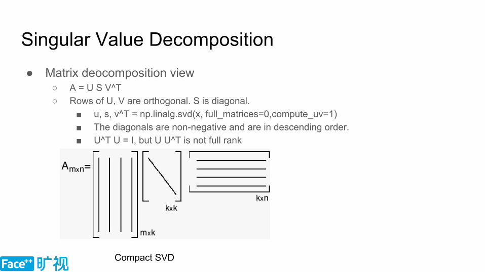
Singular Value Decomposition● Matrix deocomposition view
○ A = U S V^T○ Rows of U, V are orthogonal. S is diagonal.
■ u, s, v^T = np.linalg.svd(x, full_matrices=0,compute_uv=1)■ The diagonals are non-negative and are in descending order.■ U^T U = I, but U U^T is not full rank
Compact SVD

Truncated SVD● Assume diagonals of S are in descending order
○ Always achievable○ Just ignore the blue segments.

SVD
Kronecker Product
+


Matrix factorization => Convolution factorization● Factorization into HxW followed by 1x1
○ feature map (N H’ W’, C H W)○ first conv weights (C H W, R)○ feature map (N H’ W’, R)○ second conv weights (R, K)○ feature map (N H’ W’, K)
HxW
HxW
1x1
K
K
C
C
R
K K
CHW
R
R
CHW

Matrix factorization => Convolution factorization● conv(W, F) = reshape(W) toeplitz(F) ● toeplitz1x1(F) = F● conv(W1, conv(W2, F)) = reshape(W1) toeplitz1(reshape(W2) toeplitz2(F))
○ When toeplitz1 is a 1x1 toeplitz, RHS = reshape(W1) reshape(W2) toeplitz2(F), then the two conv's can be combined into one.

Approximating Convolution Weight● can be reshaped to a (CHW,
K) matrix, etc.● The approximation can be bound by F-norm
W W_a
M M_a
reshape reshape
approximate

Matrix factorization => Convolution factorization● Factorization into 1x1 followed by HxW
○ feature map (N H’ W’ H W, C)○ first conv weights (C, R)○ feature map (N H’ W’ H W, R) = (N H’ W’, R H W)○ second conv weights (R H W, K)○ feature map (N H’ W’, K)
● Steps○ Reshape (CHW, K) to (C, HW, K)○ (C, HW, K) = (C, R) (R, HW, K)○ Reshape (R, HW, K) to (RHW, K)
1x1
HxW
HxW
C
R
K
C
K

Horizontal-Vertical Decomposition● Approximating with Separable Filters● Original Convolution
○ feature map (N H’ W’, C H W)○ weights (C H W, K)
● Factorization into Hx1 followed by 1xW○ feature map (N H’ W’ W, C H)○ first conv weights (C H, R)○ feature map (N H’ W’ W, R) = (N H’ W’, R W)○ second conv weights (R W, K)○ feature map (N H’ W’, K)
● Steps○ Reshape (CHW, K) to (CH, WK)○ (CH, WK) = (CH, R) (R, WK)○ Reshape (R, WK) to (RW, K)
Hx1
HxW
1xW
C
K
C
K
R

Factorizing N-D convolution● Original Convolution
○ let dimension be N○ feature map (N D’_1 D’_2 … D’_Z, C D_1 D_2 … D_N)○ weights (C D_1 D_2 … D_N, K)
● Factorization into N number of D_i x1○ R_0 = C, R_Z = K○ feature map (N D’_1 D’_2 … D’_Z, C D_1 D_2 … D_N)○ weights (R_0 D_1, R_1)○ feature map (N D’_1 D’_2 … D’_Z, R_1 D_2 … D_N)○ weights (R_1 D_2, R_2)○ ...
Hx1x1
HxWxZ
1xWx1
C
K
C
R2
R1
1x1xZ
Z

Kronecker Conv● (C H W, K)● Reshape as (C_1 C_2 H W, K_1 K_2)● Steps
○ Feature map is (N C H’ W’)○ Extract patches and reshape (N H’ W’ C_2, C_1 H)○ apply (C_1 H, K_1 R)○ Feature map is (N K_1 R H’ W’ C_2)○ Extract patches and reshape (N K_1 H’ W’, R C_2 W)○ apply (R C_2 W, K_2)
● For rank efficiency, should have○ R C_2 \approx C_1

Exploiting Local Structures with the Kronecker Layer in Convolutional Networks 1512

Shared Group Convolution is a Kronecker Layer
AlexNet partitioned a conv
Conv/FC Shared Group Conv/FC

CP-decomposition and Xception● Xception: Deep Learning with Depthwise Separable Convolutions 1610● CP-decomposition with Tensor Power Method forConvolutional Neural
Networks Compression 1701● MobileNets: Efficient Convolutional Neural Networks for Mobile Vision
Applications 1704○ They submitted the paper to CVPR about the same time as Xception.

Matrix Joint Diagonalization = CP
ST
T1T1T1S3S2S1
CP
MJD
HxW
C
K
C
HxW
K

CP-decomposition with Tensor Power Method for Convolutional Neural Networks Compression 1701
Convolution
Xception
Channel-wise

Tensor Train Decomposition

Tensor Train Decomposition: just a few SVD’s

Tensor Train Decomposition on FC

Graph Summary of SVD variants
Matrix Product State

CNN layers as Multilinear Maps

Sparse Approximation

Distribution of Weights● Universal across convolutions and FC● Concentration of values near 0● Large values cannot be dropped

Sparsity of NN: statistics

Sparsity of NN: statistics

Weight Pruning: from DeepCompressionTrainNetwork Extract
Mask M TrainW => M o W ...
The model has been trained with exccessive #epoch.

Sparse Matrix at Runtime● Sparse Matrix = Discrete Mask + Continuous
values○ Mask cannot be learnt the normal way○ The values have well-defined gradients
● The matrix value look up need go through a LUT○ CSR format
■ A: NNZ values■ IA: accumulated #NNZ of rows■ JA: the column in the row

Burden of Sparseness● Lost of regularity of memory access and computation
○ Need special hardware for efficient access○ May need high zero ratio to match dense matrix
■ Matrices will less than 70% zero values, better to treat as dense matrices.

Convolution layers are harder to compress than FC

Dynamic Generation of Code● CVPR’15: Sparse Convolutional Neural Networks● Relies on compiler for
○ register allocation○ scheduling
● Good on CPU

Channel Pruning
● Learning the Number of Neurons in Deep Networks 1611
● Channel Pruning for Accelerating Very Deep Neural Networks 1707○ Also exploits low-rankness of features

Quantization

4-bit support in CPU & GPU
Intel® 4004, released 19711.1 Kops @ ??
Tesla® T4, released 2018260 Tops @ 75 Watt
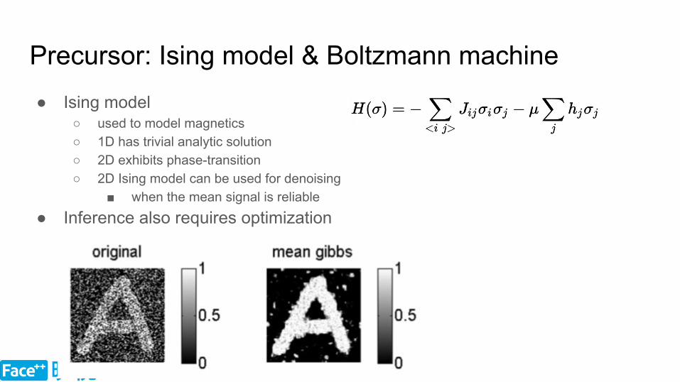
Precursor: Ising model & Boltzmann machine● Ising model
○ used to model magnetics○ 1D has trivial analytic solution○ 2D exhibits phase-transition○ 2D Ising model can be used for denoising
■ when the mean signal is reliable
● Inference also requires optimization

Neural Network Training
X
yCostd + r
Activations/Feature maps/Neurons
Gradients
Quantized Quantized
Quantized

Backpropagation
There will be no gradient flow if we quantize somewhere!

Differentiable Quantization
● Bengio ’13: Estimating or Propagating Gradients Through Stochastic Neurons for Conditional Computation○ REINFORCE algorithm○ Decompose binary stochastic neuron into stochastic and
differentiable part○ Injection of additive/multiplicative noise○ Straight-through estimator
Gradient vanishes after quantization.

Quantization also at Train time● Neural Network can adapt to the constraints imposed by quantization● Exploits “Straight-through estimator” (Hinton, Coursera lecture, 2012)
○ ○ ○ ○ ○
● Example

STE Alternative: Local Reparameterization Trick
Learning Discrete Weights using the local reparameter trick(Shayer, ICLR 2018)
● local reparameterization trick (Kingma&Welling, 2014)
● sampling weights -> sampling pre-activations
usually Gaussian
Monte Carlo approximation

Bit Neural Network● Matthieu Courbariaux et al. BinaryConnect: Training Deep Neural Networks with binary
weights during propagations. http://arxiv.org/abs/1511.00363● Itay Hubara et al. Binarized Neural Networks https://arxiv.org/abs/1602.02505v3● Matthieu Courbariaux et al. Binarized Neural Networks: Training Neural Networks with
Weights and Activations Constrained to +1 or -1. http://arxiv.org/pdf/1602.02830v3.pdf● Rastegari et al. XNOR-Net: ImageNet Classification Using Binary Convolutional Neural
Networks http://arxiv.org/pdf/1603.05279v1.pdf● Zhou et al. DoReFa-Net: Training Low Bitwidth Convolutional Neural Networks with
Low Bitwidth Gradients https://arxiv.org/abs/1606.06160● Hubara et al. Quantized Neural Networks: Training Neural Networks with Low Precision
Weights and Activations https://arxiv.org/abs/1609.07061

Binarizing AlexNetTheoretical

Scaled binarization● ● ● Sol:
= Varaince of rows of W o B

XNOR-Net

Binary weights network● Filter repetition
○ 3x3 binary kernel has only 256 patterns modulo sign.○ 3x1 binary kernel only has only 4 patterns modulo sign.○ Not easily exploitable as we are applying CHW as filter

Binarizing AlexNetTheoretical

Scaled binarization is no longer exact and not found to be useful
The solution below is quite bad, like when Y = [-4, 1]

Quantization of Activations● XNOR-net adopted STE method in their open-source our code
Input ReLU
Capped ReLU QuantizationInput

DoReFa-Net: Training Low Bitwidth Convolutional Neural Networks with Low Bitwidth Gradients
● Uniform stochastic quantization of gradients○ 6 bit for ImageNet, 4 bit for SVHN
● Simplified scaled binarization: only scalar○ Forward and backward multiplies the bit matrices from different sides.○ Using scalar binarization allows using bit operations
● Floating-point-free inference even when with BN● Future work
○ BN requires FP computation during training○ Require FP weights for accumulating gradients

SVHN
A B C D
A has two times as many channels as B. B has two times as many channels as C....

SVHN
A B C D
A has two times as many channels as B. B has two times as many channels as C....
Accuracy ∝ #bit operations = #input-channel * #output-channel * input-bitwidth * output-bitwidth

Quantization Methods● Deterministic Quantization
○○
● Stochastic Quantizaiton○ ○ ○ ○
Injection of noise realizes the sampling.

Quantization of Weights, Activations and Gradients● A half #channel 2-bit AlexNet (same bit complexity as XNOR-net)

Quantization Error measured by Cosine Similarity● Wb_sn is n-bit quantizaiton of real W● x is Gaussian R. V. clipped by tanh
Saturates


Effective Quantization Methods for Recurrent Neural Networks 2016
Our FP baseline is worse than that of Hubara.

Training Bit Fully Convolutional Network for Fast Semantic Segmentation 2016

Bitwidth decay

Benefits of Quantized Neural Networks● Reduce weight size● Reduce feature size
○ larger feature library size
● Speedup computation○ O( Bit-width ) if SIMD, O( Bit-width2 ) if special hardware○ Saves bandwidth (intra-chip and off-chip), eases P & R○ Dense computation
● Distributed training: reduces communication of weights
INT8 INT4 Binary
Tesla T4 130 T 260 T
Megvii Zynq 7020 0.05 T 0.2 T 3.2 T


FPGA is made up of many LUT's


Number format: Floating Point vs. Fixed Point● FP32● FP16● “FP8”● INT32● INT16● INT8● “INT4”● “INT2”● Ternary● Binary
Floating point
● Sharing exponent○ Block Floating Point
● Power-of-2 exponent○ DCT in JPEG

Number format: Floating Point Problems● Extreme values
○ overflow/underflow, denormal numbers
● Rounding rules○ Rounding to nearest / directed rounding
● Breaks associativity○ Kahan summation algorithm○ Pairwise summation
function NeumaierSum(input) var sum = input[1] var c = 0.0 // A running compensation for lost low-order bits. for i = 2 to input.length do var t = sum + input[i] if |sum| >= |input[i]| do c += (sum - t) + input[i] // If sum is bigger, low-order digits of input[i] are lost. else c += (input[i] - t) + sum // Else low-order digits of sum are lost sum = t return sum + c // Correction only applied once in the very end

More Low Bit Formats
bfloat16
float32
float64
float7 / float8 ?
CSD
Posit

More References● Xiangyu Zhang, Jianhua Zou, Kaiming He, Jian Sun: Accelerating Very Deep Convolutional
Networks for Classification and Detection. IEEE Trans. Pattern Anal. Mach. Intell. 38(10): 1943-1955 (2016)
● ShuffleNet: An Extremely Efficient Convolutional Neural Network for Mobile Devices https://arxiv.org/abs/1707.01083
● Aggregated Residual Transformations for Deep Neural Networks https://arxiv.org/abs/1611.05431
● Convolutional neural networks with low-rank regularization https://arxiv.org/abs/1511.06067● Optimizing Neural Networks with Kronecker-factored Approximate Curvature
https://arxiv.org/pdf/1503.05671.pdf

Backup after this slide
Slide also available at my home page:https://zsc.github.io/


TernGrad: Ternary Gradients to ReduceCommunication in Distributed Deep Learning 1705
● Weights and activations not quantized.

Low-rankness of Activations● Accelerating Very Deep Convolutional Networks for Classification and
Detection