Neural Memory Streaming Recommender Networks withAdversarial Training

Qinyong WangSchool of Information Technologyand Electrical Engineering, The

University of Queenslandqinyong.wang@uq.edu.au

Hongzhi Yin∗School of Information Technologyand Electrical Engineering, The

University of Queenslandh.yin1@uq.edu.au

Zhiting HuLanguage Technologies Institute,

Carnegie Mellon Universityzhitingh@cs.cmu.edu

Defu LianSchool of Computer Science and

Engineering, University of ElectronicScience and Technology of China

dove.ustc@gmail.com

Hao Wang360 Search Lab

cashenry@126.com

Zi HuangSchool of Information Technologyand Electrical Engineering, The

University of Queenslandhuang@itee.uq.edu.au

ABSTRACTWith the increasing popularity of various social media and E-commerce platforms, large volumes of user behaviour data (e.g.,user transaction data, rating and review data) are being continu-ally generated at unprecedented and ever-increasing scales. It ismore realistic and practical to study recommender systems withinputs of streaming data. User-generated streaming data presentsunique properties such as temporally ordered, continuous and high-velocity, which poses tremendous new challenges for the once verysuccessful recommendation techniques. Although a few temporalor sequential recommender models have recently been developedbased on recurrent neural models, most of them can only be ap-plied to the session-based recommendation scenario, due to theirshort-term memories and the limited capability of capturing users’long-term stable interests. In this paper, we propose a streaming rec-ommender model based on neural memory networks with externalmemories to capture and store both long-term stable interests andshort-term dynamic interests in a unified way. An adaptive negativesampling framework based on Generative Adversarial Nets (GAN)is developed to optimize our proposed streaming recommendermodel, which effectively overcomes the limitations of classical neg-ative sampling approaches and improves the effectiveness of themodel parameter inference. Extensive experiments are conductedon two large-scale recommendation datasets, and the experimentalresults show the superiority of our proposed model in the streamingrecommendation scenario.ACM Reference Format:Qinyong Wang, Hongzhi Yin, Zhiting Hu, Defu Lian, Hao Wang, and ZiHuang. 2018. Neural Memory Streaming Recommender Networks with

∗Corresponding author

Permission to make digital or hard copies of all or part of this work for personal orclassroom use is granted without fee provided that copies are not made or distributedfor profit or commercial advantage and that copies bear this notice and the full citationon the first page. Copyrights for components of this work owned by others than ACMmust be honored. Abstracting with credit is permitted. To copy otherwise, or republish,to post on servers or to redistribute to lists, requires prior specific permission and/or afee. Request permissions from permissions@acm.org.KDD ’18, August 19–23, 2018, London, United Kingdom© 2018 Association for Computing Machinery.ACM ISBN 978-1-4503-5552-0/18/08. . . $15.00https://doi.org/10.1145/3219819.3220004

Adversarial Training. In Proceedings of The 24th ACM SIGKDD InternationalConference on Knowledge Discovery & Data Mining (KDD ’18). ACM, NewYork, NY, USA, 9 pages. https://doi.org/10.1145/3219819.3220004

1 INTRODUCTIONThe recent study by Econsultancy [28] shows that 94% of com-panies agree that personalized recommendation has become animportant means to improve user experience, engagement, revenueand conversion rate, and is critical to current and future success.For example, Amazon and Netflix recommendations are cited bymany company observers as an outstanding means to improve rev-enues and profits. They rely on the ability of recommender systemsto recommend media content or products that users are likely toconsume. With the proliferation of smart mobile phones, mobileshopping and mobile commerce become the mainstream. In mobilecommerce, most mobile purchases (more than 58%) are made afterseeing a recommendation on a product detail page, and bringingthe most personalized recommendations to the top of a small screenmakes mobile shopping more convenient [34].

While recommender systems have attracted a large amount of re-search interest, the subarea of streaming recommender systems hasremained largely unexplored. The real-world social media and E-commerce platforms such as Amazon and Netflix generate massiveuser-item interaction data (i.e., user behavior data) at an unprece-dented rate. For example, nearly 1.5 billion transactions were madein Alibaba during its Singles Day shopping event on 11, Novem-ber 2017 [30]. Such data is temporally ordered, continuous, high-speed and time-varying, which determines the streaming natureof data in recommendation systems. Therefore, it is more practicalto study recommender systems using a streaming data framework.The real-time streaming setting poses great challenges for conven-tional recommender systems, most of which are designed for staticsettings and implemented by batch learning techniques, which usu-ally suffer from the following drawbacks when dealing with thestream situation: 1) delay on model updates caused by the expen-sive time cost of re-running the batch model; 2) inability to trackfast-changing trends (e.g., user preferences and item popularity) inthe presence of streaming data; and 3) lots of memory overhead toexplicitly store all the historical data.

As the recommender system by nature is an incremental pro-cess, some online learning techniques based on stochastic gradientdescent (SGD) and particle filters [11, 54] have been adopted ordeveloped to support streaming recommendations. However, theysuffer from the problem of “short-term memory”, i.e., since the al-gorithms to update these models are based only on the most recentdata points, and do not take into account the past observations, themodels quickly forget the patterns learned in earlier stages. Therecommendation models based on these online learning algorithmsfail to capture users’ long-term stable interests. Recently, recurrentneural model based recommender systems [17, 49] are proposedto tackle streaming recommendation problems, which adopt recur-rent neural networks (RNN) or long short-term memory (LSTM) tocapture and store sequential patterns of interacted items or users’dynamic interests. Such models learn a continuous and compactrepresentation of the input data, and perform global updates acrossthe whole memory cell at each step. These architecture designsencourage RNNs/LSTMs to capture sequential patterns from data,which makes RNNs/LSTMs based recommender systems especiallygood at capturing sequential user activity patterns or user temporaldynamics. They are often applied to the session-based recommenda-tion scenario without user profiles (i.e., users’ historical interactiondata). However, like the online learning algorithms, RNNs/LSTMshave limitations in modeling and capturing users’ long-term stableinterests which are hardly affected by temporal factors.

To this end, we propose a novel model named NeuralMemoryRecommender Networks (NMRN). NMRN is inspired by NeuralTuring Machines (NTM) [14] and Memory Network (NemNN) [37],and consists of two main components: augmented memories storinguser and item information, and an controller network interactingwith user activity data and reading or writing to the memories.Augmenting controller network with external memories separatesthe tasks of storing and processing information and makes the net-work only focus on processing information stored outside it. It alsoincreases its capability of storing knowledge, thus users’ long-termand stable preferences can persist if necessary. Moreover, NMRNcan flexibly and explicitly read from and write to the memories ondemand like physical computers. NMRN encourages local changesin memory, and this ability to directly execute local update to in-ternal memories makes NMRN powerful to integrate users’ recentinteraction data and capture their newly emerging interests.

Specifically, the external memories of NMRN compose the keymemory and the value memory. The structure of key-value memorynetworks (KV-MemNN) [26, 57] makes the original MemNN moresuitable to deal with pairwise data. Given a new user-item inter-action pair (u,v) arriving at the system in real time, NMRN firstgenerates a soft address from the key memory, activated by u. Theaddressing process is inspired by recent advances in attention mech-anism, which is popular in the fields of computer vision [27, 51] andNLP [23, 59], but is rarely studied in the field of recommender sys-tems. The atention mechanism applied in recommender systems isuseful to improve the retrieval accuracy and model interpretability.The fundamental idea of our attention design is to learn a weightedrepresentation across the key memory, which is converted into aprobability distribution by the Softmax function as the soft address.Then, NMRN reads from the value memory based on the soft ad-dress, resulting in a vector that represents both long-term stable

and short-term emerging interests of user u. Inspired by the suc-cess of pairwise personalized ranking models [32, 35] (e.g., BPR) intop-k recommendations, we adopt the Hinge-loss in our model opti-mization. As the number of unobserved examples is very huge, weemploy the negative sampling method proposed in [24] to improvethe training efficiency. Most existing negative sampling approachesuse either random sampling [1, 24, 38] or popularity-biased sam-pling strategies [5, 11]. However, the majority of negative examplesgenerated in these sampling strategies can be easily discriminatedfrom observed examples, and will contribute little towards the train-ing, because sampled items could be completely unrelated to thetarget user. Besides, these sampling approaches are not adaptiveenough to generate adversarial negative examples, because (1) theyare static and thus do not consider that the estimated similarity orproximity between a user and an item changes during the learningprocess. For example, the similarity between user u and a samplednoise item v is high at the beginning, but after several gradientdescent steps it becomes low; and (2) these samplers are global anddo not reflect how informative a noise item is w.r.t. a specific user.In light of this, we develop an adaptive noise sampler based on aGenerative Adversarial Network (GAN) [13] to optimize our model,which considers both the specific user and the current values ofthe model parameters to adaptively generate “difficult” and infor-mative negative examples. Moreover, in order to simultaneouslycapture the first-order similarity between users and items as wellas the second-order similarities between users and between itemsto learn robust representations of users and items, we adopt theEuclidean distance to measure the similarity between a user and anitem instead of the widely adopted dot product, inspired by [19].

Overall, we summarize the major contributions of this paper:

(1) To the best of our knowledge, we are the first to design anddevelop a streaming recommendermodel based onKey-ValueMemory Networks to provide real-time recommendations.It has the nice capability of capturing and storing both users’long-term stable interests and short-term dynamic interests.

(2) We propose a novel adaptive noise sampler to generate ad-versarial negative samples for model optimization, whichsignificantly improves training effectiveness of our proposedstreaming recommender model. This is the first time to in-tegrate Generative Adversarial Nets with the negative sam-pling method seamlessly for recommender systems.

(3) We conduct extensive experiments to evaluate the perfor-mance of our proposed streaming recommender model inthe streaming recommendation setting on two large-scalerecommendation datasets. The results show the superior-ity of our proposals by comparing with the state-of-the-artstreaming recommendation techniques.

2 MODEL DESCRIPTIONIn this section, we first formulate NMRN, then describe its structureand finally present how to use it for streaming recommendations.Note that in the description below, vectors and matrices are denotedwith bold small letters and bold capital letters respectively.

𝑩

𝑀𝑡−1𝑣

𝑢

𝑀𝑡𝑣

𝑀𝑡𝑘

𝑣−

𝑙𝑜𝑠𝑠

𝑀𝑡+1𝑣

𝑨

𝒗

𝒗−

Softmax

Sigmoid Tanh

𝑒𝑡 𝑎𝑡

𝒖

1-

𝑣

𝑠

𝒘

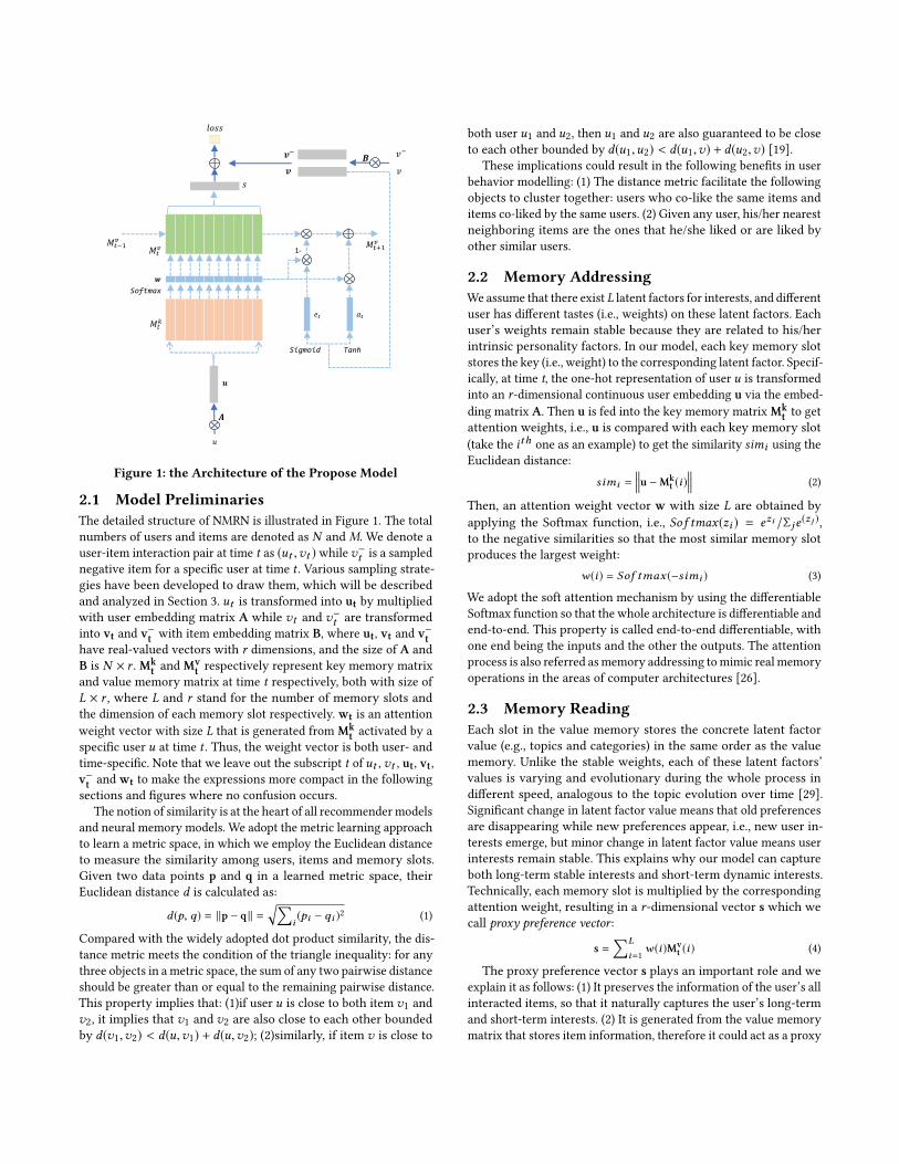
Figure 1: the Architecture of the Propose Model

2.1 Model PreliminariesThe detailed structure of NMRN is illustrated in Figure 1. The totalnumbers of users and items are denoted as N and M. We denote auser-item interaction pair at time t as (ut ,vt )whilev−t is a samplednegative item for a specific user at time t . Various sampling strate-gies have been developed to draw them, which will be describedand analyzed in Section 3. ut is transformed into ut by multipliedwith user embedding matrix A while vt and v−t are transformedinto vt and v−t with item embedding matrix B, where ut, vt and v−thave real-valued vectors with r dimensions, and the size of A andB is N × r . Mk

t and Mvt respectively represent key memory matrix

and value memory matrix at time t respectively, both with size ofL × r , where L and r stand for the number of memory slots andthe dimension of each memory slot respectively. wt is an attentionweight vector with size L that is generated from Mk

t activated by aspecific user u at time t . Thus, the weight vector is both user- andtime-specific. Note that we leave out the subscript t of ut , vt , ut, vt,v−t and wt to make the expressions more compact in the followingsections and figures where no confusion occurs.

The notion of similarity is at the heart of all recommendermodelsand neural memory models. We adopt the metric learning approachto learn a metric space, in which we employ the Euclidean distanceto measure the similarity among users, items and memory slots.Given two data points p and q in a learned metric space, theirEuclidean distance d is calculated as:

d (p, q) = ∥p − q∥ =√∑

i(pi − qi )2 (1)

Compared with the widely adopted dot product similarity, the dis-tance metric meets the condition of the triangle inequality: for anythree objects in a metric space, the sum of any two pairwise distanceshould be greater than or equal to the remaining pairwise distance.This property implies that: (1)if user u is close to both item v1 andv2, it implies that v1 and v2 are also close to each other boundedby d(v1,v2) < d(u,v1) + d(u,v2); (2)similarly, if item v is close to

both user u1 and u2, then u1 and u2 are also guaranteed to be closeto each other bounded by d(u1,u2) < d(u1,v) + d(u2,v) [19].

These implications could result in the following benefits in userbehavior modelling: (1) The distance metric facilitate the followingobjects to cluster together: users who co-like the same items anditems co-liked by the same users. (2) Given any user, his/her nearestneighboring items are the ones that he/she liked or are liked byother similar users.

2.2 Memory AddressingWe assume that there exist L latent factors for interests, and differentuser has different tastes (i.e., weights) on these latent factors. Eachuser’s weights remain stable because they are related to his/herintrinsic personality factors. In our model, each key memory slotstores the key (i.e., weight) to the corresponding latent factor. Specif-ically, at time t, the one-hot representation of user u is transformedinto an r-dimensional continuous user embedding u via the embed-ding matrix A. Then u is fed into the key memory matrixMk

t to getattention weights, i.e., u is compared with each key memory slot(take the ith one as an example) to get the similarity simi using theEuclidean distance:

simi = u −Mk

t (i) (2)

Then, an attention weight vector w with size L are obtained byapplying the Softmax function, i.e., So f tmax(zi ) = ezi /Σje

(zj ),to the negative similarities so that the most similar memory slotproduces the largest weight:

w (i) = Sof tmax (−simi ) (3)

We adopt the soft attention mechanism by using the differentiableSoftmax function so that the whole architecture is differentiable andend-to-end. This property is called end-to-end differentiable, withone end being the inputs and the other the outputs. The attentionprocess is also referred asmemory addressing tomimic real memoryoperations in the areas of computer architectures [26].

2.3 Memory ReadingEach slot in the value memory stores the concrete latent factorvalue (e.g., topics and categories) in the same order as the valuememory. Unlike the stable weights, each of these latent factors’values is varying and evolutionary during the whole process indifferent speed, analogous to the topic evolution over time [29].Significant change in latent factor value means that old preferencesare disappearing while new preferences appear, i.e., new user in-terests emerge, but minor change in latent factor value means userinterests remain stable. This explains why our model can captureboth long-term stable interests and short-term dynamic interests.Technically, each memory slot is multiplied by the correspondingattention weight, resulting in a r-dimensional vector s which wecall proxy preference vector :

s =∑L

i=1w (i)Mv

t (i) (4)

The proxy preference vector s plays an important role and weexplain it as follows: (1) It preserves the information of the user’s allinteracted items, so that it naturally captures the user’s long-termand short-term interests. (2) It is generated from the value memorymatrix that stores item information, therefore it could act as a proxy

of a user when computing the similarity between a user and an item,because users and items may be projected to different spaces (e.g.,when the size of a key memory slot is different from that of a valuememory slot), and their similarity cannot be directly computed viaEuclidean distance. In fact, the overall effect is equivalent to thatthe user and the item are projected into the joint r-dimensionalspace, which enables the similarity computation between a userand an item. Thus, given a user as query, the efficiency of the top-krecommendation at time t can be significantly improved with off-the-shelf approximate nearest-neighbor (ANN) algorithms, such aslocation-sensitive hashing (LSH).

2.4 Memory WritingTo locally update the value memory matrix to adapt to the changeof user preferences, a memory writing scheme is proposed inspiredby [14, 57]. Once a new user-item pair arrives at the system, theitem’s embedding will be written to the value memory matrix usingthe same attention weights w generated in the memory readingstage. The relevant memories are first erased and then the new iteminformation such as the item’s popularity is added to update thevalue memory.

Specifically, to update the value memory matrixMvt intoMv

t+1, alinear function is applied to the newly arrived itemv’s embedding vand then the Sigmoid function is employed to the result, obtainingthe erased vector et as follows:

et = Siдmoid (Wev + be) (5)

where We is a linear transformation matrix with size of r × r , andbe is a r-dimensional bias vector. The resulting erased vector et isa r-dimensional vector, whose values range from 0 to 1. Then thevalue memory Mv

t is partially erased, and each of its memory slotsis modified by:

M̃vt+1(i) = Mv

t (i) ◦ [I −w (i)et] (6)

where I is a r-dimensional vector with each element being 1, and◦ is element-wise multiplication. Similar to the reading case, theweighting w(i) tells us where to focus our erasing. In this way,the value location is reset to 0 if the corresponding weight andthe erased vector element are both 1, and if either is 0, the valuelocation remains unchanged. Following the erasing operation, ar-dimensional add vector at is calculated for updating the valuememory in a similar manner:

at = Tanh(Wav + ba) (7)

where Wa and ba are linear transformation matrix and bias vectorwith size r × r and r . Finally, the value memory matrix at time t + 1is updated to be Mv

t+1(i) as follows:

Mvt+1(i) = M̃v

t+1(i) +w (i)at (8)

2.5 Pairwise Loss FunctionInspired by [19, 22, 32], we design a pairwise loss function basedon Hinge-loss. Our intuition is that a user’s proxy preference vec-tor s should be similar with the interacted items while dissimilarwith the non-interacted items in order to act as a proper proxy be-tween users and items. Therefore, the loss function should pull thepositive items (i.e., neighbors) closer and push the negative items(i.e., impostors) further from the proxy preference vector. As the

number of non-interacted items of each user is huge, we adopt thenegative sampling method to perform model optimization insteadof using all unobserved examples, following skip-gram model [25].The pairwise loss function is defined as follows:

L =∑

(u,v )∈S,v−∼V−uwu,v ∗ [m + d (u, v) − d (u, v−)]+ (9)

where [z]+ = max(z; 0) denotes the standard Hinge-loss, wu,v isthe ranking loss weight (described later) andm > 0 is the safetymargin size; S is the user activities data currently available fortraining, V−

u is a set of items that u has never interacted with,currently, we simply assume that each negative item v− is uni-formly drawn from V−

u , but we will introduce a better-designedadaptive negative sampling method based on GAN in Section 3;d(u,v)/d(u,v−) is the distance between u’s proxy preference vectors and the positive/negative item vector v/v−.

2.6 Ranking Loss Weights and RegularizationA rank-based weighting scheme called Weighted Approximate-Rank Pairwise (WARP) loss [46, 47] is adopted to penalize items ata lower rank. Given a user u, let ranku,v denote the rank of item vin u’s recommendation list, we penalize a positive item v based onits rank by setting:

wu,v = log(ranku,v + 1) (10)

This scheme penalizes a positive item at a lower rank much moreheavily than at the top. However, it is computationally inefficient torank all items for each user. To avoid ranking all items, we adopt thefollowing approximate method to obtain ranku,v : for each positiveitem v of user u, it needs to draw Nu,v negative items until a v−satisfying d(u,v) − d(u,v−) +m > 0, i.e., an impostor, is found.Then the approximate rank is calculated as:

ranku,v ≈ ⌊N − 1Nu,v

⌋ (11)

Recall that N is the total number of items.If the data points in a high-dimensional space spread too widely,

the model would fail due to the curse of dimensionality [12]. Tosolve it, we bound the norm of all user/item vectors within 1 toensure the model robustness [19]: ∥u∥ ≤ 1 and ∥v∥ ≤ 1.

2.7 Top-k Recommendations with NMRNGenerating top-k recommendations for a online user u at time tis straightforward with NMRN: u is transformed into her proxypreference vector s by embedding matrix A, key memoryMk

t andvalue memoryMv

t . Then s is compared with all items vectors trans-formed by embedding matrix B to find out the most similar k itemsaccording to d(s,v). Due to the nice property of Euclidean distance,NMRN has the advantage of significantly speeding up the retrievalprocess with approximate nearest-neighbor (ANN) algorithms, suchas location-sensitive hashing (LSH), especially when a well-knownindustrial LSH library Annoy is adopted. After that, the model getsupdated based on this new item with the writing operation.

3 ADVERSARIAL TRAINING FRAMEWORKIn this section, we propose a GAN-based adversarial training frame-work to overcome the drawbacks of existing sampling methods.

𝑣1

P=0.7

𝑣2

𝑣3

𝑣4

𝑣5

P=0.1

P=0.05

P=0.05

P=0.1

reward

𝑩

𝑀𝑡−1𝑣

𝑢

𝑀𝑡𝑣

𝑀𝑡𝑘

𝑙𝑜𝑠𝑠

𝑀𝑡+1𝑣

𝑨

𝒗

𝒗−

Softmax

Sigmoid Tanh

𝑒𝑡 𝑎𝑡

𝒖

1-

𝑣

𝑠

𝒘

𝑣− = 𝑣3

D

𝑬

𝑭

𝑑𝐺

G

𝑃𝐺

Sampler

MLP

𝑢

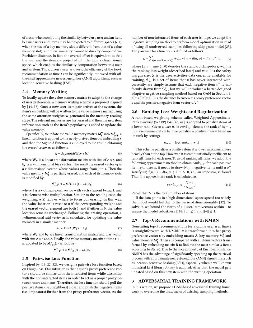
Figure 2: Overview of the Adversarial Training Framework

3.1 Problems of Existing Sampling MethodsTo obtain a negative item, the most straightforward and widelyadopted method is random sampling [1, 7, 8, 24, 38] or popularity-biased sampling strategies [5, 11]. However, there exist some prob-lems that make them unsuitable for our application. For randomsampling methods, the major problem is that the randomly gener-ated items create too many “easy” tasks for the model to learn, i.e.,these items might be completely unrelated to the user, so the modelcould easily discriminate them from the observed ones. These easytasks contribute very little for the model optimization and hinderthe model to discover more complex hidden user/item represen-tations. On the contrary, a good and “difficult” item should beinformative and could confuse the model if it has not captured thedeep user/item representations. Moreover, the common problemfor both methods is that they are not adaptive enough to generateadversarial negative items, i.e., they are static and do not considerthe change of similarity or proximity between a user and an itemduring training. For example, before the training, the item v is sam-pled as noise because its similarity with user u is high, however,after several optimization iterations, the degree of similarity mightdrop, this item v with little information is still considered as noise.Another common problem is that the sampling probability distribu-tion is usually global that applies to every user, but different usershave different interests, thus that global distribution dose not reflecthow informative a noise item is w.r.t a specific user. To this end, wepropose an adversarial training framework to adaptively generate“difficult” and informative negative examples, highly inspired byKBGAN [2].

3.2 Framework DescriptionThe proposed training framework is shown in Figure 2. In parallelto the GAN literature, we name the two models in the proposedframework as Discriminator and Generator denoted by D and Grespectively. The target for the discriminator is to tell apart thetrue items from false items produced by the generator while forthe generator is to adaptively generate an adversarial negative

item and use it to deceive the discriminator. In the adversarialtraining settings, the generator and the discriminator are trainedwith respective to its own loss function.

3.2.1 Discriminator. For the discriminator in our framework,its loss function is:

LD =∑

(u,v )∈S

wu,v ∗ [m + dD (u, v) − dD (u, v−)]+

(u, v−) ∼ PG (u, v− |u, v)(12)

where PG (u,v− |u,v) is the probability distribution for generatingnegative tuple (u,v−) by the generator given a positive tuple (u,v)(defined below); dD denotes the distance measured by the discrimi-nator, which is identical to d defined in in Eq (9). The optimizationprocedures follow what we described above. It is clear that the onlydifference between Eq (9) and Eq (12) is that the negative item v−

in Eq (12) is generated by the generator while it is drawn randomlyin Eq (9).

3.2.2 Generator. The objective of the generator maximizes theexpectation of −dD (u,v−) using the generated items so as to en-courage the generator to generate plausible items to confuse thediscriminator:

LG =∑

(u,v )∈S

E[−dD (u, v−)]

(u, v−) ∼ PG (u, v− |u, v)(13)

The distribution PG (u,v− |u,v) is modeled as:

PG (u, v− |u, v) =exp(−dG (u, v−))∑

v̄∈V−uexp(−dG (u, v̄))

(14)

where dG is the Euclidean distance between user u and item v mea-sured by the generator though a neural network. We embed u withmatrix E and embed v with matrix F, the resulting vectors are sepa-rately forward-propagated by a multilayer perceptron (MLP) suchthat user u and item v are in the same space, and dG is measuredbetween the output user and item vectors, as shown in Figure 2.V−u is a set containing all items not interacted with user u in the

history, however, this set might be large, witch would significantlydamage the efficiency. In order to reduce computational complexity,we only uniformly randomly select T items from the original wholeV−u to form a new but smallerV−

u .However, the challenge in the optimization process is that LG

can not be directly optimized by SGD because it involves a discretesampling step which blocks the flow of gradients. Following thework [2, 56], we consider it as a reinforcement learning problem,where, analogously, (u,v) is the state, PG (u,v− |u,v) is the policy,(u,v−) is the action and −dD (u,v

−) is the reward.A common optimization approach is to adopt policy gradient

based reinforcement learning (REINFORCE) [48, 56]. According tothat, the gradient of LG with respect to its parameters is:

∇θG LG =∑

(u,v )∈S

E(u,v−)∼PG [−dD (u, v−)∇θG loдPG (u, v− |u, v)]

≃∑

(u,v )∈S

1T

T∑(ui ,v

−i )∼PG ,i=1

[−dD (ui , v−i )∇θG loдPG (ui , v−

i |u, v)](15)

REINFORCE algorithm often suffers from the issue of high vari-ance. A widely adopted solution is subtracting a baseline b from thepolicy gradient. Although a good baseline should be the functionof the state value [31], it could also be chosen arbitrarily without

Algorithm 1: The Adversarial Training Algorithm

1 INPUT: user-item interaction history (u, v) ∈ S, margin m and learning rates λD and λG;2 OUTPUT: the discriminator D, the generator G and their distance measurement function dD and dG;3 Initialize the parameters θD and θG for D and G;4 b = 0; //initiate the baseline5 Pre-train D and G w.r.t. to θD and θG;6 while not convergent do7 Sample a mini-batch Sbatch ∈ S; ∆G = 0; ∆D = 0; Rbatch = 0;//zero the gradients of D and G and rewards8 for (u, v) ∈ Sbatch do9 Compute its ranking weight w(u,v);

10 Uniformly randomly sample T negative items: V−u ;

11 Measure the sampling probability distribution: PG(u, v−|u, v) =exp(−dG(u,v−))∑

v̄∈V−uexp(−dG(u,v̄))

;

12 Sample a negative item v− forming (u, v−) by the distribution PG(u, v−|u, v);13 Freeze the weights of G;

14 ∆D = ∆D +∇θD{wu,v ∗ [m+ dD(u, v)− dD(u, v−]+}; // accumulate the example gradient to ∆D

15 Rbatch = Rbatch + (−D(u, v−));16 Freeze the weights of D ;17 ∆G = ∆G + (Rbatch − b)∇θG log pG; // accumulate the example gradient to ∆G

18 end19 θD = θD − λD∆D;θG = θG + λG∆G; //minimize the loss of D while maximize the likelihood of G

20 b = Rbatch|Sbatch| ; //update the baseline

21 end

changing the expectation to avoid introducing new parameters [48].In our case, we fix keep b fix as the average reward of the wholetraining set, i.e., b =

∑(u,v)∈S E(u,v−)∼PG (u,v− |u,v)[−dD (u,v

−)].For implementation, only recent generated negative items are usedto approximate b.

Note that like many typical GAN models [40, 58], both the dis-criminator and the generator are pre-trained separately. In particu-lar, the discriminator is pre-trained according to Eq (9) with randomnegative items and the generator is pre-trained by maximizing thelog-likelihood of Eq (14). Algorithm 1 summaries this adversarialtraining process.

4 EVALUATIONIn this section, we first introduce the experimental settings andthen report the experimental results.

4.1 DatasetsTo evaluate our streaming recommendation model, we select twolarge-scale and publicly available datasets, i.e., Movielens and Net-flix, that contain time information of user-item interactions in orderto simulate the real streaming scenario.

Movielens: Movielens is a widely adopted movie dataset forevaluating recommender systems. We choose the 20M Dataset thatcontains 20 million interaction records generated by 138493 userson 26744 movies. All interaction records are associated with times-tamps ranging from the 01/09/1995 to 03/31/2015.

Netflix: Netflix is another movie dataset that consists of 24million interaction records, 470758 users and 4499 movies. Thisdataset was sampled between November, 1999 and December, 2005and reflects the distribution of all interactions received during thisperiod, and the temporal granularity is a day..

4.2 Baseline MethodsWe compare our proposed models with three state-of-the-art rec-ommendation models that support online updating. To validate

the effect of our proposed GAN-based adaptive negative samplingapproach (called NMRN-GAN for the rest of this paper), we designa baseline called NMRN-RS that adopts the simple non-adaptiverandom sampling method to draw negative items.

RRN Recurrent Recommender Networks (RRN) [49] are ableto predict future behavioral trajectories. This is achieved by en-dowing both users and movies with a Long Short-Term Memory(LSTM) [18] autoregressive model that captures temporal dynam-ics of user interests, in addition to a more traditional low-rankfactorization to capture users’ stable interests.

RKMF Regularized Kernel Matrix Factorization (RKMF) is pro-posed by Rendle et. al in [33], inspired by that the nonlinear in-teractions between feature vectors are possible with kernels. Aflexible online learning algorithm is developed for RKMF to updateon selected data instances. We use a RKMF implemented bymfrec 1.

WARPWeighted Approximate-Rank Pairwise (WARP) [46] lossis the state-of-the-art top-k recommendation method specificallydesigned for implicit feedbacks. WARP uses SGD and a smart sam-pling trick to approximate ranks, resulting in an efficient onlineoptimization strategy. A WARP implemented by LightFM2 is used.

NMRN-RSNMRN-RS is a NMRN implementation that only usesuniformly random sampling strategy to draw negative items. Wecompare with it to validate the benefits brought by our proposedGAN-based adaptive negative sampling approach.

4.3 Evaluation SetupIn this section, we describe how to simulate real streaming recom-mendation scenarios and the evaluation protocol and measurement.

4.3.1 Scenario Simulation. To mimic a real streaming recom-mendation scenario, we need to split the datasets properly. Besidesonline streaming recommendation, we also test our model in a tra-ditional offline batch-based temporal recommendation setting [52].

1github.com/mlaprise/mfrec2github.com/lyst/lightfm

1 2 3 4test set

0.00

0.05

0.10

0.15

0.20

0.25

0.30

0.35

0.40

Hits

@5

NMRN-GANNMRN-RS

RRNRKMF

WARP

(A) Hits@5

1 2 3 4test set

0.0

0.1

0.2

0.3

0.4

0.5

0.6

Hits

@10

NMRN-GANNMRN-RS

RRNRKMF

WARP

(B) Hits@10

1 2 3 4test set

0.0

0.1

0.2

0.3

0.4

0.5

0.6

0.7

Hits

@20

NMRN-GANNMRN-RS

RRNRKMF

WARP

(C) Hits@20

1 2 3 4test set

0.0

0.1

0.2

0.3

0.4

0.5

0.6

0.7

0.8

0.9

Hits

@30

NMRN-GANNMRN-RS

RRNRKMF

WARP

(D) Hits@30

1 2 3 4test set

0.00

0.05

0.10

0.15

0.20

0.25

0.30

0.35

0.40

0.45

Hits

@5

NMRN-GANNMRN-RS

RRNRKMF

WARP

(E) Hits@5

1 2 3 4test set

0.0

0.1

0.2

0.3

0.4

0.5

0.6

Hits

@10

NMRN-GANNMRS-RS

RRNRKMF

WARP

(F) Hits@10

1 2 3 4test set

0.0

0.1

0.2

0.3

0.4

0.5

0.6

0.7

Hits

@20

NMRN-GANNMRN-RS

RRNRKMF

WARP

(G) Hits@20

1 2 3 4test set

0.0

0.1

0.2

0.3

0.4

0.5

0.6

0.7

0.8

Hits

@30

NMRN-GANNMRS-RS

RRNRKMF

WARP

(H) Hits@30

Figure 3: Hits@k on Movielens (A-D) and Netflix (E-H) with Increasing k for Online Streaming Setting

For online streaming recommendation, we follow the data split-ting strategy introduced in [3]. We order all interaction recordsby timestamp and evenly split them into 6 parts. The first 2 partsform a base training set are denoted as Dtrain and the remaining4 parts are test sets denoted as Dtest

1 . . .Dtest4 , which are used to

mimic the online streaming inputs. All the comparison methods arefirst trained over Dtrain to determine the initial model parametersand the best hyper parameters (e.g., the number of latent factorsand the shapes of embedding). Once the initial training is com-pleted, the 4 test sets are sequentially predicted. During testing,the previous test set Dtest

i is used to update the model, then theupdated model predicts the current test set Dtest

i+1 . Formally, themodel is first trained with Dtrain , resulting in M0, then M0 isused to perform evaluation on Dtest

1 . After that, M0 is updatedwith Dtest

1 to beM1 and so on. For new users not contained in thetraining set, we recommend the most popular items.

For offline batch recommendation, we order all user interactionrecords in datasetD by their timestamps and split them into halves,denoted as Dtrain and Dtest . Dtrain is used to learn model pa-rameters and Dtest is for evaluating trained model.

4.3.2 Evaluation Methodology. The evaluation methodology weadopt for all comparison methods is Hits@k that is widely appliedin the recommendation research area [6, 20, 43]. For each userinteraction record (u,v) with time t in the test set: 1) We randomlysample J items that user u has never interacted with before t . It isworth mentioning that J is set to 5000 and 500 for theMovielens andNetflix respectively in our experiments; 2) Compute u’s preferencescores for these J items and v; 3) Sort these J+1 items by theirscores to form a ranked list. Let p denote the position of v withinthe list and thus the best result happens when v precedes all theother items (i.e, p = 1); 4) A top-k recommendation list is formed bypicking the k items with highest scores. If p ≤ k , we get a hit (i.e.,the ground truth v appears in u’s recommendation list), otherwise,we get a miss. The hit probability would rise as k increases or Jdecreases, thus we need to fix k and J for all comparison methodsto ensure fairness. 4) The Hit@k is finally computed as:

Hits@k =#hit@k|Dtest |

(16)

where #hit@k is the number of hits within test set Dtest .

4.4 Experimental ResultsIn this section, we present the experimental results in both on-line streaming and offline batch recommendation settings, and theoptimal hyper-parameters are also given for the convenience ofrepeating our experiments.

Our proposed NMRN-GAN achieves its best performance withthe hyper-parameters r=64, L=128, T=200 and m=3 on the Movie-lens dataset, and r=32, L=64, T=100 and m=4 for the Netflix dataset.Figure 3 reports the online streaming recommendation accuracy interms of Hits@5, Hits@10, Hits@20 and Hits@30 on both datasets.The horizontal axis is the timeline, four reference time points arechosen to simulate the “the current time”. Obviously, our proposedNMRNmodels (including NMRN-GAN and NMRN-RS) significantlyoutperform the other comparison methods on both datasets. In ad-dition, several other observations are made from the results. (1)The LSTM based recommender RRN performs much better thanother comparison methods WARP and RKMF. which validates ourstatement that a streaming recommender system should preservelong-term stable personal interests as well as capture the short-termnewly emerging interests. (2) However, RRN falls far behind ourNMRS models, although it also considers both long-term stable andshort-term dynamic user interests. This is because RRN uses twoseparate models (i.e., LSTM and the traditional matrix factorization)to model users’ two types of interests respectively and then simplyadds the results of these two models together to produce the finalrecommendations. In contrast, our NMRS models with external key-value memories naturally capture and store both long-term stableand newly emerging interests in a unified manner. (3) NMRN-GAN

5 10 20 30k

0.0

0.1

0.2

0.3

0.4

0.5

0.6

0.7

0.8

Hits@k

NMRN-GANNMRN-RS

RRNWARP

(A) Movielens

5 10 20 30k

0.0

0.1

0.2

0.3

0.4

0.5

0.6

0.7

0.8

Hits@k

NMRN-GANNMRS-RS

RRNWARP

(B) Netflix

Figure 4: Batch Recommendation on Movielens and Netflix

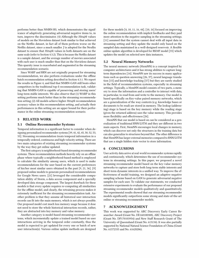
performs better than NMRN-RS, which demonstrates the signif-icance of adaptively generating adversarial negative items to, inturn, improve the discriminator. (4) Although the Hits@k valuesof models on the Movielens dataset look similar to that achievedon the Netflix dataset, in fact all of them perform worse on theNetflix dataset, since a much smaller J is adopted for the Nexflixdataset to ensure that Hits@k values in both datasets are on thesame scale (refer to Section 4.3.2). This is because the Netflix datasetis a sample dataset, and the average number of movies associatedwith each user is much smaller than that on the Movielens dataset.This sparsity issue is exacerbated and augmented in the streamingrecommendation scenario.

Since WARP and RRN are not originally proposed for streamingrecommendation, we also perform evaluations under the offlinebatch recommendation setting described in Section 4.3.1. We reportthe results in Figure 4, and find that NMRN-GAN still beats othercompetitors in the traditional top-k recommendation task, validat-ing that NMRN-GAN is capable of preserving and storing users’long-term stable interests. We also observe that (1) WARP in thissetting performs much better than in the streaming recommenda-tion setting; (2) All models achieve higher Hits@k recommendationaccuracy values in this recommendation setting, and actually theirperformances in this setting are an upper bound for their perfor-mance in the online streaming recommendation scenario.

5 RELATEDWORK5.1 Online Recommender SystemsTemporal information is a significant factor to consider when de-signing personalized recommender systems [39, 41, 42, 45, 50, 52, 53,55]. Streaming recommendation treats temporal information in atemporally ordered, continuous and high-velocity setting. There aretwo main categories of existing streaming recommender systemsby the way they get online updated.

The first category is neighborhood-based streaming recommendersystems. These recommendation methods heavily rely on an offlinephase where typically a neighborhood-based method is employedto calculate the similarity among users, which is used to makerecommendations for the user based on the current preferencesof his/her most similar users obtained in the past [9, 21, 36]. [9]proposed online models to generate personalized recommendationsfor Google News users. [21] leveraged the considerable compu-tation ability of Storm, a data access component and a speciallydeveloped data storage component. The largest drawback for thesemodels is that every update requires re-computing all similaritiesfor the offline model, and clearly, the retraining process makes itextremely inefficient for the streaming recommendation task. An-other problem is that they assume all historical user interactionrecords can fit into the main memory, which is not always possible.Our proposed model cost much less memory usage because it dosenot need to store the whole historical interaction records, rather,they are abstracted into key memory and value memory.

Another category is model-based streaming recommender sys-tems, which incrementally update a trained model based on userinteractions arriving in the temporal order constantly, thus themodel is expected to get updated for every one or batch of newuser interaction(s). Various online update methods are designed

for these models [4, 10, 11, 16, 44]. [10, 16] focused on improvingthe online recommendation with implicit feedbacks and they paidmore attention to the negative sampling in the streaming settings.[11] assumed that the system cannot deal with all input data instreaming setting and they update the model only based on thesampled data maintained in a well-designed reservoir. A flexibleonline-update algorithm is developed for RKMF model [33] whichupdates the model on selected new data instances.

5.2 Neural Memory NetworksThe neural memory network (MemNN) is a concept inspired bycomputer architectures and it has strong abilities to capture long-term dependencies [14]. MemNN saw its success in many applica-tions such as question answering [26, 37], neural language transla-tion [15] and knowledge tracking [57] but they are rarely studiedin the field of recommendation systems, especially in streamingsettings. Typically, a MemNN model consists of two parts, a mem-ory to store the information and a controller to interact with data,in particular, to read from and write to the memory. Our model isbased specifically on Key-value paired memory networks, whichare a generalization of the way contexts (e.g. knowledge bases ordocuments to be read) are stored in memory. The lookup (address-ing) stage is based on the key memory while the reading stage(given the returned address) uses the value memory. This providesmore flexibility and effectiveness [26].

MemNN that our model is based on can be considered as a gen-eralization of traditional RNN/LSTM and they are different in twomain aspects. First, MemNN encourages local changes in memory,which can discover not only the structures in the training data butcan also generalize to structures beyond that. The other difference isthat MemNN has larger external memories compared to RNN/LSTMthat use a single hidden state vector to store information.

6 CONCLUSIONSUser activity data arrive at real-world recommender systems rapidlyand continuously, which determines the use of recommender sys-tems in streaming settings. In this paper, we proposed a novelstreaming recommender model based on the key-value memorynetworks to capture and store both long-term stable interests andshort-term dynamic interests in a unified way. To improve the ef-fectiveness of model training, we designed an adaptive negativesampling scheme based on GAN to generate adversarial negativesamples for each user. To validate our statements, we conductedextensive experiments to evaluate the performance of our proposedstreaming recommender models qualitatively and quantitatively.The experimental results showed that our streaming recommendermodels significantly outperform some strong and state-of-the-artonline or streaming recommender models.

7 ACKNOWLEDGEMENTThis work was supported by ARC Discovery Early Career Re-searcher Award (Grant No. DE160100308), ARC Discovery Project(Grant No. DP170103954) and New Staff Research Grant of TheUniversity of Queensland (Grant No. 613134). It was also partiallysupported by National Natural Science Foundation of China (GrantNo. 61572335 and No. 61628206).

REFERENCES[1] Trapit Bansal, David Belanger, and Andrew McCallum. 2016. Ask the Gru: Multi-

Task Learning for Deep Text Recommendations. In RecSys. 107–114.[2] Liwei Cai and William Yang Wang. 2017. KBGAN: Adversarial Learning for

Knowledge Graph Embeddings. arXiv (2017).[3] Shiyu Chang, Yang Zhang, Jiliang Tang, Dawei Yin, Yi Chang, Mark A Hasegawa-

Johnson, and Thomas S Huang. 2017. Streaming Recommender Systems. InWWW. 381–389.

[4] Chen Chen, Hongzhi Yin, Junjie Yao, and Bin Cui. 2013. Terec: A TemporalRecommender System over Tweet Stream. VLDB 6, 12 (2013), 1254–1257.

[5] Ting Chen, Yizhou Sun, Yue Shi, and Liangjie Hong. 2017. On Sampling Strategiesfor Neural Network-based Collaborative Filtering. In SIGKDD. 767–776.

[6] Paolo Cremonesi, Yehuda Koren, and Roberto Turrin. 2010. Performance ofRecommender Algorithms on Top-N Recommendation Tasks. In RecSys. 39–46.

[7] Peng Cui, Shaowei Liu, and Wenwu Zhu. 2018. General Knowledge EmbeddedImage Representation Learning. IEEE Transactions on Multimedia 20, 1 (2018),198–207.

[8] Peng Cui, Xiao Wang, Jian Pei, and Wenwu Zhu. 2017. A Survey on NetworkEmbedding. arXiv (2017).

[9] Abhinandan S Das, Mayur Datar, Ashutosh Garg, and Shyam Rajaram. 2007.Google News Personalization: Scalable Online Collaborative Filtering. In WWW.271–280.

[10] Robin Devooght, Nicolas Kourtellis, and Amin Mantrach. 2015. Dynamic MatrixFactorization with Priors on Unknown Values. In SIGKDD. 189–198.

[11] Ernesto Diaz-Aviles, Lucas Drumond, Lars Schmidt-Thieme, and Wolfgang Nejdl.2012. Real-Time Top-n Recommendation in Social Streams. In RecSys. 59–66.

[12] Jerome Friedman, Trevor Hastie, and Robert Tibshirani. 2001. The Elements ofStatistical Learning. Vol. 1. Springer.

[13] Ian Goodfellow, Jean Pouget-Abadie, Mehdi Mirza, Bing Xu, David Warde-Farley,Sherjil Ozair, Aaron Courville, and Yoshua Bengio. 2014. Generative AdversarialNets. In NIPS. 2672–2680.

[14] Alex Graves, Greg Wayne, and Ivo Danihelka. 2014. Neural Turing Machines.arXiv (2014).

[15] Edward Grefenstette, Karl Moritz Hermann,Mustafa Suleyman, and Phil Blunsom.2015. Learning to Transduce with Unbounded Memory. In NIPS. 1828–1836.

[16] Xiangnan He, Hanwang Zhang, Min-Yen Kan, and Tat-Seng Chua. 2016. FastMatrix Factorization for Online Recommendation with Implicit Feedback. InSiGIR. 549–558.

[17] Balázs Hidasi, Alexandros Karatzoglou, Linas Baltrunas, and Domonkos Tikk.2015. Session-Based Recommendations with Recurrent Neural Networks. arXiv(2015).

[18] SeppHochreiter and Jürgen Schmidhuber. 1997. Long Short-termMemory. NeuralComputation 9, 8 (1997), 1735–1780.

[19] Cheng-Kang Hsieh, Longqi Yang, Yin Cui, Tsung-Yi Lin, Serge Belongie, andDeborah Estrin. 2017. Collaborative Metric Learning. In WWW. 193–201.

[20] Bo Hu and Martin Ester. 2013. Spatial Topic Modeling in Online Social Media forLocation Recommendation. In RecSys. 25–32.

[21] Yanxiang Huang, Bin Cui, Wenyu Zhang, Jie Jiang, and Ying Xu. 2015. Tencentrec:Real-Time Stream Recommendation in Practice. In SIGMOD. 227–238.

[22] Yehuda Koren. 2008. Factorization Meets the Neighborhood: a MultifacetedCollaborative Filtering Model. In SIGKDD. 426–434.

[23] Minh-Thang Luong, Hieu Pham, and Christopher D Manning. 2015. EffectiveApproaches to Attention-Based Neural Machine Translation. arXiv (2015).

[24] Tomas Mikolov, Kai Chen, Greg Corrado, and Jeffrey Dean. 2013. EfficientEstimation of Word Representations in Vector Space. arXiv (2013).

[25] Tomas Mikolov, Ilya Sutskever, Kai Chen, Greg S Corrado, and Jeff Dean. 2013.Distributed Representations of Words and Phrases and Their Compositionality.In NIPS. 3111–3119.

[26] Alexander Miller, Adam Fisch, Jesse Dodge, Amir-Hossein Karimi, Antoine Bor-des, and Jason Weston. 2016. Key-value Memory Networks for Directly ReadingDocuments. arXiv (2016).

[27] VolodymyrMnih, Nicolas Heess, Alex Graves, and others. 2014. Recurrent Modelsof Visual Attention. In NIPS. 2204–2212.

[28] David Moth. 2013. 94% of businesses say personalisation is crit-ical to their success. (2013). https://econsultancy.com/blog/62583-94-of-businesses-say-personalisation-is-critical-to-their-success

[29] Subhabrata Mukherjee, Hemank Lamba, and Gerhard Weikum. 2017. Item Rec-ommendation with Evolving User Preferences and Experience. arXiv (2017).

[30] Grace Noto. 2017. Alipay Dominates Alibaba Singles Day With90% of Transactions. (2017). https://bankinnovation.net/2017/11/alipay-dominates-alibaba-singles-day-with-90-of-transactions/

[31] Jan Peters and Stefan Schaal. 2008. Reinforcement Learning of Motor Skills withPolicy Gradients. Neural Networks 21, 4 (2008), 682–697.

[32] Steffen Rendle, Christoph Freudenthaler, Zeno Gantner, and Lars Schmidt-Thieme.2009. BPR: Bayesian Personalized Ranking from Implicit Feedback. In UAI. 452–461.

[33] Steffen Rendle and Lars Schmidt-Thieme. 2008. Online-Updating RegularizedKernel Matrix Factorization Models for Large-Scale Recommender Systems. InRecSys. 251–258.

[34] GTanmay Seth. 2017. M-Commerce Trends To Watch Out For In 2017. (2017).https://www.knowarth.com/m-commerce-trends-to-watch-out-for-in-2017/

[35] Amit Sharma and Baoshi Yan. 2013. Pairwise Learning in Recommendation:Experiments with Community Recommendation on Linkedin. In RecSys. 193–200.

[36] Karthik Subbian, Charu Aggarwal, and Kshiteesh Hegde. 2016. Recommendationsfor Streaming Data. In CIKM. 2185–2190.

[37] Sainbayar Sukhbaatar, Jason Weston, Rob Fergus, and others. 2015. End-To-EndMemory Networks. In NIPS. 2440–2448.

[38] Jian Tang, Meng Qu, Mingzhe Wang, Ming Zhang, Jun Yan, and Qiaozhu Mei.2015. Line: Large-Scale Information Network Embedding. In WWW. 1067–1077.

[39] Hao Wang, Yanmei Fu, Qinyong Wang, Hongzhi Yin, Changying Du, and HuiXiong. 2017. A Location-Sentiment-Aware Recommender System for Both Home-Town and Out-of-Town Users. In KDD. 1135–1143.

[40] Jun Wang, Lantao Yu, Weinan Zhang, Yu Gong, Yinghui Xu, Benyou Wang, PengZhang, and Dell Zhang. 2017. Irgan: A minimax game for unifying generativeand discriminative information retrieval models. In SIGIR. ACM, 515–524.

[41] Sibo Wang and Yufei Tao. 2018. Efficient Algorithms for Finding ApproximateHeavy Hitters in Personalized PageRanks. In SIGMOD. ACM.

[42] Sibo Wang, Renchi Yang, Xiaokui Xiao, Zhewei Wei, and Yin Yang. 2017. FORA:Simple and Effective Approximate Single-Source Personalized PageRank. InSIGKDD. ACM, 505–514.

[43] Weiqing Wang, Hongzhi Yin, Ling Chen, Yizhou Sun, Shazia Sadiq, and XiaofangZhou. 2015. Geo-Sage: A Geographical Sparse Additive Generative Model forSpatial Item Recommendation. In SIGKDD. 1255–1264.

[44] Weiqing Wang, Hongzhi Yin, Qinyong Huang, Zi Wang, Xingzhong Du, andNguyen Quoc Viet Hung. 2018. Streaming Ranking Based Recommender Systems.In SIGIR.

[45] Weiqing Wang, Hongzhi Yin, Shazia Sadiq, Ling Chen, Min Xie, and XiaofangZhou. 2016. SPORE: A Sequential Personalized Spatial Item Recommender System.In ICDE. 954–965.

[46] Jason Weston, Samy Bengio, and Nicolas Usunier. 2011. Wsabie: Scaling Up toLarge Vocabulary Image Annotation. In IJCAI, Vol. 11. 2764–2770.

[47] Jason Weston, Hector Yee, and Ron J Weiss. 2013. Learning to Rank Recommen-dations with the K-Order Statistic Loss. In RecSys. 245–248.

[48] Ronald J Williams. 1992. Simple Statistical Gradient-Following Algorithms forConnectionist Reinforcement Learning. Machine Learning 8, 3-4 (1992), 229–256.

[49] Chao-Yuan Wu, Amr Ahmed, Alex Beutel, Alexander J Smola, and How Jing.2017. Recurrent Recommender Networks. In WSDM. 495–503.

[50] Min Xie, Hongzhi Yin, Hao Wang, Fanjiang Xu, Weitong Chen, and Sen Wang.2016. Learning Graph-based POI Embedding for Location-Based Recommenda-tion. In CIKM. 15–24.

[51] Kelvin Xu, Jimmy Ba, Ryan Kiros, Kyunghyun Cho, Aaron Courville, RuslanSalakhudinov, Rich Zemel, and Yoshua Bengio. 2015. Show, Attend And Tell:Neural Image Caption Generation with Visual Attention. In ICML. 2048–2057.

[52] Hongzhi Yin, Bin Cui, Ling Chen, Zhiting Hu, and Zi Huang. 2014. A TemporalContext-Aware Model for User Behavior Modeling in Social Media Systems. InSIGMOD. 1543–1554.

[53] Hongzhi Yin, Bin Cui, Ling Chen, Zhiting Hu, and Xiaofang Zhou. 2015. DynamicUser Modeling in Social Media Systems. TOIS 33, 3 (2015), 10.

[54] Hongzhi Yin, Bin Cui, Xiaofang Zhou,WeiqingWang, Zi Huang, and Shazia Sadiq.2016. Joint Modeling of User Check-In Behaviors for Real-Time Point-Of-InterestRecommendation. TOIS 35, 2 (2016), 11.

[55] Hongzhi Yin, Weiqing Wang, Hao Wang, Ling Chen, and Xiaofang Zhou. 2017.Spatial-Aware Hierarchical Collaborative Deep Learning for POI Recommenda-tion. TKDE 29, 11 (2017), 2537–2551.

[56] Lantao Yu, Weinan Zhang, Jun Wang, and Yong Yu. 2017. SeqGAN: SequenceGenerative Adversarial Nets with Policy Gradient.. In AAAI. 2852–2858.

[57] Jiani Zhang, Xingjian Shi, Irwin King, and Dit-Yan Yeung. 2017. Dynamic Key-Value Memory Networks for Knowledge Tracing. In WWW. 765–774.

[58] Yizhe Zhang, ZheGan, and Lawrence Carin. 2016. Generating Text via AdversarialTraining. In NIPS workshop on Adversarial Training.

[59] Peng Zhou, Wei Shi, Jun Tian, Zhenyu Qi, Bingchen Li, Hongwei Hao, and BoXu. 2016. Attention-Based Bidirectional Long Short-Term Memory Networks forRelation Classification. In ACL, Vol. 2. 207–212.