Networks that learn the precise timing of event sequences

J Comput Neurosci (2015) 39:235–254DOI 10.1007/s10827-015-0574-4

Networks that learn the precise timing of event sequences

Alan Veliz-Cuba1 ·Harel Z. Shouval2 ·Kresimir Josic1,3 ·Zachary P. Kilpatrick1

Received: 24 May 2015 / Revised: 6 August 2015 / Accepted: 10 August 2015 / Published online: 3 September 2015© Springer Science+Business Media New York 2015

Abstract Neuronal circuits can learn and replay firing pat-terns evoked by sequences of sensory stimuli. After training,a brief cue can trigger a spatiotemporal pattern of neu-ral activity similar to that evoked by a learned stimulussequence. Network models show that such sequence learn-ing can occur through the shaping of feedforward excita-tory connectivity via long term plasticity. Previous modelsdescribe how event order can be learned, but they typi-cally do not explain how precise timing can be recalled.

Action Editor: J. Rinzel

Kresimir Josic and Zachary P. Kilpatrick contributed equally tothis work.

Electronic supplementary material The online version of thisarticle (doi:10.1007/s10827-015-0574-4) contains supplementarymaterial, which is available to authorized users.

� Zachary P. [email protected]

Alan [email protected]

Harel Z. [email protected]

� Kresimir [email protected]

1 Department of Mathematics, University of Houston,Houston, TX 77204, USA

2 Department of Neurobiology and Anatomy,University of Texas Medical School,Houston, TX 77030, USA

3 Department of Biology, University of Houston,Houston, TX 77204, USA

We propose a mechanism for learning both the order andprecise timing of event sequences. In our recurrent networkmodel, long term plasticity leads to the learning of thesequence, while short term facilitation enables temporallyprecise replay of events. Learned synaptic weights betweenpopulations determine the time necessary for one popula-tion to activate another. Long term plasticity adjusts theseweights so that the trained event times are matched dur-ing playback. While we chose short term facilitation as atime-tracking process, we also demonstrate that other mech-anisms, such as spike rate adaptation, can fulfill this role.We also analyze the impact of trial-to-trial variability, show-ing how observational errors as well as neuronal noise resultin variability in learned event times. The dynamics of theplayback process determines how stochasticity is inheritedin learned sequence timings. Future experiments that char-acterize such variability can therefore shed light on theneural mechanisms of sequence learning.

Keywords Serial recall · Short term facilitation ·Long term plasticity

1 Introduction

Networks of the brain are capable of precisely learning andreplaying sequences, accurately representing the timing andorder of the constituent events (Conway and Christiansen2001; Buhusi and Meck 2005). Recordings in awake mon-keys and rats reveal neural mechanisms that underlie suchsequence representation. After a training period consistingof the repeated presentation of a cue followed by a fixedsequence of stimuli, the cue alone can trigger a pattern ofneural activity correlated with the activity pattern evoked bythe stimulus sequence (Eagleman and Dragoi 2012; Xu et al.

http://crossmark.crossref.org/dialog/?doi=10.1186/10.1007/s10827-015-0574-4-x&domain=pdf

http://orcid.org/0000-0002-2835-9416

http://dx.doi.org/10.1007/s10827-015-0574-4

mailto:[email protected]




236 J Comput Neurosci (2015) 39:235–254

2012). Importantly, the temporal patterns of the stimulus-driven and cue-evoked activity are closely matched (Shulerand Bear 2006; Gavornik and Bear 2014).

Sequence learning and replay has been identified in anumber of different brain areas. Recent electrophysiolog-ical recordings have located patterned neural activity inV1 (Xu et al. 2012; Gavornik and Bear 2014) and V4(Eagleman and Dragoi 2012), corresponding to learnedvisual sequences. Experiments on motor sequence learningfound the underlying activity was coordinated by a com-bination of prefrontal, associative, and motor cortical areas(Jenkins et al. 1994; Sakai et al. 1998). Training net-works of the brain to replay motor sequences is impor-tant since it allows quick motor skill execution, fasterthan deliberate muscle control allows (Hikosaka et al.2002). In addition, learning visual sequences can aid inexperience-based prediction, so animals can react quicklyto an unexpected chain of events (Meyer and Olson 2011;Kok et al. 2012). Learning serial order is also an essentialcomponent of language and speech production in humans(Burgess and Hitch 1999). In a similar way, music per-ception and production requires that humans learn to rec-ognize and generate auditory-motor sequences (Zatorreet al. 2007). In total, sequence learning plays a largerole in the daily cognitive tasks of a wide variety ofanimals.

Various neural mechanisms have been proposed forlearning the duration of a single event (Buonomano 2000;Rao and Sejnowski 2001; Durstewitz 2003; Reutimann et al.2004; Karmarkar and Buonomano 2007; Gavornik et al.2009), as well as the order of events in a sequence (Amari1972; Kleinfeld 1986; Wang and Arbib 1990; Abbott andBlum 1996; Jun and Jin 2007; Fiete et al. 2010; Brea et al.2013). However, mechanisms for learning the precise timingof multiple events in a sequence remain largely unexplored.The activity of single neurons evolves on the timescale oftens of milliseconds. It is therefore likely that sequenceson the timescale of seconds are represented in the activ-ity of populations of cells. Recurrent network architecturecould determine activity patterns that arise in the absenceof input, but how this architecture can be reshaped bytraining to support precisely timed sequence replay is notunderstood.

Long term potentiation (LTP) and long term depres-sion (LTD) are fundamental neural mechanisms that changethe weight of connections between neurons (Kandel 2001).Learning in a wide variety of species, neuron types, andparts of the nervous system has been shown to occur throughLTP and LTD (Alberini 2009; Takeuchi et al. 2014; Nabaviet al. 2014). It is therefore natural to ask whether LTP andLTD can play a role in the learning of sequence timing(Karmarkar and Buonomano 2007; Ivry and Schlerf 2008;Bueti and Buonomano 2014), in addition to their proposed

role in learning sequence order (Abbott and Blum 1996;Fiete et al. 2010).

We introduce a neural network model capable of learn-ing the timing of events in a sequence. The connectivityand dynamics in the network are shaped by two mech-anisms: long term plasticity and short term facilitation.Long term synaptic plasticity allows the network to encodesequence and timing information in the synaptic weights,while slowly evolving short term facilitation can mark timeduring event playback. These ideas are quite general, andwe show that they do not depend on the particulars of thetime-tracking mechanisms we implemented. The impact ofstimulus variability and neural noise is largely determinedby the trajectory of the time-tracking process. Thus, we pre-dict that errors in event sequence recall may be indicative ofthe mechanism that encodes them.

2 Methods

2.1 Population rate model with short term facilitation

Pyramidal cells in cortex form highly connected clus-ters (Song et al. 2005; Perin et al. 2011), which can cor-respond to neurons with similar stimulus tuning (Ko et al.2011). We therefore considered a rate model describingthe activity of N excitatory populations (clusters) uj (j =1, . . . , N), and a single inhibitory population v. The excita-tory and inhibitory populations were coupled via long rangeconnections. Each population j received an external inputIj (t). Our model took the form:

τduj

dt= −uj + ϕ

(Ij (t) + Ij,syn − θ

),

τf

dpj

dt= 1 − pj + (pmax − 1)uj ,

τdv

dt= −v + ϕ

(N∑

k=1Zkuk − θv

), (1)

where synaptic inputs to the j th population are given by

Ij,syn = wjjuj +N∑

k �=j

wjkpkuk − Lv.

A complete description of the model functions and param-eters is given in Table 1. Population firing rates rangedbetween a small positive value (the background firing rate),and a maximal value (the rate of a driven population), nor-malized to be 0 and 1, respectively. The baseline weightof the connection from population k to j was denoted bywjk . Connections within a population were denoted wjj ,and these were not subject to short-term facilitation. Fur-thermore, the global inhibitory population, modeled by v,

was typically active for very short epochs, so the effects of

J Comput Neurosci (2015) 39:235–254 237

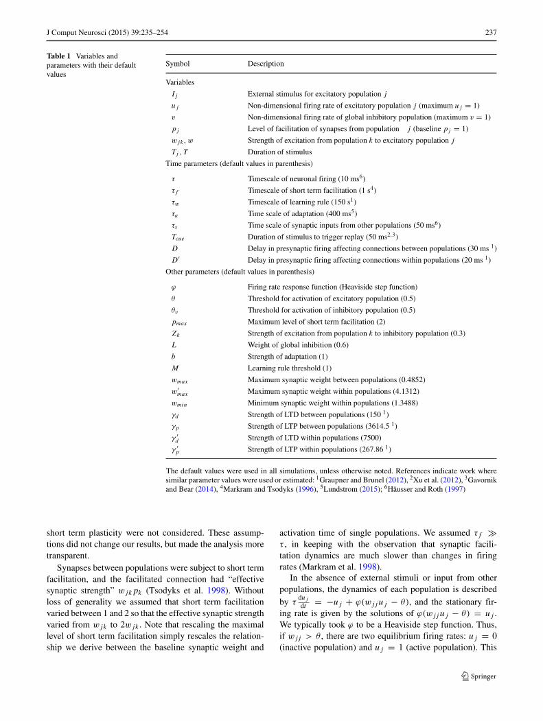
Table 1 Variables andparameters with their defaultvalues

Symbol Description

Variables

Ij External stimulus for excitatory population j

uj Non-dimensional firing rate of excitatory population j (maximum uj = 1)

v Non-dimensional firing rate of global inhibitory population (maximum v = 1)

pj Level of facilitation of synapses from population j (baseline pj = 1)

wjk, w Strength of excitation from population k to excitatory population j

Tj , T Duration of stimulus

Time parameters (default values in parenthesis)

τ Timescale of neuronal firing (10 ms6)

τf Timescale of short term facilitation (1 s4)

τw Timescale of learning rule (150 s1)

τa Time scale of adaptation (400 ms5)

τs Time scale of synaptic inputs from other populations (50 ms6)

Tcue Duration of stimulus to trigger replay (50 ms2,3)

D Delay in presynaptic firing affecting connections between populations (30 ms 1)

D′ Delay in presynaptic firing affecting connections within populations (20 ms 1)

Other parameters (default values in parenthesis)

ϕ Firing rate response function (Heaviside step function)

θ Threshold for activation of excitatory population (0.5)

θv Threshold for activation of inhibitory population (0.5)

pmax Maximum level of short term facilitation (2)

Zk Strength of excitation from population k to inhibitory population (0.3)

L Weight of global inhibition (0.6)

b Strength of adaptation (1)

M Learning rule threshold (1)

wmax Maximum synaptic weight between populations (0.4852)

w′max Maximum synaptic weight within populations (4.1312)

wmin Minimum synaptic weight within populations (1.3488)

γd Strength of LTD between populations (150 1)

γp Strength of LTP between populations (3614.5 1)

γ ′d Strength of LTD within populations (7500)

γ ′p Strength of LTP within populations (267.86 1)

The default values were used in all simulations, unless otherwise noted. References indicate work wheresimilar parameter values were used or estimated: 1Graupner and Brunel (2012), 2Xu et al. (2012), 3Gavornikand Bear (2014), 4Markram and Tsodyks (1996), 5Lundstrom (2015); 6Hausser and Roth (1997)

short term plasticity were not considered. These assump-tions did not change our results, but made the analysis moretransparent.

Synapses between populations were subject to short termfacilitation, and the facilitated connection had “effectivesynaptic strength” wjkpk (Tsodyks et al. 1998). Withoutloss of generality we assumed that short term facilitationvaried between 1 and 2 so that the effective synaptic strengthvaried from wjk to 2wjk . Note that rescaling the maximallevel of short term facilitation simply rescales the relation-ship we derive between the baseline synaptic weight and

activation time of single populations. We assumed τf �τ , in keeping with the observation that synaptic facili-tation dynamics are much slower than changes in firingrates (Markram et al. 1998).

In the absence of external stimuli or input from otherpopulations, the dynamics of each population is described

by τduj

dt= −uj + ϕ(wjjuj − θ), and the stationary fir-

ing rate is given by the solutions of ϕ(wjjuj − θ) = uj .We typically took ϕ to be a Heaviside step function. Thus,if wjj > θ , there are two equilibrium firing rates: uj = 0(inactive population) and uj = 1 (active population). This


assumption simplified the analysis, but was not necessaryfor our approach to work as shown in Section 4.2.

2.2 Rate-based long term plasticity

Connectivity between the populations in the network wassubject to long term potentiation (LTP) and long termdepression (LTD). Following experimental evidence (Blissand Lømo 1973; Dudek and Bear 1992; Markram andTsodyks 1996; Sjostrom et al. 2001), connections weremodulated using a rule based on pre- and post-synapticactivity with ‘soft’ bounds (Gerstner and Kistler 2002).

We made three main assumptions about the long termevolution of synaptic weight, w = wpre→post: (a) If thepresynaptic population activity was low (upre ≈ 0), thechange in synaptic weight was negligible (w(t) = 0); (b) Ifthe presynaptic population was highly active (upre ≈ 1) andthe postsynaptic population responded weakly (upost ≈ 0),then the synaptic weight decayed toward zero (w(t) ∝−w); and (c) If both populations had a high level of activ-ity (upost ≈ 1 and upre ≈ 1), then the synaptic weightincreased towards an upper bound (w(t) ∝ wmax − w).

Similar assumptions have been used in previous rate-based models of LTP/LTD (von der Malsburg 1973; Bienen-stock et al. 1982; Oja 1982; Miller 1994), and it has beenshown that calcium-based (Graupner and Brunel 2012)and spike-time dependent (Clopath et al. 2010; Gjorgjievaet al. 2011) plasticity rules can be reduced to such rate-based rules (Pfister and Gerstner 2006). Furthermore, thefact that pre-synaptic activity is necessary to initiate eitherLTP or LTD is supported by experimental observationsthat plasticity depends on calcium influx through NMDAreceptors (Malenka and Bear 2004). A simple differentialequation that implements these assumptions is

τw

dw

dt= −γd w upre(t − D)(M − upost (t))

+γp (wmax − w)upre(t − D)upost (t), (2)

where τw is the time scale, γd (γp) represents the strengthof LTD (LTP), D is a delay accounting for the time ittakes for the presynaptic firing rate to trigger plasticity pro-cesses, and M is a parameter that determines the thresholdand magnitude of LTD. We note that we initially modelonly the molecular processes that detect correlations in fir-ing rates, and thus set τw = 150s. We will later extendthis model to account for the longer timescales of synapticweight changes (Section 4.4).

Equation (2) describes a Hebbian rate-based plasticityrule with soft bounds involving only linear and quadraticdependences of the pre- and post-synaptic rates (Gerstnerand Kistler 2002). Temporal asymmetry that accounts forthe causal link between pre- and post-synaptic activity is

incorporated with a small delay in the dependence of pre-synaptic activity upre(t − D) (Gutig et al. 2003). Thislearning rule is a firing-rate version of the calcium-basedplasticity model proposed by (Graupner and Brunel 2012).

2.3 Encoding timing of event sequences

Our training protocol was based on several recent exper-iments that explored cortical learning in response tosequences of visual stimuli (Xu et al. 2012; Eagleman andDragoi 2012; Gavornik and Bear 2014). During a trainingtrial, an external stimulus Ij (t) activated one population at atime. Each individual stimulus could have a different dura-tion (Fig. 1b). We stimulated n populations, and enumeratedthem by order of stimulation; that is, population 1 was stim-ulated first, then population 2, and so on. This numbering isarbitrary, and the initial recurrent connections have no rela-tion to this order. We denote the duration of input j by Tj .All inputs stop at Ttot = T1 + T2 + . . . + Tn. A sequencewas presented m times.

Repeated training of the network described by Eq. (1)with a fixed sequence drove the synaptic weights wij

to equilibrium values. We assumed that during sequencepresentation, the amplitude of external stimuli Ij (t) wassufficiently strong to dominate the dynamics of the popula-tion rates, uj . Then, the activity of the populations duringtraining evolved according to:

τduj

dt= −uj + ϕ

(Ij (t) − θ

), j = 1, . . . , n,

τw

dwjk

dt= −γdwjkuk(t − D)(M − uj (t))

+γp(wmax − wjk)uk(t − D)uj (t), j �= k. (3)

Thus, the timing of population activations mimicked thetiming of the input sequence, i.e. the training stimulus.

2.3.1 Synaptic weights for consecutive activations

For simplicity, we begin by describing the case of twopopulations, N = 2, and we consider the threshold thatdetermines the level of LTD equal to 1, M = 1, so thatLTD is absent when the postsynaptic population is active(upost = 1). Suppose that I1(t) = IS on [0, T1] andI2(t) = −IH , and I2(t) = IS on [T1, T1 + T2] and I1(t) =−IH , where IS and IH are large enough so that Eq. (3) isvalid. The positive inputs with weight IS model feedforwardexcitation to cells tuned to the cue from upstream visualprocessing regions in thalamus. Negative inputs with weight−IH model strong effective feedforward inhibition to cor-tical cells that are not tuned to the present cue (Wang et al.2007; Haider et al. 2013). Representing the effect of feed-forward inhibition as static inputs simplified the model, anddid not affect our results.


time

sequence training

LTP LTD

time-codingrecurrent network

b

c

a

time (s)

firin

gra

te

0 1

timecue

before training

time (s)

firin

gra

te

0 1

timecue

after training

time (s)fi

ring

rate

0 1

1 2 3 4

arbitrary connectivity

sequence presentation

I1 I2 I3 I4

1 2 3 4

1 2 3 4

Fig. 1 The precise timing of training sequences is learned via longterm plasticity. Each stimulus in the sequence is represented by a dif-ferent shade. a. Before training, network connectivity is random, and acue does not trigger a sequential pattern of activity. b. During training,a sequence of events is presented repeatedly. Each event activates a cor-responding neural population for some amount of time, which is fixed

across presentations. Long term plasticity reshapes network architec-ture to encode the duration and order of these activations. c. Aftersufficient training, a cue triggers the pattern of activity evoked dur-ing the training period. Learned synaptic connectivity along with shortterm facilitation steer activity along the path carved by the trainingsequence (arrow width and contrast correspond to synaptic weight)

We assumed that Ti > D, Ti � τ , and τw � τ , sothat the stimulus was longer than the plasticity delay, andplasticity slower than the firing rate dynamics. Separationof timescales in Eq. (3) implies that uj ≈ ϕ(Ij (t) − θ), sothe firing rate of populations 1 and 2 is approximated byu1(t) ≈ 1 on [0, T1] and zero elsewhere, and u2(t) ≈ 1 on[T1, T1 + T2] and zero elsewhere (Fig. 2a). Hence, duringa training trial on a time interval [0, Ttot ], we obtain fromEq. (3) the following piecewise equation for the synapticweight, w21, in terms of the duration of the first stimulus,T1,

dw21

dt=

⎧⎪⎪⎪⎨

⎪⎪⎪⎩

0, t �∈ [D, T1 + D],− γd

τw

w21, t ∈ [D, T1],γp(wmax − w21)

τw

, t ∈ [T1, T1 + D].(4)

Note that we assumed that u1(t) = 0 for t < 0.Equation (4) allows the network to encode T1 using the

weight w21. Namely, solving Eq. (4) we obtain

w21(Ttot ) = w21(0)e−T1γd/τwe−(γp−γd )D/τw

+(1 − e−Dγp/τw )wmax,

which relates the synaptic weight at the end of a presenta-tion, w21(Ttot ), to the synaptic weight at the beginning ofthe presentation, w21(0) (Fig. 2a). Thus, there is a recursiverelation that relates the weight w21 at the end of the i + 1ststimulus to the weight at the end of the ith stimulus:

wi+121 = wi

21e−T1γd/τwe−(γp−γd )D/τw (5)

+(1 − e−Dγp/τw )wmax.

As long as γp > γd , the sequence (wi21) converges to

w∞21 := (1 − e−Dγp/τw )wmax

1 − e−T1γd/τwe−(γp−γd )D/τw, (6)

as seen in Fig. 2b. An equivalent expression also holds inthe case of an arbitrary number of populations.

The relative distance to the fixed point w∞21 is computed

by noting that (for T1 fixed)

|wi+121 − w∞

21 |/|wi21 − w∞

21 | = e−T1γd/τwe−(γp−γd )D/τw ,

from which we calculate

|wi21 − w∞

21 | ∝(e−T1γd/τwe−(γp−γd )D/τw

)i

.

Thus, the sequence converges exponentially with thenumber of training trials, i. The relative distance to the fixedpoint is proportional to e−mT1γd/τw , so the convergence isfaster for larger values of T1, as shown in Fig. 2c.

2.3.2 Synaptic weights of populations that are notco-activated

To compute the dynamics of w12, we note that during atraining trial on the time interval [0, Ttot ], the followingpiecewise equation governs the change in synaptic weight,

dw12

dt=

{0, t �∈ [T1 + D, T1 + T2 + D],

− γd

τw

w12, t ∈ [T1 + D, T1 + T2 + D],which can be solved explicitly to find

w12(Ttot ) = w12(0)e−T2γd/τw . (7)


We can therefore write a recursive equation for theweight after the i + 1st stimulus in terms of the weight afterthe ith stimulus

wi+112 = wi

12e−T2γd/τw ,

which converges to w∞12 = 0. Thus, w∞

jk = 0 for allpairs of populations (j, k) for which population j was notactivated immediately after population k during training.In total, sequential activation of the populations leads tothe strengthening only of the weights wj+1,j , while otherweights are weakened.

a

b

c

syna

ptic

str

engt

h w

21

Fig. 2 Encoding timing in synaptic weights. a. Synaptic connectionsevolve during training. When a presynaptic population (1) is activeand a postsynaptic population (2) is inactive, LTD reduces the synapticweight w21. When the populations (1 and 2) are co-active (overlap win-dow between dashed lines), LTP increases w21. Shortly after, globalinhibition inactivates the presynaptic population (1), so long term plas-ticity ceases (see Section 2). As in the text, wi

21 denotes the weight atthe end of the i-th trial. Arrow width and contrast correspond to synap-tic weights. b. After several training trials, the synaptic weight wi

21converges to a fixed point, w∞

21 , whose amplitude depends on the acti-vation time of the presynaptic population. c. Starting from the sameinitial value, w0

21(T1) = 0.25, the weight wi21(T1) converges to differ-

ent values, w∞21(T1), depending on the the training time, T1. Vertical

bar at T1=300 ms corresponds to the value used in (a) and (b)

2.4 Reactivation of trained networks

To examine how a sequence of event timings could beencoded by our network, the first neural population in thesequence was activated with a short cue. Typically, this cuewas of the form I1(t) = 1 for t ∈ [0, Tcue], I1(t) = 0 fort ∈ [Tcue, ∞), and Ij (t) = 0 for j �= 1 (Fig. 1c). Duringreplay, aside from the initial cue, the activity in the networkwas generated through recurrent connectivity.

We describe the case of two populations where the firstpopulation is cued, and remains active due to self-excitation(u1(t) ≈ 1), Fig. 3a. Since u2(0) = 0 and ϕ is the Heavisidestep function, the equations governing the dynamics of thesecond population are

τdu2

dt= −u2 + ϕ(w21p1 − θ),

p1(t) = pmax + (1 − pmax)e−t/τf . (8)

Thus, for population 2 to become active, w21p1(t) musthave reached θ (Fig. 3a). The time T between when u1

becomes active and u2 becomes active (“replay time”) couldbe controlled by the synaptic weight w21. Figure 3b showsthe effect of changing the synaptic weight: For very smallvalues of the baseline weight w21, the effective synap-tic strength w21p1(t) never reaches θ and activation doesnot occur. Increasing the baseline weight w21 causes morerapid activation of the second population, and for verylarge weights w21 the activation is immediate. The weightrequired for a presynaptic population to activate a postsy-naptic population after T units of time is given in closedform by

W(T ) := θ

pmax + (1 − pmax)e−T/τf

. (9)

Similarly, the inverse of this function,

T (w) := τf ln

(pmax − 1

pmax − θ/w

), (10)

gives the activation time as a function of the synaptic weight(Fig. 3c). Note that Eq. (10) is valid for θ/pmax < w < θ .If w ≤ θ/pmax , then activation of the next population doesnot occur. If w ≥ θ , activation is immediate.

To ensure the first population becomes inactive whenpopulation 2 becomes active, we assumed that global inhi-bition overcame the self excitation in the first population,w11+w12p2(T )−L−θ < 0. Also, for the second populationto remain active, we needed the self excitation plus the inputreceived from population 1 to be stronger than the globalinhibition; namely, w22+w21p1(T )−L−θ = w22−L > 0.These two inequalities are satisfied whenever w12 is smallenough and L < wjj < L + θ .


2.5 Matching training parameters to reactivationparameters

To guarantee that long term plasticity leads to a properencoding of event times, it is necessary that the learnedweight, w∞

21 given by Eq. (6), matches the desired weightW(T ) given by Eq. (9). This can be achieved by equatingthe right hand sides of Eqs. (6) and (9), so that

(1 − e−Dγp/τw )wmax

1 − e−T γd/τwe−(γp−γd )D/τw

= θ/pmax

1 + e−T/τf (1 − pmax)/pmax

. (11)

Equation (11) can be satisfied for all values of T bychoosing parameters that satisfy

τw/γd = τf ,

(1 − e−Dγp/τw )wmax = θ/pmax,

e−(γp−γd )D/τw = (pmax − 1)/pmax. (12)

Since there are fewer equations than model parameters,there is a multi-dimensional manifold of parameters forwhich Eq. (11) holds for all T . For instance, for fixed short-term facilitation parameters θ , pmax , and τf and restrictingspecific plasticity parameters τw and D, the appropriate γd ,γp, and wmax can be determined using Eq. (12). This is howwe determined the parameters in Figs. 4 and 5.

The first relationship in Eq. (12) states τw/γd = τf , relat-ing the timescale of short term facilitation to the timescaleof long term plasticity through the depression amplitudeparameter γd . It is important to note that this does not meanthat the timescales of the two processes need to match. Asstated in Table 1, following experimental data (Markramand Tsodyks 1996; Alberini 2009; Graupner and Brunel2012; Nabavi et al. 2014), we chose τf = 1s and τw = 150sfor our simulations. This implies that γd = 150, for trainingto yield the correct weights.

As we demonstrate in Supplementary Fig. 1, perturbingparameters of the long term plasticity process away fromthe optimal relationships determined by Eq. (12) does alterthe learned time. The relative size of errors depends onthe parameters we perturb, and we find the model is mostsensitive to perturbation of wmax . Perturbations of otherparameters such as γp and γd lead to to errors roughly equalin to the magnitude of the parameter perturbation (e.g., a5 % perturbation of γd leads to a 5 % change in Treplay).

For more detailed models, the analog of Eq. (12) ismore cumbersome or impossible to obtain explicitly. Specif-ically, when we incorporated noise into our models in theSection 4.1 and considered spike rate adaptation in theSection 4.3, we had to use an alternative approach. Wefound it was always possible to numerically approximateparameter sets that allowed a correspondence between the

trained and desired weight for all possible event times. Asimple way of finding such parameters was the method ofleast squares: We selected a range of stimulus durations,e.g. [.1s, 3s], and sampled timings from it, e.g. S ={.1s, .2s, .3s, . . . , 3s}. For each T ∈ S we computed thelearned weight, wlearned(T , pars), where “pars” denotes thelist of parameters to be determined. Then, we computedthe replay time, Treplay(wlearned(T , pars)). We defined the“cost” function

J (pars) =∑

T ∈S

(Treplay(wlearned(T , pars)) − T

)2,

and the desired parameters were given by

parsbest := argminpars{J (pars)}. (13)

This approach was successful for different models and train-ing protocols, and allowed us to find a working set ofparameters for models that included noise or different slowprocesses for tracking time.

Equation (13) can also be interpreted as a learning rulefor the network parameters. Starting with arbitrary networkparameter values, any update mechanism that decreases thecost function J will result in a network that can accuratelyreplay learned sequence times.

2.6 Training and replay simulations

To test our model, we trained the network with a sequence offour events. Each event in the sequence corresponded to theactivation of a single neuronal population (Fig. 4a). Sinceeach population was inactivated (received strong negativeinput) when the subsequent populations became active, wealso assumed that an additional, final population inactivatedthe population responding to the last event (additional pop-ulation not shown in the figure). Input during training wasstrong enough so that activation of the different populationswas only determined by the external stimulus overridingglobal inhibition and recurrent excitation.

During reactivation, the recurrent connections wereassumed fixed. This assumption can be relaxed if weassume that LTP/LTD are not immediate, but occur on longtimescales, as in the Section 4.4.

We used m = 10 training trials, the default parametervalues in Table 1, and estimated γd , γp, and wmax usingEq. (12). After the training trials were finished, we cuedthe first population in the sequence, using I1(t) = 1 fort ∈ [0, Tcue] and Ij (t) = 0 otherwise. We also started withthis set of weights, and retrained the network with a novelsequence of stimuli.


1 2

00

1

synapse

T

T0

a

w 21p 1(t

)w 21p 1(t)

b

1

2

imm

edia

teac

tivat

ion

timedactivation

noac

tivat

ion

facilitatedsynapse

pmax

eec

tive

stre

ngth

w21p

1

firin

gra

te

time

timeactivation

time

0

c

no activation

wA wB

immediate activation

TA activation time (s)TBsyna

ptic

str

engt

h

1

activ

atio

n tim

e (s

)

synaptic strengthwC

pmax

wAwB

wC

TB

TA

vglobal

inhibition

Fig. 3 Replay timing. a. Once population 1 is activated, the weightof the connection to population 2 slowly increases, eventually becom-ing strong enough to activate this next population in the sequence. b.Activation time T := T1 decreases monotonically with the weight ofthe connection between the populations, w := w21. For weak connec-tions (wA = 0.33) the synapses must be strongly facilitated to reachthe threshold. If the weight is larger (wB = 0.42) threshold is reachedmore quickly. For weights above the threshold (wC = 0.58 > θ ),population 2 is activated immediately. Activation will not occur whenthe synaptic connection is smaller than θ/pmax . c. Activation time T1plotted against the initial synaptic weight, w21. For intermediate val-ues of w21, the relationship is given by Eq. (10). Here wA, wB, wC

and T A, T B are the same as in panel (b)

3 Results

3.1 Training

We explore sequence learning in a network model of neu-ral populations, where each population is activated by adistinct stimulus or event. The initial connectivity betweenthe populations is random (Fig. 1a). To make our analy-sis more transparent, we initially consider a deterministicfiring rate model, Eq. (1). Each individual neural popula-tion is bistable, having both a low activity state and a highactivity state that is maintained through recurrent excitation.Our results also hold for more biologically plausible firingrate response functions and are robust to noise (Sections 4.1and 4.2).

To train the network, we stimulated populations in afixed order, similar to the training paradigm used by (Xu

b

Fig. 4 Learning and replaying event sequences. a. As the numberof training trials increases, a cue results in an activation pattern thatapproaches that evoked by the training sequence. Network architec-ture is reshaped to encode the precise duration and order of events inthe sequence, with stronger feedforward connections corresponding toshorter events (thicker and darker arrows correspond to larger synap-tic weights). All weights are learned independently and training moststrongly affects the weights wi→i+1. The event times were T1 = 0.6,T2 = 0.4, T3 = 1, and T4 = 0.5 seconds, with indices denoting thepopulation stimulated. The initial weights were w0

ij = 0.025 for i �= j

and wii = 1. b. The network in the last row of (a) was retrained withthe sequence T1 = 0.4, T4 = 1, T3 = 0.6, and T2 = 0.8, presented inthe order 1-4-3-2. After 10 training trials, the cued network replays thenew training sequence

et al. 2012; Eagleman and Dragoi 2012; Gavornik andBear 2014). The duration of each event in the trainingsequence was arbitrary (Fig. 1b), and each stimulus in thesequence drove a single neural population. Synaptic connec-tions between populations were plastic. To keep the modeltractable, population activity was assumed to immediatelyimpact the weight of synaptic connections. Our results alsoextend to a model with synaptic weights changing on longertimescales (Section 4.4).

Changes in the network’s synaptic weights depended onthe firing rates of the pre- and post-synaptic populations(Bliss and Lømo 1973; Bienenstock et al. 1982; Dudek andBear 1992; Markram and Tsodyks 1996; Sjostrom et al.2001). When a presynaptic population was active, either:(a) synapses were potentiated (LTP) if the postsynapticpopulation was subsequently active or (b) synapses weredepressed (LTD) if the postsynaptic population was not acti-vated soon after (Section 2). Such rate-based plasticity rulescan be derived from spike time dependent plasticity rules


(Kempter et al. 1999; Pfister and Gerstner 2006; Clopathet al. 2010).

To demonstrate how the timing of events can be encodedin the network architecture, we start with two populations(Fig. 2). During training, population 1 was stimulated for T1

seconds followed by stimulation of population 2 (Fig. 2a).The stimulus was strong enough to dominate the dynam-ics of the population responses (Section 2). While the firststimulus was present, population 1 was active and LTDdominated, decreasing the synaptic weight, w21, from popu-lation 1 to population 2. After T1 seconds, the first stimulusended, and the second population was activated. However,population 1 did not become inactive instantaneously, andfor some time both population 1 and 2 were active. Duringthis overlap window, LTP dominated leading to an increasein synaptic weight w21. Shortly after population 1 becameinactive, changes in the weight w21 ceased, as plasticity onlyoccurs when the presynaptic population is active. The ini-tial and final synaptic weights (w0

21 and w121, respectively)

can be computed in closed form (Section 2). Repeatedpresentations of the training sequence lead to exponen-tial convergence of the synaptic weights, wi

21 (weight afterith training trial), to a fixed value (Fig. 2b). On the otherhand, the synaptic weight w12 is weakened during eachtrial because the presynaptic population 2 is always activeafter the postsynaptic population 1 (Section 2). In thecase of N populations, each weight wk+1,k will convergeto a nonzero value associated with Tk , whereas all otherweights will become negligible during replay. Thus, thenetwork’s structure eventually encodes the order of thesequence.

The duration of activation in population 1, T1, determinesthe equilibrium value of the synaptic weight from popula-tion 1 to population 2, w∞

21 (Section 2). For larger valuesof T1, LTD lasts longer, weakening w21 (Fig. 2c). Hence,weaker synapses are associated with longer event times.Reciprocally, weaker synapses lead to longer activationtimes during replay (Section 3.2).

As the stimulus duration, T1, determines the asymptoticsynaptic weight, w∞

21(T1), there is a mapping T1 → w∞21(T1)

from stimulus times to the resulting weights. Event timingis thus encoded in the asymptotic values of the synapticweights.

3.2 A slow process allows precise temporal replay

We next describe how the trained network replayssequences. The presence of a slow process, which weassumed here to be short term facilitation, is critical. Thisslow process tracks time by ramping up until reaching apre-determined threshold. An event’s duration correspondsto the amount of time it takes the slow variable to reachthis threshold. Such ramping models have previously been

a b

c d

e f

g h

i j

Fig. 5 Effect of noise on learning and replay. The effects of addingnormally distributed noise to (a) the observed training time T := T1(duration of first stimulus) and (b) neural activity uj . Starting from auniform distribution (p(w0

21)) and considering either a noise level of(c) σ = 0.1〈T 〉 in the training time or (d) σ = 0.03 in neural activity,the probability density function p(wi

21) converges to the steady statedistribution p(w∞

21) (this is nearly identical to w1021). Increasing noise

in the training times (e) or neural activity (f) widens the steady statedistribution p(w∞

21). The mean (dashed lines) and standard deviation(shaded region) of w∞

21(T ) are pictured in panel (g) when noise withstandard deviation σ = 0.20〈T 〉 is added to the training times and(h) when noise with standard deviation σ = 0.05 is added to neuralactivity. As in Fig. 2c, the mean learned weight E

[w∞

21

]decreases

with 〈T 〉. The mean of the replay time (dashed line) and its standarddeviation (shaded region) are plotted against 〈T 〉 for the case of (i)noise in training times and (j) noise in neural populations. As the meantraining time 〈T 〉 increases, so does the effect of noise on replay time(dashed line and surrounding shading), Treplay (solid grey lines showthe diagonal line Treplay = T ). For a suitable choice of “corrected-for-noise” parameters, the effect of noise on the mean replay time canbe removed (dotted line and surrounding shading). Insets in (i) and (j)show the root-mean-square error in replay time as a function of trainingtime for the parameters obtained from the deterministic case (dashed)and corrected-for-noise parameters (dotted)


proposed as mechanisms for time-keeping (Buonomano2000; Durstewitz 2003; Reutimann et al. 2004; Karmarkarand Buonomano 2007; Gavornik et al. 2009). Without sucha slow process, cued activity would result in a sequencereplayed in the proper order, but information about eventtiming would be lost.

For simplicity we focus on two populations, where activ-ity of the first population represents a timed event (Fig. 3).To simplify the analysis, we also assumed that synapticweights are fixed during replay. This assumption is notessential (Section 4.4). After population 1 is activated witha brief cue, it remains active due to recurrent excitation(Section 2). Meanwhile, short term facilitation leads to anincrease in the effective synaptic strength from population 1to population 2. Population 2 becomes active when the inputfrom population 1 crosses an activation threshold (Fig. 3a).When both populations are simultaneously active, a suffi-cient amount of global inhibition is recruited to shut offthe first population, which receives only weak input frompopulation 2. The second population then remains active,as the strong excitatory input from the first population andrecurrent excitation exceed the global inhibition.

The weight of the connection from population 1 to pop-ulation 2 determines how long it takes to extinguish theactivity in the first population (Fig. 3b). This synapticweight therefore encodes the time of this first and onlyevent. We demonstrate how this principle extends to multi-ple event sequences in the Section 3.3. The time until theactivation of the second population decreases as the initialsynaptic weight increases, since a shorter time is neededfor facilitation to drive the input from population 1 to theactivation threshold (Fig. 3c). Note that when the baselinesynaptic weight is too weak, synaptic facilitation saturatesbefore the effective weight reaches the activation threshold,and the subsequent population is never activated. When thebaseline synaptic weight is above the activation threshold,the subsequent population is activated instantaneously.

Therefore, long term plasticity allows for encoding anevent time in the weight of the connections between popula-tions in the network, while short term facilitation is crucialfor replaying the events with the correct timing. The timeof activation during cued replay will match the timing inthe training sequence as long as training drives the synap-tic weights to the value that corresponds to the appropriateevent time (Fig. 2c):

W(T ) := θ

pmax + (1 − pmax)e−T/τf

. (14)

Here pmax and τf are the strength and timescale of facili-tation (Section 2). An exact match can be obtained by tuningparameters of the long term plasticity process so the learnedweight matches Eq. (14). There is a wide range of parame-ters for which the match occurs (Section 2). We next show

that the timing and order of sequences containing multipleevents can be learned in a similar way.

3.3 Repeated presentation of the same sequenceproduces a time-coding feedforward network

To demonstrate that the mechanism we discussed extendseasily to arbitrary sequences, we consider a concretesequence of four stimuli. We set the parameters of themodel so that the training parameters match the reactivationparameters (Eqs. (11–13) in Section 2).

We trained the network using the event sequence 1-2-3-4 (Fig. 4a), repeatedly stimulating the correspondingpopulations in succession. The duration of each populationactivation was fixed across trials. After each training trial,we cued the network by stimulating the first population for ashort period of time to trigger replay (Section 2). Thus, afterpopulation 1 is activated the subsequent activity is governedby the network’s architecture. As our theory suggests, thecue-evoked network activity pattern converged with trainingto the stimulus-driven activity pattern (Fig. 4a).

We further tested whether the same network can beretrained to encode a sequence with a different order ofactivation (1-4-3-2) with different event times. Figure 4bshows that after training, the network encodes and replaysthe new training sequence. Thus, the network architecturecan be shaped by long term plasticity to encode an arbitrarysequence of event times, and a brief cue evokes the replayof the learned sequence.

4 Extensions

4.1 Effects of noise

To examine the impact of the many sources of variabil-ity in the nervous system (Faisal et al. 2008), we exploredhow noise impacts the training and recall of event sequencesin our model. We examined the effects of stochastic eventtimes as well as noise in the network activity and the impactsuch variability has on the training and recall of eventsequences. For simplicity, we focus on the case of two pop-ulations, but our results extend to sequences of arbitrary length.

To examine the impact of variability in stimulus dura-tions, we sampled T := T1 from a normal distribution(Fig. 5a) with mean 〈T 〉 = 0.5 and variance σ 2 =(cv 〈T 〉)2, where cv = 0.1 is the coefficient of variation.Randomness in the observed event time may be due tovariability in the external world, temporal limitations onsensation (Butts et al. 2007), or other observational errors(Ma et al. 2006). We selected w0 := w0

21 from a uniformdistribution on [θ/pmax, θ ]. Figure 5c shows the evolutionof the probability density function of wm as m increases


(using 20,000 initial w0’s). The synaptic weight after theith training, wi

21, is described by a probability density func-tion that converges in the limit of many training trials.The peak (mode) of this distribution is the most likely valueof the learned synaptic weight after repeated presentation ofthe sequence (Fig. 5c). The variance of the learned synap-tic weight, w∞

21, increases monotonically with the variancein the training time, σ 2 (Fig. 5e). We explored the effectsof different levels of noise, σ = 0.1〈T 〉, 0.15〈T 〉, 0.2〈T 〉(20,000 initial conditions for each), and estimated the prob-ability density function of w∞ numerically (Fig. 5e). Tosee the effect of noise for different mean training dura-tions, we estimated the mean and standard deviation ofw∞ for 〈T 〉 ranging from 0.1s to 2s (step size of 0.05s)using σ = 0.2〈T 〉 (5,000 initial conditions for each)(Fig. 5g). For a distribution of training times with mean〈T1〉 we obtain a unimodal probability density for theweights, p(w21). As in the noise-free case, the mode ofthis weight distribution decreases with 〈T1〉. Note that theparameters given by Eq. (12), which guarantee that train-ing and replay time coincide in the deterministic case, maynot be the same as the parameters needed when noise ispresent. We numerically estimated these parameters usingEq. (13) so the mean training time and mean replay timecoincided.

To determine how noise affects activation timing dur-ing sequence replay, we compared the mean event timewith the mean replayed time. Since the network parametersused here are those obtained from the noise-free case, weexpect that replay times are biased. Indeed, Fig. 5i showsthat activity during replay is slightly longer on averagethan the corresponding training event. Also, the variancein activation during replay increases with the mean dura-tion of the trained event. We can search numerically andfind a family of parameters for which the mean activationtime during replay and training coincide (Fig. 5i). Error andthe coefficient of variation (CV) in replay time increaseswith the duration of the trained time (Fig. 5i, shaded regionand inset).

We also estimated the mean learned synaptic weight andits variance analytically: Since the synaptic weight, wi

21,evolves according to the rule

wi+121 = wi

21A(T i

)+ C,

where A(T ) := e−T γd/τwe−(γp−γd )D/τw and C := (1 −e−Dγp/τw )wmax , we obtain

E[wi+1

21

]= E

[wi

21A(T i)]

+ C.

Since wi21 only depends on T j for j < i, it follows that

wi21 and A(T i) are independent random variables; then,

E[wi+1

21

]= E

[wi

21

]E

[A(T i)

]+ C,

and by taking the limit i → ∞ and solving forlimi→∞ E

[wi

21

]we find

μw := limi→∞ E

[wi

21

]= C

1 − μA

,

where μA := E[A(T i)

]. Squaring wi+1

21 = wi21A(T i) + C

gives

(wi+1)2 = (wi)2A2(T i) + C2 + 2wi21A(T i)C,

and then it similarly follows that

σ 2w : = lim

i→∞

(E

[(wi

21)2]

− E[wi

21

]2)

= C2σ 2A

(1 − μA)2(1 − σ 2A − μ2

A),

where σ 2A := E

[A(T i)2

] − E[A(T i)

]2. To quantify the

average error, we computed numerically the mean and thestandard deviation of the replay time (Fig. 5i). The root-mean-square error (RMSE) was computed by

RMSE(〈T 〉) :=√

E[(〈T 〉 − Treplay)2

],

where the expected value is taken over the replay time,Treplay . The coefficient of variation (CV) was computed by

CV (〈T 〉) :=√

V ar(Treplay)

〈Treplay〉 .

To introduce neural noise (Fig. 5b), we added white noiseto the rate equations of the populations during training andreplay so that

duj = 1

τ

[−uj + ϕ(Ij (t) + Ij,syn − θ

)]dt + σdξj ,

where dξj is a standard white noise process with varianceσ 2. The analysis of the effect of noise in population activ-ity is similar to the analysis performed on stimulus durationnoise, the only difference being that the noise level wasσ = 0.03 in panel Fig. 5d, σ = 0.03, 0.05, 0.06 in panelFig. 5f, and σ = 0.05 in panels Fig. 5h and j. After repeatedpresentation of a sequence, the distribution of the learnedsynaptic weights converged (Fig. 5d). The variance of thesynaptic weight increased monotonically with the varianceof the noise (Fig. 5f), and the mean weight decreased mono-tonically with the event time (Fig. 5h). Since we used theparameters found from the noise-free case, we expect somebias in replay time. After training, the replayed event timesare shorter than the corresponding events in the trainingsequence (Fig. 5j), and the effect is much more signifi-cant than the lengthening of times due to observation noise.This systematic bias in the replayed time error is due tothe saturating nature of the time-tracking process, shortterm facilitation (Markram et al. 1998). Input to the sec-ond population remains close to threshold for longer periodsof time for longer trained times, leading to more frequent


a b

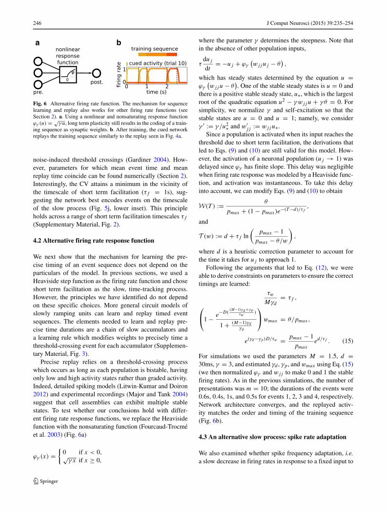
Fig. 6 Alternative firing rate function. The mechanism for sequencelearning and replay also works for other firing rate functions (seeSection 2). a. Using a nonlinear and nonsaturating response functionϕγ (u) = √

γ u, long term plasticity still results in the coding of a train-ing sequence as synaptic weights. b. After training, the cued networkreplays the training sequence similarly to the replay seen in Fig. 4a.

noise-induced threshold crossings (Gardiner 2004). How-ever, parameters for which mean event time and meanreplay time coincide can be found numerically (Section 2).Interestingly, the CV attains a minimum in the vicinity ofthe timescale of short term facilitation (τf = 1s), sug-gesting the network best encodes events on the timescaleof the slow process (Fig. 5j, lower inset). This principleholds across a range of short term facilitation timescales τf

(Supplementary Material, Fig. 2).

4.2 Alternative firing rate response function

We next show that the mechanism for learning the pre-cise timing of an event sequence does not depend on theparticulars of the model. In previous sections, we used aHeaviside step function as the firing rate function and choseshort term facilitation as the slow, time-tracking process.However, the principles we have identified do not dependon these specific choices. More general circuit models ofslowly ramping units can learn and replay timed eventsequences. The elements needed to learn and replay pre-cise time durations are a chain of slow accumulators anda learning rule which modifies weights to precisely time athreshold-crossing event for each accumulator (Supplemen-tary Material, Fig. 3).

Precise replay relies on a threshold-crossing processwhich occurs as long as each population is bistable, havingonly low and high activity states rather than graded activity.Indeed, detailed spiking models (Litwin-Kumar and Doiron2012) and experimental recordings (Major and Tank 2004)suggest that cell assemblies can exhibit multiple stablestates. To test whether our conclusions hold with differ-ent firing rate response functions, we replace the Heavisidefunction with the nonsaturating function (Fourcaud-Trocmeet al. 2003) (Fig. 6a)

ϕγ (x) ={

0 if x < 0,√γ x if x ≥ 0,

where the parameter γ determines the steepness. Note thatin the absence of other population inputs,

τduj

dt= −uj + ϕγ

(wjjuj − θ

),

which has steady states determined by the equation u =ϕγ

(wjju − θ

). One of the stable steady states is u = 0 and

there is a positive stable steady state, u∗, which is the largestroot of the quadratic equation u2 − γwjju + γ θ = 0. Forsimplicity, we normalize γ and self-excitation so that thestable states are u = 0 and u = 1; namely, we considerγ ′ := γ /u2∗ and w′

jj := wjju∗.Since a population is activated when its input reaches the

threshold due to short term facilitation, the derivations thatled to Eqs. (9) and (10) are still valid for this model. How-ever, the activation of a neuronal population (uj → 1) wasdelayed since ϕγ has finite slope. This delay was negligiblewhen firing rate response was modeled by a Heaviside func-tion, and activation was instantaneous. To take this delayinto account, we can modify Eqs. (9) and (10) to obtain

W(T ) := θ

pmax + (1 − pmax)e−(T −d)/τf

,

and

T (w) := d + τf ln

(pmax − 1

pmax − θ/w

),

where d is a heuristic correction parameter to account forthe time it takes for uj to approach 1.

Following the arguments that led to Eq. (12), we wereable to derive constraints on parameters to ensure the correcttimings are learned:

τw

Mγd

= τf ,

⎛

⎝1 − e−D(

(M−1)γd+γpτw

)

1 + (M−1)γd

γp

⎞

⎠ wmax = θ/pmax,

e(γd−γp)D/τw = pmax − 1

pmax

ed/τf . (15)

For simulations we used the parameters M = 1.5, d =30ms, γ = 3, and estimated γd , γp, and wmax using Eq. (15)(we then normalized ϕγ and wjj to make 0 and 1 the stablefiring rates). As in the previous simulations, the number ofpresentations was m = 10; the durations of the events were0.6s, 0.4s, 1s, and 0.5s for events 1, 2, 3 and 4, respectively.Network architecture converges, and the replayed activ-ity matches the order and timing of the training sequence(Fig. 6b).

4.3 An alternative slow process: spike rate adaptation

We also examined whether spike frequency adaptation, i.e.a slow decrease in firing rates in response to a fixed input to


a neural population, can play the role of a slow, time track-ing process (Benda and Herz 2003), instead of short termfacilitation. In contrast to the case of short term facilitation,adaptation causes the effective input from one population todecrease over time.

In this case population activity was modeled by

τduj

dt= −uj + ϕ(wjjuj + sj − θ − Lv − aj ),

τa

daj

dt= −aj + buj ,

τs

dsj

dt= −sj +

N∑

k �=j

wjkuk,

τdv

dt= −v + ϕ

(N∑

k=1

Zkuk − θv

)

,

where aj denotes the adaptation level of population j , τa isthe time scale of adaptation, and b is the adaptation strength.Feedback between populations was assumed to be slowerthan feedback within a population; thus, the total inputfor population j was split into self-excitation (wjjuj ), andsynaptic inputs from other populations (sj ) which evolvedon the time scale τs . Note that in the limit τs → 0, synapsesare instantaneous.

For a suitable choice of parameters, global inhibitiontracks activity faster than excitation between populations.Then, when a population becomes inactive due to adap-tation, the level of global inhibition decreases, allowingsubsequent populations to become active. This means theweight of self excitation can encode timing. Thus, in thissetup we modeled long term plasticity within a populationas well. The learning rule for wjj was analogous to wjk withthe additional assumption that since wjj represented thesynaptic weight within a population, it could not decreasebelow a certain value wmin. Also, the parameters for longterm plasticity within a population are allowed to be dif-ferent from the parameters for long term plasticity betweenpopulations.

The learning rule was then

τw

dwjj

dt= −γ ′

d(wjj − wmin)uj (t − D′)(1 − uj (t))

−γ ′p(wjj − w′

max)uj (t − D′)uj (t).

When the population was activated (u1(t) ≈ 1) fort ∈ [0, T1] (Fig. 7a), the changes in the weight w11 weregoverned by the piecewise differential equation

dw11

dt=

⎧⎪⎪⎪⎪⎨

⎪⎪⎪⎪⎩

0, t �∈ [D′, T1 + D′]γ ′p

τw

(w′max − w11) t ∈ [D′, T1]

− γ ′d

τw

(w11 − wmin) t ∈ [T1, T1 + D′].

The following equation relates the synaptic weight at theend of a presentation, w11(Ttot ), to the synaptic weight atthe beginning of the presentation, w11(0):

w11(Ttot ) = w11(0)e−T1γ′p/τwe(γ ′

p−γ ′d )D′/τw

+w′maxe

−D′γ ′d/τw (1 − e−(T1−D′)γ ′

p/τw )

+wmin(1 − e−D′γ ′d/τw ).

This recurrence relation between the weight at the i + 1ststimulus, wi+1

11 , and the weight at the ith stimulus, wi11,

implies that wi11 converges to the limit (Fig. 7b)

w∞11 = w′

maxe−D′γ ′

d/τw (1 − e−(T1−D′)γ ′p/τw )

1 − e−T1γ′p/τwe(γ ′


+ wmin(1 − e−D′γ ′d/τw )

1 − e−T1γ′p/τwe(γ ′


.

Thus, for each stimulus duration a unique synaptic weightis learned. Also, as shown in previous sections, w21 willconverge to a fixed value and w12 is weakened. Note thatin this case timing will be encoded as the weight of self-excitation, and the order will be encoded as the weightsbetween populations.

During replay a cue activates population 1, u1 = 1, andwe obtain τ

du1dt

= −u1+ϕ(w11−θ−a−L), τada1dt

= −a+b.Population 1 will become inactive (u1 ≈ 0) when w11 −a1(t) decreases to θ + L. Then, the next population willbecome active due to the decrease in global inhibition andthe remaining feedback from the first population due to theslower dynamics of feedback between populations (Fig. 7c).

The precise time of activation can be controlled by tuningthe synaptic weight w11. Furthermore, since the activationtime satisfies w11 − a1(T ) = θ + L, we have a formula thatrelates the synaptic weight to the activation time (Fig. 7d)

w11 = W(T ) := θ + L + b(1 − e−T/τa ).

When self excitation is too strong, adaptation will notaffect the activity of the first population and deactivationwill never occur. On the other hand, when self excitation istoo weak, activation is not sustained and the population willbe shut off immediately. To guarantee correct time codingand decoding, w∞

11(T ) and W(T ) had to be approximatelyequal for all T . The appropriate parameters could not befound in closed form, so we again resorted to finding themnumerically using Eq. (13).

For simulations we used the parameters Zk = 0.6, L =0.8, γp = 3750, γd = 100, γ ′

p = 267.86, γ ′d = 7500,

wmax = 1.5, w′max = 4.1312, and wmin = 1.3488. As in

the previous simulations, the number of presentations wasm = 10; the duration of the events were 0.6s, 0.4s, 1s, and0.5s for events 1, 2, 3 and 4, respectively.

This idea generalizes to any number of events and pop-ulations. Timing is encoded in the weight of the excitatoryself-connections within a population, while sequence order


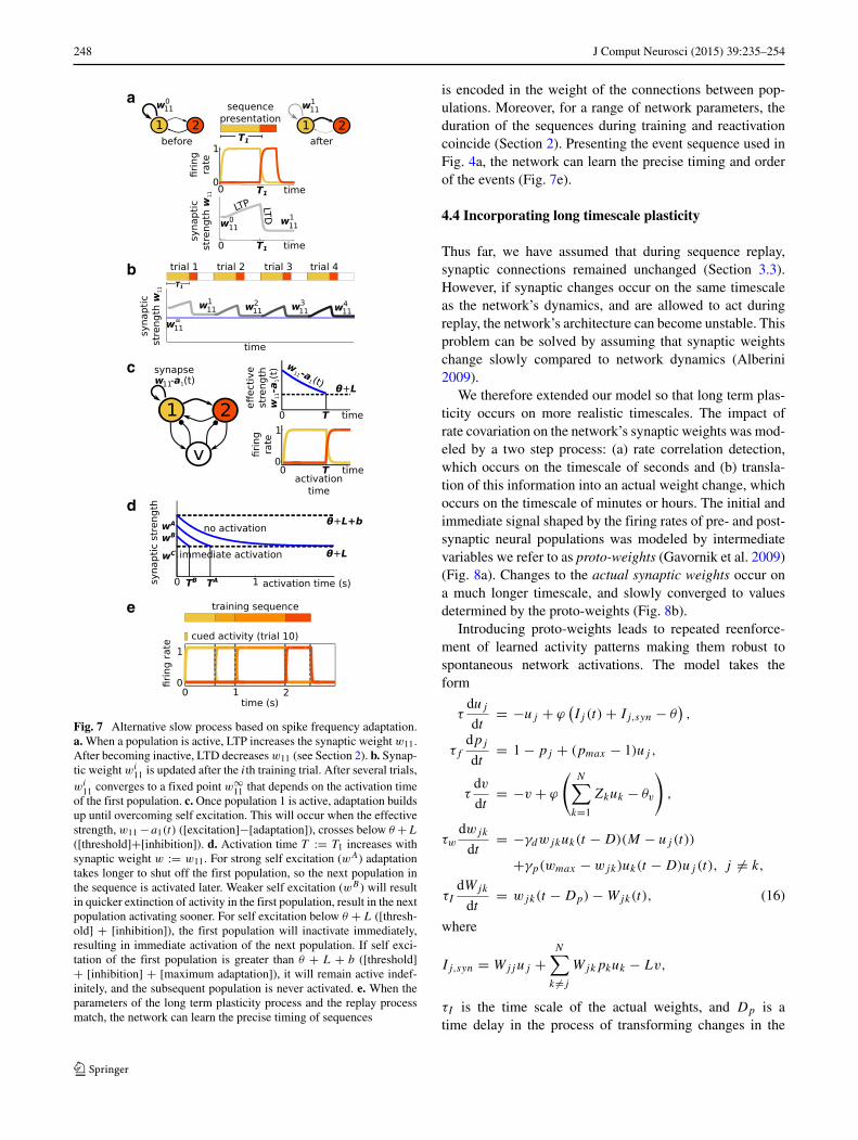
Fig. 7 Alternative slow process based on spike frequency adaptation.a. When a population is active, LTP increases the synaptic weight w11.After becoming inactive, LTD decreases w11 (see Section 2). b. Synap-tic weight wi

11 is updated after the ith training trial. After several trials,wi

11 converges to a fixed point w∞11 that depends on the activation time

of the first population. c. Once population 1 is active, adaptation buildsup until overcoming self excitation. This will occur when the effectivestrength, w11 −a1(t) ([excitation]−[adaptation]), crosses below θ +L

([threshold]+[inhibition]). d. Activation time T := T1 increases withsynaptic weight w := w11. For strong self excitation (wA) adaptationtakes longer to shut off the first population, so the next population inthe sequence is activated later. Weaker self excitation (wB ) will resultin quicker extinction of activity in the first population, result in the nextpopulation activating sooner. For self excitation below θ + L ([thresh-old] + [inhibition]), the first population will inactivate immediately,resulting in immediate activation of the next population. If self exci-tation of the first population is greater than θ + L + b ([threshold]+ [inhibition] + [maximum adaptation]), it will remain active indef-initely, and the subsequent population is never activated. e. When theparameters of the long term plasticity process and the replay processmatch, the network can learn the precise timing of sequences

is encoded in the weight of the connections between pop-ulations. Moreover, for a range of network parameters, theduration of the sequences during training and reactivationcoincide (Section 2). Presenting the event sequence used inFig. 4a, the network can learn the precise timing and orderof the events (Fig. 7e).

4.4 Incorporating long timescale plasticity

Thus far, we have assumed that during sequence replay,synaptic connections remained unchanged (Section 3.3).However, if synaptic changes occur on the same timescaleas the network’s dynamics, and are allowed to act duringreplay, the network’s architecture can become unstable. Thisproblem can be solved by assuming that synaptic weightschange slowly compared to network dynamics (Alberini2009).

We therefore extended our model so that long term plas-ticity occurs on more realistic timescales. The impact ofrate covariation on the network’s synaptic weights was mod-eled by a two step process: (a) rate correlation detection,which occurs on the timescale of seconds and (b) transla-tion of this information into an actual weight change, whichoccurs on the timescale of minutes or hours. The initial andimmediate signal shaped by the firing rates of pre- and post-synaptic neural populations was modeled by intermediatevariables we refer to as proto-weights (Gavornik et al. 2009)(Fig. 8a). Changes to the actual synaptic weights occur ona much longer timescale, and slowly converged to valuesdetermined by the proto-weights (Fig. 8b).

Introducing proto-weights leads to repeated reenforce-ment of learned activity patterns making them robust tospontaneous network activations. The model takes theform

τduj

dt= −uj + ϕ

(Ij (t) + Ij,syn − θ

),

τf

dpj

dt= 1 − pj + (pmax − 1)uj ,

τdv

dt= −v + ϕ

(N∑

k=1

Zkuk − θv

)

,

τw

dwjk

dt= −γdwjkuk(t − D)(M − uj (t))

+γp(wmax − wjk)uk(t − D)uj (t), j �= k,

τI

dWjk

dt= wjk(t − Dp) − Wjk(t), (16)

where

Ij,syn = Wjjuj +N∑

k �=j

Wjkpkuk − Lv,

τI is the time scale of the actual weights, and Dp is atime delay in the process of transforming changes in the


firin

gra

tesy

napt

icst

reng

th

0

1

proto-weight

0 5 time (s)

actual weight

proto-weight actual weight

30 time (min)

syna

ptic

stre

ngth

a

b

Fig. 8 A two-stage learning rule. a. Proto-weights track the signaledchange to synaptic connectivity brought about by firing rate covari-ance. Actual weights evolve on a slower time scale and hence do nottrack changes in the proto-weights immediately. b. Actual synapticweights approach proto-weight values on a longer timescale, so botheventually converge to the same value.

proto-weights to changes in the actual weights. Since τw

represents the timescale of changes in proto-weights, thetimescale τI represents the timescale of actual synapticweight changes. The process of translating a coincidence infiring rates into a weight change can be much longer thandetecting the coincidence, and we can thus take τI muchlarger than τw (Markram and Tsodyks 1996).

It was still possible to analyze the model given inEq. (16), but the results were less transparent. During train-ing, the proto-weights satisfied Eq. (6). As the numberof training trials increased, the proto-weights converged tothe limit given in Eq. (6). The actual weights also slowlyapproached the same limit; that is, Wjk converged to thelimit given in Eq. (6). During replay, the proto-weightsevolved according to Eq. (16), but due to the delay Dp andthe time scale τI , the actual weights remained unchangedand replay occurred accurately as in the Section 2.6.

Modeling long term plasticity as a two-stage processallowed us to incorporate more realistic details: We wereable to assume that synaptic connections are plastic duringreplay, as well as during training. Replaying the sequenceof neural population activations evokes long term plasticitysignals through the proto-weights, and alterations to actualsynaptic weights do not take place until after the epochsof neural activity. During reactivation, the actual weightsalready equal the values necessary to elicit the timed eventsequence. Then, the weakening of the connection due toLTD will precisely equal the strengthening due to LTP,resulting in no net change in the actual connection weight.As long as the time scale of synaptic weight consolidation ismuch larger than the sequence timescale, long term plastic-ity during replay reinforces the learned network of weightsthat is already present.

5 Discussion

Sequences of sensory and motor events can be encodedin the architecture of neuronal networks. These sequencescan then be replayed with correct order and timing whenthe first element of the sequence is presented, even in theabsence of any other sensory input. Experimental evidenceshows that after repeated presentations of a cued train-ing sequence, the presentation of the cue alone triggers atemporal pattern of activity similar to that evoked by thetraining stimulus (Eagleman and Dragoi 2012; Xu et al.2012; Shuler and Bear 2006; Gavornik and Bear 2014).Our goal here was to provide a biologically plausible mech-anism that could govern the learning of precisely timedsequences.

5.1 Learning both the precise timing and order ofsequences

We demonstrated how a complex learning task can beaccomplished by combining two simple mechanisms. First,the timing of a single event can be represented by a slowlyaccumulating positive feedback process (Buonomano 2000;Durstewitz 2003; Reutimann et al. 2004; Shea-Brown et al.2006; Karmarkar and Buonomano 2007; Gavornik et al.2009; Simen et al. 2011). Second, rate dependent long termplasticity can reshape synaptic weights so that the orderand precise timing of events in a sequence is encoded bythe network’s architecture (Amari 1972; Abbott and Blum1996).

To make the problem analytically tractable, we consid-ered an idealized model of neural population firing rates,long term plasticity, and short term facilitation. This allowedus to obtain clear relationships between parameters ofthe time-tracking process (short term facilitation) and thelearning process (long term plasticity). The assumptionsabout model structure and parameters that were essen-tial for sequence learning could be explicitly describedin this model. Similar conditions were required for learn-ing in more realistic models, which incorporated the longtimescale of LTP/LTD.

A novel feature of our network model is that long termplasticity influences the length of time a neural populationis active. Typical computational models of sequence learn-ing employ networks of neurons (Jun and Jin 2007; Fieteet al. 2010; Brea et al. 2013) or populations (Abbott andBlum 1996) that are each active for equal amounts of timeduring replay. However, sensory and motor processes can begoverned by networks whose neurons have a fixed stimulustuning (Xu et al. 2012; Gavornik and Bear 2014). There-fore, a sequence of events of varying time lengths shouldbe represented by neural populations that are each activefor precisely the length of time of the corresponding event.


Our model demonstrates that this can be achieved usingrate-based long term plasticity.

5.2 Experimental predictions

The general mechanisms we described here imply a num-ber of experimentally testable features of the neural sub-strates of the learning and recall of event sequences. Ouranalysis of the impact of noise on time encoding demon-strates a relationship between the dynamical mechanismfor encoding and error statistics. If time interval estima-tion is accomplished through a slow process that saturatestoward a threshold, then the relative error of an intervalin the sequence should increase with interval length, andaverage interval estimate should be shortened during replay(Fig. 5j). This provides an innate mechanistic explanationfor underestimate of time duration, contributing to existingliterature that has found environmental conditions that canlead to such systematic errors (Morrone et al. 2005; Teraoet al. 2008). When time is marked by a slow process thatscales linearly in time, average duration estimates will beclose to the true estimate and relative error will be invari-ant to trained durations (Supplementary Material, Fig. 3).We suggest a way in which average interval estimates maybe shorter than the trained interval, if the trained intervalis longer than the timescale of the slow process encodingit. If the slow process that reads out the stored time growslinearly or exponentially, average interval estimates may benearly equal or longer than the true duration (SupplementaryMaterial, Fig. 3).

The mechanics of sequence learning could be under-stood further by examining the development of sequencereplay accuracy with the number of trainings. Errors insequence recall will tend to be greatest after very few train-ings (Fig 4a). Cortical recordings reveal that, indeed, thecorrelation between replayed activity and training sequenceevoked activity increases with the number of sequence expo-sures (Eagleman and Dragoi 2012). Additionally, our modelsuggests that errors in the replayed time of each event’sbeginning will build serially, if they rely upon a sequenceof population activations. This means that errors in the totalrun time of a sequence will increase with sequence duration,as in (Hass et al. 2008). However, errors in the individualestimates of each event duration will not depend on theirplacement in the sequence. Such errors should decrease at asimilar rate across all individual events, as suggested by ouranalysis in Section 2. This prediction could be tested experi-mentally by examining how subjects’ individual event dura-tion estimates depend on the event’s position in a learnedsequence.

Lastly, we predict that event sequences can be learnedthrough rate correlation based synaptic plasticity actingon connection between stimulus-tuned populations. This

mechanism could be probed experimentally in a num-ber of ways. First, if neural activity underlying sequencelearning were being recorded electrophysiologically (Xuet al. 2012; Gavornik and Bear 2014), subsequent experi-ments could be performed to see if electrically stimulatingneurons out of sequence could disrupt learned sequencememory. This would provide evidence that plasticity mech-anisms that result from neural activity are involved inthe consolidation of sequence memory. Inactivating pop-ulations in the sequence could also disrupt the replay ofthe remainder of the sequence, supporting our networkchain model of sequence learning. For example, optoge-netic methods could be used to inactivate a large fractionof cells that respond to one of the events in sequence. Ifsuch a disruption were to terminate sequence replay, thiswould be strong evidence for the events being representedby a chain of active populations. Furthermore, long termplasticity processes could be disrupted through the localinjection of translational inhibitors (Alberini 2009). If thisleads to a reduction of sequence memory robustness, itwould constitute strong evidence for the importance of longterm plasticity in the local circuit for sequence memoryformation.

5.3 Comparison to previous models of interval timing

Several previous theoretical studies have proposed neuralmechanisms for the learning and recall of timed events.Models capable of representing serial event order haveutilized individual units that are oscillators (Brown et al.2000) or bistable populations (Grossberg and Merrill 1992).Recent studies have found that continuous temporal trajec-tories can be learned in networks of chaotic elements bytraining weights to downstream neurons that constitute alinear readout (Buonomano and Maass 2009; Hennequinet al. 2014). A complementary approach has been used toinfer time by fitting a maximum likelihood model to therates and phases of spiking neurons in hippocampal net-works (Itskov et al. 2011). Our approach is most similarto previous studies that utilize discrete populations or neu-rons to represent serial order (Grossberg and Merrill 1992;Abbott and Blum 1996; Fiete et al. 2010; Brea et al. 2013).Namely, we assume that the memory of each individualevent duration is learned in parallel with the others as in(Fiete et al. 2010), in contrast to the serial building ofchains demonstrated in the model of (Jun and Jin 2007).Reset models of sequence replay are supported by com-parisons of human behavioral data to models that markevent durations using a clock that is reset after each event(McAuley and Jones 2003), suggesting errors are madelocally in time, rather than accumulated event-to-event. Wehave extended previous work by developing a mechanismfor altering the activation time of each unit in the sequence.


This learning process is distinct from the approach outlinedin (Buonomano and Maass 2009; Hennequin et al. 2014),since it solely trains the recurrent architecture between pop-ulations encoding time; tuning of a downstream readout isunnecessary.

5.4 Internal tuning of long term plasticity parameters

There is a large set of parameters for which the network canbe trained to accurately replay training sequences. Whilesome parameter tuning is required, in simple cases wecould find these parameters explicitly. In all cases appro-priate parameters could be obtained computationally usinggradient descent. In biological systems plasticity processescould be shaped across many generations by evolution,or within an organism during development. Indeed, recentexperimental evidence suggests that networks are capableof internally tuning long term plasticity responses throughmetaplasticity (Abraham 2008). For instance, NMDA recep-tor expression can attenuate LTP (Huang et al. 1992; Philpotet al. 2001), while metabotropic glutamate receptor acti-vation can prime a network for future LTP (Oh et al.2006). We note that such mechanisms would affect thetimescale and features of LTP/LTD, not the synaptic weightsthemselves.

5.5 Models that utilize ramping processes with differenttimescales

Our proposed mechanism relies on a ramping process thatevolves on the same timescale as the training sequence.Short term facilitation (Markram et al. 1998) as well asrate adaptation (Benda and Herz 2003) can fulfill this role.However, other ramping processes that occur at the cel-lular or network level are also capable of marking time(Supplementary Material, Fig. 3). For instance, slow synap-tic receptor types such as NMDA can slowly integratesensory input (Wang 2002), resulting in population firingrate ramping similar to experimental observations in inter-val timing tasks (Xu et al. 2014). Were we to incorporateslow recurrent excitatory synapses in this way, the durationof represented events would be determined by the decaytimescale of NMDA synapses. Alternatively, we could havealso employed short term depression as the slow processin our model. Mutual inhibitory networks with short termdepression can represent dominance time durations thatdepend on the network’s inputs, characteristic of percep-tual rivalry statistics (Laing and Chow 2002). This rela-tionship between population inputs and population activitydurations could be leveraged to represent event times insequences.

Events that occur on much shorter or longer timescalesthan those we explored here could be marked by processes

matched to those timescales. For instance, fast events maybe represented simply using synaptic receptors with rapidkinetics, such as AMPA receptors (Clements 1996). AMPAreceptor states evolve on the scale of tens of milliseconds,which would allow representation of several fast succes-sive events. However, we would expect a lower bound onthe duration of an event represented by this mechanism,given by the neuronal membrane time constant (Dayan andAbbott 2001). Slow events could also be represented by along chain of sub-populations, each of which is activatedfor a shorter amount of time than the event. In the con-text of our model, this would mean each population wouldcontain sub-populations connected as a feedforward chain(Goldman 2009). Networks of cortical neurons can havedifferent subpopulations with distinct sets of timescales, dueto the variety of ion channel and synaptic receptor kinetics(Ulanovsky et al. 2004; Bernacchia et al. 2011; Pozzoriniet al. 2013; Costa et al. 2013). This reservoir of timescalescould be utilized to learn events whose timings span severalorders of magnitude.

5.6 Learning the repeated appearance of an event

We only considered training sequences in which no eventappeared more than once (e.g. 1-2-3-4). If events appearmultiple times (e.g. 1-2-1-4), then a learned synaptic weight(e.g. w21) would be weakened when the repeated eventappears again. This can be resolved by representing eachevent repetition by the activation of a different subpopula-tion of cells. There is evidence that this occurs in hippocam-pal networks responding to spatial navigation sequenceson a figure eight track (Griffin et al. 2007). Even fornetworks where each stimulus activates a specific popu-lation, sequences with repeated stimuli could be encodedin a deeper layer of the underlying sensory or motorsystem. The same idea can be used to create networksthat can store several different event sequences contain-ing the same events (e.g. 1-2-3-4; 2-4-3-1; 4-3-2-1). Ifmultiple sequences begin with the same event (e.g. 1-2-3-4; 1-3-2-4), evoking the correct sequence would requirepartial stimulation of the sequence (e.g. 1-2 or 1-3). Net-works would then be less likely to misinterpret one learnedsequence for another sequence with overlapping events(Abbott and Blum 1996).

5.7 Feedback correction in learned sequences

We emphasize that we did not incorporate any mechanismsfor correcting errors in timing during replay. However, thiscould easily be implemented by considering feedback con-trol via a stimulus that activates the population that issupposed to be active, if any slippage in event timing begins


to occur. This assumes there is some external signal indi-cating how accurately the sequence is being replayed. Forinstance, human performance of a piece of music relies onauditory feedback signals that are used by the cerebellum tocorrect motor errors (Zatorre et al. 2007; Kraus and Chan-drasekaran 2010). If feedback is absent or is manipulated,performance deteriorates (Finney and Palmer 2003; Pfor-dresher 2003). Similar principles seem to hold in the replayof visual sequences. (Gavornik and Bear 2014) showed thatportions of learned sequence are replayed more accuratelywhen preceded by the correct initial portion of the learnedsequence. We could incorporate feedback into our model byproviding external input to the network at several points intime, not just the initial cue stimulus.

5.8 Conclusions

Overall, our results suggest that a precisely timed sequenceof events can be learned by a network with long term synap-tic plasticity. Sequence playback can be accomplished bya ramping process whose timescale is similar to the eventtimescales. Trial-to-trial variability in training and neuralactivity will be inherited by the sequence representation in away that depends on the learning process and the playbackprocess. Therefore, errors in sequence representation pro-vide a window into the neural processes that represent them.Future experimental studies of sequence recall that statisti-cally characterize these errors will help to shed light on theneural mechanisms responsible for sequence learning.

Acknowledgments We thank Jeffrey Gavornik helpful comments.Funding was provided by NSF-DMS-1311755 (Z.P.K.); NSF-DMS-1517629 (K.J. and Z.P.K.); NSF/NIGMS-R01GM104974 (A.V-C. andK.J.); and NSF-DMS-1122094 (A.V-C. and K.J.).

Conflict of interests The authors declare that they have no conflictof interest.

References

Abbott, L.F., & Blum, K.I. (1996). Functional significance of long-term potentiation for sequence learning and prediction. CerebralCortex, 6(3), 406–416.

Abraham, W.C. (2008). Metaplasticity: tuning synapses and networksfor plasticity. Nature Reviews Neuroscience, 9(5), 387.

Alberini, C. (2009). Transcription factors in long-term memory andsynaptic plasticity. Physiological Reviews, 89(1), 121–145.

Amari, S.I. (1972). Learning patterns and pattern sequences by self-organizing nets of threshold elements. IEEE Transactions onComputers, 21(11), 1197–1206.

Benda, J., & Herz, A.V. (2003). A universal model for spike-frequencyadaptation. Neural Computation, 15(11), 2523–2564.

Bernacchia, A., Seo, H., Lee, D., & Wang, X.J. (2011). A reservoirof time constants for memory traces in cortical neurons. NatureNeuroscience, 14(3), 366–72.

Bienenstock, E.L., Cooper, L.N., & Munro, P.W. (1982). Theoryfor the development of neuron selectivity: orientation specificityand binocular interaction in visual cortex. The Journal of Neuro-science, 2(1), 32–48.

Bliss, T.V.P., & Lømo, T. (1973). Long-lasting potentiation of synaptictransmission in the dentate area of the anaesthetized rabbit follow-ing stimulation of the perforant path. The Journal of Physiology,232(2), 331–356.

Brea, J., Senn, W., & Pfister, J.P. (2013). Matching recall and storagein sequence learning with spiking neural networks. The Journal ofNeuroscience, 33(23), 9565–9575.

Brown, G.D., Preece, T., & Hulme, C. (2000). Oscillator-based mem-ory for serial order. Psychological Review, 107(1), 127.

Bueti, D., & Buonomano, D.V. (2014). Temporal perceptual learning.Timing & Time Perception, 2(3), 261–289.

Buhusi, C.V., & Meck, W.H. (2005). What makes us tick? func-tional and neural mechanisms of interval timing. Nature ReviewsNeuroscience, 6(10), 755–65.

Buonomano, D.V. (2000). Decoding temporal information: A modelbased on short-term synaptic plasticity. The Journal of Neuro-science, 20(3), 1129–1141.

Buonomano, D.V., & Maass, W. (2009). State-dependent compu-tations: spatiotemporal processing in cortical networks. NatureReviews Neuroscience, 10(2), 113–125.

Burgess, N., & Hitch, G.J. (1999). Memory for serial order: A net-work model of the phonological loop and its timing. PsychologicalReview, 106(3), 551.

Butts, D.A., Weng, C., Jin, J., Yeh, C.I., Lesica, N.A., Alonso, J.M., &Stanley, G.B. (2007). Temporal precision in the neural code andthe timescales of natural vision. Nature, 449(7158), 92–95.

Clements, J. (1996). Transmitter timecourse in the synaptic cleft: itsrole in central synaptic function. Trends in Neurosciences, 19(5),163–171.

Clopath, C., Busing, L., Vasilaki, E., & Gerstner, W. (2010). Con-nectivity reflects coding: a model of voltage-based stdp withhomeostasis. Nature Neuroscience, 13(3), 344–352.

Conway, C.M., & Christiansen, M.H. (2001). Sequential learning innon-human primates. Trends in Cognitive Sciences, 5(12), 539–546.

Costa, R.P., Sjostrom, P.J., & Van Rossum, M.C. (2013). Proba-bilistic inference of short-term synaptic plasticity in neocorticalmicrocircuits. Frontiers in computational neuroscience, 7.

Dayan, P., & Abbott, L.F. (2001). Theoretical neuroscience: computa-tional and mathematical modeling of neural systems. Cambridge,MA: MIT Press.

Dudek, S.M., & Bear, M.F. (1992). Homosynaptic long-term depres-sion in area ca1 of hippocampus and effects of n-methyl-d-aspartate receptor blockade. Proceedings of the NationalAcademy of Sciences of the United States of America, 89(10),4363–4367.

Durstewitz, D. (2003). Self-organizing neural integrator predicts inter-val times through climbing activity. The Journal of Neuroscience,23(12), 5342–5353.

Eagleman, S.L., & Dragoi, V. (2012). Image sequence reactivation inawake v4 networks. Proceedings of the National Academy of Sci-ences of the United States of America, 109(47), 19,450–19, 455.

Faisal, A.A., Selen, L.P., & Wolpert, D.M. (2008). Noise in the nervoussystem. Nature Reviews Neurology, 9(4), 292–303.

Fiete, I.R., Senn, W., Wang, C.Z., & Hahnloser, R.H. (2010). Spike-time-dependent plasticity and heterosynaptic competition organizenetworks to produce long scale-free sequences of neural activity.Neuron, 65, 563–576.

Finney, S., & Palmer, C. (2003). Auditory feedback and memoryfor music performance: Sound evidence for an encoding effect.Memory & Cognition, 31(1), 51–64.


Fourcaud-Trocme, N., Hansel, D., Van Vreeswijk, C., & Brunel, N.(2003). How spike generation mechanisms determine the neu-ronal response to fluctuating inputs. The Journal of Neuroscience,23(37), 11,628–11,640.

Gardiner, C.W. (2004). Handbook of stochastic methods. Berlin:Springer.

Gavornik, J.P., & Bear, M.F. (2014). Learned spatiotemporal sequencerecognition and prediction in primary visual cortex. Nature Neu-roscience, 17(5), 732–737.

Gavornik, J.P., Shuler, M.G.H., Loewenstein, Y., Bear, M.F., & Shou-val, H.Z. (2009). Learning reward timing in cortex through rewarddependent expression of synaptic plasticity. Proceedings of theNational Academy of Sciences of the United States of America,106(16), 6826–6831.

Gerstner, W., & Kistler, W.M. (2002). Mathematical formula-tions of hebbian learning. Biological Cybernetics, 87(5-6),404–15.

Gjorgjieva, J., Clopath, C., Audet, J., & Pfister, J.P. (2011). Atriplet spike-timing–dependent plasticity model generalizes theBienenstock–Cooper–Munro rule to higher-order spatiotemporalcorrelations. Proceedings of the National Academy of Sciences ofthe United States of America, 108(48), 19,383–19,388.

Goldman, M.S. (2009). Memory without feedback in a neural network.Neuron, 61(4), 621–634.

Graupner, M., & Brunel, N. (2012). Calcium-based plasticitymodel explains sensitivity of synaptic changes to spike pat-tern, rate, and dendritic location. Proceedings of the NationalAcademy of Sciences of the United States of America, 109(10),3991–3996.

Griffin, A.L., Eichenbaum, H., & Hasselmo, M.E. (2007). Spatialrepresentations of hippocampal ca1 neurons are modulated bybehavioral context in a hippocampus-dependent memory task. TheJournal of Neuroscience, 27(9), 2416–2423.

Grossberg, S., & Merrill, J.W. (1992). A neural network model ofadaptively timed reinforcement learning and hippocampal dynam-ics. Cognitive Brain Research, 1(1), 3–38.

Gutig, R., Aharonov, R., Rotter, S., & Sompolinsky, H. (2003).Learning input correlations through nonlinear temporally asym-metric hebbian plasticity. The Journal of Neuroscience, 23(9),3697–3714.

Haider, B., Hausser, M., & Carandini, M. (2013). Inhibition domi-nates sensory responses in the awake cortex. Nature, 493(7430),97–100.

Hass, J., Blaschke, S., Rammsayer, T., & Herrmann, J.M. (2008).A neurocomputational model for optimal temporal processing.Journal of Computational Neuroscience, 25(3), 449–464.

Hausser, M., & Roth, A. (1997). Estimating the time course of the exci-tatory synaptic conductance in neocortical pyramidal cells using anovel voltage jump method. The Journal of Neuroscience, 17(20),7606–7625.

Hennequin, G., Vogels, T.P., & Gerstner, W. (2014). Opti-mal control of transient dynamics in balanced networkssupports generation of complex movements. Neuron, 82(6),1394–1406.

Hikosaka, O., Nakamura, K., Sakai, K., & Nakahara, H. (2002).Central mechanisms of motor skill learning. Current Opinion inNeurobiology, 12(2), 217–222.

Huang, Y.Y., Colino, A., Selig, D.K., & Malenka, R.C. (1992). Theinfluence of prior synaptic activity on the induction of long-termpotentiation. Science, 255(5045), 730–3.

Itskov, V., Curto, C., Pastalkova, E., & Buzsaki, G. (2011). Cell assem-bly sequences arising from spike threshold adaptation keep trackof time in the hippocampus. The Journal of Neuroscience, 31(8),2828–2834.

Ivry, R.B., & Schlerf, J.E. (2008). Dedicated and intrinsic models oftime perception. Trends in Cognitive Sciences, 12(7), 273–280.

Jenkins, I., Brooks, D., Nixon, P., Frackowiak, R., & Passingham, R.(1994). Motor sequence learning: a study with positron emissiontomography. The Journal of Neuroscience, 14(6), 3775–3790.

Jun, J.K., & Jin, D.Z. (2007). Development of neural circuitry forprecise temporal sequences through spontaneous activity, axonremodeling, and synaptic plasticity. PLoS ONE, 2(8), e723.

Kandel, E.R. (2001). The molecular biology of memory storage: adialogue between genes and synapses. Science, 294(5544), 1030–1038.

Karmarkar, U.R., & Buonomano, D.V. (2007). Timing in the absenceof clocks: encoding time in neural network states. Neuron, 53(3),427–438.

Kempter, R., Gerstner, W., & van Hemmen, J.L. (1999). Hebbianlearning and spiking neurons. Physical Review E, 59, 4498–4514.

Kleinfeld, D. (1986). Sequential state generation by model neural net-works. Proceedings of the National Academy of Sciences of theUnited States of America, 83(24), 9469–9473.

Ko, H., Hofer, S.B., Pichler, B., Buchanan, K.A., Sjostrom, P.J.,& Mrsic-Flogel, T.D. (2011). Functional specificity of localsynaptic connections in neocortical networks. Nature, 473(7345),87–91.

Kok, P., Jehee, J.F., & de Lange F.P. (2012). Less is more: expecta-tion sharpens representations in the primary visual cortex. Neuron,75(2), 265–270.

Kraus, N., & Chandrasekaran, B. (2010). Music training for the devel-opment of auditory skills. Nature Reviews Neuroscience, 11(8),599–605.

Laing, C.R., & Chow, C.C. (2002). A spiking neuron model forbinocular rivalry. Journal of Computational Neuroscience, 12(1),9–53.

Litwin-Kumar, A., & Doiron, B. (2012). Slow dynamics and high vari-ability in balanced cortical networks with clustered connections.Nature Neuroscience, 15(11), 1498–505.

Lundstrom, B. (2015). Modeling multiple time scale firing rate adap-tation in a neural network of local field potentials. Journal ofComputational Neuroscience, 38(1), 189–202.

Ma, W.J., Beck, J.M., Latham, P.E., & Pouget, A. (2006). Bayesianinference with probabilistic population codes. Nature Neuro-science, 9(11), 1432–1438.

Major, G., & Tank, D. (2004). Persistent neural activity: preva-lence and mechanisms. Current Opinion in Neurobiology, 14(6),675–84.

Malenka, R.C., & Bear, M.F. (2004). Ltp and ltd: an embarrassment ofriches. Neuron, 44(1), 5–21.

von der Malsburg, C. (1973). Self-organization of orientation sensitivecells in the striate cortex. Kybernetik, 14(2), 85–100.

Markram, H., & Tsodyks, M. (1996). Redistribution of synaptic effi-cacy between neocortical pyramidal neurons. Nature, 382(6594),807–810.

Markram, H., Wang, Y., & Tsodyks, M. (1998). Differential signalingvia the same axon of neocortical pyramidal neurons. Proceed-ings of the National Academy of Sciences of the United States ofAmerica, 95(9), 5323–5328.

McAuley, J.D., & Jones, M.R. (2003). Modeling effects of rhyth-mic context on perceived duration: a comparison of interval andentrainment approaches to short-interval timing. Journal of Exper-imental Psychology: Human Perception and Performance, 29(6),1102.

Meyer, T., & Olson, C.R. (2011). Statistical learning of visual tran-sitions in monkey inferotemporal cortex. Proceedings of theNational Academy of Sciences, 108(48), 19,401–19,406.

Miller, K.D. (1994). A model for the development of simple cell recep-tive fields and the ordered arrangement of orientation columnsthrough activity-dependent competition between on-and off-centerinputs. The Journal of Neuroscience, 14, 409–441.


Morrone, M.C., Ross, J., & Burr, D. (2005). Saccadic eye movementscause compression of time as well as space. Nature Neuroscience,8(7), 950–4.

Nabavi, S., Fox, R., Proulx, C.D., Lin, J.Y., Tsien, R.Y., & Malinow, R.(2014). Engineering a memory with ltd and ltp. Nature, 511(7509),348–52.

Oh, M.C., Derkach, V.A., Guire, E.S., & Soderling, T.R. (2006).Extrasynaptic membrane trafficking regulated by glur1 serine 845phosphorylation primes ampa receptors for long-term potentiation.The Journal of Biological Chemistry, 281(2), 752–8.

Oja, E. (1982). Simplified neuron model as a principal componentanalyzer. Journal of Mathematical Biology, 15(3), 267–273.

Perin, R., Berger, T.K., & Markram, H. (2011). A synaptic organizingprinciple for cortical neuronal groups. Proceedings of the NationalAcademy of Sciences of the United States of America, 108(13),5419–5424.

Pfister, J.P., & Gerstner, W. (2006). Triplets of spikes in a model ofspike timing-dependent plasticity. The Journal of Neuroscience,26(38), 9673–9682.

Pfordresher, P.Q. (2003). Auditory feedback in music performance:Evidence for a dissociation of sequencing and timing. Journal ofExperimental Psychology: Human Perception and Performance,29(5), 949.

Philpot, B.D., Sekhar, A.K., Shouval, H.Z., & Bear, M.F. (2001).Visual experience and deprivation bidirectionally modify the com-position and function of NMDA receptors in visual cortex. Neuron,29(1), 157–169.

Pozzorini, C., Naud, R., Mensi, S., & Gerstner, W. (2013). Temporalwhitening by power-law adaptation in neocortical neurons. NatureNeuroscience, 16(7), 942–948.

Rao, R.P., & Sejnowski, T.J. (2001). Spike-timing-dependent hebbianplasticity as temporal difference learning. Neural Computation,13(10), 2221–2237.

Reutimann, J., Yakovlev, V., Fusi, S., & Senn, W. (2004). Climbingneuronal activity as an event-based cortical representation of time.The Journal of Neuroscience, 24(13), 3295–3303.

Sakai, K., Hikosaka, O., Miyauchi, S., Takino, R., Sasaki, Y., &Putz, B. (1998). Transition of brain activation from frontal toparietal areas in visuomotor sequence learning. The Journal ofNeuroscience, 18(5), 1827–1840.

Shea-Brown, E., Rinzel, J., Rakitin, B.C., & Malapani, C. (2006). Afiring rate model of parkinsonian deficits in interval timing. BrainResearch, 1070(1), 189–201.

Shuler, M.G., & Bear, M.F. (2006). Reward timing in the primaryvisual cortex. Science, 311(5767), 1606–1609.

Simen, P., Balci, F., Cohen, J.D., & Holmes, P., et al. (2011). Amodel of interval timing by neural integration. PhilosophicalTransactions of the Royal Society B, 31(25), 9238–9253.

Sjostrom, P.J., Turrigiano, G.G., & Nelson, S.B. (2001). Rate, timing,and cooperativity jointly determine cortical synaptic plasticity.Neuron, 32(6), 1149–1164.

Song, S., Sjostrom, P.J., Reigl, M., Nelson, S., & Chklovskii, D.B.(2005). Highly nonrandom features of synaptic connectivity inlocal cortical circuits. PLoS Biology, 3(3), e68.

Takeuchi, T., Duszkiewicz, A.J., & Morris, R.G. (2014). The synap-tic plasticity and memory hypothesis: encoding, storage andpersistence. Philosophical Transactions of the Royal Society B,369(1633), 20130–288.

Terao, M., Watanabe, J., Yagi, A., & Nishida, S. (2008). Reductionof stimulus visibility compresses apparent time intervals. NatureNeuroscience, 11(5), 541–2.

Tsodyks, M., Pawelzik, K., & Markram, H. (1998). Neural networkswith dynamic synapses. Neural Computation, 10(4), 821–835.

Ulanovsky, N., Las, L., Farkas, D., & Nelken, I. (2004). Multiple timescales of adaptation in auditory cortex neurons. The Journal ofNeuroscience, 24(46), 10,440–10,453.

Wang, D., & Arbib, M. (1990). Complex temporal sequence learn-ing based on short-term memory. Proceedings of the IEEE, 78(9),1536–1543.

Wang, X., Wei, Y., Vaingankar, V., Wang, Q., Koepsell, K., Sommer,F.T., & Hirsch, J.A. (2007). Feedforward excitation and inhibi-tion evoke dual modes of firing in the cat’s visual thalamus duringnaturalistic viewing. Neuron, 55(3), 465–78.

Wang, X.J. (2002). Probabilistic decision making by slow reverbera-tion in cortical circuits. Neuron, 36(5), 955–68.

Xu, M., Zhang, S.Y., Dan, Y., & Poo, Mm. (2014). Represen-tation of interval timing by temporally scalable firing pat-terns in rat prefrontal cortex. Proceedings of the NationalAcademy of Sciences of the United States of America, 111(1),480–485.

Xu, S., Jiang, W., Poo, Mm., & Dan, Y. (2012). Activity recall in avisual cortical ensemble. Nature Neuroscience, 15, 449–455.

Zatorre, R.J., Chen, J.L., & Penhune, V.B. (2007). When thebrain plays music: auditory–motor interactions in music percep-tion and production. Nature Reviews Neuroscience, 8(7), 547–558.

Networks that learn the precise timing of event sequences

Documents

Transcript of Networks that learn the precise timing of event sequences