
Networking and application interface technology for wireless sensor network surveillance and
305
Networking and Application Interface Technology for Wireless Sensor Network Surveillance and Monitoring A Thesis submitted for the degree of Doctor of Engineering (EngD) Darminder Singh Ghataoura Communications and Information Systems Research Group Department of Electronic and Electrical Engineering University College London Selex Galileo Ltd Sigma House, Christopher Martin Road, Basildon, Essex January 2012
Transcript of Networking and application interface technology for wireless sensor network surveillance and

Networking and Application Interface
Technology for Wireless Sensor
Network Surveillance and Monitoring
A Thesis submitted for the degree of Doctor of
Engineering (EngD)
Darminder Singh Ghataoura
Communications and Information Systems Research Group
Department of Electronic and Electrical Engineering
University College London
Selex Galileo Ltd
Sigma House, Christopher Martin Road, Basildon, Essex
January 2012

2
Statement of Originality
I, Darminder Singh Ghataoura, confirm that the work presented in this thesis is my
own. Where information has been derived from other sources, I confirm that this has been
indicated in the thesis.
Signed: _______________________________
Date: _________________________________

3
I dedicate this thesis to my son, Master Charandeep Singh Ghataoura, who gives me
inspiration and energy.

4
Acknowledgments
This thesis would not have been possible if it wasn’t for the help that I received from
others around me. To begin, I would like to thank all my past and present colleagues from
room 804 for all their kind support and suggestions, during my four memorable years.
Special thanks must also be made to George Matich at Selex Galileo Ltd, for giving me the
opportunity to pursue and contribute towards this project. I would like to thank him for his
support and guidance, which I believe has made this project a success and a great learning
experience for me.
I would also like to extend my gratitude to Dr. John Mitchell who took over the
supervision of this project upon Dr. Yang Yang leaving. I would like to thank him for his
many helpful suggestions, support and guidance during the project and especially,
regarding the makeup of this thesis.
I am also thankful to Dr. Yang Yang for his initial thoughts, which enabled me to develop
an understanding of the project requirements and subject area. I wish him all the best in his
current role.
Without words of support and encouragement the completion of this thesis would have felt
like a difficult prospect. For this contribution, I would especially like to thank my parents
for giving me much needed encouragement, guidance and moral support.
Most importantly, I would like to pay my humble gratitude to the almighty Waheguru for
giving me this opportunity and the ability and temperament to complete this thesis.
Darminder Singh Ghataoura
5
Abstract
Distributed unattended ground sensor (UGS) networks are commonly deployed to support
wide area battlefield surveillance and monitoring missions. The information they generate
has proven to be valuable in providing a necessary tactical information advantage for
command and control, intelligence and reconnaissance field planning. Until recently,
however, there has been greater emphasis within the defence research community for UGS
networks to fulfil their mission objectives successfully, with minimal user interaction. For
a distributed UGS scenario, this implies a network centric capability, where deployed UGS
networks can self-manage their behaviour in response to dynamic environmental changes.
In this thesis, we consider both the application interface and networking technologies
required to achieve a network centric capability, within a distributed UGS surveillance
setting. Three main areas of work are addressed towards achieving this.
The first area of work focuses on a capability to support autonomous UGS network
management for distributed surveillance operations. The network management aspect is
framed in terms of how distributed sensors can collaborate to achieve their common
mission objectives and at the same time, conserve their limited network resources. A
situation awareness methodology is used, in order to enable sensors which have similar
understanding towards a common objective to be utilised, for collaboration and to allow
sensor resources to be managed as a direct relationship according to, the dynamics of a
monitored threat.
The second area of work focuses on the use of geographic routing to support distributed
surveillance operations. Here we envisage the joint operation of unmanned air vehicles and
UGS networks, working together to verify airborne threat observations. Aerial observations
made in this way are typically restricted to a specific identified geographic area.
Information queries sent to inquire about these observations can also be routed and
restricted to using this geographic information. In this section, we present our bio-inspired
geographic routing strategy, with an integrated topology control function to facilitate this.
The third area of work focuses on channel aware packet forwarding. Distributed UGS
networks typically operate in wireless environments, which can be unreliable for packet
forwarding purposes. In this section, we develop a capability for UGS nodes to decide
which packet forwarding links are reliable, in order to reduce packet transmission failures
and improve overall distributed networking performance.
6
Contents
List of Figures………………………………………………………………………... 10
List of Tables………………………………………………………………………….
15
List of Abbreviations………………………………………………………………….
16
Glossary of Terms…………………………………………………………………….
19
1. Introduction 21
1.1 Motivation and Aims of the Work…………………………………...................... 23
1.2 Organisation of the Thesis……………………………………………………….. 27
1.3 Main Contributions……………………………………………………………..... 31
1.4 List of Publications…………………………………………………..................... 34
SECTION 1- Distributed Sensor Management 36
Introduction…………………………………………………………………………... 36
2. Distributed Surveillance Operations 39
2.1 Low Energy Adaptive Clustering Hierarchy (LEACH)………………………….. 40
2.2 Dynamic Clustering for Acoustic Target Tracking (DCATT)…………………… 41
2.3 Information Driven Sensor Querying (IDSQ)……………………………………. 42
2.4 Distributed Autonomic Surveillance Networking………………………………... 44
3. Situation Assessment for Surveillance Missions 47
3.1 PORTENT Situation Assessment System………………………………………... 47
3.2 Sensing Model……………………………………………………………………. 51
3.3 Fast Response System Model…………………………………………………….. 50
3.4 Slow Response System Model…………………………………………………… 52
3.5 PORTENT Combination Strategies……………………………………………… 56
3.5.1 PORTENT Combination – Option 1…………………………………… 57
3.5.2 PORTENT Combination – Option 2…………………………………… 57
3.5.3 PORTENT Event Detection Delay Performance………………………. 58
3.6 Characterising Threat Detection Information……………………………………. 59
3.6.1 Detection Accuracy…………………………………………………….. 59
3.6.2 Detection Certainty…………………………………………………….. 60
3.6.3 Detection Timeliness…………………………………………………… 60
3.6.4 Quality of Surveillance Information (QoSI)…………………………… 60
3.7 PORTENT Performance…………………………………………………………. 61
4. VIGILANT Situation Awareness System 66
4.1 VIGILANT– Comprehension and Group Formation Decision…………………. 67
4.2 VIGILANT Level 2 – “Context-Aware” Collaboration…………………………. 68
4.2.1 “Context-Aware” Service Discovery…………………………………... 70
4.3 VIGILANT Level 3 – “Context-Aware” Network Management………………... 72
4.3.1 Evaluating Threat “Context-Awareness” for Group Stability…………. 72
4.3.2 QoSI Service Provision Time Bound – Projection…………………….. 73
4.3.3 Group Initiator Re-Election………………………………………….…. 74
7
4.4 VIGILANT System Performance……………………………………………….. 76
4.4.1 Quality of Surveillance Information Performance…………………….. 76
4.4.2 “Context-Aware” Partner Service Provision Time Adaption…………. 79
4.4.3 Latency and Communication Energy Consumption Performance…... 80
5. VIGILANT+: Distributed Autonomic Sensor Management 87
5.1 VIGILANT+ Collaboration………………………………………………………. 89
5.1.1 Querying for Sensor Mission Objective Self-Assignment……………... 90
5.1.2 Group Initiator Re-Election……………………………………………. 93
5.2 VIGILANT+ Autonomic Transmission Control…………………………………. 93
5.2.1 MDP Formulation for Transmission Control…………………………... 94
5.2.2 POMDP Formulation for Transmission Control……………………….. 96
5.2.3 Determination of Common Threat Geo-location “Context”…………… 98
5.2.4 Mission Objective Transmission Control: Selection…………………… 100
5.2.5 Mission Objective Transmission Control: Scheduling……………….... 101
5.2.6 Mission Objective Transmission Control: Prioritisation……………….. 102
5.3 VIGILANT+ System Performance………………………………………………. 104
5.3.1 Surveillance Utility Performance………………………………………. 105
5.3.2 Communication Energy Consumption Performance…………………... 110
5.3.3 Message Latency Performance………………………………………… 112
5.3.4 VIGILANT+ Test Bed Evaluation…………………………………….. 114
5.4 VIGILANT+ POMDP Epoch Control Strategies………………………………… 118
5.4.1 POMDP Epoch Control Strategy Formulation………………………… 119
5.4.2 Strategy 1: Threat Position……………………………………………... 120
5.4.3 Strategy 2: Mission Objective “Context”………………………………. 121
5.4.4 Strategy 3: Similarity in Mission Objective “Context”………………… 122
5.4.5 VIGILANT+ POMDP Epoch Control Strategy Performance………….. 123
6. Section 1: Summary and Conclusions
131
SECTION 2- Geographic Routing to Support Distributed
Surveillance
139
Introduction…………………………………………………………………………... 139
7. Swarm Intelligence for Geographic Routing 142
7.1 Geographic Routing……………………………………………………………… 142
7.1.1 Greedy Based Forwarding for Geographic Routing Schemes…………. 143
7.1.2 Restricted Directional Flooding for Geographic Routing Schemes……. 145
7.1.3 Trajectory Based Forwarding for Geographic Routing Schemes……… 147
7.1.4 The Principles of Swarm Intelligence………………………………….. 149
7.1.5 Applying Swarm Intelligence to a Geographic Routing Scenario……... 151
7.2 Swarm Intelligent Odour Based Routing (SWOB)…………………………….… 153
7.2.1 Virtual Gaussian Odour Plume Model……………………………….… 154
7.2.2 Swarm Intelligent Odour Based Network Topology Control………….. 159
7.2.2.1 UGS Network Topology Representation…………………….. 160
7.2.2.2 UGS Node Location Model………………………………….. 161
7.2.2.3 The Required Standard Deviation to Ensure k-Connectivity… 162
7.2.2.4 Relationship to Throughput Performance using IEEE 802.11b 172
7.2.3 Overall Swarm Intelligent Odour Based Routing Algorithm………….. 178
7.3 Swarm Intelligence Odour Based Routing Performance………………………… 180
7.3.1 Latency Performance…………………………………………………... 182
8
7.3.2 Throughput Performance………………………………………………. 185
7.3.3 Energy Efficiency Performance………………………………………... 187
7.3.4 Network Load Balancing Performance………………………………… 189
8. Section 2: Summary and Conclusions
193
SECTION 3- Channel Aware Packet Forwarding 198
Introduction…………………………………………………………………………... 198
9. Impact of the Wireless Channel Environment 200
9.1 Modelling the Wireless Channel Environment………………………………….. 200
9.1.1 Large-Scale Fading……………………………………………………. 201
9.1.2 Large-Small Scale Fading…………………………………………….. 202
9.1.3 Evaluating Communication Link Reliability………………………….. 203
9.2 Impact of the Channel Environment on Link Reliability………………………... 205
9.2.1 Defining the Transitional Region……………………………………... 206
9.2.2 Impact of Transitional Region on the Optimal Forwarding Distance… 209
9.2.3 Impact of the Transitional Region on Transmission Reliability………. 213
9.2.4 Impact of Transitional Region on the Expected Transmission Count… 216
9.3 Broadcast Nature of the Wireless Channel Environment………………………... 220
9.3.1 The Expected any Path Transmission Link Quality Metric…………… 221
9.3.2 Impact of Transitional Region on the EAX Metric…………………… 222
10. Development of a Channel Aware Hop Selection Scheme 224
10.1 Channel Aware Fuzzy Logic Hop Selection Scheme…………………………... 224
10.1.1 Overview of Fuzzy Logic…………………………………………….. 225
10.1.2 Building Blocks of a Fuzzy Logic System…………………………… 226
10.1.3 Channel Aware Fuzzy Logic Node Selection………………………… 228
10.1.4 Channel Aware Fuzzy Logic System Performance…………………... 230
10.2 Genetic Adaptive Fuzzy Logic Hop Selection Scheme………………………… 236
10.2.1 Genetic Algorithms…………………………………………………… 237
10.2.2 Genetic Adaptive Channel Aware Node Selection…………………… 239
10.2.3 Channel Aware Genetic Adaptive Fuzzy Logic System Performance.. 240
11. Section 3: Summary and Conclusions
246
SECTION 4- Integrated System Performance 251
Introduction………………………………………………………………………….. 251
12. Mission Orientated Sensor Surveillance 254
12.1 VIGILANT+ Mission Orientated Performance…………………………………. 254
12.2 SWOB Mission Orientated Performance……………………………………….. 259
12.3 Section 4: Summary and Conclusions………………………………………... 264
13. Conclusions 267
13.1 Section 1: Distributed Sensor Management…………………………………….. 267
13.2 Section 2: Geographic Routing to Support Distributed Surveillance…………... 271
13.3 Section 3: Channel Aware Packet Forwarding…………………………………. 272
13.4 Section 4: Integrated System Performance……………………………………... 274
13.5 Suggestions for Further Work…………………………………………………... 274

9
APPENDICES 278
Appendix A: Flow Charts and Test Bed Evaluation Trial for Section 1 279
Appendix B: Flow Charts for Section 2 286
Appendix C: Flow Charts for Section 3 289
List of References 293
LIST OF FIGURES
10
List of Figures
1.1 UGS surveillance scenario with links to the wider tactical networking
environment……………………………………………………………………..
23
1.2 Aims of the research work in terms of the communication protocol layer stack.. 25
2.1 Endsley’s model of situation awareness adapted for surveillance operations….. 45
3.1 PORTENT situation assessment architecture…………………………………... 48
3.2 Probability of occurrence curves presented to the “fast” response system……... 51
3.3 Independent “slow” response system speed-certainty trade off performance….. 56
3.4 PORTENT option 1 and 2 event detection delay performance…………………. 58
3.5 PORTENT surveillance scenario……………………………………………….. 61
3.6 PORTENT QoSI performance for intruder position ± 10m from each
respective junction………………………………………………………………
62
3.7 PORTENT combined detection certainty and timeliness performance at both
junctions…………………………………………………………………………
63
3.8 QoSI performance against network node density……………………………… 64
4.1 Overall combined VIGILANT “situation awareness” system, derived from
figure 2.1………………………………………………………………………...
66
4.2 VIGILANT level 2 UGS localised BBN and decision for initiating group
formation………………………………………………………………………...
69
4.3 GI led “context aware” service discovery with partnership decision for UGS
self-organisation…………………………………………………………………
72
4.4 “Context-aware” partnership stability for QoSI service provision……………... 74
4.5 VIGILANT group initiator re-election operation………………………………. 75
4.6 QoSI performance for H = 0.9, HT = 5sec against threat observation certainty
(TOC)……………………………………………………………………………
77
4.7 The effect of, H, on QoSI performance under two different TOC conditions….. 78
4.8 VIGILANT QoSI Service Provision Time Adaption, H = 0.9…………………. 80
4.9 HT on latency performance, with H = 0.9………………………………………. 82
4.10 HT on communication energy performance, with H = 0.9……………………… 83
LIST OF FIGURES
11
4.11 The effect of HT on QoSI performance, with H = 0.9…………………………... 85
5.1 VIGILANT+
approach to SA informed autonomic networking, derived from
figure 4.1…………………………………………………………………….......
88
5.2 VIGILANT+BBN for localised mission objective situation analysis…………... 89
5.3 “Context” centric publish-subscribe querying for local UGS mission objective
self-assignment…………………………………………………………………..
91
5.4 MDP representation of the underlying shared state environment………………. 94
5.5 MDP projection of the decision chain to future states is driven by BSk+i………. 95
5.6 POMDP representation of the underlying common state environment………… 96
5.7 POMDP projection of the decision chain to future states is driven by BSEk+i…. 97
5.8 M1 and M2 surveillance service priority time algorithm……………………….. 103
5.9 VIGILANT+
distributed autonomic sensor management……………………….. 104
5.10 M1 performance, QoSI with level-1 TOC, v= 5m/s……………………………. 106
5.11 M2 performance CEP-50% with threat velocity, v m/s, TOC = 0.01…………... 107
5.12 M2 performance CEP-50% with threat velocity, v m/s, TOC = 0.9……………. 107
5.13 Communication energy consumption performance, with threat velocity, v m/s,
TOC = 0.01……………………………………………………………………...
110
5.14 Communication energy consumption performance, with threat velocity, v m/s,
TOC = 0.9…………………………………………………………………….....
111
5.15 M1 and M2 surveillance report update latency, with threat velocity, v m/s,
TOC = 0.01……………………………………………………………………...
112
5.16 M1 and M2 surveillance report update latency, with threat velocity, v m/s,
TOC = 0.9……………………………………………………………………….
112
5.17 M1 QoSI performance and number of active clients involved…………………. 114
5.18 Communication overhead, total messages sent between server and clients……. 115
5.19 Average processor time consumption executing VIGILANT+ SA levels 1, 2
and 3……………………………………………………………………………..
117
5.20 Decision epoch control formulation…………………………………………….. 120
5.21 Similarity “context” within the M1 and M2 surveillance environment at two
time intervals…………………………………………………………………….
122
LIST OF FIGURES
12
5.22 VIGILANT+
average communication energy consumption with vmax for TOC =
0.01 and 0.9……………………………………………………………………...
124
5.23 VIGILANT+
average network latency with vmax for TOC = 0.01 and 0.9……… 126
5.24 VIGILANT+M1 performance with vmax, for TOC = 0.01 and 0.9……………… 128
5.25 VIGILANT+M2 performance with vmax, for TOC = 0.01 and 0.9……………… 128
7.1 UGS network and UAV collaboration for supporting surveillance missions…... 140
7.2 Greedy based geographic forwarding strategies………………………………... 144
7.3 Restricted directional flooding (a) Static zone scheme (b) Adaptive distance
scheme…………………………………………………………………………...
146
7.4 Trajectory based forwarding on a sinusoidal curve…………………………….. 148
7.5 Relating UGS geographic node positions to pheromone concentration levels to
guide IQ migration………………………………………………………………
152
7.6 Network “birds-eye” view representation of our proposed virtual Gaussian
plume model to facilitate IQ forwarding to the ROI…………………………….
155
7.7 Relationship of odour plume σx and σy values with (α / β)……………………... 157
7.8 Virtual odour plume model and concentration contour map for IQ forwarding
purposes (α/β =0.11)…………………………………………………………….
157
7.9 Probability of being k-connected with transmission range RT, for 50 node
network…………………………………………………………………………..
164
7.10 Probability of being k-connected with transmission range RT, for 700 node
network…………………………………………………………………………..
164
7.11 Relationship for topology control against network density, for various k-
connectivity……………………………………………………………………...
169
7.12 Relationship for P (A Node in A is not k-isolated)N ≈ P (Random Node in A ≥
k Neighbours)N, with Node Density, for different k-connectivity………………
170
7.13 Max-Min relationship for topology control against network density, for various
k-connectivity…………………………………………………………………....
172
7.14 Validation of SWOB topology control model, for k-connectivity, k >=1……… 177
7.15 Validation of SWOB topology control model, for k-connectivity, k >=3……… 177
7.16 Validation of SWOB topology control model, for k-connectivity, k >=5……… 178
7.17 Source defined data centric address packet used for SWOB routing…………… 179
LIST OF FIGURES
13
7.18 SWOB one-way message latency performance and comparison……………….. 183
7.19 SWOB throughput performance and comparison………………………………. 185
7.20 SWOB energy efficiency performance and comparison………………………... 188
7.21 SWOB network load balancing performance and comparison…………………. 191
9.1 Network partitioning due to the unreliable wireless transmission environment
at two time interval (t) instants…………………………………………………..
199
9.2 Receiver power characteristics for channel conditions, PTX = 10mW, d0 = 1m,
λ = 0.125m, Gl =1……………………………………………………………......
203
9.3 PRR characteristics demonstrating three distinct reception regions……………. 206
9.4 Transitional region dynamics for various Ph and Pl values……………………... 207
9.5 Impact of channel parameter conditions on size of transitional region. Solid
lines represent PRX-Mean…………………………………………………………..
209
9.6 Impact of increasing the TRC on dopt…………………………………………… 212
9.7 Effect of channel environment on dopt for different (a) n and (b) σShadow with
TRC = 9.8………………………………………………………………………..
212
9.8 “Gilbert-Elliot Model: A two state Markov channel……………………………. 214
9.9 Impact of increasing the TRC on transmission reliability (π0)…………………. 215
9.10 Effect of TRC on transmission reliability for channel conditions with different
(a) n and (b) σShadow……………………………………………………………...
215
9.11 Impact of the TRC on ETX, with a fixed γ-Upper-dB value using Ph =0.9………... 219
9.12 Effect of TRC on ETX for channel conditions with different (a) n and (b)
σShadow………………………………………………………………………........
219
9.13 Effect of TRC on EAX and improvements possible over ETX………………… 223
10.1 Fuzzy Logic System Architecture………………………………………………. 226
10.2 Membership Functions for (a) Antecedent 1 and (b) Antecedent 2…………….. 229
10.3 The effect of blacklisting on throughput and average network communication
energy consumption……………………………………………………………..
232
10.4 Large-scale Fading, channel environment conditions n =4, σShadow = 4dB……... 234
10.5 Large-small-scale Fading, channel environment conditions n =4, σShadow =
8dB………………………………………………………………………………
234
LIST OF FIGURES
14
10.6 Genetic Adaptive FLS Architecture…………………………………………….. 240
10.7 Large-scale fading, channel environment conditions n =4, σShadow = 4dB……… 241
10.8 Large-small-scale fading, channel environment conditions n=4, σShadow = 4dB... 242
10.9 Large-scale fading, channel environment conditions n =4, σShadow = 8dB……… 242
10.10 Large-small-scale fading, channel environment conditions n =4, σShadow = 8dB.. 243
10.11 Large-scale fading, channel environment conditions n =4.5, σShadow = 4dB……. 243
10.12 Large-small-scale fading, channel environment conditions n =4.5, σShadow =
8dB………………………………………………………………………………
244
12.1 Proposed mission orientated capability for UGS surveillance operations……… 252
12.2 VIGILANT+ mission orientated QoSI performance (M1), large-scale-fading…. 256
12.3 VIGILANT+ mission orientated QoSI performance (M1), large-small-scale-
fading……………………………………………………………………………
256
12.4 VIGILANT+ mission orientated CEP performance (M2), large-scale fading….. 257
12.5 VIGILANT+ mission orientated CEP performance (M2), large-small-scale
fading……………………………………………………………………………
257
12.6 SWOB mission orientated throughput and comparison, large-scale-fading……. 261
12.7 SWOB mission orientated energy efficiency and comparison, large-scale-
fading……………………………………………………………………………
262
12.8 SWOB mission orientated throughput and comparison, large-small-scale-
fading……………………………………………………………………………
262
12.9 SWOB mission orientated energy efficiency and comparison, large-small-
scale-fading……………………………………………………………………...
263
A.1 Experimental test bed evaluation layout………………………………………... 283
LIST OF TABLES
15
List of Tables
1.1 Aims of the research work in support of UGS network field operations, as
shown in figure 1.1……………………………………………………………….
24
3.1 Pay-off matrix for PORTENT “fast” system response detection………………... 51
3.2 “Slow” response system pay-off matrix for PORTENT threat detection………... 53
4.1 Probability derivations from figure 4.2 for the purposes of “context-aware”
decision making…………………………………………………………………..
69
5.1 Probability derivations from figure 5.2 for initiating group formation and
facilitating “context-aware” decisions regarding a specific mission objective…..
90
5.2 MB, MD expressions for local UGS CF-Mission Objective evaluation, using
table 5.1…………………………………………………………………………..
92
7.1 Parameters used for Throughput Calculation in (7.18)………………………….. 174
9.1 Parameters used for communication link reliability performance evaluation…… 205
10.1 A summary of rules and consequents for packet forwarding node selection……. 230
A.1 Respective RMS values registered at the server position………………………... 284
A.2 Respective average RMS values registered at each client position……………… 284

LIST OF ABBREVIATIONS
16
List of Abbreviations
A Total area of a deployed node network region in metres2
||A|| Sub-set area of A in metres2
ANP NP Detection Threshold
ACM Association for Computing Machinery
ASE Absolute Square Error
bps Bits per Second
BBN Bayesian Belief Network
BS Belief State
BSE Belief State Evaluation
C2ISR Command and Control, Intelligence, Surveillance and Reconnaissance
CDF Cumulative Distribution Function
CEP Circular Error Probable
CH Cluster Head
CF Certainty Factor
CPTs Conditional Probability Tables
CR “Context” Ratios
CTL Current Threat Location
dAverage Average Forwarding Distance
dmax Maximum Node Transmission Range
dopt Optimal Forwarding Distance
dB Decibels
DKL KL discrimination
DCATT Dynamic Clustering for Acoustic Target Tracking
DCF Distributed Coordination Function
DPSK Differential Phase-Shift Keying
DSDV Destination-Sequenced Distance-Vector Routing
DSR Dynamic Source Routing
ENodes Expected Number of Nodes
EAX Expected-Any-Path-Transmissions Count
EPDC Energy Packet Delivery Consumption
ETX Expected Transmission Count
EU Expected Utility
FL Fuzzy Logic
FLS Fuzzy Logic System
GA Genetic Algorithm
GAFLS Genetic Adaptive Fuzzy Logic System
GDOP Geometric Dilution of Precision
GeRAF Geographic Random Forwarding
GI Group Initiator
GImocca GI Mission Objective “Context” Centric Address
GPS Global Positioning System
H Probability of Partner Confidence in “Context”
HT Maximum Set QoSI Service Provision Time
IDSQ Information Driven Sensor Querying
IEEE Institute of Electrical and Electronics Engineers
IET Institution of Engineering and Technology
IQ Information Query

LIST OF ABBREVIATIONS
17
k The Number of Direct Neighbours for Node Communication
KL Kullback-Leibler
LEACH Low Energy Adaptive Clustering Hierarchy
LM Location Metadata
LOS Line of Sight
M1 Mission Objective 1 – Threat Presence Detection
M2 Mission Objective 2 – Threat Geo-location
MAC Medium Access Control
MB Increased Belief
MD Disbelief
MDP Markov Decision Process
MF Membership Function
MFP Most Forward Progress
MOSN Mission Orientated Sensor Network
n Path Loss Exponent
NForward Set of Forwarding Nodes
NLOS Non-Line of Sight
NP Neyman-Pearson
NRZ Non-Return-to-Zero
OAPF Opportunistic Any-Path Forwarding
PF Link Reliability in Forward Direction Ph Upper Link Reliability Limit (PRR > Ph)
Pl Lower Link Reliability Limit (PRR < Pl)
PR Link Reliability in Reverse Direction
PDF Probability Density Function
PL Path Loss
POE Position Observation Estimate
POMDP Partially Observable Markov Decision Process
PPP Poisson Point Process
PRR Packet Reception Rate
PR Probability of Threat Presence
PRX Received Power in dB
PT Link Existence Probability
PTX Transmitted Power in dB
QoS Quality of Service
QoSI Quality of Surveillance Information
RT Communication Transmission Radius
RDF Restricted Directional Flooding
RMS Root Mean Square
ROI Region of Interest
RWP Random Waypoint Model
SA Situation Awareness
SI Swarm Intelligence
Sim Similarity Function
SNR Signal to Noise Ratio
SPRT Sequential Probability Ratio Test
SRMax Maximum Sensing Range
SRF Spatial Reuse Factor
SWOB Swarm Intelligent Odour Based Routing
TBF Trajectory Based Forwarding
TDMA Time Division Multiple Access
TDOA Time Difference of Arrival

LIST OF ABBREVIATIONS
18
TOC Threat Observation Certainty
TRC Transitional Region Coefficient
UAV Unmanned Air Vehicle
UGS Unattended Ground Sensor
WLANS Wireless Local Area Networks
WSNs Wireless Sensor Networks
GLOSSARY OF TERMS
19
Glossary of Terms
Autonomic Self-managing and self-organisation features used, in order to
enhance application-orientated decision making and
collaboration within UGS networks, in a distributed manner.
Content A network transport mechanism that is used to influence the
routing and discarding of packets. Content can be named
attributes of interest (e.g. ROI coordinates, CF values) and be
used specifically to facilitate distributed forwarding tasks and
UGS collaboration through in-network processing.
“Context” Understanding generated by deployed UGS nodes about their
local surveillance environment. This is derived from sensing
samples, using situation awareness level 2 operations. “Context”
in this sense can then be used to characterise the current mission
objective situation.
“Context-Aware” UGS networks become “context-aware” when they can use their
derived “context” to provide relevant surveillance information,
where relevancy depends on the mission objective in hand and
adapt their behaviour (e.g. for collaboration or transmission
control) according to the awareness they have regarding their
“context”.
Greedy Based
Forwarding
A routing technique, which selects the best forwarding
neighbour that can provide the most progress of a packet
towards an intended destination, according to the routing
strategy employed.
In-Network Processing The ability for UGS nodes to perform local processing of set
protocol layer instructions, in order to achieve computation load
balancing across the UGS network and facilitate distributed
UGS collaborative behaviour.
k-connectivity A network is said to have k-connectivity (k = 1, 2, 3…n) if for
each node pair there exists greater than or equal to k mutually
independent connectivity paths connecting them.
Mission Objective A required objective (task) to be completed by the deployed
UGS network. Mission objectives could entail threat presence
detection, threat geo-location or threat classification capabilities.
Mission Objective
“Context”
Through SA Level 2 operations, the level of understanding
(“context”) generated and derived by an UGS from its local
surveillance environment concerning a particular mission
objective in question.
Mission Orientated
Sensor Network
A self-reconfigurable sensor network, capable of jointly
understanding mission objectives and adapting to the dynamics
of an uncertain physical environment.

GLOSSARY OF TERMS
20
Network Centric
Capability
A network centric capability approach allows deployed UGS
networks to self-manage their behaviour in response to dynamic
environmental changes.
Odour Plume The structure and dispersion of odour (pheromone)
concentration levels from an odour source. Plumes are created
when odour molecules released from their source are taken away
by environmental forces, for example, due to a prevailing wind
direction.
Olfactory Sensing The way in which biological systems sense, detect and make
decisions regarding pheromones of interest.
Opportunistic
Forwarding
Exploiting the broadcast nature of wireless transmissions to
create packet forwarding transmission opportunities, under an
error prone wireless channel environment.
Pheromone A biological chemical signal factor secreted by social insects
that trigger social responses in members of the same species.
This could be to identify paths towards a food source or to
notify other members of approaching dangers.
Plume Traversing The ability of social insects to follow plume odour concentration
levels directly to its source, by way of maintaining consistent
contact within an odour plume for guidance purposes.
Situation Awareness Situation awareness is the perception of environmental elements
within a dynamic and uncertain volume of time and space, the
comprehension of their meaning and the projection of their
status in the near future.
Stigmery The specific social and coordination of tasks undertaken by
social insects in the natural world, in response to pheromone
concentrations.
Tactical A C2ISR defined procedure or strategy to successfully complete
an overall mission so that a threat can be nullified or restricted,
in order to achieve strategic advantage.
Threat Observation
Certainty
The variation in the mean separation between μFAST1 and μFAST0,
including μSLOW1 and μSLOW0 probability occurrence distributions,
as shown in figure 3.2.
Unicast Unicast transmission is the sending of messages to a single node
destination identified by a unique address.
CHAPTER 1- Introduction
21
CHAPTER 1
Introduction
With the advent of intelligent electronic devices becoming cheaper and more reliable with
integrated functionality (i.e. sensing, computation, actuation and communication
components), this has led to them becoming more ubiquitous in daily life. Wireless sensor
networks are one example of this new ubiquitous computing trend and represent a
powerful new data paradigm [1]. With advancement in autonomous, battery operated
sensing platforms, multi-modal sensor based systems are becoming powerful sources of
information that support a wide collection of intelligent applications [2]. Examples of these
intelligent applications can range from environmental and habitat study, battlefield
surveillance and reconnaissance, emergency environments for search and rescue,
manufacturing environments for condition based monitoring and in buildings for
infrastructure health assessment [1-3]. Until recently, wireless sensor networks have also
been actively studied as a means of creating smart homes, patient monitoring services and
body sensor networks [4]. The rise and use of wireless sensor networks in these
applications is credited to their ability to share information, which ultimately enhances an
end user’s awareness and perspective of a current monitored environment. In addition, user
interaction can be minimised further by allowing sensor networks to perform application-
specific tasks autonomously, leading to the notion of wireless “sensor-actuator” networks
[5].
In military scenarios, wireless unattended ground sensor (UGS) networks are usually
deployed to support mission objective surveillance capabilities such as threat presence
detection, classification and geo-location within a security-sensitive region. The
CHAPTER 1- Introduction
22
information they generate can enhance the decision making capabilities of command
control, intelligence, surveillance and reconnaissance (C2ISR) tactical mission planning.
This can lead to the necessary advantages in providing a relevant, timely and concise view
regarding threat monitored activities [6]. UGS network surveillance in military scenarios,
however, present challenges for application and network protocol developers because of
their dynamic operating environments. Such environments are characterised by their ad-
hoc nature, unstable wireless communication links with limited bandwidth, coupled with a
changing threat situation. In addition, UGS devices are also inherently limited by their
sensing, computation and communication capabilities, which are dictated by their battery
energy reserves. Deployment of UGS devices is usually conducted in a covert manner,
making device battery replenishment difficult, due to sensors being inaccessible for long
periods of time within the surveillance field [7].
Operational effectiveness for UGS surveillance missions, however, can be
enhanced through Network Centric Capability (NCC). Within the defence research
community, NCC or Network Centric Warfare (NCW) refers to the “coming-together” of
multiple networks of deployed assets, so that mission-critical objectives can be completed
seamlessly. The idea of NCC stems from the fact that networks should have an ability to
self-adapt to a changing mission objective environment, in a similar way business
organisations might adapt their processes to a changing competitive space [8]. One of the
similarities to draw from this comparison is that without changes in the way an
organisation does business, it is not possible to leverage the power of information to create
superior advantage [9]. A deployed UGS network is just one part of the overall combined
NCC environment, and so applying a similar self-awareness methodology to support the
overall NCC goal is equally important. In this thesis, we consider both the application
interface and networking technologies required to achieve an NCC mode of operation
within a distributed UGS surveillance setting.
CHAPTER 1-Motivation and Aims of the Work
23
1.1 Motivation and Aims of the Work
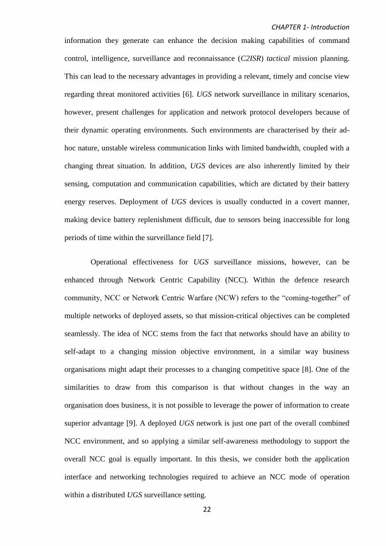
The motivational aspects of this thesis can be depicted through figure 1.1, which illustrates
a typical wide-area military surveillance scenario, with a number of deployed assets
distributed within the surveillance field. Access to the wider NCC environment is made
possible through the use of tactical communication links, which enables information to be
shared between deployed assets in order to support surveillance activities and enhance
overall mission success [10].
Figure 1.1: UGS surveillance scenario with links to the wider tactical networking environment
The aims of the work in this thesis, however, are mainly concerned with, and
restricted to, the UGS network field and not the wider tactical networking environment, as
shown in figure 1.1. From figure 1.1, UGS nodes are required to detect an imminent
approaching mobile threat and be able to collaborate (self-organise) in order to provide
timely, relevant and specific mission objective information (e.g. current threat presence
detection confidence (%) and location), as the threat traverses the UGS network field.
Information concerning the threat is typically relayed back to a gateway node located in the
far-field region of the network for further evaluation purposes, and so UGS nodes must
Command and
Control
Centre
UGS Network Field
Gateway
Node
Threat Observation
Threat Information Exchange
from UGS Network field
UGS Node UGS Self-Organisation
Aerial Reconnaissance
Tactical Link

CHAPTER 1-Motivation and Aims of the Work
24
also be able to support a multi-hop routing functionality. In addition, both sensor
collaboration and multi-hop routing functions need to be made robust within an unstable
and network resource constrained wireless environment, without reliance on any pre-
existing centralised architecture. In essence, this requires deployed sensors to have an
embedded and distributed mode of operation, which can enable them to make controlled
self-adjustments in response to dynamic environmental changes. In this thesis, a dynamic
environmental change refers to both a changing threat monitored situation and underlying
wireless channel environment. With this in mind, the aims of the work presented in this
thesis can be framed appropriately in terms of the communication protocol layer stack:
namely at the application, network, data link and physical layers, as detailed in table 1.1
and illustrated further in figure 1.2.
Aims of the Work Key Features Developed
1. Distributed Sensor Management
(Application Interface) UGS’s supporting a “problem driven collection”
approach (e.g. forming dynamic groups that can
best meet the objectives of a mission at a
particular point in time), based on decisions
derived from the shared surveillance environment.
Adaptive, application-orientated, network control
in support of both timely surveillance utility
provision and network resource management.
2. Geographic Routing (Networking) Employing efficient network topology control to
support network resource savings, whilst ensuring
that information is routed reliably within the UGS
network field.
3. Robustness in surveillance
information provision (Physical) Making informed choices for robust packet
transmission.
Providing a channel aware decision making
capability, to support reliable node selection for
information forwarding.
Table 1.1: Aims of the research work in support of UGS network field operations, as shown in figure 1.1
CHAPTER 1-Motivation and Aims of the Work
25
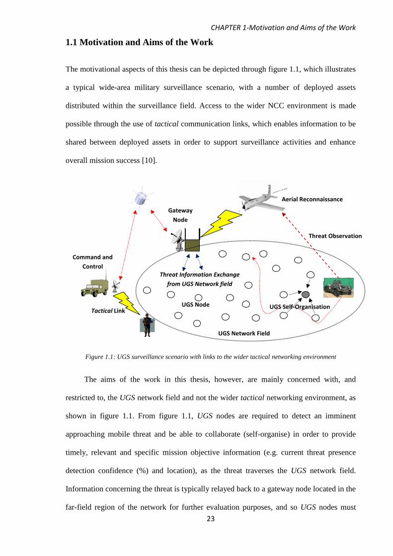
Figure 1.2: Aims of the research work in terms of the communication protocol layer stack
Table 1.1 details the key features which have been developed in this thesis to enable
an UGS NCC perspective, within a dynamic mission-orientated environment. From table
1.1 and figure 1.2, the key focus points of this thesis can be summarised below:
Providing distributed sensor management, according to the understanding (“context”)
derived from the shared mission objective surveillance environment.
Ensuring the efficient management of operational network resources within both
autonomous surveillance and geographic routing functionalities. In this thesis, network
resources refer to both communication energy and bandwidth consumption and are
considered as a means of, improving the overall network longevity goal.
Providing a means of adapting to mitigate an unreliable wireless channel environment
and integrating this within both sensor management and geographic routing
functionalities, to assist their respective operations.
Group Collaboration
- Channel contention access period scheduling
Physical Layer
Robustness to unreliable wireless channel
Opportunistic hop node selection
Medium Access Control (IEEE 802.11b)
Application Interface Layer
Mission objective autonomic sensor management:
UGS collaboration
Adaptive application orientated network control (Transmission selection, scheduling and prioritisation)
Network Layer
Topology control management
Information directivity/ Guidance to ROI
and Gateway Node
Group Collaboration
- Node selection
Network Layer
Neighbourhood membership table
Publish/Subscribe Support
Geographic Routing
- Node selection

CHAPTER 1-Motivation and Aims of the Work
26
To enable the aims of the work presented in this thesis and as detailed in table 1.1, we have
adopted the following assumptions:
For surveillance purposes, we simulate a wide area scenario that encompasses a total
area of 1 x 10⁶
m2 (i.e. 1km by 1km region).
UGS sensing and transmission radii are equal in range. For medium access control, we
use the IEEE 802.11b protocol in basic access mode.
UGS nodes have GPS capability, in order to determine their position coordinates within
the surveillance network field.
Our application interface development, assumes:
A single threat presence scenario, where threat mobility is simulated using linear and
random waypoint models. We focus only on threat presence detection and geo-location
mission objectives and assume that threat classification algorithms are already present,
for identification purposes.
The number of UGS nodes used in the simulation study ranges from 5-60 and they are
randomly deployed, in order to reflect a realistic scenario. In essence, the majority of
the simulations conducted in this thesis are only concerned with low network density
conditions and sensors that are capable of large stand-off distances (i.e. can achieve
large sensing ranges).
UGS devices have a fixed sensing range and we do not consider the effects of sensor
modality (e.g. acoustic or seismic types) or the use of multi-modal sensors on
surveillance performance.
We assume location mechanisms are running (e.g. Time Difference of Arrival) on each
UGS device, in order to deduce a current threat location, which can then be applied to
our sensor collaboration algorithms. We do not include the effects of the additional

CHAPTER 1-Organisation of the Thesis
27
signalling overhead required for the location mechanism, in our performance evaluations.
Our geographic routing scheme development, assumes:
We simulate under high network density conditions (i.e. node numbers ranging from
350-650). This is different from our main aim, which assumes low network density
conditions but, in order to gauge the performance effects of integrating topology
control within a geographic routing scheme, it was evident that this could only be
illustrated appropriately under high network density scenarios.
Our channel aware development, assumes:
Channel unreliability can be simulated using only large-scale and large-small-scale
propagation fading models.
1.2 Organisation of the Thesis
Following this introductory chapter a common structure is employed throughout this thesis.
The work presented addresses three separate aims, as detailed in table 1.1. It was found to
be more appropriate that the thesis be organised into sections which address each of the
aims detailed. Each section opens with an introductory part, detailing its contents and is
concluded with a summary of the main contributions of the section. The exception is
chapter 13, which concludes this thesis with a brief discussion of its main findings,
followed by an outline of relevant areas that should be considered for further work and
investigation.
In section 1, the first of our aims, namely distributed sensor management in support
of autonomous surveillance is detailed. The work that has been conducted to support this
section has been organised into the following five chapters:
In chapter 2, an overview of the general system characteristics related to distributed
surveillance operations is given. A review of other schemes that can support sensor

CHAPTER 1-Organisation of the Thesis
28
collaboration within a threat presence detection and geo-location sphere are also
detailed. Chapter 2 then finishes with a general discussion on the fundamentals of our
proposed autonomic approach to enable distributed UGS network management.
Chapter 3 is concerned with the first part of our intended autonomic system, using the
framework introduced in chapter 2. The chapter begins with an overview of the need to
efficiently detect, verify and acquire information about potential threats within an
uncertain (i.e. false-alarm) surveillance environment. This is then followed by a
description of our developed situation assessment system, named PORTENT, based on
a strategy, which combines a “fast” and “slow” threat detection approach. We then
outline how we characterise threat presence detection information and finally,
demonstrate PORTENT performance results.
In chapter 4, the remaining parts of our developed autonomic system, named
VIGILANT, are developed. VIGILANT, through integrating PORTENT operation is
concerned with comprehending the uncertain surveillance environment and this is
made possible through using Bayesian Belief Network (BBN) analysis. This is useful
in the sense that uncertainty can be filtered through the BBN, as the decision to initiate
a particular action is approached. This could entail initiating a group formation
response for sensor collaboration, concerning a particular mission objective in
question. The novelty in this chapter is addressed in terms of how the derived
understanding (“context”) can be further used, with additional processing functions, to
manage network resource consumption and enable transmission control. Finally,
VIGILANT performance results within a dynamic threat monitoring scenario are then
given.
In chapter 5, an improvement on VIGILANT is made. Here our VIGILANT+ system is
concerned with extending our BBN network to jointly cater for threat presence
detection and geo-location mission objectives and developing a means of supporting,

CHAPTER 1-Organisation of the Thesis
29
distributed transmission control functionality. The novelty of this chapter is the use of
confidence measures, generated with our BBN, to facilitate autonomous mission
objective assignment and distributed transmission control. In addition, we have
modelled how understanding (“context”) of the mission objective environment can be
projected using a temporal Markov decision process (MDP). This facilitates better
transmission control, as a direct relationship, in terms of the dynamics of a monitored
threat situation. Performance appraisals of using a temporal Markov decision process
within a simulated and test-bed environment are also given. The last part of this chapter
is then concerned with managing how and when transmission control decisions should
be taken within the temporal frame in order to avoid unnecessary transmission
responses.
In chapter 6, a summary with the main conclusions drawn from section 1, is then given.
In section 2, the second of our aims, namely geographic routing to support
distributed surveillance operations, is detailed. The work that has been conducted to
support this section has been organised into the following two chapters:
In chapter 7, an overview of geographic routing principles is given and reviews of
other applicable geographic routing schemes, which can be applied to a distributed
surveillance type scenario, are further detailed. The chapter then begins to focus on our
intended approach to facilitate geographic routing. Our approach has taken inspiration
from how social insects (i.e. ants) may communicate to other nest members, the
intended routes towards particular sources (i.e. food) of interest. This broad area of
applying natural principles to routing protocols is commonly referred to as, “Swarm
Intelligence”. A discussion on how we intend to use “Swarm Intelligence” to a
distributed surveillance scenario is given and subsequently, the remainder of the
chapter concerns the development of our SWarm Intelligent Odour Based Routing
(SWOB) protocol. Specifically, the novelty of this chapter is addressed in how SWOB
CHAPTER 1-Organisation of the Thesis
30
routing uses a trajectory model to mimic the effects of odour dispersion found in
nature, which can then be further used to guide (i.e. route) packets towards an intended
destination (i.e. gateway node or a region of surveillance interest). The trajectory
model itself can also assist as a means of, restricting direct communication to a certain
number of neighbours, which are to be found within a nodes transmission radius. This
can directly act as a means of, integrating network topology control within a
geographic routing functionality. Finally, the chapter finishes with results concerning
SWOB routing performance.
In chapter 8, a summary with the main conclusions drawn from section 2, is then given.
In section 3, the third aim of this thesis, namely providing a packet forwarding
mechanism, which can provide adaptability towards the unreliable channel environment, is
detailed. The work that has been conducted to support this section has been organised into
the following three chapters:
In chapter 9, we begin by detailing the wireless propagation models that are used to
portray channel unreliability with transmission distance. The chapter then utilises a
common communication link reliability measure, namely the Transitional Region
Coefficient (TRC), which can be used to describe current received channel reliability
conditions. An analysis of the effects of the TRC on the optimal forwarding distance,
transmission reliability and expected transmission count is then undertaken. This is
conducted in order to help us to better understand the impact of the channel
environment on communication link reliability. Our analysis of the TRC is then
extended further to a realistic broadcast wireless channel environment. This is
considered as a means of encouraging packet forwarding opportunities which might
arise due to the nature of the broadcast environment.
In chapter 10, the analysis of the TRC, made in chapter 9, is then utilised as a means of,
developing an overall packet forwarding decision making mechanism. The chapter

CHAPTER 1-Main Contributions
31
begins by giving an overview into the fundamentals of a fuzzy logic system, which is
used as the packet forwarding decision making mechanism. The novelty in this chapter
is addressed in how the TRC can be integrated into an overall channel-aware fuzzy
logic node selection scheme. Fuzzy logic addresses the uncertainty of the channel
environment, through its membership functions. The second novelty of this chapter
then addresses how the membership functions can be adapted using a genetic
algorithm, according to current received channel characteristics (i.e. the TRC). It is
shown that adapting membership functions, according to received channel
characteristics can help to improve overall decision making performance, with regards
to packet forwarding, when compared with normal fuzzy logic operation.
In chapter 11, a summary with the main conclusions drawn from section 3, is given.
In section 4, a performance evaluation of the work from section 1 and 2 within an
error prone wireless environment, is detailed. In chapter 12, an integrated performance
study is conducted involving sections 1 and 3. This is then followed by a similar evaluation
involving sections 2 and 3. Chapter 12 then concludes with a brief summary and the main
conclusions to be drawn from this integrated system performance study.
Finally, chapter 13 concludes the thesis with a brief discussion of its main findings
followed by an outline of areas where further research, may be appropriate.
1.3 Main Contributions
The contributions of this thesis can be categorised under headings of the three main
sections of work addressed.

CHAPTER 1-Main Contributions
32
Section 1 - Distributed Sensor Management
First experimental demonstration and application of the situation awareness (SA)
framework to an UGS surveillance network management problem. The SA framework
has the advantage of addressing the distributed sensor management problem
effectively, through an integrated approach. Results show the advantage of using a SA
approach for sensor management in terms of preventing “false alarm” detection and
establishing relevant “context” of a mission objective environment for autonomic
decision making.
Proposed a new threat detection system, which combines the use of both a “fast”
system using standard signal detection theory and a “slow” system, using the sequential
probability ratio test. Results demonstrate that in combining the “fast” and “slow”
threat detection approaches, we improve on event detection delay and QoSI
performance, when compared with independent “fast” and “slow” operations and
normal binary threat detection means.
Proposed a new approach to enable derived mission objective “context” to be
processed and used to establish an overall “context-aware” ad-hoc collaboration
mechanism. The proposed certainty factor evaluation approach allows the grouping of
immediate neighbours that share similar “context-aware” confidence levels, in a
current mission objective situation. Results show that our “context-aware”
collaboration approach reduces the impact of outliers which improves overall group
surveillance performance, when compared with schemes that utilise all deployed
neighbourhood sensors (or avoid the use of “context-awareness”).
Development of a new fully autonomic transmission control capability through the use
of a Partially Observable Markov Decision Process (POMDP). Results show that the
advantages of a POMDP approach are the reduction in reducing communication energy

CHAPTER 1-Main Contributions
33
consumption and surveillance update latency further, compared with centralised
transmission control approaches, without compromising mission objective
performance.
Section 2 - Geographic Routing to Support Distributed Surveillance
Development of a new network topology control scheme, which adjusts to current
deployed network node density conditions. We demonstrate that a desired level in
topology control can be achieved and adapted through setting a desired k-connectivity
requirement. Our experimental evaluation shows the benefits of incorporating the k-
connectivity topology control methodology within our geographic routing scheme to
achieve better throughput and energy efficiency performance, especially in conditions
with increasing network node density, when compared with traditional “most forward
progress” routing and restricted directional flooding schemes.
Section 3 - Channel Aware Packet Forwarding
A new channel aware packet forwarding system, which combines the transitional
regional coefficient within a genetic adaptive fuzzy logic scheme. Our experimental
evaluations demonstrate that, under opportunistic forwarding conditions, this can
enable UGS nodes to make relevant self-managed decisions on neighbour selection, for
reliable packet forwarding. Results also show the advantages of our proposed approach
in achieving dependable mission objective information collection under different
channel fading conditions and an improvement in throughput and energy efficiency
performance, over schemes with limited channel reliability knowledge.
CHAPTER 1-List of Publications
34
1.4 List of Publications
The research work outlined in this thesis has led to a total of 10 publications and
presentations being made at national and international conferences. These are listed in
order of most recent publication date, as shown below:
1. Ghataoura, D.S, Mitchell, J.E. and Matich, G.E. “VIGILANT+: Mission Objective
Interest Groups for Wireless Sensor Network Surveillance Applications”, IET Wireless
Sensor Systems Journal, vol.1, no.4, pp.229-240, December 2011.
2. Ghataoura, D.S, Mitchell, J.E. and Matich, G.E. “Autonomic Control for Wireless
Sensor Network Surveillance Applications”, The 30th
IEEE International Conference
on Military Communications (MILCOM), Baltimore, Maryland, USA, 7h – 10
th
November 2011.
3. Ghataoura, D.S, Mitchell, J.E. and Matich, G.E. “Networking and Application
Interface Technology for Wireless Sensor Network Surveillance and Monitoring”,
IEEE Communications Magazine, vol.49, no.10, pp.90-97, October 2011.
4. Ghataoura, D. S., Mitchell, J. E. and Matich, G. E., VIGILANT: "Situation-Aware
Quality of Information Interest Groups for Wireless Sensor Network Surveillance
Applications”, Unmanned-Unattended Sensors and Sensor Networks VII, Vol. 7833,
European SPIE Defence and Security, SPIE-International, Toulouse, France,
September 2010.
5. Ghataoura D.S., “An Architecture to Support Mission Orientated Wireless Sensor
Network Surveillance Applications”, London Communications Symposium (LCS),
University College London, September 2010.
CHAPTER 1-List of Publications
35
6. Ghataoura, D.S., Yang, Y., Mitchell, J.E. and Matich, G.E. “PORTENT: Predator
Aware Situation Assessment for Wireless Sensor Network Surveillance Applications”,
Cyber Security, Situation Management, And Impact Assessment II, Vol. 7709, SPIE-
Defence, Security and Sensing, SPIE-International, Orlando, Florida, USA, April 2010.
7. Ghataoura, D.S., Yang, Y. and Matich, G.E. “SWOB: Swarm Intelligent Odour Based
Routing for Geographic Wireless Sensor Network Applications”, The 28th
IEEE
International Conference on Military Communications (MILCOM), Boston, USA, 18th
– 21st October 2009.
8. Ghataoura D.S., “Quality of Information and Efficient Delivery in Military Sensor
Networks”, London Communications Symposium (LCS), University College London,
September 2009.
9. Ghataoura, D.S., Yang, Y. and Matich, G.E. “GAFO: Genetic Adaptive Fuzzy Hop
Selection Scheme for Wireless Sensor Networks”, The 5th
International conference on
Wireless Communications and Mobile Computing (IWCMC), Wireless Sensor
Networks Symposium, Leipzig , Germany, 21st -24
th June 2009.
10. Ghataoura, D.S., Yang, Y. and Matich, G.E. “Channel Aware Fuzzy Logic Hop
Selection for Wireless Sensor Networks”, The 16th
International Conference on
Telecommunications (ICT), Marrakech, Morocco, 25th
– 27th
May 2009.

SECTION 1- Introduction
36
SECTION 1
Distributed Sensor Management
Introduction
Unattended ground sensor (UGS) networks are classified as distributed systems, capable of
supporting mission objectives, such as threat presence detection and geo-location, within a
security-sensitive region. The information they provide can enhance decision making
abilities for command and control, intelligence, surveillance and reconnaissance (C2ISR)
tactical mission plans, primarily because of their scalability property [11]. In addition, the
inherently dynamic nature of surveillance missions does not allow time for manual system
configuration. Distributed systems can address this concern by minimising the burden of a
centralised processing architecture and by providing the necessary savings towards
network resource consumption [11-12]. As a result of distributed operation, node failures
can be tolerated and the operational longevity of the deployed UGS network field can be
increased [11-13].
Managing the distributed UGS network to assist threat presence detection and geo-
location capabilities, however, raises some interesting questions, for example:
How do deployed UGS’s decide they are suitable in meeting the objectives of a
mission? Monitoring threats within the surveillance field is a dynamic process, which
requires sensors to have actionable and precise decision making ability, in order to
minimise the propagation of false alarms, event detection delays and mission objective
inaccuracies [14-15].
When and how do deployed sensors collaborate in order to fulfil a current mission
objective successfully? A single UGS is not adequate to provide sufficient levels of

SECTION 1- Introduction
37
surveillance information, whereas many sensors collaborating towards a common
objective are able to provide benefits such as, increased surveillance utility and
reduction of both errors and the amount of redundant information being sent [16-17].
How do deployed sensors conserve their key network operational resources without
compromising the objectives of a mission? It is shown that investing in computation
efforts within the network (“in-network processing”) can have benefits towards saving
on communication costs [18-20]. This can be achieved through UGS collaboration, as
opposed to every node transmitting their independent information to an external
processing point “at the edge” of the network field.
UGS nodes, which have an ability to make their own decisions regarding a specific mission
objective, are more applicable towards supporting the questions raised above. In essence, a
self-managed perspective would allow UGS nodes to be dynamically managed and tasked,
so that the overall distributed UGS field is better able to perform surveillance on a region.
The incorporation of self-managing features within the network, however, requires use of
an autonomic framework [21]. For network management purposes, an autonomic
framework would entail the implementation of application-orientated features, necessary to
enhance both UGS decision making and collaboration in a distributed manner [21-23].
The primary goal for this section is to present a potential autonomic system that can
assist distributed UGS surveillance network management. We focus on providing an
autonomic system that supports both threat presence detection (M1) and geo-location (M2)
capability. Our aim is also to incorporate self-management features that can enable UGS
nodes to dynamically adjust their transmission behaviour to current mission objectives,
while also ensuring that the overall information utility provided is not compromised. Our
focus on transmission behaviour (transmission control) is geared towards the efficient
management of network resources, primarily communication energy and bandwidth

SECTION 1- Introduction
38
expenditure. This can therefore enable a potential autonomic system that supports the long-
term operational longevity requirement.
In this section, chapter 2 begins by introducing the general system characteristics
related to distributed surveillance operations. Continuing in chapter 2, we identify other
applicable schemes, which can support self-managing features for surveillance operations.
In section 2.4, the fundamentals of our proposed autonomic framework to enable
distributed UGS network management are introduced. Based on our proposed framework,
chapter 3 explains the first part of our intended autonomic system. In chapter 4, we then
detail the first of our developed systems termed, VIGILANT, incorporating a semi-
autonomic approach towards distributed surveillance management. In chapter 5, we
improve on VIGILANT and detail our fully autonomic system termed, VIGILANT+, to
enable a distributed self-managed perspective towards M1 and M2 UGS surveillance.
Finally in chapter 6, we summarise and conclude the main contributions of this section.

SECTION 1 – Chapter 2
39
CHAPTER 2
Distributed Surveillance Operations
Distributed surveillance operations can be strengthened through distributed processing
(“in-network processing”) and aggregation of such surveillance information [11-13],
which encourages fault-tolerant behaviour and improvements in sensing accuracy [24-25].
Support for distributed surveillance operations is possible through UGS collaboration,
according to a common mission objective [25]. Protocols and schemas that are designed to
assist ad-hoc collaboration can, as a result, provide easily accessible and high-quality
information concerning the mission objective environment. Before we can begin to
develop application support protocols that promote ad-hoc collaboration, it is crucial for us
first to specify the necessary design requirements, as described below:
Group-initiator election: A group initiator (GI) is dynamically elected within a group
of UGS nodes and as such, forms a final point for aggregation in mission objective
information. A GI node can also assist as an accurate reference point within the
surveillance field for other deployed nodes to base their level of information accuracy.
Dynamics: GI-led ad-hoc groups must also provide adaptability according to the
dynamics of a monitored threat, allowing sensors to leave and join at any time during a
mission. This can help to encourage and maintain the most timely and relevant
information concerning the monitored threat.
Stability: To establish an accurate basis in information processing, the GI led group
structure requires a level of stability to avoid undesirable fluctuations (i.e. non-
applicable nodes joining or unexpectedly priority nodes leaving) during a monitored
threat situation. Ensuring stability can help to achieve reliable levels in M1 and M2
SECTION 1 – Chapter 2
40
surveillance provision and overall improved utility for eventual C2ISR decision
making.
Group Initiator re-election: Dynamic re-election of new GI’s during a mission is
imperative in order to maintain relevant surveillance report aggregation.
System Energy Efficiency: UGS nodes are typically restricted in their communication
energy and bandwidth resources, therefore, non-essential communication overhead
should be kept to a minimum in order to prolong network lifetime and encourage
bandwidth efficiency.
In sections 2.1, 2.2 and 2.3 we identify other developed and applicable schemes, namely
LEACH, DCATT and IDSQ. These schemes are highlighted because they are the most
common schemes to be found in the WSN community that can support the system
requirements described above. In addition, these schemes can also provide an appropriate
performance comparison against our intended solution, detailed later in section 2.4.
2.1 Low Energy Adaptive Clustering Hierarchy (LEACH)
Clustering is a form of deterministic self-organisation (collaboration) used in ad-hoc sensor
networks and it can be an effective technique for achieving scalability and prolonged
network lifetime [26]. A well-known clustering algorithm for continuous, data-centric
application gathering sensor networks is the LEACH mechanism [27]. LEACH partitions
deployed nodes in a network into clusters and in each cluster a dedicated node, the cluster-
head (CH), is responsible for maintaining a time division multiple access (TDMA)
schedule for localised transmission control amongst its neighbouring nodes and data
aggregation, which encourages stability within the cluster group.
CH election, equivalent to GI election, as described above, is conducted randomly
and independently by each node on a per-round basis of a fixed duration. This helps to

SECTION 1 – Chapter 2
41
reduce further both the required signalling traffic and communication overhead. Election of
CH’s can be managed accordingly to task driven criteria, such as battery energy level,
transmission power and network connectivity [27-28]. Subsequently, GI re-election is also
based on these criteria, in order to achieve a balanced rotation of CH’s within the network
and promote system energy efficiency.
In essence, LEACH is a distributed single hop application protocol, which can be
adjusted for specific operation towards a desired mission objective. For example, CH
election and re-election can be based on both M1 and M2 accuracy errors and CH’s can act
as a point for surveillance information aggregation, using a TDMA schedule. The main
disadvantage of LEACH is its deterministic self-organisation operation, which makes it
difficult to adapt to the dynamics of a monitored threat situation without changing the per-
round CH election and group coordination phases.
2.2 Dynamic Clustering for Acoustic Target Tracking (DCATT)
In support of M2 operation only, self-organisation (collaboration) to perform energy
efficient threat geo-localisation is equally important [29-31]. DCATT [29] proposes a
simple, distributed and dynamic clustering algorithm for geo-location operation. CH
nomination is conducted in terms of a physical based localisation view, based on received
signal energy levels from the sensing field, as shown in (2.1).
iii n||xx||.ar (2.1)
From (2.1), ri is the received signal strength at the ith
sensor, a is the unknown signal
strength from the source, x is the target position, xi is the known position of the ith
sensor, α
is the known attenuation coefficient, ni is white Gaussian noise with zero-mean and
variance σ2. The fundamental principle applied in energy based approaches, as shown in
(2.1), is that the signal strength energy of a received signal decreases exponentially with

SECTION 1 – Chapter 2
42
propagation distance [22]. In DACTT, a CH is elected when the signal strength from (2.1),
is detected by a distributed node and exceeds a pre-determined system threshold. This
again utilises a metric derived from task-driven management approaches. As multiple
sensors may also detect the energy signal above the pre-determined threshold, DACTT
ensures ad-hoc group stability is maintained by only selecting the sensor that has the best
probability in reducing M2 inaccuracies. This can help to save on channel contention
access delay and as a result, increases bandwidth re-usability.
Subsequently, the elected CH broadcasts an information solicitation packet asking
neighbouring sensors to join the cluster and provide their sensing information. Received
information is then used to estimate the location of the threat using energy-based
localisation methods [33]. This, however, has the disadvantage of being only robust in the
presence of moderate noise within the received signal and small movements in trajectory
concerning the monitored threat [29]. Also, due to the energy based model, random
rotation of CHs will be common if the sensing environment is corrupted with high levels of
noise, leading to a potential degradation in M2 surveillance performance and utility.
2.3 Information Driven Sensor Querying (IDSQ)
Both LEACH and DACTT are schemes that can support both M1 and M2 operations using
mostly task-driven criteria for collaboration and management of network resources. A
different take towards sensor collaboration and management of network resources is to
consider an information-centric approach [34]. Ideally, sensors should be chosen for
collaboration which can contribute the most information towards answering a specific
mission objective, and generally this lies in the direction of the largest amount of
information gain [34-35]. IDSQ, [35] is a scheme that incorporates information-centricity.
From [35], the authors consider the goal in providing a location estimate of an event
source, as accurately as possible (low estimation error), with as little energy consumption
SECTION 1 – Chapter 2
43
as possible. This is useful in support of both stability and system energy efficiency
requirements. The problem of choosing which sensors collaborate at the lowest
communication energy cost becomes an optimisation problem and IDSQ frames this in
terms of an objective function, Mobj, defined as a mixture of both information utility gain
and cost, as shown in (2.2).
)z()1()StateBelief(.)StateBelief(M jtcosUtilityobj (2.2)
As shown in (2.2), φUtility is an information utility measure, φCost is the cost of
communication in terms of the Euclidean distance and β is the relative weighting given to
the utility and cost functions. Mobj, is defined as a function of the belief state, defined as a
probability distribution describing each new sensor measurement taken, zj, combined with
the current estimate using measurements taken from z1 to zj-1, as shown in (2.3), where x
represents the state of the target we wish to estimate.
)z,z,...,z|x(pStateBelief j1j1 (2.3)
It is clear from (2.3) that adding further sensor observations will improve both the
estimate and information utility gain. In IDSQ, an elected GI would then seek to request zj
measurements from its immediate neighbours and combine these with its own estimate, in
order to form a current belief state concerning each respective neighbour. IDSQ selects the
best neighbour for collaboration based on the sensor, which can provide the highest
expected information utility measure, given by φUtility (Belief State). By convention a large
φUtility (Belief State) would indicate less uncertainty concerning the target state. If the belief
state can be approximated well by a Gaussian distribution, then covariance-based
information utility gain measures are suitable such as, the Mahalanobis distance measure
[25-26].
Using information utility measures to decide on sensor collaboration and
organisation has been shown to provide a faster reduction in estimation uncertainty and
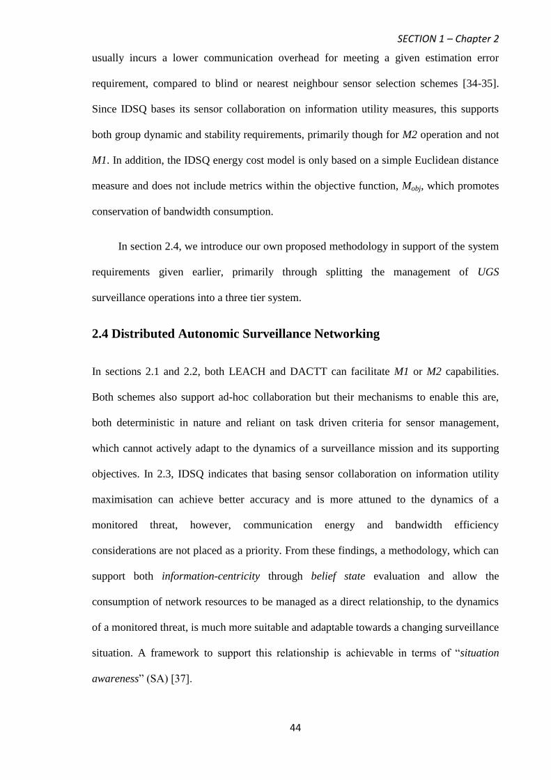
SECTION 1 – Chapter 2
44
usually incurs a lower communication overhead for meeting a given estimation error
requirement, compared to blind or nearest neighbour sensor selection schemes [34-35].
Since IDSQ bases its sensor collaboration on information utility measures, this supports
both group dynamic and stability requirements, primarily though for M2 operation and not
M1. In addition, the IDSQ energy cost model is only based on a simple Euclidean distance
measure and does not include metrics within the objective function, Mobj, which promotes
conservation of bandwidth consumption.
In section 2.4, we introduce our own proposed methodology in support of the system
requirements given earlier, primarily through splitting the management of UGS
surveillance operations into a three tier system.
2.4 Distributed Autonomic Surveillance Networking
In sections 2.1 and 2.2, both LEACH and DACTT can facilitate M1 or M2 capabilities.
Both schemes also support ad-hoc collaboration but their mechanisms to enable this are,
both deterministic in nature and reliant on task driven criteria for sensor management,
which cannot actively adapt to the dynamics of a surveillance mission and its supporting
objectives. In 2.3, IDSQ indicates that basing sensor collaboration on information utility
maximisation can achieve better accuracy and is more attuned to the dynamics of a
monitored threat, however, communication energy and bandwidth efficiency
considerations are not placed as a priority. From these findings, a methodology, which can
support both information-centricity through belief state evaluation and allow the
consumption of network resources to be managed as a direct relationship, to the dynamics
of a monitored threat, is much more suitable and adaptable towards a changing surveillance
situation. A framework to support this relationship is achievable in terms of “situation
awareness” (SA) [37].
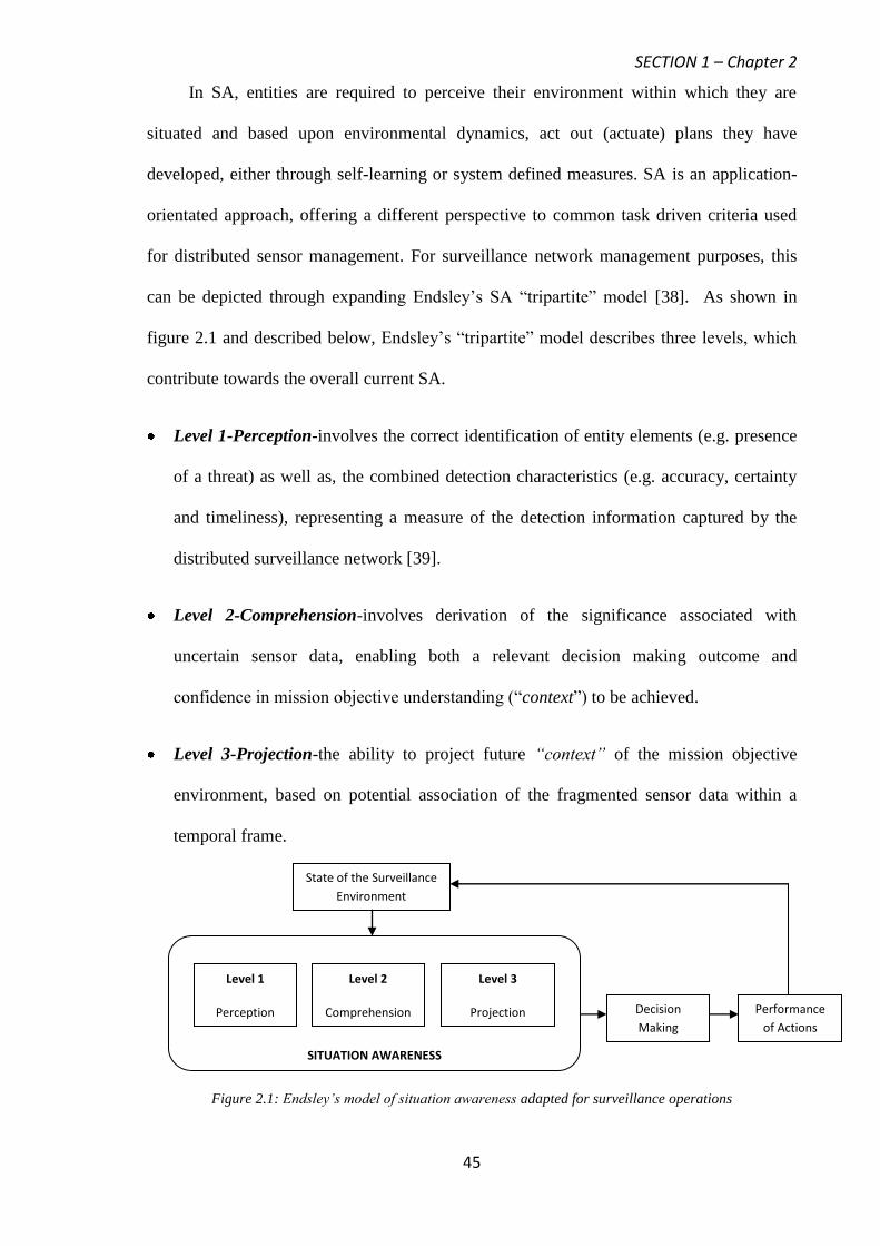
SECTION 1 – Chapter 2
45
In SA, entities are required to perceive their environment within which they are
situated and based upon environmental dynamics, act out (actuate) plans they have
developed, either through self-learning or system defined measures. SA is an application-
orientated approach, offering a different perspective to common task driven criteria used
for distributed sensor management. For surveillance network management purposes, this
can be depicted through expanding Endsley’s SA “tripartite” model [38]. As shown in
figure 2.1 and described below, Endsley’s “tripartite” model describes three levels, which
contribute towards the overall current SA.
Level 1-Perception-involves the correct identification of entity elements (e.g. presence
of a threat) as well as, the combined detection characteristics (e.g. accuracy, certainty
and timeliness), representing a measure of the detection information captured by the
distributed surveillance network [39].
Level 2-Comprehension-involves derivation of the significance associated with
uncertain sensor data, enabling both a relevant decision making outcome and
confidence in mission objective understanding (“context”) to be achieved.
Level 3-Projection-the ability to project future “context” of the mission objective
environment, based on potential association of the fragmented sensor data within a
temporal frame.
Figure 2.1: Endsley’s model of situation awareness adapted for surveillance operations
State of the Surveillance
Environment
Decision
Making
Performance
of Actions
Level 1
Perception
Level 2
Comprehension
Level 3
Projection
SITUATION AWARENESS

SECTION 1 – Chapter 2
46
As indicated in the section introduction, the primary goal for this section is the
development of a potential autonomic system that can assist distributed UGS network
surveillance management. This can be accomplished through using a SA framework in the
following ways:
Level 1 and level 2 can assist in dynamic and stable ad-hoc group collaboration, related
to a current threat situation. Collaboration in this way is primarily focused on sensors
perceiving correctly and establishing their localised “context” of the present situation
(e.g. awareness to a threat), in order to allow UGS self-assignment to a particular
mission objective.
Level 3 is useful in terms of enabling UGS nodes to self-manage their network
resources according to, how the “context” concerning the monitored threat will change
with time.
In the subsequent chapters that accompany section 1, we plan to evaluate the system
performance of our developed SA framework against LEACH, DCATT and IDSQ which
have been introduced earlier. To begin with, in chapter 3, the development concerning the
level 1 part of our SA system, namely the perception model is described.

SECTION 1 – Chapter 3 - PORTENT
47
CHAPTER 3
Situation Assessment for Surveillance Missions
The focus of surveillance missions is to efficiently detect, verify and acquire information
about potential threats within a specified region of interest. Common assessment systems
used for threat detection rely on mechanisms using basic threshold values in order to define
simple events that reduce detection accuracy or focus on the classification of event
patterns, which reduce timeliness and do not prioritise false alarm rates [40-44].
The lack of consideration given to false alarms has an impact on level 1 perception
success, as it affects positive threat detection performance. A low false alarm rate, which is
needed to avoid unnecessary responses (e.g. GI election), involves a larger sample set
being collected for threat verification. This implies greater sampling energy consumption
and reduced timeliness [42]. Threat situation assessment systems that can incorporate a
self-adjustable sensitivity towards different sensing environment uncertainties are therefore
beneficial. This would also accommodate scenarios where both a higher degree of
sensitivity is also desired, in order to capture all potential threats and especially where
larger standoff ranges (i.e. sensing ranges) are required. In sections 3.1 to 3.6, we detail our
proposed distributed situation assessment system named, PORTENT, is described which is
able to model and detect potential threats within an uncertain surveillance environment.
3.1 PORTENT Situation Assessment System
Situation assessment for real-world threat detection purposes can be related to how
mammals in the natural world perceive and assess potential threats towards them.
Mammals have always dealt with ambiguous sensory information to determine whether
predators are present or not [45]. Subsequently, through the processing of threat related
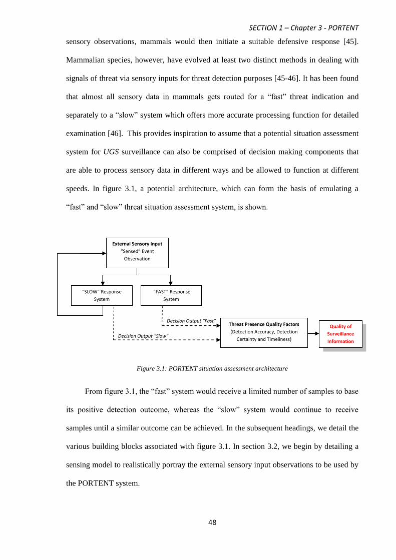
SECTION 1 – Chapter 3 - PORTENT
48
sensory observations, mammals would then initiate a suitable defensive response [45].
Mammalian species, however, have evolved at least two distinct methods in dealing with
signals of threat via sensory inputs for threat detection purposes [45-46]. It has been found
that almost all sensory data in mammals gets routed for a “fast” threat indication and
separately to a “slow” system which offers more accurate processing function for detailed
examination [46]. This provides inspiration to assume that a potential situation assessment
system for UGS surveillance can also be comprised of decision making components that
are able to process sensory data in different ways and be allowed to function at different
speeds. In figure 3.1, a potential architecture, which can form the basis of emulating a
“fast” and “slow” threat situation assessment system, is shown.
Figure 3.1: PORTENT situation assessment architecture
From figure 3.1, the “fast” system would receive a limited number of samples to base
its positive detection outcome, whereas the “slow” system would continue to receive
samples until a similar outcome can be achieved. In the subsequent headings, we detail the
various building blocks associated with figure 3.1. In section 3.2, we begin by detailing a
sensing model to realistically portray the external sensory input observations to be used by
the PORTENT system.
External Sensory Input
“Sensed” Event
Observation
“FAST” Response
System
“SLOW” Response
System
Threat Presence Quality Factors
(Detection Accuracy, Detection
Certainty and Timeliness) Decision Output “Slow”
Decision Output “Fast” Quality of
Surveillance
Information

SECTION 1 – Chapter 3 - PORTENT
49
3.2 Sensing Model
Performance of situation assessment systems can be affected by factors such as sensor type
(e.g. acoustic, seismic or infra-red), sensing environment and threat related factors, such
as: threat-to-sensor distance, propagation characteristics and the motion pattern of the
threat [42-43]. A common approach in simplifying these factors is to assume a simple
binary sensing detection model [44]. Here the sensor detects a threat with probability of
one only if the threat-to-sensor distance, d, is below a threshold distance, dt, as shown in
(3.1) and zero otherwise.
t2 d||qp||:1
Otherwise:0)q,p(S (3.1)
Accordingly in (3.1), the relationship for threat detection, S (p, q), is defined in terms of
the sensor node position at position p, observing an event at position q, where ||.||2 is the
Euclidean distance between them. Such a simplification where d alone determines threat
detection is acceptable for indoor deployments and where a line of sight can be guaranteed
[43]. However, in outdoor settings, such as UGS networks, signal quality is dependent on
the propagation environment and for this reason a better sensing model is required for
realistic situation assessment design. This can be achieved if we assume that the sensing
signal characteristic is an exponentially decaying function of d [42] [47]. For our proposed
PORTENT system, a function to depict a realistic sensing input observation model is
shown in (3.2). From (3.2), it is shown that the need for both d and dt is minimised and the
sensing model itself becomes a direct relationship with the maximum sensing range, SRMAX,
employed and ||.||2.

SECTION 1 – Chapter 3 - PORTENT
50
91.3b,)S||qp||2
S(if5.0e
3lnb,)2
S||qp||0(if
e1
1e1
)q,p(S
2RMAX2RMAX
1S
||qp||*2b
1RMAX
21b
2
S
||qp||2
S
b
RMAX
22
RMAX
2RMAX
1
(3.2)
For the purposes of our situation assessment model, we assume only one possible
threat is present and therefore, the probability of there being no threat present is (1- S (p,
q)), where S (p, q) is given, as shown in (3.1) or (3.2). In headings 3.3 and 3.4, we detail
how the S (p, q) relationship can be integrated to form part of the overall “fast” and “slow”
threat response system models, in accordance with figure 3.1.
3.3 Fast Response System Model
We represent the initial received set of sampled signals, x, by the “fast” response system as
normally distributed according to N (μFAST1, σ2
FAST) or N (μFAST0, σ2
FAST) depending upon
whether, a threat is present or not respectively, as shown in figure 3.2. The PORTENT
“fast” response system model can then be formulated in terms of, standard signal detection
theory [48]. The basis for standard signal detection theory relies upon a general detection
pay-off matrix, a critical detection threshold, L(x0), for the initial signal x and an
observation criterion, L(x). The decision at any stage for “fast” detection depends upon the
pay-off values for correct detection (VSN,Y), incorrect rejection (VSN,N), false alarm (VN,Y)
and correct rejection (VN,N), as shown in table 3.1, in the form of a general pay-off matrix
where PR is the probability of a threat being present, given by S(p, q), in (3.1) or (3.2).
Using the pay-off matrix of table 3.1, the critical threshold for initial signal level x, L(x0),
as shown in figure 3.2, is given in (3.3).
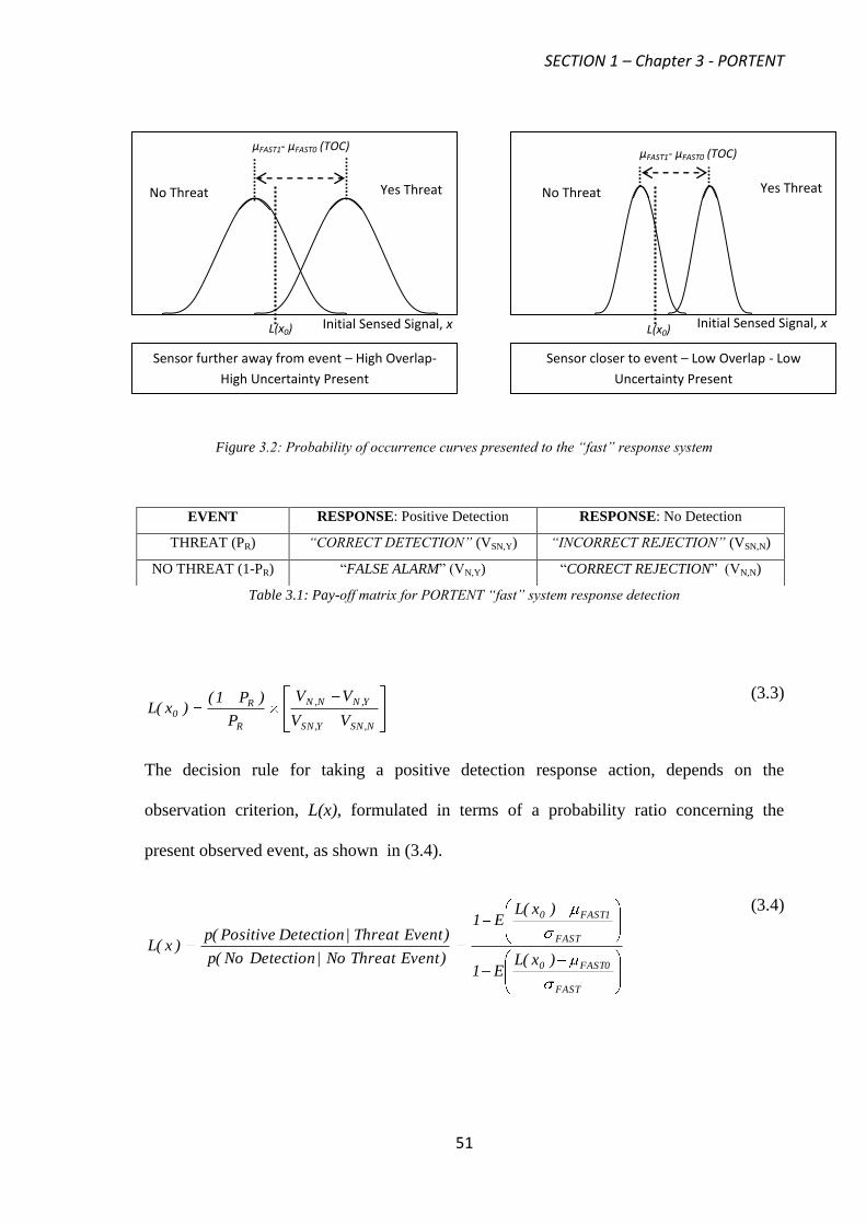
SECTION 1 – Chapter 3 - PORTENT
51
Figure 3.2: Probability of occurrence curves presented to the “fast” response system
Table 3.1: Pay-off matrix for PORTENT “fast” system response detection
N,SNY,SN
Y,NN,N
R
R0
VV
VV
P
)P1()x(L
(3.3)
The decision rule for taking a positive detection response action, depends on the
observation criterion, L(x), formulated in terms of a probability ratio concerning the
present observed event, as shown in (3.4).
FAST
0FAST0
FAST
1FAST0
)x(LE1
)x(LE1
)EventThreatNo|DetectionNo(p
)EventThreat|DetectionPositive(p)x(L
(3.4)
EVENT RESPONSE: Positive Detection RESPONSE: No Detection
THREAT (PR) “CORRECT DETECTION” (VSN,Y) “INCORRECT REJECTION” (VSN,N)
NO THREAT (1-PR) “FALSE ALARM” (VN,Y) “CORRECT REJECTION” (VN,N)
Sensor further away from event – High Overlap-
High Uncertainty Present
Sensor closer to event – Low Overlap - Low
Uncertainty Present
μFAST1- μFAST0 (TOC)
Yes Threat No Threat No Threat
Initial Sensed Signal, x
Initial Sensed Signal, x
L(x0) L(x0)
Yes Threat
μFAST1- μFAST0 (TOC)
SECTION 1 – Chapter 3 - PORTENT
52
In (3.4), E (.) denotes the cumulative distribution function for the standard normal
distribution. The decision on whether to invoke a positive detection action can be based on
the likelihood-ratio criterion, L(x) and L(x0), as shown in (3.5).
"ActionDetectionPositiveTake:Yes"THEN)x(L)x(LIF 0 (3.5)
3.4 Slow Response System Model
The PORTENT “slow” response mechanism, forming an extensive situation assessment
system, is best framed using the sequential probability ratio test (SPRT), in terms of the
Neyman-Pearson (NP) detection threshold [49-50]. The SPRT approach utilises two
alternative hypotheses representing the presence and absence of a threat, while updating
the relative likelihood ratio of each as new sensory samples arrive. The PORTENT “slow”
system design is based on using the following alternative hypotheses:
H0: Likelihood of threat presence is low gather additional sensory data (Null Hypothesis)
H1: Likelihood of threat presence is high that “positive detection” action should be taken
Assuming that an UGS receives a sequence of sampled values from the surveillance
environment, if no threat is present, each sampled value, xi (No Threat), is an independent,
identically distributed random variable from a normal distribution, N (μSLOW0, σ2
SLOW). If a
threat is present each sampled value, xi (Threat), is an independent, identically distributed
random variable from a normal distribution, N (μSLOW1, σ2SLOW). We always assume μSLOW0
< μSLOW1. After a series of n sensory samples have been taken within a time period, t, the
relevant information captured by the sensor, can be expressed as a cumulative sum of log-
likelihood ratios, Z (n), as shown in (3.6).
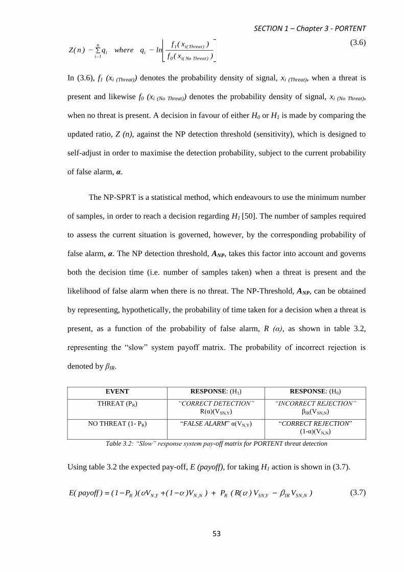
SECTION 1 – Chapter 3 - PORTENT
53
)x(f
)x(flnqwhereq)n(Z
)ThreatNo(i0
)Threat(i1
i
n
1ii
(3.6)
In (3.6), f1 (xi (Threat)) denotes the probability density of signal, xi (Threat), when a threat is
present and likewise f0 (xi (No Threat)) denotes the probability density of signal, xi (No Threat),
when no threat is present. A decision in favour of either H0 or H1 is made by comparing the
updated ratio, Z (n), against the NP detection threshold (sensitivity), which is designed to
self-adjust in order to maximise the detection probability, subject to the current probability
of false alarm, α.
The NP-SPRT is a statistical method, which endeavours to use the minimum number
of samples, in order to reach a decision regarding H1 [50]. The number of samples required
to assess the current situation is governed, however, by the corresponding probability of
false alarm, α. The NP detection threshold, ANP, takes this factor into account and governs
both the decision time (i.e. number of samples taken) when a threat is present and the
likelihood of false alarm when there is no threat. The NP-Threshold, ANP, can be obtained
by representing, hypothetically, the probability of time taken for a decision when a threat is
present, as a function of the probability of false alarm, R (α), as shown in table 3.2,
representing the “slow” system payoff matrix. The probability of incorrect rejection is
denoted by βIR.
EVENT RESPONSE: (H1) RESPONSE: (H0)
THREAT (PR) “CORRECT DETECTION”
R(α)(VSN,Y)
“INCORRECT REJECTION”
βIR(VSN,N)
NO THREAT (1- PR) “FALSE ALARM” α(VN,Y) “CORRECT REJECTION”
(1-α)(VN,N)
Table 3.2: “Slow” response system pay-off matrix for PORTENT threat detection
Using table 3.2 the expected pay-off, E (payoff), for taking H1 action is shown in (3.7).
)VV)(R(P)V)1(V()P1()payoff(E N,SNIRY,SNRN,NY,NR (3.7)

SECTION 1 – Chapter 3 - PORTENT
54
To calculate the current optimum probability of false alarm, αopt, matched to the current
sensing environment, it is noted that E (payoff) is a maximum when dE (payoff) / dαopt = 0,
as shown in (3.8).
0)VV()P1(Vd
dRP
d
)payoff(dEN,NY,NRY,SN
opt
R
opt
(3.8)
Z (n), given in (3.6) represents a summary of the accumulated sensory threat related
information up to t, which is a multiple of 1/n. At each small time step, δt, the movement
of Z (n) can be assumed to be normally distributed according to, N (μδt, η2δt), where both μ
and η are given in (3.9) and (3.10), respectively.
2
SLOW
20SLOW1SLOW
2
)(
(3.9)
2
SLOW
20SLOW1SLOW2 )(
(3.10)
Since, the time step, δt, is known, the amount of accumulated information gain through
Z(n) in that time, is a random variable with normal distribution parameters given in (3.9)
and (3.10). For a total of n sensory observations per unit time, t, the total uncertainty in
information gain from incoming sensory samples, k1, can be quantified, as shown in
(3.11).
2
22
n
)2(nn1k
(3.11)
From (3.11), it is apparent that both αopt and ANP are linked to k1, since this reflects the
current degree in H1 uncertainty, as a result of the observations being made from the
surveillance environment. Setting R (α) = αoptk1
and substituting dR/dαopt = k1αoptk1-1
into
(3.8), αopt can be rearranged to be solved, as shown in (3.12).
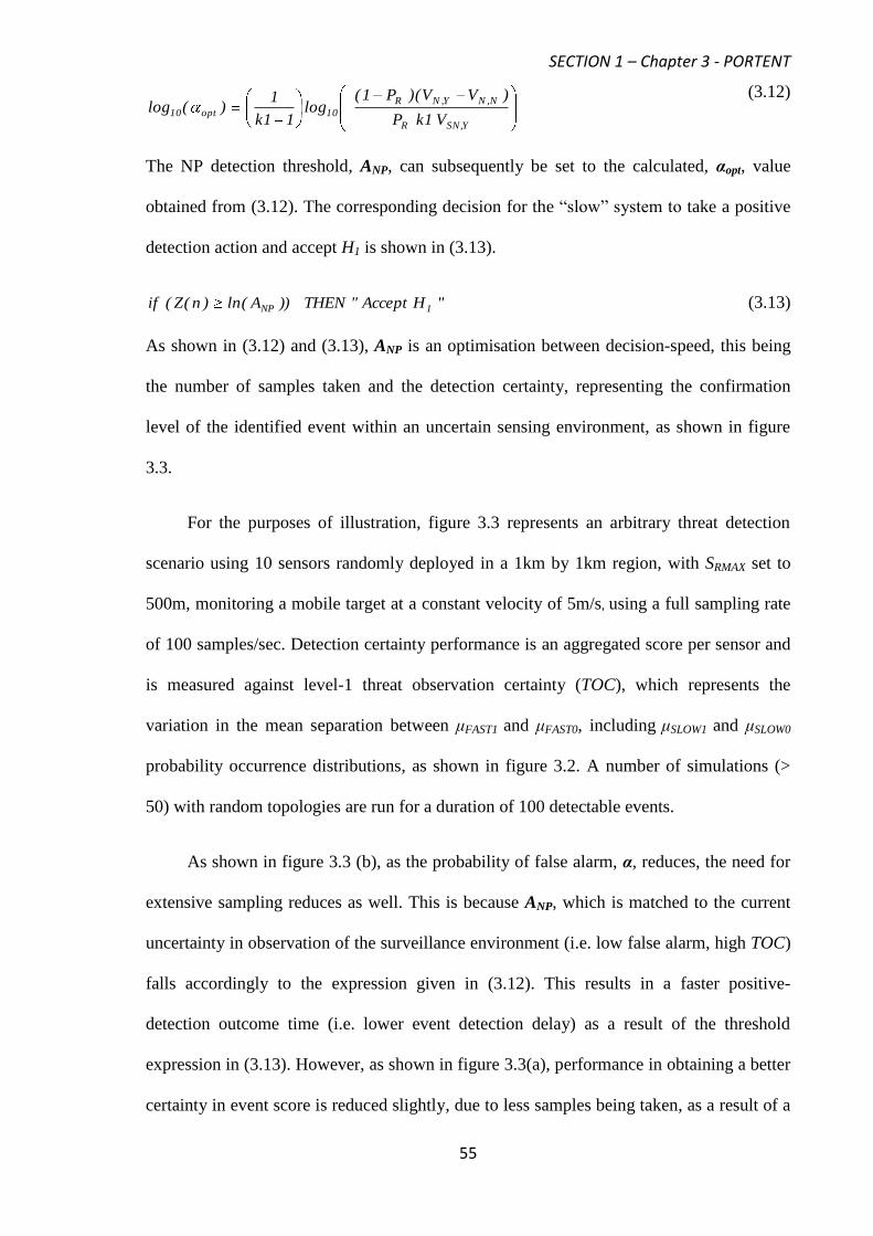
SECTION 1 – Chapter 3 - PORTENT
55
Y,SNR
N,NY,NR
10opt10V1kP
)VV()P1(log
11k
1)(log
(3.12)
The NP detection threshold, ANP, can subsequently be set to the calculated, αopt, value
obtained from (3.12). The corresponding decision for the “slow” system to take a positive
detection action and accept H1 is shown in (3.13).
"HAccept"THEN))A(ln)n(Z(if 1NP (3.13)
As shown in (3.12) and (3.13), ANP is an optimisation between decision-speed, this being
the number of samples taken and the detection certainty, representing the confirmation
level of the identified event within an uncertain sensing environment, as shown in figure
3.3.
For the purposes of illustration, figure 3.3 represents an arbitrary threat detection
scenario using 10 sensors randomly deployed in a 1km by 1km region, with SRMAX set to
500m, monitoring a mobile target at a constant velocity of 5m/s, using a full sampling rate
of 100 samples/sec. Detection certainty performance is an aggregated score per sensor and
is measured against level-1 threat observation certainty (TOC), which represents the
variation in the mean separation between μFAST1 and μFAST0, including μSLOW1 and μSLOW0
probability occurrence distributions, as shown in figure 3.2. A number of simulations (>
50) with random topologies are run for a duration of 100 detectable events.
As shown in figure 3.3 (b), as the probability of false alarm, α, reduces, the need for
extensive sampling reduces as well. This is because ANP, which is matched to the current
uncertainty in observation of the surveillance environment (i.e. low false alarm, high TOC)
falls accordingly to the expression given in (3.12). This results in a faster positive-
detection outcome time (i.e. lower event detection delay) as a result of the threshold
expression in (3.13). However, as shown in figure 3.3(a), performance in obtaining a better
certainty in event score is reduced slightly, due to less samples being taken, as a result of a
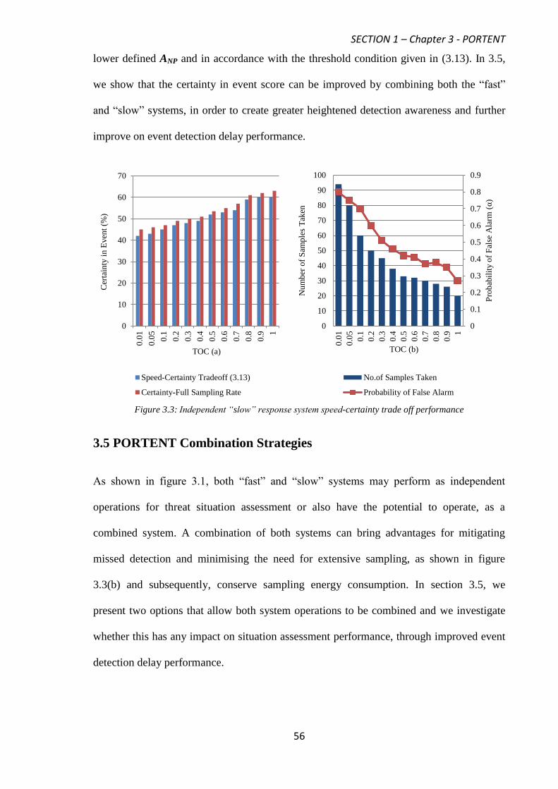
SECTION 1 – Chapter 3 - PORTENT
56
lower defined ANP and in accordance with the threshold condition given in (3.13). In 3.5,
we show that the certainty in event score can be improved by combining both the “fast”
and “slow” systems, in order to create greater heightened detection awareness and further
improve on event detection delay performance.
Figure 3.3: Independent “slow” response system speed-certainty trade off performance
3.5 PORTENT Combination Strategies
As shown in figure 3.1, both “fast” and “slow” systems may perform as independent
operations for threat situation assessment or also have the potential to operate, as a
combined system. A combination of both systems can bring advantages for mitigating
missed detection and minimising the need for extensive sampling, as shown in figure
3.3(b) and subsequently, conserve sampling energy consumption. In section 3.5, we
present two options that allow both system operations to be combined and we investigate
whether this has any impact on situation assessment performance, through improved event
detection delay performance.
0
10
20
30
40
50
60
70
0.0
1
0.0
5
0.1
0.2
0.3
0.4
0.5
0.6
0.7
0.8
0.9 1
Cer
tain
ty i
n E
ven
t (%
)
TOC (a)
Speed-Certainty Tradeoff (3.13)
Certainty-Full Sampling Rate
0
0.1
0.2
0.3
0.4
0.5
0.6
0.7
0.8
0.9
0
10
20
30
40
50
60
70
80
90
100
0.0
1
0.0
5
0.1
0.2
0.3
0.4
0.5
0.6
0.7
0.8
0.9 1
Pro
bab
ilit
y o
f F
alse
Ala
rm (
α)
Nu
mb
er o
f S
amp
les
Tak
en
TOC (b)
No.of Samples Taken
Probability of False Alarm

SECTION 1 – Chapter 3 - PORTENT
57
3.5.1 PORTENT Combination-Option 1
If the “fast” response system fails to make a decision concerning “positive detection”,
therefore, resulting in a potential missed detection, the “slow” response system can begin
to receive sensory data. The likelihood, therefore, of a threat being present if the “fast”
response system fails to act becomes less than PR. A new probability of a threat being
present, conditional upon the “fast” system failing to act, P’R, is then required and can be
formulated, as shown in (3.14).
FAST
0FAST0R
FAST
1FAST0R
FAST
1FAST0R
R
RR
RR
)x(LE)P1(
)x(LEP
)x(LEP
'P
)AlarmFalse(p)P1()jectionReIncorrect(pP
)jectionReIncorrect(pP'P
(3.14)
The probability P’R from (3.14) can be substituted for PR and used to calculate αopt,
required for the NP-threshold, ANP, calculation described in (3.12). This then allows the
overall “slow” system to function and take over “positive detection” decision making,
given by the condition in (3.13).
3.5.2 PORTENT Combination-Option 2
Again if the “fast” response system fails to make a “positive detection” outcome, it is
feasible to consider the “slow” response system having access to the signal level criterion,
L(x), used by the “fast” response system, given in (3.4). The signal level criterion, L(x),
could have the potential to provide a more accurate estimate of the probability of a threat
being present, P’’R, as shown in (3.15).
))x(L(f)P1())x(L(fP
))x(L(fP''P
0FastR1FastR
1FastRR
(3.15)
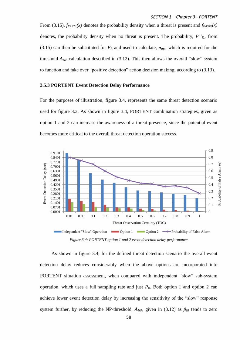
SECTION 1 – Chapter 3 - PORTENT
58
From (3.15), fFAST1(x) denotes the probability density when a threat is present and fFAST0(x)
denotes, the probability density when no threat is present. The probability, P’’R,, from
(3.15) can then be substituted for PR and used to calculate, αopt, which is required for the
threshold ANP calculation described in (3.12). This then allows the overall “slow” system
to function and take over “positive detection” action decision making, according to (3.13).
3.5.3 PORTENT Event Detection Delay Performance
For the purposes of illustration, figure 3.4, represents the same threat detection scenario
used for figure 3.3. As shown in figure 3.4, PORTENT combination strategies, given as
option 1 and 2 can increase the awareness of a threat presence, since the potential event
becomes more critical to the overall threat detection operation success.
Figure 3.4: PORTENT option 1 and 2 event detection delay performance
As shown in figure 3.4, for the defined threat detection scenario the overall event
detection delay reduces considerably when the above options are incorporated into
PORTENT situation assessment, when compared with independent “slow” sub-system
operation, which uses a full sampling rate and just PR. Both option 1 and option 2 can
achieve lower event detection delay by increasing the sensitivity of the “slow” response
system further, by reducing the NP-threshold, ANP, given in (3.12) as βIR tends to zero
0
0.1
0.2
0.3
0.4
0.5
0.6
0.7
0.8
0.9
0.0001
0.0701
0.1401
0.2101
0.2801
0.3501
0.4201
0.4901
0.5601
0.6301
0.7001
0.7701
0.8401
0.9101
0.01 0.05 0.1 0.2 0.3 0.4 0.5 0.6 0.7 0.8 0.9 1P
rob
abil
ity o
f F
alse
Ala
rm (
α)
Even
t D
etec
tio
n D
elay
(se
c)
Threat Observation Certainty (TOC)
Independent "Slow" Operation Option 1 Option 2 Probability of False Alarm

SECTION 1 – Chapter 3 - PORTENT
59
and α reduces. Figure 3.4 also indicates that option 2 has the potential to improve the
situation assessment in conditions where the “fast” response system fails to act by
achieving an overall lower, event detection delay performance. The flow chart describing
the overall combined PORTENT situation assessment system, in relation to the two
options described above is detailed in Appendix A, part 1.
3.6 Characterising Threat Detection Information
Event detection delay is just one way of measuring situation assessment performance. In
3.6, we incorporate other, relevant, threat detection measures and aggregate them into an
overall figure of merit to describe situation assessment performance. Aggregation of
captured threat detection information in this manner, is commonly referred to as, quality of
surveillance information (QoSI) [51-52]. QoSI is therefore a characterisation of the salient
features (quality factors) associated with situations of interest, detected by and flowing
through the UGS network (e.g. detection accuracy). For PORTENT threat detection
performance purposes, detection accuracy (q1), detection certainty (q2) and detection
timeliness (q3) quality factors, are specifically used.
3.6.1 Detection Accuracy
In the surveillance domain, accuracy of threat detection refers to the total number of
correctly detected events to the total number of events that occurred in the environment, as
shown in (3.16). From (3.16), EC,j is the number of correctly detected instances of the jth
event by the system over a period of time and ET,j the total number of instances of the jth
event.
j,T
j,C1 E
Eq
(3.16)

SECTION 1 – Chapter 3 - PORTENT
60
3.6.2 Detection Certainty
Detection certainty represents the confirmation level of the identified event, in the form of
a probability score. The score represents the confirmation that an identified event exists,
within an uncertain environment, as shown in (3.17).
))L|I(p(Avgq n
j2 (3.17)
From (3.17), p (Ij | Ln ) represents the probability of existence of the information item Ij
(e.g. the occurrence of the jth
event) based on the set of Ln samples. Avg is a function to
average the certainty level of an individual information item over a period of time.
3.6.3 Detection Timeliness
Detection timeliness is a measure of the timeliness of information being available at the
desired time and the ability to link related events that occur at different times (i.e. building
a coherent picture over time). PORTENT is expected to detect the jth
information item
(event) at time T of its occurrence, however if the system takes an additional time, T + ∆,
where ∆ is the event detection delay, the timeliness is then given, as shown in (3.18).
TTq3 (3.18)
3.6.4 Quality of Surveillance Information
After evaluating each respective quality factor, a linear weighted fusion strategy can be
applied to each quality factor through the assignment of normalized weights (Wb), where
the sum of all the Wb values used is equal to 1 [51-52]. Localised captured QoSI, can then
be expressed as an aggregation of these weighted quality factors, as shown in (3.19), where
V, represents the total number of quality factors used.
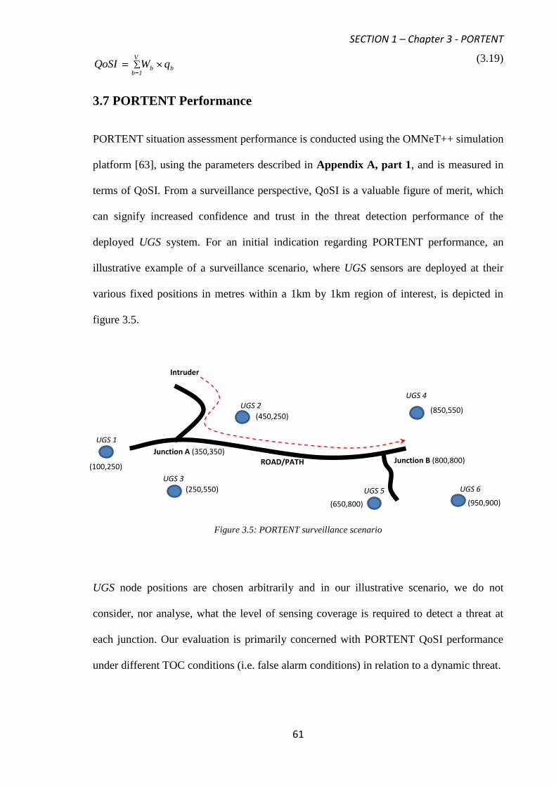
SECTION 1 – Chapter 3 - PORTENT
61
V
1bbb qWQoSI (3.19)
3.7 PORTENT Performance
PORTENT situation assessment performance is conducted using the OMNeT++ simulation
platform [63], using the parameters described in Appendix A, part 1, and is measured in
terms of QoSI. From a surveillance perspective, QoSI is a valuable figure of merit, which
can signify increased confidence and trust in the threat detection performance of the
deployed UGS system. For an initial indication regarding PORTENT performance, an
illustrative example of a surveillance scenario, where UGS sensors are deployed at their
various fixed positions in metres within a 1km by 1km region of interest, is depicted in
figure 3.5.
Figure 3.5: PORTENT surveillance scenario
UGS node positions are chosen arbitrarily and in our illustrative scenario, we do not
consider, nor analyse, what the level of sensing coverage is required to detect a threat at
each junction. Our evaluation is primarily concerned with PORTENT QoSI performance
under different TOC conditions (i.e. false alarm conditions) in relation to a dynamic threat.
Intruder
Junction B (800,800)
Junction A (350,350)
UGS 1
(950,900)
(850,550)
(250,550)
(450,250)
(100,250)
(650,800)
UGS 3 UGS 6 UGS 5
UGS 4 UGS 2
ROAD/PATH
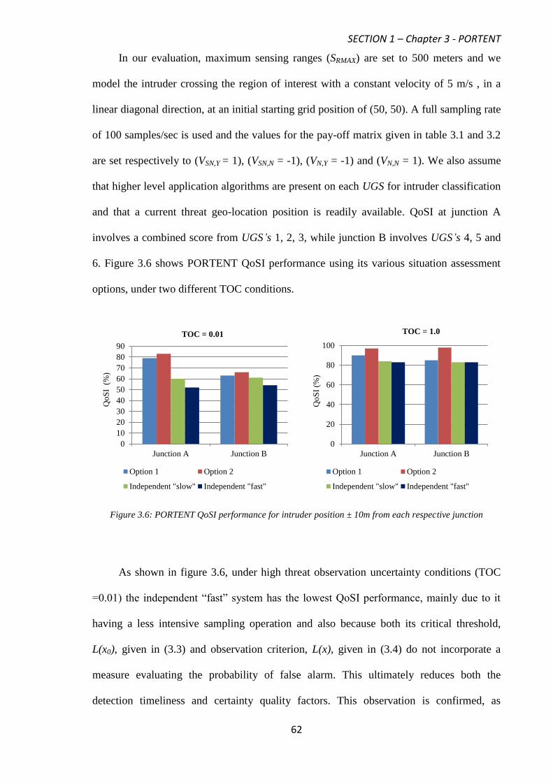
SECTION 1 – Chapter 3 - PORTENT
62
In our evaluation, maximum sensing ranges (SRMAX) are set to 500 meters and we
model the intruder crossing the region of interest with a constant velocity of 5 m/s , in a
linear diagonal direction, at an initial starting grid position of (50, 50). A full sampling rate
of 100 samples/sec is used and the values for the pay-off matrix given in table 3.1 and 3.2
are set respectively to (VSN,Y = 1), (VSN,N = -1), (VN,Y = -1) and (VN,N = 1). We also assume
that higher level application algorithms are present on each UGS for intruder classification
and that a current threat geo-location position is readily available. QoSI at junction A
involves a combined score from UGS’s 1, 2, 3, while junction B involves UGS’s 4, 5 and
6. Figure 3.6 shows PORTENT QoSI performance using its various situation assessment
options, under two different TOC conditions.
Figure 3.6: PORTENT QoSI performance for intruder position ± 10m from each respective junction
As shown in figure 3.6, under high threat observation uncertainty conditions (TOC
=0.01) the independent “fast” system has the lowest QoSI performance, mainly due to it
having a less intensive sampling operation and also because both its critical threshold,
L(x0), given in (3.3) and observation criterion, L(x), given in (3.4) do not incorporate a
measure evaluating the probability of false alarm. This ultimately reduces both the
detection timeliness and certainty quality factors. This observation is confirmed, as
0
10
20
30
40
50
60
70
80
90
Junction A Junction B
Qo
SI
(%
)
TOC = 0.01
Option 1 Option 2
Independent "slow" Independent "fast"
0
20
40
60
80
100
Junction A Junction B
Qo
SI
(%)
TOC = 1.0
Option 1 Option 2
Independent "slow" Independent "fast"
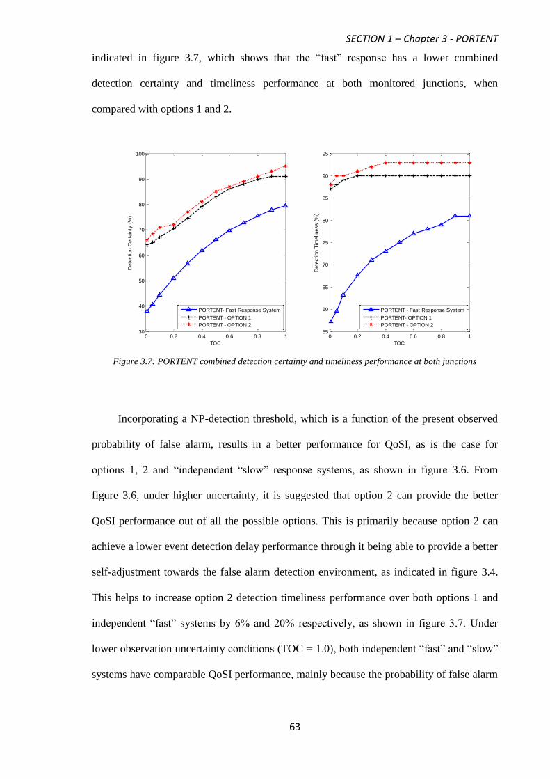
SECTION 1 – Chapter 3 - PORTENT
63
indicated in figure 3.7, which shows that the “fast” response has a lower combined
detection certainty and timeliness performance at both monitored junctions, when
compared with options 1 and 2.
Figure 3.7: PORTENT combined detection certainty and timeliness performance at both junctions
Incorporating a NP-detection threshold, which is a function of the present observed
probability of false alarm, results in a better performance for QoSI, as is the case for
options 1, 2 and “independent “slow” response systems, as shown in figure 3.6. From
figure 3.6, under higher uncertainty, it is suggested that option 2 can provide the better
QoSI performance out of all the possible options. This is primarily because option 2 can
achieve a lower event detection delay performance through it being able to provide a better
self-adjustment towards the false alarm detection environment, as indicated in figure 3.4.
This helps to increase option 2 detection timeliness performance over both options 1 and
independent “fast” systems by 6% and 20% respectively, as shown in figure 3.7. Under
lower observation uncertainty conditions (TOC = 1.0), both independent “fast” and “slow”
systems have comparable QoSI performance, mainly because the probability of false alarm
0 0.2 0.4 0.6 0.8 130
40
50
60
70
80
90
100
TOC
Dete
ction C
ert
ain
ty (
%)
0 0.2 0.4 0.6 0.8 155
60
65
70
75
80
85
90
95
TOC
Dete
ction T
imelin
ess (
%)
PORTENT- Fast Response System
PORTENT - OPTION 1
PORTENT - OPTION 2
PORTENT - Fast Response System
PORTENT- OPTION 1
PORTENT - OPTION 2
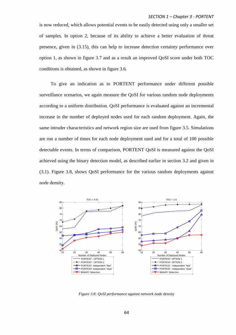
SECTION 1 – Chapter 3 - PORTENT
64
is now reduced, which allows potential events to be easily detected using only a smaller set
of samples. In option 2, because of its ability to achieve a better evaluation of threat
presence, given in (3.15), this can help to increase detection certainty performance over
option 1, as shown in figure 3.7 and as a result an improved QoSI score under both TOC
conditions is obtained, as shown in figure 3.6.
To give an indication as to PORTENT performance under different possible
surveillance scenarios, we again measure the QoSI for various random node deployments
according to a uniform distribution. QoSI performance is evaluated against an incremental
increase in the number of deployed nodes used for each random deployment. Again, the
same intruder characteristics and network region size are used from figure 3.5. Simulations
are run a number of times for each node deployment used and for a total of 100 possible
detectable events. In terms of comparison, PORTENT QoSI is measured against the QoSI
achieved using the binary detection model, as described earlier in section 3.2 and given in
(3.1). Figure 3.8, shows QoSI performance for the various random deployments against
node density.
Figure 3.8: QoSI performance against network node density
10 20 30 40 50 6045
50
55
60
65
70
75
80
85TOC = 0.01
Number of Deployed Nodes
QoS
I (%
)
10 20 30 40 50 6050
55
60
65
70
75
80
85
90TOC = 1.0
Number of Deployed Nodes
QoS
I (%
)
PORTENT- OPTION 1
PORTENT- OPTION 2
PORTENT - Independent "fast"
PORTENT - Independent "slow"
BINARY Detection
PORTENT - OPTION 1
PORTENT - OPTION 2
PORTENT- Independent "fast"
PORTENT- Independent "slow"
BINARY Detection
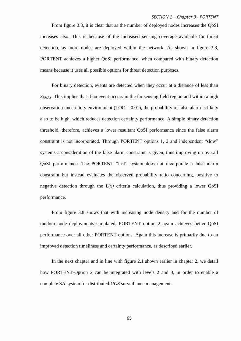
SECTION 1 – Chapter 3 - PORTENT
65
From figure 3.8, it is clear that as the number of deployed nodes increases the QoSI
increases also. This is because of the increased sensing coverage available for threat
detection, as more nodes are deployed within the network. As shown in figure 3.8,
PORTENT achieves a higher QoSI performance, when compared with binary detection
means because it uses all possible options for threat detection purposes.
For binary detection, events are detected when they occur at a distance of less than
SRMAX. This implies that if an event occurs in the far sensing field region and within a high
observation uncertainty environment (TOC = 0.01), the probability of false alarm is likely
also to be high, which reduces detection certainty performance. A simple binary detection
threshold, therefore, achieves a lower resultant QoSI performance since the false alarm
constraint is not incorporated. Through PORTENT options 1, 2 and independent “slow”
systems a consideration of the false alarm constraint is given, thus improving on overall
QoSI performance. The PORTENT “fast” system does not incorporate a false alarm
constraint but instead evaluates the observed probability ratio concerning, positive to
negative detection through the L(x) criteria calculation, thus providing a lower QoSI
performance.
From figure 3.8 shows that with increasing node density and for the number of
random node deployments simulated, PORTENT option 2 again achieves better QoSI
performance over all other PORTENT options. Again this increase is primarily due to an
improved detection timeliness and certainty performance, as described earlier.
In the next chapter and in line with figure 2.1 shown earlier in chapter 2, we detail
how PORTENT-Option 2 can be integrated with levels 2 and 3, in order to enable a
complete SA system for distributed UGS surveillance management.
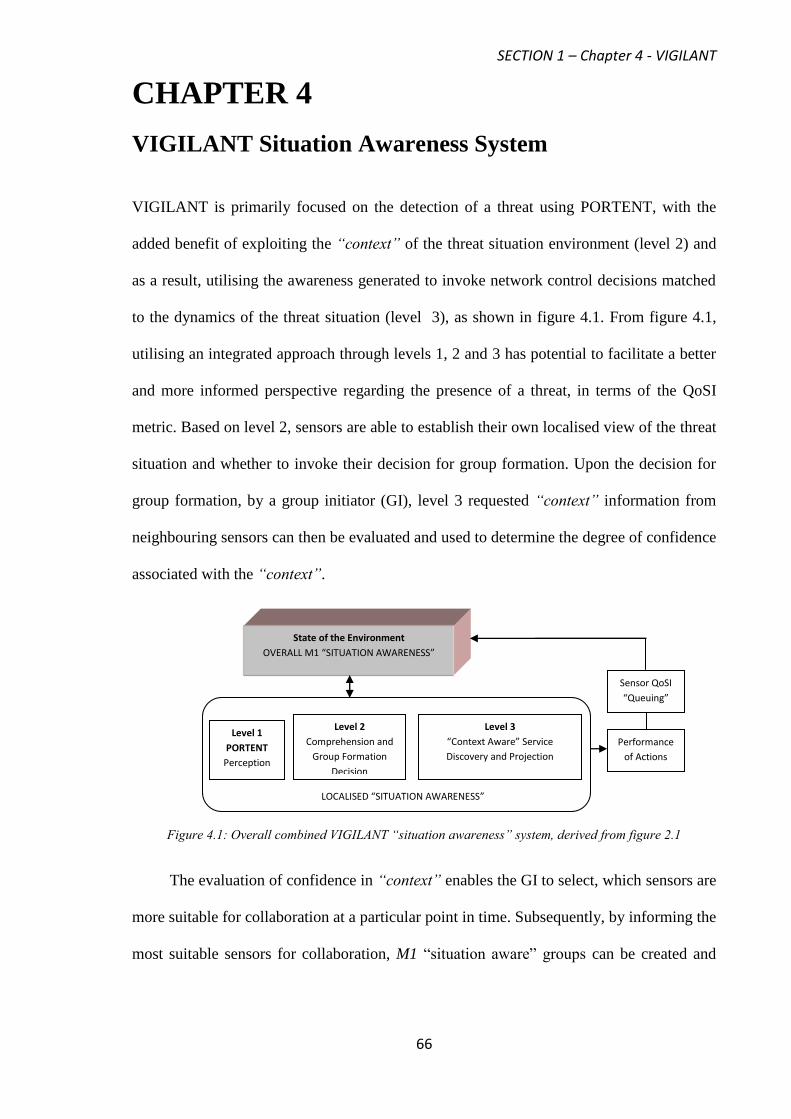
SECTION 1 – Chapter 4 - VIGILANT
66
CHAPTER 4
VIGILANT Situation Awareness System
VIGILANT is primarily focused on the detection of a threat using PORTENT, with the
added benefit of exploiting the “context” of the threat situation environment (level 2) and
as a result, utilising the awareness generated to invoke network control decisions matched
to the dynamics of the threat situation (level 3), as shown in figure 4.1. From figure 4.1,
utilising an integrated approach through levels 1, 2 and 3 has potential to facilitate a better
and more informed perspective regarding the presence of a threat, in terms of the QoSI
metric. Based on level 2, sensors are able to establish their own localised view of the threat
situation and whether to invoke their decision for group formation. Upon the decision for
group formation, by a group initiator (GI), level 3 requested “context” information from
neighbouring sensors can then be evaluated and used to determine the degree of confidence
associated with the “context”.
Figure 4.1: Overall combined VIGILANT “situation awareness” system, derived from figure 2.1
The evaluation of confidence in “context” enables the GI to select, which sensors are
more suitable for collaboration at a particular point in time. Subsequently, by informing the
most suitable sensors for collaboration, M1 “situation aware” groups can be created and
Sensor QoSI
“Queuing”
State of the Environment
OVERALL M1 “SITUATION AWARENESS”
Performance
of Actions
Level 1
PORTENT
Perception
Level 2
Comprehension and
Group Formation
Decision
Level 3
“Context Aware” Service
Discovery and Projection
LOCALISED “SITUATION AWARENESS”

SECTION 1 – Chapter 4 - VIGILANT
67
their respective QoSI values aggregated. In section 4.1, we detail the level 2 process
involved for deriving relevant “context” concerning the M1 surveillance situation.
4.1 VIGILANT – Comprehension and Group Formation Decision
VIGILANT level 2, involves comprehending the significance associated with raw sensor
data captured within an uncertain environment. Comprehending the environment in which
potential threats exist, can be argued as the most critical part of the mission requirement
since this reduces the chance of relevant events remaining undetected. Comprehension of
situations occurring in an uncertain environment requires a level of cognitive capability, in
order to derive the relevant “context” of those situations [53]. In general, there exist two
approaches to the modelling of situations within uncertain environments of interest [53-
54]. These are:
State orientated approaches look on situations as aggregated state entities of the
world.
Action orientated approaches consider situations as sequences of actions and
viewpoints originating from some declared initial world state [55].
Both these approaches facilitate the view of the current perceived situation and this
promotes a concise structure.
For VIGILANT level 2, we utilise an action orientated design approach in the form
of a Bayesian Belief Network (BBN). When compared with other action orientated
techniques, such as Dempster-Schafer theory, designs that involve BBN’s have always
proved very useful and effective in a variety of decision aiding domains, especially in
dealing with issues concerning inference within an uncertain environment [56-57]. A BBN
is a directed acyclic graph, using a collection of nodes denoting the random variables,
which represent hat situation domain [58]. Corresponding links between the nodes define

SECTION 1 – Chapter 4 - VIGILANT
68
the casual relationships between them, with conditional probability tables (CPTs) encoding
the quantitative influence. Where no link exists between nodes, the quantitative influence
can be given as marginal probabilities. The BBN network used to describe VIGILANT
level 2 is shown in figure 4.2. From figure 4.2, the topology describing the situation
“domain” for threat detection purposes consists of six binary variables, which together
encodes the qualitative knowledge of the “domain” in the following ways:
1. Sensed observation influences “yes” threat present.
2. Sensed observation influences “no” threat present.
3. Both “yes and no” threat presence jointly have a direct effect on the understanding
concerning the “current threat”.
4. The “current threat” influences the decision to form situation awareness group.
5. The “current threat” influences the decision to wait for next observation.
Table 4.1, summarises the probability expressions derived from our VIGILANT
level 2 BBN. Based on table 4.1, derivation of the “context” concerning the current
situation, in order to aid final decision making for initiating group formation, “context-
aware” collaboration and network management functions, is achieved and is described
further in 4.2 and 4.3.
4.2 VIGILANT Level 2 – “Context-Aware” Collaboration
VIGILANT collaboration is driven by the UGS, which perceives the highest current threat
established in level 2, named the Group Initiator (GI), as shown in figure 4.2. The ability to
infer situations (i.e. current threat level), is a critical function for “context-aware” systems,
acting as driver for adaptive behaviour at the application level and can be initiated using
“context-aware” service discovery mechanisms [59].
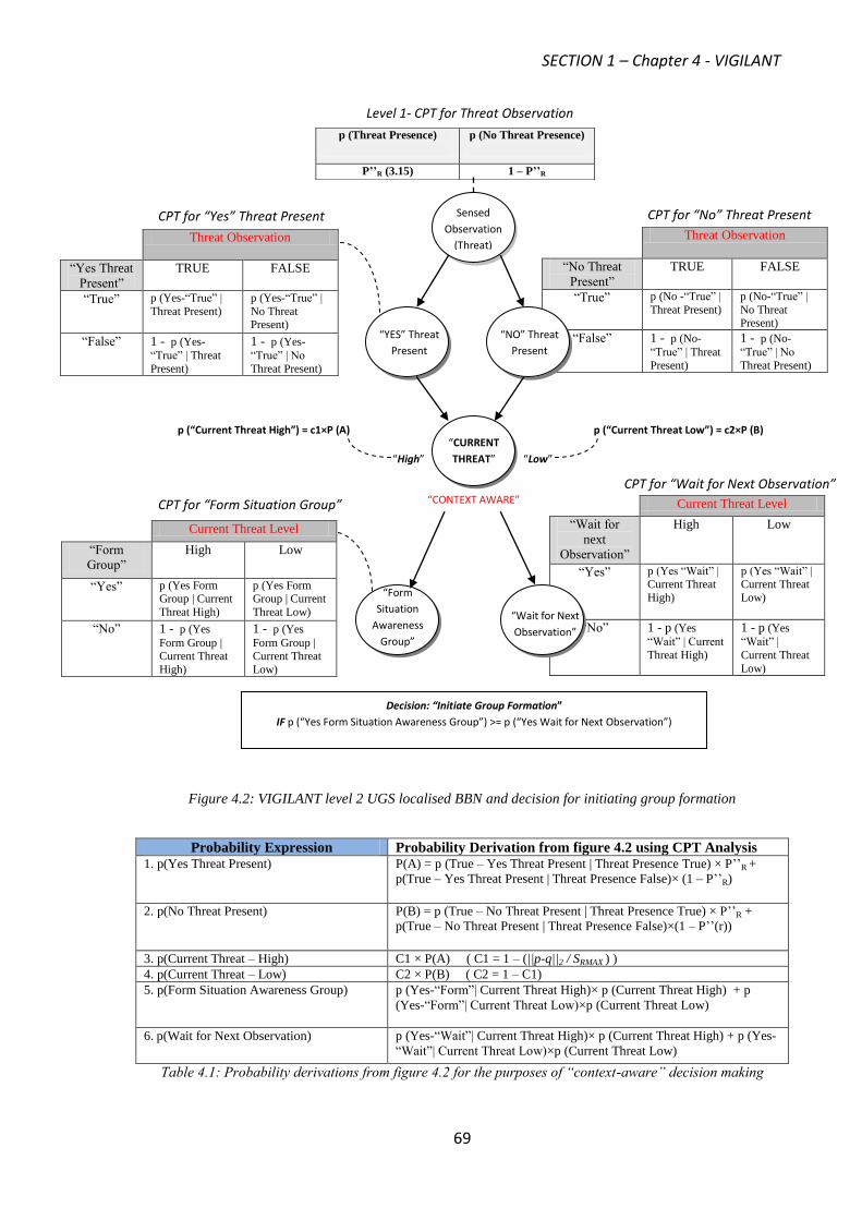
SECTION 1 – Chapter 4 - VIGILANT
69
Figure 4.2: VIGILANT level 2 UGS localised BBN and decision for initiating group formation
Probability Expression Probability Derivation from figure 4.2 using CPT Analysis 1. p(Yes Threat Present) P(A) = p (True – Yes Threat Present | Threat Presence True) × P’’R +
p(True – Yes Threat Present | Threat Presence False)× (1 – P’’R)
2. p(No Threat Present) P(B) = p (True – No Threat Present | Threat Presence True) × P’’R +
p(True – No Threat Present | Threat Presence False)×(1 – P’’(r))
3. p(Current Threat – High) C1 × P(A) ( C1 = 1 – (||p-q||2 / SRMAX ) )
4. p(Current Threat – Low) C2 × P(B) ( C2 = 1 – C1)
5. p(Form Situation Awareness Group) p (Yes-“Form”| Current Threat High)× p (Current Threat High) + p
(Yes-“Form”| Current Threat Low)×p (Current Threat Low)
6. p(Wait for Next Observation) p (Yes-“Wait”| Current Threat High)× p (Current Threat High) + p (Yes-
“Wait”| Current Threat Low)×p (Current Threat Low)
Table 4.1: Probability derivations from figure 4.2 for the purposes of “context-aware” decision making
p (Threat Presence)
p (No Threat Presence)
P’’R (3.15) 1 – P’’R
Threat Observation
“No Threat
Present”
TRUE FALSE
“True” p (No -“True” |
Threat Present) p (No-“True” |
No Threat Present)
“False” 1 - p (No-
“True” | Threat
Present)
1 - p (No-
“True” | No
Threat Present)
Threat Observation
“Yes Threat
Present”
TRUE FALSE
“True” p (Yes-“True” |
Threat Present) p (Yes-“True” |
No Threat Present)
“False” 1 - p (Yes-
“True” | Threat
Present)
1 - p (Yes-
“True” | No
Threat Present)
Current Threat Level
“Wait for
next
Observation”
High Low
“Yes” p (Yes “Wait” | Current Threat
High)
p (Yes “Wait” | Current Threat
Low)
“No” 1 - p (Yes
“Wait” | Current
Threat High)
1 - p (Yes
“Wait” |
Current Threat
Low)
Current Threat Level
“Form
Group”
High Low
“Yes” p (Yes Form Group | Current
Threat High)
p (Yes Form Group | Current
Threat Low)
“No” 1 - p (Yes
Form Group | Current Threat
High)
1 - p (Yes
Form Group | Current Threat
Low)
CPT for “Wait for Next Observation”
Sensed
Observation
(Threat)
“NO” Threat
Present
“CURRENT
THREAT”
“CONTEXT AWARE”
“Low” “High”
p (“Current Threat Low”) = c2×P (B) p (“Current Threat High”) = c1×P (A)
“Form
Situation
Awareness
Group”
Decision: “Initiate Group Formation”
IF p (“Yes Form Situation Awareness Group”) >= p (“Yes Wait for Next Observation”)
“YES” Threat
Present
“Wait for Next
Observation”
Level 1- CPT for Threat Observation
CPT for “Yes” Threat Present CPT for “No” Threat Present
CPT for “Form Situation Group”

SECTION 1 – Chapter 4 - VIGILANT
70
For M1 operation, sensors collaborate to facilitate collection of additional
information concerning the present, in order to satisfy the requirement in achieving a high
QoSI aggregation score and thus, confidence in threat presence notification. A “context-
aware” service discovery thus utilises the deployed distributed UGS network, in order to
assist the grouping of single hop UGS nodes that exhibit common “context” about the
current threat situation. In 4.2.1 we detail how VIGILANT achieves this.
4.2.1 “Context-Aware” Service Discovery
“Context-aware” service discovery can be achieved through establishing the level of
confidence in “context”, concerning the threat presence situation. The certainty factor (CF)
model is one approach towards evaluating and measuring this confidence (e.g. “context” in
threat presence) between two random entities (e.g. GI and its immediate neighbour) [60].
The CF model operates according to proportional measures of increased belief (MB)
and disbelief (MD) about a certain hypothesis. For VIGILANT, the hypothesis stems from
the degree of certainty in MB and MD that an individual UGS should form a partnership
with their GI according to, its current threat presence “context”, as shown in (4.1), where
MB and MD supporting (4.1) are derived from table 4.1 and are given in (4.2) and (4.3)
respectively.
)MD,MBmin(1)MDMB(
"Sensor"CF (4.1)
)highlevelthreatCurrent(p1
)highlevelthreatCurrent(p)highlevelthreatCurrent|GroupSAForm(pMB
(4.2)
)highlevelthreatCurrent(p
)highlevelthreatCurrent|GroupSAForm(p)highlevelthreatCurrent(pMB
(4.3)
To facilitate an on-going dynamic “context-aware” discovery mechanism, sensors would
compute their CF “sensor” values throughout a M1 surveillance mission and only report
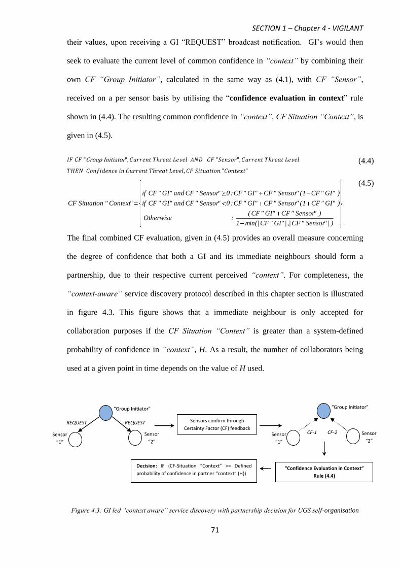
SECTION 1 – Chapter 4 - VIGILANT
71
their values, upon receiving a GI “REQUEST” broadcast notification. GI’s would then
seek to evaluate the current level of common confidence in “context” by combining their
own CF “Group Initiator”, calculated in the same way as (4.1), with CF “Sensor”,
received on a per sensor basis by utilising the “confidence evaluation in context” rule
shown in (4.4). The resulting common confidence in “context”, CF Situation “Context”, is
given in (4.5).
(4.4)
)|"Sensor"CF|,|"GI"CFmin(|1
)"Sensor"CF"GI"CF(:Otherwise
)"GI"CF1("Sensor"CF"GI"CF:0"Sensor"CFand"GI"CFif
)"GI"CF1("Sensor"CF"GI"CF:0"Sensor"CFand"GI"CFif
"Context"SituationCF
(4.5)
The final combined CF evaluation, given in (4.5) provides an overall measure concerning
the degree of confidence that both a GI and its immediate neighbours should form a
partnership, due to their respective current perceived “context”. For completeness, the
“context-aware” service discovery protocol described in this chapter section is illustrated
in figure 4.3. This figure shows that a immediate neighbour is only accepted for
collaboration purposes if the CF Situation “Context” is greater than a system-defined
probability of confidence in “context”, H. As a result, the number of collaborators being
used at a given point in time depends on the value of H used.
Figure 4.3: GI led “context aware” service discovery with partnership decision for UGS self-organisation
Sensors confirm through
Certainty Factor (CF) feedback
“Confidence Evaluation in Context”
Rule (4.4)
Decision: IF (CF-Situation “Context” >= Defined
probability of confidence in partner “context” (H))
THEN “Sensor to Form Partnership With”
Sensor
“1”
“Group Initiator”
REQUEST REQUEST
Sensor
“2”
Sensor
“1”
“Group Initiator”
CF-1 CF-2 Sensor
“2”

SECTION 1 – Chapter 4 - VIGILANT
72
4.3 VIGILANT Level 3 – “Context-Aware” Network Management
Upon the GI deciding which immediate neighbours are applicable to form collaboration
with, it also, subsequently, determines a QoSI service provision time bound. The service
provision time itself is solely based on the level of common “context-awareness” there is
concerning a threat presence. A bound on the QoSI service provision time evaluated in this
manner has the potential to facilitate the management of the collaborating group in the
following ways:
Aggregated QoSI processing at the GI. This requires a level of stability within the
collaborating group and can be supported if group members are encouraged to
communicate their QoSI scores at defined time slot periods, which is matched to the
level of common M1 “context-awareness” they have with the GI.
Communicating at defined periods has potential in reducing both packet collisions and
latency (e.g. increase bandwidth efficiency) for QoSI reporting, especially when a
contention based medium access control scheme is being utilised.
4.3.1 Evaluating Common Threat “Context-Awareness” for Group Stability
Providing an accurate basis for QoSI aggregation, implies that the group structure has to
provide a level of stability for cases where there are no “contextual” changes. This entails
that group stability is actively encouraged in conditions where the level of common M1
“context-awareness” is high. Group stability can be evaluated by modelling the joint
probability in common low threat presence “context” between the GI and its
corresponding neighbour, as a random variable, U, with probability density function
(PDF1) and cumulative distribution function (CDF1), U~ N(μcommon low threat“context”,σ2
common
low threat “context”). Additionally the joint probability of common high threat presence
“context” is a random variable, T, with a PDF2 and CDF2 , T~ N(μcommon high
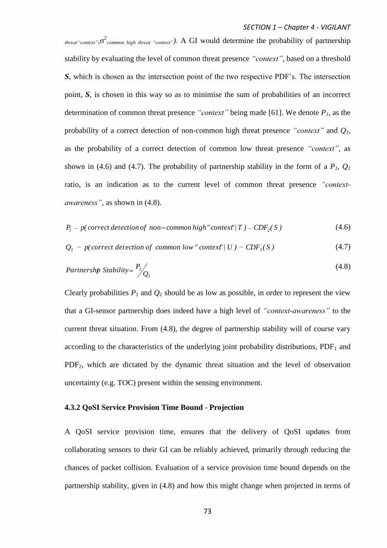
SECTION 1 – Chapter 4 - VIGILANT
73
threat“context”,σ2
common high threat “context”). A GI would determine the probability of partnership
stability by evaluating the level of common threat presence “context”, based on a threshold
S, which is chosen as the intersection point of the two respective PDF’s. The intersection
point, S, is chosen in this way so as to minimise the sum of probabilities of an incorrect
determination of common threat presence “context” being made [61]. We denote P1, as the
probability of a correct detection of non-common high threat presence “context” and Q1,
as the probability of a correct detection of common low threat presence “context”, as
shown in (4.6) and (4.7). The probability of partnership stability in the form of a P1, Q1
ratio, is an indication as to the current level of common threat presence “context-
awareness”, as shown in (4.8).
)S(CDF)T|"context"highcommonnonofectiondetcorrect(pP 21 (4.6)
)S(CDF)U|"context"lowcommonofectiondetcorrect(pQ 11 (4.7)
1
1
QP
StabilitypPartnershi (4.8)
Clearly probabilities P1 and Q1 should be as low as possible, in order to represent the view
that a GI-sensor partnership does indeed have a high level of “context-awareness” to the
current threat situation. From (4.8), the degree of partnership stability will of course vary
according to the characteristics of the underlying joint probability distributions, PDF1 and
PDF2, which are dictated by the dynamic threat situation and the level of observation
uncertainty (e.g. TOC) present within the sensing environment.
4.3.2 QoSI Service Provision Time Bound - Projection
A QoSI service provision time, ensures that the delivery of QoSI updates from
collaborating sensors to their GI can be reliably achieved, primarily through reducing the
chances of packet collision. Evaluation of a service provision time bound depends on the
partnership stability, given in (4.8) and how this might change when projected in terms of
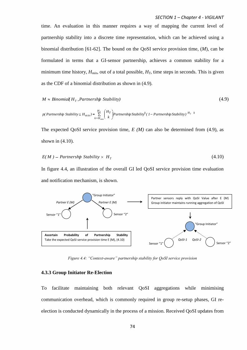
SECTION 1 – Chapter 4 - VIGILANT
74
time. An evaluation in this manner requires a way of mapping the current level of
partnership stability into a discrete time representation, which can be achieved using a
binomial distribution [61-62]. The bound on the QoSI service provision time, (M), can be
formulated in terms that a GI-sensor partnership, achieves a common stability for a
minimum time history, Hmin, out of a total possible, HT, time steps in seconds. This is given
as the CDF of a binomial distribution as shown in (4.9).
)StabilitypPartnershi,H(BinomialM T (4.9)
T
min
T
H
Hk
kHkTmin )StabilitypPartnershi1(StabilitypPartnershi
k
H)HStabilitypPartnershi(p
The expected QoSI service provision time, E (M) can also be determined from (4.9), as
shown in (4.10).
THStabilitypPartnershi)M(E (4.10)
In figure 4.4, an illustration of the overall GI led QoSI service provision time evaluation
and notification mechanism, is shown.
Figure 4.4: “Context-aware” partnership stability for QoSI service provision
4.3.3 Group Initiator Re-Election
To facilitate maintaining both relevant QoSI aggregations while minimising
communication overhead, which is commonly required in group re-setup phases, GI re-
election is conducted dynamically in the process of a mission. Received QoSI updates from
Ascertain Probability of Partnership Stability
Take the expected QoSI service provision time E (M), (4.10)
Partner sensors reply with QoSI Value after E (M)
Group initiator maintains running aggregation of QoSI Partner E (M)
Sensor “1”
“Group Initiator”
Partner E (M)
Sensor “2”
Sensor “1”
“Group Initiator”
QoSI-1 QoSI-2 Sensor “2”
SECTION 1 – Chapter 4 - VIGILANT
75
collaborating sensors, can be used by the GI to re-evaluate their current GI status, using a
relative QoSI ratio metric, as shown in (4.11).
SensorPartner
GIRatiolativeRe
QoSI
QoSIQoSI
(4.11)
Group initiators would invoke the process of passing on their lead status to a collaborating
sensor if, the QoSI Relative Ratio is less than or equal to 1. Notification of the new GI status is
then broadcast to the identified partner sensor, as shown in figure 4.5, which then re-
initialises the collaborating group, as detailed earlier in figures 4.3 and 4.4. Operations
describing the overall combined VIGILANT situation awareness system are described
further in Appendix A, part 2.
Figure 4.5: VIGILANT group initiator re-election operation
As shown in, Appendix A, part 2, the VIGILANT concept is concerned with the
collaboration of sensor nodes into groups that share common "context", where this
“context” is expressed in terms of the presence of a threat situation. This helps to support
the primary M1 concern for higher maintained QoSI (aggregated detection certainty,
accuracy and timeliness) provision levels, concerning the presence of a threat.
Sensor “1”
“Group Initiator”
QoSI-1 QoSI-2 Sensor “2”
Group initiator receives QoSI Values from partner sensors
Group initiator checks current status (4.11)
IF QoIRelative Ratio ≤ 1 THEN Invoke new
“Group initiator” status
New Group Initiator
Sensor “1”
“Group Initiator”
Sensor “2”

SECTION 1 – Chapter 4 - VIGILANT
76
4.4 VIGILANT System Performance
VIGILANT performance is simulated through the OMNeT++ network simulation platform
[63]. We utilise a fixed, 20 node and static UGS network, deployed randomly in a grid
coordinate system within a 1km by 1km region of interest. Maximum sensing ranges
(SRMAX) are set to 500 meters and we assume that higher level application algorithms are
present on each sensor for threat intruder classification purposes. Simulations are run using
a number of random deployments (>50), each with duration of 100 detectable events, using
a full sampling rate of 100samples/second and under loss free channel conditions. UGS
transmission ranges are also set to 500 metres and the IEEE802.11b protocol, in distributed
coordination function (DCF) basic access mode, is utilised for medium access control
(MAC). Surveillance is based on a mobile threat, moving at a constant velocity of 5m/s
within the region of interest in a diagonal direction.
As part of our system evaluation we do not consider the effects of sampling rate,
number of deployed nodes, velocity of threat and sensing coverage range on VIGILANT
performance. Our evaluation is more concerned about the effects of collaborating and
managing network resource consumption according to the “context-awareness” of a threat
presence within the surveillance environment. In 4.4.1, we begin by evaluating the QoSI
performance against the various VIGILANT system defined parameters.
4.4.1 Quality of Surveillance Information Performance
Since QoSI is a figure of merit characterising the presence of a threat, it is important from
a VIGILANT M1 perspective that accurate levels in QoSI are maintained. For VIGILANT
comparison purposes we use LEACH, as described earlier in chapter 2, under heading 2.1.
Using LEACH for comparison purposes is suitable since, it also supports ad-hoc
collaboration, utilising all immediate neighbours, but does not consider a “context-aware”
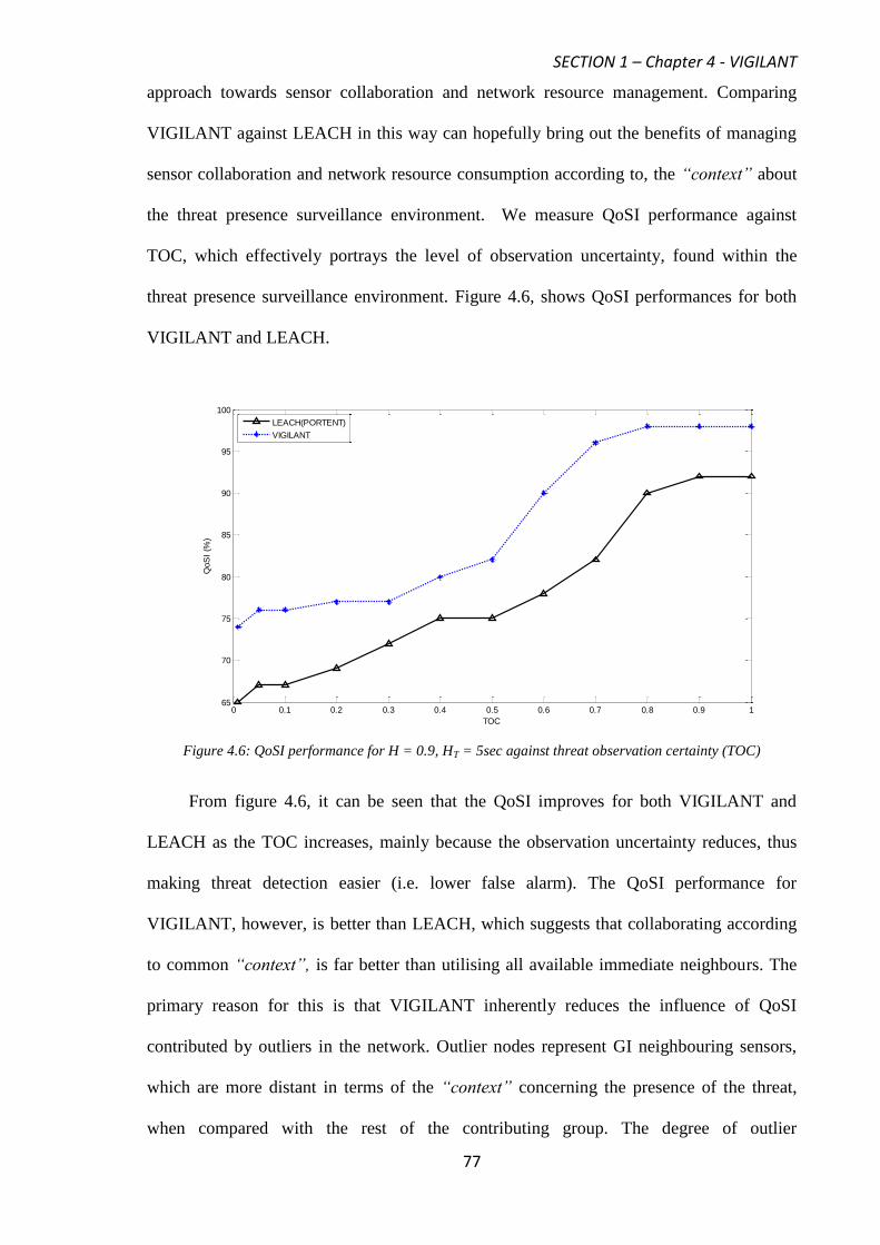
SECTION 1 – Chapter 4 - VIGILANT
77
approach towards sensor collaboration and network resource management. Comparing
VIGILANT against LEACH in this way can hopefully bring out the benefits of managing
sensor collaboration and network resource consumption according to, the “context” about
the threat presence surveillance environment. We measure QoSI performance against
TOC, which effectively portrays the level of observation uncertainty, found within the
threat presence surveillance environment. Figure 4.6, shows QoSI performances for both
VIGILANT and LEACH.
Figure 4.6: QoSI performance for H = 0.9, HT = 5sec against threat observation certainty (TOC)
From figure 4.6, it can be seen that the QoSI improves for both VIGILANT and
LEACH as the TOC increases, mainly because the observation uncertainty reduces, thus
making threat detection easier (i.e. lower false alarm). The QoSI performance for
VIGILANT, however, is better than LEACH, which suggests that collaborating according
to common “context”, is far better than utilising all available immediate neighbours. The
primary reason for this is that VIGILANT inherently reduces the influence of QoSI
contributed by outliers in the network. Outlier nodes represent GI neighbouring sensors,
which are more distant in terms of the “context” concerning the presence of the threat,
when compared with the rest of the contributing group. The degree of outlier
0 0.1 0.2 0.3 0.4 0.5 0.6 0.7 0.8 0.9 165
70
75
80
85
90
95
100
TOC
QoS
I (%
)
LEACH(PORTENT)
VIGILANT
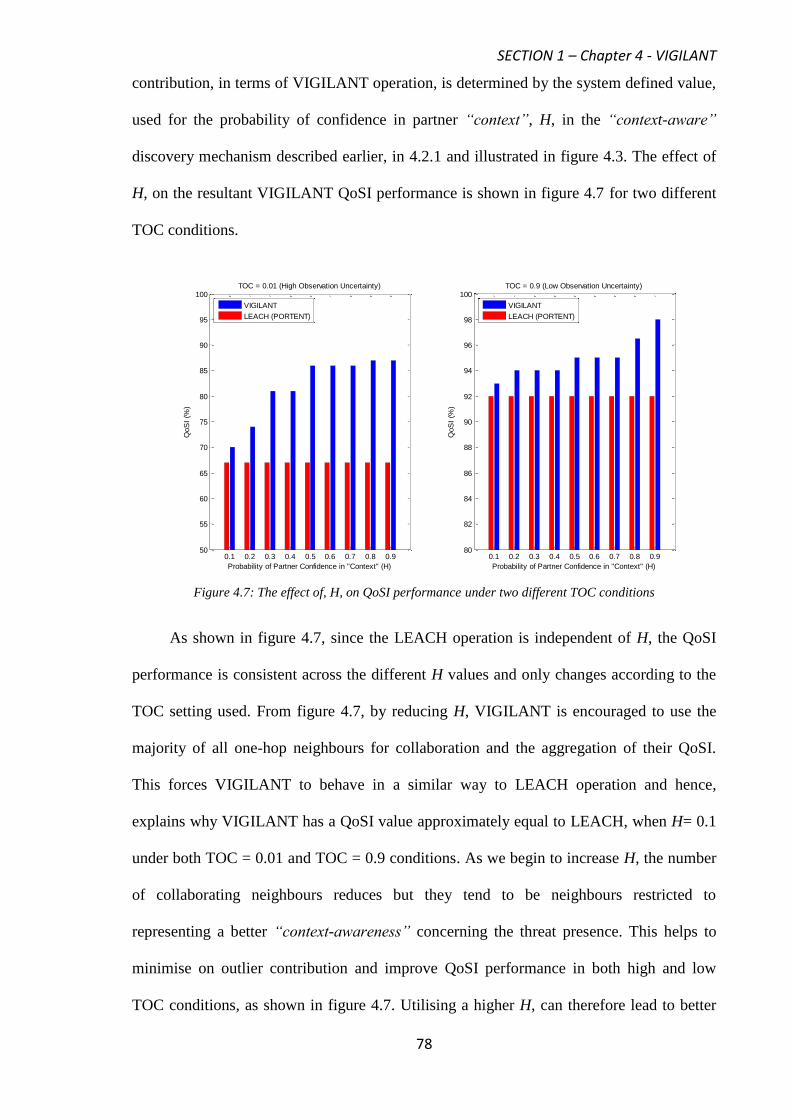
SECTION 1 – Chapter 4 - VIGILANT
78
contribution, in terms of VIGILANT operation, is determined by the system defined value,
used for the probability of confidence in partner “context”, H, in the “context-aware”
discovery mechanism described earlier, in 4.2.1 and illustrated in figure 4.3. The effect of
H, on the resultant VIGILANT QoSI performance is shown in figure 4.7 for two different
TOC conditions.
Figure 4.7: The effect of, H, on QoSI performance under two different TOC conditions
As shown in figure 4.7, since the LEACH operation is independent of H, the QoSI
performance is consistent across the different H values and only changes according to the
TOC setting used. From figure 4.7, by reducing H, VIGILANT is encouraged to use the
majority of all one-hop neighbours for collaboration and the aggregation of their QoSI.
This forces VIGILANT to behave in a similar way to LEACH operation and hence,
explains why VIGILANT has a QoSI value approximately equal to LEACH, when H= 0.1
under both TOC = 0.01 and TOC = 0.9 conditions. As we begin to increase H, the number
of collaborating neighbours reduces but they tend to be neighbours restricted to
representing a better “context-awareness” concerning the threat presence. This helps to
minimise on outlier contribution and improve QoSI performance in both high and low
TOC conditions, as shown in figure 4.7. Utilising a higher H, can therefore lead to better
0.1 0.2 0.3 0.4 0.5 0.6 0.7 0.8 0.950
55
60
65
70
75
80
85
90
95
100
Probability of Partner Confidence in "Context" (H)
QoS
I (%
)
TOC = 0.01 (High Observation Uncertainty)
0.1 0.2 0.3 0.4 0.5 0.6 0.7 0.8 0.980
82
84
86
88
90
92
94
96
98
100
Probability of Partner Confidence in "Context" (H)
QoS
I (%
)
TOC = 0.9 (Low Observation Uncertainty)
VIGILANT
LEACH (PORTENT)
VIGILANT
LEACH (PORTENT)
SECTION 1 – Chapter 4 - VIGILANT
79
collaboration between the GI and its immediate neighbours by ensuring that only sensors
with a high level of confidence in common “context” about the presence of a threat, as
determined using the CF model given in (4.5), are utilised. This provides an advantage for
ensuring that the relevant sensing coverage is extended over outlier nodes, in order to
maintain accurate levels of threat QoSI, a necessity for M1 surveillance operations.
4.4.2 “Context-Aware” Partner Service Provision Time Adaption
VIGILANT can improve on its own QoSI performance and continually over LEACH
because of the use of feedback from the sensing environment, as detailed in Appendix A,
part 2. The feedback is used to re-evaluate the current partnership stability given in (4.8),
on every QoSI update received from immediate GI collaborating neighbours. As a result,
QoSI service provision times, E (M), given in (4.10), can adapt according to changes in
common threat presence “context”. The effect of ensuring QoSI service provision times
are refreshed to guard against changes to common threat presence “context”, is shown in
figure 4.8. From figure 4.8, VIGILANT–No Adaption entails collaborating sensors that
continue to send their QoSI updates at every HT seconds and not at a re-evaluated time, E
(M) given in (4.10), according to figure 4.4 and Appendix A, part 2.
As shown in figure 4.8, non-adaption of the QoSI service provision times as HT
increases (VIGILANT-No adaption), can lead to a degradation in QoSI performance when
compared with VIGILANT. QoSI updates, which are sent on every HT second, ignore the
dynamics of the monitored threat. VIGILANT ensures that QoSI provision levels are
maintained according to the “context” of a dynamic threat presence, through re-evaluating
the current partnership stability given in (4.8), on every received QoSI update. This can
help to both improve and maintain a more consistent QoSI performance, as the TOC
environment increases.
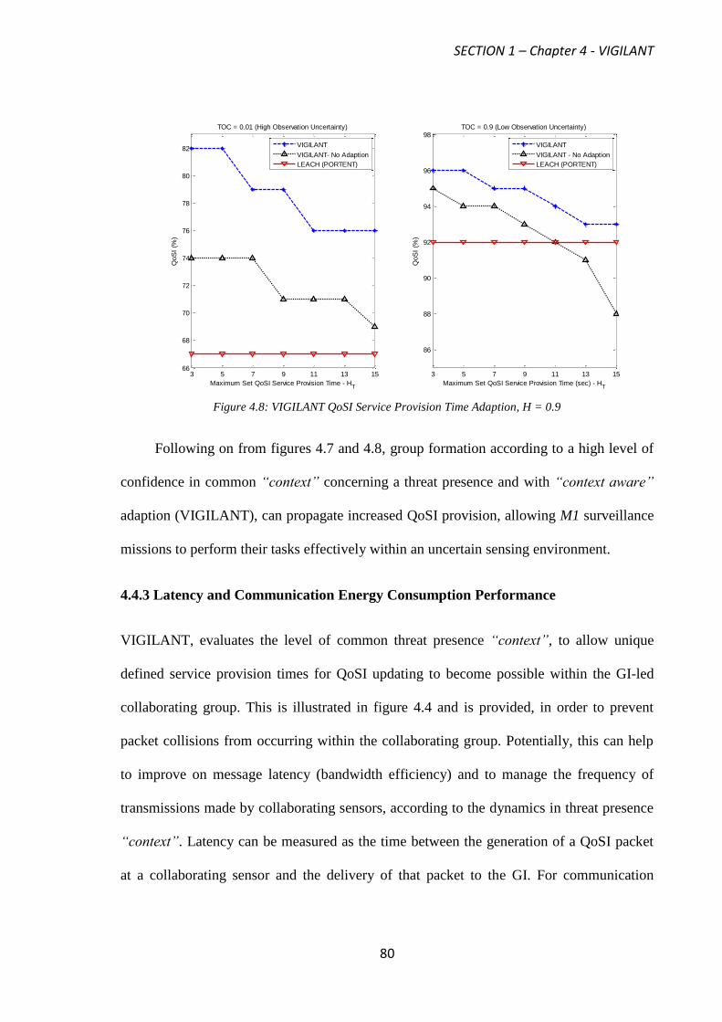
SECTION 1 – Chapter 4 - VIGILANT
80
Figure 4.8: VIGILANT QoSI Service Provision Time Adaption, H = 0.9
Following on from figures 4.7 and 4.8, group formation according to a high level of
confidence in common “context” concerning a threat presence and with “context aware”
adaption (VIGILANT), can propagate increased QoSI provision, allowing M1 surveillance
missions to perform their tasks effectively within an uncertain sensing environment.
4.4.3 Latency and Communication Energy Consumption Performance
VIGILANT, evaluates the level of common threat presence “context”, to allow unique
defined service provision times for QoSI updating to become possible within the GI-led
collaborating group. This is illustrated in figure 4.4 and is provided, in order to prevent
packet collisions from occurring within the collaborating group. Potentially, this can help
to improve on message latency (bandwidth efficiency) and to manage the frequency of
transmissions made by collaborating sensors, according to the dynamics in threat presence
“context”. Latency can be measured as the time between the generation of a QoSI packet
at a collaborating sensor and the delivery of that packet to the GI. For communication
3 5 7 9 11 13 1566
68
70
72
74
76
78
80
82
TOC = 0.01 (High Observation Uncertainty)
Maximum Set QoSI Service Provision Time - HT
QoS
I (%
)
3 5 7 9 11 13 15
86
88
90
92
94
96
98TOC = 0.9 (Low Observation Uncertainty)
Maximum Set QoSI Service Provision Time (sec) - HT
QoS
I (%
)
VIGILANT
VIGILANT - No Adaption
LEACH (PORTENT)
VIGILANT
VIGILANT- No Adaption
LEACH (PORTENT)
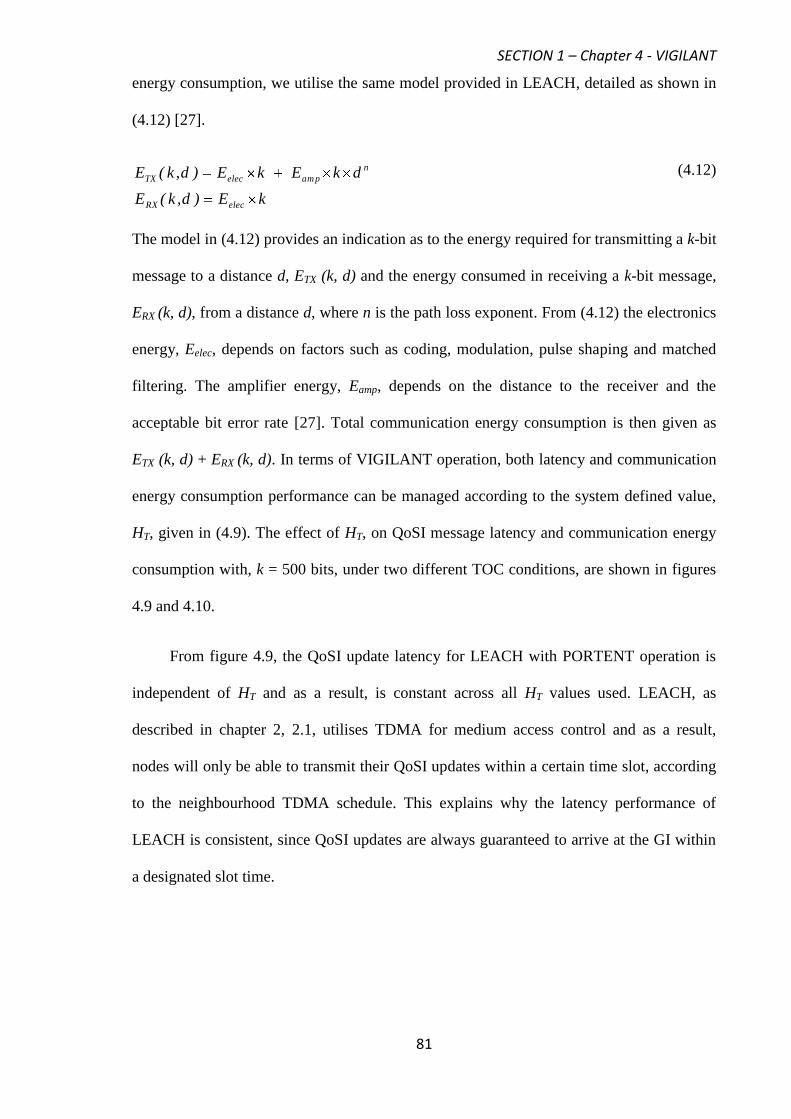
SECTION 1 – Chapter 4 - VIGILANT
81
energy consumption, we utilise the same model provided in LEACH, detailed as shown in
(4.12) [27].
kE)d,k(E
dkEkE)d,k(E
elecRX
n
am pelecTX
(4.12)
The model in (4.12) provides an indication as to the energy required for transmitting a k-bit
message to a distance d, ETX (k, d) and the energy consumed in receiving a k-bit message,
ERX (k, d), from a distance d, where n is the path loss exponent. From (4.12) the electronics
energy, Eelec, depends on factors such as coding, modulation, pulse shaping and matched
filtering. The amplifier energy, Eamp, depends on the distance to the receiver and the
acceptable bit error rate [27]. Total communication energy consumption is then given as
ETX (k, d) + ERX (k, d). In terms of VIGILANT operation, both latency and communication
energy consumption performance can be managed according to the system defined value,
HT, given in (4.9). The effect of HT, on QoSI message latency and communication energy
consumption with, k = 500 bits, under two different TOC conditions, are shown in figures
4.9 and 4.10.
From figure 4.9, the QoSI update latency for LEACH with PORTENT operation is
independent of HT and as a result, is constant across all HT values used. LEACH, as
described in chapter 2, 2.1, utilises TDMA for medium access control and as a result,
nodes will only be able to transmit their QoSI updates within a certain time slot, according
to the neighbourhood TDMA schedule. This explains why the latency performance of
LEACH is consistent, since QoSI updates are always guaranteed to arrive at the GI within
a designated slot time.
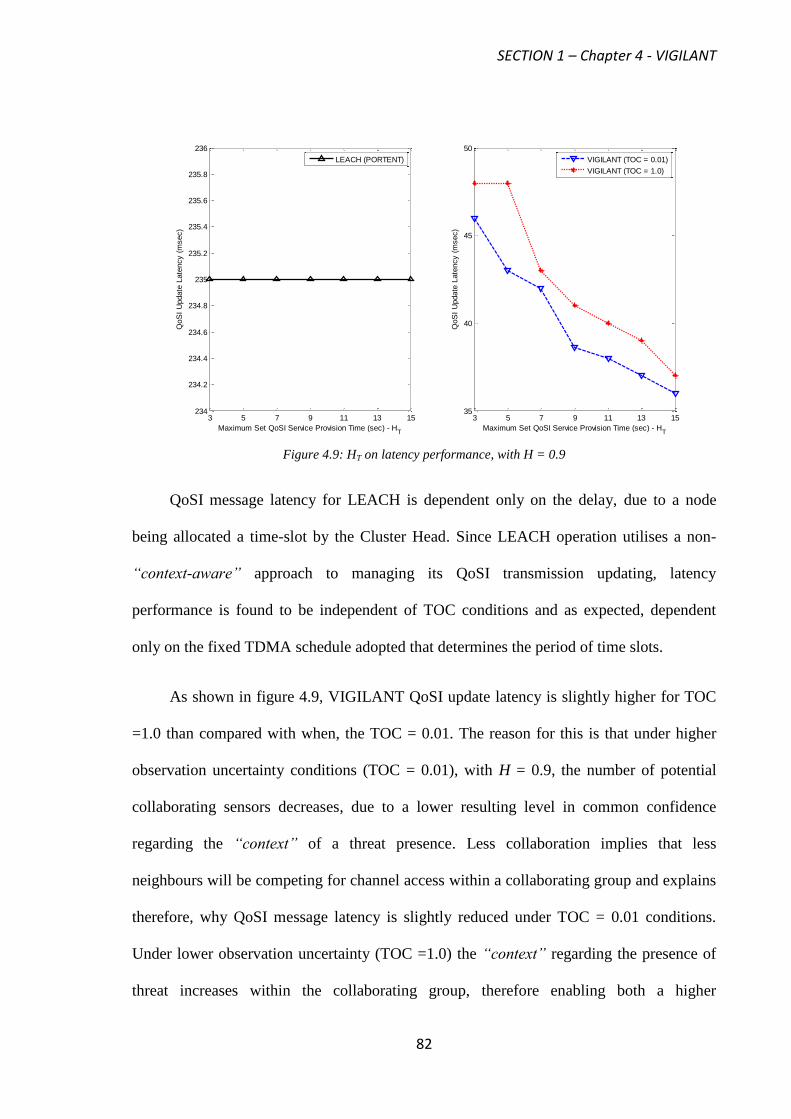
SECTION 1 – Chapter 4 - VIGILANT
82
Figure 4.9: HT on latency performance, with H = 0.9
QoSI message latency for LEACH is dependent only on the delay, due to a node
being allocated a time-slot by the Cluster Head. Since LEACH operation utilises a non-
“context-aware” approach to managing its QoSI transmission updating, latency
performance is found to be independent of TOC conditions and as expected, dependent
only on the fixed TDMA schedule adopted that determines the period of time slots.
As shown in figure 4.9, VIGILANT QoSI update latency is slightly higher for TOC
=1.0 than compared with when, the TOC = 0.01. The reason for this is that under higher
observation uncertainty conditions (TOC = 0.01), with H = 0.9, the number of potential
collaborating sensors decreases, due to a lower resulting level in common confidence
regarding the “context” of a threat presence. Less collaboration implies that less
neighbours will be competing for channel access within a collaborating group and explains
therefore, why QoSI message latency is slightly reduced under TOC = 0.01 conditions.
Under lower observation uncertainty (TOC =1.0) the “context” regarding the presence of
threat increases within the collaborating group, therefore enabling both a higher
3 5 7 9 11 13 15234
234.2
234.4
234.6
234.8
235
235.2
235.4
235.6
235.8
236
Maximum Set QoSI Service Provision Time (sec) - HT
QoS
I U
pdate
Late
ncy (
msec)
3 5 7 9 11 13 1535
40
45
50
Maximum Set QoSI Service Provision Time (sec) - HT
QoS
I U
pdate
Late
ncy (
msec)
LEACH (PORTENT) VIGILANT (TOC = 0.01)
VIGILANT (TOC = 1.0)
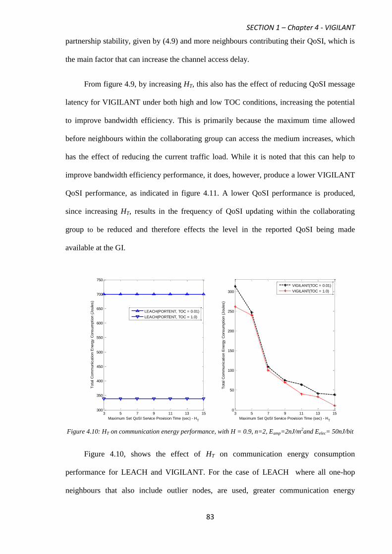
SECTION 1 – Chapter 4 - VIGILANT
83
partnership stability, given by (4.9) and more neighbours contributing their QoSI, which is
the main factor that can increase the channel access delay.
From figure 4.9, by increasing HT, this also has the effect of reducing QoSI message
latency for VIGILANT under both high and low TOC conditions, increasing the potential
to improve bandwidth efficiency. This is primarily because the maximum time allowed
before neighbours within the collaborating group can access the medium increases, which
has the effect of reducing the current traffic load. While it is noted that this can help to
improve bandwidth efficiency performance, it does, however, produce a lower VIGILANT
QoSI performance, as indicated in figure 4.11. A lower QoSI performance is produced,
since increasing HT, results in the frequency of QoSI updating within the collaborating
group to be reduced and therefore effects the level in the reported QoSI being made
available at the GI.
Figure 4.10: HT on communication energy performance, with H = 0.9, n=2, Eamp=2nJ/m2and Eelec= 50nJ/bit
Figure 4.10, shows the effect of HT on communication energy consumption
performance for LEACH and VIGILANT. For the case of LEACH where all one-hop
neighbours that also include outlier nodes, are used, greater communication energy
3 5 7 9 11 13 15300
350
400
450
500
550
600
650
700
750
Maximum Set QoSI Service Provision Time (sec) - HT
Tota
l C
om
munic
ation E
nerg
y C
onsum
ption (
Joule
s)
3 5 7 9 11 13 150
50
100
150
200
250
300
Maximum Set QoSI Service Provision Time (sec) - HT
Tota
l C
om
munic
ation E
nerg
y C
onsum
ption (
Joule
s)
VIGILANT(TOC = 0.01)
VIGILANT(TOC = 1.0)
LEACH(PORTENT, TOC = 0.01)
LEACH(PORTENT, TOC = 1.0)

SECTION 1 – Chapter 4 - VIGILANT
84
is consumed and a lower resulting QoSI performance occurs when compared with
VIGILANT, as indicated in figures 4.6 and 4.10.
An observation from figure 4.10, also shows that the communication energy
consumption for LEACH is independent of HT but can be reduced by using a lower
observation uncertainty (TOC = 1.0). LEACH for the purposes of comparison has been
integrated with PORTENT-Option 2 operation, in order to assist the CH re-election and
rotation phases, as described earlier in chapter 2, under section 2.1. This has been enabled
according to, which sensors can achieve the greatest threat detecton certainty. Under a
higher threat observation uncertainty (TOC = 0.01), when the probability of false alarm is
deemed to be at its greatest, this can lead to a greater fluctuation in threat detection
certainty being captured within the cluster group. This can result in a greater number of
CH’s being re-elected during the CH rotation phase. A greater number of CH’s being used
is a possiblity as to why higher communication energy is consumed for LEACH under
TOC = 0.01 conditions, than compared with TOC = 1.0 since, the probabilty of false alarm
is reduced and the detection certainty becomes much more stable within the cluster group,
leading to a lower number of CH’s being rotated.
VIGILANT, however through its integrated level 1 and 2 operation can avoid the
unneccessary rotations in GI’s and ensures GI’s are only elected according to QoSI, which
is a combined threat charcterisation measure, rather than just threat detection certainty, as
used in LEACH. This can lead to VIGILANT having a much more stable operation and as
a result, a lower communication energy consumption profile. In addition, managing the
number of colloborating neighbours according to the level of confidence in common threat
presence “context”, can subsequently, manage the number of active communicating
neighbours at a given point in time. This explains why VIGILANT helps to improve on
communication energy consumption, while also maintaining a higher QoSI output level,
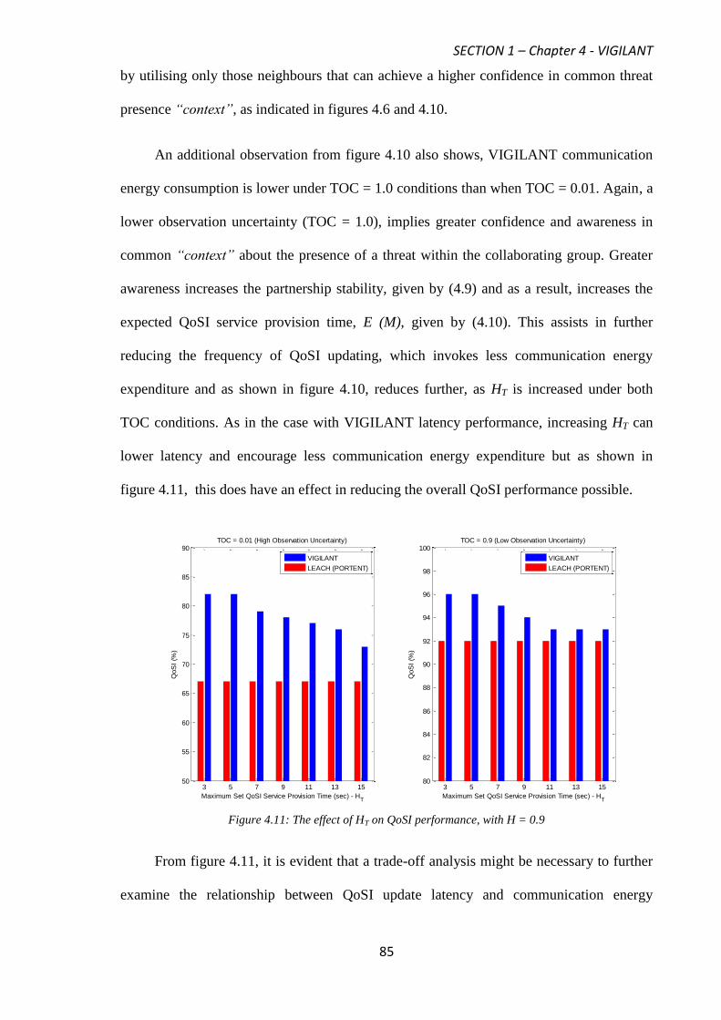
SECTION 1 – Chapter 4 - VIGILANT
85
by utilising only those neighbours that can achieve a higher confidence in common threat
presence “context”, as indicated in figures 4.6 and 4.10.
An additional observation from figure 4.10 also shows, VIGILANT communication
energy consumption is lower under TOC = 1.0 conditions than when TOC = 0.01. Again, a
lower observation uncertainty (TOC = 1.0), implies greater confidence and awareness in
common “context” about the presence of a threat within the collaborating group. Greater
awareness increases the partnership stability, given by (4.9) and as a result, increases the
expected QoSI service provision time, E (M), given by (4.10). This assists in further
reducing the frequency of QoSI updating, which invokes less communication energy
expenditure and as shown in figure 4.10, reduces further, as HT is increased under both
TOC conditions. As in the case with VIGILANT latency performance, increasing HT can
lower latency and encourage less communication energy expenditure but as shown in
figure 4.11, this does have an effect in reducing the overall QoSI performance possible.
Figure 4.11: The effect of HT on QoSI performance, with H = 0.9
From figure 4.11, it is evident that a trade-off analysis might be necessary to further
examine the relationship between QoSI update latency and communication energy
3 5 7 9 11 13 1550
55
60
65
70
75
80
85
90TOC = 0.01 (High Observation Uncertainty)
Maximum Set QoSI Service Provision Time (sec) - HT
QoS
I (%
)
3 5 7 9 11 13 1580
82
84
86
88
90
92
94
96
98
100TOC = 0.9 (Low Observation Uncertainty)
Maximum Set QoSI Service Provision Time (sec) - HT
QoS
I (%
)
VIGILANT
LEACH (PORTENT)
VIGILANT
LEACH (PORTENT)

SECTION 1 – Chapter 4 - VIGILANT
86
expenditure through variations in HT and the level of QoSI performance required, under
different TOC conditions. Alternatively, developing an improved VIGILANT system that
can decide itself the correct confidence measure in M1 “context” to use for collaboration
purposes (replacing H) and when to transmit their surveillance update packets (replacing
HT), is an interesting option. In chapter 5, we describe how an improved VIGILANT
system can be developed in order to cater for these concerns.
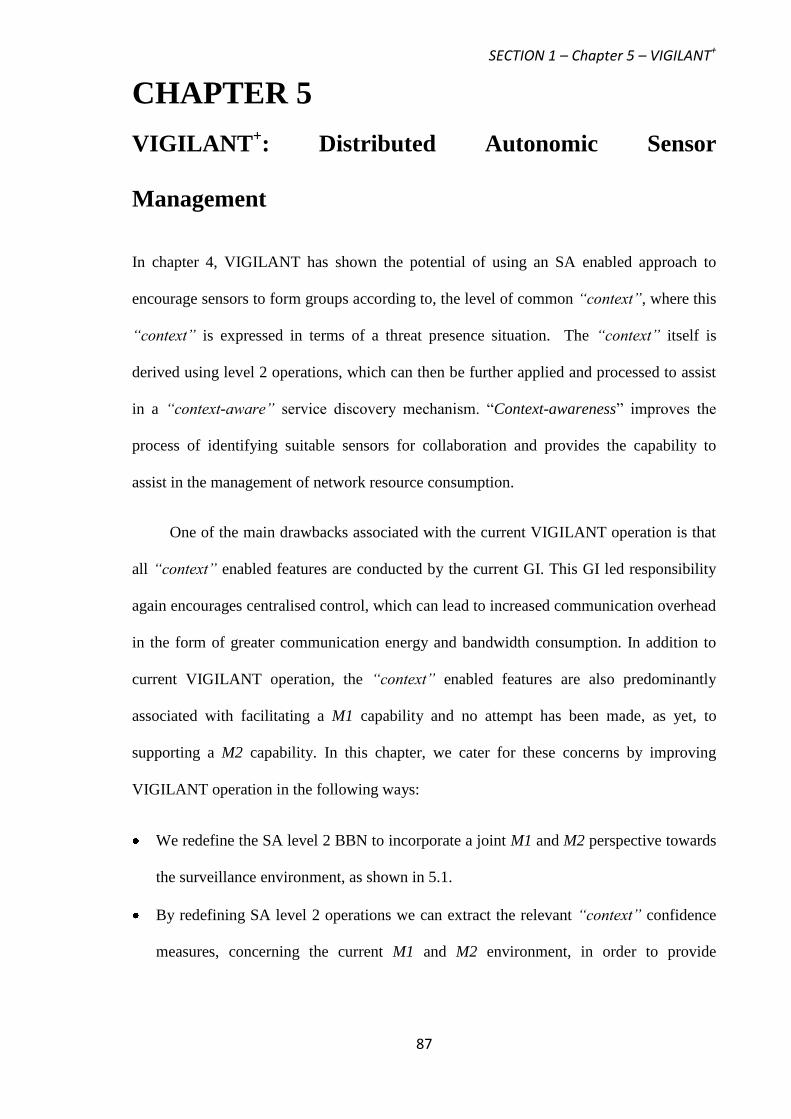
SECTION 1 – Chapter 5 – VIGILANT+
87
CHAPTER 5
VIGILANT+: Distributed Autonomic Sensor
Management
In chapter 4, VIGILANT has shown the potential of using an SA enabled approach to
encourage sensors to form groups according to, the level of common “context”, where this
“context” is expressed in terms of a threat presence situation. The “context” itself is
derived using level 2 operations, which can then be further applied and processed to assist
in a “context-aware” service discovery mechanism. “Context-awareness” improves the
process of identifying suitable sensors for collaboration and provides the capability to
assist in the management of network resource consumption.
One of the main drawbacks associated with the current VIGILANT operation is that
all “context” enabled features are conducted by the current GI. This GI led responsibility
again encourages centralised control, which can lead to increased communication overhead
in the form of greater communication energy and bandwidth consumption. In addition to
current VIGILANT operation, the “context” enabled features are also predominantly
associated with facilitating a M1 capability and no attempt has been made, as yet, to
supporting a M2 capability. In this chapter, we cater for these concerns by improving
VIGILANT operation in the following ways:
We redefine the SA level 2 BBN to incorporate a joint M1 and M2 perspective towards
the surveillance environment, as shown in 5.1.
By redefining SA level 2 operations we can extract the relevant “context” confidence
measures, concerning the current M1 and M2 environment, in order to provide
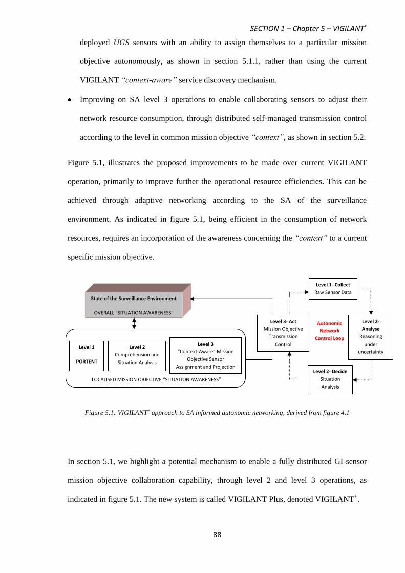
SECTION 1 – Chapter 5 – VIGILANT+
88
deployed UGS sensors with an ability to assign themselves to a particular mission
objective autonomously, as shown in section 5.1.1, rather than using the current
VIGILANT “context-aware” service discovery mechanism.
Improving on SA level 3 operations to enable collaborating sensors to adjust their
network resource consumption, through distributed self-managed transmission control
according to the level in common mission objective “context”, as shown in section 5.2.
Figure 5.1, illustrates the proposed improvements to be made over current VIGILANT
operation, primarily to improve further the operational resource efficiencies. This can be
achieved through adaptive networking according to the SA of the surveillance
environment. As indicated in figure 5.1, being efficient in the consumption of network
resources, requires an incorporation of the awareness concerning the “context” to a current
specific mission objective.
Figure 5.1: VIGILANT+
approach to SA informed autonomic networking, derived from figure 4.1
In section 5.1, we highlight a potential mechanism to enable a fully distributed GI-sensor
mission objective collaboration capability, through level 2 and level 3 operations, as
indicated in figure 5.1. The new system is called VIGILANT Plus, denoted VIGILANT+.
Level 1- Collect
Raw Sensor Data
Level 2-
Analyse
Reasoning
under
uncertainty
Level 2- Decide
Situation
Analysis
Level 3- Act
Mission Objective
Transmission
Control
State of the Surveillance Environment
OVERALL “SITUATION AWARENESS”
Level 1
PORTENT
Level 2
Comprehension and
Situation Analysis
Level 3
“Context-Aware” Mission
Objective Sensor
Assignment and Projection
LOCALISED MISSION OBJECTIVE “SITUATION AWARENESS”
Autonomic
Network
Control Loop
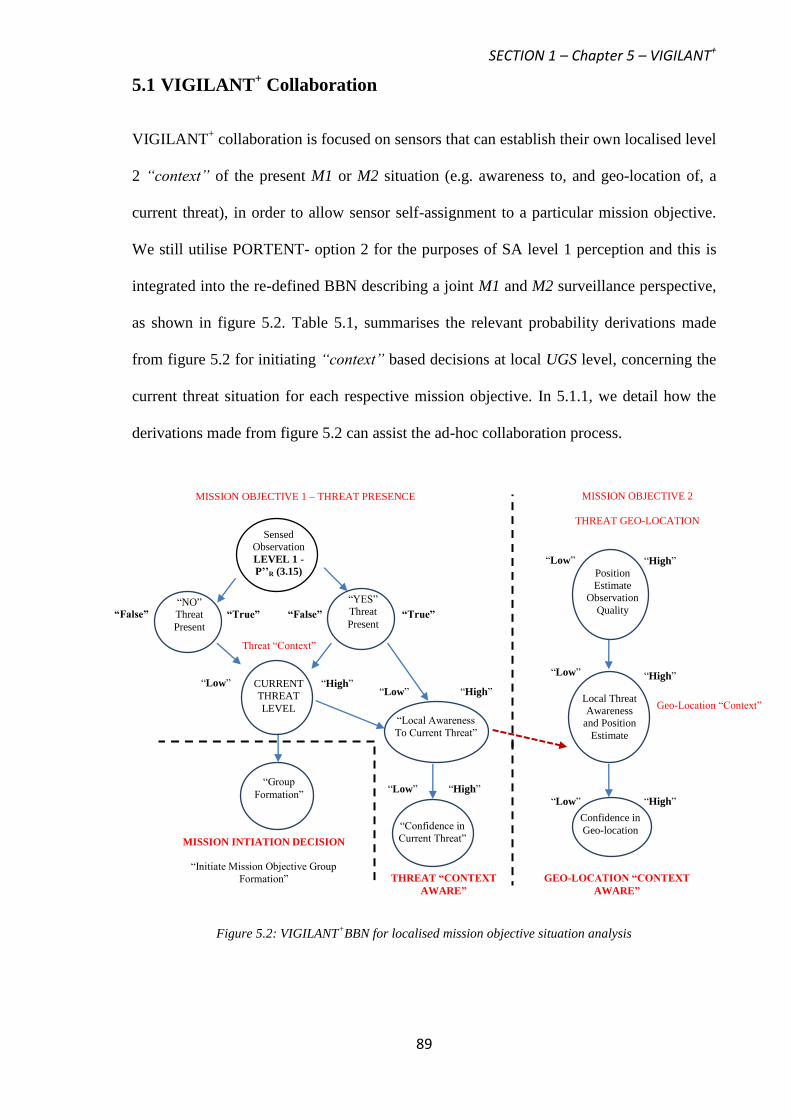
SECTION 1 – Chapter 5 – VIGILANT+
89
5.1 VIGILANT+ Collaboration
VIGILANT+ collaboration is focused on sensors that can establish their own localised level
2 “context” of the present M1 or M2 situation (e.g. awareness to, and geo-location of, a
current threat), in order to allow sensor self-assignment to a particular mission objective.
We still utilise PORTENT- option 2 for the purposes of SA level 1 perception and this is
integrated into the re-defined BBN describing a joint M1 and M2 surveillance perspective,
as shown in figure 5.2. Table 5.1, summarises the relevant probability derivations made
from figure 5.2 for initiating “context” based decisions at local UGS level, concerning the
current threat situation for each respective mission objective. In 5.1.1, we detail how the
derivations made from figure 5.2 can assist the ad-hoc collaboration process.
Figure 5.2: VIGILANT+BBN for localised mission objective situation analysis
“NO”
Threat
Present
THREAT “CONTEXT
AWARE”
GEO-LOCATION “CONTEXT
AWARE”
“High” “Low”
“High” “Low”
Geo-Location “Context”
“High” “Low”
“High” “Low”
MISSION OBJECTIVE 1 – THREAT PRESENCE
MISSION INTIATION DECISION
“Initiate Mission Objective Group
Formation”
“False” “True” “True” “False”
Threat “Context”
“High” “Low”
MISSION OBJECTIVE 2
THREAT GEO-LOCATION
“High” “Low”
“Group
Formation”
“YES”
Threat
Present
“Local Awareness
To Current Threat”
“Confidence in
Current Threat”
Confidence in
Geo-location
Position
Estimate
Observation
Quality
Local Threat
Awareness
and Position
Estimate
CURRENT
THREAT
LEVEL
Sensed
Observation
LEVEL 1 -
P’’R (3.15)

SECTION 1 – Chapter 5 – VIGILANT+
90
Probability Expression Probability Derivation from figure 5.2 using CPT
Analysis 1. p( Yes Threat Present – “True” (C) ) p(C | Threat Presence True) × P’’R + p(C| Threat Presence False)×
(1 – P’’R)
2. p( No Threat Present – “True” (D) ) p(D | Threat Presence True) × P’’R + p(D | Threat Presence
False)× (1 – P’’R)
3. p(Current Threat Level – “High” (F) ) [p(F| C,D) × p(C) × p(D)] + [p(F | ~C,D) × p(~C) × p(D)] +
[p(F|C,~D) × p(C) × p(~D)] + [p(F | ~C,~D) × p(~C) × p(~D)]
4. p(Threat-High)
Group Formation: if p(Threat-“High”) > 1 –
p(Threat- “High”)
p(Yes-“Form”| F)× p(F) + p(Yes-“Form”| ~F)×p(~F)
5.p(Local Awareness to Current Threat )– “High” (L) [p(L | C,F) × p(C) × p(F)] + [p(L | ~C,F) × p(~C) × p(F)] + [p(L |
C,~F) × p(C) × p(~F)] + [p( L | ~C,~D) × p(~C) × p(~F)]
6. Mission Objective 1
p(Confidence in Current Threat – “High” (Q) )
p(Q | L) × p(L) + p(Q| ~L)× p(~L)
7. p(L and Position Observation Estimate (POE) –
“High” (E) )
[p(E | L,POE) × p(L) × p(POE)] + [p(E | ~L,POE) × p(~L) ×
p(POE)] + [p(E | L,~POE) × p(L) × p(~POE)] + [p( E | ~L,~POE)
× p(~L) × p(~POE)]
8. Mission Objective 2
p(Confidence in Geo-Location – “High” (S) )
p(S | E) × p(E) + p(S | ~E)× p(~E)
Table 5.1: Probability derivations from figure 5.2 for initiating group formation and facilitating “context-
aware” decisions regarding a specific mission objective
5.1.1 Querying for Sensor Mission Objective Self-Assignment
The development of VIGILANT has already shown that ad-hoc collaboration of single hop
sensors can be enhanced by assigning sensors to a group that have similar confidence in
common “context” concerning a threat presence, using the CF model. The evaluation of
confidence in common threat presence “context”, however, in VIGILANT, is conducted
by the GI using CF feedback from immediate neighbours, as shown in chapter 4, figure
4.3. The CF model, however, is a procedure which can also be performed locally by the
immediate neighbourhood. This is made possible if neighbours are notified by the GI of its
own CF value, named as CF “GI”, which is only sent as content within a publish “request”
packet during the group formation phase, after the condition in entry 4, table 5.1, is met.
Evaluation of distributed mission objective “context” assisted through, CF “GI”, in
this way, enforces uncoupled coordination, where distributed sensors are modelled as a set
of components interacting with each other through, analysing and reacting to their
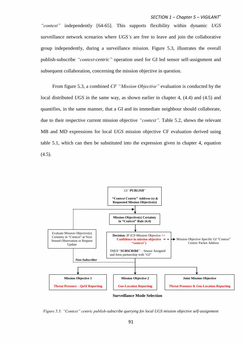
SECTION 1 – Chapter 5 – VIGILANT+
91
“context” independently [64-65]. This supports flexibility within dynamic UGS
surveillance network scenarios where UGS’s are free to leave and join the collaborative
group independently, during a surveillance mission. Figure 5.3, illustrates the overall
publish-subscribe “context-centric” operation used for GI led sensor self-assignment and
subsequent collaboration, concerning the mission objective in question.
From figure 5.3, a combined CF “Mission Objective” evaluation is conducted by the
local distributed UGS in the same way, as shown earlier in chapter 4, (4.4) and (4.5) and
quantifies, in the same manner, that a GI and its immediate neighbour should collaborate,
due to their respective current mission objective “context”. Table 5.2, shows the relevant
MB and MD expressions for local UGS mission objective CF evaluation derived using
table 5.1, which can then be substituted into the expression given in chapter 4, equation
(4.5).
Figure 5.3: “Context” centric publish-subscribe querying for local UGS mission objective self-assignment
GI “PUBLISH”
“Context Centric” Address (s) &
Requested Mission Objective(s)
Mission Objective(s) Certainty
in “Context” Rule (4.4)
Decision: IF (CF-Mission Objective >=
Confidence in mission objective
“context”)
THEN “SUBSCRIBE” – Sensor Assigned and form partnership with “GI”
Mission Objective Specific GI “Context” Centric Packet Address
Mission Objective 1
Threat Presence – QoSI Reporting
Mission Objective 2
Geo-Location Reporting
Joint Mission Objective
Threat Presence & Geo-Location Reporting
Surveillance Mode Selection
Evaluate Mission Objective(s)
Certainty in “Context” at Next
Sensed Observation or Request Update
Non-Subscriber

SECTION 1 – Chapter 5 – VIGILANT+
92
Table 5.2: MB, MD expressions for local UGS CF-Mission Objective evaluation, using table 5.1
As indicated in figure 5.3, the GI itself specifies which mission objective is required
within the received publish “request” packet. The querying for mission objective self-
assignment is then conducted against the GI “context-centric” address, which is derived
using entries 6 and 8, from table 5.1 and sent within the content of the received GI publish
“request” packet. In figure 5.3, feedback is also used by non-subscribers to re-evaluate
their position if local “contextual” changes do occur. This can help to improve the GI led
collaborating group performance by maintaining a relevant and up-to date group
perspective towards, the M1 or M2 surveillance environment during a mission.
Querying against the GI “context-centric” address can also help to minimise the
communication overhead incurred during the collaboration phase, compared with
VIGILANT, since both CF evaluation and mission objective assignment are conducted
locally by the UGS and not at the GI. In addition, the need for a fixed, system defined
value for sensor confidence in “context” for CF evaluation comparison, as in the case with
VIGILANT (given by H) is not required. Instead, sensor confidence becomes a dynamic
value, which varies according to “contextual” changes during a dynamic surveillance
mission, given by entries 6 and 8, in table 5.1.
Mission Objective 1 – Threat
Presence
Mission Objective 2 – Threat Geo-
Location
Increased Belief
(MB) Expression
)L(p1
)L(p)L|ThreattoAwareness(p
)E(p1
)E(p)E|AwarenessLocationGeo(p
Increased Disbelief
(MD) Expression
)L(p
)L|ThreattoAwareness(p)L(p
)E(p
)E|AwarenessLocationGeo(p)E(p

SECTION 1 – Chapter 5 – VIGILANT+
93
5.1.2 Group Initiator Re-Election
GI re-election is dynamically conducted in the process of a mission. Assigned sensors rely
on the current GI mission objective “context” centric address (GImocca) sent in the initial
publish “request” packet, to re-evaluate whether a “new” GI status needs to be initiated, as
shown in (5.1).
StatusquestReObjectiveMissionGI"New"Publish,Then
)GI()"context"objectivemissioncurrentinConfidence(if mocca
(5.1)
Upon the condition in (5.1) being satisfied, locally, distributed sensors re-evaluate their
mission objective “context” certainty, as shown in figure 5.3. The resulting new ad-hoc
collaborating group can further facilitate in maintaining, a relevant and on-going
aggregation of mission objective information utility.
5.2 VIGILANT+ Autonomic Transmission Control
UGS’s that decide to assign themselves to a specific or joint mission objective follow by
initiating autonomic transmission control, which is orientated towards the management of
network resources at infrastructure level, through applying direct feedback and acting upon
temporal environmental dynamics. Being efficient to network resource consumption
implies an approach, which provides projection capabilities (level 3) concerning the
“context” to a current specific mission objective. This indicates the need to employ a
temporal framework that can establish and evaluate future “context-awareness” of the
progressive mission objective surveillance environment, in order to assist the transmission
control decision making process. Transmission control can be formalised using a random
discrete time state representation, commonly referred to as either a, Markov Decision
Process (MDP) or Partially Observable MDP (POMDP) and is detailed further in 5.2.1 and
5.2.2.
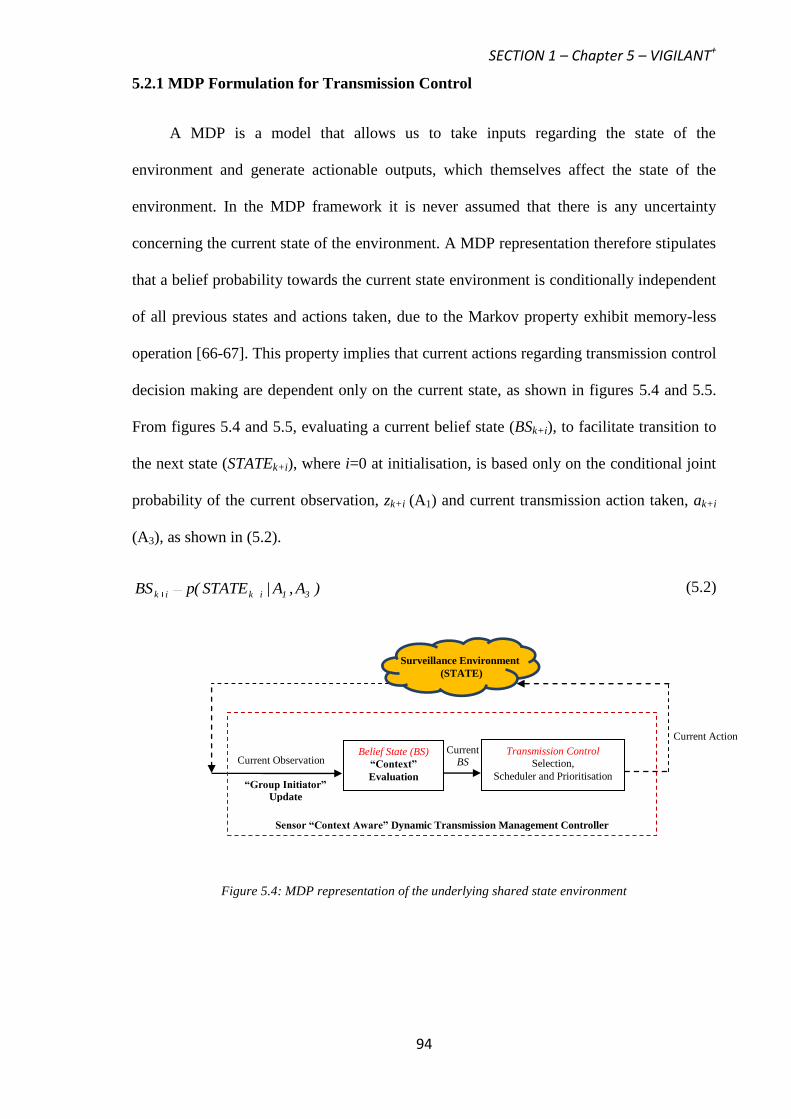
SECTION 1 – Chapter 5 – VIGILANT+
94
5.2.1 MDP Formulation for Transmission Control
A MDP is a model that allows us to take inputs regarding the state of the
environment and generate actionable outputs, which themselves affect the state of the
environment. In the MDP framework it is never assumed that there is any uncertainty
concerning the current state of the environment. A MDP representation therefore stipulates
that a belief probability towards the current state environment is conditionally independent
of all previous states and actions taken, due to the Markov property exhibit memory-less
operation [66-67]. This property implies that current actions regarding transmission control
decision making are dependent only on the current state, as shown in figures 5.4 and 5.5.
From figures 5.4 and 5.5, evaluating a current belief state (BSk+i), to facilitate transition to
the next state (STATEk+i), where i=0 at initialisation, is based only on the conditional joint
probability of the current observation, zk+i (A1) and current transmission action taken, ak+i
(A3), as shown in (5.2).
)A,A|STATE(pBS 31ikik (5.2)
Figure 5.4: MDP representation of the underlying shared state environment
Belief State (BS)
“Context”
Evaluation
Transmission Control
Selection,
Scheduler and Prioritisation
Current Observation
Current Action
Sensor “Context Aware” Dynamic Transmission Management Controller
“Group Initiator” Update
Surveillance Environment
(STATE)
Current BS
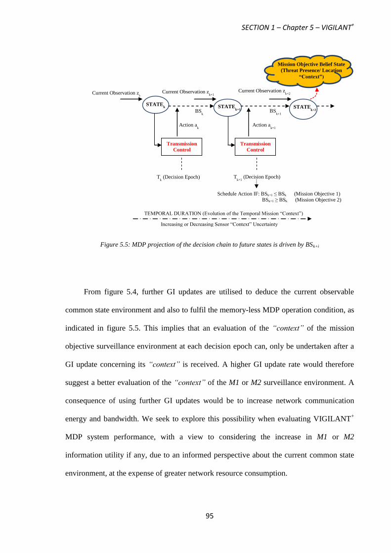
SECTION 1 – Chapter 5 – VIGILANT+
95
Figure 5.5: MDP projection of the decision chain to future states is driven by BSk+i
From figure 5.4, further GI updates are utilised to deduce the current observable
common state environment and also to fulfil the memory-less MDP operation condition, as
indicated in figure 5.5. This implies that an evaluation of the “context” of the mission
objective surveillance environment at each decision epoch can, only be undertaken after a
GI update concerning its “context” is received. A higher GI update rate would therefore
suggest a better evaluation of the “context” of the M1 or M2 surveillance environment. A
consequence of using further GI updates would be to increase network communication
energy and bandwidth. We seek to explore this possibility when evaluating VIGILANT+
MDP system performance, with a view to considering the increase in M1 or M2
information utility if any, due to an informed perspective about the current common state
environment, at the expense of greater network resource consumption.
Transmission
Control
Transmission
Control
Current Observation zk Current Observation z
k+1
Action ak Action a
k+1
Current Observation zk+2
Tk (Decision Epoch) T
k+1 (Decision Epoch)
BSk BS
k+1
STATEk STATE
k+1 STATE
k+2
Schedule Action IF: BSk+1 ≤ BSk (Mission Objective 1) BSk+1 ≥ BSk (Mission Objective 2)
Increasing or Decreasing Sensor “Context” Uncertainty
TEMPORAL DURATION (Evolution of the Temporal Mission “Context”)
Mission Objective Belief State
(Threat Presence/ Location
“Context”)
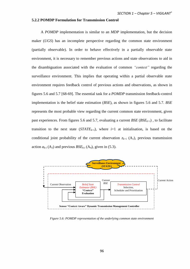
SECTION 1 – Chapter 5 – VIGILANT+
96
5.2.2 POMDP Formulation for Transmission Control
A POMDP implementation is similar to an MDP implementation, but the decision
maker (UGS) has an incomplete perspective regarding the common state environment
(partially observable). In order to behave effectively in a partially observable state
environment, it is necessary to remember previous actions and state observations to aid in
the disambiguation associated with the evaluation of common “context” regarding the
surveillance environment. This implies that operating within a partial observable state
environment requires feedback control of previous actions and observations, as shown in
figures 5.6 and 5.7 [68-69]. The essential task for a POMDP transmission feedback-control
implementation is the belief state estimation (BSE), as shown in figures 5.6 and 5.7. BSE
represents the most probable view regarding the current common state environment, given
past experiences. From figures 5.6 and 5.7, evaluating a current BSE (BSEk+i) , to facilitate
transition to the next state (STATEk+i), where i=1 at initialisation, is based on the
conditional joint probability of the current observation zk+i (A1), previous transmission
action ak-i (A3) and previous BSEk-i (A4), given in (5.3).
Figure 5.6: POMDP representation of the underlying common state environment
Belief State
Estimator (BSE)
“Context”
Evaluation
Transmission Control
Selection,
Scheduler and Prioritisation
Current Observation
Current
BSE Current Action
Sensor “Context Aware” Dynamic Transmission Management Controller
Surveillance Environment
(STATE)
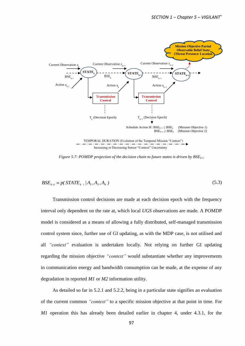
SECTION 1 – Chapter 5 – VIGILANT+
97
Figure 5.7: POMDP projection of the decision chain to future states is driven by BSEk+i
)A,A,A|STATE(pBSE 431ikik (5.3)
Transmission control decisions are made at each decision epoch with the frequency
interval only dependent on the rate at, which local UGS observations are made. A POMDP
model is considered as a means of allowing a fully distributed, self-managed transmission
control system since, further use of GI updating, as with the MDP case, is not utilised and
all “context” evaluation is undertaken locally. Not relying on further GI updating
regarding the mission objective “context” would substantiate whether any improvements
in communication energy and bandwidth consumption can be made, at the expense of any
degradation in reported M1 or M2 information utility.
As detailed so far in 5.2.1 and 5.2.2, being in a particular state signifies an evaluation
of the current common “context” to a specific mission objective at that point in time. For
M1 operation this has already been detailed earlier in chapter 4, under 4.3.1, for the
Transmission
Control
Current Observation zk Current Observation z
k+1
Action ak-1
Action ak+1
Current Observation zk+2
Tk (Decision Epoch) T
k+1 (Decision Epoch)
BSEk BSE
k+1
STATEk STATE
k+1 STATE
k+2
Mission Objective Partial
Observable Belief State
(Threat Presence/ Location
“Context”)
Transmission
Control
BSEk-1
Action ak
Schedule Action IF: BSEk+1 ≤ BSEk (Mission Objective 1) BSEk+1 ≥ BSEk (Mission Objective 2)
Increasing or Decreasing Sensor “Context” Uncertainty
TEMPORAL DURATION (Evolution of the Temporal Mission “Context”)

SECTION 1 – Chapter 5 – VIGILANT+
98
VIGILANT system and the probability of correct detection in common threat awareness
“context”, T1, is equal to (1- P1), where P1, given in (4.6) forms the basis for the eventual
evaluation of BSk+i or BSEk+i, as shown in (5.4).
)A,T|STATE(pBS 31ikik
)A,A,T|STATE(pBSE 431ikik
(5.4)
In 5.2.3, we detail how the evaluation of current common M2 “context” can be made to
facilitate MDP and POMDP transmission control. Evaluating “context” for each respective
mission objective according to either the MDP or POMDP framework, as shown in figures
5.5 and 5.7, can then enable us to make the necessary transmission control decisions
(selection, scheduling and prioritisation), detailed further in 5.2.4 to 5.2.6.
5.2.3 Determination of Common Threat Geo-location “Context”
For M2 operation, we assume that the sensors have the ability to obtain current threat
position (xThreat, yThreat) using techniques such as time difference of arrival (TDOA).
Obtaining a current threat position can subsequently be used to calculate the current
geometric dilution of precision (GDOPk), with respect to the GI. GDOPk measures the
accuracy in common geo-location “context”, quantifying the mapping of measurement
errors into position errors, magnified by the geometric relation of UGS to threat geometry
[70-71]. The geometry matrix HT
H, at each decision epoch, for N active sensors, is
expressed in (5.5). In all cases we assume, GI (xGI, yGI) and active sensor (xi, yi) positions
are known.
1N
1i
2
yryiyryi
1N
1i
2
xrxi
yryi
1N
1i
2
xrxi
1N
1i
2
xrxiT
)aa()aa()aa(
)aa()aa()aa(HH
(5.5)

SECTION 1 – Chapter 5 – VIGILANT+
99
Where, 22 )()()( iThreatiThreatiThreatxi yyxxxxa , 22 )()()( GIThreatGIThreatGIThreatxr yyxxxxa
22 )()()( iThreatiThreatiThreatyi yyxxyya and 22 )()()( iThreatiThreatiThreatxi yyxxxxa .
Since the matrix (HT
H) is symmetric and positive definite, all eigenvalues λ1, λ2 are real
and positive [71]. The eigenvalues λ1, λ2 gives an indication as to the current amount of
error present, in relation to the GI and sensor to-threat geometry and therefore smaller
values of λ1, λ2 correspond to a lower dilution of error and better geo-location accuracy
[72]. The trace of the matrix (HT
H), then quantifies the total error present and is equal to
the sum of the eigenvalues λ1, λ2, given in (5.6).
1N
1i
2
yryi
2
xrxi21
T ])aa()aa([)HH(trace (5.6)
A final current precision measure in GI-sensor-to-threat geometry error, GDOPk, is
therefore given as shown in (5.7).
1T
k )HH(traceGDOP (5.7)
Utilising the GDOPk measure to serve as an approximation of the current threat location
(CTL) in terms of circular error probable (CEP) [73-74], we can obtain a likelihood
measure for common “context” (Q1), forming the basis for eventual BSk+i or BSEk+i
evaluation, given in (5.8).
)A,Q|STATE(pBS 31ikik
)A,A,Q|STATE(pBSE 431ikik
ErrorRange2
ErrorRange
2
kMAX
1 22
)GDOPGDOP(exp()GDOP|CTL(pQ
(5.8)
The CEP is a measure of the uncertainty in the CTL estimate relative to its mean value. If
the CTL estimate is unbiased, the CEP forms a direct measure of the CTL uncertainty
relative to its true position [74]. From (5.8), GDOPMAX, represents the maximum
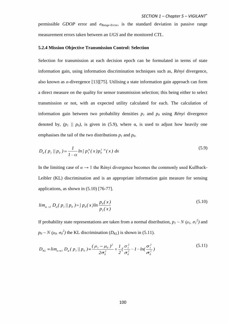
SECTION 1 – Chapter 5 – VIGILANT+
100
permissible GDOP error and σRange-Error, is the standard deviation in passive range
measurement errors taken between an UGS and the monitored CTL.
5.2.4 Mission Objective Transmission Control: Selection
Selection for transmission at each decision epoch can be formulated in terms of state
information gain, using information discrimination techniques such as, Rényi divergence,
also known as α-divergence [13][75]. Utilising a state information gain approach can form
a direct measure on the quality for sensor transmission selection; this being either to select
transmission or not, with an expected utility calculated for each. The calculation of
information gain between two probability densities p1 and p0 using Rényi divergence
denoted by, (p1 || p0), is given in (5.9), where α, is used to adjust how heavily one
emphasises the tail of the two distributions p1 and p0.
dx)x(p)x(pln1
1)p||p(D 1
0101
(5.9)
In the limiting case of α → 1 the Rényi divergence becomes the commonly used Kullback-
Leibler (KL) discrimination and is an appropriate information gain measure for sensing
applications, as shown in (5.10) [76-77].
)x(p
)x(pln)x(p)p||p(Dlim
1
0
0011 (5.10)
If probability state representations are taken from a normal distribution, p1 ~ N (μ1, σ12) and
p0 ~ N (μ0, σ02) the KL discrimination (DKL) is shown in (5.11).
)ln(1(2
1
2
)()p||p(DlimD
2
0
2
1
2
0
2
1
2
0
2
01
011KL
(5.11)
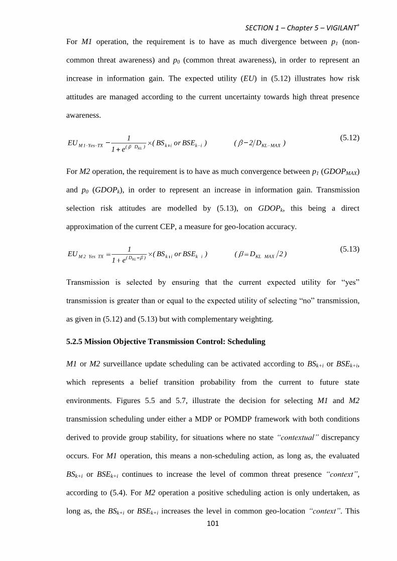
SECTION 1 – Chapter 5 – VIGILANT+
101
For M1 operation, the requirement is to have as much divergence between p1 (non-
common threat awareness) and p0 (common threat awareness), in order to represent an
increase in information gain. The expected utility (EU) in (5.12) illustrates how risk
attitudes are managed according to the current uncertainty towards high threat presence
awareness.
)D2()BSEorBS(e1
1EU MAXKLikik)D(TXYes1M
KL
(5.12)
For M2 operation, the requirement is to have as much convergence between p1 (GDOPMAX)
and p0 (GDOPk), in order to represent an increase in information gain. Transmission
selection risk attitudes are modelled by (5.13), on GDOPk, this being a direct
approximation of the current CEP, a measure for geo-location accuracy.
)2D()BSEorBS(e1
1EU MAXKLikik)D(TXYes2M
KL
(5.13)
Transmission is selected by ensuring that the current expected utility for “yes”
transmission is greater than or equal to the expected utility of selecting “no” transmission,
as given in (5.12) and (5.13) but with complementary weighting.
5.2.5 Mission Objective Transmission Control: Scheduling
M1 or M2 surveillance update scheduling can be activated according to BSk+i or BSEk+i,
which represents a belief transition probability from the current to future state
environments. Figures 5.5 and 5.7, illustrate the decision for selecting M1 and M2
transmission scheduling under either a MDP or POMDP framework with both conditions
derived to provide group stability, for situations where no state “contextual” discrepancy
occurs. For M1 operation, this means a non-scheduling action, as long as, the evaluated
BSk+i or BSEk+i continues to increase the level of common threat presence “context”,
according to (5.4). For M2 operation a positive scheduling action is only undertaken, as
long as, the BSk+i or BSEk+i increases the level in common geo-location “context”. This
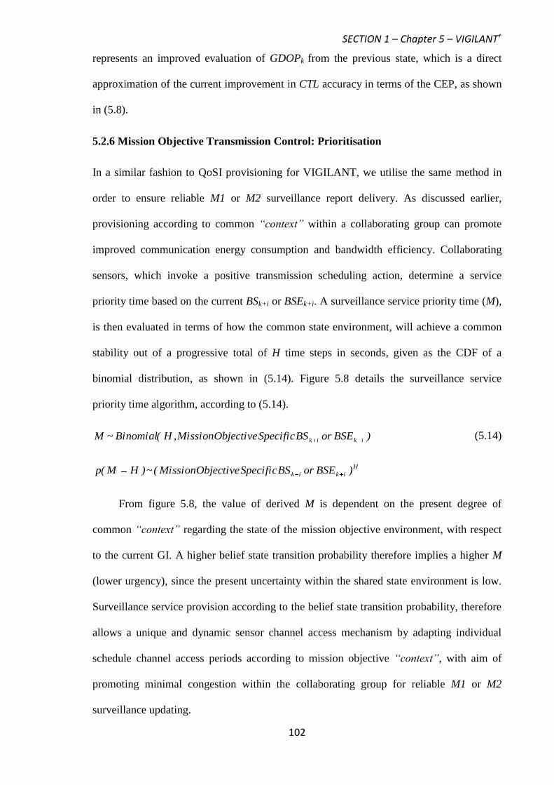
SECTION 1 – Chapter 5 – VIGILANT+
102
represents an improved evaluation of GDOPk from the previous state, which is a direct
approximation of the current improvement in CTL accuracy in terms of the CEP, as shown
in (5.8).
5.2.6 Mission Objective Transmission Control: Prioritisation
In a similar fashion to QoSI provisioning for VIGILANT, we utilise the same method in
order to ensure reliable M1 or M2 surveillance report delivery. As discussed earlier,
provisioning according to common “context” within a collaborating group can promote
improved communication energy consumption and bandwidth efficiency. Collaborating
sensors, which invoke a positive transmission scheduling action, determine a service
priority time based on the current BSk+i or BSEk+i. A surveillance service priority time (M),
is then evaluated in terms of how the common state environment, will achieve a common
stability out of a progressive total of H time steps in seconds, given as the CDF of a
binomial distribution, as shown in (5.14). Figure 5.8 details the surveillance service
priority time algorithm, according to (5.14).
H
ikik
ikik
)BSEorBSSpecificObjectiveMission(~)HM(p
)BSEorBSSpecificObjectiveMission,H(Binomial~M
(5.14)
From figure 5.8, the value of derived M is dependent on the present degree of
common “context” regarding the state of the mission objective environment, with respect
to the current GI. A higher belief state transition probability therefore implies a higher M
(lower urgency), since the present uncertainty within the shared state environment is low.
Surveillance service provision according to the belief state transition probability, therefore
allows a unique and dynamic sensor channel access mechanism by adapting individual
schedule channel access periods according to mission objective “context”, with aim of
promoting minimal congestion within the collaborating group for reliable M1 or M2
surveillance updating.
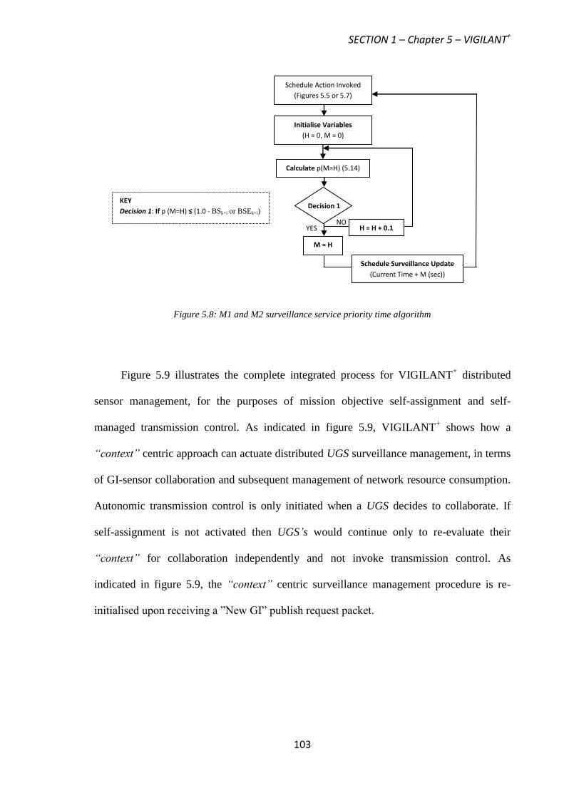
SECTION 1 – Chapter 5 – VIGILANT+
103
Figure 5.8: M1 and M2 surveillance service priority time algorithm
Figure 5.9 illustrates the complete integrated process for VIGILANT+ distributed
sensor management, for the purposes of mission objective self-assignment and self-
managed transmission control. As indicated in figure 5.9, VIGILANT+ shows how a
“context” centric approach can actuate distributed UGS surveillance management, in terms
of GI-sensor collaboration and subsequent management of network resource consumption.
Autonomic transmission control is only initiated when a UGS decides to collaborate. If
self-assignment is not activated then UGS’s would continue only to re-evaluate their
“context” for collaboration independently and not invoke transmission control. As
indicated in figure 5.9, the “context” centric surveillance management procedure is re-
initialised upon receiving a ”New GI” publish request packet.
Calculate p(M=H) (5.14)
Schedule Action Invoked
(Figures 5.5 or 5.7)
Initialise Variables
(H = 0, M = 0)
KEY
Decision 1: If p (M=H) ≤ (1.0 - BSk+i or BSEk+i)
H = H + 0.1
M = H
Decision 1
YES NO
Schedule Surveillance Update
(Current Time + M (sec))
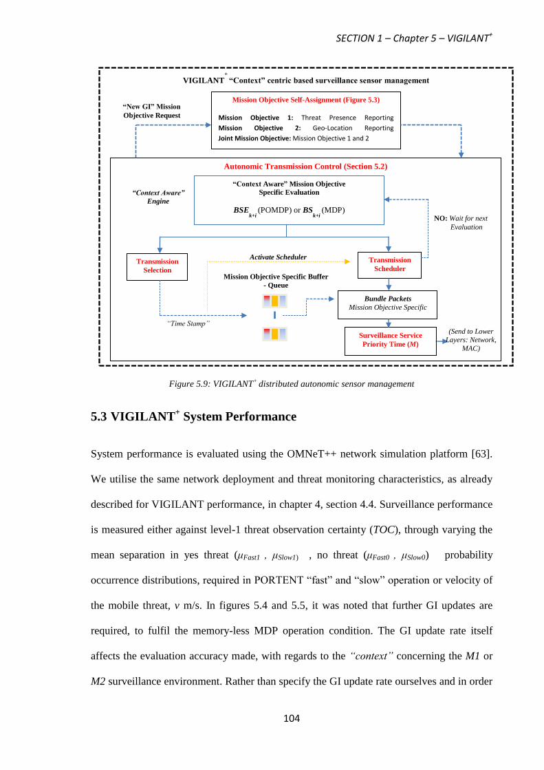
SECTION 1 – Chapter 5 – VIGILANT+
104
Figure 5.9: VIGILANT+
distributed autonomic sensor management
5.3 VIGILANT+ System Performance
System performance is evaluated using the OMNeT++ network simulation platform [63].
We utilise the same network deployment and threat monitoring characteristics, as already
described for VIGILANT performance, in chapter 4, section 4.4. Surveillance performance
is measured either against level-1 threat observation certainty (TOC), through varying the
mean separation in yes threat (μFast1 , μSlow1) , no threat (μFast0 , μSlow0) probability
occurrence distributions, required in PORTENT “fast” and “slow” operation or velocity of
the mobile threat, v m/s. In figures 5.4 and 5.5, it was noted that further GI updates are
required, to fulfil the memory-less MDP operation condition. The GI update rate itself
affects the evaluation accuracy made, with regards to the “context” concerning the M1 or
M2 surveillance environment. Rather than specify the GI update rate ourselves and in order
VIGILANT+
“Context” centric based surveillance sensor management
“Context Aware” Mission Objective
Specific Evaluation
BSEk+i
(POMDP) or BSk+i
(MDP)
Transmission
Selection
Transmission
Scheduler
Mission Objective Specific Buffer
- Queue
Bundle Packets
Mission Objective Specific
(Send to Lower
Layers: Network,
MAC)
NO: Wait for next
Evaluation
Activate Scheduler
“Time Stamp”
Surveillance Service
Priority Time (M)
“Context Aware”
Engine
Autonomic Transmission Control (Section 5.2)
Mission Objective Self-Assignment (Figure 5.3)
Mission Objective 1: Threat Presence Reporting
Mission Objective 2: Geo-Location Reporting
Joint Mission Objective: Mission Objective 1 and 2
“New GI” Mission
Objective Request
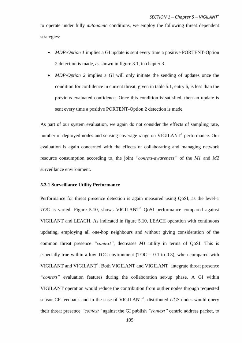
SECTION 1 – Chapter 5 – VIGILANT+
105
to operate under fully autonomic conditions, we employ the following threat dependent
strategies:
MDP-Option 1 implies a GI update is sent every time a positive PORTENT-Option
2 detection is made, as shown in figure 3.1, in chapter 3.
MDP-Option 2 implies a GI will only initiate the sending of updates once the
condition for confidence in current threat, given in table 5.1, entry 6, is less than the
previous evaluated confidence. Once this condition is satisfied, then an update is
sent every time a positive PORTENT-Option 2 detection is made.
As part of our system evaluation, we again do not consider the effects of sampling rate,
number of deployed nodes and sensing coverage range on VIGILANT+ performance. Our
evaluation is again concerned with the effects of collaborating and managing network
resource consumption according to, the joint “context-awareness” of the M1 and M2
surveillance environment.
5.3.1 Surveillance Utility Performance
Performance for threat presence detection is again measured using QoSI, as the level-1
TOC is varied. Figure 5.10, shows VIGILANT+ QoSI performance compared against
VIGILANT and LEACH. As indicated in figure 5.10, LEACH operation with continuous
updating, employing all one-hop neighbours and without giving consideration of the
common threat presence “context”, decreases M1 utility in terms of QoSI. This is
especially true within a low TOC environment (TOC = 0.1 to 0.3), when compared with
VIGILANT and VIGILANT+. Both VIGILANT and VIGILANT
+ integrate threat presence
“context” evaluation features during the collaboration set-up phase. A GI within
VIGILANT operation would reduce the contribution from outlier nodes through requested
sensor CF feedback and in the case of VIGILANT+, distributed UGS nodes would query
their threat presence “context” against the GI publish “context” centric address packet, to
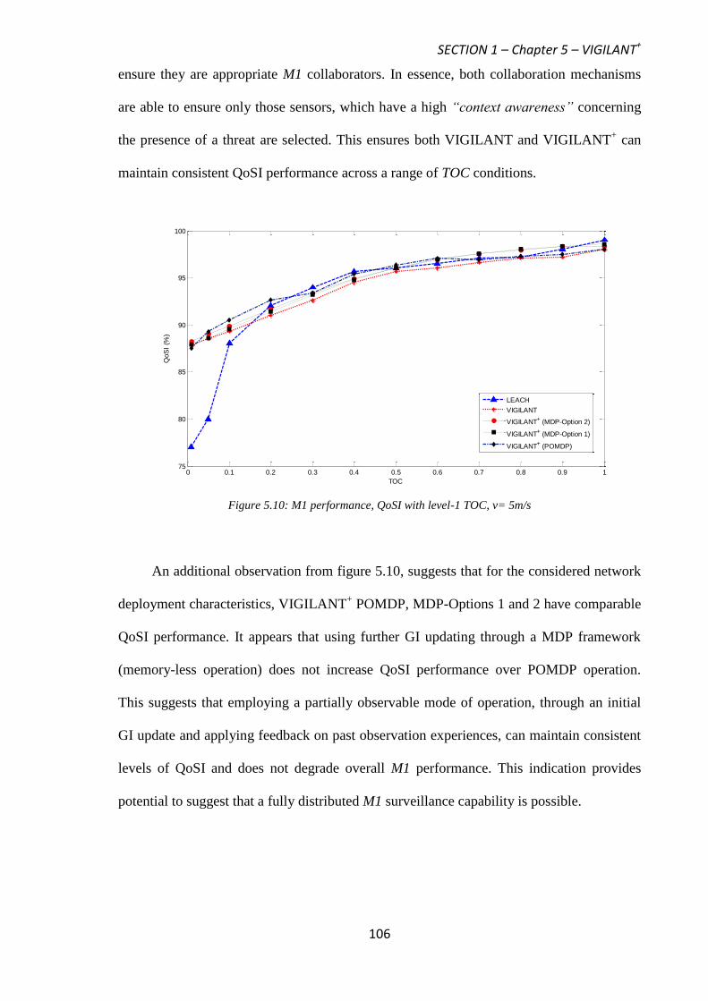
SECTION 1 – Chapter 5 – VIGILANT+
106
ensure they are appropriate M1 collaborators. In essence, both collaboration mechanisms
are able to ensure only those sensors, which have a high “context awareness” concerning
the presence of a threat are selected. This ensures both VIGILANT and VIGILANT+ can
maintain consistent QoSI performance across a range of TOC conditions.
Figure 5.10: M1 performance, QoSI with level-1 TOC, v= 5m/s
An additional observation from figure 5.10, suggests that for the considered network
deployment characteristics, VIGILANT+ POMDP, MDP-Options 1 and 2 have comparable
QoSI performance. It appears that using further GI updating through a MDP framework
(memory-less operation) does not increase QoSI performance over POMDP operation.
This suggests that employing a partially observable mode of operation, through an initial
GI update and applying feedback on past observation experiences, can maintain consistent
levels of QoSI and does not degrade overall M1 performance. This indication provides
potential to suggest that a fully distributed M1 surveillance capability is possible.
0 0.1 0.2 0.3 0.4 0.5 0.6 0.7 0.8 0.9 175
80
85
90
95
100
TOC
QoS
I (%
)
LEACH
VIGILANT
VIGILANT+ (MDP-Option 2)
VIGILANT+ (MDP-Option 1)
VIGILANT+ (POMDP)
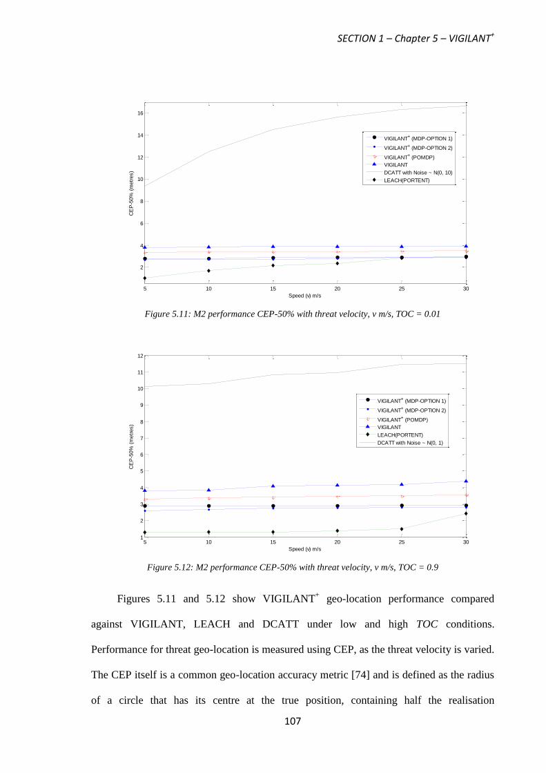
SECTION 1 – Chapter 5 – VIGILANT+
107
Figure 5.11: M2 performance CEP-50% with threat velocity, v m/s, TOC = 0.01
Figure 5.12: M2 performance CEP-50% with threat velocity, v m/s, TOC = 0.9
Figures 5.11 and 5.12 show VIGILANT+ geo-location performance compared
against VIGILANT, LEACH and DCATT under low and high TOC conditions.
Performance for threat geo-location is measured using CEP, as the threat velocity is varied.
The CEP itself is a common geo-location accuracy metric [74] and is defined as the radius
of a circle that has its centre at the true position, containing half the realisation
5 10 15 20 25 30
2
4
6
8
10
12
14
16
Speed (v) m/s
CE
P-5
0%
(m
etr
es)
VIGILANT+ (MDP-OPTION 1)
VIGILANT+ (MDP-OPTION 2)
VIGILANT+ (POMDP)
VIGILANT
DCATT with Noise ~ N(0, 10)
LEACH(PORTENT)
5 10 15 20 25 301
2
3
4
5
6
7
8
9
10
11
12
Speed (v) m/s
CE
P-5
0%
(m
etr
es)
VIGILANT+ (MDP-OPTION 1)
VIGILANT+ (MDP-OPTION 2)
VIGILANT+ (POMDP)
VIGILANT
LEACH(PORTENT)
DCATT with Noise ~ N(0, 1)

SECTION 1 – Chapter 5 – VIGILANT+
108
uncertainties of the random vector. A lower CEP value would provide a basis for
distinguishing a better geo-location performance. As shown in figures 5.11 and 5.12,
LEACH threat geo-location performance degrades with increasing threat velocity and this
is more prevalent under TOC = 0.01 conditions. This is because utilising just PORTENT-
Option 2 detection certainty, as a means of selecting and rotating the GI, can lead to far
greater fluctuations under a low TOC setting (higher observation uncertainty) since, the
probability of false alarm is at its greatest. SA level 2 operations can minimise on false
alarm effects propagating down to GI selection and “New GI” rotation decision making, as
in the case with VIGILANT+, leading to a greater group stability and consistent geo-
location performance across a range of threat velocities.
Both figures 5.11 and 5.12 also illustrate the fact that by not integrating a geo-
location “context” capability, in terms of GDOP (i.e. VIGILANT) or relying on received
signal energy corrupted with noise from the sensing environment (i.e. DCATT) can result
in geo-location performance shortfalls, when compared with VIGILANT+. Under
conditions with a high level of noise corruption, figure 5.11 shows how DCATT geo-
location performance degrades with increasing threat velocity. Increasing the noise in the
environment leads to greater group instability since DCATT relies on the CH which
receives the greatest signal energy in the neighbourhood and as a result, CH rotation
becomes more unstable. Random CH election and rotation can lead to greater inaccuracies,
as a point of reference, in order to conduct geo-location from, leading to CEP performance
shortfalls. Under low noise corruption this can lead to a better geo-location performance
for DCATT, primarily because the rotation of CHs is less, increasing group stability
slightly.
For VIGILANT its operation is mainly focused on threat presence detection and not
geo-location. Both figures 5.11 and 5.12 confirm that geo-location based on just using

SECTION 1 – Chapter 5 – VIGILANT+
109
threat presence “context” can lead to CEP performance shortfalls when compared with
VIGILANT+. VIGILANT
+ incorporates both an ability to evaluate threat presence and
geo-location “context” and this can help to maintain both a consistent and improved geo-
location performance across the range of threat velocities, when compared with
VIGILANT, as shown in figures 5.11 and 5.12.
In terms of VIGILANT+ CEP performance figures 5.11 and 5.12 suggest that
utilising a MDP framework, which relies on further GI updates to maintain the memory-
less Markov condition, improves geo-location performance over using just the POMDP
framework. In addition MDP-Option 2, which ensures greater GI confidence in threat
presence is established before initiating GI updating, has the greatest improvement in geo-
location performance out of all VIGILANT+
modes of operation.
Utilising further GI updates clearly encourages a better evaluation of geo-location
“context” in terms of GDOP and figures 5.11 and 5.12 proposes to us to consider that
geo-location is an exercise best preserved to some degree as a centralised operation, rather
than a fully distributed operation. Evidence to support this notion is also shown through
LEACH operation, which provides the most improvement (lower CEP) in geo-location
performance, as shown in figures 5.11 and 5.12. From (5.5), the GDOP error itself is
magnified through the geometry matrix, HT
H and can be reduced if the number of active
sensors utilised, N, increases. LEACH in itself is centralised and utilises all one-hop
neighbours to gauge a level of geo-location accuracy. Utilising all one-hop neighbours
incorporates the use of a greater N and so improves on LEACH geo-location performance,
confirmed through figures 5.11 and 5.12, when compared with VIGILANT and
VIGILANT+.
With the POMDP framework a fully distributed mode of operation is encouraged and
as a result, threat position updates at each decision epoch interval can only be conducted
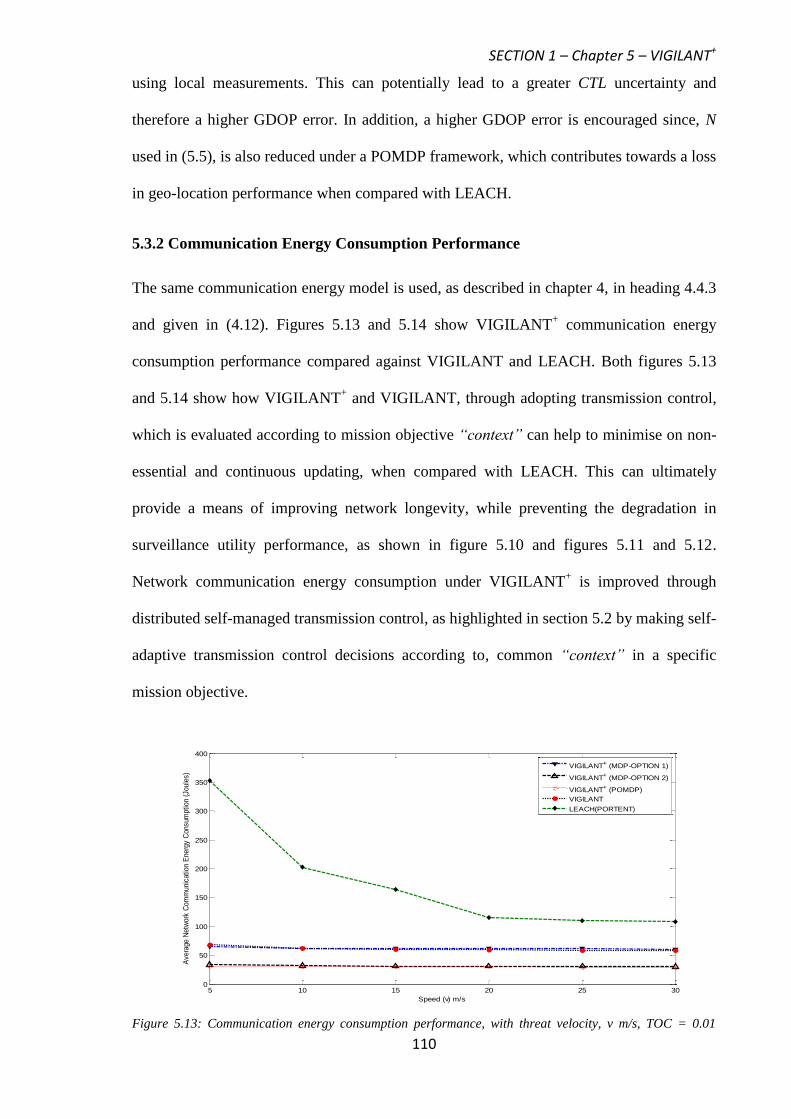
SECTION 1 – Chapter 5 – VIGILANT+
110
using local measurements. This can potentially lead to a greater CTL uncertainty and
therefore a higher GDOP error. In addition, a higher GDOP error is encouraged since, N
used in (5.5), is also reduced under a POMDP framework, which contributes towards a loss
in geo-location performance when compared with LEACH.
5.3.2 Communication Energy Consumption Performance
The same communication energy model is used, as described in chapter 4, in heading 4.4.3
and given in (4.12). Figures 5.13 and 5.14 show VIGILANT+ communication energy
consumption performance compared against VIGILANT and LEACH. Both figures 5.13
and 5.14 show how VIGILANT+ and VIGILANT, through adopting transmission control,
which is evaluated according to mission objective “context” can help to minimise on non-
essential and continuous updating, when compared with LEACH. This can ultimately
provide a means of improving network longevity, while preventing the degradation in
surveillance utility performance, as shown in figure 5.10 and figures 5.11 and 5.12.
Network communication energy consumption under VIGILANT+ is improved through
distributed self-managed transmission control, as highlighted in section 5.2 by making self-
adaptive transmission control decisions according to, common “context” in a specific
mission objective.
Figure 5.13: Communication energy consumption performance, with threat velocity, v m/s, TOC = 0.01
5 10 15 20 25 300
50
100
150
200
250
300
350
400
Speed (v) m/s
Avera
ge N
etw
ork
Com
munic
ation E
nerg
y C
onsum
ption (
Joule
s)
VIGILANT+ (MDP-OPTION 1)
VIGILANT+ (MDP-OPTION 2)
VIGILANT+ (POMDP)
VIGILANT
LEACH(PORTENT)
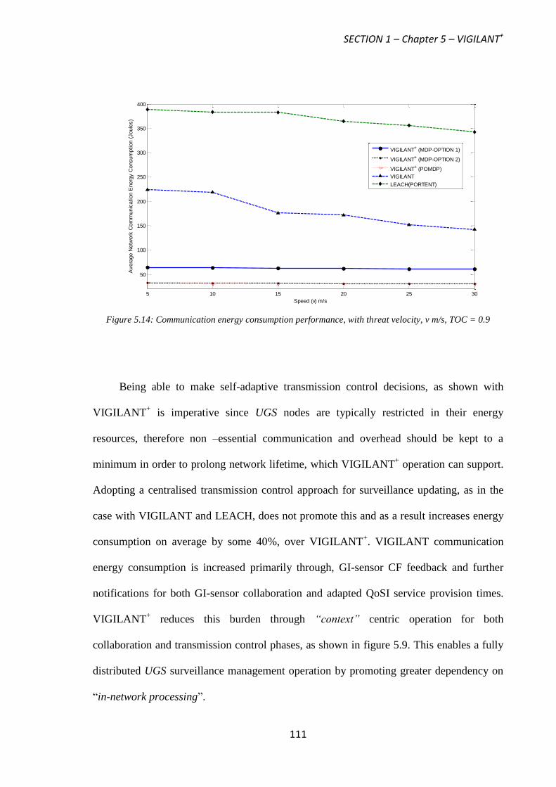
SECTION 1 – Chapter 5 – VIGILANT+
111
Figure 5.14: Communication energy consumption performance, with threat velocity, v m/s, TOC = 0.9
Being able to make self-adaptive transmission control decisions, as shown with
VIGILANT+ is imperative since UGS nodes are typically restricted in their energy
resources, therefore non –essential communication and overhead should be kept to a
minimum in order to prolong network lifetime, which VIGILANT+ operation can support.
Adopting a centralised transmission control approach for surveillance updating, as in the
case with VIGILANT and LEACH, does not promote this and as a result increases energy
consumption on average by some 40%, over VIGILANT+. VIGILANT communication
energy consumption is increased primarily through, GI-sensor CF feedback and further
notifications for both GI-sensor collaboration and adapted QoSI service provision times.
VIGILANT+ reduces this burden through “context” centric operation for both
collaboration and transmission control phases, as shown in figure 5.9. This enables a fully
distributed UGS surveillance management operation by promoting greater dependency on
“in-network processing”.
5 10 15 20 25 30
50
100
150
200
250
300
350
400
Speed (v) m/s
Avera
ge N
etw
ork
Com
munic
ation E
nerg
y C
onsum
ption (
Joule
s)
VIGILANT+ (MDP-OPTION 1)
VIGILANT+ (MDP-OPTION 2)
VIGILANT+ (POMDP)
VIGILANT
LEACH(PORTENT)
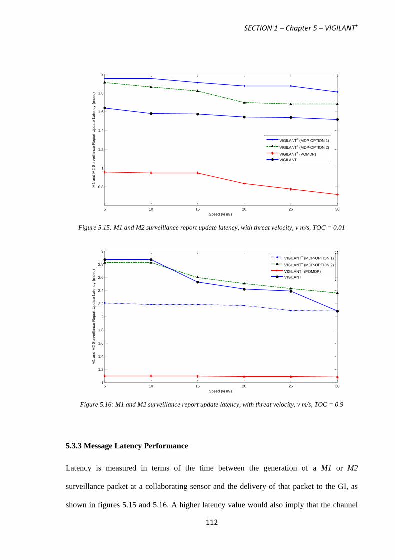
SECTION 1 – Chapter 5 – VIGILANT+
112
Figure 5.15: M1 and M2 surveillance report update latency, with threat velocity, v m/s, TOC = 0.01
Figure 5.16: M1 and M2 surveillance report update latency, with threat velocity, v m/s, TOC = 0.9
5.3.3 Message Latency Performance
Latency is measured in terms of the time between the generation of a M1 or M2
surveillance packet at a collaborating sensor and the delivery of that packet to the GI, as
shown in figures 5.15 and 5.16. A higher latency value would also imply that the channel
5 10 15 20 25 30
0.8
1
1.2
1.4
1.6
1.8
2
Speed (v) m/s
M1 a
nd M
2 S
urv
eill
ance R
eport
Update
Late
ncy (
msec)
VIGILANT+ (MDP-OPTION 1)
VIGILANT+ (MDP-OPTION 2)
VIGILANT+ (POMDP)
VIGILANT
5 10 15 20 25 301
1.2
1.4
1.6
1.8
2
2.2
2.4
2.6
2.8
3
Speed (v) m/s
M1 a
nd M
2 S
urv
eill
ance R
eport
Update
Late
ncy (
msec)
VIGILANT+ (MDP-OPTION 1)
VIGILANT+ (MDP-OPTION 2)
VIGILANT+ (POMDP)
VIGILANT
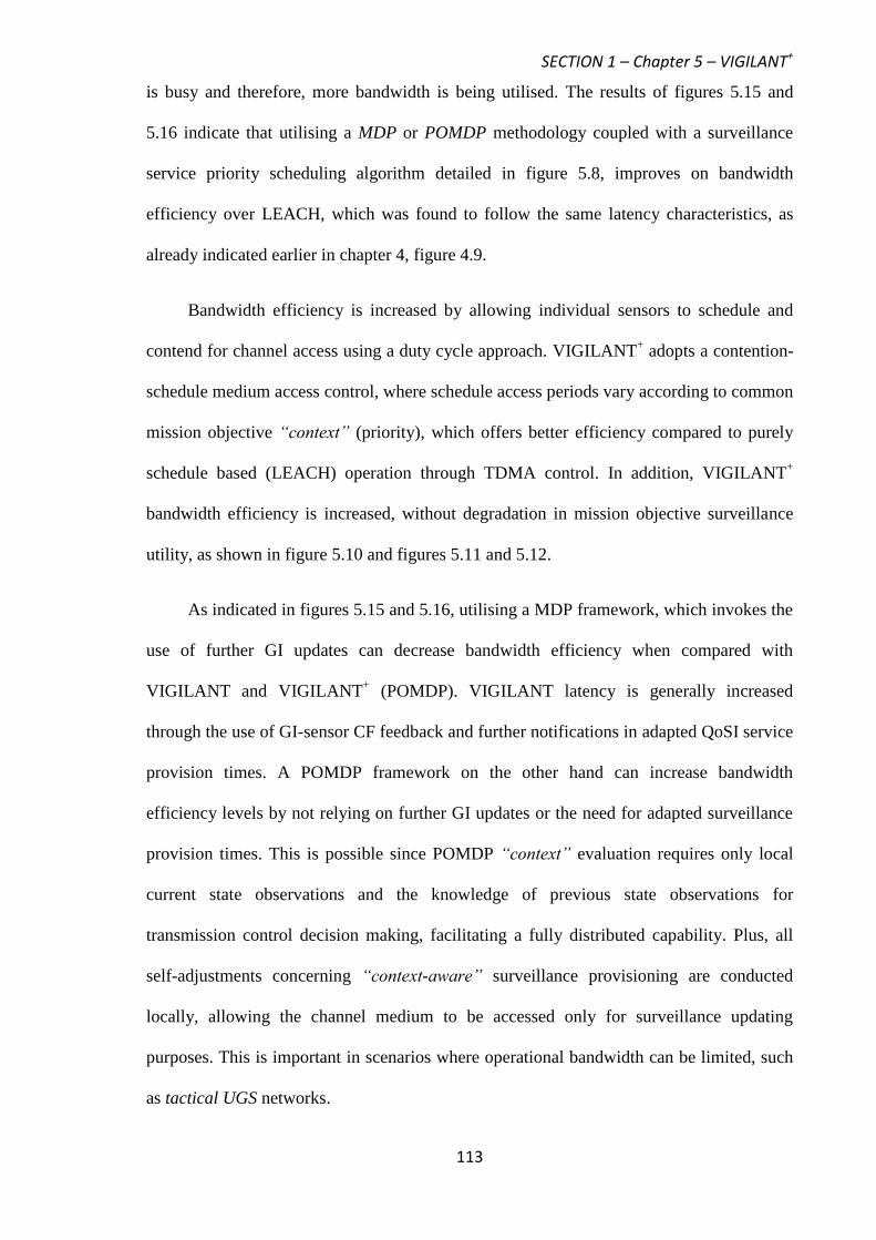
SECTION 1 – Chapter 5 – VIGILANT+
113
is busy and therefore, more bandwidth is being utilised. The results of figures 5.15 and
5.16 indicate that utilising a MDP or POMDP methodology coupled with a surveillance
service priority scheduling algorithm detailed in figure 5.8, improves on bandwidth
efficiency over LEACH, which was found to follow the same latency characteristics, as
already indicated earlier in chapter 4, figure 4.9.
Bandwidth efficiency is increased by allowing individual sensors to schedule and
contend for channel access using a duty cycle approach. VIGILANT+ adopts a contention-
schedule medium access control, where schedule access periods vary according to common
mission objective “context” (priority), which offers better efficiency compared to purely
schedule based (LEACH) operation through TDMA control. In addition, VIGILANT+
bandwidth efficiency is increased, without degradation in mission objective surveillance
utility, as shown in figure 5.10 and figures 5.11 and 5.12.
As indicated in figures 5.15 and 5.16, utilising a MDP framework, which invokes the
use of further GI updates can decrease bandwidth efficiency when compared with
VIGILANT and VIGILANT+ (POMDP). VIGILANT latency is generally increased
through the use of GI-sensor CF feedback and further notifications in adapted QoSI service
provision times. A POMDP framework on the other hand can increase bandwidth
efficiency levels by not relying on further GI updates or the need for adapted surveillance
provision times. This is possible since POMDP “context” evaluation requires only local
current state observations and the knowledge of previous state observations for
transmission control decision making, facilitating a fully distributed capability. Plus, all
self-adjustments concerning “context-aware” surveillance provisioning are conducted
locally, allowing the channel medium to be accessed only for surveillance updating
purposes. This is important in scenarios where operational bandwidth can be limited, such
as tactical UGS networks.
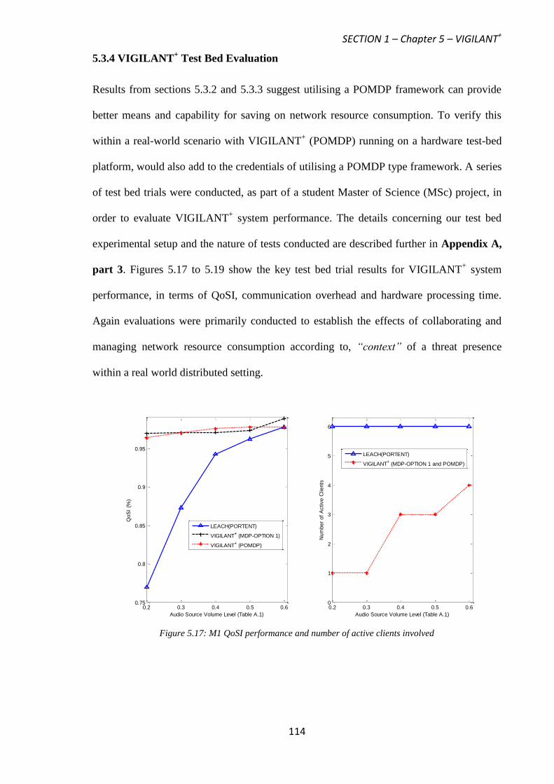
SECTION 1 – Chapter 5 – VIGILANT+
114
5.3.4 VIGILANT+ Test Bed Evaluation
Results from sections 5.3.2 and 5.3.3 suggest utilising a POMDP framework can provide
better means and capability for saving on network resource consumption. To verify this
within a real-world scenario with VIGILANT+ (POMDP) running on a hardware test-bed
platform, would also add to the credentials of utilising a POMDP type framework. A series
of test bed trials were conducted, as part of a student Master of Science (MSc) project, in
order to evaluate VIGILANT+ system performance. The details concerning our test bed
experimental setup and the nature of tests conducted are described further in Appendix A,
part 3. Figures 5.17 to 5.19 show the key test bed trial results for VIGILANT+ system
performance, in terms of QoSI, communication overhead and hardware processing time.
Again evaluations were primarily conducted to establish the effects of collaborating and
managing network resource consumption according to, “context” of a threat presence
within a real world distributed setting.
Figure 5.17: M1 QoSI performance and number of active clients involved
0.2 0.3 0.4 0.5 0.60.75
0.8
0.85
0.9
0.95
Audio Source Volume Level (Table A.1)
QoS
I (%
)
0.2 0.3 0.4 0.5 0.60
1
2
3
4
5
6
Audio Source Volume Level (Table A.1)
Num
ber
of
Active C
lients
LEACH(PORTENT)
VIGILANT+ (MDP-OPTION 1 and POMDP)
LEACH(PORTENT)
VIGILANT+ (MDP-OPTION 1)
VIGILANT+ (POMDP)
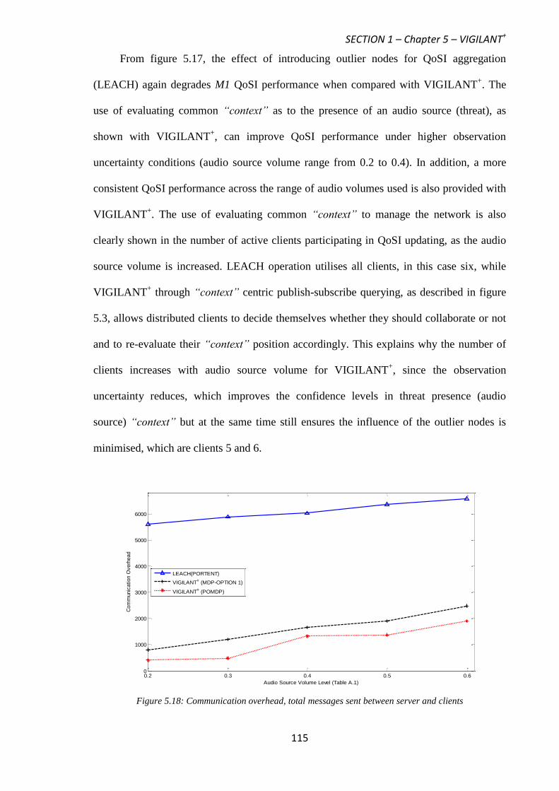
SECTION 1 – Chapter 5 – VIGILANT+
115
From figure 5.17, the effect of introducing outlier nodes for QoSI aggregation
(LEACH) again degrades M1 QoSI performance when compared with VIGILANT+. The
use of evaluating common “context” as to the presence of an audio source (threat), as
shown with VIGILANT+, can improve QoSI performance under higher observation
uncertainty conditions (audio source volume range from 0.2 to 0.4). In addition, a more
consistent QoSI performance across the range of audio volumes used is also provided with
VIGILANT+. The use of evaluating common “context” to manage the network is also
clearly shown in the number of active clients participating in QoSI updating, as the audio
source volume is increased. LEACH operation utilises all clients, in this case six, while
VIGILANT+ through “context” centric publish-subscribe querying, as described in figure
5.3, allows distributed clients to decide themselves whether they should collaborate or not
and to re-evaluate their “context” position accordingly. This explains why the number of
clients increases with audio source volume for VIGILANT+, since the observation
uncertainty reduces, which improves the confidence levels in threat presence (audio
source) “context” but at the same time still ensures the influence of the outlier nodes is
minimised, which are clients 5 and 6.
Figure 5.18: Communication overhead, total messages sent between server and clients
0.2 0.3 0.4 0.5 0.60
1000
2000
3000
4000
5000
6000
Audio Source Volume Level (Table A.1)
Com
munic
ation O
verh
ead
LEACH(PORTENT)
VIGILANT+ (MDP-OPTION 1)
VIGILANT+ (POMDP)

SECTION 1 – Chapter 5 – VIGILANT+
116
Figure 5.18 shows the total number of messages sent between the server and clients
(communication overhead) and gives us an indication as to the level in network resources
consumed. With LEACH, as expected, utilising all nodes to participate in QoSI increases
the communication overhead and would imply greater communication energy and
bandwidth consumption. Utilising all nodes degrades M1 QoSI performance and inflicts
greater network resource consumption, making this inefficient from an UGS surveillance
management perspective.
VIGILANT+ again shows the benefit of introducing self-managed transmission
control according to common “context” concerning the presence of an audio source
(threat). As observation uncertainty reduces (higher audio source volume level), naturally
this increases the number of messages sent since there is greater confidence in “context”
but a higher level of control over LEACH is still achieved. From a VIGILANT+
performance point of view the benefits of not utilising further GI updates, as occurs with
MDP operation, is clearly shown with the POMDP framework. The lower communication
overhead incurred with VIGILANT+ POMDP operation over MDP operation would imply
potential to save on network resource consumption. This is also an added benefit given that
the POMDP framework does not subject degradation in M1 QoSI performance, as
indicated in figure 5.17.
Figure 5.19 gives an indication as to the average level of processing time required to
execute VIGILANT+ commands according to, the described SA levels 1, 2 and 3 at each
client, across the full range of audio source volumes used. Test-bed trial results indicate
that processing times associated with SA levels 1 and 2 are similar for both VIGILANT+
MDP and POMDP operations and this is expected since, the functionality for these two
levels is common. The difference in processing time performance is really felt within SA
level 3, which is the associated self-managed transmission control methodology.
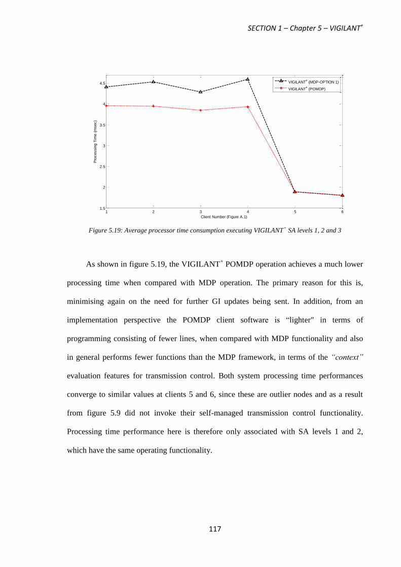
SECTION 1 – Chapter 5 – VIGILANT+
117
Figure 5.19: Average processor time consumption executing VIGILANT+ SA levels 1, 2 and 3
As shown in figure 5.19, the VIGILANT+ POMDP operation achieves a much lower
processing time when compared with MDP operation. The primary reason for this is,
minimising again on the need for further GI updates being sent. In addition, from an
implementation perspective the POMDP client software is “lighter" in terms of
programming consisting of fewer lines, when compared with MDP functionality and also
in general performs fewer functions than the MDP framework, in terms of the “context”
evaluation features for transmission control. Both system processing time performances
converge to similar values at clients 5 and 6, since these are outlier nodes and as a result
from figure 5.9 did not invoke their self-managed transmission control functionality.
Processing time performance here is therefore only associated with SA levels 1 and 2,
which have the same operating functionality.
1 2 3 4 5 61.5
2
2.5
3
3.5
4
4.5
Client Number (Figure A.1)
Pro
cessin
g T
ime (
msec)
VIGILANT+ (MDP-OPTION 1)
VIGILANT+ (POMDP)
SECTION 1 – Chapter 5 – VIGILANT+
118
5.4 VIGILANT+ POMDP Epoch Control Strategies
VIGILANT+ performance evaluations have revealed that for the simulated network
deployment scenario and from additional test bed evaluation trials, that utilising a POMDP
framework, can increase the savings to be made on network resource consumption. This is
achieved primarily through minimising the need for further GI updates. Evaluations have
also indicated that, while not using further GI updates has little impact on M1 surveillance
utility performance it can affect the level of M2 surveillance performance possible. There
are two main reasons for this, firstly, a POMDP framework for M2 operation requires CTL
observations to be made locally and secondly, M2 “context” evaluations are conducted
using a fixed decision epoch interval, which ignores the dynamic characteristics of the
monitored threat.
A MDP framework for M2 surveillance performance has the advantage of
considering the dynamics of the monitored threat and this is reflected in the frequency in
GI updating, according to MDP options 1 or 2. Subsequently, GI updating would either
increase or decrease as the dynamics of the threat (i.e. TOC) change, giving a better
evaluation of current M2 “context”. A POMDP framework being fully distributed cannot
achieve this without implementing some form of self-adaption to its own decision epoch
interval selection. Utilising a fixed decision epoch interval at a pre-determined observation
frequency may also encourage unnecessary transmission control actions to occur, leading
to an unnecessary increase in network resource consumption. In order to maintain the
POMDP advantage of providing savings in network resource consumption and maintaining
a fully distributed capability over the MDP framework, in this section, we seek to develop
strategies to allow self-adaptable POMDP decision epoch interval selection.

SECTION 1 – Chapter 5 – VIGILANT+
119
5.4.1 POMDP Epoch Control Strategy Formulation
Providing control strategies for when POMDP decision epochs should occur is mostly
aimed at further improving network resource consumption efficiency. Extending the
POMDP operation to adapt decision epoch frequencies according to the characteristics of a
monitored threat situation, is one possible way of achieving improved efficiency savings.
We portray and define the characteristics associated with a monitored threat in two ways:
Physical characteristics (i.e. position observations in order to derive changes in threat
velocity dynamics).
Mission objective specific “context” characteristics (i.e. probabilistic confidence
measures derived in SA level 2 with respect to M1 or M2).
To formulate the decision epoch control process we employ a time frame window in which
characteristics concerning the monitored threat are observed. This is detailed as follows
with further illustration, given in figure 5.20:
A total of l threat characteristic observations are made within a designated time frame
window (Tj) in seconds, where j denotes the identification of the monitored threat.
Threat characteristics are observed at each time interval (T^j)
n, equal to 1 / l seconds,
where n = 0, at the start of an observation time frame, with condition, n < l.
A current decision epoch interval (∆DEj) is evaluated and scheduled at the end of each
(Tj).
(∆DEj)Previous denotes the decision epoch interval calculated in the previous designated
time frame window (Tj).

SECTION 1 – Chapter 5 – VIGILANT+
120
Figure 5.20: Decision epoch control formulation
Figure 5.20 shows how the decision epoch interval is controlled according to ∆DEj
determined by the monitored threat characteristics. For example, if a threat were to move at
a constant velocity or remain static, this would imply setting a larger decision epoch
interval through ∆DEj, with strategies used to define ∆DEj being specified in a suitable
way to reflect this, as detailed in headings 5.4.2 to 5.4.4.
5.4.2 Strategy 1: Threat Position
Threat position observation estimates (POE), (xThreat-j, yThreat-j), are conducted by local UGSs
within an x-y plane, representing the surveillance field. Location Metadata (LM) of the last l
observations taken within Tj, concerning the monitored threat is modeled, as shown in
(5.15).
tjjj dd)T(LM
(5.15)
Where dj denotes the net distance travelled by the monitored threat, during the last l
observations, as shown in (5.16).
21ln
jThreat
0n
jThreat
21ln
jThreat
0n
jThreatj )yy()xxd
(5.16)
The total distance travelled by the threat during the last l observations, dtj, forming the
threat position observation history within Tj, is given in (5.17).
Tj (l threat characteristic observations)
(T^
j) n
n
Epoch Interval ((∆DEj)
Previous + ∆DE
j) ∆DE
j

SECTION 1 – Chapter 5 – VIGILANT+
121
21n
jThreat
n
jThreat
21n
jThreatln0n
n
jThreattj )yy()xx(d
(5.17)
In (5.17), (xThreat-jn+1
, yThreat-jn+1
) are the updated threat positions observed at (T^j)
n+1. As
shown in (5.15), LM, dictated by dtj, is equal to unity if the threat moves in a completely
uniform manner and is < 1, if threat dynamics change in a non-uniform manner. Therefore,
LM is bounded by the interval (0 < LM <= 1), within (Tj). For strategy 1, ∆DEj, is assumed
to be a linear function of LM, ∆DEj = f (LM (Tj)), and can be calculated, as shown in (5.18).
)T(LM)DE(DE jeviousPrjj (5.18)
5.4.3 Strategy 2: Mission Objective “Context”
Mission objective “context” characteristics can be derived using SA- level 2 and follows the
probability derivations made from figure 5.2, which are summarised in table 5.1. Using
table 5.1, strategy 2 provides probabilistic confidence measures for presence (P1j) and geo-
location (P2j) of threat, given as entries six and eight respectively. Utilising P1j and P2j
derivations, specific mission objective “context” ratios (CR) can be established, as shown in
(5.19) and (5.20).
)P,....Pmax()P,....Pmin()T(CR 1ln
j1
0n
j1
1ln
j1
0n
j1jj1M (5.19)
)P,....Pmax()P,....Pmin()T(CR 1ln
j2
0n
j2
1ln
j2
0n
j2jj2M (5.20)
From (5.19) and (5.20), min and max are functions calculating the final minimum and
maximum confidence measures obtained, within Tj. Using min and max functions in this
instance, helps to determine the degree of “contextual” variation, present within Tj. If there
is low variation present, this would imply a higher CR being set. The value of CR, is
therefore bounded by the interval (0 < CR <= 1), within Tj. For strategy 2, ∆DEj, is assumed
to be a linear function of CR, ∆DEj = f (CR (Tj)), and can be calculated, for each specific
mission objective, as shown in (5.21) and (5.22).

SECTION 1 – Chapter 5 – VIGILANT+
122
)T(CR)DE(DE jj1M1MeviousPrjj (5.21)
)T(CR)DE(DE jj2M2MeviousPrjj (5.22)
5.4.4 Strategy 3: Similarity in Mission Objective “Context”
Confidence measures P1j and P2j, can assist in portraying the level of similarity that exists
about the current mission objective surveillance environment. We define dimensional (l -1)
confidence measure vectors, B and X, where B = (P1j n=0
,…, P1j n=l-1
) and X = (P2j n=0
,…, P2j
n=l-1), observed within Tj. Utilising a similarity function we can capture the extent to which
B and X, convey similar “context” towards the mission objective surveillance environment,
within Tj. A similarity function (Sim) can be defined as a logical distance measure of
“context” between B and X. This implies that if B and X have high similarity, they exhibit a
small “context” distance between them. “Context” distance, measuring a similarity towards
the current mission objective surveillance environment at two time intervals, can be
illustrated as shown in figure 5.21.
Figure 5.21: Similarity “context” within the M1 and M2 surveillance environment at two time intervals
As shown in figure 5.21 the degree in similarity in M1 and M2 “context” is reflected
through the included angle, α and can be formulated using figure 5.21, as shown in (5.23).
P1j
n=0
B (M1- Threat Presence)
X (M2 - Threat Geo-location)
P1j
n=1
P2j
n=0
P2j
n=1
α
(T^
j)
n=0
(T^
j)
n=1
Similarity “Context”
β
γ

SECTION 1 – Chapter 5 – VIGILANT+
123
sinsincoscos)cos()cos( (5.23)
21n
j2
20n
j2
21n
j1
20n
j1
1n
j2
1n
j1
0n
j2
0n
j1
)P()P()P()P(
PPPP)cos(
Taking into consideration the full, (l-1) dimensional vectors B and X, within an allocated Tj
and by expanding (5.23), the complete summary of the similarity in B and X in Tj, is shown
in (5.24).
1ln0n
2n
j21ln
0n2n
j1
1ln0n
n
j2
n
j1
)P()P(
PP)cos(
(5.24)
As shown in (5.24), the cosine of the included angle of B and X, α, is in fact an
accuracy description of correlations (similarity) between two types of “context” measures,
in view of the current mission objective surveillance environment. Defined in this way, cos
(α) will vary between 0 when B and X are orthogonal (low similarity “context”) and 1
when B and X are identical or proportional (high similarity “context”). For strategy 3, we
define Sim (Tj) = cos (α), reflecting the distance measurement between B and X, which
increases if B and X have more common similarity “context”. ∆DEj is assumed to be a
linear function of Sim (Tj), ∆DEj = f (Sim (Tj)), as shown in (5.25).
)T(Sim)DE(DE jeviousPrjj (5.25)
5.4.5 VIGILANT+ POMDP Epoch Control Strategy Performance
System performance is evaluated using the OMNeT++ network simulation platform [63].
We utilise the same network deployment characteristics already described for VIGILANT
and VIGILANT+ performance evaluations, in 4.4 and 5.3. Threat mobility characteristics
are however different and simulated using the random waypoint (RWP) model, with a
dynamic velocity (m/s) set from a uniform distribution, uniform (0, vmax). A RWP
simulation model is considered because of its extensive use within surveillance type
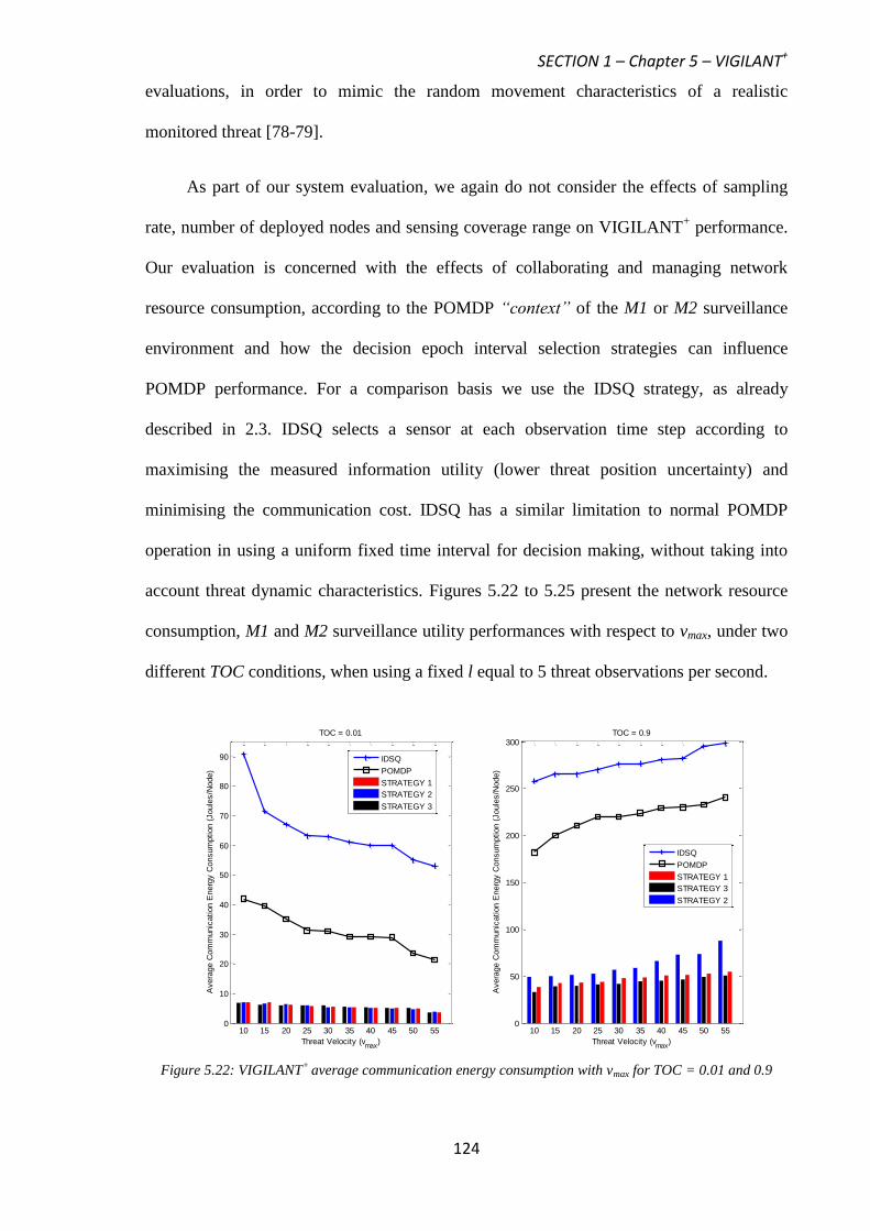
SECTION 1 – Chapter 5 – VIGILANT+
124
evaluations, in order to mimic the random movement characteristics of a realistic
monitored threat [78-79].
As part of our system evaluation, we again do not consider the effects of sampling
rate, number of deployed nodes and sensing coverage range on VIGILANT+ performance.
Our evaluation is concerned with the effects of collaborating and managing network
resource consumption, according to the POMDP “context” of the M1 or M2 surveillance
environment and how the decision epoch interval selection strategies can influence
POMDP performance. For a comparison basis we use the IDSQ strategy, as already
described in 2.3. IDSQ selects a sensor at each observation time step according to
maximising the measured information utility (lower threat position uncertainty) and
minimising the communication cost. IDSQ has a similar limitation to normal POMDP
operation in using a uniform fixed time interval for decision making, without taking into
account threat dynamic characteristics. Figures 5.22 to 5.25 present the network resource
consumption, M1 and M2 surveillance utility performances with respect to vmax, under two
different TOC conditions, when using a fixed l equal to 5 threat observations per second.
Figure 5.22: VIGILANT+
average communication energy consumption with vmax for TOC = 0.01 and 0.9
10 15 20 25 30 35 40 45 50 550
10
20
30
40
50
60
70
80
90
Threat Velocity (vmax
)
Avera
ge C
om
munic
ation E
nerg
y C
onsum
ption (
Joule
s/N
ode)
TOC = 0.01
10 15 20 25 30 35 40 45 50 550
50
100
150
200
250
300
Threat Velocity (vmax
)
Avera
ge C
om
munic
ation E
nerg
y C
onsum
ption (
Joule
s/N
ode)
TOC = 0.9
IDSQ
POMDP
STRATEGY 1
STRATEGY 2
STRATEGY 3
IDSQ
POMDP
STRATEGY 1
STRATEGY 3
STRATEGY 2

SECTION 1 – Chapter 5 – VIGILANT+
125
As indicated from figure 5.22, employing decision epoch interval control strategies
can improve on communication energy consumption from a total deployed network
perspective (i.e. joules consumed/node), when compared with non-adaption (IDSQ and
POMDP). Both the normal POMDP framework and IDSQ in our simulation would invoke
a transmission control decision on every observation made per second. Managing decision
epoch intervals according to threat characteristics (strategies 1, 2, 3) can adapt the interval
selection, in order to reflect on the dynamics of the threat (i.e. changes in threat velocity)
and therefore, as a result, achieve improved energy consumption performance.
From figure 5.22, it suggests that strategy 3 achieves the most improved
communication energy consumption performance in both TOC conditions. Strategy 3 itself
measures the similarity “context” within the M1 and M2 surveillance environment through
cos (α), given in (5.24). This suggests the cos (α) metric can offer a better “context”
derivation as to the dynamics associated with the combined M1 and M2 environment,
which can influence better control on POMDP epoch interval selection for transmission
control decision making. Strategy 2 achieves a lower communication energy consumption
performance under both TOC conditions, which suggests that finding the degree in
individual M1 or M2 “context” variation present within the environment is not an
appropriate method to use.
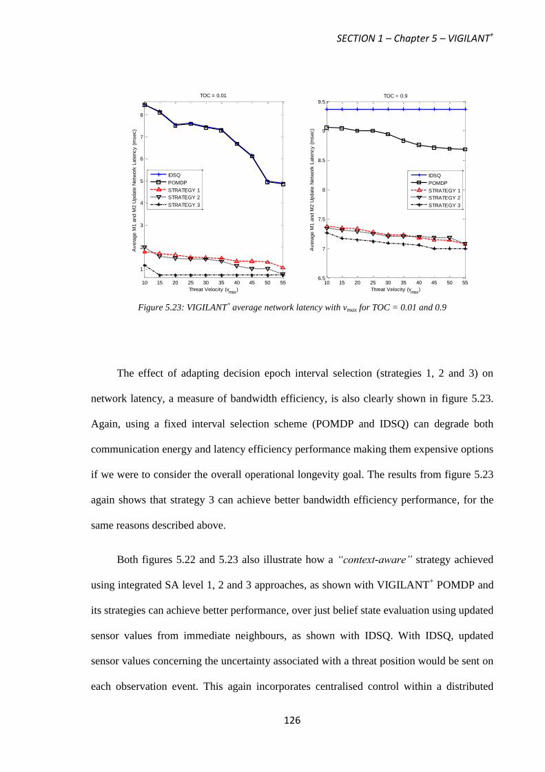
SECTION 1 – Chapter 5 – VIGILANT+
126
Figure 5.23: VIGILANT+
average network latency with vmax for TOC = 0.01 and 0.9
The effect of adapting decision epoch interval selection (strategies 1, 2 and 3) on
network latency, a measure of bandwidth efficiency, is also clearly shown in figure 5.23.
Again, using a fixed interval selection scheme (POMDP and IDSQ) can degrade both
communication energy and latency efficiency performance making them expensive options
if we were to consider the overall operational longevity goal. The results from figure 5.23
again shows that strategy 3 can achieve better bandwidth efficiency performance, for the
same reasons described above.
Both figures 5.22 and 5.23 also illustrate how a “context-aware” strategy achieved
using integrated SA level 1, 2 and 3 approaches, as shown with VIGILANT+ POMDP and
its strategies can achieve better performance, over just belief state evaluation using updated
sensor values from immediate neighbours, as shown with IDSQ. With IDSQ, updated
sensor values concerning the uncertainty associated with a threat position would be sent on
each observation event. This again incorporates centralised control within a distributed
10 15 20 25 30 35 40 45 50 55
1
2
3
4
5
6
7
8
Threat Velocity (vmax
)
Avera
ge M
1 a
nd M
2 U
pdate
Netw
ork
Late
ncy (
msec)
TOC = 0.01
10 15 20 25 30 35 40 45 50 556.5
7
7.5
8
8.5
9
9.5
Threat Velocity (vmax
)
Avera
ge M
1 a
nd M
2 U
pdate
Netw
ork
Late
ncy (
msec)
TOC = 0.9
IDSQ
POMDP
STRATEGY 1
STRATEGY 2
STRATEGY 3
IDSQ
POMDP
STRATEGY 1
STRATEGY 2
STRATEGY 3
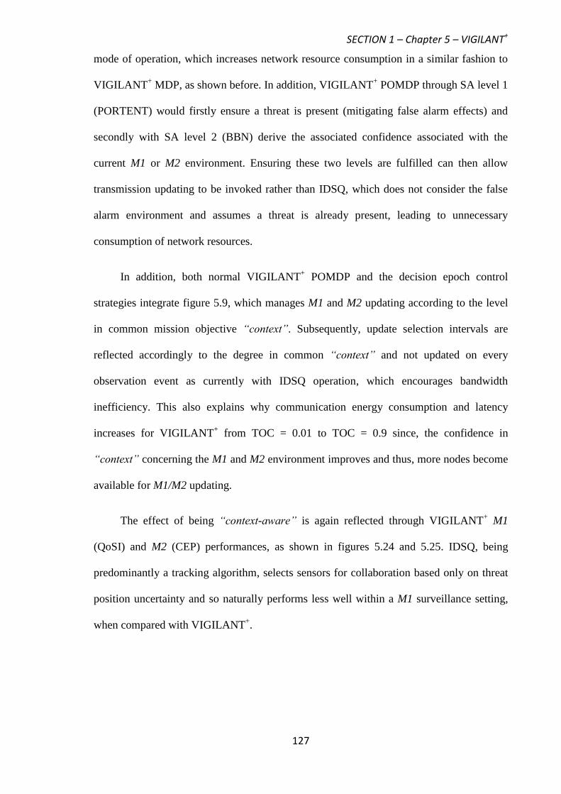
SECTION 1 – Chapter 5 – VIGILANT+
127
mode of operation, which increases network resource consumption in a similar fashion to
VIGILANT+ MDP, as shown before. In addition, VIGILANT
+ POMDP through SA level 1
(PORTENT) would firstly ensure a threat is present (mitigating false alarm effects) and
secondly with SA level 2 (BBN) derive the associated confidence associated with the
current M1 or M2 environment. Ensuring these two levels are fulfilled can then allow
transmission updating to be invoked rather than IDSQ, which does not consider the false
alarm environment and assumes a threat is already present, leading to unnecessary
consumption of network resources.
In addition, both normal VIGILANT+ POMDP and the decision epoch control
strategies integrate figure 5.9, which manages M1 and M2 updating according to the level
in common mission objective “context”. Subsequently, update selection intervals are
reflected accordingly to the degree in common “context” and not updated on every
observation event as currently with IDSQ operation, which encourages bandwidth
inefficiency. This also explains why communication energy consumption and latency
increases for VIGILANT+ from TOC = 0.01 to TOC = 0.9 since, the confidence in
“context” concerning the M1 and M2 environment improves and thus, more nodes become
available for M1/M2 updating.
The effect of being “context-aware” is again reflected through VIGILANT+ M1
(QoSI) and M2 (CEP) performances, as shown in figures 5.24 and 5.25. IDSQ, being
predominantly a tracking algorithm, selects sensors for collaboration based only on threat
position uncertainty and so naturally performs less well within a M1 surveillance setting,
when compared with VIGILANT+.
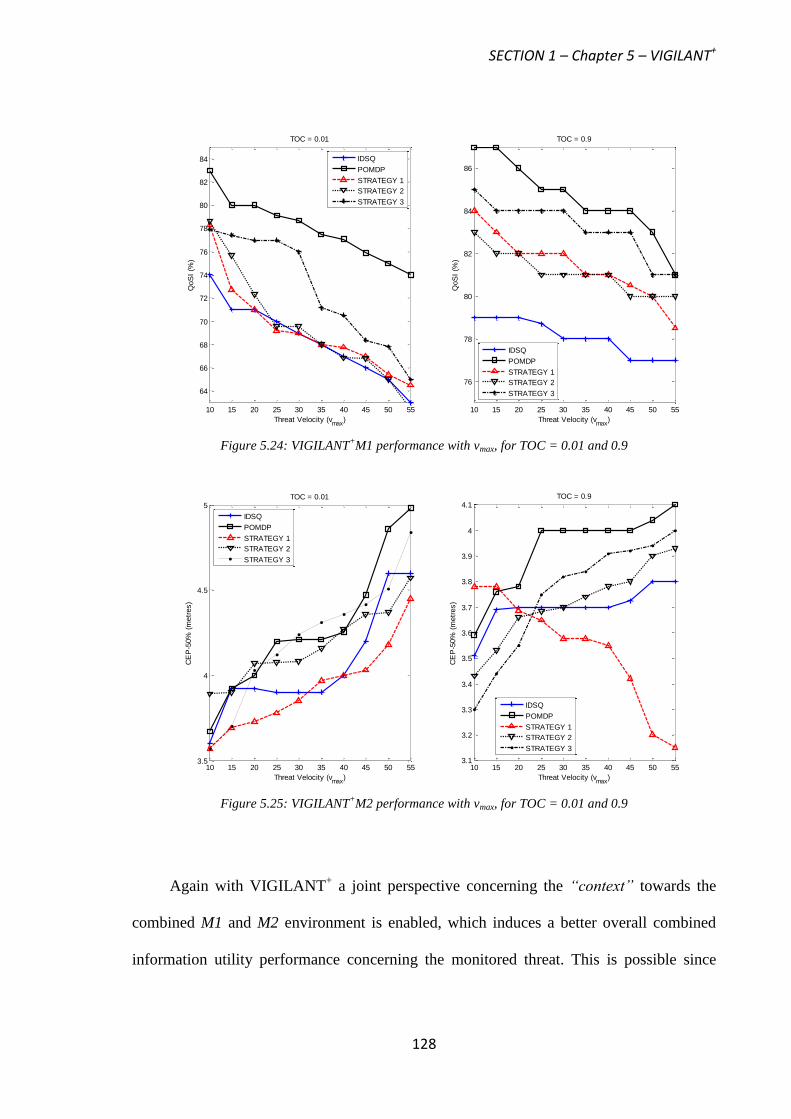
SECTION 1 – Chapter 5 – VIGILANT+
128
Figure 5.24: VIGILANT+M1 performance with vmax, for TOC = 0.01 and 0.9
Figure 5.25: VIGILANT+M2 performance with vmax, for TOC = 0.01 and 0.9
Again with VIGILANT+ a joint perspective concerning the “context” towards the
combined M1 and M2 environment is enabled, which induces a better overall combined
information utility performance concerning the monitored threat. This is possible since
10 15 20 25 30 35 40 45 50 55
64
66
68
70
72
74
76
78
80
82
84
Threat Velocity (vmax
)
QoS
I (%
)
TOC = 0.01
10 15 20 25 30 35 40 45 50 55
76
78
80
82
84
86
Threat Velocity (vmax
)
QoS
I (%
)
TOC = 0.9
IDSQ
POMDP
STRATEGY 1
STRATEGY 2
STRATEGY 3
IDSQ
POMDP
STRATEGY 1
STRATEGY 2
STRATEGY 3
10 15 20 25 30 35 40 45 50 553.5
4
4.5
5
Threat Velocity (vmax
)
CE
P-5
0%
(m
etr
es)
TOC = 0.01
10 15 20 25 30 35 40 45 50 553.1
3.2
3.3
3.4
3.5
3.6
3.7
3.8
3.9
4
4.1
Threat Velocity (vmax
)
CE
P-5
0%
(m
etr
es)
TOC = 0.9
IDSQ
POMDP
STRATEGY 1
STRATEGY 2
STRATEGY 3
IDSQ
POMDP
STRATEGY 1
STRATEGY 2
STRATEGY 3

SECTION 1 – Chapter 5 – VIGILANT+
129
VIGILANT+ incorporates both threat presence “context” and GDOP to achieve a better
QoSI and geo-location estimate (CEP) when compared with IDSQ, which just relies on
threat position uncertainty and ignores the associated uncertainty concerning the presence
of threat (non-consideration of false alarm effects).
For M2 performance shown in figure 5.25, results indicate that incorporating a
decision epoch interval strategy using updated physical threat position observations
(strategy 1) can achieve better performance over IDSQ, POMDP and strategy 2 and 3.
Threat geo-location performance is, in itself, dependent on the velocity of the threat since
this naturally influences current threat position at each observation time, when a GDOP
evaluation is made. Incorporating the changes associated with the velocity of the threat is
therefore crucial, which explains why strategy 1 performs well as vmax increases, as shown
in figure 5.25. Strategies ignoring the physical effects of threat position (i.e. velocity) do
not perform as well and thus CEP performance degrades with threat velocity, vmax. Due to
threat observation certainty being poor under a TOC = 0.01 setting, CEP performance
degrades as vmax increases, but with strategy 1 incorporating physical threat velocity effects
it is still able to provide a better performance over the other options tested.
The disadvantage of using a decision epoch interval selection strategy however is
portrayed through M1 QoSI performance, as shown in figure 5.24. When compared with
POMDP, strategies 1, 2 and 3 all induce a loss in performance. This would imply strategies
1, 2 and 3 through decision epoch interval adaption encourages a loss in threat presence
“context” evaluation, which increases with threat velocity, vmax. Results from figures 5.24
and 5.25 would therefore suggest employing a decision epoch interval strategy has benefits
only for M2 CEP performance and not M1 QoSI performance.

SECTION 1 – Chapter 5 – VIGILANT+
130
Utilising a normal POMDP decision epoch interval framework where M1 “context”
evaluations are matched to the number of observations to be made per second (l), is more
suitable for maintaining consistent QoSI performance against vmax. Overall though, one
should not discredit the benefits of using strategy 3 to promote improved network resource
consumption performance, as discussed earlier and also as a means of providing the most
improved QoSI performance out of strategies 1 and 2.

SECTION 1 – Chapter 6 – Summary and Conclusions
131
CHAPTER 6
Section 1: Summary and Conclusions
Deploying distributed unattended ground sensor (UGS) networks are primarily used to
support mission objective surveillance capabilities such as, threat presence detection and
geo-location, within a security-sensitive region. Distributed operation can provide the
following advantages for tactical mission plans through:
Promoting scalability, which increases the tactical reach that C2ISR planners can
operate at.
Minimising the burden for centralised processing architecture and manual system
configuration.
Catering against UGS node failures and improving the operational longevity of the
deployed UGS network.
Managing the distributed UGS network to support these mission objectives, however,
present challenges because of their inherently dynamic network operating environments.
Such environments are characterised by limited bandwidth, coupled with a changing threat
situation. UGS devices are also limited by their sensing, computation and communication
capabilities, which are dictated by their battery energy reserves. The management of
network resources therefore becomes crucial in extending the operational longevity of the
overall deployed UGS network field. The primary goal of section 1, therefore, concerns
the autonomic management of distributed UGS networks deployed to support specific
mission objectives (M1 or M2) and the conservation of their network resources.
Incorporating a methodology, which allows the consumption of network resources to
be managed as a direct causal relationship to the dynamics of the monitored threat, is much
more suitable and adaptable towards a changing surveillance situation. Utilising the

SECTION 1 – Chapter 6 – Summary and Conclusions
132
situation awareness (SA) framework can achieve this and ensures that sensed elements
from a current changing threat scenario are integrated (levels 1, 2 and 3) effectively, to
create new SA meaning and establish relevant autonomic decision making outcomes for
critical operations such as, distributed surveillance.
In chapter 3, our level 1 perception system named PORTENT is highlighted with its
primary aim of ensuring that false alarm effects are minimised within an uncertain threat
observation environment. False alarm rates have a distinct impact on surveillance
performance and especially on intruder detection. Enforcing a low false alarm rate to avoid
unnecessary response costs implies a larger data set (samples taken) and hence greater
sampling energy consumption. In critical scenarios, a high degree of sensitivity is also
desired to capture all potential threats. PORTENT alleviates these concerns through a
system that has self-adjustable sensitivity towards capturing relevant QoSI, while also
accommodating to the varying uncertainties present within the sensing environment.
PORTENT consolidates both a “fast” sensing system allowing a broad assessment
and quick overview of the current situation and a “slow” extensive threshold assessment
system. The “slow” system can be used either independently or to verify current situations,
in cases where the “fast” system fails potential threat detection. The “slow” system uses a
threshold designed to self-adapt to the current uncertainty (false alarm) present in the
sensed observation environment, thus minimising on both false alarm detection and the
need for full extensive sampling. PORTENT in addition, incorporates options involving
the efficient combination of both the “fast” and “slow” sensing system.
Extensive simulation evaluations show that PORTENT does indeed provide
increased QoSI threat situation assessment performance over just simple binary detection
means. In high uncertainty environments (TOC = 0.01) involving operation under higher
probabilities of false alarm, PORTENT through options 1 and 2 provides improved QoSI

SECTION 1 – Chapter 6 – Summary and Conclusions
133
performance gains, when compared with the baseline independent “fast” and binary threat
detection sensing systems. Findings from simulations conducted under a realistic
surveillance scenario suggests that PORTENT option 2, under a low threat observation
certainty environment improves overall QoSI performance, predominantly by reducing
threat detection delay when compared with option 1. The advantage provided with option 2
when compared with option 1, lies in increasing further the level of sensitivity, due to an
increased level of a perceived threat being present, through reducing the detection
threshold, incorporated within the “slow” PORTENT system. As a result, heightened threat
awareness is achieved within the sensing environment, in conditions where potential
missed threat detection can result, providing suitability for surveillance missions. This
allows increased QoSI relevancy to be captured with reduced threat detection delay, while
also ensuring threat detection sensitivity remains matched to the current uncertainty (false
alarm) levels of the sensed observation environment.
In chapter 4, the first of our SA enabled autonomic system named, VIGILANT is
described, which allows the consumption of network resources to be managed as a direct
causal relationship to the dynamics of the monitored threat, through the complete
integration of SA levels 1, 2 and 3. VIGILANT itself is primarily aimed at supporting M1
(threat presence detection) operations.
VIGILANT as a system, through SA level 2 operations promotes effective
comprehension of the uncertain surveillance environment. VIGILANT level 2 employs
Bayesian Belief Network (BBN) analysis to ascertain and derive relevant understanding
(“context”) of the pervading uncertain surveillance situation, for localised active decision
making. Derived “context” is used to gauge the level of confidence a UGS node might
have, in order to fulfil the required threat presence detection capability. Utilising derived
M1“context”, primarily through level 2 Bayesian Belief Network operations can also assist

SECTION 1 – Chapter 6 – Summary and Conclusions
134
in filtering the uncertainty associated with a current threat situation, in order to improve on
surveillance utility performance (QoSI). The “context” itself can also assist the efficient
management of the deployed network, through SA level 3 operations. The use of a
“context-aware” ad-hoc collaboration mechanism, as described in 4.2.1, allows the
grouping of immediate neighbours, which share the same level of confidence concerning
the “context” of a current threat detection situation. Simulation results indicate that
collaborating according to a high level of confidence in M1 “context” maintains accurate
levels in QoSI by:
Minimising on outlier contribution. Outliers represent neighbouring sensors, which
are distant in terms of “context” when compared with the rest of the contributing
group. Facilitating collaboration according to a high confidence in sensor “context”
can propagate increased QoSI surveillance provision and robustness. A higher QoSI
surveillance value indicates better urgency and utility for effective C2ISR decision
making.
The level in M1 “context-awareness” can also facilitate the requirement for stability
within the collaborating group. This is essential for ensuring an accurate basis in
aggregated QoSI processing can be supported. In 4.3 and also indicated from simulation
results in 4.4, QoSI updating from collaborating sensors using a service provision time
bound, which is evaluated according to the level of common “context-awareness”
concerning a threat presence, promotes better network management performance in the
following ways:
Maintaining accurate levels in QoSI provision through “context-aware” adaption as
indicated Appendix A, part 2. Re-evaluating QoSI service provision times to cater for
changes in M1 “context” propagates increased QoSI provision, allowing surveillance
applications to perform their tasks effectively.
SECTION 1 – Chapter 6 – Summary and Conclusions
135
Improving on bandwidth efficiency, when compared with a continuous updating
approach, which utilises a schedule based MAC scheme (e.g. LEACH-TDMA). Results
indicate that setting a high confidence measure on sensor “context” and utilising a
contention-schedule MAC scheme, where access schedule periods are adapted
according to the level of common M1 “context-awareness”, promotes reception of
QoSI update packets in a timely manner.
By limiting transmissions according to the evaluated QoSI service provision time
bound, improved communication energy consumption performance is promoted.
Managing transmissions according to M1 “context-awareness” can minimise on non-
essential communication, which ultimately improves network longevity and prevents
QoSI performance degradation.
The main drawback with VIGILANT operation is that all “context” enabled features are
conducted by the current group initiator (GI). This again encourages more centralised
network management control functionality, which can increase unnecessary
communication overhead and as a result, greater communication energy and bandwidth
consumption. In addition, no consideration has also been made to providing a M2
capability.
In chapter 5, an improvement on VIGILANT is made through VIGILANT+, which
essentially places more of the management control functionality onto the distributed
network, through greater “in-network processing”, in the following ways:
A consideration of the M1 and M2 surveillance environment is made by VIGILANT+
through redefining the SA level 2 BBN, to incorporate a joint M1 and M2 perspective
towards the surveillance environment.
SECTION 1 – Chapter 6 – Summary and Conclusions
136
Communication overhead is minimised by VIGILANT+, through incorporating a
partial and fully observable Markov Decision Process within SA level 3 operations
enabling a fully autonomic transmission control capability.
VIGILANT+
adopts a distributed SA design approach for sensor network self-management,
in order to provide an improvement in operational effectiveness. Such an approach firstly
allows for autonomic collaboration of sensors to meet the needs of a specific mission
objective, through “context” querying, as described in 5.1.1, within sensing environmental
constraints. Secondly, utilising a MDP or POMDP methodology for autonomic
transmission control can enable efficient management of network resource consumption,
without compromising on mission objective surveillance utility. VIGILANT+ simulation
results indicate that by incorporating the above system improvements, a better combined
M1 and M2 surveillance utility and network resource consumption performance, can be
achieved by:
Integration of a geo-location “context” capability through GDOP evaluation leads to
an improved M2 performance than when compared with VIGILANT, which performs
geo-location based only on threat presence “context”, through QoSI updating.
Minimising on the need for further notifications required for sensor collaboration and
adapted QoSI service provision times to be sent, as the case with VIGILANT.
In addition, simulation results for VIGILANT+ performance reveal the following
observations:
Utilising a POMDP framework encourages the best use of communication energy and
bandwidth consumption. MDP operation through using further GI updates increases
bandwidth consumption even when compared with VIGILANT.

SECTION 1 – Chapter 6 – Summary and Conclusions
137
Results indicate that utilising a MDP or POMDP framework induces comparable QoSI
performance, which leads us to suggest that a fully M1 distributed surveillance
capability is achievable through a POMDP operation.
Utilising further GI updates to maintain the memory-less MDP condition, improves
geo-location performance over just using the POMDP framework.
LEACH provides the best overall geo-location performance, which implies geo-
location should be kept as a centralised mode of operation with the utilisation of all
immediate neighbours, to evaluate current geo-location accuracy.
Test bed evaluation trials, as described in 5.3.4, also indicate that a POMDP mode of
operation encourages better communication overhead and processing time performance.
POMDP has advantages in promoting a fully distributed surveillance management
capability and only relies on local and previous “context” evaluations (memory), to
perform self-managed transmission control. However, as shown with M2 performance
results, a POMDP framework can induce a lower geo-location performance. This is
because a POMDP framework ignores the dynamic characteristics of the monitored threat,
in order to adapt its decision epoch interval selection when M2 “context” evaluations are
made accordingly.
In 5.4, a consideration towards adapting the POMDP decision epoch interval
selection is made. This is undertaken in order to, maintain a fully distributed surveillance
management capability through a POMDP framework, to encourage better M2
performance using the POMDP and to increase further, the savings made on network
resource consumption. Simulation results from the strategies employed to facilitate
POMDP decision epoch interval adaption reveal the following observations:
Adapting POMDP decision epoch interval selection according to the “context” and
physical threat position observations of a dynamic monitored threat, can improve on

SECTION 1 – Chapter 6 – Summary and Conclusions
138
both consumption of communication energy and bandwidth, when compared with
normal POMDP and IDSQ, which employ a fixed non-adaptable interval selection
strategy.
Strategy 3, which adapts decision epoch interval selection by measuring the similarity
“context” within the combined M1 and M2 surveillance environment, induces the most
improved network resource consumption performance.
Strategy 1, which adapts decision epoch interval selection according to, physical threat
position observations, achieves the most improved geo-location performance against
threat velocity.
The disadvantage of using decision epoch interval selection strategies is felt through
M1 QoSI performance, which shows normal POMDP operation can achieve better and
more consistent performance against threat velocity.
In summary, both VIGILANT and VIGILANT+ systems have shown how the
management of the distributed UGS network, from both a mission objective collaboration
and transmission control perspective can be enhanced through being, “context-aware”
towards the M1 or M2 surveillance environment. Autonomic behaviour can be achieved
through sensors evaluating their common “context” associated within the M1 and M2
surveillance environment. Overall this can assist in reducing the network resource burden,
promoting a more distributed capability and help to achieve a more consistent surveillance
utility performance according to, dynamic threat characteristics. It should be noted that no
consideration has yet been made, as to the effects of operating within an error prone
wireless environment. This ultimately influences the overall and possible M1 and M2
utility performance that can be achieved. In section 3, a consideration of the error prone
wireless environment is given and afterwards in section 4, an evaluation to gauge
VIGILANT+ M1 and M2 surveillance performance within an unreliable wireless channel
environment, is undertaken.
SECTION 2 – Introduction
139
SECTION 2
Geographic Routing to Support Distributed
Surveillance
Introduction
As highlighted in section 1, supporting battlefield surveillance and monitoring missions
requires UGS’s that are distributed across the surveillance field, so that they can provide
both a tactical reach and advantage for C2ISR mission planning. In addition, unmanned air
vehicles (UAV’s) are becoming increasingly common in military operations, in order to
provide support for distributed UGS surveillance operations [80-83]. This is illustrated in
figure 7.1, where UAV’s have the potential to perform airborne surveillance and to notify
through a gateway node, sensors within a relevant geographic, region of interest (ROI), to
initiate sensing operations. A benefit of using this approach is that only those sensors
relevant to a ROI are utilised, in order to enable the correct sensing coverage to verify
airborne threat observations and fulfil current surveillance mission objectives.
As shown in figure 7.1, potential threats, which are identified using airborne
reconnaissance, are usually restricted to a specific geographic region. Generation of
information queries (IQs) regarding a potential threat can also be constrained, to the
identified geographic region. Such a method, which effectively utilises geographic
partitioning to achieve surveillance goals, can offer better UGS network management
since:
This focuses C2ISR efforts for surveillance provision needs concerning a current threat
(e.g. classification, current location and future track of threat) towards a specific
identified geographic ROI, therefore increasing the utility in information received for
tactical C2ISR mission planning purposes.
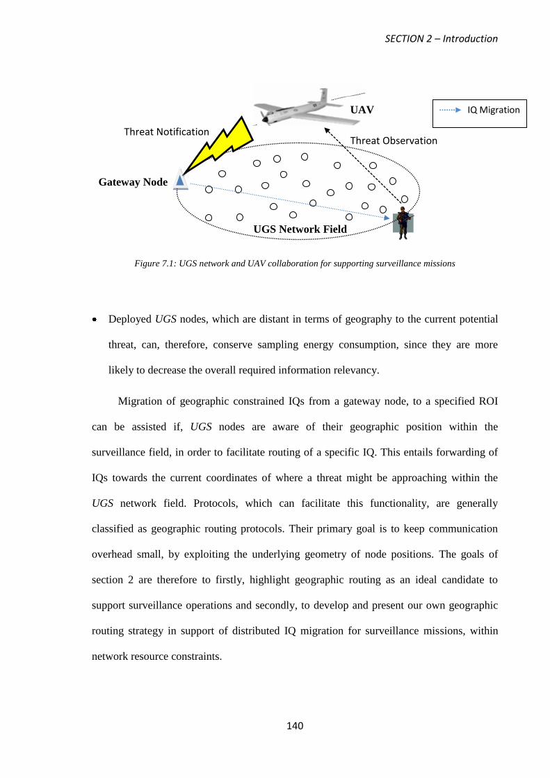
SECTION 2 – Introduction
140
Figure 7.1: UGS network and UAV collaboration for supporting surveillance missions
Deployed UGS nodes, which are distant in terms of geography to the current potential
threat, can, therefore, conserve sampling energy consumption, since they are more
likely to decrease the overall required information relevancy.
Migration of geographic constrained IQs from a gateway node, to a specified ROI
can be assisted if, UGS nodes are aware of their geographic position within the
surveillance field, in order to facilitate routing of a specific IQ. This entails forwarding of
IQs towards the current coordinates of where a threat might be approaching within the
UGS network field. Protocols, which can facilitate this functionality, are generally
classified as geographic routing protocols. Their primary goal is to keep communication
overhead small, by exploiting the underlying geometry of node positions. The goals of
section 2 are therefore to firstly, highlight geographic routing as an ideal candidate to
support surveillance operations and secondly, to develop and present our own geographic
routing strategy in support of distributed IQ migration for surveillance missions, within
network resource constraints.
Threat Observation Threat Notification
UAV
Gateway Node
UGS Network Field
IQ Migration

SECTION 2 – Introduction
141
In this section, chapter 7 begins by summarising both the nature of geographic
routing and the common packet forwarding strategies that can be used to support
geographic routing schemes. In 7.1.4, an initial discussion on using biological strategies
from the social insect’s domain and the advantages found, in terms of how they locate and
route to particular distant sources of interest, is given. Based on this initial discussion, in
7.1.5, a strategy is then outlined as to how some of these basic natural principles can be
transferred and implemented, to support a geographic routing surveillance scenario. In 7.2,
based on the discussion made in 7.1.4 and 7.1.5, a presentation of our own bio-inspired
geographic routing protocol to support IQ migration to an identified ROI, as shown in
figure 7.1, is highlighted. Performance results are provided for our bio-inspired geographic
routing protocol, in 7.3, with comparisons made against the techniques described in 7.1.1
to 7.1.3 and a well-known geographic routing protocol. Finally in chapter 8, we then
summarise and conclude our main contributions of this section.
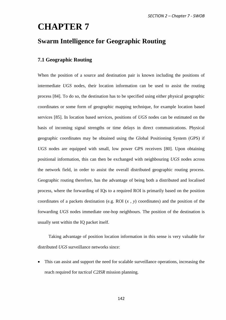
SECTION 2 – Chapter 7 - SWOB
142
CHAPTER 7
Swarm Intelligence for Geographic Routing
7.1 Geographic Routing
When the position of a source and destination pair is known including the positions of
intermediate UGS nodes, their location information can be used to assist the routing
process [84]. To do so, the destination has to be specified using either physical geographic
coordinates or some form of geographic mapping technique, for example location based
services [85]. In location based services, positions of UGS nodes can be estimated on the
basis of incoming signal strengths or time delays in direct communications. Physical
geographic coordinates may be obtained using the Global Positioning System (GPS) if
UGS nodes are equipped with small, low power GPS receivers [80]. Upon obtaining
positional information, this can then be exchanged with neighbouring UGS nodes across
the network field, in order to assist the overall distributed geographic routing process.
Geographic routing therefore, has the advantage of being both a distributed and localised
process, where the forwarding of IQs to a required ROI is primarily based on the position
coordinates of a packets destination (e.g. ROI (x , y) coordinates) and the position of the
forwarding UGS nodes immediate one-hop neighbours. The position of the destination is
usually sent within the IQ packet itself.
Taking advantage of position location information in this sense is very valuable for
distributed UGS surveillance networks since:
This can assist and support the need for scalable surveillance operations, increasing the
reach required for tactical C2ISR mission planning.

SECTION 2 – Chapter 7 - SWOB
143
The routing states required to be setup and maintained is a minimum (stateless),
reducing the communication routing overhead further.
Most importantly, IQ migration to a specified ROI can be made responsive to the
dynamics of a monitored threat [85]. This implies, if various ROIs need to be specified
in scenarios where multiple threats have been identified or to maintain continuous
monitoring of a threat as it traverses the UGS network field, this can be easily
supported, without the need for further exchange and maintenance of new routing state
information.
Routing tables are typically constructed as a list of direct forwarding neighbours associated
with a local UGS node, each with their respective 2-Dimensional (i.e. x, y) position
coordinates. These respective coordinates can then be used to make routing decisions as to
node selection for IQ forwarding in accordance with the geographic forwarding strategy in
operation. Operations to support geographic routing schemes are mainly segregated in
terms of how the next-hop is selected for packet forwarding. Typically, this can be
distinguished and classified as being greedy based, restricted directional flooding and
trajectory based forwarding, as described further in 7.1.1, 7.1.2 and 7.1.3.
7.1.1 Greedy Based Forwarding for Geographic Routing Schemes
In greedy based packet forwarding an UGS node may forward a packet to a one-hop
neighbour in a unicast manner, which is located closer to the destination than the
forwarding node itself. This implies that intermediate UGS nodes upon receiving a packet
(e.g. IQ) tend to forward to a neighbour lying in the general direction of the destination.
Ideally this process is repeated until the destination has been reached, as shown in figure
7.2. Greedy forwarding may entail the following possible strategies, for a source (S) and
destination (D) pair, within the sources maximum communication range r, as shown in
figure 7.2:

SECTION 2 – Chapter 7 - SWOB
144
The first intuitive strategy is to forward the packet to the node that makes most
progress towards D. As indicated in figure 7.2, this would be node C. This greedy
based strategy tries to minimise the number of hops a packet has to traverse, in order to
reach D, making it ideal for time-sensitive applications, such as surveillance missions.
The second strategy would be still to make forward progress towards D but also
minimise on the probability of packet collisions occurring within the neighbourhood of
S. This greedy based strategy therefore tries to increase the likelihood of successful
transmission and therefore the average progress a packet makes towards D. As
indicated in figure 7.2, this would be node A.
The third strategy is to select neighbours closest to the straight line between source and
destination, making selection closer in direction rather than closer in distance to D.
This greedy based strategy is classified as directional and tries to minimise on the
spatial distance a packet travels [86]. As indicated in figure 7.2, this would be node B,
since it has the minimum deviation, in terms of directional line angle α, from D.
Figure 7.2: Greedy based geographic forwarding strategies
Greedy based forwarding is very efficient in dense uniform networks, where it is
possible to make progress at each step [84]. Greedy forwarding, however, fails in the
presence of voids or dead-ends, which can occur in scenarios when less dense networks are
in operation. In this case, a dead-end node cannot find a one-hop neighbour closer to the
D S
A
B
C
r Directional Line to D
α

SECTION 2 – Chapter 7 - SWOB
145
destination and therefore a forwarding path to the intended destination, even though
alternative routing paths may exist. A possible remedy is to use limited flooding at the
dead-end node as a recovery strategy. Only nodes that are closer to the destination then
reply back, with the closest node to the destination among those nodes, being chosen to
forward the packet [87]. Alternatively a probabilistic approach, which picks a random
intermediate node and routes the packet through it to the destination, is suggested [88]. The
random intermediate node is picked randomly from an area between the source and
destination and is increased, each time the routing recovery strategy decision fails.
7.1.2 Restricted Directional Flooding for Geographic Routing Schemes
Alternatively, forwarding of data packets to a destination can be achieved by using a subset
of nodes that are located in an indicated region. Forwarding in this sense is referred to as
geo-casting [89-90]. A simple way to implement geo-casting is to base it on flooding but
also somehow restrict the area where packets are forwarded, in order to avoid flooding the
whole network. Positional information of deployed UGS nodes can assist this by placing a
geographical “forwarding zone”. Only nodes within the forwarding zone are allowed to
forward a received data packet, while nodes outside the forwarding zone discard the
packet. The forwarding zone can be defined in various ways as indicated in [89] and [91]:
Static Zone. This represents the smallest rectangle that contains both the source and the
entire destination region, with its sides parallel to the axes of the 2-dimensional
coordinate system, (x, y), as shown in figure 7.3 (a).
Adaptive Zone. Each forwarding node recalculates the forwarding zone definition,
using its own position as the source. This way, nodes that would be included in the
static zone but would represent a detour from the intended destination are excluded
from packet forwarding. This implies the adaptive zone is calculated in terms of
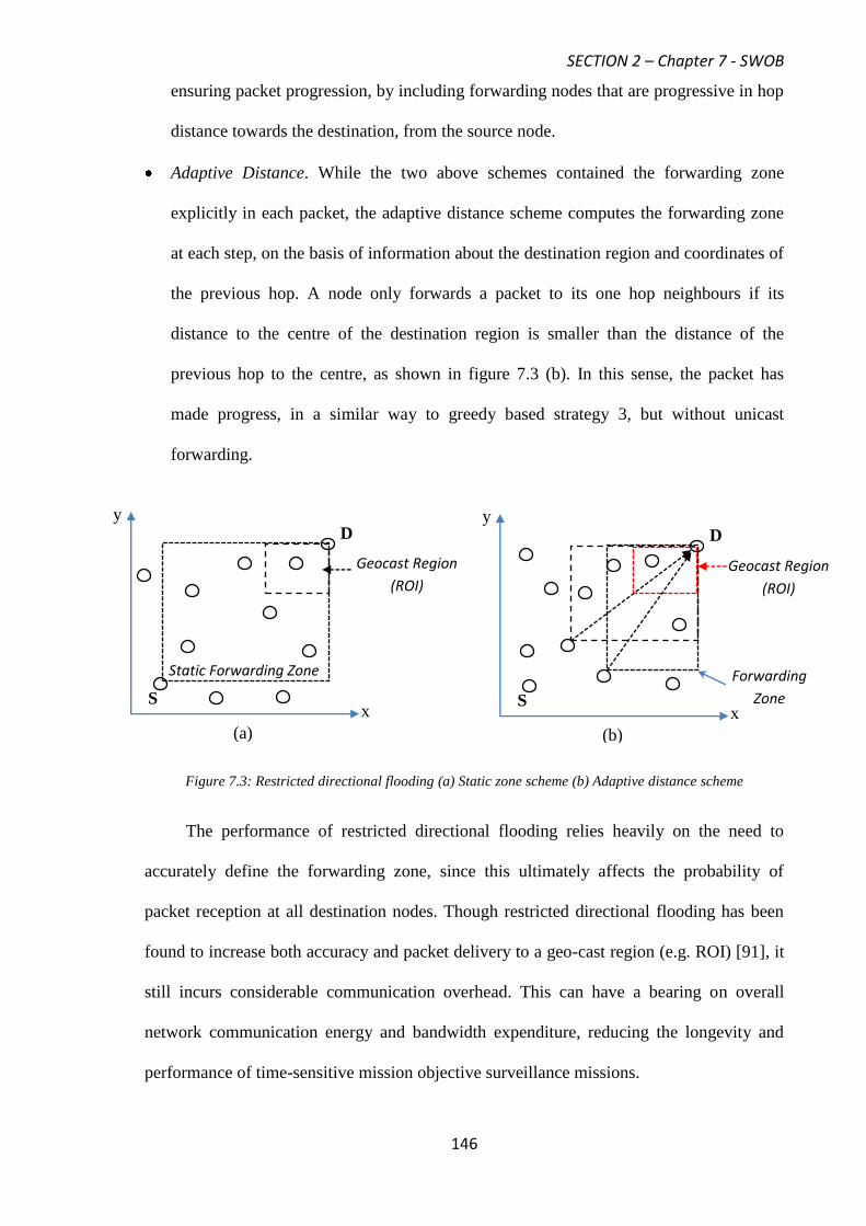
SECTION 2 – Chapter 7 - SWOB
146
ensuring packet progression, by including forwarding nodes that are progressive in hop
distance towards the destination, from the source node.
Adaptive Distance. While the two above schemes contained the forwarding zone
explicitly in each packet, the adaptive distance scheme computes the forwarding zone
at each step, on the basis of information about the destination region and coordinates of
the previous hop. A node only forwards a packet to its one hop neighbours if its
distance to the centre of the destination region is smaller than the distance of the
previous hop to the centre, as shown in figure 7.3 (b). In this sense, the packet has
made progress, in a similar way to greedy based strategy 3, but without unicast
forwarding.
Figure 7.3: Restricted directional flooding (a) Static zone scheme (b) Adaptive distance scheme
The performance of restricted directional flooding relies heavily on the need to
accurately define the forwarding zone, since this ultimately affects the probability of
packet reception at all destination nodes. Though restricted directional flooding has been
found to increase both accuracy and packet delivery to a geo-cast region (e.g. ROI) [91], it
still incurs considerable communication overhead. This can have a bearing on overall
network communication energy and bandwidth expenditure, reducing the longevity and
performance of time-sensitive mission objective surveillance missions.
S
D
x
y
Static Forwarding Zone
(a)
Geocast Region
(ROI)
S
D
x
y
Forwarding
Zone
(b)
Geocast Region
(ROI)
SECTION 2 – Chapter 7 - SWOB
147
7.1.3 Trajectory Based Forwarding for Geographic Routing Schemes
Trajectory based forwarding (TBF) is a hybrid technique combining source based routing
[91] and greedy based forwarding, but uses a continuous representation of the route.
Similar to source based routing, in TBF, the path is indicated by the source, but without
actually specifying all the intermediate nodes. Decisions taken at each node are greedy, as
highlighted in 7.1.1, but are not based on distance to the destination rather the measure is
based on the distance along a desired trajectory. Packets follow a trajectory established at
the source with each forwarding node making a decision to select a neighbour that is
geographically closest to the trajectory, which is indicated by the source. The trajectory
between a source-destination pair, can be specified in the packet header being forwarded
and can either be specified simply as a straight line, which reduces the packet forwarding
to strategy 3, as described in 7.1.1 or in terms of a function, in the form Y = f(X) describing
a curved trajectory line, as shown in (7.1) [92].
)ssin(r)X(fY max (7.1)
As shown in 7.1, the parameter s indicates, the direct incremental distance travelled
from the source towards the destination, while rmax being the set maximum UGS
transmission range, as shown in figure 7.4. The amplitude of the function Y= sin (s), can
therefore be varied, according to the maximum set UGS transmission range. Since,
choosing a next hop for packet forwarding should be towards the advancement on the
curved trajectory line towards the destination, only the portion of the curve with s being
greater than the x-coordinate of the forwarding node, should be considered. Several
policies of choosing a next hop are possible based on the trajectory in operation [92]. The
most common policy would be to consider nodes closest to the curve, with the minimum
residual (Δyr), since this would tend to produce a lower deviation from the ideal trajectory,
as shown in figure 7.4.
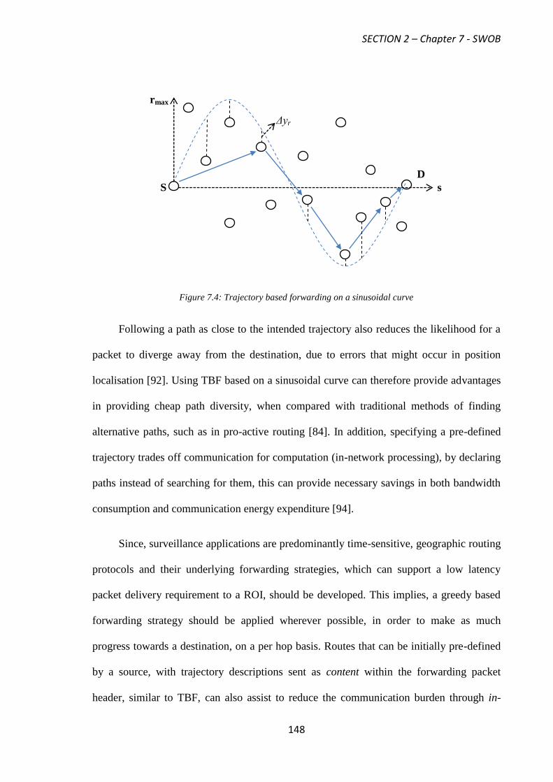
SECTION 2 – Chapter 7 - SWOB
148
Figure 7.4: Trajectory based forwarding on a sinusoidal curve
Following a path as close to the intended trajectory also reduces the likelihood for a
packet to diverge away from the destination, due to errors that might occur in position
localisation [92]. Using TBF based on a sinusoidal curve can therefore provide advantages
in providing cheap path diversity, when compared with traditional methods of finding
alternative paths, such as in pro-active routing [84]. In addition, specifying a pre-defined
trajectory trades off communication for computation (in-network processing), by declaring
paths instead of searching for them, this can provide necessary savings in both bandwidth
consumption and communication energy expenditure [94].
Since, surveillance applications are predominantly time-sensitive, geographic routing
protocols and their underlying forwarding strategies, which can support a low latency
packet delivery requirement to a ROI, should be developed. This implies, a greedy based
forwarding strategy should be applied wherever possible, in order to make as much
progress towards a destination, on a per hop basis. Routes that can be initially pre-defined
by a source, with trajectory descriptions sent as content within the forwarding packet
header, similar to TBF, can also assist to reduce the communication burden through in-
S
D
s
rmax
Δyr
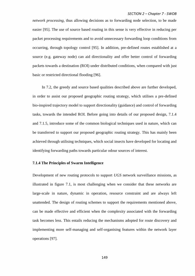
SECTION 2 – Chapter 7 - SWOB
149
network processing, thus allowing decisions as to forwarding node selection, to be made
easier [95]. The use of source based routing in this sense is very effective in reducing per
packet processing requirements and to avoid unnecessary forwarding loop conditions from
occurring, through topology control [95]. In addition, pre-defined routes established at a
source (e.g. gateway node) can aid directionality and offer better control of forwarding
packets towards a destination (ROI) under distributed conditions, when compared with just
basic or restricted directional flooding [96].
In 7.2, the greedy and source based qualities described above are further developed,
in order to assist our proposed geographic routing strategy, which utilises a pre-defined
bio-inspired trajectory model to support directionality (guidance) and control of forwarding
tasks, towards the intended ROI. Before going into details of our proposed design, 7.1.4
and 7.1.5, introduce some of the common biological techniques used in nature, which can
be transferred to support our proposed geographic routing strategy. This has mainly been
achieved through utilising techniques, which social insects have developed for locating and
identifying forwarding paths towards particular odour sources of interest.
7.1.4 The Principles of Swarm Intelligence
Development of new routing protocols to support UGS network surveillance missions, as
illustrated in figure 7.1, is most challenging when we consider that these networks are
large-scale in nature, dynamic in operation, resource constraint and are always left
unattended. The design of routing schemes to support the requirements mentioned above,
can be made effective and efficient when the complexity associated with the forwarding
task becomes less. This entails reducing the mechanisms adopted for route discovery and
implementing more self-managing and self-organising features within the network layer
operations [97].

SECTION 2 – Chapter 7 - SWOB
150
Until recently, existing investigations into developing self-managing features for
routing protocols in WSNs have begun to take inspiration from biological systems, as a
source of innovative network design [98]. The use of biological principles in network
design begins by observing the dynamics of natural systems, which have used established
laws, as a result of millions of years of evolution to govern them. Typically these laws that
govern particular biological functions or tasks are found to be surprisingly small in number
and generic. It is only through applying these simple generic rules that biological systems
or societies have been found to yield collaborative and effective patterns of complex
behaviour, for task coordination and resource management purposes. In addition,
application of these simple rules to network scenarios, can facilitate the necessary scalable
features required in surveillance missions, including efficient task allocation and inherent
resiliency to node failures, without the need for any external controlling entity [99].
Swarm Intelligence (SI) is a novel field that was originally defined as “Any attempt
to design algorithms or distributed problem-solving devices inspired by the collective
behaviour of social insect colonies and other animal societies” [100]. More recently, SI
generally refers to the study of collective behaviour of multi-component distributed
systems that coordinate their tasks, according to defined, de-centralised controls. The basic
rationale of SI for routing purposes lies in the observation that insect societies, as a
collective unit, do actually solve routing problems. Insects themselves need to discover and
establish paths that can be used by single insects, to effectively move back and forth from
the nest of the colony, to sources of food. Routing paths then emerge through synergistic
interactions among a large number of simple individual insects that concurrently sample
paths and inform others about their characteristics, using a variety of communication
schemes (e.g. pheromone-mediate communication in ants) [101]. In 7.1.5, the principles of
Swarm Intelligence are transferred to a geographic routing scenario to potentially support
surveillance operations, as shown in figure 7.1.

SECTION 2 – Chapter 7 - SWOB
151
7.1.5 Applying Swarm Intelligence to a Geographic Routing Scenario
It has been observed that ants tend to converge on the shortest among different paths
connecting their nest (source) and their food (destination) [99-100]. Ants tend to exhibit
shortest path behaviour, by following pheromone (volatile chemical) signals released in the
environment by their fellow colony members to invoke specific social responses and
coordination of tasks, known as stigmergy [100]. The general rule applied here, is that ants
tend to preferentially move towards areas of higher pheromone intensity, through olfactory
sensing [100], since this represents a higher order of relevance in finding a required,
designated food source [102]. These paths will then attract more ants, which in return will
increase the pheromone intensity, until there is a convergence of the majority of ants on to
the shortest path. Applying this SI principle to a geographic routing process inspired by ant
foraging behaviours as described above, seems to suggest ants use both an exploration
phase, where routes are discovered towards the destination and a set-up phase, to
communicate potential routes accordingly, between the source-destination pair.
In our intended scenario, the exploration phase however, can be avoided, since the
intended ROI destination coordinates are known to the gateway node, as shown in figure
7.1. In this sense, all that remains is a way to model and mimic UGS nodes, as potential
deposits of pheromone concentration made within the network field, in order to guide the
forwarding of IQs to the intended ROI, as shown in figure 7.5. Avoiding the exploration
phase also helps to minimise the transmission and use of control packets, which would
have been required to set-up pheromone concentration levels between the intended gate-
way node-destination pair. This can therefore provide benefits towards reducing both
network communication energy and bandwidth expenditure further. With the exploration
phase avoided, the scenario as illustrated in figure 7.5 then becomes simplified to one of
locating an odour source, through plume traversing techniques, based on pheromone
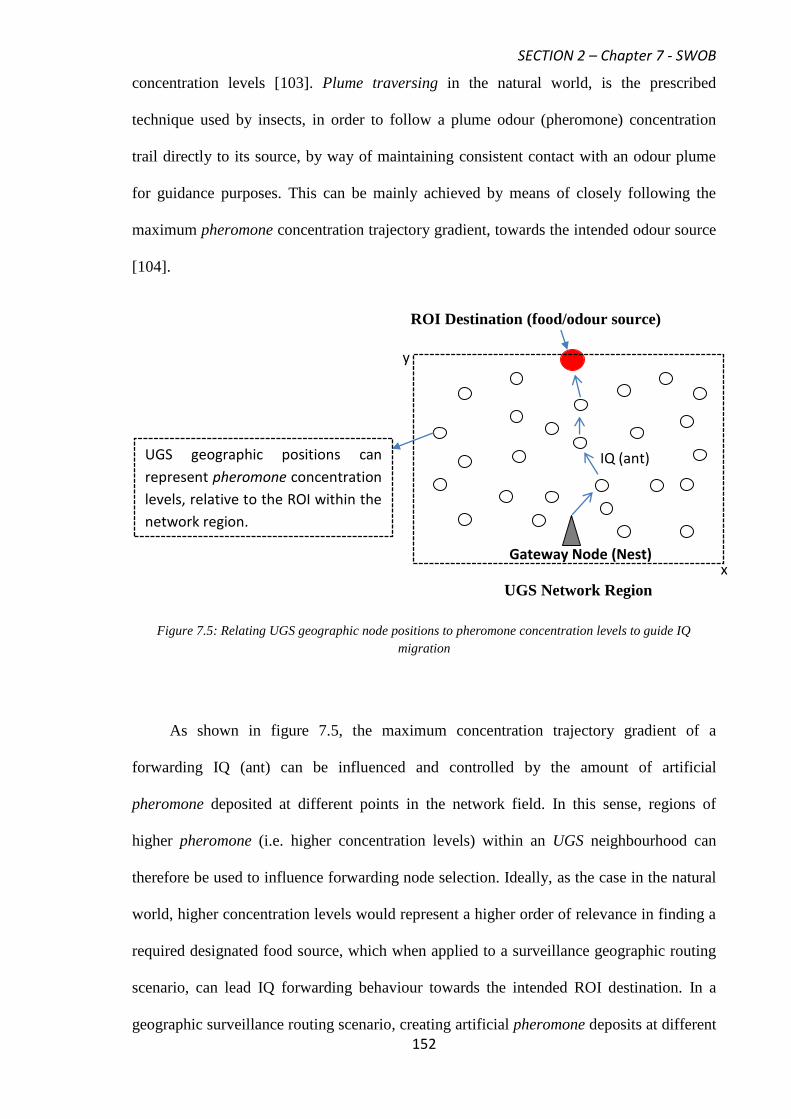
SECTION 2 – Chapter 7 - SWOB
152
concentration levels [103]. Plume traversing in the natural world, is the prescribed
technique used by insects, in order to follow a plume odour (pheromone) concentration
trail directly to its source, by way of maintaining consistent contact with an odour plume
for guidance purposes. This can be mainly achieved by means of closely following the
maximum pheromone concentration trajectory gradient, towards the intended odour source
[104].
Figure 7.5: Relating UGS geographic node positions to pheromone concentration levels to guide IQ
migration
As shown in figure 7.5, the maximum concentration trajectory gradient of a
forwarding IQ (ant) can be influenced and controlled by the amount of artificial
pheromone deposited at different points in the network field. In this sense, regions of
higher pheromone (i.e. higher concentration levels) within an UGS neighbourhood can
therefore be used to influence forwarding node selection. Ideally, as the case in the natural
world, higher concentration levels would represent a higher order of relevance in finding a
required designated food source, which when applied to a surveillance geographic routing
scenario, can lead IQ forwarding behaviour towards the intended ROI destination. In a
geographic surveillance routing scenario, creating artificial pheromone deposits at different
ROI Destination (food/odour source)
Gateway Node (Nest) x
y
UGS Network Region
UGS geographic positions can
represent pheromone concentration
levels, relative to the ROI within the
network region.
IQ (ant)

SECTION 2 – Chapter 7 - SWOB
153
points in the network field can be accordingly governed by considering, the relative
positions of deployed UGS nodes, to the designated destination (ROI/food source). To
achieve this aim, requires firstly a way of modelling the concentration dispersion effects
from an odour source (ROI), as found in nature, so that artificial pheromone concentration
levels can be mapped and established onto the UGS network region, to facilitate IQ
forwarding.
In 7.2 an odour plume model is introduced, in order to allow UGS node positions to
be geographically mapped with artificial pheromone concentrations. Subsequently, each
distributed UGS node can then become aware of their local concentration levels, relative to
the intended ROI. The ability to achieve this forms the basis towards formulating our own
proposed geographic routing strategy, utilising both greedy and source based techniques,
which were highlighted previously in 7.1.1 and 7.1.3.
7.2 Swarm Intelligent Odour Based Routing
In 7.2, our bio-inspired routing protocol namely, SWarm Intelligent Odour Based Routing
(SWOB), is described further. SWOB itself takes its inspiration from the basic principles
and examples provided by social insects in odour localisation and the methods they use for
route finding towards an intended odour source, through plume traversing. Locating
odours of interest is a twofold strategy. Firstly odours need to discovered and then
followed as to make positive progress towards the direction of the source. In 7.2.1, a model
is highlighted to mimic the odour dispersion effects of a discovered source, as a way of
establishing plume traversing and subsequently a shortest-path route towards an odour
source. A discovered odour source in our scenario, relates to the given coordinates of a
ROI, which can be identified through using airborne reconnaissance methods, as shown in
figure 7.1.

SECTION 2 – Chapter 7 - SWOB
154
7.2.1 Virtual Gaussian Odour Plume Model
In natural circumstances, the structures of odour concentration plumes are established by
the physics of atmospheric dispersion. Odour plumes are created when odour molecules
released from their source are taken away by environmental forces, for example, due to a
prevailing wind direction. In nature and the real world, the strength and length of a plume
is commonly dictated by the size of the odour source and general wind speed conditions
[104]. A common observation however to draw from this fact is that, odour plume
structures tend to naturally exhibit high levels of odour concentration at the source, but
with the average odour concentration levels falling away, if travelling further down-wind
from the origin of the source [104].
A common way to sufficiently portray this real-world odour diffusion characteristic
can be achieved through using a Gaussian function model. A Gaussian model of diffusion
is a widely used and accepted model to accurately portray the natural odour dispersion
phenomenon, for a wide range of atmospheric conditions [105]. Using a Gaussian model
assumes conservation of mass and a continuous odour emission effects from a source,
within steady state conditions [105]. In 7.2.1, a 2-Dimensional Gaussian function plume
model with ground level odour point source, is used to artificially construct odour and
pheromone concentration levels, given by C(x , y) , within the UGS network region, as
shown in (7.2) [105].
2y
20
2x
20
2
)yy(
2
)xx(
g eA)y,x(C
(7.2)
From (7.2), x and y denote the 2-Dimensional geographic position coordinates of a
deployed UGS node within the network region, x0 and y0 denote the designated centre
coordinates of the specified ROI, which behaves as the odour source, Ag represents the
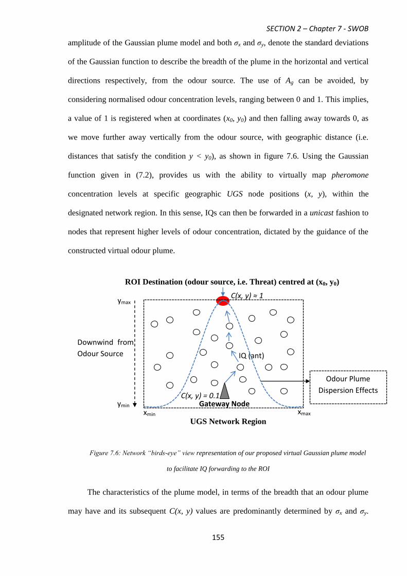
SECTION 2 – Chapter 7 - SWOB
155
amplitude of the Gaussian plume model and both σx and σy, denote the standard deviations
of the Gaussian function to describe the breadth of the plume in the horizontal and vertical
directions respectively, from the odour source. The use of Ag can be avoided, by
considering normalised odour concentration levels, ranging between 0 and 1. This implies,
a value of 1 is registered when at coordinates (x0, y0) and then falling away towards 0, as
we move further away vertically from the odour source, with geographic distance (i.e.
distances that satisfy the condition y < y0), as shown in figure 7.6. Using the Gaussian
function given in (7.2), provides us with the ability to virtually map pheromone
concentration levels at specific geographic UGS node positions (x, y), within the
designated network region. In this sense, IQs can then be forwarded in a unicast fashion to
nodes that represent higher levels of odour concentration, dictated by the guidance of the
constructed virtual odour plume.
Figure 7.6: Network “birds-eye” view representation of our proposed virtual Gaussian plume model
to facilitate IQ forwarding to the ROI
The characteristics of the plume model, in terms of the breadth that an odour plume
may have and its subsequent C(x, y) values are predominantly determined by σx and σy.
ROI Destination (odour source, i.e. Threat) centred at (x0, y0)
Gateway Node xmax
UGS Network Region
Odour Plume
Dispersion Effects
IQ (ant)
C(x, y) ≈ 1
C(x, y) = 0.1
Downwind from
Odour Source
xmin
ymin
ymax

SECTION 2 – Chapter 7 - SWOB
156
Calculating the required standard deviations, from (x0, y0) can be conducted in terms of
user defined, unit less concentration levels, given as α at the gateway node with
coordinates (xsink , ysink) and β at a communication transmission radius, RT, away from the
odour source, with condition β > α. The derived simultaneous equations relating α and β to
σx and σy are shown in (7.3) and (7.4).
2y
21
2x
2T
2
)X(
2
)R(
e
(7.3)
2y
2T
2x
2T
2
)R(
2
)R(
e
(7.4)
From (7.3), X1 = √[(x0 – xsink)2 + (y0 – ysink)
2] – RT, denoting the Euclidean distance up to
RT, from the odour source. As shown in (7.3), α is a derived expression, which relates C(x,
y) values to be found at a distance RT in the x direction and X1 in the y direction from the
gateway node. Dividing (7.3) by (7.4) provides us with a method of comparing the ratio of
artificial concentration values, at the gateway node and at a distance of RT from the odour
source, as shown in (7.5).
2y
2T
2y
21
2
)R(
2
)X(
e
e
(7.5)
Setting user defined values α and β accordingly, for example α = 0.1 and β = 0.9, σy
can be solved for a known RT, with designated ROI centre coordinates (x0, y0) and gateway
node coordinates (xsink , ysink). The solved σy value can then be substituted back into (7.3),
in order to obtain the required network value for σx.
Figure 7.7, shows the relationship for α / β ratio concentration values and subsequent
σx and σy values obtained through solving (7.5), for a 1km by 1km network region, with
odour source coordinates (x0, y0), reflecting the centre coordinates of an intended ROI,
being (500, 900) respectively, with α fixed at 0.1, (xsink , ysink) = (500, 100), and RT =
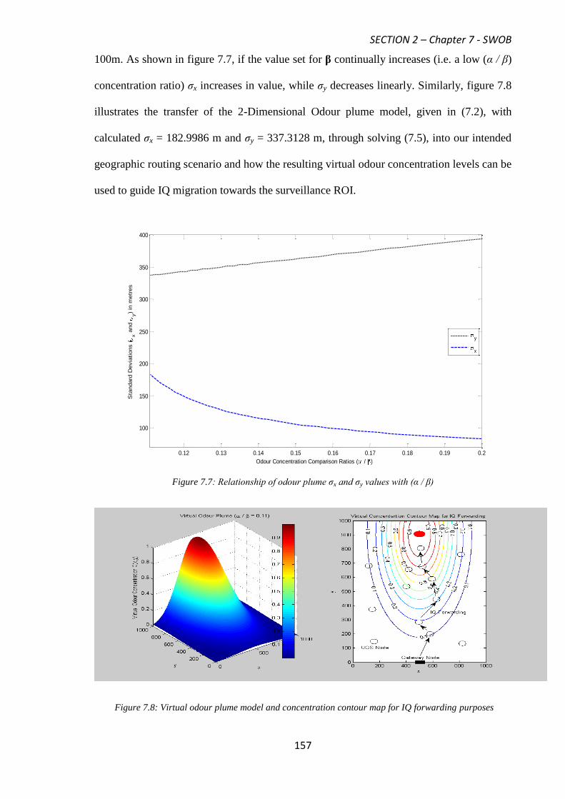
SECTION 2 – Chapter 7 - SWOB
157
100m. As shown in figure 7.7, if the value set for β continually increases (i.e. a low (α / β)
concentration ratio) σx increases in value, while σy decreases linearly. Similarly, figure 7.8
illustrates the transfer of the 2-Dimensional Odour plume model, given in (7.2), with
calculated σx = 182.9986 m and σy = 337.3128 m, through solving (7.5), into our intended
geographic routing scenario and how the resulting virtual odour concentration levels can be
used to guide IQ migration towards the surveillance ROI.
Figure 7.7: Relationship of odour plume σx and σy values with (α / β)
Figure 7.8: Virtual odour plume model and concentration contour map for IQ forwarding purposes
0.12 0.13 0.14 0.15 0.16 0.17 0.18 0.19 0.2
100
150
200
250
300
350
400
Odour Concentration Comparison Ratios ( / )
Sta
ndard
Devia
tions (
x a
nd
y)
in m
etr
es
y
x

SECTION 2 – Chapter 7 - SWOB
158
Figure 7.8, illustrates and reveals some potential benefits inherently achieved
through using a Gaussian type model, which can be used to provide support for UGS
network management. These potential advantages are as follows:
The virtual Gaussian plume model and resulting contour map reveals that not all
deployed UGS nodes will have designated C(x,y) values, relative to the ROI that can be
used for IQ forwading purposes. These nodes are typically found geographically
outside of the Gaussian plume shape and resulting contour map. This is a useful
observation to make since, realistically, these nodes will not take part in IQ forwarding,
which can assit in balancing overall network load and also additionally support the
notion of making bandwidth and communication energy consumption savings,
wherever possible.
Using a virtual Gaussian plume model allows forwarding and eventual IQ migration to
be controlled within the bounds of the plume, with the eventual aim of providing
guidance (plume traversing) to the designated region of interest, as shown by the
contour map.
These inherent characteristics, as detailed above, can be used to develop a
mechanism, which can restrict routing and subsequent IQ forwarding to particular areas
only, but without loosing the necessary guidance required towards the designated ROI.
Such a mechanism can provide an advantage as a means of integrating network topology
control functionality, within normal geographic routing. Utilising a topology control
implementation can also provide a far better way of defining the necessary σx or σy values
required for the Gaussian plume shape, since this can be directly related to the
characteristics of a current deployed network, rather than, them being based on user
defined values, as described earlier.
SECTION 2 – Chapter 7 - SWOB
159
Topology control in our proposed scheme, is essentially governed by the breadth a
Gaussian plume may have, through σx or σy and to vary these variables accordingly, in
order to reflect on the degree of control (restriction) required. A reliable way of achieving
and establishing a required plume breadth shape, is to formulate σx or σy , in terms of
ensuring that any deployed node, found within the Gaussian plume, will still have a certain
number of direct neighbours to communicate with. Formulating a topology control
mechanism in this manner is important since, it ensures nodes will not be prevented from
carrying out their normal IQ forwarding tasks, even in the presence of topology restriction.
To define such a topology control relationship, firstly requires a way of modelling
probabilistically the location of UGS nodes within the network region and secondly
relating this to a desired network connectivity, in order to ensure direct, restricted
communication, while also avoiding the condition for UGS node isolation, as explained
further in 7.2.2.
7.2.2 Swarm Intelligent Odour Based Network Topology Control
In densley deployed UGS networks (> 100 nodes), a single UGS node may have many
neighbouring nodes with which direct communication is possible depending on the
communication transmission radius, RT, being used. While dense networks can create the
necessary connectivity opportunities for UGS node communication it can, however, also
aggrevate node intereference. This primarily places a burden on the medium access
control, resulting in an increased number of retransmissions required to successfully
deliver a packet and limiting the ability of the deployed network to reuse wireless
bandwidth.
A potential way of overcoming some of the problems mentioned above, is to apply
some form of topology control. The idea here is to deliberatley restrict the set of UGS
nodes that are considered neighbours of a given node, therefore controlling a set of active
SECTION 2 – Chapter 7 - SWOB
160
links a node may have and subsequently it’s connectivity. Common ways of achieving
connectivity control would be to directly control transmission power, by turning off nodes
for certain periods of time (sleep-wakeup scheduling) or to implement hierarchy, in the
form of clustering, within the network [106]. An alternative way is to force the fact that
deployed nodes, to only communicate with k direct neighbours (connectivity) within a
certain geographic distance [107]. A network is set to be connected if for every pair of
nodes, a path exists between them. All nodes of a connected network can therefore
communicate with each other over one or multiple hops (links). Equivalently a network is
said to be k-connected (k = 1, 2, 3…n), if for each node pair there exists greater than k
mutually independent paths connecting them [28]. Applying this to our SWOB routing
scenario therefore requires a way of calculating the σx value, according to, the relationship
of being k-connected.
The relationship of being k-connected is best defined in terms of the probabilty of
being k-connected. Obtaining a probabilty expression, which defines a certain k-
connectivity firstly requires an ability to evaluate the average number of nodes to be found
within an UGS node’s RT. This implies a network toplogy representation and a random
node location model is essential as described further in headings 7.2.2.1 and 7.2.2.2 . In
7.2.2.3, an expression is then formulated and described , in order to calculate the required
standard deviation value in the x-direction, σxr, to ensure a desired k-connectivity for
toplogy control purposes, under different network node densities. In 7.2.2.4, a confirmation
as to the validity of our SWOB topology control mechanism is then given, in terms of
saturated throughput performance, using the IEEE 802.11b MAC protocol.
7.2.2.1 UGS Network Topology Representation
The topology of the underlying deployed UGS network can be represented as an
undirected geometric random graph [108-109], denoted by G (N, RT) at each time instant,

SECTION 2 – Chapter 7 - SWOB
161
in which a total of N nodes are independently, uniformly and randomly distributed in
metric space, with transmission range RT. A "graph" in this setting refers to a collection of
vertices or “nodes” and a collection of edges that connect pairs of vertices. The random
graph used is modelled as undirected, meaning that there is no distinction between the two
vertices associated with each edge and also to denote the fact that the edges of the graph do
not have any orientation, meaning all link connectivity relations on node pairs, are
symmetric in nature. An assumption is to also consider that the transmission range of a
random UGS node can be modelled as “Disk Graph” of radius RT [110]. In other words, the
topology can be represented as a random graph in which the link existence probability (PT)
between two nodes u and v is determined by their geometric distance, in a way that PT = 1
for || u – v || ≤ RT and PT = 0 otherwise. Here || u – v || represents the Euclidian distance
between u and v.
7.2.2.2 UGS Node Location Model
The modelling of the random geographic UGS node locations within a vast 2-Dimensional
region can be assisted if it is assumed, the locations are uniformly and independently
distributed within the region. Such an assumption is clearly viable in scenarios where a
priori knowledge of the network region is not available, due to the mode of deployment in
operation, for example, UGS’s being air-dropped into unfriendly environments [111].
Under this direct assumption, the location of UGS nodes can be modelled by utilising a
stationary 2-Dimensional Poisson Point Process (PPP) [112-113]. Denoting the node
density of the underlying PPP as λ, which represents the expected number of UGS’s to be
found per unit area and is calculated as (N / Total Network Area). The exact number of
UGS’s located in a network region with total area A m2, M (A), follows a Poisson
distribution of parameter λ×A, with i = 1, 2….,N, as shown in (7.6).
SECTION 2 – Chapter 7 - SWOB
162
!i
)A(e)i)A(M(P
iA
(7.6)
We denote the subset of the network region, with total area, A m2 , by ||A|| m
2. The
expected number of nodes (ENodes) therefore to be found in a region ||A|| is given, as shown
in (7.7).
||A||ENodes (7.7)
7.2.2.3 The Required Standard Deviation to Ensure k-Connectivity
In any topology control scheme, such as SWOB the existence of isolated nodes is an
undesirable characteristic, since in static scenarios isolated nodes cannot communicate any
information. If communication connectivity of UGS nodes is to be restricted through a
virtual Gaussian odour plume, by variation of the standard deviation, σxr, in the horizontal
x-direction from x0, we require finding the probability that each node has greater than k
neighbours, within x0 ± σxr. This requires us to formulate the following conditions, as
detailed below:
We denote ti (i =1, 2…, m) as the two dimensional (x, y) coordinates of N Poisson
Point distributed nodes, where m represents the number of deployed nodes.
For j = 2, 3…, m we denote tj – tj-1 by ∆i, which represents the Euclidian distance
between two random nodes of the network.
∆i is a measure of the nearest neighbour distance, which represents the distance of
a random node to its closest neighbouring node.
Taking into account the above conditions for a homogenous PPP in two dimensions, the
probability density function of ∆i is given, as shown in (7.8).
2)i(ie2)i(f (7.8)

SECTION 2 – Chapter 7 - SWOB
163
For a random node to be connected it must have a ∆i that is ≤ RT , as described earlier in
7.2.2.1 and therefore the probability that a random node has at least one neighbour and is
connected is given, as shown in (7.9).
T 2T
R
0i
R
T e1id)i(f)Ri(P (7.9)
Since we require a network in which none of the N deployed nodes are isolated and using
the statistical property that ∆i is mutually exclusive for each deployed node, the probability
that N nodes have ∆i lengths ≤ RT and therefore remain connected, denoted by PConnected(N),
is given as shown in (7.10).
NR
)N(Connected )e1(P2T (7.10)
As shown in (7.10), the expression relates to the connectivity for N nodes within a network
region of total area, A m2, as function of RT. The equation in (7.10) however, represents a
lower bound on what is required to achieve a connected network. To achieve robustness
for node or link outages we need to ensure that a random node is k-connected. This implies
that a random node should have greater than or equal to k neighbours. The probability that
a random node, assuming statistical independence, with transmission range RT, has greater
than or equal to k neighbours and therefore is k –connected within a network region with
total area A m2 is given, as shown in (7.11).
2TR
1k
0n
n2T e!n
)R(1
)NeighbourskAinNodeRandom(P)connectedkisAinNodeRandom(P
(7.11)
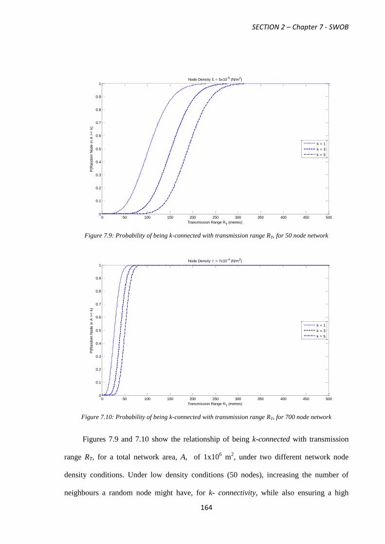
SECTION 2 – Chapter 7 - SWOB
164
Figure 7.9: Probability of being k-connected with transmission range RT, for 50 node network
Figure 7.10: Probability of being k-connected with transmission range RT, for 700 node network
Figures 7.9 and 7.10 show the relationship of being k-connected with transmission
range RT, for a total network area, A, of 1x10⁶ m
2, under two different network node
density conditions. Under low density conditions (50 nodes), increasing the number of
neighbours a random node might have, for k- connectivity, while also ensuring a high
0 50 100 150 200 250 300 350 400 450 5000
0.1
0.2
0.3
0.4
0.5
0.6
0.7
0.8
0.9
1Node Density = 5x10⁻⁵ (N/m2)
Transmission Range RT (metres)
P(R
andom
Node in A
>=
k)
k = 1
k = 3
k = 5
0 50 100 150 200 250 300 350 400 450 5000
0.1
0.2
0.3
0.4
0.5
0.6
0.7
0.8
0.9
1Node Density = 7x10⁻⁴ (N/m2)
Transmission Range RT (metres)
P(R
andom
Node in A
>=
k)
k = 1
k = 3
k = 5

SECTION 2 – Chapter 7 - SWOB
165
reliability, requires a node to have a large RT , approximatley 300m, as shown in figure 7.9.
Under high density conditions (700 nodes) as expected, the condition to increase k-
connectivity is reversed for RT. In all cases, increasing the condition for k-connectivity,
increases the required RT. This observation is common and in accordance with the “phase-
transition” phenomenon (i.e k-connectivity) in random geometric graph theory, which
states most standard properties of random graphs arise rather suddenly [108]. In figure 7.9
and 7.10, this “phase-transition” phenomenon is primarily due to an increasing RT.
If we are concerned with implementing k-connectivity, within a subset region, ||A||,
of total network area A m2, in order to ensure topology control, we need to satisfy that each
node found within ||A||, has greater than or equal to k neighbours and that any node found
in ||A|| continues to remain un-isolated, for the k neighbour requirement. The probability
expression that has potential to satisfy this need, is expressed and can be formulated, as
shown in (7.12).
2T
2T
Nodes Rk
0i
i2TR
1k
0n
n2T
E
0i
Ai
Nodes
xr
e!i
)R(1e
!n
)R(1e
!i
)A(1
)k||A||inNodeA(P)k||A||inNodeRandom(P)||A||inEFinding(P
||:A|| ty within,connectivi-kforncalculatioBoundMaximum
(7.12)
From (7.12), the probability expression to the left of the in-equality relates to
remaining k-connected for > ENodes and to the right, relating to a random node found in ||A||
is not k-isolated. The expression in (7.12), determines the approximate number of nodes
(ENodes) needed to cover a certain Gaussian plume area ||A||, in the x-direction, in order to
maintain a desired k-connectivity. This expression ultimately reflects and determines the
flexibility possible for network topology control, which is ascertained firstly by, the
expected number of neighbours (k) to be found in a node’s transmission neighbourhood
and secondly the probability of a random node in ||A|| as not being k-isolated. The

SECTION 2 – Chapter 7 - SWOB
166
probability expression in (7.12), is only true, when the probability of having k-connectivity
in ||A|| is less than or equal to a random node in ||A|| being k-isolated, which as a result
determines the required σxr maximum bound value, through ENodes, required to achieve this.
From (7.12), ENodes can be expressed as the expected number of nodes to be found in
||A||, as given in (7.7). Solving (7.12) therefore requires finding the sub-set area of the
network region, ||A||, in terms of the virtual Gaussian odour plume model. Since, topology
control is expressed through node k-connectivity, which is to be restricted within x0 ± σxr,
this can be formulated, according to a Gaussian function along the horizontal x-axis, as
shown in (7.13).
2AdxeA||A|| xrg
2
)xx(
g
2xr
20
(7.13)
The expression for calculating ||A|| given in (7.13) uses integral limits, which define
the network region as being infinite in length along the x-axis, for conditions that satisfy x0
– 4σxr > xmin and x0 + 4σxr < xmax, therefore ensuring the total Gaussian plume in the x-
direction is contained within the start, xmin and the end of the network region, xmax. The
definition of the condition described above for use in (7.13), is a measure concerning the
number of standard deviations, σxr, from the mean x0. As shown in (7.13), these conditions
have been derived as being plus or minus 4σxr, because this is a direct approximation, of
being 99.9% certain under normalised conditions that the complete Gaussian plume
function will be found within xmin and xmax.
In a realistic scenario however, the Gaussian plume function can be expected to
operate within a restricted network region, which does not usually satisfy the condition,
xmin > x0 ± 4σxr < xmax. If this is true, it cannot be guaranteed, therefore, to find an accurate
evaluation of all possible ENodes to be found within the Gaussian plume in the x-direction,
making the equation given in (7.13) invalid. In this case, it is required to find the difference

SECTION 2 – Chapter 7 - SWOB
167
in plume area restricted using σxr, to the total plume area, which is < xmin or > xmax,
according to the following given bounded network region conditions, as shown in (7.14)
and (7.15). The conditions used in (7.14) and (7.15) have been derived to reflect and
approximate the situation of not finding the total Gaussian odour plume contained within a
specific network region, dictated by the condition x0 ± 4σxr. As shown in (7.14) and (7.15)
the fraction of the total Gaussian plume area outside the network region is approximated
using the error function, denoted as erf (.).
)2/4
xx44(erf)2A(||A||
dxedxeA||A||
dxedxeA||A||
x)4x(if
xr
m ax0xrxrg
x4x
0x
2
)xx(
2
)xx(
g
x
2
)xx(
2
)xx(
g
m axxr0
maxxr 2xr
20
2xr
20
max
2xr
20
2xr
20
(7.14)
)2/4
xx44(erf)2A(||A||
dxedxeA||A||
dxedxeA||A||
x)4x(if
xr
m in0xrxrg
x
4xx
2
)xx(
2
)xx(
g
x2
)xx(
2
)xx(
g
m inxr0
min
xrmin
2xr
20
2xr
20
min 2xr
20
2xr
20
(7.15)

SECTION 2 – Chapter 7 - SWOB
168
In conditions, where the Gaussian odour plume can be found outside both xmin and xmax, it
is therefore required to find the combined fraction of the total area, which is < xmin and >
xmax and subtract this from the total plume area, as shown in (7.16).
)2/4
xx4
4
xx44(erf)2A(||A||
dxedxedxeA||A||
dxedxedxeA||A||
x)4x(&x)4x(if
xr
max0xr
xr
min0xrxrg
x4x
x
2
)xx(x
4xx
2
)xx(
2
)xx(
g
x
2
)xx(x
2
)xx(
2
)xx(
g
maxxr0minxr0
maxxr
max
2xr
20
min
xrmin
2xr
20
2xr
20
max
2xr
20
min 2xr
20
2xr
20
(7.16)
If the above conditions do not hold, then ||A|| can continued to be calculated in the same
manner, as detailed in (7.13). Evaluating the correct ||A|| expression to use, according to
the bounded network region conditions, allows the approximated ENodes value to be
calculated and substituted back into (7.12).
The inequality expression given in (7.12) can also be rearranged to show how the
Gaussian plume area, ||A||, can be increased or decreased by σxr ,through ENodes, in order to
reflect the ratio of being k-isolated and having k-connectivity, for a current underlying
deployed node density, as shown in (7.17).
2T
2T
Nodes
R1k
0n
n2T
Rk
0i
i2T
E
0i
Ai
e!n
)R(1
e!i
)R(1
e!i
)A(1
(7.17)
Following on from (7.17), the complete algorithm developed to solve this inequality,
which determines the required σxr value, to ensure nodes have a desired k-connectivity
within ||A||, is outlined further in Appendix B, part 1. For the network scenario shown in

SECTION 2 – Chapter 7 - SWOB
169
figure 7.8, described earlier in section 7.2.1, figure 7.11 shows how the relationship for
topology control through the required maximum bound σxr values, varies against network
node density, for various k-connectivity requirements.
As shown in figure 7.11, increasing the node density has the effect of decreasing the
required σxr value, for various k-connectivity requirements. Figure 7.11 also shows,
however, that by increasing the k-connectivity requirement it has the effect of increasing
σxr. This is expected since increasing the number of k-neighbours a node should have,
requires a larger plume search area to achieve this, but this is also dependent on node
density. For example, a 100 node network σxr increases by 13.5% for k ≥ 1 to k ≥ 5, while
for a 750 node network σxr increases by 6.2% for k ≥ 1 to k ≥ 5.
Figure 7.11: Relationship for topology control against network density, for various k-connectivity
The difference in percentage increases for these two node deployments is primarily
due to the fact that under higher node densities, the requirement for node k-connectivity
(topology control), primarily through the P (A Node in A is not k-isolated) → 1. As this
limit is approached and reached, a smaller plume coverage area can then be guaranteed for
a certain k-connectivity requirement, while also ensuring the condition for the inequality in
100 200 300 400 500 600 700
400
420
440
460
480
500
520
Transmission Range, RT = 100m, A = 1x10⁶ m2
Number of Deployed Network Nodes
Gaussia
n P
lum
e S
tandard
Devia
tion (
xr)
k >= 1
k >= 3
k >= 5
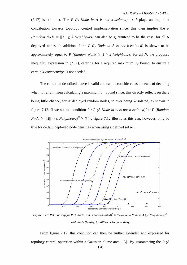
SECTION 2 – Chapter 7 - SWOB
170
(7.17) is still met. The P (A Node in A is not k-isolated) → 1 plays an important
contribution towards topology control implementation since, this then implies the P
(Random Node in ||A|| ≥ k Neighbours) can also be guaranteed to be the case, for all N
deployed nodes. In addition if the P (A Node in A is not k-isolated) is shown to be
approximately equal to P (Random Node in A ≥ k Neighbours) for all N, the proposed
inequality expression in (7.17), catering for a required maximum σxr bound, to ensure a
certain k-connectivity, is not needed.
The condition described above is valid and can be considered as a means of deciding
when to refrain from calculating a maximum σxr bound since, this directly reflects on there
being little chance, for N deployed random nodes, to ever being k-isolated, as shown in
figure 7.12. If we set the condition for P (A Node in A is not k-isolated)N ≈ P (Random
Node in ||A|| ≥ k Neighbours)N ≥ 0.99, figure 7.12 illustrates this can, however, only be
true for certain deployed node densities when using a defined set RT.
Figure 7.12: Relationship for P (A Node in A is not k-isolated)N ≈ P (Random Node in A ≥ k Neighbours)
N,
with Node Density, for different k-connectivity
From figure 7.12, this condition can then be further extended and expressed for
topology control operation within a Gaussian plume area, ||A||. By guaranteeing the P (A
0 100 200 300 400 500 600 700 8000
0.1
0.2
0.3
0.4
0.5
0.6
0.7
0.8
0.9
1
Transmission Range, RT =100 metres, A = 1x10⁶ m2
Number of Deployed Network Nodes (N)
(Pro
babili
ty o
f bein
g k
-connecte
d)N
P(Random Node in A >= 5 Neighbours)
P(Random Node in A >= 3 Neighbours)
P(Random Node in A >= 1 Neighbour)
P(k > 3)N ~ P(k >= 3)N >= 0.99
P(k > 5)N ~ P(k >= 5)N >= 0.99
P(k > 1)N ~ P(k >= 1)N >= 0.99
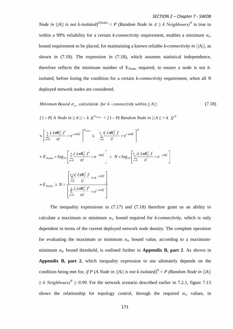
SECTION 2 – Chapter 7 - SWOB
171
Node in ||A|| is not k-isolated)ENodes
≈ P (Random Node in A ≥ k Neighbours)N is true to
within a 99% reliability for a certain k-connectivity requirement, enables a minimum σxr
bound requirement to be placed, for maintaining a known reliable k-connectivity in ||A||, as
shown in (7.18). The expression in (7.18), which assumes statistical independence,
therefore reflects the minimum number of ENodes required, to ensure a node is not k-
isolated, before losing the condition for a certain k-connectivity requirement, when all N
deployed network nodes are considered.
2T
2T
2T
2T
2T
Nodes
2T
Nodes
Rk
0n
n2T
R1k
0i
i2T
Nodes
R1k
0i
i2T
10R
k
0n
n2T
10Nodes
N
R1k
0i
i2T
E
Rk
0n
n2T
NE
xr
e!n
)R(
e!i
)R(
NE
e!i
)R(logNe
!n
)R(logE
e!i
)R(e
!n
)R(
)]k||A||inNodeRandom(P1[)]k||A||inNodeA(P1[
||:A|| ty within,connectivi-kforncalculatioBoundMinimum
(7.18)
The inequality expressions in (7.17) and (7.18) therefore grant us an ability to
calculate a maximum or minimum σxr bound required for k-connectivity, which is only
dependent in terms of the current deployed network node density. The complete operation
for evaluating the maximum or minimum σxr bound value, according to a maximum-
minimum σxr bound threshold, is outlined further in Appendix B, part 2. As shown in
Appendix B, part 2, which inequality expression to use ultimately depends on the
condition being met for, if P (A Node in ||A|| is not k-isolated)N ≈ P (Random Node in ||A||
≥ k Neighbours)N ≥ 0.99. For the network scenario described earlier in 7.2.1, figure 7.13
shows the relationship for topology control, through the required σxr values, in
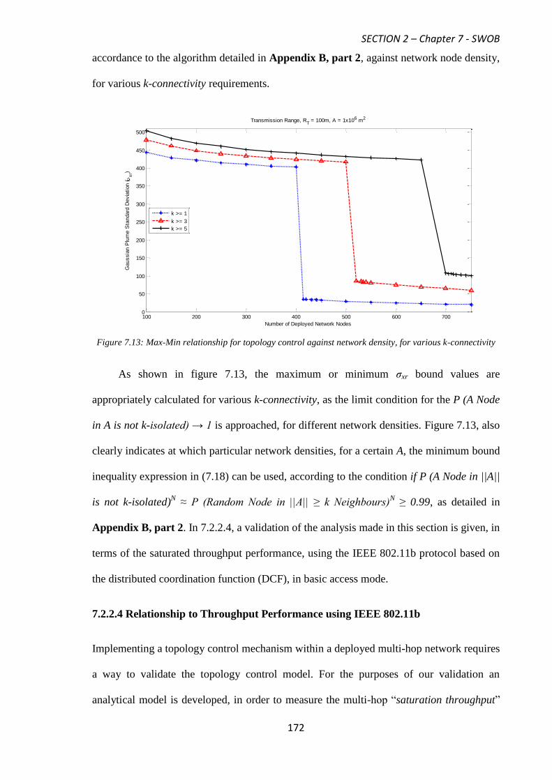
SECTION 2 – Chapter 7 - SWOB
172
accordance to the algorithm detailed in Appendix B, part 2, against network node density,
for various k-connectivity requirements.
Figure 7.13: Max-Min relationship for topology control against network density, for various k-connectivity
As shown in figure 7.13, the maximum or minimum σxr bound values are
appropriately calculated for various k-connectivity, as the limit condition for the P (A Node
in A is not k-isolated) → 1 is approached, for different network densities. Figure 7.13, also
clearly indicates at which particular network densities, for a certain A, the minimum bound
inequality expression in (7.18) can be used, according to the condition if P (A Node in ||A||
is not k-isolated)N ≈ P (Random Node in ||A|| ≥ k Neighbours)
N ≥ 0.99, as detailed in
Appendix B, part 2. In 7.2.2.4, a validation of the analysis made in this section is given, in
terms of the saturated throughput performance, using the IEEE 802.11b protocol based on
the distributed coordination function (DCF), in basic access mode.
7.2.2.4 Relationship to Throughput Performance using IEEE 802.11b
Implementing a topology control mechanism within a deployed multi-hop network requires
a way to validate the topology control model. For the purposes of our validation an
analytical model is developed, in order to measure the multi-hop “saturation throughput”
100 200 300 400 500 600 7000
50
100
150
200
250
300
350
400
450
500
Transmission Range, RT = 100m, A = 1x10⁶ m2
Number of Deployed Network Nodes
Gaussia
n P
lum
e S
tandard
Devia
tion (
xr)
k >= 1
k >= 3
k >= 5

SECTION 2 – Chapter 7 - SWOB
173
of the network, as the desired k-connectivity is increased for various network densities. The
author in [114] was the first to analyse and define the “saturation throughput”, S, as the
throughput limit reached by the system, as the offered load increases, thus representing the
maximum load that the system can carry in stable conditions. The correct S in our case
depends on using the correct expressions given in (7.13), (7.14), (7.15) or (7.16) and as
detailed in Appendix B, part 2. If this were not the case, then incorrect S values and loss
of accuracy in S will be apparent, when a direct comparison of the analytical and
simulation results is made.
From [114] a single-hop throughput model is developed for the IEEE 802.11b DCF
MAC protocol, assuming ideal channel conditions (i.e. no hidden terminals or capture
[115]) and that a node within a fixed deployed network, will always have a packet
available for transmission. The single-hop model from [114] is shown in (7.19), with PTR
being, the probability for a least one node transmission occurring and PS being, the
probability of a successful transmission given that one of the channel contending nodes
transmits. Table 7.1, details the various parameters used in (7.19) and in general for the
throughput, topology control validation exercise.
(7.19)
Within a multi-hop network setting, a node only contends with a fraction of the total nodes
in the network, namely NCont, which can then be substituted into (7.19). As shown in table
7.1, NCont is directly related to the number of ENodes found within the approximated
Gaussian plume area, ||A||, according to the conditions, as detailed in Appendix B, part 2.
TR
1NCont
SN
TR
CSTRTRSTRS
TRSHop1
P
)1(NPand)1(1P,With
T)P1(P)P1()TPP(
PP]P[E)N(S
Cont
Cont
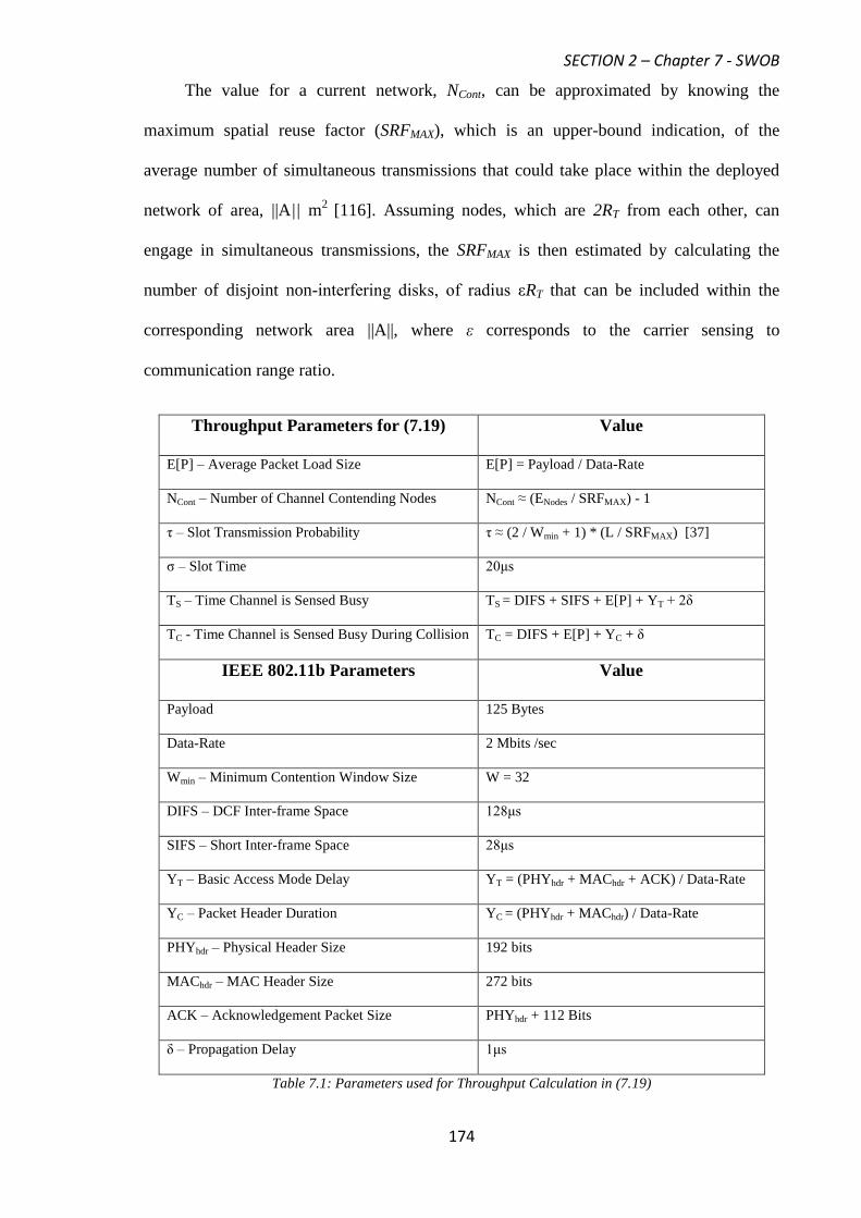
SECTION 2 – Chapter 7 - SWOB
174
The value for a current network, NCont, can be approximated by knowing the
maximum spatial reuse factor (SRFMAX), which is an upper-bound indication, of the
average number of simultaneous transmissions that could take place within the deployed
network of area, ||A|| m2
[116]. Assuming nodes, which are 2RT from each other, can
engage in simultaneous transmissions, the SRFMAX is then estimated by calculating the
number of disjoint non-interfering disks, of radius εRT that can be included within the
corresponding network area ||A||, where ε corresponds to the carrier sensing to
communication range ratio.
Throughput Parameters for (7.19) Value
E[P] – Average Packet Load Size E[P] = Payload / Data-Rate
NCont – Number of Channel Contending Nodes NCont ≈ (ENodes / SRFMAX) - 1
τ – Slot Transmission Probability τ ≈ (2 / Wmin + 1) * (L / SRFMAX) [37]
σ – Slot Time 20μs
TS – Time Channel is Sensed Busy TS = DIFS + SIFS + E[P] + YT + 2δ
TC - Time Channel is Sensed Busy During Collision TC = DIFS + E[P] + YC + δ
IEEE 802.11b Parameters Value
Payload 125 Bytes
Data-Rate 2 Mbits /sec
Wmin – Minimum Contention Window Size W = 32
DIFS – DCF Inter-frame Space 128μs
SIFS – Short Inter-frame Space 28μs
YT – Basic Access Mode Delay YT = (PHYhdr + MAChdr + ACK) / Data-Rate
YC – Packet Header Duration YC = (PHYhdr + MAChdr) / Data-Rate
PHYhdr – Physical Header Size 192 bits
MAChdr – MAC Header Size 272 bits
ACK – Acknowledgement Packet Size PHYhdr + 112 Bits
δ – Propagation Delay 1μs
Table 7.1: Parameters used for Throughput Calculation in (7.19)

SECTION 2 – Chapter 7 - SWOB
175
By setting a carrier sensing to communication range ratio of ε = 1 (i.e. carrier sensing
radius = RT), the SRFMAX can be approximated, for the maximum σxr bound given in (7.12),
as shown in (7.20).
2
T
Max)R(
||A||SRF
(7.20)
For the minimum σxr bound outlined in (7.18), the average number of simultaneous
transmissions that can occur increases, due to a lower Gaussian plume area, ||A||, thus
increasing the SRFMAX which can be approximated, as shown in (7.21).
2
T
Max)R(
||A||ASRF
(7.21)
To estimate the throughput of a multi-hop network also requires us finding the average
path length, L, in terms of the approximate number of hops that a packet has to traverse, in
order to reach its intended destination, as shown in (7.22).
]e!n
)R(1[)]e1(R[
)Neighboursk||A||inNodeRandom(P)i(d)i(fR)i(E,With
)i(E
)yy()xx(L
2T
2T
T
R1k
0n
n2TR
T
R
0iT
2ksin0
2ksin0
(7.22)
E (Δi), in (7.22) represents the average k-connectivity link distance between two random
PPP nodes, with f (Δi) as detailed in (7.8), representing the PDF between two random PPP
nodes. The one-hop saturated throughput model, as shown in (7.19), can then be used to
approximate the saturated throughput performance for a multi-hop network scenario, S,
within a network defined region ||A||, as shown in (7.23) [116].

SECTION 2 – Chapter 7 - SWOB
176
L
SRF)N(SS Max
Hop1 (7.23)
A simulation run was conducted to provide confirmation of the validity of our virtual
Gaussian topology control model, for the network scenario shown in figure 7.8, described
earlier in section 7.2.1. The simulation is run for a length of time for the network to
become saturated and in order for results to converge. Preliminary simulation results are
ignored when the network is in initial stages since these do not represent values under
saturated conditions.
Validity of our model can be confirmed by measuring S, achieved at the centre of the
ROI and comparing this with analytical results from our model, given in (7.23). For
confirmation of (7.23) to be accurate and to match closely with simulation results, it
requires use of the correct ENodes value. Figures 7.14 to 7.16, show results of the validation
exercise against network density, under various k-connectivity conditions, with RT set to
100m, within a network region of A = 1x10⁶ m
2.
From figures 7.14 to 7.16, the analytical results show a good match with our
simulation results to within an average loss in accuracy of 3.5% across the different
network densities, for each k-connectivity condition. The figures, however, also do confirm
that (7.23) is an appropriate relationship, which can be applied to approximate the multi-
hop saturated network throughput, S, performance, under different network densities, for
various SWOB topology control k-connectivity conditions.
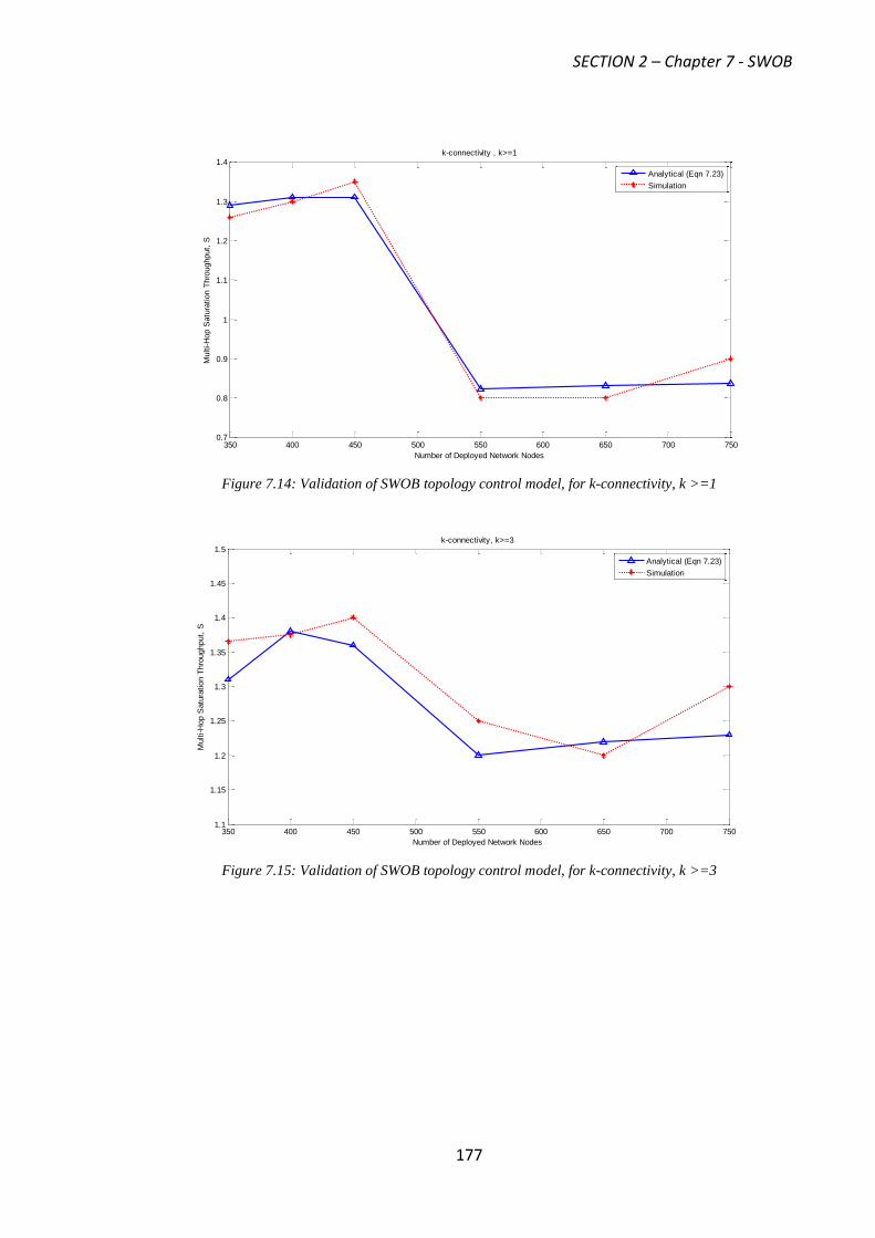
SECTION 2 – Chapter 7 - SWOB
177
Figure 7.14: Validation of SWOB topology control model, for k-connectivity, k >=1
Figure 7.15: Validation of SWOB topology control model, for k-connectivity, k >=3
350 400 450 500 550 600 650 700 7500.7
0.8
0.9
1
1.1
1.2
1.3
1.4k-connectivity , k>=1
Number of Deployed Network Nodes
Multi-H
op S
atu
ration T
hro
ughput,
S
Analytical (Eqn 7.23)
Simulation
350 400 450 500 550 600 650 700 7501.1
1.15
1.2
1.25
1.3
1.35
1.4
1.45
1.5k-connectivity, k>=3
Number of Deployed Network Nodes
Multi-H
op S
atu
ration T
hro
ughput,
S
Analytical (Eqn 7.23)
Simulation
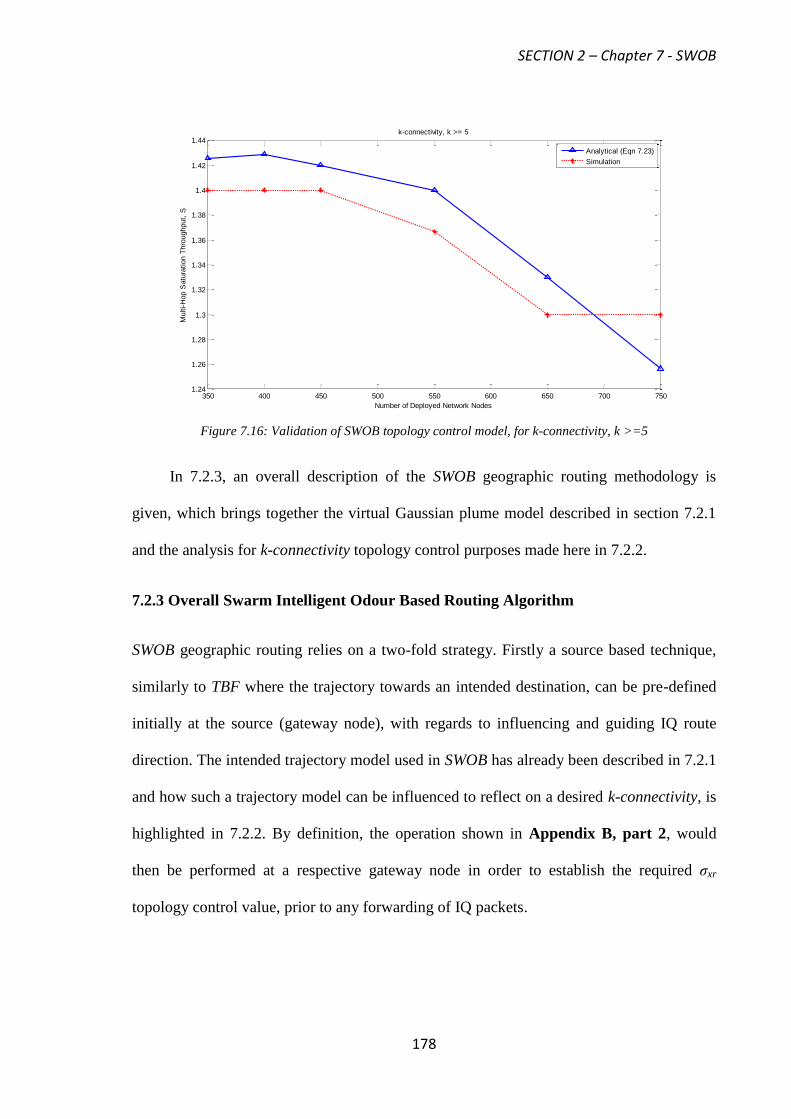
SECTION 2 – Chapter 7 - SWOB
178
Figure 7.16: Validation of SWOB topology control model, for k-connectivity, k >=5
In 7.2.3, an overall description of the SWOB geographic routing methodology is
given, which brings together the virtual Gaussian plume model described in section 7.2.1
and the analysis for k-connectivity topology control purposes made here in 7.2.2.
7.2.3 Overall Swarm Intelligent Odour Based Routing Algorithm
SWOB geographic routing relies on a two-fold strategy. Firstly a source based technique,
similarly to TBF where the trajectory towards an intended destination, can be pre-defined
initially at the source (gateway node), with regards to influencing and guiding IQ route
direction. The intended trajectory model used in SWOB has already been described in 7.2.1
and how such a trajectory model can be influenced to reflect on a desired k-connectivity, is
highlighted in 7.2.2. By definition, the operation shown in Appendix B, part 2, would
then be performed at a respective gateway node in order to establish the required σxr
topology control value, prior to any forwarding of IQ packets.
350 400 450 500 550 600 650 700 7501.24
1.26
1.28
1.3
1.32
1.34
1.36
1.38
1.4
1.42
1.44k-connectivity, k >= 5
Number of Deployed Network Nodes
Multi-H
op S
atu
ration T
hro
ughput,
S
Analytical (Eqn 7.23)
Simulation
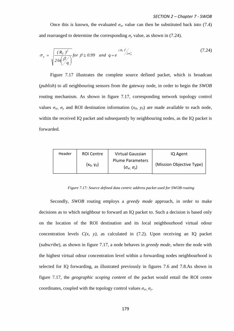
SECTION 2 – Chapter 7 - SWOB
179
Once this is known, the evaluated σxr value can then be substituted back into (7.4)
and rearranged to determine the corresponding σy value, as shown in (7.24).
2xr
2T
2
)R(2T
y eqand99.0for
qln2
)R(
(7.24)
Figure 7.17 illustrates the complete source defined packet, which is broadcast
(publish) to all neighbouring sensors from the gateway node, in order to begin the SWOB
routing mechanism. As shown in figure 7.17, corresponding network topology control
values σxr, σy and ROI destination information (x0, y0) are made available to each node,
within the received IQ packet and subsequently by neighbouring nodes, as the IQ packet is
forwarded.
Figure 7.17: Source defined data centric address packet used for SWOB routing
Secondly, SWOB routing employs a greedy mode approach, in order to make
decisions as to which neighbour to forward an IQ packet to. Such a decision is based only
on the location of the ROI destination and its local neighbourhood virtual odour
concentration levels C(x, y), as calculated in (7.2). Upon receiving an IQ packet
(subscribe), as shown in figure 7.17, a node behaves in greedy mode, where the node with
the highest virtual odour concentration level within a forwarding nodes neighbourhood is
selected for IQ forwarding, as illustrated previously in figures 7.6 and 7.8.As shown in
figure 7.17, the geographic scoping content of the packet would entail the ROI centre
coordinates, coupled with the topology control values σxr, σy.
ROI Centre
(x0, y0)
Virtual Gaussian
Plume Parameters
(σxr, σy)
Header IQ Agent
(Mission Objective Type)

SECTION 2 – Chapter 7 - SWOB
180
Using such an alternative can assist in further reductions in both the overall IQ
packet delivery time to the ROI, communication overhead and energy expenditure, since
nodes found to be outside the virtual Gaussian plume (i.e. outside the scope of the
geographic content message), will not take part in the SWOB routing process. The overall
SWOB geographic routing algorithm, which can be applied by any distributed UGS node to
determine next hop forwarding within the restricted x0 ± σxr virtual Gaussian plume, is
detailed further in Appendix B, part 3.
Relative (x, y) coordinates can be provided, if UGS nodes are equipped with small
low power GPS receivers, in order to discover their own absolute position within the
deployed network field. Such a mechanism is beneficial for surveillance operations since,
this will allow for network scalability and tactical reach, which are important attributes
needed for C2ISR providing type networks, such as UGS sensor networks [81] [84].
Relative (x, y) coordinates of neighbouring nodes, can therefore be exchanged initially
within the, RT neighbourhood and stored in a local table, in order to fulfil the SWOB
geographic routing algorithm detailed in Appendix B, part 3.
7.3 Swarm Intelligence Odour Based Routing Performance
SWOB geographic routing is primarily aimed at maintaining UGS network operational
longevity and supporting delay sensitive surveillance missions. IQ packets sent to inquire
and obtain information about a particular surveillance observation, should be transmitted
reliably with low latency and equally to have conservation of communication energy
consumption in mind. Our aim is therefore to achieve performance gains that can exhibit
both low latency and achieve high throughput, but with low communication energy
consumption. Conducting simulations to measure SWOB geographic routing performance
against these criteria, is therefore imperative. In addition, we are interested in measuring

SECTION 2 – Chapter 7 - SWOB
181
performance against increasing network node densities conditions, in order to gauge the
benefits of integrating topology control within geographic routing.
For the purpose of comparison, the following alternative geographic routing
strategies are considered, since these alternatives can also be easily applied to a geographic
surveillance scenario, as illustrated in figure 7.1:
Most forward progress (MFP) towards the destination, within RT, as already described
in 7.1.1, when considering the first strategy as shown, in figure 7.2.
Restricted directional flooding (RDF) using the adaptive distance scheme, as already
described in 7.1.2 and shown in figure 7.3 (b).
Trajectory Based Forwarding (TBF), which also employs topology control within
geographic routing, as already described in 7.1.3 and shown in figure 7.4.
Geographic random forwarding (GeRAF) [121-122]. GeRAF utilises geographical
routing on a best-effort basis, where the actual forwarding node is not known a-priori
by the sender, but rather is decided after the transmission has taken place. Forwarding
in this sense then relies on the broadcast nature of the wireless environment. This
allows multiple nodes to receive a packet and for each node being able to decide and
assess their own priority, as to acting as a forwarding node, in terms of how close they
are to the destination. In essence, GeRAF utilises a broadcast forwarding strategy, with
the MFP strategy used as the mechanism for deciding forwarding, node priority
selection. Nodes, which therefore receive packets, firstly calculate their respective
Euclidean distance to the destination (MFP) and compare this directly with their
neighbours, as a way of identifying whether they are the node closest towards the
destination (priority selection). If not, nodes drop their packets since an alternative
neighbour is identified as being the closest node in the RT neighbourhood. Prioritising
SECTION 2 – Chapter 7 - SWOB
182
selection in this manner can subsequently assist in providing further communication
energy and bandwidth consumption savings.
Simulations are performed using the OMNeT++ network modeller tool [63] for a
number of different network topologies (>50), each with N randomly deployed nodes
according to the PPP, within a network region area, A = 1x10⁶ m
2, with node RT = 100m
and using the IEEE 802.11b MAC protocol, under lossless channel conditions. Simulations
are run for a duration, which entails the gateway node sending a total of 100 packets, of
packet length, as shown in table 7.1. The same network gateway and ROI centre
coordinates are used, as described in 7.2.1. Headings 7.3.1 to 7.3.4 describe the various
metrics used, to measure and gauge performance of the SWOB geographic routing protocol
against the comparisons listed above.
7.3.1 Latency Performance
Latency is a QoS metric used within packet-switched networks and is typically measured
as the one-way delay time, from the source sending an initial packet, to the destination
receiving it [41]. In our evaluation, latency is therefore measured as the time between the
generation of an initial IQ packet at the gateway node and the delivery of that IQ packet to
the destination (centre of the ROI). Latency measured in this sense, becomes a direct
reflection on the delay sensitivity of the routing strategy employed since transporting the
initial IQ packet towards the destination with minimum time, is a key requirement, when
considering the nature of surveillance missions. Figure 7.18, shows SWOB latency
performance, with N, against the comparisons listed above.
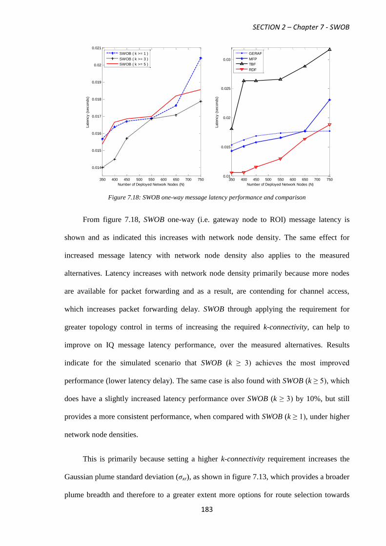
SECTION 2 – Chapter 7 - SWOB
183
Figure 7.18: SWOB one-way message latency performance and comparison
From figure 7.18, SWOB one-way (i.e. gateway node to ROI) message latency is
shown and as indicated this increases with network node density. The same effect for
increased message latency with network node density also applies to the measured
alternatives. Latency increases with network node density primarily because more nodes
are available for packet forwarding and as a result, are contending for channel access,
which increases packet forwarding delay. SWOB through applying the requirement for
greater topology control in terms of increasing the required k-connectivity, can help to
improve on IQ message latency performance, over the measured alternatives. Results
indicate for the simulated scenario that SWOB (k ≥ 3) achieves the most improved
performance (lower latency delay). The same case is also found with SWOB (k ≥ 5), which
does have a slightly increased latency performance over SWOB (k ≥ 3) by 10%, but still
provides a more consistent performance, when compared with SWOB (k ≥ 1), under higher
network node densities.
This is primarily because setting a higher k-connectivity requirement increases the
Gaussian plume standard deviation (σxr), as shown in figure 7.13, which provides a broader
plume breadth and therefore to a greater extent more options for route selection towards
350 400 450 500 550 600 650 700 750
0.014
0.015
0.016
0.017
0.018
0.019
0.02
0.021
Number of Deployed Network Nodes (N)
Late
ncy (
seconds)
350 400 450 500 550 600 650 700 7500.01
0.015
0.02
0.025
0.03
Number of Deployed Network Nodes (N)
Late
ncy (
seconds)
GERAF
MFP
TBF
RDF
SWOB ( k >= 1 )
SWOB ( k >= 3 )
SWOB ( k >= 5 )
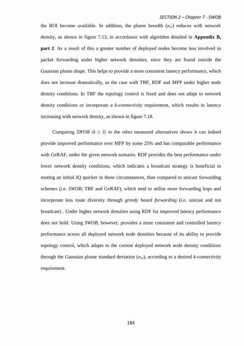
SECTION 2 – Chapter 7 - SWOB
184
the ROI become available. In addition, the plume breadth (σxr) reduces with network
density, as shown in figure 7.13, in accordance with algorithm detailed in Appendix B,
part 2. As a result of this a greater number of deployed nodes become less involved in
packet forwarding under higher network densities, since they are found outside the
Gaussian plume shape. This helps to provide a more consistent latency performance, which
does not increase dramatically, as the case with TBF, RDF and MFP under higher node
density conditions. In TBF the topology control is fixed and does not adapt to network
density conditions or incorporate a k-connectivity requirement, which results in latency
increasing with network density, as shown in figure 7.18.
Comparing SWOB (k ≥ 3) to the other measured alternatives shows it can indeed
provide improved performance over MFP by some 25% and has comparable performance
with GeRAF, under the given network scenario. RDF provides the best performance under
lower network density conditions, which indicates a broadcast strategy is beneficial in
routing an initial IQ quicker in these circumstances, than compared to unicast forwarding
schemes (i.e. SWOB, TBF and GeRAF), which tend to utilise more forwarding hops and
incorporate less route diversity through greedy based forwarding (i.e. unicast and not
broadcast) . Under higher network densities using RDF for improved latency performance
does not hold. Using SWOB, however, provides a more consistent and controlled latency
performance across all deployed network node densities because of its ability to provide
topology control, which adapts to the current deployed network node density conditions
through the Gaussian plume standard deviation (σxr), according to a desired k-connectivity
requirement.
SECTION 2 – Chapter 7 - SWOB
185
7.3.2 Throughput Performance
To measure overall network bandwidth utilisation efficiency during a simulation run it is
best to capture this, in terms of the number of packets (bits) that can be sent per second,
namely throughput. Measured in this way, throughput become a direct reflection on how
efficient the SWOB geographic routing methodology is as detailed in Appendix B, part 3,
and the comparison alternatives are towards utilising and re-using communication
bandwidth. Figure 7.19, shows SWOB throughput performance with N, against the
comparisons listed above, in the opening section.
Figure 7.19: SWOB throughput performance and comparison
From figure 7.19, SWOB throughput performance as shown increases with network
density. This is primarily due to the greater availability of deployed nodes to participate in
packet forwarding and subsequently, contribute to the overall network throughput. By
increasing the requirement for topology control, in terms of the required k-connectivity,
SWOB can again help to improve on throughput performance over TBF, which
incorporates topology control in terms of the sin function, but does not adapt the control
function according to the deployed network density conditions. Results indicate
incorporating a k-connectivity restriction for topology control purposes, can achieve
350 400 450 500 550 600 650 700 7502
3
4
5
6
7
8
9
Number of Deployed Network Nodes (N)
Thro
ughput
(kbits/s
econd)
350 400 450 500 550 600 650 700 750
2
3
4
5
6
7
8
9
Number of Deployed Network Nodes (N)
Thro
ughput
(kbits/s
econd)
SWOB (k >= 1)
SWOB (k >= 3)
SWOB (k >= 5)
GERAF
MFP
TBF
RDF
SECTION 2 – Chapter 7 - SWOB
186
improved throughput performance for the given network scenario. This is primarily
because setting a higher SWOB k-connectivity requirement varies the Gaussian plume
standard deviation (σxr), according to the min-max k-connectivity relationship, as detailed
in Appendix B, part 2 and as shown in figure 7.13.
As a result of this relationship SWOB, C(x, y), concentration values given in (7.2),
which dictate route selection (i.e. packet forwarding node selection) become more focused
with network density, as a result of a lower σxr value. This in turn provides better
geographic directivity for IQ routing to the ROI under higher network densities. As a
result, a lower σxr value under higher network density conditions can achieve higher
bandwidth utilisation, since a larger proportion of deployed nodes become less involved in
packet forwarding (i.e. more nodes lie outside the virtual Gaussian plume shape and do not
participate in packet forwarding) for improved throughput performance. Since throughput
forms a direct reflection on channel bandwidth utilisation efficiency, SWOB can
outperform the measured alternatives under higher network densities (N ≥ 600).
Advancing a packet as to minimise the number of hops a packet has to traverse, as
shown in MFP, does not promote bandwidth efficiency under a majority of network node
densities, hence it achieves lower throughput performance by some 60% when compared
with SWOB. Again broadcast strategies through GeRAF and RDF do not promote
bandwidth utilisation efficiency and as a result, achieve lower throughput. SWOB through
the use of its topology control mechanism can, as a result, provide greater flexibility
towards route selection and facilitate a better spatial bandwidth re-usability factor, under
higher network density conditions for improved throughput performance.

SECTION 2 – Chapter 7 - SWOB
187
7.3.3 Energy Efficiency Performance
Energy is a precious resource in UGS networks and so conserving on energy expenditure,
wherever possible becomes a priority. Energy efficiency is a way of measuring how well a
routing system can conserve on energy consumption, while still completing its packet
forwarding tasks. From a geographic routing perspective, energy efficiency would entail
putting the delivered network throughput, in bits and the communication energy
expenditure required to do so into perspective. Defined in this way, energy efficiency for
SWOB geographic routing performance is determined as the total network communication
energy consumed, to transport one packet of received payload information from the
gateway node to the destination (centre of ROI), as shown in (7.24). The same
communication energy consumption model is used, as already described in section 1, under
heading 4.4.3.
)bits(ceivedRePacketsNetworkTotal
)Joules(eExpenditurEnergyionCommunicatNetworkTotalEfficiencyEnergy
(7.24)
As shown in (7.24), routing schemes which promote lower energy expenditure in
order to transport more packets of a certain length in bits are ideal and therefore, more
energy efficient. Figure 7.20, shows SWOB energy efficiency performance with N, against
the comparisons described earlier in the opening of 7.3.
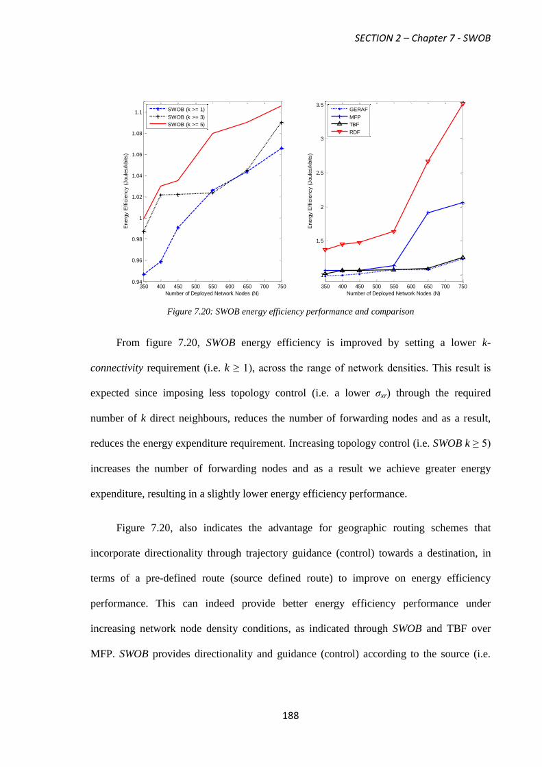
SECTION 2 – Chapter 7 - SWOB
188
Figure 7.20: SWOB energy efficiency performance and comparison
From figure 7.20, SWOB energy efficiency is improved by setting a lower k-
connectivity requirement (i.e. k ≥ 1), across the range of network densities. This result is
expected since imposing less topology control (i.e. a lower σxr) through the required
number of k direct neighbours, reduces the number of forwarding nodes and as a result,
reduces the energy expenditure requirement. Increasing topology control (i.e. SWOB k ≥ 5)
increases the number of forwarding nodes and as a result we achieve greater energy
expenditure, resulting in a slightly lower energy efficiency performance.
Figure 7.20, also indicates the advantage for geographic routing schemes that
incorporate directionality through trajectory guidance (control) towards a destination, in
terms of a pre-defined route (source defined route) to improve on energy efficiency
performance. This can indeed provide better energy efficiency performance under
increasing network node density conditions, as indicated through SWOB and TBF over
MFP. SWOB provides directionality and guidance (control) according to the source (i.e.
350 400 450 500 550 600 650 700 7500.94
0.96
0.98
1
1.02
1.04
1.06
1.08
1.1
Number of Deployed Network Nodes (N)
Energ
y E
ffic
iency (
Joule
s/k
bits)
350 400 450 500 550 600 650 700 750
1
1.5
2
2.5
3
3.5
Number of Deployed Network Nodes (N)
Energ
y E
ffic
iency (
Joule
s/k
bits)
GERAF
MFP
TBF
RDF
SWOB (k >= 1)
SWOB (k >= 3)
SWOB (k >= 5)

SECTION 2 – Chapter 7 - SWOB
189
gateway node) defined virtual Gaussian plume (i.e. σxr and σy), while TBF does the same
through the sin function given in (7.1).
In GeRAF directionality is assisted differently by increasing route diversity for
greedy based forwarding on a per hop basis, through broadcasting towards the destination.
Nodes, which therefore receive packets, firstly calculate their respective Euclidean distance
to the destination (ROI) and compare this directly with their neighbours, as a way of
identifying whether they are the node closest towards the destination (priority selection).
Nodes that do not meet this priority selection requirement subsequently drop packets. This
can assist in achieving a more consistent energy efficiency performance with increasing
network node density. MFP does not provide any means for a source defined route
capability within its routing operation and as a result, energy efficiency reduces with
network density by some 45% when compared with SWOB. This is also because nodes
over larger hop distances are primarily preferred, which can increase energy consumption.
Energy efficiency is also poor for RDF, which provides limited guidance through
restricting the number of forwarding nodes according to a static zone, as shown in figure
7.3 (a). In wide area surveillance scenarios the static forwarding zone can become large
and so the number of actively employed nodes used for packet forwarding, increases with
network density. Without using further guidance and topology control towards an intended
destination (i.e. ROI) within the static forwarding zone, every node found within the zone,
can become a potential packet forwarding node and as a result, expend energy. This
explains why energy efficiency reduces quite considerably for RDF, as network node
density conditions increase.
7.3.4 Network Load Balancing Performance
Maximising the lifetime of the deployed UGS network is also an important attribute, since
UGS devices are inherently limited by their battery energy reserves. Consumption of
SECTION 2 – Chapter 7 - SWOB
190
communication energy and the balancing of the load in terms of throughput, which is
placed on the network both become crucial and can assist in extending, the overall
operational longevity of the deployed UGS network field. Network load balancing from a
geographic routing perspective therefore encompasses being able to transport packets
efficiently, across the number of forwarding nodes required to do so. Defined in this sense,
network load balancing is a direct reflection on the energy efficiency from (7.24),
consumed across the total number of forwarding nodes used to deliver the packets, NForward,
which can only be determined by the routing strategy employed, as shown in (7.25).
ForwardN
)bits/Joules(EfficiencyEnergyBalancingLoadNetwork
(7.25)
From (7.25), a geographic routing scheme which can provide less communication
energy expenditure for transporting packets, while also maintaining a consistent NForward
set as the network density increases, can achieve better network load balancing
performance. Geographic routing schemes, which can therefore reduce (7.25) or provide a
more consistent level of network load balancing performance as network node density
conditions increase, can appropriately assist towards achieving greater operational
longevity. Figure 7.21, shows SWOB network load balancing performance with N, against
the comparisons listed above in the opening section.
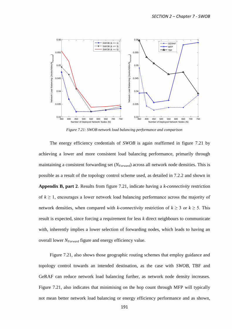
SECTION 2 – Chapter 7 - SWOB
191
Figure 7.21: SWOB network load balancing performance and comparison
The energy efficiency credentials of SWOB is again reaffirmed in figure 7.21 by
achieving a lower and more consistent load balancing performance, primarily through
maintaining a consistent forwarding set (NForward) across all network node densities. This is
possible as a result of the topology control scheme used, as detailed in 7.2.2 and shown in
Appendix B, part 2. Results from figure 7.21, indicate having a k-connectivity restriction
of k ≥ 1, encourages a lower network load balancing performance across the majority of
network densities, when compared with k-connectivity restriction of k ≥ 3 or k ≥ 5. This
result is expected, since forcing a requirement for less k direct neighbours to communicate
with, inherently implies a lower selection of forwarding nodes, which leads to having an
overall lower NForward figure and energy efficiency value.
Figure 7.21, also shows those geographic routing schemes that employ guidance and
topology control towards an intended destination, as the case with SWOB, TBF and
GeRAF can reduce network load balancing further, as network node density increases.
Figure 7.21, also indicates that minimising on the hop count through MFP will typically
not mean better network load balancing or energy efficiency performance and as shown,
350 400 450 500 550 600 650 700 7500.03
0.035
0.04
0.045
0.05
0.055
0.06
Number of Deployed Network Nodes (N)
Netw
ork
Load B
ala
ncin
g (
Joule
s/k
bits/N
Forw
ard
)
350 400 450 500 550 600 650 700 7500.03
0.035
0.04
0.045
0.05
0.055
0.06
Number of Deployed Network Nodes (N)
Netw
ork
Load B
ala
ncin
g (
Joule
s/k
bits/N
Forw
ard
)
SWOB (k >= 1)
SWOB (k >= 3)
SWOB (k >= 5)
GERAF
MFP
TBF

SECTION 2 – Chapter 7 - SWOB
192
this increases with network node density. The MFP strategy is designed to use fewer hops,
but with similar implications described earlier will require increased communication
energy expenditure, in order to cover the larger hop distances and as a result, an increased
forwarding set, NForward and lower energy efficiency value.
SECTION 2 – Chapter 8 – Summary and Conclusions
193
CHAPTER 8
Section 2: Summary and Conclusions
Distributed surveillance operations can be assisted if the relevant UGS’s are utilised, in
order to verify both threat observations and fulfil current mission objectives. As shown in
figure 7.1, this can be assisted through using UAV’s, which would typically survey a
surveillance region and then communicate potential threat coordinates to a gateway node.
Subsequently, a gateway node would generate the relevant information queries (IQs) to
verify this potential threat within an identified ROI, using the coordinates provided by the
UAV collaborator.
The basis of section 2 was to investigate strategies for allowing IQs to be routed to
the identified ROI, as shown in figure 7.1, from a gateway node located in the far region of
the surveillance field efficiently, within both communication energy and bandwidth
constraints. Routing protocols, which can facilitate this functionality, are generally
classified as geographic routing protocols, with their primary goal to keep communication
overhead small by exploiting the underlying geometry of node positions.
In chapter 7, we began by giving an explanation concerning both the nature of
geographic routing and the common packet forwarding strategies engaged to support
geographic routing. Geographic routing is an efficient technique, which requires minimal
direct use of routing tables, except for the location of the destination and local
neighbourhood UGS node positions, making it ideal for distributed surveillance operations.
In 7.1.4, a presentation of an alternative strategy with regards to forwarding of IQ
packets towards an identified ROI is given. In general, this section outlines the principles,
which social insect’s use to route towards particular sources of interest. Strategies derived
from the social insect natural world, can be broadly classified under the category called

SECTION 2 – Chapter 8 – Summary and Conclusions
194
“Swarm Intelligence” and in 7.1.5, we explained how such a strategy can be applied and
transferred to our intended surveillance scenario, as illustrated in figure 7.1.
The work presented in 7.2, forms the main contribution of this section, where we
apply some of the biological principles, described in 7.1.5, towards developing our own
biological inspired geographic routing strategy. Our geographic routing protocol named
SWOB utilises both source based techniques, which allows route discovery mechanisms to
be avoided and greedy based forwarding, in order to allow packets to make much
advancement towards the destination (low latency). Subsequently, a source defined
trajectory model based on the natural odour dispersion effects found in nature was
developed, providing the necessary guidance for IQ forwarding towards the ROI
destination. Our developed source-defined trajectory model contains the following
features:
A Gaussian function model is used to sufficiently portray the real-world odour
diffusion plume characteristics found in nature, as illustrated in figures 7.6 and 7.8. The
characteristics of the Gaussian function allow us a mechanism to artificially construct
odour concentration levels according to UGS node geographic position, relative to the
ROI, in order to facilitate IQ forwarding. As a result of this, the following potential
advantages can then be used:
- The virtual Gaussian plume model and resulting contour map reveals that not
all deployed UGS nodes are typically found geographically inside the Gaussian
plume shape and resulting contour map, as shown in figure 7.8.
- Subsequently, using a virtual Gaussian plume model allows forwarding and
eventual IQ routing to be controlled within the bounds of the plume shape.
Based on the notion of using a virtual Gaussian plume model to control and restrict
IQ forwarding within the deployed UGS network, in 7.2.2, we defined a topology control

SECTION 2 – Chapter 8 – Summary and Conclusions
195
relationship to reflect on the degree of control (restriction) required. A reliable way of
achieving and establishing control, is to vary the required Gaussian plume breadth shape
according to, a probabilistic relationship that ensures any deployed node found within the
Gaussian plume, can still have a certain number of k-direct neighbours to communicate
with. This requires a methodology involving the following attributes:
Firstly, a probabilistic model to describe the random location of UGS nodes found
within the network region, as described in 7.2.2.1 and 7.2.2.2.
Secondly, relating node location to a desired network k-connectivity, in order to ensure
direct restricted communication is possible, while also avoiding the condition for UGS
node isolation, as described in 7.2.2.3.
A validation of our virtual Gaussian plume topology mechanism is then given primarily
through, measuring the approximate saturated multi-hop throughput performance achieved,
using the IEEE 802.11b MAC protocol and a confirmation of this approximation, is shown
in figures 7.14 to 7.16. In 7.2.3, a complete description of SWOB routing algorithm is
given, including an explanation, as to the greedy based forwarding method employed
within SWOB routing.
In 7.3, we provide SWOB routing performance and gauge this against deployed
network node density. Alternative geographic forwarding strategies are also used for
SWOB comparison purposes. SWOB geographic routing is primarily aimed at supporting
delay sensitive surveillance missions. IQ packets sent to inquire and obtain information
about a particular surveillance observation, should be transmitted reliably with low latency
and equally to have conservation of communication energy consumption, in mind. Our aim
is therefore to achieve performance gains that can exhibit low latency, high throughput and
low communication energy consumption making it imperative to appraise SWOB
geographic routing performance, against these criteria. From the simulations conducted,
SECTION 2 – Chapter 8 – Summary and Conclusions
196
using the deployed network conditions described in 7.3, the following points can be made:
SWOB indicates that both network latency and throughput performance can be
improved by incorporating topology control within geographic routing functionality,
especially in conditions with increasing network node density. SWOB provides a more
consistent and controlled latency and throughput performance across all deployed
network node densities because of its ability to provide topology control, which adapts
to the current deployed network node density conditions through the Gaussian plume
standard deviation (σxr), according to a desired k-connectivity requirement. In TBF the
topology control is fixed and does not adapt to network density conditions or
incorporate a k-connectivity requirement, which results in latency increasing and a
lower throughput performance being achieved under higher network node density
conditions, as shown in figures 7.18 and 7.19.
Figure 7.21, shows those geographic routing schemes that employ directivity guidance
towards an intended destination (i.e. ROI), as shown with SWOB, TBF and GeRAF can
reduce network load balancing and increase energy efficiency performance further, as
network node density increases. For SWOB guidance is achieved through the Gaussian
plume function (i.e. σxr and σy). In TBF guidance is achieved in terms of the sin
function given in (7.1), while GeRAF provides guidance by allowing nodes to measure
their Euclidean distance towards an intended destination for priority selection, within a
broadcast transmission range of RT.
In summary, the results in figures 7.18 to 7.21 lead us to conclude that utilising a
Gaussian plume model to guide SWOB IQ forwarding, can therefore assist in providing the
following advantages:

SECTION 2 – Chapter 8 – Summary and Conclusions
197
A distributed and scalable surveillance mode of operation. Deployed UGS nodes need
only to know their geographic position and the ROI centre coordinates and apply the
SWOB routing methodology, as detailed in Appendix B, part 3.
Supporting the notion of maintaining bandwidth and communication energy
consumption savings, through an integrated geographic routing and topology control
approach.
It is also worth noting that the performance results for SWOB have also been conducted
under loss free channel conditions, which in reality is not the case from a wireless UGS
network point of view. In section 4, we do indeed consider SWOB performance under
different error prone channel environments. Before we can consider this, in section 3, we
aim first to analyse the error prone wireless channel environment, with view towards
assisting packet forwarding decisions and further go onto present our own decision making
mechanism, to provide reliable packet forwarding node selection under dynamic channel
conditions. In section 4, we investigate whether the findings in section 3, can help to
improve on fault-tolerant SWOB routing performance under a dynamic channel
environment setting.
SECTION 3 – Introduction
198
SECTION 3
Channel Aware Packet Forwarding
Introduction
UGS networks typically operate in wireless environments, which can vary considerably in
both space and time, due to multi-path propagation effects. Such propagation effects
determine the probability of successful packet reception, which, as a result, can influence
communication link reliability between node pairs and overall network throughput. Where
harsh conditions are prevalent, resulting in channel fading (received signal amplitude
fluctuations) or if protocols designed to mitigate these effects by periodically shutting
down their communication links, in order to conserve on energy are in operation, this
results in link disruption (intermittent connectivity) [123]. Subsequently, intermittent
connectivity due to the dynamic wireless transmission environment can create unreliable
paths to exist between nodes at any given point in time, resulting in network partitioning
and local topological changes to occur, as illustrated in figure 9.1.
The highly dynamic and loss nature of the wireless medium is a challenging problem
and becomes a key factor, in support of upper layer operations (i.e. application and
network layers), therefore influencing overall distributed networking performance.
Adapting well to the dynamic wireless environment where packet transmission failures can
occur frequently is imperative, in order to avoid excessive link-level packet
retransmissions and unnecessary consumption of network resources [124]. However,
selecting nodes to support packet forwarding of mission critical surveillance information
can be made robust, by allowing deployed UGS nodes to evaluate their local
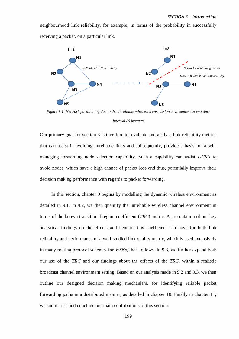
SECTION 3 – Introduction
199
neighbourhood link reliability, for example, in terms of the probability in successfully
receiving a packet, on a particular link.
Figure 9.1: Network partitioning due to the unreliable wireless transmission environment at two time
interval (t) instants
Our primary goal for section 3 is therefore to, evaluate and analyse link reliability metrics
that can assist in avoiding unreliable links and subsequently, provide a basis for a self-
managing forwarding node selection capability. Such a capability can assist UGS’s to
avoid nodes, which have a high chance of packet loss and thus, potentially improve their
decision making performance with regards to packet forwarding.
In this section, chapter 9 begins by modelling the dynamic wireless environment as
detailed in 9.1. In 9.2, we then quantify the unreliable wireless channel environment in
terms of the known transitional region coefficient (TRC) metric. A presentation of our key
analytical findings on the effects and benefits this coefficient can have for both link
reliability and performance of a well-studied link quality metric, which is used extensively
in many routing protocol schemes for WSNs, then follows. In 9.3, we further expand both
our use of the TRC and our findings about the effects of the TRC, within a realistic
broadcast channel environment setting. Based on our analysis made in 9.2 and 9.3, we then
outline our designed decision making mechanism, for identifying reliable packet
forwarding paths in a distributed manner, as detailed in chapter 10. Finally in chapter 11,
we summarise and conclude our main contributions of this section.
N3
N1
N2
N4
N5
t =1
Reliable Link Connectivity
N1
N2
N3 N4
N5
t =2
Network Partitioning due to
Loss in Reliable Link Connectivity

SECTION 3 – Chapter 9- Impact of the Wireless Channel Environment
200
CHAPTER 9
Impact of the Wireless Channel Environment
9.1 Modelling the Wireless Channel Environment
Understanding the impact that the wireless medium has on link reliability, stems from how
we can realistically model the channel environment, in a simulation setting. Due to the
complexity of real wireless channels, stochastic models are mostly used [125]. Signals
propagating in a wireless channel environment are commonly subject to a distance-
dependent loss of power (attenuation), path loss (PL), which is defined as the ratio in
decibel (dB) between the transmitted power (PTX) and received power (PRX) in Watts (W),
as shown in (9.1).
RX
TX10
P
Plog10)dB(PL
(9.1)
If the wireless channel propagation characteristics are not specified, it is usual to infer that
signal propagation takes place over an ideal free space environment, PLFree-Space, in dB
forming a line of sight (LOS) channel [126] and can be expressed, as shown in (9.2).
2
2
10)(
)4(log10)()(
l
SpaceFreeG
ddBdPL
(9.2)
In (9.2), Gl is the product of transmit and receive antenna field radiation patterns in the
LOS direction, d is the distance between the transmitter-receiver pair and λ is the
wavelength of the propagating signal.
The PL model of free space treats the wireless channel environment as being free of
all objects that might absorb, reflect and scatter transmission signal energy. However, in
realistic wireless environments, it is also well known that signal propagation includes
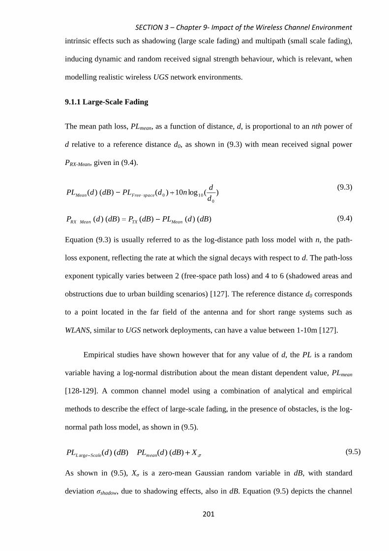
SECTION 3 – Chapter 9- Impact of the Wireless Channel Environment
201
intrinsic effects such as shadowing (large scale fading) and multipath (small scale fading),
inducing dynamic and random received signal strength behaviour, which is relevant, when
modelling realistic wireless UGS network environments.
9.1.1 Large-Scale Fading
The mean path loss, PLmean, as a function of distance, d, is proportional to an nth power of
d relative to a reference distance d0, as shown in (9.3) with mean received signal power
PRX-Mean, given in (9.4).
)(log10)()()(0
100d
dndPLdBdPL spaceFreeMean
(9.3)
)()()()()( dBdPLdBPdBdP MeanTXMeanRX
(9.4)
Equation (9.3) is usually referred to as the log-distance path loss model with n, the path-
loss exponent, reflecting the rate at which the signal decays with respect to d. The path-loss
exponent typically varies between 2 (free-space path loss) and 4 to 6 (shadowed areas and
obstructions due to urban building scenarios) [127]. The reference distance d0 corresponds
to a point located in the far field of the antenna and for short range systems such as
WLANS, similar to UGS network deployments, can have a value between 1-10m [127].
Empirical studies have shown however that for any value of d, the PL is a random
variable having a log-normal distribution about the mean distant dependent value, PLmean
[128-129]. A common channel model using a combination of analytical and empirical
methods to describe the effect of large-scale fading, in the presence of obstacles, is the log-
normal path loss model, as shown in (9.5).
XdBdPLdBdPL meanScaleeL )()()()(arg (9.5)
As shown in (9.5), Xσ is a zero-mean Gaussian random variable in dB, with standard
deviation σshadow, due to shadowing effects, also in dB. Equation (9.5) depicts the channel
SECTION 3 – Chapter 9- Impact of the Wireless Channel Environment
202
environment in which significant variations in d, or the movement beyond obstacles lead to
variations of the long-term mean signal strength at the receiver, referred to as “slow”
fading. In our simulation studies we model Xσ as a constant random variable over time for
a particular link. In large-scale fading, the received power, PRX-Large-Scale, is shown in (9.6).
)()()()()( argarg dBdPLdBPdBdP ScaleeLTXScaleeLRX (9.6)
9.1.2 Large-Small Scale Fading
In realistic channel propagation environments, a number of signal copies with
stochastically independent signal amplitudes of the same mean value can overlap at the
receiver. This implies, the received signal power will also show fading consisting of rapid
amplitude fluctuations (small-scale fading) around the mean signal level, superimposed on
relatively slow variations (large-scale fading) of the mean level. Rapid amplitude
fluctuations are mostly caused by local multipath propagation effects and it is well known
that the amplitude distribution of the received signal power can be approximated by a
Rayleigh distribution [130]. The Rayleigh PDF, used to model just small-scale fading
scenarios, is shown in (9.7).
02 2
)(xx
o
ex
xxP
(9.7)
As shown in (9.7), x is the amplitude of the received signal envelope and x0 the mean
received power. Incorporating the effects due to large scale-fading into the Rayleigh
distribution, the instantaneous power of the received signal, PRX-Large-Small-Scale, can be
approximated, as shown in (9.8) [130].
)(
argarg
1)()( MeanRXScaleeLRX PP
MeanRX
ScaleSmalleLRX eP
dBdP (9.8)
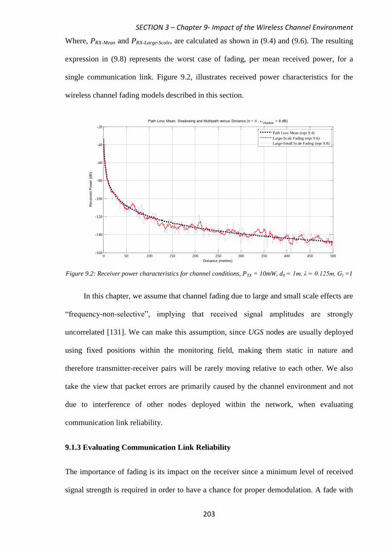
SECTION 3 – Chapter 9- Impact of the Wireless Channel Environment
203
Where, PRX-Mean and PRX-Large-Scale, are calculated as shown in (9.4) and (9.6). The resulting
expression in (9.8) represents the worst case of fading, per mean received power, for a
single communication link. Figure 9.2, illustrates received power characteristics for the
wireless channel fading models described in this section.
Figure 9.2: Receiver power characteristics for channel conditions, PTX = 10mW, d0 = 1m, λ = 0.125m, Gl =1
In this chapter, we assume that channel fading due to large and small scale effects are
“frequency-non-selective”, implying that received signal amplitudes are strongly
uncorrelated [131]. We can make this assumption, since UGS nodes are usually deployed
using fixed positions within the monitoring field, making them static in nature and
therefore transmitter-receiver pairs will be rarely moving relative to each other. We also
take the view that packet errors are primarily caused by the channel environment and not
due to interference of other nodes deployed within the network, when evaluating
communication link reliability.
9.1.3 Evaluating Communication Link Reliability
The importance of fading is its impact on the receiver since a minimum level of received
signal strength is required in order to have a chance for proper demodulation. A fade with
0 50 100 150 200 250 300 350 400 450 500-160
-140
-120
-100
-80
-60
-40
-20
Distance (metres)
Receiv
ed P
ow
er
(dB
)
Path Loss Mean, Shadowing and Multipath versus Distance (n = 4 , shadow
= 8 dB)
Path Loss Mean (eqn 9.4)
Large-Scale Fading (eqn 9.6)
Large-Small Scale Fading (eqn 9.8)
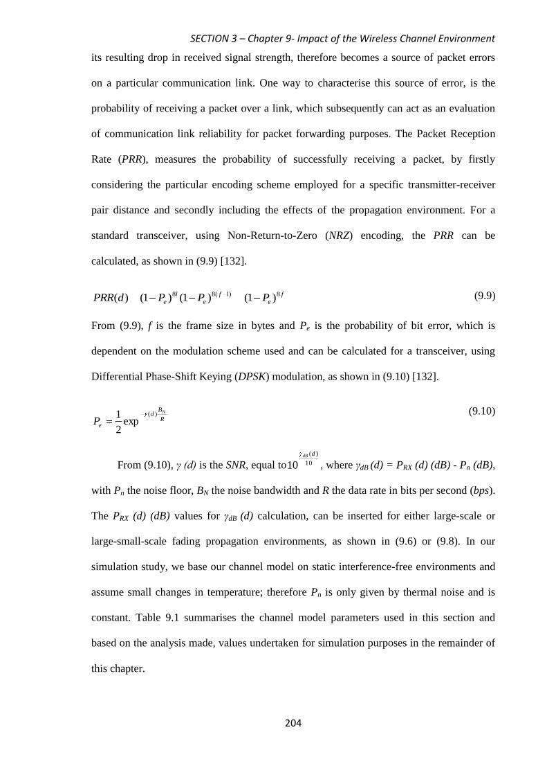
SECTION 3 – Chapter 9- Impact of the Wireless Channel Environment
204
its resulting drop in received signal strength, therefore becomes a source of packet errors
on a particular communication link. One way to characterise this source of error, is the
probability of receiving a packet over a link, which subsequently can act as an evaluation
of communication link reliability for packet forwarding purposes. The Packet Reception
Rate (PRR), measures the probability of successfully receiving a packet, by firstly
considering the particular encoding scheme employed for a specific transmitter-receiver
pair distance and secondly including the effects of the propagation environment. For a
standard transceiver, using Non-Return-to-Zero (NRZ) encoding, the PRR can be
calculated, as shown in (9.9) [132].
f
e
lf
e
l
e PPPdPRR 8)(88 )1()1()1()( (9.9)
From (9.9), f is the frame size in bytes and Pe is the probability of bit error, which is
dependent on the modulation scheme used and can be calculated for a transceiver, using
Differential Phase-Shift Keying (DPSK) modulation, as shown in (9.10) [132].
R
Bd
e
N
P)(
exp2
1
(9.10)
From (9.10), γ (d) is the SNR, equal to 10
)(
10
ddB
, where γdB (d) = PRX (d) (dB) - Pn (dB),
with Pn the noise floor, BN the noise bandwidth and R the data rate in bits per second (bps).
The PRX (d) (dB) values for γdB (d) calculation, can be inserted for either large-scale or
large-small-scale fading propagation environments, as shown in (9.6) or (9.8). In our
simulation study, we base our channel model on static interference-free environments and
assume small changes in temperature; therefore Pn is only given by thermal noise and is
constant. Table 9.1 summarises the channel model parameters used in this section and
based on the analysis made, values undertaken for simulation purposes in the remainder of
this chapter.
SECTION 3 – Chapter 9- Impact of the Wireless Channel Environment
205
Channel Model Parameter Value
λ, Propagating Signal 0.125m (frequency = 2.4 GHz)
PTX, Transmission Power 10mW
dmax, Node Transmission Range 500m
Gl, (eqn. 9.2) 1
d0 , reference distance (eqn. 9.3) 10m
Xσ ~ N(0, σshadow) (eqn. 9.5) σshadow = 2,4,6,8,10 dB
f, frame size (eqn. 9.9) 125 Bytes
Pn, noise floor (eqn. 9.10) -130dB
BN, Noise Bandwidth (eqn. 9.10) 20MHz [132]
R, Data Rate (eqn. 9.10) 2Mbps [132]
Medium Access Control (MAC) IEEE 802.11b
Table 9.1 Parameters used for communication link reliability performance evaluation
9.2 Impact of the Channel Environment on Link Reliability
Empirical studies have revealed the existence of three distinct reception regions in a
wireless link, these being connected, transitional and disconnected [133-134]. In the
connected region, links are often of good quality, stable and symmetric and the
disconnected region has no practical links for transmission. By contrast, the transitional
region is crucial to link reliability since it is characterised by high variance in PRR and
asymmetric connectivity, which grows with distance and is often quite significant in size,
as shown in figure 9.3. In 9.2.1, we begin to define the transitional region and quantify its
size in terms of a transitional region coefficient (TRC) metric, for different channel
environments.

SECTION 3 – Chapter 9- Impact of the Wireless Channel Environment
206
Figure 9.3: PRR characteristics demonstrating three distinct reception regions
9.2.1 Defining the Transitional Region
The extent of the transitional region can be quantified by specifying the desired level in
PRR, in order to insure high link reliability. This implies bounding the connected and
disconnected regions in terms of specific desirable SNR values, γdB. Defining high link
reliability to be with PRR > Ph, and low link reliability with PRR < Pl, the upper SNR
value, γ-Upper-dB, and lower SNR value, γ-Lower-dB, can be calculated using (9.10), as shown in
(9.11).
)))P1(2ln()BR((log10f81
hN10dBUpper (9.11)
)))P1(2ln()BR((log10f81
lN10dBLower
Figure 9.4, shows a PRR curve, with various Ph and Pl values and the impact which this
has on the transitional region. Figure 9.4, illustrates by reducing Pl for the disconnected
region and increasing Ph for the connected region, can have the effect of increasing the
0 50 100 150 200 250 300 350 400 450 5000
0.1
0.2
0.3
0.4
0.5
0.6
0.7
0.8
0.9
1
Transmitter-Receiver Pair Distance (metres)
PR
R
Packet Reception Rate (PRR) versus Distance
Connected
Region
Transitional Region Disconnected
Region
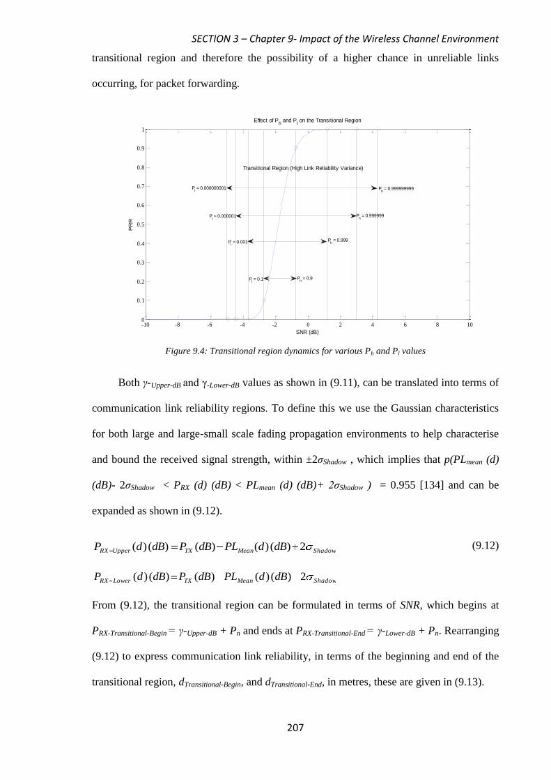
SECTION 3 – Chapter 9- Impact of the Wireless Channel Environment
207
transitional region and therefore the possibility of a higher chance in unreliable links
occurring, for packet forwarding.
Figure 9.4: Transitional region dynamics for various Ph and Pl values
Both γ-Upper-dB and γ-Lower-dB values as shown in (9.11), can be translated into terms of
communication link reliability regions. To define this we use the Gaussian characteristics
for both large and large-small scale fading propagation environments to help characterise
and bound the received signal strength, within ±2σShadow , which implies that p(PLmean (d)
(dB)- 2σShadow < PRX (d) (dB) < PLmean (d) (dB)+ 2σShadow ) = 0.955 [134] and can be
expanded as shown in (9.12).
ShadowMeanTXUpperRX dBdPLdBPdBdP 2)()()()()( (9.12)
ShadowMeanTXLowerRX dBdPLdBPdBdP 2)()()()()(
From (9.12), the transitional region can be formulated in terms of SNR, which begins at
PRX-Transitional-Begin = γ-Upper-dB + Pn and ends at PRX-Transitional-End = γ-Lower-dB + Pn. Rearranging
(9.12) to express communication link reliability, in terms of the beginning and end of the
transitional region, dTransitional-Begin, and dTransitional-End, in metres, these are given in (9.13).
-10 -8 -6 -4 -2 0 2 4 6 8 100
0.1
0.2
0.3
0.4
0.5
0.6
0.7
0.8
0.9
1
SNR (dB)
PR
R
Effect of Ph and P
l on the Transitional Region
Ph = 0.999999
Ph = 0.999
Transitional Region (High Link Reliability Variance)
Pl = 0.000000001
Pl = 0.000001
Pl = 0.001
Pl = 0.1 P
h = 0.9
Ph = 0.999999999

SECTION 3 – Chapter 9- Impact of the Wireless Channel Environment
208
n
dPLPP
BeginalTransition
ShadowSpaceFreeTXdBUppern
d 10
2)( 0
10 (9.13)
n
dPLPP
EndalTransition
ShadowSpaceFreeTXdBLowern
d 10
2)( 0
10
The impact of the channel environment on the transitional region is neatly described
through (9.13) and figure 9.5. As shown in figure 9.5, increasing σShadow has the effect of
increasing the transitional region, while increasing the path loss exponent n, due to faster
decay of received signal strength, has the effect of reducing it. From figure 9.5, channel
conditions with a high path loss exponent n, and low σShadow, therefore reduce size of the
transitional region. A ratio, which brings together dTransitional-Begin and dTransitional-End, in order
to describe the relative size of the transitional region, can be derived in terms of the
Transitional Region Coefficient (TRC), as shown in (9.14) [134-135].
1)10(d
ddTRC n10
4)(
BeginalTransition
BeginalTransitionEndalTransitionShadowdB_LowerdBUpper
(9.14)
As shown in (9.14), TRC represents a value of merit in link reliability giving an indication
of the extent of the transitional region to connected region parts of a network, which are
independent of Pn and PTX. According to (9.14), achieving a lower TRC is therefore better,
since this implies a larger connected region compared to a transitional one.
However, as detailed in 9.2.2, increasing the size of the transitional region (higher
TRC) for a fixed PRR curve can help to achieve an improved optimal link forwarding
distance, for a defined path loss exponent n and σShadow channel environment. Evaluating
the optimal link forwarding distance with respect to the transitional region is important
since, this enables us to establish how link reliability might behave within an unreliable
channel environment, across a range of potential communication link distances present
within a deployed network. In addition, knowing how the optimal link forwarding distance
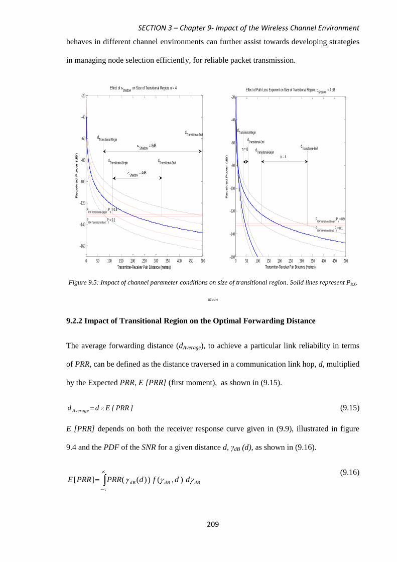
SECTION 3 – Chapter 9- Impact of the Wireless Channel Environment
209
behaves in different channel environments can further assist towards developing strategies
in managing node selection efficiently, for reliable packet transmission.
Figure 9.5: Impact of channel parameter conditions on size of transitional region. Solid lines represent PRX-
Mean
9.2.2 Impact of Transitional Region on the Optimal Forwarding Distance
The average forwarding distance (dAverage), to achieve a particular link reliability in terms
of PRR, can be defined as the distance traversed in a communication link hop, d, multiplied
by the Expected PRR, E [PRR] (first moment), as shown in (9.15).
]PRR[Edd Average (9.15)
E [PRR] depends on both the receiver response curve given in (9.9), illustrated in figure
9.4 and the PDF of the SNR for a given distance d, γdB (d), as shown in (9.16).
dBdBdB ddfdPRRPRRE ),())((][ (9.16)
0 50 100 150 200 250 300 350 400 450 500
-160
-140
-120
-100
-80
-60
-40
-20
Effect of Shadow
on Size of Transitional Region, n = 4
Transmitter-Receiver Pair Distance (metres)
Receiv
ed P
ow
er (dB
)
Shadow = 8dB
Shadow = 4dB
PRX-Transitional-Begin
, Ph = 0.9
PRX-Transitional-End
, Pl = 0.1
dTransitional-Begin
dTransitional-End
dTransitional-Begin
dTransitional-End
0 50 100 150 200 250 300 350 400 450 500-160
-140
-120
-100
-80
-60
-40
-20
Effect of Path Loss Exponent on Size of Transitional Region, Shadow
= 4 dB
Transmitter-Receiver Pair Distance (metres)
Receiv
ed P
ow
er (dB
) n = 4
PRX-Transitional-Begin
, Ph = 0.9
PRX-Transitional-End
, Pl = 0.1
dTransitional-End
dTransitional-Begin
dTransitional-Begin
dTransitional-End
n = 8

SECTION 3 – Chapter 9- Impact of the Wireless Channel Environment
210
As shown in (9.16), f (γdB, d) represents the SNR PDF, which is given by SNR ~ N
(γdB-Mean, σShadow), where γdB-Mean = PRX-Mean – Pn. Due to the complexity in solving (9.16),
we can estimate and represent the receiver response curve, by using a linear function, in
order to derive an approximate expression to E [PRR]. Firstly, defining the limits of the
integral, in terms of the transitional region, we obtain E [PRR] as shown in (9.17), where Q
(.), is defined as the tail integral of a unit Gaussian (Q-function).
dBLower
dBdBdB d)d,(f))d((PRR]PRR[E (9.17)
dBUpper
dBUpper
dBLower
dBdBdBdBedBe d)d,(fd)d,(f)hT(]PRR[E
)(Q)(Q)(Q)hT(]PRR[EShadow
MeandBdBUpper
Shadow
MeandBdBUpper
Shadow
MeandBdBLoweredBe
As shown in (9.17), PRR (γdB (d)) has been approximated by a linear function within
the limits, γ-Lower-dB ≥ γdB ≤ γ-Upper-dB, where )(
PPT
dBLowerdBUpper
lhe and
)(
))P()P((h
dBLowerdBUpper
dBLowerhdBUpperl
e , with γ-Upper-dB and γ-Lower-dB calculated, as shown in
(9.11). It is also assumed from (9.17) that E [PRR] = 0 for, γdB < γ-Lower-dB and E [PRR] = 1
for, γdB > γ-Upper-dB. The optimal forwarding distance (dopt) can therefore be formulated as
the link distance, which maximises the average forwarding distance (dAverage). This implies
maximising E [PRR], for all φ, where φ is defined as (1 ≥ φ ≤ dmax), and dmax being the
maximum node transmission range, as shown in (9.18) and is illustrated, as shown in
figure 9.6, with dmax set to 500m.
)]PRR[E(maxarg)d(maxargdd
averaged
opt (9.18)
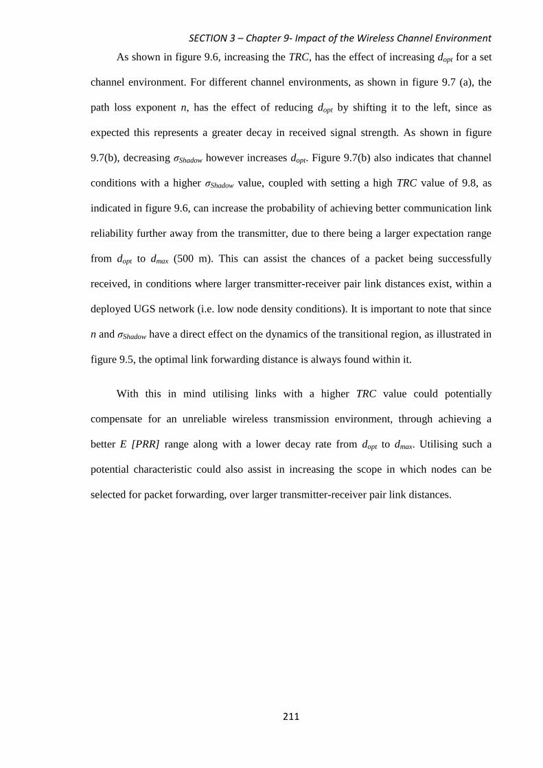
SECTION 3 – Chapter 9- Impact of the Wireless Channel Environment
211
As shown in figure 9.6, increasing the TRC, has the effect of increasing dopt for a set
channel environment. For different channel environments, as shown in figure 9.7 (a), the
path loss exponent n, has the effect of reducing dopt by shifting it to the left, since as
expected this represents a greater decay in received signal strength. As shown in figure
9.7(b), decreasing σShadow however increases dopt. Figure 9.7(b) also indicates that channel
conditions with a higher σShadow value, coupled with setting a high TRC value of 9.8, as
indicated in figure 9.6, can increase the probability of achieving better communication link
reliability further away from the transmitter, due to there being a larger expectation range
from dopt to dmax (500 m). This can assist the chances of a packet being successfully
received, in conditions where larger transmitter-receiver pair link distances exist, within a
deployed UGS network (i.e. low node density conditions). It is important to note that since
n and σShadow have a direct effect on the dynamics of the transitional region, as illustrated in
figure 9.5, the optimal link forwarding distance is always found within it.
With this in mind utilising links with a higher TRC value could potentially
compensate for an unreliable wireless transmission environment, through achieving a
better E [PRR] range along with a lower decay rate from dopt to dmax. Utilising such a
potential characteristic could also assist in increasing the scope in which nodes can be
selected for packet forwarding, over larger transmitter-receiver pair link distances.
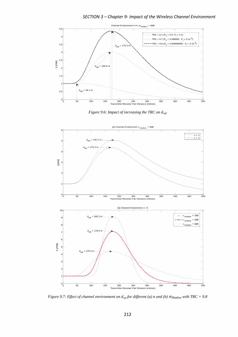
SECTION 3 – Chapter 9- Impact of the Wireless Channel Environment
212
Figure 9.6: Impact of increasing the TRC on dopt
Figure 9.7: Effect of channel environment on dopt for different (a) n and (b) σShadow with TRC = 9.8
0 50 100 150 200 250 300 350 400 450 5000
0.5
1
1.5
2
2.5
3
3.5
4
4.5
Channel Environment n=4 ,shadow
= 8dB
Transmitter-Receiver Pair Distance (metres)
E [
PR
R]
TRC = 6.1 (Ph = 0.9, P
l = 0.1)
TRC = 8.7 (Ph = 0.999999 , P
l = 0.1e-5)
TRC = 9.8 (Ph = 0.999999999 , P
l = 0.1e-8)
dopt
= 169.8 m
dopt
= 49.1 m
dopt
= 175.3 m
0 50 100 150 200 250 300 350 400 450 5000
1
2
3
4
5
6
(a) Channel Environment shadow
= 8dB
Transmitter-Receiver Pair Distance (metres)
E[P
RR
]
n = 4
n = 2d
opt = 182.2 m
dopt
= 175.3 m
0 50 100 150 200 250 300 350 400 450 5000
1
2
3
4
5
6
7
8
9
10(b) Channel Environment n =4
Transmitter-Receiver Pair Distance (metres)
E [
PR
R]
shadow = 2dB
shadow = 4dB
shadow = 8dB
dopt
= 180.3 m
dopt
= 178.9 m
dopt
= 175.3 m
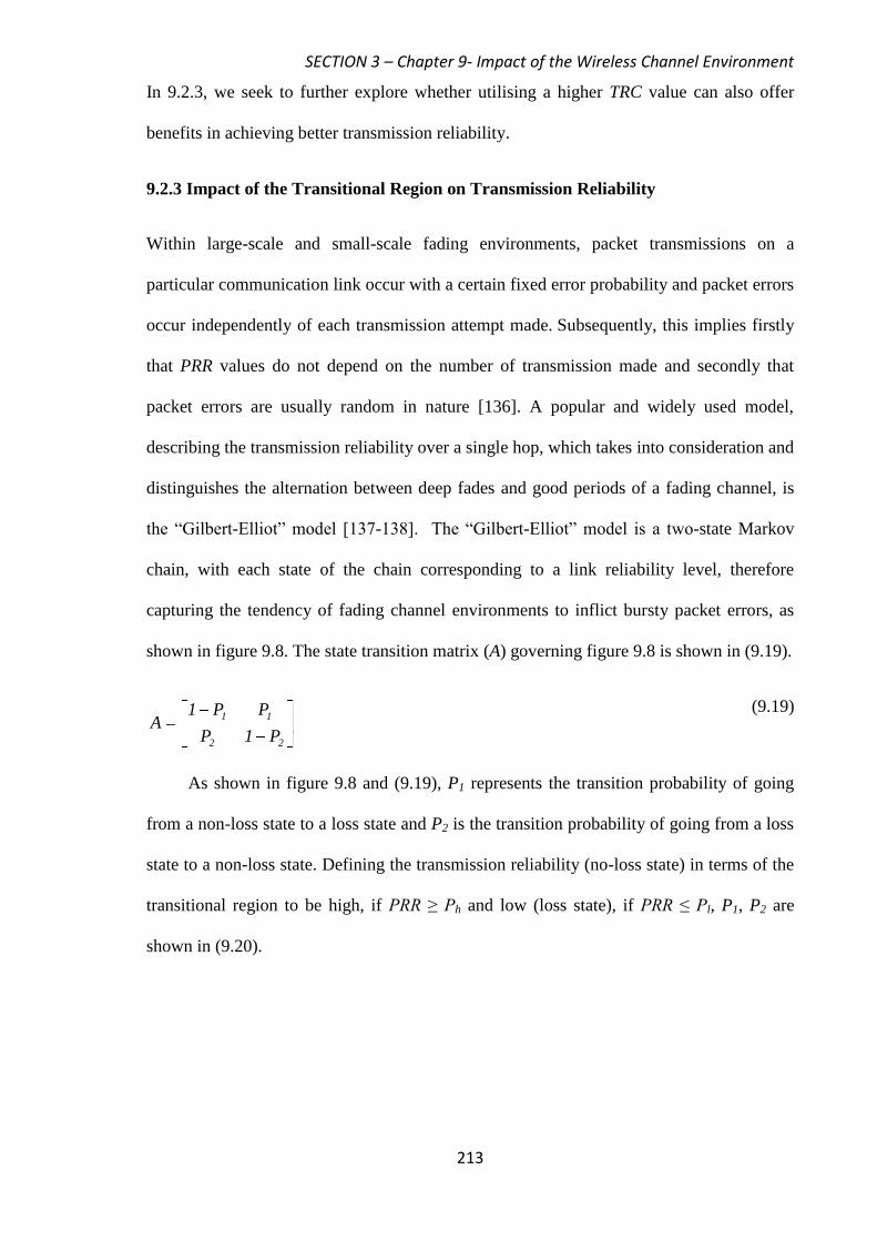
SECTION 3 – Chapter 9- Impact of the Wireless Channel Environment
213
In 9.2.3, we seek to further explore whether utilising a higher TRC value can also offer
benefits in achieving better transmission reliability.
9.2.3 Impact of the Transitional Region on Transmission Reliability
Within large-scale and small-scale fading environments, packet transmissions on a
particular communication link occur with a certain fixed error probability and packet errors
occur independently of each transmission attempt made. Subsequently, this implies firstly
that PRR values do not depend on the number of transmission made and secondly that
packet errors are usually random in nature [136]. A popular and widely used model,
describing the transmission reliability over a single hop, which takes into consideration and
distinguishes the alternation between deep fades and good periods of a fading channel, is
the “Gilbert-Elliot” model [137-138]. The “Gilbert-Elliot” model is a two-state Markov
chain, with each state of the chain corresponding to a link reliability level, therefore
capturing the tendency of fading channel environments to inflict bursty packet errors, as
shown in figure 9.8. The state transition matrix (A) governing figure 9.8 is shown in (9.19).
22
11
P1P
PP1A
(9.19)
As shown in figure 9.8 and (9.19), P1 represents the transition probability of going
from a non-loss state to a loss state and P2 is the transition probability of going from a loss
state to a non-loss state. Defining the transmission reliability (no-loss state) in terms of the
transitional region to be high, if PRR ≥ Ph and low (loss state), if PRR ≤ Pl, P1, P2 are
shown in (9.20).

SECTION 3 – Chapter 9- Impact of the Wireless Channel Environment
214
Shadow
MeandBdBUpper
h1 Q1)PPRR(pP (9.20)
Shadow
MeandBdBLowerl2 Q)PPRR(pP
Figure 9.8: “Gilbert-Elliot Model: A two state Markov channel
As shown in (9.20), P1 and P2 signify state transition probabilities within the defined
size of the transitional region, given by γ-Upper-dB and γ-Lower-dB. From A, as shown in (9.19),
the stationary state probabilities, π0 for state 0 and π1 for state 1 can be calculated as shown
in (9.21).
21
11
21
20
PP
P,
PP
P
(9.21)
As shown in (9.21), π0 represents the average arrival probability and π1 represents the mean
loss probability. We define transmission reliability, over a single communication hop link,
to be π0, as shown in figure 9.8. Figure 9.9, shows the impact on transmission reliability
through increasing the TRC metric.
0 (No Loss) 1 (Loss)
P1
1- P1 1- P2
P2
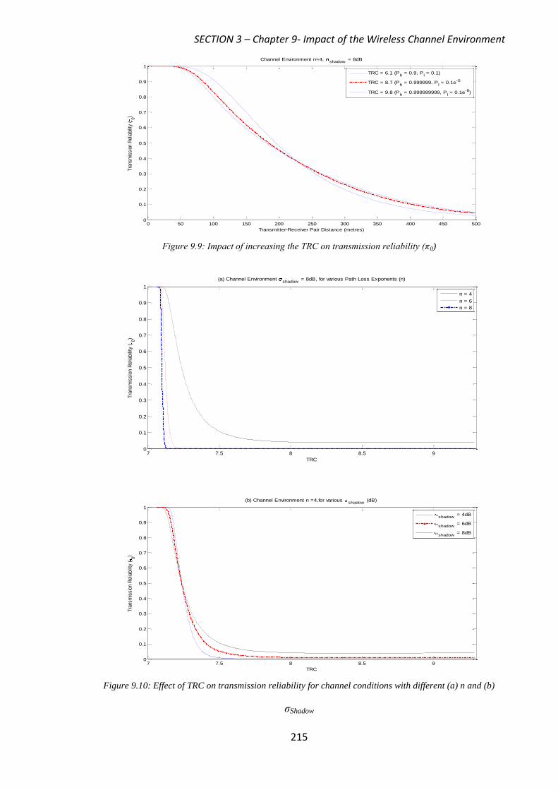
SECTION 3 – Chapter 9- Impact of the Wireless Channel Environment
215
Figure 9.9: Impact of increasing the TRC on transmission reliability (π0)
Figure 9.10: Effect of TRC on transmission reliability for channel conditions with different (a) n and (b)
σShadow
0 50 100 150 200 250 300 350 400 450 5000
0.1
0.2
0.3
0.4
0.5
0.6
0.7
0.8
0.9
1
Channel Environment n=4, shadow
= 8dB
Transmitter-Receiver Pair Distance (metres)
Tra
nsm
issi
on R
elia
bilit
y (
0)
TRC = 6.1 (Ph = 0.9, P
l = 0.1)
TRC = 8.7 (Ph = 0.999999, P
l = 0.1e-5
TRC = 9.8 (Ph = 0.999999999, P
l = 0.1e-8)
7 7.5 8 8.5 90
0.1
0.2
0.3
0.4
0.5
0.6
0.7
0.8
0.9
1
(a) Channel Environment shadow
= 8dB, for various Path Loss Exponents (n)
TRC
Tra
nsm
issio
n R
elia
bili
ty (
0)
n = 4
n = 6
n = 8
7 7.5 8 8.5 90
0.1
0.2
0.3
0.4
0.5
0.6
0.7
0.8
0.9
1
(b) Channel Environment n =4,for various shadow
(dB)
TRC
Tra
nsm
issi
on R
elia
bilit
y (
0)
shadow = 4dB
shadow = 6dB
shadow = 8dB
SECTION 3 – Chapter 9- Impact of the Wireless Channel Environment
216
From figure 9.9, defining a lower TRC value, achieves a better transmission
reliability performance over shorter communication link distances, however utilising a
higher TRC value is more beneficial over larger single hop communication link distances.
This is expected since a higher TRC value, as indicated in figure 9.6, can increase the E
[PRR] range and therefore the chances of reliable packet reception over larger hop
distances, which might be the case within a realistic UGS network deployment setting. As
shown in figure 9.10(a), increasing TRC has no effect on improving transmission reliability
performance, in channel conditions with increasing n. As shown in figure 9.10(b) and
initially verified through figure 9.9, defining a higher TRC value is again only beneficial in
channel environments with a fixed n but varying σShadow.
The transmission reliability however, as a value of merit only reflects the average
packet arrival probability and does not give an indication, as to the number of
transmissions required to achieve a desired transmission reliability. The number of packet
transmission attempts required to successfully deliver a packet, ultimately reflects on the
amount of energy consumed over a particular link and so must be actively considered.
Identifying forwarding nodes, which minimise the expected total number of link packet
transmission attempts, is therefore crucial and in 9.2.4, we explore whether utilising a
higher TRC value has any bearing on this.
9.2.4 Impact of Transitional Region on the Expected Transmission Count
So far our analysis concerning the impact of the channel environment (TRC) on
communication reliability has not considered using link quality performance metrics, as a
potential way towards identifying reliable packet forwarding nodes. An initial indication
has been given to this, in 9.2.2, by restricting packet forwarding to nodes with hop
distances that can maximise daverage, given in (9.18), which can primarily be achieved
through using links with a higher TRC, as shown in figure 9.6. An additional way of
SECTION 3 – Chapter 9- Impact of the Wireless Channel Environment
217
identifying reliable packet forwarding nodes is to use communication links, which can
minimise on the expected number of transmissions required for successful packet delivery
[139]. This can therefore help to achieve higher link throughput rates, but most importantly
lower communication energy expenditure.
The authors of [139] argue that traditional routing protocols such as DSR and DSDV
are more focused on identifying nodes in rapidly changing topology environments and
scalability issues, rather than identifying high-quality links, within an unreliable wireless
channel environment. As with the case in DSR and DSDV type protocols, identifying
routing paths which minimise on hop-count can maximise the distance travelled by a
packet towards its destination to achieve better QoS (message latency), but is likely to
induce lower received packet signal strength, increasing the chance for higher packet loss
ratios (lower transmission reliability).
The derivation of the expected number of transmissions (ETX) link quality metric
starts with first measuring the underlying PRR in both the forward (PF) and reverse (PR)
directions, in order to handle the asymmetric nature of bi-directional links, through
incorporating the PRR in each direction. By denoting P, as the probability that a packet
transmission across an arbitrary bi-directional link is not successful, this is given in (9.22).
])P()P([1P RF (9.22)
For analysis purposes, we assume that both PF and PR for an arbitrary link share the same
PRR characteristics, as shown in figure 9.4. Defined in this way, allows us to further
simplify P, so that it can be formulated in terms of the lower limit of the transitional
region, as shown in (9.23).
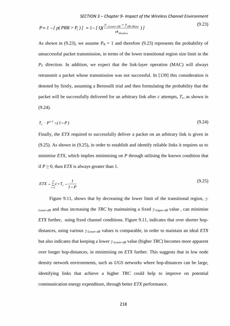
SECTION 3 – Chapter 9- Impact of the Wireless Channel Environment
218
])(Q[1])PPRR(p[1PShadow
MeandBdBLowerl
(9.23)
As shown in (9.23), we assume PR = 1 and therefore (9.23) represents the probability of
unsuccessful packet transmission, in terms of the lower transitional region size limit in the
PF direction. In addition, we expect that the link-layer operation (MAC) will always
retransmit a packet whose transmission was not successful. In [139] this consideration is
denoted by firstly, assuming a Bernoulli trial and then formulating the probability that the
packet will be successfully delivered for an arbitrary link after c attempts, Tc, as shown in
(9.24).
)P1(PT 1cc (9.24)
Finally, the ETX required to successfully deliver a packet on an arbitrary link is given in
(9.25). As shown in (9.25), in order to establish and identify reliable links it requires us to
minimise ETX, which implies minimising on P through utilising the known condition that
if P ≥ 0, then ETX is always greater than 1.
1cc
P1
1TcETX
(9.25)
Figure 9.11, shows that by decreasing the lower limit of the transitional region, γ-
Lower-dB and thus increasing the TRC by maintaining a fixed γ-Upper-dB value , can minimise
ETX further, using fixed channel conditions. Figure 9.11, indicates that over shorter hop-
distances, using various γ-Lower-dB values is comparable, in order to maintain an ideal ETX
but also indicates that keeping a lower γ-Lower-dB value (higher TRC) becomes more apparent
over longer hop-distances, in minimising on ETX further. This suggests that in low node
density network environments, such as UGS networks where hop-distances can be large,
identifying links that achieve a higher TRC could help to improve on potential
communication energy expenditure, through better ETX performance.
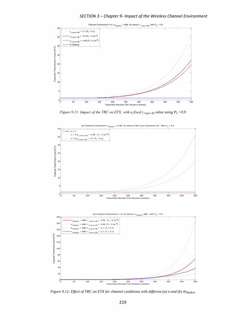
SECTION 3 – Chapter 9- Impact of the Wireless Channel Environment
219
Figure 9.11: Impact of the TRC on ETX, with a fixed γ-Upper-dB value using Ph =0.9
Figure 9.12: Effect of TRC on ETX for channel conditions with different (a) n and (b) σShadow
0 50 100 150 200 250 300 350 400 450 5000
5
10
15
20
25
30
35
40
Channel Environment n=4, shadow
= 8dB, for various -Low er-dB
, with Ph = 0.9
Transmitter-Receiver Pair Distance (metres)
Expecte
d T
ransm
issio
ns C
ount
(ET
X)
-Low er-dB = -2.7 (P
l = 0.1)
-Low er-dB = -4.4 (P
l = 0.1e-5)
-Low er-dB = -4.95 (P
l = 0.1e-8)
ETX(Ideal)
0 50 100 150 200 250 300 350 400 450 5000
5
10
15
20
25
30
35
40
(a) Channel Environment shadow
= 8 dB, for various Path Loss Exponents (n) , with Ph = 0.9
Transmitter-Receiver Pair Distance (metres)
Exp
ecte
d T
rans
mis
sion
Cou
nt (
ET
X)
n = 2
n = 4 (-Low er-dB
= -4.95 , Pl = 0.1e-8)
n =4 (-Low er-dB
= -2.7, Pl = 0.1)
0 50 100 150 200 250 300 350 400 450 5000
20
40
60
80
100
120
140
160
180
200
(b) Channel Environment n =4, for various shadow
(dB) , with Ph = 0.9
Transmitter-Receiver Pair Distance (metres)
Exp
ecte
d T
rans
mis
sion
Cou
nt (
ET
X)
shadow = 6dB (
-Low er-dB = -4.95 , P
l = 0.1e-8)
shadow = 8dB (
-Low er-dB = -4.95, P
l = 0.1e-8)
shadow = 6dB (
-Low er-dB = -2.7, P
l = 0.1)
shadow = 8dB (
-Low er-dB = -2.7, P
l = 0.1)

SECTION 3 – Chapter 9- Impact of the Wireless Channel Environment
220
Figures 9.12 (a) and (b) illustrate the effect that the channel environment has on ETX.
In figure 9.12 (a) increasing the path loss exponent has the effect of increasing ETX, while
increasing σShadow has the effect of reducing ETX over larger hop-distances. As shown in
figures 9.12 (a) and (b) increasing the TRC, through setting a lower γ-Lower-dB value can
minimise ETX, within both an increasing n and σShadow channel environment. This gives
both a reason to believe and an indication, as to the benefit in increasing the TRC , in order
to mitigate on n and σshadow channel conditions further, thus improving on overall ETX
performance.
9.3 Broadcast Nature of the Wireless Channel Environment
Packet forwarding in wireless networks have traditionally focused on identifying nodes,
which satisfy the best-path (i.e. minimum number of hops to a destination with favourable
link reliability) criteria between nodes. While best-path forwarding is suitable for wireless
environments with relatively stable and reliable point-to-point links, it is not an ideal
approach in realistic wireless environments that express time varying qualities over larger
hop-distances, as detailed in 9.1. As a result, best-path routing in this scenario, will require
higher packet retransmissions and more frequent path rediscoveries. With a view to further
improving on packet retransmissions, the impact of the error prone channel environment
on packet forwarding can be further mitigated by exploiting the broadcast nature of
wireless transmissions (opportunistic forwarding) and many schemes have been proposed,
which the major ones are detailed and surveyed in [140-142].
Utilising an opportunistic forwarding strategy, allows nodes to maximise the
progress a packet makes towards the destination that each received broadcast transmission
may provide. Thus, in contrast to best-path packet forwarding where a packet is unicast to
the predetermined next-hop, under opportunistic forwarding, a next-hop is determined per-
packet after its broadcast transmission has been received. Primarily, all opportunistic
SECTION 3 – Chapter 9- Impact of the Wireless Channel Environment
221
forwarding schemes operate by actively involving multiple neighbouring nodes
(forwarding candidates) for each packet relay in order to firstly, make the forwarding task
insensitive to link quality variations and secondly further improve on network throughput,
as surveyed in [142-143]. As shown in [142-143] opportunistic forwarding schemes differ
mainly on how they improve on selecting forwarding candidates, in order to avoid packet
duplication at the destination. Many of the surveyed schemes predominantly rely on the
ETX metric or maximising the geo-graphical distance on a hop-by-hop basis towards the
destination, as their prioritisation selection mechanisms.
In 9.3, we do not propose a new protocol for opportunistic forwarding but analyse
the impact of the channel environment (TRC) on the expected any-path transmission (EAX)
link quality metric [144]. EAX, which builds on the ETX format, is a link quality metric,
which neatly captures the ETX between a node pair, under an opportunistic forwarding
environment. By employing the EAX metric, within an opportunistic any-path forwarding
(OAPF) environment, as detailed in [144-145], we seek to inquire whether we can indeed
reduce the required number of transmissions further, in order to achieve reliable delivery of
a packet to its destination.
9.3.1 The Expected any Path Transmission Link Quality Metric
We now define the EAX for a source s and destination d pair, given a simple arbitrary static
network topology. Let Cs, d
, denote the potential set of forwarding candidates (f1,.…, fi),
between s and d, where i ≤ Cs, d
, and let Ci s,d
be the ith
forwarding candidate, within dmax
(Table 9.1) of s. We denote the underlying probability of delivery success considering both
PF and PR, as introduced in 9.2.4, from s to Cts, d
as pi. As defined in [145], the EAX needed
for reliable delivery of a packet from a source s to a destination d, given the Cs, d
and
assuming PR = 1, is shown in (9.26).
SECTION 3 – Chapter 9- Impact of the Wireless Channel Environment
222
)d,s(Z)d,s(S)d,s(EAX (9.26)
Where,
ii )p1(1
1)d,s(S and
i
1i
1jji
d,s
i )p1(p)d,C(EAX)d,s(Z .
By doing a direct comparison between (9.25) and (9.26), we can see that using (9.25)
merely considers a best path scenario from each node in the network, in terms of ETX. As
shown in (9.26), the opportunistic forwarding framework is neatly captured by S(s, d),
which describes the ETX for successfully transmitting a packet from source s, to at least
one of the next hop forwarding candidates Ci s,d
and Z(s, d), which captures the ETX for
delivering the packet in turn from those candidates to a destination, d.
9.3.2 Impact of Transitional Region on the EAX Metric
The TRC in it’s own right can serve as a value of merit for current link reliability, by
giving an indication of the extent of the transitional region to connected region, associated
with a single communication link. By considering the transistional region defined by the
TRC as a potential way of mitgating link unreliabilty within an OAPF environment, we
analyse if this has any effect on EAX performance, within a 2-hop scenerio ( i.e. the set of
forwarding candidates, Cs, d
, are the first hop nodes to a destination d). We also assume for
the purposes of analysis that Cs, d
nodes all have equal priority, for packet forwarding
selection. Figure 9.13, shows the effect of increasing TRC on EAX performance, while
maintaining a fixed Ph (γ-Upper-dB) value. By increasing the TRC, it is shown through the
EAX metric that we can further reduce the number of transmissions required for sucessful
packet delivery.
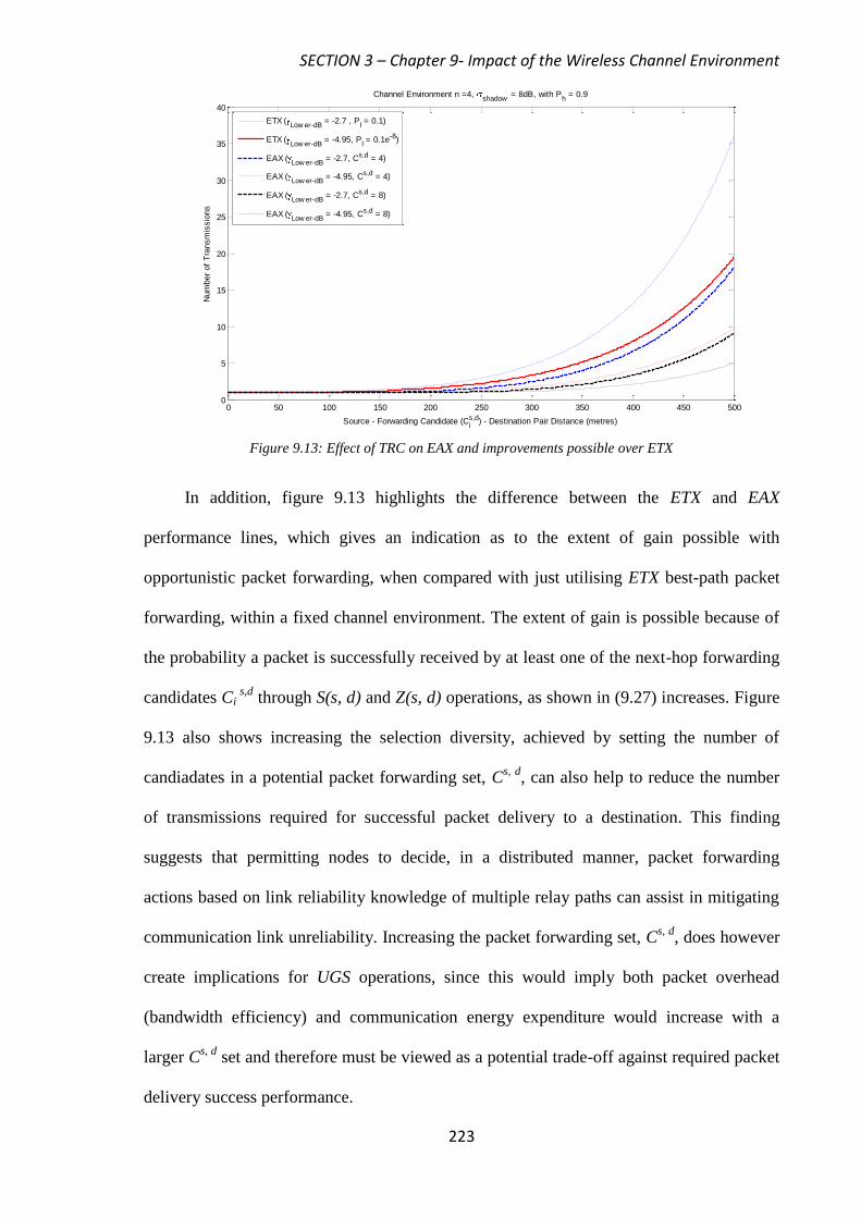
SECTION 3 – Chapter 9- Impact of the Wireless Channel Environment
223
Figure 9.13: Effect of TRC on EAX and improvements possible over ETX
In addition, figure 9.13 highlights the difference between the ETX and EAX
performance lines, which gives an indication as to the extent of gain possible with
opportunistic packet forwarding, when compared with just utilising ETX best-path packet
forwarding, within a fixed channel environment. The extent of gain is possible because of
the probability a packet is successfully received by at least one of the next-hop forwarding
candidates Ci s,d
through S(s, d) and Z(s, d) operations, as shown in (9.27) increases. Figure
9.13 also shows increasing the selection diversity, achieved by setting the number of
candiadates in a potential packet forwarding set, Cs, d
, can also help to reduce the number
of transmissions required for successful packet delivery to a destination. This finding
suggests that permitting nodes to decide, in a distributed manner, packet forwarding
actions based on link reliability knowledge of multiple relay paths can assist in mitigating
communication link unreliability. Increasing the packet forwarding set, Cs, d
, does however
create implications for UGS operations, since this would imply both packet overhead
(bandwidth efficiency) and communication energy expenditure would increase with a
larger Cs, d
set and therefore must be viewed as a potential trade-off against required packet
delivery success performance.
0 50 100 150 200 250 300 350 400 450 5000
5
10
15
20
25
30
35
40
Channel Environment n =4, shadow
= 8dB, with Ph = 0.9
Source - Forwarding Candidate (Cis,d) - Destination Pair Distance (metres)
Num
ber
of
Tra
nsm
issio
ns
ETX (Low er-dB
= -2.7 , Pl = 0.1)
ETX (Low er-dB
= -4.95, Pl = 0.1e-8)
EAX (Low er-dB
= -2.7, Cs,d = 4)
EAX (Low er-dB
= -4.95, Cs,d = 4)
EAX (Low er-dB
= -2.7, Cs,d = 8)
EAX (Low er-dB
= -4.95, Cs,d = 8)
SECTION 3 – Chapter 10 – Development of a Channel Aware Hop Selection Scheme
224
CHAPTER 10
Development of a Channel Aware Hop Selection Scheme
10.1 Channel Aware Fuzzy Logic Hop Selection Scheme
As detailed in chapter 9, in sections 9.2 and 9.3, we have studied how the TRC can affect
both link reliability and known link quality metrics, such as ETX and EAX. In section 9.3, it
is also shown how the packet forwarding task can be improved, in a distributed manner,
through using the TRC within an OAPF environment. In this chapter, we highlight our
decision making mechanism based on the benefits we have discovered and knowledge
gained about the TRC, as a potential metric to achieve improved packet forwarding
performance within a dynamic channel environment.
A decision mechanism of this kind would serve UGS nodes the advantage and ability
to self-manage their own packet forwarding tasks on a per hop basis, based solely on the
TRC information gained from the channel environment, in a distributed and opportunistic
manner. Since the uncertainty associated with the dynamic channel environment is a key
factor towards data packets being successfully received, controlling node selection for
packet forwarding efficiently, according to current channel conditions (channel
awareness), becomes a key design requirement. In this section, we propose to use a Fuzzy
Logic System (FLS) as our control implementation for packet forwarding, utilising the
current received TRC, as its control input source.
Fuzzy Logic (FL) has the potential to deal with conflicting real-world uncertainties
without needing complex mathematical modelling, through using heuristic reasoning
[146]. Such a FLS scheme can be applied to hop node selection for data forwarding in
varying channel conditions. In addition, our other reason for applying a FLS decision
making capability is to see if any advantages can be achieved in allowing nodes to improve

SECTION 3 – Chapter 10 – Development of a Channel Aware Hop Selection Scheme
225
their node selection capability against techniques, which currently rely on defined metrics,
as detailed in [147-148]. Defined metrics have the disadvantage of not promoting adaptive
behaviour towards packet forwarding links, which can become unreliable and result in
changes to local network topology. We begin initially in 10.1.1, by giving an overview to
FL. In 10.1.2, we then introduce the building blocks associated with a FLS and based on
this introduce our proposed FLS design in heading 10.1.3. In 10.1.4, we perform
simulations for large-scale and large-small scale fading channel environments using our
proposed FLS approach against other common packet forwarding strategies.
10.1.1 Overview of Fuzzy Logic
The principles of FL and its application to real-world engineering problems have been well
reviewed and studied [149-151], since being initially established as a field of genuine
study, by L.Zadeh [152-153]. In [152-153], L.Zadeh argued that the majority of real-world
decision making problems could not be assisted by completely formulating problems using
either objective (i.e. use of mathematical models) or subjective (i.e. use of linguistic based
rule systems) techniques, but that a combination of both methods of problem solving
should be incorporated and utilised effectively. An example of this might be temperature
control in a room, which could be objectively modelled but also subjectively perceived as
being either “warm”, “hot” or “cool”.
In essence, FL principles [152-153] allow a logical and rational way in which both
forms of problem solving can be coordinated jointly and effectively, in order to provide
assistance in a decision making process to a realistic problem. The ability to map the
objective world to the subjective way of thinking has been the key driver towards FL being
adopted and used as decision making capability for a wide range of scenarios. In terms of
our proposed decision making mechanism, the TRC metric and our subsequent analysis
made on communication link reliability has so far been modelled objectively. However, the
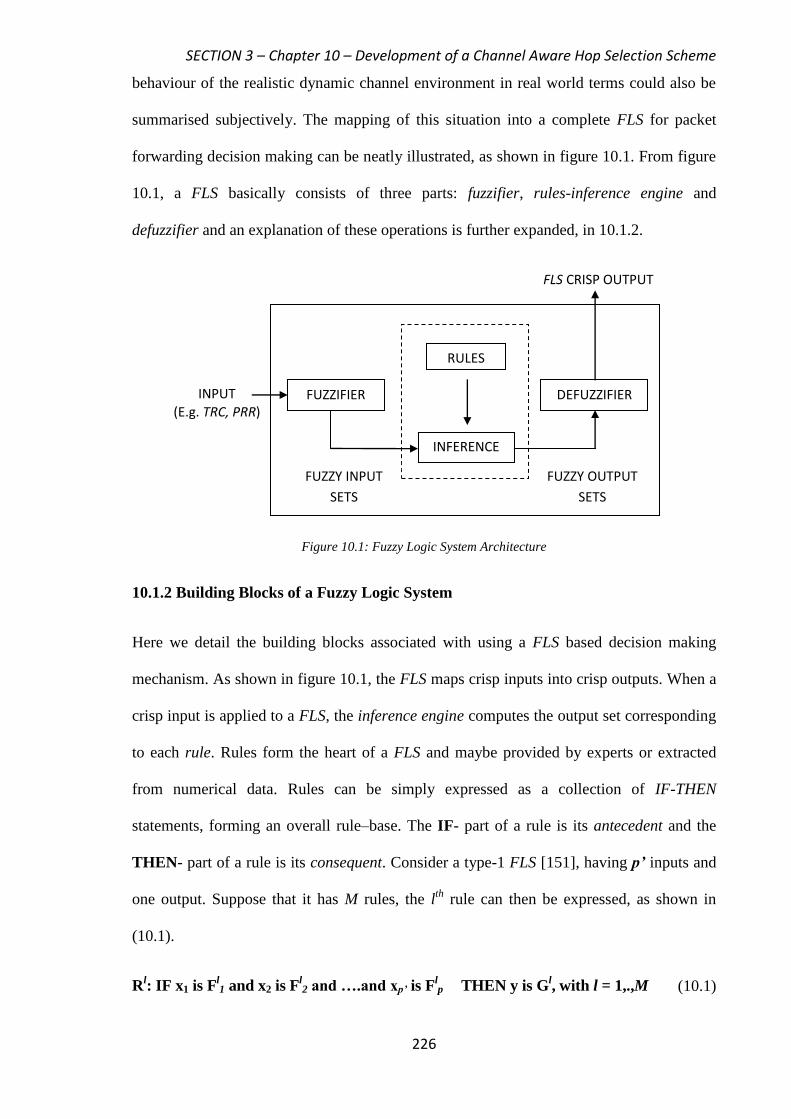
SECTION 3 – Chapter 10 – Development of a Channel Aware Hop Selection Scheme
226
behaviour of the realistic dynamic channel environment in real world terms could also be
summarised subjectively. The mapping of this situation into a complete FLS for packet
forwarding decision making can be neatly illustrated, as shown in figure 10.1. From figure
10.1, a FLS basically consists of three parts: fuzzifier, rules-inference engine and
defuzzifier and an explanation of these operations is further expanded, in 10.1.2.
Figure 10.1: Fuzzy Logic System Architecture
10.1.2 Building Blocks of a Fuzzy Logic System
Here we detail the building blocks associated with using a FLS based decision making
mechanism. As shown in figure 10.1, the FLS maps crisp inputs into crisp outputs. When a
crisp input is applied to a FLS, the inference engine computes the output set corresponding
to each rule. Rules form the heart of a FLS and maybe provided by experts or extracted
from numerical data. Rules can be simply expressed as a collection of IF-THEN
statements, forming an overall rule–base. The IF- part of a rule is its antecedent and the
THEN- part of a rule is its consequent. Consider a type-1 FLS [151], having p’ inputs and
one output. Suppose that it has M rules, the lth
rule can then be expressed, as shown in
(10.1).
Rl: IF x1 is F
l1 and x2 is F
l2 and ….and xp’ is F
lp THEN y is G
l, with l = 1,.,M (10.1)
INPUT (E.g. TRC, PRR)
RULES
INFERENCE
FUZZIFIER DEFUZZIFIER
FUZZY INPUT
SETS
FUZZY OUTPUT
SETS
FLS CRISP OUTPUT

SECTION 3 – Chapter 10 – Development of a Channel Aware Hop Selection Scheme
227
As shown in (10.1), x1…xp’ are crisp inputs, representing the objective space while Fl1…
Flp are linguistic variables representing the subjective space. G
l represents the subjective
consequent of the eventual decision. All the rules are processed in a parallel manner by the
inference engine. Any rule that fires, contributes to the final FLS decision solution space.
The degree of uncertainty associated with a received channel input is evaluated by the
fuzzification process. A common fuzzification process used in FLS’s is singleton
fuzzification [152-153]. The uncertainty (fuzziness) is essentially characterised by fuzzy sets
or membership functions (MFs), taking on values (degrees of membership) in the interval
[0, 1]. Fuzzy sets, through its MFs are the mechanism through which the FLS interfaces
with the outside world. The rule base then relates the input fuzzy variables with the output
fuzzy variables using linguistic variables, each of which is described by a fuzzy set (MF)
and a fuzzy implication operator (i.e. AND, OR etc.). The nature of the rule base determines
how and which consequent output fuzzy set is then copied to the final fuzzy solution space
(final decision outcome).
Defuzzification is the last process in a FLS and finds a crisp output value from the
fuzzy output solution space, in order to determine the combined truth of the antecedent
using MINIMUM or MAXIMUM functions. Common defuzzification methods include
maximum, mean-of-maxima, centroid, centre-of-sums and centre-of-sets [154]. In our
proposed design we focus on simplicity and therefore undertake singleton defuzzification,
(centre of singleton method), which implies that the output fuzzy sets (MFs) are represented
by single spikes (zero-order Sugeno fuzzy model) [154]. Therefore in this sense, each
output MF assigns the value 1 to a single point and 0, to all other points. We consider this
method since, it is both computational quicker and simpler to implement than the methods
listed above, which is an added benefit operating within a varying channel environment.
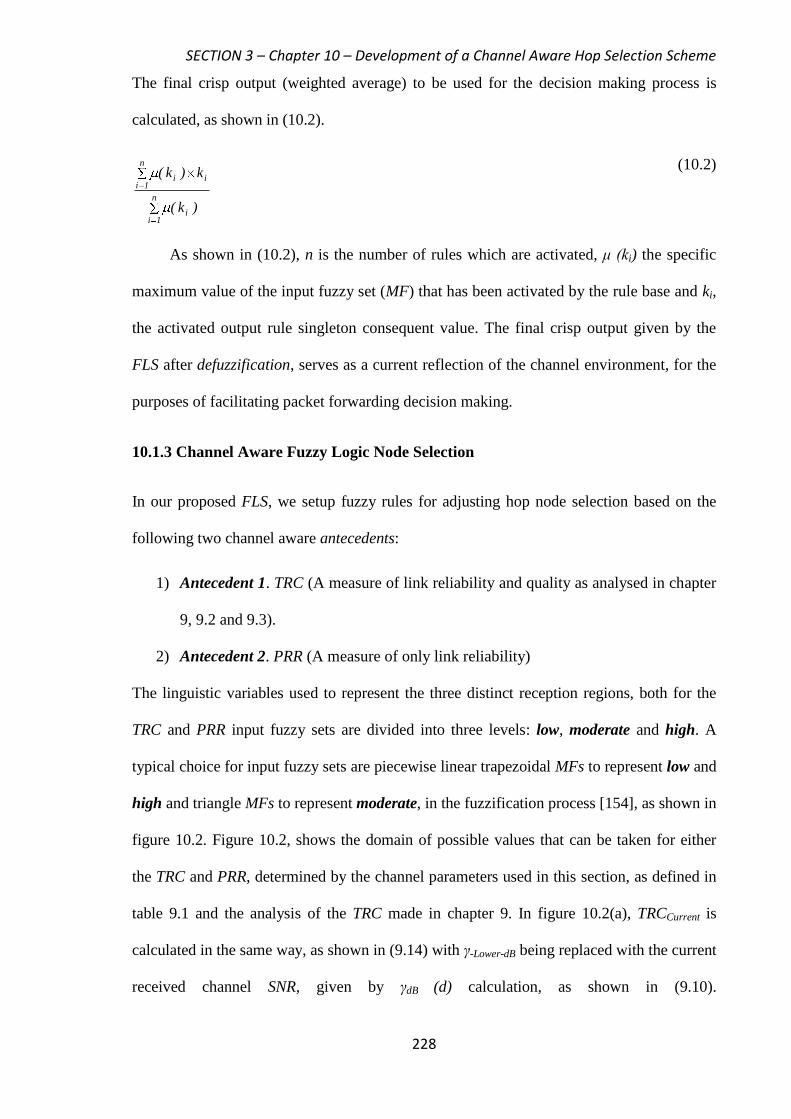
SECTION 3 – Chapter 10 – Development of a Channel Aware Hop Selection Scheme
228
The final crisp output (weighted average) to be used for the decision making process is
calculated, as shown in (10.2).
n
1ii
n
1iii
)k(
k)k(
(10.2)
As shown in (10.2), n is the number of rules which are activated, μ (ki) the specific
maximum value of the input fuzzy set (MF) that has been activated by the rule base and ki,
the activated output rule singleton consequent value. The final crisp output given by the
FLS after defuzzification, serves as a current reflection of the channel environment, for the
purposes of facilitating packet forwarding decision making.
10.1.3 Channel Aware Fuzzy Logic Node Selection
In our proposed FLS, we setup fuzzy rules for adjusting hop node selection based on the
following two channel aware antecedents:
1) Antecedent 1. TRC (A measure of link reliability and quality as analysed in chapter
9, 9.2 and 9.3).
2) Antecedent 2. PRR (A measure of only link reliability)
The linguistic variables used to represent the three distinct reception regions, both for the
TRC and PRR input fuzzy sets are divided into three levels: low, moderate and high. A
typical choice for input fuzzy sets are piecewise linear trapezoidal MFs to represent low and
high and triangle MFs to represent moderate, in the fuzzification process [154], as shown in
figure 10.2. Figure 10.2, shows the domain of possible values that can be taken for either
the TRC and PRR, determined by the channel parameters used in this section, as defined in
table 9.1 and the analysis of the TRC made in chapter 9. In figure 10.2(a), TRCCurrent is
calculated in the same way, as shown in (9.14) with γ-Lower-dB being replaced with the current
received channel SNR, given by γdB (d) calculation, as shown in (9.10).

SECTION 3 – Chapter 10 – Development of a Channel Aware Hop Selection Scheme
229
Figure 10.2: Membership Functions for (a) Antecedent 1 and (b) Antecedent 2
The output fuzzy singleton consequent sets, defining the possibility of a node being selected
for packet forwarding, are divided into 5 levels, Very High, High, Medium, Low and Very
Low. The overall rule base therefore needs to be setup with 9 rules (32), for the FLS because
every antecedent has 3 fuzzy sets (MFs).
The design of the overall rule base is constructed utilising rules such as shown below:
IF TRC is High and PRR is Low, THEN Possibility for this node being selected is _____.
As indicated in 9.2.2, our analytical observations suggest it is best to segregate the
network according to link distance, in terms of dopt, which is ultimately defined by the
conditions of the operating channel environment (n and σShadow). As suggested in 9.2.2, link
distances, which are ≤ dopt are best utilised if they can achieve a lower TRC and vice versa
for link distances, which are ≥ dopt, in order to compensate for an increasing n and σShadow
channel environment. To address this leads us to draw up consequents, which reflect this
channel environment defined condition, as summarised in table 10.1. Table 10.1, indicates
our proposed rule base, in terms of individual rules and consequents used for packet
forwarding node selection, based on dopt and the TRC analysis made in chapter
PRR
Degree of Membership Degree of Membership
5.31 6.52 TRCCurrent
Low High 1.0
0
Moderate
7.98 (Pl) 0.1e-8 0.5
Low High 1.0
0
Moderate
(Ph) 0.999
(a) (b)
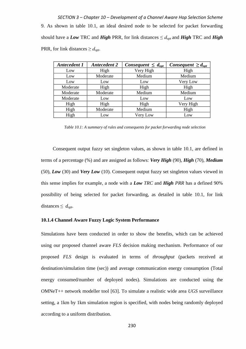
SECTION 3 – Chapter 10 – Development of a Channel Aware Hop Selection Scheme
230
9. As shown in table 10.1, an ideal desired node to be selected for packet forwarding
should have a Low TRC and High PRR, for link distances ≤ dopt and High TRC and High
PRR, for link distances ≥ dopt.
Antecedent 1 Antecedent 2 Consequent ≤ dopt Consequent ≥ dopt
Low High Very High High
Low Moderate Medium Medium
Low Low Low Very Low
Moderate High High High
Moderate Moderate Medium Medium
Moderate Low Low Low
High High High Very High
High Moderate Medium High
High Low Very Low Low
Table 10.1: A summary of rules and consequents for packet forwarding node selection
Consequent output fuzzy set singleton values, as shown in table 10.1, are defined in
terms of a percentage (%) and are assigned as follows: Very High (90), High (70), Medium
(50), Low (30) and Very Low (10). Consequent output fuzzy set singleton values viewed in
this sense implies for example, a node with a Low TRC and High PRR has a defined 90%
possibility of being selected for packet forwarding, as detailed in table 10.1, for link
distances ≤ dopt.
10.1.4 Channel Aware Fuzzy Logic System Performance
Simulations have been conducted in order to show the benefits, which can be achieved
using our proposed channel aware FLS decision making mechanism. Performance of our
proposed FLS design is evaluated in terms of throughput (packets received at
destination/simulation time (sec)) and average communication energy consumption (Total
energy consumed/number of deployed nodes). Simulations are conducted using the
OMNeT++ network modeller tool [63]. To simulate a realistic wide area UGS surveillance
setting, a 1km by 1km simulation region is specified, with nodes being randomly deployed
according to a uniform distribution.
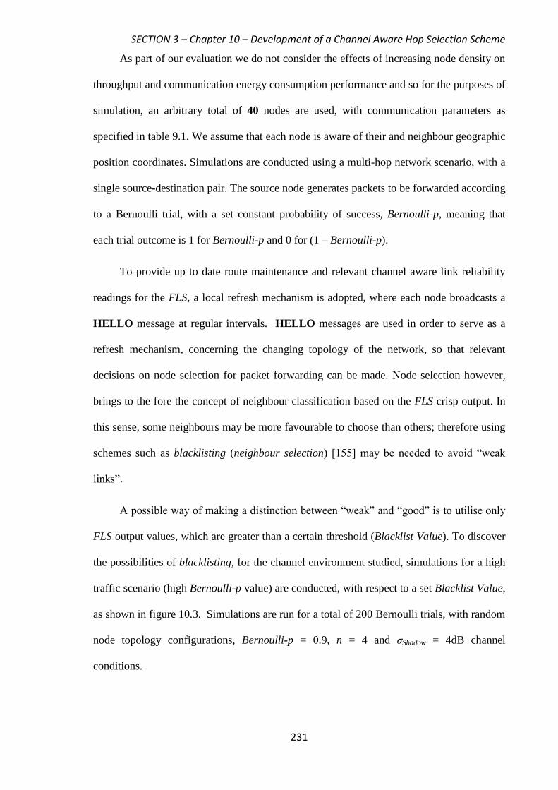
SECTION 3 – Chapter 10 – Development of a Channel Aware Hop Selection Scheme
231
As part of our evaluation we do not consider the effects of increasing node density on
throughput and communication energy consumption performance and so for the purposes of
simulation, an arbitrary total of 40 nodes are used, with communication parameters as
specified in table 9.1. We assume that each node is aware of their and neighbour geographic
position coordinates. Simulations are conducted using a multi-hop network scenario, with a
single source-destination pair. The source node generates packets to be forwarded according
to a Bernoulli trial, with a set constant probability of success, Bernoulli-p, meaning that
each trial outcome is 1 for Bernoulli-p and 0 for (1 – Bernoulli-p).
To provide up to date route maintenance and relevant channel aware link reliability
readings for the FLS, a local refresh mechanism is adopted, where each node broadcasts a
HELLO message at regular intervals. HELLO messages are used in order to serve as a
refresh mechanism, concerning the changing topology of the network, so that relevant
decisions on node selection for packet forwarding can be made. Node selection however,
brings to the fore the concept of neighbour classification based on the FLS crisp output. In
this sense, some neighbours may be more favourable to choose than others; therefore using
schemes such as blacklisting (neighbour selection) [155] may be needed to avoid “weak
links”.
A possible way of making a distinction between “weak” and “good” is to utilise only
FLS output values, which are greater than a certain threshold (Blacklist Value). To discover
the possibilities of blacklisting, for the channel environment studied, simulations for a high
traffic scenario (high Bernoulli-p value) are conducted, with respect to a set Blacklist Value,
as shown in figure 10.3. Simulations are run for a total of 200 Bernoulli trials, with random
node topology configurations, Bernoulli-p = 0.9, n = 4 and σShadow = 4dB channel
conditions.
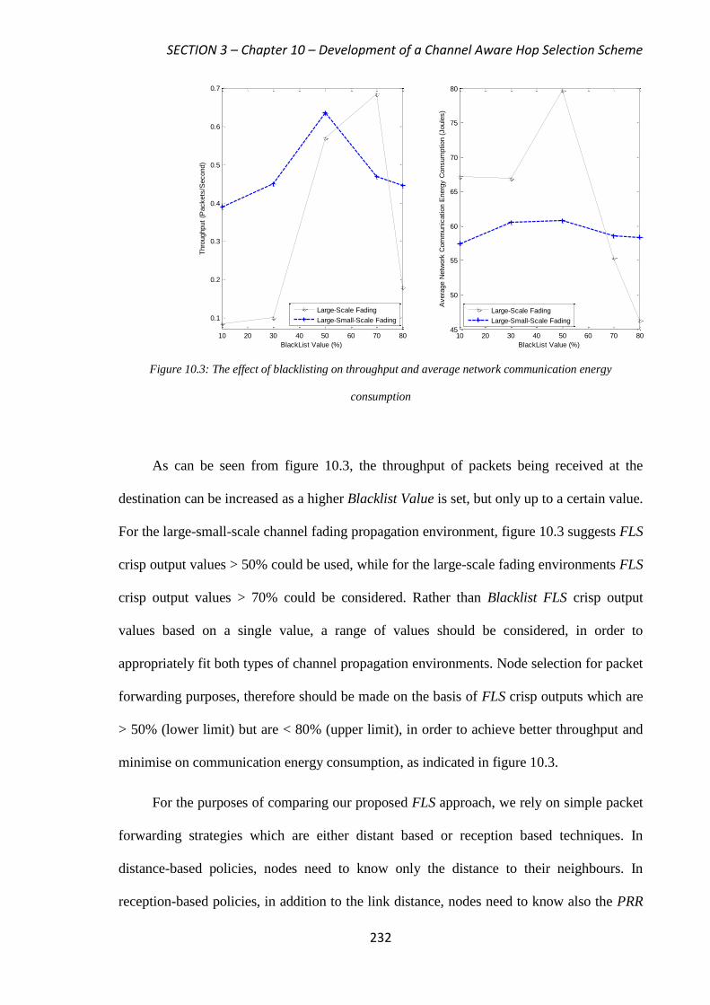
SECTION 3 – Chapter 10 – Development of a Channel Aware Hop Selection Scheme
232
Figure 10.3: The effect of blacklisting on throughput and average network communication energy
consumption
As can be seen from figure 10.3, the throughput of packets being received at the
destination can be increased as a higher Blacklist Value is set, but only up to a certain value.
For the large-small-scale channel fading propagation environment, figure 10.3 suggests FLS
crisp output values > 50% could be used, while for the large-scale fading environments FLS
crisp output values > 70% could be considered. Rather than Blacklist FLS crisp output
values based on a single value, a range of values should be considered, in order to
appropriately fit both types of channel propagation environments. Node selection for packet
forwarding purposes, therefore should be made on the basis of FLS crisp outputs which are
> 50% (lower limit) but are < 80% (upper limit), in order to achieve better throughput and
minimise on communication energy consumption, as indicated in figure 10.3.
For the purposes of comparing our proposed FLS approach, we rely on simple packet
forwarding strategies which are either distant based or reception based techniques. In
distance-based policies, nodes need to know only the distance to their neighbours. In
reception-based policies, in addition to the link distance, nodes need to know also the PRR
10 20 30 40 50 60 70 80
0.1
0.2
0.3
0.4
0.5
0.6
0.7
BlackList Value (%)
Thro
ughput
(Packets
/Second)
10 20 30 40 50 60 70 8045
50
55
60
65
70
75
80
BlackList Value (%)
Avera
ge N
etw
ork
Com
munic
ation E
nerg
y C
onsum
ption (
Joule
s)
Large-Scale Fading
Large-Small-Scale Fading
Large-Scale Fading
Large-Small-Scale Fading

SECTION 3 – Chapter 10 – Development of a Channel Aware Hop Selection Scheme
233
or SNR of their neighbour link states. Two common schemes, which cover the simple
packet forwarding techniques discussed above and used for comparison purposes, are
detailed below:
Most Forward with Fixed Radius (MFR) [156]. MFR is a pragmatic single path packet
forwarding strategy relying on neighbouring nodes which are only closest to the
destination. In this sense MFR is a shortest path scheme using a strategy on minimising
the number of hops required to the destination, in order to ensure high spatial reuse
(bandwidth) efficiency.
Nearest with Forward Progress (NFP) [157]. NFP is a simple best reception neighbour
strategy, where each node forwards to the neighbour that has the highest PRR and is
closer to the destination. NFP is again a shortest path scheme but incorporates a simple
path loss link reliability dependent metric, within its decision making routine.
All the techniques discussed above rely on packet forwarding to the node closest to
the destination, among their remaining neighbours, with MFR however being the most
aggressive, but not including any channel aware metrics. To evaluate our proposed FLS
design, it is also integrated within the NFP strategy, in order to substantiate whether any
improvements can be gained over just using a simple PRR metric. An evaluation is also
considered against the ETX metric, introduced in chapter 9, whose analysis under different
channel environments using the TRC metric formed the basis towards our eventual
proposed FLS design. This evaluation will hopefully seek to insure whether the analytical
observations made in 9.2.4, which have been incorporated into our FLS design, are indeed
correct. The overall flow chart algorithm illustrating the FLS strategy in selecting nodes for
packet forwarding, is detailed in, Appendix C, part 1. In figures 10.4 and 10.5, the
throughput and communication energy consumption performance for the above mentioned
schemes and our FLS system are shown. The same energy consumption model is used as
already described in section 1, under heading 4.4.3.
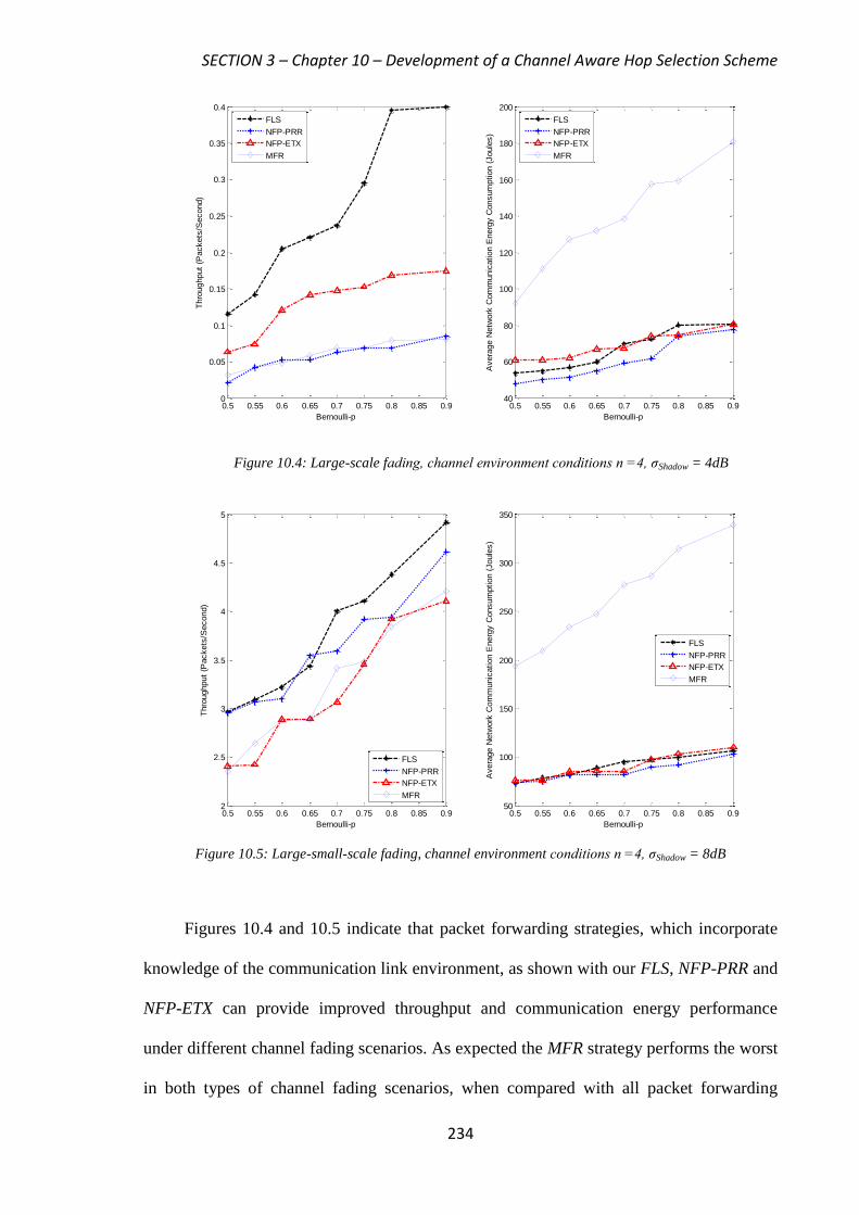
SECTION 3 – Chapter 10 – Development of a Channel Aware Hop Selection Scheme
234
Figure 10.4: Large-scale fading, channel environment conditions n =4, σShadow = 4dB
Figure 10.5: Large-small-scale fading, channel environment conditions n =4, σShadow = 8dB
Figures 10.4 and 10.5 indicate that packet forwarding strategies, which incorporate
knowledge of the communication link environment, as shown with our FLS, NFP-PRR and
NFP-ETX can provide improved throughput and communication energy performance
under different channel fading scenarios. As expected the MFR strategy performs the worst
in both types of channel fading scenarios, when compared with all packet forwarding
0.5 0.55 0.6 0.65 0.7 0.75 0.8 0.85 0.90
0.05
0.1
0.15
0.2
0.25
0.3
0.35
0.4
Bernoulli-p
Thro
ughput
(Packets
/Second)
FLS
NFP-PRR
NFP-ETX
MFR
0.5 0.55 0.6 0.65 0.7 0.75 0.8 0.85 0.940
60
80
100
120
140
160
180
200
Bernoulli-p
Avera
ge N
etw
ork
Com
munic
ation E
nerg
y C
onsum
ption (
Joule
s)
FLS
NFP-PRR
NFP-ETX
MFR
0.5 0.55 0.6 0.65 0.7 0.75 0.8 0.85 0.92
2.5
3
3.5
4
4.5
5
Bernoulli-p
Thro
ughput
(Packets
/Second)
0.5 0.55 0.6 0.65 0.7 0.75 0.8 0.85 0.950
100
150
200
250
300
350
Bernoulli-p
Avera
ge N
etw
ork
Com
munic
ation E
nerg
y C
onsum
ption (
Joule
s)
FLS
NFP-PRR
NFP-ETX
MFR
FLS
NFP-PRR
NFP-ETX
MFR

SECTION 3 – Chapter 10 – Development of a Channel Aware Hop Selection Scheme
235
strategies, as shown in figures 10.4 and 10.5. This is primarily because minimising on hop
count entails using forwarding nodes, which are over longer communication link distances
and therefore become more susceptible to channel variations, resulting in increased packet
retransmissions and increased communication energy expenditure, with traffic intensity.
From figures 10.4 and 10.5, FLS, NFP-PRR and NFP-ETX all have similar
communication energy expenditure profiles, for the different traffic condition scenarios
(Bernoulli-p) used. The FLS strategy however, outperforms on throughput performance
against the alternative forwarding schemes in all cases, as shown in figures 10.4 and 10.5.
An efficient UGS network is also one in that can pass as many packets as possible (higher
throughput), while minimising the energy consumption burden. From figures 10.4 and 10.5
for conditions with Bernoulli-p > 0.7, our proposed FLS scheme can increase the
throughput performance whilst maintain a consistent communication energy consumption
performance under the simulated channel environment scenario. This leads us to suggest
that our proposed FLS strategy, under the simulated scenario, can support the throughput-
energy efficiency requirement.
There are two reasons for this. Firstly, the FLS strategy utilises the broadcast medium
to encourage opportunistic forwarding, thus increasing the chance a packet is received at
the destination via diversification of routes used (selection diversity), which assists on
increasing throughput and reducing the need for consuming further communication energy.
Secondly, by segregating the network according to dopt and incorporating both the TRC
metric and PRR, as shown in table 10.1, the FLS strategy can increase a nodes ability to
make better decisions as to selecting nodes for packet forwarding. In addition, it is also
worth noting how all strategies can achieve better throughput performance levels, in
channel environments with a higher σShadow. This result seems to agree with the analysis
made in chapter 9, under 9.2.2 and also, as shown in figure 9.7 (b).
SECTION 3 – Chapter 10 – Development of a Channel Aware Hop Selection Scheme
236
10.2 Genetic Adaptive Fuzzy Logic Hop Selection Scheme
One of the most important considerations to be made in the application and use of FL is the
accurate derivation of both the rules to be used in the rule base and their corresponding
MFs. Both play a crucial role in overall FLS performance, so it becomes important to both
derive and adjust these parameters accurately to the process being controlled, which in our
scenario entails ensuring the best decision, as to node selection for packet forwarding, is
achieved.
The derivation of FLS rule base parameters can be commonly performed using
learning based techniques [149] [151], while the adjustments of MF parameters are best
performed using tuning based techniques [158]. In a learning process, rules and
corresponding MF’s are directly obtained by learning from available measurement data
concerning the control process. Tuning based processes assume there is already an existing
rule base and MF definition present. Our proposed FLS design highlighted in 10.1 uses
rules and MF’s that have been defined by us, as shown in table 10.1 and figure 10.1, which
has been made possible, based on the analysis made in chapter 9. In this sense, our proposed
FLS is typically classified as an expert based system and so a prime candidate for a tuning
process where parameters of the rule base and corresponding MFs can be adjusted, in order
to improve on overall FLS control performance [159].
In 10.2, an improvement on our initial FLS detailed in 10.1 is considered, in order to
allow the FLS to automatically adapt their MF parameters by means of a genetic algorithm
(GA) according to, the current channel environment. The tuning of input MF’s, as
illustrated in figure 10.2, is important since these serve as an interface to and representation
of the channel environment dynamics, for our FLS inference engine. Adjusting the MF’s
would therefore improve on the overall fuzzification process whose primary operation as
discussed earlier, is to determine the degree of uncertainty present within the channel
SECTION 3 – Chapter 10 – Development of a Channel Aware Hop Selection Scheme
237
environment, so that decisions concerning the most reliable node for packet forwarding can
be made and selected. In 10.2.1, we begin by providing an overview to GAs and their
functionality. In 10.2.2, we then introduce our proposed genetic adaptive FLS architecture
and in 10.2.3, we again perform simulations for large-scale and large-small scale fading
channel environments using our proposed genetic adaptive FLS approach and compare this
against, our non-genetic adaptive FLS operation.
10.2.1 Genetic Algorithms
The tuning of FLS MF’s can be considered as an optimisation or search process. A GA is a
search algorithm, widely known to be capable of finding near optimal solutions in complex
search spaces [159-160]. Genetic algorithms use operations found in natural genetics,
which guide the process through a search space. The use of natural genetic techniques
follows the “survival of the fittest strategy”, whereby the fittest individuals of any
population tend to reproduce and survive to the next generation, thus improving on the
quality of successive generations [159]. The main components involved in a GA are the
initial population, fitness function, selection, reproduction each of which is expanded
below:
Initial Population represents the initial set of randomly generated solutions after which
these will be recombined to obtain further new generations. A random initial
population set assures diversity and avoids bias. In our case, the initial population is
randomly generated according to the initial MF parameters being used, as shown in
figure 10.2. An individual population member is labelled as a chromosome and is used
to reflect a set of possible initial MF parameter values that have been undertaken within
a population set.

SECTION 3 – Chapter 10 – Development of a Channel Aware Hop Selection Scheme
238
Fitness Function is used to determine a fitness value for each respective chromosome
within the initial population set. Determining a fitness function value allows the
selection process to choose chromosomes, which should be used to form further new
generations. In our case the fitness value for each chromosome is calculated using the
common absolute square error (ASE) measure, as shown in (10.3), where F (xl) is the
crisp output value obtained from the FLS, when the lth
chromosome is considered,
using the current received channel reliability values (TRC and PRR) and yl being the
known desired output.
2ll
l )y)x(F(ASE (10.3)
Selection of a chromosome to produce successive generations plays an extremely
important role in a GA, since this allows fitter generations to be achieved. A common
selection approach is to assign a probability of selection, Pj, to each respective
chromosome, as shown in (10.4) [162].
N
ll
l
j
ASE
ASEP
(10.4)
As shown in (10.4), Pj is a ratio measure of a chromosome’s own calculated fitness
value, compared with the whole population of size N (fitness proportionate selection).
A chromosome that has the most minimum value (i.e. lowest error) within the
population set would then be selected, since this represents the current fittest MF
parameter values, within a current generation. In order to avoid the local minima
condition, only the two fittest chromosomes are selected for the reproduction
operation.
Reproduction entails both a crossover and mutation operation. The two fittest
chromosomes, which have been selected, are crossed over in order to generate new
chromosomes for the next generation. Several types of crossover operators can be used
[39-40] but in our design we employ a one-point crossover operation, implying each
SECTION 3 – Chapter 10 – Development of a Channel Aware Hop Selection Scheme
239
chromosome is split from its middle point, with the latter half being swapped between
each chromosome. Mutation is used to provide increased diversity within the new
chromosome, so that the GA may search broader spaces. This prevents chromosomes
becoming too similar to each other, avoiding local minima, which can limit further
evolution. Mutation in our case means adding a small random value to each MF
parameter value, contained within the new chromosome.
The complete GA process for searching optimal input MF parameters is shown in
Appendix C, part 2. The decision to terminate the GA is usually defined after a fixed
number of generations have passed. Subsequently, the best chromosome is then selected
containing the final input MF parameters to be used by the FLS, as described above using
(10.4).
10.2.2 Genetic Adaptive Channel Aware Node Selection
The overall genetic adaptive FLS (GAFLS) for selecting packet forwarding nodes is shown
in figure 10.6. From figure 10.6, the GA operation works as a stand-alone module
providing adjusted MF parameters to be used by the inference engine. For the purposes of
selecting nodes for packet forwarding the GA functionality module works in an offline
manner. This means the GA searches for optimal MF’s parameters according to current
received channel reliability metrics (TRC and PRR), whilst applying the normal FLS
operation. Upon termination, the GA comes back online in order to provide the final
adjusted MF parameters to the inference engine, so that a node selection decision can be
made.
The adjusted parameters thus vary the shape of the input MF’s to reflect on current
received channel reliability and as such influencing overall FLS performance. As shown in
(10.3) calculating the fitness function value for each respective chromosome requires the
ASE function to have a known desired output. For the purposes of node selection the
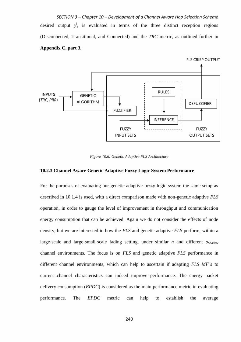
SECTION 3 – Chapter 10 – Development of a Channel Aware Hop Selection Scheme
240
desired output yl, is evaluated in terms of the three distinct reception regions
(Disconnected, Transitional, and Connected) and the TRC metric, as outlined further in
Appendix C, part 3.
Figure 10.6: Genetic Adaptive FLS Architecture
10.2.3 Channel Aware Genetic Adaptive Fuzzy Logic System Performance
For the purposes of evaluating our genetic adaptive fuzzy logic system the same setup as
described in 10.1.4 is used, with a direct comparison made with non-genetic adaptive FLS
operation, in order to gauge the level of improvement in throughput and communication
energy consumption that can be achieved. Again we do not consider the effects of node
density, but we are interested in how the FLS and genetic adaptive FLS perform, within a
large-scale and large-small-scale fading setting, under similar n and different σShadow
channel environments. The focus is on FLS and genetic adaptive FLS performance in
different channel environments, which can help to ascertain if adapting FLS MF’s to
current channel characteristics can indeed improve performance. The energy packet
delivery consumption (EPDC) is considered as the main performance metric in evaluating
performance. The EPDC metric can help to establish the average
INPUTS (TRC, PRR)
RULES
INFERENCE
FUZZIFIER
DEFUZZIFIER
FUZZY
INPUT SETS
FUZZY
OUTPUT SETS
FLS CRISP OUTPUT
GENETIC
ALGORITHM
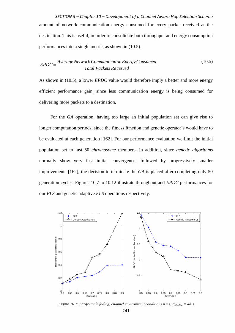
SECTION 3 – Chapter 10 – Development of a Channel Aware Hop Selection Scheme
241
amount of network communication energy consumed for every packet received at the
destination. This is useful, in order to consolidate both throughput and energy consumption
performances into a single metric, as shown in (10.5).
ceivedRePacketsTotal
ConsumedEnergyionCommunicatNetworkAverageEPDC
(10.5)
As shown in (10.5), a lower EPDC value would therefore imply a better and more energy
efficient performance gain, since less communication energy is being consumed for
delivering more packets to a destination.
For the GA operation, having too large an initial population set can give rise to
longer computation periods, since the fitness function and genetic operator’s would have to
be evaluated at each generation [162]. For our performance evaluation we limit the initial
population set to just 50 chromosome members. In addition, since genetic algorithms
normally show very fast initial convergence, followed by progressively smaller
improvements [162], the decision to terminate the GA is placed after completing only 50
generation cycles. Figures 10.7 to 10.12 illustrate throughput and EPDC performances for
our FLS and genetic adaptive FLS operations respectively.
Figure 10.7: Large-scale fading, channel environment conditions n =4, σShadow = 4dB
0.5 0.55 0.6 0.65 0.7 0.75 0.8 0.85 0.90
0.2
0.4
0.6
0.8
1
1.2
Bernoulli-p
Thro
ughput
(Packets
/Second)
0.5 0.55 0.6 0.65 0.7 0.75 0.8 0.85 0.90
0.5
1
1.5
2
2.5
Bernoulli-p
EP
DC
(Joule
s/P
acket
Receiv
ed)
FLS
Genetic Adaptive FLS
FLS
Genetic Adaptive FLS
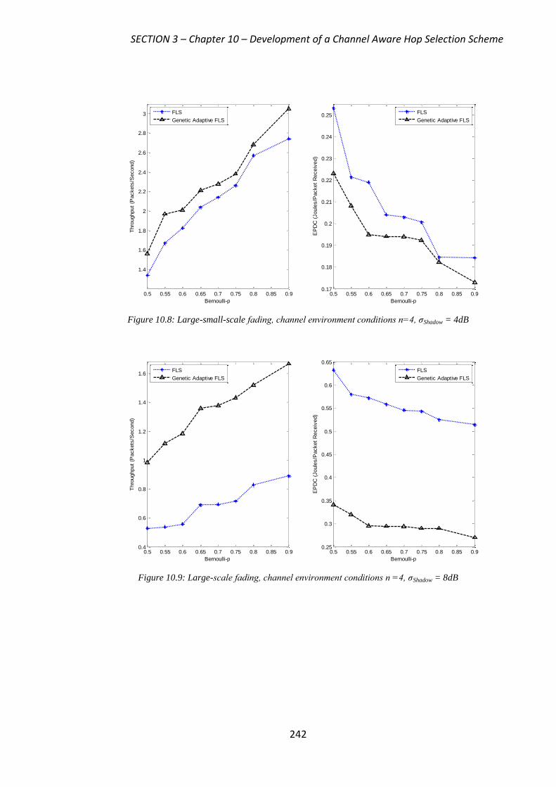
SECTION 3 – Chapter 10 – Development of a Channel Aware Hop Selection Scheme
242
Figure 10.8: Large-small-scale fading, channel environment conditions n=4, σShadow = 4dB
Figure 10.9: Large-scale fading, channel environment conditions n =4, σShadow = 8dB
0.5 0.55 0.6 0.65 0.7 0.75 0.8 0.85 0.9
1.4
1.6
1.8
2
2.2
2.4
2.6
2.8
3
Bernoulli-p
Thro
ughput
(Packets
/Second)
0.5 0.55 0.6 0.65 0.7 0.75 0.8 0.85 0.90.17
0.18
0.19
0.2
0.21
0.22
0.23
0.24
0.25
Bernoulli-p
EP
DC
(Joule
s/P
acket
Receiv
ed)
FLS
Genetic Adaptive FLS
FLS
Genetic Adaptive FLS
0.5 0.55 0.6 0.65 0.7 0.75 0.8 0.85 0.90.4
0.6
0.8
1
1.2
1.4
1.6
Bernoulli-p
Thro
ughput
(Packets
/Second)
0.5 0.55 0.6 0.65 0.7 0.75 0.8 0.85 0.90.25
0.3
0.35
0.4
0.45
0.5
0.55
0.6
0.65
Bernoulli-p
EP
DC
(Joule
s/P
acket
Receiv
ed)
FLS
Genetic Adaptive FLS
FLS
Genetic Adaptive FLS
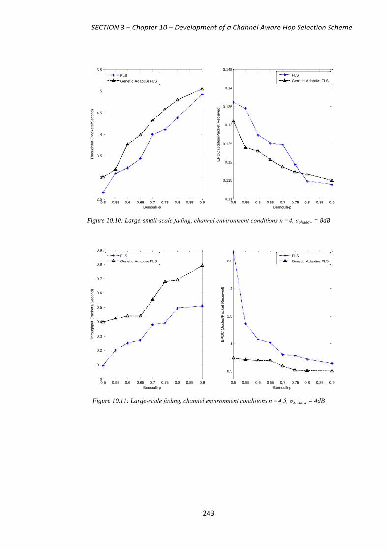
SECTION 3 – Chapter 10 – Development of a Channel Aware Hop Selection Scheme
243
Figure 10.10: Large-small-scale fading, channel environment conditions n =4, σShadow = 8dB
Figure 10.11: Large-scale fading, channel environment conditions n =4.5, σShadow = 4dB
0.5 0.55 0.6 0.65 0.7 0.75 0.8 0.85 0.92.5
3
3.5
4
4.5
5
5.5
Bernoulli-p
Thro
ughput
(Packets
/Second)
0.5 0.55 0.6 0.65 0.7 0.75 0.8 0.85 0.90.11
0.115
0.12
0.125
0.13
0.135
0.14
0.145
Bernoulli-p
EP
DC
(Joule
s/P
acket
Receiv
ed)
FLS
Genetic Adaptive FLS
FLS
Genetic Adaptive FLS
0.5 0.55 0.6 0.65 0.7 0.75 0.8 0.85 0.90
0.1
0.2
0.3
0.4
0.5
0.6
0.7
0.8
0.9
Bernoulli-p
Thro
ughput
(Packets
/Second)
0.5 0.55 0.6 0.65 0.7 0.75 0.8 0.85 0.9
0.5
1
1.5
2
2.5
Bernoulli-p
EP
DC
(Joule
s/P
acket
Receiv
ed)
FLS
Genetic Adaptive FLS
FLS
Genetic Adaptive FLS
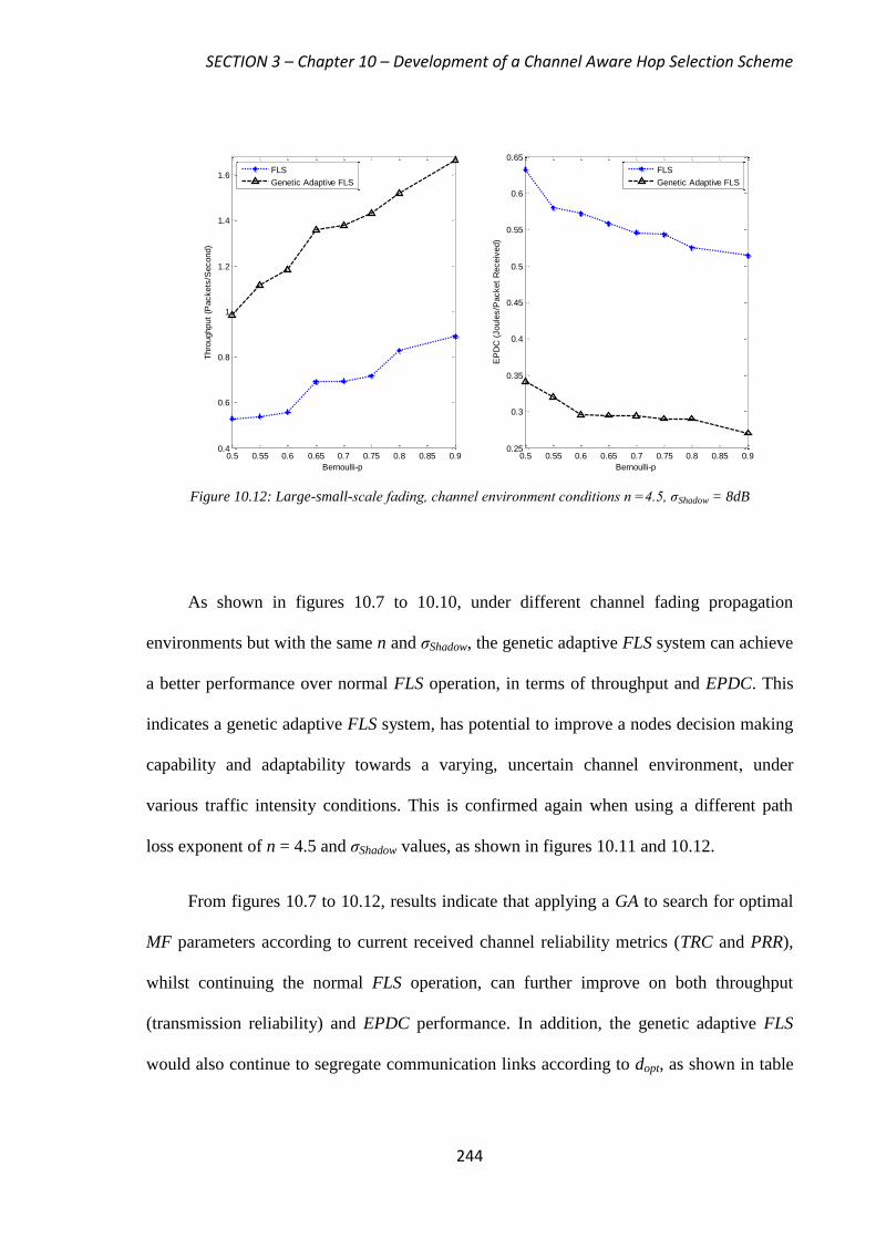
SECTION 3 – Chapter 10 – Development of a Channel Aware Hop Selection Scheme
244
Figure 10.12: Large-small-scale fading, channel environment conditions n =4.5, σShadow = 8dB
As shown in figures 10.7 to 10.10, under different channel fading propagation
environments but with the same n and σShadow, the genetic adaptive FLS system can achieve
a better performance over normal FLS operation, in terms of throughput and EPDC. This
indicates a genetic adaptive FLS system, has potential to improve a nodes decision making
capability and adaptability towards a varying, uncertain channel environment, under
various traffic intensity conditions. This is confirmed again when using a different path
loss exponent of n = 4.5 and σShadow values, as shown in figures 10.11 and 10.12.
From figures 10.7 to 10.12, results indicate that applying a GA to search for optimal
MF parameters according to current received channel reliability metrics (TRC and PRR),
whilst continuing the normal FLS operation, can further improve on both throughput
(transmission reliability) and EPDC performance. In addition, the genetic adaptive FLS
would also continue to segregate communication links according to dopt, as shown in table
0.5 0.55 0.6 0.65 0.7 0.75 0.8 0.85 0.90.4
0.6
0.8
1
1.2
1.4
1.6
Bernoulli-p
Thro
ughput
(Packets
/Second)
0.5 0.55 0.6 0.65 0.7 0.75 0.8 0.85 0.90.25
0.3
0.35
0.4
0.45
0.5
0.55
0.6
0.65
Bernoulli-p
EP
DC
(Joule
s/P
acket
Receiv
ed)
FLS
Genetic Adaptive FLS
FLS
Genetic Adaptive FLS

SECTION 3 – Chapter 10 – Development of a Channel Aware Hop Selection Scheme
245
10.1. This leads us to consider when combining both a genetic adaptive capability to vary
FLS MF parameters and to enforce node selection according to dopt, can support better
throughput and EPDC performance. Figures 10.7 to 10.12 also show that a genetic
adaptive FLS can increase throughput performance and at the same time consume on
average less energy for every packet received, as traffic intensity conditions increase, when
compared with normal FLS operation by some 44%. For the simulated network scenario,
this indicates that the genetic adaptive FLS system can achieve improved energy-load
balancing. Improvement in energy-load balancing is possible since, a genetic adaptive FLS
system would actively seek to identify links opportunistically, which exhibit a higher TRC
according to its adapted MF’s, to increase performance over normal FLS operation.
An additional observation from figures 10.10, 10.11 and 10.12, when compared with
figures 10.7, 10.8 and 10.9, shows the effect of the large-small-scale channel fading
environment on improving throughput on average by 17% and EPDC performance on
average by 40%. Operating in a large-small-scale channel fading environment, which
would typically be a similar wireless environment to be found in a realistic UGS
surveillance setting, can assist in increasing throughput and reducing EPDC further. The
effects of a large-small-scale channel fading environment suggests it can naturally
encourage better opportunistic forwarding selection and therefore, encourage a higher
chance of successful packet reception, but without some further investigation this finding
cannot be made completely conclusive.
SECTION 3 – Chapter 11 – Summary and Conclusions
246
CHAPTER 11
Section 3: Summary and Conclusions
UGS networks typically operate in wireless environments, which can vary considerably in
both space and time, due to channel fading propagation effects. Chapter 9 began by
quantifying the channel fading propagation effects, in terms of being either large-scale or
large-small-scale fading. Channel fading effects can determine the success in packet
reception, which as a result can influence communication link reliability between node
pairs, communication energy consumption and overall network throughput. It is also
shown that mitigating on the effects of communication link unreliability can be assisted by
dividing packet reception into three distinct reception regions, these being connected,
transitional and disconnected, according to link distance.
In 9.2, we then introduced the transitional region, which is characterised by
asymmetric connectivity with high variance in PRR. We then quantified the size of the
transitional region by defining a known metric called the TRC. The TRC in its own right
can serve as a value of merit for current link reliability, by giving an indication of the
extent of the transitional to connected region parts of a communication link. The TRC, as
expected is effected by the channel environment conditions, with σshadow increasing TRC
and n reducing the TRC, as shown in figure 9.5.
One of the main contributions of this chapter was then to study, understand and
examine what impact the TRC might have on communication link reliability, in terms of
the optimal packet forwarding distance (dopt), transmission reliability and ETX, within
different channel fading environments. In headings 9.2.2 to 9.2.4, we analysed how
communication link reliability and link quality (ETX metric) performance can be affected
SECTION 3 – Chapter 11 – Summary and Conclusions
247
by the TRC within different channel environments, which the main findings are
summarised as follows:
In 9.2.2, a higher TRC can increase dopt by maximising E [PRR] for a set channel
environment, as shown in figure 9.6 and for various σshadow, as shown in figure 9.7(b).
These findings indicate that a higher TRC could potentially compensate for an
unreliable wireless environment, through achieving a better E [PRR] range, with a
lower decay rate from dopt to dmax, as shown in figure 9.7 (b).
In 9.2.3, a lower TRC achieves better transmission reliability performance over shorter
communication link distances and this is reversed for a small gain in performance over
larger distances, as shown in figure 9.9. A lower TRC should be used for channel
environments with an increasing n and higher TRC for increasing σshadow, as shown in
figure 9.10.
In 9.2.4, a higher TRC value can minimise on ETX, over larger communication link
distances through maintaining the same Ph (γ-Upper-dB) value and lowering the Pl (γ-Lower-
dB) value. Over shorter hop-distances increasing the TRC has no effect on minimising
ETX, but remains in an ideal state. Figure 9.12, also indicates that increasing the TRC
can however mitigate on channel environment conditions with increasing n and σshadow,
over longer hop-distances for improved ETX performance.
The findings from above lead us to suggest that potential packet forwarding nodes can be
best achieved through identifying links with a higher TRC value, due to a higher E[PRR]
range and better ETX performance (whilst maintaining a fixed Ph value). However over
shorter hop distances (≤ dopt), we conclude that identifying links with a lower TRC are
given priority since this achieves better transmission reliability, while maintaining an ideal
ETX.
SECTION 3 – Chapter 11 – Summary and Conclusions
248
As a matter of further reassurance in 9.3, the impact of the TRC on further reducing
the number of transmissions required for successful packet delivery within a realistic
wireless broadcast environment is detailed. We considered the broadcast environment
since this has the advantage of allowing multiple paths (diversity) from a source towards a
destination to exist. In 9.3, we explored the idea behind OAPF as a potential way to further
reducing the number of transmissions required for successful packet reception and
therefore as a means of mitigating against the unreliable channel environment, to inflict
changes on local topology. OAPF, through the EAX metric, considers the broadcast nature
of wireless channel transmissions as opportunities that can be taken advantage of in a
distributed manner, so as to increase the chance a packet is received successfully towards
its destination. Utilising a distributed hop-by-hop strategy for packet forwarding in this
manner can also offer advantages by firstly, being easier to implement and secondly in
achieving network scalability, which are important attributes required for UGS surveillance
operations. The main findings of whether combining the TRC within an OAPF
environment can affect the number of transmissions required for successful packet delivery
for a 2-hop scenario, are summarised below:
Our analytical findings indicate that utilising a higher TRC through varying Pl (γ-Lower-
dB) with a set Ph (γ-Upper-dB) value within an OAPF environment, can indeed achieve
better ETX performance.
We also conclude that the number of transmissions required for a successful packet
delivery is improved within an OAPF (EAX metric) environment against ETX over
higher transmission ranges, as shown in figure 9.13.
Increasing the forwarding selection diversity (number of nodes deployed between a
source and destination), can also help to reduce the number of transmissions required
for successful packet delivery. This finding suggests that permitting nodes to decide,
packet forwarding actions based on link reliability knowledge of multiple relay paths,
SECTION 3 – Chapter 11 – Summary and Conclusions
249
in a distributed manner, can assist in providing robustness against communication link
unreliability.
In general, utilising the broadcast transmission channel to select nodes opportunistically
assists in reducing the number of transmissions required for successful packet reception
and subsequently, can help to mitigate the effects of communication link unreliability
further.
Based on the TRC study made in chapter 9, under 9.3 and 9.4, the second main
contribution of this chapter was to bring these findings together into an overall decision
making mechanism, in order to cater against the effects of the channel fading environment.
Such a mechanism would then allow UGS nodes to evaluate and select nodes for reliable
packet forwarding, in a distributed manner. For this purpose a FLS system is used and
deemed suitable because of its ability to assist in making decisions within high uncertainty
environments, similar to channel fading, as described in chapter 10, under 10.1.
Normal FLS operation performance can also be improved by providing a mechanism,
which can adjust to the channel environment, in order to make decision making relevant to
a current underlying channel environment. For this purpose a GA is implemented and
integrated within normal FLS operation, in order to provide adaptability to the channel
environment, as detailed in section 4.6 and shown in figure 10.6. Simulation results
conducted under different channel fading environments indicate that for a Genetic adaptive
FLS operation an improvement is indeed made, in terms of throughput and EDPC over
normal FLS operation. An improvement is possible since, a genetic adaptive FLS system
would actively seek to identify links opportunistically, which exhibit either a lower TRC (if
≤ dopt) or higher TRC (if ≥ dopt) according to its adapted MF’s, to increase performance
over normal FLS operation.
SECTION 3 – Chapter 11 – Summary and Conclusions
250
In summary, results for the simulated network scenario made in 10.2.3, suggest
utilising a genetic adaptive FLS has potential to provide the following advantages:
A fully distributed approach, where each UGS node only needs to evaluate its network
link quality values (TRC and PRR) and apply the genetic adaptive FLS system, for
packet forwarding node selection.
A genetic adaptive FLS can therefore allow UGS nodes to make relevant self-managed
decisions on, which one-hop neighbour should be chosen for reliable packet forwarding
at discrete points in time.
In addition, findings from this section show that a genetic adaptive FLS scheme has
potential to improve distributed surveillance missions by allowing it to be integrated with,
upper-layer operations. In this way, advantages within an unreliable communication
environment can be achieved in the following way:
Only a reduced number of nodes (those with good channel reliability) will be
competing for available bandwidth, which can help to increase network throughput,
but with lower communication energy consumption.
It is important to also note that the computational expense of applying a genetic adaptive
FLS on every packet received has not been evaluated. This of course will be very high
given the nature of using a genetic optimiser [162] and as a result, will contribute towards
increasing overall energy consumption and a reduction in network longevity which may
prove to be impractical, given the nature of UGS deployment.
In section 4, however, we continue to investigate whether the use of channel
reliability information from the physical layer that is processed using our genetic adaptive
FLS scheme and then shared with both the application (VIGILANT+) and network layers
(SWOB geographic routing), can assist their respective procedures and improve on overall
distributed operation within an unreliable wireless channel environment.

SECTION 4 – Introduction
251
SECTION 4
Integrated System Performance
Introduction
Unattended ground sensor (UGS) networks are classified as distributed systems, capable of
supporting mission objectives such as, threat presence detection and geo-location within a
security-sensitive region. Our performance appraisals concerning distributed mission
objective operation, as detailed in sections 1 and 2 have, thus far, been evaluated under
error free wireless channel conditions (physical environment). For an overall performance
viewpoint, UGS networks should ultimately be assessed as distributed systems, operating
within both their deployed surveillance and physical environment. UGS networks, which
are assessed in this manner, are commonly referred to as mission orientated sensor
networks (MOSN) [163]. A mission orientated capability is an important attribute to have,
since, the notion of self-reconfigurable UGS networks capable of fulfilling mission
objective requirements within an uncertain physical environment, is supported [163-166].
As a result of mission orientated operation, UGS networks can ensure that a dependable
infrastructure for information collection is available.
The purpose of section 4, is to evaluate a potential mission orientation capability,
through the integration of our genetic adaptive fuzzy logic system (GAFLS), detailed in
section 3, with VIGILANT+, detailed in section 1 and SWOB, detailed in section 2. Our
proposed mission orientated approach can be summarised, as shown in figure 12.1. From
figure 12.1, a potential cross-layer approach towards enabling UGS surveillance operations
within a dynamic mission-orientated environment, is illustrated. In essence, the GAFLS
mechanism is responsible for providing reliable forwarding node selection knowledge to
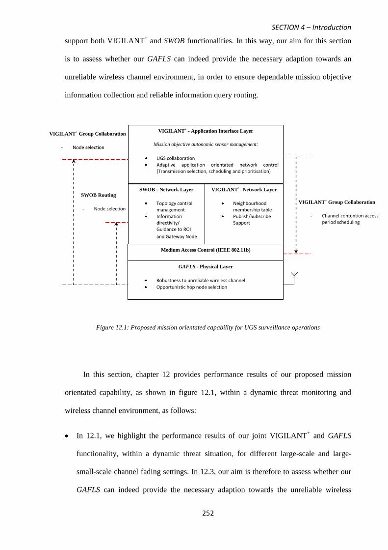
SECTION 4 – Introduction
252
support both VIGILANT+ and SWOB functionalities. In this way, our aim for this section
is to assess whether our GAFLS can indeed provide the necessary adaption towards an
unreliable wireless channel environment, in order to ensure dependable mission objective
information collection and reliable information query routing.
Figure 12.1: Proposed mission orientated capability for UGS surveillance operations
In this section, chapter 12 provides performance results of our proposed mission
orientated capability, as shown in figure 12.1, within a dynamic threat monitoring and
wireless channel environment, as follows:
In 12.1, we highlight the performance results of our joint VIGILANT+ and GAFLS
functionality, within a dynamic threat situation, for different large-scale and large-
small-scale channel fading settings. In 12.3, our aim is therefore to assess whether our
GAFLS can indeed provide the necessary adaption towards the unreliable wireless
VIGILANT+ Group Collaboration
- Channel contention access period scheduling
GAFLS - Physical Layer
Robustness to unreliable wireless channel
Opportunistic hop node selection
Medium Access Control (IEEE 802.11b)
VIGILANT+ - Application Interface Layer
Mission objective autonomic sensor management:
UGS collaboration
Adaptive application orientated network control (Transmission selection, scheduling and prioritisation)
SWOB - Network Layer
Topology control management
Information directivity/ Guidance to ROI
and Gateway Node
VIGILANT+ Group Collaboration
- Node selection
VIGILANT+- Network Layer
Neighbourhood membership table
Publish/Subscribe Support
SWOB Routing
- Node selection

SECTION 4 – Introduction
253
channel environment, in order to ensure dependable mission objective information
collection.
In 12.2, a similar exercise is repeated for SWOB but only for different large-scale and
large-small-scale channel fading settings. In 12.2, our aim is to assess whether our
GAFLS can indeed provide the necessary adaption towards the unreliable wireless
channel environment, in order to ensure reliable information query routing to a
designated ROI.
In 12.3, we then summarise and conclude the main contributions of this section.

SECTION 4 – Chapter 12- Mission Orientated Sensor Surveillance
254
CHAPTER 12
Mission Orientated Sensor Surveillance
12.1 VIGILANT+ Mission Orientated Performance
Simulations are conducted using the OMNeT++ network modeller tool [63]. To simulate a
realistic wide area UGS surveillance setting, a 1km by 1km simulation region is specified,
with nodes being randomly deployed according to a uniform distribution. Simulations are
run using a number of random deployments (>50), each with duration of 100 detectable
events. As part of our evaluation we do not consider the effects of increasing node density
on VIGILANT+ mission orientated performance and so for the purposes of simulation, an
arbitrary total of 20 nodes are used with communication parameters, as specified in table
9.1, from section 3, chapter 9. We do not consider the effects of increasing node density,
since, in this section our evaluation is primarily concerned with VIGILANT+ performance
within an uncertain and variable wireless channel environment setting.
Threat mobility characteristics are again simulated using the random waypoint
(RWP) model, with a dynamic velocity (m/s) set from a uniform distribution, uniform (0,
vmax). A RWP simulation model is again considered because of its extensive use within
surveillance type evaluations, in order to mimic the random movement characteristics of a
realistic monitored threat [78-79]. For the purposes of VIGILANT+ performance, we only
simulate for a single vmax condition. In addition, the effects of threat velocity have already
been discussed in section 1, chapter 5, under heading 5.4. We also assume that deployed
sensors have accurate knowledge concerning a threat presence and therefore, we operate in
a low false alarm surveillance environment (i.e. Threat Observation Certainty (TOC) =
0.9). We consider this condition, since the effects of the false alarm environment on
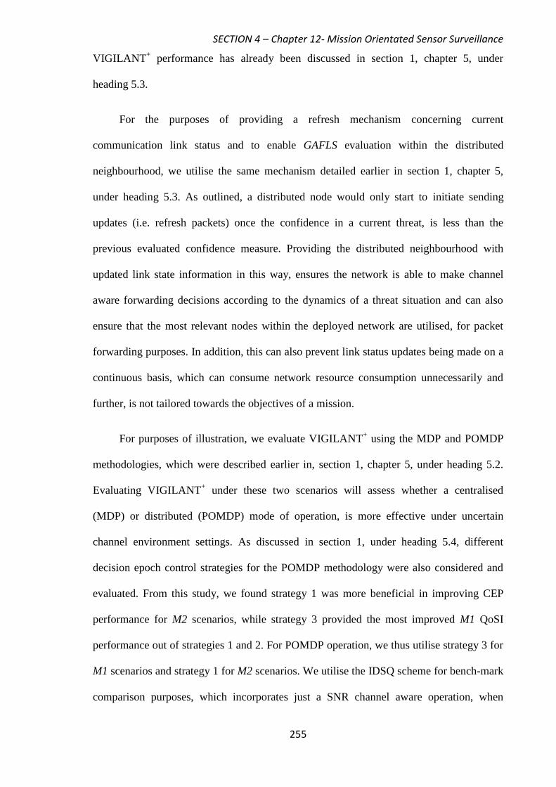
SECTION 4 – Chapter 12- Mission Orientated Sensor Surveillance
255
VIGILANT+ performance has already been discussed in section 1, chapter 5, under
heading 5.3.
For the purposes of providing a refresh mechanism concerning current
communication link status and to enable GAFLS evaluation within the distributed
neighbourhood, we utilise the same mechanism detailed earlier in section 1, chapter 5,
under heading 5.3. As outlined, a distributed node would only start to initiate sending
updates (i.e. refresh packets) once the confidence in a current threat, is less than the
previous evaluated confidence measure. Providing the distributed neighbourhood with
updated link state information in this way, ensures the network is able to make channel
aware forwarding decisions according to the dynamics of a threat situation and can also
ensure that the most relevant nodes within the deployed network are utilised, for packet
forwarding purposes. In addition, this can also prevent link status updates being made on a
continuous basis, which can consume network resource consumption unnecessarily and
further, is not tailored towards the objectives of a mission.
For purposes of illustration, we evaluate VIGILANT+ using the MDP and POMDP
methodologies, which were described earlier in, section 1, chapter 5, under heading 5.2.
Evaluating VIGILANT+ under these two scenarios will assess whether a centralised
(MDP) or distributed (POMDP) mode of operation, is more effective under uncertain
channel environment settings. As discussed in section 1, under heading 5.4, different
decision epoch control strategies for the POMDP methodology were also considered and
evaluated. From this study, we found strategy 1 was more beneficial in improving CEP
performance for M2 scenarios, while strategy 3 provided the most improved M1 QoSI
performance out of strategies 1 and 2. For POMDP operation, we thus utilise strategy 3 for
M1 scenarios and strategy 1 for M2 scenarios. We utilise the IDSQ scheme for bench-mark
comparison purposes, which incorporates just a SNR channel aware operation, when
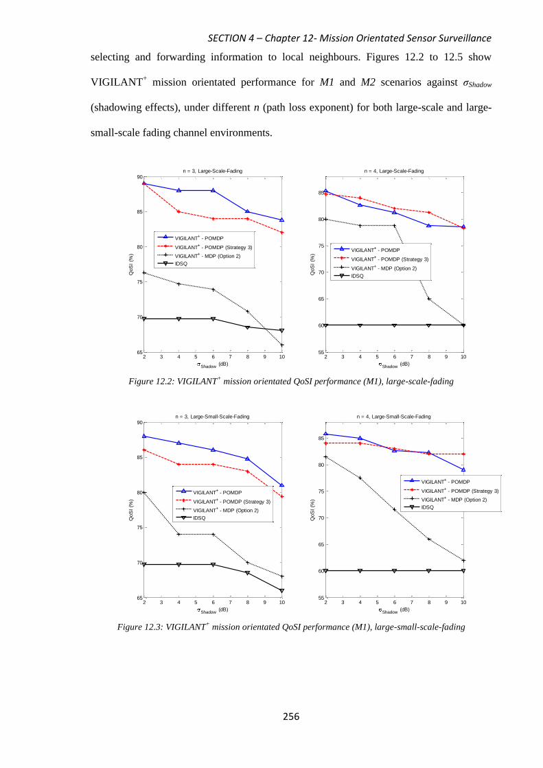
SECTION 4 – Chapter 12- Mission Orientated Sensor Surveillance
256
selecting and forwarding information to local neighbours. Figures 12.2 to 12.5 show
VIGILANT+ mission orientated performance for M1 and M2 scenarios against σShadow
(shadowing effects), under different n (path loss exponent) for both large-scale and large-
small-scale fading channel environments.
Figure 12.2: VIGILANT+ mission orientated QoSI performance (M1), large-scale-fading
Figure 12.3: VIGILANT+ mission orientated QoSI performance (M1), large-small-scale-fading
2 3 4 5 6 7 8 9 1065
70
75
80
85
90n = 3, Large-Scale-Fading
Shadow (dB)
QoS
I (%
)
2 3 4 5 6 7 8 9 1055
60
65
70
75
80
85
n = 4, Large-Scale-Fading
Shadow (dB)
QoS
I (%
)
VIGILANT+ - POMDP
VIGILANT+ - POMDP (Strategy 3)
VIGILANT+ - MDP (Option 2)
IDSQ
VIGILANT+ - POMDP
VIGILANT+ - POMDP (Strategy 3)
VIGILANT+ - MDP (Option 2)
IDSQ
2 3 4 5 6 7 8 9 1065
70
75
80
85
90
Shadow (dB)
QoS
I (%
)
n = 3, Large-Small-Scale-Fading
2 3 4 5 6 7 8 9 1055
60
65
70
75
80
85
Shadow (dB)
QoS
I (%
)
n = 4, Large-Small-Scale-Fading
VIGILANT+ - POMDP
VIGILANT+ - POMDP (Strategy 3)
VIGILANT+ - MDP (Option 2)
IDSQ
VIGILANT+ - POMDP
VIGILANT+ - POMDP (Strategy 3)
VIGILANT+ - MDP (Option 2)
IDSQ
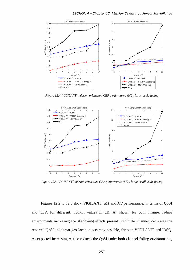
SECTION 4 – Chapter 12- Mission Orientated Sensor Surveillance
257
Figure 12.4: VIGILANT+ mission orientated CEP performance (M2), large-scale fading
Figure 12.5: VIGILANT+ mission orientated CEP performance (M2), large-small-scale fading
Figures 12.2 to 12.5 show VIGILANT+ M1 and M2 performance, in terms of QoSI
and CEP, for different, σShadow, values in dB. As shown for both channel fading
environments increasing the shadowing effects present within the channel, decreases the
reported QoSI and threat geo-location accuracy possible, for both VIGILANT+ and IDSQ.
As expected increasing n, also reduces the QoSI under both channel fading environments,
2 3 4 5 6 7 8 9 102.6
2.8
3
3.2
3.4
3.6
3.8
4
4.2
4.4
4.6
Shadow (dB)
CE
P-5
0%
(m
etr
es)
n = 3, Large-Scale-Fading
2 3 4 5 6 7 8 9 102
4
6
8
10
12
14
Shadow (dB)
CE
P-5
0%
(m
etr
es)
n = 4, Large-Scale-Fading
VIGILANT+ - POMDP
VIGILANT+ - POMDP (Strategy 1)
VIGILANT+ - MDP (Option 2)
IDSQ
VIGILANT+ - POMDP
VIGILANT+ - POMDP (Strategy 1)
VIGILANT+ - MDP (Option 2)
IDSQ
2 3 4 5 6 7 8 9 102.8
3
3.2
3.4
3.6
3.8
4
4.2
4.4
4.6
4.8
Shadow (dB)
CE
P-5
0%
(m
etr
es)
n = 3, Large-Small-Scale Fading
2 3 4 5 6 7 8 9 102
4
6
8
10
12
14
Shadow (dB)
CE
P-5
0%
(m
etr
es)
n = 4, Large-Small-Scale Fading
VIGILANT+ - POMDP
VIGILANT+ - POMDP (Strategy 1)
VIGILANT+ - MDP (Option 2)
IDSQ
VIGILANT+ - POMDP
VIGILANT+ - POMDP (Strategy 1)
VIGILANT+ - MDP (Option 2)
IDSQ
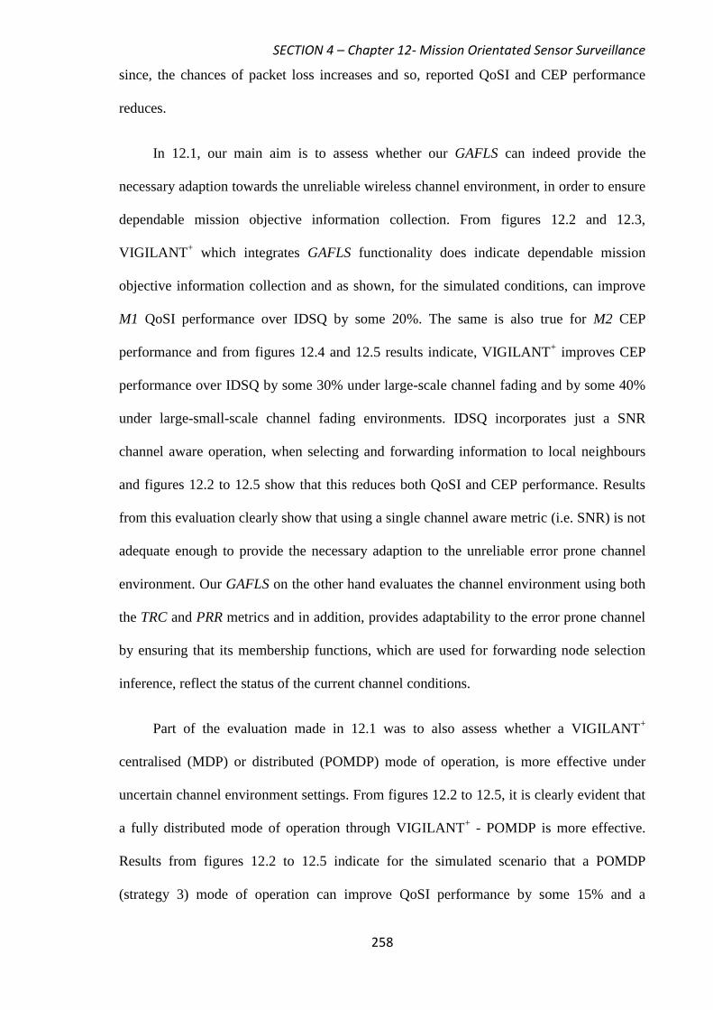
SECTION 4 – Chapter 12- Mission Orientated Sensor Surveillance
258
since, the chances of packet loss increases and so, reported QoSI and CEP performance
reduces.
In 12.1, our main aim is to assess whether our GAFLS can indeed provide the
necessary adaption towards the unreliable wireless channel environment, in order to ensure
dependable mission objective information collection. From figures 12.2 and 12.3,
VIGILANT+ which integrates GAFLS functionality does indicate dependable mission
objective information collection and as shown, for the simulated conditions, can improve
M1 QoSI performance over IDSQ by some 20%. The same is also true for M2 CEP
performance and from figures 12.4 and 12.5 results indicate, VIGILANT+ improves CEP
performance over IDSQ by some 30% under large-scale channel fading and by some 40%
under large-small-scale channel fading environments. IDSQ incorporates just a SNR
channel aware operation, when selecting and forwarding information to local neighbours
and figures 12.2 to 12.5 show that this reduces both QoSI and CEP performance. Results
from this evaluation clearly show that using a single channel aware metric (i.e. SNR) is not
adequate enough to provide the necessary adaption to the unreliable error prone channel
environment. Our GAFLS on the other hand evaluates the channel environment using both
the TRC and PRR metrics and in addition, provides adaptability to the error prone channel
by ensuring that its membership functions, which are used for forwarding node selection
inference, reflect the status of the current channel conditions.
Part of the evaluation made in 12.1 was to also assess whether a VIGILANT+
centralised (MDP) or distributed (POMDP) mode of operation, is more effective under
uncertain channel environment settings. From figures 12.2 to 12.5, it is clearly evident that
a fully distributed mode of operation through VIGILANT+ - POMDP is more effective.
Results from figures 12.2 to 12.5 indicate for the simulated scenario that a POMDP
(strategy 3) mode of operation can improve QoSI performance by some 15% and a
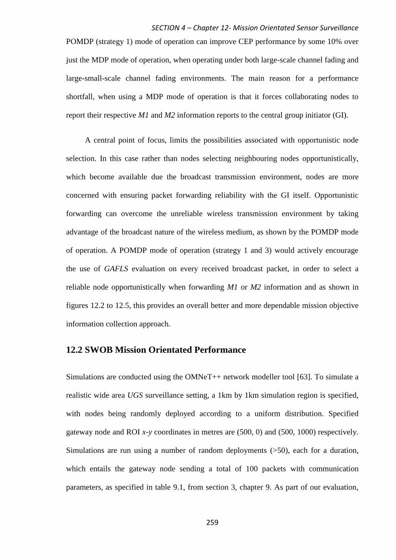
SECTION 4 – Chapter 12- Mission Orientated Sensor Surveillance
259
POMDP (strategy 1) mode of operation can improve CEP performance by some 10% over
just the MDP mode of operation, when operating under both large-scale channel fading and
large-small-scale channel fading environments. The main reason for a performance
shortfall, when using a MDP mode of operation is that it forces collaborating nodes to
report their respective M1 and M2 information reports to the central group initiator (GI).
A central point of focus, limits the possibilities associated with opportunistic node
selection. In this case rather than nodes selecting neighbouring nodes opportunistically,
which become available due the broadcast transmission environment, nodes are more
concerned with ensuring packet forwarding reliability with the GI itself. Opportunistic
forwarding can overcome the unreliable wireless transmission environment by taking
advantage of the broadcast nature of the wireless medium, as shown by the POMDP mode
of operation. A POMDP mode of operation (strategy 1 and 3) would actively encourage
the use of GAFLS evaluation on every received broadcast packet, in order to select a
reliable node opportunistically when forwarding M1 or M2 information and as shown in
figures 12.2 to 12.5, this provides an overall better and more dependable mission objective
information collection approach.
12.2 SWOB Mission Orientated Performance
Simulations are conducted using the OMNeT++ network modeller tool [63]. To simulate a
realistic wide area UGS surveillance setting, a 1km by 1km simulation region is specified,
with nodes being randomly deployed according to a uniform distribution. Specified
gateway node and ROI x-y coordinates in metres are (500, 0) and (500, 1000) respectively.
Simulations are run using a number of random deployments (>50), each for a duration,
which entails the gateway node sending a total of 100 packets with communication
parameters, as specified in table 9.1, from section 3, chapter 9. As part of our evaluation,

SECTION 4 – Chapter 12- Mission Orientated Sensor Surveillance
260
we do not consider the effects of increasing node density on SWOB mission orientated
performance and so, for the purposes of simulation an arbitrary total of 20 nodes are used.
We do not consider the effects of increasing node density, since, our evaluation is
primarily again concerned with SWOB performance within an uncertain and variable
wireless channel environment setting.
We also evaluate SWOB mission orientated performance under opportunistic
forwarding conditions and in this sense, overheard broadcast messages from neighbouring
nodes are used for the purposes of providing a refresh mechanism, concerning current
communication link status and to enable GAFLS evaluation, within the distributed
neighbourhood. Providing the distributed neighbourhood with updated link status in this
way, ensures the network is able to make channel aware forwarding decisions according to
the current dynamics of the channel environment. In addition, this can also prevent link
status updates being made on a continuous basis, which can consume network resource
consumption unnecessarily.
The main SWOB performance evaluation aims conducted in section 2, chapter 7, in
7.3 were to measure throughput and energy efficiency performance. In 12.2, we maintain
these two performance criteria’s when evaluating SWOB under different large-scale and
large-small-scale channel fading settings. In this sense, using a throughput metric measures
overall network bandwidth utilisation efficiency, while energy efficiency measures how
well SWOB conserves on energy consumption, in order to complete its forwarding tasks,
under an error prone wireless channel environment. The same equation given in section 2,
chapter 7, as (7.24) is used to calculate energy efficiency. For SWOB comparison purposes,
we utilise the GeRAF routing strategy, as detailed earlier in 7.3. GeRAF is used, since it
also employs a geographic opportunistic forwarding strategy to overcome the drawback of
the unreliable transmission environment. Figures 12.6 to 12.9 show SWOB mission
SECTION 4 – Chapter 12- Mission Orientated Sensor Surveillance
261
orientated performance against σShadow (shadowing effects), under different n (path loss
exponent) for both large-scale and large-small-scale fading channel environments.
In 12.2, our main aim is to assess whether our GAFLS can indeed provide the
necessary adaption towards the unreliable wireless channel environment, in order to ensure
reliable information query routing to a designated ROI. From figures 12.6 to 12.9, SWOB
which integrates GAFLS functionality can improve on both throughput and energy
efficiency performance over GeRAF.
Figure 12.6: SWOB mission orientated throughput and comparison, large-scale-fading
2 3 4 5 6 7 8 9 102
4
6
8
10
12
14
16
18
Shadow (dB)
Thro
ughput
(kbits/s
econd)
n = 3, Large-Scale-Fading
2 3 4 5 6 7 8 9 103
4
5
6
7
8
9
10
11
12
13
Shadow (dB)
Thro
ughput
(kbits/s
econd)
n = 4, Large-Scale-Fading
SWOB (k >= 5) - GAFLS
GERAF
SWOB (k >= 5) - GAFLS
GERAF
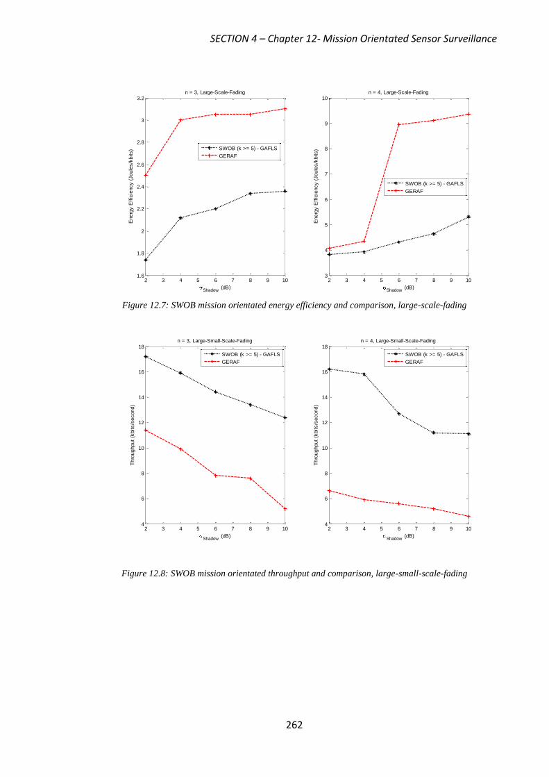
SECTION 4 – Chapter 12- Mission Orientated Sensor Surveillance
262
Figure 12.7: SWOB mission orientated energy efficiency and comparison, large-scale-fading
Figure 12.8: SWOB mission orientated throughput and comparison, large-small-scale-fading
2 3 4 5 6 7 8 9 101.6
1.8
2
2.2
2.4
2.6
2.8
3
3.2
Shadow (dB)
Energ
y E
ffic
iency (
Joule
s/k
bits)
n = 3, Large-Scale-Fading
2 3 4 5 6 7 8 9 103
4
5
6
7
8
9
10
Shadow (dB)
Energ
y E
ffic
iency (
Joule
s/k
bits)
n = 4, Large-Scale-Fading
SWOB (k >= 5) - GAFLS
GERAF
SWOB (k >= 5) - GAFLS
GERAF
2 3 4 5 6 7 8 9 104
6
8
10
12
14
16
18
Shadow (dB)
Thro
ughput
(kbits/s
econd)
n = 3, Large-Small-Scale-Fading
2 3 4 5 6 7 8 9 104
6
8
10
12
14
16
18
Shadow (dB)
Thro
ughput
(kbits/s
econd)
n = 4, Large-Small-Scale-Fading
SWOB (k >= 5) - GAFLS
GERAF
SWOB (k >= 5) - GAFLS
GERAF
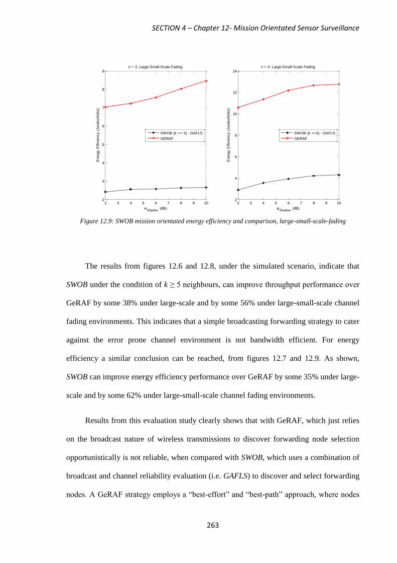
SECTION 4 – Chapter 12- Mission Orientated Sensor Surveillance
263
Figure 12.9: SWOB mission orientated energy efficiency and comparison, large-small-scale-fading
The results from figures 12.6 and 12.8, under the simulated scenario, indicate that
SWOB under the condition of k ≥ 5 neighbours, can improve throughput performance over
GeRAF by some 38% under large-scale and by some 56% under large-small-scale channel
fading environments. This indicates that a simple broadcasting forwarding strategy to cater
against the error prone channel environment is not bandwidth efficient. For energy
efficiency a similar conclusion can be reached, from figures 12.7 and 12.9. As shown,
SWOB can improve energy efficiency performance over GeRAF by some 35% under large-
scale and by some 62% under large-small-scale channel fading environments.
Results from this evaluation study clearly shows that with GeRAF, which just relies
on the broadcast nature of wireless transmissions to discover forwarding node selection
opportunistically is not reliable, when compared with SWOB, which uses a combination of
broadcast and channel reliability evaluation (i.e. GAFLS) to discover and select forwarding
nodes. A GeRAF strategy employs a “best-effort” and “best-path” approach, where nodes
2 3 4 5 6 7 8 9 102
3
4
5
6
7
8
9
Shadow (dB)
Energ
y E
ffic
iency (
Joule
s/k
bits)
n = 3, Large-Small-Scale Fading
2 3 4 5 6 7 8 9 102
4
6
8
10
12
14
Shadow (dB)
Energ
y E
ffic
iency (
Joule
s/k
bits)
n = 4, Large-Small-Scale Fading
SWOB (k >=5) - GAFLS
GERAF
SWOB (k >= 5) - GAFLS
GERAF

SECTION 4 – Chapter 12- Mission Orientated Sensor Surveillance
264
receiving packets judge their forwarding suitability according to, their Euclidean distance
to the destination. As shown in figures 12.6 and 12.8, such an approach can result in a very
poor packet delivery rate (throughput).
SWOB with GAFLS ensures reliable opportunistic forwarding node selection. In
general SWOB on its own would focus on node selection, according to its greedy based
forwarding algorithm (Appendix B, part 3) but, with the addition of a GAFLS, alternative
forwarding nodes can be selected according to both channel reliability and greedy based
forwarding. As shown in figures 12.6 to 12.9, such an approach can result in an improved
packet delivery rate and energy efficiency performance. In addition, the strategy also
employed by GeRAF does not provide any adaption towards the error prone wireless
channel environment. A GAFLS approach used with SWOB can, by ensuring that its
membership functions, which are used for forwarding node selection inference, reflect the
status of the current channel conditions, to help improve throughput and energy efficiency
performance.
12.3 Section 4: Summary and Conclusions
UGS networks should ultimately be assessed as distributed systems, operating within both
their deployed surveillance and physical environments. An assessment of this kind refers to
UGS networks as, mission orientated sensor networks. A Mission orientated capability
supports the notion of self-configurable UGS networks, capable of fulfilling mission
objective requirements within an uncertain physical environment. In this section, we
proposed a potential mission orientation capability, which involved the integration of our
genetic adaptive fuzzy logic system (GAFLS), detailed in section 3, with VIGILANT+,
detailed in section 1 and our SWOB routing protocol, detailed in section 2, as shown in
figure 12.1. We then undertook a performance evaluation of our VIGILANT+
system and
SWOB routing protocol, under an error prone wireless channel environment. The purpose

SECTION 4 – Chapter 12- Mission Orientated Sensor Surveillance
265
of our evaluation was to inquire whether the GAFLS mechanism can indeed provide
reliable forwarding node selection knowledge, to support both VIGILANT+
and SWOB
routing functionalities.
In 12.1, we evaluated VIGILANT+ mission orientated performance for M1 and M2
scenarios against σShadow (shadowing effects in dB), under different n (path loss exponent)
for both large-scale and large-small-scale fading channel environments. Results show that:
VIGILANT+ with integrated GAFLS functionality does indeed provide a dependable
mission objective information collection approach and as shown, for the simulated
conditions, can improve M1 and M2 performance over IDSQ by some 30% under
large-scale channel fading and by some 40% under large-small-scale channel fading
environments.
A VIGILANT+- MDP mode of operation forces a centralised point of focus (i.e. GI) for
mission objective information collection and as a result, reduces M1 and M2
performance. A centralised approach can limit the possibilities associated with
opportunistic forwarding node selection. In this case, rather than nodes selecting
neighbouring nodes opportunistically, which become available due the broadcast
transmission environment, nodes are more concerned with ensuring packet forwarding
reliability with the GI.
A VIGILANT+- POMDP mode of operation (strategy 1 and 3) can actively encourage
the use of GAFLS evaluation on every received broadcast transmission packet, in order
to select reliable nodes opportunistically when forwarding M1 or M2 information. This
provides an overall better and more dependable mission objective information
collection approach.

SECTION 4 – Chapter 12- Mission Orientated Sensor Surveillance
266
In 12.2, we evaluated SWOB mission orientated performance against σShadow
(shadowing effects), under different n (path loss exponent) for both large-scale and large-
small-scale fading channel environments. Results show that:
SWOB with integrated GAFLS functionality can improve on both throughput and
energy efficiency performance over GeRAF. The results indicate that SWOB under the
condition of k ≥ 5 neighbours, can improve throughput performance over GeRAF by
some 38% under large-scale and by some 56% under large-small-scale channel fading
environments. This indicates that a simple broadcast forwarding strategy to cater
against the error prone channel environment is not bandwidth or energy efficient.
SWOB with the addition of GAFLS, can create alternative forwarding nodes to be
selected according to both channel reliability and greedy based forwarding. Such an
approach can result in an improved packet delivery rate (throughput) and energy
efficiency performance. This indicates a combination of both broadcast transmission
(opportunistic forwarding) and channel reliability evaluation (i.e. GAFLS) to discover
and select reliable forwarding nodes, can achieve the better performance.
CHAPTER 13 - Conclusions
267
CHAPTER 13
Conclusions
In this thesis, we studied both the application interface and networking technologies
required to achieve a network centric capability (NCC), within a distributed unattended
ground sensor (UGS) surveillance setting. The key research aims presented in this thesis
are summarised in table 1.1 and are further developed, with view that UGS networks
should be able to fulfil their mission objectives and conserve on their network resource
consumption, within a dynamic mission-orientated environment. In this thesis, a dynamic
mission-orientated environment refers to both a changing threat monitoring situation and
underlying wireless channel environment. The thesis is then organised into four relevant
sections, in order to address the key research aims outlined in table 1.1.
13.1 Section 1: Distributed Sensor Management
In section 1, the area of work concerned with distributed sensor management is addressed.
Here the situation awareness methodology is applied to create the “context-awareness”
element associated with a, specific mission objective surveillance situation. It is shown that
the situation awareness framework can enable sensors to autonomously collaborate, in
support of threat presence detection (M1) and geo-location (M2) mission objectives. This is
possible, since, the situation awareness framework ensures that different elements from a
current changing threat scenario are integrated (levels 1, 2 and 3) effectively to create new
“context-awareness”, which can then be used to establish relevant autonomic decision
making outcomes for critical operations such as, distributed surveillance.

CHAPTER 13 - Conclusions
268
The level 1 part of the situation awareness framework entails how deployed sensors
can effectively detect and assess, whether a threat is present within the “false alarm”
surveillance environment. Simulation performance results of our developed PORTENT
system demonstrate that:
The Neyman-Pearson (NP) detection threshold remains consistent and adapts to the
varying “false alarm” uncertainties present within the sensing observation environment,
with only a small loss in detection certainty, as shown in figure 3.3. As shown in figure
3.8, through PORTENT-option 1 and 2, adapting the NP detection threshold ensures
that relevant threat detection information is captured and aggregated, in terms of QoSI.
This assists in maintaining a relevant and accurate picture (i.e. confidence) concerning
the threat presence detection surveillance environment.
PORTENT can reduce threat event detection delay by consolidating both “fast” and
“slow” systems. The options developed and presented in this thesis, as part of the “fast-
slow” system consolidated approach, are designed to increase the level of a perceived
threat being present through further reduction of the NP detection threshold, as shown
in figure 3.4. This is made possible through applying feedback on the initial signal
level detection criterion used by the “fast” response system, to further improve the
detection probability estimate of a threat being present, subject to the current “false
alarm”. As shown in figure 3.8, PORTENT-option 2 can improve QoSI performance
over option 1 by 10% and over normal binary detection by 40%.
Our complete situation awareness enabled system, VIGILANT, integrates
PORTENT-option 2, with its level 2 Bayesian Belief Network (BBN). This enables an
effective analysis and comprehension to be made of the uncertain surveillance
environment. VIGILANT performance results demonstrate that using derived “context”
can, assist the management of the deployed network in the following ways:

CHAPTER 13 - Conclusions
269
The dynamic grouping of relevant immediate neighbours (i.e. minimising on outlier
contribution), which share the same level of confidence concerning the “context” of a
threat presence detection situation. This assists in maintaining higher levels in QoSI
provision when compared with LEACH, as shown in figure 4.6.
Evaluating the level of common “context-awareness” concerning a threat presence
situation allows transmission updating to be adapted according to, the dynamics of a
threat. This prevents non-essential communication from occurring, which improves
latency and communication energy consumption, as shown in figures 4.9 and 4.10 and
at the same time prevents QoSI performance degradation, as shown in figure 4.6.
With VIGILANT it is found that having all “context” evaluation features being
conducted and evaluated at a central node, results in greater communication energy and
bandwidth being consumed. An improvement in this aspect is made from VIGILANT to
the VIGILANT+ system, which allows sensors to take over more of the management
control functionality, in a distributed manner. This is made possible through:
“Context” querying. In this way, distributed nodes are only made aware of the most
relevant “context” confidence measure concerning a specific mission objective, which
can then be used to compare with their own locally derived “context”.
Evaluating “context-awareness” of a specific mission objective through the
incorporation of a Markov Decision Process (MDP) and Partial Observable MDP
(POMDP) methodology, which can then be used further to establish distributed
autonomic transmission control.
VIGILANT+ simulation results demonstrate that by incorporating the above system
improvements a better combined M1 and M2 surveillance utility and network resource
consumption performance can be achieved mainly through:
CHAPTER 13 - Conclusions
270
An integration of a geo-location “context” capability through GDOP evaluation leading
to a combined improvement of 13%, when compared with VIGILANT, which
performs geo-location based only on threat presence “context”, through QoSI updating,
as shown in figures 5.11 and 5.12.
As shown in figures 5.10, 5.11 and 5.12, results demonstrate that setting a high
confidence measure on sensor mission objective “context” and utilising a contention-
schedule MAC scheme, where access periods are adapted in a distributed manner (e.g.
VIGILANT+-POMDP) according to, the level of common M1 or M2 “context-
awareness”, promotes reception of M1 and M2 update packets in a timely manner. This
attribute is again demonstrated with figures 5.15 and 5.16, when compared with more
centralised schemes (e.g. VIGILANT / VIGILANT+-MDP) and continuous updating
approaches, which adopts a schedule based MAC scheme (e.g. LEACH-TDMA).
VIGILANT+ simulation and test bed evaluation trials reveal that a POMDP mode of
operation encourages better communication energy and bandwidth consumption, including
processing time performance, as shown in figures 5.18 and 5.19. However, as shown in
figures 5.11 and 5.12, a normal POMDP framework can induce a lower geo-location
performance. This was found to be because a normal POMDP framework does not adapt
its decision epoch selection interval according to, the dynamic characteristics of a
monitored threat. Results show this can lead to a lower M2 surveillance utility, since, less
frequent M2 “context” evaluations are being made accordingly. By improving on this fact,
performance results show that:
Adapting POMDP interval selection according to, a history of physical threat position
observations made within a designated time frame window can achieve the most

CHAPTER 13 - Conclusions
271
improved geo-location performance against threat velocity by 22% over normal
POMDP operation, as shown in figure 5.25.
The disadvantage of using decision epoch interval selection strategies is felt through
QoSI performance, which shows that normal POMDP operation can achieve better and
more consistent performance against threat velocity, as shown in figure 5.24. Adapting the
decision epoch interval selection by measuring the similarity “context” within the
combined M1 and M2 surveillance environment, however, achieves the most improved
combined network resource consumption performance, by 23% on top of normal POMDP
operation, as shown in figures 5.22 and 5.23.
13.2 Section 2: Geographic Routing to Support Distributed Surveillance
In section 2, our SWOB geographic routing protocol to support distributed surveillance
operations is developed. SWOB takes its inspiration from how social insects can create
routes towards particular odour sources of interest. Subsequently, a source defined
trajectory model based on the natural odour dispersion effects found in nature is developed.
It is shown that a Gaussian plume model can provide an effective way to guide and create
network topology control for IQ forwarding, towards the ROI destination. In our network
topology control scheme the required Gaussian plume breadth shape is varied according to,
a probabilistic relationship that ensures any deployed node found within the Gaussian
plume is still able to have, a certain number of k-direct neighbours to communicate with.
This relationship is then validated, in terms of saturated throughput performance and as
shown in figures 7.14, 7.15 and 7.16, our analytical model provides a good match with our
simulation results.
Based on our developed network topology control relationship, SWOB routing
performance against deployed network node density, demonstrates that:
CHAPTER 13 - Conclusions
272
Network latency and throughput performance can be improved by 35% over TBF and
by 33% over MFP, through incorporating topology control within geographic routing
functionality, especially in conditions with increasing network node density, as shown
in figures 7.18 and 7.19.
Employing directivity guidance towards an intended destination (i.e. ROI), in the form
of the Gaussian plume model can increase energy efficiency performance further by
47% over MFP and by 70% over RDF, as network node density increases, as shown in
figures 7.20 and 7.21.
13.3 Section 3: Channel Aware Packet Forwarding
In section 3, a consideration of the error prone wireless environment is given and a
potential decision making mechanism, which adapts to current channel characteristics in
order to assist reliable packet forwarding, is highlighted. Our analysis of the TRC on
communication link reliability, in terms of the optimal packet forwarding distance (dopt),
transmission reliability (TR), expected transmission count (ETX) and expected-any-path-
transmissions count (EAX), within different channel fading environments show that:
A higher TRC can increase dopt by maximising the expected packet reception rate (E
[PRR]) under the same shadowing effect (σshadow) condition, as shown in figure 9.6.
A lower TRC achieves better TR performance over shorter communication link
distances and this is reversed for a small gain in TR performance over larger distances,
as shown in figure 9.9.
A higher TRC value can minimise the ETX, over larger communication link distances
through maintaining the same upper link reliability limit, Ph (γ-Upper-dB) value and
setting a lower link reliability limit, Pl (γ-Lower-dB) value, as shown in figure 9.11.

CHAPTER 13 - Conclusions
273
The number of transmissions required for a successful packet delivery is reduced
within an EAX environment against ETX, over higher transmission ranges (250m-
500m), when utilising communication links with a higher TRC, as shown in figure
9.13.
Based on the TRC analytical study, an overall decision making mechanism, in order
to cater against the effects of the channel fading environment is developed. For this
purpose an initial fuzzy logic system (FLS) system is developed and it is later shown that
normal FLS performance can be improved by providing a mechanism, which can adjust the
FLS membership functions (MFs) according to, the channel environment. For this purpose,
a genetic algorithm (GA) is implemented and integrated within normal FLS operation, in
order to provide this adaptability to the channel environment.
Results for the simulated network scenario, as shown in figures 10.7 to 10.12
demonstrate that utilising a genetic adaptive FLS provides a combined improvement in
throughput performance by 66% and energy efficiency by 46% over normal FLS. An
improvement is possible since, a genetic adaptive FLS system would actively seek to
identify links opportunistically, which exhibit either a lower TRC (if ≤ dopt) or higher TRC
(if ≥ dopt) according to its adapted membership functions (MF’s), to increase performance
over normal FLS operation.
13.4 Section 4: Integrated System Performance
In section 4, a potential mission orientation capability is evaluated through the
integration of our genetic adaptive fuzzy logic system (GAFLS), detailed in section 3, with
VIGILANT+, detailed in section 1 and SWOB, detailed in section 2. The integrated system
performance results show that:

CHAPTER 13 - Conclusions
274
VIGILANT+ with integrated GAFLS functionality does indeed provide a dependable
mission objective information collection approach and as shown for the simulated
scenario, can improve M1 and M2 performance over IDSQ by 34% under large-scale
channel fading and by some 40% under large-small-scale channel fading environments,
as shown in figures 12.2 to 12.5.
A VIGILANT+- POMDP mode of operation can actively encourage the use of GAFLS
evaluation on every received broadcast transmission packet (opportunistic forwarding),
in order to select reliable nodes when forwarding M1 or M2 information. This provides
an overall better and more dependable mission objective information collection
approach.
SWOB under the condition of k ≥ 5 neighbours, can improve throughput and energy
efficiency performance over GeRAF by 38% under large-scale and by 56% under
large-small-scale channel fading environments, as shown in figures 12.6 to 12.9. This
indicates that a simple opportunistic broadcast forwarding strategy to cater against the
error prone channel environment is neither bandwidth nor energy efficient.
13.5 Suggestions for Further Work
The areas of future research comprise mostly practical and theoretical work that may be
categorised into the main sections covered in this thesis, as follows.
Section 1 - Distributed Sensor Management
1. An evaluation of VIGILANT+
performance using multiple (i.e. more than a single
threat scenario) and dynamic threat mobility scenarios are required.
2. The development of our VIGILANT+ system assumes that information regarding the
presence and geo-location of a threat can be obtained immediately without any loss. In
realistic deployment scenarios this may not be the case and indeed there may be
CHAPTER 13 - Conclusions
275
periods during a mission where the “context-awareness” regarding the presence or geo-
location of a threat is incomplete, affecting the outcomes for relevant autonomic
decision making (e.g. transmission control). Until recently, information gap theory has
been formalised as a means of supporting model-based decisions under severe
uncertainty [167]. The uncertainty may be expressed as a value of a parameter, such as,
probabilities that a threat is present in each of several possible geographical cells (i.e.
positions). An information-gap may then be expressed in the shape of a robustness
utility function assessing the greatest tolerable horizon of uncertainty. Through
applying a relevant robustness function on top of normal VIGILANT+ operation a
quantitative answer to the questions: how wrong can we be in our current “context” or
whether the action we are considering (i.e. transmission selection) will still lead to an
acceptable outcome (i.e. QoSI update), can be applied.
3. Currently, the provisioning of “context” information in VIGILANT+ assumes it is
available when it is required. This is invalid if one were to consider that the sources
and mechanisms to enable sharing of “context” information within the surveillance
neighbourhood (e.g. sensors) may fail or become disconnected overtime. It is therefore
important to consider an evaluation of VIGILANT+ performance under the sensor
“failure” condition. A possible way to overcome the sensor “failure” condition is to
consider the opportunistic use of sensors within the neighbourhood, or a decision tree
preference based method.
4. From a practical evaluation viewpoint and to extend the current test bed environment,
VIGILANT+ performance should also be conducted within a dynamic threat
monitoring experimental scenario. For this, we might envisage a moving audio source
within a distributed mobile sensing environment, similar to the one described in
Appendix A, part 3.

CHAPTER 13 - Conclusions
276
Section 2 - Geographic Routing to Support Distributed Surveillance
1. Again a consideration of evaluating SWOB routing performance within a multiple and
dynamic threat mobility environment scenario, is also required.
2. In SWOB, network topology control and routing directivity provided by use of the
Gaussian function, currently does not support rotation. At present, both virtual odour
plume concentration calculations and k-connectivity evaluations assume the Gaussian
function remains central and static, relative to both the gateway node and intended
region of interest (ROI). If the ROI coordinates were to change relative to the gateway
node, a rotatable Gaussian function, which moves to the new ROI coordinates and
maintains the highest odour concentration to be found at the centre of the new
identified ROI (i.e. routing directivity), would be required. This can therefore provide a
means to support multiple ROI coordinates, which would potentially become available
during a changing surveillance mission.
3. Consideration of creating high-priority routes to rapidly send information queries to an
ROI and to convey important events within SWOB routing is also required. We would
envisage both of these routing functions to occur at the same time within a dynamic
surveillance mission scenario and so, a possible way to cater for this is to create both
high-priority and secondary routes. Different routes could then be selected and matched
to forwarding nodes, which can support the priority, required (i.e. forwarding nodes
that have similar “context-awareness” concerning the presence of a threat or can
achieve higher security levels).
Section 3 - Channel Aware Packet Forwarding
Currently, knowledge about the channel environment is only used to influence
forwarding node selection. The knowledge generated could also be used to adapt or
influence the packet being forwarded. For example, larger packets can lead to longer

CHAPTER 13 - Conclusions
277
packet transfer times whereas, current channel status processed using the genetic
adaptive fuzzy logic system could adapt packet size length (i.e. message fragmentation)
accordingly to, suit the current channel. This has potential to further improve the
utilisation of bandwidth and increase the connectivity opportunities of the network.
Section 4 - Integrated System Performance
1. For VIGILANT+ an intelligent caching mechanism should be considered, in order to
enable storage of local mission objective information, when reliable forwarding node
selection knowledge becomes unavailable. Currently, an opportunistic forwarding node
would be selected to forward information to immediately, which can lead to a
performance shortfall. If we were to consider the history of neighbour communication
link statuses this could allow us to adopt a cache and forward policy, which ensures
that relevant information is only forwarded during periods of reliable connectivity
based on historical evidence of specific neighbouring nodes. This has potential to then
further increase both M1 and M2 surveillance utility performance, within a dynamic
mission orientated environment.
2. A complete joint evaluation performance of VIGILANT+ and SWOB functions
working together within a dynamic, multiple threat mission orientated environment
scenario, is also required. An evaluation of this nature would give an overall integrated
system performance perspective.
Finally, it is also hoped that the work presented in this thesis will lead to a good
appreciation of the role that NCC can play in distributed network management and the
potentially new areas of associated research that may be developed.
APPENDICES
278
APPENDICES
The Appendices are organised into three sections:
Appendix A, lists all of the flow charts for section 1, describing the operations for
PORTENT and VIGILANT systems. In Appendix A, part 1, it details PORTENT
threat situation assessment operation. In Appendix A, part 2, it details VIGILANT
situation awareness system, showing the complete integrated level 1, 2 and 3 functions
for QoSI updating. In addition, Appendix A, part 3, details the test bed evaluation
experiment setup used for evaluating VIGILANT+ performance.
Appendix B, lists all of the flow charts for section 2, describing SWOB topology
control operations to ensure a certain k-connectivity requirement is achieved, shown in
parts 1 and 2, while the overall SWOB routing algorithm, is described in part 3.
Appendix C, lists all of the flow charts for section 3, describing operations for our FLS
and GAFLS. In part 1, the mechanism for packet forwarding using our FLS system is
described. In part 2, the Genetic Algorithm (GA) to search for optimal FLS input MF
parameters is given and in part 3, the desired system output in order to tune the GA
fitness function, is given. In part 4, the mechanism for packet forwarding using our
GAFLS is detailed.
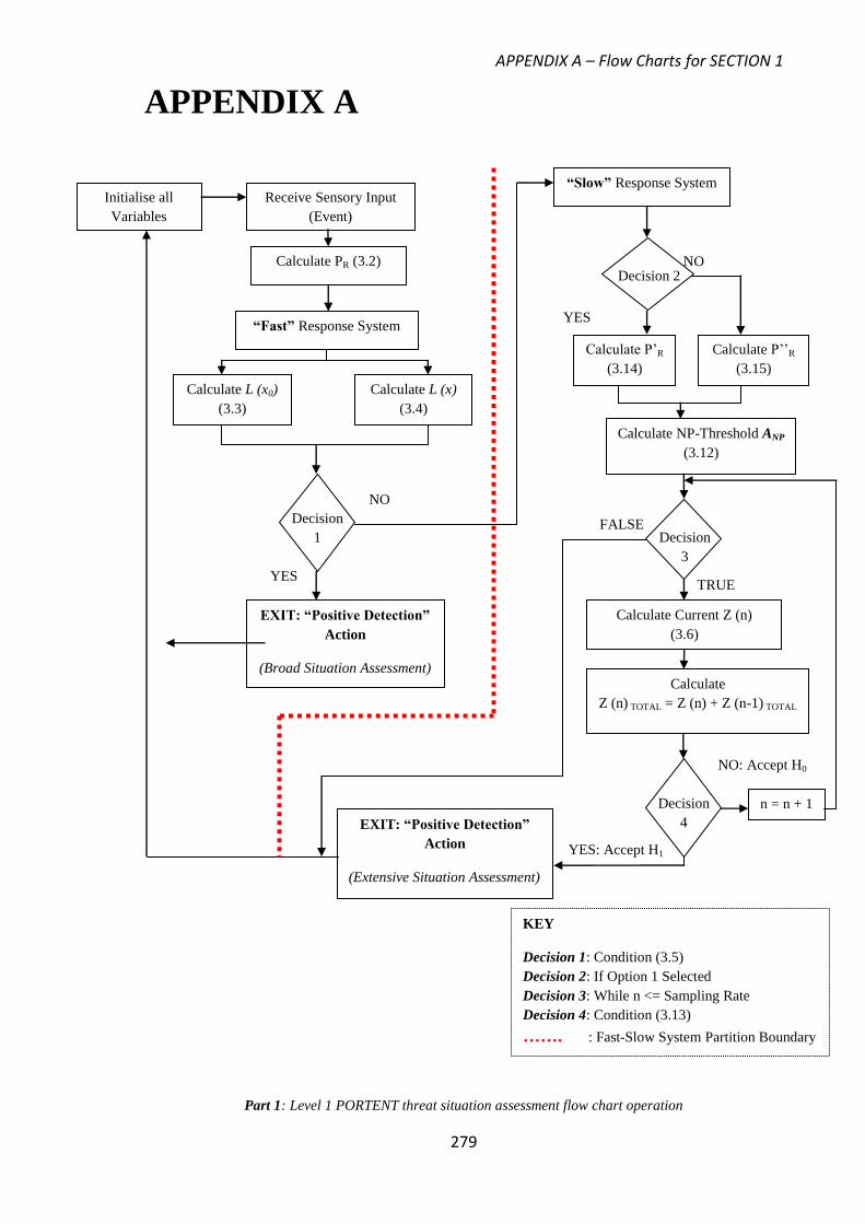
APPENDIX A – Flow Charts for SECTION 1
279
APPENDIX A
Part 1: Level 1 PORTENT threat situation assessment flow chart operation
Initialise all
Variables
Receive Sensory Input
(Event)
Calculate PR (3.2)
“Fast” Response System
Calculate L (x)
(3.4)
Decision
1
EXIT: “Positive Detection”
Action
(Broad Situation Assessment)
“Slow” Response System
Calculate P’R
(3.14)
Calculate L (x0)
(3.3)
Calculate P’’R
(3.15)
Calculate NP-Threshold ANP
(3.12)
Decision
3
Calculate Current Z (n)
(3.6)
Calculate
Z (n) TOTAL = Z (n) + Z (n-1) TOTAL
Decision
4 EXIT: “Positive Detection”
Action
(Extensive Situation Assessment)
n = n + 1
YES
NO
NO
YES
FALSE
TRUE
YES: Accept H1
NO: Accept H0
Decision 2
KEY
Decision 1: Condition (3.5)
Decision 2: If Option 1 Selected
Decision 3: While n <= Sampling Rate
Decision 4: Condition (3.13)
……. : Fast-Slow System Partition Boundary

APPENDIX A – Flow Charts for SECTION 1
280
Part 2: VIGILANT flow chart operation showing an integrated level 1, 2, 3 process for QoSI updating
Sensed
Observation
(Threat)
Calculate P’’R (3.15)
PORTENT
Operation
(Figure 3.1)
Localised QoSI
Presentation
(3.19)
“Threat” Decision
Making –
VIGILANT BBN
(Table 4.1)
Decision
1
NO
Current “Group
Initiator”
Send REQUEST
Calculate CF “Group
Initiator” (4.1)
Evaluate “Confidence in
Context” rule (4.4)
Evaluate “Partnership
Stability” (4.8)
Evaluate QoI
Surveillance Provision
Time E (M) (4.10)
YES
Next Sensor
NO
YES
Send E (M) to
Partnership Sensors
Sensor QoSI
Queuing
Receive QoSI
Update
“Overall” State of Environment
QoSI Presentation
NO
Invoke new
“GI” Status to
(Figure 4.5)
YES
LEVEL 1 LEVEL 2
LEVEL 3
Surveillance Environment
Feedback: “Context Aware” Partner
Adaption
Decision
2
NO
YES
Decision
4
Decision
3
KEY
Decision 1: “Initiate Group Formation” (Fig. 4.2)
Decision 2: Part of a Group
Decision 3: “Sensor to Form Partnership” (Fig. 4.3)
Decision 4: QoIRelative Ratio ≤ 1 (4.11)
……. : System Level Partition Boundaries

APPENDIX A – Test Bed Trial Evaluation
281
Part 3: VIGILANT+ Test Bed Trial Evaluation
General Background
For the purpose of the test bed trials, we propose the development of a new kind of static
sensor network, which consists of a number of deployed Android-based smart phones. For
test bed trial evaluation purposes, smart phones running the Android Operating System
(OS) are used.
Android is an open-source software stack that includes an operating System, middleware
and key application routines. The readily available Android Software Development Kit
(SDK) allows anyone to develop their own applications in Java. Android SDK provides all
the tools and Application Programming Interfaces (API) that are required for the
application development, intended to be run on Android phones.
Aim
The main purpose of the trial is to develop the appropriate software using Java, in order to
exploit the phones microphone as a “sensor” and test the VIGILANT+ sensor algorithm.
The nature of the experiment is to reduce the sensors energy consumption caused by inter-
device communication and at the same time prevent captured QoSI degradation.
Method
Test Bed experimentations are based on correctly perceiving (SA- Level 1) and identifying
a fixed audio source generator (SA –Level 2), to mimic a basic static threat detection
monitoring scenario and to record how transmissions are being managed (SA- Level 3), for
example, total number of transmissions made (i.e. communication overhead).
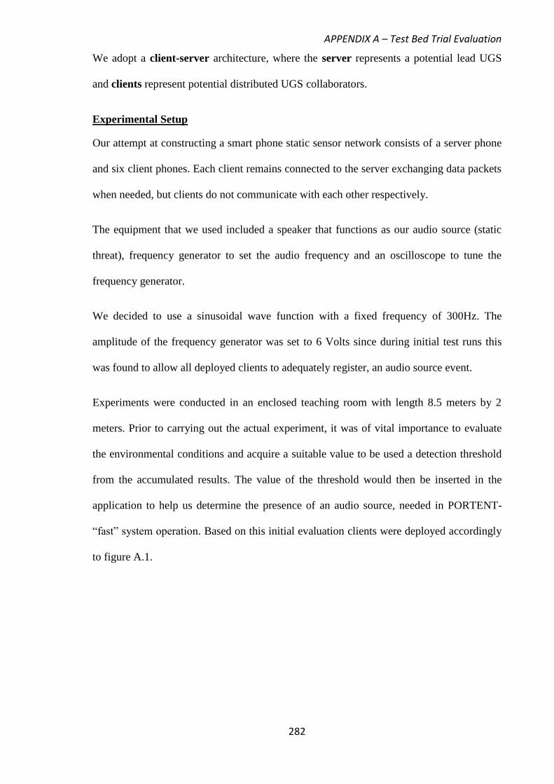
APPENDIX A – Test Bed Trial Evaluation
282
We adopt a client-server architecture, where the server represents a potential lead UGS
and clients represent potential distributed UGS collaborators.
Experimental Setup
Our attempt at constructing a smart phone static sensor network consists of a server phone
and six client phones. Each client remains connected to the server exchanging data packets
when needed, but clients do not communicate with each other respectively.
The equipment that we used included a speaker that functions as our audio source (static
threat), frequency generator to set the audio frequency and an oscilloscope to tune the
frequency generator.
We decided to use a sinusoidal wave function with a fixed frequency of 300Hz. The
amplitude of the frequency generator was set to 6 Volts since during initial test runs this
was found to allow all deployed clients to adequately register, an audio source event.
Experiments were conducted in an enclosed teaching room with length 8.5 meters by 2
meters. Prior to carrying out the actual experiment, it was of vital importance to evaluate
the environmental conditions and acquire a suitable value to be used a detection threshold
from the accumulated results. The value of the threshold would then be inserted in the
application to help us determine the presence of an audio source, needed in PORTENT-
“fast” system operation. Based on this initial evaluation clients were deployed accordingly
to figure A.1.
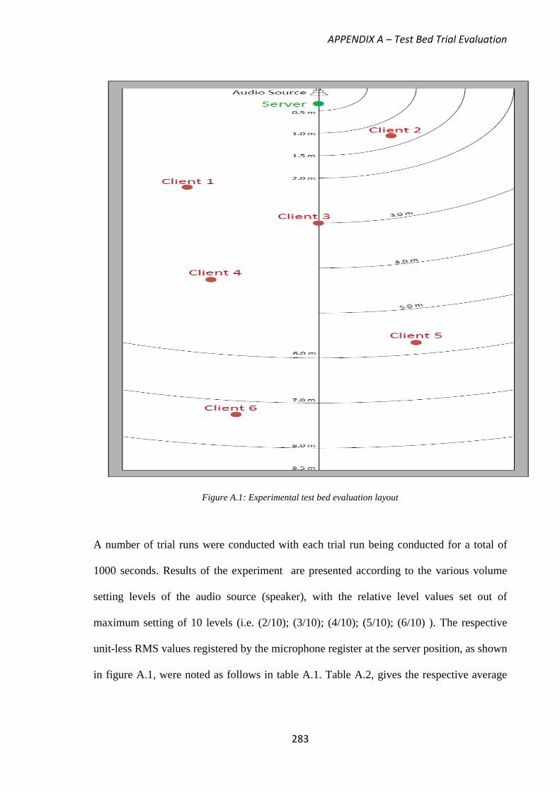
APPENDIX A – Test Bed Trial Evaluation
283
Figure A.1: Experimental test bed evaluation layout
A number of trial runs were conducted with each trial run being conducted for a total of
1000 seconds. Results of the experiment are presented according to the various volume
setting levels of the audio source (speaker), with the relative level values set out of
maximum setting of 10 levels (i.e. (2/10); (3/10); (4/10); (5/10); (6/10) ). The respective
unit-less RMS values registered by the microphone register at the server position, as shown
in figure A.1, were noted as follows in table A.1. Table A.2, gives the respective average
APPENDIX A – Test Bed Trial Evaluation
284
RMS values registered by the clients deployed accordingly to figure A.1 and measured
across the range of volume level settings, as used in table A.1.
Volume Level RMS Value
2 / 10 15098.64
3 / 10 17651.02
4 / 10 19927.89
5 / 10 21867.37
6 / 10 23596.73
Table A.1: Respective RMS values registered at the server position
Client Average RMS Value
1 2550.63
2 3720.43
3 2078.72
4 1501.25
5 1149.89
6 841.21
Table A.2: Respective average RMS values registered at each client position
The test-bed evaluations were carried out for comparison purposes using three different
system operations:
• Fully Distributed: Emphasises more on the distributed client's retrieved local state
“context” from the microphone sensor after an initial server assumption concerning an
event, for transmission control decision making. (Memory Operation –POMDP)
APPENDIX A – Test Bed Trial Evaluation
285
• Semi-Distributed: Takes into account the need for updated threat (audio source)
observations made by both the server and collaborating clients to deduce state
“context”, for transmission control decision making. (Memory-less Operation –
MDP-Option 1)
• Centralised: Constitutes the server and clients utilising only SA level 1 and ignoring
SA levels 2, 3 (i.e. Threat comprehension and Projection). Clients send their updated
threat detection information values on every server request, which is sent every time a
positive SA-level 1 detection is made. This constitutes as a non-“context aware”
approach.
Assumptions
There are some limitations to our approach. The phone's sensing ability is limited to sound-
emitting objects only. Taking this into consideration we do not actively consider the effects
of background noise and other factors, such as the reflection of sound waves inside the
room. These assumptions are important since we do not implement any classification
algorithms that can distinguish between our fixed audio source and other audio source
anomalies.
Our primary concern is to evaluate how VIGILANT+ operation can improve on
transmission control decision making and as a result, provide the necessary network
resource consumption benefits.
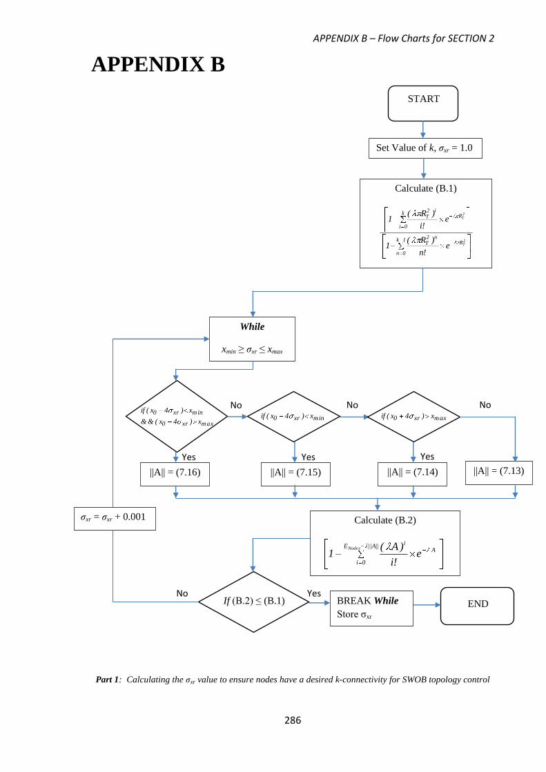
APPENDIX B – Flow Charts for SECTION 2
286
APPENDIX B
m axxr0
minxr0
x)4x(&&
x)4x(if minxr0 x)4x(if maxxr0 x)4x(if
Part 1: Calculating the σxr value to ensure nodes have a desired k-connectivity for SWOB topology control
START
Set Value of k, σxr = 1.0
END
Calculate (B.1)
2T
2T
R1k
0n
n2T
Rk
0i
i2T
e!n
)R(1
e!i
)R(1
||A|| = (7.16)
While
xmin ≥ σxr ≤ xmax
||A|| = (7.14)
Calculate (B.2)
||A||E
0i
Ai
Nodes
e!i
)A(1
If (B.2) ≤ (B.1)
σxr = σxr + 0.001
BREAK While
Store σxr
Yes
Yes
No
||A|| = (7.15)
||A|| = (7.13)
No No No
Yes Yes
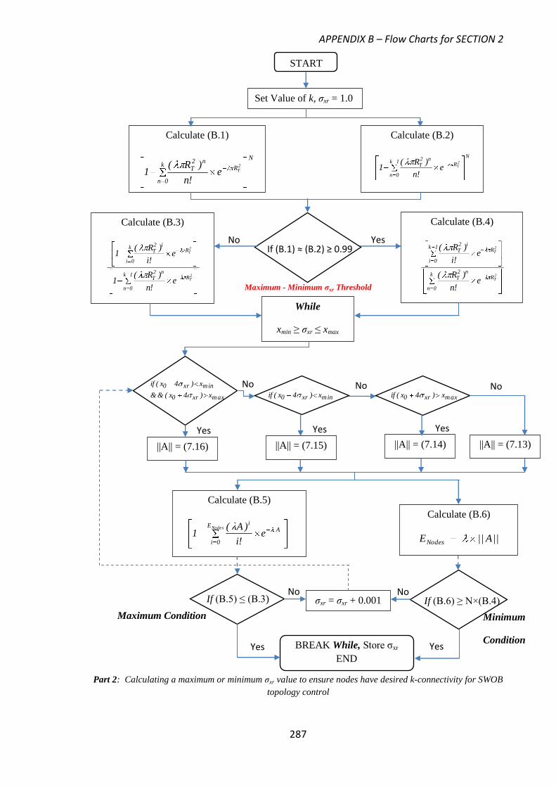
APPENDIX B – Flow Charts for SECTION 2
287
m axxr0
minxr0
x)4x(&&
x)4x(if
minxr0 x)4x(if maxxr0 x)4x(if
Part 2: Calculating a maximum or minimum σxr value to ensure nodes have desired k-connectivity for SWOB
topology control
START
Set Value of k, σxr = 1.0
BREAK While, Store σxr
END
Calculate (B.1)
N
Rk
0n
n2T
2Te
!n
)R(1
Calculate (B.4)
2T
2T
Rk
0n
n2T
R1k
0i
i2T
e!n
)R(
e!i
)R(
||A|| = (7.16)
While
xmin ≥ σxr ≤ xmax
||A|| = (7.14)
Calculate (B.5)
NodesE
0i
Ai
e!i
)A(1
If (B.5) ≤ (B.3) σxr = σxr + 0.001
Yes
Yes
No
||A|| = (7.15)
||A|| = (7.13)
No
No
No
Yes Yes
Calculate (B.2)
N
R1k
0n
n2T
2Te
!n
)R(1
If (B.1) ≈ (B.2) ≥ 0.99 Yes
Calculate (B.6)
||A||ENodes
If (B.6) ≥ N×(B.4)
Yes
No
Minimum
Condition
Maximum Condition
No
Calculate (B.3)
2T
2T
R1k
0n
n2T
Rk
0i
i2T
e!n
)R(1
e!i
)R(1
Maximum - Minimum σxr Threshold
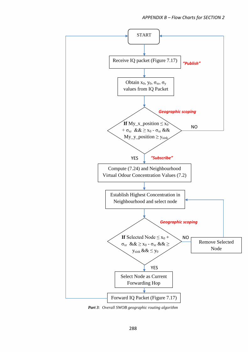
APPENDIX B – Flow Charts for SECTION 2
288
Part 3: Overall SWOB geographic routing algorithm
Receive IQ packet (Figure 7.17)
Obtain x0, y0, σxr, σy
values from IQ Packet
Compute (7.24) and Neighbourhood
Virtual Odour Concentration Values (7.2)
Establish Highest Concentration in
Neighbourhood and select node
If My_x_position ≤ x0
+ σxr && ≥ x0 - σxr &&
My_y_position ≥ ysink
Select Node as Current
Forwarding Hop
Remove Selected
Node
Forward IQ Packet (Figure 7.17)
YES
NO
YES
NO
Geographic scoping
“Subscribe”
Geographic scoping
START
“Publish”
If Selected Node ≤ x0 +
σxr && ≥ x0 - σxr && ≥
ysink && ≤ y0
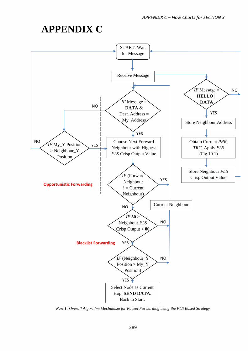
APPENDIX C – Flow Charts for SECTION 3
289
APPENDIX C
Part 1: Overall Algorithm Mechanism for Packet Forwarding using the FLS Based Strategy
START. Wait
for Message
Receive Message
IF Message =
HELLO ||
DATA
Store Neighbour Address
Obtain Current PRR,
TRC. Apply FLS
(Fig.10.1)
Store Neighbour FLS
Crisp Output Value
IF Message =
DATA &
Dest_Address =
My_Address
IF 50 >
Neighbour FLS
Crisp Output < 80
Select Node as Current
Hop. SEND DATA.
Back to Start.
IF My_Y Position
> Neighbour_Y
Position
Choose Next Forward
Neighbour with Highest
FLS Crisp Output Value
YES
NO
YES
YES
YES NO
NO
NO
Opportunistic Forwarding
Blacklist Forwarding
IF (Neighbour_Y
Position > My_Y
Position)
Current Neighbour
IF (Forward
Neighbour
! = Current
Neighbour)
YES
NO
YES
NO
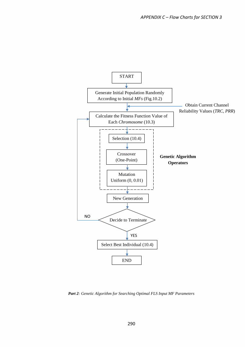
APPENDIX C – Flow Charts for SECTION 3
290
Obtain Current Channel
Reliability Values (TRC, PRR)
START
Generate Initial Population Randomly
According to Initial MFs (Fig.10.2)
Calculate the Fitness Function Value of
Each Chromosome (10.3)
Selection (10.4)
Crossover
(One-Point)
Mutation
Uniform (0, 0.01)
New Generation
Select Best Individual (10.4)
END
Genetic Algorithm
Operators
NO
YES
Decide to Terminate
Part 2: Genetic Algorithm for Searching Optimal FLS Input MF Parameters
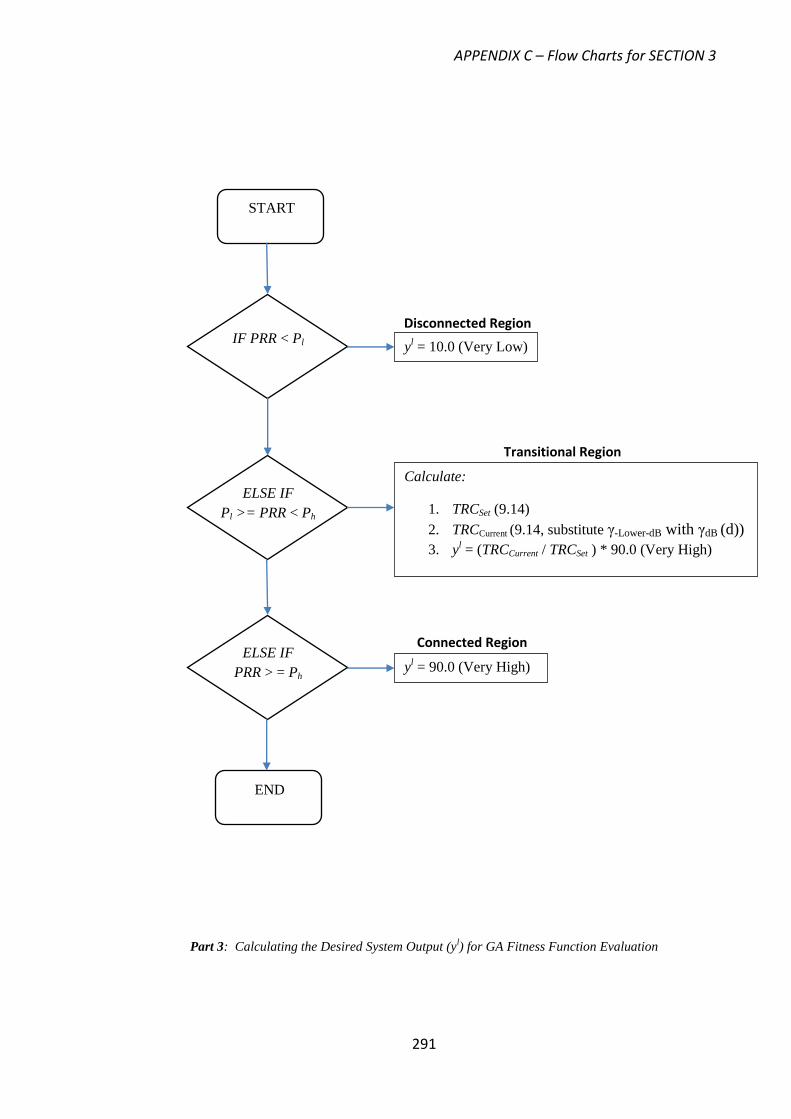
APPENDIX C – Flow Charts for SECTION 3
291
Part 3: Calculating the Desired System Output (yl) for GA Fitness Function Evaluation
START
IF PRR < Pl
ELSE IF
Pl >= PRR < Ph
ELSE IF
PRR > = Ph
yl = 10.0 (Very Low)
Calculate:
1. TRCSet (9.14)
2. TRCCurrent (9.14, substitute γ-Lower-dB with γdB (d))
3. yl = (TRCCurrent / TRCSet ) * 90.0 (Very High)
yl = 90.0 (Very High)
END
Disconnected Region
Transitional Region
Connected Region
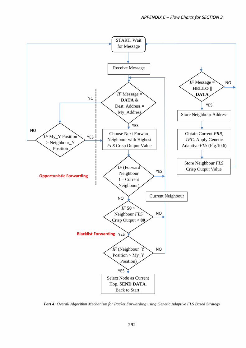
APPENDIX C – Flow Charts for SECTION 3
292
Part 4: Overall Algorithm Mechanism for Packet Forwarding using Genetic Adaptive FLS Based Strategy
START. Wait
for Message
Receive Message
IF Message =
HELLO ||
DATA
Store Neighbour Address
Obtain Current PRR,
TRC. Apply Genetic
Adaptive FLS (Fig.10.6)
Store Neighbour FLS
Crisp Output Value
IF Message =
DATA &
Dest_Address =
My_Address
IF 50 >
Neighbour FLS
Crisp Output < 80
Select Node as Current
Hop. SEND DATA.
Back to Start.
IF My_Y Position
> Neighbour_Y
Position
Choose Next Forward
Neighbour with Highest
FLS Crisp Output Value
YES
NO
YES
YES
YES
NO
NO
NO
Opportunistic Forwarding
Blacklist Forwarding
IF (Neighbour_Y
Position > My_Y
Position)
Current Neighbour
IF (Forward
Neighbour
! = Current
Neighbour)
YES
NO
YES
NO
REFERENCES
293
References
[1] J.Zheng and A.Jamalipour, “Wireless Sensor Networks: A Networking Perspective”,
Chapter 1: “Introduction to Wireless Sensor Networks”, Wiley-IEEE Press, 1st Edition,
pp.1-18, 2009.
[2] J.Gehrke and Liu.Ling, “Introduction: Sensor Network Applications”, IEEE Internet
Computing, vol.10, no.2, pp.16-17, March-April 2006.
[3] T. Becker, M.Kulge, J.Schalk, K.Tiplady and C.Paget, “Autonomous Sensor Nodes for
Aircraft Structural Health Monitoring”, IEEE Sensors Journal, vol.9, no.11, pp.1589-
1595, November 2009.
[4] K.Gill, S.H.Yang, F.Yao, X.Lu, “A ZigBee-Based Home Automation System”, IEEE
Transactions on Consumer Electronics, vol.55, no.2, pp.422-430, May 2009.
[5] R.V.Kulkarni, A.Forster and G.K.Venayagamoorthy, “Computational Intelligence in
Wireless Sensor Networks: A Survey”, IEEE Communications Surveys and Tutorials,
vol.13, no.1, pp.68-96, January-March 2011.
[6] D.L.Hall, J.Llinas, “An Introduction to Multi-Sensor Data Fusion”, Proceedings of the
IEEE, vol.85, no.1, pp.6-23, January 1997.
[7] J.Clare and D.S.Ryl, “Energy Efficient Area Monitoring for Sensor Networks”, IEEE
Computer, vol.37, no.2, pp.40-46, February 2004.
[8] D.S.Alberts, J.J.Garstka and F.P.Stein, “Network Centric Warfare: Developing and
Leveraging Information Superiority”, CCRP Publication Series, 2nd
Edition, Chapter 5,
pp.87-108, February 2000.
[9] D.S.Alberts, J.J.Garstka and F.P.Stein, “Network Centric Warfare: Developing and
Leveraging Information Superiority”, CCRP Publication Series, 2nd
Edition, Chapter 8,
pp.140-148, February 2000.
[10] J.L.Burbank, P.F.Chimento, B.K.Haberman and K.T.Kasch, “Key Challenges of
Military Tactical Networking and the Elusive Promise of MANET Technology”, IEEE
Communications Magazine, vol.44, no.11, pp.39-45, November 2006.
[11] H.Leung, S.Chandana and S.Wei, “Distributed Sensing Based on Intelligent Sensor
Networks”, IEEE Circuits and Systems Magazine, vol.8, no.2, pp.38-52, May 2008.
[12] I.Akyildiz, W.Su, E.Cayirci, “A Survey on Sensor Networks”, IEEE
Communications Magazine, vol.40, no.8, pp.102-114, 2002.
[13] C.Kreucher, A.Hero, K.Kastella and M.Morelande, “An Information-Based
Approach to Sensor Management in Large Dynamic Networks”, Proceedings of the
IEEE, vol.95, no.5, pp.978-998, May 2007.
REFERENCES
294
[14] D.Puccinelli and M.Haenggi, “Wireless Sensor Networks: Applications and
Challenges of Ubiquitous Sensing”, IEEE Circuits and Systems Magazine, vol.5, no.3,
pp.19-31, 2005.
[15] R.R Hoffman and J.F. Yates, “Decision Making”, IEEE Intelligent Systems
Magazine, vol.20, no.4, pp.76-83, July/August 2005.
[16] P.K Biswas and S.Phoha, “Self-Organising Sensor Networks for Integrated Target
Surveillance”, IEEE Transactions on Computers, vol.55, no.8, pp.1033-1047, August
2006.
[17] J.E.Bevington, “Distributed Sensor Management and Target Tracking for
Unattended Ground Sensor Networks”, Proceedings of SPIE Security and Defence,
Battle-space Digitisation and Network Centric Systems IV, vol.5441, pp.25-35, 2004.
[18] K.Romer, O.Kasten and F.Mattern, “Middleware Challenges for Wireless Sensor
Networks”, ACM Mobile Communication and Communications Review, vol.6, no.2,
pp.59-61, October 2002.
[19] Y.Tian and E.Ekici, “Cross-Layer Collaborative In-Network Processing in Multi-
hop Wireless Sensor Networks”, IEEE Transactions on Mobile Computing, vol.6, no.3,
pp.297-310, March 2007.
[20] S. Eswaran, M. Johnson, A. Misra, and T. La Porta, “Adaptive In-Network
Processing for Bandwidth and Energy Constrained Mission-Oriented Multi-hop
Wireless Networks. In Distributed Computing in Sensor Systems”, Proceedings of the
5th IEEE International Conference on Distributed Computing in Sensor Systems
(DCOSS), Marina Del Rey, CA, USA, pp.87-102, June 2009.
[21] D. Marsh, R. Tynan, D. O’Kane, G. O’Hare, “Autonomic Wireless Sensor
Networks”, ELSEVIER Journal of Engineering Applications of Artificial Intelligence,
vol.17, no.7, pp.741-748, October 2004.
[22] S. Dobson, E. Gelenbe, D. Gaiti, A. Fernandez, S. Denazis, F. Massacci, P. Nixon,
F. Saffre, N. Schmidt, F . Zambonelli, “A Survey of Autonomic Communications”,
ACM Transactions on Autonomous and Adaptive Systems, vol.1, no.2, pp.223-259,
December 2006.
[23] A. Forster, R.V Kulkarni, G.K Venayagamoorthy, “Computational Intelligence in
Wireless Sensor Networks: A Survey”, IEEE Communications Survey and Tutorials,
vol.13, no.1, pp.68-96, February 2011.
[24] T.Onel, C.Esroy, “Information Content-Based Sensor Selection and Transmission
Power Adjustment for Collaborative Target Tracking”, IEEE Transactions on Mobile
Computing, vol.8, no.8, pp.1103-1116, August 2009.
[25] D.Gracanin, K.P Adams, M.Eltoweissy, “Data Replication in Collaborative Sensor
Network Systems”, Proceedings of the 25th
International Conference on Performance,
Computation and Communications (IPCCC), pp. 390-396, Phoenix, Arizona, USA,
April 2006.
REFERENCES
295
[26] S.K Singh, “Routing Protocols in Wireless Sensor Networks- A Survey”,
International Journal of Computer Science and Engineering Survey (IJCSES), vol.1,
no.2, pp.63-83, November 2010.
[27] W.Heinzelman, “An Application Specific Protocol Architecture for Wireless Micro
Sensor Networks”, IEEE Transactions on Wireless Communications, vol.1, no.4,
pp.660-670, October 2002.
[28] O. Younis and S.Fahmy, “Distributed Clustering in Ad-Hoc Sensor Networks: A
Hybrid and Energy Efficient Approach”, Proceedings of the 23rd
Conference of the
IEEE Communication Society- IEEE INFOCOM, Hong Kong, 7th
-11th
March 2004.
[29] W.P Chen, J.C Hou and L.Sha, “Dynamic clustering for acoustic target tracking in
wireless sensor networks”, IEEE Transactions on Mobile Computing, vol.3, no.3,
pp.258-271, July-September 2004.
[30] D. Roelant, K. Yen and Z. Hao, “ Self Organisation of Unattended Wireless
Acoustic Sensor Networks for Ground Target Tracking”, ELSEVIER Journal of
Pervasive and Mobile Computing, vol.5 , no.2, pp.148 -164, April 2009.
[31] J.Lee, K.Cho, S.Lee, T.Kwon and Y.Choi, “Distributed and Energy-Efficient
Target Localisation and Tracking in Wireless Sensor Networks”, ELSEVIER Journal of
Computer Communications, vol.29, no.13-14, pp.2494-2505, August 2006.
[32] R.Brooks, C.Griffin and D.S. Friedlander, “Self-Organised Distributed Sensor
Network Entity Tracking”, International Journal of High Performance Computer
Applications, vol.16, no.3, pp.207-219, August 2002.
[33] D.Li, K.Wong Y.Hu and A.Sayeed, “Detection, Classification, Tracking of Targets
in Micro-Sensor Networks”, IEEE Signal Processing Magazine, vol.19, no.2, pp.17-29,
March 2002.
[34] F.Zhao, J.Shin and J.Reich, “Information-Driven Dynamic Sensor Collaboration”,
IEEE Signal Processing Magazine, vol.19, no.2, pp. 61-72, March 2002.
[35] F.Zhao, J.Liu, L.Guibas, J.Reich, “Collaborative Signal and Information
Processing: An Information-Directed Approach”, Proceedings of the IEEE, vol.91,
no.8, pp. 1199-1209, August 2003.
[36] L.Guibas, “Sensing, Tracking, and Reasoning with Relations”, IEEE Signal
Processing Magazine, vol.19, no.1, pp.73-85, March 2002.
[37] R.Roman, J.Lopez, S.Gritzalis, “Situation Awareness Mechanisms for Wireless
Sensor Networks”, IEEE Communications Magazine, vol.46, no.4, pp.102-107, April
2008.
[38] M.R.Endsley, “Toward a Theory of Situation Awareness in Dynamic Systems”,
Journal of Human Factors, vol.37, no.1, pp.32-64, March 1995.
REFERENCES
296
[39] C.Bisdikian, “On Sensor Sampling and Quality of Information: A Starting Point”,
Proceedings of the 5th
Annual IEEE Conference on Pervasive Computing and
Communication (PERCOM), White Plains, New York, USA, pp.279-284, March 2007.
[40] M.Walchli, T.Braun, M.Meer, P.Skoczylas, “Distributed Event Localization and
Tracking with Wireless Sensors”, 5th International Conference on Wired/Wireless
Internet Communications (WWIC), Coimbra, Portugal, pp.247-258, May 2007.
[41] K.Romer, “Discovery of Frequent Distributed Event Patterns in Sensor Networks”,
Proceedings of the 5th European conference on Wireless sensor networks (EWSN),
Bologna, Italy, pp.106-124, January 2008.
[42] E.Onur, C.Ersoy, H.Delic and L.Akarun, “Surveillance Wireless Sensor Networks:
Deployment Quality Analysis”, IEEE Network, vol.21, no.6, pp.48-53,
November/December 2007.
[43] E.Onur, C.Ersoy and H.Delic, “Quality of Deployment in Surveillance Wireless
Sensor Networks”, International Journal of Wireless Information Networks, vol.12,
no.1, pp.61-67, January 2005.
[44] X.Y.Li, P.J.Wan and O.Frieder, “Coverage in Wireless Ad Hoc Sensor Networks”,
IEEE Transactions on Computers, vol.52, no.6, pp.753-763, June 2003.
[45] J.A.R Marshall, “On optimal decision making in brains and social insects”, Journal
of the Royal Society, pp.1-10, January 2009.
[46] P.C Trimmer, “Mammalian Choices”, Proceedings of the Royal Society, pp. 2353-
2361, July 2008.
[47] E.Onur, C.Ersoy and H.Delic, “How Many Sensors for An Acceptable Breach
Probability Level?”, Journal of Computer Communications, vol.29, no.2, pp.172-82,
January 2006.
[48] J.P.Egan, “Signal Detection Theory and ROC Analysis”, New York, Academic
Press pp.16-18,
[49] D.Kazakos, P.P.Kazakos, “Detection and Estimation”, Computer Science Press,
Rockville, MD, 1990.
[50] K.F.Wong, “A Recurrent Network Mechanism of Time Integration in Perceptual
Decisions”, Journal of Neuroscience, vol.26, no.4, pp.1314-1328, January 2006.
[51] S.Zahedi and C.Bisdikian. “A Framework for QoI-Inspired Analysis for Sensor
Network Deployment Planning”, 2nd
International Workshop on Performance Control
in Wireless Sensor Networks (PWSN), Austin, Texas, USA, October 2007.
[52] C.Bisdikian, R.Damarala, T.Pham, V.Thomas, “Quality of Information in Sensor
Networks”, 2nd
Annual Conference of the International Technology Alliance (ACITA),
London, U.K, September 2008.
REFERENCES
297
[53] G. Jakobson, J. Buford, L. Lewis, “A framework of cognitive situation modelling
and recognition”, Proceedings of the 25th
IEEE Military Communications Conference
(MILCOM), Washington, USA, pp. 1-7, October 2006.
[54] P.Smart, A.Bahrami, D.Braines, D.M.Spencer, J.Yuan and N.R.Shadbolt,
“Semantic Technologies and Enhanced Situation Awareness”, 1st Annual Conference of
the International Technology Alliance (ACITA), East Adelphi, Maryland, USA,
September 2007.
[55] J.Salerno, M.Hinman, D.Boulware, “Building a Framework for Situation
Awareness”, Proceedings of the 7th
International Conference on Information Fusion,
Stockholm, Sweden, pp.219-226, June 2004.
[56] F.V.Jensen, “Bayesian Networks and Decision Graphs”, Springer, New York, 2nd
Edition, 2007.
[57] X.Ye, G.Kamath and L.A.Osadciw, “Using Bayesian Inference for Sensor
Management of Air Traffic Control Systems”, IEEE Symposium on Computational
Intelligence in Multi-Criteria Decision Making, Nashville, Tennessee, USA, pp.23-29,
March 2009.
[58] S.Das, D.Lawless, “Trustworthy Situation Assessment via Belief Networks”,
Proceedings of the 5th
International Conference on Information Fusion, Annapolis,
Maryland, USA, pp.543-549, July 2002.
[59] A.Ranganathan, J.Al-Muhtadi, R.Campbell, “Reasoning about Uncertain Contexts
in Pervasive Computing Environments”, IEEE Pervasive Computing, vol.3, no.2,
pp.62-70, July 2004.
[60] P.Krause, “Representing Uncertain Knowledge”, Intellect Books, 1st Edition, pp.52-
56, 1993.
[61] R.M.Perianu, C.Lombriser, P.Havinga, H.Scholten and G.Troster, “Tandem: A
Context-Aware Method for Spontaneous Clustering of Dynamic Wireless Sensor
Nodes”, Proceedings of the 1st International Conference on The Internet of Things,
Appears in Lecture Notes in Computer Science, vol.4952, pp.341-359, March 2008.
[62] C.Lombriser, M.M.Perianu, R.M.Perianu, D.Rogen, P.Havinga, G.Troster,
“Organizing Context Information Processing in Dynamic Wireless Sensor Networks”,
Proceedings of the 3rd
International Conference on Intelligent Sensors, Sensor
Networks and Information Processing (ISSNIP), pp.67-72, Melbourne, Australia,
December 2007.
[63] A.Varga, “Using the OMNeT++ Discrete Event Simulation System in Education,
IEEE Transactions on Education, vol.42, no.4, November 1999.
[64] E.Souto and J.Kelner, “Mires: A Publish/Subscribe Middleware for Sensor
Networks”, Journal of Personal Ubiquitous Computing, vol.10, no.1, pp.37-44,
December 2005.

REFERENCES
298
[65] K.Henricksen and R.Robinson, “A Survey of Middleware for Sensor Networks:
State-of-the-Art and Future Directions”, Proceedings of the International Workshop on
Middleware for Sensor Networks (MidSens), pp.60-65, Melbourne, Australia,
November/December 2006.
[66] O.H Lerma, “Adaptive Markov Control Processes”, Applied Mathematical
Sciences, Springer-Verlag, New York, 2001.
[67] L.P.Kaelbling, M.L.Litman, A.R.Cassandra, “Planning and Acting in Partially
Observable Stochastic Domains”, Journal of Artificial Intelligence, vol.101, no.1-2,
pp.99-134, May 1998.
[68] E.K.P.Chong, C.M.Kreucher, A.O.Hero, “Partially Observable Markov Decision
Process Approximations for Adaptive Sensing”, Journal of Discrete Event Dynamic
Systems, vol.19, no.3, pp.377-422, May 2009.
[69] E.K.P.Chong, L.W.Krakow, K.N.Groom, J.Harrington, Y.Li, B.Rigdon, “Control
of Perimeter Surveillance Wireless Sensor Networks via Partially Observable Markov
Decision Process”, Proceedings of the 40th
Annual IEEE International Carnahan
Conference on Security Technology (ICCST), Lexington, USA, pp.261-268, October
2006.
[70] I.Kadar, “Optimum Geometry Selection for Sensor Fusion”, SPIE: Defence,
Security and Sensing, Proceedings of the Conference on Signal Processing, Sensor
Fusion and Target Recognition VII, vol. 3374, Orlando, Florida, USA, pp. 96-107,
April 1998.
[71] A.G.Dempster, “Dilution of Precision in Angle-of-Arrival Positioning Systems,
IET Electronics Letters, vol.42, no.6, 2nd
March 2006.
[72] R.A.Burne, I.Kadar, A.Buczak, “A Self-Organising Cooperative Sensor Network
for Remote Surveillance: Target Tracking while Optimising the Geometry between
Bearing-Reporting Sensors and the Target”, SPIE: Security and Defence, Proceedings
of the Conference on Unattended Ground Sensor Technologies and Applications III,
vol.4393, pp.173-182, September 2001.
[73] H.B.Lee, “A Novel Procedure for Assessing the Accuracy of Hyperbolic Multi-
lateration Systems”, IEEE Transactions on Aerospace and Electronic Systems,
vol.AES-11, no.1, pp.2-15, January 1975.
[74] D.J.Torrieri, “Statistical Theory of Passive Location Systems”, IEEE Transactions
on Aerospace and Electronic Systems, vol.AES-20, no.2, pp.183-198, March 1984.
[75] J.M.Augenbaugh, B.R.L.Cour, “Metric Selection for Information Theoretic Sensor
Management”, Proceedings of the 11th
International Conference on Information
Fusion, Cologne, Germany, pp. 1-8, July 2008.
[76] K. Kastella, “Discrimination Gain to Optimize Classification”, IEEE Transactions
on Systems, Man & Cybernetics-Part A: Systems and Humans, Vol.27, no. 1, pp.112-
116, January 1997.
REFERENCES
299
[77] M.P.Kolba and L.M.Collins, "Information-Theoretic Sensor Management for
Multimodal Sensing," Proceedings of the IEEE International Geoscience and Remote
Sensing Symposium (IGARSS), Denver, Colorado, USA, pp. 3935-3938, August 2006.
[78] Y.Dong, W.K.Hon and D.K.Y Yau, “On Area of Interest Area of Coverage in
Surveillance Mobile Sensor Networks”, Proceedings of the 15th
IEEE International
Workshop on Quality of Service, Evanston, Illinois, USA, pp.87-90, June 2007.
[79] H.Kim, E.Kim and K.Han, “An Energy Efficient Tracking Method in Wireless
Sensor Networks”, SpringerLink Lecture Notes in Computer Science, 6th
International
Conference on Next Generation Teletraffic and Wired/Wireless Advanced Networking,
Volume 4003, pp.278-286, June 2006.
[80] A.T Erman, L.V.Hoesel and P.Havinga, “Enabling Mobility in Heterogeneous
Wireless Sensor Networks Cooperating with UAVs for Mission Critical Management”,
IEEE Wireless Communications, vol.15, no.6, pp.38-46, December 2008.
[81] E.P de Freitas, T.Heimfarth, C.E.Pereira, T.Larsson, F.R Wagner and F.M Ferreira,
“Evaluation of Coordination Strategies for Heterogeneous Sensor Networks Aiming at
Surveillance Applications”, Proceedings of the IEEE Conference on Sensors, pp.591-
596, Christchurch, New Zealand, October 2009.
[82] E.P de Freitas, T.Heimfarth, C.E.Pereira, T.Larsson, F.R Wagner and F.M Ferreira,
“Decentralized Task Distribution Among Cooperative UAVs in Surveillance Systems
Applications”, Proceedings of the 7th international conference on Wireless on-
demand network systems and services (WONS), pp.121-128, Obergurgl, Austria,
January 2010.
[83] L.Tong, Q.Zhao, S.Adireddy, “Sensor Networks with Mobile Agents”, Proceedings
of the IEEE Conference on Military Communications (MILCOM), pp.688-693, Boston,
U.S.A, October 2003.
[84] I.Stojmenovic, “Position-Based Routing in Ad Hoc Networks”, IEEE
Communications Magazine, vol.40, no.7, pp. 128-134, July 2002.
[85] J.Li, J.Jannotti, D.S.J De Couto, D.R Karger and R.Morris, “A Scalable Location
Service for Geographic Ad Hoc Routing”, Proceedings of the 6th
ACM international
Conference on Mobile Computing and Networking, pp.120-130, Boston, U.S.A, August
2000.
[86] E.Kranakis, H.Singh and J.Urrutia, “Compass Routing on Geometric Networks”,
Proceedings of the 11th
Canadian Conference on Computational Geometry, pp.51-54,
Vancouver, August 1999.
[87] G.G.Finn, “Routing and Addressing Problems in Large Metropolitan – Scale
Internet Works”, Information Sciences Institute Technical Report ISI/RR-87-180,
March 1987.
[88] D.De.Couto and R.Morris, “Location Proxies and Intermediate Node Forwarding
for Practical Geographic Forwarding”, MIT Laboratory for Computer Science
Technical Report MIT-LCS-TR-824, June 2001.
REFERENCES
300
[89] C.Maihofer, “A Survey of Geocast Routing Protocols”, IEEE Communications
Surveys & Tutorials, vol.6, no.2, pp.32-42, Second Quarter 2004.
[90] J.Navas, T.Imielinski, “GeoCast-Geographic Addressing and Routing”,
Proceedings of the 3rd annual ACM/IEEE International Conference on Mobile
Computing and Networking (MobiCom), pp.66-76, Budapest, Hungary, 1997.
[91] Y.B.Ko, N.H.Vaidya, “Flooding Based Geo-casting Protocols for Mobile Ad Hoc
Networks”, Journal of Mobile Networks and Applications, vol.7, no.6, pp.471-480,
2002.
[92] D.B.Johnson, D.A.Maltz, “Dynamic Source Routing in Ad Hoc Wireless
Networks”, Mobile Computing, Kluwer Academic Publishers, 1996.
[93] B.Nath and D.Niculescu, “Routing on a Curve”, ACM SIGCOMM Computer
Communications Review, vol.33, no.1, pp.155-160, January 2003.
[94] B.Warneke, M.Last, B.Leibowitz and K.Pister, “Smart Dust: Communicating with
a Cubic-Millimetre Computer”, IEEE Computer, vol.34, no.1, pp.45-51, January 2001.
[95] A.Boukerche, M.Ahmad, B.Turgut and D.Turgut, “A Taxonomy of Routing
Protocols in Sensor Networks”, Algorithms and Protocols for Wireless Sensor
Networks, Wiley, 1st Edition, Chapter 6, pp.129-160, 2008.
[96] K. Chakrabarty and S. S. Iyengar, “Scalable Infrastructure for Distributed Sensor
Networks”, New York: Spinger-Verlag, 1st Edition, 2005.
[97] J.Kephart and D.Chess, “The Vision of Autonomic Computing”, IEEE Computer
Magazine, vol.36, no.1, pp.41-50, 2003.
[98] F.Dressler and O.B.Akan, “A Survey on Bio-Inspired Networking”, ELSEVIER
Journal of Computer Networks, vol.54, no.6, pp.881-900, April 2010.
[99] F.Dressler and O.B.Akan, “Bio-Inspired Networking: From Theory to Practise”,
IEEE Communications Magazine, vol.48, no.11, pp.176-183, November 2010.
[100] E.Bonabeau, M.Dorigo, G.Theraulaz, “Swarm Intelligence: From Natural to
Artificial Systems”, Oxford University Press, New York, USA, 1999.
[101] S.S.Iyengar, H.C.Wu, N.Balakrishnan and S.Y.Chang, “Biologically Inspired
Cooperative Routing for Wireless Mobile Sensor Networks”, IEEE Systems Journal,
vol.1, no.1, pp.29-37, 2007.
[102] A.Gosh, A.Halder, M.Kothari, and S.Gosh, “Aggregation Pheromone Density
Based Data Clustering”, ELSEVIER Journal of Information Science, vol.178, no.13,
pp.2816-2831, July 2008.
[103] A.T.Hayes, A.Martinoli and R.M.Goodman, “Distributed Odour Source
Localization”, IEEE Sensors Journal, vol.2, no.3, pp.260-271, June 2002.
[104] J.Murlis, J.S.Elkinton, R.T.Carde, “Odour Plumes and How Insects Use Them”,
annual review of entomology, vol.37, pp.505-532, 1992.
REFERENCES
301
[105] D.B.Turner, “Workbook of Atmospheric Dispersion Estimates: An Introduction to
Dispersion Modelling”, Lewis Publication, 2nd
Edition, 1994.
[106] X.Li, Y.Mao, Y.Liang, “A Survey on Topology Control in Wireless Sensor
Networks”, Proceedings of the 10th
International Conference on Control, Automation,
Robotics and Vision (ICARCV), Singapore, pp.251-255, December 2008.
[107] P.Santi, D.M.Blough, “The Critical Transmitting Range for Connectivity in Sparse
Wireless Ad Hoc Networks”, IEEE Transactions on Mobile Computing, vol.2, no.1,
pp.25-39, January-March 2003.
[108] B.Bollobas, “Modern Graph Theory”, Springer, Chapter 7, 1st Edition, 1998.
[109] J.Diaz, M.D.Penrose, J.Petit and M.Serna, “Convergence Theorems for Some
Layout Measures on Random Lattice and Random Geometric Graphs”, Journal of
Combinatorics, Probability and Computing, vol.9, no.6, pp.489-511, 2000.
[110] C.Bettstetter, “On the Minimum Node Degree and Connectivity of a Wireless
Multi-hop Network”, Proceedings of the 3rd ACM International Symposium on Mobile
Ad Hoc Networking and Computing (MobiHoc), pp. 80-91, Lausanne, Switzerland,
June 2002.
[111] B.Liu, D.Towsley, “A Study of the Coverage of Large-Scale Sensor Networks”,
Proceedings of the IEEE International Conference on Mobile Ad-Hoc and Sensor
Systems (MASS), pp.475-483, October 2004.
[112] S.Karlin and H.M.Taylor, “A First Course in Stochastic Processes”, Academic
Press, San Diego, CA, section 1.3, 2nd
Edition, 1975.
[113] S.Karlin and H.M.Taylor, “A Second Course in Stochastic Processes”, Academic
Press, San Diego, CA, Chapter 16, 1981.
[114] G.Bianchi, “Performance Analysis of the IEEE 802.11 Distributed Coordination
Function”, IEEE Journal on Selected Areas In Communications, vol.18, no.3, pp.535-
547, March 2000.
[115] K.C.Huang and K.C.Chen, “Interference Analysis of Non-persistent CSMA with
hidden terminals in multi-cell wireless data networks”, Proceedings of the IEEE
Conference on Personal, Indoor and Mobile Radio Communications (PIMRC),
Toronto, Canada, pp. 907-911, September 1995.
[116] R.Khalaf and I.Rubin, “Throughput and Delay Analysis in Single Hop and
Multihop IEEE 802.11 Networks”, Proceedings of the 3rd
International Conference on
Broadband, Communications and Network systems (BROADNETS) ,San Jose, U.S.A,
October 2006.
[117] C.Intanagonwiwat, D.Estrin, R.Govindan, J.Heidman, and F.Silva, “Directed
Diffusion for Wireless Sensor Networks”, IEEE/ACM Transactions on Networking,
vol.11, no.1, pp.2-16, February 2003.
[118] N.Magharei and R.Rejaie. “PRIME: Peer-to-peer receiver-driven mesh-based
streaming”, IEEE/ACM Transactions on Networking, vol.17, no.4, pp.1052–1065,
August 2009.
REFERENCES
302
[119] S. Sanghavi, B. Hajek, and L. Massoulie, “Gossiping with multiple messages”,
IEEE Transactions on Information Theory, vol.53, no.12, pp.4640-4654, December
2007.
[120] J.N. Al-Karaki and A.E. Kamal, “Routing Techniques in Wireless Sensor
Networks: A Survey”, IEEE Wireless Communications, vol.11, no.6, pp.6-28,
December 2004.
[121] M.Zorzi and R.Rao, “Geographic Random Forwarding for Ad Hoc and Sensor
Networks: Multi-hop Performance”, IEEE Transactions on Mobile Computing, vol.2,
no.4, pp.337-347, October-December 2003.
[122] M.Zorzi and R.Rao, “Geographic Random Forwarding for Ad Hoc and Sensor
Networks: Energy and Latency Performance”, IEEE Transactions on Mobile
Computing, vol.2, no.4, pp.349-365, October-December 2003.
[123] Z.Zhang, “Routing in Intermittently Connected Mobile Ad Hoc Networks and
Delay Tolerant Networks: Overview and Challenges”, IEEE Communications Surveys
and Tutorials, vol.8, no.1, pp.24-37, 1st Quarter 2006.
[124] R.Vidhyapriya and P.T.Vanath, “Energy Aware Routing for Wireless Sensor
Networks”, Proceedings of the IEEE International Conference on Signal Processing,
Communications and Networking (ICSCN), pp.554-550, February 2007.
[125] Z.Ren, G.Wang, Q.Chen, H.Li, “Modelling and Simulation of Rayleigh Fading,
Path Loss and Shadowing Fading for Wireless Mobile Networks”, ELSEVIER Journal
of Simulation Modelling Practise and Theory, vol.19, no.2, pp.626-637, February 2011.
[126] A.Goldsmith, “Wireless Communications”, Cambridge University Press, 1st
Edition, pp. 31-34, 2005.
[127] B.Sklar, “Rayleigh Fading Channels in Mobile Digital Communication Systems
Part 1: Characterization”, IEEE Communications Magazine, vol.35, no.7, pp.90-100,
July 1997.
[128] S.Y.Seidel, “Path Loss, Scattering and Multipath Delay Statistics in Four European
Cities for Digital Cellular and Microcellular Radiotelephone”, IEEE Transactions on
Vehicular Technology, vol.40, no.4, pp.721-30, November 1991.
[129] J.B.Andersen, T.S.Rappaport and S.Yoshida, “Propagation Measurements and
Models for Wireless Communications Channels”, IEEE Communications Magazine,
vol.33, no.1, pp.42-49, January 1995.
[130] F.Hansen, “Mobile Fading-Rayleigh and Lognormal Superimposed”, IEEE
Transactions on Vehicular Technology, vol.26, no.4, pp.332-335, November 1977.
[131] R.L.Bogusch, F.W.Guigliano, D.L.Knepp, A.H.Michelet, “Frequency Selective
Propagation Effects on Spread-Spectrum Receiver Tracking”, Proceedings of the
IEEE, vol.69, no.7, pp.787-96, July 1981.
[132] A.Woo, T.Tong and D.Culler, “Taming the Underlying Issues of Reliable Multi-
hop Routing in Sensor Networks”, Proceedings of the 1st International Conference on
REFERENCES
303
Embedded Networked Sensor Systems (SenSys), Los Angeles, U.S.A, pp.14-27,
November 2003.
[133] J.Zhao and R.Govindan, “Understanding Packet Delivery Performance in Dense
Wireless Sensor Networks”, Proceedings of the 1st International Conference on
Embedded Networked Sensor Systems (SenSys), Los Angeles, U.S.A, pp.1-13,
November 2003.
[134] M.Zuniga and B.Krishnamachari, “Analyzing the Transitional Region in Low
Power Wireless Links”, Proceedings of the 1st IEEE Conference on Sensor, Ad-Hoc
and Communication Networks (SECON), Santa Clara, U.S.A, pp.517-526, October
2004.
[135] M.Zuniga and B.Krishnamachari, “An Analysis of Unreliability and Asymmetry in
Low-Power Wireless Links”, ACM Transactions on Sensor Networks, vol.3, no.2,
Article Number 7, June 2007.
[136] R.Draves, J.Padhye, B.Zill, “Routing in Multi-Radio, Multi-Hop Wireless Mesh
Networks”, Proceedings of the 10th
Annual International Conference on
Computing and Networking (MobiCom), Philadelphia, Pennsylvania, U.S.A, pp.114-
128, October 2004.
[137] E.N.Gilbert, “Capacity of a Burst-Noise Channel”, Bell Systems Technical Journal,
vol.39, pp.1253-1265, 1960.
[138] E.O.Elliot, “Estimates of Error Rates for Codes on Burst-Noise Channels, Bell
Systems Technical Journal, vol.42, pp.1977-1997, 1963.
[139] D.S.J. De Couto, D.Aguayo, J.Bicket, R.Morris, “A High-Throughput Path Metric
for Multi-Hop Wireless Routing”, Proceedings of the 9th
Annual International
Conference on Computing and Networking (MobiCom), San Diego, California, U.S.A,
pp.134-146, September 2003.
[140] M.Conti, S.Giordano, M.May, A.Passarella, “From Opportunistic Networks to
Opportunistic Computing”, IEEE Communications Magazine, vol.48, no.9, pp.126-
138, September 2010.
[141] M.Conti, L.Pelusi, A.Passarella, “Opportunistic Networking: Data Forwarding in
Disconnected Mobile Ad Hoc Networks”, IEEE Communications Magazine, vol.44,
no.11, pp.134-141, November 2006.
[142] H.Liu, Z.Baoxian, H.Mouftah, M.Jian, S.Xiaojun, “Opportunistic Routing for
Wireless Ad Hoc and Sensor Networks: Present and Future Directions”, IEEE
Communications Magazine, vol.47, no.12, pp.103-109, December 2009.
[143] M.Xufei, T. Shaojei, X.Xu, “Energy-Efficient Opportunistic Routing in Wireless
Sensor Networks”, IEEE Transactions on Parallel and Distributed Systems, vol.22,
no.11, pp.1934-1942, November 2011.
[144] Z.Zhong and S.Nelakuditi, “On the Efficacy of Opportunistic Routing”,
Proceedings of the 4th
Annual IEEE Conference on Sensor, Ad-Hoc and
Communication Networks (SECON), San Diego, U.S.A, pp.441-450, June 2007.
REFERENCES
304
[145] Z.Zhong and S.Nelakuditi, “On Selection of Candidates for Opportunistic Any-Path
Forwarding”, ACM SIGMOBILE Mobile Computing and Communications Review,
Vol.10, no. 4, pp.1-2, October 2006.
[146] S.Gosh, “A Survey of Recent Advances in Fuzzy Logic in Telecommunications
Networks and New Challenges”, IEEE Transactions on Fuzzy Systems, Vol. 6, No.3,
pp.443-447, August 1998.
[147] J.N. Al-Karaki and A.E.Kamal, “Routing Techniques in Wireless Sensor Networks:
A Survey”, IEEE Wireless Communications, vol.11, no.6, pp. 6-28, December 2004.
[148] S. Lindsey, C. Raghavendra and K.M.Sivalingam “Data Gathering Algorithms in
Sensor Networks Using Energy Metrics”, IEEE Transactions on Parallel and
Distributed Systems, vol.13, no.9, pp.924-935, 2002.
[149] E.H.Mamdani, “Applications of Fuzzy Logic to Approximate Reasoning Using
Linguistic Systems”, IEEE Transactions on Systems, Man and Cybernetics, Vol.26,
no.12, pp.1182 -1191, 1977.
[150] Q.Liang, “Fault-Tolerant and Energy Efficient Wireless Sensor Networks: A Cross-
Layer Approach”, Proceedings of the 24th
IEEE Conference on Military
Communications (MILCOM), Atlantic City, New Jersey, U.S.A, pp.1862-1868,
October 2005.
[151] J.M.Mendel, “Fuzzy Logic Systems for Engineering: A Tutorial”, Proceedings of
the IEEE, vol.83, no.3, pp.345-377, March 1995.
[152] L.A.Zadeh, “Fuzzy Sets”, Journal of Information and Control, vol.8, pp.338-353,
1965.
[153] L.A.Zadeh, “Outline of a New Approach to the Analysis of Complex Systems and
Decision Processes”, IEEE Transactions on Systems, Man and Cybernetics, Vol.3,
no.1, pp.28-44, 1973.
[154] J.Yen, R.Langari and L.Zadeh, “Industrial Applications of Fuzzy Logic and
Intelligent Systems”, IEEE Press, 1st Edition, New York, 1995.
[155] O.Gnawali, M.Yarvis, J.Heidemann, and R.Govindan “Interaction of
Retransmission, Blacklisting, and Routing Metrics for Reliability in Sensor Network
Routing”, Proceedings of the 1st IEEE Conference on Sensor, Ad-Hoc and
Communication Networks (SECON), Santa Clara, U.S.A, pp.34-43, October 2004.
[156] H.Takagi, L.Kleinrock, “Optimal Transmission Ranges for Randomly Distributed
Packet Radio Terminals”, IEEE Transactions on Communications, vol.32, no.3,
pp.246-257, March 1984.
[157] T.C.Hou, V.O.K.Li, “Transmission Range Control in Multi-Hop Packet Radio
Networks”, IEEE Transactions on Communications, vol.34, no.1, pp.38-44, January
1986.
REFERENCES
305
[158] B.D.Liu, “Design of Adaptive Fuzzy Logic Controller Based on Linguistic-Hedge
Concepts and Genetic Algortitms”, IEEE Transactions on Systems, Man and
Cybernetics, Vol.31, no.1, pp.32-52, February 2001.
[159] F.Herera, “Tuning Fuzzy Logic Controllers by Genetic Algorithms”, International
Journal of Approximate Reasoning, Vol.12, pp.299 -315, April-May 1995.
[160] J.Casillas, O.Cordon, F.Herrera, “Genetic Tuning of Fuzzy Rule Deep Structures
for Linguistic Modelling”, IEEE Transactions on Fuzzy Systems, Vol.13, no.1, pp.13-
29, 2005.
[161] A.S.Fabio, M.Vinicius and L. Barrosso, “An Application of Genetic Fuzzy Systems
for Wireless Sensor Networks”, Proceedings of the IEEE International Conference on
Fuzzy Systems (FUZZ), Taipei, Taiwan, pp.2473-2480, June 2011.
[162] F.Herera, L.Magdalena, “Genetic Fuzzy Systems: A Tutorial”, Tatra Mountains
Mathematical Publications, Vol.13, pp.93 -121, 1997.
[163] S.Phoha, “Guest Editorial: Special Section on Mission-Oriented Sensor Networks”,
IEEE Transactions on Mobile Computing, vol. 3, no.3, p.209, July-August 2004.
[164] S.Phoha and T.LaPorta, “Overview of Mission-Oriented Sensor Networks”, In
Sensor Network Operations (eds S. Phoha, T. LaPorta and C. Griffin), John Wiley &
Sons, Inc., Hoboken, NJ, USA, 2005.
[165] E.Eswaran, S.Misra and T.La Porta, “Utility-Based Adaptation in Mission-Oriented
Wireless Sensor Networks”, 5th
Annual IEEE Conference on Sensor, Mesh and Ad-Hoc
Communications and Networks (SECON), San Francisco, California, USA, pp.278-
286, June 2008.
[166] X.Chang, R.Tan, G.Xing, Z.Yuan, C.Lu, Y.Chen and Y.Yang, “Sensor Placement
Algorithms for Fusion-Based Surveillance Networks”, IEEE Transactions on Parallel
and Distributed Systems, vol.28, no.8, August 2011.
[167] S.G.Pierce, Y.B.Haim, K.Worden, G.Manson, “Evaluation of Neural Network
Robust Reliability Using Information-Gap Theory”, IEEE Transactions on Neural
Networks, vol.17, no.6, pp. 1349-1361, November 2006.